Engaging smallholder-farmers in model-based identification ...

Godlove Elidaima Kirimbo

August 2017

MSc Thesis Report

Farming Systems Ecology Group

Droevendaalsesteeg 1 – 6708 PB Wageningen – The Netherlands

Engaging smallholder-farmers in model-based identification of alternative options, trade-offs and synergies for sustainable intensification in North-

Tanzania

Engaging smallholder-farmers in model-based identification of alternative options, trade-offs and synergies for sustainable

intensification in North-Tanzania

Name student: Godlove Elidaima Kirimbo

Registration number student: 830725436060

Credits: 36 ECT

Code number: FSE 80436

Course name: Master Thesis Farming Systems Ecology

Period: 2016–2017

Supervisor (s): dr. ir. J.C.J. Groot, Carl Timler and Isaac Jambo

Professor/Examiner: dr. ir. Felix Bianchi

i

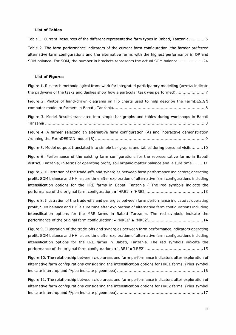
Acknowledgement

This work is part of the United States Agency for International development (USAID) funded Africa RISING East and Southern Africa (ESA) regional project that is implemented by the International Institute of Tropical Agriculture (IITA). We acknowledge USAID and the administration of IITA at Arusha, Tanzania for hosting us during the study. My MSc. Studies here in the Netherlands was financially supported by the Netherlands Universities Foundation for International Cooperation (NUFFIC) under the Netherlands Fellowship Programme (NFP). I am really thankful to NUFFIC and NFP.

We are grateful to researchers particularly to Dr Victor Afari-Sefa and Justus Ochieng (PhD) of the World Vegetable Centre (AVRDC) East and Southern Africa, Dr Job Kihara and Dr Fred Kizito of International Centre for Tropical Agriculture (CIAT) Nairobi Kenya, Dr Ben Lukuyu of International Livestock Research Institute (ILRI) Uganda and Gregory Sikumba (PhD graduate fellow) University of Nairobi for their willingness to share their experimental data with us that without them there would have never been such successful work. We extend our gratitude to Festo Ngulu of International Institute of Tropical Agriculture (IITA) for helping us in contacting these researchers.

Sincere thanks goes also to all famers and extension workers who stopped their activities and joined this study. Farmers and extension workers participated in this study with enthusiasm and contributed to discussions that provided valuable feedback on the model outputs.

Special thanks to supervisors of this study; Dr. Jeroen Groot for his inspiration and support with the FarmDESIGN model and professional advice and guidance in the report writing. Isaac Jambo for his guidance in organizing field works, taking pictures, supports and encouragements. Carl Timler for sharing with me his plan on how I could share the simulation model results with the farmers and his valuable comments that led to the improvement of the work.

We are again thankful to Hashim Rashid for his support in making hand drawings and taking notes and also pictures during workshops and personal visits and to the all staff of IITA in Arusha office for their hospitality and good time we had.

ii

Abstract

Crop-livestock farming systems in Babati are under severe pressure from a fast growing human population. Continuing soil fertility degradation and the extinction of communal resources are linked to low crop yields and high poverty rates among the smallholder farmers. Alternative intensification options such as the use of improved seeds, phosphorus based fertilizers and manure in maize-pigeon pea intercrop and tomato as a new crop have been proposed by the Africa RISING project to improve farm productivity. The feasibility of these field level options needs to be assessed at farm-scale to give insight into the interactions between crops, soils, animals and the household. We used the farm-scale model, FarmDESIGN, to explore alternative options for differently resource endowed farms to enhance their farm performances in terms of economic, environmental and social indicators by combining the current farm resources with the AR interventions. Two sample farms of each farm type were selected. In addition, the study attempted to engage smallholder farmers and extension workers. Data for the current farms were obtained from a previous study while data for the novel interventions were gathered from literature reviews and ongoing research experiments. The windows of opportunities and the preferred innovations depended on available land sizes, current cropping systems and livestock ownership. The High Resource Endowed farms showed widest ranges of potential improvements in terms of operating profit followed by the Medium Resource Endowed farms while the Low Resource Endowed farms showed modest improvements. Improvements in terms of operating profit and soil organic matter were possible by reducing area under the currently grown crops and adopting the Africa RISING interventions. However, often strong trade-offs with household leisure time were evident due to the high labour demand of these inventions. Cultivation of the high value tomato crop with its characteristic low soil organic matter inputs created strong trade-offs between operating profit and organic matter balance. Adopting the new practices of maize-pigeon pea intercrop, maintaining or slightly increase animal numbers as well as incorporating a portion of the crop residues into the soil played a key roles in increasing organic matter balances on all farm types. The interactions with farmers allowed virtual experiential learning to take place and provided evidence that the farmers found the simulation outcomes credible and meaningful. We conclude that the model is an effective tool in exploring windows of opportunity within smallholder farming systems and promotes the discussion of future farm development options between smallholder farmers and extension workers.

Key words: Smallholder farmers, Babati, intensification options, Multi-objective optimization

Table of Contents

Acknowledgement .................................................................................................................................. i

Abstract ............................................................................................................................................... ii

List of Tables ....................................................................................................................................... iii

List of Figures ...................................................................................................................................... iii

1. Introduction ................................................................................................................................. 1

1.1. Background ........................................................................................................................... 1

1.2. Problem statement ................................................................................................................. 2

1.3. Objectives ............................................................................................................................. 3

1.3.1. Main objective ................................................................................................................ 3

1.3.2. Specific objectives .......................................................................................................... 3

1.3.3. Research questions ......................................................................................................... 3

2. Material and methods .................................................................................................................... 4

2.1. Characterization of the study area ............................................................................................ 4

2.2. Model description and exploration procedures ............................................................................ 4

2.3. Conceptual framework ............................................................................................................ 5

2.3.1. Farm typologies .............................................................................................................. 5

2.3.2. Tested intensification options ........................................................................................... 6

2.3.3. Participatory engagement workshops and personal visits ..................................................... 7

3. Results ...................................................................................................................................... 11

3.1. Performance of the current farms ........................................................................................... 11

3.2. Explorations of the alternative farm plans ................................................................................ 12

3.2.1. Trade off and synergies between farmers’ competing objectives. ........................................ 12

3.2.2. Adjustments required in farm configurations to improve farm performance indicators ........... 16

3.2.3. Pareto optimization of the current farms .......................................................................... 21

3.3. Engagement workshops and personal visits ............................................................................. 22

3.3.1. Workshops ................................................................................................................... 22

3.3.2. Personal visits .............................................................................................................. 24

4. Discussion ................................................................................................................................. 28

5. Conclusion and recommendation .................................................................................................. 31

References .......................................................................................................................................... 32

6. Appendices ................................................................................................................................ 35

iii

List of Tables

Table 1. Current Resources of the different representative farm types in Babati, Tanzania ............ 5

Table 2. The farm performance indicators of the current farm configuration, the farmer preferred

alternative farm configurations and the alternative farms with the highest performance in OP and

SOM balance. For SOM, the number in brackets represents the actual SOM balance. .................. 24

List of Figures

Figure 1. Research methodological framework for integrated participatory modelling (arrows indicate

the pathways of the tasks and dashes show how a particular task was performed) ...................... 7

Figure 2. Photos of hand-drawn diagrams on flip charts used to help describe the FarmDESIGN

computer model to farmers in Babati, Tanzania. ...................................................................... 8

Figure 3. Model Results translated into simple bar graphs and tables during workshops in Babati

Tanzania ............................................................................................................................ 8

Figure 4. A farmer selecting an alternative farm configuration (A) and interactive demonstration

/running the FarmDESIGN model (B) ..................................................................................... 9

Figure 5. Model outputs translated into simple bar graphs and tables during personal visits ......... 10

Figure 6. Performance of the existing farm configurations for the representative farms in Babati

district, Tanzania, in terms of operating profit, soil organic matter balance and leisure time. ....... 11

Figure 7. Illustration of the trade-offs and synergies between farm performance indicators; operating

profit, SOM balance and HH leisure time after exploration of alternative farm configurations including

intensification options for the HRE farms in Babati Tanzania ( The red symbols indicate the

performance of the original farm configuration; ■ ‘HRE1’ ● ‘HRE2’ ............................................ 13

Figure 8. Illustration of the trade-offs and synergies between farm performance indicators; operating


intensification options for the MRE farms in Babati Tanzania. The red symbols indicate the

performance of the original farm configuration; ♦ ‘MRE1’ ▲ ‘MRE2’. .......................................... 14

Figure 9. Illustration of the trade-offs and synergies between farm performance indicators operating


intensification options for the LRE farms in Babati, Tanzania. The red symbols indicate the

performance of the original farm configuration; ● ‘LRE1’ ■ ‘LRE2’ ............................................. 15

Figure 10. The relationship between crop areas and farm performance indicators after exploration of

alternative farm configurations considering the intensification options for HRE1 farms. (Plus symbol

indicate intercrop and P/pea indicate pigeon pea). .................................................................. 16

Figure 11. The relationship between crop areas and farm performance indicators after exploration of

alternative farm configurations considering the intensification options for HRE2 farms. (Plus symbol

indicate intercrop and P/pea indicate pigeon pea). .................................................................. 17

iv

Figure 12. The relationship between crop areas and the farm performance indicators after exploration

of alternative farm configurations considering the intensification options for MRE1 (-indicate

traditional, and P/pea stand for pigeon pea) .......................................................................... 18


of alternative farm configurations considering the intensification options for MRE2 farms. (P/pea

stand for pigeon pea) .......................................................................................................... 19


of alternative farm configurations considering the intensification options for LRE1 farms. ............ 20


of alternative farm configurations considering the intensification options for LRE2 farms. ............ 21

Figure 16. Relative change of the farms considering the highest and current values for objectives in

the sets of alternatives obtained by multi-objective optimization without (A) and with intensification

options (B) for high, HRE1,HRE2, MRE1, MRE2, LRE1 and LRE2) .............................................. 22

Figure 17. Trade-offs between the objectives increasing operating profit and SOM balance for the

farms used in the workshops in Sabilo ‘A’ Matufa ‘B’ and Seloto ‘C’ villages in Babati district, Tanzania.

........................................................................................................................................ 23

Figure 18. Trade-offs between high operating profit and SOM balance and between maximizing

income and reducing labour requirements and synergy for HRE1, MRE1, MRE2, MRE3, LRE1 and LRE2

farms observed by individual farmers during the personal visits after Pareto-optimization ........... 27

1

1. Introduction

1.1. Background

Despite a number of problems facing smallholder famers, agriculture is still the only option for the majority of rural populations in sub-Saharan Africa (SSA) and other developing countries (Arias et al. 2013). Smallholder farmers in developing countries contribute a large share of the world’s food supply (Herrero et al. 2017). Approximately there are about 500 million small farms with less than 2 ha of land area worldwide (Wiggins 2010). In many parts of the tropics, particularly in SSA, smallholder farmers practice mixed crop–livestock systems. Crops provide food, cash when sold and residues to feed livestock, whereas animals in addition to food also provide manure and draft power (Herrero et al. 2014).

Studies indicate that many arable lands in SSA are under severe pressure to enhance agricultural productivity to feed a fast growing human population (Waithaka et al. 2006). Areas with good soil fertility are characterized by high population density and they represent severe cases of ongoing land deterioration. Rapid land degradation in these areas is mainly associated with high population pressure (Tittonell et al. 2009). Babati district in Tanzania is a good example of this (Hillbur 2013 ; IITA 2013). Adoption of sustainable land management practices such as improved fallows in these highly populated areas is constrained by land shortages (Shepherd & Soule 1998). Apart from poor soil fertility due land degradation and shortage of land, insufficient labour resources are another important factor limiting productivity of smallholder farming systems in SSA (Giller et al. 2006). Shortage of labour resources is mentioned as a key factor in determining farmers’ choice of crops and production methods (Zingore et al. 2009). Smallholder farmers in SSA often face multiple trade-offs when deciding on the allocation of their limited resources like labour, land and capital to competing production activities within their farms (Giller et al. 2006; Tittonell et al. 2007). Furthermore, the daily decisions made by farmers on the allocation of resources have significant short-and long-term consequences for the sustainability of their farms (Tittonell et al. 2007).

Re-designing sustainable farming systems of smallholder farmers must aim to make these systems more stable, adaptable and resilient to external changes and more efficient in the productive use of resources (Tittonell et al. 2009). Researchers have to develop effective technologies and/or interventions that would increase farm productivity and enhance sustainability and thereby improve farmers livelihoods (Waithaka et al. 2006). Since opportunities to increase the availability of resources in smallholder farmers is limited, improving the efficiency with which resources like nutrients, land and labour are used is necessary for increasing farm productivity (Giller et al. 2006). To improve the performance level of the smallholder farming systems, we need to explore alternative options that can improve the management of the key components of the farming system and their interactions. On the other hand, understanding the trade-offs between farmers’ competing objectives such as food production, income generation and maintaining or increasing soil organic matter (SOM) balance is necessary to increase productivity and ensure sustainability of smallholder farming systems. Identifying such trade-offs enables farmers to make appropriate decisions regarding increasing the productivity and sustainability of their farming systems (Tittonell et al. 2007).

Nevertheless, smallholder farming systems in SSA are complex due to complicated interactions occurring between soil, crops and livestock under unfavourable socio-economic circumstances (Thornton & Herrero 2001). This makes the potential sustainable intensification options of crop–livestock systems challenging to understand, as its complexity makes it impossible to use empirical farm scale data to separate features in these systems (Bell & Moore 2012). For instance if a fodder crop is added into an existing grain cropping system it changes an array of important attributes like labour requirements, economic returns, grain and livestock enterprise balances and environmental impacts. An additional complexity is that a number of practices involving crop–livestock integration have positive and negative effects on different aspects of the system, it is thus hard to reconcile their overall effect (Bell & Moore 2012). Methods that can be used to show farmers the effects of using different novel technologies or interventions are scarce, in particular when taking a holistic farming systems perspective. As a result many approaches only consider certain farm components like livestock only or crops at a field level, and thus do not reflect the reality of farmers’ decision-making (Waithaka et al. 2006).

Researchers recognized this limitation and developed bio-economic models that integrate biophysical and socio-economic data at farm-scale level to allow holistic assessment of the performance and feasibility of interventions (Thornton & Herrero 2001; Arriaga-jorda 2003). Additionally, bio-economic models allow for the identification and analysis of trade-offs in resource allocation strategies in resource constrained smallholder farms (Tittonell et al. 2007). With these tools

2

researchers can address farmers’ key questions on targeted resource allocation to enhance their productivity and profitability at the farm scale. For instance, how should their limited labour and land resources be targeted to maximize production of different crops grown for food or income generation? Should land use be adjusted to respond to changes in prices of crop products? Should crop residues be used for animal feed or returned to soil for maintenance of soil organic matter balance?

Zingore et al. (2009) used combined generic farm-scale database, linear programming (LP) model and simulation models to assess the performance of wealthy (2.5 ha with eight cattle) and poor (0.9 ha without cattle) farms to analyse their opportunities to increase their farm income by improving the productivity of nutrients, labour and land in Zimbabwe. They showed that increasing the land area for groundnut production from existing 0.05 to 0.20 ha could increase the income of the poor farms from 1 US$.year-1 to 19 US$.year-1. The net income of the wealthy farm could be increased to 1,175 US$.year-1 from 290 US$.year-1 by re-allocating the available 240 hired labour-days more efficiently. However, there was a trade-off as this reallocation significantly reduced soil nutrient balance by 74 kg N.ha-1 and 11 kg P.ha-1, causing negative nutrient balances. Komarek et al. (2015) modelled the whole-farm effects of introducing a forage crop into current wheat-maize cropping systems in Xifeng, western China. The result indicated that introducing a third crop into the existing grain cropping system increased overall average whole-farm profit. Nevertheless trade-offs occurred between labour-use efficiency and profit, as forage crop intensification increased labour demands. On the other hand, replacing a grain crop with a forage crop in current grain-cropping systems had a negative effect on the profits of the whole farm.

Tittonell et al. (2007) used inverse modelling techniques to explore alternative management options to optimize maize production and perform a trade-off analysis of farming systems in the highlands of western Kenya under three scenarios of financial liquidity to invest in labour and inputs. The model simulations indicated that increasing maize yield above 2.7 Mg.ha-1 using fertilizer as a strategy resulted in higher N losses by leaching, run off and erosion. The model suggested to use most of the funds (45–85%) investing in land preparation, to allow early planting in order to fulfil the joint objectives of maximizing yields and minimizing N losses. Generally in all cash availability scenarios the model suggested putting priority in investing in hiring labour over fertiliser use to achieve the highest yields and favour the more fertile fields. Waithaka et al. (2006) used integrated mathematical programming and biophysical simulation modelling to evaluate intensification options for enhancing resource use in crop-livestock systems in Vihiga district, Kenya. In their study they revealed that a minimum farm size of 0.4 ha and the introduction of high-value cash crops were crucial to considerably increase the returns of smallholder farmers. In the Ecuadorian Andes, Stoorvogel et al. (2004) applied a combination of a trade-off model and a biophysical model to design options for the ideal management of the potato-pasture production system. The study indicated that price of potatoes was the key factor driving farmers’ decisions regarding the area allocated for potato production, pest management and amount of fertilizer use.

The present study aimed to follow up on the farm characterization done by Timler et al. (2014). The study used the bio-economic FarmDESIGN model (Groot et al. 2012) to optimize farmers’ objectives, and analyse trade-offs at farm-scale relevant to the sustainable intensification of smallholder farming systems in Babati, Tanzania. We aimed to identify viable alternative options that would help smallholder farmers to evaluate, in an ex ante manner, the impacts of different intensification options. The model-based explorations intended to optimize three farmers’ objectives: maximize operating profit (OP), maximize the soil organic matter (SOM) balance and minimize farm labour requirements. These three aspects carry the economic, environmental and social dimensions of sustainability. We wanted farmers to be able to evaluate for themselves the potential benefits and trade-offs of the introduced novel technologies/practices. We therefore, proposed to engage farmers and extension workers in simulation modelling through participatory workshops and personal farm visits for this purpose and to seek feedback that could be used for adjustments to the model analysis and exploration. A participatory modelling study allows the objectives and priorities of the farmers involved to be taken into account (Andrieu et al. 2012). An experience of using simulation models with smallholder farmers in SSA was reported by P. Carberry, Gladwin, and Twomlow (2002) in Zimbabwe.

1.2. Problem statement

Due to its good soil fertility and potential for agriculture, Babati district has continuously attracted many people from different parts of Tanzania and investors from different parts of the world (Löfstrand 2005). Apart from the continuous in-migration, population growth of the district, and the Manyara region in general, is among the highest in the country (Wiredu et al. 2014). High population pressure has led to degradation of agricultural land and extinction of communal resources causing

3

land shortage for crop cultivation and pasture (Hillbur 2013). Farm surveys by IITA (2013); Timler et al. (2014 and Kihara et al. (2015) revealed high variability in crop yields for the main crops of which almost all fell below expected yield levels. Timler et al. (2014) reported soils with extremely low levels of soil organic matter as one of the constraints of agriculture that is attributed by poor management of animal manure and crop residues. IITA (2013) and Kihara et al. (2015) emphasized that poor soil fertility is the main reason for low productivity of farms in Babati. Striga weed infestation is also mentioned as the key reason for poor yields in the fields of cereal crops (Timler et al. 2014). This work sets out to assess at farm-scale the feasibility and practicality of various alternative options for sustainable intensification that are tested by the AfricaRISING (AR) project in the area at the field level. Cropping systems or interventions that look promising at field level might not be feasible when considered at farm level (Cortez-Arriola et al. 2014).

1.3. Objectives

1.3.1. Main objective

The overall study objective was to explore the potential impact of alternative interventions (technologies or practices) that can be applied in smallholder farms of different types, in Tanzania, in order to enhance their economic, social and environmental performance and to analyse trade-offs and synergies associated with these interventions.

1.3.2. Specific objectives

The specific objectives of the study were to:

1. a) Analyse current performance of representative farms in the case study area. b) Identify and select new interventions (technologies or practices) that can be applied to

enhance the productivity in representative farms. c) Explore alternative farm configurations that can enhance farm economic, environmental

and social performance by combining current farm components with interventions in new farm configurations.

2. Analyse trade-offs and synergies that exist between the farmers’ competing objectives 3. Engage with the farmers and other stakeholders working in the study site to inform their

decision-making and to iteratively improve the farm analysis and redesign. 4. Monitor the interaction process to assess the mutual learning, decision-making and

adaptation processes of the farmers.

1.3.3. Research questions

1. What are the effects of the currently applied farming practices on farm productivity, profitability and environmental impact?

2. What are the possible intensification interventions that could be part of the window of opportunities for these different types of farms?

3. What are the relations between indicators of productive, economic and environmental farm performance of different types of farms when including the intensification options? Which adjustments have to be made in the farm configurations to improve performance of the indicators?

4. What would farmers like to improve in their farm and test in the model exploration? 5. How do farmers respond to the modelling results and how can these be further fine-tuned to

support learning, decision-making and adaptation processes in a cycle of participatory extension?

4

2. Material and methods

2.1. Characterization of the study area

The study was conducted in Babati, one of the districts in Manyara region found in the North Western part of Tanzania that is located between latitudes 3° and 4° S and longitudes 35° and 36° E. It covers a total land area of 6 069 km2 lying in diverse altitudes ranging from 900 to 2 200 m above sea level (Kihara et al. 2015). A report from National Bureau of Statistics (2013) showed that Babati district has a population of 12 392 people with an average household size of 5.2 persons. Soil types are sandy to clay loams that are dominated mostly by the red colours of sesquioxides – secondary clay minerals and black colours in low lands (Löfstrand 2005; Timler et al. 2014). Annual average rainfall which is extremely variable, ranges from 500 - 1 200 mm. The area experiences bi-modal rains; long rains that starts from February to May and short rains from November to December (Löfstrand 2005). The main economic activity is subsistence, mixed crop-livestock farming and some pastoralist farming (IITA 2013). Maize cropping systems are common in the area and are usually intercropped with common bean or a late maturing pigeon pea (Kihara et al. 2015). Some areas also marginally grow crops like wheat, rice, millet, cassava, sweet potatoes, cotton, sunflower, sesame, groundnuts, finger millet and lablab (Löfstrand 2005; Timler et al. 2014). In these systems, draught animals play a large role in land cultivation while tractors are available to only a small part of the farming community. Activities like land clearance for agriculture and homestead expansions, land cultivation, seed sowing, and weeding operations are carried out by hand using basic farm tools such as hand hoes, machetes and axes (Löfstrand 2005).

2.2. Model description and exploration procedures

We used the multi-objective, optimization model FarmDESIGN (Groot et al. 2012) to explore the consequences of re-configuration of farms based on different farm performance indicators (farmers’ objectives) and trade-offs between these objectives. The model is purposely developed for supporting a learning and decision-making process of redesign (Mandryk et al. 2014). Because its bio-economic component is linked to its multi-objective Pareto-based differential evolution algorithm, the tool can simultaneously optimize a large set of variables to achieve objectives like optimising operating profit, SOM balances, labour balance and analyse nutrient balances and flows as well as other economic, nutritional and environmental indicators on an annual basis (Cortez-Arriola et al. 2016). The outputs of the optimization runs are alternative farm configurations relative to the original farm configuration that are evaluated in terms of the multiple objectives (Mandryk et al. 2014).

While operating profit, SOM balance and labour balance were set as objectives to optimize crop areas, animal numbers and crop residues were set as variables. Farm areas and feed balance were set as constraints (Cortez-Arriola et al. 2016). The FarmDESIGN model has a flexible set-up that allows the performance indicators to become either objectives to be optimized or constraints (i.e. their values be restricted to a user-defined ranges) depending on the user’s desires (Mandryk et al. 2014). In setting decision variables; crop areas were given a range between zero hectares up to all the available land. In setting animal variables, all animal numbers ranged between the current value and double the current value. All residues in the current farms were fed to animals and thus the parameter ‘used as feed for animals’ had a value of 1 in the model. Making this parameter into a decision variable gave the model an option to allocate part of the residues to the soil as green manure and part as feed to animals. The parameter ‘used as green manure’ therefore had a range between 0 (all residues to animal feed) and 10 (almost all residues to soil). Grazing grass from the community land was set with a very high upper limit (9 999 kg DM) to allow continuous inclusion of this external farm resource. Farm areas were constrained such that the minimum value was 10% less than the available land (to allow for model manoeuvring space) and the maximum value was fixed as the currently available land since smallholders have limited land. The animal feed balance components were constrained so as to avoid exploration of solutions where the animals would be over or under fed or where they would obtain insufficient nutrients. The constraints set were between 0 and 5% deviation for energy, 0 and 30% deviation for protein and -999 and 0% deviation for intake capacity. Groot et al. (2012) provides a more detailed model description including explanation of the calculations involved.

The optimization process was run for 1 000 iterations and the default values for other optimization parameters of the evolutionary algorithm were used: the probability of crossover (CR = 0.85), the amplitude of mutations (F = 0.15) (Cortez-Arriola et al. 2016) and number of solutions (n = 500). During the exploration we assumed that all manure produced by farm animals, when they were in the yard, was applied on the farm fields (Flores-Sánchez et al. 2014). We also assumed that farmers continued growing current crops with their current management as was recorded by the

5

characterization survey by Timler et al. (2014). Another assumption was that, each farm had three household members who work on the farm for eight hours five days per week. This assumption was based on the National Bureau of Statistics (2013).

2.3. Conceptual framework

Figure 1 summarises the key steps for this study and how they link into each other. The research methodological framework included: (1) Selecting farm types-case studies (2) Analysing the performance of current farms (3) Listing alternative intensification options from literature and ongoing research (4) Exploring windows of opportunities(5) Presentation of model outcomes (6) Testing of farmers’ desired options (7) Final selection of alternative options.

2.3.1. Farm typologies

Farming systems in Sub-Saharan-Africa are highly heterogeneous in terms of farmers’ resource endowments. Classifying these farms according to their resource endowment is important when searching for solutions that improve their productivity as there is no single silver bullet for improving productivity in such highly heterogeneous farming systems (Giller et al. 2006). The present study used the farm typologies based on the detailed characterization done by Timler et al. (2014) who classified the farms in the area according to land sizes and livestock ownership. Based on this criterion, farms were categorized as High Resource Endowed (HRE), Medium Resource Endowed (MRE) and Low Resource Endowed (LRE). In this study two representative farms were selected from each farm type for exploration (Table 1) the third farm from medium, resource endowment farm (MRE3) was only used during the personal visits.

Table 1. Current Resources of the different representative farm types in Babati, Tanzania

HRE1 HRE2 MRE1 MRE2 MRE3 LRE1 LRE2

Farm area 5.2 4.8 1.8 2.4 2.6 0.8 0.4

crop currently grown Lablab Maize Maize Maize Maize Maize Maize

Rice Pigeon pea

Bean Bean Bean Bean P/pea

Sorghum

P/pea P/pea P/pea P/pea

Groundnut

Sunflower Sunflowe

r Sorghum

Maize

Sorghum Chickpea Chickpea

P/pea

Pasture

Sesame

Animal currently own

cows 12 8 5 12 2 3

improved cows

1

Goats

5

24 2 4 7

Bulls

5 6 6 4

Chicken

4 10 12 15 7 7

Donkeys

3 3

Sheep

3 10 2

6

2.3.2. Tested intensification options

This study defined a basket of intensification options that could be combined with the current farm components to explore the desired improvements. Sources for these interventions were literature reviews and interactions with researchers from the Africa RISING (AR) project. Appendix 7 and 8 shows the overview of parameters for the new interventions and existing farm components, respectively. The tested intensification options included:

AR-Maize-pigeon pea intercrop: AR in Babati district is working to improve soil fertility, productivity and incomes of smallholder farmers through the intensification of the maize-pigeon peas cropping system. Improved maize varieties are intercropped with improved varieties of several legume crops like common beans, pigeon peas and soybean with application of small amounts of phosphorus-based fertilizers (Minjingu and DAP) in the planting hole (Pers. Comm. Ngulu, 2017). In this study we tested the performance of a maize-pigeon pea intercrop and we referred it as AR-maize-pigeon peas intercrop.

Tomato: Researchers from AR are researching the integration of vegetables into maize based farming systems to enhance household nutrition and improve family income. The technology involves production of healthy seedlings through the use of good quality seed varieties, proper spacing, mulching, timely weed control and integrated pest management. The vegetables currently being tested and grown by farmers include, Tomato (cv. Tengeru 2010), African eggs plants (cv. Tengeru white) and Amarath (cv. Madira1) (Pers. Comm. Roman. 2017). However, only tomatoes were included in the exploration as we could not find sufficient data for other vegetables.

Napier grass: AR is working on improving farmers’ livestock feed supplies through testing alternative grass, legume, and tree fodder species for cows and goats. These fodder crops are grown as boundary planting, fodder banks, erosion structure strengthening or as intercrops with food crops (IITA 2013). We were able to obtain yield data for Napier grass and we used this data for exploration in the FarmDESIGN model.

Push pull technology: This involves intercropping of maize and a legume (Desmodium spp) crop with Napier grass planted around the field. The purpose is for the control of cereal stem borers and witch weeds (Striga spp). Desmodium and Napier grass also provide nutritious fodder for domestic animals (Khan et al. 2008). The technology is not yet implemented in Babati by the project. However, we explored it as an ex ante evaluation because cereal stem borers and Striga weeds are also a problem in Babati (Timler et al. 2014). The data for yields of the products, price and labour requirement was obtained from Vanlauwe & Kanampiu (2015).

7

Figure 1. Research methodological framework for integrated participatory modelling (arrows indicate the pathways of the tasks and dashes show how a particular task was performed)

2.3.3. Participatory engagement workshops and personal visits

2.3.3.1. Workshop

We engaged 46 farmers and three extension workers to demonstrate simulation modelling outputs in Sabilo, Seloto and Matufa villages of Babati district using an interactive workshop approach. Swahili language that is common in the area and in the country at large was used as a medium of communication throughout the interactions. During the workshop farmers were first asked to brainstorm their objectives for farming. In all villages farmers mentioned food production for households and increasing family income as their most important objectives. Improving soil fertility and minimization of labour requirements were mentioned as another key objectives in Matufa and Sabilo, whereas only farmers in Matufa village mentioned improving human nutrition.

The model outputs discussed included optimization of the three performance indicators, that is, operating profits (referred as family income throughout the interaction), SOM balance and labour balance. The decision variables used were crop areas, number of animals and the destination of crop residues. Participating farmers proposed to use the acre as a unit of measurement for land area instead of hectare and to use the local currency, Tanzania shillings (Tsh), for economic results. For easier communication with farmers, the original objective of improvement of SOM balance was replaced by the term “soil fertility” the common term used by the farmers. In each workshop we started the discussion by asking the participating farmers to say something about what they knew about a farming system. Participating farmers and extension workers could recognize three components/sub systems of a farming system in their area; a crop production system, an animal production system and a household system. It was clearly understood that these sub systems interact with each other at the farm level.

Hand-drawn diagrams on flipcharts (Figure 2) were used to help describe the FarmDESIGN model to the smallholder farmers (Carberry et al. 2002). Firstly, the concept of input-output relations using the data required by the computer model (input) and its outputs (performance indicators and adjusted decision variables) were discussed (Figure 2A). Next the quantification of nutrient flows and

8

cycles by the model were discussed, starting with the destinations of crop and animal products and followed by the imports and exports of materials (Figure 2B and Figure 2C). Once we had completed the discussion about the computer model with the farmers, the idea of using the computer to ask ‘What if’ questions (Figure 2D) was introduced (Carberry et al. 2002; Nidumolu et al. 2016). Farm level bio-economic models have previously been used to support farm production planning decisions and enable explorations of ‘what if’ questions (Janssen & van Ittersum 2007).

After the description of the computer model and ‘what if’ questions, we presented simulation outputs of an example farm. Outcomes of the simulation were presented to farmers in three ways; on the computer, translated into tables and in simple bar graphs on flipcharts similar to Carberry et al.(2002); Twomlow & Carberry (2003) and Sempore et al. (2015) (Figure 3).

D

A B

C

Figure 2. Photos of hand-drawn diagrams on flip charts used to help describe the FarmDESIGN computer model to farmers in Babati, Tanzania.

Figure 3. Model Results translated into simple bar graphs and tables during workshops in Babati Tanzania

9

We included new interventions, which included new technologies/practices that were not grown/practiced on the example farm, but which AR is introducing in the area. The cloud of solutions (the alternative farm configurations) generated by the computer model representing two objectives was drawn on a flip chart (Figure 4A). The values of the axes were made identical to the model output. This helped to guide the farmers and extension workers in choosing an alternative farm configuration before the actual demonstrations began. Thereafter the model was demonstrated to groups of five to six farmers (Figure 4B). Since most of participating farmers were computer illiterate, it was not possible for the farmers to run the model themselves, rather it required an interactive approach. The approach ensured that simulations were done and outputs presented in a way that facilitated thinking by participating farmers and extension workers. The interaction process was similar to playing a farming game. Under this approach, the items in describe window of the model were written in Swahili. The participants were guided through the various steps of the FarmDESIGN model (Figure 4B) to allow them to understand the basic inputs and outputs of the model (Thi et al. 2013). This approach was also useful to show the farmers that the FarmDESIGN model can reasonably mimic their real farming system. The crops and animals in the representative farm were shown to the farmers in order to help them understand that the same crops were grown and the same animals were kept ‘on the computer’ as where grown and kept on their real farms (i.e. what types of crops are grown, what each crop’s field size was, what each crop’s price was, what types and numbers of animals are kept) etc.

The model was run, and from the set of alternative configurations generated, the farmers from each group were asked to select one preferred alternative farm configuration. We stimulated and facilitated the discussion during the selection process to provide a good understanding of the participating farmers’ reasoning behind their decision-making in a style similar to Mandryk et al. (2014). In the next step the model outcomes and the values of the decision variables for the selected alternative configurations were presented on the flips charts as hand drawn tables and bar graphs (Figure 3). A collective discussion followed to select the most preferred alternative farm configuration based on the feasibilities of the values of the decision variables and the level of improvements of the performance indicators. The process of running the model and the presentation of the simulated results was repeated two or three times in each workshop until a good level of understanding was achieved (Thi et al. 2013).

B A

Figure 4. A farmer selecting an alternative farm configuration (A) and interactive demonstration /running the FarmDESIGN model (B)

10

2.3.3.2. Personal visits

Five individual farmers were visited at their farms, two from Sabilo, one from Matufa and two from Seloto. All visited farmers had attended one of the workshops. All data for their current farms as well as data for the new technologies/practices were already entered in the models of their respective farms before the day of the personal visit. Each visit lasted either a morning or afternoon. The aim of this individual farm visit was to present the modelling outputs for their own farms to the famers rather than to formulate examples based on average farm characteristics (Mandryk et al. 2014). The objective was to allow farmers to understand the meaning of the model outputs to allow them to use the outputs to make future decisions. In these personal visits we ran the model interactively with the farmer, following the idea suggested by Bob McCown in 1993 (Carberry et al. 2002). Together with the farmer we first examined the inputs of FarmDESIGN in the describe windows to ensure that the crop and animal data were correct. The farmers were curious to see if the model was a real representation of their own farms. This was one way to make famers trust that the model was the actual representative of their farming system. When a visited farmer was satisfied that the data in the model was a real representation of his farm, the next step was to present the simulation outputs of his own farm done before the visit. The model outputs were presented on graph papers as simple bar graphs and as tables (Figure 5). The presentation was followed by a short discussion to allow farmers to comment on or to give his opinions about the presented outputs. The farmer would then choose the new AR technologies/practices he desired from a list. If the farmer only chose one technology/practice the remaining technologies could be deleted from the farm model. Thereafter we encouraged the farmers to choose the objectives that he would like to optimize.

The model was run together with the farmer, as was done in the workshop, and farmers were encouraged and facilitated to select their preferred alternative farm configuration from the set of alternatives (Mandryk et al. 2014). Using the skills learned from the workshop in examining performance indications from a two dimensional graph, farmers could choose several farm configurations and save them as new farms. The performance indicators of the selected farms were discussed one by one and compared. The decision variables for the selected farms were presented to the farmer in table form and the farmer was given time to examine the variables and their consequences for the values of the performance indicators. Considering the farmers’ viewpoints on the decision variables they selected their most preferred farm configurations.

Figure 5. Model outputs translated into simple bar graphs and tables during personal visits

11

3. Results

3.1. Performance of the current farms

Figure 6 indicates how each farm currently performs in terms of the selected farmers’ objectives operating profit (OP), SOM balance and household (HH) leisure time. The performance of the farms related to these selected indicators was quite different due to differences in: farm sizes, initial farm configurations and the acreage and type of crops grown. Generally, SOM balance was negative in all farms analysed. The two high resource endowed farms (HRE1 & HRE2) showed the highest performance in terms of economic results. These farms have large cropping land areas and they grow a large share of crops that contribute a large percentage of their gross margins, 47% for HRE1 and 86.5% for HRE2. The HRE1 farm also performed the best in terms of SOM balance as a result of high amount of manure produced by farm animals. Large share of crops cultivated also adds a significant amount of effective organic matter to the soil. The best performance in terms of household leisure time was observed for farm LRE2. This farm has the smallest land area (0.4 ha) and only few small ruminants (7 goats). As an inference from this fact, less labour is required for crop and livestock management. In contrast to HH leisure time, the farm exhibited worse performance in terms of operating profit (-1 227.40 US$.year-1) due to the same reasons. The negative sign indicates that this farm is not making any profit but rather a loss. Farms MRE1 and MRE2 are medium farms with intermediate land areas and family incomes compared to the other two farm types. The LRE farms performed the best in terms of SOM balance after the HRE1. Farms HRE1 and HRE2 demonstrated the poorest performance in in terms of HH leisure time because high labour is required for crop and herd management. Despite having relatively high numbers of animals and a high diversity of crops grown, the lowest performance in terms of SOM balance was observed for the farm MRE1. This farm had the highest SOM degradation (3 510 kg. ha -1.year-1).

-2000 3000 8000 13000 180000

2000

4000

6000

Operating profit (US$.year-1)

HH le

isure

tim

e (h

.yea

r-1)

-2000 3000 8000 13000 18000

-3000

-2000

-1000

0


SO

M b

alan

ce (

kg.h

a.ye

ar-1

) 0 2000 4000 6000

-3000

-2000

-1000

0

HH leisure time(h.year -1)

SOM

bal

ance

(kg.

ha-1

year

-1)

Figure 6. Performance of the existing farm configurations for the representative farms in Babati district, Tanzania, in terms of operating profit, soil organic matter balance and leisure time.

12

3.2. Explorations of the alternative farm plans

The FarmDESIGN model was used to explore new windows of opportunities by generating clouds of alternative farm configurations for the case study farms. The model calculated the values of the farm performance indicators and found combinations of crop areas, animal numbers and destinations of residues that optimized each farm’s performance. The results of the explorations showed that improvements for Operating profit and SOM balance were possible for all representative farms (Figure 7, Figure 8 and Figure 9). Improvements could be achieved by re-designing the current farm resources and by combining the current farm components with the new intensification options, AR maize-pigeon pea intercrop and tomato. However, the model selected very small areas (close to zero hectares) for the push-pull technology and sole Napier grass for all farms. Significant areas were allocated for both push pull technology and sole Napier grass when each option was tested as single alternative option for HRE and MRE farms (Results not shown). Destination of crop residues was the main variable (alongside the destination of the farm manure) that influenced the maximization of SOM balances in all farm types. The AR-maize-pigeon pea intercrop intensification option resulted in the largest maize residue production and the highest grain yield. For this reason, the model selected it as the key option for increasing operating profit and SOM balance for farms HRE1, MRE2, LRE1 and LRE2. The tomato crop was important to maximize family income for HRE2, LRE1 and LRE2 farms. Furthermore, the two intensification options; tomato and AR maize-pigeon pea intercrop have relatively high labour requirements when compared to the current practices. Details are provided in the section 3.2.2 where the performance of the individual farm is discussed for each selected performance indicator and the adjustments required.

3.2.1. Trade off and synergies between farmers’ competing objectives.

To assess the relationships between the different objectives, we plotted the alternative farm configurations generated by the FarmDESIGN model in two-dimensional spaces (Figure 7, Figure 8 and Figure 9). We observed that some pairs of objectives showed trade-offs while others exhibited synergies given the data set used. For instance, we found trade-offs between the objectives of increasing operating profit and HH leisure time for HREs and MREs farms (Figure 7A and Figure 8A). Farms HRE1 and MRE2 showed high degree of trade-offs between high SOM balance and high HH leisure time (Figure 7C and Figure 8C). Furthermore, trade-offs existed between the objectives of increasing SOM balance and high operating profit for HRE2, MRE1 and LRE1 farms (Figure 7B, Figure 8B and Figure 9B). Synergies were observed between the objectives of maximizing operating profit and increasing SOM balances for the farms HRE1, MRE2 and LRE2 (Figure 7B, Figure 8B and Figure 9B). This positive relation is also found between objectives of increasing SOM balance and HH leisure time for HRE2 and MRE1 farms (Figure 7C and Figure 8C).

13

0 10000 20000 30000 400000

200

400

600

800

1000


HH le

isure

tim

e (h

.yea

r-1)

A

0 10000 20000 30000 40000-1000

0

1000

2000

3000

4000

Operating Profit (US$.year-1)

SOM

bal

ance

(Kg.

ha-1

year

-1)

B

0 200 400 600 800 1000-1000

0

1000

2000

3000

4000

HH leisure time (h.year-1)

OM

bal

ance

(kg.

ha-1

year

-1)

C

Figure 7. Illustration of the trade-offs and synergies between farm performance indicators; operating profit, SOM balance and HH leisure time after exploration of alternative farm configurations including intensification options for the HRE farms in Babati Tanzania ( The red symbols indicate the performance of the original farm configuration; ■ ‘HRE1’ ● ‘HRE2’

14

0 5000 10000 15000800

1100

1400

1700

2000

Operating profit (US$/year)

HH le

isure

tim

e (h

.yea

r-1)

A

0 5000 10000 15000-3000

-1000

1000

3000


SOM

bal

ance

(kg.

ha-1

.yea

r-1)

B

800 1100 1400 1700 2000-3000

-2000

-1000

0

1000

2000

3000


C

Figure 8. Illustration of the trade-offs and synergies between farm performance indicators; operating profit, SOM balance and HH leisure time after exploration of alternative farm configurations including intensification options for the MRE farms in Babati Tanzania. The red symbols indicate the performance of the original farm configuration; ♦ ‘MRE1’ ▲ ‘MRE2’.

15

1500

2500

3500

4500

5500

-2000 5000 12000HH le

isure

tim

e (h

.yr -1

)

Operating Profit (US$.yr-1)

A

-1000

0

1000

2000

3000

4000

-2000 5000 12000

SOM

bal

ance

(kg.

ha -1

yr -1

)

Operating profit (US$/year)

B

-1000

0

1000

2000

3000

4000

0 4000 8000HH leisure time (hyear -1)

C

Figure 9. Illustration of the trade-offs and synergies between farm performance indicators operating profit, SOM balance and HH leisure time after exploration of alternative farm configurations including intensification options for the LRE farms in Babati, Tanzania. The red symbols indicate the performance of the original farm configuration; ● ‘LRE1’ ■ ‘LRE2’

16

3.2.2. Adjustments required in farm configurations to improve farm performance indicators

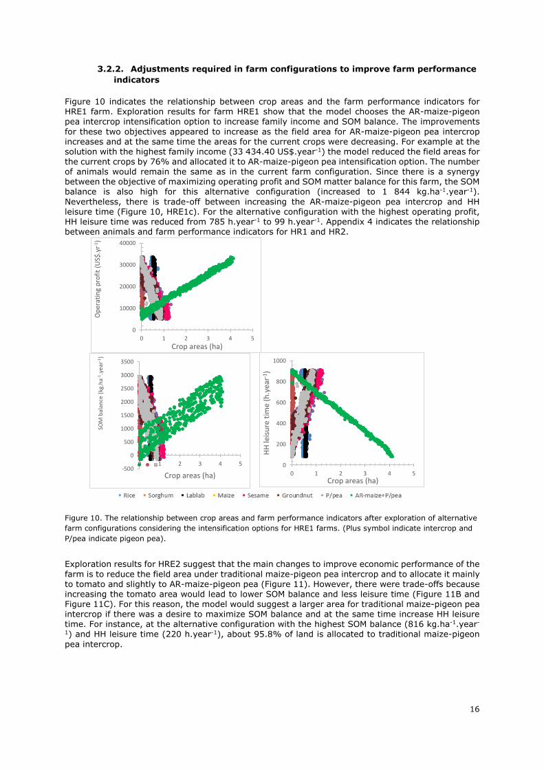
Figure 10 indicates the relationship between crop areas and the farm performance indicators for HRE1 farm. Exploration results for farm HRE1 show that the model chooses the AR-maize-pigeon pea intercrop intensification option to increase family income and SOM balance. The improvements for these two objectives appeared to increase as the field area for AR-maize-pigeon pea intercrop increases and at the same time the areas for the current crops were decreasing. For example at the solution with the highest family income (33 434.40 US$.year-1) the model reduced the field areas for the current crops by 76% and allocated it to AR-maize-pigeon pea intensification option. The number of animals would remain the same as in the current farm configuration. Since there is a synergy between the objective of maximizing operating profit and SOM matter balance for this farm, the SOM balance is also high for this alternative configuration (increased to 1 844 kg.ha-1.year-1). Nevertheless, there is trade-off between increasing the AR-maize-pigeon pea intercrop and HH leisure time (Figure 10, HRE1c). For the alternative configuration with the highest operating profit, HH leisure time was reduced from 785 h.year-1 to 99 h.year-1. Appendix 4 indicates the relationship between animals and farm performance indicators for HR1 and HR2.

Exploration results for HRE2 suggest that the main changes to improve economic performance of the farm is to reduce the field area under traditional maize-pigeon pea intercrop and to allocate it mainly to tomato and slightly to AR-maize-pigeon pea (Figure 11). However, there were trade-offs because increasing the tomato area would lead to lower SOM balance and less leisure time (Figure 11B and Figure 11C). For this reason, the model would suggest a larger area for traditional maize-pigeon pea intercrop if there was a desire to maximize SOM balance and at the same time increase HH leisure time. For instance, at the alternative configuration with the highest SOM balance (816 kg.ha-1.year-

1) and HH leisure time (220 h.year-1), about 95.8% of land is allocated to traditional maize-pigeon pea intercrop.

0

10000

20000

30000

40000

0 1 2 3 4 5

Ope

ratin

g pr

ofit

(US$

.yr-1

)

Crop areas (ha)

-500

0

500

1000

1500

2000

2500

3000

3500

0 1 2 3 4 5

SOM

bal

ance

(kg.

ha-1

.yea

r-1)

Crop areas (ha)0

200

400

600

800

1000

0 1 2 3 4 5

HH le

isure

tim

e (h

.yea

r-1)

Crop areas (ha)

Figure 10. The relationship between crop areas and farm performance indicators after exploration of alternative farm configurations considering the intensification options for HRE1 farms. (Plus symbol indicate intercrop and P/pea indicate pigeon pea).

17

The main changes to improve the economic and SOM balance performance for MRE1 farm would be to rely more on re-arranging initial crop areas and allocate small land area of about 5.5% for tomato and AR-maize-pigeon pea intercrop (Figure 12). To increase operating profit, the changes would mainly be to increase the area under traditional maize, bean, pigeon pea and sunflower intercrop and increase the number of chickens to 50. For example, for the alternative farm with the best performance in operating profit (11 255.2 US$.year-1), 0.9 ha of land was allocated to traditional maize, bean, pigeon pea and sunflower intercrop and zero area for sorghum. At this alternative configuration, the model also suggested an increase of 3 extra cows while goats and sheep numbers would remain the same. However, sorghum is an important crop for improving SOM balance. Increasing the area of sorghum led to an increased SOM balance. For the alternative configuration with the highest SOM balance (-693 kg.ha-1.year-1), the area selected for sorghum was 0.95 ha. The number of animals was the same as in the alternative farm configuration with the highest operating profit.

7000

10000

13000

16000

19000

22000

25000

0 1 2 3 4 5

Ope

ratin

g pr

ofit

(US$.

year

-1)

Crop areas (ha)

-700

-400

-100

200

500

800

1100

0 1 2 3 4 5

SO

M b

alan

ce (

kg.h

a-1 .

year

-1)

Crop areas (ha)

0

50

100

150

200

250

0 1 2 3 4 5

HH

leis

ure

time(

h.ye

ar-1

)

Crop areas (ha)

Figure 11. The relationship between crop areas and farm performance indicators after exploration of alternative farm configurations considering the intensification options for HRE2 farms. (Plus symbol indicate intercrop and P/pea indicate pigeon pea).

A

B C

18

AR-Maize-pigeon pea intercrop exhibited a positive relationship between the field size and the two objectives; maximising operating profit and OM balance for the farm MRE2 (Figure 13A and Figure 13B). For the alternative farm configuration with the highest family income 14 226.80 US$.year-1, the model allocated 75% of available land for AR-maize-pigeon pea intercrop and 8% for maize, bean, pigeon peas and sunflower under current practice. The area for chickpea remains the same as in the current farm. The model also suggested an increase of 34 chickens while two goats and two sheep were reduced. Other animal numbers remained as they are in the current farm configuration. In the case of the configuration with the highest OM balance (2 805 kg.ha-1.year-1), 1.7 ha of land was allocated to AR-maize-pigeon peas intercrop and 0.3 ha to the traditional intercrop of maize, bean, pigeon pea and sunflower. Three more chickens were proposed while other animal numbers were kept as for the alternative configuration with the highest operating profit. Appendix 5 indicates the relationship between animals and farm performance indicators for MR1 and MR2 farms.

4000

5000

6000

7000

8000

9000

10000

11000

12000

0 0.2 0.4 0.6 0.8 1

Ope

ratin

g pr

ofit

(US$.

year

-1)

Crop areas (ha)

-3000

-2500

-2000

-1500

-1000

-500

00 0.2 0.4 0.6 0.8 1

SOM

bal

ance

(kg.

ha-1

.yr-1

)

Crop areas (ha)

1500

1550

1600

1650

1700

1750

1800

0 0.2 0.4 0.6 0.8 1

HH

leis

ure

time

(h.y

ear-

1 )

Crop areas (ha)

Figure 12. The relationship between crop areas and the farm performance indicators after exploration of alternative farm configurations considering the intensification options for MRE1 (-indicate traditional, and P/pea stand for pigeon pea)

19

Exploration results indicated that AR-maize-pigeon pea intercrop and tomato would be the best solutions for the low resource endowed (LRE) farms for improving operating profit. AR-maize-pigeon pea intercrop is also one of the key options selected to increase soil organic matter balance in these small farms. Figure 14& Figure 15 shows the relationships between the crop areas and the farm performance indicators for LRE1 and LRE2 farms. The model choose to decrease the area of the traditional intercrop of maize, bean and pigeon pea and replace it with the AR-maize-pigeon pea intercrop and tomato to improve family incomes for LRE1. The alternative farm with the best result for operating profit (8 562.00 US$.year-1) was achieved by allocating 0.34 ha to tomato and 0.45 ha to AR maize-pigeon pea intercrop. The model also suggested increasing the number of chickens to 49 and the number of cows to nine. The farm configuration with the highest soil organic matter balance (3 359 kg.ha-1.yearr-1) could be achieved by allocating almost all the land area to AR-maize -pigeon pea intercrop. The number of animals was identical to the farm configuration with the best operating profit. For LRE2, for the alternative farm configuration with the highest operating profit (3 438.40 US$.year-1) the model suggested to divide the available land (0.4 ha) currently under traditional maize-pigeon pea intercrop equally to AR-maize-pigeon intercrop and tomato. The model also suggested an increase in the number of chickens to 41 and to increase the number of goats to seven. For this farm configuration the SOM balance would be improved to 932 kg.ha-1.year-1. Appendix 6 indicates the relationship between animals and farm performance indicators for LR1 and LR2 farms.

0

2000

4000

6000

8000

10000

12000

14000

16000

0 1 2

Ope

ratin

g pr

ofit

(US$.

year

-1)

Crop areas (ha)

-1000

-500

0

500

1000

1500

2000

2500

3000

0 1 2

SO

M b

alan

ce (

kg.h

a-1 .

year

-1)

Crop areas (ha)

800

850

900

950

1000

1050

1100

0 1 2

HH

leis

ure

time

(h.y

ear-

1 )

Crop areas (ha)

Figure 13. The relationship between crop areas and the farm performance indicators after exploration of alternative farm configurations considering the intensification options for MRE2 farms. (P/pea stand for pigeon pea)

B C

A

20

0

1000

2000

3000

4000

5000

6000

7000

8000

9000

0 0.2 0.4 0.6 0.8 1

Ope

ratin

g pr

ofit

(US$.

year

-1)

Crop areas (ha)

-1000

-500

0

500

1000

1500

2000

2500

3000

3500

4000

0 0.2 0.4 0.6 0.8 1

SO

M b

alan

ce (

kg.h

a-1 .

year

-1)

Crop areas (ha)

1520

1540

1560

1580

1600

1620

1640

1660

1680

1700

0 0.2 0.4 0.6 0.8 1

HH

leis

ure

time

(h.y

ear-

1 )

Crop area (ha)

Figure 14. The relationship between crop areas and the farm performance indicators after exploration of alternative farm configurations considering the intensification options for LRE1 farms.

21

3.2.3. Pareto optimization of the current farms

The FarmDESIGN model was used to explore alternative solutions for the farms based on re-arrangement of the existing farm components. The relative performance change was calculated after optimization of the farms without (Figure 16A) and with (Figure 16B) the intensification options. The calculation used a simple formula (Equation 1). The results obtained enable us to assess the relevance of the intensification options to the improvements of the farms’ performance indicators.

R = (Vh- Vc) / Vc (1)

Where R is the relative change for a specific objective, Vh is the best value obtained for that objective and VC is the current value of the objective. The results indicated that all farms had higher relative performance change (R) in terms of operating profit and SOM balance when the alternative farm configurations were explored by including the intensification options than when the intensification options were not included (Figure 16A and Figure 16B). This justifies that alternative intensification options were necessary in order to improve the performance of farms in terms of economic and

-2000

-1000

0

1000

2000

3000

4000

0 0.2 0.4 0.6

Ope

ratin

g pr

ofit

(US$.

year

-1)

Crop areas (ha)

-1000

-500

0

500

1000

1500

2000

2500

3000

3500

4000

4500

0 0.2 0.4 0.6

SO

M b

alan

ce (

kg.h

a-1 .

year

-1)

Crop areas (ha)

5000

5100

5200

5300

0 0.2 0.4 0.6

HH le

isure

tim

e (h

.yea

r-1)

Crop areas (ha)

Figure 15. The relationship between crop areas and the farm performance indicators after exploration of alternative farm configurations considering the intensification options for LRE2 farms.

22

environmental indicators of smallholder farming systems in Babati. However, exploration without including the interventions resulted into higher R in terms of HH leisure time than when interventions were included due to high labour inputs required by the new intensification options.

3.3. Engagement workshops and personal visits

3.3.1. Workshops

When asked for their reaction after presentation, one farmer asked that “you said you will use the computer to explore the results of changes in the land use in our farming practices how long will it take for us to see the results?” Participants also wanted know how nutrients are lost from their farms and if our model can quantify the losses. These reactions were followed by the actual demonstrations of the simulation modelling that answered these questions. The model was run with the alternative crops/practices included in each workshop and farmers were to choose the most preferred alternative farm configuration. It was interesting to see that farmers in Sabilo and Matufa villages were struggling to get an alternative farm configuration with the best improvements in both family income and in SOM balance. It was not possible due to trade-offs that existed between these two objectives (Figure 17A and Figure 17B respectively). When they found it not possible, farmers wanted to know why the farms with high income have low soil fertility and those with high soil quality have low income. According to them improved soil quality should provide high income, they were surprised why the opposite was true. The facilitated discussion then addressed why these trade-offs occur. The discussion made clear that trade-offs were the results of allocating constrained resources like labour and money (i.e. the improvement of both soil quality and income required investment of resources). The discussions also added that variation in prices for different crops, and that different crop types exhibit different traits on soil quality are another reason for the presence of trade-offs. We used an example of tomato, a crop that poorly supports physical soil properties, but it fetches a premium price in the market. Tomato was also included in the exploration that was demonstrated to the participants. The extension workers and some knowledgeable famers contributed a lot in the discussions and helped us to explain to other farmers in a way they could understand easily. Some farmers also seemed to have the basic knowledge on nitrogen fixing crops as they added this point to the discussion. The example farms used in Matufa and Sabilo also exhibited trade-offs between the objectives of increasing family income and reducing labour requirement. Farmers in both

B

Figure 16. Relative change of the farms considering the highest and current values for objectives in the sets of alternatives obtained by multi-objective optimization without (A) and with intensification options (B) for high, HRE1,HRE2, MRE1, MRE2, LRE1 and LRE2)

0.26

1.38

0.55

0.06

0.89

0.10.

36

0.05

0.63

0.29 0.42

1.06

0.31

0.29

0.24

0.08 0.

55

0.03

Operating Profit(US$/yr)

OM balance (kg/ha/yr) HH leisure time (h/yr)0

0.51

1.52

2.53

3.54

4.55

5.56

6.57

7.58

8.59

9.510

Rela

tive

chan

ge

A HRE1

HRE2

MRE1

MRE2

LRE1

LRE2

23

workshops agreed with this type of trade-off. For example in Matufa one farmer commented that “yes, we agree with this, if we want to get more income, we need to work more”.

To improve SOM balance the model suggested farmers leave at least 50% of crop residue in the fields. However, farmers were reluctant to accept this suggestion though they agreed that it is important to maintain soil organic matter fertility for their fields. They argued that they have to feed crop residues to animals because they have no alternative during dry seasons. Finally, they concluded that they could feed crop residues to animals and return the left-over residues and manure from the livestock sheds to the fields. However, we did not demonstrate the Nitrogen losses to answer the second farmers’ question as we promised due to time limit. During the exercise of selecting the most preferred alternative configuration, farmers in Matufa also drew attention to the issue of groundnut field area and soil fertility.

The workshop in Seloto was not very successful. Farmers had another community meeting from morning till 1:00 pm. We had to wait them to finish their meeting before we could start the workshop and we started the workshop around 1:30 pm. Farmers were already tired and they were not very active during the workshop. However, we were able to present the model results that had been generated and demonstrated the simulations in groups. Though there were trade-offs between the objectives of increasing soil fertility and family income (Figure 17C) the farmers were not interested to discuss these, most likely because they were tired.

Appendix 1 shows the decision variables (crop areas) for the most preferred alternative farm configurations selected by participants during the workshops. The alternative farm configurations selected by farmers in Sabilo had an increase of 5 090.9US$.year-1 from the current value and SOM balance enhanced to 159 kg.ha-1.year-1. In Matufa the preferred alternative farm configuration had family income increased by 6 272.73 US$.year-1 and SOM balance improved to 413 kg.ha-1. The alternative farm selected in Seloto had 3 954.56US$.year-1 an improvement of 1 636.36US$ from the original farm and SOM balance was improved to 1 122 kg.ha-1.yr-1. The improvements that

-500

-400

-300

-200

-100

0

100

200

300

9000 14000 19000 24000 29000 34000SOM

bal

ance

(kg.

ha-1

.yer

-1)


A

-500

0

500

1000

1500

5000 15000 25000 35000SOM

bal

ance

(kg.

ha-1

.yea

r-1)


B

0 5000 10000-500

500

1500

2500

3500

Operating Profit (US$.year-1)

SOM

bal

ance

(kgh

a-1ye

ar-1

)

C

Figure 17. Trade-offs between the objectives increasing operating profit and SOM balance for the farms used in the workshops in Sabilo ‘A’ Matufa ‘B’ and Seloto ‘C’ villages in Babati district, Tanzania.

24

farmers and extension workers suggested for the simulation modelling include, seasonal climate forecasting and prediction of fertilizers synergies to avoid over application. Proving their feedbacks after the workshop 91.7% of the participants said they understood the simulated model results demonstrated, 6.3% said they did not understand and 2% were neutral.

3.3.2. Personal visits

Personal meetings with each farmer started with a presentation of the simulated results a day before the visit. Most farmers visited preferred to introduce only one to two new crops, except for one farmer who said he did not want to make any changes. Thus for each farmer’s farm model the undesired new crops/practices were removed leaving only the new crop/option desired by farmers. The model was then run again and the farmer was facilitated with selecting his preferred alternative farm configuration. The performance indicators of the alternative farm configurations most preferred by the farmers visited are indicated in Table 2 and the overview of the decision variables (crop area and animal number) matching these configurations are provided in Appendices 2 and 3. Most farmers visited avoided selecting the configurations with the highest improvements in term of family income and SOM balance due to the existence of trade-offs and/or unpractical or unfeasible decision variables suggested by the model.

Table 2. The farm performance indicators of the current farm configuration, the farmer preferred alternative farm configurations and the alternative farms with the highest performance in OP and SOM balance. For SOM, the number in brackets represents the actual SOM balance.

Objectives OP (US$.year-1)

OM added (kg.ha-

1.year-1) HLT (h.year1)

FARM1 (HRE1)

Current performance 10 000.00 1457(-340) 969

Preferred alternative 15 409.10 1937(140) 776

Alternative at highest OP 31 545.00 1333(-464) -239

Alterative at highest OM 12 090. 09 2068 (271) 962

FARM2 (MRE2)

Current performance 4 014.90 833 (-905) 418

Preferred alternative 5 454.55 982 (-755) 421

Alternative at highest OP 5 545.45 959 (-778) 419

Alternative at highest OM 5 045.42 1161 (-576) 422

FARM3 (MRE1)


Preferred alternative 9 272.73 607 (-2904) 1176



FARM4 (LRE1)


Preferred alternative 6 818.18 1423 (1348) 576

Alternative at highest OP 7 454.54 1670 (744) 571

Alternative at highest OM 6 954.55 2399 (1473) 754

FARM5 (MRE3)

Current performance 50.40 626 (-2884) 844

Preferred alternative 5 090. 91 1898 (-1612) 562

25



Farm1 (HRE1): After the presentation of the initial results, simulated a day before, the farmer asked if the simulation could be done without the AR-maize-pigeon pea intercrop, and only with tomato included as a new crop. He explained that he wanted to start growing tomato as a new crop as he is already interested in the AR demonstration plot in his village. The simulation was redone. The farmer remembered how to select an alternative farm configuration from what he had learnt in the workshop. He avoided selecting the farms with the highest profit due to the existence of trade-offs between having high family income and increasing HH leisure time (Figure 18 HRE1) and also between increasing SOM balance and family income. In addition, the farmer also avoided alternative farms with tomato areas larger than 0.4ha and those with extra cows. Examining the model output, a configuration with no increase in cow numbers and with 0.42 ha allocated to tomato was found. The farmer was happy with this configuration since there was a high improvement in terms of family income and soil organic matter balance, though there was slight decrease in leisure time (Table 2). Regarding his opinions about the simulation outputs presented to him, the farmer said that the results were understandable and that the model is helpful in choosing profitable crops to grow. He added that the computer (simulation model) is helpful to plan the crop areas required for a specific crop to optimize objectives. The other thing he liked about the model is that it can generate many alternative configurations so it gives wide choice to farmers when selecting a desirable configuration. He concluded that more training is required in order for farmers to become confident in the process of decision-making using the outputs from simulation modelling.

Farm2 (MRE2): The farmer only wanted to explore improvement options by re-arranging the current farm components. The new crops/practices were removed and the model was run. However, the farmer did not find an alternative configuration of his interest. He claimed the area for chickpea was reduced too much (from 0.4 ha almost to zero hectares). His plan was to increase the area for this crop to more than 0.4 ha. We asked him why he wanted to increase the area for chickpea, he said the price for the crop has increased from 700 Tsh (0.3 US$) to 2 000 Tsh (0.9 US$) per kg so he was interested in increasing the area under chickpea. The new price was entered in the model and the model was re-run. The area for the chickpea crop increased with a range from 0.4 to 0.7 ha. The farmer was interested in configurations with the highest chickpea area (0.7 ha) and he was happy that the model was in line with his idea. He disclosed another plan to grow wheat as a new crop and asked if we could enter it in the computer and make another simulation. Unfortunately we could not simulate as we did not have data for this crop. Though there were trade-offs between the objectives increasing the family income and SOM balance (Figure 18 MRE2), the farmer was ready to sacrifice a certain percent of SOM to meet his interest in the new crop areas suggested by the model with the improved income. About the use of the computer model as a tool for decision making, the farmer said it was a good tool that can make predictions about the impact of a particular practice or changes on the farm. Nevertheless he thinks this technology will take a long time to be used in his area as farmers do not know about it and they have no computer knowledge.

Farm3 (MRE1): He did not have much time to talk with us as he was rushing to the market. He rejected the initial simulation results done before the meeting despite the high improvement in the family income and SOM balance from this simulation. The reason for rejection was that, all the alternative farm configurations had almost zero area for Napier grass. He explained that his plan is to grow Napier grass in his pasture field on an area of more than 1 ha and also to introduce chickpeas. We removed tomato and the AR maize-pigeon pea intercrop in the farm model and included chickpea and Napier grass in his farm and re-ran the model, the results showed that a significant areas for Napier grass and chickpeas were located by the model. The challenge was to choose the preferred alternative farm configuration due to the trade-off existing between high family income and SOM balance (Figure 18 MRE1) as he wanted to see both objectives improved. He therefore choose a farm configuration that had moderate improvements in both objectives and that had significant area

26

allocated to Napier grass and chickpea (Appendix 2 MRE1). When asked about his opinion about the model he only said “I think it can be important tool in the future” without any explanation.

Farm4 (LRE1): The simulation results that included the alternative crops and technologies was presented to him and his son together with two neighbours that were interested in the “modelling game” and decided to stay and watch. After the presentation of results the farmer wanted to know what the result would be if he changed his current crop, maize-pigeon pea intercrop, to the AR-maize-pigeon pea intercrop. We removed the tomato crop and the model was re-run. The model allocated 90% of the available area to AR-maize-pigeon pea intercrop and there were high improvements in terms of family income and SOM balance. The simulation outputs indicated synergies between the increasing family income and SOM balance (Figure 18 LRE1). However the farmer did not select the farm configuration with the highest family income due to the additional number of cows suggested. Regarding the model results he said that the results are clear and easy to understand, though he commented that some alternative farm configurations have very high income that is not easy to attain in reality.

Farm5 (MRE3): He explained his desire to adopt the AR maize-pigeon pea intercrop on at least half of his available land (2.6 ha). He is currently not doing this because of the relatively expensive inputs required. We ran the model to explore the effect of his desired changes. When selecting the most attractive farm configuration, the farmer was happy to see that the field with sorghum was greatly reduced and replaced with AR maize-pigeon pea intercrop (Appendix 2 MRE3) The farmer was pleased with the model outputs that indicated to reduce the sorghum area and replace it with the AR-maize-pigeon pea intercrop. He said that this is exactly what he wants to do because sorghum is low yielding and has low prices. Regarding his opinion about the model, he said it has an advantage in planning for more profitable farm configurations. He added that a farmer also needs to examine the configurations carefully because not everything that looks beneficial on the computer is also beneficial in reality. Using an example of the simulation results that we presented to him during the start of the meeting he said that the results showed a very high improvement in terms of family income but this may not be true because tomato is also very susceptible to diseases, wind and drought. So it is very easy to completely lose the crop. He added that the production costs for tomato are also very high and that a small farmer may not be able to afford them.

27

4000

5000

6000

7000

8000

9000

10000

-3200 -3000 -2800 -2600 -2400

Ope

ratin

g Pr

ofit

(US$

.yea

r-1)

SOM balance (kg.ha-1.year-1)

MRE1

4000

4500

5000

5500

6000

-1000 -800 -600 -400SOM balance (kg.ha-1.year-1)

MRE2

10000

15000

20000

25000

30000

35000

-300 700

Ope

ratin

g pr

ofit

(US$

.yea

r-1)


HRE1

-500 500 1500 25002000

3000

4000

5000

6000

7000

8000


LRE1

-1500-500500

150025003500450055006500

500 700 900HH leisure time (h.year-1)

MRE3

Figure 18. Trade-offs between high operating profit and SOM balance and between maximizing income and reducing labour requirements and synergy for HRE1, MRE1, MRE2, MRE3, LRE1 and LRE2 farms observed by individual farmers during the personal visits after Pareto-optimization

Ope

ratin

g pr

ofit

(US$/

YEAR

28

4. Discussion

The FarmDESIGN model (Groot et al. 2012) allowed us to explore alternative options for sustainable intensification of smallholder farmers in Babati district by combining the current production activities of the farmers with novel interventions. We paid attention to optimizing family income, SOM balance, and labour inputs. Additionally, this modelling exercise provided an opportunity to analyse trade-offs that existed between different farmers’ objectives and the potential management of various decision variables. Our analysis indicated that optimization of income and SOM balance in smallholder farms is strongly dependent on land sizes, livestock ownership, crop residue availability and labour. Zingore et al. (2009) commented that the availability of labour, farm size and livestock ownership are the most important factors that impact decision making by the smallholder farmers.

By assessing the current farming systems we found that all farms had low or negative SOM balances. This high degree of soil organic matter depletion affects the potential supply of the plant macronutrients N, P and K (Crowley & Carter 2000; Mulder 2000). The low SOM balance is largely attributed to the management practice of feeding crop residues to animals rather than returning them to the soil. Farm surveys conducted by Kihara et al. (2015) in the Babati area indicated that 100% of crop residues are destined for animal feed and 100% of pigeon pea stalks are destined for fuelwood. Therefore, the addition of organic matter sources should be an important component of any restoration plan to enhance long-term productivity of these soils (Chivenge et al. 2007).

In our exploration, increases in SOM balances could be attained in different ways: Firstly, by producing a larger amount of biomass through the adoption of AR-maize-pigeon pea intercrop that resulted in greater yields and hence larger amounts of crop residues. This was due to the use of improved seeds and the application of phosphorus-based fertilizers. The model allocated significant areas for this intensification option in order to get sufficient crop residues to be returned to the soil. This option to increase SOM balance was in line with Tittonell et al. (2009) who reported that to maintain organic C in the soils, crop productivity should be improved and residues retained in the fields. To increase SOM balances, the model also retained or slightly increased farm animal numbers to produce more manure. Similar results reported by Flores-Sánchez et al. (2014) who used the same model in Southwest Mexico. On the other hand, increasing SOM balance required high labour inputs and this caused trade-offs between high operating profit and SOM balance and between high SOM balance and HH leisure time similar to (Flores-Sánchez et al. 2014). Trade-offs were the result of the optimization of the objectives. These indicated that either the maximum profit could be attained while accepting lower levels of SOM balance or that the maximum SOM balance that could be achieved by sacrificing high profits. This kind of trade-off corresponds to that of Tittonell et al. (2007) who found clear trade-offs between increased maize yields and larger soil losses using inverse modelling techniques as high labour inputs are required for soil erosion control.

Regarding improving economic results, the analysis showed that cropping activities contributed a large share of the cash generated on the farms. Our exploration indicated that that HRE and MRE farms had the considerable improvements between 11 000 and 33 000 US$. The huge variation is attributed by the different resource endowment across the farm types. HRE and MRE farms had sufficient land to produce crops for home consumption and for sale. The LRE farms showed modest improvements of between 3 000 and 8 000 US$. The smallest farm (0.4 ha) had the lowest improvement of 3 034 US$ compared to other farms. According to Waithaka et al. (2006) farming alone would not enable such small farms to meet their minimum consumption requirements even if they were to adopt the most remunerative technologies. To enhance economic performance the model chose to allocate a significant area to AR-maize-pigeon pea intercrop, this is because of the increased grain yields obtained from this intervention. The high value crop tomato was another intervention that the model opted to use to increase income for the farms. Synergies between tomato and AR-maize-pigeon pea intercrop areas could be observed for farms LRE1 and LRE2 as shown by their highest incomes. Synergy was predicted when 0.45 ha was allocated to AR maize-pigeon pea intercrop and 0.34 ha to tomato for the LRE1 farm. On the LRE2 farm, synergy was observed when 0.16 ha was allocated to AR maize-pigeon pea intercrop and 0.23 ha to tomato. However, tomato cultivation demands high labour inputs and high cultivation costs making it more expensive to grow than other crops. As a result 7.3% of the total area could not be cultivated in farm HRE2. In farms

29

MRE1, LRE2 and LRE1 only 0.04 ha, 0.2 ha and 0.3 ha respectively was allocated to tomato and it was not allocated at all for farms HRE1 and MRE2. These results resemble that of Zingore et al. (2009) where a less profitable maize production option was selected over a more profitable but higher labour demanding option involving the use of manure.

High labour input in tomato crop results in trade-offs between increasing operating profit and HH leisure time in these farms. Additionally, tomato has a poor rooting system and therefore fails to improve physical soil properties and it is has a great demand for soil nutrients as well. Effort therefore is required to maintain soil fertility and this was the reason for trade-offs between high operating profit and increasing SOM balance in the farms where tomato was selected. On the other hand, synergies between increasing operating profit and SOM balance were observed on the farms where AR maize-pigeon pea intercrop was selected as a key crop because this option resulted in high grain yields and high production of crop residues. Trade-offs between increasing HH leisure time and high operating profit can be explained by the increased labour inputs due to the extra activities of planting using measurements when following the recommended spacing and application of fertilizer in the planting holes. Push-pull technology and sole Napier grass were not selected in either of the farms, we think that they were outcompeted by other more profitable novel interventions. Increasing the number of large animals such as cows in order to increase operating profit was avoided due to the high investment costs. But free range chickens were one of the options that the model selected to increase incomes for most farms. This is due to the extremely low inputs and low investments required.

Re-arrangement of current farm resources was another strategy that the model used to optimize operating profit and SOM balance similar to the results reported by Cortez-Arriola et al. (2016). For example to increase family income in the farm MRE1, the model increased the area under maize, bean, pigeon pea and sunflower intercrop by reducing the area under sorghum, presumably due to low yield and price of sorghum. However, sorghum was selected to increase SOM balance due to its high effective organic matter 1 285 kg.ha-1 compared to 750 kg.ha-1 for the intercropping system. Improving HH leisure time was possible only by avoiding allocation of land areas for high labour demanding crops like tomato and AR maize-pigeon pea intercrop. Though, there were relatively small differences between the best and the current values of HH leisure time for most farms indicating that this objective could hardly be improved. This is probably due the importance of the labour resource in smallholder farms that is needed for food production and increasing operating profit and SOM balance performance of the farms.

The engagement of farmers in simulation modelling showed that simulation outputs were relevant to farmers. Despite their lack of background in computer modelling, farmers showed energy and enthusiasm to explore the impact of the potential changes in their farming practices using the model. Farmers actively participated in the study by asking questions and giving their own views. They asked questions about the simulated outputs, specified scenarios to be simulated, gave their opinions about the simulated outcomes and showed a willingness to explain why certain outputs occurred. We regarded these observations as indicators of real engagement and of learning taking place. Farmers gained confidence in modelling through iteratively running the model using a participatory approach where they could suggest scenarios to be simulated and interpreted the results presented to them.

Interaction through the workshops and the personal visits allowed ‘virtual’ experiential learning to take place for a majority of the participating farmers and extension officers. This kind of interaction provided evidence that farmers found the simulation results to be credible and meaningful for their farming practices. Some feedback from the farmers on the re-arrangement of crop fields based on the multi-objective optimization of the model were consistent with the farmers’ expectations. A large cloud of alternative farm configurations generated by the model provided the farmers with a wide range of choice to select their most preferred alternative farm configuration. This was the reason that in each workshop and personal visit, farmers could choose several preferred alternative farm configurations. The occurrence of trade-offs between the objectives which explained the impacts of different labour allocation strategies and the choice of crop types was appreciated by farmers. Some farmers were heard commenting during discussion that “this is exactly what happens in our real life”. All these observations indicate that the farmers found the simulation exercise and the model

30

outcomes to be credible and meaningful for their real life. This provides confidence on the validity and credibility of the model that it can be a practical support tool for decision making in smallholder farmers.

The techniques used during the workshops such as the use of hand-drawn diagrams, eliciting questions, asking participants for their assessment of the outcome, revealing the results and debating what had happened, appeared to be an appropriate process for this engagement. Asking the farmers for their views of the simulation outcomes allowed thinking among the farmers. Examining the farm data through the describe window of the model together with the farmer during the personal visit worked very well. It provided the farmers confidence in the validity of the model as real representative of their farms. Giving farmers the opportunity to choose the crops/practices to be simulated for their own farms stimulated their curiosity to learn what the impact would be and lead to an eagerness of farmers to experience the personal visit. However, a major limitation in the present study was that we did not have data for all crops that the farmers would have wanted to test in the model.

31

5. Conclusion and recommendation

We conclude that, Improvements for both operating profit and SOM balance differ across the farm types with each farm type requiring a different solution. The model proved to be an effective tool in exploring windows of opportunity in mixed smallholder farming systems to improve farm performance in terms of operating profit, Soil organic matter balance and household leisure time. It can play a key role in the re-designing of smallholder mixed farming systems and strongly support the learning and decision-making processes of smallholder farmers, extension workers, and researchers. In this study Windows of opportunity for improvement strongly depended on the original farm configuration, and as a result HRE farms showed higher improvements in terms of operating profit than other farm types. Strategies for improvement included re-arrangement of existing farm resources and adopting new technologies/practices, particularly tomatoes and the AR-maize-pigeon pea intercrop. It is anticipated that the insights generated during the model exploration of alternative farm configurations may help inform policy makers, research and extension efforts in the Babati area. For example, the government of Tanzania may start a policy focusing on phosphorus based fertilizer subsidies to help farmers more readily adopt AR maize-pigeon pea intercrop which has indicated to be an important option for the improvement of both family income and SOM balance in all farm types. Engaging farmers and extension workers in simulation modelling is an essential component of the learning cycle. It helped participants to gain an understanding on the impacts of changing their farming practices and resource allocation strategies. The exercise showed that participatory simulation modelling can help farmers and extension workers evaluate and interpret responses to changes in their farming systems. However, for the participatory modelling to be a success, researchers need to have all crop data for crops grown in the targeted area and be able to sacrifice enough time to stay with the famers in the field. Lastly, many important interventions were not evaluated due to this lack of sufficient data and this could potentially be addressed up in subsequent studies.

32

References

Andrieu, N. et al., 2012. Validating a Whole Farm Modelling with Stakeholders : Evidence from a West African Case. , 4(9), pp.159–173.

Anon, smallholder integration in changing food markets Smallholder integration in changing food markets,

Arriaga-jorda, C., 2003. A Decision Support System for smallholder campesino maize – cattle production systems of the Toluca Valley in Central Mexico . Part I — Integrating biological and socio-economic models into a holistic system. , 75, pp.1–21.

Bell, L.W. & Moore, A.D., 2012. Integrated crop-livestock systems in Australian agriculture: Trends, drivers and implications. Agricultural Systems, 111, pp.1–12. Available at: http://dx.doi.org/10.1016/j.agsy.2012.04.003.

Carberry, P., Gladwin, C. & Twomlow, S., 2002. Linking Simulation Modelling to Participatory Research in Smallholder Farming Systems.

Carberry, P.S. et al., 2002. The FARMSCAPE approach to decision support: Farmers’, advisers’, researchers’ monitoring, simulation, communication and performance evaluation,

Chivenge, P.P. et al., 2007. Long-term impact of reduced tillage and residue management on soil carbon stabilization : Implications for conservation agriculture on contrasting soils. , 94, pp.328–337.

Cortez-Arriola, J. et al., 2016. Alternative options for sustainable intensification of smallholder dairy farms in North-West Michoacán, Mexico. Agricultural Systems, 144, pp.22–32. Available at: http://dx.doi.org/10.1016/j.agsy.2016.02.001.

Cortez-Arriola, J. et al., 2014. Resource use efficiency and farm productivity gaps of smallholder dairy farming in North-west Michoacán, Mexico. Agricultural Systems, 126, pp.15–24.

Crowley, E.L. & Carter, S.E., 2000. Agrarian Change and the Changing Relationships Between Toil and Soil in Maragoli , Western Kenya ( 1900 – 1994 ). , 28(3).

Flores-Sánchez, D. et al., 2014. Options to improve family income, labor input and soil organic matter balances by soil management and maize–livestock interactions. Exploration of farm-specific options for a region in Southwest Mexico. Renewable Agriculture and Food Systems, 22, pp.1–19. Available at: http://www.scopus.com/inward/record.url?eid=2-s2.0-84914180325&partnerID=tZOtx3y1.

Giller, K.E. et al., 2006. Resource use dynamics and interactions in the tropics: Scaling up in space and time. Agricultural Systems, 88(1), pp.8–27.

Groot, J.C.J., Oomen, G.J.M. & Rossing, W.A.H., 2012. Multi-objective optimization and design of farming systems. Agricultural Systems, 110, pp.63–77. Available at: http://dx.doi.org/10.1016/j.agsy.2012.03.012.

Herrero, A.M. et al., 2017. Smart Investments in Sustainable Food Production : Revisiting Mixed Crop-Livestock Systems Linked references are available on JSTOR for this article : Smart Investments in Sustainable Food Production : Revisiting Mixed Crop-Livestock Systems.

Herrero, M. et al., 2014. Exploring future changes in smallholder farming systems by linking socio-economic scenarios with regional and household models. Global Environmental Change, 24(1), pp.165–182.

Hillbur, P., 2013. The Africa RISING research sites in Tanzania - Opportunities and challenges to sustainable intensification and institutional innovation. , (July).

IITA, 2013. Research in Sustainable Intensification in the sub-humid maize-based cropping systems of Babati. , p.31.

Janssen, S. & van Ittersum, M.K., 2007. Assessing farm innovations and responses to policies: A

33

review of bio-economic farm models. Agricultural Systems, 94(3), pp.622–636.

Khan, Z.R. et al., 2008. Economic performance of the “ push – pull ” technology for stemborer and Striga control in smallholder farming systems in western Kenya. , 27, pp.1084–1097.

Kihara, J. et al., 2015. Agronomic survey to assess crop yield, controlling factors and management implications: a case-study of Babati in northern Tanzania. Nutrient Cycling in Agroecosystems, 102(1), pp.5–16. Available at: http://link.springer.com/10.1007/s10705-014-9648-3.

Komarek, A.M. et al., 2015. Whole-farm economic, risk and resource-use trade-offs associated with integrating forages into crop-livestock systems in western China. Agricultural Systems, 133, pp.63–72. Available at: http://dx.doi.org/10.1016/j.agsy.2014.10.008.

Löfstrand, F., 2005. Conservation Agriculture in Babati District, Tanzania Impacts of Conservation Agriculture for small-scale farmers and methods for increasing soil fertility.

Mandryk, M. et al., 2014. The role of farmers’ objectives in current farm practices and adaptation preferences: A case study in Flevoland, the Netherlands. Regional Environmental Change, 14(4), pp.1463–1478.

Mulder, I., 2000. Soil Fertility : QUEFTS and Farmers ’ Perceptions. , (30).

National Bureau of Statistics, 2013. 2012 Population and housing census; Population Distribution by Adminstrative Areas. National Bureau of Statistics.

Nidumolu, U.B. et al., 2016. Engaging farmers on climate risk through targeted integration of bio-economic modelling and seasonal climate forecasts. Agricultural Systems, 149, pp.175–184. Available at: http://linkinghub.elsevier.com/retrieve/pii/S0308521X16305431 [Accessed March 9, 2017].

Sempore, A.W. et al., 2015. Environmental Modelling & Software Relevancy and role of whole-farm models in supporting smallholder farmers in planning their agricultural season. Environmental Modelling and Software, 68, pp.147–155. Available at: http://dx.doi.org/10.1016/j.envsoft.2015.02.015.

Shepherd, K.D. & Soule, M.J., 1998. Soil fertility management in west Kenya: Dynamic simulation of productivity, profitability and sustainability at different resource endowment levels. Agriculture, Ecosystems and Environment, 71(1–3), pp.131–145.

Stoorvogel, J.J. et al., 2004. The tradeoff analysis model: Integrated bio-physical and economic modeling of agricultural production systems. Agricultural Systems, 80(1), pp.43–66.

Thi, N. et al., 2013. Use of computer simulation models to encourage farmers to adopt best rodent management practices in lowland irrigated rice systems in An Giang Province , the Mekong Delta , Vietnam. Agricultural Systems, 116, pp.69–76. Available at: http://dx.doi.org/10.1016/j.agsy.2012.11.003.

Thornton, P.K. & Herrero, M., 2001. Integrated crop-livestock simulation models for scenario analysis and impact assessment. Agricultural Systems, 70(2–3), pp.581–602.

Timler, C. et al., 2014. Characterization of farming systems in Africa RISING intervention sites in Malawi, Tanzania, Ghana and Mali. , (August), pp.86–109. Available at: https://cgspace.cgiar.org/handle/10568/42331.

Tittonell, P. et al., 2007. Analysing trade-offs in resource and labour allocation by smallholder farmers using inverse modelling techniques: A case-study from Kakamega district, western Kenya. Agricultural Systems, 95(1), pp.76–95.

Tittonell, P. et al., 2009. Beyond resource constraints - Exploring the biophysical feasibility of options for the intensification of smallholder crop-livestock systems in Vihiga district, Kenya. Agricultural Systems, 101(1–2), pp.1–19. Available at: http://dx.doi.org/10.1016/j.agsy.2009.02.003.

Twomlow, S. & Carberry, P., 2003. Application of new tools : exploring the synergies between

34

simulation models and participatory research in smallholder farming ... Global Theme 3 : Water , Soil and Agrodiversity Management for Ecosystem Resilience and Peter. , (November 2016).

Vanlauwe, B. & Kanampiu, F., 2015. Integrated management of Striga hermonthica , stemborers , and declining soil fertility in western Kenya. , (May 2008).

Waithaka, M.M. et al., 2006. Bio-economic evaluation of farmers’ perceptions of viable farms in western Kenya. Agricultural Systems, 90(1–3), pp.243–271.

Wiggins, S., 2010. The Future of Small Farms. , 38(10), pp.1341–1348.

Wiredu, A.N., Martey, E. & Fosu, M., 2014. Tropentag 2014 , Prague , Czech Republic. , pp.2–5.

Zingore, S. et al., 2009. An integrated evaluation of strategies for enhancing productivity and profitability of resource-constrained smallholder farms in Zimbabwe. Agricultural Systems, 101(1–2), pp.57–68. Available at: http://dx.doi.org/10.1016/j.agsy.2009.03.003.

35

6. Appendices

Appendix 1: Farmers' crop choice and the modelled crop choice for the alternative farm configuration selected by the farmers during the workshops in Matufa, Sabilo and Seloto villages in Babati district Tanzania.

Appendix 2: Farmers' crop choice and the modelled crop choice for the alternative farm configurations selected by the farmers during the personal visits for HRE1, MRE1, MRE2, MRE3, LRE1 and LRE2 farms after pareto-optimization including their interested options.

Rice

Sorg

hum

Lab

lab

Mai

zeSe

sam

eGr

ound

nut

P/Pe

aTo

mat

oAR

-mz+

P/pe

a0

0.5

1

1.5

2

Crop

are

a (a

cre)

Matufa

0

1

2

3

4

5 Sabilo

00.5

11.5

22.5

Seloto

0

1

2

3

4

Crop

are

as (a

cres

)

HRE1

0

0.5

1

1.5

2

2.5

Mz+Bn+P/pea AR-mz+P/pea

Crop

are

as (A

cres

)

LRE1

012345

Crop

are

as (a

cres

)

MRE3

0123456

MRE2

0

0.5

1

1.5

2 MRE1

36

Appendix 3: Farmers’ animal number choice and the modelled choice for the alternative farm configurations selected by the farmers during the personal visits for HRE1, MRE1, MRE2, MRE3, LRE1 and LRE2 farms after pareto-optimization including their interested options. Animal number for farm HRE1 was similar for both farmers’ choice and modelled choice.

Appendix 4: Relationships between farm performance indicators and animal numbers after exploration of alternative farm configuration including the novel intensification options for HRE1 and HRE2 farms.

0

10

20

30

40

50

60

Bulls Cows Goats Chickens

Num

be o

f ani

mal

s

LRE1

05

101520253035 MRE3

0

10

20

30

40

Num

ber o

f ani

mal MRE2

0

5

10

15

20 MRE1

11.6

11.8

12

12.2

12.4

5000 25000 45000

Num

ber o

f cow

s


HRE1

11.6

11.8

12

12.2

12.4

-300 1700 3700SOM balance (kg.ha-1.year-1)

HRE1

11.6

11.8

12

12.2

12.4

0 500 1000 1500HH leisure time (h.year-1)

HRE1

0

2

4

6

8

10

7500 17500 27500

Anim

al n

umbe

r


HRE2

3

5

7

9

-600 -100 400 900SOM balance (kg.ha-1.yera-1)

HRE2

02468

10

0 1000 2000 3000


HRE2

37

Appendix 5: Relationships between farm performance indicators and animal numbers after exploration of alternative farm configuration including the novel intensification options for MRE1 and MRE2 farms.

Appendix 6: Relationships between farm performance indicators and animal numbers after exploration of alternative farm configuration including the novel intensification options for LRE1 and LRE2 farms.

0

20

40

60

4000 9000 14000

Num

ber o

f ani

mal

s


MRE1

0

20

40

60

-3000 -2000 -1000 0SOM balance(kg.ha-1.year-1)

MRE1

0

20

40

60

1400 1600 1800 2000

Anim

al n

umbe

r


MRE1

0

20

40

60

-100 9900

Anim

al n

umbe

r


MRE2

0

20

40

60

-1000 0 1000 2000 3000SOM balance (kg.ha-1.year-1)

MRE2

0

20

40

60


MRE2

0

20

40

60

1000 6000 11000

Anim

al n

umbe

r


LRE1

0

20

40

60

-500 1500 3500 5500SOM balance (kg.ha-1.year-1)

LRE1

0

20

40

60


LRE1

6

16

26

36

46

56

-1500 500 2500 4500

Anim

al n

umbe

r


LRE2

0

20

40

60

-600 1400 3400 5400


LRE2

6

26

46

66


LRE2

38

Appendix 7. Parameters for novel interventions used in explorations of windows of opportunity

Intervention Cultivation costs (US$)

Labour requirement

(hours) Products Yield fresh

matter (kg/ha) Price/kg (US$)

Maize-pigeon pea intercrop +

Phosphorous based fertiliser

285.2 1750

Maize grain 7226 0.22 maize residue 25517 0.1

maize cob 2853 -

Pigeon pea grain 2018 0.5 Pigeon pea hay 1050 0.1

Pigeon pea threshed pods 3010 0.1 Tomato (cv

Tengeru 2010) 2133.4 5550 Tomatoes 65 0.36

Push-pull technology

370

3216

Desmodium 7,393 0.08

Napier 12,291 0.12

Maize grain 1,333 0.23 Maize residue 1,231 0.09

Maize cob 219 - Sole Napier grass 171.1 602 Napier 16 666 0.12

Appendix 8. Parameters for the existing cropping systems

Farm type Traditional system Cultivation costs

(US$) Labour requirement

(hours) Products

Yield fresh matter (kg/ha)

Price/kg (US$)

HRE 1

Lablab 40.45

140

grain 1,750 1.14

residue 3,000 0.09

Rice 59.09

372

grain 4,375 0.91

residue 2,762 0.09

Sorghum 90.91

108

grain 2,500 0.18

residue 1,230 0.09

Maize 90.91

240

grain 2,250 0.18

Stover 2,000 0.09

Groundnut 30.45 138

grain 750 0.91

residue 100 0.14

Pigeon pea 54.55

134

grain 250 0.55

residue 1,100 0.05

Sesame 39.09 180

grain 250 1.36

residue

39

HRE 2 Maize-pigeon pea

intercrop 103.64

260

maize grain 4000 0.18

maize residue 2000 0.09

pigeon pea grain

800 0.55

pigeon pea residue

1500 0.05

MRE 1

Maize + Bean + Pigeon pea + Sunflower

103.64

260



Bean grain 500 0.91

bean residue 450 0.05

pigeon pea grain

413 0.55

pigeon pea residue

128 0.05

Sunflower seed

175 0.32

Sunflower residue

658 -

Sorghum 84.09

176

Sorghum grain 825 0.18

Sorghum residue

MRE 2 Maize + Bean + Pigeon

pea + Sunflower 126.48

379



Bean grain 300 0.91


pigeon pea grain

335 0.55

pigeon pea residue

113 0.05

Sunflower seed

670 0.32

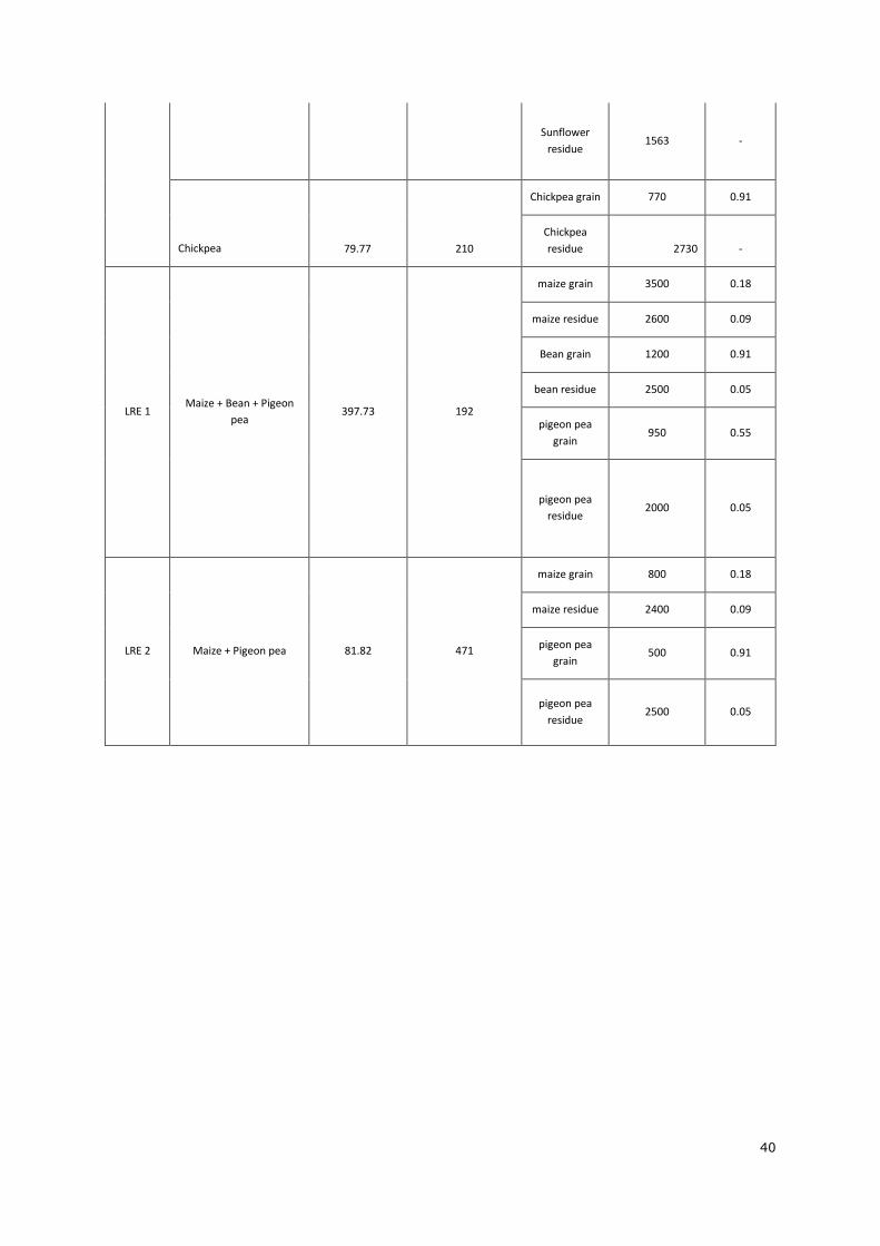
40

Sunflower residue

1563 -

Chickpea 79.77 210

Chickpea grain 770 0.91

Chickpea residue 2730 -

LRE 1 Maize + Bean + Pigeon

pea 397.73

192



Bean grain 1200 0.91


pigeon pea grain

950 0.55

pigeon pea residue

2000 0.05

LRE 2 Maize + Pigeon pea 81.82

471



pigeon pea grain

500 0.91

pigeon pea residue

2500 0.05

Engaging smallholder-farmers in model-based identification ...

Documents

Transcript of Engaging smallholder-farmers in model-based identification ...