Supply-Side Economics “Supply creates its own demand” - Say’s Law.

HAL Id: tel-01760424https://pastel.archives-ouvertes.fr/tel-01760424
Submitted on 6 Apr 2018
HAL is a multi-disciplinary open accessarchive for the deposit and dissemination of sci-entific research documents, whether they are pub-lished or not. The documents may come fromteaching and research institutions in France orabroad, or from public or private research centers.
L’archive ouverte pluridisciplinaire HAL, estdestinée au dépôt et à la diffusion de documentsscientifiques de niveau recherche, publiés ou non,émanant des établissements d’enseignement et derecherche français ou étrangers, des laboratoirespublics ou privés.
Energy Supply and Demand Side Management inIndustrial Microgrid Context
Alemayehu Desta
To cite this version:Alemayehu Desta. Energy Supply and Demand Side Management in Industrial Microgrid Context.Modeling and Simulation. Université Paris-Est, 2017. English. �NNT : 2017PESC1234�. �tel-01760424�

T H È S Een vue de l’obtention du titre de
Docteurde l’Université Paris-Est
Spécialité : Informatique
Alemayehu Addisu Desta
Energy Supply and Demand SideManagement in Industrial Microgrid
Context
soutenue le 4 décembre 2017
Jury
Directeur : Laurent George – ESIEE Paris (LIGM), FranceCo-encadrant : Hakim Badis – UPEM (LIGM), FranceRapporteurs : Maryline Chetto – Université de Nantes (IRCCyN), France
Leandro Soares Indrusiak – Université de York, AngleterreExaminateurs : Pierre Courbin – METRON, France
Bruno Gaujal – INRIA, FranceYe-Qiong Song – Université de Lorraine, France
Invité : David Menga – EDF R&D, France

PhD prepared atESIEE Paris2 boulevard Blaise Pascal,Cité Descartes BP 99,93162 Noisy-le-Grand Cedex, France
PhD in collaboration withMETRON102 rue Réaumur,75002 Paris, France
PhD in collaboration withLIGMLaboratoire d’Informatique Gaspard-MongeCité Descartes, Batiment Copernic5 boulevard Descartes,77454 Marne-la-vallée Cedex 2, France

To my wife and son,To my parents,
To my grandparents, still there or already gone,To my brother and many sisters,
To all my family,To all my friends,
To all the people who have graced my life.
Because each encounter, even a brief one,is an occasion to rediscover oneself
and to marvel.
À ma femme et mon fils,À mes parents,
À mes grands parents, encore là ou déjà partis,À mon frère et mes nombreux sœurs,
À toute ma famille,À tous mes amis,
À toutes les personnes que j’ai eu le privilge de croiser.
Parce que chaque personne rencontre, même brièvement,est une occasion exceptionnelle de se redécouvrir
et de s’émerveiller.


Acknowledgments
I would like to take this opportunity to wholeheartedly thank my thesis supervisor,Prof Laurent George. Since my master’s thesis in ECE Paris, he has been aninspirational figure for me and I thank him for his invaluable help in both academicand private matters. I also wish to express my thanks to my co-supervisor, DrHakim Badis. My sincere gratitude also goes to Dr Pierre Courbin (technicaldirector at METRON) whom I collaborated with for research works that gavefruitful results in this thesis. Around the start of my PhD, he told me to be"fier" (it means "proud" in English) of my thesis. After that moment, I havebeen in "strings attached" mode with my thesis. Mrs Sylvie Cache (secretary ofUPEM’s doctoral school) should also be thanked. I also thank my jury membersProf Maryline Chetto, Dr Leandro Soares Indrusiak, Prof Ye-Qiong Song, DrBruno Gaujal and Mr David Menga for willing to accept our invitations to bejury members of this thesis.
As this thesis is financed by METRON, my special thanks go to Dr VincentSciandra (CEO and co-founder of METRON) and Mr David Tagliabue (presidentof METRON) for their priceless support throughout my thesis. I must say thankyou to my colleagues in METRON (order has no significance): Julien Calderan,José Lopez, Nifemi Ogundare, Anthony Gadiou, Jérémie Rendolet, Victor Nicolas,Yann Le Bail, Jonathan Carmignac and the new employees.
Now, it is time to thank my friends that have special places in my heart. Life couldbe difficult without their friendship and supports. Here they are: Zerihun Gedeb,Getachew Tilahun, Wosen Eshetu, Yirgalem Bereka, Gelila Tafese, EmanuelKassa, Ephrem Berhe, Bezaye Taye, Sergut Tekuamework, Varun Deshpande andAbdenour Kifouche. If a friend of mine could not find his/her name in the list,please pardon me; it is not intentional at all.
Last but no least, I want to thank my wife Meskerem. She put her utmost effortto single-handedly raise my son Leul (it means "Prince" in English and French).I am very much indebted to you madame Meskerem. I also express my warmthanks to my parents, brother and many sisters. Lastly, I would like to thankthe almighty God who I strongly believe gave me the power and the strength toaccomplish this task. Praised be the lord! Amen.


Abstract
Energy Supply and Demand Side Managementin Industrial Microgrid Context
Due to increased energy costs and environmental concerns such as elevated carbonfootprints, centralized power generation systems are restructuring themselvesto reap benefits of distributed generation in order to meet the ever growingenergy demands. Microgrids are considered as a possible solution to deploydistributed generation which includes Distributed Energy Resources (DERs)(e.g., solar, wind, battery, etc). In this thesis, we are interested in addressingenergy management challenges in an industrial microgrid where energy loadsconsist of industrial processes. Our plan of attack is to divide the microgridenergy management into supply and demand sides.
In supply side, the challenges include modeling of power generations and smooth-ing out fluctuations of the DERs. To model power generations, we propose amodel based on service curve concepts of Network Calculus (NC). Using thismathematical tool, we determine a minimum amount of power the DERs can gen-erate and aggregating them will give us total power production in the microgrid.After that, if there is an imbalance between energy supply and demand, we putforward different strategies to minimize energy procurement costs. Based on realpower consumption data of an industrial site located in France, significant costsavings can be achieved by adopting the strategies. In this thesis, we also studyhow to mitigate the effects of power fluctuations of DERs in conjunction withEnergy Storage Systems (ESSs). For this purpose, we propose a Gaussian-basedsmoothing algorithm and compare it with state-of-the-art smoothing algorithms.We found out that the proposed algorithm uses less battery size for smoothingpurposes when compared to other algorithms. To this end, we are also interestedin investigating effects of allowable range of fluctuations on battery sizes.
In demand side, the aim is to reduce energy costs through Demand SideManagement (DSM) approaches such as Demand Response (DR) and EnergyEfficiency (EE). As industrial processes are power-hungry consumers, a smallpower consumption reduction using the DSM approaches could translate intocrucial savings. This thesis focuses on DR approach that can leverage timevarying electricity prices to move energy demands from peak to off-peak hours.To attain this goal, we rely on a queuing theory-based model to characterizetemporal behaviors (arrival and departure of jobs) of a manufacturing system.After defining job arrival and departure processes, an effective utilization function

viii Abstract
is used to predict workstation’s (or machine’s) behavior in temporal domainthat can show its status (working or idle) at any time. Taking the status ofevery machine in a production line as an input, we also propose a DR schedulingalgorithm that adapts power consumption of a production line to available powerand production rate constraints. The algorithm is coded using DeterministicFinite State Machine (DFSM) in which state transitions happen by inserting ajob (or not inserting) at conveyor input. We provide conditions for existence offeasible schedules and conditions to accept DR requests positively.
To verify analytical computations on the queuing part, we have enhancedObjective Modular Network Testbed in C++ (OMNET++) discrete eventsimulator for fitting it to our needs. We modified various libraries in OMNET++to add machine and conveyor modules. In this thesis, we also setup a testbedto experiment with a smart DR protocol called Open Automated DemandResponse (OpenADR) that enables energy providers (e.g., utility grid) to askconsumers to reduce their power consumption for a given time. The objective isto explore how to implement our DR scheduling algorithm on top of OpenADR.

Contents
I General Introduction and Concepts 1
1 General Introduction 31.1 Introduction . . . . . . . . . . . . . . . . . . . . . . . . . . . . . . 31.2 Why microgrids? . . . . . . . . . . . . . . . . . . . . . . . . . . . 41.3 Challenges in two sides of a microgrid . . . . . . . . . . . . . . . . 5
1.3.1 Supply side challenges . . . . . . . . . . . . . . . . . . . . 51.3.2 Demand side challenges . . . . . . . . . . . . . . . . . . . 6
1.4 Motivations and contributions of the thesis . . . . . . . . . . . . . 71.5 Thesis organization . . . . . . . . . . . . . . . . . . . . . . . . . . 8
2 General Concepts and Models 92.1 Introduction . . . . . . . . . . . . . . . . . . . . . . . . . . . . . . 102.2 Microgrid Concept . . . . . . . . . . . . . . . . . . . . . . . . . . 10
2.2.1 Microgrid Architecture . . . . . . . . . . . . . . . . . . . . 112.2.2 Models of Wind, Solar and Storage . . . . . . . . . . . . . 12
2.2.2.1 Wind power . . . . . . . . . . . . . . . . . . . . . 122.2.2.2 Solar PV power . . . . . . . . . . . . . . . . . . . 132.2.2.3 Energy storage systems . . . . . . . . . . . . . . 14
2.2.3 Industrial loads and manufacturing types . . . . . . . . . . 162.2.3.1 Serial production (or transfer) lines . . . . . . . . 162.2.3.2 Assembly/disassembly lines . . . . . . . . . . . . 182.2.3.3 Parallel lines . . . . . . . . . . . . . . . . . . . . 182.2.3.4 Split/merge system . . . . . . . . . . . . . . . . . 182.2.3.5 Closed-loop lines . . . . . . . . . . . . . . . . . . 18
2.2.4 Spot market . . . . . . . . . . . . . . . . . . . . . . . . . . 182.3 Demand Response (DR) . . . . . . . . . . . . . . . . . . . . . . . 19
2.3.1 DR programs . . . . . . . . . . . . . . . . . . . . . . . . . 202.3.1.1 Price-based DR programs . . . . . . . . . . . . . 202.3.1.2 Incentive-based DR programs . . . . . . . . . . . 21
2.3.2 Potential benefits of DR . . . . . . . . . . . . . . . . . . . 232.3.3 Mathematical problems and approaches in DR . . . . . . . 24
2.3.3.1 Utility maximization . . . . . . . . . . . . . . . . 242.3.3.2 Cost minimization . . . . . . . . . . . . . . . . . 242.3.3.3 Price forecast . . . . . . . . . . . . . . . . . . . . 242.3.3.4 Renewable energy integration . . . . . . . . . . . 25
2.3.4 OpenADR - a DR tool . . . . . . . . . . . . . . . . . . . . 252.3.4.1 OpenADR architecture . . . . . . . . . . . . . . . 252.3.4.2 OpenADR services . . . . . . . . . . . . . . . . . 27

x Contents
2.3.4.3 OpenADR implementations . . . . . . . . . . . . 292.4 Service curves of Network Calculus . . . . . . . . . . . . . . . . . 29
2.4.1 Min-plus and Max-plus Algebras . . . . . . . . . . . . . . 302.4.1.1 Min-plus Algebra . . . . . . . . . . . . . . . . . . 302.4.1.2 Max-plus Algebra . . . . . . . . . . . . . . . . . . 32
2.4.2 Service curve concepts . . . . . . . . . . . . . . . . . . . . 322.4.2.1 Common functions as service curves . . . . . . . 342.4.2.2 Strict service curve . . . . . . . . . . . . . . . . . 342.4.2.3 Maximum service curve . . . . . . . . . . . . . . 352.4.2.4 Concatenation and aggregation of service curves . 35
2.4.3 Applications of Network Calculus . . . . . . . . . . . . . . 362.5 Queuing theory overview . . . . . . . . . . . . . . . . . . . . . . . 36
2.5.1 Kendall’s notation for queues . . . . . . . . . . . . . . . . 372.5.2 Little’s Formula . . . . . . . . . . . . . . . . . . . . . . . . 382.5.3 Average-based performance measures of D/D/1 queue . . 39
2.5.3.1 Server Utilization . . . . . . . . . . . . . . . . . . 392.5.3.2 Mean queue length . . . . . . . . . . . . . . . . . 402.5.3.3 Mean waiting time . . . . . . . . . . . . . . . . . 40
2.5.4 Temporal evolution of arrivals and departures . . . . . . . 402.5.5 Applications of queuing theory to manufacturing . . . . . 41
2.6 Summary . . . . . . . . . . . . . . . . . . . . . . . . . . . . . . . 42
II Energy Management in Supply and Demand Sides 43
3 Modeling and Smoothing of DERs 453.1 Introduction . . . . . . . . . . . . . . . . . . . . . . . . . . . . . . 453.2 Related work . . . . . . . . . . . . . . . . . . . . . . . . . . . . . 46
3.2.1 DER modeling . . . . . . . . . . . . . . . . . . . . . . . . 463.2.2 Smoothing of energy production . . . . . . . . . . . . . . . 47
3.3 DER modeling using Service Curves . . . . . . . . . . . . . . . . . 483.3.1 Service curves of DERs . . . . . . . . . . . . . . . . . . . . 48
3.3.1.1 Service curves of solar and wind . . . . . . . . . . 483.3.1.2 Energy storage . . . . . . . . . . . . . . . . . . . 49
3.3.2 Energy supply and demand balance . . . . . . . . . . . . . 503.3.3 Cost minimization strategies . . . . . . . . . . . . . . . . . 51
3.3.3.1 Strategy 1 – Sell excess energy . . . . . . . . . . 513.3.3.2 Strategy 2 – Store excess energy . . . . . . . . . 533.3.3.3 Strategy 3 – Use external energy to charge battery 53
3.4 Smoothing renewable energy production . . . . . . . . . . . . . . 543.4.1 Smoothing algorithms . . . . . . . . . . . . . . . . . . . . 55
3.4.1.1 Moving average-based smoothing . . . . . . . . . 55
Contents xi
3.4.1.2 Gaussian-based smoothing . . . . . . . . . . . . . 563.4.2 Measure of smoothness . . . . . . . . . . . . . . . . . . . . 573.4.3 Constraint on successive power levels . . . . . . . . . . . . 573.4.4 Determining battery size . . . . . . . . . . . . . . . . . . . 57
3.4.4.1 Charging capacity . . . . . . . . . . . . . . . . . 573.4.4.2 Discharging capacity . . . . . . . . . . . . . . . . 583.4.4.3 Final battery capacity . . . . . . . . . . . . . . . 58
3.5 Simulation results . . . . . . . . . . . . . . . . . . . . . . . . . . . 603.5.1 Description of datasets . . . . . . . . . . . . . . . . . . . . 60
3.5.1.1 Solar PV data . . . . . . . . . . . . . . . . . . . 603.5.1.2 Wind speed data . . . . . . . . . . . . . . . . . . 613.5.1.3 Battery parameters . . . . . . . . . . . . . . . . . 623.5.1.4 Energy demand data . . . . . . . . . . . . . . . . 623.5.1.5 Spot market price data . . . . . . . . . . . . . . . 63
3.5.2 Results and discussions on modeling of DERs . . . . . . . 643.5.2.1 Performance of the strategies . . . . . . . . . . . 653.5.2.2 Effect of battery sizes . . . . . . . . . . . . . . . 653.5.2.3 Effect of spot market prices . . . . . . . . . . . . 663.5.2.4 Payback period estimation . . . . . . . . . . . . . 67
3.5.3 Results and discussions on smoothing . . . . . . . . . . . . 693.5.3.1 Performance of the smoothing algorithms . . . . 693.5.3.2 The final power production curve . . . . . . . . . 74
3.6 Summary . . . . . . . . . . . . . . . . . . . . . . . . . . . . . . . 75
4 Industrial Demand Side Management 774.1 Introduction . . . . . . . . . . . . . . . . . . . . . . . . . . . . . . 774.2 Related Work . . . . . . . . . . . . . . . . . . . . . . . . . . . . . 79
4.2.1 Production line modeling . . . . . . . . . . . . . . . . . . . 794.2.2 Scheduling in production lines . . . . . . . . . . . . . . . . 80
4.3 Modeling a Synchronous Production Line . . . . . . . . . . . . . . 814.3.1 Virtual cell . . . . . . . . . . . . . . . . . . . . . . . . . . 814.3.2 Queuing theory-based model for the SPL . . . . . . . . . . 82
4.3.2.1 Arrival instants . . . . . . . . . . . . . . . . . . . 834.3.2.2 Arrival processes at machines . . . . . . . . . . . 864.3.2.3 Departure processes at machines . . . . . . . . . 864.3.2.4 Utilization function . . . . . . . . . . . . . . . . . 874.3.2.5 Power consumption and utilization function . . . 87
4.4 Scheduling in the SPL system . . . . . . . . . . . . . . . . . . . . 884.4.1 Scheduling problem . . . . . . . . . . . . . . . . . . . . . . 904.4.2 DFSM schedule coding . . . . . . . . . . . . . . . . . . . . 914.4.3 Optimal schedule under DR . . . . . . . . . . . . . . . . . 92
4.4.3.1 Phase 1 - Existence of feasible schedule . . . . . . 93

xii Contents
4.4.3.2 Phase 2 - Finding optimal schedule . . . . . . . . 944.4.3.3 Phase 3 - Path to optimal schedule . . . . . . . . 99
4.4.4 DR acceptance conditions . . . . . . . . . . . . . . . . . . 1004.5 Analytical and Simulation Results . . . . . . . . . . . . . . . . . . 101
4.5.1 Results on SPL modeling . . . . . . . . . . . . . . . . . . . 1024.5.1.1 Analytical results . . . . . . . . . . . . . . . . . . 1024.5.1.2 Simulation results . . . . . . . . . . . . . . . . . 104
4.5.2 Result on DR scheduling . . . . . . . . . . . . . . . . . . . 1064.5.2.1 Finding schedule words . . . . . . . . . . . . . . 1074.5.2.2 Monetary gains of accepting DR . . . . . . . . . 109
4.6 Experimentation with OpenADR . . . . . . . . . . . . . . . . . . 1104.6.1 Testbed setup . . . . . . . . . . . . . . . . . . . . . . . . . 110
4.6.1.1 Hardware . . . . . . . . . . . . . . . . . . . . . . 1104.6.1.2 Software . . . . . . . . . . . . . . . . . . . . . . . 111
4.6.2 Description of a DR event . . . . . . . . . . . . . . . . . . 1124.6.3 Communicating DR events between VTN and VEN . . . . 113
4.7 Summary . . . . . . . . . . . . . . . . . . . . . . . . . . . . . . . 114
III Conclusions and Perspectives 115
5 Conclusions and Perspectives 1175.1 Conclusions . . . . . . . . . . . . . . . . . . . . . . . . . . . . . . 117
5.1.1 Modeling of DERs and cost minimization strategies . . . . 1185.1.2 Smoothing of RESs . . . . . . . . . . . . . . . . . . . . . . 1195.1.3 A queue theory-based model of a production line . . . . . 1195.1.4 DR scheduling in a production line . . . . . . . . . . . . . 120
5.2 Perspectives . . . . . . . . . . . . . . . . . . . . . . . . . . . . . . 120
List of symbols 123
Glossaries 125Acronyms . . . . . . . . . . . . . . . . . . . . . . . . . . . . . . . . . . 125Glossary . . . . . . . . . . . . . . . . . . . . . . . . . . . . . . . . . . . 129
Author’s publication list 135
Bibliography 137

List of Figures
1.1 Share of renewables in satisfying global energy consumption over10 years (from 2004 to 2014) [ZL17]. . . . . . . . . . . . . . . . . 5
1.2 Hourly electricity prices in France, Germany and Switzerland on31/07/2017 (from EPEX spot [EPE17]). . . . . . . . . . . . . . . 6
2.1 Architecture of a microgrid. . . . . . . . . . . . . . . . . . . . . . 112.2 Characteristic of wind power production. . . . . . . . . . . . . . . 13
2.2.1 Air flow through rotor area A (m2) at speed V (m/s) . . . . 132.2.2 Power curve of a 3MW wind turbine [Ves] . . . . . . . . . . 13
2.3 Characteristic of solar power production, adapted from [Mer13]. . 132.3.1 Solar radiation on PV array . . . . . . . . . . . . . . . . . . 132.3.2 PV power curve . . . . . . . . . . . . . . . . . . . . . . . . . 13
2.4 Classification of production systems, adapted from [Li+09]. . . . . 162.5 A synchronous production line. . . . . . . . . . . . . . . . . . . . 172.6 EPEX spot energy supply and demands curves. . . . . . . . . . . 192.7 Illustration of PDRs: (a) Time Of Use (TOU), (b) Real-Time
Pricing (RTP), and (c) Inclining Block Rate (IBR) [Den+15]. . . 222.8 Time scales of Demand Response (DR) programs [Qdr06] . . . . 232.9 OpenADR architecture [Haa13]. . . . . . . . . . . . . . . . . . . . 262.10 Example of interactions between VTN and VEN [Haa13]. . . . . . 272.11 VTN and VEN communications using OpenADR services [Haa13]. 282.12 An illustration of service curve concept [LBT01]. . . . . . . . . . . 332.13 Common functions as service curves: (a) peak-rate (b) burst-delay
(c) rate-latency, and (d) affine functions. Adapted from [LBT01]. . 332.14 Concatenation of service curves [VBK16]. . . . . . . . . . . . . . . 362.15 A queuing system. . . . . . . . . . . . . . . . . . . . . . . . . . . 372.16 A realization of arrival and departure processes of jobs where
the left curve represents cumulative arrivals and the right curverepresents cumulative departures [CF10]. . . . . . . . . . . . . . . 41
3.1 Service curve example for a node of DERs (solar or wind). . . . . 493.1.1 Solar/wind power generation . . . . . . . . . . . . . . . . . 493.1.2 Corresponding service curve . . . . . . . . . . . . . . . . . . 49
3.2 Energy demand and supply curves [Add+15]. . . . . . . . . . . . 513.3 Conceptual schematic representation of solar, wind and battery
hybrid system [Add+17c]. . . . . . . . . . . . . . . . . . . . . . . 543.4 Pitfalls of a moving average method. . . . . . . . . . . . . . . . . 56
3.4.1 An example to show limitation of moving average where F(x)is an original function and f(x) is a smoothed output . . . . 56
xiv List of Figures
3.4.2 A 20-min moving average of an actual PV output [AMS14] . 563.5 An illustrating example for battery size computation where the As
and Bs represent charging and discharging cases, respectively. . . 583.6 Solar and wind input data for year 2014 and their power curves. . 61
3.6.1 Hourly average solar power data . . . . . . . . . . . . . . . . 613.6.2 Hourly average wind speed data . . . . . . . . . . . . . . . . 613.6.3 Solar PV power curve . . . . . . . . . . . . . . . . . . . . . 613.6.4 Wind turbine power curve . . . . . . . . . . . . . . . . . . . 61
3.7 Actual and predicted solar and wind data for a period of 24 hours. 623.7.1 Predicted solar power . . . . . . . . . . . . . . . . . . . . . 623.7.2 Predicted wind speed . . . . . . . . . . . . . . . . . . . . . . 623.7.3 Actual and predicted total power . . . . . . . . . . . . . . . 62
3.8 Hourly energy demand of a factory from METRONLab server. . . 633.9 EPEX Day-ahead spot price data for 2014. . . . . . . . . . . . . . 643.10 The three strategies with different battery sizes and fixed spot
price limit of 5AC/MWh for strategy 3. . . . . . . . . . . . . . . . 653.11 Effect of varying spot price with fixed battery capacity of 20MWh. 663.12 Performance of strategy 3 with spot prices in the range [0,50]AC/MWh
and battery size in the range [10,30]MWh. . . . . . . . . . . . . . 673.13 Smoothing performance of SimpleMovingAverage (SMA),Exponential
Moving Average (EMA), and Gaussian-based algorithms with dif-ferent smoothing parameter values. . . . . . . . . . . . . . . . . . 703.13.1Smoothing when σ is 1 and w is 3 . . . . . . . . . . . . . . . 703.13.2Smoothing when σ is 2 and w is 5 . . . . . . . . . . . . . . . 70
3.14 Charging and discharging rates where positive values representcharging and negative values represent discharging. . . . . . . . . 713.14.1Charging and discharging rates when σ is 1 and w is 3 . . . 713.14.2Charging and discharging rates when σ is 2 and w is 5 . . . 71
3.15 Battery sizing based on successive power level constraints with γ∈ [0.05,0.30]. . . . . . . . . . . . . . . . . . . . . . . . . . . . . . 723.15.1Battery sizes when σ is 1 and w is 3 . . . . . . . . . . . . . 723.15.2Battery sizes when σ is 2 and w is 5 . . . . . . . . . . . . . 72
3.16 Power curves for a day-ahead forecast considering different of valuesγ and when σ is 1 and w is 3. . . . . . . . . . . . . . . . . . . . . 733.16.1When γ = 5% . . . . . . . . . . . . . . . . . . . . . . . . . . 733.16.2When γ = 10% . . . . . . . . . . . . . . . . . . . . . . . . . 733.16.3When γ = 15% . . . . . . . . . . . . . . . . . . . . . . . . . 733.16.4When γ = 25% . . . . . . . . . . . . . . . . . . . . . . . . . 73
3.17 Power curves for a day-ahead forecast considering different valuesof γ and when σ is 2 and w is 5. . . . . . . . . . . . . . . . . . . . 743.17.1When γ = 5% . . . . . . . . . . . . . . . . . . . . . . . . . . 743.17.2When γ = 10% . . . . . . . . . . . . . . . . . . . . . . . . . 74
List of Figures xv
3.17.3When γ = 15% . . . . . . . . . . . . . . . . . . . . . . . . . 743.17.4When γ = 25% . . . . . . . . . . . . . . . . . . . . . . . . . 74
3.18 Gaussian-based power production curves for day-ahead forecastconsidering the two cases. . . . . . . . . . . . . . . . . . . . . . . 753.18.1Power curve when σ is 1 and battery size is 294kWh . . . . 753.18.2Power curve when σ is 1, γ is 10%, and battery size is 834kWh 75
4.1 General configuration of a synchronous production line . . . . . . 824.2 An SPL system with 13 virtual cells and 4 machines. . . . . . . . 844.3 Power consumption blocks and additional energy from DERs. . . 884.4 DR mechanism and available power levels. . . . . . . . . . . . . . 894.5 A DFSM for an SPL system with three machines . . . . . . . . . 924.6 DR timelines . . . . . . . . . . . . . . . . . . . . . . . . . . . . . 934.7 Feasible schedule under DR constraint. . . . . . . . . . . . . . . . 944.8 Prefix searching example. . . . . . . . . . . . . . . . . . . . . . . . 974.9 Optimal sub-word searching example. . . . . . . . . . . . . . . . . 974.10 Shortest path to the optimal schedule (phase 3) marked in red
dotted lines. . . . . . . . . . . . . . . . . . . . . . . . . . . . . . . 1004.11 Arrival and departure processes, utilization and effective utilization
of the four machines with processing time of 3s, 6s, 9s and 12s formachine 1, 2, 3 and 4, respectively. . . . . . . . . . . . . . . . . . 1034.11.1Arrival processes using Equation (4.8) . . . . . . . . . . . . 1034.11.2Departure processes using Equation (4.10) . . . . . . . . . . 1034.11.3Utilization using Equation (4.13) . . . . . . . . . . . . . . . 1034.11.4Effective utilization using Equation (4.11) . . . . . . . . . . 103
4.12 Analytical power consumption of machineM2 using Equation (4.14)which is derived from the effective utilization function. . . . . . . 104
4.13 A real power consumption of a typical production process fromMETRONLab server. . . . . . . . . . . . . . . . . . . . . . . . . . 104
4.14 OMNET++ network description of the SPL system with 4 machines.1054.15 The OMNET++-based SPL system in action. . . . . . . . . . . . 1064.16 OMNET++ time line graph for the SPL system. . . . . . . . . . 1064.17 Testbed for implementing OpenADR. . . . . . . . . . . . . . . . . 1104.18 Web interface of the VTN. . . . . . . . . . . . . . . . . . . . . . . 1124.19 Parameters of a DR event. . . . . . . . . . . . . . . . . . . . . . . 1124.20 Real-time status of the pump during normal periods. . . . . . . . 1134.21 Real-time status of the pump during DR periods. . . . . . . . . . 114
5.1 Summary of our works in this thesis. . . . . . . . . . . . . . . . . 118

List of Tables
3.1 Characteristics of two common battery types [Che+09; GFKR15;WLD15; MW15]. . . . . . . . . . . . . . . . . . . . . . . . . . . . 63
3.2 Cost comparison of different strategies (taking 40AC/MWh for costof utility grid energy, battery size of 20MWh for the three strategies,and spot market price limit of 5AC/MWh for strategy 3). . . . . . 64
3.3 Simulation results for payback period estimation by taking 100Photovoltaics (PV) units, a 3MW wind turbine, and varying sizesof two battery types with costs of $400/kWh and $100/kWh forLithium-ion and Lead-acid batteries, respectively. . . . . . . . . . 68
3.4 Maximum charge/discharge rates and smoothness measure of thealgorithms (when σ is 1 and 2 and w is 3 and 5). . . . . . . . . . 70
3.5 Battery sizes for different smoothing parameters of the algorithmswhere ηc = ηd = 85%. . . . . . . . . . . . . . . . . . . . . . . . . 71
3.6 Smoothness measures of the algorithms with successive power levelconstraints of γ% (resulted from Equation (3.12)). . . . . . . . . . 72
4.1 Instantaneous arrival times of tasks on the virtual cells. . . . . . . 844.2 Prefix and sub-word when DR threshold is 100kW. . . . . . . . . 1074.3 Prefix and sub-word when DR threshold is 300kW. . . . . . . . . 108


Part I
General Introduction andConcepts


Chapter 1
General Introduction
Contents1.1 Introduction . . . . . . . . . . . . . . . . . . . . . . . . . . 31.2 Why microgrids? . . . . . . . . . . . . . . . . . . . . . . . . 41.3 Challenges in two sides of a microgrid . . . . . . . . . . . 5
1.3.1 Supply side challenges . . . . . . . . . . . . . . . . . . . . 51.3.2 Demand side challenges . . . . . . . . . . . . . . . . . . . 6
1.4 Motivations and contributions of the thesis . . . . . . . . 71.5 Thesis organization . . . . . . . . . . . . . . . . . . . . . . 8
1.1 IntroductionCurrent power system is dominated by centralized generation in which electricityis distributed to consumers through a macrogrid (e.g., utility grid). Due tochallenges such as increased energy costs and global emissions of greenhouse gases(e.g., carbon dioxide (CO2), chlorofluorocarbons (CFCs), etc), the centralizedgeneration systems need to be restructured in order to meet the ever growingenergy demands [CN09]. A possible solution to these challenges is to deploydistributed generation systems including Distributed Energy Resources (DERs)(e.g., solar, wind, battery, etc) which are normally small in generation capacity(from kW to a few MW capacity range). These resources can be installed close toconsumers’ premises. Being considered as an alternative to centralized generation,microgrids are emerging power systems to manage distributed generations.
Microgrids are relatively small-scale power systems that include electricalloads (any device that consumes electric power, e.g., refrigerators, industrialmachines, etc), DERs and a control system (a formal definition of microgrid isgiven in section 2.2 of the next chapter). A microgrid can operate as a singlesystem (island mode) or it can be connected to a utility grid (grid-connectedmode). Due to introduction of Information and Communications Technologies(ICT) to microgrids, a two-way communication of energy data between producersand consumers is made possible [SW12]. Hence, informed decisions can be takenbased on the information gathered on microgrid components.

4 Chapter 1. General Introduction
According to Hayden [Hay13], microgrids are categorized into 5 types: campusenvironment/institutional, remote off-grid, military base, community/utility andcommercial and industrial (C&I) microgrids. In this thesis, we consider anindustrial microgrid where electrical loads comprise of industrial machines whichare intensive power consumers. The motivation to consider this type of microgridis that we have access to real power consumption data of an industrial plantlocated in France. Thanks to METRON’s platform, we can exploit the data foranalytical and simulation purposes throughout the thesis.
In this chapter, we discuss some potential benefits of microgrids in section 1.2.Then, section 1.3 highlights the challenges in microgrids. After that, we provideour motivations and contributions of this thesis in section 1.4. Finally, section1.5 gives a bird’s eye view of contents of the remaining chapters.
1.2 Why microgrids?According to Parhizi et al. [Par+15], the installed microgrid capacity hasestimated growth of 1.1 GW in 2012 to 4.7 GW in 2017 with an estimatedmarket opportunity of $17.3 billion. The significant benefits associated withmicrogrids have led to vast efforts to expand their penetration in power systems.Based on a report in [VEZ14], potential benefits of microgrids include:
• Renewable integration: Renewable Energy Sources (RESs) play major rolesin satisfying some parts of global energy consumption. From Figure 1.1, wenotice that the average growth rate of modern RESs (except biomass) ismore than twice (around 4.7%) the rate of energy demand in the periodbetween 2004 and 2014. In 2016, the RESs’ share increased to 24.5%according to a report by REN21 (Renewable Energy Policy Network for the21st Century) [ZL17] which is based in Paris, France. Hence, to reap thebenefits of RESs, microgrids are becoming indispensable.
• Increased reliability and resilience: The ability of microgrids to islandenables them to continue providing power to their consumers during eventsof power outage. The ability to island can also be effective in partitioningdistribution feeders in order to isolate faults.
• Relationship of the microgrid to the utility grid: To create smart grids,microgrids can be viewed as fundamental building blocks. This is to saythat future utility grids could be a collection of networked microgrids basedon interactions among control systems that balance energy demand andsupply at micro and macro levels.
• Microgrids as a grid resource: From the utility grid’s view, microgrids canserve as a reliable energy resource, an ancillary service resource, a Demand

1.3. Challenges in two sides of a microgrid 5
Figure 1.1 – Share of renewables in satisfying global energy consumption over 10years (from 2004 to 2014) [ZL17].
Response (DR) (shedding loads in response to requests from utility grid, seeformal definition in section 2.3 of chapter 2) resource or a power consumptionresource (in case of excess generation). Microgrids can also participate inelectricity wholesale markets in order to generate revenues by exportingsurplus power productions.
1.3 Challenges in two sides of a microgridBased on the side of energy generation or consumption, we divide the industrialmicrogrid in two sides: supply and demand sides. In this thesis, we consider twoRESs, namely, solar Photovoltaics (PV) panels and wind turbines in the supplyside. The other side consists of industrial loads. Energy Storage Systems (ESSs)can be in both sides: in supply side when discharging and in demand side whencharging. The following sections describe the challenges we address in both sidesof industrial microgrid energy management.
1.3.1 Supply side challenges
As mentioned above, RESs offer a considerable amount of energy in meeting theglobal energy consumption. However, these resources are intermittent in nature.For instance, the output of solar PV power changes frequently depending onthe position of the sun and clouds. In the same way, wind power is subject tosome of the same types of daily and seasonal variations. The variability in powerproductions of these resources poses challenges to seamlessly integrate them to

6 Chapter 1. General Introduction
Figure 1.2 – Hourly electricity prices in France, Germany and Switzerland on31/07/2017 (from EPEX spot [EPE17]).
a microgrid. The challenges can be categorized into two: how to model RESs’power production and ways to reduce power fluctuations.
Regarding power generation modeling of RESs, we can ask a question likehow to mathematically model the minimum amount of energy that an energyresource can provide? Furthermore, there is also a question of supply and demandbalance: how can we minimize energy costs when demand is greater than supply?To reduce power fluctuations, important questions include how to smooth out thefluctuations using ESSs? What is the size of ESSs to smooth intermittency givenallowable ranges of fluctuations?
1.3.2 Demand side challenges
In the demand side, the concern is how to reduce energy costs. Based on a surveyby the International Energy Agency [IEA16], the industrial plants are accountedfor 42.5% of global electricity consumption in 2015. This will cost them dearlyif cost minimization mechanisms are not put in place. The potential to reduceenergy costs can be gained through implementing Demand Side Management(DSM) approaches such as Energy Efficiency (EE) and DR. The focus of thisthesis is on DR that can leverage the varying electricity prices as shown inFigure 1.2. A cost saving can be achieved through DR mechanisms which includepeak-shaving and load shifting for moving loads from peak to off-peak hours.
Considering DR mechanisms, a scheduling problem could arise: which machine

1.4. Motivations and contributions of the thesis 7
to turn ON or OFF according to a given power threshold? What are the conditionsfor existence of feasible schedules? Conditions to accept a DR positively? Anotherquestion could be how to characterize temporal behaviors (arrival and departureof jobs) of a manufacturing system?
1.4 Motivations and contributions of the thesisOur motivations are two fold. First, to address the challenges detailed above,we believe that concepts from different disciplines should come together. Inthe beginning of this thesis, our area of expertise includes Computer Science,Network Communication and Telecommunication. From these fields, we relyon important concepts such as Network Calculus (NC) and queuing theory toaddress the challenges in energy domain which broaden our field of expertise.Second, nowadays researches on renewables and energy cost reduction are hottopics as a means of securing our energy future. Hence, we want to contributeour part to this global cause.
Contributions of this thesis are classified according to supply and demandsides of industrial microgrid energy management. They are listed below:
• Supply side:
– To attain the minimum power generation of DERs, we proposed amodel based on service curves of NC. Based on actual power con-sumption data of a factory, we also proposed different strategies forminimizing energy costs.
– To mitigate power fluctuations using ESSs, a Gaussian-based smooth-ing algorithm is proposed. The algorithm attains lower ESSs size whencompared to other smoothing algorithms.
• Demand side:
– For characterizing a production system in a temporal domain, weproposed a queuing theory-based model. The model is used to describesystem temporal behaviors such as job/task arrivals and departuresand utilization of a station (or machine). To verify our analyticalworks, we have developed multiple modules in Objective ModularNetwork Testbed in C++ (OMNET++) discrete event simulator.
– For respecting available power and production rate constraints, a graphactivity model is proposed. This model adapts power consumption ofindustrial processes when a utility grid emits a DR signal to consumersin order to reduce power consumption. We also provide conditions ofaccepting DR requests positively and existence of feasible schedules.

8 Chapter 1. General Introduction
1.5 Thesis organizationThe remaining of this thesis consists of four chapters. Contents of each chapterare briefly introduced as follows:
Chapter 2 presents relevant concepts to understand this work. In section 2.2, wediscuss basic concepts of microgrid and models of microgrid elements suchas solar and wind powers, ESSs and electrical loads. Then, section 2.3details DR concepts together with DR program types, benefits of DR,approaches and mathematical problems in DR and a DR protocol whichis called Open Automated Demand Response (OpenADR). After that,we present concepts of service curves of NC that are used to model powergeneration of RESs. Finally, for an objective of modeling a manufacturingsystem, we describe a queuing model with its notations in section 2.5.
Chapter 3 details our works in the supply side of industrial microgrid energy man-agement. The works in the chapter are modeling of DERs and smoothingpower production of RESs. In section 3.3, we provide our model of DERsbased on concepts of service curves of NC. In this context, we use servicecurves to obtain minimum power production of the energy sources. Then,to reduce power generation fluctuations of RESs, we propose a smooth-ing algorithm in section 3.4. We compare its performances against othersmoothing algorithms.
Chapter 4 proposes a queuing model of manufacturing systems and a DR schedulingalgorithm. These two works are categorized under the demand side ofindustrial microgrid energy management. In section 4.3, we detail modelingof a Synchronous Production Line (SPL) system based on a queuing model.We use the model to define SPL system’s temporal characteristics such asjob arrival and departure processes to/from a machine. Then, section 4.4presents our DR scheduling algorithm that adapts SPL’s power consumptionto constraints of available power and production rate. We also provide ourexperiments with OpenADR in section 4.6.
Chapter 5 concludes the works of this thesis by highlighting important points that areraised in each chapter and the corresponding publications. Perspectives ofthe thesis are also provided in the chapter.
In this chapter, we provided research contexts of this thesis and our motivationsto pursue energy management in industrial microgrid. The next chapter discussesessential concepts such as microgrid, service curves of Network Calculus (NC),Demand Response (DR) and queuing theory. These concepts will be used inchapter 3 and 4.

Chapter 2
General Concepts and Models
Contents2.1 Introduction . . . . . . . . . . . . . . . . . . . . . . . . . . 10
2.2 Microgrid Concept . . . . . . . . . . . . . . . . . . . . . . . 10
2.2.1 Microgrid Architecture . . . . . . . . . . . . . . . . . . . . 11
2.2.2 Models of Wind, Solar and Storage . . . . . . . . . . . . . 12
2.2.3 Industrial loads and manufacturing types . . . . . . . . . 16
2.2.4 Spot market . . . . . . . . . . . . . . . . . . . . . . . . . . 18
2.3 Demand Response (DR) . . . . . . . . . . . . . . . . . . . 19
2.3.1 DR programs . . . . . . . . . . . . . . . . . . . . . . . . . 20
2.3.2 Potential benefits of DR . . . . . . . . . . . . . . . . . . . 23
2.3.3 Mathematical problems and approaches in DR . . . . . . 24
2.3.4 OpenADR - a DR tool . . . . . . . . . . . . . . . . . . . . 25
2.4 Service curves of Network Calculus . . . . . . . . . . . . 29
2.4.1 Min-plus and Max-plus Algebras . . . . . . . . . . . . . . 30
2.4.2 Service curve concepts . . . . . . . . . . . . . . . . . . . . 32
2.4.3 Applications of Network Calculus . . . . . . . . . . . . . . 36
2.5 Queuing theory overview . . . . . . . . . . . . . . . . . . . 36
2.5.1 Kendall’s notation for queues . . . . . . . . . . . . . . . . 37
2.5.2 Little’s Formula . . . . . . . . . . . . . . . . . . . . . . . 38
2.5.3 Average-based performance measures of D/D/1 queue . . 39
2.5.4 Temporal evolution of arrivals and departures . . . . . . . 40
2.5.5 Applications of queuing theory to manufacturing . . . . . 41
2.6 Summary . . . . . . . . . . . . . . . . . . . . . . . . . . . . 42

10 Chapter 2. General Concepts and Models
2.1 IntroductionThis chapter discusses fundamental concepts including microgrid,DemandResponse(DR), service curves and queuing theory. These concepts are relevant to our worksin the following chapters. We begin with the concept of microgrid in section 2.2.For understanding the characteristics of microgrids, we provide generic models onDistributed Energy Resources (DERs) such as wind turbines, solar Photovoltaics(PV) panels and Energy Storage Systems (ESSs). Then, in section 2.3, we detailconcepts of DR focusing on DR programs, DR mathematical problems, and anautomated DR enabler technology. Focusing on DR concepts, chapter 4 presentsa DR scheduling algorithm that adapts production in a manufacturing systemaccording to available power and production rate constraints. After that, section2.4 discusses concepts of service curves of Network Calculus (NC) together withbasic mathematical notations and theories. Based on the service curve concepts,chapter 3 details modeling of energy generations of DERs. Next, in section 2.5,we provide an overview of queuing theory by highlighting performance measuresof a relevant queuing model which is used to characterize temporal evolution of amanufacturing system in chapter 4. Finally, section 2.6 summarizes this chapterby mentioning the main points discussed in the chapter.
2.2 Microgrid ConceptThe term microgrid was first coined by Lasseter and Paigi [LP04]. Afterwards,different definitions are given in the literature. We adopt a definition of microgridfrom U.S. Department of Energy (DoE) as given below.
Definition 2.1 (Microgrid [DOE11]).A microgrid is a group of interconnected loads and DERs within clearly definedelectrical boundaries that acts as a single controllable entity with respect to thegrid and that connects and disconnects from such grid to enable it to operate inboth grid-connected (a microgrid supplies or draws power to/from a utility grid)or island mode (a microgrid is disconnected from a utility grid).
Based on this definition, a microgrid is characterized by the following threedistinct features [Par+15]:
• DERs installations must have clearly defined boundaries, i.e., they shouldbe bounded to only one microgrid,
• total power generations need to exceed peak demands so that it could bedisconnected from a utility grid, i.e., it can be in island mode, and
• it must contain computer systems that monitor, control and balance energydemand, supply and storage in response to changing energy needs.

2.2. Microgrid Concept 11
Hence, these characteristics show that a microgrid is a small-scale power systemwith ability of self-healing when there is power interruption in a utility grid.
In the following sections, we first present an architecture of industrial microgridwhere energy demand includes industrial loads (e.g., manufacturing processes).Then, we provide generic models of wind, solar and energy storage in section 2.2.2.In section 2.2.3, we give notations of a manufacturing system which is relevant tochapter 4. At last, a description of spot market is given in section 2.2.4.
2.2.1 Microgrid ArchitectureAn architecture of a microgrid is shown in Figure 2.1. The main microgridcomponents include solar PV panels, wind turbines, ESSs, loads (industrial loadsin our case), energy spot markets, and a microgrid controller. Through a Point ofCommon Coupling (PCC) circuit breaker, it is possible to connect or disconnectthe microgrid from the utility grid. Under normal conditions, the microgrid isconnected to the utility grid for the purpose of energy transactions. However,when there is fault (e.g., power outage, low power quality, etc) in the utility grid,the PCC disconnects the microgrid to be an autonomous system, i.e., it is inisland mode. In this case, local generations in the microgrid should support theloads of the microgrid.
Figure 2.1 – Architecture of a microgrid.
Control and management of microgrids can be established in centralized ordistributed manner. As shown in Figure 2.1, centralized control mechanismrelies on a central controller and it coordinates the DERs in terms of energy

12 Chapter 2. General Concepts and Models
generation scheduling and protection from over-current due to short circuits. Forglobal optimality, the centralized control manner can have the advantage of highefficiency according to Liang and Zhuang [LZ14]. Decentralized control andoperation could be useful in case where distributed control is required (e.g., inremote areas). In such areas, communication network between the DERs and thecentral controller can be interrupted due to geographical distance or unreliablenetwork connections.
2.2.2 Models of Wind, Solar and StorageThis section discusses models of basic microgrid components such as wind turbines,solar PV panels and ESSs.
2.2.2.1 Wind power
Wind turbines generate electrical power by extracting kinetic energy from airflow using rotors and blades (refer to Figure 2.2.1). If the turbines are installedin locations with strong and sustainable winds, the generated power could be ofa significant amount to meet some energy demands.
A typical wind turbine is characterized by its power curve [Car+13] as shownin Figure 2.2.2. The power curve relates wind power to wind speed. The powerPwind (W) extracted from wind speed is proportional to the density of the air,the rotor area, and the cube of the wind speed as in [SPK03]:
Pwind = ρ
2 ∗ Aw ∗ cp(λw, θ) ∗ v3 (2.1)
where
• ρ is air density (kg/m3),
• cp is performance or power coefficient,
• λw is ratio vt/vw (ratio between blade tip speed vt(m/s) and wind speed athub height upstream the rotor vw(m/s)),
• θ is angle of the blade chord to the plane of rotation (or pitch angle), and
• Aw is area covered by rotor of wind turbine (m2).
A conventional way of characterizing the ability of a wind turbine to capturewind power is to use the power coefficient cp which is a function of tip speedratio (λw) and pitch angle (θ). According to Betz’s limit [RR11], the maximumachievable value of cp is 16/27 (59.3%). This upper-bound applies for any type ofwind turbine, i.e., no wind turbine can extract kinetic energy from wind speedhigher than this coefficient. The power coefficient of modern commercial windturbines reaches values between 40 to 50% according to [EBL08].

2.2. Microgrid Concept 13
2.2.1: Air flow through rotor area A (m2) atspeed V (m/s)
2.2.2: Power curve of a 3MW wind turbine [Ves]
Figure 2.2 – Characteristic of wind power production.
2.3.1: Solar radiation on PV array 2.3.2: PV power curve
Figure 2.3 – Characteristic of solar power production, adapted from [Mer13].
2.2.2.2 Solar PV power
Sunlight is an ambient energy source that is available almost everywhere and canbe used to satisfy some parts of energy demand. Solar panels convert the sunlightinto electrical energy in a PV system. Solar panels are composed of a numberof solar cells that contain semiconducting materials which exhibit photovoltaiceffects. To increase conversion efficiency, the PV panel has to operate at itsMaximum Power Point (MPP) on its PV power curve [EC07]. Figure 2.3 showsa PV array and its power curve characteristic.
In a PV system, the electricity generated by solar cells is given as [RY07]:
PP V = SR ∗ cosφ ∗ ηm ∗ Ap ∗ ηp, (2.2)
where

14 Chapter 2. General Concepts and Models
• SR is solar radiation (W/m2),
• φ is angle of incidence calculated by considering β = 45°,
• ηm is efficiency of the Maximum Power Point Tracking (MPPT),
• Ap is area of the PV panel (m2),
• ηp is efficiency of the PV panel.
According to MacKay [Mac08], typical solar panels have efficiency (ηp) of about10%; expensive ones with tracking device can perform up to 20%. The MPPTefficiency (ηm) can have a value of 96% according to [RY07].
2.2.2.3 Energy storage systems
As mentioned in the previous chapter, there is a huge potential in RenewableEnergy Sources (RESs) to produce clean electricity and decrease greenhouse gasemissions by reducing our dependence on fossil fuels as primary energy resources.However, the variability of RESs has led to concerns regarding the reliability ofan electric grid that derives a large fraction of its energy from these sources aswell as the cost of reliably integrating large amounts of variable generation intothe power system. Due to these effects, there has been an increased call for thedeployment of ESSs as an essential component of future energy systems that uselarge amounts of variable renewable resources.
As described in [Den+10], ESSs play an important role in electric grid. Thesignificant impact of ESSs is on energy arbitrage in which energy is purchasedduring low-cost off-peak periods and sold back during expensive peak periods.This reduces use of peaking plants (power plants that run only when there is ahigh demand) and can lower fuel costs. Other roles of ESSs include smoothingof renewable energy generation, operating reserves for electricity regulation,load following to follow longer term (hourly) changes in electricity demand, toblack-start a system after system-wide failure (blackout), etc.
Common energy storage technologies in use today include mechanical, ther-modynamic, electromagnetic and electrochemical [Che+09]. Mechanical energystorage devices are classified into three types: pumped hydroelectric storage(PHS), compressed air energy storage (CAES) and flywheels. Thermodynamicenergy storage (e.g., combined heat and power (CHP)) allows excess thermalenergy to be collected for later use. Electromagnetic storage devices such ascapacitors and super-capacitors store energy in the magnetic field created by theflow of direct current in a superconducting coil. Among electrochemical storagetechnologies, the most common Battery Energy Storage Systems (BESSs) arelead-acid and lithium-ion batteries.

2.2. Microgrid Concept 15
The BESSs have less cost per kWh and commonly used in different applicationssuch as microgrids and electric vehicles. Since we consider BESSs size/capac-ity determination in chapter 3, we detail their important characteristics from[GFKR15] in the following list:
• Battery storage capacity (B): it is the maximum amount of electric chargea BESSs can store. Storage capacity is measured in Amp-hour (Ah). Thefraction of the stored charge that a BESS can deliver depends on factorssuch as BESSs type, ambient temperature, charge/discharge rate, terminalvoltage, etc.
• State of Charge (SoC) (06SoC6100%): it describes how full a storagedevice is. We say that a BESSs is fully charged when its SoC is 100%.
• Depth of Discharge (DoD) (06DoD6100%): it describes how deeply thebattery is discharged. For instance, if a battery is fully charged, its DoDis 0%. Moreover, if a battery is empty, its DoD is 100%. The relationshipbetween DoD and SoC can be described as SoC = 100% - DoD. For somebattery types such as lithium-ion, it is not advisable to discharge them100% DoD, as such discharge could shorten battery life. For this reason,maximum DoD (DoDmax) can be set to lower value than 100% (e.g., 90%).
• State of Health (SoH) (06SoH6100%): This factor reflects the generalcondition of the storage device with respect to its initial condition.
• Efficiency (06 η 6100%): each unit of energy stored is reduced by η unitsthat can be used at a later time. This happens due to inefficiencies inBESSs materials. The efficiency η can be charge efficiency ηc or dischargeefficiency ηd. In our case, we consider η = ηc = ηd.
• Self-discharge (in W): it is due to non-current-producing side chemicalreactions when there is no load attached to the BESSs. In most cases,self-discharge amount ranges from 8 to 20% per year at room temperature.
• Life cycle: number of full charge/discharge cycles before the capacity ofBESSs is reduced to 80%.
Charging and discharging models A BESSs charging/discharging processis described as [CGW12]:
b(t+ ∆t) =b(t) + ∆t ∗ P c(t) charging,b(t)−∆t ∗ P d(t) discharging,
(2.3)
where b(t) represents state of the BESSs at time t, ∆t is time step, and P c(t) andP d(t) are charging and discharging rates at time t, respectively.

16 Chapter 2. General Concepts and Models
For normal operations of BESSs, constraints should be imposed on power andenergy limits. For example, stored energy cannot be greater than its predefinedbattery capacity (B) and cannot be lower than its minimum battery capacity(Bmin), i.e., Bmin 6 b(t) 6 B, where Bmin = (1 - DoDmax)*B. Furthermore,charging/discharging rate constraints are 0 6 P c(t) 6 P c
max(t) and 0 6 P d(t) 6P d
max(t), where P cmax(t) is maximum charging rate and P d
max(t) is maximumdischarge rate at time t.
2.2.3 Industrial loads and manufacturing typesIndustrial load consists of electrical load demands by manufacturing plants orindustries. According to Zhang et al. [Zha+16], most manufacturing plants havealready installed smart meters and control infrastructures which are necessary forDR. In this section, we discuss a specific manufacturing type that we use for ourwork on DR in chapter 4. Furthermore, we provide a brief description of othermanufacturing types (just for comparison of their working principles) as depictedin Figure 2.4.
Production Systems
SerialLines
Assembly/disassemby
Systems
ParallelLines
Split/MergeScrapping
Closed LoopSystems
ReworkLoops
Loops withConstant Number
of carriers
Figure 2.4 – Classification of production systems, adapted from [Li+09].
2.2.3.1 Serial production (or transfer) lines
Since we use notations and concepts of serial production lines in chapter 4, wegive more emphasis on these manufacturing types. Serial lines are the mostpractical production systems in many manufacturing plants. Serial lines havebeen classified according to the type of part transfers: continuous, asynchronousand synchronous [GF99]. In continuous part transfer lines, the movement of partsis continuous with constant speed. In systems with asynchronous part transfer,each part moves independently of other parts which results in cycle variationsbetween workstations/machines. Parts move simultaneously between machines in

2.2. Microgrid Concept 17
systems with synchronous part transfer. Focusing on the Synchronous ProductionLine (SPL) shown in Figure 2.5, the following assumptions are defined [DG92;Li+09]:
• the production line consists of M machines in series that are connected bya conveyor system,
• each part is processed on a machine for some fixed duration, i.e., itsprocessing time,
• the machines are reliable, i.e., there is no failure among the machines,
• the conveyor is blocked until the machine with the maximum processingtime finishes,
• machine Mi consumes pi amount of power when it processes a part,
• the production rate, i.e., number of finished parts per time unit, dependson the processing rate of the last machine(MM) in the system.
Figure 2.5 – A synchronous production line.
Regarding the working principle of the serial production line, we assume thatthe machines start processing at the same time but may not necessarily finishequally because the processing times could be different. In the system, unfinishedtasks are processed first at machine M1, then at machine M2, and so on untilthe last machine MM after which they leave the system. All the tasks have tobe processed for a duration of Ci at machine Mi. When the conveyor is moving,all the machines wait until an unfinished task arrives in their respective slots.Hence, the system uses Blocking After Service (BAS) mechanism to handlesynchronization between the machines and the conveyor.

18 Chapter 2. General Concepts and Models
2.2.3.2 Assembly/disassembly lines
In assembly systems, the assembly machine will only process a part when upstreambuffers are not empty, i.e., parts have to wait not only for the machine to becomeavailable but also for the other parts of the assembly to arrive before the machinecan begin processing. This imposes synchronization constraints at assemblystations and this introduces dependencies between the machines. More detailsand models are provided by Li, Alden, and Rabaey [LAR05].
2.2.3.3 Parallel lines
To increase production, parallel lines have been used in manufacturing system.The machines at each stage could have identical processing times and aggregatingthe machines at the stage can form a serial production line to simplify analysisand modeling. Details can be found in [Li04].
2.2.3.4 Split/merge system
Split and merge operations are typically used to increase production capacity andvariety, improve product quality, and implement product control and schedulingpolicies. Merge operations load parts at the same time to compose them to asingle part when parts exist in the upstream buffers. Split operations split a partinto multiple parts when downstream buffers are not full [LH05].
2.2.3.5 Closed-loop lines
Closed-loop lines are serial production systems where one or more loops areattached to the line. The loops can be used for rework of defective parts or qualityimprovement. Frein, Commault, and Dallery [FCD96] and Gershwin andWerner [GW07] give more details on this manufacturing type.
2.2.4 Spot marketAn electricity spot market can be regarded as a market where the electricity canbe sold or purchased at varying prices throughout a day. Wholesale transactions(bids and offers) in electricity are managed by the market operator. In Europe,EPEX (European Power EXchange) handles these transactions. It operatesin France, Germany, the United Kingdom, the Netherlands, Belgium, Austria,Switzerland and Luxembourg. EPEX spot manages two types of spot markets,namely, day-ahead and real-time markets.
In day-ahead spot markets, an auction process is organized by EPEX spot. Itdetermines market price based on the intersection of supply and demand curvesas shown in Figure 2.6. Once the prices are determined for each hour of the

2.3. Demand Response (DR) 19
Figure 2.6 – EPEX spot energy supply and demands curves.
following day, the results are published to buyers and sellers from 11:10 am (inSwitzerland) and 12:55 pm (in all other markets) [EPE17].
For real-time spot markets, the transaction of energy is performed closeto real-time (e.g., in 15 minutes) based on contracts. These contracts help toaccommodate intermittent energy resources by responding to intra-hour variationsof energy production and consumption.
In this section, we discussed concepts of microgrids including the architectureand basic components of an industrial microgrid. The following section presentsan important concept: DR.
2.3 Demand Response (DR)In legacy power systems, the main focus has been improving power supply basedon evolution of electricity demands. However, due to recent emergence of smartgrids, a Demand Side Management (DSM) also plays a crucial role by managingflexible loads. According to a World Bank report prepared by River [Riv05],DSM is defined as follows.
Definition 2.2 (DSM [Riv05]).DSM encompasses systematic utility and government activities designed to changethe amount and/or timing of the customer’s use of electricity for the collectivebenefit of the society, the utility and its customers.
Under DSM, there are two concepts: Energy Efficiency (EE) and DR. Referringto [YK05], a definition of EE is given below.
Definition 2.3 (EE [YK05]).EE involves technology measures that produce the same or better levels of energy
20 Chapter 2. General Concepts and Models
services (e.g., light, space conditioning, motor drive power, etc.) using less energy.The technologies that comprise efficiency measures are generally long-lastingand save energy across all times when the end-use equipment is in operation.Depending on the timing of equipment use, EE measures can also producesignificant reductions in peak demand.
According to this definition, EE programs involve replacing existing consumers’devices with new devices that are energy efficient (e.g., replacing old incandescentlamps with new fluorescent lamps). These programs offer financial incentives toencourage customers to acquire, install and adopt more energy efficient technolo-gies. EE actions incorporate both short-term conservation actions and long-terminvestments in EE. Besides investing in EE, customers can also participate inDR programs (see section 2.3.1). The objective of this section is to pursue in thedirection of DR because the concepts we discuss here lay the groundwork for ourwork in chapter 4.
In a power system, DR is regarded as an effective approach to increaseelectricity grid performance and consumer benefits. According to US FederalEnergy Regulatory Commission [Kat+12], DR is defined as follows.
Definition 2.4 (DR [Kat+12]).DR refers to changes in electric usage by end-use customers from their normalconsumption patterns in response to changes in the price of electricity over time,or to incentive payments designed to induce lower electricity use at times of highwholesale market prices or when system reliability is jeopardized.
In the following sections, we first discuss different categories of DR programs.Then, discussions of DR potential benefits and mathematical problems andapproaches in DR are provided. The concluding section of DR portion of thischapter gives a brief description of a smart DR enabling technology called OpenAutomated Demand Response (OpenADR).
2.3.1 DR programsDR programs throttle energy demands of different loads such as industrial,commercial and residential for adjusting demands to available power productions.DR programs are mainly divided into two branches: price- and incentive-based DRprograms. The following sections discuss the two DR programs citing referencessuch as [Riv05; Qdr06; Den+15; ZG16].
2.3.1.1 Price-based DR programs
In price-based DR (PDR) programs, the price of electricity varies over time sothat customers are motivated to adjust their power consumption patterns. Theprice of electricity may differ from peak to off-peak times significantly. Hence,

2.3. Demand Response (DR) 21
customers would pay the highest prices during the peak periods and the lowestprices during the off-peak periods. The prices can be communicated to customersa day in advance or in real-time based on pricing mechanisms. The pricingmechanisms are classified into 4 types [Riv05; Qdr06; Den+15]:
• Time Of Use (TOU): customers are charged with different prices whenthey consume electricity at different time intervals of a day or differentseasons of a year. In most cases, the time intervals are divided into block of1 hour. TOU rates charge customers based on tariffs for off-peak and peaktime blocks. Electricity prices at the peak time blocks are much higherthan that at off-peak time blocks.
• Critical Price Peaking (CPP): in this pricing mechanism, customers areon TOU rates for most hours of the year. However, they face additionalcharges during a small number of critical hours when system reliabilityis jeopardized or very high prices are encountered in wholesale marketsbecause of extreme weather conditions. During non-CPP periods, CPPcustomers typically receive a price discount. The Tempo tariff of EDF(Électricité de France) is an example of CPP tariff. With tempo tariff, ayear is divided into 22 red, 43 white and 300 blue days, and each day has apeak and an off-peak periods and corresponding tariffs [Alt+11].
• Real-Time Pricing (RTP): in this tariff type, the electricity price usuallyvaries at different time intervals of a day close to real-time, i.e., every 15minutes or every hour. RTP prices are typically known to customers ona day-ahead, hour-ahead or 15 minutes ahead basis (see an illustration inFigure 2.7b).
• Inclining Block Rate (IBR): rate structure of this tariff has two levels: lowerand higher blocks (see Figure 2.7c). If customers’ hourly/daily/monthlyenergy consumption exceeds a predefined threshold, electricity prices climbup to the higher block. Several energy providers in USA such as Pacific Gasand Electric (PG&E), Southern California Edison (SCE), San Diego Gasand Electric (SDG&E) have been using IBR tariffs since the 1980s [Bor08].
A graphical summary of some of the price-based DR programs is shown inFigure 2.7. In the figure, the TOU rates are divided into three time block types:off-peak, mid-peak, and on-peak. The electricity price at the on-peak time block ismuch higher than that at the mid-peak and off-peak time blocks so that customersshift their loads over another time horizon.
2.3.1.2 Incentive-based DR programs
Incentive-based DR (IDR) programs reward participating customers for reducingtheir electricity usage in response to DR requests from grid operators. IDR

22 Chapter 2. General Concepts and Models
Figure 2.7 – Illustration of PDRs: (a) TOU, (b) RTP, and (c) IBR [Den+15].
programs diversify the ways in which demand side management contributes toreliable and efficient grid operations because these programs can be tailoredaccording to specific requirements. The programs in this category are listed asfollows [Qdr06; ZG16]:
• Direct load control is a program in which customers receive incentive pay-ments for allowing the utility operator some degree of control over theirequipments such as air conditioners and water heaters. While direct loadcontrol programs are primarily offered to residential and small commercialcustomers, it usually cannot be applied to industrial customers due to safetyconcerns.
• Interruptible/curtailable service is used to provide customers with a discountrate or bill for agreeing to reduce load on request. These services havetraditionally been offered only to the largest industrial and commercialcustomers.
• Demand Bidding/Buyback Programs encourage large customers to bid intoa wholesale electricity market by providing load reduction prices at whichthey are going to be curtailed.
• Emergency Demand Response Programs provide incentive payments forcustomers to reduce loads during reliability-triggered events. Enrolledcustomers that do not respond to this program may incur penalties.
• Capacity Market Programs give incentive payments for customers that cancommit to providing pre-specified load reductions when system contingenciesarise. These programs typically entail significant penalties for customersthat do not respond when asked for load reduction.
• Ancillary Services Market Programs provide incentive payments for cus-tomers from the grid operator for committing load curtailment to be standbyas operating reserves. If load curtailment is requested from the operator,the customers may get paid according to prices on the spot market.

2.3. Demand Response (DR) 23
Figure 2.8 – Time scales of DR programs [Qdr06]
Figure 2.8 shows time scales of both price- and incentive-based DR programs.Price-based DR programs can be incorporated into utilities’ planning at differenttime scales that can include TOU, CPP and RTP rates. Incentive-based DRprograms may be introduced at virtually all time scales which can notify customersin hourly, daily, and real-time fashions based on the programs. In chapter 4, weconsider the incentive-based DR in which power consumption is upper boundedby the request of the utility grid.
2.3.2 Potential benefits of DR
DR has a broad range of potential benefits primarily as resource savings (e.g.,reduction in peaking plants) that improve the efficiency of power systems. Inpractice, these benefits depend on many factors including purpose, design, andperformance of the implemented DR programs, the enabling technologies and thestructure of the electricity markets [Qdr06]. The benefits of demand response canbe classified in terms of whether they are interesting directly to participants orto some or all groups of electricity consumers as follows:
• Participant bill savings: electricity bill savings and incentive payments forcustomers willing to adjust their loads in response to current supply costsor other incentives.
• Bill savings for other customers: DR results in lower wholesale marketprices which in turn reduces supply costs to retailers that provide electricityto non-DR costumers.

24 Chapter 2. General Concepts and Models
• Reliability benefits: refers to reduced probability of power outages and notincurring higher financial costs and inconvenience for customers.
• Market performance: DR prevents the exercise of market power by electricpower producers, i.e., it encourages fair marketers (e.g., prevents overreduction of prices to influence the market).
• Improved choices: more options for customers to manage their electricitycosts by choosing energy providers according to their will.
• Power system security: grid operators are endowed with more flexible meansto meet contingencies and reduce costs.
2.3.3 Mathematical problems and approaches in DRBased on a survey by Deng et al. [Den+15], this section provides a list of existingmathematical problems in DR and different approaches for solving them. Themajor DR mathematical problems include utility maximization, cost minimization,price forecast, and renewable energy integration.
2.3.3.1 Utility maximization
In utility maximization problem, the aim is to first define utility functions thatquantify levels of customer satisfactions as a function of customer’s power consump-tion [Sam+10; LCL11]. Then, the objective function is to maximize customer’swelfare respecting varies constraints including power consumption profiles ofdevices, available power, etc. Several approaches such as convex optimization[Sam+10] and dynamic programming [JL11] are proposed in the literature totackle this problem.
2.3.3.2 Cost minimization
This problem defines an energy consumption scheduling where the objective isto minimize energy costs for the customers. Potential approaches include gametheory and convex optimization [Sam+10].
2.3.3.3 Price forecast
In price prediction problem, the goal is to include a dynamic price predictor inan energy consumption scheduler. The dynamic price predictor computes pricesthat can reflect the actual wholesale price at the time of consumption and type ofa day (working or weekend). Mohsenian-Rad and Leon-Garcia [MRLG10]proposed a linear programming (LP) approach for the price prediction problem.

2.3. Demand Response (DR) 25
2.3.3.4 Renewable energy integration
This problem considers integration of DR with intermittent RESs such as wind,solar, etc. It incorporates energy generation of the resources into an optimizationproblem (e.g., minimizing cost by using locally generated power when electricityprice is high or storing for later use). This type of DR problem was consideredby Jiang and Low [JL11].
2.3.4 OpenADR - a DR toolOpenADR [All13] was developed at Demand Response Research Center (DRRC)of Lawrence Berkeley National Laboratory (LBNL) [LBN] and its first specificationwas released in 2009. To enhance the development, adoption and compliance ofOpenADR standards throughout the energy industry, a collaboration betweenindustry stakeholders was initiated to form an OpenADR Alliance [Ope] in2010. The alliance was created to standardize, automate and simplify DR, tomeet growing cost effective energy demand of utilities, and to allow customerscontrolling the way they use energy. In the version 1.0 of the specification [Pie+09],the LBNL described OpenADR as follows.
Definition 2.5 (OpenADR [Pie+09]).OpenADR is a communication data model designed to facilitate sending andreceiving DR signals from a utility or independent system operator to electriccustomers. The intention of the data model is to interact with building andindustrial control systems that are pre-programmed to take action based on a DRsignal, enabling a demand response event to be fully automated, with no manualintervention. The OpenADR specification is a highly flexible infrastructure designto facilitate common information exchange between a utility or IndependentSystem Operator (ISO) and their end-use participants. The concept of an openspecification is intended to allow anyone to implement the signalling systems,providing the automation server or the automation clients.
The OpenADR 1.0 specification was based on OASIS (Organization of Struc-tured Information Standards) Energy Interoperation (EI) standard [OAS]. UnderOASIS’ EI, OpenADR 2.0 profile builds on OpenADR 1.0 and it handles morecomplex interactions of DR and DERs, while keeping in mind the requirementsof diverse markets and stakeholders needs. In this section, we discuss OpenADRarchitecture, some services and implementations of OpenADR 2.0.
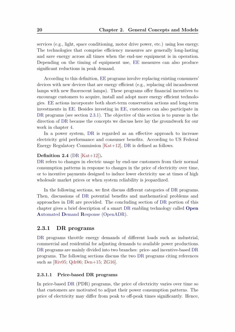
2.3.4.1 OpenADR architecture
In OpenADR architecture, there are two communicating nodes that act as clientsor servers:
26 Chapter 2. General Concepts and Models
Figure 2.9 – OpenADR architecture [Haa13].
• nodes that publish and communicate event information to other nodes (e.g.,utilities). These nodes are called Virtual Top Node (VTN) and act asOpenADR servers,
• nodes that receive, process and respond to the information (e.g., electricityconsumers). These nodes are called Virtual End Node (VEN) and act asOpenADR clients.
Figure 2.9 shows an architecture of OpenADR with different combination ofVTN and VEN interactions. In the figure, a VTN (i.e., DR service provider)can communicate events (e.g., electricity prices, grid reliability, etc) directly toan end customer (e.g., site A) or to an aggregator VEN. Then, the aggregatorbecomes VTN for another VENs such as site C, D, and E. Based on pair-wiserelationship of VTN–VEN, a complex structure could be implemented that canaddress complex interactions in DR such as shown in Figure 2.10.
In Figure 2.10, certain nodes (B, E and G) act as both VTN and VEN. Thearrows from VTN to its VENs could model a DR event initiated by the utilitygrid A that can invoke an operation on its second level VTNs (B to E) which aregroup of aggregators. For example, the second level VTN B can invoke serviceson its VENs F , G and H, which represent their customers. The customers mightbe industrial parks with multiple facilities, real estate developments with multipletenants, or a company headquarters with facilities in many different geographical

2.3. Demand Response (DR) 27
Figure 2.10 – Example of interactions between VTN and VEN [Haa13].
areas.Regarding to communication protocols, the VTN and VEN can communicate
using HTTP (HyperText Transfer Protocol) either in PUSH mode where the VTNinitiates communication or in a PULL mode where the VEN continuously requestsVTN for information [All13]. XML Messaging and Presence Protocol (XMPP)can also be used as transport mechanism between VTN and VEN. Both HTTPand XMPP use XML (eXtensible Markup Language) format for a standardizeddata representation during OpenADR message communication. According to theprotocol specification, the VTN should support both HTTP and XMPP protocols,but the VEN should support either of the two.
2.3.4.2 OpenADR services
To facilitate common information exchanges between VTNs and VENs, OpenADR2.0 provides the following 8 services [All13]:
• EiRegisterParty: used by VENs to perform in-band registration to VTNs.In this service, VENs and VTNs agree on parameters such as transportmechanisms (HTTP or XMPP), OpenADR profiles (2.0a or b), etc.
• EiEnroll: used by VENs to enroll their resources to participate in DR.
• EiMarketContext: used to discover DR program rules, standard reports,etc. Since market information rarely changes, it is not necessary to sendmarket information every time.
• EiEvent: used by VTNs to convey DR events to VENs to indicate whetherresources are going to participate in the event. It is a core function in theinformation models of OpenADR.
• EiQuote: used by VTNs to communicate complex dynamic prices such asblock and tier tariffs to VENs.

28 Chapter 2. General Concepts and Models
• EiReport: used by VTNs and VENs to exchange historical, telemetry, andforecast reports. Using this service, VENs can report their resource statusincluding availability, forecast, real-time energy and curtailment readings.
• EiOpt: used by VENs to communicate Opt-in and Opt-out (temporaryavailability to accept DR) schedules to VTNs. The VEN sends Opt-inmessage to the VTN if it accepts the DR request or Opt-out otherwise.
• EiAvail: used by VENs to indicate when an event may or may not beaccepted. VENs execute EiAvail with respect to a Market Context. IfVTNs know the availability and opt information of VENs, they can improvetheir ability to estimate VEN’s response to events or requests.
Figure 2.11 – VTN and VEN communications using OpenADR services [Haa13].
As shown in Figure 2.11, VTN and VEN commences communication byusing EiRegisterParty service which is sent from VEN to VTN, assuming thatenrollment and market information exchange were done a priori. After agreeingon OpenADR parameters in EiRegisterParty, VEN and VTN exchange reportcapabilities using EiReport service. Then, the VTN can send DR event to VENby specifying DR start time, DR duration, amount/percentage of load shedding,etc in EiEvent service. At this moment, the VEN not only responds with EiOptbut also with temporary availability schedule. The communication continues withexchange of periodic reports to verify if the DR event has resulted in the targetedload shed. The VTN and VEN can repeat the same process in other times tonotify another DR event.

2.4. Service curves of Network Calculus 29
2.3.4.3 OpenADR implementations
Existing implementations of OpenADR use either HTTP or XMPP as trans-port mechanisms. OpenADR Alliance certified OpenADR implementations aremostly provided by two organizations: EPRI (Electric Power Research Institute)and EnerNOC. EPRI selected a simple HTTP implementation and uses C#programming language to implement the OpenADR services in VEN side andRuby on Rails web-application framework for VTN side. Source codes for VTNand VEN are available from [EPR]. EnerNOC provides XMPP-based OpenADRimplementation and use Java and Python programming languages for VEN andGrails/Groovy web-application framework for VTN. Source codes are available inEnerNOC’s GitHub [Ene].
Since the OpenADR protocol specification is based on XML, the availabilityof Java language specific tools for creating, manipulating and binding XMLdocuments to program elements encourages us to choose the EnerNOC imple-mentations of OpenADR. As both Java and Python languages are frequentlyused in the enterprise METRON, the integration of OpenADR to METRON’sarchitecture was done with relative ease. Since the source code of EnerNOC onlyprovide the EiEvent service, we modified the code to add the other services. Inchapter 4, we provide a use case of OpenADR in METRON.
In the next section, we detail relevant concepts of service curve which will beused in chapter 3 to model power generation of DERs.
2.4 Service curves of Network CalculusNC is a system theory that has been developed to give a theoretical frameworkfor analyzing performance guarantees in computer networks based on min-plusand max-plus algebras. Specifically, NC is used to compute worst case bounds ondelay and buffer requirements in a network. It was initially introduced by Cruz[Cru91] for communication network elements where the analysis of delay boundsand buffer requirements followed a non-probabilistic approach. After this initialwork on NC, two works were published around the beginning of 2000. In 2000,the book of Chang [Cha00] gave formal presentation of the operators of the NCand their use in a case where time and data are discrete values. Then, in 2001,Le Boudec and Thiran [LBT01] described all the necessary tools of NC aswell as the conditions of application and provided several illustrating examples ofapplication on different problems in their book.
NC consists of two branches: stochastic and deterministic NC. In StochasticNetwork Calculus (SNC), computations of worst case performance bounds arebased on probabilistic distributions, i.e., some violations of the deterministicbounds are tolerable with small probability. More details on SNC can be found

30 Chapter 2. General Concepts and Models
in [JL08]. In this work, we focus on the deterministic Network Calculus (DNC)where deterministic worst case performance bounds are computed. Under DNC,NC provides basic concepts including arrival, service curves and shapers. Sincewe don’t rely on arrival curves and shapers, a reader may want to refer to [LBT01]for more details on the two concepts.
In the following sections, focusing on the service curve concepts, we discussnotations and theories which are relevant to our work on modeling of energygeneration of DERs in chapter 3. First, a brief overview of min-plus and max-plusalgebras is given in section 2.4.1. Next, section 2.4.2 details the service curveconcepts with few demonstrating examples. Finally, some applications of NC areprovided in section 2.4.3.
2.4.1 Min-plus and Max-plus Algebras
Before defining the concepts of service curves, we first introduce the two importantunderlying mathematical concepts: min-plus and max-plus algebras. Since themin-plus algebra is frequently used in service curves, we give more emphasison the concepts of the min-plus algebra and detail only few notations on themax-plus algebra concepts.
2.4.1.1 Min-plus Algebra
In conventional algebra, addition and multiplication are the two most commonoperations on real R and integer Z numbers. The particular properties of the twooperators make the algebraic structure (Z, +, x) as a commutative ring and (R,+, x) as a commutative field [LBT01]. In min-plus algebra, the multiplicationoperator is replaced by the addition operator and the addition operator is replacedby the infimum (or minimum if it exists) operator (∧). Min-plus operators canalso be applied to +∞ that results in another algebraic structure (R∪{+∞},∧,+).Algebraic properties of the structure such as associativity, commutativity, etc aredetailed in the book of Le Boudec and Thiran [LBT01](page 105). Basedon the properties of the min-plus algebra, we discuss important features such asproperty of wide-sense increasing functions and convolutions that are necessaryto define service curve concepts.
Wide-sense increasing functions A function f is said to be wide-senseincreasing if and only if f(s) > f(t), ∀s > t. We adopt the following notations:
• G: a set of non-negative wide-sense increasing functions,
• F : a set of non-negative wide-sense increasing functions such that f(t) = 0if t < 0.

2.4. Service curves of Network Calculus 31
The range of F and G functions is R+ = [0, +∞]. Some of these functions canbe used as service curves (see section 2.4.2.1).
Pseudo-inverse of wide-sense increasing functions For an invertible func-tion f , there exists a function f−1 such that f−1(f(t)) = t for all t. However,wide-sense increasing functions are not always invertible. Hence, a pseudo-inversef−1 of a function f ∈ F is defined as:
f−1(x) = inft>0{t : f(t) > x}. (2.4)
Concave and convex functions Concave and convex functions are importantfunctions of the min-plus algebra. A function f : R 7→ R is convex if and only if
f(ux+ (1− u)y) 6 uf(x) + (1− u)f(y), ∀x, y ∈ R, u ∈ [0, 1], (2.5)
and, a function f : R 7→ R is concave if and only if −f is convex or if and only if
f(ux+ (1− u)y) > uf(x) + (1− u)f(y), ∀x, y ∈ R, u ∈ [0, 1]. (2.6)
Some functions such as rate-latency functions are convex functions and somepiece-wise linear functions are concave functions.
Min-plus convolution In classical system theory, the convolution of twofunctions f(t) and g(t) is defined as:
(f ∗ g)(t) =∫ t
0f(t− s)g(s) ds, t > 0. (2.7)
Changing the addition into infimum and the multiplication into addition, thefollowing definition of the min-plus convolution is given.
Definition 2.6 (Min-plus convolution).Assuming that f, g ∈ F , the min-plus convolution of f and g is:
(f ⊗ g)(t) = inf06s6t{f(t− s) + g(s)}, (2.8)
given that (f ⊗ g)(t) = 0 if t < 0.
An important property of min-plus convolution is that if f and g are convexand piece-wise linear functions, their convolution f⊗g is obtained by putting end-to-end the different linear pieces of the individual functions, sorted by increasingslopes. This property is very useful during concatenation of two functions as willbe shown in section 2.4.2.4.

32 Chapter 2. General Concepts and Models
Min-plus deconvolution The dual operation of the min-plus convolution isdefined as follows.
Definition 2.7 (Min-plus deconvolution).Assuming that two functions f and g are in F , their min-plus deconvolution isgiven by:
(f � g)(t) = supu>0{f(t+ u)− g(u)}. (2.9)
Illustrating examples and proofs are provided in the work of Le Boudec andThiran [LBT01], and Van Bemten and Kellerer [VBK16]. These referencescan be consulted if more details are required.
2.4.1.2 Max-plus Algebra
In max-plus algebra, the algebraic structure is changed into (R ∪ {−∞},∨,+) byreplacing the infimum operator by supremum operator ∨ and +∞ by −∞. Sincewe don’t use the max-plus algebra in this work, interested readers may want torefer to the book of Le Boudec and Thiran [LBT01]. The following sectiondiscusses the concepts of service curves.
2.4.2 Service curve conceptsThe concept of service curve is used to abstract the details of packet schedulingwhich requires a network or node to offer some guarantees to flows. The followingdefinition of a service curve gives a general service curve concept used in NC.Referring to [LBT01], a service curve is defined as follows.
Definition 2.8 (Service curve [LBT01]).Consider a system S and a flow through S with input and output functions Rand R∗, respectively. We say that S offers to the flow a service curve β if andonly if for all t > 0, there exists some s > 0, with s 6 t, such that
R∗(t)−R(s) > β(t− s), (2.10)
or equivalently,R∗ > R⊗ β, (2.11)
or alternatively,R∗(t) > inf
s6t{R(s) + β(t− s)}, (2.12)
where β(0) = 0, β is wide-sense increasing, and R(t)/R∗(t) are cumulative numberof input/output bits in interval (0,t].
Figure 2.12 illustrates the concept of service curve. In the figure, the outputR∗ of the system must always be greater than the convolution of the input R

2.4. Service curves of Network Calculus 33
Figure 2.12 – An illustration of service curve concept [LBT01].
with the service curve β of the system. The output R∗ lies in the area betweenthe input R and R⊗ β. From the figure, we can also see that the service curveconcept provides a lower bound on the service a system can offer. Based on thisgeneral definition of service curves, the following sections detail three types ofservice curves: functions as service curves, strict, and maximum service curves.Furthermore, we investigate concatenation of service curves.
Figure 2.13 – Common functions as service curves: (a) peak-rate (b) burst-delay(c) rate-latency, and (d) affine functions. Adapted from [LBT01].

34 Chapter 2. General Concepts and Models
2.4.2.1 Common functions as service curves
The functions most commonly used as service curves include peak-rate, burst-delay,rate-latency, and affine functions. They are defined as follows:
• peak-rate function: for some rate R > 0, a peak-rate function is defined as:(see Figure 2.13a):
λR(t) =Rt if t > 0,
0 otherwise.(2.13)
• burst-delay function: referring to Figure 2.13b, a burst-delay function withdelay time T > 0 is given as:
δT (t) =+∞ if t > T,
0 otherwise.(2.14)
By convolving any function with δT , it can be shifted to the right by T .
• rate-latency function: with delay T > 0 and rate R > 0, a rate-latencyfunction can be expressed as (see Figure 2.13c):
βR,T (t) = R[t− T ]+ =R(t− T ) if t > T,
0 otherwise.(2.15)
The rate-latency service curve is usually used to model a generalized processsharing (GPS) scheduler where each flow gets a share of at least R.
• affine function: for some rate r > 0 and burst b > 0, an affine function isdefined as (see Figure 2.13d):
γr,b(t) =rt+ b if t > 0,
0 otherwise.(2.16)
2.4.2.2 Strict service curve
Definition 2.9 (Strict service curve).A system S offers a strict service curve β to a flow if, during any backloggedperiod of duration d, the output R∗ of the system is at least equal to β(d).Mathematically, for any backlogged period (s, t],
R∗(t)−R∗(s) > β(t− s). (2.17)In strict service curve property, a flow is guaranteed a service during any
backlogged period, which is not possible with the general service curve. Since thestrict service curve is stricter than the general service curve, if a node offers βservice curve to a flow, then it also offers the same curve β as a general servicecurve to the flow. For example, a GPS node offers a strict service curve in theform of β = rt because it will always serve the backlogged data at least at thepromised rate r.

2.4. Service curves of Network Calculus 35
2.4.2.3 Maximum service curve
Definition 2.10 (Maximum service curve).Considering a system S with input R and output R∗ functions, we say that Soffers a maximum service curve γ to a flow if and only if γ ∈ F and
R∗ 6 R⊗ γ, (2.18)
or alternatively,R∗(t) 6 R(s) + γ(r − s), ∀t, s 6 t, (2.19)
or equivalently with consideration of backlog B(·),
R∗(t)−R∗(s) 6 B(s) + γ(r − s), ∀t, s 6 t. (2.20)
In the maximum service curve concept, a system is allowed to provide anupper bound on the service it can give to the flows. For example, a node is said tooffer a maximum service curve of δT if and only if it imposes a minimum virtualdelay of T . In the same way, the virtual delay d(t) satisfies d(t) 6 D for all t if aflow traverses a node with maximum service curve γ such that γ(D) = 0.
2.4.2.4 Concatenation and aggregation of service curves
In the above section, we have discussed several service curves for a standalonesystem. Now, we would like to concatenate the service curves and find a servicecurve that represents a global view of the systems concatenated in series. Assumethat a flow traverses two systems S1 and S2 in series and the systems offer servicecurves β1 and β2 to the flow, respectively. Hence, for the input R at S1, theoutput R∗ at S2 can be expressed as:
R∗ > (R⊗ β1)⊗ β2 = R⊗ (β1 ⊗ β2). (2.21)
According to Van Bemten and Kellerer [VBK16], β1⊗β2 is not necessary stricteven if β1 and β2 are strict service curves. Figure 2.14 shows the concatenation oftwo rate-latency service curves βR1,T1 and βR2,T2 of systems S1 and S2, respectively.Generally, for n rate-latency service curves βRi,Ti , i ∈ [1, 2, ..., n], the concatenationbecomes βmin{R1,...,Rn},T1+...+Tn which is also a rate-latency service curve.
For aggregation property, a single service curve can be obtained by summingservice curves of the systems. For example, if there are n service curves, theaggregated system service curve becomes βR1+...+Rn,T1+...+Tn . A similar expressionis also provided in [Wan+12]. We rely on this aggregation property in chapter 3to model a composite power production curve of DERs.

36 Chapter 2. General Concepts and Models
Figure 2.14 – Concatenation of service curves [VBK16].
2.4.3 Applications of Network CalculusMost of the applications of NC are in the context of computer and communicationnetworks. For instance, in [GDR11], the authors relied on network calculusconcepts to determine whether a switched network may satisfy timing constraintsof a real-time application. They computed upper bound on end-to-end delay inan Ethernet switch by setting service curves for fair queuing and weighted roundrobin scheduling algorithms.
Focusing on wireless networks, a work in [AZLB12] used NC to analyse delayand backlog performance metrics for multi-hop fading communication channels.Other applications on NC include delay and queue size analysis in AFDX (AvionicsFull-Duplex Switched Ethernet) [FFG06] and guaranteed service networks [LB98].
In our work, we extend the service curve concepts of NC to energy domainand we will describe it in chapter 3. The next section discusses basic queuingtheories which are relevant to chapter 4.
2.5 Queuing theory overviewIn general, queues (waiting lines) are parts of our daily life. For example, oncewe finished shopping in a supermarket, we wait at checkouts if there are peopleahead of us. What happens if we arrive at the checkouts during peak hours? Howmany checkout points to activate or deactivate based on the number of customersin the queue? The very same questions can be asked in queuing systems such asmanufacturing systems, data communication, computer systems, etc. To analyzesuch situations in queuing systems, a queuing theory-based model is particularlya useful tool.
The first queuing theory problem was raised by calls in telephone exchange inwhich Erlang [Erl09] was the first to address congestion problems of calls atthe beginning of 20th century. Engineers and mathematicians were inspired byhis work to further extend the results in computer science, operation research,
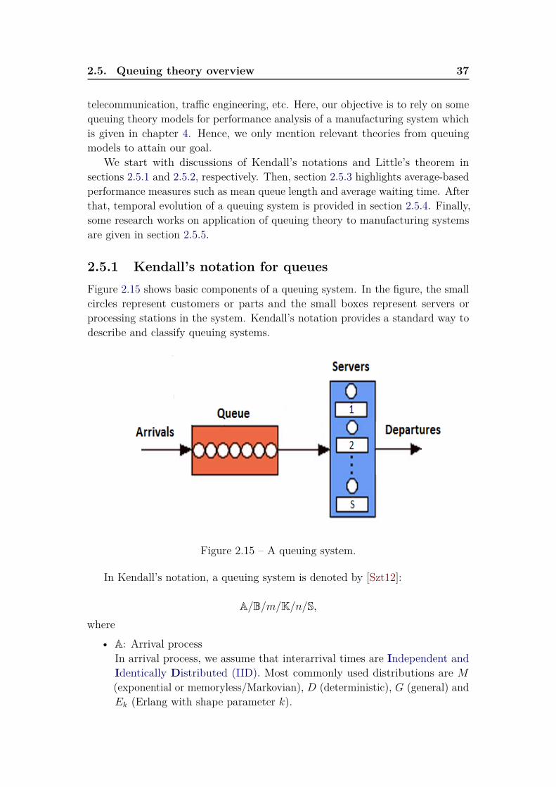
2.5. Queuing theory overview 37
telecommunication, traffic engineering, etc. Here, our objective is to rely on somequeuing theory models for performance analysis of a manufacturing system whichis given in chapter 4. Hence, we only mention relevant theories from queuingmodels to attain our goal.
We start with discussions of Kendall’s notations and Little’s theorem insections 2.5.1 and 2.5.2, respectively. Then, section 2.5.3 highlights average-basedperformance measures such as mean queue length and average waiting time. Afterthat, temporal evolution of a queuing system is provided in section 2.5.4. Finally,some research works on application of queuing theory to manufacturing systemsare given in section 2.5.5.
2.5.1 Kendall’s notation for queuesFigure 2.15 shows basic components of a queuing system. In the figure, the smallcircles represent customers or parts and the small boxes represent servers orprocessing stations in the system. Kendall’s notation provides a standard way todescribe and classify queuing systems.
Figure 2.15 – A queuing system.
In Kendall’s notation, a queuing system is denoted by [Szt12]:
A/B/m/K/n/S,where
• A: Arrival processIn arrival process, we assume that interarrival times are Independent andIdentically Distributed (IID). Most commonly used distributions are M(exponential or memoryless/Markovian), D (deterministic), G (general) andEk (Erlang with shape parameter k).

38 Chapter 2. General Concepts and Models
• B: Service time distributionService times are also assumed to be IID and they can have the samedistributions as the arrival process.
• m: Number of serversAvailable servers to serve customers. For example, the G/G/1 queue hassingle server while the G/G/c queue has c servers.
• K: Number of places in the systemIt represents the maximum number of customers allowed in the systemincluding those in service. Incoming customers may be refused to enter thesystem if this value is the maximum number the system can hold.
• n: Client/costumer source sizen indicates a population size from which customers arrive to a queuingsystem. For instance, in the M/M/1 notation, the population size isconsidered to be unlimited or infinite.
• S: Service disciplineServers serve customers based on a specific service discipline. The servicedisciplines in queuing systems include First In First Out (FIFO), LIFO(Last in First Out), PS (Process Sharing), SIRO (Service In Random Order),and SPT (Shortest Processing Time first). The default service discipline isFIFO if it is not mentioned explicitly.
As an example of Kendall’s notation, the shorthand M/M/m/K/n standsfor a system where arrival and service processes are exponential distributed, theservice is carried out with m servers to serve n customer sources and systemcapacity of K slots with FIFO service discipline. In our work, we use a D/D/1queue where both arrival and service processes are deterministic and a single serverserves unlimited number of customers with FIFO service discipline. The queuingsystem is used to represent a processing station (or machine) in a manufacturingsystem. Consequently, production line of a manufacturing system can be viewedas a tandem of D/D/1 queues. Hence, we limit ourselves to give details onperformance measures of D/D/1 queues.
2.5.2 Little’s FormulaLittle’s formula or theorem was proposed by John Little [Lit61] to prove a queuingformula that relates average number of customers in a queue to average waitingtime and arrival rate of the customers. The theorem is defined as follows.
Definition 2.11 (Little’s theorem, adapted from [Lit61]).Under steady state conditions, the long-term average number of customers in a

2.5. Queuing theory overview 39
stable system is equal to the mean arrival rate multiplied by the average time acustomer spends in the system.
Based on this definition, the stationary mean queue length E[Q] of queue Qis formulated as follows:
E[Q] = λE[DQ] (2.22)
where λ is mean arrival rate and E[DQ] represents the mean delay of customerin queue Q from the time it enters to the queue until its service is completed.In section 2.5.3.3, we use this formula to obtain the average delay E[DQ] aftercomputing the average queue length E[Q].
2.5.3 Average-based performance measures of D/D/1 queueA D/D/1 queuing system is the simplest queuing type (but very useful) wherearrival rates (λ) have deterministic IID inter-arrival times and service times (µ)are also distributed in the same way. To avoid that the queue eventually growsto infinity, we have to require that λ 6 µ, with the equality case also stable indeterministic queues. Important performance measures in the queuing systeminclude mean waiting times and average number of customers in the system (ormean queue length).
In this section, we provide server utilization and the average-based performancemeasures such as the mean waiting time and mean queue length in the D/D/1queue. Now, we recall some performance measures of the D/D/1 queue fromworks of Sztrik [Szt12] and Zukerman [Zuk13]. Assume that if an arrival and adeparture occur at the same time, the departure takes place first. This assumptionis not required for Markovian queuing systems such as M/M/1, G/M/1, andM/G/1 queues since occurrences arrival and departure events are probabilistic.In the following sections, analytical results of the performance measures of theD/D/1 queue are provided.
2.5.3.1 Server Utilization
The server utilization of the D/D/1 queue can be considered in two cases. If weconsider the case where λ > µ, the queue size grows to infinity as t → ∞. Hence,there is always a customer in the queue waiting for service which makes the serveralways busy. The result is that the utilization is equal to one. However, in thiscase, the system becomes unstable due its queue size.
In the other case where λ < µ, the system is always stable. Let us assumethat the first customer arrives at t = 0. Its service time ends at t = 1/µ. Then,the second arrival will occur at t = 1/λ and it will be served at t = 1/µ + 1/λ.This continues for all arrivals and it forms a deterministic cyclic process wherethe queue size is either 0 or 1. Thus, the cycle contains three parts: a periodof customer arrival of 1/λ, then there is a customer to be served for a period of

40 Chapter 2. General Concepts and Models
1/µ, and a period where there is no activity (1/λ - 1/µ). Therefore, the serverutilization becomes U = (1/µ)/(1/λ) = λ/µ.
2.5.3.2 Mean queue length
If λ < µ (i.e., when the system is stable), customers entering the system areserved before the next one arrives. This means that the queue length alternatesbetween 1 or 0 with 1/λ time spent in state 1 and (1/λ - 1/µ) time spent instate 0. Assume that the probability of having n customers in the queue Q at arandomly chosen point in time is P(Q = n), the mean queue length is defined as[Zuk13]:
E[Q] =∞∑
n=0nP(Q = n) (2.23)
Now, the probability that there is one customer in the queue Q is P(Q = 1)= (1/µ)/(1/λ), and the probability that there is no customer is P(Q = 0) =1 - (1/µ)/(1/λ). Based on equation (2.23), the mean queue length is E[Q] =0*P(Q = 0) + 1*P(Q = 1) = λ/µ, which is the same as the server utilizationgiven above.
2.5.3.3 Mean waiting time
Using the Little’s formula (see section 2.5.2), the mean waiting time is E[DQ]= E[Q]/λ = (λ/µ)/λ = 1/µ. According to Sztrik [Szt12], every other queuingsystem (M/M/1, G/G/1, etc) has greater mean waiting time than D/D/1.
2.5.4 Temporal evolution of arrivals and departuresThe performance measures discussed above are time-averaged values under steadystate conditions. The steady state measures are independent of the initialconditions of the system. To characterize and predict the behavior (transientand steady state) of the system at any time t, we define two processes: arrivalArr(t) and departure Dep(t) processes. The process Arr(t) is defined as thetotal number of arrivals and Dep(t) is defined as the total number of departuresduring the interval [0,t]. For a system in which arrivals and departures occur oneat a time (e.g., D/D/1 queue), a realization of Arr(·) and Dep(·) is displayed inFigure 2.16. From these two processes, we can compute the average values suchas mean waiting time and average number of jobs in the queue.
Now, let taj and tdj are arrival and departure times of job j, respectively.Assuming that the system starts working at time ta and finishes at time tb, theaverage waiting times (WT ) of jobs can be expressed as [CF10]:
WTta,tb = 1n
n∑j=0
(tdj − taj
)= E[DQ], (2.24)

2.5. Queuing theory overview 41
Figure 2.16 – A realization of arrival and departure processes of jobs where theleft curve represents cumulative arrivals and the right curve represents
cumulative departures [CF10].
where n is the number of job arrivals to the system during the interval (ta,tb).The area between Arr(t) and Dep(t) represents the integral of the number ofjobs in the system at time t (see Figure 2.16). Hence, the average number of jobswaiting in the system during the time interval (ta, tb) is given by:
Nta,tb = 1tb − ta
∫ tb
ta
[Arr(t)−Dep(t)
]dt = E[Q]. (2.25)
According to Curry and Feldman [CF10], Equation 2.25 is called work-in-process in manufacturing systems where jobs are either undergoing processing orwaiting in a queue for processing. From Little’s theorem, the relationship betweenthe mean waiting time and the average number of jobs is given as:
Nta,tb = λ ∗WTta,tb , (2.26)
where λ = n/(tb − ta) is the mean arrival rate of the jobs arriving to the systemin the interval (ta, tb).
The above equations depend on the values of Arr(·) and Dep(·) to computeaverage-based performance measures. In chapter 4, we analytically compute thetemporal arrival and departure processes for a manufacturing system. Then, weverify the analytical computations using simulations.
2.5.5 Applications of queuing theory to manufacturingA considerable body of research has shown that queueing theory can be a usefulanalysis tool for several application domains. Besides its application in telecommu-nications and computer networks, queuing theory based models for manufacturing

42 Chapter 2. General Concepts and Models
systems have been gained much attention since three decades ago with initialworks by Buzacott and Shanthikumar [BS92]. After this work, severalapplications of queuing models in manufacturing systems are provided in theliterature.
Considering multi-stage assembly lines, Manitz [Man08] proposed aG/G/1/K(general arrival and service processes, single server with FIFO service disciplineand system capacity of K slots) queuing model for performance evaluation ofthe system with general processing times and finite buffers between machines.Another work on assembly lines with Bernoulli reliability model and finite buffersis given in [Jia+16]. Further surveys on queuing theory-based manufacturingsystems are provided in [PH96], [GF99] and [Li+09].
2.6 SummaryIn this chapter, we discussed several important concepts, models and theorieswhich are relevant to the next chapters. The following list summarizes this chapterreferring back to the sections:
• Section 2.2 presented the microgrid concept focusing on issues such asarchitecture of microgrid, models of wind/solar power and energy storages,industrial/manufacturing load types and spot market.
• In section 2.3, we detailed Demand Response (DR) programs (price- andincentive-based), benefits of DR, approaches and mathematical problemsin DR and an automated DR protocol called Open Automated DemandResponse (OpenADR).
• Then, the service curve concepts of Network Calculus (NC) were discussedin section 2.4. Not only the underlying mathematical concepts such asmin-plus and max-plus algebras but also concatenation and aggregation ofservice curves were provided.
• Finally, in section 2.5, we presented basic queuing theory notations suchas Kendall’s notations and Little’s theorem. Moreover, some performancemeasures and temporal evolution of the D/D/1 queue were discussed.
Based on these relevant concepts, the following chapter details our work onenergy supply side of the industrial microgrid. Specifically, we rely on servicecurve concepts to model power production of Distributed Energy Resources(DERs). The next chapter also discusses on smoothing of power generation ofwind and solar using Battery Energy Storage Systems (BESSs).

Part II
Energy Management in Supplyand Demand Sides


Chapter 3
Modeling and Smoothing ofDERs
Contents3.1 Introduction . . . . . . . . . . . . . . . . . . . . . . . . . . 45
3.2 Related work . . . . . . . . . . . . . . . . . . . . . . . . . . 46
3.2.1 DER modeling . . . . . . . . . . . . . . . . . . . . . . . . 46
3.2.2 Smoothing of energy production . . . . . . . . . . . . . . 47
3.3 DER modeling using Service Curves . . . . . . . . . . . . 48
3.3.1 Service curves of DERs . . . . . . . . . . . . . . . . . . . 48
3.3.2 Energy supply and demand balance . . . . . . . . . . . . 50
3.3.3 Cost minimization strategies . . . . . . . . . . . . . . . . 51
3.4 Smoothing renewable energy production . . . . . . . . . 54
3.4.1 Smoothing algorithms . . . . . . . . . . . . . . . . . . . . 55
3.4.2 Measure of smoothness . . . . . . . . . . . . . . . . . . . . 57
3.4.3 Constraint on successive power levels . . . . . . . . . . . . 57
3.4.4 Determining battery size . . . . . . . . . . . . . . . . . . . 57
3.5 Simulation results . . . . . . . . . . . . . . . . . . . . . . . 60
3.5.1 Description of datasets . . . . . . . . . . . . . . . . . . . . 60
3.5.2 Results and discussions on modeling of DERs . . . . . . . 64
3.5.3 Results and discussions on smoothing . . . . . . . . . . . 69
3.6 Summary . . . . . . . . . . . . . . . . . . . . . . . . . . . . 75
3.1 IntroductionIn this chapter, we present two of our works on the energy supply side of theindustrial microgrid. In section 3.2, we provide a literature review on modeling ofDistributed Energy Resources (DERs) and smoothing of their power productions.Then, based on the service curve concepts defined in the previous chapter (section

46 Chapter 3. Modeling and Smoothing of DERs
2.4), we give a service curve model of the power generations of DERs in section3.3. The model will help us know the minimum power produced by DERs sothat we can do energy transactions on spot markets or with the utility gridif there is energy deficit or surplus. Section 3.4 discusses smoothing of therenewable resources using three smoothing algorithms. Performance measuresof the algorithms are also provided in the section. After that, numerical resultsare given in section 3.5. Finally, section 3.6 concludes the chapter by invokingimportant results discussed in this chapter.
3.2 Related workThe intermittent nature of Renewable Energy Sources (RESs) such as solarand wind cause significant power fluctuations and integrating them to powersystems requires control mechanisms in the form of smoothing and modeling ofthese resources. This section provides a review of relevant research works onthe two categories: modeling and smoothing of DERs in sections 3.2.1 and 3.2.2,respectively.
3.2.1 DER modelingA challenging aspect of DERs in the microgrid is that the energy produced bythe renewable resources is intermittent. Hence, individual components of DERsshould be modeled in order to know system’s total available energy and thenenergy transactions can be done to minimize energy costs. To model powergeneration of DERs, there are two type of models: simulation and analyticalmodels. In [ZYF07] and [CS02], the authors considered simulations models toestimate the actual performance of Photovoltaics (PV) modules under varyingoperating conditions. In simulation models, the models may not capture thesystem’s dynamics and the results could be inaccurate and misleading due toinappropriate simulation parameters or other factors. However, analytical modelscan capture complex dynamics of the system better than simulation models.Following the description in [WJM12], generic analytical frameworks such asNetwork Calculus (NC) provide better performance modeling and evaluationof DERs. The research works mentioned above relied on complex probabilityfunctions to give probabilistic upper and lower bounds on energy production. Inthis work, we use the deterministic version of NC to give a deterministic lowerbound on an energy DERs produce.
As noted in the preceding chapter (section 2.4.3), the application of NCtheories were limited to performance analysis of computer and communicationnetworks. There are only few research papers on NC’s application in energydomain. For example, [WLL11] and [Wan+12] considered a stochastic NCframework for modeling DERs and energy demands. They used probabilistic

3.2. Related work 47
cumulative distribution functions to express energy arrival processes to an energyqueue. Stochastic NC is also used in [WJM12] for performance modeling andevaluation of network systems powered with RESs. Le Boudec and Tomozei[LBT12] relied on the concept of service curves to ensure the existence of a feasiblebattery charging and discharging schedules given an energy demand curve. Theycomputed a sufficient battery size so that the feasible online schedule can beensured during the scheduling period.
Our motivation to extend NC theory to energy management in a microgrid isthat the theory can provide an analytical framework for different scenarios andits applicability to different research domains. Among the concepts of networkcalculus theory, we rely on the concepts of service curves as described in section2.4 of chapter 2. In our context, we use service curves to model DERs of thepower system. After that, we obtain the total energy production which is used tosatisfy some part or the total energy demand. Then, when the demand is greaterthan the supplies, we can purchase energy from either spot markets or the utilitygrid. Hence, we also discuss different strategies to minimize energy procurementcosts by using locally produced energies as much as possible.
3.2.2 Smoothing of energy production
One way to reduce power fluctuations in RESs is to smooth power productionusing Energy Storage Systems (ESSs) such as electric double-layer capacitor[Kak+09], superconducting magnetic energy storage [TKF89], fuel cells [RT88],and Battery Energy Storage Systems (BESSs) [HGB10]. The ESSs can be usedto store surplus energy and to shave peak demands. Further roles of ESSs inpower systems are described in section 2.2.2.3 of the previous chapter. In thiswork, we use BESSs such as lithium-ion and lead-acid batteries for the purposeof smoothing.
For smoothing power production of RESs, different approaches have beenproposed in the literature. A Simple Moving Average (SMA) based smoothingwas proposed by Ellis et al. [Ell+12], Johnson et al. [Joh+13], and Hund,Gonzalez, and Barrett [HGB10]. They used the SMA method to mitigateshort-term fluctuations of PV power using BESSs. An Exponential MovingAverage (EMA) method with hydrogen storage system is used by Tesfahunegnet al. [Tes+11]. The EMA gives more weights on recent values. In both SMA andEMA, length of the averaging window determines how the storage systems chargeor discharge. If the window is long, it requires the storage systems to cover thedifference between the actual and smoothed powers, even if the fluctuation is notsignificant. In [Li+11], a fuzzy wavelet transform method is used to smooth outwind and solar power productions using BESSs.
Although the moving average methods (SMA and EMA) are easy to implementalongside the BESSs, they are affected by peaks and troughs during power

48 Chapter 3. Modeling and Smoothing of DERs
generations which could result in bigger battery sizes. In [Add+17c], we proposeda Gaussian-based smoothing algorithm that solves the pitfalls of the movingaverage methods. Gaussian filters have been extensively used in computer visionand image processing domains. In our work, we would like to investigate it inenergy domain. Section 3.4.1 describes the Gaussian-based, SMA and EMAmethods in more details. Then, in section 3.5.3, we compare performances of thethree approaches using real and forecast datasets.
In the following section, we present one of the two works, namely, modelingenergy generation of DERs using service curves.
3.3 DER modeling using Service CurvesThis section details the modeling of DERs power productions using the conceptof service curves. We first provide the service curve model of solar and windpowers in section 3.3.1. After having the two service curves, we modify thebattery equation to reflect the changes by including the service curves and energydemands. Then, in section 3.3.2, we discuss a problem of energy supply anddemand by incorporating the service curves of DERs. Finally, cost minimizationstrategies are provided in section 3.3.3.
3.3.1 Service curves of DERsWe consider a system where solar and wind powers provide energy and a batterysystem that can charge or discharge according to difference between energy supplyand demand. Based on the description of service curves in chapter 2 (section2.4), we define service curves to model the minimum amount of energy that theDERs can provide. A service curve Si(t) is defined as:
Si(t) = αi + βi ∗ t (3.1)
where (αi, βi) are service curve parameters of energy resource i. This is to saythat the node of DERs provides the amount of energy which is represented byits service curve Si(t) that can be seen as a local minimum [Flo+13] amount ofenergy at time t. Equation (3.1) is similar to Equation (2.16) (defined in section2.4.2.1 of chapter 2) which is one of the common functions as service curves.
3.3.1.1 Service curves of solar and wind
Performing mathematical integration on extracted power over a specific timeinterval will give us energy (in kWh). From these sets of data, we can obtainthe service curve parameters such as αi (in kWh) and βi (in kW) where i is acomponent of DERs (solar or wind).

3.3. DER modeling using Service Curves 49
3.1.1: Solar/wind power generation 3.1.2: Corresponding service curve
Figure 3.1 – Service curve example for a node of DERs (solar or wind).
Figure 3.1 illustrates how to setup a service curve for a solar or wind power.For the sake of simplicity, assume that the power generation is constant over ashort period of time as shown in Figure 3.1.1. Referring to Figure 3.1.1 and 3.1.2,in the time interval [t0, t1], the generated power is 200kW and the correspondinglinear line has a slope of 200. Therefore, the service curve in this interval is S(t)= 200t, t ∈ [t0, t1], that is α = 0 and β = 200. Then, when t is between t1 andt2, the new service curve becomes S(t) = 200 + 250t, that is α = 200 and β =250. Hence, the curve in Figure 3.1.2 is piece-wise linear curve that contains thedifferent service curves in the interval [t0, t3].
In the above example, we setup a service curve for a single energy resource.Now, we would like to aggregate the different service curves. The aggregation ofheterogeneous power supply sources provide a single service curve that representsthe total energy production. Consider a power system which consists of Nrenewable power producers in parallel. If a power producer n (n = 1, 2, ..., N)provides an energy service curve Sn, then the power system provides a systemservice curve defined as:
S(t) = S1(t) + S2(t) + · · ·+ SN(t), (3.2)
As noted in previous chapter (section 2.4.2.4), aggregated system service curvecan be obtained by summation of the individual service curves of the energyresources. Next, we incorporate the system service curve into battery chargingand discharging processes.
3.3.1.2 Energy storage
The energy storage (e.g., battery) is modeled by a discrete time process b(t) (referto section 2.2.2.3 of chapter 2), with maximum battery capacity B and it can bedefined recursively. If the energy generated from the PV/wind hybrid system isgreater than the load for a particular hour, then the surplus energy is stored in

50 Chapter 3. Modeling and Smoothing of DERs
the battery and the battery is charged as:
b(t) = min{B, b(t− 1) + [S(t)−D(t)] ∗ ηc
}, (3.3)
where S(t) represents a system service curve as shown in equation 3.2, D(t) is anenergy demand at time t, and ηc is charge efficiency of the battery. When thebattery reaches its maximum value B, any excess energy generated is wasted andhence the battery cannot be charged.
In the discharging case, if the energy demand is greater than the supply for aparticular hour, then the battery is discharged in order to fill the void betweenenergy supply and demand. The battery can be discharged as below:
b(t) = max{
(1−DoDmax) ∗B, b(t− 1)− [D(t)− S(t)]/ηd
}, (3.4)
where ηd is the battery discharge efficiency. Due to physical constraints, the mini-mum battery level should be lower bounded with the value of Depth of Discharge(DoD). For instance, if DoDmax has a value of 80% (for lead-acid/lithium-ionbattery as shown in Table 3.1), then the minimum battery level (Bmin) is de-termined as Bmin = (1 - 0.8)*B = 0.2B. Hence, if the battery decreases to itsminimum value Bmin, then the energy deficit cannot be met by the battery.
3.3.2 Energy supply and demand balance
In the above section, we provided our approach of modeling the DERs usingservice curves of NC. In this section, we use the models to formulate our problemwhich is to balance demand and supply. We consider a constant energy demandD for a particular period and N energy resources. Suppose that each resourcen = 1, 2, ..., N provides a service curve guarantee Sn. Then, the total energydemand is satisfied if:
S1(t) + S2(t) + · · ·+ SN(t) > Dt (3.5)
Equation (3.5) can be interpreted as the aggregation of all the source servicecurves have to be greater than the demand curve.
As shown in Figure 3.2, the cumulative energy demand is given by straightline Dt which has a slope of D. When the summation of energy provided bywind and solar is greater than the demand line, we say that the demand is met.Otherwise, we discharge the battery if there is enough energy. If the battery isunable to cover the shortage, we need to buy the required energy from eitherspot market or utility grid based on costs of energy. In the following section, weoutline different strategies that minimizes energy procurement costs and enableus to use as much as possible locally produced energy.

3.3. DER modeling using Service Curves 51
Figure 3.2 – Energy demand and supply curves [Add+15].
3.3.3 Cost minimization strategiesBefore discussing different strategies for procurement cost minimization, we definea net energy procurement cost as follows:
Netcost =∑
t∈year
[Prbuy(t) ∗ Ebuy(t)− Prsell(t) ∗ Esell(t)
](3.6)
where Pr(·) and E(·) are selling/buying prices in AC/MWh and sold/boughtenergy in MWh, respectively. When we consume local energy from wind, solar orbattery, we assume that the energy cost is zero. Furthermore, we assume thatthere is no upper bound on the amount of energy that can be bought from thespot market. However, there are minimum limits on energy volume that we wantto sell or buy as discussed below.
In this section, we define three strategies that minimize the reliance on externalenergy sources and make use of local energy more often. We compare them basedon their performances against the total net energy procurement cost definedby Equation (3.6). Algorithm 1 describes an implementation of the three costminimization strategies. The following three strategies are taken from our workon service curves [Add+15].
3.3.3.1 Strategy 1 – Sell excess energy
In this strategy, we would like to sell the excess energy which is a leftover after ademand is met, i.e., when S[t] > D[t] in Algorithm 1. According to EPEX Spot[EPE17] (see section 2.2.4 of chapter 2), the possibility to sell energy on the spot

52 Chapter 3. Modeling and Smoothing of DERs
Algorithm 1 Cost minimization strategiesRequire: (S, D, grid_price, spot_price, B)net_cost ← 0 . energy procurement net coststored_energy ← ε . stored energy in the batteryT ← 8760 . Number of hours in a yearbuy_when_cheap ← false . To buy energy from spot when it is cheapsell_excess_energy ← false . To sell excess energy or notspot_energy_volume ← 1000 . Minimum energy to sell on spot in kWhmax_spot_price ← ε . Max. spot price we wish to buysold_energy ← 0 . aggregated sold energybought_energy ← 0 . aggregated bought energywhile t < T do
difference← S[t] - D[t]if difference > spot_energy_volume then . Surplus energy
if sell_excess_energy == true then . STRATEGY 1sold_energy ← sold_energy + difference
net_cost← net_cost - (spot_price[t] ∗ difference)/1000else . STRATEGY 2
if stored_energy + difference 6 B then . If battery is not fullstored_energy ← stored_energy + difference
else if diff == stored_energy + difference - B > 1000 thenstored_energy ← B
sold_energy ← sold_energy + diff
net_cost← net_cost - (spot_price[t] ∗ diff)/1000else if 0 < difference < spot_energy_volume then
if stored_energy < B then . Store the leftoverstored_energy ← min(B, stored_energy + difference)
else . There is no enough energy, BUY!bought_energy ← bought_energy + difference
net_cost ← net_cost + min(spot_price[t], grid_price[t]) ∗difference/1000
if spot_price[t] < max_spot_price then . STRATEGY 3stored_energy ← B . Make the battery fullbought_energy ← bought_energy + (B − stored_energy)net_cost← net_cost + spot_price[t] ∗ (B − stored_energy)/1000

3.3. DER modeling using Service Curves 53
market depends on the minimum energy volume available to be sold. In EPEXSpot, the minimum volume is 1MWh (spot_energy_volume in the algorithm).Therefore, if we have an excess energy greater than 1MWh for some period, wecan sell it on the spot market at market price. Otherwise (i.e., excess energy lessthan 1MWh ), if the battery is not full, we store it for future use.
3.3.3.2 Strategy 2 – Store excess energy
Under this strategy, instead of selling the excess energy, we would like to storeit for future use if the battery is not full. If the battery is full, there are twopossibilities: either sell the excess energy if it is above 1MWh or otherwise disposeit. For bigger battery sizes, this condition cannot happen too often because theycan store much of the surplus energy due to their sizes. However, for smallerbattery sizes, if there are lower energy consumption, the user can opt to sell theexcess energy. This could be another good strategy. Strategy 2 also minimizes thenet energy cost by providing zero-cost local energy from solar, wind and battery.If the energy from battery, solar and wind cannot meet the load, we buy fromeither the utility grid or spot market whichever has lower energy price.
3.3.3.3 Strategy 3 – Use external energy to charge battery
The objective of this strategy is to make use of the varying prices of electricityin spot markets. The cost of energy on the spot market is cheap during someperiods of the day. Charging the batteries during these periods can be a goodstrategy to minimize the net energy procurement cost defined by Equation 3.6.We assume that the battery can start charging at the beginning of a particulartime slot (which has length of 1 hour) and it can be ready at the end of theslot. We give charging precedence for locally produced energy from solar andwind. Moreover, if the battery is not full yet, we can buy the energy from thespot market. For this, we set a price limit that we would like to buy from themarket (max_spot_price in the algorithm). For example, If we set this limit to20AC/MWh, then we buy energy from the market whenever the price is under20AC/MWh. Under this strategy, we store more energy for future use.
In section 3.5.2, we compare the performance of the strategies using realdatasets of energy demand of a factory, sport prices, solar and wind data. Thesection also provides discussions on payback periods which are the period of timerequired to recoup the funds expended in an investment on solar PV panels, windturbines and batteries.
The above sections presented our work on modeling of DERs using conceptsof service curve. The following section outlines the second part of this work:smoothing energy production of the RESs.

54 Chapter 3. Modeling and Smoothing of DERs
3.4 Smoothing renewable energy productionAs discussed in section 3.2.2, there are ways to deal with fluctuations in renewableenergy resources by implementing smoothing in conjunction with energy storagesystems. In the literature, the commonly used approaches for smoothing (forinstance, simple and exponential moving averages) result in a big battery size.Hence, we would like to come up with a smoothing algorithm which has moreperformance in terms of battery sizes, i.e., it has to attain lower battery sizes.
Figure 3.3 – Conceptual schematic representation of solar, wind and batteryhybrid system [Add+17c].
We consider a scenario where the energy supply side of the microgrid has acombination of solar PV panels, wind turbines and battery. Figure 3.3 showsa conceptual schema of solar, wind and battery hybrid system. Based on thefigure, we first aggregate the solar and wind power productions. Then, we applysmoothing algorithms to smooth out power fluctuations. After that, to make-upthe difference between the actual power and the smoothed one, we charge ordischarge the battery accordingly. The final smoothed power Psm(·) is expressedas:
Psm(t) =Ppv(t) + Pwind(t) + P d
bat(t) discharge battery (release power)Ppv(t) + Pwind(t) - P c
bat(t) charge battery (absorb power),(3.7)
where Ppv(t) and Pwind(t) are solar and wind powers, and P cbat(t) and P d
bat(t) arecharging and discharging rates at time t, respectively. P c
bat(·) and P dbat(·) should
respect the charging and discharging constraints described in chapter 2 (section2.2.2.3). The battery can be then charged or discharged based on the output of

3.4. Smoothing renewable energy production 55
the smoothing algorithms.
3.4.1 Smoothing algorithmsIn this section, we present three smoothing algorithms, namely, simple movingaverage, exponential moving average, and Gaussian-based algorithm. Withdemonstrating examples, we show how parameters of the algorithms affect thesmoothing of solar and wind power generations.
3.4.1.1 Moving average-based smoothing
A moving average (rolling average or running average) is a technique to get anoverall idea of the trends in a data set. The averaging technique is based ona sliding window size. Under moving average, we consider two types: simplemoving average and exponential moving average.
Simple Moving Average (SMA) According to Alessio et al. [Ale+02], amoving average method is a well-known low-pass filter for time series and it isdefined as:
y(i) = 1w
w−1∑k=0
y(i− k) (3.8)
where y(·) is a time series data with window length w. Although it is simple andtraditionally accepted way to reduce fluctuations in renewable resources [AMS14],it exhibits a memory effect which depends on the length of the averaging window.Numerically, a moving average with window length of w contains only (1/w)%of present values of a fluctuating variable. To see the effect, a demonstratingexample is shown in Figure 3.4. In Figure 3.4.1, an input signal with a glitch andits smoothed output using a moving window of 10 samples are shown. The effectof the glitch lasts for the size of the averaging window.
In [AMS14], the authors also showed the memory effect of a moving averagemethod on a PV power data obtained from National Renewable Energy Laboratory(NREL). Figure 3.4.2 shows an actual PV power and its 20 minutes moving averagetaken from [AMS14]. From the figure, we can see that the moving average valuesin the broken circles deviate significantly from the actual PV power due to memoryeffect of the moving average. However, there is no much fluctuations in poweroutput during these periods. Hence, to accommodate the difference, the batteryhas to be charged or discharged and this forces a battery to operate frequently.
Exponential Moving Average (EMA) The moving average has an extensionin the form of EMA. The EMA gives greater weights to recent changes in data,i.e., only one old value has to be remembered if it is of first order [BN02]. Hence,

56 Chapter 3. Modeling and Smoothing of DERs
3.4.1: An example to show limitation of movingaverage where F(x) is an original function and f(x)
is a smoothed output
3.4.2: A 20-min moving average of an actual PVoutput [AMS14]
Figure 3.4 – Pitfalls of a moving average method.
based on Equation (3.8), a new estimation y is calculated as follows:
y(i) = (1− α)y(i− 1) + αy(i), (3.9)
where α ∈ [0,1] is an exponential weight. The choice of α has two effects: with alarge value the estimation follows the measurement truly, but does not suppresspeaks, whereas with a small value peaks are suppressed but the estimation followsreal changes too slowly.
As noted above, both SMA and EMA have the memory effects. To lessenthese effects and to have more smoother power production curves of solar andwind, we rely on a Gaussian-base method as proposed in our work [Add+17d]and we detail it in the next section.
3.4.1.2 Gaussian-based smoothing
The Gaussian filter has been a de-facto standard for applications such as imageprocessing and computer vision. In one dimension, a first order zero-meanGaussian filter is given as [Wei02]:
G(y, σ) = 1√2πσ
e−y2
2σ2 , (3.10)
where the parameter σ is the standard deviation of the Gaussian distributionand y is a one dimensional input variable. Typically σ is used as a parameterfor smoothing. Hence, we change the values of σ to obtain different results forsmoothing purpose.
In [RLK06], Gaussian filters are used to effectively suppress impulse noises inimage processing. In our context, the impulse noises are glitches of wind and solarpower productions. Suppressing the peaks and troughs could result in smooth

3.4. Smoothing renewable energy production 57
power generation from the renewable resources and helps to seamlessly integratethem into a power system. But, how do we measure the smoothness of powerproduction curves? The answer is given in the next section.
3.4.2 Measure of smoothnessAccording to Adams and Van Deventer [AVD94], an expression for commonmathematical definition of smoothness is written as:
Z =∫ T
0[f ′′(s)]2ds, (3.11)
for function f(t), where t ∈ [0, ..., T ]. Equation (3.11) is described as an integralof squared second-order differential of function f(·). The minimum value of Zcorresponds to the maximum smoothness level [AVD94]. Hence, this parametercan be used to compare the performance of the three smoothing algorithms (SMA,EMA, and Gaussian-based). In simulation results section (section 3.5), we willuse Equation (3.11) to show which algorithm is better in terms of smoothnessmeasure.
3.4.3 Constraint on successive power levelsFor big solar plants and wind farms, it is necessary that the power generationdifferences from one time to another is kept as minimum as possible. For example,in La Réunion island (overseas region of France), the grid operator asks energyproviders to provide power with a bounded difference in consecutive time slots.One way to define this constraint is to take the derivative of the generated powerP (·) as follows:
Diff(t) =∣∣∣∣∣∆P (t)
∆t
∣∣∣∣∣ 6 γ, (3.12)
where γ is desired power level difference at time t ∈ [1, 2, ..., T ]. By changing thevalue of γ, we can obtain different battery sizes for smoothing power productionswhich we deal with it in the next section.
3.4.4 Determining battery sizeTo determine the battery capacity B (in kWh) needed to absorb fluctuations inpower generations of RESs, we consider charging and discharging cases and thenwe take the maximum of the two cases.
3.4.4.1 Charging capacity
First, we consider a charging case for storing energy in the battery. When actualpower of solar and wind Pact(·) is greater than smoothed power Psm(·), the

58 Chapter 3. Modeling and Smoothing of DERs
Figure 3.5 – An illustrating example for battery size computation where the Asand Bs represent charging and discharging cases, respectively.
capacity is calculated as follows:
Echarge =∫ T
1
[Pact(t)− Psm(t)
]dt, (3.13)
where t ∈ [1, 2, ..., T ]. In Figure 3.5, Equation 3.13 refers to the aggregated areasof the As (i.e., A1 + A2 + A3).
3.4.4.2 Discharging capacity
Secondly, the discharge capacity is calculated as follows:
Edis =∫ T
1
[Psm(t)− Pact(t)
]dt, (3.14)
provided that smoothed power Psm(t) is greater than actual power Pact(t) at timet ∈ [1, 2, ..., T ]. Equation 3.14 refers to the aggregated areas of the Bs (i.e., B1+ B2 + B3) in Figure 3.5.
3.4.4.3 Final battery capacity
Finally, the rated capacity B of a battery is given as:
B = max(Echargeηc, Edis/ηd
), (3.15)
which is the maximum of Equation (3.13) and (3.14) after incorporating ηc andηd as charging and discharging efficiencies, respectively. Equation (3.15), whichis similar to an equation defined in [CGW12], determines the size of a batteryconsidering charging and discharging cycles separately. This results in a bigger

3.4. Smoothing renewable energy production 59
battery size. In reality, the battery alternately charges and discharges multipletimes during the considered period which could result in a smaller battery size.
Besides the above case, if we take the difference between the charging anddischarging capacities as:
B =∣∣∣Echargeηc − Edis/ηd
∣∣∣, (3.16)
then, the resulted battery size is smaller than the size determined by Equation(3.15). However, if the charging and discharging capacities are equivalent, wearrive at very small battery size which cannot be sufficient to smooth the powerproductions. Hence, a compromise between the two methods of battery size deter-mination is important. For instance, a compromise between the two approaches isto look for consecutive charging and discharging cycles to determine battery size[Add+17c]. For this, we setup a recursive function that sums up the consecutivecharging/discharging cycles. Then, the battery size is determined as the maximalvalue of the charging and discharging cases. Mathematically, a recursive functionfor a charging case is expressed as follows:
Ec(t+ 1) =Ec(t) + Pact(t+ 1) - Psm(t+ 1) if Pact(t) > Psm(t),∀t > 0
0 otherwise.(3.17)
Then, the charging capacity is Echarge = max(Ec). By the same manner, afunction for a discharging case is given below:
Ed(t+ 1) =Ed(t) + Psm(t+ 1) - Pact(t+ 1) if Psm(t) > Pact(t),∀t > 0
0 otherwise.(3.18)
Then, the discharging capacity is Edis = max(Ed). Finally, battery size isdetermined by taking the maximum of the charging and discharging cases, i.e., B= max(Echargeηc, Edis/ηd) which is the same as Equation (3.15).
To make the calculations, we refer to Figure 3.5 as an illustrating example.In the figure, a sample solar and wind power production and their predictionsare given (see section 3.5.3 for more description of the data). We consider alithium-ion battery with ηc and ηd set to 85% which is a common value forlithium-ion batteries according to [CGW12]. Now, using Equation (3.17) for thecharging case, we find that A2 (646kWh) is the maximum of the As. Then, forthe discharging case, B2 (1316kWh) is found to be the maximum of the Bs. Thisleads to battery size of 1316kWh. However, if we compute the battery size usingEquation (3.15), we arrive at a size of 2028kWh which is 712kWh bigger than B2.Hence, we attained a 35% reduction in battery size by applying our approach.Moreover, if we use Equation (3.16) to compute the battery size, this will result

60 Chapter 3. Modeling and Smoothing of DERs
in a capacity of 670kWh. Apparently, this value is not sufficient for a dischargingcase at B2 which is 1316kWh. The limitations to our approach could be for thecases where discharging cycles are small and charging cycles are big. In thesecases, if we consider consecutive charging/discharging cycles to determine thebattery sizes, the energy to be stored will be bigger than the determined batterysize. The approach in Equation (3.15) that considers charging and dischargingcycles separately could be better for these cases.
In this section, we discussed the smoothing algorithms and outlined how tocomputer battery sizes. The following section provides numerical results on thetwo parts of this chapter: modeling of DERs and smoothing.
3.5 Simulation results
In this section, we provide descriptions of our datasets and discussions on resultsof different simulation results on both DERs modeling and smoothing parts whichare discussed in the above sections.
3.5.1 Description of datasets
For our experiments, we consider a real datasets of solar and wind power datafor an industrial site located in Bourbourg, France. The datasets consist of solar,wind, energy demand of the factory, EPEX spot market prices, and batteryparameters.
3.5.1.1 Solar PV data
Based on the PVWatts of NREL [PW], we retrieved hourly per unit (25m2)solar PV data as shown in Figure 3.6.1. The PVWatts calculator uses Equation(2.2) (see section 2.2.2.2 in the preceding chapter) as a reference and it alsoincorporates temperature effect to the equation. For our experiments, We takepower production of 100 units of PV panels with the power curve shown inFigure 3.6.3. For forecasting purpose, we use Auto Regressive Integrated MovingAverage (ARIMA) (in the book of Wei [Wei94], chapter 4) model to predictday-ahead solar power production. The ARIMA model has been widely used intime series forecasting applications such as stock [PL05] and next-day electricityprices forecasts [Con+03]. In our simulations, the ARIMA model is trained withsolar data of 1 hour interval for 245 days. Then, the prediction is performed forthe 246th day. Forecast and real solar powers are depicted in Figure 3.7.1.

3.5. Simulation results 61
3.6.1: Hourly average solar power data 3.6.2: Hourly average wind speed data
3.6.3: Solar PV power curve 3.6.4: Wind turbine power curve
Figure 3.6 – Solar and wind input data for year 2014 and their power curves.
3.5.1.2 Wind speed data
We obtained hourly average wind speed data for the year 2014 from Weatherunderground website [WU]. The hourly wind speed data is shown in Figure 3.6.2.The forecasting process is also performed following the same procedure as that ofthe solar data. Forecast and real wind speeds are shown in Figure 3.7.2. UsingEquation (2.1) in section 2.2.2.1 of the previous chapter, we computed the powerextracted from the wind speed for a 3MW wind turbine which has the powercurve depicted in Figure 3.6.4. In Figure 3.7.3, the aggregation of actual andpredicted solar and wind powers are provided.

62 Chapter 3. Modeling and Smoothing of DERs
3.7.1: Predicted solar power 3.7.2: Predicted wind speed
3.7.3: Actual and predicted total power
Figure 3.7 – Actual and predicted solar and wind data for a period of 24 hours.
3.5.1.3 Battery parameters
A battery can be characterized by its maximum battery capacity B, DoD, charg-ing and discharging rates, efficiency and other parameters. Table 3.1 showsthe characteristics of Lead-acid and Lithium-ion batteries. Descriptions of theparameters are provided in section 2.2.2.3 of chapter 2.
3.5.1.4 Energy demand data
For energy demand (load) data, we obtained hourly energy consumption datafrom METRONLab servers (see Figure 3.8). These data represent a yearly energydemand of the industrial site.

3.5. Simulation results 63
Table 3.1 – Characteristics of two common battery types [Che+09; GFKR15;WLD15; MW15].
Characteristics Lead-acid Lithium-ionEfficiency (%) 75 85Charge time 8-16h 2-4hDischarge to charge rate ratio 10 5Self-discharge per day (%) 0.3 0.1Depth of Discharge (%) 80 80Energy density (Wh/L) 80 150Power density (W/L) 125 450Lifetime cycle 2000 5000Expected lifetime (Years) 4 10Cost ($/kWh) 100 - 200 400 - 600
Figure 3.8 – Hourly energy demand of a factory from METRONLab server.
3.5.1.5 Spot market price data
We retrieved hourly market price from EPEX Spot website [EPE17]. These priceswere published for the day-ahead spot market in 2014 and they are shown inFigure 3.9. Based on these data, we detail results and discussions on modeling ofDERs in the next section.

64 Chapter 3. Modeling and Smoothing of DERs
Figure 3.9 – EPEX Day-ahead spot price data for 2014.
3.5.2 Results and discussions on modeling of DERs
In this section, we provide different results on the performance of the costminimization strategies, namely, sell surplus energy (Strategy 1), store excessenergy (Strategy 2), and use external energy to charge battery (Strategy 3).These strategies are described in section 3.3.3 alongside their implementation inAlgorithm 1 which relied on the service curve models of DERs. As a performancemetric, we refer to Equation (3.6) that computes the net energy procurementcost and we compare the strategies based on the equation. As initial simulationconditions, we set a price of 40AC/MWh to buy electricity from a utility grid andbatteries can be considered full in beginning of the simulations.
Table 3.2 – Cost comparison of different strategies (taking 40AC/MWh for cost ofutility grid energy, battery size of 20MWh for the three strategies, and spot
market price limit of 5AC/MWh for strategy 3).
Strategies Net energy procurement cost (in AC)Grid-only 621,915Spot-only 586,301Strategy 1 400,845Strategy 2 405,815Strategy 3 396,387

3.5. Simulation results 65
3.5.2.1 Performance of the strategies
First, we compare the strategies against the case of no strategies, i.e., we buy allthe energy demand from the utility grid (Grid-only) or on the spot market (Spot-only). Table 3.2 shows the results of the annual net procurement costs (definedby Equation 3.6) that are calculated by using the strategies with fixed batterysize of 20MWh, sport market price limit of 5AC/MWh, and utility grid price of40AC/MWh. From the table, we can see that the actual annual cost of the factoryis 621,915AC if it buys all the energy from the utility grid. However, if the factorybuys all its demands from the sport market, then the cost decreases to 586,301ACper annum. With the specified parameter settings, the three strategies can becomparable with respect to the net energy cost. However, when compared tothe Grid-only and Spot-only strategies, using Strategy 3 (since it is the minimumof the three) could save upto 36% (from 621,915 down to 396,387AC) and 33%(from 586,301 down to 396,387AC), respectively. Next, we investigate the effect ofbattery sizes on the performance of the strategies.
Figure 3.10 – The three strategies with different battery sizes and fixed spotprice limit of 5AC/MWh for strategy 3.
3.5.2.2 Effect of battery sizes
Now, by varying the battery sizes, we compare the performance of the strategiesagainst each other using the performance metric defined in Equation (3.6). Theresults of the three strategies are depicted in Figure 3.10. From the figure, we cansee that for smaller battery sizes (B 6 10MWh), Strategy 1 is the best among

66 Chapter 3. Modeling and Smoothing of DERs
the three strategies because its net cost is less than the other two. This showsthat it is better to sell energy instead of storing it when the battery size is lessthan 10MWh. However, as the battery size increases (B > 10MWh), Strategy 3outperforms the others. Hence, for bigger battery sizes, a good strategy is to buyenergy from the spot market and then store it. The stored energy could be usedlater when the prices are high or load-shedding is required.
Figure 3.11 – Effect of varying spot price with fixed battery capacity of 20MWh.
3.5.2.3 Effect of spot market prices
Figure 3.11 shows the effect of different spot market prices and a fixed batterysize of 20MWh. The variable spot market prices have likely effect on Strategy3 than the others because this strategy buys energy on spot markets to chargethe battery during lower price periods. For Strategy 3, an optimal point is foundat [30AC/MWh, 329,749AC] which corresponds to a saving of 47%. The otherstrategies remain unaltered under variable spot market prices.
In Figure 3.11, we considered a fixed battery size to determine the effectof variable sport market prices. To see how different battery sizes affect theperformance of Strategy 3, we use three battery sizes: 10, 20, and 30MWh. Theresulting curves are shown in Figure 3.12. From the figure, we can see that theoptimal point of the three curves are obtained when the spot market price is30AC/MWh. However, the cost saving has inverse relationship with the batterysizes: the smaller the battery size the less cost saved. With bigger battery sizes,the cost of having these storage devices could hinder cost savings and it mayresult in longer payback periods.

3.5. Simulation results 67
Figure 3.12 – Performance of strategy 3 with spot prices in the range[0,50]AC/MWh and battery size in the range [10,30]MWh.
3.5.2.4 Payback period estimation
One of the major hindering factors of microgrid development is the cost ofmicrogrid components such as batteries, wind turbines, solar PV panels, AC/DC(Alternating Current/Direct Current) converters, etc [Bur+13]. To perform thepayback period estimation, we consider the costs of the microgrid components(solar, wind, and battery) used in our experiments. Nowadays, the cost of aLithium-ion battery ranges from $400 to 600 per kWh and that of Lead-acidranges from $100 to 200 per kWh (see Table 3.1). For solar PV panels, a PVpanel that produces 1W cost $4.9 according to [Fel+12]. Concerning the costof wind turbines, Bolinger and Wiser [BW11] did a study on trends of windturbine prices for the past decade (from 2000 to 2010). According to the authors,the trend for wind turbine prices declined on an average of 20% from 2002 to2010. They also pointed out that the price for a wind turbine ranges from $900to 1,400 per kW and the average cost is $1,100/kW.
We use the following equation to calculate payback periods:
Payback = Costbattery + CostP V + Costwind
CostGrid−only − minCoststgi
(in years), (3.19)
where srgi ∈ [Strategy 1, Strategy 2, Strategy 3 ] and Coststgi is computed usingEquation 3.6 which is the net energy cost metric.
Taking into account the above device costs, we now calculate payback periodsby setting costs of PV panels to $4.9/W, the average cost of $1,100/kW for the

68 Chapter 3. Modeling and Smoothing of DERs
Table 3.3 – Simulation results for payback period estimation by taking 100 PVunits, a 3MW wind turbine, and varying sizes of two battery types with costs of$400/kWh and $100/kWh for Lithium-ion and Lead-acid batteries, respectively.
Battery Solar Wind Payback (in years)Type Size (in MWh)Lithium-ion 1 X X ∼23Lithium-ion 5 X X ∼27Lithium-ion 10 X X ∼33Lead-acid 1 X X ∼22Lead-acid 5 X X ∼22Lead-acid 10 X X ∼22Lithium-ion 1 7 X ∼15Lithium-ion 5 7 X ∼20Lithium-ion 10 7 X ∼26Lead-acid 1 7 X ∼14Lead-acid 5 7 X ∼14Lead-acid 10 7 X ∼15
wind turbine, $400/kWh for Lithium-ion, and $100/kWh for Lead-acid battery.Table 3.3 shows the estimation of payback periods with different battery sizes(for both Lithium-ion or Lead-acid), with/without solar PV panels, and 1 windturbine. Since the wind turbine generates more power than solar power, wealways assume that we have the wind power in the energy mix. Hence, cost ofPV panels is $1.96m (or approx. 1.76mAC at the time of thesis writing) and costof a 3MW wind turbine is $3.3m (or approx. 2.95mAC). Since the cost of bigbattery sizes are very high, we use smaller battery sizes (B 6 10MWh). Theresults shown in Table 3.3 use Equation (3.19) to compute the payback periods.When the battery size is 1MWh, Strategy 1 results in less net cost (408,432AC)compared to the other two (refer to Figure 3.10). However, for battery sizes of 5and 10MWh, Strategy 3 (taking the optimal market price limit) performs betterthan the others.
From Table 3.3, we can infer a couple of important points. The first point isthat the inclusion of solar PV panels into the energy mix increases the paybackperiods. For example, considering a 1MWh Lithium-ion battery, the paybackperiod increased from 15 years (without taking account PV panels) to 23 yearswhen there are PV panels. This is because the area where the factory is locatedhas small amount of solar radiation per annum due to its geographical location.Hence, it is better to use a hybrid system of wind and battery in this location.Another important point is that the the payback period depends on both batterytype and size. Since the cost of Lead-acid batteries are less than that of Lithium-ion, the payback periods are also less for the Lead-acid batteries. However,

3.5. Simulation results 69
Lead-acid batteries have low energy and power densities and shorter expectedlifetime (see Table 3.1). The following sections discusses the second part of thischapter, namely, smoothing of solar and wind power generations.
3.5.3 Results and discussions on smoothingIn this section, we first compare the performance of the smoothing algorithms,viz., Simple Moving Average (SMA), Exponential Moving Average (EMA),and Gaussian-based which are presented in section 3.4.1. To measure theirperformances, we vary their respective smoothing parameters. Then, we determineminimum battery sizes considering two cases: with and without successive powerdifference constraints. Finally, we determine a power production curve for aday-ahead forecast period based on the real datasets described in section 3.5.1.
3.5.3.1 Performance of the smoothing algorithms
As for the smoothing parameters, we use the standard deviation (σ) for Gaussian-based and window length (w) for moving average based smoothing algorithms.Hence, we compare the algorithms by changing smoothing parameters and seethe effects of increasing or decreasing these parameters. In the following experi-mentation, we consider the two case: with and without power level constraints.
Case 1 - no constraint To start our comparisons, we set σ to 1 for Gaussian-based and w to 3 for moving average methods without imposing constraints onconsecutive power levels. Figure 3.13.1 shows smoothing performance of the threealgorithms (SMA, EMA, and Gaussian-based) when the smoothing parametersσ and w are 1 and 3, respectively. In the figure, the Gaussian-based smoothedpower closely follows the predicted total power of solar and wind. This showsthat the smaller the difference between the smoothed and unsmoothed powers,the lesser available power to charge or discharge a battery at any given time.This leads to smaller battery sizes for smoothing.
Using Equation (3.11), we compute the smoothness measures and the resultsare shown in Table 3.4. From the table, we can see that Gaussian-based algorithmhas lower charge/discharge rates than both EMA and SMA. The effect of lowercharge/discharge rates is that the smoothness measures will have lower valuesas the minimum value corresponds to the smoothest curve (see section 3.4.2).In this aspect, the Gaussian-based method performs better than the other twoalgorithms. Numerically, Gaussian-based is 34% more smoother than EMA and47% more smoother than EMA.
To investigate the effects of increased smoothing parameters, we refer toFigure 3.13.2 where σ and w set to 2 and 5, respectively. From the figure, wecan see that the Gaussian-based approach is more smoother but the difference

70 Chapter 3. Modeling and Smoothing of DERs
3.13.1: Smoothing when σ is 1 and w is 3 3.13.2: Smoothing when σ is 2 and w is 5
Figure 3.13 – Smoothing performance of SMA, EMA, and Gaussian-basedalgorithms with different smoothing parameter values.
Table 3.4 – Maximum charge/discharge rates and smoothness measure of thealgorithms (when σ is 1 and 2 and w is 3 and 5).
Models Parameters Charge rate (kW) Discharge rate (kW) Smoothness measure Z
Gaussian-based σ = 1 106 89 15980σ = 2 110 105 4217
SMA w = 3 116 127 24189w = 5 254 163 11163
EMA w = 3 135 149 30204w = 5 186 310 11444
between the predicted and smoothed powers is getting bigger. The same is truefor SMA and EMA. Their curves are shifted right by the size of the averagingwindow. These bring up a dilemma between increase of smoothness and frequentcharging/discharging. When the smoothing parameters are smaller, the resultwill have less smoothed feature and higher frequency of charging/discharging. Onthe other hand, as the parameters increase, it is more smooth but the deviationfrom real values is bigger and this could result in bigger battery sizes. Hence, thechoice of the parameters need to align with required applications.
To determine battery sizes, we take the difference between the actual solarand wind powers and the predicted (and smoothed) ones. The positive differenceshows a charging case and the negative shows otherwise. Figure 3.14 depictspower charge and discharge rates by varying the smoothing parameters of thethree smoothing algorithms. Moreover, maximum charging and discharging ratesare also shown in Table 3.5. From Figure 3.14.1 and 3.14.2, we can deduce thatwhen the smoothing parameters increase, the positive and negative amplitudesdecrease which give rise to smaller battery sizes. However, the increase in the

3.5. Simulation results 71
3.14.1: Charging and discharging rates when σ is 1and w is 3
3.14.2: Charging and discharging rates when σ is 2and w is 5
Figure 3.14 – Charging and discharging rates where positive values representcharging and negative values represent discharging.
Table 3.5 – Battery sizes for different smoothing parameters of the algorithmswhere ηc = ηd = 85%.
Capacity (kWh) Gaussian-based SMA EMAσ=1 σ=2 w=3 w=5 w=3 w=5
Ec = Echargeηc 184 276 232 567 316 734Ed = Edis/ηd 294 404 361 729 514 938B = max(Ec, Ed) 294 404 361 729 514 938
amplitudes of charging and discharging will result in bigger battery sizes.
Based on the charge/discharge rates, we then compute battery sizes by apply-ing Equation (3.17) and (3.18) and taking the maximum of the two values. Table3.5 shows the results of battery size computations when charge and dischargeefficiencies are set to 85%. From the table, we can infer that for smaller smoothingparameters, i.e., when σ is 1 and w is 3, the Gaussian-based method achieves19% (from 361 to 294kWh) smaller battery size than SMA and 43% (from 514to 294kWh) smaller than EMA. The table also shows the effect of increasedsmoothing parameters. In Gaussian-based method, the battery size is increasedfrom 294kWh to 404kWh when σ increased from 1 to 2. Moreover, for SMA andEMA, when window w increased from 3 to 5, the battery sizes are also increasedfrom 361 to 729kWh in case of SMA and from 514 to 938kWh in case of EMA.Next, we introduce constraints on power levels between consecutive time slots.

72 Chapter 3. Modeling and Smoothing of DERs
Table 3.6 – Smoothness measures of the algorithms with successive power levelconstraints of γ% (resulted from Equation (3.12)).
γ (%) Gaussian-based SMA EMAσ=1 σ=2 w=3 w=5 w=3 w=5
5 2037 1614 1686 2349 3247 143310 5298 6373 8368 4078 4493 492315 8261 4217 13961 15583 20183 766620 15037 4217 11674 11163 20183 1726625 15980 4217 24189 11163 30204 1144430 15980 4217 24189 11163 30204 11444
3.15.1: Battery sizes when σ is 1 and w is 3 3.15.2: Battery sizes when σ is 2 and w is 5
Figure 3.15 – Battery sizing based on successive power level constraints with γ ∈[0.05,0.30].
Case 2 - power level constraint The above results are obtained withoutconsidering power level constraints between two successive time slots. In thiscase, we now impose the constraints on the power differences and evaluate theperformance of the smoothing algorithms in terms of smoothness measure andbattery sizes. We use Equation (3.12) to upper bound the successive powerdifferences to some fixed value γ (in %). The value of γ could range from 5 to 30%of the peak power which is found to be 541kW from the datasets. To computethe power differences in power levels in this case, we first smooth the unsmoothedsolar and wind data and then apply an averaging mechanism when the differenceexceeds Pdiff = (γ*541kW)/100. We apply recursively the averaging mechanismuntil the power difference is less or equal to Pdiff .
Table 3.6 shows the results of smoothness measures (denoted as Z in Equation(3.11)) of the three algorithms with different smoothing parameters and powerlevel constraints. From the table, we can see that for smaller values of γ (i.e., more

3.5. Simulation results 73
3.16.1: When γ = 5% 3.16.2: When γ = 10%
3.16.3: When γ = 15% 3.16.4: When γ = 25%
Figure 3.16 – Power curves for a day-ahead forecast considering different ofvalues γ and when σ is 1 and w is 3.
stringent constraint), the value of Z is small when compared to bigger values of γ.This is due to the fact that when γ is small, the averaging mechanism smoothsthe power data so that the resulted smoothed curve has minimum differencebetween the successive points. However, as the γ increases, the value of Z alsoincreases until there is no more to smooth. When γ is above 25%, the smoothnessmeasures are the same as Table 3.5 where the constraints are not considered.
To determine battery sizes in this case, we follow the same procedure as theabove case where the battery sizes are computed using Equation (3.17) and (3.18)and then we take the maximum of the two. Figure 3.15 shows the battery sizes forthe values of γ ranging from 5 to 30% of the peak power and when the smoothingparameters are σ ∈ {1,2} and w ∈ {3,5}. In both Figure 3.15.1 and 3.15.2, we

74 Chapter 3. Modeling and Smoothing of DERs
3.17.1: When γ = 5% 3.17.2: When γ = 10%
3.17.3: When γ = 15% 3.17.4: When γ = 25%
Figure 3.17 – Power curves for a day-ahead forecast considering different valuesof γ and when σ is 2 and w is 5.
can see that for smaller values of γ (for γ < 10%), the battery sizes are bigger.However, as the constraint is relaxed (for γ > 10%), the battery sizes are reduced.Here also, when γ > 25%, the battery sizes are the same as the case of withoutconstraints.
3.5.3.2 The final power production curve
The final output of our simulations is to determine a power production curve fora day-ahead forecast period. The power production curve enables one to knowprecise power production of solar and wind and helps one to decide buying energyfrom the utility grid or the spot market if energy demand is higher than energysupply. To attain this goal, we did multiple simulations considering the three

3.6. Summary 75
3.18.1: Power curve when σ is 1 and battery size is294kWh
3.18.2: Power curve when σ is 1, γ is 10%, andbattery size is 834kWh
Figure 3.18 – Gaussian-based power production curves for day-ahead forecastconsidering the two cases.
smoothing algorithms: Gaussian-based, SMA, and EMA. In Figure 3.16 and 3.17,the power production curves are shown for the smoothing algorithms consideringpower level constraints and different smoothing parameters. From these figures,we can see that the peak powers for the smoothed curves are less when theconstraints are strict, i.e., smaller values of γ. For example, fixing σ to 1, w to3 and γ to 5%, the peak power is 310kW for Gaussian-based, 300kW for SMA,and 320kW for EMA. However, when γ is increased to 10%, the peak powersare also increased by 14%, 22% and 10% for Gaussian-based, SMA and EMA,respectively. This shows that by relaxing the constraints, we could have morepeak power and it requires smaller battery sizes to smooth the power productionsof the Renewable Energy Sources (RESs).
Among the smoothing algorithms, the Gaussian-based algorithm performedbetter than the other two in terms of battery sizes and smoothness measures inboth cases. Figure 3.18 shows the power curves for a day-ahead period consideringthe two cases. These curves are determined by Gaussian-based algorithm withbattery size of 294kWh in no-constraint case and 836kWh in the other case. Inthe above simulations, we considered smoothing and battery sizing for only oneday-ahead. Our approaches can be extended easily to handle multiple days.
3.6 SummaryThis chapter discussed two of our works on the supply side of the industrialmicrogrid. In section 3.3, we adopted service curves of Network Calculus theoriesto model Distributed Energy Resources (DERs) such as solar, wind and battery.

76 Chapter 3. Modeling and Smoothing of DERs
We relied on the service curve concepts for modeling the capacity of DERs. Inthis context, the service curves model the minimum amount of energy that a DERcan offer. After modeling the resources, we set up three strategies for testing thebenefits of our approach in terms of minimizing energy procurement costs. Thestrategies are sell surplus energy (Strategy 1), store excess energy (Strategy 2),and use external energy to charge battery (Strategy 3). Based on real datasets,we compared the performance of different strategies. Our results show that wecould gain an energy cost saving upto 47% which can be very interesting to largeindustries.
Section 3.4 detailed the Gaussian-based smoothing algorithm and compared itsperformances by bench-marking two classical approaches, namely, Simple MovingAverage (SMA) and Exponential Moving Average (EMA) to smooth out powerfluctuations of renewable energy sources. In our simulations, we used real datasetsof energy demand, spot market prices, solar and wind for an industrial site locatedin France. To show the performances of the algorithms, we considered two cases:with and without power level constraints. In both cases, the Gaussian-basedalgorithm performed better than SMA and EMA when smoothness measure istaken to account. Furthermore, the proposed method required up to 19% lessbattery size than the other two for the purpose of smoothing a day-ahead forecast.Finally, we determined a power production curve for a day-ahead forecast periodusing the Gaussian-based algorithm as it performed better than SMA and EMA.
The above two paragraphs summed up our works on the energy supply side.In the following chapter, we move to the demand side of the industrial microgridand we present our works on Demand Response and related concepts.

Chapter 4
Industrial Demand SideManagement
Contents4.1 Introduction . . . . . . . . . . . . . . . . . . . . . . . . . . 774.2 Related Work . . . . . . . . . . . . . . . . . . . . . . . . . . 79
4.2.1 Production line modeling . . . . . . . . . . . . . . . . . . 79
4.2.2 Scheduling in production lines . . . . . . . . . . . . . . . 80
4.3 Modeling a Synchronous Production Line . . . . . . . . . 814.3.1 Virtual cell . . . . . . . . . . . . . . . . . . . . . . . . . . 81
4.3.2 Queuing theory-based model for the SPL . . . . . . . . . 82
4.4 Scheduling in the SPL system . . . . . . . . . . . . . . . . 884.4.1 Scheduling problem . . . . . . . . . . . . . . . . . . . . . 90
4.4.2 DFSM schedule coding . . . . . . . . . . . . . . . . . . . . 91
4.4.3 Optimal schedule under DR . . . . . . . . . . . . . . . . . 92
4.4.4 DR acceptance conditions . . . . . . . . . . . . . . . . . . 100
4.5 Analytical and Simulation Results . . . . . . . . . . . . . 1014.5.1 Results on SPL modeling . . . . . . . . . . . . . . . . . . 102
4.5.2 Result on DR scheduling . . . . . . . . . . . . . . . . . . . 106
4.6 Experimentation with OpenADR . . . . . . . . . . . . . . 1104.6.1 Testbed setup . . . . . . . . . . . . . . . . . . . . . . . . . 110
4.6.2 Description of a DR event . . . . . . . . . . . . . . . . . . 112
4.6.3 Communicating DR events between VTN and VEN . . . 113
4.7 Summary . . . . . . . . . . . . . . . . . . . . . . . . . . . . 114
4.1 IntroductionThis chapter details our works in the demand side of industrial microgrid energymanagement. In the industrial context, the energy demand side consists of

78 Chapter 4. Industrial Demand Side Management
different industrial processes to produce a variety of end products. Accordingto [IEA16], the industrial processes are one of the major energy consumersthat are accounted for 42.5% of global electricity consumption in 2015. Dueto increased energy costs and environmental concerns such as elevated carbonfootprint, manufacturing sectors are investigating different options to addressthese challenges. The potential to reduce energy costs can be gained throughimplementing Demand Side Management (DSM) approaches such as EnergyEfficiency (EE) and Demand Response (DR). EE refers to achieving the sameoutput with less energy consumption by adopting a more efficient technologyor production processes or enforcing policies to commonly accepted methods toreduce energy losses. However, EE is not the only approach to reduce energyconsumption in manufacturing sectors. There are also DR mechanisms whichinclude peak-shaving and load shifting for moving loads from peak to off-peakhours to reduce energy cost.
DR programs throttle energy demands of different loads such as industrial,commercial and residential for adjusting demands to available productions. Forexample, with DR, a manufacturing plant is requested to stop energy consumptionby a legacy energy provider (e.g., Électricité de France (EDF) in France). In sodoing, the plant can get paid for not consuming. This helps the energy provider tosmooth consumption peaks instead of buying energy at the highest price on spotmarkets. Hence, the more a consumer has DR potential the more stable the gridperformance will be and more benefits for both parties (for detailed descriptionon DR types and benefits, refer to section 2.3 of chapter 2). According to a studyin [SAM13] on top 20 USA industries, the DR potential in those industries couldreach up to 12GW in available load flexibility.
To harness the potential of DR in industrial context, a crucial step could bemerging both production process modeling and scheduling which were separatelytackled in the literature. For production process modeling, a substantial amountof research is devoted to analyze performance metrics such as throughput analysisand job completion time using queuing theory models. These models capturethe dynamics of production processes better than simulation approaches. In theproduction scheduling and cost minimization aspects, the objective is to adaptproduction according to available power and production rate constraints. Thischapter provides analytical and simulation results for both problems beginningwith a literature review in section 4.2. Then, in section 4.3, we present our workson modeling of a production line using models from queuing theory which werediscussed in section 2.5 of chapter 2. We use the queuing model to characterizetemporal evolution of a production line. After that, section 4.4 details a DRscheduling algorithm that adapts power consumption of a production line toavailable power and production rate constraints. In section 4.6, we provide ourexperiments with Open Automated Demand Response (OpenADR) protocol.Finally, we summarize this chapter in section 4.7.

4.2. Related Work 79
4.2 Related WorkThis section provides a literature review on the two aspects, namely, modeling ofproduction lines and DR scheduling under available power and production rateconstraints.
4.2.1 Production line modeling
Modeling and analysis of manufacturing systems are important factors to supportdesign and operational decision makings. According to Papadopoulos andHeavey [PH96], modeling techniques such as generative and evaluative modelsare used to address manufacturing design and operational problems. Generativemodels provide optimal solutions to a modeling problem. However, they arerestrictive in terms of their structural assumptions that are only transparent tothe model designer. Unlike generative models, evaluative models are more flexible,but they don’t guarantee optimal solutions. Nevertheless, they provide valuableperformance measures of the problem under consideration. In this thesis, weconsider queuing theory-based models which are evaluative models. Referring tothe book of Curry and Feldman [CF10], the queuing models estimate system’sperformance measures from cumulative number of arrivals and departures of jobsor parts to/from workstations.
Queuing theory-based models for manufacturing systems have been gainedmuch attention since a couple of decades ago with initial works by Buzacott andShanthikumar [BS92], Askin and Standridge [AS93], and Govil and Fu[GF99]. Comparing with simulation, queuing theory based analytical modelingis much faster in estimating manufacturing system performance and providesmore insights for performance improvement. However, existing queuing modelsfocus on simple extensions of the classical queuing theory and fail to questionits applicability to the complicated manufacturing systems. To address thisissue, different works on the extensions of queuing theory have been given in theliterature. For instance, Manitz [Man08] used a queuing model for performanceanalysis in assembly manufacturing lines in which work-pieces from two or moreinput workstations have to be merged to form a new one for further processingdownstream. The author set up a mathematical model to find an optimal schedulein a single workstation scheduling problem. The output of the model decideswhen to turn ON or OFF the workstation based on energy prices.
Another recent work on the performance analysis of manufacturing systemsusing queuing models is described in [Jia+16]. The authors focused only on atransient state of the manufacturing system to study performance metrics such asproduction rate, workstation starvation and blockage. For throughput analysis offlow lines (can be named as production lines or serial lines), there is an extensivebody of research that considered reliable and unreliable workstations, see research

80 Chapter 4. Industrial Demand Side Management
works in [BS93], [DPH07] and [Alt12]. These works mostly aimed at performanceanalysis of asynchronous transfer lines and other manufacturing types discussedin section 2.2.3 of chapter 2. However, models on a Synchronous Production Line(SPL) are less addressed. We see a gap in the literature on these manufacturingtypes and we rely on a queuing model for performance analysis of both transientand steady states. In section 4.3, we formulate the arrival and departure processesat workstations of an SPL system based on the queuing model described in section2.5 of chapter 2.
4.2.2 Scheduling in production lines
On the scheduling side, the most important production scheduling problemsin manufacturing systems include minimizing makespan [MDC04], improvingproduction efficiency, reducing power consumption and energy costs [Shr+14].In the literature, different optimization approaches and mathematical modelshave been used in the production scheduling problems. Most of these methodsconsist of algorithms such as linear programming, integer programming, dynamicprogramming, genetic algorithms, etc. Among these techniques, few handlespecific objectives and few tackle specific problem instances that takes intoaccount necessary computational times.
Fang et al. [Fan+11] proposed a general multi-objective mixed integer linearprogramming for flow shop scheduling problem that considers peak power load,energy consumption, and associated carbon footprint in addition to makespan.They considered the operation speed of two workstations in the flow shop as anindependent variable that can be changed to affect the peak load and energyconsumption. However, it is not necessary true that all workstations are regulatedby their processing speeds as some workstations have only ON and OFF modes(e.g., hydraulic presses, grinders, choppers, etc) according to [SAM13].
Focusing on scheduling during off-peaks times, Luo et al. [Luo+13] used antcolony optimization to solve a hybrid flow shop scheduling considering productionand EE. They proposed a multi-objective optimization solution for minimizingmakespan and energy consumption power with Time Of Use (TOU) prices. Theyassumed fixed electricity price during some time of a day. However, changes ofelectricity prices in short periods should also be considered as it is the case witha real-time pricing DR mechanism such as Real-Time Pricing (RTP). Similarworks are also discussed in [MSP13], [Shr+14] and [THL13].
All the research works mentioned above used heuristic algorithms to solvecost minimization problems by relying on variable electricity prices. That is,they focused on price-based DR programs discussed in section 2.3.1.1 of chapter2. However, an incentive-based DR (refer to section 2.3.1.2 of chapter 2) wasnot considered. In this type of DR, power consumption is upper bounded withthe request of a legacy energy provider. For instance, in France, EDF asks its

4.3. Modeling a Synchronous Production Line 81
customers to shave some percentage of their loads in response to changes inelectricity prices due to environmental conditions. Then, in case of industrialcustomers, they stop some industrial processes to respect the upper bound on theirpower consumption. Hence, finding an scheduling algorithm to adapt the powerconsumption of the industrial processes to the available power has a paramountsignificance. In section 4.4, we present our DR scheduling algorithm which adaptspower consumption of industrial processes to available power and production rateconstraints. Illustrating examples for an SPL system are also provided.
In the following section, we detail our works on the modeling of an SPL systemusing a queuing theory-based model.
4.3 Modeling a Synchronous Production LineIn this section, we first define a virtual cell concept which is used to modelthe property of an SPL system. Secondly, we provide a theoretical frameworkbased on queuing theory to analyze temporal evolution of the system. For formaldescription of the SPL system, refer to section 2.2.3.1 of chapter 2.
4.3.1 Virtual cellVirtual cell is a logical concept that allows us to decompose conveyor of theSPL system into several consecutive areas of the same size and shape. Eachpart/task is placed in the cell center when it arrives to the system. The distancebetween two cell centers is computed according to conveyor speed, Vc, and fixedinter-arrival time, Ta, of tasks at the conveyor. Let V Ci denote the virtual cellat position i, and dist(V Ci, V Ci+1) denote the distance between V Ci and V Ci+1cell centers. Then, dist(V Ci, V Ci+1) is given by the following formula:
dist(V Ci, V Ci+1) = Vc ∗ Ta. (4.1)
According to Equation (4.1), the time the conveyor needs to move tasks betweentwo consecutive cells is Ta. In order to establish the synchronization (processingat the same time) between workstations (machines hereafter), their positionsmust coincide with cell centres. It means that the position of any machine fromthe 1st virtual cell is a multiple of cell size. More formally, for machine MQ, thereexists a strictly positive integer l such that:
dist(V C1,MQ) = l ∗ dist(V Ci, V Ci+1). (4.2)
Since the positions of machines are fixed with respect to the conveyor, the taskinter-arrival time must be carefully selected to satisfy Equation (4.2). Thus, for

82 Chapter 4. Industrial Demand Side Management
l ∈ N∗ and merging both Equation (4.1) and (4.2), the value of Ta is given by:
Ta = dist(VC1,MQ)l ∗ Vc
. (4.3)
4.3.2 Queuing theory-based model for the SPLBased on the virtual cell concept discussed above, the SPL system can beconstructed as shown in Figure 4.1. We assume that the system contains Mmachines labeled as M1, M2, ..., MM located on virtual cells at K1, K2, ..., KM ,respectively with K0 = V C1 6 K1 6 K2 6 ... 6 KM = V Ck 6 KM+1 = ∞.Machine Mi has a constant processing time Ci, 0 < Ci <∞, to process a task.Note that processing times of two machines Mi and Mj, i 6= j, can be the same(Ci = Cj) or different (Ci 6= Cj). For mathematical convenience, we assign C0= 0 as an initial condition for fictitious machine M0. The inter-arrival time oftasks to the conveyor is noted as Ta. Due to the idle time of the conveyor whenthe machines process tasks, Ta is modified according to the maximum processingtime among the machines.
Figure 4.1 – General configuration of a synchronous production line
We decompose the SPL system into M sub-systems (since there are M
machines). We assume that the sub-systems are reliable, i.e., there is no failure.Each sub-system i is composed of machine Mi and a set of virtual cells of sizeKi −Ki−1 − 1 that are just after the predecessor machine Mi−1. We representthe sub-system i as D/D/1/(Ki −Ki−1) queuing system (for descriptions of thequeue model, refer to section 2.5 of chapter 2). Indeed, each queue has a singleserver (which is the machine itself), a buffer composed of a set of virtual cellswith capacity Ki −Ki−1 and a First In First Out (FIFO) service discipline. Theinter-arrival and service times of each queue are deterministic and they can evolvebased on synchronization between the queues. Tasks entering the queue areblocked when there is no free virtual cell downstream. Moreover, if the processingtime of machine Mi is greater than that of Mi−1, machine Mi−1 suspends anyactivity (i.e., it is blocked) and the tasks waits until a departure occurs frommachine Mi. After this, simultaneous departures take place in both machines. In

4.3. Modeling a Synchronous Production Line 83
general case, the machine with maximum service time blocks all other machinesand all departures happen at the same time. This is why the SPL system can bemodeled as a network of D/D/1/(Ki−Ki−1) queues with Blocking After Service(BAS) mechanism.
Before defining temporal behaviors of the machines, we first need to ensuresteady state conditions. For this purpose, we provide the following lemma.
Lemma 4.1 (Steady state conditions).Once the SPL system starts working, it will always reach a steady state.
Proof. To be in a steady state, the inter-arrival time must be greater than themaximum processing time among the machines. Injecting tasks on the conveyorare stopped when at least one machine is processing. It means that the initialdeterministic inter-arrival time Ta is modified to take into account the blockagetime. The blocking time takes the maximum processing time among the machinesand it can be changed as the first task moves from the first machine to amachine having the maximum processing time (any machine downstream). Thisphase represents a transient state. After that, the system is in steady state.Consequently, the modified inter-arrival time T ∗a is given below:
T ∗a = Ta + max16j6M
Cj > Ta (4.4)
�
Now, our objective is to characterize and predict the behavior of each machinein temporal domain. In other words, we need to know the exact state of thesystem at any time t. We don’t focus on expressing the performance of the systemin average values. Hence, we don’t rely on the well-known results of queuingnetwork theories with BAS mechanism. To attain our goal, we define a temporalbehavior of any machine MQ as a function of utilization, UMQ
(t), for any time t.Before providing the utilization function, we define arrival instants of tasks tothe machines. This helps us to characterize arrival and departure processes atevery machine. The utilization function is based on the two processes.
4.3.2.1 Arrival instants
Let us denote arrival instant of task n to the virtual cell corresponding to MQ
as Inst(n,MQ). To compute the arrival instant Inst(n,MQ), we consider theSPL configuration example shown in Figure 4.2 where four machines havingdifferent processing times are linked by the same conveyor. The arrival instantsof tasks to the virtual cells (machines included) are given in Table 4.1. Fromthe table, we note that the arrival instants of tasks to machine 1, Inst(n,M1),are divided into four levels (highlighted by colored cases) based on incrementson Ta (it is due to synchronizations between machines). The 1st level represents

84 Chapter 4. Industrial Demand Side Management
Figure 4.2 – An SPL system with 13 virtual cells and 4 machines.
Table 4.1 – Instantaneous arrival times of tasks on the virtual cells.
Tasks VC1 VC2 VC3 M1 VC5 M2 VC7 VC8 VC9 VC10 M3 VC12 M4 VC14
1 0 5 10 15 23 31 42 53 64 75 86 100 114 1312 5 10 15 23 31 42 53 64 75 86 100 114 131 1483 10 15 23 31 42 53 64 75 86 100 114 131 148 1654 15 23 31 42 53 64 75 86 100 114 131 148 165 1825 23 31 42 53 64 75 86 100 114 131 148 165 182 1996 31 42 53 64 75 86 100 114 131 148 165 182 199 2167 42 53 64 75 86 100 114 131 148 165 182 199 216 2338 53 64 75 86 100 114 131 148 165 182 199 216 233 2509 64 75 86 100 114 131 148 165 182 199 216 233 250 26710 75 86 100 114 131 148 165 182 199 216 233 250 267 28411 86 100 114 131 148 165 182 199 216 233 250 267 284 30112 100 114 131 148 165 182 199 216 233 250 267 284 301 31813 114 131 148 165 182 199 216 233 250 267 284 301 318 33514 131 148 165 182 199 216 233 250 267 284 301 318 335 352
the time between receiving the 1st task by machines 1 and 2. In this level, theincrement value is Ta + C1 = 8s and concerns tasks 1, 2 and 3. We can see thatInst(2,M1) = Inst(1,M1) + (Ta + C1) and Inst(3,M1) = Inst(2,M1) + (Ta + C1).The 2nd level represents the time between receiving the 1st task by machines2 and 3. The increment value of this level is Ta + max
16j62Cj = Ta + C2 = 11s,
and the concerned tasks are from 4 to 8. The 3rd level represents the timebetween receiving the 1st task by machines 3 and 4, and the increment valueis Ta + max
16j63Cj = Ta + C3 = 14s. The last level begins when the 1st task is
received by machine 4 until the last task is processed. The increment valuebecomes Ta + max
16j64Cj = Ta + C4 = 17s. In the same way, we remark that the
arrival instants of tasks to machines 2, 3 and 4 have three, two and one levels,respectively. In general case, the arrival instant levels of tasks to a machinedepend on the maximum processing times of other machines and on the order ofsuccessors/predecessors. To determine the existence of new levels, we give thefollowing lemma.
Lemma 4.2 (Level change).The arrival instant of tasks to machine Mi will have a new level if and only if

4.3. Modeling a Synchronous Production Line 85
there exits a machine Mj (downstream of Mi) having a greater processing time.
Proof. The proof contains two aspects. First, let us consider machine Mj whichis downstream of Mi with Cj > Ci. Before the 1st task arrives at machine Mj,the maximum increment value is Ta + max
16l<jCl. When it arrives at the machine,
the new increment value will be Ta + Cj > Ta + max16l<j
Cl. Hence, we have a newlevel. Secondly, let us consider that machine Mi has new level. It means thatwe have a new increment value Ta + α with α > Ta. This shows that there ismachine Mk downstream with Ck = α. �
Based on Lemma 4.2, if a task arrives in a machine with maximum processingtime among all the machines, we won’t have a new level. If the first machine isthe one with the maximum processing time, all the machine will have only onelevel. Now, we give a lemma to show the arrival instants of tasks at beginning ofeach level. For mathematical simplicity, we suppose that the levels of machineMQ are numbered from Q. That is, the first level of machine MQ is numbered asQ, second level as Q+ 1, and so on. The following lemma formalizes task arrivalinstants to the machines.
Lemma 4.3 (Beginning of level change due to task arrival).A level m = Q,Q + 1, ...,M in machine MQ begins with an arrival instantt0 +∑m−1
i=0 (Ki+1 −Ki)(Ta + max06j6i
Cj).
Proof. The 1st level of each machine begins when the 1st task arrives at themachine. The corresponding arrival instants can be given by:
Inst(1,M1) = t0 + (K1 −K0)(Ta + max06j60
Cj)
Inst(1,M2) = Inst(1,M1) + (K2 −K1)(Ta + max06j61
Cj)...Inst(1,MM) = Inst(1,MM−1) + (KM −KM−1)(Ta + max
06j6M−1Cj)
(4.5)
By replacing the recursive equations, we generalize as Inst(1,MQ) = t0+∑Q−1i=0 (Ki+1−
Ki)(Ta + max06j6i
Cj), where Q = 1, 2, ...,M . Now, let us consider level m > 1of machine MQ. Based on Lemma 4.2, there exists a machine MQ′ whereQ′ > Q having greater processing time. When task number 1 arrives atthis machine, a new level begins on all upstream machines. It is easy tosee that MQ′ is the same with Mm due to synchronization (see diagonal val-ues in Table 4.1). We recall that m > Q. Let tasks number 1 and n ar-rive simultaneously at machines MQ and Mm, respectively. It implies thatInst(n,MQ) = Inst(1,Mm) = t0 +∑m−1
i=0 (Ki+1 −Ki)(Ta + max06j6i
Cj) �
To generalize the arrival instants of tasks for every machine, we provide thefollowing theorem.

86 Chapter 4. Industrial Demand Side Management
Theorem 1 (Arrival instant of tasks).The instantaneous arrival time of task n in machine MQ is given by:
Inst(n,MQ) =t0 +m−1∑i=0
(Ki+1 −Ki)(Ta + max06j6i
Cj)+
(n− (Km −KQ)− 1)(Ta + max16j6m
Cj),
with Km −KQ + 1 6 n < Km+1 −KQ + 1,and m = Q,Q+ 1, ...,M
(4.6)
Proof. It can be easily proved by generalizing Equation (4.5) to handle n arrivalsto all machines. �
4.3.2.2 Arrival processes at machines
Now, under steady state conditions and based on the arrival instant function, thearrival processes to every machine in the SPL system can be given as:
AMQ(t) =
0 if t0 6 t < Inst(1,MQ),n if Inst(n,MQ) 6 t < Inst(n+ 1,MQ).
(4.7)
Then, by applying Theorem 1 to Equation 4.7, we can compute generalized arrivalprocesses as follows:
AMQ(t) =
0 if t0 6 t < Inst(1,MQ), t−(t0+∑m−1
i=0 (Ki+1−Ki)(Ta+ max06j6i
Cj)−(Km−KQ)(Ta+ max16j6m
Cj))
Ta+ max16j6m
Cj
+ 1
if Inst(n,MQ) 6 t < Inst(n+ 1,MQ).
(4.8)
4.3.2.3 Departure processes at machines
Under the same assumptions as the arrival processes, the departure processesfrom the machines in the SPL system can be given as:
DMQ(t) =
0 if t0 6 t < Inst(1,MQ) + max
16j6QCj,
n if Inst(n,MQ) + max16j6m
Cj 6 t < Inst(n+ 1,MQ) + max16j6m
Cj.
(4.9)By applying Theorem 1 to Equation 4.9, we generalize the departure processes asfollows:
DMQ(t) =
0 if t0 6 t < Inst(1,MQ) + max16j6Q
Cj, t−(t0+∑m−1
i=0 (Ki+1−Ki)(Ta+ max06j6i
Cj)−(Km−KQ)(Ta+ max16j6m
Cj))+ max16j6m
Cj
Ta+ max16j6m
Cj
+ 1
if Inst(n,MQ) 6 t < Inst(n+ 1,MQ).(4.10)
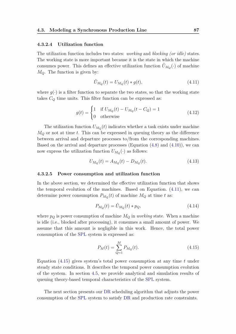
4.3. Modeling a Synchronous Production Line 87
4.3.2.4 Utilization function
The utilization function includes two states: working and blocking (or idle) states.The working state is more important because it is the state in which the machineconsumes power. This defines an effective utilization function UMQ
(·) of machineMQ. The function is given by:
UMQ(t) = UMQ
(t) ∗ g(t), (4.11)
where g(·) is a filter function to separate the two states, so that the working statetakes CQ time units. This filter function can be expressed as:
g(t) =1 if UMQ
(t)− UMQ(t− CQ) = 1
0 otherwise(4.12)
The utilization function UMQ(t) indicates whether a task exists under machine
MQ or not at time t. This can be expressed in queuing theory as the differencebetween arrival and departure processes to/from the corresponding machines.Based on the arrival and departure processes (Equation (4.8) and (4.10)), we cannow express the utilization function UMQ
(·) as follows:
UMQ(t) = AMQ
(t)−DMQ(t). (4.13)
4.3.2.5 Power consumption and utilization function
In the above section, we determined the effective utilization function that showsthe temporal evolution of the machines. Based on Equation. (4.11), we candetermine power consumption PMQ
(t) of machine MQ at time t as:
PMQ(t) = UMQ
(t) ∗ pQ, (4.14)
where pQ is power consumption of machineMQ in working state. When a machineis idle (i.e., blocked after processing), it consumes a small amount of power. Weassume that this amount is negligible in this work. Hence, the total powerconsumption of the SPL system is expressed as:
PM(t) =M∑
Q=1PMQ
(t). (4.15)
Equation (4.15) gives system’s total power consumption at any time t understeady state conditions. It describes the temporal power consumption evolutionof the system. In section 4.5, we provide analytical and simulation results ofqueuing theory-based temporal characteristics of the SPL system.
The next section presents our DR scheduling algorithm that adjusts the powerconsumption of the SPL system to satisfy DR and production rate constraints.

88 Chapter 4. Industrial Demand Side Management
4.4 Scheduling in the SPL systemThe second part of this chapter describes our DR scheduling algorithm whichis used to adapt power consumption of all machines to the available power (orDR threshold). In section 4.4.1, we highlight the scheduling problem in the SPLsystem. Then, section 4.4.2 presents the scheduling algorithm using examples. DRoptimality conditions are discussed in section 4.4.3. We also illustrate existenceand feasibility conditions of schedules. Finally, we provide a necessary andsufficient conditions to accept DR requests positively in section 4.4.4. At first,we provide the following definitions.
Definition 4.1 (Production rate).In manufacturing systems, production rate is the number of items that can beproduced during a given period of time, i.e., items per unit time.
Definition 4.2 (Power consumption block).Power consumption block of a machine is defined by its height which representsthe amount of power required to process a task on the machine and by its widthwhich represents the processing time of a task.
Figure 4.3 – Power consumption blocks and additional energy from DERs.
We refer to Figure 4.3 for better understanding of definition 4.2. From thefigure, we can see that machine M1 has a power consumption block of C1*p1where C1 is its processing time and p1 is its power consumption when it processesa task. Under normal conditions, the available power is enough to accept all thepower consumption blocks. However, during DR interval, the available power maysatisfy only one consumption block at a time. The existence of local DistributedEnergy Resources (DERs) can increase the total available power so that one ormore consumption blocks can be added to maximize the production rate (see

4.4. Scheduling in the SPL system 89
definition 4.1). However, the intermittent nature of DERs requires energy storagedevices (e.g., battery) to fill voids created by forecasting errors. For this purpose,determining battery size and smoothing out of fluctuations were investigated inchapter 3, but we do not consider it in this chapter. Based on the above definition,we now define production mode of a manufacturing system.
Definition 4.3 (Production mode).Production mode of a manufacturing system is defined by the available power levelswhich defines discrete values to match power consumption blocks of machines.
Figure 4.4 – DR mechanism and available power levels.
To clarify the above definition, we refer to Figure 4.4. In the figure, possiblepower levels are marked by L0, L1, ..., Lmax. L0 corresponds to a case wherethere is no available power. At this power level, the system is in power outage (orin complete shutdown). However, at Lmax, power requirement of all machines canbe satisfied and this provides the maximum production rate in the system. Basedon these information, we can construct status and power consumption vectorsthat consist of the status (ON/OFF) of machines and their corresponding powerconsumption. Let xi (1 for ON and 0 for OFF) denotes the status of machine Mi
and pi denotes power consumption of Mi when it is processing a task. Hence, astatus vector for a production line with M machines is represented as X = [x1,x2, ..., xM ] and the corresponding power consumption vector is p = [p1, p2, ...,pM ]. Then, total power consumption is given by:
P = XT ∗ p. (4.16)
Figure 4.4 also shows power consumption modes under maximum availablepower and observed power consumption during DR interval. Under normal

90 Chapter 4. Industrial Demand Side Management
conditions, every machine can get its share of the available power. To enterthe DR power consumption mode, a DR event (with reduction percentage andduration) should be communicated at some time (Time to DR in the figure)before the actual mode change happens. Assume that the DR event is emittedfrom a legacy energy provider at tj and the actual load shaving starts at tk. Werepresent the difference between these times (tk - tj) by DDR (deadline for DR).The length of DDR can vary from 10 minutes to 1 hour. In most of the cases, DRevent is communicated 1 hour earlier than the start of DR. In some cases, a DRevent can be issued in short time (emergency DR) to correct forecast errors or tohandle some unanticipated events such as partial electricity grid failure. In suchsituations, the availability of local DERs such as wind, solar, etc could help themanufacturing plants to accept the DR call positively.
The following section states the scheduling problem of the SPL system underavailable power and production rate constraints.
4.4.1 Scheduling problemA schedule in the SPL system is a finite sequence of actions spaced by a de-terministic (not necessarily constant) inter-arrival time and performed at theconveyor input. An action consists of inserting a new task (denoted by symbol I)or not inserting (I). Consequently, a schedule can be considered as a word overalphabet Σ = {I, I}. Each schedule word has a prefix, sub-word and suffix. Theprefix is used to resume actions in transient phases, while the sub-word representssteady phases, and the suffix word is used to flush the conveyor (i.e., to emptythe system). Note that the prefix word necessarily begins with I and has lengthK, the sub-word is a periodic sequence of symbols, and the suffix word takesI
K value where K is the number of virtual cells in the system. For instance,for the SPL shown in Figure 4.2, a schedule is I13InI
13 where I13 is the prefixword formed by thirteen consecutive task insertions (in a transient phase), In
is the sub-word representing the insertion of n consecutive tasks in the steadystate, and finally I
13 is the suffix word to purge the conveyor formed by notinserting tasks for 13 times. It is clear that this schedule provides a maximumproduction rate, and results in higher total power consumption because all themachines work simultaneously. However, the schedule I(I12
I)nI
13 ensures that ateach time only one task is finished before inserting a new task and at maximumonly one machine is working and this results in reduced power consumption. Inthe following lemma, we show how to compare two schedule words based on aproduction rate.
Lemma 4.4 (A schedule word with higher production rate).For two schedule words of the same length, the schedule having more number ofoccurrence of I produces maximum number of finished tasks.

4.4. Scheduling in the SPL system 91
Proof. Let w1 and w2 are two schedule words of the same length, i.e., ||w1|| = ||w2||.Let n1 and n2 (with n1 > n2) are number of occurrence of symbol I within w1 andw2, respectively. Based on schedule word definition, both words ends with thesame suffix IK where K is number of virtual cells in the system. Consequently,there are no tasks on the conveyor when the schedule ends. All the inserted tasksare processed in both schedules. Since n1 > n2, schedule word w1 produces morefinished tasks than w2. �
Now, we formally define the scheduling algorithm based on the constructionof a graph of activities with power consumption constraints.
4.4.2 DFSM schedule codingThe working principle of SPL can be regarded as a Deterministic Finite StateMachine (DFSM) [Sak09] where states represent whether there is a task or notin each virtual cell and transitions from one state to another represent symbolsof schedules. We distinguish left and right successors according to the symbols,i.e., we go to the left for symbol I and go to the right for symbol I. We write astate with binary values of size K, the number of virtual cells. More precisely,a state is expressed as (b1b2...bK)2 where bi can be 1 if there is a task in V Ci or0 otherwise. The state (00...0)2 is both start and end state. The left successorof (b1b2...bK)2 corresponds to shifting right by one bit and adding (2K−1)2. Thenew state will have (b1b2...bK)2 � 1 ⊕ (2K−1)2 value. The right successor of(b1b2...bK)2 corresponds to shifting right by one bit. Then, the new state will have(b1b2...bK)2 � 1 value. The duration of each transition in the DFSM takes thedeterministic inter-arrival Ta time units. The time spent in each state dependson maximum processing time among working machines. Figure 4.5 illustrates anexample of DFSM of an SPL system with three machines. We consider that eachmachine corresponds to a virtual cell, i.e., there are three virtual cells in the SPL.
Based on the above description, the DFSM is defined as a quintuple (Σ, V, v0, δ, F ),where:
• Σ = {I, I} is the input alphabet;
• V is the set of states with cardinality O(2K),
• vo = (00...0)2 is the initial state,
• δ is the state transition function, δ: V × Σ→ V . According to the inputsymbol: δ(I, (b1b2...bK)2) shifts right the state value by one bit and adds2K−1
2, and δ(I, (b1b2...bK)2) shifts right by one bit,
• F is the set of final states. It has only one state, v0.

92 Chapter 4. Industrial Demand Side Management
000start
100
010110
001101011111
I
I
I
I
I
I
I
I
I
I
II
I
II
I
Figure 4.5 – A DFSM for an SPL system with three machines
A default schedule in the SPL is to insert a task every Ta time unit. Therefore,the corresponding schedule word is given by IKInI
K , where n is the number ofconsecutive tasks inserted during the steady state. Regarding the DFSM, theprefix of the default schedule (IK) is to go from the first state (00...0)2 to (11...1)2taking the left successors during transitions. The sub-word (In) is to stay in thestate (11...1)2 by looping for n times. The suffix (IK) is to go back to end state(00...0)2.
4.4.3 Optimal schedule under DRWhen a given schedule transits to state (11...1)2, the SPL system consumesmaximum power. The following lemma confirms this SPL behavior.
Lemma 4.5 (State of peak power consumption).The peak power consumption is attained when the system is in state (11...1)2.
Proof. The total power consumption at state (11...1)2 is ∑Mi=1 pi which is derived
from Equation (4.16). Since it is the state where all machines are working, it isobvious that the power consumption is peak. �
Since the default schedule is looping in state (11...1)2, the power consumptionis peak from the above lemma. Assume that a DR signal is emitted at tr fromstart of the SPL demanding to reduce power consumption in DDR time unit forduration of Γ by an amount of ∆ (refer to Figure 4.6). During the DR interval,

4.4. Scheduling in the SPL system 93
Start SPL
DR notification
DR interval
DDR Γ
t0•
tr• • •
Time
Figure 4.6 – DR timelines
the default schedule is not attainable due to its peak power limitation, i.e., theavailable power is not enough for all machines to work at the same time. Now,we need to find a new schedule reducing the peak power consumption in the DRinterval by amount of ∆ as formulated below:P (t) 6max{P (t′)} −∆,
with t0 6 t′ < tr +DDR and tr +DDR 6 t 6 tr +DDR + Γ(4.17)
Under the DR constraints, the scheduling algorithm consists of three phases.The first phase determines if a feasible schedule exits or not. Then, the secondphase computes the optimal schedule satisfying DR constraints. Finally, in thethird phase, we search for the shortest path to go from the previous schedule tothe new optimal one. The procedures in the three phases are described in thefollowing section.
4.4.3.1 Phase 1 - Existence of feasible schedule
In phase one, we would like to know if a feasible schedule exists or not. Thefollowing lemma considers if a schedule exits or not under DR constraint.
Lemma 4.6 (Existence of feasible schedule).A feasible schedule exists if the power consumption of each machine is less thanthe available power.
Proof. A simple schedule is when there is only one task in the SPL system at atime. Consequently, only one machine is processing in the system at maximum.Since the power consumption of each machine is below DR threshold, the totalconsumption using this schedule is less than the available power. Hence, theschedule word exists and it is given by I(IK−1
I)nI
K . �
Based on Lemma 4.6, a DR constraint cannot be less than a lower boundgiven by the schedule in which only one machine is processing a task at a time.This schedule (I(IKM−1
I)nI
K) corresponds to go from state (00...0)2 as 1st stepto the most right side state (00...01)2 until state (10...0)2 and go back to state(00...01)2 to form a cycle. For example, let us see the feasible schedule of an SPL

94 Chapter 4. Industrial Demand Side Management
000start
100
010110
001101011111
0kW
100kW
300kW
600kW
500kW 400kW300kW
200kW
I
I
I
I
I
I
I
I
I
I
II
I
II
I
Figure 4.7 – Feasible schedule under DR constraint.
system with three machines in three consecutive virtual cells. We assume thatthe power consumption of machines 1, 2 and 3 are 100kW, 200kW and 300kW,respectively. Furthermore, we set ∆ to 200kW. Hence, the new available power(or DR threshold) is 400kW according to Equation (4.17). The feasible schedule isto go from state (000)2 to (100)2, then we take right until state (001)2. After that,we go back to state (100)2. The transitions (thick lines) in Figure 4.7 represent afeasible schedule. We can see that the peak power consumption in the SPL is300kW which is less than the DR threshold of 400kW.
4.4.3.2 Phase 2 - Finding optimal schedule
In phase 2, the objective is to find, if possible, an optimal schedule better thanthe feasible schedule that satisfies DR power constraint. This schedule mustgive the maximum production rate under the constraint. In other words, thenumber of occurrence of I in the schedule should be higher. A simple algorithmconsists of exploring the DFSM by taking left successors to increase number ofIs verifying the DR constraint at each state. This algorithm can be seen as abranch and bound (B&B) [Cla99] algorithm where the entire candidate solutionsare enumerated and a search is optimized based on upper and lower bounds. Thisalgorithm tries to find a prefix word going from initial state to the depth (K) ofDFSM and then it finds the shortest cycle that satisfies DR power constraints toform a sub-word.
In order to find the optimal prefix, we apply Algorithm 2 to the binary tree

4.4. Scheduling in the SPL system 95
Algorithm 2 Prefix searching in DFSMRequire: (Σ, V, v0, δ, F ), a DFSMPow_dr, the available power under DRx.state← v0x.visited_left← false
x.visited_right← false
Prefix ← ε
Sub-word ← ε
while |Prefix| < K doif x.visited_left == true & x.visited_right == true then
x← parent[x]Prefix← Prefix− Last_symbol(Prefix)
elseif x.visited_left == false then
y ← left[x]x.visited_left← true
if y.power 6 Pow_dr thenPrefix← Prefix.I
elsey ← x
elsey ← right[x]x.visited_right← true
if y.power 6 Pow_dr thenPrefix← Prefix.I
elsey ← x
x← y
resulted by removing cycles from the DFSM. All states having impaired valueor the last bit fixed to one, (1)2, become leaf nodes. This algorithm defines apreorder traversal: while a leaf node is not visited and under meeting the DRconstraint, we recursively do a preorder traversal of the left sub-tree, followed bya recursive preorder traversal of the right sub-tree.
Figure 4.8 illustrates the optimal prefix (transitions in thick lines) afterexecuting Algorithm 2 on the binary tree of the DFSM shown in Figure 4.7. We

96 Chapter 4. Industrial Demand Side Management
Algorithm 3 Sub-word searching in DFSMRequire: (Σ, V, v0, δ, F ), a DFSM, and the last state found by the prefix searchingalgorithm, vprefixPow_dr, the available power under DRx.state← vprefixx.visited_left← false
x.visited_right← false
cycle← false
Sub-word ← ε
while cycle == false doif x.visited_left == true & x.visited_right == true then
x← parent[x]Sub-word← Sub-word− Last_symbol
elseif x.visited_left == false then
y ← left[x]x.visited_left← true
if y.power 6 Pow_dr thenPrefix← Sub-word.Iif y.state == vprefix then
cycle← true
elsey ← x
elsey ← right[x]x.visited_right← true
if y.power 6 Pow_dr thenPrefix← Sub-word.Iif y.state == vprefix then
cycle← true
elsey ← x
x← y
can see that the peak power consumption of this prefix in the SPL is 400kWwhich is equal to the DR threshold.

4.4. Scheduling in the SPL system 97
000start
100
010110
001101011111
0kW
100kW
300kW
600kW
500kW 400kW300kW
200kW
I
I
I
I
I
I
I
I
Figure 4.8 – Prefix searching example.
000start
100
010110
001101011111
0kW
100kW
300kW
600kW
500kW 400kW300kW
200kW
I
I
I
I
I
I
I
I
I
I
II
I
II
I
Figure 4.9 – Optimal sub-word searching example.
In order to find the sub-word of the schedule, we search a cycle going from thelast state (at depth K) obtained by prefix searching and that eventually returnsto the state. It is easy to see that the best method to continue producing athigher rate is the same as that used for prefix searching, i.e., while the startingstate is not visited twice and under meeting DR power constraint, we recursivelydo a preorder traversal of the left successors, followed by a recursive preorder

98 Chapter 4. Industrial Demand Side Management
traversal of the right successors. Algorithm 3 details such a principle.Figure 4.9 illustrates the optimal sub-word (transitions in thick lines) after
executing Algorithms 3 on the DFSM shown in Figure 4.7. We can see that thepeak power consumption of this sub-word in the SPL system is 400kW which isequal to the DR threshold.
The performance of Algorithms 2 and 3 depend on the number of virtualcells K of the system. When K increases, the total number of states increasesexponentially to 2K states. Hence, the worst time complexity to search in theDFSM is O(2K). Since the number of cells on the conveyor is limited, thisalgorithm could be of great help to find optimal solutions. To reduce this curse ofdimensionality, we rely on a more efficient algorithm to search for a near-optimalsolution based on linear programming (LP) formulations. To compute the prefixword, we find theoretically the best leaf state in the binary tree having a pathfrom the root state satisfying the DR power consumption on each intermediatestate. Then, we use the reverse path to set the prefix. The LP problem for theleaf state can be formulated as follows:
maxK∑
i=1xi (4.18)
s.t: A ∗ x 6 Pavail (4.19)
xi ∈ {0, 1}, i = 1, 2, ..., K − 1 and xK = 1
where:
• xi indicates whether a task exists or not in virtual cell i. For the leaf states,the last bit is set to one, i.e., xK = 1,
• x is the vector of xi,
• A is an upper triangular matrix representing power of intermediate statesin the binary tree:
A =
p1 p2 · · · · · · pK
p1 · · · · · · pK−1. . . · · · ...
0 . . . · · ·p1
(4.20)
• Pavail is the available power.
The objective function (Equation (4.18)) is to choose machines so as to maximizeproduction rate and Equation (4.19) poses constraint on total power consumptionin the path from root to leaf states to respect the available power constraint.

4.4. Scheduling in the SPL system 99
By applying the LP equations to the binary tree of the DFSM shown inFigure 4.7, we find that the state (101)2 satisfies both DR threshold and max-imum number of 1s in the vector x. The reverse path is (000)2 → (100)2 →(010)2 → (101)2, and so the prefix is III which corresponds to the one foundusing Algorithm 2. To find a cycle starting and ending at the state obtained bythe LP equations above, we rely on the well known problem of finding minimumcycle in weighted directed graphs [Kar78]. We replace cost metric by powerconsumption metric. We define the power consumption of an arc as the maximumbetween its ending states, and a path’s power consumption as the maximumpower consumption among its arcs. The mathematical formulation of the problemcan be given as:
maximizez(e)
{p(e)z(e), e ∈ E}
subject to∑
e∈V +(v)z(e)−
∑e∈V −(v)
z(e) = 0, ∀v ∈ V∑e∈E
z(e) = 1
p(e) 6 pavail
z(e) > 0
(4.21)
where V +(v) is the set of arcs having extremities in v, V −(v) is the set of arcsoriginated in v and z(e) is the variable associated to each arc e in the DFSM. Byapplying our LP equations for cycle searching in the DFSM (shown in Figure 4.7),we find a loop between (101)2 and (101)2.
4.4.3.3 Phase 3 - Path to optimal schedule
In phase three, we would like to find a shortest path from current state to thestate obtained in phase 2 (transitions in red dotted lines in Figure 4.10). For thispurpose, we use the well-known Dijkstra’s algorithm [Dij59].
Dijkstra’s algorithm finds a shortest path starting from an initial node to atarget node (or all other nodes) on a graph. The algorithm assigns initial distancevalues and try to improve them step by step. In our case, we would like to findthe shortest path between two states on the DFSM graph (see Figure 4.10), i.e.,the short path between the optimal state (101)2 found in phase 2 and the initialstate which is (111)2. The following steps are used to find the shortest pathstarting from initial state (111)2:
(1) Assign some values for every state on the DFSM graph: set zero for theinitial state (111)2 and infinity for all other states,
(2) Set the initial state as current. Mark all other state unvisited. Constructan unvisited set for representing all unvisited states within the DFSM,

100 Chapter 4. Industrial Demand Side Management
000start
100
010110
001101011111
0kW
100kW
300kW
600kW
500kW 400kW300kW
200kW
I
I
I
I
I
I
I
I
I
I
II
I
II
I
Figure 4.10 – Shortest path to the optimal schedule (phase 3) marked in reddotted lines.
(3) For the current state, consider all of its neighbors and calculate theirtentative distances. Here, we assign a distance of value 1 for a neighborstate. For example, the distance beween states (111)2 and (011)2 is 1 ascan be seen from Figure 4.10,
(4) After examining all the neighbors of the current state, mark the currentstate as visited and remove it from the unvisited set,
(5) If the destination state has been marked visited, then stop. The algorithmhas finished, else
(6) Select the unvisited state that is marked with the smallest distance, i.e.,state (011)2 and set it as the new current node, and go back to step (3).
By following the above steps, state (101)2 can be reached with a distancevalue of 2 which is the shortest path through state (011)2. This path is markedby dotted lines in Figure 4.10.
The total duration the shortest path takes from current state to the stateobtained in phase 2 determines if it is possible to accept the DR request or not.The next section analyses acceptance conditions of a DR request.
4.4.4 DR acceptance conditionsWe now give a necessary and sufficient condition to be able to accept a DR requestpositively or not.

4.5. Analytical and Simulation Results 101
Lemma 4.7 (Condition to accept DR).A necessary and sufficient condition to be able to positively answer to a DRrequest is that the time to switch from any state A to another state B satisfyingthe maximum power imposed by DR should be less than or equal to duration ofDDR (deadline to DR, refer to Figure 4.4). This time is equal to the duration ofeach visited states in the DFSM graph described in Figure 4.10 plus the time ofthe state transitions (Ta) for each transition.
Proof. Under normal conditions, the system is at the state (11...1)2 with durationcorresponding to the maximum processing time among the machines. Then,starting from this state, we go to right successor to the next state (11..10)2 whichtakes Ta and its processing time coincides with the working machines. We sumboth the maximum processing time and transition time until we arrive at therequired state B. If this sum is less than duration of DDR, it is obvious that theDR requested can be accepted. �
From phase 3 above, the transition path required for DR in the DFSM graphof Figure 4.10 leads to a state maximizing the production rate by searching for ashortest path to the state. As an example, let us consider the case of a productionline with three machines represented by a DFSM in Figure 4.7. During normalproduction periods, the system is at state (111)2 (i.e., current state) and thesystem’s total power consumption is 600kW. If DR asks for a maximum powerconsumption of 400kW, which corresponds to state (101)2, the production linesystem will follow, according to Algorithm 2, the path (111)2 with state transitionI of duration Ta reaching state (011)2 where M1 will not be working. Then aftera state transition I of duration Ta, we reach at state (101)2 where M2 will not beworking. The state is still valid for the power threshold of 400kW. A productioncycle satisfying maximum power 400kW can indeed start after DR, i.e., the cycleis (101)2 → (010)2 → (101)2, . . .. Notice that it is the production cycle thatmaximizes the production rate. The total duration for answering DR to reach thisproduction cycle is then max(C1, C2, C3) + Ta + max(C2, C3) + Ta that shouldbe less than or equal to duration of DDR from Lemma 4.7, where Ci is processingtime of machine Mi, i = 1, 2, 3.
In the above sections, we discussed the two works: modeling of the SPL systemusing a queuing model and DR scheduling under constraints of available powerand production rate. In the following section, we provide numerical results.
4.5 Analytical and Simulation ResultsIn this section, we present our analytical and simulation results of both modelingof SPL and DR scheduling under available power constraint. As a study model,

102 Chapter 4. Industrial Demand Side Management
we consider the example shown in Figure 4.2 which has 13 virtual cells and 4machines. For processing times (Ci) of the machines, we take values of 3s, 6s, 9sand 12s (s = seconds) for machine 1, 2 , 3 and 4, respectively. Since there is norestrictions on these values, any other values can be taken. We assume that eachmachine consumes 100kW when it processes a task and 0kW otherwise. We alsoassume that the SPL system starts working at time t = 0. We commence withresults on SPL modeling in the following section.
4.5.1 Results on SPL modelingAs discussed in section 4.3, we relied on queuing theories to model the SPL systemwith deterministic inter-arrival and service times. The D/D/1 queuing modelwas used to characterize arrivals and departures of parts/tasks in the SPL system.This section presents analytical and simulation results of the system.
4.5.1.1 Analytical results
To analyze the SPL system, we used python programming language to implementEquation (4.8) and (4.10) which represent the arrivals and departures processes atthe machines, respectively. Based on these processes, the utilization and effectiveutilization functions (Equation (4.13) and (4.11)) are also implemented in python.Moreover, analytical power consumption function PMi
(·), for machine Mi, i = 1,2, ..., M , is also computed by using Equation (4.14). Then, we compare it with areal power consumption of a typical production process of a factory taken fromMETRONLab server.
Figure 4.11.1 shows cumulative arrivals of tasks to the 4 machines. From thefigure, we can see that the arrival of the 1st task to machine M1 at time t = 15sinitializes the SPL system in a transient phase. As soon as the 1st task arrivesat machine M2, the two machines (M1 and M2) synchronize themselves. Thiscontinues until the 1st task reaches machine M4 in which all the machines aresynchronized to the one with the maximum processing time (i.e., C4). Furthermore,the arrival of the 1st task at M4 at t = 114s signals the end of the transientphase. Afterwards, the SPL system is in a steady state. The cumulative numberof departed tasks from the machines are shown in Figure 4.11.2. In the steadystate, the departures from all of the machines occur at the same time.
In Figure 4.11.3, the difference between the cumulative number of arrivals anddepartures (i.e., the utilization) of all the machines are shown. For clearer view,we added some constant value to each UMi
(·) so that the curves are moved upthe y-axis. However, the values of UMi
(·) is either 1 or 0 because only one task isprocessed at any time because each machine is considered as a single server. Sincethe utilization functions are derived from the arrival and departure processes, thefigure can also show both the transient and steady states. However, the utilizationfunction cannot differentiate between the two modes of a machine (working or

4.5. Analytical and Simulation Results 103
4.11.1: Arrival processes using Equation (4.8) 4.11.2: Departure processes using Equation (4.10)
4.11.3: Utilization using Equation (4.13) 4.11.4: Effective utilization using Equation (4.11)
Figure 4.11 – Arrival and departure processes, utilization and effective utilizationof the four machines with processing time of 3s, 6s, 9s and 12s for machine 1, 2,
3 and 4, respectively.
idle) and it cannot show us the power consuming mode of the machines. Hence,we use the effective utilization functions as depicted in Figure 4.11.4. The figureshows that the machine start processing tasks at the same time but don’t finishat the same as their processing times are different. The idle modes are effectivelysuppressed and only the working modes are prevailed. This is important becausewe can multiply the effective utilization function of a machine by its powerconsumption to get a power consumption curve. For example, Figure 4.12 showssuch a power consumption curve for machine M2 when it consumes 300kW whileprocessing a task. This value is taken from a real production process powerconsumption trace shown in Figure 4.13. As can be seen from Figure 4.12 and4.13, there is a small difference between the approximated power curve (i.e., based

104 Chapter 4. Industrial Demand Side Management
Figure 4.12 – Analytical power consumption of machine M2 using Equation(4.14) which is derived from the effective utilization function.
Figure 4.13 – A real power consumption of a typical production process fromMETRONLab server.
on the queuing model) and the real power curve. This happens when a machinechanges its mode from idle to working and vice-versa. The difference can becorrected by adding a positive slope when the mode changes from idle to workingand a negative slope when the mode changes from working to idle. The slopescan be inferred from the real power consumption curve.
4.5.1.2 Simulation results
To verify our analytical works, we use an Objective Modular Network Testbedin C++ (OMNET++) [OMN] simulator which is a modular, component-basedC++ simulation library and framework, primarily used for building networksimulators. It has been widely used as a modeling tool in applications such ascommunication networks, distributed or parallel systems, etc [Var01]. In ourwork, we modified source codes of OMNET++ so that it fits to our objectiveof modeling the SPL system using a queuing library in OMNET++. In the

4.5. Analytical and Simulation Results 105
Figure 4.14 – OMNET++ network description of the SPL system with 4machines.
queuing library, OMNET++ contains modules such as source, sink, delay, queue,etc to describe a specific topology that users want to simulate. Descriptionsof the modules and use cases are provided in the website of [OMN]. However,these modules could not satisfy our needs to simulate the SPL system in theOMNET++ simulator. Hence, we created conveyor and machine modules inOMNET++ by modifying the C++ source codes of the queuing library.
As shown in Figure 4.14, we use 5 different OMNET++ module types todescribe the SPL system. The modules are given below:
• The source module is used to generate the tasks labeled from 1 to n,
• The machine module is used to represent a machine. The source codes of aqueue module in queuing library is modified for this purpose,
• The conveyor module is synchronizing the machines by realizing the tasksat a specific time,
• The delay module is used to keep (or delay) a task until a downstreammachine is available.
• The sink module can be viewed as a storage for finished tasks.
After creating the necessary modules, a NEtwork Description (NED) file iscreated by drag and drop of the modules. The final NED graph is shown inFigure 4.14. The next step is to run the OMNET++ program so that live tasktransfers between the machines can be viewed. Figure 4.15 shows when the SPLsystem is running in OMNET++. After the source module releases tasks (marked

106 Chapter 4. Industrial Demand Side Management
Figure 4.15 – The OMNET++-based SPL system in action.
Figure 4.16 – OMNET++ time line graph for the SPL system.
by red dot), the tasks pass under each machine until the sink module collectsthem. From the OMNET++ simulator, we can also see the arrival and departuretimes of the tasks to and from the machine as depicted in Figure 4.16. Fromthe figure, we notice that the system synchronizes when the 1st task arrives atmachine M4. This is in accordance with the one that we have achieved using theanalytical effective utilization function shown in Figure 4.11.4.
4.5.2 Result on DR schedulingIn section 4.4, we provided details of the our DR scheduling algorithm thatadapts power consumption of the SPL system to available power and productionrate constraints. We used different illustrating examples and described the pparticiples on how the algorithm works. In this section, we use the exemplarySPL system configuration shown in Figure 4.2 with 4 machines and 13 virtualcells to compute prefixes and sub-words of schedules. As describe in the abovesection, processing times (Ci) are set to values 3s, 6s, 9s and 12s for machine 1,2, 3 and 4, respectively. Now, we assume that each machine consumes 100kWwhen it processes a task (but this value can be any amount). Furthermore, the

4.5. Analytical and Simulation Results 107
Table 4.2 – Prefix and sub-word when DR threshold is 100kW.
State Symbol max. power conso. (kW) maxCi (sec)1111111111111 . 400 120111111111111 I 400 120011111111111 I 400 120001111111111 I 400 120000111111111 I 300 120000011111111 I 300 120000001111111 I 200 120000000111111 I 200 120000000011111 I 200 120000000001111 I 200 120000000000111 I 200 120000000000011 I 100 121000000000001 I 100 121100000000000 I 0 00110000000000 I 0 00011000000000 I 100 30001100000000 I 100 30000110000000 I 100 60000011000000 I 100 60000001100000 I 0 00000000110000 I 0 00000000011000 I 0 00000000001100 I 100 90000000000110 I 100 9
available power levels for DR (i.e., DR thresholds) are considered to be 400, 300,200, 100, and 50kW. These values are used to find the schedule words in the nextsection. We also investigate the monetary gain of accepting DR request positivelyin section 4.5.2.2.
4.5.2.1 Finding schedule words
Based on Lemma 4.6, when the available power is 50kW, there is no feasibleschedule as it is not enough even for a single machine. The next threshold iswhen the available power is 100kW in which a simple feasible schedule exists.Table 4.2 shows the resulting symbols of a schedule that satisfies the DR thresholdof 100kW. In the table, each row of the 1st column has length of 13 bits whichcorrespond to the virtual cells (1 if there is a task in a virtual cell or 0 otherwise).

108 Chapter 4. Industrial Demand Side Management
Table 4.3 – Prefix and sub-word when DR threshold is 300kW.
State Symbol max. power conso. (kW) maxCi (sec)1111111111111 . 400 120111111111111 I 400 120011111111111 I 400 121001111111111 I 400 120100111111111 I 300 120010011111111 I 300 121001001111111 I 300 121100100111111 I 200 121110010011111 I 300 121111001001111 I 300 121111100100111 I 300 121111110010011 I 300 121111111001001 I 300 121111111100100 I 300 90111111110010 I 200 60011111111001 I 300 121001111111100 I 300 90100111111110 I 200 9
Machine 1, 2, 3 and 4 are on virtual cell 4, 6, 11 and 13, respectively (see Figure4.2). Hence, the values of these virtual cells are required to compute the system’stotal power consumption (3rd column) and the maximum processing times amongthe machines (4th column). The 2nd column represent an action of inserting (I)or not (I) a task at the conveyor input.
From Table 4.2, we can easily find the prefix and the sub-word of the schedulewhen the available power is 100kW. The prefix (path to optimal state) is I8, i.e.,we arrive at this state by not inserting tasks for 8 times or taking right successors8 times from the initial state (11...1)2. Then, the sub-word is (II2I
10) (graycolored rows) which repeats until the end of the DR interval. During this interval,the peak power consumption is 100kW, i.e., only one machine is working at a time.In the sub-word, the number of Is determines the production rate per sub-word’stotal duration. The duration can be computed from the 4th column of the tableby summing up the processing times (12 + 12 + ... + 9 = 60s) at each state inthe DR interval and the transition times (12*5 = 60s). Hence, the productionrate in the sub-word is 2 items per 120 seconds (1 item per minute). However,under normal conditions, the production rate is 13 items per 216 seconds (3.6items per minute).

4.5. Analytical and Simulation Results 109
To see the effect of less strict DR constraint than the above case, we consideranother case where the available power is 300kW. Table 4.3 shows results underthe given DR constraint. In this case, the length of prefix (I2
II2) is shorter than
the prefix of the above case. It means that we arrived at the optimal state withfew transitions. The sub-word is found to be (II8I
2II). Referring to the table,
the number of Is in the sub-word is 9 and their total duration is 165s (12*9 + 9*3+ 6 + 5*12). The resulting production rate becomes 9 items per 2.75 minutes(approx. 3 items per minute). In this case, the number of Is in sub-word is higherthan that of the above case and is in accordance with Lemma 4.4 that comparetwo schedule words based on the number of Is for higher production rate.
4.5.2.2 Monetary gains of accepting DR
Based on our discussion in section 2.3.1.2 of chapter 2, incentive-based DRprograms pay customers for not consuming power (or consuming less) in DRintervals. Hence, customers can benefit from monetary gain for accepting the DRpositively. The monetary gain can be formulated as follows:
Gmoney =(Nnorm −NDR
)∗ Prunit ∗ Inpct (4.22)
where Nnorm is number of items produced during normal periods, NDR is numberof items produced during DR periods, Prunit is unit price of an item and Inpct ispercentage of incentive for the items that are not produced due to DR.
Now, we use Equation (4.22) to calculate a monetary gain for positivelyanswering a DR request. Assume that a factory could receive 20% as an incentivefor not consuming power to produce items using the default schedule ((I13)n,n >0). In the default schedule, the factory produces 13 items. As a first case,we consider that the available power is 100kW and the corresponding numberof produced items are 2. That is, only two items are produced instead of 13items and the factory gets paid for the remaining 11 items that are not produced.Taking 50AC per item, the monetary gain is found to be Gmoney = (13 - 2)*0.2*50= 110AC.
Considering an available power of 300kW where the number of produced itemsare 9, the monetary gain could be Gmoney = (13 - 9)*0.2*50 = 40AC. This showsthat the less the factory consumes the more money paid for not consuming powerand vice-versa. If the factory owns some Renewable Energy Sources (RESs) inits local premises, this will help it benefit more from the DR mechanism. Assumethat the RESs generate power in order of 100kW. That means, the total availablepower is 400kW that is enough for all the machines. In this way, the numberof items produced is 13 which is the same with the default schedule. Besidesproducing at full capacity, the factory can save 40AC. In conclusion, the benefitsshould be interesting for the factory to participate in DR programs.

110 Chapter 4. Industrial Demand Side Management
In the above sections, we discussed analytical and simulation results of ourworks on modeling of an SPL system and DR scheduling. In the next section, wedetails our experiments with the DR protocol: OpenADR.
4.6 Experimentation with OpenADRBased on the description of OpenADR in section 2.3.4 of chapter 2, the objectiveof OpenADR is to facilitate information exchange between electricity serviceproviders, aggregators and energy consumers. In this section, we provide theexperiments that are done in METRON for the purpose of integrating OpenADRto METRONLab platform and testing OpenADR on a real testbed. Setupprocedures of the testbed is given below.
Figure 4.17 – Testbed for implementing OpenADR.
4.6.1 Testbed setupFigure 4.17 shows our testbed that is used to implement the OpenADR protocol.The testbed contains two parts: hardware and software parts.
4.6.1.1 Hardware
The hardware part of the testbed consists of:
• Personal computer (PC): a PC with Ubuntu 16.04 is used as a Virtual TopNode (VTN). It emits DR requests as per users requirements,
• METRONLab: the METRONLab device hosts the Virtual End Node(VEN). The VEN processes DR requests of the VTN,

4.6. Experimentation with OpenADR 111
• Water pump: the pump is used as a controllable load, i.e., it can be turnedON or OFF based on DR requests,
• Raspberry Pi: the raspberry pi (Model B) board receives a command fromthe METRONLab and controls the pump through a relay. A relay modulecan be interfaced to the pi board by soldering the module on the GeneralPurpose Input/Output (GPIO) pins.
4.6.1.2 Software
In the software part, the following software are used in the experiment:
• OpenADR source code: VTN and VEN source codes are available in Ener-NOC’s GitHub [Ene]. Since the source code of EnerNOC only provide theEiEvent service, major modifications have been done to implement the rest7 services of OpenADR described in section 2.3.4 of chapter 2.
• XML Messaging and Presence Protocol (XMPP) server : as an XMPPserver, we used an OpenFire [OFR] server which is instant messaging andgroup chat server. OpenFire accounts (JID - Jabber ID) are created forboth VTN and VEN nodes,
• Modbus TCP (Transmission Control Protocol): Modbus [Mod04] is a de-facto standard communication protocol for connecting industrial electronicdevices. It is a software originally developed in Schneider Electric. ModbusTCP is used for communications over TCP/IP (Internet Protocol) networks,
• Open Platform Communications Unified Architecture (OPC UA): OPCUA is a machine to machine communication protocol developed for indutrialautomation. For more decription of the OPC UA protocol, refer to [LM06].As shown in Figure 4.17, we included codes of the VEN node together withOPC UA client in METRONLab device.
• Grails/Groovy: For web application framework in VTN, we used Grails/-Groovy [GRL] web framework which is used in the OpenADR source code.We extended the Grails/Groovy source code so that a user can view thestatus of a VEN as a form of live feed (see Figure 4.18).
After configuring both the hardware and software parts, a simple web pagecan be displayed as shown in Figure 4.18. In the right hand side of the figure, aportion is dedicated for showing incoming messages and the sending VENs. Thetabs at the center display information including real-time status, available VENs,DR event creation and emitting to VENs, and market context (i.e., available DRprograms such as TOU, RTP, etc).
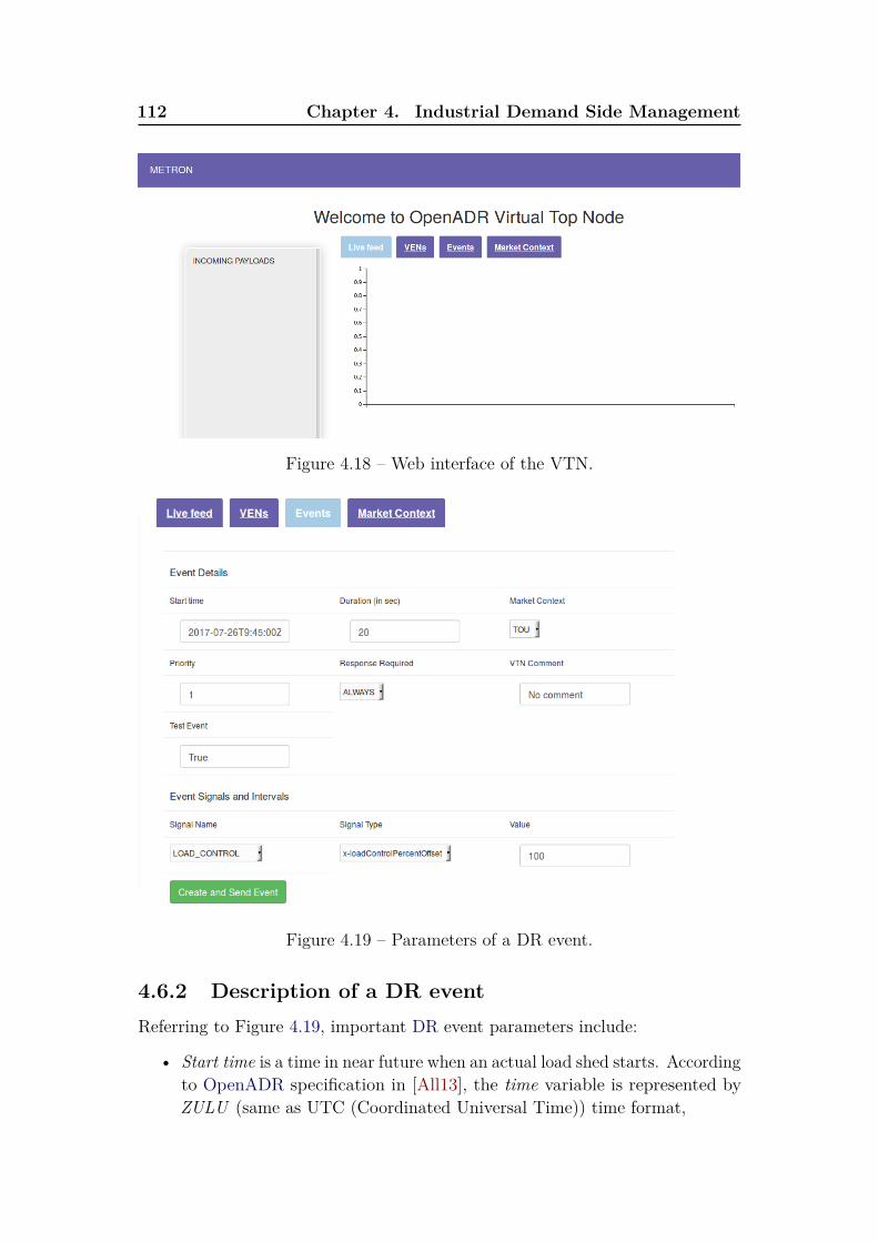
112 Chapter 4. Industrial Demand Side Management
Figure 4.18 – Web interface of the VTN.
Figure 4.19 – Parameters of a DR event.
4.6.2 Description of a DR eventReferring to Figure 4.19, important DR event parameters include:
• Start time is a time in near future when an actual load shed starts. Accordingto OpenADR specification in [All13], the time variable is represented byZULU (same as UTC (Coordinated Universal Time)) time format,

4.6. Experimentation with OpenADR 113
• Duration is the length of the DR interval (Γ in Figure 4.6),
• Market Context is a DR program (e.g., TOU, RTP, etc),
• Priority is set to 1 if the event has higher priority than the other eventswhich were emitted and that did not start,
• Response Required is set to ALWAYS if a response is required for a DRevent that a VTN sent to a VEN,
• Signal Name is a name of an event signal (e.g., ELECTRICITY_PRICE,LOAD_DISPATCH, LOAD_CONTROL, etc),
• Signal Type is an element of a signal name (e.g., LOAD_CONTROL hassignal types of x-LoadControlPercentOffset, x-LoadControlSetpoint, etc).[All13] provides the full list of signal names and types,
• Value is a corresponding value to the chosen signal name and type.
Figure 4.20 – Real-time status of the pump during normal periods.
4.6.3 Communicating DR events between VTN and VENFor description of service types to establish initial communication between VTNand VEN, see section 2.3.4.2 of chapter 2. During normal periods, the statusof the water pump is ON (or 1) as shown in Figure 4.20. At some time, ifthe VTN wants to send a DR event to the VEN, it uses oadrDistributeEventpayload of EiEvent service. The oadrDistributeEvent payload specifies all the

114 Chapter 4. Industrial Demand Side Management
Figure 4.21 – Real-time status of the pump during DR periods.
event parameters described in the above section. After the VEN receives theevent, it replies with oadrCreatedEvent payload of EiEvent service. As shownin Figure 4.21, the pump has changed its status from ON to OFF (or 0) for thespecified duration (20 seconds) to respect the DR constraint.
4.7 SummaryThis chapter presented two of our works on the demand side of the industrialmicrogrid together with experiments of a Demand Response (DR) protocol. Insection 4.3, we detailed modeling of a Synchronous Production Line (SPL) basedon D/D/1 queuing model. The SPL system was represented by a tandem ofD/D/1 queues. It was used to characterize temporal properties such as arrivaland departure processes, utilization and effective utilization of the SPL system.Analytical and simulation results were also given for a specific SPL configuration.
Then, section 4.4 discussed our DR scheduling algorithm that adapts powerconsumption of the SPL system to constraints of production rate and availablepower. The algorithm was coded using Deterministic Finite State Machine(DFSM) in which state transitions happen by inserting a task or not. Findingan optimal schedule under DR constraint has followed three phases: existence ofa schedule, finding optimal schedule and shortest path to optimal schedule. Weshowed different results of the scheduling algorithm using illustrative examples.
Finally, we provided our experiments with a DR protocol called OpenAutomated Demand Response (OpenADR) in section 4.6. For this, we setup atestbed that contains devices such as water pump, raspberry pi and METRONLab.
The following chapter summarizes the works done in thesis by mentioningimportant points. It also highlights perspectives of the thesis.

Part III
Conclusions and Perspectives


Chapter 5
Conclusions and Perspectives
Contents5.1 Conclusions . . . . . . . . . . . . . . . . . . . . . . . . . . . 117
5.1.1 Modeling of DERs and cost minimization strategies . . . 118
5.1.2 Smoothing of RESs . . . . . . . . . . . . . . . . . . . . . . 119
5.1.3 A queue theory-based model of a production line . . . . . 119
5.1.4 DR scheduling in a production line . . . . . . . . . . . . . 120
5.2 Perspectives . . . . . . . . . . . . . . . . . . . . . . . . . . . 120
5.1 ConclusionsIn this thesis, we have addressed energy management challenges in the contextof industrial microgrid. The challenges can be categorized into the two sides ofmicrogrid energy management:
• In the supply side:
– We proposed a mathematical framework that is used to model powergenerations ofDistributed EnergyResources (DERs) so that the powersources can be seamlessly integrated into the microgrid. Moreover, wealso proposed cost minimization strategies that enable us choose froman energy mix (solar, wind, battery, utility grid) which reduces totalenergy costs,
– To reduce the inherent power fluctuation behavior of RenewableEnergy Sources (RESs), an approach of smoothing their power pro-duction was also proposed. Its performance comparisons have beendone against other smoothing algorithms.
• In the demand side:
– A queuing theory-based mathematical model was proposed that pro-vides temporal characterization of a Synchronous Production Line(SPL) such as arrival and departure processes,

118 Chapter 5. Conclusions and Perspectives
– We proposed a Demand Response (DR) scheduling algorithm whichaddresses how an SPL system adapts its power consumption to con-straints such as available power and production rate.
Figure 5.1 summarizes the works in this thesis with corresponding publications.The following sections provide more insights to the works in both supply anddemand sides of microgrid energy management.
Thesis works in the context of Industrial Microgrid
In Supply Side
Modeling of DERs andCost minimization strategies
[Add+15]
Smoothing of RESs[Add+17c][Add+17d]
In Demand Side
Production line modeling[Add+17b]
DR scheduling[Add+17a][Add+17b]
Figure 5.1 – Summary of our works in this thesis.
5.1.1 Modeling of DERs and cost minimization strategiesWe discussed modeling of DERs in the supply side of the industrial microgrid insection 3.3 of chapter 3. The following questions can be inferred from the section:
• What is a minimum power produced by DERs? How can we model thisvalue using a mathematical framework?
• When energy demand is greater than energy supply, can we buy energyfrom spot markets, utility grid, or discharge from Battery Energy StorageSystems (BESSs)? What happens if supply is greater than demand?
A service curve concept ofNetworkCalculus (NC) was proposed for respondingto the above questions. We used service curves to model the minimum power theDERs can provide. To obtain total power production, we aggregate the servicecurves of the DERs. After that, a balance should be reached between energydemand and supply. For cases of imbalance (i.e., when supply is greater thandemand or vice-versa), we proposed different strategies that minimize energyprocurement costs. The strategies were sell surplus energy, store excess energyand use external energy to charge battery. To compare the performance of thestrategies, we used real power consumption data of a factory located in France.Our results showed that interesting saving can be made by adopting the strategies.

5.1. Conclusions 119
5.1.2 Smoothing of RESsIn section 3.4 of chapter 3, we focused on smoothing of RESs to reduce powerfluctuations in conjunction with BESSs. The following questions were raised:
• How to smooth power production curves of RESs and how to measure thesmoothness of the curves?
• What battery size is required so that a production curve for a day-aheadforecast period can be guaranteed?
• From regulatory aspect, how much power differences between any twosuccessive time slots are tolerated?
To deal with the above questions, we proposed a Gaussian-based smoothingalgorithm. We compared its performances by bench-marking classical approachessuch as SimpleMovingAverage (SMA) and ExponentialMovingAverage (EMA)for the purpose of smoothing out power fluctuations of RESs. The performancesof the algorithms were showed based on real datasets and considered two cases:with and without power level constraints. In both cases, the Gaussian-basedalgorithm performed better than both SMA and EMA when smoothness measuresand battery sizes are taken to account.
5.1.3 A queue theory-based model of a production lineWe discussed modeling of an SPL system using a queuing model in section 4.3 ofchapter 4.4. It could give an interesting solution to the following inquiries:
• How to model temporal behaviors of an SPL system such as arrival anddeparture processes to/from a machine? Which model to use?
• Relationship between effective utilization functions and real power consump-tion of a machine?
Based on the description of an SPL system in section 2.2.3 of chapter 2, wemodeled each machine in SPL as D/D/1 queue where each queue has a singleserver (which is the machine itself) with First In FirstOut (FIFO) service disciple,deterministic inter-arrival and service times. Hence, the SPL system is consideredas a tandem of D/D/1 queues that can be synchronized by a conveyor. Aftersetting up the system, we defined temporal behaviors of the machines in the formof arrival and departure processes and utilization functions. Then, the effectiveutilization functions can be used predict the behavior of a machine in temporaldomain and it can help us know the status of a machine (either working or idle).
To validate mathematical computations, we showed analytical and simulationresults in section 4.5.1 of chapter 4. For analytical results, we used python
120 Chapter 5. Conclusions and Perspectives
programming language to implement different equations. For simulation results,ObjectiveModularNetwork Testbed in C++ (OMNET++) simulation softwarewas used to simulate the SPL system with 13 virtual cells and 4 machines.
5.1.4 DR scheduling in a production lineIn section 4.4 of chapter 4.4, we presented our works on a DR scheduling algorithmwhich can respond to the following questions:
• How can we effectively schedule the SPL system considering available powerand production rate constraints?
• What are the conditions for existence of feasible schedules?
• What are the conditions for accepting a DR request positively?
• If we accept a DR request positively, how much could we gain in terms ofmonetary values?
To respond to the above questions, we proposed a novel scheduling algorithmthat adapts the power consumption of the SPL system to available power underDR. The algorithms was coded in Deterministic Finite State Machine (DFSM).The term deterministic refers to a deterministic action of either inserting a taskor not at a conveyor input in the SPL system. Through multiple illustratingexamples, we not only studied feasibility conditions for existence of schedulesbut also showed DR acceptance conditions. Besides these conditions, we setup aprocedure on how to find optimal schedules under DR constraints. We have alsoinvestigated the monetary gain of accepting DR requests and showed analyticalresults of a specific SPL system configuration with 4 machines.
Alongside our DR scheduling algorithm, we also presented a use case of OpenAutomated Demand Response (OpenADR) protocol which is a DR protocol forcommunicating DR signals. In OpenADR, a Virtual Top Node (VTN) (e.g.,utility grid) sends a DR requests to Virtual End Node (VEN) (e.g., electricitycustomers) due to surge in total power consumption of the VTN’s premises. Atestbed is setup in METRON for implementing OpenADR and making it anintegral part of METRONLab platform.
5.2 PerspectivesWe are sure that this thesis has opened up a lot of interesting questions andfurther improvements can be investigated. As usual, we divide a non-exhaustivelist of perspectives into supply and demand sides as follows:
• In supply side:

5.2. Perspectives 121
– Since the service curve models of DERs are offline approach, extendingit to an online approach is conceivable. In the online approach, thesystem can adapt to real-time supply and demand,
– Regarding the smoothing algorithms (Gaussian-based, SMA and EMA),we considered fixed smoothing parameters. An interesting extensionto this aspect could be finding optimal smoothing parameters givenbattery size and allowable range of power fluctuations,
– Multiple days-ahead smoothing and energy losses due to conversioncould be interesting to incorporate into the smoothing algorithms.
• In demand side:
– Our queuing theory-based model can be extended to model other man-ufacturing systems described in section 2.2.3 of chapter 2. Furthermore,another queuing model could also be provisioned based on workingprinciples of the manufacturing systems,
– Our DFSM-based DR scheduling algorithm can be enhanced by fur-ther studies and possibly extended to handle different manufacturingsystems,
– Another extension to our DR scheduling algorithm could be to addsome probabilities in the DFSM graph. This can handle a case wherethe machines are unreliable and could fail with a given probability.We have started working on it for while but cannot add to thesismanuscript due to time limitations.
– As given in our work [Add+17a], a mixed-criticality approach (refer to[Ves07] and [BD13]) is an interesting aspect to investigate how mixed-criticality scheduling principles can be used to address DR schedulingin production lines. Hence, it requires further study into the problemformulation.
Collaborative works are also on the horizon that expand the theories andpractices of research developed during this thesis to other application areas:
• To further expand the scope of our DR scheduling algorithm, we areinvestigating other domains where the algorithm can be applied. Applicationof the algorithms to energy efficiency in data centers seems interestingbecause data centers are one of immense energy consumers,
• After having fruitful discussions with Dr Rafik Zitouni (lecturer at Engi-neering School of Paris - ECE Paris), applications of energy managementin DERs powered Road Side Unit (RSU) of Vehicular Networks seemspromising.

List of symbols
Z Integers numbers: . . . ,−2,−1, 0, 1, 2, . . .N Natural numbers: 0, 1, 2, . . .R Real numbersdxe Ceiling of xbxc Floor of x|x| Absolute value of x ( |x| = x if x >0 else -x)||x|| Cardinality of x (i.e., number of elements in set x)x⊗ y Convolution of functions x and y[x, y] Interval of real values: {a ∈ R|x 6 a 6 y}[x, y) Half-open interval of real values: {a ∈ R|x 6 a < y}max Maximummin MinimumW Watt (unit of power derived from joule per second)Wh Watt-hour (unit of energy derived from joule)Si(t) Service curve of energy resource i at time tαi Service curve parameter of energy resource i (in kWh)βi Service curve parameter of energy resource i (in kW)N Total number of Renewable Energy Sources (RESs)Pr(t) Selling or buying energy price at time t (in AC/MWh)Esell(t) Sold energy volume at time t (in MWh)Ebuy(t) Bought energy volume at time t (in MWh)D(t) Energy demand at time tb(t) Battery status (stored energy) at time tηc Charge efficiency of a batteryηd Discharge efficiency of a batteryB Rated battery capacity (or maximum capacity)Bmin Minimum battery level in terms of stored energyP c
bat(t) Charge rate of a battery at time tP d
bat(t) Discharge rate of a battery at time tEcharge Charged energy volume to a batteryEdis Discharged energy volume from a batteryPpv(t) Solar PV power at time tPwind(t) Wind power at time tPact(t) Actual power of solar and wind at time tPsm(t) Smoothed power of solar and wind at time tZ Smoothness measure of solar and wind powersγ Desired power level difference between successive time slotsTa Inter-arrival time of parts/tasks on a conveyor system

124 List of symbols
n Sequence number of parts/tasksInst(n, Si) Arrival instant of part n at machine/station iCi Processing time of machine iV Ci Virtual cell at position idist(V Ci, V Ci+1) Distance between V Ci and V Ci+1 virtual cell centersK Number of virtual cells in a production lineKi Position of machine Mi on a conveyorM Number of machines in a production linepi Power consumption of machine i when processing a taskASi(t) Total number of arrivals at time t in station iDSi(t) Total number of departures at time t in station iNSi(t) Effective number of parts at time t in station iUSi(t) Utilization of station i at time tUSi(t) Effective utilization of station i at time tPi(t) Power consumption of machine i at time tLj Available power at level j∆ Amount of energy to be reduced in Demand Response (DR) intervalDDR Time between DR notification and start of DRΓ Duration of DR (or DR interval)

Glossaries
AcronymsARIMA
Auto Regressive Integrated Moving Average. 60, 129,— Glossary: ARIMA
BAS
Blocking After Service. 17, 83, 129,— Glossary: BAS
BESSs
Battery Energy Storage Systems. 14–16, 42, 47, 118, 119, 129,— Glossary: BESSs
CPP
Critical Price Peaking. 21, 23, 129,— Glossary: CPP
DERs
Distributed Energy Resources. vii, 3, 7, 8, 10–12, 25, 29, 30, 35, 42, 45–48,50, 53, 60, 63, 64, 75, 76, 88–90, 117, 118, 121, 129, 131,— Glossary: DERs
DFSM
Deterministic Finite State Machine. viii, 91, 92, 94–96, 98, 99, 101, 114,120, 121, 129,— Glossary: DFSM
DoD
Depth of Discharge. 15, 16, 50, 62, 129, 132,— Glossary: DoD
DR
Demand Response. vii, viii, xiii, 4, 6–8, 10, 16, 19–21, 23–28, 42, 78–81,87–90, 92–101, 106–114, 118, 120, 121, 124, 129, 130, 132, 133,— Glossary: DR

126 Acronyms
DSM
Demand Side Management. vii, 6, 19, 78, 130,— Glossary: DSM
EE
Energy Efficiency. vii, 6, 19, 20, 78, 80, 130,— Glossary: EE
EMA
Exponential Moving Average. xiv, 47, 48, 55–57, 69–72, 75, 76, 119, 121,130,— Glossary: EMA
ESSs
Energy Storage Systems. vii, 5–8, 10–12, 14, 47, 130,— Glossary: ESSs
FIFO
First In First Out. 38, 42, 82, 119, 130,— Glossary: FIFO
IBR
Inclining Block Rate. xiii, 21, 22, 130,— Glossary: IBR
IID
Independent and Identically Distributed. 37–39, 131,— Glossary: IID
MPP
Maximum Power Point. 13, 131,— Glossary: MPP
MPPT
Maximum Power Point Tracking. 14, 131,— Glossary: MPPT
NC
Network Calculus. vii, 7, 8, 10, 29, 30, 36, 42, 46, 47, 50, 118, 131,— Glossary: NC

Acronyms 127
NEDNEtwork Description. 105, 131,— Glossary: NED
OMNET++Objective Modular Network Testbed in C++. viii, 7, 104–106, 120, 131,— Glossary: OMNET++
OPC UAOpen Platform Communications Unified Architecture. 111, 131,— Glossary: OPC UA
OpenADROpen Automated Demand Response. viii, 8, 20, 25–29, 42, 78, 110–112,114, 120, 132, 133,— Glossary: OpenADR
PCCPoint of Common Coupling. 11, 132,— Glossary: PCC
PVPhotovoltaics. xvii, 5, 10–14, 46, 47, 49, 53–55, 60, 67, 68, 131, 132,— Glossary: PV
RESsRenewable Energy Sources. 4–6, 8, 14, 25, 46, 47, 53, 57, 75, 109, 117, 119,123, 129, 132,— Glossary: RESs
RTPReal-Time Pricing. xiii, 21–23, 80, 111, 113, 132,— Glossary: RTP
SMASimple Moving Average. xiv, 47, 48, 55–57, 69–72, 75, 76, 119, 121, 132,— Glossary: SMA
SoCState of Charge. 15, 129, 132,— Glossary: SoC

128 Acronyms
SoHState of Health. 15, 132,— Glossary: SoH
SPLSynchronous Production Line. 8, 17, 80–83, 86–88, 90–94, 96, 98, 101, 102,104–106, 110, 114, 117–120, 129, 133,— Glossary: SPL
TOUTime Of Use. xiii, 21–23, 80, 111, 113, 133,— Glossary: TOU
VENVirtual End Node. 26–29, 110, 111, 113, 114, 120, 133,— Glossary: VEN
VTNVirtual Top Node. 26–29, 110, 111, 113, 120, 133,— Glossary: VTN
XMPPXML Messaging and Presence Protocol. 27, 29, 111, 133,— Glossary: XMPP
Glossary 129
GlossaryARIMA
Auto Regressive Integrated Moving Average (ARIMA) models are appliedto time series data in order to better understand the data or performforecasting of future data points. 125
BAS
In queuing systems, the Blocking After Service (BAS) mechanism allows ajob to be blocked upon service completion at a node until a downstreamnode is available to process the job. 125
BESSs
Battery Energy Storage Systems (BESSs) are electrochemical storagetechnologies. The most common BESSs are lead-acid and lithium-ionbatteries. 125
CPP
Critical Price Peaking (CPP) is a price-based Demand Response (DR)mechanism in which prices for electricity during a specified time period issubstantially raised due to utilities’ anticipation of high wholesale marketprices or power system emergency conditions. 125
DERs
Distributed Energy Resources (DERs) are not limited to generations ofelectricity by Renewable Energy Sources (RESs) but also include a deviceto store energy. 125
DFSM
A Deterministic Finite State Machine (DFSM) is a deterministic version ofFSM (Finite State Machine) which is a mathematical model of computation.In DFSM, state change is deterministic, i.e., transitions are only occurred byfew known conditions. For example, In our Synchronous Production Line(SPL) model, transitions happen by inserting a task or not at a conveyor.125
DoD
Depth of Discharge (DoD) describes how deeply the battery is discharged.DoD uses percentage points (100% = empty; 0% = full). The DoD is thecomplement of State of Charge (SoC): as one increases, the other decreases.125
130 Glossary
DRDR refers to changes in electric usage by end-use customers from their normalconsumption patterns in response to changes in the price of electricity overtime, or to incentive payments designed to induce lower electricity useat times of high wholesale market prices or when system reliability isjeopardized. 125
DSMThe Demand Side Management (DSM) encompasses systematic utility andgovernment activities designed to change the amount and/or timing of thecustomer’s use of electricity for the collective benefit of the society, theutility and its customers. 126
EEEnergy Efficiency (EE) involves technology measures that produce thesame or better levels of energy services (e.g., light, space conditioning,motor drive power, etc.) using less energy. The technologies that compriseefficiency measures are generally long-lasting and save energy across alltimes when the end-use equipment is in operation. Depending on the timingof equipment use, EE measures can also produce significant reductions inpeak demand. 126
EMAAn Exponential Moving Average (EMA), also known as an exponentiallyweighted moving average (EWMA), is a type of infinite impulse responsefilter that applies weighting factors which decrease exponentially. That is,it gives more weights to recent values in a sliding window. 126
ESSsEnergy Storage Systems (ESSs) capture of energy generated at one timefor use at a later time. Common ESSs include mechanical, thermodynamic,electromagnetic, and electrochemical storage systems. 126
FIFOFirst In First Out (FIFO) is a service discipline where customers are servedaccording to their order of arrival to a system (e.g., queuing system). 126
IBRInclining Block Rate (IBR) divides the electricity price into blocks. The1st block of electricity is at the lowest price. As the customer purchasesmore electricity during a month, the electricity bought will eventually fallin the 2nd block which is more expensive than price of the 1st block. 126

Glossary 131
IID
Random variables are said to be Independent and Identically Distributed(IID) if each random variable has the same probability distribution as theothers and all are mutually independent. 126
MPP
The Maximum Power Point (MPP) is a point on a power curve of aPhotovoltaics (PV) system that has the highest value of the product of itscorresponding voltage and current, or the highest power output. 126
MPPT
Maximum Power Point Tracking (MPPT) is a technique used commonlywith solar PV system to maximize power extraction by tracking the sun.The MPPT finds the MPP and keeps it there. 126
NC
Network Calculus (NC) a set of mathematical results which give insightsinto man-made systems such as concurrent programs, digital circuits andcommunication networks. It gives a theoretical framework for analysingperformance guarantees (e.g., delay and backlog) in computer networks.We used the concepts of service curves in NC to model power production ofDERs. 126
NED
NEtworkDescription (NED) is the topology description language ofObjectiveModular Network Testbed in C++ (OMNET++). NED lets users declaresimple modules, and connect and assemble them into compound modules.127
OMNET++
OMNET++ is a modular, component-based C++ simulation library andframework, primarily for building network simulators. It is a discrete eventsimulator. 127
OPC UA
Open Platform Communications Unified Architecture (OPC UA) is a plat-form independent service-oriented architecture that allows communicationof machine to machine for industrial automation. 127

132 Glossary
OpenADR
Open Automated Demand Response (OpenADR) is a communicationsdata model designed to facilitate sending and receiving DR signals from autility or independent system operator to electric customers. 127
PCC
The Point of Common Coupling (PCC) is a point in the electrical systemwhere multiple electrical sources or loads may be connected. For instance,the PCC circuit breaker connect or disconnect a microgrid to/from a utilitygrid. 127
PV
PV is a term that refers to the conversion of sunlight into electricity usingsemiconducting materials that exhibit photovoltaic effects. 127
RESs
RESs are naturally replenished energy resources such as solar, wind, waves,etc. 127
RTP
Real-Time Pricing (RTP) gives consumers information about the actualcost of electricity at any given time (every 15 minutes or one hour). It letsconsumers adjust their electricity usage accordingly, for example, schedulingusage during periods of low demand to pay cheaper rates. 127
SMA
A Simple Moving Average (SMA) is an arithmetic moving average calcu-lated by adding data points inside a sliding window and then dividing thistotal by the window’s length. 127
SoC
SoC describes how full a battery is. The units of SoC are percentage points(0% = empty; 100% = full). The SoC is the complement of DoD: as oneincreases, the other decreases. 127
SoH
State of Health (SoH) is a measurement that reflects the general conditionof a battery and its ability to deliver the specified performance comparedwith initial conditions of a battery. It takes into account such factors ascharge acceptance, internal resistance, voltage and self-discharge. 128
Glossary 133
SPLThe SPL is a manufacturing system where transfer of parts/tasks aresynchronous in which stations/machines start working simultaneously. 128
TOUTime Of Use (TOU) tariffs apply different prices for electricity at differenttimes of the day. Mostly, time is divided into peak and off-peak. Duringoff-peak periods electricity prices will be cheaper than peak periods. 128
VENIn OpenADR, Virtual End Node (VEN) acts as a client and it is used tointeract with the Virtual Top Node (VTN). 128
VTNIn OpenADR, VTN acts as a server and it is used to interact with theresources enrolled in DR programs. 128
XMPPXML Messaging and Presence Protocol (XMPP) is a communications pro-tocol for message-oriented middleware based on XML (Extensible MarkupLanguage). It enables the near-real-time exchange of structured yet exten-sible data between any two or more network entities. 128


Author’s publication list
Journal papersEnergyProcedia’17 Alemayehu Addisu, Laurent George, Pierre Courbin, and Vin-
cent Sciandra. “Smoothing of renewable energy generation using Gaussian-based method with power constraints”. In: Energy Procedia 134 (2017),pages 171–180. doi: 10.1016/j.egypro.2017.09.555
IJMERR’17 Alemayehu Addisu, Pierre Courbin, Vincent Sciandra, and Lau-rent George. “Gaussian-Based Smoothing of Wind and Solar PowerProductions Using Batteries”. In: International Journal of Mechani-cal Engineering and Robotics Research 6.2 (2017), pages 154–159. doi:10.18178/ijmerr.6.2.154-159
Conference papersSmartGridComm’17 Alemayehu Addisu, Hakim Badis, Laurent George, and Pierre
Courbin. “An efficient production scheduling based on queuing theory insystems with synchronous part transfer during a demand response event”.In: IEEE International Conference on Smart Grid Communications (Smart-GridComm 2017) 8 (2017), pages 558–564
CSCI’15 Alemayehu Addisu, Laurent George, Pierre Courbin, and Vin-cent Sciandra. “Modelling of Distributed Energy Resources in IndustrialContext Using Service Curves of Network Calculus”. In: Computational Sci-ence and Computational Intelligence (CSCI), 2015 International Conferenceon. IEEE. 2015, pages 330–335. doi: 10.1109/CSCI.2015.81
Workshop paperRTSOPS’17 Alemayehu Addisu, Laurent George, Hakim Badis, and Pierre
Courbin. “A Mixed Criticality Approach for Industrial Smart Energy Man-agement and Demand Response”. In: International Real-Time SchedulingOpen Problems Seminar (RTSOPS 2017) 8 (2017), pages 7–8


Bibliography
[AVD94] Kenneth J Adams and Donald R Van Deventer. “Fittingyield curves and forward rate curves with maximum smoothness”.In: The Journal of Fixed Income 4.1 (1994), pages 52–62.
(Cited on page 57).
[Add+17a] Alemayehu Addisu, Laurent George, Hakim Badis, andPierre Courbin. “A Mixed Criticality Approach for IndustrialSmart Energy Management and Demand Response”. In: Interna-tional Real-Time Scheduling Open Problems Seminar (RTSOPS2017) 8 (2017), pages 7–8.
(Cited on pages 118, 121, 135).
[Add+17b] Alemayehu Addisu, Hakim Badis, Laurent George, andPierre Courbin. “An efficient production scheduling based onqueuing theory in systems with synchronous part transfer duringa demand response event”. In: IEEE International Conference onSmart Grid Communications (SmartGridComm 2017) 8 (2017),pages 558–564.
(Cited on pages 118, 135).
[Add+17c] Alemayehu Addisu, Pierre Courbin, Vincent Sciandra, andLaurent George. “Gaussian-Based Smoothing of Wind and SolarPower Productions Using Batteries”. In: International Journal ofMechanical Engineering and Robotics Research 6.2 (2017), pages 154–159. doi: 10.18178/ijmerr.6.2.154-159.
(Cited on pages 48, 54, 59, 118, 135).
[Add+15] Alemayehu Addisu, Laurent George, Pierre Courbin, andVincent Sciandra. “Modelling of Distributed Energy Resourcesin Industrial Context Using Service Curves of Network Calculus”.In: Computational Science and Computational Intelligence (CSCI),2015 International Conference on. IEEE. 2015, pages 330–335. doi:10.1109/CSCI.2015.81.
(Cited on pages 51, 118, 135).
138 Bibliography
[Add+17d] Alemayehu Addisu, Laurent George, Pierre Courbin, andVincent Sciandra. “Smoothing of renewable energy generationusing Gaussian-based method with power constraints”. In: EnergyProcedia 134 (2017), pages 171–180. doi: 10.1016/j.egypro.2017.09.555.
(Cited on pages 56, 118, 135).
[AZLB12] Hussein Al-Zubaidy, Jorg Liebeherr, and Almut Burchard.“A network calculus approach for the analysis of multi-hop fadingchannels”. In: arXiv preprint arXiv:1207.6630 (2012).
(Cited on page 36).
[AMS14] MJE Alam, Kashem M Muttaqi, and Danny Sutanto. “Anovel approach for ramp-rate control of solar PV using energy storageto mitigate output fluctuations caused by cloud passing”. In: EnergyConversion, IEEE Transactions on 29.2 (2014), pages 507–518. doi:10.1109/TEC.2014.2304951.
(Cited on pages 55, 56).
[Ale+02] E Alessio, A Carbone, G Castelli, and V Frappietro.“Second-order moving average and scaling of stochastic time se-ries”. In: The European Physical Journal B-Condensed Matter andComplex Systems 27.2 (2002), pages 197–200. doi: 10.1140/epjb/e20020150.
(Cited on page 55).
[All13] OpenADR Alliance. “OpenADR 2.0 profile specification, B pro-file”. In: document 20120912–1 (2013).
(Cited on pages 25, 27, 112, 113).
[Alt12] Tayfur Altiok. Performance analysis of manufacturing systems.Springer Science & Business Media, 2012. isbn: 9781461219248.
(Cited on page 80).
[Alt+11] Matthias Altmann et al. “Effect of smart metering on electricityprices”. In: Study for the European Parliament 130 (2011).
[AS93] Ronald G Askin and Charles R Standridge. Modeling andanalysis of manufacturing systems. John Wiley & Sons Inc, 1993.isbn: 978-0-471-51418-3.
(Cited on page 79).

Bibliography 139
[BW11] Mark Bolinger and Ryan Wiser. Understanding trends in windturbine prices over the past decade. Report LBNL-5119E. LawrenceBerkeley National Laboratory, Oct. 2011.
(Cited on page 67).
[Bor08] Severin Borenstein. “Equity effects of increasing-block electricitypricing”. In: Center for the Study of Energy Markets (2008).
(Cited on page 21).
[BN02] Lars Burgstahler and Martin Neubauer. “New modificationsof the exponential moving average algorithm for bandwidth estima-tion”. In: Proc. of the 15th ITC Specialist Seminar. 2002.
(Cited on page 55).
[BD13] Alan Burns and Robert Davis. “Mixed criticality systems-areview”. In: Department of Computer Science, University of York,Tech. Rep (2013).
(Cited on page 121).
[Bur+13] Michael T Burr et al. Minnesota microgrids: barriers, oppor-tunities, and pathways toward energy assurance. Report CRA No.D06090. Microgrid Institute, Sept. 2013.
(Cited on page 67).
[BS92] John A Buzacott and J George Shanthikumar. “Designof manufacturing systems using queueing models”. In: Queueingsystems 12.1-2 (1992), pages 135–213. doi: 10.1007/BF01158638.
(Cited on pages 42, 79).
[BS93] John A Buzacott and J George Shanthikumar. Stochasticmodels of manufacturing systems. Volume 4. Prentice Hall EnglewoodCliffs, NJ, 1993. isbn: 978-0138475673.
(Cited on page 80).
[Car+13] C Carrillo, AF Obando Montaño, J Cidrás, and E Díaz-Dorado. “Review of power curve modelling for wind turbines”. In:Renewable and Sustainable Energy Reviews 21 (2013), pages 572–581.doi: 10.1109/TEC.2003.816593.
(Cited on page 12).

140 Bibliography
[CS02] Luis Castaner and Santiago Silvestre. Modelling photovoltaicsystems using PSpice. JohnWiley and Sons, 2002. isbn: 9780470855539.
(Cited on page 46).
[Cha00] Cheng-Shang Chang. Performance Guarantees in Communica-tion Networks. Springer-Verlag London, 2000. isbn: 978-1-4471-1147-4. doi: 10.1007/978-1-4471-0459-9.
(Cited on page 29).
[Che+09] Haisheng Chen et al. “Progress in electrical energy storage system:A critical review”. In: Progress in Natural Science 19.3 (2009),pages 291–312. issn: 10020071. doi: 10.1016/j.pnsc.2008.07.014.
(Cited on pages 14, 63).
[CGW12] SX Chen, Hoay Beng Gooi, and MingQiang Wang. “Sizingof energy storage for microgrids”. In: IEEE Transactions on SmartGrid 3.1 (2012), pages 142–151. doi: 10.1109/TSG.2011.2160745.
(Cited on pages 15, 58, 59).
[Cla99] Jens Clausen. “Branch and bound algorithms-principles and ex-amples”. In: Department of Computer Science, University of Copen-hagen (1999), pages 1–30.
(Cited on page 94).
[CN09] CM Colson and MH Nehrir. “A review of challenges to real-timepower management of microgrids”. In: Power & Energy SocietyGeneral Meeting, 2009. PES’09. IEEE. IEEE. 2009, pages 1–8. doi:10.1109/PES.2009.5275343.
(Cited on page 3).
[Con+03] Javier Contreras, Rosario Espinola, Francisco J Nogales,and Antonio J Conejo. “ARIMA models to predict next-dayelectricity prices”. In: IEEE transactions on power systems 18.3(2003), pages 1014–1020. doi: 10.1109/TPWRS.2002.804943.
(Cited on page 60).
[Cru91] Rene L Cruz. “A calculus for network delay. I. Network elementsin isolation”. In: IEEE Transactions on information theory 37.1(1991), pages 114–131. doi: 10.1109/18.61109.
(Cited on page 29).

Bibliography 141
[CF10] Guy L Curry and Richard M Feldman. Manufacturing systemsmodeling and analysis. Springer Science & Business Media, 2010.isbn: 9783642166181.
(Cited on pages 40, 41, 79).
[DOE11] DOE. DOE Microgrid Workshop. Technical report. Office of Elec-tricity Delivery and Energy Reliability Smart Grid R&D Program,Aug. 2011.
(Cited on page 10).
[DG92] Yves Dallery and Stanley B Gershwin. “Manufacturing flowline systems: a review of models and analytical results”. In: Queueingsystems 12.1-2 (1992), pages 3–94. doi: 10.1007/BF01158636.
(Cited on page 17).
[Den+15] Ruilong Deng, Zaiyue Yang, Mo-Yuen Chow, and JimingChen. “A survey on demand response in smart grids: Mathemati-cal models and approaches”. In: IEEE Transactions on IndustrialInformatics 11.3 (2015), pages 570–582. doi: 10.1109/TII.2015.2414719.
(Cited on pages 20, 21, 22, 24).
[Den+10] Paul Denholm, Erik Ela, Brendan Kirby, and MichaelMilligan. “The role of energy storage with renewable electricitygeneration”. In: (2010).
(Cited on page 14).
[DPH07] Alexandros C Diamantidis, Chrissoleon T Papadopoulos,and Cathal Heavey. “Approximate analysis of serial flow lineswith multiple parallel-machine stations”. In: IIE Transactions 39.4(2007), pages 361–375. doi: 10.1080/07408170600838423.
(Cited on page 80).
[Dij59] Edsger W Dijkstra. “A note on two problems in connexion withgraphs”. In: Numerische mathematik 1.1 (1959), pages 269–271. doi:10.1007/BF01386390.
(Cited on page 99).
[EPE17] Spot EPEX. Day-ahead auction. 2017. url: http://www.epexspot.com/en/market-data/dayaheadauction.
(Cited on pages 6, 19, 51, 63).

142 Bibliography
[EPR] EPRI. Electric Power Research Institute. url: https://www.epri.com/#/.
(Cited on page 29).
[Ell+12] Abraham Ellis, David Schoenwald, Jon Hawkins, SteveWillard, and Brian Arellano. “PV output smoothing withenergy storage”. In: Photovoltaic Specialists Conference (PVSC),2012 38th IEEE. IEEE. 2012, pages 001523–001528. doi: 10.1109/PVSC.2012.6317885.
(Cited on page 47).
[Ene] EnerNOC. EnerNOC’s GitHub. url: https : / / github . com /EnerNOC.
(Cited on pages 29, 111).
[EBL08] Sandra Eriksson, Hans Bernhoff, and Mats Leijon. “Evalu-ation of different turbine concepts for wind power”. In: Renewableand Sustainable Energy Reviews 12.5 (2008), pages 1419–1434. doi:10.1016/j.rser.2006.05.017.
(Cited on page 12).
[Erl09] Agner Krarup Erlang. “The theory of probabilities and tele-phone conversations”. In: Nyt Tidsskrift for Matematik B 20.33-39(1909), page 16.
(Cited on page 36).
[EC07] Trishan Esram and Patrick L Chapman. “Comparison of pho-tovoltaic array maximum power point tracking techniques”. In: IEEETransactions on energy conversion 22.2 (2007), pages 439–449. doi:10.1109/TEC.2006.874230.
(Cited on page 13).
[Fan+11] Kan Fang, Nelson Uhan, Fu Zhao, and John W Sutherland.“A new approach to scheduling in manufacturing for power consump-tion and carbon footprint reduction”. In: Journal of ManufacturingSystems 30.4 (2011), pages 234–240. doi: 10.1016/j.jmsy.2011.08.004.
(Cited on page 80).

Bibliography 143
[Fel+12] David Feldman et al. Photovoltaic (PV) pricing trends: historical,recent, and near-term projections. Report LBNL-6019E. LawrenceBerkeley National Laboratory, Nov. 2012.
(Cited on page 67).
[Flo+13] Christodoulos A Floudas et al. Handbook of test problems inlocal and global optimization. Volume 33. Springer Science & BusinessMedia, 2013. isbn: 978-1-4757-3040-1.
(Cited on page 48).
[FFG06] Fabrice Frances, Christian Fraboul, and Jérôme Grieu.“Using network calculus to optimize the AFDX network”. In: (2006).
(Cited on page 36).
[FCD96] Yannick Frein, Christian Commault, and Yves Dallery.“Modeling and analysis of closed-loop production lines with unreli-able machines and finite buffers”. In: IIE transactions 28.7 (1996),pages 545–554. doi: 10.1080/15458830.1996.11770699.
(Cited on page 18).
[GRL] GRL. Grails: a powerful Groovy-based web application framework.url: https://grails.org/.
(Cited on page 111).
[GDR11] Jean-Philippe Georges, Thierry Divoux, and Éric Rondeau.“Network calculus: application to switched real-time networking”.In: Proceedings of the 5th International ICST Conference on Per-formance Evaluation Methodologies and Tools. 2011, pages 399–407.isbn: 978-1-936968-09-1.
(Cited on page 36).
[GW07] Stanley B Gershwin and Loren M Werner. “An approximateanalytical method for evaluating the performance of closed-loop flowsystems with unreliable machines and finite buffers”. In: Interna-tional Journal of Production Research 45.14 (2007), pages 3085–3111.doi: 10.1080/00207540500385980.
(Cited on page 18).

144 Bibliography
[GFKR15] Yashar Ghiassi-Farrokhfal, Srinivasan Keshav, and Cather-ine Rosenberg. “Toward a realistic performance analysis of storagesystems in smart grids”. In: IEEE Transactions on Smart Grid 6.1(2015), pages 402–410. issn: 1949-3061. doi: 10.1109/TSG.2014.2330832.
(Cited on pages 15, 63).
[GF99] Manish K Govil and Michael C Fu. “Queueing theory in man-ufacturing: A survey”. In: Journal of manufacturing systems 18.3(1999), page 214.
(Cited on pages 16, 42, 79).
[Haa13] Barry Haaser. Enabling The Standard for Automated DemandResponse. 2013. url: http://www.openadr.org/assets/docs/openadr%20plma%20seminar_final.pdf.
(Cited on pages 26, 27, 28).
[Hay13] Ernie Hayden. “Introduction to microgrids”. In: Securicon Report(2013), pages 1–13.
(Cited on page 4).
[HGB10] Thomas D Hund, Sigifredo Gonzalez, and Keith Barrett.“Grid-tied PV system energy smoothing”. In: Photovoltaic SpecialistsConference (PVSC), 2010 35th IEEE. IEEE. 2010, pages 002762–002766. doi: 10.1109/PVSC.2010.5616799.
(Cited on page 47).
[IEA16] IEA. Key World Energy Statistics, International Energy Agency,2016. url: https://www.iea.org/publications/freepublications/publication/KeyWorld2016.pdf.
(Cited on pages 6, 78).
[Jia+16] Zhiyang Jia, Liang Zhang, Jorge Arinez, and Guoxian Xiao.“Performance Analysis of Assembly Systems With Bernoulli Ma-chines and Finite Buffers During Transients”. In: IEEE Transactionson Automation Science and Engineering 13.2 (2016), pages 1018–1032. doi: 10.1109/TASE.2015.2442521.
(Cited on pages 42, 79).

Bibliography 145
[JL11] Libin Jiang and Steven Low. “Real-time demand response withuncertain renewable energy in smart grid”. In: Communication,Control, and Computing (Allerton), 2011 49th Annual Allerton Con-ference on. IEEE. 2011, pages 1334–1341. doi: 10.1109/Allerton.2011.6120322.
(Cited on pages 24, 25).
[JL08] Yuming Jiang and Yong Liu. Stochastic network calculus. Vol-ume 1. Springer, 2008. isbn: 978-1-84800-127-5.
(Cited on page 30).
[Joh+13] Jay Johnson et al. “PV output smoothing using a battery andnatural gas engine-generator”. In: Photovoltaic Specialists Confer-ence (PVSC), 2013 IEEE 39th. IEEE. 2013, pages 1811–1816. doi:10.1109/PVSC.2013.6744494.
(Cited on page 47).
[Kak+09] Naoto Kakimoto, Hiroyuki Satoh, Satoshi Takayama, andKouichi Nakamura. “Ramp-rate control of photovoltaic generatorwith electric double-layer capacitor”. In: IEEE Transactions onEnergy Conversion 24.2 (2009), pages 465–473. doi: 10.1109/TEC.2008.2001580.
(Cited on page 47).
[Kar78] Richard M Karp. “A characterization of the minimum cycle meanin a digraph”. In: Discrete mathematics 23.3 (1978), pages 309–311.doi: 10.1016/0012-365X(78)90011-0.
(Cited on page 99).
[Kat+12] David Kathan et al. Assessment of Demand Response and Ad-vanced Metering. Staff Report. Federal Energy Regulatory Commis-sion, Dec. 2012.
(Cited on page 20).
[LBN] LBNL. Demand Response Research Center. url: https://drrc.lbl.gov.
(Cited on page 25).

146 Bibliography
[LP04] Robert H Lasseter and Paolo Paigi. “Microgrid: a conceptualsolution”. In: Power Electronics Specialists Conference, 2004. PESC04. 2004 IEEE 35th Annual. Volume 6. IEEE. 2004, pages 4285–4290.doi: 10.1109/PESC.2004.1354758.
(Cited on page 10).
[LB98] Jean-Yves Le Boudec. “Application of network calculus to guar-anteed service networks”. In: IEEE Transactions on Informationtheory 44.3 (1998), pages 1087–1096. doi: 10.1109/18.669170.
(Cited on page 36).
[LBT01] Jean-Yves Le Boudec and Patrick Thiran. Network calculus: atheory of deterministic queuing systems for the internet. Volume 2050.Springer Science & Business Media, 2001. isbn: 9783540453185.
(Cited on pages 29, 30, 32, 33).
[LBT12] Jean-Yves Le Boudec and Dan-Cristian Tomozei. “A demand-response calculus with perfect batteries”. In: International GI/ITGConference on Measurement, Modelling, and Evaluation of Comput-ing Systems and Dependability and Fault Tolerance. Springer. 2012,pages 273–287. doi: 10.1007/978-3-642-28540-0_23.
(Cited on page 47).
[LM06] Stefan-Helmut Leitner and Wolfgang Mahnke. “OPC UA–service-oriented architecture for industrial applications”. In: ABBCorporate Research Center (2006).
(Cited on page 111).
[Li04] Jingshan Li. “Modeling and analysis of manufacturing systemswith parallel lines”. In: IEEE transactions on automatic control49.10 (2004), pages 1824–1832. doi: 10.1109/TAC.2004.835584.
(Cited on page 18).
[LAR05] Jingshan Li, Jeffrey M Alden, and John R Rabaey. “Approx-imating feeder line reliability statistics with partial data collectionin assembly systems”. In: Computers & Industrial Engineering 48.2(2005), pages 181–203. doi: 10.1016/j.cie.2005.01.006.
(Cited on page 18).
Bibliography 147
[LH05] Jingshan Li and Ningjian Huang. “Modelling and analysis of amultiple product manufacturing system with split and merge”. In: In-ternational Journal of Production Research 43.19 (2005), pages 4049–4066. doi: 10.1080/00207540500031899.
(Cited on page 18).
[Li+09] Jingshan Li, Dennis E. Blumenfeld, Ningjian Huang, andJeffrey M. Alden. “Throughput analysis of production systems:recent advances and future topics”. In: International Journal ofProduction Research 47.14 (2009), pages 3823–3851. doi: 10.1080/00207540701829752.
(Cited on pages 16, 17, 42).
[LCL11] Na Li, Lijun Chen, and Steven H Low. “Optimal demandresponse based on utility maximization in power networks”. In:Power and Energy Society General Meeting, 2011 IEEE. IEEE.2011, pages 1–8. doi: 10.1109/PES.2011.6039082.
(Cited on page 24).
[Li+11] Xiangjun Li, Yong Li, Xiaojuan Han, and Dong Hui. “Applica-tion of fuzzy wavelet transform to smooth wind/PV hybrid power sys-tem output with battery energy storage system”. In: Energy Procedia12 (2011), pages 994–1001. doi: 10.1016/j.egypro.2011.10.130.
(Cited on page 47).
[LZ14] Hao Liang and Weihua Zhuang. “Stochastic modeling andoptimization in a microgrid: A survey”. In: Energies 7.4 (2014),pages 2027–2050. doi: 10.3390/en7042027.
(Cited on page 12).
[Lit61] John DC Little. “A proof for the queuing formula: L= λ W”. In:Operations research 9.3 (1961), pages 383–387.
(Cited on page 38).
[Luo+13] Hao Luo, Bing Du, George Q Huang, Huaping Chen, andXiaolin Li. “Hybrid flow shop scheduling considering machine elec-tricity consumption cost”. In: International Journal of ProductionEconomics 146.2 (2013), pages 423–439. doi: 10.1016/j.ijpe.2013.01.028.
(Cited on page 80).

148 Bibliography
[Mac08] David JC MacKay. Sustainable Energy–without the hot air. UITCambridge, 2008. isbn: 0954452933.
(Cited on page 14).
[Man08] Michael Manitz. “Queueing-model based analysis of assemblylines with finite buffers and general service times”. In: Computers &Operations Research 35.8 (2008), pages 2520–2536. doi: 10.1016/j.cor.2006.12.016.
(Cited on pages 42, 79).
[MW15] Schuyler Matteson and Eric Williams. “Residual learningrates in lead-acid batteries: Effects on emerging technologies”. In:Energy Policy 85 (2015), pages 71–79. doi: 10.1016/j.enpol.2015.05.014.
(Cited on page 63).
[MDC04] Sharif Melouk, Purushothaman Damodaran, and Ping-YuChang. “Minimizing makespan for single machine batch processingwith non-identical job sizes using simulated annealing”. In: Interna-tional journal of production economics 87.2 (2004), pages 141–147.doi: 10.1016/S0925-5273(03)00092-6.
(Cited on page 80).
[Mer13] Konrad Mertens. Photovoltaics: Fundamentals, Technology andPractice. John Wiley & Sons, 2013. isbn: 9781118703373.
(Cited on page 13).
[Mod04] IDA Modbus. “Modbus application protocol specification v1. 1a”.In: North Grafton, Massachusetts (www. modbus. org/specs. php)(2004).
(Cited on page 111).
[MRLG10] Amir-Hamed Mohsenian-Rad and Alberto Leon-Garcia.“Optimal residential load control with price prediction in real-timeelectricity pricing environments”. In: IEEE transactions on SmartGrid 1.2 (2010), pages 120–133. doi: 10.1109/TSG.2010.2055903.
(Cited on page 24).

Bibliography 149
[MSP13] Joon-Yung Moon, Kitae Shin, and Jinwoo Park. “Optimiza-tion of production scheduling with time-dependent and machine-dependent electricity cost for industrial energy efficiency”. In: TheInternational Journal of Advanced Manufacturing Technology 68.1-4(2013), pages 523–535. doi: 10.1007/s00170-013-4749-8.
(Cited on page 80).
[OAS] OASIS. Organization of Structured Information Standards. url:https://www.oasis-open.org/.
(Cited on page 25).
[OFR] OFR. Openfire Server from Ignite Realtime. url: https://www.igniterealtime.org/projects/openfire/.
(Cited on page 111).
[OMN] OMNET++. Objective Modular Network Testbed in C++. url:https://omnetpp.org/.
(Cited on pages 104, 105).
[Ope] OpenADR. OpenADR Alliance. url: http://www.openadr.org/.(Cited on page 25).
[PW] PW. PVWatts Calculator. url: http : / / pvwatts . nrel . gov /pvwatts.php.
(Cited on page 60).
[PL05] Ping-Feng Pai and Chih-Sheng Lin. “A hybrid ARIMA andsupport vector machines model in stock price forecasting”. In: Omega33.6 (2005), pages 497–505. doi: 10.1016/j.omega.2004.07.024.
(Cited on page 60).
[PH96] HT Papadopoulos and Cathal Heavey. “Queueing theory inmanufacturing systems analysis and design: A classification of modelsfor production and transfer lines”. In: European journal of operationalResearch 92.1 (1996), pages 1–27. doi: 10.1016/0377-2217(95)00378-9.
(Cited on pages 42, 79).

150 Bibliography
[Par+15] Sina Parhizi, Hossein Lotfi, Amin Khodaei, and Shay Bahrami-rad. “State of the art in research on microgrids: A review”. In: IEEEAccess 3 (2015), pages 890–925. issn: 2169-3536. doi: 10.1109/ACCESS.2015.2443119.
(Cited on pages 4, 10).
[Pie+09] Mary Ann Piette, Ghatikar Girish, Kiliccote Sila, Palen-sky Peter, and McParland Charles. “Open automated demandresponse communications specification (Version 1.0)”. In: LawrenceBerkeley National Laboratory (2009).
(Cited on page 25).
[Qdr06] Q Qdr. “Benefits of demand response in electricity markets andrecommendations for achieving them”. In: US department of energy(2006).
(Cited on pages 20, 21, 22, 23).
[RR11] Magdi Ragheb and Adam M Ragheb. Wind turbines theory-the betz equation and optimal rotor tip speed ratio. Edited by RuppCarriveau. It is chapter 2 of the book "Fundamental and AdvancedTopics in Wind Power". INTECH Open Access Publisher, 2011. isbn:978-953-307-508-2.
(Cited on page 12).
[RY07] Md Habibur Rahman and Susumu Yamashiro. “Novel dis-tributed power generating system of PV-ECaSS using solar energyestimation”. In: IEEE Transactions on Energy Conversion 22.2(2007), pages 358–367. doi: 10.1109/TEC.2006.870832.
(Cited on pages 13, 14).
[RT88] Saifur Rahman and Kwa-sur Tam. “A feasibility study ofphotovoltaic-fuel cell hybrid energy system”. In: IEEE transactionson energy conversion 3.1 (1988), pages 50–55. doi: 10.1109/60.4199.
(Cited on page 47).
[Riv05] Charles River. Primer on demand side management: with anEmphasison Price-Responsive Programs. Report CRA No. D06090.World Bank, Feb. 2005.
(Cited on pages 19, 20, 21).

Bibliography 151
[RLK06] S Mansoor Roomi, IM Lakshmi, and V Abhai Kumar. “Arecursive gaussian weighted filter for impulse noise removal”. In:GVIP Journal 6.3 (2006), pages 33–37.
(Cited on page 56).
[Sak09] Jacques Sakarovitch. Elements of automata theory. CambridgeUniversity Press, 2009. isbn: 0521844258 9780521844253.
(Cited on page 91).
[Sam+10] Pedram Samadi, Amir-Hamed Mohsenian-Rad, Robert Schober,Vincent WS Wong, and Juri Jatskevich. “Optimal real-timepricing algorithm based on utility maximization for smart grid”.In: Smart Grid Communications (SmartGridComm), 2010 FirstIEEE International Conference on. IEEE. 2010, pages 415–420. doi:10.1109/SMARTGRID.2010.5622077.
(Cited on page 24).
[Shr+14] Fadi Shrouf, Joaquin Ordieres-Meré, Alvaro García-Sánchez,and Miguel Ortega-Mier. “Optimizing the production schedul-ing of a single machine to minimize total energy consumption costs”.In: Journal of Cleaner Production 67 (2014), pages 197–207. doi:10.1016/j.jclepro.2013.12.024.
(Cited on page 80).
[SPK03] JG Slootweg, H Polinder, and WL Kling. “Representingwind turbine electrical generating systems in fundamental frequencysimulations”. In: IEEE Transactions on energy conversion 18.4(2003), pages 516–524. issn: 0885-8969. doi: 10.1109/TEC.2003.816593.
(Cited on page 12).
[SAM13] Michael Starke, Nasr Alkadi, and Ookie Ma. “Assessmentof Industrial Load for Demand Response across US Regions of theWestern Interconnect”. In: Oak Ridge National Laboratory (2013).
(Cited on pages 78, 80).
[SW12] Wencong Su and Jianhui Wang. “Energy management systemsin microgrid operations”. In: The Electricity Journal 25.8 (2012),pages 45–60. doi: 10.1016/j.tej.2012.09.010.
(Cited on page 3).

152 Bibliography
[Szt12] János Sztrik. “Basic queueing theory”. In: University of Debrecen,Faculty of Informatics 193 (2012).
(Cited on pages 37, 39, 40).
[THL13] Yuan-yuan TAN, Ying-lei HUANG, and Shi-xin LIU. “Two-stage mathematical programming approach for steelmaking processscheduling under variable electricity price”. In: Journal of Iron andSteel Research, International 20.7 (2013), pages 1–8. doi: 10.1016/S1006-706X(13)60118-1.
(Cited on page 80).
[TKF89] K-S Tam, Prem Kumar, and Mark Foreman. “Enhancing theutilization of photovoltaic power generation by superconductive mag-netic energy storage”. In: IEEE Transactions on Energy Conversion4.3 (1989), pages 314–321. doi: 10.1109/60.43230.
(Cited on page 47).
[Tes+11] Samson G Tesfahunegn, Øystein Ulleberg, Preben JS Vie,and Tore M Undeland. “PV fluctuation balancing using hydrogenstorage–A smoothing method for integration of PV generation intothe utility grid”. In: Energy Procedia 12 (2011), pages 1015–1022.doi: 10.1016/j.egypro.2011.10.133.
(Cited on page 47).
[VBK16] Amaury Van Bemten and Wolfgang Kellerer. “NetworkCalculus: A Comprehensive Guide”. In: Technical University ofMunich (2016).
(Cited on pages 32, 35, 36).
[Var01] András Varga. “Discrete event simulation system”. In: Proc. ofthe European Simulation Multiconference (ESM’2001). 2001.
(Cited on page 104).
[Ves07] Steve Vestal. “Preemptive scheduling of multi-criticality systemswith varying degrees of execution time assurance”. In: Real-TimeSystems Symposium, 2007. RTSS 2007. 28th IEEE International.IEEE. 2007, pages 239–243. doi: 10.1109/RTSS.2007.47.
(Cited on page 121).
[Ves] Vestas. V90-3.0 MW wind turbine of Vestas. url: https://www.vestas.com/en/products/turbines/v90%203_0_mw#!.
(Cited on page 13).

Bibliography 153
[VEZ14] Christopher Villarreal, David Erickson, and Marzia Za-far. Microgrids: A regulatory perspective. Technical report. Califor-nia Public Utilities Commission Policy & Planning Division, Apr.2014.
(Cited on page 4).
[WU] WU. Weather Underground. url: https://www.wunderground.com/.
(Cited on page 61).
[WLL11] Kai Wang, Steven Low, and Chuang Lin. “How stochastic net-work calculus concepts help green the power grid”. In: Smart GridCommunications (SmartGridComm), 2011 IEEE International Con-ference on. IEEE. 2011, pages 55–60. doi: 10.1109/SmartGridComm.2011.6102385.
(Cited on page 46).
[Wan+12] Kai Wang, Florin Ciucu, Chuang Lin, and Steven H Low. “Astochastic power network calculus for integrating renewable energysources into the power grid”. In: IEEE Journal on Selected Areas inCommunications 30.6 (2012), pages 1037–1048. doi: 10.1109/JSAC.2012.120703.
(Cited on pages 35, 46).
[Wei94] William Wu-Shyong Wei. Time series analysis. Addison-Wesleypubl Reading, 1994. isbn: 9780691042893.
(Cited on page 60).
[Wei02] Eric W Weisstein. “Gaussian function”. In: (2002).(Cited on page 56).
[WLD15] David L Wood, Jianlin Li, and Claus Daniel. “Prospects forreducing the processing cost of lithium ion batteries”. In: Journalof Power Sources 275 (2015), pages 234–242. doi: 10.1016/j.jpowsour.2014.11.019.
(Cited on page 63).

154 Bibliography
[WJM12] Kui Wu, Yuming Jiang, and Dimitri Marinakis. “A stochas-tic calculus for network systems with renewable energy sources”.In: Computer Communications Workshops (INFOCOM WKSHPS),2012 IEEE Conference on. IEEE. 2012, pages 109–114. doi: 10.1109/INFCOMW.2012.6193470.
(Cited on pages 46, 47).
[YK05] Dan York and Martin Kushler. “Exploring the RelationshipBetween Demand Response and Energy Efficiency: A Review ofExperience and Discussion of Key Issues”. In: American Council foran Energy-Efficient Economy. 2005.
(Cited on page 19).
[ZL17] Arthouros Zervos and Christine Lins. Renewables 2017 globalstatus report. report REN21 2017. Renewable Energy Policy Networkfor the 21st Century, 2017.
(Cited on pages 4, 5).
[ZG16] Qi Zhang and Ignacio E Grossmann. “Planning and schedulingfor industrial demand side management: advances and challenges”.In: Alternative Energy Sources and Technologies. Springer, 2016,pages 383–414. doi: 10.1007/978-3-319-28752-2_14.
(Cited on pages 20, 22).
[Zha+16] Xiao Zhang, Gabriela Hug, J Zico Kolter, and Iiro Har-junkoski. “Model predictive control of industrial loads and en-ergy storage for demand response”. In: Power and Energy Soci-ety General Meeting (PESGM), 2016. IEEE. 2016, pages 1–5. doi:10.1109/PESGM.2016.7741228.
(Cited on page 16).
[ZYF07] Wei Zhou, Hongxing Yang, and Zhaohong Fang. “A novelmodel for photovoltaic array performance prediction”. In: Appliedenergy 84.12 (2007), pages 1187–1198. doi: 10.1016/j.apenergy.2007.04.006.
(Cited on page 46).
[Zuk13] Moshe Zukerman. “Introduction to queueing theory and stochas-tic teletraffic models”. In: arXiv preprint arXiv:1307.2968 (2013).
(Cited on pages 39, 40).