Energy Optimization of Brackish Groundwater Reverse ... · Energy Optimization of Brackish...

Energy Optimization of Brackish Groundwater Reverse Osmosis Desalination Final Report for Contract Number 0804830845 by Principal Investigator: John P. MacHarg

Texas Water Development Board P.O. Box 13231, Capital Station Austin, Texas 78711-3231 September 2011

This page is intentionally blank.

Texas Water Development Board

Contract Report Number 0804830845

Energy Optimization of Brackish Groundwater Reverse Osmosis Desalination

by John P. MacHarg Affordable Desalination Collaboration

September 2011

This page is intentionally blank.

iii

Table of Contents Executive Summary ........................................................................................................................ 1 1 Project Background .................................................................................................................... 2

1.1 Introduction ..................................................................................................................... 2 1.2 Purpose of the study ........................................................................................................ 3 1.3 Organization of the report ............................................................................................... 4

2 Methodology .............................................................................................................................. 4 2.1 Problem statement ........................................................................................................... 4 2.2 Project approach and optimization criteria ..................................................................... 5

3 Project implementation ............................................................................................................. 10 3.1 Pilot plant set-up ........................................................................................................... 11 3.2 Source water characterization ....................................................................................... 13 3.3 Equipment ..................................................................................................................... 13 3.4 Project monitoring and reporting .................................................................................. 13

4 Results ...................................................................................................................................... 15 4.1 Optimized isobaric energy configuration ...................................................................... 15 4.2 Brine recirculation configuration (under-flush) ............................................................ 18 4.3 Reverse osmosis membrane scanning electron microscopy and elemental analysis .... 21 4.4 Energy requirements of an optimized brackish groundwater desalination system ....... 21 4.5 Life-cycle cost analysis ................................................................................................. 27

5 Conclusions and recommendations .......................................................................................... 31 6 Dissemination/Outreach Activities ........................................................................................... 32 7 References ................................................................................................................................ 33 Appendix A: Validation Protocol ................................................................................................. 34 Appendix B: Data ......................................................................................................................... 35 Appendix C: White Papers ............................................................................................................ 36 Appendix D: TWDB Review Comments ..................................................................................... 37

List of Figures Figure 1. Pressure exchanger internal flow path. ....................................................................... 5 Figure 2. Optimized brackish water reverse osmosis system design. ........................................ 7 Figure 3. Balanced flow, over and under-flushing versus pressure exchanger mixing (ERI Doc No. 80088-01)............................................................................................. 9 Figure 4. Aerial view of the Kay Bailey Hutchison Desalination Plant and Affordable Desalination Collaboration demonstration pilot location. ........................................ 10 Figure 5. Affordable Desalination Collaboration pilot demonstration unit (Single Stage left view, Two Stage right view). ...................................................... 11 Figure 6. Process schematic with the Kay Bailey Hutchison Desalination Plant and Affordable Desalination Collaboration systems. ...................................................... 12 Figure 7. Recovery and normalized permeate flow for the optimized configuration. ............. 16 Figure 8. Balanced flow curve for reverse osmosis specific energy and water quality at various flux rates. .................................................................................................. 17 Figure 9. Recovery and normalized permeate flow for the underflush configuration. ............ 19

iv

Figure 10. Unbalanced flow curve for reverse osmosis process power and water quality at 14.9 gallons feet per day. ...................................................................... 20 Figure 11. Scanning Electron Microscope image of the foulant on the membrane surface. .. 22 Figure 12. Graphical representation of the inorganic constituents found on the membrane surface. ................................................................................................ 23 Figure 13. Reverse osmosis process specific energy comparison. ......................................... 25 Figure 14. Reverse osmosis process specific energy comparison for Year 0 to 5. ................ 30

List of Tables Table 1. Energy recovery devices in brackish water installations project reference. ............... 5 Table 2. Affordable Desalination Collaboration study under-flush experiment matrix. .......... 9 Table 3. Demonstration scale test potable water quality goals. .............................................. 11 Table 4. Design feed water quality. ........................................................................................ 13 Table 5. BWRO demonstration scale test equipment criteria. ................................................ 14 Table 6. Updated feed water quality. ...................................................................................... 23 Table 7. Pump efficiencies for reverse osmosis specific energy calculations. ....................... 27 Table 8. Reverse osmosis power and reverse osmosis power cost comparison. .................... 29 Table 9. Reverse osmosis power cost comparison. ................................................................. 31 Table 10. Conceptual capital cost to implement energy recovery for a full-scale 3-million gallons per day reverse osmosis train ....................................................... 31 Table 11. Dissemination and outreach activities. ..................................................................... 32

Texas Water Development Board Contract Report Number 0804830845

1

Executive Summary A key challenge facing inland desalination today is to develop a new generation of reverse osmosis plants that deliver high quality, fresh water at reduced economic and environmental cost. Texas has a large reserve of brackish groundwater in its aquifers, approximately 125 million acre-feet in the Far West Texas region, where the Kay Bailey Hutchison Desalination plant is located. As the salinity level of the groundwater increases, the feed pressure required to desalt this water also increases in the reverse osmosis process. Membrane desalination is an energy intensive process, whereby energy is a major contribution to facility operation and maintenance cost. To reduce the cost of desalination, the key is to minimize energy consumption.

Two key areas of focus in this Texas Water Development Board study are minimizing energy consumption for brackish groundwater desalination through energy recovery and optimizing the achievable reverse osmosis recoveries of inland brackish water systems. The Affordable Desalination Collaboration was awarded a contract from the TWDB to pursue the following tasks.

1. Test and demonstrate state of the art isobaric energy recovery technology in an optimized brackish water reverse osmosis design. The Affordable Desalination Collaboration-TWDB project achieved a 14 percent energy savings compared to a similar system but without energy recovery, and 24 percent compared to a traditional design without energy recovery or interstage boost.

2. Develop and demonstrate process designs that are possible as a result of the isobaric energy recovery technologies.

Galvanized by Affordable Desalination Collaboration’s successful demonstration of incorporating isobaric energy devices in seawater reverse osmosis to reduce the energy consumption of the membrane desalination process, it is anticipated that the energy recovery technology can also be applicable to the brackish groundwater desalination market. However, traditional seawater reverse osmosis consists of single stage membrane processes, whereas brackish groundwater reverse osmosis can have two- or even three- stages. Given this difference in membrane configuration, the isobaric energy device will have to be configured differently as well. It is the purpose of this study to validate that the isobaric energy recovery device can be incorporated in brackish groundwater desalination plants and still save energy. To achieve this goal, different process configurations at different recovery points were tested.

The Affordable Desalination Collaboration Demonstration Pilot unit initially tested an optimized flow configuration. In traditional seawater designs where pressure exchangers have been primarily used the pressure exchanger booster pump is applied at outlet of the pressure exchanger unit, which is the feed to the reverse osmosis membranes. However, in a brackish water system there is an opportunity to optimize the location of the pressure exchanger booster pump by applying it in between the first and second reverse osmosis stages. In this position the pressure exchanger booster pump also acts as an interstage booster pump to help balance the flux between the first and second stages, thereby creating and optimized pressure exchanger design for brackish water applications. The optimum operating point was at 80 percent reverse osmosis Recovery. Full-scale model extrapolations to 3-million gallons per day reverse osmosis train


2

determined a 1.59 kilowatt hours per 1000 gallon reverse osmosis specific energy, which includes the pressure exchanger and pressure exchanger/interstage boost pump. This configuration minimizes energy consumption as compared to a similar 3-million gallons per day reverse osmosis train with permeate throttling, where the reverse osmosis specific energy was calculated to be 2.26 kilowatt hours per 1000 gallon.

The Affordable Desalination Collaboration-TWDB project also tested a brine recirculation process that is achievable by underflushing of the pressure exchanger unit. Flux decline occurred in the second stage of the reverse osmosis train during experiment runs at system recoveries over 85 percent, and repeated chemical cleaning cycles were not able to re-establish original flux conditions. The lag membrane element was sent for membrane autopsy and the results revealed presence of amorphous structures that were determined to be silicates, even though silica antiscalant was consistently dosed to prevent silica fouling.

A payback period of 5.05 years was calculated by dividing the initial capital investment over the annual energy savings for a 3-million gallon per day reverse osmosis train. A present worth analysis determined an energy savings over 20 years for $891,415 for a 3 million gallons per day reverse osmosis train with an isobaric pressure exchanger system 80 percent reverse osmosis recovery, with a total capital cost (including debt service of 5 percent) for $479,127. Compared to a reverse osmosis train without energy recovery, the present worth savings approximated $412, 551.

1 Project Background

1.1 Introduction

A key challenge facing inland desalination today is to develop a new generation of reverse osmosis plants that deliver high quality, fresh water at reduced economic and environmental cost. Texas has a large reserve of brackish groundwater in its aquifers, approximately 125 million acre-feet in the Far West Texas region, where the Kay Bailey Hutchison Desalination plant is located. As the salinity level of the groundwater increases, the feed pressure required to desalt this water also increases in the reverse osmosis process. Membrane desalination is an energy intensive process, whereby energy costs makes up to 40 percent of the operating cost. To reduce the cost of desalination, the key is to minimize energy consumption.

Isobaric Pressure Exchanger energy recovery for seawater desalination is a technology that has been proven worldwide in the last decade. In United States, the Affordable Desalination Collaboration was formed in 2004 to fund and execute the first part (Affordable Desalination Collaboration I) of what has become a multiple phase Affordable Desalination Demonstration Project. The Affordable Desalination Collaboration built and operated a demonstration plant at the United States Navy’s Seawater Desalination Test Facility in Pt. Hueneme, California and achieved remarkable results by desalinating seawater at energy levels between 6.0-6.9 kilowatt-hours per thousand gallons (1960-2250 kilowatt-hours per acre-foot). However, isobaric energy recovery for brackish groundwater systems has not been demonstrated in municipalities previously and the goal for this study is to incorporate isobaric pressure exchanger energy recovery devices in brackish groundwater reverse osmosis desalination.

The Affordable Desalination Collaboration represents a unique collaboration leading government agencies, municipalities, reverse osmosis manufacturers, consultants and professionals that are


3

working together to improve the designs and technology applied in state of the art desalination systems. Our demonstration plant, processes, and personnel have proven to meet project goals and produce valid data on the operation of desalination systems. A partial list of member/participants that contributed in the Affordable Desalination Collaboration-TWDB project includes:

Carollo Engineers, Inc.

Energy Recovery Inc.

Hydranautics Membrane

FilmTec Corporation

Koch Membrane Systems

Zenon

Professional Water Technologies

Toray Membrane America

California Department of Water Resources

City of Santa Cruz Water Department

United States Bureau of Reclamation

West Basin Water District

Marin Municipal Water District

San Diego County Water Authority

California Energy Commission

Municipal Water District of Orange County

Naval Facilities Engineering Service Center

New Water Supply Coalition (US Desal Coalition)

1.2 Purpose of the study

The objectives of the Affordable Desalination Collaboration are to demonstrate affordable, reliable, and environmentally responsible reverse osmosis desalination technologies and to provide a platform by which cutting edge technologies can be tested and measured for their ability to reduce the overall cost of the reverse osmosis treatment process. Affordable Desalination Collaboration-TWDB funded work included testing the following brackish water reverse osmosis process alternatives:

1. Test and demonstrate state of the art isobaric energy recovery technology in an optimized brackish water design in order to demonstrate energy savings over traditional designs.

2. Develop and demonstrate new process designs that are possible as a result of the isobaric energy recovery technologies. The project should use the Affordable Desalination Collaboration demonstration scale system to test and demonstrate these new flow schemes in order to push the recoveries beyond what has been traditionally achievable.


4

1.3 Organization of the report

This report contains five sections. Section 1 describes the background of the Affordable Desalination Collaboration and its experience on energy recovery technology, and relates how the technology will be applied for brackish water desalination in Texas. A technology review for isobaric energy recovery is included in Section 2, where an isobaric pressure exchanger will be incorporated in a brackish water reverse osmosis system to optimize energy consumption. In this section, the project approach and criteria are outlined. Section 3 consists of the pilot setup and experimentation protocols. Results and discussions for the pilot study, including a cost analysis for a full-scale (3 million gallons per day train) system are included in Section 4. Final conclusions and recommendations are summarized in Section 5.

2 Methodology

2.1 Problem statement

Brackish groundwater desalination via reverse osmosis is an energy intensive process. Encouraged by the success of reducing energy consumption for seawater reverse osmosis with isobaric energy recovery, it is anticipated that the energy recovery technology could be applied in brackish groundwater desalination. However, isobaric energy recovery has limited use in the brackish groundwater reverse osmosis market whereby the water recovery is maximized via different process configurations. In traditional isobaric energy recovery with seawater applications, the reverse osmosis process is usually a one-stage system with a water recovery of 40 to 50 percent. In brackish groundwater desalination processes, to meet the product water goals and maximize the water recovery, the reverse osmosis process is usually a two-stage system with a water recovery of 70 to 85 percent. Due to the different configurations of the brackish groundwater reverse osmosis process and the seawater reverse osmosis process, the incorporation of the isobaric energy recovery devices in the seawater to brackish groundwater systems will also differ.

Pressure exchanger isobaric energy recovery is a technology that has been used in the seawater reverse osmosis industry since 1997 (Hauge and Ludvigsen, 1999). It is currently the market leader amongst other energy recovery technologies in the seawater desalination market with over 7,000 installations in service worldwide. However, the pressure exchanger has only been applied to a relatively few brackish water systems providing little opportunity to demonstrate and optimize the technology in brackish water applications.

Pressure exchangers as energy recovery devices have been installed in brackish water treatment facilities worldwide to reduce energy consumption of desalinating water. Table 1 is a list of project references obtained from the manufacturer for the types of pressure exchangers installed.

Further follow-up indicated that while these membrane facilities mainly treat high TDS brackish water, the majority of the membrane trains are not two-stage systems like Kay Bailey Hutchison Desalination Plant. However, it is evident that the concept of energy recovery in brackish water desalination is a viable option for both single stage and two stage systems.


5

Table 1. Energy recovery devices in brackish water installations project reference.

Quantity Installed Type Location 1 PX-45SB Mayan Desalination Services S.A. 2 PX-45SB 2 PX-220B St Water Purification Inc 6 PX-140SB 7 PX-90SB The Shores at Kohanaiki – Single Stage 3 PX-180B Aramco Dahran Reverse Osmosis- Two Stage 3 PX-180B Upgrade Drinking Water Production, Damman, Dahran 2 PX-70SB DSD Shatin 1000 CMD Project 3 PX-220B Altona – Two Stage

2.2 Project approach and optimization criteria

2.2.1 Pressure Exchanger Isobaric Energy Recovery

The pressure exchanger unit utilizes the principle of positive displacement to pressurize filtered reverse osmosis feed water by direct contact with the concentrated high-pressure brine/reject stream from a brackish water reverse osmosis system. Pressure transfer occurs in longitudinal ducts in a ceramic rotor, which rotates inside a ceramic sleeve. Each duct operates as an individual isobaric vessel or chamber. The rotor-sleeve assembly is held between two ceramic end covers. At any given instant, half of the ducts are exposed to high pressure flow and half the ducts are exposed to the low pressure flow. As the rotor turns, ducts pass a sealing area that separates the high pressure flow from the low pressure flow. This separation allows the high and low pressure flows to operate independently at different pressures, rates and even in opposite directions. Figure 1 illustrates pressure exchanger operation, when the high and low-pressure flows are balanced i.e. B=D and I = H.

Figure 1. Pressure exchanger internal flow path.


6

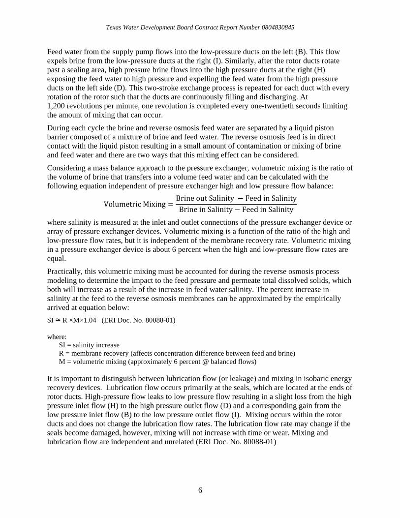
Feed water from the supply pump flows into the low-pressure ducts on the left (B). This flow expels brine from the low-pressure ducts at the right (I). Similarly, after the rotor ducts rotate past a sealing area, high pressure brine flows into the high pressure ducts at the right (H) exposing the feed water to high pressure and expelling the feed water from the high pressure ducts on the left side (D). This two-stroke exchange process is repeated for each duct with every rotation of the rotor such that the ducts are continuously filling and discharging. At 1,200 revolutions per minute, one revolution is completed every one-twentieth seconds limiting the amount of mixing that can occur.

During each cycle the brine and reverse osmosis feed water are separated by a liquid piston barrier composed of a mixture of brine and feed water. The reverse osmosis feed is in direct contact with the liquid piston resulting in a small amount of contamination or mixing of brine and feed water and there are two ways that this mixing effect can be considered.

Considering a mass balance approach to the pressure exchanger, volumetric mixing is the ratio of the volume of brine that transfers into a volume feed water and can be calculated with the following equation independent of pressure exchanger high and low pressure flow balance:

VolumetricMixingBrineoutSalinity FeedinSalinityBrineinSalinity FeedinSalinity

where salinity is measured at the inlet and outlet connections of the pressure exchanger device or array of pressure exchanger devices. Volumetric mixing is a function of the ratio of the high and low-pressure flow rates, but it is independent of the membrane recovery rate. Volumetric mixing in a pressure exchanger device is about 6 percent when the high and low-pressure flow rates are equal.

Practically, this volumetric mixing must be accounted for during the reverse osmosis process modeling to determine the impact to the feed pressure and permeate total dissolved solids, which both will increase as a result of the increase in feed water salinity. The percent increase in salinity at the feed to the reverse osmosis membranes can be approximated by the empirically arrived at equation below:

SI ≅ R ×M×1.04 (ERI Doc. No. 80088-01) where:

SI = salinity increase R = membrane recovery (affects concentration difference between feed and brine) M = volumetric mixing (approximately 6 percent @ balanced flows)

It is important to distinguish between lubrication flow (or leakage) and mixing in isobaric energy recovery devices. Lubrication flow occurs primarily at the seals, which are located at the ends of rotor ducts. High-pressure flow leaks to low pressure flow resulting in a slight loss from the high pressure inlet flow (H) to the high pressure outlet flow (D) and a corresponding gain from the low pressure inlet flow (B) to the low pressure outlet flow (I). Mixing occurs within the rotor ducts and does not change the lubrication flow rates. The lubrication flow rate may change if the seals become damaged, however, mixing will not increase with time or wear. Mixing and lubrication flow are independent and unrelated (ERI Doc. No. 80088-01)


7

2.2.2 Pressure exchanger system design and operation

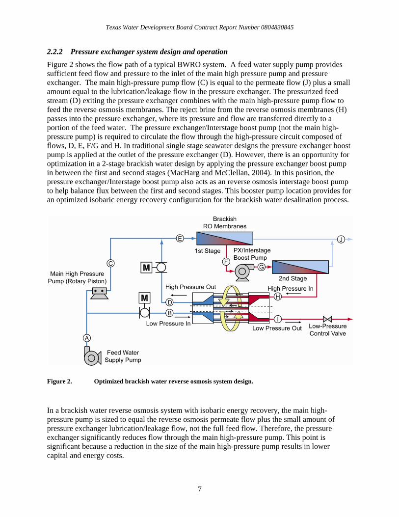
Figure 2 shows the flow path of a typical BWRO system. A feed water supply pump provides sufficient feed flow and pressure to the inlet of the main high pressure pump and pressure exchanger. The main high-pressure pump flow (C) is equal to the permeate flow (J) plus a small amount equal to the lubrication/leakage flow in the pressure exchanger. The pressurized feed stream (D) exiting the pressure exchanger combines with the main high-pressure pump flow to feed the reverse osmosis membranes. The reject brine from the reverse osmosis membranes (H) passes into the pressure exchanger, where its pressure and flow are transferred directly to a portion of the feed water. The pressure exchanger/Interstage boost pump (not the main high-pressure pump) is required to circulate the flow through the high-pressure circuit composed of flows, D, E, F/G and H. In traditional single stage seawater designs the pressure exchanger boost pump is applied at the outlet of the pressure exchanger (D). However, there is an opportunity for optimization in a 2-stage brackish water design by applying the pressure exchanger boost pump in between the first and second stages (MacHarg and McClellan, 2004). In this position, the pressure exchanger/Interstage boost pump also acts as an reverse osmosis interstage boost pump to help balance flux between the first and second stages. This booster pump location provides for an optimized isobaric energy recovery configuration for the brackish water desalination process.

Figure 2. Optimized brackish water reverse osmosis system design.

In a brackish water reverse osmosis system with isobaric energy recovery, the main high-pressure pump is sized to equal the reverse osmosis permeate flow plus the small amount of pressure exchanger lubrication/leakage flow, not the full feed flow. Therefore, the pressure exchanger significantly reduces flow through the main high-pressure pump. This point is significant because a reduction in the size of the main high-pressure pump results in lower capital and energy costs.


8

Because of the pressure exchange process inherent in the pressure exchanger, the high and low pressure flows are independent and must be controlled separately. In Figure 2, the high pressure flow is controlled through variable frequency drive operation of the boost pump and a high pressure flow meter and the low pressure flow is controlled via the low pressure control valve and a separate flow meter. It is traditional to maintain the high pressure and low pressure flows at approximately equal rates, but in some cases, it can be desirable to create an imbalance in these flows.

2.2.3 Balanced flow, over-flush and under-flush

There are several ways in which the low and high-pressure flows can be adjusted during pressure exchanger operation.

Balanced pressure exchanger Flows – Low pressure inlet flow equals the high pressure outlet flow or B = D and H = I. At balanced flows the membrane recovery (J/E) and system recovery (J/A) are equal.

Over-flush – The ratio of low-pressure inlet flow divided by high-pressure outlet flow is greater than 1. Over-flush occurs when B > D, I > H and decreases system recovery (J/A).

Under-flush – The ratio of low-pressure inlet flow divided by high-pressure outlet flow is less than 1. Under-flush flow occurs when D > B, H > I and can be used to increase system recovery (J/A) while maintaining or decreasing reverse osmosis recovery (J/E).

Flows B and I are controlled using the low pressure control valve and are independent from flows D and H. Flows D and H are controlled by a variable frequency drive on the pressure exchanger/interstage booster pump.

To reduce mixing in isobaric devices excess feed water is supplied to over-flush the chambers of any residual brine. Over-flushing reduces mixing in the energy recovery device as illustrated in Figure 3. However, this over-flush condition will require increased feed flow, reducing system recovery. Under-flushing can be used to create a brine recirculation process to decrease reverse osmosis recovery while maintaining or increasing system recovery.

2.2.4 Brine recirculation process for higher system recovery

By incorporating the pressure exchanger into a reverse osmosis system, brine recirculation to yield an increased overall system recovery can be achieved by unbalancing the flows through the pressure exchanger device. Under-flushing can reduce reverse osmosis recovery while maintaining or increasing system recovery. Recirculation of the reverse osmosis brine with the source water will occur to produce the increase in reverse osmosis feed flow i.e. lower reverse osmosis recovery. Under-flushing the pressure exchanger to induce brine recirculation is part of the test conditions outlined for this study. The advantages of this mode of operation include:

Improved membrane boundary layer condition by maintaining “high” velocity flows

Maintain brine flow requirements within manufacturers’ specifications

Maximum allowable recoveries within manufacturer’s specifications

Table 2 provides a matrix of system recovery to reverse osmosis recovery points that were tested at 14.9 gallons per foot per day. When under-flushing the pressure exchanger for higher system


9

recovery, the procedure was to set the system recovery equal to the reverse osmosis recovery and then increase the system recovery in 5 percent increments. X’s represent points that were successfully tested and O’s represent points that were tested but rapid scaling prevented data collection.

Figure 3. Balanced flow, over and under-flushing versus pressure exchanger mixing (ERI Doc No. 80088-01).

Table 2. Affordable Desalination Collaboration study under-flush experiment matrix.

Percent reverse osmosis recovery

75 80

Per

cen

t S

yste

m R

ecov

ery

75 x

80 x x

85 x x

90 x o

% Flow Balance = (B-D)/B * 100


10

3 Project implementation The Affordable Desalination Collaboration operated at the Kay Bailey Hutchison Desalination Plant and used the same feed water as the full-scale plant diverted following sand removal. The desalination plant draws feed water from a number of brackish groundwater wells from the Hueco-Mesilla Bolson (Basin) in El Paso, Texas. Figure 4 shows the location of the Affordable Desalination Collaboration demonstration pilot unit at the Kay Bailey Hutchison Desalination Plant. The demonstration system was designed to closely mimic the full-scale plant so that comparisons could be made between the pilot system performance and the full-scale plant performance. While evaluating these brackish water process alternatives, it is important that product water quality met primary and secondary standards. Potable water quality goals for this Affordable Desalination Collaboration-TWDB study are summarized in Table 3.

Figure 4. Aerial view of the Kay Bailey Hutchison Desalination Plant and Affordable Desalination Collaboration demonstration pilot location.


11

Table 3. Demonstration scale test potable water quality goals.

Parameter Value Total dissolved solids1 < 500 milligrams per liter Chloride1 < 250 milligrams per liter Nitrate2 < 10 milligrams per liter as nitrate- Nitrite2 < 1 milligrams per liter as nitrogen dioxide Fluoride2 < 4 milligrams per liter Sulfate1 < 250 milligrams per liter pH1 6.5-8.5 1. U.S. Environmental Protection Agency Secondary Standard 2. U.S. Environmental Protection Agency Primary Standard Source: EPA 816-F-09-0004, May 2009

3.1 Pilot plant set-up

In January of 2010, the Affordable Desalination Collaboration demonstration unit was reconfigured to a two-stage brackish water system and was mobilized to the Kay Bailey Hutchison Desalination Plant in El Paso, Texas (Figure 5). The startup testing initiated in February 2010, and testing continued through December 2010.

Figure 5. Affordable Desalination Collaboration pilot demonstration unit (Single Stage left view, Two Stage right view).


12

The Kay Bailey Hutchison Desalination Plant uses the same pretreatment and membranes (Hydranautics ESPA 1) as the Affordable Desalination Collaboration system (Figure 6). The two stage 2:1 array with seven 8-inch elements configuration in each vessel is also identical. At the Kay Bailey Hutchison Desalination Plant, the permeate flux between the reverse osmosis stages is balanced by permeate throttling. In the demonstration unit, permeate flux balance is achieved via an inter-stage boost pump. Balancing the permeate flux between membrane stages has the advantages of minimizing the rate of foulant deposition over the greatest membrane area and improving the permeate quality when the flux is increased in the later stages. To maintain the flux balance between stages, first stage permeate can be throttled to generate sufficient permeate back-pressure to balance the feed flow entering the second stage. When using first stage permeate throttling to balance flux, the rule of thumb is not to exceed 30 pressure per square inch permeate back-pressure. At permeate back-pressures beyond 30 pressure per square inch, operating cost savings can be realized by investing capital costs into an inter-stage boost pump or an energy recovery device.

The significant differences in the pilot unit are the pump type for the feed water into the reverse osmosis, inter-stage boost pump, energy recovery system, and motor and pump efficiency. Recovery for the Affordable Desalination Collaboration system included the identical 80 percent recovery operating point as Kay Bailey Hutchison Desalination Plant.

Figure 6. Process schematic with the Kay Bailey Hutchison Desalination Plant and Affordable Desalination Collaboration systems.


13

3.2 Source water characterization

The Kay Bailey Hutchison Desalination Plant is supplied by brackish groundwater wells from the Hueco-Mesilla Basin, where the total dissolved solids of the combined feed into the plant averages a total dissolved solids of approximately 2,000 milligrams per liter. Table 4 lists the water quality constituents in the design feed water for the demonstration testing.

Table 4. Design feed water quality.

Constituent Unit Concentration Calcium milligrams per liter 135 Magnesium milligrams per liter 35 Sodium milligrams per liter 609 Potassium milligrams per liter 19 Barium milligrams per liter 0.11 Strontium milligrams per liter 2 Carbonate milligrams per liter as

Calcium Carbonate 0.2

Bicarbonate milligrams per liter as Calcium Carbonate

57

Sulfate milligrams per liter 187 Chloride milligrams per liter 1093 Fluoride milligrams per liter 0.6 Nitrate milligrams per liter 0.1 Silica milligrams per liter 32 Temperature degrees Celsius 26 pH pH unit 7.2 TDS milligrams per liter 2183 Turbidity Nephelometric Turbidity Unit < 1

3.3 Equipment

This section will describe the major equipment that make up the demonstration test unit. The criteria used to size the demonstration scale brackish water reverse osmosis and cartridge pretreatment equipment are presented in Table 5.

3.4 Project monitoring and reporting

Deliverables for the Affordable Desalination Collaboration-TWDB project were provided in the form of monthly reports. According to TWDB Contract Number 0804830845 Sect II, Art III.5, “The contractor will submit progress reports with submittal of payments according to the payment submission schedule. Progress reports shall be in written form and shall include a brief statement of the overall progress made since the last status report; a brief description of any problems that have been encountered during the previous reporting period that will affect the study, delay the timely completion of any portion of this contract, inhibit the completion of or cause a change in any of the study's products or objectives; and a description of any action the contractor plans to take to correct any problems that have been encountered.”


14

Table 5. BWRO demonstration scale test equipment criteria.

Parameter Value Feed, flush, cleaning pump

Manufacturer/model AMPCO, ZC2 2.5 x 2

Duty range 170 gallons per minute @

80 feet Total Dynamic Head Cartridge filter

Manufacturer/model Eden Excel, 88EFCT4-4C150 Quantity 22

String wound cartridge specs #XL1-EP050-PLC40, 5 micron Pressure vessels

Manufacturer/model Codeline, 80A100-7 Quantity 3

No. of membrane elements per vessel 7 Membrane elements

Manufacturer/model Hydranautics ESPA1-7 Quantity 21 Diameter 8 inches

Surface area 400 square feet Total membrane area (Asys)

Permeate Flow Salt Rejection

Maximum Operating Temperature pH Tolerance

The stated performance is initial (data taken after 30 minutes of operation), based on the following conditions:

8,400 square feet 12,000 gpd

99.3% 113 oF (45 oC)

2-10

1500 PPM NaCl solution 150 psi (1.05 MPa) Applied Pressure 77 oF (25 oC) Operating Temperature 15% Permeate Recovery 6.5 - 7.0 pH Range

Reference

High pressure pump Pump type Positive Displacement, Variable Frequency Drive

Manufacturer/model Danfoss 2 x APP-10.2

High pressure pump flow 40-90 gallons per minute (7-15 gallons per

square foot of membrane per day)

High pressure pump total dynamic head 349 – 2,698 feet water

(150 – 1,160 pounds per square inch) pressure exchanger boost pump

Pump type Multi-stage centrifugal, VFD Manufacturer/model Energy Recovery, Inc. HP-8504

pressure exchanger boost pump total dynamic head

70– 115 feet water (30 – 50 pounds per square inch)

Energy recovery device Type Pressure Exchanger

Manufacturer/model Energy Recovery, Inc. PX-45S BW Quantity 1


15

4 Results

4.1 Optimized isobaric energy configuration

To achieve and mimic the 80 percent reverse osmosis recovery at the Kay Bailey Hutchison Desalination Plant, the resulting reverse osmosis brine flow was below the normal operating range of the energy recovery (PX-45S) unit. To simulate full-scale pressure exchanger operation and maintain the manufacturer recommended of less than 5 percent salinity increase at the reverse osmosis feed, over flushing of the pressure exchanger system was performed. Figure 7 illustrates the results of the reverse osmosis, overall system recovery, and the normalized permeate flows from each stage of the demonstration pilot unit in the optimized pressure exchanger/interstage booster configuration. Relative stable operation was observed during the demonstration period. Optimization experiments were conducted from February 2010 to August 2010. Due to over flushing of the pressure exchanger, the reverse osmosis recovery is greater than the system recovery. The 80 percent reverse osmosis recovery was established as baseline for the system during optimization experiments. Periodically the system would be operated at 80 percent recovery to ensure that the system was maintaining stable performance between operating points.

Figure 8 shows how the reverse osmosis specific energy consumption and water quality vary with varying recovery and flux at balanced pressure exchanger flows i.e., System recovery = reverse osmosis recovery. The following points of interest can be observed from the graphs:

There is an optimum point or low energy point that occurs around 80 percent recovery as shown in Figure 8. This appears to be analogous to a similar optimum point that occurs in single stage seawater systems at around 35-40 percent recovery (MacHarg, 2003).

Energy consumption appears to increase proportionally with increasing flux between 12-16 gallons feet per day.

As expected, water quality improved with increasing flux according to membrane solubility laws and decreased with increasing recovery due to the increase in brine concentration.

New membranes were tested and therefore produced the best possible results in terms of energy consumption. Extended testing could be conducted to determine the effect of membrane aging on energy consumption between cleaning cycles, however, membrane projections can provide designers with a good understanding of system performance over time if long-term experiments cannot be executed due to time constraints.

16

Texas W

ater Developm

ent Board C

ontract Report N

umber 0804830845

Figure 7. Recovery and normalized permeate flow for the optimized configuration.

17

Texas W

ater Developm

ent Board C

ontract Report N

umber 0804830845

Figure 8. Balanced flow curve for reverse osmosis specific energy and water quality at various flux rates.


18

4.2 Brine recirculation configuration (under-flush)

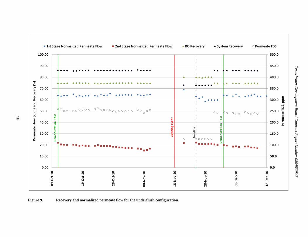
To exceed the 80 percent system recovery, a 2-month long-term test was carried out that included brine recirculation by under-flushing. The resulting reverse osmosis recovery in this configuration will be lower than the system recovery, and in this unbalanced flow scheme, the system is synonymous to brine recycling where the reverse osmosis unit produces more reject flow to feed the pressure exchanger unit. Figure 9 illustrates the results of the reverse osmosis and overall system recovery, and the normalized permeate flows from each stage in the pilot unit for the under-flushing configuration. Under-flush flow testing was conducted from August 2010 to December 2010.

Second stage flux decline was continually observed despite several cycles of high pH cleaning to remove possible organic foulants. Although the reverse osmosis recovery was returned to baseline conditions after each clean, flux decline continued to affect the optimal operation of the pilot. In September, the lag membrane element in the second stage was sent for membrane autopsy to determine the cause for flux decline and new second stage membranes were installed in the reverse osmosis unit. Membrane autopsy results were received in November 2010, and revealed no visible foulants or mineral scalants on the membrane surface. Energy dispersive X-ray analysis showed a high concentration of silica presence (45.8 percent). Even with silica-specific anti-scalant dosing, fouling in the second stage was persistent at system recoveries of 85 percent due to super-saturation of silica in the brine concentrate.

Figure 10 shows how the energy consumption and water quality vary as the system recovery increased, while maintaining a constant reverse osmosis recovery with brine recirculation through under-flushing the pressure exchanger. A flux of 14.9 gallons per feet per day was maintained for the 75 percent and 80 percent reverse osmosis recovery regimes. The following points of interest can be observed from the graphs:

At 75 percent reverse osmosis recovery increasing system recovery resulted in a steady increase in energy use, compared to the balanced flow conditions where their appeared to be a low energy inflection point around 80 percent recovery.

Between 80-85 percent system recovery, there was minimal difference in performance between the 75 percent and 80 percent reverse osmosis recovery points. However, with 75 percent reverse osmosis recovery we were able to achieve 90 percent system recovery, while at 80 percent reverse osmosis recovery the system recovery could not exceed 85 percent without rapid scaling.

Permeate water quality decreased significantly with increasing system recovery due to increasing brine salinity.

Texas W

ater Developm

ent Board C

ontract Report N

umber 0804830845

19

Figure 9. Recovery and normalized permeate flow for the underflush configuration.

Texas W

ater Developm

ent Board C

ontract Report N

umber 0804830845

20

Figure 10. Unbalanced flow curve for reverse osmosis process power and water quality at 14.9 gallons feet per day.


21

4.3 Reverse osmosis membrane scanning electron microscopy and elemental analysis

Experiments conducted between February 2010 and August 2010 to determine the optimum operating points for the Affordable Desalination Collaboration Demonstration Unit included higher reverse osmosis recovery runs up to 90 percent. During this testing period, a continuous permeate flux decline in the second stage of the reverse osmosis train was observed as reverse osmosis recovery was increased. The reduction in the permeate production in the second stage membranes was compensated by an increased permeate production in the first stage membranes at the set reverse osmosis recovery. Despite several cleaning cycles to remove organic foulants, the gradual decline in the second stage flux could not recovered completely. In September 2010, the lag membrane element in the second stage reverse osmosis train was removed for Scanning Electron Microscopy and elemental analysis for membrane autopsy.

No visible foulants, mineral scalants, or membrane discoloration was observed when the membrane sheets were dissembled from the element casing. Under 1050X magnification on the Scanning Electron Microscopy, amorphous structures on the membrane surface were detected as seen in Figure 11. Further elemental analysis conducted for the membrane surface revealed a high presence of silica and sulfur, as shown in Figure 12.

The antiscalant dosed in the pilot is reported to be effective for silica concentrations up to 300 milligrams per liter, and the manufacturer has cited other cases where stable reverse osmosis operation was observed for silica concentrations up to 340 milligrams per liter. At 80 percent and 85 percent reverse osmosis recoveries, the silica concentrations in the reject were 156 and 208 milligrams per liter, respectively. Once the reverse osmosis recovery approached 90 percent, the silica concentration in the reject stream increased to 312 milligrams per liter. However, trivalent ions in the water, such as iron and aluminum can effectively bind with silica in the water and form silica-metal complexes even before silica reaches its supersaturation level in the presence of antiscalants, as seen from the presence of iron and silica on the membrane surface in Figure 12. Sulfur presence can be attributed to the polysulfone support layer of the membranes.

4.4 Energy requirements of an optimized brackish groundwater desalination system

4.4.1 Model assumptions

During the testing period from February 2010 to December 2010, feed water quality fluctuated from the projected design water quality due to the activation of higher salinity brackish wells to supply feed water into the plant. A separate feed water analysis was conducted in July 2010 and the results indicated that the feed water TDS increased by 1,000 milligrams per liter compared to the design water quality data (Shown in Table 4). The updated feed water analysis is presented in Table 6.


22

Figure 11. Scanning Electron Microscope image of the foulant on the membrane surface.


23

Figure 12. Graphical representation of the inorganic constituents found on the membrane surface.

Table 6. Updated feed water quality.

Constituent Unit Updated

Concentration Original

Concentration Calcium milligrams per liter 147 135 Magnesium milligrams per liter 38 35 Sodium milligrams per liter 963.6 609 Potassium milligrams per liter 34 19 Barium milligrams per liter 0.05 0.11 Aluminum micrograms per liter 70 - Strontium milligrams per liter 4.45 2 Iron micrograms per liter 679 - Carbonate milligrams per liter as Calcium Carbonate 0.6 0.2 Bicarbonate milligrams per liter as Calcium Carbonate 89.6 57 Sulfate milligrams per liter 320 187 Chloride milligrams per liter 1600 1093 Fluoride milligrams per liter 0.5 0.6 Nitrate milligrams per liter 2.0 0.1 Silica milligrams per liter 31.2 32 Temperature degrees Celsius 26.5 26 pH pH unit 7.8 7.2 TDS milligrams per liter 3231 2183 Turbidity Nephelometric Turbidity Unit < 1 < 1

0.0%

5.0%

10.0%

15.0%

20.0%

25.0%

30.0%

35.0%

40.0%

45.0%

50.0%

Silicon Sulfur Chloride Iron Calcium Sodium

Percentage

of Inorganic Constituents on Analyzed

Membrane Surface

Inorganic Constituents


24

Reverse osmosis membrane modeling simulations for the demonstration unit operations was calibrated against the actual demonstration data at the 80 percent recovery baseline condition. The predicted feed pressure for the projected high-pressure pump and reject/brine pressure were within 1-5 percent of the actual operating data. Given the level of accuracy of our model predictions, full-scale extrapolation was simulated for the 80 percent reverse osmosis Recovery with and without pressure exchanger.

The energy required to produce fresh water from brackish water is defined by the specific power consumption of the desalination system, (i.e., the power per unit of time required to produce a unit of water.) The specific energy for the reverse osmosis process includes the main horsepower pump power and pressure exchanger interstage/booster pump power divided by the permeate flow rate. The power required for brackish raw water supply, pretreatment, post treatment and distribution is not included. We have chosen to isolate the reverse osmosis process specific energy for the following reasons:

The reverse osmosis process specific energy is the least understood and most over estimated energy number in the total treatment process.

The pre-treatment, concentrate disposal and post treatment energy requirements varies from site to site for brackish water treatment.

In Figure 13, the reverse osmosis process specific energies were compared. The actual Affordable Desalination Collaboration test results are presented on the left, while the extrapolations to a full-scale 3 million gallons per day system are presented on the right. Several scenarios were considered:

Affordable Desalination Collaboration Actual:

“80 percent reverse osmosis Recovery Baseline (pressure exchanger + Boost Pump)”:

Actual demonstration test results from the Affordable Desalination Collaboration demonstration unit for the overflush configuration with pilot pump and motor efficiencies.

“75 percent reverse osmosis-85 percent System Recovery (pressure exchanger + Boost Pump):

Actual demonstration test results from the Affordable Desalination Collaboration demonstration unit for the underflush configuration with pilot pump and motor efficiencies.

Affordable Desalination Collaboration Calculated:

“Full-Scale 80 percent reverse osmosis Recovery (pressure exchanger + Boost Pump)”:

3 million gallons per day full-scale reverse osmosis train projection using pump energy requirements from the pilot 80 percent reverse osmosis Recovery Baseline (pressure exchanger) test data, accounting for additional 5 percent salinity increase of the reverse osmosis feed due to mixing in the pressure exchanger. Pump and motor efficiencies for the high pressure feed pumps were obtained from Kay Bailey Hutchison Desalination Plant’s pump data, whereas assumptions for the interstage boost pump and motor efficiencies were obtained from manufacturer pump curves.

Texas W

ater Developm

ent Board C

ontract Report N

umber 0804830845

25

Figure 13. Reverse osmosis process specific energy comparison.


26

“Full-Scale 75 percent reverse osmosis-95 percent System Recovery (pressure exchanger + Boost Pump)”:

3 million gallons per day full-scale reverse osmosis train projection using pump energy requirements from the pilot 75 percent reverse osmosis-85 percent system Recovery (pressure exchanger) test data. Pump and motor efficiencies for the high pressure feed pumps were obtained from Kay Bailey Hutchison Desalination Plant’s pump data, whereas assumptions for the interstage boost pump and motor efficiencies were obtained from manufacturer pump curves.

“Full-Scale 80 percent reverse osmosis Recovery with Interstage Boost”:

3 million gallons per day full-scale reverse osmosis train projection for a reverse osmosis recovery of 80 percent without pressure exchanger, but with an interstage boost pump to achieve flux balance in between two stages. Pump and motor efficiencies for the high pressure feed pumps were obtained from Kay Bailey Hutchison Desalination Plant’s pump data, whereas assumptions for the interstage boost pump and motor efficiencies were obtained from manufacturer pump curves.

“Full-Scale 80 percent reverse osmosis Recovery with Permeate Throttling”:

3 million gallons per day full-scale reverse osmosis train projection for a reverse osmosis recovery of 80 percent without either pressure exchanger or an interstage boost pump. Permeate throttling was modeled here to simulate Kay Bailey Hutchison reverse osmosis process conditions. Pump and motor efficiencies for the high pressure feed pumps were obtained from Kay Bailey Hutchison Desalination Plant’s pump data.

The assumed pump efficiencies are presented in Table 7. At the same feed total dissolved solids and system pump efficiency into the system, in decreasing specific energy ranking:

Full-Scale 80 percent reverse osmosis Recovery with Permeate Throttling

Full-Scale 75 percent reverse osmosis-85 percent System Recovery with pressure exchanger + Boost Pump

Full-Scale 80 percent reverse osmosis Recovery with Interstage Boost

Full-Scale 80 percent reverse osmosis Recovery with pressure exchanger + Boost Pump

An energy savings comparison was performed for the full-scale 3 million gallons per day flow scenario using the Full-Scale 80 percent reverse osmosis Recovery with pressure exchanger + Boost Pump as a baseline. At full-scale flows, the Full-Scale 80 percent reverse osmosis Recovery with pressure exchanger + Boost Pump configuration will save 13 percent energy consumed compared to the Full-Scale 80 percent reverse osmosis Recovery with Interstage Boost configuration, 24 percent compared to Full-Scale 75 percent reverse osmosis-85 percent System Recovery with pressure exchanger + Boost Pump configuration, and 30 percent compared to the Full-Scale 80 percent reverse osmosis Recovery with Permeate Throttling configuration.


27

Table 7. Pump efficiencies for reverse osmosis specific energy calculations.

VFD Efficiency 95%

High Pressure / Feed Pump Boost Pump

Flow (gpm)

Pressure (psi)

Assumed Pump/Motor Efficiencies

(%) Flow (gpm)

Pressure (psi)

Assumed Pump/Motor Efficiencies

(%)

80% reverse osmosis Recovery (pressure exchanger + Boost Pump)

2088 133 81/94.5 809 40 77/95

80% reverse osmosis Recovery (Interstage Boost)

2604 109 81/94.5 1159 90 77/95

80% reverse osmosis Recovery (Permeate Throttling)

2604 187 81/94.5 - - -

75% reverse osmosis-85% System Recovery (pressure exchanger + Boost Pump)

2090 177 81/94.5 1180 46 77/95

4.5 Life-cycle cost analysis

Incorporating isobaric energy recovery to an existing brackish water desalination facility provides the opportunity to reduce power consumption and power cost over the life of the facility. Cost savings associated with a reduction in specific energy in a desalination system with an integrated energy recovery device may offset the additional capital cost when compared to a brackish water desalination system with permeate thottling. Figure 14 provides a specific energy modeled comparison at year 0 and year 5 membrane life for a 3 million gallon per day brackish desalination train. The specific energy data was calculated based on the same water quality conditions as outlined in Table 6. In order to evaluate the life-cycle cost, year 0 and year 5 specific energy were averaged for both the Full Scale 80 percent recovery with Energy Recovery and the Full Scale 80 percent recovery with permeate thottling as shown in Figure 13.

One must consider the additional capital cost associated with implementing energy recovery technology to an existing system and the debt service associated with the cost of the capital. Table 10 provides a conceptual cost to implement energy recovery into a 3 million gallon per day train (Similar to the Kay Bailey Hutchison Desalination Plant’s train configuration)

Factors that affect the capital and energy cost include the facilities on-line use, energy cost, rebate incentive from power suppliers, interest/ bond rate for capital improvement, and inflation rate.


28

The following assumptions are made for this conceptual life-cycle cost analysis:

On-line use factor = 90 percent

Energy Cost = $0.095 per kilowatt hour (United States Energy Information Administration).

Annual energy inflation rate of 3 percent used based on Texas average annual energy inflation from 1990 to 2009 (United States Energy Information Administration).

No utility rebate incentive used in cost analysis.

5 percent annual interest rate for interest rate for energy recovery device capital improvement.

20 year project life cycle

Membrane life of 5 years (Used to determine the Average Specific Energy)

5 year average Reverse Osmosis specific energy for 3 million gallon per day train at 80 percent recovery with Energy Recovery Device is 1.70 kilowatt hour per 1000 gallons

5 year average Reverse Osmosis specific energy for 3 million gallon per day train at 80 percent recovery with Permeate Thottling for Stage flux balance is 2.34 kilowatt hour per 1000 gallons

The following calculation shows the specific energy savings of a 3 million gallons per day train with Energy Recovery when compared with a 3 million gallons per day train with Permeate Thottling using the assumptions above:

Average reverse osmosis specific energy savings=

=2.34 kilowatt hours per 1000 gallons – 1.70 kilowatt hour per 1000 gallons

= 0.64 kilowatt hour per 1000 gallons

Payback period is defined as the length of time for the cumulative net annual profit to equal the initial investment. Therefore:

Payback = initial investment Net annual profit

To determine the payback period in implementing energy recovery a conceptual capital cost is use as the initial investment and the net annual profit is the energy saving realized by energy recovery technology. Therefore:

Initial investment = $302,500.00 (Refer to Table 10 for breakdown of conceptual cost) 3 million gallons per day Train Permeate Production with 90 percent online use factor = 112,500 gallons per hour.

Table 8 below outlines the reverse osmosis power cost associated with a permeate thottled train configurations and train with energy recovery. The table provides a resulting annual power cost savings using energy recovery of ($219,077 - $159,158)= $59,919.


29

Table 8. Reverse osmosis power and reverse osmosis power cost comparison.

Configuration for 3 MGD train at 80% recovery

Specific Energy

Kwh/1000 gallons

reverse osmosis Power Consumed

(based on 5 year Average Specific Energy and 90%

online use)

reverse osmosis Power Cost per year

(based on Energy cost of $0.095/KWh)

Train with Permeate Thottling

2.34

263.25 kw $ 219,077

Train with Energy Recovery

1.70

191.25 kw

$ 159,158

MGD = million gallons per day % = percent kw = kilowatt

Payback = initial investment = $302,500.00 = 5.05 year Net annual profit (Energy Savings) $59,934.81

In addition to determining the simple payback, a 20 year life cycle analysis is important to determine the anticipated 20 year present worth of the investment. This conceptual project cost analysis accounts for energy inflation over time as well as the cost to finance the capital investment. The same 90 percent on-line use factor is used for the life cycle analysis.

The uniform series present worth calculation is used to determine the impact of inflation over time and is shown as present worth reverse osmosis power cost for a 20 year life cycle. An annual energy inflation rate of 3 percent is used based on Texas average annual energy inflation from 1990 to 2009.

In Table 9, a present worth comparison reveals an energy saving over 20 year of $891,415. The present worth total capital cost (from Table 10 below), including debt service (5 percent, 20 year loan) is $479,127.

The 20 year present worth life cycle savings for a 3 million gallons per day Train with energy recovery when comparing to a 3 million gallons per day train with permeate thottling will be approximately $412,288.00

30

Texas W

ater Developm

ent Board C

ontract Report N

umber 0804830845

Figure 14. Reverse osmosis process specific energy comparison for Year 0 to 5.


31

Table 9. Reverse osmosis power cost comparison.

Train Configuration Power Cost annual

amount

Present Worth reverse osmosis Power Cost (P/A,

3% Energy Inflation, Discount rate of 6%,20

years)

Capital Cost including debt service with 5% interest,

20 year payback 3MGD, 80% recovery with Permeate Throttling

$ 219,077

$3,259,208

$0

3MGD,80% recovery with Energy Recovery

$ 159,158

$2,367,793

Capital Cost $302,500.00 Debt Service $176,627.00 Total Cost $479,127.00

Table 10. Conceptual capital cost to implement energy recovery for a full-scale 3-million gallons per day reverse osmosis train

Quantity Description Unit budgetary price Final price/ train

2 BPX-300 device 32,000 64,000

1 Interstage/Boost pump 55,000 55,000

1 Instrumentation 15,000 15,000

1 Boost pump variable frequency drive

7,500 7,500

1 316 SS Fittings 3,500 3,500

1 Piping Manifolds 20,000 20,000

1 Miscellaneous Valving 15,000 15,000

1 Programming 7,000 7,000

1 Engineering 25,000 25,000

1 Construction Installation 60,000 60,000

1 Start-up and Commissioning 3,000 3,000

Subtotal $ 275,000.00

10% Contingency $ 27,500.00

Total ERD Capital Cost

$ 302,500.00

5 Conclusions and recommendations 80 percent reverse osmosis recovery was determined to be the optimum operating point

for the isobaric energy recovery with brackish groundwater reverse osmosis process to give the lowest reverse osmosis specific energy. Projected energy savings are 23 percent.

Under flush (concentrate recycle) may improve boundary layer conditions at the reverse osmosis; however, high concentrations of silica in the presence of heavy metals limited recovery.


32

Feed water quality challenges with respect to silica supersaturation prevented system recovery from exceeding 80 percent, despite antiscalant dosing.

At the optimum 80 percent reverse osmosis Recovery, a 3 million gallons per day full-scale simulation revealed significant energy savings for incorporating pressure exchanger with brackish water reverse osmosis system

Isobaric Energy Recovery can provide significant energy savings when compared to traditional two stage brackish groundwater reverse osmosis using permeate throttling to balance flux between stages.

Optimizing the position of the pressure exchanger booster between the first and second reverse osmosis stages successfully provided interstage boost pressure and flux balance while simultaneously circulating flow through the pressure exchanger system.

6 Dissemination/Outreach Activities During the Affordable Desalination Collaboration -TWDB contract period of performance the Affordable Desalination Collaboration provided the papers, presentation and/or articles as listed in Table 11 and Appendix C for copies of the papers, articles, and press releases.

Table 11. Dissemination and outreach activities.

Trade show/conference/publication

Date(s) Author(s) Presenter TWDB

submittal Innovative Designs to Be Tested in Affordable Desalination Collaboration , D&WR

Sept/Nov 2007 John P. MacHarg

n/a

Q2-09

Joint Affordable Desalination Collaboration -AMTA workshop, Annual Conference, Austin, Texas

July 2009

n/a

Various

Q2-09

IDA Annual Conference, Dubai-2009, Optimizing Low Energy Seawater Desalination

Aug-2009 S. Dundorf, J. MacHarg, B. Sessions, T. Seacord

S. Dundorf Final Report

Texas Water Innovation Presentation

Sept-2010

John MacHarg

n/a

Oct-2010

Multi-State Salinity Coalition March 2011 Sessions, Shih, MacHarg

n/a Final Report

Joint Affordable Desalination Collaboration -AMTA workshop, Annual Conference, Miami, FL

July-2011

n/a Various

Final Report

Optimizing Brackish Water Reverse Osmosis for Affordable Desalination, AMTA-SEDA Annual Conference

July-2011

Sessions, Shih, MacHarg, Dundorf and Arroyo

Sessions

Final Report


33

7 References ERI Technical Bulletin Isobaric Device Mixing, Doc. No. 80088-01

Hauge, L. J. and F. Ludvigsen. 1999. "Field Installation of Pressure Exchanger in an 80 m3/D SWRO Plant” Costa Teguise, Lanzarote, Canary Islands, 1999 IDA San Diego

Hauge, L. J. and F. Ludvigsen. 1999. "Field Installation of Pressure Exchanger in an 80 m3/D SWRO Plant” Costa Teguise, Lanzarote, Canary Islands, 1999 IDA San Diego

MacHarg, J.P. 2003. Exchanger Test Verifies 2.0 kWh/m3 SWRO Energy Use. Desalination and Water Reuse Vol 11/1, June-2003

MacHarg, J.P.and S.A. McClellan, 2004, Pressure Exchanger Helps Reduce Energy Consumption in Brackish Water Design, Journal AWWA, November 2004

USEPA, 2009, U.S. Environmental Protection Agency Primary Standard 816-F-09-0004, May 2009

USEPA, 2009, U.S. Environmental Protection Agency Secondary Standard 816-F-09-0004, May 2009

U.S. Energy Information Administration, Form EIA-861, "Annual Electric Power Industry Report.


34

Appendix A: Validation Protocol

9-12-11 i

AFFORDABLE DESALINATION COLLABORATION

TEXAS WATER DEVELOPMENT BOARD

BRACKISH GROUNDWATER RO DEMONSTRATION STUDY

LOCATION: EL PASO DESALINATION PLANT

VALIDATION PROTOCOL

ADC Demonstration Pilot System

Affordable Desalination Collaboration, 2419 E. Harbor Blvd, #173, Ventura, CA 93001 Tel: 650-283-7976 – Fax: 805-658-8060 – www.affordabledesal.com – [email protected]

9-12-11 ii

TABLE OF CONTENTS

Page

1.0 INTRODUCTION ................................................................................................................ 1

1.1 Background .............................................................................................................. 1 1.2 TWDB-ADC Demonstration Study Objectives .......................................................... 2

2.0 VALIDATION PROTOCOL ................................................................................................. 3 2.1 Demonstration Scale Brackish RO Equipment ......................................................... 3

2.1.1 Optimized Isobaric Energy Recovery Demonstration ................................ 4 2.1.2 Brine Recirculation Process for Higher Recovery in Single Stage Array . 10

2.2 Testing Operation and Monitoring .......................................................................... 14 2.3 Membrane Cleaning & Storage .............................................................................. 19

2.3.1 RO Membranes ....................................................................................... 19 2.4 Determining Affordability ........................................................................................ 20

APPENDIX A: Process and Instrumentation Diagrams

ADC-TWDB Brackish Groundwater Desalination Project

9-12-11 1

Affordable Desalination Collaboration

ADC-TWDB BRACKISH GROUNDWATER RO DEMONSTRATION STUDY

1.0 INTRODUCTION

1.1 Background

The Affordable Desalination Collaboration (ADC) is a California non - profit organization comprised of state and federal government agencies, water districts, and industry leaders working together to demonstrate seawater desalination as a reliable, affordable, an environmentally sound source of potable water. The original objective of the ADC was to design, build and test a scalable SWRO plant using commercially available technology that can demonstrate efficient energy consumption. The ADC’s demonstration scale SWRO plant (rated seawater capacity of 48,000 gpd to 75,600 gpd) was tested at the U.S. Navy’s Desalination Research Center, located in Port Hueneme, California, and operated from May 2005 through July 2009. Key achievements of our initial seawater testing included:

Demonstrating that SWRO is a viable water supply alternative for Southern California, as shown in Figure 1.1.

Setting a world record low SWRO process energy consumption of 6.0 kWh/kgal of permeate produced.

Test and demonstrate 7 membrane models from four manufacturers providing performance comparison under similar feed water conditions.

Test and demonstrate Dow Filmtec’s “hybrid membrane” design, by staging membranes of various performance in a single seven element vessel

Test and demonstrate Dow Filmtec’s high boron rejection membrane for seawater


9-12-11 2

Demonstrate new process design configurations to achieve higher system recoveries in seawater (i.e., over 50%)

Test and demonstrate the performance of GE/Zenon ZeeWeed® 1000 ultrafiltration (UF) membrane technology as a reliable method of pretreatment for SWRO systems for feed water conditions at the Port Hueneme Test Facility.

By testing and demonstrating these new technologies and designs and sharing the results, the ADC has been able to provide information to SWRO designers and industry stake holders that seawater desalination is an affordable, viable and reliable source of potable water for the future. The ADC website: www.affordabledesal.com details the goals, previous publications and information related to the ADC.

1.2 TWDB-ADC Demonstration Study Objectives

The objectives of this Texas Water Development Board Brackish (TWDB) Ground Water Demonstration Projects are as follows:

1. Develop and demonstrate new process designs that are possible as a result of the isobaric energy recovery technologies. As a natural result of the pressure exchanger (PX) technology in particular, there are new kinds of flow schemes that can improve the performance of higher recovery brackish water systems. We will use the ADC pilot system to test and demonstrate these new flow schemes in order to push the recoveries beyond what has been traditionally achievable.

2. Test and demonstrate state of the art isobaric energy recovery technology in an optimized brackish water design. The ADC expects to achieve 15-30% energy savings over traditional brackish water systems even where energy recovery turbines are applied.

The ADC will operate at the El Paso Brackish Water Desalination facility and use the same feed water as the full scale plant. In so far as possible, the pilot system design will mimic the full scale plant so that comparisons may be made between the pilot system performance and the full scale plant performance.

While evaluating these brackish water process alternatives, it is important that potable water quality meets primary and secondary standards. Potable water quality goals for this ADC TWDB study are summarized in Table 1.2.

Table 1.2 Demonstration Scale Test Potable Water Quality Goals Brackish RO Demonstration Study Affordable Desalination Collaboration Part II

Parameter Unit Value Basis

TDS mg/L < 500 Federal Secondary Standard

Chloride mg/L < 250 Federal Secondary Standard


9-12-11 3

2.0 VALIDATION PROTOCOL

This section describes the materials and methods used to validate that the following process design concepts and their potential to reduce either or both capital costs or energy consumption while meeting potable water quality goals.

Optimized brackish water design with isobaric energy recovery

Higher recovery operation through isobaric brine recirculation

2.1 Demonstration Scale Brackish RO Equipment

Criteria used to size the demonstration scale Brackish RO and UF Pretreatment equipment are presented in Table 2.1. A process flow diagrams are presented in Figures 2.1, 2.2, and 2.3.

Table 2.1 BWRO Demonstration Scale Test Equipment Criteria Brackish water RO Demonstration Study ADC-TWDB Brackish Water Demonstration Project

Parameter Unit Value

Feed, Flush, Cleaning Pump

Manufacture/Model AMPCO, ZC2 2.5x2

Duty Range gpm @ ft H2O 170gpm @ 80 ft TDH

Media Filter

Manufacturer ALAMO

Quantity No. 2

Diameter Inch 48

Height Inch 72

Loading Rate gpm/ft2 3 to 6

Cartridge Filter

Manufacturer/Model Eden Excel, 88EFCT4-4C150

Quantity No. 22

String Wound Cartridge Specs #XL1-EP050-PLC40, 5 micron

Pressure Vessels

Manufacturer/Model Codeline, 80A100-7

Quantity No. 3

No. of Membrane Elements per Vessel No. 7

Membrane Element


9-12-11 4

Table 2.1 BWRO Demonstration Scale Test Equipment Criteria Brackish water RO Demonstration Study ADC-TWDB Brackish Water Demonstration Project

Parameter Unit Value

Manufacturers/ Models Hydranautics ESPA1-7

Quantity No. 21

Diameter inch 8

Surface Area ft2 400

Total Membrane Area (ASYS) ft2 8400

High Pressure Pump

High Pressure Feed Pump Type Positive Displacement

Manufacturer Danfoss

Model 2 x APP-10.2

Driver VFD

High Pressure Pump flow gpm 40-90 (7-15 gfd)

High Pressure Pump TDH ft H2O (psi) 349 to 2698 (150 to 1160)

PX Booster Pump

PX Booster Pump Type Multi-stage Centrifugal

Manufacturer Energy Recovery, Inc.

Model HP-8504

Driver VFD

PX Booster Pump TDH 70 to 115 (30 to 50)

Energy Recovery

Energy Recovery Devise Type Pressure Exchanger

Manufacturer Energy Recovery, Inc.

Model PX-70S SW / PX-?? BW

Quantity No. 2

Notes:

2.1.1 Optimized Isobaric Energy Recovery Demonstration

An isobaric energy recovery system utilizes the principle of positive displacement to pressurize filtered feed water by direct contact with the high-pressure concentrate (waste) stream or reject from an RO system. Within a pressure exchanger (PX) pressure transfer occurs in the longitudinal ducts of a ceramic rotor that spins inside a ceramic sleeve. The rotor-sleeve assembly is held between two ceramic end covers. At any given instant, half of the ducts are


9-12-11 5

exposed to the high pressure fluid side and half the ducts are exposed to the low pressure fluid side. Figure 2.1 shows the flow path of a typical seawater reverse osmosis (SWRO) PX system. The concentrate from the RO membranes (G) passes through the PX, where its pressure is transferred directly to a portion of the incoming feed water at up to 97% efficiency. This pressurized feed water stream (D), which is approximately equal in volume and pressure to the reject stream, passes through a PX auxiliary pump (not the main high-pressure pump) to add the small amount of pressure lost due to the differential pressure across the membranes and to friction in the associated piping and the PX. The PX booster pump drives the flow through the high-pressure side (G and D) of the PX. Fully pressurized feed water then merges with the main feed water line of the RO system after the main high-pressure pump. In an RO-PX system, the main pump is sized to equal the RO permeate flow plus a small amount of rotor lubrication flow, not the full RO feed flow. Therefore, the PX significantly reduces flow through the main pump. This point is significant because a reduction in the size of the main pump results in lower power consumption and operating costs.

Figure 2.1. Typical Seawater Pressure Exchanger Diagram.

The RO-PX system requires a booster pump to make up the small amount of pressure losses through the membranes, PX, and the associated piping circuit. In the standard single stage seawater system this pump is applied at the outlet of the PX. However, in a 2 stage brackish water system the PX booster pump can serve 2 purposes by being installed in between stages 1 and 2 as shown in Figure 2-2. In this configuration the PX booster pump also acts as an interstage booster pump helping to reduce the required pressure from the main high pressure feed pump, by balancing the flux between the 1st and 2nd stages

Main High Pressure Pump

PX Booster Pump

PX

RO I

B A

C

D

E

H

G

Feed/Supply

Fresh Water F


9-12-11 6

The example in figure 2-2 (see Appendix A for detail P&ID) shows that while the PX booster is supplying the energy to drive the water around the PX circuit it is also conveniently providing 55 psi of interstage boost pressure. In addition to improving the flux balance, it also results in significant savings by both the PX reducing the main HP pump size and the lower 1st stage feed pressure inherent to an interstage booster design. Table 1 shows the PX power savings verses a standard interstage booster design. Table 2-2. Projected PX Savings in Interstage Booster system

Std ERI Feed pump efficiency 83% 83% Feed pump motor efficiency 94% 94% Feed pump power, kW 172.9 130.3 Booster pump efficiency 80% 80% Booster pump motor efficiency 94% 94% Booster pump power, kW 23.2 31.8 RO Feed Pressure, PSI 175 175 RO Recovery, % 75% 75% KWh/kgal 2.19 1.82 17% savings yields $17,500/year @ $0.06/kWh

In conclusion, an optimally designed brackish water PX system can provide many benefits including energy savings and flux balance. These concepts could save operators of brackish water systems as much 10-30% of the operating energy compared to traditional systems while simultaneously improving the performance of the RO membranes.

2.1.1.1 - Procedure for testing Brine Recirculation Process

Demonstration scale tests of the Optimized Isobaric Energy Recovery system will occur over an approximate 6 month period. As presented in Table 2-3, each phase of testing consists of the following:

Figure 2-2. Example Interstage Booster PX Design @ 75% RO Recovery

HP Feed Pump

2000 gpm

175 psi

1500 gpm Product

PX Array

500 gpm

190 psi

490 gpm

20 psi

490 gpm

175 psi

500 gpm

5 psi

Booster Pump

2000 gpm

20 psi

1510 gpm

20 psi 1000 gpm 155 psi

1000 gpm 210 psi

1st stage 2nd stage


9-12-11 7

Two weeks (weeks 1-2) of “ripening” at a typical flux and recovery rate. This “ripening” period has been included based upon past experience operating new membranes. Experience has indicated that approximately two and one half weeks are required before some new membrane’s performance (e.g., pressure and salt rejection) reaches a steady state condition. It is possible that pre-ripened membranes will be used in this test and this period may be shortened or omitted accordingly.

Four weeks (weeks 3-6) of testing at different system flux and RO recovery points. Each flux and recovery point will be operated for 1 day to obtain the approximate energy and water quality performance at a given point.

2 month demonstration at a single flux and recovery point.

Tables 2-3 indicates the desired flux and recovery that will be set for this test. The applicable equations are as follows:

100

SYSF

SYSP

Q

QR Equation 2.4

REJECTSYSPSYSF QQQ Equation 2.5

QPX- HP-out = leakagegpmQREJECT _5.1 Equation 2.6

leakagegpmQQ PumpHPFSYSP _5.1 Equation 2.7

Where: R = Recovery, % QF-SYS = RO system feed flow, gpm QF-HP-Pump = High pressure positive displacement pump flow, gpm QPX-HP-out = QPX-Pump = PX High Pressure Outlet, gpm

QReject = RO membrane reject flow, gpm

Between each system flux and recovery matrix, the original/ripening flux and recovery (i.e., the flux and recovery tested during weeks 1-2) will be retested to confirm membrane performance at baseline conditions.

Approximately 8 weeks of operating at the RO-System recovery point determined, through testing, to 1) meet water quality goals for TDS and 2) results in the most affordable operation, as determined by a net present value analysis, or 3) and operating point that best matches the current operating conditions of full scale El Paso plant.

The data gathered from these tests shall be used to develop graphs that show the power consumption rate and water quality that can be achieved at each condition. Power consumption rate shall be measured to include the following electrical loads:

High Pressure RO Pump (P2)


9-12-11 8

PX Booster Pump (P3)

The following will not be included in the power consumption rate measurements

Intake Lift Pump (P1)

Chemical Metering Pumps

Instrumentation and Controls

Product water pumping

Pretreatment pumping

While the intake lift pump may provide suction side pressure to the High Pressure Positive Displacement pump, thereby reducing the overall TDH, it will not be included in the power monitoring. For the affordability analysis, an intake pump’s horsepower will be assumed based upon flow and overall lift TDH of 200 ft of H2O.


9-12-11 9

Table 2-3 Schedule of Testing Conditions

Optimized Isobaric Energy Recovery Demonstration

ADC TWDB Desalination Demonstration Project

Parameter 1-2 Weeks Ripening Day 1 Day 2 Day 3 Day 4 Day 5 Day 6 Day 7 Day 8

Membrane sq-ft 400 Base Line Base Line Flux, gfd 14.9 12 12 12 14.9 14.9 14.9 14.9 14.9 RO recovery 80.0% 75.0% 80.0% 85.0% 80.0% 75.0% 80.0% 85.0% 80.0% System Recovery 80.0% 75.0% 80.0% 85.0% 80.0% 75.0% 80.0% 85.0% 80.0%

High Pressure RO Pump (QF-HP Pump), gpm 88.4 71.5 71.5 71.5 88.4 88.4 88.4 88.4 88.4

PX HP Outlet, (QPX-HP-Out), gpm 20.2 21.8 16.0 10.9 20.2 27.5 20.2 13.8 20.2

Permeate (QP-SYS), gpm 86.9 70.0 70.0 70.0 86.9 86.9 86.9 86.9 86.9 PX Low Pressure Inlet, gpm 20.2 21.8 16.0 10.9 20.2 27.5 20.2 13.8 20.2 Concentrate, gpm 21.7 23.3 17.5 12.4 21.7 29.0 21.7 15.3 21.7 Base Line

Day 9 Day 10 Day 11 Day 12 2 Month

Demo Point Flux, gfd 16 16 16 14.9 TBD RO recovery 75.0% 80.0% 85.0% 80.0% TBD System Recovery 75.0% 80.0% 85.0% 80.0% TBD

High Pressure RO Pump (QF-HP Pump), gpm 94.8 94.8 94.8 88.4 TBD

PX HP Outlet, (QPX-HP-Out), gpm 29.6 21.8 15.0 20.2 TBD

Permeate (QP-SYS), gpm 93.3 93.3 93.3 86.9 TBD PX Low Pressure Inlet, gpm 29.6 21.8 15.0 20.2 TBD Concentrate, gpm 31.1 23.3 16.5 21.7 TBD

Notes:

1. Maximum system pressure is 600 psi. If any point exceeds 600 psi system will shutdown and point will need to be skipped.

2. Flows assume 400 sq-ft membrane

3. QF-HP Pump = High pressure positive displacement pump flow = Product flow +1.5 gpm (PX leakage).

4. QPX-HP-Out = PX booster pump flow= Concentrate flow gpm - 1.5 gpm (PX leakage).

5. QP-SYS = SWRO system permeate flow.


9-12-11 10

2.1.2 Brine Recirculation Process for Higher Recovery in Single Stage Array

The brine recirculation process is achieved through unbalancing the flows through an isobaric energy recovery device. As a natural result of isobaric energy recovery systems there are new kinds of flow schemes that may improve the performance of higher recovery seawater and brackish water systems. One example is shown in Figure 2-3 below where a PX is intentionally unbalanced yielding an overall system recovery (F divided by A) of 85% and 2000 tds feed water, but the membrane recovery (F divided by E) is at 65% and 4,886 tds feed water.

Figure 2-3 The Unbalanced Pressure Exchanger Diagram Single Stage Array

Table 2-4 Unbalanced PX 65/85% Recovery Projection Single Stage Array Mechanisms associated with this novel mode of operation that might lead to improved performance at higher recoveries include:

Improved boundary layer conditions by maintaining “high” velocities/flow

Main High Pressure Pump

PX Booster Pump

PX

RO I

B A

C

D

E

H

G

Feed/Supply

Fresh Water F

A B C D E F G HFlow gpm 1774 250 1524 775 2299 1500 799 274

gpd 2,554,560 360,000 2,194,560 1,116,000 3,310,560 2,160,000 1,150,560 394,560 Pressure PSI 25 25 241 221 241 5 231 10Quality mg/l TDS 2,000 2,000 2,000 10,563 4,886 92.0 14,000 14,000

PX Brine cross flow = 549 gpmPX-70 QTY 4 Temperature = 25ºCPX UNIT FLOW GPM 200 Flux ~ 13 gfdPX Internal Bypass GPM 24Membrane Differential PSI 10RO Recovery % 65%System Recovery % 85%

HIGH PRESS. PUMPFeed Pump eff % 90%Motor eff % 93%VFD eff % 97% Total RO Process (kW ) 189.1Power kW 176.2

BOOSTER PUMP kW h/m3 Permeate 0.55Boost Pump Eff % 60% kW h/1000 gal Permeate 2.10

Motor Eff % 90% kW h/acre-ft Permeate 684VFD eff % 97%Power kW 12.9

Supply/Feed Pump kW 0.0


9-12-11 11

Balanced membrane flux through increased lead element velocities Balanced membrane flux through increased lead element salinity Minimum brine flow requirements within manufacturers specifications Maximum allowable recoveries within manufacturers specifications

Testing this brine recirculation process is straight forward and will be achieved with the ADC Demonstration system in its Optimized Isobaric Energy Recovery Configuration as shown in Figure 2-2 and the detailed P&ID in Appendix A.

2.1.2.1 - Procedure for testing Brine Recirculation Process

Demonstration scale tests of the unbalance PX system will occur over an approximate 6 month period. As presented in Table 2-5, each phase of testing consists of the following:

Two weeks (weeks 1-2) of “ripening” at a typical flux and recovery rate. This “ripening” period has been included based upon past experience operating new membranes. Experience has indicated that approximately two and one half weeks are required before some new membrane’s performance (e.g., pressure and salt rejection) reaches a steady state condition. It is possible that pre-ripened membranes will be used in this test and this period may be shortened or omitted accordingly.

Four weeks (weeks 3-6) of testing at different system and RO recovery points. Each recovery point will be operated for 1 day. The flux rates will be maintained at a constant 14.9 gallons per square foot of membrane area per day (gfd).

2 month demonstration at a single flux and recovery point

As indicated in Tables 2.6, two separate recovery rates will need to be determined and set for this test. These are the RO membrane recovery, which is determined by the PX booster pump flow and the total system recovery, which is determined by the PX LP inlet flow. The applicable equations are as follows:

RO R = QP-SYS / QRO feed flow

System 100

SYSF

SYSP

Q

QR Equation 2.4

REJECTSYSPSYSF QQQ Equation 2.5

leakagegpmQQ REJECTPumpPX _5.1 Equation 2.6

leakagegpmQQ PumpHPFSYSP _5.1 Equation 2.7

Where: R = Recovery, % QF-SYS = RO system feed flow, gpm


9-12-11 12

QF-SYS = QPX-HP-out + QF-HP-Pump QF-HP-Pump = High pressure positive displacement pump flow, gpm QPX-HP-out = PX High Pressure Outlet, gpm QReject = RO membrane reject flow, gpm

Between each system recovery matrix, the original/ripening flux and recovery (i.e., the flux and recovery tested during weeks 1-2) will be retested to confirm membrane performance at baseline conditions.

Approximately 8 weeks of operating at the RO-System recovery point determined, through testing, to 1) meet water quality goals for TDS and 2) results in the most affordable operation, as determined by a net present value analysis or 3) an operating point that best matches the current operating conditions of full scale El Paso plant.

The data gathered from these tests shall be used to develop graphs that show the power consumption rate and water quality that can be achieved at each condition. Power consumption rate shall be measured to include the following electrical loads:

High Pressure RO Pump (P2)

PX Booster Pump (P3)

The following will not be included in the power consumption rate measurements

Intake Lift Pump (P1)

Chemical Metering Pumps

Instrumentation and Controls

Product water pumping

Pretreatment pumping

While the intake lift pump may provide suction side pressure to the High Pressure Positive Displacement pump, thereby reducing the overall TDH, it will not be included in the power monitoring. For the affordability analysis, an intake pump’s horsepower will be assumed based upon flow and a overall lift TDH of 200 ft of H2O.


9-12-11 13

Table 2.5 Schedule of Testing Conditions

Brine Recirculation Process for Higher Recovery in two Stage Array

ADC TWDB Desalination Demonstration Project

Parameter

1-2 Weeks

Ripening Day 1 Day 2 Day 3 Day 4 Day 5 Day 6 Day 7 Day 8 Day 9

Membrane sq-ft 400 Base Line

Flux, gfd 14.9 14.9 14.9 14.9 14.9 14.9 14.9 14.9 14.9 14.9 RO recovery 80.0% 75.0% 75.0% 75.0% 75.0% 75.0% 80.0% 80.0% 80.0% 80.0% System Recovery 80.0% 75.0% 80.0% 85.0% 90.0% 95.0% 80.0% 80.0% 85.0% 90.0%

High Pressure RO Pump (QF-HP Pump), gpm 88.4 88.4 88.4 88.4 88.4 88.4 88.4 88.4 88.4 88.4

PX HP Outlet, (QPX-HP-Out), gpm 20.2 27.5 27.5 27.5 27.5 27.5 20.2 20.2 20.2 20.2

Permeate (QP-SYS), gpm 86.9 86.9 86.9 86.9 86.9 86.9 86.9 86.9 86.9 86.9 PX Low Pressure Inlet, gpm 20.2 27.5 20.2 13.8 8.2 3.1 20.2 20.2 13.8 8.2 Concentrate, gpm 21.7 29.0 21.7 15.3 9.7 4.6 21.7 21.7 15.3 9.7

Base Line

Base Line

Base Line

Day 10 Day 11 Day 12 Day 13 Day 14 Day 15 Day 16 Day 17 Day 18

2 Month Demo Point

Flux, gfd 14.9 14.9 14.9 14.9 14.9 14.9 14.9 14.9 14.9 TBD RO recovery 80.0% 80.0% 85.0% 85.0% 85.0% 80.0% 90.0% 95.0% 80.0% TBD System Recovery 95.0% 80.0% 85.0% 90.0% 95.0% 80.0% 90.0% 90.0% 80.0% TBD

High Pressure RO Pump (QF-HP Pump), gpm 88.4 88.4 88.4 88.4 88.4 88.4 88.4 88.4 88.4 TBD

PX HP Outlet, (QPX-HP-Out), gpm 20.2 20.2 13.8 13.8 13.8 20.2 8.2 3.1 20.2 TBD

Permeate (QP-SYS), gpm 86.9 86.9 86.9 86.9 86.9 86.9 86.9 86.9 86.9 TBD PX Low Pressure Inlet, gpm 3.1 20.2 13.8 8.2 3.1 20.2 8.2 8.2 20.2 TBD Concentrate, gpm 4.6 21.7 15.3 9.7 4.6 21.7 9.7 9.7 21.7 TBD

Notes:

1. Maximum system pressure is 600 psi. If any point exceeds 600 psi system will shutdown and point will need to be skipped.

2. Flows assume 400 sq-ft membrane

3. QF-HP Pump = High pressure positive displacement pump flow = Product flow +1.5 gpm (PX leakage).

4. QPX-HP-Out = PX booster pump flow= Concentrate flow gpm - 1.5 gpm (PX leakage).

5. QP-SYS = SWRO system permeate flow.


9-12-11 14

2.2 Testing Operation and Monitoring

Hydraulic and water quality data will be collected to evaluate the operation of the demonstration scale equipment relative to the project goals for power consumption and treated water quality. These data shall be collected and evaluated by Carollo Engineers, P.C.

Tables 2.6-2.7 presents a matrix for monitoring hydraulic data from the demonstration scale brackish water RO equipment. Hydraulic data collected from this equipment consists of both pressure and flow data. The frequency of monitoring for each type of data is presented based upon the type/phase of operation. In general, data shall be collected once daily or at each individual flux and recovery during the 18 point data matrixes and 3 times per week during the 2 month demonstration phases. When applicable, flow meter calibration shall be checked at least weekly using a graduated bucket and a stop watch.

Hydraulic data shall be recorded in the data spreadsheet presented in Appendix B. The data spreadsheet shall be emailed weekly (i.e., Friday) to Carollo Engineers, P.C. Bradley Sessions ([email protected]) and the ADC’s, P.C. John MacHarg ([email protected]) for data evaluation.

Water quality data shall be collected at the locations and frequencies presented in Tables 2.7 and analyzed by the methods presented in Table 2.8. These data shall then be recorded in the the spreadsheet in Appendix B. The data spreadsheet shall be emailed weekly (i.e., Friday) to Carollo Engineers, P.C. Bradley Sessions ([email protected]) and the ADC’s, P.C. John MacHarg ([email protected]). One sampling for TOC, iron, manganese, and aluminum from location SC-1 every nine weeks will also be provided.


9-12-11 15

Table 2.6 Hydraulic Monitoring – Brackish water RO System ADC TWDB Desalination Demonstration Project

Parameter Unit

Each Flux/recovery

point

Demonstration and Ripening Periods Data

Logger

Monday Tuesday Wednesday Thursday Friday

Pressure

PMF-in (PI1) psig 1x 1x - 1x - 1x

PMF-out / PCF-in (PI1) psig 1x 1x - 1x - 1x

PCF-out (PI1) psig 1x 1x - 1x - 1x

PPX-HP-out (PI2) psig 1x 1x - 1x - 1x PT1

PStage1-out (PI4) psig 1x 1x - 1x - 1x PT2

PStage2-In (PI4) psig 1x 1x - 1x - 1x PT2

PStage2-out (PI2) psig 1x 1x - 1x - 1x PT2

PP-SYS (PI3) psig 1x 1x - 1x - 1x

Flow

QF-HP Pump (FI3) gpm 1x 1x - 1x - 1x

QPX-LP-IN (FI2) gpm 1x 1x - 1x - 1x FT2

QPX-HP-Out (FI5) gpm 1x 1x - 1x - 1x FT5

QP-stage1 (FI6) gpm 1x 1x - 1x - 1x FT4

QP-stage2 (FI7) kWh 1x 1x - 1x - 1x AM1

QP-SYS (FI4) kWh 1x 1x - 1x - 1x AM1

Power Consumption kWh 1x 1x - 1x - 1x AM1


9-12-11 16

Table 2.6 Hydraulic Monitoring – Brackish water RO System ADC TWDB Desalination Demonstration Project

Parameter Unit

Each Flux/recovery

point


Logger

Monday Tuesday Wednesday Thursday Friday Notes: 1. PMF-in = Pressure on the influent side of the media filters (PI1a) 2. PMF-out / PCF-in = Pressure on the effluent side of the media filters / Pressure on the inlet side of the cartridge filters (PI1b) 3. PCF-out = Pressure on the effluent side of the cartridge filters (PI1c) 4. PPX-HP-out = Feed water pressure at the PX high pressure outlet and inlet to Stage 1 membranes (PI2). 5. PStage1-out = Stage 1 outlet pressure and PX booster pump inlet pressure (PI2) 6. PStage2-in = Stage 2 inlet pressure and PX booster pump outlet pressure (PI2) 7. PStage2-out = Stage 2 outlet pressure (PI2) 8. PPX-LP-out = Discharge pressure at the PX low pressure outlet, before the system recovery control valve (PI3b) 9. PP-SYS = RO system permeate pressure 10. QF-HP Pump = High pressure positive displacement pump flow (FI3) 11. QPX-LP-IN = Low pressure flow into the PX (FI2) 12. QPX-HP-Out= High pressure flow out of PX (FI5) 13. QP-Stage1 = Product flow from stage 1 array 14. QP-Stage2 = Product flow from stage 2 array 15. QP-SYS = RO system permeate flow (FI4) 16. Power consumption will be calculated based on hydraulic data collected. On line measurements are taken from the Amp Meter. 17. Facility monitoring during weeks 3-6 will be required once per day.


9-12-11 17

Table 2.7 Water Quality Monitoring Brackish Water RO System ADC TWDB Desalination Demonstration Project

Parameter Unit

Each Flux and Recovery Point


Logger

Monday Tuesday Wednesday Thursday Friday

Location No. of Times Location

No. of Times Location




No. of Times

Temperature oC (oF) SC5, SC6,

SC11 1x SC5, SC6,

SC11 1x - -

SC5, SC6, SC11 1x

- - SC5, SC6,

SC11 1x

pH

SC3, SC4, SC5, SC6, SC7, SC11 1x

SC3, SC4, SC5, SC6, SC7, SC11

1x - -


1x - -


1x

Conductivity mS/cm

SC3, SC5, SC6, SC7,

SC11, SC12, SC13 1x

SC3, SC5, SC6, SC7,

SC11, SC12, SC13

1x

- -

SC3, SC5, SC6, SC7,

SC11, SC12, SC13

1x

- -

SC3, SC5, SC6, SC7,

SC11, SC12, SC13

1x

Total Dissolved Solids mg/L

SC3, SC5, SC6, SC7,

SC11, SC12, SC13 1x

SC3, SC5, SC6, SC7,

SC11, SC12, SC13

1x

- -

SC3, SC5, SC6, SC7,

SC11, SC12, SC13

1x

- -

SC3, SC5, SC6, SC7,

SC11, SC12, SC13

1x

Turbidity NTU Meter 1x Meter 1x - - Meter 1x - - Meter 1x NTU1

Silt Density Index SC3 1x SC3 1x - - SC3 1x - - SC3 1x

Notes: 1. NS = No Sample 2. NA = Not applicable (e.g., value calculated) 3. Sample connection numbers per Harn P&ID revision 2, 4-19-05.


9-12-11 18

Table 2.8 Water Quality Testing Methods Brackish water RO Demonstration Study Affordable Desalination Collaboration

Parameter

Method

Seawater RO Permeate

Temperature, oC SM 2550 N/A

pH SM 4500-H+ SM 4500-H+

Conductivity, S/cm SM 2510 SM 2510

TDS, mg/L SM 2540C SM 2540C

Turbidity, NTU SM 2130 N/A

Silt Density Index ASTM D4189-95 N/A

Boron, mg/L EPA 200.7 EPA 200.7

Bromide, mg/L EPA 300.0 EPA 300.0

Total Organic Carbon, mg/L SM 5310C SM 5310C

Iron, mg/L EPA 200.7 EPA 200.7

Manganese, mg/L EPA 200.7 EPA 200.7

Aluminum, mg/L EPA 200.7 EPA 200.7

Calcium, mg/L EPA 200.7 EPA 200.7

Magnesium, mg/L EPA 200.7 EPA 200.7

Sodium, mg/L EPA 200.7 EPA 200.7

Potassium, mg/L EPA 200.7 EPA 200.7

Alkalinity, mg/L as CaCO3 SM 2320B/EPA 310.1 SM 2320B/EPA 310.1

Carbon Dioxide, mg/L SM4500-CO2-D SM4500-CO2-D

Carbonate, mg/L SM 2320B/EPA 310.1 SM 2320B/EPA 310.1

Bicarbonate, mg/L SM 2320B/EPA 310.1 SM 2320B/EPA 310.1

Sulfate, mg/L EPA 300.0 EPA 300.0

Chloride, mg/L EPA 300 EPA 300.0

Fluoride, mg/L SM4500F-C SM4500F-C/EPA 300.0

Notes: SM = Standard Methods for the Examination of Water and Wastewater, 20th Edition ASTM = American Society for Testing and Materials N/A = Not applicable

Water quality samples requiring analysis by a local, outside lab shall be shipped to a certified testing laboratory (to be determined).


9-12-11 19

Samples should be collected in a 125 ml polypropylene bottle, filled to the top with no head space. Preserve samples in accordance with the standards reference in Table 2.16, bubble rapped and shipped in a cooler overnight to the address above. Label sample bottles using a permanent marker with the:

Location they were collected (e.g., “Raw”, “Feed”, “Permeate”, “PX Booster Pump Discharge”),

Date collected

Return authorization number (RA #) provided by lab.

Standard laboratory quality assurance and quality control procedures shall be practiced. Laboratory instruments shall be calibrated in a manner consistent with the Standard or EPA method procedure. Duplicate and blank samples shall be analyzed as required by the testing method. On-line instruments shall be calibrated as recommended by the instrument manufacturer’s specifications.

2.3 Membrane Cleaning & Storage

2.3.1 RO Membranes

Membrane cleaning will be performed if bench-mark testing (i.e., conducted between test during weeks 3-5) indicates a higher differential pressure across the RO system when compared to the initial (Weeks1 through 3) test performance. Membrane cleaning procedures will be per the recommendations of the respective membrane supplier. A summary of cleaning procedures provided by each membrane supplier is provided in Appendix C.

The ADC may conduct more testing at other sites in the future. Membranes shall be stored to ensure that they will be able to perform for these future studies. The following procedures shall be followed for membrane storage:

Unless the elements have experienced significant performance decline it should not be necessary to clean the elements prior to storage. However, elements will be flushed with stored permeate (in the CIP/suck back tank) until a TDS less than 800 mg/L is recorded from sample location SC5 (Refer to Appendix B).

If enough stored permeate remains, the CIP tank will be used to flush the membrane elements with a 1 to 1.5% bisulfite solution. If there is not enough stored permeate remaining, upon removal from the pressure vessels, the elements should be drained of excess water by standing on end after removal from the pressure vessel. The elements should then be submerged in a small tank or barrel of 1 to 1.5% sodium bisulfite/permeate solution for a minimum of 1 hour. Distribution of the preservative solution is enhanced if the element is lifted, drained, and re-submerged 2-3 times during the soak time.


9-12-11 20

The elements will arrive sealed in oxygen barrier bags that can be reused to store the elements. As much excess air as possible should be removed from the bag prior to sealing it with tape. If possible, bags should be vacuum-sealed.

For optimal storage conditions the bagged elements should be stored out of direct sunlight at a temperature <25°C.

For long-term storage, 2 elements should be opened and the pH determined of the residual preservative solution every 2-3 months. If the pH drops below 3, the elements should be re-preserved.

2.4 Determining Affordability

After completion of the variable flux and recovery tests, a present value analysis will be conducted to establish the most affordable operating condition, which accounts for both capital and operations costs.

The criteria presented in Table 2-9 shall be the basis for the present value analysis.

Table 2-9 Present Value Analysis Criteria Brackish Water RO Demonstration Study Affordable Desalination Collaboration

Criteria Value

Project Size 25 MGD

Capital Cost

Pretreatment Media followed by cartridge

Desalination Plant To be developed using WTCOST based upon demonstration test condition

Project Life 20 years

Bond Payment Period 20 years

Interest 3.5%

Inflation 3%

Construction Contingencies 15% of capital cost

Contractor OH&P 10% of capital cost

Engineering & Const. Mgmt. 25% of capital cost

Annual Maintenance Costs 1.5% of the capital cost

Power Cost $0.12 per kWhr

Intake Lift Pump TDH 200 ft H2O

High Service Pump TDH 200 ft H2O

Intake/High Service Pump Efficiency TBD

Intake/High Service Lift Pump Motor Efficiency TBD


9-12-11 21

Table 2-9 Present Value Analysis Criteria Brackish Water RO Demonstration Study Affordable Desalination Collaboration

Criteria Value

Membrane Life 5 years

Membrane Element Cost TBD

No. of Plant Staff and Salary TBD

Labor overhead multiplier x 1.75

Cartridge Filter Loading Rate 3 gpm per 10-inches

Cartridge Filter Cost $3 per 10-inches

Cartridge Filter Life Determined during demonstration test

Carbon Dioxide Dose 16 mg/L

Carbon Dioxide Cost $0.04 per pound

Lime Dose 44 mg/L

Lime Cost $0.05 per pound

Sodium Hypochlorite Dose (post treatment) 1.5 mg/L NOTES: 1. Includes costs for RO equipment, CIP equipment, building, process electrical and instrumentation,

yard piping, post treatment chemical facilities, 5-MG of ground storage and high service pumping. 3. Inflation based upon historic ENR cost index inflation over 50 years. Inflation will be applied annually. 4. Assumes no chlorine demand. 4.6 mg/L of SBS will quench 2 mg/L of Cl2.


9-12-11 22

Appendix A

PROCESS AND INSTRUMENTATION DIAGRAMS


37

Appendix B: Data

Hydraulic and Power Data

TIME CALCULATED PARAMETERS TEMP PRESSRE FLOWS MAIN PANEL KW METER VFD KW METER

Operation System ROAve. Sys.

Flux1st Stage

Flux2nd Stage

Flux Power Influent PCF-in PCF-out PPX-Feed In PPX-conc out PX-HP out RO 1 fe PRO 2 feed PC-RO1 PX Booster inlet PC-RO2 PP-SYS QF-HP Pump QPX HP-out Q Feed PX-In QP-Stage 1 QP-Stage 2 QP-SYS Asys P HP/PX P booster Power PX powerHP

PowerFeed Pump

Date Time Time Recovery % Recovery % Gfd Gfd Gfd kWh/m3 Temp F (psi) (psi) (psi) (psi) (psi) (psi) (psi) (psi) (psi) (gpm) (gpm) (gpm) (gpm) (gpm) (gpm) amp (kw) (kw) Factor (kw) (kw) (kw) NotesMM/DD/YY hh:mm hh.hh 17 3 4 5 6 7 8 9 10 11 12 13 14 15 16 17 18 19 20 21 22 23 24Optimized Isobaric Energy Recovery Demonstration - Hydranautics ESPA 1 Membranes Membrane Ripening Period (BASELINE) 1

02/11/10 13:00 12335.8 69.0% 79.7% 14.14 14.91 12.60 0.69 70.0 32.5 30.5 29.0 23.8 175 200 150 178 21.3 80.0 21.00 37.02 58.00 24.50 82.50 19.50 12.90 4.1 0.700 1.70 10.1 3.402/11/10 17:06 12339 74.4% 80.0% 12.09 13.37 9.51 0.59 71.0 31.5 29.7 29.0 26.5 155 170 133.7 158 14.5 70.5 17.62 24.26 52.00 18.50 70.50 14.50 9.48 3.3 0.753 1.10 7.5 2.202/12/10 9:01 12355.1 73.2% 79.9% 14.06 14.91 12.34 0.67 70.5 32.5 30.0 29.2 25.5 175 195 150 178 20.5 80.0 20.64 30.01 58.00 24.00 82.00 19.40 12.54 4.3 0.775 1.60 9.9 3.602/18/10 15:41 12357.5 76.1% 80.5% 14.14 14.91 12.60 0.67 71.0 32.5 30.0 29.2 26.5 170 190 148 172 17.2 80.0 20.02 25.97 58.00 24.50 82.50 19.15 12.49 3.86 0.771 1.60 9.8 2.6 Total product data is calculated.02/25/10 13:10 12375.3 76.0% 80.2% 14.14 15.04 12.34 0.66 70.0 32.3 30.0 29.3 26.5 171 190 149 172 17.2 81.0 20.40 26.02 58.50 24.00 82.50 18.77 12.40 3.12 0.779 1.60 9.7 2.402/26/10 15:41 124000 76.3% 80.2% 14.23 15.17 12.34 0.66 70.5 32.5 30.0 29.2 26.3 172 190 150 172.5 17.3 80.5 20.50 25.78 59.00 24.00 83.00 18.94 12.52 3.36 0.777 1.60 9.8 1.9 Plant was shut off when arrived due to lo02/27/10 12:27 12420.7 76.0% 80.0% 14.13 15.04 12.29 0.66 72.0 32.3 30.0 29.3 26.2 172 191 150 175 17.2 81.0 20.66 26.03 58.50 23.90 82.40 19.30 12.29 3.19 0.778 1.60 9.7 1.902/28/10 12:00 12444.2 76.1% 79.9% 14.23 15.17 12.34 0.65 71.5 32.5 30.2 29.3 26.5 172 191 150 175 17.3 80.0 20.93 26.03 59.00 24.00 83.00 19.23 12.27 3.27 0.776 1.50 9.6 203/01/10 14:04 12470.4 76.1% 80.1% 14.13 15.04 12.29 0.65 71.0 32.5 30.0 29.5 26.3 172 191 150 175 17.2 80.0 20.48 25.89 58.50 23.90 82.40 18.86 12.21 3.147 0.787 1.50 9.6 1.803/02/10 12:05 12492.4 76.1% 80.3% 14.23 15.30 12.09 0.65 71.0 32.2 31.0 29.4 26.5 172 191 150 175 17.0 81.0 20.37 26.05 59.50 23.50 83.00 18.76 12.24 3.43 0.784 1.40 9.7 2.203/03/10 15:06 12519.4 75.8% 80.0% 14.09 15.17 11.93 0.65 73.0 32.2 30.1 29.3 26.2 173 191 150 175 17.3 80.0 20.56 26.22 59.00 23.20 82.20 19.44 12.19 3.33 0.780 1.50 9.7 2.1 Vessel 1 is leaking water from end cap03/04/10 12:21 12540.6 76.0% 79.9% 14.19 15.30 11.98 0.65 73.0 32.5 30.2 29.3 26.3 172 191 150 176 17.2 81.0 20.84 26.12 59.50 23.30 82.80 19.28 12.27 3.44 0.784 1.50 9.7 2.303/05/10 14:25 12563.8 75.8% 79.9% 14.23 15.38 11.93 0.66 73.0 32.5 30.0 29.2 29.2 172 191 150 177 17.3 80.0 20.94 26.54 59.80 23.20 83.00 18.88 12.37 3.14 0.790 1.50 9.8 1.6 Plant was shut off when arrived due to lo03/06/10 11:20 12584.8 76.1% 80.1% 14.14 15.17 12.09 0.65 73.0 32.3 29.9 29.4 26.3 174 192 151 178 17.4 80.0 20.51 25.95 59.00 23.50 82.50 18.60 12.22 3.11 0.783 1.50 9.7 1.803/07/10 13:42 12611.1 75.7% 79.7% 14.09 15.17 11.93 0.65 74.0 32.5 30.1 29.3 26.2 174 192 150 178 17.3 80.0 20.97 26.34 59.00 23.20 82.20 18.89 12.21 3.15 0.782 1.50 9.7 1.703/08/10 15:20 12636.8 76.0% 80.2% 14.40 15.43 12.34 0.64 73.0 32.5 30.0 29.2 26.3 175 193 151 179 17.2 79.0 20.74 26.49 60.00 24.00 84.00 18.44 12.28 3.36 0.784 1.40 9.8 1.903/09/10 14:02 12659.5 76.2% 80.4% 14.38 15.43 12.29 0.64 73.0 33.0 30.1 29.4 26.2 175 193 151 179 17.1 80.0 20.48 26.23 60.00 23.90 83.90 18.66 12.25 3.25 0.784 1.50 9.7 1.803/10/10 12:55 12681.7 76.5% 80.3% 14.57 15.69 12.34 0.64 71.0 32.5 29.9 29.3 26.1 176 194 152 178 17.1 80.0 20.90 26.04 61.00 24.00 85.00 18.95 12.30 3.36 0.773 1.50 9.7 1.903/16/10 15:50 12705.8 76.3% 80.6% 14.71 16.71 10.70 0.67 70.0 32.8 30.1 29.2 26.5 179 196 158 180 18.0 88.0 20.66 26.60 65.00 20.80 85.80 19.89 13.07 2.7 0.775 1.40 10.6 1 Plant start up after replacing old rotor and03/26/10 16:18 12718.1 75.8% 79.7% 14.43 16.51 10.29 0.70 74.0 32.2 30.0 29.5 26.5 186 207 162 190 17.6 87.0 21.45 26.88 64.20 20.00 84.20 20.06 13.47 2.722 0.782 1.50 10.8 0.8 plant start up after new filters, cleaned ou03/27/10 16:20 12720.45 72.2% 79.7% 13.89 16.20 9.26 0.67 72.0 31.0 28.0 29.2 25.8 182 200 165 188 17.5 85.0 20.68 31.13 63.00 18.00 81.00 18.85 12.27 2.566 0.773 1.20 10.1 1 Cartridge Filget Pressure Gause has a cra04/02/10 15:26 12726 67.1% 71.3% 12.17 12.86 10.80 0.62 72.0 32.2 30.0 29.3 25.0 142 171 120 149 15.0 73.0 28.64 34.88 50.00 21.00 71.00 15.41 9.92 2.7 0.765 2.00 6.9 1.104/02/10 17:50 12728.4 61.2% 71.0% 12.17 12.86 10.80 0.61 72.0 33.0 30.2 29.0 22.0 141 170 119 145 15.0 73.0 28.93 45.04 50.00 21.00 71.00 15.32 9.81 2.723 0.765 2.00 6.8 1.204/08/10 14:43 12731.8 62.0% 71.8% 12.17 12.86 10.80 0.60 73.0 32.9 30.2 29.3 22.5 135 165 111 140 10.7 74.0 27.88 43.53 50.00 21.00 71.00 15.14 9.64 2.69 0.768 2.10 6.6 1.104/09/10 15:00 12740.1 62.1% 72.4% 12.26 12.86 11.06 0.60 75.0 32.9 30.1 29.2 22.5 135 165 111 139 11.0 73.0 27.23 43.61 50.00 21.50 71.50 15.50 9.70 3.921 0.752 2.00 6.6 3.2

04/10/10 12:00 12761.2 62.1% 71.6% 12.26 12.86 11.06 0.60 75.0 32.8 30.2 29.3 22.7 136 165 111 139 10.9 74.0 28.42 43.61 50.00 21.50 71.50 15.32 9.68 3.709 0.754 2.10 6.6 2.9

04/11/10 13:11 12786.3 62.0% 71.7% 12.27 12.86 11.11 0.60 76.0 32.9 30.3 29.2 23.3 135 165 111 139 11.0 73.0 28.21 43.85 50.00 21.60 71.60 16.19 9.71 3.14 0.753 2.10 6.6 2.8

04/12/10 17:07 12814.3 62.1% 71.5% 12.26 12.86 11.06 0.60 77.0 32.9 30.3 29.2 22.5 135 165 111 140 11.1 73.0 28.49 43.68 50.00 21.50 71.50 14.90 9.78 3.649 0.751 2.20 6.7 2.9

04/21/10 15:33 12833 62.2% 71.7% 12.26 12.86 11.06 0.59 76.0 32.9 30.3 29.3 22.6 130 160 108 135 11.2 73.0 28.17 43.37 50.00 21.50 71.50 14.85 9.55 3.344 0.756 2.10 6.4 2.5

04/23/10 15:50 12853.3 62.6% 70.6% 12.31 12.86 11.21 0.60 70.0 33.0 30.3 29.5 22.8 131 161 109 136 11.3 73.0 29.94 42.98 50.00 21.80 71.80 15.59 9.74 3.915 0.750 2.20 6.6 2.7

04/24/10 11:38 12873.1 62.5% 71.1% 12.31 12.93 11.06 0.59 73.0 32.9 30.2 29.4 22.6 131 161 109 136 11.2 73.0 29.16 43.11 50.30 21.50 71.80 15.64 9.65 3.883 0.750 2.10 6.5 2.7

04/25/10 10:55 12896.4 62.5% 71.4% 12.34 13.11 10.80 0.59 74.0 33.0 30.2 29.3 22.6 131 161 109 138 11.0 73.0 28.84 43.22 51.00 21.00 72.00 15.47 9.60 3.808 0.750 2.20 6.5 2.7

04/26/10 17:11 12926.2 62.1% 71.6% 12.17 12.86 10.80 0.59 78.0 32.9 30.3 29.5 22.7 131 161 109 138 11.0 73.0 28.13 43.41 50.00 21.00 71.00 15.15 9.56 3.768 0.746 2.10 6.5 2.6

04/27/10 13:32 12946.5 62.8% 72.0% 12.53 13.11 10.75 0.57 75.0 32.9 30.3 29.4 22.5 132 162 109 138 11.3 74.0 28.37 43.26 51.00 20.90 73.10 14.94 9.46 3.254 0.755 2.10 6.4 1.7 New flow rate/totalizer fixed and register

04/28/10 16:24 12973.4 71.4% 79.8% 14.18 15.69 10.18 0.60 78.0 32.9 30.2 29.5 25.1 159.0 178.0 137.0 161.0 14.3 85.0 20.87 33.16 61.0 19.8 82.70 18.10 11.24 3.513 0.765 1.40 8.8 2.4 Adjusted flows to baseline 80% recovery

04/29/10 12:25 12993.4 71.3% 80.0% 14.21 15.94 9.93 0.60 76.0 33.0 30.2 29.4 25.3 160.1 180 138 163 13.8 84.5 20.68 33.29 62.00 19.30 82.90 17.75 11.31 3.457 0.769 1.40 8.9 2.3

04/30/10 17:02 13017.5 71.3% 79.8% 14.16 16.20 9.51 0.60 72.0 33.0 30.3 29.4 25.2 162.0 180.0 141.0 165.0 11.5 84.5 20.88 33.20 63.00 18.5 82.60 17.10 11.28 2.814 0.769 1.30 9.0 1.1

05/01/10 12:09 13036.6 71.4% 79.8% 14.14 16.25 9.41 0.60 73.0 32.8 30.1 29.5 25.2 167.0 183.0 144.0 170.0 13.8 84.5 20.86 33.10 63.20 18.3 82.50 16.85 11.27 2.524 0.772 1.30 8.9 0.8

05/02/10 13:07 13061.6 71.2% 79.4% 14.09 16.28 9.21 0.60 74.0 32.9 30.0 28.8 24.5 168.0 185.0 145.0 170.0 13.8 84.5 21.33 33.18 63.30 17.9 82.20 17.66 11.27 2.94 0.770 1.30 9.0 1.6

05/03/10 17:06 13089.6 71.2% 79.6% 14.18 16.35 9.05 0.60 76.0 33.0 30.0 29.4 25.0 168.0 186.0 145.0 170.0 13.6 84.5 21.22 33.38 63.60 17.6 82.70 17.26 11.25 2.487 0.772 1.30 9.8 0.8

05/05/10 16:00 13112.6 70.9% 79.8% 14.14 16.38 9.15 0.60 77.0 34.5 32.0 31.0 27.0 168.0 185.0 145.0 170.0 13.8 84.0 20.86 33.91 63.70 17.8 82.50 16.50 11.28 2.52 0.781 1.30 9.1 1.2

05/06/10 16:32 13137.2 70.3% 79.6% 14.07 16.41 8.85 0.60 78.0 35.0 32.2 31.0 26.8 169.0 186.0 145.0 171.0 14.0 84.0 21.10 34.74 63.80 17.2 82.10 17.42 11.27 2.473 0.781 1.30 8.9 0.9

05/07/10 15:03 13155.8 71.2% 79.6% 14.14 16.46 8.85 0.59 79.0 33.2 30.1 29.5 25.1 161.0 180.0 139.0 165.0 6.1 84.5 21.17 33.38 64.00 17.2 82.50 16.34 11.02 2.537 0.785 1.30 8.7 1 Pressures reflect permeate deflection to p

05/08/10 13:15 13178 71.2% 79.7% 14.09 16.71 8.74 0.59 76.0 33.0 30.2 29.5 25.3 162.0 181.0 140.0 165.0 5.7 85.0 20.98 33.19 65.00 17.0 82.20 16.92 11.06 2.598 0.774 1.20 8.8 1.1

05/09/10 14:06 13202.8 71.1% 79.1% 14.13 16.53 8.69 0.59 79.0 33.1 30.1 29.4 25.2 161.0 181.0 140.0 166.0 5.8 85.0 21.76 33.44 64.30 16.9 82.40 15.61 11.02 2.45 0.776 1.30 8.7 0.9

05/10/10 17:44 13230.5 71.2% 79.2% 14.09 16.66 8.38 0.59 79.0 33.2 30.1 29.6 25.2 162.0 181.0 141.0 167.0 5.9 84.5 21.64 33.29 64.80 16.3 82.20 15.53 11.06 2.508 0.776 1.30 8.8 0.9

05/11/10 14:52 13251.6 71.2% 79.1% 14.11 16.71 8.33 0.59 79.0 33.3 30.2 29.4 25.2 163.0 182.0 141.0 168.0 5.7 84.0 21.68 33.21 65.00 16.2 82.30 16.10 11.04 2.597 0.779 1.20 8.9 1.1

05/12/10 16:00 13276.7 71.3% 79.4% 14.13 16.84 8.28 0.59 77.0 33.5 30.3 29.5 25.2 165.0 182.0 142.0 168.0 5.8 84.3 21.42 33.20 65.50 16.1 82.40 17.17 11.10 2.62 0.778 1.20 8.8 1.1

05/13/10 14:20 13299.2 71.1% 79.2% 14.09 16.92 8.18 0.60 78.0 33.7 30.2 29.5 25.1 165.0 183.0 142.0 169.0 5.7 84.0 21.55 33.41 65.80 15.9 82.20 17.28 11.13 2.971 0.773 1.20 8.8 1.605/20/10 12:18 13327 70.8% 79.6% 14.11 15.22 11.31 0.58 78.0 32.8 30.2 29.3 25.0 151.0 171.0 129.0 154.0 5.8 85.0 21.05 33.96 59.20 22.0 82.30 17.01 10.92 2.922 0.773 1.50 8.4 2.1 Data reflects 19 hrs running after cleanin

05/22/10 12:49 13360.4 72.4% 80.8% 14.85 16.41 11.52 0.61 79.0 33.0 30.2 29.3 25.2 160.0 179.0 138.0 162.0 6.8 88.0 20.53 33.03 63.80 22.4 86.60 17.90 11.91 2.905 0.774 1.40 9.3 2

05/23/10 13:39 13385.2 72.2% 81.0% 14.86 16.38 11.42 0.60 79.0 33.1 30.2 29.2 25.1 161.0 180.0 138.0 163.0 6.7 88.0 20.32 33.31 63.70 22.2 86.70 18.02 11.88 2.513 0.781 1.50 9.4 1.4

05/24/10 12:32 13408.1 72.4% 81.1% 14.85 16.46 11.42 0.61 78.0 33.1 30.2 29.4 25.0 161.0 180.0 138.0 164.0 6.8 88.0 20.20 33.01 64.00 22.2 86.60 17.71 11.93 2.593 0.781 1.40 9.4 1.3Optimized Isobaric Energy Recovery Demonstration - Hydranautics ESPA 1 Membranes 12 gfd flux

05/25/10 12:40 13432.2 70.9% 81.2% 12.10 13.89 8.23 0.50 78.0 32.0 29.9 29.3 26.0 138 151 120 139 3.5 71.7 16.36 28.92 54.00 16.00 70.6 11.08 7.96 2.105 0.740 0.80 6.1 0.9

Optimized Isobaric Energy Recovery Demonstration - Hydranautics ESPA 1 Membranes BASELINE05/26/10 12:00 13455.5 72.0% 80.8% 14.88 16.46 11.31 0.61 79.0 33.1 30.2 29.5 25.1 162 181 139 165 6.9 88.1 20.60 33.75 64.00 22.00 86.8 17.67 12.05 2.612 0.786 1.50 9.5 1.4

Optimized Isobaric Energy Recovery Demonstration - Hydranautics ESPA 1 Membranes 14.9 gfd flux

Page 1




Flux1st Stage

Flux2nd Stage


PowerFeed Pump

Date Time Time Recovery % Recovery % Gfd Gfd Gfd kWh/m3 Temp F (psi) (psi) (psi) (psi) (psi) (psi) (psi) (psi) (psi) (gpm) (gpm) (gpm) (gpm) (gpm) (gpm) amp (kw) (kw) Factor (kw) (kw) (kw) NotesMM/DD/YY hh:mm hh.hh 17 3 4 5 6 7 8 9 10 11 12 13 14 15 16 17 18 19 20 21 22 23 24

Optimized Isobaric Energy Recovery Demonstration - Hydranautics ESPA 1 Membranes BASELINE

Optimized Isobaric Energy Recovery Demonstration - Hydranautics ESPA 1 Membranes 16 gfd flux05/27/10 9:19 13476.8 72.9% 81.5% 15.98 20.47 12.34 0.66 78.0 33.5 30.2 29.5 24.9 177 197 150 180 8.5 95.0 21.20 34.56 79.60 24.00 93.2 20.65 13.98 3.374 0.793 1.70 11.2 2.6

Optimized Isobaric Energy Recovery Demonstration - Hydranautics ESPA 1 Membranes BASELINE05/27/10 19:05 13486.6 72.4% 80.8% 14.88 16.46 10.95 0.61 79.0 33.1 30.2 29.5 25.1 163 182 140 168 6.7 88.1 20.57 33.09 64.00 21.30 86.8 15.39 11.98 2.984 0.765 1.40 9.5 205/29/10 11:37 13508.1 72.5% 80.8% 14.90 16.59 10.90 0.61 80.0 33.0 0.2 29.4 25.2 164 183 141 178 7.0 88.3 20.64 32.90 64.50 21.20 86.9 16.89 12.03 2.779 0.776 1.40 9.4 1.705/30/10 11:40 13532.2 72.4% 80.8% 14.86 16.51 10.80 0.61 80.0 33.1 30.2 29.6 25.1 165 184 141 178 6.9 88.2 20.55 33.04 64.20 21.00 86.7 17.38 12.10 2.882 0.776 1.40 9.5 1.905/31/10 11:00 13555.5 72.4% 81.2% 14.86 16.71 10.75 0.61 79.0 33.0 30.1 29.4 25.1 166 185 141 170 7.0 88.0 20.13 33.07 65.00 20.90 86.7 17.97 12.09 2.997 0.777 1.40 9.6 2.106/01/10 12:01 13580.5 72.4% 80.8% 14.85 16.84 10.59 0.62 79.0 33.0 30.2 29.3 25.0 168 185 142 171 6.9 88.0 20.64 33.08 65.50 20.60 86.6 20.90 12.15 2.762 0.770 1.40 9.6 1.706/02/10 13:00 13605.5 72.4% 81.1% 14.86 16.92 10.39 0.62 80.0 33.2 30.1 29.3 25.0 168 187 143 171 7.2 88.2 20.23 33.13 65.80 20.20 86.7 20.07 12.19 3.092 0.776 1.40 9.6 2.206/03/10 12:25 13628.9 72.4% 80.8% 14.90 16.97 10.29 0.62 79.5 33.1 30.2 29.3 25.1 168 187 142 172 7.0 88.0 20.67 33.15 66.00 20.00 86.9 20.49 12.20 2.761 0.777 1.40 9.7 1.706/05/10 13:24 13653.6 72.0% 80.5% 14.86 16.97 10.23 0.62 81.0 33.1 30.2 29.5 25.1 168 186 142 171 6.9 88.1 20.95 33.68 66.00 19.90 86.7 15.89 12.13 3.41 0.777 1.40 9.7 2.606/06/10 13:24 13677.6 72.1% 80.3% 14.81 16.97 10.13 0.62 81.0 33.2 30.1 29.3 25.0 169 187 143 171 7.0 88.0 21.19 33.49 66.00 19.70 86.4 17.18 12.15 2.941 0.786 1.40 9.7 2.106/07/10 12:32 13700.7 72.3% 80.8% 14.85 17.10 9.87 0.62 80.0 33.1 30.1 29.4 25.0 170 188 145 172 7.2 88.0 20.54 33.25 66.50 19.20 86.6 19.95 12.19 3.196 0.784 1.40 9.6 2.606/08/10 12:00 13724.2 72.2% 80.6% 14.81 17.13 9.77 0.62 80.0 33.2 30.1 29.4 25.1 170 189 146 172 7.2 88.0 20.73 33.34 66.60 19.00 86.4 18.97 12.26 3.376 0.788 1.30 9.8 2.706/09/10 11:03 13747.2 72.2% 80.6% 14.85 17.23 9.67 0.62 80.5 33.3 30.2 29.2 25.0 171 189 147 175 7.0 88.1 20.89 33.40 67.00 18.80 86.6 18.77 12.27 3.363 0.784 1.30 9.8 2.706/10/10 11:00 13771.2 72.0% 80.8% 14.88 17.31 9.46 0.62 80.0 33.5 30.3 29.4 25.1 172 190 148 175 7.2 88.1 20.69 33.74 67.30 18.40 86.8 18.91 12.32 3.442 0.780 1.40 9.8 2.606/12/10 12:30 13796.5 72.2% 81.2% 14.88 17.33 9.41 0.62 80.0 33.5 30.3 29.5 25.0 172 190 148 175 7.0 88.0 20.09 33.50 67.40 18.30 86.8 19.48 12.27 3.527 0.783 1.30 9.8 2.806/13/10 16:07 13824.2 72.1% 80.2% 14.81 17.49 9.26 0.63 80.0 33.8 30.1 29.5 25.0 173 191 149 176 7.0 88.0 21.30 33.39 68.00 18.00 86.4 18.66 12.34 3.538 0.781 1.30 9.9 2.706/15/10 12:16 13862.6 71.9% 80.5% 14.79 17.54 8.85 0.62 80.0 34.0 30.1 29.3 25.2 174 191 150 178 7.0 88.0 20.84 33.78 68.20 17.20 86.3 19.78 12.22 3.373 0.782 1.30 9.9 2.8

Optimized Isobaric Energy Recovery Demonstration - Hydranautics ESPA 1 Membranes 12 gfd flux 75% Recovery06/16/10 11:40 13886 67.4% 76.2% 12.05 14.27 7.30 0.53 80.0 33.0 30.5 29.4 25.0 141 160 121 145 3.5 71.8 21.90 33.94 55.50 14.20 70.3 12.82 8.38 2.795 0.756 1.10 6.3 2.1

Optimized Isobaric Energy Recovery Demonstration - Hydranautics ESPA 1 Membranes 14.9 gfd flux 75% Recovery06/17/10 12:18 13910.7 67.5% 75.9% 14.90 17.23 9.82 0.66 80.0 35.0 30.6 29.4 24.0 171 196 143 176 7.0 88.0 27.53 41.76 67.00 19.10 86.9 19.35 12.95 4.169 0.787 1.90 9.8 3.8 Raw water feed pressure very low about

Optimized Isobaric Energy Recovery Demonstration - Hydranautics ESPA 1 Membranes 16 gfd flux 75% Recovery06/18/10 8:39 13931 66.7% 75.9% 16.03 18.46 11.26 0.72 79.5 36.0 30.8 29.3 21.0 182 212 150 189 8.1 94.5 29.73 46.66 71.80 21.90 93.5 22.70 15.26 4.615 0.809 2.50 11.7 4.8 Raw water feed pressure very low about

Optimized Isobaric Energy Recovery Demonstration - Hydranautics ESPA 1 Membranes BASELINE06/22/10 11:38 13972.7 72.5% 81.1% 14.88 17.74 8.38 0.63 81.0 35.2 30.1 29.3 25.0 178 195 154 180 7.1 88.2 20.21 32.94 69.00 16.30 86.8 19.41 12.45 3.07 0.782 1.30 10.1 2.506/23/10 12:32 13997.6 71.5% 81.0% 14.86 18.26 7.66 0.64 81.0 35.3 30.2 29.4 25.1 188 203 165 190 7.0 88.3 20.34 34.50 71.00 14.90 86.7 19.23 12.64 2.474 0.787 1.10 10.3 1.6 Main plant switched one well 97 to 512, 06/24/10 22:48 14019.3 71.6% 80.8% 14.81 18.44 7.66 0.65 80.0 35.3 30.1 29.5 25.0 190 208 169 192 7.0 88.1 20.54 34.27 71.70 14.90 86.4 19.25 12.85 2.748 0.785 1.20 10.6 1.906/26/10 12:17 14042.0 71.5% 80.9% 14.85 18.49 7.66 0.65 80.0 35.5 30.2 29.2 24.8 190 208 169 192 6.9 88.3 20.50 34.48 71.90 14.90 86.6 20.25 12.84 2.483 0.783 1.10 10.7 1.706/29/10 11:46 14073.6 71.4% 80.9% 14.85 18.51 7.20 0.67 79.0 35.1 30.1 29.3 24.8 200 215 179 202 7.0 88.4 20.48 34.65 72.00 14.00 86.6 19.94 13.12 3.135 0.778 1.10 10.9 2.606/30/10 11:32 14096.1 71.4% 81.1% 14.86 18.62 7.10 0.67 79.0 35.2 30.1 29.4 24.9 200 217 180 203 7.1 88.2 20.25 34.78 72.40 13.80 86.7 20.39 13.15 2.889 0.778 1.00 11.1 2.607/07/10 11:34 14119.9 71.4% 81.1% 14.83 18.51 7.61 0.66 79.0 35.1 30.2 29.2 24.7 195 211 173 198 7.0 88.2 20.22 34.60 72.00 14.80 86.5 20.02 13.03 3.18 0.782 1.10 10.8 2.507/08/10 10:47 14143.2 71.3% 81.1% 14.90 18.21 7.97 0.63 78.0 34.9 30.2 29.4 24.8 181 198 160 183 7.1 88.1 20.23 34.92 70.80 15.50 86.9 18.91 12.45 2.918 0.791 1.20 10.2 2.207/10/10 15:00 14182.8 71.4% 80.6% 14.85 18.08 7.97 0.64 78.0 34.8 30.2 29.3 24.9 181 199 160 185 7.1 88.0 20.84 34.72 70.30 15.50 86.6 19.36 12.53 3.132 0.780 1.20 10.2 2.607/11/10 10:26 14202.3 71.0% 80.6% 14.86 18.00 7.87 0.63 78.0 34.8 30.2 29.2 24.7 181 199 159 184 7.0 88.0 20.93 35.34 70.00 15.30 86.7 18.90 12.46 3.106 0.784 1.20 10.3 2.607/13/10 12:17 14252.1 71.0% 80.8% 14.90 18.00 7.97 0.63 79.0 34.8 30.2 29.2 24.5 180 198 159 182 5.9 88.1 20.71 35.53 70.00 15.50 86.9 19.28 12.44 3.111 0.786 1.20 10.2 2.707/14/10 12:12 14276.0 71.9% 80.2% 14.86 18.00 7.97 0.63 80.0 34.8 30.1 29.2 25.0 180 198 158 182 5.8 88.0 21.41 33.95 70.00 15.50 86.7 19.04 12.40 3.084 0.784 1.10 10.1 2.407/15/10 12:14 14300.1 71.6% 80.7% 14.85 18.00 8.02 0.63 80.0 34.8 30.3 29.2 25.0 181 198 159 182 5.5 88.0 20.77 34.30 70.00 15.60 86.6 18.74 12.43 2.984 0.786 1.10 10.1 2.407/17/10 12:10 14324.6 71.9% 80.8% 14.85 18.00 7.97 0.63 80.0 34.7 30.2 29.4 25.0 180 198 158 182 5.7 88.4 20.53 33.92 70.00 15.50 86.6 18.74 12.44 3.125 0.782 1.10 10.3 2.607/18/10 12:32 14348.9 71.8% 80.9% 14.83 18.00 7.97 0.63 80.0 34.5 30.2 29.6 25.0 180 198 159 182 5.5 88.2 20.48 34.00 70.00 15.50 86.5 20.15 12.43 3.112 0.782 1.20 10.2 2.507/19/10 12:02 14372.5 71.7% 80.6% 14.81 18.26 7.77 0.63 80.0 34.8 30.1 29.3 25.0 180 197 159 183 5.5 88.2 20.73 34.16 71.00 15.10 86.4 18.93 12.40 3.193 0.784 1.10 10.1 2.607/20/10 12:00 14396.4 71.7% 80.5% 14.81 18.13 7.87 0.63 79.0 34.7 30.2 29.3 25.0 180 198 159 182 5.8 88.3 20.90 34.08 70.50 15.30 86.4 18.54 12.41 2.934 0.786 1.20 10.2 2.307/21/10 12:26 14420.8 71.7% 81.0% 14.83 18.00 7.82 0.63 80.0 34.6 30.3 29.3 24.9 180 198 159 183 5.7 88.4 20.27 34.16 70.00 15.20 86.5 18.59 12.39 3.06 0.785 1.20 10.2 2.507/22/10 12:30 14444.9 71.7% 80.7% 14.83 18.00 7.82 0.63 80.0 34.9 30.2 29.4 25.0 180 198 159 184 5.8 88.3 20.63 34.10 70.00 15.20 86.5 18.95 12.35 3.857 0.789 1.10 10.2 2.607/25/10 13:30 14492.0 72.0% 80.7% 14.85 18.00 7.82 0.63 79.0 34.7 30.2 29.3 24.9 180 197 158 182 5.6 88.4 20.68 33.72 70.00 15.20 86.6 18.76 12.37 3.915 0.776 1.10 10.1 3.507/27/10 12:10 14537.9 71.8% 81.0% 14.85 18.13 7.87 0.63 77.0 34.8 30.2 29.5 24.9 180 197 158 182 5.8 88.2 20.30 34.02 70.50 15.30 86.6 19.40 12.41 3.838 0.780 1.20 10.1 3.4

Optimized Isobaric Energy Recovery Demonstration - Hydranautics ESPA 1 Membranes 12 gfd flux 85% Recovery07/28/10 12:44 14560.6 74.7% 86.4% 12.00 15.38 4.27 0.52 80.0 33.0 29.9 29.5 27.0 161 170 148 162 3.0 71.3 11.03 23.76 59.80 8.30 70 12.77 8.20 2.896 0.754 0.40 6.9 1.9

Optimized Isobaric Energy Recovery Demonstration - Hydranautics ESPA 1 Membranes 14.9 gfd flux 85% Recovery07/29/10 13:48 14584.9 74.8% 86.2% 14.88 18.57 6.27 0.63 80.0 34.3 30.2 29.2 26.0 190 201 171 192 6.8 89.0 13.92 29.22 72.20 12.20 86.8 19.05 12.37 3.21 0.780 0.70 10.6 2.8

Optimized Isobaric Energy Recovery Demonstration - Hydranautics ESPA 1 Membranes 16 gfd flux 85% Recovery07/30/10 12:15 14607.4 73.1% 85.9% 16.01 20.06 7.10 0.67 80.0 35.0 30.5 29.3 24.8 201 213 181 204 7.5 94.2 15.35 34.31 78.00 13.80 93.4 21.93 14.23 3.691 0.789 0.90 12.3 3.5

Optimized Isobaric Energy Recovery Demonstration - Hydranautics ESPA 1 Membranes BASELINE07/31/10 14:07 14633.3 71.3% 81.0% 14.85 18.26 7.71 0.63 78.0 34.9 30.3 29.5 24.8 181 198 160 185 5.8 88.2 20.36 34.80 71.00 15.00 86.6 19.29 12.42 2.723 0.786 1.20 10.2 1.808/01/10 14:10 14657.3 71.5% 81.1% 14.95 18.26 7.71 0.63 78.0 35.0 30.2 29.3 24.9 181 199 160 187 5.8 88.2 20.30 34.73 71.00 15.00 87.2 19.34 12.49 2.684 0.785 1.20 10.3 1.808/02/10 11:48 14678.9 71.3% 80.6% 14.88 18.13 7.71 0.63 78.0 34.9 30.2 29.4 24.9 181 199 160 185 6.0 88.0 20.89 34.98 70.50 15.00 86.8 19.19 12.46 2.554 0.785 1.20 10.2 1.708/03/10 12:55 14704.0 71.5% 81.1% 14.91 18.26 7.77 0.63 78.0 35.0 30.1 29.2 24.8 181 199 160 185 6.0 88.0 20.21 34.75 71.00 15.10 87 19.51 12.43 2.546 0.784 1.20 10.2 1.808/04/10 12:06 14727.2 71.4% 80.5% 14.93 18.00 7.71 0.63 79.0 34.9 30.1 29.3 24.8 182 199 160 186 5.9 88.2 21.05 34.97 70.00 15.00 87.1 18.74 12.48 2.853 0.787 1.20 10.2 1.808/05/10 12:23 14751.5 71.4% 80.5% 14.90 18.00 7.66 0.63 79.0 35.0 30.2 29.1 24.8 182 199 160 185 6.0 88.0 21.10 34.85 70.00 14.90 86.9 18.92 12.49 2.698 0.786 1.20 10.2 1.508/07/10 14:13 14775.2 71.4% 81.0% 14.85 18.00 7.71 0.62 79.0 34.9 30.1 29.3 25.0 180 198 158 181 5.7 88.1 20.30 34.66 70.00 15.00 86.6 18.57 12.24 2.858 0.786 1.10 10.0 1.908/08/10 12:57 14798.0 71.1% 80.6% 14.78 17.74 7.71 0.63 79.0 34.9 30.2 29.3 24.9 180 198 158 182 5.9 88.2 20.75 34.96 69.00 15.00 86.2 18.73 12.28 3.062 0.781 1.20 10.0 2.3

Page 2




Flux1st Stage

Flux2nd Stage


PowerFeed Pump


08/09/10 10:45 14819.8 77.7% 81.1% 14.81 18.00 7.66 0.62 78.0 35.0 30.1 29.4 24.9 180 198 158 182 5.7 88.0 20.20 24.74 70.00 14.90 86.4 18.78 12.26 3.007 0.783 1.10 10.1 208/11/10 12:27 14868.9 71.3% 80.4% 14.88 18.00 7.71 0.63 79.0 35.1 30.3 29.3 25.0 180 199 159 181 5.8 89.0 21.22 34.95 70.00 15.00 86.8 19.07 12.38 3.034 0.780 1.20 10.1 2.108/12/10 12:58 14893.4 71.3% 80.9% 14.86 18.00 7.66 0.63 79.0 35.2 30.1 29.5 25.0 181 199 159 185 5.9 88.0 20.51 34.82 70.00 14.90 86.7 18.79 12.36 2.631 0.788 1.10 10.2 1.808/17/10 16:57 14894.6 71.5% 81.0% 14.85 16.20 11.06 0.62 82.0 33.1 30.1 29.5 25.0 169 189 145 171 5.8 88.2 20.31 34.44 63.00 21.50 86.6 18.07 12.15 2.792 0.783 1.40 9.6 1.608/18/10 12:09 14913.9 71.5% 80.6% 14.85 16.46 10.70 0.61 81.0 33.5 30.2 29.6 25.0 169 188 143 171 5.5 88.2 20.90 34.56 64.00 20.80 86.6 18.57 12.09 2.95 0.785 1.40 9.5 1.108/19/10 12:40 14938.4 71.6% 80.5% 14.85 16.97 10.03 0.62 80.0 33.3 30.1 29.5 25.0 170 190 148 175 5.8 89.0 20.97 34.40 66.00 19.50 86.6 18.60 12.14 3.042 0.785 1.40 9.6 1.408/21/10 19:19 14969.8 71.6% 80.9% 14.85 16.97 9.77 0.61 80.0 33.5 30.2 29.3 25.0 170 189 148 172 5.8 88.0 20.45 34.35 66.00 19.00 86.6 18.39 12.01 3.135 0.778 1.30 9.7 1.508/22/10 18:54 14993.4 71.5% 81.0% 14.86 15.43 9.51 0.62 80.0 33.2 30.2 29.3 25.0 171 189 148 173 5.9 89.0 20.30 34.52 60.00 18.50 86.7 18.23 12.14 3.382 0.778 1.30 9.7 1.9

Optimized Isobaric Energy Recovery Demonstration - Hydranautics ESPA 1 Membranes 14.9 gfd flux 75-75% Recovery08/24/10 17:10 15031.8 66.1% 76.0% 14.88 16.46 11.31 0.64 78.0 34.0 30.5 29.3 22.5 165 191 140 170 6.5 88.0 27.42 44.42 64.00 22.00 86.8 19.54 12.66 3.226 0.789 2.10 9.5 1.8


Optimized Isobaric Energy Recovery Demonstration - Hydranautics ESPA 1 Membranes 14.9 gfd flux 75-85% Recovery08/26/10 12:10 15073.4 84.7% 75.5% 14.91 17.74 8.23 0.71 78.0 36.0 34.5 35.0 34.0 210 235 185 212 6.5 89.0 28.25 15.74 69.00 16.00 87 20.69 13.97 2.507 0.802 1.80 11.2 0.9 Main plant is experirencing problems wit

Optimized Isobaric Energy Recovery Demonstration - Hydranautics ESPA 1 Membranes BASELINE 14.9 gfd flux 80-80% Recovery08/26/10 21:41 15082.9 71.7% 81.1% 14.90 17.74 8.74 0.62 78.0 33.8 30.2 29.3 25.0 179 195 158 181 7.0 89.0 20.31 34.25 69.00 17.00 86.9 18.28 12.31 2.736 0.784 1.20 10.1 0.9




Optimized Isobaric Energy Recovery Demonstration - Hydranautics ESPA 1 Membranes BASELINE 14.9 gfd flux 80-80% Recovery09/02/10 13:12 15159.2 68.0% 80.6% 14.81 18.51 5.40 0.65 80.0 33.6 30.5 29.3 23.5 191 210 175 198 7.0 88.0 20.85 40.60 72.00 10.50 86.4 18.88 12.68 3.481 0.780 1.00 10.9 2.509/03/10 13:00 15183.0 68.1% 79.8% 14.88 19.80 4.47 0.65 79.0 33.7 30.5 29.2 23.0 200 218 180 205 7.0 88.0 21.95 40.58 77.00 8.70 86.8 19.07 12.82 3.222 0.784 1.00 10.8 2.4

Optimized Isobaric Energy Recovery Demonstration - Hydranautics ESPA 1 Membranes BASELINE 14.9 gfd flux 80-80% Recovery10/01/10 14:44 15185.7 69.9% 81.1% 14.88 15.94 12.34 0.61 77.0 33.2 30.0 29.5 25.0 162 180 140 168 7.0 88.0 20.21 37.39 62.00 24.00 86.8 18.19 12.03 3.602 0.781 1.50 9.3 310/02/10 12:19 15207.4 69.8% 80.7% 14.86 15.94 12.34 0.60 78.0 33.0 30.2 29.5 24.5 162 181 140 168 6.9 89.0 20.75 37.54 62.00 24.00 86.7 18.02 11.90 3.526 0.777 1.50 9.5 2.910/03/10 11:35 15230.6 69.9% 80.8% 14.88 15.69 12.45 0.60 77.0 33.1 30.0 29.5 24.4 162 181 140 168 7.0 88.0 20.58 37.36 61.00 24.20 86.8 19.01 11.91 3.325 0.779 1.50 9.4 310/04/10 12:14 15255.2 69.5% 80.7% 14.90 15.69 12.45 0.60 78.0 33.1 30.5 29.5 24.0 161 180 139 165 6.5 88.0 20.76 38.10 61.00 24.20 86.9 19.18 11.88 3.361 0.775 1.50 9.3 310/05/10 12:29 15279.5 70.0% 80.8% 14.90 15.94 12.60 0.60 77.0 33.0 30.2 29.3 24.5 163 182 140 68 6.9 88.1 20.69 37.17 62.00 24.50 86.9 18.64 11.92 3.347 0.774 1.50 9.3 310/06/10 12:25 15303.4 69.4% 80.5% 14.85 15.69 12.50 0.60 78.0 33.2 30.3 29.5 24.0 161 180 138 165 6.0 89.0 20.96 38.23 61.00 24.30 86.6 18.43 11.86 3.374 0.777 1.50 9.3 3.110/07/10 11:09 15326.2 69.7% 80.7% 14.90 15.94 12.60 0.60 78.0 33.2 30.1 29.5 24.0 162 181 140 166 6.8 88.0 20.84 37.80 62.00 24.50 86.9 18.59 11.91 3.304 0.778 1.60 9.3 3.110/09/10 14:04 15351.4 69.6% 80.6% 14.85 15.69 12.34 0.61 78.0 33.3 30.5 29.5 24.3 162 181 140 168 7.0 89.0 20.81 37.86 61.00 24.00 86.6 18.87 11.93 3.792 0.775 1.40 9.6 3.310/10/10 12:49 15374.1 69.7% 81.0% 14.90 15.94 12.34 0.61 77.0 33.2 30.1 29.5 24.1 163 182 140 168 7.0 88.0 20.32 37.79 62.00 24.00 86.9 19.15 11.95 3.789 0.779 1.50 9.3 3.3

Optimized Isobaric Energy Recovery Demonstration - Hydranautics ESPA 1 Membranes 14.9 gfd flux 75-85% Recovery 2 month Demo Point10/11/10 12:57 15398.3 86.2% 75.9% 14.90 16.46 11.31 0.70 77.0 32.0 30 29.5 27.8 200 222 179 208 6.5 89.0 27.66 13.89 64.00 22.00 86.9 21.34 13.85 3.024 0.789 1.80 11.0 2.110/12/10 12:05 15421.4 86.2% 75.9% 14.88 16.46 10.80 0.70 78.0 32.0 30.0 29.5 28.5 200 222 178 208 6.3 90.0 27.53 13.94 64.00 21.00 86.8 21.03 13.76 2.889 0.782 1.80 10.9 1.910/13/10 12:08 15445.5 86.1% 75.9% 14.88 16.46 10.80 0.70 77.0 32.0 30.0 29.7 28.5 201 224 179 207 6.5 89.0 27.61 13.99 64.00 21.00 86.8 20.35 13.82 2.758 0.795 1.80 11.0 1.710/14/10 12:07 15469.5 86.1% 76.0% 14.88 16.46 10.75 0.70 77.0 32.0 29.9 29.7 28.5 201 224 179 208 6.3 89.0 27.42 14.01 64.00 20.90 86.8 20.27 13.76 3.021 0.793 1.80 11.0 210/16/10 12:24 15494.9 85.8% 76.0% 14.91 16.46 10.80 0.70 76.0 32.0 30.0 29.5 28.6 201 224 179 208 6.5 90.0 27.50 14.36 64.00 21.00 87 21.35 13.91 2.979 0.787 1.80 11.0 1.910/17/10 12:55 15519.5 85.9% 76.0% 14.90 16.46 10.80 0.71 78.0 32.1 30.0 29.5 28.5 201 222 179 208 6.5 89.0 27.51 14.26 64.00 21.00 86.9 21.47 13.92 2.94 0.785 1.90 11.1 1.810/18/10 12:20 15542.9 86.2% 75.8% 14.85 16.71 10.54 0.71 77.0 32.2 30.1 29.7 28.6 205 227 180 210 6.4 89.0 27.64 13.90 65.00 20.50 86.6 21.45 13.90 2.915 0.790 1.80 11.0 1.910/19/10 12:34 15567.1 86.3% 75.7% 14.88 16.46 10.75 0.71 77.0 32.2 30 29.5 28.6 203 228 180 210 6.3 89.0 27.85 13.75 64.00 20.90 86.8 20.91 13.97 2.935 0.789 1.80 11.1 1.810/20/10 12:33 15591.1 86.2% 75.8% 14.88 16.71 10.54 0.71 77.0 32.0 30.0 29.5 28.7 205 228 180 209 6.3 90.0 27.76 13.91 65.00 20.50 86.8 21.49 13.96 2.947 0.785 1.80 11.2 1.910/21/10 14:19 15616.8 86.3% 75.5% 14.88 16.71 10.54 0.71 77.0 32.0 29.9 29.5 28.7 205 228 180 210 6.0 89.0 28.15 13.80 65.00 20.50 86.8 21.47 13.96 3.079 0.860 1.80 11.1 210/23/10 14:35 15649.7 86.2% 75.9% 14.91 16.46 10.54 0.71 76.0 32.0 30.0 29.5 28.7 205 229 180 210 6.3 89.0 27.62 13.90 64.00 20.50 87 21.37 13.96 3.415 0.784 1.80 11.2 2.410/24/10 13:03 15672.2 86.2% 75.7% 14.88 16.46 10.54 0.71 76.0 32.1 30.0 29.7 28.8 207 228 180 210 6.5 89.0 27.88 13.90 64.00 20.50 86.8 21.63 13.99 2.995 0.787 1.80 11.2 1.910/25/10 12:00 15695.1 86.2% 75.7% 14.90 16.71 10.54 0.71 76.0 32.0 30.0 29.5 28.8 207 228 180 210 6.5 89.0 27.89 13.93 65.00 20.50 86.9 21.87 14.02 3.056 0.788 1.80 11.2 210/26/10 11:21 15718.5 86.3% 75.7% 14.88 16.71 10.34 0.71 76.0 32.0 29.9 29.7 28.5 208 229 181 211 6.4 90.0 27.93 13.82 65.00 20.10 86.8 21.40 14.03 3.029 0.850 1.90 11.3 2.110/27/10 12:19 15743.4 86.2% 75.8% 14.88 16.71 10.29 0.71 76.0 32.1 30.0 29.5 28.8 207 229 181 211 6.3 89.0 27.66 13.92 65.00 20.00 86.8 21.49 13.97 3.047 0.788 1.70 11.3 210/28/10 11:17 15766.4 86.3% 75.8% 14.91 16.97 10.23 0.71 75.0 31.9 29.9 29.3 28.5 209 230 183 212 6.5 90.0 27.83 13.83 66.00 19.90 87 20.95 14.05 3.077 0.786 1.80 11.3 2.110/30/10 12:57 15802.5 86.1% 75.9% 14.88 16.71 10.18 0.71 76.0 32.0 30.0 29.6 28.7 208 229 181 210 6.0 90.0 27.55 13.96 65.00 19.80 86.8 20.80 13.90 2.511 0.798 1.70 11.0 1.310/31/10 12:36 15826.2 86.1% 75.9% 14.88 16.97 10.03 0.71 76.0 32.0 30.0 29.5 28.8 209 230 185 212 6.5 89.0 27.58 14.01 66.00 19.50 86.8 21.59 13.93 2.939 0.793 1.70 11.2 1.811/01/10 12:59 15850.6 86.0% 75.8% 14.86 16.97 9.87 0.71 76.0 32.0 30.0 29.5 28.7 209 231 185 212 6.3 89.0 27.67 14.07 66.00 19.20 86.7 21.23 13.99 2.802 0.792 1.70 11.1 1.611/02/10 11:36 15873.2 86.2% 76.0% 14.91 16.97 9.77 0.71 75.0 32.0 30.0 29.5 28.8 210 231 187 215 6.5 89.0 27.51 13.98 66.00 19.00 87 21.12 14.04 2.618 0.792 1.70 11.3 1.411/03/10 11:43 15897.3 86.2% 75.8% 14.93 16.97 9.77 0.71 75.0 32.0 29.9 29.5 28.8 210 232 187 216 6.3 89.0 27.84 13.95 66.00 19.00 87.1 21.95 14.06 2.791 0.793 1.70 11.2 1.511/04/10 12:06 15921.7 86.2% 76.0% 14.86 16.97 9.67 0.71 75.0 32.1 29.9 29.6 28.8 211 232 188 218 6.5 89.0 27.44 13.90 66.00 18.80 86.7 21.05 13.95 2.779 0.792 1.70 11.2 1.611/06/10 11:29 15946.6 86.1% 76.0% 14.86 16.97 9.51 0.71 75.0 32.0 29.9 29.5 28.8 210 231 187 213 6.3 89.0 27.42 14.03 66.00 18.50 86.7 21.68 13.89 3.037 0.787 1.70 11.3 1.911/07/10 12:01 15972.2 86.6% 75.8% 14.85 17.23 9.31 0.71 76.0 32.0 30.0 29.5 28.8 211 231 188 215 6.3 89.0 27.68 13.35 67.00 18.10 86.6 21.45 14.00 3.049 0.787 1.60 11.3 211/08/10 12:09 15996.3 86.3% 75.9% 14.85 17.23 9.21 0.71 76.0 32.0 30.0 29.6 28.8 212 231 189 218 6.2 89.0 27.46 13.78 67.00 17.90 86.6 20.94 13.93 2.995 0.786 1.60 11.3 1.911/09/10 12:21 16020.5 86.3% 75.8% 14.86 17.49 8.90 0.71 76.0 31.9 29.9 29.8 28.8 213 235 190 220 6.3 89.0 27.66 13.79 68.00 17.30 86.7 20.96 14.03 3.026 0.791 1.60 11.4 1.911/10/10 11:03 16043.2 86.2% 75.7% 14.85 17.49 8.74 0.71 75.0 32.0 29.9 29.5 28.8 215 235 191 220 6.5 89.0 27.77 13.83 68.00 17.00 86.6 21.73 14.00 3.01 0.794 1.60 11.4 1.911/21/10 10:51 16044.1 86.4% 75.9% 14.88 17.23 9.21 0.71 71.0 32.0 30.0 29.5 28.8 212 231 190 219 6.0 89.0 27.54 13.65 67.00 17.90 86.8 21.23 14.07 3.257 0.786 1.60 11.4 2.2

Optimized Isobaric Energy Recovery Demonstration - Hydranautics ESPA 1 Membranes 14.9 gfd flux 80-80% Recovery Baseline11/25/10 15:03 16070.1 73.1% 81.0% 14.86 16.20 11.57 0.60 69.0 33.0 30.3 29.5 25.3 170 185 147 172 6.8 88.0 20.30 31.98 63.00 22.50 86.7 18.11 11.83 3.576 0.768 1.30 9.6 2.7 Data Reflects silica CIP11/26/10 13:29 16092.5 73.3% 81.1% 14.86 16.20 11.57 0.60 72.0 32.9 30.2 29.4 25.5 169 183 143 171 6.8 88.0 20.22 31.59 63.00 22.50 86.7 18.02 11.75 3.485 0.768 1.30 9.4 2.7

Page 3




Flux1st Stage

Flux2nd Stage


PowerFeed Pump


11/27/10 12:03 16115.1 73.2% 81.0% 14.88 16.20 11.57 0.60 71.0 33.0 30.1 29.5 25.2 169 183 142 170 6.6 89.0 20.36 31.86 63.00 22.50 86.8 18.62 11.87 3.522 0.770 1.40 9.5 2.611/28/10 13:23 16140.5 73.1% 81.1% 14.86 15.94 11.47 0.61 73.0 33.0 30.2 29.4 25.3 170 185 145 171 6.9 88.0 20.21 31.83 62.00 22.30 86.7 18.29 11.92 3.481 0.769 1.30 9.6 2.711/29/10 13:13 16164.3 73.0% 80.7% 14.88 16.20 11.31 0.60 72.0 33.0 30.3 29.3 25.4 170 186 148 171 7.0 88.0 20.82 32.12 63.00 22.00 86.8 18.65 11.90 3.506 0.770 1.40 9.6 2.811/30/10 12:41 16187.8 73.2% 81.1% 14.90 16.20 11.31 0.60 72.0 33.0 30.2 29.4 25.3 170 185 148 172 7.0 88.0 20.28 31.83 63.00 22.00 86.9 18.28 11.87 3.489 0.771 1.30 9.6 2.712/01/10 12:05 16211.2 73.1% 81.1% 14.86 16.20 11.37 0.60 72.0 33.0 30.1 29.2 25.3 170 185 148 172 6.8 88.0 20.24 31.88 63.00 22.10 86.7 18.46 11.88 3.517 0.769 1.30 9.5 2.812/02/10 12:54 16236 73.2% 81.0% 14.90 16.20 11.42 0.60 72.0 22.9 30.2 29.5 25.3 170 184 147 171 6.8 89.0 20.38 31.88 63.00 22.20 86.9 18.30 11.93 3.558 0.770 1.40 9.6 2.7

Optimized Isobaric Energy Recovery Demonstration - Hydranautics ESPA 1 Membranes 14.9 gfd flux 75-85% Recovery 2 month Demo Point12/04/10 12:24 16257.5 86.3% 75.8% 14.88 16.46 10.54 0.71 73.0 32.0 29.9 29.5 28.8 205 228 180 210 6.3 90.0 27.78 13.82 64.00 20.50 86.8 20.87 13.90 2.573 0.790 1.80 11.1 1.212/05/10 11:47 16280.9 86.1% 75.7% 14.88 16.46 10.39 0.71 73.0 32.0 30.0 29.4 28.9 206 229 180 210 6.4 89.0 27.81 14.05 64.00 20.20 86.8 21.03 13.91 2.658 0.792 1.80 11.0 1.412/07/10 13:55 16330.5 86.2% 75.7% 14.90 16.46 10.29 0.70 73.0 32.0 30.0 29.3 28.8 208 229 181 211 6.5 90.0 27.88 13.96 64.00 20.00 86.9 21.26 13.90 3.011 0.783 1.70 11.3 1.912/08/10 12:48 16353.4 86.3% 75.8% 14.88 16.71 10.03 0.71 72.0 32.0 30.0 29.5 28.7 209 230 182 211 6.4 89 27.77 13.78 65 19.5 86.8 21.13 14.02 3.018 0.783 1.8 11.2 1.912/09/10 14:18 16378.9 86.2% 76.0% 14.88 16.71 9.87 0.71 74.0 32.0 30.0 29.5 28.9 209 230 183 211 6.4 89 27.41 13.9 65 19.2 86.8 21.25 13.93 2.99 0.785 1.8 11.2 1.912/11/10 12:10 16403 86.2% 76.0% 14.91 16.71 10.03 0.70 74.0 32.0 30.0 29.5 28.7 209 230 182 211 6.3 89 27.43 13.91 65 19.5 87 20.82 13.91 2.375 0.795 1.7 11.2 1.712/12/10 14:15 16429.1 86.2% 75.7% 14.88 16.97 9.77 0.71 74.0 31.7 29.9 29.4 28.8 210 230 183 213 6.5 88 27.81 13.86 66 19 86.8 20.36 14.05 2.504 0.794 1.8 11.3 1.212/13/10 13:09 16452.03 86.2% 75.7% 14.90 16.97 9.72 0.71 73.0 32.0 29.9 29.6 28.8 210 231 185 214 6.3 90 27.93 13.89 66 18.9 86.9 20.87 14.02 2.656 0.789 1.7 11.3 1.412/14/10 11:16 16474.1 86.2% 75.7% 14.86 16.97 9.62 0.70 73.0 32.0 30.1 29.5 28.8 209 230 183 212 6.4 89 27.8 13.87 66 18.7 86.7 21.1 13.81 2.569 0.79 1.7 11.3 1.312/15/10 12:10 16499 86.2% 75.7% 14.90 16.97 9.51 0.70 74.0 32.0 30.0 29.2 28.5 210 230 185 212 6.4 90 27.87 13.94 66 18.5 86.9 21.08 13.89 2.391 0.79 1.7 11.2 1.212/16/10 12:00 16522.8 86.1% 75.9% 14.85 16.97 9.36 0.70 74.0 32.0 30.0 29.5 28.8 210 230 186 214 6.5 89 27.45 13.94 66 18.2 86.6 20.59 13.84 2.284 0.793 1.7 11.2 112/18/10 12:24 16548.2 86.1% 75.8% 14.88 16.97 9.21 0.70 73.0 32.0 29.9 29.5 28.8 211 231 188 217 6.3 89 27.76 13.99 66 17.9 86.8 20.77 13.86 2.769 0.79 1.6 11.3 1.712/23/10 20:24 16676.2 86.1% 76.0% 14.90 18.00 7.97 0.70 73.0 32.0 30.0 29.5 28.7 219 237 195 222 6.5 89 27.47 13.98 70 15.5 86.9 20.37 13.8 2.762 0.794 1.3 11.6 1.812/25/10 16:00 16677.2 86.2% 76.0% 14.90 16.71 10.44 0.71 70.0 32.0 30.0 29.5 28.8 210 230 187 215 6.3 89 27.44 13.88 65 20.3 86.9 20.36 13.97 2.428 0.788 1.8 11.2 1.2 Data Reflects silica CIP12/26/10 13:20 16698.6 86.3% 75.7% 14.88 16.97 10.39 0.70 72.0 32.0 30.0 29.5 28.9 208 229 182 210 6 89 27.9 13.74 66 20.2 86.8 20.91 13.78 2.495 0.788 1.8 11 1.412/27/10 13:01 16722.2 86.3% 75.8% 14.86 16.97 10.29 0.70 72.0 32.0 30.0 29.4 28.8 209 230 183 11 6 89 27.72 13.76 66 20 86.7 20.7 13.74 2.101 0.793 1.7 11.2 0.8

Optimized Isobaric Energy Recovery Demonstration - Hydranautics ESPA 1 Membranes 14.9 gfd flux 85-85% Recovery12/28/10 16:21 16745.2 76.5% 86.2% 14.88 17.49 9.00 0.60 72.0 33.0 30.0 29.5 26.5 180 190 162 182 6.8 89 13.9 26.59 68 17.5 86.8 18.16 11.77 2.941 0.768 0.8 10 1.912/29/10 13:09 16766.05 76.7% 86.1% 14.90 17.49 9.00 0.60 73.0 32.8 30.1 29.5 26.3 180 190 162 181 6.7 89 14.08 26.4 68 17.5 86.9 18.11 11.75 2.963 0.771 0.8 10.1 2.312/31/10 13:01 16812.9 76.8% 86.1% 14.88 18.00 8.38 0.59 70.0 33.0 30.2 29.3 26.0 183 191 168 185 6.5 89 13.96 26.21 70 16.3 86.8 17.98 11.7 2.887 0.77 0.8 10.1 2

Optimized Isobaric Energy Recovery Demonstration - Hydranautics ESPA 1 Membranes 14.9 gfd flux 80-80% Recovery Baseline01/01/11 14:27 16838.3 73.7% 80.9% 14.88 16.46 11.31 0.60 70.0 33.0 30.1 29.3 25.5 170 187 148 172 6.5 88 20.45 31.03 64 22 86.8 17.76 11.75 3.032 0.766 1.3 9.5 2.3

Page 4

Water Quality Data

TIME pH CONDUCTIVITY TDS TURBIDITY SDI OTHER

Operation pH Conductivity (mS/cm) TDS (mg/L) Turbidity (NTU)Density Index

Inhibitor Pump HP VFD PX VFD

FEED VFD

Date Time Time pHF-sys pHP-sys pHC-sys CCF-out CF-PX-out CF-sys CP-total sys CP-1st stage 1 CP-1st stage 2 CP-2nd stage C- Interstage CC-sys CC-PX-out TDSCF-out TDSF-PX-out % Inc TDSF-sys TDSP-sys TDSP-1st stage TDSP-1st stage TDSP-2nd stageTDSInterstage TDSC-sys TDSC-PX-out NTUMF-in NTUCF-out SDICF-out VTANK Speed Speed Speed SpeedMM/DD/YY hh:mm hh.hh SC5 SC11 SC7 SC3 SC6 SC5 SC11 SC14 SC10 SC 13 SC12 SC7 SC3 SC6 @ memb in SC5 SC11 SC14 SC10 SC 13 SC12 SC7 SC1 meter CART (gallons) (gph) (Hertz) (Hertz) (Hertz) Notes

25 26 27 28 29 30 31 32 33 34 35 36 37 28 29 30 31 32 33 34 35 36 37 30 38 39 40 41-02 42-02 43-02Optimized Isobaric Energy Recovery Demonstration - Hydranautics ESPA 1 Membranes Membrane Ripening Period

02/11/10 16:15 12338.00 7.90 6.50 7.99 4490 nd 4529 237.2 139.6 135.4 473.5 9470 18.26 13.45 nd nd nd nd nd nd nd nd nd nd nd 0.037 nd 20 20/30 53.35 42.51 51.3202/11/10 17:16 12339.00 7.98 6.50 8.12 4514 nd 4626 294 166.3 160.8 659.7 10.11 18.52 15.5 nd nd 192.10 106.60 102.80 447.40 8487.00 16.98 13.85 nd 0.032 nd 20 20/30 45.79 35.86 45.0702/12/10 9:11 12355.30 7.86 6.88 6.86 4477 nd 4505 274.1 158.1 155 559.2 9539 18.62 15.04 3461.00 nd 0.8% 3487.00 177.90 101.00 98.84 376.50 7958.00 17.11 13.33 nd 0.029 nd 20 20/30 53.50 41.54 52.5802/18/10 15:52 12357.60 7.77 6.60 7.99 4464 nd 4617 293.7 170.6 167.8 597.7 9633 18.53 16.27 3446.00 nd 3.9% 3581.00 191.80 109.20 107.10 404.20 802.00 17.09 14.53 nd 0.035 nd 20 20/30 53.58 41.72 47.1802/25/10 13:22 12375.40 7.88 6.50 8.14 4490 nd 4651 304.6 178.5 175.1 625.4 9679 18.62 16.22 3477.00 nd 4.4% 3629.00 201.30 114.70 112.40 423.80 8085.00 17.05 14.51 nd 0.037 nd 20 20/30 53.67 41.46 40.6002/26/10 15:54 12400.20 7.84 6.51 7.99 4499 nd 4622 300 176.7 174.1 613.1 9680 18.65 16.3 3463.00 nd 3.2% 3573.00 196.20 113.30 111.70 414.80 8046.00 17.09 14.59 nd 0.055 nd 19.5 20/30 53.70 41.54 42.6002/27/10 12:35 12420.90 7.85 6.52 7.95 4492 nd 4649 299.9 176.8 174.1 612.7 9727 18.67 16.32 3482.00 nd 3.9% 3619.00 196.00 113.50 111.60 415.70 8090.00 17.16 14.59 nd 0.029 nd 19.5 20/30 53.64 41.42 41.1002/28/10 12:04 12444.30 7.87 6.53 7.97 4495 nd 4650 296.1 175.9 173.1 598.2 9707 18.55 16.22 3478.00 nd 4.2% 3624.00 193.70 113.30 111.00 405.30 8095.00 17.04 14.52 nd 0.029 nd 19 20/30 53.70 41.57 42.5103/01/10 14:20 12470.60 7.85 6.54 8.09 4488 nd 4655 297.5 177.5 173.9 604.1 9714 18.19 16.21 3464.00 nd 4.1% 3605.00 194.70 113.90 111.50 409.10 8089.00 16.61 14.51 nd 0.028 nd 19 20/30 53.64 41.46 40.6103/02/10 12:18 12492.60 7.87 6.56 8.05 4478 nd 4603 301.5 178.1 175.2 622.2 9813 18.71 16.21 3452.00 nd 3.2% 3563.00 197.20 114.30 112.40 421.40 8176.00 17.18 14.49 nd 0.026 nd 19 20/30 53.64 41.04 44.2703/03/10 15:14 12519.50 7.78 6.47 7.88 4479 nd 4615 299.8 179.1 176 614.5 9759 18.48 16.19 3449.00 nd 4.0% 3588.00 197.30 114.90 112.80 415.70 8124.00 16.89 14.48 nd 0.026 nd 18.5 20/30 53.58 41.25 43.0703/04/10 12:40 12540.90 7.76 6.46 7.99 4472 nd 4597 298.6 179.2 176 612.7 9768 18.44 16.18 3443.00 nd 3.0% 3548.00 195.00 115.00 112.90 414.10 8116.00 16.82 14.42 nd 0.027 nd 18.5 20/30 53.58 41.34 43.0003/05/10 14:39 12564.10 7.75 6.46 7.82 4472 nd 4605 299.6 179.9 176.3 611.2 9737 18.36 16.09 3444.00 nd 3.1% 3551.00 195.60 115.60 113.00 413.90 8120.00 16.74 14.35 nd 0.027 nd 18.5 20/30 53.67 41.46 40.8603/06/10 11:33 12585.00 7.83 6.50 7.92 4510 nd 4631 298.4 180 176.4 606.8 9728 17.96 16.02 3481.00 nd 3.0% 3586.00 195.10 115.60 113.40 410.90 8084.00 15.64 14.28 nd 0.027 nd 18 20/30 53.64 41.48 39.3603/07/10 13:55 12611.30 7.77 6.47 7.86 4470 nd 4622 297.8 180.4 177.5 608.6 9747 18.21 15.98 3441.00 nd 3.6% 3566.00 194.80 115.80 113.90 411.50 8105.00 16.57 14.26 nd 0.028 nd 17.8 20/30 53.58 41.46 37.8003/08/10 15:33 12637.00 7.86 6.36 7.85 4476 nd 4613 299.1 180.1 176 615.4 9828 18.37 16.07 3454.00 nd 3.2% 3566.00 196.50 115.80 112.90 417.80 8181.00 16.76 14.10 nd 0.028 nd 17.8 20/30 53.67 41.13 40.7903/09/10 14:14 12659.70 7.76 6.15 7.97 4612 nd 4789 311.1 - - - - - - 3579.00 nd 4.0% 3721.00 204.30 - - - - - - nd - nd - - - - - Plant shut down during data collection due to03/10/10 13:07 12681.90 7.77 6.33 7.96 4481 nd 4649 298.6 180.8 177.2 611.3 9849 18.27 16.1 3440.00 nd 5.1% 3614.00 195.40 116.00 113.70 414.20 8254.00 16.68 14.37 nd 0.028 nd 17.8 20/30 53.70 41.37 41.2303/16/10 16:04 12706.10 7.79 6.53 7.91 4487 5038 4510 332.8 195.7 192.3 768.4 10.64 18.84 16.33 3470.00 3920.00 13.0% 3477.00 219.20 126.30 124.20 524.50 8954.00 17.27 14.61 nd nd 17.8 20/30 55.34 40.08 35.0403/26/10 16:29 12718.20 7.80 6.60 7.85 5250 6456 5419 388.2 235.7 232 870.7 12.19 20.28 18.22 4103.00 5166.00 25.9% 4245.00 257.20 152.90 150.50 598.80 10.43 18.84 16.60 nd 0.034 nd 17.8 20/30 54.80 41.95 30.0003/27/10 16:28 12720.58 7.80 6.69 7.75 5274 5705 5286 407.1 242.9 237.9 978.4 12.4 20.56 16.71 4140.00 4510.00 8.9% 4133.00 270.50 157.60 154.50 677.30 10.62 19.20 15.01 nd 0.030 nd 17.8 20/30 52.62 38.79 30.0004/02/10 15:35 12726.22 7.79 6.78 7.80 4134 4787 4197 255.9 182.4 178.7 444.6 8147 12.96 11.48 3168.00 3709.00 17.1% 3206.00 165.90 117.30 114.60 297.50 6647.00 11.16 9740.00 nd 0.033 nd 17.6 50/90 46.28 45.73 35.7304/02/10 17:57 12728.58 7.65 6.69 7.77 4072 4247 4098 232.6 166.1 163.3 396.4 7633 12.2 9857 3118.00 3282.00 5.3% 3125.00 151.10 106.20 104.40 263.00 6183.00 10.43 8204.00 nd 0.033 nd 17.5 50/90 46.26 46.20 33.3804/08/10 14:50 12731.97 7.60 6.60 7.66 4060 4242 4092 240.3 169.6 167 409.9 7705 12.4 10.01 3071.00 3215.00 4.7% 3075.00 154.40 107.40 105.70 269.80 6205.00 10.51 8265.00 nd 0.029 nd 17 50/90 46.29 46.11 33.2604/09/10 15:10 12740.34 7.70 6.38 7.73 4003 4175 4035 235 166.7 164.1 401.3 7545 12.22 9887 3017.00 3171.00 5.1% 3029.00 151.00 105.50 103.70 263.70 6054.00 10.33 8143.00 nd 0.033 nd 16.1 50/90 46.26 46.14 48.0204/10/10 12:11 12761.37 7.66 6.41 7.64 4011 4187 4040 230.8 164.9 162.5 388.6 7499 12.12 9845 3021.00 3165.00 4.8% 3044.00 148.40 104.30 102.70 255.00 5997.00 10.25 8115.00 nd 0.027 nd 14.2 50/90 46.25 46.55 46.6704/11/10 13:17 12786.47 7.65 6.43 7.65 4009 4169 4054 231 165.2 162.4 386.9 7510 12.1 9836 3026.00 3149.00 4.1% 3051.00 148.50 104.50 102.60 253.80 6007.00 10.22 8097.00 nd 0.032 nd 12 50/90 46.20 46.88 50.7904/12/10 17:15 12814.43 7.73 6.46 7.75 4053 4222 4088 232.8 167.1 164.4 389.6 7562 12.13 9951 3053.00 3193.00 4.6% 3079.00 149.70 105.70 103.90 255.60 6047.00 10.24 8200.00 nd 0.028 nd 23 50/90 46.23 46.96 43.79 Filled up anti-scallent tank with 10:1 dilution04/21/10 15:44 12833.22 7.49 6.21 7.65 4065 4249 4121 241.2 172.1 169.6 406.8 7598 12.26 10.01 3063.00 3216.00 5.0% 3107.00 155.00 109.10 107.40 267.40 6079.00 10.37 8253.00 nd 0.032 nd 21.3 50/90 46.26 46.73 46.9004/23/10 16:00 12853.47 7.62 6.31 7.72 4035 4148 4051 234.2 168.1 165.5 391.8 7522 12.09 10.04 3033.00 3141.00 3.6% 3062.00 150.70 106.40 104.80 257.60 6039.00 10.22 8266.00 nd 0.035 nd 19.3 50/90 46.41 47.29 46.6504/24/10 11:46 12873.25 7.54 6.33 7.65 4059 4274 4131 238.7 171.2 168.2 400.6 7607 12.15 9979 3068.00 3248.00 5.9% 3120.00 153.50 108.50 106.50 263.30 6091.00 10.27 8231.00 nd 0.033 nd 17.4 50/90 46.32 46.99 46.7704/25/10 11:03 12896.51 7.53 6.30 7.63 4055 4196 4091 238.1 171.4 168.4 402.4 7614 12.11 9916 3058.00 3171.00 3.7% 3084.00 153.10 108.60 106.60 264.50 6096.00 10.23 8172.00 nd 0.037 nd 15.5 50/90 46.29 46.99 46.8604/26/10 17:16 12926.28 7.37 6.22 7.37 4044 4212 4081 238.4 171.5 168.7 408.5 7650 12.14 9929 3040.00 3184.00 4.7% 3073.00 153.10 108.60 106.70 268.50 6125.00 10.25 8179.00 nd 0.035 nd 12.2 50/90 46.26 46.85 46.9704/27/10 13:39 12946.67 7.55 6.33 7.66 3880 4037 3915 219.6 156.3 153.7 378.7 7495 11.77 9598 2913.00 3047.00 4.6% 2938.00 141.10 98.72 97.02 248.40 5902.00 9920.00 7891.00 nd 0.032 nd 20.2 50/90 46.32 46.49 37.58 Filled up anti-scallent tank with 10:1 dilution04/28/10 16:40 12973.68 7.39 6.13 7.41 4024 4223 4032 268 164.9 162.9 594.3 9134 15.74 12.33 3021.00 3138.00 3.9% 3032.00 171.90 104.30 102.30 397.60 7489.00 13.83 10.43 nd 0.032 nd 17.6 50/90 52.53 41.07 44.5804/29/10 12:43 12993.73 7.55 6.21 7.57 4131 4275 4141 277 171.5 168.5 620.4 9452 16.07 12.63 3118.00 3238.00 3.8% 3124.00 178.10 108.70 106.60 415.60 7746.00 14.18 10.72 nd 0.030 nd 15.5 50/90 52.59 41.16 44.1704/30/10 5:09 13017.66 7.68 6.29 7.59 4280 4438 4287 298.2 181.6 178.1 696.9 10.06 17.01 13.14 3253.00 3375.00 3.8% 3250.00 192.90 115.50 113.10 470.60 8308.00 15.13 11.22 nd 0.029 nd 13.2 50/90 52.57 40.08 30.77 Had to adjust % salinity, main plant had switc05/01/10 12:17 13036.81 7.59 6.26 7.63 4329 4442 4343 301 185.6 182.1 711.6 10.17 17.05 13.17 3288.00 3354.00 2.0% 3297.00 194.80 118.20 115.90 478.80 8418.00 15.18 11.26 nd 0.030 nd 11.6 50/90 52.45 40.05 32.22 During data collection 5 salinity was low. 5 m05/02/10 13:14 13061.76 7.65 6.36 7.65 4366 4505 4372 301.6 186.9 183 721.4 10.32 17.07 13.4 3320.00 3431.00 3.3% 3320.00 195.20 119.10 116.50 485.40 8555.00 15.24 11.47 nd 0.030 nd 9.2 50/90 52.44 40.16 30.73 After data collection, filled up anti-scallent ta05/03/10 17:25 13089.94 7.55 6.34 7.61 4377 4581 4387 303.1 188.1 184.3 721.4 10.33 16.98 13.32 3325.00 3495.00 5.1% 3331.00 196.10 120.00 117.30 485.80 8560.00 15.08 11.39 nd 0.031 nd 21.5 50/90 52.41 40.31 33.4405/05/10 16:14 13112.90 7.52 6.36 7.52 4391 4585 4418 309.2 191.5 187.5 742.8 10.35 16.97 12.83 3342.00 3488.00 4.4% 3352.00 200.20 122.00 119.40 500.10 8552.00 15.06 10.91 nd 0.032 nd 19 50/90 52.38 40.32 30.0005/06/10 16:39 13137.32 7.35 6.30 7.35 4390 4512 4407 306 190.8 187.1 739.6 10.41 16.94 13.34 3318.00 3433.00 3.5% 3343.00 198.00 121.60 119.10 497.60 8622.00 15.03 11.42 nd 0.032 nd 16.8 50/90 52.32 40.17 34.9605/07/10 15:09 13155.95 7.62 6.38 7.52 4405 4587 4428 309.8 192.8 188.8 755.2 10.55 17.1 13.44 3342.00 3497.00 4.6% 3361.00 200.60 122.90 120.20 508.80 8758.00 15.20 11.53 nd 0.029 nd 15 50/90 52.38 40.17 31.5605/08/10 13:21 13178.14 7.67 7.39 7.52 4397 4591 4408 305.7 190.2 186.3 748.2 10.56 17.01 13.4 3343.00 3501.00 4.7% 3349.00 198.00 121.30 118.60 504.20 8774.00 15.13 11.48 nd 0.031 nd 12.8 50/90 52.38 40.02 38.7805/09/10 14:12 13203.00 7.48 6.22 7.42 4396 4549 4423 304.3 191.2 187.2 749.3 10.59 16.96 13.45 3335.00 3464.00 3.9% 3357.00 196.80 121.80 119.10 504.60 8785.00 15.08 11.51 nd 0.031 nd 10.3 50/90 52.32 40.11 35.4505/10/10 17:50 13230.63 7.53 6.32 7.46 4389 4576 4421 302.2 190.6 186.6 750.6 10.65 16.94 13.48 3329.00 3487.00 4.7% 3350.00 195.40 121.40 118.80 505.70 8849.00 15.08 11.54 nd 0.031 1.22 22 50/90 52.35 40.11 31.42 Filled up anti-scallent tank with 10:1 dilution05/11/10 14:58 13251.77 7.54 6.29 7.42 4400 4575 4431 302.8 191.5 187.7 758.3 10.7 16.93 13.47 3336.00 3486.00 4.5% 3364.00 195.80 122.00 119.50 511.10 8895.00 15.07 11.54 nd 0.026 1.33 20.1 50/90 52.35 40.05 32.0205/12/10 16:03 13276.85 7.54 6.31 7.50 4402 4585 4417 300.8 190.5 186.7 757.7 10.76 16.94 13.4 3347.00 3507.00 4.8% 3355.00 194.50 121.50 118.90 511.20 8961.00 15.05 11.47 nd 0.026 17.5 50/90 52.38 39.99 33.0305/13/10 14:25 13299.21 7.55 6.29 7.56 4401 4546 4423 302.6 192.3 188.2 767.3 10.78 16.86 13.36 3342.00 3473.00 3.9% 3362.00 195.70 122.60 119.80 517.70 8998.00 15.01 11.47 nd 0.026 1.68 15.6 50/90 52.35 39.81 38.0805/20/10 12:25 13327.52 7.44 6.39 7.59 4342 4450 4352 241.2 146.6 142.4 500.3 9385 17.09 13.31 3293.00 3383.00 2.7% 3300.00 155.00 92.44 89.72 331.60 7690.00 15.18 11.37 nd 0.031 nd 12.5 50/90 52.32 41.72 43.4205/22/10 12:55 13360.50 7.50 6.27 7.42 4304 4462 4320 257.6 152.5 147.5 560.2 9708 18.02 13.77 3252.00 3394.00 4.4% 3270.00 165.20 96.04 92.82 372.50 7980.00 16.17 11.91 nd 0.032 nd 9.3 50/90 55.02 41.40 34.15 After data collection, filled up anti-scallent ta05/23/10 13:44 13385.34 7.50 6.29 7.45 4321 4473 4345 262.6 155.5 151.2 575.6 9797 18.06 13.79 3274.00 3403.00 3.9% 3291.00 168.50 98.06 95.23 383.00 8057.00 16.20 11.94 nd 0.029 nd 22 50/90 55.02 41.40 41.3105/24/10 12:37 13408.19 7.61 6.33 7.56 4330 4505 4358 264.2 156.9 152.3 580.5 9813 18.08 13.83 3286.00 3434.00 4.5% 3306.00 169.60 99.04 96.10 386.60 8077.00 16.26 11.98 nd 0.029 1.12 19.7 50/90 55.08 41.43 42.56

Optimized Isobaric Energy Recovery Demonstration - Hydranautics ESPA 1 Membranes 12 gfd flux 05/25/10 12:46 13432.34 7.56 6.32 7.59 4310 4446 4351 321.1 189.8 184.7 771.5 10.16 17.41 12.95 3265.00 3391.00 3.9% 3300.00 208.40 120.90 117.40 520.90 8403.00 15.54 11.03 nd 0.028 1.13 17.3 50/90 44.93 34.63 30.00

Optimized Isobaric Energy Recovery Demonstration - Hydranautics ESPA 1 Membranes BASELINE05/26/10 12:03 13455.64 7.57 6.33 7.55 4293 4446 4318 262.6 157.5 153.1 576.9 9742 17.78 13.69 3246.00 3379.00 4.1% 3270.00 168.40 99.34 96.51 382.90 8022.00 15.66 11.84 nd 0.027 0.998 15 50/90 55.28 41.92 41.55

Optimized Isobaric Energy Recovery Demonstration - Hydranautics ESPA 1 Membranes 16 gfd flux05/27/10 9:27 13477.02 7.53 6.26 7.54 4289 4441 4296 251.8 147.9 143.7 558.1 9826 18.39 14.02 3248.00 3376.00 3.9% 3253.00 161.50 93.18 90.50 371.10 8089.00 16.59 12.16 nd 0.025 0.922 12.7 50/90 59.56 43.62 43.10

Optimized Isobaric Energy Recovery Demonstration - Hydranautics ESPA 1 Membranes BASELINE05/27/10 19:11 13486.77 7.46 6.27 7.42 4303 4418 4324 269.6 159.8 155.4 608.2 9929 17.99 13.75 3247.00 3351.00 3.2% 3273.00 172.70 100.80 97.96 406.80 8161.00 16.14 11.89 nd 0.027 nd 11.8 50/90 55.14 41.25 35.2005/29/10 11:41 13508.21 7.52 6.30 7.45 4359 4498 4391 280.8 166.5 161.7 637.5 10.1 18.17 13.98 3298.00 3428.00 3.9% 3332.00 180.60 105.20 102.10 427.20 8379.00 16.33 12.12 nd 0.027 nd 24.8 50/90 55.17 41.31 42.7005/30/10 11:45 13532.27 7.51 6.33 7.46 4359 4509 4381 280.7 166.6 161.9 637.7 10.07 18.05 13.87 3303.00 3432.00 3.9% 3323.00 180.50 105.30 102.30 427.20 8282.00 16.19 12.01 nd 0.024 nd 22.4 50/90 55.20 41.31 41.2505/31/10 11:05 13555.60 7.50 6.25 7.45 4368 4496 4397 280.9 167.6 162.7 642.5 10.11 17.95 13.84 3309.00 3418.00 3.3% 3336.00 180.60 106.00 102.80 430.50 8348.00 16.10 11.98 nd 0.025 nd 20.2 50/90 55.20 41.31 41.0606/01/10 12:08 13580.65 7.59 6.36 7.58 4383 4533 4402 280.9 168.2 163.2 649 10.18 17.92 13.87 3323.00 3450.00 3.8% 3344.00 180.70 106.50 103.10 435.10 8409.00 16.07 12.00 nd 0.024 nd 17.8 50/90 55.20 41.28 42.3306/02/10 13:07 13605.53 7.55 6.39 7.48 4391 4503 4405 283.7 169.2 164.2 660.4 10.21 17.88 13.78 3322.00 3428.00 3.2% 3342.00 182.60 107.10 103.70 442.70 8436.00 16.00 11.92 nd 0.028 1.17 15.1 50/90 55.20 41.25 43.4606/03/10 12:30 13629.03 7.68 6.43 7.74 4431 4589 4450 282.1 168.9 163.9 664.8 10.45 18.07 14.14 3363.00 3498.00 4.0% 3379.00 181.50 106.80 103.50 445.80 8639.00 16.41 12.27 nd 0.026 nd 12.8 50/90 55.17 41.25 43.61 New Myron L meter readings06/05/10 13:29 13653.70 7.58 6.44 7.66 4259 4374 4298 279.2 164 159.2 651.5 10.11 17.47 13.55 3308.00 3422.00 3.4% 3351.00 184.60 106.50 103.30 448.90 8659.00 16.05 12.06 nd 0.027 nd 25.3 50/90 55.14 41.16 45.95 Filled up anti scallent tank with 15 gallons of06/06/10 13:30 13677.71 7.60 6.43 7.66 4274 4413 4295 276.4 164.7 159.6 658.4 10.17 17.63 13.31 3317.00 3447.00 3.9% 3344.00 182.70 106.90 103.60 453.50 8638.00 16.24 11.72 nd 0.032 nd 22.8 50/90 55.11 41.16 47.6306/07/10 12:38 13700.85 7.58 6.39 7.68 4256 4425 4268 272.4 143.2 158.7 657.1 10.24 17.52 13.57 3313.00 3458.00 4.4% 3324.00 179.90 106.00 103.10 453.00 8726.00 16.14 12.08 nd 0.026 nd 20.6 50/90 55.17 41.16 46.5806/08/10 12:05 13724.30 7.72 6.56 7.64 4269 4412 4301 272.6 164.7 159.8 663.5 10.26 17.43 13.49 3317.00 3449.00 4.0% 3352.00 180.10 107.20 103.70 457.40 8754.00 16.04 12.00 nd 0.027 nd 18 50/90 55.20 41.16 47.1706/09/10 11:08 13747.35 7.63 6.48 7.63 4262 4410 4280 271.8 164.6 159.8 668.2 10.3 17.42 13.57 3319.00 3454.00 4.1% 3336.00 179.60 107.00 103.80 460.80 8790.00 16.02 12.80 nd 0.029 1.43 15.9 50/90 55.17 41.16 47.4606/10/10 11:08 13771.35 7.51 6.42 7.60 4257 4385 4296 274.8 165.3 160 671.5 10.35 17.17 13.53 3310.00 3427.00 3.5% 3351.00 181.70 107.40 103.90 463.20 8840.00 15.75 12.04 nd 0.028 nd 13.3 50/90 55.22 41.13 47.6106/12/10 12:32 13796.64 7.56 6.44 7.59 4242 4410 4263 273.6 166.3 160.3 677.2 10.27 17.14 13.33 3303.00 3450.00 4.5% 3320.00 180.80 108.00 104.10 467.10 8768.00 15.74 11.84 nd 0.029 nd 10.2 50/90 55.20 41.10 47.2106/13/10 16:12 13824.30 7.67 6.55 7.63 4239 4343 4263 263.4 165.7 160.6 682.8 10.39 17.39 13.3 3298.00 3393.00 2.9% 3321.00 173.60 107.70 104.30 471.20 8872.00 16.00 11.82 nd 0.029 nd 22.8 50/90 55.20 41.13 47.77 Filled up anti scallent tank with 15 gallons of06/15/10 12:21 13862.77 7.51 6.42 7.64 4241 4359 4248 275.1 167.7 162.5 710.9 10.58 17.33 13.06 3301.00 3405.00 3.2% 3310.00 181.90 109.10 105.50 491.30 9061.00 15.92 11.48 nd 0.026 nd 18.6 50/90 55.05 40.46 48.50

Optimized Isobaric Energy Recovery Demonstration - Hydranautics ESPA 1 Membranes 12 gfd flux 75% Recovery06/16/10 11:46 13886.18 7.57 6.47 7.63 4235 4343 4261 293.6 187.3 182 676 9697 14.64 11.97 3293.00 3391.00 3.0% 3318.00 194.90 122.60 119.00 466.40 8206.00 13.16 10.41 nd 0.026 .74, .71 16.3 50/90 45.06 38.47 43.88 SDI was done twice to comfirm first value

Optimized Isobaric Energy Recovery Demonstration - Hydranautics ESPA 1 Membranes 14.9 gfd flux 75% Recovery06/17/10 12:23 13910.80 7.54 6.44 7.66 4235 4358 4265 237 155.6 151 531.4 9554 15.09 11.9 3290.00 3404.00 3.5% 3321.00 156.40 100.90 97.83 362.70 8069.00 13.60 10.34 nd 0.026 0.935 13.8 50/90 55.55 45.79 53.88

Optimized Isobaric Energy Recovery Demonstration - Hydranautics ESPA 1 Membranes 16 gfd flux 75% Recovery06/18/10 8:46 13931.18 7.47 6.37 7.61 4236 4376 4264 214.6 143.1 138.9 457.7 9287 14.75 11.74 3304.00 3422.00 3.6% 3324.00 141.50 92.66 89.93 311.00 7831.00 13.26 10.19 nd 0.025 0.896 11.7 50/90 59.85 50.24 58.27

Optimized Isobaric Energy Recovery Demonstration - Hydranautics ESPA 1 Membranes BASELINE06/22/10 11:42 13972.79 7.55 6.40 7.65 4276 4460 4312 285.4 174.8 169.4 768.9 10.97 17.56 13.64 3323.00 3492.00 5.1% 3363.00 189.10 114.00 110.30 532.20 9402.00 16.17 12.14 nd 0.027 nd 17.9 50/90 55.15 40.17 46.6606/23/10 12:39 13997.74 7.48 6.42 7.59 4914 5074 4937 352.6 215.9 209.3 1012 12.93 19.92 15.14 3874.00 4017.00 3.7% 3899.00 236.60 142.40 137.80 710.70 11.35 18.82 13.66 nd 0.026 nd 15.6 50/90 55.14 39.15 39.43

Water Quality Data




FEED VFD


06/24/10 22:53 14019.47 7.52 6.47 7.59 5037 5239 5057 365.2 223.6 216.7 1050 13.27 20.4 15.71 3991.00 4170.00 4.5% 4009.00 245.70 147.80 143.00 741.20 11.70 19.35 14.24 nd 0.026 nd 12.9 50/90 55.20 39.29 38.7006/26/10 12:22 14042.20 7.48 6.47 7.61 5108 5247 5134 374.3 229.9 223 1080 13.41 20.52 15.94 4050.00 4173.00 3.0% 4077.00 252.10 151.80 147.20 762.10 11.92 19.49 14.47 nd 0.026 nd 10.4 50/90 55.20 39.23 40.6306/29/10 11:52 14073.72 7.47 6.48 7.56 5721 5927 5742 458.5 281.3 272.6 1405 15.5 23.22 17.54 4597.00 4771.00 3.8% 4609.00 311.70 186.40 180.20 1004.00 14.03 22.55 16.18 nd 0.027 nd 7.5 50/90 55.25 38.20 49.9206/30/10 11:38 14096.30 7.50 6.49 7.57 5703 5893 5733 451.2 277.6 269.5 1369 15.38 23.02 17.44 4577.00 4741.00 3.6% 4600.00 306.50 183.70 178.00 977.10 13.92 22.28 16.07 nd 0.026 nd 19.9 50/90 55.25 38.53 45.9407/07/10 11:40 14120.08 7.48 6.50 7.58 5636 5832 5667 438.2 268.4 260.6 910.1 14.75 22.31 17.04 4524.00 4689.00 3.6% 4546.00 297.70 177.50 171.90 909.90 13.27 21.51 15.65 nd 0.029 nd 17.5 50/90 55.28 39.23 45.3207/08/10 10:53 14143.29 7.49 6.53 7.66 4575 4720 4598 318.5 192.9 187.2 900.6 11.94 18.81 14.18 3599.00 3721.00 3.4% 3614.00 212.80 126.60 122.70 630.60 10.38 17.57 12.71 nd 0.029 nd 15.2 50/90 55.25 39.35 42.7007/10/10 15:03 14182.90 7.54 6.50 7.68 4642 4764 4655 327.3 198.1 192.2 923.2 12.09 18.93 14.39 3650.00 3760.00 3.0% 3665.00 219.00 130.20 126.10 647.00 10.53 17.71 12.92 nd 0.030 nd 11 50/90 55.25 39.38 47.2307/11/10 10:30 14202.39 7.51 6.50 7.68 4645 4757 4656 327.2 198.2 192.1 919.4 12.06 18.89 14.2 3650.00 3756.00 2.9% 3663.00 218.90 130.20 126.00 644.40 10.50 17.66 12.72 nd 0.031 nd 9 50/90 55.22 39.40 47.0507/13/10 12:22 14252.26 7.63 6.53 7.65 4639 4779 4661 324.8 198.2 192.1 914.5 12.04 18.78 14.71 3648.00 3769.00 3.3% 3666.00 217.20 130.20 126.00 640.70 10.47 17.52 13.24 nd 0.029 0.46 24 50/90 55.20 39.46 44.82 Filled Antiscallent tank with 20 gals of 10:1 d07/14/10 12:19 14276.22 7.54 6.52 7.65 4638 4829 4656 323.8 198 192.2 912.5 12.04 18.76 14.5 3644.00 3811.00 4.6% 3661.00 216.40 130.10 126.10 639.20 10.47 17.51 13.02 nd 0.028 nd 21.8 50/90 55.20 39.52 43.9107/15/10 12:18 14300.16 7.46 6.55 7.66 4632 4787 4663 324 198.3 192.2 916.1 12.04 18.78 13.7 3635.00 3774.00 3.8% 3667.00 216.50 130.20 126.10 641.50 10.48 17.53 13.35 nd 0.029 nd 19 50/90 55.17 39.46 41.3107/17/10 12:14 14324.69 7.50 6.56 7.66 4624 4798 4647 329.6 199.2 193.2 929.6 12.07 18.83 14.48 3633.00 3785.00 4.2% 3656.00 220.60 130.90 126.80 651.90 10.51 17.60 13.01 nd 0.028 nd 16.7 50/90 55.20 33.35 46.1607/18/10 12:37 14349.07 7.52 6.54 7.66 4615 4809 4625 324.3 197.7 191.9 917.5 12.01 18.71 14.43 3629.00 3795.00 4.6% 3636.00 216.90 129.90 125.90 642.80 10.44 17.47 12.96 nd 0.028 nd 14 50/90 55.23 39.40 46.2507/19/10 12:07 14372.57 7.54 6.52 7.65 4596 4725 4631 325.1 197.9 191.8 921.3 11.98 18.65 14.29 3606.00 3721.00 3.2% 3637.00 217.30 130.00 125.80 645.00 10.42 17.40 12.82 nd 0.027 nd 11.8 50/90 55.19 39.35 46.4707/20/10 12:03 14396.51 7.51 6.52 7.70 4617 4810 4640 324.9 197.5 192 919.3 12 18.63 14.37 3629.00 3796.00 4.6% 3646.00 217.20 129.80 125.80 643.60 10.44 17.38 12.90 nd 0.026 nd 9.2 50/90 55.22 39.40 43.45 Added 5 gallons of antiscalled 10:1 dilutions07/21/10 12:30 14420.97 7.50 6.54 7.68 4598 4720 4622 324.9 197.9 191.9 924.6 12.02 18.69 14.35 3610.00 3717.00 3.0% 3631.00 217.20 130.00 125.90 648.00 10.46 17.45 12.87 nd 0.026 0.697 11.3 50/90 55.17 39.29 43.2707/22/10 12:33 14445.01 7.55 6.59 7.69 4595 4717 4610 326.7 198 191.9 932.1 12.09 18.76 14.51 3606.00 3716.00 3.1% 3622.00 218.70 130.10 126.00 654.10 10.52 17.54 13.04 nd 0.028 nd 9 50/90 55.20 39.17 46.19 main plant switch wells to 515. Added 5 gals07/25/10 13:34 14492.08 7.61 6.56 7.70 4536 4673 4553 316.7 193.6 187.7 895.5 11.8 18.34 14.23 3560.00 3678.00 3.3% 3573.00 211.50 127.10 123.00 627.10 10.25 17.03 12.76 nd 0.031 nd 9.1 50/90 55.20 39.52 52.1007/27/10 12:12 14537.99 7.49 6.55 7.72 4524 4711 4537 313.6 192.5 186.6 882.9 11.73 18.17 14.14 3553.00 3715.00 4.6% 3561.00 209.50 126.40 122.30 617.60 10.18 16.89 12.67 nd 0.027 nd 4.7 50/90 55.22 39.64 51.89

Optimized Isobaric Energy Recovery Demonstration - Hydranautics ESPA 1 Membranes 12 gfd flux 85% Recovery07/28/10 12:57 14560.86 7.52 6.65 7.68 4527 4654 4539 495.2 283.4 274.8 2064 14.98 22.06 14.67 3548.00 3661.00 3.2% 3561.00 337.60 187.90 181.80 1526.00 13.51 21.23 13.20 nd 0.028 0.324 25 20/45 44.62 27.71 42.79

Optimized Isobaric Energy Recovery Demonstration - Hydranautics ESPA 1 Membranes 14.9 gfd flux 85% Recovery07/29/10 13:55 14585.09 7.56 6.57 7.71 4495 4643 4496 393.2 220.2 212.9 1428 14.04 22.58 15.22 3520.00 3651.00 3.7% 3523.00 265.50 145.40 140.30 1022.00 12.55 21.82 13.75 nd 0.037 0.381 24.6 23/45 55.37 33.75 48.49

Optimized Isobaric Energy Recovery Demonstration - Hydranautics ESPA 1 Membranes 16 gfd flux 85% Recovery07/30/10 12:20 14607.52 7.61 6.59 7.71 4489 4665 4501 365.7 204.4 197.6 1296 13.95 22.68 14.55 3520.00 3670.00 4.3% 3531.00 246.20 134.50 129.80 923.30 12.47 21.90 13.08 nd 0.028 0.394 24 25/45 59.53 35.83 52.10

Optimized Isobaric Energy Recovery Demonstration - Hydranautics ESPA 1 Membranes BASELINE07/31/10 14:15 14633.42 7.57 6.58 7.62 4575 4778 4585 317.7 195.7 189.7 909.5 12.01 18.39 14.22 3596.00 3769.00 4.8% 3602.00 212.30 128.50 124.40 637.50 10.45 17.10 12.74 nd 0.028 nd 23.7 24/45 55.43 39.52 40.4108/01/10 14:14 14657.41 7.51 6.55 7.67 4570 4754 4592 317.2 195.6 190 909.5 11.37 18.38 14.1 3590.00 3749.00 4.4% 3608.00 211.80 128.50 124.60 637.20 9823.00 17.10 12.62 nd 0.031 nd 23 24/45 55.43 39.46 40.7508/02/10 11:54 14679.08 7.59 6.56 7.52 4595 4743 4584 316.6 195.4 189.5 907.8 12.02 18.42 14.2 3611.00 3738.00 3.5% 3600.00 211.40 128.30 124.30 635.90 10.46 17.12 12.72 nd 0.028 nd 22.4 24/45 55.41 39.58 38.7808/03/10 13:00 14704.18 7.62 6.54 7.69 4578 4706 4591 316.9 195.4 189.7 907.2 12 18.27 14.16 3597.00 3708.00 3.1% 3607.00 211.90 128.40 124.50 635.60 10.44 16.99 12.68 nd 0.028 nd 22 24/45 55.43 39.61 40.5108/04/10 12:14 14727.42 7.57 6.51 7.76 4570 4697 4592 312.6 195 189.3 899.9 11.96 17.86 14.09 3589.00 3698.00 3.0% 3606.00 208.60 128.10 124.20 630.50 10.40 16.52 12.61 ns 0.027 nd 21.7 24/45 55.40 39.67 39.7808/05/10 12:27 14751.64 7.50 6.50 7.72 4571 4713 4585 315.7 195.4 189.4 900.7 11.91 18.15 13.97 3590.00 3716.00 3.5% 3600.00 210.80 128.30 124.20 630.70 10.35 16.80 12.48 nd 0.027 nd 21.2 24/45 55.43 39.67 40.5008/07/10 14:18 14775.38 7.53 6.54 7.65 4551 4686 4546 318.1 195.1 188.7 902.3 11.8 18.25 13.74 3569.00 3690.00 3.4% 3567.00 212.60 128.20 123.70 631.60 10.25 16.86 12.26 nd 0.037 nd 20.7 24/45 55.11 39.64 38.1408/08/10 13:02 14798.11 7.49 6.56 7.61 4542 4691 4556 316.2 194.5 188.4 898.4 11.79 18.26 14.05 3565.00 3694.00 3.6% 3575.00 211.10 127.80 123.50 628.80 10.23 16.97 12.57 nd 0.037 nd 20 24/45 55.10 39.61 41.6008/09/10 10:50 14819.90 7.58 6.58 7.73 4551 4710 4566 314.8 193.5 187.8 895.1 11.81 18.17 14.07 3575.00 3711.00 3.8% 3585.00 210.30 127.10 123.20 626.70 10.26 16.88 12.60 nd 0.038 nd 19.7 24/45 55.11 39.67 41.6808/11/10 12:33 14869.06 7.59 6.60 7.67 4563 4697 4570 315.2 194.2 188.4 900.6 11.86 18.2 14.07 3582.00 3699.00 3.3% 3586.00 210.40 127.50 123.50 630.40 10.31 16.87 12.59 nd 0.038 nd 18.3 24/45 55.37 39.61 39.8908/12/10 13:03 14893.53 7.57 6.61 7.62 4539 4657 4567 314.1 193.7 187.4 899.3 11.85 18.2 14.1 3557.00 3665.00 3.0% 3583.00 209.60 127.20 122.80 629.60 10.29 16.87 12.63 nd 0.039 nd 18 24/45 55.40 39.64 42.8608/17/10 17:05 14894.82 7.48 6.58 7.62 4529 4649 4568 236.4 142.6 137.6 526.2 10.32 18.57 14.31 3544.00 3659.00 3.2% 3580.00 156.00 92.31 89.15 359.20 8808.00 17.31 12.82 nd 0.043 nd 17.9 24/45 55.08 41.60 39.0508/18/10 12:14 14913.98 7.48 6.59 7.67 4533 4661 4549 264 158.3 153.2 605.2 10.49 18.34 14.26 3549.00 3665.00 3.3% 3567.00 174.10 102.80 99.34 416.50 8976.00 17.02 12.78 nd 0.039 nd 17.7 24/45 55.05 41.31 39.2808/19/10 12:46 14938.52 7.47 6.57 7.65 4525 4672 4550 267 161.1 156.1 631.3 10.57 17.94 14.23 3553.00 3678.00 3.5% 3573.00 176.30 104.70 101.30 435.20 9064.00 16.63 12.76 nd 0.034 nd 17.2 24/45 55.13 41.31 37.0708/21/10 19:25 14969.95 7.53 6.68 7.65 4489 4606 4509 277.7 165.6 160.3 680.4 10.7 18.13 14.04 3511.00 3619.00 3.1% 3533.00 183.80 107.70 104.10 469.70 9186.00 16.85 12.56 nd 0.042 nd 16.4 24/45 55.05 40.45 31.8608/22/10 19:00 14993.54 7.40 6.66 7.67 4464 4581 4489 279.8 165.9 160.6 691.9 10.8 18.24 14.09 3480.00 3608.00 3.7% 3516.00 185.20 107.90 104.30 477.80 9274.00 16.95 12.61 nd 0.039 nd 16 24/45 55.37 40.31 39.56

Optimized Isobaric Energy Recovery Demonstration - Hydranautics ESPA 1 Membranes 14.9 gfd flux 75-75% Recovery08/24/10 17:16 15031.98 7.47 6.59 7.64 4471 4613 4505 240.6 155.4 150.9 503.7 9571 15.66 12.58 3505.00 3629.00 3.5% 3536.00 158.80 100.80 97.89 343.40 8097.00 14.20 11.02 nd 0.032 0.638 15.5 24/45 55.28 47.48 42.05

Optimized Isobaric Energy Recovery Demonstration - Hydranautics ESPA 1 Membranes 14.9 gfd flux 75-80% Recovery08/25/10 12:26 15051.15 7.77 6.56 7.63 4478 9531 5487 337.4 218.8 217.3 732.4 12.32 19.01 19.04 3511.00 8072.00 129.9% 4389.00 226.30 144.70 143.70 508.40 10.77 17.81 17.84 nd 0.028 0.6 15 24/45 55.55 46.67 31.60

Optimized Isobaric Energy Recovery Demonstration - Hydranautics ESPA 1 Membranes 14.9 gfd flux 75-85% Recovery08/26/10 12:16 15073.50 7.72 6.60 7.75 4484 15410 6556 489.2 308.5 307.1 1205 16.3 23.62 23.74 3514.00 13960.00 297.3% 5321.00 333.40 205.70 204.70 854.80 14.84 22.99 23.11 nd 0.036 nd 14.5 23/45 55.49 44.56 30.00

Optimized Isobaric Energy Recovery Demonstration - Hydranautics ESPA 1 Membranes BASELINE 14.9 gfd flux 80-80% Recovery08/26/10 21:45 15082.99 7.60 6.62 7.68 4488 4685 4512 284.8 169.9 164.4 759.4 11.3 18.41 14.12 3522.00 3689.00 4.7% 3542.00 189.00 110.80 106.90 527.50 9769.00 17.09 12.65 nd 0.030 nd 14 24/45 55.60 39.35 31.82

Optimized Isobaric Energy Recovery Demonstration - Hydranautics ESPA 1 Membranes 14.9 gfd flux 80-80% Recovery08/28/10 12:12 15108.11 7.52 6.58 7.66 4525 4715 4546 292 173.5 168.3 778.3 11.36 18.46 14.2 3550.00 3714.00 4.6% 3569.00 194.00 113.20 109.60 540.60 9831.00 17.20 12.73 nd 0.030 nd 13.8 24/45 55.61 39.40 41.88

Optimized Isobaric Energy Recovery Demonstration - Hydranautics ESPA 1 Membranes 14.9 gfd flux 80-85% Recovery08/29/10 12:40 15132.58 7.73 6.66 7.70 4523 15160 5645 521.2 323.2 321.2 1542 17.76 25.65 25.66 3545.00 13690.00 286.2% 4607.00 355.70 216.00 214.60 1113.00 16.42 25.26 25.24 nd 0.037 0.711 13.2 23/45 55.60 39.40 30.48

Optimized Isobaric Energy Recovery Demonstration - Hydranautics ESPA 1 Membranes 14.9 gfd flux 75-90% Recovery08/30/10 12:03 15155.80 7.92 6.76 7.66 4536 26,670 9114 701.9 608.1 659 3500 31.84 33.6 33.47 3557.00 26450.00 643.6% 7666.00 484.50 418.60 454.50 2679.00 32.46 34.60 34.51 nd 0.037 nd 12.3 29/45 55.58 38.96 30.00

Optimized Isobaric Energy Recovery Demonstration - Hydranautics ESPA 1 Membranes BASELINE 14.9 gfd flux 80-80% Recovery09/02/10 13:16 15159.30 7.49 6.68 7.67 4520 4725 4535 300 170.3 164.8 1202 13.04 18.05 12.85 3540.00 3717.00 5.0% 3556.00 199.60 110.90 107.10 852.60 11.47 16.73 11.28 nd 0.039 nd 12.2 24/45 55.14 37.68 45.2009/03/10 13:05 15183.12 7.53 6.53 7.64 4514 4795 4553 300 176.9 171.2 1404 13.67 17.65 12.64 3542.00 3784.00 6.8% 3575.00 199.70 115.60 111.60 1005.00 12.19 16.30 11.09 nd 0.030 nd 12 24/45 55.20 36.68 45.44

Optimized Isobaric Energy Recovery Demonstration - Hydranautics ESPA 1 Membranes BASELINE 14.9 gfd flux 80-80% Recovery10/01/10 14:49 15185.85 7.58 6.58 7.66 4562 4682 4572 270.8 160.8 155.8 558.7 9901 18.58 13.56 3585.00 3687.00 2.8% 3592.00 179.00 104.50 101.10 382.30 8409.00 17.34 12.09 nd 0.039 nd 12 24/45 55.52 41.45 49.4710/02/10 12:24 15207.42 7.55 6.64 7.68 4565 4702 4588 267.3 162.2 157.3 548.1 9950 18.58 13.61 3581.00 3703.00 3.4% 3604.00 176.60 105.50 102.10 374.80 8456.00 17.34 12.14 nd 0.040 nd 11.3 24/45 55.46 41.51 48.8910/03/10 11:40 15230.69 7.50 6.59 7.70 4570 4747 4597 264 162.3 157.6 531.2 9896 18.39 13.7 3591.00 3745.00 4.3% 3614.00 174.20 105.60 102.40 362.10 8407.00 17.13 12.23 nd 0.040 nd 10.6 24/45 55.37 42.01 49.2410/04/10 12:20 15255.36 7.62 6.56 7.69 4565 4724 4579 261.3 161.8 157.3 519.5 9810 18.28 13.48 3588.00 3723.00 3.8% 3602.00 172.40 105.30 102.20 355.00 8324.00 17.03 12.01 nd 0.040 nd 10 24/45 55.37 42.19 49.3310/05/10 12:34 15279.61 7.61 6.58 7.67 4560 4773 4584 260.4 161.9 157.4 517.3 9826 18.33 13.71 3587.00 3766.00 5.0% 3604.00 171.80 105.30 102.30 353.50 8341.00 17.07 12.26 nd 0.032 nd 9.5 24/45 55.40 42.45 49.0510/06/10 12:29 15303.52 7.55 6.59 7.69 4564 4716 4603 260.8 162.2 157.7 517.7 9800 18.27 13.45 3584.00 3717.00 3.7% 3617.00 172.00 105.50 102.40 353.40 8309.00 17.05 12.00 nd 0.041 nd 9 24/45 55.37 42.22 49.5910/07/10 11:14 15326.28 7.62 6.62 7.69 4577 4768 4605 259.9 162.5 158 514.5 9840 18.31 13.56 3598.00 3763.00 4.6% 3621.00 171.50 105.70 102.70 351.40 8353.00 17.05 12.08 nd 0.042 nd 8.5 24/45 55.40 42.45 49.3110/09/10 14:04 15351.53 7.56 6.61 7.66 4558 4727 4582 267.1 164.3 159.8 538.1 9894 18.36 13.48 3580.00 3727.00 4.1% 3600.00 176.40 106.80 103.80 367.80 8412.00 17.09 12.01 nd 0.040 nd 17.8 24/45 55.53 41.66 51.31 Added 10 gals to to anti-scalent tant 1:4 Dilut10/10/10 13:00 15374.36 7.53 6.60 7.69 4550 4727 4579 262.7 163.2 158.9 526.5 9866 18.39 13.46 3577.00 3727.00 4.2% 3599.00 173.30 106.20 103.20 359.70 8378.00 17.15 12.03 nd 0.040 nd 17.3 24/45 55.58 41.89 51.46

Optimized Isobaric Energy Recovery Demonstration - Hydranautics ESPA 1 Membranes 14.9 gfd flux 75-85% Recovery 2 Motnth Demo Point10/11/10 13:02 15398.40 7.74 6.66 7.71 4554 16790 6917 514.7 328.9 329.3 1075 16.16 25.66 25.6 3577.00 15380.00 330.0% 5642.00 351.20 219.90 220.60 759.50 14.70 25.31 25.26 nd 0.040 0.41 16.8 23/45 55.55 44.36 43.6810/12/10 12:09 15421.52 7.75 6.65 7.70 4573 16720 7042 516.4 331.9 331.1 1081 16.21 25.74 25.65 3595.00 15300.00 325.6% 5760.00 352.60 222.20 221.50 764.60 14.76 25.37 25.31 nd 0.040 nd 16.2 23/45 55.34 44.30 41.9710/13/10 12:12 15445.56 7.78 6.61 7.71 4552 16480 6084 506.9 326.2 327.3 1052 16.01 25.44 25.39 3577.00 15040.00 320.5% 4912.00 345.80 218.30 219.00 744.30 14.56 25.07 25.01 nd 0.040 nd 15.9 23/45 55.37 44.41 43.1210/14/10 12:11 15469.55 7.79 6.69 7.71 4554 16540 6245 510.4 325.6 326.5 1053 15.97 25.33 25.25 3581.00 15090.00 321.4% 5050.00 348.40 217.80 218.50 744.20 14.52 24.94 24.87 nd 0.039 nd 15.3 23/45 55.37 44.30 43.2110/16/10 12:29 15495.05 7.76 6.64 7.55 4556 16410 5893 506.7 327.6 325.4 1061 15.96 25.42 25.37 3581.00 14990.00 318.6% 4759.00 345.90 219.30 217.80 749.80 14.52 25.07 24.98 nd 0.042 nd 14.8 23/45 55.72 44.36 41.5110/17/10 13:00 15519.56 7.60 6.62 7.70 4552 16420 6080 507.6 325.9 326.8 1056 15.95 25.37 25.26 3573.00 14970.00 319.0% 4904.00 346.40 218.40 218.80 745.50 14.49 24.94 24.86 nd 0.042 nd 14.3 23/45 55.72 44.44 41.5010/18/10 12:25 15542.98 7.79 6.62 7.69 4550 16850 7104 521.4 334 335.6 1098 16.29 25.7 25.66 3577.00 15430.00 331.4% 5816.00 356.30 223.90 225.10 778.80 14.84 25.34 25.29 nd 0.041 0.68 13.8 23/45 55.52 44.09 41.6310/19/10 12:41 15567.26 7.75 6.67 7.71 4554 16930 6218 521 336.6 336.9 1083 16.23 25.61 25.42 3579.00 15510.00 333.4% 5028.00 355.90 225.70 225.90 765.70 14.77 25.23 25.05 nd 0.042 nd 13.5 23/45 55.52 44.44 41.5410/20/10 12:38 15591.21 7.82 6.66 7.70 4556 16920 6612 520.2 336.1 334.8 1093 16.34 25.77 25.69 3580.00 15510.00 333.2% 5371.00 355.30 225.30 224.50 773.60 14.89 25.46 25.35 nd 0.042 0.46 13 23/45 55.55 44.18 42.0610/21/10 14:22 15616.95 7.77 6.66 7.68 4558 16850 7247 520.7 336.7 337.6 1081 16.27 25.57 25.57 3584.00 15430.00 330.5% 5948.00 355.70 225.70 226.40 764.10 14.82 25.19 25.22 nd 0.042 nd 12.5 23/45 55.55 44.53 43.5410/23/10 14:42 15649.86 7.77 6.69 7.69 4561 16890 6458 526.2 339.9 338.9 1105 16.3 25.5 25.53 3590.00 15510.00 332.0% 5240.00 359.70 228.10 227.40 781.40 14.85 25.14 25.16 nd 0.043 nd 11.9 23/45 55.58 44.36 42.3610/24/10 13:09 15672.32 7.80 6.69 7.72 4566 17050 7353 529.1 341.2 342.8 1109 16.48 25.66 25.61 3594.00 15660.00 335.7% 6048.00 358.90 229.10 230.10 785.40 15.05 25.31 25.26 nd 0.043 nd 11.3 23/45 55.58 44.33 42.3910/25/10 12:02 15695.17 7.82 6.71 7.72 4562 16810 7310 518.5 337.1 336.9 1077 16.15 25.45 25.38 3590.00 15380.00 328.4% 6009.00 354.30 226.10 226.00 761.90 14.70 25.07 25.01 nd 0.042 nd 11 23/45 55.61 44.38 42.7710/26/10 11:26 15718.60 7.77 6.63 7.74 4562 17010 6607 517.9 338.6 339.2 1079 16.48 25.6 25.55 3593.00 15640.00 335.3% 5368.00 353.80 227.10 227.60 763.80 15.05 25.24 25.19 nd 0.042 nd 12.3 23/45 55.61 44.50 43.0210/27/10 12:26 15743.60 7.83 6.66 7.65 4559 16850 6611 514.5 336.1 337.1 1081 16.47 25.61 25.56 3590.00 15510.00 332.0% 5372.00 351.50 225.40 226.10 764.30 15.03 25.25 25.20 nd 0.042 0.561 11.9 24/45 55.52 44.09 43.1010/28/10 11:23 15766.54 7.83 6.67 7.74 4565 17150 6913 520.6 339.2 341.7 1095 16.66 25.83 25.78 3596.00 15780.00 338.8% 5642.00 355.80 227.60 229.30 775.60 15.25 25.55 25.45 nd 0.042 nd 11.3 24/45 55.61 44.12 43.4910/30/10 13:12 15802.84 7.74 6.63 7.64 4572 16380 6415 505.3 333.2 335.9 1064 16.29 25.33 25.23 3594.00 14940.00 315.7% 5198.00 344.90 223.30 225.20 750.70 14.84 24.92 24.85 nd 0.042 nd 8.8 24/45 55.55 44.18 39.2910/31/10 12:41 15826.32 7.66 6.69 7.71 4568 16580 6895 505 333.9 335.8 1059 16.37 25.3 25.28 3588.00 15220.00 324.2% 5624.00 344.80 223.80 225.20 748.80 14.93 24.93 24.88 nd 0.042 nd 8 24/45 55.58 44.30 39.53

Water Quality Data




FEED VFD


11/01/10 13:05 15850.72 7.74 6.68 7.72 4565 16780 6620 511.4 338.1 338.3 1089 16.58 25.52 25.57 3595.00 15380.00 327.8% 5380.00 349.30 226.90 227.00 770.50 15.16 25.13 25.20 nd 0.034 0.528 23 24/45 55.61 43.77 39.56 Added 15 gals to to anti-scalent tant 1:4 Dilut11/02/10 11:40 15873.33 7.66 6.70 7.70 4554 16880 6632 511.8 338.1 340.9 1097 16.68 25.61 25.56 3588.00 15480.00 331.4% 5405.00 349.70 226.90 228.80 775.80 15.27 25.26 25.20 nd 0.032 nd 22.3 24/45 55.61 43.62 33.4711/03/10 11:46 15897.41 7.79 6.66 7.69 4561 16810 6735 506.8 338.4 340.3 1088 16.67 25.44 25.37 3589.00 15410.00 329.4% 5481.00 346.10 227.00 228.40 769.50 15.25 25.06 24.99 nd 0.039 nd 21.8 24/45 55.61 43.59 39.5611/04/10 12:10 15921.81 7.73 6.64 7.71 4560 16770 6307 505.8 340.1 340.1 1092 16.8 25.58 25.48 3589.00 15400.00 329.1% 5107.00 345.40 228.10 228.50 772.80 15.40 25.21 25.12 nd 0.039 0.396 21.3 24/45 55.40 43.38 39.1711/06/10 11:34 15946.78 7.80 6.67 7.74 4552 16540 6748 508.7 337.1 338.8 1106 16.61 25.24 25.18 3584.00 15130.00 322.2% 5494.00 347.50 226.10 227.30 782.60 15.20 24.81 24.75 nd 0.043 nd 20.8 24/45 55.40 43.21 42.5511/07/10 12:05 15972.29 7.75 6.69 7.71 4564 17020 6714 519.7 346.8 349.3 1131 16.99 25.48 25.38 3590.00 15630.00 335.4% 5461.00 355.00 233.00 234.70 801.10 15.59 25.10 25.01 nd 0.043 nd 20.2 24/45 55.37 43.27 42.6911/08/10 12:13 15996.42 7.79 6.70 7.71 4565 17010 6591 511.7 347.5 347.8 1113 17.05 25.43 25.39 3595.00 15610.00 334.2% 5355.00 349.60 233.40 233.60 787.20 15.67 25.08 25.01 nd 0.043 nd 19.8 24/45 55.37 43.27 42.1811/09/10 12:25 16020.62 7.80 6.70 7.68 4560 16690 6746 499.5 338.7 339.7 1103 16.98 25.35 25.3 3589.00 15270.00 325.5% 5490.00 341.50 227.20 228.00 780.70 15.58 24.93 24.89 nd 0.043 0.451 18.9 24/45 55.40 42.71 42.3411/10/10 11:06 16043.31 7.81 6.66 7.69 4552 17070 7177 510.8 348.7 347.5 1137 17.37 25.58 25.49 3583.00 15690.00 337.9% 5888.00 348.90 234.30 233.40 805.50 16.01 25.21 25.13 nd 0.043 nd 18.3 24/45 55.43 42.51 42.3411/21/10 10:57 16044.23 7.72 6.71 7.61 4564 17270 5580 521.9 338.5 339.8 1204 17.41 25.85 25.75 3618.00 15910.00 339.7% 4477.00 357.10 227.90 228.20 855.40 16.07 25.51 25.45 nd nd nd 18.3 24/45 55.40 42.69 44.95

Optimized Isobaric Energy Recovery Demonstration - Hydranautics ESPA 1 Membranes 14.9 gfd flux 80-80% Recovery Baseline11/25/10 15:07 16070.23 7.58 6.51 7.79 4530 4674 4553 237.8 145.1 142.3 505.9 10.26 18.82 14.89 3578.00 3691.00 3.2% 3585.00 157.50 94.20 92.25 345.70 8772.00 17.61 13.45 nd 0.044 nd 18 25/45 55.22 39.96 47.01 Data reflect silica clean11/26/10 13:34 16092.68 7.74 6.68 7.81 4523 4735 4569 250.3 154.8 151.8 524.8 10.19 18.52 14.96 3569.00 3736.00 4.7% 3595.00 165.40 100.50 98.54 358.90 8695.00 17.57 13.51 nd 0.043 nd 17.5 25/45 55.11 40.31 47.0611/27/10 12:08 16115.24 7.74 6.69 7.84 4529 4726 4543 250 155.4 152.5 522.5 10.19 18.61 14.94 3569.00 3731.00 4.5% 3574.00 165.20 101.00 99.06 357.30 8709.00 17.39 13.50 nd 0.040 nd 16.8 25/45 55.52 40.40 47.3011/28/10 13:28 16140.58 7.67 6.70 7.78 4531 4691 4575 251 157.2 153.9 523 10.21 18.51 14.93 3570.00 3716.00 4.1% 3599.00 165.80 102.10 99.98 357.90 8726.00 17.24 13.47 nd 0.042 nd 16 25/45 55.49 40.43 47.5111/29/10 13:17 16164.39 7.73 6.69 7.83 4525 4746 4550 252.1 156.3 153.6 527 10.25 18.57 14.94 3580.00 3751.00 4.8% 3582.00 166.60 101.70 99.79 360.50 8772.00 17.34 13.50 nd 0.043 nd 15.5 25/45 55.55 40.25 47.2111/30/10 12:45 16187.87 7.75 6.67 7.81 4531 4691 4545 253.5 157.9 154.8 533.3 10.25 18.58 14.82 3571.00 3705.00 3.8% 3576.00 167.50 102.60 100.50 364.90 8777.00 17.32 13.38 nd 0.042 nd 14.5 25/45 55.52 40.17 47.1512/01/10 12:12 16211.31 7.79 6.69 7.82 4525 4708 4550 254.1 158.1 154.9 534.5 10.25 18.53 14.89 3571.00 3710.00 3.9% 3581.00 167.80 102.70 101.00 365.90 8768.00 17.36 13.45 nd 0.042 nd 14 25/45 55.52 40.22 47.5612/02/10 12:59 16236.10 7.75 6.69 7.80 4522 4700 4535 253.7 159 156 529.8 10.18 18.43 14.87 3563.00 3705.00 4.0% 3563.00 167.50 103.30 101.30 362.40 8688.00 17.13 13.42 nd 0.043 0.574 13.2 25/45 55.47 40.46 47.39

Optimized Isobaric Energy Recovery Demonstration - Hydranautics ESPA 1 Membranes 14.9 gfd flux 75-85% Recovery 2 Motnth Demo Point12/04/10 12:30 16257.62 7.93 6.71 7.77 4487 16670 6422 487.6 318.6 322.2 1015 16.17 25.14 25.05 3526.00 15250.00 332.5% 5206.00 332.80 213.10 215.70 716.20 14.71 24.72 24.64 nd 0.041 nd 12.5 24/45 55.61 44.33 36.2312/05/10 11:52 16280.99 7.86 6.68 7.80 4475 16670 6026 483.5 315.8 321.9 1009 16.19 25.13 25.17 3520.00 15260.00 333.5% 4864.00 329.80 211.20 215.60 711.90 14.75 24.75 24.77 nd 0.042 nd 11.8 24/45 55.61 44.36 36.7712/07/10 14:00 16330.61 7.84 6.68 7.79 4499 16720 6657 485.9 319.2 324.6 1025 16.35 25.29 25.21 3546.00 15320.00 332.0% 5418 331.40 213.60 217.30 722.90 14.91 24.88 24.82 nd 0.045 nd 10.3 24/45 55.61 44.03 41.9512/08/10 12:54 16353.51 7.84 6.75 7.8 4494 16770 6804 486.5 321 324 1018 16.32 25.17 25.09 3535.00 15370.00 334.8% 5546 332.00 214.90 216.90 718.10 14.89 24.75 24.69 nd 0.045 0.609 9.8 24/45 55.63 44.09 41.1312/09/10 14:22 16378.98 7.89 6.75 7.8 4481 16720 6426 485.2 319.7 325.2 1020 16.34 25.14 25.07 3521.00 15320.00 335.1% 5216 331.10 213.90 217.70 719.40 14.89 24.73 24.66 nd 0.044 nd 9 24/45 55.63 44.06 42.0612/11/10 12:14 16403.11 7.83 6.69 7.8 4489 16410 6669 480.1 318.3 322.1 1010 16.21 24.99 24.94 3529.00 14970.00 324.2% 5425 327.10 212.90 215.50 712.40 14.79 24.54 24.5 nd 0.043 nd 8.3 24/45 55.66 43.95 34.1412/12/10 14:20 16429.22 7.86 6.67 7.76 4484 16570 6307 478.9 317.4 321.9 1008 16.29 25.06 25.1 3525.00 15170.00 330.4% 5110 326.60 212.30 215.40 710.40 14.85 24.64 24.69 nd 0.045 nd 7.8 24/45 55.72 43.97 34.9312/13/10 13:16 16452.14 7.78 6.71 7.79 4475 16990 6218 490.3 325.1 332.6 1044 16.74 25.51 25.42 3533.00 15580.00 341.0% 5032 334.70 217.70 223.00 738.30 15.34 25.15 25.08 nd 0.044 nd 22.7 24/45 55.69 43.68 33.4612/14/10 11:16 16474.22 7.78 6.72 7.79 4484 16780 6522 483.4 323.2 328.1 1038 16.68 25.5 25.37 3532.00 15410.00 336.3% 5299 329.90 216.30 219.90 731.40 15.27 25.07 25.02 nd 0.044 nd 21.9 24/45 55.4 43.45 34.8512/15/10 12:15 16499.13 7.82 6.69 7.75 4496 16660 6256 476.1 320.6 324.8 1012 16.5 25.04 24.94 3536.00 15280.00 332.1% 5064 324.50 214.40 217.50 714.10 15.08 24.61 24.53 nd 0.043 0.503 21.2 24/45 55.4 43.48 36.1512/16/10 12:04 16522.94 7.83 6.71 7.8 4485 16720 6698 479.7 325.9 328.5 1023 16.7 25.26 25.22 3529.00 15330.00 334.4% 5450 327.10 218.30 220.10 722.60 15.29 24.86 24.84 nd 0.045 nd 20.5 24/45 55.37 43.51 3012/18/10 12:28 16548.33 7.85 6.64 7.69 4478 16610 6636 477.9 323.4 325.6 1047 16.72 25.08 25.03 3523.00 15200.00 331.5% 5392 325.90 216.40 218.10 736.40 15.32 24.67 24.61 nd 0.044 nd 19.8 24/45 55.58 43.04 40.8312/23/10 20:30 16676.37 7.81 6.68 7.73 4475 16650 6389 462.5 325.2 329.1 1050 17.42 25.12 25.03 3523.00 15270.00 333.4% 5185 315.30 217.90 220.80 741.80 16.08 24.72 24.65 nd 0.046 nd 16 24/45 55.72 41.95 40.3712/25/10 16:07 16677.38 7.73 6.6 7.57 4459 17370 6752 469 306 309.9 976.7 16.52 25.62 25.55 3516.00 15930.00 353.1% 5504 319.00 204.10 207.00 688.00 15.11 25.27 25.22 nd 0.045 nd 16 24/45 55.28 44.44 35.4 Data reflect silica CIP12/26/10 13:26 16698.69 7.75 6.69 7.81 4481 17000 6644 487.1 319.1 323.4 1009 16.33 25.17 25.09 3524.00 15750.00 346.9% 5408 332.60 213.40 216.50 711.60 14.9 24.78 24.68 nd 0.045 nd 15.7 24/45 55.47 44.31 36.8112/27/10 13:04 16722.33 7.8 6.69 7.79 4457 16860 6889 483.5 317.1 321.6 1009 16.23 25.2 25.12 3505.00 15490.00 341.9% 5627 330.00 212.10 215.30 712.10 14.79 24.81 24.72 nd 0.046 nd 15 24/45 55.49 43.97 38.64

Optimized Isobaric Energy Recovery Demonstration - Hydranautics ESPA 1 Membranes 14.9 gfd flux 85-85% Recovery12/28/10 16:26 16745.33 7.57 6.66 7.79 4478 4631 4472 324.7 176.5 172.1 893.1 12.06 22.43 16.04 3526.00 3649.00 3.5% 3511 217.60 115.40 112.40 626.10 10.52 21.68 14.61 nd 0.045 nd 14 24/45 55.61 33.9 43.4512/29/10 13:13 16766.12 7.58 6.72 7.79 4461 4602 4469 322.1 176.2 171.8 887.6 12.08 22.56 16.16 3513.00 3623.00 3.1% 3508 215.80 115.30 112.20 621.90 10.54 21.83 14.73 nd 0.045 0.654 13.3 24/45 55.58 33.9 39.4312/31/10 13:07 16813.04 7.62 6.69 7.81 4474 4608 4473 341.5 181.7 176.6 1002 12.64 23.42 16.24 3537.00 3632.00 2.7% 3518 229.80 119.10 115.60 707.30 11.09 22.83 14.83 nd 0.044 nd 12 24/45 55.43 32.75 42.61

Optimized Isobaric Energy Recovery Demonstration - Hydranautics ESPA 1 Membranes BASELINE01/01/11 2:36 PM 16838.43 7.55 6.63 7.82 4467 4650 4480 251.8 158.1 154.8 525.7 10.09 18.42 14.68 3515 3665 4.3% 3522 166.40 102.80 100.60 359.90 8609 17.22 13.23 nd 0.045 nd 11 25/45 55.43 40.11 44.64


38

Appendix C: White Papers From 2005-2009 the Affordable Desalination Collaboration operated at Port Hueneme, California using a surface seawater feed source. Many of the ideas and concepts that were developed during this initial seawater testing provided a foundation for this TWDB brackish ground water study. For example, the high recovery under-flush process was first developed and tested at Port Hueneme to achieve seawater recoveries up to 65 percent. Therefore, we are also including in this section the white papers from the earlier testing that provide context to both seawater and brackish water applications.

device from Energy Recovery Inc. (ERI),which has been proven effective in hun-dreds of seawater reverse osmosis (RO)applications, has now been shown to save

money in brackish RO plants as well. In the sea-water desalination industry, ERI’s PressureExchangerTM (PXTM) is well known as a reliable

energy-recovery device that dramaticallylowers operating costs. Until recently itwas unknown whether the PX couldachieve similar results in brackish waterapplications, but in February 2004 thisquestion was answered at the CardSound Golf Club desalination facility atthe Ocean Reef Club in Key Largo, Fla.

An ERI retrofit project at the Florida facility hasshown that the PX can significantly lower thecosts of brackish water RO applications—it is sav-ing the Ocean Reef desalination facility an esti-mated $15,000 per year.

HOW THE PX WORKSThe PX unit uses the principle of positive dis-

placement to pressurize filtered feedwater by directcontact with the high-pressure concentrate (waste)stream or the reject fluid from an RO system. Pres-sure transfer occurs in the longitudinal ducts of aceramic rotor that spins inside a ceramic sleeve.The rotor-sleeve assembly is held between twoceramic end covers. At any given instant, half ofthe ducts are exposed to the side with high-pres-sure fluid and half are exposed to the side withlow-pressure fluid. As the rotor turns, ducts pass asealing area that separates the high-pressure sidefrom the low-pressure side. This process is illus-trated in Figure 1.

Feedwater pumped from the brackish watersupply at low pressure flows into a duct on the leftside of the figure. This flow expels concentratefrom the duct on the right side of the figure. Afterthe rotor turns past a sealed area, high-pressure

techtalk

B Y G A R Y M I N E R , S E C T I O N E D I T O R

Pressure Exchanger Helps Reduce Energy Costsin Brackish Water RO SystemBy John P. MacHarg and Stuart A. McClellan

A

MacHarg

44 NOVEMBER 2004 | JOURNAL AWWA

Rotation

High-pressure feedwatergoing to PX™ pump

Low-pressure feedwaterinlet from brackish supplypump

D

B

G

H

Feedwater Reject fluid Liquid piston

High-pressure concentrate orreject fluid from reverse osmosis membranes

Low-pressure concentrate orreject fluid to drain

PX—Pressure Exchanger™

High pressure

Sealed area

Low pressure

FIGURE 1 PPXXTTMM sseeccttiioonnaall vviieeww

JOURNAL AWWA | NOVEMBER 2004 45

concentrate flows into the right side ofthe duct, pressurizing the feedwater.Pressurized feedwater then flows intothe high-pressure feed line going to thePX pump. This pressure-exchangeprocess is repeated for every duct witheach revolution of the rotor such thatthe ducts are alternately filling anddischarging. At a speed of 1,200 rpm,one revolution is completed every 1/20of a second.

Figure 2 and Table 1 show the flowpath of a typical RO–PX system. Theconcentrate from the RO membranes(G) passes through the PX, where itspressure is transferred directly to aportion of the incoming feedwater atup to 91% efficiency. This pressurizedstream of feedwater (D), which isapproximately equal in volume andpressure to the reject stream, passesthrough a PX auxiliary pump (not themain high-pressure pump) to add backthe small amount of pressure lost fromthe differential pressure across themembranes and from friction in thepiping and the PX. The PX boosterpump drives the flow through thehigh-pressure side (G and D) of thePX. Fully pressurized feedwater thenmerges with the main feedwater line ofthe RO system after the main high-pressure pump.

In an RO–PX system, the mainpump is sized to equal the RO perme-ate flow plus a small amount of rotorlubrication flow, not the full RO feedflow. Therefore, the PX significantlyreduces flow through the main pump.This point is significant because areduction in the size of the main pumpresults in lower power consumption andoperating costs.

PX RETROFIT AT THE OCEAN REEF CLUBERI first learned of the Ocean Reef

PX retrofit project in mid-2001. It wasreported that the golf resort paid asmuch as $6/1,000 gal ($1.59/1,000 L)from the local water authority, whichmade onsite desalination an attractivecost-saving option. Because of its highefficiency, the ERI PX promised a

capacity expansion with the lowestpossible capital and operations andmaintenance costs when comparedwith other energy-recovery technolo-gies. However, many issues had to beovercome, including the installation ofnew raw water wells. There was also aquestion of whether the PX could pro-duce adequate savings in this low-pres-sure brackish RO system.

Although the PX had proven itselfin hundreds of seawater and severalbrackish water applications aroundthe world, it had not yet been used ina brackish water plant in the United

States. There was concern that thePX might not be a viable solution forthe brackish treatment marketbecause of the relatively low operat-ing pressures. However, when thePX–220B was put online, the result-ing power savings of 37% put theseconcerns to rest. The 0.46-mgd(1.74-ML/d) plant at the Ocean ReefClub saves 25 kW at $0.09/kW·h—which results in a projected savingsof nearly $15,000 per year. Runningwith the PX, electricity costs are nowaround $0.20/1,000 gal ($0.05/1,000 L)at the facility.

techtalk

PX

PX™ pump


H

C

E

D

B

A

F

G

Supply pump

Main high-pressure pump

Productwater

FIGURE 2 TTyyppiiccaall PPXXTTMM ssyysstteemm

Diagram Flow Rate PressureLocation Description gpm (L/s) psi (kPa)

A Feed supply 495 (31.2) 28 (190)

B PXTM low-pressure inlet 171 (10.8) 28 (190)

C Main pump outlet 324 (20.4) 200 (1,380)

D PX high-pressure outlet 171 (10.8) 184 (1,270)

E PX pump outlet 171 (10.8) 200 (1,380)

F Reverse osmosis feed stream 495 (31.2) 200 (1,380)

G PX high-pressure inlet/reject 175 (11.0) 190 (1,310)

H PX low-pressure outlet/reject 175 (11.0) 17 (120)

I Product water 320 (20.2) 3 (20)

PX—Pressure ExchangerTM

TABLE 1 FFllooww rraatteess aanndd pprreessssuurreess aatt tthhee OOcceeaann RReeeeff CClluubb ddeessaalliinnaattiioonn ffaacciilliittyy

The entire project included expand-ing the original plant by replacing andadding new membranes (12 pressurevessels with six elements1), replacingthe old pumps with two new high-pressure pumps2, and installing abooster pump3 for the PX–220B

energy recovery unit. The designincluded redundancy with two mainpumps as shown in Figure 3. Thehigh-pressure pumps can supply thetotal feed flow to the RO membranes,or one pump can be taken off-line andreplaced with the PX system.

The design offered an excellentplatform to compare a standardbrackish RO system with no energyrecovery to a system with a PX (Table

2). The Ocean Reef retrofit demon-strates that the PX can provide signifi-cant savings in brackish water ROapplications.

INTERSTAGE BOOSTER DESIGNIn some applications, even more

savings are possible by applying thePX booster pump as an interstagebooster pump in multistaged arrays.The PX system requires a boosterpump to make up the small amount ofpressure loss that occurs through themembranes, the friction in the PX, andthe piping circuit. In single-stage sys-tems, this pump is applied at the outletof the PX (Figures 2 and 3). However,in a two-stage brackish water system,the PX booster pump can serve twopurposes by being installed betweenstages 1 and 2 (Figure 4). In this con-figuration, the PX booster pump alsoacts as an interstage booster pumpthat helps reduce the required pressurefrom the main high-pressure feedpump and balance the flux betweenstages 1 and 2.

Figure 4 (page 48) shows that whilethe PX booster is supplying the energyto drive the water around the PX circuit,it is also providing 55 psi (380 kPa) of

46 NOVEMBER 2004 | JOURNAL AWWA

PX-220B

PX array

175 gpm(11.0 L/s)

175 gpm(11.0 L/s)

190 psi(1,310 kPa)

17 psi(120 kPa)

171 gpm (10.8 L/s)

171 gpm (10.8 L/s)

200 psi (1,380 kPa)

171 gpm(10.8 L/s)

184 psi(1,270 kPa)

28 psi (190 kPa)

28 psi(190 kPa)

28 p

si(1

90 k

Pa)

PX™ boosterpump

Standbypump

High-pressure feed pump 495 gpm

(31.2 L/s)495 gpm(31.2 L/s)

200 psi(1,380 kPa)

324 gpm(20.4 L/s)

320 gpm (20.2 L/s)Product water


FIGURE 3 TThhee OOcceeaann RReeeeff CClluubb’’ss rreevveerrssee oossmmoossiiss ppllaanntt

Parameter Standard Reverse Osmosis Energy Recovery Inc.

Feed pump efficiency—% 83 83

Feed pump motor efficiency—% 94 94

Feed pump power—kW 172.9 130.3

Booster pump efficiency—% 80 80

Booster pump motor efficiency—% 94 94

Booster pump power—kW 23.2 31.8

Power consumption/volume— 2.19 1.82kW·h/1,000 gal (3,785 L)

PX—Pressure ExchangerTM

TABLE 3 PPXXTTMM ssaavviinnggss ccoommppaarriissoonn iinn aann iinntteerrssttaaggee bboooosstteerr ssyysstteemm ffoorr bbrraacckkiisshhwwaatteerr

Power Consumption/Feed Total Product Water Volume

Pressure Power Flow Rate kW·h/1,000 galProject Stage psi (kPa) kW gpm (L/s) (3,785 L)

Original system 300 (2,070) 60.8 200 (12.6) 5.06

Two new high-pressure 200 (1,380) 63.3 340 (21.5) 3.10pumps

One high-pressure pump 200 (1,380) 37.8 320 (20.2) 1.96and Pressure ExchangerTM

TABLE 2 PPoowweerr ccoommppaarriissoonn aatt tthhee OOcceeaann RReeeeff CClluubb rreevveerrssee oossmmoossiiss ppllaanntt

THE PX SIGNIFICANTLY REDUCES FLOW

THROUGH THE MAIN PUMP. THIS POINT

IS SIGNIFICANT BECAUSE A REDUCTION

IN THE SIZE OF THE MAIN PUMP RESULTS

IN LOWER POWER CONSUMPTION

AND OPERATING COSTS.

techtalk

interstage boost pressure. Inaddition to improving the fluxbalance, the PX also results insignificant savings by reducingthe size of the main high-pres-sure pump and lowering thefirst-stage feed pressure inher-ent to an interstage boosterdesign. Table 3 shows thepower savings in a PX systemversus a standard interstagebooster system.

As Table 3 indicates, thePX results in savings of 17%when applied to a typical75% recovery brackish waterRO system. In this exampleof a 2.1 mgd (7.9 ML/d) sys-tem (and with a power costof $0.06/kW·h), the PX willsave approximately $17,500per year.

The PX has been proven in hundredsof seawater applications around theworld, and it has now been shown effec-tive in providing similar power savingsin lower-pressure, higher-recovery

brackish water plants. With savings typ-ically ranging between 10 and 30% inlower-pressure, higher-recovery systems,the PX may become as common in thebrackish RO market as it is in seawatermarkets.

—John P. MacHarg is gen-eral manager of Energy

Recovery Inc. Previously hewas a vice-president at Vil-

lage Marine Technology,where he was involved in the

design, manufacture, andsales of packaged seawater

desalination equipment. Hehas been working in the

desalination industry for 15years. He can be reached at

the ERI offices in San Leandro, Calif.,at (510) 483-7370 or by e-mail at

[email protected]. StuartA. McClellan is a director emeritus onthe board of directors of the American

Membrane Technology Associationand is president of Successfully AppliedMembranes. Since 1986 McClellan hasdeveloped technical information for the

use of FILMTEC® Membrane Prod-ucts. A co-founder of Basic Technolo-

gies Inc., McClellan pioneered the suc-cessful application of RO technologyin potable and industrial water treat-

ment, introducing the concept of mem-brane softening (nanofiltration) in

1976. He has been working with ROmembranes for more than 30 years.

He can be reached at his offices inPalm Beach Gardens, Fla., at(561) 625-0031 or by e-mail

[email protected].

FOOTNOTES1BW30-440, FILMTEC Products, The DowChemical Co., Midland, Mich.

24×6–9 MPV, Afton Pumps Inc., Houston, Texas32×3–7 ILVS, Afton Pumps Inc., Houston, Texas

JOURNAL AWWA | NOVEMBER 2004 47

Energy Recovery Inc.’s retrofit

installation at the Ocean Reef

Club in Key Largo, Fla., shows

(from left to right) the PX220-B,

the reverse osmosis rack, the

booster pump, and the high-

pressure pumps.

techtalk

PH

OTO

: ER

I

175 psi (1,210 kPa)

175 psi(1,210 kPa)

2,000 gpm(126.2 L/s)

1,510 gpm(95.27 L/s)

2,000 gpm(126.2 L/s)

190 psi(1,310 kPa)

20 psi(140 kPa)

490 gpm (30.9 L/s)

490 gpm (30.9 L/s)

20 psi (140 kPa)

20 psi(140 kPa)

155 psi (1,070 kPa)

PX array

High-pressure feed pump

500 gpm(31.5 L/s)


1,000 gpm (63.09 L/s)

PX™boosterpump Stage 2Stage 1

Product water

5 psi (30 kPa)

500 gpm (31.5 L/s)

210 psi (1,450 kPa)

1,000 gpm (63.09 L/s)

1,500 gpm(94.64 L/s)

FIGURE 4 IInntteerrssttaaggee bboooosstteerr PPXXTTMM ddeessiiggnn ffoorr aa ttwwoo--ssttaaggee ssyysstteemm

International Desalination Association World Congress REF: DB09-154 AbstractManuscript 1

Optimizing Lower Energy Seawater Desalination, The Affordable Desalination Collaboration Authors: Stephen Dundorf, John MacHarg, Bradley Sessions, Thomas F. Seacord Presenter: Stephen Dundorf Environmental Engineer - Bureau of Reclamation - USA Abstract Increasing demand for freshwater resources, drought, and the need for a diverse water supply portfolio are among the many reasons that people across the United States and the world are looking to the sea as a potential source. However, in the United States, the high cost of desalination relative to other sources has historically hindered interest in seawater as a possible fresh water supply. Sensitive to the issue of cost as a limitation to realizing large-scale implementation of seawater desalination, engineers, scientists, and the manufacturing industry have worked to reduce both the capital and operating cost associated with desalinated water. The Affordable Desalination Collaboration (ADC) is a California non-profit organization composed of leading companies and agencies in the desalination industry that have agreed to pool their resources and share their expertise in the mission to realize the affordable desalination of seawater. Using a combination of energy efficient, commercially available RO technologies including pumps, membranes and energy recovery equipment, the ADC has demonstrated that seawater reverse osmosis can produce water at a cost and energy consumption rate comparable to other supply alternatives. The ADC’s demonstration scale seawater reverse osmosis treatment plant uses an isobaric energy recovery technology (Pressure Exchanger (PX)) and has a one-pass RO array consisting of three 7-element 8” diameter pressure vessels in parallel. The flux and recovery can be varied from 6-9 gfd and 35-60% respectively. The product capacity of the system can be varied from approximately 50,000-80,000 gpd (200-300 m3/day). The treatment system has been in use for the past three years at the Navy’s Seawater Desalination Test Facility in Port Hueneme, California. The research to be presented concerns development and testing of innovative process designs that utilize isobaric energy recovery technology. As a result of the PX in particular, there are flow schemes that can increase the recovery of seawater and brackish water systems. The PX operates with the high pressure concentrate boosting the pressure of a portion of the feed flow in an energy recycling process. Under normal operating conditions, there is minimal mixing from the concentrate to the feed flow streams. The unbalanced PX involves decreasing the low pressure system feed flow while maintaining the high pressure concentrate flow through the pressure exchanger. The result is an increased system recovery while the membranes operate at a lower recovery, but at the expense of a higher feed water salinity due to concentrate flow recirculating through the PX (i.e., unbalanced flow). The flow scheme of the “unbalanced PX” has been used to demonstrate recoveries of seawater systems above 50%, while still producing acceptable quality water at low energy consumption and maintaining membrane manufacturer’s standard warranties. Results have shown that at least a 10% increase in system recovery (over 50%) can be achieved with a proportional increase in energy consumption, but at lower overall total treatment costs due to the decrease in pretreatment and capital costs. Optimum operating points for minimum overall cost (capital and O&M) were found at system recovery/RO membrane recovery values of 50/45 and 55/50, along

International Desalination Association World Congress REF: DB09-154 AbstractManuscript 2

with other nearby operating points. This resulted in a projected total water cost of $3.00/kgal ($0.79/m3) for a 50 MGD (189,000 m3/day) seawater desalination plant using media filtration pretreatment. Continuous testing of the unbalanced PX was completed for a period of 1 month to demonstrate the feasibility and reliability of operation with a 60/45 flow regime. Pretreatment using a UF membrane system took the place of media filtration in July 2008 and was used for these high recovery tests. . The ADC is helping to confirm that as an industry we have achieved the monumental accomplishment of making fresh water from seawater affordable and at acceptable levels of energy consumption when compared to many traditional sources. The challenge that lies before us is to effectively communicate our accomplishment to the appropriate decision makers and applicable stakeholders in our various regions of the world.

IDA World Congress – Atlantis, The Palm – Dubai, UAE November 7-12, 2009 REF: IDAWC/DB09-154

3

DISCLAIMER Information contained in this report regarding commercial products or firms was supplied by those firms. It may not be used for advertising or promotional purposes and is not to be construed as an endorsement of any product or firm by the Bureau of Reclamation. The information contained in this report was developed for the Bureau of Reclamation; no warranty as to the accuracy, usefulness, or completeness is expressed or implied. I. INTRODUCTION Increasing demand for allocated freshwater resources, drought, and the need for a diverse water supply portfolio are among the many reasons that people across the United States and the world are looking to the sea as a potential water supply. Many arid locations around the world, and especially those with lower energy costs, have a substantial history of seawater desalination. However, in the United States where many water source options have been prevalent, the high cost of desalination has hindered interest in seawater as a possible fresh water supply. Sensitive to the issue of cost as a limitation to realizing large scale implementation of seawater desalination, engineers, scientists, and the manufacturing industry have worked over the last fifty years to reduce both the capital and operating cost associated with desalinated water. The Affordable Desalination Collaboration (ADC) is a California non-profit organization composed of a group of leading companies and agencies in the desalination industry that have agreed to pool their resources and share their expertise in the mission to realize the affordable desalination of seawater. Using a combination of energy efficient, commercially available RO technologies including pumps, membranes and energy recovery equipment, the ADC has demonstrated that seawater reverse osmosis can be used to produce water at an affordable cost and energy consumption rate comparable to other supply alternatives. The research approach and results are made possible through the collaboration of members and participants that include: Amiad Filtration Systems Bureau of Reclamation California Department of Water Resources California Energy Commission Carollo Engineers City of Santa Cruz / Soquel Creek Water

District FilmTec Corporation Hydranautics – Nitto Denko Koch Membrane Systems Marin Municipal Water District

Metropolitan Municipal Water District of Southern California

Municipal Water District of Orange County Naval Facilities Engineering Service Center New Water Supply Coalition Pentair - CodeLine Pressure Vessels Poseidon Resources San Diego County Water Authority Toray Membrane USA West Basin Municipal Water District Zenon - GE

The ADC’s demonstration scale seawater reverse osmosis (SWRO) treatment system uses pressure exchanger technology for energy recovery (Figure 1.1). The RO array consists of 3 each x 7 element 8” diameter CodeLine pressure vessel. The flux and recovery can be varied from 6-9 gfd (244-367 L/m2/d) and 35-60%, respectively. The overall capacity of the system can be varied from approximately 200-300 m3/day (50,000-80,000 gpd) by changing the recovery and pump speed. The demonstration scale testing is located at the US Navy’s Seawater Desalination Test Facility in Port Hueneme, California.


4

Figure 1.1 Process flow schematic The objective of this project is to test a state-of-the-art, energy efficient, demonstration scale SWRO process, designed and built using scalable, commercially available and/or new technologies, in a manner that would provide preliminary information necessary for estimating both capital and operating costs for a 50-MGD seawater desalination plant to supply potable water. The overall goal of this project is to:

Improve seawater desalination treatment technologies in terms of cost, energy use, and environmental considerations

Use the estimated costs generated as a result of this work to further refine the paradigm for engineers, planners, OEMs, membrane manufacturers, and policy makers related to the costs of seawater desalination.

1.1 Phase I The first phase of testing began in May 2005 and was completed in April 2006. Phase I focused on demonstrating the cost of optimized desalination using a combination of state-of-the-art, commercially available technologies that minimize energy consumption and are typically scalable to 50 MGD (189,000 m3/day). The positive displacement main high pressure pump is not scalable to 50 MGD, but there are pumps that operate at similar efficiencies that would be used in a 50 MGD facility. Testing included three membrane sets and varying flux and recovery to seek the most cost effective operating point. The most cost effective operating point was estimated by calculating the net present value for each tested condition, accounting for both capital and operating costs. The RO specific energy consumption using the ADC’s SWRO process design was demonstrated to range from 6.81 to 8.90 kW-hr/kgal (1.80 to 2.00 kW-hr/m3) at the most cost effective operating point (i.e., 9 gfd, 50% recovery for the HR membrane and XLE membrane, and 6 gfd, 50% recovery for the HR membrane). The lowest RO process energy consumption, 5.98 kW-hr/kgal (1.58 kW-hr/m3), was demonstrated using the XLE

Prefiltration (Media, UF, or Pre-filter)

Cartridge Filter 5 um High Pressure Pump

(Positive Displacement)

PX Booster Pump

Pressure Exchanger

Seawater RO Membranes

Open Ocean Intake

Stream Description A B C D E F G

Main HP Pump Outlet PX LP Inlet / Seawater PX HP Outlet / PX Booster pump In PX HP Inlet / RO Concentrate PX LP Outlet / System Concentrate RO Feed Stream RO Permeate

HP = high pressure, LP = low pressure

Coagulant (optional)

Intake Screen 3 mm

PX

A

B

C D

E

GF

Basket Strainer 3 mm


5

membrane at 6 gfd (244 L/m2/d), 42.5% recovery. Results were presented at the 2006 AMTA biennial conference in Los Angeles, CA [1]. 1.2 Phase II Phase II incorporates Phase I recommendations along with objectives from the California Department of Water Resources (DWR) Proposition 50, a major funding source. Phase I recommendations incorporated in Phase II include:

Pretreatment System configuration Increased recovery research

Relevant California DWR Proposition 50 goals include:

Opportunities for energy efficiency Improved membranes with high salt rejection and less susceptibility to scaling and fouling Strategies for brine/concentrate management Better feed water pretreatment processes and strategies

Based on Phase I recommendations and Proposition 50 goals, pretreatment specific objectives are as follows:

Determine optimal design parameters for the system that will generate stable membrane performance.

Demonstrate that the UF membrane pre-treatment system will produce high quality effluent and meet applicable standards.

Develop effective cleaning regimes, including type of chemicals and minimum time between cleanings.

The second phase began in August 2007 and includes 3 stages as follows: 1.2.1 Stage 1: Low Energy Membrane Testing & Demonstration – This included testing and demonstrating three additional manufacturers’ membranes using a similar protocol as Phase I. The Phase II typical test protocol included the addition of a 10 gfd flux test (flux rates tested were: 6.0, 7.5, 9.0, 10.0 gfd), elimination of the 35% recovery point, and addition of a 46% recovery point (recoveries test were: 42%, 46%, 50%). Each set of membranes were run through a 12 point approximate eight week test protocol. In testing membranes from three additional manufacturers the ADC expands the Phase I work and validates that overall low energy numbers can be achieved with elements from more than one commercial membrane supplier. Furthermore, the ADC is able to provide a general matrix of performance, using natural Southern California seawater in a full scale configuration, showing energy consumption, salt rejection, and boron rejection from four leading membrane manufacturers. It should be noted that membrane testing was not performed “side by side” and that there were variations in feed water quality between membrane tests. Figure 1.2 shows some results from the various membranes tested in Phase I & II. Demonstrating additional membranes has validated our results from Phase I and shown that similar results can be


6

achieved with all four leading membrane manufactures products. However, raw water quality was not exactly the same between tests so data can not be compared in an absolute fashion.

Figure 1.2 Energy vs recovery at 6 gfd (244 L/m2/d) flux 1.2.2 Stage 2: Staged Membrane Testing - In addition to demonstrating the new commercially available and proven membrane technology described above, we tested a design from one manufacturer, which they are calling their hybrid approach. This concept internally stages membranes of different performance down a single 7 element pressure vessel and seeks to balance the feed water distribution and flux rate from the lead element to the end element. These membranes include both low energy and high rejection membranes with the membranes operated at a higher 55% recovery per manufacturer request. The results show that the extra low energy only membrane tests out perform the hybrid approach except for boron removal which is very close to the absolute 1.45 mg/L California action level limit (Figure 1.3 & Figure 1.4) . Both membranes are above the 1.045 ADC most affordable point goal. The hybrid membrane setup does offer some energy savings over higher rejection models and lower total treatment costs at 55% recovery vs. lower recoveries.

4.0

5.0

6.0

7.0

8.0

9.0

10.0

11.0

12.0

13.0

14.0

15.0

35% 40% 45% 50% 55%

RO Recovery (%)

Sp

ecif

ic P

ow

er

Poly. (SW30HR-380 SWRO)

Poly. (SW30XLE-400i SWRO )

Poly. (SW30HRLE-400i SWRO)

Poly. (SWC5 SWRO)

Poly. (ISD Hybrid SWRO)

Poly. (TM800E-400 SWRO)

Poly. (TFC 2822HF-400 SWRO)

Poly. (SW30HR-380 Total)

Poly. (SW30XLE-400i Total)

Poly. (SW30HRLE-400i Total)

Poly. (TFC 2822HF-400 Total)

Poly. (SWC5 Total)

Poly. (ISD Hybrid Total)

Poly. (TM800E-400 Total)

50 mgd Projected Total Treatment Energy

ADC SWRO Treatment Energy

1. SWRO energy includes actual ADC energy figures for main HP pump and PX booster pump only. 2. Total energy includes allowances for intake, pretreatment, conveyance, and product pumping to storage tank for 50 MGD facility.

kWh/kgal

3.17

2.38

2.64

2.91

1.58

1.85

2.11

kWh/m3

1.32

1.06

3.96

3.70

3.43


7

0

50

100

150

200

250

300

350

400

450

500

35% 40% 45% 50% 55%

RO recovery (%)

Per

me

ate

(m

g/L

TD

S)

0.0

1.0

2.0

3.0

4.0

5.0

6.0

7.0

8.0

9.0

10.0

Per

mea

te B

oro

n (

mg

/l)

Poly. (SW30HR-380 TDS)

Poly. (SW30XLE-400i TDS)

Poly. (SW30HRLE-400i TDS)

Poly. (ISD Hybrid TDS)

Poly. (SW30HR-380 Boron)

Poly. (SW30XLE-400i Boron )

Poly. (SW30HRLE-400i Boron)

Poly. (ISD Hybrid Boron)

Permeate TDS

Permeate Boron

California Boron limit is < 1.45 mg/l to comply notification level of 1 mg/L

ADC Boron MAP goal < 1.045 mg/L

ADC TDS MAP goal < 200 mg/L.

Figure 1.3 Water quality for standard vs hybrid membrane setup at 6 gfd (244 L/m2/d) flux

4.0

5.0

6.0

7.0

8.0

9.0

10.0

11.0

12.0

13.0

14.0

15.0

35% 40% 45% 50% 55%

RO Recovery (%)

Sp

ecif

ic P

ow

er

Poly. (SW30HR-380 SWRO)

Poly. (SW30XLE-400i SWRO )

Poly. (SW30HRLE-400i SWRO)

Poly. (ISD Hybrid SWRO)

Poly. (SW30HR-380 Total)

Poly. (SW30XLE-400i Total)

Poly. (SW30HRLE-400i Total)

Poly. (ISD Hybrid Total)

50 mgd Projected Total Treatment Energy

ADC SWRO Treatment Energy

1. SWRO energy includes actual ADC energy figures for main HP pump and PX booster pump only. 2. Total energy includes allowances for intake, pretreatment, conveyance, and product pumping to storage tank for 50 MGD facility.

kWh/kgal

3.17

2.38

2.64

2.91

1.58

1.85

2.11

kWh/m3

1.32

1.06

3.96

3.70

3.43

Figure 1.4 Energy use for standard vs hybrid membrane setup at 6 gfd (244 L/m2/d) flux


8

1.2.3 Stage 3: Innovative Flow Regimes - As a natural result of isobaric energy recovery technology in particular, there are flow schemes that can improve the performance of higher recovery seawater and brackish water systems. These new flow schemes were used to demonstrate recoveries of seawater systems above 50%, while still maintaining acceptable water quality and low energy consumption. Test were conducted at a variety of test conditions to determine the range of possible operating conditions and the optimum operating point. Finally, the ADC continues to test and demonstrate advanced prefiltration technologies including an ultrafiltration system. In general, use of membranes for seawater pretreatment is limited and this work provides valuable information for the U.S. and world. II MATERIALS AND METHODS The ADC’s SWRO plant is being tested at the U.S. Navy’s Desalination Research Center, located in Port Hueneme, California. This facility was chosen based upon the availability of experienced staff familiar with the operation of SWRO process equipment and the availability of an existing ocean intake and outfall. The ADC’s demonstration scale system design and testing protocols were developed by Carollo Engineers and reviewed by the ADC’s members. The design and testing protocols established the basis for the study, how the equipment is to be tested, how the data is to be interpreted, and the cost estimating procedures. This process helps to ensure that the data and results developed during the study will not be influenced by a desired result. A detailed testing protocol including manufacturer specific information is available on the ADC’s website: www.affordabledesalination.com, and is summarized below. 2.1 Equipment The ADC’s demonstration scale SWRO plant is designed to produce between 48,100 to 75,600 gallons per day (182 to 286 m3/day) of permeate. The configuration is similar to Phase I presented in Figure 1.1. As indicated, the process uses an open intake, pretreatment filter, cartridge filter, high efficiency positive displacement pump, and high efficiency isobaric energy recovery device. The media filter used for pretreatment in Phase I was replaced by ultrafiltration membranes after stage 1 was complete. The design criteria for these components are presented in Table 2.1.

Parameter Unit Value Filter (Media)

Loading Rate 3 to 6 120 to 240

gpm/ft2 lpm/m2

Depth/Grain Size/U.C. of Anthracite 18 / 0.85-0.95 / <1.4 in/mm/- Depth/Grain Size/U.C. of Sand 10 / 0.45-0.55 / <1.4 in/mm/-

Depth/Grain Size/U.C. of Gravel 6 / 0.3 / <1.4 in/mm/- Filter (Membrane)

Size UF (0.01 micron)

Flux 20 815

gfd L/m2/day

Cartridge Filter Cartridge Specs #2, 5-micron

Loading Rate ~1 ~10

gpm/10-in. lpm/m

Membrane System Models Various Diameter 8 Inch Elements per Vessel 7 No. Vessels 3 No. High Pressure Pump


9

Type Positive Displacement

TDH 1385 to 2790 (600 to 1200) 422 to 844 (4137 to 8274)

ft (psig) m (kPa)

Energy Recovery Type Pressure Exchanger (PX) PX Booster Pump Type Multi-stage Centrifugal

TDH 70 to 115 (20 to 50) 21 to 35 (138 to 345)

ft (psig) m (kPa)

Table 2.1 Equipment design criteria

2.2 Operation and Monitoring 2.2.1 Schedule The system is being operated for approximately 32 months with work divided into 3 stages (Table 2.2). Months

Year 2005 2006 2007 2008 2009

Stage Description

1 2 3 4 5 6 7 8 9 10

11

12

13

14

15

16

17

18

19

20

21

22

23

24

25

26

27

28

29

30

31

32

1 Low Energy Membranes

2 Staged Membranes

3 Innovative Flow Regimes

Media Filtration

Ultrafiltration

Pre

-tr

eatm

ent

Prefilter

Table 2.2 Project timeline

2.2.2 Innovative Flow Regimes - This involves the development and testing of process flows that are possible in conjuction with isobaric energy recovery technologies. As a natural result of PX technology in particular there are flow schemes that may improve the overall system performance of higher recovery seawater and brackish water systems. The intentionally unbalanced PX concept developed by John MacHarg in Figure 2.1 yields a higher overall system recovery of “F” divided by “A” (i.e. 54%), but a lower membrane recovery of “F” divided by “E” (i.e. 44%). In addition, there are other flow regimens discussed at the end of the paper under next steps.


10

Figure 2.1 Unbalanced pressure exchanger diagram 2.2.3 Test Protocol The unbalanced testing uses a further revised set of test operating conditions due to the unique combinations of membrane and system recoveries, shown below at 9 gfd (Table 2.3). Goal Actual

RO

Rec

ove

ry %

Sys

tem

Rec

ove

ry %

RO

Rec

ove

ry %

Sys

tem

Rec

ove

ry %

Flu

x

(gfd

)

HP

pu

mp

Flo

w

(gp

m)

PX

Bo

ost

er P

um

p F

low

(g

pm

)

Per

mea

te F

low

(g

pm

)

PX

In

let

Flo

w

(gp

m)

Co

nce

ntr

ate

Flo

w

(gp

m)

Ripening 42.5 42.5 42.0 41.9 8.97 72.5 72.2 52.3 52.3 72.240 40.2 40.3 8.97 77.7 77.3 52.3 52.3 77.345 40.4 45.6 8.98 77.2 62.5 52.4 52.4 62.550 40.4 50.7 8.98 77.3 50.9 52.4 52.4 50.955 40.4 55.8 8.95 77.1 41.3 52.2 52.2 41.3

40

60 40.4 61.1 9.00 77.3 33.5 52.5 52.5 33.545 45.6 45.6 9.02 62.8 62.7 52.6 52.6 62.750 45.4 50.7 8.98 62.9 51.0 52.4 52.4 51.055 45.4 55.7 8.97 63.0 41.6 52.3 52.3 41.6

45

60 45.5 61.1 9.00 63.0 33.4 52.5 52.5 33.450 50.5 50.6 8.97 51.2 51.0 52.3 52.3 51.055 50.6 56.0 9.00 51.3 41.2 52.5 52.5 41.250

60 50.5 61.1 9.00 51.4 33.5 52.5 52.5 33.555 55.7 55.9 8.98 41.6 41.4 52.4 52.4 41.4

Multi-Point Testing

55 60 55.7 60.9 9.00 41.7 33.7 52.5 52.5 33.7

40 40 40.2 40.3 8.97 77.7 77.3 52.3 52.3 77.345 45 45.6 45.6 9.02 62.8 62.7 52.6 52.6 62.750 50 50.5 50.6 8.97 51.2 51.0 52.3 52.3 51.0

Balanced RO & System Recovery Points (shown for reference) 55 55 55.7 55.9 8.98 41.6 41.4 52.4 52.4 41.4

Table 2.3 Test operating conditions at 9 gfd

High Pressure Pump

PX Booster Pump

Pressure Exchanger


PX

Pretreated Seawater

Permeate

Concentrate

E FA


11

Testing begins with a 2 week ripening period to ensure the membranes have reached steady state operation before the flux or recovery is modified. The multi-point testing involves changing the RO and system recovery approximately daily to collect data over the range of recoveries. The multi-point testing is performed at a flux of 7.5 and 9.0 gfd (306 and 367 L/m2/d). Upon completion of the tests, data are analyzed and a net present value analysis is conducted (described below) to determine which test condition(s) is the most cost effective operating point(s) known as the most affordable point (MAP). The system was finally operated at 45% RO recovery and 60% system recovery at 7.5 gfd for a period of 1 month. 2.2.4 Water Quality and Operation Data Collection During each testing condition, hydraulic, water quality and energy data are collected at periodic intervals. Table 2.4 presents the type and frequency of manually collected data.

Parameter Weeks 1-2 and 6-8 Weeks 3-5

Flow Permeate, Raw Water (PD Pump), Raw Water (into PX), Raw Water (out of PX)

1x per day 3x per week

Pressure Filter Inlet, Filter Outlet, Cartridge Filter Outlet, PX Booster Pump Suction, PX Brine Outlet, RO Feed, RO Brine, RO Permeate

1x per day 3x per week

Energy PD Pump & PX Booster Pump 1x per day 3x per week

Temperature, Turbidity, SDI Raw: 1x per day 3x per week

pH, Conductivity, TDS, Raw: 1x per day RO Feed: 1x per day Permeate: 1x per day

Raw: 3x per week RO Feed: 3x per week Permeate: 3x per week Water

Quality Boron, Bromide, Iron, Manganese, Aluminum, Calcium, Magnesium, Sodium, Potassium, Bicarbonate, Carbonate, Sulfate, Chloride, Fluoride

Raw: 2x per week RO Feed: 2x per week Permeate: 2x per week

Raw: 3x per week RO Feed: 3x per week Permeate: 3x per week

Table 2.4 Type and frequency of manual data collection

Water quality parameters sampled daily are analyzed using field kits and those parameters monitored weekly are analyzed using EPA or Standard Methods [2]. Key water quality parameters are shown below (Table 2.5).

Parameter Location Mean Range

TDS (mg/L) Raw 34,000 31,400 – 36,300

Temperature (oC) Raw 15 12 – 20

Boron (mg/L) Raw 4.8 3.9 – 6.1

Turbidity (NTU) Raw 1.6 0.25 - 12

Turbidity (NTU) RO Feed 0.06 0.02 – 0.25

SDI – from Media Filter RO Feed 4.0 1.8 – 11.4

SDI – from UF RO Feed 2.6 1.2-4.3

Table 2.5 Key raw water quality parameters

2.2.5 Advanced Pretreatment Advanced filtration system(s) were added in the later part of the testing to replace the conventional media filtration system. The first advanced filtration system to be tested is a 0.01 micron UF membrane demonstration scale system. This is a low energy immersed membrane process that consists of outside-in, hollow-fiber modules immersed directly in the feed-water. The small


12

pore size of the membranes ensures that no particulate matter, including Cryptosporidium oocysts, Giardia cysts, or suspended solids pass into the treated water stream. If needed, oxidation and/or coagulation can be added to remove colloidal and dissolved components such as iron and natural organic matter. These features and advantages will help the ADC and other full scale seawater desalination systems operate more reliably through the California summer water conditions that include green algae blooms and red tide events. 2.3 Cost Estimating Procedures A present value analysis model, which accounts for both capital and operating costs, was developed and used to establish the MAP. The present value analysis model is operated at the completion of the membrane/system recovery variation tests, presented previously in Table 2.3. The conditions for the present value analysis model were established as part of the testing protocol and are presented below (Table 2.6). Plant Capacity 50 MGD High Service Pump TDH 200 ft H2O (61 m)

Plant Average Demand 95% of Plant Capacity Intake/High Service Pump Eff. 80%

Plant Utilization Factor 95% Intake/High Service Pump Motor Eff. 95%

RO Process Energy Demand Study data2

RO Membrane Life Refer to Table 2.7

Capital Cost 1 Determined with WTCOST Model and Manufacturer Quotes RO Membrane Element Cost $550

Electrical Systems 12% of Capital Cost RO Pressure Vessel 3 $8547

Instrumentation & Control 10% of Capital Cost Sodium Hypochlorite Dose (pretreatment)

2 mg/L

Project Life 30 years Sodium Hypochlorite Cost $1.2/lb ($0.54/kg)

Bond Payment Period 30 years Sodium Bisulfite Dose 4.6 mg/L

Interest 5% Sodium Bisulfite Cost $0.3/lb ($0.14/kg)

Construction Contingencies 15% of capital cost Cartridge Filter Loading Rate 3 gpm/10-in (31 lpm/m)

Contractor OH&P 10% of capital cost Cartridge Filter Cost $5/10-in

Engineering & Const. Mgmt. 25% of capital cost Cartridge Filter Life 1000 hours

Permitting Cost $10-million Carbon Dioxide Dose 16 mg/L

Annual Maintenance Costs 1.5% of capital cost Carbon Dioxide Cost $0.04/lb ($0.02/kg)

Labor 25 operators @ $96,250/yr ea.

Lime Dose 44 mg/L

Energy Costs $0.11 per kW-hr Lime Cost $0.05/lb ($0.02/kg)

Intake Pump TDH 200 ft H2O (61 m) Sodium Hypochlorite Dose (finished water)

1.5 mg/L

Note: O&M does not include administrative, laboratory, legal, reporting, and management fees since these costs vary widely. 1 Includes intake pump station, prechlorination/dechlorination systems, ferric chloride systems, media filtration, media filter

backwash system, filtered water lift station, cartridge filters, SWRO equipment, RO bldg., permeate flush system, clean-in-place system, transfer pump station, process piping, yard piping, lime system, carbon dioxide system, chlorination system, high service pump station, site work.

2 Energy meter readings 3 Installed, includes all ancillary piping, frames and fittings. 4 Land costs and Inflation are not included in the Present Value Analysis

Table 2.6 Present value analysis conditions

Capital costs are determined under the assumption that the SWRO facilities would be co-located with a power plant. Therefore, the capital costs developed do not include any new intake or outfall facilities.


13

Pretreatment was considered similar to the demonstration scale test equipment, however, media filters were estimated in accordance with the deep bed filter concepts use for the Point Lisas SWRO facility in Trinidad (i.e., 4 gpm/ft2, 5-ft anthracite, 2.5-ft sand, 2-ft garnet) [3,4]. Such a design has demonstrated to be more compatible with challenging raw water qualities (i.e., than the ADC’s demonstration scale media filters), such as those associated with red tide events. Membrane Life (Years)

RO Recovery %

System Recovery %

7.5 gfd (306 L/m2/d)

9.0 gfd (367 L/m2/d)

40 6.25 5.0045 6.25 5.0050 6.00 4.8055 5.75 4.60

40

60 5.50 4.4045 5.75 4.6050 5.75 4.6055 5.50 4.4060 5.25 4.20

45

65 5.00 4.0050 5.25 4.2055 4.75 3.8050

60 4.50 3.6055 4.75 3.80

55 60 4.50 3.60

Table 2.7 Estimated RO membrane life

Table 2.7 establishes the expected membrane life with respect to recovery. The expected membrane life is used to estimate membrane replacement cost. Membrane replacement resulting from warranty maintenance by the manufacturer was not part of the replacement cost. The ADC demonstration plant employs a David Brown Union TD-60 positive displacement main high pressure pump that operates at very high efficiencies of 88-90%. Although positive displacement plunger pumps operate at a high efficiency it is not practical to employ the technology to very large systems because of their high maintenance requirements and pulsating flows. For large treatment plants centrifugal pumps with efficiencies between 55-89% are used. The achievable efficiency of a centrifugal pump depends on the size or flow rate of the pump, where lower flows typically will operate at lower efficiency compared to the larger pumps [5]. Table 2.8 is an example using the standard ADC II membrane tests that projects the total energy consumption of various system capacities. A 0.3 MGD (1136 m3/d) system that employs a 69% efficient centrifugal main high pressure pump and 70% efficient intake and pre-filtration pumps to be 15.0 kWh/kgal (3.96 kWh/m3). By contrast, the 50 MGD projections use an efficiency of 89% for the main high pressure pump and 80% for the intake and pre-filtration pumps. In addition, the motors and control systems are generally more efficient for the largest systems resulting in a projected total treatment energy of 11.3 kWh/kgal (2.98 kWh/m3).

Projected energy consumption of various system capacities

Treatment Step ADC II MAP

from Std Tests 0.3 MGD

(1136 m3/day) 2 10 MGD

(37854 m3/day )2 50 MGD

(189271 m3/day) 2

RO Process 7.6 / 2.00 1 10.5 / 2.80 8.6 / 2.27 7.6 / 2.00


14

Intake 2 2.19 / 0.58 2.01 / 0.53 1.74 / 0.46 1.72 / 0.45

Pre-filtration 2 1.15 / 0.30 1.06 / 0.28 0.91 / 0.24 0.90 / 0.24

Permeate treatment 2 0.25 / 0.07 0.23 / 0.06 0.17 / 0.04 0.16 / 0.04

Permeate distribution 2 1.27 / 0.33 1.17 / 0.31 0.86 / 0.23 0.85 / 0.22

Total Treatment 12.4 / 3.27 15.0 / 3.96 12.3 / 3.25 11.3 / 2.98 1 MAP average value from 7 membrane tests. 2 Projected values based on typical parameters and conditions. 3 Units for the table are in kWh/kgal / kWh/m3

Table 2.8 ADC energy consumption at MAP and projected energy consumption at larger plant capacities

2.4 Quality Assurance and Quality Control The ADC’s quality assurance program consists of the following elements:

Review of the testing protocol by all ADC members to establish testing procedures and cost estimating methods before conducting any of the work. This is done to ensure that the data does not influence the tests results or conclusions.

Hydraulic data recorded both manually to compare and resolve discrepancies. Energy data is recorded by two separate power meters. Data is compared to resolve discrepancies

and provide assurance that data is accurate. Water quality data analyzed according to EPA or Standard Methods procedures, including

quality control. Final reporting prepared by a licensed professional engineer with an ethical duty to act in the

public’s interest. Peer review of present value model and final reporting. Peer reviewers are independent, third

parties such as utility/agency members of the ADC and/or their consultants. III RESULTS AND DISCUSSION 3.1 Raw Water Quality Raw feed water was taken from an open intake at the end of a pier located in the Port Hueneme shipping channel feed by the Pacific Ocean (Figure 3.1).


15

Figure 3.1 Raw water intake at Port Hueneme Feed water quality is summarized in Table 3.1. Salinity, boron, and temperature are shown in figure 3.2. It should be noted that once through cooling applications (SWRO intake using co-located power plant intake) would have higher temperatures, which would lead to different permeate qualities and lower energy consumptions than those reported by the ADC.

During Unbalanced Test During All Testing

Parameter Location Mean Range Mean Range

TDS (mg/L) Raw 31,900 31,400 – 33,300 34,000 31,400 – 36,300

Temperature (oC) Raw 15 13 – 18 15 12 – 20

Boron (mg/L) Raw 5.1 4.5 – 5.8 4.8 3.9 – 6.1

Turbidity (NTU) Raw 2.3 0.0 - 6.6 1.6 0.25 – 12

Turbidity (NTU) RO Feed 0.03 0.02 - 0.06 0.06 0.02 – 0.25

SDI – from Cartridge Filter RO Feed 2.6 1.7 – 4.3 3.5 1.2 – 11.4

Table 3.1 Water quality during unbalanced flow testing compared to all testing

Intake

Open Pacific Ocean


16

0

5

10

15

20

25

30

35

40

45

50

55

60

65

70

Jan-05 Jan-06 Jan-07 Jan-08 Jan-09

Date

Fee

d S

alin

ity

(KT

DS

) &

F

eed

Bo

ron

(m

g/L

)

.

35

40

45

50

55

60

65

70

Tem

per

atu

re

Feed salinity

Feed boron

Feed Temp

21.1

4.4

7.2

10.0

12.7

15.5

18.3

1.7

ºCºF

ADC I ADC II

Figure 3.2 Salinity, boron, and temperature

3.2 Pretreatment System Performance The pretreatment process, from June 2008 through 2009, has been two 3 mm strainers, followed by a submerged UF system operating at 20 gfd (815 L/m2/d), followed by 5 micron cartridge filtration. The system has performed well during this time, producing a consistent high quality product (Figure 3.3 & Figure 3.4).


17

0

5

10

15

20

25

30

Jun-08 Sep-08 Dec-08 Mar-09 Jun-09

Date

Flu

x -

no

rmal

ized

to

20

oC

(g

al/f

t 2 /d

ay)

.

Figure 3.3 Normalized filtrate flux (@20 oC) for the UF membrane system

0

1

2

3

4

5

Jun-08 Sep-08 Dec-08 Mar-09 Jun-09

Date

Filt

rate

SD

I

0.000

0.010

0.020

0.030

0.040

0.050

0.060

0.070

Filt

rate

Tu

rbid

ity

(NT

U)

.

Filtrate SDI Filtrate Turbidity

Figure 3.4 Turbidity & SDI for the UF membrane system The UF performance compared to the media filter performance is shown below (Figure 3.5).


18

0

1

2

3

4

5

6

7

8

9

10

11

12

Jan-05 Jan-06 Jan-07 Jan-08 Jan-09

Date

Raw

Tu

rbid

ity

(NT

U)

&

Fil

trat

e S

DI

.

0

0.05

0.1

0.15

0.2

0.25

0.3

Fil

trat

e T

urb

idit

y (N

TU

)

.

Raw Turbidity

Filtrate SDI

Filtrate Turbidity

Media Filter UF Membrane

Figure 3.5 Turbidity & SDI for the UF membrane and media filter systems

It should be noted that in the summer of 2005, Southern California experienced localized and prolonged periods of red tides and extensive algae blooms. Red tides tend to occur most frequently in the spring and fall months and average 1-2 weeks in duration. The summer of 2005 was recognized as an anomalous period and stressed the media filtration system. In contrast, since the start of ADC II from August-2007 until July-2008 the ADC has experience approximately 8 discrete days in which satisfactory water quality could not be achieved using the basic multi-media system. In full scale applications, more robust designs would be applied to ensure that water quality and continuous operation could be maintained through these challenging but brief events that occur in Southern California costal waters. After an initial optimization period, the UF membrane system performed very well with filtrate turbidity reduced by 97% and filtrate SDI values consistently below 4. This is compared to media filtration system SDI of 4 on average, but spikes up to 8 and turbidity reduced by 94%. Cartridge differential pressures following the UF system were typically flat for the first month of operation, and then began to rise at a variable rate to the maximum of 15 to 20 psi (103-138 kPa) before replacement. 3.3 Unbalanced Flow 3.3.1 Multi-point Testing Results The multi-point tests were conducted at a flux of both 7.5 and 9.0 gfd (306 and 367 L/m2/d). Most of the 7.5 gfd test points were re-run after discovering that the baseline


19

performance could not be achieved at the end of the testing. This was potentially due to membrane compaction during the initial high recovery and high feed pressure tests. Subsequent testing did not include the highest recovery points and included a baseline performance check between each different system recovery point. The results from the 7.5 gfd multi-point testing are shown in Table 3.2 and Figure 3.6. Results from the 9.0 gfd multi-point testing are shown in Figure 3.6 and Figure 3.7. Goal Actual

RO

Rec

ove

ry %

Sys

tem

Rec

ove

ry %

RO

Rec

ove

ry %

Sys

tem

Rec

ove

ry %

RO

Sp

ecif

ic E

ner

gy

(kW

h/m

3 )

Fee

d T

DS

(m

g/L

)

Per

mea

te T

DS

(m

g/L

)

RO

Mem

bra

ne

Fee

d

Pre

ssu

re (

kWh

/m3 )

Flu

x (g

fd)

Tem

per

atu

re (

oC

)

Tes

t #

Ripening 42.5 42.5 42.6 42.6 1.77 33,250 119 770 7.53 15 1 40 40.6 40.7 1.81 32,670 129 783 7.51 14 1 45 40.7 45.6 1.94 34,520 137 842 7.51 14 1 50 40.6 51.0 2.13 37,190 158 928 7.49 14 1 55 40.4 55.9 2.31 39,970 181 1005 7.47 14 1

40

60 40.5 61.1 2.54 43,660 205 1105 7.53 14 1 45 45.5 45.6 1.94 32,790 147 867 7.51 13 2 50 45.5 50.8 2.06 34,220 165 922 7.49 14 2 55 45.7 56.1 2.25 36,920 186 1015 7.51 14 2 60 45.6 61.2 2.51 40,370 217 1120 7.49 14 2

45

65 45.3 66.1 2.81 45,210 235 1242 7.44 13 2 50 50.2 50.2 2.06 32,950 148 930 7.47 14 2 55 51.0 55.9 2.20 34,850 194 998 7.53 16 2 50 60 50.8 61.1 2.43 37,830 226 1099 7.49 16 2 55 55.9 55.9 2.14 32,940 194 979 7.51 16 2

Multi-Point Testing

55 60 56.2 61.3 2.43 36,980 222 1107 7.49 16 2

40 40 40.6 40.7 1.81 32,670 129 783 7.51 14 1 45 45 45.5 45.6 1.94 32,790 147 867 7.51 45.5 2 50 50 1

50.2 50.2 2.06 32,950 148 930 7.47 50.2 2

Balanced RO & System Recovery Points (shown for reference) 55 55 1

55.9 55.9 2.14 32,940 194 979 7.51 55.9 2 Test 1: Original 7.5 gfd test. 40% RO Recovery was not performed in test 2, so a direct comparison can not be made. Test 2: Re-run of 7.5 gfd test. (1) At 50% and 55% recovery PX flow rates were below manufacturer’s minimum requirements, which resulted in excessive mixing performance at balanced flows. At these points, over flushing with the low pressure flow was used to control mixing and simulate normal mixing levels. Therefore, in the NPV analysis RO recovery was substituted for System recovery at these points.

Table 3.2 Multi-point testing results at 7.5 gfd (306 L/m2/d) Figure 3.7 shows a minimum energy use point at 45% membrane and system recovery. Also shown on the 45% membrane recovery curve is the ability to increase the system recovery to some degree without a substantial sacrifice on energy.


20

1.00

1.20

1.40

1.60

1.80

2.00

2.20

2.40

2.60

2.80

3.00

35.0% 40.0% 45.0% 50.0% 55.0% 60.0% 65.0%

System Recovery (%)

RO

Pro

cess

Po

wer

(kW

h/m

3 )

40% RO Recovery 9.0 gfd 45% RO Recovery 9.0 gfd 50% RO Recovery9.0 gfd 55% RO Recovery 9.0 gfd45% RO Recovery 7.5 gfd 50% RO Recovery 7.5 gfd 55% RO Recovery 7.5 gfd

Figure 3.6 Unbalanced system recovery vs. energy use at 9 and 7.5 gfd (306 and 367 L/m2/d)

0

20

40

60

80

100

120

140

160

180

200

35.0% 40.0% 45.0% 50.0% 55.0% 60.0% 65.0%

System Recovery (%)

Per

mea

te T

DS

(m

g/L

)

0.0

1.0

2.0

3.0

4.0

5.0

Bo

ron

(m

g/L

)

40% RO Recovery 45% RO Recovery 50% RO Recovery 55% RO Recovery

Boron 40% RO Recovery Boron 45% RO Recovery Boron 50% RO Recovery Boron 55% RO Recovery

Figure 3.7 Unbalanced recovery vs. water quality at 9 gfd (367 L/m2/d)


21

The conditions for the 50% system recovery / 45% RO recovery point are shown below (Figure 3.8, Table 3.3).

Figure 3.8 Unbalanced pressure exchanger diagram

Sys

tem

F

eed

PX

Low

P

ress

ure

in

Hig

h P

ress

ure

Pum

p O

ut

PX

Hig

h P

ress

ure

Out

RO

M

embr

ane

Fee

d

Mem

bran

e P

erm

eate

Mem

bran

e C

once

ntra

te

Sys

tem

C

once

ntra

te

A B C D E F G H gpm 87.9 41.9 46.0 52.3 98.3 43.8 54.5 44.1gpd 126,547 60,307 66,240 75,355 141,595 63,072 78,523 63,475Flow

m3/day 479 228 251 285 536 239 297 240psi 31 30 860 842 860 3.3 852 26

Pressure kPa 214 208 5929 5805 5929 23 5874 180

Quality mg/L TDS 32,270 32,270 32,270 40,250 34,690 154 68,690 68,090

(a) PX Unit Flow High Pressure Feed Flow (gpm/lpm) G 46 / 174

PX Internal Bypass (gpm/lpm) C-F 2.2 / 8

PX Differential HP side (psi/kPa) G-D 10 / 69

PX Differential LP side (psi/kPa) G-H 826 / 5694

PX Efficiency (%) (H+D)/(B+G) 1 94.7%

Membrane Differential (psi/kPa) E-G 8 / 55

RO Recovery (%) F/E 44.5%

System Recovery F/A 51.1%1 (FHPH +FDPD) / (FBPB + FGPG) (b)

High Pressure Pump

PX Booster Pump

Pressure Exchanger


PX

C

B

D G

H

FEA

Pretreated Seawater

Permeate

Concentrate


22

All values are assumed except for Energy.

(c)

Table 3.3 Unbalanced pressure exchanger and system data at the 50/45 point (a) system data, (b) pressure exchanger data, (c) pump data

The following findings are drawn from these results: All tests up to 65% system recovery and 55% membrane recovery show acceptable product water

TDS of up to 250 mg/L.

Over the range of recoveries tested, RO membrane specific energy increases with recovery while the WTP facility energy required for treatment decreases or remains steady up to 45% recovery. This is due to the increased volume of raw feed water that must be pumped and treated at lower recovery rates to obtain the same volume of permeate. Above 45% system recovery, RO membrane specific energy increases at a higher rate, therefore increasing the total energy required as recovery increases. Therefore, these results show the importance of analyzing a facility process as a whole, and not just the RO specific energy.

Mechanisms associated with this novel unbalanced mode of operation that might lead to improved and/or sustainable performance at higher recoveries include:

Improved boundary layer conditions in the elements through increased feed velocities Optimal hydraulic conditions at the “low energy” recovery point Balanced membrane flux through increased lead element velocities Minimum brine flow requirements within manufacturers specifications Maximum allowable recoveries within manufacturers specifications

3.3.2 Longer Term Testing The multi-point testing results indicated that higher recoveries of 60% to 65% were likely sustainable. Therefore, longer term testing was performed at a 60/45 instead of the 50/45 MAP to test the system limits. The test covered 1 month of continuous operation (Figure 3.8). This graph shows both stable energy use and product TDS. Pressure, recovery, and flux all remained constant. While longer term testing of 6 months would provide a more definitive indication of reliability, the results look promising for higher recovery operation when the associated higher energy use can be justified for expanded capacity.

High Pressure

Pump PX Booster

Pump Feed Pump Efficiency 90% 60%Motor Efficiency 93% 90%VFD Efficiency 97% 97%Total Efficiency 81% 52%Energy (KW) 17.7 0.7


23

1.0

1.2

1.4

1.6

1.8

2.0

2.2

2.4

2.6

2.8

3.0

5/27 6/1 6/6 6/11 6/16 6/21 6/26 7/1 7/6

System Recovery (%)

RO

Pro

cess

Po

wer

(kW

h/m

3 )

0

50

100

150

200

250

300

350

400

450

500

Per

mea

te T

DS

(m

g/L

)

Process Power

Permeate TDS

Figure 3.8 Longer term testing

3.4 Cost Estimates Estimated costs for the ADC’s conceptual 50 MGD facility are presented in Figure 3.9 and 3.10. These costs are in 2008 dollars.


24

$-

$0.50

$1.00

$1.50

$2.00

$2.50

$3.00

$3.50

0.35 0.40 0.45 0.50 0.55 0.60 0.65 0.70

System Recovery

O&

M &

To

tal

Co

sts

$-

$2.00

$4.00

$6.00

$8.00

$10.00

$12.00

$14.00

Cap

ital

Co

sts

45% RO recovery Total costs 50% RO recovery Total costs 55% RO recovery Total costs

45% RO recovery O&M costs 50% RO recovery O&M costs 55% RO recovery O&M costs

45% RO recovery Capital costs 50% RO recovery Capital costs 55% RO recovery Capital costs

Total Costs

O&MCosts

Capital Costs

$0.92

$0.53

$0.66

$0.79

$0.13

$0.26

$0.40

$/m3 $/kgal$3,699

$2,114

$2,642

$3,170

$528

$/m3/day$/gpd

$1,585

$1,057

Figure 3.9 Projected costs for 50 MGD (189,000 m3/day) treatment plants at 7.5 gfd (306 L/m2/d) flux

$-

$0.50

$1.00

$1.50

$2.00

$2.50

$3.00

$3.50

35% 40% 45% 50% 55% 60% 65% 70%

System Recovery

O&

M &

To

tal

Co

sts

$-

$2.00

$4.00

$6.00

$8.00

$10.00

$12.00

$14.00

Cap

ital

Co

sts

40% RO recovery Total costs 45% RO recovery Total costs 50% RO recovery Total costs 55% RO recovery Total costs

40% RO recovery O&M costs 45% RO recovery O&M costs 50% RO recovery O&M costs 55% RO recovery O&M costs

40% RO recovery Capital costs 45% RO recovery Capital costs 50% RO recovery Capital costs 55% RO recovery Capital costs

Total Costs

O&MCosts

Capital Costs

$0.92

$0.53

$0.66

$0.79

$0.13

$0.26

$0.40

$/m3 $/kgal

$3,699

$2,114

$2,642

$3,170

$528

$/m3/day$/gpd

$1,585

$1,057

Figure 3.10 Projected costs for 50 MGD (189,000 m3/day) treatment plants at 9 gfd (367 L/m2/d) flux


25

The costs include the estimated capital cost as well as the operation and maintenance cost over the range of membrane and system recovery conditions tested for these unbalanced tests. As presented previously, these costs assume that the facility can share an existing open ocean intake and outfall and include in-line coagulation, deep bed media filtration, six RO trains with dedicated pumps, lime and carbon dioxide post treatment, new finished water pumping facilities. The following findings are drawn from these cost estimates: According to the ADC’s 50 MGD (189,000 m3/day) net present value model for the projected cost of

water over the range of recoveries ranged from $3.00-3.16/kgal ($0.77-$0.82/m3) for the7.5 gfd (306 L/m2/d) flux tests and $3.00-3.15/kgal ($0.79-$0.82/m3) for the 9.0 gfd (367 L/m2/d) flux tests.

Over the range of flux and RO membrane recoveries that were tested, the cost per unit volume remained nearly constant between 45 and 55% system recovery.

The RO energy consumption of 7.81 kWh/kgal (2.06 kWh/m3) at the 50/45 MAP and flux of 7.5 gfd (306 L/m2/d) is within the range of MAP points ((6.92-8.32 kWh/kgal (1.83-2.20 kWh/ m3)) found during balanced flow tests in ADC I and II.

While the MAP shown below did not produce the best water quality, of the tests, the TDS of 150 mg/L is still quite good at this point.

The cost per unit volume reaches a minimum point at 50% system recovery / 45% RO membrane recovery at 9.0 gfd and at 55%/50% at 7.5 gfd, The previous ADC I and II testing on the suite of membranes from various manufacturer showed the lowest estimated total water cost at 50% recovery based on balanced PX operation. Operating at a recovery of 50% is slightly different than recommendation of some in the industry that advocate lower recoveries (e.g. 45%) to maximize membrane life, reduce cleaning frequencies and produce the highest quality permeate [6,7]. However, the impact of high recovery on membrane replacement costs, cleaning frequencies, and permeate quality are factored into the ADC’s cost estimate.

As expected, the capital costs continue to decrease as the recovery increases at the expense of higher energy use and higher potential for membrane fouling. However, these higher system recoveries that still maintain acceptable membrane recoveries can be invaluable for water treatment plants that either have substantial space limitations or need to increase capacity and can prevent or delay construction of additional facilities by increasing recovery. There are other factors such as a typical feed pressure limit of 1200 psi (8273 kPa) including room for membrane fouling.

At 7.5 gfd (306 L/m2/d), O&M costs comprise approximately 66% of the total water cost. RO energy consists of approximately 29% of the total water cost at the 50/45 MAP.

IV CONCLUSIONS The following results and conclusions can be made from the ADC’s demonstration study data and a conceptual 50 MGD SWRO facility: Testing was performed consecutively and was not conducted as a side by side evaluation. Therefore

the results should not be used to make a direct performance comparison to the previous testing results, but estimated differences in performance and cost can be derived.

Though the RO specific energy generally increases with recovery rate, between 40-45% system recovery the total energy required for treatment decreases or remains stable up to approximately 50%. This is due to the increased volume of raw feed water that must be pumped and treated at lower recovery rates to obtain the same volume of permeate.


26

For seawater RO systems with varying feed water TDS, the ability to unbalance the PX and increase system recovery can help maintain stable RO feed pressures keeping the main HP pump operation at desired and efficient operating points. Furthermore, pretreatment energy and operating costs can be saved.

The lowest projected WTP facility energy consumption occurred at 45% system recovery /45% RO membrane recovery. This is consistent with previous testing and typical industry recommendations for lowest energy operation.

The projected total water cost reached a minimum at 50% system recovery / 45% RO membrane recovery at 9 gfd and at 55%/50% at 7.5 gfd, but other nearby points were of similar cost. These result potentially expand the lowest cost operating point options from typical industry recommendations.

The unbalanced PX flow conditions allow for system recoveries greater than the 50% membrane recovery limits for the typical warranty considerations. Results show that system recoveries of up to 65% are potentially sustainable. Longer term testing for 1 month at 60% system recovery / 45% RO recovery show reliable membrane operation.

The UF membrane pretreatment system showed reliable operation with over 6 months of operating time. The feed water to the RO system was of consistent water quality unaffected by changes in feed water turbidity.

The ADC has been able to demonstrate total energy consumption for seawater desalination at 11.28 kWh/kgal (2.98 kWh/m3) at a projected total cost of $3.00/kgal ($0.79/m3). These costs include escalations in commodity costs and other factors compared with previous ADC low energy / low cost results of 10.4 to 11.3 kW-hr/kgal (2.75-2.98 kWh/m3) at a projected total cost of $2.83-3.00/kgal ($0.75-$0.79/m3). These energy levels and cost figures are comparable to other traditional sources. For example, in Southern California the State Water Project which transports water from Northern California to Southern California consumes on average 10.4 kWh/kgal (2.75 kWh/m3) [8]. And in San Diego, California end users can pay more than $6.00/kgal ($1.58/m3) [9]. Therefore, Southern Californian seawater desalination is a drought-proof affordable and reliable new source of high quality fresh water.

V ACKNOWLEDGEMENTS The authors would like to acknowledge the members of the ADC for their material, technical and financial support in completing this work. VI REFERENCES 1. Seacord, T., S. Coker, and J. MacHarg. 2006. Affordable Desalination Collaboration. 2006 AMTA

Biennial Conference. Los Angeles, CA. 2. L.S. Clesceri, A.E. Greenburg, and A.D. Eaton. 1998. Standard Methods for the Examination of

Water and Wastewater, 20th Edition. APHA, AWWA, WEF. 3. Trussell, R.R., J. Jacangelo and R. Cass. 2004. Design and Performance of the Pretreatment for the

Point Lisas Desalter. Proc. 2004 AWWA Annual Conference. Orlando, FL. 4. Irwin. K.J. and J.D. Thompson. 2003. Point Lisas SWRO Plant Trinidad - First Year Success. The

International Desalination & Water Reuse Quarterly. 13:3 (12-16).


27

5. Seacord, T.F., S. Dundorf, and J. MacHarg. Affordable Desalination Collaboration 10 MGD Conceptual Case Study. Proc. 2007 AMTA Conference. Las Vegas, Nevada.

6. MacHarg, J. 2001. Exchanger Tests Verify 2.0 kWh/m3 SWRO Energy Use. International Desalination and Water Reuse Quarterly. Vol 11/No. 1

7. Proto, T., E. Schoepke, L. Etchinson, T. O’Brien, B. Hernon, K. Perry, and M. Peterson. 2000. Production of High Purity Water from Seawater. Proc. 2000 North American Biennial Conference of the American Desalting Association. South Lake Tahoe, Nevada.

8. Water Sources Powering Southern California, by Robert C. Wilkinson Ph.D., January 2004. 9. Water and Desalination Report, vol 41, #42, These prices represent the volumetric price of water,

including taxes, for domestic consumers using less than 15 m3 per month.


Permeate Recovery Rate Optimization at the Alicante Spain SWRO Plant Authors: Richard Stover, Antonio Ordonez Fernandez, Joan Galtes Presenter: Richard Stover Chief Technical Officer – Energy Recovery, Inc. – USA Abstract The permeate recovery rate in a reverse osmosis (RO) process is generally defined as the permeate flow rate divided by the membrane feed flow rate. An alternative definition is the permeate flow rate divided by the process feed flow rate. Historically, the process and membrane feed flow rates have been equal. A high recovery rate means a high process yield. However, in a desalination process, operation at high recovery results in higher average concentrate salinities in the membrane elements, higher osmotic pressures and higher membrane feed pressures compared to operation at low recovery. In addition, supersaturation of the concentrate can result in more scaling and high membrane flux can result in more fouling. On the other hand, low recovery rate operation directly reduces process yield and can result in excess pretreatment and supply-pumping expenses. Permeate recovery rate optimization, therefore, is a critical exercise for RO process design and operation. In most seawater RO processes being built today, such as the seawater RO plant built and operated by Inima (Grupo OHL) in Alicante Spain, isobaric energy recovery devices (ERDs) are applied to save energy. The flow rates of the high- and low-pressure streams through the devices to be unequal or unbalanced. Earlier turbine-based ERDs did not allow this flexibility. As a result, permeate recovery rate and process recovery rate can be set separately in RO processes equipped with isobaric ERDs. This feature adds a degree of freedom to recovery rate optimization and an opportunity for reducing energy consumption and/or improving process yield. The authors present a detailed consideration of permeate recovery rate optimization in seawater RO processes equipped with centrifugal high-pressure pumps and PX Pressure Exchanger energy recovery devices. Optimization models are developed using practical process controls as independent variables. Modeling results are verified with process data collected at the Alicante seawater RO plant.


-2-

I. INTRODUCTION

In a reverse osmosis desalination process, the recovery rate or conversion rate is the ratio of membrane permeate flow rate to the membrane feed flow rate. Historically, these processes were operated at the highest possible recovery rate to obtain the maximum amount of permeate possible from the pressurized membrane feed water. However, the introduction of “isobaric” or pressure-equalizing energy recovery devices (ERDs) changed this practice (1).

In a seawater reverse osmosis (SWRO) process operating at a 45% recovery rate, isobaric ERDs supply 55% of the membrane feed flow, reducing the load on the high-pressure pump by a corresponding amount. Energy is consumed by a circulation pump that works in series with the ERDs, however, because the circulation pump merely circulates and does not pressurize water, its energy consumption is minimal. Therefore, more than half of the membrane feed flow is pressurized with almost no energy input. This means that seawater RO processes with isobaric ERDs can operate affordably at lower permeate recovery rates compared to processes operating with no energy recovery devices or with turbine-based devices. As a result, in most seawater RO processes being built today, such as the SWRO plant built and operated by Inima in Alicante, Spain (“the Alicante plant”), isobaric ERDs and a recovery rate of between 40% and 45% are applied to save energy.

Isobaric ERDs allow the flow rates of the high- and low-pressure streams through the devices to be unequal or unbalanced. As a result, the membrane recovery rate and the overall process recovery rate can be adjusted independently. This feature adds a degree of freedom that can result in further reductions in energy consumption and/or process yield improvement. This paper considers recovery rate optimization for the Alicante plant.

II. ALICANTE PLANT OVERVIEW

Alicante is a city of approximately 350,000 people located in southeastern Spain south of Valencia. The desalination plant is located on the coast just south of the city. Alicante II was commissioned in April 2008. It is the second membrane desalination facility built on the site, the first having been put in operation in 2003. Alicante II was designed and built by Spanish original equipment manufacturer Inima of Grupo OHL, Construcciones Alpi and Sampol..

The plant is fed from beach wells. The high-pressure portion of the plant consists of seven independent SWRO trains with a combined permeate production capacity of 65,000 m3/day. Each train has 128 vessels of Dow Filmtec membranes, with six SW30HRLE-400i elements plus one SW30XLE-400i element per vessel. The trains are fed with Flowserve 8 x 10 x 13 DMX axially-split double-volute pumps driven by a Siemens 1100 kW, 2,980 rpm, 6000 volt motors. Each train is also equipped with a Flowserve 8HHPX15C horizontal circulation/booster pump with a 90 kW, maximum maximum 1,475 rpm, 400 volt motor equipped with a variable speed drive (VSD). A photograph of one of the SWRO trains is given in Figure 1.


-3-

Figure 1 – High Pressure Pump, Circulation Pump and Membrane Array

Energy recovery is achieved with arrays of twelve ERI PX-220 devices dedicated to each SWRO train. In Alicante, the PX devices are installed in the piping run below the membrane arrays, as shown in Figure 2.

Figure 2 – PX Energy Recovery Device Array

PX energy recovery devices (ERDs) are positive displacement isobaric devices commonly used in SWRO processes built since 2003 (2). Pressure transfer occurs through direct contact between the high-pressure concentrate and pressurized seawater inside the devices. Because there are no pistons or


-4-

barriers in the flow paths, high- and low-pressure flow rates through the devices can be manipulated freely.

The Alicante plant started production in April 2008. The plant was designed to operate at a 45% recovery rate with sufficient capacity in the energy recovery device arrays and circulation pumps to operate at a recovery rate of as low as 39% if desired. At 45% recovery, each train is designed to produce 411 m3/hr of permeate for a nominal plant production capacity of 65,000 m3/day.

Shortly after startup, fouling struck the membranes. This increased the membrane feed pressure by about 4 bar and decreased permeate production. When it was realized that the fouling was persistent and unavoidable, the recovery rate of the SWRO process was lowered to approximately 40%. Lowering recovery lowered the membrane feed pressure resulting in an increase in permeate production to the design flow rate.

After their success with recovery adjustment, the plant operations team was open to consider further optimization of SWRO system flows. A recovery optimization model was developed and run over a range of process conditions. The model results were verified with tests run on the system. A detailed description of the analysis and results is given in the following sections.

III. RECOVERY OPTIMIZATION

To explain recovery and how it is adjusted, a simplified process flow diagram is shown in Figure 3. Concentrate rejected by the membranes (stream G) flows to the ERDs, driven by a circulation pump. The ERDs replace the concentrate with feedwater from the low-pressure supply system (streams A and B). The pressurized feedwater (stream D) merges with the discharge of the high-pressure pump (stream C) to feed the membranes (stream E). Water leaves the process as permeate from the membranes (stream F) or as spent low-pressure concentrate from the ERDs (stream H). In these systems, the high-pressure pump flow rate equals the permeate flow rate plus the leakage loss through the ERD. The leakage loss is very small such that the permeate flow rate and the high-pressure pump flow rate are always nearly equal (2).

Figure 3: Simplified Diagram of an RO Process with Isobaric ERDs

With reference to Figure 3, the following terms are defined:

Membrane Recovery Rate – Permeate flow rate divided by the membrane feed flow rate or F / E.

HIGH PRESSURE

PUMP

R.O. MEMBRANES

ISOBARIC ERD

CIRCULATION PUMP

A

E

B

G

C

D

F

H


-5-

Overall Recovery Rate – Permeate flow rate divided by the system feed flow rate or F / A.

Balanced ERD Flows – Flow rate of low pressure water fed to the ERD equals flow rate of high pressure water taken from the ERD or B = D and G = H. At balanced flow, membrane recovery and overall recovery are equal.

Lead Flow – Ratio of low-pressure flow rate to ERD divided by high-pressure flow rate from ERD, set by adjustment of low-pressure flow rate. A positive lead flow occurs when B > D.

Lag Flow – Ratio of high-pressure flow from ERD divided by low-pressure rate to ERD, set by adjustment of high-pressure flow rate. A positive lag flow occurs when D > B.

The membrane recovery rate, also known as the conversion rate, quantifies the amount of permeate extracted from the membrane feed. This, in turn, determines the concentration of the dissolved solids in the membrane reject stream. At high membrane recovery rates, the osmotic pressure of the concentrate stream is high, resulting in a high membrane feed pressure. Membrane recovery rate can be manipulated by altering the circulation pump speed. This, in turn, alters the membrane feed flow rate and changes the denominator in equation that defines the membrane recovery rate.

Lead or lag flow can be imposed by adjusting the low-pressure flow rate through the ERDs or by adjusting the speed of the circulation pump, respectively. However, for the sake of clarity in this analysis, the term lead flow will be used to refer to adjustments made by changing just the low-pressure flow rate through the ERDs. Therefore, positive or negative lead flows will be considered. Lag flow will be used throughout this analysis to refer to flow adjustments made by changing just the circulation pump speed. Positive and negative lag flows will be considered.

Some mixing occurs in the ERDs as a result of the direct contact between seawater and concentrate inside the devices. The ratio of ERD flows has a distinct affect on mixing as illustrated in Figure 4. If operated at positive lead flow, the excess seawater fed to the ERDs flushes the devices and reduces the salinity of the high-pressure water flowing from the devices. Negative lead flow results in some breakthrough of the concentrate to the high-pressure water flowing from the devices, evident as an increase in mixing. Lag flow has a similar affect on ERD mixing with a negative lag flow resulting in reduced mixing. Reduced mixing, in turn, results in lower salinity in the membrane elements and a corresponding reduction in the osmotic and membrane feed pressures.


-6-

Figure 4 – ERD Mixing Versus Lead Flow

IV. PROCESS MODEL

The Alicante plant SWRO process was modeled using the characteristic curves of the high-pressure pump, the circulation pump, the membranes and the ERDs. Figure 5 shows the high-pressure pump curve, with head plotted as a function of flow. Adjustment of the high-pressure pump feed pressure, high-pressure throttling or permeate throttling can shift the pump curve up or down the chart. The duty point of the pump, however, always stays on the curve. For example, higher membrane feed pressure results in a lower flow rate as the duty point moves to the right and down the chart.

Figure 5 – High-Pressure Pump and Membrane Characteristic Curves

Membrane responses from the projection software for three different recovery rates were superimposed on the high-pressure pump curve in Figure 5. It is valid to consider these curves on the same chart because the high-pressure pump flow rate and the permeate rate are always nearly equal as described

0%

5%

10%

15%

-10% -5% 0% 5% 10% 15%

ERD Lead Flow

ERD

Vol

umet

ric M

ixin

g

37%41%

45% Recovery

0

100

200

300

400

500

600

700

800

900

1000

0 50 100 150 200 250 300 350 400 450 500 550Flow (m3/hr)

Hea

d (m

)

High Pressure Pump

Membranes


-7-

above. The membrane curves indicate that increased feed pressure results in higher permeate flow rates. These curves also indicate that higher pressures are required at higher recovery rates. Seawater temperature, seawater salinity and membrane fouling shift the membrane curves up or down the chart. The process operates at the pressure and flow rate where the membrane curve and the pump curve intersect.

Two characteristic curves for the circulation pump are given in Figure 6, corresponding to two different pump and motor rotation speeds. Although the duty point of the circulation pump always stays on a flow-head curve, adjustment of the VSD allows the operator to shift pump duty point from one curve to another. Therefore, the circulation pump can essentially be operated at any combination of flows and pressures within the operating envelope provided by the pump, motor and VSD. The circulation pump drives flow through the membrane concentrate channels and the ERDs such that the operation of these elements is coupled.

Figure 6 – Circulation Pump Characteristic Curves

The performance of the ERDs is also described by characteristic curves. These are shown in Figure 7 for a model PX-220 device. The flow rates through the ERD determine the pressure drops along the high-pressure and low-pressure flow paths. Conversely, with multiple ERDs operating in a device array, the flow rate through a particular device is determined by the pressure difference between the inlet and outlet manifolds at the manifold positions of the ERD (3). The ERD high-pressure flow is driven by the circulation pump and the low-pressure flow by the low-pressure supply pump.

0

10

20

30

40

50

60

70

80

0 100 200 300 400 500 600 700 800 900Flow (m3/hr)

Hea

d (m

)

1475 rpm

1280 rpm


-8-

Figure 7 – PX-220 ERD Characteristic Curves

Resolution of the SWRO operating point for a given set of flow, pressure, salinity and temperature conditions involves the simultaneous consideration of the characteristic curves of the pumps, membranes and ERD. It is, therefore, an iterative computational process. After the system flows, pressures and corresponding pump hydraulic output requirements are determined, the energy consumption of the pump motors are computed using the pump and motor efficiencies (4, 5).

4.1 Lead Flow Modeling Results Modeling results for a range of system recovery and membrane recovery combinations under lead flow conditions are shown in Figure 8. Specific energy in Figure 8 is the sum of the supply pump, the circulation pump and the high-pressure pump energy consumption divided by the SWRO permeate flow rate. Lead flow and overall recovery were adjusted by changing the low-pressure flow rate through the ERDs while holding constant the high-pressure flow rate of the circulation pump.

Figure 8 – Lead Flow Modeling Results

DIFFERENTIAL PRESSURE

0

5

10

15

130 150 170 190 210 230Flow Rate

Pres

sure

0.0

0.2

0.4

0.6

0.8

1.0

1.2

gpm

psi

m3/hr

HP DP

barLP DP

30 35 40 45 50

39%

41%

43% membrane recovery

2.80

2.82

2.84

2.86

2.88

2.90

36% 38% 40% 42% 44%

Overall Recovery

Spec

ific

Ener

gy (k

Wh/

m3 )


-9-

Considering any of the membrane recovery curves shown in Figure 8, as overall recovery is increased with reduced seawater fed to the ERDs, energy consumption by the high-pressure pump increases. This energy consumption increase corresponds with the increase in salinity in the membrane feed caused by extra mixing in the ERD in accordance with Figure 4. As overall recovery is reduced with extra seawater fed to the ERDs, excess energy is consumed by the system supply pump. The optimum overall recovery rate corresponding with the lowest SWRO specific energy consumption, therefore, is achieved by optimizing the low-pressure flow rate supplied to the ERDs by the supply pump.

At 41% membrane recovery, minimum energy consumption is predicted to occur at an overall recovery rate of nearly one percent less than the membrane recovery rate, corresponding to positive lead flow. At 43% membrane recovery, the optimal low-energy point is at an overall recovery rate that is about 1.5% lower than the membrane recovery, corresponding to more positive lead flow. At 39% membrane recovery, the optimal overall recovery is above 39%, corresponding with slight negative lead flow.

These data suggest that the system has a “sweet spot” close to 41.5% membrane recovery and 41% overall recovery. These recovery rates are close to balanced flow with 2% extra low-pressure seawater supply or 2% lower concentrate flow. If the membrane recovery is increased above 41.5% by reducing circulation pump speed, specific energy consumption can be reduced by reducing overall recovery by applying more low-pressure flow to the ERDs. Similarly, if the system is operating at a lower-than-optimal membrane recovery, overall recovery can be increased slightly by reducing low-pressure flow to the ERDs to reduce energy consumption.

It is important to note that this analysis does not take into account the full cost of pretreatment, the capacity of the pretreatment system or the energy or cost required for post-treatment. Recovery optimization requires consideration of equipment, contractual and cost constraints. For example, there is insufficient pretreatment capacity to allow the entire plant to operate at 41% recovery. However, the analysis does take into account changes in mixing through the ERDs and the associated impact upon membrane feed pressure. Volumetric mixing ranges from 2 to 13% in the data presented in Figure 8 in accordance with the lead flow dependency given in Figure 4.

4.2 Lag Flow Modeling Results A similar iterative procedure was used to resolve the characteristic equations of the components to generate specific energy curves for a range of overall and membrane recovery rates for lag flow conditions. Lag flow and membrane recovery were adjusted by just changing circulation pump speed. For example, increased circulation pump speed resulted in positive lag flow and reduced membrane recovery. The results are shown in Figure 9.


-10-

Figure 9 – Lag Flow Modeling Results

The overall trend of the data for the lag flow modeling was similar to the lead flow data. Considering any of the overall recovery curves, positive lag flow and reduced membrane recovery increased energy consumption by raising the salinity of the membrane feed and the corresponding duty of the high-pressure pump. Negative lag flow and increased membrane recovery increased energy consumption by raising the osmotic pressure within the membrane array. The optimum membrane recovery rate corresponding with the lowest overall specific energy consumption, therefore, is achieved by optimizing the high-pressure flow rate supplied to the ERDs by the circulation pump. As in the lead flow analysis, the “sweet spot” is at about 41.5% membrane recovery and 41% overall recovery.

Note that the overall recovery curves in the lag flow modeling results are more curved than the lead flow curves when the system is shifted away from its minimum energy points. Circulation pump speed changes alter both the mixing within the ERD and the salinity within the membrane elements. The compound affect of membrane recovery rate changes results in the steep curves in Figure 9. These results show that the process is more sensitive to the high-pressure flow rate through the ERDs than it is to the low-pressure flow rate through the ERDs.

It should also be noted that the overall range in specific energy indicated in Figures 8 and 9 is about 1.4% despite a variation in ERD flow of nearly 30%. This suggests that the system’s energy performance is robust and somewhat insensitive to flow imbalance through the ERD. The optimization exercise described above is “fine tuning.” However, its importance is magnified when multiple years of operation and multiple SWRO trains are considered. In the Alicante plant, if the price of power is $0.09 per kilowatt hour, a 1.4% reduction in energy consumption would save nearly $90,000 per year in power costs.

Again, it is important to note that this analysis does not take into account equipment, contractual and cost constraints which may shift the optimal recovery rate of the process. However, the trend of the results can be useful for process optimization at any recovery rate. For example, if the process is operated at an overall recovery rate of 45%, the analysis above suggests that reducing the membrane recovery rate to below 45% will improve specific energy consumption. This can be achieved by

41%

43% overall

recovery39%

2.80

2.82

2.84

2.86

2.88

2.90

36% 38% 40% 42% 44%

Membrane Recovery

Spec

ific

Ener

gy (k

Wh/

m3 )


-11-

increasing the speed of the circulation pump with no other changes to the process. Conversely, at overall recovery rates below 41%, increased membrane recovery rates and lower circulation pump speeds are energetically favored.

V. PROCESS PERFORMANCE

Between when the analysis above was conducted and process performance data was collected, several changes were made to the process. First, a partial open intake was added to the beach wells resulting in a decrease in the average salinity of the feedwater to the process from about 42,300 to about 39,300 ppm and reducing membrane feed pressure by about 1 bar. Second, the membranes of some SWRO trains were chemically treated to address the fouling problem resulting in a membrane feed pressure reduction of approximately 2 bar. Both of these changes reduced the specific energy consumption of the process compared to the energy consumption measured at the start of the analysis and predicted by the model.

Process data was collected in the Alicante plant from the SCADA screen in the plant control room at 41 and 43.5% overall recovery. The circulation pump speed or the low-pressure feed rate to the PX devices was varied and pump power consumption was measured. ERD efficiency ranged from 96.6 to 97.2% and volumetric mixing ranged from 3.6 to 10.6%. Specific energy data as a function of recoveries is shown in Figure 10. The curve identified as “43.5% overall recovery” was collected on a train that had received chemical treatment for fouling.

Figure 10 – Process Data

These data clearly demonstrate the energy reduction benefits of the feedwater and membrane changes. The data also suggest that the lowest specific energy was measured when the membrane recovery and overall recovery were set equal, at which point the ERDs were operating at balanced flow. However, the change in specific energy consumption and the ERD efficiency measured over the range of the membrane recovery rates examined was minimal despite the rather large range of mixing observed from the ERDs. This observation supports the conclusion that SWRO processes operating with isobaric ERDs are relatively insensitive to flow and flow ratio variations through the ERDs.

41% Overall

Recovery

43.5%

2.36

2.40

2.44

2.48

2.52

2.56

36% 38% 40% 42% 44%

Membrane Recovery

Spec

ific

Ener

gy (k

Wh/

m3 )


-12-

VI. SUMMARY AND CONCLUSIONS

The isobaric energy recovery devices in use in the Alicante plant gave the operators the flexibility to reduce recovery to achieve the plant’s permeate production target despite persistent fouling that increased the membrane feed pressure. In addition, the PX devices used for energy recovery in the plant allow the operators to adjust the ratio of high- and low-pressure flows through the devices and thereby independently adjust the membrane recovery rate and overall recovery rate of the process. An analysis of the system over a range of recovery rates reveals the existence of a specific combination of overall and membrane recovery rates that results in minimum energy consumption. The analysis indicates how the membrane recovery rate could be adjusted to minimize energy consumption at whatever overall recovery rate that plant is operating. The results of the analysis were corroborated with process data.

VII. REFERENCES

1. MacHarg, J.P. and G.G. Pique, How to Design and Operate SWRO Systems Built Around a New Pressure Exchanger Device, International Desalination Association World Congress Manama, Bahrain 2002.

2. Stover, R.L., Development of a Fourth Generation Energy Recovery Device – A CTO’s Notebook, Desalination, 165, pp. 313-321, August 2004.

3. Stover, R.L., J.G. Martin and M. Nelson, The 200,000 m3/day Hamma Seawater Desalination Plant, Proceedings of the International Desalination Association World Congress, Maspalomas, Gran Canaria, Spain, October 2007.

4. Moch, I. and C. Harris, What Seawater Energy Recovery System Should I Use? – A Modern Comparative Study, Proceedings of the International Desalination Association World Congress, Manama, Bahrain, March 2002.

5. Stover, R.L., Energy Recovery Device Performance Analysis, Proceedings of the Water Middle East Conference, Bahrain, November 2005.


39

Appendix D: TWDB Review Comments

EnergyOptimizationofBrackishGroundwaterReverseOsmosisDesalination

Contract # 0804830845

The report describes the development and testing of innovative process designs that utilize isobaric energy recovery technology in brackish groundwater desalination.

Please note that the contract (Section II, Standard Agreement, Article III, Schedule, Reports and Other Products) stipulates the following regarding draft and final reporting under this contract:

“3. The CONTRACTOR (S) will complete the Scope of Work and will deliver seven (7) double-sided copies of a draft final report to the EXECUTIVE ADMINISTRATOR no later than the STUDY COMPLETION DATE. The draft final report will include the scope of work; a description of the research performed; the methodology and materials used; any diagrams or graphics used to explain the procedures related to the study; any data collected; an electronic copy of any computer programs, maps, or models along with an operations manual and any sample data set(s) developed under the terms of this contract; analysis of the research results; conclusions and recommendations; a list of references, a Table of Contents, List of Figures, List of Tables, an Executive Summary, and any other pertinent information. All final reports should be prepared according to Exhibit E, Guidelines for Authors Submitting Contract Reports to the Texas Water Development Board. After a 30-day review period, the EXECUTIVE ADMINISTRATOR will return review comments to the CONTRACTOR (S). 4. The CONTRACTOR(S) will consider incorporating comments from the EXECUTIVE ADMINISTRATOR and other commentors on the draft final report into a final report. The CONTRACTOR(S) will include a copy of the EXECUTIVE ADMINISTRATOR's comments in the final report. The CONTRACTOR(S) will submit one (1) electronic copy of the entire FINAL REPORT in Portable Document Format (PDF) and nine (9) bound double-sided copies of the final report to the EXECUTIVE ADMINISTRATOR no later than the FINAL REPORT DEADLINE. The CONTRACTOR(S) will submit one (1) electronic copy of any computer programs or models and an operations manual developed under the terms of this CONTRACT. After a 30-day review period, the EXECUTIVE ADMINISTRATOR will either accept or reject the final report. If the final report is rejected, the rejection letter sent to the CONTRACTOR(S) shall state the reasons for rejection and the steps the CONTRACTOR(S) need to take to have the final report accepted and the retainage released.”

The TWDB staff reviewed the Draft Final report and provides the following comments; we ask that you include these comments, along with your responses, as an Appendix in the final report.

TitleandCoverPage1. The title of this report should be “Energy Optimization of Brackish Groundwater Reverse

Osmosis Desalination” and the subtitle should read “Final Report for Contract Number 0804830845.” Title has been changed according to comment.

OrganizationoftheReport2. The report would benefit from a section describing the project methodology. Methodology,

section 2, page 4 has been added. 3. The inclusion of ADC white paper publications regarding past seawater desalination work is

unnecessary and could be incorporated by reference where needed. Comment number 29 below was incorporated to include the reasoning for certain seawater papers to be included into our Appendix C, White Papers.

4. The report needs to clearly describe the results of the project in terms of the energy savings that can be accomplished through an optimized brackish groundwater desalination process and the corresponding life-cycle costs of this approach. Energy savings and life cycle costs have been revised and included in our section 4, pages 21-30.

5. The readability of the report would be much improved if the notation for the different components of the pilot plant, the process and the control points are introduced early on in the report –such as in Figure 2- and this notation is used consistently throughout the report: in the narrative, the equations and the data tables. Please consider adding a Glossary of Terms and a List of Acronyms and Abbreviations. We have revised the report to define our terminology and used it more consistently throughout.

6. Please consider organizing the report in the following manner or similar:

1 Executive Summary 1.1 Introduction 1.2 Purpose of the study 1.3 Organization of the report

2 Methodology 2.1 Problem statement

2.2 Project approach and Optimization Criteria 2.3 Control points and data collection

3 Project Implementation 3.1 Pilot plant set-up

3.2 Source water characterization 3.3 Equipment 3.4 Project monitoring and reporting

4 Results 4.1 Energy requirements of an optimized

brackish groundwater desalination system

4.2 Life-cycle cost analysis 5 Conclusions and recommendations References Appendix A- Validation Protocol Appendix B- Data

Appendix C- White papers Appendix D- TWDB Review Comments We have organized the report according to TWDB comment 6.

ExecutiveSummary7. Regarding the reference to “inland brackish desalination systems;” the Texas Water

Development Board (TWDB) funding for this project was provided as part of the Brackish Groundwater Desalination Program; this project tested reverse-osmosis in a brackish groundwater setting; surface brackish desalination would have additional treatment –and energy- requirements. Please ensure that the brackish groundwater nature of the project is clearly stated and consistently used in the report. We have revised the report to reflect brackish ground water were applicable.

8. Please replace the words, “kilowatt-hours per acre-feet” to “kilowatt-hours per acre foot”. Noted and corrected.

9. Results should not be reported in the list of tasks. Please consider providing key findings of the study in a separate paragraph. Noted and revised.

10. Please provide a complete list of member organizations that participated in the Affordable Desalination Collaboration. Section 1.1, page 1-2 provides a complete list of participants.

11. Please replace the name “United States Bureau of Reclamation” with the name “U.S. Department of Interior, Bureau of Reclamation”.

Methodology(Proposed)11. This report requires a methodology section to help others understand and replicate the

lessons learned from the project. Please include a problem statement and a clear description of how the problem will be addressed and how success –energy savings and reduced life cycle cost- will be measured. Methodology section 2, pages 4-9 has been incorporated into the report.

12. Please explain in this section the concept of flow management at the pressure exchanger unit, why it needs to occur and how it is accomplished and the role this tool has in optimizing the energy requirements vs. production recovery in the system. Please consider an approach similar to that used in the white paper by Richard Stover and others, See Section 8, Permeate Recovery Rate Optimization at the Alicante Spain SWRO Plant. Methodology section 2, pages 4-9 has been incorporated into the report.

ProjectImplementation13. In its current form, this section is of limited value; adding a methodology section to precede

it will fill the apparent gap in the flow of the report. Also, please consider including a

timeline of the project’s key tasks along with sketches and description of the pilot plant site layout, equipment, source water characterization, and the execution of the testing protocol. Implementation and Methedology section include site layout, equipment, descriptions.

14. Page 2, 2nd paragraph (Section 3): “…feed water as the full-scale plant. The desalination plant…” should read “..feed water as the full-scale plant diverted following sand removal. The desalination plant…” Noted and revised.

15. Page 2, 3rd paragraph: Consider replacing “potable” with “product.” Noted and revised. 16. Table 1

a. The “basis” column is mostly redundant and its contents could be captured in a footnote or the table’s caption noting that primary and secondary standards of potable water quality are set by U.S. Environmental Protection Agency.

b. Move unit to after the value (e.g. <500 mg/l). Noted and revised. 17. The report uses different names for the El Paso desalination plant. In some instances, the

plant is called the El Paso Brackish Water Desalination facility, while in other instances it is called the Kay Bailey Hutchison Desalination Plant. Please consider using the name, “Kay Bailey Hutchison Desalination Plant” in all instances. Noted and revised.

ProjectResults18. Please consider re-aligning the contents of this section to the suggested report outline. Noted

and revised. 19. Although valuable as a reference on the work of ADC on seawater desalination matters, these

are not deliverables from this project thus is questionable that the results section should begin with this particular topic. Please note that there is only one white paper publication directly related to the current project. Noted and revised.

20. Section 4.1, Affordable Desalination Collaboration Pilot System: a. Table 2 lists two Pressure Exchanger Energy Recovery, Inc. PX-70S SW and PX-45S

BW units. Why is it necessary to have two units? Are these units optimally sized for the needs of the project? Please explain. Table 5 in section 3.3 has been revised to remove any reference to the PX-70S SW.

b. Please describe the membranes used in this study. The description may include the production rate, rejection capacity, pH, and temperature tolerance of the membranes. See Table 5 in section 3.

c. Please explain how the equipment selected for this project is conducive to an optimized reverse-osmosis desalination process. Please discuss whether the selected equipment carries a higher cost if compared to the equipment normally used in brackish groundwater reverse osmosis desalination. See section 2.2.2, Pressure Exchanger System Design and Operation for a description of how the design has been optimized for brackish water applications. See section 4.5, Life Cycle Cost Analysis for a description and comparison of costs.

d. Page 4, last paragraph, includes a reference to “permeate throttling;” please describe how this is accomplished and revise Figure 2 to facilitate understanding this concept. See section 3.1, Pilot Plant Set-Up for a description of permeate throttling.

e. Page 4, last paragraph, first line; please delete the word ‘membrane’ before the word ‘pretreatment’ so that it does not sound like there are membranes doing the pretreatment. Noted and revised.

f. Figure 2 is very informative about the project approach and the process components. Please explain the figure in detail in the text and ensure that all components of the demonstration project and relevant control points are duly noted and that these are consistently used throughout the report. Noted and revised.

21. Section 4.1.1, Optimized Isobaric Energy Recovery:

a. Please provide a reference for the second sentence of the opening paragraph. Section 2.1, Hauge and Ludvigsen, 1999, provides the first published reference to a pressure exchanger installation.

b. To maintain the consistency between the illustration of Figure 2 and the following text, please replace the words ‘main pump’ with the words ‘high pressure pump’ in the last paragraph of page 6. Noted and revised.

c. Please explain the criteria of an optimized system in the last paragraph of page 6. See section 2.2.2, Pressure Exchanger System Design and Operation for a description of how the design has been optimized for brackish water applications.

d. Figure 3; please provide the credits for this illustration. Also, later in the report, there are references to manipulating the flow at the pressure exchanger to achieve greater overall efficiency. Figure 3 and the description of the pressure exchanger –pages 6 through 8- do not adequately describe how this manipulation is accomplished. Section 2.2.1 provides reference to ERI Doc. No. 80088-01 for related figures and descriptions.

e. The reference to a figure in the second paragraph in page 6 lacks the figure number. Noted and revised.

22. Section 4.1.2, Brine Recirculation Process for High Recovery: The comments below have been noted and revised into our section 2.2, Project Approach and Optimization Criteria, pages 3-9.

a. Figure 4 and the narrative following it, are confusing. The system lay-out in Figure 4 differs from that presented in Figure 2 (location of the inter-stage booster pump).

b. The concept of “normal operation” at the pressure exchanger where high pressure concentrate flow into the unit is equal to the discharged low pressure concentrate flow should perhaps be referred to a “balanced flow” to help explain the use of “unbalanced flow” in the text.

c. Is the rate of flow across the pressure exchanger managed by throttling the low pressure discharge? Please describe the purpose of the valve shown next to control point “H.”

d. The stated purpose for increasing the mixing of concentrate with the filtered feed is to increase the system’s overall recovery. Conceivably, the increased recovery could be achieved by recirculation of the low pressure concentrate discharge to the feed prior to the high pressure pump; please discuss briefly the advantages/disadvantages of this option.

e. The text indicates that “result is the reverse osmosis recovery will be lower than the system recovery;” please explain the significance of this statement and provide the relevant equations supporting the statement.

f. There are four bulleted advantages listed in Section 4.1.2. Please discuss these in greater detail; The first advantage seems out of place given that the illustration lacks the inter-

stage layout of Figure 2. Please explain why it is advantageous to improve the boundary layer conditions by increasing the cross flow velocity.

What does “Balanced membrane flux through increased lead element velocities and salinity” mean?

What does “Minimum brine flow requirements within manufacturers’ specifications” mean?

g. The narrative in Section 4.1.2 lacks a discussion of the main objective of this project; optimizing the energy requirements of the system while maintaining or increasing the system’s recovery.

23. Section 4.3.1, Optimized Isobaric Energy Recovery Configuration: The comments below have been noted and revised into our section 2.2, Project Approach and Optimization Criteria, pages 3-9.

a. The text mentions the need for over flushing; following the discussion in subsection 4.1.2 and Figure 4, “over flushing” would mean a condition where the high pressure concentrate flow into the unit is less than the discharged low pressure concentrate flow, in which case the difference in volume would leak across the pressure exchanger to mix with the filtered feed. Is this correct? If so, please provide more detail in the text so the reader can follow the process more easily.

b. Please clarify the reference to 4 percent “salinity mixing;” is this a volume ratio or a 4 percent salinity increase in the filtered feed source?

c. This paragraph contains a reference to a figure that lacks the figure number. d. Figure 5 is difficult to interpret. Too much information is included in the figure. The

X-axis of the current figure is plotted using a 5-day of interval. Please consider plotting the figure using 15-day of interval. The figure contains numerous vertical dashed lines. Therefore, it is difficult to identify which data points represent baseline recovery of the system.

24. Section 4.3.2, Concentrate Recirculation Configuration (unbalance/underflush): Noted. See revised section 4.2, pages 18-20.

a. Please add the figure [6] number in the text. b. Figure 6 is difficult to interpret. The X-axis of the current figure is plotted using a 5-

day of interval. Please consider plotting the figure using 15-day of interval. The figure contains numerous vertical dashed lines. Therefore, it is difficult to identify which data points represent baseline recovery of the system.

c. The description, regarding impurities found from the membrane autopsy, is not clear. The report does not discuss in addition to silica what other constituents were found during the membrane autopsy.

25. Section 4.3.3, Reverse Osmosis Process Specific Energy: The comments below have been noted and revised into section 4.4, Energy requirements of an optimized brackish groundwater desalination, System pages 21-26. a. Figure 7

Please add the figure [7] number in the text; It would be useful if the “Reverse Osmosis process specific energy” values were

either shown in Figure 7 or in a separate table. The bulleted list of operational scenarios and the illustration in Figure 7 do not

match. Please number the options and provide a complete non-abbreviated description to better communicate the results.

b. Please note that it is not clear from the text what an “80 % Optimized” scenario means; please add an explanation in the methodology section describing the optimization goal and the protocol to achieve it.

c. Please consider a tabular presentation of the energy requirements for each one of the scenarios discussed and the respective life-cycle cost; please discuss these results.

d. Please provide the data for the text shown in the last paragraph of Page 11. e. Please explain how the power consumption rate of the system was measured. f. Please clarify if the project energy savings are listed as annual values. g. Please discuss if the cost savings in the calculation include capital costs.

ProjectDeliverables26. Please incorporate this information as part of the proposed “Project Implementation” section.

Noted and revised.

DisseminationandOutreachActivities27. Table 5; please consider revising the list to limit it to events directly related to the TWDB-

funded project. Section 6, Table 10 list all of the papers, presentations and other outreach

activities that were conducted during the project period, where specific references and descriptions of the TWDB funded work would have been made.

BudgetandFinancialBreakdown28. This section is unnecessary in the final report. Noted and revised.

PapersandArticles29. The papers add value to this report; however, they refer to ADC’s seawater desalination

experience. To address the logic gap, please consider a brief introduction to the section describing the contents of the section and explaining how these papers inform the demonstration project. Noted and revised.

ValidationProtocol30. This document is currently labeled “draft;” please final to include in the final project report.

Noted and revised. 31. Please ensure that references to the project are specific to brackish groundwater. Noted and

revised. 32. Table 2.2 illustrates the energy savings that can be gained by the use of the inter-stage

booster and the energy recovery unit; however, because the optimization criteria concept has not been explained, it is premature to refer to this as an optimized design. See section 2.2 in the final report for a more detailed description of the optimization criteria.

33. Please supplement the information in Table 2.2 with the life-cycle cost for the modified reverse osmosis desalination process. See section 4.5 in the final report for a detailed description of life cycle costs.

34. Please revise the equations in pages 7 and 11 to make sure that all equipment components and control points are consistently labeled and defined. Please provide a readable and clear schematic to accompany this section. Label consistency to be revised in final draft. See P&ID in appendix A of the test protocol for the schematic.

ContractAdministration35. The April 25, 2011 issue of the Water Desalination Report announces the sale of the pilot

plant used for the TWDB project. The article lists the equipment included in the sale offer. Please identify all of the equipment that was purchased with TWDB funding, the date of purchase and the purchase price. A determination on the final disposition of equipment purchased with TWDB funding requires explicit TWDB approval. A list of equipment purchased during the TWDB contract period has been provided.

Energy Optimization of Brackish Groundwater Reverse ... · Energy Optimization of Brackish...

Documents

Transcript of Energy Optimization of Brackish Groundwater Reverse ... · Energy Optimization of Brackish...