Energy-Minimizing Microstructures in Multiphase...

Energy-Minimizing Microstructuresin Multiphase Elastic Solids

Thesis by

Isaac Vikram Chenchiah

In Partial Fulfillment of the Requirements

for the Degree of

Doctor of Philosophy

California Institute of Technology

Pasadena, California

2004

(Defended 5th January 2004)

ii

c© 2004

Isaac Vikram Chenchiah

All Rights Reserved

iii

Nos itaque ista quae fecisti videmus, quia sunt, tu autem quia vides ea, sunt.

iv

Acknowledgements

It has been a joy to be a graduate student with Kaushik Bhattacharya. Kaushik epitomizes for

me one of the four great virtues in classical Greek thought – σωφρoσυνη1. He has guided without

hampering initiative, nurtured without ceasing to challenge and related personally without losing

professional detachment. Kaushik has also taught me — though I fear I have learnt only little — the

value of asking the right questions, distinguishing the essence of a problem from its accidents and

focusing on the crucial parts without losing sight of the whole. I wish for many more opportunities

to interact with him in the future.

I have greatly enjoyed and have been very instructed by interaction with Johannes Zimmer and

especially thank him for his mentorship – I hope it will continue!

For invaluable encouragement and support from September to December 2003, apart from Kaushik, I

thank Anne Chen, Meenakshi Dabhade, Jennifer Johnson, Raymond Jones, Prashant Purohit, Denny

& Carolyn Repko, Anja Schloemerkemper, Deborah Smith, Ivan Veselic; my parents, Rajkumar

& Mercy Chenchiah; my sister, Hephzibah Chenchiah; and especially Thomas Hall, Daniel Katz,

Swaminathan Krishnan, Christopher Lee, Judith Mitrani, Robert Nielsen and Winnie “Metafont”

Wang. Ubi caritas et amor, Deus ibi est.

1 Sophrosyne: self-possession; harmonious balance in the soul; soundness of mind, self-knowledge. ‘Temperance’is a common (as in the traditional list of the four cardinal virtues) though weak translation. Impossible to translateinto one single English word, it is the spirit behind the two famous Greek sayings: “nothing in excess” and “knowthyself”. Sophrosyne is the theme of Plato’s Charmides. For more on sophrosyne see St. Thomas Aquinas, SummaTheologica, I-II, 64 and II-II, 141–170.

v

Abstract

This thesis concerns problems of microstructure and its macroscopic consequences in multiphase

elastic solids, both single crystals and polycrystals.

The elastic energy of a two-phase solid is a function of its microstructure. Determining the infimum

of the energy of such a solid and characterizing the associated extremal microstructures is an im-

portant problem that arises in the modeling of the shape memory effect, microstructure evolution

(precipitation, coarsening, etc.), homogenization of composites and optimal design. Mathematically,

the problem is to determine the relaxation under fixed volume fraction of a two-well energy.

We compute the relaxation under fixed volume fraction for a two-well linearized elastic energy in

two dimensions with no restrictions on the elastic moduli and transformation strains; and show that

there always exist rank-I or rank-II laminates that are extremal. By minimizing over the volume

fraction we obtain the quasiconvex envelope of the energy. We relate these results to experimental

observations on the equilibrium morphology and behavior under external loads of precipitates in

Nickel superalloys. We also compute the relaxation under fixed volume fraction for a two-well lin-

earized elastic energy in three dimensions when the elastic moduli are isotropic (with no restrictions

on the transformation strains) and show that there always exist rank-I, rank-II or rank-III laminates

that are extremal.

Shape memory effect is the ability of a solid to recover on heating apparently plastic deformation

sustained below a critical temperature. Since utility of shape memory alloys critically depends on

their polycrystalline behavior, understanding and predicting the recoverable strains of shape memory

polycrystals is a central open problem in the study of shape memory alloys. Our contributions to

the solution of this problem are twofold:

We prove a dual variational characterization of the recoverable strains of shape memory polycrystals

and show that dual (stress) fields could be signed Radon measures with finite mass supported on

sets with Lebesgue measure zero. We also show that for polycrystals made of materials undergoing

cubic-tetragonal transformations the strains fields associated with macroscopic recoverable strains

are related to the solutions of hyperbolic partial differential equations.

vi

Contents

Acknowledgements iv

Abstract v

List of Figures ix

List of Tables xi

1 Introduction 1

1.1 Equilibrium morphology of precipitates . . . . . . . . . . . . . . . . . . . . . . . . . . . 2

1.2 The shape memory effect . . . . . . . . . . . . . . . . . . . . . . . . . . . . . . . . . . . 6

1.3 Overview of the thesis . . . . . . . . . . . . . . . . . . . . . . . . . . . . . . . . . . . . . 11

2 Mathematical framework and statement of results 13

2.1 Equilibrium morphology of precipitates . . . . . . . . . . . . . . . . . . . . . . . . . . . 13

2.2 The shape memory effect . . . . . . . . . . . . . . . . . . . . . . . . . . . . . . . . . . . 16

2.2.1 The shape memory effect in single crystals . . . . . . . . . . . . . . . . . . . . . 16

2.2.2 The shape memory effect in polycrystals . . . . . . . . . . . . . . . . . . . . . . 22

2.3 Statement of results . . . . . . . . . . . . . . . . . . . . . . . . . . . . . . . . . . . . . . 25

2.3.1 Two-phase solids . . . . . . . . . . . . . . . . . . . . . . . . . . . . . . . . . . . . 25

2.3.2 Polycrystals . . . . . . . . . . . . . . . . . . . . . . . . . . . . . . . . . . . . . . . 26

3 Two-phase solids in two dimensions 28

3.1 An optimal lower bound on the relaxed energy . . . . . . . . . . . . . . . . . . . . . . . 28

3.1.1 A lower bound by the translation method . . . . . . . . . . . . . . . . . . . . . 28

3.1.2 The determinant as translation . . . . . . . . . . . . . . . . . . . . . . . . . . . . 29

3.1.3 Determining the amount of translation . . . . . . . . . . . . . . . . . . . . . . . 30

3.1.4 Explicit expressions for the optimal strains . . . . . . . . . . . . . . . . . . . . . 32

3.1.5 A lower bound on the relaxed energy . . . . . . . . . . . . . . . . . . . . . . . . 33

3.1.6 Equal elastic moduli . . . . . . . . . . . . . . . . . . . . . . . . . . . . . . . . . . 34

vii

3.2 Extremal microstructures . . . . . . . . . . . . . . . . . . . . . . . . . . . . . . . . . . . 35

3.2.1 Laminates . . . . . . . . . . . . . . . . . . . . . . . . . . . . . . . . . . . . . . . . 36

3.2.2 Regime I - rank-I laminates . . . . . . . . . . . . . . . . . . . . . . . . . . . . . . 38

3.2.3 Regime II - rank-I laminates . . . . . . . . . . . . . . . . . . . . . . . . . . . . . 39

3.2.4 Regime III - rank-II laminates . . . . . . . . . . . . . . . . . . . . . . . . . . . . 40

3.3 Related relaxed energy densities . . . . . . . . . . . . . . . . . . . . . . . . . . . . . . . 43

3.3.1 The uniform traction problem . . . . . . . . . . . . . . . . . . . . . . . . . . . . 43

3.3.2 The quasiconvex envelope . . . . . . . . . . . . . . . . . . . . . . . . . . . . . . . 45

3.4 Application to equilibrium morphology of precipitates . . . . . . . . . . . . . . . . . . 45

3.4.1 Explit expressions for aligned cubic moduli . . . . . . . . . . . . . . . . . . . . . 46

3.4.2 The three regimes . . . . . . . . . . . . . . . . . . . . . . . . . . . . . . . . . . . 48

3.4.3 Rafting . . . . . . . . . . . . . . . . . . . . . . . . . . . . . . . . . . . . . . . . . . 49

3.4.4 Correlation with experimental results . . . . . . . . . . . . . . . . . . . . . . . . 53

4 Two-phase isotropic solids in three dimensions 55

4.1 Rotated diagonal subdeterminants as translations . . . . . . . . . . . . . . . . . . . . . 55

4.2 Determining the amount of translation . . . . . . . . . . . . . . . . . . . . . . . . . . . 58

4.2.1 Isotropic elastic moduli . . . . . . . . . . . . . . . . . . . . . . . . . . . . . . . . 60

4.3 Explicit expressions for the optimal strains . . . . . . . . . . . . . . . . . . . . . . . . . 70

4.4 An optimal rotation diagonalizes the optimal strain jump . . . . . . . . . . . . . . . . 71

4.4.1 Doubly stochastic matrices . . . . . . . . . . . . . . . . . . . . . . . . . . . . . . 71

4.4.2 Proof of theorem 4.10 . . . . . . . . . . . . . . . . . . . . . . . . . . . . . . . . . 74

4.5 A lower bound on the relaxed energy . . . . . . . . . . . . . . . . . . . . . . . . . . . . 76

4.6 Extremal microstructures . . . . . . . . . . . . . . . . . . . . . . . . . . . . . . . . . . . 78

4.6.1 Regime I - rank-I laminates . . . . . . . . . . . . . . . . . . . . . . . . . . . . . . 78

4.6.2 Regime II - rank-I laminates . . . . . . . . . . . . . . . . . . . . . . . . . . . . . 79

4.6.3 Regimes III and IV - rank-II and rank-III laminates . . . . . . . . . . . . . . . 81

4.6.3.1 Regime III - rank-II laminates . . . . . . . . . . . . . . . . . . . . . . . 82

4.6.3.2 Regime IV - rank-III laminates . . . . . . . . . . . . . . . . . . . . . . 85

4.A Appendix: A family of quasiconvex quadratic functionals on M3×3sym . . . . . . . . . . . 87

5 Polycrystals 89

5.1 Dual variational characterization of the zero-set of polycrystals . . . . . . . . . . . . . 89

5.2 The problem in two dimensions . . . . . . . . . . . . . . . . . . . . . . . . . . . . . . . . 96

5.2.1 Fields in a grain . . . . . . . . . . . . . . . . . . . . . . . . . . . . . . . . . . . . 97

5.2.2 Polycrystals . . . . . . . . . . . . . . . . . . . . . . . . . . . . . . . . . . . . . . . 101

5.3 Cubic-tetragonal materials . . . . . . . . . . . . . . . . . . . . . . . . . . . . . . . . . . . 113

viii

6 Conclusions 121

Bibliography 122

ix

List of Figures

1.1 Evolution of microstructure in a nickel silicon alloy. . . . . . . . . . . . . . . . . . . . . . 2

1.2 Evolution of microstructure in a nickel silicon alloy. . . . . . . . . . . . . . . . . . . . . . 3

1.3 Micrographs of solid tin particles embedded in eutectic Pb-Sn matrix. . . . . . . . . . . 4

1.4 Directional coarsening in nickel aluminum alloy. . . . . . . . . . . . . . . . . . . . . . . . 4

1.5 Series of equilibrium shapes for a single particle in a matrix. . . . . . . . . . . . . . . . 6

1.6 A schematic illustration of martensitic phase transformation. . . . . . . . . . . . . . . . 7

1.7 A high-resolution transmission electron micrograph of fine twinning in nickel-aluminum. 7

1.8 Optical micrographs of the microstructure in an alloy of copper, aluminum and nickel. 8

1.9 The shape memory effect. . . . . . . . . . . . . . . . . . . . . . . . . . . . . . . . . . . . . 9

1.10 Schematic of a polycrystal. . . . . . . . . . . . . . . . . . . . . . . . . . . . . . . . . . . . 10

1.11 Domain patters in a polycrystalline specimen of BaTiO3. . . . . . . . . . . . . . . . . . 11

2.1 The three variants of martensite in a cubic-tetragonal transformation. . . . . . . . . . . 17

2.2 The energy density at various temperatures. . . . . . . . . . . . . . . . . . . . . . . . . . 18

2.3 The microscopic, mesoscopic and macroscopic energy densities. . . . . . . . . . . . . . . 20

3.1 Rank-I laminate. . . . . . . . . . . . . . . . . . . . . . . . . . . . . . . . . . . . . . . . . . 36

3.2 Rank-II laminate. . . . . . . . . . . . . . . . . . . . . . . . . . . . . . . . . . . . . . . . . . 37

3.3 The three regimes. . . . . . . . . . . . . . . . . . . . . . . . . . . . . . . . . . . . . . . . . 49

3.4 Rafting. . . . . . . . . . . . . . . . . . . . . . . . . . . . . . . . . . . . . . . . . . . . . . . 52

3.5 Rafting. . . . . . . . . . . . . . . . . . . . . . . . . . . . . . . . . . . . . . . . . . . . . . . 53

4.1 The set Bi,II+ for `i = 1 and µi = 12 . . . . . . . . . . . . . . . . . . . . . . . . . . . . . . . 63

4.2 The set Bi,II+ for `i = 1 and µi = 12 . . . . . . . . . . . . . . . . . . . . . . . . . . . . . . . 64

4.3 The surfaces B(1)i,II+, B

(2)i,II+ and B

(3)i,II+ for ` = 1 and µ = 1

2 . . . . . . . . . . . . . . . . . . . 65

4.4 The set Bi,III ∪Bi,IV for ` = 1 and µ = 12 . . . . . . . . . . . . . . . . . . . . . . . . . . . . 66

4.5 Rank-I laminate. . . . . . . . . . . . . . . . . . . . . . . . . . . . . . . . . . . . . . . . . . 79

5.1 The mesoscopic energy and the indicator function of its zero-set. . . . . . . . . . . . . . 90

5.2 The mesoscopic energy. . . . . . . . . . . . . . . . . . . . . . . . . . . . . . . . . . . . . . 97

x

5.3 The set bSθ. . . . . . . . . . . . . . . . . . . . . . . . . . . . . . . . . . . . . . . . . . . . . . 97

5.4 The ‘space-like’ and ‘time-like’ directions of the wave operator 2θ. . . . . . . . . . . . . 98

5.5 A rigid checkerboard. . . . . . . . . . . . . . . . . . . . . . . . . . . . . . . . . . . . . . . 104

5.6 A dual field for the rigid checkerboard. . . . . . . . . . . . . . . . . . . . . . . . . . . . . 106

5.7 A dual field for the rigid checkerboard. . . . . . . . . . . . . . . . . . . . . . . . . . . . . 106

5.8 A flexible checkerboard. . . . . . . . . . . . . . . . . . . . . . . . . . . . . . . . . . . . . . 107

5.9 A strain field for the flexible checkerboard. . . . . . . . . . . . . . . . . . . . . . . . . . . 108

5.10 A dual field for the flexible checkerboard. . . . . . . . . . . . . . . . . . . . . . . . . . . . 111

5.11 The same dual field as in Figure 5.10 with more grains shown. . . . . . . . . . . . . . . 111

5.12 Free body diagrams for dual field shown in Figure 5.10. . . . . . . . . . . . . . . . . . . 112

5.13 A flexible polycrystal. . . . . . . . . . . . . . . . . . . . . . . . . . . . . . . . . . . . . . . 113

5.14 A polycrystal with 120 symmetry. . . . . . . . . . . . . . . . . . . . . . . . . . . . . . . . 114

5.15 A polycrystal with 120 symmetry. . . . . . . . . . . . . . . . . . . . . . . . . . . . . . . . 114

5.16 Dual fields for the a polycrystal with 120 symmetry. . . . . . . . . . . . . . . . . . . . . 115

xi

List of Tables

2.1 Examples of materials undergoing cubic-tetragonal transformation. . . . . . . . . . . . . 18

2.2 Examples of materials undergoing cubic-orthorhombic transformation. . . . . . . . . . . 18

1

Chapter 1

Introduction

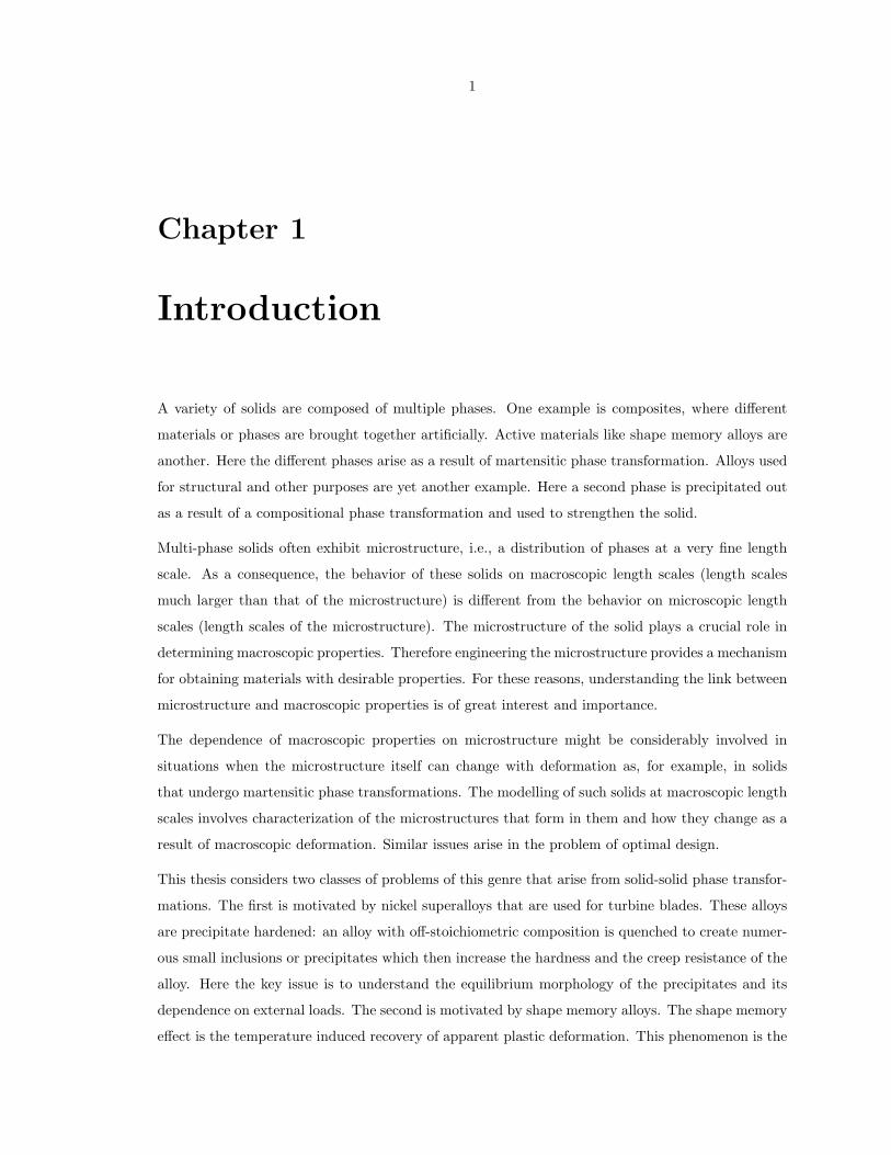
A variety of solids are composed of multiple phases. One example is composites, where different

materials or phases are brought together artificially. Active materials like shape memory alloys are

another. Here the different phases arise as a result of martensitic phase transformation. Alloys used

for structural and other purposes are yet another example. Here a second phase is precipitated out

as a result of a compositional phase transformation and used to strengthen the solid.

Multi-phase solids often exhibit microstructure, i.e., a distribution of phases at a very fine length

scale. As a consequence, the behavior of these solids on macroscopic length scales (length scales

much larger than that of the microstructure) is different from the behavior on microscopic length

scales (length scales of the microstructure). The microstructure of the solid plays a crucial role in

determining macroscopic properties. Therefore engineering the microstructure provides a mechanism

for obtaining materials with desirable properties. For these reasons, understanding the link between

microstructure and macroscopic properties is of great interest and importance.

The dependence of macroscopic properties on microstructure might be considerably involved in

situations when the microstructure itself can change with deformation as, for example, in solids

that undergo martensitic phase transformations. The modelling of such solids at macroscopic length

scales involves characterization of the microstructures that form in them and how they change as a

result of macroscopic deformation. Similar issues arise in the problem of optimal design.

This thesis considers two classes of problems of this genre that arise from solid-solid phase transfor-

mations. The first is motivated by nickel superalloys that are used for turbine blades. These alloys

are precipitate hardened: an alloy with off-stoichiometric composition is quenched to create numer-

ous small inclusions or precipitates which then increase the hardness and the creep resistance of the

alloy. Here the key issue is to understand the equilibrium morphology of the precipitates and its

dependence on external loads. The second is motivated by shape memory alloys. The shape memory

effect is the temperature induced recovery of apparent plastic deformation. This phenomenon is the

2

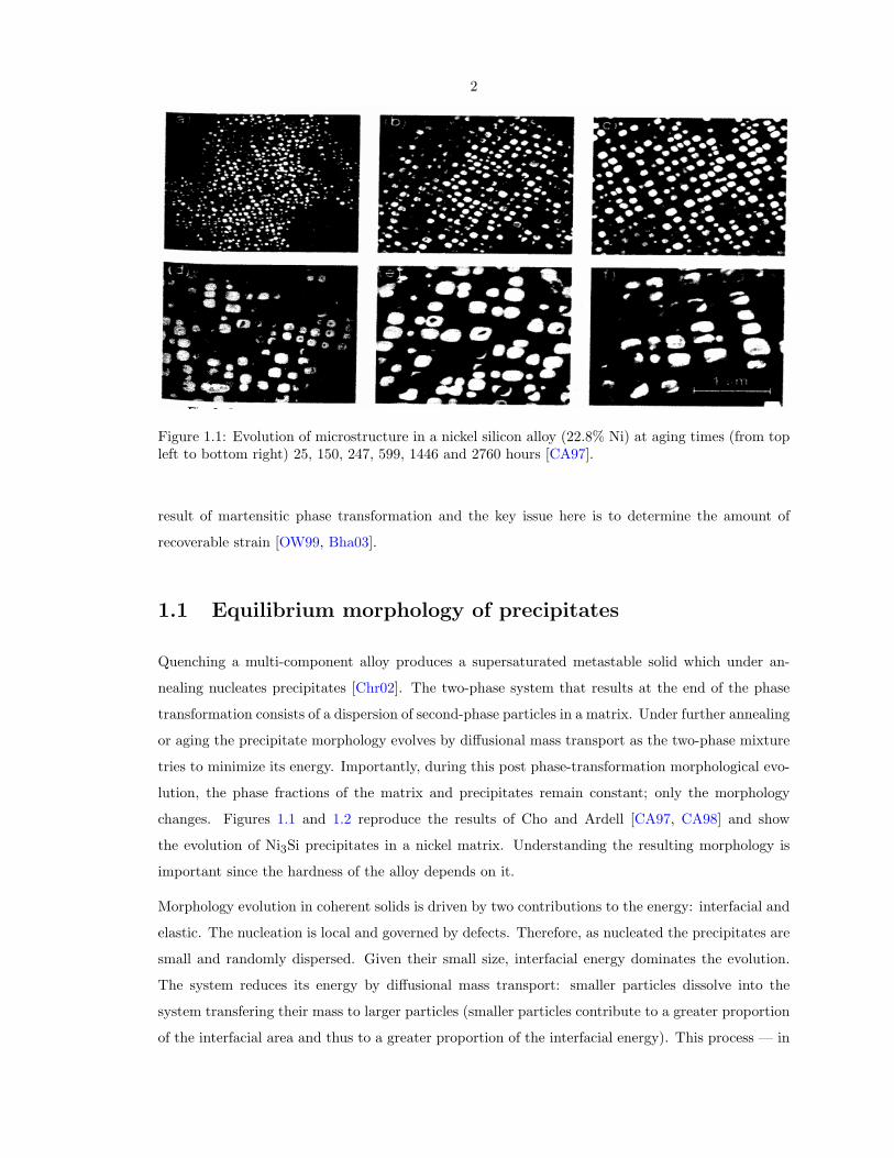
Figure 1.1: Evolution of microstructure in a nickel silicon alloy (22.8% Ni) at aging times (from topleft to bottom right) 25, 150, 247, 599, 1446 and 2760 hours [CA97].

result of martensitic phase transformation and the key issue here is to determine the amount of

recoverable strain [OW99, Bha03].

1.1 Equilibrium morphology of precipitates

Quenching a multi-component alloy produces a supersaturated metastable solid which under an-

nealing nucleates precipitates [Chr02]. The two-phase system that results at the end of the phase

transformation consists of a dispersion of second-phase particles in a matrix. Under further annealing

or aging the precipitate morphology evolves by diffusional mass transport as the two-phase mixture

tries to minimize its energy. Importantly, during this post phase-transformation morphological evo-

lution, the phase fractions of the matrix and precipitates remain constant; only the morphology

changes. Figures 1.1 and 1.2 reproduce the results of Cho and Ardell [CA97, CA98] and show

the evolution of Ni3Si precipitates in a nickel matrix. Understanding the resulting morphology is

important since the hardness of the alloy depends on it.

Morphology evolution in coherent solids is driven by two contributions to the energy: interfacial and

elastic. The nucleation is local and governed by defects. Therefore, as nucleated the precipitates are

small and randomly dispersed. Given their small size, interfacial energy dominates the evolution.

The system reduces its energy by diffusional mass transport: smaller particles dissolve into the

system transfering their mass to larger particles (smaller particles contribute to a greater proportion

of the interfacial area and thus to a greater proportion of the interfacial energy). This process — in

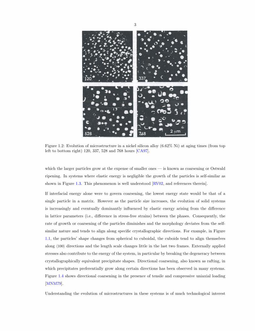
3

Figure 1.2: Evolution of microstructure in a nickel silicon alloy (6.62% Ni) at aging times (from topleft to bottom right) 120, 337, 528 and 768 hours [CA97].

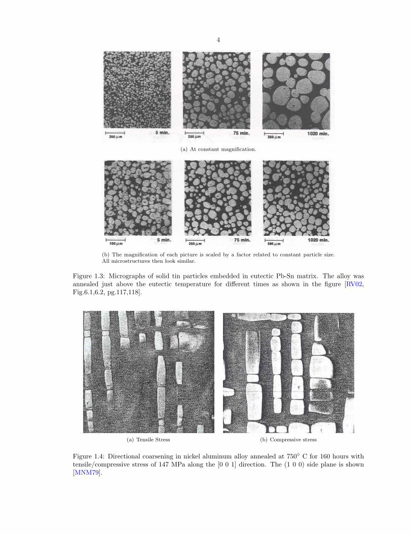
which the larger particles grow at the expense of smaller ones — is known as coarsening or Ostwald

ripening. In systems where elastic energy is negligible the growth of the particles is self-similar as

shown in Figure 1.3. This phenomenon is well understood [RV02, and references therein].

If interfacial energy alone were to govern coarsening, the lowest energy state would be that of a

single particle in a matrix. However as the particle size increases, the evolution of solid systems

is increasingly and eventually dominantly influenced by elastic energy arising from the difference

in lattice parameters (i.e., difference in stress-free strains) between the phases. Consequently, the

rate of growth or coarsening of the particles diminishes and the morphology deviates from the self-

similar nature and tends to align along specific crystallographic directions. For example, in Figure

1.1, the particles’ shape changes from spherical to cuboidal, the cuboids tend to align themselves

along 〈100〉 directions and the length scale changes little in the last two frames. Externally applied

stresses also contribute to the energy of the system, in particular by breaking the degeneracy between

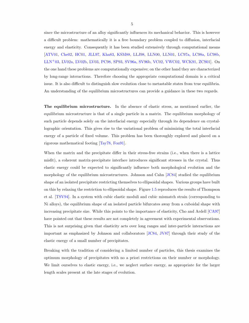
crystallographically equivalent precipitate shapes. Directional coarsening, also known as rafting, in

which precipitates preferentially grow along certain directions has been observed in many systems.

Figure 1.4 shows directional coarsening in the presence of tensile and compressive uniaxial loading

[MNM79].

Understanding the evolution of microstructures in these systems is of much technological interest

4

(a) At constant magnification.

(b) The magnification of each picture is scaled by a factor related to constant particle size.All microstructures then look similar.

Figure 1.3: Micrographs of solid tin particles embedded in eutectic Pb-Sn matrix. The alloy wasannealed just above the eutectic temperature for different times as shown in the figure [RV02,Fig.6.1,6.2, pg.117,118].

(a) Tensile Stress (b) Compressive stress

Figure 1.4: Directional coarsening in nickel aluminum alloy annealed at 750 C for 160 hours withtensile/compressive stress of 147 MPa along the [0 0 1] direction. The (1 0 0) side plane is shown[MNM79].

5

since the microstructure of an alloy significantly influences its mechanical behavior. This is however

a difficult problem: mathematically it is a free boundary problem coupled to diffusion, interfacial

energy and elasticity. Consequently it has been studied extensively through computational means

[ATV01, Che02, HC01, JLL97, Kha83, KSM88, LLJ98, LLN00, LLN01, LC97a, LC98a, LC98b,

LLN+03, LV02a, LV02b, LV03, PC98, SP93, SV96a, SV96b, VC02, VWC02, WCK91, ZCS01]. On

the one hand these problems are computationally expensive; on the other hand they are characterized

by long-range interactions. Therefore choosing the appropriate computational domain is a critical

issue. It is also difficult to distinguish slow evolution close to metastable states from true equilibria.

An understanding of the equilibrium microstructures can provide a guidance in these two regards.

The equilibrium microstructure. In the absence of elastic stress, as mentioned earlier, the

equilibrium microstructure is that of a single particle in a matrix. The equilibrium morphology of

such particle depends solely on the interfacial energy especially through its dependence on crystal-

lographic orientation. This gives rise to the variational problem of minimizing the total interfacial

energy of a particle of fixed volume. This problem has been thoroughly explored and placed on a

rigorous mathematical footing [Tay78, Fon91].

When the matrix and the precipitate differ in their stress-free strains (i.e., when there is a lattice

misfit), a coherent matrix-precipitate interface introduces significant stresses in the crystal. Thus

elastic energy could be expected to significantly influence both morphological evolution and the

morphology of the equilibrium microstructures. Johnson and Cahn [JC84] studied the equilibrium

shape of an isolated precipitate restricting themselves to ellipsoidal shapes. Various groups have built

on this by relaxing the restriction to ellipsoidal shape. Figure 1.5 reproduces the results of Thompson

et al. [TSV94]. In a system with cubic elastic moduli and cubic mismatch strain (corresponding to

Ni alloys), the equilibrium shape of an isolated particle bifurcates away from a cuboidal shape with

increasing precipitate size. While this points to the importance of elasticity, Cho and Ardell [CA97]

have pointed out that these results are not completely in agreement with experimental observations.

This is not surprising given that elasticity acts over long ranges and inter-particle interactions are

important as emphasized by Johnson and collaborators [JC84, JV87] through their study of the

elastic energy of a small number of precipitates.

Breaking with the tradition of considering a limited number of particles, this thesis examines the

optimum morphology of precipitates with no a priori restrictions on their number or morphology.

We limit ourselves to elastic energy, i.e., we neglect surface energy, as appropriate for the larger

length scales present at the late stages of evolution.

6

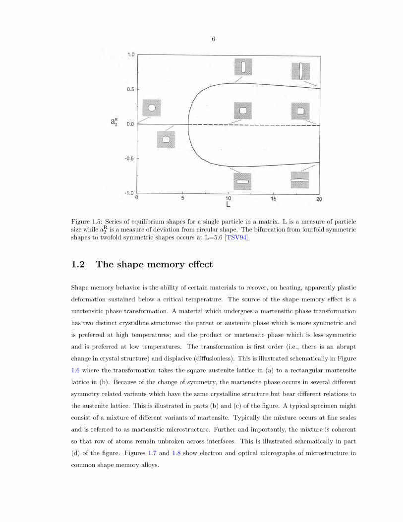
Figure 1.5: Series of equilibrium shapes for a single particle in a matrix. L is a measure of particlesize while aR

2 is a measure of deviation from circular shape. The bifurcation from fourfold symmetricshapes to twofold symmetric shapes occurs at L=5.6 [TSV94].

1.2 The shape memory effect

Shape memory behavior is the ability of certain materials to recover, on heating, apparently plastic

deformation sustained below a critical temperature. The source of the shape memory effect is a

martensitic phase transformation. A material which undergoes a martensitic phase transformation

has two distinct crystalline structures: the parent or austenite phase which is more symmetric and

is preferred at high temperatures; and the product or martensite phase which is less symmetric

and is preferred at low temperatures. The transformation is first order (i.e., there is an abrupt

change in crystal structure) and displacive (diffusionless). This is illustrated schematically in Figure

1.6 where the transformation takes the square austenite lattice in (a) to a rectangular martensite

lattice in (b). Because of the change of symmetry, the martensite phase occurs in several different

symmetry related variants which have the same crystalline structure but bear different relations to

the austenite lattice. This is illustrated in parts (b) and (c) of the figure. A typical specimen might

consist of a mixture of different variants of martensite. Typically the mixture occurs at fine scales

and is referred to as martensitic microstructure. Further and importantly, the mixture is coherent

so that row of atoms remain unbroken across interfaces. This is illustrated schematically in part

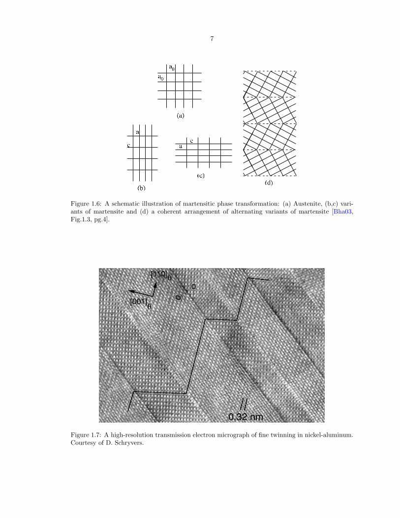
(d) of the figure. Figures 1.7 and 1.8 show electron and optical micrographs of microstructure in

common shape memory alloys.

7

Figure 1.6: A schematic illustration of martensitic phase transformation: (a) Austenite, (b,c) vari-ants of martensite and (d) a coherent arrangement of alternating variants of martensite [Bha03,Fig.1.3, pg.4].

Figure 1.7: A high-resolution transmission electron micrograph of fine twinning in nickel-aluminum.Courtesy of D. Schryvers.

8

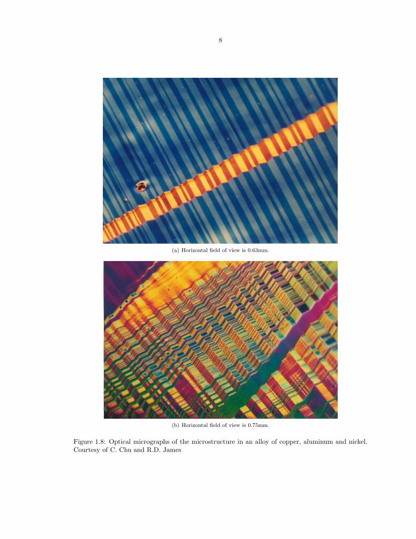
(a) Horizontal field of view is 0.63mm.

(b) Horizontal field of view is 0.75mm.

Figure 1.8: Optical micrographs of the microstructure in an alloy of copper, aluminum and nickel.Courtesy of C. Chu and R.D. James

9

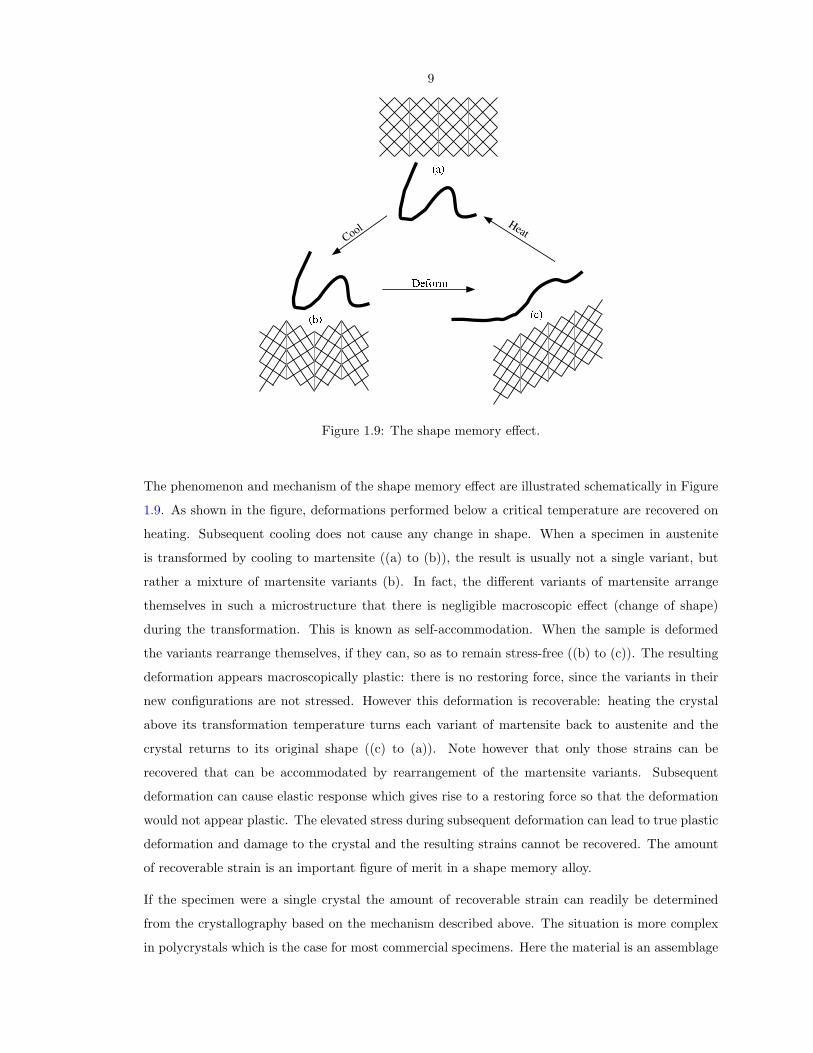
Figure 1.9: The shape memory effect.

The phenomenon and mechanism of the shape memory effect are illustrated schematically in Figure

1.9. As shown in the figure, deformations performed below a critical temperature are recovered on

heating. Subsequent cooling does not cause any change in shape. When a specimen in austenite

is transformed by cooling to martensite ((a) to (b)), the result is usually not a single variant, but

rather a mixture of martensite variants (b). In fact, the different variants of martensite arrange

themselves in such a microstructure that there is negligible macroscopic effect (change of shape)

during the transformation. This is known as self-accommodation. When the sample is deformed

the variants rearrange themselves, if they can, so as to remain stress-free ((b) to (c)). The resulting

deformation appears macroscopically plastic: there is no restoring force, since the variants in their

new configurations are not stressed. However this deformation is recoverable: heating the crystal

above its transformation temperature turns each variant of martensite back to austenite and the

crystal returns to its original shape ((c) to (a)). Note however that only those strains can be

recovered that can be accommodated by rearrangement of the martensite variants. Subsequent

deformation can cause elastic response which gives rise to a restoring force so that the deformation

would not appear plastic. The elevated stress during subsequent deformation can lead to true plastic

deformation and damage to the crystal and the resulting strains cannot be recovered. The amount

of recoverable strain is an important figure of merit in a shape memory alloy.

If the specimen were a single crystal the amount of recoverable strain can readily be determined

from the crystallography based on the mechanism described above. The situation is more complex

in polycrystals which is the case for most commercial specimens. Here the material is an assemblage

10

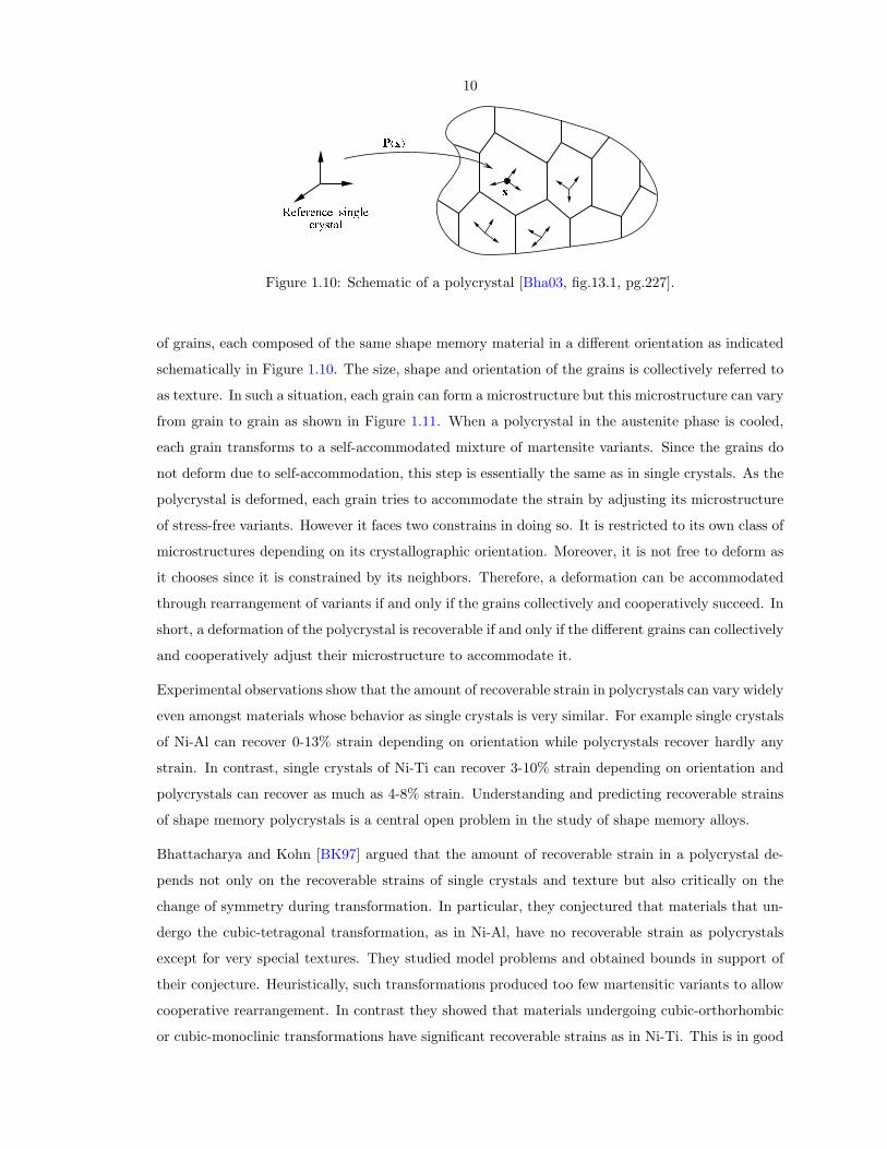
Figure 1.10: Schematic of a polycrystal [Bha03, fig.13.1, pg.227].

of grains, each composed of the same shape memory material in a different orientation as indicated

schematically in Figure 1.10. The size, shape and orientation of the grains is collectively referred to

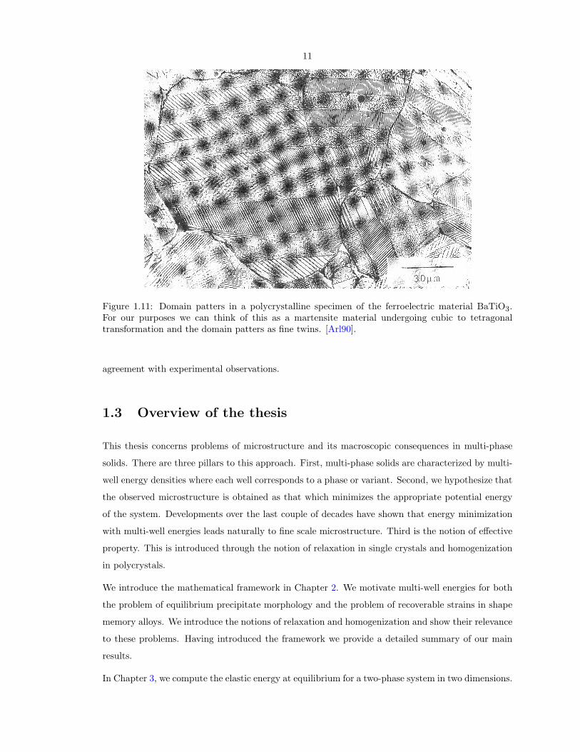
as texture. In such a situation, each grain can form a microstructure but this microstructure can vary

from grain to grain as shown in Figure 1.11. When a polycrystal in the austenite phase is cooled,

each grain transforms to a self-accommodated mixture of martensite variants. Since the grains do

not deform due to self-accommodation, this step is essentially the same as in single crystals. As the

polycrystal is deformed, each grain tries to accommodate the strain by adjusting its microstructure

of stress-free variants. However it faces two constrains in doing so. It is restricted to its own class of

microstructures depending on its crystallographic orientation. Moreover, it is not free to deform as

it chooses since it is constrained by its neighbors. Therefore, a deformation can be accommodated

through rearrangement of variants if and only if the grains collectively and cooperatively succeed. In

short, a deformation of the polycrystal is recoverable if and only if the different grains can collectively

and cooperatively adjust their microstructure to accommodate it.

Experimental observations show that the amount of recoverable strain in polycrystals can vary widely

even amongst materials whose behavior as single crystals is very similar. For example single crystals

of Ni-Al can recover 0-13% strain depending on orientation while polycrystals recover hardly any

strain. In contrast, single crystals of Ni-Ti can recover 3-10% strain depending on orientation and

polycrystals can recover as much as 4-8% strain. Understanding and predicting recoverable strains

of shape memory polycrystals is a central open problem in the study of shape memory alloys.

Bhattacharya and Kohn [BK97] argued that the amount of recoverable strain in a polycrystal de-

pends not only on the recoverable strains of single crystals and texture but also critically on the

change of symmetry during transformation. In particular, they conjectured that materials that un-

dergo the cubic-tetragonal transformation, as in Ni-Al, have no recoverable strain as polycrystals

except for very special textures. They studied model problems and obtained bounds in support of

their conjecture. Heuristically, such transformations produced too few martensitic variants to allow

cooperative rearrangement. In contrast they showed that materials undergoing cubic-orthorhombic

or cubic-monoclinic transformations have significant recoverable strains as in Ni-Ti. This is in good

11

Figure 1.11: Domain patters in a polycrystalline specimen of the ferroelectric material BaTiO3.For our purposes we can think of this as a martensite material undergoing cubic to tetragonaltransformation and the domain patters as fine twins. [Arl90].

agreement with experimental observations.

1.3 Overview of the thesis

This thesis concerns problems of microstructure and its macroscopic consequences in multi-phase

solids. There are three pillars to this approach. First, multi-phase solids are characterized by multi-

well energy densities where each well corresponds to a phase or variant. Second, we hypothesize that

the observed microstructure is obtained as that which minimizes the appropriate potential energy

of the system. Developments over the last couple of decades have shown that energy minimization

with multi-well energies leads naturally to fine scale microstructure. Third is the notion of effective

property. This is introduced through the notion of relaxation in single crystals and homogenization

in polycrystals.

We introduce the mathematical framework in Chapter 2. We motivate multi-well energies for both

the problem of equilibrium precipitate morphology and the problem of recoverable strains in shape

memory alloys. We introduce the notions of relaxation and homogenization and show their relevance

to these problems. Having introduced the framework we provide a detailed summary of our main

results.

In Chapter 3, we compute the elastic energy at equilibrium for a two-phase system in two dimensions.

12

We show that the equilibrium microstructures always include laminates. Our results in this chapter

are also relevant to the problem of recoverable strains in single crystal shape memory alloys. In

Chapter 4 we present results for the problem in three dimensions when the phases are isotropic.

Chapter 5 contains our contributions to the effort to characterize the recoverable strains of shape

memory polycrystals in terms of the symmetry change during transformation, recoverable strains

for the corresponding single crystals and texture. Specifically our goal is a deeper understanding

of this problem. We prove a dual variational principle and show that dual (stress) fields could be

signed Radon measures with finite mass. We end with results specific to materials that undergo the

cubic-tetragonal transformation.

13

Chapter 2

Mathematical framework andstatement of results

In this chapter we introduce the mathematical framework to model and study the problems in

multiphase solids discussed above. We work in the framework of infinitesimal kinematics. We treat

the different phases as linear elastic solids, each with its own elastic modulus and stress-free (residual

or transformation) strain. We formulate the two problems independently but the connection between

them will be clear.

2.1 Equilibrium morphology of precipitates

Consider the Ni-Si system described in §1.1. We have two phases, nickel which forms the matrix

and Ni3Si which forms the precipitate. They have different preferred lattice parameters and elastic

moduli. The precipitates are coherent, i.e., the rows of atoms are unbroken at the interfaces. Thus

the crystal lattice might be internally stressed. Since the structure is coherent, we refer both latices

to a single reference state and the configuration of the crystal through continuous displacements

relative to this reference state. The two phases have distinct stress-free strains reflecting their

different preferred lattice parameters. For generality, we present a formulation for N phases.

Consider a material with N phases. Let εTi be the stress-free stain of the ith phase relative to the

chosen reference configuration and αi be its elastic modulus. Suppose further that the chemical

energy of the ith phase is wi. We can then say that the energy of this phase subject to a strain ε is

given by

Wi(ε) =1

2

˙αi(ε− εT

i ), (ε− εTi )¸

+ wi. (2.1)

14

The inner product1 is defined as usual by ∀A, B ∈ Mn×n, 〈A, B〉 := Tr(ATB). Now consider an

arrangement of N phases described by the characteristic functions χi : Ω → 0, 1, i = 1, . . . , N where

Ω is the region occupied by the solid. These functions are chosen such that χi(x) = 1 if the point

x ∈ Ω is occupied by the ith phase and χi(x) = 0 otherwise. Consequently

χεiχ

εj = δij ,

NXi=1

χεi = 1.

The phase fraction of the ith phase is given by

λi :=1

volume(Ω)

ZΩ

χεi(x) dx.

Given some phase arrangement χi and a displacement field u, the total energy of the crystal is

ZΩ

NXi=1

χεi(x)Wi(ε(u)) dx,

where ε(u) = 12 (∇u + (∇u)T ).

Displacement boundary conditions. In order to find the optimal microstructure we seek to

find the χi and u that minimize this energy subject to the constraints of volume fractions and

displacement boundary conditions, respectively. This problem is specimen specific, i.e., it depends

on the domain Ω. It is convenient instead to look at a unit cell of representative volume element,

also labelled Ω with abuse of notation, and consider the problem of finding the optimal arrangement

of phases and the displacement when the volume fractions and average strain are given. We define

the effective energy cWλ through the variational problem

cWλ(ε) := inf〈χi〉=λi

infu|∂Ω=ε·x

−ZΩ

NXi=1

χi(x)Wi(ε(x)) dx (2.2)

(as convenient shorthands we use −RΩ · dx and 〈·〉 to mean 1

volume(Ω)

RΩ · dx). The problem we study

is to characterize cWλ and the optimal or energy minimizing microstructures χi. The passage from

the specimen specific problem to the unit cell problem is justified by the mathematical theory of

relaxation which we shall describe in the context of shape memory alloys in the next section. Finally

note that it is possible to define cWλ using periodic boundary conditions instead of affine boundary

1 We use 〈 , 〉 to denote the inner product in Mn×n and · to denote the inner product in Rn.

15

conditions:

cWλ(ε) = inf〈χi〉=λi

infε : periodic〈e(x)〉=ε

−ZΩ

NXi=1

χi(x)Wi(ε(x)) dx (2.3)

Traction boundary conditions. When the specimen is subjected to tractions at the boundary

the relevant potential energy is not (2.2) but

ZΩ

NXi=1

χεi(x)Wi(ε(x)) dx−

Z∂Ω

t(x) · u(x) dS.

If it is further supposed that the applied traction corresponds to a uniform stress, i.e., t(x) = σ · n(x)

where n is the unit normal to ∂Ω this reduces to

ZΩ

NXi=1

χεi(x)Wi(ε(x))− 〈σ, ε(x)〉 dx.

As before, in order to find the optimal microstructure we seek to find the χi and u that minimize

this energy subject to the constraint on volume fractions. Again, since this problem is specimen

specific we look instead at a unit cell of representative volume element also labelled Ω. We define

the effective energy cWσλ through the variational problem

cWσλ (σ) := inf

〈χi〉=λi

infε

u|∂Ω=ε·x−ZΩ

NXi=1

χi(x)Wi(ε(x))− 〈σ, ε(x)〉 dx. (2.4)

It is easy to show that cWσλ is the negative of the conjugate (Legendre-Fenchel transform) of cWλ:

−(Wλ)?(σ) := −maxε

〈σ, ε〉 −cW (ε)

= minε

cW (ε)− 〈σ, ε〉

= minε

0@ inf〈χi〉=λi

infu|∂Ω=ε·x

−ZΩ

NXi=1

χi(x)Wi(ε(x)) dx− 〈σ, ε〉

1A= inf〈χi〉=λi

infε

u|∂Ω=ε·x−ZΩ

NXi=1

χi(x)Wi(ε(x))− 〈σ, ε〉 dx

= cWσλ .

16

2.2 The shape memory effect

2.2.1 The shape memory effect in single crystals

Martensitic transformation in shape memory alloys is coherent, i.e., it does not damage the crystalline

lattice. It may therefore be modelled in the framework of elasticity following a long tradition c.f.,

e.g., Eshelby [Esh61], Wayman [Way64, WW71, Way92], Roytburd [Roy78, Roy93], Khachaturtan

[Kha83], Ericksen [Eri84], Ball and James [BJ87, BJ92] and Kohn [Koh90, Koh91]. Here the states

of the crystal are identified with strains relative to a fixed reference configuration. We confine

ourselves to infinitesimal kinematics2 and neglect ordinary thermal expansion.3 It is convenient to

use the austenite phase at the transition temperature as our reference state. Thus the stress-free

strain of austenite is εT0 = 0. The transformation from austenite to the ith variant of martensite

can be described as a deformation whose strain is εTi relative to the reference austenite. Thus εT

i

is the transformation or stress-free strain of the ith variant of martensite and can be determined

from lattice parameters. We illustrate this with the example of cubic-tetragonal, cubic-trigonal and

cubic-orthorhombic transformations:

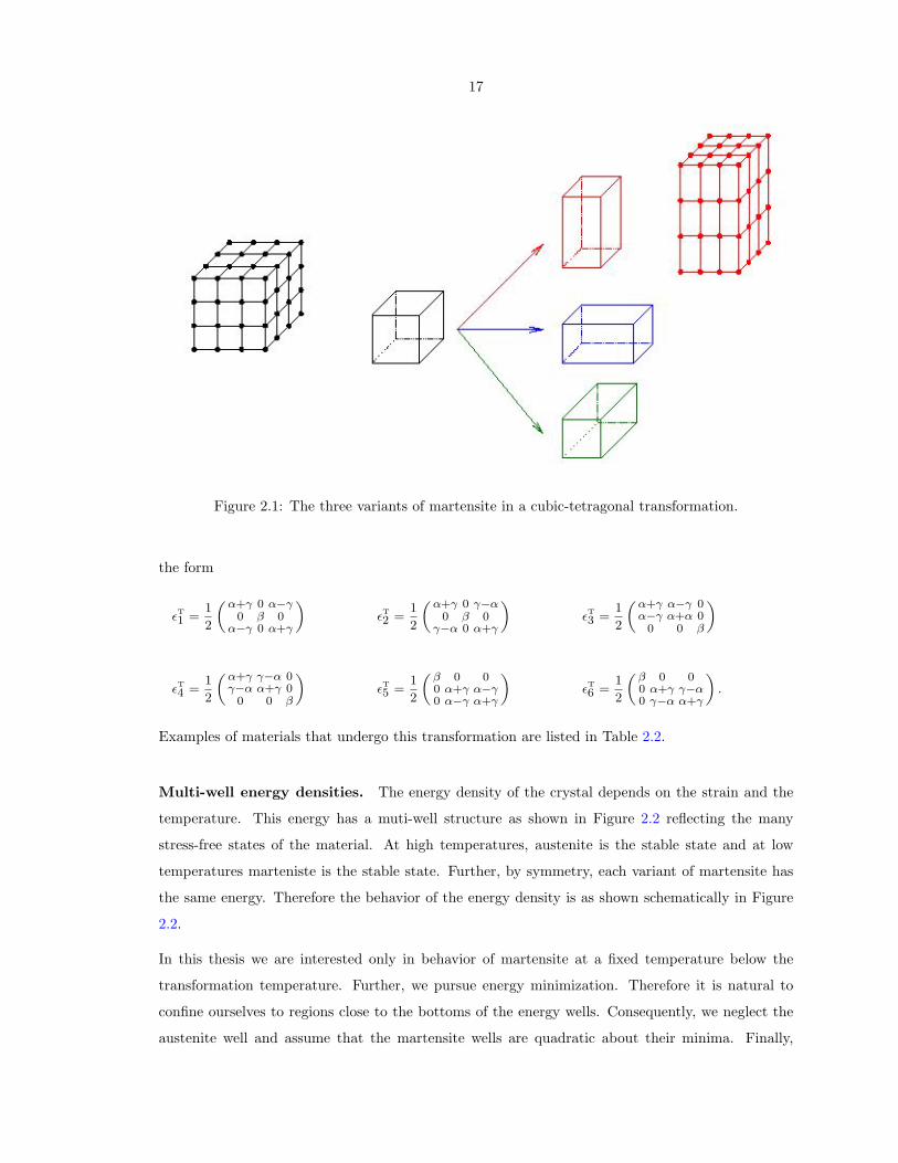
Cubic-tetragonal, cubic-trigonal and cubic-orthorhombic transformations. The unit cell

of austenite is a cube of side, say, ao. For the cubic-tetragonal transformation the unit cell of each

variant of martensite is a cuboid of sides, say, a, a and c (see Figure 2.1). Then the transformation

strains for a cubic-tetragonal transformation are

εT1 =

„β 0 00 α 00 0 α

«εT2 =

„α 0 00 β 00 0 α

«εT3 =

„α 0 00 α 00 0 β

«,

where α = aao− 1 and β = c

ao− 1. Examples of materials that undergo this transformation are listed

in Table 2.1. For a cubic-trigonal transformation, the transformation strains are of the form

εT1 =

β α αα β αα α β

!εT2 =

β −α −α−α β α−α α β

!εT3 =

β α −αα β −α−α −α β

!εT4 =

β −α α−α β −αα −α β

!.

The transformation in Ni-Ti from austenite to R-phase is of this kind; the parameters strongly

depend on temperature. For a cubic-orthorhombic transformation, the transformation strains are of2 See [Bha93] for a detailed discussion of this assumption3 This is reasonable since we are interested in fixed temperatures, and is easy to generalize.

17

Figure 2.1: The three variants of martensite in a cubic-tetragonal transformation.

the form

εT1 =

1

2

„α+γ 0 α−γ0 β 0

α−γ 0 α+γ

«εT2 =

1

2

„α+γ 0 γ−α0 β 0

γ−α 0 α+γ

«εT3 =

1

2

„α+γ α−γ 0α−γ α+α 0

0 0 β

«

εT4 =

1

2

„α+γ γ−α 0γ−α α+γ 0

0 0 β

«εT5 =

1

2

„β 0 00 α+γ α−γ0 α−γ α+γ

«εT6 =

1

2

„β 0 00 α+γ γ−α0 γ−α α+γ

«.

Examples of materials that undergo this transformation are listed in Table 2.2.

Multi-well energy densities. The energy density of the crystal depends on the strain and the

temperature. This energy has a muti-well structure as shown in Figure 2.2 reflecting the many

stress-free states of the material. At high temperatures, austenite is the stable state and at low

temperatures marteniste is the stable state. Further, by symmetry, each variant of martensite has

the same energy. Therefore the behavior of the energy density is as shown schematically in Figure

2.2.

In this thesis we are interested only in behavior of martensite at a fixed temperature below the

transformation temperature. Further, we pursue energy minimization. Therefore it is natural to

confine ourselves to regions close to the bottoms of the energy wells. Consequently, we neglect the

austenite well and assume that the martensite wells are quadratic about their minima. Finally,

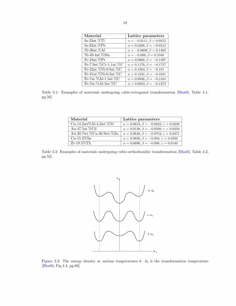
18

Material Lattice parametersIn-23at.%Tl α = −0.0111, β = 0.0212

In-32at.%Pb α = 0.0208, β = −0.0312

Ni-36at.%Al α = −0.0608, β = 0.1302

Ni-49.4at.%Mn α = −0.088, β = 0.1940

Fe-24at.%Pt α = 0.0868, β = −0.1497

Fe-7.9at.%Cr-1.1at.%C α = 0.1176, β = −0.1757

Fe-22at.%Ni-0.8at.%C α = 0.1083, β = −0.181

Fe-31at.%Ni-0.3at.%C α = 0.1241, β = −0.1941

Fe-7at.%Al-1.5at.%C α = 0.0946, β = −0.1454

Fe-7at.%Al-2at.%C α = 0.0833, β = −0.1273

Table 2.1: Examples of materials undergoing cubic-tetragonal transformation [Bha03, Table 4.1,pg.50].

Material Lattice parametersCu-14.2wt%Al-4.3wt.%Ni α = 0.0619, β = −0.0822, γ = 0.0230

Au-47.5at.%Cd α = 0.0138, β = −0.0509, γ = 0.0350

Au-20.7wt.%Cu-30.9wt.%Zn α = 0.0649, β = −0.0752, γ = 0.0371

Cu-15.3%Sn α = 0.0820, β = −0.094, γ = 0.0350

Zr-19.5%Th α = 0.0690, β = −0.098, γ = 0.0140

Table 2.2: Examples of materials undergoing cubic-orthorhombic transformation [Bha03, Table 4.2,pg.52].

W

e

Figure 2.2: The energy density at various temperatures θ. θo is the transformation temperature[Bha03, Fig.4.4, pg.60].

19

with no loss of generality, we assume that the minimum is zero. Putting these together, we write

the energy density of the material with N variants of martensite as the minimum over N quadratic

energy wells:

W (ε) := mini=1,...N

Wi(ε). (2.5a)

Here, ε is the linearized strain and the energy density of the ith phase is given by

Wi(ε) =1

2

˙αi(ε− εT

i ), (ε− εTi )¸, (2.5b)

where αi is the elastic modulus of the ith phase. We postulate that the state of the single crystal is

described by the displacement field that minimizes the total energy:

ZΩ

W (ε(u)) dx, (2.6)

where Ω is the region occupied by the crystal. Since W has a multi-well structure, the problem

of minimizing the total energy might not have any solution; instead minimizing sequences develop

oscillations and do not converge in any classical sense [Dac89]. In other words, we find ourselves in

a situation where we can reduce the energy with strain fields that have finer and finer oscillations

but can never attain the minimum. We interpret this as the emergence of microstructure [BJ87]

(also [CK88]). For an accessible introduction we refer the reader to [Bha03].

The relaxed energy density. Thus, once a material forms microstructure, its effective behavior

is not described by W but by a energy density cW that describes its overall effective energy after

the formation of microstructure. The theory of relaxation [AF84, Dac89, KP91, DM93] provides a

convenient framework for defining such an energy. Let cW be defined as

cW (ε) := infu|∂Ω=ε·x

−ZΩ

W (ε(u)) dx. (2.7)

cW is the energy density of a material with overall strain ε after it has formed microstructure.

Therefore we call W the microscopic energy density and cW the mesoscopic density energy. This is

shown schematically in Figure 2.3.

The relaxed energy density can be thought of as the average energy density of the solid account-

ing for microstructures and describes the behavior of the solid on macroscopic length scales. The

theory justifies this since minimizing −RΩ W (ε) dx with specified boundary conditions is equivalent to

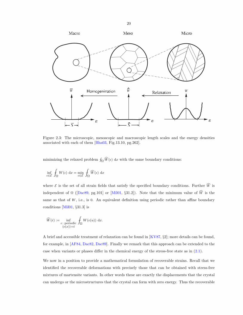
20

WWW

eee

Figure 2.3: The microscopic, mesoscopic and macroscopic length scales and the energy densitiesassociated with each of them [Bha03, Fig.13.10, pg.262].

minimizing the relaxed problem −RΩcW (ε) dx with the same boundary conditions:

infε∈E

−ZΩ

W (ε) dx = minε∈E

−ZΩ

cW (ε) dx

where E is the set of all strain fields that satisfy the specified boundary conditions. Further cW is

independent of Ω ([Dac89, pg.101] or [Mil01, §31.2]). Note that the minimum value of cW is the

same as that of W , i.e., is 0. An equivalent definition using periodic rather than affine boundary

conditions [Mil01, §31.3] is

cW (ε) := infε : periodic〈e(x)〉=ε

−ZΩ

W (ε(u)) dx.

A brief and accessible treatment of relaxation can be found in [KV87, §2]; more details can be found,

for example, in [AF84, Dac82, Dac89]. Finally we remark that this approach can be extended to the

case when variants or phases differ in the chemical energy of the stress-free state as in (2.1).

We now in a position to provide a mathematical formulation of recoverable strains. Recall that we

identified the recoverable deformations with precisely those that can be obtained with stress-free

mixtures of martensite variants. In other words these are exactly the displacements that the crystal

can undergo or the microstructures that the crystal can form with zero energy. Thus the recoverable

21

deformations are in one-to-one correspondence with the minimizers of (2.6). In light of the discussion

above we define the recoverable strains to be the zero-set of the mesoscale energy cW :

bS := ε | cW (ε) = 0.

To summarize: to predict the recoverable strains of a shape-memory single crystal, we start from the

stress-free strains of its martensite variants, εT1 , . . . , εT

N . We first form the microscopic elastic energy

W , defined by (2.5). Then we pass to its relaxation, the mesoscopic energy cW defined by (2.7).

Finally we look at the set bS where cW achieves its minimum value. According to our model, the

elements of bS are the overall strains which are recoverable for this crystal. bS is compact; non-empty

when the austenite is cubic and the martensite is tetragonal, trigonal, orthorhombic or monoclinic

[BK97, (2.7), pg.108]; and convex when the martensite is tetragonal, trigonal or orthorhombic [BK97,

§3].

Relationship between cWλ and cW . The problem of computing cW is related to the problem of

computing cWλ described in §1.1. For our W , we can write the problem of computing cW as (c.f. (2.5)

and (2.7))

cW (ε) = infu|∂Ω=ε·x

ZΩ

mini=1,...,N

Wi(ε) dx.

Note that the minimization over i is to be carried out pointwise. We can rewrite this using the

characteristic functions χi introduced earlier.

cW (ε) = infu|∂Ω=ε·x

ZΩ

minχi

NXi=1

χi(x)Wi(ε(x)) dx

= infu|∂Ω=ε·x

minχi

ZΩ

NXi=1

χi(x)Wi(ε(x)) dx

= infχi

infu|∂Ω=ε·x

ZΩ

NXi=1

χi(x)Wi(ε(x)) dx

= minλi

inf〈χi〉=λi

infu|∂Ω=ε·x

ZΩ

NXi=1

χi(x)Wi(ε(x)) dx

= minλi

cWλ(ε). (2.8)

Note that the last problem is a simple algebraic problem if we were given cWλ. Thus the central

problem of computing cW is that of computing cWλ.

22

Previous results. We close this section with a description of known results for cW . Pipkin [Pip91]

and Kohn [Koh91] considered the above problem in arbitrary dimension for the special case of a

two-phase material with equal elastic moduli (α1 = α2). Pipkin’s approach was to determine the

rank-I lamination envelope of the energy and then show that it coincided with the quasiconvex hull.

This approach fails when the elastic moduli are unequal since then rank-I laminates are no longer

necessarily extremal [Lu93, Gra96]. Kohn’s approach was to compute a lower bound using Fourier

analysis and then show its optimality by constructing microstructures whose energies attain this

bound. Fourier analysis is not an useful approach when α1 6= α2. Kohn also used the translation

method, and it remains viable even when α1 6= α2. Our work here develops on it though the

translation we use is different from that used by Kohn.

Allaire and Kohn in a series of papers considered this and related problems for the case of two

well ordered materials in arbitrary dimension [AK93b], two isotropic materials in two dimensions

[AK93a] and two non-well ordered materials in arbitrary dimension [AK94]. In these papers, the

transformation strain of both phases was taken to be equal.

Jiangbo Lu [Lu93] solved this problem in two dimensions using the translation method under the

simplifying assumption of two isotropic phases with different elastic moduli. The same approach

was used by Grabovsky [Gra96], again in two dimensions, for two materials with arbitrary elastic

moduli but equal transformation strains. Our work completes this by studying a general two-phase

material in two dimensions with no restrictions on the elastic moduli or transformation strains.

For a material with more than two phases, cW is the convexification of the W when the elastic moduli

are equal and the transformation strains are pair-wise compatible [Bha03, result 12.1, pg.215]. The

problem remains open, even for equal moduli, when the transformation strains are not compatible.

For a discussion of difficulties see [Koh91]; for recent progress see [SW99, GMH02].

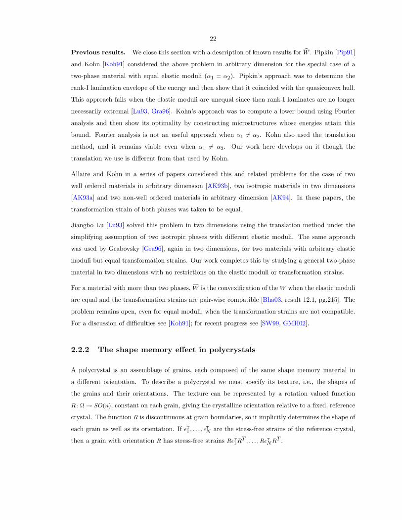
2.2.2 The shape memory effect in polycrystals

A polycrystal is an assemblage of grains, each composed of the same shape memory material in

a different orientation. To describe a polycrystal we must specify its texture, i.e., the shapes of

the grains and their orientations. The texture can be represented by a rotation valued function

R : Ω → SO(n), constant on each grain, giving the crystalline orientation relative to a fixed, reference

crystal. The function R is discontinuous at grain boundaries, so it implicitly determines the shape of

each grain as well as its orientation. If εT1 , . . . , εT

N are the stress-free strains of the reference crystal,

then a grain with orientation R has stress-free strains RεT1RT , . . . , RεT

NRT .

23

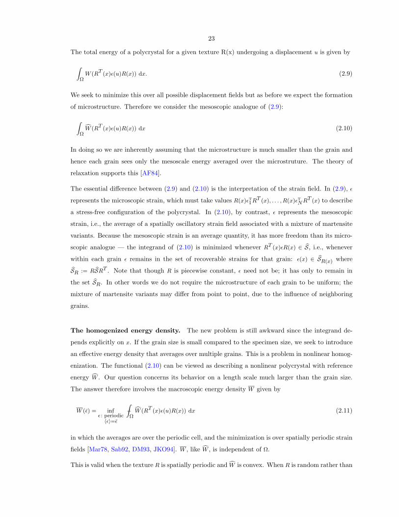
The total energy of a polycrystal for a given texture R(x) undergoing a displacement u is given by

ZΩ

W (RT (x)ε(u)R(x)) dx. (2.9)

We seek to minimize this over all possible displacement fields but as before we expect the formation

of microstructure. Therefore we consider the mesoscopic analogue of (2.9):

ZΩ

cW (RT (x)ε(u)R(x)) dx (2.10)

In doing so we are inherently assuming that the microstructure is much smaller than the grain and

hence each grain sees only the mesoscale energy averaged over the microstruture. The theory of

relaxation supports this [AF84].

The essential difference between (2.9) and (2.10) is the interpretation of the strain field. In (2.9), ε

represents the microscopic strain, which must take values R(x)εT1RT (x), . . . , R(x)εT

NRT (x) to describe

a stress-free configuration of the polycrystal. In (2.10), by contrast, ε represents the mesoscopic

strain, i.e., the average of a spatially oscillatory strain field associated with a mixture of martensite

variants. Because the mesoscopic strain is an average quantity, it has more freedom than its micro-

scopic analogue — the integrand of (2.10) is minimized whenever RT (x)εR(x) ∈ bS, i.e., whenever

within each grain ε remains in the set of recoverable strains for that grain: ε(x) ∈ bSR(x) wherebSR := R bSRT . Note that though R is piecewise constant, ε need not be; it has only to remain in

the set bSR. In other words we do not require the microstructure of each grain to be uniform; the

mixture of martensite variants may differ from point to point, due to the influence of neighboring

grains.

The homogenized energy density. The new problem is still awkward since the integrand de-

pends explicitly on x. If the grain size is small compared to the specimen size, we seek to introduce

an effective energy density that averages over multiple grains. This is a problem in nonlinear homog-

enization. The functional (2.10) can be viewed as describing a nonlinear polycrystal with reference

energy cW . Our question concerns its behavior on a length scale much larger than the grain size.

The answer therefore involves the macroscopic energy density W given by

W (ε) = infε : periodic〈ε〉=ε

−ZΩ

cW (RT (x)ε(u)R(x)) dx (2.11)

in which the averages are over the periodic cell, and the minimization is over spatially periodic strain

fields [Mar78, Sab92, DM93, JKO94]. W , like cW , is independent of Ω.

This is valid when the texture R is spatially periodic and cW is convex. When R is random rather than

24

periodic, there is an analogous definition using ensemble averaging. For a more general approach

based on Γ-convergence c.f., e.g., [DM93, JKO94]. For the relationship between these definitions

c.f., e.g., [Mar78, GP83].

W (ε) can be viewed as the average stored energy when the average strain is ε. The passage from cWto W is formally similar to that from W to cW , except that (i) the averaging is done on a different

length scale and (ii) the passage from W to cW is associated with the multiwell character of W , and

it involves averaging over mixtures of martensite variants on a subgrain length scale; the passage

from cW to W , in contrast, is associated with the polycrystalline texture, and it involves averaging

over many grains.

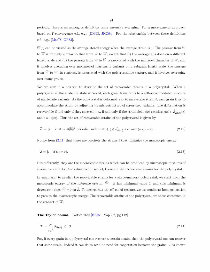
We are now in a position to describe the set of recoverable strains in a polycrystal. When a

polycrystal in the austenite state is cooled, each grain transforms to a self-accommodated mixture

of martensite variants. As the polycrystal is deformed, say to an average strain ε, each grain tries to

accommodate the strain by adjusting its microstructure of stress-free variants. The deformation is

recoverable if and only if they succeed, i.e., if and only if the strain field ε(x) satisfies ε(x) ∈ bSR(x)(x)

and ε = 〈ε(x)〉. Thus the set of recoverable strains of the polycrystal is given by

S := ε | ∃ε : Ω → Mn×nsym periodic, such that ε(x) ∈ bSR(x) a.e. and 〈ε(x)〉 = ε. (2.12)

Notice from (2.11) that these are precisely the strains ε that minimize the mesoscopic energy:

S = ε | W (ε) = 0. (2.13)

Put differently, they are the macroscopic strains which can be produced by microscopic mixtures of

stress-free variants. According to our model, these are the recoverable strains for the polycrystal.

In summary: to predict the recoverable strains for a shape-memory polycrystal, we start from the

mesoscopic energy of the reference crystal, cW . It has minimum value 0, and this minimum is

degenerate since cW = 0 on bS. To incorporate the effects of texture, we use nonlinear homogenization

to pass to the macroscopic energy. The recoverable strains of the polycrystal are those contained in

the zero-set of W .

The Taylor bound. Notice that [BK97, Prop.2.2, pg.112]

T :=\

x∈Ω

SR(x) ⊆ S. (2.14)

For, if every grain in a polycrystal can recover a certain strain, then the polycrystal too can recover

that same strain. Indeed it can do so with no need for cooperation between the grains. T is known

25

as the Taylor bound. T is nonempty when the martensite is tetragonal, trigonal, orthorhombic or

monoclinic [BK97, pg.112]. For materials that undergo cubic-tetragonal or cubic-trigonal transfor-

mations, except when the polycrystal has a very special texture, T contains precisely one point. In

this case we say that the Taylor bound is trivial. In contrast the Taylor bound is non-trivial for any

cubic-orthorhombic polycrystal.

Previous results. Bhattachary and Kohn [BK97] have conjectured that the Taylor bound is in

fact an estimate: in general only polycrystals with non-trivial Taylor bounds will be able to recover

any strain. This is in excellent agreement with experimental observations. Consider three examples

cited in [BK96, BK97]:

Ni-37at%Al undergoes a cubic-tetragonal transformation. Single crystals recover tensile strains

ranging from 0 to 13% depending on orientation [EMT+81]. Polycrystals are very poor shape

memory materials, recovering only about 0.2% strain in compression [KW92].

Fe-27Ni-0.8C (wt%) also undergoes a cubic-tetragonal transformation. Polycrystalline cold-rolled

plates do not fully recover their strains on heating. However they do recover about 50% of a 5–7%

tensile strain [KK90].

Cu-14Al-4Ni (wt.%) undergoes both cubic-orthorhombic and cubic-monoclinic transformations, de-

pending on experimental conditions. Single crystals recover tensile strains ranging from 2 to 9%

depending on orientation. Polycrystalline ribbons with uncontrolled texture recover only about

2.5% tensile strain, but specially textured polycrystalline ribbons fully recover about 6.5% tensile

strain [EH90].

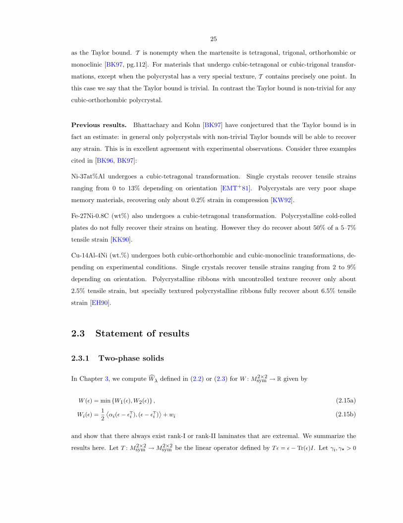
2.3 Statement of results

2.3.1 Two-phase solids

In Chapter 3, we compute cWλ defined in (2.2) or (2.3) for W : M2×2sym → R given by

W (ε) = min W1(ε), W2(ε) , (2.15a)

Wi(ε) =1

2

˙αi(ε− εT

i ), (ε− εTi )¸

+ wi (2.15b)

and show that there always exist rank-I or rank-II laminates that are extremal. We summarize the

results here. Let T : M2×2sym → M2×2

sym be the linear operator defined by Tε = ε− Tr(ε)I. Let γi, γ? > 0

26

be defined by

γi := − maxε

det(ε)<0

〈αiε, ε〉2 det(ε)

,

γ? := mini=1,2

γi.

Then

cWλ(ε) = λ1W1(ε?1) + λ2W2(ε?2) + βλ1λ2 det(ε?2 − ε?1) (2.16)

where

ε?1 = (λ2α1 + λ1α2 − β?T )−1 `(α2 − β?T )ε− λ2(α2εT2 − α1εT

1)´

ε?2 = (λ2α1 + λ1α2 − β?T )−1 `(α1 − β?T )ε + λ1(α2εT2 − α1εT

1)´

and β? is chosen as follows. For β ∈ [0, γ?], let

f(β) := det“(λ2α1 + λ1α2 − βT )−1 `α2(εT

2 − ε)− α1(εT1 − ε)

´”

be a quadratic in β. When f(0) > 0 and f(γ?) < 0, f(β) = 0 has a unique root, βII. Let

β? =

8>>>>><>>>>>:0 if f(0) < 0 (Regime I)

βII if f(0) > 0 and f(γ?) < 0 (Regime II)

γ? if f(γ?) > 0. (Regime III)

We prove this by first using the translation method to show that the right-hand side of (2.16) is a

lower bound for Wλ, and then constructing microstructures whose effective energy equals this bound:

In regime I, there exists two rank-I laminates that are extremal; other extremal microstructures might

also exist. In regime II, the unique extremal microstructure is a rank-I laminate. In regime III, there

exists two rank-II laminates that are extremal; other extremal microstructures might also exist but

no rank-I laminate is extremal.

In Chapter 4 we solve the problem in three dimensions when the elastic moduli are isotropic.

2.3.2 Polycrystals

In Chapter 5, we begin by proving a dual variational characterization of the zero-set of polycrystals.

This characterization suggests that dual (stress) fields could be signed Radon measures with finite

27

mass. For a two-dimensional material whose microscopic energy is of the form (2.15), we exhibit

examples where this is indeed the case. These examples also illustrate discontinuous dependence

of the zero-set (of polycrystals) on microstructure and effects of symmetry. They also enable us

to comment on connections to percolation theory observed earlier [BK97]. For the two-dimensional

material and for materials that undergo cubic-tetragonal transformations, we show that strain fields

associated with macroscopically recoverable strains are related to solutions of hyperbolic partial

differential equations.

28

Chapter 3

Two-phase solids in two dimensions

3.1 An optimal lower bound on the relaxed energy

We use the translation method to obtain a lower bound on the relaxed energy. Good introduc-

tions and overviews of the translation method can be found in [Che00, Chs.8,15,16] and [Mil01,

Chs.4,24,25]. For development of the method and applications to a wide range of problems see,

for example, Tartar [Tar79a, Tar85, Tar79b]; Murat [Mur87]; Murat and Tartar [MT85]; Lurie and

Cherkaev [LC81, LC82a, LC82b, LC86a]; Cherkaev and Gibiansky [CG92]; Gibiansky and Cherkaev

[GC84, GC87]; Kohn and Strang [KS82, KS83, KS86a, KS86b, KS86c]; Strang and Kohn [SK88];

Avellaneda, Cherkaev, Lurie and Milton [ACLM88]; Firoozye [Fir91] and Milton [Mil90a, Mil90b].

3.1.1 A lower bound by the translation method

Proposition 3.1 (Translation lower bound). Let W , W1 and W2 be as in (2.5), f : Mn×nsym → R

be quasiconvex and β ∈ R. Then

cWλ(ε) > maxβ>0

Wi−βf : convex

minε1,ε2∈Mn×n

symλ1ε1+λ2ε2=ε

λ1(W1 − βf)(ε1) + λ2(W2 − βf)(ε2) + βf(ε). (3.1)

Proof. From (2.2),

cWλ(ε) := inf<χi>=λi

infu|∂Ω=ε·x

−ZΩ

χ1W1(ε) + χ2W2(ε) dx.

From the definition of quasiconvexity,

f(ε) 6 infu|∂Ω=ε·x

−ZΩ

f(ε) dx.

29

Thus we have the lower bound

cWλ(ε) > inf<χi>=λi

infu|∂Ω=ε·x

−ZΩ

χ1(W1(ε)− βf(ε)) + χ2(W2(ε)− βf(ε)) dx + βf(ε)

for each β > 0. Restricting ourselves to β such that the function Wi − βf is convex (the reason for

this will become clear in the next step), we have

cWλ(ε) > maxβ>0

Wi−βf : convex

min<χi>=λi

infu|∂Ω=ε·x

−ZΩ

χ1(W1(ε)− βf(ε)) + χ2(W2(ε)− βf(ε)) dx + βf(ε).

Since Wi − βf is convex, using Jensen’s inequality,

cWλ(ε) > maxβ>0

Wi−βf : convex

min<χi>=λi

infu|∂Ω=ε·x

λ1(W1 − βf)

„−RΩ χ1ε dx

−RΩ χ1 dx

«

+ λ2(W2 − βf)

„−RΩ χ2ε dx

−RΩ χ2 dx

«+ βf(ε).

Setting εi =〈χiε〉〈χi〉

and noting that λ1ε1 + λ2ε2 = ε, we obtain the desired result (3.1).

3.1.2 The determinant as translation

The lower bound presented above is valid for any translation f : Mn×nsym → R which is quasiconvex.

This is the mathematics of the translation method; the art of the translation method lies in choosing

the right translation. In two dimensions we pick the translation to be the negative of the determinant:

f(ε) ≡ φ(ε) := − det(ε) = ε212 − ε11ε22.

This choice of the translation might appear to be arbitrary, but in fact is a posteriori natural. φ

is quasiconvex on the space of all symmetrized gradients since it is quadratic and rank-I convex

[Dac89, pg.126]: ∀m, n ∈ R2, φ(m ⊗s n) > 0. Here m ⊗s n := 12 (n ⊗ m + m ⊗ n); m ⊗ n is defined as

usual by (m⊗ n)ij = minj .

Since φ is quadratic there exists a (unique) linear operator T : M2×2sym → M2×2

sym such that

φ(ε) =1

2〈Tε, ε〉 .

It is easy to verify that T is self-adjoint and is given by Tε = ε − Tr(ε)I (i.e., −Tε is the adjoint of

ε). T has eigenvalues −1 and 1, repeated once and twice, respectively: TI = −I and Tε = ε for all

ε ∈ M2×2sym such that Tr(ε) = 0 (a two-dimensional subspace of M2×2

sym ). It follows that T is invertible

and is neither positive nor negative definite.

30

To further understand T and for future use, note thatn`

1 00 1

´,“

1 00 −1

”,`

0 11 0

´oform an orthogonal

basis for M2×2sym and let Λh, Λd and Λo : M2×2

sym → M2×2sym be orthogonal projection operators defined

by

Range(Λh) = Span˘`

1 00 1

´¯, (3.2a)

Range(Λd) = Spann“

1 00 −1

”o, (3.2b)

Range(Λo) = Span˘`

0 11 0

´¯. (3.2c)

It is easy to see that T ≡ −Λh + Λd + Λo. Thus T is a reflection about the plane of deviatoric (i.e.,

trace-free) strains.

With this choice for the translation, exploiting the quadraticity of Wi and φ, (3.1) may be rewritten

as

cWλ(ε) > maxβ>0

Wi−βφ : convex

Wλ(β, ε) (3.3a)

where

Wλ(β, ε) := minε1,ε2∈M2×2

symλ1ε1+λ2ε2=ε

λ1W1(ε1) + λ2W2(ε2)− βλ1λ2φ(ε2 − ε1). (3.3b)

3.1.3 Determining the amount of translation

Our next step is to characterize the set β | β > 0, Wi − βφ : convex.

Lemma 3.2 (Convexity of translated energies). Let γi, γ? > 0 be defined by

γi := minε

φ(ε)>0

〈αiε, ε〉2φ(ε)

,

γ? := mini=1,2

γi.

Then

[0, γ?] = β | β > 0, Wi − βφ : convex,

[0, γ?) = β | β > 0, Wi − βφ : strictly convex.

Proof. By quadraticity, the convexity of Wi − βφ is equivalent to the nonnegativity of ε 7→ 〈(αi −

31

βT )ε, ε〉. Thus

〈(αi − βT )ε, ε〉 > 0 ⇔ 〈αiε, ε〉 − 2βφ(ε) > 0

⇔ maxε

φ(ε)<0


6 β 6 minε

φ(ε)>0


⇔ β 6 γi

where the last step follows since αi > 0 and β > 0. Thus for Wi − βφ to be convex we need β < γi.

This shows that [0, γ?] = β | β > 0, Wi − βφ : convex.

Alternatively,

〈(αi − βT )ε, ε〉 =

fi√

αi

„I − βα

− 12

i Tα− 1

2i

«√

αiε, ε

fl= ‖ε‖2 − β

fiα− 1

2i Tα

− 12

i ε, ε

fl

where ε =√

αiε and √αi is the unique positive-definite self-adjoint square root of αi. Thus

Wi − βφ : strictly convex ⇔ ∀ε 6= 0, ‖ε‖2 − β

fi„α− 1

2i Tα

− 12

i

«ε, ε

fl> 0

⇔ ∀ε 6= 0,1

β>

fi„α− 1

2i Tα

− 12

i

«ε, ε

fl‖ε‖2

where we have used the invertibility of √αi. Note that in this case an equivalent definition for γi is

1

γi= max‖ε‖=1

fi„α− 1

2i Tα

− 12

i

«ε, ε

fl.

γi is non-negative since T has a positive eigenvalue and all eigenvalues of αi are non-negative. The

result follows.

Remark 3.3. When αi is cubic, aligning our axis with the principal axis of αi (which might be

different for each phase), we have

αi = 2κiΛh + 2µiΛd + 2ηiΛo,

where κi, µi and ηi are, respectively, the bulk, diagonal shear and off-diagonal shear moduli of the

ith phase. (Λh, Λd and Λo : M2×2sym → M2×2

sym are orthogonal projection operators defined by (3.2).)

Since T ≡ −Λh + Λd + Λo,

α− 1

2i Tα

− 12

i =−1

2κiΛh +

1

2µiΛd +

1

2ηiΛo ⇒ 1

γi= max

„1

2µi,

1

2ηi

«

Thus when αi is cubic, γi = 2minµi, ηi. When αi is isotropic, setting µi = ηi, γi = 2µi.

32

3.1.4 Explicit expressions for the optimal strains

Let us return to the minimization problem (3.3b) and find the minimizers ε?1(β, ε) and ε?2(β, ε). By

differentiating the argument on the right-hand side of (3.3b),

α1(ε?1 − εT1)− α2(ε?2 − εT

2) + βT (ε?2 − ε?1) = 0. (3.4)

In other words,

∆σ? = βT∆ε? (3.5)

where ∆ε? := ε?2 − ε?1, ∆σ? := σ?2 − σ?

1 and σ?i = αi(ε

?i − εT

i ). Using λ1ε1 + λ2ε2 = ε, (3.4) gives

(λ2α1 + λ1α2 − βT )ε?1 = (α2 − βT )ε + λ2(α1εT1 − α2εT

2)

(λ2α1 + λ1α2 − βT )ε?2 = (α1 − βT )ε− λ1(α1εT1 − α2εT

2)

(λ2α1 + λ1α2 − βT )∆ε? = (α2εT2 − α1εT

1)− (∆α)ε.

where ∆α := α2 − α1. Thus

(λ2α1 + λ1α2 − βT )∂∆ε?

∂β− T∆ε? − βT

∂∆ε?

∂β= 0.

To get explicit expressions we need the invertibility of λ2α1+λ1α2−βT . Note that λ2α1+λ1α2−βT =

λ2(α1−βT )+λ1(α2−βT ). Hence, for β ∈ [0, γ?), it is the sum of two positive definite linear operators

and consequently positive definite and thus invertible. In fact even when β = γ?, λ2α1 + λ1α2 − βT

is invertible as long as ker(α1 − γ?T ) ∩ ker(α2 − γ?T ) = 0. In either case,

ε?1 = (λ2α1 + λ1α2 − βT )−1 `(α2 − βT )ε− λ2`α2εT

2 − α1εT1´´

, (3.6a)

ε?2 = (λ2α1 + λ1α2 − βT )−1 `(α1 − βT )ε + λ1`α2εT

2 − α1εT1´´

, (3.6b)

∆ε? = (λ2α1 + λ1α2 − βT )−1 ``α2εT2 − α1εT

1´− (∆α)ε

´, (3.6c)

and

∂∆ε?

∂β= (λ2α1 + λ1α2 − βT )−1T∆ε?. (3.7)

33

3.1.5 A lower bound on the relaxed energy

Applying lemma 3.2 to the lower bound (3.3a), we have

cWλ(ε) > maxβ∈[0,γ?]

Wλ(β, ε). (3.8)

Determining this maximum is easy since we have the following lemma:

Lemma 3.4. When γ? > 0, β 7→ Wλ(β, ε) is either constant or strictly concave for β ∈ (0, γ?).

Proof. From (3.3b) and (3.7),

∂

∂βWλ(β, ε) = −λ1λ2φ(∆ε?(β, ε)) (3.9)

∂2

∂β2Wλ(β, ε) = −λ1λ2

fiT∆ε?,

∂∆ε?

∂β

fl= −λ1λ2

DT∆ε?, (λ2α1 + λ1α2 − βT )−1T∆ε?

E< 0

except when ∆ε?(β, ε) = 0. Note, from (3.6), that ∆ε?(β, ε) = 0 for some β implies that ∆ε?(β, ε) = 0

for all β. However when ∆ε? ≡ 0, from (3.9), Wλ(β, ε) is independent of β.

Theorem 3.5. Let βII be the unique solution of φ(∆ε?(βII, ε)) = 0. Then

cWλ(ε) > cW lλ(ε)

where

cW lλ(ε) =

8>>>>><>>>>>:Wλ(0, ε) if φ(∆ε?(0, ε)) > 0 (Regime I)

Wλ(βII, ε) otherwise (Regime II)

Wλ(γ?, ε) if φ(∆ε?(γ?, ε)) < 0. (Regime III)

(3.10)

Note from (3.6) that

φ(∆ε?(β, ε)) ≡ φ“(λ2α1 + λ1α2 − βT )−1 `(α2εT

2 − α1εT1)−∆αε

´”.

Proof. From (3.6), ∆ε?(β, ε) ≡ 0 precisely when α2(ε − εT2) = α1(ε − εT

1). Then, from lemma 3.4,

β 7→ Wλ(β, ε) is constant and thus (3.10) is the same as (3.8). Consider the case when β 7→ Wλ(β, ε)

is strictly concave.

34

Using (3.9), from the concavity of β 7→ Wλ(β, ε), the maximum occurs at β = 0 whenever φ(∆ε?(0, ε)) >

0 and at β = γ? whenever φ(∆ε?(γ?, ε)) exists and is less than zero.

Since β 7→ Wλ(β, ε) is strictly concave, from (3.9), β 7→ φ(∆ε?(β, ε)) is strictly increasing. Thus when

φ(∆ε?(γ?, ε)) does not exist, φ(∆ε?(β, ε)) → ∞ as β → γ?. If in addition φ(∆ε?(0, ε)) 6 0, it follows

that for some unique βII ∈ [0, γ?), φ(∆ε?(βII, ε)) = 0.

The remaining possibility is that φ(∆ε?(0, ε)) 6 0 and φ(∆ε?(γ?, ε)) > 0. Then again from the strict

convexity of β 7→ Wλ(β, ε), there exists a unique βII such that φ(∆ε?(βII, ε)) = 0 and the maximum

occurs at β = βII. Note that it is possible that βII ∈ 0, γ?.

Remark 3.6. Regime III does not occur whenever φ(∆ε?(γ?, ε)) does not exist. From §3.1.4 this

happens when ker(α1− γ?T )∩ ker(α2− γ?T ) 6= 0. This includes, in particular, the cases (i) α1 = α2

and (ii) both phases being isotopic with equal shear moduli. We will show below that in this case

there exists a rank-I laminate that is extremal. This is consistent with the results in [Koh91, Pip91].

3.1.6 Equal elastic moduli

In this section we consider the special case of equal elastic moduli. From (3.6), ∆ε?(0, ε) = εT2 − εT

1 .

From remark 3.6, regime III does not occur in this case. Thus, from (3.10), cW lλ, the lower bound

for cWλ reduces to

cW lλ(ε) =

8>><>>:Wλ(0, ε) if φ(εT

2 − εT1) > 0

Wλ(βII, ε) otherwise, i.e., if φ(εT2 − εT

1) 6 0,

where βII is the unique solution of

φ“(α− βT )−1α(εT

2 − εT1)”

= 0.

A moment’s thought reveals that this is infact equivalent to

cW lλ(ε) =

8>><>>:Wλ(0, ε) if φ(εT

2 − εT1) > 0

Wλ(βII, ε) otherwise, i.e., if φ(εT2 − εT

1) < 0.

That is (c.f. §3.2.1),

cW lλ(ε) =

8>><>>:Wλ(0, ε) if εT

1 and εT2 are compatible

Wλ(βII, ε) otherwise, i.e., if εT1 and εT

2 are incompatible.(3.11)

35

Explicit expressions for the optimal strains when the elastic moduli are equal. (3.6)

simplifies to

ε?1 = ε− λ2(α− βT )−1α(εT2 − εT

1), (3.12a)

ε?2 = ε + λ1(α− βT )−1α(εT2 − εT

1), (3.12b)

∆ε? = (α− βT )−1α(εT2 − εT

1). (3.12c)

If, in addition, β = 0, then,

ε?1 = ε− λ2(εT2 − εT

1), (3.12d)

ε?2 = ε + λ1(εT2 − εT

1), (3.12e)

∆ε? = εT2 − εT

1 . (3.12f)

From (3.11) and (3.12), we obtain,

cW lλ(ε) =

8>>>>>>>>>><>>>>>>>>>>:

λ1W1`ε− λ2(εT

2 − εT1)´

+ λ2W2`ε + λ1(εT

2 − εT1)´

if εT1 and εT

2 are compatible

λ1W1

“ε− λ2(α− βT )−1α(εT

2 − εT1)”

+λ2W2

“ε + λ1(α− βT )−1α(εT

2 − εT1)”

−βλ1λ2φ“(α− βT )−1α(εT

2 − εT1)”

if εT1 and εT

2 are incompatible.

3.2 Extremal microstructures

In this section we prove that the lower bound presented in theorem 3.5 is optimal,

cWλ(ε) = cW lλ(ε) (3.13)

Our strategy of proof is determining upper bounds by explicitly constructing microstructures. Given

any (sequence of) microstructures χi that satisfy 〈χi〉 = λi, it follows from the definition of cWλ in

(2.2) that

cWλ(ε) 6 infu|∂Ω=ε·x

−ZΩ

χ1W1(ε) + χ2W2(ε) dx =: cWχλ (ε). (3.14)

So we have

cWχλ (ε) > cWλ(ε) > cW l

λ(ε). (3.15)

36

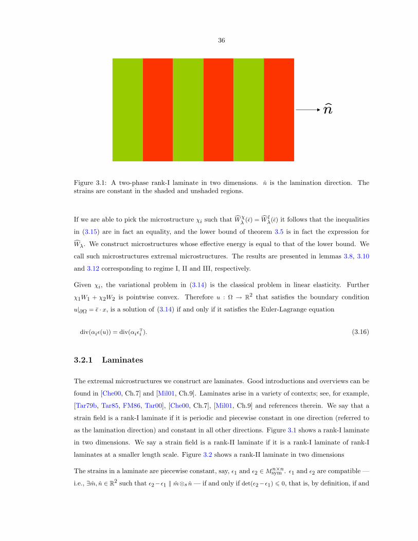
n

Figure 3.1: A two-phase rank-I laminate in two dimensions. n is the lamination direction. Thestrains are constant in the shaded and unshaded regions.

If we are able to pick the microstructure χi such that cWχλ (ε) = cW l

λ(ε) it follows that the inequalities

in (3.15) are in fact an equality, and the lower bound of theorem 3.5 is in fact the expression forcWλ. We construct microstructures whose effective energy is equal to that of the lower bound. We

call such microstructures extremal microstructures. The results are presented in lemmas 3.8, 3.10

and 3.12 corresponding to regime I, II and III, respectively.

Given χi, the variational problem in (3.14) is the classical problem in linear elasticity. Further

χ1W1 + χ2W2 is pointwise convex. Therefore u : Ω → R2 that satisfies the boundary condition

u|∂Ω = ε · x, is a solution of (3.14) if and only if it satisfies the Euler-Lagrange equation

div(αiε(u)) = div(αiεTi ). (3.16)

3.2.1 Laminates

The extremal microstructures we construct are laminates. Good introductions and overviews can be

found in [Che00, Ch.7] and [Mil01, Ch.9]. Laminates arise in a variety of contexts; see, for example,

[Tar79b, Tar85, FM86, Tar00], [Che00, Ch.7], [Mil01, Ch.9] and references therein. We say that a

strain field is a rank-I laminate if it is periodic and piecewise constant in one direction (referred to

as the lamination direction) and constant in all other directions. Figure 3.1 shows a rank-I laminate

in two dimensions. We say a strain field is a rank-II laminate if it is a rank-I laminate of rank-I

laminates at a smaller length scale. Figure 3.2 shows a rank-II laminate in two dimensions

The strains in a laminate are piecewise constant, say, ε1 and ε2 ∈ Mn×nsym . ε1 and ε2 are compatible —

i.e., ∃m, n ∈ R2 such that ε2−ε1 ‖ m⊗s n — if and only if det(ε2−ε1) 6 0, that is, by definition, if and

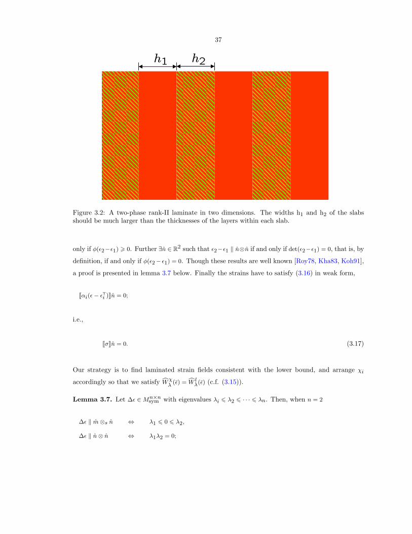
37

h1 h2

Figure 3.2: A two-phase rank-II laminate in two dimensions. The widths h1 and h2 of the slabsshould be much larger than the thicknesses of the layers within each slab.

only if φ(ε2−ε1) > 0. Further ∃n ∈ R2 such that ε2−ε1 ‖ n⊗n if and only if det(ε2−ε1) = 0, that is, by

definition, if and only if φ(ε2− ε1) = 0. Though these results are well known [Roy78, Kha83, Koh91],

a proof is presented in lemma 3.7 below. Finally the strains have to satisfy (3.16) in weak form,

Jαi(ε− εTi )Kn = 0;

i.e.,

JσKn = 0. (3.17)

Our strategy is to find laminated strain fields consistent with the lower bound, and arrange χi

accordingly so that we satisfy cWχλ (ε) = cW l

λ(ε) (c.f. (3.15)).

Lemma 3.7. Let ∆ε ∈ Mn×nsym with eigenvalues λi 6 λ2 6 · · · 6 λn. Then, when n = 2

∆ε ‖ m⊗s n ⇔ λ1 6 0 6 λ2,

∆ε ‖ n⊗ n ⇔ λ1λ2 = 0;

38

and when n > 2,

∆ε ‖ m⊗s n ⇔ λ1 6 0 = λ2, . . . , λn−1 = 0 6 λn

∆ε ‖ n⊗ n ⇔ λ2 = λ3 = · · · = λn−1 = 0 and λ1λn = 0

m and n are unique to a choice of sign.

Proof. Necessity: Assume ∆ε = |m| (m⊗s n) =|m|2 (m⊗ n + n⊗ m). We consider the case m ∦ n;

a similar proof holds otherwise. ∆ε has n − 2 zero eigenvalues since ∀~v ∈ Span m, n⊥, ∆ε~v = 0.

∆εn =|m|2 (m + (m · n)n) and ∆εm =

|m|2 ((m · n)m + n). Thus

∆ε(n + m) =|m|2

(m · n + 1)(n + m) ⇒ |m|2

(m · n + 1) is an eigenvalue

∆ε(n− m) =|m|2

(m · n− 1)(n− m) ⇒ |m|2

(m · n− 1) is an eigenvalue

Clearly one of these is nonnegative and the other is nonpositive. Further one of these is zero if and

only if m ‖ n. Note also that λn − λ1 = |m|.

Sufficiency: Assume that the eigenvalues of ∆ε satisfy λ1 6 0 = λ2, . . . , λn−1 = 0 6 λn. Let

∆ε′ =“√

λnvn +p−λ1v1

”⊗s

“√λnvn −

p−λ1v1

”

where v1 and vn are orthonormal eigenvectors of ∆ε corresponding to λ1 and λn, respectively. We will

show that ∆ε = ∆ε′ by showing that they have the same eigenvalues and corresponding eigenspaces.

Clearly ∆ε′ has n− 2 zero eigenvalues. Further

∆ε′v1 =−p−λ1

2

“√λnvn +

p−λ1v1

”+

p−λ1

2

“√λnvn −

p−λ1v1

”= λ1v1

∆ε′vn =

√λn

2

“√λnvn +

p−λ1v1

”+

√λn

2

“√λnvn −

p−λ1v1

”= λnvn

which completes the proof.

3.2.2 Regime I - rank-I laminates

We show that the lower bound cWλ(ε) > Wλ(0, ε) is optimal:

Lemma 3.8. In regime I there exist a pair of extremal rank-I laminates.

Proof. From (3.10), φ(∆ε?) > 0: the strains ε?1 and ε?2 are compatible. Since from (3.5), ∆σ? = 0,

the stress jump condition is satisfied across any interface between regions with strain ε?1 and ε?2. It

39

follows that there exist precisely two rank-I laminates (that differ only in lamination direction) in

which the strain of phase i is ε?i .

These rank-I laminates show that in regime I,

cWλ(ε) = Wλ(0, ε) = λ1W1(ε?1) + λ2W2(ε?2).

The average values of the optimal strain fields are obtained by substituting β = 0 in (3.6):

ε?1 = (λ2α1 + λ1α2)−1 `α2ε− λ2`α2εT

2 − α1εT1´´

ε?2 = (λ2α1 + λ1α2)−1 `α1ε + λ1`α2εT

2 − α1εT1´´

and

σ?1 = σ?

2 = α1 (λ2α1 + λ1α2)−1 α2`ε−

`λ1εT

1 + λ2εT2´´

= α2 (λ2α1 + λ1α2)−1 α1`ε−

`λ1εT

1 + λ2εT2´´

.

Since ∆σ? = 0 in this regime, the stress is constant in any extremal microstructure.

From the strict convexity of W1 and W2 it follows that ε?i is the unique constant strain in phase i.

However it does not follow that rank-I laminates are unique extremal microstructures: for example,

as is easy to see, an extremal rank-II laminate can be formed by laminating the two extremal rank-I

laminates.

3.2.3 Regime II - rank-I laminates

We need the following result which says that when the jump in stress is parallel to the adjoint of the

jump in strain, both strain compatibility and equilibrium (i.e., (3.17)) are satisfied precisely when

the strain jump is rank-I.

Lemma 3.9. Let ∆ε, ∆σ ∈ M2×2sym be such that ∆σ ‖ T∆ε. Then the following are equivalent:

1. ∃m, n ∈ R2 such that ∆ε ‖ m⊗s n and either ∆σm = 0 or ∆σn = 0.

2. ∃n ∈ R2 such that ∆ε ‖ n⊗ n and ∆σn = 0.

3. φ(∆ε) = 0.

Proof. (1) ⇒ (3): From (3.5), ∆σn ‖ (T∆ε) n ‖ T (m⊗s n) n = (m⊗s n− (m · n)I) n =

12 (m− (m · n)n). Similarly ∆σm ‖ 1

2 (n− (n · m)m). Thus ∆σm = 0 or ∆σn = 0 ⇒ m ‖ n ⇒

φ(∆ε) = 0.

40

(3) ⇒ (2): Assume φ(∆ε) = 0; that is, ∃n ∈ R2, ∆ε ‖ n⊗ n. It is easy to check that T (n⊗ n) = n⊗ n−I.

Thus, ∆σn ‖ (T∆ε) n ‖ (T n⊗ n) n = (n⊗ n− I) n = 0.

Finally (2) ⇒ (1) trivially.

We are now ready to show that the lower bound cWλ(ε) > Wλ(βII, ε) is optimal:

Lemma 3.10. In regime II the unique extremal microstructure is a rank-I laminate.

Proof. From (3.10), φ(∆ε?) = 0 and from (3.5), ∆σ? = βIIT∆ε?. Thus from lemma 3.9, ∃n 3 ∆ε? ‖

n ⊗ n and ∆σ?n = 0. It follows that there exists a rank-I laminate in which the strain of phase i is

ε?i . This shows that in regime II,

cWλ(ε) = Wλ(βII, ε) = λ1W1(ε?1) + λ2W2(ε?2).

From the strict convexity of W1 and W2 it follows that ε?i is the unique constant strain in phase i.

Further since ∆ε? ‖ n ⊗ n, the strains are compatible only across a plane with normal n. Thus the

microstructure is uniquely a rank-I laminate.

3.2.4 Regime III - rank-II laminates

In regime III, since φ(∆ε?) < 0, ε?1 and ε?2 cannot form a rank-I laminate. We show the existence of

extremal rank-II laminates.

Let Ni := ker(αi − γiT ). Note that

ε ∈ Ni ⇒ αiε = γiTε (3.18a)

and ε ∈ Ni implies that φ(ε) ≡ 12 〈Tε, ε〉 = 1

2γi〈αiε, ε〉 > 0, giving

φ(ε) < 0 ⇒ ε /∈ Ni. (3.18b)

Since (c.f. lemma 3.2) γ? = γi for i = 1 or 2, Ni 6= 0 for i = 1 or 2. Thus either Wi−γ?φ or Wi−γ?φ

is convex but not strictly convex. By the convexity of Wi − γ?φ on N⊥i and its affineness on Ni, the

strain field εi(x) in phase i of any extremal microstructure must satisfy:

ΛN⊥i

εi(x) = ΛN⊥i

ε?i (3.19a)

−ZΩ

χiΛNiεi(x)dx = λiΛNi

ε?i (3.19b)

41

Where ΛNiand Λ

N⊥iare projection operators on Ni and N⊥

i , respectively. (When Ni = 0, from

(3.19a), εi(x) = ε?i and (3.19b) is trivially satisfied.)

We first present a necessary and sufficient condition for the existance of an extremal rank-II laminate

in regime III. As a convenient shorthand we denote by R(ρ, ε1, ε2) the rank-I laminate in which phase

1 has phase fraction ρ ∈ (0, λ1) and strain ε1 and phase 2 has phase fraction 1− ρ and strain ε2.

Lemma 3.11. Let dim(N1) 6= 0. There exists a rank-II laminate R“

λ1−ρ1−ρ , εII

1 ,R(ρ, εI1, ε?2)”

with

ρ ∈ (0, λ1) and εI1, εII1 ∈ ε?1 +N1 if and only if there exists εn ∈ N1 such that

φ`∆ε? − εn

´= 0 and φ

„∆ε? +

ρ

λ1 − ρεn

«= 0

Proof. Since εI1 ∈ ε?1 +N1, ∃εn ∈ N1 such that εI1 = ε?1 + εn. The average strain in phase 1 is ε?1:

ε?1 =1

λ1

„ρ

λ21− ρ

εI1 +λ1 − ρ

1− ρεII1

«⇒ εII

1 = ε?1 −ρλ2

λ1 − ρεn

For the rank-I laminate R(ρ, ε?1 + εn, ε?2), the jump in strain across the interface is ε?2 − (ε?1 + εn) =

∆ε? − εn. The jump in stress is

α2(ε?2 − εT2)− α1(εI1 − εT

1) = α2(ε?2 − εT2)− α1(ε?1 − εT

1)− α1εn = ∆σ? − γ1Tεn ‖ T`∆ε? − εn

´where we have used (3.5) and (3.18). Thus from lemma 3.9, φ(∆ε?−εn) = 0 is necessary and sufficient

for strain and stress compatibility for this rank-I laminate R(ρ, ε?1 + εn, ε?2).

For the rank-II laminate R“


1 ,R(ρ, εI1, ε?2)”

the jump in strain across the interface is

εII1 −

“ρεI1 + (1− ρ)ε?2

”‖ ∆ε? +

ρ

λ1 − ρεn.

The jump in stress, again using (3.5) and (3.18) is

ρα1(εI1 − εT1) + (1− ρ)α2(ε?2 − εT

2)− α1(εII1 − εT

1)

= ρα1`ε?1 − εT

1 + εn´

+ (1− ρ)σ?2 − α1

„ε?1 − εT

1 −ρλ2

λ1 − ρεn

«= (1− ρ)∆σ? +

ρ(1− ρ)

λ1 − ρα1εn

‖ ∆σ? + γ1ρ

λ1 − ρTεn

‖ T

„∆ε? +

ρ

λ1 − ρεn

«

Thus from lemma 3.9, φ(∆ε? + ρλ1−ρ εn) = 0 is necessary and sufficient for strain and stress compat-

ibility for the rank-II laminate.

42

It remains to be shown that the layering direction in R(ρ, ε?1 + εn, ε?2) and R“


1 ,R(ρ, εI1, ε?2)”

are not parallel. Assume on the contrary that they are. Then from lemma 3.9 we have1 ∆ε? − εn ‖

∆ε? + ρλ1−ρ εn. Therefore either ρ

λ1−ρ = −1, i.e., λ1 = 0 — which is not possible — or ∆ε? ∈ N1,

which contradicts (3.18).

We are now ready to prove that the lower bound cWλ(ε) > Wλ(γ?, ε) is optimal:

Lemma 3.12. When dim(N1) = 1 there exist precisely two extremal rank-II laminates. When

dim(N1) = 2 there exist uncountable extremal rank-II laminates.2 (dim(Ni) 6 2 since T has eigen-

values −1 and 1 repeated once and twice, respectively.)

Proof. Let εn ∈ N1. Note that the quadratic polynomial z 7→ φ(∆ε? + zεn) has two real roots of

opposite sign:

φ(∆ε? + zεn) = 0 ⇔ φ(∆ε?) + z˙T∆ε?, εn

¸+ z2φ(εn) = 0. (3.20)

In this regime φ(∆ε?) < 0 and from (3.18), φ(εn) > 0. Thus the discriminant of the quadratic equation

(3.20),˙T∆ε?, εn

¸2 − 4φ(εn)φ(∆ε?), is positive and the product of the roots, φ(∆ε?)φ(εn)

is negative: the

polynomial z 7→ φ(∆ε? + zεn) has two real roots of opposite sign.

Let −r, r > 0 be the ratio of the roots. From the comments above r can take precisely two values

whose product is 1. If we set − ρλ1−ρ = −r then ρ = r

r+1λ1 ∈ (0, λ1). Thus from the previous lemma,

associated with N1 are precisely two rank-II laminates R“


1 ,R(ρ, εI1, ε?2)”. When dim(N1) = 1

there exists only one 1-D subspace of N1. Else there exist uncountable 1-D subspaces of N1. The

result follows.

By a similar argument, when dim(N2) 6= 0, rank-II laminates R“

λ1ρ ,R(ρ, ε?1, εI2), εII

2

”, ρ ∈ (λ1, 1)

which satisfy (3.19) exist and are extremal. These rank-II lamiantes show that in regime III,

cWλ(ε) = Wλ(γ?, ε) = λ1W1(ε?1) + λ2W2(ε?2)− λ1λ2γ?φ(∆ε?).

When dim(Ni) = 2 for i = 1 or 2 extremal microstructures that are not laminates — for example,

‘confocal ellipses’ or ‘Vigredgauz microstructures’ — also exist. The reader is referred to [Lu93,

Vig94, GK95a, GK95b, GK95c, Gra96] for a discussion of these microstructures.

Remark 3.13. Let αi > 0 and dim(Ni) = 1 for i = 1 or 2. Then in any (classical) extremal

microstructure εi(x) must be piecewise constant.1 ∀m, n ∈ R2, m ‖ n ⇒ n⊗ n ‖ m⊗ m2 For example, when α1 is isotropic, Ni is precisely the set of all deviatoric strains and dim(N1) = 2.

43

Proof. Let εn ∈ Ni, εn 6= 0. Viewed as linear operators on R2, εn and αiεn are invertible:

det(εn) = −1

2〈Tεn, εn〉 = − 1

2γi〈αiεn, εn〉 < 0

det(αiεn) = −1

2〈Tαiεn, αiεn〉 = −γi

2〈αiεn, εn〉 < 0

Where we have used (3.18) and T 2 = I. Let dim(Ni) = 1. Then from (3.19) there exists 0 6= εn ∈ Ni

and c : Ω → R such that εi(x) = ε?i + c(x)εn and −RΩ χic(x)dx = 0. Thus

divσi(x) = 0 ⇒ div(αi(ε?i − εT

i )) + div(c(x)αiεn) ⇒ αiεn∇c(x) = 0 ⇒ ∇c(x) = 0

Where the last step follows because αiεn is invertible. Thus c : Ω → R is piecewise constant.

3.3 Related relaxed energy densities

3.3.1 The uniform traction problem

We now turn to the uniform traction problem (2.4) for W given by (2.5). Note first that Wλ(β, ε) is

strictly convex in ε:

∂2Wλ

∂ε2= λ1

∂2

∂ε2(W1 − βφ)(ε?1(β, ε)) + λ2

∂2

∂ε2(W2 − βφ)(ε?2(β, ε)) + β

∂2

∂ε2φ(ε)

= λ1(α1 − βT ) + λ2(α2 − βT ) + βT

= λ1α1 + λ2α2

> 0

where ε?1 and ε?2, are as defined in (3.6). Since Wλ(β, ε) is convex in ε and concave in β (lemma 3.4),

from a saddle point theorem [ET76, Proposition II.2.4, pg176],

minε

maxβ∈[0,γ?]

Wλ(β, ε) = maxβ∈[0,γ?]

minε

Wλ(β, ε). (3.21)

44

From (2.4)

cWσλ (σ) = inf

<χi>=λi

infε

infu|∂Ω=ε·x

−ZΩ

χ1(x)W1(ε(x)) + χ2(x)W2(ε(x))− 〈σ, ε〉 dx

= infε

inf<χi>=λi

infu|∂Ω=ε·x

−ZΩ

χ1(x)W1(ε(x)) + χ2(x)W2(ε(x)) dx− 〈σ, ε〉

= infε

max

β∈[0,γ?]Wλ(β, ε)− 〈σ, ε〉

!

= maxβ∈[0,γ?]

„min

εWλ(β, ε)− 〈σ, ε〉

«

where we have used (3.21). Note that

Wi(ε)− 〈σ, ε〉 =1

2〈αi(ε− εT

i ), (ε− εTi )〉+ wi − 〈σ, ε〉

=1

2〈αiε, ε〉 −

Dαi(ε

Ti + α−1

i σ), εE

+1

2

Dαi(ε

Ti − α−1

i σ), (εTi − α−1

i σ)E

+ wi + 〈αiεTi , σ〉+

1

2〈α−1

i σ, σ〉.

Thus substituting εTi + α−1

i σ for εTi and wi + 〈αiε

Ti , σ〉+ 1

2 〈α−1i σ, σ〉 for wi, cWλ(β, ε)−〈σ, ε〉 can be put

in the same form as cWλ(β, ε). Further let ε?1(β) and ε?2(β) minimize Wλ(β, ε). Explicitly performing

the minimization in (3.3b) without the constraint λ1ε1 + λ2ε2 = ε, we obtain

α1(ε?1 − εTi ) + βλ2T (ε?2 − ε?1) = σ

α2(ε?2 − εTi )− βλ1T (ε?2 − ε?1) = σ.

Thus as in (3.5), ∆σ? = βT∆ε?. In explicit form,

ε?1 = (α2Tα1 − β(λ1α1 + λ2α2))−1 `α2Tα1εT1 + α2Tσ − β(λ1α1εT

1 + λ2α2εT2)− βσ

´(3.22a)

ε?2 = (α1Tα2 − β(λ1α1 + λ2α2))−1 `α1Tα2εT2 + α1Tσ − β(λ1α1εT

1 + λ2α2εT2)− βσ

´. (3.22b)

Recall that ε is given by

ε = λ1ε?1 + λ2ε?2. (3.22c)

We conclude that the uniform traction problem reduces to an affine displacement problem and the

results in §3.1.5 and §3.2 remain valid with the appropriate substitutions from (3.22).

Remark 3.14. If α1Tα2 = α2Tα1, which occurs, for example, (i) when α1 = α2, (ii) for cubic

45

materials with aligned moduli3 and (iii) for isotropic materials,

∆ε?(β, σ) = (α1Tα2 − β(λ1α1 + λ2α2))−1 `α1Tα2(εT2 − εT

1)− (∆α)Tσ´

(3.23)

3.3.2 The quasiconvex envelope

For the case of equal elastic moduli with compatible transformation strains, from (2.8), (3.13), (3.11)

and (3.3b),

cW (ε) = minλ1,λ2∈[0,1]λ1+λ2=1

minε1,ε2∈M2×2

symλ1ε1+λ2ε2=ε

λ1W1(ε1) + λ2W2(ε2).

Thus, in this case, the quasiconvex hull coincides with the convex hull. This is a special case of a

more general result [Bha03, result 12.1, pg.215].

3.4 Application to equilibrium morphology of precipitates

Remark 3.15 (Matrix and inclusions). From remark 3.3, for cubic elastic moduli

γ? = mini=1,2

minµi, ηi.

In conjunction with lemmas 3.11 and 3.12 this implies that when the microstructure consists of

inclusions in a matrix (i.e., in regime III) always the material with the smaller shear modulus forms

the matrix and the material with the larger shear modulus forms the inclusion. This has been

observed before [AK93a, pg.697, remark 2.8]. Thus Cho and Ardell [CA97, pg.1399] were right in

speculating that it is more than coincidental that aligned Ni3Al precipitates, which are elastically

softer than the matrix, coalesce relatively readily into plates while Ni3Al precipitates, which are

harder than the matrix, do not. For materials with arbitrary elastic moduli, that material forms the

inclusion, for which the largest eigenvalue of α−12 Tα−

12 is larger. This follows from lemma 3.2.

Morphological transitions and rafting. As the applied load (strain or stress) changes, the

optimal regime might change and consequently the morphology of the extremal microstructure might

also change. For example, along a certain loading path the optimal regime could change from regime

III to regime II and consequently the extremal microstructure would change from a rank-II laminate

to a rank-I laminate. We call such transitions morphological transitions. Further, even within the3 We explain what we mean by ‘cubic materials with aligned moduli’ in §3.4.

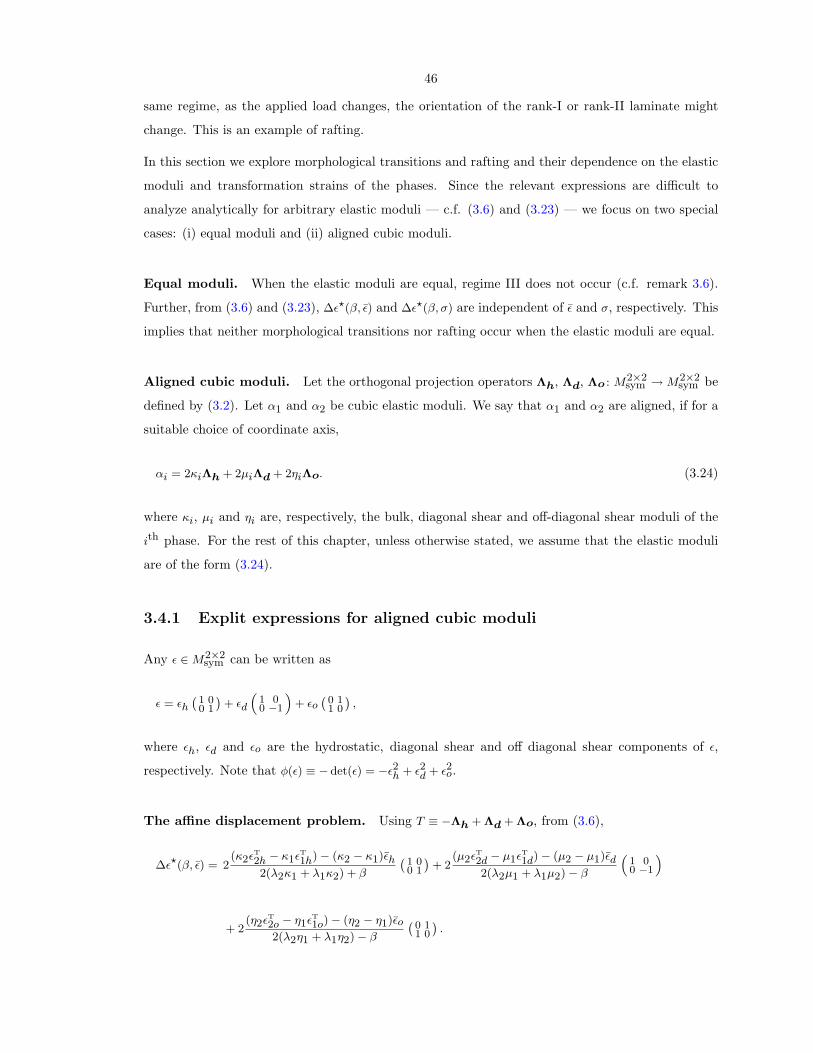
46

same regime, as the applied load changes, the orientation of the rank-I or rank-II laminate might

change. This is an example of rafting.

In this section we explore morphological transitions and rafting and their dependence on the elastic

moduli and transformation strains of the phases. Since the relevant expressions are difficult to

analyze analytically for arbitrary elastic moduli — c.f. (3.6) and (3.23) — we focus on two special

cases: (i) equal moduli and (ii) aligned cubic moduli.

Equal moduli. When the elastic moduli are equal, regime III does not occur (c.f. remark 3.6).

Further, from (3.6) and (3.23), ∆ε?(β, ε) and ∆ε?(β, σ) are independent of ε and σ, respectively. This

implies that neither morphological transitions nor rafting occur when the elastic moduli are equal.

Aligned cubic moduli. Let the orthogonal projection operators Λh, Λd, Λo : M2×2sym → M2×2

sym be

defined by (3.2). Let α1 and α2 be cubic elastic moduli. We say that α1 and α2 are aligned, if for a

suitable choice of coordinate axis,

αi = 2κiΛh + 2µiΛd + 2ηiΛo. (3.24)

where κi, µi and ηi are, respectively, the bulk, diagonal shear and off-diagonal shear moduli of the

ith phase. For the rest of this chapter, unless otherwise stated, we assume that the elastic moduli

are of the form (3.24).

3.4.1 Explit expressions for aligned cubic moduli

Any ε ∈ M2×2sym can be written as

ε = εh`

1 00 1

´+ εd

“1 00 −1

”+ εo

`0 11 0

´,

where εh, εd and εo are the hydrostatic, diagonal shear and off diagonal shear components of ε,

respectively. Note that φ(ε) ≡ − det(ε) = −ε2h + ε2d + ε2o.

The affine displacement problem. Using T ≡ −Λh + Λd + Λo, from (3.6),

∆ε?(β, ε) = 2(κ2εT

2h − κ1εT1h)− (κ2 − κ1)εh

2(λ2κ1 + λ1κ2) + β

`1 00 1

´+ 2

(µ2εT2d − µ1εT

1d)− (µ2 − µ1)εd2(λ2µ1 + λ1µ2)− β

“1 00 −1

”

+ 2(η2εT

2o − η1εT1o)− (η2 − η1)εo

2(λ2η1 + λ1η2)− β

`0 11 0

´.

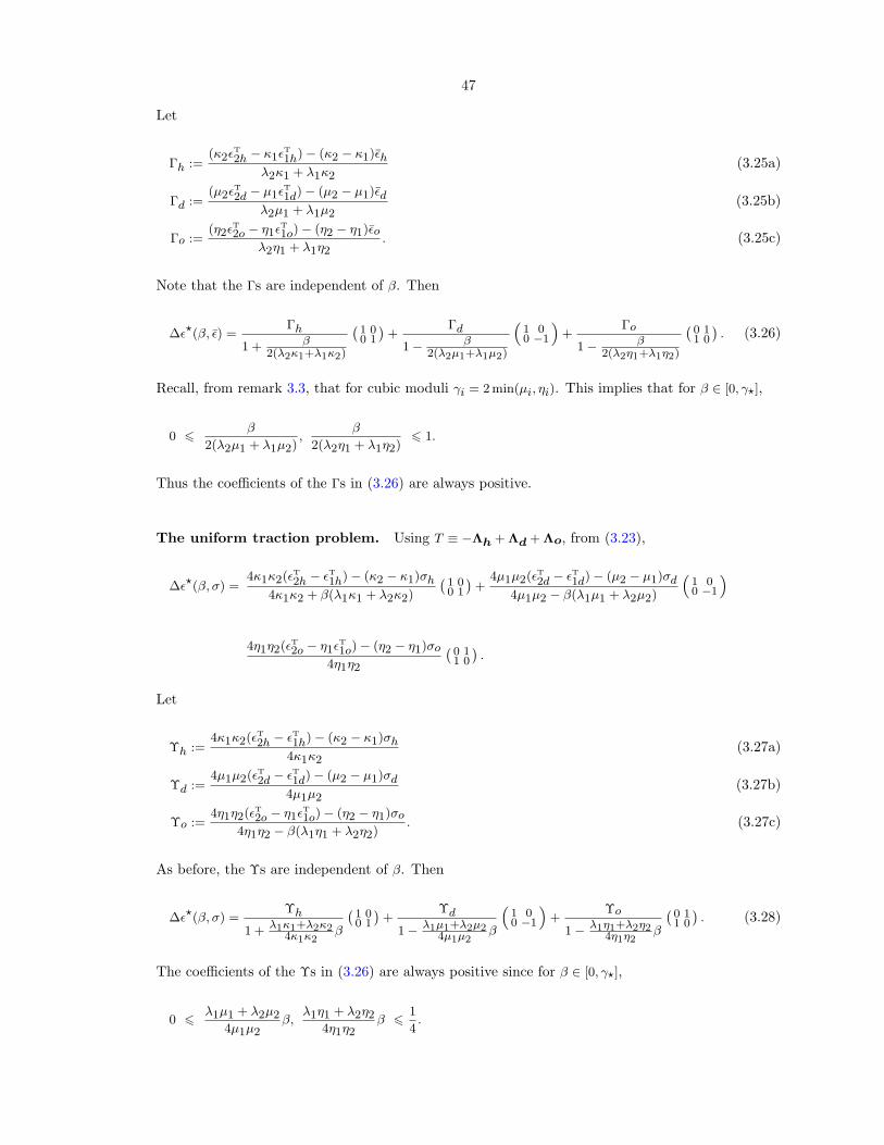
47

Let

Γh :=(κ2εT

2h − κ1εT1h)− (κ2 − κ1)εh

λ2κ1 + λ1κ2(3.25a)

Γd :=(µ2εT

2d − µ1εT1d)− (µ2 − µ1)εd

λ2µ1 + λ1µ2(3.25b)

Γo :=(η2εT

2o − η1εT1o)− (η2 − η1)εo

λ2η1 + λ1η2. (3.25c)

Note that the Γs are independent of β. Then

∆ε?(β, ε) =Γh

1 + β2(λ2κ1+λ1κ2)

`1 00 1

´+

Γd

1− β2(λ2µ1+λ1µ2)

“1 00 −1

”+

Γo

1− β2(λ2η1+λ1η2)

`0 11 0

´. (3.26)

Recall, from remark 3.3, that for cubic moduli γi = 2 min(µi, ηi). This implies that for β ∈ [0, γ?],

0 6β

2(λ2µ1 + λ1µ2),

β

2(λ2η1 + λ1η2)6 1.

Thus the coefficients of the Γs in (3.26) are always positive.

The uniform traction problem. Using T ≡ −Λh + Λd + Λo, from (3.23),

∆ε?(β, σ) =4κ1κ2(εT

2h − εT1h)− (κ2 − κ1)σh

4κ1κ2 + β(λ1κ1 + λ2κ2)

`1 00 1

´+

4µ1µ2(εT2d − εT

1d)− (µ2 − µ1)σd

4µ1µ2 − β(λ1µ1 + λ2µ2)

“1 00 −1

”

4η1η2(εT2o − η1εT

1o)− (η2 − η1)σo

4η1η2

`0 11 0

´.

Let

Υh :=4κ1κ2(εT

2h − εT1h)− (κ2 − κ1)σh

4κ1κ2(3.27a)

Υd :=4µ1µ2(εT

2d − εT1d)− (µ2 − µ1)σd

4µ1µ2(3.27b)

Υo :=4η1η2(εT

2o − η1εT1o)− (η2 − η1)σo

4η1η2 − β(λ1η1 + λ2η2). (3.27c)

As before, the Υs are independent of β. Then

∆ε?(β, σ) =Υh

1 +λ1κ1+λ2κ2

4κ1κ2β

`1 00 1

´+

Υd

1− λ1µ1+λ2µ24µ1µ2

β

“1 00 −1

”+

Υo

1− λ1η1+λ2η24η1η2

β

`0 11 0

´. (3.28)

The coefficients of the Υs in (3.26) are always positive since for β ∈ [0, γ?],

0 6λ1µ1 + λ2µ2

4µ1µ2β,

λ1η1 + λ2η24η1η2

β 61

4.

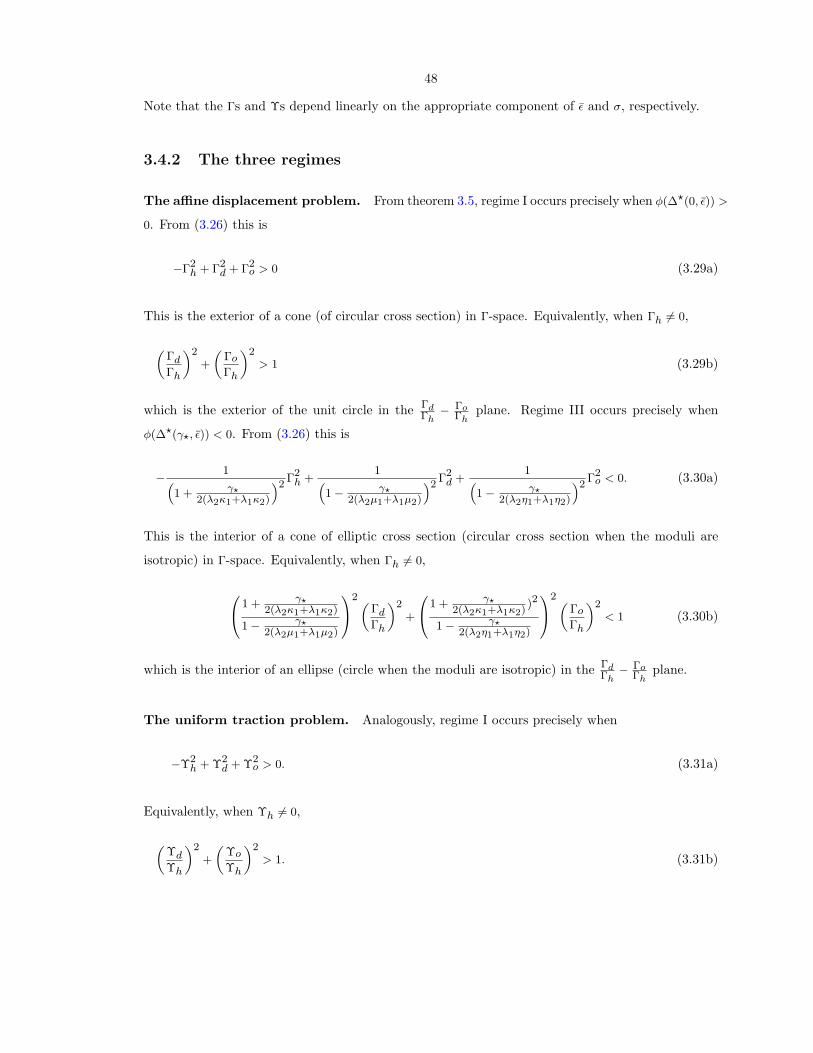
48

Note that the Γs and Υs depend linearly on the appropriate component of ε and σ, respectively.

3.4.2 The three regimes

The affine displacement problem. From theorem 3.5, regime I occurs precisely when φ(∆?(0, ε)) >

0. From (3.26) this is

−Γ2h + Γ2

d + Γ2o > 0 (3.29a)

This is the exterior of a cone (of circular cross section) in Γ-space. Equivalently, when Γh 6= 0,

„ΓdΓh

«2+

„Γo

Γh

«2> 1 (3.29b)

which is the exterior of the unit circle in the ΓdΓh

− ΓoΓh

plane. Regime III occurs precisely when

φ(∆?(γ?, ε)) < 0. From (3.26) this is

− 1“1 + γ?

2(λ2κ1+λ1κ2)

”2Γ2

h +1“

1− γ?2(λ2µ1+λ1µ2)

”2Γ2

d +1“

1− γ?2(λ2η1+λ1η2)

”2Γ2

o < 0. (3.30a)

This is the interior of a cone of elliptic cross section (circular cross section when the moduli are

isotropic) in Γ-space. Equivalently, when Γh 6= 0,

0@ 1 + γ?2(λ2κ1+λ1κ2)

1− γ?2(λ2µ1+λ1µ2)

1A2„ΓdΓh

«2+

0@1 + γ?2(λ2κ1+λ1κ2)

)2

1− γ?2(λ2η1+λ1η2)

1A2„Γo

Γh

«2< 1 (3.30b)

which is the interior of an ellipse (circle when the moduli are isotropic) in the ΓdΓh

− ΓoΓh

plane.

The uniform traction problem. Analogously, regime I occurs precisely when

−Υ2h + Υ2

d + Υ2o > 0. (3.31a)

Equivalently, when Υh 6= 0,

„ΥdΥh

«2+

„Υo

Υh

«2> 1. (3.31b)

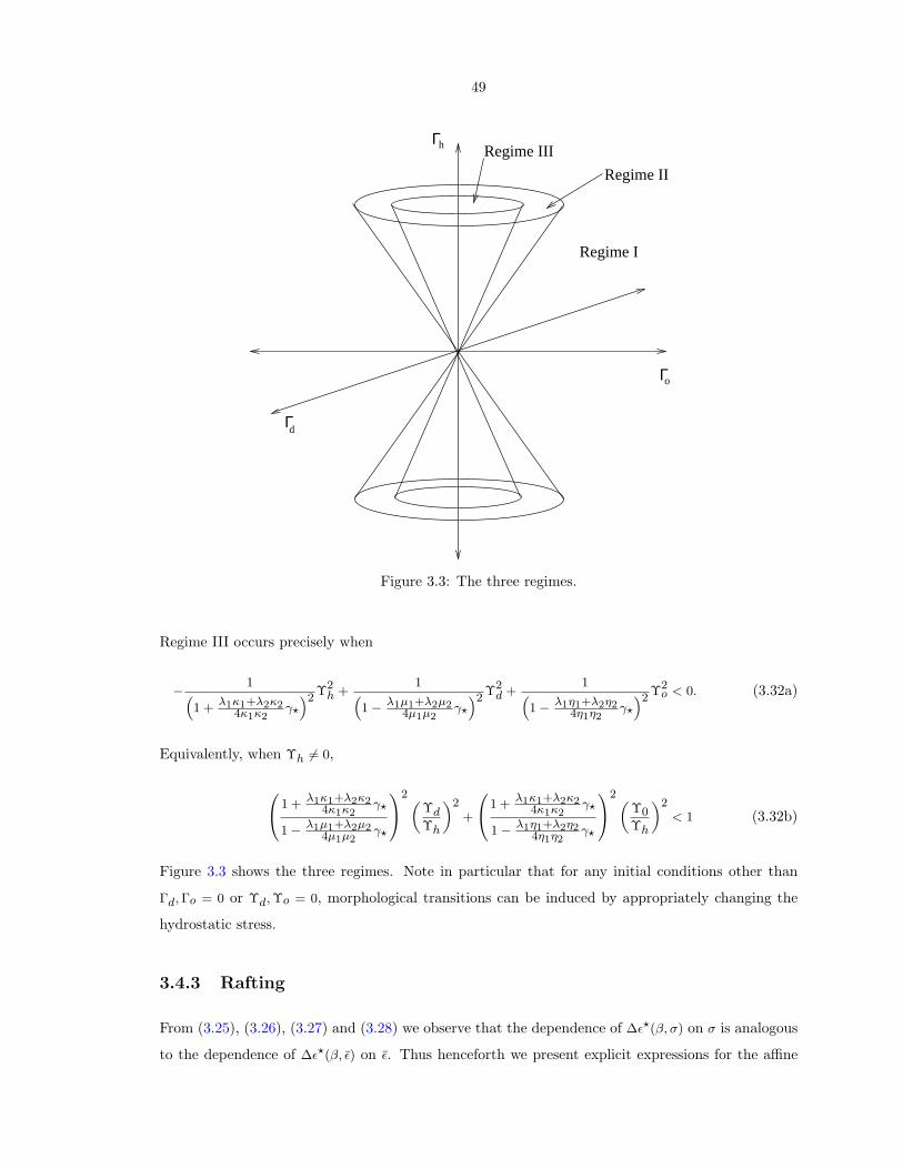
49

Γ

Γh

o

Γd

Regime I

Regime II

Regime III

Figure 3.3: The three regimes.

Regime III occurs precisely when

− 1“1 +

λ1κ1+λ2κ24κ1κ2

γ?

”2Υ2

h +1“

1− λ1µ1+λ2µ24µ1µ2

γ?

”2Υ2

d +1“

1− λ1η1+λ2η24η1η2

γ?

”2Υ2

o < 0. (3.32a)

Equivalently, when Υh 6= 0,

0@ 1 +λ1κ1+λ2κ2

4κ1κ2γ?

1− λ1µ1+λ2µ24µ1µ2

γ?

1A2„ΥdΥh

«2+

0@1 +λ1κ1+λ2κ2

4κ1κ2γ?

1− λ1η1+λ2η24η1η2

γ?

1A2„Υ0Υh

«2< 1 (3.32b)

Figure 3.3 shows the three regimes. Note in particular that for any initial conditions other than

Γd, Γo = 0 or Υd, Υo = 0, morphological transitions can be induced by appropriately changing the

hydrostatic stress.

3.4.3 Rafting

From (3.25), (3.26), (3.27) and (3.28) we observe that the dependence of ∆ε?(β, σ) on σ is analogous

to the dependence of ∆ε?(β, ε) on ε. Thus henceforth we present explicit expressions for the affine

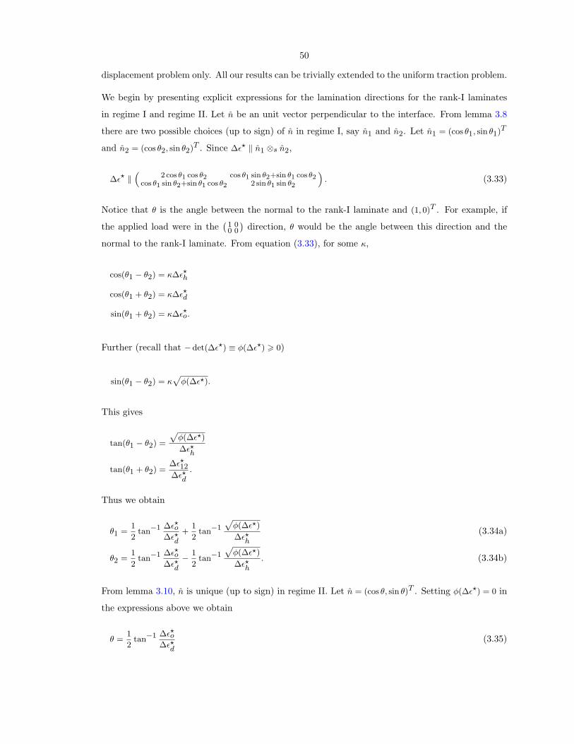
50

displacement problem only. All our results can be trivially extended to the uniform traction problem.

We begin by presenting explicit expressions for the lamination directions for the rank-I laminates

in regime I and regime II. Let n be an unit vector perpendicular to the interface. From lemma 3.8

there are two possible choices (up to sign) of n in regime I, say n1 and n2. Let n1 = (cos θ1, sin θ1)T

and n2 = (cos θ2, sin θ2)T . Since ∆ε? ‖ n1 ⊗s n2,

∆ε? ‖“

2 cos θ1 cos θ2 cos θ1 sin θ2+sin θ1 cos θ2cos θ1 sin θ2+sin θ1 cos θ2 2 sin θ1 sin θ2

”. (3.33)

Notice that θ is the angle between the normal to the rank-I laminate and (1, 0)T . For example, if

the applied load were in the`

1 00 0

´direction, θ would be the angle between this direction and the

normal to the rank-I laminate. From equation (3.33), for some κ,

cos(θ1 − θ2) = κ∆ε?h

cos(θ1 + θ2) = κ∆ε?d

sin(θ1 + θ2) = κ∆ε?o.

Further (recall that − det(∆ε?) ≡ φ(∆ε?) > 0)

sin(θ1 − θ2) = κp

φ(∆ε?).

This gives

tan(θ1 − θ2) =

pφ(∆ε?)

∆ε?h

tan(θ1 + θ2) =∆ε?12∆ε?d

.

Thus we obtain

θ1 =1

2tan−1 ∆ε?o

∆ε?d+

1

2tan−1

pφ(∆ε?)

∆ε?h(3.34a)

θ2 =1

2tan−1 ∆ε?o

∆ε?d− 1

2tan−1

pφ(∆ε?)

∆ε?h. (3.34b)

From lemma 3.10, n is unique (up to sign) in regime II. Let n = (cos θ, sin θ)T . Setting φ(∆ε?) = 0 in

the expressions above we obtain

θ =1

2tan−1 ∆ε?o

∆ε?d(3.35)

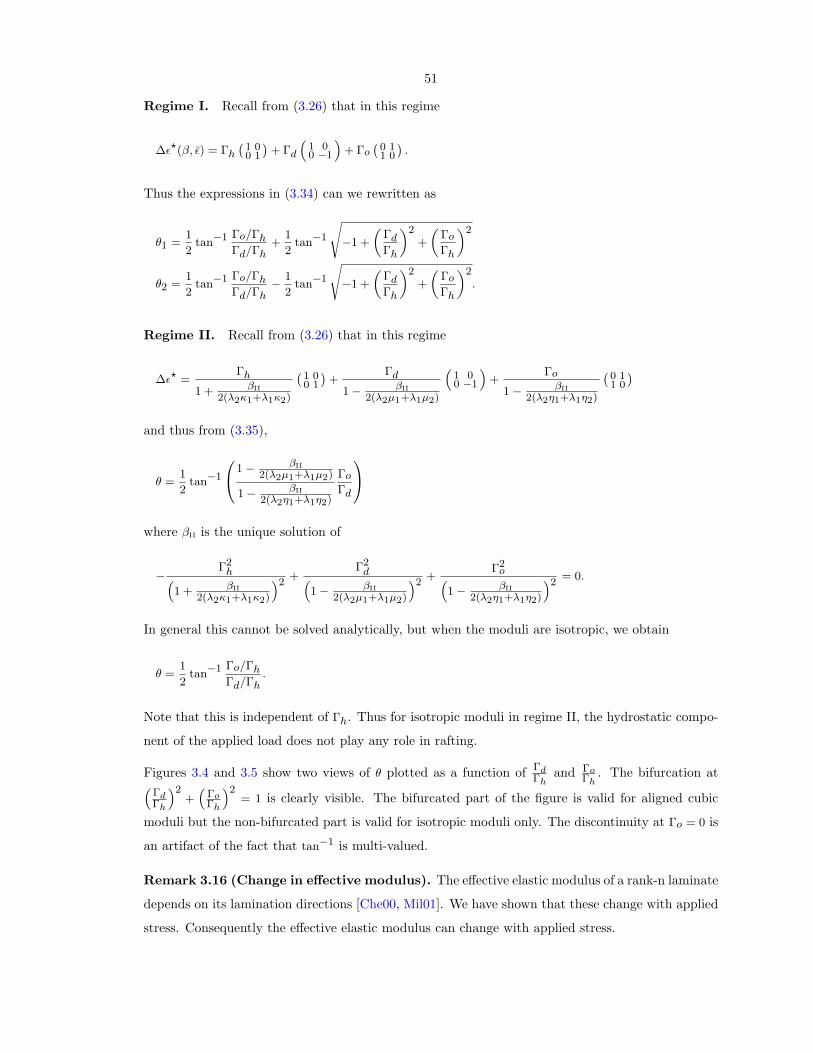
51

Regime I. Recall from (3.26) that in this regime

∆ε?(β, ε) = Γh`

1 00 1

´+ Γd

“1 00 −1

”+ Γo

`0 11 0

´.

Thus the expressions in (3.34) can we rewritten as

θ1 =1

2tan−1 Γo/Γh

Γd/Γh+

1

2tan−1

s−1 +

„ΓdΓh

«2+

„Γo

Γh

«2

θ2 =1

2tan−1 Γo/Γh

Γd/Γh− 1

2tan−1

s−1 +

„ΓdΓh

«2+

„Γo

Γh

«2.

Regime II. Recall from (3.26) that in this regime

∆ε? =Γh

1 + βII

2(λ2κ1+λ1κ2)

`1 00 1

´+

Γd

1− βII

2(λ2µ1+λ1µ2)

“1 00 −1

”+

Γo

1− βII

2(λ2η1+λ1η2)

`0 11 0

´

and thus from (3.35),

θ =1

2tan−1

0@1− βII

2(λ2µ1+λ1µ2)

1− βII

2(λ2η1+λ1η2)

Γo

Γd

1Awhere βII is the unique solution of

−Γ2

h“1 + βII

2(λ2κ1+λ1κ2)

”2+

Γ2d“

1− βII

2(λ2µ1+λ1µ2)

”2+

Γ2o“

1− βII

2(λ2η1+λ1η2)

”2= 0.

In general this cannot be solved analytically, but when the moduli are isotropic, we obtain

θ =1

2tan−1 Γo/Γh

Γd/Γh.

Note that this is independent of Γh. Thus for isotropic moduli in regime II, the hydrostatic compo-

nent of the applied load does not play any role in rafting.

Figures 3.4 and 3.5 show two views of θ plotted as a function of ΓdΓh

and ΓoΓh

. The bifurcation at“ΓdΓh

”2+“

ΓoΓh

”2= 1 is clearly visible. The bifurcated part of the figure is valid for aligned cubic

moduli but the non-bifurcated part is valid for isotropic moduli only. The discontinuity at Γo = 0 is

an artifact of the fact that tan−1 is multi-valued.

Remark 3.16 (Change in effective modulus). The effective elastic modulus of a rank-n laminate

depends on its lamination directions [Che00, Mil01]. We have shown that these change with applied

stress. Consequently the effective elastic modulus can change with applied stress.

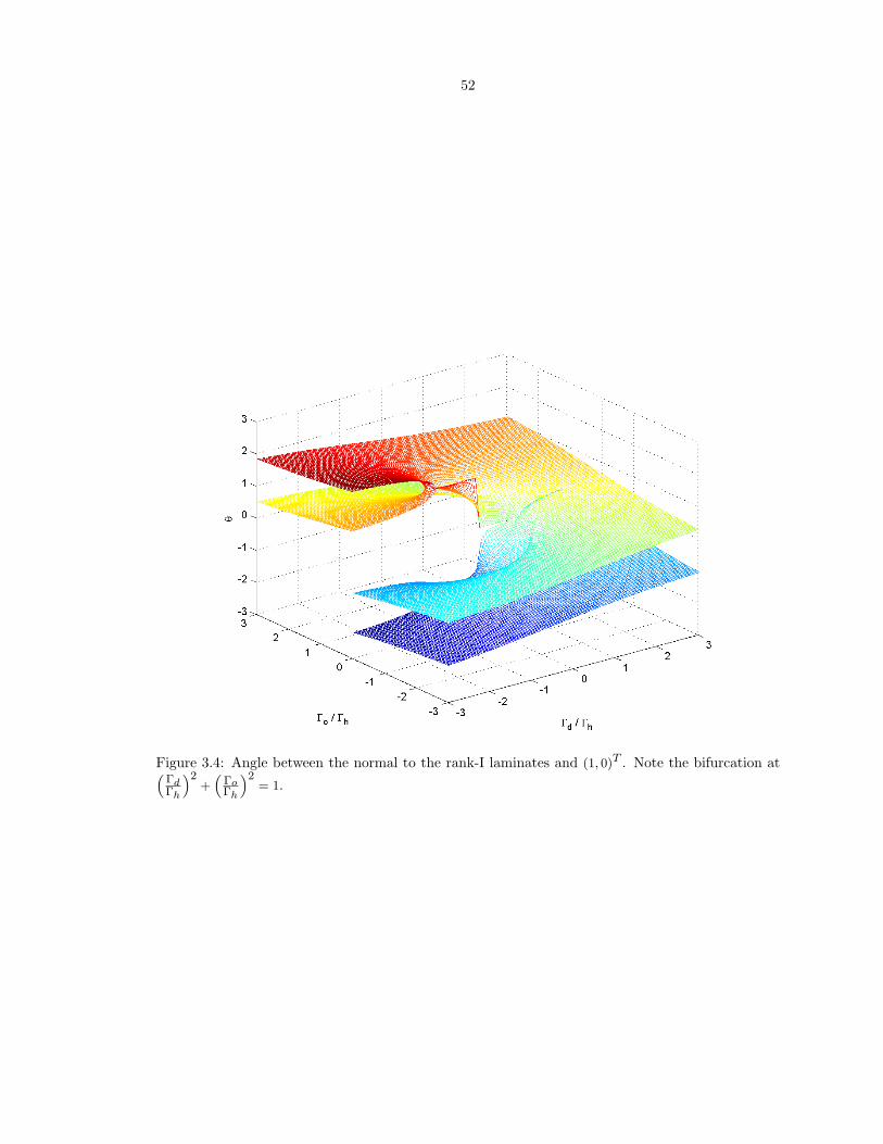
52

Figure 3.4: Angle between the normal to the rank-I laminates and (1, 0)T . Note the bifurcation at“ΓdΓh

”2+“

ΓoΓh

”2= 1.

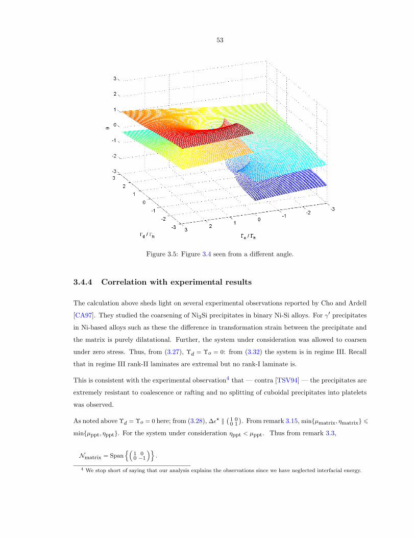
53

Figure 3.5: Figure 3.4 seen from a different angle.

3.4.4 Correlation with experimental results

The calculation above sheds light on several experimental observations reported by Cho and Ardell

[CA97]. They studied the coarsening of Ni3Si precipitates in binary Ni-Si alloys. For γ′ precipitates

in Ni-based alloys such as these the difference in transformation strain between the precipitate and

the matrix is purely dilatational. Further, the system under consideration was allowed to coarsen

under zero stress. Thus, from (3.27), Υd = Υo = 0: from (3.32) the system is in regime III. Recall

that in regime III rank-II laminates are extremal but no rank-I laminate is.

This is consistent with the experimental observation4 that — contra [TSV94] — the precipitates are

extremely resistant to coalescence or rafting and no splitting of cuboidal precipitates into platelets

was observed.

As noted above Υd = Υo = 0 here; from (3.28), ∆ε? ‖`

1 00 1

´. From remark 3.15, minµmatrix, ηmatrix 6

minµppt, ηppt. For the system under consideration ηppt < µppt. Thus from remark 3.3,

Nmatrix = Spann“

1 00 −1

”o.

4 We stop short of saying that our analysis explains the observations since we have neglected interfacial energy.

54

It follows that εn in lemmas 3.11 and 3.12 should be picked to be parallel to“

1 00 −1

”. Thus, from

lemma 3.11, the strain jump in the two layers of the extremal rank-II laminate is parallel to

`1 00 1

´+“

1 00 −1

”, i.e.,

`1 00 0

´

and

`1 00 1

´−“

1 00 −1

”, i.e.,

`0 00 1

´for it is precisely these two linear combinations of

`1 00 1

ánd

“1 00 −1

”that have determinant zero.

It follows that the layering directions are`

10

ánd

`01

´. This is consistent with observations [CA97,

pg.1399] that the precipitates are aligned along 〈100〉.

Let us explore the other alternative: ηppt < µppt. Then, from remark 3.3,

Nmatrix = Span˘`

0 11 0

´¯.

It follows that εn in lemmas 3.11 and 3.12 should be picked to be parallel to`

0 11 0

´. Thus, from

lemma 3.11, the strain jump in the two layers of the extremal rank-II laminate is parallel to

`1 00 1

´+`

0 11 0

´, i.e.,

`1 11 1

´

and

`1 00 1

´−`

0 11 0

´, i.e.,

“1 −1−1 1

”

for it is precisely these two linear combinations of`

1 00 1

ánd

`0 11 0

´that have determinant zero. It

follows that the layering directions are`

11

ánd

“1−1

”.

Finally note that since the system is in regime III regardless of the phase fraction of the precipitates,

the particle morphology should be independent of the precipitate phase fraction, exactly as reported

[CA97, pg.1395 and ref.31 therein].

55

Chapter 4

Two-phase isotropic solids in threedimensions

We generalize the preceding approach to solve the problem in three dimensions when the elastic

moduli are isotropic. The determinant is a useful translation in two dimensions because it captures

information on strain compatibility: ε1, ε2 ∈ M2×2sym are compatible if and only if det(ε2 − ε1) 6 0.

The three-dimensional analogue is that ε1, ε2 ∈ M3×3sym are compatible if and only if of the three

eigenvalues of ε2 − ε1, one is non-negative, another is zero and the third is non-positive (c.f. lemma

3.7).

4.1 Rotated diagonal subdeterminants as translations

Choice of translations. Motivated by this we choose three translations

φMj (ε) := φj(M

T εM) (4.1a)

where M ∈ M3×3 is yet to be determined and φj : M3×3sym → R are the diagonal subdeterminants:

φ1(ε) := ε223 − ε22ε33 (4.1b)

φ2(ε) := ε231 − ε33ε11 (4.1c)

φ3(ε) := ε212 − ε11ε22. (4.1d)

56

For notational convenience we define Φ: M3×3sym → R3 and ΦM : M3×3

sym → R3 by

Φ(ε) :=

0BBBB@φ1(ε)

φ2(ε)

φ3(ε)

1CCCCA ,

ΦM (ε) :=

0BBBBB@φM1 (ε)

φM2 (ε)

φM3 (ε)

1CCCCCA .

Note that φIj = φj and ΦI = Φ.

Quasiconvexity of the translations. φMj is quasiconvex since it is quadratic and rank-I convex:

∀m′, n′ ∈ R3,

φMj (m′ ⊗s n′) = φj(M

T (m′ ⊗s n′)M) = φj((MT m′)⊗s (MT n′)) = φj(m⊗s n)

where m = MT m′, n = MT n′ and

φ1(m⊗s n) =1

4(m2n3 + m3n2)2 −m2n2m3n3 =

1

4(m2n3 −m3n2)2 > 0

with similar results for φM2 and φM

3 . It follows that ∀β ∈ (R+)3, M3×3sym 3 ε 7→ 〈β, Φ(ε)〉 ∈ R is

quasiconvex (R+ := x ∈ R | x > 0).

Quadraticity of the translations. Since φj is quadratic there exists a (unique) linear operator

Tj : M3×3sym → M3×3

sym such that

φj(ε) =1

2〈Tjε, ε〉.

Similarly there exists a (unique) linear operator TMj : M3×3

sym → M3×3sym such that

φMj (ε) =

1

2〈TM

j ε, ε〉.

57

It is easy to verify that Tj is given by

T1ε =

„0 0 00 −ε33 ε230 ε23 −ε22

«, (4.2a)

T2ε =

„−ε33 0 ε310 0 0

ε31 0 −ε11

«, (4.2b)

T3ε =

„−ε22 ε12 0ε12 −ε11 00 0 0

«. (4.2c)

and TMj by

TMj ε = M

“Tj(M

T εM)”

MT . (4.2d)

Note that (T1+T2+T3)ε = ε−Tr(ε)I. For β ∈ R3, let β ·T : M3×3sym → M3×3

sym and β ·TM : M3×3sym → M3×3

sym

to be the linear operators defined by

β · Tε =

3Xj=1

βjTjε, (4.3a)

β · TM ε =

3Xj=1

βjTMj ε = M

0@ 3Xj=1

βjTj(MT εM)

1AMT = M“β · T (MT εM)

”MT . (4.3b)

Thus

〈β, Φ(ε)〉 =1

2〈(β · T )ε, ε〉,

〈β, ΦM (ε)〉 =1

2〈(β · TM )ε, ε〉.

Restrictions on the choice of translations. For reasons that will become clear later we restrict

M to be in SO(3). For R ∈ SO(3), let

Bi(R) := β ∈ (R+)3 | Wi − β · ΦR : convex,

B(R) := ∩2i=1Bi(R).

By quadraticity, the convexity of Wi − β · ΦR is equivalent to the nonnegativity of

ε 7→ 12 〈αiε, ε〉 − β · ΦR(ε).

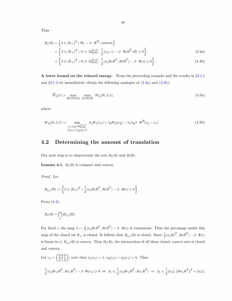
58

Thus

Bi(R) =n

β ∈ (R+)3 | Wi − β · ΦR : convexo

=

β ∈ (R+)3 | ∀ε ∈ M3×3

sym ,1

2〈αiε, ε〉 − β · Φ(RT εR) > 0

ff(4.4a)

=

β ∈ (R+)3 | ∀ε ∈ M3×3

sym ,1

2〈αiRεRT , RεRT 〉 − β · Φ(ε) > 0

ff. (4.4b)

A lower bound on the relaxed energy. From the preceeding remarks and the results in §3.1.1

and §3.1.2 we immediately obtain the following analogue of (3.3a) and (3.3b):

cWλ(ε) > maxR∈SO(3)

maxβ∈B(R)

Wλ(R, β, ε), (4.5a)

where

Wλ(R, β, ε) := minε1,ε2∈M3×3

symλ1ε1+λ2ε2=ε

λ1W1(ε1) + λ2W2(ε2)− λ1λ2β · ΦR(ε2 − ε1). (4.5b)

4.2 Determining the amount of translation

Our next step is to characterize the sets Bi(R) and B(R).

Lemma 4.1. Bi(R) is compact and convex.

Proof. Let

Bi,ε(R) :=

β ∈ (R+)3 | 1


ff.

From (4.4),

Bi(R) =\ε

Bi,ε(R).

For fixed ε, the map β 7→ 12 〈αiRεRT , RεRT 〉 − β · Φ(ε) is continuous. Thus the pre-image under this

map of the closed set R+ is closed. It follows that Bi,ε(R) is closed. Since 12 〈αiRεT , RεRT 〉 − β ·Φ(ε)

is linear in β, Bi,ε(R) is convex. Thus Bi(R), the intersection of all these closed, convex sets is closed

and convex.

Let ε1 =

„0 0 00 0 10 1 0

«; note that φ1(ε1) = 1, φ2(ε1) = φ3(ε1) = 0. Thus

1

2〈αiRε1RT , Rε1RT 〉− β ·Φ(ε1) > 0 ⇔ β1 6

1

2〈αiRε1RT , Rε1RT 〉 ⇒ β1 6

1

2‖αi‖ ‖Rε1RT ‖2 = ‖αi‖,

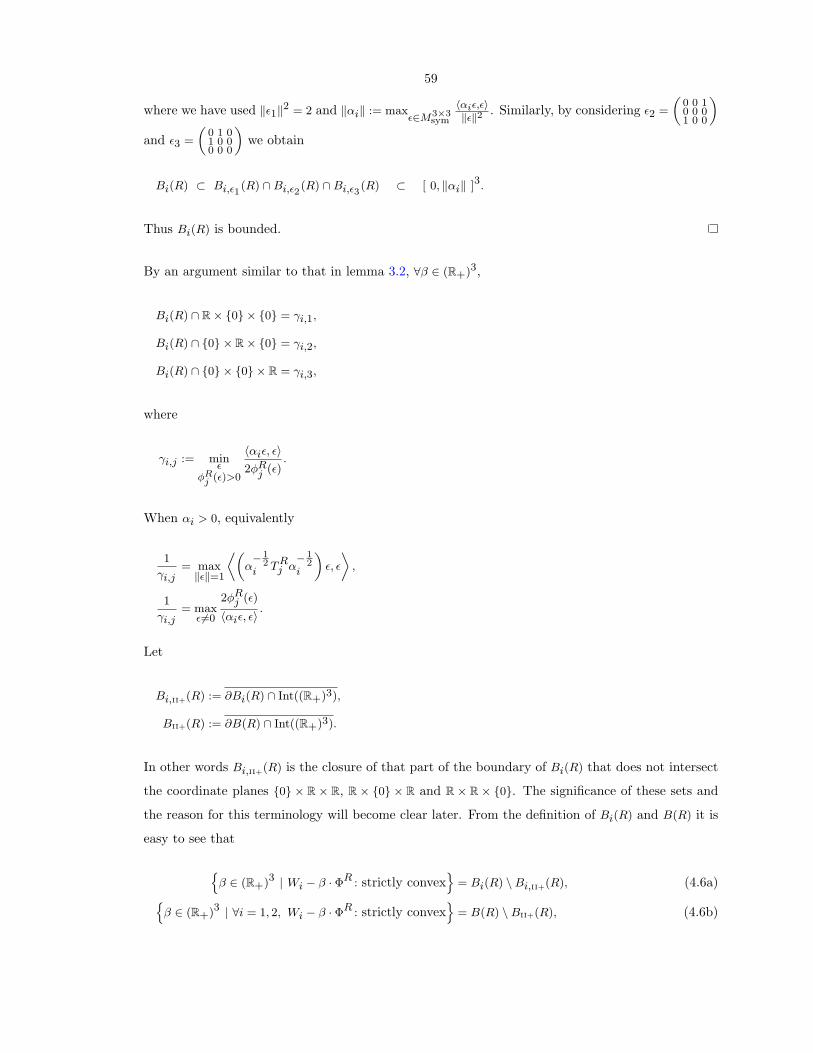
59

where we have used ‖ε1‖2 = 2 and ‖αi‖ := maxε∈M3×3

sym

〈αiε,ε〉‖ε‖2 . Similarly, by considering ε2 =

„0 0 10 0 01 0 0

«and ε3 =

„0 1 01 0 00 0 0

«we obtain

Bi(R) ⊂ Bi,ε1(R) ∩Bi,ε2(R) ∩Bi,ε3(R) ⊂ [ 0, ‖αi‖ ]3.

Thus Bi(R) is bounded.

By an argument similar to that in lemma 3.2, ∀β ∈ (R+)3,

Bi(R) ∩ R× 0 × 0 = γi,1,

Bi(R) ∩ 0 × R× 0 = γi,2,

Bi(R) ∩ 0 × 0 × R = γi,3,

where

γi,j := minε

φRj (ε)>0

〈αiε, ε〉2φR

j (ε).

When αi > 0, equivalently

1

γi,j= max‖ε‖=1

fi„α− 1

2i TR

j α− 1

2i

«ε, ε

fl,

1

γi,j= max

ε6=0

2φRj (ε)

〈αiε, ε〉.

Let

Bi,II+(R) := ∂Bi(R) ∩ Int((R+)3),

BII+(R) := ∂B(R) ∩ Int((R+)3).

In other words Bi,II+(R) is the closure of that part of the boundary of Bi(R) that does not intersect

the coordinate planes 0 × R × R, R × 0 × R and R × R × 0. The significance of these sets and

the reason for this terminology will become clear later. From the definition of Bi(R) and B(R) it is

easy to see that

nβ ∈ (R+)3 | Wi − β · ΦR : strictly convex

o= Bi(R) \Bi,II+(R), (4.6a)n

β ∈ (R+)3 | ∀i = 1, 2, Wi − β · ΦR : strictly convexo

= B(R) \BII+(R), (4.6b)

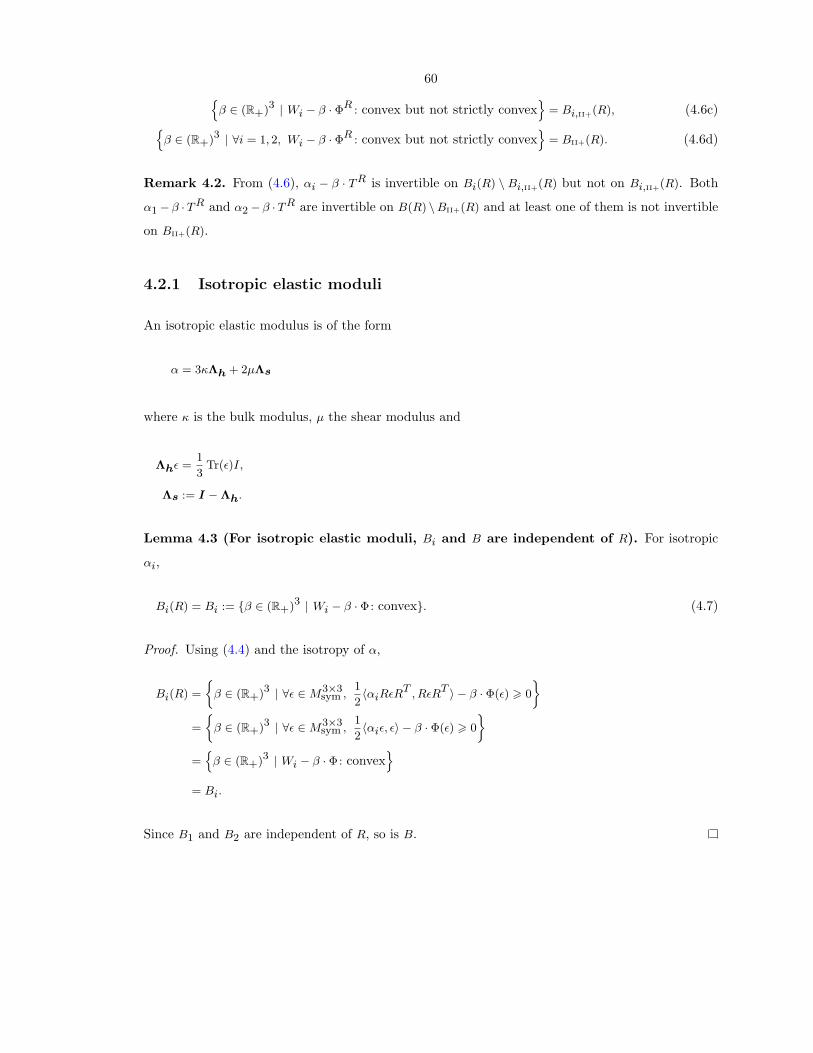
60nβ ∈ (R+)3 | Wi − β · ΦR : convex but not strictly convex

o= Bi,II+(R), (4.6c)n

β ∈ (R+)3 | ∀i = 1, 2, Wi − β · ΦR : convex but not strictly convexo

= BII+(R). (4.6d)

Remark 4.2. From (4.6), αi − β · TR is invertible on Bi(R) \ Bi,II+(R) but not on Bi,II+(R). Both

α1− β ·TR and α2− β ·TR are invertible on B(R) \BII+(R) and at least one of them is not invertible

on BII+(R).

4.2.1 Isotropic elastic moduli

An isotropic elastic modulus is of the form

α = 3κΛh + 2µΛs

where κ is the bulk modulus, µ the shear modulus and

Λhε =1

3Tr(ε)I,

Λs := I −Λh.

Lemma 4.3 (For isotropic elastic moduli, Bi and B are independent of R). For isotropic

αi,

Bi(R) = Bi := β ∈ (R+)3 | Wi − β · Φ: convex. (4.7)

Proof. Using (4.4) and the isotropy of α,

Bi(R) =

β ∈ (R+)3 | ∀ε ∈ M3×3

sym ,1


ff=

β ∈ (R+)3 | ∀ε ∈ M3×3

sym ,1

2〈αiε, ε〉 − β · Φ(ε) > 0

ff=n

β ∈ (R+)3 | Wi − β · Φ: convexo

= Bi.

Since B1 and B2 are independent of R, so is B.

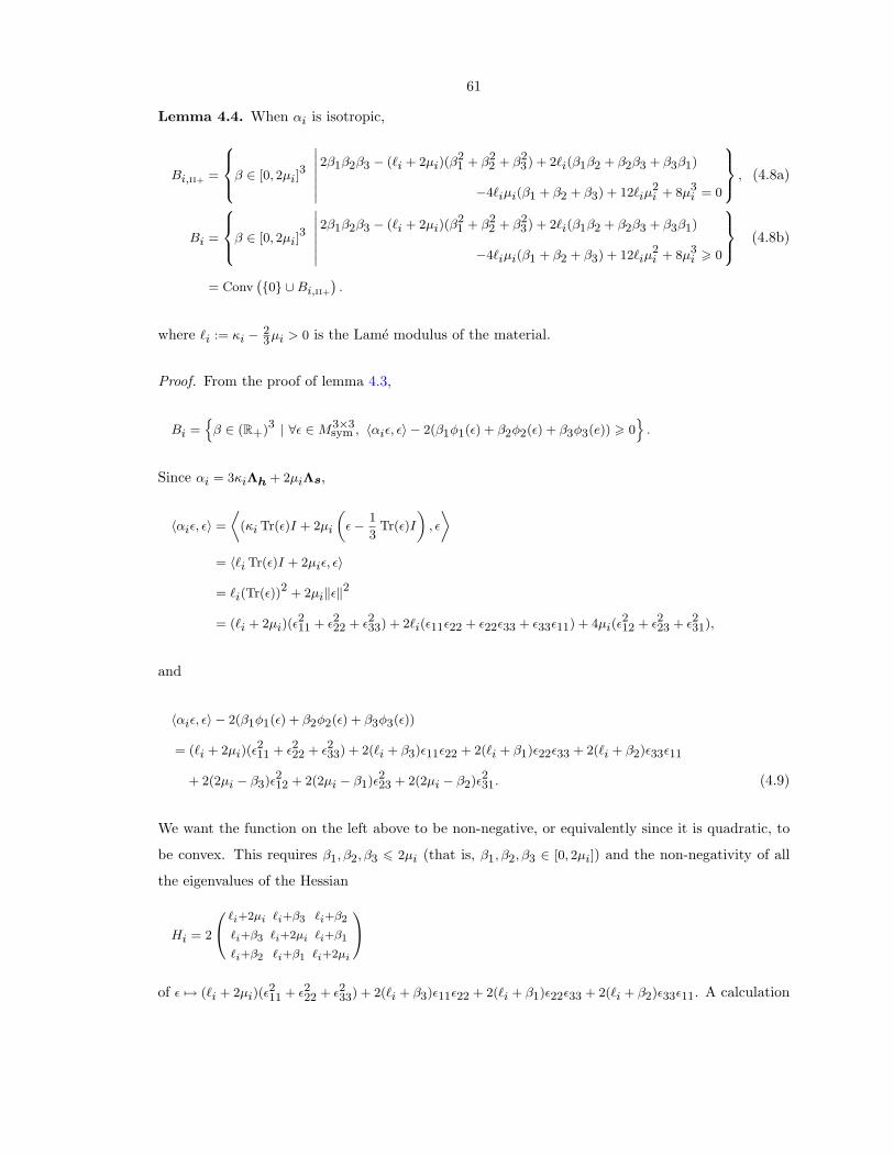
61

Lemma 4.4. When αi is isotropic,

Bi,II+ =

8><>:β ∈ [0, 2µi]3

˛˛ 2β1β2β3 − (ì + 2µi)(β

21 + β2

2 + β23) + 2ì(β1β2 + β2β3 + β3β1)

−4ìµi(β1 + β2 + β3) + 12ìµ2i + 8µ3

i = 0

9>=>; , (4.8a)

Bi =

8><>:β ∈ [0, 2µi]3

˛˛ 2β1β2β3 − (ì + 2µi)(β

21 + β2

2 + β23) + 2ì(β1β2 + β2β3 + β3β1)

−4ìµi(β1 + β2 + β3) + 12ìµ2i + 8µ3

i > 0

9>=>; (4.8b)

= Conv`0 ∪Bi,II+

´.

where ì := κi − 23µi > 0 is the Lame modulus of the material.

Proof. From the proof of lemma 4.3,

Bi =n

β ∈ (R+)3 | ∀ε ∈ M3×3sym , 〈αiε, ε〉 − 2(β1φ1(ε) + β2φ2(ε) + β3φ3(e)) > 0

o.

Since αi = 3κiΛh + 2µiΛs,

〈αiε, ε〉 =

fi(κi Tr(ε)I + 2µi

„ε− 1

3Tr(ε)I

«, ε

fl= 〈ì Tr(ε)I + 2µiε, ε〉

= ì(Tr(ε))2 + 2µi‖ε‖2

= (ì + 2µi)(ε211 + ε222 + ε233) + 2ì(ε11ε22 + ε22ε33 + ε33ε11) + 4µi(ε

212 + ε223 + ε231),

and

〈αiε, ε〉 − 2(β1φ1(ε) + β2φ2(ε) + β3φ3(ε))

= (ì + 2µi)(ε211 + ε222 + ε233) + 2(ì + β3)ε11ε22 + 2(ì + β1)ε22ε33 + 2(ì + β2)ε33ε11

+ 2(2µi − β3)ε212 + 2(2µi − β1)ε223 + 2(2µi − β2)ε231. (4.9)

We want the function on the left above to be non-negative, or equivalently since it is quadratic, to

be convex. This requires β1, β2, β3 6 2µi (that is, β1, β2, β3 ∈ [0, 2µi]) and the non-negativity of all

the eigenvalues of the Hessian

Hi = 2

0@ ì+2µi ì+β3 ì+β2

ì+β3 ì+2µi ì+β1

ì+β2 ì+β1 ì+2µi

1Aof ε 7→ (ì + 2µi)(ε

211 + ε222 + ε233) + 2(ì + β3)ε11ε22 + 2(ì + β1)ε22ε33 + 2(ì + β2)ε33ε11. A calculation

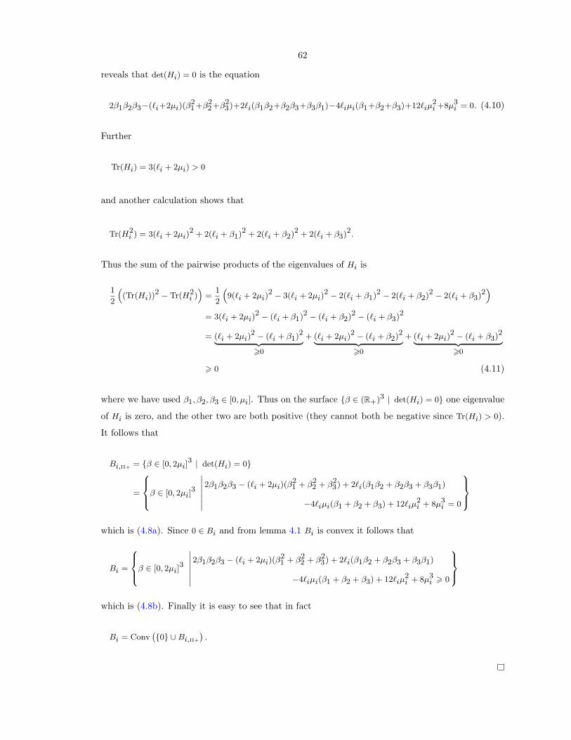
62

reveals that det(Hi) = 0 is the equation

2β1β2β3−(ì+2µi)(β21+β2

2+β23)+2ì(β1β2+β2β3+β3β1)−4ìµi(β1+β2+β3)+12ìµ

2i +8µ3

i = 0. (4.10)

Further

Tr(Hi) = 3(ì + 2µi) > 0

and another calculation shows that

Tr(H2i ) = 3(ì + 2µi)

2 + 2(ì + β1)2 + 2(ì + β2)2 + 2(ì + β3)2.

Thus the sum of the pairwise products of the eigenvalues of Hi is

1

2

“(Tr(Hi))

2 − Tr(H2i )”

=1

2

“9(ì + 2µi)

2 − 3(ì + 2µi)2 − 2(ì + β1)2 − 2(ì + β2)2 − 2(ì + β3)2

”= 3(ì + 2µi)

2 − (ì + β1)2 − (ì + β2)2 − (ì + β3)2

= (ì + 2µi)2 − (ì + β1)2| z >0

+ (ì + 2µi)2 − (ì + β2)2| z >0

+ (ì + 2µi)2 − (ì + β3)2| z >0

> 0 (4.11)

where we have used β1, β2, β3 ∈ [0, µi]. Thus on the surface β ∈ (R+)3 | det(Hi) = 0 one eigenvalue

of Hi is zero, and the other two are both positive (they cannot both be negative since Tr(Hi) > 0).

It follows that

Bi,II+ = β ∈ [0, 2µi]3 | det(Hi) = 0

=

8><>:β ∈ [0, 2µi]3

˛˛ 2β1β2β3 − (ì + 2µi)(β

21 + β2

2 + β23) + 2ì(β1β2 + β2β3 + β3β1)

−4ìµi(β1 + β2 + β3) + 12ìµ2i + 8µ3

i = 0

9>=>;which is (4.8a). Since 0 ∈ Bi and from lemma 4.1 Bi is convex it follows that

Bi =

8><>:β ∈ [0, 2µi]3

˛˛ 2β1β2β3 − (ì + 2µi)(β

21 + β2

2 + β23) + 2ì(β1β2 + β2β3 + β3β1)

−4ìµi(β1 + β2 + β3) + 12ìµ2i + 8µ3

i > 0

9>=>;which is (4.8b). Finally it is easy to see that in fact

Bi = Conv`0 ∪Bi,II+

´.

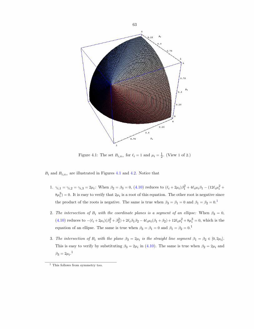
63

Figure 4.1: The set Bi,II+ for ì = 1 and µi = 12 . (View 1 of 2.)

Bi and Bi,II+ are illustrated in Figures 4.1 and 4.2. Notice that

1. γi,1 = γi,2 = γi,3 = 2µi: When β2 = β3 = 0, (4.10) reduces to (ì + 2µi)β21 + 4ìµiβ1 − (12ìµ

2i +

8µ3i ) = 0. It is easy to verify that 2µi is a root of this equation. The other root is negative since

the product of the roots is negative. The same is true when β3 = β1 = 0 and β1 = β2 = 0.1

2. The intersection of Bi with the coordinate planes is a segment of an ellipse: When β3 = 0,

(4.10) reduces to −(ì + 2µi)(β21 + β2

2) + 2ìβ1β2− 4ìµi(β1 + β2) + 12ìµ2i + 8µ3

i = 0, which is the

equation of an ellipse. The same is true when β3 = β1 = 0 and β1 = β2 = 0.1

3. The intersection of Bi with the plane β3 = 2µi is the straight line segment β1 = β2 ∈ [0, 2µi].

This is easy to verify by substituting β3 = 2µi in (4.10). The same is true when β2 = 2µi and

β3 = 2µi.1

1 This follows from symmetry too.

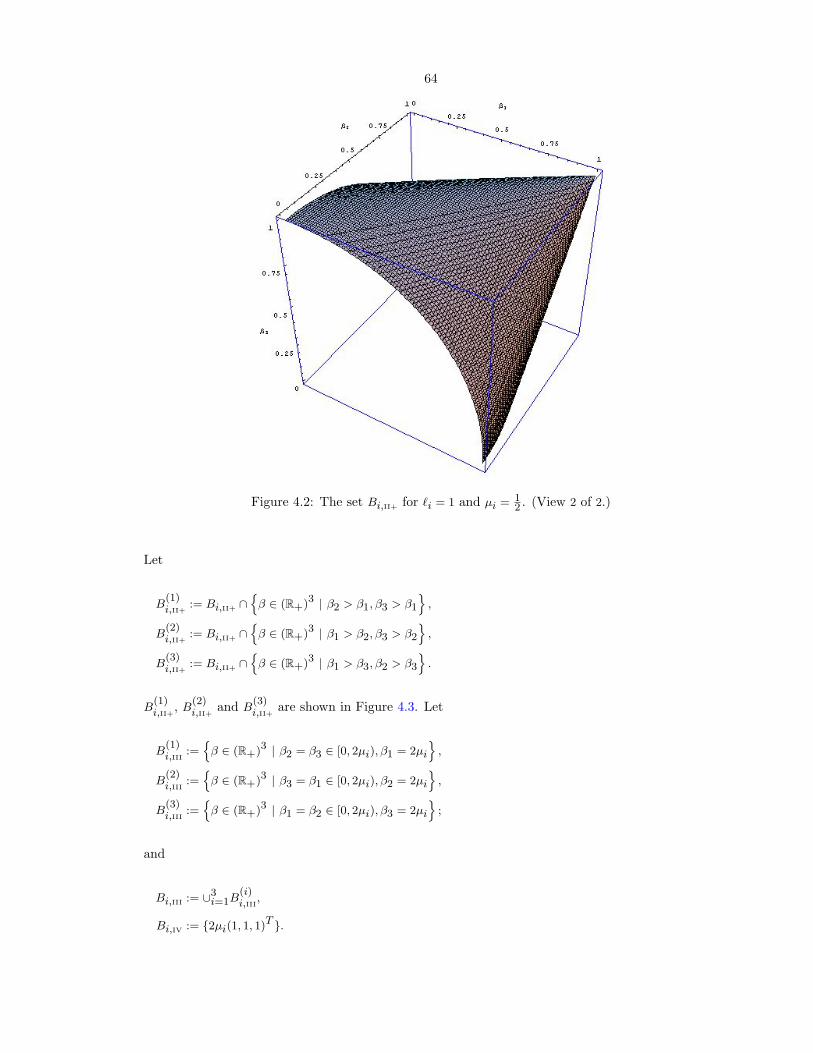
64

Figure 4.2: The set Bi,II+ for `i = 1 and µi = 12 . (View 2 of 2.)

Let

B(1)i,II+ := Bi,II+ ∩

nβ ∈ (R+)3 | β2 > β1, β3 > β1

o,

B(2)i,II+ := Bi,II+ ∩

nβ ∈ (R+)3 | β1 > β2, β3 > β2

o,

B(3)i,II+ := Bi,II+ ∩

nβ ∈ (R+)3 | β1 > β3, β2 > β3

o.

B(1)i,II+, B

(2)i,II+ and B

(3)i,II+ are shown in Figure 4.3. Let

B(1)i,III :=

nβ ∈ (R+)3 | β2 = β3 ∈ [0, 2µi), β1 = 2µi

o,

B(2)i,III :=

nβ ∈ (R+)3 | β3 = β1 ∈ [0, 2µi), β2 = 2µi

o,

B(3)i,III :=

nβ ∈ (R+)3 | β1 = β2 ∈ [0, 2µi), β3 = 2µi

o;

and

Bi,III := ∪3i=1B

(i)i,III,

Bi,IV := 2µi(1, 1, 1)T .

65

(a) The surface B(1)i,II+. (b) The surface B

(2)i,II+.

(c) The surface B(3)i,II+.

Figure 4.3: The surfaces B(1)i,II+, B

(2)i,II+ and B

(3)i,II+ for ` = 1 and µ = 1

2 .

Bi,III ∪ Bi,IV is shown in Figure 4.4. Note that the seven sets B(1)i,II+, B

(2)i,II+, B

(3)i,II+, B

(1)i,III, B

(2)i,III, B

(3)i,III

and Bi,IV are disjoint and their union is Bi,II+.

The sets B(1)III , B

(2)III , B

(3)III , BIII and BIV are defined in an analogous manner. Let j ∈ 1, 2 such

that µj = minµ1, µ2. From the preceeding it should be clear that B(1)III = B

(1)j,III, B

(2)III = B

(2)j,III,

B(3)III = B

(3)j,III, BIII = Bj,III and BIV = Bj,IV.

Remark 4.5. From (4.11) note that (Tr(Hi))2−Tr(H2

i ) > 0 except when β1 = β2 = β3 = 2µi. Thus,

when β ∈ Bi,II+, precisely one eigenvalue of Hi is zero, except when β1 = β2 = β3 = 2µi (in which

case two eigenvalues are zero). In conjunction with (4.9) this implies that

dim (ker(α− β · T )) =

8>>>>>><>>>>>>:1 when β ∈ Bi,II+ \ (Bi,III ∪Bi,IV)

2 when β ∈ Bi,III

5 when β ∈ Bi,IV.

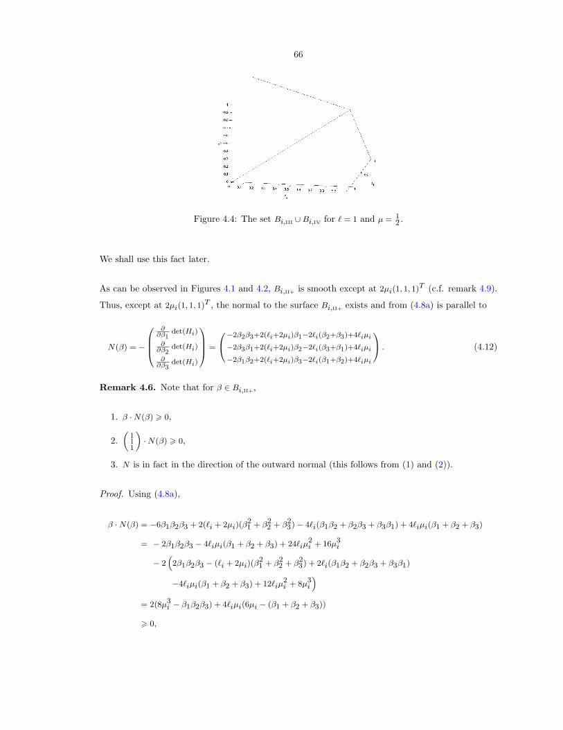
66

Figure 4.4: The set Bi,III ∪Bi,IV for ` = 1 and µ = 12 .

We shall use this fact later.

As can be observed in Figures 4.1 and 4.2, Bi,II+ is smooth except at 2µi(1, 1, 1)T (c.f. remark 4.9).

Thus, except at 2µi(1, 1, 1)T , the normal to the surface Bi,II+ exists and from (4.8a) is parallel to

N(β) = −

0BB@∂

∂β1det(Hi)

∂∂β2

det(Hi)

∂∂β3

det(Hi)

1CCA =

0@−2β2β3+2(ì+2µi)β1−2ì(β2+β3)+4ìµi

−2β3β1+2(ì+2µi)β2−2ì(β3+β1)+4ìµi

−2β1β2+2(ì+2µi)β3−2ì(β1+β2)+4ìµi

1A . (4.12)

Remark 4.6. Note that for β ∈ Bi,II+,

1. β ·N(β) > 0,

2.„

111

«·N(β) > 0,

3. N is in fact in the direction of the outward normal (this follows from (1) and (2)).

Proof. Using (4.8a),

β ·N(β) = −6β1β2β3 + 2(ì + 2µi)(β21 + β2

2 + β23)− 4ì(β1β2 + β2β3 + β3β1) + 4ìµi(β1 + β2 + β3)

= − 2β1β2β3 − 4ìµi(β1 + β2 + β3) + 24ìµ2i + 16µ3

i

− 2“2β1β2β3 − (ì + 2µi)(β

21 + β2

2 + β23) + 2ì(β1β2 + β2β3 + β3β1)

−4ìµi(β1 + β2 + β3) + 12ìµ2i + 8µ3

i

”= 2(8µ3

i − β1β2β3) + 4ìµi(6µi − (β1 + β2 + β3))

> 0,

67

and

„111

«·N(β) = −2(β1β2 + β2β3 + β3β1) + 4µi(β1 + β2 + β3)− 2ì(β1 + β2 + β3) + 12ìµi

= 2 (2µi(β1 + β2 + β3)− (β1β2 + β2β3 + β3β1)) + 2ì (6µi − (β1 + β2 + β3))

> 0

(the first term is non-negative since βj ∈ [0, 2µi] ⇒ βjβk ∈ [0, 2µiβk]).

We end this section with an important lemma.

Lemma 4.7 (sign(N) on Bi,II+).

1. On B(1)i,II+, sign(N) =

„−++

«.


„+−+

«.


„++−

«.

4. On B(1)i,III, sign(N) =

„+00

«.


„0+0

«.


„00+

«.

Remark 4.8. Let ci :=ì

ì+2µi∈ (0, 1). With the transformation β′j :=

ì+βjì+2µi

∈ [ci, 1], in the proof

of lemma 4.4

Hi ‖ H ′i :=

0@ 1 β′3 β′2β′3 1 β′1β′2 β′1 1

1A .

Thus (4.10) is equivalent to

2

3Yj=1

β′j − ‖β′‖2 + 1 = 0

and (4.8a) and (4.8b) can be written as

Bi,II+ =

8<:β ∈ [ci, 1]3 | 2

3Yj=1

β′j − ‖β′‖2 + 1 = 0

9=; (4.13)

68

and

Bi =

8<:β ∈ [ci, 1]3 | 2

3Yj=1

β′j − ‖β′‖2 + 1 > 0

9=;respectively. Finally from (4.12),

N(β′) ‖

0B@ β′1−β′2β′3β′2−β′3β′1β′3−β1β2

1CA .

Proof of lemma 4.7. We prove the first statement; the next two follow from symmetry. The last

three statements follow from the first three statements and in any case are easy to verify. It might

be helpful to refer to Figures 4.3(a) and 4.4.

It will be convenient to work in the coordinates β′ (c.f. remark 4.8). Now

∇β′N1(β′) ‖

1

−β′3−β′2

!.

Clearly, ∇β′N1(β′) 6= 0. Further, ∇β′N1(β′) ∦ N(β′) on Bi,II+ \ Bi,IV as can be easily verified by a

simple calculation. Thus the maximum and minimum of N1 on Bi,II+ is attained at its boundary,

i.e., on B(2)i,III ∪ B

(3)i,III ∪ Bi,IV ∪ (B

(1)i,II+ ∩ β | β − 1 = 0). A simple calculation shows that N1 = 0 on

B(2)i,III, B

(3)i,III and Bi,IV.2 In the next paragraph we show that N1 < 0 on B

(1)i,II+ ∩ β | β − 1 = 0. It

follows that N1(β) < 0 on B(1)i,III.

Proof that N1 < 0 on B(1)i,II+ ∩ β | β − 1 = 0: Note from remark 4.8 (in particular (4.13)) that

B(1)i,II+ ∩ β | β − 1 = 0 is the curve

(β′3)2 − 2cβ′2β′3 + c2 + (β′2)2 − 1 = 0, β′2, β′3 ∈ (c, 1).

solving for β′3, we obtain, β′3 = cβ′2 ±q

(1− c2)(1− (β′2)2). However,

cβ′2 −q

(1− c2)(1− (β′2)2) < cβ′2 − (1− (β′2)2)2 = cβ′2 + (β′2)2 − 1 < cβ′2 < c.

2 This also proves part of (5) and (6).

69

Thus the solution we seek is β′3 = cβ′2 +q

(1− c2)(1− (β′2)2). Thus on B(1)i,II+ ∩ β | β − 1 = 0,

N1(β′) = c− c(β′2)2 − (β′2)q

(1− c2)(1− (β′2)2)

< c− c(β′2)2 − cq

(1− c2)(1− (β′2)2)

< c− c(β′2)2 − c(1− (β′2)2)

= 0.

This completes the proof that sign(N1) < 0 on β ∈ B(1)i,II+.

Now β ∈ B(1)i,II+ implies that β2 > β1 and β3 > β1. Thus,

N2 = −2β3β1 + 2(ì + 2µi)β2 − 2ì(β3 + β1) + 4ìµi

> −2β3β1 + 2(ì + 2µi)β1 − 2ì(β3 + β1) + 4ìµi

= −2β3β1 + 4µiβ1 − 2ìβ3 + 4ìµi

= 2(ì + β1)(2µi − β3)

> 0

and

N3 = −2β1β2 + 2(ì + 2µi)β3 − 2ì(β1 + β2) + 4ìµi

> −2β1β2 + 2(ì + 2µi)β1 − 2ì(β1 + β2) + 4ìµi

= −2β1β2 + 4µiβ1 − 2ìβ2 + 4ìµi

= 2(ì + β1)(2µi − β2)

> 0.

Remark 4.9. From (4), (5) and (6) in lemma 4.7 it follows that the surface is not smooth at

2µ(1, 1, 1)T (i.e., on Bi,IV) for,

limβ→2µi(1,1,1)T

β∈B(1)i,III

N(β) 6= limβ→2µi(1,1,1)T

β∈B(2)i,III

N(β) 6= limβ→2µi(1,1,1)T

β∈B(3)i,III

N(β).

70

4.3 Explicit expressions for the optimal strains3

Let us return to the minimization problem (4.5b) and find the minimizers ε?1(R, β, ε) and ε?2(R, β, ε).

By differentiating the argument on the right-hand side of (4.5b),

α1(ε?1 − εT1)− α2(ε?2 − εT

2) + (β · TR)(ε?2 − ε?1) = 0 (4.14)

In other words,

∆σ? = (β · TR)∆ε? (4.15)

where ∆ε? = ε?2 − ε?1, ∆σ? := σ?2 − σ?

1 and σ?i = αi(ε

?i − εT

i ). Using λ1ε1 + λ2ε2 = ε, (4.14) gives

(λ2α1 + λ1α2 − β · TR)ε?1 = (α2 − β · TR)ε + λ2(α1εT1 − α2εT

2),

(λ2α1 + λ1α2 − β · TR)ε?2 = (α1 − β · TR)ε− λ1(α1εT1 − α2εT

2),

(λ2α1 + λ1α2 − β · TR)∆ε? = (α2εT2 − α1εT

1)− (∆α)ε.

where ∆α := α2−α1. To get explicit expressions we need the invertibility of λ2α1+λ1α2−β ·TR. Note

that λ2α1+λ1α2−β ·TR = λ2(α1−β ·TR)+λ1(α2−β ·TR). Hence, for β ∈ B(R)\BII+, it is the sum of

two positive definite linear operators and consequently positive definite and thus invertible. In fact

even when β ∈ BII+, λ2α1+λ1α2−β ·TR is invertible as long as ker(α1−β ·TR)∩ker(α2−β ·TR) = 0.

In either case,

ε?1 =“λ2α1 + λ1α2 − β · TR

”−1 “(α2 − β · TR)ε− λ2

`α2εT

2 − α1εT1´”

, (4.16a)

ε?2 =“λ2α1 + λ1α2 − β · TR

”−1 “(α1 − β · TR)ε + λ1

`α2εT

2 − α1εT1´”

, (4.16b)

∆ε? =“λ2α1 + λ1α2 − β · TR

”−1 ``α2εT

2 − α1εT1´− (∆α)ε

´. (4.16c)

and

∂∆ε?

∂βi= (λ2α1 + λ1α2 − β · TR)−1TR

i ∆ε? (4.17)

3The expressions in this section can be obtained from those in section 3.1.4 by the formal substitution of β · T R

for βT , β ∈ B(R) \BII+(R) for β ∈ [0, γ?) and β ∈ BII+(R) for β = γ?.

71

4.4 An optimal rotation diagonalizes the optimal strain jump

Henceforth we assume that the elastic moduli are isotropic. From lemma 4.3, for isotropic moduli

B is independent of R. Thus from (4.5a), we have the lower bound

cWλ(ε) > maxβ∈B

Wλ(β, ε) (4.18a)

where

Wλ(β, ε) := maxR∈SO(3)

minε1,ε2∈M3×3

symλ1ε1+λ2ε2=ε

λ1W1(ε1) + λ2W2(ε2)− λ1λ2β · ΦR(ε2 − ε1). (4.18b)

Theorem 4.10 (An optimal rotation diagonalizes the optimal strain jump). There exist

R?(β, ε) ∈ SO(3), ε?1(R?, β, ε), ε?2(R?, β, ε) ∈ M3×3sym that extremize (4.18b) such that RT

? ∆ε?R? is

diagonal.

Our proof of theorem 4.10 uses doubly stochastic matrices and is presented at the end of this section.

4.4.1 Doubly stochastic matrices

A doubly stochastic matrix is a square matrix, all of whose entries are positive and each of whose

rows and columns add up to one. Let Ω3 be the set of all doubly stochastic matrices in M3×3. Ω3 is

a four-dimensional convex set the set of whose extreme points is P3, the set of permutation matrices

in M3×3 [Bir46] (or, e.g., [MI79, pg.19,34]). P3 = Pj | j = 1, 2 . . . 6, where

P1 :=

„1 0 00 1 00 0 1

«, P2 :=

„0 1 00 0 11 0 0

«, P3 :=

„0 0 11 0 00 1 0

«,

P4 :=

„1 0 00 0 10 1 0

«, P5 :=

„0 1 01 0 00 0 1

«, P6 :=

„0 0 10 1 01 0 0

«.

Note that the first three of these belong to SO(3) and the next three to O(3) \ SO(3).

Remark 4.11.

1. ∀P ∈ P3, Φ(PT εP ) = PT Φ(ε).

2. ∀P ∈ P3 there exists R(P ) ∈ SO(3) such that Φ(PT εP ) = Φ(R(P )T εR(P )).

Proof. The first statement is easily verified. Each P ∈ P is a matrix precisely three of whose

components is 1. For each P ∈ P ∩ SO(3) replacing none or two 1s by −1 generates a matrix

72

R(P ) ∈ SO(3). For each P ∈ P\SO(3) replacing one or three 1 by −1 generates a matrix R(P ) ∈ SO(3).

It is easily verified that for every such choice of R(P ), Φ(PT εP ) = Φ(R(P )T εR(P )).

A map from SO(3) to Ω3. Define S : SO(3) → Ω3 by

SO(3) 3

0BBBB@R11 R12 R13

R21 R22 R23

R31 R32 R33

1CCCCA S7→

0BBBBB@R2

11 R212 R2

13

R221 R2

22 R223

R231 R2

32 R233

1CCCCCA ∈ Ω3. (4.19)

For R(P ) defined as in remark 4.11, S(R(P )) = P . Thus P3 ⊂ Range(S). The following remark and

lemma will shed light on some subsequent comments.

Remark 4.12. Since the only fixed points of R 3 x 7→ x2 ∈ R are 0 and 1, it follows that

1. The fixed points of S are precisely P3 ∩ SO(3).

2. S can be extended to a map from O(3) to Ω3, in which case its fixed points are precisely P3.

Lemma 4.13 ([Kat03]). S is not onto.

Proof. Assume on the contrary that ∃R ∈ SO(3) such that

S(R) =1

3

„1 1 11 1 11 1 1

«∈ Ω3.

Then, from (4.19), for some choice of signs

R =1√3

„±1 ±1 ±1±1 ±1 ±1±1 ±1 ±1

«.

However the rows and columns of this R cannot be orthogonal: R /∈ SO(3), which is a contradiction.

Let σ : 1, 2, 3 → 1, 2, 3 be a permutation (i.e., invertible function). For ε ∈ M3×3sym let υ1(ε), υ2(ε)

and υ3(ε) be the eigenvalues of ε. By diag(ε) we denote an arbitrary (but fixed) matrix of the form

0@ υσ(1)(ε) 0 0

0 υσ(2)(ε) 0

0 0 υσ(3)(ε)

1A .

In other words, diag(ε) is a diagonal matrix whose diagonal elements are the eigenvalues of ε in some

arbitrary (but fixed) order. Similarly, let

Υ(ε) :=

0@ υσ(2)(ε) υσ(3)(ε)

υσ(3)(ε) υσ(1)(ε)

υσ(1)(ε) υσ(2)(ε)

1A .

73

Lemma 4.14. ∀R ∈ SO(3), ∀ε ∈ M3×3sym , ∃D ∈ Ω3 such that β · ΦR(ε) = −Dβ ·Υ(ε).

Proof. There exist Rd(ε) ∈ SO(3) such that

ε = (Rd(ε))T diag(ε) Rd(ε).

Thus

RT εR = (Rd(ε)R)T diag(ε) Rd(ε)R

= (R′)T diag(ε) R′

where R′ := Rd(ε)R. An easy exercise reveals that

−φ1(RT εR) = (R′22R′33 −R′32R′23)2υσ(2)(ε)υσ(3)(ε) + (R′23R′31 −R′33R′21)2υσ(3)(ε)υσ(1)(ε)

+ (R′21R′32 −R′31R′22)2υσ(1)(ε)υσ(2)(ε)


+ (R′31R′12 −R′11R′32)2υσ(1)(ε)υσ(2)(ε)


+ (R′11R′22 −R′21R′12)2υσ(1)(ε)υσ(2)(ε).

We obtain

β · Φ(RT εR) = −β ·

0BBBBB@(R′22R′33 −R′32R′23)2 (R′23R′31 −R′33R′21)2 (R′21R′32 −R′31R′22)2

(R′32R′13 −R′12R′33)2 (R′33R′11 −R′13R′31)2 (R′31R′12 −R′11R′32)2

(R′12R′23 −R′22R′13)2 (R′13R′21 −R′23R′11)2 (R′11R′22 −R′21R′12)2

1CCCCCAΥ(ε)

Note that the ijth element of the matrix above is the square of the ijth sub-determinant of R′. Since

R′ ∈ SO(3), its rows and columns are orthonormal: R′22R′33 − R′32R′23 = R′11, R′23R′31 − R′33R′21 =

74

R′12 . . . . This gives

β · ΦR(ε) = −β ·

0BBBBB@(R′11)2 (R′12)2 (R′13)2

(R′21)2 (R′22)2 (R′23)2

(R′31)2 (R′13)2 (R′11)2

1CCCCCAΥ(ε)

= −β · S(R′)Υ(ε)

= −(S(Rd(ε)R))T β ·Υ(ε) (4.20)

= Dβ ·Υ(ε).

where D := −(S(Rd(ε)R))T .

Corollary 4.15 (P3

j=1 φRj is independent of R). With β = (1, 1, 1)T in (4.20), since any doubly

stochastic matrix has (1, 1, 1)T as eigenvector with eigenvalue 1, we obtain

3Xj=1

φj(RT εR) = −D

„111

«·Υ(ε) = −

„111

«·Υ(ε) = −(υ2(ε)υ3(ε) + υ3(ε)υ1(ε) + υ1(ε)υ2(ε))

which is independent of R.

We are now ready to prove theorem 4.10.

4.4.2 Proof of theorem 4.10

The existence of R? and ε?i follows from the convexity for each R ∈ SO(3) of Wi−β ·ΦR, the continuity

for each ε ∈ M3×3sym of R 7→ ΦR(ε) and the compactness of SO(3). It remains to show that RT

? ∆ε?R?

is diagonal. From (4.18b) and (4.20),

Wλ(β, ε) = maxR∈SO(3)

minε1,ε2∈M3×3

symλ1ε1+λ2ε2=ε

λ1W1(ε1) + λ2W2(ε2) + λ1λ2ST (Rd(ε2 − ε1)R)β ·Υ(ε2 − ε1).

Thus

Wλ(β, ε) 6 maxS∈Ω3

minε1,ε2∈M3×3

symλ1ε1+λ2ε2=ε

λ1W1(ε1) + λ2W2(ε2) + λ1λ2Sβ ·Υ(ε2 − ε1), (4.21)

75

where the inequality arises since (a) we are replacing ST (Rd(ε2− ε1)R) with an arbitrary S ∈ Ω3 and

(b) the maximization is performed over S ∈ Ω3 and not just Range(S) ( Ω3. Now

Ω3 3 S 7→ minε1,ε2∈M3×3

symλ1ε1+λ2ε2=ε

λ1W1(ε1) + λ2W2(ε2) + λ1λ2Sβ ·Υ(ε2 − ε1)

is convex: ∀θ ∈ (0, 1),

minε1,ε2∈M3×3

symλ1ε1+λ2ε2=ε

λ1W1(ε1) + λ2W2(ε2) + λ1λ2(θS + (1− θ)S′)β ·Υ(ε2 − ε1)

> minε1,ε2∈M3×3

symλ1ε1+λ2ε2=ε

θλ1W1(ε1) + θλ2W2(ε2) + θλ1λ2Sβ ·Υ(ε2 − ε1)

+ minε1,ε2∈M3×3

symλ1ε1+λ2ε2=ε

(1− θ)λ1W1(ε1) + (1− θ)λ2W2(ε2) + (1− θ)λ1λ2S′β ·Υ(ε2 − ε1),

where we have used minx(f(x) + g(x)) > minx f(x) + minx g(x). Since convex functions attain their

maximum on the extreme points of convex sets, there exists S? ∈ P3 that maximizes the left-hand

side of (4.21). Since P3 ⊂ Range(S), this implies the existence of R? ∈ SO(3) such that S(RdR?) = S?

which maximizes the left-hand side of (4.18b). Thus the inequality in (4.21) is actually an equality.

Further

S(RdR?) ∈ P3 ⇒ RdR? is a signed permutation matrix

⇒ (RdR?)T diag(∆ε?)(RdR?) is diagonal

⇒ RT? ∆ε?R? is diagonal


Note that, since RT? ∆ε?R? is diagonal,

RT? ∆ε?R? =

0@ υσ(1)(∆ε?) 0 0

0 υσ(2)(∆ε?) 0

0 0 υσ(3)(∆ε?)

1Aand thus

φ1(RT? ∆ε?R?) = −υσ(2)(∆ε?) υσ(3)(∆ε?), (4.22a)

φ2(RT? ∆ε?R?) = −υσ(3)(∆ε?) υσ(1)(∆ε?), (4.22b)

φ3(RT? ∆ε?R?) = −υσ(1)(∆ε?) υσ(2)(∆ε?). (4.22c)

76

4.5 A lower bound on the relaxed energy

Recall from (4.18a) and (4.18b) that we have the lower bound

cWλ(ε) > maxβ∈B

Wλ(β, ε) (4.18a)

where

Wλ(β, ε) := maxR∈SO(3)

minε1,ε2∈M3×3

symλ1ε1+λ2ε2=ε

λ1W1(ε1) + λ2W2(ε2)− λ1λ2β · ΦR(ε2 − ε1). (4.18b)

Determining maxβ∈B Wλ(β, ε) is easy since we have the following lemma.

Lemma 4.16. β 7→ Wλ(β, ε) is concave for β ∈ B \BII+.

Proof. Let θ ∈ (0, 1). Using minx f(x) + minx g(x) 6 minx(f(x) + g(x)),

θWλ(β, ε) + (1− θ)Wλ(β′, ε)

= minλ1ε1+λ2ε2=ε

θλ1W1(ε1) + θλ2W2(ε2)− θλ1λ2β · ΦR(ε2 − ε1)

+ minλ1ε1+λ2ε2=ε

(1− θ)λ1W1(ε1) + (1− θ)λ2W2(ε2)− (1− θ)λ1λ2β′ · Φ(ε2 − ε1).

6 Wλ((θβ + (1− θ)β′), ε).

From (4.18b),

∂

∂βiWλ(β, ε) = −λ1λ2φ

R?(β,ε)i (∆ε?(R?(β, ε), β, ε)); (4.23a)

in other words,

∇βWλ(β, ε) = −λ1λ2ΦR?(β,ε)(∆ε?(R?(β, ε), β, ε)). (4.23b)

From lemma 4.16, β1 7→ Wλ(β, ε) is concave for β ∈ B \BII+. Fix β2, β3 ∈ R such that B ∩ (R×β2×

β3) is nonempty. Then ∃β1? ∈ R such that

(β1?, β2, β3)T = BII+ ∩ (R× β2 × β3).

77

By an argument similar to that in theorem 3.5 we obtain the following lower envelope for cWλ(ε):

cWλ(ε)

> maxβ1∈[0,β1?]

Wλ((β1, β2, β3)T , ε)

=

8>>>>>>>>><>>>>>>>>>:

Wλ((0, β2, β3)T , ε) if φR?((0,β2,β3)T ,ε)1 (∆ε?(R?((0, β2, β3)T , ε), (0, β2, β3)T , ε)) > 0

Wλ((β1II, β2, β3)T , ε) otherwise

Wλ((β1?, β2, β3)T , ε) if φR?((β1?,β2,β3)T ,ε)1 (∆ε?(R?((β1?, β2, β3)T , ε), (β1?, β2, β3)T , ε))

exists and is less than zero

where β1II satisfies φR?((β1II,β2,β3)T ,ε)1 (∆ε?(R?((β1II, β2, β3)T , ε), (β1II, β2, β3)T , ε)) = 0. Note that it is

possible that β1II = β1?.

Similarly by considering β2 7→ Wλ(β, ε) and β3 7→ Wλ(β, ε) we obtain two other lower bounds forcWλ(ε). Together they give

cWλ(ε) >

8>>>>>>>>>>>>>>>>>>>>>>>>>>>><>>>>>>>>>>>>>>>>>>>>>>>>>>>>:

Wλ(βI, ε) if ∃βI ∈ B ∩ ∂(R+)3 such that

∀j = 1, 2, 3, φR?(βI,ε)j (∆ε?(R?(βI, ε), βI, ε)) > 0

and ∃j ∈ 1, 2, 3, φR?(βI,ε)j (∆ε?(R?(βI, ε), βI, ε)) > 0 (Regime I)

Wλ(βII, ε) otherwise (Regime II)

Wλ(βII+, ε) if ∃βII+ ∈ BII+,∃j ∈ 1, 2, 3 such that

φR?(βII+,ε)j (∆ε?(R?(βII+, ε), βII+, ε)) (Regimes III

exists and is less than 0 and IV)

(4.24)

where βII satisfies ΦR?(βII,ε)(∆ε?(R?(βII, ε), βII, ε)) = 0. Further, for j = 1, 2, 3, if (βI)j 6= 0, then βI

satisfies φR?(βI,ε)j (∆ε?(R?(βI, ε), βI, ε)) = 0. Note that it is possible that βI, βII ∈ BII+.

Remark 4.17. As in the two-dimensional case, whenever φR?(βII+,ε)j (∆ε?(R?(βII+, ε), βII+, ε)) does

not exist, regimes III and IV do not occur. From §4.3 this happens when ker(α1−βII+ ·TR?(βII+,ε))∩

ker(α2 − βII+ · TR?(βII+,ε)) 6= 0 which occurs, for example, when α1 = α2 or when both phases are

isotopic and the shear moduli are equal. We will show below that in this case there exists a rank-I

laminate that is extremal. This is consistent with the results in [Koh91, Pip91].

78

4.6 Extremal microstructures

In this section we prove that the lower bound presented in (4.24) is optimal. Our strategy is the

same as in §3.2.

Lemma 4.18. Let ε ∈ M3×3sym . Then ∃n ∈ R3 such that ε ‖ n⊗ n if and only if Φ(ε) = 0.

Proof. It is easy to verify that Φ(n⊗ n) = 0. We need to show that Φ(ε) = 0 implies that ε is rank-I.

From (4.1),

φ1(ε) = 0 ⇒ ∃κ1 ∈ R such that ε23 = κ1ε22 and ε33 = κ1ε23 = κ21ε22;

φ2(ε) = 0 ⇒ ∃κ2 ∈ R such that ε31 = κ2ε33 = κ2κ21ε22 and ε11 = κ2ε31 = κ2

2κ21ε22;

φ3(ε) = 0 ⇒ ∃κ3 ∈ R such that ε12 = κ3ε11 = κ3κ22κ2

1ε22 andε22 = κ3ε12 = κ23κ2

2κ21ε22.

The last equation implies that κ21κ2

2κ23 = 1. Thus

Φ(ε) = 0 ⇒ ∃κ1, κ2, κ3 ∈ R, ε ‖

0@ κ21κ2

2 κ21κ2

2κ3 κ21κ2

κ21κ2

2κ3 1 κ1

κ21κ2 κ1 κ2

1

1A =: K

Let η1, η2, η3 be the eigenvalues of K. An easy calculation shows that

η1η2η3 = det(K) = 0,

η1η2 + η2η3 + η3η1 = (Tr(K))2 − Tr(K2) = 0.

Thus two of the three eigenvalues of K are zero. This implies that K, and thus ε, is rank-I.

4.6.1 Regime I - rank-I laminates

We show that the lower bound cWλ(ε) > Wλ(βI, ε) is optimal:

Lemma 4.19 (Extremal microstructures in Regime I). In regime I there exist a pair of

extremal rank-I laminates. A rank-I laminate in three dimensions is shown in Figure 4.5.

Proof. From (4.24), ∀j = 1, 2, 3, φR?j (∆ε?) > 0. From (4.22),

υ2(∆ε?) υ3(∆ε?) 6 0,

υ3(∆ε?) υ1(∆ε?) 6 0,

υ1(∆ε?) υ2(∆ε?) 6 0.

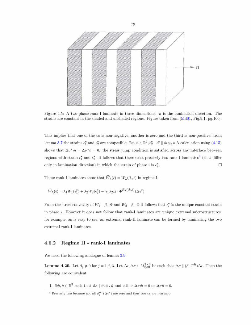
79

Figure 4.5: A two-phase rank-I laminate in three dimensions. n is the lamination direction. Thestrains are constant in the shaded and unshaded regions. Figure taken from [Mil01, Fig.9.1, pg.160].

This implies that one of the υs is non-negative, another is zero and the third is non-positive: from

lemma 3.7 the strains ε?1 and ε?2 are compatible: ∃m, n ∈ R3, ε?2−ε?1 ‖ m⊗s n A calculation using (4.15)

shows that ∆σ?m = ∆σ?n = 0: the stress jump condition is satisfied across any interface between

regions with strain ε?1 and ε?2. It follows that there exist precisely two rank-I laminates4 (that differ

only in lamination direction) in which the strain of phase i is ε?i .

These rank-I laminates show that cWλ(ε) = Wλ(βI, ε) in regime I:

cWλ(ε) = λ1W1(ε?1) + λ2W2(ε?2)− λ1λ2βI · ΦR?(βI,ε)(∆ε?).

From the strict convexity of W1−βI ·Φ and W2−βI ·Φ it follows that ε?i is the unique constant strain

in phase i. However it does not follow that rank-I laminates are unique extremal microstructures:

for example, as is easy to see, an extremal rank-II laminate can be formed by laminating the two

extremal rank-I laminates.

4.6.2 Regime II - rank-I laminates

We need the following analogue of lemma 3.9.

Lemma 4.20. Let βj 6= 0 for j = 1, 2, 3. Let ∆ε, ∆σ ∈ M3×3sym be such that ∆σ ‖ (β ·TR)∆ε. Then the

following are equivalent

1. ∃m, n ∈ R3 such that ∆ε ‖ m⊗s n and either ∆σm = 0 or ∆σn = 0.

4 Precisely two because not all φR?j (∆ε?) are zero and thus two υs are non zero

80

2. ∃n ∈ R3 such that ∆ε ‖ n⊗ n and ∆σn = 0.

3. Φ(∆ε) = 0.

Proof. We begin with some preliminary calculations:

T1(m⊗s n) =

„0 0 00 −2m3n3 m3n2+m2n30 m3n2+m2n3 −2m2n2

«and (T1(m⊗s n))n = (m× n)1

„0

n3−n2

«

T2(m⊗s n) =

„ −2n3m3 0 m3n1+m1n30 0 0

m3n1+m1n3 0 −2m1n1

«and (T2(m⊗s n))n = (m× n)2

„−n30

n1

«

T3(m⊗s n) =

„ −2m2n2 m2n1+m1n2 0m2n1+m1n2 −2m1n1 0

0 0 0

«and (T3(m⊗s n))n = (m× n)3

„ n2−n1

0

«

These give

((β · T )(m⊗s n))n =

0@ β3(m×n)3n2−β2(m×n)2n3

β1(m×n)1n3−β3(m×n)3n1

β2(m×n)2n1−β1(m×n)1n2

1A = n×

β1 0 00 β2 00 0 β3

!(m× n).

Thus

((β · T )(m⊗s n))n = 0 ⇒

β1 0 00 β2 00 0 β3

!(m× n) ‖ n

⇒

β1 0 00 β2 00 0 β3

!(m× n) · (m× n) = 0

⇒ m× n = 0

⇒ m ‖ n.

By a similar calculation the same conclusion follows from ((β · T )(m⊗s n))m = 0. We are now ready

to prove the lemma:

(1) ⇒ (3): ∆σ ‖ (β ·TR)∆ε ‖ (β ·TR)(m⊗s n). Thus from the calculation above ∆σm = 0 or ∆σn =

0 ⇒ m ‖ n ⇒ φ(∆ε) = 0.

(3) ⇒ (2): Assume Φ(∆ε) = 0; that is, ∃n ∈ R3, ∆ε ‖ n ⊗ n. From the calculation above, ∀m ∈

R3, (Tjm⊗ m)m = 0. Thus, ∆σn ‖“(β · TR)∆ε

”n ‖ R

“(β · T )RT (n⊗ n)R

”RT n = R(β ·T )(RT n⊗

RT n)(RT n) = 0.

We are now ready to show that cWλ(ε) > Wλ(βII, ε) is optimal:

Lemma 4.21 (Extremal microstructures in Regime II). In regime II there exists a rank-I

laminate that is extremal.

81

Proof. From (4.24), ΦR?(∆ε?) = 0 and from (4.15) ∆σ? = (βII · TR?)∆ε?. Thus from lemma 4.20,

∃n 3 ∆ε? ‖ n⊗ n and ∆σ?n = 0. It follows that there exists a rank-I laminate in which the strain of

phase i is ε?i . This shows that in regime II,

cWλ(ε) = Wλ(βII, ε) = λW1(ε?1) + (1− λ)W2(ε?2).

4.6.3 Regimes III and IV - rank-II and rank-III laminates

In regimes III and IV, since φR?j (∆ε?) < 0 for some j ∈ 1, 2, 3, from (4.22) atleast two eigenvalues

are non-zero and have the same sign. Thus, from lemma 3.7, the phases cannot form a rank-I

laminate. We show the existence of extremal rank-II and rank-III laminates.

From (4.24), in this regime βII+ (the optimal value of β) is contained in BII+. In fact this statement

can be greatly strengthened:

Lemma 4.22. βII+ ∈ BIII ∪BIV.

Proof. Using (4.23) and (4.22),

∇βWλ(β, ε) = −λ1λ2

0B@ φR?(β,ε)1 (∆ε?(R?(β,ε),β,ε))

φR?(β,ε)1 (∆ε?(R?(β,ε),β,ε))

φR?(β,ε)1 (∆ε?(R?(β,ε),β,ε))

1CA = λ1λ2

0@ υσ(2)(∆ε?) υσ(3)(∆ε?)

υσ(3)(∆ε?) υσ(1)(∆ε?)

υσ(1)(∆ε?) υσ(2)(∆ε?)

1A .

Since B 3 β 7→ Wλ(β, ε) attains its maximum at βII ∈ BII+, ∇βWλ(β, ε) must point along the outward

normal to BII+ at βII. If βII ∈ BIII \ (BIII ∪BIV), then from lemma 4.7,

sign

0@0@ υσ(2)(∆ε?) υσ(3)(∆ε?)

υσ(3)(∆ε?) υσ(1)(∆ε?)

υσ(1)(∆ε?) υσ(2)(∆ε?)

1A1A ∈„−

++

«,

„+−+

«,

„++−

«ff.

But of the pairwise products of three numbers it is impossible for precisely one to be negative and

precisely two to be positive.

We shall consider the case βII+ ∈ BIII (regime III) and the case βII+ ∈ BIV (regime IV) separately.

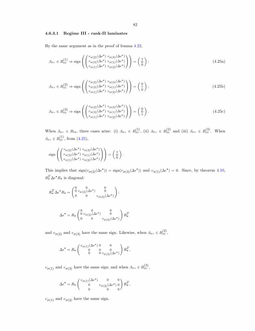
82

4.6.3.1 Regime III - rank-II laminates

By the same argument as in the proof of lemma 4.22,

βII+ ∈ B(1)III ⇒ sign

0@0@ υσ(2)(∆ε?) υσ(3)(∆ε?)

υσ(3)(∆ε?) υσ(1)(∆ε?)

υσ(1)(∆ε?) υσ(2)(∆ε?)

1A1A =

„+00

«; (4.25a)


0@0@ υσ(2)(∆ε?) υσ(3)(∆ε?)

υσ(3)(∆ε?) υσ(1)(∆ε?)

υσ(1)(∆ε?) υσ(2)(∆ε?)

1A1A =

„0+0

«; (4.25b)


0@0@ υσ(2)(∆ε?) υσ(3)(∆ε?)

υσ(3)(∆ε?) υσ(1)(∆ε?)

υσ(1)(∆ε?) υσ(2)(∆ε?)

1A1A =

„00+

«. (4.25c)

When βII+ ∈ BIII, three cases arise: (i) βII+ ∈ B(1)III , (ii) βII+ ∈ B

(2)III and (iii) βII+ ∈ B

(3)III . When

βII+ ∈ B(1)III , from (4.25),

sign

0@0@ υσ(2)(∆ε?) υσ(3)(∆ε?)

υσ(3)(∆ε?) υσ(1)(∆ε?)

υσ(1)(∆ε?) υσ(2)(∆ε?)

1A1A =

„+00

«.

This implies that sign(υσ(2)(∆ε?)) = sign(υσ(3)(∆ε?)) and υσ(1)(∆ε?) = 0. Since, by theorem 4.10,

RT? ∆ε?R? is diagonal:

RT? ∆ε?R? =

0 0 00 υσ(2)(∆ε?) 0

0 0 υσ(3)(∆ε?)

!;

∆ε? = R?

0 0 00 υσ(2)(∆ε?) 0

0 0 υσ(3)(∆ε?)

!RT

?

and υσ(2) and υσ(3) have the same sign. Likewise, when βII+ ∈ B(2)III ,

∆ε? = R?

υσ(1)(∆ε?) 0 0

0 0 00 0 υσ(3)(∆ε?)

!RT

? ,

υσ(1) and υσ(3) have the same sign; and when βII+ ∈ B(3)III ,

∆ε? = R?

υσ(1)(∆ε?) 0 0

0 υσ(2)(∆ε?) 0

0 0 0

!RT

? ,

υσ(1) and υσ(2) have the same sign.

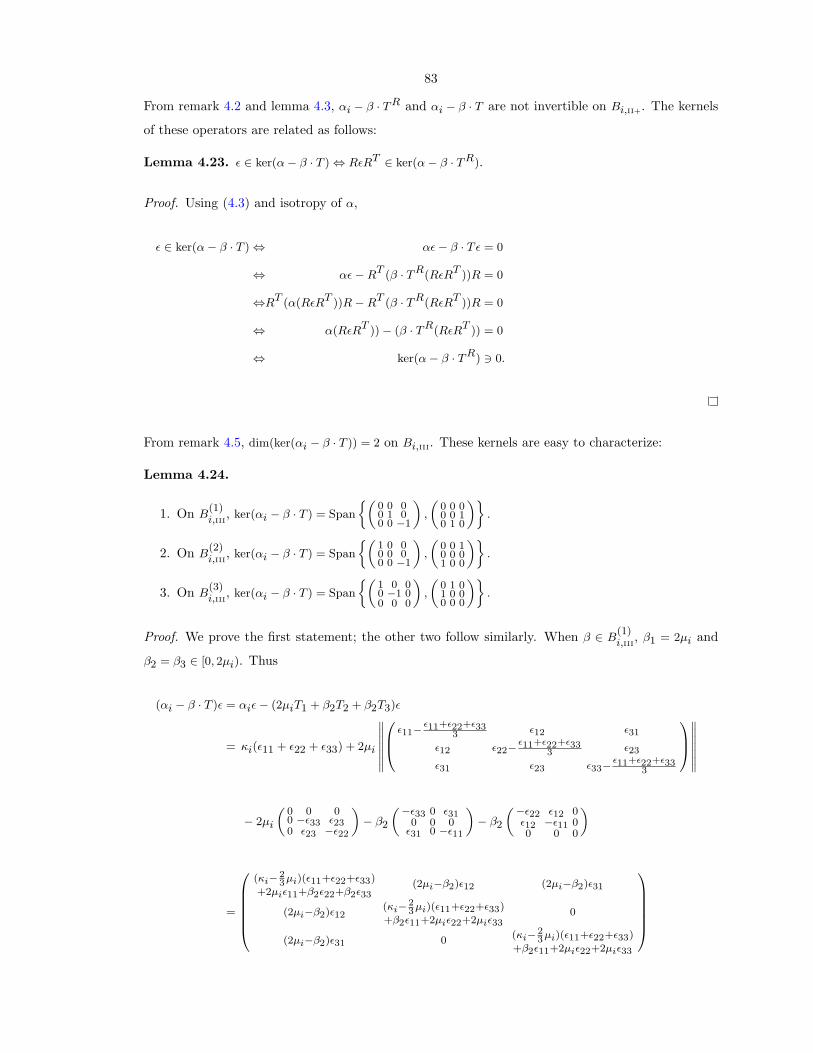
83

From remark 4.2 and lemma 4.3, αi − β · TR and αi − β · T are not invertible on Bi,II+. The kernels

of these operators are related as follows:

Lemma 4.23. ε ∈ ker(α− β · T ) ⇔ RεRT ∈ ker(α− β · TR).

Proof. Using (4.3) and isotropy of α,

ε ∈ ker(α− β · T ) ⇔ αε− β · Tε = 0

⇔ αε−RT (β · TR(RεRT ))R = 0

⇔RT (α(RεRT ))R−RT (β · TR(RεRT ))R = 0

⇔ α(RεRT ))− (β · TR(RεRT )) = 0

⇔ ker(α− β · TR) 3 0.

From remark 4.5, dim(ker(αi − β · T )) = 2 on Bi,III. These kernels are easy to characterize:

Lemma 4.24.

1. On B(1)i,III, ker(αi − β · T ) = Span

„0 0 00 1 00 0 −1

«,

„0 0 00 0 10 1 0

«ff.


„1 0 00 0 00 0 −1

«,

„0 0 10 0 01 0 0

«ff.


„1 0 00 −1 00 0 0

«,

„0 1 01 0 00 0 0

«ff.

Proof. We prove the first statement; the other two follow similarly. When β ∈ B(1)i,III, β1 = 2µi and

β2 = β3 ∈ [0, 2µi). Thus

(αi − β · T )ε = αiε− (2µiT1 + β2T2 + β2T3)ε

= κi(ε11 + ε22 + ε33) + 2µi

‚‚‚‚‚‚‚0B@ ε11−

ε11+ε22+ε333 ε12 ε31

ε12 ε22−ε11+ε22+ε33

3 ε23

ε31 ε23 ε33−ε11+ε22+ε33

3

1CA‚‚‚‚‚‚‚

− 2µi

„0 0 00 −ε33 ε230 ε23 −ε22

«− β2

„−ε33 0 ε310 0 0

ε31 0 −ε11

«− β2

„−ε22 ε12 0ε12 −ε11 00 0 0

«

=

0BBBBB@(κi− 2

3µi)(ε11+ε22+ε33)

+2µiε11+β2ε22+β2ε33(2µi−β2)ε12 (2µi−β2)ε31

(2µi−β2)ε12(κi− 2

3µi)(ε11+ε22+ε33)

+β2ε11+2µiε22+2µiε330

(2µi−β2)ε31 0(κi− 2

3µi)(ε11+ε22+ε33)

+β2ε11+2µiε22+2µiε33

1CCCCCA

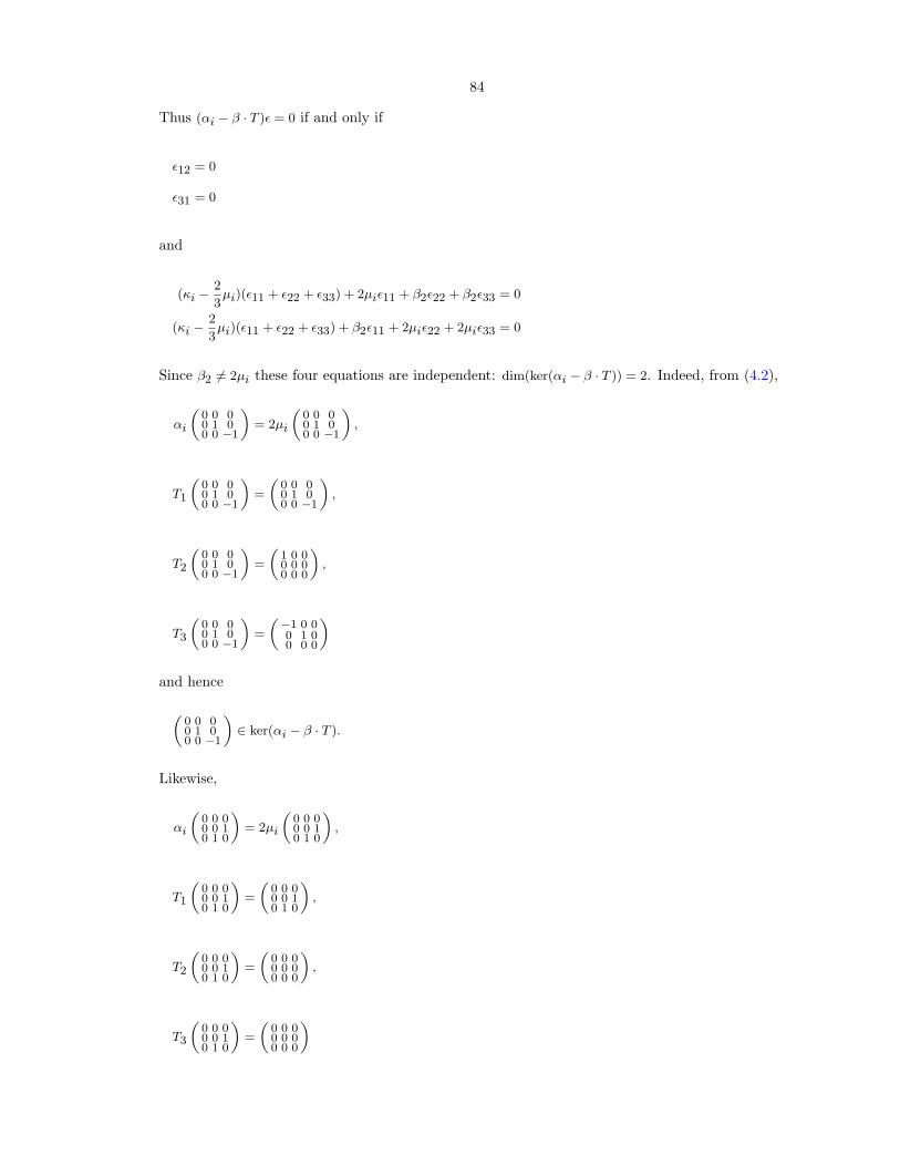
84

Thus (αi − β · T )ε = 0 if and only if

ε12 = 0

ε31 = 0

and

(κi −2

3µi)(ε11 + ε22 + ε33) + 2µiε11 + β2ε22 + β2ε33 = 0

(κi −2

3µi)(ε11 + ε22 + ε33) + β2ε11 + 2µiε22 + 2µiε33 = 0

Since β2 6= 2µi these four equations are independent: dim(ker(αi − β · T )) = 2. Indeed, from (4.2),

αi

„0 0 00 1 00 0 −1

«= 2µi

„0 0 00 1 00 0 −1

«,

T1

„0 0 00 1 00 0 −1

«=

„0 0 00 1 00 0 −1

«,

T2

„0 0 00 1 00 0 −1

«=

„1 0 00 0 00 0 0

«,

T3

„0 0 00 1 00 0 −1

«=

„−1 0 00 1 00 0 0

«

and hence

„0 0 00 1 00 0 −1

«∈ ker(αi − β · T ).

Likewise,

αi

„0 0 00 0 10 1 0

«= 2µi

„0 0 00 0 10 1 0

«,

T1

„0 0 00 0 10 1 0

«=

„0 0 00 0 10 1 0

«,

T2

„0 0 00 0 10 1 0

«=

„0 0 00 0 00 0 0

«,

T3

„0 0 00 0 10 1 0

«=

„0 0 00 0 00 0 0

«

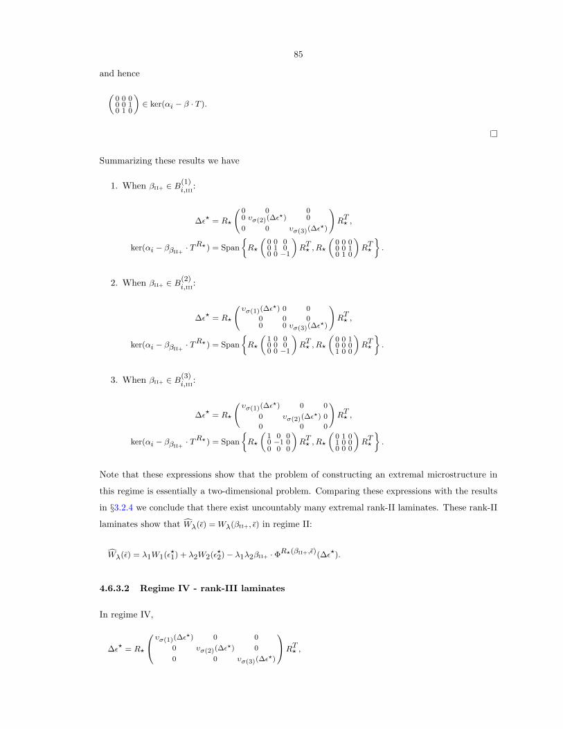
85

and hence

„0 0 00 0 10 1 0

«∈ ker(αi − β · T ).

Summarizing these results we have

1. When βII+ ∈ B(1)i,III:

∆ε? = R?

0 0 00 υσ(2)(∆ε?) 0

0 0 υσ(3)(∆ε?)

!RT

? ,

ker(αi − ββII+· TR?) = Span

R?

„0 0 00 1 00 0 −1

«RT

? , R?

„0 0 00 0 10 1 0

«RT

?

ff.


∆ε? = R?

υσ(1)(∆ε?) 0 0

0 0 00 0 υσ(3)(∆ε?)

!RT

? ,


R?

„1 0 00 0 00 0 −1

«RT

? , R?

„0 0 10 0 01 0 0

«RT

?

ff.


∆ε? = R?

υσ(1)(∆ε?) 0 0

0 υσ(2)(∆ε?) 0

0 0 0

!RT

? ,


R?

„1 0 00 −1 00 0 0

«RT

? , R?

„0 1 01 0 00 0 0

«RT

?

ff.

Note that these expressions show that the problem of constructing an extremal microstructure in

this regime is essentially a two-dimensional problem. Comparing these expressions with the results

in §3.2.4 we conclude that there exist uncountably many extremal rank-II laminates. These rank-II

laminates show that cWλ(ε) = Wλ(βII+, ε) in regime II:

cWλ(ε) = λ1W1(ε?1) + λ2W2(ε?2)− λ1λ2βII+ · ΦR?(βII+,ε)(∆ε?).

4.6.3.2 Regime IV - rank-III laminates

In regime IV,

∆ε? = R?

0@ υσ(1)(∆ε?) 0 0

0 υσ(2)(∆ε?) 0

0 0 υσ(3)(∆ε?)

1ART? ,

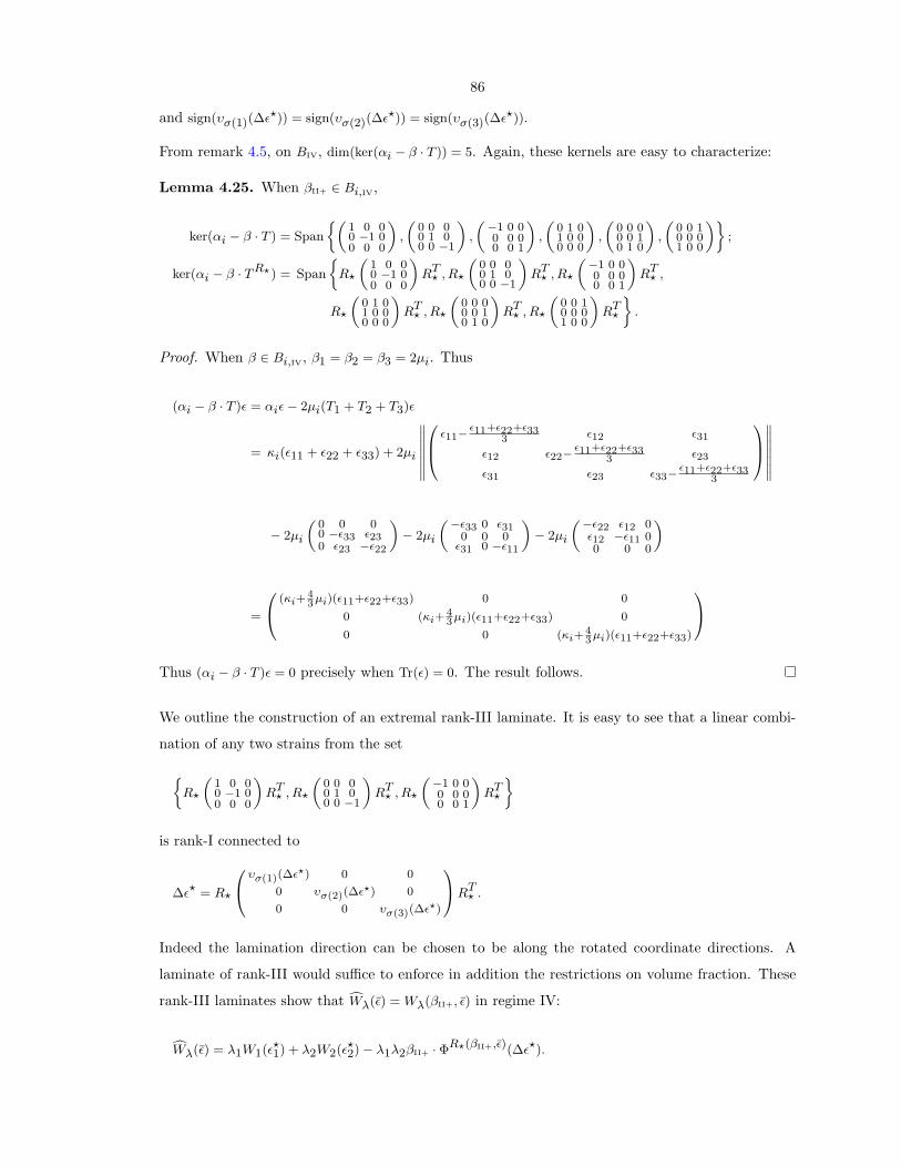
86

and sign(υσ(1)(∆ε?)) = sign(υσ(2)(∆ε?)) = sign(υσ(3)(∆ε?)).

From remark 4.5, on BIV, dim(ker(αi − β · T )) = 5. Again, these kernels are easy to characterize:

Lemma 4.25. When βII+ ∈ Bi,IV,

ker(αi − β · T ) = Span

„1 0 00 −1 00 0 0

«,

„0 0 00 1 00 0 −1

«,

„−1 0 00 0 00 0 1

«,

„0 1 01 0 00 0 0

«,

„0 0 00 0 10 1 0

«,

„0 0 10 0 01 0 0

«ff;

ker(αi − β · TR?) = Span

R?

„1 0 00 −1 00 0 0

«RT

? , R?

„0 0 00 1 00 0 −1

«RT

? , R?

„−1 0 00 0 00 0 1

«RT

? ,

R?

„0 1 01 0 00 0 0

«RT

? , R?

„0 0 00 0 10 1 0

«RT

? , R?

„0 0 10 0 01 0 0

«RT

?

ff.

Proof. When β ∈ Bi,IV, β1 = β2 = β3 = 2µi. Thus

(αi − β · T )ε = αiε− 2µi(T1 + T2 + T3)ε

= κi(ε11 + ε22 + ε33) + 2µi

‚‚‚‚‚‚‚0B@ ε11−

ε11+ε22+ε333 ε12 ε31

ε12 ε22−ε11+ε22+ε33

3 ε23

ε31 ε23 ε33−ε11+ε22+ε33

3

1CA‚‚‚‚‚‚‚

− 2µi

„0 0 00 −ε33 ε230 ε23 −ε22

«− 2µi

„−ε33 0 ε310 0 0

ε31 0 −ε11

«− 2µi

„−ε22 ε12 0ε12 −ε11 00 0 0

«

=

0@ (κi+43µi)(ε11+ε22+ε33) 0 0

0 (κi+43µi)(ε11+ε22+ε33) 0

0 0 (κi+43µi)(ε11+ε22+ε33)

1AThus (αi − β · T )ε = 0 precisely when Tr(ε) = 0. The result follows.

We outline the construction of an extremal rank-III laminate. It is easy to see that a linear combi-

nation of any two strains from the set

R?

„1 0 00 −1 00 0 0

«RT

? , R?

„0 0 00 1 00 0 −1

«RT

? , R?

„−1 0 00 0 00 0 1

«RT

?

ff

is rank-I connected to

∆ε? = R?

0@ υσ(1)(∆ε?) 0 0

0 υσ(2)(∆ε?) 0

0 0 υσ(3)(∆ε?)

1ART? .

Indeed the lamination direction can be chosen to be along the rotated coordinate directions. A

laminate of rank-III would suffice to enforce in addition the restrictions on volume fraction. These

rank-III laminates show that cWλ(ε) = Wλ(βII+, ε) in regime IV:

cWλ(ε) = λ1W1(ε?1) + λ2W2(ε?2)− λ1λ2βII+ · ΦR?(βII+,ε)(∆ε?).

87

4.A Appendix: A family of quasiconvex quadratic function-

als on M 3×3sym

The translations introduced in §4.1 were related to the diagonal subdeterminants — c.f. (4.1) — of

the elements of M3×3sym . As shown in that section, these diagonal subdeterminants are quasiconvex.

The three other subdeterminants of ε ∈ M3×3sym ,

φ12(ε) := ε12ε33 − ε23ε31,

φ23(ε) := ε11ε23 − ε31ε12,

φ31(ε) := ε12ε23 − ε22ε31,

are neither quasiconvex nor quasiconcave5.

It is of interest to ask which linear combinations of these six subdeterminants are quasiconvex. This

appendix provides a partial answer to this question by presenting a family of quasiconvex quadratic

functionals on M3×3sym . The translations introduced in (4.1) belong to this family.

Lemma 4.26. For M ∈ M3×3, let φM12 , φM

23 and φM31 be defined analogous to (4.1). Then ∀M ∈ M3×3

and ∀p, q, r ∈ R,

p2φM1 + q2φM

2 + r2φM3 − 2pqφM

12 − 2qrφM23 − 2rpφM

31 : M3×3sym → R (4.26)

is quasiconvex.

Proof. For m, n ∈ R3, let

ω1(m, n) := m2n3 −m3n2,

ω2(m, n) := m1n3 −m3n1,

ω3(m, n) := m1n2 −m2n1.

Note that

0 ω3(m,n) ω2(m,n)

−ω3(m,n) 0 ω1(m,n)ω2(m,n) ω1(m,n) 0

!5 Since these subdeterminants are quadratic, it suffices to show that they are neither rank-I convex nor rank-

I concave. That is, it suffices to find m, n, m′, n′ ∈ R3 such that φij(m ⊗s n) > 0 and φij(m′ ⊗s n′) < 0 for

i, j = 1, 2, 3; i 6= j. It is easy to find such m, n, m′, n′.

88

is the anti-symmetric component of m⊗ n. Now

φ1(m⊗s n) = (m2n3 + m3n2)2 − 4m2n2m3n3 = (m2n3 −m3n2)2 = ω21(m, n)

with similar results for φ2 and φ3. Likewise

φ12(m⊗s n) = (m1n2 + m2n1)(2m3n3)− (m2n3 + m3n2)(m1n3 + m3n1)

= −(m1n3 −m3n1)(m2n3 −m3n2)

= −ω1(m, n) ω2(m, n)

with similar results for φ23 and φ31. To summarize:

φ1(m⊗s n) = ω21(m, n),

φ2(m⊗s n) = ω22(m, n),

φ3(m⊗s n) = ω23(m, n),

φ12(m⊗s n) = −ω1(m, n) ω2(m, n),

φ23(m⊗s n) = −ω2(m, n) ω3(m, n),

φ31(m⊗s n) = −ω3(m, n) ω1(m, n).

We are now ready to prove the lemma. Since any linear combination of the φs is quadratic it suffices

to prove rank-I convexity:

“p2φM

1 + q2φM2 + r2φM

3 − 2pqφM12 − 2qrφM

23 − 2rpφM31

”(m⊗s n)

=“p2φ1 + q2φ2 + r2φ3 − 2pqφ12 − 2qrφ23 − 2rpφ31

”(MT m⊗s MT n)

=(pω1(MT m, MT n) + qω2(MT m, MT n) + rω3(MT m, MT n))2

>0


Remark 4.27.

1. There are quasiconvex quadratic functionals not of the form (4.26), for example, φ1 + φ2.

2. Positive linear combinations of functionals of the form (4.26) are quasiconvex (and quadratic).

3. From the proof above, ∃n ∈ R3 such that ε ‖ n⊗ n if and only if

φ1(ε) = φ2(ε) = φ3(ε) = φ12(ε) = φ23(ε) = φ31(ε) = 0.

89

Chapter 5

Polycrystals

The study of shape-memory polycrystals is an area of active research. Theoretical models in-

clude Taylor models [Ono90a, Ono90b, OS88, OSO89, TA01], Sachs models [SN00] and models

based on mean-field approximations [BL99a, BL99b, BL99c, BL99d, BL96, Fal89, LW98, LTT+00,

NBZACP02, PEB88, PEB93, PBEB94, SPBE99, SH93a, SH93b]. For computational studies that

explicitly compute the microstructure within the grains see [ALS03, AJK02]. Experimental studies

include [MNK+00, LVB+02, SLN+02, SNL+02]. The energy of the polycrystal plays a central role

in most of these approaches.

Our work is a departure from this since we focus on the zero-set of the mesoscopic energy and

make explicit use of the compatibility equation. In §5.1 we prove a dual variational characterization

of the zero-set of polycrystals. Uses of this characterization are illustrated through examples in

§5.2.2. In §5.2.1 and §5.3 we show that for a two-dimensional material and for materials undergoing

cubic-tertagonal transformations, compatibility forces the strain fields to be related to solutions of

hyperbolic partial differential equations.

We work in the setting of periodic polycrystals. Each grain has an non-empty interior and Lipschitz

boundary. Recall the mathematical framework introduced in §2 and in particular in §2.2.2.

5.1 Dual variational characterization of the zero-set of poly-

crystals

Observe from the discussion in §2.2.2 (in particular (2.12)) that to characterize the recoverable

strains of a polycrystal it suffices to characterize strain fields constrained locally (i.e., pointwise in

each grain) to lie in the zero-set of the mesoscopic energy. In other words, it is not so much the

mesoscopic energy cW that is of relevance but its zero-set bS. Motivated by this observation we shift

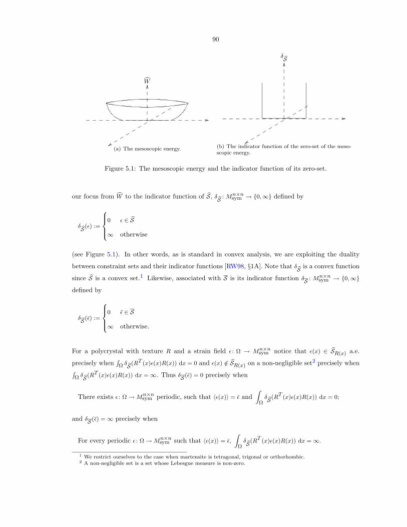
90

cWOO

yyrr

rr

rr

rr

rr

r

//___________________

(a) The mesoscopic energy.

δ bSOO

yyr rr

rr

rr

rr

rr

//___________________

(b) The indicator function of the zero-set of the meso-scopic energy.

Figure 5.1: The mesoscopic energy and the indicator function of its zero-set.

our focus from cW to the indicator function of bS, δ bS : Mn×nsym → 0,∞ defined by

δ bS (ε) :=

8>><>>:0 ε ∈ bS∞ otherwise

(see Figure 5.1). In other words, as is standard in convex analysis, we are exploiting the duality

between constraint sets and their indicator functions [RW98, §1A]. Note that δ bS is a convex function

since bS is a convex set.1 Likewise, associated with S is its indicator function δS : Mn×nsym → 0,∞

defined by

δS (ε) :=

8>><>>:0 ε ∈ S

∞ otherwise.

For a polycrystal with texture R and a strain field ε : Ω → Mn×nsym notice that ε(x) ∈ bSR(x) a.e.

precisely whenRΩ δ bS (RT (x)ε(x)R(x)) dx = 0 and ε(x) /∈ bSR(x) on a non-negligible set2 precisely whenR

Ω δ bS (RT (x)ε(x)R(x)) dx = ∞. Thus δS (ε) = 0 precisely when

There exists ε : Ω → Mn×nsym periodic, such that 〈ε(x)〉 = ε and

ZΩ

δ bS (RT (x)ε(x)R(x)) dx = 0;

and δS (ε) = ∞ precisely when

For every periodic ε : Ω → Mn×nsym such that 〈ε(x)〉 = ε,

ZΩ

δ bS (RT (x)ε(x)R(x)) dx = ∞.

1 We restrict ourselves to the case when martensite is tetragonal, trigonal or orthorhombic.2 A non-negligible set is a set whose Lebesgue measure is non-zero.

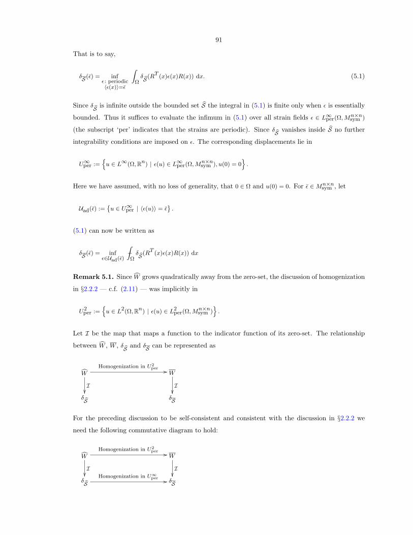
91

That is to say,

δS (ε) = infε : periodic〈ε(x)〉=ε

ZΩ

δ bS (RT (x)ε(x)R(x)) dx. (5.1)

Since δ bS is infinite outside the bounded set bS the integral in (5.1) is finite only when ε is essentially

bounded. Thus it suffices to evaluate the infimum in (5.1) over all strain fields ε ∈ L∞per(Ω, Mn×nsym )

(the subscript ‘per’ indicates that the strains are periodic). Since δ bS vanishes inside bS no further

integrability conditions are imposed on ε. The corresponding displacements lie in

U∞per :=n

u ∈ L∞(Ω, Rn) | ε(u) ∈ L∞per(Ω, Mn×nsym ), u(0) = 0

o.

Here we have assumed, with no loss of generality, that 0 ∈ Ω and u(0) = 0. For ε ∈ Mn×nsym , let

Uad(ε) :=˘u ∈ U∞per | 〈ε(u)〉 = ε

¯.

(5.1) can now be written as

δS (ε) = infε∈Uad(ε)

−ZΩ

δ bS (RT (x)ε(x)R(x)) dx

Remark 5.1. Since cW grows quadratically away from the zero-set, the discussion of homogenization

in §2.2.2 — c.f. (2.11) — was implicitly in

U2per :=

nu ∈ L2(Ω, Rn) | ε(u) ∈ L2

per(Ω, Mn×nsym )

o.

Let I be the map that maps a function to the indicator function of its zero-set. The relationship

between cW , W , δ bS and δS can be represented as

cWI

Homogenization in U2per // W

I

δ bS δS

For the preceding discussion to be self-consistent and consistent with the discussion in §2.2.2 we

need the following commutative diagram to hold:

cWI

Homogenization in U2per // W

I

δ bS Homogenization in U∞per // δS

92

Guided by this, work on the modeling of locking materials (remark 5.2), and the work of Carbone, De

Arcangelis et al. on the homogenization of unbounded functionals3 [CA01, and references therein]

we conjecture that δS is indeed the homogenized limit in U∞per of δ bS .

We proceed, on the assumption that this conjecture is true.

Remark 5.2 (Connections to locking materials). The mathematical framework described here

is closely connected to that which arises in the analysis of locking materials. These are hyperelastic

materials for which the strain tensor is constrained to stay in a convex set (with interior). See

[Pra57, Pra58, DS86, Dem85a, Dem85b].

In the sequel we will use the following definitions: Let R := R ∪ ∞. The conjugate of δ bS is

δ?bS : Mn×nsym → R defined by

δ?bS (σ) := supε∈Mn×n

sym

ε · σ − δ bS (ε).

δ?bS is the support function of bS [RW98, Eg.11.4(a), pg.477]. Let S ⊂ L∞(Ω, Mn×nsym ) be defined by

S :=n

ε | ∃u ∈ U∞per, ε = ε(u) and ε(x) ∈ bSR(x)

o.

Let M1per(Ω, Mn×n

sym ) ≡ (L∞per(Ω, Mn×nsym ))? be the space of all periodic signed Radon measures with

finite mass and let

Sad :=n

σ ∈ M1per(Ω, Mn×n

sym ) | div(σ) = 0o

.

Theorem 5.3 (Dual variational characterization of polycrystalline zero-sets). The indica-

tor function of the zero-set of a polycrystal has the dual variational characterization:

δS (ε) = supσ∈Sad

−ZΩ

σ · ε− δ?bS (RT (x)σ(x)R(x)) dx. (5.2)

Our proof follows the same strategy used to prove a similar result in [DS86]. The proof is presented

after lemma 5.4, lemma 5.5 and proposition 5.6 below.

Lemma 5.4. The following inequality holds:

supσ∈Sad

−ZΩ

σ · ε− δ?bS (RT (x)σ(x)R(x)) dx 6 infu∈Uad(ε)

−ZΩ

δ bS (RT (x)ε(x)R(x)) dx ≡ δS (ε).

3 Unbounded functionals are functionals taking values in R.

93

Moreover, the variational problem on the left is the dual of the variational problem on the right.

Proof. We shall denote the indicator function of Uad(ε) on U∞per by Fε:

Fε(u) :=

8>><>>:0 u ∈ Uad(ε)

∞ otherwise;

F ?ε (−ε?(σ)) : (U∞per)

? → R is given by [ET76]:

F ?ε (−ε?(σ)) =

8>><>>:〈σ〉 · ε if div(σ) = 0

∞ otherwise.

Let G : L∞per(Ω, Mn×nsym ) → R be defined by

G(ε) := −ZΩ

δ bS (RT (x)ε(x)R(x)) dx;

it is easy to verify that G? : M1per(Ω, Mn×n

sym ) → R is given by

G?(σ) = −ZΩ

δ?bS (RT (x)σ(x)R(x)) dx.

Fε and G are convex, proper4 and lower semi-continuous. Let ε? : M1per(Ω, Mn×n

sym ) → (U∞per)? be the

conjugate of the continuous map U∞per 3 u 7→ ε(u) ∈ L∞per(Ω, Mn×nsym ). δS (ε) is the solution of the

problem

P : infu∈U∞per

Fε(u) + G(ε(u)).

From a theorem in convex analysis [ET76], the dual of P is

P ? : supσ∈M1

per(Ω,Mn×nsym )

−F ?ε (−ε?(σ))−G?(σ).

In particular, P ? 6 P . 5 The result follows.

We now show that the inequality in lemma 5.4 above is in fact an equality. We do so by regularizing

the problem with a small parameter η and then taking the limit η → 0.4 That is, not everywhere ∞ [ET76, pg.8] [RW98, pg.5].5Further, if ∃u ∈ U∞per such that Fε(u) < ∞ and G is finite and continuous at ε(u), then P ? = P < ∞ and P ?

possesses at least one solution. We shall use this fact later.

94

For η ∈ R+, let cWη : Mn×nsym → R be defined by

cWη(ε) :=

8>>>>>><>>>>>>:

0 ε ∈ bS1

1− 1η d(ε, bS)

− 1 0 < d(ε, bS) < η

∞ otherwise

where d(ε, bS) is the distance in Mn×nsym between ε and bS:

d(ε, bS) := max16i,j6n

maxε′∈ bS |εij − ε′ij |.

Note that d(RT εR, bS) = d(ε, cRSRT ) = d(ε, bSR). cW0 ≡ δ bS and cWη is continuous for η > 0. Let cW ?η be

the conjugate of cWη.

Lemma 5.5. For η > 0, the following inequality holds:

supσ∈Sad

−ZΩ

σ · ε−cW ?η (RT (x)σ(x)R(x)) dx 6 inf

u∈Uad(ε)−ZΩ

cWη(RT (x)ε(x)R(x)) dx.

Moreover, the variational problem on the left is the dual of the variational problem on the right.

Further, if Uad(ε) ∩ S 6= ,

supσ∈Sad

−ZΩ

σ · ε−cW ?η (RT (x)σ(x)R(x)) dx = inf

u∈Uad(ε)−ZΩ

cWη(RT (x)ε(x)R(x)) dx = 0.

Proof. Let Gη : L∞per(Ω, Mn×nsym ) → R be defined by

Gη(ε) := −ZΩ

cWη(RT (x)ε(x)R(x)) dx.

Gη is convex, proper and lower semi-continuous. It is easy to verify that G?η : M1

per(Ω, Mn×nsym ) → R

is given by

G?η(σ) = −

ZΩ

cW ?η (RT (x)σ(x)R(x)) dx.

We introduce the problem

Pη : infu∈Uad(ε)

−ZΩ

cWη(RT (x)ε(x)R(x)) dx,

which can also be written as

infu∈U∞per

Fε(u) + Gη(ε(u)).

95

From the afore mentioned theorem in convex analysis, the dual of Pη is

P ?η : sup

σ∈M1per(Ω,Mn×n

sym )

−F ?ε (−ε?(σ))−G?

η(σ)

and P ?η 6 Pη. When Uad(ε) ∩ S 6= , from the same theorem (including footnote (5)): P ?

η = Pη =

0.

Proposition 5.6. When Uad(ε) ∩ S 6= , P = 0.

Proof. Let Uad(ε) ∩ S 6= . Let uη be a solution of Pη. Since Pη < ∞,

‖ε(uη)‖L∞(Ω,Mn×n

sym )= ess supx∈Ω‖ε(uη)(x)‖

6 ess supx∈Ω

8<: maxε′∈ bSR(x)

‖ε(uη)(x)− ε′‖+ maxε′∈ bSR(x)

‖ε′‖

9=;6 η + max

R∈SO(n)maxε∈ bSR

‖ε‖.

Thus ε(uη) is bounded in L∞(Ω, Mn×nsym ). From [Dem85a, Prop.1.1 and Prop.1.2], uη is bounded in

U∞per. It follows that ∃uo ∈ U∞per such that

uη? uo in U∞per.

On the other hand, d(ε(uη)(x), bSR(x)) < η for a.e. x ∈ Ω. Let D(ε,S) := supε′∈S ‖ε− ε′‖L∞(Ω,Mn×n

sym ),

so D(ε,S) = ess supx∈Ωd(ε(uη)(x), bSR(x)) < η. Since D(·,S) is weak? lower semi-continuous

D(ε(uo),S) 6 lim infη→0

d(ε(uη),S) = 0.

Thus ε(uo) ∈ S. In other words uo is in fact a solution of P : P = 0.

Proof of theorem 5.3. Note that cWη 6 δ bS , i.e., Gη 6 G. Thus Pη 6 P . Moreover Gη 6 G implies

that G?η > G? [RW98, pg.475]. Thus P ?

η 6 P ?. From lemma 5.4, P ? 6 P < ∞.

When Uad(ε) ∩ S 6= , from lemma 5.5, P ?η = Pη = 0 and from proposition 5.6 P = 0. Thus

0 = Pη = P ?η 6 P ? 6 P = 0

which shows that P ? = 0 = P .

When Uad(ε) ∩ S = , P ?η = ∞ for some η. Since P ?

η 6 P ? this shows that P ? = ∞ = P .

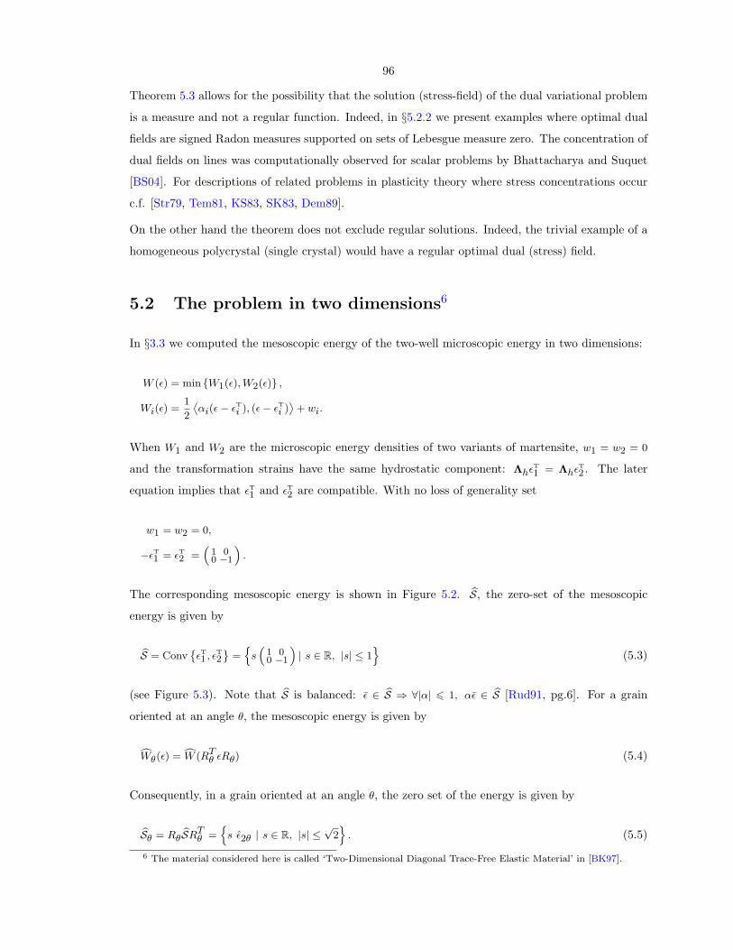
96

Theorem 5.3 allows for the possibility that the solution (stress-field) of the dual variational problem

is a measure and not a regular function. Indeed, in §5.2.2 we present examples where optimal dual

fields are signed Radon measures supported on sets of Lebesgue measure zero. The concentration of

dual fields on lines was computationally observed for scalar problems by Bhattacharya and Suquet

[BS04]. For descriptions of related problems in plasticity theory where stress concentrations occur

c.f. [Str79, Tem81, KS83, SK83, Dem89].

On the other hand the theorem does not exclude regular solutions. Indeed, the trivial example of a

homogeneous polycrystal (single crystal) would have a regular optimal dual (stress) field.

5.2 The problem in two dimensions6

In §3.3 we computed the mesoscopic energy of the two-well microscopic energy in two dimensions:

W (ε) = min W1(ε), W2(ε) ,

Wi(ε) =1

2

˙αi(ε− εT

i ), (ε− εTi )¸

+ wi.

When W1 and W2 are the microscopic energy densities of two variants of martensite, w1 = w2 = 0

and the transformation strains have the same hydrostatic component: ΛhεT1 = ΛhεT

2 . The later

equation implies that εT1 and εT

2 are compatible. With no loss of generality set

w1 = w2 = 0,

−εT1 = εT

2 =“

1 00 −1

”.

The corresponding mesoscopic energy is shown in Figure 5.2. bS, the zero-set of the mesoscopic

energy is given by

bS = Conv˘εT1 , εT

2¯

=n

s“

1 00 −1

”| s ∈ R, |s| ≤ 1

o(5.3)

(see Figure 5.3). Note that bS is balanced: ε ∈ bS ⇒ ∀|α| 6 1, αε ∈ bS [Rud91, pg.6]. For a grain

oriented at an angle θ, the mesoscopic energy is given by

cWθ(ε) = cW (RTθ εRθ) (5.4)

Consequently, in a grain oriented at an angle θ, the zero set of the energy is given by

bSθ = RθbSRT

θ =n

s ε2θ | s ∈ R, |s| ≤√

2o

. (5.5)

6 The material considered here is called ‘Two-Dimensional Diagonal Trace-Free Elastic Material’ in [BK97].

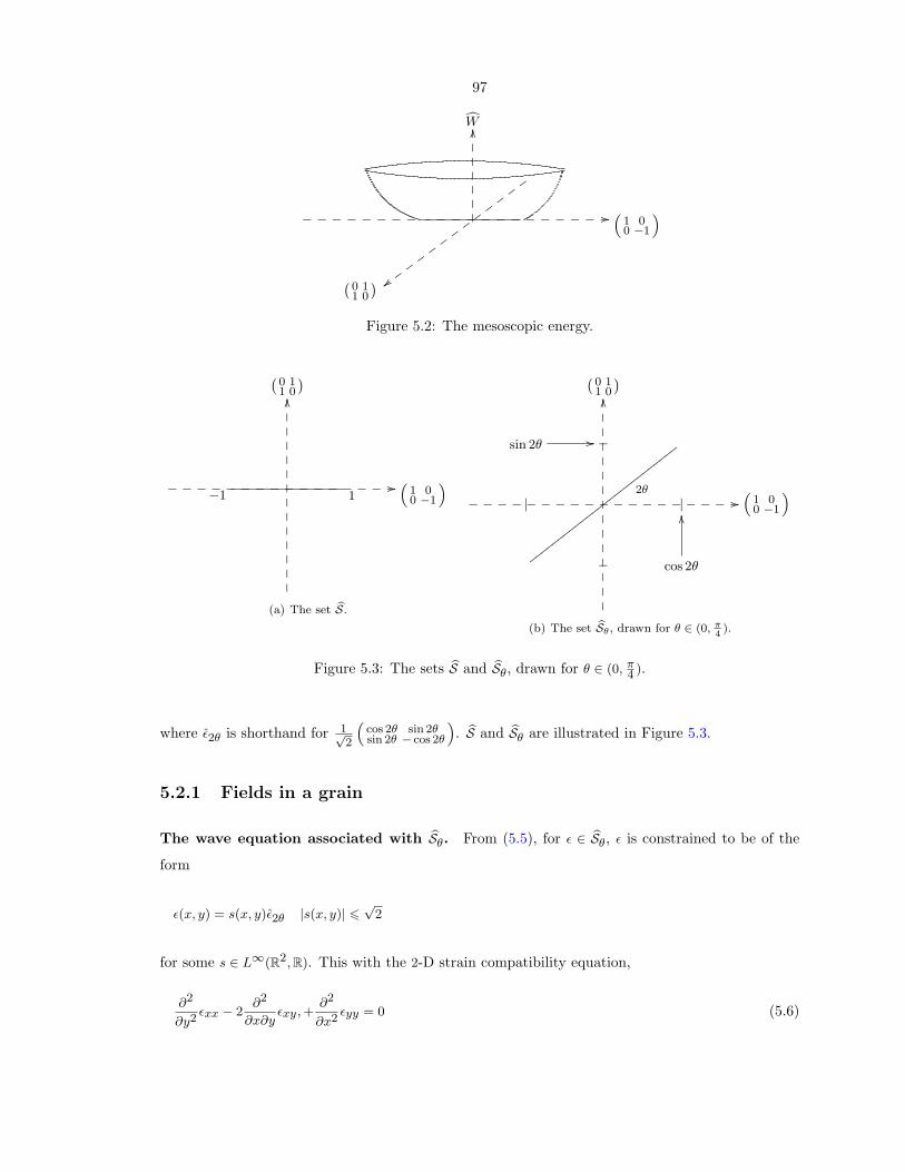
97

cWOO

ww

ww

ww

ww

ww

ww

w

//_____________________ “1 00 −1

”

`0 11 0

´Figure 5.2: The mesoscopic energy.

`0 11 0

´OO

//________________−1 1

“1 00 −1

”

(a) The set bS.

`0 11 0

´OO

sin 2θ // −

xxxxxxxxxxxxxxxxxxxxxxxxxx

//___________________ | |2θ “

1 00 −1

”

− cos 2θ

OO

(b) The set bSθ, drawn for θ ∈ (0, π4).

Figure 5.3: The sets bS and bSθ, drawn for θ ∈ (0, π4 ).

where ε2θ is shorthand for 1√2

“cos 2θ sin 2θsin 2θ − cos 2θ

”. bS and bSθ are illustrated in Figure 5.3.

5.2.1 Fields in a grain

The wave equation associated with bSθ. From (5.5), for ε ∈ bSθ, ε is constrained to be of the

form

ε(x, y) = s(x, y)ε2θ |s(x, y)| 6√

2

for some s ∈ L∞(R2, R). This with the 2-D strain compatibility equation,

∂2

∂y2εxx − 2

∂2

∂x∂yεxy , +

∂2

∂x2εyy = 0 (5.6)

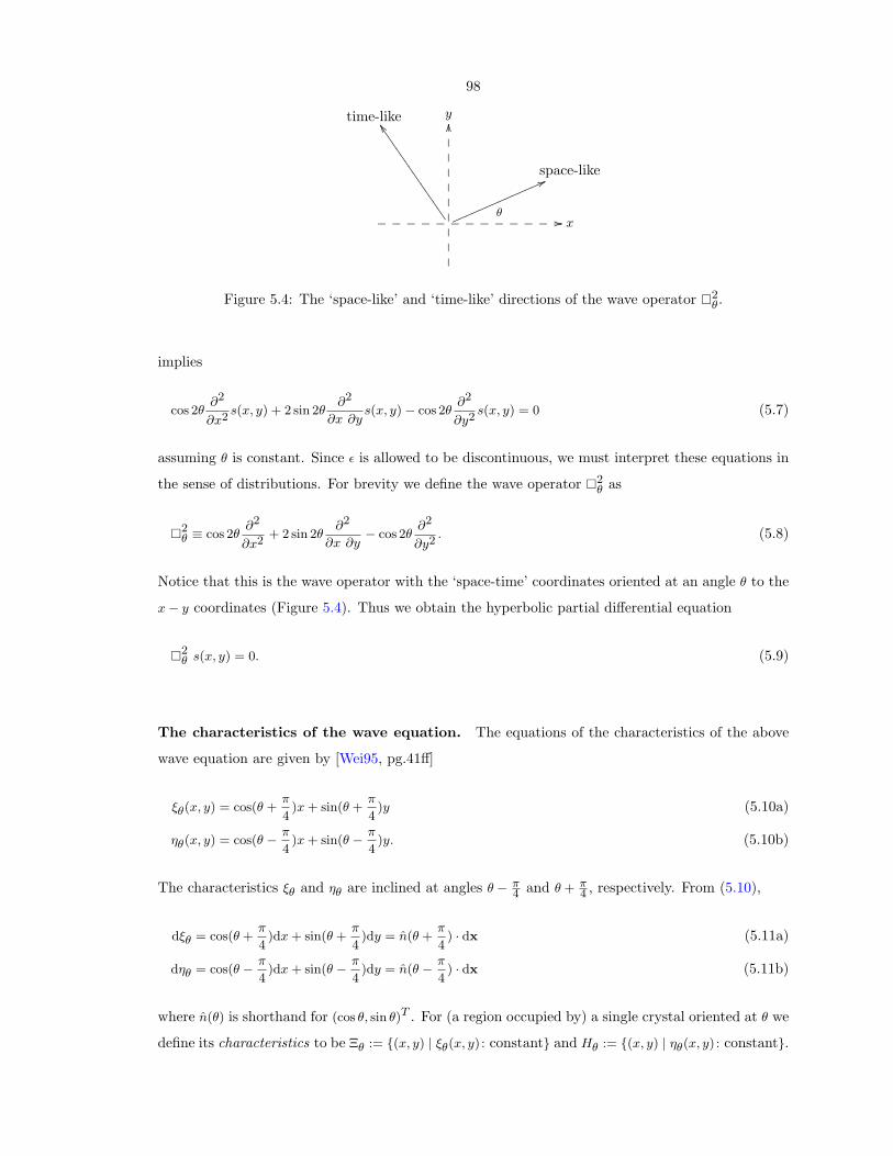
98

time-like yOO

space-like

//_____________

ZZ5555555555555555

66mmmmmmmmmmmmmm θx

Figure 5.4: The ‘space-like’ and ‘time-like’ directions of the wave operator 2θ.

implies

cos 2θ∂2

∂x2s(x, y) + 2 sin 2θ

∂2

∂x ∂ys(x, y)− cos 2θ

∂2

∂y2s(x, y) = 0 (5.7)

assuming θ is constant. Since ε is allowed to be discontinuous, we must interpret these equations in

the sense of distributions. For brevity we define the wave operator 2θ as

2θ ≡ cos 2θ

∂2

∂x2+ 2 sin 2θ

∂2

∂x ∂y− cos 2θ

∂2

∂y2. (5.8)

Notice that this is the wave operator with the ‘space-time’ coordinates oriented at an angle θ to the

x− y coordinates (Figure 5.4). Thus we obtain the hyperbolic partial differential equation

2θ s(x, y) = 0. (5.9)

The characteristics of the wave equation. The equations of the characteristics of the above

wave equation are given by [Wei95, pg.41ff]

ξθ(x, y) = cos(θ +π

4)x + sin(θ +

π

4)y (5.10a)

ηθ(x, y) = cos(θ − π

4)x + sin(θ − π

4)y. (5.10b)

The characteristics ξθ and ηθ are inclined at angles θ − π4 and θ + π

4 , respectively. From (5.10),

dξθ = cos(θ +π

4)dx + sin(θ +

π

4)dy = n(θ +

π

4) · dx (5.11a)

dηθ = cos(θ − π

4)dx + sin(θ − π

4)dy = n(θ − π

4) · dx (5.11b)

where n(θ) is shorthand for (cos θ, sin θ)T . For (a region occupied by) a single crystal oriented at θ we

define its characteristics to be Ξθ := (x, y) | ξθ(x, y) : constant and Hθ := (x, y) | ηθ(x, y) : constant.

99

The strain field. From (5.10), in every convex domain, s : R2 → R which satisfies 2θ s(x, y) = 0

in a distributional sense is constrained to be of the form

s(x, y) = p(ξθ) + q(ηθ) (5.12)

for some p, q ∈ L∞(R). For a strain field ε(x, y) ≡ s(x, y) ε2θ with 2θ s(x, y) = 0, we define the strain

on the characteristic ξθ to be p(ξθ)ε2θ and the strain on the characteristic ηθ to be q(ηθ)ε2θ.

The displacement gradient. Let H := ∇u be the displacement gradient. Since ε ≡ sym(H), the

constraint ε ∈ bSθ is equivalent to the constraint H ∈ bSθ ⊕ Spann“

0 1−1 0

”o:

H(x, y) = s(x, y)ε2θ + ω(x, y)1√2

“0 1−1 0

”|s(x, y)| 6

√2 (5.13)

for some s ∈ L∞(R2, R) and some ω : R2 → R. This with the compatibility condition ∇ × H = 0

implies

− sin 2θ∂

∂xs(x, y) + cos 2θ

∂

∂ys(x, y) =

∂

∂xw(x, y) (5.14a)

cos 2θ∂

∂xs(x, y) + sin 2θ

∂

∂ys(x, y) =

∂

∂yw(x, y). (5.14b)

These are a pair on non-homogeneous transport equations which can be written as

∇w(x, y) =“− sin 2θ cos 2θcos 2θ sin 2θ

”∇s(x, y). (5.15)

This implies that

2θ w(x, y) = 0. (5.16)

Note that“− sin 2θ cos 2θcos 2θ sin 2θ

”is a reflection operator that leaves n(θ + π

4 ) invariant. From (5.11) and

(5.12),

∇s(x, y) = p′(ξθ) n(θ +π

4) + q′(ηθ) n(θ − π

4).

Using this in (5.15),

∇w(x, y) = p′(ξθ) n(θ +π

4) − q′(ηθ) n(θ − π

4)

100

and thus,

w(x, y) = p(ξθ)− q(ηθ) + constant. (5.17)

From these we obtain

H(x, y) = s(x, y)ε2θ + w(x, y)1√2

“0 1−1 0

”= p(ξθ)

„ε2θ +

1√2

“0 1−1 0

”«+ q(ηθ)

„ε2θ −

1√2

“0 1−1 0

”«+ c

“0 1−1 0

”=√

2p(ξθ)n(θ − π

4)⊗ n(θ +

π

4) +

√2q(ηθ)n(θ +

π

4)⊗ n(θ − π

4) + c

“0 1−1 0

”. (5.18)

Here c is a constant and we have used (5.12), (5.17) and the relations

ε2θ =√

2n(θ − π

4)⊗s n(θ +

π

4) (5.19a)“

0 1−1 0

”= n(θ − π

4)⊗ n(θ +

π

4)− n(θ +

π

4)⊗ n(θ − π

4) (5.19b)

ε2θ +1√2

“0 1−1 0

”=√

2n(θ − π

4)⊗ n(θ +

π

4) (5.19c)

ε2θ −1√2

“0 1−1 0

”=√

2n(θ +π

4)⊗ n(θ − π

4). (5.19d)

In an un-oriented grain θ = 0, and thus from (5.13),

H(x, y) =1√2

“s(x,y) w(x,y)−w(x,y) −s(x,y)

”(5.20)

For a strain field ε(x, y) ≡ s(x, y)ε2θ that satisfies 2θ s(x, y) = 0, we define the displacement gradient on

the characteristic ξθ to be p(ξθ)“ε2θ + 1√

2

“0 1−1 0

””=√

2p(ξθ)n(θ− π4 )⊗ n(θ+ π

4 ) and the displacement

gradient on the characteristic ηθ to be q(ηθ)“ε2θ − 1√

2

“0 1−1 0

””=√

2q(ηθ)n(θ + π4 )⊗ n(θ − π

4 ).

Remark 5.7. From (5.17), ω ∈ L∞(R2, R) and thus from (5.13) H ∈ L∞(R2, M2×2). Thus u is in

fact in W 1,∞(Ω, R2).

The displacement. From (5.18) and (5.11) the displacement u(x) =R

H(x)dx in every convex

subset of a grain oriented at θ is given by

u(x, y) =√

2

Zp(ξθ)n− ⊗ n⊥− dx +

√2

Zq(ηθ)n⊥− ⊗ n− dx + c

Z “0 1−1 0

”dx

=√

2

Z(p(ξθ) + c)n⊥− · dxn− +

√2

Z(q(ηθ)− c)n− · dxn⊥−

=

„√2

Zp(ξθ) dξθ + cξθ

«n(θ − π

4) +

„√2

Zq(ηθ) dηθ − cηθ

«n(θ +

π

4) + d

where c ∈ R and d ∈ R2 are constants.

101

Characterization of dual fields with zero conjugate energy. The conjugate of cW is [BK97,

pg. 125]

cW ?θ (σ) := sup

ε∈M2×2sym

nε · σ −cWθ(ε)

o=√

2|σ · ε2θ|. (5.21)

From (5.21), cW ?θ (σ) = 0 precisely when σ · ε2θ = 0. This occurs precisely when σ is of the form

σ(x, y) = σh(x, y)I +√

2t(x, y)ε2θ+π2

.

Here I is shorthand for`

1 00 1

´. This with the compatibility equation div(σ) = 0 implies

− sin 2θ∂

∂xt(x, y) + cos 2θ

∂

∂yt(x, y) =

∂

∂xσh(x, y) (5.22a)

cos 2θ∂

∂xt(x, y) + sin 2θ

∂

∂yt(x, y) =

∂

∂yσh(x, y). (5.22b)

These are a pair on non-homogeneous transport equations which can be written as

∇σh(x, y) =“− sin 2θ cos 2θcos 2θ sin 2θ

”∇t(x, y). (5.23)

These imply that

2θ t(x, y) = 0, (5.24a)

2θ σh(x, y) = 0. (5.24b)

Compare (5.22) with (5.14); (5.23) with (5.15); and (5.24) with (5.9) and (5.16). In particular the

characteristics of each of the two wave equations in (5.24) are inclined at angles θ − π4 and θ + π

4 .

5.2.2 Polycrystals

Note that 0 ∈ S for any polycrystal since the Taylor bound T = 0. We shall call a polycrystal

‘rigid’ if S = 0 and ‘flexible’ otherwise. The characterization of strain fields in a grain in §5.2.1

leads to the following observation: any polycrystal in which a non-negligible set of characteristics

percolate — i.e., do not intersect interfaces — is flexible. Example 5.13 presents one such polycrystal.

However the flexibility of any polycrystal is limited:

Proposition 5.8. For any polycrystal, dim(S) 6 1.

Bhattacharya and Kohn [BK97, Thm. 5.3, pg.163] used a translation to prove this result for strain

fields in L2(Ω, M2×2sym ). Here we use duality in the context of L∞per(Ω, M2×2

sym ).

102

Proof. We shall prove the equivalent statement: for any polycrystal, dim(S) 6= 0 ⇒ dim(S) = 1. Let

0 6= ε ∈ S. Thus ∃s, w ∈ L∞per(Ω, R) such that in a grain oriented at θ, the displacement gradient H is

of the form

H(x, y) =√

2s(x, y)ε2θ + w(x, y)“

0 1−1 0

”(5.13)

where

∇w(x, y) =“− sin 2θ cos 2θcos 2θ sin 2θ

”∇s(x, y); (5.15)

at an interface between grains, for all (x, y) in the interface,

JH(x, y)K ‖ n⊥(x, y)⊗ n(x, y); (5.25)

and

√2〈s(x, y)ε2θ(x,y)〉 = ε. (5.26)

Consider the field which in each grain is given by

σ(x, y) = w(x, y)I +√

2s(x, y)ε2θ(x,y)+π2

. (5.27)

Note that σ(x, y) · ε2θ(x,y) = 0. Observe that this is a dual field since it is divergence free: in each

grain, (c.f. (5.15)),

div(σ(x, y)) = ∇w(x, y)−“− sin 2θ cos 2θcos 2θ sin 2θ

”∇s(x, y) = 0;

at an interface between grains, for all (x, y) in the interface, Jσ(x, y)Kn(x, y) = 0:

Jσ(x, y)K = Jw(x, y)I +√


K

= J√

2s(x, y)ε2θ(x,y) + w(x, y)“

0 1−1 0

”K“

0 1−1 0

”= JH(x, y)K

“0 1−1 0

”= (n⊥(x, y)⊗ n(x, y))

“0 1−1 0

”= n⊥(x, y)⊗ n⊥(x, y)

103

where we have used ε2θ(x,y)+π2

= ε2θ(x,y)

“0 1−1 0

”and (5.25). Thus, using (5.26),

〈σ(x, y)〉 = 〈w(x, y)〉I + 〈√

2s(x, y)ε2θ(x,y)+π2〉

= 〈w(x, y)〉I + 〈√

2s(x, y)ε2θ(x,y)〉“

0 1−1 0

”= 〈w(x, y)〉I + ε

“0 1−1 0

”. (5.28)

Let ε′ be such that Tr ε′ = 0. By the dual variational principle (theorem 5.3) and (5.21),

δS (ε′) > 〈σ(x, y)〉 · ε′ − 〈|σ(x, y) · ε2θ(x,y)|〉

= 〈σ(x, y)〉 · ε′

= 〈w(x, y)〉I · ε′ + (ε′“

0 1−1 0

”) · ε

= (ε′“

0 1−1 0

”) · ε

> 0,

(by changing the sign of σ if necessary) except when ε′ ‖ ε. Thus

0 6= ε ∈ S ⇒ S ⊂ Span ε ⇒ dim(S) = 1

We also present a variant of the above proof that does not use the dual variational principle:

Proof. Assume on the contrary that for a polycrystal dim(S) = 2. Then, since S is balanced7 and

convex, there exists ε 6= 0 such that ε ∈ S and RTπ4

εRπ4

= ε“

0 1−1 0

”∈ S. Since ε ∈ S, as in the proof

above, there exist s, w ∈ L∞per(Ω, R) such that σ ∈ L∞per(Ω, M2×2sym ) given by

σ(x, y) = w(x, y)I +√


. (5.27)

and satisfying

〈σ(x, y)〉 = 〈w(x, y)〉I + ε“

0 1−1 0

”(5.28)

is divergence free. Since ε“

0 1−1 0

”∈ S, there exist s′, w′ ∈ L∞per(Ω, R) such that H ∈ L∞per(Ω, M2×2)

given by

H(x, y) =√

2s′(x, y)ε2θ(x,y) + w′(x, y)“

0 1−1 0

”(5.29)

7 This follows from bS being balanced.

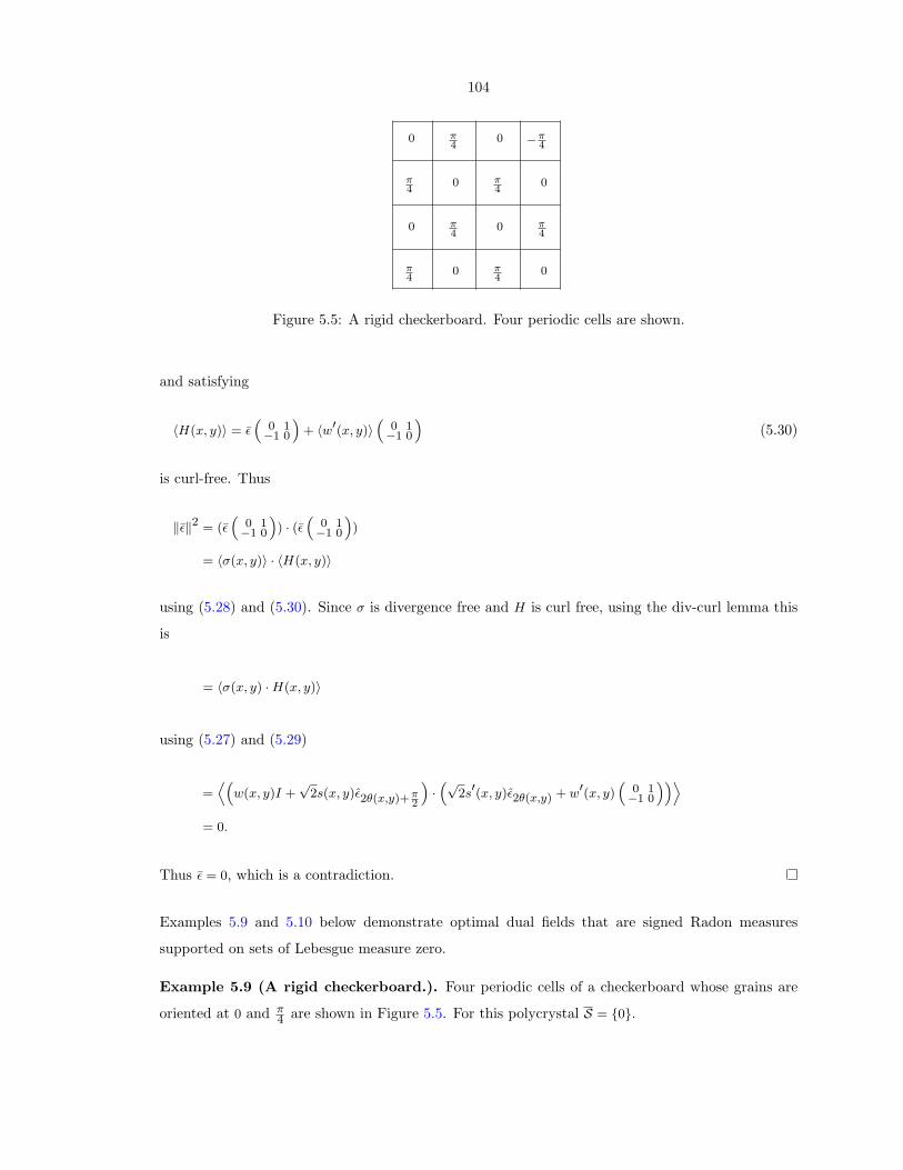
104

0 π4

0 −π4

π4

0 π4

0

0 π4

0 π4

π4

0 π4

0

Figure 5.5: A rigid checkerboard. Four periodic cells are shown.

and satisfying

〈H(x, y)〉 = ε“

0 1−1 0

”+ 〈w′(x, y)〉

“0 1−1 0

”(5.30)

is curl-free. Thus

‖ε‖2 = (ε“

0 1−1 0

”) · (ε

“0 1−1 0

”)

= 〈σ(x, y)〉 · 〈H(x, y)〉

using (5.28) and (5.30). Since σ is divergence free and H is curl free, using the div-curl lemma this

is

= 〈σ(x, y) ·H(x, y)〉

using (5.27) and (5.29)

=D“

w(x, y)I +√


”·“√

2s′(x, y)ε2θ(x,y) + w′(x, y)“

0 1−1 0

””E= 0.

Thus ε = 0, which is a contradiction.

Examples 5.9 and 5.10 below demonstrate optimal dual fields that are signed Radon measures

supported on sets of Lebesgue measure zero.

Example 5.9 (A rigid checkerboard.). Four periodic cells of a checkerboard whose grains are

oriented at 0 and π4 are shown in Figure 5.5. For this polycrystal S = 0.

105

Proof. Consider a measure valued field σ supported on the diagonal line shown in Figure 5.6 and

taking the value`

11

´⊗`

11

´=`

1 11 1

´. Note that this field is divergence free and thus is contained in

Sad. The average of this field is 12

`1 11 1

´. The support of the dual field lies within the grains oriented

at 0. From the remark following (5.24) the conjugate energy of the dual field is zero. Thus from the

dual variational principle (theorem 5.3), δS (ε) > 〈σ〉 · ε which — changing the sign of σ if necessary

— is positive except when ε ‖“

1 00 −1

”.

Consider next a family σθ of measure valued fields, parameterized by θ ∈ (0, π4 ), supported on the

lines shown in Figure 5.6 and taking the value

8>>>>>>>>>>>>>>>>>><>>>>>>>>>>>>>>>>>>:

`01

´⊗`

01

´on the vertical line

(which, in a grain, is of length 1− tan θ),

12 sin θ

“cos θsin θ

”⊗“

cos θsin θ

”on the lines inclined at θ

(which, in a grain, are of total length 1sin θ ),

12 sin θ

“cos θ− sin θ

”⊗“

cos θ− sin θ

”on the lines inclined at −θ

(which, in a grain, are of total length 1sin θ ).

Note that the field is divergence free and thus is contained in Sad. The support of the dual field lies

within the grains oriented at π4 . The average value of this field is

〈σθ〉 =1

2

„(1− tan θ)

`01

´⊗`

01

´+

1

2 sin2 θ

“cos θsin θ

”⊗“

cos θsin θ

”+

1

2 sin2 θ

“cos θ− sin θ

”⊗“

cos θ− sin θ

”«=

1

2(1− tan θ)

`0 00 1

´+

1

4 sin2 θ

““cos2 θ − cos θ sin θ

− cos θ sin θ sin2 θ

”+“

cos2 θ cos θ sin θcos θ sin θ sin2 θ

””=

1

2(1− tan θ)

`0 00 1

´+

1

2 sin2 θ

“cos2 θ 0

0 sin2 θ

”=

1

2

„1

tan2 θ0

0 2−tan θ

«.

The average conjugate energy is

〈δ?bS (RT (x)σθR(x))〉 =

√2

4 sin2 θ|− cos θ sin θ|+

√2

4 sin2 θ|cos θ sin θ| = 1√

2 tan θ.

Note that the ratio

〈δ?bS (RT (x)σθR(x))〉

〈σθ〉 ·“

1 00 −1

” =2√

2 tan θ1

tan2 θ− 2 + tan θ

→ 0+ as θ → 0.

Thus for every 0 6= ε ‖“

1 00 −1

”with ‖ε‖ sufficiently small, there exists θ such that δS (ε) > 〈σθ〉 · ε −

〈δ?bS (RT (x)σθR(x))〉 > 0.

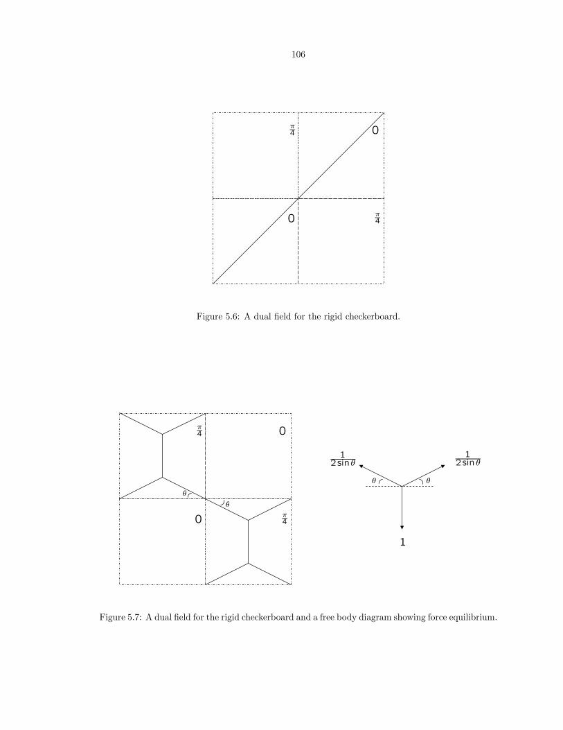
106

π4

π4

0

0

Figure 5.6: A dual field for the rigid checkerboard.

π4

π4

0

0

θ

θ

θθ

1

12sinθ

12sinθ

Figure 5.7: A dual field for the rigid checkerboard and a free body diagram showing force equilibrium.

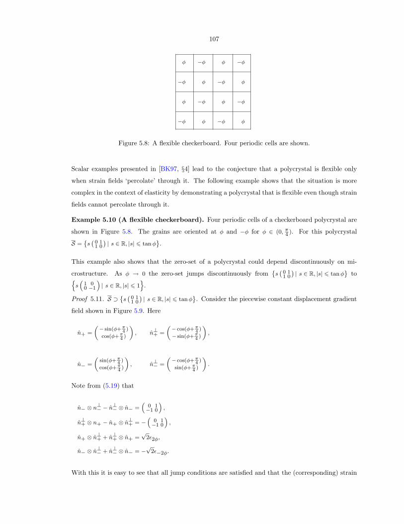
107

φ −φ φ −φ

−φ φ −φ φ

φ −φ φ −φ

−φ φ −φ φ

Figure 5.8: A flexible checkerboard. Four periodic cells are shown.

Scalar examples presented in [BK97, §4] lead to the conjecture that a polycrystal is flexible only

when strain fields ‘percolate’ through it. The following example shows that the situation is more

complex in the context of elasticity by demonstrating a polycrystal that is flexible even though strain

fields cannot percolate through it.

Example 5.10 (A flexible checkerboard). Four periodic cells of a checkerboard polycrystal are

shown in Figure 5.8. The grains are oriented at φ and −φ for φ ∈ (0, π4 ). For this polycrystal

S =˘s`

0 11 0

´| s ∈ R, |s| 6 tan φ

¯.

This example also shows that the zero-set of a polycrystal could depend discontinuously on mi-

crostructure. As φ → 0 the zero-set jumps discontinuously from˘s`

0 11 0

´| s ∈ R, |s| 6 tan φ

¯ton

s“

1 00 −1

”| s ∈ R, |s| 6 1

o.

Proof 5.11. S ⊃˘s`

0 11 0

´| s ∈ R, |s| 6 tan φ

¯. Consider the piecewise constant displacement gradient

field shown in Figure 5.9. Here

n+ =

„− sin(φ+π

4 )

cos(φ+π4 )

«, n⊥+ =

„− cos(φ+π

4 )

− sin(φ+π4 )

«,

n− =

„sin(φ+π

4 )

cos(φ+π4 )

«, n⊥− =

„− cos(φ+π

4 )

sin(φ+π4 )

«.

Note from (5.19) that

n− ⊗ n⊥− − n⊥− ⊗ n− =“

0 1−1 0

”,

n⊥+ ⊗ n+ − n+ ⊗ n⊥+ = −“

0 1−1 0

”,

n+ ⊗ n⊥+ + n⊥+ ⊗ n+ =√

2ε2φ,

n− ⊗ n⊥− + n⊥− ⊗ n− = −√

2ε−2φ.

With this it is easy to see that all jump conditions are satisfied and that the (corresponding) strain

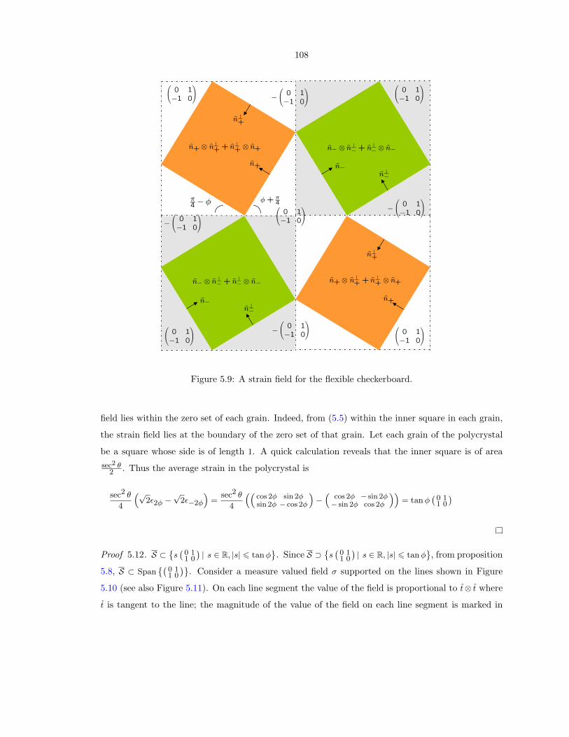
108

Ã0 1−1 0

! Ã0 1−1 0

!

Ã0 1−1 0

!

Ã0 1−1 0

! Ã0 1−1 0

!

−Ã0 1−1 0

!

−Ã0 1−1 0

! −Ã0 1−1 0

!

−Ã0 1−1 0

!

φ+ π4

π4 − φ

n−n⊥−

n+

n⊥+

n−n⊥−

n+

n⊥+

n+⊗ n⊥+ + n⊥+ ⊗ n+ n− ⊗ n⊥−+ n⊥− ⊗ n−

n− ⊗ n⊥−+ n⊥− ⊗ n− n+⊗ n⊥+ + n⊥+ ⊗ n+

Figure 5.9: A strain field for the flexible checkerboard.

field lies within the zero set of each grain. Indeed, from (5.5) within the inner square in each grain,

the strain field lies at the boundary of the zero set of that grain. Let each grain of the polycrystal

be a square whose side is of length 1. A quick calculation reveals that the inner square is of areasec2 θ

2 . Thus the average strain in the polycrystal is

sec2 θ

4

“√2ε2φ −

√2ε−2φ

”=

sec2 θ

4

““cos 2φ sin 2φsin 2φ − cos 2φ

”−“

cos 2φ − sin 2φ− sin 2φ cos 2φ

””= tan φ

`0 11 0

´

Proof 5.12. S ⊂˘s`

0 11 0

´| s ∈ R, |s| 6 tan φ

¯. Since S ⊃

˘s`

0 11 0

´| s ∈ R, |s| 6 tan φ

¯, from proposition

5.8, S ⊂ Span˘`

0 11 0

´¯. Consider a measure valued field σ supported on the lines shown in Figure

5.10 (see also Figure 5.11). On each line segment the value of the field is proportional to t⊗ t where

t is tangent to the line; the magnitude of the value of the field on each line segment is marked in

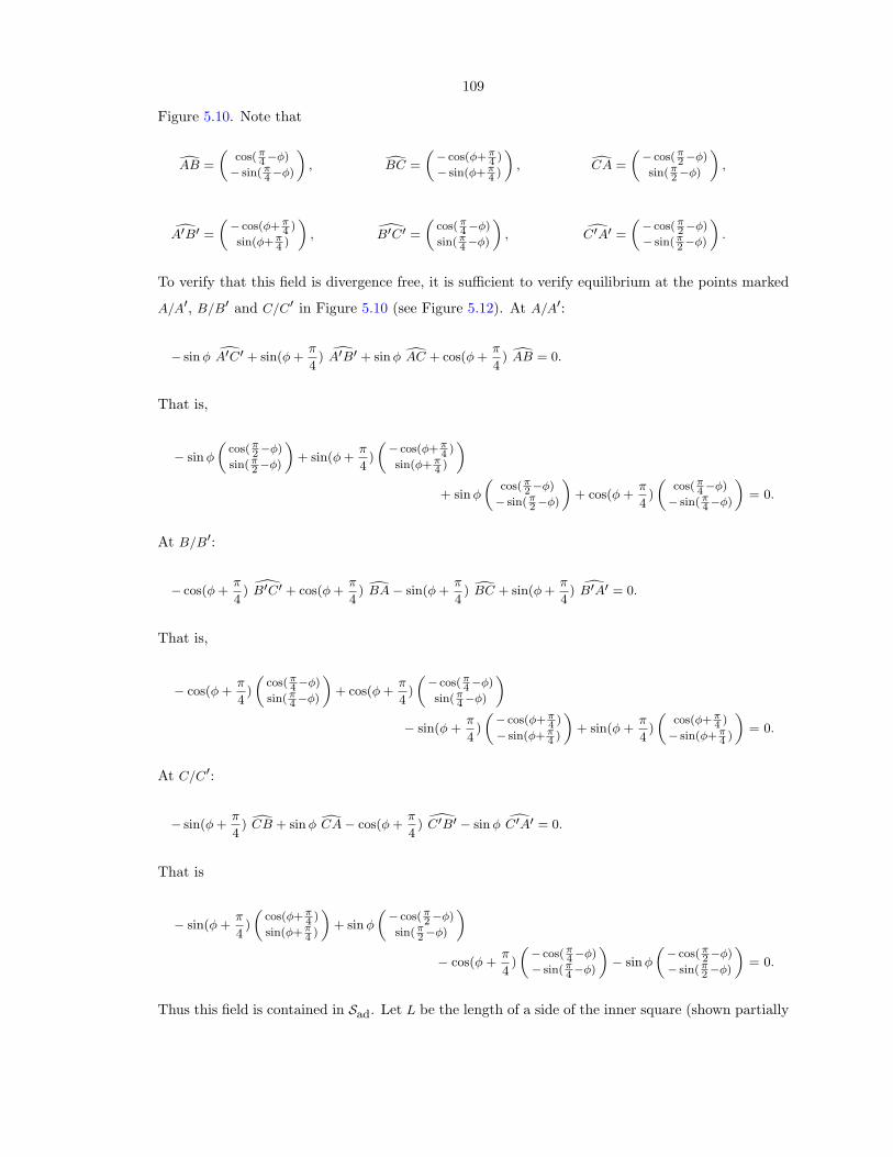
109

Figure 5.10. Note that

dAB =

„cos(π

4−φ)

− sin(π4−φ)

«, dBC =

„− cos(φ+π

4 )

− sin(φ+π4 )

«, dCA =

„− cos(π

2−φ)

sin(π2−φ)

«,

dA′B′ =

„− cos(φ+π

4 )

sin(φ+π4 )

«, B′C′ =

„cos(π

4−φ)

sin(π4−φ)

«, dC′A′ =

„− cos(π

2−φ)

− sin(π2−φ)

«.

To verify that this field is divergence free, it is sufficient to verify equilibrium at the points marked

A/A′, B/B′ and C/C′ in Figure 5.10 (see Figure 5.12). At A/A′:

− sin φ dA′C′ + sin(φ +π

4) dA′B′ + sin φ dAC + cos(φ +

π

4) dAB = 0.

That is,

− sin φ

„cos(π

2−φ)

sin(π2−φ)

«+ sin(φ +

π

4)

„− cos(φ+π

4 )

sin(φ+π4 )

«+ sin φ

„cos(π

2−φ)

− sin(π2−φ)

«+ cos(φ +

π

4)

„cos(π

4−φ)

− sin(π4−φ)

«= 0.

At B/B′:

− cos(φ +π

4) B′C′ + cos(φ +

π

4) dBA− sin(φ +

π

4) dBC + sin(φ +

π

4) dB′A′ = 0.

That is,

− cos(φ +π

4)

„cos(π

4−φ)

sin(π4−φ)

«+ cos(φ +

π

4)

„− cos(π

4−φ)

sin(π4−φ)

«− sin(φ +

π

4)

„− cos(φ+π

4 )

− sin(φ+π4 )

«+ sin(φ +

π

4)

„cos(φ+π

4 )

− sin(φ+π4 )

«= 0.

At C/C′:

− sin(φ +π

4) dCB + sin φ dCA− cos(φ +

π

4) C′B′ − sin φ dC′A′ = 0.

That is

− sin(φ +π

4)

„cos(φ+π

4 )

sin(φ+π4 )

«+ sin φ

„− cos(π

2−φ)

sin(π2−φ)

«− cos(φ +

π

4)

„− cos(π

4−φ)

− sin(π4−φ)

«− sin φ

„− cos(π

2−φ)

− sin(π2−φ)

«= 0.

Thus this field is contained in Sad. Let L be the length of a side of the inner square (shown partially

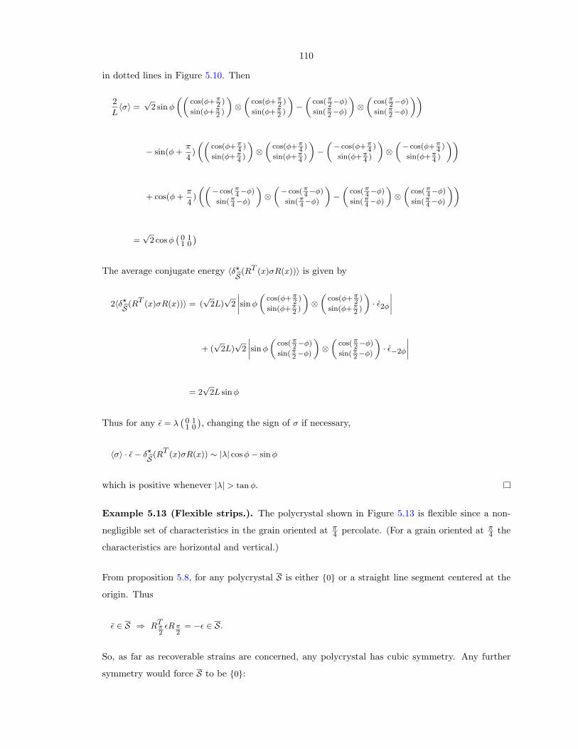
110

in dotted lines in Figure 5.10. Then

2

L〈σ〉 =

√2 sin φ

„„cos(φ+π

2 )

sin(φ+π2 )

«⊗„

cos(φ+π2 )

sin(φ+π2 )

«−„

cos(π2−φ)

sin(π2−φ)

«⊗„

cos(π2−φ)

sin(π2−φ)

««

− sin(φ +π

4)

„„cos(φ+π

4 )

sin(φ+π4 )

«⊗„

cos(φ+π4 )

sin(φ+π4 )

«−„− cos(φ+π

4 )

sin(φ+π4 )

«⊗„− cos(φ+π

4 )

sin(φ+π4 )

««

+ cos(φ +π

4)

„„− cos(π

4−φ)

sin(π4−φ)

«⊗„− cos(π

4−φ)

sin(π4−φ)

«−„

cos(π4−φ)

sin(π4−φ)

«⊗„

cos(π4−φ)

sin(π4−φ)

««

=√

2 cos φ`

0 11 0

´The average conjugate energy 〈δ?bS (RT (x)σR(x))〉 is given by

2〈δ?bS (RT (x)σR(x))〉 = (√

2L)√

2

˛sin φ

„cos(φ+π

2 )

sin(φ+π2 )

«⊗„

cos(φ+π2 )

sin(φ+π2 )

«· ε2φ

˛

+ (√

2L)√

2

˛sin φ

„cos(π

2−φ)

sin(π2−φ)

«⊗„

cos(π2−φ)

sin(π2−φ)

«· ε−2φ

˛

= 2√

2L sin φ

Thus for any ε = λ`

0 11 0

´, changing the sign of σ if necessary,

〈σ〉 · ε− δ?bS (RT (x)σR(x)) ∼ |λ| cos φ− sin φ

which is positive whenever |λ| > tan φ.

Example 5.13 (Flexible strips.). The polycrystal shown in Figure 5.13 is flexible since a non-

negligible set of characteristics in the grain oriented at π4 percolate. (For a grain oriented at π

4 the

characteristics are horizontal and vertical.)

From proposition 5.8, for any polycrystal S is either 0 or a straight line segment centered at the

origin. Thus

ε ∈ S ⇒ RTπ2

εRπ2

= −ε ∈ S.

So, as far as recoverable strains are concerned, any polycrystal has cubic symmetry. Any further

symmetry would force S to be 0:

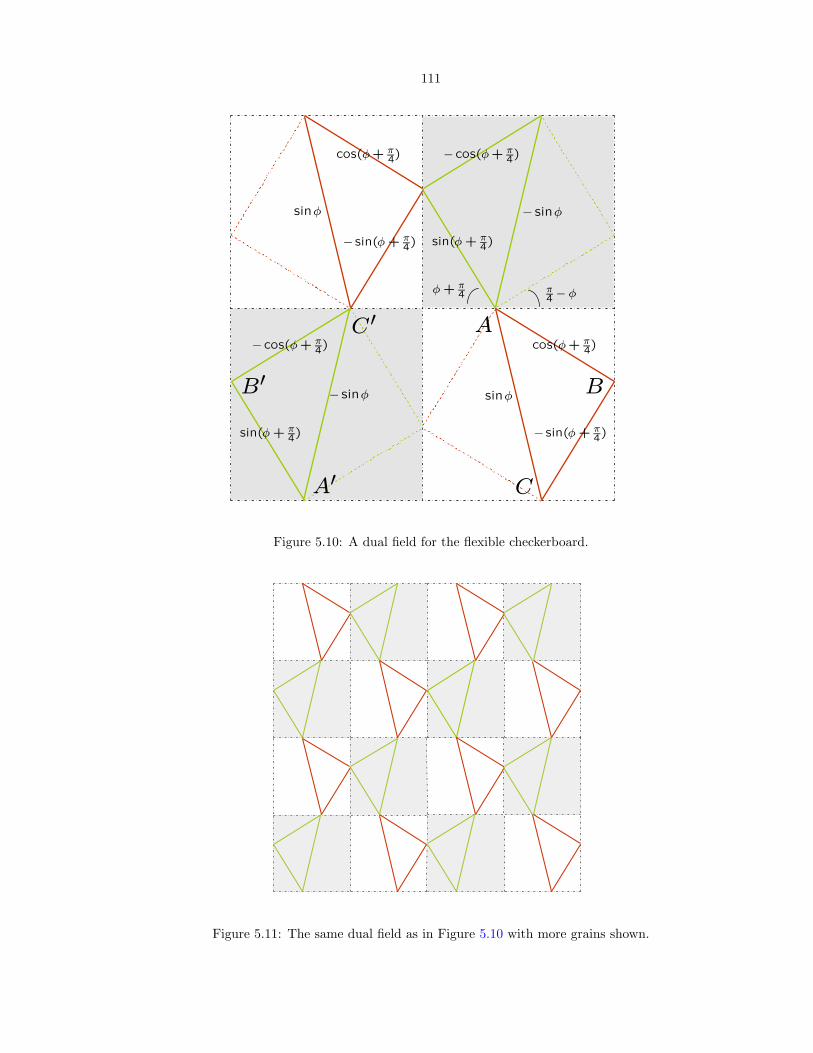
111

− sinφ

sin(φ+ π4)

sinφ

sinφ

sin(φ+ π4)

− sin(φ+ π4)

− sin(φ+ π4)

cos(φ+ π4)

cos(φ+ π4)

− cos(φ+ π4)

− cos(φ+ π4)

− sinφ

π4 − φφ+ π

4

A

A0

BB0

C

C 0

Figure 5.10: A dual field for the flexible checkerboard.

Figure 5.11: The same dual field as in Figure 5.10 with more grains shown.

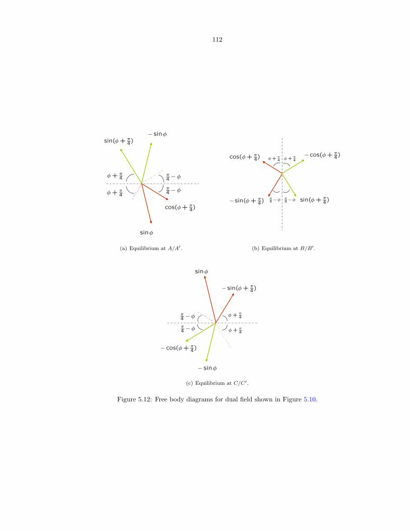
112

cos(φ+ π4)

sin(φ+ π4)

π4 − φπ4 − φ

φ+ π4

φ+ π4

− sinφ

sinφ

(a) Equilibrium at A/A′.

sin(φ+ π4)− sin(φ+ π

4)

cos(φ+ π4)

− cos(φ+ π4)φ+ π

4 φ+ π4

π4 − φ π

4 − φ

(b) Equilibrium at B/B′.

sinφ

− sin(φ+ π4)

− cos(φ+ π4)

φ+ π4

π4 − φ

φ+ π4

π4 − φ

− sinφ

(c) Equilibrium at C/C′.

Figure 5.12: Free body diagrams for dual field shown in Figure 5.10.

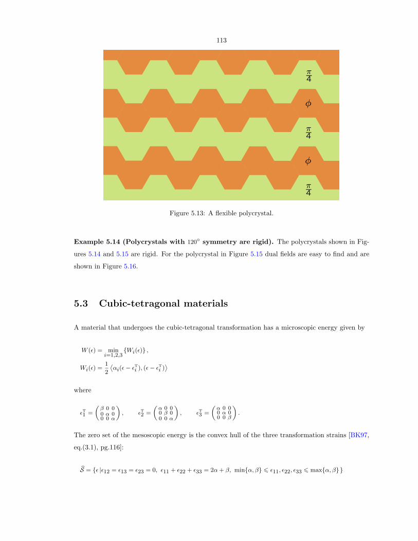
113

π4

π4

π4

φ

φ

Figure 5.13: A flexible polycrystal.

Example 5.14 (Polycrystals with 120 symmetry are rigid). The polycrystals shown in Fig-

ures 5.14 and 5.15 are rigid. For the polycrystal in Figure 5.15 dual fields are easy to find and are

shown in Figure 5.16.

5.3 Cubic-tetragonal materials

A material that undergoes the cubic-tetragonal transformation has a microscopic energy given by

W (ε) = mini=1,2,3

Wi(ε) ,

Wi(ε) =1

2

˙αi(ε− εT

i ), (ε− εTi )¸

where

εT1 =

„β 0 00 α 00 0 α

«, εT

2 =

„α 0 00 β 00 0 α

«, εT

3 =

„α 0 00 α 00 0 β

«.

The zero set of the mesoscopic energy is the convex hull of the three transformation strains [BK97,

eq.(3.1), pg.116]:

bS = ε |ε12 = ε13 = ε23 = 0, ε11 + ε22 + ε33 = 2α + β, minα, β 6 ε11, ε22, ε33 6 maxα, β

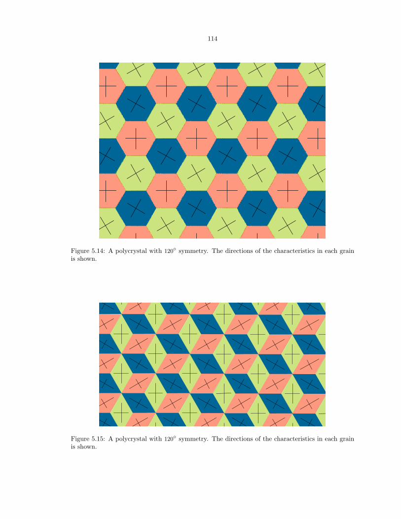
114

Figure 5.14: A polycrystal with 120 symmetry. The directions of the characteristics in each grainis shown.

Figure 5.15: A polycrystal with 120 symmetry. The directions of the characteristics in each grainis shown.

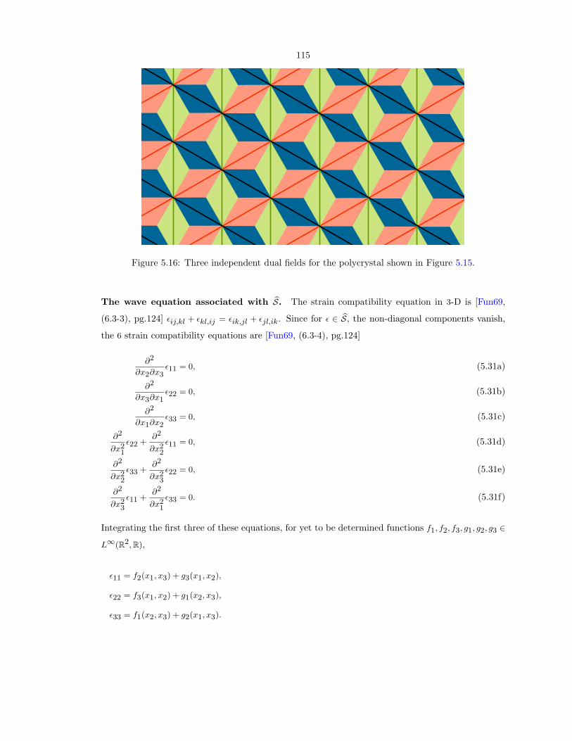
115

Figure 5.16: Three independent dual fields for the polycrystal shown in Figure 5.15.

The wave equation associated with bS. The strain compatibility equation in 3-D is [Fun69,

(6.3-3), pg.124] εij,kl + εkl,ij = εik,jl + εjl,ik. Since for ε ∈ bS, the non-diagonal components vanish,

the 6 strain compatibility equations are [Fun69, (6.3-4), pg.124]

∂2

∂x2∂x3ε11 = 0, (5.31a)

∂2

∂x3∂x1ε22 = 0, (5.31b)

∂2

∂x1∂x2ε33 = 0, (5.31c)

∂2

∂x21

ε22 +∂2

∂x22

ε11 = 0, (5.31d)

∂2

∂x22

ε33 +∂2

∂x23

ε22 = 0, (5.31e)

∂2

∂x23

ε11 +∂2

∂x21

ε33 = 0. (5.31f)

Integrating the first three of these equations, for yet to be determined functions f1, f2, f3, g1, g2, g3 ∈

L∞(R2, R),

ε11 = f2(x1, x3) + g3(x1, x2),

ε22 = f3(x1, x2) + g1(x2, x3),

ε33 = f1(x2, x3) + g2(x1, x3).

116

Since ε11 + ε22 + ε33 = 2α + β (a constant) we have

f1(x2, x3) + g1(x2, x3) + f2(x1, x3) + g2(x1, x3) + f3(x1, x2) + g3(x1, x2) = 2α + β.

The first two terms are independent of x1; the second two of x2; and the last two of x3. Thus the

sum of these six terms can add to an constant if and only if for constants c1, c2 and c3,

f1(x2, x3) + g1(x2, x3) = c1,

f2(x1, x3) + g2(x1, x3) = c2,

f3(x1, x2) + g3(x1, x2) = c3.

Here c1 + c2 + c3 = 2α + β. Thus we obtain

ε11 = f2(x1, x3)− f3(x1, x2) + c3,

ε22 = f3(x1, x2)− f1(x2, x3) + c1,

ε33 = f1(x2, x3)− f2(x1, x3) + c2.

From these equations and (5.31),

∂2

∂x22

ε33 +∂2

∂x23

ε22 = 0 ⇒

∂2

∂x22

− ∂2

∂x23

!f1(x2, x3) = 0,

∂2

∂x23

ε11 +∂2

∂x21

ε33 = 0 ⇒

∂2

∂x23

− ∂2

∂x21

!f2(x1, x3) = 0,

∂2

∂x21

ε22 +∂2

∂x22

ε11 = 0 ⇒

∂2

∂x21

− ∂2

∂x22

!f3(x1, x2) = 0.

The strain field. To summarize, the strain field in any un-oriented grain must be of the form

ε11 = f2(x1, x3)− f3(x1, x2) + c3, (5.32a)

ε22 = f3(x1, x2)− f1(x2, x3) + c1, (5.32b)

ε33 = f1(x2, x3)− f2(x1, x3) + c2 (5.32c)

117

where f1, f2, f3 ∈ L∞(R2, R) satisfy

∂2

∂x22

− ∂2

∂x23

!f1(x2, x3) = 0, (5.33a)

∂2

∂x23

− ∂2

∂x21

!f2(x1, x3) = 0, (5.33b)

∂2

∂x21

− ∂2

∂x22

!f3(x1, x2) = 0. (5.33c)

As in §5.2 (c.f. (5.10)), associated with the three wave operators in (5.33) are three pairs of charac-

teristic planes:

Ξ(1) := (x2, x3) | ξ(1) : constant, H(1) := (x2, x3) | η(1) : constant;

Ξ(2) := (x3, x1) | ξ(2) : constant, H(2) := (x3, x1) | η(2) : constant;

Ξ(3) := (x1, x2) | ξ(3) : constant, H(3) := (x1, x2) | η(3) : constant.

The displacement gradient. For ε ∈ bS the corresponding displacement gradient has the form

H =

„ ε11 w12 −w31−w12 ε22 w23w31 −w23 ε33

«.

Since H is a gradient, each of its rows is curl free. For the first row:

∂

∂x2w31 +

∂

∂x3w12 = 0, (5.34a)

∂

∂x3ε11 +

∂

∂x1w31 = 0, (5.34b)

∂

∂x1w12 −

∂

∂x2ε11 = 0. (5.34c)

For the second row:

∂

∂x2w23 −

∂

∂x3ε22 = 0, (5.34d)

∂

∂x3w12 +

∂

∂x1w23 = 0, (5.34e)

∂

∂x1ε22 +

∂

∂x2w12 = 0. (5.34f)

118

For the third row:

∂

∂x2ε33 +

∂

∂x3w23 = 0, (5.34g)

∂

∂x3w31 −

∂

∂x1ε33 = 0, (5.34h)

∂

∂x1w23 +

∂

∂x2w31 = 0. (5.34i)

Six of these equations involve ε. These with the first three equations of (5.31) give

∂2

∂x1∂x2w31 = − ∂2

∂x2∂x3ε11 = 0,

∂2

∂x3∂x1w12 =

∂2

∂x2∂x3ε11 = 0,

∂2

∂x1∂x2w23 =

∂2

∂x3∂x1ε22 = 0,

∂2

∂x2∂x3w12 = − ∂2

∂x1∂x3ε11 = 0,

∂2

∂x3∂x1w23 = − ∂2

∂x1∂x2ε33 = 0,

∂2

∂x2∂x3w31 =

∂2

∂x1∂x2ε33 = 0.

That is,

∂2

∂x1∂x2w23 =

∂2

∂x3∂x1w23 = 0,

∂2

∂x2∂x3w31 =

∂2

∂x1∂x2w31 = 0,

∂2

∂x3∂x1w12 =

∂2

∂x2∂x3w12 = 0.

From the above equations, for yet to be determined functions h1, h2, h3 : R2 → R, w23 = h1(x2, x3),

w31 = h2(x1, x3) and w12 = h3(x1, x2). This with (5.32) and the six equations of (5.34) that involve

119

ε gives

∂

∂x2f1(x2, x3) +

∂

∂x3h1(x2, x3) = 0,

∂

∂x3f1(x2, x3) +

∂

∂x2h1(x2, x3) = 0,

∂

∂x3f2(x3, x1) +

∂

∂x1h2(x3, x1) = 0,

∂

∂x1f2(x3, x1) +

∂

∂x3h2(x3, x1) = 0,

∂

∂x1f3(x1, x2) +

∂

∂x2h3(x1, x2) = 0,

∂

∂x2f3(x1, x2) +

∂

∂x1h3(x1, x2) = 0

(the three equations of (5.34) that involve only ws are trivially satisfied). Thus we obtain three pairs

of non-homogeneous transport equations for h1, h2 and h3:

∇23 h1 = −`

0 11 0

´∇23 f1

∇31 h2 = −`

0 11 0

´∇31 f2

∇12 h3 = −`

0 11 0

´∇12 f3

where∇ij is shorthand for

0@ ∂∂xi∂

∂xj

1A. This implies that h1, h2, h3 ∈ L∞(R2, R). Thus H ∈ L∞(R3, M3×3)

and u ∈ W 1,∞(R3, R3). To summarize, the displacement gradient H in any un-oriented grain is of

the form

H(x) = H(1)(x2, x3) + H(2)(x3, x1) + H(3)(x1, x2) (5.35a)

where

H(1) =

0@ 0 0 0

0 −f1(x2,x3) h1(x2,x3)

0 −h1(x2,x3) f1(x2,x3)

1A , (5.35b)

H(2) =

0@ f2(x1,x3) 0 −h2(x1,x3)

0 0 0

h2(x1,x3) 0 −f2(x1,x3)

1A , (5.35c)

H(3) =

0@−f3(x1,x2) h3(x1,x2) 0

−h3(x1,x2) f3(x1,x2) 0

0 0 0

1A ; (5.35d)

120

f1, f2, f3 ∈ L∞(R2, R) satisfy

∂2

∂x22

− ∂2

∂x23

!f1(x2, x3) = 0,

∂2

∂x23

− ∂2

∂x21

!f2(x1, x3) = 0,

∂2

∂x21

− ∂2

∂x22

!f3(x1, x2) = 0;

and h1, h2, h3 ∈ L∞(R2, R) satisfy

∇23 h1 = −`

0 11 0

´∇23 f1, (5.36a)

∇31 h2 = −`

0 11 0

´∇31 f2, (5.36b)

∇12 h3 = −`

0 11 0

´∇12 f3. (5.36c)

Comparing (5.35) to (5.20); (5.33) to (5.7) (with θ = 0); and (5.36) to (5.15) (with θ = 0), notice

that each of H(1), H(2) and H(3) is essentially identical in form to the displacement gradient for the

material considered in §5.2.

121

Chapter 6

Conclusions

In Chapters 3 and 4 we studied the relaxation of a two-well energy (possibly under fixed volume

fractions) and discussed the applications of these results to the study of Nickel super-alloys used in

turbine blades and other high temperature applications. The results we prove here, especially insights

into extremal microstructures, provide a benchmark to evaluate computations of microstructure

evolution.

From a mathematical standpoint, the methods we use follow closely those that have been used

before. However, we find a surprising extension to three dimensions when the moduli are isotropic.

The method also provides a lower bound when the moduli are anisotropic; however it is not yet clear

if this bound is optimal. Similarly, the extension of such methods to more than two wells remains

open.

In Chapter 5 we discussed some model problems that provide insight into the nature of stress and

strains fields in polycrystals made of shape-memory alloys. The dual of the problem studied here

concerns rigid-perfectly plastic materials. In this setting, if the single crystal of a material has a

deficient number of slip systems, an important question is whether a polycrystal of this material is

macroscopically rigid-perfectly plastic or simply rigid. It was recently formulated in a setting dual

to ours [KL98]. Our results also have a direct implication to these problems.

Both the shape-memory and the plasticity problem have been studied extensively recently using

examples [BK97, KL98, BKK99, Gol01, Gol03, GK03]. However, all of this literature has been

confined to two-dimensional scalar problems. We considered two-dimensional elasticity and noted

that there are nontrivial differences.

122

Bibliography

[ACLM88] M. Avellaneda, Andrej V. Cherkaev, K. A. Lurie, and Graeme W. Milton, On the

effective conductivity of polycrystals and a three-dimensional phase interchange in-

equality, Journal of Applied Physics 63 (1988), 4989–5003. (Cited on page 28.)

[AF84] E. Acerbi and N. Fusco, Semicontinuity problems in the calculus of variations, Archive

for Rational Mechanics and Analysis 86 (1984), 125–145. (Cited on pages 19, 20

and 23.)

[AJK02] A. Artemev, Y. M. Jin, and A. G. Khachaturyan, Three-dimensional phase field model

and simulation of cubic-tetragonal martensitic transformation in polycrystals, Philo-

sophical Magazine A 82 (2002), 1249–1270. (Cited on page 89.)

[AK93a] Gregoire Allaire and Robert V. Kohn, Explicit optimal bounds on the elastic energy

of a two-phase composite in two space dimensions, Quarterly of Applied Mathematics

12 (1993), no. 4, 643–674. (Cited on pages 22 and 45.)

[AK93b] , Optimal bounds on the effective behavior of a mixture of two well-ordered

elastic materials, Quarterly of Applied Mathematics 12 (1993), no. 4, 643–674. (Cited

on page 22.)

[AK94] , Optimal lower bounds on the elastic energy of a composite made from two

non-well-ordered isotropic materials, Quarterly of Applied Mathematics 52 (1994),

no. 2, 311–333. (Cited on page 22.)

[ALS03] R. Ahluwalia, T. Lookman, and A. Saxena, Elastic deformation of polycrystals, Phys-

ical Review Letters 91 (2003), no. 5. (Cited on page 89.)

[Arl90] G. Arlt, Twinning in ferroelectric and ferroelastic ceramics stress relief, Journal of

Materials Science 25 (1990), 2655–2666. (Cited on page 11.)

[ATV01] Norio Akaiwa, K. Thornton, and Peter W. Voorhees, Large-scale simulations of mi-

crostructural evolution in elastically stressed solids, Journal of Computational Physics

173 (2001), 61–86. (Cited on page 5.)

123

[Bha93] Kaushik Bhattacharya, Comparison of the geometrically nonlinear and linear theories

of martensitic transformation, Continuum Mechanics and Thermodynamics 5 (1993),

205–242. (Cited on page 16.)

[Bha03] , Microstructure of martensite: Why it forms and how it gives rise to the

shape-memory effect?, Oxford Series on Materials Modelling 2, Oxford University

Press, 2003. (Cited on pages 2, 7, 10, 18, 19, 20, 22 and 45.)

[Bir46] G. Birkhoff, Tres observaciones sobre el algebra lineal, Univ. Nac. Tucuman Rev. Ser.

A 5 (1946), 147–151. (Cited on page 71.)

[BJ87] John M. Ball and Richard D. James, Fine phase mixtures as minimizers of energy,

Archive for Rational Mechanics and Analysis 100 (1987), no. 1, 13–52. (Cited on

pages 16 and 19.)

[BJ92] , Proposed experimental tests of a theory of fine microstructure, Philosophical

Transactions of the Royal Society of London. Series A 338 (1992), 389–450. (Cited

on page 16.)

[BK96] Kaushik Bhattacharya and Robert V. Kohn, Symmetry, texture and the recoverable

strains of shape-memory polycrystals, Acta Materialia 44 (1996), no. 2, 529–542.

(Cited on page 25.)

[BK97] , Elastic energy minimization and the recoverable strains of polycrystalline

shape-memory materials, Archive for Rational Mechanics and Analysis 139 (1997),

99–180. (Cited on pages 10, 21, 24, 25, 27, 96, 101, 107, 113 and 121.)

[BKK99] Kaushik Bhattacharya, Robert V. Kohn, and S. Kozlov, Some examples of nonlinear

homogenization involving nearly degenerate energies, Proceedings of the Royal Society

of London. Series A - Mathematical Physical and Engineering Sciences 455 (1999),

567–583. (Cited on page 121.)

[BL96] J. G. Boyd and D. C. Lagoudas, A thermodynamical constitute model for shape mem-

ory materials I. The monolithic shape memory alloy, International Journal of Plastic-

ity 12 (1996), 805–842. (Cited on page 89.)

[BL99a] Z. H. Bo and D. C. Lagoudas, Thermomechanical modeling of polycrystalline SMAs

under cyclic loading I. Theoretical derivations, International Journal of Engineering

Science 37 (1999), 1089–1140. (Cited on page 89.)

[BL99b] , Thermomechanical modeling of polycrystalline SMAs under cyclic loading

II. Material characterization and experimental results for a stable transformation cy-

124

cle, International Journal of Engineering Science 37 (1999), 1141–1173. (Cited on

page 89.)

[BL99c] , Thermomechanical modeling of polycrystalline SMAs under cyclic loading III.

Evolution of plastic strains and two-way shape memory effect, International Journal

of Engineering Science 37 (1999), 1175–1203. (Cited on page 89.)

[BL99d] , Thermomechanical modeling of polycrystalline SMAs under cyclic loading IV.

Modeling of minor hysteresis loops, International Journal of Engineering Science 37

(1999), 1205–1249. (Cited on page 89.)

[BS04] Kaushik Bhattacharya and P. Suquet, A model problem for recoverable strains in

polycrystals (draft). (Cited on page 96.)

[CA97] J. H. Cho and A. J. Ardell, Coarsening of Ni3Si precipitates in binary Ni-Si alloys at

intermediate to large volume fractions, Acta Materialia 45 (1997), no. 4, 1393–1400.

(Cited on pages 2, 3, 5, 45, 53 and 54.)

[CA98] , Coarsening of Ni3Si precipitates at volume fractions from 0.03 to 0.30, Acta

Materialia 46 (1998), no. 16, 5907–5916. (Cited on page 2.)

[CA01] Luciano Carbone and Riccardo De Arcangelis, Unbounded functionals in the calculus

of variations: Representation, relaxation and homogenization, Monographs and Sur-

veys in Pure and Applied Mathematics 125, Chapman and Hall / CRC, 2001. (Cited

on page 92.)

[CG92] Andrej V. Cherkaev and L. V. Gibiansky, The exact coupled bounds for effective ten-

sors of electrical and magnetic properties of two-component two-dimensional compos-

ites, Proceedings of the Royal Society of Edinburgh. Section A, Mathematical and

Physical Sciences 122 (1992), no. 1-2, 93–125. (Cited on page 28.)

[Che00] Andrej V. Cherkaev, Variational methods for structural optimization, Applied Math-

ematical Sciences 140, Springer, 2000. (Cited on pages 28, 36 and 51.)

[Che02] L. Q. Chen, Phase-field models for microstructure evolution, Annual Review of Mate-

rials Research 32 (2002), 113–140. (Cited on page 5.)

[Chr02] John Wyrill Christian, The theory of transformations in metals and alloys, 3 ed.,

Pergamon Press, 2002. (Cited on page 2.)

[CK88] M. Chipot and D. Kinderlehrer, Equilibrium configurations of crystals, Archive for

Rational Mechanics and Analysis 103 (1988), 237–277. (Cited on page 19.)

125

[Dac82] Bernard Dacorogna, Quasiconvexity and relaxation of nonconvex problems in the cal-

culus of variations, Journal of Functional Analysis 31 (1982), 102–118. (Cited on

page 20.)

[Dac89] , Direct methods in the calculus of variations, Applied Mathematical Sciences

78, Springer-Verlag, 1989. (Cited on pages 19, 20 and 29.)

[Dem85a] Francoise Demengel, Deplacements a deformations bornees et champs de contrainte

mesures [Displacements with bounded deformations and measure stress fields], Annali

della Scuola Normale Superiore di Pisa. Classe di Scienze. Serie IV 12 (1985), no. 2,

243–318. (Cited on pages 92 and 95.)

[Dem85b] , Relaxation et existence pour le probleme des materiaux a blocage [Relax-

ation and existence for the problem of locking materials], RAIRO Modelisation

Mathematique et Analyse Numerique 19 (1985), no. 3, 351–395. (Cited on page 92.)

[Dem89] , Compactness theorems for spaces of functions with bounded derivatives and

applications to limit analysis problems in plasticity, Archive for Rational Mechanics

and Analysis 105 (1989), no. 2, 123–161. (Cited on page 96.)

[DM93] G. Dal Maso, An introduction to Γ-convergence, Birkhauser, 1993. (Cited on pages 19,

23 and 24.)

[DS86] Francoise Demengel and Pierre Suquet, On locking materials, Acta Applicandae Math-

ematicae 6 (1986), 185–211. (Cited on page 92.)

[EH90] S. Eucken and J. Hirsch, The effect of textures on shape memory behaviour, Materials

Science Forum 56–58 (1990), 487–492. (Cited on page 25.)

[EMT+81] K. Enami, V. V. Martynov, T. Tomie, L. G. Khandros, and S. Nenno, Deformation

behavior of Ni-Al L1o (3R) martensite, Trans. Jap. Inst. Metals 22 (1981), 357–366.

(Cited on page 25.)

[Eri84] J. L. Ericksen, The cauchy and born hypothesis for crystals, Phase transformations and

material instabilities in solids (M. E. Gurtin, ed.), Academic Press, 1984, pp. 61–78.

(Cited on page 16.)

[Esh61] J. D. Eshelby, Elastic inclusions and inhomogenities, Progress in solid mechanics (I. N.

Sneddon and R. Hill, eds.), 1961, pp. 87–140. (Cited on page 16.)

[ET76] I. Ekeland and Roger Temam, Convex analysis and variational problems, North-

Holland, 1976. (Cited on pages 43 and 93.)

126

[Fal89] F. Falk, Pseudoelastic stress-strain curves of polycrystalline shape memory alloys

calculated from single crystal data, International Journal of Engineering Science 27

(1989), 277–284. (Cited on page 89.)

[Fir91] Nikan B. Firoozye, Optimal use of the translation method and relaxations of varia-

tional problems, Communications on Pure and Applied Mathematics 44 (1991), 643–

678. (Cited on page 28.)

[FM86] G. A. Francfort and S. Muller, Homogenization and optimal bounds in linear elasticity,

Archive for Rational Mechanics and Analysis 94 (1986), no. 4, 307–334. (Cited on

page 36.)

[Fon91] I. Fonseca, The Wulff theorem revisited, Proceedings of the Royal Society of London.

Series A - Mathematical Physical and Engineering Sciences 432 (1991), 125–145.

(Cited on page 5.)

[Fun69] Y. C. Fung, A first course in continuum mechanics, Prentice Hall, 1969. (Cited on

page 115.)

[GC84] L. V. Gibiansky and Andrej V. Cherkaev, Design of composite plates of extremal

rigidity, Tech. Report 914, Ioffe Physico-technical Institute, Academy of Sciences,

USSR, Leningrad, USSR, 1984, English translation in [GC97a]. (Cited on pages 28

and 126.)

[GC87] , Microstructures of composites of extremal rigidity and exact bounds on the as-

sociated energy density, Tech. Report 1115, Ioffe Physico-technical Institute, Academy

of Sciences, USSR, Leningrad, USSR, 1987, English translation in [GC97b]. (Cited

on pages 28 and 126.)

[GC97a] , Design of composite plates of extremal rigidity, Topics in the mathematical

modelling of composite materials (Andrej V. Cherkaev and Robert V. Kohn, eds.),

Progress in nonlinear differential equations and their applications 31, Birkhauser,

1997, English translation of [GC84], pp. 95–137. (Cited on page 126.)

[GC97b] , Microstructures of composites of extremal rigidity and exact bounds on the

associated energy density, Topics in the mathematical modelling of composite materi-

als (Andrej V. Cherkaev and Robert V. Kohn, eds.), Progress in nonlinear differential

equations and their applications 31, Birkhauser, 1997, English translation of [GC87],

pp. 273–317. (Cited on page 126.)

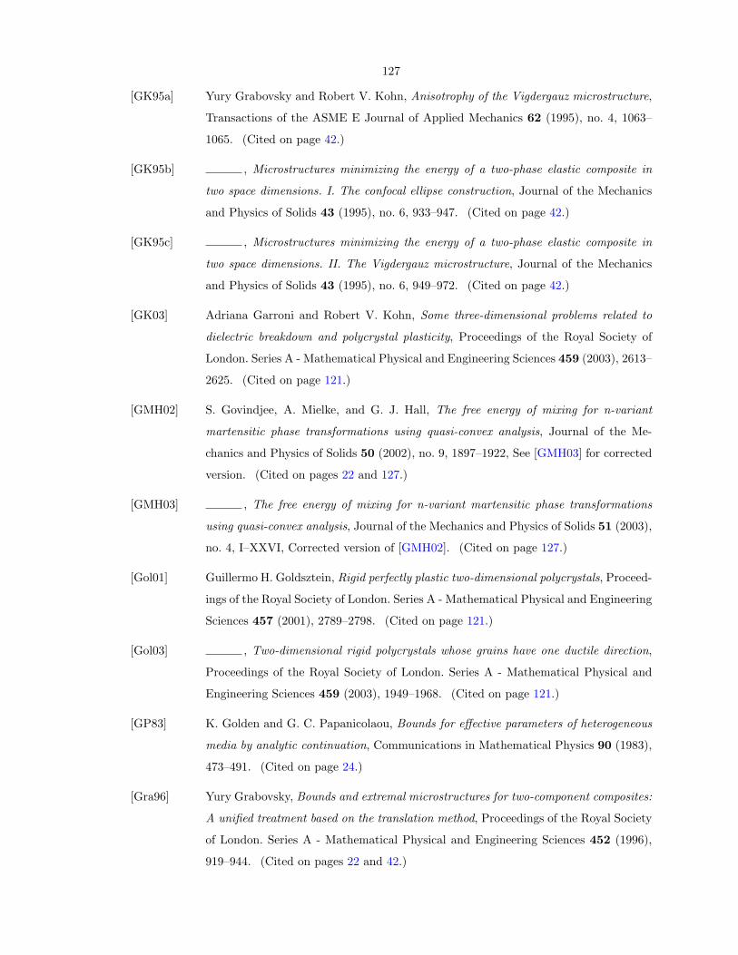
127

[GK95a] Yury Grabovsky and Robert V. Kohn, Anisotrophy of the Vigdergauz microstructure,

Transactions of the ASME E Journal of Applied Mechanics 62 (1995), no. 4, 1063–


[GK95b] , Microstructures minimizing the energy of a two-phase elastic composite in

two space dimensions. I. The confocal ellipse construction, Journal of the Mechanics

and Physics of Solids 43 (1995), no. 6, 933–947. (Cited on page 42.)

[GK95c] , Microstructures minimizing the energy of a two-phase elastic composite in

two space dimensions. II. The Vigdergauz microstructure, Journal of the Mechanics

and Physics of Solids 43 (1995), no. 6, 949–972. (Cited on page 42.)

[GK03] Adriana Garroni and Robert V. Kohn, Some three-dimensional problems related to

dielectric breakdown and polycrystal plasticity, Proceedings of the Royal Society of

London. Series A - Mathematical Physical and Engineering Sciences 459 (2003), 2613–


[GMH02] S. Govindjee, A. Mielke, and G. J. Hall, The free energy of mixing for n-variant

martensitic phase transformations using quasi-convex analysis, Journal of the Me-

chanics and Physics of Solids 50 (2002), no. 9, 1897–1922, See [GMH03] for corrected

version. (Cited on pages 22 and 127.)

[GMH03] , The free energy of mixing for n-variant martensitic phase transformations

using quasi-convex analysis, Journal of the Mechanics and Physics of Solids 51 (2003),

no. 4, I–XXVI, Corrected version of [GMH02]. (Cited on page 127.)

[Gol01] Guillermo H. Goldsztein, Rigid perfectly plastic two-dimensional polycrystals, Proceed-

ings of the Royal Society of London. Series A - Mathematical Physical and Engineering

Sciences 457 (2001), 2789–2798. (Cited on page 121.)

[Gol03] , Two-dimensional rigid polycrystals whose grains have one ductile direction,

Proceedings of the Royal Society of London. Series A - Mathematical Physical and

Engineering Sciences 459 (2003), 1949–1968. (Cited on page 121.)

[GP83] K. Golden and G. C. Papanicolaou, Bounds for effective parameters of heterogeneous

media by analytic continuation, Communications in Mathematical Physics 90 (1983),

473–491. (Cited on page 24.)

[Gra96] Yury Grabovsky, Bounds and extremal microstructures for two-component composites:

A unified treatment based on the translation method, Proceedings of the Royal Society

of London. Series A - Mathematical Physical and Engineering Sciences 452 (1996),

919–944. (Cited on pages 22 and 42.)

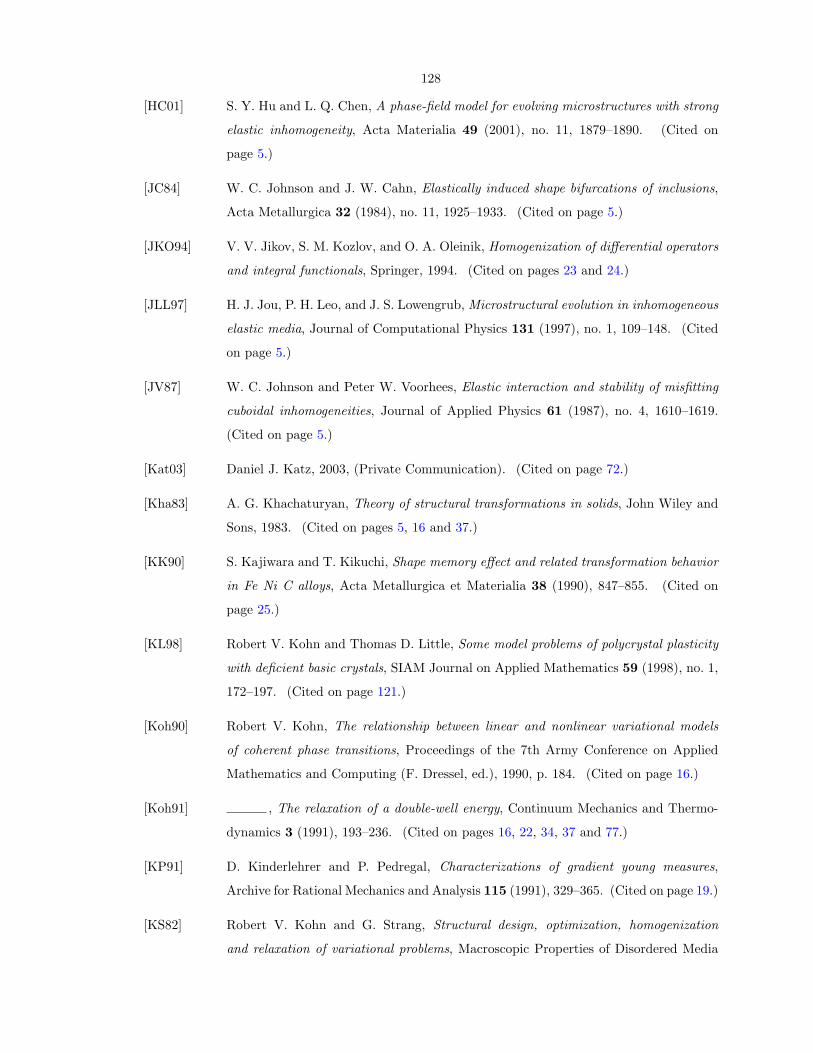
128

[HC01] S. Y. Hu and L. Q. Chen, A phase-field model for evolving microstructures with strong

elastic inhomogeneity, Acta Materialia 49 (2001), no. 11, 1879–1890. (Cited on

page 5.)

[JC84] W. C. Johnson and J. W. Cahn, Elastically induced shape bifurcations of inclusions,

Acta Metallurgica 32 (1984), no. 11, 1925–1933. (Cited on page 5.)

[JKO94] V. V. Jikov, S. M. Kozlov, and O. A. Oleinik, Homogenization of differential operators

and integral functionals, Springer, 1994. (Cited on pages 23 and 24.)

[JLL97] H. J. Jou, P. H. Leo, and J. S. Lowengrub, Microstructural evolution in inhomogeneous

elastic media, Journal of Computational Physics 131 (1997), no. 1, 109–148. (Cited

on page 5.)

[JV87] W. C. Johnson and Peter W. Voorhees, Elastic interaction and stability of misfitting

cuboidal inhomogeneities, Journal of Applied Physics 61 (1987), no. 4, 1610–1619.

(Cited on page 5.)

[Kat03] Daniel J. Katz, 2003, (Private Communication). (Cited on page 72.)

[Kha83] A. G. Khachaturyan, Theory of structural transformations in solids, John Wiley and

Sons, 1983. (Cited on pages 5, 16 and 37.)

[KK90] S. Kajiwara and T. Kikuchi, Shape memory effect and related transformation behavior

in Fe Ni C alloys, Acta Metallurgica et Materialia 38 (1990), 847–855. (Cited on

page 25.)

[KL98] Robert V. Kohn and Thomas D. Little, Some model problems of polycrystal plasticity

with deficient basic crystals, SIAM Journal on Applied Mathematics 59 (1998), no. 1,

172–197. (Cited on page 121.)

[Koh90] Robert V. Kohn, The relationship between linear and nonlinear variational models

of coherent phase transitions, Proceedings of the 7th Army Conference on Applied

Mathematics and Computing (F. Dressel, ed.), 1990, p. 184. (Cited on page 16.)

[Koh91] , The relaxation of a double-well energy, Continuum Mechanics and Thermo-

dynamics 3 (1991), 193–236. (Cited on pages 16, 22, 34, 37 and 77.)

[KP91] D. Kinderlehrer and P. Pedregal, Characterizations of gradient young measures,

Archive for Rational Mechanics and Analysis 115 (1991), 329–365. (Cited on page 19.)

[KS82] Robert V. Kohn and G. Strang, Structural design, optimization, homogenization

and relaxation of variational problems, Macroscopic Properties of Disordered Media

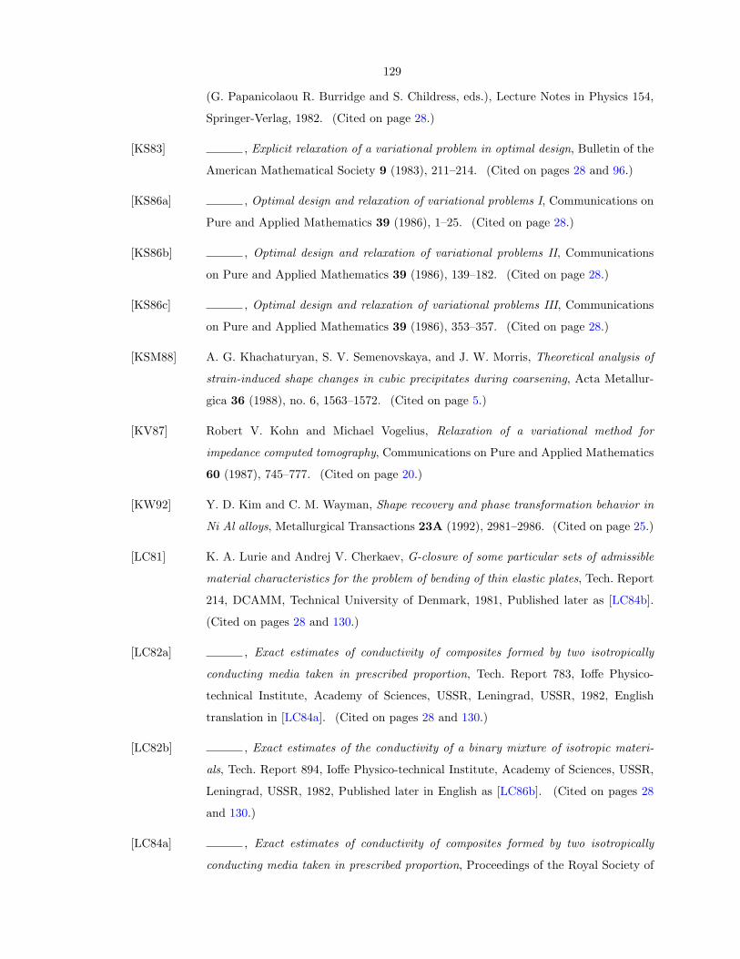
129

(G. Papanicolaou R. Burridge and S. Childress, eds.), Lecture Notes in Physics 154,

Springer-Verlag, 1982. (Cited on page 28.)

[KS83] , Explicit relaxation of a variational problem in optimal design, Bulletin of the

American Mathematical Society 9 (1983), 211–214. (Cited on pages 28 and 96.)

[KS86a] , Optimal design and relaxation of variational problems I, Communications on

Pure and Applied Mathematics 39 (1986), 1–25. (Cited on page 28.)

[KS86b] , Optimal design and relaxation of variational problems II, Communications

on Pure and Applied Mathematics 39 (1986), 139–182. (Cited on page 28.)

[KS86c] , Optimal design and relaxation of variational problems III, Communications

on Pure and Applied Mathematics 39 (1986), 353–357. (Cited on page 28.)

[KSM88] A. G. Khachaturyan, S. V. Semenovskaya, and J. W. Morris, Theoretical analysis of

strain-induced shape changes in cubic precipitates during coarsening, Acta Metallur-

gica 36 (1988), no. 6, 1563–1572. (Cited on page 5.)

[KV87] Robert V. Kohn and Michael Vogelius, Relaxation of a variational method for

impedance computed tomography, Communications on Pure and Applied Mathematics

60 (1987), 745–777. (Cited on page 20.)

[KW92] Y. D. Kim and C. M. Wayman, Shape recovery and phase transformation behavior in

Ni Al alloys, Metallurgical Transactions 23A (1992), 2981–2986. (Cited on page 25.)

[LC81] K. A. Lurie and Andrej V. Cherkaev, G-closure of some particular sets of admissible

material characteristics for the problem of bending of thin elastic plates, Tech. Report

214, DCAMM, Technical University of Denmark, 1981, Published later as [LC84b].

(Cited on pages 28 and 130.)

[LC82a] , Exact estimates of conductivity of composites formed by two isotropically

conducting media taken in prescribed proportion, Tech. Report 783, Ioffe Physico-

technical Institute, Academy of Sciences, USSR, Leningrad, USSR, 1982, English

translation in [LC84a]. (Cited on pages 28 and 130.)

[LC82b] , Exact estimates of the conductivity of a binary mixture of isotropic materi-

als, Tech. Report 894, Ioffe Physico-technical Institute, Academy of Sciences, USSR,

Leningrad, USSR, 1982, Published later in English as [LC86b]. (Cited on pages 28

and 130.)

[LC84a] , Exact estimates of conductivity of composites formed by two isotropically

conducting media taken in prescribed proportion, Proceedings of the Royal Society of

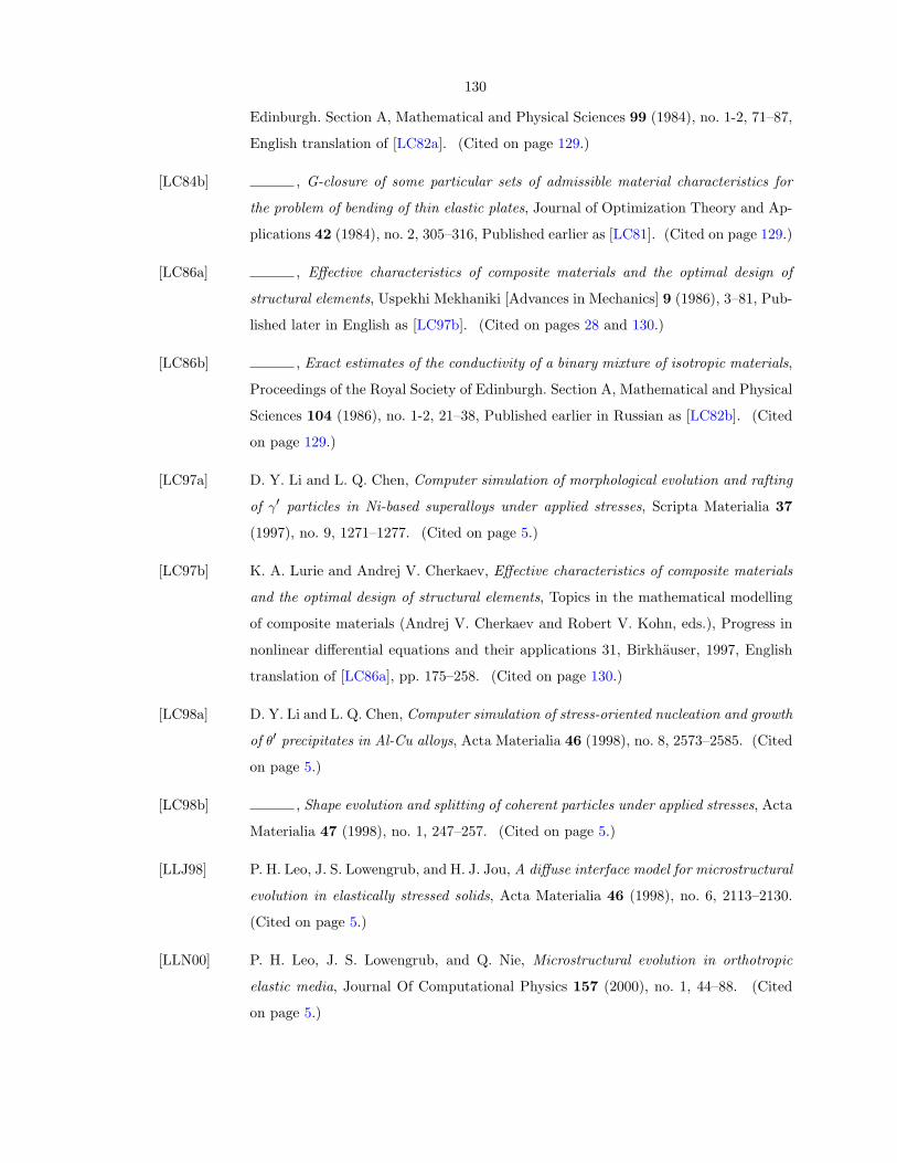
130

Edinburgh. Section A, Mathematical and Physical Sciences 99 (1984), no. 1-2, 71–87,

English translation of [LC82a]. (Cited on page 129.)

[LC84b] , G-closure of some particular sets of admissible material characteristics for

the problem of bending of thin elastic plates, Journal of Optimization Theory and Ap-

plications 42 (1984), no. 2, 305–316, Published earlier as [LC81]. (Cited on page 129.)

[LC86a] , Effective characteristics of composite materials and the optimal design of

structural elements, Uspekhi Mekhaniki [Advances in Mechanics] 9 (1986), 3–81, Pub-

lished later in English as [LC97b]. (Cited on pages 28 and 130.)

[LC86b] , Exact estimates of the conductivity of a binary mixture of isotropic materials,

Proceedings of the Royal Society of Edinburgh. Section A, Mathematical and Physical

Sciences 104 (1986), no. 1-2, 21–38, Published earlier in Russian as [LC82b]. (Cited

on page 129.)

[LC97a] D. Y. Li and L. Q. Chen, Computer simulation of morphological evolution and rafting

of γ′ particles in Ni-based superalloys under applied stresses, Scripta Materialia 37

(1997), no. 9, 1271–1277. (Cited on page 5.)

[LC97b] K. A. Lurie and Andrej V. Cherkaev, Effective characteristics of composite materials

and the optimal design of structural elements, Topics in the mathematical modelling

of composite materials (Andrej V. Cherkaev and Robert V. Kohn, eds.), Progress in

nonlinear differential equations and their applications 31, Birkhauser, 1997, English

translation of [LC86a], pp. 175–258. (Cited on page 130.)

[LC98a] D. Y. Li and L. Q. Chen, Computer simulation of stress-oriented nucleation and growth

of θ′ precipitates in Al-Cu alloys, Acta Materialia 46 (1998), no. 8, 2573–2585. (Cited

on page 5.)

[LC98b] , Shape evolution and splitting of coherent particles under applied stresses, Acta


[LLJ98] P. H. Leo, J. S. Lowengrub, and H. J. Jou, A diffuse interface model for microstructural

evolution in elastically stressed solids, Acta Materialia 46 (1998), no. 6, 2113–2130.

(Cited on page 5.)

[LLN00] P. H. Leo, J. S. Lowengrub, and Q. Nie, Microstructural evolution in orthotropic

elastic media, Journal Of Computational Physics 157 (2000), no. 1, 44–88. (Cited

on page 5.)

131

[LLN01] , On an elastically induced splitting instability, Acta Materialia 49 (2001),

no. 14, 2761–2772. (Cited on page 5.)

[LLN+03] X. F. Li, J. Lowengrub, Q. Nie, V. Cristini, and P. Leo, Microstructure evolution in

three-dimensional inhomogeneous elastic media, Metallurgical and Materials Trans-

actions A-Physical Metallurgy and Materials Science 34A (2003), no. 7, 1421–1431.

(Cited on page 5.)

[LTT+00] A.H.Y. Lue, Y. Tomota, M. Taya, K. Inoue, and T. Mori, Micro-mechanic modeling

of the stress-strain curves of a TiNiCu shape memory alloy, Materials Science and

Engineering A - Structural Materials Properties Microstructure and Processing 285

(2000), 326–337. (Cited on page 89.)

[Lu93] Jiangbo Lu, Extremal microstructures for two isotropic phases with distinct stress-free

strains in two space dimensions, Ph.D. thesis, New York University, 1993. (Cited on

pages 22 and 42.)

[LV02a] A. C. Lund and Peter W. Voorhees, Effects of elastic stress on coarsening in the Ni-Al

system, Acta Materialia 50 (2002), 2085–2098. (Cited on page 5.)

[LV02b] , Effects of elastic stress on microstructural development: The three-

dimensional microstructure of a γ − γ′ alloy, Acta Materialia 50 (2002), 2585–2598.

(Cited on page 5.)

[LV03] , A quantitative assessment of the three-dimensional microstructure of a γ− γ′

alloy, Philosophical Magazine 83 (2003), no. 14, 1719–1733. (Cited on page 5.)

[LVB+02] C. Lexcellent, A. Vivet, C. Bouvet, S. Calloch, and P. Blanc, Experimental and nu-

merical determinations of the initial surface of phase transformation under biaxial

loading in some polycrystalline shape-memory alloys, Journal of the Mechanics and

Physics of Solids 50 (2002), 2717–2753. (Cited on page 89.)

[LW98] Z.K. Lu and G.J. Weng, A self-consistent model for the stress-strain behavior of shape-

memory alloy polycrystals, Acta Materialia 46 (1998), 5423–5433. (Cited on page 89.)

[Mar78] P. Marcellini, Periodic solutions and homogenization of nonlinear variational prob-

lems, Annali di Matematica Pura ed Applicata 117 (1978), 139–152. (Cited on

pages 23 and 24.)

[MI79] Albert W. Marshall and Olkin Ingram, Inequalities: Theory of majorization and its

applications, Mathematics in Science and Engineering 143, Academic Press, 1979.

(Cited on page 71.)

132

[Mil90a] Graeme W. Milton, A brief review of the translation method for bounding effective

elastic tensors of composites, Continuum Models and Discrete Systems (G. A. Maugin,

ed.), Longman Scientific and Technical, 1990, pp. 60–74. (Cited on page 28.)

[Mil90b] , On characterizing the set of possible effective tensors of composites: The

variational method and the translation method, Communications on Pure and Applied

Mathematics 43 (1990), no. 1, 63–125. (Cited on page 28.)

[Mil01] , The theory of composites, Cambridge Monographs on Applied and Compu-

tational Mathematics 6, Cambridge University Press, 2001. (Cited on pages 20, 28,

36, 51 and 79.)

[MNK+00] S. Miyazaki, V. H. No, K. Kitamura, A. Khantachawana, and H. Hosoda, Texture

of Ti-Ni rolled thin plates and sputter-deposited thin films,, International Journal of

Plasticity 16 (2000), 1135–1154. (Cited on page 89.)

[MNM79] Toru Miyazaki, Kozo Nakamura, and Hirotaro Mori, Experimental and theoretical in-

vestigations on morphological changes of γ′ precipitates in Ni-Al single crystals during

uniaxial stress-annealing, Journal of Materials Science 14 (1979), 1827–1837. (Cited

on pages 3 and 4.)

[MT85] F. Murat and L. Tartar, Calcul des variations et homogeneisation [Calculus of vari-

ations and homogenization], Collection de la Direction des Etudes et Recherches

d’Electricite de France 57 (1985), 319–369, Homogenization methods: Theory and ap-

plications in physics (Breau-sans-Nappe, 1983). English translation in [MT97]. (Cited

on pages 28 and 132.)

[MT97] , Calculus of variations and homogenization, Topics in the mathematical mod-

elling of composite materials (Andrej V. Cherkaev and Robert V. Kohn, eds.), Progress

in nonlinear differential equations and their applications 31, Birkhauser, 1997, English

translation of [MT85], pp. 139–173. (Cited on page 132.)

[Mur87] F. Murat, A survey on compensated compactness, Contributions to Modern Calculus

of Variations (L. Cesari, ed.), Longman Scientific and Technical, 1987, pp. 145–183.

(Cited on page 28.)

[NBZACP02] C. Niclaeys, T. Ben Zineb, S. Arbab-Chirani, and E. Patoor, Determination of the in-

teraction energy in the martensitic state, International Journal of Plasticity 18 (2002),

1619–1647. (Cited on page 89.)

133

[Ono90a] N. Ono, Pseudoelastic behavior in a polycrystalline Cu-Al-Ni shape memory alloy in

comparison with the modified taylor model, Mat. Trans. Jap. Inst. Metals 31 (1990),

855–860. (Cited on page 89.)

[Ono90b] , Pseudoelastic deformation in a polycrystalline Cu-Zn-Al shape memory alloy,

Mat. Trans. Jap. Inst. Metals 31 (1990), 381–385. (Cited on page 89.)

[OS88] N. Ono and A. Sato, Plastic deformation governed by the stress induced martensitic

transformation in polycrystals, Mat. Trans. Jap. Inst. Metals 29 (1988), 267–273.

(Cited on page 89.)

[OSO89] N. Ono, A. Sato, and H. Ohta, A discussion on the mechanical properties of shape

memory alloys based on a polycrystal model, Mat. Trans. Jap. Inst. Metals 30 (1989),

756–764. (Cited on page 89.)

[OW99] Kazuhiro Otsuka and Clarence M. Wayman (eds.), Shape memory materials, Cam-

bridge University Press, 1999. (Cited on page 2.)

[PBEB94] E. Patoor, M. Bensalah, A. Eberhard, and M. Berveiller, Micromechanical aspects of

shape memory behavior, Proc. ICOMAT-92 (C. M. Wayman and J. Perkins, eds.),

Monterey Inst. Adv. Studies, 1994, pp. 401–406. (Cited on page 89.)

[PC98] R. Poduri and L. Q. Chen, Computer simulation of morphological evolution and coars-

ening kinetics of δ′ Al3Li precipitates in Al-Li alloys, Acta Materialia 46 (1998),

no. 11, 3915–3928. (Cited on page 5.)

[PEB88] E. Patoor, A. Eberhard, and M. Berveiller, Thermomechanical behavior of shape mem-

ory alloys, Archives of Mechanics 40 (1988), 775–794. (Cited on page 89.)

[PEB93] , Micromechanical modelling of superelasticity in shape memory alloys,

Progress in Partial Differential Equations: The Metz Surveys. 2 (M. Chipot, ed.),

Pitman Research Notes in Mathematics 296, Longman Scientific, 1993, pp. 38–54.

(Cited on page 89.)

[Pip91] Allen C. Pipkin, Elastic materials with two preferred states, Quarterly Journal of

Applied Mathematics 44 (1991), no. 1, 1–15. (Cited on pages 22, 34 and 77.)

[Pra57] William Prager, On ideal locking materials, Transactions of the Society of Rheology

1 (1957), no. 1, 169–175. (Cited on page 92.)

[Pra58] , Elastic solids of limited incompressibility, Proceedings of the 9th International

Congress on Applied Mechanics, vol. 5, 1958, pp. 205–211. (Cited on page 92.)

134

[Roy78] A. L. Roytburd, Martensitic transformation as a typical phase transformation in

solids, Solid State Physics 33 (1978), 317–390. (Cited on pages 16 and 37.)

[Roy93] , Elastic domains and polydomain phases in solids, Phase Transitions 45

(1993), 1–33. (Cited on page 16.)

[Rud91] Walter Rudin, Functional analysis, 2 ed., International Series in Pure and Applied

Mathematics, McGraw Hill, Inc., 1991. (Cited on page 96.)

[RV02] Lorenz Ratke and Peter W. Voorhees, Growth and coarsening: Ripening in material

processing, Engineering Materials, Springer, 2002. (Cited on pages 3 and 4.)

[RW98] Tyrrell R. Rockafellar and Roger J-B. Wets, Variational analysis, Grundlehren der

mathematischen Wissenschaften 317, Springer, 1998. (Cited on pages 90, 92, 93

and 95.)

[Sab92] K. Sab, On the homogenization and the simulation of random materials, European

Journal of Mechanics A-Solids 11 (1992), 585–607. (Cited on page 23.)

[SH93a] Q. P. Sun and K. C. Hwang, Micromechanics modelling for the constitutive behavior

of polycrystalline shape memory alloys - I. Derivation of general relations, Journal of

the Mechanics and Physics of Solids 41 (1993), 1–17. (Cited on page 89.)

[SH93b] , Micromechanics modelling for the constitutive behavior of polycrystalline

shape memory alloys - II. Study of the individual phenomena, Journal of the Me-

chanics and Physics of Solids 41 (1993), 19–33. (Cited on page 89.)

[SK83] G. Strang and Robert V. Kohn, Hencky-Prandtl nets and constrained Michell trusses,

Computer Methods in Applied Mechanics and Engineering 36 (1983), 207–222. (Cited

on page 96.)

[SK88] , Optimal design of a two-way conductor, Topics in Nonsmooth Mechanics

(J. Moreau et al., ed.), Birkhauser, 1988, pp. 143–155. (Cited on page 28.)

[SLN+02] P. Sittner, P. Lukas, D. Neov, M. R. Daymond, V. Novak, and G. M. Swallowe, Stress-

induced martensitic transformation in Cu-Al-Zn-Mn polycrystal investigated by two in-

situ neutron diffraction techniques, Materials Science and Engineering A - Structural

Materials Properties Microstructure and Processing 324 (2002), 225–234. (Cited on

page 89.)

[SN00] P. Sittner and V. Novak, Anisotropy of martensitic transformations in modeling of

shape memory alloy polycrystals, International Journal of Plasticity 16 (2000), 1243–


135

[SNL+02] P. Sittner, V. Novak, P. Lukas, D. Lugovsky, D. Neov, and M. Tovar, Load partition in

NiTi shape memory alloy polycrystals investigated by in-situ neutron diffraction and

micromechanics modelling, Materials Science Forum 404 (2002), 829–834. (Cited on

page 89.)

[SP93] S. Socrate and D. M. Parks, Numerical determination of the elastic driving force for

directional coarsening in Ni-Superalloys, Acta Metallurgica et Materialia 41 (1993),

no. 7, 2185–2209. (Cited on page 5.)

[SPBE99] N. Siredey, E. Patoor, M. Berveiller, and A. Eberhardt, Constitutive equations for

polycrystalline thermoelastic shape memory alloys. I. Intragranular interactions and

behavior of the grain, International Journal of Solids and Structures 36 (1999), 4289–.

(Cited on page 89.)

[Str79] G. Strang, A minimax problem in plasticity theory, Functional analysis methods in nu-

merical analysis: Special session, American Mathematical Society, St. Louis, Missouri,

1977 (M. Zuhair Nashed, ed.), Lecture notes in mathematics 701, Springer-Verlag,

1979, pp. 319–333. (Cited on page 96.)

[SV96a] C. H. Su and Peter W. Voorhees, The dynamics of precipitate evolution in elastically

stressed solids - I. inverse coarsening, Acta Materialia 44 (1996), no. 5, 1987–1999.

(Cited on page 5.)

[SV96b] , The dynamics of precipitate evolution in elastically stressed solids - II. particle

alignment, Acta Materialia 44 (1996), no. 5, 2001–2016. (Cited on page 5.)

[SW99] V. P. Smyshlyaev and J. R. Willis, On the relaxation of a three-well energy, Proceed-

ings of the Royal Society of London. Series A - Mathematical Physical and Engineering

Sciences 455 (1999), no. 1983, 779–814. (Cited on page 22.)

[TA01] P. Thamburaja and L. Anand, Polycrystalline shape-memory materials: Effect of

crystallographic texture, Journal of the Mechanics and Physics of Solids 49 (2001),

709–737. (Cited on page 89.)

[Tar79a] L. Tartar, Compensated compactness and applications to partial differential equations,

Nonlinear Analysis and Mechanics (R.J. Knops, ed.), Heriot-Watt Symposium, IV,

Pitman Publishing, 1979, pp. 136–212. (Cited on page 28.)

[Tar79b] , Estimation de coefficients homogeneises [Estimation of homogenized coeffi-

cients], Computing methods in applied sciences and engineering: Third international

symposium, Versilles, France, December 5–7, 1977 (R. Glowinski and J. L. Lions,

136

eds.), Springer-Verlag, 1979, English translation in [Tar97]. (Cited on pages 28, 36

and 136.)

[Tar85] , Estimation fines des coeffcients homogeneises [Fine estimations of homoge-

nized coefficients], Ennio de Giorgi Colloquium: Papers Presented at a Colloquium

Held at the H. Poincare Institute in November 1983 (P. Kree, ed.), Pitman Publishing,

1985, pp. 168–187. (Cited on pages 28 and 36.)

[Tar97] , Estimation of homogenization coefficients, Topics in the mathematical mod-

elling of composite materials (Andrej V. Cherkaev and Robert V. Kohn, eds.), Progress

in nonlinear differential equations and their applications 31, Birkhauser, 1997, English

translation of [Tar79b], pp. 9–20. (Cited on page 136.)

[Tar00] , An introduction to the homogenization method in optimal design, Optimal

shape design. Lectures given at the joint C.I.M./C.I.M.E. Summmer school held at

Troia, June 1–6, 1998 (A. Cellina and A. A. Ornelas, eds.), Springer-Verlag, 2000,

pp. 47–156. (Cited on page 36.)

[Tay78] J. E. Taylor, Crystalline variational problems, Bulletin of the American Mathematical

Society 84 (1978), no. 4, 568–588. (Cited on page 5.)

[Tem81] Roger Temam, An existence theorem for a variational problem of plasticity, Nonlinear

problems of analysis in geometry and mechanics (M. Atteia, D. Bancel, and I. Gu-

mowski, eds.), Research notes in mathematics 46, Pitman, 1981, pp. 57–70. (Cited

on page 96.)

[TSV94] M. E. Thompson, C. S. Su, and Peter W. Voorhees, The equilibrium shape of a misfit-

ting precipitate, Acta Metallurgica et Materialia 42 (1994), no. 6, 2107–2122. (Cited

on pages 5, 6 and 53.)

[VC02] V. Vaithyanathan and L. Q. Chen, Coarsening of ordered intermetallic precipitates

with coherency stress, Acta Materialia 50 (2002), no. 16, 4061–4073. (Cited on

page 5.)

[Vig94] S. B. Vigdergauz, Two-dimensional grained composites of extreme rigidity, Transac-

tions of the ASME E Journal of Applied Mechanics 61 (1994), no. 2, 390–394. (Cited

on page 42.)

[VWC02] V. Vaithyanathan, C. Wolverton, and L. Q. Chen, Multiscale modelling of precipi-

tate microstructure evolution, Physical Review Letters 88 (2002), no. 12. (Cited on

page 5.)

137

[Way64] C. M. Wayman, Introduction to the crystallography of martensitic transformations,

Macmillan, 1964. (Cited on page 16.)

[Way92] , Shape memory and related phenomena, Progress in Materials Science 36

(1992), 203–224. (Cited on page 16.)

[WCK91] Y. Z. Wang, L. Q. Chen, and A. G. Khachaturyan, Shape evolution of a precipitate

during strain-induced coarsening - A computer-simulation, Scripta Metallurgica et


[Wei95] H.F. Weinberger, A first course in partial differential equations with complex variables

and transform methods, Dover Publications Inc., 1995. (Cited on page 98.)

[WW71] M. Watanabe and C. M. Wayman, Crystallography of the martensite transformation in

Fe-Al-C alloys, Metallurgical Transactions 2 (1971), 2229–2236. (Cited on page 16.)

[ZCS01] Jingzhi Zhu, Long-Qing Chen, and Jie Shen, Morphological evolution during phase

separation and coarsening with strong inhomogeneous elasticity, Modelling and Simu-

lation in Materials Science and Engineering 9 (2001), 499–511. (Cited on page 5.)

Energy-Minimizing Microstructures in Multiphase...

Documents

Transcript of Energy-Minimizing Microstructures in Multiphase...