Energy Management and Trajectory Optimization for UAV ...

1

Energy Management and Trajectory

Optimization for UAV-Enabled Legitimate

Monitoring Systems

Shuyan Hu, Qingqing Wu, Member, IEEE, and Xin Wang, Senior Member, IEEE

Abstract

Thanks to their quick placement and high flexibility, unmanned aerial vehicles (UAVs) can be very

useful in the current and future wireless communication systems. With a growing number of smart

devices and infrastructure-free communication networks, it is necessary to legitimately monitor these

networks to prevent crimes. In this paper, a novel framework is proposed to exploit the flexibility of

the UAV for legitimate monitoring via joint trajectory design and energy management. The system

includes a suspicious transmission link with a terrestrial transmitter and a terrestrial receiver, and a

UAV to monitor the suspicious link. The UAV can adjust its positions and send jamming signal to

the suspicious receiver to ensure successful eavesdropping. Based on this model, we first develop an

approach to minimize the overall jamming energy consumption of the UAV. Building on a judicious (re-

)formulation, an alternating optimization approach is developed to compute a locally optimal solution

in polynomial time. Furthermore, we model and include the propulsion power to minimize the overall

energy consumption of the UAV. Leveraging the successive convex approximation method, an effective

iterative approach is developed to find a feasible solution fulfilling the Karush-Kuhn-Tucker (KKT)

conditions. Extensive numerical results are provided to verify the merits of the proposed schemes.

Work in this paper was supported by the National Natural Science Foundation of China under Grant No. 61671154, the

Shanghai Science Foundation under Grant No. 18ZR1402700, and the Innovation Program of Shanghai Municipal Education

Commission.

S. Hu is with the State Key Laboratory of ASIC and System, the School of Information Science and Technology, Fudan

University, Shanghai 200433, China (e-mail: [email protected]).

Q. Wu is with the Department of Electrical and Computer Engineering, National University of Singapore, Singapore 119077

(e-mail: [email protected]).

X. Wang is with the State Key Laboratory of ASIC and System, the Shanghai Institute for Advanced Communication and

Data Science, the Department of Communication Science and Engineering, Fudan University, Shanghai 200433, China (e-mail:

[email protected]).

April 24, 2020 DRAFT

arX

iv:2

004.

1091

8v1

[ee

ss.S

P] 2

3 A

pr 2

020

2

Index Terms

Legitimate mornitoring, energy management, solar energy harvesting, alternating optimization, suc-

cessive convex approximation.

I. INTRODUCTION

Featuring high flexibility, swift deployment, and wide coverage, unmanned aerial vehicles

(UAVs) have been extensively applied to activities such as search and rescue in disaster areas,

inspection of landscapes, and surveillance of forrest fires. Recently, UAVs have found many

use cases in wireless communication networks as cost-effective and on-demand aerial wireless

platforms for areas without cellular coverage [1]–[3], or as flying mobile users within a cellular

network [4], [5]. Cellular-connected UAVs can enhance connectivity, coverage, flexibility and

reliability of wireless communication networks [4], [5]. The UAVs are anticipated to engage

significantly in the fifth-generation (5G) and beyond 5G (B5G) wireless networks, and provide

new services such as real-time image transmission [6], caching and multicasting [7], [8], data

dissemination or collection [1], [9], [10], mobile relaying and edge computing [11]–[13], and

wireless power transfer [2], [14], [15].

As the applications of the internet-of-things (IoT) continue to expand in the current and future

wireless networks, many infrastructure-free wireless links (such as bluetooth, Wi-Fi, and UAV-

enabled transmission) have been established to support communications among IoT devices.

Yet, these convenient networks can be abused for crimes and terrorism, if in the wrong hands.

Therefore, it is necessary for authorized parties to surveil these suspicious communication links

(see [16]–[25]). Optimization metrics for legitimate monitoring typically focused on maximizing

the eavesdropping rate or the non-outage probability [16]. Spoofing schemes were proposed for a

malicious transmission link to maximize the eavesdropping rate [17], or to intervene and change

the communicated data [18]. For a suspicious communication link in [19], the largest achievable

monitoring non-outage probability and comparative intercepting rate were obtained under delay-

sensitive and delay-tolerant scenarios, respectively. Proactive jamming schemes were developed

to maximize the average monitoring rate for multi-input multi-output (MIMO) channels [21],

relay networks [22], UAV-aided links [23], and with a deep-learning approach [24].

Most existing works considered a fixed ground node (GN) as the legitimate monitor, whose

channel typically suffers from severe large-scale path loss and small-scale fading. Yet, the UAV-

enabled monitor can enjoy high-probability of line-of-sight (LoS) channels as its flying altitude


3

rises. It is therefore easier for the UAV to obtain its channel gains with the GNs if their locations

are known. Thanks to its flexibility, the UAV can dynamically adjust its positions for better

eavesdropping rate, e.g., by flying closer to the suspicious transmitter. Categorized by the power

sources, there are two types of UAVs, namely, the tethered UAVs and the untethered UAVs [26].

A tethered UAV is linked with a ground control platform, and is powered stably through a cable

or a wire. The lack of mobility has constrained tethered UAVs to a targeted area only [27]–[30].

In particular, the horizontal positions of the UAVs were optimized in [29] to cover a set of

GNs with the least possible number of UAVs. The optimal three-dimensional (3D) deployment

scheme of a UAV was developed in [30] to cover as many GNs as possible with a minimum

transmit power budget.

By contrast, untethered UAVs are powered by laser-beam, on-board battery, and/or solar panel.

They can fly freely and enjoy full mobility in wide 3D space. Communication throughput was

maximized for a laser-powered UAV in [31]. In spite of their flexibility, the battery-powered

UAVs have to revisit their home base repeatedly to refill their batteries during operations,

due to the limited capacity of on-board batteries [32]. The optimal UAV trajectory and power

management schemes were developed in [12] to obtain the largest achievable data rate of a

relaying system, and in [8] to minimize the data dissemination time of a multicasting system.

Since solar panels at the UAVs can harness and convert energy to electric power, supporting

long endurance flights, solar-powered UAVs have also received great research interests. The

optimal 3D trajectory optimization and resource assignment for a solar-powered UAV-aided

communication system were developed in [32] to achieve the largest overall data rate in a fixed

time horizon.

Apart from transmit power, the UAVs consume additional propulsion power to support hover-

ing and moving activities. As a result, the energy management for UAV-enabled communications

noticeably differs from that in current systems on the ground. The largest value of energy effi-

ciency in bits/Joule was obtained in [33] for a fixed-wing UAV via trajectory optimization. Total

(including communication and propulsion) energy usage of a rotary-wing UAV was minimized

in [34] to satisfy the throughput requirement of each GN.

In this paper, we propose a simple model for a rotary-wing UAV enabled monitoring system.

The suspicious transmission link on the ground consists one source (transmitting) node S and

one destination (receiving) node D. When the UAV’s channel condition is worse than that

of node D, the UAV sends jamming signal to the latter as noise to degrade its channel for


4

Suspicious source Suspicious destination

Legitimate monitor (UAV)!(xt, yt, H)!

S�0,0,0�

D�d,0,0�

Y

X

Z

Suspicious transmission link

Eave

sdro

pping

link Jam

ming link

Fig. 1. A UAV-enabled legitimate monitoring system.

successful eavesdropping. The total jamming energy consumption of the UAV is minimized in

a finite period via joint trajectory optimization and power allocation, based on the assumption

of successful eavesdropping at each slot. By judicious reformulation, we transform this non-

convex optimization task into two separable subproblems, each of which is convex when the

other set of variables are fixed. The alternating optimization method is leveraged to develop an

efficient approach that is ensured to converge to a locally optimal solution. Based on such a

solution, some useful insights are also drawn on the changing patterns of the UAV’s trajectory

and jamming policy. To achieve energy-efficient UAV operations in practice, we further consider

a solar-powered rotary-wing UAV enabled monitoring system by including the propulsion power

consumption besides the jamming power. Capitalizing on the successive convex approximation

(SCA) method, an efficient iterative approach is put forth to find a feasible solution fulfilling the

Karush-Kuhn-Tucker (KKT) conditions. Numerical results demonstrate that with UAV trajectory

optimization, the overall energy consumption can be greatly suppressed.

The rest of the paper is organized as follows. Section II describes the system models. Section

III develops an approach to the UAV trajectory design and jamming energy minimization,

while Section IV addresses the trajectory design and total (jamming and propulsion) energy

management for a solar-powered UAV. Numerical results are provided in Section V. The paper

is concluded in Section VI.


5

II. SYSTEM MODELS

Consider a point-to-point, frequency non-selective wireless communication link from a suspi-

cious source node S to a suspicious destination node D which are geographically set apart by d

meters on the ground. An untethered UAV, traveling at a fixed altitude of H meters, serves as the

legitimate monitor to eavesdrop this link; see Fig. 1.1 The UAV can move forward horizontally

or hover in the air. It can travel in the vicinity above the GNs to improve its eavesdropping

performance. Suspicious nodes S and D have one antenna each, and the UAV operates with

two antennas, one for monitoring and intercepting information from the S-D link (receiving)

and the other for sending jamming signals to node D (transmitting). Therefore the UAV can

perform in a full-duplex state to jam and monitor simultaneously. Since its initial and final

locations are given, the UAV’s channel power gain can be worse than that of D at certain time.

In this case, the UAV sends jamming signal to the latter as noise to degrade its channel for

successful eavesdropping. We assume that the UAV can completely annul its self-interference

from the transmitting antenna to the receiving antenna by adopting state-of-the-art analog and

digital self-interference cancelation schemes [19].

A. UAV Mobility Model

Without loss of generality, we consider a 3D Cartesian coordinate system with nodes S and D

located at (0, 0, 0) and (d, 0, 0), respectively. The UAV is deployed for the monitoring mission

in a finite scheduling horizon of T seconds. We split the period T into Tw time slots given by

T := {1, . . . , Tw}; the duration of each slot is the same as δ. The slot length is selected to

be short enough so that the UAV can be treated as static within each slot. Consequently, the

time-varying coordinates of the UAV are given by (xt, yt, H), ∀t ∈ T , with xt and yt being

the UAV’s x- and y-coordinates over time, respectively. The initial and final locations of the

legitimate monitor are pre-defined and given by (x0, y0, H), and (xT , yT , H), respectively. The

minimum traveling distance for the UAV to finish during the scheduling horizon T is thereby

dmin =√

(xT − x0)2 + (yT − y0)2. Given the maximum speed of the UAV Vm, we let Vm ≥

1Although design freedom can be increased by further optimizing UAV’s altitude, energy consumption as well as risks of

instability and collision will rise. Therefore, rather than frequently adjusting altitude, it may be better for the UAV to fly at a

fixed altitude and avoid vertical movement due to airspace regulation, collision avoidance, energy saving and safety concerns.


6

dmin/T so that at least one feasible trajectory can be found from the UAV’s initial to final

locations.2

Consequently, the UAV’s mobile activity constraints, including its initial and final locations

and speed constraints are given by [12]:

(x1 − x0)2 + (y1 − y0)2 ≤ V 2m (1a)

(xt+1 − xt)2 + (yt+1 − yt)2 ≤ V 2m, ∀t ∈ T (1b)

(xT − xT−1)2 + (yT − yT−1)2 ≤ V 2m (1c)

where Vm := Vmδ stands for the largest traveling distance of the UAV for each slot.

Remark 1. (The choice of Tw): In general, Tw is chosen such that the UAV can be treated as

(quasi-) static within each time slot, observed from the ground. To guarantee a certain accuracy,

the ratio of the largest traveling distance within each time slot Vmδ and the UAV altitude H

can be restricted below a threshold, i.e., Vmδ/H ≤ εm, where εm is the given threshold and

δ = T/Tw. Then, the minimum number of time slots required for achieving the accuracy with a

given εm can be obtained as Tw ≥ VmT/(Hεm). The optimization gets more precise with more

discretized time samples, i.e., larger value of Tw. Yet, the computational complexity, given by

O(T 3.5w ), also increases significantly with the value of Tw. Therefore, the number of time slots

Tw can be properly chosen in practice to balance between the accuracy and complexity [9].

B. Communication Channel Model

Malicious users of infrastructure-free wireless communication networks are more likely to

appear in wide rural areas, where surveillance is overlooked. In open rural areas, the buildings

and trees are sparsely distributed. LoS channels can be dominant even for communications

between GNs. Therefore, we can suppose that the communication links between S, D, and UAV

(i.e., node U) are all dominated by LoS channels, which can facilitate analysis on the structural

properties of the optimal solution. The case with non-LoS channels will be accordingly addressed

later. We further suppose that the Doppler effect resulted from the UAV’s mobile activities is

2By considering the time for acceleration, the proposed maximum speed Vm may be infeasible. However, in practice, the

acceleration time could be very short and thus reasonably ignored, especially when the total flying period or distance is sufficiently

long. From this perspective, we provide a lower bound for the maximum speed.


7

completely neutralized [12], [35]. The distance between S and D is fixed during the entire

scheduling horizon, i.e., dSD = d meters. Hence, the channel power gain of the suspicious link

from S to D is constant and can be expressed as

h0 =β0

dSD2 =

β0

d2(2)

where β0 stands for the channel power at the reference distance d0 = 1 meter. At each slot t,

the channel power gain from S to U for legitimate eavesdropping follows the LoS model as

ht1 =β0

dt12 =

β0

x2t + y2

t +H2, ∀t ∈ T (3)

where dt1 =√x2t + y2

t +H2 is the link distance between S and U at slot t. Similarly, the channel

power gain from U to D for jamming is

ht2 =β0

dt22 =

β0

(d− xt)2 + y2t +H2

, ∀t ∈ T (4)

where dt2 =√

(d− xt)2 + y2t +H2 is the separation distance between U and D at slot t.

Let P tx stand for the transmit power by S at time slot t, and P t

j the jamming power from U

to D to interfere the channel at the suspicious receiver for a successful eavesdropping. Clearly,

the signal-to-interference-plus-noise ratio (SINR) at the suspicious receiver D is

γtD =h0P

tx

ht2Ptj + σ2

, ∀t ∈ T (5)

where σ2 is variance of the additive white Gaussian noise (AWGN). On the other hand, the

UAV can completely annul its self-interference from its jamming antenna to its receiving an-

tenna. Hence, the SINR (which in fact reduces to signal-to-noise ratio, SNR) of the legitimate

eavesdropping channel at U is

γtU =ht1P

tx

σ2, ∀t ∈ T . (6)

Successful eavesdropping at the UAV requires γtU ≥ γtD. The UAV can achieve this goal by

dynamically adjusting its trajectory to fly close to the source node, and/or adjusting its jamming

power to reduce the channel gain of the suspicious receiver D at each time slot, when the channel

condition of the UAV is worse than that of D.3

3When the channel condition of the legitimate monitor (the S-U link) is better than that of the suspicious receiver (the S-D

link), eavesdropping is performed successfully without the UAV sending jamming signals to the receiver. However, when the

S-U link suffers a worse channel condition than the S-D link, successful eavesdropping can be enabled through letting the UAV

send jamming signals to the receiver to degrade its channel condition.


8

Note that the assumption of successful eavesdropping at each time slot is tenable and non-

trivial. In fact, malicious users of infrastructure-free wireless communication networks can also

develop counter-eavesdropping measures to ensure secure transmissions on their behalf. One

important method is to transmit secret information in cipher. In order to learn the pattern and

decode the secret information, the legitimate agency treasures every bit of information. In this

case, the cipher transmitted in each time slot is of equal importance for the legitimate agency to

piece together the whole picture. Hence, it is of paramount importance if the eavesdropper can

intercept information from the suspicious link successfully in every time slot.

Remark 2. (Decoding the intercepted information): In this paper, we aim to investigate the

fundamental performance limits of the physical layer approach for eavesdropping, and thus

do not consider encryption for the suspicious link, which is a higher layer technique and can

be resolved as long as there are powerful computing resources. On the other hand, to avoid

being monitored and tracked by legitimate parties, the suspicious link is very likely built, used

and discarded or destroyed in a day, which makes the link not complete or mature enough in

terms of software and hardware to preserve privacy and security. We can thereby reasonably

assume that the temporarily-established infrastructure-free suspicious link is not vigilant against

eavesdropping and does not employ any countermeasures such as signal encryption or anti-

surveillance detection. From this perspective, the UAV can successfully decode the intercepted

information from the suspicious link.

III. LEGITIMATE EAVESDROPPING WITH JAMMING

To ensure successful eavesdropping, the UAV may need to jam the transmission from S to

D. For an untethered UAV without incessant power supply, it is clear that we wish to minimize

its overall jamming energy consumption. Building on the UAV’s mobile activity constraints

(1a)–(1c), together with the SINR expressions (5)–(6), the optimization task of interest can be

formulated as

min{P t

j },{xt,yt}

∑t∈T

P tj δ (7a)

s.t.h0P

tx

ht2Ptj + σ2

≤ ht1Ptx

σ2, ∀t (7b)

(x1 − x0)2 + (y1 − y0)2 ≤ V 2m (7c)


9

(xt+1 − xt)2 + (yt+1 − yt)2 ≤ V 2m, ∀t (7d)

(xT − xT−1)2 + (yT − yT−1)2 ≤ V 2m (7e)

P tj ≥ 0, ∀t. (7f)

Here we in fact aim to pursue the optimal jamming policy and trajectory design for the UAV.

Note that the transmit power P tx by S can be canceled from the both sides of the inequality

constraints in (7b). This implies that the UAV does not need to know the P tx when making its

jamming and trajectory decisions. This is of practical interest as the suspicious source is certainly

reluctant to let the UAV know its transmit power value.

A. Proposed Solution

Problem (7) is not a convex program because of the non-convex constraints in (7b); hence,

it cannot be dealt with by classic convex optimization methods. To make the problem more

tractable, we introduce two slack variables ut := x2t + y2

t +H2, and wt := (d− xt)2 + y2t +H2,

and rewrite (7) as

min{P t

j ,ut,wt},{xt,yt}

∑t∈T

P tj δ (8a)

s.t. x2t + y2

t +H2 − ut ≤ 0, ∀t (8b)

ut − 2dxt + d2 − wt ≤ 0, ∀t (8c)utwtd2− wt − P t

jβ0/σ2 ≤ 0, ∀t (8d)

wt ≥ H2, ∀t (8e)

(7c)− (7f)

where (8d) results from (7b) by the following step

h0

P tjβ0/wt + σ2

≤ β0/utσ2

, ∀t. (9)

Note that we change the “=” signs to “≤” signs in (8b) and (8c) to convexify those constraints. It

can be justified that upon obtaining the optimal solution for (8), constraints (8b) and (8c) should

always be met with equality, since otherwise, we can always decrease ut and wt, respectively,

to improve the channel condition of the corresponding eavesdropping and jamming link, leading

to smaller total jamming energy consumption. Therefore, problems (7) and (8) are equivalent.


10

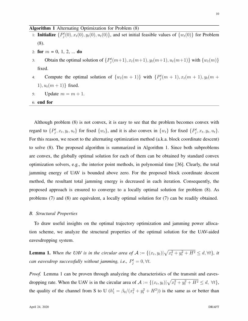
Algorithm 1 Alternating Optimization for Problem (8)1: Initialize {P t

j (0), xt(0), yt(0), ut(0)}, and set initial feasible values of {wt(0)} for Problem

(8).

2: for m = 0, 1, 2, ... do

3: Obtain the optimal solution of {P tj (m+1), xt(m+1), yt(m+1), ut(m+1)} with {wt(m)}

fixed.

4: Compute the optimal solution of {wt(m + 1)} with {P tj (m + 1), xt(m + 1), yt(m +

1), ut(m+ 1)} fixed.

5: Update m = m+ 1.

6: end for

Although problem (8) is not convex, it is easy to see that the problem becomes convex with

regard to {P tj , xt, yt, ut} for fixed {wt}, and it is also convex in {wt} for fixed {P t

j , xt, yt, ut}.

For this reason, we resort to the alternating optimization method (a.k.a. block coordinate descent)

to solve (8). The proposed algorithm is summarized in Algorithm 1. Since both subproblems

are convex, the globally optimal solution for each of them can be obtained by standard convex

optimization solvers, e.g., the interior point methods, in polynomial time [36]. Clearly, the total

jamming energy of UAV is bounded above zero. For the proposed block coordinate descent

method, the resultant total jamming energy is decreased in each iteration. Consequently, the

proposed approach is ensured to converge to a locally optimal solution for problem (8). As

problems (7) and (8) are equivalent, a locally optimal solution for (7) can be readily obtained.

B. Structural Properties

To draw useful insights on the optimal trajectory optimization and jamming power alloca-

tion scheme, we analyze the structural properties of the optimal solution for the UAV-aided

eavesdropping system.

Lemma 1. When the UAV is in the circular area of A := {(xt, yt)|√x2t + y2

t +H2 ≤ d,∀t}, it

can eavesdrop successfully without jamming, i.e., P tj = 0,∀t.

Proof. Lemma 1 can be proven through analyzing the characteristics of the transmit and eaves-

dropping rate. When the UAV is in the circular area of A := {(xt, yt)|√x2t + y2

t +H2 ≤ d, ∀t},

the quality of the channel from S to U (ht1 = β0/(x2t + y2

t +H2)) is the same as or better than


11

that from S to D (h0 = β0/d2). It then readily follows that the UAV can eavesdrop successfully

without jamming.

The circular area of A can be referred to as the jamming-free area. When the UAV is out of

the range of A, the channel quality from S to U is worse than that from S to D. In this case, the

UAV can only eavesdrop successfully by degrading the SINR of the S-D link through jamming.

The amount of the jamming power at each time slot increases with the UAV’s distance to S.

Based on Lemma 1, it can be inferred that when both the initial and final locations of the

UAV are inside A, the optimal jamming policy is always zero, i.e., P tj∗

= 0, ∀t. As a result,

the optimization problem (7) reduces to find a feasible trajectory within the circular area of A

with P tj = 0, ∀t, i.e.,

find {xt, yt}

s.t. x2t + y2

t +H2 ≤ d2, ∀t

(7c)− (7e).

(10)

Since problem (10) is convex, a classic convex solver can be leveraged to obtain the optimal

solution, which is not necessarily unique.

Lemma 2. When the scheduling horizon T is larger than the minimum traveling time of the

UAV Tmin = dmin/Vm, the UAV will first fly towards the jamming-free area, then fly to its final

location.

Lemma 2 is quite intuitive, as the UAV enjoys a better channel condition when it is closer to

S. Based on Lemma 2, we can further characterize the changing patterns of the UAV’s jamming

policy.

Proposition 1. In general, the UAV’s jamming power obeys the rule of first non-increasing then

non-decreasing. In some special cases, the jamming power either always non-increasing, or

always non-decreasing.

Proof. When the UAV trajectory is fixed, (7) reduces to a jamming energy minimization problem:

min{P t

j }

∑t∈T

P tj δ

s.t.h0P

tx

ht2Ptj + σ2

≤ ht1Ptx

σ2, ∀t

P tj ≥ 0, ∀t.

(11)


12

For each time slot, the optimal solution of the jamming power is given by P tj∗

= max{0, σ2

ht2(h0ht1−

1)}, where P tj∗

= 0 when the UAV is in the jamming-free area of A, and P tj∗

= σ2

ht2(h0ht1− 1) > 0

when the UAV is outside A. The latter can be rewritten into

P tj∗

=σ2

β0d2[(d− xt)2 + y2

t +H2][(x2t + y2

t +H2)− d2] (12)

where x2t + y2

t + H2 ≥ d2. The projection of the jamming-free area on the ground is a circle

centered at S (0,0), with the radius of√d2 −H2. To observe how P t

j∗ changes with xt outside

A, we let y2t = d2 −H2 and take the first-order partial derivative of P t

j∗ over xt:

∂P tj∗/∂xt = 4x3

t − 6dx2t + 4d2xt = xt[(2xt − 3d/2)2 + 7d2/4]. (13)

Clearly, the optimal jamming power P tj∗ increases with xt when xt > 0, and decreases with it

when xt < 0. The same pattern can be drawn from P tj∗ with respect to yt. In one word, P t

j∗

increases as the UAV flies away from S.

Now consider the following three cases.

Case i): Initial and final locations are both outside A. When the UAV’s traveling time is

abundant, i.e., T > Tmin, it always seeks the trajectory that yields the least energy consumption.

Therefore, the UAV first flies towards A, then to its final destination. The jamming power

experiences the process of first decreasing then increasing. The same jamming policy applies

when T = Tmin and the line segment connecting the initial and final points goes through A.

Case ii): Initial (or final) location is inside (or outside) A, or vice versa. In the first scenario,

the jamming power first decreases to zero, then stays constant till the eavesdropping mission is

accomplished. The jamming power is always non-increasing. If we switch the initial and final

locations, the jamming power then experiences a non-decreasing process.

Case iii): Both the initial and final locations are inside A. The jamming power is always zero

in this scenario.

Combining Cases i)–iii), the proposition follows.

Proposition 1 provides important insights on the optimal jamming policy of the UAV according

to different initial and final locations. It shows that the UAV is willing to travel slowly inside

the jamming-free area and even take detours to reduce the jamming power consumption. Such

a strategy of the UAV is typically the consequence of minimizing the jamming energy only.

Remark 3. (In and out of the jamming-free area): The UAV usually stays in the home base,

awaiting mission assignment, and is dispatched as a legitimate monitor once a suspicious link


13

is detected. As the exact location of the suspicious link is not predictable, it is not likely that

the UAV happens to be within the jamming-free area every time. Furthermore, by studying the

UAV’s trajectory with its initial and final locations in or out of the jamming-free area, we can

provide more perspectives and insights for UAV trajectory design when it is assigned a mission

of monitoring. In fact, this is why we consider a more general problem formulation and the

proposed solution is applicable to different scenarios, wherever the suspicious link is located.

C. Extension to Non-LoS Channels

If the suspicious transmission and legitimate monitoring links are located in an urban area,

the channel between the suspicious source and destination experiences Rayleigh fading, which

can be modeled as [37]

ht0 = β0ξtd−κ, ∀t (14)

where ξt is an exponentially distributed random variable with unit mean, and κ ≥ 2 is the path

loss exponent. The UAV-GN links can be formulated by considering the probabilities of both

LoS and non-LoS (NLoS) channels, where the LoS probability at each time slot for the S-U

(j = 1) or U-D (j = 2) link ptLoS,j is given by [34]

ptLoS,j =1

1 + C exp (−D[θtj − C]), ∀t. (15)

Here the values of C and D is reliant on the propagation environment, and θtj = 180π

sin−1(H/dtj)

is the elevation angle in degree, which is closely related to the UAV’s distance from the source

node dt1 or the destination node dt2. Thereby, the channel power gains of the UAV-GN links are

given by [34]

htj = ptLoS,jβ0dtj−κ

+ (1− ptLoS,j)ζβ0dtj−κ, ∀t (16)

where ζ < 1 is the extra reduction factor for the NLoS channel.

The Rayleigh fading in (14) does not affect the original problem (7), while the NLoS com-

ponent in (16) renders problem (7) hardly tractable for existing solvers. To deal with it, we

consider the case when κ = 2; then (16) can be approximated by [14]

htj ≈ η1dtj−2

+ η2, ∀t (17)

where η1 and η2 are two coefficients relying on the UAV altitude. Using the expressions in (17),

the objective function and constraints for the NLoS scenario are generally in the same form as


14

those in the original problem (7). Similar to problem (8), the variables in the NLoS scenario

can be separated into three blocks, namely, {P tj , xt, yt}, {ut}, and {wt}, due to the product

of P tjutwt invited in constraints (8d) by the NLoS component. The NLoS problem is convex

regarding each block of variables when the other two blocks are fixed, and can thus be solved

by the proposed block coordinate descent approach. Note that due to the approximation in (17),

only a sub-optimal solution can be obtained.

D. Generalization to eavesdropping non-outage events

In this section, we propose a stochastic model for the eavesdropping system by considering

Rayleigh fading for the suspicious S-D link, i.e., ht0 = β0ξtd−κ, ∀t [cf. Eq. (14)]. The UAV

channels are all LoS, and successful eavesdropping is not required within each time slot anymore.

Instead, we impose a constraint of non-outage probability to guarantee that the total successful

eavesdropping events satisfy a certain threshold over time. We introduce the following indicator

function It,∀t to denote the successful eavesdropping event of the UAV:

It =

1, if γtU ≥ γtD

0, otherwise(18)

where It = 1 and It = 0 indicate eavesdropping non-outage and outage events, respectively.

The original problem is extended to the following form.

min{P t

j },{xt,yt}

∑t∈T

P tj δ (19a)

s.t.∑t

It ≥ pnonTw (19b)

(7c)− (7f)

where pnon ∈ [0, 1] is the eavesdropping non-outage probability and constraint (19b) guarantees

that at least 100pnon% of the total eavesdropping performances are successfully operated. Con-

straint (19b) is actually a relaxed (or generalized) version of constraints (7b), which can also

take the form of non-outage probability:

P(γ1U ≥ γ1

D, . . . , γTwU ≥ γTwD ) ≥ pnon. (20)

When pnon = 1, problem (19) specializes to the original problem (7). On the other hand, if

pnon = 0, jamming is not needed at all and the optimal value of the objective function∑

t Ptj δ


15

is zero. In this case, problem (19) reduces to the feasibility problem of finding a trajectory

constrained by the UAV’s maximum speed with P tj = 0,∀t. At optimality, jamming signals will

be suppressed for at most 100(1 − pnon)% of the Tw time slots with worse S-U channels (or

higher jamming power consumptions), and they will be sent, if necessary, in time slots with

better S-U channels. As problem (19) is a relaxed one of the original problem (7), the optimal

UAV trajectory for (7) is also an optimal one for (19), and the optimal jamming energy in (7)

serves as an upper bound for that in (19). Problem (19) can be solved by first solving (7), then

ranking the values of {P t∗j }t from large to small and setting the top 100(1− pnon)% to zero.

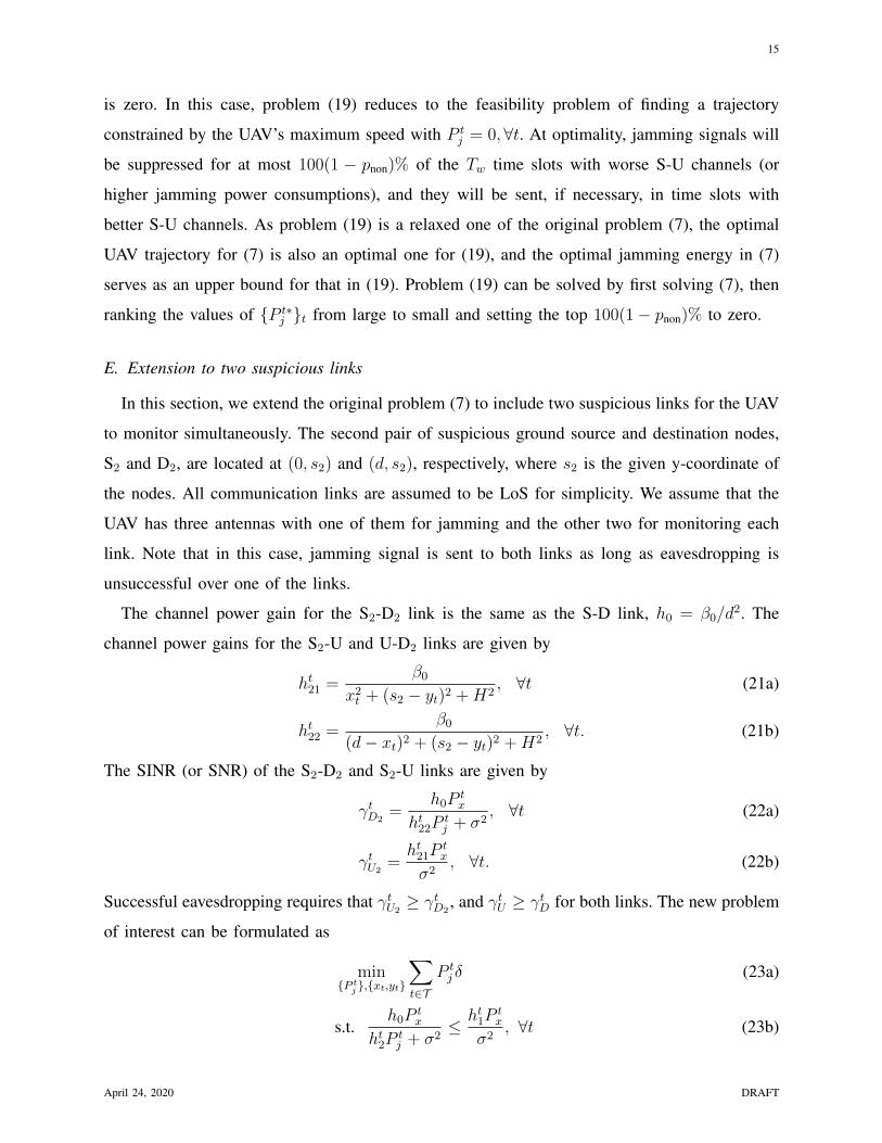
E. Extension to two suspicious links

In this section, we extend the original problem (7) to include two suspicious links for the UAV

to monitor simultaneously. The second pair of suspicious ground source and destination nodes,

S2 and D2, are located at (0, s2) and (d, s2), respectively, where s2 is the given y-coordinate of

the nodes. All communication links are assumed to be LoS for simplicity. We assume that the

UAV has three antennas with one of them for jamming and the other two for monitoring each

link. Note that in this case, jamming signal is sent to both links as long as eavesdropping is

unsuccessful over one of the links.

The channel power gain for the S2-D2 link is the same as the S-D link, h0 = β0/d2. The

channel power gains for the S2-U and U-D2 links are given by

ht21 =β0

x2t + (s2 − yt)2 +H2

, ∀t (21a)

ht22 =β0

(d− xt)2 + (s2 − yt)2 +H2, ∀t. (21b)

The SINR (or SNR) of the S2-D2 and S2-U links are given by

γtD2=

h0Ptx

ht22Ptj + σ2

, ∀t (22a)

γtU2=ht21P

tx

σ2, ∀t. (22b)

Successful eavesdropping requires that γtU2≥ γtD2

, and γtU ≥ γtD for both links. The new problem

of interest can be formulated as

min{P t

j },{xt,yt}

∑t∈T

P tj δ (23a)

s.t.h0P

tx

ht2Ptj + σ2

≤ ht1Ptx

σ2, ∀t (23b)


16

h0Ptx

ht22Ptj + σ2

≤ ht21Ptx

σ2, ∀t (23c)

(7c)− (7f).

Problem (23) can be solved by following the same procedure summarized in Algorithm 1. The

jamming-free area of the S2-D2 link is A2 := {(xt, yt)|√x2t + (s2 − yt)2 +H2 ≤ d,∀t}. When

|s2| ≤ 2d, the common jamming-free area, i.e., the jamming-free area for problem (23) is the

intersection of A and A2, which is essentially the intersection of two circles centered at (0, 0)

and (0, s2), respectively, both with a radius of d. When |s2| > 2d, the common jamming-free

area does not exist as A∩A2 = ∅.

It is worth noting that the problem of two suspicious links can be further extended to address

multiple suspicious links with different separating distances, or aerial (rather than ground)

suspicious nodes with 3D optimization of the UAV trajectory.

In a nutshell, we address the problem of jamming energy minimization for a UAV-enabled

monitoring system based on the assumption of sufficient power supply. We provide useful insights

on the UAV trajectory design and reveal its impact on the jamming policy. However, in practice,

such a trajectory design could result in a great cost (and waste) of propulsion power. Furthermore,

it is not possible for untethered UAVs to possess infinite power supply during flight. Motivated by

this, we next investigate the energy optimization based on a more practical setting, by considering

finite power supply and propulsion power consumption at the UAV.

IV. ENERGY MANAGEMENT FOR SOLAR-POWERED UAV

Compared with cables, laser-beams, and on-board batteries, the solar-powered UAVs enjoy a

high flexibility and a long flight endurance in practical deployment. Apart from communication

and jamming power, the UAV consumes additional propulsion power to maintain airborne and

support its movement. Energy-efficient operation of the UAV needs to be achieved by considering

propulsion energy management in system design [34].

Suppose that the UAV has a solar panel to harvest energy and an on-site battery to save energy.

The UAV’s battery is initially charged with E0 amount of energy, and that it can consume ϑ

portion of E0 during the entire working period, and save the (1 − ϑ) portion for emergency

during landing (to a prescribed platform or home base). The UAV can fly horizontally and adjust

its positions dynamically to enhance the eavesdropping performance. We pursue the optimal

trajectory design and energy management scheme of the UAV by minimizing the total jamming


17

0 10 20 30 40 50 60 700

50

100

150

200

250

300

UAV Flying Speed (m/s)

Pro

pu

lsio

n p

ow

er

(W)

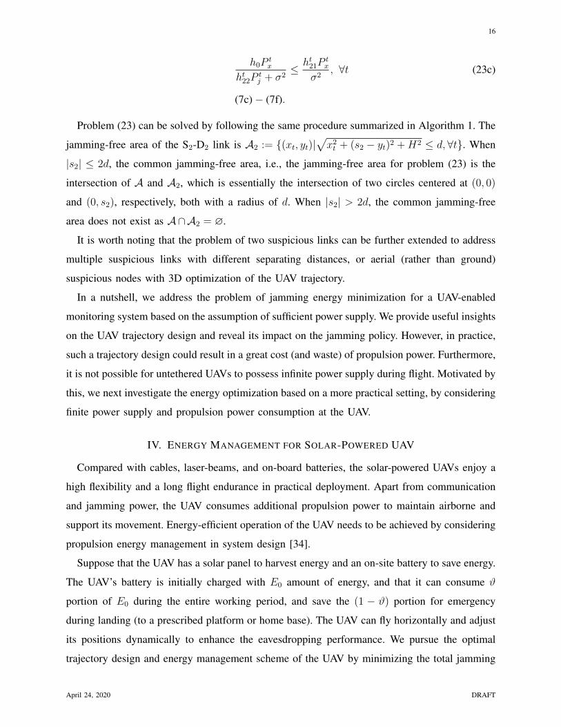
Fig. 2. Propulsion power versus UAV speed.

TABLE I

PARAMETERS FOR PROPULSION POWER [34]

UAV weight 2 kg

Blade profile power and induced power, P0, P1 3.4 W, 118 W

Rotor solidity and disc area, s, A 0.03, 0.28 m2

Tip speed of the rotor blade, Utip 60 m/s

Mean rotor induce velocity, v0 5.4 m/s

Atmospheric density and fuselage drag ratio, ρ, df 1.225 kg/m3, 0.3

and propulsion energy consumption for the solar-powered rotary-wing UAV enabled monitoring

system.

A. UAV Propulsion Power Model

Besides transmit (jamming) power, the communication related power includes also that for

communication circuitry, information receiving and decoding, signal processing, etc. For sim-

plicity, we suppose that such communication connected power is a constant, represented by Pc

in watt (W) [38], [39]. The propulsion power, which typically depends on the UAV speed, is

essential to support the UAV’s hovering and moving activities. For a rotary-wing UAV with


18

0 500 1000 1500100

110

120

130

140

150

160

170

180

190

Altitude of UAV (m)

Ha

rve

ste

d s

ola

r p

ow

er

(W)

Fig. 3. Harvested solar power versus UAV altitude.

speed Vt, the propulsion power at time slot t, denoted by P tm, is given by [34]

P tm =P0

(1 +

3V 2t

U2tip

)+ P1

(√1 +

V 4t

4v40

− V 2t

2v20

) 12

+1

2dfρsAV

3t

(24)

where P0 and P1 have fixed values and stand for the blade profile power and induced power

under hovering mode, respectively, Utip is the tip speed of the rotor blade, v0 denotes the average

rotor induced velocity in hover, df and s represent the fuselage drag ratio and rotor solidity,

and ρ and A are the atmospheric density and rotor disc area, respectively. When Vt = 0, (24)

corresponds to the power consumption of the hovering state. Fig. 2 depicts the typical curve

of P tm versus Vt. The parameters are set according to Table I [34]. It is revealed by Fig. 2

that the UAV speed achieving the least power consumption, i.e., about 41.84 W, happens at

approximately Ve = 22.36 m/s.

We suppose that within each slot t, the UAV maintains a constant speed, which is given by

Vt =√

(xt − xt−1)2 + (yt − yt−1)2/δ, ∀t. (25)

By substituting (25) into (24), we find that the first and the third terms of (24) are jointly convex

with respect to (xt, xt−1, yt, yt−1), whereas the second term is neither convex nor concave.


19

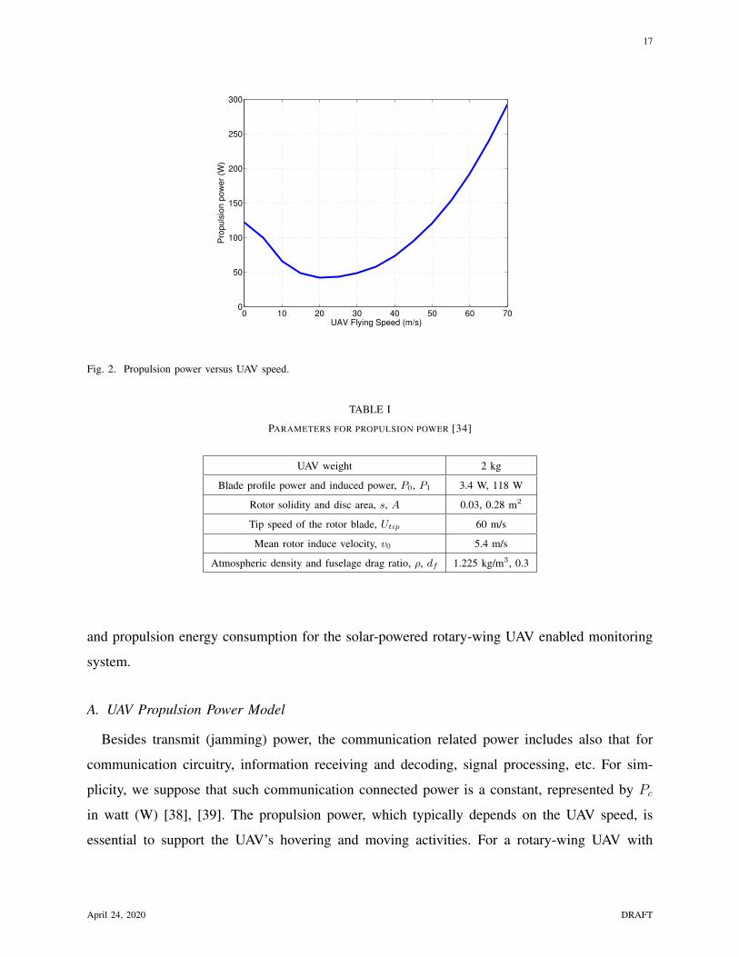
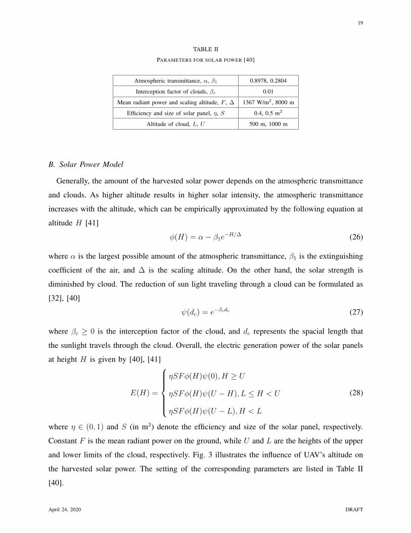
TABLE II

PARAMETERS FOR SOLAR POWER [40]

Atmospheric transmittance, α, β1 0.8978, 0.2804

Interception factor of clouds, βc 0.01

Mean radiant power and scaling altitude, F , ∆ 1367 W/m2, 8000 m

Efficiency and size of solar panel, η, S 0.4, 0.5 m2

Altitude of cloud, L, U 500 m, 1000 m

B. Solar Power Model

Generally, the amount of the harvested solar power depends on the atmospheric transmittance

and clouds. As higher altitude results in higher solar intensity, the atmospheric transmittance

increases with the altitude, which can be empirically approximated by the following equation at

altitude H [41]

φ(H) = α− β1e−H/∆ (26)

where α is the largest possible amount of the atmospheric transmittance, β1 is the extinguishing

coefficient of the air, and ∆ is the scaling altitude. On the other hand, the solar strength is

diminished by cloud. The reduction of sun light traveling through a cloud can be formulated as

[32], [40]

ψ(dc) = e−βcdc (27)

where βc ≥ 0 is the interception factor of the cloud, and dc represents the spacial length that

the sunlight travels through the cloud. Overall, the electric generation power of the solar panels

at height H is given by [40], [41]

E(H) =

ηSFφ(H)ψ(0), H ≥ U

ηSFφ(H)ψ(U −H), L ≤ H < U

ηSFφ(H)ψ(U − L), H < L

(28)

where η ∈ (0, 1) and S (in m2) denote the efficiency and size of the solar panel, respectively.

Constant F is the mean radiant power on the ground, while U and L are the heights of the upper

and lower limits of the cloud, respectively. Fig. 3 illustrates the influence of UAV’s altitude on

the harvested solar power. The setting of the corresponding parameters are listed in Table II

[40].


20

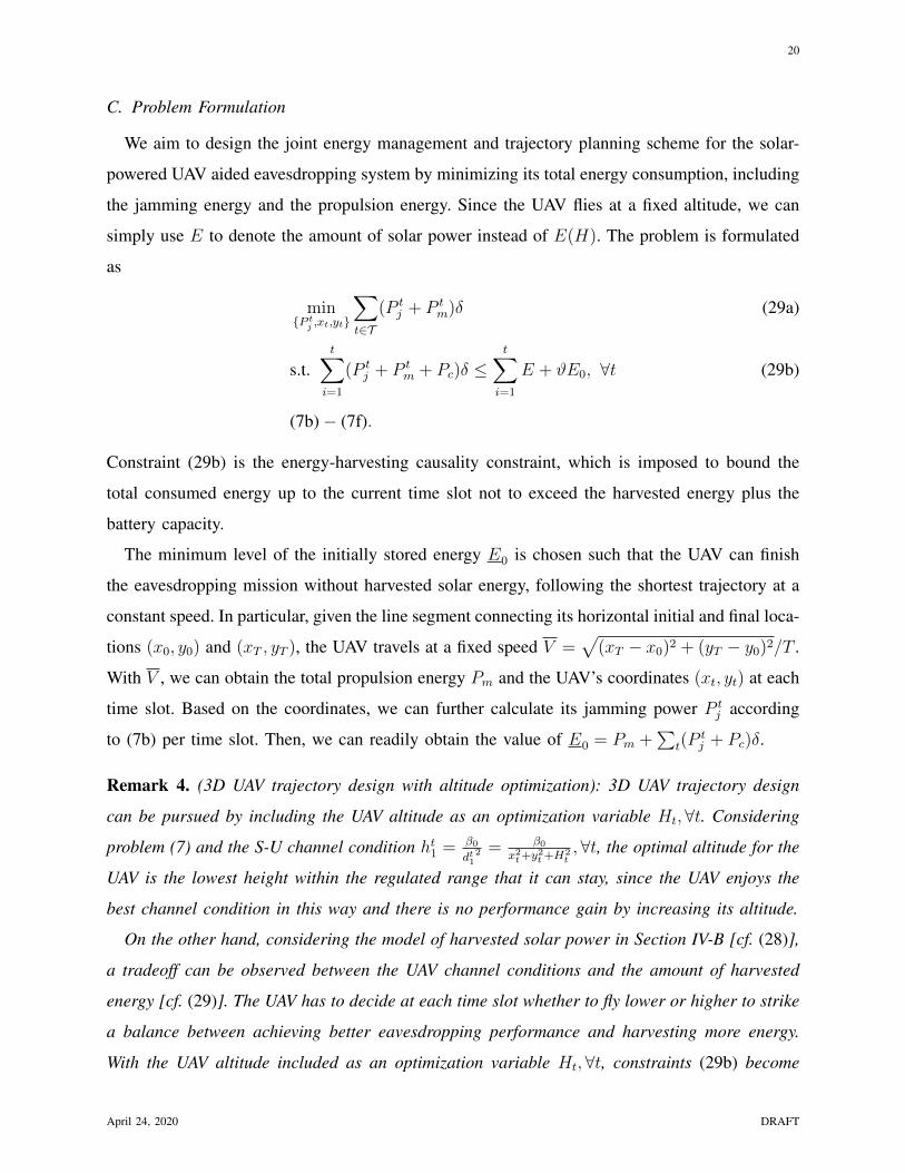
C. Problem Formulation

We aim to design the joint energy management and trajectory planning scheme for the solar-

powered UAV aided eavesdropping system by minimizing its total energy consumption, including

the jamming energy and the propulsion energy. Since the UAV flies at a fixed altitude, we can

simply use E to denote the amount of solar power instead of E(H). The problem is formulated

as

min{P t

j ,xt,yt}

∑t∈T

(P tj + P t

m)δ (29a)

s.t.t∑i=1

(P tj + P t

m + Pc)δ ≤t∑i=1

E + ϑE0, ∀t (29b)

(7b)− (7f).

Constraint (29b) is the energy-harvesting causality constraint, which is imposed to bound the

total consumed energy up to the current time slot not to exceed the harvested energy plus the

battery capacity.

The minimum level of the initially stored energy E0 is chosen such that the UAV can finish

the eavesdropping mission without harvested solar energy, following the shortest trajectory at a

constant speed. In particular, given the line segment connecting its horizontal initial and final loca-

tions (x0, y0) and (xT , yT ), the UAV travels at a fixed speed V =√

(xT − x0)2 + (yT − y0)2/T .

With V , we can obtain the total propulsion energy Pm and the UAV’s coordinates (xt, yt) at each

time slot. Based on the coordinates, we can further calculate its jamming power P tj according

to (7b) per time slot. Then, we can readily obtain the value of E0 = Pm +∑

t(Ptj + Pc)δ.

Remark 4. (3D UAV trajectory design with altitude optimization): 3D UAV trajectory design

can be pursued by including the UAV altitude as an optimization variable Ht,∀t. Considering

problem (7) and the S-U channel condition ht1 = β0dt1

2 = β0x2t+y2t +H2

t,∀t, the optimal altitude for the

UAV is the lowest height within the regulated range that it can stay, since the UAV enjoys the

best channel condition in this way and there is no performance gain by increasing its altitude.

On the other hand, considering the model of harvested solar power in Section IV-B [cf. (28)],

a tradeoff can be observed between the UAV channel conditions and the amount of harvested

energy [cf. (29)]. The UAV has to decide at each time slot whether to fly lower or higher to strike

a balance between achieving better eavesdropping performance and harvesting more energy.

With the UAV altitude included as an optimization variable Ht,∀t, constraints (29b) become


21

non-convex as the amount of harvested energy Et is altitude-dependent and time-varying. It is

difficult to convert (29b) to convex constraints due to the complicated expression of Et, thus

rendering the new problem hardly tractable for existing solvers. Furthermore, to the best of our

knowledge, there is not a general model to capture the power consumptions incurred by both

horizontal and vertical movements of the UAV, which in turn makes it difficult to pursue a joint

3D UAV trajectory design and power allocation. It will be an interesting direction to pursue in

our future works with altitude optimization.

D. SCA-based Convexification and Solution

The problem (29) is not convex since it consists the non-convex term(√

1 +V 4t

4v40− V 2

t

2v20

) 12

in

P tm, and the non-convex constraints (7b). The latter can be handled by leveraging the same method

as in Section III. With slack variables {ut, wt,∀t}, (7b) can be replaced with the constraints (8b)-

(8e).

To tackle the non-convexity with P tm, we first bring in slack variables {qt ≥ 0} such that

q2t =

√1 +

V 4t

4v40

− V 2t

2v20

, ∀t (30)

which is equivalent to1

q2t

= q2t +

V 2t

v20

, ∀t. (31)

The second term of (24) can thus be substituted by the linear component P1qt, with the additional

constraints (31). For the purpose of exposition, we now integrate the expression for Vt in (25)

and letP tm :=P0 +

3P0

U2tipδ

2

[(xt − xt−1)2 + (yt − yt−1)2

]+ P1qt

+df2δ3

ρsA[(xt − xt−1)2 + (yt − yt−1)2

]3/2, ∀t.

(32)

We can see that P tm is now jointly convex with respect to (xt, xt−1, yt, yt−1, qt). With such a

manipulation, problem (29) can be written as

min{P t

j ,qt,ut}{xt,yt,wt}

∑t∈T

(P tj + P t

m)δ (33a)

s.t.t∑i=1

(P tj + P t

m + Pc)δ ≤t∑i=1

E + ϑE0, ∀t (33b)

1

q2t

≤ q2t +

(xt − xt−1)2 + (yt − yt−1)2

v20

, ∀t (33c)


22

(7c)− (7f), (8b)− (8e)

where v20 = v2

0δ2.

Note that constraints (33c) are obtained from (31) by replacing the equations with inequalities.

Yet, equivalence still holds between problems (29) and (33). To examine this, we assume that

if any of the constraints in (33c) is met with strict inequality when achieving optimality for

problem (33), we can decrease the related value of variable qt to enable constraint (33c) met

with equality, while reducing the total energy consumption (objective value) at the same time.

Therefore, all constraints in (33c) are met with equality at optimality. The same equivalence also

holds for constraints (8b) and (8c) as explained in Section III. Hence, problems (29) and (33)

are equivalent.

Problem (33) is still non-convex since it consists the non-convex constraints in (33c). However,

it can be tackled with the successive convex approximation (SCA) method by calculating the

global lower bounds at a given local point. In particular, for (33c), the left-hand-side (LHS) is

a convex function in qt, and the right-hand-side (RHS) is a jointly convex function regarding qt

and (xt, xt−1, yt, yt−1). Since the first-order Taylor expansion serves as the global lower bound

of a convex function, we can obtain the following inequality for the RHS of (33c)

q2t +

(xt − xt−1)2 + (yt − yt−1)2

v20

≥ q(l)2t + 2q

(l)t (qt − q(l)

t )

+2

v20

[(x(l)t − x

(l)t−1)(xt − xt−1) + (y

(l)t − y

(l)t−1)(yt − yt−1)]

− 1

v20

[(x(l)t − x

(l)t−1)2 + (y

(l)t − y

(l)t−1)2]

(34)

where q(l)t , x(l)

t , and y(l)t are the present values of the corresponding variables at the l-th iteration,

respectively. By substituting the non-convex constraints (33c) with its lower bound at the l-th

iteration acquired by (34), we can establish the following optimization problem

min{P t

j ,qt,ut}{xt,yt,wt}

∑t∈T

(P tj + P t

m)δ (35a)

s.t.1

q2t

≤ q(l)2t + 2q

(l)t (qt − q(l)

t ) +2

v20

[(x(l)t − x

(l)t−1)(xt − xt−1) + (y

(l)t − y

(l)t−1)(yt − yt−1)]

− 1

v20

[(x(l)t − x

(l)t−1)2 + (y

(l)t − y

(l)t−1)2], ∀t (35b)

qt ≥ 0, ∀t (35c)

(7c)− (7f), (8b)− (8e), (33b).


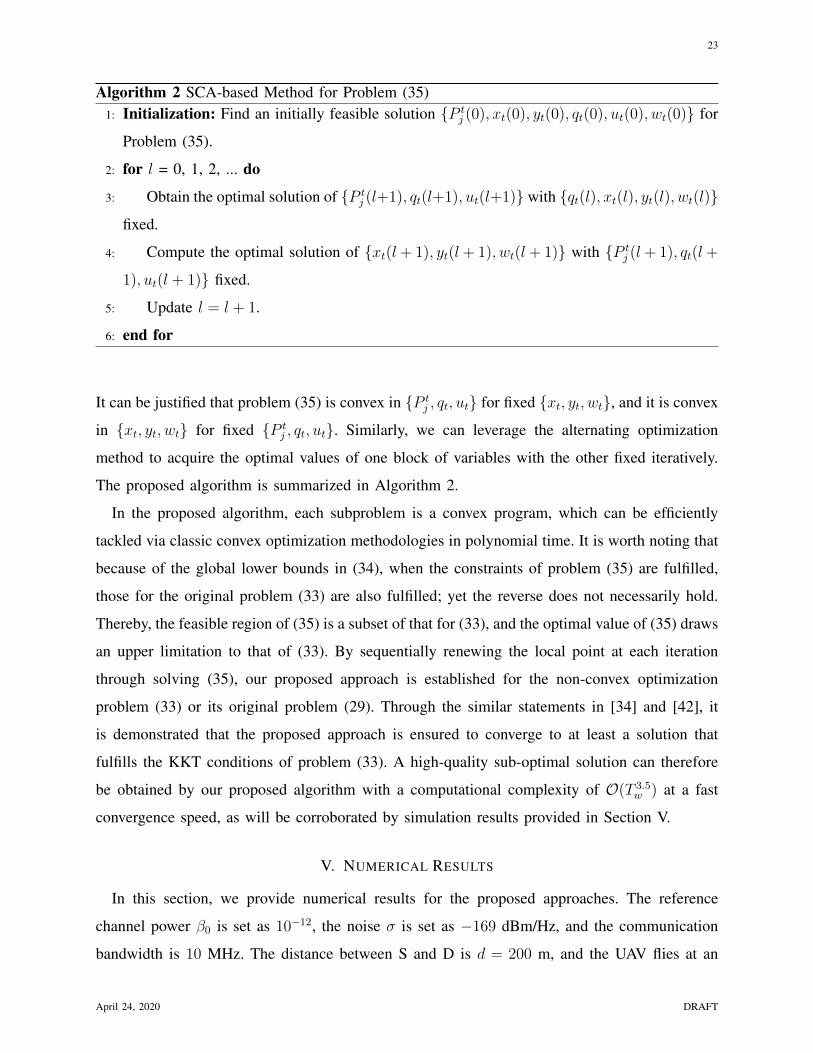
23

Algorithm 2 SCA-based Method for Problem (35)1: Initialization: Find an initially feasible solution {P t

j (0), xt(0), yt(0), qt(0), ut(0), wt(0)} for

Problem (35).

2: for l = 0, 1, 2, ... do

3: Obtain the optimal solution of {P tj (l+1), qt(l+1), ut(l+1)} with {qt(l), xt(l), yt(l), wt(l)}

fixed.

4: Compute the optimal solution of {xt(l+ 1), yt(l+ 1), wt(l+ 1)} with {P tj (l+ 1), qt(l+

1), ut(l + 1)} fixed.

5: Update l = l + 1.

6: end for

It can be justified that problem (35) is convex in {P tj , qt, ut} for fixed {xt, yt, wt}, and it is convex

in {xt, yt, wt} for fixed {P tj , qt, ut}. Similarly, we can leverage the alternating optimization

method to acquire the optimal values of one block of variables with the other fixed iteratively.

The proposed algorithm is summarized in Algorithm 2.

In the proposed algorithm, each subproblem is a convex program, which can be efficiently

tackled via classic convex optimization methodologies in polynomial time. It is worth noting that

because of the global lower bounds in (34), when the constraints of problem (35) are fulfilled,

those for the original problem (33) are also fulfilled; yet the reverse does not necessarily hold.

Thereby, the feasible region of (35) is a subset of that for (33), and the optimal value of (35) draws

an upper limitation to that of (33). By sequentially renewing the local point at each iteration

through solving (35), our proposed approach is established for the non-convex optimization

problem (33) or its original problem (29). Through the similar statements in [34] and [42], it

is demonstrated that the proposed approach is ensured to converge to at least a solution that

fulfills the KKT conditions of problem (33). A high-quality sub-optimal solution can therefore

be obtained by our proposed algorithm with a computational complexity of O(T 3.5w ) at a fast

convergence speed, as will be corroborated by simulation results provided in Section V.

V. NUMERICAL RESULTS

In this section, we provide numerical results for the proposed approaches. The reference

channel power β0 is set as 10−12, the noise σ is set as −169 dBm/Hz, and the communication

bandwidth is 10 MHz. The distance between S and D is d = 200 m, and the UAV flies at an


24

0 50 100 150 200 250 3000

100

200

300

400

Initial location

Final location

Jamming−free area

(a) x (m)y (

m)

T=10s

T=30s

T=60s

Low speed

Fly half

Two lines

NLoS

0 10 20 30 40 50 600

20

40

60

(b) Time slot (s)

Ja

mm

ing

po

we

r (W

)

T=10s

T=30s

T=60s

Low speed

Fly half

Two lines

NLoS

Fig. 4. UAV trajectory designs and jamming power allocations under NF scenario.

altitude of H = 100 m. The maximum horizontal speed of the UAV is set as Vm = 40 m/s.

The slot length is δ = 0.1 s. The original capacity of the battery E0 is 7 × 103 J. Parameters

concerning the propulsion power and the harvested solar power are the same as in Tables I and

II. To evaluate the proposed optimal trajectory design and power allocation schemes, we test

three pairs of coordinates for the initial and final locations of the UAV. The three test cases are:

1) JF (Jamming Free) scenario: both the initial and final locations are inside the jamming-free

area of A, namely, (x0, y0) = (−50 m,−100 m), and (xT , yT ) = (100 m, 140 m); 2) IF (Initial

jamming Free) scenario: the initial location is inside A and the final location is outside A, namely,

(x0, y0) = (−50 m, 0), and (xT , yT ) = (100 m, 350 m); and 3) NF (No jamming Free) scenario:

both locations are outside A, namely, (x0, y0) = (300 m, 200 m), and (xT , yT ) = (200 m, 400 m).

To further observe the UAV’s behavior, we adopt three time horizons for each scenario, namely,

T = 10 s, 30 s and 60 s. Trajectory and power consumptions of the UAV are depicted every

second. Note that all pairs of coordinates are carefully selected such that at least one feasible

trajectory can be found for the UAV in the shortest time horizon.

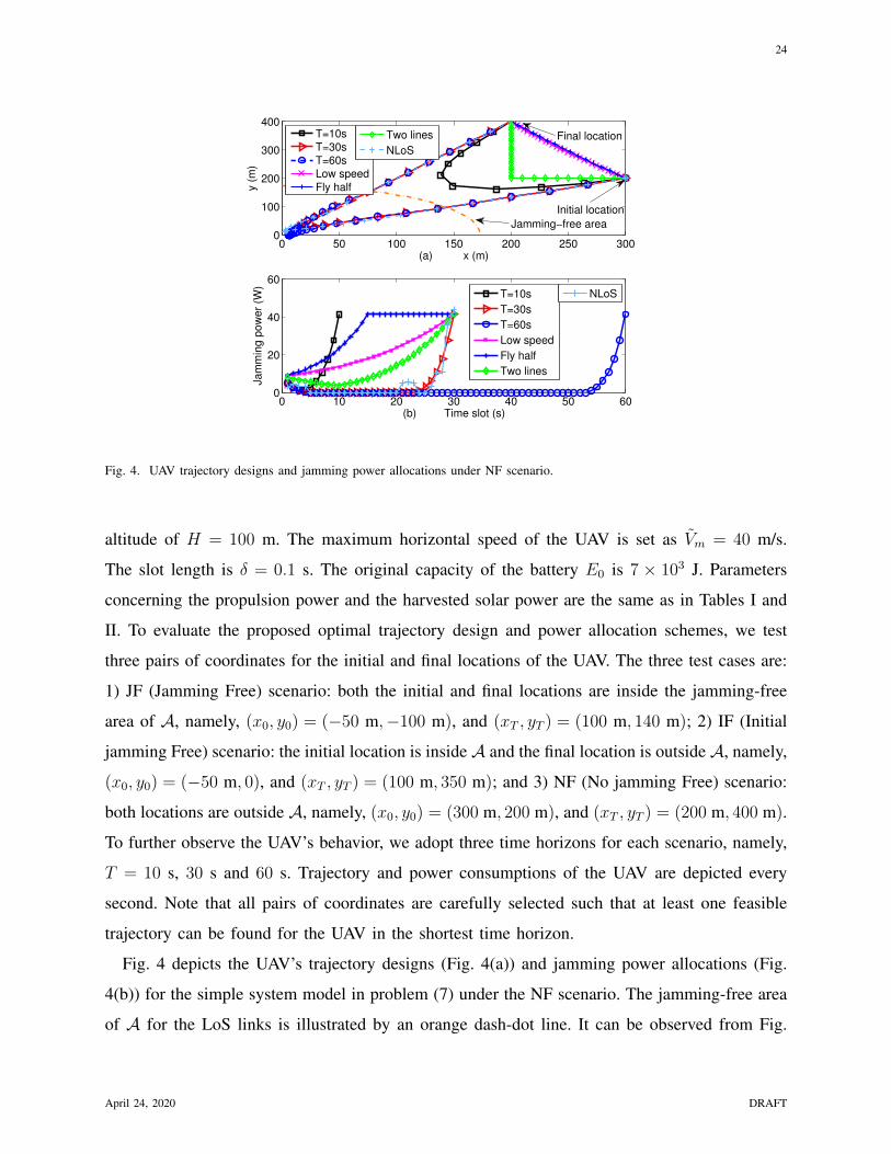
Fig. 4 depicts the UAV’s trajectory designs (Fig. 4(a)) and jamming power allocations (Fig.

4(b)) for the simple system model in problem (7) under the NF scenario. The jamming-free area

of A for the LoS links is illustrated by an orange dash-dot line. It can be observed from Fig.


25

0 1 2 3 4 5 6 7 80

100

200

300

400

500

600

700

800

900

1000

Optimization schemes

To

tal e

ne

rgy c

on

su

mp

tio

n (

J)

Low speed

Fly half

Two lines

Proposed (T=10s)

Proposed (T=30s)

Proposed (T=60s)

NLoS

Fig. 5. Total jamming energy consumptions of the UAV under NF scenario.

4 that when both the initial and final locations are outside A, the UAV intends to fly towards

A first, then travel to the final location. With sufficient traveling time (T = 30 s and 60 s), the

UAV first flies fast to A, then takes a detour at a very low speed inside A, and finally travels

quickly to its final location. During this process, the jamming power first decreases, then stays

at zero, and finally increases quickly in the last few time slots. This is consistent with the results

in Lemma 2 and Proposition 1. We also include the performance of the UAV with NLoS links

when T = 30 s in Fig. 4 (labeled as “NLoS”). It can be seen that the UAV’s trajectory does not

vary much under this scenario, and that its jamming power does not change smoothly with its

distance from the source due to the randomness invited by the S-D link. To further validate the

advantage of trajectory design on energy reduction, we examine three baseline schemes of the

UAV under the NF scenario when T = 30 s. The first scheme is labeled as “Low speed”, where

the UAV travels straightly from the initial location to the final location at a fixed speed (7.46

m/s). The second scheme is labeled as “Fly half”, where the UAV flies straightly to the final

location at a constant speed (14.91 m/s) during the first half of the period (15 s), and hovers

at the destination for the rest of the period. The third scheme is labeled as “Two lines”, where

the UAV first flies directly towards the point (200 m, 200 m), then flies to the final location,

following the trajectory of two line segments at a constant speed of 10 m/s.


26

−200 −150 −100 −50 0 50 100 150 200−200

−150

−100

−50

0

50

100

150

200

x (m)

y (

m)

Initial location

Final locationJamming−free area

Initial location

Final location

T=10s

T=30s

T=60s (iter=10)

T=60s (iter=30)

T=60s (iter=50)

T=60s (iter=60)

Fig. 6. UAV trajectory designs under JF scenario.

0 10 20 30 40 50 6040

42

44

46

48

50

52

54

56

58

Time slot (s)

Pro

pu

lsio

n p

ow

er

(W)

T=10s

T=30s

T=60s (iter=10)

T=60s (iter=30)

T=60s (iter=50)

T=60s (iter=60)

Fig. 7. UAV power allocations under JF scenario.

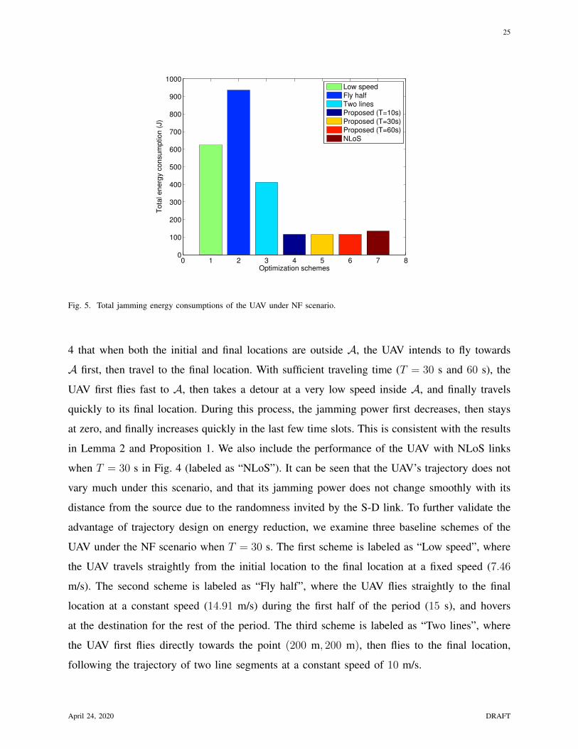
Fig. 5 shows the total energy consumptions of the UAV under the NF scenario. It is unveiled

by Figs. 4 and 5 that the UAV consumes significantly more jamming energy without careful

trajectory design. The overall energy consumption of the “Fly half” scheme is almost ninefold

of that of our proposed scheme, since the UAV flies quickly to the destination and hovers there


27

−100 −50 0 50 100 150 200 250 300−200

0

200

400

(a) x (m)y (

m)

Initial location

Final locationJamming−free area

T=10s

T=30s

T=60s

10 20 30 40 50 600

20

40

60

80

(b) Time slot (s)

Po

we

r (W

)

Jamming power

Propulsion power

T=10s

T=30s

T=60s

Fig. 8. UAV trajectory designs and power allocations under IF scenario.

5 10 15 20 25 300

20

40

60

Time slot (s)

Ja

mm

ing

po

we

r (W

)

Fly first Hover first Round trip Low speed

Two lines

Proposed

5 10 15 20 25 30

20

40

60

80

100

120

Time slot (s)

Pro

pu

lsio

n p

ow

er

(W)

Fly first Hover first Round trip Low speed

Two lines

Proposed

Fig. 9. UAV power allocations for baseline schemes under NF scenario.

for a relatively long period. As the destination is far from the source node, the longer the UAV

stays there, the more jamming energy it consumes. The “Two lines” scheme is the most energy-

efficient among the baseline schemes as it amounts to a simple optimization of the trajectory.

Under the same parameter setting, the UAV consumes more energy with NLoS links than with


28

0 1 2 3 4 5 6 70

500

1000

1500

2000

2500

3000

3500

4000

Optimization schemes

To

tal e

ne

rgy c

on

su

mp

tio

n (

J)

Fly first

Hover first

Round trip

Low speed

Two lines

Proposed

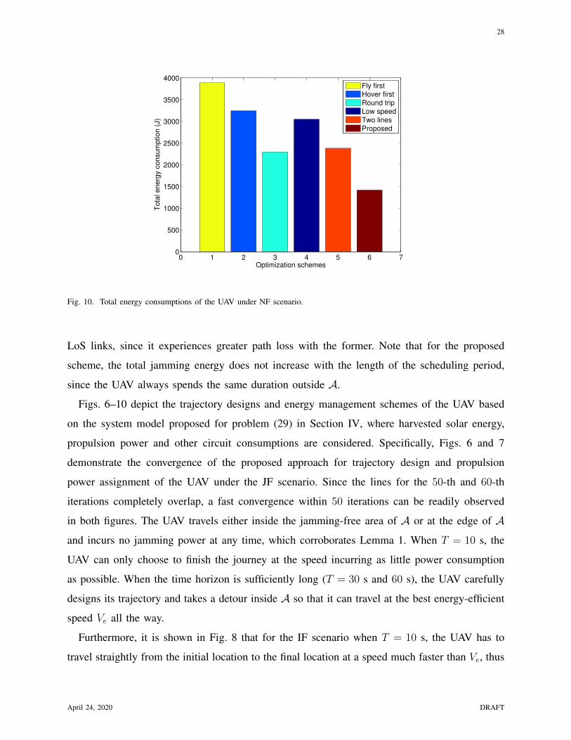
Fig. 10. Total energy consumptions of the UAV under NF scenario.

LoS links, since it experiences greater path loss with the former. Note that for the proposed

scheme, the total jamming energy does not increase with the length of the scheduling period,

since the UAV always spends the same duration outside A.

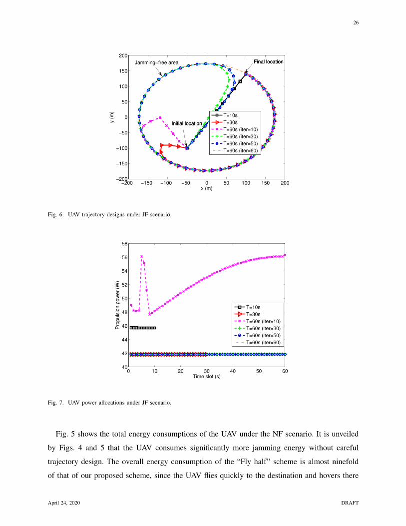
Figs. 6–10 depict the trajectory designs and energy management schemes of the UAV based

on the system model proposed for problem (29) in Section IV, where harvested solar energy,

propulsion power and other circuit consumptions are considered. Specifically, Figs. 6 and 7

demonstrate the convergence of the proposed approach for trajectory design and propulsion

power assignment of the UAV under the JF scenario. Since the lines for the 50-th and 60-th

iterations completely overlap, a fast convergence within 50 iterations can be readily observed

in both figures. The UAV travels either inside the jamming-free area of A or at the edge of A

and incurs no jamming power at any time, which corroborates Lemma 1. When T = 10 s, the

UAV can only choose to finish the journey at the speed incurring as little power consumption

as possible. When the time horizon is sufficiently long (T = 30 s and 60 s), the UAV carefully

designs its trajectory and takes a detour inside A so that it can travel at the best energy-efficient

speed Ve all the way.

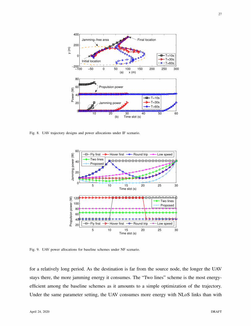
Furthermore, it is shown in Fig. 8 that for the IF scenario when T = 10 s, the UAV has to

travel straightly from the initial location to the final location at a speed much faster than Ve, thus


29

leading to a significant amount of propulsion power consumption at each slot. If there is surplus

time, the UAV first travels inside A at a constant speed of Ve, which minimizes the propulsion

power consumption. Then it flies to the final location, which is outside A, in the last few time

slots. This trajectory design enables the UAV to stay inside A for as long as possible, since the

shorter time it stays outside A, the less jamming energy it consumes.

To fully demonstrate the influence and merits of delicate trajectory design for the UAV, we

again compare with three baseline schemes where the UAV adopts different flying protocols for

the same trajectory as the “Low speed” scheme when T = 30 s. The first protocol is labelled

as “Fly first”, where the UAV flies to the final location at approximately Ve = 22.36 m/s in

the first 10 s, then hovers at the destination for the rest 20 s. The second protocol is labelled

as “Hover first”, where the UAV hovers above the initial location in the first 20 s, then flies to

the final location for the rest 10 s at speed Ve. The third protocol is labelled as “Round trip”,

where the UAV first takes a round trip between the initial and final locations, then flies again to

the destination, at speed Ve during the flight period. To facilitate comparison, we also include

the “Low speed”, “Two lines”, and our proposed schemes under the NF scenario. Figs. 9 and

10 depict the jamming and propulsion power allocations at each time slot, and the total energy

consumptions of the UAV, respectively. Table III lists the respective jamming and propulsion

energy consumptions for different schemes. It can be readily seen from Fig. 9 that the UAV

needs to send jamming signals at every time slot under the five baseline schemes, as it is always

traveling outside A. The propulsion power consumption for hovering triples that for traveling at

speed Ve. The “Fly first” scheme incurs the largest energy consumption for both jamming and

propulsion, due to its 20 s hovering at the farthest point from the suspicious source. It is further

revealed in Fig. 10 that the total energy consumption of the “Round trip” scheme is the lowest

among the baseline schemes, since it adopts a simple trajectory design with the energy-efficient

speed. It is observed from Table III that the jamming energy consumption is the highest for the

“Fly first” and “Round trip” schemes, while the propulsion energy consumption is the highest

for the “Fly first” and “Hover first” schemes. Our proposed scheme consumes the least jamming

energy and propulsion energy. Clearly, all of the baseline schemes consume more energy than

our proposed scheme. In a nutshell, the UAV suffers significant waste of energy without careful

trajectory optimization.

Remark 5. (Mitigating the interference on other links): When the suspicious link intentionally


30

TABLE III

RESPECTIVE JAMMING AND PROPULSION ENERGY CONSUMPTIONS FOR DIFFERENT SCHEMES UNDER NF SCENARIO.

Optimization schemes Jamming energy (J) Propulsion energy (J)

Fly first 1042.9 2850.0

Hover first 396.3 2850.0

Round trip 1042.9 1255.2

Low speed 623.7 2427.5

Two lines 412.8 1968.6

Proposed 165.2 1255.2

chooses to be located in a wild rural area to avoid surveillance by existing monitoring infras-

tructures, there would be few communication links in the vicinity, and the interference caused by

jamming could thereby be reduced to the minimum level, which is negligible. In fact, it typically

depends on the access scheme whether jamming suppresses communications of other links. For

instance, if the suspicious link occupies a certain frequency band all to itself, the UAV is able

to send exclusive jamming signals to it, which will not affect other links. On the other hand, if

serious communication degradation is reported by legitimate users within the neighborhood, the

UAV can release the specific transmitted (and encrypted) information to these users so that they

can decode the jamming signals and will not be interfered. Note that the maximum jamming

power of 40 W in Figs. 4 and 9 is the worst-case value tested in the simulation. Yet in practice,

the UAV is not usually that far away from the suspicious source and does not incur such a high

jamming power consumption.

VI. CONCLUSION

We addressed joint energy management and trajectory optimization for a rotary-wing UAV

enabled legitimate monitoring system. Building on a judicious (re-)formulation, we leveraged

the alternating optimization and successive convex approximation methodologies to minimize

the overall energy consumption of the UAV. Efficient algorithms were developed to compute

the locally optimal solution or at least a feasible solution fulfilling the KKT conditions. We

provided extensive numerical test results to justify the effectiveness of the proposed schemes.

The proposed framework also inspires new directions for future researches on security issues


31

in UAV-aided wireless networks such as wireless power transfer and/or mobile edge computing

based ones, especially with non-LoS channels and 3D trajectory planning.

REFERENCES

[1] Y. Zeng, R. Zhang, and T. J. Lim, “Wireless communications with unmanned aerial vehicles: Opportunities and challenges,”

IEEE Commun. Mag., vol. 54, no. 5, pp. 36–42, May 2016.

[2] Q. Wu, L. Liu, and R. Zhang, “Fundamental tradeoffs in communication and trajectory design for UAV-enabled wireless

network,” IEEE Wireless Commun., vol. 26, no. 1, pp. 36–44, Feb. 2019.

[3] Y. Zeng, Q. Wu, and R. Zhang, “Accessing from the sky: A tutorial on UAV communications for 5G and beyond,” Proc.

IEEE, vol. 107, no. 12, pp. 2327–2375, Dec. 2019.

[4] A. Fotouhi, H. Qiang, M. Ding, M. Hassan, L. Garcia-Giordano, A. G. Rodriguez, and J. Yuan, “Survey on UAV cellular

communications: Practical aspects, standardization advancements, regulation, and security challenges,” IEEE Commun.

Surv. Tut., vol. 21, no. 4, pp. 3417–3442, 4th Quart., 2019.

[5] M. Mozaffari, W. Saad, M. Bennis, Y.-H. Nam, and M. Debbah, “A tutorial on UAVs for wireless networks: Applications,

challenges, and open problems,” IEEE Commun. Surv. Tut., vol. 21, no. 3, pp. 2334–2360, 3rd Quart., 2019.

[6] N. H. Motlagh, M. Bagaa, and T. Taleb, “UAV-based IoT platform: A crowd surveillance use case,” IEEE Commun. Mag.,

vol. 55, no. 2, pp. 128–134, Feb. 2017.

[7] X. Xu, Y. Zeng, Y. Guan, and R. Zhang, “Overcoming endurance issue: UAV-enabled communications with proactive

caching,” IEEE J. Sel. Areas Commun., vol. 36, no. 6, pp. 1231–1244, Jun. 2018.

[8] Y. Zeng, X. Xu, and R. Zhang, “Trajectory optimization for completion time minimization in UAV-enabled multicasting,”

IEEE Trans. Wireless Commun., vol. 17, no. 4, pp. 2233–2246, Apr. 2018.

[9] Q. Wu, Y. Zeng, and R. Zhang, “Joint trajectory and communication design for multi-UAV enabled wireless networks,”

IEEE Trans. Wireless Commun., vol. 17, no. 3, pp. 2109–2121, Mar. 2018.

[10] Q. Wu and R. Zhang, “Common throughput maximization in UAV-enabled OFDMA systems with delay consideration,”

IEEE Trans. Commun., vol. 66, no. 12, pp. 6614–6627, Dec. 2018.

[11] K. Li, W. Ni, X. Wang, R. Liu, S. Kanhere, and S. Jha, “Energy-efficient cooperative relaying for unmanned aerial vehicles,”

IEEE Trans. Mobile Comput., vol. 15, no. 6, pp. 1377–1386, Jun. 2016.

[12] Y. Zeng, R. Zhang, and T. J. Lim, “Throughput maximization for UAV-enabled mobile relaying systems,” IEEE Trans.

Commun., vol. 64, no. 12, pp. 4983–4996, Dec. 2016.

[13] Z. Yang, C. Pan, K. Wang, and M. Shikh-Bahaei, “Energy efficient resource allocation in UAV-enabled mobile edge

computing networks,” IEEE Trans. Wireless Commun., vol. 18, no. 9, pp. 4576–4589, Sep. 2019.

[14] M. Mozaffari, W. Saad, M. Bennis, and M. Debbah, “Mobile unmanned aerial vehicles (UAVs) for energy-efficient internet

of things communications,” IEEE Trans. Wireless Commun., vol. 16, no. 11, pp. 7574–7589, Nov. 2017.

[15] J. Xu, Y. Zeng, and R. Zhang, “UAV-enabled wireless power transfer: Trajectory design and energy optimization,” IEEE

Trans. Wireless Commun., vol. 17, no. 8, pp. 5092–5106, Aug. 2018.

[16] S. Huang, Q. Zhang, Q. Li, and J. Qin, “Robust proactive monitoring via jamming with deterministically bounded channel

errors,” IEEE Signal Process. Lett., vol. 25, no. 5, pp. 690–694, May 2018.

[17] Y. Zeng and R. Zhang, “Wireless information surveillance via proactive eavesdropping with spoofing relay,” IEEE J. Sel.

Topics Signal Process., vol. 10, no. 8, pp. 1449–1461, Dec. 2016.

[18] J. Xu, L. Duan, and R. Zhang, “Transmit optimization for symbol-level spoofing,” IEEE Trans. Wireless Commun., vol. 17,

no. 1, pp. 41–55, Jan. 2018.


32

[19] ——, “Proactive eavesdropping via cognitive jamming in fading channels,” IEEE Trans. Wireless Commun., vol. 16, no. 5,

pp. 2790–2806, May 2017.

[20] ——, “Surveillance and intervention of infrastructure-free mobile communications: A new wireless security paradigm,”

IEEE Wireless Commun., vol. 24, no. 4, pp. 152–159, Aug. 2017.

[21] H. Cai, Q. Zhang, Q. Li, and J. Qin, “Proactive monitoring via jamming for rate maximization over MIMO rayleigh fading

channels,” IEEE Commun. Lett., vol. 21, no. 9, pp. 2021–2024, Sep. 2017.

[22] D. Hu, Z. Qi, Y. Ping, and J. Qin, “Proactive monitoring via jamming in amplify-and-forward relay networks,” IEEE Signal

Process. Lett., vol. 24, no. 11, pp. 1714–1718, Nov. 2017.

[23] H. Lu, H. Zhang, H. Dai, W. Wu, and B. Wang, “Proactive eavesdropping in UAV-aided suspicious communication

systems,” IEEE Trans. Veh. Tech., vol. 68, no. 2, pp. 1993–1997, Feb. 2019.

[24] J. Moon, S. H. Lee, H. Lee, S. Baek, and I. Lee, “Deep learning-based proactive eavesdropping for wireless surveillance,”

in IEEE Intl. Conf. Commun. (ICC), 2019.

[25] Q. Wu, W. Mei, and R. Zhang, “Safeguarding wireless networks with UAV: A physical layer security perspective,” IEEE

Wireless Commun., vol. 26, no. 5, pp. 12–18, Oct. 2019.

[26] Q. Wu, J. Xu, and R. Zhang, “Capacity characterization of UAV-enabled two-user broadcast channel,” IEEE J. Sel. Areas

Commun., vol. 36, no. 9, pp. 1955–1971, Sep. 2018.

[27] R. I. B. Yaliniz, A. El-Keyi, and H. Yanikomeroglu, “Efficient 3-D placement of an aerial base station in next generation

cellular networks,” in IEEE Intl. Conf. Commun. (ICC), 2016.

[28] P. Yang, X. Cao, C. Yin, Z. Xiao, X. Xi, and D. Wu, “Proactive drone-cell deployment: Overload relief for a cellular

network under flash crowd traffic,” IEEE Trans. Intell. Transp. Syst., vol. 18, no. 10, pp. 2877–2892, Oct. 2017.

[29] J. Lyu, Y. Zeng, R. Zhang, and T. J. Lim, “Placement optimization of UAV-mounted mobile base stations,” IEEE Commun.

Lett., vol. 21, no. 3, pp. 604–607, Mar. 2017.

[30] M. Alzenad, A. El-Keyi, F. Lagum, and H. Yanikomeroglu, “3D placement of an unmanned aerial vehicle base station

(UAV-BS) for energy-efficient maximal coverage,” IEEE Wireless Commun. Lett., vol. 6, no. 4, pp. 434–437, Aug. 2017.

[31] J. Ouyang, Y. Che, J. Xu, and K. Wu, “Throughput maximization for laser-powered UAV wireless communication systems,”

in IEEE Intl. Conf. Commun. (ICC), 2018.

[32] Y. Sun, D. W. K. Ng, D. Xu, L. Dai, and R. Schober, “Optimal 3D-trajectory design and resource allocation for solar-

powered UAV communication systems,” IEEE Trans. Commun., vol. 67, no. 6, pp. 4281–4298, Jun. 2019.

[33] Y. Zeng and R. Zhang, “Energy-efficient UAV communication with trajectory optimization,” IEEE Trans. Wireless Commun.,

vol. 16, no. 6, pp. 3747–3760, Jun. 2017.

[34] Y. Zeng, J. Xu, and R. Zhang, “Energy minimization for wireless communication with rotary-wing UAV,” IEEE Trans.

Wireless Commun., vol. 18, no. 4, pp. 2329–2345, Apr. 2019.

[35] X. Lin, V. Yajnanarayana, S. D. Muruganathan, S. Gao, H. Asplund, H. L. Maattanen, B. A. Mattias, S. Euler, and Y. P. E.

Wang, “The sky is not the limit: LTE for unmanned aerial vehicles,” IEEE Commun. Mag., vol. 56, no. 4, pp. 204–210,

Apr. 2018.

[36] S. Boyd and L. Vandenberghe, Convex Optimization. Cambridge University Press, 2004.

[37] G. Zhang, Q. Wu, M. Cui, and R. Zhang, “Securing UAV communications via joint trajectory and power control,” IEEE

Trans. Wireless Commun., vol. 18, no. 2, pp. 1376–1389, Feb. 2019.

[38] S. Zhang, Q. Wu, S. Xu, and G. Y. Li, “Fundamental green tradeoffs: Progresses, challenges, and impacts on 5G networks,”

IEEE Commun. Surv. Tut., vol. 19, no. 1, pp. 33–56, 1st Quart. 2017.

[39] S. Hu, X. Chen, W. Ni, X. Wang, and E. Hossain, “Modeling and analysis of energy harvesting and smart grid-powered


33

wireless communication networks: A contemporary survey,” IEEE Trans. Green Commun. Netw., pp. 1–36, to appear, Apr.

2020.

[40] A. Kokhanovsky, “Optical properties of terrestrial clouds,” Earth-Science Reviews, vol. 64, no. 3, pp. 189–241, Feb. 2004.

[41] J. S. Lee and K.-H. Yu, “Optimal path planning of solar-powered uav using gravitational potential energy,” IEEE Trans.

Aerosp. Electron. Syst., vol. 53, no. 3, pp. 1442–1451, Jun. 2017.

[42] A. Zappone, E. Bjornson, L. Sanguinetti, and E. Jorswieck, “Globally optimal energy-efficient power control and receiver

design in wireless networks,” IEEE Trans. Signal Process., vol. 65, no. 11, pp. 2844–2859, Jun. 2017.


Energy Management and Trajectory Optimization for UAV ...

Documents

Transcript of Energy Management and Trajectory Optimization for UAV ...