Energy Management And Control Of Smart Power Distribution ...

University of Texas at El Paso University of Texas at El Paso

ScholarWorks@UTEP ScholarWorks@UTEP

Open Access Theses & Dissertations

2019-01-01

Energy Management And Control Of Smart Power Distribution Energy Management And Control Of Smart Power Distribution

Systems Systems

Eric Galvan University of Texas at El Paso

Follow this and additional works at: https://digitalcommons.utep.edu/open_etd

Part of the Electrical and Electronics Commons

Recommended Citation Recommended Citation Galvan, Eric, "Energy Management And Control Of Smart Power Distribution Systems" (2019). Open Access Theses & Dissertations. 2853. https://digitalcommons.utep.edu/open_etd/2853

This is brought to you for free and open access by ScholarWorks@UTEP. It has been accepted for inclusion in Open Access Theses & Dissertations by an authorized administrator of ScholarWorks@UTEP. For more information, please contact [email protected].

https://digitalcommons.utep.edu/

https://digitalcommons.utep.edu/open_etd

https://digitalcommons.utep.edu/open_etd?utm_source=digitalcommons.utep.edu%2Fopen_etd%2F2853&utm_medium=PDF&utm_campaign=PDFCoverPages

http://network.bepress.com/hgg/discipline/270?utm_source=digitalcommons.utep.edu%2Fopen_etd%2F2853&utm_medium=PDF&utm_campaign=PDFCoverPages

https://digitalcommons.utep.edu/open_etd/2853?utm_source=digitalcommons.utep.edu%2Fopen_etd%2F2853&utm_medium=PDF&utm_campaign=PDFCoverPages

mailto:[email protected]

ENERGY MANAGEMENT AND CONTROL OF SMART POWER DISTRIBUTION

SYSTEMS

ERIC GALVAN

Doctoral Program in Electrical and Computer Engineering

APPROVED:

Paras Mandal, Ph.D., Chair

Miguel Velez-Reyes, Ph.D.

Yuanrui Sang, Ph.D.

Tzu-Liang (Bill) Tseng, Ph.D.

Stephen L. Crites, Jr., Ph.D.

Dean of the Graduate School .

Copyright ©

by

Eric Galvan

2019

Dedication

I would like to dedicate this work to my beloved parents Fernando and Leticia, my brother

Fernando, my fiancé Maribel, my cousin Salvador and his family, and my aunt Lucila – for all

your love and support during this journey.

ENERGY MANAGEMENT AND CONTROL OF SMART POWER DISTRIBUTION

SYSTEMS

by

ERIC GALVAN, M.S. in E.E.

DISSERTATION

Presented to the Faculty of the Graduate School of

The University of Texas at El Paso

in Partial Fulfillment

of the Requirements

for the Degree of

DOCTOR OF PHILOSOPHY

Department of Electrical and Computer Engineering

THE UNIVERSITY OF TEXAS AT EL PASO

December 2019

v

Acknowledgements

First, I thank God for providing endless blessings, health, knowledge, strength, and

perseverance to complete my doctoral research and this dissertation. I would like to express my

sincere gratitude to my Ph.D. advisor, Dr. Paras Mandal, who provided an excellent and a

constructive guidance and mentorship throughout my dissertation period by allowing me to

enhance my knowledge in electric power and energy systems, primarily, distribution system/smart

grid, renewable energy integration, and energy management and control. I also thank Dr. Mandal

for providing me an excellent working environment at the Power and Renewable Energy Systems

(PRES) Lab and for encouraging me to attend conferences, publish my research findings in

journals, and helping me to become an independent researcher. I am very grateful to Dr. Miguel

Velez-Reyes for his continuous advice, encouragement, and support not only as my dissertation

committee member but also as the department chair of Electrical and Computer Engineering

(ECE). Thank you for all the support with teaching assistantships and fellowships that allowed me

to concentrate on my doctoral studies and research. I am also thankful to Dr. Yuanrui Sang and

Dr. Bill Tseng for serving as dissertation committee members and providing valuable comments

and feedback to improve the quality of the dissertation.

I am very grateful for the love and support of my parents Fernando and Leticia, your

example and guidance to never shy away from hard work throughout my life have made me the

person I am and has led me to accomplish all the goals I have set upon myself. My brother

Fernando, for always being there when I needed advice and words of encouragement, especially

in the tough moments. My fiancé Maribel who has stood by me through all my absences, thank

you for your patience and unmatched love. To my cousin Sal, Ruth, Paco, and aunt Lucila, no

vi

words are enough to thank you for the love and support I have received from you. I am truly

grateful for all your help and especially for making me part of your home.

I also want to recognize Priscilla and the ECE department office personnel for the countless

times I received help from them throughout my doctoral studies. To all the ECE department faculty

members that I had the opportunity to work with as a teaching assistant, I also thank you for your

words of encouragement. To all my friends who supported me during my doctoral studies at UTEP

– thank you. Finally, I would like to thank all the members of the PRES Lab. for your valuable

support as well as unforgettable friendship.

vii

Abstract

With the development of distributed energy resources (DERs) and advancements in

technology, microgrids (MGs) appear primed to become an even more integral part of the future

distribution grid. In this transition to the smart power grid of the future, MGs must be properly

managed and controlled to allow efficient integration of DERs. Over the past years, there has been

rapid adoption of roof-top solar photovoltaic (PV) and battery electric vehicles (BEVs). Although

roof-top solar PV and BEVs can provide environmental benefits (e.g., reduction of emissions),

they also create various challenges for power system operators. For example, roof-top solar PV

generation can create larger valleys in the demand before peak periods leading to high demand

ramp rates. Furthermore, BEVs can draw large amounts of power when charging, leading to high

demand spikes that may further increase the demand during peak time. As DERs become more

prominent at the distribution level, actions must be taken to maximize their benefits and minimize

any adverse effects they might impose on the distribution grid. The work described in this

dissertation proposes a microgrid energy management system (MGEMS) based on a hybrid control

algorithm that combines Transactive Control (TC) and Model Predictive Control (MPC) for

efficient management and integration of DERs in prosumer-centric networked MGs. The proposed

transactive MGEMS determines a charge schedule for the battery electric vehicle (BEV) and a

charge-discharge schedule for the roof-top solar photovoltaic (PV) and a battery energy storage

system (BESS). By managing the charge of the BEV and the power output of roof-top solar PV

through the use of a BESS, the utility or system operator can prevent overloading of their

infrastructure, and residential customers can reduce their costs and improve their overall savings.

The proposed networked MGEMS strategy is evaluated under different BEV and solar PV-BESS

penetration scenarios to study the potential impacts (e.g., voltage violations, overloading

viii

transformers and feeders) that large amounts of BEVs and solar PV-BESS systems can have on

the distribution systems and how different pricing mechanisms can mitigate these impacts. This

dissertation also contributes to examining the impact of DERs on the resiliency of the power

distribution system to natural disasters. Test results demonstrate that the proposed microgrid

energy management and control strategy shows potential to reduce peak load and power losses as

well as to enhance customers’ savings. Moreover, the results also indicate that, when managed

effectively, distributed energy resources can enhance the resiliency of the distribution grid.

The major contributions of this dissertation are the following. Chapter 3 contributes to the

development of (i) an efficient strategy to optimally incorporate and locate renewable energy

sources in smart distribution networks to reduce overall power losses, peak load, and GHG

emissions; (ii) an integrated energy management system that allows the resolution of unit

commitment and economic dispatch problems using forecasted and actual data of wind, solar PV,

and demand; (iii) an efficient BESS strategy that utilizes the forecasted data of wind power output

to determine the optimal charge/discharge cycle of the BESS. Chapter 4 contributes to (iv) the

development of a new hybrid TC-MPC mechanism to manage BEVs, solar PV, and BESS of

networked MGs; (v) the development of transactive incentive and feedback signals based on

distribution locational marginal price; (vi) provide detailed analysis of the impacts on the

distribution grid due to an effective use of transactive controls for DERs management, i.e., bus

voltage and power loss impacts; (vii) provide detailed cost/savings analysis for

consumers/prosumers under different pricing rates when they are equipped with BEVs, roof-top

solar, and BESS. Finally, Chapter 5 contributes to the development of (viii) detailed resiliency

analysis of realistic case studies that show the potential benefits that DERs managed in networked

MGs can provide a power distribution grid; and (ix) calculation of resilience metrics for electrical

ix

service and monetary impacts using DERs, i.e., total customer-hours of outage, total customer

energy not served, total and average number of customers experiencing outage, total loss of utility

revenue, and total outage costs.

x

Table of Contents

Acknowledgements ..........................................................................................................................v

Abstract ......................................................................................................................................... vii

Table of Contents .............................................................................................................................x

List of Tables ............................................................................................................................... xiii

List of Figures .............................................................................................................................. xiv

Nomenclature .................................................................................................................................xv

Chapter 1: Introduction ....................................................................................................................1

1.1 Background and Research Motivation ...........................................................................1

1.2 Problem Statement and Rationale for the Study ............................................................4

1.3 Dissertation Objectives ..................................................................................................6

1.4 Scope and Limitations....................................................................................................7

1.5 Dissertation Organization ..............................................................................................8

Chapter 2: Literature Review .........................................................................................................11

2.1 Distributed Energy Resources and Their Impact on Power Distribution Systems ......11

2.2 Transactive Energy in Power Distribution Systems ....................................................13

2.3 Distributed Energy Resources Impacts on Resiliency of Power Distribution

Systems ........................................................................................................................17

Chapter 3: Integration of Distributed Energy Resources into Power Distribution Systems ..........20

3.1 Introduction ..................................................................................................................20

3.2 Planning Strategy to Determine the Optimal Location of Distributed Energy

Resources .....................................................................................................................20

3.2.1 Battery Energy Storage System Model ...............................................................21

3.2.2 Day-Ahead Unit Commitment ............................................................................22

3.2.3 Real-Time Economic Dispatch ...........................................................................23

3.3 Numerical Results and Discussion...............................................................................25

3.3.1 Test System and Data..........................................................................................25

3.3.2 Hybrid Forecasting Models and Forecast Data ...................................................26

3.3.3 Case Study Results and Discussion ....................................................................27

xi

3.3.3.1 Optimal location of Distributed Energy Resources Scenario 1-Sunny

day ..............................................................................................................28

3.3.3.2 Optimal location of Distributed Energy Resources Scenario 2-

Cloudy day .................................................................................................31

3.3.3.3 Optimal location of Distributed Energy Resources Scenario 3-Rainy

day ..............................................................................................................32

3.4 Summary ......................................................................................................................35

Chapter 4: Transactive Control Mechanisms for Prosumer-Centric Networked Microgrids ........36

4.1 Introduction ..................................................................................................................36

4.2 Transactive Control Based Microgrid Energy Management System ..........................36

4.2.1 Optimization and Control Procedure ..................................................................37

4.2.2 Monte Carlo Simulation ......................................................................................38

4.2.3 Transactive Model Predictive Control Formulation ...........................................39

4.2.3.1 Battery Electric Vehicle Schedule Optimization ....................................40

4.2.3.2 Battery Energy Storage System Schedule Optimization ........................41

4.2.4 Transactive Control Signals ................................................................................42

4.2.4.1 Transactive Incentive Signal ...................................................................42

4.2.4.2 Transactive Feedback Signal ..................................................................43



4.3.2 Case 3: Fixed Price Signal Scenario ...................................................................49

4.3.3 Case 4: Time-of-Use Price Signal Scenario ........................................................51

4.3.4 Case 5: Dynamic Price Signal Scenario ..............................................................54

4.4 Summary ......................................................................................................................64

Chapter 5: Resiliency Improvement in Networked Microgrids by Utilizing Distributed

Energy Resources..................................................................................................................65

5.1 Introduction ..................................................................................................................65

5.2 System Modeling and Resiliency Metrics ...................................................................65

5.2.1 Classification of Consequences and Resiliency Metrics ....................................66

5.2.2 Definition of Hazards and Level of Disruption of the Distribution System .......66

5.2.3 Consequences and Resiliency Metrics Calculations ...........................................67

5.2.3.1 Electrical Service Class...........................................................................67

5.2.3.2 Monetary Class .......................................................................................68

xii



5.3.2 Resiliency Analysis of Distribution Grid-Moderate Damage Case ....................70

5.3.3 Resiliency Analysis of Distribution Grid-Heavy Damage Case .........................78

5.4 Summary ......................................................................................................................84

Chapter 6: Conclusions and Recommendations for Future Work .................................................85

6.1 Introduction ..................................................................................................................85

6.2 Summary and Conclusions ..........................................................................................85

6.3 Contributions................................................................................................................87

6.4 Recommendations for Future Work.............................................................................89

References ......................................................................................................................................90

Appendix I: Data Utilized in Case Studies of Chapter 3 ...............................................................99

Appendix II: Data Utilized in Case Studies of Chapter 4 ............................................................102

Appendix III: Data Utilized in Case Studies of Chapter 5...........................................................105

Appendix IV: List of Publications ...............................................................................................106

Vita .............................................................................................................................................108

xiii

List of Tables

Table 3.1 Thermal Generator Status. ............................................................................................ 28 Table 3.2 Sunny Day: Possible Bus Locations for RES-ESS and Optimal Solution ................... 30 Table 3.3 Cloudy Day: Possible Bus Locations for RES-ESS and Optimal Solution. ................. 32 Table 3.4. Rainy Day: Possible Bus Locations for RES-ESS and Optimal Solution ................... 32 Table 3.5 Comparison of Optimal Locations of RES-ESS for the Three Scenarios. ................... 34

Table 4.1 Parameters of Random Components of Residential Customer BEV. ........................... 45 Table 4.2 Battery Electric Vehicle Data [115].............................................................................. 47 Table 4.3 Battery Energy Storage System Data [116]. ................................................................. 47 Table 4.4 Case Study Data. ........................................................................................................... 47 Table 4.5 Case Study Characteristics............................................................................................ 48

Table 4.6 Aggregated BEV Charge Schedule and Driving Pattern (Case 3). ............................... 50

Table 4.7 Aggregated BEV Charge Schedule and Driving Pattern (Case 4). ............................... 53 Table 4.8 Aggregated BEV Charge Schedule and Driving Pattern (Case 5). ............................... 55

Table 4.9 Comparison of Total System Power Losses. ................................................................ 58

Table 4.10 Summary of Bus Voltages Improvements. ................................................................. 59 Table 4.11 Total Daily Costs ($) and Savings ($) Comparison per Microgrid............................. 61 Table 4.12 Net Costs ($) Comparison Per Microgrid. .................................................................. 63

Table 5.1 Consequence Categories and Resilience Metrics ......................................................... 66 Table 5.2 Resiliency Analysis Case Study Data. .......................................................................... 72

Table 5.3 Resiliency Metrics for Electrical Service Impact: Case 1 Moderate Damage. ............. 77 Table 5.4 Resiliency Metrics for Monetary Impact: Case 1 Moderate Damage. ......................... 77 Table 5.5 Resiliency Metrics for Electrical Service Impact: Case 2 Heavy Damage. .................. 83

Table 5.6 Resiliency Metrics for Monetary Impact: Case 2 Heavy Damage. .............................. 83

Table AI.1 Actual and Forecasted Wind Power Output. .............................................................. 99 Table AI.2 Actual and Forecasted Load. ...................................................................................... 99 Table AI.3 Actual and Forecasted PV Power – Sunny Day. ...................................................... 100

Table AI.4 Actual and Forecasted PV Power – Cloudy Day. ..................................................... 100 Table AI.5 Actual and Forecasted PV Power – Rainy Day. ....................................................... 101

Table AII.1 Historical BEV Daily Driving Patterns. .................................................................. 102 Table AII.2 Load Data for the 33-Bus Distribution System. ...................................................... 102 Table AII.3 Load Data for Klamath Falls, Oregon. .................................................................... 103

Table AII.4 Load Data for Medford-Rogue Valley, Oregon. ..................................................... 103 Table AII.5 Load Data for Redmond, Oregon. ........................................................................... 104 Table AII.6 Solar PV Power for Ashland, Oregon Sunny-Day. ................................................. 104

Table AIII.1 Solar PV Power for Ashland, Oregon Rainy-Day. ................................................ 105

xiv

List of Figures

Figure 1.1: Role of transactive energy signals in a multi-MG electrical distribution system. ....... 3 Figure 1.2: Organization of the dissertation. .................................................................................. 9 Figure 2.1: Stages of adoption of transactive operations for industry [5]. ................................... 13 Figure 3.1: The proposed strategy to determine the optimal location of RES-ESS. .................... 24 Figure 3.2: A 16-bus test system................................................................................................... 26

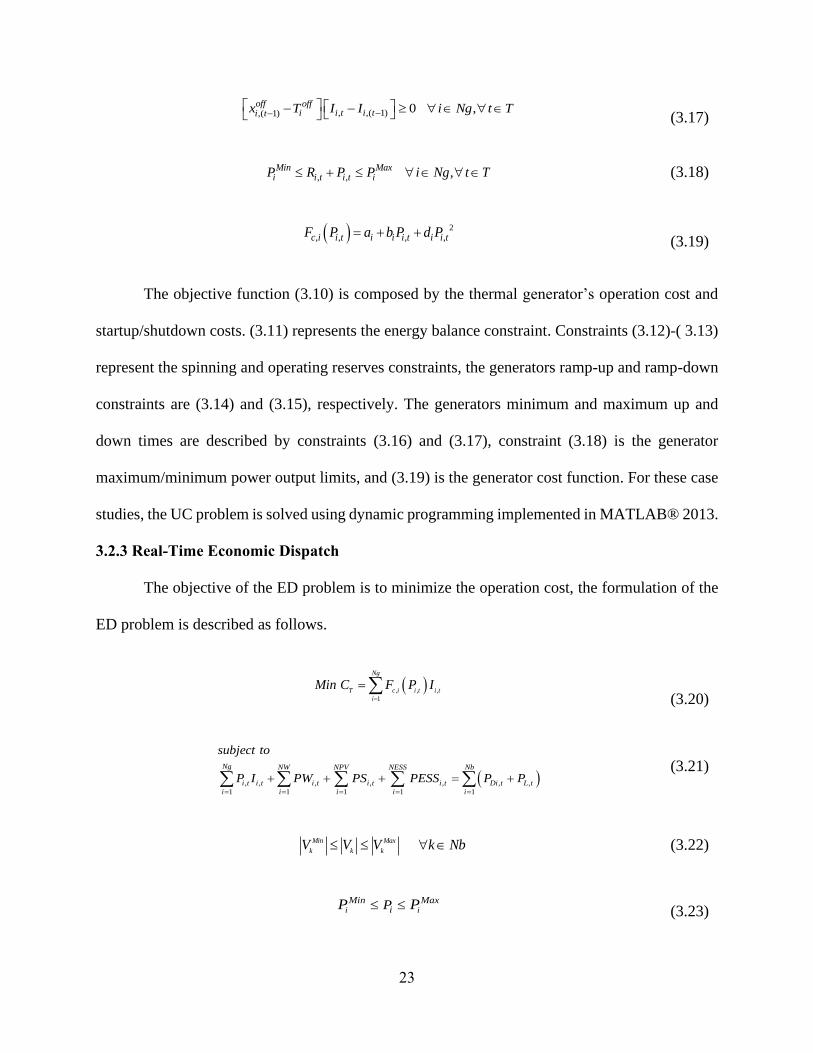
Figure 3.3: Forecasted load vs actual load. ................................................................................... 29 Figure 3.4: Forecasted PV power vs actual PV power (Scenario 1). ............................................ 29 Figure 3.5: Forecasted wind power vs actual wind power............................................................ 30 Figure 3.6: Forecasted wind-ESS charge/discharge schedule. ..................................................... 30 Figure 3.7: Forecasted PV power vs actual PV power (Scenario 2). ............................................ 31

Figure 3.8: Forecasted PV power vs actual PV power (Scenario 3). ............................................ 33

Figure 3.9: Comparison of the ED results for the three scenarios. ............................................... 34 Figure 3.10: Total system demand for the optimal solution of each scenario. ............................. 34

Figure 4.1: Flowchart of the proposed optimization and control procedure. ................................ 38

Figure 4.2: Networked microgrids in an IEEE 33-bus distribution network. ............................... 44 Figure 4.3: Residential solar PV power output profile on a sunny summer day. ......................... 46 Figure 4.4: Optimal charge schedule and driving pattern of BEVs located in PCG2-MG1 (Case

3). .................................................................................................................................................. 49 Figure 4.5: Aggregated BEV charge schedule and driving pattern of the three MGs (Case 3). ... 51

Figure 4.6: Optimal charge schedule and driving pattern of BEVs located in PCG2-MG1 (Case

4). .................................................................................................................................................. 52 Figure 4.7: Aggregated BEV charge schedule and driving pattern of the three MGs (Case 4). ... 53


5). .................................................................................................................................................. 54 Figure 4.9: Aggregated BEV charge schedule and driving pattern of the three MGs (Case 5). ... 56 Figure 4.10: Overall system net load comparison for each case. .................................................. 57

Figure 5.1: Networked microgrids in an IEEE 33-bus distribution network – moderate damage

case. ............................................................................................................................................... 71

Figure 5.2: Bus voltage profiles base scenario 1.1 – moderate damage case. .............................. 73 Figure 5.3: Bus voltage profiles sunny day scenario 1.2 – moderate damage case. ..................... 74 Figure 5.4: Bus voltage profiles sunny day scenario 1.3 – moderate damage case. ..................... 74

Figure 5.5: Bus voltage profiles rainy day scenario 1.4 – moderate damage case. ...................... 75 Figure 5.6: Bus voltage profiles rainy day scenario 1.5 – moderate damage case. ...................... 76 Figure 5.8: Bus voltage profiles base scenario 2.1 – heavy damage case. ................................... 79

Figure 5.9: Bus voltage profiles sunny day scenario 2.2 – heavy damage case. .......................... 80

Figure 5.10: Bus voltage profiles sunny day scenario 2.3 – heavy damage case. ........................ 80

Figure 5.11: Bus voltage profiles rainy day scenario 2.4 – heavy damage case........................... 81 Figure 5.12: Bus voltage profiles rainy day scenario 2.5 – heavy damage case........................... 82

xv

Nomenclature

, ,i i ia b d Coefficients of the production cost function

TC Total production costs

j Round-trip efficiency of ESS j

,

SOC

j tESS State of charge of ESS j at time t

,max

SOC

jESS Maximum capacity of ESS j in Wh

,min

SOC

jESS Minimum capacity of ESS j in Wh

,c iF Production cost function of unit i

,i tI Commitment state of unit i at time t

Nc Total number of bus combinations

NESS Total number of energy storage systems

Ng Total number of generating units

Nb Total number of buses

NPV Total number of PV aggregates

NW Total number of wind turbines

,D tP

Load demand at time t

,i tPESS Active power of ESS i at time t

,j tPESS Active power output of ESS j at time t

,

ch

j tPESS Charging power of ESS j at time t

,

dch

j tPESS Discharging power of ESS j at time t

,max

ch

jPESS Maximum charging limit of ESS j

,max

dch

jPESS Maximum discharging limit of ESS j

,i tP Active power generation of unit i at time t Max

iP

Maximum active power generation of unit i

Min

iP

Minimum active power generation of unit i

,L tP Active power losses

,l tPR Active power output of RES l

,i tPS Active power generation of PV i at time t

,i tPW Active power generation of wind turbine i at time t

iRD Ramp-down rate limit of unit i

,i tR Reserve of unit i at time t

,Si tR Spinning reserve of unit i at time t

,S tR System spinning reserve at time t

,Oi tR Operating reserve of unit i at time t

,O tR System operating reserve at time t

iRU Ramp-up rate limit of unit i

xvi

,i tSD Shutdown cost of unit i at time t

,i tSU Startup cost of unit i at time t

T Total number of time periods off

iT

Minimum up time of unit i

on

iT

Minimum down time of unit i

,j tu ESS j discharging mode decision variable

,

c

j tu ESS j charging mode decision variable

kV Voltage magnitude at bus k

Max

kV Maximum voltage magnitudes at bus k

Min

kV Minimum voltage magnitudes at bus k

lW Maximum power ramp-down decrement of lPR

( 1)

off

i tx − OFF time of unit i at time t

( 1)

on

i tx − ON time of unit i at time t

lZ Maximum power ramp-up increment of lPR

1

Chapter 1: Introduction

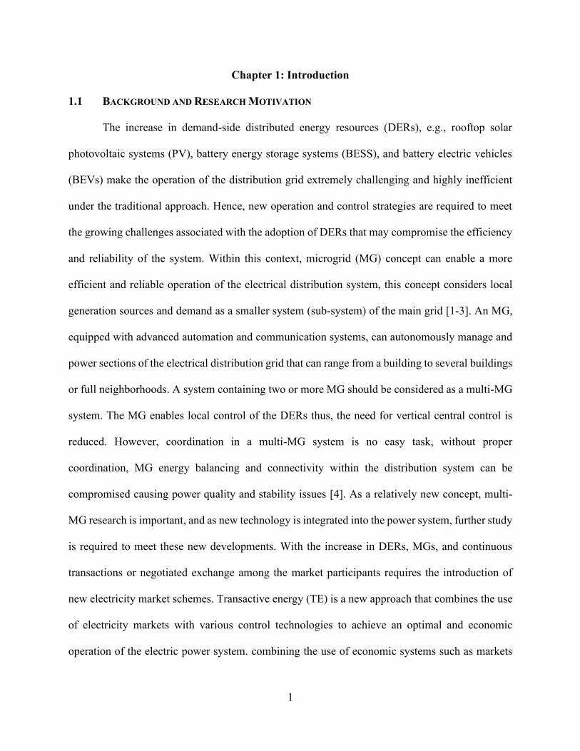
1.1 BACKGROUND AND RESEARCH MOTIVATION

The increase in demand-side distributed energy resources (DERs), e.g., rooftop solar

photovoltaic systems (PV), battery energy storage systems (BESS), and battery electric vehicles

(BEVs) make the operation of the distribution grid extremely challenging and highly inefficient

under the traditional approach. Hence, new operation and control strategies are required to meet

the growing challenges associated with the adoption of DERs that may compromise the efficiency

and reliability of the system. Within this context, microgrid (MG) concept can enable a more

efficient and reliable operation of the electrical distribution system, this concept considers local

generation sources and demand as a smaller system (sub-system) of the main grid [1-3]. An MG,

equipped with advanced automation and communication systems, can autonomously manage and

power sections of the electrical distribution grid that can range from a building to several buildings

or full neighborhoods. A system containing two or more MG should be considered as a multi-MG

system. The MG enables local control of the DERs thus, the need for vertical central control is

reduced. However, coordination in a multi-MG system is no easy task, without proper

coordination, MG energy balancing and connectivity within the distribution system can be

compromised causing power quality and stability issues [4]. As a relatively new concept, multi-

MG research is important, and as new technology is integrated into the power system, further study

is required to meet these new developments. With the increase in DERs, MGs, and continuous

transactions or negotiated exchange among the market participants requires the introduction of

new electricity market schemes. Transactive energy (TE) is a new approach that combines the use

of electricity markets with various control technologies to achieve an optimal and economic

operation of the electric power system. combining the use of economic systems such as markets

2

and the use of control systems technology. TE is defined as “A set of economic and control

mechanisms that allows the dynamic balance of supply and demand across the entire electrical

infrastructure using value as a key operational parameter” [5].

• The main value drivers for deployment of TE systems are the following:

• Reduce consumer energy cost; increase prosumer energy revenue;

• Enable participation of demand-side capabilities to enhance power system

reliability and reduce power system operation costs at the distribution and bulk

power system levels respectively;

• Transition energy production and consumption to become more environmentally

friendly;

• Provide investment opportunities for clean energy technologies.

The aforementioned points should be achieved within the consumer/prosumer comfort

range and with minimal imposition on power system operators (minimal or no additional manual

intervention) [6]. TE system utilizes two major transactive signals, i.e., transactive incentive signal

(TIS) and transactive feedback signal (TFS). These signals are produced by the distribution system

operator (DSO) and are sent through the smart grid infrastructure back and forth between utilities,

grid operators, and individual assets, that help communicate the real-time flow and cost of power.

These signals propagate through an information network, which is the transactive control (TC)

system embedded in the electrical network. A TC structure that combines both the dynamic market

transactions at the higher level within a region and unit-level control at the lower levels is

becoming more and more important as new time-scales with uncertainties become more prominent

[7]. Also, more regular and constant information exchange is required to mitigate costs imposed

due to intermittency and uncertainty of the DERs [8]. The TIS represents the actual delivered cost

of electric energy ($/kWh) and the TFS the net electric load (kW) at a specific system location

known as a transactive node (TN). Both signals include the current value and a forecast of future

3

values, as forward-looking signals. TCs can be located in different areas of the distribution system,

e.g., in an MG. The TN can represent load points, e.g., distribution substation, distribution

transformer, prosumer, consumer, and others. TIS and TFS can be communicated to TNs located

in the same MG and among other MGs for energy balancing utilizing a transactive coordination

system (TCS) [9].

Figure 1.1 illustrates the application of TCs, which is a single, integrated, smart grid

incentive signaling approach that combines multiple objectives and constraints (economic and

operational) using uniform TIS and TFS. In Figure 1.1, the role of the TC is to respond to system

conditions represented by incoming TIS and TFS. Also, in Figure 1.1, each load point (e.g., MG-

1 under TC) represents a TN.

Figure 1.1: Role of transactive energy signals in a multi-MG electrical distribution system.

It has been reported in the Pacific Northwest Smart Grid Demonstration Project

(PNWSGD) [10], that in order to better take advantage of transactive system benefits, further work

is needed in the following areas:

• Improved load models and forecasting techniques;

• Different methods to monetize system objectives to produce the transactive

incentive signals;

4

• Development of libraries of system models that accurately represent system assets

to be used by the transactive algorithms;

• Research that identifies business models and policies that can be utilized by utilities

and their customers to enable customer engagement through the use of transactive

systems;

• Research on policies that enable the use of a dynamic cost or price signal that

incentivizes customer participation;

• Analysis and testing of transactive control systems to verify their stability and

convergence.

These findings suggest that TE is an area of great research opportunities to improve smart

grid operations.

1.2 PROBLEM STATEMENT AND RATIONALE FOR THE STUDY

Over the past years, technological developments have driven an increase in DERs across

the distribution network, particularly at the demand side. DERs are changing the electrical

landscape from a conventional demand-driven power grid to a transactive supply following energy

system where customers (as electricity consumers and/or producers) are actively engaged in

transactions and participating in the operation and management of the power grid [5,11,12].

Although the overall installed capacity of DERs is still significantly low, projections indicate a

ramp-up in the coming years. According to the U.S. Energy Information Administration (EIA),

solar PV generation at the distribution level (Utility-scale and small-scale) has grown 232% over

the past five years (2014-2018) going from a total net generation of 28,925 MWh in 2014 to 96,147

MWh in 2018 [13]. Moreover, the EIA in its 2019 annual energy outlook projects electricity

generation from solar PV will reach 15% of total U.S. electricity generation by 2050 [14].

On another front, transportation has also been experiencing important changes around the

world. According to the international energy agency (IEA), in 2017 a new milestone was reached

5

with more than 3 million BEVs on the road worldwide [15]. Furthermore, the same report projects

the worldwide BEVs fleet to reach 13 million and 130 million by 2020 and 2030, respectively.

Thus, it can be seen that in the next few years, the increase in BEVs and solar PV generation will

cause various integration challenges on the electric grid. The current power grid was not designed

to host the increase of load caused by BEV charging and power flow fluctuations caused by solar

PV generation, especially low voltage distribution networks.

The growing attention for DER, BESS, EVs, and a transactive grid reflects the increase in

awareness that the conventional operation and control of the electric system has become outdated

and is no longer suitable for the modern, digitized information-driven economy [16]. Several

assumptions that have been the drivers for operation and regulation of the electric industry are now

outdated, e.g., consumer demand is largely inelastic, centralized power generation and control are

the best; reliance on DER will result in higher electricity costs. Another important issue is the gap

in price signals between customer-side resources with system costs and benefits. Also, in part due

to the centralized approach customer-side generation adds more complexity to the operation and

control of the conventional system [16]. Whereas, under the decentralized approach, control

decisions are made locally [17].

Although decentralized control of the power system has been studied in the literature, there

is still a considerable void in the research of power system control and operations under TE

framework. Specifically, at the distribution level where a high penetration of DERs is occurring, a

TE approach could ensure an efficient integration to enhance the operation of the power

distribution system. Thus, a new transactive-model predictive control approach based on TE

framework is introduced to improve the efficiency, reliability, and resilience of power distribution

systems.

Furthermore, research is required to design and construct transactive signals as they can

result in proper decision-making tools for transactive market participants (e.g., DSO and MGs).

Very limited literature is available apart from the work done by the Pacific Northwest National

Laboratory (PNNL) in the PNWSGD explaining how to model transactive signals. The PNWSGD

6

determined TIS and TFS as the total cost per total energy resources and sum of all predicted elastic

and inelastic loads, respectively [9]. Where the TFS was calculated at the interface between utility-

side nodes and the transmission zone nodes that supply the energy. The transactive signals reported

in [9] were developed to allow energy balancing between TNs that shared a TCS in which the

energy management system had the transactive controls embedded for local control and decision

making.

Hence, the development of a TC based MG energy management system (MGEMS)

constituted by DERs and using transactive signals will enable a more effective and efficient

operation of the distribution system. As dynamic demand-side management could improve power

quality, system cost minimization, generation-load balancing, and load-shaping support for the

grid.

1.3 DISSERTATION OBJECTIVES

The main objective of this dissertation is to derive an efficient energy management and control

strategy for the economical and resilient operation of the smart power distribution systems that are

heavily constituted by DERs. This dissertation also investigates and studies different mechanisms that

enable customers owning DERs to become more active participants in the operation of the electric

distribution grid, in particular networked microgrids. In order to achieve the main objective of this

dissertation, the following specific objectives are carried out.

• Objective 1: Efficient Integration of Distributed Energy Resources into Power

Distribution Systems

This objective involves the design and development of control models for DERs

(specifically BESS and solar PV) to manage their location and power exchange with the

distribution grid to allow efficient integration of the DERs into electrical distribution systems. For

objective 1, a planning strategy that considers forecasted power outputs of the DERs and their

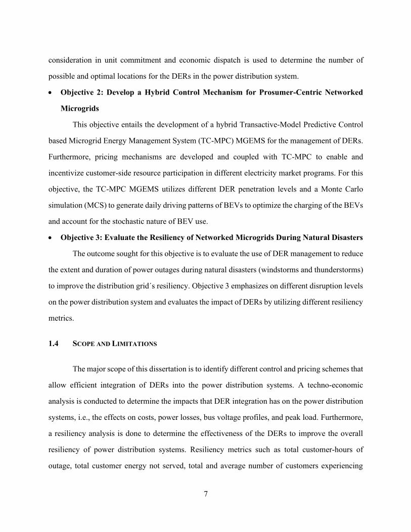
7

consideration in unit commitment and economic dispatch is used to determine the number of

possible and optimal locations for the DERs in the power distribution system.

• Objective 2: Develop a Hybrid Control Mechanism for Prosumer-Centric Networked

Microgrids

This objective entails the development of a hybrid Transactive-Model Predictive Control

based Microgrid Energy Management System (TC-MPC) MGEMS for the management of DERs.

Furthermore, pricing mechanisms are developed and coupled with TC-MPC to enable and

incentivize customer-side resource participation in different electricity market programs. For this

objective, the TC-MPC MGEMS utilizes different DER penetration levels and a Monte Carlo

simulation (MCS) to generate daily driving patterns of BEVs to optimize the charging of the BEVs

and account for the stochastic nature of BEV use.

• Objective 3: Evaluate the Resiliency of Networked Microgrids During Natural Disasters

The outcome sought for this objective is to evaluate the use of DER management to reduce

the extent and duration of power outages during natural disasters (windstorms and thunderstorms)

to improve the distribution grid´s resiliency. Objective 3 emphasizes on different disruption levels

on the power distribution system and evaluates the impact of DERs by utilizing different resiliency

metrics.

1.4 SCOPE AND LIMITATIONS

The major scope of this dissertation is to identify different control and pricing schemes that

allow efficient integration of DERs into the power distribution systems. A techno-economic

analysis is conducted to determine the impacts that DER integration has on the power distribution

systems, i.e., the effects on costs, power losses, bus voltage profiles, and peak load. Furthermore,

a resiliency analysis is done to determine the effectiveness of the DERs to improve the overall

resiliency of power distribution systems. Resiliency metrics such as total customer-hours of

outage, total customer energy not served, total and average number of customers experiencing

8

outage, total loss of utility revenue, and total outage costs are utilized to determine the possible

impacts DERs can have on the resiliency of the power distribution system.

The following are the limitations of this dissertation.

• The forecasted information required for simulation purposes has been acquired

from available databases or data generated by existing forecasting tools.

• Battery degradation of BESS and BEV is not studied in this dissertation.

• The purchase and installation costs of DERs are not considered in the cost-benefit

analysis.

• Communication systems are not part of the scope of this dissertation, it will be

assumed that the system under study has the required communication network to

exchange the required data.

• Protection system coordination is not considered while simulating and analyzing

the power distribution systems.

• Cybersecurity is not considered while developing the TC+MPC based MGEMS.

1.5 DISSERTATION ORGANIZATION

This dissertation is constituted by 6 chapters and is organized as presented in Figure 1.2.

This section presents a brief description of each chapter.

• Chapter 2 presents a literature review, providing an in-depth analysis of literature

regarding the integration of DER technologies specifically solar PV, BESS, and BEVs

with a focus on residential customers located in MGs. The literature review first

describes impacts of location of DERs in the electrical distribution system. Afterwards,

a comparison of various transactive control methodologies used to integrate DERs in

MGs and networked-MGs is presented, and finally, a summary of previous studies that

utilize DERs to improve power distribution systems resiliency is discussed.

9

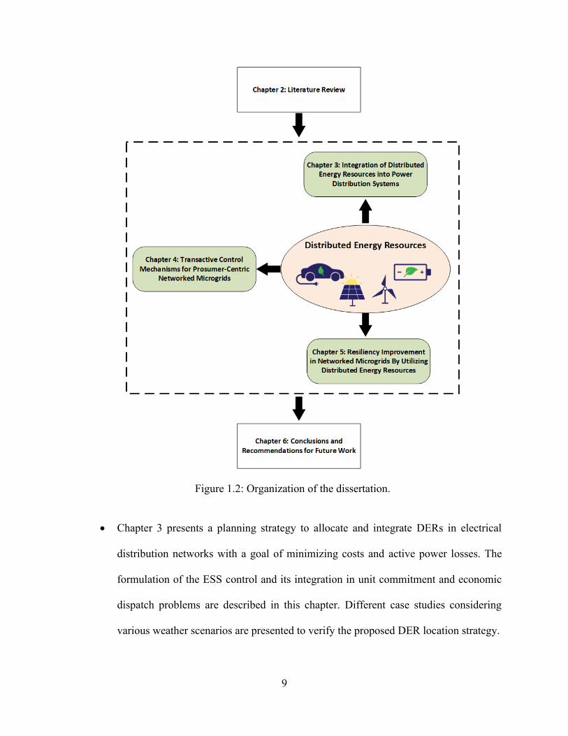
Figure 1.2: Organization of the dissertation.

• Chapter 3 presents a planning strategy to allocate and integrate DERs in electrical

distribution networks with a goal of minimizing costs and active power losses. The

formulation of the ESS control and its integration in unit commitment and economic

dispatch problems are described in this chapter. Different case studies considering

various weather scenarios are presented to verify the proposed DER location strategy.

10

• Chapter 4 describes a proposed MGEMS based on a hybrid control algorithm that

combines TC and MPC for efficient management of DERs in prosumer-centric

networked MGs. The mathematical formulation of the TC-MPC and an MCS that is

utilized to generate daily driving patterns of BEVs are described in detail. An

evaluation of the proposed networked MGEMS strategy under different BEV and PV-

BESS penetration scenarios to study the potential impact that large amounts of BEV

and PV-BESS systems can have on the distribution system and how different pricing

mechanisms can mitigate these impacts is also presented in this chapter.

• Chapter 5 is focused on presenting a resiliency analysis process to determine the

impacts DERs can have on improving the power distribution system resiliency to

natural disasters. The chapter provides the resiliency analysis goals and metrics under

different disaster scenarios, as well as, simulated results comparison and discussion.

• Finally, Chapter 6 summarizes the major findings and contributions of the dissertation

as well as providing directions for potential future research work.

11

Chapter 2: Literature Review

2.1 DISTRIBUTED ENERGY RESOURCES AND THEIR IMPACT ON POWER DISTRIBUTION

SYSTEMS

A transition to clean and sustainable energy systems involves various social, economic,

environmental, technical, and political factors [18]. With a growing need to cut down on

greenhouse gas (GHG) emissions, solutions involve integrating intermittent renewable energy

sources (RES), primarily wind and solar. The grid in-feed takes place at the distribution level;

however, most power distribution systems were not built to handle multiple, distributed generators,

bi-directional power flow, and intermittency issues. Hence, they lack the capacity and technical

prerequisites to successfully integrate large amounts of RES and distributed generation (DG).

As we move into the future, it is expected that RES and DG will grow rapidly in distribution

networks (DNs). With a large penetration of RES and DG, power utilities will face more challenges

to handle integration issues and inherent uncertainty associated with RES. Therefore, power

system operators need efficient tools to model and analyze the electric grid with newly added

components in order to facilitate their smooth integration within given constraints. Furthermore,

as the margin between system load and system capacity decreases, utilities require innovative

solutions. To address the aforementioned issues, energy storage systems (ESS) can be a viable

solution [19]. A well-designed hybrid energy system consisting of RES and ESS can improve the

power system performance and reliability. For example, smart grids, which consist of RES, DG,

ESS, demand response (DR) programs and other efficient technologies, are heavily automated.

The automation enhances the capability of the smart grids to manage and meet the load in an

effective and efficient manner. The role of distributed energy resources in smart grid operations

can increase system efficiency, reliability, security, stability, and power quality [20]. To achieve

these benefits electric utilities, need to find the optimal location where the units (i.e., RES, DG,

and ESS) will be installed to maximize their potential benefits.

12

The positive and negative impacts of DG in DNs have been discussed in detail in the

literature [21]-[27]. While reducing the power losses and increasing the reliability of the power

system are the direct benefits of DG installation. It can also benefit the DSO to reduce the

congestion of DNs due to growth in load demand as DG can help defer investments [28,29]. Most

technical and economic advantages of DG can be achieved by determining its optimal location.

Several papers are available in the literature that discuss the optimal location and sizing of

DG in DNs considering different objectives. Loss reduction in a DN is discussed in [30] and [31]

where different methods are applied to determine an optimal allocation of DG. An optimization

technique based on genetic algorithm (GA) was proposed in [32] to evaluate the optimal sizing

and location of DG in radial distribution systems to minimize losses. Multi-objective optimization

was also applied in [33] where a single DG was located on various standard DNs to find the optimal

location. Moreover, impact indices and a trade-off technique are used for DG location planning as

reported in [34]. However, references [30]-[34] considered only controllable or dispatchable

generation.

Different optimization algorithms are available in the literature to achieve optimal size and

location of RES. A hybrid algorithm between the Chu-Beasly Genetic Algorithm (CBGA) and

particle swarm optimization (PSO) is applied to optimally locate wind, PV, and small-scale hydro

generation [35]. A constrained discrete PSO technique is reported in [36] to select optimal

locations and sizes of PV, wind turbines, and capacitor banks. References [35], [36] considered a

fixed power output of the RES. In [37], optimal location of PV is determined by using PSO for

loss reduction and frequency control. Pandžić et al. [38] proposed a planning technique to

determine the optimal locations and parameters of distributed storage units with wind farms to

reduce congestion. Kalkhambkar et al. [39] proposed an analytical method for determining the size

of solar PV and battery and concluded that minimization of losses and variable output power of

PV are the main parameters to consider when optimally sizing and placing solar PV and battery

storage.

13

A thorough literature review, as presented above, suggests that there is still a great need to

consider the unpredictability and intermittency associated with RES while optimally locating them

in the DNs. Failing to consider these characteristics of the RES can cause a less efficient operation

and unreliable output from these resources.

2.2 TRANSACTIVE ENERGY IN POWER DISTRIBUTION SYSTEMS

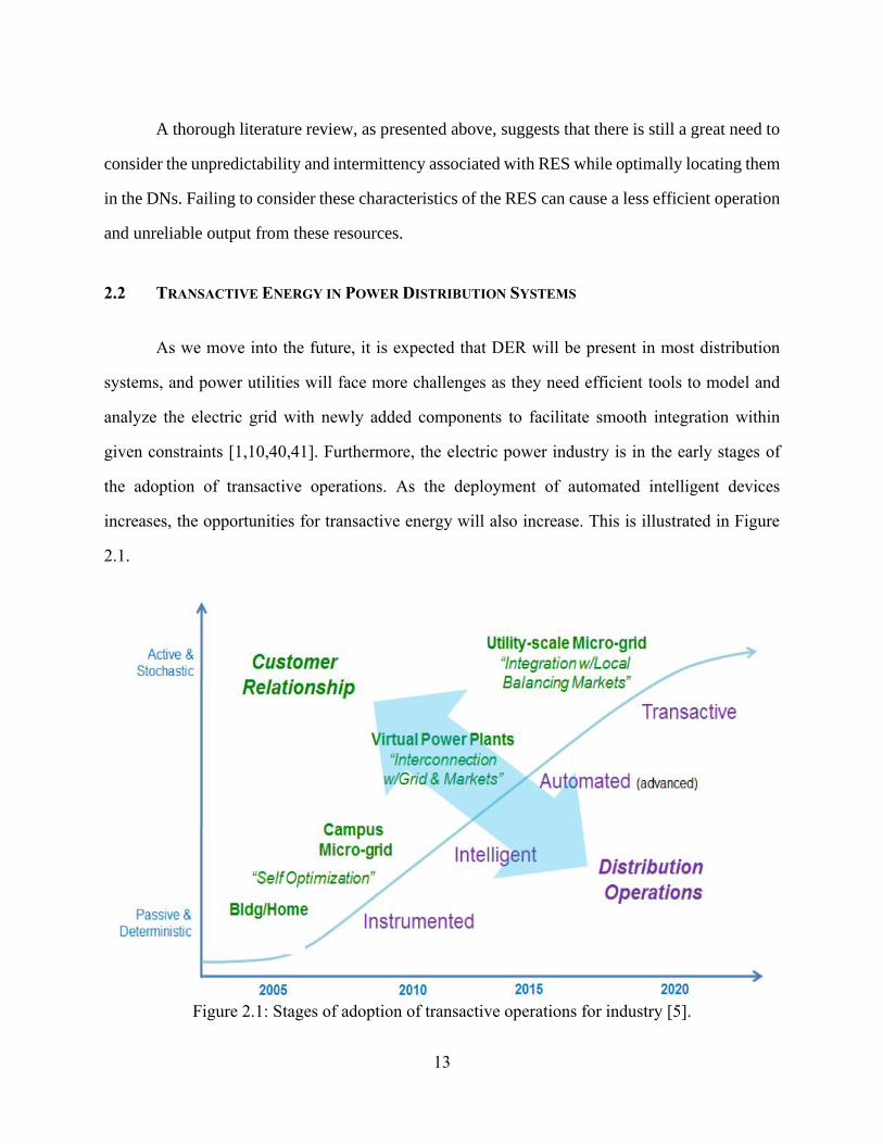
As we move into the future, it is expected that DER will be present in most distribution

systems, and power utilities will face more challenges as they need efficient tools to model and

analyze the electric grid with newly added components to facilitate smooth integration within

given constraints [1,10,40,41]. Furthermore, the electric power industry is in the early stages of

the adoption of transactive operations. As the deployment of automated intelligent devices

increases, the opportunities for transactive energy will also increase. This is illustrated in Figure

2.1.

Figure 2.1: Stages of adoption of transactive operations for industry [5].

14

Under the TE framework, the transactions can take place among prosumers, prosumers,

and utilities, between distribution utilities and the power system operators at the wholesale market

level. Thus, the development of a new DSO is fundamental to reach the goal of the future grid.

The DSO could be an independent entity, or an electric utility [42,43]. The DSO should be able to

integrate customer-side assets and consider them during the planning stage of the distribution

system and for operation practices, also creating price signals that prosumers can use for

investment and operation purposes for long-term and short-term time spans while maintaining the

distribution system reliability, efficiency, and security. TE in coordination with TC technology

and architecture can elucidate the convergence of technologies, policies, and financial

drivers required to evolve the grid’s centralized control model to a distributed control architecture

[5,6,9,44,45]. The PNNL with the Olympic Peninsula Project One has applied TE framework in

the form of a double auction market mechanism utilized to control demand-side assets. This was

achieved through the use of two-way communication providing actual demand and price

signals; the results indicated that price can be an effective control signal to alleviate congestion in

transmission and distribution systems [45]. In [46], a summary of highlights of a five-year

PNWSGD is presented where the project’s transactive system operated for approximately two

years and demonstrated the potential of TCs. Furthermore, findings of the projects showed that

research is also needed into the policies to encourage customers to respond to incentive signals.

As it is still unclear for large-scale deployment whether to use dynamic cost signals as a dynamic

tariff, or an approach based on periodic compensation for which customers agree to respond to the

dynamic signal [46]. Other important research that is taking place in the U.S. related to TE is

reported in [47]-[49]. The National Institute of Standards and Technology (NIST) through the

Transactive Energy Modeling and Simulation Challenge for the Smart Grid (“TE Challenge”) plan

to develop and demonstrate standardized models and simulation platforms to apply TE [47]. The

NYISO is planning to adopt policies toward future energy to maximize the financial benefits of

the network where they have studied the benefits and market potential for demand response and

future smart grid concept believing that dynamic pricing could be the best strategy to motivate

15

consumers to participate in the demand response. That is why the NYISO Consumer Advisory

recommends that the NYISO should intelligently monitor the emerging TE community of

innovation to get a deep insight on how to expand the role of demand response at scale consistent

with the New York regulatory environment [48]. TeMix inc. prepared a TE vision for CAISO as

an alternative approach. They believe that TE is a more efficient and transparent scheme than

centrally distributed models. Moreover, they envision that transactive tariffs will lower the cost of

electric power system operations and encourage consumers to buy more DER, helping California

reach its clean energy and sustainable goals [49].

In recent years, TC mechanism use in smart grid and MG applications has been studied

due to its potential for efficient DER management and the creation of opportunities to engage in

transactions between the different entities that constitute the electrical distribution system, e.g.,

electric utility and customers. A review of the state-of-the-art of transactive energy systems and

concepts are presented in [50]. In [51], a transactive bilateral energy trading mechanism is

proposed to minimize the costs for individual participants while ensuring the reliability of the

power distribution system, where Nash bargaining theory and alternating direction method of

multipliers (ADMM) were used to model the problem. A multi-agent transactive energy

management framework for networked MGs is presented in [52]. The multi-agent system manages

energy imbalances in the MGs using demand response and battery energy storage systems (BESS)

with an objective of minimizing the costs for the MG customers. A multi-agent system is also

proposed in [53], where an auction-based locational marginal price (LMP) has been used to

incentivize energy trading between MGs. In [54], a day-ahead transactive market framework is

proposed for DER scheduling to reduce local supply costs. TCs are used for BEV charging in [55-

57]. A TC based on model predictive control (MPC) is utilized for real-time scheduling of BEVs

in [55], where the MPC is used to clear a day-ahead transactive market. In [56], the charging

demand of the BEV is used to manage uncertainties of the building PV generation. Hu et al. [57]

implemented a TC with the purpose of minimizing the BEV charging cost as well as preventing

grid congestions and voltage violations. A reactive power incentive program to maintain

16

distribution system reliability is presented in [58]. In [59], A Nash bargaining formulation is

proposed for energy trading between networked MGs for MG operation cost reduction. A TC

coupled with a pricing rule is proposed for grid-connected, islanded, and congested networked

MGs in [60]. DC MGs have also been studied for application of TCs [61-63]. In [61], a framework

is proposed for short-term operation of DERs, controllable demands, and MGs in a transactive

energy architecture, with a focus on the distributed energy management of hybrid AC/DC

microgrids. Jingpeng et al. [62] presented a centralized energy management system approach

based on transactive energy to reduce the total operation cost and achieve efficiency in a DC

residential system. In [63], a transactive energy management system for supply/demand

coordination with demand response programs was implemented to manage rural DC MGs.

Several other models have been proposed for BEVs charging/discharging and pricing

scheduling [64-69]. The impact of variable prices on the behavior of BEV users is studied in [64]

where the variable prices are based on the distribution locational marginal price (DLMP) and

updated continuously based on the users’ trips and behavior. In [65], an optimal Time-of-Use

(TOU) schedule and a controlled BEV charging algorithm are utilized to maximize both customer

and utility benefits and for which, the controlled charging provided voltage profile improvements

while taking into account customer preferences. In [66], meta-heuristic techniques are utilized for

charging coordination of BEVs with simultaneous operation of capacitor switching to minimize

power losses and voltage deviation in a distribution system. Furthermore, a TOU electricity tariff

was included in the proposed charging coordination to reduce the PEV charging cost. Cherikad et

al. [67] proposed a variable pricing model for BEVs charge/discharge scheduling coupled with an

energy management system in an MG. Their model consisted of a cloud-software define

networking communication architecture and a linear optimization approach to achieve efficiency

in the MG. A model to estimate the cost of BEV charging while considering the impacts of solar

PV generation on the charging costs of BEVs is presented in [68]. The model described in [68]

estimated the costs considering demand charges and utility loss of revenue and was compared to a

TOU tariff. In [69], a two-stage real-time optimization algorithm is proposed to recharge a fleet of

17

plug-in BEVs to minimize costs, avoid creating new peaks in the demand profile, and improve

utilization of power system equipment. The optimization algorithm used a dynamic price signal

based on probabilistic models developed utilizing historical price data.

All the aforementioned papers had significant contribution in the matters of energy

management using TCs. Nonetheless, there are still gaps in the development of the TE approach,

which need to be addressed.

2.3 DISTRIBUTED ENERGY RESOURCES IMPACTS ON RESILIENCY OF POWER DISTRIBUTION

SYSTEMS

Today’s electricity grid faces challenging issues with aging infrastructure and high

concerns regarding cyber and physical system security. As infrastructure ages, many risks arise

with it, e.g., increased maintenance and operation costs, equipment failure, inefficient operation,

and in severe cases cascading blackouts [70]. While blackouts are considered as low-probability

events, the socioeconomic costs and impacts are extensive [71]. Over the past decades hundreds

of major blackouts have occurred in the U.S. causing an estimated one billion dollars per event

and over one trillion dollars in total damages [72]. Where most of these outages (over 90%) have

occurred at the distribution level [73]. As these events become more recurrent in the U.S. (30

weather/climate events where losses exceed 1 billion dollars over the past two years 2017-2018)

[72] coupled with a high dependency on electricity in today’s society for almost all activities,

creates an urgent need to improve the resiliency of the electric power grid to reduce the potential

impacts these types of events could have. In recent years, microgrids (MGs) have continued to be

developed as different research and pilot projects have shown the potential of MGs to improve

resiliency of power distribution grids.

18

There are various publications that have focused on control strategies for MGs [74-78].

The concept of community MGs where MGs interact with the main grid and among other MGs

has also been studied [79,80]. In [81], the coordination of different control levels in a MG was

implemented to achieve an economic operation of the MG. The control of DERs within a MG

pilot-project at the Illinois Institute of Technology showed to be an effective way to improve the

resiliency of the MG under emergency events [82]. In [83], an optimal arrangement of MGs is

proposed using graph-related theories based on modularity to quantify the resiliency level of

electric distribution systems. A methodology to quantify the resilience improvement in a building

MG by adding photovoltaic solar energy and electrochemical storage has been presented in [84].

A two-stage stochastic program for designing resilient distribution grids with networked MGs is

proposed in [85]. Where, individual MGs, hardened networks, and a combination (networked

MGs) were utilized to evaluate costs of increasing system resiliency. In [86], an MG formation

method based on network reconfiguration is proposed for a resilient operation of distribution

systems under emergency situations. A software-defined networking (SDN) architecture equipped

with event-triggered communication is presented in [87], to transform isolated local MGs into

integrated networked MGs capable of power-sharing to improve system efficiency and resiliency.

An islanding detection algorithm was used to detect sectioned areas of a distribution system to

ensure the system remained operational while experiencing islands [88]. In [89], a detailed

literature review of resilience enhancement strategies for power systems is presented. A conceptual

framework that considers resiliency during the planning stages of a MG is reported in [90]. In [91],

a model to determine the location of MGs for resiliency improvements in a power grid by

considering probability of equipment failure was presented. A flood preventive scheduling scheme

that isolates vulnerable areas of a MG during floods has been proposed to improve MG resiliency

19

[92]. In [93], a network reconfiguration algorithm for MGs that considered grid topology and

hierarchy of loads (critical and no-critical) was presented and evaluated utilizing different

resilience metrics.

Although there are many publications related to the resiliency of power distribution

systems, there are still gaps in the literature, specifically in developing realistic case studies and

utilizing appropriate resilience metrics.

20

Chapter 3: Integration of Distributed Energy Resources into Power Distribution Systems

3.1 INTRODUCTION

This chapter presents an efficient strategy to optimally allocate RES, primarily wind and

solar PV, and ESS in electrical distribution networks with a goal of minimizing costs and active

power losses. A planning strategy is used to determine the number of possible and optimal

locations for the hybrid RES-ESS system. This chapter also presents a control scheme to optimally

dispatch the output of ESS, which increases the effective utilization of RES by reducing their day-

ahead forecast errors in order to minimize the deviation between forecasted and actual values. In

the proposed strategy, the location that produces the least overall power losses complying with the

system constraints is considered as the optimal one. Numerical results and discussion are presented

towards the end of the chapter where the effectiveness of the proposed method is evaluated.

3.2 PLANNING STRATEGY TO DETERMINE THE OPTIMAL LOCATION OF DISTRIBUTED

ENERGY RESOURCES

A DSO can reduce overall system costs and losses by coordinating conventional generation

with RES. The objectives of DSO are to (i) minimize the power production costs, (ii) determine

an efficient operation of DG, (iii) minimize power losses, and (iv) determine the optimal placement

of RES. While planning the integration of RES to grids and their expansion, it is of high importance

to consider the appropriate location of RES and their impact on the system. Neglecting the optimal

siting of the RES can lead to reliability issues and increased real power losses. In addition, by not

considering the output power of RES and ESS in the UC and ED problems, it can lead to increased

energy costs, which could be due to overcommitting thermal generation or increased operational

reserves, and a non-optimal charge/discharge cycle of the ESS.

21

3.2.1 Battery Energy Storage System Model

The control algorithm for the ESS is embedded in both UC and ED formulation as a sub-

problem, which optimizes the scheduling of the ESS by maximizing its power output. The problem

is formulated as described below.

,1 1

T n

i tt iMax PESS

= = (3.1)

, , , ,1 1

,1

, ( . . )n ns c

j t j t j t j ti j

nr

l tl

i t

subject to

PESS PESS u PESS u

PR

= =

=

= − +

(3.2)

, , 1 ,c

j t j tu u j t+ (3.3)

, , 1 , ,1. . .SOC SOC ch dch

j t j t j t j j t jj

ESS ESS PESS PESS −

= + −

(3.4)

,min , ,max ,SOC SOC SOC

j j t jESS ESS ESS j t (3.5)

, ,max ,0 . ,ch ch c

j t j j tPESS PESS u j t (3.6)

, ,max ,0 . ,dch dch

j t j j tPESS PESS u j t (3.7)

, , 1

,

, , 1

1

0

l t l t l

j t

l l t l t l

if PR PR Wu

if W PR PR Z

−

−

− =

− (3.8)

,

, , 1

, , 1

1

0

c

j t

l t l t l

l l t l t l

if PR PR Zu

if W PR PR Z

−

−

− =

− (3.9)

The objective function (3.1) is the total power output of the ESS. Constraint (3.2) represents

22

the total available active power, constraint (3.3) is the state of the ESS, (3.4)-( 3.5) are the storage

balancing constraints, (3.6)-(3.7) are the charge/discharge limits constraints, and (3.8)-(3.9)

represent the charge/discharge decision variables.

3.2.2 Day-Ahead Unit Commitment

The day-ahead model determines the UC operational decisions and is used during the ED

phase. The objective function of the UC problem is to minimize the energy costs and is described

as follows.

( ), , , , ,

1

Ng

c i i t i t i t i t

t

Min F P I SU SD=

+ + (3.10)

, , , , , ,

1 1 1 1

Ng NW NPV NESS

i t i t i t i t i t D t

i i i i

subject to

P I PW PS PESS P t T= = = =

+ + + = (3.11)

, , ,

1

Ng

Si t i t S t

i

R I R t T=

(3.12)

, , ,

1

Ng

Oi t i t O t

i

R I R t T=

(3.13)

( ) ( ), ,( 1) , ,( 1) , ,( 1)1 1 1

( 1,..., )( 1,..., )

Min

i t i t i t i t i i t i t iP P I I RU I I P

i Ng t T

− − − − − − + −

= = (3.14)

( ) ( ) ( ),( 1) , ,( 1) , ,, 11 1 1

( 1,..., )( 1,..., )

Min

i t i t i t i t i i t ii tP P I I RD I I P

i Ng t T

− − − − − − + −

= = (3.15)

,( 1) ,( 1) , 0 ,on on

i t i i t i tx T I I i Ng t T− − − − (3.16)

23

, ,( 1),( 1) 0 ,off off

i i t i ti tx T I I i Ng t T−− − − (3.17)

, , ,Min Maxi i t i t iP R P P i Ng t T + (3.18)

( ) 2

, , , ,c i i t i i i t i i tF P a b P d P= + + (3.19)

The objective function (3.10) is composed by the thermal generator’s operation cost and

startup/shutdown costs. (3.11) represents the energy balance constraint. Constraints (3.12)-( 3.13)

represent the spinning and operating reserves constraints, the generators ramp-up and ramp-down

constraints are (3.14) and (3.15), respectively. The generators minimum and maximum up and

down times are described by constraints (3.16) and (3.17), constraint (3.18) is the generator

maximum/minimum power output limits, and (3.19) is the generator cost function. For these case

studies, the UC problem is solved using dynamic programming implemented in MATLAB® 2013.

3.2.3 Real-Time Economic Dispatch

The objective of the ED problem is to minimize the operation cost, the formulation of the

ED problem is described as follows.

( ), , ,

1

Ng

T c i i t i t

i

Min C F P I=

= (3.20)

( ), , , , , , ,

1 1 1 1 1

Ng NW NPV NESS Nb

i t i t i t i t i t Di t L t

i i i i i

subject to

P I PW PS PESS P P= = = = =

+ + + = + (3.21)

Min Max

k k kV V V k Nb (3.22)

i i

Min MaxiPP P (3.23)

24

The objective function (3.20) is the sum of the thermal generation costs. The energy

balance constraint is shown in (3.21), constraint (3.22) represents the bus voltage limits, and (3.23)

represents the thermal generators power output limits. In this study, the ED and power flow

problems are solved using MATPOWER version 5.1 [94].

Figure 3.1 depicts a flowchart of the proposed strategy to optimally determine the location

for RES-ESS. Note that our proposed strategy can be applied to any time scale, e.g., very short-

term (5 to 30 minutes-ahead) and short-term (day-ahead to week-ahead).

Figure 3.1: The proposed strategy to determine the optimal location of RES-ESS.

The algorithm to solve short-term coordination problems (UC and ED) and then to

determine the optimal location of RES and ESS can be described as follows.

25

1) Forecast day-ahead hourly load, wind power, PV power, and ESS power output.

Define the initial conditions for the thermal generators. Determine the total number

of bus locations (nc) for PV, wind, and ESS.

2) Subtract PV, wind, and ESS power output from the forecasted load.

3) Solve the day-ahead UC problem with the updated load.

4) Determine bus location for PV, wind, ESS, nc=nc – 1.

5) Update the net real-time load by subtracting the output power of wind, PV, and ESS

from the system load.

6) Solve the ED problem with actual data.

7) Run power flow to determine losses, overloads, and bus voltage magnitudes.

8) If this is the last hour period, stop; otherwise, go to step 5.

9) If this is the last bus location, stop; otherwise, go to step 4.

3.3 NUMERICAL RESULTS AND DISCUSSION

3.3.1 Test System and Data

This research study considers a 16-bus test system that represents a small DN. The

complete network data is acquired and modified from [95], [96]. There are two thermal units at

buses 8 and 15. The thermal generation data is described in [95]. It is considered that buses 1, 2

and 3 are connected to a substation that interconnects with the power grid from where energy is

purchased. A 2.5 MW PV installation and a 6 MW wind farm are considered for the study.

Interconnected with the wind farm is a 1 MW NaS-ESS, which can operate at its rated power (±1

MW) for extended periods. The NaS-ESS characteristics and attributes are described in detail in

[95].

26

Figure 3.2: A 16-bus test system.

The total installed capacity of RES-ESS (9.5 MW) is 34% of the peak load and is

considered the maximum allowable sizing of RES-ESS for this system. Any value above this

installed capacity can cause adverse effects on the system, e.g., over-voltages and an increase in

the requirement of spinning reserve.

3.3.2 Hybrid Forecasting Models and Forecast Data

In this study, hybrid intelligent algorithms are used for day-ahead hourly forecasts of load, wind

power, and solar PV power. Details of the forecast models are presented in [97]-[99] and a brief

description is presented below.

Solar PV Power Forecasting

In this study, solar PV output power forecasting was carried out using the combination of a data

filtering technique based on wavelet transform (WT) and artificial intelligence technique based on

generalized regression neural network (GRNN), which is optimized by a PSO technique [97].

Wind Power Forecasting

For this study, a combination of WT and Fuzzy ARTMAP (FA) network, was used to produce

27

hourly wind power forecasts. The accuracy of the predictions was tested by comparing the forecast

to a persistence method [98].

Load Forecasting

In this study, load demand forecasted data is obtained from a hybrid intelligent model that

combines WT and FA where the FA network is optimized by meta-heuristic firefly (FF)

optimization algorithm [99]. This combination of algorithms provided more accurate forecasted

data.

3.3.3 Case Study Results and Discussion

To carry out simulations, three different PV output power scenarios are considered: (i)

scenario 1: sunny day, (ii) scenario 2: cloudy day, and (iii) scenario 3: rainy day. The actual and

forecasted data of load, wind power, and PV power are used in these scenarios. In this study, we

consider the sunny day, cloudy day, and rainy day based on the data of direct solar radiation [97].

Tables AI.1-AI.5 in Appendix I show the actual and forecasted data used for the simulations.

The following are the assumptions made for simulation purposes.

• Wind-ESS power output and system load are assumed to be the same for all the

aforementioned three scenarios.

• The ESS and wind turbine, i.e., hybrid wind-ESS, are assumed to be located at bus 13 for

scenario 1, bus 12 for scenario 2, and bus 4 for scenario 3.

• PV panels can be placed at any of the following buses 4, 6, 7, 11, 12, 15, and 16; however,

our proposed strategy (see Figure 3.1) will determine its optimal location.

28

• The RES-ESS are assumed to be owned by independent power producers. Therefore,

installation, operation, and maintenance costs are covered by them, and these costs are not

considered in these case studies.

The wind farm location must be chosen where wind speeds are strong and constant. On the

other hand, PV panels must be placed where they receive direct solar irradiance. Based on the

aforementioned assumptions, this study considered certain bus locations in the DNs that meet the

requirements for a wind farm and PV siting, e.g., land rights, required area, adequate wind, and

direct solar irradiance. Thus, the ESS and wind farm are assumed to be located at bus 13 (scenario

1), bus 12 (scenario 2), and bus 4 (scenario 3). For each scenario, UC and ED problems will utilize

the forecasted information and real-time data, respectively, this is described in Figure 3.1. The

real-time data is the updated net load data (see Figure 3.1), which is close to the real or target time.

Table 3.1 shows the UC results for the considered three scenarios. Test results of the ED problem

associated with each scenario are described in forthcoming sub-sections.

Table 3.1 Thermal Generator Status. Hour 1 2 3 4 5 6 7 8 9 10 11 12 13 14 15 16 17 18 19 20 21 22 23 24

Sc.

1 G1 1 1 1 1 1 1 1 1 1 1 1 1 1 1 1 1 1 1 1 1 1 1 1 1

G2 1 1 1 1 1 1 1 1 1 1 1 0 1 1 1 1 1 1 1 1 1 1 1 1

G3 1 1 1 1 1 1 1 1 1 1 1 0 1 1 1 1 1 1 1 1 1 1 1 1

Sc.

2 G1 1 1 1 1 1 1 1 1 1 1 1 1 1 1 1 1 1 1 1 1 1 1 1 1

G2 1 1 1 1 1 1 1 1 1 1 1 0 1 1 1 1 1 1 1 1 1 1 1 1

G3 1 1 1 1 1 1 1 1 1 1 1 0 1 1 1 1 1 1 1 1 1 1 1 1

Sc.

3 G1 1 1 1 1 1 1 1 1 1 1 1 1 1 1 1 1 1 1 1 1 1 1 1 1

G2 1 1 1 1 1 1 1 1 1 1 1 0 1 1 1 1 1 1 1 1 1 1 1 1

G3 1 1 1 1 1 1 1 1 1 1 1 1 1 1 1 1 1 1 1 1 1 1 1 1

3.3.3.1 Optimal location of Distributed Energy Resources Scenario 1-Sunny day

In this scenario, the optimal location problem is solved assuming the weather conditions

are those of a sunny day. Figure 3.3 depicts the day-ahead hourly forecasted system load and the

29

actual load. Figures 3.4 and 3.5 show the forecasted and actual power output of the PV and wind,

respectively. As it can be observed in Figures 3-5, our hybrid intelligent models are able to produce

forecasted values close to the actual ones for load, PV, and wind power. The maximum system

load and PV power are 27.42 MW and 2.24 MW, respectively. The maximum power of the wind-

ESS aggregate is 5.85 MW.

Figure 3.3: Forecasted load vs actual load.

Figure 3.4: Forecasted PV power vs actual PV power (Scenario 1).

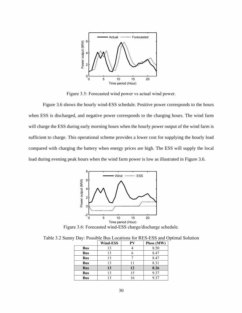
30

Figure 3.5: Forecasted wind power vs actual wind power.

Figure 3.6 shows the hourly wind-ESS schedule. Positive power corresponds to the hours

when ESS is discharged, and negative power corresponds to the charging hours. The wind farm

will charge the ESS during early morning hours when the hourly power output of the wind farm is

sufficient to charge. This operational scheme provides a lower cost for supplying the hourly load

compared with charging the battery when energy prices are high. The ESS will supply the local

load during evening peak hours when the wind farm power is low as illustrated in Figure 3.6.

Figure 3.6: Forecasted wind-ESS charge/discharge schedule.

Table 3.2 Sunny Day: Possible Bus Locations for RES-ESS and Optimal Solution Wind-ESS PV Ploss (MW)

Bus 13 4 8.50

Bus 13 6 8.47

Bus 13 7 8.47

Bus 13 11 8.31

Bus 13 12 8.26

Bus 13 15 9.37

Bus 13 16 9.37

31

Table 3.2 presents a summary of the combinations of the bus location (for hybrid wind-

ESS and only PV) and the power losses (Ploss) associated with each location. It can be seen from

Table 3.2 that there are 7 possible locations for the PV system in the considered DNs. We can

observe that the best siting for the PV system, determined by our proposed method, is bus 12 as

this bus presents the least power losses (8.26 MW) compared to other bus locations. Moreover, it

can be noted that the wind-ESS is located at bus 13 for all the combinations, which are the results

of the assumptions made in this study as previously described. Thus, the optimal location for the

PV and wind-ESS under the sunny day scenario are buses 12 and 13, respectively.

3.3.3.2 Optimal location of Distributed Energy Resources Scenario 2-Cloudy day

In scenario 2, the optimal location problem is solved assuming the weather conditions are

those of a cloudy day. Figure 7 shows the forecasted/actual PV power. The maximum system load

is 27.42 MW. The maximum PV power (1.54 MW) is comparatively lower than that of the sunny

day (2.24 MW), i.e., there is a reduction of 31% in the maximum PV power output. The maximum

power output of the wind-ESS system is 5.85 MW.


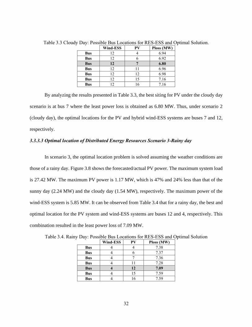
32

Table 3.3 Cloudy Day: Possible Bus Locations for RES-ESS and Optimal Solution. Wind-ESS PV Ploss (MW)

Bus 12 4 6.94

Bus 12 6 6.92

Bus 12 7 6.80

Bus 12 11 6.96

Bus 12 12 6.98

Bus 12 15 7.16

Bus 12 16 7.16

By analyzing the results presented in Table 3.3, the best siting for PV under the cloudy day

scenario is at bus 7 where the least power loss is obtained as 6.80 MW. Thus, under scenario 2

(cloudy day), the optimal locations for the PV and hybrid wind-ESS systems are buses 7 and 12,

respectively.

3.3.3.3 Optimal location of Distributed Energy Resources Scenario 3-Rainy day

In scenario 3, the optimal location problem is solved assuming the weather conditions are

those of a rainy day. Figure 3.8 shows the forecasted/actual PV power. The maximum system load

is 27.42 MW. The maximum PV power is 1.17 MW, which is 47% and 24% less than that of the

sunny day (2.24 MW) and the cloudy day (1.54 MW), respectively. The maximum power of the

wind-ESS system is 5.85 MW. It can be observed from Table 3.4 that for a rainy day, the best and

optimal location for the PV system and wind-ESS systems are buses 12 and 4, respectively. This

combination resulted in the least power loss of 7.09 MW.

Table 3.4. Rainy Day: Possible Bus Locations for RES-ESS and Optimal Solution Wind-ESS PV Ploss (MW)

Bus 4 4 7.38

Bus 4 6 7.37

Bus 4 7 7.36

Bus 4 11 7.28

Bus 4 12 7.09

Bus 4 15 7.59

Bus 4 16 7.59

33


Comparing the three scenarios (sunny, cloudy and rainy), the best solution for the optimal

location for the PV and wind-ESS systems is the one obtained in scenario 2. In other words, the

PV system located at bus 7 and hybrid wind-ESS system located at bus 12 (see Table 3.3) produces

the least power loss (6.80 MW), which is comparatively 17% and 4.1% less than those of the

optimal solutions obtained in scenarios 1 and 3, respectively. Furthermore, to ensure that the

solution obtained in scenario 2 is the optimal one. The optimal location of each scenario is

simulated under three weather conditions, i.e., sunny day, cloudy day, and rainy day. Table 3.5

presents the comparison of the simulation results for these weather conditions and also illustrates

that the optimal location is the one provided by scenario 2 (cloudy day) as it produces the least

overall power losses. With the reduction of the power losses, there is an associated reduction in

power generation, this, in turn, will have a significant impact on cutting down energy production

costs. Figure 3.9 presents the ED results for the three scenarios. It can be seen from Figure 3.10

that for all the scenarios, there is a reduction in peak load; in particular when it is a sunny day, the

PV power production will be higher and it has a significant influence in lowering the peak load.

Thus, our proposed planning strategy is able to optimally locate the hybrid RES-ESS system in the

DNs efficiently and cost-effectively.

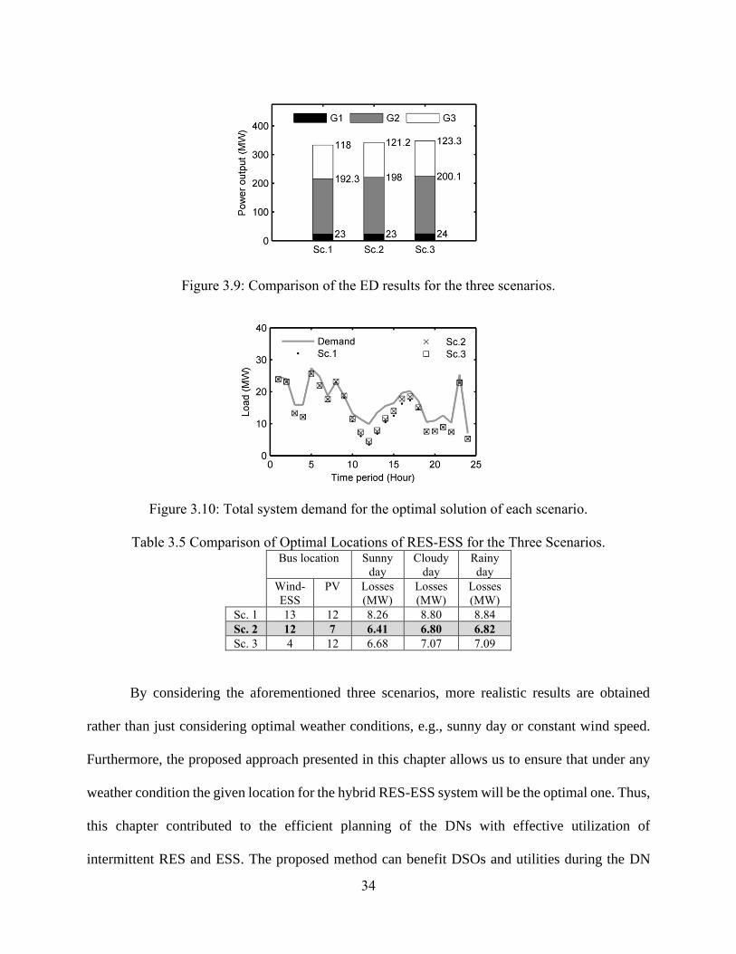
34

Figure 3.9: Comparison of the ED results for the three scenarios.

Figure 3.10: Total system demand for the optimal solution of each scenario.

Table 3.5 Comparison of Optimal Locations of RES-ESS for the Three Scenarios. Bus location Sunny

day

Cloudy

day

Rainy

day

Wind-

ESS

PV Losses

(MW)

Losses

(MW)

Losses

(MW)

Sc. 1 13 12 8.26 8.80 8.84

Sc. 2 12 7 6.41 6.80 6.82

Sc. 3 4 12 6.68 7.07 7.09

By considering the aforementioned three scenarios, more realistic results are obtained

rather than just considering optimal weather conditions, e.g., sunny day or constant wind speed.

Furthermore, the proposed approach presented in this chapter allows us to ensure that under any

weather condition the given location for the hybrid RES-ESS system will be the optimal one. Thus,

this chapter contributed to the efficient planning of the DNs with effective utilization of

intermittent RES and ESS. The proposed method can benefit DSOs and utilities during the DN

35

expansion planning stage, allowing them to determine the optimal site to locate new or future RES-

ESS facilities in the most cost-effective manner. The proposed method has been implemented in

MATLAB® 2013 and simulated in a personal computer with 2.8 GHz CPU, 4 GB RAM. It should

be noted that increasing the size of the test system, i.e., the number of buses, the simulation time

will also increase. In this situation, it is necessary to limit the search for possible bus locations. A

solution for this problem is to consider locations that meet pre-set requirements, e.g., having the

required area for the installation of the wind farm or PV array. This strategy can simplify the size

of the networks and reduce the computation cost.

3.4 SUMMARY

This chapter presented an efficient strategy to optimally allocate RES and ESS in electrical

distribution networks with a goal of minimizing costs and active power losses. A proposed

planning strategy was used to determine the number of possible and optimal locations for the

hybrid RES-ESS system. In order to evaluate the effectiveness of the proposed method, a case

study of a 16-bus test system constituted by different loads, wind farm, solar PV, and ESS was

utilized. The test results demonstrated that by determining the optimal bus location for the RES-

ESS system, overall power losses, as well as peak load, can be significantly reduced1.

1 Research findings of this chapter have been published in a peer-reviewed journal as indicated below:

E. Galvan, P. Mandal, A. U. Haque, and B. Tseng, “Optimal Placement of Intermittent Renewable Energy

Resources and Energy Storage System in Smart Power Distribution Networks,” Electric Power Components and

Systems, Vol. 45, No. 14, pp. 1543-1553, Dec. 2017.

36

Chapter 4: Transactive Control Mechanisms for Prosumer-Centric Networked Microgrids

4.1 INTRODUCTION

This chapter covers a proposed MGEMS based on a hybrid control algorithm that combines

TC and MPC for efficient management of DERs in prosumer-centric networked MGs. This chapter

starts with an introduction followed by details of the essential components of the proposed

TC+MPC-based MGEMS with the uncertainty modeling and the incentive signal formulation.

Afterwards, numerical test results and discussion are presented followed by the summary of the

chapter.

Motivated by the promising benefits of using TCs described in Section 2.2 in literature

review, in this chapter a hybrid control mechanism based on the combination of TC and MPC for

efficient management of DERs in prosumer-centric networked MGs is proposed. Hereinafter, the

proposed control approach is termed TC+MPC. This chapter further presents a detailed analysis

of the impacts (economical and technical) produced by the TC+MPC within the MGs, and the

distribution system as a whole is presented. To carry out this analysis, a Monte Carlo Simulation

(MCS) is proposed to consider BEV driving uncertainties and the proposed hybrid TC+MPC

management system is used to manage DERs. The hybrid TC+MPC combines the control

capabilities and features of the MPC with the TIS–TFS signals of the TC, creating a robust control

mechanism that is driven by price signals. The objective of the TC+MPC management system is

to produce optimal BEV charge and solar PV-BESS charge/discharge schedules to significantly

reduce the residential MG customers’ operational cost and to improve their overall savings. The

proposed MGEMS is evaluated considering different case studies and scenarios to analyze the

impacts that BEV and PV-BESS systems can have on the distribution network.

4.2 TRANSACTIVE CONTROL BASED MICROGRID ENERGY MANAGEMENT SYSTEM

This subsection describes the detailed TC-based MGEMS formulations and comprises the

step-by-step procedures followed by several contextual elements required for the optimization

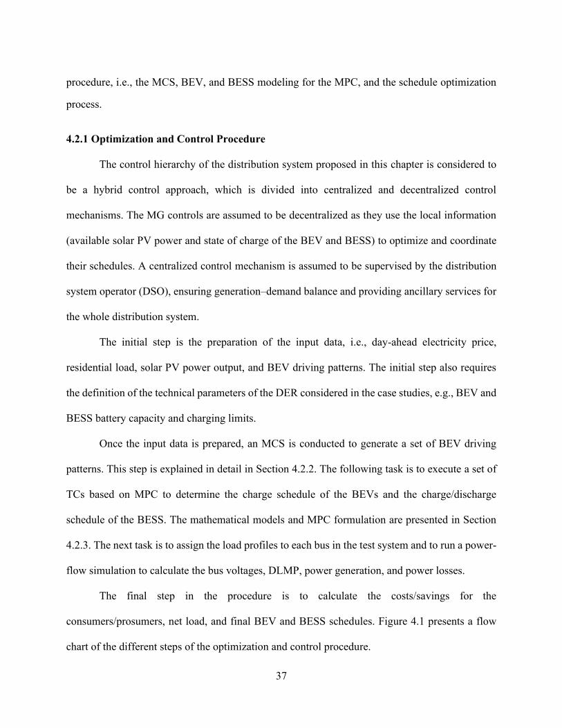
37

procedure, i.e., the MCS, BEV, and BESS modeling for the MPC, and the schedule optimization

process.

4.2.1 Optimization and Control Procedure

The control hierarchy of the distribution system proposed in this chapter is considered to

be a hybrid control approach, which is divided into centralized and decentralized control

mechanisms. The MG controls are assumed to be decentralized as they use the local information

(available solar PV power and state of charge of the BEV and BESS) to optimize and coordinate

their schedules. A centralized control mechanism is assumed to be supervised by the distribution

system operator (DSO), ensuring generation–demand balance and providing ancillary services for

the whole distribution system.

The initial step is the preparation of the input data, i.e., day-ahead electricity price,

residential load, solar PV power output, and BEV driving patterns. The initial step also requires

the definition of the technical parameters of the DER considered in the case studies, e.g., BEV and

BESS battery capacity and charging limits.

Once the input data is prepared, an MCS is conducted to generate a set of BEV driving

patterns. This step is explained in detail in Section 4.2.2. The following task is to execute a set of

TCs based on MPC to determine the charge schedule of the BEVs and the charge/discharge

schedule of the BESS. The mathematical models and MPC formulation are presented in Section

4.2.3. The next task is to assign the load profiles to each bus in the test system and to run a power-

flow simulation to calculate the bus voltages, DLMP, power generation, and power losses.

The final step in the procedure is to calculate the costs/savings for the

consumers/prosumers, net load, and final BEV and BESS schedules. Figure 4.1 presents a flow

chart of the different steps of the optimization and control procedure.

38

Figure 4.1: Flowchart of the proposed optimization and control procedure.

4.2.2 Monte Carlo Simulation

MCS is an accurate technique to estimate probability density functions (PDFs) using

historical data. In this chapter, an MCS is used to consider the uncertainties and stochastic nature

of BEV driving patterns. The MCS requires historical BEV driving patterns (𝛿) to generate a

random BEV driving pattern. To consider uncertainties, the underlying stochastic formulation of

MCS must include two random components; a uniform distribution (𝑅𝑈) and a normal distribution

(𝑅𝑁). The random driving pattern can be formulated as follows [100].

, , ,( ) (1 )i i i i

n k k n k n kd RU RN= + +, (4.1)

where 𝑑𝑛,𝑘𝑖 is the stochastic driving pattern of BEV 𝑖 at time period 𝑘, and scenario 𝑛. 𝛿𝑘

𝑖 is

the expected energy consumption of BEV 𝑖 at time period 𝑘. This process is repeated for a specified

number of scenarios n and ensures convergence over a simulation period t .

Samples of historical data are utilized for the MCS and are constituted by BEV driving

patterns in terms of BEV battery energy usage [100]. These BEV driving patterns reflect

conventional driving by residential customers and are considered as the base driving patterns.

39

4.2.3 Transactive Model Predictive Control Formulation

MPC is also known as Receding Horizon Control (RHC) has been developed considerably

over the past years and has widely been recognized for its application in academic research and

industry. MPC is a control strategy that utilizes current inputs and outputs of a process model to

predict future states or outputs [101]. The MPC is solved as an optimization problem with an

objective function that considers present and future constraints. The MPC solves the optimization

problem in an iterative manner for each time interval of the determined horizon.

In this chapter, the BEV and BESS batteries are formulated as discrete time space models

to be utilized in a MPC. The discrete state space model is formulated as follows [101].

1 kk k k kx Ax Bu Ed N+ = + + , (4.2)

kk ky Cx N= , (4.3)

0(0)x x=, (4.4)

where 𝑥𝑘 is the state at time period 𝑘, 𝑢𝑘 is the input variable, 𝑦𝑘 is the output variable, 𝑑𝑘

is a random variable acting on the state transition, 𝐴 is the state transition matrix, 𝐵 is the input

matrix, 𝐸 is the disturbance matrix, 𝐶 is the output matrix, and 𝑥0 is the initial state. In (4.2), 𝑢𝑘

represents the control variable and the battery state of charge (SOC) is equal to the output variable

𝑦𝑘 = 𝑥𝑘. In the case of the BEV model, BEV driving usage is represented by 𝑑𝑘 as a disturbance of

the battery SOC. When modeling the BESS 𝑑𝑘 represents the residual solar PV power. The BEV

daily usage is modeled using BEV driving patterns generated by the MCS. The state space matrices

of the model are the following (4.5)-(4.8).

1A = , (4.5)

max( / )B BEV Ts=, (4.6)

40

1C = , (4.7)

max( / )E BEV Ts= −, (4.8)

where η is the BEV or BESS efficiency, BEVmax is the maximum charging of the BEV or

BESS, and 𝑇𝑠 is the chosen time sample. The state transition matrix (𝐴) and the output matrix (𝐶)

are set to 1 as it is assumed no other factors are affecting the state of charge of the batteries. If

other factors were to be considered (e.g., battery degradation, temperature) to affect the state of

charge of the batteries, these matrices would be modified. For BESS modeling matrix 𝐵 is negative

and 𝐸 is positive. The change in signs of matrices 𝐵 and 𝐸 for the BESS model, is because the input

variable (𝑢𝑘) is now controlling the discharge of the battery (decreasing the SOC of the battery)

and the solar PV power (𝑑𝑘) is charging the battery (increasing the SOC of the battery).

4.2.3.1 Battery Electric Vehicle Schedule Optimization

Adopting the discrete time space model presented in (4.2)-(4.8), the optimal BEV charge

schedule is achieved while minimizing the charging costs as shown in the objective function (4.9),

which is subject to constraints (4.10)-(4.13).

1

,

0

min F *( )N

k BEV k

k

p u−

=

=, (4.9)

, 1 , , ,

subject to

BEV k BEV k BEV k BEV kx Ax Bu Ed k N+ = + + , (4.10)

, , BEV k BEV ky Cx k N= , (4.11)

min , max, BEV BEV k BEV ku u u k N , (4.12)

min , max BEV BEV k BEVy y y k N , (4.13)

41

in (4.9) 𝑁 is the prediction horizon, 𝑝𝑘 is the electricity price, and 𝑢𝐵𝐸𝑉,𝑘 is the charging

power. The discharge constraints are not considered for BEV modelling as the BEV discharge is

based on the customer driving patterns and is controlled by the on-board computer of the BEV.

From (4.10), 𝑥𝐵𝐸𝑉,𝑘+1 is the BEV future SOC. 𝑦𝐵𝐸𝑉,𝑘 is the current battery SOC, 𝑢𝐵𝐸𝑉𝑚𝑖𝑛 and

𝑢𝐵𝐸𝑉 𝑚𝑎𝑥, 𝑘 are the battery minimum and maximum charging power, respectively. And constraint

(4.13) represents the minimum and maximum SOC of the battery. The optimal BEV charging plan

𝑢𝐵𝐸𝑉,𝑘 will be solved for the determined prediction horizon 𝑁. To carry out the simulations and

determine the optimal charging schedule forecasted BEV load 𝑑𝐵𝐸𝑉,𝑘 and electricity price 𝑝𝑘 are

used.

4.2.3.2 Battery Energy Storage System Schedule Optimization

Similar to BEV, the BESS is modeled as (4.2)-(4.8). The objective function (4.14) is to

maximize the savings of prosumers by optimizing the BESS discharging schedule subject to

constraints (4.14)-(4.19). The objective function for the MPC can be formulated as follows

[102,103].

1

,

0

max F *( )N

k BESS k

k

p u−

=

=, (4.14)

, 1 , , ,

subject to

BESS k BESS k BESS k BESS kx Ax Bu Ed k N+ = + + , (4.15)

, , BESS k BESS ky Cx k N= , (4.16)

min , max, BESS BESS k BESS ku u u k N , (4.17)

min , max, BESS BESS k BESS kd d d k N , (4.18)

min , max BESS BESS k BESSy y y k N , (4.19)

42

in the above equations 𝑥𝐵𝐸𝑆𝑆,𝑘+1 is the future SOC of the BESS, 𝑦𝐵𝐸𝑆𝑆,𝑘 is the BESS SOC,

𝑢𝐵𝐸𝑆𝑆𝑚𝑖𝑛 and 𝑢𝐵𝐸𝑆𝑆 𝑚𝑎𝑥, 𝑘 are the BESS minimum and maximum discharging power, respectively. In

(4.18), 𝑑𝐵𝐸𝑆𝑆𝑚𝑖𝑛 and 𝑑𝐵𝐸𝑆𝑆 𝑚𝑎𝑥, 𝑘 are the minimum and maximum charging power of the BESS and in

(4.19) 𝑦𝐵𝐸𝑆𝑆𝑚𝑖𝑛/𝑦𝐵𝐸𝑆𝑆𝑚𝑎𝑥are the minimum and maximum SOC of the BESS. The optimal BESS

discharging plan 𝑢𝐵𝐸𝑆𝑆,𝑘 will also be solved for the determined prediction horizon N. To determine

the optimal discharging schedule, forecasted solar PV power (𝑑𝐵𝐸𝑆𝑆,𝑘) is considered as the

disturbance.

4.2.4 Transactive Control Signals

In this section, DLMP is considered for energy pricing and used for the TC operation. The

DLMPs are determined by minimizing the cost of generation considering the physical constraints

of the distribution system, thus producing a marginal price at each bus. The DLMP is constructed

based on three components: (i) the wholesale locational marginal price (LMP), (ii) system

conditions (available generation, load demand, and losses), and (iii) uplift costs (operation and

maintenance costs). The LMP is defined as the marginal increase in the overall system costs for

the additional per-unit active power consumption at each transmission bus. For simulation

purposes, it is assumed that the DSO receives the LMP and determines the DLMP at each bus of

the distribution network for the next day and also updates the DLMP in an hourly manner.

Equations (4.20) and (4.21) describe the calculations for TIS and TFS, respectively [103]. The TIS

is formulated in the following manner.

4.2.4.1 Transactive Incentive Signal

, t t ti tTIS DLMP LC TOC LOLC= + + +

, (4.20)

where DLMPt is the DLMP at time t, LCt the cost of distribution losses at time t, total

owning costs (TOC) of the transformer, and a penalty cost for transformer loss of life cost (LOLC).

43

The estimated transformer TOC considers installation, operation, and maintenance cost over its

expected life cycle. The transformer LOLC is estimated based on the loading of the transformer.

4.2.4.2 Transactive Feedback Signal

Similarly, TFS signal represents the net load of the customer, and is calculated by.

, , ,i t i t i tTFS D BEVL= +

, (4.21)

where 𝐷𝑖,𝑡 is the demand of customer i at time t and 𝐵𝐸𝑉𝐿𝑖,𝑡 the BEV charging demand of

customer i at time t.

The TIS and TFS signals are utilized in the MPC formulations presented in subsections

4.2.3.1 and 4.2.3.2 to create a hybrid TC+MPC mechanism. This is achieved by replacing the

electricity price 𝑝𝑘 with the TIS and employing the TFS as a disturbance in the MPC discrete time

space models.



In this section, case studies are presented to test the proposed hybrid TC+MPC scheduling

method on an IEEE 33-bus radial distribution system. For simulation purposes BEV penetration

is considered based on the EV30@30 campaign [104]. The EV30@30 campaign was launched at

the Eighth Clean Energy Ministerial in 2017, in which the collective goal for all Electric Vehicle

Initiative members is to reach a 30% market share for BEVs by 2030. In the case studies a total of

242 households are assumed to be located in three MGs. Data from the US Census Bureau [105],

was used to estimate the number of households that own vehicles and assuming a 30% BEV

penetration a fleet of 74 BEVs is considered to be distributed among the households located in

each MG. Three BEV historical driving patterns are considered for the case studies [100]. Detailed

historical BEV driving data expressed in kWh is shown in Table AII.1 in Appendix II. For the

44

simulation, 1000 scenarios are generated for each BEV type. Table 4.1 shows the BEV parameters

utilized to calculate the random components that are needed for generating BEV driving patterns

by MCS.

The three MGs considered for the simulations are assumed to be located in a 33-bus radial

distribution system as shown in Figure 4.2 The test system data was acquired and modified from

[106], by placing three MGs along the feeders of the test system and modifying the load values.

Detailed bus load data for the 33-bus distribution system is shown in Table AII.2 in Appendix II.

In Figure 4.2, each bus represents a distribution transformer and the dotted lines indicate normally

open tie lines. Connected to the transformer are sets of residential customers that are aggregated

as CGs or PCGs depending on their classification, i.e., consumer or prosumer.

Figure 4.2: Networked microgrids in an IEEE 33-bus distribution network.

45

Table 4.1 Parameters of Random Components of Residential Customer BEV.

Parameter BEV1 BEV2 BEV3

No. of Scenarios 1000 1000 1000

RN Stand. Dev (kWh) 2 1 2

Mean (kWh) 1 0.5 1

Interval RU (kWh) 0-1 0-1 0-1

Confidence Interval µ Lower Bound (kWh) .5668 0.1471 0.3748

Upper Bound (kWh) 0116 0.8170 1.7552

Confidence Interval σ Lower Bound (kWh) 1.3297 0.6166 1.2705

Upper Bound (kWh) 2.3999 1.1128 2.2930

To run the simulations, actual hourly data of load, PV power output, and electricity price

have been used. Price data (Fixed and Time of Use rates) was obtained from El Paso Electric, a

utility in the U.S. southwest [107,108]. The LMP price data was obtained from PJM market [109].

The load data was obtained from the U.S. Department of Energy Open Data Catalog, residential

load at TMY3 locations for the surrounding region of Ashland, Oregon [110]. The specific

locations are Klamath Falls, Medford-Rogue Valley, and Redmond, all from Oregon. The

individual customer load data for each location is shown in Tables AII.3-5 in Appendix II. The

solar PV power output data was obtained from a solar PV system located in Ashland, Oregon. The

solar PV power output profile is representative of a sunny summer day. Table AII.6 in Appendix

II presents the solar PV data used for the simulations. Figure 4.3 shows the solar PV power output

profile considered for each prosumer. The load data was selected for these locations to make the

simulation more realistic as the PV power output is considered for the same region. Moreover, by

utilizing real load, price, and PV data, the case studies results can better illustrate the potential

benefits that can be achieved by using a TC+MPC for BESS and BEV management in residential

networked MGs.

46

Figure 4.3: Residential solar PV power output profile on a sunny summer day.

Most of the latest BEV models (2019 and newer) that are being produced have driving

ranges above 200 miles and are equipped with batteries that have capacities between 60 kWh and

100 kWh [101]. Furthermore, five of the top ten selling BEVs in the U.S. have battery capacities

of 60 kWh or higher [112]. Therefore, it is expected that newer BEV models will continue this

trend and will become the norm in most distribution systems in the future. Hence, for BEV

modeling a Tesla Model S is considered [113]. The Model S offers various battery capacity

presentations; we considered the 70 kWh battery. It is assumed that the maximum charging power

is 10 kW which is based on a 240 V, 40 A connection. A large scale EV deployment project known

as My Electric Avenue was conducted in the United Kingdom between January 2013 and

December 2015 [114] in which, one of the major findings was that the likelihood of a BEV being

charged when its initial SOC was 16.6% or lower is less than 15%. Another study conducted by

the Idaho National Laboratory, U.S.A. found that the average percentage of users who started a

commute or a charge with a SOC of 20% or lower is less than 5% [115]. Thus, for the simulation

purposes, we assume the minimum/maximum BEV SOC to be 20% and 100%, respectively. The

BESS considered for the simulations is a Tesla Powerwall [116]. The PowerWall battery has a

capacity of 13.5 kWh and a charging/discharging power of 5 kW. The minimum/maximum BESS

SOC are set as 0% and 100%, respectively. The information regarding the BEVs and BESS is

47

presented in Tables 4.2 and 4.3, respectively. The data used for the case study is summarized in

Table 4.4, where households are abbreviated as HHs, Load represents the peak load, PV represents

the maximum PV power output, BEV represents the peak BEV load, and BESS – Capacity and

Output are the BESS storage capacity and rated power output, respectively.

Table 4.2 Battery Electric Vehicle Data [115].

EV Parameter Value

EV battery size 70 kWh

EV battery efficiency 90%

Maximum charging power 10 kW

Minimum SOC 20%

Maximum SOC 100%

Table 4.3 Battery Energy Storage System Data [116].

BESS Parameter Value

Energy Capacity 13.5 kWh

Operating Voltage 240 V

Operating Current 48 A

Peak Power 7 kW

Continuous Power 5 kW

Round-trip Efficiency 90%

Depth of Discharge 100%

Table 4.4 Case Study Data.

Bus HHs Load

(kW)

PV

(kW)

BEV

(kW)

BESS

Capacity

(kWh)

Output

(kW)

Microgrid 1

PCG1 23 10 32 50 60 270 50

PCG2 24 12 34 60 50 324 60

CG1 25 15 42 - 50 - -

Microgrid 2

PCG3 19 10 28 50 50 270 50

CG2 20 11 30 - 60 - -

PCG4 21 12 38 60 40 324 60

PCG5 22 12 34 60 30 324 60

Microgrid 3

CG3 7 40 70 - 50 - -

CG4 8 40 100 - 60 - -

PCG6 9 20 48 100 70 540 100

PCG7 10 20 48 100 70 540 100

CG5 11 20 35 - 70 - -

PCG8 12 25 45 125 80 675 125

48

The operation of the proposed TC+MPC was analyzed considering five case studies. The

following case studies were tested and compared with the base case and among each other. Table

4.5 presents a summary of the different case studies.

1. Case 1: Considering Load and BEV (Without PV and BESS) – Under Fixed Price Signal

Scenario

2. Case 2: Considering Load, BEV and PVs (Without BESS) – Under Fixed Price Signal

Scenario

3. Case 3: Considering Load, BEV, PV, and BESS – Under Fixed Price Signal Scenario

4. Case 4: Considering Load, BEV, PV, and BESS – Under Time of Use price Signal Scenario

5. Case 5: Considering Load, BEV, PV, and BESS – Under Dynamic Price Signal Scenario

Table 4.5 Case Study Characteristics.

Load BEV PV BESS Price Signal

Case 1 ✓ ✓ Fixed

Case 2 ✓ ✓ ✓ Fixed

Case 3 ✓ ✓ ✓ ✓ Fixed

Case 4 ✓ ✓ ✓ ✓ Time-of-Use (TOU)

Case 5 ✓ ✓ ✓ ✓ Dynamic (DP)

The base case considers only residential and BEV loads. The base case (Case 1) is similar

to current electrical distribution systems throughout the United States and around the world. Case

2 is the next step of evolution of the conventional distribution system, where customers also have

roof-top solar PV installations. Cases 3, 4, and 5 assume customers have BESS technology which

enables them to participate in an electricity retail market and respond to incentives signals

generated by the DSO. For all case studies the following assumptions are considered

• It is assumed the consumers/prosumers are equipped with home energy management

system (HEMS) in which, the hybrid TC+MPC mechanism is embedded.

• The hybrid TC+MPC mechanism is used for all case studies.

49

• The BEV charge is analyzed only at the consumer/prosumer household, i.e., charging

between 6 am and 6 pm is not available.

• Net metering is considered for cost/savings calculations.

• The BEV SOC must remain at least at 20% throughout the day.

4.3.2 Case 3: Fixed Price Signal Scenario

In this case a fixed cost is utilized [107]. This case can be considered as the conventional

case as most residential customers around the world pay the electric utility or DSO a fixed rate for

electricity. In the US, normally it is expressed in dollars per kilowatt-hour ($/kWh). Under this

pricing rate there is no incentive for customers who own BEVs to charge at different times, e.g.,

during off-peak hours. Thus, BEV charging is uncontrolled and BEVs are charged at any time. In

the case of customers that own PV-BESS systems, the BESS discharge is also uncontrolled and

can be discharged at any time as there is no incentive to discharge for example during peak load

hours. Figure 4.4 presents a sample of the individual BEV charge/discharge schedules of five

BEVs that comprise prosumer group 2 and are located in MG1.


3).

50

Table 4.6 presents the numerical values of the BEV charge and usage schedule per MG.

The positive values (bold numbers) are the BEVs charging demand and the negative demand

represents the BEVs discharging while being driven. Figure 4.5 presents a comparison of the BEVs

charge and discharge patterns in each MG. The Figure illustrates the aggregated BEV drive

patterns and BEV charge schedules for CGs and PCGs in MG1, MG2, and MG3, respectively. In

this case the customer charges the vehicle all night until their departure in the morning (6:00 am),

and then another charge is conducted around (7:00 pm) to have enough energy for the commutes

between (8:00–9:00 pm). It is clear that since the price is fixed throughout the day the customer

doesn’t have any incentive to charge at a different time.

Table 4.6 Aggregated BEV Charge Schedule and Driving Pattern (Case 3).

Hour 1 2 3 4 5 6 7 8 9 10 11 12

Price ($/kWh) 0.10 0.10 0.10 0.10 0.10 0.10 0.10 0.10 0.10 0.10 0.10 0.10

BEV-MG1

(kWh) 157 110 110 81 0 -56 -70 -71 -6 -17 -23 -25

BEV-MG2

(kWh) 177 130 126 74 0 -67 -82 -70 -5 -36 -47 -25

BEV-MG3

(kWh) 383 270 259 143 0

-

139

-

167

-

146 -14 -71 -93 -49

Hour 13 14 15 16 17 18 19 20 21 22 23 24

Price ($/kWh) 0.10 0.10 0.10 0.10 0.10 0.10 0.10 0.10 0.10 0.10 0.10 0.10

BEV-MG1

(kWh) -24 0 -13 -56 -68 -24 48 -49 -53 0 0 0

BEV-MG2

(kWh) -25 0 -25 -68 -68 -7 54 -63 -67 0 0 0

BEV-MG3

(kWh) -49 0 -51

-

138

-

141 -17 113

-

125

-

132 0 0 0

51

Figure 4.5: Aggregated BEV charge schedule and driving pattern of the three MGs (Case 3).

4.3.3 Case 4: Time-of-Use Price Signal Scenario

In this case a Time-of-Use (TOU) price is considered for a day in Summer. The TOU plans

are based on the time of day and the season. By utilizing TOU customers can manage their energy

costs. This is achieved by taking advantage of lower rates during off-peak periods and avoiding

on-peak periods when energy resources are in high demand. The TOU price that is being tested

for this specific case study considers the on-peak period from 12:00 pm through 6:00 pm, Monday

through Friday, for the months of June through September. The off-peak period considers all other

hours not covered in the on-peak period [108]. Figure 4.6 shows a sample of the individual BEV

charge schedules and driving patterns of five BEVs that constitute prosumer group 2 and are

located in MG1.

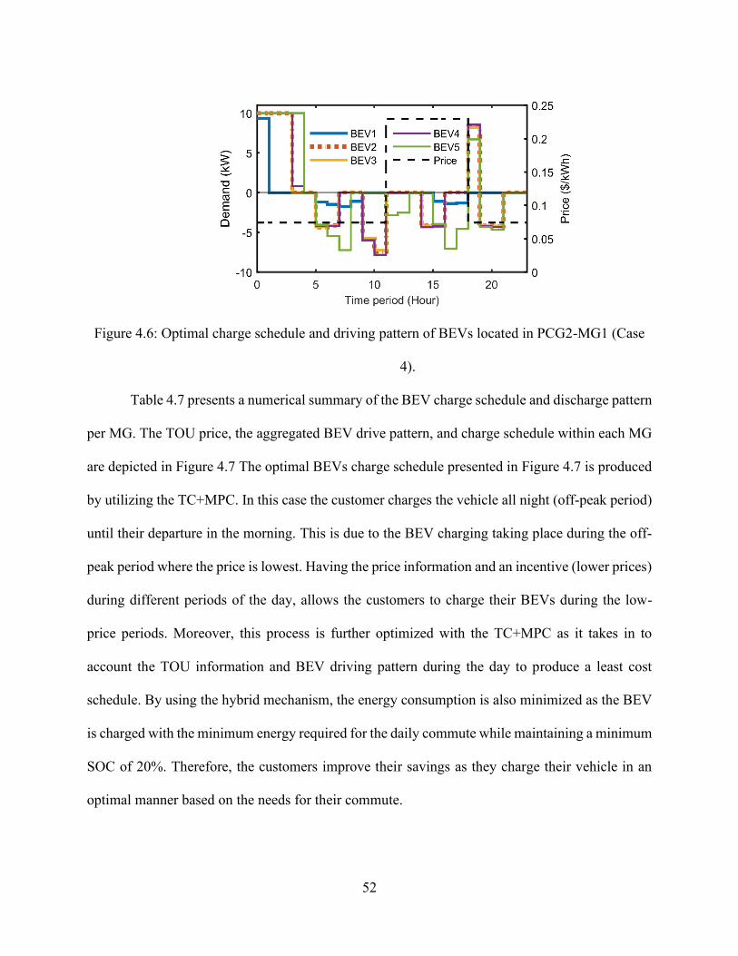
52


4).

Table 4.7 presents a numerical summary of the BEV charge schedule and discharge pattern

per MG. The TOU price, the aggregated BEV drive pattern, and charge schedule within each MG

are depicted in Figure 4.7 The optimal BEVs charge schedule presented in Figure 4.7 is produced

by utilizing the TC+MPC. In this case the customer charges the vehicle all night (off-peak period)

until their departure in the morning. This is due to the BEV charging taking place during the off-

peak period where the price is lowest. Having the price information and an incentive (lower prices)

during different periods of the day, allows the customers to charge their BEVs during the low-

price periods. Moreover, this process is further optimized with the TC+MPC as it takes in to

account the TOU information and BEV driving pattern during the day to produce a least cost

schedule. By using the hybrid mechanism, the energy consumption is also minimized as the BEV

is charged with the minimum energy required for the daily commute while maintaining a minimum

SOC of 20%. Therefore, the customers improve their savings as they charge their vehicle in an

optimal manner based on the needs for their commute.

53


Hour 1 2 3 4 5 6 7 8 9 10 11 12

Price ($/kWh) 0.07 0.07 0.07 0.07 0.07 0.07 0.07 0.07 0.07 0.07 0.07 0.23

BEV-MG1

(kWh) 157 110 110 81 0 -56 -70 -71 -6 -17 -23 -25

BEV-MG2

(kWh) 177 140 133 64 0 -67 -82 -70 -5 -36 -47 -25

BEV-MG3

(kWh) 383 280 273 133 0

-

139

-

167

-

146 -14 -71 -93 -49

Hour 13 14 15 16 17 18 19 20 21 22 23 24

Price ($/kWh) 0.23 0.23 0.23 0.23 0.23 0.23 0.07 0.07 0.07 0.07 0.07 0.07

BEV-MG1

(kWh) -24 0 -13 -56 -68 -50 73 -49 -53 0 0 0

BEV-MG2

(kWh) -25 0 -25 -68 -68 -50 89 -63 -67 0 0 0

BEV-MG3

(kWh) -49 0 -51

-

138

-

141

-

102 184

-

125

-

132 0 0 0


Comparing the charge schedules with the ones obtained in Case 3, it can be seen that having

an incentive (lower price) at different times of the day the TC+MPC increases the charging power

(4-8%) between (2:00-3:00 am). The charging power is also increased (52-65%) at 7:00 pm to take

advantage of the low price available after 6:00 pm.

54

4.3.4 Case 5: Dynamic Price Signal Scenario

In the final case a dynamic price signal is considered. The price signal is based on the

system DLMP (see section 4.2.4). For this case study the DLMP accounts for marginal costs of

generation, marginal costs of losses, and is updated hourly.

Although the customers are receiving the hourly price information it can be difficult and

time consuming for a customer to manually be observing the electricity price for that specific hour

and decide when to charge their BEV. The HEMS with the embedded TC+MPC can assist the

customers by automating the BEV charging. The TC+MPC uses the forecasted DLMP and a

forecasted BEV demand pattern to determine the optimal BEV charge schedule that minimizes the

customers charging costs. The main differences with the fixed price and TOU is that the DLMP

(i) is time varying (in this case hourly) and (ii) it accounts for the system conditions (generation,

load, and losses). Figure 4.8 depicts a sample of the individual BEV charge schedules and driving

patterns of five BEVs that comprise prosumer group 2 and are located in MG1. A detailed analysis

of the numerical values of the aggregated BEV charge schedule and discharge pattern per MG is

presented in Table 4.8.


5).

55


Hour 1 2 3 4 5 6 7 8 9 10 11 12

Price ($/kWh) 0.09 0.08 0.08 0.08 0.08 0.09 0.09 0.09 0.09 0.09 0.10 0.10

BEV-MG1

(kWh) 106 110 110 157 0 -56 -70 -71 -6 -17 -23 -25

BEV-MG2

(kWh) 111 140 140 177 0 -67 -82 -70 -5 -36 -47 -25

BEV-MG3

(kWh) 229 280 280 383 0

-

139

-

167

-

146 -14 -71 -93 -49

Hour 13 14 15 16 17 18 19 20 21 22 23 24

Price ($/kWh) 0.10 0.10 0.10 0.11 0.11 0.11 0.10 0.10 0.10 0.10 0.09 0.09

BEV-MG1

(kWh) -24 0 -13 -56 -68 -50 48 -49 -53 0 0 0

BEV-MG2

(kWh) -25 0 -25 -68 -68 -50 34 -63 -67 0 0 0

BEV-MG3

(kWh) -49 0 -51

-

138

-

141

-

102 81

-

125

-

132 0 0 0

Figure 4.9 shows the aggregated BEVs drive pattern and the optimal charge schedule

respectively, for each MG utilizing the TC+MPC. It can be seen from Table 4.8 and Figure 4.9,

how the TC+MPC optimizes the BEV charge by selecting the hours where the price is lowest.

Specifically, the maximum charging occurs between 2-4 am when the price is lowest and another

lower charging period occurs at 7:00 pm. When using the TC+MPC, the BEV is charged with

sufficient energy for the daily commute of the customer while minimizing the costs. Comparing

the results of this case with Cases 3 there is a decrease between 32-40% at 1:00 am and an increase

between 94-168% at 4:00 am. These results explicitly show how the TC+MPC identifies the hours

(3:00-4:00 am) with the lowest prices and maximizes the charging at those hours to avoid incurring

additional costs during high price hours. When compared to Case 4 there are similarities as both

price signals have low price periods. However, for the TOU the low-price periods are fixed

regardless of the distribution system conditions.

56


Figure 4.10 shows the comparison of the overall system net load for each case. Comparing

the four cases with the base case (Case 1) it can be seen that the overall system net load is lower

for all the cases, which is due to the solar PV power output. It can also be seen from Figure 4.10

that having BESS available allows the prosumers to shift the surplus power production of solar PV

(from 7:00 am to 3:00 pm) to peak load periods (between 6:00 and 10:00 pm). Shifting surplus

power from off-peak periods can reduce peak load and also avoid steep load ramps. It can also be

seen in Figure 4.10 that due to the BESS discharge during the peak period, the demand curve

becomes more volatile. Although, compared to the demand ramp rate observed in Case 2 (no

BESS), the demand ramp rate created by the BESS discharge in Cases 3-5 is lower. This is an

important aspect to consider while setting the BESS discharge constraints in order to minimize

negative impacts due to the BESS discharge. Also, incentivizing customers to charge their BEVs

during low price periods (off-peak) can reduce peak load and help alleviate steep load ramps.

57

Figure 4.10: Overall system net load comparison for each case.

As it was explained in section 4.2.1, a power flow simulation is conducted to calculate

system power losses and bus voltage profiles. The power flow results are obtained using

MATPOWER [117]. In MATPOWER, when BEVs and BESS are charging these are treated as

load. For every hour, an energy balance is conducted at each bus, i.e., solar PV power is subtracted

from the load (household load + BEV and BESS charge). If the net load is negative (i.e., solar PV

power generation is greater than the load) then the bus becomes a PV bus. On the other hand, if

the net load is positive, the bus remains as a PQ bus. Once the values are assigned for the time

period (1-hour), the power flow is executed. This process is repeated for the simulation horizon of

24 hours. Table 4.9 shows a comparison of the total system losses for each case. Comparing the

overall system losses of Cases (2-5) with the base Case (Case 1), it can be seen that all the Cases

reduce power losses and the highest reduction in losses (11.7%) is achieved in Case 2. Case 2

assumes customers have BEVs and rooftop solar PV installations and any surplus PV power is

injected back to the utility grid. Cases 3-5 achieve an overall system power loss reduction of 6.7%

compared to the base Case (Case 1). The difference in power loss reduction between Case 2 and

Cases 3-5 can be attributed to power losses in storing surplus power in the BESS and the residual

58

energy that remains stored in the BESS. Although there is a higher power loss reduction in Case 2

compared to Cases 3-5, there are other benefits achieved in Cases 3-5. These benefits are (i)

reduction in peak load, (ii) reduction in load ramps, (iii) BEV owners can minimize their charging

cost, and (iv) prosumers are able to participate in a retail electricity market and maximize their

savings by using the power stored in the BESS during high price periods. Benefit number iv) gives

the customers flexibility to utilize the energy for their own use or to sale to other customers when

high prices are available.

Table 4.9 Comparison of Total System Power Losses.

Power Losses (kW) Reduction (%)

Case 1 (Without PV or BESS) 1788 0%

Case 2 (Without BESS) 1582 11.5%

Case 3 (Fixed Price) 1672 6.5%

Case 4 (TOU Price) 1676 6.3%

Case 5 (Dynamic Price) 1667 6.8%

Voltage profiles are also analyzed to observe the effects produced by the BEVs charging

and BESSs discharge schedules for each case. Table 4.10 presents a comparative summary of bus

voltage violations (undervoltages) that were recorded when running the simulations as well as

improvements to the bus voltage profiles. It should be mentioned that no overvoltages were

observed in any of the buses of the test system. The bus voltages that are not shown in Table 4.10

did not present violations (over/under voltages). The comparative analysis summarized in Table

4.10 is done between the base case (Case 1) and Cases 2-5. The values shown in the undervoltage

column indicate the number of hours an undervoltage has been recorded in the corresponding case.

The values presented in the difference column indicate the difference in number of hour(s) the

corresponding case recorded an undervoltage compared to the base case (Case 1). A negative sign

(-) indicates a reduction in hour(s), positive sign (+) indicates an increase in hour(s), and a zero (0)

indicates no difference.

59

Table 4.10 Summary of Bus Voltages Improvements.

Hours

Under Voltage

(<0.95 p.u.)

Hour

Difference

Hours

Under Voltage

(<0.95 p.u.)

Hour

Difference Bus Case Bus Case

9

1 4 0

17

1 11 0

2 4 0 2 7 -4

3 2 -2 3 6 -5

4 1 -3 4 6 -5

5 1 -3 5 6 -5

10

1 5 0

18

1 11 0

2 4 -1 2 7 -4

3 2 -3 3 6 -5

4 2 -3 4 6 -5

5 2 -3 5 6 -5

11

1 6 0

28

1 5 0

2 4 -2 2 4 -1

3 2 -4 3 2 -3

4 2 -4 4 2 -3

5 2 -4 5 2 -3

12

1 7 0

29

1 8 0

2 5 -2 2 5 -3

3 3 -4 3 5 -3

4 3 -4 4 5 -3

5 3 -4 5 5 -3

13

1 8 0

30

1 10 0

2 5 -3 2 6 -4

3 4 -4 3 5 -5

4 6 -2 4 5 -5

5 6 -2 5 5 -5

14

1 9 0

31

1 12 0

2 6 -3 2 7 -5

3 6 -3 3 7 -5

4 6 -3 4 7 -5

5 6 -3 5 7 -5

15

1 9 0

32

1 13 0

2 6 -3 2 8 -5

3 6 -3 3 9 -4

4 6 -3 4 9 -4

5 6 -3 5 8 -5

16

1 11 0

33

1 13 0

2 7 -4 2 8 -5

3 6 -5 3 9 -4

4 6 -5 4 9 -4

5 6 -5 5 9 -4

60

By further analyzing the results presented in Table 4.10, it can be stated that having rooftop

solar PV installations (Case 2) can improve bus voltage profiles from 20% and up to 42%

compared to the base case (Case 1). However, having a hybrid PV-BESS system (Cases 3-5) can

improve voltage profiles between 25% and 75% compared to the base case. In all but one bus (Bus

33), the cases where BESS is present render a higher voltage profile improvement. Thus, having

controllable demand-side DER can protect the system from overvoltages that can be incurred in

the uncontrolled case (Case 2) while also providing the benefits that have been previously

discussed.

Finally, a cost/savings analysis is carried out to compare the total daily costs and savings

for the PCGs and CGs located in each MG. The daily costs and savings data is presented in Tables

4.11 and 4.12. In Table 4.11, the Costs ($) refer to the amount paid for the daily energy

consumption and Savings ($) refer to energy cost reduction associated to the use of rooftop solar

PV and BESS.

Comparing the results of the five cases (see Table 4.11), we can observe that the highest

overall savings are achieved by PCGs in Cases 4 (TOU) and 5 (DP). Also, Cases 3-5 produced

greater savings then Cases 1 and 2. Specifically, the savings difference were between 52%-76%

(Case 3), 128%-144% (Case 4), and 95%-123% (Case 5). When comparing the costs of Cases 2-5

to those of Case 1 (base case) they all achieve a cost reduction. The total cost reductions compared

to Case 1 are Case 2 (29%), Case 3 (45%), Case 4 (57%), and Case 5 (37%). The results

comparison demonstrates that by having the BESS, the reduction in total costs for Cases 3-5 is

improved. This is more noticeable in Case 5 as the demand during high price periods is fulfilled

by the energy stored in the BESS. With the reduction of the peak demand between 6:00 pm and

9:00 pm (see Figure 4.10), there is an associated reduction in electricity price, which in turn has a

61

significant impact on the total costs of the CGs and PCGs. We can clearly observe that by shifting

the surplus PV generation with BESS (controlled by TC) to peak load hours, PCGs can reduce

their total energy costs.

Table 4.11 Total Daily Costs ($) and Savings ($) Comparison per Microgrid.

Case 1 Case 2 Case 3

Total

Costs

Total

Savings

Total

Costs

Total

Savings

Total

Costs

Total

Savings

PCG1 54.66 0.00 40.96 13.70 31.36 23.30

MG1 PCG2 70.65 0.00 51.90 18.75 37.60 33.05

CG1 52.99 0.00 52.99 0.00 52.99 0.00

PCG3 51.79 0.00 36.17 15.62 27.32 24.47

MG2 CG2 43.84 0.00 43.84 0.00 43.84 0.00

PCG4 55.85 0.00 39.41 16.44 29.93 25.92

PCG5 43.54 0.00 30.91 12.64 23.88 19.66

CG3 108.42 0.00 108.42 0.00 108.42 0.00

CG4 165.86 0.00 165.86 0.00 165.86 0.00

MG3 PCG6 89.73 0.00 62.33 27.40 46.09 43.64

PCG7 92.15 0.00 60.90 31.25 44.63 47.52

CG5 72.44 0.00 72.44 0.00 72.44 0.00

PCG8 91.00 0.00 64.67 26.33 50.99 40.01

Case 4 Case 5

Total

Costs

Total

Savings

Total

Costs

Total

Savings

PCG1 25.50 31.90 39.79 29.63

MG1 PCG2 33.15 45.76 45.73 41.98

CG1 53.29 0.00 65.07 0.00

PCG3 21.52 36.59 34.44 29.19

MG2 CG2 42.65 0.00 55.63 0.00

PCG4 23.72 38.19 35.04 32.01

PCG5 18.54 24.92 27.15 24.66

CG3 118.57 0.00 134.84 0.00

CG4 202.87 0.00 209.43 0.00

MG3 PCG6 37.72 63.07 71.20 56.12

PCG7 36.74 71.29 62.49 62.32

CG5 25.50 31.90 39.79 29.63

PCG8 33.15 45.76 45.73 41.98

Table 4.12 presents the comparison of net costs and the difference between each case and

the base case. In Table 4.12, Net Costs are the Costs minus Savings (Costs – Savings), and the

percentage column indicates an increase (Inc.) if it is positive and a reduction (Red.) if negative

62

Further analysis of the net costs results (see Table 4.12) shows that Case 4 achieves the

highest net cost reduction percentages for both CGs and PCGs followed by Case 5, which produces

a higher net cost reduction for PCGs. Also, CGs achieve more net cost reduction under Fixed and

TOU pricing schemes (Cases 3 and 4) compared to a DP scheme (Case 5). These results are

reasonable as CGs do not possess alternative sources of generation to fulfill their own demand and

can only participate by deferring or shifting load to low price periods.

Therefore, it can be inferred that a DP scheme is better suited for PCGs that are able to

respond to price signals via BESS or other controllable distributed generation sources. It should

be noted that for simulation purposes in Case 2-5 the price signal is considered the same for buying

and selling power (net metering). In different electricity markets, utilities and DSOs have lower

paying costs for selling power to the grid. Consequently, the total savings for Cases 2-4 could be

lower under these pricing schemes when compared to Case 5, thus adding more value to TC+MPC

and BESS for customers under those pricing schemes.

It should be noted that the test results are only representatives and are obtained under

simulated conditions for the considered test system. More case studies could be further conducted

for longer time horizons (e.g., weeks and months) with different scenarios, test systems, and MG

locations in order to be able to conclude that the benefits mentioned in the case studies will be

achieved with high certainty.

63

Table 4.12 Net Costs ($) Comparison Per Microgrid.

Case 1 Case 2 Case 3

Net Costs

($)

Inc. / Red.

(%)

Net Costs

($)

Inc. / Red.

(%)

Net Costs

($)

Inc. / Red.

(%)

PCG1 54.66 0.00 27.26 -50.13 8.06 -85.25

MG1 PCG2 70.65 0.00 33.15 -53.07 4.55 -93.57

CG1 52.99 0.00 52.99 0.00 52.99 0.00

PCG3 51.79 0.00 20.54 -60.33 2.85 -94.50

MG2 CG2 43.84 0.00 43.84 0.00 43.84 0.00

PCG4 55.85 0.00 22.97 -58.87 4.01 -92.81

PCG5 43.54 0.00 18.27 -58.05 4.22 -90.31

CG3 108.42 0.00 108.42 0.00 108.42 0.00

CG4 165.86 0.00 165.86 0.00 165.86 0.00

MG3 PCG6 89.73 0.00 34.93 -61.07 2.44 -97.28

PCG7 92.15 0.00 29.66 -67.82 -2.90 -103.14

CG5 72.44 0.00 72.44 0.00 72.44 0.00

PCG8 91.00 0.00 38.34 -57.87 10.97 -87.94

Case 4 Case 5

Net Costs

($)

Inc. / Red.

(%)

Net Costs

($)

Inc. / Red.

(%)

PCG1 -6.40 -111.7 10.17 -81.40

MG1 PCG2 -12.61 -117.8 3.75 -94.69

CG1 53.29 0.57 65.07 22.79

PCG3 -15.06 -129.1 5.26 -89.85

MG2 CG2 42.65 -2.73 55.63 26.89

PCG4 -14.47 -125.9 3.03 -94.58

PCG5 -6.38 -114.6 2.49 -94.28

CG3 118.57 9.37 134.84 24.37

CG4 202.87 22.31 209.43 26.27

MG3 PCG6 -25.35 -128.2 15.08 -83.20

PCG7 -34.55 -137.5 0.17 -99.82

CG5 72.33 -0.14 103.88 43.41

PCG8 -14.18 -115.6 40.30 -55.71

The TC+MPC formulation presented in this chapter has been implemented in MATLAB

R2017a and solved with YALMIP and GUROBI (Gurobi Optimization, LLC., Beaverton, OR,

USA). MATLAB (The MathWorks Inc., Natick, MA, USA) is used as the programming

environment, while YALMIP structures the optimization problem into matrices with the objective

function, the optimization variables, and the equality and inequality constraints [118]. GUROBI is

64

used as an external solver to find the optimal solution of the problem [119]. All simulations were

conducted using a personal computer with 2.8 GHz CPU, 4 GB RAM.

4.4 SUMMARY

In this chapter, a MGEMS based on a hybrid control algorithm that combines TC and MPC

for an efficient management of DERs in prosumer-centric networked MGs has been presented.

The proposed hybrid TC+MPC combines the control capabilities and features of the MPC and the

TC, creating a robust control mechanism that is driven by transactive incentive signals, and thus,

also providing the MGEMS capability to deal with the stochastic nature of BEV driving by using

a MCS to generate the BEV driving patterns. The proposed TC+MPC was able to effectively

generate the BEV-charge and BESS-discharge schedules for the CGs/PCGs located in each MG.

Test results demonstrated the potential of using pricing mechanisms for demand-side management

of DERs2.

2 Research findings of this chapter have been published in a peer-reviewed journal as indicated below:

E. Galvan, P. Mandal, S. Chakraborty, and T. Senjyu, “Efficient Energy Management System Using A Hybrid

Transactive-Model Predictive Control Mechanism for Prosumer-Centric Networked Microgrids,” Sustainability,

Vol. 11, No. 19, Sep. 2019.

65

Chapter 5: Resiliency Improvement in Networked Microgrids by Utilizing Distributed

Energy Resources

5.1 INTRODUCTION

This chapter considers the advantages and challenges of having sections of a power

distribution system constituted by networked MGs to manage DERs to improve distribution

system resiliency to natural disasters. A detailed resiliency analysis process is presented with two

case studies that are tested under different scenarios and evaluated utilizing different resiliency

metrics. This chapter contributes to provide realistic case studies that show the potential benefits

that DERs managed in networked MGs can provide a power distribution grid.

5.2 SYSTEM MODELING AND RESILIENCY METRICS

To evaluate the resiliency of the distribution grid with networked MGs and DERs, an

analysis based on the Resilience Analysis Process (RAP) is conducted. The RAP was developed

at SANDIA national laboratories to provide a means and a set of metrics to analyze the resiliency

of energy systems [120]. Frequently, resiliency and reliability are confused as being similar

although they account for different types of events and use different metrics, i.e., resiliency

analysis considers low probability, high consequence events and the resiliency metrics focus on

the impacts on humans. Contrary to the resiliency analysis, reliability analysis considers high

probability, low impact events and the focus is on system impacts [120].

The main goal of this chapter is to analyze and evaluate potential improvements of a power

distribution systems resiliency to natural disasters using solar PV and BESS. The specific goals

are (1) evaluate the impact of outages to the system loads when utilizing MGs and DERs and (2)

the monetary impacts the utility or system operator will experience due to the natural disaster.

66

5.2.1 Classification of Consequences and Resiliency Metrics

For the present study, the consequences and resiliency metrics that are considered for the

case studies are described in Table 5.1. The metrics shown in Table 5.1 are based on consequences

and resiliency metrics reported in [26].

Table 5.1 Consequence Categories and Resilience Metrics

Consequence Class Resiliency Metric

Electrical Service Total customer-hours of outages (h)

Total customer energy not served (kWh)

Total and average number of customers experiencing

outage during the specified time period

Monetary Total loss of utility revenue ($)

Total outage costs ($)

Total avoided outage cost ($)

5.2.2 Definition of Hazards and Level of Disruption of the Distribution System

The potential hazards that are considered for simulation purposes are storms of different

intensities, i.e., moderate intensity and high intensity. The level of damage the grid assets are

anticipated to suffer under the storm scenarios are based on the hazard’s intensity, i.e., similar

damages will be considered (moderate damage and high damage). Specifically, the damages that

are anticipated to occur in the distribution grid are downed distribution lines and feeders. The

consequence data of the hazards for the case studies is obtained through the execution of power

flow in the distribution system [117]. When running the power flow analysis, the bus voltages and

power outputs of the DERs are calculated to estimate which loads would be unserved during the

outage. In this case, power flow will be executed for the case studies time period (1-day) under the

different scenarios that are described in subsection 5.3.1. These simulations will allow to determine

and quantify the effects of the hazards on the customers being served in the distribution system

and the ability of the utility or system operator to deliver electrical energy to its customers.

67

5.2.3 Consequences and Resiliency Metrics Calculations

The consequence and resiliency metrics that have been evaluated are listed in Table 5.1.

Each metric is calculated as follows.

5.2.3.1 Electrical Service Class

Total customer-hours of outage

1 1

( )n k

i

t i

x t= =

(5.1)

where ( )ix t is the number of customer-hours without power of customer i for the duration

of event n , for all customers k experiencing an outage..

Total customer energy not served

1 1

( )n k

i

t i

E t= =

(5.2)

where ( )iE t is the total energy not served per customer i for the duration of event n , for

all customers k experiencing an outage..

Total and average number of customers experiencing outage during the specified time

period

,

1 1

sT k

i s

s i

s

x

XT

= ==

(5.3)

where X is the average number of customers experiencing an outage during scenario s ,

k the total number of customers experiencing an outage, and sT the total number of scenarios.

68

5.2.3.2 Monetary Class

Total loss of utility revenue

, ,

1 1

* ( )n k

LUR s e i s

t i

C C E t= =

=

(5.4)

where ,LUR sC is the loss of utility revenue ($) of scenario s , eC is the cost of energy

($/kWh), , ( )i sE t is the total energy not served for the duration of event n , during scenario s , for

all customers k experiencing an outage.

Total outage costs

, ,

1 1

* ( )n k

out s o i s

t i

C C x t= =

=

(5.5)

where ,out sC is the total outage cost ($) of scenario s , oC is the outage cost per hour ($/h),

, ( )i sx t the number of customer-hours without power for the duration of event n , during scenario

s , for all customers k experiencing an outage.

Total avoided outage cost

, ,avd s out base out sC C C−= − (5.6)

Where ,avd sC are the avoided costs ($) of scenario s , out baseC − is the total outage cost ($) of

the base scenario, and ,out sC is the total outage cost ($) of scenario s .


In this section, case studies are presented to evaluate the resiliency metrics proposed in the

previous subsections. For the proposed research study two cases are considered, (1) case where

moderate damage affects the power distribution system and (2) a case where heavy damage occurs

to the system. For both cases, it is assumed groups of residential customers own roof-top solar PV.

69

A 33-bus test system with three MGs is considered to run the simulations [121]. The simulations

are carried out for each case and then a comparison of the statistics of each case with a base case

that has no DERs is shown. This process is modeled for a day (24 hours) with outages occurring

over a three-hour period following the natural disaster event. To estimate the cost of energy not

served a fixed energy rate is assumed [107]. In the case of outage costs, a value of 3 $/h is utilized

to calculate the total costs [122]. The following assumptions are made for the case studies:

• There are sufficient repair crews to attend all damaged lines

• The estimated time for line repairs is 3 hours

• All lines are repaired simultaneously

• BESS units are utility-owned


The IEEE 33-bus radial distribution system with three MGs presented in section 4.3 is used

for simulation purposes with minor changes made to the system data. Table 5.2 shows the data

utilized in the test system. The differences between the test data used for the case studies in this

chapter with those of chapter 4 is that in these case studies BEVs are not considered and the BESS

is assumed to be utility owned. The solar PV power output data used in simulations for the sunny-

day scenarios is presented in Appendix II, Table AII.6. For the rainy-day scenarios, the data is

shown in Table III.1 in Appendix III.

For the proposed resiliency analysis, two case studies and five scenarios for each case study

are considered. The case studies that were tested and compared with the base scenario and among

each other are the following.

Case 1: Moderate Damage

1.1. Base scenario no DERs

70

1.2. Sunny day preceding the event and all load supplied

1.3. Sunny day preceding the event and only critical loads are supplied

1.4. Rainy day preceding the event and all load supplied

1.5. Rainy day preceding the event and only critical loads are supplied

Case 2: Heavy Damage

2.1. Base scenario no DERs

2.2. Sunny day preceding the event and all load supplied

2.3. Sunny day preceding the event and only critical loads are supplied

2.4. Rainy day preceding the event and all load supplied

2.5. Rainy day preceding the event and only critical loads are supplied

The base scenarios consider there are no DERs interconnected with the power distribution

system. For the rest of the scenarios DERs are considered to be interconnected to the distribution

grid.

5.3.2 Resiliency Analysis of Distribution Grid-Moderate Damage Case

For this case, three MGs are assumed to be located in a 33-bus radial distribution system

as shown in Figure 5.1. In Figure 5.1, each bus represents a distribution transformer and the dotted

lines indicate normally open tie lines. Connected to the transformer are sets of residential

customers that are aggregated as consumer groups (CG) or prosumer groups (PCG) depending on

their classification, i.e., consumer or prosumer. To evaluate the impact of the MGs and the DERs

to the resiliency of the distribution system to natural disasters it is assumed a storm occurred and

created moderate damage to the feeders of the system. Specifically, to branches 2-19, 3-23, and 6-

7, as shown in Figure 5.1. The event is assumed to have occurred at 17:00 hrs. (5:00 pm) and the

duration of the outage is 3 hours (17:00 hrs. to 19:00 hrs.). The 3-hour time period is based on the

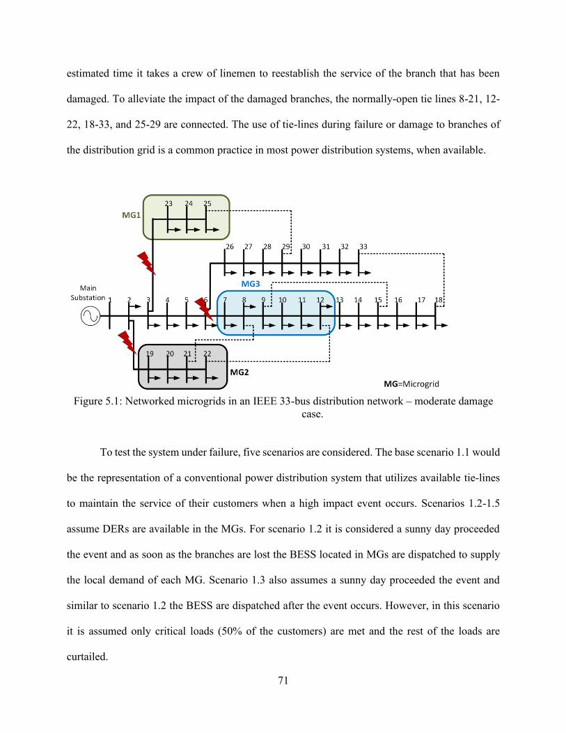
71

estimated time it takes a crew of linemen to reestablish the service of the branch that has been

damaged. To alleviate the impact of the damaged branches, the normally-open tie lines 8-21, 12-

22, 18-33, and 25-29 are connected. The use of tie-lines during failure or damage to branches of

the distribution grid is a common practice in most power distribution systems, when available.

Figure 5.1: Networked microgrids in an IEEE 33-bus distribution network – moderate damage

case.

To test the system under failure, five scenarios are considered. The base scenario 1.1 would

be the representation of a conventional power distribution system that utilizes available tie-lines

to maintain the service of their customers when a high impact event occurs. Scenarios 1.2-1.5

assume DERs are available in the MGs. For scenario 1.2 it is considered a sunny day proceeded

the event and as soon as the branches are lost the BESS located in MGs are dispatched to supply

the local demand of each MG. Scenario 1.3 also assumes a sunny day proceeded the event and

similar to scenario 1.2 the BESS are dispatched after the event occurs. However, in this scenario

it is assumed only critical loads (50% of the customers) are met and the rest of the loads are

curtailed.

72

Table 5.2 Resiliency Analysis Case Study Data.

Bus HHs Load

(kW)

PV

(kW)

BEV

(kW)

BESS

Capacity

(kWh)

Output

(kW)

Microgrid 1

PCG1 23 10 32 50 - 270 50

PCG2 24 12 34 60 - 324 60

CG1 25 15 42 - - - -

Microgrid 2

PCG3 19 10 28 50 - 270 50

CG2 20 11 30 - - - -

PCG4 21 12 38 60 - 324 60

PCG5 22 12 34 60 - 324 60

Microgrid 3

CG3 7 40 70 - - - -

CG4 8 40 100 - - - -

PCG6 9 20 48 100 - 540 100

PCG7 10 20 48 100 - 540 100

CG5 11 20 35 - - - -

PCG8 12 25 45 125 - 675 125

Rest of System

CG6 2 15 48 - - - -

CG7 3 20 56 - - - -

CG8 4 48 120 - - - -

CG9 5 24 60 - - - -

CG10 6 24 60 - - - -

CG11 13 24 60 - - - -

CG12 14 48 120 - - - -

CG13 15 24 60 - - - -

CG14 16 24 60 - - - -

CG15 17 24 60 - - - -

CG16 18 36 90 - - - -

CG17 26 24 60 - - - -

CG18 27 24 60 - - - -

CG19 28 24 60 - - - -

CG20 29 48 120 - - - -

CG21 30 80 200 - - - -

CG22 31 60 150 - - - -

CG23 32 84 210 - - - -

CG24 33 24 60 - - - -

Scenario 1.4 observes the same operation of scenario 1.2 with the difference that a rainy

day proceeded the event. Similarly, scenario 1.5 considers the same operation as scenario 1.3 under

73

rainy day conditions before the event. These scenarios were chosen to represent the various

operational strategies that could be considered as well as varying weather. The weather aspect is

of fundamental importance as this will affect how much energy is produced by the roof-top solar

generators and at the same time how much energy can be stored in the BESS to dispatch when

events like the ones considered here occur.

Once the damage to the system and the contingency measures have been set, the

distribution system operation is simulated. For all simulations in this chapter power flow is utilized

to resemble the operation of the distribution system. When power flow is executed, the power

outputs of the roof-top solar and BESS are determined as well as the bus voltages of the distribution

network. For simulation purposes it is assumed that the load at any bus with a voltage under 0.9

p.u. will be curtailed. This assumption is made because loads cannot operate under normal

conditions with voltages below this value. Figure 5.2 shows the bus voltages for the full day under

study. It can be seen that from 5:00 pm to 7:00 pm the voltage at buses 7-22 and 31-33 are below

0.9 p.u. and therefore would be curtailed.

Figure 5.2: Bus voltage profiles base scenario 1.1 – moderate damage case.

74

Analyzing Figure 5.3 (scenario 1.2) it is noticeable that all bus voltages are above 0.9 p.u.

This is achieved by having the MGs supply their local demand through the energy stored in BESSs.

Under this scenario no load has to be curtailed during the duration of the outage.

Figure 5.3: Bus voltage profiles sunny day scenario 1.2 – moderate damage case.

Figure 5.4: Bus voltage profiles sunny day scenario 1.3 – moderate damage case.

In the case of scenario 1.3 (Figure 5.4), only critical loads (50% of loads) remain connected

and the rest are curtailed. Having to supply only critical loads ensures that all bus voltages remain

above 0.9 p.u. during the duration of the outage. Furthermore, the BESS units can supply the local

75

demand of each MG for longer periods of time. Figures 5.5 and 5.6, depict the bus voltages for

scenarios 1.4 and 1.5, respectively. These scenarios assume a rainy day proceeds the outage. In

scenario 1.4, it is observed that from 6:00 pm to 7:00 pm the voltage at buses 7-22 and 31-33 are

below 0.9 p.u., therefore loads connected to those buses would be curtailed. Another observation

is that due to the outage being proceeded by a rainy day the BESSs can only provide support for 1

hour compared to 3 hours when the outage occurs after a sunny day.

Figure 5.5: Bus voltage profiles rainy day scenario 1.4 – moderate damage case.

For scenario 1.5, critical loads are met by the BESS and the demand is supplied at the MGs

for 2 hours (17:00 hrs. to 18:00 hrs.). Afterwards, the loads at buses 7-14 and 19-22 have to be

curtailed at 19:00 hrs. as the BESSs can no longer supply the demand of the MGs. These two

scenarios clearly show the impact weather has on the support capabilities the BESS can provide

as it is dependent on the power that is being produced by the roof-top solar generators. Tables 5.4

and 5.5 present a summary of the two resilience metrics categories that are used to measure the

resiliency impacts that DERs can have.

76

Figure 5.6: Bus voltage profiles rainy day scenario 1.5 – moderate damage case.

Table 5.3 shows the resiliency metrics for the electrical service consequence category. The

metrics for this category are cumulative customer-hours of outage, cumulative customer energy

demand not served, number and percentage of customers experiencing outage, and average number

of customers experiencing outage. Comparing the scenarios, scenario 1.2 had the best performance

out of all the scenarios for all resilience metrics, i.e., no customer service was interrupted and

therefore no energy demand was unserved. Scenario 1.4 also had a good performance and averaged

with scenario 1.2 under these conditions the number of customers experiencing an outage is

reduced 30% when compared to the base scenario. Scenarios 1.3 and 1.5, had a much lower

improvement compared to the base scenario only a 10% difference in the average number of

customers experiencing outage. However, it should be noted that the outage was a low duration

outage (3 hours) and that in cases where the outage spans a longer time frame the supply of only

critical loads could be more beneficial.

77

Table 5.3 Resiliency Metrics for Electrical Service Impact: Case 1 Moderate Damage.

Total Customer-Hours of Outage (h)

Base Scenario 1.1 Scenario 1.2 Scenario 1.3 Scenario 1.4 Scenario 1.5

1,674 0 1,389 1,116 1,668

Total Customer Energy Not Served (kWh)


3,415 0 2,796 2,277 3,196

Total Number and Percentage of Customers Experiencing Outage


558 (60%) 0 (0%) 463 (50%) 558 (60%) 463 (50%)

Average Number and Percentage of Customers Experiencing Outage

Base Scenario 1.1 Scenarios 1.2 and 1.4 Scenarios 1.3 and 1.5

558 (60%) 279 (30%) 463 (50%)

Table 5.4 Resiliency Metrics for Monetary Impact: Case 1 Moderate Damage.

Total Loss of Utility Revenue ($)


355 0 290 236 332

Total Outage Costs ($)


5,022 0 4,167 3,348 5,004

Total Avoided Outage Costs ($)


0 5,022 855 1,674 18

From a monetary consequence perspective (Table 5.4), a similar outcome is observed,

scenarios 1.2 and 1.4 obtained the best performance as their average avoided outage cost is $3,348

78

or a 67% reduction compared to the base scenario. In the case of loss of utility revenue, the best

outcome was obtained by scenario 1.2. An interesting observation are the great differences

between the loss of utility revenue and outage costs, i.e., it provides a good context of the financial

impacts that are created when electric energy is lost.

5.3.3 Resiliency Analysis of Distribution Grid-Heavy Damage Case

In this case, three MGs are also assumed to be located in a 33-bus radial distribution system

as shown in Figure 5.7. To evaluate the impact of the MGs and the DERs to the resiliency of the

distribution system to natural disasters it is assumed a storm occurred and created heavy damage

to the feeders of the system. Specifically, to the main feeder branch 1-2 as shown in Figure 5.7.

The event is assumed to have occurred at 17:00 hrs. (5:00 pm) and the duration of the outage is 3

hours (17:00 hrs. to 19:00 hrs.). To test the system under failure, five scenarios are considered.

The base scenario 2.1 would be the representation of a conventional power distribution system. In

this case, the use of tie lines is not sufficient to reestablish the power distribution system as the

main feeder guides power to the whole distribution system. Scenarios 2.2-2.5 assume DERs are

available in the MGs. For scenario 2.2 it is considered a sunny day proceeded the event and that

as soon as the main branch is lost the BESS located in MGs are dispatched to supply the local

demand of each MG. Scenario 2.3 also assumes a sunny day proceeded the event and similar to

scenario 2.2 the BESS are dispatched after the event occurs. However, in this scenario it is assumed

only critical loads (50% of the customers) are met and the rest of the loads are curtailed. Scenario

2.4 observes the same operation of scenario 2.2 with the difference that a rainy day proceeded the

event. Scenario 2.5 considers the same operation as scenario 2.3 under rainy day conditions before

the event.

79

Once the damage to the system and the contingency measures have been set, the

distribution system operation is simulated. In the same manner as case 1, for simulation purposes,

it is assumed that the load at any bus with a voltage under 0.9 p.u. will be curtailed.

Figure 5.7: Networked microgrids in an IEEE 33-bus distribution network – heavy damage case.

Figure 5.8: Bus voltage profiles base scenario 2.1 – heavy damage case.

Figure 5.8 shows the bus voltages for the full day under study. It can be seen that from

17:00 hrs. to 19:00 hrs. the voltage at buses 2-33 is below 0.9 p.u. and therefore would be curtailed.

80

Analyzing Figure 5.8 (scenario 2.1) it is noticeable that due to the damage suffered to the main

branch 1-2 the whole system goes into a blackout. For scenario 2.2 (Figure 5.9) only the MGs

buses 7-12 and 19-25 remain energized through the use of the roof-top solar and the BESSs for

the duration of the outage (3 hours).

Figure 5.9: Bus voltage profiles sunny day scenario 2.2 – heavy damage case.

Figure 5.10: Bus voltage profiles sunny day scenario 2.3 – heavy damage case.

81

When supplying only critical loads and curtailing the remaining 50% of the loads (scenario

2.3) the MGs are also the only buses of the distribution system that remain operational. This can

be seen in Figure 5.10. In the scenario where a rainy day precedes the outage (Figure 5.11), only

buses 23-25 can remain operational for the time frame of the outage (3 hours), with buses 7-12

and 19-22 remaining online for only 1 hour, and the rest of the buses being under complete

blackout. And finally, for scenario 2.5 (rainy day and only critical loads supplied) only buses 23-

25 can remain operational for the 3-hour outage, buses 7-12 and 19-22 remaining online for 2

hours, and the rest of the buses are under outage (Figure 5.12).

Figure 5.11: Bus voltage profiles rainy day scenario 2.4 – heavy damage case.

82

Figure 5.12: Bus voltage profiles rainy day scenario 2.5 – heavy damage case.

One of the interesting observations from scenario 2.5 is that curtailing load and only

supplying critical loads extends the period of time for which the BESSs could provide energy. As

is seen when comparing Figures 5.11 and 5.12, buses 7-12 and 19-22 went from only being

supplied for 1-hour to 2-hours. This reinforces what has been mentioned in sub-section 5.3.2, that

in certain situations especially, for long-duration outages or when limited energy is stored in the

BESS curtailing the load can allow sections of the distribution system to remain online instead of

all being under blackout. When analyzing the resiliency metrics for electrical service (Table 5.5),

it is shown that scenarios 2.2 and 2.4 had the best performance by having on average 33% fewer

customers under outage. Compared to case 1 (moderate damage) the tie lines are not sufficient to

maintain the system under operation as the main feeder was lost and all customers would be lost

if no DERs were present.

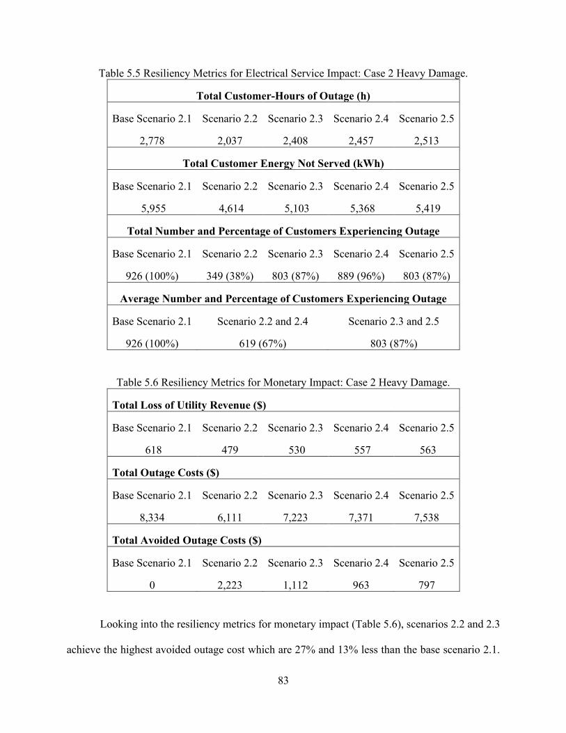
83

Table 5.5 Resiliency Metrics for Electrical Service Impact: Case 2 Heavy Damage.

Total Customer-Hours of Outage (h)


2,778 2,037 2,408 2,457 2,513

Total Customer Energy Not Served (kWh)


5,955 4,614 5,103 5,368 5,419

Total Number and Percentage of Customers Experiencing Outage


926 (100%) 349 (38%) 803 (87%) 889 (96%) 803 (87%)

Average Number and Percentage of Customers Experiencing Outage

Base Scenario 2.1 Scenario 2.2 and 2.4 Scenario 2.3 and 2.5

926 (100%) 619 (67%) 803 (87%)

Table 5.6 Resiliency Metrics for Monetary Impact: Case 2 Heavy Damage.

Total Loss of Utility Revenue ($)


618 479 530 557 563

Total Outage Costs ($)


8,334 6,111 7,223 7,371 7,538

Total Avoided Outage Costs ($)


0 2,223 1,112 963 797

Looking into the resiliency metrics for monetary impact (Table 5.6), scenarios 2.2 and 2.3

achieve the highest avoided outage cost which are 27% and 13% less than the base scenario 2.1.

84

In this specific case, where there is a major failure to the distribution system, outage costs and loss

of utility revenue are high for all scenarios. Showing that although DERs can provide support to

the power distribution system, the support is dependent on the weather (solar irradiance

availability) and the BESS capacity, i.e., a low capacity BESS can only provide limited support to

the distribution grid.

5.4 SUMMARY

This chapter provided a detailed analysis of the impacts DERs can have on the resiliency

of a power distribution system to natural disasters. A resiliency analysis process was presented

with two case studies that are tested under different scenarios and evaluated utilizing different

resilience metrics. This chapter contributed to providing realistic case studies that show the

potential benefits that DERs managed in networked MGs can provide a power distribution grid.

Test results indicated that DERs can provide support to the power distribution system by

scheduling the discharge of BESS during outages. For the specific case studies presented in this

chapter having roof-top solar and BESS managed by networked MGs on an average can reduce

the number of customers experiencing an outage between 38%-58% on a sunny day and 8%-9%

on a rainy day when compared to the base scenarios that do not consider DERs. Also, on an average

the avoided outage costs during sunny days can be between 20%-58% and between 11%-17% on

a rainy day. It should be emphasized that these results were obtained for specific case studies;

hence more case studies with different components and a larger test system could provide further

solid conclusions. Nonetheless, it is shown that DERs can improve the resiliency of power

distribution systems.

85

Chapter 6: Conclusions and Recommendations for Future Work

6.1 INTRODUCTION

The final chapter of this dissertation is divided into three major sections (1) summary and

conclusions, (2) contributions, and (3) recommendations for future work. The summary and

conclusions section presents the findings of the study to justify the objectives of this dissertation.

The contributions section outlines the major contributions of this dissertation and the final section

provides recommendations for future research.

6.2 SUMMARY AND CONCLUSIONS

A summary of this dissertation is outlined as follows.

Chapter 2 presented a literature review of various DER integration methodologies. Issues

with control and management of DERs were described. The emerging transactive framework and

the smart grid of the future coupled with MG energy management methodologies were discussed.

The urgent need to enhance the resilience of the electric power grid and vulnerabilities of existing

infrastructure were presented as well.

Chapter 3 presented an efficient strategy to optimally incorporate and locate RES-ESS in

smart DNs. The proposed planning strategy allows the resolution of the UC and ED problems and

optimally determines the best bus location to integrate PV and wind-ESS systems. A comparison

of the test results demonstrated that power losses and peak loads are significantly reduced,

achieving increased savings and a reduction in GHG emissions. Another benefit is that wind power

becomes more dispatchable by using the day-ahead forecasted information with efficient

utilization of ESS. This efficient charge/discharge of the ESS leads to a reduction in forecast error

freeing-up thermal capacity and avoiding the commitment of expensive thermal units. Moreover,

savings can be increased if other benefits are taken into consideration, such as reliability

86

improvement and the mitigation of power quality problems. The proposed method can be applied

to larger networks and for different time scales; however, the computation time may slightly

increase.

In Chapter 4, a new hybrid TC+MPC control mechanism for residential prosumer-centric

networked MGs was presented. The proposed hybrid TC+MPC combined the control capabilities

and features of the MPC and the TC, creating a robust control mechanism that is driven by

transactive incentive signals, and thus, also providing the MGEMS capability to deal with the

stochastic nature of BEV driving by using an MCS to generate the BEV driving patterns. The

proposed TC+MPC was able to effectively generate the BEV-charge and BESS-discharge

schedules for the CGs/PCGs located in each MG. Test results demonstrated the potential of using

pricing mechanisms for demand-side management of DERs. The results can be summarized as

follows: (i) reduction in peak load (between 21–30%) by shifting surplus PV power from off-peak

hours using BESS; (ii) reduction in load ramp rates between 39–58%; (iii) reduction in power

losses between 6.3–6.8%; (iv) bus voltage improvements between 25–75% for busses that present

undervoltages; and (v) total cost reductions between 29–57% and savings between 52–144%.

Therefore, the main objectives of the MGEMS are met by allowing CGs/PCGs to minimize their

costs as well as to maximize their savings. It can also be inferred from the results that the incentives

provided by the pricing mechanisms can encourage customers to not only reduce peak demand but

also to install more demand-side energy resources (e.g., but not limited to BESS and rooftop solar).

Moreover, the DSO or utility operators can benefit from controlled customer participation by

reducing their system power losses, by improving bus voltage profiles, and by reducing

overloading system components. An important finding of the case studies is that the BESS-

discharging operation can create steep load ramp rates when discharging during peak periods. This

87

aspect should be considered high priority when defining the discharge constraints to avoid

incurring negative impacts on the grid. For the case studies presented in this chapter, we assumed

full BESS discharging (SOC = 0%). It should be noted that this discharging operation could impact

the expected life of the BESS.

Chapter 5 provided a detailed analysis of the impacts DERs can have on the resiliency of

a power distribution system to natural disasters. A resiliency analysis process was presented with

two case studies that are tested under different scenarios and evaluated utilizing different resilience

metrics. The results indicate that DERs can provide support to the power distribution system by

scheduling the discharge of BESS during outages. For the specific case studies presented in this

chapter having roof-top solar and BESS managed by networked MGs on average can reduce the

number of customers experiencing an outage between 38%-58% on a sunny day and 8%-9% on a

rainy day when compared to the base scenarios that don’t have DERs. Also, on average the avoided

outage costs on sunny days can be between 20%-58% and between 11%-17% on rainy days.

6.3 CONTRIBUTIONS

In contrast to the existing literature, the major contributions of this dissertation to the state-

of-the-art are the following.

• An efficient strategy to optimally incorporate and locate RES-ESS in smart DNs to

reduce overall power losses and peak load;

• An integrated energy management system that allows the resolution of UC and ED

problems using the forecasted and actual data of wind, PV, and load. This prevents

the over commitment of thermal generation and increases in spinning reserve;

88

• An efficient ESS control strategy that utilizes the forecasted data of wind power

output for its operation. Thus, our ESS control strategy determines the optimal

charge/discharge cycle of the ESS.

• Development of a new hybrid TC+MPC control mechanism to manage DERs

(BEVs, solar PV, and BESS) of networked MGs constituted by consumer groups

and prosumer groups and detailed study of their behavior while being incentivized

by different price signals;

• Development of TIS and TFS signals where TIS is based on DLMP and distribution

system conditions, whereas TFS development is based on CGs/PCGs net load and

BEV driving patterns generated by MCS.

• Detailed analysis of the impacts on the distribution grid due to the use of TCs for

DER management, i.e., bus voltage and power loss impacts.

• Detailed Cost/Savings analysis for consumers/prosumers under different pricing

rates when they are equipped with BEVs, solar PV, and hybrid solar PV-BESS

systems.

• Development of a detailed resiliency analysis of realistic case studies that show the

potential benefits that DERs managed in networked MGs can provide a power

distribution grid.

• Calculation of resilience metrics for electrical service and monetary impacts using

DERs, i.e., total customer-hours of outage, total customer energy not served, total

and average number of customers experiencing outage, total loss of utility revenue,

and total outage costs.

89

6.4 RECOMMENDATIONS FOR FUTURE WORK

There are different aspects that have not been considered in this dissertation. Following are

the potential areas or topics that could be addressed in future research.

• Future work would be interesting to study the depth of discharge impacts on the

BESS life cycle for larger time frames (e.g., months and years) to analyze the

effects of continuous BEV and BESS charge/discharge cycles.

• It would also be interesting to carry out energy trading in local MG and among

MGs and study the effects on power flows and voltage levels.

• From an economic perspective, different TOU and dynamic tariffs could also be

tested to further verify the capabilities of the TC. Costs associated with DER

purchase and installation could be included to better reflect the net costs/savings.

• From a resiliency perspective, random duration faults could be considered to test

the ability of the DERs to support the distribution system during longer periods of

time. Other resiliency metrics could also be considered, e.g., time of recovery and

restoration costs.

90

References

[1] EPRI, “Vision for a holistic power supply and delivery chain,” Technical report: 1018587,

2009.

[2] F.D. Wattjes and J.G. Slootweg, “Design considerations for smart microgrids,” in Proc.

Power Engineering Conference (UPEC), pp. 1-6. Sep. 2013.

[3] M. Parvizimosaed, A. Anvari-Moghaddam, A. Ghasemkhani, and A. Rahimi-Kian, “Multi-

objective dispatch of distributed generations in a gridconnected micro-grid considering

demand response actions,” in Proc. Electricity Distribution (CIRED), Jun. 2013.

[4] Q. Wang and P. Zhang, “Energy management system for multi-microgrid,” in Proc. China

International Conference on Electricity Distribution (CICED), Sep. 2014.

[5] GridWise Architecture Council. GridWise transactive energy framework, Technical report,

2017.

[6] F. Rahimi, “Valuation of transactive energy systems,” in Proc. of Valuation of Transactive

Energy Systems Technical Meeting, Jul., 2015.

[7] A. K. Bejestani, A. Annaswamy, and T. Samad “A Hierarchical transactive control

architecture for renewables integration in smart grids: analytical modeling and stability,”

IEEE Transactions on Smart Grid, vol. 5, no. 4, Jul. 2014.

[8] D. Jin, X. Zhang, and S. Ghosh, "Simulation models of network design and hierarchical

transactive control mechanisms in smart grids," in Proc. IEEE PES GM 2012, Jan. 2012.

[9] Transactive Coordination Signals, U.S. Department of Energy, August 2013 [Online].

Available: http://www.pnwsmartgrid.org/docs/Transactive_Coordination_Signals.pdf.

[10] Pacific Northwest Smartgrid Demonstration Project, “Technology performance report

highlights,” April, 2015.

[11] Cazalet, E., De Martini, P., Price, J., Woychik, E., and Caldwell, J. “Transactive energy

models,” NIST Transactive energy challenge: business and regulatory models, White Paper,

2016.

[12] GridWise Architecture Council, “Transactive energy systems research, development and

deployment roadmap,” White paper, 2018.

[13] U.S. Energy Information Administration, “Electricity Data Browser Net Generation by

Energy Source: 2001 – 2018,” 2019. [ONLINE] Available online:

https://www.eia.gov/electricity/annual/html/epa_03_01_a.html (accessed on April 2019).

[14] U.S. Energy Information Administration, “Annual Energy Outlook 2019 with projections to

2050,” 2019. [ONLINE] Available online: www.eia.gov/aeo (accessed on January 2019).

[15] International Energy Agency-IEA, “Global EV Outlook 2018,” Technical report, 2018.

[16] A. Zibelman, “REVing up the energy vision in New York,” IEEE Power and Energy

Magazine, vol. 14, pp. 18-24, May 2016.

[17] K. Kok and S. Widergren, “A society of devices: integrating intelligent distributed resources

with transactive energy,” IEEE Power and Energy Magazine, vol. 14, no. 3, pp. 34-45, May.

2016.

http://www.pnwsmartgrid.org/docs/Transactive_Coordination_Signals.pdf

91

[18] Wang, Y., Zhou, S., and Huo, H. “Cost and CO2 reductions of solar photovoltaic power

generation in China: Perspectives for 2020,” Renewable and Sustainable Energy Reviews,

vol. 39, pp. 370–380, November 2014.

[19] Tan, M., Serrano, B., and Mohammed, O. "Fuzzy logic based power and thermal

management system design for multi-cell lithium-ion battery bank protection and operation,"

in Proc. Power Systems Conference (PSC), Clemson University, pp.1-5, March 2014.

[20] Al-Muhaini, M., and Heydt, G.T. “A novel method for evaluating future power distribution

system reliability,” IEEE Trans. on Power Systems, Vol. 28, No. 3, pp. 3018–3027, August

2013.

[21] El-Khattam, W., and Salama, M. M. A. “Distributed generation technologies, definitions and

benefits,” Elect. Power Syst. Res., Vol. 71, No. 2, pp. 119–128, October 2004.

[22] G. Pepermans, J. Driesen, D. Haeseldonckx, R. Belmans, and W. D’Haeseleer, “Distributed

generation: Definition, benefits and issues,” Energy Policy, Vol. 33, pp. 787–798, 2005.

[23] D. H. Popovi´c, J. A. Greatbanks, M. Begovi´c, and A. Pregelj, “Placement of distributed

generators and reclosers for distribution network security and reliability,” Int. J. Elect. Power

& Energy Syst., vol. 27, no. 5–6, pp. 398–408 June–July 2005.

[24] D. Zhu, R.P. Broadwater, K.S. Tam, R. Seguin, and H. Asgeirsson, “Impact of DG placement

on reliability and efficiency with time-varying loads,” IEEE Transactions on Power Systems,

vol. 21, no. 1, pp. 419 - 427, January 2006.

[25] P. Chiradeja and R. Ramakumar, “An approach to quantify the technical benefits of

distributed generation,” IEEE Transactions on Energy Conversion, vol. 19, no. 4, pp. 764–

773, December 2004.

[26] D.M. Cao, D. Pudjianto, G. Strbac, A. Martikainen, S. Karkkainen, and J. Farin, “Costs and

benefits of DG connections to grid system—studies on the UK and finish systems,” DG-

GRID Project—European Commission, December 2006.

[27] L.F. Ochoa, A. Padilha-Feltrin, and G.P. Harrison, “Evaluating distributed generation

impacts with a multiobjective index,” IEEE Transactions on Power Delivery, vol. 21, no. 3,

pp. 1452–1458, July 2006.

[28] H.A. Gil and G. Joos, “On the quantification of the network capacity deferral value of

distributed generation,” IEEE Transactions on Power Systems, vol. 21, no. 4, pp. 1592–1599,

November 2006.

[29] G.P. Harrison, A. Piccolo, P. Siano, and A.R. Wallace, “Exploring the trade-offs between

incentives for distributed generation developers and DNOs,” IEEE Transactions on Power

Systems, vol. 22, no. 2, pp. 821–828, May 2007.

[30] V.V.S.N. Murthy and A. Kumar, “Comparison of optimal DG allocation methods in radial

distribution systems based on sensitivity approaches,” Int. J. Elect. Power Energy Syst., vol.

53, pp. 450–467, December 2013.

[31] S. Ghosh and S.P. Ghoshal, “Two analytical approaches for optimal placement of distributed

generation unit in power systems,” in Proc. International Conference on Power Systems

(ICPS), pp. 1–6, December 2009.

92

[32] T.N. Shukla, S.P. Singh, V. Srinivasarao, and K.B. Naik, “Optimal sizing of distributed

generation placed on radial distribution systems,” Electric Power Components and Systems,

vol. 38, no. 3, pp. 260–274, January 2010.

[33] S. Ghosh, S.P. Ghoshal, and S. Ghosh, “Optimal sizing and placement of distributed

generation in a network system,” Int. J. Elect. Power Energy Syst., vol. 32, no. 8, pp. 849–

856, October 2010.

[34] R.K. Singh and S.K. Goswami, “Multi-objective optimization of distributed generation

planning using impact indices and trade-off technique,” Electric Power Components and

Systems, vol. 39, no. 11, pp. 1175–1190, August 2011.

[35] L.F. Grisales, A. Grajales, O.D. Montoya, R.A. Hincapié, and M. Granada, “Optimal

location and sizing of distributed generators using a hybrid methodology and considering

different technologies,” in Proc. IEEE 6th Latin American Symposium on Circuits & Systems

(LASCAS), pp. 1-4, February 2015.

[36] P. Kayal, T. Ashish, and C.K. Chanda, “Simultaneous placement and sizing of renewable

dgs and capacitor banks in distribution network,” in Proc. International Conference on

Circuit, Power and Computing Technologies (ICCPCT), pp. 607-611, March 2014.

[37] H. Keshtkar, J. Solanki, and S.K. Solanki, “Analyzing multi-microgrid with stochastic

uncertainties including optimal PV allocation,” in Proc. Int. Conf. on Smart Cities and Green

ICT Systems (SMARTGREENS), pp. 1-9, May 2015.

[38] H. Pandžić, Y. Wang, T. Qiu, Y. Dvorkin, and D.S. Kirschen, “Near-optimal method for

siting and sizing of distributed storage in a transmission network,” in IEEE Transactions on

Power Systems, vol. 30, no. 5, September 2015.

[39] V. Kalkhambkar, R. Kumar, and R. Bhakar, “Optimal sizing of PV-battery for loss reduction

and intermittency mitigation,” in Proc. IEEE Int. Conference on Recent Advances and

Innovations in Engineering (ICRAIE), pp. 1-6, May 2014.

[40] EPRI, “Methodological approach for estimating the benefits and costs of smart grid

demonstration projects,” Technical report: 1020342, 2010.

[41] The US Department of Energy, “The smart grid: an introduction,” 2008.

[42] P. Zhang, F. Li and N. Bhatt, “Next-Generation Monitoring, Analysis, and Control for the

Future Smart Control Center,” IEEE Transactions on Smart Grid, vol. 1, no. 2, pp. 186-192,

September 2010.

[43] F. Rahimi, A. Ipakchi, and F. Fletcher, “The changing electrical landscape,” IEEE Power

and Energy Magazine, vol. 14, pp. 52-62, May 2016.

[44] L. Kristov, P. De Martini, and J.D. Taft, “A tale of two visions: designing a decentralized

transactive electric system,” IEEE Power and Energy Magazine, vol. 14, no. 3, pp. 63-69,

May 2016.

[45] D. J. Hammerstrom, R. Ambrosio, J. Brous, T. A. Carlon, D. P. Chassin, J. G. DeSteese, R.

T. Guttromson, G. R. Horst, O. M. Järvegren, R. Kajfasz, and S. Katipamula, “Pacific

northwest gridwise testbed demonstration projects - Part I” Olympic Peninsula Project,

October 2007.

93

[46] Battelle Memorial Institute, “Pacific Northwest Smartgrid Demonstration Project:

technology performance report,” Technical report, vol. 1, Jun. 2015.

[47] National Institute of Standards and Technology (NIST), “Transactive Energy Modeling and

Simulation Challenge for the Smart Grid”, [Online]. Available

http://www.nist.gov/smartgrid/techallenge.cfm

[48] Recommendations of the NYISO Consumer Advisory Council to the NYISO Board of

Directors, Final Report. [Online]. Available:

http://www.nyiso.com/public/webdocs/markets_operations/committees/consumer_advisory

_council/Final%20NYISO%20CAC%20Report%20Nov%2011%202013.pdf

[49] Energy Storage and Distributed Energy Resources Enhancements Phase 2 Issue Paper,

Comments of TeMix Inc., CAISO. [Online]. Available:

https://www.caiso.com/Documents/TeMixIncComments-

EnergyStorageandDistributedEnergyResourcesPhase2-IssuePaper.pdf

[50] Z. Liu, Q. Wu, S. Huang, and H. Zhao, “Transactive energy: a review of state of the art and

implementation,” Proc. IEEE PowerTech Manchester, pp. 1-6, 2017.

[51] J. Li, C. Zhang, Z. Xu, J. Wang, J. Zhao, and Y.J.A. Zhang, “Distributed transactive energy

trading framework in distribution networks,” IEEE Transactions on Power Systems, vol. 33,

no. 6, pp. 7215–7227, 2018.

[52] H.S.V.S.K. Nunna and D. Srinivasan, “Multiagent-based transactive energy framework for

distribution systems with smart microgrids,” IEEE Transactions on Industrial Informatics,

vol. 13, no. 5, pp. 2241–2250, 2017.

[53] Y. Amanbek, Y. Tabarak, H.S.V.S.K. Nunna, and S. Doolla, “Decentralized transactive

energy management system for distribution systems with prosumer microgrids,” in Proc.

19th Int. Carpathian Control Conf., pp. 553–558, 2018.

[54] Y.K. Renani, M. Ehsan, and M. Shahidehpour, “Optimal transactive market operations with

distribution system operators,” IEEE Transactions on Smart Grid, vol. 9, no. 6, pp. 6692–

6701, 2018.

[55] Z. Liu, Q. Wu, K. Ma, M. Shahidehpour, Y. Xue, and S. Huang, “Two-stage optimal

scheduling of electric vehicle charging based on transactive control,” IEEE Transactions on

Smart Grid, vol. 10, no. 3, pp. 2948–2958, 2019.

[56] Z. Liu, Q. Wu, M. Shahidehpour, C. Li, Huang, S.; Wei, W. “Transactive real-time electric

vehicle charging management for commercial buildings with pv on-site generation,” IEEE

Transactions on Smart Grid, 2018, (Early Access).

[57] J. Hu, G. Yang, and H.W. Bindner, “Network constrained transactive control for electric

vehicles integration,” in Proc. 2015 IEEE PESGM, 2015, pp. 1-5, 2015.

[58] R. Shigenobu, M. Kinjo, P. Mandal, A. Howlader, and T. Senjyu, “Optimal operation

method for distribution systems considering distributed generators imparted with reactive

power incentive”, Applied Sciences, vol. 8, no. 8, 2018.

[59] H. Wang and J. Huang, “Incentivizing energy trading for interconnected microgrids, IEEE

Transactions on Smart Grid,” vol. 9, no. 4, pp. 2647–2657, 2018.

http://www.nist.gov/smartgrid/techallenge.cfm

http://www.nyiso.com/public/webdocs/markets_operations/committees/consumer_advisory_council/Final%20NYISO%20CAC%20Report%20Nov%2011%202013.pdf

http://www.nyiso.com/public/webdocs/markets_operations/committees/consumer_advisory_council/Final%20NYISO%20CAC%20Report%20Nov%2011%202013.pdf

https://www.caiso.com/Documents/TeMixIncComments-EnergyStorageandDistributedEnergyResourcesPhase2-IssuePaper.pdf

https://www.caiso.com/Documents/TeMixIncComments-EnergyStorageandDistributedEnergyResourcesPhase2-IssuePaper.pdf

94

[60] W. Liu, J. Zhan, and C.Y. Chung, “A novel transactive energy control mechanism for

collaborative networked microgrids,” IEEE Transactions on Power Systems, vol. 34, no. 3,

pp. 2048 – 2060, 2019.

[61] M.E. Khodayar, S.D. Manshadi, and A. Vafamehr, “The short-term operation of microgrids

in a transactive energy architecture”. The Electricity Journal, vol. 29, no. 10, pp. 41–48,

2016.

[62] Y. Jingpeng, H. Zhijian, L. Chendan, J.C. Vasquez, and J.M. Guerrero, “Economic power

schedule and transactive energy through an intelligent centralized energy management

system for a dc residential distribution system,” Energies, vol. 10, 2017.

[63] G. Prinslooa, A. Mammolib, and R. Dobsona, “Customer domain supply and load

coordination: A case for smart villages and transactive control in rural off-grid microgrids,”

Energy, vol.135, pp. 430-441, 2017.

[64] B. Canizes, J. Soares, A. Costa, T. Pinto, F. Lezama, P. Novais, and Z. Vale “Electric

vehicles’ user charging behavior simulator for a smart city,” Energies, vol. 12, no. 8, 2019.

[65] A. Dubey and S. Santoso, “Electric vehicle charging on residential distribution systems:

impacts and mitigations,” IEEE Access, vol. 3, 2015.

[66] H. Suyono, M.T. Rahman, H. Mokhlis, M. Othman, H. Azil Illias, and H. Mohamad,

“Optimal scheduling of plug-in electric vehicle charging including time-of-use tariff to

minimize cost and system stress,” Energies, vol. 12, no. 8, 2019.

[67] D.A. Chekired, L. Khoukhi, and H.T. Mouftah, “Decentralized cloud-SDN architecture in

smart grid: a dynamic pricing model,” IEEE Transactions on Industrial Informatics, vol. 14,

no. 3, pp. 1220-1231, 2018.

[68] M. Pasetti, S. Rinaldi, A. Flammini, M. Longo, and F. Foiadelli, “Assessment of electric

vehicle charging costs in presence of distributed photovoltaic generation and variable

electricity tariffs,” Energies, vol. 12, no. 3, 2019.

[69] S. Liu and A.H. Etemadi, “A dynamic stochastic optimization for recharging plug-in electric

vehicles,” IEEE Transactions on Smart Grid, vol. 9, no. 5, pp. 4154-4161, 2018.

[70] R. E. Brown, C. S. Wilson, and H. van Nispen, “Becoming the utility of the future,” IEEE

Power and Energy Magazine, pp. 57-65, September-October 2016.

[71] A. Golami, F. Aminifar, and M. Shahidehpour, “Front lines against the darkness,” IEEE

Electrification Magazine, vol. 4, no. 1, pp. 18-24, March 2016.

[72] Office for Coastal Management, National Oceanic and Atmosperic Administration,

“Weather Disasters and Costs,” Available online: https://coast.noaa.gov/states/fast-

facts/weather-disasters.html.

[73] L. Ren, Y. Qin, B. Wang, P. Zhang, P. B. Luh, and R. Jin, “Enabling resilient microgrid

through programmable network,” IEEE Transactions on Smart Grid, vol. 8, no. 6, pp. 2826

– 2836, November 2017.

[74] P. C. Loh, L. Ding. Y. Chai, and F. Blaabjerg, “Autonomous operation of hybrid microgrid

with AC and DC subgrids,” IEEE Transactions on Power Electronics, vol. 28, No. 5, pp.

2214–2223, May 2013.

95

[75] R. Majumder, “A hybrid microgrid with DC connection at back to back converters,” IEEE

Trans. Smart Grid, vol. 5, No. 1, pp. 251–259, January 2014.

[76] N. Eghtedarpour and E. Farjah, “Power control and management in a hybrid AC/DC

microgrid,” IEEE Transactions on Smart Grid, vol. 5, No. 3, pp. 1–12, April 2014.

[77] M. Pipattanasomporn, H. Feroze and S. Rahman, “Securing critical loads in a PV-based

microgrid with a multi-agent system,” Renewable Energy, vol. 39, no. 1, pp. 166-174, March

2012.

[78] R. Zamora and A.K. Srivastava, “Controls for microgrids with storage: Review, challenges,

and research needs,” Renewable and Sustainable Energy Reviews, vol. 14, pp. 2009-2018,

2010.

[79] E. J. Ng and R. A. El-Shatshat, “Multi-microgrid control systems (MMCS),” in Proc. IEEE

PESGM 2010, pp. 1–6, July 2010.

[80] L. Mariam, M. Basu, and M. F. Conlon, “Development of a simulation model for a

community microgrid system,” in Proc. 49th Int. Univ. Power Eng. Conf. (UPEC), pp. 1–6,

September 2014.

[81] L. Che, M. Shahidehpour, A. Alabdulwahab, and Y. Al-Turki, “Hierarchical coordination of

a community microgrid with AC and DC microgrids,” IEEE Transactions on Smart Grid,

vol. 6, no.6, pp. 3042 – 3051, March 2015.

[82] L. Che and M. Shahidehpour, “DC Microgrids: Economic Operation and Enhancement of

Resilience by Hierarchical Control,” IEEE Transactions on Smart Grid, vol. 5, No. 5, pp.

2517- 2526, September 2014.

[83] S. Mousavizadeha, T. Ghanizadeh Bolandib, M. R. Haghifama, M. Moghimic, and J. Luc,

“Resiliency analysis of electric distribution networks: a new approach based on modularity

concept,” Electrical Power and Energy Systems, vol. 117, May 2020.

[84] E. Rosales-Asensio, M. S. Martín, D. Borge-Diez, J.J. Blanes-Peiro, and A. Colmenar-

Santos, “Microgrids with energy storage systems as a means to increase power resilience:

An application to office buildings,” Energy, vol. 172, pp.1005-1015, February 2019.

[85] A. Barnes, H. Nagarajan, E. Yamangil, R. Bent, and S. Backhaus, “Resilient design of large-

scale distribution feeders with networked microgrids,” Electric Power Systems Research,

vol. 171, pp. 150–157, February 2019.

[86] J. Zhua, Y. Yuana, and W. Wang, “An exact microgrid formation model for load restoration

in resilient distribution system,” Electrical Power and Energy Systems, vol. 116, October

2019.

[87] L. Ren, Y. Qin, Y. Li, P, Zhang, B. Wang, P.B. Luh, S. Han, T. Orekan, and T. Gong,

“Enabling resilient distributed power sharing in networked microgrids through software

defined networking,” Applied Energy, vol. 210, pp. 1251–1265, June 2017.

[88] M.U. Shahida, M. Mansoor Khan, K. Hashmi, R. Boudina, A. Khana, J. Yuning, and H.

Tang, “Renewable energy source (RES) based islanded DC microgrid with enhanced

resilient control,” Electrical Power and Energy Systems, vol. 113, pp. 461–471, May 2019.

96

[89] A. Hussain, V.H. Bui, and H.M. Kim “Microgrids as a resilience resource and strategies used

by microgrids for enhancing resilience,” Applied Energy, vol. 240, pp. 56–72, February

2019.

[90] M. S. S. Danish, H. Matayoshi, H.R. Howlader, S. Chakraborty, P. Mandal, and T. Senjyu,

“Microgrid planning and design: resilience to sustainability,” in Proc. 2019 IEEE PES GTD

Grand International Conference and Exposition Asia (GTD Asia), March 2019.

[91] R. Eskandarpour, H. Lotfi, and A. Khodaei, “Optimal microgrid placement for enhancing

power system resilience in response to weather events,” in Proc. 2016 North American

Power Symposium, pp. 1-6, November 2016.

[92] M.H. Amirioun, F. Aminifar, and H. Lesani, “Towards proactive scheduling of microgrids

against extreme floods,” IEEE Transactions on Smart Grid, vol. 9, no. 4, pp. 3000-3902,

July 2018.

[93] S. Chanda and A.K. Srivastava, “Defining and enabling resiliency of electric distribution

systems with multiple microgrids,” IEEE Transactions on Smart Grid, vol. 7, no. 6, pp.

2859- 2868, November 2016.

[94] Zimmerman, R. D., Murillo-Sánchez, C. E., and Thomas, R. J. "MATPOWER: steady-state

operations, planning and analysis tools for power systems research and education," IEEE

Trans. on Power Systems, vol. 26, no. 1, pp. 12-19, February 2011.

[95] E. Galvan and G. Gutierrez-Alcaraz, “Two-phase short-term scheduling with renewable

energy resources and storage,” in Proc. 2013 North American Power Symposium (NAPS),

pp. 1-6, September 2013.

[96] S. Civanlar, J.J. Grainger, and S.H. Lee, “Distribution feeder reconfiguration for loss

reduction,” IEEE Transactions on Power Delivery, vol. 3, no. 3, pp. 1217-1223, July 1988.

[97] D.I. AlHakeem, P. Mandal, A.U. Haque, A. Yona, T. Senjyu, and B. Tseng, “A new strategy

to quantify uncertainties of Wavelet-GRNN-PSO based solar PV power forecasts using

bootstrap confidence intervals,” in Proc. 2015 IEEE PES GM, pp. 1-5, July 2015.

[98] A.U. Haque, P. Mandal, J. Meng, A.K. Srivastava, T.L. Tseng, and T. Senjyu, “A novel

hybrid approach based on wavelet transform and Fuzzy ARTMAP networks for predicting

wind farm power production,” IEEE Transactions on Industry Applications, vol. 49, no. 5,

pp. 2253-2261, September/Octctober 2013.

[99] A.U. Haque, P. Mandal, J. Meng, and R.L. Pineda, “Performance evaluation of different

optimization algorithms for power demand forecasting applications in a smart grid

environment,” Complex Adaptive Systems, Procedia Computer Science, vol. 12, pp. 320 –

325, 2012.

[100] M. Pantos, “Exploitation of electric-drive vehicles in electricity markets,” IEEE

Transactions on Power Systems, vol. 27, no. 2, pp. 682 – 694, 2012.

[101] E.F. Camacho and C. Bordons, “Model Predictive Control,” 2nd ed.; Publisher: Springer-

Verlag, London, pp. 1–30, 2007.

97

[102] E. Galvan, P. Mandal, A.U. Haque, and B. Tseng, “Optimal placement of intermittent

renewable energy resources and energy storage system in smart power distribution

networks,” Electric Power Components and Systems, vol. 45, no. 14, pp. 1543-1553, 2017.

[103] E. Galvan, P. Mandal, S. Chakraborty, and A.Y. Saber, “Efficient transactive control for

energy storage management system in prosumer-centric networked microgrids,” in Proc.

North American Power Symposium (NAPS), pp. 1 – 6, January 2019.

[104] International Energy Agency (IEA). Global EV outlook: towards cross-modal electrification,

Technical Report, 2018.

[105] United States Census Bureau. Comparative housing characteristics. Available online:

https://factfinder.census.gov/faces/tableservices/jsf/pages/productview.xhtml?pid=ACS_17

_5YR_CP04&prodType=table (accessed on 15 January 2019).

[106] M.E. Baran and F.F. Wu, “Network reconfiguration in distribution systems for loss reduction

and load balancing,” IEEE Transactions on Power Delivery, vol. 4, no. 2, pp. 1401-1407,

1989.

[107] El Paso Electric Company. Residential service rate 2018. Available online:

https://www.epelectric.com/files/html/Rates_and_Regulatory/Docket_46831_Stamped_Tar

iffs/03_-_Rate_01_Residential_Service_Rate.pdf. (accessed on 15 January 2019).

[108] El Paso Electric Company. Electric vehicle charging rate 2018. Available online:

https://www.epelectric.com/files/html/Rates_and_Regulatory/Docket_46831_Stamped_Tar

iffs/36_-_Rate_EVC_Electric_Vehicle_Charging_Rate.pdf. (accessed on 15 January 2019).

[109] PJM. Price data. Available online:

http://www.pjm.com/markets-and-operations/energy.aspx (accessed on 15 January 2019).

[110] U.S. Department of Energy, Office of Energy Efficiency & Renewable Energy (EERE) Open

Data Catalog. Residential load at TMY3. Available online:

https://openei.org/datasets/files/961/pub/. (accessed on 15 January 2019).

[111] InsideEVs.com. Available online: https://insideevs.com/reviews/344001/compare-evs/

(accessed on 30 August 2019).

[112] Edison Electric Institute (EEI) https://www.eei.org. Electric vehicle sales: facts & figures

Available online:

https://www.eei.org/issuesandpolicy/electrictransportation/Documents/FINAL_EV_Sales_

Update_April2019.pdf (accessed on 30 August 2019).

[113] Tesla Motors. Tesla charging, 2019. Available online: https://www.tesla.com/models-

charging#/basics. (accessed on 30 May 2019).

[114] J. Quiros-Tortos, L.F. Ochoa, and T. Butler, “How electric vehicles and the grid work

together: lessons learned from one of the largest electric vehicle trials in the world,” IEEE

Power and Energy Magazine, vol. 16, no. 6, pp. 64-76, 2018.

[115] Idaho National Laboratory, U.S. Department of Energy Office of Energy Efficiency and

Renewable Energy. Plug-in electric vehicle and infrastructure analysis, Technical Report,

2015.

https://factfinder.census.gov/faces/tableservices/jsf/pages/productview.xhtml?pid=ACS_17_5YR_CP04&prodType=table

https://factfinder.census.gov/faces/tableservices/jsf/pages/productview.xhtml?pid=ACS_17_5YR_CP04&prodType=table

https://www.epelectric.com/files/html/Rates_and_Regulatory/Docket_46831_Stamped_Tariffs/03_-_Rate_01_Residential_Service_Rate.pdf

https://www.epelectric.com/files/html/Rates_and_Regulatory/Docket_46831_Stamped_Tariffs/03_-_Rate_01_Residential_Service_Rate.pdf

https://www.epelectric.com/files/html/Rates_and_Regulatory/Docket_46831_Stamped_Tariffs/36_-_Rate_EVC_Electric_Vehicle_Charging_Rate.pdf

https://www.epelectric.com/files/html/Rates_and_Regulatory/Docket_46831_Stamped_Tariffs/36_-_Rate_EVC_Electric_Vehicle_Charging_Rate.pdf

http://www.pjm.com/markets-and-operations/energy.aspx

https://openei.org/datasets/files/961/pub/

https://insideevs.com/reviews/344001/compare-evs/

https://www.eei.org/issuesandpolicy/electrictransportation/Documents/FINAL_EV_Sales_Update_April2019.pdf

https://www.eei.org/issuesandpolicy/electrictransportation/Documents/FINAL_EV_Sales_Update_April2019.pdf

98

[116] Tesla Motors. Tesla powerwall, 2019. Available online: https://www.tesla.com/powerwall.

(accessed on 15 January 2019).

[117] R.D. Zimmerman, C.E. Murillo-Sánchez, R.J. Thomas, “MATPOWER: steady-state

operations, planning and analysis tools for power systems research and education,” IEEE

Transactions on Power Systems, vol. 26, no. 1, pp. 12-19, 2011.

[118] YALMIP. Available online: https://yalmip.github.io/ (accessed on 15 January 2019).

[119] GUROBI. Available online: https://www.gurobi.com/ (accessed on 15 January 2019).

[120] J.P. Watson, R. Guttromson, C. Silva-Monroy, et al., “Conceptual Framework for

Developing Resilience Metrics for the Electricity, Oil, and Gas Sectors in the United States,”

Technical Report SAND2014-18019, Sandia National Laboratories, September 2015.

Available online:

http://energy.gov/sites/prod/files/2015/09/f26/EnergyResilienceReport_Final_SAND2014-

18019.pdf

[121] E. Galvan, P. Mandal, S. Chakraborty, and T. Senjyu, “Efficient Energy Management

System Using A Hybrid Transactive-Model Predictive Control Mechanism for Prosumer-

Centric Networked Microgrids,” Sustainability, vol. 11, no. 19, September 2019.

[122] L. Lawton, M. Sullivan, K. Van Liere, A. Katz, and J. Eto “A Framework and Review of

Customer Outage Costs: Integration and Analysis of Electric Utility Outage Cost Surveys,”

Lawrence Berkeley National Laboratory, Technical report, November 2003.

https://yalmip.github.io/

https://www.gurobi.com/

http://energy.gov/sites/prod/files/2015/09/f26/EnergyResilienceReport_Final_SAND2014-18019.pdf

http://energy.gov/sites/prod/files/2015/09/f26/EnergyResilienceReport_Final_SAND2014-18019.pdf

99

Appendix I: Data Utilized in Case Studies of Chapter 3

Table AI.1 Actual and Forecasted Wind Power Output.

Hour

(h)

Actual

Power

(MW)

Forecasted

Power

(MW)

Hour

(h)

Actual

Power

(MW)

Forecasted

Power

(MW)

1 0.53 0.58 13 3.25 4.01

2 0.68 0.67 14 2.12 3.35

3 1.92 0.82 15 1.36 2.30

4 2.85 2.10 16 1.09 1.52

5 2.08 2.99 17 1.16 1.24

6 2.88 2.26 18 1.55 1.31

7 1.55 3.02 19 1.48 1.71

8 0.63 1.71 20 1.74 1.64

9 0.52 0.76 21 1.99 1.91

10 1.49 0.66 22 1.41 2.17

11 3.38 1.65 23 1.13 1.57

12 4.00 3.46 24 0.55 1.28

Table AI.2 Actual and Forecasted Load.

Hour

(h)

Actual

Power

(MW)

Forecasted

Power

(MW)

Hour

(h)

Actual

Power

(MW)

Forecasted

Power

(MW)

1 24.62 27.15 13 13.46 9.50

2 24.03 22.37 14 15.54 17.19

3 15.85 23.81 15 16.43 16.03

4 15.90 16.30 16 19.63 16.82

5 27.42 30.34 17 20.23 19.72

6 24.80 22.02 18 17.16 20.27

7 18.73 20.54 19 10.53 11.47

8 23.02 21.90 20 10.94 11.68

9 18.64 20.87 21 12.58 15.03

10 13.18 12.82 22 10.25 13.43

11 11.42 15.95 23 25.33 14.45

12 9.88 12.76 24 6.99 10.05

100

Table AI.3 Actual and Forecasted PV Power – Sunny Day.

Hour

(h)

Actual

Power

(MW)

Forecasted

Power

(MW)

Hour

(h)

Actual

Power

(MW)

Forecasted

Power

(MW)

1 0.00 0.00 13 2.23 2.24

2 0.00 0.00 14 2.24 2.26

3 0.00 0.00 15 2.14 2.12

4 0.00 0.00 16 1.90 1.91

5 0.00 0.00 17 1.29 1.31

6 0.00 0.00 18 0.45 0.49

7 0.00 0.00 19 0.15 0.18

8 0.22 0.22 20 0.02 0.02

9 0.80 0.82 21 0.00 0.00

10 1.34 1.40 22 0.00 0.00

11 1.78 1.83 23 0.00 0.00

12 2.08 2.11 24 0.00 0.00

Table AI.4 Actual and Forecasted PV Power – Cloudy Day.

Hour

(h)

Actual

Power

(MW)

Forecasted

Power

(MW)

Hour

(h)

Actual

Power

(MW)

Forecasted

Power

(MW)

1 0.00 0.00 13 1.54 1.47

2 0.00 0.00 14 1.41 1.20

3 0.00 0.00 15 0.67 1.60

4 0.00 0.00 16 0.50 0.58

5 0.00 0.00 17 0.28 0.54

6 0.00 0.00 18 0.10 0.05

7 0.00 0.00 19 0.00 0.05

8 0.00 0.00 20 0.00 0.00

9 0.01 0.01 21 0.00 0.00

10 0.32 0.58 22 0.00 0.00

11 0.80 0.89 23 0.00 0.00

12 1.38 1.47 24 0.00 0.00

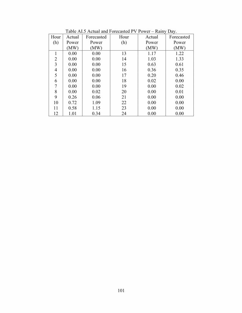
101

Table AI.5 Actual and Forecasted PV Power – Rainy Day.

Hour

(h)

Actual

Power

(MW)

Forecasted

Power

(MW)

Hour

(h)

Actual

Power

(MW)

Forecasted

Power

(MW)

1 0.00 0.00 13 1.17 1.22

2 0.00 0.00 14 1.03 1.33

3 0.00 0.00 15 0.63 0.61

4 0.00 0.00 16 0.36 0.35

5 0.00 0.00 17 0.20 0.46

6 0.00 0.00 18 0.02 0.00

7 0.00 0.00 19 0.00 0.02

8 0.00 0.02 20 0.00 0.01

9 0.26 0.06 21 0.00 0.00

10 0.72 1.09 22 0.00 0.00

11 0.58 1.15 23 0.00 0.00

12 1.01 0.34 24 0.00 0.00

102

Appendix II: Data Utilized in Case Studies of Chapter 4

Table AII.1 Historical BEV Daily Driving Patterns.

BEV Driving Patterns (kWh)

Hour (h) BEV1 BEV2 BEV3 Hour (h) BEV1 BEV2 BEV3

1 0.0 0.0 0.0 13 1.6 0.0 0.0

2 0.0 0.0 0.0 14 0.0 0.0 0.0

3 0.0 0.0 0.0 15 0.0 0.0 2.7

4 0.0 0.0 0.0 16 2.7 1.3 2.7

5 0.0 0.0 0.0 17 4.8 1.6 0.0

6 2.7 1.3 2.7 18 3.2 1.6 0.0

7 3.8 1.9 2.7 19 0.0 0.0 0.0

8 4.8 2.4 0.0 20 2.7 0.0 2.7

9 0.0 1.3 0.0 21 3.0 0.0 2.7

10 0.0 0.0 4.0 22 0.0 0.0 0.0

11 0.0 0.0 5.4 23 0.0 0.0 0.0

12 1.6 0.0 0.0 24 0.0 0.0 0.0

Table AII.2 Load Data for the 33-Bus Distribution System.

Bus Pd

(kW)

Qd (kVAR) Bus Pd (kW) Qd (kVAR)

2 97 60 18 64 40

3 80 40 19 24 40

4 117 80 20 19 40

5 43 30 21 29 40

6 58 20 22 21 40

7 71 100 23 24 50

8 97 100 24 29 200

9 49 20 25 27 200

10 48 20 26 58 25

11 35 30 27 58 25

12 44 35 28 58 20

13 58 35 29 85 70

14 117 80 30 195 600

15 43 10 31 145 70

16 58 20 32 204 100

17 58 20 33 58 40

103

Table AII.3 Load Data for Klamath Falls, Oregon.

Hour

(h)

Power

(kW)

Hour

(h)

Power

(kW)

1 1.35 13 1.29

2 1.18 14 1.23

3 1.12 15 1.22

4 1.11 16 1.37

5 1.11 17 1.91

6 1.19 18 2.74

7 1.47 19 3.19

8 1.91 20 3.00

9 1.80 21 2.87

10 1.50 22 2.67

11 1.42 23 2.18

12 1.37 24 1.76

Table AII.4 Load Data for Medford-Rogue Valley, Oregon.

Hour

(h)

Power

(kW)

Hour

(h)

Power

(kW)

1 1.07 13 1.30

2 0.94 14 1.27

3 0.87 15 1.28

4 0.86 16 1.41

5 0.87 17 1.79

6 0.95 18 2.45

7 1.21 19 2.79

8 1.64 20 2.60

9 1.55 21 2.48

10 1.35 22 2.27

11 1.33 23 1.87

12 1.33 24 1.49

104

Table AII.5 Load Data for Redmond, Oregon.

Hour

(h)

Power

(kW)

Hour

(h)

Power

(kW)

1 1.12 13 1.34

2 0.96 14 1.31

3 0.89 15 1.32

4 0.88 16 1.44

5 0.89 17 1.83

6 0.96 18 2.50

7 1.21 19 2.83

8 1.64 20 2.63

9 1.58 21 2.51

10 1.39 22 2.29

11 1.37 23 1.89

12 1.36 24 1.52

Table AII.6 Solar PV Power for Ashland, Oregon Sunny-Day.

Hour

(h)

Power

(kW)

Hour

(h)

Power

(kW)

1 0.00 13 4.63

2 0.00 14 4.45

3 0.00 15 3.92

4 0.00 16 2.72

5 0.00 17 1.15

6 0.02 18 0.46

7 0.72 19 0.06

8 1.94 20 0.00

9 2.97 21 0.00

10 3.80 22 0.00

11 4.38 23 0.00

12 4.62 24 0.00

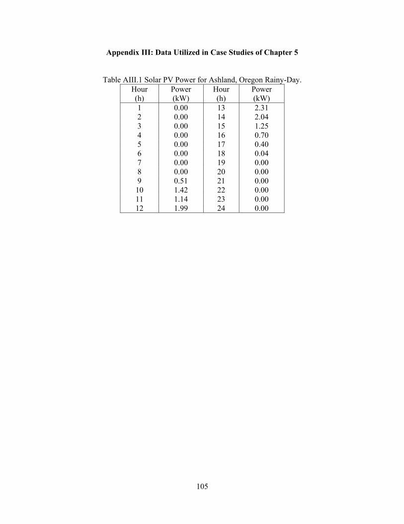
105

Appendix III: Data Utilized in Case Studies of Chapter 5

Table AIII.1 Solar PV Power for Ashland, Oregon Rainy-Day.

Hour

(h)

Power

(kW)

Hour

(h)

Power

(kW)

1 0.00 13 2.31

2 0.00 14 2.04

3 0.00 15 1.25

4 0.00 16 0.70

5 0.00 17 0.40

6 0.00 18 0.04

7 0.00 19 0.00

8 0.00 20 0.00

9 0.51 21 0.00

10 1.42 22 0.00

11 1.14 23 0.00

12 1.99 24 0.00

106

Appendix IV: List of Publications

List of publications that were generated during my Ph.D. studies at UTEP.

Peer-reviewed Journal Papers

*: my Ph.D. advisor and corresponding author of the paper

1. E. Galvan, P. Mandal*, S. Chakraborty, and T. Senjyu, “Efficient Energy Management

System Using A Hybrid Transactive-Model Predictive Control Mechanism for Prosumer-

Centric Networked Microgrids,” Sustainability, Vol. 11, No. 19, Sep. 2019.

2. E. Galvan, P. Mandal*, A. U. Haque, and B. Tseng, “Optimal Placement of Intermittent

Renewable Energy Resources and Energy Storage System in Smart Power Distribution

Networks,” Electric Power Components and Systems, Vol. 45, No. 14, pp. 1543-1553, Dec.

2017.

Peer-reviewed Manuscript Under Review

3. E. Galvan, P. Mandal*, and Y. Sang, “Resiliency Analysis of Networked Microgrids in

Power Distribution Systems,” International Journal of Electrical Power & Energy Systems

(Submitted in December 2019)

Peer-reviewed Conference Papers

1. E. Galvan, P. Mandal*, S. Chakraborty, and A. Y. Saber, “Efficient Transactive Control

for Energy Storage Management System in Prosumer-Centric Networked Microgrids,” in

Proc. North American Power Symposium (NAPS 2018), Sep. 2018.

2. E. Galvan, P. Mandal*, M. Velez-Reyes, and S. Kamalasadan, “Transactive Control

Mechanism for Efficient Management of EVs Charging in Transactive Energy

Environment,” in Proc. North American Power Symposium (NAPS 2016), Sep. 2016.

3. E. Galvan, P. Mandal*, T. L. Tseng, and M. Velez-Reyes, “Energy Storage Dispatch

Using Adaptive Control Scheme Considering Wind-PV in Smart Distribution Network,”

in Proc. North American Power Symposium (NAPS 2015), Oct. 2015.

107

Symposium Papers

4. E. Galvan and P. Mandal*, “Transactive Control for Energy Storage Dispatch in

Microgrids,” in Proc. Southwest Emerging Technology Symposium, Apr. 2018.

5. E. Galvan and P. Mandal*, “Smart Microgrid Energy Management System and Control,”

UTEP Graduate Student Research Expo, Nov. 2017.

6. E. Galvan and P. Mandal*, “Transactive Energy Systems,” in Proc. Southwest Emerging

Technology Symposium, Apr. 2016.

7. E. Galvan and P. Mandal*, “Optimal Placement of Intermittent Renewable Energy

Resources and Energy Storage Systems in Smart Power Distribution Network,” UTEP

Graduate Student Research Expo, Nov. 2015.

8. E. Galvan and P. Mandal*, “Optimal Operation Strategy for Grid Connected WIND/PV

and Energy Storage System,” in Proc. Southwest Energy Science and Engineering

Symposium, Apr. 2015.

108

Vita

Eric Galvan was born in Kansas City, Kansas, USA. He received his Bachelor of Science

and Master of Science degrees in Electrical Engineering from the Instituto Tecnológico de

Morelia, Morelia, Michoacán, Mexico in 2010 and 2013, respectively. In January 2015, he joined

the Department of Electrical and Computer Engineering (ECE) at the University of Texas at El

Paso (UTEP) to pursue Doctor of Philosophy in Electrical and Computer Engineering (Ph.D. in

ECE). His doctoral research career started in January 2015 when he joined the Power and

Renewable Energy Systems (PRES) Lab within the ECE Department and started his doctoral

research under the direct supervision of PRES Lab’s director Dr. Paras Mandal who guided and

mentored him throughout his dissertation period in the area of Smart Power Distribution Systems.

During his doctoral studies, he was a recipient of (i) Kenneth R. Heitz/El Paso Electric Company

Endowed Scholarship, (ii) Fellowship of the Hispanic Alliance for the Professoriate in

Environmental Sciences and Engineering, and (iii) UTEP Graduate Student Travel Award (which

he received three times in order to present his research findings at IEEE conferences). He has

presented his research findings at several meetings, symposiums, and international conferences.

His work has appeared in the proceedings of these conferences as well as in peer-reviewed

journals. A list of publications that he generated from his Ph.D. period is provided in Appendix

IV. While pursuing his Ph.D. degree at UTEP, he worked as a Teaching Assistant for the ECE

department and also as an Assistant Instructor for the College of Engineering. In Summer 2019,

he obtained a full-time position at the El Paso Electric Company in El Paso, Texas where he is

currently working as a researcher at the Economic Research Department.

Contact Information: [email protected]

This dissertation was typed by Eric Galvan.

Energy Management And Control Of Smart Power Distribution ...

Documents

Transcript of Energy Management And Control Of Smart Power Distribution ...