Energy Efficient Scheduling of Real Time Tasks on Large ...
188
INDIAN INSTITUTE OF TECHNOLOGY GUWAHATI Energy Efficient Scheduling of Real Time Tasks on Large Systems and Cloud by Manojit Ghose A thesis submitted in partial fulfillment for the degree of Doctor of Philosophy in the Department of Computer Science and Engineering Under the supervision of Aryabartta Sahu and Sushanta Karmakar December 2018
Transcript of Energy Efficient Scheduling of Real Time Tasks on Large ...

INDIAN INSTITUTE OF TECHNOLOGY GUWAHATI
Energy Efficient Scheduling of
Real Time Tasks on Large
Systems and Cloud
by
Manojit Ghose
A thesis submitted in partial fulfillment for the
degree of Doctor of Philosophy
in the
Department of Computer Science and Engineering
Under the supervision of
Aryabartta Sahu and Sushanta Karmakar
December 2018

Declaration of Authorship
I, Manojit Ghose, do hereby confirm that:
� The work contained in this thesis is original and has been carried out by
myself under the guidance and supervision of my supervisors.
� This work has not been submitted to any other institute or university for
any degree or diploma.
� I have conformed to the norms and guidelines given in the ethical code of
conduct of the institute.
� Whenever I have used materials (data, theoretical analysis, results) from
other sources, I have given due credit to them by citing them in the text of
the thesis and giving their details in the reference.
Manojit Ghose
Research Scholar,
Department of CSE,
Indian institute of Technology Guwahati,
Guwahati, Assam, INDIA 781039,
[email protected], [email protected]
Date: July 27, 2018
Place: IIT Guwahati
iii


Certificate
This is to certify that the thesis entitled “Energy Efficient Scheduling of Real
Time Tasks on Large Systems and Cloud” being submitted by Mr. Mano-
jit Ghose to the department of Computer science and Engineering, Indian In-
stitute of Technology Guwahati, is a record of bonafide research work under my
supervision and is worthy of consideration for the award of the degree of Doctor
of Philosophy of the institute.
Aryabartta Sahu
Department of CSE,
Indian Institute of Technology Guwahati,
Guwahati, Assam, INDIA 781039,
Sushanta Karmakar
Department of CSE,
Indian Institute of Technology Guwahati,
Guwahati, Assam, INDIA 781039,
Date: July 27, 2018
Place: IIT Guwahati
v

Dedicated to
Late Prafulla Bala Ghose (my grandmother)
vii


Acknowledgements
I feel extremely humble and blessed when I look back and feel the amount of
kindness, encouragement, help, and support that everyone has offered during the
journey of my Ph. D. Our success is not only determined by our own effort
and dedication, but it is actually a collective outcome of the efforts, sacrifices,
contributions, help, and support of others. I take this platform to thank each one
of them who has directly or indirectly helped me to reach this stage.
I start by expressing my deep and sincere gratitude to my thesis supervisor Dr.
Aryabartta Sahu for his valuable guidance, constant support, persistent encour-
agement. I wouldn’t have been completed this work without his expertise, valuable
inputs, and suggestions. His friendly nature always helped in healthy debates and
discussions. I specially thank him for his tireless efforts and countless numbers
of revisions of the thesis and publications. He is indeed a helpful person and a
great human being. I couldn’t have attended the conferences abroad without his
generous help and support. I am indeed ever grateful to him.
Next, I would like to thank my thesis co-supervisor Dr. Sushanta Karmakar for
his invaluable guidance and the advice throughout my Ph. D. tenure. I would
like to express my gratitude and gratefulness to all the members of my Doctoral
Committee, Prof. Diganta Goswami, Dr. Santosh Biswas, and Dr. Partha Sarathi
Mandal for their constructive criticism and corrective feedback. Their valuable
suggestions and inputs helped me a lot to improve the quality of my work.
Further, I would like to sincerely thank Prof. S. V. Rao, the Head of the De-
partment of Computer Science and Engineering and other faculty members for
their constant supports and helps, and encouragements. I specially thank Prof.
Hemangee K. Kapoor, Prof. Pradip K. Das for their generosity. Furthermore, I
express my thanks and regards to all the technical and administrative staff mem-
bers of the department for their help whenever I asked for. I would also like to take
the opportunity to thank my Government for providing such a high-class facility
which stands far beyond the life of an average Indian citizen.
I am ever grateful to Prof. Sukumar Nandi and Prof. Ratnajit Bhattacharjee for
their encouragement, help, and support whenever I needed. They remain a source
of inspiration for me. I would also to express my sincere thanks and gratitude
to Mrs. Nandini Bhattacharya for her constant love and care. Also, I would
like to express my appreciation and thanks to some of my teachers whose words
of encouragement still motivate me to work. They are Prof. Manoj Das, Mr.
Sushanta Saha, Mr. Subhendu Saha, Dr. Rupam Baruah, and others.
ix
I had a wonderful time at IIT Guwahati, met many beautiful minds, spent qual-
ity time, and finally made good friends. All of them have directly or indirectly
helped me to achieve my dream. To name a few of them, they are Nilakshi, Parik-
shit, Chinmaya, Shirsendu, Binita, Debanjan, Roshan, Shounak, Satish, Pradip,
Shibaji, Sathisa, Himangshu, Rakesh, Hema, Sourav, Ferdausa, Needhi, Mayank,
Pranab, Barasa, Vasudevan, Sanjit, Sanjay, Diptesh, Rahul, Sayan, Rajashree,
Udeshna, Rana, Biplab, Arunabha, and others. I also worked with a couple
of masters students during my Ph. D. They are Pratyush, Sawinder, Anoop,
Sandeep, and Hardik. It was indeed a wonderful experience to work and share
ideas with them. I also thank all my well-wishers, friends inside and outside the
IIT Guwahati. I sincerely thank my colleagues at DUIET for extending their help
and support during the last phase of my Ph. D.
During the course of my study, I had the opportunity to know some amazing
human beings: Dr. Devanand Pathak, Mr. Vishnu Prakash, Mr. Avinash Tiku,
Mr. Ram Bahadur Gurung, Dr. Azd Zayoud, and others. It was indeed a matter
of joy and fun to learn various skills from them.
Finally, I express my thanks and regards toward all the family members for their
constant support. It was a tough time for them to accept my decision of joining
the Ph. D. leaving my job. But finally, they are happy and I could bring a smile
to their faces. I also express my thanks to the anonymous reviewers of my papers
and thesis for their constructive comments and feedbacks.
Abstract
Large systems and cloud computing paradigm have emerged as a promising com-
puting platform of recent time. These systems attracted users from various do-
mains, and their applications are getting deployed for several benefits, such as
reliability, scalability, elasticity, pay-as-you-go pricing model, etc. These applica-
tions are often of real-time nature and require a significant amount of computing
resources. With the usages of the computing resources, the energy consumption
also increases, and the high energy consumption of the large systems has become
a serious concern. A reduction in the energy consumption for the large systems
yields not only monetary benefits to the service providers, but also yields perfor-
mance and environmental benefits as a whole. Hence, designing energy-efficient
scheduling strategies for the real-time applications on the large systems becomes
essential.
Considering power consumption construct at a finer granularity with only DVFS
technique may not be sufficient for the large systems. The first work of the thesis
devises a coarse-grained thread-based power consumption model which exploits
the power consumption pattern of the recent multi-threaded processors. Based on
this power consumption model, an energy-efficient scheduling policy, called Smart
scheduling policy, is proposed for efficiently executing a set of online aperiodic real-
time tasks on a large multi-threaded multiprocessor system. This policy shows an
average energy consumption reduction of around 47% for the synthetic data set and
approximately 30% for the real-world trace data set as compared to the baseline
policies. Thereafter, three improvements of the basic Smart scheduling policy are
proposed to handle different types of workloads efficiently.
The second work of the thesis considers a utilization-based power consumption
model for a virtualized cloud system where the utilization of a host can be divided
in three ranges (low : utilization is below 40%, medium: utilization is from 40%
to 70%, and high: utilization is above 70%) based on the power consumption of
the host. Then two energy-efficient scheduling policies, namely, UPS and UPS-ES
are designed addressing this range based utilization of the hosts. These schedul-
ing policies are designed based on the urgent points of the real-time tasks for a
heterogeneous computing environment. Experiments are conducted on CloudSim
toolkit with a wide variety of synthetic data set and real-world trace data including
the Google cloud tracelog and Metacentrum trace data. Results show an average
energy improvement of almost 24% for the synthetic data set and almost 11% for
the real-world trace as compared to the state-of-art scheduling policy.
As the cloud providers often offer VMs with discrete compute capacities and sizes,
which leads to discrete host utilization, the third work of the thesis considers
scheduling a set of real-time tasks on a virtualized cloud system which offers VMs
with discrete compute capacities. This work calculates a utilization value for the
hosts, called critical utilization where the energy consumption is minimum and
the host utilization is maintained at this value. The problem is divided into four
sub-problems based on the characteristics of the tasks and solutions are proposed
for each sub-problem. For the sub-problem with arbitrary execution time and
arbitrary deadline, different clustering techniques are used to divide the entire
task set into clusters of tasks. Results show that the clustering technique can be
decided based on the value of the critical utilization.
The fourth work of the thesis considers scheduling of online scientific workflows
on the virtualized cloud system where a scientific workflow is taken as a chain
of multi-VM tasks. As the tasks may require multiple VMs for their execution,
two different VM allocation methodologies are tried: non-splittable (all the VMs
executing a task must be allocated on the same host) and splittable (VMs executing
a task may be allocated to different hosts). In addition, this work discusses several
options and restrictions considering migration and slack distribution. A series of
scheduling approaches are proposed considering these options and restrictions.
Experiments are conducted on the CloudSim toolkit and the comparison is done
with a state-of-art scheduling policy. Results show that the proposed scheduling
policy under non-splittable VM allocation category consumes a similar amount of
energy as the baseline policy but with a much lesser number of migrations. For the
splittable VM allocation category, the proposed policies achieve energy reduction
of almost 60% as compared to the state-of-art policy.

Contents
Declaration of Authorship iii
Certificate v
Acknowledgements ix
Abstract xi
List of Figures xvii
List of Tables xix
Abbreviations xxi
Notations xxiii
1 Introduction 1
1.1 Multiprocessor Scheduling . . . . . . . . . . . . . . . . . . . . . . . 1
1.2 Classification of Multiprocessor Scheduling Algorithms . . . . . . . 3
1.3 Real Time Scheduling . . . . . . . . . . . . . . . . . . . . . . . . . . 4
1.3.1 Scheduling of periodic real-time task scheduling . . . . . . . 4
1.3.2 Scheduling of aperiodic real-time task scheduling . . . . . . 5
1.4 Aperiodic Real-Time Task Scheduling on Multiprocessor Environment 6
1.5 Large Systems and Cloud . . . . . . . . . . . . . . . . . . . . . . . 7
1.5.1 Cloud computing and virtualization . . . . . . . . . . . . . . 7
1.6 Real-Time Scheduling for Large Systems and Cloud . . . . . . . . . 8
1.6.1 Workflow Scheduling for Large Systems and Cloud . . . . . 9
1.7 Energy Consumption in Large Systems . . . . . . . . . . . . . . . . 9
1.7.1 Power consumption models . . . . . . . . . . . . . . . . . . . 9
1.7.2 Impact of high power consumption . . . . . . . . . . . . . . 12
1.8 Motivation of the Thesis . . . . . . . . . . . . . . . . . . . . . . . . 13
1.9 Contributions of the Thesis . . . . . . . . . . . . . . . . . . . . . . 15
1.9.1 Scheduling online real-time tasks on LMTMPS . . . . . . . . 15
1.9.2 Scheduling online real-time tasks on virtualized cloud system 15
xiii

1.9.3 Scheduling real-time tasks on VMs with discrete utilization . 16
1.9.4 Scheduling scientific workflows on virtualized cloud system . 16
1.10 Summary . . . . . . . . . . . . . . . . . . . . . . . . . . . . . . . . 17
1.11 Organization of the Thesis . . . . . . . . . . . . . . . . . . . . . . . 18
2 Energy Efficient Scheduling in Large Systems: Background 19
2.1 Fine Grained Approaches . . . . . . . . . . . . . . . . . . . . . . . . 19
2.1.1 Non-virtualized system . . . . . . . . . . . . . . . . . . . . . 20
2.1.2 Virtualized system . . . . . . . . . . . . . . . . . . . . . . . 21
2.2 Coarse Grained Approaches . . . . . . . . . . . . . . . . . . . . . . 22
2.2.1 Non-virtualized system . . . . . . . . . . . . . . . . . . . . . 23
2.2.2 Virtualized system . . . . . . . . . . . . . . . . . . . . . . . 24
2.3 Energy Efficient Workflow Scheduling . . . . . . . . . . . . . . . . . 26
2.3.1 Workflow scheduling on large systems . . . . . . . . . . . . . 26
2.3.2 Energy-efficient scheduling of workflows . . . . . . . . . . . . 27
3 Scheduling Online Real-Time Tasks on LMTMPS 31
3.1 Introduction . . . . . . . . . . . . . . . . . . . . . . . . . . . . . . . 31
3.2 System Model . . . . . . . . . . . . . . . . . . . . . . . . . . . . . . 34
3.3 Power Consumption Model . . . . . . . . . . . . . . . . . . . . . . . 36
3.4 Task Model: Synthetic Data Sets and Real-World Traces . . . . . . 37
3.4.1 Synthetic tasks . . . . . . . . . . . . . . . . . . . . . . . . . 37
3.4.1.1 Execution time variation . . . . . . . . . . . . . . . 38
3.4.1.2 Deadline variation . . . . . . . . . . . . . . . . . . 39
3.4.2 Real-world traces . . . . . . . . . . . . . . . . . . . . . . . . 40
3.5 Objective in the Chapter . . . . . . . . . . . . . . . . . . . . . . . . 41
3.6 Standard Task Scheduling Policies . . . . . . . . . . . . . . . . . . . 41
3.6.1 Utilization based allocation policy (UBA) . . . . . . . . . . 41
3.6.2 Front work consolidation (FWC) . . . . . . . . . . . . . . . 43
3.6.3 Rear work consolidation (RWC) . . . . . . . . . . . . . . . . 45
3.6.4 Utilization based work consolidation (UBWC) . . . . . . . . 46
3.6.5 Earliest deadline first scheduling policy (EDF) . . . . . . . . 47
3.7 Proposed Task Scheduling Policies . . . . . . . . . . . . . . . . . . 47
3.7.1 Smart scheduling policy (Smart) . . . . . . . . . . . . . . . . 48
3.7.2 Smart scheduling policy with early dispatch (Smart-ED) . . 50
3.7.3 Smart scheduling policy with reserve slots (Smart-R) . . . . 52
3.7.4 Smart scheduling policy with handling immediate urgency(Smart-HIU) . . . . . . . . . . . . . . . . . . . . . . . . . . 52
3.8 Experiment and Results . . . . . . . . . . . . . . . . . . . . . . . . 53
3.8.1 Experimental setup . . . . . . . . . . . . . . . . . . . . . . . 53
3.8.2 Parameter setup . . . . . . . . . . . . . . . . . . . . . . . . 53
3.8.2.1 Machine parameters . . . . . . . . . . . . . . . . . 53
3.8.2.2 Task parameters . . . . . . . . . . . . . . . . . . . 53
3.8.2.3 Migration overhead . . . . . . . . . . . . . . . . . . 54
3.8.3 Instantaneous power consumption . . . . . . . . . . . . . . . 55

3.8.4 Results and discussions . . . . . . . . . . . . . . . . . . . . . 56
3.8.5 Experiments with real workload traces . . . . . . . . . . . . 60
3.8.6 Migration count . . . . . . . . . . . . . . . . . . . . . . . . . 62
3.9 Summary . . . . . . . . . . . . . . . . . . . . . . . . . . . . . . . . 62
4 Scheduling Online Real-Time Tasks on Virtualized Cloud 63
4.1 Introduction . . . . . . . . . . . . . . . . . . . . . . . . . . . . . . . 63
4.2 System Model . . . . . . . . . . . . . . . . . . . . . . . . . . . . . . 66
4.3 Task Model . . . . . . . . . . . . . . . . . . . . . . . . . . . . . . . 67
4.4 Energy Consumption Model . . . . . . . . . . . . . . . . . . . . . . 69
4.5 Objective in the Chapter . . . . . . . . . . . . . . . . . . . . . . . . 70
4.6 Scheduling Strategies . . . . . . . . . . . . . . . . . . . . . . . . . 71
4.6.1 Urgent point aware scheduling (UPS) . . . . . . . . . . . . 73
4.6.1.1 Scheduling at urgent critical point (SCUP) . . . . 74
4.6.1.2 Scheduling at task completion (STC ) . . . . . . . . 75
4.6.1.3 Scheduling with consolidation (SWC ) . . . . . . . 77
4.6.2 UPS - early scheduling (UPS − ES) . . . . . . . . . . . . . 77
4.7 Performance Evaluation . . . . . . . . . . . . . . . . . . . . . . . . 79
4.7.1 Simulation environment and parameter setup . . . . . . . . 80
4.7.2 Experiments with synthetic data . . . . . . . . . . . . . . . 80
4.7.3 Experiments with real-world data: Metacentrum . . . . . . . 81
4.7.4 Experiments with real-world data: Google tracelog . . . . . 83
4.8 Summary . . . . . . . . . . . . . . . . . . . . . . . . . . . . . . . . 83
5 Scheduling Real-Time Tasks on VMs with Discrete Utilization 85
5.1 Introduction . . . . . . . . . . . . . . . . . . . . . . . . . . . . . . . 85
5.2 System Model . . . . . . . . . . . . . . . . . . . . . . . . . . . . . . 87
5.3 Energy Consumption Model . . . . . . . . . . . . . . . . . . . . . . 90
5.4 Objective in the Chapter . . . . . . . . . . . . . . . . . . . . . . . . 92
5.5 Classification of cloud systems . . . . . . . . . . . . . . . . . . . . . 93
5.5.1 Calculation of hot thresholds for the hosts . . . . . . . . . . 94
5.5.2 Hosts with negligible static power consumption (uc = 0) . . 96
5.5.3 Hosts with significantly high static power consumption (uc >1) . . . . . . . . . . . . . . . . . . . . . . . . . . . . . . . . 97
5.6 Scheduling Methodology for the Systems with General Specifica-tions (0 < uc ≤ 1) . . . . . . . . . . . . . . . . . . . . . . . . . . . . 98
5.6.1 Scheduling n tasks of same type (Case 1: (e, d)) . . . . . . . 98
5.6.2 Scheduling approach for two types of tasks having samedeadline (Case 2: (e1, d) and (e2, d)) . . . . . . . . . . . . . . 103
5.6.3 Scheduling approach for the requests with multiple numberof task types having same deadline (Case 3: (ei, d)) . . . . . 105
5.6.4 Scheduling approach for general synced real-time tasks (Case4: (ei, di)) . . . . . . . . . . . . . . . . . . . . . . . . . . . . 107
5.7 Performance Evaluation . . . . . . . . . . . . . . . . . . . . . . . . 110
5.8 Summary . . . . . . . . . . . . . . . . . . . . . . . . . . . . . . . . 111
6 Scheduling Scientific Workflows on Virtualized Cloud System 113
6.1 Introduction . . . . . . . . . . . . . . . . . . . . . . . . . . . . . . . 113
6.2 System Model . . . . . . . . . . . . . . . . . . . . . . . . . . . . . . 115
6.3 Application Model . . . . . . . . . . . . . . . . . . . . . . . . . . . 117
6.4 Energy Consumption Model . . . . . . . . . . . . . . . . . . . . . . 118
6.5 Objective in the Chapter . . . . . . . . . . . . . . . . . . . . . . . . 120
6.6 Scheduling Options and Restrictions in Workflow Scheduling . . . . 121
6.6.1 VM placement . . . . . . . . . . . . . . . . . . . . . . . . . 121
6.6.2 Migration . . . . . . . . . . . . . . . . . . . . . . . . . . . . 123
6.6.3 Slack distribution . . . . . . . . . . . . . . . . . . . . . . . . 124
6.7 Scheduling Policies . . . . . . . . . . . . . . . . . . . . . . . . . . . 126
6.8 Scheduling with Non-splittable VM Allocation (NSVM) . . . . . . 127
6.8.1 Non-splittable VMs without migration (NSVMNM) . . . . . 127
6.8.1.1 Slack to first task (SFT NSVMNM) . . . . . . . . 128
6.8.1.2 Slack forwarding (SFW NSVMNM) . . . . . . . . 129
6.8.1.3 Slack division and forwarding (SDF NSVMNM) . 130
6.8.2 Non-splittable VMs with limited migration (NSVMLM) . . 131
6.8.3 Non-splittable VMs with full migration (NSVMFM) . . . . 132
6.9 Scheduling with Splittable VM Allocation (SVM) . . . . . . . . . . 133
6.9.1 Splittable VMs without migration (SVMNM) . . . . . . . . 133
6.9.1.1 Slack to first task (SFT SVMNM) . . . . . . . . . 134
6.9.1.2 Slack forwarding (SFW SVMNM) . . . . . . . . . 134
6.9.1.3 Slack division and forwarding (SDF SVMNM) . . 135
6.9.2 Splittable VMs with limited migration (SVMLM) . . . . . . 136
6.9.3 Splittable VMs with full migration (SVMFM) . . . . . . . . 136
6.10 Performance Evaluation . . . . . . . . . . . . . . . . . . . . . . . . 139
6.10.1 Simulation platform and parameter setup . . . . . . . . . . . 139
6.10.2 Real scientific work-flow . . . . . . . . . . . . . . . . . . . . 140
6.10.3 Impact of slack distribution . . . . . . . . . . . . . . . . . . 141
6.10.4 Trade-off between energy consumption, migration count andsplit count . . . . . . . . . . . . . . . . . . . . . . . . . . . . 142
6.10.5 Different mixes of scientific workflows . . . . . . . . . . . . . 143
6.11 Summary . . . . . . . . . . . . . . . . . . . . . . . . . . . . . . . . 144
7 Conclusion and Future Work 145
7.1 Summary of Contributions . . . . . . . . . . . . . . . . . . . . . . . 145
7.2 Scope for Future Work . . . . . . . . . . . . . . . . . . . . . . . . . 147
Bibliography 149
Bio-data and Publications 163

List of Figures
1.1 Cloud computing architecture . . . . . . . . . . . . . . . . . . . . . 8
1.2 Component wise power consumption values for a Xeon based server[1] . . . . . . . . . . . . . . . . . . . . . . . . . . . . . . . . . . . . 11
1.3 An approximate power breakdown of a server in Google data center[1] . . . . . . . . . . . . . . . . . . . . . . . . . . . . . . . . . . . . 11
3.1 Power consumption plot of a few recent commercial processors withnumber of active threads [2, 3] . . . . . . . . . . . . . . . . . . . . . 32
3.2 Online scheduling of real-time tasks on LMTMPS . . . . . . . . . . 34
3.3 Power consumption of LMTMPS (when values of PBase = 100, δ =10 and r = 8) . . . . . . . . . . . . . . . . . . . . . . . . . . . . . . 36
3.4 Different deadline schemes with µ = 10 and σ = 5 . . . . . . . . . . 38
3.5 Illustration of front work consolidation of real-time tasks . . . . . . 43
3.6 With extra annotated information to Figure 3.3 to explain the smartscheduling policy (C = 100, δ = 10 and r = 8) . . . . . . . . . . . . 49
3.7 Instantaneous power consumption for common deadline scheme withµ = 20, σ = 10 . . . . . . . . . . . . . . . . . . . . . . . . . . . . . 51
3.8 Smart scheduling policy with early dispatch (Smart-ED) . . . . . . 51
3.9 Instantaneous power consumption verses time under Scheme2 (Gaus-sian) deadline scheme (µ = 40 and σ = 20, and execution schemeis random) . . . . . . . . . . . . . . . . . . . . . . . . . . . . . . . . 55
3.10 Instantaneous power consumption verses time for different schedul-ing policies under random execution time scheme (µ = 30 andσ = 15), and deadline scheme is random . . . . . . . . . . . . . . . 56
3.11 Energy consumption for different scheduling policies under differentexecution time schemes with random deadline distribution . . . . . 57
3.12 Energy consumption in case of deadline centric synthetic data andreal data sets . . . . . . . . . . . . . . . . . . . . . . . . . . . . . . 58
3.13 Average energy reduction of smart policy compared to baseline poli-cies for synthetic data . . . . . . . . . . . . . . . . . . . . . . . . . 59
3.14 Energy reduction of proposed policy as compared to baseline poli-cies for real-world trace data . . . . . . . . . . . . . . . . . . . . . . 59
4.1 Power consumption of a server versus the utilization of the host asreported in [4] . . . . . . . . . . . . . . . . . . . . . . . . . . . . . . 64
4.2 Urgent points of a task with deadline 24 . . . . . . . . . . . . . . . 71
xvii
4.3 Schematic representation of the cloud system for the proposed schedul-ing polices . . . . . . . . . . . . . . . . . . . . . . . . . . . . . . . . 73
4.4 Normalized energy consumption of various scheduling policies forsynthetic dataset . . . . . . . . . . . . . . . . . . . . . . . . . . . . 81
4.5 Task and VM information for λ = 10 . . . . . . . . . . . . . . . . . 82
4.6 Energy reduction of the proposed policies for real-trace data . . . . 82
5.1 System model . . . . . . . . . . . . . . . . . . . . . . . . . . . . . . 88
5.2 Energy consumption versus total utilization of the host . . . . . . . 91
5.3 Options for scheduling the new task . . . . . . . . . . . . . . . . . . 94
5.4 Hot threshold (uc + ut) versus uc . . . . . . . . . . . . . . . . . . . 95
5.5 Energy consumption versus utilization of extreme cases . . . . . . . 96
5.6 Scheduling approach for case 3: SC3(ei, d, n) . . . . . . . . . . . . . 106
5.7 Description for clustering techniques . . . . . . . . . . . . . . . . . 108
5.8 Energy consumption of cloud system . . . . . . . . . . . . . . . . . 110
6.1 System architecture . . . . . . . . . . . . . . . . . . . . . . . . . . . 116
6.2 Application model . . . . . . . . . . . . . . . . . . . . . . . . . . . 116
6.3 System state with different VM allocation type . . . . . . . . . . . 122
6.4 WorkFlow (WFp(ap = 10, dp = 33)) to be scheduled on the system . 128
6.5 System state at different time (t) instant under SFT NSVMNM
scheduling policy . . . . . . . . . . . . . . . . . . . . . . . . . . . . 130
6.6 System state after scheduling second task (t = 20) in SFW NSVMNM
scheduling policy . . . . . . . . . . . . . . . . . . . . . . . . . . . . 131
6.7 System state at different time (t) instant under SFT SVMNM schedul-ing policy . . . . . . . . . . . . . . . . . . . . . . . . . . . . . . . . 134
6.8 System state at different time (t) instant under SDF SVMNM
scheduling policy . . . . . . . . . . . . . . . . . . . . . . . . . . . . 135
6.9 WorkFlow (WFq(ap = 10, dq = 30)) to be scheduled on the system . 135
6.10 Power consumption of hosts and VMs . . . . . . . . . . . . . . . . . 139
6.11 Examples of scientific workflows . . . . . . . . . . . . . . . . . . . . 140
6.12 Impact of slack distribution on energy consumption . . . . . . . . . 142
6.13 Normalized values of energy consumption, migration and split count 143
6.14 Energy consumption of the system (normalized) for different bench-mark mixes . . . . . . . . . . . . . . . . . . . . . . . . . . . . . . . 144

List of Tables
2.1 Some major works in the area of energy-efficient scheduling in cloudcomputing environment . . . . . . . . . . . . . . . . . . . . . . . . . 29
3.1 Power consumption behaviour of commercial processors [2, 3] . . . . 32
3.2 Different experimental parameter values for execution time schemes 54
3.3 Different experimental parameter values for deadline schemes . . . . 54
3.4 Number of migrations occurred in different scheduling policies fordifferent data sets (ES: Execution time Scheme, DS: Deadline Scheme,RWDTD: Real-World Trace Data) . . . . . . . . . . . . . . . . . . . 61
4.1 Different experimental parameter values . . . . . . . . . . . . . . . 80
6.1 Parameters determining scheduling policies . . . . . . . . . . . . . . 126
xix


Abbreviations
HT Hardware Thread
DVFS Dynamic Voltage and Frequency Scaling
LMTMPS Large Multi-Threaded Multiprocessor Systems
FWC Front Work Consolidation
RWC Rear Work Consolidation
UBWC Utilization Based Work Consolidation
ED Early Dispatch
HIU Handling Immediate Urgency
BPC Base Power Consumption
TPC Total Power Consumption
TEC Total Energy Consumption
UBA Utilization Based Allocation
IPC Instantaneous Power Consumption
UPS Urgent Point aware Scheduling
UPS-ES Urgent Point aware Scheduling - Early Scheduling
FUP Future Urgent Point
CUP Critical Urgent Point
GWQ Global Waiting Queue
EARH Energy Aware Rolling Horizon
SCUP Scheduling at Critical Urgent Point
STC Scheduling at Task Completion
SWC Scheduling With Consolidation
NSVM Non-Splittable VM allocation
SVM Splittable VM allocation
SFT Slack To First task
SFW Slack Forward
SDF Slack Forwarding and Distribution
xxi

Notations
PBase Base power consumption of a processor
δ Power consumption of a thread in a processor
ai Arrival time of a task
ei Execution time of a task
di Deadline of a task
si Start time of a task
fi Finish time of a task
vjk jth VM on kth host
CP (vjk) Compute capacity of VM vjk
eijk Execution time of task ti when executed by VM vjk
rt(vjk) Ready time of VM vjk
st(vjk) Start time of VM vjk
slk(ti) Slack time of task ti
uc Critical utilization of a host
ti,p ith task of a workflow WFp
ap Arrival time of a workflow
dp Deadline of a workflow
ni,p VM requirement of the task ti,p
li,p Length of the task ti,p
eipjk Execution time of the task ti,p when executed by the VM vjk
xxiii


Chapter 1
Introduction
1.1 Multiprocessor Scheduling
In general, multiprocessor scheduling is defined as executing a set of tasks T ={t1,
t2, t3, · · · , tn} on a set of processors P = {P1, P2, · · · , Pm} to meet some predefined
objective functions [5, 6, 7]. A scheduling problem is represented by a triple α|β|γwhere α indicates processor environment, β indicates task environment and γ
indicates objective function.
Processor environment (α): The processor environment is characterized by
a string α = α1α2 where α1 indicates machine type and α2 is an integer which
indicates number of machines. α1 can have values P , Q, R, etc. P indicates
identical parallel machine, that is, the processing time of a task is same for all the
machines. Q indicates uniform parallel machine, that is, the processing time of a
task depends on the speed of the machine. R indicates unrelated parallel machine,
that is, the processing time of the tasks are not related at all.
Task environment (β): The task environment in a multiprocessor scheduling
specifies the properties of the task set. This is represented using a string β =
β1β2β3β4β5β6. These parameters are described below.
• β1 indicates whether preemption is allowed or not. A value pmtn means
preemption is allowed and an empty field indicates preemption is not allowed.
• β2 indicates the precedence constraints among the tasks in the task set. An
empty value indicates that the tasks are independent.
1

Chapter 1. Introduction 2
• β3 indicates the release time or the arrival time of the tasks.
• β4 indicates some additional specifications like the processing time of the
tasks.
• β5 specifies the deadline of the tasks if any. A task with a specified deadline
is called a real-time task.
• β6 indicates whether the task set is to be processed in a batch processing
mode.
Objective function (γ): The objective function of a scheduling problem is also
termed as the optimality criteria for the problem. The objective functions can
be the bottleneck objectives or the sum objectives. One of the most common
optimality criteria in multiprocessor scheduling is the total schedule length. This is
also called as makespan time in literature. Makespan time indicates the completion
time of the task which finishes at last. This is expressed as Cmax = max{Ci}, where
Ci is the completion time of task ti and i varies from 1 to n (n is total number of
tasks). Other common objective functions of multiprocessor scheduling problem
are total flow time∑n
i=1Ci, total weighted flow time∑n
i=1wiCi, etc. In case of
real-time tasks, the optimality criteria are normally expressed using the deadline
of the tasks. One common objective function in this case is Lmax = max{Ci− di},where di is the deadline of a task ti, and Li is termed as lateness. Other objective
functions can be the number of tasks missing their deadline constraints, number
of tasks failing service level agreements, etc. Moreover, the objective function of a
scheduling problem can also be expressed as a combination of two or more different
functions.
Example of some scheduling problems:
• P |pmtn|Cmax denotes the scheduling problem with M identical machines
where a set of tasks is to be executed to minimize the total schedule length,
and the preemption of the tasks is allowed. This can be solved in O(n) time
where the tasks are assigned to the processors in any order with a uniform
share of processing time. A task is split into parts in case it requires more
time than the share [8].
• P ||Cmax denotes the scheduling problem with M identical machines where
a set of tasks is to be executed to minimize the total schedule length, and

Chapter 1. Introduction 3
the preemption of the tasks is not allowed. When preemption is not allowed,
the problem becomes difficult and this problem is proved to be NP-hard
[8]. For the two processor case (represented as P2||Cmax), the problem gets
mapped to the subset sum problem where n numbers (i.e. tasks) needs to
be partitioned into two subsets with almost equal sum and the problem is a
known to be a NP-complete problem [9].
• R|pmtn; ri|Lmax denotes the problem of scheduling a set of tasks on a mul-
tiprocessor system of unrelated machines to minimize the maximum late-
ness. The tasks can have arbitrary arrival time. This problem can be solved
polynomially by formulating linear programs considering the tasks in non-
decreasing order of their deadlines [8].
1.2 Classification of Multiprocessor Scheduling
Algorithms
Scheduling algorithms can be classified based on various parameters [6]. Here we
mention a few classifications which are based on some important parameters.
Preemption: If the execution of a task is interrupted at any time to assign
the processor to some other task, it is called preemptive scheduling. When the
task execution cannot be interrupted at all, it is called non-preemptive scheduling.
However, if the tasks can be preempted at certain points only, the scheduling is
termed as co-operative scheduling.
Priority: If the priority of a task changes in the course of execution, it is termed
as dynamic priority scheduling. If the priority of the tasks does not change during
execution, it is termed as static priority scheduling. Priority of a task may be
assigned based on parameters, such as deadline, laxity, execution time, etc.
Migration: When a task can migrate from one processor to any other processor,
it is termed as global scheduling. When a task cannot migrate from one processor
to another, it is termed as partitioned scheduling. But when a task can migrate
from one processor to a set of processors, it is termed as semi-partitioned schedul-
ing.
Online or offline: An online task is the one whose information becomes avail-
able only after its arrival. Scheduling algorithm decides dynamically whenever
the tasks arrive at the system. These scheduling algorithms are termed as on-
line scheduling. On the other hand, offline scheduling deals with the tasks whose
information is available beforehand.
Chapter 1. Introduction 4
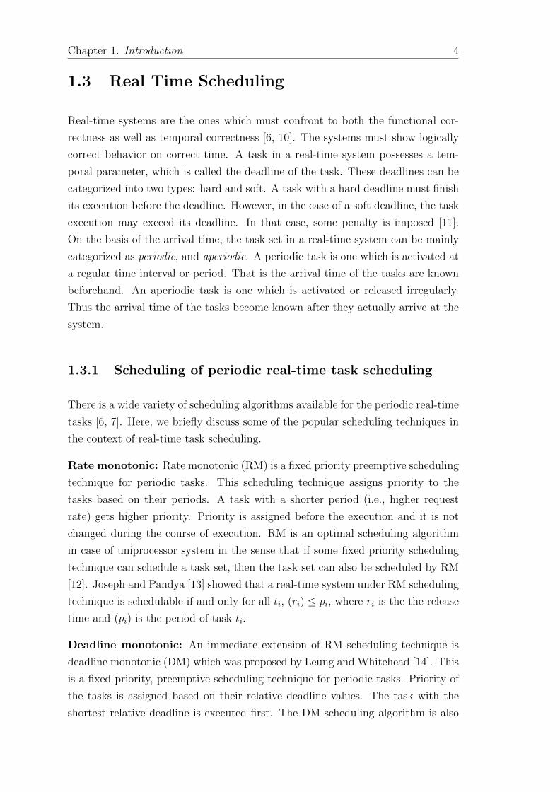
1.3 Real Time Scheduling
Real-time systems are the ones which must confront to both the functional cor-
rectness as well as temporal correctness [6, 10]. The systems must show logically
correct behavior on correct time. A task in a real-time system possesses a tem-
poral parameter, which is called the deadline of the task. These deadlines can be
categorized into two types: hard and soft. A task with a hard deadline must finish
its execution before the deadline. However, in the case of a soft deadline, the task
execution may exceed its deadline. In that case, some penalty is imposed [11].
On the basis of the arrival time, the task set in a real-time system can be mainly
categorized as periodic, and aperiodic. A periodic task is one which is activated at
a regular time interval or period. That is the arrival time of the tasks are known
beforehand. An aperiodic task is one which is activated or released irregularly.
Thus the arrival time of the tasks become known after they actually arrive at the
system.
1.3.1 Scheduling of periodic real-time task scheduling
There is a wide variety of scheduling algorithms available for the periodic real-time
tasks [6, 7]. Here, we briefly discuss some of the popular scheduling techniques in
the context of real-time task scheduling.
Rate monotonic: Rate monotonic (RM) is a fixed priority preemptive scheduling
technique for periodic tasks. This scheduling technique assigns priority to the
tasks based on their periods. A task with a shorter period (i.e., higher request
rate) gets higher priority. Priority is assigned before the execution and it is not
changed during the course of execution. RM is an optimal scheduling algorithm
in case of uniprocessor system in the sense that if some fixed priority scheduling
technique can schedule a task set, then the task set can also be scheduled by RM
[12]. Joseph and Pandya [13] showed that a real-time system under RM scheduling
technique is schedulable if and only for all ti, (ri) ≤ pi, where ri is the the release
time and (pi) is the period of task ti.
Deadline monotonic: An immediate extension of RM scheduling technique is
deadline monotonic (DM) which was proposed by Leung and Whitehead [14]. This
is a fixed priority, preemptive scheduling technique for periodic tasks. Priority of
the tasks is assigned based on their relative deadline values. The task with the
shortest relative deadline is executed first. The DM scheduling algorithm is also

Chapter 1. Introduction 5
an optimal scheduling algorithm in case of uniprocessor system in the sense that
if some fixed priority scheduling technique can schedule a task set, then the task
set can also be scheduled by DM [12].
Earliest deadline first: Earliest deadline first (EDF) is implicitly a preemptive
scheduling technique where priority is assigned based on the deadline of a task. A
task with earlier deadline indicates higher priority and it preempts the execution of
a task with a later deadline. EDF is found to be an optimal scheduling technique
for uniprocessor systems in the sense that if any task set is schedulable by an
algorithm, then EDF can also schedule the task set.
1.3.2 Scheduling of aperiodic real-time task scheduling
In this section, we present some of the popular scheduling algorithms for the
aperiodic tasks.
Jackson’s algorithm: This is another popular algorithm for scheduling a set of
aperiodic tasks. This algorithm considers scheduling a set of synchronous tasks
on a single processor to minimize the maximum lateness. This algorithm is a non-
preemptive version of EDF and commonly termed as the earliest due date (EDD)
first scheduling. EDD algorithm guarantees that if any feasible schedule exists for
a task set, then the algorithm finds it. The algorithm runs by sorting the tasks
based on their due date. Thus for a task set with n tasks, the algorithm takes
O(nlogn) time.
Earliest deadline first: As the EDF scheduling policy does not assume anything
about the periodicity of the tasks while scheduling, it works for both periodic and
aperiodic tasks in the same way (EDF is already defined for periodic tasks in the
previous section). This is also known as Horn’s algorithm [15]. The complexity
of this algorithm depends on the implementation of the ready queue. If the ready
queue is implemented as a list, then the complexity becomes O(n2). If the ready
queue is implemented as a heap, then the complexity becomes O(nlogn).
Least laxity first: This is an immediate derivation of EDF scheduling technique
where the priority of a task changes during the course of execution. Priority of
task ti at time instant t is calculated as di − t; which is the laxity value at that
time instant. This is a dynamic priority-based preemptive scheduling technique.
The complexity of this algorithm is O(n1 + n22), where n1 is the total number of

Chapter 1. Introduction 6
requests in a hyper-period of periodic tasks in the system if any, and n2 is the
total number of aperiodic tasks in the system [16].
Bratley’s algorithm: This algorithm tries to find a feasible schedule for a set of
non-preemptive independent tasks for a single processor system. The algorithm
does an exhaustive search in order to get a solution. While doing so, the algo-
rithm constructs a partial schedule by adding a new task in each step. A path
is discarded whenever the algorithm encounters a task which misses its deadline.
This algorithm is a tree-based search algorithm and for each task, the algorithm
might need to explore all the partial paths originating at that node. Thus the
time complexity of this algorithm becomes O(n · n!).
1.4 Aperiodic Real-Time Task Scheduling on Mul-
tiprocessor Environment
The above-mentioned algorithms were initially designed for a single processor sys-
tem. But as we move into the multiprocessor systems, a new dimension is added to
the scheduling problems, that is, the number of processors is increased from 1 to m.
Choosing a processor from a pull of free processors is termed as allocation problem
and is popularly known as mapping [17]. The allocation problem is often viewed
as a bin packing problem and several popular bin-packing heuristics, such as First
Fit, Next Fit, Best Fit, Worst Fit, etc. are clubbed with the uniprocessor schedul-
ing algorithms. In addition, the multiprocessor scheduling algorithms make use of
another factor for designing efficient scheduling policies. This is called migration
of tasks from one processor to another. In case of migration, the execution of one
task on a processor is preempted and the task is assigned to another processor.
Thus the task needs to shift (i.e. migrate) from one processor to another.
Majority of the scheduling problems for the aperiodic task set on multiprocessor
environment are non-polynomial except for task sets with restricted execution time
and the deadline [5]. Thus various heuristics are proposed to solve these problems.
When these algorithms are clubbed with the bin packing algorithms [18] to fit into
the multiprocessor environment, they are named as Earliest Deadline First - First
Fit (EDFFF), Earliest Deadline First - Best Fit (EDFBF), Earliest Due Date First
- Best Fit (EDDBF), etc. [19, 20, 21, 22].

Chapter 1. Introduction 7
1.5 Large Systems and Cloud
Large systems refer to the computing platform where a number of computing nodes
(or systems) are connected via a high-speed network to form a single computing
hub. These computing hubs are also known as data centers. The basic objective
of these systems is to meet the computation requirement of the recent high-end
scientific applications of various domains. These systems include Cluster, Grid,
and Cloud. In Cluster computing, the physical distance between the participating
nodes is not much, and they are often connected using LAN (local area network).
The computing nodes in a cluster are typically of homogeneous nature. In the
case of Grid computing, the computing nodes are geographically distributed and
belong to multiple administrative domains. The grid is a decentralized distributed
computing paradigm where the users rent the computing facility on an hourly
basis. On the other hand, Cloud comes under a centralized model where a single
service provider usually owns the resources.
1.5.1 Cloud computing and virtualization
Cloud computing is an emerging resource sharing computing platform which offers
a large amount of space and computing capability to its users via the Internet.
The users are charged as “pay-as-go” model based on their resource usages. There
exist various definitions of the cloud computing paradigm. One of the commonly
accepted definitions proposed by the National Institute of Standards and Technol-
ogy (NIST) is
“cloud computing is a model for enabling ubiquitous, convenient, on-demand net-
work access to a shared pool of configurable computing resources (e.g., networks,
servers, storage, applications and services) that can be rapidly provisioned and
released with minimal management effort or service provider interaction” [23].
Figure 1.1 shows the three-layered architecture of a typical cloud computing paradigm.
The system consists of an application layer, a virtualization layer, and a hardware
layer. The user requests arrive in the form of applications or tasks. These tasks are
accumulated in a single place for its processing based on the underlying scheduling
policy. The next layer is the virtualization layer. This layer plays the most vital
role and makes the cloud computing paradigm the popular, efficient and attrac-
tive. This layer accepts the requests from the application layer. The user tasks
may require any specific application software or operating system (OS), etc. for

Chapter 1. Introduction 8
User
Task
Task
User
Task
Task
User
Task
Task
User
Task
Task
Virtualizer
VM VM VM
Virtualizer
VM VM VM
Virtualizer
VM VM VM
VM Selector and Manager
VM to Host Scheduler
Task to VM Scheduler
Task Accumulator and ManagerApplication
Layer
VirtualizationLayer
Hardware
Layer
VM OS ImagesLibrary of
Figure 1.1: Cloud computing architecture
their execution. The job of the VM scheduler and manager is to facilitate an
appropriate virtual machine (VM) which meets the requirement of the task. If re-
quired, a VM with the requirement is created with the help of the VM OS library.
The bottom-most layer is the hardware layer which consists of the physical hosts
where the VMs are placed with the help of the virtualizer. The main benefit of
this architecture is that it can cater the user requests with any specific OS and
platform requirements irrespective of the host OS and underlying hardware. In
addition, various OSes can run together in the form of VMs sharing the resources
of the same hardware. This reduces the hardware requirement and thereby the
cost.
1.6 Real-Time Scheduling for Large Systems and
Cloud
Large computing systems such as the cloud provide some important features to
its users, such as dynamic pricing model, reliability, scalability, elasticity, dynamic
and seamless addition and removal of resources, etc. These features have attracted
applications from several domains for their deployment [24, 25, 11]. These applica-
tions are often of real-time nature. Thus the real-time scheduling for large systems
becomes crucial.
Chapter 1. Introduction 9
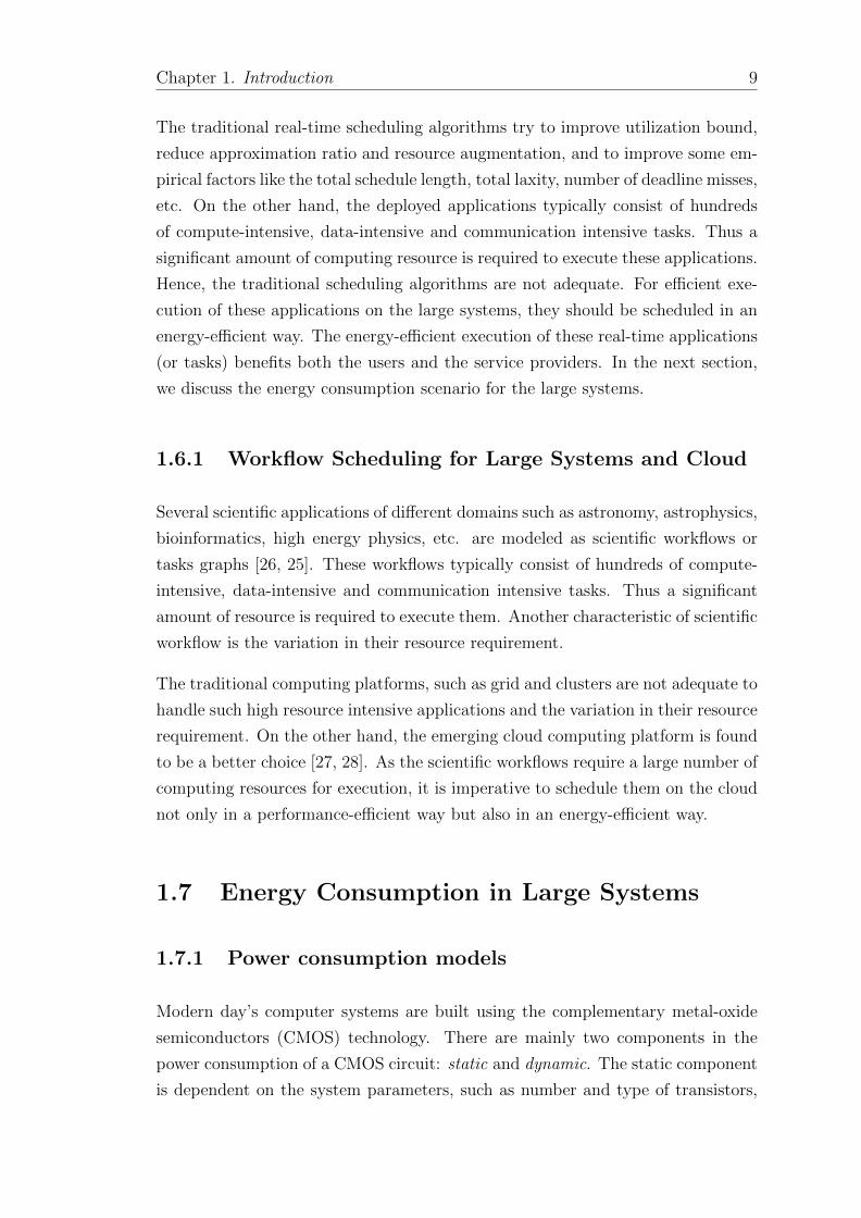
The traditional real-time scheduling algorithms try to improve utilization bound,
reduce approximation ratio and resource augmentation, and to improve some em-
pirical factors like the total schedule length, total laxity, number of deadline misses,
etc. On the other hand, the deployed applications typically consist of hundreds
of compute-intensive, data-intensive and communication intensive tasks. Thus a
significant amount of computing resource is required to execute these applications.
Hence, the traditional scheduling algorithms are not adequate. For efficient exe-
cution of these applications on the large systems, they should be scheduled in an
energy-efficient way. The energy-efficient execution of these real-time applications
(or tasks) benefits both the users and the service providers. In the next section,
we discuss the energy consumption scenario for the large systems.
1.6.1 Workflow Scheduling for Large Systems and Cloud
Several scientific applications of different domains such as astronomy, astrophysics,
bioinformatics, high energy physics, etc. are modeled as scientific workflows or
tasks graphs [26, 25]. These workflows typically consist of hundreds of compute-
intensive, data-intensive and communication intensive tasks. Thus a significant
amount of resource is required to execute them. Another characteristic of scientific
workflow is the variation in their resource requirement.
The traditional computing platforms, such as grid and clusters are not adequate to
handle such high resource intensive applications and the variation in their resource
requirement. On the other hand, the emerging cloud computing platform is found
to be a better choice [27, 28]. As the scientific workflows require a large number of
computing resources for execution, it is imperative to schedule them on the cloud
not only in a performance-efficient way but also in an energy-efficient way.
1.7 Energy Consumption in Large Systems
1.7.1 Power consumption models
Modern day’s computer systems are built using the complementary metal-oxide
semiconductors (CMOS) technology. There are mainly two components in the
power consumption of a CMOS circuit: static and dynamic. The static component
is dependent on the system parameters, such as number and type of transistors,

Chapter 1. Introduction 10
process technology, etc. On the other hand, the dynamic power consumption is
basically driven by the circuit activities and traditionally it was believed to be the
major contributor [29]. A wide volume of research on scheduling is done which
considers only the dynamic power consumption [30, 31, 32, 33, 34].
Mathematically, we write
Ptotal = Pbase + Pdyn (1.1)
where, Pbase is the static power consumption, and Pdyn is the dynamic power
consumption.
The dynamic power consumption is expressed as a function of voltage (V ) and
operating frequency (f). Mathematically, it can be written as follows.
Pdyn =1
2CV 2f (1.2)
Again, there are various power consuming components present in a large system
(such as cloud). The total energy (or power) consumption of such a system com-
prises of their individual power consumptions. These components include CPU,
memory, disk, storage, and network. Various studies [35, 36, 37] have been done
to express the total power consumption as a combination of these components.
For instance, Ge et al. [35] have used energy consumption of CPU, memory, disk,
and NIC (network interface card) to model the energy consumption of the system.
Song et al. [36] expands this model where they expressed the energy consumption
as a product of the power consumption of the components with the operation time
of the corresponding component.
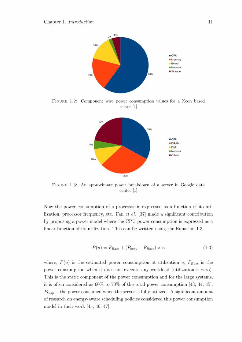
Though there are many power consuming components in a typical server, the
CPU is the major contributor [38, 39] and a wide range of scheduling algorithms
are proposed considering the energy consumption of the processor only [30, 40,
41, 42]. As reported in [1], the CPU consumes almost 60% of the total power
consumption for a Xeon based server and Figure 1.2 shows the component-wise
power consumption for that server. We see that the processor consumes 60% of
the total power, and memory is the second highest contributor with 19%. We also
present the power breakdown of a server placed at the Google data center using
Figure 1.3. Though memory consumes a significant chunk of power, CPU remains
to be the major contributor.
Chapter 1. Introduction 11
Figure 1.2: Component wise power consumption values for a Xeon basedserver [1]
Figure 1.3: An approximate power breakdown of a server in Google datacenter [1]
Now the power consumption of a processor is expressed as a function of its uti-
lization, processor frequency, etc. Fan et al. [37] made a significant contribution
by proposing a power model where the CPU power consumption is expressed as a
linear function of its utilization. This can be written using the Equation 1.3.
P (u) = PBase + (Pbusy − PBase)× u (1.3)
where, P (u) is the estimated power consumption at utilization u, PBase is the
power consumption when it does not execute any workload (utilization is zero).
This is the static component of the power consumption and for the large systems,
it is often considered as 60% to 70% of the total power consumption [43, 44, 45].
Pbusy is the power consumed when the server is fully utilized. A significant amount
of research on energy-aware scheduling policies considered this power consumption
model in their work [45, 46, 47].

Chapter 1. Introduction 12
In case of a virtualized environment, the total power consumption can also be
expressed as the summation of the individual power consumptions of the VMs
and the base power consumption [48], and this can be written as
Ptotal = Pbase +ν∑i=1
Pvm(i) (1.4)
where, Pbase indicates the static component, Pvm(i) indicates the power consump-
tion of the ith VM, and ν indicates the total number of VMs placed on the server.
Scheduling policies which target the dynamic power consumption of the hosts
(or processors) primarily uses the DVFS (dynamic voltage and frequency scaling)
technique by reducing the frequency and voltage to reduce the power consumption.
In DVFS technique, the operating voltage and frequency of the processors are
adjusted dynamically to adjust the speed of the processor. This in tern, effects
the power consumption of the processor [33, 49, 50, 51, 52]. On the other hand,
scheduling policies for the large systems, in general, try to reduce the static power
consumption by reducing the number of active components of the system [53, 54,
55, 56].
In addition to the computation energy consumption discussed above, a significant
chunk of the total energy consumption of a data center is contributed by the cooling
devices, AC/DC transformation devices, etc. We consider the total computation
energy as the total energy of the system and use this throughout the thesis.
1.7.2 Impact of high power consumption
High energy consumption in the servers and data centers has many demerits, and
this can be categorized in three directions: (i) economic, (ii) performance, (iii)
environmental. The energy consumption of a data center is almost equal to that of
25,000 households and it is around 2.2% of total electrical usages [48]. In addition,
the energy consumption cost of a data center is increasing significantly. This yields
a high operating electricity cost. Furthermore, high energy consumption imposes
a higher cooling cost. Data center owners need to spend a significant portion of
their budget for powering and cooling their servers. For instance, it is reported
that Amazon spends almost 50% of their management budget for powering and
cooling the data centers [57]. In [58], Koomey presented that the total power
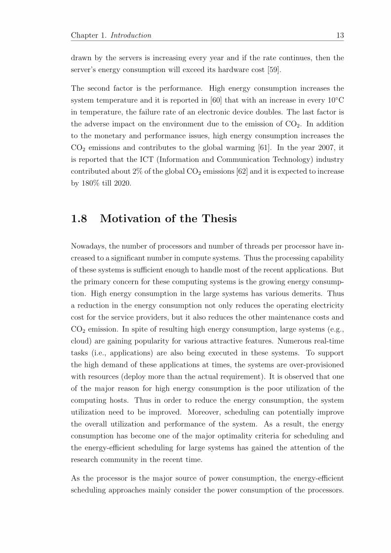
Chapter 1. Introduction 13
drawn by the servers is increasing every year and if the rate continues, then the
server’s energy consumption will exceed its hardware cost [59].
The second factor is the performance. High energy consumption increases the
system temperature and it is reported in [60] that with an increase in every 10◦C
in temperature, the failure rate of an electronic device doubles. The last factor is
the adverse impact on the environment due to the emission of CO2. In addition
to the monetary and performance issues, high energy consumption increases the
CO2 emissions and contributes to the global warming [61]. In the year 2007, it
is reported that the ICT (Information and Communication Technology) industry
contributed about 2% of the global CO2 emissions [62] and it is expected to increase
by 180% till 2020.
1.8 Motivation of the Thesis
Nowadays, the number of processors and number of threads per processor have in-
creased to a significant number in compute systems. Thus the processing capability
of these systems is sufficient enough to handle most of the recent applications. But
the primary concern for these computing systems is the growing energy consump-
tion. High energy consumption in the large systems has various demerits. Thus
a reduction in the energy consumption not only reduces the operating electricity
cost for the service providers, but it also reduces the other maintenance costs and
CO2 emission. In spite of resulting high energy consumption, large systems (e.g.,
cloud) are gaining popularity for various attractive features. Numerous real-time
tasks (i.e., applications) are also being executed in these systems. To support
the high demand of these applications at times, the systems are over-provisioned
with resources (deploy more than the actual requirement). It is observed that one
of the major reason for high energy consumption is the poor utilization of the
computing hosts. Thus in order to reduce the energy consumption, the system
utilization need to be improved. Moreover, scheduling can potentially improve
the overall utilization and performance of the system. As a result, the energy
consumption has become one of the major optimality criteria for scheduling and
the energy-efficient scheduling for large systems has gained the attention of the
research community in the recent time.
As the processor is the major source of power consumption, the energy-efficient
scheduling approaches mainly consider the power consumption of the processors.
Chapter 1. Introduction 14
The scheduling policies try to reduce the power (or energy) consumption of the
processor in different ways. Out of these, a majority of the research exploits the
DVFS technique, and they focus only on the dynamic energy consumption of the
processor. It is still a challenge to design an energy-efficient scheduling technique
for the real-time tasks considering both static and dynamic energy consumption
of the processors and satisfying other criteria, such as meeting the deadline con-
straints of the tasks.
Another promising way to increase the utilization of the system resources is by vir-
tualization [63, 48]. Here, a set of virtual machines (VMs) is created on the top of
physical hardware. User tasks are assigned to the VMs and the VMs are placed on
the physical machines (also called as hosts). Cloud is the most popular virtualized
system of the recent time and it is considered to be the future for energy-efficient
computing paradigm. Energy-efficient scheduling for the cloud system adjusts the
compute capacity of a VM as per the requirement and assigns the user tasks on
them. A majority of these scheduling policies assumes a continuous domain for
the compute capacity of the VMs. But in practice, the service providers often
offer VMs with discrete compute capacity. Our third work considers a virtualized
cloud system which deals with the VMs with discrete compute capacities.
With the increase in the popularity of the cloud computing paradigm, several
applications from different domains are getting deployed. These applications are
often of real-time in nature and they have huge resource requirements. Thus their
efficient execution is very much crucial. These applications are modeled as sci-
entific applications and various scheduling algorithms are developed for efficiently
executing the scientific applications in the cloud environment. But the majority
of the work mainly focuses on (i) reducing the overall execution time, (ii) meet-
ing the deadline constraint, (iii) ensuring the quality of services, etc. It is still a
challenging and promising research area to schedule these scientific applications
(which are represented as scientific workflows) on the cloud in an energy-efficient
way while satisfying other essential criteria such as the deadline. Moreover, the
amount of research on real-time scheduling tasks with multiple VM requirement is
thin. Hence our fourth work is about scheduling a set of online scientific workflows
on the cloud environment.

Chapter 1. Introduction 15
1.9 Contributions of the Thesis
The thesis proposes a number of energy-efficient scheduling policies for efficiently
executing real-time tasks on the large multi-threaded systems and the cloud. While
doing so, the thesis considers different machine and task environments. The con-
tributions can be summarized as follows.
1.9.1 Scheduling online real-time tasks on LMTMPS
In our first contribution, we consider scheduling a set of online independent aperi-
odic real-time tasks on a large compute systems where the processors are equipped
with the multi-threaded feature. We name such systems as large multi-threaded
multiprocessor systems (LMTMPS). Based on the power consumption pattern of
some of the recent multi-threaded processors, we devise a simple power model
where the total power consumption of a processor depends on the number of
active threads of that processor. Then we propose an energy-efficient real-time
scheduling policy, named smart scheduling policy which is designed based on the
urgent point of the tasks. This policy works on two fundamentals, (i) all the
switched-on processors are always tried to use fully, and (ii) new processors are
not switched-on as long as possible. The proposed policy shows an average energy
reduction of around 47% for the synthetic dataset and around 30% for the real
trace dataset. Furthermore, we have proposed three variations of the basic smart
policy to improve the energy consumption further and to handle special kinds of
workloads. These are (a) smart - early dispatch scheduling policy, (b) smart -
reserve scheduling policy and (c) smart - handling immediate urgency scheduling
policy.
1.9.2 Scheduling online real-time tasks on virtualized cloud
system
The second contribution of the thesis deals with scheduling the same task set for
a virtualized cloud computing environment. Here the hosts are heterogeneous,
and each host can accommodate a number of virtual machines (VM). VMs are
also heterogeneous with respect to their compute capacities and energy consump-
tions. Under this setup, we consider a region based non-linear power consumption
model for the hosts which is derived from the power consumption pattern of a

Chapter 1. Introduction 16
typical server. Accordingly, we set two thresholds for the utilization of the hosts
and depending on the urgency of the tasks, the scheduler dynamically uses the
threshold value. In this work, we first introduce the concept of urgent point for
a real-time task in case of a heterogeneous cloud environment and then propose
two energy-efficient scheduling policies, (i) urgent point aware scheduling (UPS ),
and (ii) urgent point aware scheduling - early scheduling (UPS-ES ), for efficiently
executing a set of online real-time tasks. As compared to a state-of-art policy
energy-efficient policy, the proposed policies achieve an average energy reduction
of around 24% for the synthetic data and approximately 11% for the real-trace
data.
1.9.3 Scheduling real-time tasks on VMs with discrete uti-
lization
The third contribution of the thesis considers a cloud system where the VMs are of
discrete compute capacity. The discrete compute capacity contributes a discrete
utilization to the hosts. We introduce the concept of critical utilization where the
energy consumption of the host is minimum. The scheduler tries to maintain the
utilization of all the running hosts close to the critical utilization. In order to
propose solutions to this problem, we first divide the task set into four different
cases. Case 1 handles tasks with the same length and same deadline. Case 2
deals with tasks of two different lengths but the same deadline. In case 3, we
consider tasks with arbitrary lengths but the same deadline. Finally, the task set
with arbitrary length and the arbitrary deadline is considered under case 4. The
solution method starts by proposing a solution of case 1, then the solution of case
1 is used to solve case 2 and so on. For case 4, we apply four different techniques to
cluster the tasks and to bring it under case 3. The experimental results show that
depending on the value of the system parameter, we can decide the task clustering
technique.
1.9.4 Scheduling scientific workflows on virtualized cloud
system
All the above problems consider real-time tasks which are independent but in this
contribution, we consider a set of online dependent real-time tasks for efficiently
executing in the cloud environment. The dependent task set is represented by

Chapter 1. Introduction 17
scientific workflows. Each workflow contains a chain of multi-VM tasks and it
arrives at the cloud system with a predefined deadline. We use three different
approaches by efficiently utilizing the slack time of each workflow to decide the
best scheduling time for a task of a workflow. We have exploited two different
possibilities for allocating the VMs of a task, (i) non-splittable, (ii) splittable.
We propose a series of energy-efficient scheduling policies considering different
allocation policies, different migration strategies, and different slack distribution
techniques. Along with the energy consumption of the system, we analyze the
migration count and split count for each policy. As far as energy consumption
is concerned, proposed policies under the non-splittable VM allocation category
performs at par with the state-of-art policy. But they perform much better than
the state-of-art policy terms of the number of migrations. But proposed policies
under splittable VM allocation category performs significantly better than the
state-of-art policy both in terms of energy consumption and migration count.
1.10 Summary
Nowadays, the number of processors and the number of threads per processor
have increased to a significant number in compute systems. Thus the processing
capability of these systems is sufficient enough to handle most of the recent appli-
cations. As the processing capability increases, the power (or energy) consumption
also increases by a significant margin. The high power consumption for the large
systems has many demerits and thus reducing power consumption will benefit
both the users and the service providers in several ways. Though there are many
power consuming components present in a computing system, the processor alone
consumes a significant portion of that. Thus the research community mainly fo-
cuses on the power consumption of the processors while designing energy-efficient
scheduling techniques.
There are three components of any scheduling problem: machine environment, task
environment, and optimality criteria. Different work on scheduling considers dif-
ferent values for these components and present solutions accordingly. In our work,
for the machine environment, we consider both virtualized and non-virtualized
system with a large number of processors. For the task environment, we con-
sider both independent and dependent real-time task set. We set the optimality
criteria as the minimization of energy consumption without missing the deadline
constraints of the tasks. Hence the focus of this thesis work is to design scheduling

Chapter 1. Introduction 18
approaches for executing real-time applications (expressed as real-time tasks) on
large systems to minimize the energy consumption of the system while meeting
the deadline constraints of the tasks. The first work considers a non-virtualized
large multi-threaded multiprocessor system (LMTMPS) and the other three works
consider a virtualized cloud system. The power (or energy) consumption of the
system is taken as a function of the utilization of the hosts, or the number of active
threads in a processor, or the summation of the power consumption of the running
VMs of a host.
1.11 Organization of the Thesis
The rest of the thesis is organized as follows:
• Chapter 2 presents brief literature summarizing the seminal works in the
area of the energy-efficient scheduling of large systems.
• Chapter 3 presents the first contribution, where the scheduling of aperiodic
online real-time tasks is considered for LMTMPS.
• Chapter 4 describes our second contribution, which deals with the scheduling
of aperiodic online real-time tasks for the heterogeneous virtualized cloud
system.
• Chapter 5 considers scheduling for a virtualized cloud system where the
utilization values of the VMs are discrete. We put forward a mathematical
analysis regarding the energy consumption and the utilization of the hosts.
• Chapter 6 presents a series of scheduling heuristics for a set of multi-VM
dependent tasks, represented by scientific workflows.
• Chapter 7 finally concludes the thesis with some possible future research
directions.
Chapter 2
Energy Efficient Scheduling in
Large Systems: Background
The scheduling algorithms whose optimality criteria is the reduction of the power
consumption or the energy consumption is commonly known as energy-efficient
(or energy-aware) scheduling. In this Chapter, we present a brief overview of
literature in the context of the energy-efficient scheduling techniques, specially
for the large systems. The work can be broadly studied in two approaches: (i)
fine-grained, (ii) coarse-grained. Fine-grained approach basically deals with the
dynamic power consumption of the hosts. Scheduling approaches under this cat-
egory extensively use the DVFS technique in various ways. On the other hand,
scheduling approaches under coarse-grained category primarily deal with the static
power consumption of the hosts whose aim is to minimize the number of active
hosts.
2.1 Fine Grained Approaches
A reduction in the operating frequency of the processor ideally results in a cu-
bic reduction in the dynamic power consumption of the processor. But with a
reduction in the operating frequency, the execution time of the task running on
that processor increases. Thus the primary idea of the DVFS technique in the
context of real-time task execution is to adjust the operating frequency such that
the power consumption can be reduced without missing the deadline of the task.
Here we present a few seminal works for non-virtualized and virtualized systems
which uses the fine-grained approach to reduce the energy consumption.
19
Chapter 2. Background 20
2.1.1 Non-virtualized system
Weiser et al. [31] was the pioneer to start the research in this direction by as-
sociating power consumption with scheduling and used DVFS technique to study
the power consumption of some scheduling techniques. They took advantage of
CPU idle time and reduced the operating frequency of CPU so that the tasks were
finished without violating any deadline. Aydin et al. [32, 64] ported this idea for
real-time systems where they initially designed a static algorithm for computing
the optimal frequency for a periodic task set assuming their worst-case behavior.
After that, they devised an online speed adjustment algorithm for dynamically
claiming the energy not used by the tasks finishing earlier than the worst case
time and achieved up to 50% power saving as compared to the worst-case sce-
nario. Zhu et al. [33] has extended the technique proposed by Aydin et al. [32] for
the multiprocessor environment. In their policy, they mention about teo different
approaches for utilizing the slack created by a task to reduce the energy consump-
tion. In first approach, slack created by a task in one processor was utilized by
another task in the same processor, and in the second approach, the slack was
shared among the tasks in different processors.
Isci et al. [65] has proposed a global power management policy for chip multi-
processors where every processor can operate in three different modes: turbo (no
reduction), eff1 (5% voltage and frequency reduction), eff2 (15% voltage and fre-
quency reduction). They studied the relationship between the operating modes
of the processors and the corresponding performances. Lee and Zomaya [66, 67]
have proposed makespan-conservative energy reduction along with simple energy
conscious scheduling to find a trade-off between the makespan time and energy
consumption, where they reduced both makespan time and energy consumption of
precedence constraint graph on heterogeneous multiprocessor systems supporting
DVFS technique. Recently, Li and Wu [49, 68, 69] have considered the execu-
tion of various task models by further exploiting the DVFS technique for both
homogeneous and heterogeneous processor environments.
The above studies mainly consider the small systems. DVFS technique is equally
used for the high-performance computing (HPC) systems and clusters. For in-
stance, Hotta et al. [70] used the DVFS technique to design a scheme for the high-
performance computing (HPC) clusters where the program execution is split into
multiple regions, and the optimal frequency is chosen for the individual region.
Ge et al. [50] has designed an application-level power management framework
and proposed scheduling strategies for scientific applications in case of distributed

Chapter 2. Background 21
DVFS enabled clusters. Kim et al. [71] considered scheduling of bag-of-tasks
applications, and presented scheduling approaches considering space shared and
time shared resource sharing strategies. The applications were scheduled in an
energy-efficient manner and the quality of service (QoS) is measured as meeting
the deadline constraints of the applications. In [51], Chetsa et al. presented a
partial phase recognition based dynamic power management architecture for the
HPC systems. They have designed two setups. In first setups, they consider
optimization of the processor power consumption only and in the second setup,
processor, disk, and network power consumptions are considered. Chen et al. [72]
considered energy-efficient matrix multiplication in a DVFS enabled cluster where
they divide the matrices and the computation is distributed among different cores.
In case of computation phase, the CPU frequency is set to the highest level and
in case of idle and communication phase, the frequency is set to the lowest level.
2.1.2 Virtualized system
In the context of a virtualized system, the user tasks are assigned to the VMs and
the VMs execute on the CPU cores. The speed (or the compute capacity) of a VM
is determined by the operating frequency of the underlying processor. The speed is
typically expressed in terms of million instructions per second (MIPS). Whenever
the speed (i.e. the compute capacity) of a VM increases, the power consumption
increases but the execution time of the task assigned to that VM decreases. The
DVFS based energy-efficient scheduling algorithms in the virtualized environment
adjust the speed of the VMs as per the requirement. In this section, we present a
few important works in this direction.
In [73], Calheiros and Buyya considered scheduling of urgent bag-of-tasks using
DVFS where they assume that one CPU core is exclusively available to one VM.
Changing the frequency of the core directly reflects the speed of the VM running
on it. The algorithm specified four different operating conditions and they are
ranked accordingly. The conditions are: (i) task is executed by a running VM
without increasing its frequency, (ii) task is executed by a running VM but an
increase in frequency is needed, (iii) task is executed by an idle VM placed on an
active host, (iv) task is executed by an idle VM and the host is brought to an
active state from a sleep or low power consuming state. The algorithm categorizes
the first condition as the best and the last condition as the worst.

Chapter 2. Background 22
In [74], Elnozahy et al. have proposed five different energy-efficient scheduling
policies which considered both DVFS and node on-off technique to reduce the
power consumption of the server clusters. The first policy is termed as independent
voltage scaling (IVS) which employs different voltage levels to the individual server.
The second policy is termed as the coordinated voltage scaling (CVS) where the
scaling is applied to different processors in a coordinated way. The third one is
termed as VOVO (Vary On and Vary Off) where the entire server is turned on
or off. The last two policies are the combination of IVS and CVS with VOVO
(VOVO-IVS and VOVO-CVS).
Recently, Zhu et al. [30] has considered scheduling of aperiodic real-time tasks on
the cloud. They proposed an energy-efficient scheduling algorithm, named EARH
which is based on a rolling horizon optimization technique. The primary idea
here is to consider the previously scheduled (but not started execution) tasks from
local queues of the VMs while scheduling new tasks. But in their approach, they
have considered only the dynamic energy consumption of the hosts; and the target
utilization of hosts is 100%.
Wu et al. [52] considered scheduling of real-time tasks in the cloud environment
where each task is specified with a minimum and a maximum frequency. Simi-
larly, each server is specified with a minimum and a maximum working frequency.
To execute a task on a specified server, it must satisfy both the minimum and
maximum frequency conditions. The policy uses the DFVS technique to set the
working frequency of a task on an appropriate server.
2.2 Coarse Grained Approaches
The primary idea of the coarse-grained scheduling policies is to reduce the number
of active hosts in the large system or data center. Whenever a host becomes active,
it consumes a significant amount of power even if it does not execute any task.
This is the base power consumption of the host. A reduction in the number of
active hosts reduces the overall power consumption of the system. The dynamic
power management (DPM) technique uses this coarse-grained approach to reduce
the power consumption of the system. DPM uses different power consumption
states for the components and dynamically switches between the states as per the
requirement [75]. In the following subsections, we present a few seminal works for

Chapter 2. Background 23
non-virtualized and virtualized systems which uses the coarse-grained approach to
reduce the energy consumption.
2.2.1 Non-virtualized system
Chase et al. [53] proposed a coarse-grained power management techniques for
Internet server clusters where an energy conscious switch is placed on top of the
servers that maintain a list of active servers. Depending on the traffic behavior and
a predetermined threshold value of utilization of the servers, the switch dynami-
cally adjusts the list by keeping them either in active mode or low power mode.
In [76], Chase et al. have extended this idea to develop an economic model based
architecture, called Muse to find the trade-off between the service quality and the
cost in terms of energy. The policy avoids static over-provisioning of resources by
dynamically allocating sufficient resources to meet certain quality requirements.
Choi et al. [77] studied the characteristics of the applications running in data
centers in order to impose appropriate bounds on power consumption. They pre-
sented consolidation techniques which are based on two kinds of power budgets:
average and sustained. Costa et al. [78] designed a three-level energy aware frame-
work, named GREEN-NET which was based on the distributed automatic energy
sensors. They developed an adapted resource and job management system (OAR)
unit to facilitate automatic shut-down of the nodes in under-utilized periods.
In [54], Pinheiro et al. have proposed strategies for inspecting the system sta-
tus periodically and then to dynamically add or remove computing nodes to the
cluster based on the requirements. After addition or removal of the nodes, a load
re-distribution policy runs to decide the placement and migrations of the load
from one node to another to ensure system performance. The authors have also
imposed several restrictions to limit the number of migrations. Zikos et al. [55]
proposed three scheduling policies for a set of heterogeneous servers with differ-
ent power consumption and performance. One policy reduces energy consumption
with average response time. Another policy is customized for performance but
consumes high energy consumption. The last one performs best for medium load
scenario. The author considered compute-intensive tasks where the service time
is not known. Research is also done considering the energy consumption cost of
the data centers. For instance, Jonardi et al. [79] proposed two heuristics for
geographically distributed data centers where they studied the co-location (CL)
interference effect of workloads. They claimed that the heuristic FDLD-CL (Force
Directed Load Distribution) performs better when the workload profile does not
Chapter 2. Background 24
change rapidly and GALD-CL (Genetic Algorithm Load Distribution) performs
better otherwise.
As the cooling energy is a significant chunk of the total energy in data centers, a
good number of works [80, 81, 82, 83, 84] is done to reduce the thermal energy
consumption. For instance, Oxley et al. [81] considered a noble framework for
heterogeneous computing systems where they used offline analysis to find optimal
mapping of workload to the cores. In [84], Oxley et al. considered scheduling tasks
on a heterogeneous compute systems with given thermal and deadline constraints.
They studied the effect of the co-location on the execution time of the tasks and
proposed greedy heuristics for the same.
2.2.2 Virtualized system
All the above studies presented some exciting results, but none of them considered
the virtualization technique in the system. Virtualization technology is known
to be a promising technique to improve the resource usages in the cloud. In a
virtualized system, tasks are assigned to the VMs and the VMs are placed on
the hosts. Energy efficient scheduling in virtualized environment mainly deals
with two parameters to reduce the energy consumption [85, 86, 56]. The first
parameter is the consolidation of the VMs into a fewer number of hosts and the
second parameter is the efficient placement of VMs on the hosts of the cloud
resource. Here we present a few seminal works in the context of the energy-efficient
scheduling in a virtualized environment.
Consolidation operation mainly targets to reduce the number of active hosts in
the system. To reduce the number of active hosts, the hosts should be utilized
to their maximum capacity [30, 44, 45]. For instance, Lee and Zomaya in [45],
developed two energy-efficient scheduling policies: ECTC and maxUtil ; both the
policies try to utilize the switched-on processors fully (i.e. 100%). MaxUtil takes
the task placement decision based on the host utilization while ECTC takes the
decision based on the energy consumption of the task only. On the other hand, a
wide range of research [46, 86, 87, 88] is done where the host is not utilized fully,
rather they are used to a threshold value. The idea behind using threshold-based
utilization approaches is that the system performance degrades when the host
utilization crosses a limit. In addition to reduce the energy consumption, these
policies also aim to meet the performance or the service level agreement (SLA) of
the user tasks.

Chapter 2. Background 25
Verma et al. [89] has done a nice study regarding the power consumption pattern of
various HPC applications and the typical workload behavior of a virtualized server
and in [90] they developed a framework called pMapper where the applications
are placed onto different servers for execution based on the utilization values of
the server. Srikantaiah et al. [56] studied the relationship between the energy
consumption and the performance of the system which was determined by the
CPU ( or processor) utilization and disk utilization. The problem was viewed as
a bin packing problem where applications are mapped into servers optimally.
Lee et al. [45] proposed two energy-efficient scheduling algorithms for a virtu-
alized cluster where they expressed the power consumption of a processor as a
linear function of utilization and the servers are utilized to their full capacities.
Beloglazov et al. [46] proposed a series of heuristics to dynamically allocate VMs
and manage resources at runtime depending on the overall utilization of the sys-
tem. In [91], authors presented two ant colony optimization based approaches for
VM placement and VM consolidation. They studied the trade-off between the
energy consumption and the SLA requirements.
Chen et al. [44] considered the execution of independent real-time tasks on a vir-
tualized cloud environment where the task execution time of the tasks comes with
some uncertainties. They reduce the overall energy consumption of the system
while meeting the task’s guarantee ratio. Hosseinimotlagh et al. [92] proposed a
two-tier task scheduling approach for the cloud environment where the benefits of
both the users and the service providers are taken into consideration. The global
scheduler efficiently maps the tasks to the VMs while the local scheduler tries to
utilize the hosts with an optimum CPU utilization. The task scheduler initially
assigns the minimum average computing power to each and the remaining com-
puting power is distributed among the tasks in a proportionate way. In [93], Shi
et al. presented a series of approaches for scheduling embarrassingly parallel tasks
in the cloud where they initially provide an analytical solution to the resource al-
location problem. Then they formulate a single job scheduling problem as a linear
program where they aim to schedule only one job which contained multiple tasks
within it. Furthermore, they design an online scheduler for periodically scheduling
the tasks by applying shortest job first policy.
Majority of the VM consolidation problem considers only the CPU utilization
while allocating the VMs on the hosts. But a few research has been conducted
where the other parameters such as memory, disk, etc. are also considered in
addition to the CPU. For instance, Mastroianni et al. [85] considered memory

Chapter 2. Background 26
in addition to the CPU utilization. They claim that the deterministic approach
of VM consolidation is not suitable for large data centers and they proposed a
probabilistic approach to tackle the problem. The effectiveness of their approach
is measured using five different parameters: resource utilization, number of active
servers, power consumption, migration frequency, and SLA violation. SLA viola-
tion is expressed as an overload of the CPU utilization. They have validated their
claim by conducting experiments for both CPU intensive and memory intensive
applications. In [94], authors have used a bi-directional bin packing approach to
placing the VMs on the hosts. They have used linear regression and K-nearest
neighbor regression prediction models to estimate the future resource utilization.
Research has also been done to predict the future resource requirement. For in-
stance, in [86], authors use an exponentially weighted moving average (EWMA)
load prediction method to estimate the future resource requirement. They intro-
duce the concept of skewness among the hosts to maintain a uniform resource
utilization of the hosts. They reduce the energy consumption of the system by re-
ducing the number of active hosts and maintain the performance by avoiding host
over-utilization. Authors used four different threshold values to balance between
the energy consumption and the system performance. CPU intensive, memory
intensive, and network intensive workloads are clubbed to together as a mix to
improve the resource utilization. In [88], authors have presented a profiling-based
framework for server consolidation where they studied the co-location effect of
different types of workloads. They further design a way to transform the current
VM allocation scenario into a target VM allocation scenario with the minimum
migration count.
2.3 Energy Efficient Workflow Scheduling
2.3.1 Workflow scheduling on large systems
Workflow scheduling on large systems such as grid and cloud system has been
extensively studied from a few years. As the problem is known to be an NP-hard
[95], numerous heuristic and meta-heuristic approaches [96, 97, 27, 98, 26, 95,
99] are proposed which mainly aim to reduce makespan time, the overall cost of
execution, energy consumption, etc. Studies have also been done which considered
deadline centric and budget constrained execution of scientific workflows in the
cloud. For instance, Abrishami et al. [96] has initially proposed a partial critical
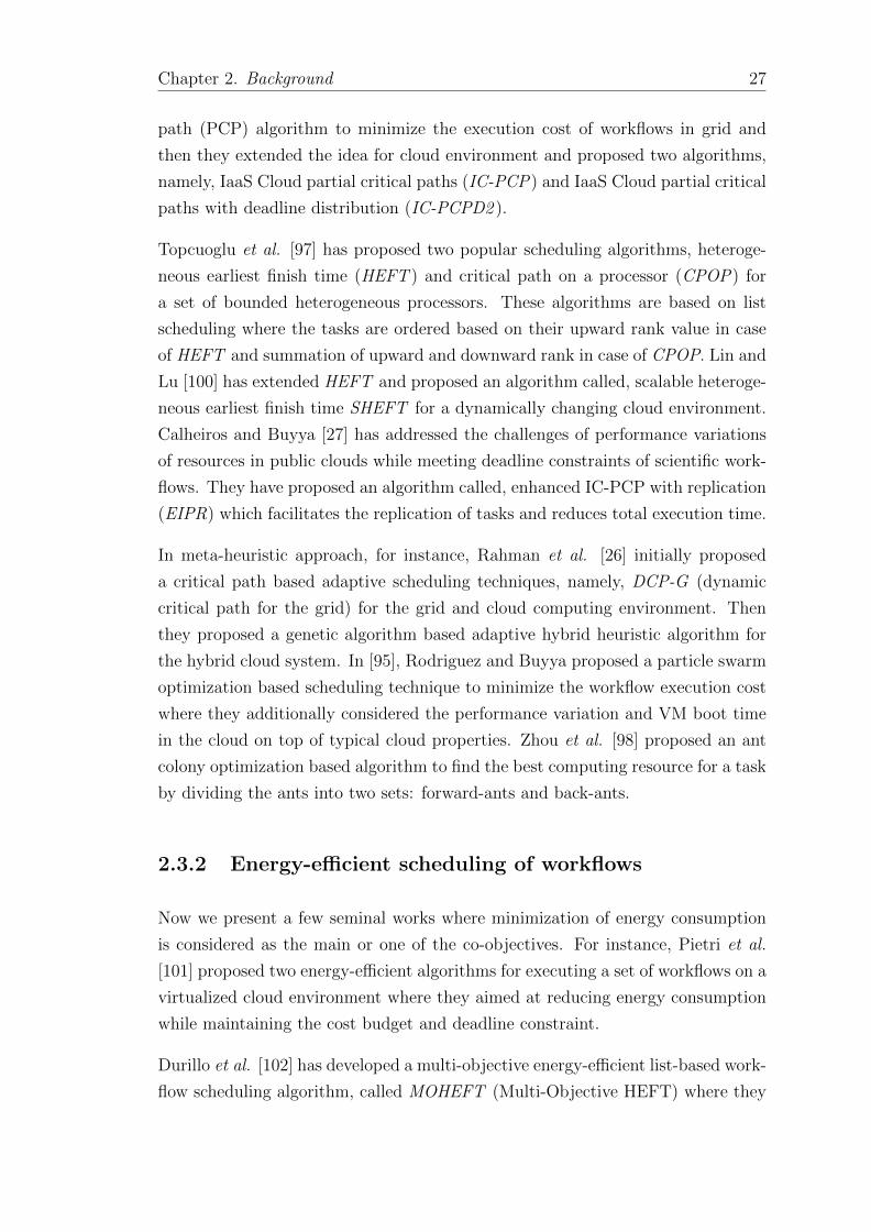
Chapter 2. Background 27
path (PCP) algorithm to minimize the execution cost of workflows in grid and
then they extended the idea for cloud environment and proposed two algorithms,
namely, IaaS Cloud partial critical paths (IC-PCP) and IaaS Cloud partial critical
paths with deadline distribution (IC-PCPD2 ).
Topcuoglu et al. [97] has proposed two popular scheduling algorithms, heteroge-
neous earliest finish time (HEFT ) and critical path on a processor (CPOP) for
a set of bounded heterogeneous processors. These algorithms are based on list
scheduling where the tasks are ordered based on their upward rank value in case
of HEFT and summation of upward and downward rank in case of CPOP. Lin and
Lu [100] has extended HEFT and proposed an algorithm called, scalable heteroge-
neous earliest finish time SHEFT for a dynamically changing cloud environment.
Calheiros and Buyya [27] has addressed the challenges of performance variations
of resources in public clouds while meeting deadline constraints of scientific work-
flows. They have proposed an algorithm called, enhanced IC-PCP with replication
(EIPR) which facilitates the replication of tasks and reduces total execution time.
In meta-heuristic approach, for instance, Rahman et al. [26] initially proposed
a critical path based adaptive scheduling techniques, namely, DCP-G (dynamic
critical path for the grid) for the grid and cloud computing environment. Then
they proposed a genetic algorithm based adaptive hybrid heuristic algorithm for
the hybrid cloud system. In [95], Rodriguez and Buyya proposed a particle swarm
optimization based scheduling technique to minimize the workflow execution cost
where they additionally considered the performance variation and VM boot time
in the cloud on top of typical cloud properties. Zhou et al. [98] proposed an ant
colony optimization based algorithm to find the best computing resource for a task
by dividing the ants into two sets: forward-ants and back-ants.
2.3.2 Energy-efficient scheduling of workflows
Now we present a few seminal works where minimization of energy consumption
is considered as the main or one of the co-objectives. For instance, Pietri et al.
[101] proposed two energy-efficient algorithms for executing a set of workflows on a
virtualized cloud environment where they aimed at reducing energy consumption
while maintaining the cost budget and deadline constraint.
Durillo et al. [102] has developed a multi-objective energy-efficient list-based work-
flow scheduling algorithm, called MOHEFT (Multi-Objective HEFT) where they

Chapter 2. Background 28
present a trade-off between the energy consumption and the makespan time. They
performed extensive experiments with different workflow characteristics. The pro-
posed algorithm achieved shorter or same makespan time as compared to HEFT
algorithm but with lesser energy consumption. Cao et al. [103] proposed energy-
efficient scheduling technique for executing a set of scientific workflows in a col-
lection of data centers. Depending on the amount of energy consumption, they
considered four different modes for servers: active, idle, sleep and transition in
their work. Authors used the DVFS technique and tasks were run at optimal
frequencies to reduce the energy consumption. In [28], Bousselmi et al. initially
partitioned the workflow to reduce network energy consumption by reducing the
amount of data communication among them. Then in the next step, they used the
cat swarm optimization based heuristic to schedule each partition on a set of VMs
in an energy-efficient manner. Chen et al. [104] designed an online scheduling
algorithm, called, energy-efficient online scheduling, EONS to schedule tasks from
different workflows. System resources are dynamically adjusted to maintain the
weighted square frequencies of the hosts.
Recently, Li et al. [61] addressed both energy consumption and the execution cost
while guaranteeing the deadline constraints of the tasks. The authors considered
an hourly based pricing model for the VMs and a task is mapped to an optimal
VM. They developed strategies to merge sequence tasks and parallel tasks for
meeting performance constraints by reducing execution cost and energy consump-
tion. They have also used the DVFS technique to use the slack time efficiently.
Xu et al. [41] considered the execution of online scientific workflows to minimize
the energy consumption of cloud resources. The authors transformed the workflow
into a set of sequential tasks. They applied a static time partitioning to calculate
the arrival time of the individual task of the workflow. The authors considered
homogeneous VMs with heterogeneous hosts. At the time of scheduling, the sched-
uler considers all the running tasks as new tasks with possibly lesser length and
schedules them along with the current tasks. We consider a similar setup in our
last contribution where we deal with scheduling real-time dependent tasks.
Table 2.1 lists some seminal work in the area of energy-efficient scheduling policies
for the cloud environment. The table also contains the key considerations of each
of the work and some lacunae in their work.
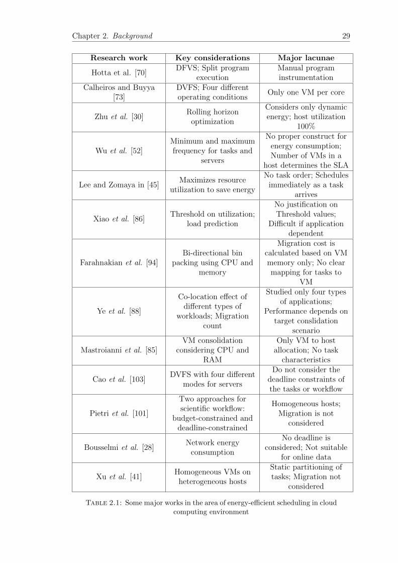
Chapter 2. Background 29
Research work Key considerations Major lacunae
Hotta et al. [70]DFVS; Split program
executionManual programinstrumentation
Calheiros and Buyya[73]
DVFS; Four differentoperating conditions
Only one VM per core
Zhu et al. [30]Rolling horizon
optimization
Considers only dynamicenergy; host utilization
100%
Wu et al. [52]Minimum and maximumfrequency for tasks and
servers
No proper construct forenergy consumption;Number of VMs in a
host determines the SLA
Lee and Zomaya in [45]Maximizes resource
utilization to save energy
No task order; Schedulesimmediately as a task
arrives
Xiao et al. [86]Threshold on utilization;
load prediction
No justification onThreshold values;
Difficult if applicationdependent
Farahnakian et al. [94]Bi-directional bin
packing using CPU andmemory
Migration cost iscalculated based on VMmemory only; No clearmapping for tasks to
VM
Ye et al. [88]
Co-location effect ofdifferent types of
workloads; Migrationcount
Studied only four typesof applications;
Performance depends ontarget conslidation
scenario
Mastroianni et al. [85]VM consolidation
considering CPU andRAM
Only VM to hostallocation; No task
characteristics
Cao et al. [103]DVFS with four different
modes for servers
Do not consider thedeadline constraints ofthe tasks or workflow
Pietri et al. [101]
Two approaches forscientific workflow:
budget-constrained anddeadline-constrained
Homogeneous hosts;Migration is not
considered
Bousselmi et al. [28]Network energy
consumption
No deadline isconsidered; Not suitable
for online data
Xu et al. [41]Homogeneous VMs onheterogeneous hosts
Static partitioning oftasks; Migration not
considered
Table 2.1: Some major works in the area of energy-efficient scheduling in cloudcomputing environment

Chapter 3
Scheduling Online Real-Time
Tasks on LMTMPS
This chapter first presents an energy-efficient scheduling policy for executing a
set of online independent real-time tasks on a large computing system where the
processors are empowered with the multi-threaded facility. We term this kind of
computing systems as Large Multi-threaded Multiprocessor Systems (LMTMPS).
Further, the chapter presents three variations of the basic scheduling policy to
efficiently handle some special cases. The proposed scheduling policies consider
a thread-based power consumption model which is devised based on the power
consumption pattern of some of the recent commercial processors.
3.1 Introduction
Nowadays, various scientific and real-time applications of different domains such
as avionics, bioinformatics, signal processing, image processing, etc. are being
deployed in the large systems, for their efficient execution [24, 27]. These ap-
plications typically consist of hundreds of compute-intensive, data-intensive and
communication intensive tasks. Thus a significant amount of resource is required
to execute these applications. On the other hand, the compute systems of today’s
world is equipped with a large number of processors and these processors are em-
powered with the multi-threaded feature. Thus the processing capability of these
systems is sufficient enough to handle these high-end applications. But with an
increase in the processing capability, the energy consumption of these large sys-
tems is also increasing. This growing energy consumption has sought the attention
31

Chapter 3. Scheduling Online Real-Time Tasks on LMTMPS 32
0
50
100
150
200
250
0 1 2 3 4 5 6 7 8 9
Po
wer
co
nsu
mp
tio
n (
in W
atts
)
Number of active threads
Phenom II X6Intel i7-860
Qualcom HexaV3Phenom 9900
Core 2 Quad Q9450Core 2 Quad Q6600
Figure 3.1: Power consumption plot of a few recent commercial processorswith number of active threads [2, 3]
Power Consumption (in Watts)
#Active-threads→ 1 2 3 4 5 6 8Processor ↓
Phenom-II-X6 40 58 73 88 103 115 -
Intel i7-860 165 174 186 193 204 212 228
Qualcom Hexa V3 40 55 60 72 82 90 -
AMD-Phenom-9900 76 95 114 131 - - -
Core-2-Quad Q9450 28 41 53 58 - - -
Core-2-Quad Q6600 48 62 72 79 - - -
Table 3.1: Power consumption behaviour of commercial processors [2, 3]
of the research community of to a great extent. As a result, a good number of
scheduling algorithms for reducing the energy consumption of such large systems
are proposed [53, 76, 50, 70, 71, 55]. Majority of these research consider power
consumption at a finer granularity and use the DFVS technique to reduce the en-
ergy consumption. For instance, Hotta et al. [70] split the program execution into
multiple regions and each region is executed using an optimal frequency for that
region. Ge et al. [50] considered a distributed DVFS environment to reduce the
energy consumption of the cluster. But none of these energy-efficient scheduling
approaches for the large systems sufficiently consider scheduling of the real-time
tasks in their work. In this chapter, we consider scheduling of online real-time
tasks for a large multi-threaded multiprocessor system and consider the power
construct at a coarser granularity.
Figure 3.1 shows a plot of the power consumption of a few recent multiproces-
sors (multi-threaded processors) versus the number of running hardware threads
(HTs) in them. We see that the power consumption values follow an interesting
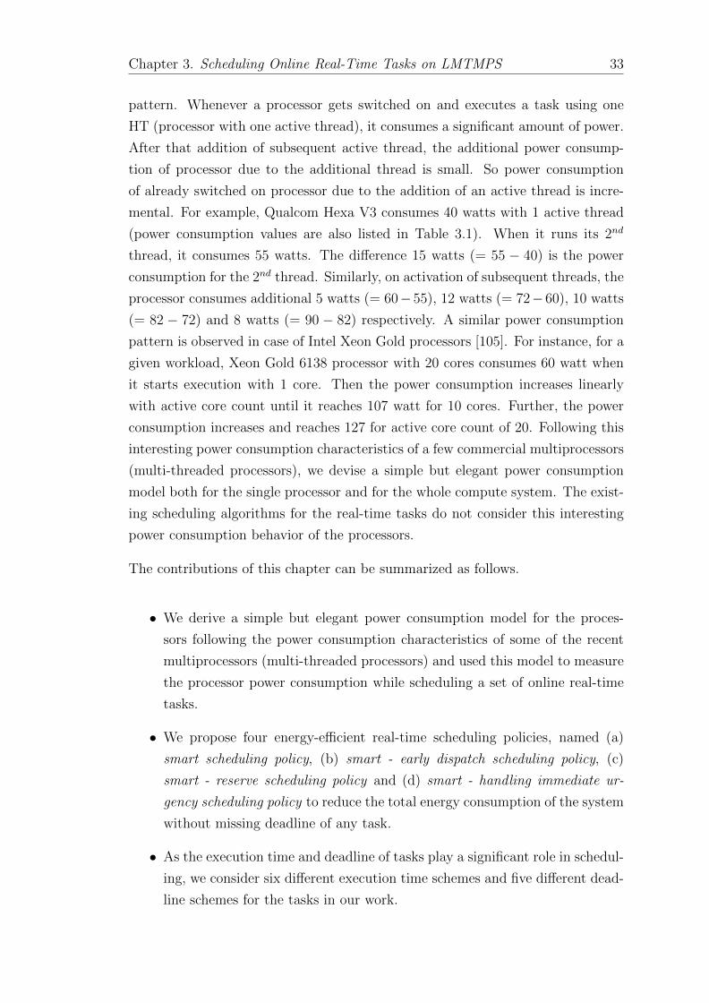
Chapter 3. Scheduling Online Real-Time Tasks on LMTMPS 33
pattern. Whenever a processor gets switched on and executes a task using one
HT (processor with one active thread), it consumes a significant amount of power.
After that addition of subsequent active thread, the additional power consump-
tion of processor due to the additional thread is small. So power consumption
of already switched on processor due to the addition of an active thread is incre-
mental. For example, Qualcom Hexa V3 consumes 40 watts with 1 active thread
(power consumption values are also listed in Table 3.1). When it runs its 2nd
thread, it consumes 55 watts. The difference 15 watts (= 55 − 40) is the power
consumption for the 2nd thread. Similarly, on activation of subsequent threads, the
processor consumes additional 5 watts (= 60−55), 12 watts (= 72−60), 10 watts
(= 82 − 72) and 8 watts (= 90 − 82) respectively. A similar power consumption
pattern is observed in case of Intel Xeon Gold processors [105]. For instance, for a
given workload, Xeon Gold 6138 processor with 20 cores consumes 60 watt when
it starts execution with 1 core. Then the power consumption increases linearly
with active core count until it reaches 107 watt for 10 cores. Further, the power
consumption increases and reaches 127 for active core count of 20. Following this
interesting power consumption characteristics of a few commercial multiprocessors
(multi-threaded processors), we devise a simple but elegant power consumption
model both for the single processor and for the whole compute system. The exist-
ing scheduling algorithms for the real-time tasks do not consider this interesting
power consumption behavior of the processors.
The contributions of this chapter can be summarized as follows.
• We derive a simple but elegant power consumption model for the proces-
sors following the power consumption characteristics of some of the recent
multiprocessors (multi-threaded processors) and used this model to measure
the processor power consumption while scheduling a set of online real-time
tasks.
• We propose four energy-efficient real-time scheduling policies, named (a)
smart scheduling policy, (b) smart - early dispatch scheduling policy, (c)
smart - reserve scheduling policy and (d) smart - handling immediate ur-
gency scheduling policy to reduce the total energy consumption of the system
without missing deadline of any task.
• As the execution time and deadline of tasks play a significant role in schedul-
ing, we consider six different execution time schemes and five different dead-
line schemes for the tasks in our work.
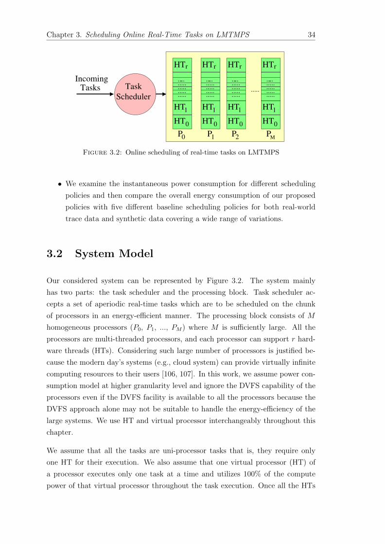
Chapter 3. Scheduling Online Real-Time Tasks on LMTMPS 34
HT
HT
HT
.....
.....
.....
.....
.....
0
1
r
HT
HT
HT
.....
.....
.....
.....
.....
0
1
r
P0
HT
HT
HT
.....
.....
.....
.....
.....
0
1
r
P1 P2
Scheduler
Task Incoming
Tasks
HT
HT
HT
.....
.....
.....
.....
.....
0
1
r
.....
PM
Figure 3.2: Online scheduling of real-time tasks on LMTMPS
• We examine the instantaneous power consumption for different scheduling
policies and then compare the overall energy consumption of our proposed
policies with five different baseline scheduling policies for both real-world
trace data and synthetic data covering a wide range of variations.
3.2 System Model
Our considered system can be represented by Figure 3.2. The system mainly
has two parts: the task scheduler and the processing block. Task scheduler ac-
cepts a set of aperiodic real-time tasks which are to be scheduled on the chunk
of processors in an energy-efficient manner. The processing block consists of M
homogeneous processors (P0, P1, ..., PM) where M is sufficiently large. All the
processors are multi-threaded processors, and each processor can support r hard-
ware threads (HTs). Considering such large number of processors is justified be-
cause the modern day’s systems (e.g., cloud system) can provide virtually infinite
computing resources to their users [106, 107]. In this work, we assume power con-
sumption model at higher granularity level and ignore the DVFS capability of the
processors even if the DVFS facility is available to all the processors because the
DVFS approach alone may not be suitable to handle the energy-efficiency of the
large systems. We use HT and virtual processor interchangeably throughout this
chapter.
We assume that all the tasks are uni-processor tasks that is, they require only
one HT for their execution. We also assume that one virtual processor (HT) of
a processor executes only one task at a time and utilizes 100% of the compute
power of that virtual processor throughout the task execution. Once all the HTs
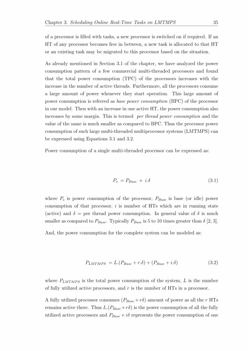
Chapter 3. Scheduling Online Real-Time Tasks on LMTMPS 35
of a processor is filled with tasks, a new processor is switched on if required. If an
HT of any processor becomes free in between, a new task is allocated to that HT
or an existing task may be migrated to this processor based on the situation.
As already mentioned in Section 3.1 of the chapter, we have analyzed the power
consumption pattern of a few commercial multi-threaded processors and found
that the total power consumption (TPC) of the processors increases with the
increase in the number of active threads. Furthermore, all the processors consume
a large amount of power whenever they start operation. This large amount of
power consumption is referred as base power consumption (BPC) of the processor
in our model. Then with an increase in one active HT, the power consumption also
increases by some margin. This is termed per thread power consumption and the
value of the same is much smaller as compared to BPC. Thus the processor power
consumption of such large multi-threaded multiprocessor systems (LMTMPS) can
be expressed using Equations 3.1 and 3.2.
Power consumption of a single multi-threaded processor can be expressed as:
Ps = PBase + i.δ (3.1)
where Ps is power consumption of the processor, PBase is base (or idle) power
consumption of that processor, i is number of HTs which are in running state
(active) and δ = per thread power consumption. In general value of δ is much
smaller as compared to PBase. Typically PBase is 5 to 10 times greater than δ [2, 3].
And, the power consumption for the complete system can be modeled as:
PLMTMPS = L.(PBase + r.δ) + (PBase + i.δ) (3.2)
where PLMTMPS is the total power consumption of the system, L is the number
of fully utilized active processors, and r is the number of HTs in a processor.
A fully utilized processor consumes (PBase + rδ) amount of power as all the r HTs
remains active there. Thus L.(PBase+rδ) is the power consumption of all the fully
utilized active processors and PBase + iδ represents the power consumption of one

Chapter 3. Scheduling Online Real-Time Tasks on LMTMPS 36
0
100
200
300
400
500
600
0 5 10 15 20 25
Po
wer
co
nsu
mp
tio
n (
in W
atts
)
Number of active HTs in the system
Figure 3.3: Power consumption of LMTMPS (when values of PBase = 100, δ =10 and r = 8)
partially filled processor where i number of HTs are active in that. In case there is
no processor is partially filled in the system, the value of PBase + iδ is 0. Here, we
assume that the scheduler has a task consolidation agent which regularly migrates
tasks from an active host to another so as to consolidate tasks into a fewer number
of processors (hosts); and this is done such that at the end of the consolidation
process, at most one processor remains partially filled. All other remaining active
processors become fully utilized. Processors without an active HTs are switched
off. In this process, neighboring processors are chosen so as to reduce the power
wastage due to distribution.
3.3 Power Consumption Model
Figure 3.3 shows an example cased for the power consumption behavior of our
considered system. In this example case, the processor BPC is taken as 100 Watts.
That is whenever a processor is started, it consumes 100 Watts of power. On
activation of each thread, additional 10 Watts of power is consumed by the system;
which is the thread power consumption δ. We have considered every processor
can accommodate a maximum of 8 HTs. We observe from the graph that power
consumption value increases significantly with a sharp jump when active thread
number (also called virtual processor) reaches 1, 9 and 17. When the system runs
8 threads, the power consumption of the processor becomes 180 (=100 + 8 × 10)
Watts. When the active thread count reaches 9, the power consumption value
increases by 110 Watts and the total system power consumption becomes 290
(= 180 + 110) Watts.

Chapter 3. Scheduling Online Real-Time Tasks on LMTMPS 37
Thus in our considered system, the total processor power consumption value is
not proportional to the number of active HTs (or utilization) of the processor.
But most of the earlier research considers them to be proportional specially, in
case of scheduling real-time tasks. A similar type of power consumption model
was used by Gao et al. [108] where they considered the power consumption of a
virtualized data center as a function of the server utilization. Lee et al. [45] also
used another similar energy model where the energy consumption of a processor
was expressed as a function of its utilization. But in our case, we consider the
power consumption of a processor with respect to its number of active HTs. In
addition, we consider the BPC of processors, which is the static component of the
processor power consumption.
3.4 Task Model: Synthetic Data Sets and Real-
World Traces
In this work, we consider scheduling of a set of online aperiodic independent real-
time tasks, T = {t1, t2, t3 . . . } onto a large multi-threaded multiprocessor system.
Each task ti is represented by three-tuple ti(ai, ei, di) where ai is the arrival time,
ei is the execution time (or computation time) and di is the deadline of the task.
For all ti, di ≥ (ai + ei). All the tasks are assumed to be sequential and uni-
processor that is, a task is executed by only one HT (virtual processor) and utilize
100% of the compute power of the virtual processors throughout their execution.
We consider scheduling of both synthetic real-time tasks and real-world trace data
which are described in the following subsections.
3.4.1 Synthetic tasks
As already explained in the previous subsection, we consider three parameters
of a task: arrival time, execution time, and deadline. In the synthetic data set,
we assume that aperiodic independent real-time tasks are entering to the system
following Gaussian distribution. That is, the inter-arrival pattern of the tasks
follow the Gaussian distribution. For the execution time and deadline, we consider
various schemes. We describe these in the following subsections.
Chapter 3. Scheduling Online Real-Time Tasks on LMTMPS 38
0
100
200
300
400
500
600
0 100 200 300 400 500 600 700 800 900 1000
Re
lati
ve
De
ad
lin
e o
f T
as
ks
Task Number
(a) Gaussianly distributed (µ = 10 and σ = 5)
0
500
1000
1500
2000
2500
3000
3500
4000
4500
5000
5500
0 100 200 300 400 500 600 700 800 900 1000
Re
lati
ve
De
ad
lin
e o
f T
as
ks
Task Number
(b) Increasing (k = 3)
0
500
1000
1500
2000
2500
3000
3500
4000
4500
5000
5500
0 100 200 300 400 500 600 700 800 900 1000
Re
lati
ve
De
ad
lin
e o
f T
as
ks
Task Number
(c) Decreasing (k = 3)
10100
10150
10200
10250
10300
10350
0 100 200 300 400 500 600 700 800 900 1000
Ab
so
lute
De
ad
lin
e o
f T
as
ks
Task Number
(d) Common
Figure 3.4: Different deadline schemes with µ = 10 and σ = 5
3.4.1.1 Execution time variation
As the execution (or computation) time of tasks is a key factor in scheduling and
it has a significant impact on the performance of the system [109, 110], we have
considered a wide variety of task execution time with different distributions in
order to establish the effectiveness of our work. Here we have considered four
different distributions: Random, Gaussian, Poisson and Gamma. In random
distribution, the execution time ei of a task ti is randomly distributed between
1 to Rmax, where Rmax is a user-defined value. In addition, we consider two
simple distributions where execution time of tasks is expresses as a function of
task sequence number or time: INC(i) and DEC(i). In INC(i), execution time
of tasks increases with task number. INC(i) is taken as k.i, i ∈ {1, 2, . . . , N}.Similarly, inDEC(i), execution time of tasks decreases with task number. DEC(i)
is taken as k.(N + 1− i), i ∈ {1, 2, . . . , N}.

Chapter 3. Scheduling Online Real-Time Tasks on LMTMPS 39
3.4.1.2 Deadline variation
Performance of various real-time applications also depends on their deadline val-
ues. Thus in addition to the variations of execution time, we have considered five
different variations in the deadline of tasks. The slack of a task mainly determines
the variation in deadline scheme. For a task ti (ai, ei, di), the value of di− (ai + ei)
is called slack time (SLK) of the task. This slack time can be a function of time,
a function of task sequence number, a function of some external parameters or
a constant. Different deadline schemes considered based on the variation of the
slack time of tasks are stated below.
1. Deadline Scheme 1 (Deadlines are assigned based on the randomly
distributed slack)
In this scheme, the slack time for the tasks is randomly distributed. Deadline
of a task ti arriving at time ai is di = ai + ei + z; where z is slack time and
the value of z is random number varies in the range 0 to Zmax. Tasks under
this deadline scheme have similar relative deadlines. Relative deadline of a
task is the absolute deadline of the task minus its arrival time.
2. Deadline Scheme 2 (Deadlines are assigned based on the Gaussian
distribution of slack)
Under this scheme, the slack time of tasks varies as per Gaussian distribution.
The deadline of a task is expressed as: di = ai + ei + g(µ, σ); where the
function g(µ, σ) is follows discretized Gaussian distribution with parameter
µ and σ as mean and variance respectively. Figure 3.4(a) shows an example
plot of relatives deadline of tasks verses task number with µ = 10 and σ = 5.
3. Deadline Scheme 3 (Deadlines are assigned based on increasing
slack)
This scheme says that the relative deadline of tasks is tight initially and
with an increase in time (or task sequence number of tasks), the deadline
becomes relaxed. The tight deadline means that the slack time of a task
is comparatively less and relaxed deadline means that the slack time of a
task is comparatively more. In this Scheme 3, deadline of the task di is
represented as di = ai + ei + INC(i); where i is sequence of task and the
value of function INC(i) is increase as i increase, i ∈ {1, 2, . . . , N}, and N
is number of tasks. Figure 3.4(b) represents an example plot of the relative
deadline of tasks versus task number. We have taken INC(i) = k · i with
k = 3 for the example.

Chapter 3. Scheduling Online Real-Time Tasks on LMTMPS 40
4. Deadline Scheme 4 (Deadlines are assigned based on decreasing
slack)
This is the opposite to last scheme. Here the relative deadline of tasks
are relaxed initially and with increase in time (or task sequence number of
tasks), the deadline becomes tight. Mathematically, it can be represented as
di = ai + ei + DEC(i); where i is sequence of task ti, the value of function
DEC(i) decreases as i increase, i ∈ {1, 2, . . . , N}, and N is number of tasks.
Figure 3.4(c) demonstrates this scheme. We have taken DEC(i) = k ·(N−i)with k = 3 for the example.
5. Deadline Scheme 5 (Common deadline for all the tasks)
This a special kind of scheme which is popular as common due date problems
in literature [8]. Here the absolute deadlines of all the tasks are the same.
Mathematically, this can be expressed as di = D; where D is the common
deadline for all the tasks and D ≥ max{ai + ei}. Figure 3.4(d) represents
an example plot of the absolute deadline of tasks versus task number to
represent this scheme where the deadlines for all the tasks are taken as
10205 time unit.
3.4.2 Real-world traces
In addition to synthetic real-time tasks with many variations (as described in
the previous subsection), we have also considered four different real workload
traces: MetaCentrum-1, CERIT-SC, Zewura and MetaCentrum-2 in our work
[111]. These traces contain the job attributes of a few clusters which were gen-
erated from PBSpro and TORQUE traces at various times. CERIT-SC workload
trace consists of 17, 900 jobs collected during the first 3 months of the year 2013.
MetaCentrum-1 workload trace has job descriptions of 495, 299 jobs which are col-
lected during the months of January to June of the year 2013. Zewura workload
trace contains 17, 256 jobs of 80 CPU clusters which are collected during the first
five months of the year 2012. MetaCentrum-2 workload trace consists of 103, 656
jobs descriptions of 14 clusters containing 806 CPUs which are collected during
the first five months of the year 2009. The logs also contain several other useful
information such as node descriptions, queue descriptions, machine descriptions,
etc.

Chapter 3. Scheduling Online Real-Time Tasks on LMTMPS 41
3.5 Objective in the Chapter
In this chapter, we wish to design energy-efficient scheduling policies for online ape-
riodic independent tasks onto large multiprocessor systems (with multi-threaded
processors) such that all the tasks meet their deadline constraints. Here we assume
the system with a sufficiently large number of processors i.e. that the computing
capability of the system is very high. In general, the large systems consume a
considerable amount of power. There is a static component in the power con-
sumption of the large system, and the total power consumption (TPC) of such
systems depends hugely on the number of active processors. Furthermore, in a
multi-threaded processor, the power consumption is depended on the number of
the active threads of the processor and static power consumption (i.e., BPC).
Thus the power consumption in such multi-threaded multiprocessor systems un-
der the considered model is non-proportional to resource utilization of the system
(resource utilization of the system can also be expressed as the total number of
active threads). In this work, we have used this power consumption behavior to
minimize the total energy consumption (TEC) of the system.
3.6 Standard Task Scheduling Policies
In this section, we present three standard task scheduling policies, namely, utiliza-
tion based scheduling policy, front work consolidation and rear work consolidation.
We also state the standard earliest deadline first policy and describe the state of
art task scheduling policy, namely, utilization based work consolidation policy in
details.
3.6.1 Utilization based allocation policy (UBA)
In this policy, the utilization value of a task is used as a determining parameter
for its allocation. Utilization of a task is the required amount of processor’s share
to execute the task such that the task is finished exactly at its deadline (in a
uni-processor environment). Utilization ui of task ti can be defined as.
ui =ei
di − ai(3.3)

Chapter 3. Scheduling Online Real-Time Tasks on LMTMPS 42
where, ei is the execution time, di is deadline and ai is the arrival time of the task
ti.
As the tasks enter the system, they are assigned the required (ui) portions of the
processor’s share for their executions. For a task in LMTMPS, it requires the ui
amount of processor’s share throughout its execution time from ai to d− 1. This
policy assumes that an infinite number of migrations and preemptions are allowed
for the tasks. Virtually, a task ti start execution in the system from its arrival
time ai to its deadline di but with the least processor share ui. The start time
(si) and finish time (fi) of a task ti is given by Equation 3.4.
si = ai; fi = di (3.4)
At any instant of time t, the total number of virtual processors required to execute
all the tasks and to meet their deadlines can be defined as the summation of
utilization values of all the tasks present in the system. It can be written as
PNt =
⌈Nactive tasks∑
i= 0
ui
⌉(3.5)
where, PNt is number of virtual processors required andNactive tasks is total number
of tasks currently running in the system (or the number of tasks for which ai ≤t ≤ di).
This policy provides the minimum processor share (i.e. utilization) required for a
task for all the time instants from the arrival time till the deadline of that task.
Thus the execution of a task ti spreads for the whole duration with minimum
processor requirement ui at every time instant between ai and di. It aims to
reduce the instantaneous power consumption of the processor by allocating the
minimum amount of processor share. This policy is mainly of theoretical interest
as the premise in this scheduling policy is that the value of PNt gets calculated
continuously and the way PNt is calculated, the system requires virtually huge
number of migrations to perform scheduling in an actual scenario.
Theorem 3.1. Total energy consumption of the system with UBA is minimum if
the followings hold
• Processor (system) instantaneous power consumption PCt is proportional to
instantaneous processor (system) utilization, and that is PCt ∝ PNt.

Chapter 3. Scheduling Online Real-Time Tasks on LMTMPS 43
time0 1 2 3 4 5 6 7 8 9 10 11 12
a1 a3a2
T1(0,4,8) T2(1,2,4) T3(4,6,12)
time0 1 2 3 4 5 6 7 8 9 10 11 12
.66 .66 .66u2
u3 .75 .75.75 .75 .75 .75 .75 .75
T1
T2
T3 X X
u 1 12 2 1 1 1 1 1 1 0 0time0 1 2 3 4 5 6 7 9 10 11 128
0.5 0.5 0.5 0.5 0.5 0.5 0.5 0.5u1
u1
u3u2
d2 d1 d3
Figure 3.5: Illustration of front work consolidation of real-time tasks
• All the processors are single threaded and all tasks are sequential.
• Unrestricted number of migrations and preemptions are allowed for all the
tasks without any cost.
• Number of processors in the system is sufficiently large (we can assume it to
be ∞)
Proof. Total energy consumption of the system can be represented as
E =
∫ ∞t=0
PCt.dt = K.
∞∑t=0
PNt (3.6)
where K is proportionality constant.
The total amount of utilizations (from all the tasks) at the time instant t is PNt
and thus∑∞
t=0 PNt is the total amount of utilizations in the system for the entire
duration of the tasks execution. This total amount of utilizations does not depend
on the tasks execution order. Thus any scheduler yields minimum this amount of
utilizations. Hence, the energy consumption happens to be minimum.
3.6.2 Front work consolidation (FWC)
In this policy, the execution of tasks is brought towards the front of the time
axis. As soon as a task arrives, it is allocated to an HT of a processor so that

Chapter 3. Scheduling Online Real-Time Tasks on LMTMPS 44
the execution of the task starts immediately. Here, start time (si) and finish time
(fi) of a task ti is given by Equation 3.7. Since the execution of a task begins as
soon as it reaches the system, the policy can also be called as as-soon-as-possible
(ASAP) policy. This kind of immediate allocation is feasible because we con-
sidered the system with sufficiently large number compute resource (processors).
This scheduling policy turns out to be non-preemptive and non-migrative (do not
require migration of tasks).
si = ai; fi = ai + ei (3.7)
To describe the front work consolidation (FWC) policy, let us consider an example
with three tasks t1(a1 = 0, c1 = 4, d1 = 8), t2(1, 2, 4) and t3(4, 6, 12) as shown in
Figure 3.5. We can calculate utilization of task t1 (u1=0.5) between time 0 and 8,
utilization of task t2 (u2 =0.667) between time 1 and 4, and utilization of task t3
(u3=0.75) between time 4 and 12. If we schedule these tasks based on utilization
then at least one task will be in execution between time 0 to 12 and it is shown
in the middle part of Figure 3.5. In front consolidation, we try to consolidate
(i.e. summing up) all the utilization values towards the beginning of time axis and
thus for all the tasks, utilization values get consolidated towards the arrival time
of tasks. As we assume that the tasks are sequential and they can be executed
on one processor at a time, consolidated utilization of one task ti in any time slot
cannot exceed ui · di − aiei. Consolidated utilization indicates the total amount of
work to be done for a task with a particular utilization value. If the consolidated
utilization exceeds this limit then it needs to be put into next time slot and the
process is continued until there is no work left. In the above case, for task t1, the
total consolidated utilization becomes u1 · (di − ai)=0.5 · 8=4, so it needs to be
spread into four slots with consolidated utilizations u1 · d1 − a1ei=0.5 · (8 − 0)/4=1
in all the time slots from 1 to 4. Executing the example tasks set using this FWC
policy, there will be no work in time slot 11 and 12. If there is no work, there is no
power consumption (static power). This reduces the overall energy of the system.
Lemma 3.2. If all the conditions of Theorem 3.1 hold then the total energy con-
sumption of the system with front consolidation scheduling is minimum
Proof. In front consolidation scheduling policy, the policy consolidates the task
execution or utilization to the front and it does not increase the total system
utilization. As the amount of work needed to execute in both cases is the same
Chapter 3. Scheduling Online Real-Time Tasks on LMTMPS 45
and instantaneous power consumption of the system is proportional to utilization,
this policy also consumes minimum energy.
If the instantaneous power consumption of the system is not-proportional to
instantaneous system utilization then the above lemma is not true and in case
of the multi-threaded processor, they are not proportional. Thus the Lemma 3.2
does not hold for the multi-threaded multiprocessor system.
3.6.3 Rear work consolidation (RWC)
This task scheduling policy is similar to the previous but here the tasks are con-
solidated towards their deadlines. All the tasks get accumulated and added to the
waiting queue as soon as they arrive. A task lies in the waiting queue as long as its
deadline constraint allow it to wait. Then the execution begins at their respective
urgent points only. Urgent point is the time at which if the task starts its execution
and runs without any interruption, it will be completed exactly at its deadline.
This policy can be called as Delayed Scheduling Policy. since the execution of a
task is delayed until the system time reaches its urgent points. This is also known
as as-late- as-possible (ALAP) [112, 113]. Since the considered system is assumed
to have sufficiently large number compute capacity, tasks can be scheduled under
this policy without missing their deadlines. Start time (si) and finish time (fi) of
a task ti is given by Equation 3.8.
si = di − ei; fi = di (3.8)
Lemma 3.3. If all the conditions of Theorem 3.1 hold then the overall system
energy consumption with rear work consolidation scheduling is minimum.
Proof. In rear consolidation scheduling, the policy consolidates the task execution
or utilization to the rear end of the task deadline and it does not increase the total
system utilization. As the amount of work needed to execute in both UBA and
RWC are same and instantaneous power consumption of the system is proportional
to utilization, this also consumes minimum energy.
Chapter 3. Scheduling Online Real-Time Tasks on LMTMPS 46
3.6.4 Utilization based work consolidation (UBWC)
Here the scheduler intends to keep the active processor count minimum. The
execution time of the tasks are divided into unit length and they are distributed
across the time axis such that no task miss their deadlines and the total number of
active processors remain minimum [114, 56, 115, 116]. Processor count increases
when the total utilization exceeds a whole number. For a processor with r HT,
we can safely assume that when a unit execution time of a task get scheduled at
any time slot, the utilization of that slot increases by 1r. For a processor with
single HT, UBWC policy will consume an equal amount of energy as previously
discussed policies: UBA, FWC, and RWC. But multi-threaded processor systems,
the policy reduces the energy consumption significantly. This is because the task
execution is serial and in every time instant the policy aims to keep the processor
count minimum and minimum processor count implies the minimum amount of
static energy consumption which is a significant portion.
Every incoming task to the system has arrival time ai, deadline di and execu-
tion time ei. When a task ti arrives at system at ai, there may be some tasks
already present in the system and their remaining part of execution must have
been scheduled between ai and max{dj}, where dj is the deadline of the task tj
currently present in the system except ti. For systems with enough number of
multi-threaded processors having r threads per processor, the UBWC scheduler
inserts ei · 1r
units of computation between ai and di with preference to early slots,
so that it minimizes the number of running processors in every time slot between
ai and dj. This minimization criteria for UBWC can be written as
min
{dj∑t=ai
⌈number of task scheduled at time t
r
⌉}(3.9)
where r is the number of HTs per processor. In general, if we switch-on a new
processor it consumes a significantly high amount of energy as compared to ex-
ecuting on an HT (virtual processor) of an already switched-on processor. This
scheduling policy requires preemption and migration of the tasks; but the number
of preemptions and number of migrations for a task ti is bounded by ei − 1 if we
assume the time axis is discretized in the unit time slot.
Lemma 3.4. For systems with an infinite single-threaded processor (r = 1), if
all the conditions of Theorem 3.1 hold then the total energy consumption of the
system with utilization based consolidation scheduling is minimum.

Chapter 3. Scheduling Online Real-Time Tasks on LMTMPS 47
Proof. The amount of work in UBWC remains same as that of UBA. When the
instantaneous power consumption of the system is proportional to the processor
utilization, it consumes the same amount of energy as UBA and thus the energy
consumption is minimum.
3.6.5 Earliest deadline first scheduling policy (EDF)
Earliest deadline first (EDF) is a well-known scheduling policy where tasks are
considered depending on their deadlines. The task with the earliest (i.e., closest)
deadline value is selected for execution first [117]. The scheduling policy considers
all the waiting tasks and the one with minimum deadline value is taken for exe-
cution. EDF policy requires a fixed number of processors for its execution. In our
work, we consider the non-preemptive version of EDF with a minimum processor
count so that no task misses its deadline. The start time of task ti and finish time
of the same task follow the inequalities 3.10 and 3.11.
ai <= si <= (di − ei) (3.10)
(ai + ei) <= fi <= di (3.11)
3.7 Proposed Task Scheduling Policies
Here we present four energy-efficient task scheduling policies to run a set of online
aperiodic independent real-time tasks on the large multi-threaded multiprocessor
system. The system follows the power consumption model which was described in
Section 3.2. The power model assumes non-proportionality between the instanta-
neous power consumption and instantaneous system utilization. Execution of the
tasks in all the policies is almost continuous (ignoring time for migration), that is
ei = (fi − si), where ei, si, and fi are the execution time, start time and finish
time of a task ti respectively. Based on our experimental evidence, task execu-
tion with our designed scheduling policies consume less amount of overall energy
on LMTMPS as compared to UBWC and other policies (experimental validation
is given in Section 3.8), even if all the tasks execute continuously. These task
scheduling policies are described in the following subsections.

Chapter 3. Scheduling Online Real-Time Tasks on LMTMPS 48
3.7.1 Smart scheduling policy (Smart)
We have designed a task scheduling policy for online real-time tasks called smart
scheduling policy for the large multi-threaded multiprocessor system. This schedul-
ing policy focuses an important parameter that is time. Typically scheduling poli-
cies focus on selecting a task from a set of tasks (which factor) for execution to a
machine from a set of machines (where factor) whenever the machine is available
for execution. But our proposed scheduling policy also considers the instant of
time when a task to be dispatched (when factor) for execution even if machines
are available for execution. Depending on the system state, the policy handles this
when factor in a smart way such that the overall energy consumption is minimized.
The policy is based on two main ideas: (i) to keep the number of active hosts as
low as possible, (ii) to maximize the utilization of all the active hosts.
The proposed smart scheduling policy can be explained using the Algorithm 1.
This is an online scheduling policy and the policy runs in case of the occurrence
of an event. The events can be (i) the arrival of a task, (ii) the completion of a
task, (iii) occurrence of the urgent point of any task. The policy first runs through
the waiting queue and finds if there are any urgent tasks (line number 5 in the
pseudo code). An urgent task is a task whose execution must start immediately
to avoid deadline miss. Whenever the execution time (ei) of a task ti is equal
to the difference between the deadline (di) and current time, it becomes urgent
(line number 3 of Procedure find UrgentTask() ). The policy then schedules all
the urgent tasks either to the free threads of the running processor (if available)
or to threads of the newly switched-on processor. After scheduling the urgent
tasks of the system, the policy considers if there are any free HTs available in the
active processor list. These processors are termed as partially filled processors. If
available, then the policy selects waiting tasks from the queue and schedules on
them. For simplicity, in this scheduling technique, tasks were selected in first come
first serve (FCFS) basis. This policy was then improved and tasks were selected
based on their deadline values which is described in Subsection 3.7.4.
The smart scheduling policy can be described using Figure 3.6. The Figure shows
the power consumption versus the number of active threads (active threads is
also called active virtual processor) similar to Figure 3.3. As already explained in
Section 3.3, the system power consumption value makes a sharp jump whenever
the number of active HTs reaches a certain value. This observation motivated us
to introduce two points: (i) wait and (ii) go. The focus of the scheduling policy
to hold the system in wait state. But the deadline for the tasks might not permit

Chapter 3. Scheduling Online Real-Time Tasks on LMTMPS 49
0
100
200
300
400
500
600
0 5 10 15 20 25
Po
wer
co
nsu
mp
tio
n (
in W
att
s)
Number of virtual processor running
Power consumption vs virtual processor
Filling Fast Region
gowait
Figure 3.6: With extra annotated information to Figure 3.3 to explain thesmart scheduling policy (C = 100, δ = 10 and r = 8)
Algorithm 1 Smart scheduling policy1: t ← currentT ime;2: while an event occurs do3: if a task arrives, add the new task to WaitingQueue.4: while ti = find UrgentTask() is not NULL do5: if free HT exists in any one of the active processor then6: allocate ti to a free HT7: else8: Switch on a new processor and initiate a HT on it.9: Allocate ti to the HT.
10: si ← t; fj ← t+ ei11: Remove ti from the WaitingQueue
12: while there is free HTs in any processor do13: Choose a task tj from WaitingQueue based on the some policy14: Assign the tj to a free HT of that processor.15: sj ← t; fj ← t+ ej;16: Remove tj from the WaitingQueue
1: procedure find UrgentTask()2: for each task ti in Waiting Queue do3: if di = ei + currentT ime then4: return ti5: end for6: return NULL7: end procedure
the system to wait at this point for a long time. Once the system is required to
move to go point, the scheduling policy enters into a hurry mode. Here the policy
looks for the tasks in the waiting queue. If tasks are available, they are scheduled.

Chapter 3. Scheduling Online Real-Time Tasks on LMTMPS 50
This task dispatch process is continued until the system reaches the next wait
point. This is indicated by Filling Fast region in the Figure. The significance
of the wait point is that all the active processors are utilized fully. Smart is an
online scheduling policy and it takes scheduling decision dynamically at runtime.
Even if the actual execution time of a task is not known beforehand and the actual
execution time of a task is mostly lesser than the specified worst-case execution
time (ei), the smart policy can handle this dynamic situation because the mapping
of tasks to the HTs of a processor is done irrespective to the execution time of the
tasks.
3.7.2 Smart scheduling policy with early dispatch (Smart-
ED)
In smart scheduling policy, initially, all the arrived tasks wait in the waiting queue
until the time instant when further waiting will result in a deadline miss. At this
time instant, at least one task becomes urgent. We name this time instant as
urgent point. If the urgent points for many tasks (>> r) get accumulated to one
time instant, then we need to switch on many processors and it will create a high
jump in the instantaneous power consumption value. To handle such situation
we have modified our proposed smart scheduling policy and the modified policy
includes early dispatch along with the smart scheduling.
In smart scheduling with early dispatch policy, at any time instant, a new processor
is switched on if the number of waiting tasks ≥ r. After switching on the processor,
r number of tasks from the waiting queue is selected and are allocated to all the
threads of the newly switched-on processor. The selection can be done using any
policy. We have used EDF in our case. Using EDF, the schedule provides the
further advantage of delaying the occurrence of the next urgent point. It might
also avoid the occurrence of the urgent point itself. Here the tasks are dispatched
earlier than the urgent point.
Figure 3.8 shows an example of task scheduling system, where 10 tasks (with
ei = 4) arrived at the system on or before time 3 and the earliest deadline of the
tasks is at time 9. So the scheduler switches on a new processor (assuming each
processor has r = 8 HTs) and schedules execution of 8 tasks (based on EDF) on
to the system at time 3. Based on EDF, the selected and scheduled tasks at time
3 are t4, t1, t2, t3, t5, t10, t6, and t9 of HTs hwt0 to hwt7 of processor P0. In this

Chapter 3. Scheduling Online Real-Time Tasks on LMTMPS 51
0
2000
4000
6000
8000
10000
0 5000 10000 15000 20000 25000
Ins
tan
tan
eo
us
Po
we
r C
on
su
mp
tio
n
Time
(a) Smart Policy
0
500
1000
1500
2000
0 5000 10000 15000 20000 25000
Ins
tan
tan
eo
us
Po
we
r C
on
su
mp
tio
n
Time
(b) Smart-ED Policy
Figure 3.7: Instantaneous power consumption for common deadline schemewith µ = 20, σ = 10
0 1 2 3 4 5 6 9 13 14
time
7 8 10 11 12
a1a2a3
a8a4a5a6a7
a9a10
d2 d3 d9
d1 d5d10d6
d8
d7
d4
P0
T4 to hwt0T1 to hwt1T2 to hwt2T3 to hwt3T5 to hwt4T10 to hwt5T6 to hwt6T9 to hwt7
Arriavals
Deadlines
EDF Selection
Early Dispatch at time=3
Figure 3.8: Smart scheduling policy with early dispatch (Smart-ED)
policy, at all the time instants, the scheduler selects the earliest deadline task and
schedules onto an already switched-on processor if any HT is free.
This policy also reduces the power consumption by fully utilizing the switched on
processors. This policy efficiently handles the common deadline scheme where the
sharp jump in the instantaneous power value near the urgent point is avoided.
Instead, the policy tries to distribute the power consumption value across the
timeline equally. Figure 3.7 shows the instantaneous power consumption for both
smart and smart-ED policy for the common deadline scheme. This figure clearly
depicts the difference between these two policies. Smart policy shows a huge jump
in the power consumption value from 0 to 12570 units at time 20155. On the other
hand, Smart-ED policy equally distributes the power consumption value across the
time slots. This policy is preferred over the smart policy when the system is not
capable of handling such high value of power consumption or a huge jump in the

Chapter 3. Scheduling Online Real-Time Tasks on LMTMPS 52
value. Another benefit of this policy is that it reduces the waiting time for the
tasks.
3.7.3 Smart scheduling policy with reserve slots (Smart-
R)
This is a variation of the smart scheduling policy where a fraction of the processor
capacity is reserved for future urgent use. In the filling fast region (as described
in Figure 3.6), all the free HTs of the processor is not filled; rather a few threads
(called Reserve Factor ) are kept free such that they can execute suddenly arriving
urgent tasks (for these tasks slack time (di − (ei + ai)) is almost zero). This
reduces the number of processors to be switched on (by compulsion) for servicing
the suddenly arriving urgent tasks. This, in turn, reduces the power consumption.
This policy will be highly beneficial for the applications where some critical tasks
(having a tight deadline) arrive in between regular tasks.
3.7.4 Smart scheduling policy with handling immediate
urgency (Smart-HIU)
In the baseline smart scheduling policy, when there is free HTs (represented by fast
filling region in Figure 3.6), the policy selects some tasks from the waiting queue
using FCFS in order to utilize the free HTs. But it might so happen that FCFS
method selects tasks whose deadlines are relatively far. The near deadline tasks
will eventually become urgent in near future. This urgency may force the system
to start a new processor. Again it is already discussed earlier that switching on a
processor by compulsion generally increases energy consumption and it is always
beneficial to avoid the compulsion scenario.
So in this modified smart scheduling policy (Smart- handling immediate urgency
scheduling policy), we select and execute the tasks whose deadlines are near. That
is tasks with the earliest deadline (immediate urgent) from the waiting queue is
selected to utilize the free HTs. This, in turn, results in forming a long time gap
between the current time and time of occurrence of the next urgent point. This
longtime gap allows the scheduler to avoid switching on a new processor and this
eventually reduces the instantaneous power consumption of the system.

Chapter 3. Scheduling Online Real-Time Tasks on LMTMPS 53
3.8 Experiment and Results
3.8.1 Experimental setup
A simulation environment is created to simulate large multi-threaded multiproces-
sor system for carrying out the experiments where maximum processor number,
the maximum number of threads for each processor, the base power consumption
of the processor, thread power consumption, etc. can be varied. The simulation
environment has an embedded task generator, which is capable of generating tasks
with different deadline schemes, different execution time schemes as discussed in
Section 3.4.1. Also, the simulation environment can take real-world trace datasets
as input. The created simulation environment produces a large variety of statis-
tics which includes the instantaneous power consumption of the system for all the
time slots (or instants) and the overall system power consumption. These output
parameters are captured for all the scheduling policies for different input parame-
ters. To the best our knowledge, the existing energy-efficient scheduling techniques
of real-time tasks in case of large compute systems are not directly comparable
to our work and thus we performed all the comparisons with the standard task
scheduling policies which were discussed in Section 3.6.
3.8.2 Parameter setup
3.8.2.1 Machine parameters
Research says that idle (or static) power consumption of a processor (or host)
is around 60% to 70% of the total power consumption (TPC) [45, 43]. In this
work, we have taken TPC of all the processors as 100 Watt and thus base power
consumption (BPC) becomes 70 Watt for each processor (i.e. 70% of 100). Each
processor can run at most r = 8 HTs and thread power consumption is taken as
δ = 3.75 Watt ( = (100− 70)/8).
3.8.2.2 Task parameters
The task sets consists of both synthetic data and real-world trace which are de-
scribed in Section 3.4. The inter-arrival time between consecutive tasks in the
synthetic data follows a discrete Gaussian distribution. We used four pairs of (µ,
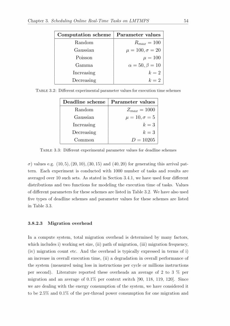
Chapter 3. Scheduling Online Real-Time Tasks on LMTMPS 54
Computation scheme Parameter values
Random Rmax = 100
Gaussian µ = 100, σ = 20
Poisson µ = 100
Gamma α = 50, β = 10
Increasing k = 2
Decreasing k = 2
Table 3.2: Different experimental parameter values for execution time schemes
Deadline scheme Parameter values
Random Zmax = 1000
Gaussian µ = 10, σ = 5
Increasing k = 3
Decreasing k = 3
Common D = 10205
Table 3.3: Different experimental parameter values for deadline schemes
σ) values e.g. (10, 5), (20, 10), (30, 15) and (40, 20) for generating this arrival pat-
tern. Each experiment is conducted with 1000 number of tasks and results are
averaged over 10 such sets. As stated in Section 3.4.1, we have used four different
distributions and two functions for modeling the execution time of tasks. Values
of different parameters for these schemes are listed in Table 3.2. We have also used
five types of deadline schemes and parameter values for these schemes are listed
in Table 3.3.
3.8.2.3 Migration overhead
In a compute system, total migration overhead is determined by many factors,
which includes i) working set size, (ii) path of migration, (iii) migration frequency,
(iv) migration count etc. And the overhead is typically expressed in terms of i)
an increase in overall execution time, (ii) a degradation in overall performance of
the system (measured using loss in instructions per cycle or millions instructions
per second). Literature reported these overheads an average of 2 to 3 % per
migration and an average of 0.1% per context switch [90, 118, 119, 120]. Since
we are dealing with the energy consumption of the system, we have considered it
to be 2.5% and 0.1% of the per-thread power consumption for one migration and

Chapter 3. Scheduling Online Real-Time Tasks on LMTMPS 55
0
20
40
60
80
100
120
140
160
180
200
0 5000 10000 15000 20000 25000 30000 35000 40000 45000
Ins
tan
tan
eo
us
Po
we
r C
on
su
mp
tio
n
Time
(a) FWC
0
20
40
60
80
100
120
140
160
180
200
0 5000 10000 15000 20000 25000 30000 35000 40000 45000
Ins
tan
tan
eo
us
Po
we
r C
on
su
mp
tio
n
Time
(b) RWC
0
20
40
60
80
100
120
140
160
180
200
0 5000 10000 15000 20000 25000 30000 35000 40000 45000
Ins
tan
tan
eo
us
Po
we
r C
on
su
mp
tio
n
Time
(c) UBA
0
20
40
60
80
100
0 5000 10000 15000 20000 25000 30000 35000 40000 45000
Ins
tan
tan
eo
us
Po
we
r C
on
su
mp
tio
n
Time
(d) Smart
Figure 3.9: Instantaneous power consumption verses time under Scheme2(Gaussian) deadline scheme (µ = 40 and σ = 20, and execution scheme is
random)
one preemption respectively. Thus the total overhead increases with their count.
But these overhead were not included for the utilization based scheduling policy
as the policy is mainly of theoretical interest and suffers from an infinitely large
number of preemption and migration (already discussed in Section 3.6).
3.8.3 Instantaneous power consumption
The instantaneous power consumption of the system for different scheduling poli-
cies under deadline scheme 2 (execution scheme is random) is shown in Figure 3.9.
Similarly, Figure 3.10 shows the same for the random execution time scheme with
random deadline scheme. We observe that our proposed policy (Smart) shows an
attractive power consumption behavior as compared to others and we see many
gaps in the power consumption graph (Figures 3.9(d) and 3.10(d)). These gaps
indicate zero instantaneous power consumption value for that time instant. The
Figures also established the fact system does not consume any power until the
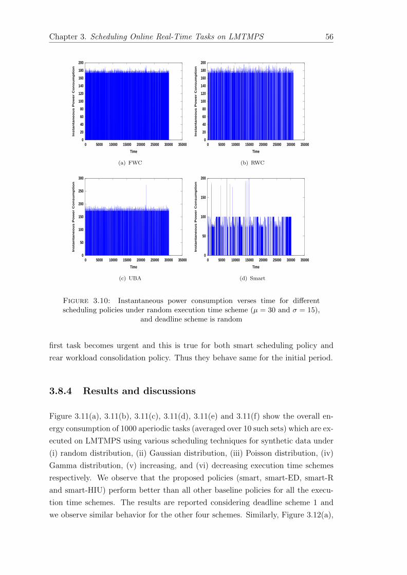
Chapter 3. Scheduling Online Real-Time Tasks on LMTMPS 56
0
20
40
60
80
100
120
140
160
180
200
0 5000 10000 15000 20000 25000 30000 35000
Ins
tan
tan
eo
us
Po
we
r C
on
su
mp
tio
n
Time
(a) FWC
0
20
40
60
80
100
120
140
160
180
200
0 5000 10000 15000 20000 25000 30000 35000
Ins
tan
tan
eo
us
Po
we
r C
on
su
mp
tio
n
Time
(b) RWC
0
50
100
150
200
250
300
0 5000 10000 15000 20000 25000 30000 35000
Ins
tan
tan
eo
us
Po
we
r C
on
su
mp
tio
n
Time
(c) UBA
0
50
100
150
200
0 5000 10000 15000 20000 25000 30000 35000
Ins
tan
tan
eo
us
Po
we
r C
on
su
mp
tio
n
Time
(d) Smart
Figure 3.10: Instantaneous power consumption verses time for differentscheduling policies under random execution time scheme (µ = 30 and σ = 15),
and deadline scheme is random
first task becomes urgent and this is true for both smart scheduling policy and
rear workload consolidation policy. Thus they behave same for the initial period.
3.8.4 Results and discussions
Figure 3.11(a), 3.11(b), 3.11(c), 3.11(d), 3.11(e) and 3.11(f) show the overall en-
ergy consumption of 1000 aperiodic tasks (averaged over 10 such sets) which are ex-
ecuted on LMTMPS using various scheduling techniques for synthetic data under
(i) random distribution, (ii) Gaussian distribution, (iii) Poisson distribution, (iv)
Gamma distribution, (v) increasing, and (vi) decreasing execution time schemes
respectively. We observe that the proposed policies (smart, smart-ED, smart-R
and smart-HIU) perform better than all other baseline policies for all the execu-
tion time schemes. The results are reported considering deadline scheme 1 and
we observe similar behavior for the other four schemes. Similarly, Figure 3.12(a),

Chapter 3. Scheduling Online Real-Time Tasks on LMTMPS 57
0
10
20
30
40
50
60
70
80
(10,5) (20,10) (30,15) (40,20)
En
erg
y C
onsu
mp
tio
n (
in 1
05 u
nits)
Gaussian Parameters
FWCRWCUBAEDF
UBWCSmart
Smart-RSmart-ED
Smart-HIU
(a) Random distribution (Rmax = 100)
0
10
20
30
40
50
60
70
80
(10,5) (20,10) (30,15) (40,20)
En
erg
y C
onsu
mp
tio
n (
in 1
05 u
nits)
Gaussian Parameters
FWCRWCUBAEDF
UBWCSmart
Smart-RSmart-ED
Smart-HIU
(b) Gaussian distribution (µ = 100, σ = 20)
0
10
20
30
40
50
60
70
80
(10,5) (20,10) (30,15) (40,20)
En
erg
y C
onsu
mp
tio
n (
in 1
05 u
nits)
Gaussian Parameters
FWCRWCUBAEDF
UBWCSmart
Smart-RSmart-ED
Smart-HIU
(c) Poisson distribution (µ = 100)
5
6
7
8
9
10
11
12
13
14
(10,5) (20,10) (30,15) (40,20)
En
erg
y C
onsu
mp
tio
n (
in 1
06 u
nits)
Gaussian Parameters
FWCRWCUBAEDF
UBWCSmart
Smart-RSmart-ED
Smart-HIU
(d) Gamma distribution (α = 50, β = 10)
10
12
14
16
18
20
(10,5) (20,10) (30,15) (40,20)
En
erg
y C
onsu
mp
tio
n (
in 1
06 u
nits)
Gaussian Parameters
FWCRWCUBAEDF
UBWCSmart
Smart-RSmart-ED
Smart-HIU
(e) Increasing (k = 2)
10
12
14
16
18
20
(10,5) (20,10) (30,15) (40,20)
En
erg
y C
onsu
mp
tio
n (
in 1
06 u
nits)
Gaussian Parameters
FWCRWCUBAEDF
UBWCSmart
Smart-RSmart-ED
Smart-HIU
(f) Decreasing (k = 2)
Figure 3.11: Energy consumption for different scheduling policies under dif-ferent execution time schemes with random deadline distribution
3.12(b), 3.12(c), 3.12(d) and 3.12(e) show the overall energy consumption of the
system under five different deadline schemes (considering random execution time
scheme). We can clearly observe that the energy consumption under our proposed
policies is significantly lesser than all other baseline policies for all kinds of task
models.

Chapter 3. Scheduling Online Real-Time Tasks on LMTMPS 58
0
10
20
30
40
50
60
70
(10,5) (20,10) (30,15) (40,20)
En
erg
y C
onsu
mp
tio
n (
in 1
05 u
nits)
Gaussian Parameters
UBAFWCRWCEDF
UBWCSmart
Smart-RSmart-ED
Smart-HIU
(a) Randomly distributed deadline
0
10
20
30
40
50
60
70
(10,5) (20,10) (30,15) (40,20)
En
erg
y C
onsu
mp
tio
n (
in 1
05 u
nits)
Gaussian Parameters
UBAFWCRWCEDF
UBWCSmart
Smart-RSmart-ED
Smart-HIU
(b) Gaussianly distributed deadline
0
10
20
30
40
50
60
70
80
(10,5) (20,10) (30,15) (40,20)
En
erg
y C
onsu
mp
tio
n (
in 1
05 u
nits)
Gaussian Parameters
UBAFWCRWCEDF
UBWCSmart
Smart-RSmart-ED
Smart-HIU
(c) Increasing deadline
0
10
20
30
40
50
60
70
(10,5) (20,10) (30,15) (40,20)
En
erg
y C
onsu
mp
tio
n (
in 1
05 u
nits)
Gaussian Parameters
UBAFWCRWCEDF
UBWCSmart
Smart-RSmart-ED
Smart-HIU
(d) Decreasing deadline
0
10
20
30
40
50
60
70
80
(10,5) (20,10) (30,15) (40,20)
En
erg
y C
onsu
mp
tio
n (
in 1
05 u
nits)
Gaussian Parameters
UBAFWCRWCEDF
UBWCSmart
Smart-RSmart-ED
Smart-HIU
(e) Common deadline
0
5
10
15
20
25
30
35
40
MetaCentrum-1 CERIT MetaCentrum-2 Zerua
En
erg
y C
onsu
mp
tio
n (
in 1
06 u
nits)
Workload Traces
UBAFWCRWC
EDFUBWCSmart
Smart-RSmart-ED
Smart-HIU
(f) Real data sets
Figure 3.12: Energy consumption in case of deadline centric synthetic dataand real data sets
The tasks arrive at the system in an online fashion and the inter-arrival time
between two consecutive tasks follows a Gaussian distribution. When the Gaussian
parameter (µ and σ) values are less, inter-arrival time of consecutive tasks is also
less. In such case, our proposed scheduling policy cannot fully utilize the idea
for saving energy. Thus the energy reduction with respect to other scheduling
policies is comparatively lesser. But with an increase in µ and σ values, the

Chapter 3. Scheduling Online Real-Time Tasks on LMTMPS 59
0
10
20
30
40
50
60
70
80
90
Random Gaussian Poisson Gamma Inc Dec
Av
era
ge
Re
du
cti
on
in
EC
(in
%)
Execution Time Schemes
UBAFWCRWCEDF
UBWC
(a) Execution time schemes
40
50
60
70
80
90
Random Gaussian Increasing Decreasing Common
Ave
rag
e R
ed
ucti
on
in
EC
(in
%)
Deadline Schemes
UBAFWCRWCEDF
UBWC
(b) Deadline schemes
Figure 3.13: Average energy reduction of smart policy compared to baselinepolicies for synthetic data
25
30
35
40
45
50
55
60
Smart Smart-R Smart-ED Smart-HIU
Ma
xim
um
Re
du
cti
on
in
EC
(in
%)
Allocation Schemes
UBAFWCRWCEDF
UBCA
(a) Maximum
20
25
30
35
40
45
Smart Smart-R Smart-ED Smart-HIU
Ave
rag
e R
ed
ucti
on
in
EC
(in
%)
Allocation Schemes
UBAFWCRWCEDF
UBCA
(b) Average
Figure 3.14: Energy reduction of proposed policy as compared to baselinepolicies for real-world trace data
time difference also increases. In such case, smart can take full benefit of it. As
the tasks become sparser, energy reduction in smart policy becomes more. The
experimental results also establish our claim that Smart-R and Smart-HIU can
further reduce the energy consumption of the system almost in all the cases. But
the total energy consumption for Smart-ED is same or little higher than Smart.
The motivation behind introducing Smart-ED policy was to avoid the sharp jump
in the power consumption value. As already explained in Section 3.7.2 with an
example, this policy distributes the power consumption value across the time axis.
Figure 3.13(a) shows the average (across Gaussian parameters) energy reduction
of our proposed scheduling technique with respect to the baseline policies for
different execution time schemes. The proposed technique achieves an energy
reduction of 37% (average) as compared to others. Similarly, Figure 3.13(b) shows
the average energy reduction of our proposed scheduling technique with respect

Chapter 3. Scheduling Online Real-Time Tasks on LMTMPS 60
to the baseline policies for different deadline schemes. The proposed technique
achieves an energy reduction of 55% (average) as compared to others. Based
on this experimental result, we can firmly say that our proposed policies reduce
system energy consumption by a significant margin for the synthetic workload
with all the considered variations in execution time and the deadline of tasks.
3.8.5 Experiments with real workload traces
To establish the importance and effectiveness of our work, the experiments were
performed for real-world trace data. The experiments were performed for four
different workloads: MetaCentrum-1, CERIT-SC, MetaCentrum-2 and Zewura
data sets. CERIT-SC and Zewura contain job descriptions of 17900 jobs (same
as tasks) and 17256 jobs respectively. We have considered the execution of all the
jobs for both the CERIT-SC and Zewura workload traces. On the other hand,
MetaCentrum-1 and MetaCentrum-2 workload traces contains job descriptions of
495299 jobs and 103656 job respectively. Since it is relatively difficult to conduct
experiments with such large numbers, we have taken first 15000 jobs in our exper-
iments. Each record contains the job id (represented as task number in our work),
arrival time, execution time along with other information. Deadline of a task is
taken as arrival time + execution time + Rand Int; where Rand Int is a random
integer, varies in the range 0 to 1000.
Energy consumption for real-world trace data under different scheduling policies
is shown in Figure 3.12(f). It is seen that our proposed policies perform signifi-
cantly better than all other policies. Figures 3.14(a) shows the maximum energy
reduction of our proposed smart scheduling policies Smart, Smart-ED, Smart-R
and Smart-HIU with respect to the baseline policies for real workload traces. Our
proposed policies achieve maximum energy reduction up to 44% as compared to
all baseline policies. Similarly 3.14(b) shows the average energy reduction of our
proposed smart scheduling policies as compared others for real workload traces.
The proposed policies achieve energy reduction of 30% (average) as compared to
the baseline policies. Experimental results show that the energy reduction in case
of real workload trace is lesser (compared to synthetic data). This is because the
inter-arrival time among consecutive tasks in case of real-world trace data is lesser
(similar to the case with low µ and σ values) and the smart policy cannot take
the benefit by switching the processors off for a longer time.
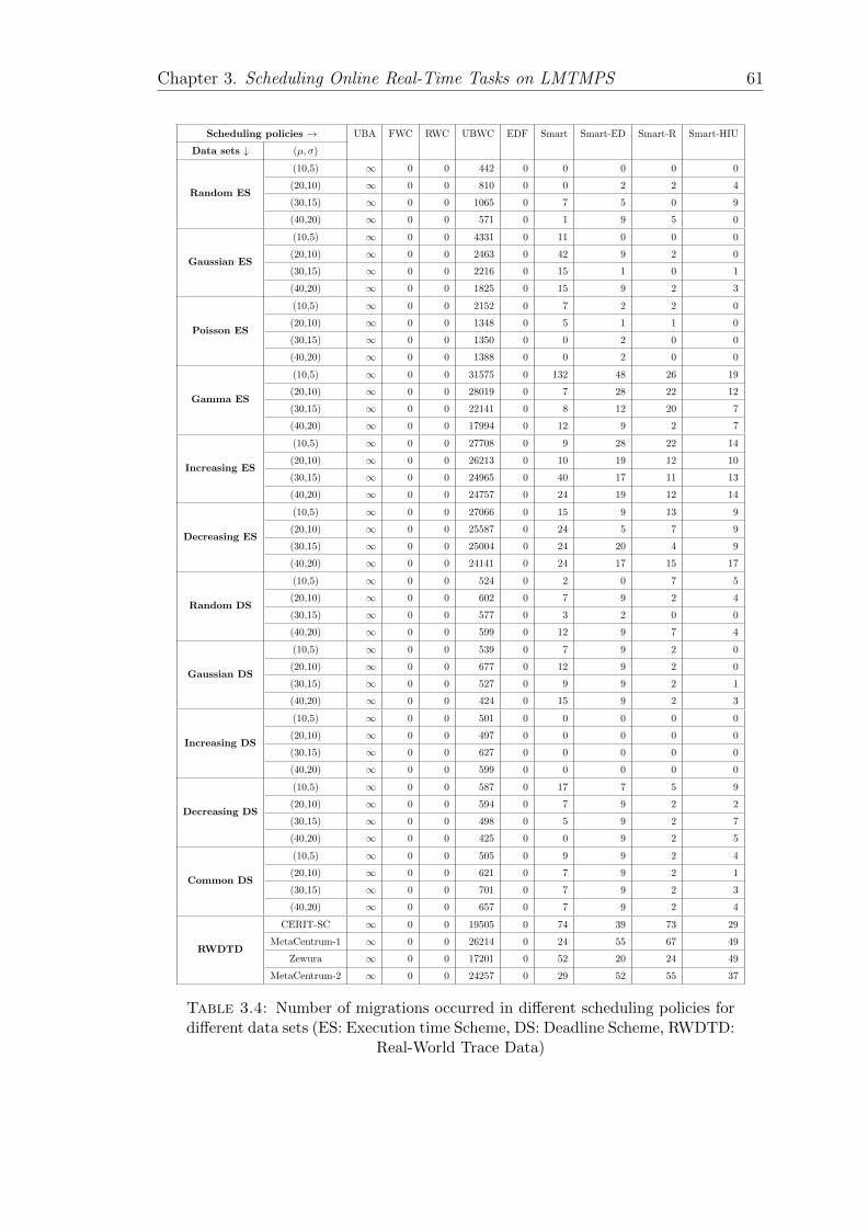
Chapter 3. Scheduling Online Real-Time Tasks on LMTMPS 61
Scheduling policies → UBA FWC RWC UBWC EDF Smart Smart-ED Smart-R Smart-HIU
Data sets ↓ (µ, σ)
Random ES
(10,5) ∞ 0 0 442 0 0 0 0 0
(20,10) ∞ 0 0 810 0 0 2 2 4
(30,15) ∞ 0 0 1065 0 7 5 0 9
(40,20) ∞ 0 0 571 0 1 9 5 0
Gaussian ES
(10,5) ∞ 0 0 4331 0 11 0 0 0
(20,10) ∞ 0 0 2463 0 42 9 2 0
(30,15) ∞ 0 0 2216 0 15 1 0 1
(40,20) ∞ 0 0 1825 0 15 9 2 3
Poisson ES
(10,5) ∞ 0 0 2152 0 7 2 2 0
(20,10) ∞ 0 0 1348 0 5 1 1 0
(30,15) ∞ 0 0 1350 0 0 2 0 0
(40,20) ∞ 0 0 1388 0 0 2 0 0
Gamma ES
(10,5) ∞ 0 0 31575 0 132 48 26 19
(20,10) ∞ 0 0 28019 0 7 28 22 12
(30,15) ∞ 0 0 22141 0 8 12 20 7
(40,20) ∞ 0 0 17994 0 12 9 2 7
Increasing ES
(10,5) ∞ 0 0 27708 0 9 28 22 14
(20,10) ∞ 0 0 26213 0 10 19 12 10
(30,15) ∞ 0 0 24965 0 40 17 11 13
(40,20) ∞ 0 0 24757 0 24 19 12 14
Decreasing ES
(10,5) ∞ 0 0 27066 0 15 9 13 9
(20,10) ∞ 0 0 25587 0 24 5 7 9
(30,15) ∞ 0 0 25004 0 24 20 4 9
(40,20) ∞ 0 0 24141 0 24 17 15 17
Random DS
(10,5) ∞ 0 0 524 0 2 0 7 5
(20,10) ∞ 0 0 602 0 7 9 2 4
(30,15) ∞ 0 0 577 0 3 2 0 0
(40,20) ∞ 0 0 599 0 12 9 7 4
Gaussian DS
(10,5) ∞ 0 0 539 0 7 9 2 0
(20,10) ∞ 0 0 677 0 12 9 2 0
(30,15) ∞ 0 0 527 0 9 9 2 1
(40,20) ∞ 0 0 424 0 15 9 2 3
Increasing DS
(10,5) ∞ 0 0 501 0 0 0 0 0
(20,10) ∞ 0 0 497 0 0 0 0 0
(30,15) ∞ 0 0 627 0 0 0 0 0
(40,20) ∞ 0 0 599 0 0 0 0 0
Decreasing DS
(10,5) ∞ 0 0 587 0 17 7 5 9
(20,10) ∞ 0 0 594 0 7 9 2 2
(30,15) ∞ 0 0 498 0 5 9 2 7
(40,20) ∞ 0 0 425 0 0 9 2 5
Common DS
(10,5) ∞ 0 0 505 0 9 9 2 4
(20,10) ∞ 0 0 621 0 7 9 2 1
(30,15) ∞ 0 0 701 0 7 9 2 3
(40,20) ∞ 0 0 657 0 7 9 2 4
RWDTD
CERIT-SC ∞ 0 0 19505 0 74 39 73 29
MetaCentrum-1 ∞ 0 0 26214 0 24 55 67 49
Zewura ∞ 0 0 17201 0 52 20 24 49
MetaCentrum-2 ∞ 0 0 24257 0 29 52 55 37
Table 3.4: Number of migrations occurred in different scheduling policies fordifferent data sets (ES: Execution time Scheme, DS: Deadline Scheme, RWDTD:
Real-World Trace Data)

Chapter 3. Scheduling Online Real-Time Tasks on LMTMPS 62
3.8.6 Migration count
Table 3.4 shows the number of migrations with different scheduling policies both
for the synthetic dataset and real-world trace data. As already explained earlier,
UBA is of theoretical interest and has an unlimited number of migrations. FWC
and RWC are of non-preemptive nature and do not require any migration but they
lack in the overall energy consumption with respect to the proposed policies. We
have considered a non-preemptive implementation of EDF and thus the number
of migrations, in this case, is also 0. Energy consumption in case of UBWC is
in general lesser than that of UBA, FWC, and RWC but this policy incurs a
significant number of migrations. It can be lucidly seen from the experimental
data that our proposed policies not only reduce overall energy consumption by a
substantial margin, but also the number of migrations in these policies is within
a reasonable range. Thus it can be concluded that even in case of high migration
overhead system, the proposed policies will achieve a significant energy reduction.
3.9 Summary
Recent compute systems comprise of multiple processors and each processor con-
sists of multiple threads within it. Thus the processing capabilities of these systems
are adequate to handle high-end real-time applications. With the increase in the
processing capability of the systems, the energy consumption also increases. As
the real-time applications consume a significant amount of resources, it yields a
significant amount energy consumption and the existing energy-efficient schedul-
ing considering power construct at a lower granularity is not sufficient. Thus the
energy-aware scheduling at a coarser granularity level has become essential for
the large multi-threaded multiprocessor systems. In this work, we have devised
an elegant power consumption model for such large systems with multi-threaded
features in processors and proposed an online energy-efficient task scheduling tech-
nique, namely, smart scheduling policy for executing a set of online independent
aperiodic real-time tasks. We have then proposed three variations of this policy
to reduce the energy consumption further and to efficiently handle different sit-
uations which might occur at runtime. The experimental result shows that our
proposed policies perform significantly better than all other five baseline policies
for both synthetic data sets and real workload traces.

Chapter 4
Scheduling Online Real-Time
Tasks on Virtualized Cloud
This chapter first presents a power consumption model for the cloud system con-
sidering both the static and the dynamic components of it. The model assumes a
nonlinear relationship between the power consumption and the utilization of the
hosts. Then the concept of urgent points of real-time tasks in the context of a
heterogeneous cloud computing environment are introduced. Then the chapter
presents two proposed energy-efficient scheduling approaches, named UPS and
UPS-ES for executing a set of online aperiodic real-time tasks in the virtualized
cloud environment.
4.1 Introduction
In the previous chapter, we considered scheduling a set of real-time tasks in a
non-virtualized computing environment. In this chapter, we consider a virtualized
cloud environment. Virtualization is a popular technique where multiple VMs
of different types and specifications are placed on a physical machine with the
help of virtualizer to improve the resource utilization of the system and thereby
reduces the overall hardware cost. Cloud has emerged as a promising virtualized
computing environment of recent time [121]. Cloud has attracted the users from
various domains by providing exciting features such as the pay-as-you-go pricing
model, scalability, reliability, etc. As the demand for the cloud system increase,
several companies have also started to render the service. Cloud system not only
provides exciting features to its user, it also offers similar features to the service
63

Chapter 4. Scheduling Online Real-Time Tasks on Virtualized Cloud 64
70
80
90
100
110
120
130
140
0 20 40 60 80 100
Po
we
r c
on
su
mp
tio
n (
Wa
tts
)
CPU utilization
Range IIIRange IIRange I
Figure 4.1: Power consumption of a server versus the utilization of the hostas reported in [4]
providers. Elasticity is one of the feature where VM can be added to and removed
from the hosts seamlessly as and when required by the service providers to meet
the user’s need [121, 63].
Cloud has proved itself as a perfect platform for various high-end scientific ap-
plications [27, 30]. These applications exhibit a unique characteristic, that is the
variation of their resource requirements. However, traditional computing plat-
forms, such as grid and clusters are not adequate to handle such high resource
intensive applications and the variation in their resource requirement. Thus the
cloud is proved to be a promising computing platform to meet the demand of these
applications [27, 24].
To support the high demand at times, the cloud systems are over-provisioned with
resources. It is observed that one of the major reason for high energy consumption
is the poor utilization of the hosts. As the scheduling deals with the utilization of
the host and it impacts the overall performance of the system, energy consumption
has become one of the major optimality criteria of scheduling. These are termed
as energy-efficient scheduling or power-aware scheduling [75, 122]. Each physical
machine hosts a number of virtual machines (VM) and the VMs executes user
tasks. These VMs are of different types, sizes, and capacities. Thus the execution
time of a task depends on the VM which runs it. In this work, we consider
scheduling of real-time tasks and completing their execution before the deadline
is essential.
We address two conflicting parameters regarding the energy consumption of a
host in the cloud system. The first parameter is the utilization of the hosts, and
the second parameter is the number of active hosts. With an increase in the

Chapter 4. Scheduling Online Real-Time Tasks on Virtualized Cloud 65
utilization, the temperature of the system increases. It is reported in [60] that
with an increase in every 10◦C in temperature, the failure rate of an electronic
device doubles. Thus the first parameter puts a restriction on the utilization of
the hosts. As the utilization of the hosts moves above some threshold value, the
performance of the VMs starts getting deteriorated [108, 88]. Thus to maintain
the performance of the system, hosts should not be overloaded, and that implies
that their utilization should be kept below some threshold value. On the contrary,
to save the energy consumption, we should use the minimum number of hosts in
the system. In order to minimize the active host count, the utilization of the hosts
should be kept high.
Now, if we observe the power consumption pattern of the servers, we see an inter-
esting pattern. Dayarathna et al. [48] presented a survey paper which contains the
description of several power models. The power consumption of a host is typically
expressed as a function of host utilization, frequency, VM power consumption, etc.
Lien et al. [4] presented a nice study and measured the power consumption of the
server for six different workloads. As per their study, the power consumption varies
non-linearly with utilization. Figure 4.1 shows the power consumption of a server
versus the host utilization as reported in [4]. We can roughly divide the graph
in three ranges, where utilization varies: (i) 0% to 40% (denoted as Range-I), (ii)
40% to 70% (denoted as Range-II), and (iii) 70% to 100% (denoted as Range-III).
We can observe that when the host is switched on, it consumes 70W of power.
Then the power consumption increase rate is less with respect to the utilization of
Range-I. In case of Range-II, the increase rate is more than Range-I but not too
high. The increase is significantly high in case of Range-III. To the best of our
knowledge, the existing energy-efficient scheduling algorithms of real-time tasks
for the cloud computing domain do not sufficiently consider this interesting power
consumption behavior of the hosts.
We can now interestingly link the “restriction on the utilization of hosts” and “the
power consumption behavior of the servers” together in scheduling. We define a
threshold on the utilization of the host when the power consumption takes a sharp
jump from Range-II to Range-III. The target of the scheduler is to usually keep
the host at this utilization (in between Range-I and Range-II). This will prevent
the system from performance degradation as we are not utilizing 100% of the
computing resources of the hosts. On the other hand, we are dealing with real-
time tasks and meeting the deadline of the tasks is a must. Thus we allow the
hosts to accommodate more tasks (i.e. VMs) and to exceed the threshold when it
becomes necessary to meet task deadline.
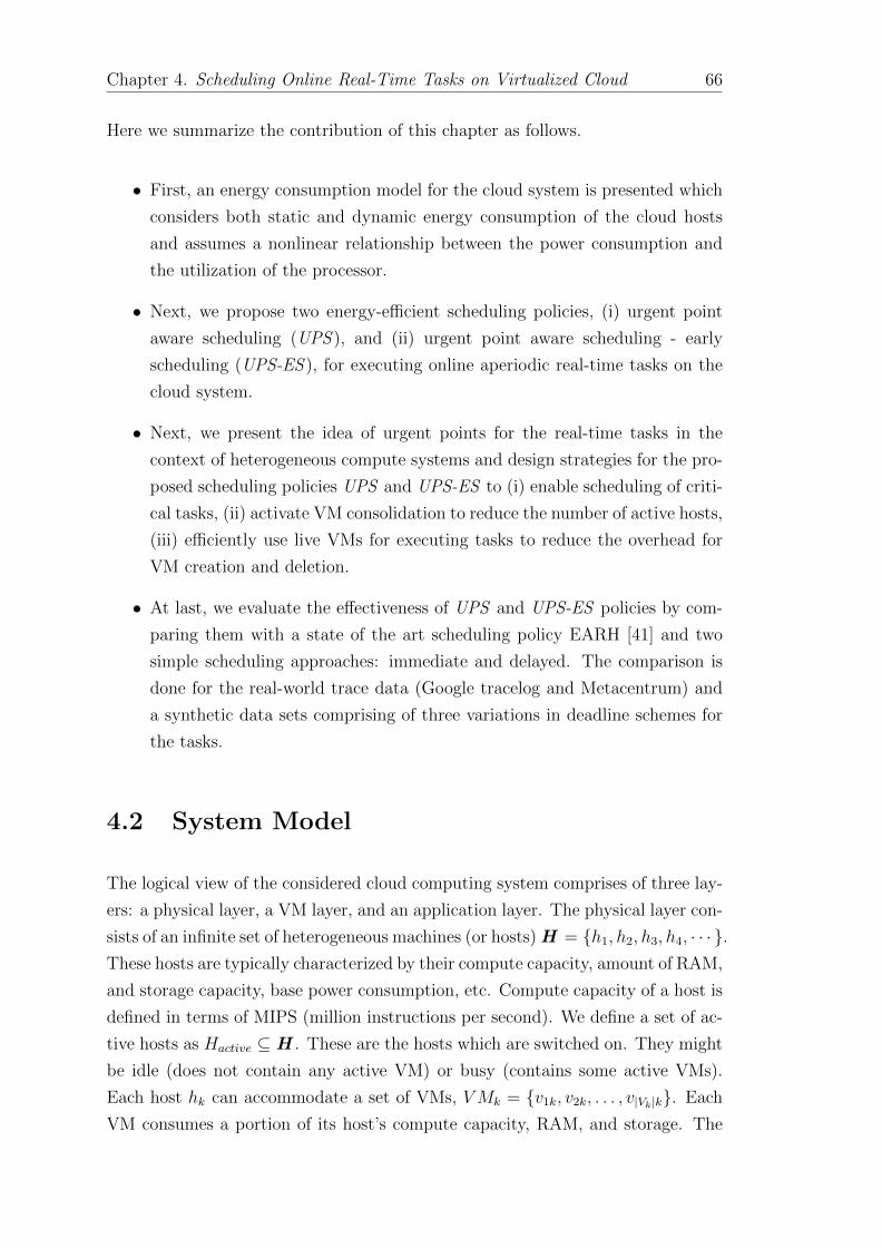
Chapter 4. Scheduling Online Real-Time Tasks on Virtualized Cloud 66
Here we summarize the contribution of this chapter as follows.
• First, an energy consumption model for the cloud system is presented which
considers both static and dynamic energy consumption of the cloud hosts
and assumes a nonlinear relationship between the power consumption and
the utilization of the processor.
• Next, we propose two energy-efficient scheduling policies, (i) urgent point
aware scheduling (UPS ), and (ii) urgent point aware scheduling - early
scheduling (UPS-ES ), for executing online aperiodic real-time tasks on the
cloud system.
• Next, we present the idea of urgent points for the real-time tasks in the
context of heterogeneous compute systems and design strategies for the pro-
posed scheduling policies UPS and UPS-ES to (i) enable scheduling of criti-
cal tasks, (ii) activate VM consolidation to reduce the number of active hosts,
(iii) efficiently use live VMs for executing tasks to reduce the overhead for
VM creation and deletion.
• At last, we evaluate the effectiveness of UPS and UPS-ES policies by com-
paring them with a state of the art scheduling policy EARH [41] and two
simple scheduling approaches: immediate and delayed. The comparison is
done for the real-world trace data (Google tracelog and Metacentrum) and
a synthetic data sets comprising of three variations in deadline schemes for
the tasks.
4.2 System Model
The logical view of the considered cloud computing system comprises of three lay-
ers: a physical layer, a VM layer, and an application layer. The physical layer con-
sists of an infinite set of heterogeneous machines (or hosts) H = {h1, h2, h3, h4, · · · }.These hosts are typically characterized by their compute capacity, amount of RAM,
and storage capacity, base power consumption, etc. Compute capacity of a host is
defined in terms of MIPS (million instructions per second). We define a set of ac-
tive hosts as Hactive ⊆ H . These are the hosts which are switched on. They might
be idle (does not contain any active VM) or busy (contains some active VMs).
Each host hk can accommodate a set of VMs, VMk = {v1k, v2k, . . . , v|Vk|k}. Each
VM consumes a portion of its host’s compute capacity, RAM, and storage. The

Chapter 4. Scheduling Online Real-Time Tasks on Virtualized Cloud 67
portion of the resources assigned to a VM does not get changed during its lifetime.
Moreover, we consider a fully elastic cloud where VMs can be dynamically added
and removed from the hosts based on the requirement.
When a VM executes a task, it consumes a portion of the resources of the physical
machine it is hosted on. Each VM vjk (jth VM on kth host) has some compute
capacity (expressed in MIPS) and it represented as CP (vjk). Thus the VMs are
of heterogeneous nature (specially, in their compute capacity and power consump-
tion). For simplicity, we assume that the compute capacity of the VMs lie within a
range:[minCP,maxCP
]. The minCP and maxCP indicates the minimum and
maximum compute capacity of the VMs respectively. Without any loss of gener-
ality, we assume that the utilization associated with an active VM (running some
task) is proportional to its compute capacity. For, a VM vjk, the corresponding
utilization ujk can be expressed as
ujk =CP (vjk)
CP (hk)× 100 % (4.1)
where CP (hk) is the compute capacity of the host hk.
As the VM finishes the task assigned to it, it becomes idle and the corresponding
utilization of the VM becomes negligible and we ignore this in our work. We
further assume that a VM hosted on one host can be migrated to another host if
required.
4.3 Task Model
In our work, we consider a set of online aperiodic independent real-time tasks,
T = {t1, t2, t3, · · · }. Each task ti is characterized by three-tuple (ai, li, di) where
ai is the arrival time, li is the length, and di is the deadline of the task. The length
of the tasks is expressed in million instructions (MI). All the tasks are assumed to
be sequential and uni-VM, that is, a task is executed by only one VM. We assume
that the inter-arrival time of the tasks follows the Poisson distribution.
Suppose a task ti is executed by a VM vjk. Then, the task requires li/CP (vjk)
amount time for its completion. This becomes the execution time of task ti on
VM vjk and it is represented by eijk. Mathematically, it can be written as:

Chapter 4. Scheduling Online Real-Time Tasks on Virtualized Cloud 68
eijk =li
CP (vjk)(4.2)
We define the ready time of a VM, rt(vj,k) as:
rt(vjk) = st(vjk) + eijk (4.3)
where, st(vjk) is the start time of the VM which indicates the time instant when
the VM vjk has started executing the task ti.
We define a VM vjk as a candidate VM for executing a task ti if the following
condition is satisfied.
rt(vjk) ≤ di − eijk (4.4)
Now we introduce maximum execution time (etmax(ti)) and minimum execution
time (etmin(ti)) of a task ti as follows.
etmax(ti) =li
minCP; etmin(ti) =
li
maxCP(4.5)
Then slack of a task can be defined as slk(ti) = di − etmax(ti)− ai.
We assume the task sets with three different types of deadline schemes: Random,
Tight, and Relax. In Random deadline scheme, the slack of the tasks are
generated from a random distribution; where slk(ti) varies in the range from Rmin
to Rmax. In case of Tight deadline scheme, the time difference between the
deadline and execution time of the task is short. This can be written as: slk(ti) ≤Dmax. In Relax deadline scheme, the time difference between the deadline and
execution time of task is long; where slk(ti) ≥ Dmin. Here, Rmin, Rmax, Dmin, and
Dmax are user defined deadline threshold values.

Chapter 4. Scheduling Online Real-Time Tasks on Virtualized Cloud 69
4.4 Energy Consumption Model
A cloud computing system comprises various components, such as the computation
nodes, storage, network equipment, etc. Out of these components, the major
portion of the power is drowned by the computation node, i.e., the host. Thus, in
this work, we consider the energy consumption model of the host only. The power
consumption of a host has two parts: static power consumption and dynamic
power consumption. A significant amount of research in the area of real-time task
scheduling considered only the dynamic power consumption [33, 30, 52, 67]. But
static power consumption plays the vital role, and it contributes almost 60% to
70% of the total power consumption [45, 43]. Thus in our work, we consider both
static and dynamic power consumption of the hosts of the cloud system. The
summation of the power consumption over the total time interval produces the
energy consumption of the system. Thus, it can be written as, E =∫∞t=0
PCt.dt,
where PCt is the total instantaneous power consumption of the system at time t.
Now, the power consumption of a host is expressed as a function of its total
utilization. For a host hk, at any time instant, the total utilization Uk is defined
as
Uk =
VMk∑j=1
ujk (4.6)
where, ujk is the resource utilization of the VM vjk.
As mentioned in the Section 4.1 and reported in Figure 4.1, we have considered
three different ranges for the power consumption of a host and this can be written
as
Ptotal = Pstatic + α1 × Uk, if Uk ≤ 40% (in Range-I)
= Pstatic + α2 × Uk, if 40% < Uk ≤ 70% (in Range-II)
= Pstatic + α3 × Uk, if Uk > 70% (in Range-III)
(4.7)

Chapter 4. Scheduling Online Real-Time Tasks on Virtualized Cloud 70
where, α3 > α2 > α1 and α3 > (α1 + α2)
Now, the energy consumption of a host can be expressed as
Ehk =
∫ ∞t=0
Ptotal · dt (4.8)
Thus the energy consumption of the cloud system can be expressed as
Etotal =
|Hactive|∑k=1
Ehk (4.9)
As demonstrated in the Figure 4.1 and formulated in the Equation 4.7, the slope
of the power function is much higher when the utilization of the host moves above
70%. Keeping this into consideration, we have used two threshold values THU1 and
THU2 in our work. THU1 indicates the boundary of the second region (i.e., when
the utilization of the host moves above 70%) and THU2 indicates the maximum
permissible utilization for a host which is taken as 100%. Usages of these thresholds
are described in the Section 4.6.
The power consumption model indicated by Equation 4.7 used in our work assumes
that there is a local power optimization module (DVFS or DPM) at each host.
The local optimization module at a host controls the frequency and the sleep slate
the compute system which may have more then one compute components. As a
whole, the power consumption is depended on the utilization of the host. We can
safely assume that whenever the host runs at the highest utilization, it is running
at its highest capable frequency of operation, and the frequency of operation of a
host is proportional to the utilization of the host.
4.5 Objective in the Chapter
In this chapter, we wish to design energy-efficient scheduling policies for online ape-
riodic independent real-time tasks for the virtualized cloud system (as described
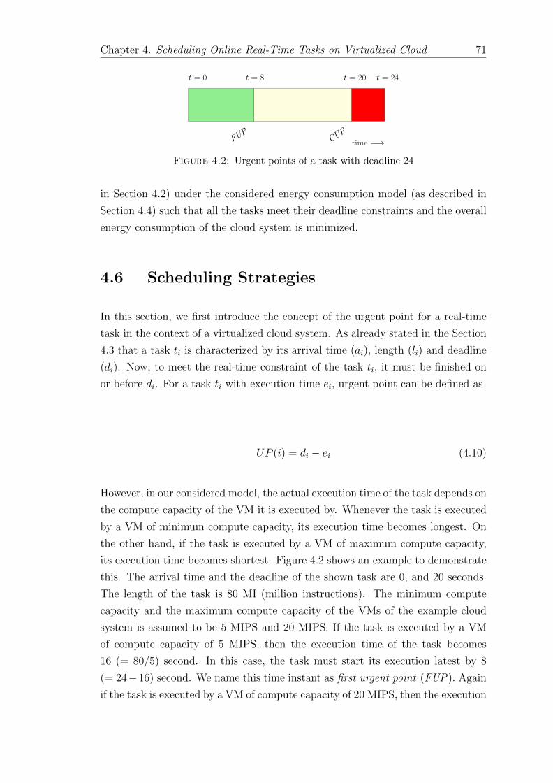
Chapter 4. Scheduling Online Real-Time Tasks on Virtualized Cloud 71
FUP
CUP
t = 0 t = 8 t = 20 t = 24
time −→
Figure 4.2: Urgent points of a task with deadline 24
in Section 4.2) under the considered energy consumption model (as described in
Section 4.4) such that all the tasks meet their deadline constraints and the overall
energy consumption of the cloud system is minimized.
4.6 Scheduling Strategies
In this section, we first introduce the concept of the urgent point for a real-time
task in the context of a virtualized cloud system. As already stated in the Section
4.3 that a task ti is characterized by its arrival time (ai), length (li) and deadline
(di). Now, to meet the real-time constraint of the task ti, it must be finished on
or before di. For a task ti with execution time ei, urgent point can be defined as
UP (i) = di − ei (4.10)
However, in our considered model, the actual execution time of the task depends on
the compute capacity of the VM it is executed by. Whenever the task is executed
by a VM of minimum compute capacity, its execution time becomes longest. On
the other hand, if the task is executed by a VM of maximum compute capacity,
its execution time becomes shortest. Figure 4.2 shows an example to demonstrate
this. The arrival time and the deadline of the shown task are 0, and 20 seconds.
The length of the task is 80 MI (million instructions). The minimum compute
capacity and the maximum compute capacity of the VMs of the example cloud
system is assumed to be 5 MIPS and 20 MIPS. If the task is executed by a VM
of compute capacity of 5 MIPS, then the execution time of the task becomes
16 (= 80/5) second. In this case, the task must start its execution latest by 8
(= 24−16) second. We name this time instant as first urgent point (FUP). Again
if the task is executed by a VM of compute capacity of 20 MIPS, then the execution
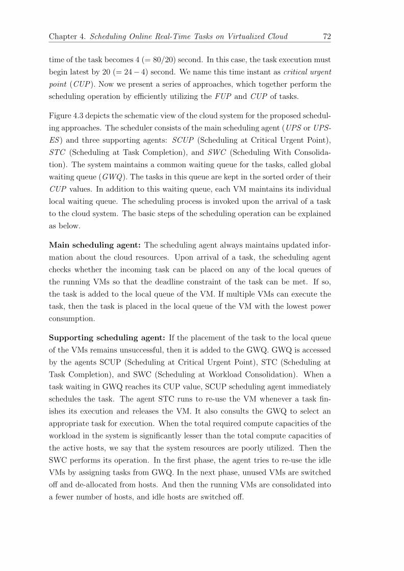
Chapter 4. Scheduling Online Real-Time Tasks on Virtualized Cloud 72
time of the task becomes 4 (= 80/20) second. In this case, the task execution must
begin latest by 20 (= 24− 4) second. We name this time instant as critical urgent
point (CUP). Now we present a series of approaches, which together perform the
scheduling operation by efficiently utilizing the FUP and CUP of tasks.
Figure 4.3 depicts the schematic view of the cloud system for the proposed schedul-
ing approaches. The scheduler consists of the main scheduling agent (UPS or UPS-
ES ) and three supporting agents: SCUP (Scheduling at Critical Urgent Point),
STC (Scheduling at Task Completion), and SWC (Scheduling With Consolida-
tion). The system maintains a common waiting queue for the tasks, called global
waiting queue (GWQ). The tasks in this queue are kept in the sorted order of their
CUP values. In addition to this waiting queue, each VM maintains its individual
local waiting queue. The scheduling process is invoked upon the arrival of a task
to the cloud system. The basic steps of the scheduling operation can be explained
as below.
Main scheduling agent: The scheduling agent always maintains updated infor-
mation about the cloud resources. Upon arrival of a task, the scheduling agent
checks whether the incoming task can be placed on any of the local queues of
the running VMs so that the deadline constraint of the task can be met. If so,
the task is added to the local queue of the VM. If multiple VMs can execute the
task, then the task is placed in the local queue of the VM with the lowest power
consumption.
Supporting scheduling agent: If the placement of the task to the local queue
of the VMs remains unsuccessful, then it is added to the GWQ. GWQ is accessed
by the agents SCUP (Scheduling at Critical Urgent Point), STC (Scheduling at
Task Completion), and SWC (Scheduling at Workload Consolidation). When a
task waiting in GWQ reaches its CUP value, SCUP scheduling agent immediately
schedules the task. The agent STC runs to re-use the VM whenever a task fin-
ishes its execution and releases the VM. It also consults the GWQ to select an
appropriate task for execution. When the total required compute capacities of the
workload in the system is significantly lesser than the total compute capacities of
the active hosts, we say that the system resources are poorly utilized. Then the
SWC performs its operation. In the first phase, the agent tries to re-use the idle
VMs by assigning tasks from GWQ. In the next phase, unused VMs are switched
off and de-allocated from hosts. And then the running VMs are consolidated into
a fewer number of hosts, and idle hosts are switched off.

Chapter 4. Scheduling Online Real-Time Tasks on Virtualized Cloud 73
Scheduling Agent
.....
h
h
h
1
3
2
Status Info.
Global Queue
SWCSTCSCUP
User tasks ( UPS / UPS−ES )
Figure 4.3: Schematic representation of the cloud system for the proposedscheduling polices
4.6.1 Urgent point aware scheduling (UPS)
Algorithm 2 shows the pseudocode of the UPS policy. This algorithm acts as a
scheduling agent which runs on the arrival of a task to the cloud system. Once a
task arrives at the system, the scheduling policy first checks whether the running
VMs on the system can execute the task. A set of eligible VMs (candidateVMSet
in the pseudocode) are listed which can meet the deadline constraint of the task
maintaining the utilization threshold of the corresponding host below THU1. The
target of the policy is to keep the utilization of the hosts close to THU1. If an
existing VM can execute the task satisfying its deadline constraint, then the task
is placed in the local queue of the VM. In case, multiple VMs can execute the
task, the policy selects the VM with the least energy consumption. Line numbers
4 to 9 of the Algorithm 2 represents these steps. If the attempt fails, then the
task is added to the global waiting queue (GWQ). The scheduling window of the
task is set as: [FUP (ti), CUP (ti)]; where FUP (ti) is the first urgent point of
the task, and CUP (ti) is the critical urgent point of the task. This means that
the task can be scheduled at any time instant from FUP (ti) to CUP (ti). Once
the tasks are added to GWQ (if current system state cannot handle) under this
scheduling policy, they can be further handled by policies which scan the queue.
These policies are described in the Sections 4.6.1.1, 4.6.1.2 and 4.6.1.3. The target
of UPS scheduling policy is to delay the execution of an incoming task if the
current system state cannot execute the task energy-efficiently.

Chapter 4. Scheduling Online Real-Time Tasks on Virtualized Cloud 74
Algorithm 2 Urgent Point aware Scheduling (UPS)
On arrival of a task ti(ai, li, di)
1: Calculate the FUP (ti) and CUP (ti)2: findVMFlag ← FALSE3: Find the candidateVMset for the task maintaining host utilization thresholdTHU1
4: if candidateVMset is not NULL then5: Select the VM such that host utilization remains closest to THU1
(best fit policy)6: if Multiple VM exists then Select the VM with least power consumption
7: Schedule the task ti at current ready time of the VM8: Update ready time of the VM9: findVMFlag ← TRUE
10: if findVMFlag = FALSE then11: Add the task to GWQ12: Set the scheduling window for the task: [FUP (ti), CUP (ti)]
4.6.1.1 Scheduling at urgent critical point (SCUP)
Algorithm 3 shows the pseudocode for scanning the GWQ looking for the tasks
whose CUP is reached. The tasks in GWQ are sorted based on their deadline.
If such a task is found. the scheduler first checks whether there is any idle VM
in the system and whether the VM is a candidate for the task. If such VM
exists, the scheduler selects the VM with the least energy consumption. If no
such VM exists, then a new VM with the minimum required compute capacity is
created and the VM is tried to place on an active host. As the task is critically
urgent, we allow the host utilization to go up to THU2. If multiple active hosts can
accommodate the VM, the scheduler selects the VM such that the utilization of the
host after addition of the VM remains close to threshold THU1. If an active host
can accommodate the VM, then it is placed on the host, and the task is assigned
to the VM. If the scheduler fails to find a host, then a consolidation operation is
performed on the active set of hosts to create sufficient space (i.e., utilization) for
the new VM. The algorithm achieves this via a procedure call to createSpace().
The pseudocode for createSpace() is shown using the Procedure creatSpace(). The
procedure migrates VMs from lowly utilized hosts to the highly utilized hosts. The
procedure returns the host once it gets a host which can accommodate the VM.
Until this point, the scheduler tried to get a host from the active set only. If it
fails, then a new host is switched on and then it is added to the list of the active
set of hosts. After the task is assigned to the VM and the VM is placed on the
host, the scheduler then fills the remaining utilization of the newly switched-on

Chapter 4. Scheduling Online Real-Time Tasks on Virtualized Cloud 75
Algorithm 3 Scheduling at Critical Urgent Point (SCUP )
1: for each task ti in GWQ do2: if currentT ime = CUP (ti) then3: findVMFlag ← FALSE4: if any idle VM in the system can execute the task then5: Assign the task to the VM6: Update the ready time of the VM7: findVMFlag ← TRUE
8: if findVMFlag = FALSE then9: Create a VM, v with minimum required compute capacity so that
the deadline constraint of the task is met10: Choose the host from Ha such that after the addition of the VM
its utilization is close to threshold THU1
(if multiple hosts exist)11: if Success then12: Assign the task to the VM and place the VM on the host13: Update the ready time of the VM14: findVMFlag ← TRUE
15: if findVMFlag = FALSE then16: hk ← createSpace(v)17: if hk is not NULL then18: Assign the task to the VM and place the VM on the host19: Update the ready time of the VM20: findVMFlag ← TRUE
21: if findVMFlag = FALSE then22: Start a new host hk23: Place the VM on the host and assign the task to the VM24: Set ready time of the VM25: Call procedure fillHost(hk)
26: end for
processor by placing new VMs on it. Procedure fillHost() shows the pseudocode
for this. The process of VM placement is repeated until the utilization of the host
reaches the target utilization threshold THU1.
4.6.1.2 Scheduling at task completion (STC )
As the tasks are assigned to the VMs and the executions start, the mapping
remains the same and eventually, the tasks finish their executions and the corre-
sponding VMs become idle. Now the motivation of the scheduler is to re-use the
VMs for executing the other tasks. Algorithm 4 shows the pseudocode for this

Chapter 4. Scheduling Online Real-Time Tasks on Virtualized Cloud 76
1: procedure createSpace(v)2: Sort the active host set Ha in increasing order of their utilization3: migrationF lag ← FALSE;4: sourceHost← NULL5: for each host hk in Ha do6: Find the VM vj with least utilization in hk s.t. it can accommodate
v after removal of vj7: for each host hi in Ha (considered in descending order) do8: if hi can accommodate vj then9: Perform the migration of VM vj from host hk to hi
10: return hk11: end for12: end for13: return NULL14: end procedure
1: procedure fillHost(hk)2: Set the utilization threshold of the host hk as THU1
3: while Uk < THU1 do4: Calculate the maximum possible MIPS for the remaining host
utilization5: Scan GWQ and find the feasible set of tasks for this6: Choose the task with closest CUP value7: Create a VM with required compute capacity for executing the task8: Set the ready time of the VM
9: end procedure
Algorithm 4 Scheduling at Task Completion (STC)
On completion of a task ti
1: Get the corresponding VM v and its compute capacity CP (v)2: Scan through the GWQ and find a task tj so that currentT ime lies in the
scheduling window and v is a candidate VM for the task and the requiredcompute capacity is close to CP (v)
3: if Successful then4: Assign the task tj to the VM5: Update the ready time of the VM
operation. This algorithm runs whenever a task finishes its execution. The algo-
rithm runs through GWQ and finds the task which best fits the compute capacity
of the VM released by the completed task.
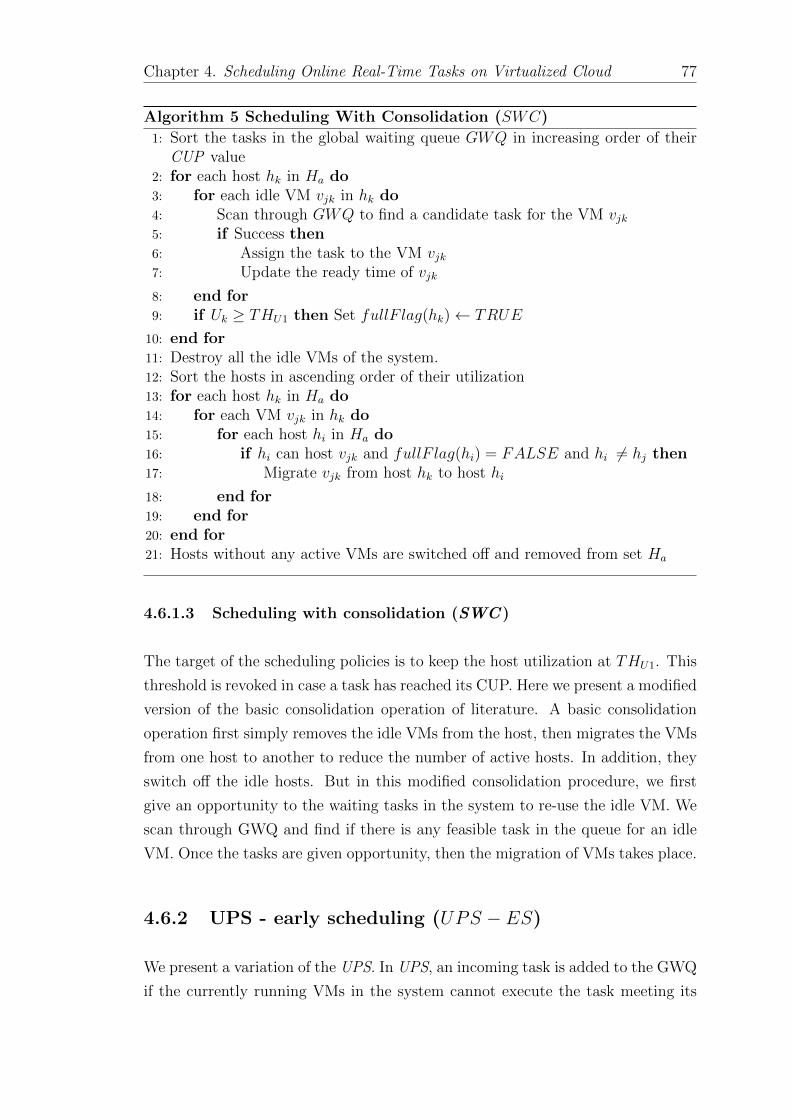
Chapter 4. Scheduling Online Real-Time Tasks on Virtualized Cloud 77
Algorithm 5 Scheduling With Consolidation (SWC)
1: Sort the tasks in the global waiting queue GWQ in increasing order of theirCUP value
2: for each host hk in Ha do3: for each idle VM vjk in hk do4: Scan through GWQ to find a candidate task for the VM vjk5: if Success then6: Assign the task to the VM vjk7: Update the ready time of vjk
8: end for9: if Uk ≥ THU1 then Set fullF lag(hk)← TRUE
10: end for11: Destroy all the idle VMs of the system.12: Sort the hosts in ascending order of their utilization13: for each host hk in Ha do14: for each VM vjk in hk do15: for each host hi in Ha do16: if hi can host vjk and fullF lag(hi) = FALSE and hi 6= hj then17: Migrate vjk from host hk to host hi
18: end for19: end for20: end for21: Hosts without any active VMs are switched off and removed from set Ha
4.6.1.3 Scheduling with consolidation (SWC )
The target of the scheduling policies is to keep the host utilization at THU1. This
threshold is revoked in case a task has reached its CUP. Here we present a modified
version of the basic consolidation operation of literature. A basic consolidation
operation first simply removes the idle VMs from the host, then migrates the VMs
from one host to another to reduce the number of active hosts. In addition, they
switch off the idle hosts. But in this modified consolidation procedure, we first
give an opportunity to the waiting tasks in the system to re-use the idle VM. We
scan through GWQ and find if there is any feasible task in the queue for an idle
VM. Once the tasks are given opportunity, then the migration of VMs takes place.
4.6.2 UPS - early scheduling (UPS − ES)
We present a variation of the UPS. In UPS, an incoming task is added to the GWQ
if the currently running VMs in the system cannot execute the task meeting its

Chapter 4. Scheduling Online Real-Time Tasks on Virtualized Cloud 78
Algorithm 6 Urgent Point aware Scheduling - Early Scheduling (UPS−ES)
On arrival of a task ti(ai, li, di)
1: Find the candidateVMset-I for the task maintaining host utilizationthreshold THU1
2: if candidateVMset-I is not NULL then3: Select the VM such that host utilization remains closest to THU1
(best fit policy)4: if Multiple VM exists then Select the VM with least power consumption
5: Schedule the task ti at current ready time of the VM6: Update ready time of the VM7: findVMFlag ← TRUE
8: if (FUP (ti)− currentT ime) < THVMCDT then9: Find the candidateVMset-II for the task considering host utilization
THU2
10: if candidateVMset-II is not NULL then11: Select the VM with minimal power consumption12: Schedule the task ti at current ready time of the VM13: Update ready time of the VM14: findVMFlag ← TRUE15: else16: Start a new host hk17: create a new VM vjk on hk with minimal compute capacity such that
the task deadline can be met18: Place the VM on the host and assign the task to the VM19: Set ready time of the VM20: Call procedure fillHost(hk)
21: else22: Add the task to the Global Waiting Queue Q23: Set the scheduling window for the task: [FUP (ti), CUP (ti)]
deadline constraint. But in this policy, we first check whether the deadline of the
incoming task is close. The policy first tries to put an incoming task to the local
queue of an existing VM if the VM can execute satisfying the deadline constraint
of the task. This step is similar to that of policy UPS. If this step fails, then
the scheduling policy checks whether the deadline of the task is near. If yes, then
the policy tries to schedule the task by allowing the host utilization to go up
to the next threshold level THU2. We determine the nearness by comparing the
difference between the FUP and the current time with a pre-defined threshold
THVMCDT . We take the value of the threshold THVMCDT as the summation of
the creation time and the deletion time of a VM. If the occurrence of the FUP is
not near, then the scheduler puts the task to GWQ with the scheduling window
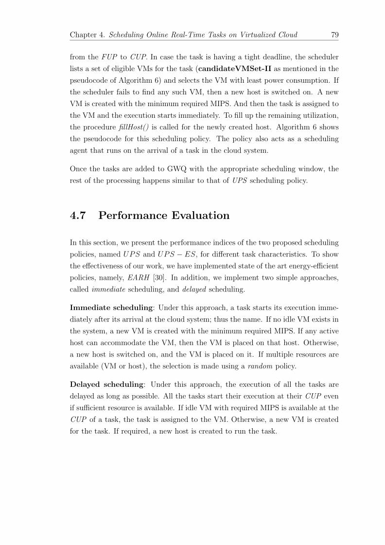
Chapter 4. Scheduling Online Real-Time Tasks on Virtualized Cloud 79
from the FUP to CUP. In case the task is having a tight deadline, the scheduler
lists a set of eligible VMs for the task (candidateVMSet-II as mentioned in the
pseudocode of Algorithm 6) and selects the VM with least power consumption. If
the scheduler fails to find any such VM, then a new host is switched on. A new
VM is created with the minimum required MIPS. And then the task is assigned to
the VM and the execution starts immediately. To fill up the remaining utilization,
the procedure fillHost() is called for the newly created host. Algorithm 6 shows
the pseudocode for this scheduling policy. The policy also acts as a scheduling
agent that runs on the arrival of a task in the cloud system.
Once the tasks are added to GWQ with the appropriate scheduling window, the
rest of the processing happens similar to that of UPS scheduling policy.
4.7 Performance Evaluation
In this section, we present the performance indices of the two proposed scheduling
policies, named UPS and UPS − ES, for different task characteristics. To show
the effectiveness of our work, we have implemented state of the art energy-efficient
policies, namely, EARH [30]. In addition, we implement two simple approaches,
called immediate scheduling, and delayed scheduling.
Immediate scheduling: Under this approach, a task starts its execution imme-
diately after its arrival at the cloud system; thus the name. If no idle VM exists in
the system, a new VM is created with the minimum required MIPS. If any active
host can accommodate the VM, then the VM is placed on that host. Otherwise,
a new host is switched on, and the VM is placed on it. If multiple resources are
available (VM or host), the selection is made using a random policy.
Delayed scheduling: Under this approach, the execution of all the tasks are
delayed as long as possible. All the tasks start their execution at their CUP even
if sufficient resource is available. If idle VM with required MIPS is available at the
CUP of a task, the task is assigned to the VM. Otherwise, a new VM is created
for the task. If required, a new host is created to run the task.

Chapter 4. Scheduling Online Real-Time Tasks on Virtualized Cloud 80
Parameter ValuesTask count 10, 000Task length (MI) Randomly distributed from 10, 000 to 100, 000Task arrival λ = 10, 20, 50Deadline parameters Rmin = 100, Rmax = 1000, Dmax = 200, Dmin = 1000Thresholds THU1 = 70%, THU2 = 100%Compute capacities:Host 1000, 1500, 2000 (MIPS)Compute capacities:VM minCP = 100, maxCP = 500 (MIPS)
Table 4.1: Different experimental parameter values
4.7.1 Simulation environment and parameter setup
To evaluate the performance of our scheduling policies, a set of comprehensive
simulations and experiments are conducted using cloudSim toolkit [123]. We have
made necessary changes in the simulator to include different parameters. Table
4.1 lists the important parameters along with their considered value for our ex-
periments. We have performed the experiments for 10, 000 tasks and considered
three different deadline schemes. Length of the tasks is expressed in million in-
structions (MI). The experiments are performed for 10 such sets to minimize the
system error, and the average result is reported in the following section.
4.7.2 Experiments with synthetic data
Figure 4.4 shows the overall energy consumption (normalized) of 10, 000 aperiodic
real-time tasks (averaged over 10 such sets) when executed in the simulated cloud
environment. The results were produced for two different values of arrival param-
eter, λ = 10, λ = 20, and λ = 50. Figures show the energy consumption for three
different types of deadline schemes: Random, Tight, and Relax. We observe that
the proposed scheduling policies (UPS and UPS-ES ) perform significantly better
than all other baseline policies for all the deadline schemes and the energy con-
sumption pattern remains similar for different values of λ. In case of the random
deadline scheme, the proposed policies consume around 15% lesser energy than
EARH. In case of the tight deadline, the reduction is around 10%. And in case of
the relax deadline, the reduction is around 24%. The reduction in energy increases
with an increase in the arrival parameter value. For λ = 20, the corresponding
reduction in energy consumption are around 18%, 11%, and 29% and for λ = 50,
the corresponding reduction in energy consumption are around 22%, 15%, and
37%.
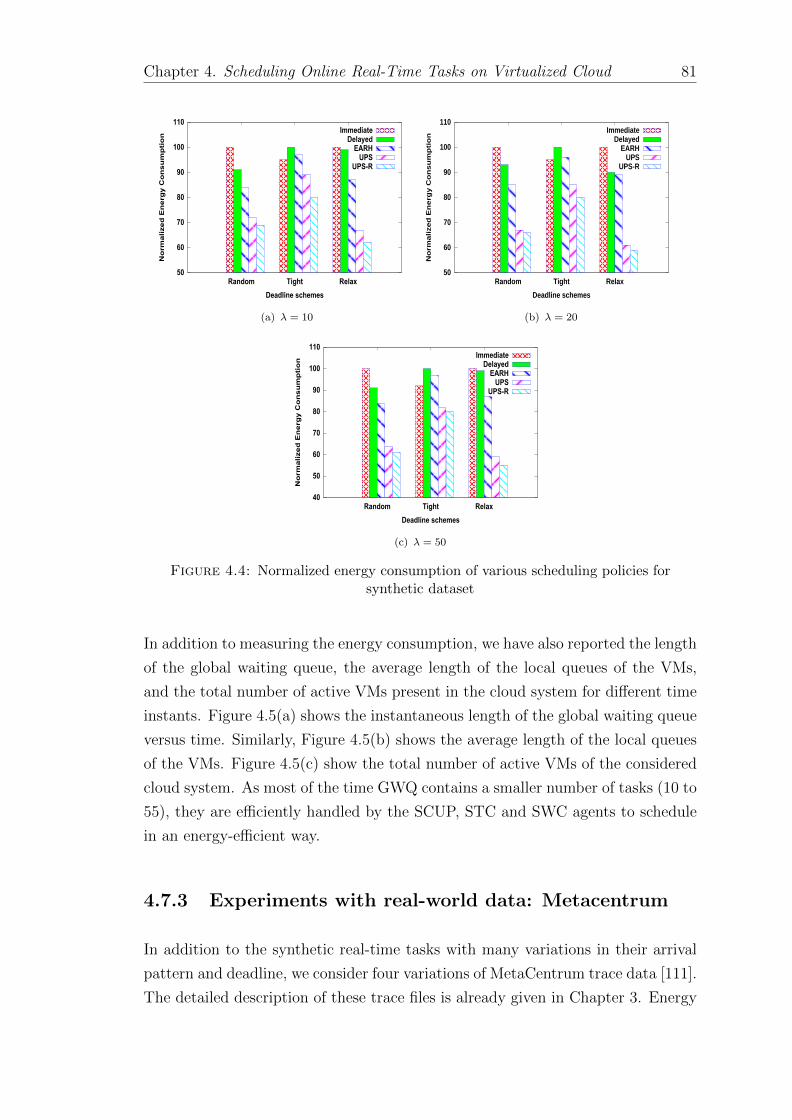
Chapter 4. Scheduling Online Real-Time Tasks on Virtualized Cloud 81
50
60
70
80
90
100
110
Random Tight Relax
No
rm
ali
ze
d E
ne
rg
y C
on
su
mp
tio
n
Deadline schemes
ImmediateDelayed
EARHUPS
UPS-R
(a) λ = 10
50
60
70
80
90
100
110
Random Tight Relax
No
rm
ali
ze
d E
ne
rg
y C
on
su
mp
tio
n
Deadline schemes
ImmediateDelayed
EARHUPS
UPS-R
(b) λ = 20
40
50
60
70
80
90
100
110
Random Tight Relax
No
rm
ali
ze
d E
ne
rg
y C
on
su
mp
tio
n
Deadline schemes
ImmediateDelayed
EARHUPS
UPS-R
(c) λ = 50
Figure 4.4: Normalized energy consumption of various scheduling policies forsynthetic dataset
In addition to measuring the energy consumption, we have also reported the length
of the global waiting queue, the average length of the local queues of the VMs,
and the total number of active VMs present in the cloud system for different time
instants. Figure 4.5(a) shows the instantaneous length of the global waiting queue
versus time. Similarly, Figure 4.5(b) shows the average length of the local queues
of the VMs. Figure 4.5(c) show the total number of active VMs of the considered
cloud system. As most of the time GWQ contains a smaller number of tasks (10 to
55), they are efficiently handled by the SCUP, STC and SWC agents to schedule
in an energy-efficient way.
4.7.3 Experiments with real-world data: Metacentrum
In addition to the synthetic real-time tasks with many variations in their arrival
pattern and deadline, we consider four variations of MetaCentrum trace data [111].
The detailed description of these trace files is already given in Chapter 3. Energy

Chapter 4. Scheduling Online Real-Time Tasks on Virtualized Cloud 82
0
10
20
30
40
50
60
0 20000 40000 60000 80000 100000 120000
Glo
ba
l q
ueu
e l
en
gth
Time
(a) Global waiting queue
0
1
2
3
4
5
6
0 20000 40000 60000 80000 100000 120000
Av
era
ge
lo
ca
l q
ue
ue
len
gth
Time
(b) Local waiting queue of VMs
0
2
4
6
8
10
12
14
16
18
0 20000 40000 60000 80000 100000 120000
Ac
tiv
e V
M c
ou
nt
Time
(c) Active VM count
Figure 4.5: Task and VM information for λ = 10
50
60
70
80
90
100
110
CERIT MetaCentrum1 Zerua MetaCentrum2
No
rm
alized
En
erg
y C
on
su
mp
tio
n
Real trace data
ImmediateDelayed
EARHUPS
UPS-ES
(a) Metacentrum
0
5
10
15
20
25
30
35
40
UPS UPS-ES
En
erg
y r
ed
ucti
on
Proposed scheduling policies
ImmediateDelayed
EARH
(b) Google trace
Figure 4.6: Energy reduction of the proposed policies for real-trace data
consumption (normalized) for these trace data set when executed on the considered
cloud system is represented using Figure 4.6(a). We observe that the proposed
policies UPS and UPS-ES perform better than the baseline policies for all the
trace data. In case of CERIT, the energy reduction is around 30% with respect
to Immediate and around 15% with respect to EARH. In case of MetaCentrum-1,
these reductions are around 25% and 9%. In case of Zerua, the reductions are
around 30% and 17% and for MetaCentrum-2, these are around 24% and 6%. We

Chapter 4. Scheduling Online Real-Time Tasks on Virtualized Cloud 83
further see that the energy reduction in case of CERIT and Zerua is comparatively
more than MataCentrum-1 and MataCentrum-2. We believe that this is because
the inter-arrival time in case of CERIT and Zerua is comparatively more than that
of MataCentrum-1 and MataCentrum-2.
4.7.4 Experiments with real-world data: Google tracelog
We also perform our experiments for Google cloud tracelog [124]. The tracelog
contains over 25 million tasks and 925 users span a period of 1 month. It is difficult
to perform experiments in a simulated environment with such an enormous task
count. Thus we have decided to consider first 10, 000 tasks of the day 18 as day 18
is reported as a sample day in [125]. We have also made the trivial assumptions
regarding the task execution and failure as reported in [30, 125]. Length of a task
is not directly reported in the trace and it is calculated from the start and end
time of the task. Deadline of the tasks are assigned similar to the synthetic tasks
and we have assumed Random distribution only. In Figure 4.6, we have plotted
the reduction in energy consumption of the two proposed policies with respect to
all three baseline policies. We see that UPS scheduling policy achieves an energy
reduction of 24%, 22%, and 11% with respect to Immediate, Delayed, and EARH
respectively. On the other hand, UPS-ES achieves an energy reduction of 27%,
25%, and 10% with respect to Immediate, Delayed, and EARH respectively.
4.8 Summary
Cloud computing environment has evolved as a popular and promising utility-
based computing paradigm of the recent time. As a result, applications from
various domains are getting deployed in the cloud system. But these applica-
tions consume an enormous amount of resources and hence the energy-efficient
scheduling has become crucial. The scheduling operation becomes more challeng-
ing when both static and dynamic power consumption of the hosts are considered
in the power consumption model. In this work, we have devised a power consump-
tion model for the cloud system based on the utilization of the hosts. We have
then introduced the concept of an urgent point in the context of a heterogeneous
computing environment. Then two scheduling techniques, UPS, and UPS-ES are
proposed based on the urgent point of the tasks. We have also designed three
other supporting procedures as complementary policies to the primary scheduling

Chapter 4. Scheduling Online Real-Time Tasks on Virtualized Cloud 84
policies. We have performed an extensive simulation work to validate our work
with different task parameters. Results show that the proposed scheduling poli-
cies reduce energy consumption by an average of almost 24% for synthetic data
as compared to the baselines. For MetaCentrum trace data, the average energy
reduction is almost 12% and for Google tracelogs, it is around 10%.

Chapter 5
Scheduling Real-Time Tasks on
VMs with Discrete Utilization
This chapter presents scheduling strategies for efficiently executing a set of offline
real-time tasks on a virtualized cloud system where the hosts of the system offer
VMs with discrete utilization values. Generally, time triggered activities generate
offline tasks. Examples include tasks in air-traffic control system, digital signal
processing, etc. Here we first calculate a utilization value for which the energy
consumption of the hosts of the cloud system is minimum. We term it as critical
utilization. The target of the scheduling policies is to keep the utilization of the
hosts close to the critical utilization. The problem is divided into four different
subproblems and a solution is proposed for each subproblem.
5.1 Introduction
In the last chapter, we discussed scheduling online real-time tasks for a virtual-
ized cloud system where the compute capacities of the VMs are considered to be
continuous. As a VM with certain compute capacity is created on a host, the VM
starts utilizing a proportionate amount of resources of that host. This results in a
certain increase in the utilization of the host. Because the compute capacities of
the VMs are considered to be continuous, the corresponding utilization values are
also continuous. Accordingly, several studies [126, 30, 45] on the energy-efficient
scheduling have been done in the context of cloud computing environment and
these studies also consider a continuous compute capacity of the VMs.
85

Chapter 5. VMs with Discrete Utilization 86
When the cloud service providers offer Infrastructure as a service (IaaS) [127,
128], they provide virtualized resources in the form of VMs to the users. Each
VM has different CPU, memory, storage and bandwidth capacities. Users select
the VM instance based on the requirement. For instance, Amazon EC2 [129]
offers configurations, such as small, medium, large, extra-large, etc. The compute
capacities of these configurations are discrete. As the compute capacity of a VM
corresponds to the resource utilization, the resource utilization of the VMs for the
hosts becomes discrete. In this chapter, we consider that the VMs are specified
with utilization values. Bigger VMs have higher host utilization requirement and
smaller VMs are having smaller host utilization requirement. The purpose of
this work is to propose approaches to select a suitable type of VM for each user
requested real-time task and to allocate the selected VMs to hosts. The tasks are
scheduled on their respective VMs. Bigger VM (i.e., VM having higher utilization)
executes the task faster then the smaller VMs and the execution time of task on
a VM is inversely proportional to the utilization of VM. We consider the cloud
system provides k discrete types of VMs and each VM type is specified with
host utilization requirement, where the cloud system consists of an infinitely large
number of homogeneous hosts.
The main aim of this work is to schedule a set of real-time aperiodic tasks on
the cloud environment. The scheduler chooses VM for each task. Resulting VM
allocation must consume the minimum amount of energy, and all the tasks must
complete before their respective deadlines. Such a scheduling approach comes with
following complementary challenges.
1. Meeting deadlines - each task comes with a deadline and its execution time
at maximum utilization. Using these two values, we need to find a minimum
value of utilization at which a task must be executed so that it meets its
deadline.
2. Minimizing energy consumption- whenever a physical machine is active, it
consumes some amount of energy. Energy consumption depends on the time
for which the host is active and utilization of host during its active period.
These two factors are contradicting because when a task executes at higher uti-
lization, although it completes earlier, but consumes more power. On the other
hand, at lower utilization, power consumption is lower but the task takes more
time to complete and in the worst case it may miss its deadline. Our objective is
to find an optimal or near-optimal solution to this problem.

Chapter 5. VMs with Discrete Utilization 87
The UPS and UPS-ES scheduling policies discussed in the last chapter makes
use of two threshold values of host utilization. One threshold was used while
scheduling the non-urgent tasks, and the other one was used when scheduling an
urgent task. But in this work, we have formally computed an optimum value
of host utilization at which the host consumes the minimum amount of energy
known as critical utilization (described later in Section 5.3 in detail). Depending
on the specification of the task and the value of critical utilization, we allocate a
VM of suitable type to each task, so that, no deadline is missed and minimum
amount of energy is consumed. For scheduling the selected VMs to the available
physical hosts, we have divided our problem into several cases and solved each
case separately. We thus summarize the contribution of this chapter as follows.
• First, we calculate the critical utilization value for the cloud host where the
energy consumption is minimum.
• Next, we put forward an analysis regarding two choices while allocating a
task. These are (i) to increase the utilization of a running host, and (ii)
switching on a new host.
• Then, we divide the problem of scheduling into four different subproblems
based on the task characteristics and propose a solution for each subproblem.
5.2 System Model
In most of the cloud systems, the user tasks get executed on virtual machines and
the virtual machines get allocated to physical hosts. So the natural way to model
the cloud system is a three-layer system and these layers are the task layer, virtual
resource layer, and physical layer. Cloud consists of physical machines which host
the virtual resources to satisfy the needs of user requested tasks.
These layers can be described as follows:
• Physical Layer: The cloud system that we are considering consists of a set
of m homogeneous physical machines (or hosts) PM = {h1, h2, h3, · · · , hm}.We specially consider that the compute capacities and the hardware spec-
ification of the hosts are same. Several virtual machines can be placed on
a single host and the resource utilization of a host gets shared among the
hosted virtual machines depending on their types. The utilization of a host

Chapter 5. VMs with Discrete Utilization 88
vt1
vt2
vtk
PM
PM
PM
PMm
2
1
3
t2
t1
t n
Cloud System
k VM types m PMs
n Tasks
Figure 5.1: System model
is the maximum when it is utilized to its maximum compute capacity. For
a host hk, its utilization U(hk) ranges in between 0 and 1. These hosts con-
sume energy which depends on the total utilization of the host. All the hosts
possess one more property that is critical utilization, uc. It is the utilization
at which energy consumption is minimum (this is defined formally in next
section).
• Virtual Resource Layer: This layer constitutes virtual machines which
need to be hosted on physical machines for task execution. The utilization
of a VM is proportional to its compute capacity and it expressed in MIPS
(million instructions per second). We have taken k types of VMs based
on the values of utilization they provide to a task. The set of VM types
is denoted by V T = {vt1, vt2, · · · , vtk}. The compute capacity offered to
the tasks by these VM types is not continuous. For each VM type, there
is no limit on the number of VMs. These VM types are characterized by
the amount of CPU utilization (proportional to the compute capacity) they
provide to a task when hosted to a physical machine, also when the VM with
utilization u runs on top a host, it consumes u fraction of compute (CPU)
resource of the host. For a VM type vtj, there is a constant uj, which is the
amount of utilization that vtj will provide for the task. The value of uj is
between 0 and 1 that is 0 < uj ≤ 1. When VMs are allocated to a host at a
particular time, the sum of their total utilization must be less than or equal
to 1, which isν∑j=1
uj ≤ 1, where ν is the number of VMs allocated to that
host and uj is the utilization of vmj.
For the sake of simplicity, we have considered five types of VMs (k = 5) :
tiny (T), small (S), medium (M), large (L) and extra large (XL) with discrete
utilization values uT = 0.2, uS = 0.4, uM = 0.6, uL = 0.8, and uXL = 1.0
Chapter 5. VMs with Discrete Utilization 89
respectively. But the work can be easily extended for any value of k. For
instance, the compute capacity of a tiny type VM placed on a host with
compute capacity of 1000 MIPS will be CP (VMT ) = 1000 · uT = 1000 · 0.2= 200 MIPS. Similarly, the compute capacities of S, M, L and XL type VMs
will be 400, 600, 800, and 1000 MIPS respectively.
• Task Layer : The users send requests to the cloud system in form of tasks.
The set or bag of n tasks is denoted by T = {t1, t2, · · · , tn}. The tasks in user
requests are independent. Each task is an indivisible unit which needs to be
executed on one VM (and one host) only. Any such task ti can be described
using 3-tuple: ti = (ai, ei, di), where ai is arrival time, ei is the execution
time when run at maximum utilization (umax = 1) and di is the deadline
for the task. We are considering synced tasks to be scheduled (ai = 0 for
all the tasks). Therefore, tasks can be represented using 2-tuple in our case
ti = (ei, di).
The execution time of a task is expressed in seconds and this can be calcu-
lated from the length of the task. For a task ti with length li, the execution
time ei can be expressed as
ei =li
CP (VMXL)(5.1)
where CP (VMXL) is the compute capacity of the VMs of type XL. When
the task is executed by a VM of other type, its execution time will increase;
but it is dependent on its length li.
The minimum value of utilization required by ti is ui = eidi
. Therefore, if we
execute the task at utilization ui, it finishes exactly at di. But the utilizations
of the VMs available in the system are discrete (equi-spaced on utilization
line). Let uLF (ti) be the utilization of the least feasible VM type among the
available k VM types for a task ti(ei, di). Then this can be written as
uLF (ti) = 1kd eidi· ke (5.2)
where k is the number of VM types available in the system. This formula
works for the cases when utilizations provided by VM types is equally dis-
tributed over the range (0, 1.0]. All the VM types with utilization value
greater than or equal to uLF (as computed by Equation 5.2) are suitable
for the task ti. We do not allow a task with utilization requirement more
than 1 in our system. We assume that the VM creation and deletion time is

Chapter 5. VMs with Discrete Utilization 90
negligible in our work. Thus as soon as a task gets scheduled for execution to
a VM of a particular type, the execution of the task can immediately start.
Moreover we assume that the tasks are specified with the
5.3 Energy Consumption Model
A user task is allocated to a suitable VM type, and the selected VM is then
hosted on the physical machine of the cloud system. When the tasks execute,
physical machines consume some energy. Energy consumption E is the amount
of total power consumption during the active period of the physical machine.
Which can be written as E =ttotal∫
0
P (t)dt, where P (t) is the power consumed by
the host at time t and ttotal is the total time for which that host is active. P (t)
has two components: static power consumption and dynamic power consumption.
Static power consumption Pmin (same as Pstatic or Pbase in earlier chapters) is
the minimum amount of power consumed when a host is switched on. Static
power consumption depends on the host’s internal activities and maintenance of
tasks. Dynamic power consumption (Pdyn(t)) varies with the current frequency
of the host machine. So the total power consumption can be written as P (t) =
Pmin + Pdyn(t) and as stated in [48], dynamic power consumption be formulated
as Pdyn(t) ∝ f(t)3, where f(t) is the frequency of the host at time t. For single
processor systems, we may safely assume that frequency is directly proportional
to the utilization u of the host. So, f(t) ∝ u(t), where u(t) is the utilization of
the host at time t as stated in [48]. Therefore, we can say
P (t) = Pmin + αu(t)3, (5.3)
where α is a constant.
eu
is the actual execution time of a task when running on VM with utilization u.
Therefore, if we assume that utilization does not vary throughout the execution
of the task, then, energy consumed by the host can be computed as
E =(Pmin + αu3
)· eu
= e ·(Pmin
u+ αu2
)(5.4)
Figure 5.2 shows energy consumption of tasks executed at different utilization
values of a host with Pmin = 100 and α = 70. The resultant plot is an inverted

Chapter 5. VMs with Discrete Utilization 91
0
200
400
600
800
1000
0 0.5 1 1.5 2
uc
Energ
y C
onsum
pti
on
Utilization of the host
For Pmin = 100 and = 70
Figure 5.2: Energy consumption versus total utilization of the host
bell curve. The lowermost point shows the minimum energy consumed by the host
and the corresponding utilization is called critical utilization, uc.
At critical utilization uc,dEdu
= 0, from Equation 5.4
dE
du= e.
(Pminu
+ αu2)
= 0,⇒ e.(− Pmin
u2+ 2αu
)= 0
⇒ uc =3
√Pmin2α
(5.5)
So, we can see that the value of the critical utilization is independent of the
execution time (i.e. the length) of task executed the system. It only depends on
the values of Pmin and α.
From Equation 5.5, we get
Pmin = 2αu3c (5.6)
Substituting the value of Pmin in Equation 5.3, we get
E =(
2αu3c + αu3
)· eu
Thus the total energy consumption of a host can be expressed as
E = α(2uc3 + u3) · e
u(5.7)
Chapter 5. VMs with Discrete Utilization 92
As mentioned in the previous chapter, the power model used in this chapter also
assumes that there is a local power optimization module (DVFS or DPM) at each
host. The local optimization module at a host controls the frequency and sleep
state of the compute system which may have more then one compute components.
As the power consumption is dependent on the utilization of the host, we can
safely assume when the host is running at highest utilization, it is running at the
highest capable frequency of operation and the frequency of operation of the host
is proportional to the utilization of the host.
5.4 Objective in the Chapter
Given a set of user tasks T = {t1, t2, ..., tn}, of size n, this chapter aims to find a
set of suitable VM type for each task and allocate all the resulting VMs to physical
machines. The objective of the resulting schedule is to minimize the amount of
energy consumed without missing the deadline of any task.
As uc is the critical utilization for each host, we try to maintain the utilization for
each active host closest to uc. If ν is the number of VMs allocated to a host, then
the sum of values of utilization of these VMs is maintained to be approximately
equal to uc for every instant of time.
ν∑j=1
uj ≈ uc, (5.8)
The tasks that need utilization above uc, are exceptions to this because if they are
executed at lower utilization, they won’t meet their deadlines. Hence, they should
be scheduled on separate hosts individually using a suitable VM type. Now, the
problem gets reduced to finding a combination of VMs with ui ≈ uc, which can be
allocated to the same host while minimizing the amount of energy consumption.
The scheduling policies discussed in this chapter tries to minimize the number of
active hosts along with maintaining the host utilization close to uc such that no
task misses its deadline.

Chapter 5. VMs with Discrete Utilization 93
5.5 Classification of cloud systems
We have analyzed the energy consumption characteristics of the hosts of the cloud
system which are based on the value of critical utilization, uc (as calculated in
Equation 5.5). The value of uc depends on the values of Pmin and α. Since
we are considering a homogeneous cloud system, these values are same for all
the hosts. Based on this, we have categorized our problem into three types of
systems, out of which two fall in the category of systems with extreme static power
consumption and the third type refers to the systems with general specifications.
In general systems, we classify the cloud system based on host or physical machine
characteristics into three categories and these categories or types are:
• Type 1: Host with negligible static power consumption and in this type of
cloud, the Pmin of the host is negligible with respect to αu3 and the critical
utilization of the hosts is 0 (i.e. uc = 0).
• Type 2: Host with significantly high static power consumption, and critical
utilization of the host is above 1 (i.e. uc > 1).
• Type 3: This is the most common type of cloud, where the host critical
utilization uc lies between 0 and 1.
Scheduling approaches for type 1 and type 2 systems are described in Subsections
5.5.2 and 5.5.3, respectively and for type 3 systems, the scheduling approach is
described in Section 5.6.
For the case when 0 < uc ≤ 1, both static and dynamic power consumption play
significant roles. The value of critical utilization lies in the range (0, 1.0]. But the
VMs available within the system can provide only discrete values of utilization i.e.,
uT = 0.2, uS = 0.4, uM = 0.6, uL = 0.8, and uXL = 1.0 for T, S, M, L, and XL
types of VM respectively. So when more than one task run in parallel on a host,
the total value of utilization may not be exactly equal to uc. Hence, we calculate
a value of utilization ut by which the utilization can be increased when the exact
value of uc cannot be reached.
As seen in Section 5.3, for a single physical machine, when only one task is exe-
cuting, energy consumption is minimum at its critical utilization, uc. If more than
one task gets scheduled to a machine, they should execute for approximately same
time, so that, total utilization of the host remains same throughout the time for
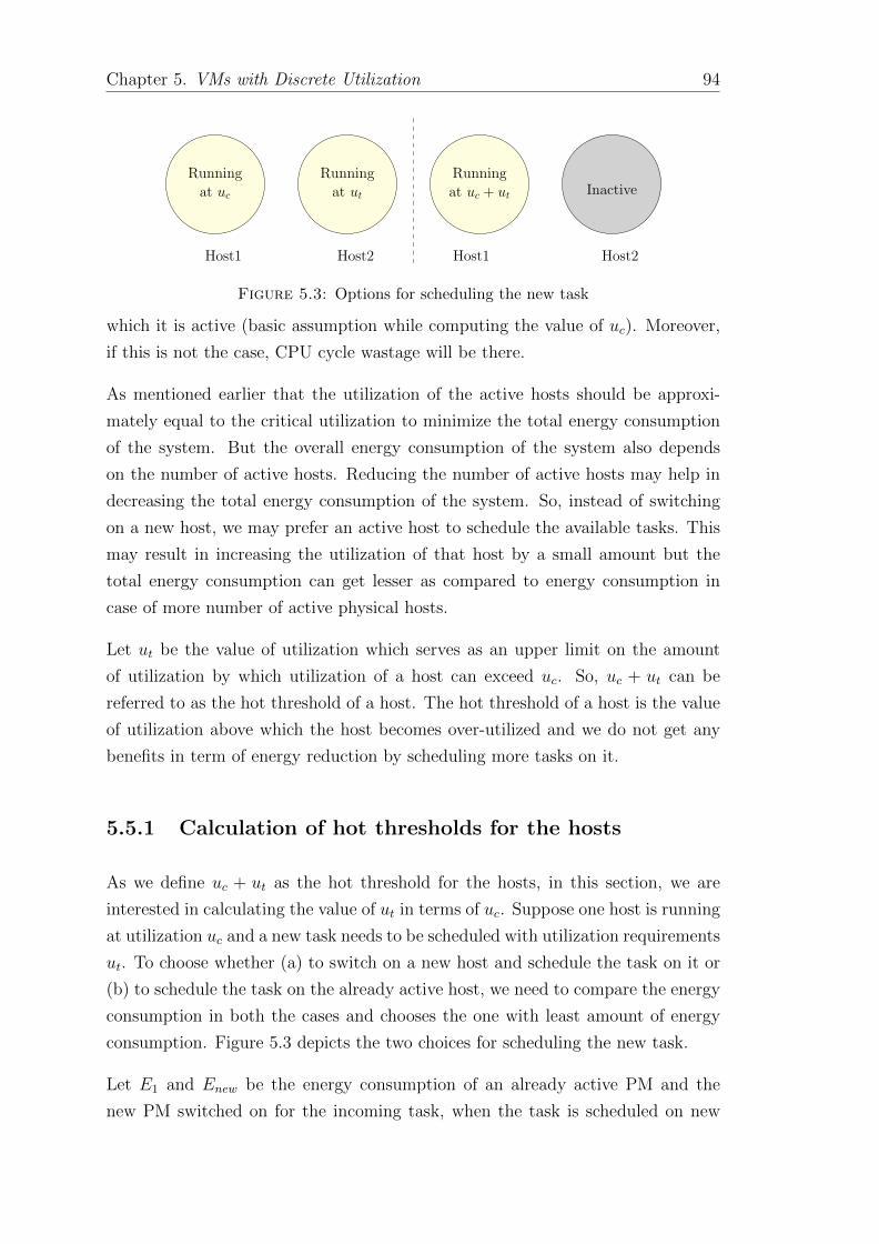
Chapter 5. VMs with Discrete Utilization 94
Running
at ��
Running
at �t
Running
at �� � �tInactive
Host1 Host2 Host1 Host2
Figure 5.3: Options for scheduling the new task
which it is active (basic assumption while computing the value of uc). Moreover,
if this is not the case, CPU cycle wastage will be there.
As mentioned earlier that the utilization of the active hosts should be approxi-
mately equal to the critical utilization to minimize the total energy consumption
of the system. But the overall energy consumption of the system also depends
on the number of active hosts. Reducing the number of active hosts may help in
decreasing the total energy consumption of the system. So, instead of switching
on a new host, we may prefer an active host to schedule the available tasks. This
may result in increasing the utilization of that host by a small amount but the
total energy consumption can get lesser as compared to energy consumption in
case of more number of active physical hosts.
Let ut be the value of utilization which serves as an upper limit on the amount
of utilization by which utilization of a host can exceed uc. So, uc + ut can be
referred to as the hot threshold of a host. The hot threshold of a host is the value
of utilization above which the host becomes over-utilized and we do not get any
benefits in term of energy reduction by scheduling more tasks on it.
5.5.1 Calculation of hot thresholds for the hosts
As we define uc + ut as the hot threshold for the hosts, in this section, we are
interested in calculating the value of ut in terms of uc. Suppose one host is running
at utilization uc and a new task needs to be scheduled with utilization requirements
ut. To choose whether (a) to switch on a new host and schedule the task on it or
(b) to schedule the task on the already active host, we need to compare the energy
consumption in both the cases and chooses the one with least amount of energy
consumption. Figure 5.3 depicts the two choices for scheduling the new task.
Let E1 and Enew be the energy consumption of an already active PM and the
new PM switched on for the incoming task, when the task is scheduled on new

Chapter 5. VMs with Discrete Utilization 95
0
0.2
0.4
0.6
0.8
1
0 0.2 0.4 0.6 0.8 1
uc +
ut
Critical Utilization
Graph for uc + ut vs uc
Figure 5.4: Hot threshold (uc + ut) versus uc
PM (as shown in left side of Figure 5.3). Also E ′1 be the energy consumption
of the already active host when the incoming task gets scheduled to the active
host instead of a new host (as shown in right side of Figure 5.3). Also, ut ∈(0, 1.0]. Let t be the execution time of the tasks. Then the energy consumption
E1, Enew and E ′1 can be written as E1 = t(Pmin+αuc3), Enew = t(Pmin+αut
3) and
E ′1 = t(Pmin + α(uc + ut)3) respectively. The incoming task will be scheduled on
already active hosts, if it is beneficial in term of energy consumption as compared
to switching on a new host (even if it makes total utilization of the host, u > uc),
which is E ′1 < E1 + Enew. So
t(Pmin + α(uc + ut)3) < t(Pmin + αuc
3 + Pmin + αut3)
⇒ 3αucut(uc + ut) < Pmin
⇒ ucut2 + uc
2ut <23uc
3 [Pmin = 2αuc3, Eqn 5.5]
This is a quadratic Equation in ut. Thus, ut <(√
33−3)uc6
and this can be simplified
to
ut < 0.4574uc (5.9)
Figure 5.4 shows a graph for variation of the value of hot threshold (uc + ut) with
respect to uc. Since ut is the value of utilization by which we can exceed the total
utilization above uc, therefore, while allocating VMs we should target for uc + ut
as total utilization. Whenever uc + ut > 1, we round off its value to 1.

Chapter 5. VMs with Discrete Utilization 96
0 10 20 30 40 50 60 70 80
0 0.2 0.4 0.6 0.8 1
uc = 0
Energ
y C
onsum
pti
on
Utilization of the host
For Pmin = 0 and α = 70
(a) Energy consumption versus utilization for negligi-ble Pmin (uc = 0)
0
200
400
600
800
1000
0 0.5 1 1.5 2
uc = 1.26
Energ
y C
onsum
pti
on
Utilization of the host
For Pmin = 100 and α = 20
(b) Energy consumption versus utilization with uc >1
Figure 5.5: Energy consumption versus utilization of extreme cases
Algorithm 7 Scheduler for system with uc = 0
Require: Schedule for real-time tasksEnsure: All the tasks meet their deadline and minimum energy gets consumed
1: for Each task ti in task set T = {t1, t2, ..., tn} do2: Take the VM type with utilization just above or equal to ui = ei
di3: Host the resulting VM on a new host and execute the tasks on their selected
VM.4: end for
5.5.2 Hosts with negligible static power consumption (uc =
0)
Figure 5.5(a) shows the variation of energy consumption of a host with respect to
its total utilization. The host has negligible static power consumption. When Pmin
is negligible as compared to αu3, we can take its value to be 0 for all the hosts.
As a result, we get uc = 0 from Equation 5.5. To maintain total utilization values
as close as possible to uc, that is 0 in this case, we should allocate a suitable VM
type with least utilization value to a task and schedule them on separate hosts.
A suitable VM type for task ti is the one which completes the task before the
deadline when the task is allocated to it, that is, the VM type with utilization
greater than eidi
, which is the least feasible VM type and this can be calculated using
Equation 5.2. The total energy spent will only depend on the squares of utilization
of the hosts. Beloglazov et al. [130] have considered only the current utilization
as the deciding factor for scheduling the user requests. But such systems fall in
the category of systems with extreme specifications which can be solved trivially.
The pseudocode of the scheduler is shown in Algorithm 7. The scheduler simply
chooses the least feasible VM type for each task in the task set T = {t1, t2, ..., tn},
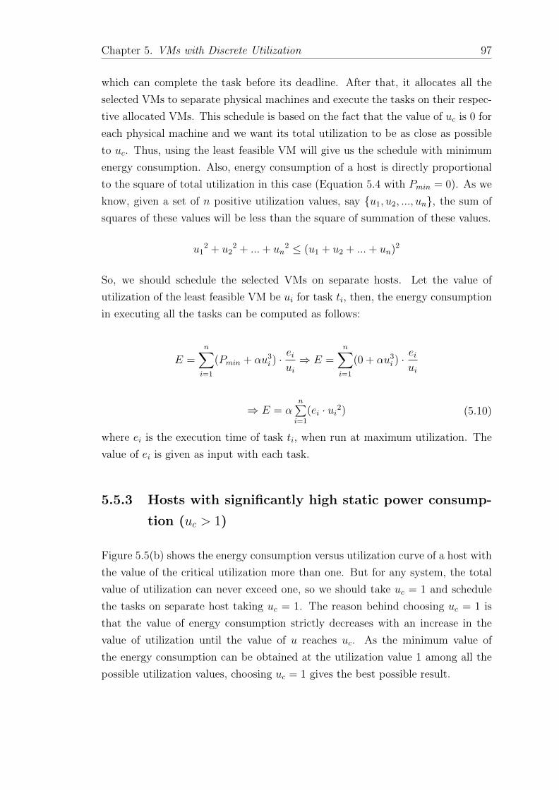
Chapter 5. VMs with Discrete Utilization 97
which can complete the task before its deadline. After that, it allocates all the
selected VMs to separate physical machines and execute the tasks on their respec-
tive allocated VMs. This schedule is based on the fact that the value of uc is 0 for
each physical machine and we want its total utilization to be as close as possible
to uc. Thus, using the least feasible VM will give us the schedule with minimum
energy consumption. Also, energy consumption of a host is directly proportional
to the square of total utilization in this case (Equation 5.4 with Pmin = 0). As we
know, given a set of n positive utilization values, say {u1, u2, ..., un}, the sum of
squares of these values will be less than the square of summation of these values.
u12 + u2
2 + ...+ un2 ≤ (u1 + u2 + ...+ un)2
So, we should schedule the selected VMs on separate hosts. Let the value of
utilization of the least feasible VM be ui for task ti, then, the energy consumption
in executing all the tasks can be computed as follows:
E =n∑i=1
(Pmin + αu3i ) ·
eiui⇒ E =
n∑i=1
(0 + αu3i ) ·
eiui
⇒ E = αn∑i=1
(ei · ui2) (5.10)
where ei is the execution time of task ti, when run at maximum utilization. The
value of ei is given as input with each task.
5.5.3 Hosts with significantly high static power consump-
tion (uc > 1)
Figure 5.5(b) shows the energy consumption versus utilization curve of a host with
the value of the critical utilization more than one. But for any system, the total
value of utilization can never exceed one, so we should take uc = 1 and schedule
the tasks on separate host taking uc = 1. The reason behind choosing uc = 1 is
that the value of energy consumption strictly decreases with an increase in the
value of utilization until the value of u reaches uc. As the minimum value of
the energy consumption can be obtained at the utilization value 1 among all the
possible utilization values, choosing uc = 1 gives the best possible result.

Chapter 5. VMs with Discrete Utilization 98
5.6 Scheduling Methodology for the Systems with
General Specifications (0 < uc ≤ 1)
Scheduling and analysis of the tasks for the general specifications are tricky and
difficult. Thus, we divide the problem into four sub-problems and solved sepa-
rately. Based on the type of tasks in the request, the energy-efficient scheduling
of real-time tasks can be done by dividing them into four sub-problems (e and d
refer to the execution time of the task at maximum utilization and the deadline
of the task, respectively). The considered cases of sub-problems are:
1. Case 1: All the n tasks are of same type i.e. ti(ei = e, di = d).
2. Case 2: Two type of tasks with different execution times but same deadline
i.e. ti(ei ∈ {e1, e2}, di = d).
3. Case 3: Tasks with different execution times but same deadline i.e. ti(ei, di =
d).
4. Case 4: All the n tasks having their own ei and di, i.e. ti(ei, di).
The reason behind choosing this set of cases is that, the scheduling approach of
every case is dependent on the scheduling approach for the previous one (except
for the first case, which depends on the scheduling approach for base case). And
we can apply the solution approach of one case to generate the solution approach
of the next case. This will be clear from the detailed discussion of scheduling
approaches for these cases described in next subsections.
5.6.1 Scheduling n tasks of same type (Case 1: (e, d))
This case refers to the requests with n tasks having same specifications ti(e, d).
An iterative approach has been followed to solve this problem. We start with a
suitable VM type with least utilization value that complete the task within the
deadline. Then we check whether the VM type with the next higher utilization
performs better. If uc is the critical utilization of the hosts and tasks require a
VM with utilization u, the number of VMs that can be scheduled per host are
β = ducue or γ = buc
uc. For example, when uc = 0.7 and uT = 0.2, the values of β
and γ are 4 and 3 respectively. Suppose β gets chosen out of these two, then, we
have these two following cases for the number of tasks getting scheduled:

Chapter 5. VMs with Discrete Utilization 99
1. If n is a perfect multiple of β then all the tasks are scheduled according to
our method and the number of hosts required to execute all the tasks will
be m = nβ, where n is the number of tasks in the request.
2. If n is not multiple of β then m = bnβc − 1 number of hosts will execute mβ
tasks and the remaining tasks (n−mβ) are scheduled according to the base
case. The remaining number of tasks are guaranteed to be less than 2β.
For scheduling the tasks in the base case, we have used a first fit method. For
this, we have sorted the tasks in decreasing order of their utilization requirements
and the VMs are allocated to hosts using the first-fit approach for bin packing.
Instead of taking bin capacities as 1, we take these as uc + ut. Moreover, in this
case, the tasks have the same specifications, so, we do not need to sort them. Also,
the maximum value of β can be 5 (when the least feasible VM type is tiny with
uT = 0.2), the maximum number of tasks that will be in the base case is 10.
Energy consumption in this case is given by,
E = m.e
u.α(2uc
3 + (uβ)3) + Ebase (5.11)
where m is the number of active hosts, eu
is the execution time of a task (or we can
say the time for which the hosts are active), α(2uc3+(uβ)3) is the amount of power
consumption of each host and Ebase is the energy consumption for scheduling of
the tasks that are in base case.
We have a set of suitable VM types for a task which can complete the task before
its deadline. For choosing the best VM type among the suitable VM types, we
have computed certain relation through which we can make the decision based on
the value of uc of the hosts.
1. Relation between β and γ for same VM type: Let u be the utilization
provided by current VM type and n1 and n2 be the total number of hosts
needed with β and γ number of VMs per host, respectively. Schedule with
γ number of VMs per host consumes lesser energy than the schedule with
β number of VMs per host when total energy consumption in former case
is lesser as compared to total energy consumption in the latter case (can
be derived from Equation 5.11). The high number (γ) of VMs per host is
preferable if The high number (γ) of VMs per host is preferable if

Chapter 5. VMs with Discrete Utilization 100
n2.e
u.α(2uc
3 + (uγ)3) < n1.e
u.α(2uc
3 + (uβ)3)
2n2uc3 − 2n1uc
3 < n1(uβ)3 − n2(uγ)3
uc < u 3
√n1β3 − n2γ3
2(n2 − n1)(5.12)
For example, when the least feasible VM type is S (uS = 0.4) and uc ∈(0.40, 0.49], the resulting values of β and γ are 2 and 1, respectively. And in
this case, schedule with one VM per host consumes lesser energy as compared
to the schedule with two VMs per host.
2. Relation between two different VM types: Let u1 and u2 be the values
of utilizations provided by the two VM types which we need to compare.
The corresponding number of tasks per host be β1 and β2, as a result of
above relation. Let m1 and m2 be the corresponding number of hosts and
u1 < u2. Choosing the VM with higher utilization will give lesser energy
consumption when
m1.e
u1
.α(2uc3 + (β1u1)3) > m2.
e
u2
.α(2uc3 + (β2u2)3)
m1u2(2uc3 + (β1u1)3) > m2u1(2uc
3 + (β2u2)3)
2uc3(u1m2 − u2m1) < m1u2(β1u1)3 −m2u1(β2u2)3 (5.13)
For example, when the least feasible VM type is S and uc ∈ (0.50, 0.69],
schedule using L type of VMs consumes lesser energy as compared to the
schedule using S type of VMs.
Pseudo-code for scheduling the single type of tasks is shown in Algorithm 8. We
start with finding the minimum utilization required by the tasks. Based on the
minimum utilization required, we select the VM type with the least utilization
among the set of suitable VM types. We call the utilization of this VM type u1.
This can also be calculated as u =⌈ed· 5⌉/5. Then, we check the satisfiability
of the relation given in Equation 5.12 to choose the number of tasks per host to
execute. If it gets satisfied then schedule with γ VMs per host performs better
than the schedule with β VMs per host. The chosen number of VMs per host
is set as β1 and the corresponding number of hosts is assigned to m1. Similarly,
for the next VM type with utilization u2, find the values of β2 and m2. Now,
we check which of the two VM types gives us better results. For this, we check
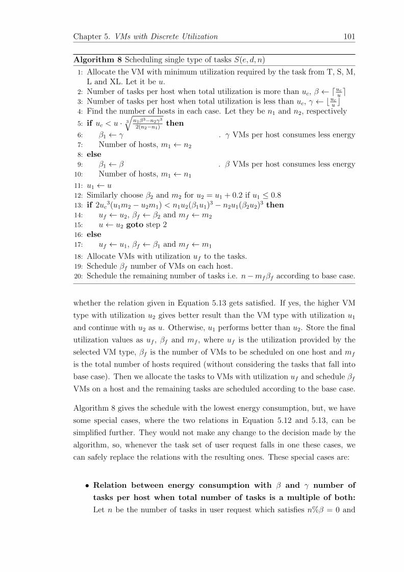
Chapter 5. VMs with Discrete Utilization 101
Algorithm 8 Scheduling single type of tasks S(e, d, n)
1: Allocate the VM with minimum utilization required by the task from T, S, M,L and XL. Let it be u.
2: Number of tasks per host when total utilization is more than uc, β ← ducu e3: Number of tasks per host when total utilization is less than uc, γ ← bucu c4: Find the number of hosts in each case. Let they be n1 and n2, respectively
5: if uc < u · 3
√n1β3−n2γ3
2(n2−n1)then
6: β1 ← γ . γ VMs per host consumes less energy7: Number of hosts, m1 ← n2
8: else9: β1 ← β . β VMs per host consumes less energy
10: Number of hosts, m1 ← n1
11: u1 ← u12: Similarly choose β2 and m2 for u2 = u1 + 0.2 if u1 ≤ 0.813: if 2uc
3(u1m2 − u2m1) < n1u2(β1u1)3 − n2u1(β2u2)3 then14: uf ← u2, βf ← β2 and mf ← m2
15: u← u2 goto step 216: else17: uf ← u1, βf ← β1 and mf ← m1
18: Allocate VMs with utilization uf to the tasks.19: Schedule βf number of VMs on each host.20: Schedule the remaining number of tasks i.e. n−mfβf according to base case.
whether the relation given in Equation 5.13 gets satisfied. If yes, the higher VM
type with utilization u2 gives better result than the VM type with utilization u1
and continue with u2 as u. Otherwise, u1 performs better than u2. Store the final
utilization values as uf , βf and mf , where uf is the utilization provided by the
selected VM type, βf is the number of VMs to be scheduled on one host and mf
is the total number of hosts required (without considering the tasks that fall into
base case). Then we allocate the tasks to VMs with utilization uf and schedule βf
VMs on a host and the remaining tasks are scheduled according to the base case.
Algorithm 8 gives the schedule with the lowest energy consumption, but, we have
some special cases, where the two relations in Equation 5.12 and 5.13, can be
simplified further. They would not make any change to the decision made by the
algorithm, so, whenever the task set of user request falls in one these cases, we
can safely replace the relations with the resulting ones. These special cases are:
• Relation between energy consumption with β and γ number of
tasks per host when total number of tasks is a multiple of both:
Let n be the number of tasks in user request which satisfies n%β = 0 and

Chapter 5. VMs with Discrete Utilization 102
n%γ = 0. Let n1 and n2 be the number of hosts in case of β and γ number of
VMs per host, respectively. Then n1 = nβ
and n2 = nγ. Energy consumption
is lower with γ number of VMs per host when a VM with utilization u is
used if the following condition is satisfied
n
γ.e
u.α(2uc
3 + (uγ)3) <n
β.e
u.α(2uc
3 + (uβ)3)
⇒2uc3 + (uγ)3
γ<
2uc3 + (u(γ + 1))3
γ + 1[as β = γ + 1]
⇒(γ + 1)(2uc3 + (uγ)3) < γ(2uc
3 + (u(γ + 1))3)
⇒2uc3 + (uγ)3 < γu3(3γ2 + 3γ + 1)
⇒ uc <3
√γu3(2γ2 + 3γ + 1)
2. (5.14)
So if the above Equation is satisfied then the γ number of VMs per host
is allocated to have minimum energy consumption, otherwise β number of
VMs per host have lesser energy consumption.
• Comparing energy consumption by two different VM types when
number of tasks is a multiple of both β1 and β2: Let n is the number
of tasks and u1 and u2 (u1 < u2) be the values of utilization provided by the
two VM types that need to be compared. If β1 and β2 are the respective
number of tasks per host and n satisfies n%β1 = 0 and n%β2 = 0 , then
energy consumption is lower at u2 if:
n
β2
.e
u2
.α(2uc3 + (u2β2)3) <
n
β1
.e
u1
.α(2uc3 + (u1β1)3)
u1β1(2uc3 + (u2β2)3) < u2β2(2uc
3 + (u1β1)3)
2uc3(u1β1 − u2β2) < u2β2(u1β1)3 − u1β1(u2β2)3
2uc3(u1β1 − u2β2) < u1u2β1β2
((u1β1)2 − (u2β2)2)
2uc3(u1β1 − u2β2) < u1u2β1β2(u1β1 − u2β2)
(u1β1 + u2β2)
The final relation depends on the value of (u1β1 − u2β2).2uc3 > u1u2β1β2(u1β1 + u2β2) (u1β1 − u2β2) < 0
2uc3 < u1u2β1β2(u1β1 + u2β2) else

Chapter 5. VMs with Discrete Utilization 103
⇒
uc >3
√u1u2β1β2(u1β1+u2β2)
2(u1β1 − u2β2) < 0
uc <3
√u1u2β1β2(u1β1+u2β2)
2else
(5.15)
• When β1 and β2 are equal in the above case: This case refers to a
situation where both values of utilization result in same β values. Since
u2 > u1 and β1 = β2 , say β, the value of u1β1−u2β2 will always be less than
0. Therefore, 3
√12u1u2ββ(u1β + u2β) can be written as β 3
√12u1u2(u1 + u2).
So if the following condition
uc > β3
√1
2u1u2(u1 + u2) (5.16)
is satisfied then, the VM type with higher utilization will consume lesser
amount of energy as compared to the VM type with lesser utilization value.
5.6.2 Scheduling approach for two types of tasks having
same deadline (Case 2: (e1, d) and (e2, d))
This case refers to the requests where there are only 2 types of tasks. They may
have any one of the two available execution times but they ought to have the
same deadline. Let n1 and n2 be the number of tasks with specification (e1, d) and
(e2, d), respectively. These tasks may run independently on separate hosts or may
run in together on the same host. When the tasks run individually, the problem
gets reduced to case 1, but when they run together, total energy consumption will
have two components:
1. Energy consumption of the hosts where both types of tasks reside.
2. Energy consumption of the hosts where a single type of tasks resides.
The second component occurs when one type of task is much higher in number
than the other type of tasks, and all the former type of tasks could not be combined
with the latter type.
As discussed in the previous case, the tasks running on the same host must have
approximately the same execution time so that the total utilization of the host
remains the same throughout its active period. For achieving this, we allocate the
least feasible VM type to all the tasks and to approximate their execution time

Chapter 5. VMs with Discrete Utilization 104
Algorithm 9 Scheduling two types of tasks with same deadline(D(e1, e2, d, n1, n2))
1: Let u1 and u2 be the utilization of VM types which satisfies the minimumrequirements of tasks with specification (e1, d) and (e2, d), respectively
2: Compute (β1, β2) such that total utilization is approximately equal to uc andshould not be more than uc + ut.
3: for each combination c of (β1, β2) do4: if bn1
β1c > bn2
β2c then
5: swap the two types of tasks.
6: number of hosts with both type of tasks, numHostsc ← bn1
β1c
7: Remaining second type task NRc ← n2 − bn1
β1cβ2
8: Ec ← bn1
β1cd(2uc
3 + (u1β1 + u2β2)3) + Epart + S(e2, d,NRc)9: end for
10: Esingle ← S(e1, d, n1) + S(e2, d, n2) + Epart11: Compare energy consumption in all the cases and choose least one.
to deadline d. The reason behind choosing the least feasible VM type is that it
completes the task just before its deadline. All the tasks have the same deadline
in this case, so, if we allocate them to their least feasible VM type, the execution
time of all the tasks will be approximately equal to deadline d.
Now, let u1 and u2 be the utilization of the VM types allocated to the two types
of tasks and β1 and β2 be the non-zero number of tasks of each type on a host.
When either of the two is zero, the tasks run individually. Also, based on the
values of uc, u1 and u2, the pair (β1, β2) may assume several values. The decision
on whether to run the tasks individually or in one of the combinations need to be
made. For this, we compare the total energy consumption in each case and choose
the one with the least value.
The pseudo-code for scheduling two type of tasks with the same deadline is given
in Algorithm 9. We first find the least feasible VM that can be allocated to both
the task types. Let u1 and u2 be the utilization of selected VM types. To obtain
total utilization of the hosts approximately equal to uc (preferably higher), these
VM types can be scheduled together. Let β1 and β2 be the corresponding number
of VMs on one host when they are scheduled together. Also, there is an option
for scheduling both the type of tasks individually (S(e1, d, n1) and S(e2, d, n2)
scheduled described in Algorithm 8). So, for all the available options, we compute
the energy consumption and choose the best one out of these options. As we are
comparing all the cases exhaustively and choose the best one, we always get the
result with the minimum energy consumption.

Chapter 5. VMs with Discrete Utilization 105
5.6.3 Scheduling approach for the requests with multiple
number of task types having same deadline (Case 3:
(ei, d))
This case refers to the requests where tasks may take different execution times
at utilization 1 but have the same deadline. For each task, we initially allocate
the least feasible VM type as done in the previous case. This way the tasks get
classified into 5 categories based on the category of the VM type allocated to
them. These categories contain tasks that need T, S, M, L and XL VM types
respectively.
One important observation for solving this problem is that there cannot be VMs
from more than two categories on the same host as the number of discrete VM
types is 5 where all VM types are equi-spaced in terms of utilization. This can be
seen from the following example, that even with uc = 1.0, which is the highest
among all the possible values of uc, not more than two types of VMs can be
combined. There are at most five possible combinations of VM types for any
value of uc (sum of utilization values of three least powerful VMs T, S and M is
0.2 + 0.4 + 0.6 = 1.2 > 1.0). These permissible combinations are: (a) one VM of
type T with one VM of type L (uT + uL ≤ 1.0), (b) two VMs of type T with one
VM of type M (2uT + uM ≤ 1.0), (c) one VM of type S with one VM of type M
(uS+uM ≤ 1.0), (d) three VMs of type T with one VM of type S (3uT +uS ≤ 1.0),
and (e) one VM of type T and two VMs of type S (uT + 2uS ≤ 1.0). Even if we
execute them separately, the total utilization will never be 1.0 except for u = 0.2.
As we can see, even with the highest value of utilization only five combinations
are possible, so the number of combinations will be even lesser with smaller values
of utilization. So, we can exhaustively check each of the possible cases and choose
the best option. For each of the possible combinations, we use the approach used
for solving case 2, as both the problems are same, i.e., two types of tasks having
the same deadline.
Scheduling approach for case 3 is given in Figure 5.6. We start with all the
five categories of tasks which have been allocated to VMs of types T, S, M, L,
and XL, respectively. Since the XL VMs cannot be scheduled with any other
VMs, therefore, tasks of that category get scheduled individually on separate hosts
(which is shown in Figure 5.6 as Schdind XL VMs). The combination of VM
types depends on the value of critical utilization, so, depending on the values of
uc, there are several possible flows and we choose the one which consumes the
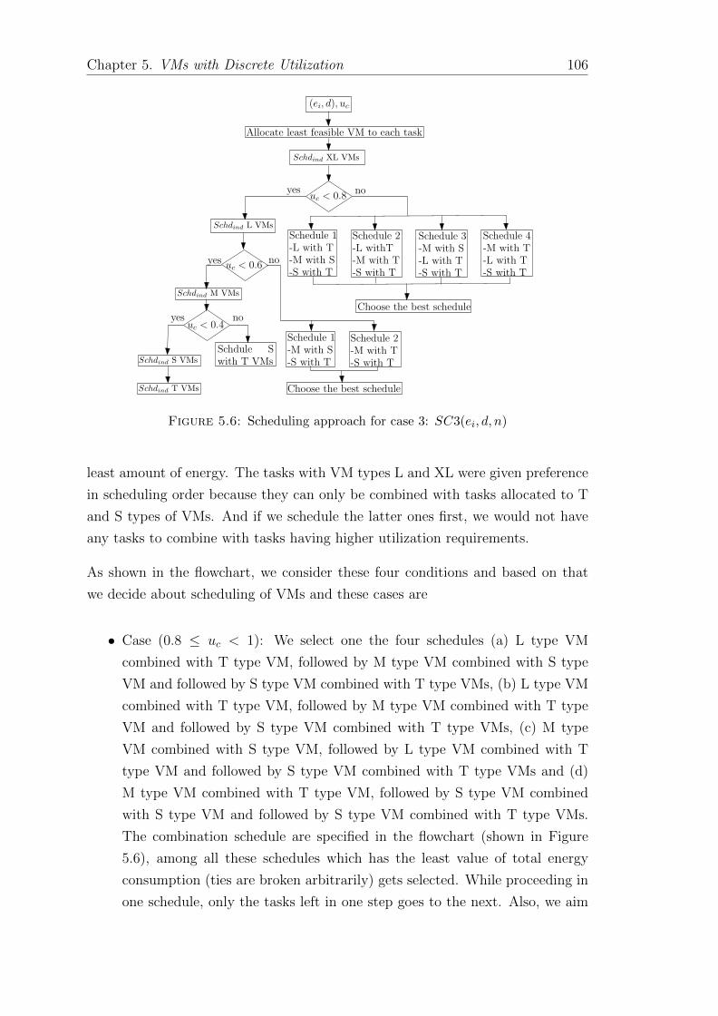
Chapter 5. VMs with Discrete Utilization 106
�chdin� X� VMs
�ei; d); u�
u� < 0�8
u� < 0�6
u� < 0�4
�chdin� � VMs
Schedule 3-M with S-L with T-S with T
Schedule 4-M with T-L with T-S with T
�chdin� T VMs
yes no
yes no
yes no
Schedule 1-L with T-M with S-S with T
Schedule 2-L withT-M with T-S with T
�chdin� M VMs
Schedule 1-M with S-S with T
Schedule 2-M with T-S with T�chdin� S VMs
Choose the best schedule
Schdule Swith T VMs
Choose the best schedule
Allocate least feasible VM to each task
Figure 5.6: Scheduling approach for case 3: SC3(ei, d, n)
least amount of energy. The tasks with VM types L and XL were given preference
in scheduling order because they can only be combined with tasks allocated to T
and S types of VMs. And if we schedule the latter ones first, we would not have
any tasks to combine with tasks having higher utilization requirements.
As shown in the flowchart, we consider these four conditions and based on that
we decide about scheduling of VMs and these cases are
• Case (0.8 ≤ uc < 1): We select one the four schedules (a) L type VM
combined with T type VM, followed by M type VM combined with S type
VM and followed by S type VM combined with T type VMs, (b) L type VM
combined with T type VM, followed by M type VM combined with T type
VM and followed by S type VM combined with T type VMs, (c) M type
VM combined with S type VM, followed by L type VM combined with T
type VM and followed by S type VM combined with T type VMs and (d)
M type VM combined with T type VM, followed by S type VM combined
with S type VM and followed by S type VM combined with T type VMs.
The combination schedule are specified in the flowchart (shown in Figure
5.6), among all these schedules which has the least value of total energy
consumption (ties are broken arbitrarily) gets selected. While proceeding in
one schedule, only the tasks left in one step goes to the next. Also, we aim
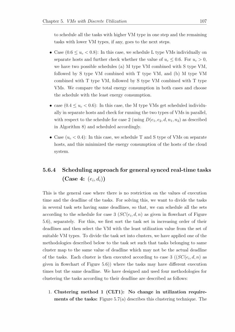
Chapter 5. VMs with Discrete Utilization 107
to schedule all the tasks with higher VM type in one step and the remaining
tasks with lower VM types, if any, goes to the next steps.
• Case (0.6 ≤ uc < 0.8): In this case, we schedule L type VMs individually on
separate hosts and further check whether the value of uc ≤ 0.6. For uc > 0,
we have two possible schedules (a) M type VM combined with S type VM,
followed by S type VM combined with T type VM, and (b) M type VM
combined with T type VM, followed by S type VM combined with T type
VMs. We compare the total energy consumption in both cases and choose
the schedule with the least energy consumption.
• case (0.4 ≤ uc < 0.6): In this case, the M type VMs get scheduled individu-
ally in separate hosts and check for running the two types of VMs in parallel,
with respect to the schedule for case 2 (using D(e1, e2, d, n1, n2) as described
in Algorithm 8) and scheduled accordingly.
• Case (uc < 0.4): In this case, we schedule T and S type of VMs on separate
hosts, and this minimized the energy consumption of the hosts of the cloud
system.
5.6.4 Scheduling approach for general synced real-time tasks
(Case 4: (ei, di))
This is the general case where there is no restriction on the values of execution
time and the deadline of the tasks. For solving this, we want to divide the tasks
in several task sets having same deadlines, so that, we can schedule all the sets
according to the schedule for case 3 (SC(ei, d, n) as given in flowchart of Figure
5.6), separately. For this, we first sort the task set in increasing order of their
deadlines and then select the VM with the least utilization value from the set of
suitable VM types. To divide the task set into clusters, we have applied one of the
methodologies described below to the task set such that tasks belonging to same
cluster map to the same value of deadline which may not be the actual deadline
of the tasks. Each cluster is then executed according to case 3 ((SC(ei, d, n) as
given in flowchart of Figure 5.6)) where the tasks may have different execution
times but the same deadline. We have designed and used four methodologies for
clustering the tasks according to their deadline are described as follows:
1. Clustering method 1 (CLT1): No change in utilization require-
ments of the tasks: Figure 5.7(a) describes this clustering technique. The
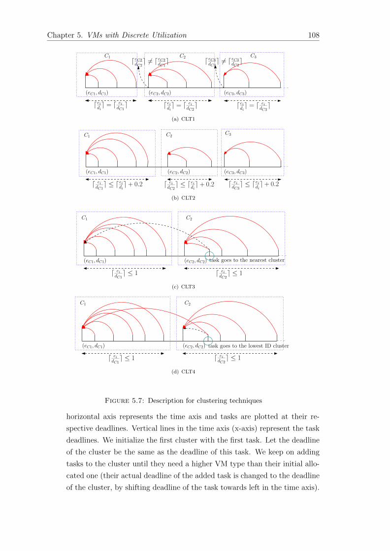
Chapter 5. VMs with Discrete Utilization 108
(eC1, dC1) (eC2, dC2) (eC3, dC3)
deidie = d eidC1
e deidie = d eidC2
e
deC2dC2
e 6= deC2dC1
e deC3dC3
e 6= deC3dC2
e
deidie = d eidC3
e
C1 C2 C3
(a) CLT1
(eC1, dC1) (eC3, dC3)(eC2, dC2)
C1 C2C3
d eidC1e ≤ deidie + 0.2 d ei
dC2e ≤ deidie + 0.2 d ei
dC3e ≤ deidie + 0.2
(b) CLT2
(eC1, dC1) (eC2, dC2)
d eidC1e ≤ 1 d ei
dC2e ≤ 1
C1 C2
task goes to the nearest cluster
(c) CLT3
(eC1, dC1) (eC2, dC2)
d eidC1e ≤ 1 d ei
dC2e ≤ 1
C1 C2
task goes to the lowest ID cluster
(d) CLT4
Figure 5.7: Description for clustering techniques
horizontal axis represents the time axis and tasks are plotted at their re-
spective deadlines. Vertical lines in the time axis (x-axis) represent the task
deadlines. We initialize the first cluster with the first task. Let the deadline
of the cluster be the same as the deadline of this task. We keep on adding
tasks to the cluster until they need a higher VM type than their initial allo-
cated one (their actual deadline of the added task is changed to the deadline
of the cluster, by shifting deadline of the task towards left in the time axis).
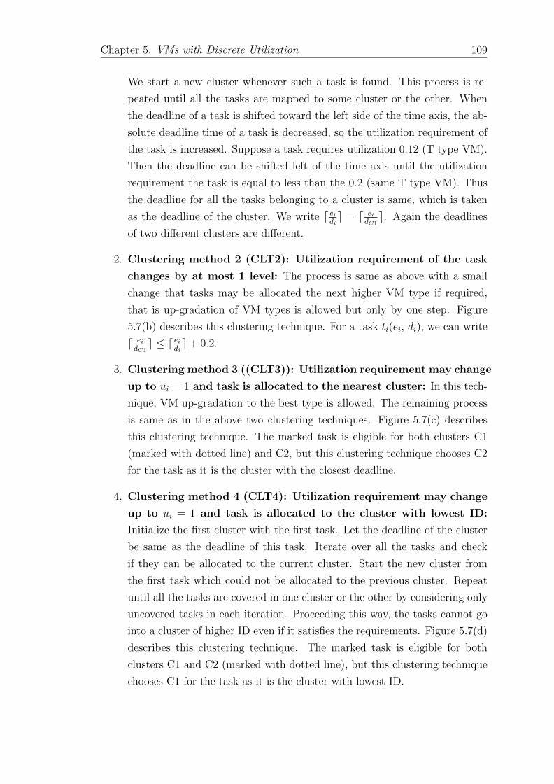
Chapter 5. VMs with Discrete Utilization 109
We start a new cluster whenever such a task is found. This process is re-
peated until all the tasks are mapped to some cluster or the other. When
the deadline of a task is shifted toward the left side of the time axis, the ab-
solute deadline time of a task is decreased, so the utilization requirement of
the task is increased. Suppose a task requires utilization 0.12 (T type VM).
Then the deadline can be shifted left of the time axis until the utilization
requirement the task is equal to less than the 0.2 (same T type VM). Thus
the deadline for all the tasks belonging to a cluster is same, which is taken
as the deadline of the cluster. We write d eidie = d ei
dC1e. Again the deadlines
of two different clusters are different.
2. Clustering method 2 (CLT2): Utilization requirement of the task
changes by at most 1 level: The process is same as above with a small
change that tasks may be allocated the next higher VM type if required,
that is up-gradation of VM types is allowed but only by one step. Figure
5.7(b) describes this clustering technique. For a task ti(ei, di), we can write
d eidC1e ≤ d ei
die+ 0.2.
3. Clustering method 3 ((CLT3)): Utilization requirement may change
up to ui = 1 and task is allocated to the nearest cluster: In this tech-
nique, VM up-gradation to the best type is allowed. The remaining process
is same as in the above two clustering techniques. Figure 5.7(c) describes
this clustering technique. The marked task is eligible for both clusters C1
(marked with dotted line) and C2, but this clustering technique chooses C2
for the task as it is the cluster with the closest deadline.
4. Clustering method 4 (CLT4): Utilization requirement may change
up to ui = 1 and task is allocated to the cluster with lowest ID:
Initialize the first cluster with the first task. Let the deadline of the cluster
be same as the deadline of this task. Iterate over all the tasks and check
if they can be allocated to the current cluster. Start the new cluster from
the first task which could not be allocated to the previous cluster. Repeat
until all the tasks are covered in one cluster or the other by considering only
uncovered tasks in each iteration. Proceeding this way, the tasks cannot go
into a cluster of higher ID even if it satisfies the requirements. Figure 5.7(d)
describes this clustering technique. The marked task is eligible for both
clusters C1 and C2 (marked with dotted line), but this clustering technique
chooses C1 for the task as it is the cluster with lowest ID.
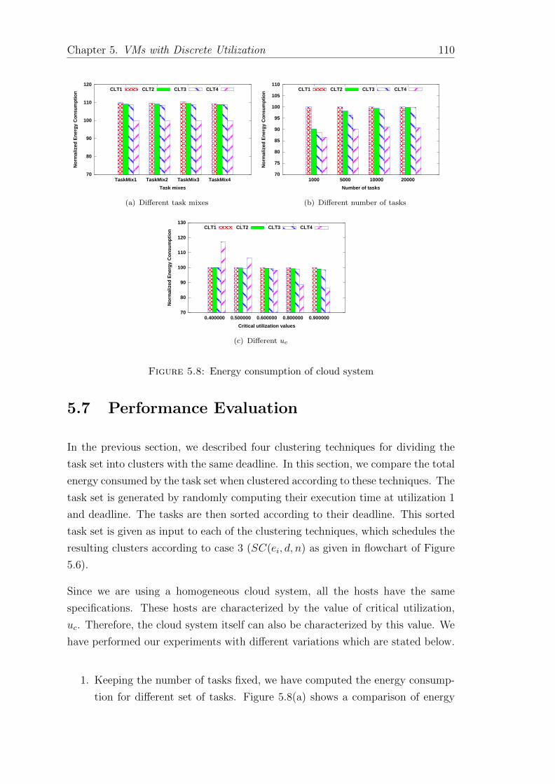
Chapter 5. VMs with Discrete Utilization 110
70
80
90
100
110
120
TaskMix1 TaskMix2 TaskMix3 TaskMix4
No
rmalized
En
erg
y C
on
su
mp
tio
n
Task mixes
CLT1 CLT2 CLT3 CLT4
(a) Different task mixes
70
75
80
85
90
95
100
105
110
1000 5000 10000 20000
No
rmalized
En
erg
y C
on
su
mp
tio
n
Number of tasks
CLT1 CLT2 CLT3 CLT4
(b) Different number of tasks
70
80
90
100
110
120
130
0.400000 0.500000 0.600000 0.800000 0.900000
No
rmalized
En
erg
y C
on
su
mp
tio
n
Critical utilization values
CLT1 CLT2 CLT3 CLT4
(c) Different uc
Figure 5.8: Energy consumption of cloud system
5.7 Performance Evaluation
In the previous section, we described four clustering techniques for dividing the
task set into clusters with the same deadline. In this section, we compare the total
energy consumed by the task set when clustered according to these techniques. The
task set is generated by randomly computing their execution time at utilization 1
and deadline. The tasks are then sorted according to their deadline. This sorted
task set is given as input to each of the clustering techniques, which schedules the
resulting clusters according to case 3 (SC(ei, d, n) as given in flowchart of Figure
5.6).
Since we are using a homogeneous cloud system, all the hosts have the same
specifications. These hosts are characterized by the value of critical utilization,
uc. Therefore, the cloud system itself can also be characterized by this value. We
have performed our experiments with different variations which are stated below.
1. Keeping the number of tasks fixed, we have computed the energy consump-
tion for different set of tasks. Figure 5.8(a) shows a comparison of energy

Chapter 5. VMs with Discrete Utilization 111
consumption values between all the four clustering techniques for the same
cloud system. We have taken uc = 0.73 in this case. As we can see, cluster-
ing techniques CLT4 gives us the least energy consumption for all the task
mixes.
2. Figure 5.8(b) shows a comparison of energy consumption values between
all the four clustering techniques when the requests have different number
of tasks. We have normalized the energy consumption of all the clustering
techniques with respect to CLT1 for same task set. This comparison is done
for same cloud system with uc = 0.73. As we can see, a similar pattern is
being followed for all the task sets. Here CLT4 is giving the least energy
consumption in all the cases.
3. Keeping the task set same, Figure 5.8(c) shows a comparison of energy con-
sumption values between all the four clustering techniques on a different
cloud system. Here also, we have compared the normalized values of energy
consumption with respect to CLT1 for the same cloud system. Clustering
techniques CLT1, CLT2, and CLT3 produced better results than CLT4 when
the value of the critical utilization (uc) is less than 0.6, whereas, for the value
of uc > 0.6, CLT4 produced a better result.
From the above results, we can say that choosing the clustering techniques does
not depend on the user request but on the specification of the cloud system.
As the value of uc is known for a cloud system, we can choose the clustering
technique, without looking at the task mix. For cloud systems with lower critical
utilization values, that is uc ≤ 0.6, choose any one of CLT1, CLT2 or CLT3, as
they all produce comparable results. For systems with a higher uc, it is better to
choose CLT4 as the clustering technique to minimize the energy consumption of
the system.
5.8 Summary
In this chapter, we investigate the problem of energy-efficient scheduling of a set
of offline real-time tasks in a virtualized cloud environment. The virtual resource
layer of the cloud system consists of a set of different type of VMs, where each VM
type is specified by its utilization. We assume that the bigger VMs (having higher
compute capacity and thus requires lesser time to execute a task) provide higher

Chapter 5. VMs with Discrete Utilization 112
utilization and smaller VMs (having lesser compute capacity and thus requires
more time to execute a task) provide lower utilization to the host. In this chapter,
we have carefully used the energy consumption versus the utilization characteris-
tics of the hosts of the cloud system to minimize the overall energy consumption
of the system. We first calculate critical utilization value when the host energy
is minimum and the target of the scheduling policy is to keep the host utiliza-
tion close to the critical utilization. We categorize the problem of energy-efficient
scheduling of a set of real-time tasks into four subproblems and then solve them
individually.

Chapter 6
Scheduling Scientific Workflows
on Virtualized Cloud System
This chapter presents a series of energy-efficient scheduling techniques for exe-
cuting a set of online dependent tasks, represented as scientific workflows. Each
task in a workflow requires multiple VMs to execute and we use two different VM
allocation approaches for this. We consider three different migration policies: no
migration, limited migration, and full migration in designing our scheduling ap-
proaches. Extensive simulation experiments are conducted on Cloudsim toolkit
to establish the superiority of the proposed work as compared to a state-of-art
energy-efficient scheduling policy.
6.1 Introduction
The overwhelming popularity of the cloud system has attracted the users from
different domains to host their applications at an affordable cost. The availability
of high-end resources in the cloud has made itself a better choice for the scientific
applications [95]. The elasticity feature added advantage to the cloud domain to
efficiently handle the variation in the resource requirement of these scientific ap-
plications. These scientific applications often come from fields, such as astronomy,
astrophysics, bioinformatics, high energy physics, etc., and they are modeled as
scientific workflows [24, 25, 41].
Because of the significant cost of the compute servers of the cloud system, most
of the cloud system provider does not procure all the servers (or hosts) of their
113

Chapter 6. Scheduling Scientific Workflows on Virtualized Cloud System 114
cloud system in one go; instead, they purchase servers in phases and add them
to their existing cloud system. In fact, a data center might contain multiple
generations of hardware [86]. Thus, in most of the cases, cloud systems are bound
to be heterogeneous. But for the cloud user, this heterogeneity gets hidden by
the virtualization layer and user’s requests require machines in terms of VMs and
most of the cases the requests are for homogeneous VM. So to cater this particular
behavior of cloud system, in this work, we have considered scheduling of workflows
to be run on top of a set of homogeneous virtual machines while the cloud system
essentially consists of heterogeneous servers (hosts).
Scientific workflows are typically expressed as a precedence constraint graph. But
the graphs are structured in such a way that most of them can also be represented
as a chain of tasks [131, 132]. Each task in the chain represents a collection of
sub-tasks. Each task has also its individual execution time or length. A collection
of VMs ( in case of a virtualized system) or a set of threads (in case of a non-
virtualized system) together execute a task where each VM or thread executes a
sub-task. Thus in case of a virtualized cloud system, a task of a scientific workflow
requires multiple VMs for its execution. In this chapter, we consider the scheduling
of this structured scientific workflows for the cloud system. Now there may be two
different types of VM allocations for a task of a workflow: (i) non-splittable VM
allocation (NSVM), and (ii) splittable VM allocation (SVM). In case of NSVM, all
the required VMs of a task must be placed on one host. And in case of SVM, the
VMs can be placed on different hosts. In our work, we have considered scheduling
of a set of online scientific workflows so as to reduce the energy consumption where
each workflow has a deadline and the schedule must satisfy the deadline constraint.
A substantial amount of research has already been done to schedule scientific work-
flows in the cloud system in an energy-efficient manner [102, 103, 61, 41, 95, 99].
For instance, Durillo et al. [102] has developed a multi-objective energy-efficient
list-based workflow scheduling algorithm, called MOHEFT (Multi-Objective HEFT)
where they present a trade-off between the energy consumption and the makespan
time. In [28], Bousselmi et al. partitioned the workflow to reduce the data com-
munication among them, thereby reduced the network energy consumption. Then
they used the cat swarm optimization based heuristic to schedule each partition
on a set of VMs in an energy-efficient manner. Chen et al. [104] designed an online
scheduling algorithm, called, energy-efficient online scheduling EONS to schedule
tasks from different workflows. In this approach, system resources are dynamically
adjusted to maintain the weighted square frequencies of the hosts.

Chapter 6. Scheduling Scientific Workflows on Virtualized Cloud System 115
Recently, Li et al. [61] has considered reducing both the energy consumption
and the execution cost of workflow while guaranteeing deadline constraints. They
considered only the dynamic energy consumption of the hosts and used DVFS
technology to utilize the slack time of a task. Xu et al. [41] considered the
execution of scientific workflows to minimize the energy consumption of cloud
resources. They transformed a workflow into a set of sequential tasks and each
task arrives at the system with a predefined start time. Their considered cloud
system consists of heterogeneous hosts and a set of homogeneous VMs placed on
those hosts execute the tasks.
In this chapter, we consider similar kinds of environment (homogeneous VMs on
heterogeneous hosts) as considered in [41] to schedule a set of online scientific
workflows in the cloud system. But we do not consider the static partition of the
tasks; instead, the start time of each task of a workflow is calculated dynami-
cally based on the usages of the slack time of the workflow. We summarize the
contributions of this chapter as follows.
• An energy consumption model for the cloud is presented catering to both
static and dynamic energy consumption.
• Two different VM allocation techniques (splittable and non-splittable) is
presented
• Three different slack distribution and utilization technique is presented.
• A series of energy-efficient online scheduling techniques are presented for
executing a set of online scientific workflows in the cloud environment.
• Trade-off between the energy consumption, the number of migrations and
number of splits is addressed.
6.2 System Model
The considered virtualized cloud system accepts a set of online workflows. Each
workflow is represented by a chain of tasks. These tasks are to be executed on
some virtual machines (VMs) which are hosted on a set of physical machines. The
physical layer of the cloud system consists of a sufficiently large number (can be
considered as infinite) of physical machines (or hosts), H = {h1, h2, h3, h4, · · · }.
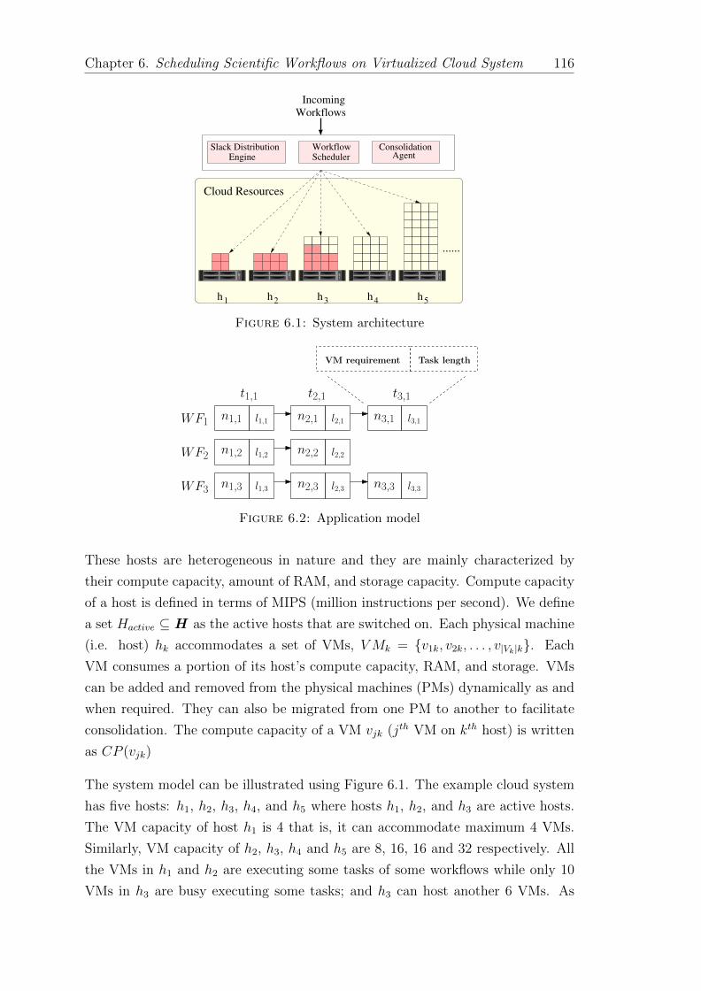
Chapter 6. Scheduling Scientific Workflows on Virtualized Cloud System 116
Workflows
Incoming
ConsolidationAgent
WorkflowSchedulerEngine
Slack Distribution
Cloud Resources
h 2 h3 4 h51 h h
......
Figure 6.1: System architecture
n1,1 l1,1 n2,1 l2,1 n3,1 l3,1WF1
n1,2 l1,2 n2,2 l2,2WF2
n1,3 l1,3 n2,3 l2,3 n3,3 l3,3WF3
VM requirement Task length
t1,1 t2,1 t3,1
Figure 6.2: Application model
These hosts are heterogeneous in nature and they are mainly characterized by
their compute capacity, amount of RAM, and storage capacity. Compute capacity
of a host is defined in terms of MIPS (million instructions per second). We define
a set Hactive ⊆ H as the active hosts that are switched on. Each physical machine
(i.e. host) hk accommodates a set of VMs, VMk = {v1k, v2k, . . . , v|Vk|k}. Each
VM consumes a portion of its host’s compute capacity, RAM, and storage. VMs
can be added and removed from the physical machines (PMs) dynamically as and
when required. They can also be migrated from one PM to another to facilitate
consolidation. The compute capacity of a VM vjk (jth VM on kth host) is written
as CP (vjk)
The system model can be illustrated using Figure 6.1. The example cloud system
has five hosts: h1, h2, h3, h4, and h5 where hosts h1, h2, and h3 are active hosts.
The VM capacity of host h1 is 4 that is, it can accommodate maximum 4 VMs.
Similarly, VM capacity of h2, h3, h4 and h5 are 8, 16, 16 and 32 respectively. All
the VMs in h1 and h2 are executing some tasks of some workflows while only 10
VMs in h3 are busy executing some tasks; and h3 can host another 6 VMs. As

Chapter 6. Scheduling Scientific Workflows on Virtualized Cloud System 117
the workflows enter the cloud system, they pass through the slack distribution
engine. The job of the slack distribution engine is to distribute the whole slack
of a workflow among different tasks of that workflow. The next phase is the
workflow scheduling phase. The job of the workflow scheduler is to efficiently
schedule the tasks of an incoming workflow on the existing state of the cloud
resources such that the overall energy of the cloud system is minimized (considering
the energy consumption model described in Section 6.4). The system consists of
a consolidation agent and the job of the agent is to consolidate the VMs to a
minimum number of hosts to reduce the total number of active hosts in the system.
6.3 Application Model
The application model consists of a set of online workflows WF = {WF1,WF2, · · · }.Each workflow WFp is represented by a sequence of tasks {t1,p, t2,p, · · · , t|WFp|,p}with a chain constraint among them [131, 132]. Each workflow WFp has its arrival
time ap. Each task ti,p of a workflow WFp is characterized by two parameters: (a)
VM requirement of the task ni,p, and (b) the length of the task (li,p); where i is
the task sequence number in the workflow and p is the workflow number. VM re-
quirement of a task means total number of parallel VMs needed at the same time
to execute the task. The length of the task is expressed as million instructions
(MI).
Figure 6.2 shows an example of such workflow system consisting of 3 different
workflows or chains WF1, WF2, and WF3 having 3, 2, and 3 tasks respectively.
A task of a workflow can not start execution before complete execution of its
predecessor tasks of the same workflow. We assume that there is no dependency
among different workflows and thus execution of one workflow can overlap with
others.
Suppose a task ti,p requires only one VM for its execution and it is executed by a
VM vjk. Then it will require li,p/CP (vjk) amount time for its completion. This
becomes the execution time of task ti,p on VM vjk and is represented by eipjk.
Mathematically, it can be written as:
eipjk =li,p
CP (vjk)(6.1)

Chapter 6. Scheduling Scientific Workflows on Virtualized Cloud System 118
We also define the ready time of a VM, r(vj,k) as:
rt(vjk) = st(vjk) + eipjk (6.2)
where, st(vjk) is the start time of the VM which indicates the time instant when
the VM vjk has started executing the task tip.
Every workflow has a user-defined deadline dp; that is execution of all the tasks in
the workflow must finish their execution by time dp. Deadline of a workflow WFp
satisfies the relation dp ≥∑|WFp|
i=1 eipjk + ap.
The time difference between the deadline and the summation of execution time
for all the tasks of a workflow WFp is called the slack time slkp and this can be
represented as
slkp = dp − ap −( |WFp|∑
i=1
eipjk
)(6.3)
where slkp is the total amount of slack time for the workflow WFp, |WFp| indicates
the length of the workflow (or chain) that is the total number of tasks for the
workflow WFp. In case of homogeneous VMs, slkp can be calculated beforehand.
6.4 Energy Consumption Model
Cloud system consists of many power consuming components but a major portion
of the power in a cloud data center is consumed by the host (or compute node)
itself. Again the host power consumption is mainly driven by that of the processor
(CPU), memory, network interface and disk storage. Power consumption of a host
has two components: static and dynamic. A large volume of research has already
been done considering only the dynamic power consumption of the host, specially
when scheduling of real-time tasks was considered [33, 30, 52, 67]. But research
also reveals the fact that static power consumption of a host is nearly 60% to 70%
of the total power consumption [45, 43] which is significant and should not be
ignored.
Thus in our work, we have considered both the static and dynamic power con-
sumption of the host to schedule a set of scientific workflows in the cloud where

Chapter 6. Scheduling Scientific Workflows on Virtualized Cloud System 119
each workflow consists of a chain of real-time tasks. The summation of these power
consumption values over the total time interval gives the energy consumption of
the system. Mathematically, it can be written as E =∫∞t=0
PCt.dt, where PCt is
the total power consumption of the system at time t. Total energy consumption
of an active host hk can be expressed as follows.
Ehk = Ehk s + Ehk d (6.4)
where, Ehk is the total energy consumption of a host hk, Ehk s is the static energy
consumption of the host, and Ehk d is the dynamic energy consumption of the host.
Thus total energy consumption of the cloud system can be expressed as
Etotal =
|Hactive|∑k=1
Ehk (6.5)
We assume that all non-active hosts are switched off and they do not consume any
energy.
In this work, we considered that the hosts in the cloud system are heterogeneous
and their base power (or energy) consumptions are different, similar to the energy
consumption model considered in [41]. Base (or static) energy consumption of a
host hk can be written as
Ehk s = ECRbasek .t (6.6)
where, ECRbasek is the base energy consumption rate of host hk and t is the total
active time for host hk.
The base energy consumption rate of the hosts can be taken as the function of
their VM capacity which is explained in details with example in Section 6.10. Ac-
cordingly, the base energy consumption rate of hosts in the system model (Figure
6.1) can be expressed as follows.

Chapter 6. Scheduling Scientific Workflows on Virtualized Cloud System 120
ECRbase1 ≤ ECRbase2 ≤ ECRbase3 ≤ ECRbase4 ≤ · · · (6.7)
which means the base energy consumption rate of host h1 is less than or equal
to the base energy consumption rate of host h2, which is tern less or equal to
the base energy consumption rate of host h3 and so on. This is because the VM
capabilities of host h1 is less than VM capabilities of host h2, which is less than
VM capabilities of host h3, and so on.
Again the dynamic energy consumption of a host is basically contributed by the
active VMs when they execute some tasks. In our work, we considered the dynamic
energy consumption model similar to [30]. Suppose VM vjk executes task ti,p. Then
the energy consumption of the VM, Evipjk can be written as follows.
Evipjk = ECRvjk .eipjk (6.8)
where, ECRvjk is the energy consumption rate of VM vjk, eipjk is the time taken
by VM vjk to execute task ti,p .
Now the total dynamic energy consumption of a host can be represented as
Ehk d =
|VMk|∑j=1
|WFp|∑i=1
Evipjk (6.9)
In order to achieve energy efficiency, the workflow scheduler always try to put the
tasks of workflows in the hosts with lower energy consumption.
6.5 Objective in the Chapter
The chapter aims to schedule a set on online workflows, represented by WF =
{WF1,WF2,WF3, · · · } onto a virtualized cloud system, represented by an infinite
set of physical machines (or hosts), H = {h1, h2, h3, h4, · · · } such that the overall
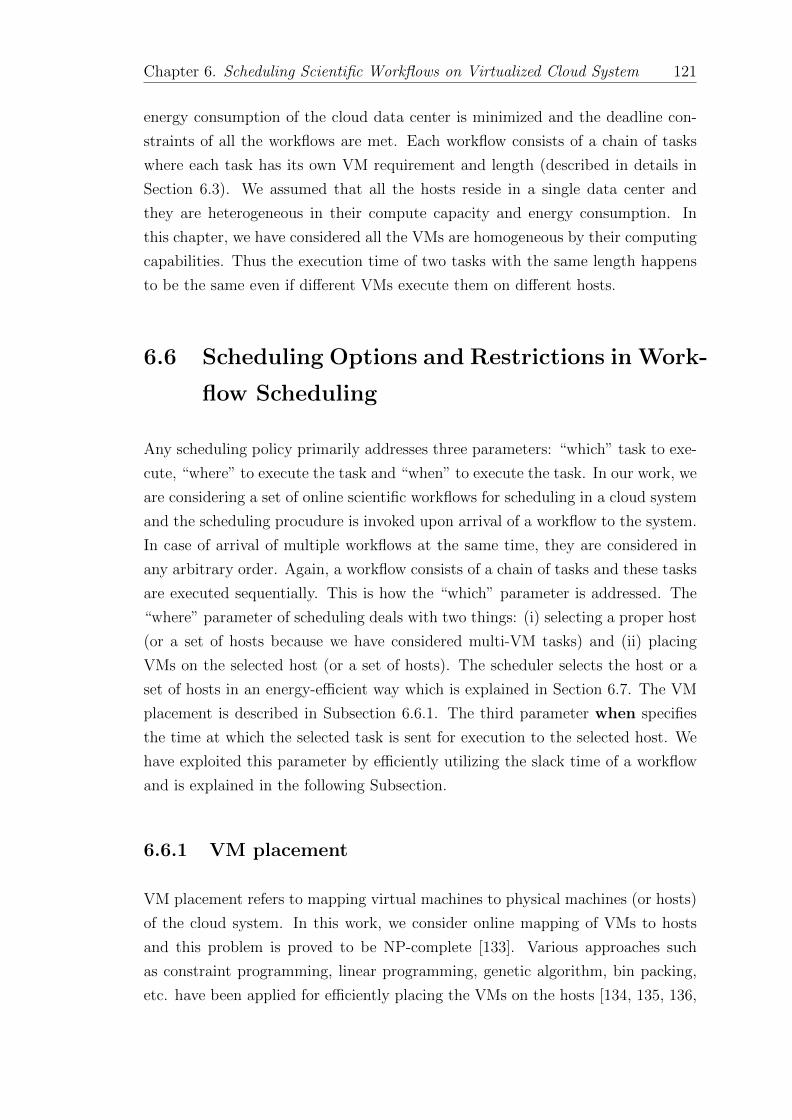
Chapter 6. Scheduling Scientific Workflows on Virtualized Cloud System 121
energy consumption of the cloud data center is minimized and the deadline con-
straints of all the workflows are met. Each workflow consists of a chain of tasks
where each task has its own VM requirement and length (described in details in
Section 6.3). We assumed that all the hosts reside in a single data center and
they are heterogeneous in their compute capacity and energy consumption. In
this chapter, we have considered all the VMs are homogeneous by their computing
capabilities. Thus the execution time of two tasks with the same length happens
to be the same even if different VMs execute them on different hosts.
6.6 Scheduling Options and Restrictions in Work-
flow Scheduling
Any scheduling policy primarily addresses three parameters: “which” task to exe-
cute, “where” to execute the task and “when” to execute the task. In our work, we
are considering a set of online scientific workflows for scheduling in a cloud system
and the scheduling procudure is invoked upon arrival of a workflow to the system.
In case of arrival of multiple workflows at the same time, they are considered in
any arbitrary order. Again, a workflow consists of a chain of tasks and these tasks
are executed sequentially. This is how the “which” parameter is addressed. The
“where” parameter of scheduling deals with two things: (i) selecting a proper host
(or a set of hosts because we have considered multi-VM tasks) and (ii) placing
VMs on the selected host (or a set of hosts). The scheduler selects the host or a
set of hosts in an energy-efficient way which is explained in Section 6.7. The VM
placement is described in Subsection 6.6.1. The third parameter when specifies
the time at which the selected task is sent for execution to the selected host. We
have exploited this parameter by efficiently utilizing the slack time of a workflow
and is explained in the following Subsection.
6.6.1 VM placement
VM placement refers to mapping virtual machines to physical machines (or hosts)
of the cloud system. In this work, we consider online mapping of VMs to hosts
and this problem is proved to be NP-complete [133]. Various approaches such
as constraint programming, linear programming, genetic algorithm, bin packing,
etc. have been applied for efficiently placing the VMs on the hosts [134, 135, 136,

Chapter 6. Scheduling Scientific Workflows on Virtualized Cloud System 122
t1h1 h2 h3
t2 t2
t2 t2
t2 t3
t3
t3 t3 t3 t3
t3t3t3
t3
t1
(a) Allocation under non-splittable VM category
t1h1 h2 h3
t3
t3
t1 t3 t3 t3
t3t3t3
t3 t3 t2
t2 t2 t2 t2t2
(b) Allocation under splittable VM category
Figure 6.3: System state with different VM allocation type
137, 56, 138]. Best fit decreasing order (BFD) and first fit decreasing order (FFD)
are two effective heuristics when the problem is mapped to bin packing problem
[41, 43]. In our work, we have used a variation of BFD and combination of BFD
and FFD depending on the VM allocation type and migration planning.
A task ti in the system is specified with its length li and VM requirement ni. Thus
a task may require more than one VM for its execution and a host might fail to
accommodate the task. Keeping this scenario into consideration, we have used
two types of VM allocation in our work.
(1) Non-splittable VMs (NSVM): In this category, the VM allocation for a
single task cannot be split; thus the name. All the required VMs of a task must be
hosted on the same physical machine of the cloud system for the entire duration of
the task execution. A task can be scheduled on a host only if it can accommodate
the task completely, i.e. the idle number of VMs of a host must be greater than
or equal to the number of VMs required by the task for its execution.
(2) Splittable VMs (SVM): In the second category, the VM allocation for a
task can be split. That is the required VMs of a task can be hosted on more than
one physical machines of the cloud system. A task can be scheduled when a set of
hosts in the system can collectively satisfy the VM requirement of the task.
In case of the non-splittable VM allocation category, the system might experience a
poor utilization of the resources. This is illustrated using Figure 6.3. For instance,
let there be 3 types of hosts with VM capacities 4, 8 and 16 respectively. Let
us assume that base power consumptions of the hosts are 50W, 75W and 100W
respectively. Now we suppose that there are 3 tasks with VM requirements 2, 5,
and 7 which are to be placed on the hosts. In this case, the system will remain
underutilized and there will be a wastage of 39% of the VM capacity. Figure 6.3(a)
represents the system state after scheduling these tasks. The power consumption
will be 50 + 75 + 100 + 17x10 = 395W (assuming per VM power consumption is
10W).

Chapter 6. Scheduling Scientific Workflows on Virtualized Cloud System 123
On the other hand, relaxation on VM placement condition in case of splittable
type provides an opportunity to the scheduler to utilize the system resources more
effectively. Now the scheduler searches for a collection of hosts which can collec-
tively satisfy the VM requirement of a task. We see that for the given example,
the total VM requirement of the tasks is 17(= 2 + 5 + 10) and this can be met
only by only two hosts (h1 and h3). Host h2 can be put in switched-off mode and
this will not consume any power. Figure 6.3(b) represents the system status after
this schedule. This reduces the number of active hosts; which in turn reduces the
overall energy (or power) consumption of the system. Power consumption of the
system under this allocation type is 50 + 100 + 17x10 = 320W. But whenever, the
VMs of a single task reside in different hosts, they need to communicate among
themselves. The energy consumption due to this communication can be modeled
as shown below which is considered similar to [41].
ECcomm =
|Hactive|∑i=1
|Hactive|∑j=1
Di,j
bwi,jECRcomm (6.10)
where Di,j represents the total data transferred from host hi to hj, bwi,j is the
network bandwidth between hi and hj, and ECRcomm is energy consumption rate
for communication between two different hosts.
This extra energy will be added to the total energy consumption of Equation 6.5
in order to find the overall energy consumption of the system.
6.6.2 Migration
The workflow scheduler described in Section 6.1 has a consolidation agent. The
job of the consolidation agent is to run through the active hosts and to migrate
VMs from the hosts with lower utilization value to the hosts with higher utilization
value. For this operation, we define a threshold called MigThreshold. Consolida-
tion operation can be performed on a host if its utilization value falls below the
MigThreshold. Under this setups, we outline three approaches as described below.
• No migration (NM): Under this approach, the consolidation operation
is not performed. Thus the existing mappings between a task to VM and
VM to host do not get changed during the course of execution. Whenever a
new task of a workflow arrives at the cloud system, the scheduler performs

Chapter 6. Scheduling Scientific Workflows on Virtualized Cloud System 124
scheduling of this task only and finds the best mapping for the task. The
scheduler does not consider already scheduled tasks while scheduling the
current task. Hence the number of migrations in this approach is zero; thus
the name no migration.
• Limited migration (LM): Whenever a workflow arrives, it is scheduled
on the cloud system without changing the mapping of the already scheduled
tasks. Under this setup, the utilization of a host changes only when a task fin-
ishes its execution, thus releases the corresponding VM. Then consolidation
agent checks whether the host utilization falls below the MigThreshold value.
The agent performs the consolidation operation only if the host utilization
falls below the threshold. After the consolidation operation is performed,
the agent marks the active hosts without any active VMs on them and then
it puts such hosts in switched off mode.
• Full migration (FM): Under this approach, the consolidation operation is
performed along with the scheduling operation. Thus the existing mapping
of tasks to VMs and VMs to hosts might get changed. The newly arrived
tasks and the existing tasks in the system (both running and waiting) are
considered to be fresh tasks and energy-efficient scheduling policies are ap-
plied to get new mappings. As per the new mapping, if the associated VMs
of a task are mapped to their previous hosts, then no migration is required.
Otherwise, the system needs to migrate VMs from the current host to the
newly mapped hosts.
6.6.3 Slack distribution
Here the slack time of the task (or workflow) plays an important role. Suppose a
workflow consists of m number of tasks and slack time for the workflow is z. If
we consider discrete scheduling time, then the first task in the workflow can have
m.z choices to utilize the slack. Suppose, the task fails to utilize the slack. Then
in the worst case, the second task in the workflow will have m.z choices and this
continued till the last task of the workflow. Thus in case of brute force approach,
the total number of choice for utilizing the slack time will be exponential. In our
work, we have used three simple but effective heuristics to utilize this slack time
efficiently in our proposed scheduling techniques.
(1) Slack to first task (SFT): Only the first task of every workflow enjoys
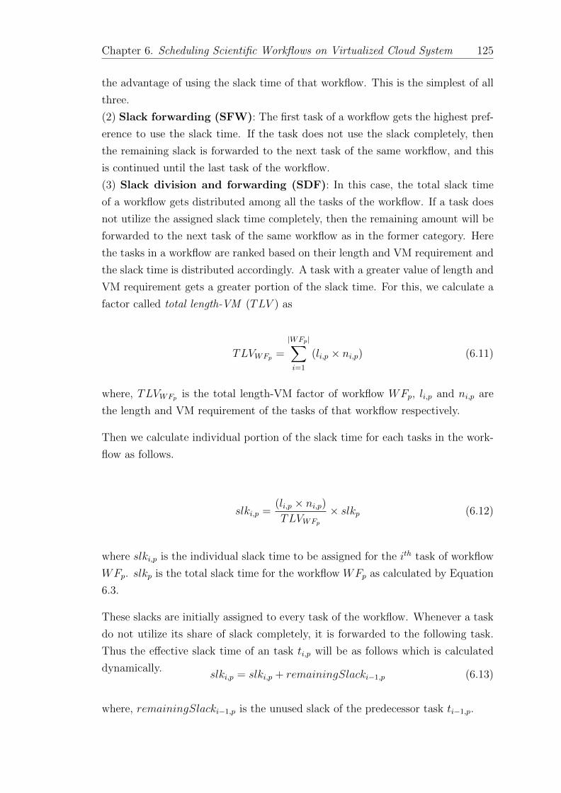
Chapter 6. Scheduling Scientific Workflows on Virtualized Cloud System 125
the advantage of using the slack time of that workflow. This is the simplest of all
three.
(2) Slack forwarding (SFW): The first task of a workflow gets the highest pref-
erence to use the slack time. If the task does not use the slack completely, then
the remaining slack is forwarded to the next task of the same workflow, and this
is continued until the last task of the workflow.
(3) Slack division and forwarding (SDF): In this case, the total slack time
of a workflow gets distributed among all the tasks of the workflow. If a task does
not utilize the assigned slack time completely, then the remaining amount will be
forwarded to the next task of the same workflow as in the former category. Here
the tasks in a workflow are ranked based on their length and VM requirement and
the slack time is distributed accordingly. A task with a greater value of length and
VM requirement gets a greater portion of the slack time. For this, we calculate a
factor called total length-VM (TLV ) as
TLVWFp =
|WFp|∑i=1
(li,p × ni,p) (6.11)
where, TLVWFp is the total length-VM factor of workflow WFp, li,p and ni,p are
the length and VM requirement of the tasks of that workflow respectively.
Then we calculate individual portion of the slack time for each tasks in the work-
flow as follows.
slki,p =(li,p × ni,p)TLVWFp
× slkp (6.12)
where slki,p is the individual slack time to be assigned for the ith task of workflow
WFp. slkp is the total slack time for the workflow WFp as calculated by Equation
6.3.
These slacks are initially assigned to every task of the workflow. Whenever a task
do not utilize its share of slack completely, it is forwarded to the following task.
Thus the effective slack time of an task ti,p will be as follows which is calculated
dynamically.slki,p = slki,p + remainingSlacki−1,p (6.13)
where, remainingSlacki−1,p is the unused slack of the predecessor task ti−1,p.
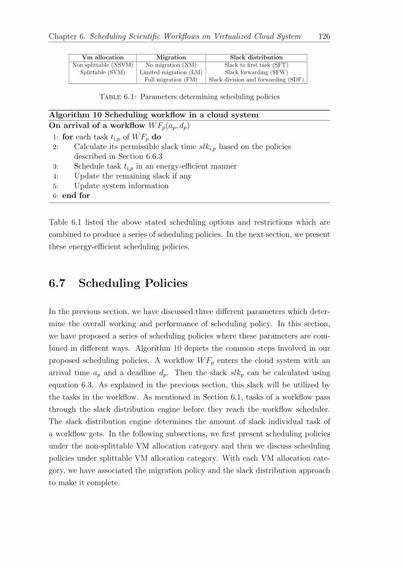
Chapter 6. Scheduling Scientific Workflows on Virtualized Cloud System 126
Vm allocation Migration Slack distributionNon splittable (NSVM) No migration (NM) Slack to first task (SFT)
Splittable (SVM) Limited migration (LM) Slack forwarding (SFW)Full migration (FM) Slack division and forwarding (SDF)
Table 6.1: Parameters determining scheduling policies
Algorithm 10 Scheduling workflow in a cloud system
On arrival of a workflow WFp(ap, dp)
1: for each task ti,p of WFp do2: Calculate its permissible slack time slki,p based on the policies
described in Section 6.6.33: Schedule task ti,p in an energy-efficient manner4: Update the remaining slack if any5: Update system information6: end for
Table 6.1 listed the above stated scheduling options and restrictions which are
combined to produce a series of scheduling policies. In the next section, we present
these energy-efficient scheduling policies.
6.7 Scheduling Policies
In the previous section, we have discussed three different parameters which deter-
mine the overall working and performance of scheduling policy. In this section,
we have proposed a series of scheduling policies where these parameters are com-
bined in different ways. Algorithm 10 depicts the common steps involved in our
proposed scheduling policies. A workflow WFp enters the cloud system with an
arrival time ap and a deadline dp. Then the slack slkp can be calculated using
equation 6.3. As explained in the previous section, this slack will be utilized by
the tasks in the workflow. As mentioned in Section 6.1, tasks of a workflow pass
through the slack distribution engine before they reach the workflow scheduler.
The slack distribution engine determines the amount of slack individual task of
a workflow gets. In the following subsections, we first present scheduling policies
under the non-splittable VM allocation category and then we discuss scheduling
policies under splittable VM allocation category. With each VM allocation cate-
gory, we have associated the migration policy and the slack distribution approach
to make it complete.

Chapter 6. Scheduling Scientific Workflows on Virtualized Cloud System 127
6.8 Scheduling with Non-splittable VM Alloca-
tion (NSVM)
In this section, we present scheduling approaches with the restriction that all the
VMs executing a task of a workflow must reside on the same host. A variation of
best fit decreasing order policy is used to put the VMs on the hosts. The scheduler
maintains the host list in non-decreasing order of their base power consumption
and the job of the scheduler is to find the host with lowest base power consumption
such that the host can hold all the VMs required by the task. In the following
subsections, we present different scheduling policies considering non-splittable VM
allocation.
6.8.1 Non-splittable VMs without migration (NSVMNM)
This scheduling technique is described using Algorithm 11. For each task of the
workflow, the algorithm first calculates its individual slack time. Then it inspects
the current system state and finds the best time to schedule the task in the system.
For this, the algorithm calls a Procedure findBestSlack(). This procedure inspects
all the active hosts in sorted order to find a host which can satisfy the VM require-
ment of the task. As soon as such a host is found, the procedure returns the host
with the best slack time when the host becomes available for executing the task
with minimum energy consumption. If no active host can hold the task within
the slack range, the procedure returns a NULL value. These steps are stated in
Procedure findBestSlack().
Then the Algorithm 11 schedules the task using another Procedure schedule().
If any active host can hold the task, the task gets scheduled on the VMs of that
host whenever it can hold (line number 4). If no active host can hold the task,
then a new host with minimum base power consumption is switched on such that
it can hold the task completely. Then the task is scheduled immediately without
wasting any slack time. This scheduling policy does not change the mapping of
the already scheduled tasks. Thus the execution of tasks are continuous and there
is no migration of tasks (or VMs). Now depending on the slack distribution logic,
the individual slack assigned to a task varies. For SFT slack distribution logic,
slki,p happens to be 0 for i ≥ 2.

Chapter 6. Scheduling Scientific Workflows on Virtualized Cloud System 128
5 4 4 8WFp:
Figure 6.4: WorkFlow (WFp(ap = 10, dp = 33)) to be scheduled on the system
6.8.1.1 Slack to first task (SFT NSVMNM)
Figure 6.5 describes an example of the working of the scheduling policy when
applied with SFT slack distribution logic. 6.5(a) shows the system state with
three active hosts having VM capacity of 4, 8 and 16 respectively. Each filled cell
of a host indicates a VM and the values inside represents the running task and the
ready time for that VM. A blank cell indicates free slot for new VM. We assume
that the hosts are in sorted in increasing order of their base power consumption.
All the VMs of host h1 is busy in executing task t1,1 and their ready time is 20.
VMs in host h2 is executing two tasks t1,2 and t2,4 and their ready times are 15
and 12 respectively. Host h2 can instantiate two more VMs on it. And in host h3,
ready time for eight VMs are 22 and it can instantiate another 8 VMs on it.
Now let us consider a workflow with two tasks as shown in Figure 6.4 with arrival
time 10 and deadline 33. As all the VMs in our cloud system is assumed to be
homogeneous, the length of a task can easily be taken as the execution time for the
task. Thus slack is calculated by Equation 6.3 as 33 − 10 − (4 + 8) = 11. The
first task of the workflow requires 5 VMs to execute and currently host h3 can
easily hold the task. But the scheduler does not schedule the task in h3. As the
slack value is 11, the scheduler can schedule the task any time from time 10 to
21 (= 10 + 11). Scheduler checks that the VMs of the host can hold the task h2
also and it prefers to schedule on h2 only because the base power consumption
of h2 is lesser than that of h3. But h2 can hold 5 VMs only at time 15. As it
lies in the slack range, the scheduler schedules the task on host h2 to schedule at
time instant 15, rather than immediate scheduling it on h3 (though enough active
resource is available). Figure 6.5(b) shows the system state after scheduling the
first task of the workflow. Now scheduling of remaining tasks of the workflow will
immediately start from time 19 because the finish time of the first task becomes
19(= 15 + 4). There is only one task remaining to be scheduled in the workflow
and it is to be scheduled at time 19. VM requirement of this task is 4. Thus it
has only one choice and the scheduler accordingly schedules the task on host h2.
Figure 6.5(c) shows the system state after this schedule.

Chapter 6. Scheduling Scientific Workflows on Virtualized Cloud System 129
Algorithm 11 NSVM without migration (NSVMNM)
On arrival of a workflow WFp(ap, dp)
1: Calculate the slack time slkp by Equation 6.32: leftSlack ← 03: schdT ime← ap4: for each task ti,p in WFp do5: Calculate its permissible slack time slki,p based on the policies
described in Section 6.6.36: slki,p ← slki,p + leftSlack7: < hk, bestSlk >← findBestSlack(ti,p, schdT ime, slki,p)8: schedule(ti,p, hk, schdT ime, bestSlk)9: schdT ime← schdT ime+ eipjk
10: leftSlack ← slki,p − bestSlk11: end for
1: procedure findBestSlack(ti,p, startT ime, slack)2: Sort the hosts in ascending order of their base power consumption3: for each host hk in Hactive do4: for t = 0 to slack do5: idleV m← 06: for each VM vjk of hk do7: if r(vjk) ≤ (t+ startT ime) then8: idleV m← idleV m+ 1
9: end for10: if idleV m ≥ ni,p then11: return < hk, t >12: end for13: end for14: return < NULL, 0 >15: end procedure
6.8.1.2 Slack forwarding (SFW NSVMNM)
From the stated example of the previous case, we see that the first task did not
utilize the slack completely and 6 units of slack time were left after scheduling the
first task. We also see that the VMs in host h1 becomes ready at time 20 whose
base power consumption is lesser than that of h2. But as the second task was
to be scheduled immediately, the scheduler was bound to schedule it on higher
power consuming host h2. This issue is addressed in this scheduling technique
with slack forwarding (SFW NSVMNM). Under this approach, the remaining
slack of a task is forwarded to its successor task for utilization. If we execute the
same workflow as shown in Figure 6.4 with the same system state as of 6.5(a),
scheduling of the first task remains same and is represented by Figure 6.5(b).

Chapter 6. Scheduling Scientific Workflows on Virtualized Cloud System 130
1: procedure schedule(ti,p, hk, schdT ime, bestSlk)2: effSchdT ime← schdT ime+ bestSlk3: if hk is not NULL then4: Schedule ti,p on host hk at time effSchdT ime5: Set ready time of the selected VMs of hk as
effSchdT ime+ eipjk6: else7: Get the first host hm from the sorted order s.t. |Vm| ≥ ni,p8: Switch-on the host and initiate ni,p number of VMs9: Add hm to the active host list
10: Schedule ti,p on hm at time schdT ime11: Set ready time for VMs of hm as schdT ime+ eipjm
12: end procedure
t1,1(20) t1,1(20)
t1,1(20) t1,1(20) t1,2(15)
t2,4(12) t2,4(12)
t1,2(15) t1,2(15)
t1,2(15) t2,7(22) t2,7(22) t2,7(22) t2,7(22)
t2,7(22) t2,7(22) t2,7(22) t2,7(22)
h1 h2 h3
t2,7(22) t2,7(22)
t2,7(22)
(a) Initial state (t = 10)
t1,1(20) t1,1(20)
t1,1(20) t1,1(20) t1,p(19) t2,7(22) t2,7(22) t2,7(22) t2,7(22)
t2,7(22) t2,7(22) t2,7(22) t2,7(22)
h1 h2 h3
t1,p(19)
t1,p(19) t1,p(19)
t1,p(19) t2,7(22) t2,7(22)
t2,7(22)
(b) After scheduling first task (t =15)
t1,1(20) t1,1(20)
t1,1(20) t1,1(20) t2,7(22) t2,7(22) t2,7(22) t2,7(22)
t2,7(22) t2,7(22) t2,7(22) t2,7(22)
h1 h2 h3
t1,p(27) t1,p(27)
t1,p(27) t1,p(27)
t2,7(22) t2,7(22)
t2,7(22)
(c) After scheduling secondtask (t = 19)
Figure 6.5: System state at different time (t) instant under SFT NSVMNM
scheduling policy
But for the second task, the scheduler will not schedule it on host h2 at time 19.
Rather it will look for better option from time 19 to time 25(= 19 + 6). On the
other hand, host h1 becomes available at time 20 and its base power consumption
is lesser. Moreover, it has sufficient VM capacity to execute the task. Thus the
scheduler will schedule the task on host h1 only at time 20. Figure 6.6 shows the
system state after scheduling the task t2,p of the workflow WFp.
6.8.1.3 Slack division and forwarding (SDF NSVMNM)
Here we present another variation of our algorithm. We can observe from the
previous algorithm that the order of the tasks in workflow was the only parameter
which was used in slack sharing. The first task of a workflow gets the complete
liberty of using the whole slack of the workflow. And in general initial tasks get
more priority of using the slack than later tasks in the workflow. But this might
not be beneficial for few workflows, specially with a longer chain and with variety
in VM requirement of tasks in a workflow. Thus we present an approach where

Chapter 6. Scheduling Scientific Workflows on Virtualized Cloud System 131
t2,p(28) t2,p(28)
t2,p(28) t2,p(28) t2,7(22) t2,7(22) t2,7(22) t2,7(22)
t2,7(22) t2,7(22) t2,7(22) t2,7(22)
h1 h2 h3
t1,p(27) t1,p(27)
t1,p(27) t1,p(27)
t2,7(22) t2,7(22)
t2,7(22)
Figure 6.6: System state after scheduling second task (t = 20) inSFW NSVMNM scheduling policy
the length and the VM requirement of a task together decide the percentage of
slack it gets. Initially, the whole slack of a workflow is distributed among the tasks
of that workflow using Equation 6.12. However, if the assigned slack time to a
given task is not used completely, then the remaining amount is forwarded to the
next task of the same workflow and this process continues till the last task of the
workflow.
Under the non-splittable VMs category without migration (NSVMNM), for all the
stated scheduling policies (SFT NSVMNM , SFW NSVMNM , SDF NSVMNM),
whenever a host remains idle for more than a preset threshold time, the scheduler
puts the host in switched off mode.
6.8.2 Non-splittable VMs with limited migration (NSVMLM)
This scheduling policy is similar to the already discussed policy NSVMNM . But
in case of NSVMNM , the consolidation operation is not performed and thus there
is no migration of VMs from one host to another. However, in case of NSVMLM ,
consolidation operation is performed separately. As mentioned in the Section 6.6,
whenever the utilization of a host falls below MigThreshold, the host is selected
and the consolidation operation is fired for that host. The consolidation agent
checks whether all the VMs of a task (of the selected host) can be accommodated
to a host with higher utilization. If multiple hosts can accommodate, then the
host with the lowest base energy consumption rate is chosen as the target host.
Then the migration operation from the selected host to the target host. This
process is repeated for all the hosts whose utilization falls below MigThreshold.
Then the hosts with no active VMs are switched off. The consolidation operation
reduces the number of active hosts in the cloud system. Thus the total energy
consumption of the system is also reduced as compared to NSVMNM .

Chapter 6. Scheduling Scientific Workflows on Virtualized Cloud System 132
Algorithm 12 SVM without migration (SVMNM)
On arrival of a workflow WFp(ap, dp)
1: Sort the hosts in ascending order of their base power consumption2: Calculate the slack time slkp by Equation 6.33: nextSchdT ime← ap4: for each task ti,p in WFp do5: flag ← FALSE6:
7: Calculate its permissible slack time slki,p based on thepolicies described in Section 6.6.3
8: slack ← slki,p + remainingSlacki−1,p
9: EminMap ←∞10: while slack > 0 do11: Hselect = findMapping(nextSchdT ime, ni,p)12: Emap ← 013: for each host hk in Hselect do14: Calculate Ehk by Equation 6.415: Emap ← Emap + Ehk16: end for17: if Emap < EminMap then18: EminMap ← Emap19: HminEnergy ← Hselect
20: nextSchdT ime← t21: flag ← TRUE
22: if flag = FALSE then23: HminEnergy = findMapping(nextSchdT ime, ni,p)
24: Schedule the task ti,p on HminEnergy at nextSchdT ime25: Set the ready time for the VMs in HminEnergy
26: Update nextSchdT ime27: Update remaining slack for task ti,p28: end for
6.8.3 Non-splittable VMs with full migration (NSVMFM)
This scheduling policy is similar to EnReal [41] which is taken as a baseline policy
in our work. Here every time, a fresh task set is generated comprising of newly
arrived tasks and the currently running tasks. Then the scheduler finds an energy-
efficient mapping for the entire task set. This policy differs from EnReal in the
slack distribution logic. EnReal uses a static time partition among the tasks of a
workflow and NSVMFM uses a dynamic partition in the form of slack distribution.

Chapter 6. Scheduling Scientific Workflows on Virtualized Cloud System 133
1: procedure findMapping(t, ni,p)2: Hselect ← NULL3: for each host hk in host list do4: for each VM vjK in host hk do5: if r(vjk ≤ t) then6: idleV mCount← idleV mCount+ 17: Add hk in Hselect
8: end for9: if idleV mCount ≥ ni,p then
10: return set of hosts Hselect
11: end for12: end procedure
6.9 Scheduling with Splittable VM Allocation
(SVM)
In the last section, we described scheduling policies considering that all the re-
quired number of VMs of a task must reside in the same physical machine. But
that restriction does not hold good here. Introducing this relaxation to the schedul-
ing policy might reduce the energy consumption of the system significantly. This
was already explained using an example in Subsection 6.6.1. In the following
subsections, we present different scheduling policies considering splittable VM al-
location.
6.9.1 Splittable VMs without migration (SVMNM)
Algorithm 12 shows the pseudocode for the SVMNM policy. The policy basically
aims to find a set of minimum energy consuming hosts such that the VM require-
ment of a task is satisfied. To achieve this, the hosts are initially sorted based on
their base (or static) power consumption value. To get a mapping of the minimum
energy consumption, the scheduler performs this checking for the entire permis-
sible slack time for a task. Then the scheduler runs through the sorted hosts to
select a set such that the total idle VM count in the set reaches the VM require-
ment. A VM becomes idle whenever its ready time is less than or equal to the
scheduling time. Procedure findMapping() encloses the steps to search for such
collection of hosts. Then the scheduler selects the set with the minimum energy
consumption and schedules the task to that set of hosts. In this case, also, we

Chapter 6. Scheduling Scientific Workflows on Virtualized Cloud System 134
t1,1(20) t1,1(20)
t1,1(20) t1,1(20) t1,2(15)
t2,4(12) t2,4(12)
t1,2(15) t1,2(15)
t1,2(15) t2,7(22) t2,7(22) t2,7(22) t2,7(22)
t2,7(22) t2,7(22) t2,7(22) t2,7(22)
h1 h2 h3
t2,7(22)
t2,7(22)t2,7(22)
(a) Initial state (t = 10)
t1,q(24)
t1,q(24)
t2,7(22)
t2,7(22) t2,7(22) t2,7(22) t2,7(22)
t2,7(22) t2,7(22) t2,7(22) t2,7(22)
h1 h2 h3
t2,7(22)t2,7(22)
t1,q(24) t1,q(24)
t1,q(24) t1,q(24)
t1,q(24)
t1,q(24)
t1,q(24)
(b) After scheduling first task (t =20)
h1 h2 h3
t2,q(29) t2,q(29)
t2,q(29) t2,q(29)
t2,q(29) t2,q(29)
t2,q(29) t2,q(29)
(c) After scheduling second task(t = 24)
Figure 6.7: System state at different time (t) instant under SFT SVMNM
scheduling policy
have considered three different ways to handle the slack time among the tasks of
the workflow. This is similar to the approach as described in the previous section.
6.9.1.1 Slack to first task (SFT SVMNM)
To understand the working of this scheduling policy, let us take an example system
state as represented by Figure 6.7(a) and suppose a workflow (represented by
Figure 6.9) is to be scheduled using SFT SVMNM scheduling approach. The
first task in the workflow requires 9 VMs. Now we see that host h2 contains 2
free VMs and host h3 contains 5 free VMs. Hence currently the task cannot be
scheduled in any active host. But at time 12, another two VMs will become free
in host h2. At this point, the task can be scheduled combining both host h2 and
h3. But the scheduler does not schedule this way. Rather it checks whether low
power consuming hosts become available within the slack range and it finds that
h2 becomes free at time 15 and h1 becomes free at time 20. Thus it can schedule
the task at time 20 on hosts h1 and h2. Figure 6.7(b) reflects the system state
after this schedule. As slack is given only to the first task, the next task must be
scheduled at time 24. This task requires 8 VMs and the scheduler schedules this
task on host h2 at time 24. Figure 6.7(c) represents the system state at time 24.
6.9.1.2 Slack forwarding (SFW SVMNM)
The slack handling technique for this scheduling policy is same as SFW NSVMNM .
The unused slack for one task gets forwarded to the successor task of the same
workflow. But this policy differs from SFW NSVMNM in the sense that a task
need not be scheduled on the VMs of the same host; rather it can be scheduled
on the VMs which are placed on different hosts.

Chapter 6. Scheduling Scientific Workflows on Virtualized Cloud System 135
t1,1(20) t1,1(20)
t1,1(20) t1,1(20) t1,2(15)
t2,4(12) t2,4(12)
t1,2(15) t1,2(15)
t1,2(15) t2,7(22) t2,7(22) t2,7(22) t2,7(22)
t2,7(22) t2,7(22) t2,7(22) t2,7(22)
h1 h2 h3
t2,7(22)
t2,7(22)t2,7(22)
(a) Initial state (t = 10)
t1,1(20) t1,1(20)
t1,1(20) t1,1(20) t1,q(19) t2,7(22) t2,7(22) t2,7(22) t2,7(22)
t2,7(22) t2,7(22) t2,7(22) t2,7(22)
h1 h2 h3
t2,7(22)
t1,q(19)
t1,q(19) t1,q(19)
t1,q(19) t1,q(19) t1,q(19) t1,q(19) t1,q(19)
t2,7(22) t2,7(22)
(b) After scheduling first task (t =15)
t2,q(27)
h1 h2 h3
t2,q(27)
t2,q(27) t2,q(27)
t2,q(27) t2,q(27)
t2,q(27) t2,q(27)
(c) After scheduling second task(t = 22)
Figure 6.8: System state at different time (t) instant under SDF SVMNM
scheduling policy
9 4 8 5WFq:
Figure 6.9: WorkFlow (WFq(ap = 10, dq = 30)) to be scheduled on the system
6.9.1.3 Slack division and forwarding (SDF SVMNM)
This approach is similar to that of SDF NSVMNM , i.e., the total slack of a work-
flow is initially distributed among all the tasks of that workflow using Equation
6.12. Then upon scheduling of one task, the remaining slack is forwarded to suc-
cessor task of the same workflow. The effective slack of a task is dynamically
calculated using Equation 6.13.
Let us consider the same workflow as shown in Figure 6.9 to be scheduled using
SDF SVMNM policy where the current system state is shown in Figure 6.8(a).
Slack of the whole workflow is calculated as 11 (by Equation 6.3). Then the initial
individual slack times for all the tasks in that workflow are calculated by Equations
6.11 and 6.12. So, TLV becomes 76 (= 9× 4 + 8× 5 = 76). The first task of the
workflow will get only 5 units of slack (9×476× 11 = 5). Thus it is to be scheduled
from time 10 to 15 (arrival time of the workflow is 10). The task requires 9 VMs
to execute and the current set of active hosts cannot execute this task. But the
scheduler checks that two VMs will be ready on h2 at time 12 and another four
at time 15. Thus at time 15, the task can be scheduled where h2 will hold 6 VMs
and another 3 VMs will be hosted on h3. Figure 6.8(b) represents the system state
at time 15. Then for the second task, its individual slack time is 6 and since its
predecessor forwards no slack, its effective slack remains 6 only. This task can be
scheduled at any time instant from 19 to 25. The scheduler checks that if the task
can be scheduled on h2 and h3 at time 19 but it can be on h1 and h2 at time 20.
Further at time 22, the task can be scheduled only on host h2. Now, the energy
consumption for all the options are compared (h2 and h3 combined, h1 and h2

Chapter 6. Scheduling Scientific Workflows on Virtualized Cloud System 136
combined, and only h2) and the scheduler chooses the lowest energy consumption
set and in this case, it is h2 alone. Accordingly, the task is scheduled on host h2
at time 22. Figure 6.8(c) represents the system state after scheduling the second
task of the workflow.
6.9.2 Splittable VMs with limited migration (SVMLM)
All three scheduling policies discussed in the previous subsection are of non-
migratory nature, that is once a task is scheduled to a host, it executes in the
same for the entire duration. But in SVMLM scheduling, the scheduler occasion-
ally performs a consolidation operation whenever the utilization of a host falls
below MigThreshold. Whenever a task finishes its execution, the VMs associated
with the task becomes free. These VMs might reside in different hosts. Thus the
completion of one task might create spaces for VMs in different hosts. The con-
solidation agent migrates the VMs of the host to the hosts with higher utilization
(target hosts are considered as decreasing order of their utilization). Then the con-
solidation agent finds all the idle hosts in the system and puts them in switched
off mode. Rest of the scheduling operation is same as that of the SVMNM .
6.9.3 Splittable VMs with full migration (SVMFM)
In the previous section, we have discussed scheduling policies where the VM alloca-
tion was splittable and the consolidation agent performs occasional consolidation
operations to migrate the VMs from the lower utilized hosts to the higher utilized
host. Scheduling policies also did not interfere the already running tasks of the
system while scheduling a new task. All the existing mapping of tasks to the
VMs and VMs to the hosts remained unchanged. This can not ensure that all
the VMs will be running in lower power consuming hosts. But in this scheduling
policy, a fresh task set is formed consisting of all the existing running tasks and the
newly arrived task. Then the VMs are placed to the hosts with minimum energy
consumption. We have used a combination of best fit decreasing order and first
fit decreasing order heuristics for allocating VMs to hosts. As a workflow enters
the cloud system, the slack distribution engine calculates the permissible slack for
each task in that workflow. Then the scheduler finds the best time for the new
task to schedule and accordingly creates a scheduling event at that time. This
time is referred as the best scheduling point for the task. There can be various
ways to find the best scheduling point of a task. We have used the time when
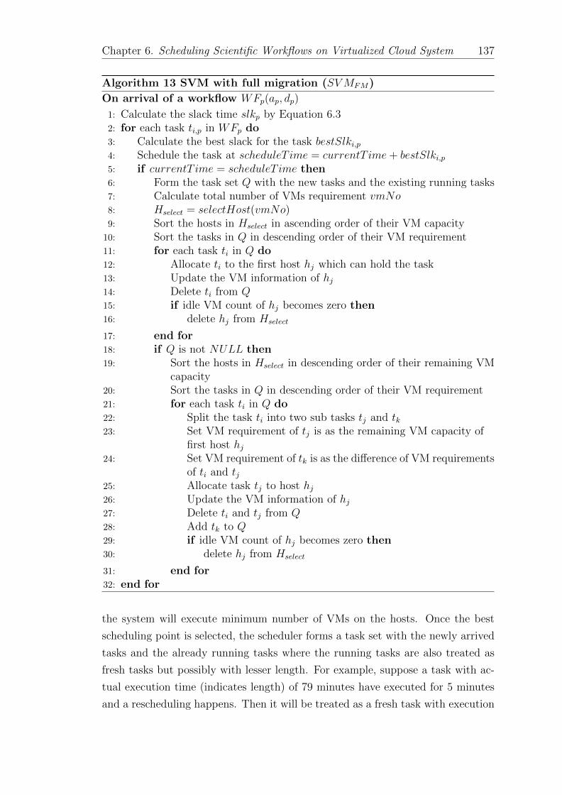
Chapter 6. Scheduling Scientific Workflows on Virtualized Cloud System 137
Algorithm 13 SVM with full migration (SVMFM)
On arrival of a workflow WFp(ap, dp)
1: Calculate the slack time slkp by Equation 6.32: for each task ti,p in WFp do3: Calculate the best slack for the task bestSlki,p4: Schedule the task at scheduleT ime = currentT ime+ bestSlki,p5: if currentT ime = scheduleT ime then6: Form the task set Q with the new tasks and the existing running tasks7: Calculate total number of VMs requirement vmNo8: Hselect = selectHost(vmNo)9: Sort the hosts in Hselect in ascending order of their VM capacity
10: Sort the tasks in Q in descending order of their VM requirement11: for each task ti in Q do12: Allocate ti to the first host hj which can hold the task13: Update the VM information of hj14: Delete ti from Q15: if idle VM count of hj becomes zero then16: delete hj from Hselect
17: end for18: if Q is not NULL then19: Sort the hosts in Hselect in descending order of their remaining VM
capacity20: Sort the tasks in Q in descending order of their VM requirement21: for each task ti in Q do22: Split the task ti into two sub tasks tj and tk23: Set VM requirement of tj is as the remaining VM capacity of
first host hj24: Set VM requirement of tk is as the difference of VM requirements
of ti and tj25: Allocate task tj to host hj26: Update the VM information of hj27: Delete ti and tj from Q28: Add tk to Q29: if idle VM count of hj becomes zero then30: delete hj from Hselect
31: end for32: end for
the system will execute minimum number of VMs on the hosts. Once the best
scheduling point is selected, the scheduler forms a task set with the newly arrived
tasks and the already running tasks where the running tasks are also treated as
fresh tasks but possibly with lesser length. For example, suppose a task with ac-
tual execution time (indicates length) of 79 minutes have executed for 5 minutes
and a rescheduling happens. Then it will be treated as a fresh task with execution
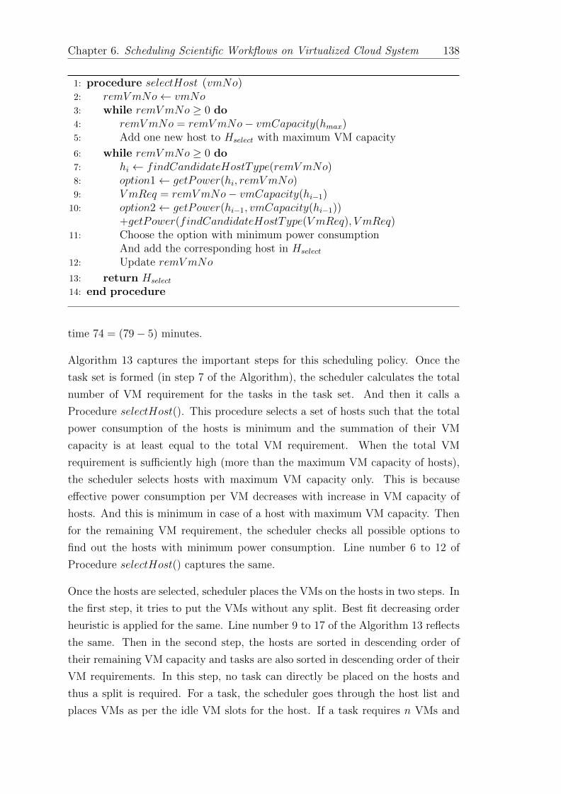
Chapter 6. Scheduling Scientific Workflows on Virtualized Cloud System 138
1: procedure selectHost (vmNo)2: remVmNo← vmNo3: while remVmNo ≥ 0 do4: remVmNo = remVmNo− vmCapacity(hmax)5: Add one new host to Hselect with maximum VM capacity
6: while remVmNo ≥ 0 do7: hi ← findCandidateHostType(remVmNo)8: option1← getPower(hi, remVmNo)9: V mReq = remVmNo− vmCapacity(hi−1)
10: option2← getPower(hi−1, vmCapacity(hi−1))+getPower(findCandidateHostType(V mReq), V mReq)
11: Choose the option with minimum power consumptionAnd add the corresponding host in Hselect
12: Update remVmNo
13: return Hselect
14: end procedure
time 74 = (79− 5) minutes.
Algorithm 13 captures the important steps for this scheduling policy. Once the
task set is formed (in step 7 of the Algorithm), the scheduler calculates the total
number of VM requirement for the tasks in the task set. And then it calls a
Procedure selectHost(). This procedure selects a set of hosts such that the total
power consumption of the hosts is minimum and the summation of their VM
capacity is at least equal to the total VM requirement. When the total VM
requirement is sufficiently high (more than the maximum VM capacity of hosts),
the scheduler selects hosts with maximum VM capacity only. This is because
effective power consumption per VM decreases with increase in VM capacity of
hosts. And this is minimum in case of a host with maximum VM capacity. Then
for the remaining VM requirement, the scheduler checks all possible options to
find out the hosts with minimum power consumption. Line number 6 to 12 of
Procedure selectHost() captures the same.
Once the hosts are selected, scheduler places the VMs on the hosts in two steps. In
the first step, it tries to put the VMs without any split. Best fit decreasing order
heuristic is applied for the same. Line number 9 to 17 of the Algorithm 13 reflects
the same. Then in the second step, the hosts are sorted in descending order of
their remaining VM capacity and tasks are also sorted in descending order of their
VM requirements. In this step, no task can directly be placed on the hosts and
thus a split is required. For a task, the scheduler goes through the host list and
places VMs as per the idle VM slots for the host. If a task requires n VMs and

Chapter 6. Scheduling Scientific Workflows on Virtualized Cloud System 139
200
400
600
800
1000
1200
1400
1600
1800
2000
4 8 16 32 64 80Ba
se
po
we
r c
on
su
mp
tio
n (
Wa
tts
)
Host type with no. of maximum supported VMs
(a) Base power consumption of different host types
20
40
60
80
100
120
4 8 16 32 64 80
Eff
ec
tiv
e P
C p
er
VM
(in
Wa
tts
)
Host type with no. of maximum supported VMs
(b) Effective power consumption per VM in differenthost types
Figure 6.10: Power consumption of hosts and VMs
the first host has m free VMs ( m ≤ n), then a new task is created with m VM
requirement and it is placed on the host. For the remaining VM requirement, the
next host is tried and the process goes on.
6.10 Performance Evaluation
In this work, we have evaluated the performance of six scheduling policiesNSVMNM ,
NSVMLM , NSVMFM , SVMNM , SVMLM , and SVMFM . We have also combined
these policies with three different slack distribution approaches and analyzed their
performances. To show the effectiveness of our work, we have also implemented
a state of art energy-efficient scheduling policy for scientific workflow, namely,
EnReal [41] and compared performances of the proposed policies.
6.10.1 Simulation platform and parameter setup
To evaluate the performance of our proposed approaches, a set of comprehensive
simulations and experiments are conducted. We have used CloudSim toolkit [123]
as the simulation platform and we did necessary changes to support multi-VM
tasks. Observing the power consumption pattern of some real systems, we set the
parameter values for our simulation. For instance, blade or rack server systems
with 4, 8, 16, 32, 64, 80 hardware threads need to be installed with approximately
400W, 800W, 1200W, 1800W, 2800W and 3200W power supply respectively. A
hardware thread can host one VM and in a rack, i.e. a host with 16 hardware
threads can host 16 homogeneous VMs seamlessly.

Chapter 6. Scheduling Scientific Workflows on Virtualized Cloud System 140
mProjectPP
mDiffFit
mBackground
mImgTbl
mAdd
mShrink
mJPEG
mConcatFit
mBgModel
(a) Montage
fastQSplit
filterContams
sol2Sanger
fastQ2Bf
map
mapMerge
maqIndex
pileUp
(b) Epigenomics
extractSGT
sismogramSynthesis
zipSeis
peakValCalOkaya
zipPSA
(c) CyberShake
tmpitBank
inspiral
thinka
triBank
inspiral
thinka
(d) Inspiral
Figure 6.11: Examples of scientific workflows
In our experiment, we have considered six different types of hosts which can sup-
port 4, 8, 16, 32, 64, 80 number of VMs respectively. Figure 6.10(a) shows the base
power consumption (BPC) of different host types considered in our work. BPC
is taken as 60% of the total power consumption. BPC increases with an increase
in the number of maximum supported VMs in the hosts. But the effective power
consumption per VM decreases with an increase in the number of maximum sup-
ported VMs in the hosts. Effective power consumption for a VM is more in case
of a smaller host and it is less in case of a bigger host. Figure 6.10(b) shows the
relationship between the effective power consumption per VM with the host type.
6.10.2 Real scientific work-flow
We have used many scientific workflows such as CyberShake, Epigenomics, Mon-
tage, Inspiral, Sipht and many others to carry out our experiments [25]. Montage
workflow was created by NASA/IPAC. It was used to create custom mosaics of the
sky by stitching together multiple input images taken by satellite. CyberShake
workflow was used to characterize earthquake hazards by the Southern Calfornia
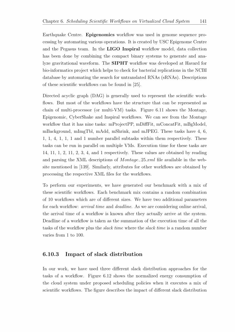
Chapter 6. Scheduling Scientific Workflows on Virtualized Cloud System 141
Earthquake Centre. Epigenomics workflow was used in genome sequence pro-
cessing by automating various operations. It is created by USC Epigenome Centre
and the Pegasus team. In the LIGO Inspiral workflow model, data collection
has been done by combining the compact binary systems to generate and ana-
lyze gravitational waveform. The SIPHT workflow was developed at Havard for
bio-informatics project which helps to check for bacterial replications in the NCBI
database by automating the search for untranslated RNAs (sRNAs). Descriptions
of these scientific workflows can be found in [25].
Directed acyclic graph (DAG) is generally used to represent the scientific work-
flows. But most of the workflows have the structure that can be represented as
chain of multi-processor (or multi-VM) tasks. Figure 6.11 shows the Montage,
Epigenomic, CyberShake and Inspiral workflows. We can see from the Montage
workflow that it has nine tasks: mProjectPP, mDiffFit, mConcatFit, mBgModel,
mBackground, mImgTbl, mAdd, mShrink, and mJPEG. These tasks have 4, 6,
1, 1, 4, 1, 1, 1 and 1 number parallel subtasks within them respectively. These
tasks can be run in parallel on multiple VMs. Execution time for these tasks are
14, 11, 1, 2, 11, 2, 3, 4, and 1 respectively. These values are obtained by reading
and parsing the XML descriptions of Montage−25.xml file available in the web-
site mentioned in [139]. Similarly, attributes for other workflows are obtained by
processing the respective XML files for the workflows.
To perform our experiments, we have generated our benchmark with a mix of
these scientific workflows. Each benchmark mix contains a random combination
of 10 workflows which are of different sizes. We have two additional parameters
for each workflow: arrival time and deadline. As we are considering online arrival,
the arrival time of a workflow is known after they actually arrive at the system.
Deadline of a workflow is taken as the summation of the execution time of all the
tasks of the workflow plus the slack time where the slack time is a random number
varies from 1 to 100.
6.10.3 Impact of slack distribution
In our work, we have used three different slack distribution approaches for the
tasks of a workflow. Figure 6.12 shows the normalized energy consumption of
the cloud system under proposed scheduling policies when it executes a mix of
scientific workflows. The figure describes the impact of different slack distribution

Chapter 6. Scheduling Scientific Workflows on Virtualized Cloud System 142
0
20
40
60
80
100
NSVMNM NSVMLM NSVMFM SVMNM SVMLM SVMFM
En
erg
y c
on
su
mp
tio
n i
n W
att
(n
orm
ali
ze
d)
Scheduling policies
SFTSFWSDF
Figure 6.12: Impact of slack distribution on energy consumption
approaches when they are merged with scheduling policies. The energy consump-
tion of the system for slack to first task (SFT) approach is more compared to the
other two approaches. But SFT approach is the simplest one and incurs lesser
overhead on the online scheduler. On the other hand, SFW and SDF approaches
perform almost similar. This pattern remains the same for all the policies. The
figure also reveals that the energy consumption of the system is comparatively
lesser in case of splittable VM allocation compared to non-splittable allocation.
6.10.4 Trade-off between energy consumption, migration
count and split count
Here we present three different output parameters, that is energy consumption,
migration count and split count together under the same graph. The split count
in case of scheduling with non-splittable VM allocation is zero because all the
required VMs of a task is allocated on one host and thus the task is not split. But
the energy consumption under these approaches is relatively higher. When all the
VMs of a task t cannot be placed on one host, we need to divide the task into
subtasks; and we treat the subtasks as new tasks with lesser VM requirement. The
number of split increases with each such division. On the other hand, whenever
the VMs executing a task need to migrate from one host to another, the migration
count is increased by one.
Figure 6.13 shows the normalized values for energy consumption, migration count
and split count for different scheduling policies when a mix of scientific workflows
is executed in the cloud system. All the proposed policies applied SDF slack
distribution approach. We make the following observations from the graph.

Chapter 6. Scheduling Scientific Workflows on Virtualized Cloud System 143
0
20
40
60
80
100
EnR
eal
NSVM
NM
NSVM
LM
NSVM
FM
SVM
NM
SVM
LM
SVM
FM
No
rmalized
valu
es
Scheduling policies
Energy MigrationCount SplitCount
Figure 6.13: Normalized values of energy consumption, migration and splitcount
• Scheduling policies under non-splittable VM allocation policy perform sim-
ilarly to the state-of-art policy, EnReal; but the proposed policies beat En-
Real in terms of the number of migrations. NSVMLM and NSVMFM incur
approximately 90% and 80% lesser number of migrations respectively than
EnReal.
• Scheduling policies under splittable VM allocation policy perform signifi-
cantly better than splittable VM allocation policies regarding energy con-
sumption. Reduction in energy consumption in case of SVMNM , SVMLM ,
and SVMFM are approximately 50%, 60%, and 64% respectively as com-
pared to EnReal.
• In case of splittable policies, tasks are split, and we observe a significant split
count as compared to non-splittable policies and EnReal. Systems need to
incur additional overhead for a split.
6.10.5 Different mixes of scientific workflows
To ascertain the performances of the proposed policies, we have performed our
experiments with 5 different benchmark mixes (MIX1, MIX2, MIX3, MIX4,
MIX5) which were generated from the scientific workflows as described in 6.10.2.
Figure 6.14 shows the energy consumption of the cloud system for 5 different
mixes under different scheduling policies along with EnReal. Slack distribution
and forwarding (SDF) technique are applied to distribute the slack time among
the tasks of a workflow. We observe similar energy consumption pattern for all the
benchmark mixes. Splittable policies reduce energy consumption by approximately
60% as compared to EnReal.

Chapter 6. Scheduling Scientific Workflows on Virtualized Cloud System 144
0
20
40
60
80
100
MIX1 MIX2 MIX3 MIX4 MIX5
No
rma
lize
d E
ne
rgy
co
ns
um
pti
on
Scheduling policies
EnRealNSVMNM
NSVMLMNSVMFM
SVMNMSVMLM
SVMFM
Figure 6.14: Energy consumption of the system (normalized) for differentbenchmark mixes
6.11 Summary
The high availability of high-end computing resources has made the cloud system a
popular choice for hosting the scientific applications. Another inherent character-
istic of these applications is the sharp variation in their resource requirement and
the elasticity feature of the cloud system can efficiently handle this. As these ap-
plications consume a significant amount of resources, energy-efficient execution of
these applications in the cloud becomes essential. These applications are modeled
as scientific workflows where there is a dependency between the tasks.
We describe the scheduling of a set of online dependent tasks, represented as sci-
entific workflows in the cloud environment and proposes a series of energy-efficient
scheduling techniques considering both the static and dynamic energy consump-
tion. The chapter describes several approaches regarding three important factors:
VM allocation, migration, and slack distribution which affects the performance
of scheduling. Extensive simulation is carried out in Cloudsim toolkit and perfor-
mance is compared with a state of art energy-efficient scheduling technique EnReal
[41] and found that the energy consumption of the proposed policies under split-
table VM category is significantly lesser than EnReal. The proposed policies under
non-splittable VM allocation performs at par with the state-of-art policy, but with
a smaller number of migrations. All the proposed policies meet the deadline con-
straints of the workflows.

Chapter 7
Conclusion and Future Work
In recent time, the growing energy consumption of the large computing systems
has gained the attention of the scientific community. At the same time, these
computing platforms become a perfect choice for the high-end scientific applica-
tions which are often of real-time nature. The energy-efficient execution of these
applications is essential because these applications consume a significant amount
of computing resources for a substantial amount of time. It is observed that a
major portion of the energy gets wasted due to poor utilization of the system. As
scheduling can potentially improve the utilization of a system, designing energy-
efficient scheduling techniques for the large system becomes important where these
applications will be executed both energy and performance efficient way.
Any scheduling problem is typically represented by the machine environment, the
task environment and the objective function. In our work, machine environment
consists both virtualized and non-virtualized system with a large number of pro-
cessors. For the task environment, we consider both independent and dependent
real-time task set. We set the optimality criteria as the minimization of energy
consumption without missing the deadline of any task. We summarize the contri-
butions of the thesis as follows.
7.1 Summary of Contributions
We solved four different scheduling problems in our thesis. This section contains
the summary of our work.
145
Chapter 8. Conclusion 146
• At first, we have considered a non-virtualized system having a large number
of processors and each processor is equipped with the multi-threaded fea-
ture. The task set consists of online independent aperiodic real-time tasks.
We exploit the power consumption pattern of some recent multi-threaded
processors and derive a simple but elegant power consumption model where
the total power consumption of a processor is expressed as a function of the
number of active threads of that processor. We then design four energy-
efficient scheduling policies to reduce the energy consumption of the system
maintaining the deadline constraints of all the tasks. Experiments are con-
ducted for a wide range of synthetic data and real-world trace. We consider
a variety of deadline and execution time schemes in the synthetic workload.
Experimental results show that the proposed policies show an average energy
reduction of around 47% for the synthetic workload and around 30% for the
real-world traces.
• In the second contribution of the thesis, we have considered a heterogeneous
virtualized cloud system where a host accommodates a number of VMs. A
user task is assigned to a VM and the VM is placed on a host. Heterogeneity
is mainly determined by the compute capacity and the energy consumption.
Under this setup, we have considered a region based non-linear power con-
sumption model for the hosts derived from the power consumption pattern
of a typical server. We have designed two energy-efficient scheduling ap-
proaches, (i) Urgent Point aware Scheduling (UPS ), and (ii) Urgent Point
aware Scheduling - Early Scheduling (UPS-ES ). These approaches are based
on the urgent points of a task, and dynamically used two threshold val-
ues. We have performed our experiments in the CloudSim toolkit by making
necessary changes. Experimental results show that the proposed policies
achieve an average energy reduction of around 24% for the synthetic data,
and around 11% for the real-trace data.
• We have considered scheduling a set of real-time tasks on the VMs having
discrete utilization. For a host, we have first calculated the critical utiliza-
tion value where the energy consumption happens to be the minimum. We
have designed scheduling approaches by dividing the problem into four sub-
problems. At first, we put forward the solution of the task set where all the
tasks have the same length and same deadline. Then we target the problem
of scheduling task set with two different lengths but the same deadline. To
solve this sub-problem, we have used the solution of the previous solution.
The third sub-problem deals with tasks having arbitrary lengths but same

Chapter 8. Conclusion 147
deadline, which is solved using the solution method of second sub-problem.
Finally, we have designed the solution approach for arbitrary lengths and
arbitrary deadlines of tasks. For the last sub-problem, we classified the task
set into different classes and we concluded that this classification technique
can be determined from the system parameters.
• In the last contribution of the thesis, we have considered scheduling a set
of dependent real-time tasks on a cloud system. The task set is taken as
scientific workflows, where each workflow has an end-to-end deadline. The
tasks in the workflow are multi-VM tasks; thus they need multiple VMs
simultaneously for their execution. We have designed a series of scheduling
policies to execute an incoming workflow efficiently. We have considered
several options and restrictions in the context of VM allocation, migration,
and slack distribution. In addition to the energy consumption, we have also
considered migration count and split count. Experiments are conducted on
CloudSim toolkit by adding necessary functionalities to it. The proposed
policies under non-splittable VM allocation category reduces the migration
count significantly (forNSVMNM , it is 0) compared to the state-of-art policy
with almost same amount energy consumption. In case of splittable VM
allocation category, we have achieved an energy reduction up to 64% as
compared to the state-of-art policy with reasonable migration count and
split count.
7.2 Scope for Future Work
The contributions of this thesis can be extended in a number of ways. Some of
these possible future research directions are listed below:
• Hierarchical organization of hosts: In our work, we have considered the
energy consumption for the processors assuming that all the processors are
connected in one level. But in practice, they are often connected in a hierar-
chical order. A server contains multiple chassis, a chassis contains multiple
racks, a rack contains different containers, and cores are placed on contain-
ers. Considering power consumption at each level while designing scheduling
policies for real-time tasks will be an interesting research direction. This will

Chapter 8. Conclusion 148
make the setup more realistic. Furthermore, instead of reporting the migra-
tion count, a location-based cost matrix can be used to measure the impact
of migration for such a hierarchical arrangement.
• Resource provisioning based on the application behavior and ar-
rival pattern: Another future research of the thesis can be toward usages
of some machine learning based techniques to predict the future the resource
requirement and to prepare the system accordingly. Idle VMs and idle hosts
are generally switched off to reduce the energy consumption. But deletion
and creation of VMs, waking up a host from the sleep state has some inherent
penalties. Making a trade-off between the overheads and the energy saving
based on the application behavior and arrival pattern can be an interesting
problem to solve.
• Study as multi-objective function: In our last contribution of scheduling
workflows, we have observed that different policies perform better in differ-
ent directions: energy consumption, number of migrations, and number of
splits. Migration count and split count have overheads associated with them.
Designing scheduling policies combining all these three factors can be a chal-
lenging research direction, where the objective function will be expressed as
a combination of energy consumption, migration count, and split count.
• Imrovement on VM splitting: When a task requires multiple VMs to
execute and the VMs are placed on different hosts (splittable VM allocation),
the VMs need to communicate among them. This results in some extra
energy consumption. Based on the placement location of the VMs (belonging
to the same task), energy consumption will vary. We see a promising research
direction to study the splitting criteria and the placement of the VMs while
designing scheduling techniques for multi-VM tasks.
• Trade-off between energy consumption and SLA violation: All the
scheduling policies designed in the thesis considered hard real-time tasks and
thus the deadline constraints of all the tasks are met. But in case of soft
real-time tasks, violation of the deadline constraints of a few tasks may be
allowed. But this imposes some additional penalty. It will be an interesting
research direction where some penalty can be associated with the violation of
SLA of the tasks (or applications) while minimizing the energy consumption
or the overall cost of execution.
Bibliography
[1] K. T. Malladi, B. C. Lee, F. A. Nothaft, C. Kozyrakis, K. Periyathambi,
and M. Horowitz, “Towards Energy-proportional Datacenter Memory with
Mobile DRAM,” SIGARCH Comput. Archit. News, vol. 40, no. 3, pp. 37–48,
Jun. 2012.
[2] “Power Consumption Tests.” [Online]. Available: http://www.xbitlabs.
com/
[3] “Power Consumption Qualcom Hexagon V3.” [Online]. Available: http:
//www.bdti.com/
[4] C. H. Lien, M. F. Liu, Y. W. Bai, C. H. Lin, and M. B. Lin, “Measurement
by the Software Design for the Power Consumption of Streaming Media
Servers,” in IEEE Instrumentation and Measurement Technology Conference
Proceedings, April 2006, pp. 1597–1602.
[5] P. Brucker, Scheduling Algorithms, 3rd ed. Secaucus, NJ, USA: Springer-
Verlag New York, Inc., 2001.
[6] G. Buttazzo, Hard Real-Time Computing Systems: Predictable Scheduling
Algorithms and Applications, ser. Real-Time Systems Series. Springer, 2011.
[7] J. W. S. W. Liu, Real-Time Systems, 1st ed. Prentice Hall PTR, 2000.
[8] P. Brucker, Scheduling Algorithms, 5th ed. Springer, 2010.
[9] J. Lenstra, A. Rinnooy Kan, and P. Brucker, “Complexity of Machine
Scheduling Problems,” Annals of Discrete Mathematics, vol. 1, pp. 343–362,
1977.
[10] R. I. Davis and A. Burns, “A Survey of Hard Real-time Scheduling for
Multiprocessor Systems,” ACM Comput. Surv., vol. 43, no. 4, pp. 35:1–
35:44, Oct. 2011.
149

Bibliography 150
[11] Y. Du and G. D. Veciana, “Scheduling for Cloud-Based Computing Systems
to Support Soft Real-Time Applications,” ACM Trans. Model. Perform.
Eval. Comput. Syst., vol. 2, no. 3, pp. 13:1–13:30, Jun. 2017.
[12] C. L. Liu and J. W. Layland, “Scheduling Algorithms for Multiprogramming
in a Hard-Real-Time Environment,” J. ACM, Jan. 1973.
[13] M. Joseph and P. Pandya, “Finding Response Times in a Real-Time Sys-
tem,” The Computer Journal, pp. 390–395, 1986.
[14] J. Y.-T. Leung and J. Whitehead, “On the complexity of fixed-priority
scheduling of periodic, real-time tasks,” Performance Evaluation, vol. 2,
no. 4, pp. 237 – 250, 1982.
[15] W. Horn, “Some simple scheduling algorithms,” Quarterly, vol. 21, no. 1,
pp. 177 – 185, 1974.
[16] A. Mohammadi and S. G. Akl, “Scheduling Algorithms for Real-Time Sys-
tems,” School of Computing, Queens University, Tech. Rep., July 2005.
[17] A. Singh, M. Shafique, A. Kumar, and J. Henkel, “Mapping on multi/many-
core systems: Survey of current and emerging trends,” in 50th ACM / EDAC
/ IEEE Design Automation Conference (DAC), May 2013, pp. 1–10.
[18] R. Lewis, “A General-purpose Hill-climbing Method for Order Independent
Minimum Grouping Problems: A Case Study in Graph Colouring and Bin
Packing,” Comput. Oper. Res., pp. 2295–2310, Jul 2009.
[19] S. K. Dhall and C. L. Liu, “On a Real-Time Scheduling Problem,” Operations
Research, vol. 26, no. 1, 1978.
[20] Y. Oh, Y. Oh, S. H. Son, and S. H. Son, “Tight Performance Bounds of
Heuristics for a Real-Time Scheduling Problem,” University of Virginia,
Charlottesville, VA 22903, Tech. Rep., 1993.
[21] Y. Oh and S. Son, “Allocating fixed-priority periodic tasks on multiprocessor
systems,” Real-Time Systems, pp. 207–239, 1995.
[22] A. Burchard, J. Liebeherr, Y. Oh, and S. Son, “New strategies for assigning
real-time tasks to multiprocessor systems,” IEEE Transactions on Comput-
ers, pp. 1429–1442, Dec 1995.
[23] P. Mell and T. Grance, “The NIST definition of cloud computing,” National
Institute of Standards and Technology, vol. 53, no. 6, 2009.
Bibliography 151
[24] X. Liu, Y. Yang, Y. Jiang, and J. Chen, “Preventing Temporal Violations in
Scientific Workflows: Where and How,” IEEE Trans. on Sof. Engg., vol. 37,
no. 6, pp. 805–825, Nov 2011.
[25] G. Juve, A. Chervenak, E. Deelman et al., “Characterizing and profiling
scientific workflows,” Futu. Gen. Comp. Sys., vol. 29, no. 3, pp. 682 – 692,
2013.
[26] M. Rahman, R. Hassan, R. Ranjan, and R. Buyya, “Adaptive workflow
scheduling for dynamic grid and cloud computing environment,” Concu.
and Compu.: Prac. and Exp., vol. 25, no. 13, pp. 1816–1842, 2013.
[27] R. N. Calheiros and R. Buyya, “Meeting deadlines of scientific workflows in
public clouds with tasks replication,” IEEE Tran. on Para. and Dist. Sys.,
vol. 25, no. 7, pp. 1787–1796, July 2014.
[28] K. Bousselmi, Z. Brahmi, and M. M. Gammoudi, “Energy Efficient Parti-
tioning and Scheduling Approach for Scientific Workflows in the Cloud,” in
IEEE Int. Conf. on Serv. Compu., June 2016, pp. 146–154.
[29] G.-Y. Wei, M. Horowitz, and J. Kim, Energy-Efficient Design of High-Speed
Links. Boston, MA: Springer US, 2002, pp. 201–239.
[30] X. Zhu, L. Yang, H. Chen, J. Wang, S. Yin, and X. Liu, “Real-Time Tasks
Oriented Energy-Aware Scheduling in Virtualized Clouds,” Cloud Comput-
ing, IEEE Transactions on, vol. 2, no. 2, pp. 168–180, April 2014.
[31] M. Weiser, B. Welch, A. Demers, and S. Shenker, “Scheduling for Reduced
CPU Energy,” in Proc. of USENIX Conf. on OS Design and Impl., ser.
OSDI ’94, 1994.
[32] H. Aydin, R. Melhem, D. Mosse, and P. Mejia-Alvarez, “Dynamic and Ag-
gressive Scheduling Techniques for Power Aware Real Time Systems,” in
IEEE Proc. Real-Time Systems Symp., Dec 2001, pp. 95–105.
[33] D. Zhu, R. Melhem, and B. Childers, “Scheduling with dynamic volt-
age/speed adjustment using slack reclamation in multiprocessor real-time
systems,” Parallel and Distributed Systems, IEEE Transactions on, vol. 14,
no. 7, pp. 686–700, July 2003.
Bibliography 152
[34] C. Isci, A. Buyuktosunoglu, C.-Y. Chen, P. Bose et al., “An Analysis of Ef-
ficient Multi-Core Global Power Management Policies: Maximizing Perfor-
mance for a Given Power Budget,” in 39th Annual IEEE/ACM International
Symposium on Microarchitecture, MICRO, Dec 2006, pp. 347–358.
[35] R. Ge, X. Feng, and K. W. Cameron, “Modeling and evaluating energy-
performance efficiency of parallel processing on multicore based power aware
systems,” in 2009 IEEE International Symposium on Parallel Distributed
Processing, May 2009, pp. 1–8.
[36] S. L. Song, K. Barker, and D. Kerbyson, “Unified Performance and Power
Modeling of Scientific Workloads,” in Proceedings of the 1st International
Workshop on Energy Efficient Supercomputing, ser. E2SC ’13. New York,
NY, USA: ACM, 2013, pp. 4:1–4:8.
[37] X. Fan, W.-D. Weber, and L. A. Barroso, “Power Provisioning for a
Warehouse-sized Computer,” SIGARCH Comput. Archit. News, vol. 35,
no. 2, pp. 13–23, Jun. 2007.
[38] P. Bohrer, E. N. Elnozahy, T. Keller, M. Kistler, C. Lefurgy, C. McDowell,
and R. Rajamony, “Power Aware Computing,” R. Graybill and R. Melhem,
Eds. Norwell, MA, USA: Kluwer Academic Publishers, 2002, ch. The Case
for Power Management in Web Servers, pp. 261–289.
[39] Y. Gao, H. Guan, Z. Qi, B. Wang, and L. Liu, “Quality of service aware
power management for virtualized data centers,” Journal of Systems Archi-
tecture, vol. 59, no. 4, pp. 245 – 259, 2013.
[40] Y. C. Lee and A. Zomaya, “Energy-Conscious Scheduling for Distributed
Computing Systems under Different Operating Conditions,” IEEE Trans.
on Parallel and Distributed Systems, pp. 1374–1381, Aug 2011.
[41] X. Xu, W. Dou, X. Zhang, and J. Chen, “EnReal: An Energy-Aware Re-
source Allocation Method for Scientific Workflow Executions in Cloud Envi-
ronment,” IEEE Transactions on Cloud Computing, vol. 4, no. 2, pp. 166–
179, April 2016.
[42] H. Chen, X. Zhu, H. Guo, and et al., “Towards Energy-Efficient Schedul-
ing for Real-Time Tasks under Uncertain Cloud Computing Environment,”
Journal of Systems and Software, vol. 99, pp. 20 – 35, 2015.

Bibliography 153
[43] Y. Maa, B. Gonga, R. Sugihara, and R. Gupta, “Energy Efficient Deadline
Scheduling for Heterogeneous Systems,” Journal of Parallel and Distributed
Computing, vol. 72, no. 12, pp. 1725 – 1740, 2012.
[44] H. Chen et al., “Towards Energy-Efficient Scheduling for Real-Time Tasks
under Uncertain Cloud Computing Environment,” Journal of Systems and
Software, vol. 99, pp. 20 – 35, 2015.
[45] Y. C. Lee and A. Y. Zomaya, “Energy efficient utilization of resources in
cloud computing systems,” The Journal of Supercomputing, vol. 60, no. 2,
pp. 268–280, 2012.
[46] “Energy-Aware Resource Allocation Heuristics for Efficient Management of
Data Centers for Cloud Computing ,” Future Generation Computer Systems,
vol. 28, no. 5, pp. 755 – 768, 2012.
[47] Y. Gao, H. Guan, Z. Qi, Y. Hou, and L. Liu, “A multi-objective ant colony
system algorithm for virtual machine placement in cloud computing,” Jour-
nal of Computer and System Sciences, vol. 79, no. 8, pp. 1230 – 1242, 2013.
[48] M. Dayarathna, Y. Wen, and R. Fan, “Data Center Energy Consumption
Modeling: A Survey,” IEEE Commun. Surv. Tutorials, vol. 18, no. 1, pp.
732–794, 2016.
[49] D. Li and J. Wu, “Energy-Aware Scheduling for Aperiodic Tasks on Multi-
core Processors,” in 43rd International Conference on Parallel Processing
(ICPP), 2014, pp. 361–370.
[50] R. Ge, X. Feng, and K. W. Cameron, “Performance-constrained Distributed
DVS Scheduling for Scientific Applications on Power-aware Clusters,” in
Supercomputing, 2005. Proceedings of the ACM/IEEE SC 2005 Conference,
Nov 2005, pp. 34–34.
[51] G. L. T. Chetsa, L. Lefevre, J. M. Pierson, P. Stolf, and G. D. Costa, “Be-
yond CPU Frequency Scaling for a Fine-grained Energy Control of HPC
Systems,” in 2012 IEEE 24th International Symposium on Computer Archi-
tecture and High Performance Computing, Oct 2012, pp. 132–138.
[52] C.-M. Wu, R.-S. Chang, and H.-Y. Chan, “A green energy-efficient schedul-
ing algorithm using the DVFS technique for cloud datacenters,” Future Gen-
eration Computer Systems, vol. 37, pp. 141 – 147, 2014.

Bibliography 154
[53] J. S. Chase and R. P. Doyle, “Balance of Power: Energy Management for
Server Clusters,” in In Proceedings of the Eighth Workshop on Hot Topics
in Operating Systems (HotOS’01), 2001.
[54] E. V. C. E. Pinheiro, R. Bianchini and T. Heath, “Load balancing and unbal-
ancing for power and performance in cluster-based systems,” in Workshop
on Compilers and Operating Systems for Low Power, 2001, pp. 182–195.
[55] S. Zikos and H. D. Karatza, “Performance and energy aware cluster-level
scheduling of compute-intensive jobs with unknowdynan service times,” Sim-
ulation Modelling Practice and Theory, vol. 19, no. 1, pp. 239 – 250, 2011.
[56] S. Srikantaiah, A. Kansal, and F. Zhao, “Energy Aware Consolidation for
Cloud Computing,” in Proceedings of Conference on Power Aware Comput-
ing and Systems, ser. HotPower, 2008.
[57] J. J. Durillo, V. Nae, and R. Prodan, “Multi-objective Workflow Schedul-
ing: An Analysis of the Energy Efficiency and Makespan Tradeoff,” in 13th
IEEE/ACM Int. Sympo. on CCGrid Comp., May 2013, pp. 203–210.
[58] J. G. Koomey, “Estimating Total Power Consumption by Servers in the U.S.
and the World,” Analytics Press, 2007.
[59] L. A. Barroso, “The Price of Performance,” Queue, vol. 3, no. 7, pp. 48–53,
Sep. 2005.
[60] W.-c. Feng, “Making a Case for Efficient Supercomputing,” Queue, vol. 1,
no. 7, pp. 54–64, Oct. 2003.
[61] Z. Li, J. Ge, H. Hu et al., “Cost and Energy Aware Scheduling Algorithm
for Scientific Workflows with Deadline Constraint in Clouds,” IEEE Tran.
on Serv. Compu., vol. PP, no. 99, pp. 1–1, 2017.
[62] “Gartner Estimates ICT Industry Accounts for 2 Percent of Global CO2
Emissions.” [Online]. Available: https://www.gartner.com/newsroom/id/
503867
[63] R. Buyya, C. S. Yeo, S. Venugopal et al., “Cloud computing and emerging
it platforms: Vision, hype, and reality for delivering computing as the 5th
utility,” Futu. Gen. Com. Sys., vol. 25, no. 6, pp. 599 – 616, 2009.
[64] H. Aydin, R. Melhem, D. Mosse, and P. Mejia-Alvarez, “Optimal Reward-
Based Scheduling for Periodic Real-Time Tasks,” Computers, IEEE Trans-
actions on, vol. 50, no. 2, pp. 111–130, Feb 2001.

Bibliography 155
[65] C. Isci, A. Buyuktosunoglu, C.-Y. Chen, P. Bose et al., “An Analysis of
Efficient Multi-Core Global Power Management Policies: Maximizing Per-
formance for a Given Power Budget,” in 39th International Symposium on
Microarchitetcure (MICRO)., 2006.
[66] Y. C. Lee and A. Y. Zomaya, “Minimizing Energy Consumption for
Precedence-Constrained Applications Using Dynamic Voltage Scaling,” in
Proceedings of the 9th IEEE/ACM International Symposium on CCGrid,
2009.
[67] Y. C. Lee and A. Zomaya, “Energy Conscious Scheduling for Distributed
Computing Systems under Different Operating Conditions,” IEEE Transac-
tion on Para. and Distr. Sys., 2011.
[68] D. Li and J. Wu, “Minimizing Energy Consumption for Frame-Based Tasks
on Heterogeneous Multiprocessor Platforms,” IEEE Tranactions on Parallel
and Distributed Systems, vol. 26, no. 3, pp. 810–823, 2015.
[69] ——, “Energy-Aware Scheduling for Frame-Based Tasks on Heterogeneous
Multiprocessor Platforms,” in 41st International Conference on Parallel Pro-
cessing (ICPP), 2012, pp. 430–439.
[70] Y. Hotta, M. Sato, H. Kimura, S. Matsuoka, T. Boku, and D. Takahashi,
“Profile based Optimization of Power-Performance by using Dynamic Volt-
age Scaling on a PC Cluster,” in Int. Symp. on Parallel and Distributed
Processing, April 2006.
[71] K. H. Kim, R. Buyya, and J. Kim, “Power Aware Scheduling of Bag-of-
Tasks Applications with Deadline Constraints on DVS-enabled Clusters,” in
Seventh IEEE International Symposium on Cluster Computing and the Grid
(CCGrid ’07), May 2007, pp. 541–548.
[72] L. Chen, P. Wu, Z. Chen, R. Ge, and Z. Zong, “Energy Efficient Paral-
lel Matrix-Matrix Multiplication for DVFS-enabled Clusters,” in 2012 41st
International Conference on Parallel Processing Workshops, Sept 2012, pp.
239–245.
[73] R. N. Calheiros and R. Buyya, “Energy-Efficient Scheduling of Urgent Bag-
of-Tasks Applications in Clouds through DVFS,” in 2014 IEEE 6th Interna-
tional Conference on Cloud Computing Technology and Science, Dec 2014,
pp. 342–349.
Bibliography 156
[74] E. N. Elnozahy, M. Kistler, and R. Rajamony, “Energy-efficient Server Clus-
ters,” in Proceedings of the 2nd International Conference on Power-aware
Computer Systems, ser. PACS’02. Berlin, Heidelberg: Springer-Verlag,
2003, pp. 179–197.
[75] S. Zhuravlev, J. Saez, S. Blagodurov, A. Fedorova, and M. Prieto, “Survey
of Energy Cognizant Scheduling Techniques,” IEEE Transaction on Parallel
and Distributed Systems, pp. 1447–1464, July 2013.
[76] J. S. Chase, D. C. Anderson, P. N. Thakar, A. M. Vahdat, and R. P. Doyle,
“Managing Energy and Server Resources in Hosting Centers,” SIGOPS Op-
erating System Reviews, vol. 35, no. 5, 2001.
[77] J. Choi, S. Govindan, J. Jeong, B. Urgaonkar, and A. S., “Power Consump-
tion Prediction and Power Aware Packing in Consolidated Environments,”
IEEE Trans. on Computers, vol. 59, no. 12, pp. 1640–1654, 2010.
[78] G. Da Costa, M. D. de Assuncao, J.-P. Gelas, Y. Georgiou, L. Lefevre, A.-C.
Orgerie, J.-M. Pierson, O. Richard, and A. Sayah, “Multi-facet Approach
to Reduce Energy Consumption in Clouds and Grids: The GREEN-NET
Framework,” in Proceedings of the 1st International Conference on Energy-
Efficient Computing and Networking. ACM, 2010, pp. 95–104.
[79] E. Jonardi, M. A. Oxley, S. Pasricha, A. A. Maciejewski, and H. J. Siegel,
“Energy cost optimization for geographically distributed heterogeneous data
centers,” in 2015 Sixth International Green and Sustainable Computing Con-
ference (IGSC), Dec 2015, pp. 1–6.
[80] A. M. Al-Qawasmeh, S. Pasricha, A. A. Maciejewski, and H. J. Siegel,
“Power and Thermal-Aware Workload Allocation in Heterogeneous Data
Centers,” IEEE Transactions on Computers, vol. 64, no. 2, pp. 477–491,
Feb 2015.
[81] M. A. Oxley, S. Pasricha, A. A. Maciejewski, H. J. Siegel, and P. J.
Burns, “Online Resource Management in Thermal and Energy Con-
strained Heterogeneous High Performance Computing,” in 2016 IEEE
14th Intl Conf on Dependable, Autonomic and Secure Computing, 14th
Intl Conf on Pervasive Intelligence and Computing, 2nd Intl Conf on
Big Data Intelligence and Computing and Cyber Science and Technology
Congress(DASC/PiCom/DataCom/CyberSciTech), Aug 2016, pp. 604–611.

Bibliography 157
[82] E. K. Lee, H. Viswanathan, and D. Pompili, “Proactive thermal-aware re-
source management in virtualized hpc cloud datacenters,” IEEE Transac-
tions on Cloud Computing, vol. 5, no. 2, pp. 234–248, April 2017.
[83] X. Li, P. Garraghan, X. Jiang, Z. Wu, and J. Xu, “Holistic virtual machine
scheduling in cloud datacenters towards minimizing total energy,” IEEE
Transactions on Parallel and Distributed Systems, vol. 29, no. 6, pp. 1317–
1331, June 2018.
[84] M. A. Oxley, E. Jonardi, S. Pasricha, A. A. Maciejewski, H. J. Siegel, P. J.
Burns, and G. A. Koenig, “Rate-based Thermal, Power, and Co-location
Aware Resource Management for Heterogeneous Data Centers,” J. Parallel
Distrib. Comput., vol. 112, no. P2, pp. 126–139, Feb. 2018.
[85] C. Mastroianni, M. Meo, and G. Papuzzo, “Probabilistic Consolidation of
Virtual Machines in Self-Organizing Cloud Data Centers,” IEEE Transac-
tions on Cloud Computing, vol. 1, no. 2, pp. 215–228, July 2013.
[86] Z. Xiao, W. Song, and Q. Chen, “Dynamic resource allocation using virtual
machines for cloud computing environment,” IEEE Transactions on Parallel
and Distributed Systems, vol. 24, no. 6, pp. 1107–1117, June 2013.
[87] J. Zheng, T. S. E. Ng, K. Sripanidkulchai, and Z. Liu, “Pacer: A Progress
Management System for Live Virtual Machine Migration in Cloud Com-
puting,” IEEE Transactions on Network and Service Management, vol. 10,
no. 4, pp. 369–382, December 2013.
[88] K. Ye, Z. Wu, C. Wang et al., “Profiling-Based Workload Consolidation and
Migration in Virtualized Data Centers,” IEEE Transactions on Parallel and
Distributed Systems, vol. 26, no. 3, pp. 878–890, March 2015.
[89] A. Verma, P. Ahuja, and A. Neogi, “Power-aware Dynamic Placement of
HPC Applications,” in Proceedings of the 22nd Annual International Con-
ference on Supercomputing, ser. ICS, 2008, pp. 175–184.
[90] ——, “pMapper: Power and Migration Cost Aware Application Placement
in Virtualized Systems,” in Proceedings of the 9th ACM/IFIP/USENIX In-
ternational Conference on Middleware, ser. Middleware ’08, 2008, pp. 243–
264.
Bibliography 158
[91] M.-H. Malekloo, N. Kara, and M. E. Barachi, “An energy efficient and sla
compliant approach for resource allocation and consolidation in cloud com-
puting environments,” Sustainable Computing: Informatics and Systems,
vol. 17, pp. 9 – 24, 2018.
[92] S. Hosseinimotlagh, F. Khunjush, and S. Hosseinimotlagh, “A Coopera-
tive Two-Tier Energy-Aware Scheduling for Real-Time Tasks in Comput-
ing Clouds,” in 2014 22nd Euromicro International Conference on Parallel,
Distributed, and Network-Based Processing, Feb 2014, pp. 178–182.
[93] L. Shi, Z. Zhang, and T. Robertazzi, “Energy-Aware Scheduling of Em-
barrassingly Parallel Jobs and Resource Allocation in Cloud,” IEEE Trans.
Parallel Distrib. Syst., vol. 28, no. 6, pp. 1607–1620, Jun. 2017.
[94] F. Farahnakian, T. Pahikkala, P. Liljeberg, and et al., “Energy-aware VM
Consolidation in Cloud Data Centers Using Utilization Prediction Model,”
IEEE Trans. on Cloud Computing, vol. PP, no. 99, pp. 1–1, 2016.
[95] M. A. Rodriguez and R. Buyya, “Deadline Based Resource Provisioning and
Scheduling Algorithm for Scientific Workflows on Clouds,” IEEE Trans. on
Cloud Comp., vol. 2, no. 2, pp. 222–235, April 2014.
[96] S. Abrishami, M. Naghibzadeh, and D. H. Epema, “Deadline-constrained
Workflow Scheduling Algorithms for Infrastructure As a Service Clouds,”
Futu. Gen. Comp. Sys., vol. 29, no. 1, pp. 158–169, Jan. 2013.
[97] H. Topcuouglu, S. Hariri, and M. Wu, “Performance-Effective and Low-
Complexity Task Scheduling for Heterogeneous Computing,” IEEE Trans.
on Para. and Dist. Sys., vol. 13, no. 3, pp. 260–274, Mar. 2002.
[98] Y. Zhou and X. Huang, “Scheduling Workflow in Cloud Computing Based
on Ant Colony Optimization Algorithm,” in 6th Int. Conf. on Business In-
telligence and Financial Engg., Nov 2013, pp. 57–61.
[99] Z. Wu, Z. Ni, L. Gu, and X. Liu, “A Revised Discrete PARTICLE Swarm
Optimization for Cloud Workflow Scheduling,” in Proceed. of the Int. Conf.
on Compu. Intell. and Secu. IEEE Computer Society, 2010, pp. 184–188.
[100] C. Lin and S. Lu, “Scheduling Scientific Workflows Elastically for Cloud
Computing,” in 4th IEEE Int. Conf. on Cloud Compu., July 2011, pp. 746–
747.

Bibliography 159
[101] I. Pietri, M. Malawski, G. Juve et al., “Energy-Constrained Provisioning for
Scientific Workflow Ensembles,” in Int. Conf. on Cloud and Green Compu.,
Sept 2013, pp. 34–41.
[102] J. J. Durillo, V. Nae, and R. Prodan, “Multi-objective energy-efficient work-
flow scheduling using list-based heuristics,” Futu. Gen. Comp. Sys., vol. 36,
pp. 221 – 236, 2014.
[103] F. Cao, M. M. Zhu, and C. Q. Wu, “Energy-Efficient Resource Management
for Scientific Workflows in Clouds,” in IEEE World Congress on Services,
June 2014, pp. 402–409.
[104] H. Chen, X. Zhu, D. Qiu, H. Guo, L. T. Yang, and P. Lu, “EONS: Minimiz-
ing Energy Consumption for Executing Real-Time Workflows in Virtualized
Cloud Data Centers,” in 45th ICPPW, Aug 2016, pp. 385–392.
[105] “Power Consumption pattern of Xeon Gold Processors.”
[Online]. Available: https://software.intel.com/en-us/forums/
software-tuning-performance-optimization-platform-monitoring/topic/
779810
[106] S. Srirama, V. Ivanistsev, P. Jakovits, and C. Willmore, “Direct Migration
of Scientific Computing Experiments to the Cloud,” in International Confer-
ence on High Performance Computing and Simulation (HPCS), July 2013,
pp. 27–34.
[107] Z. Mahmood, Cloud Computing: Methods and Practical Approaches.
Springer Publishing Company, Incorporated, 2013.
[108] Y. Gao, H. Guan, Z. Qi, B. Wang, and L. Liu, “Quality of service aware
power management for virtualized data centers,” Journal of Systems Archi-
tecture, vol. 59, no. 45, pp. 245 – 259, 2013.
[109] S. Ali, H. J. Siegel, M. Maheswaran, D. Hensgen, and S. Ali, “Task ex-
ecution time modeling for heterogeneous computing systems,” in Proc. of
Heterogeneous Computing Workshop, 2000, pp. 185–199.
[110] J. Kim and K. G. Shin, “Execution time analysis of communicating tasks in
distributed systems,” IEEE Trans. on Comput., vol. 45, no. 5, pp. 572–579,
May 1996.
[111] “MetaCentrum data sets,” https://www.fi.muni.cz/ xklusac/in-
dex.php?page=meta2009.
Bibliography 160
[112] M. Zaharia, D. Borthakur, J. Sen Sarma, K. Elmeleegy, S. Shenker, and
I. Stoica, “Delay Scheduling : A Simple Technique for Achieving Locality and
Fairness in Cluster Scheduling,” in Proc. of European Conf. on Computer
Systems, ser. EuroSys’10, 2010, pp. 265–278.
[113] Y. Guo, H. Su, D. Zhu, and H. Aydin, “Preference Oriented Real-time
Scheduling and Its Application in Fault-tolerant Systems,” J. of System
Architecture, vol. 61, no. 2, pp. 127–139, Feb. 2015.
[114] A. Beloglazov, J. Abawajy, and R. Buyya, “Energy Aware Resource Allo-
cation Heuristics for Efficient Management of Data-Centers for Cloud Com-
puting,” Future Generation Computer Systems, vol. 28, no. 5, pp. 755 – 768,
2012.
[115] J. Choi, S. Govindan, J. Jeong, B. Urgaonkar, and A. Sivasubramaniam,
“Power Consumption Prediction and Power-Aware Packing in Consolidated
Environments,” IEEE Transactions on Computers, vol. 59, no. 12, pp. 1640–
1654, 2010.
[116] N. Fisher, J. Goossens, and S. Baruah, “Optimal Online Multiprocessor
Scheduling of Sporadic Real-time Tasks is Impossible,” Real-Time Systems,
vol. 45, no. 1-2, pp. 26–71, Jun. 2010.
[117] G. C. Buttazzo, Hard Real Time Computing Systems: Predictable Scheduling
Algorithms and Applications. Springer, 2011.
[118] S. Holmbacka, W. Lund, S. Lafond, and J. Lilius, “Task Migration for Dy-
namic Power and Performance Characteristics on Many-Core Distributed
Operating Systems,” in 2013 21st Euromicro International Conference on
Parallel, Distributed, and Network-Based Processing, Feb 2013, pp. 310–317.
[119] Q. Teng, P. F. Sweeney, and E. Duesterwald, “Understanding the Cost of
thread migration for multi threaded Java applications running on a multicore
platform,” in Performance Analysis of Systems and Software, IEEE Int.
Symp. on, April 2009, pp. 123–132.
[120] T. Constantinou, Y. Sazeides, P. Michaud, D. Fetis, and A. Seznec, “Per-
formance Implications of Single Thread Migration on a Chip Multi-core,”
SIGARCH Comput. Archit. News, vol. 33, no. 4, pp. 80–91, Nov. 2005.
[121] M. Armbrust, A. Fox, R. Griffith, A. D. Joseph, R. Katz, A. Konwinski,
G. Lee, D. A. Patterson, A. Rabkin, I. Stoica, and M. Zaharia, “Above the
Clouds: A Berkeley View of Cloud Computing,” Feb 2009.
Bibliography 161
[122] M. Bambagini, M. Marinoni, H. Aydin, and G. Buttazzo, “Energy-Aware
Scheduling for Real-Time Systems: A Survey,” ACM Trans. Embed. Com-
put. Syst., vol. 15, no. 1, pp. 7:1–7:34, Jan. 2016.
[123] R. N. Calheiros, R. Ranjan, A. Beloglazov et al., “CloudSim: A Toolkit for
Modeling and Simulation of Cloud Computing Environments and Evaluation
of Resource Provisioning Algorithms,” Softw. Pract. Exper., vol. 41, no. 1,
pp. 23–50, Jan. 2011.
[124] “Google cluster data v2,” http://code.google.com/p/googlecluster-
data/wiki/ClusterData2011 1, 2011.
[125] I. S. Moreno, P. Garraghan, P. Townend, and J. Xu, “An Approach for Char-
acterizing Workloads in Google Cloud to Derive Realistic Resource Utiliza-
tion Models,” in 2013 IEEE Seventh International Symposium on Service-
Oriented System Engineering, March 2013, pp. 49–60.
[126] L. Wang, G. von Laszewski, J. Dayal, and F. Wang, “Towards Energy
Aware Scheduling for Precedence Constrained Parallel Tasks in a Cluster
with DVFS,” in Proceedings of the 2010 10th IEEE/ACM International Con-
ference on Cluster, Cloud and Grid Computing, ser. CCGRID ’10. IEEE
Computer Society, 2010, pp. 368–377.
[127] C. Q. Wu, X. Lin, D. Yu, W. Xu, and L. Li, “End-to-End Delay Minimization
for Scientific Workflows in Clouds under Budget Constraint,” IEEE Trans.
on Cloud Computing, vol. 3, no. 2, pp. 169–181, April 2015.
[128] N. Sharma and R. M. Guddeti, “Multi-Objective Energy Efficient Virtual
Machines Allocation at the Cloud Data Center,” IEEE Transactions on Ser-
vices Computing, pp. 1–1, 2016.
[129] “https://aws.amazon.com/ec2/.”
[130] A. Beloglazov and R. Buyya, “Energy Efficient Resource Management in Vir-
tualized Cloud Data Centers,” in IEEE/ACM Int. Conf. on Cluster, Cloud
and Grid Computing, May 2010, pp. 826–831.
[131] J. Bawicz and Z. Liu, “Scheduling multiprocessor tasks with chain con-
straints,” Euro. J. of Op. Research, vol. 94, no. 2, pp. 231 – 241, 1996.
[132] T. K. Agrawal, A. Sahu, M. Ghose, and R. Sharma, “Scheduling chained
multiprocessor tasks onto large multiprocessor system,” Computing, pp. 1–
22, 2017.

Bibliography 162
[133] X. Li, Z. Qian, S. Lu, and J. Wu, “Energy efficient virtual machine placement
algorithm with balanced and improved resource utilization in a data center,”
Mathematical and Computer Modelling, vol. 58, no. 5, pp. 1222 – 1235, 2013.
[134] S. Chaisiri, B.-S. Lee, and D. Niyato, “Optimal virtual machine placement
across multiple cloud providers,” in IEEE Asia-Pacific Services Computing
Conference (APSCC), Dec 2009, pp. 103–110.
[135] B. Speitkamp and M. Bichler, “A Mathematical Programming Approach for
Server Consolidation Problems in Virtualized Data Centers,” IEEE Trans.
on Services Computing, vol. 3, no. 4, pp. 266–278, Oct 2010.
[136] H. Mi, H. Wang, G. Yin, Y. Zhou, D. Shi, and L. Yuan, “Online Self-
Reconfiguration with Performance Guarantee for Energy-Efficient Large-
Scale Cloud Computing Data Centers,” in IEEE Int. Conf. on Serv. Comp.,
July 2010, pp. 514–521.
[137] H. N. Van, F. D. Tran, and J. M. Menaud, “Performance and Power Man-
agement for Cloud Infrastructures,” in IEEE 3rd International Conference
on Cloud Computing, July 2010, pp. 329–336.
[138] E. Feller, L. Rilling, and C. Morin, “Energy-Aware Ant Colony Based Work-
load Placement in Clouds,” in 2011 IEEE/ACM 12th International Confer-
ence on Grid Computing, Sept 2011, pp. 26–33.
[139] “Scientific workflow xml files,” https://confluence.pegasus.isi.edu/.
Bio-data and Publications
Brief Bio-data of Manojit Ghose Manojit Ghose has com-
pleted his B. E. degree from Jorhat Engineering College (Dibrugarh University,
Govt. of Assam, India) in 2007 in Computer Science and Engineering. He has
completed his M. Tech. degree from IIT Guwahati in 2013. He joined his Ph.D.
in 2013 at IIT Guwahati in the Department of Computer Science and Engineering
under the scholarship of MHRD, Govt. of India. His research area of interests
is multiprocessor scheduling, cloud computing, and computer architecture. One
of his research paper has received the “Best Paper Award” in Computer Science
track in IEEE INDICON 2016. Recently, he has joined Dibrugarh Institute of En-
gineering and Technology (DUIET) as an Assistant Professor under NPIU, Govt.
of India.
Publications: published
• M. Ghose, A. Sahu, S. Karmakar, “Energy Efficient Online Scheduling of
Real Time Tasks onto Large Multi-threaded Multiprocessor Systems,” in The
Journal of Information Science and Engineering, 34(6) : 1599− 1615, 2018.
• T. K. Agrawal, A. Sahu, M. Ghose, and R. Sharma, “Scheduling chained
multiprocessor tasks onto large multiprocessor system”. Computing, 99(10) :
1007− 1028, 2017.
• M. Ghose, P. Verma, S. Karmakar, A. Sahu, “Energy Efficient Scheduling of
Scientific Workflows in Cloud Environment,” in The 19th IEEE International
Conference on High Performance Computing and Communications (HPCC
2017), pages 170− 177, Bangkok, Dec 2017.
• S. Kaur, M. Ghose, A. Sahu, “Energy Efficient Scheduling of Real-Time
Tasks in Cloud Environment,” in The 19th IEEE International Conference
on High Performance Computing and Communications (HPCC 2017), pages
178− 185, Bangkok, Dec 2017.
• M. Ghose, A. Sahu, S. Karmakar, “Energy Efficient Scheduling of Real
Time Tasks on Large Systems,” in The 17th IEEE International Confer-
ence on Parallel and Distributed Computing, Applications and Technologies
(PDCAT-16), pages 99− 104, Dec 2016.

• M. Ghose, A. Sahu, S. Karmakar, “Energy Efficient Online Scheduling
of Aperiodic Real Time Task on Large Multi-threaded Multiprocessor Sys-
tems,” in The 13th International IEEE Annual India Conference (INDI-
CON), pages 1− 6, Dec 2016.
Publications: under review
• M. Ghose, A. Sahu, S. Karmakar, “Urgent Point Aware Energy Efficient
Online Scheduling of Real Time Tasks on Cloud System,” Sustainable Com-
puting: Informatics and Systems, Elsevier.
• M. Ghose, S. Kaur, A. Sahu, “Scheduling Real-Time Tasks in an Energy-
Efficient Way with VMs having Discrete Utilization,” Computing, Springer.
• M. Ghose, P. Verma, S. Karmakar, A. Sahu, “Energy Efficient Online
Scheduling of Scientific Workflows in Cloud Domain,” IEEE Transactions
on Cloud Computing.