
Energy Efficiency Electronic Book Version 1548_PowerGenerationHandbook v1_1
363
Power Generation Energy Efficient Design of Auxiliary Systems in Fossil-Fuel Power Plants
Transcript of Energy Efficiency Electronic Book Version 1548_PowerGenerationHandbook v1_1

8/12/2019 Energy Efficiency Electronic Book Version 1548_PowerGenerationHandbook v1_1
http://slidepdf.com/reader/full/energy-efficiency-electronic-book-version-1548powergenerationhandbook-v11 1/361
Power Generation
Energy Efficient Design of Auxiliary Systemsin Fossil-Fuel Power Plants

8/12/2019 Energy Efficiency Electronic Book Version 1548_PowerGenerationHandbook v1_1
http://slidepdf.com/reader/full/energy-efficiency-electronic-book-version-1548powergenerationhandbook-v11 2/361

8/12/2019 Energy Efficiency Electronic Book Version 1548_PowerGenerationHandbook v1_1
http://slidepdf.com/reader/full/energy-efficiency-electronic-book-version-1548powergenerationhandbook-v11 3/361
The Smart Grid begins withEfficient GenerationEnergy Efficient Design of Auxiliary
Systems in Fossil-Fuel Power Plants
A technology overview for design of drive power,electrical power and plant automation systems
ABB, Inc.in collaboration with Rocky Mountain Institute, USA
8/12/2019 Energy Efficiency Electronic Book Version 1548_PowerGenerationHandbook v1_1
http://slidepdf.com/reader/full/energy-efficiency-electronic-book-version-1548powergenerationhandbook-v11 4/361
Table of contents
Introduction 11
Scope 12
Technologies Scope 12
Industry and Plant Scope 13
Why Focus on Auxiliaries? 14
Role of Auxiliaries in Operation 14
Auxiliaries Consume High-Quality Power 14
Auxiliaries Impact on Reliabil ity has Energy Consequences 15
Auxiliaries Enable New Duty Cycles 15
Auxiliaries Redesigns and Retrofi ts are Justifiable 15
Justifying the Focus on Design and Engineering 16
Energy Management versus Energy Engineering 16
Operational Energy Assessment versus Design Audit 16
Design versus Engineering 17
Why an Engineering Handbook and Course 17
Commodity Product versus Custom Engineering 18
Industry versus Academia 18Who Should Read this Handbook 18
Acknowledgements 19
Notice 19
Copyright and Confidentiality 20
Acronyms and Abbreviations 20
Industry-Specific Terminology 21
Keywords 21
Module 1A: The Need for Efficient Power Generation 23
Module Summary 23
Trends in Power Demand and Supply 23
Trends in Steam Plant Designs and Efficiency 25
Sub-Critical Plant Types 25
Super-Critical Coal-Fired Steam Plants 25
Combined-Cycle Gas Turbine (CCGT) 26
Some Steam Plants are Lagging 26
Plant Auxiliary Power Usage is on the Rise 27
Plant Auxiliary Energy Efficiency Improvements 28
2 | ABB Energy Efficiency Handbook

8/12/2019 Energy Efficiency Electronic Book Version 1548_PowerGenerationHandbook v1_1
http://slidepdf.com/reader/full/energy-efficiency-electronic-book-version-1548powergenerationhandbook-v11 5/361
Module 1B: The Potential for Energy Efficiency 29
Technical Efficiency Improvement Potential 29
Energy Efficiency is Attracting Interest and Investment 31
From Corporate Energy Managers 31
From Industry Investors 31
Carbon Dioxide Emissions Must be Reduced 31
Energy Efficiency is Key to CO2 Mitigation 32
Multiple Benefits of Energy Efficiency 34
Non-Technical Barriers to Energy Efficient Design 35
Local, State, National and International Regulatory Authorities 36
Shareholders & Investors 36
Facility Operators 37
Design and Engineering Companies 38
Equipment Vendors and Design Tool Providers 39
Professional and Standards Organizations 40
Educators and Academia 40
Standards, Best Practice, Incentives, and Regulations 41Role of Standards in Energy Efficiency 41
Standards and Best Practice 41
Efficiency and Lifecycle Cost Calculations 46
Efficiency Calculations 46
Energy and Power Calculations 46
Savings Calculations 47
Lifecycle Costing Methods 48
Energy Accounting for Reliability 52
Module 2: Drive Power Systems 53
Module Summary 53
Introduction to Drive Power 53
Role of Drive Power in Energy Efficiency 54
Potential for Energy Efficiency 54
Pump Systems 56
Pump Types and Concepts 56
Pump Characteristics 57
Pump System Load Curves 59
Table of Contents | 3

8/12/2019 Energy Efficiency Electronic Book Version 1548_PowerGenerationHandbook v1_1
http://slidepdf.com/reader/full/energy-efficiency-electronic-book-version-1548powergenerationhandbook-v11 6/361
Table of Contents
Pump Power and Energy Efficiency 60
Pump Flow Control Methods 63
Pump System Pipes, Valves and Fittings 72
Pump System Design & Engineering 73
Multiple Pump Systems 76
Pump Automation 77
Pump System Design Guidelines - Summary 78
Pump Drive Train 79
Pump System Maintenance 81
Pump System Cost Calculations 83
Fan Systems 84
Fan Types and Concepts 85
Fan Characteristics 85
Fan Power and Energy Efficiency 86
Fan System Load Curves 87
Fan Flow Control Methods 89
Fan System Design and Engineering 93Multiple Fan Systems 97
Fan Automation 98
Fan System Design Guidelines - Summary 98
Fan Drive Trains 99
Fan System Maintenance 101
Fan System Cost Calculations 102
Other Drive Power Loads 103
Conveying & Grinding Systems 103HVAC Systems 104
Compressed Air Systems 104
Motors and Drive Trains 105
Motor Types and Concepts 106
Motor System Loads 111
Motor Characteristics 116
Motor Power and Efficiency 119
Motor Couplings, Speed Control & Variable Frequency Drives 125
Motor System Design & Engineering 128
4 | ABB Energy Efficiency Handbook
8/12/2019 Energy Efficiency Electronic Book Version 1548_PowerGenerationHandbook v1_1
http://slidepdf.com/reader/full/energy-efficiency-electronic-book-version-1548powergenerationhandbook-v11 7/361
Motor Sizing and Selection 131
Motors in Retrofit Situations 133
Motor Sizing and Selection Tools 135
Motor System Guidelines – Summary 135
Motor System Maintenance 135
Motor System Cost Calculations 136
Variable Frequency Drives 136
VFD Concepts 136
VFD Types and Applications 143
VFD Topologies 146
VFD Control Methods 148
VFD Performance & Efficiencies 154
VFD Harmonics 156
VFD Application Design and Engineering 157
VFD Selection and Sizing 157
VFD Maintenance 171
VFD Cost and Technical Calculations 172
Module 3: Electric Power Systems for Auxilaries 175
Module Summary 175
Role of Power Systems in Energy Efficiency 176
Need for an Integrative Design Approach 176
Power System – Overview 177
Power System Concepts 177
Electrical Power 177Electrical Power Losses 179
Power Factor 180
Reactive Power Compensation Concepts 181
Motor Soft-Starting 182
VAR Compensators 183
Active Rectifier Units on Motor Drives 186
Power Quality – Harmonics 187
Harmonics Concepts 187
Harmonics Mitigation 189
Table of Contents | 5
8/12/2019 Energy Efficiency Electronic Book Version 1548_PowerGenerationHandbook v1_1
http://slidepdf.com/reader/full/energy-efficiency-electronic-book-version-1548powergenerationhandbook-v11 8/361
Table of Contents
Power Quality - Voltage and Frequency Variation 193
Transient Effects 193
Sustained Voltage Variations 194
Power Quality - Phase Voltage Unbalance 195
Voltage Unbalance – Causes and Effects 195
Mitigation through Design 196
Power System Control and Protection 196
Efficient Power System Design and Engineering 198
Power System Studies 201
Load List and Analysis 201
Load Analysis 201
Power Flow and System Voltages 202
Startup Analysis (Motor Starting) 202
Harmonic Analysis 203
Equipment Sizing and Bus Design 204
Short Circuit Analysis 205
Power Transformers 205 Transformer Concepts 205
Transformer Losses & Efficiency 207
Estimating Transformer Losses 208
Selection & Sizing 214
Transformer Retrofits 217
Transformer Cost Calculations 218
Plant Power System Layout & Cabling 219
Cable Selection & Sizing 219Power and Load Management 222
Power System Design and Analysis Tools 223
Power System Maintenance 223
On-Line Condition Monitoring & Control 223
Off-Line Condition Monitoring 225
Power System Assessments 225
Power System Efficiency Guidelines – Summary 226
Module 4: Automation Systems 227
Module Summary 227
Automation Concepts 227
6 | ABB Energy Efficiency Handbook
8/12/2019 Energy Efficiency Electronic Book Version 1548_PowerGenerationHandbook v1_1
http://slidepdf.com/reader/full/energy-efficiency-electronic-book-version-1548powergenerationhandbook-v11 9/361
Role of Automation in Energy Efficiency 228
Instruments and Actuators 229
Process Instruments 229
Analytical Instruments 231
Process Actuators 231
Control Valves 232
Dampers and Louvers 233
Sequential Control 234
Feedback Control 235
Process Characteristics 236
Advanced Control and Optimization 238
Model-Based Control 239
Inferential Control 240
Linear Programming with Mixed Integer Programming (LP/MIP) 240
Multi-Level Real-Time Optimization 240
Process Model-Based Real-Time Optimization 242
Lifecycle Model-Based Real-Time Optimization 243Supervisory Control 243
Performance Monitoring Systems 243
Condition Monitoring Systems 245
Rotating Machinery 245
Heat Exchanger Monitoring 246
Control Systems 246
Evolution of Control Systems 246
Motor Control Centers 248 Automation System Design and Engineering 250
Automation System Design Guidelines – Summary 251
Module 5: Power Plant Automation Systems 253
Module Summary 253
Gross Heat Rate and Capacity 253
Power Plant Efficiency Concepts 254
Parameters for Increased Thermal Efficiency 255
Power Plant Automation Standards and Best Practice 258
Plant Operating Modes 259
Table of Contents | 7

8/12/2019 Energy Efficiency Electronic Book Version 1548_PowerGenerationHandbook v1_1
http://slidepdf.com/reader/full/energy-efficiency-electronic-book-version-1548powergenerationhandbook-v11 10/361
Table of Contents
Boiler-Turbine Control 258
Boiler vs. Turbine Following Modes 258
Constant Pressure vs. Sliding Pressure Operation 259
Coordinated Boiler-Turbine Control 263
Combustion Control 265
Feedwater Flow Control 268
Flue Gas Recirculation Control 270
Turbine-Generator Control 271
Excess Air Control 274
Steam Temperature Controls 277
Burner Management Systems 282
Burner Controls 282
Boiler Startup and Protection 282
Emissions Controls 285
Condenser Systems 289
Condensate System 292
Fuel Handling Systems 295Sootblowing Systems 297
Ash Handling Systems 298
Module 6: Case Studies In Integrative Design 299
Module Summary 299
Causes of Energy Inefficiency 299
Energy Efficiency Design Assessments 301
Integrative Design for Auxiliaries 302Energy Efficiency Design Improvements 304
Base Case Unit 304
Change of Duty from Baseload to Intermediate 304
Efficiency Design Improvements 304
Unit Improvement Targets 306
Implementation Issues 306
Base Case Plant Design and Performance Data 307
Plant Unit Assumptions 308
Base Case Plant Improvement 311
#1 Improved Fan Flow Control 311
8 | ABB Energy Efficiency Handbook

8/12/2019 Energy Efficiency Electronic Book Version 1548_PowerGenerationHandbook v1_1
http://slidepdf.com/reader/full/energy-efficiency-electronic-book-version-1548powergenerationhandbook-v11 11/361
#2 Improved Pump Flow Control 312
#3 High-Efficiency Motors & Drive-trains 313
#4 Boiler Turbine Coordinated Controls and Sliding Pressure Operation 315
#5 Advanced Steam Temperature Control 315
#6 Stabilization of Firing Rate 316
#7 Improved Airflow Control - Excess O2 Reduction 317
#8 Improved Feedwater Pressure & Level Control 318
#9 Electric Power System Improvement 319
Su mmary of Benefits 321
Module 7 : Managing Energy Efficiency Improvement 323
Module Summary 323
Indicators of Energy Inefficiency 323
Energy Assessment Processes 324
Plant Design & Modeling Tools 325
Importance of Design Documentation 326
Large Capital Project Processes 327Project Phases and Energy Efficiency Impact 327
Integrated Approach to Energy Project Management 328
Benefits of Integrated Project Management 328
Module 8: High Performance Energy Design 331
Module Summary 331
Tunneling thru the Cost Barrier 331
Auxiliaries in Best-Available-Technology Plants 331Supercritical and Ultra-Supercritical Boilers 331
Circulating Fluidized Bed (CFB) Furnaces 332
Combined Cycle Gas Turbines 332
Integrated Gasification - Combined Cycle IGCC 333
Powering and Re-Powering with Biomass 333
Combined Heat and Power / Co-Generation 334
Energy Storage Systems 335
Carbon Capture and Storage 336
Alternative Design Options 336
Smart Grid and Smart Generation™ Technologies 338
Table of Contents | 9

8/12/2019 Energy Efficiency Electronic Book Version 1548_PowerGenerationHandbook v1_1
http://slidepdf.com/reader/full/energy-efficiency-electronic-book-version-1548powergenerationhandbook-v11 12/361
Table of Contents
Appendix A: Technical Symbols 339
Appendix B: Steam Plant Cycle & Equipment 341
Thermodynamic Cycle 341
Steam Cycle Equipment 342
Cycle Operation 342
Boiler Operation 343
Appendix C: Integrat ive Design Principles 345
References 349
On-Line Resources 353
Revision History 356
10 | ABB Energy Efficiency Handbook

8/12/2019 Energy Efficiency Electronic Book Version 1548_PowerGenerationHandbook v1_1
http://slidepdf.com/reader/full/energy-efficiency-electronic-book-version-1548powergenerationhandbook-v11 13/361
“It is the greatest of all mistakes to do nothing becauseyou can only do a little” Sydney Smith (1771–1845)Energy efficiency is the least expensive way for power and process industries tomeet a growing demand for cleaner energy, and this applies to the power generatingindustry as well.
In most fossil-fuel steam power plants, between 7 to 15 percent of thegenerated power never makes it past the plant gate, as it is diverted back tothe facility’s own pumps, fans and other auxiliary systems.
This auxiliary equipment has a critical role in the safe operation of the plant and canbe found in all plant systems. Perhaps the diversity of applications is one reasonwhy a comprehensive approach to auxiliaries is needed to reduce their proportion of
gross power and to decrease plant heat rate.
This handbook takes a comprehensive view of auxiliary systems and describes somecommon approaches to energy efficient design which can be applied in retrofit andnew plant projects. This handbook reviews drive-power concepts, and providesuseful design and engineering guidelines that can help to improve energy efficiency.
The extent of these energy savings are shown in fully worked-out numericalexamples and in actual plant case histories throughout the text.
This handbook may be used as part of a training course for managers andtechnical staff in operating and engineering service companies, and may also beused in mechanical or electrical engineering university programs. This handbookcomplements existing best practices for power plant engineering and is not asubstitute for detailed plant design and safety guidelines published by standardsbodies and industry associations. The relevant sources for detailed guidelines arelisted in the References section.
IntroductionEnergy Efficient Design of Fossil-Fuel-FiredSteam Power Plant Auxiliary Systems
Introduction | 11

8/12/2019 Energy Efficiency Electronic Book Version 1548_PowerGenerationHandbook v1_1
http://slidepdf.com/reader/full/energy-efficiency-electronic-book-version-1548powergenerationhandbook-v11 14/361
ScopeTechnologies Scope
This handbook defines plant ‘auxiliaries’ to include all motor-driven loads, all electricalpower conversion and distribution equipment, and all instruments and controls.Process chemical and thermodynamic efficiency is not directly within the scope of thishandbook. The controllable losses which are within the reach of automation systemsare of interest, as are methods of recovering waste heat or energy from the cycleusing drivepower technologies.
Some industry sources may use the overly-narrow term ‘auxiliary’ to refer onlyto certain fan and pump systems. An overly-broad term that includes all auxiliarysystems (and much more) is ‘balance of plant’: (BoP). Starting from this level, we candefine three categories of auxiliary systems:
− A subset of BoP that encompasses drive power components such as pumps, fans,motors and their power electronics such as variable-frequency drives. These providedrive power for fuel handling, furnace draft, and feedwater pumping. These systems andcomponents will be referred to as ‘Drivepower’.
− A subset of BoP that encompasses only the electrical power system’s conversion,protection, and distribution equipment, excluding motors and variable-frequency drives.
This subset includes power transformers and LV and MV equipment. These systems
and components will be referred to as Eelectrical BoP (‘EeBoP’) or ‘Electric PowerSystems.’
− A subset of BoP that encompasses only the instruments, control, and optimizationsystems. These provide boiler-turbine and other control functions. These systems andcomponents will be referred to as ‘I&C’ or simply ‘Automation’
Some examples of auxiliary equipment from these categories are shown on the cutawayview of a plant on the following page. A common aspect of auxiliary technologies is that
they handle all the electrical power and control signals throughout the entire plant.
All the technologies discussed are commercially available and the engineering practicesdescribed in this handbook are non-proprietary. Some newer technologies and theirenergy efciency potential are reviewed in the nal module of the handbook.
12 | ABB Energy Efficiency Handbook

8/12/2019 Energy Efficiency Electronic Book Version 1548_PowerGenerationHandbook v1_1
http://slidepdf.com/reader/full/energy-efficiency-electronic-book-version-1548powergenerationhandbook-v11 15/361
Industry and Plant Scope The material and guidelines in this handbook are generally applicable to all powergeneration and process industries. These industries generally are more energy-intensive than the discrete manufacturing sector. Material which is industry-specificfor particular version of the handbook is shown in a blue box.
Plant Type Scope The focus of this handbook version is on fossil-fuel-fired electrical powergenerating plants that have a steam cycle. The fuels these plants use includecoal, oil, gas, biomass, and solid waste. Pulverized coal (PC) sub-critical boilerplants receive special attention in this handbook due to the large number ofexisting plants (and continued construction of them globally), their heavy-dutycycle as base-loaded plants, their poor average efficiency, and their considerablecarbon dioxide emissions. PC plants also use up to twice as much auxiliary poweras compared to liquid or gas-fueled plants
Industrial boilers and co-generation systems share many of the same technologiesand designs as their counterparts in utility power generation. An industrial powergeneration facility is sometimes referred to as a ‘power house’ to distinguish itfrom the larger power plants used by power generation companies. The term‘utility’ includes all operators of large-scale power generation facilities, regardless
of the form of ownership.
Figure I.1 - Plant cutaway showing location and type of auxiliary equipment (ABB Inc. USA Productsfor Power Generation Industry)
Introduction | 13

8/12/2019 Energy Efficiency Electronic Book Version 1548_PowerGenerationHandbook v1_1
http://slidepdf.com/reader/full/energy-efficiency-electronic-book-version-1548powergenerationhandbook-v11 16/361
Why Focus on Auxiliaries?Role of Auxiliaries in Operation
In power plants, auxiliaries serve to keep the steam-water cycle safelycirculating, and to return it to its thermodynamic starting point. Withoutthese auxiliary systems, the steam-water cycle would suffer either animmediate collapse or a dangerous and non-sustainable expansion. The basicthermodynamic shape and efficiency of the cycle, shown on a Pressure-Volumediagram below, is the job of the cycle designer. The main purpose of theauxiliary systems is to preserve the designed shape of this cycle across a widerange of conditions and over time, using a minimum of input energy and with amaximum of availability.
In power plant terminology, auxiliary power is sometimes referred to as ‘stationload’, ‘house load’ or even ‘parasitic load’.
Auxiliaries Consume High-Quality Power Auxiliaries consume the highest quality energy in the plant, namely electrical energy. The power supplied to in-house loads is power that could otherwise have been saved
(or sold, in the case of a power plant operating at full load). The convenience andcontrollability of electrical power is behind the trend towards electric motors displacingother forms of auxiliary drive power, such as steam for turbine-driven pumps.
Auxiliary power consumption is ‘downstream’ power; efficiency improvements inauxiliary loads have a multiplier effect as one moves upstream to the primary energysource, within or outside the plant.
Based on the typical 33 percent thermal efficiency that many older power plantsachieve, the generated electricity is at least three times the price of the input fuelenergy, when all the added fixed and financial costs of electricity generation are alsoincluded.
14 | ABB Energy Efficiency Handbook

8/12/2019 Energy Efficiency Electronic Book Version 1548_PowerGenerationHandbook v1_1
http://slidepdf.com/reader/full/energy-efficiency-electronic-book-version-1548powergenerationhandbook-v11 17/361
The share of auxiliary drivepower of total plant power has been increasing for otherreasons too, mainly from the installation of mandatory anti-pollution equipment,increased fuel variability, and general performance degradation due to theaccumulated effects of aging on plant equipment.
Auxiliaries Impact on Reliability has Energy ConsequencesNo other resource affects plant availability and the bottom line like reliableelectrical power. What may not be so apparent is the energy efficiencydimension of reliability problems. Many metrics exist to account for planned orunplanned (forced outage) downtime, but the general assumption has alwaysbeen that downtime does not affect plant energy efficiency, which is normallycalculated under some steady state operating condition.
Long periods of unsalable production (or power generation in the case ofpower plants) during unit startup and shutdown caused by reliability-relateddowntime events should be considered as the reduced efficiency of a‘reliability asset.’ The efficiency of this virtual asset is proportional to reliabilitypercentage, at plant, unit, and equipment levels. A temporary de-rating due toa reliability issue will have energy efficiency consequences as well. The energycosts of poor reliability have been hiding behind the much greater opportunitycosts of downtime and now deserve a proper accounting, as shown in the
Energy Accounting for Reliability section.
Auxiliaries Enable New Duty CyclesPerhaps the most compelling reason to address auxiliary systems design is themovement of the power generation industry towards deregulation, more renewablesupply, and carbon dioxide emissions limits. All these factors can turn the duty cycleof today’s fleet of plants on its head, with the workhorse base-loaded coal-fired units
moving into mid-range or even peaking duty, and lower-emissions combined-cycleplants being base-loaded instead. Auxiliary systems design improvement is important toprop up the older plants efciency under all load scenarios, to improve control response(ramp rate) for more rapid load changes, and to automate for more rapid startups.
Auxiliaries Redesigns and Retrofits are JustifiableFinally, it is economically relatively easy to justify a closer look at the economicsof auxiliary systems improvements because, unlike main process equipment, theyare generally less expensive and easier to retrofit, at much lower installed cost andincurring little or no downtime. The relatively modest costs associated with auxiliaryredesigns and retrofits, compared to main process equipment, are reflected in their
Introduction | 15

8/12/2019 Energy Efficiency Electronic Book Version 1548_PowerGenerationHandbook v1_1
http://slidepdf.com/reader/full/energy-efficiency-electronic-book-version-1548powergenerationhandbook-v11 18/361
relative new plant contract prices. The following data is for power plants, but appliesto most other large process plants as well:
Fans and motors : 2.2% of total contract price
Controls and instruments: 1.5% of total contract price
Electrical equipment (EBoP): 0.9% of total contract price
(IEA CoalOnline, 2007)
In power plants, the cost to build one new MW of coal-fired capacity isapproximately $1.3M-$2.2M USD. The capital cost and risks associated withnew central plant construction have increased more rapidly than the price sincethe mid 1980’s. Plant licensing and staffing issues can be the largest stumblingblocks for getting to the point of ground-breaking of new plant projects.
Justifying the Focus on Design and EngineeringEnergy Management versus Energy Engineering
The scope of this handbook is energy design and engineering in the context ofnew plant and retrofit projects of modest capital investment. ‘Energy management’works through ongoing operational maintenance and monitoring activities and seeksincremental efficiency improvements within the technical constraints of existing plant
systems.
Operational Energy Assessment versus Design Audit An Energy Assessment is a process that evaluates existing plant performance. Thecustomer for an energy assessment is usually a facility operator, who will set theframe of reference for the assessment at the start. If only operational or energymanagement and budgets are involved, then the assessment will naturally focus onoperational improvements. A wider scope and larger budget may lead assessors to
investigate design and engineering modifications.
There is continuum between design and operational assessments, depending onthe project context and timeframe. The sooner an assessment is performed in theplant’s lifecycle, the greater the efficiency improvement potential. There are manygood references available on traditional energy assessment procedures, which focusstrongly on measurement and prioritization techniques. A design handbook typicallyfocuses on the theory of energy performance so that good practice can be appliedeven in a conceptual design review, before there are any operational data. Thishandbook is therefore a complementary reference to design guidelines, to help guidethe focus of energy assessments, and energy performance improvement projects.
16 | ABB Energy Efficiency Handbook

8/12/2019 Energy Efficiency Electronic Book Version 1548_PowerGenerationHandbook v1_1
http://slidepdf.com/reader/full/energy-efficiency-electronic-book-version-1548powergenerationhandbook-v11 19/361
In large capital engineering projects, the early design phase accounts for just 1percent of a project’s up-front costs, but at that point up to 70 percent of its life-cycle costs may already have been committed (Lovins, 1999). Energy-inefficientdesigns are then frozen-in, often for several decades in the case of largeprocess or power plants. Therefore, it is important for designers and engineersto learn how to quickly review their energy design options and perform relativecost analyses before the final design concept is firmly established; the focus is on‘quickly’, because that 1 percent time window is not very long at all. For example, ina three year project, that window will be less than two weeks.
Designreview
Energy Audit
Design Audit
HighInvestment
ModestInvestment
LowInvestment
ConceptualDesign
DetailEngineering
Operation Retrot& Upgrade
Figure I.2 - Investment return vs. project phase for energy design assessments
Design versus EngineeringDesign comes before engineering, and is concerned with overall process flowsand capacities. Design determines the mass balances and energy balances, andhow the system is controlled. Engineering is concerned with implementation of adesign - selection and sizing of process equipment and how it is to be instrumentedand controlled. Designers have the most freedom to improve energy efficiencyduring new projects and large re-development projects. In typical retrofit situations,
however, it is the engineering function that has the most freedom. A special wordof encouragement, therefore, to engineers starting a retrofit project: You may havemore freedom and opportunity than you realize to improve plant energy performance!
Why an Engineering Handbook and CourseUtilities, state or local authorities, and other public entities offer operational efficiencyprograms to support corporate energy management goals—particularly at the plantlevel (Hoffmann, 2008), but there are fewer on-the-job learning options for generationor company staff to learn about energy efficiency design and engineering techniques,which can yield much greater improvements.
Introduction | 17

8/12/2019 Energy Efficiency Electronic Book Version 1548_PowerGenerationHandbook v1_1
http://slidepdf.com/reader/full/energy-efficiency-electronic-book-version-1548powergenerationhandbook-v11 20/361
The market for learning about industrial plant energy efficiency is large and growing. According to a recent survey of corporate energy managers (Johnson Controls,2008), 70 percent have invested in educating staff and other facility users to increasesupport for improving internal energy efficiency.
Commodity Product versus Custom EngineeringMany of the technologies that comprise plant auxiliaries are becoming less custom-engineered items and taking on more of a commodity status. This commercializationof technology advances brings benefits to customers such as lower price,shorter delivery times, and increased reliability. On the other hand, more complextechnologies, such as variable speed drives, may not be ‘plug-and-play’ ready forall applications. Operating and engineering staff need to learn to recognize thesesituations so that commodity solutions can be still be applied successfully withoutthe deep involvement of supplier engineers. The guidelines and information in thishandbook provide a bridge between off-the-shelf auxiliary equipment, such as VFDs,motors, and some DCS packages, and the plant applications they are supposed toserve.
Industry versus Academia Academic training of engineers is important, but there is also a history of technicaleducation for power generation and process industries within the engineering andsupplier industries. For example, ABB’s Automation University, as well as GE’s
‘Power Systems Engineering Course’ and its accompanying Design Guides, whichhave been taught to practicing engineers for 60 years. and AspenTech’s Universityare all examples of the industry educating their own.
Who Should Read this Handbook Anyone who can influence the design, engineering, technical procurement andexecution activities should read this handbook.
− Plant electrical and mechanical department engineers − Operating company energy managers, at all levels − Plant operators, plant managers, and project managers − Engineering planners − Financial officers and procurement managers − Supplier company technical staff − Engineering company process, mechanical, and electrical engineers − Industry regulators’ technical staff
18 | ABB Energy Efficiency Handbook

8/12/2019 Energy Efficiency Electronic Book Version 1548_PowerGenerationHandbook v1_1
http://slidepdf.com/reader/full/energy-efficiency-electronic-book-version-1548powergenerationhandbook-v11 21/361
The fossil fuel plant version of this handbook assumes that the reader is familiarwith the basic design and operation of a fossil-fuel steam boiler. The Appendix has a brief overview of sub-critical boiler’s main components and their function.
Acknowledgements This handbook is the result of collaboration between ABB Inc., Power SystemsDivision, and the Rocky Mountain Institute. Rocky Mountain Institute (RMI) is anindependent, entrepreneurial, nonprofit organization. Special thanks to Dr. AmoryLovins, Chief Scientist of RMI for his valuable comments and inspiring work onenergy efficiency for industry, and for the opportunity to complete this work at RMIoffices in Snowmass, Colorado, USA. The RMI-Competitek DrivePower and CoolingManuals are an often-cited, valuable source of reference material for this handbook.
Thanks also to all the ABB engineers and scientists without whose contribution oftime and material this handbook would not have been possible; for automation:Daniel J. Lee, Pekka Immonen, and Robert Herdman. For motors and VFDs:Moledina M. Varvani, Dennis Kron, and Jiuping Pan. For electrical power systems:Hamid SaharKhiz, Majid Rahimi, Brian D.Scott.
Special thanks to Richard W. Vesel of ABB Power Systems USA for his generous
support, technical guidance and encouragement, and to Arash Babaee of ABBPower Systems Canada for his review and comments. The ABB ApplicationGuides were a valuable reference for this handbook, and have been frequentlycited, although no special permissions have been yet been sought for internallycopyrighted graphics and case examples from this ABB-owned material.
This handbook was written and edited by Robert P. Martinez at RMI, Snowmass,USA while on sabbatical leave generously provided by the ABB Norway, Strategic
R&D department, led by John Pretlove. Thanks to Cameron Burns of RMI for copy-editing the first draft and for being a friend during my family’s stay at RMI. Finalediting, review and publication was carried out by Richard Vesel, with support fromprogram manager Milovan Grbic and marketing director Andy Gavrilos.
Notice The information in this document is subject to change without notice and shouldnot be construed as a commitment by ABB. ABB assumes no responsibility for anyerrors that may appear in this document.
In no event shall ABB be liable for direct, indirect, special, incidental or consequentialdamages of any nature or kind arising from the use of this document, nor shall ABB
Introduction | 19

8/12/2019 Energy Efficiency Electronic Book Version 1548_PowerGenerationHandbook v1_1
http://slidepdf.com/reader/full/energy-efficiency-electronic-book-version-1548powergenerationhandbook-v11 22/361
be liable for incidental or consequential damages arising from use of any software orhardware described in this document. This document and parts thereof cannot bereproduced or copied without written permission from ABB, and the contents thereofmust not be imparted to a third party nor used for any unauthorized purpose.
Copyright and Confidentiality This handbook is published in two versions: one version will be made broadlyavailable to educators and other public consumers as part of Rocky MountainInstitute’s public service efforts to increase awareness of energy efficient designthough their 10xE program. Another version will be published internally by ABB andmay contain confidential portions not intended for wide circulation.
Acronyms and AbbreviationsBoP Balance of PlantCCGT Combined-Cycle Gas TurbineCFB Circulating Fluidized BedCHP Combined Heat and PowerDCS Distributed Control SystemDoE US Department of EnergyEBoP BoP but same as above, but limited only to electrical equipmentEHV Extra High Voltage (345000-765000 V)
FOF Forced Outage FactorFOR Forced Outage RateGT Gas TurbineHV High Voltage (115000-230000)IEA International Energy AgencyIGCC Integrated Gasification Combined CycleLV Low Voltage (IEEE Std. 666-2007:0 -1000V)MCR Maximum Continuous Rating
MPC Model Predictive ControlMV Medium Voltage (typically 2400V,4160V,4800V,13,800V)NEMA National Electrical Manufacturers AssociationNPHR Net Plant Heat RatePOF Planned Outage FactorSST Station Service / Startup TransformerUAT Unit Auxiliary TransformerUCF Unit Capability FactorUSC Ultra Supercritical
VFD Variable Frequency Drive VSD/ASD Variable Speed Drive, Adjustable Speed DriveUT Unit (Step-up) Transformer
20 | ABB Energy Efficiency Handbook
8/12/2019 Energy Efficiency Electronic Book Version 1548_PowerGenerationHandbook v1_1
http://slidepdf.com/reader/full/energy-efficiency-electronic-book-version-1548powergenerationhandbook-v11 23/361
MPC Model Predictive ControlMV Medium Voltage (typically 2400V,4160V,4800V,13,800V)NEMA National Electrical Manufacturers AssociationNPHR Net Plant Heat RatePOF Planned Outage FactorSST Station Service / Startup TransformerUAT Unit Auxiliary TransformerUCF Unit Capability FactorUSC Ultra Supercritical
VFD Variable Frequency Drive VSD/ASD Variable Speed Drive, Adjustable Speed DriveUT Unit (Step-up) Transformer
Industry-Specic TerminologyBackpressure power Higher pressure steam at turbine output; good for CHP
Banked A unit in reduced load (spinning reserve) operation
Base loading unit Unit operated at constant load 24 hrs/day, 7 days week
Condensing power Low pressure steam at turbine output
Day/night loading Unit operated at constant load during day, then banked or shutdown
overnight
Dispatchable/mid-range A plant which receives dispatch commands to follow load; may be
cycled, does not operate much at capacityFrequency response Operated at nominal load (one of above) but modulated to compensate
for network frequency disturbances
Gross Plant Heat Rate Fuel heat input per gross power output as measured at generator
busbar
Annual Capacity Factor Actual generated energy divided by rated annual output (accounts for
outages and low load operation)
Heat rate Required input fuel heat to generate a unit of electric power (Btu/kW).
The higher the heat rate, the less efficient a plant is.Shift loading Unit operated at constant load during each 8-hour shift.
Spinning reserve A unit operated at low load, in anticipation of rapid ramp-up
Unit An integrated single boiler system sending steam to a single multi-stage
turbine powering a single main generator (typically).
KeywordsEnergy Assessment, Energy Efficiency, Energy Management, Generating Station,Power Plant, Variable Frequency Drives, Transformers, Power Factor
Introduction | 21

8/12/2019 Energy Efficiency Electronic Book Version 1548_PowerGenerationHandbook v1_1
http://slidepdf.com/reader/full/energy-efficiency-electronic-book-version-1548powergenerationhandbook-v11 24/361
22 | ABB Energy Efficiency Handbook

8/12/2019 Energy Efficiency Electronic Book Version 1548_PowerGenerationHandbook v1_1
http://slidepdf.com/reader/full/energy-efficiency-electronic-book-version-1548powergenerationhandbook-v11 25/361
Module Summary This module makes the business case for energy efficient plant auxiliary systems anddiscusses some trends in electricity markets and power generation technologies.
The information in this module section is specific to power generation industriesand/or process plants with large on-site power and/or steam heat generation.
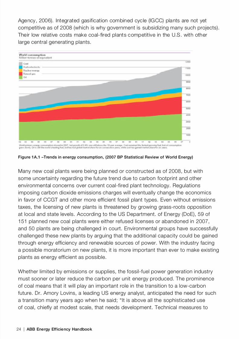
Trends in Power Demand and SupplyCurrently growing 2.6 percent per year, world electricity demand is projected todouble by 2030. The share of coal-fired generation in total generation will likelyincrease from 40 percent in 2006 to 44 percent in 2030. The share of coal in theglobal energy consumption mix is shown in the figure below. This share is nowincreasing because of relatively high natural gas prices and strong electricity demand
in Asia, where coal is abundant. Coal has been the least expensive fossil fuel on anenergy-per-Btu basis since 1976.
China expanded coal use by 11 percent in 2005 and surpasses U.S. as the numberone coal user in 2009. Coal is the most abundant fossil fuel, with proven globalreserves at the end of 2005 of 909 billion metric tons, equivalent to 164 years ofproduction at current rates (International Energy Agency, 2006).
In the U.S., coal-fired plants currently provide 51 percent of total generating capacity(Woodruff, 2005), or about 400 GW , from about 600 power plants . Total electricalgeneration capacity additions are estimated to be 750 GW by 2030 (InternationalEnergy Agency, 2006). Of that new capacity, 156 GW is projected to be providedby coal plants (Ferrer, Green Strategies for Aging Coal Plants: Alternatives, Risks& Benefits, 2008). Other estimates put capacity addition to 2030 at 280 coal-fired500MW plants (Takahashi, 2007).
Higher natural gas prices are reversing a trend toward more energy efficient andlower-emission plant designs. The generating costs of combined-cycle gas turbine(CCGT) plants, which use natural gas, are expected to be between 5–7 cents perkWh, while coal-fired plants are in the range 4–6 cents/kWh (International Energy
Module 1A The Need for Efficient Power Generation
Module 1A | 23
8/12/2019 Energy Efficiency Electronic Book Version 1548_PowerGenerationHandbook v1_1
http://slidepdf.com/reader/full/energy-efficiency-electronic-book-version-1548powergenerationhandbook-v11 26/361
Agency, 2006). Integrated gasification combined cycle (IGCC) plants are not yetcompetitive as of 2008 (which is why government is subsidizing many such projects).
Their low relative costs make coal-fired plants competitive in the U.S. with otherlarge central generating plants.
Figure 1A.1 –Trends in energy consumption, (2007 BP Statistical Review of World Energy)
Many new coal plants were being planned or constructed as of 2008, but with
some uncertainty regarding the future trend due to carbon footprint and otherenvironmental concerns over current coal-fired plant technology. Regulationsimposing carbon dioxide emissions charges will eventually change the economicsin favor of CCGT and other more efficient fossil plant types. Even without emissionstaxes, the licensing of new plants is threatened by growing grass-roots oppositionat local and state levels. According to the US Department. of Energy (DoE), 59 of151 planned new coal plants were either refused licenses or abandoned in 2007,and 50 plants are being challenged in court. Environmental groups have successfully
challenged these new plants by arguing that the additional capacity could be gainedthrough energy efficiency and renewable sources of power. With the industry facinga possible moratorium on new plants, it is more important than ever to make existingplants as energy efficient as possible.
Whether limited by emissions or supplies, the fossil-fuel power generation industrymust sooner or later reduce the carbon per unit energy produced. The prominenceof coal means that it will play an important role in the transition to a low-carbonfuture. Dr. Amory Lovins, a leading US energy analyst, anticipated the need for sucha transition many years ago when he said; “It is above all the sophisticated useof coal, chiefly at modest scale, that needs development. Technical measures to
24 | ABB Energy Efficiency Handbook

8/12/2019 Energy Efficiency Electronic Book Version 1548_PowerGenerationHandbook v1_1
http://slidepdf.com/reader/full/energy-efficiency-electronic-book-version-1548powergenerationhandbook-v11 27/361
permit the highly efficient use of this widely available fuel would be the most valuabletransitional technologies.” (A. Lovins, Energy Strategy: The Road Not Taken 1976)
Trends in Steam Plant Designs and EfciencyLarge fossil-fuel-fired steam plants use a closed steam cycle in which water isconverted to steam in a boiler. This steam is then superheated and then expandedthrough the blades of a turbine whose shaft rotates an electrical generator. Thesteam exits the turbine and condenses to water, which is pumped back up to boilerpressure. The Appendix section of this handbook discusses the steam cycle ingreater detail, and describes some variations on this design which improve the‘cycle’ efficiency.
Sub-Critical Plant Types The most common type of plant using this design is alternatively referred to as‘drum boiler’ or ‘subcritical,’ because water is circulated within the boiler betweena vessel (the drum) and the furnace water-wall tubing where it absorbs combustionheat, but does not exceed critical pressure. Existing subcritical pulverized coal (PC)boiler steam power plants can theoretically achieve up to 36–40 percent efficiencyat full load. Due to major process design changes such as supercritical boilers andother technology improvements , the average efficiencies of the newest coal-firedplants are up to 46 percent compared to 42 percent for new plants in the 1990s (IEA
CoalOnline, 2008).
Energy efficiency improvements of several percentage points in new plants haveresulted from improved designs of the main components and auxiliaries in steampower plants: including auxiliary drivepower:
− Improvements in turbine blade design − Improvements in fans and flue gas treatment methods
− Reduction of furnace exit gas temperature − Increase of feed water temperature − Reduction of condensing pressure
− Use of double reheat on main steam flow − Optimization and reduction of the consumption of auxiliary drivepower
Super-Critical Coal-Fired Steam PlantsSupercritical plants, also called ‘once-through’ plants because boiler water doesnot circulate multiple times as it does in drum-boiler designs, have efficiencies inthe mid-40 percent range. New ‘ultra critical’ designs using pressures of 4,400 psi(30 MPa) and dual stage reheat are capable of reaching about 48 percent efficiency(IEA Coal Online - 2, 2007). Plant availability problems with the first generation of
Module 1A | 25

8/12/2019 Energy Efficiency Electronic Book Version 1548_PowerGenerationHandbook v1_1
http://slidepdf.com/reader/full/energy-efficiency-electronic-book-version-1548powergenerationhandbook-v11 28/361
large supercritical boilers led to the conclusion that pulverized coal-fired electricitygeneration was a mature technology, with an efficiency limited by practical andeconomic considerations to around 40 percent. However, improvements inconstruction materials and in computerized control systems led to new designs forsupercritical boilers that have overcome the problems of the earlier plants (IEA CoalOnline - 2, 2007). Although most new coal-fired plants are expected to use drumsteam boilers, the share of supercritical technology is rising gradually (InternationalEnergy Agency, 2006).
Combined-Cycle Gas Turbine (CCGT) A combined-cycle gas turbine (CCGT) power plant uses a gas turbine in conjunctionwith a heat recovery steam generator (HRSG). It is referred to as a combined-cyclepower plant because it combines the Brayton cycle of the gas turbine with theRankine cycle of the HRSG. The thermal efficiency of these plants has reached arecord heat rate of 5690 Btu/kWh, or just under 60 percent.
Some Steam Plants are Lagging At the beginning of the 21st century, it was believed that a single-cycle coal-firedpower station with an efficiency of more than 50 percent would be possible by 2015(Kjær and Boisen, 1996 in IEA Coal Online - 2, 2007). The efficiency of some newdesign plants may be high, but almost 75 percent of the existing coal-based fleet ofplants in the U.S. is over 35 years old, with an average net plant efficiency of only
slightly above 30 percent (Ferrer, ‘Green Strategies for Aging Coal Plants,’ 2008).
In addition to the less efficient design of core equipment, these older plants sufferan additional efficiency handicap due to plant aging; they become less reliable andgenerally less efficient due to leakage, fouling, and other mechanical factors. Anothertrend which lowers efficiency is the change in fuel supply systems toward off-designcoals for which the boiler has not been optimized (IEA Coal Online - 2, 2007). Fuelsupplies may be subject to further tweaking as generating companies seek to reduce
their carbon footprint by substituting a portion of the coal they use with biomass.
Another important reason that older plants are lagging in efficiency is that many ofthem are operating at 30–50 percent below their rated capacities, where efficienciesof all sub-systems are lower. The realities of a more deregulated and competitivemarketplace, with renewable and distributed energy sources and new systemoperating reserve requirements, have led to previously baseloaded plants beingoperated as dispatchable plants; an unforeseen operating regime (ABB PowerSystems, 2008). One view of this latter issue is the global distribution of load factorof nominally baseloaded steam turbine plants less than 500MW for the period 2001–2005. The following figure shows that the median load factor is only 64 percent.
26 | ABB Energy Efficiency Handbook

8/12/2019 Energy Efficiency Electronic Book Version 1548_PowerGenerationHandbook v1_1
http://slidepdf.com/reader/full/energy-efficiency-electronic-book-version-1548powergenerationhandbook-v11 29/361
Figure 1A.2 - Distribution of load factor of base-loaded plants, (World Energy Council, 2007)
Plant Auxiliary Power Usage is on the Rise The share of total plant auxiliary electrical power in the fleet of fossil-fuel steamplants has been increasing due to these main factors:
− Addition of anti-pollution devices such as precipitators and sulfur dioxidescrubbers which restrict stack flow and require in-plant electric drive power.
About 40 percent of the cost of building a new coal plant is spent on pollutioncontrols, and they use up about 5 percent of gross power generated (Masters,2004).
− Additional cooling water pumping demands to satisfy environmental thermaldischarge rules. − A trend away from mechanical (e.g. condensing steam turbine) drives toward
electrical motors as the prime mover for in-plant auxiliary pump and fan drives.
For PC power plants, the auxiliary power requirements are now in the range of7–15 percent of a generating unit’s gross power output for PC plants. OlderPC plants with mechanical drives and fewer anti-pollution devices had auxiliarypower requirements of only 5 to 10 percent (GE Electric Utility Engineering, 1983).
These figures are for traditional drum boiler type plants, but the auxiliary powerrequirements of supercritical boilers are not any lower. The feedwater pump powerrequired to reach the much higher boiler pressure is approximately 50 percent
Module 1A | 27

8/12/2019 Energy Efficiency Electronic Book Version 1548_PowerGenerationHandbook v1_1
http://slidepdf.com/reader/full/energy-efficiency-electronic-book-version-1548powergenerationhandbook-v11 30/361
greater than in drum boiler designs. Increased demand for auxiliary power increasesa plant’s net heat rate and reduces the amount of salable power.
Plant Auxiliary Energy Efciency ImprovementsIn-plant electrical power, when taken from the generator bus, may be pricedartificially low in some utility companies’ auxiliary lifecycle calculations. A processindustry customer, however, must always pay high commercial rates (and sometimespenalties), thus providing a strong incentive to improve their auxiliary energyefficiency. Price dis-incentives, regulations permitting cost-pass thru, and other non-technical barriers are discussed in the handbook section on Barriers to IncreasedEnergy Efficiency .
These barriers may result in sub-optimal energy designs for power plant auxiliaries,most commonly in oversized motors, fans and pumps. These design decisionshave particularly negative consequences when the base-loaded plant then movesto a new operating mode at 50–70 percent capacity (see previous section for adiscussion of this trend). Auxiliaries such as pumps and fans that use constantspeed motors and some form of flow restriction for control will waste much morepower when operating under such partial-load conditions. Other plant systemswill also run less effectively below their design points. Boilers at partial loads, forexample, run with relatively higher excess air to achieve complete combustion,
which lowers efficiency; these topics are discussed in greater detail in the handbooksections on Drivepower and Automation .
28 | ABB Energy Efficiency Handbook

8/12/2019 Energy Efficiency Electronic Book Version 1548_PowerGenerationHandbook v1_1
http://slidepdf.com/reader/full/energy-efficiency-electronic-book-version-1548powergenerationhandbook-v11 31/361
Technical Efficiency Improvement Potential A recent study by the International Energy Agency (IEA) suggests a technicalefficiency improvement potential of 18–26 percent for the manufacturing industryworldwide if the best available (proven) technologies were applied. Most of theunderlying energy-saving measures would be cost-effective in the long term. Anotherstudy, by the U.S. Dept. of Energy, focused on the energy efficiency opportunityprovided by automation and electric power systems in process industries. Animprovement potential of 10–25 percent was suggested by industry experts, whowere asked to consider improvements within the context of operational or retrofitsituations. The results of that study are shown in the figure below, and in more detailin the Automation module sections of this handbook.
Figure 1B.1 - Process industry survey results on potential of energy efficiency, (US DoE, 2004)
Potential Revealed Through Performance Benchmarking Access to power generation plant performance data is important for identifyingareas for improvement and for showing the results of best practice. Marketfragmentation and the increased competitiveness of de-regulated marketsin the past have made access to data difficult. There has also been a lack ofstandards or practices for measuring performance.
Module 1B The Potential for Energy Efficiency
Module 1B | 29

8/12/2019 Energy Efficiency Electronic Book Version 1548_PowerGenerationHandbook v1_1
http://slidepdf.com/reader/full/energy-efficiency-electronic-book-version-1548powergenerationhandbook-v11 32/361
The World Energy Council (WEC), through its Performance of Generating Plant(PGP) Committee, is now gathering and normalizing such data so that validcomparisons can be made across countries and markets.
Similar performance benchmarking efforts are done in the U.S., but throughindustry-funded organizations like EPRI. Standardization efforts are bestrepresented by IEEE Std 762-2006 IEEE Standard for Definitions for Use inReporting Electric Generating Unit Reliability, Availability, and Productivity.
Interestingly, the WEC found that ‘new drivers geared toward profitability,cost control, environmental stewardship, and market economics are shiftingthe focus away from traditional measures of technical excellence such asavailability, reliability, forced outage rate, and heat rate’ (World Energy Council,2007). Their PGP database has added individual unit design and performanceindices that can be used to compare efficiency and reliability across designs.
The published performance data will help industry improve practices, and willput a spotlight on under-performing plants and companies.
Efficiency Potential Revealed by Country Comparisons The potential for energy efficiency, at least from a U.S. perspective, is alsoindicated in a recent (2007) comparison of fossil-fuel-based power generationefficiencies between nations that together generate 65 percent of worldwide
fossil-fuel-based power. The Nordic countries, Japan, the United Kingdom,and Ireland were found to perform best in terms of fossil-fuel-based generatingefficiency and were, respectively, 8 percent, 8 percent and 7 percent aboveaverage in 2003. The United States is 2 percent below average. Australia,China, and India perform 7 percent, 9 percent and 13 percent, respectively,below average. The energy savings potential and carbon dioxide emissionsreduction potential if all countries produce electricity at the highest efficienciesobserved (42 percent for coal, 52 percent for natural gas and 45 percent for
oil-fired power generation), corresponds to potential reductions of 10 exajoulesof consumed thermal energy and 860 million metric tons of carbon dioxide,respectively (Graus, 2007).
The IEA analysis mentions that more than half of the estimated energy andcarbon dioxide savings potential is in whole-system approaches that oftenextend beyond the process level (Gielen, 2008). ‘Integrative Design’ is thishandbook’s approach to the most challenging energy efficiency issues in plantauxiliary design.
30 | ABB Energy Efficiency Handbook

8/12/2019 Energy Efficiency Electronic Book Version 1548_PowerGenerationHandbook v1_1
http://slidepdf.com/reader/full/energy-efficiency-electronic-book-version-1548powergenerationhandbook-v11 33/361
Energy Efciency is Attracting Interest and Investment
The previous sections showed an engineer’s view of the importance of energyefficiency. What are the views and plans of corporate energy decision makersand investors?
From Corporate Energy Managers According to a recent survey on energy efficiency of corporate and plant-level energymanagers at more than 1,100 North American companies (Johnson Controls, 2008):
− 57 percent expect to make energy-efficiency improvements during the sametime period, devoting an average of 8 percent of capital expenditure budgets onenergy-efficiency projects.
− 64 percent anticipate using funds from operating budgets, allocating 6 percent toenergy-efficiency improvements.
− 40 percent have replaced inefficient equipment before the end of its useful life inthe past year.
− 70 percent have invested in educating staff and other facility users as a way toincrease support for increasing internal energy efficiency.
From Industry InvestorsWhen 18 U.S. investment organizations were surveyed about energy efficiency, the
results indicated that the technologists should have no trouble funding their projects. According to that study (Martin, 2004), the energy technology attracting the greatestinvestment interest is energy intelligence (smart instruments, advanced control,and automation). The handbook sections on Instruments, Controls & Automation discuss these technologies and how they can be used to improve plant energyefficiency.
Carbon Dioxide Emissions Must be Reduced According to a 2005 report from the World Wide Fund for Nature (WWF), coal-basedpower stations are at the top of the list of least ‘carbon efficient’ power stationsin terms of the level of carbon dioxide produced per unit of electricity generated.Based on current developments in Europe and in the U.S., regulations which limit ortax carbon dioxide emissions seem inevitable for all Western economies. A carboncharge of $25 per metric tonne (carbon dioxide) is a conservative estimate used inIEA scenarios. The impact of carbon pricing on fossil-fuel plant generating costs,shown in the figure below, is dramatic compared to most other generation methods.
At prices above $20 per metric tonne coal-based plants become the most expensivetype to operate at current non-optimized cost levels.
Module 1B | 31

8/12/2019 Energy Efficiency Electronic Book Version 1548_PowerGenerationHandbook v1_1
http://slidepdf.com/reader/full/energy-efficiency-electronic-book-version-1548powergenerationhandbook-v11 34/361
China and India account for four-fths of the incremental demand for coal, mainlyfor power generation. For the rst time, China’s carbon dioxide power emissions in2008 exceeded the United States’ emissions; the lower quality coal used in India andother rapidly expanding economies, decreases plant efciency and leads to increasedcarbon dioxide emissions per unit electricity (International Energy Agency, 2006).
Energy Efciency is Key to CO2 Mitigation The IEA Energy Technology Perspectives model is a bottom-up, least-costoptimization program. The model was developed to describe the global potentialfor energy efficiency and carbon dioxide emissions reduction in the period to 2050,particularly in the industrial sector. In the ‘accelerated technology scenario’ (ACT),the potentials for carbon dioxide reduction on all power consumption are shownin the figure below. This figure illustrates the scenario in which carbon dioxideemissions are stabilized globally in 2050 to 2005 levels, and the world narrowlyavoids a costly climate crisis.
Figure 1B.2 Relative share of CO2 mitigation efforts, all consumption, (International Energy Agency,2006)
The Role of Power Generation in Reducing Emissions The IEA’s ACT scenario suggests that power generation efficiency cancontribute significantly to the overall global effort to stabilize carbon dioxideemissions by 2050 at or near 2005 levels. Surprisingly, the model shows thatpower generation efficiency alone, which includes improved auxiliaries andother measures, has a larger climate impact than even nuclear power.
32 | ABB Energy Efficiency Handbook

8/12/2019 Energy Efficiency Electronic Book Version 1548_PowerGenerationHandbook v1_1
http://slidepdf.com/reader/full/energy-efficiency-electronic-book-version-1548powergenerationhandbook-v11 35/361
When the model is applied to process industries alone, the impact of energyefficiency is proportionately larger. The figure below shows the ‘blue’ scenario,which uses the same ACT scenario describe above, but with a higher carbondioxide charge of $50 per (metric) tonne, instead of $25/tonne (Taylor, 2008).
Figure 1B.3 - Relative share of CO2 mitigation efforts in process industries, (Taylor, 2008)
Applying this model to the power generation sector in particular suggests thatits carbon dioxide emissions are cut by 36 percent using all of the approachesshown. Half of those savings (18% of total) can be attributed to relatively low-technology energy efficiency measures alone.
Energy efficiency measures are the most important of all the carbon dioxidemitigation approaches for process industries, contributing to almost half of
the impact on emissions (Martin, 2004). Although these predictions apply toprocess industries, the relative potentials are likely to be valid for the steampower generation sub-sector as well.
Module 1B | 33

8/12/2019 Energy Efficiency Electronic Book Version 1548_PowerGenerationHandbook v1_1
http://slidepdf.com/reader/full/energy-efficiency-electronic-book-version-1548powergenerationhandbook-v11 36/361
Multiple Benets of Energy Efciency The primary benefits of a increased plant energy efficiency are reduced emissionsand energy or fuel costs.
Power plants which operate partially or wholly at full load will have more salablepower. At less than capacity, the fuel savings are significant. In coal-fired steampower plants, fuel costs are 60-70% of operating costs.
The following is a more complete list of benefits accompanying energy efficiencydesign improvements for plant auxiliaries:
Operational Benefits − Improved reliability/availability. As has been found with stricter safety design
regulations, any extra attention to the process is rewarded with improved uptime. − Improved controllability: energy is wasted in a swinging, unstable process, partly
through inertia in the swings, but mainly because operators in such situations donot dare operate closer to the plant’s optimum constraints.
− Reduced noise and vibration, reduced maintenance costs.
Results of Improved Efficiency on Plant Operations and Profitability − Better allocation: under deregulation, as utilities dispatch plants within a fleet,
heat rate improvement can earn plants a better position on the dispatch list(Larsen, 2007).
− Avoiding a plant de-rating due to efficiency losses after anti-pollution retrofits orother plant design changes.
− Improved fuel flexibility—by efficiently using a wider variety of fuels (coalvarieties) and, in some cases, increasing the firing of biomass, for example.
− Improved operational flexibility 1) Improved plant-wide integration betweenunits will reduce startup-shutdown times; this benefit applies mainly to de-regulated markets. 2) The heat rate versus capacity curve is made flatter andlower, which allows the plant to operate more efficiently across a wider loadingrange.
Plant Investment Benefits − Avoiding forced retirement due to pollution non-compliance: An ambitious retrofit
programme may save some older plants from early retirement due to non-compliance with regulations.
34 | ABB Energy Efficiency Handbook

8/12/2019 Energy Efficiency Electronic Book Version 1548_PowerGenerationHandbook v1_1
http://slidepdf.com/reader/full/energy-efficiency-electronic-book-version-1548powergenerationhandbook-v11 37/361
− Tax credits—take advantage of newer policies such as EPACT 2005, which mayprovide tax credits for efficiency efforts. Similar policies are in effect in the EU andChina.
− Mainstream industry authority Engineering News–Record’s influential Top Listsrankings now include “Top Green Design Firms” and “Top Green Contractors”:‘The market for sustainable design has passed the tipping point and is rapidlybecoming mainstream’ ( http://enr.construction.com/ ).
− Increasingly, shareholders and capital markets are rewarding companies who treattheir environmental mitigation costs as investments (Russel, 2005).
Retrofitting may save some older plants from early retirement due to non-compliance with regulations such as the EU’s Large Combustion PlantDirective on pollution (nitrous oxides, sulfur dioxide, mercury, and particulates)(International Energy Agency, 2006). In the US, increased compliance maysmooth permitting of new units or plants.
All of the ‘dirty dozen’ in Carbon Monitoring For Action’s (CARMA) list oftop carbon dioxide emitting sources in the U.S. are coal-fired power plants,emitting an average of about 20 million tonnes of carbon dioxide per yearper plant. ‘Blacklists’ like these, which include rankings by company as well,are increasingly being consulted by large institutional investors and sovereign
wealth funds. With tightened credit markets, there is therefore an evengreater incentive for top management to watch carbon dioxide emissions.See the section on Benchmarking for other global efforts toward increasedtransparency.
Non-Technical Barriers to Energy Efcient DesignDespite all of the benefits and incentives, and the low-capital-cost improvement
potential described in previous sections, the implementation of integrative, energyefficient design and operation is still hindered by several obstacles. Methods forimproved design are known and the required technologies are widely available ‘offthe shelf.’ Individual components are generally available in high-efficiency variants.So why are power and industrial process plants energy inefficient in their design asa whole? One clue, is the fragmentation found in engineering disciplines, vendorequipment packages, and even in the way projects are executed.
The current situation with energy efficiency is analogous to the status of safety inprocess industries a decade or two ago. Operational safety was acknowledged asimportant and was codified, but there were no standards on how safety could bemanaged during the design process—on how it could be ‘designed-in’ from the
Module 1B | 35

8/12/2019 Energy Efficiency Electronic Book Version 1548_PowerGenerationHandbook v1_1
http://slidepdf.com/reader/full/energy-efficiency-electronic-book-version-1548powergenerationhandbook-v11 38/361
start. The recent Functional Safety standards IEC-61508 and 61511 point the wayforward for energy design and management standards evolution.
Many of the barriers listed below are managerial or procedural rather than technicalin nature. These important non-technical aspects are discussed in the final module ofthis handbook. The discussion is generic for most large power and process facilities,but a specific industry will have additional competitive and regulatory pressures.
Local, State, National and International Regulatory Authorities Authorities provide the regulatory framework for the activities of all the otherstakeholders. The efforts of authorities are closely linked with those of the standardsorganizations. These factors, however, may contribute to inefficient plant designs:
− Regulations often permit pass-thru of all fuel-related costs directly to the ratebase. This financially discourages any economization efforts related to fuelconsumption, i.e. efficiency.
− Lack of clarity, unity and commitment to emissions charging makes investors waryof long-term investments in energy efficiency and/or carbon dioxide emissionsreduction.
− Deregulation and the ensuing volatility in fuel and energy prices may alsodiscourage the long-term thinking necessary to make some efficiency and carbondioxide emissions reduction schemes justifiable.
Shareholders & Investors The observations in this paragraph regarding shareholders and investors applymainly to new construction or large-scale redevelopment projects. See the followingparagraphs for barriers more applicable to facility owner/operators of older plantsand retrofit project contexts. Shareholders and investors often influence projectschedules, contract clauses, functional specs for new construction and majorretrofits of plants. These factors, however, may contribute to plants that areultimately energy inefficient:
− Project schedules are compressed; front-end design and concept studies areunderfunded or curtailed.
− Scope of redevelopment projects is narrow because investors ‘generally wantto avoid changes to the long remaining lifespan of the standing capital stock’(International Energy Agency, 2006).
− Designs are ‘frozen’ early by a pre-established milestone date, even if importantdata may be missing.
− Cost analysis methods are too crude, or not coupled tightly enough to theconceptual process design, or have wrong initial assumptions regarding risk,return, and lifetime; calculations may ignore significant indirect costs and savingssuch as substitution costs, maintenance savings, and peak energy prices.
36 | ABB Energy Efficiency Handbook

8/12/2019 Energy Efficiency Electronic Book Version 1548_PowerGenerationHandbook v1_1
http://slidepdf.com/reader/full/energy-efficiency-electronic-book-version-1548powergenerationhandbook-v11 39/361
− Operational energy costs may be treated as a fixed cost and therefore receivemuch less attention than a variable cost.
− Low-bid, fixed-price contracting without strong, well-defined and enforceableenergy performance guarantees, at the plant, unit and equipment levels.
− Purchasing managers seek multiple suppliers to reduce cost; this strategy leadsto increased design and data fragmentation. Purchasing managers may still preferindividual vendors versus full-service/system integrators.
− Energy-expert consulting companies are usually the last to be hired, and thereforehave much less influence over the conceptual design.
− Drawings are issued ‘for construction’ before even the first vendor drawing isseen, much less approved (Mansfield, 1993), leading to hasty, often energy-inefficient re-design at the interfaces.
− Capital scarcity might favor smaller plants with lower efficiency (Gielen, 2008).
Facility OperatorsFacility Operators craft the original specifications, validate the design duringcommissioning and acceptance trials, determine operational loading andmaintenance of facility, and usually initiate and manage retrofit projects. Thesefactors, however, may contribute to plants that are ultimately energy inefficient:
− Retrofit projects to improve energy efficiency are funded from operating budgets,not from larger capital expenditure budgets; payback expectations and discount
rates are all generally much higher than in green-field projects. − Managers focus on optimizing process productivity, in which energy is only one
of several other cost functions and may not receive the consideration it deserves;many modern plant-wide optimization systems optimize for productivity, whichonly indirectly improves energy efficiency.
− There is a war for money between process improvement and energy efficiencycamps in a typical plant; process improvement teams and their measures seem to‘get more respect.’
− An increasing number of plants are centralizing purchasing, which means lessengineer involvement in purchasing decisions. ‘Since purchasing centralization…we’ve seen companies shift away from using a lifecycle cost model, which seemsvery short-sighted to us. Some of the decisions customers have been making arecommitting them to a stream of ongoing expenses that could have been reduced.’(Control Engineering article 8/15/2005).
− Facility operators receiving a new/retrofitted plant/unit are under-pressure to beginoperations as soon as possible so they are therefore less critical with respect toenergy targets during acceptance tests.
− Facility operators do not or cannot operate plant at design capacities due tochanges in market or other factors.
Module 1B | 37

8/12/2019 Energy Efficiency Electronic Book Version 1548_PowerGenerationHandbook v1_1
http://slidepdf.com/reader/full/energy-efficiency-electronic-book-version-1548powergenerationhandbook-v11 40/361
− Plant engineering and maintenance teams are losing experienced older staff;facility operators do not provide adequate training for staff on energy efficiency.
− Power plant/power house energy managers (superintendents or maintenancedirectors) lack the necessary communication and salesmanship skills to push throughgood energy efficiency proposals. (a post on J. Cahill’s blog, 2007).
− Reluctance to admit non-optimal, energy inefficient, operation to uppermanagement – the perception is that this reflects badly on plant management andtheir plant operations team.
− Fear of production disruptions from new equipment or new procedures to improveefficiency (International Energy Agency, 2006); doubts about safety, controllabilityor maintainability
− Expansion projects will simply duplicate an existing unit on the same site,repeating many of the same design mistakes, to reduce the up-front engineeringhours; low-labor copy-and-paste projects may also overlook opportunities forrationalization & integration with the existing unit(s).
Design and Engineering CompaniesDesign and engineering companies determine design specs of facility, selectcomponents and execute the design. These factors, however, may contribute toenergy inefficient plants:
− A tendency to oversize pumps, fans, and motors by one rating, and oversize them
again after handoff to another discipline, and then again by project leaders:– Bottom limits in standards already have a safety margin, but these limits
are interpreted as a bare minimum (from fear of litigation) and an additionalsafety margin is added.
– Overload maximums received from process engineer are interpreted bymechanical and electrical teams as continuous minimums; fat margins areadded in lieu of detailed loading study.
– Additional margins are then added for future, but unplanned, capacity
increases.– Engineers on auxiliary systems are inordinately fearful of undersizing and riskbeing singled out as the bottleneck that prevents operation at full designcapacity of other, more expensive, hardware
– Large, commodity motors and fans are commercially available only in discretesizes. After all the margins, an engineer will choose the next size up if thedesign point falls between two sizes.
− A tendency to aggressively reduce engineering hours to increase margins onfixed-priced contracts and to avoid selecting premium components for suchcontracts.
38 | ABB Energy Efficiency Handbook

8/12/2019 Energy Efficiency Electronic Book Version 1548_PowerGenerationHandbook v1_1
http://slidepdf.com/reader/full/energy-efficiency-electronic-book-version-1548powergenerationhandbook-v11 41/361
− Trade-offs between floor space and pipe/ductwork efficiency are not life-cyclecost-estimated; civil and architectural concerns are the default winners due totheir early head start in most projects.
− Trade-offs between reliability and energy efficiency are not life-cycle cost-estimated. Higher energy costs are seen as insurance against large, but virtualopportunity costs.
− Lack of energy design criteria and efficiency assessment steps in the standardengineering workflow. There is typically a design optimization step for cost, safety,reliability, and other concerns, but not for energy efficiency.
− Shortage of engineers in key industries; junior and outsourced engineers aremaking higher-impact decisions.
− A reluctant to deviate from their ‘standard design’ templates, especially onexpansion projects where the design has been delivered on previous units. Thisleads to short cuts and uncritical copying-and-pasting of older, non-optimaldesigns.
− Engineers work mainly within the confines of their discipline and do not seeopportunities for inter-disciplinary optimization of the total design. For example:– Mechanical engineers miss out on optimizations from chemical engineering
to use waste heat and to optimize plant thermodynamics or create usefulby-products.
– Process engineers do not leverage the full potential of automation, selectinginstead familiar equipment like valves to perform control tasks better suited to a
variable frequency drive.– Electrical engineers do not fully understand the process needs for power, such
as duty cycles, and therefore do not fully optimize their designs.– None of the engineers mentioned above are typically very quick to leverage
advances in materials science, which enable higher operating parameters.
Equipment Vendors and Design Tool ProvidersEquipment Vendors and Design Tool Providers determine component energy
efficiencies. The vendor’s tools directly affect the engineer’s workflow, models, anddocumentation. These factors, however, may contribute to energy inefficient plants:
− Vendors provide black-box components with closed/proprietary/rigid interfaces,which are not easily optimized for the whole system; this is the result of a trendtoward ‘commoditization.’
− Proliferation of design tools and data formats which are non-integrated and theirdesign model is non-navigable between vendor tools; this hinders integrativedesign.
− Lack of full-scope energy-optimization functionality in the leading design andmodeling tools
Module 1B | 39

8/12/2019 Energy Efficiency Electronic Book Version 1548_PowerGenerationHandbook v1_1
http://slidepdf.com/reader/full/energy-efficiency-electronic-book-version-1548powergenerationhandbook-v11 42/361
− As components become commodities, salesmen are replacing sales engineers,and misapplications are increasing (Plant Services.com, 2008)
Professional and Standards OrganizationsProfessional and standards organizations provide basic education standards andbest practice certifications. These factors, however, may contribute to energyinefficient designs:
− No widely accepted standards specifically for energy efficient designs of entireplants; some operational energy management standards are in development,however.
− No widely accepted certification for energy design for whole plant systems; anenergy manager certification is available in the USA, however.
− Lack of mandatory international labeling system for industrial motors,transformers, and other equipment to enable comparison.
− Protectionism and turf wars limit the global adoption of a single set of standards;the divisions between English and SI units are a cause for some confusion, designerrors, and incompatibilities.
Educators and AcademiaEducators and academia provide basic skills and certification (by diploma) of thenext generation of designers and engineers. These factors, however, may contribute
to inefficient designs:
− Educators tend to focus on the abstract and theoretical, as opposed to bestpractice design using state-of-the art commercially available engineeringcomponents.
− Systems engineering courses are not mandatory or sometimes not even offered inthe average curriculum.
− Electrical engineering curricula increasingly favor more modern topics of
electronics and discrete logic at the expense of courses on old-fashioned powerengineering; courses on power station design have been dropped. − Programs or degrees toward industrial or engineering management are too
general: the specifics of each discipline cannot be made more abstract.− Some engineering schools offer no ‘capstone’ design course that encourages
synthesis of all the disciplines toward a single design task.
40 | ABB Energy Efficiency Handbook

8/12/2019 Energy Efficiency Electronic Book Version 1548_PowerGenerationHandbook v1_1
http://slidepdf.com/reader/full/energy-efficiency-electronic-book-version-1548powergenerationhandbook-v11 43/361
Standards, Best Practice, Incentives, and RegulationsStandards are the designer’s and engineer’s best design guidelines. Standards alsooffer customers and authorities an objective measure for applying regulation andincentives. ‘Best practices’ encompass more than standards, and include casestudies, more application details, and some costing information.
Role of Standards in Energy EfficiencyEnergy efficiency is an invisible quality and is subject to various interpretations; it isimportant, therefore, for engineers and managers to be able to have some commondefinitions and methodologies when assessing efficiency performance. Internationalstandards for energy design and management are emerging and some countries,including the U.S., have some standards in these areas. It is likely that thesestandards will be closely linked to future carbon dioxide compensation schemes,whether at national or international levels (ISO, 2007).
Common benchmarking for performance is good, but at a deeper level, standardscan provide the equipment and system inter-operability that can enable a higherperformance design. Highly efficient components which are mismatched orpoorly integrated make for an inefficient overall system. A joint ISO/IEA technicalcommittee that was recently formed to identify gaps in industrial standards coveragerecommended more emphasis on the systemic approach and encouraged a focus
on energy efficiency of overall systems and processes as well as retrofitting andrefurbishing. This expert committee also recommended that standards shouldaddress efficiency improvements through industrial automation .
Standards and Best Practice The standardization efforts relevant to plant auxiliaries’ energy performance cover awide variety of disciplines. The list far below refers to existing standards relevant tothe systems in this handbook that specify design, application, labeling and minimum
energy performance standards. The list focus is on U.S. standards, but someimportant international standards are also mentioned, in italicized text. The premier,official sources of unbiased standards are the national standards bodies such as
American National Standard Institute (ANSI) for the U.S., CEN/CENELEC (for theEU) and the international bodies such as the IEC and the ISO. A convenient way tosearch for U.S. and global standards is by using the ANSI NSSN search engine atwww.nssn.org. Search by title ‘power station design’ or ‘power plant.’
Module 1B | 41

8/12/2019 Energy Efficiency Electronic Book Version 1548_PowerGenerationHandbook v1_1
http://slidepdf.com/reader/full/energy-efficiency-electronic-book-version-1548powergenerationhandbook-v11 44/361
Other sources of objective standards are the professional societies and industryassociations, although the latter may show more bias toward their industry in certainsituations:
− Institute of Electrical and Electronic Engineers (IEEE)− Instrumentation, Systems, and Automation Society (ISA)
− The Hydraulic Institute (HI) − National Fluid Power Association (NFPA) − Air Movement and Control Association (AMCA) − American Society of Mechanical Engineers (ASME)
− National Fire Protection Association (NFPA)
Many standards for steam-water cycle design of cycle equipment can be foundin the various ASME and NFPA codes, but these are not within the scope of thishandbook. The ASME test codes for determining efficiency, however, are of interest.Energy is a political as well as a technical subject; some ‘associations’ (not thosementioned above) promoting best practice are actually lobby groups with strong,but not obvious, links to commercial or political entities with various agendas. Thesesources can be useful if their advice is taken together with the objective sourceslisted above. Some of these unofficial sources of design guidance are listed in theReference section of this handbook. The following list is not a comprehensive listof all relevant standards; appearing here are only those that have some relevance to
plant auxiliaries’ energy performance and design.
Power Plant Facilities − IEEE Std 666-2007 IEEE Design Guide for Electric Power Service Systems for
Generating Stations (Revision of IEEE Std 666-1991) − IEEE Std 762-2006: Standard for Definitions for Use in Reporting Electric
Generating Unit Reliability, Availability, and Productivity
− ANSI/ISA S77.43.01-1994 (R2002) : Fossil Fuel Power Plant Unit/PlantDemand Development (formerly ANSI/ISA S77.43-1994) − ANSI/ASME PTC 46-1996: Overall Plant Performance codes − ASME PTC 47-2006: Integrated Gasification Combined-Cycle Plants − IEEE 803.1-1992 : Recommended Practice for Unique Identification in Power
Plants and Related Facilities - Principles and Definitions − ISO 13600 series (1997–2002): Technical energy systems. Methods for analysis
of technical energy systems, - enabling the full costing and life cycle analysis
42 | ABB Energy Efficiency Handbook

8/12/2019 Energy Efficiency Electronic Book Version 1548_PowerGenerationHandbook v1_1
http://slidepdf.com/reader/full/energy-efficiency-electronic-book-version-1548powergenerationhandbook-v11 45/361
Best Practices − DoE EERE Best Practice guides for Steam, Pumping Systems, Fans www1.
eere.energy.gov/industry/bestpractices − EPRI studies and reports – there is a large population of useful reports − ABB Electrical Transmission and Distribution Reference Book (the ‘T&D’
manual)
Pump and Fan Systems − ANSI/HI 1.3-2007 : Rotodynamic (Centrifugal) Pumps for Design and Application − ANSI /HI Pump Standards : Available through the Hydraulic Institute, a standards
partner (www.pumps.org/ )
Best Practices for Pump and Fan Systems − ANSI/HI Optimizing Pumping Systems Guidebook − US DoE Sourcebook (2006). Improving Pump System Performance, from EERE
Industrial Technologies Program: − US DoE Sourcebook (2006). Improving Fan System Performance. from EERE
Industrial Technologies Program − Air Movement and Control Association (AMCA) International
Motors and Drives
− NEMA MG 1 : Motors and Generators − NEMA ANSI C50.41:2000 : Polyphase induction motors for power generating
stations − IEEE Std 958-2003 : Guide for Application of AC Adjustable-Speed Drives on
2400 to 13,800 Volt Auxiliary Systems in Electric Power Generating Stations − IEC 60034-3 Ed. 6.0 b:2007 Revises IEC 60034-3 Ed. 5.0 b:2005 Rotating
electrical machines - Part 3: Specific requirements for synchronous generatorsdriven by steam turbines or combustion gas turbines
− IEC 60034-2-1: Motor efficiency testing (September 2007); published as EN60034-2-1 at CENELEC level. Best Practices for Motors and Drives
− DoE Motor System Best Practices
The Energy Independence and Security Act of 2007 (EISA) calls for increasedefficiency of motors manufactured after December 19, 2010.
Module 1B | 43

8/12/2019 Energy Efficiency Electronic Book Version 1548_PowerGenerationHandbook v1_1
http://slidepdf.com/reader/full/energy-efficiency-electronic-book-version-1548powergenerationhandbook-v11 46/361
Electric Power Systems − IEEE 493 Design of Reliable Industrial and Commercial Power Systems, also has
useful equipment reliability data. − C57.116-1989 IEEE Guide for Transformers Directly Connected to Generators
− IEEE Std C37.010™, IEEE Standard Application Guide for AC High-Voltage CircuitBreakers Rated on a Symmetrical Current Basis.64, 65
− IEEE 519-2006 Harmonic voltage and current distortion limits − IEEE Std 946-2004 IEEE Recommended Practice for the Design of DC Auxiliary Power Systems for Generating Stations
− IEEE Std C37.21-2005 IEEE Standard for Control Switchboards − 525-1992 IEEE Guide for the Design and Installation of Cable Systems in Substations − C62.92-1993 IEEE Guide for the Application of Neutral Grounding in Electrical
Utility Systems, Part III-Generator Auxiliary Systems − IEC 60076-1 Power Transformers (VDE 0532 Part 101) − IEC 62271-1 Ed. 1.0 b:2007 High-voltage switchgear and controlgear
− IEC 61000-2-4 (Worldwide) Harmonic voltage and current distortion limits Best Practices for Electric Power Systems
− ABB Switchgear Manual, 11th edition, 2006 (available online) − ABB Transformer Manual, 2007
Energy & Environmental Management
− ISO 14064 and ISO 14065 provide a methodology to help organizations assesscarbon footprints and implement emissions trading schemes
− ISO 14001 is an internationally recognized framework for environmentallegislation, regulation, management, measurement, evaluation, andauditingassessing.
− ISO 13600 series provides guidelines on technical energy systems
Instrumentation & Control Automation Systems
− ANSI/ISA-77.44.01-2007 - Fossil Fuel Power Plant - Steam Temperature Controls − ANSI/ISA-RP77.60.05-2001 (R2007) - Fossil Fuel Power Plant Human-MachineInterface: Task Analysis
− ANSI/ISA-77.42.01-1999 (R2006) - Fossil Fuel Power Plant Feedwater ControlSystem – Drum-Type
− ANSI/ISA-77.20-1993 (R2005) - Fossil Fuel Power Plant Simulators - FunctionalRequirements
− ANSI/ISA-77.41.01-2005 - Fossil Fuel Power Plant Boiler Combustion Controls − ANSI/ISA-RP77.60.02-2000 (R2005) - Fossil Fuel Power Plant Human-Machine
Interface: Alarms
44 | ABB Energy Efficiency Handbook

8/12/2019 Energy Efficiency Electronic Book Version 1548_PowerGenerationHandbook v1_1
http://slidepdf.com/reader/full/energy-efficiency-electronic-book-version-1548powergenerationhandbook-v11 47/361
− ANSI/ISA-77.70-1994 (R2005) - Fossil Fuel Power Plant Instrument PipingInstallation
− ANSI/ISA-77.43.01-1994 (R2002) - Fossil Fuel Power Plant Unit/ DemandDevelopment-Drum Type
− ANSI/ISA-77.13.01-1999 - Fossil Fuel Power Plant Steam Turbine Bypass System − 502-1985 IEEE Guide for Protection, Interlocking, and Control of Fossil-Fueled
Unit-Connected Steam Stations − ASME PTC PM-1993 Performance Monitoring Guidelines for Steam Power Plants − ISO 13380:2002 Condition monitoring and diagnostics of machines - General
guidelines on using performance parameters − ISO/TS 18876-1:2003 Industrial automation systems and integration - Integration
of industrial data for exchange, access and sharing Best I&C Practices
− ISA Instruments and Automation Society, http://isa.org/ , both a standards andindustry organization with sources on best practice
Power Generation Regulations and Incentives The regulatory environment for coal-fired plants appears likely to changesignificantly before 2010. Some US states (2008) are considering a moratoriumon new coal plant construction , and may slow or stop permitting of plants
under construction. A US Supreme Court ruling in 2007 determined that CO2 isan air pollutant; this raises the possibility that CO2 will soon be regulated as suchunder the Clean Air Act. Some of the most relevant existing regulations are listedbelow:
− EPACT: Energy Policy Act (1992)− EPACT: Energy Policy Act (2005)− CAAA: Clean Air Act (1970, 1990) and National Ambient Air Quality Standards
(NAAQS)
EPACT 2005: tax credits for the construction of coal-fired generation projectsrequisite on meeting efficiency and emissions targets. (International Energy
Agency, 2006): According to the IEA, this leads to an increased share of IGCCand ‘clean coal’ projects, but may also have impact on traditional coal-fired plantdesigns and operation.
The recent legislation in the Energy Independence and Security Act of 2007 (EISA)will also have an impact on the design and operation of fossil-fuel fired powerplants. EISA calls for increased efficiency of motors manufactured after December19, 2010, for example.
Module 1B | 45

8/12/2019 Energy Efficiency Electronic Book Version 1548_PowerGenerationHandbook v1_1
http://slidepdf.com/reader/full/energy-efficiency-electronic-book-version-1548powergenerationhandbook-v11 48/361
Engineering Basic Standards − IEEE 280: Standard Letter Symbols for Quantities Used in Electrical Science and
Electrical Engineering − ISO 15926: A meta-structure for information concerning engineering, construction
and operation of production facilities. − ISO 31: Quantities and units, International Organization for Standardization, 1992,
now being superseded by the harmonized ISO/IEC 80000 standard.
Efciency and Lifecycle Cost CalculationsEfficiency CalculationsEfficiency is a measure of how effective a system or component can convert inputto output. Efficiency is normally given in units of percentage, or as a value from 0 (0percent) to 1.0 (100 percent). Energy efficiency can be calculated using either energy(kW/h) or power (kW)
Efficiency percent = (Useful Power Out (kW) / Power In (kW)) x 100
Energy and Power CalculationsEnergy must always be defined relative to a given time period or to a given volume,etc. The energy consumed by a system or components during a given time period
is determined by multiplying its input power over a time period. The common term‘losses’ means wasted energy. Losses can be treated as energy (kWh) in all thecalculations in this section. The common term ‘loads’ means output power. Mostenergy calculations are based on a year’s time, and a year is conventionally assumedto be only 8,000 hours to account for system downtime, when energy consumptionis 0. (There are otherwise 8,760 hours in a full year.)
Annual energy consumption (kWhr) = 8,000 (hrs/year) x Power (kW)
Load ProfileIn practice, power levels (or ‘loads’) are not constant, as assumed in the formulaabove. Loads vary over a given period due to changes in the process or ambientconditions. This variation is described by the component’s ‘load profile,’ whichdescribes the percentage of time (in hours per year) at each loading level (as apercentage of full load) as shown in the sample load profile below:
46 | ABB Energy Efficiency Handbook

8/12/2019 Energy Efficiency Electronic Book Version 1548_PowerGenerationHandbook v1_1
http://slidepdf.com/reader/full/energy-efficiency-electronic-book-version-1548powergenerationhandbook-v11 49/361
% Hours % of Full Load
5% 400 100
10% 800 90
15% 1200 80
20% 1600 70
20% 1600 60
15% 1200 50
10% 800 40
5% 400 30
0% 0 20
100% 8,000 hrs Weighted Avg 65
A more accurate view of annual energy consumption for the above component’sprofile is the sum of the energies at each load level:
Annual Energy (kWhr) = Σ (hrs) at load level(i) x (%) full load at load level(i) x fullload (kW)
Duty cycle is similar to load profile, but is used to refer to shorter time periods (daysor hours) and for cycling (on-off) loads, rather than more continuously variable loads.
Energy and Power Units
Energy has many forms and can be described using many units. The most commonunits and their conversion factors are given in the Appendix.
1 horsepower (hp) = 0.7457 kW = 2546 Btu/hr
Savings CalculationsSavings calculations are used to determine the difference in energy and costbetween two components or systems.
By combining the formulas above, one can compare the annual savings of energy fortwo components or systems of varying efficiency E1(%) and E2(%). The result is anenergy saving (Se) in kW per year (assume 8,000 hrs in absence of data):
Annual Energy Savings (kWhr) = 0.746(kW/hp) x P(hp) x 8,000 x 100(%) x (1/E2 –1/E1)
Module 1B | 47

8/12/2019 Energy Efficiency Electronic Book Version 1548_PowerGenerationHandbook v1_1
http://slidepdf.com/reader/full/energy-efficiency-electronic-book-version-1548powergenerationhandbook-v11 50/361
One can then multiply by the cost of energy (in $/Kwh) to determine the financial (orcapitalized) cost of the annual energy savings calculated above, in $:
Annual Dollar Savings ($) = Se (kWh) x Q ($/kWh), where Q is the price per kWh ofelectricity
In these calculations the price (Q) of energy is assumed to be constant. In fact,energy prices may change as often as every 15 minutes in a de-regulated market,with much higher prices during peak periods. The average annual price of electricityshows a rising trend. See the section on present value for methods to account forthis change.
Lifecycle Costing MethodsLife-cycle costing (LCC) is a method of calculating the cost of a system over itsentire lifespan. LCC is calculated in the same way as ‘total cost of ownership’(TCO). A technical accounting of systems costs includes initial costs, installation andcommissioning costs, energy, operation, maintenance and repair costs as well asdown time, environmental, decommissioning and disposal costs. These technicalcosts, for an example transformer, are listed below.
LCC = C A + C E + C I +nƩ0 (CPM + CC M + CO P + CO 0 + CR) + CD
where C A = cost of apparatus
CE = cost of erection C I = cost of infrastructure CP M = cost of planned maintenance CC M = cost of corrective maintenance COP = cost of operation (load and no-load losses) CR = cost of refurbishment or replacement CD = cost of disposal n = years of operational life span
Additional, non-technical costs that should be accounted for in budgetary estimatesinclude insurance premiums, taxes, and depreciation.
All costs in an LCC calculation should be discounted to present value (PV) dollarsusing the present value formulas in the following section. A very simplified LCCcalculation with fewer terms considers only the cost of apparatus and the cost ofoperation, and does not consider inflation or variation in price of energy per kWh.
The operational cost term in an LCC formula is typically the annual energy costscalculated using the formulas above, discounted to PV dollars. See the sectionMotor System Calculations for a numerical example.
48 | ABB Energy Efficiency Handbook

8/12/2019 Energy Efficiency Electronic Book Version 1548_PowerGenerationHandbook v1_1
http://slidepdf.com/reader/full/energy-efficiency-electronic-book-version-1548powergenerationhandbook-v11 51/361
For systems that directly emit carbon dioxide or other pollutants, the cost ofoperation should include remediation costs, and the taxes which authorities charge(or may charge) per unit of emissions. For electrical loads powered from a fossil-fuel-based source, the carbon dioxide amounts (in tons) are still relevant, but the carbondioxide tax (in $) should not be added to that component’s operational costs if thetax has already been factored into the price of the consumed electricity.
Carbon dioxide cost calculationsFor coal-fired power plants, 1.3 tons of carbon dioxide is emitted per MW hour(C.P. Robie, P.A. Ireland, for EPRI, 1991). A conservative estimate for a futurecarbon dioxide tax is $25 per metric ton, globally and in the U.S. The tax maytake many forms, ether as a direct tax or a traded quota, etc. A metric ton(1,000kg = 2240 lbs) is also written ‘tonne.’
The energy and dollar savings calculations can now be applied, using the abovedata, to give a carbon dioxide (tons) saving and a carbon dioxide dollar savings($) for reducing power from a fossil-fuel-based source:
Annual carbon dioxide savings (tonnes) = 0.746(kW/hp) x P(hp) x 8,000 x100(%) x (1/E2 – 1/E1) x 1,300
Annual carbon dioxide tax savings ($) = $25/tonne x annual carbon dioxidesavings (tonnes)
A rule of thumb for coal-fired plants: a 2 percent steam cycle efficiencyimprovement can reduce carbon dioxide emissions by up to 5 percent (Ferrer,‘Small-Buck Change Yields Big-Bang Gain,’ 2007).
Limitations of LCC MethodsLCC analyses often count only single benefits, such as the electricity directly savedby a new motor’s higher nameplate efficiency. In fact, there are numerous otherbenefits to reduce electricity consumption on the size and wear of upstream, powersystem components. Other benefits that are hard to quantify in LCC analysis includereduced maintenance via the elimination of the control valve, for example. In adetailed LCC calculation it is important to consider substitution cost.
Present Value FormulasMost of the costs shown in the LCC calculation accrue in the future. Thesepayments must be translated into present values using the time-value of moneyformulas given here.
Module 1B | 49

8/12/2019 Energy Efficiency Electronic Book Version 1548_PowerGenerationHandbook v1_1
http://slidepdf.com/reader/full/energy-efficiency-electronic-book-version-1548powergenerationhandbook-v11 52/361
Present value (PV) of a future amount (FV) at period ‘n’ in the future at ‘i’ interestrate is:
PV = FV n x 1/(1 + i)n
Present value of a uniform series of payments, each of size US (for Uniform Series):PV
us = US x ((1 + i)n - 1 )/i(1 + i)n
Where ‘i’ is the interest rate from 0-1 (for a 6% rate, i = 0.06)
The formula for PV of a uniform series can be used to determine the value of annualenergy savings, where the annual cost is calculated as shown at the start of thissection.
If the average annual price of electricity rises at p% per year, then the flat rate Qmust be multiplied by the following rising price factor ‘f’:
f = (qn– 1) / (q – 1)
Where: q = 1 + p/100 And p is the price increase in %
Using the formula for a 1 kW loss after 20 years shows an accumulated cost whichis 41 times the cost of the first year if the average annual increase in the energy price
is 7 percent (ABB Ltd,Transformers, 2007).
Payback CalculationsIf the PV of the energy savings over ‘n’ periods (years) exceeds that of theinvestment cost (X), then the investment should be made. The number of periodsrequired for PV to equal X is the ‘payback’ period. For a given value of X, therefore,the payback period ‘n’ can be calculated.
The monetary value of energy losses, called the capitalized loss value, is dened as themaximum amount of money the user is willing to invest to invest to reduce losses by 1 kW.
Levelized Cost CalculationsFor non-uniform payments, use the levelized cost (LC) method to determine thelevelized amount. This method simply uses the PV formula on each amount todetermine the total PV of the stream, then applies the inverse of the PVus formulato determine a levelized amount for each period. To evaluate projects, one can useeither the total PV or the LC method. Both will reach the same conclusion, exceptthat the LC shows a comparison by period. In evaluating energy efficiency projectalternatives, it may be useful to calculate the ‘capital equivalent cost’ (CEC). The
50 | ABB Energy Efficiency Handbook
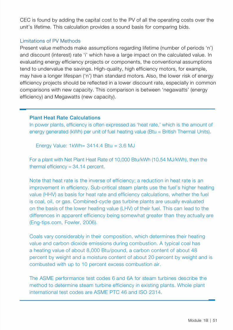
8/12/2019 Energy Efficiency Electronic Book Version 1548_PowerGenerationHandbook v1_1
http://slidepdf.com/reader/full/energy-efficiency-electronic-book-version-1548powergenerationhandbook-v11 53/361
CEC is found by adding the capital cost to the PV of all the operating costs over theunit’s lifetime. This calculation provides a sound basis for comparing bids.
Limitations of PV MethodsPresent value methods make assumptions regarding lifetime (number of periods ‘n’)and discount (interest) rate ‘i’ which have a large impact on the calculated value. Inevaluating energy efficiency projects or components, the conventional assumptionstend to undervalue the savings. High-quality, high efficiency motors, for example,may have a longer lifespan (‘n’) than standard motors. Also, the lower risk of energyefficiency projects should be reflected in a lower discount rate, especially in commoncomparisons with new capacity. This comparison is between ‘negawatts’ (energyefficiency) and Megawatts (new capacity).
Plant Heat Rate CalculationsIn power plants, efciency is often expressed as ‘heat rate,’ which is the amount ofenergy generated (kWh) per unit of fuel heating value (Btu = British Thermal Units).
Energy Value: 1kWh= 3414.4 Btu = 3.6 MJ
For a plant with Net Plant Heat Rate of 10,000 Btu/kWh (10.54 MJ/kWh), then thethermal efciency = 34.14 percent.
Note that heat rate is the inverse of efficiency; a reduction in heat rate is animprovement in efficiency. Sub-critical steam plants use the fuel’s higher heatingvalue (HHV) as basis for heat rate and efficiency calculations, whether the fuelis coal, oil, or gas. Combined-cycle gas turbine plants are usually evaluatedon the basis of the lower heating value (LHV) of their fuel. This can lead to thedifferences in apparent efficiency being somewhat greater than they actually are(Eng-tips.com, Fowler, 2006).
Coals vary considerably in their composition, which determines their heatingvalue and carbon dioxide emissions during combustion. A typical coal hasa heating value of about 8,000 Btu/pound, a carbon content of about 48percent by weight and a moisture content of about 20 percent by weight and iscombusted with up to 10 percent excess combustion air.
The ASME performance test codes 6 and 6A for steam turbines describe themethod to determine steam turbine efficiency in existing plants. Whole plantinternational test codes are ASME PTC 46 and ISO 2314.
Module 1B | 51

8/12/2019 Energy Efficiency Electronic Book Version 1548_PowerGenerationHandbook v1_1
http://slidepdf.com/reader/full/energy-efficiency-electronic-book-version-1548powergenerationhandbook-v11 54/361
Energy Accounting for ReliabilityReliability Concepts
The methods and terminology in this section are common to the field of quantitativereliability analysis. Reliability (R) is the probability that a unit is still operational afterone year, based on the unit’s mean time between failure (MTBF) specification.Reliability is expressed as failure rate on per year basis.
R = e (-8760hr/MTBF)
Availability (A) of a unit can be calculated as: A = MTBF / (MTBF + MTTR)
Where:MTTR = mean time to repair
Energy Cost of Plant Trips The total cost of a plant trip is composed of many parts, including opportunity costof lost power sales, cost of substitute purchased power, ISO fines, trip-inducedrepairs, and energy.
The energy wasted per year due to trip events is therefore R multiplied by energywasted during startup/shutdown procedures (R x Ess). The wasted energy due to acomplete shutdown and cold restart (Ess) is composed of two parts:
E(shutdown energy) + E(startup energy) =Ess
Where:E(startup energy) = hours duration of startup x energy input/hr
E(shutdown energy) = rotational energy in all machinery + chemical energy inprocess lines
E for shutdown is more difficult to measure and calculate. As a rough estimation,therefore, E shutdown is assumed to be ¾ of the E startup. So ultimately, the annualenergy costs of plant trips :
R x Ess = R x 1.75 x hours duration of startup x energy input (MMBtu)/hr x Energyprice ($/MMBtu)
52 | ABB Energy Efficiency Handbook

8/12/2019 Energy Efficiency Electronic Book Version 1548_PowerGenerationHandbook v1_1
http://slidepdf.com/reader/full/energy-efficiency-electronic-book-version-1548powergenerationhandbook-v11 55/361
To the optimist, the glass is half full.To the pessimist, the glass is half empty.To the efficiency engineer, the glass is twice as big as it needs to be.
Module Summary This module describes the impact of design and engineering on the energy-efciencyperformance of auxiliary drive power systems; motors, fans & pump systems, andvariable speed drives.
The information in this module may be generally applied to process industries;industry-specific text is indented with a rule above and below as shown here.
This section examines drive power systems from an energy efciency perspective onlyand does not provide guidance on critical aspects of drive power engineering such as
safety interlocking or fault-tolerant design. See the References and Standards sectionsfor more complete guidance on all other aspects of drive power design & engineering.
Introduction to Drive PowerDrive power is the combination of a prime mover, such as an electric motor, a coupling,and a speed controller that drives the shaft load of the nal element, such as a pump,which puts power into an industrial process. Pump, fan and compressor systems are
so-called ‘cube-law’ applications because their power requirements increase as the thirdpower of their speed. A pump or fan running at half speed consumes only one-eighth ofthe energy compared to one running at full speed. These ‘cube-law’ systems representmore than half of all industrial motor applications and electrical consumption. The focusin this handbook is on large drive power requirements (200 hp (150 kW) or greater)involving pumps and fans. The prime mover for the vast majority of drive power systemsare electric motors, so these will also be examined in detail.
This handbook takes an integrative design approach that considers the entire drivepower system from energy input to its end-use on the uid or gas of the process, asshown in the gure below:
Module 2Drive Power Systems
Module 2 | 53

8/12/2019 Energy Efficiency Electronic Book Version 1548_PowerGenerationHandbook v1_1
http://slidepdf.com/reader/full/energy-efficiency-electronic-book-version-1548powergenerationhandbook-v11 56/361
Figure 2.1 – Schematic of an entire drivepower system (Plant Engineering 10/1/2000)
Role of Drive Power in Energy EfciencyPumping represents the world’s largest use of electric motors, and fans are in secondplace. Taken together, these two applications account for half of all motors in use.Pumping systems alone account for nearly 20% of all energy used by electric motors(US DoE, 2008).
A large motor, running constantly, uses its capital cost in electricity every few weeks;
this explains why more than 90% of the total cost of pump ownership (TCO) is energyconsumption. Every one percent improvement in a continuous-duty induction motorsystem has a present value of $70/kW, assuming a 5%/yr real discount rate for 20 yrs,$0.05/Kwh, no reactive losses, heating or demand charges (Lovins, 2008).
Potential for Energy Efficiency Two leading energy research institutions, RMI (1989) and EPRI (1990), found that halfof all typical industrial motor-system energy could be saved by retrots, paying back
their initial investment in about 16 months, and in much less time at today’s higherenergy prices. In other studies, ABB (2005) found that pump energy consumption couldtypically be reduced by up to 20% using well-proven technologies.
Where is the wasted energy in industrial fan & pumping systems that allows such largesavings?
− Oversized and under-loaded motors. − Inefficient motors and couplings. − Inefficient applications, especially those which use throttling for flow control. − Equipment running unnecessarily, or for unnecessarily long hours, such as stirrers
on empty tanks, deadheading pumps, and ventilation fans running continuously.
54 | ABB Energy Efficiency Handbook

8/12/2019 Energy Efficiency Electronic Book Version 1548_PowerGenerationHandbook v1_1
http://slidepdf.com/reader/full/energy-efficiency-electronic-book-version-1548powergenerationhandbook-v11 57/361
This handbook module offers design and engineering guidelines that may help preventsome of this energy waste in new and retrotted power plants and industrial processapplications.
Auxiliary drive power is used in a variety of applications in a steam generatingplant, from coal conveyors, grinders and pulverizers to furnace draft fans,condensate and feed water pumps (when electrically driven), circulating waterpumps, and various emission control equipment. The table below shows estimatesof some major auxiliary drive power loads as % of gross generation:
Electrically driven boiler feed pump 2.5% (Goodall, 1981)Draft fans and pulverizers 2.0% (Juniper and Pohl, 1996)Flue gas desulphurization (FGD) 1.5% (IEA Coal Online - 2, 2007)Remaining auxiliaries 1.5% (IEA Coal Online - 2, 2007)
A more complete list of drive power consumers found in fossil-fuel steampower plants:Boiler feed water pumping:− feed water pumps
− feed water booster pumps − boiler recirculating pumps
Condensate and coolant pumps and fans− condensate or hot well pumps
− condensate booster pumps − circulating water pumps − cooling tower pumps and fans
Furnace draft and combustion air fans
− primary air (PA) fans − forced draft (FD) fans − induced draft (ID) fans
Fuel handling drive power
− drive power for conveyors, coal mills & pulverizers − ash handling pumps − fuel gas booster compressors (for GT plants)
Emissions control drive power (for ue gas desulphurization, catalytic reductionetc.)
− flue gas ID booster fans
Module 2 | 55
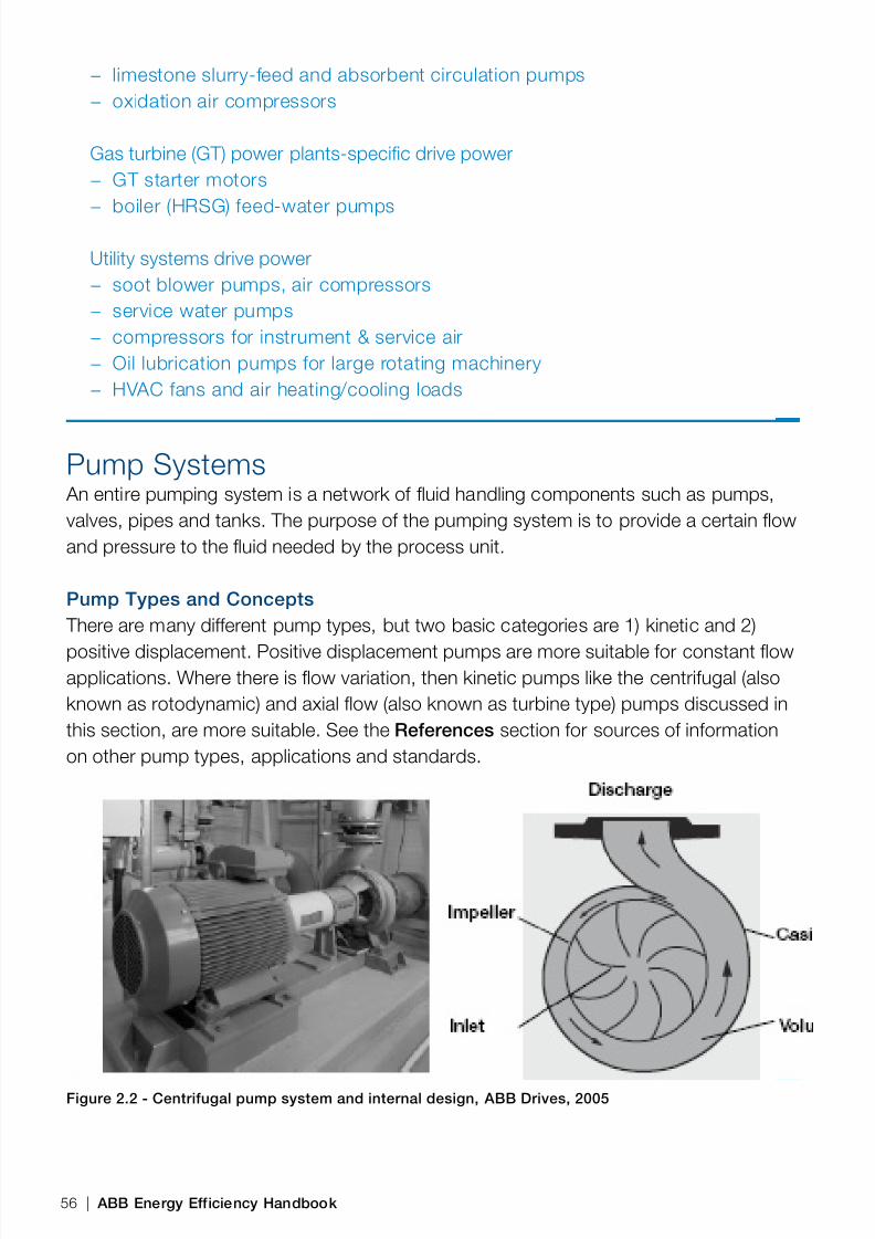
8/12/2019 Energy Efficiency Electronic Book Version 1548_PowerGenerationHandbook v1_1
http://slidepdf.com/reader/full/energy-efficiency-electronic-book-version-1548powergenerationhandbook-v11 58/361
− limestone slurry-feed and absorbent circulation pumps− oxidation air compressors
Gas turbine (GT) power plants-specic drive power − GT starter motors − boiler (HRSG) feed-water pumps
Utility systems drive power− soot blower pumps, air compressors− service water pumps
− compressors for instrument & service air − Oil lubrication pumps for large rotating machinery − HVAC fans and air heating/cooling loads
Pump Systems An entire pumping system is a network of uid handling components such as pumps,valves, pipes and tanks. The purpose of the pumping system is to provide a certain owand pressure to the uid needed by the process unit.
Pump Types and Concepts There are many different pump types, but two basic categories are 1) kinetic and 2)
positive displacement. Positive displacement pumps are more suitable for constant owapplications. Where there is ow variation, then kinetic pumps like the centrifugal (alsoknown as rotodynamic) and axial ow (also known as turbine type) pumps discussed inthis section, are more suitable. See the References section for sources of informationon other pump types, applications and standards.
Figure 2.2 - Centrifugal pump system and internal design, ABB Drives, 2005
56 | ABB Energy Efficiency Handbook
8/12/2019 Energy Efficiency Electronic Book Version 1548_PowerGenerationHandbook v1_1
http://slidepdf.com/reader/full/energy-efficiency-electronic-book-version-1548powergenerationhandbook-v11 59/361
In a centrifugal pump, the uid enters the pump at the impeller eye, the center of thepump. This is the ‘suction’ part of the pump. The rotating impeller imparts velocity(kinetic energy) to the uid as it is accelerated along the impeller blades and squeezedthrough the narrow volute, at right angle to its line of entry. As the volute cross-sectionarea increases, the uid velocity decreases and a higher pressure (head) developstowards the discharge end of the pump.
In an axial pump, the uid is accelerated by the action of a propeller and moves parallelto the axis or shaft of the pump. In mixed ow pumps, the impeller uses both radial andaxial motion to accelerate the uid along a path that exits the pump at an angle with thepump axis or shaft.
Pump Characteristics The performance of the pump is given by pump curves, which show how much pressure(Head) can be developed at various ow rates (capacities) at a given speed. Note thatHead (H) has units of length (ft.) but is actually a measure of a uid’s energy per unitweight. The distance refers to the height that a column of the uid could support undergravity. A useful approximate conversion formula between Head and psi is:
H (ft) = ( H (psi) x 2.31 ) / Sp Sp =1 (for water, approximately)H (m) = (H (kp) x 9.8) / Sp
The head of a uid has four components:
− Static head, which is independent of flow, increases with vertical height above thepump centerline and is negative for heights below the pump.
− Pressure head, which is due to other forces such as backpressure in a closedtank, and is also independent of flow.
− Friction head, which is due to resistance in elements such as pipes, valves &fittings, and increases with flow.
− Dynamic head, which is a function of the velocity of the fluid, and is given by :
Hv = V 2 / 2g.
Where:Hv = velocity head (ft or m)
V = uid velocity (ft/s or m/s)g = acceleration due to gravity (32.2 ft/s 2 or 9.8 m/s 2 )
Note that the dynamic head is usually rather small and may be ignored in mostpumping applications.
Module 2 | 57
8/12/2019 Energy Efficiency Electronic Book Version 1548_PowerGenerationHandbook v1_1
http://slidepdf.com/reader/full/energy-efficiency-electronic-book-version-1548powergenerationhandbook-v11 60/361
Axial-flow pump performance curves are steep, meaning that they can delivernearly constant flow over a wide range of pressure. Centrifugal pump curves aremuch flatter, meaning that they can provide a range of flows over a relatively narrowpressure range.
Power Plant Pump Applications:In a power plant, the circulating pump supplies cooling water at large ow rateand low head to the condenser for heat exchange. Condensate (also knownas hotwell) pumps are medium ow, medium head pumps which move thecondensed steam from the condenser, through feedwater heat exchangers, to thede-aerator tank. The boiler feedwater booster pump moves water from the de-aerator to the man boiler feedwater pump, which supplies water at high pressureto the steam generator (boiler).
Circulating water pumps:Circulating pumps are usually mixed flow pumps, with axial designs beingused for very low head applications. Note that although dynamic (velocity)head is typically ignored in most pump applications, it is a significant factor inlow head, high capacity systems such as the plant cooling water-circulatingsystem. Typical flow rates for circulating water pumps are between 0.35gpmand 0.75gpm per generated kW. (GE Utility Division 1983)
Condensate pumps:Condensate pumps are usually 2-stage pumps that operate with a highvacuum on the inlet. The discharge pressure must be sufficient to overcomethe friction in the piping and low-pressure feed-water heaters, and any staticlift required to pump the condensate to the level of the low-pressure feed-water heaters. (Homer M. Rustebakke, GE Utility Division, 1983).Typical powerrequired by condensate pumps is on the order of 3hp per MW of generating
capacity
Boiler feedwater (BFW) pumps:Boiler feedwater (BFW) pumps are usually multi-stage, volute type centrifugalpumps. Typical boiler feed pump power requirements are about 10,000hp(7500kW) for a 300MW plant, then increase by 3300hp (2500kW) for every100MW (Homer M. Rustebakke, GE Utility Division, 1983). The head of boilerfeed pump depends upon the boiler load and thus steam pressure, whichvaries with plant loading. On large units, there is still usually a feed watercontrol valve for filling and very low load, with pump speed taking over as loadrises past some threshold (ISA 2005). Feed-water pumps are characterized byhigh reliability requirements and fairly high dynamics during plant load changes.
58 | ABB Energy Efficiency Handbook

8/12/2019 Energy Efficiency Electronic Book Version 1548_PowerGenerationHandbook v1_1
http://slidepdf.com/reader/full/energy-efficiency-electronic-book-version-1548powergenerationhandbook-v11 61/361
They normally make the biggest contribution to the plant’s in-house energyconsumption. Another estimate for boiler-feedwater pump consumption isaround 15 MWe on a 600 MWe plant, or around 2.5% of gross power (Goodall,1981).
Total Developed HeadFrom the perspective of the pump, the process unit is a load that is a combination ofpressure, static and friction heads. These latter two exist on the inlet and dischargesides of the pump. On the suction (inlet) side, the pump must ‘lift’ the fluid if it iscoming from a lower elevation and overcome any friction pressure drops throughthe inlet, together called the Total Suction Head. On the discharge side, the pumpmust ‘push’ the fluid against system’s static head, pressure and friction pressuredrops, together called the Total Discharge Head. The pump(s) must develop enoughpressure (head) to meet the combined effect of these energies when deliveringthe required flow. An important design criterion for any pump is therefore the TotalDeveloped Head (TDH):
TDH = Total Discharge Head – Total Suction Head
Pump Net Positive Suction HeadOn the suction side, the system must also provide sufficient suction head so that
the pump does not cavitate. Cavitation is a low-pressure phenomenon that reducesperformance and may lead to pump damage. Sufficient suction head is calledNPSHA (Net Positive Suction Head Available) and designers must compare this withthe pumps characteristic curve for NPSHR (Net Positive Suction Head Required)provided by the supplier.
In power plants, the typical margins over this published NPSHR values may run
from 50% to100% for a complex boiler feedwater (BFW) system with transientsuction condition operations. Particular attention to NPSH margin should begiven to boiler feedwater system where load rejection and system transientsare expected, (Black & Veatch, 1996)
The suction requirements of BFW pumps are sometimes met by specifying alower-head booster pump upstream of the main BFW pump.
Pump System Load Curves The typical load curve shows a system with fixed static and pressure head as well asfriction that increases exponentially with flow. Systems without any static or pressure
Module 2 | 59

8/12/2019 Energy Efficiency Electronic Book Version 1548_PowerGenerationHandbook v1_1
http://slidepdf.com/reader/full/energy-efficiency-electronic-book-version-1548powergenerationhandbook-v11 62/361
head have curves starting at the zero point. Systems with high friction have steepercurves. Systems with low friction but high flow requirement will have flatter curves.
The figure below shows the pump curve for a typical centrifugal pump as well as thesystem load curve for the head and flow it must deliver. The pump will operate atthe values of head and flow where the two curves intersect, known as the operatingpoint, where supply meets demand.
− If two pumps operate in parallel, their pump curves are added horizontally, givinga single equivalent pump curve with higher capacity, but with heads the same asone of the pumps operating singly.
− If two pumps operate in series, then their characteristic curves are summedvertically, to give a single equivalent pump curve with higher heads, but capacitiesthe same as one of the pumps operating singly.
Figure 2.3 – Pump head vs. f low performance and system curves
Pump curve
Static& pressure head
System curve
Operating point
Frictionlosses
Q (flow)
H ( H
e a
d )
Pump Power and Energy EfficiencyPump output power (water horsepower: WHP) to the fluid is given by:
WHP = (Q x H x Sp) / 3960 kW = (Q x H x Sp) / 6128
Where:Q = capacity: in GPM (Gallons Per Minute) (l/min)H = total developed head (ft) (m)
60 | ABB Energy Efficiency Handbook

8/12/2019 Energy Efficiency Electronic Book Version 1548_PowerGenerationHandbook v1_1
http://slidepdf.com/reader/full/energy-efficiency-electronic-book-version-1548powergenerationhandbook-v11 63/361
Sp = specific gravity (density) of the pumped fluid (water = 1)
Pump input power required (also known as Brake Horsepower: (BHP) is the waterhorsepower divided by the pump efficiency: Eff
BHP = WHP / Eff Motor Power = kW/ η (η = EFF)
For estimation of efficiency (using SI units) in centrifugal pumps with developed head(H) between 15 to 100m water and flowrate (Q) between 20 and 300 cu.m/hr onecan use the following pump model (Rajan 2003) which has a standard error of about1%:
Eff (%) = 65.08 x H -0.12446 x Q0.094734
Affinity LawsPumps of similar design but different impeller sizes can be compared by usingthe pump affinity laws. These affinity laws (see below) below describe the relationbetween the rotational speeds of the pump (n), flow rate (Q), head generated (H) andpower absorbed (P) by the fluid:
Figure 2.4 – Pump affinity laws, (ABB Oy. Drives, 2006)
For a given speed, a pump curve has an operating point where efficiency ismaximum, referred to as the Best Efficiency Point (BEP). The region of high efficiencyclose to the BEP is called the ’bullseye’. Designers strive to make this the actualoperating range for the system, as this will reduce both energy and maintenancecosts. When the operating point moves away from the BEP , then relatively morebrake horsepower (input power) is required per unit water horsepower output.
Module 2 | 61
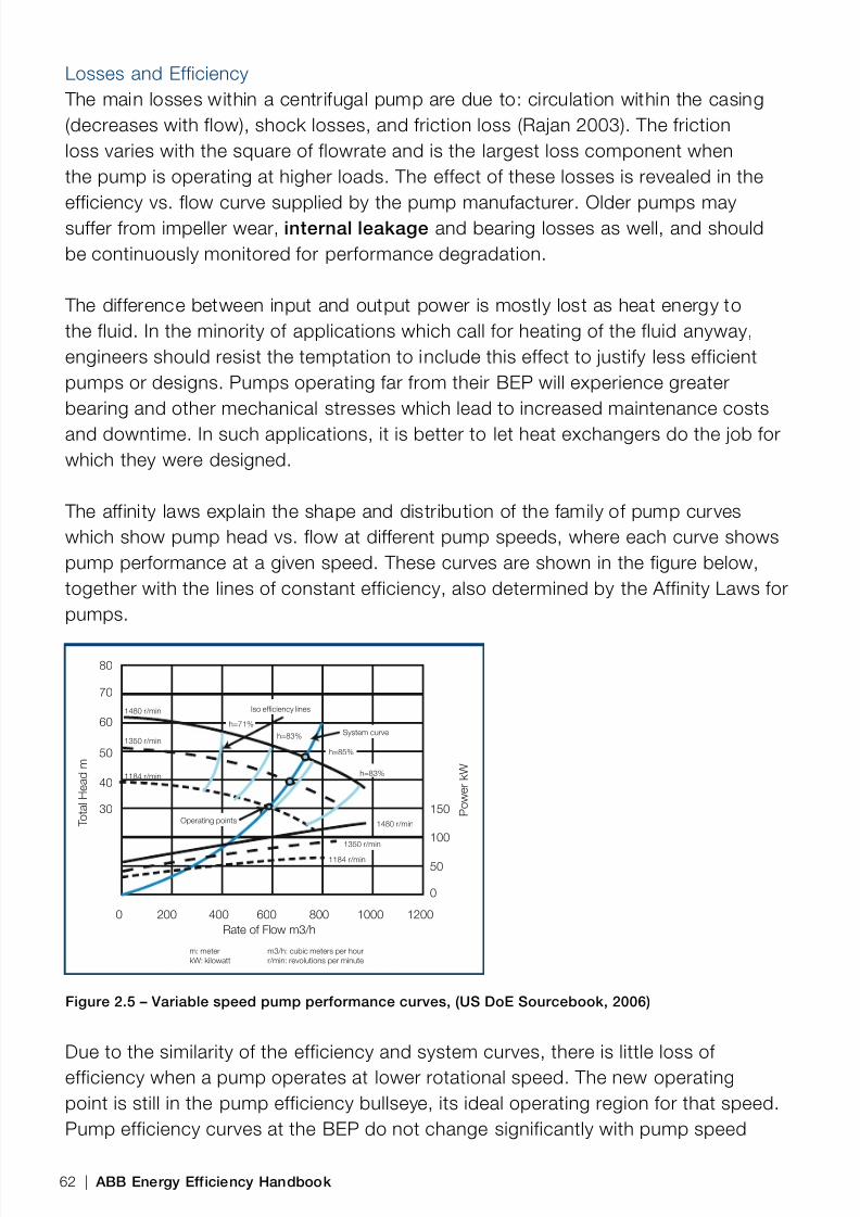
8/12/2019 Energy Efficiency Electronic Book Version 1548_PowerGenerationHandbook v1_1
http://slidepdf.com/reader/full/energy-efficiency-electronic-book-version-1548powergenerationhandbook-v11 64/361
Losses and Efficiency The main losses within a centrifugal pump are due to: circulation within the casing(decreases with flow), shock losses, and friction loss (Rajan 2003). The frictionloss varies with the square of flowrate and is the largest loss component whenthe pump is operating at higher loads. The effect of these losses is revealed in theefficiency vs. flow curve supplied by the pump manufacturer. Older pumps maysuffer from impeller wear, internal leakage and bearing losses as well, and shouldbe continuously monitored for performance degradation.
The difference between input and output power is mostly lost as heat energy tothe fluid. In the minority of applications which call for heating of the fluid anyway,engineers should resist the temptation to include this effect to justify less efficientpumps or designs. Pumps operating far from their BEP will experience greaterbearing and other mechanical stresses which lead to increased maintenance costsand downtime. In such applications, it is better to let heat exchangers do the job forwhich they were designed.
The affinity laws explain the shape and distribution of the family of pump curveswhich show pump head vs. flow at different pump speeds, where each curve showspump performance at a given speed. These curves are shown in the figure below,together with the lines of constant efficiency, also determined by the Affinity Laws forpumps.
0 200 400 600 800 1000 1200
80
70
60
50
40
30 P o w e r
k W
T o t a l H e a d m
Rate of Flow m3/h
m: meter m3/h: cubic meters per hourkW: kilowatt r/min: revolutions per minute
150
100
50
0
1480 r/min
1350 r/min
1184 r/min
Operating points
Iso efciency lines
System curveh=71%
h=83%
h=85%
h=83%
1480 r/min
1350 r/min
1184 r/min
Figure 2.5 – Variable speed pump performance curves, (US DoE Sourcebook, 2006)
Due to the similarity of the efficiency and system curves, there is little loss ofefficiency when a pump operates at lower rotational speed. The new operatingpoint is still in the pump efficiency bullseye, its ideal operating region for that speed.Pump efficiency curves at the BEP do not change significantly with pump speed
62 | ABB Energy Efficiency Handbook

8/12/2019 Energy Efficiency Electronic Book Version 1548_PowerGenerationHandbook v1_1
http://slidepdf.com/reader/full/energy-efficiency-electronic-book-version-1548powergenerationhandbook-v11 65/361
within the family of pump performance curves. When speed is reduced by half ofthe rated speed, pump efficiency at the new speed’s BEP may only be reduced by3%, for example. Pump efficiency is relatively unchanged, but the decrease in powerconsumption at the lower pump speed is substantial.
Figure 2.6 – Pump power and efficiency curves
BHP
BEP
Pump curve
Q (ow)
Efciency
H ( H
e a
d )
Recall that pumps and fans are ‘cube-law’ applications because their powerconsumption varies with the cube of the speed of the pump or fan.
− This relationship yields large power savings even from modest speed reductions,and favors designs that seek to reduce speed, such as using Variable SpeedDrives (VSDs). See section on Pump Flow Control Methods .
− The cube law also strongly favors selecting the right size of pump for theoperating conditions. See section on Pump System Design & Engineering forguidelines on correct pump sizing.
Designers can also benefit from selecting high efficiency pumps, which are generally
4% to 7% more efficient and may cost little or no more than standard efficiencypumps. Using a lifecycle approach, super-efficient pumps are even more costeffective. Efficiency varies widely with pump type and flow range; according to theHydraulic Institute, the pump efficiency of ‘large’ single-stage end-suction pumpsoperating at their BEP and at flow rates in the 100 cu.m/h range is 81%.
Pump Flow Control MethodsSome of this section is adapted from the application guide: ‘Using Variable SpeedDrives in Pump Applications’ (ABB Oy. Drives, 2006)
The process system will usually require variable flow rates from the pump. Thereare four common methods to control the output of a pumping system: Throttling,
Module 2 | 63

8/12/2019 Energy Efficiency Electronic Book Version 1548_PowerGenerationHandbook v1_1
http://slidepdf.com/reader/full/energy-efficiency-electronic-book-version-1548powergenerationhandbook-v11 66/361
Bypassing, On-Off, and Variable speed control, as shown in the figure below. Variable speed control may be achieved by motor frequency modulation using a Variable Frequency Drive , or by using gears and hydraulic couplings .
Figure 2.7 - Common flow control methods, (ABB Oy) Drives, 2006)
The relative power consumption of the different control methods can be estimatedfrom the area between the x and y-axes and the operating point on a pressure-flow
curve as shown in the figure below. This comparison is based on the formula forpump power (P): flow x head (P=Q x H). In the example shown, the relative powerconsumption for an average flow rate of 70% (of full flow) is calculated using typicalvalues for the different flow control methods.
ThrottlingFlow control can be achieved by modulating a valve immediately downstream fromthe pump. Throttling effectively changes the process system curve seen by the
pump: the valve introduces friction into the system; this makes the system curvesteeper so that it intersects the pump curve at the lower, desired flow rate, as shownin the top left chart in the figure below. In this example, the operating point is movedfrom (Q = 10, H = 10) to (Q = 7, H = 12.7). The relative power consumption can becalculated by P = 7 x 12.7 = 89.
64 | ABB Energy Efficiency Handbook

8/12/2019 Energy Efficiency Electronic Book Version 1548_PowerGenerationHandbook v1_1
http://slidepdf.com/reader/full/energy-efficiency-electronic-book-version-1548powergenerationhandbook-v11 67/361
This method has low capital costs, but throttled systems waste energy in two mainways: pressure drop across the valve, and because at reduced capacity the pumpperforms below its optimum efficiency point.
Figure 2.8 - Energy efficiency impact of various flow control methods, (ABB Oy. Drives, 2006)
In power plants, excess pump and throttling energy is not entirely wasted inapplications that call for heating of the fluid anyway; as is the case in boilerfeedwater regenerative heating. There are three reasons to avoid using such
indirect heating to justify continued use of throttling control:
− Higher maintenance costs of the pump operating far from its BEP− A highly-oversized valve will operate in a nearly closed state, which is not
stable. This situation arises in constant speed pumping systems where eachlayer of engineering bureaucracy adds its own safety margin in calculatingpressure drops through pipes, heat exchangers etc. and then, finally,in selecting the pumps. The control valve ends up with all these safetymargins, as added pressure drops. (Liptak, 2005)
Module 2 | 65
8/12/2019 Energy Efficiency Electronic Book Version 1548_PowerGenerationHandbook v1_1
http://slidepdf.com/reader/full/energy-efficiency-electronic-book-version-1548powergenerationhandbook-v11 68/361
− Most importantly, for high pressure systems such as power plant boilerfeedwater, is the severe wear on valve components from throttling at 2,400psig (16.5 MPa) (Black & Veatch, 1996)
Bypassing Although not commonly used for flow control, bypassing (also known as“recirculation”) is applied mainly to circulation duty pumps. The flow output to thesystem is reduced by bypassing part of the pump discharge flow to the pumpsuction. Flow through the bypass system is controlled by valves. This means that thetotal flow increases (from 10 to 12.4), but the head decreases (from 10 to 6.6). Therelative power consumption is P = 12.4 x 6.6 = 82.
A ‘minimum ow’ recirculation system is sometimes necessary if the pump operates forextended periods at low ow rates, when the pressure is too low to induce adequateow into the system. Recirculating ow wastes energy and should therefore be keptto a minimum. Automatic modulating control of the recirculating ow system willensure that that the recirculation ow control valve only opens when measured pumpow drops below a certain minimum threshold. Recirculating systems are sometimesrequired on systems equipped with variable speed ow control to guard against lowow conditions. The drive logic of a VFD speed controller may also be programmed towarn operators and to shut off the pump in these cases.
In power plants, this type of pump control may be used in boiler feedand condensate pumping systems to provide flow control and to preventoverheating of the pump at low flow rates. (Black & Veatch, 1996)
Another reason why designers may add a recirculating flow loop is to keep thepump at a higher state of readiness for increased demand. An improved design
may make use of any existing, smaller and more responsive startup pumpinstead of a recirculation loop.
On-Off ControlOn-off control is often used where stepless control is not necessary, such askeeping the pressure in a tank between preset limits; in these applications, the pumpis either running or stopped. The average flow is the relationship between the ‘on’time and the ‘total’ time, on plus off. The relative power consumption can then beeasily calculated by P = 0.7 x 100 = 70.
66 | ABB Energy Efficiency Handbook
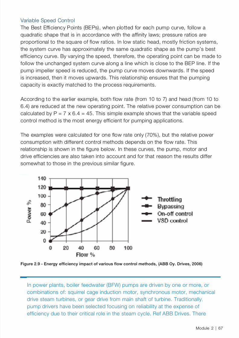
8/12/2019 Energy Efficiency Electronic Book Version 1548_PowerGenerationHandbook v1_1
http://slidepdf.com/reader/full/energy-efficiency-electronic-book-version-1548powergenerationhandbook-v11 69/361
Variable Speed Control The Best Efficiency Points (BEPs), when plotted for each pump curve, follow aquadratic shape that is in accordance with the affinity laws; pressure ratios areproportional to the square of flow ratios. In low static head, mostly friction systems,the system curve has approximately the same quadratic shape as the pump’s bestefficiency curve. By varying the speed, therefore, the operating point can be made tofollow the unchanged system curve along a line which is close to the BEP line. If thepump impeller speed is reduced, the pump curve moves downwards. If the speedis increased, then it moves upwards. This relationship ensures that the pumpingcapacity is exactly matched to the process requirements.
According to the earlier example, both flow rate (from 10 to 7) and head (from 10 to6.4) are reduced at the new operating point. The relative power consumption can becalculated by P = 7 x 6.4 = 45. This simple example shows that the variable speedcontrol method is the most energy efficient for pumping applications.
The examples were calculated for one flow rate only (70%), but the relative powerconsumption with different control methods depends on the flow rate. Thisrelationship is shown in the figure below. In these curves, the pump, motor anddrive efficiencies are also taken into account and for that reason the results differsomewhat to those in the previous similar figure.
Figure 2.9 - Energy efficiency impact of various flow control methods, (ABB Oy. Drives, 2006)
In power plants, boiler feedwater (BFW) pumps are driven by one or more, orcombinations of: squirrel cage induction motor, synchronous motor, mechanicaldrive steam turbines, or gear drive from main shaft of turbine. Traditionally,pump drivers have been selected focusing on reliability at the expense ofefficiency due to their critical role in the steam cycle. Ref ABB Drives. There
Module 2 | 67
8/12/2019 Energy Efficiency Electronic Book Version 1548_PowerGenerationHandbook v1_1
http://slidepdf.com/reader/full/energy-efficiency-electronic-book-version-1548powergenerationhandbook-v11 70/361
have been several studies (Black & Veatch 1996, EPRI 1995, ABB 2008) tocompare the different options for pump drivers (prime movers) on base-loadedpulverized coal steam power plans, and the effect on net plant heat rate.
In all studies the option with a constant speed motor-driven BFW pump usingthrottle valve control is the least efficient, wasting significant energy at loads<100% throttle flows. The two basic options involving speed control are slip-type adjustable speed drives and non-slip VFD drives.
In all options except the VFD there is likely a need for mechanical reducing gearif the pump has a design speed greater than the motor rated speed. Reducinggears are efficient, but still lose up to 1.5% of the input shaft power. For an8MW pump, this loss represents almost 1GWh lost per year.
In all studies, the VFD option to vary motor output speed achieved better netturbine heat rate and better turbine output at all throttle flows when comparedwith speed control via slip-type hydraulic coupling. (Black & Veatch, 1996)
A third option is the steam turbine-driven feed pump. This pump is drivenby a condensing turbine that takes steam extracted from the IP/LP turbineand exhausts to the main condenser. The disadvantages of this type of drivearrangement are the extra valving and piping, plus added complexity in startup,
requiring an additional startup electrical motor. The VFD alternative’s outputdoes not directly depend on the available steam flows, which vary with loadingand season.
In the comparison between the different drivers, a slightly better heat rate isachieved with the turbine driven alternative. At the cost of more valve andpiping complexity, the turbine exhaust may be used in feedwater regenerativeheating, further enhancing the viability of this alternative.
Still another design option, found in some older plants, is a main turbine shaftdrive. These require variable speed coupling for speed control and gears,plus an additional startup electrical motor. (Homer M. Rustebakke, GE UtilityDivision, 1983). The added complexity and lower reliability has made thisdesign less common on newer plants.
A comparison of the above four BFWP drive alternatives was done for a500MW unit with 2 x 50% capacity BFPs in parallel (Black & Veatch 1996).
The comparison was done at 3 different load rates: 100, 75 and 50% throttleflow and considers net turbine heat rate (NTHR) and electrical output (NTO).In that comparison, the VFD alternative offers better NTHR and NTO than the
68 | ABB Energy Efficiency Handbook

8/12/2019 Energy Efficiency Electronic Book Version 1548_PowerGenerationHandbook v1_1
http://slidepdf.com/reader/full/energy-efficiency-electronic-book-version-1548powergenerationhandbook-v11 71/361
hydraulic coupling alternative, at all throttle flows. At 50% load, the throttlealternative has bhp=14,459 (10.8 MW) whereas the VFD alternative has bhp=9,185 (6.9 MW).
This difference is a substantial 36% improvement, representing a netreduction of 3.9 MW continuous power consumption.
High Static Head or High Pressure SystemsIn high static head or high pressure systems, the system curve is more horizontalthan vertical. Referring to the family of pump speed curves, a lower pump speedintersects the system curve at a point of much lower flow and efficiency, which hasthese consequences:
− The required speed reductions are smaller, and so are the power savings, in highhead systems.
− The efficiencies are lower at lower speeds; this further reduces the power savingsfrom the above speed reduction.
− The lower speed pump curves may not form a well-defined operating point withthe flatter system curve, leading to large changes in flow for small changes inspeed and hence a more challenging flow control task.
Despite the reduced savings compared to mostly frictional systems, pump speedcontrol in this case is still more economical than throttling the flow with a controlvalve. The added mechanical stresses on pump, motor and valve also favor speedcontrol even in this case.
A compromise design of high-static head systems combines one constant speedpump and one speed-controlled pump. The constant speed pump overcomes thehigh static head, and the VSD-equipped pump provides the additional, variable
capacity. According to the ISA, the use of only one VSD-equipped pump is the rightselection if the static head of the system is between 50% and 67% of the pump’s TDH.
Case ExampleHelsinki Energy, FinlandHelsinki Energy is one of the leading experts in the world in the field ofCombined Heat and Power (CHP) technology and one of the biggest energycompanies producing and distributing electricity and district heat in Finland.Helsinki Energy’s Hanasaari B power plant is located by the seaside in thecity of Helsinki and has a capacity of 220 MW for electricity and 445 MW for
Module 2 | 69

8/12/2019 Energy Efficiency Electronic Book Version 1548_PowerGenerationHandbook v1_1
http://slidepdf.com/reader/full/energy-efficiency-electronic-book-version-1548powergenerationhandbook-v11 72/361
district heating. The power plant’s efficiency is 85%. In 1990 Helsinki Energywas granted the UN International Environmental Award for its pioneeringand determined work in developing CHP technology and the consequentimprovement of the city’s air quality.
Originally, the Hanasaari power plant’s equipment was selected among thebest available technologies at the time of construction to fulfill the requirementsof high availability and efficiency. However, since the time of construction,variable speed drive technology had taken a big leap forward. Even thoughthe old ASEA and Strömberg wound-rotor motors with slip recovery controlsystems operated very well, Helsinki Energy decided to upgrade them in orderto reduce maintenance work and to further improve the plant’s efficiency. Given
the efficiency problem of boiler feedwater pumps driven by fixed speed motorsat partial loads, the most economic control is achieved with a variable speeddrive system. The boiler feed-water pump is rated at 4500 kW (6050 hp).
In the spring of 1999, Helsinki Energy ordered from ABB four water-cooled ACS 1000 drive systems with AMB 560 motors and oil-immersed 3-windingsupply transformers. The Hanasaari B power plant’s automation upgradeproject was executed together with Helsinki Energy’s Helen Engineering that
specializes in the design of energy production and distribution equipmentas well as in the related project management. The aim of these design andconstruction services is to support the profitability of business operationsthroughout the life cycle of the equipment.
Boiler feed-water pumps are one of the biggest energy consumers in a power plant.Operating feedwater pumps with variable speed drives can signicantly increase theefciency of a power plant. Outside the boiler feed-water pump’s nominal range, thecapacity needs to be sufcient to handle rare but possible abnormal situations in a boilerthat operates under very high pressure. Depending on the local authorities’ requirements,the pump, and the supplying drive, must be capable of delivering 10-25 % over pressure
70 | ABB Energy Efficiency Handbook

8/12/2019 Energy Efficiency Electronic Book Version 1548_PowerGenerationHandbook v1_1
http://slidepdf.com/reader/full/energy-efficiency-electronic-book-version-1548powergenerationhandbook-v11 73/361
or overow. As a consequence, the drive operates practically all the time under partialload, a situation where a variable speed drive offers the best available efciency.
Using ACS1000 variable speed drives as level control devices for feedwater drumscan reduce maintenance of the feedwater throttling valves. These haven’t necessarilybeen designed for the full pressure differential resulting from throttling the flow withfixed speed motors. Further savings can be achieved by designing a new generatingunit’s electricity distribution network for feedwater pumps operated by VariableFrequency Drives. As main loads, their across-the-line starting behavior typicallyimpacts on - depending on impedance of the plant transformer- capital cost, eitherthrough a more expensive transformer, through higher fault currents, or a moreexpensive switchboard. Variable speed drives as such act as soft starters and causeno starting current peaks. The ACS1000 can be connected via the most commonfieldbuses to become an integral part of the plant’s control system. Original case textfrom ABB Switzerland , MV Drives, 2008.
Case Example
Power Losses in KW
Pump Speed in RPM
300
250
200
150
100
50
0
3567 3645 3724 3850 3976 4150 4322
Fluid Coupling
Speed Range
VFD
EnergySavings
A European power plant was comparing fluid coupling with AC drive for its feedpump (1,450 kW) control. The comparison shows that within the speed rangeneeded, the AC drive consumed about 150 kW less than the fluid drive.− Energy saving: about 1,200,000 kWh/year
− Reduction in CO2 emissions: 600,000 kg/year (660 tons) − Reduced reactive power − Reduced stress to the supply − Reduced need for maintenance
Case text provided by: (ABB Oy. Drives, 2006)
Module 2 | 71

8/12/2019 Energy Efficiency Electronic Book Version 1548_PowerGenerationHandbook v1_1
http://slidepdf.com/reader/full/energy-efficiency-electronic-book-version-1548powergenerationhandbook-v11 74/361
Pump System Pipes, Valves and FittingsPipes, valves and fittings serve to direct and control the flow, but all of thesecomponents can introduce extra friction that requires more input power. Manyreferences exist on how to reduce friction in pump systems. In this section, only theenergy efficiency impact of piping elements are discussed.
Valves There are many types of valves, and these have varying degrees of resistance toflow. Wide-open friction is 25 to 35% larger for globe valves (which are common inthrottling applications) when compared to ball or gate type valves. Further reductionsin friction can also be achieved by optimizing pipe layout such that redundant and3-way valves may be eliminated. The case for eliminating control valves for flowcontrol is made in the Flow Control section in this module. A close look at all fittingsand valves to eliminate unnecessary flow restrictions is worthwhile from a lifecycleenergy perspective.
Pipes & FittingsFriction in pipes is related to:
− Pipe diameter and length− Internal smoothness of the pipe− Pipe layout with regard to bends, elbows and size changes.
Friction is proportional to almost the fifth power of the diameter. Lifecycle costingmay reveal that very large pipes are the most economical choice, even whenthe high price of steel is considered. It is important to include the capital cost ofpumping power in such a calculation, as smaller pumps and motors are the rewardfor reducing downstream friction.
Pipe wall roughness also increases friction. If application standards and materials
allow, then a ‘smooth pipe’ design should be lifecycle cost estimated and thencompared to the standard design. Pipe layout, which is typically done afterequipment layout, may have sharp bends and elbows that increase the friction inthe system. Short, straight, fat pipes not only reduce friction and upstream pumpingcosts, but have lower capital cost. The potential for energy efficiency throughimproved piping engineering is often limited by project phase considerations andeven by the design tools that engineers use. Popular pipe layout design softwarepackages may not even be capable of optimizing layout according to the criteriadiscussed here; such computer aided engineering (CAE) tools are indispensable onall but the smallest projects. RMI found that manual review of one automatic layoutreduced the number of elbows from 28 to only 3 (Lovins,A, 17/72008)
72 | ABB Energy Efficiency Handbook

8/12/2019 Energy Efficiency Electronic Book Version 1548_PowerGenerationHandbook v1_1
http://slidepdf.com/reader/full/energy-efficiency-electronic-book-version-1548powergenerationhandbook-v11 75/361
Taken together, all the above effects make the efficiency of an average lengthindustrial, rough-walled, average diameter pipe typically about 69% (deAlmeida,2006). Using low friction piping techniques can increase the efficiency of piping to90%.
In power plants, steam temperature is controlled by attemperation, whichinvolves spraying feedwater into the superheated steam. In designs thattake the water from the economizer inlet, throttling of the main feedwaterflow path may be required to ensure adequate pressure drop & flow thru theattemperation line.
Around 2–5% of the main flow may be diverted for attemperation of thesuperheated and reheated steam, so the pumping power wasted across thisthrottle valve is significant.
Pump System Design & Engineering The pump (or fan) sizing and selection process generally follows this sequence:
− Gather data on the system flow configuration : from PFDs − Flow paths ( i.e.: single, parallel or serial configurations)
− Liquid specification with density, temperature etc.
− Gather data on the general piping layout; from rough P&IDs − Pipe run lengths − Vertical head changes − Valves and other fittings
− Determine the basic output hydraulic requirements
− Required flow (capacity) with variation ranges for average AND peak flows.Flows are determined by process requirements and flow paths from step 1) − Calculate or measure the pressure drops across components from step 2),
using standard formulae; sum these pressure drops to determine system headand flow characteristic.
− Based on the above, calculate average and maximum pump power
− Determine the input basic hydraulic requirements− Required suction & discharge pressure ,with variation ranges
− Specify pump material and casing − Depends on fluid composition, temperature
Module 2 | 73
8/12/2019 Energy Efficiency Electronic Book Version 1548_PowerGenerationHandbook v1_1
http://slidepdf.com/reader/full/energy-efficiency-electronic-book-version-1548powergenerationhandbook-v11 76/361
− Maximum differential pressure for the pump casing
− Ambient and mounting specifications − Working conditions
− Any special conditions in the mounting space
The sizing and selection process then moves to the electrical engineering domainand is discussed in the Motors and VFD sections of this module:
− Specify pump prime mover and drive train− Electric motor vs. other types
− Exceptional starting, stopping and other running conditions − Shaft coupling method
− Specify sequencing and/or pump flow control method − VFD or other methods of speed control (VSD) − Additional components for power system compatibility
Pump Sizing and Selection The following simplified small pump example reveals some basic steps in the sizingprocess.
Required flow = 300 l/s (79.2 gps)Required discharge pressure head = 30m (98.4 ft)
Using the pump curves from the manufacturer’s catalog shown in the figure below: − Find the required flow, 300 l/s − Move upwards to match the required head, 30 m − Required performance is achieved with pump of 1400 rpm speed − For needed power, move down to the lower curve set along with 300l/s line
− When crossing the 1400 rpm curve move to left to read the power needed at theoperating point (110 kW)
Margins and Oversizing The selected pump is the smallest one capable for the operating point required. If weknow that there is no need for higher capacity, either now or in the future, there is noneed to choose a larger pump, as it would lead to both higher initial and operating costs.
It is estimated that 75% of pump systems are oversized, many by more than 20%.Uncertainty about static head and/or load flow variation leads designers to specify alarge pump with consequently larger efficiency bullseye to handle this variation.
74 | ABB Energy Efficiency Handbook

8/12/2019 Energy Efficiency Electronic Book Version 1548_PowerGenerationHandbook v1_1
http://slidepdf.com/reader/full/energy-efficiency-electronic-book-version-1548powergenerationhandbook-v11 77/361
Engineers may also tend to oversize pumps so that the ratio between minimumand maximum energy loss is not large. This means that the gain will not changemuch with load (Liptak, 2005), making their control task easier, but at the expenseof wasted energy. Pumping system authorities provide these additional sizingguidelines for selecting a centrifugal pump in combination with a VFD:
‘For a system with some static head, a pump should be chosen such that themaximum flow rate is slightly to the right-hand side of the best efficiency point(BEP). The exception is for a constant flow regulated system, in which case therecommendation is to select a pump that operates to the left of BEP at maximumpressure. This approach optimizes pump operating efficiency’ (US DoE, 2008).
Figure 2.10 - Pump sizing example, (ABB Oy. Drives, 2006)
Power Plant Pump Design Requirements:In power plants, the design criteria for boiler feedwater (BFW) pumps,condensate pumps and other plant components are typically for the valves-wide-open (VWO) and a 5% overpressure full load condition. However, newmarket situations may require plants initially intended for base-load operationnear their full load design point to now operate in a low to medium load range,and to do so efficiently.
Flow Requirements: The main flow requirements come from the cycle mass and energy balances atthe VWO load condition. Some flows, such as attemperation, soot blowing andboiler blow down, do not contribute to power generation but require pumping
Module 2 | 75

8/12/2019 Energy Efficiency Electronic Book Version 1548_PowerGenerationHandbook v1_1
http://slidepdf.com/reader/full/energy-efficiency-electronic-book-version-1548powergenerationhandbook-v11 78/361
power nevertheless. These flows should be minimized wherever possible. A 5%margin is commonly added to the final maximum flow value.
For steam temperature control, the careful control of combustion, possibly withthe aid of tilting burners, will reduce the need for steam attemperation flows.
Attemperation flows (and their cycle efficiency impact) can be eliminated onsupercritical boilers by controlling the firing rate to match the feedwater flow(IEA Coal Online - 2, 2007).
Attemperation is from 2 to 5% of the main steam flow. Soot blowing usesup to 0.5% of the main steam flow and, like attemperation, is taken onlyintermittently. Boiler blow down on drum boilers to control the water quality willalso result in some loss of heat from the cycle and additional pumping power.Once-through (supercritical) boilers do not have blowdown, because they haveno drum to store a supply of blowdown water (IEA Coal Online - 2, 2007).
Head Requirements: The BFW pump(s) must have a combined total developed head (TDH), plusa design margin of 5 to 10%, to meet the following pressure requirements:throttle pressure at turbine valve, pressure drop due to friction throughsuperheater, reheater, economizer, and high-pressure feedwater heaters, plusthe static heads due to height difference between pump outlet and drum water
level. (Black & Veatch 1996)
Under infrequent circumstances, perhaps to satisfy peak demand in a hotsummer day, the BFW pump may be required to operate for a short time10-15% above its nominal range. The pump and motor must be capable ofsupplying this added power, so they are specified accordingly. Speed control(using a VFD for example) will provide efficient power modulation at partialloads, where the BFW pump operates for most of the time.
Multiple Pump SystemsIt is worthwhile to consider specifying multiple pumps, each optimized for a pieceof the load curve; this design is efficient when VFDs are not used. Another energy-efficiency strategy is to consider two or more smaller pumps instead of one largerpump so that excess pump capacity can be turned off. If VFDs are available to thedesigner, then one or more of the pumps in the system can have a VFD for top-endspeed control. The section on VFD Multi-Drive describes an efficient and flexiblearchitecture for driving and controlling multiple motors.
76 | ABB Energy Efficiency Handbook

8/12/2019 Energy Efficiency Electronic Book Version 1548_PowerGenerationHandbook v1_1
http://slidepdf.com/reader/full/energy-efficiency-electronic-book-version-1548powergenerationhandbook-v11 79/361
Recall that the combined performance characteristic of a multiple pump system canbe determined as follows:
− Pumps operating in series have a combined performance curve which is calculatedby adding the individual curves vertically, providing increased total head.
− Pumps operating in parallel have a combined performance curve which is calculatedby adding the individual curves horizontally, providing increased total ow.
The advantages (right-sizing, reliability) of using multiple pumps must be weighedagainst some additional costs; the extra equipment requires additional cabling,piping and space. Isolation or check valves between multiple pumps in parallel maybe necessary to avoid fluid flow through inactive pumps. The LCC analysis of thisconfiguration should also consider the generally lower efficiency of smaller motorscompared to larger ones. The direct on-line (DOL) motors will also incur a powerfactor penalty, compared to using a VFD for speed control on a single larger motor.
The reliability advantage of parallel pumps, each controlled with a VSD, is that if onepump fails, the remaining pumps can continue uninterrupted.
In power plant applications that require high availability and redundancy,additional BFW pumps are specified. If the main BFW pump trips then a back-up auxiliary feed pump is started and the boiler’s firing rate is rapidly reduced in
order to prevent the furnace-tubing temperature from rising excessively (Kirmseand others, 2000). Another common pump configuration for increased reliabilityconsists of 2 x 50% capacity BFW pumps operating in parallel.
The high-flow, low-head requirements of circulating condenser cooling wateralso leads to multiple pump configurations. Pump automation can cycle thesepumps to provide a range of flows without the need for excessive throttling.
A 4-pump configuration would be more efficient than a system with fewer,
larger pumps, and the greater efficiency would offset the higher capital costsof the extra pumps; this rule is still recommended in some design guidelines:(Black & Veatch 1996) The evolution of reliable and lower cost VFDs, however,favor parallelism mainly for reliability reasons only, because the flow can becontinuously controlled through varying the pump speed.
Pump AutomationProper control of multiple pump arrangements is essential to realizing their fullenergy saving potential. Pump priority control balances the operating time of allthe pumps in the system over the long term. This can boost energy efficiency by
Module 2 | 77
8/12/2019 Energy Efficiency Electronic Book Version 1548_PowerGenerationHandbook v1_1
http://slidepdf.com/reader/full/energy-efficiency-electronic-book-version-1548powergenerationhandbook-v11 80/361
operating pumps closer to their best efficiency point according to the required flow(duration curve or actual signal) and pump capacities.
Pump automation is important to take advantage of the speed control provided by VFD-equipped pumps. The applications are varied, but one common design usessignals from flow or pressure transmitters as input to a feedback loop, which thenmodulates the output to the VFD. The desired flow or head setpoint is providedby a unit-level control system. In head-controlled systems, differential pressuretransmitters (PDTs) are commonly used to provide the pressure drop across unitloads. For proper head control, the placement of PDTs must span the target loadplus the additional loads incurred by piping and valves. If the unit has a commonsupply ‘header’ to supply multiple loads, then the ISA recommends that pressuretransmitters for this header should not be located near any major load junctions.
In some multiple pump systems, a VFD-driven pump is combined with a constant-speed pump. In these cases, automation can be used to provide additional flowcontrol on either (or both) sides of the constant speed pump’s BEP. For low-flowcontrol when the VFD pump approaches its maximum speed, then a switch or signalwill auto-start the constant speed pump. According to the ISA guidelines (ISA 2005),extra increments of pumping capacity are started by pressure (when demand isincreasing), but stopped by flow (when demand is decreasing).
See the section in Automation module on Feedwater Control systems for adescription of typical pump automation applications in power plants.
Pump System Design Guidelines - SummarySources for this section are RMI (Lovins A. 2007), the US DoE EERE (US DoE BestPractices, 2008) Pumping Tip Sheet, Hydraulic Institute and Europump.
Reduce Static & Pressure Head and Flow Requirements
Gather data to understand the actual loading requirements, especially the duty cycleand load profile of the pump.
Consider process design or operational control alternatives that reduce themaximum and average flows and static or pressure head required.
In power plant auxiliaries, a good example of this rule is adopting a slidingpressure control strategy, which reduces the boiler pressure head and hencepump power requirements, assuming that pump speed control is used
78 | ABB Energy Efficiency Handbook

8/12/2019 Energy Efficiency Electronic Book Version 1548_PowerGenerationHandbook v1_1
http://slidepdf.com/reader/full/energy-efficiency-electronic-book-version-1548powergenerationhandbook-v11 81/361
instead of flow throttling; see the section on sliding pressure control in the Automation module of this handbook.
Right-Size the Components− Do not oversize for ‘flexibility’: do not choose a larger pump than what is
necessary; the larger size leads to both higher initial and operating costs.− If conditions change, it may be cheaper to trim the impeller or retrofit the entire
pump than running an oversized pump over the entire period; specify pad andgeometry to accommodate other sizes.
− Employ a control strategy that optimizes multiple pump systems . − Where possible, use pumps operating as turbines to recover pressure energy that
would otherwise be wasted, as described in the section on VFD RegenerativeBraking
Reduce Friction in Pumping Systems− Select gate or ball valves instead of globe valves where appropriate; strive to use
larger pipes and smaller pumps instead of vice versa.− For above efforts, start downstream so that sizing calculations of upstream
components can benefit from efforts at reducing friction downstream.
Use Variable Speed for Flow Control
− Use variable frequency drives to control flow, rather than throttling, bypassing orsequencing.
− The benefits of VFDs are larger on low static head, high friction systems &systems with varying flow
Select Energy Efficient Components − Select an energy-efficient centrifugal pump design.
− Select an energy-efficient motor to drive the pump.
Install Components Correctly − If using control valves , ensure that they are properly linearized for good control
response. − For pump hookups, allow at least > 5 clear pipe diameters on inlet and > 3 pipe
diameters on outlet. − Ensure that there is sufficient suction head or suction lift .
Pump Drive TrainSpeed and Slip
The inevitable slip of induction motors means that actual RPMs will be slightly less,approximately 1% to 5%, than the motor’s nameplate speed rating. The amount of
Module 2 | 79

8/12/2019 Energy Efficiency Electronic Book Version 1548_PowerGenerationHandbook v1_1
http://slidepdf.com/reader/full/energy-efficiency-electronic-book-version-1548powergenerationhandbook-v11 82/361
slip is generally lower if high-efficiency motors are used; the extra rotational speedfrom a motor efficiency retrofit must be accounted for in the new application design.
Startup Conditions The inertia of centrifugal pumps is normally small enough to be ignored where theprime mover is an induction motor. However, this inertia should be consideredtogether with motor pull-in torque requirements if a synchronous motor is used.
Torque developed by an induction motor varies roughly with the square of theapplied voltage. Voltage drops during startup of large motors may lead to insufficientstartup torque. On most true centrifugal pumps, closing the discharge valve willreduce the power requirement during early startup. On axial pumps the opposite istrue, so the discharge valve should remain open during startup. On mixed designpumps, the discharge valve is opened at some point during startup, when axialbehavior begins to dominate (IEEE, 2007).
The reduced torque demand will make it less likely for the electrical engineer to tradeaway optimum running efficiency for a design with high starting torque capability .Pump startup against very high static head or system pressures will increase thestarting torque requirements of the prime mover, which is most often an electricmotor. If the process allows it, then any method should be used to reduce a highstartup torque requirement.
In power plants, the check valve on the boiler feedwater pump discharge lineisolates the pump from boiler drum pressure during startup to at least 70%full speed. When the check valve opens, torque and speed demand increasesrapidly, the 10% margin of motor over load torque may disappear and startupmay not succeed (IEEE, 2007). The concern over long startups and overheatingmay prompt the electrical engineer to trade away optimum running efficiency
for a design with high starting torque capability. The inrush of power late in thestartup may lead the engineer to oversize other power system components,such as a unit auxiliary transformer, at the expense of lower continuousoperating efficiency.
In some plant designs a motor-driven startup boiler feedwater pump is specified. This is a requirement for steam-turbine driven main BFW pumps, but hasadvantages even when the prime mover is an electric motor. Depending on itsdesign, this pump may also be used outside of its startup role to provide additionalcapacity and response. (Black & Veatch 1996). Turbine driven pumps have lower
80 | ABB Energy Efficiency Handbook

8/12/2019 Energy Efficiency Electronic Book Version 1548_PowerGenerationHandbook v1_1
http://slidepdf.com/reader/full/energy-efficiency-electronic-book-version-1548powergenerationhandbook-v11 83/361
efficiency at low loads compared to motor-driven pumps. A unit’s efficiency couldbe increased by using the motor-driven startup pumps at low loads.
See the Power Systems, Transformer section for details on transformer sizingfor startup and the Motor Startup section for details on motor sizing for reducedvoltage startup.
Power Factor The chosen speed control method also has a significant impact on power factor (PF). Lower PF leads to oversized power supply equipment and reduced efficiency.
The following figure shows how PF suffers when a motor operates much below itsrated speed, as is the case in throttling flow with a control valve.
Figure 2.11 - Effect on PF of different flow control methods, (ABB Motors & Drives, 2004 S. Weingarth)
Pump System Maintenance
Impeller wear will lead to increased agitation and the resulting heating of the fluidcan be revealed by monitoring the temperature differential across the pump. Closerunning tolerances should be maintained between stationary and rotating wear rings;the losses from a C% change in this clearance (Rajan 2003) can be estimated by thefollowing model:
BHP % = 141.49 x C 0.85836 x Ns -1.10219
Where:C%Wr = percent change in clearance from design (“C” is 1 for a 1% change, 2 for
2%, etc.)Ns = suction specific speed
Module 2 | 81

8/12/2019 Energy Efficiency Electronic Book Version 1548_PowerGenerationHandbook v1_1
http://slidepdf.com/reader/full/energy-efficiency-electronic-book-version-1548powergenerationhandbook-v11 84/361
Pump electrical horsepower can be compared to water horsepower calculatedfrom real-time measurements of flow and head. Any protracted deviation from theexpected pump efficiency at given flowrates is a likely indicator of pump degradationand signals the need for maintenance.
Another, more precise method of monitoring pump efficiency uses a thermodynamicmeasuring method (according to the British Standard EN ISO 51983). This methodrequires the installation of extremely sensitive temperature sensors – preciselycalibrated –measure the pump’s suction and delivery water temperature a shownin the figure below. One vendor (ABB) has patented a highly accuracy delta-Ttransmitter (HADTT) device. The HADTT enables extremely accurate (in the milli-Kelvin range) temperature differences. High-accuracy water pressure measurementsare also required for the unit to calculate the enthalpy gain and water horsepower.
These measurements are provided by intelligent pressure transducers with typicalaccuracies of 0.075 percent. Continuous monitoring of pump efficiency and flowmeasurements will inevitably lead to saved energy and reduced operating costs.
A Pump Efficiency Monitoring System (PEMS) can perform continual analysis of thepump historical data and propose specific maintenance activity. Additionally, it canenable the operator to choose the most efficient pump or combinations of pumps touse in a complex system (ABB Review 2/2008).
Other elements of the pump drive train can be monitored by the methods describedin the section on Condition Monitoring of Rotating Machinery .
Figure 2.12 – Pump Efficiency Monitoring System, (ABB Review 2/2008)
82 | ABB Energy Efficiency Handbook

8/12/2019 Energy Efficiency Electronic Book Version 1548_PowerGenerationHandbook v1_1
http://slidepdf.com/reader/full/energy-efficiency-electronic-book-version-1548powergenerationhandbook-v11 85/361
Pump System Cost CalculationsFor pumping systems, the three main lifecycle costs (LCC) are energy, initialinvestment and maintenance. The initial investment cost is composed of hardware,engineering and installation costs (including civil costs). Energy consumption isthe dominating element of the LCC, especially if a pump runs more than 2,000hours per year. To perform a lifecycle cost valuation one needs the following dataparameters, shown with sample units:
− Pump type and Impeller type − Nominal flow (l/s or gpm) − Liquid density (lb/cu.ft, kg/l) − Efficiency (%) − Static head (ft or m) − Nominal head (ft or m) − Max head (ft or m) − Flow control method − Transmission nominal efficiency (%) − Motor efficiency (%) − Motor supply voltage (V) − Annual running time (hrs) − Operating profile (% hrs for % nominal flow) − Energy price ($/kWh or €/kWh) − Investment cost ($ or €)
− Interest rate (%/yr) − Service life (yrs)
The output of system cost calculations are usually the following parameters: − Specific pump power (kW/(l/s)) (kW/(cf/s) or kW/gpm) − Required input motor power (hp or kW) − Annual energy consumption (kWh) − Annual energy saving (kWh)
− Annual money saving ($ or €) − Payback period − Net Present Value ($ or €)
See the Case Studies section for fully worked-out examples lifecycle costcalculations with benefits.
Pump Power Calculation Tools There are several freely available software tools for calculating fan powerconsumption and savings from certain optimization upgrades. A comprehensive listof tools is available from the US DoE web site.
− The ‘Pumping System Assessment Tool’ (PSAT), from the US DoE , EERE program.
Module 2 | 83
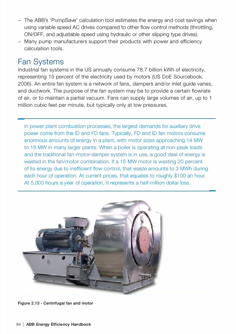
8/12/2019 Energy Efficiency Electronic Book Version 1548_PowerGenerationHandbook v1_1
http://slidepdf.com/reader/full/energy-efficiency-electronic-book-version-1548powergenerationhandbook-v11 86/361

8/12/2019 Energy Efficiency Electronic Book Version 1548_PowerGenerationHandbook v1_1
http://slidepdf.com/reader/full/energy-efficiency-electronic-book-version-1548powergenerationhandbook-v11 87/361
Fan Types and ConceptsIn a centrifugal fan, air moves perpendicular to the shaft. Centrifugal fans accelerateair as it moves along an impeller blade toward the outer rim. This extra kinetic energyis converted to static pressure as it slows in the fan discharge. Centrifugal fans cangenerate high pressures and can host blade designs suitable for applications withhigh particulate count and high moisture.
In axial fans, air moves parallel to the shaft, where it is pressurized by fan bladeswith an airfoil shape. Axial fans have less rotation mass (inertia) than equivalentcentrifugal fans, and higher rotational speeds (US DoE Sourcebook, 2006). Axialfans can maintain higher efficiencies over a wider load range than can constantspeed centrifugal fans controlled with inlet dampers or vanes. Axial fans have ahigher capital cost than centrifugal fans, and because of more numerous parts andcomplexity, they also require more maintenance (Black & Veatch, 1996)
Fans must develop enough static pressure (SP, usually measured in inches ofwater) to overcome the resistance if the system of ducts and elbows and deliver therequired volumetric flow (usually measured in aCFM (actual cubic feet per minute).Unlike pumps, centrifugal fan output pressure drops to zero at maximum flow, aphenomenon that is called fan ‘runout’.
Fan Characteristics
The pressure and flow characteristics of fans are dependent on the orientation andshape of the fan blades. Backward-curved blades have the highest efficiency, upto 90%, higher than straighter ‘radial’ designs that achieve up to 75% efficiency.Backward-curved blade fans also have the advantage of a non-overloadinghorsepower characteristic (Black & Veatch, 1996). Fans whose blade design hasoverloading characteristics have a sharply increasing power demand as flowincreases past the fan’s best efficiency point (BEP). The lower air velocities alongbackward-curved blades, however, promote more build-up of contaminants and may
preclude their use in ‘dirty applications’.
An additional blade design factor is the cross-sectional shape of the blade, whichmay be flat, curved or airfoil shapes. Airfoil shapes are the most energy efficient.
The airfoil shape, however, creates regions of unstable operation leading to stalling. To avoid operation in these stall regions may require installation of energy-wastingdevices such as recirculation or bleed valves (US DoE Sourcebook, 2006).
In power plants, fans used to supply combustion air are termed forceddraft (FD) fans, and fans used to exhaust combustion flue gases are termedinduced draft (ID) fans. Primary air (PA) fans supply air to carry an air+fuel
Module 2 | 85

8/12/2019 Energy Efficiency Electronic Book Version 1548_PowerGenerationHandbook v1_1
http://slidepdf.com/reader/full/energy-efficiency-electronic-book-version-1548powergenerationhandbook-v11 88/361
mixture through ducts to the burner nozzle (or fuel bed) and on into the steamgenerator. Together, all the fans electric drive power may add up to 2-3% of theplant’s rated output.
Single stage (one rotor/blade set) axial fans are typically used in FD serviceon balanced draft steam generators. FD fans are sometimes referred to as‘blowers’. If a centrifugal fan is used, then it is likely to have backward curvedblades for improved efficiency.
Axial fans in ID service have higher pressure needs that require a 2-stage fan. Axial fans with variable pitch blades are expected to be used more often inID service, due to more stringent emission control requirements. A loweredparticulate count can reduce some concerns associated with axial fan bladefouling (Black & Veatch, 1996). If a centrifugal fan is used instead of an axialfan, then it is likely to have forward-curved blades. The higher stack pressuredrop due to emissions control equipment has led to increased horsepowerrequirements of ID fans and booster fans. The ID hp is typically doubled by theaddition of a wet limestone scrubber, with some units requiring up to 4 timesmore horsepower (GE Utility Division, 1983).
On larger plants, all these fans are typically congured in pairs working in parallel,mainly for reasons of redundancy. See section on Multiple Fan Systems for more
details.
Fan curve
BEP
Efciency
BHP
Flow
P r e s s u r e
Figure 2.14 -Typical fan performance curve, showing efficiency and power relationships
Fan Power and Energy Efficiency The input shaft brake horsepower (BHP) required by a fan is proportional to theproduct of pressure rise and flow, and is given by:
86 | ABB Energy Efficiency Handbook

8/12/2019 Energy Efficiency Electronic Book Version 1548_PowerGenerationHandbook v1_1
http://slidepdf.com/reader/full/energy-efficiency-electronic-book-version-1548powergenerationhandbook-v11 89/361
BHP = (k)(P)(FLOW) / (EFFm)(6354) (kW = kPF/EFFm)
Where:EFFm = mechanical efficiency, %FLOW = airflow, cubic feet per minute (m3 /sec)P = total pressure rise across the fan, inches of water (millibar)k = compressibility factor, dimensionlessBHP = brake horsepower (kW)
Stated another way, efficiency is given by:EFFm = (k)(P)(FLOW )/ (BHP x 6354)
Values for k depend on the absolute inlet and outlet pressures. Using a rangeof typical k factors, the mechanical efficiency of different fan types and designscan be calculated:
Centrifugal fan; forward-curved blade 45-60%Centrifugal fan; radial-tipped blade 60-70%Centrifugal fan; backward-curved blade 75-85%Centrifugal fan; airfoil blade 80-90%
Axial flow fan 85-90%Ref : (Babcock & Wilcox, 2005)
Static pressure (SP) is often used instead of total pressure in discussing fanperformance. Fans are rated by either their total efficiency or their static efficiency.For large fans at design speed, most of the fan total pressure is in the form of staticpressure, so the difference between the two efficiency measures is small.
The Afnity Laws for fans are the same as for pumps, but with an additional factor to
account for change in air or gas density. Fans, like pumps, are cube-law applicationswhose power consumption increases with the cube of fan rotational speed.
Fan System Load Curves The system of ducts, elbows, dampers etc. create a resistance load that isproportional to the square of the volumetric flow. When plotted as Pressure vs. Flow,the system load curve has a parabolic (quadratic) shape. In reality, the pressuredrops are slightly greater, and the curve slightly steeper, due to losses in flowirregularities such as vortices and swirls (US DoE Sourcebook, 2006).
Module 2 | 87

8/12/2019 Energy Efficiency Electronic Book Version 1548_PowerGenerationHandbook v1_1
http://slidepdf.com/reader/full/energy-efficiency-electronic-book-version-1548powergenerationhandbook-v11 90/361
Efciency
Operating point
System curve
Flow
P r e s s u r e
Figure 2.15- Typical system load curve, showing efficiency and power
Supply fans generally work against a system back pressure, while return fansexhaust to low-pressure i.e.: the atmosphere. The system curve for supply fans istherefore typically shifted higher up the vertical axis than that of return fans. In highconstant pressure systems, the system curve is shifted vertically up the pressureaxis and is flatter at operating flows.
In power plants terminology, the supply fans are the Primary Air (PA), Forced
Draft (FD) and the Gas Recirculation (GR) fans which supply air to the furnacechamber. The return fans are the Induced Draft (ID) and FGD booster fans.
Designs with both FD and ID fans are termed ‘balanced draft’ plants, and thebalance point of zero gauge pressure is the furnace.
FD fans must develop pressure to overcome system resistance in ductwork,air heater, burner or fuel bed and the furnace itself. FD fans must supply
enough flow to serve needs of fuel combustion plus flow lost due to air leaksin the heater and other areas. FD fans draw fresh air and therefore are morevulnerable to density changes due to outside air temperature change than IDfans. Colder, denser air increases the mass flow and power requirements.
Fan Stability At low flow, there may be no clear intersection of the fan and system curves, andthus no clear stable operating point,. This causes unstable operation in which thefan pulsates as it ‘hunts’ back and forth for an operating point, reducing the energyefficiency and increasing the wear on fan components. On most fans, this unstableregion occurs to the left of the maximum pressure point, so fans should always
88 | ABB Energy Efficiency Handbook

8/12/2019 Energy Efficiency Electronic Book Version 1548_PowerGenerationHandbook v1_1
http://slidepdf.com/reader/full/energy-efficiency-electronic-book-version-1548powergenerationhandbook-v11 91/361
operate to the right of that point. Pulsation is more likely in fans whose pressure riseexceeds 10 in. of water. (ISA, 2005)
These unstable modes are more likely to occur in variable speed operation atvery low speeds, or when outlet dampers are throttling the flow to create highbackpressure conditions, or in multiple parallel fan systems operating at low flowrates. If a VFD is used for flow control, then it can be easily programmed to avoidthese areas of operation.
Pipes, Ducts and ElbowsResistance pressure drops vary generally with the square of the flow rate. Someadditional useful rules of thumb for energy-conscious designers of ductwork:
− Pressure drops along ducts vary roughly with the fourth power of the ductdiameter and are responsible for much of the total system resistance. Even smallincreases in diameter will have a large impact on energy efficiency of the system.
− Energy is wasted in irregular flows such as swirls and vortices. Elbows, especiallynear fan inlet or outlet, cause especially high losses, decreasing the flow by up to30% (US DoE Sourcebook, 2006). These resistances are also known as ‘systemeffects’.
− Round ducts have less surface area per unit of cross-section, and smoother flowcompared to ducts with square cross-sections.
Fan Flow Control MethodsWhen centrifugal fans are required to operate at variable loads, the pressure andflow may be controlled by one of the following methods:
− Inlet dampers − Inlet guide vanes − Outlet dampers
− Two-speed motor control − Variable speed control by VFD or hydraulic coupling methods
When inlet dampers and guide vanes are partially closed they create a pre-swirl inthe direction of rotation of the fan. This motion reduces the relative velocity of the airwith respect to the fan blades and therefore reduces the fan capacity and pressure.(Black & Veatch, 1996)
Inlet guide vane control is more efficient than inlet dampers due to reduced friction increating the pre-swirl movement.
Module 2 | 89
8/12/2019 Energy Efficiency Electronic Book Version 1548_PowerGenerationHandbook v1_1
http://slidepdf.com/reader/full/energy-efficiency-electronic-book-version-1548powergenerationhandbook-v11 92/361
Outlet dampers are least efficient of all methods; they throttle the airflow to removepower supplied by the fan. As outlet dampers close, the system curve becomessteeper, intersecting the fan curve at the required lower flow rate, and at a pointbelow the fan’s BEP.
Vane or damper control is highly non-linear, and little control is possible near the full-open position
Inlet guide vanes are more effective on forward-curved than backward-curved fans;an important consideration in some retrofit situations (Competitek, 1995). The strutsand actuators needed for inlet guide vanes obstruct flow and will slightly reduceefficiency.
In power plants, VFDs are an increasingly popular solution for variable speedcontrol, but ID fan speed control in may also be achieved by other means, such assingle-speed motors with variable speed uid couplings. The relative performanceand merits of these alternatives in are explored in the Pump Flow Control section,but the conclusions apply generally to most fan applications as well.
Axial fan control is provided by variable pitch fan blades whose angle can be
changed in real-time to adjust the load on the fan. The effect of variable pitch fanblade has a similar effect as inlet guide vanes on the flow. In large applications, theblade pitch is changed using hydraulic actuators. If speed changes are infrequent,then manually adjustable pitch blades or belt-drive systems with different diametersmay be used, but these methods require the fan to be at standstill for some time.
The efficiency of variable pitch fan control is similar to that of VFD speed control,but the increased number of moving parts and decreased motor efficiency at off-
capacity loading make a VSD an attractive alternative, even on axial fans. In largetwo-speed induction motors, typically, the low speed is selected for the mostcommon operating point and the higher speed for all the higher loads. Switchingbetween speeds in large motors, however, is neither trivial nor smooth and may leadto process transients and upsets.
Some power generating plants that have experienced problems with speedchanges simply keep the fan at high constant speed with consequently higherenergy loss. (Black & Veatch, 1996), due to the sensitivity of furnace conditionsto fan pressure fluctuations. Also, if the 2-speed fan has been oversized, a
90 | ABB Energy Efficiency Handbook

8/12/2019 Energy Efficiency Electronic Book Version 1548_PowerGenerationHandbook v1_1
http://slidepdf.com/reader/full/energy-efficiency-electronic-book-version-1548powergenerationhandbook-v11 93/361
very common engineering practice, then it is likely that the top speed willnever be used.
VFD Speed ControlIn applications requiring variable flow and pressure, VFDs are the most efficientmethod of control. Varying the speed of the fan adjusts the flowrate to the systemrequirements without the need of additional mechanical devices, and at highefficiency. The benefits of VFDs are diminished in applications with higher system(back) pressures, where the system curve is flatter. The relative power requirementsfor the different control methods are shown in the graph below:
Figure 2.16 - Input power for different centrifugal fan control methods, (ABB Drives, 2005)
In power plants, ID fans are ideal candidates for VFD control, as the following
short case histories illustrate. Axial ID fans in particular, with their inherently lowturndown capability and steep pressure vs. flow curves compared to centrifugalfans, are also well suited for VSD control. Good control can be achieved eitherby VFD motor speed control or by variable pitch blades, which have a good,nearly linear response.
In PC plants, the relatively high and constant system pressures (mostly dueto the windbox and burner pressures) to be overcome by PA fans over a largerange of flow, may make them less attractive for VSD speed control. PA fansare typically matched and packaged together with the burner assembly andmay therefore not lend themselves to retrofit engineering.
Module 2 | 91

8/12/2019 Energy Efficiency Electronic Book Version 1548_PowerGenerationHandbook v1_1
http://slidepdf.com/reader/full/energy-efficiency-electronic-book-version-1548powergenerationhandbook-v11 94/361
Case Example #1Power Plant, UK
The ID fans at a UK power plant (200 kW + 150 kW) were running at full speedwith flow control by dampers, but as the boiler ran at low loads for long periods,management believed that energy could be saved with variable speed control. Whenvariable speed AC drives were installed for flow control, and dampers locked in openposition, these benefits were noted:
− Energy saving: 1,000,000 kWh/year − Reduction in CO2 emissions: 500,000 kg/year − Faster response to load changes (Immonen, 2003) − Noise level reduced from 89 dBA to 77 dBA − Payback period of just 16 months
Case Example #2Industrial Power Plant
Inlet Vanes AC DriveFan shaft power
120
100
80
60
40
20
00 30 60 90
A Finnish pulp mill’s industrial power plant compared hydraulic coupling to ACdrive (1,370 kW) for its power plant ID (Induced Draft) fan. The power plant isrunning continuously and the flue gas flow varies from 50% to 90% of the maximumcapacity. With AC drive:
− Energy saving: 376,000 kWh/year − Reduction in CO2 emissions: 188,000 kg/year − Better pressure control − Less maintenance by soft starting − Fan critical speeds can be avoided
92 | ABB Energy Efficiency Handbook

8/12/2019 Energy Efficiency Electronic Book Version 1548_PowerGenerationHandbook v1_1
http://slidepdf.com/reader/full/energy-efficiency-electronic-book-version-1548powergenerationhandbook-v11 95/361
Case Example #3Industrial Power Plant
Inlet Vanes AC DriveFan shaft power
120
100
80
60
40
20
00 30 60 90
An industrial power plant compared inlet guide vanes to AC drives (110 kW each) forits FD (Forced Draft) fan. The power plant is running continuously and the fresh airflow varies from 50% to 90% of the maximum capacity. With AC drives: Power plantFD fan - AC drive instead of inlet guide vanes, Power plant booster fan - AC driveinstead of inlet guide vanes− Energy saving: 482,000 kWh/year− Reduction in CO2 emissions: 241,000 kg/year
− Better pressure control with varying loads − Less maintenance by soft starting − Efficient combustion
Case Example #4 Abbott Power Plant, UI, USA In a drive to reduce the plant’s operational costs, Abbott Power Plant engineersselected ABB’s ACS1000 standard medium-voltage (MV) drive to control a 1000 hpfixed speed scrubber booster fan that was previously regulated by inlet vanes, andthereby improved the overall efficiency with reduced maintenance effort.
− Energy savings of USD $63,000 per year, an improvement by 25% on inlet vanes
− Reduced maintenance and hardware savings : USD $10,000 per year − Payback on investment period was 24 months − Additional benefits of the variable speed drives include:
− no motor start-up problems − total process controllability
Fan System Design and EngineeringFan selection and sizing is based on many factors. The most important criteria arethe system’s pressure and flow requirements and how these vary under operatingconditions.
Module 2 | 93

8/12/2019 Energy Efficiency Electronic Book Version 1548_PowerGenerationHandbook v1_1
http://slidepdf.com/reader/full/energy-efficiency-electronic-book-version-1548powergenerationhandbook-v11 96/361
Margins and Oversizing As with other turbo-machinery, most industrial fans are oversized or under loaded,for a variety of reasons. First, there is uncertainty in the flow requirement due tochanges in demand, changes in temperature and air density, and system leakageincreases due to deteriorating seals. Second, there is uncertainty in the pressurerequirements due to system resistance. The common practice of freezing theequipment layout before the connections between equipment creates sub-optimaldesigns; from higher losses due to convoluted ductwork and/or from grossoversizing of the fan drive system.
The latter point is a common problem, as the ductwork contractor may decide late inthe detail engineering phase to add additional turns to avoid interference with certainequipment; the number of 90-degree elbow turns is not known for certain until laterin the project. The uncertainty surrounding these and other criteria is behind theunfortunate practice of high design margins and oversizing. A 15% design marginon flow is accepted in industrial applications. Given that power is proportional tothe cube of flow, this margin will mean a 50% increase in power consumption atcapacity unless counteracted by VFD speed control or, far less efficiently, by guidevanes or dampers.
Oversizing of the fan usually also entails oversizing of the motor plus drive train andthe power supply equipment. The Fan Drive Train section discusses the futility
of oversizing motors on non-overloading type of fans. All this equipment is lessefficient when operated much below their rated loads; the Motors and Power Systemsections list other negative consequences of oversizing. In existing fans, an indicatorof gross oversizing is that vanes or dampers are almost always in a nearly closedposition.
For axial fans, there is an additional penalty for operating an oversized machine. Thelower flow brings the operating point closer to the fan’s stall line, increasing the risk
of stall during transient downstream pressure conditions (Black & Veatch, 1996). A fan can operate in stalled condition, but is much less efficient and at the cost ofincreased vibration stress on fan components.
In power plants, fans in furnace draft service may be oversized by engineersto be quite certain that the fans will not be a bottleneck for (the much moreexpensive) boiler capacity. Chief among these concerns is uncertainty in theflow requirement due to changes in fuel quality and granularity. Power plantengineering texts advise a 20-30% margin on fan head capacity and a 15-20%margin on flow. (Babcock & Wilcox, 2005). In some plants, boiler fan capacitydoes in fact limit plant capacity during peak power production on very hot
94 | ABB Energy Efficiency Handbook

8/12/2019 Energy Efficiency Electronic Book Version 1548_PowerGenerationHandbook v1_1
http://slidepdf.com/reader/full/energy-efficiency-electronic-book-version-1548powergenerationhandbook-v11 97/361
days. Energy efficiency efforts, including radial leakage reduction in air heaters,could be sufficient to remove such a capacity restriction in these plants
ID fan capacity may, however, be a real bottleneck for some plants potentialto burn waste fuels. VFD overspeed may provide the additional short-durationcapacity needed to burn a small inventory of waste fuel. For longer term firingwith waste fuel, a fan retrofit or booster fan may be required. Generally, useof VFDs is the only way to get additional capacity from a fan system ifthe overall combustion process is “fan limited” when running full out atnominal frequency. Running a VFD at 5-10% overfrequency is possible, aslong as the overall design of the fan/motor/drive system is appropriate foroverspeed operation.
Fan Selection and SizingCalculating or measuring the system resistance curve is essential to proper sizingand selection of the fans that will supply it. The design analysis steps are:
1. Gather data: Plant capacity and estimated or historical performance data, Processflow diagrams, P&ID drawings to determine system configuration.
2. Determine the system flow requirements at maximum continuous rating (MCR)conditions, taking air density, moisture content and leakage flows into account,
plus only a small margin (<10%).The flow requirement is based on process needs.3. Calculate the pressure drop across all the individual components using the
governing equation and coefficient for that component (duct, damper, elbow etc.),and include the boiler furnace pressure. The resulting curve is called the ‘boilerresistance line’.
4. Add the above pressure drops to determine overall system pressure required atthe MCR flow condition.
5. Estimate or measure the load profile and duty cycle of the fan in operation: % of
time at % of loading, including vane and damper positions.6. Estimate or measure the particulate levels, air temperature ranges, floor spacewhich influences the selection of fan and blade types.
7. From previous step’s requirements, narrow down selection to fan type (axialvs. centrifugal), blade orientation, and shape. Gather data from fan supplier,especially pressure and power curves showing efficiencies, stall line. A fanselection diagram may also be provided.
8. Using data from previous step, apply the system curve to an appropriate fan’sperformance curve (specific speed and specific size) to verify that the fan’s BEP isat 100% system rated capacity.
Module 2 | 95

8/12/2019 Energy Efficiency Electronic Book Version 1548_PowerGenerationHandbook v1_1
http://slidepdf.com/reader/full/energy-efficiency-electronic-book-version-1548powergenerationhandbook-v11 98/361
The load factor determination of existing fan systems should also include theposition of any mechanical flow control devices (inlet vanes, dampers etc.), as thismay reveal an energy-saving retrofit opportunity for variable frequency control.
In power plants, the basic flow requirement for FD fans is the stoichiometricamount of air given by the chemical oxidation reaction equation, plus a certainamount of excess air to compensate for imperfect mixing during combustion,less the flows to the PA fans. The stoichiometric amount varies with the coal orfuel type. Values for these are available from ASME standards and test codes.For ID fans, the basic flow requirement is given by the stoichiometric (chemicalequation) products of combustion, plus leakage flows.
On balanced draft boilers, where the furnace is under slight negative pressure,air tends to leak in, especially as boilers age. Leakage in air heaters is a sourceof 1) reduced cycle efficiency and 2) increased auxiliary power. Air heaters areused to recycle heat from the flue gas back into the boiler, by pre-heating thefresh air for prior to combustion. Air heaters increase the boiler efficiency by10% to 15% (Babcock & Wilcox 2005) and are typically located immediatelydownstream of the economizer. Air heater leakage reduction will improve heattransfer in the air heater and therefore will also improve overall cycle efficiency.
Regenerative air heaters transfer heat from hot to cold sides by warming upmetal tubing set into a slowly rotating rotor. The efficiency of the air heater itselfis typically 85% to 90% (Rajan 2003). Typical leakage values for regenerativeair heaters range from 6-15%, and values increase with age and consequentwear of seals, and air leakage rates of 20% are not uncommon (Guffre 2007).
Tubular and heat-pipe (recuperative) air heaters have no mechanical seals andtherefore have low leakage rates, typically under 3%.
Process design attention to reducing air leakages will reduce the loading onthe ID fans. At typical rates, air seal leakage accounts for up to 25% of fanhorsepower (Guffre 2007), which represents between 0.5MW to 2.0MW offan auxiliary power, depending on plant design. Radial leakage in regenerativeair heaters is unwanted flow from cold to hot sides of the heater. Radialleakage adds to the fan load and, because it is not pre-heated, does notaid combustion either. Leakage also disturbs the balance between primaryand secondary flow and has been observed to cause poor flame stabilityand increased desuperheating (attemperation) spray flows (McIlvaine, 2008).
The leakage of fresh air into the flue gas stream decreases the efficiency ofdownstream emissions control equipment such as the electrostatic precipitator.
96 | ABB Energy Efficiency Handbook

8/12/2019 Energy Efficiency Electronic Book Version 1548_PowerGenerationHandbook v1_1
http://slidepdf.com/reader/full/energy-efficiency-electronic-book-version-1548powergenerationhandbook-v11 99/361
The fan pressure requirements at unit MCR conditions can be estimated usingcomponent pressure drop equations, but the industry sources named abovehave typical, empirically determined values. For FD fans, the largest pressuredrops are across the burner/windboxes and across the air heater. For ID fans,the largest pressure drops are across the scrubber, air heater, and economizeroutlet. Special attention to the design of these components, especially theregenerative air heater, will have a beneficial effect on auxiliary system andthermal energy efficiency. The rotary design of regenerative air heaters stillused in new plants dates back to 1923. Reducing gaps and installing modernseals can lead to a 50% reduction in radial leakage on existing regenerative airheaters (McIlvaine, 2008).
See power generation industry texts (Black & Veatch, 1996) and (Babcock &Wilcox, 2005) for details on the individual leakage flows and pressure drops forFD, ID and PA fans.
Multiple Fan SystemsIn applications with very wide range of flow, it is worthwhile to consider specifyingmultiple fans, each optimized for a piece of the system load curve, where they canoperate close to their BEP. With two or more smaller fans instead of one larger fan,excess fan capacity can be turned off. One or more of the fans in the system can
have a VFD for some finer degree of flow control. Redundancy is the more likelyreason to favor pairs of fans in large industrial applications, however.
The combined performance curve of fans operating in series (typically no more than2 fans operate in series) is calculated by adding the individual curves vertically.Fans operating in parallel have their curves added horizontally. One or more ofthe fans in the system can have a VFD for top-end speed control. When operatingfans in parallel, it is most energy efficient to split the load equally between the fans
(Babcock & Wilcox, 2005). The References section contains references to fansystem guidelines on how to determine rating of fans in parallel and series.
Supply and exhaust fans operating on opposite ends of a system decreasethe pressure build-up in a duct or space compared to a single fan. It is usuallyeasier to control a zero point location or maintain low pressures, such asthe draft in a boiler, if supply and exhaust fans are used (Greenheck, 2008).
Another advantage of forced/induced fan combination is that the lowerpressures will help to reduce leaks (US DoE Sourcebook, 2006).
Module 2 | 97

8/12/2019 Energy Efficiency Electronic Book Version 1548_PowerGenerationHandbook v1_1
http://slidepdf.com/reader/full/energy-efficiency-electronic-book-version-1548powergenerationhandbook-v11 100/361
Fan AutomationProper control of multiple fan arrangements is essential to realizing their full energysaving potential and to avoid unstable or stall operation due to interactions betweenmultiple fans at low flows, especially for fans in parallel. Isolation dampers betweenmultiple fans in parallel may also be necessary to avoid air flow through inactivefans. In fans with damper control, a flow cascade loop is typical, with the mastercomparing actual to demanded airflow. The setpoint is sent to the cascade slaveloop for comparison with a sum of the damper position signals. The ISA Control &Optimization handbook contains details on this loop and additional control loopsfor optimizing cycling fans with dampers (ISA, 2005). Good fan flow control isvery important if the downstream process is combustion, in which air supply willdetermine the intensity and the safety of the process.
In power plants, stable FD fan pressure is essential to the stability and efficiency ofthe combustion process downstream in the furnace. Smooth variation of pressurewith flow is necessary, and this can be achieved through either adjustable pitchblades on axial fans or with VFD speed control. Multiple fans pose a specialchallenge for smooth control; to ensure smooth performance design requires thecombined effort of both the controls and mechanical engineering disciplines.
Fan flow control is important to several critical boiler & turbine control systems:Combustion control (firing rate, fuel/air) control , involving FD fans, - Excess air (O2)
control involving ID fans, Furnace draft (pressure) control, involving ID fans, Gas flowdistribution (recirculation) control, involving GR fans.
Correct instrumentation and actuation is also important to the overall controllabilityof these loops. Flow transmitters are typically not calibrated or not capable at lowflow rates (<25%). Louver-damper fan systems pose a particular control challenge,due to the non-linearity, hysteresis and leakage (up to 10%) of dampers (ISA, 2005).Dampers with smart positioners will increase the controllability of these actuators.
Automation also plays an important energy efficiency role in reducing powerrequirements during large fan startup; see the Fan Drive Train section for details.
Fan System Design Guidelines - SummarySources for this summary section are: (Lovins A. 2007) and the DoE EERE (US DoEBest Practices, 2008) Fan SourceBook.
Reduce Static & Pressure Head and Flow Requirements− Consider process design or operational control alternatives that reduce the
maximum and average static or pressure head required. Consider these aspectsalso under startup conditions .
98 | ABB Energy Efficiency Handbook

8/12/2019 Energy Efficiency Electronic Book Version 1548_PowerGenerationHandbook v1_1
http://slidepdf.com/reader/full/energy-efficiency-electronic-book-version-1548powergenerationhandbook-v11 101/361
Right-Size the Components− Gather data, take time to understand and document the real loading
requirements; the actual duty cycle and load profile of the fan. − If implementing a multiple-fan system , use a control strategy which optimizes parallel fans
Reduce Friction in Fan Systems− Be aware of trade-off in floor space vs. fan system pressure drops caused by
elbows and ductwork. − Reduce system effects by using flow straighteners and other passive fittings that
eliminate energy-sapping vortices and swirls. − Reduce system duct friction by specifying larger diameter ducts, and shorter runs. − For the above efforts, start downstream so that sizing calculations of upstream
components can benefit from efforts at reducing friction downstream.
Use Variable Speed Drives for Flow Control − Use variable speed drives to control flow , rather than outlet or inlet dampers or
even guide vanes. − The benefits of VSDs are larger on lower static head, high friction systems, and on
systems with varying flow rates.
Select Energy Efficient Components − Select an energy-efficient fan type and blade design where the application allows − Select an energy-efficient motor to drive the fan, as described in Motor Power
and Efficiency
Install Equipment Correctly − If using dampers for flow control , ensure that they have minimal hysteresis and
their control function has been linearized for good control response. − Ensure that there is sufficient distance from an elbow on the fan inlet and outlet.
Fan Drive Trains
Motor and Coupling Axial fans with direct drive expose the motor to potential damage from particulatesand/or high temperatures. Belt drives are sometimes specified in axial fans for thisreason, as the motor can then be located outside of the air stream. Motors forcentrifugal fans can more easily be located for direct drive outside of the enclosure(US DoE Sourcebook, 2006).
In power plants, Gas Recirculation (GR) fans operate in high temperature andparticulate airows, making them unsuitable for axial fans with directly exposed motors.
Module 2 | 99
8/12/2019 Energy Efficiency Electronic Book Version 1548_PowerGenerationHandbook v1_1
http://slidepdf.com/reader/full/energy-efficiency-electronic-book-version-1548powergenerationhandbook-v11 102/361
Fans with non-overloading blade design, common in power plant draft service,have absolutely no benefit from an oversized motor, because horsepowerdrops with increasing flow beyond the BEP.
Speed and Slip The inevitable slip of induction motors means that actual RPMs will be slightly less(approx 1- 5%) less than nameplate speed. Synchronous motors do not exhibit slip.
Startup ConditionsFans, especially centrifugal fans more so than axial fans, have a large rotatingmass and hence high inertia, given approximately by mR 2 (where m is the massand R is the fan radius). According to Newton’s law, Torque = (mR 2 ) x A, where Ais the angular acceleration. The larger the inertia, the greater the torque required toaccelerate the fan to its normal operating speed. Air mass within the fan adds to thestarting torque requirements (US DoE Sourcebook, 2006). An example of applyingNewton’s formula to determine acceleration time for a fan is described in the Motorsection on Torque ,Inertia and Acceleration
The Motor Selection and Sizing section discusses the trade-offs between highstartup torque and good running efficiency in motors. Large centrifugal fans typically
exceed the NEMA normal inertia limits and require special designs. (IEEE, 2007). Forsmaller fans the NEMA high-slip design ‘D’ offers high torque starting capability, butreduced running efficiency.
− Soft-starters and VFDs are useful in fan applications to reduce the high startupcurrent and resulting stress on the power system and the motor.
− The motor windings receive an amount of thermal energy equivalent to thekinetic energy of the rotating mass of the fan at operating speed. Higher winding
temperatures may lead to maintenance problems and reduced motor efficiency.
Given the high inertia of fans, i t is good design practice to use any means to reducethe inertia and/or load on the motor during startup. For centrifugal fan types, thepower requirement can be reduced by closing inlet vanes or dampers during start-up. Axial fans with certain blade profiles may require a different strategy, dependingon the power vs. flow curve for that particular fan. Axial fans with variable pitchcontrol typically should be started with reduced blade pitch. Starting multiple vaneaxial fans should be done with both at the same reduced pitch. When both fans areup to speed and aerodynamically balanced, increase the blade pitch of both fans tothe desired operating condition (Greenheck, 2008).
100 | ABB Energy Efficiency Handbook

8/12/2019 Energy Efficiency Electronic Book Version 1548_PowerGenerationHandbook v1_1
http://slidepdf.com/reader/full/energy-efficiency-electronic-book-version-1548powergenerationhandbook-v11 103/361
In older designs, piggyback or ‘pony’ motors were used to allow engineers to specify aright-sized, high–efciency main motor. If the application allows some method to keepthe fan rotating at low speed, then a VFD with ‘ying start’ capability can then use thatrotational energy in the startup sequence, thus reducing the heat load on the motor.
The Motor Startup section has some guidelines for reduced voltage startup.
In power plants, a 1500-hp ID fan motor may use its full rated starting torquewith a safety margin of only 10%, but then drop to 30 to 50% of full load onceit has settled to run at normal speed. This motor will typically lose, at 50% load,about 1.8% points in efficiency and over 2% points in power factor. At 30%load the motor does much worse, perhaps a 4% efficiency loss (Competitek,1996).
ID fans have a high duty factor, and each % point of efciency loss in such largemotors is worth tens of thousands of dollars per year. The savings will justifymany efforts to provide some form of starting assistance to these motors.
Fan System MaintenanceContinuous and pro-active maintenance is essential to preserving energy efficiencyof the system during operation. Fans used in air streams with high levels of
particulates may become fouled or eroded, with consequent reduction in energyefficiency and performance. Backward-curved blade designs are more prone tobuild-up of such contaminants than straighter, radial designs.
Vibration monitoring and analysis equipment will usually reveal build-up ofcontaminants on the fan blades, in addition to other imbalance problems. Thisequipment can be installed to run continuously and provide real-time data to plantmaintenance staff and alarms to plant operators. See the section on Condition
Monitoring Systems .
Another condition that deserves real-time monitoring is the stalling potential of axialfans. Stall operation is very energy inefficient and is accompanied by damagingvibrations. Instrumenting the fan with upstream flow and pressure sensors willprovide detection of pre-stall conditions and warning to operators. (Black & Veatch,1996)
Module 2 | 101

8/12/2019 Energy Efficiency Electronic Book Version 1548_PowerGenerationHandbook v1_1
http://slidepdf.com/reader/full/energy-efficiency-electronic-book-version-1548powergenerationhandbook-v11 104/361
Fan System Cost CalculationsFor fan systems, the three main lifecycle costs (LCC) are energy, initial investmentand maintenance. The initial investment cost is composed of hardware, engineeringand installation costs (including civil costs). Energy consumption is by far thedominant element of the LCC, especially if the fan runs more than 2,000 hours peryear. To perform a lifecycle cost valuation, one needs the following data, shown withsample units:
− Fan type (centrifugal vs. axial flow) − Air or gas temperature or density (lb.cu ft, kg/cu m.) − Impeller type (Forward curved, backward curved, radial blades) − Nominal volume flow (cfm, cms) − Total pressure increase (inches of water, psi, or millibar) − Nominal Efficiency (%) − Flow control method − Transmission nominal efficiency (%) − Motor efficiency (%) − Motor supply voltage (V) − Annual running time (hrs) − Operating profile (% hrs for % nominal flow) − Energy price ($/kWh or €/kWh) − Investment cost ($ or €)
− Interest rate (%/yr) − Service life (yrs) − Drive data: Nominal efficiency 95%
The output of system cost calculations are usually: − Specific fan power (kW/(cu.m/s) or kW/(cf/m)) − Required input motor power (hp or kW) − Annual energy consumption (kWh)
− Annual energy saving (kWh) − Annual money saving ($ or €) − Payback period − Net Present Value ($ or €)
The Case Studies section has a fully worked-out example of retrofit costcalculations.
Fan Power Calculation Tools There are several freely available software tools for calculating fan powerconsumption and savings from certain optimization upgrades:
102 | ABB Energy Efficiency Handbook

8/12/2019 Energy Efficiency Electronic Book Version 1548_PowerGenerationHandbook v1_1
http://slidepdf.com/reader/full/energy-efficiency-electronic-book-version-1548powergenerationhandbook-v11 105/361
− The ‘Fan System Assessment Tool’ (FSAT) from US DoE. The FSAT calculatespower consumption and efficiency of upgraded fan systems.
− ABB’s ‘FanSave’ calculation tool compares AC VFD drive control againsttraditional flow control methods for fans (outlet damper, inlet vane or pitch controlmethods). The tool provides financial and environmental estimates for eachcontrol method retrofit project and recommends a suitable VFD drive type.
Note that some fan calculation tools assume a parabolic fan curve and a systemcurve with zero constant pressure. This latter assumption may invalidate some of theresults for high constant-pressure applications.
Other Drive Power LoadsConveying & Grinding SystemsMaterial handling systems involving conveying and grinding are typically constanttorque applications. These are linear-law applications; the required power varieswith the square of the motor speed. The design guidelines in the motor sizing &selection section still apply to these applications. These types of applications varygreatly, but they share a common need for control of torque as well as speed. Theuse of Variable Frequency Drives (VFDs) for Variable Torque Control of conveyorscan save energy through improved controllability and a more direct drive train withfewer losses.
Large conveying systems with up and downhill sections may benefit from energyrecovery through 4-quadrant VFD speed control . The braking power generated bydownhill conveyors is transferred to the common DC busbar by means of an energyrecovery unit, significantly reducing the energy consumption of the complete system.
Figure 2.17 – Conveyor systems and VSD energy savings diagrams (De Almeida, 2006 )
Module 2 | 103
8/12/2019 Energy Efficiency Electronic Book Version 1548_PowerGenerationHandbook v1_1
http://slidepdf.com/reader/full/energy-efficiency-electronic-book-version-1548powergenerationhandbook-v11 106/361
In many conveyor systems, the conveyors are running at maximum speed and thefeeder controls the flow of material. Energy can be saved by using some form ofvariable speed control via a VFD on the motor; the speed of the conveyor can thenbe varied with the amount of material flow. When there is no flow, the conveyor runsat minimum speed; material sensors can be used to detect if the conveyor is emptyor not.
HVAC Systems The large fans at the heart of HVAC systems are cube-law applications whose powerrequirement increases as the cube of the motor speed. Commercial and residentialbuildings offer the highest energy saving potential, but even industrial facilities’HVAC systems can yield energy efficiency gains through careful redesign of theirair handling components. Most of the design guidelines from the section on FanSystems also apply to HVAC air handling systems, but are re-stated here only insummary form.
The most efficient HVAC fans (70-85 % total efficiency) are axial design or backward-curved centrifugal fans. Large, round ducts with a minimum of sharp elbows willreduce pressure requirements. A right-sized and energy-efficient electric motor willsave from 5-15% over a standard, oversized one. VFD speed control can save afurther 20-40% for fans operating at lower loads and dramatically reduce noise. Evenwhen compared to axial fans with variable pitch blades, VFDs are still a slightly more
efficient method of air flow control.
Compressed Air Systems Reciprocating pumps and rotary screw pumps which are used in compressed airsystems are a linear law load, whose power requirements vary linearly with motorspeed, as shown in the figure below. Air compressors account for 10% of industrialconsumption of electricity, yet they have poor energy efficiency. Estimates of thepotential energy savings are in the range from 5% to 50% (De Almeida, 2006),
and average savings are estimated to be 25%. These estimated are based on thefollowing assumptions: Power-110 kW, Equipment life span-15 years, Operatinghours-4000 h/year, Electricity price- 5 c€/kWh.
In linear-law systems, it is the running time of the motor at various speeds whichwill determine the energy demand and the potential for savings. (Competitek 1996).Some systems have their compressors running continuously just to maintain theminimum required pressure; a smaller helper motor could be used to handle suchsituations more efficiently. An even better option is to use a variable frequencydrive (VFD) to control the speed of the compressor. The figure below shows energysaved by using a VFD for speed control on a rotary screw air compressor:
104 | ABB Energy Efficiency Handbook

8/12/2019 Energy Efficiency Electronic Book Version 1548_PowerGenerationHandbook v1_1
http://slidepdf.com/reader/full/energy-efficiency-electronic-book-version-1548powergenerationhandbook-v11 107/361
Figure 2.18 – Compressed air power required by control method, (De Almeida, 2006)
Motors and Drive Trains The purpose of a motor is to provide torque greater than or equal to the load torqueof the machine being driven, such as a pump or fan. The driven machine’s shaft willthen rotate and perform useful work within a process unit. Electric motors use two-thirds of industry’s electricity, and this consumption is reflected in the high operatingcosts; for a large motor in continuous duty the operating costs represent more than
95% of the total cost of ownership.
Industry surveys show that there is room for improvement in the engineering ofenergy efficient motor systems. Data from the US electric power utility PG&E showedthat one-half of industrial motors are operating at less than 60% of their rated load,and one-third are operating at less than half their rated load (cited in (Competitek1996) Ch.9). These underloaded motors suffer an efficiency penalty from 0.5 to 4.0percentage points.
Many References already exist on the subject of electric motors and drive trains. This handbook section provides information to help engineers and designersunderstand the energy impact of their choices and guidelines to help improve theefficiency of the motor drive train from power supply to motor shaft. The Pump andFan sections discuss energy efficiency of the application.
Module 2 | 105

8/12/2019 Energy Efficiency Electronic Book Version 1548_PowerGenerationHandbook v1_1
http://slidepdf.com/reader/full/energy-efficiency-electronic-book-version-1548powergenerationhandbook-v11 108/361
Figure 2.19 - Small LV (left) and large (right) MV induction motors, (ABB Drives, 2008)
Motor Types and ConceptsBy far the most common large motor types used in power and process industriesare AC synchronous and AC induction motors. In both these motor types a magneticfield, rotating in a physically fixed outer stator, exerts a force on another magneticfield within the inner rotor, whose rotating shaft provides power needed by theindustrial process. Unless otherwise specified, the common motor type assumed inthis handbook is assumed to be an induction motor.
Induction Motor Types
In an AC induction motor, the rotating stator magnetic field induces a current inthe rotor conductors. The two magnetic fields interact to produce a torque on therotating rotor shaft. This torque continues as long as there is relative motion of thetwo magnetic fields, which is why the rotor lags the stator rotation by an amountknown as ‘slip’. Slip is defined at the motor’s nominal point, which occurs whenthe motor is powered at the nameplate voltage, frequency and current. Due to slip,the nominal (nameplate) speed (n n ) will be less than the synchronous speed (n s ) atthat frequency, which is why motors of this type are also known as ‘asynchronous;
motors. Slip is defined according to this difference, as shown by the followingformula:
s n (%) = 100 x ( ns – nn ) / n s
From the above, it can be seen that slip is equal to zero at synchronous speed. The synchronous speed, (n s in RPM) of a synchronous motor is proportional to thenominal frequency of the power supply (f n in Hz ) and inversely proportional to thenumber of pairs of poles in the winding, according to the formula:
n s (RPM) = ( 2 x f n x 60 ) / pole number
106 | ABB Energy Efficiency Handbook

8/12/2019 Energy Efficiency Electronic Book Version 1548_PowerGenerationHandbook v1_1
http://slidepdf.com/reader/full/energy-efficiency-electronic-book-version-1548powergenerationhandbook-v11 109/361
For example, a 60Hz , 4-pole motor with 1.5 % slip has a synchronous speed n s = (2x 60 x 60 ) / 4 = 1,800 RPM, and a nominal speed n n = (100 – 1.5)/100 x 1800 = of1,773 RPM.
The motor’s maximum torque (also called breakdown torque and pull-out torque)occurs at about 80% of nominal speed. A standard induction motor’s maximumtorque is typically 2 to 3 times the nominal torque. The maximum torque T max occursat slip s max, which is greater than nominal slip.
The slip at which maximum torque occurs is proportional to rotor resistance. Inorder to use an induction motor efficiently the motor slip should be in the range 0 tos max . This can be achieved through right-sizing of the motor to its application, or bycontrolling voltage and frequency by using a variable frequency drive (VFD).
In a ‘squirrel cage’ type of induction motor, shown in the figure below, the rotorconductors are placed longitudinally. The cross-section of these bars determinesthe torque and speed characteristics of the motor. Their simple operation andconstruction make squirrel cage induction motors the workhorses of industry. Thesemotors exhibit versatility, reliability, and are available in all sizes up to 18MW. Otherbasic types of induction motors are wound rotor motors and some variations onthese two designs, such as multispeed motors.
Figure 2.20 - Induction motor cutaway view, ABB Motors & Drives, 2007
Synchronous Motor TypeIn a synchronous motor the rotor moves in lockstep with the rotating field in thestator, whereas in asynchronous (induction) motors there is slip between rotorand stator fields. Since there is no slip, the rotor magnetic field must be createdthrough a separate DC excitation system. For the same reason, starting of a
Module 2 | 107

8/12/2019 Energy Efficiency Electronic Book Version 1548_PowerGenerationHandbook v1_1
http://slidepdf.com/reader/full/energy-efficiency-electronic-book-version-1548powergenerationhandbook-v11 110/361
synchronous motor requires temporary use of the induction principle; a small numberof conducting bars in the rotor are used to develop startup torque until the rotorhas sufficient speed to ‘pull-in’ to the stator speed, at about 85% full speed, andthereafter operate fully synchronously. The standard horsepower, speed, and voltageratings of synchronous motors are listed in Sections 21.10 and 21.12 of NEMAstandard MG1
Synchronous Motor vs. Gas Turbine The following section is based on information from ABB and IEEE Std.666-2005,paragraph 11.3.1.1:
For very high-power applications, four-pole synchronous motors are a cost-effectivealternative to powerful mechanical drives such as turbines; this may be the reasonbehind a trend toward ever larger synchronous motors. Compared to steam orgas turbine drive, synchronous motors are more energy efficient and require lessmaintenance. A gas turbine averages only 25 to 38% efficiency and less than 25%at off-peak loads. The efficiency of a large synchronous motor is between 97 and99%. Gas turbines require frequent costly attention and have other drawbackscompared to electric drive, as shown in the table below. One facility (Statoil Snøhvitplant) reported an additional 10 normalized on-stream days per year for their LNGliquefaction compression application after converting to a motorized drive system.
Characteristic Gas Turbine Synchronous Motor Weight and space Light unit, but large &
heavy auxiliaries
Similar to that for gas turbines
Efficiency Narrow peak range High over wide range
Average operational efficiency 25-38% 97% Drive (+ 95% HVDC
Transmission + 60-80% generat ion)
Major maintenance cycle 20,000 hrs 100,000 hrs
Minor maintenance cycle 2,500 - 4,000 hours 25,000 hours
Minor maintenance durat ion 6-10 days 1-2 daysIn operation system MTBF 4,000 hours > 25,000 hours
Control Response Slow Medium to quick
Logistics Delivery time 3-4 years 1-2 years
Synchronous Motor Power and EfficiencyElectrical drives have more than 10 times faster response and excellent dynamicperformance. This improved controllability has an energy efficiency benefit for theapplication as well. In the case of compression, the improved controllability allowsbetter balance between compressor stages and consequently less energy-wastingrecirculation flow. An electrically-driven compressor can operate with a lower surgemargin which improves the thermodynamic performance range. Higher efficiency and
108 | ABB Energy Efficiency Handbook
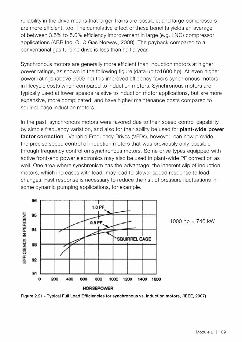
8/12/2019 Energy Efficiency Electronic Book Version 1548_PowerGenerationHandbook v1_1
http://slidepdf.com/reader/full/energy-efficiency-electronic-book-version-1548powergenerationhandbook-v11 111/361
reliability in the drive means that larger trains are possible; and large compressorsare more efficient, too. The cumulative effect of these benefits yields an averageof between 3.5% to 5.0% efficiency improvement in large (e.g. LNG) compressorapplications (ABB Inc, Oil & Gas Norway, 2008). The payback compared to aconventional gas turbine drive is less than half a year.
Synchronous motors are generally more efficient than induction motors at higherpower ratings, as shown in the following figure (data up to1600 hp). At even higherpower ratings (above 9000 hp) this improved efficiency favors synchronous motorsin lifecycle costs when compared to induction motors. Synchronous motors aretypically used at lower speeds relative to induction motor applications, but are moreexpensive, more complicated, and have higher maintenance costs compared tosquirrel-cage induction motors.
In the past, synchronous motors were favored due to their speed control capabilityby simple frequency variation, and also for their ability be used for plant-wide powerfactor correction . Variable Frequency Drives (VFDs), however, can now providethe precise speed control of induction motors that was previously only possiblethrough frequency control on synchronous motors. Some drive types equipped withactive front-end power electronics may also be used in plant-wide PF correction aswell. One area where synchronism has the advantage; the inherent slip of inductionmotors, which increases with load, may lead to slower speed response to load
changes. Fast response is necessary to reduce the risk of pressure fluctuations insome dynamic pumping applications, for example.
Figure 2.21 - Typical Full Load Efficiencies for synchronous vs. induction motors, (IEEE, 2007)
1000 hp = 746 kW
Module 2 | 109

8/12/2019 Energy Efficiency Electronic Book Version 1548_PowerGenerationHandbook v1_1
http://slidepdf.com/reader/full/energy-efficiency-electronic-book-version-1548powergenerationhandbook-v11 112/361
The pulling-in requirement of synchronous motors makes them generallyunsuitable for large fan applications as found in power generating stationsforced and induced draft drive power.
Switched Reluctance MotorsSwitched reluctance motors offer very high efficiency, but are still limited to relativelylow-power applications, typically up to only 75 kW. This motor technology is in rapiddevelopment and may lead to higher power ratings in the near future.
Permanent Magnet MotorsIn PM motors a magnet is used in the stator for generating a magnetic field. Theposition of the rotor is determined by motor control electronics, which then adjustthe modulated stator field accordingly. By eliminating one set of windings and theassociated ohmic losses, this motor design is more efficient than induction motortypes. High cost of the magnet material has restricted this motor type to relativelylow power (< 2kW) applications. Changes in the relative prices of magnets andcopper, coupled with lower prices of motor electronics, may eventually make thismotor feasible for higher power situations.
Motor Nameplate Terminology
Standards bodies such as the NEC and NEMA have agreed on definitions for thefollowing induction motor parameters which must be prominently displayed on themotor nameplate and provided with the vendor’s documentation.
− Rated voltage or voltages: This value has a 10% tolerance covering commonvoltage variation in some industrial networks
− Rated full-load amps for each voltage level: The nameplate FLA is usedto select the correct wire size, motor starter, and overload protection devices
necessary to serve and protect the motor. − Frequency: This value is either 60 Hz in North America, and 50 or 60 Hzelsewhere.
− Phase: Either single or 3-phase − Rated full-load speed (rpm): The motor speed under full load conditions.
− Insulation class and rated ambient temperature: A measure of motor’s abilityto dissipate heat.
− Rated horsepower: The work available from motor at full load torque and speed − Time rating: Standard motors can operate continuously at their full-load torque
and speed. For intermittent duty applications, a time rated motor can be selectedto reduce weight, size and costs.
110 | ABB Energy Efficiency Handbook

8/12/2019 Energy Efficiency Electronic Book Version 1548_PowerGenerationHandbook v1_1
http://slidepdf.com/reader/full/energy-efficiency-electronic-book-version-1548powergenerationhandbook-v11 113/361
− Locked-rotor code letter: A code letter that defines an inrush current a motorrequires when starting it.
− Manufacturer’s name and address
In addition to this required information, motor nameplates may also include datasuch as frame size, NEMA design letter, service factor, full-load efficiency, and powerfactor.
Motor System Loads A motor application is fundamentally defined by the load’s torque-speedrequirement, the duty cycle, and the load profile.
Load Torque vs. Speed Requirement According to these definitions from ABB’s Technical Guide (ABB Drives 2002) andthe Competitek Drive Power manual (Competitek 1996), the applications can becategorized by how the power varies with motor speed.
− Linear-law loads require constant torque across the entire speed range, andpower consumption varies linearly with speed. Examples of this type of load are:reciprocating compressors , positive displacement pumps, drilling machines,conveyors and grinding systems (curve (a) on page 112).
− Cube law loads require a torque which varies with the square of speed, and
power consumption varies with the cube of that speed. Examples of thistype of load are: pumps and fans and winders. The prevalence and highpower consumption of these loads is why they deserve special attention indesigns for improved energy efficiency (curve (b)).
− Constant power loads; A constant power load is normal in steelmaking whenmaterial is being rolled and the diameter changes during rolling. The power isconstant and the torque is inversely proportional to the speed (curve (c)).
− Constant torque, then constant power loads. This load type is common in the
paper industry. It is a combination of constant power and constant torqueload types. This load type is often a consequence of dimensioning the systemaccording to the need for certain power at high speed (curve (d)).
− Square law loads require a torque which is directly proportional to speed, andpower consumption varies with the square of that speed. Examples of this type ofload are hoists and winches.
− Constant speed loads are applications which require constant speed but varyingtorque. Examples of such applications are grinding and milling machines, sawmillblade cutters and escalators (Competitek 1996), and extruders, all of which mustrun at the same speed regardless of loading.
Module 2 | 111

8/12/2019 Energy Efficiency Electronic Book Version 1548_PowerGenerationHandbook v1_1
http://slidepdf.com/reader/full/energy-efficiency-electronic-book-version-1548powergenerationhandbook-v11 114/361
(a) Constant torque (b) Cube-law loads
(c) Constant power (d) Constant torque, then constant power
Figure 2.22 – Load types by torque vs. speed performance, (ABB Drives 2002)
Load Duty Cycle and Load Profile The term ‘duty’ describes how the load is used over a fixed time period. Loadswhich are frequently turned off and on are known as ‘cycling loads’. A repeatingpattern of load activation over a time period is known as the duty cycle.
Near-continuous loads are known as ‘heavy-duty’ loads. These loads are bestcharacterized by their loading profile over a fixed period of time. This profile is the %of time spent at various discrete % of load levels, as shown in the figure below.
112 | ABB Energy Efficiency Handbook

8/12/2019 Energy Efficiency Electronic Book Version 1548_PowerGenerationHandbook v1_1
http://slidepdf.com/reader/full/energy-efficiency-electronic-book-version-1548powergenerationhandbook-v11 115/361
Figure 2.23 – Load profile showing %-load versus %-total time (annual)
Load Startup RequirementStartup torque requirements vary widely, from a fraction of the full-load torque toapplications that require several times the full-load torque for starting. The load curvefor a high starting torque type of application is shown in the figure below. Typicalapplications for this load type are centrifugal fans, extruders and screw pumps/ compressors.
Figure 2.24 – Load type curve where high starting torque is needed, (ABB Drives 2002)
Motor soft-starting is needed in applications which are sensitive to shock or highmotor torque during startup. For example, NEMA Design B motors produce astarting torque which is about twice its full load torque (Competitek 1996). Otherdrive-train components can also benefit from the smooth acceleration provided bysoft-starting.
Module 2 | 113

8/12/2019 Energy Efficiency Electronic Book Version 1548_PowerGenerationHandbook v1_1
http://slidepdf.com/reader/full/energy-efficiency-electronic-book-version-1548powergenerationhandbook-v11 116/361
Dynamic Torque and Acceleration The load characteristic curves shown above reflect the steady-state torque requiredat different speeds. Accelerating (or decelerating) between different speeds requiresa positive (or negative, braking) ‘dynamic’ torque to be supplied by the motordrive system in addition to the load torque which the application (pump or fan, forexample) requires.
The driving torque of a motor during startup is the ‘run-up’ torque and theacceleration time to achieve nominal speed is known as ‘run-up’ time. The drivingtorque must exceed the load torque by a margin in order for satisfactory accelerationto occur.
Torque T [Nm] is related to speed through Newton’s Law for rotating bodies of inertiaJ [kgm 2]. Torque is proportional to the rate of change of this speed n [rpm], whenexpressed as [radians/s 2]. The change of rotational speed within a given time periodis its acceleration (or deceleration) and is as follows:
T = T m - T load = J x (Δn / Δt) x 2π/60
Moment of inertia J is the sum of the load and motor moments of inertia, as suppliedby the machine builders. If the rotating components are circular, with radius r and arelatively homogenous mass m, then J can be found by:
J = ½ x m x r 2
The above formula can be applied to large fans, for example. If there is a mechanicalgearbox between motor shaft (1) and load shaft (2), then all load-side inertias mustbe reduced by the square of the inverse of the gear ratio (the ratio of the number ofteeth) as follows:
J = J 2 x (n2 /n 1 )2
These formulas are useful for determining acceleration times of large inertia loads, asshown in the following example from an ABB Technical Guide (ABB Drives 2002);
For example: accelerating a fan to nominal speed is done with nominal torque. At nominal speed, torque is 87%. The fan’s moment of inertia is 1200 kgm 2 andthe motor’s moment of inertia is 11 kgm 2. The load characteristic of the fan T load isquadratic as shown in the figure below, relative to nominal. Motor nominal power is200 kW and nominal speed is 991 rpm. Calculate the approximate starting time fromzero speed to nominal speed.
114 | ABB Energy Efficiency Handbook

8/12/2019 Energy Efficiency Electronic Book Version 1548_PowerGenerationHandbook v1_1
http://slidepdf.com/reader/full/energy-efficiency-electronic-book-version-1548powergenerationhandbook-v11 117/361
Figure 2.25 – Fan torque vs. speed, with relative values at five equidistant speed points, (ABB Drives2002)
Motor nominal torque is:
T n = 9550 x 200 / 991 =1927 Nm
The starting time is calculated by dividing the speed range into five sectors. Ineach sector (198 rpm wide) the torque is assumed to be constant. Torque for eachsector is taken from the middle point of the sector. This is acceptable becausethe quadratic behavior is reasonably approximated to be linear in each sector. Thetime to accelerate the motor (fan) with nominal torque can found by re-arrangingNewton’s formula as follows:
Δt = J x Δn /( T m - T load ) x 2π/60
Acceleration times for each of the five different speed sections are:
0 to 198.2 rpm Δt = 1211 x 198.2 /( 0.99 x 1927) x 2π/60 = 13.2 s198.2 to 396.4rpm Δt = 1211 x 198.2 /( 0.92 x 1927) x 2π/60 = 14.3 s396.4 to 594.6rpm Δt = 1211 x 198.2 /( 0.78 x 1927) x 2π/60 = 16.7 s594.6 to 792.8 rpm Δt = 1211 x 198.2 /( 0.57 x 1927) x 2π/60 = 22.9 s792.8 to 991 rpm Δt = 1211 x 198.2 /( 0.29 x 1927) x 2π/60 = 45.0 s
The total starting time from 0 to 991 rpm is approximately 112 seconds.
Module 2 | 115

8/12/2019 Energy Efficiency Electronic Book Version 1548_PowerGenerationHandbook v1_1
http://slidepdf.com/reader/full/energy-efficiency-electronic-book-version-1548powergenerationhandbook-v11 118/361

8/12/2019 Energy Efficiency Electronic Book Version 1548_PowerGenerationHandbook v1_1
http://slidepdf.com/reader/full/energy-efficiency-electronic-book-version-1548powergenerationhandbook-v11 119/361
Figure 2.26 - Torque vs. speed for squirrel cage induction motor, (ABB Drives 2002)
Small to medium-sized motors are a commodity item. For these standardized,polyphase induction motors NEMA has developed a rating designation (A,B,C,D,E)for different application requirements. Large motors, however, are typically customengineered to a specific set of loading and service conditions, and are therefore notsubject to easy rating or classification. Large motors still share some characteristics
with the NEMA motor classes described below.
Normal Starting Torque Motors − Normal starting torque, normal starting current, low-slip and high efficiency.
− Centrifugal pumps and motor generator sets, infrequent starting duty; used wherehigh efficiency and high full-load speed are required. Modification of the motordesign can provide variations in torque characteristics and increased thermalcapability required for drives such as high inertia fans.
High Starting Torque Motors − High starting torque, normal starting current Centrifugal pumps, fans, unloaded
conveyor, vacuum pumps. This is the general-purpose motor suitable for pumpand fan drives.
− High torque, high slip motor; has relatively high starting torque and normal efciencyat full load. Positive displacement pumps, compressors, loaded conveyors,crushers without ywheels, pulverizers. This motor has the high starting torquemotor with almost constant torque throughout the entire speed range
Module 2 | 117

8/12/2019 Energy Efficiency Electronic Book Version 1548_PowerGenerationHandbook v1_1
http://slidepdf.com/reader/full/energy-efficiency-electronic-book-version-1548powergenerationhandbook-v11 120/361
− High torque, high starting torque, but with lower starting current. Car puller,crusher with flywheel, pulverizers, and high inertia drives that do not require highefficiency. Design D has higher starting torque than C, but motor efficiency islower.
Motor Service FactorMotors will have a service factor (SF), typically 1.0, or 1.1, or 1.15. As an example;a 1000hp motor with an SF of 1.15 means that the motor could be run at 1150 hpindefinitely without risk of overheating, but only at the rated voltage and frequencyconditions. The standards specify that the motor can operate at a nameplatetemperature rise of 90°C at service factor horsepower. SF offers a means to avoidoversizing a motor to handle temporary modest increases in load and uncertaintyabout loading.
Designers must be aware that higher temperatures will reduce a motor’s ability towithstand some of the other effects, such as increased harmonics, which stress theinsulation. The IEEE offers some further warning; the efficiency and power factor atservice factor load can be different from the respective values at rated nameplatelevels. It may not be energy-efficient to run for long periods at SF horsepower.
Another consideration for designers wishing to actually use the SF margin is that themotor’s starting and breakdown torque capability is based on rated horsepower only.If the starting torque requirement was high to begin with, and was then significantly
increased under the new SF operating conditions, then there is no guarantee thatthe motor will be able to start within an acceptable time limit.
With careful design of the power system, as described in the Power Systemssection , a well understood loading condition, and with robust real-time monitoring ofthe motor, it is worthwhile and defensible to exploit allowable SF margins of a high-quality motor. The motor will be more correctly sized to its application and will offerimproved efficiency at normal operating conditions.
In some applications, extra drive power is required for short durations; forexample to maintain condenser performance during peak supply on a hotsummer day. In these cases, a VFD will be able to increase speed to withinthe SF limits, while the VFD drive diagnostics continually monitors motortemperature.
A NEMA committee warned a long time ago (in the 1960’s) against use of SF onlarge motors as an alternative to a higher standard horsepower rating. Their adviceon this issue is reproduced below:
118 | ABB Energy Efficiency Handbook

8/12/2019 Energy Efficiency Electronic Book Version 1548_PowerGenerationHandbook v1_1
http://slidepdf.com/reader/full/energy-efficiency-electronic-book-version-1548powergenerationhandbook-v11 121/361
− ‘Standard horsepower increments in the larger ratings are usually within a 1.15range, so that the next larger standard horsepower can be reasonably selected inlieu of the service factor.
− ‘Use of a larger horsepower when overload is required avoids exceeding thenominal temperature rating for the class of insulation system used and avoids anyencroachments upon the thermal life of these larger, vital motors.’
− ‘Use of a larger horsepower when overload is required eliminates any reduction intorque margin.’
Advances in motor technology over the last half-century, however, may eventuallylead NEMA to a revision of their old guidelines and allow designers the room toimprove energy efficiency without any fear of compromising reliability.
Motor Power and Efficiency The power and speed requirements are set by the application’s load prole. Forexample, in pump and fan applications, the load torque decreases with the square ofthe speed; this is a direct result of the Afnity Laws discussed in the Pump and Fansystems sections. The power rating of a motor indicates its output mechanical power,often stated in horsepower or kW. Motor electrical (input) power is usually stated in kVA.
Motor Mechanical Power The motor’s mechanical output power is simply the output torque multiplied by
motor speed. In SI units:
Pm = T x N
Where: T = torque, (Nm)Pm = mechanical power at the shaft (watts)N = speed, (rad/s)
The same formula with power in kW and speed N in rpm (where 1 rpm = 2 x π / 60) is:
Pm = T x N / 9550
Where: T = torque, (Nm)
Pm = mechanical power at the shaft (kW)
N = speed, (rpm)
Module 2 | 119

8/12/2019 Energy Efficiency Electronic Book Version 1548_PowerGenerationHandbook v1_1
http://slidepdf.com/reader/full/energy-efficiency-electronic-book-version-1548powergenerationhandbook-v11 122/361
The same formula again, in all English units is:
Pm = T x N / 5252
Where: T = torque, (lb.ft)Pm = mechanical power at the shaft (rated hp)N = speed, (rpm)
For example: a motor has nominal power of 250 hp and nominal speed is 1480 rpm.What is the nominal torque of the motor (in lb.ft)? Using the last of the above formulas:
T n = P m x 5252 / N = 250 x 5252 / 1480 = 887 lb-ft.
Motor Input Power and Current The nominal electrical motor input power (in kW) can be calculated based onthe mechanical output power, as was calculated in the above formulas, and thenameplate efficiency:
P in = P m / η
Where:
P in = input power (kW)Pm = mechanical output power (kW)η = per-unit efficiency of the motor (0 to 1)
If the output power is given in horsepower (hp), then use the conversion factor 1 hp= 0.746 kW. The total input power in kVA can be expressed as:
S = (P m x 0.746 ) / ( η * FP )
Where:S = total input power (kVA)Pm = mechanical output power (hp)η = per-unit efficiency of the motor (0 to 1)PFP = per-unit power factor
The active power (kW) at the motor terminals can also be calculated from electricalparameters P
in= 3½ x V
L-L x I
L x PF
P
120 | ABB Energy Efficiency Handbook

8/12/2019 Energy Efficiency Electronic Book Version 1548_PowerGenerationHandbook v1_1
http://slidepdf.com/reader/full/energy-efficiency-electronic-book-version-1548powergenerationhandbook-v11 123/361
Where:P in = power (kW)
V L-L = three phase line-to-line voltage (kV)PFP = per-unit power factor (cos( ϕ n ))
For example: What is the nominal efficiency of a 400 kW ( V= 4.16kV, 71A and PFP =
0.85) motor?
The above formulas can be used to calculate the nominal efficiency of the motor asfollows
η n = P m / P in = 400 / (3 ½ x 4.16 x 71 x 0.85 ) = 0.92 (approx)
To calculate the input electrical energy cost for R running hours, given input voltageand current and a Price:
Cost= 3 1/2 x V L-L x IL x PFP x R x Price$/kWh /1000
The VFD section contains additional formulas for estimating motor current , andadditional electric power formulas are in the Electric Power System part of thishandbook.
Motor EfficiencyMotor efficiency refers to the amount of input electrical power required to achievea particular output from the motor. Using the power formula from above, a 100 hprated motor with 93% efficiency at rated load will draw 89.1 kVA from the supplywhen running at full load and 0.9 power factor. The motor current at this operatingpoint is shown as the FLA (full load amp) rating on the motor nameplate.
Most motors will the show nominal full load efficiency value on their nameplate as
determined by a highly-accurate dynamometer and a procedure described by IEEEStandard 112, Method B. These measurements provide average values from a largetest sample of motors. The motor efficiency of an individual motor in the field canonly be determined by field testing methods, such as measurements with a watt-meter. Statistics on the manufacturer’s test sample provide a minimum efficiencyvalue which also appears as the ‘guaranteed minimum efficiency’ on the nameplate;this value assumes that the worst motor in the sample could have losses as muchas 20% higher than the average. These minimum values are in Table 12-8 in NEMAMG-1 (Cowern, Baldor Electric, 2004).
Standard motors tend to operate most efficiently at between 75–110% of full loadspeed. Smaller motors are less efficient than larger motors. Standard motors below
Module 2 | 121

8/12/2019 Energy Efficiency Electronic Book Version 1548_PowerGenerationHandbook v1_1
http://slidepdf.com/reader/full/energy-efficiency-electronic-book-version-1548powergenerationhandbook-v11 124/361
200 hp have efficiency between 80 to 90%, while the efficiency for motors in therange of 250 to 5000 hp varies between 90 to 96%. Larger motors with higher peakefficiencies tend to have flatter efficiency curves above 50% load, as shown bycurves (1) and (2) in the figure below. For these larger motors, maximum efficiency isstill at about 95%, but with only a small (0.3 to 1.0%) decrease to full load.
Figure 2.27- Efficiency vs. Load for squirrel cage induction motors, (IEEE, 2007)
As the curve shows, efficiency drops sharply below 50% load for all motors. Anaverage 100 hp standard- efficiency motor loses 15% in efficiency as load decreasesfrom 50% to 25% of full load (Competitek 1996). As a general rule, smaller motors
lose more efficiency than larger motors at lower loads.
Motor Losses and Efficiency The greatest losses in a motor are the iron losses that occur in the rotor andstator, accounting for 50 percent of the total loss. This can be improved by usinglow loss steel and thinner laminations. Copper losses account for 20 percent.Using an optimum slot fill design and larger conductors can reduce these losses.Bearing friction and windage losses total 23 percent and can be reduced by using
a smaller cooling fan. Stray losses, which account for 7 percent of the total, canbe reduced by improving the slot geometry. The main sources of motor losses andcorresponding design improvements are shown in the figure below from the ABBReview Special Report on Motors & Drives, 2005. By virtue of these design changes,motors have improved in efficiency by an average of 3 percent in the last decade(from 1995 to 2005).
There are important design trade-offs between losses and torque performance; lowrotor resistance results in high full load speed (low slip), high efficiency (low rotorlosses), and slightly higher starting current. High rotor resistance results in highstarting torque for line current drawn and slightly lower current during starting, butresults in lower full load speed and lower efficiency (high rotor losses).
122 | ABB Energy Efficiency Handbook

8/12/2019 Energy Efficiency Electronic Book Version 1548_PowerGenerationHandbook v1_1
http://slidepdf.com/reader/full/energy-efficiency-electronic-book-version-1548powergenerationhandbook-v11 125/361
Figure 2.28 – Cutaway view showing sources of motor losses, (ABB Drives, 2006)
Rotor ohmic (I2R) losses are proportional to slip and are in the rotor winding ofa squirrel cage motor. Higher-efficiency motors tend to have lower slip and will
therefore rotate faster under the same loading conditions: one percent increase inefficiency is equal to about a 1/3 of a percentage point decrease in induction motorslip. Voltage at the motor terminals also has an effect on efficiency, as discussed inthe section on Power Quality - Voltage and Frequency Variation
Power FactorPower factor (PF) is a measure of the amount of reactive power which the motordraws from the power source. A PF less than 1.0 means that some reactive power,
which is induced by the motor coils, must be generated and carried by the powersupply system. Industrial end-users pay a demand charge based on maximumreactive power usage within a certain time period. This charge is in addition to theregular cost of energy, charged per kWh, and covers the provider’s cost for theincreased size of their power delivery equipment. An oversized electric motor willtypically decrease (i.e. worsen) the PF by 10% compared to a right-sized motor.
PF in induction motors generally follows the same shape as the efficiency curveswith respect to % loading.
PF is a minimum at no load and reaches a maximum near full-load condition. Thisrelationship between PF and motor speed is shown in the figure below, from IEEE
Module 2 | 123

8/12/2019 Energy Efficiency Electronic Book Version 1548_PowerGenerationHandbook v1_1
http://slidepdf.com/reader/full/energy-efficiency-electronic-book-version-1548powergenerationhandbook-v11 126/361
Std 666. The average 100 hp standard-efficiency motor loses about 10% points inPF from full load to 50% load, and almost 20 more points moving down to 25% load.
The PF as listed on the nameplate applies to the full load operating condition.
Figure 2.29 - PF vs. Load for squirrel cage induction motors, (IEEE, 2007)
The capacity of the power system to deliver real power (the only kind which can doreal work) can be increased by applying various reactive power compensationmethods , either at the motor, or centrally in the electrical power supply system.
High-Efficiency MotorsWith the Energy Policy Act (the EPAct) of 1992, the USA and Canada imposednew, minimum efficiency standards, effective from October 1997, for general-purpose induction motors of NEMA designs A and B. These motors are typically 3–8percentage points higher in efficiency than standard motors. The EPAct specificallytargets motors from 1 to 110 hp (0.75 to 150 kW) as prime candidates forimprovement, with a published list of high-efficiency motors and reduced electricity
tariffs for users of these motors..
A similar program by the Danish Energy Authority published a list of high efficiencymotors and offers subsidies for motors purchased from this list: US$ 10 per kilowattfor both new plant and for replacements. In the EU there are three class levels ofefficiency, known as Eff1, Eff2 and Eff3, applying to low voltage two- and four-polemotors with ratings between 1.1 and 90 kW. Both the US DoE and the EU requirethat a motor’s efficiency rating be prominently displayed on the motor’s nameplate.
A higher-efficiency, ‘premium’ NEMA class of motors is also available, known asclass E. The price of these premium, higher efficiency motors ranges from 10 to20 percent higher than standard motors in continuous duty applications (US DoE
124 | ABB Energy Efficiency Handbook

8/12/2019 Energy Efficiency Electronic Book Version 1548_PowerGenerationHandbook v1_1
http://slidepdf.com/reader/full/energy-efficiency-electronic-book-version-1548powergenerationhandbook-v11 127/361
Sourcebook, 2006). A high efficiency motor has lower energy losses (describedin the figure below), hence lower running temperature and improved reliability; alldesirable characteristics in critical and high-duty applications. These NEMA premiumefficiency 3-phase motors have efficiencies ranging from 86.5% at 1 hp (750 W) to95.8% at 300 hp (220 kW).
The recent legislation in the Energy Independence and Security Act of 2007 (EISA)calls for increased efficiency of motors manufactured after December 19, 2010.EISA regulation re-classifies EPACT minimum efficiency motors as Subtype I, sothese motors will be required to have nominal full-load efficiencies that meet thelevels defined as ‘premium’ by NEMA MG-1 (2006). The EISA law also creates acompletely new category (Subtype 2) of motors which regulates efficiency for motordesigns that were not covered under previous legislation, such as polyphase motorsrated at less than 600 volts.
Motor Slip and Energy EfficiencyHigh efficiency motors tend to have less slip at a given load compared to standardefficiency motors. The reduced slip may provide improved torque vs. speedcharacteristics, but the increased speed at operating point may incur power lossesgreater than the gains of increased motor efficiency. The increased speed is animportant factor to consider when facing a motor retrofit situation . A generalrule of thumb is that every 1% increase in efficiency is equivalent to about a 1/3%
decrease in slip (Competitek, 1996). The losses due to increased speed occur onlyin constant speed applications, and are largest in cube-law applications such as fanand pump systems. The gains from using high-efficiency motors can be preservedby 1) specifying a variable speed drive to reduce speed, 2) specifying a smaller ratedmotor (if peak loads allow) or 3) compensate by trimming the pump impeller or fanblades (Competitek, 1996) 4) specifying a high-slip, but still relatively more efficientreplacement motor.
Motor Couplings, Speed Control & Variable Frequency DrivesMotor Shaft Couplings A motor’s shaft can be either directly coupled to the drive shaft of a pump or fan,or indirectly coupled by using chains, belts or gears. Indirect coupling is necessarywhen physical space or layout restrictions prevent the motor from being in-line withthe drive shaft, or to allow for mechanical speed adjustment.
Speed ‘adjustment’ is not the same as speed control, in which speed can be variedcontinuously by a signal from an operator or an automatic controller. The pros andcons of the various coupling methods are discussed below, but direct shaft-to-shaftcoupling is the only method with zero drive-train losses.
Module 2 | 125

8/12/2019 Energy Efficiency Electronic Book Version 1548_PowerGenerationHandbook v1_1
http://slidepdf.com/reader/full/energy-efficiency-electronic-book-version-1548powergenerationhandbook-v11 128/361

8/12/2019 Energy Efficiency Electronic Book Version 1548_PowerGenerationHandbook v1_1
http://slidepdf.com/reader/full/energy-efficiency-electronic-book-version-1548powergenerationhandbook-v11 129/361
Multiple speed motor systems have some inherent disadvantages; 1) for largemotors, switching between speeds is neither trivial nor smooth and may lead toprocess transients and upsets. The sequence of power breaker and pole switchingmust be closely coordinated with motor speed 2) Multiple speed motors tend tobe slightly less efficient than single speed motors, due to compromises in theirdesign to allow for multiple sets of windings. Although they deliver savings in cube-law applications, they are still less efficient than the VFD plus single-speed motorcombination.
Wound Rotor MotorsWound rotor motors are induction motors with a slip-ring and brush assembly whichconnects the rotor to an external variable resistor. Varying this resistance will changethe rotor resistance and slip, hence speed of the motor. The disadvantage of thismotor type is that significant slip energy is dissipated in the resistor (Competitek1996). Slip-recovery variations (Kramer and Scherbius drives) on wound rotordesigns increase the efficiency to VFD plus motor levels (Competitek 1996). Thebrush assembly is similar to that found on DC motors and is a source for the samemaintenance and reliability issues associated with DC motors.
Variable Speed Control Technologies There are a number of different coupling technologies specifically for continuousspeed control which are commercially available and feasible for large industrial
machinery: hydrodynamic, hydro-viscous, magnetic, and DC or AC variable speeddrives (known as a Variable Frequency Drive (VFD ) for AC systems). All of thesetechnologies provide the necessary speed control and achieve energy savings overthe less efficient flow control methods such as control valve or damper throttling.
− In hydrodynamic type couplings, the shaft drives an impeller which imparts energyto oil which then transfers it to blades of a runner fixed to another shaft. Controlis achieved by varying the amount of oil via a scoop tube. The hydrodynamic
coupling will always have slip losses, even at rated speed, typically 2%-3%. Thehydraulic coupling offers a form of soft-start capability, but this comes at theexpense of controllability at low speeds (Competitek 1996). This type of variablespeed arrangement is still common in many existing plants (Black & Veatch,1996).
− In the hydro-viscous type of variable speed control, a thin film of oil between aseries of discs transfers energy from the driving shaft to the output shaft throughshear forces. Speed control is achieved by varying the pressure on the discs. Thehydro-viscous coupling can be locked at rated speed, incurring no losses, whichmake this type of drive useful as a clutch for starting.
Module 2 | 127

8/12/2019 Energy Efficiency Electronic Book Version 1548_PowerGenerationHandbook v1_1
http://slidepdf.com/reader/full/energy-efficiency-electronic-book-version-1548powergenerationhandbook-v11 130/361

8/12/2019 Energy Efficiency Electronic Book Version 1548_PowerGenerationHandbook v1_1
http://slidepdf.com/reader/full/energy-efficiency-electronic-book-version-1548powergenerationhandbook-v11 131/361
8/12/2019 Energy Efficiency Electronic Book Version 1548_PowerGenerationHandbook v1_1
http://slidepdf.com/reader/full/energy-efficiency-electronic-book-version-1548powergenerationhandbook-v11 132/361
Starting a Direct-On-Line (DOL) over-sized motor means the motor starter andother power system components will need to be oversized, as the majority ofstarting current is reactive and dependent on the motor size; larger motors takemore starting current. For this reason, VFDs and Soft Starters should be evaluatedfor suitability during the motor specification process. As the section on VariableFrequency Drives explains, these devices can correct for all accumulated designmargins and also provide the required soft-start capability.
Engineers may wish to believe that the widespread problem of oversizing is actuallydue to under-loading; in other words, that the plant is operating at much less thanits target rated capacity due to prevailing market conditions beyond their control.
An analysis of the large motors in a US pulp and paper mill, however, revealed anaverage load times capacity factor of 43% at a time when the mills where operatingat nearly full rated capacity (cited in Drive Power manual Competitek, 1996). Datasuch as these suggest that the problem of oversizing is real, and that it must besolved by engineers and technical managers.
Causes of Motor Oversizing The causes of technical oversizing are investigated in detail throughout thishandbook, but the story of how margins ‘creep’ in a typical project is told below, inthe case of a large industrial motor:
The process designer, following the guidelines in the Pump and Fan Systemssections of this handbook, will provide the electrical engineer with the maximumrequired pump or fan torque at the required operating speed. This processspecification is often misinterpreted, by the electrical engineer, to mean the minimumacceptable continuous torque for the motor even if the requirement is actually apeak load which must be sustained only for a small fraction of the motor’s duty(Competitek, 1996).
The electrical engineer may further oversize the motor in the face of uncertain,high-starting torque requirements and other power system uncertainties, just asthe process designer may have overstated the torque and speed requirementsto account for later changes in piping design or capacity demands. Customer orcompany guidelines may force the electrical engineer to specify a high service factor(1.15) machine and class ‘F’ insulation, all of which add even more unnecessarymargin.
The project lead engineer may add further layers of margin fat by applying an across-the board-design ‘margin of error or safety’, as well as a generous ‘future capacityincrease’ margin. Finally, if the resulting specification is only slightly higher than astandard commercial rating, then the next and higher rating is usually selected. The
130 | ABB Energy Efficiency Handbook

8/12/2019 Energy Efficiency Electronic Book Version 1548_PowerGenerationHandbook v1_1
http://slidepdf.com/reader/full/energy-efficiency-electronic-book-version-1548powergenerationhandbook-v11 133/361
gap between standard ratings is larger as motor power increases, which makes thiscommon practice costly in the long run. Most of the above margins are compounded(margin as a percentage of the margin below), the end-result is a motor which isoften twice as large as it needs to be.
Motor Sizing and Selection The motor design and engineering procedure described previously will help toestablish whether the maximum torque specification is a normal maximum or ashort-duration peak maximum. If the value represents a transient peak torque, thenother methods, such as a motor service factor margin should be investigatedbefore this value is used as the baseline for sizing. The design procedure thencalculates, from the maximum required torque at the required operating speed, themotor’s power rating according to the motor power formulas and will establishthe system (bus) voltages. (See ANSI C50.41-1982 for list of preferred motor ratedvoltages.) The nominal system voltages are slightly higher than the rated motorvoltage due to anticipated steady state voltage regulation in the power supplysystem. Special attention to motor starting conditions is important for energyefficient design. As with peak running loads, transient conditions should be carefullyvetted before they are allowed to form a minimum requirement. Other transientconditions such as high ambient temperature should receive the same criticalprofiling analysis as duty cycle. Worst-case estimation of ambient temperature maylead to extra thermal margins and larger than necessary machines.
Average Load SizingMaximum load sizing is the default method for sizing, but the alternative ‘Andreas’method uses average-load power. This average load sizing is only for applicationsthat do not require high inertia load starting or frequent starting, and whichoperate at varying loads. Since motor heating is a limiting factor in sizing a motor,this method uses the RMS (root-mean-square) losses, approximated by RMShorsepower over the load cycle, to determine the thermal suitability of a motor. The
RMS horsepower is defined as ‘that equivalent steady-state hp which would resultin the same motor temperature rise as that of a defined load cycle’ (See referenceCompetitek, 1996, for an example calculation.) The calculated RMS hp will indicatethe required motor rating from thermal considerations, but the maximum peak loadmust still be within the range of that motor’s service factor.
Motor Starting Conditions - Acceleration The NEMA MG1 and ANSI C50.41 standards provide sizing rules based on thetorque required for accelerating the inertia of a rotating mass. Induction motors builtaccording to these standards develop at least 70% of their full load torque duringstartup, which should be sufficient for most load applications.
Module 2 | 131

8/12/2019 Energy Efficiency Electronic Book Version 1548_PowerGenerationHandbook v1_1
http://slidepdf.com/reader/full/energy-efficiency-electronic-book-version-1548powergenerationhandbook-v11 134/361
Motors serving high inertia loads such as fans, however, exceed the NEMA normalinertia limits. These special motors required for those applications tend to beoversized with additional thermal capacity to account for load torque and possiblelow voltage conditions, factors which slow the acceleration time period and thusallow the motor to accumulate more heat. See the example for determiningacceleration time of an industrial fan in the Fan Systems section.
Motor Starting Conditions - VoltageLow voltage conditions during startup are a particular challenge for large motorapplications. The effect of low voltage starting conditions on developed torque ismagnified, because torque drops with the square of the applied voltage. Very longacceleration times and increased heating or even the inability to reach full operatingspeed are some of the consequences of inadequate design for startup.
For motors running in island mode networks, such as oil platforms, even smallermotors might require starting methods other than DOL due to the lower short circuitcapacity of such networks (ABB Review, Ahlinder, 2001).
The three most common designs for motor startup are: 1) Direct-On-Line (DOL), 2)Star-Delta 3) Soft-starters, which also include VFDs. Direct-on-line simply connectsthe motor terminals directly to the supply network. DOL is the lowest capital costand most used system to start small squirrel-cage asynchronous motors. As shown
on the figure (left) below, starting is carried out at full voltage, high current andwith constant frequency; this develops a high starting torque with much reducedacceleration times. This method is useful for full-load starting applications. Highinrush currents, first of 10-12 times rated current, then holding at up to 6-8 timeswell into startup, will stress both the power system and motor.
Star-delta and soft-starters or VFDs are collectively referred to as reduced voltagemethods, with star-delta being the most common. In star-delta, inrush currents are
reduced by using first a star circuit, then switching over to a delta circuit during laterstartup.
132 | ABB Energy Efficiency Handbook

8/12/2019 Energy Efficiency Electronic Book Version 1548_PowerGenerationHandbook v1_1
http://slidepdf.com/reader/full/energy-efficiency-electronic-book-version-1548powergenerationhandbook-v11 135/361
Figure 2.30 - Relative startup characteristics for different starting methods Ref (ABB Motors & Drives,2007)
Carefully designed special lubrication and cooling systems will provide some extrathermal support margin needed by the motor for high transient load conditions.Existing motors can avoid being de-rated if extra cooling is available for suchsituations. Learning more about the process load and duty cycle, then carefulcalculation and proper mitigation efforts will help in right-sizing a motor under all
conditions.
A high-starting torque design motor has lower operating efficiency at full load. Forsome applications with many starts & stops and short running times, however, ahigh-starting torque motor may be the overall most energy efficient selection.
Motors in Retrofit SituationsDownsize an Underloaded Motor
An underloaded motor has poorer efficiency and power factor. These motors can beidentified in an energy assessment process. The replacement motor can be sizedbased on the actual load factor; a 100 hp (75 kW) motor at 50% loading can bereplaced by a 50 hp (37 kW) motor. This replacement motor should be chosen tohave higher efficiency, but careful attention to slip is important.
In an economic analysis of motor downsizing performed by RMI in their CompetitekDrivepower Manual, an average 100 hp (75 kW) standard motor at less than 50%loading can be downsized (to a much smaller, but slightly more efficient model)for a payback in under 3 years, in a cube-law application. Additional benefitsof a downsized replacement motor are a smaller motor starter and smaller, lessexpensive conductors (Competitek 1996).
Module 2 | 133

8/12/2019 Energy Efficiency Electronic Book Version 1548_PowerGenerationHandbook v1_1
http://slidepdf.com/reader/full/energy-efficiency-electronic-book-version-1548powergenerationhandbook-v11 136/361
Motor Upgrade to Higher Efficiency ModelIn a fixed speed application, a motor upgrade to a higher-efficiency model with thesame rating may inadvertently lead to increased power consumption if the newmotor runs faster than the previous one, due to lower slip. The section on MotorEnergy Efficiency offers guidelines on how to avoid this situation. See the sectionon Lifecycle Costing (LCC) for methods to calculate the energy and money savingsrelated to motor efficiency improvements; a numerical LCC case example is providedat the end of this module.
Motor Rewinding Another pitfall in retrofits is the loss of efficiency due to successive rewinds of anold motor. Typical rewinding practice degrades motor efficiency by between 0.5% to2.5% for each rewind (Competitek, 1996)
A study by Ontario Hydro found an average efficiency reduction of 1.1% in small (<15kW) rewound motors, concluding that an upgrade to a higher efficiency modelwas more worthwhile on motor failure.
Efficiency is lost in rewinds for several reasons: core losses increase due to the hightemperatures experienced during failure; stripping the motor for repair also damagesthe laminations; copper losses increase because of the practice of using smallerconductors, increasing I 2R losses. Finally, fitting of universal cooling fans, which
may not be designed for the particular motor, leads to an increase in windage losses(ABB Review, Special Report Motors & Drives, 2003).
Older, standard motors which have been rewound several times will be morethan 10% less efficient than a high-efficiency motor. Rewound motors are alsoat risk of increased phase unbalance within the motor. The negative effects ofphase unbalance are described in the section on Power Quality - Phase VoltageUnbalance .
Upgrade from DC to AC A common retrofit opportunity involves upgrading older DC drives and motors tonew AC ones. This upgrade is an opportunity to improve harmonics, power factor,uptime, spare part savings and other maintenance costs. In the past, DC drives andmotors were the only solution for high starting torque and accurate speed controlbut this is not the case today. DC drives generate a high level of harmonic distortionand are high maintenance due to brush and collector wearing. Both of these factorsreduce energy efficiency. The upgrade potential to AC is larger in certain industrieswhich have a population of older, energy-inefficient DC motor controls; typically inthe steel, cement and paper industries.
134 | ABB Energy Efficiency Handbook

8/12/2019 Energy Efficiency Electronic Book Version 1548_PowerGenerationHandbook v1_1
http://slidepdf.com/reader/full/energy-efficiency-electronic-book-version-1548powergenerationhandbook-v11 137/361
A DC motor upgrade may be an opportunity to use a VFD with variable torquetechnology . This drive can provide high starting torque and accurate speed control,along with the side benefits of reduced maintenance, improved PF, and reducedharmonics.
Motor Sizing and Selection Tools A software package, MotorMaster+ 3.0 is available from the US DoE’s ‘BestPractices Program’ to assist with motor selection. The software includes a built-in database of more than 27,000 U.S. motors and has the capability to comparedifferent motors and compute relative costs (including initial, annual energy, and lifecycle costs) and savings for the motors being considered.
Another package, DriveSize, is available from ABB Drives to help select a motor anda drive, and then calculate combined motor & drive efficiency.
Motor System Guidelines – Summary The following design guidelines will generally improve the energy efficiency of thedesign or re-design of a motor system, at relatively low capital cost, with a shortpayback period:
− Downsize underloaded motors − Upgrade to higher efficiency motors
− Upgrade old DC motors and controls to AC − Use VFDs for speed control − Avoid margin creep; follow proper sizing procedures
Many more tips for energy efficient motor systems can be found in the DoE EERE(US DoE Best Practices, 2008) Motor Tip Sheet.
Motor System Maintenance
The large number of motors in a plant requires a comprehensive motor managementprogram to ensure they are managed cost-effectively. Such a policy helps bringtogether capital, maintenance and revenue budgets, showing the effect they haveon each other when different types of motors are selected. Industrial users benefitfrom such a policy through reduced energy costs, by upgrading to high-efficiencymotors at the most cost-effective time. The forward planning inherent in the practicehelps reduce downtime. Inventory can also be reduced through a fast track deliveryagreement. (ABB Review, Special report, Motors & Drives, 2005). Many technicaltips for motor systems maintenance can be found in the DoE EERE (US DoE BestPractices, 2008) Motor Tip Sheet.
Module 2 | 135

8/12/2019 Energy Efficiency Electronic Book Version 1548_PowerGenerationHandbook v1_1
http://slidepdf.com/reader/full/energy-efficiency-electronic-book-version-1548powergenerationhandbook-v11 138/361
Motor System Cost Calculations The investment costs for a motor are mainly hardware, engineering and installationcosts. Combined, these costs are referred to as the total installed cost (TIC) of themotor. The hardware cost per hp generally decreases with the size of the motor, butvaries greatly with motor type and other factors. As a first approximation, a large(>500 hp) standard induction motor has a hardware cost of about $100 per hp. Thetotal installed cost can be approximated by adding 60% of the hardware cost, so the
TIC in this case will be $160 per hp. A motor rewind can cost between $25 to $40per hp.
Value Calculation CaseSample comparison of two 2000 hp (1.5 MW) motors at 85 and 97 % efficiency over1 year:
Energy Savings = 2000 hp x 0.746 kW/hp x 8,000 hrs/yr x 100(1/85 – 1/97) =1,737,198 kWhDollar Savings = 1,737,198 kWh x $0.07/kWh = $121,603
Now applying LCC methods to determine the present value of the savings over 20years at 6% RoR:
PV = 121,600 x ((1 + 0.06)20 - 1 ) / 0.06(1 + 0.06)20
PV = $1,394,742
The Case Studies section has a fully worked-out example of retrofit costcalculations with payback.
Variable Frequency Drives VFD Concepts
Electric AC motors are the most common source of process industry drivepowerdue to their reliability and low cost. An additional feature of electric motors is thatshaft speed or torque can be controlled by varying the electrical supply at the motorterminals. This feature is exploited by a separate piece of power electronic hardwareknown as the Variable Frequency Drive (VFD), some of which are pictured in thefigure below.
136 | ABB Energy Efficiency Handbook

8/12/2019 Energy Efficiency Electronic Book Version 1548_PowerGenerationHandbook v1_1
http://slidepdf.com/reader/full/energy-efficiency-electronic-book-version-1548powergenerationhandbook-v11 139/361
Figure 2.31 - Torque-speed curves for idealized VFD, (ABB Drives 2002)
VFD Energy Efficiency Potential The main benefits of applying VFDs come from matching the input power to theneeds of the process. These benefits are magnified in cube-law applications suchas pumps and fan systems, where power requirements increase with the cube ofspeed, and the savings are typically between 30 and 50%. The following sections
introduce the technical features of VFDs with the greatest potential for energyefficiency.
Speed Control instead of ThrottlingOf the estimated 65 percent of industrial energy used by electric motors, some20 percent is lost by wasteful flow throttling mechanisms. The mechanics of flowthrottling is described in the fan and pump sections of this handbook. Additionalenergy is wasted in inefficient variable speed coupling methods . VFDs allow
application speed to be controlled without energy-wasting flow throttling or inefficientbelts and hydraulic couplings.
VFD controlled pumps and fans can respond faster and more reliably than flowthrottling valves or dampers, especially at flow extremes when control valvesbecome highly non-linear . VFDs avoid the problem of poorly-sized control valveswhich may be unstable for control at less than 10% opening. In fan systems, the useof a VFD for speed control avoids the deadband and hysteresis found in mechanicaldampers or inlet guide vanes control methods. Damper leakage is also avoidedwhen using VFDs for flow control. Compared to throttling control methods, VFDshave lower inspection & maintenance costs. Any reduction in speed achieved by
Module 2 | 137
8/12/2019 Energy Efficiency Electronic Book Version 1548_PowerGenerationHandbook v1_1
http://slidepdf.com/reader/full/energy-efficiency-electronic-book-version-1548powergenerationhandbook-v11 140/361
using a VFD has major benefits in reducing pump wear, particularly in impellers,bearings and seals.
There are some additional side-benefits for VFD-flow control in pumping systems.With a VFD receiving a signal from a pressure transmitter, it is possible to monitorthe pressure of the incoming pipeline and configure the converter to take steps ifthe risk of cavitation is high; i.e. if pressure falls below NPSHR plus a margin. Waterhammer is caused by rapid changes in flow. These flow changes are followed byrapid pressure transients that cause pipes, pipe supports and valves to be damagedcausing leakage. VFDs allow the user to gradually ramp pump acceleration at a saferate to avoid hammering.
Despite the potential for 60% savings in many cube-law applications, only 5%of all industrial motors are controlled by VFDs, and it is estimated that 30% ofexisting motors can be cost-effectively retrofitted with VFDs (ABB Drives, 2006).
The potential is larger in smaller applications (under 2.2 kW) where 97 percent of allmotors have no form of speed control at all, equating to some 37 million industrialmotors sold annually worldwide (ABB Review, Special Report Motors & Drives,2003). 40 percent of the value (and 90 percent in units) of all drives shipped arerated at less than 40 kW.
Improved Motor Efficiency
Another benefit of VFDs is the improved energy performance of the motor itself. The VFD control allows the motor to operate closer to its best efficiency point. The drivecan generate a family of characteristic curves for the motor, in the same way that aspeed-controlled motor generates a family of characteristic pump curves. In bothcases, the intersection with the load characteristic curve gives an operating pointwhich is near to the area of optimum efficiency for the equipment.
VFDs can correct for oversized motors by running them at reduced speed. The
operational benefits of such correction can justify a VFD even in applications whichdo not call for speed control.
Compared to most other speed control methods described in the Motors andDriveTrains section, with a VFD there is no loss due to mechanical slip betweenmotor and load.
Two and Four Quadrant OperationQuadrant operation is the term used to describe a drive’s ability to provide braking,reversing (2-quadrant) and regenerative (4-quadrant) power. The ‘quadrant’ refers tothe space these modes occupy on a torque-speed axis shown in the figure below.
138 | ABB Energy Efficiency Handbook

8/12/2019 Energy Efficiency Electronic Book Version 1548_PowerGenerationHandbook v1_1
http://slidepdf.com/reader/full/energy-efficiency-electronic-book-version-1548powergenerationhandbook-v11 141/361
For loads which generate power for only a short time, then it is typical to offer only abraking resistor where the power generated is dissipated as heat losses.
T 4 1
3 2
Decelerating
Accelerating
Accelerating
Decelerating
n
T
n
T
n
T
n
Figure 2.32 – Four quadrants of VFD operation
Active rectifiers will allow these losses to be regenerated into electrical power for thenetwork. The type of rectifier will determine if power can flow in both directions. Aconventional passive diode rectifier only supports motor loads where the power flowis only in one direction.
Motor Soft-Starting VFDs provide the same functionality as a dedicated soft-starter - a power-electronicsdevice installed in-line with the motor that slowly ramps up the voltage for a smootherstartup. Soft starting is mainly used to limit large motor starting currents and to bettermanage power factor during startup so that the electric power system is not undulystressed. Soft-starting therefore improves voltage bus stability, reduces currentsand allows reduction in transformer size, and other power system hardware. There
is also reduced risk of process disturbance due to voltage drops; and fewer trips ofother electrical devices connected to the same bus. Most motors experience startupin-rush currents that are 5 to 6 times higher than normal operating currents, which isreduced to 1.5 with VFDs, thus reducing wear on the motor. Soft starting reduces heatload and allows a greater number of starts within a given time period, increasing theexibility of the control system to optimize the process. (Motors not equipped with a
VFD or other form of soft startup power electronics are referred to as ‘Direct-On-Line’(DOL) motors. ) Note that the load itself may also benet from a smooth ramping upof torque and speed. The sections on Motor Starting Conditions and VFD StartingTorque Conditions discuss design criteria for startup conditions.
Module 2 | 139

8/12/2019 Energy Efficiency Electronic Book Version 1548_PowerGenerationHandbook v1_1
http://slidepdf.com/reader/full/energy-efficiency-electronic-book-version-1548powergenerationhandbook-v11 142/361
Power Factor Correction The internal design of a VFD helps to improve a motor’s power factor (PF). Whena VFD is installed, the reactive power that is the source of low PF circulates mainlybetween the DC link and the motor, and therefore it cannot affect the input ACelectric power supply system. Higher power factor will reduce I2R losses in thepower network transformers and cables. A VFD-equipped motor system will typicallyhave high PF of 0.98 compared to 0.83 for a typical DOL motor. The PF when usinga VFD does not degrade with decreased speed, as is the case with DOL motors.
The VFD’s rectifier unit can optionally be of the ‘active’ type that performs leadingand lagging PF correction, which is to the benefit of the entire input side of theelectric power system. The potential for such an Active Rectifier Unit (ARU), alsoknown as ‘active front end’ is discussed in the handbook section on reactive powercompensation .
Slip CompensationWithout a VFD, when the motor load torque is increased, the speed of the motorwill decrease as shown in the figure below. To compensate for this slip, the torquevs. speed curve is modified with use of a VFD so that the torque increase can beaccomplished while maintaining a constant speed (ABB Oy. Drives, 2002). This slip-compensation is a standard function on most VFD drives and is especially useful inapplications which require constant speed but varying torque .
Figure 2.33 – Slip compensation of a VFD shown on motor torque vs. speed curve, (ABB Oy. Drives,2002)
Speed Setpoint Control The VFD drive is more than just a speed control actuator - most VFDs are alsoequipped with programmable PID loop control functionality to maintain a desired
140 | ABB Energy Efficiency Handbook

8/12/2019 Energy Efficiency Electronic Book Version 1548_PowerGenerationHandbook v1_1
http://slidepdf.com/reader/full/energy-efficiency-electronic-book-version-1548powergenerationhandbook-v11 143/361
motor speed or torque setpoint. Having the PID controller onboard the drive reducesloop latency to a minimum and allows faster response to process changes whencompared to central speed control. The extra responsiveness is useful in a fewapplications with highly varying load torques, where precise speed control is arequirement. VFD control can hold the process at a steady set point , instead ofexhibiting cycling that may occur with other means of speed control.
VFD programming tools are equipped with libraries of application-specific controlfunctions for pumps, fans, cranes etc. The control blocks in these libraries have pre-defined Input-Output characteristics and are optimized for these applications
Regenerative BrakingSome VFDs are able to ‘harvest’ wasted energy through motors acting asgenerators. This is also known as 4-quadrant operation. The LCI and VSI drivetypes (described below) can be ordered with inverter-equipped front-ends that arecapable of such 4-quadrant operation. In conveyor systems with uphill and downhillconveying, some VFD drives can manage energy sources and sinks using a commonbus principle, with optimum efficiency and energy flow between motors of motoringand generating mode (ABB Switzerland, MV Drives, 2002 p.16, Fact Pack #2).
Inherent Motor Monitoring and Protection VFDs have built-in power functionality needed to protect a motor from abnormal
conditions in the power supply or within the motor itself. Most critically, VFDs haveacceleration and deceleration ramp limiting functions and motor current limitersto prevent driving torques which cannot be sustained by the motor. VFDs isolatemotors from the electrical supply line, which can reduce motor stress and inefficiencycaused by varying line voltages, phase imbalance and poor input waveform.
Many of these vital protective functions would otherwise require the installationof separate devices. The most common protective functions are: short-circuit,
over current, unbalanced phase, ground fault, motor temperature, and motorstall. VFDs also monitor for underloaded situations, as in the activation of safetyrelease mechanisms in the driven equipment, and will also detect phase loss on theincoming side. If a problem is detected, the VFD will send a warning or an alarm tooperators, and initiate a drive trip.
Built-in monitoring of motor current and temperature, plus many other parametersallows the VFD to detect, warn and even take action to mitigate the effects of certaindrive system problems. For example, if the motor current is oscillating, this mayindicate a problem at the couplings. No extra current transducer is required for thismonitoring. VFDs may also be programmed to take action when a faulty gearboxor bearing sends a high-temperature signal when operating at full load, but no
Module 2 | 141

8/12/2019 Energy Efficiency Electronic Book Version 1548_PowerGenerationHandbook v1_1
http://slidepdf.com/reader/full/energy-efficiency-electronic-book-version-1548powergenerationhandbook-v11 144/361
such warning at lower loads. In this situation, the VFD can decrease the load untilan appropriate time for maintenance on the faulty equipment. These monitoringfunctions can improve the uptime of a plant, with benefits as described in the sectionon Lifecycle Costing Calculations - Energy cost of a trip
Overspeed CapabilityBy controlling the frequency and voltage, VFDs can achieve higher motor speedsthan otherwise possible from only a fixed electric power supply. This overspeedcapability may be sufficient to handle modest production capacity increases withoutthe investment needed to replace the motor or actuator. Speed increases of 5-20percent are not a problem for VFDs on most motors. This extra capacity is within theratings of most installed motors, which are specified with generous margins plus aservice factor. Margins and more details on over-speeding can be found in the NEMAMG-1 standard.
Variable torque applications , such as pumps and fans, require increasing torquewith speed. If the intention is to run above the motor’s nominal speed, then it maybe necessary to oversize the motor due to the reduced torque in the field weakeningregion.
Voltage Fluctuation Ride-Through This feature is especially useful on weaker networks (for example, in industrial boiler
applications) with transient voltage dips; VFDs allow the motor to ride throughsuch dips thus avoiding a trip. Dips may last from a few cycles to a few hundredmilliseconds. See the section on Lifecycle Costing Calculations - Energy cost ofa trip
Voltage Boost and IR Compensation At low speeds during startup (<20 Hz), a VFD can provide a temporary increase involtage to help motors achieve a higher breakaway torque, without the high currents
associated with DOL starting. One pitfall with voltage boost is the risk of overheatingof very lightly loaded motors at speeds under 10 Hz (Bezesky 2001). Voltageboost applies a fixed extra voltage, but with IR compensation the extra voltage isproportional to the motor current, as shown in the figure below. IR compensationwill therefore only provide extra voltage for motors under load and drawing current,reducing the risk of saturation and overheating.
Both of these features apply only to voltage/frequency (scalar) drives, or vectordrives operating in scalar mode. Vector drives by design can generate higherstarting torques and do not need a voltage boost feature; these drives can provideseveral hundred percent higher than nominal torque for motor starting. The ability of
142 | ABB Energy Efficiency Handbook
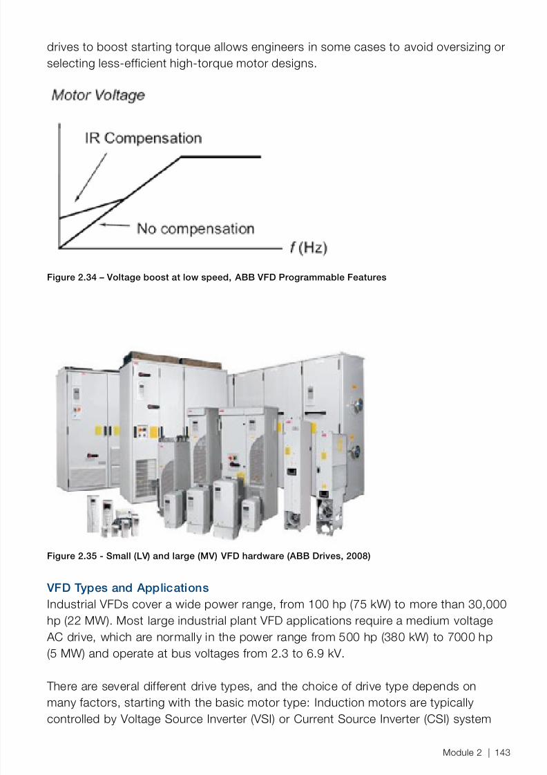
8/12/2019 Energy Efficiency Electronic Book Version 1548_PowerGenerationHandbook v1_1
http://slidepdf.com/reader/full/energy-efficiency-electronic-book-version-1548powergenerationhandbook-v11 145/361
drives to boost starting torque allows engineers in some cases to avoid oversizing orselecting less-efficient high-torque motor designs.
Figure 2.34 – Voltage boost at low speed, ABB VFD Programmable Features
Figure 2.35 - Small (LV) and large (MV) VFD hardware (ABB Drives, 2008)
VFD Types and ApplicationsIndustrial VFDs cover a wide power range, from 100 hp (75 kW) to more than 30,000hp (22 MW). Most large industrial plant VFD applications require a medium voltage
AC drive, which are normally in the power range from 500 hp (380 kW) to 7000 hp(5 MW) and operate at bus voltages from 2.3 to 6.9 kV.
There are several different drive types, and the choice of drive type depends onmany factors, starting with the basic motor type: Induction motors are typicallycontrolled by Voltage Source Inverter (VSI) or Current Source Inverter (CSI) system
Module 2 | 143

8/12/2019 Energy Efficiency Electronic Book Version 1548_PowerGenerationHandbook v1_1
http://slidepdf.com/reader/full/energy-efficiency-electronic-book-version-1548powergenerationhandbook-v11 146/361
topologies. Synchronous motors are typically controlled by Load CommutedInverters or Cycloconverters, all described in the following sections.
The internal converter control method also varies between topologies, and there mayeven be more than one control method to choose from for any given topology. Seethe ABB Guide to Standard MV VFDs (‘Fact Packs #1 and #2)
VFD Internal Design VFDs are power electronics devices that convert a constant input frequency andvoltage into variable frequency and voltage output for the motor. A complete VFDsystem may consist of all these elements: cabling, an input isolation transformer,power factor correction equipment, harmonic filters, the frequency converter itself,output filter, and an electric motor. The combination of all the above elements is thephysical ‘topology’ of the AC drive system. The converter element’s power switchingfunction is the ’motor control platform’, which should not be confused with a low-voltage Motor Control Center described elsewhere in this handbook.
The physical topology provides the electrical ‘hardware’ and the motor control is the‘software’ which performs the power switching routine.
3 Load
Rectier
Supply Side Motor
InverterIntermediateDC Link
Converter
Variable Speed Drive
Figure 2.36 – Diagram showing VFD nomenclature, (ABB Switzerland, MV Drives, 2002)
The most common converter topology is composed of three main equipment stages: − A ‘front-end’ rectifier unit on the 3-phase supply side to convert AC to DC power
and to ensure that harmonics drawn from the network are kept within tolerance.
− A DC link composed of one or more capacitors and inductors which filter andsmooth the DC voltage − An inverter unit, using one of the power electronics technologies described in the
sections below, performs the inversion and modulation of the voltage which isapplied to the motor windings.
The effect of these stages on the sinusoidal input AC supply is shown in the figurebelow:
144 | ABB Energy Efficiency Handbook

8/12/2019 Energy Efficiency Electronic Book Version 1548_PowerGenerationHandbook v1_1
http://slidepdf.com/reader/full/energy-efficiency-electronic-book-version-1548powergenerationhandbook-v11 147/361
Figure 2.37 - VFD waveform at different stages, using PWM-type drive as an example (ABB Inc. 1998)
VFD Power Electronics The switching elements at the heart of much power electronics are thyristors, alsoknown as Silicon Controlled Rectifiers (SCRs). These are turned on (conduct power)by a control signal and will continue conducting until current drops near zero, a
feature known as ‘self-commutation’ (Competitek 1996). The number of switchingelements (or ‘pulses’) in the converter is a measure of the ‘resolution’ of the drivein supplying output to the motor. The number of pulses will roughly determine theamount of VFD harmonics induced in the motor and drawn from the power supply.
The power electronics switching technologies that are in use today are:
− IGCTs (Integrated Gate Commutated Thyristor) offer fast switching (like atransistor) and inherently low losses (conducts like a thyristor); in other words,
it combines the best of both technologies above. IGCT technology is the mostcommon switch in MV drives sold today. − IGBTs (Insulated Gate Bipolar Transistor) are fast switching and low cost, but
losses are high at medium to high voltage levels. Used in LV applications. − GTOs (Gate Turn-Off Thyristor) are thyristors with a controllable ‘off’ switch,
additional circuitry that lowers overall reliability, slows the switching and increasesexpense. GTOs are used in high-current, high-power applications, but haverelatively high MV losses.
From an energy efficiency perspective, a semiconductor drive technology that haslow losses means greater energy efficiency, less cooling equipment, and greaterreliability of the VFD device.
Module 2 | 145
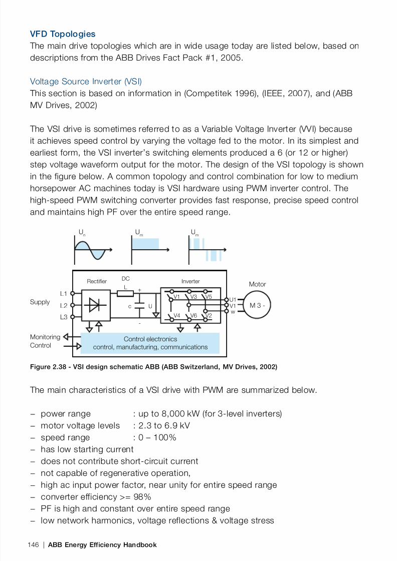
8/12/2019 Energy Efficiency Electronic Book Version 1548_PowerGenerationHandbook v1_1
http://slidepdf.com/reader/full/energy-efficiency-electronic-book-version-1548powergenerationhandbook-v11 148/361
VFD Topologies The main drive topologies which are in wide usage today are listed below, based ondescriptions from the ABB Drives Fact Pack #1, 2005.
Voltage Source Inverter (VSI) This section is based on information in (Competitek 1996), (IEEE, 2007), and (ABBMV Drives, 2002)
The VSI drive is sometimes referred to as a Variable Voltage Inverter (VVI) becauseit achieves speed control by varying the voltage fed to the motor. In its simplest andearliest form, the VSI inverter’s switching elements produced a 6 (or 12 or higher)step voltage waveform output for the motor. The design of the VSI topology is shownin the figure below. A common topology and control combination for low to mediumhorsepower AC machines today is VSI hardware using PWM inverter control. Thehigh-speed PWM switching converter provides fast response, precise speed controland maintains high PF over the entire speed range.
Control electronicscontrol, manufacturing, communications
Motor
Un Um Um
M 3 -Supply
MonitoringControl
DC
L +
-
InverterRectier
L1L2
L3
Uc
V1 U1 V1
w
V3 V5
V4 V6 V2
Figure 2.38 - VSI design schematic ABB (ABB Switzerland, MV Drives, 2002)
The main characteristics of a VSI drive with PWM are summarized below.
− power range : up to 8,000 kW (for 3-level inverters) − motor voltage levels : 2.3 to 6.9 kV − speed range : 0 – 100% − has low starting current − does not contribute short-circuit current − not capable of regenerative operation, − high ac input power factor, near unity for entire speed range
− converter efficiency >= 98% − PF is high and constant over entire speed range − low network harmonics, voltage reflections & voltage stress
146 | ABB Energy Efficiency Handbook
8/12/2019 Energy Efficiency Electronic Book Version 1548_PowerGenerationHandbook v1_1
http://slidepdf.com/reader/full/energy-efficiency-electronic-book-version-1548powergenerationhandbook-v11 149/361
− full torque even at standstill & very low speed− standard drives for pumps, fans, compressors, conveyors
Although PWM is the most common converter control method, other methods suchas Flux Vector can also be used together with the underlying VSI topology.
Current Source Inverter (CSI) This section was adapted from these sources: (IEEE, 2007) and (ABB Switzerland,MV Drives, 2002)
The CSI drive system controls current output to the motor using a gate-turn-off-thyristor current source inverter on the load side. The inverter is operated in a self-commutating mode over the full speed range of the drive; they turn off by themselvesevery time current passes through zero. The amplitude of the motor current isadjusted by the supply-side rectifier, whereas the frequency and thus motor speedis controlled by the load-side inverter. Most modern CSI drives are configured with a12-pulse output (Competitek 1996). A simpler, but less efficient design makes thesedrives suitable for larger induction motors operating at higher speeds. The maincharacteristics of a CSI drive type are summarized below.
− Suitable for larger induction motors− Horsepower range typically 500-10 000 hp (380 kW–7.5 MW) (but is rated up to
80 MW) − Often applied as a retrofit adjustable speed drive system for existing motors. − Output voltage 2.3 to 6.9 kV − Typical applications are pumps, blowers and fans − Capable of regenerative operation
− High efficiency at speeds above 50% − Continuous operation at very low speeds is not always possible. − PF is not constant over entire speed range, and is poor at low speed
− The large filter capacitor (DC–link) introduces additional losses and larger size. − Converter efficiency: 97% − Speed control range 2-100%
Load Commutated Inverter (LCI)For conventional synchronous motors, the most common power electronics drivetechnology is Load Commutated inverter (LCI). Permanent magnet synchronousmotors also use the PWM drive technology.
The following section is based on information from (IEEE, 2007) and (ABBSwitzerland, MV Drives, 2002).
Module 2 | 147

8/12/2019 Energy Efficiency Electronic Book Version 1548_PowerGenerationHandbook v1_1
http://slidepdf.com/reader/full/energy-efficiency-electronic-book-version-1548powergenerationhandbook-v11 150/361
In the LCI design the DC current is switched directly to the synchronous machine’swindings, which behave like a DC machine. LCI drives have a simple and robustdesign because no special switching circuit is needed; the thyristors are switchedby the action of the current waveform of the load itself (Competitek 1996). A controlfunction using a feedback sensor in the motor prevents the rotor from falling out ofstep. The LCI drive system can be furnished with regenerative braking capability,which is discussed in the section on VFD Regenerative Braking . The maincharacteristics of this drive type are:
− Unmodified, it is suitable only for synchronous motors, with brushless or slip ringexcitation
− Wide speed and power range 1- 80 MW − Speed control range (0)-10-100% − More expensive than other drives − Poor power factor at low speed − Suitable for continuous operation
− Fans & pumps, compressors − Converter efficiency > 99%
A modified LCI drive with a large DC-link capacitor can use CSI technology to driveeither synchronous or induction motors. The capacitor also servers to shape thewaveform so that harmonic heating in the motor is reduced (Competitek 1996).
Cycloconverter The Cycloconverter design does not use any intermediate DC circuit, which limits theload frequency to a maximum of 83% of the line frequency (for cross-current typeof drive). Cycloconverters are used for high power, low speed synchronous motordrives such as rolling mill drives, and ship propulsion. The main characteristics ofthis drive type are:
− Power range 1.5 – 30MW − Excellent performance and speed control at low speeds − Non-constant PF − High harmonic distortion − Capable of regenerative operation − Maximum speed limitation 600/720 for 50/60 Hz supply
VFD Control Methods Also referred to as Motor Control Platform, the drive control method is the logic whichswitches the power electronics elements to produce a certain output waveform.
148 | ABB Energy Efficiency Handbook

8/12/2019 Energy Efficiency Electronic Book Version 1548_PowerGenerationHandbook v1_1
http://slidepdf.com/reader/full/energy-efficiency-electronic-book-version-1548powergenerationhandbook-v11 151/361
Pulse Width Modulation (PWM)In small to medium-sizes, the voltage amplitude is held constant and the PWMcontrols average (RMS) voltage by varying the pulse duration and frequency(Competitek 1996) as shown in the gure below. In larger drives the voltage amplitudeis also modulated. PWM outputs current to the motor as a nearly sinusoidal waveform.PWM control is also sometimes referred to as ‘scalar’ or voltage/frequency (V/F)control because a certain voltage is generated for a given frequency.
Voltage
Figure 2.39 – Modulated width voltage pulses from a PWM drive
Scalar vs. Vector Drives The V/F control method is ‘open-loop’ because it does not receive any feedbackfrom the motor itself. In these drives, a fixed volts/Hz pattern is applied to the motor,and the actual torque is then determined by the motor and its load. Precise torque
control is not possible with these drives, and speed control is not possible below10Hz; limitations also commonly associated with DC motors.
‘Vector’ drive control emulates the operating characteristics of a DC motor bytracking the spatial position of the rotor magnetic flux in an AC induction motor.Some common limitations of vector drives: 1) they cannot be used in multi-drive configurations of the type described in the next section 2) they cannot beused if there is a transformer between the drive and the motor. However, vector
drives can produce much higher torques at lower speeds ( 3 to 5 Hz) than PWMdrives, and have torque response and speed accuracy which is several orders ofmagnitude greater than PWM (ABB Oy. Drives 2002). Pump, fan and other cube-lawapplications, however, do not normally require the enhanced torque and low-speedcontrol provided by vector drives. In these applications, lower-cost scalar drives aresufficient.
[ The following descriptions of these drive technologies was adapted from the ABB Technical Guide (ABB Switzerland, MV Drives, 2002).]
Module 2 | 149

8/12/2019 Energy Efficiency Electronic Book Version 1548_PowerGenerationHandbook v1_1
http://slidepdf.com/reader/full/energy-efficiency-electronic-book-version-1548powergenerationhandbook-v11 152/361
Flux Vector ControlFlux vector control (often simply called ‘vector’ control) can produce full torqueat much lower speeds than V/F drive types. By closing the loop with motor statefeedback, vector drives provide a torque response and speed accuracy that areseveral orders of magnitude greater than with open-loop scalar drives. Flux vectorcontrol, however, requires an extra speed feedback device (encoder) between motorand the drive control system to sense the speed and position of the shaft.
Sensor-less Vector Control The ‘sensor-less’ flux vector technology uses a motor model to eliminate the needfor feedback from a tachometer or encoder. The model uses internal measurementsof motor current within the drive to determine torque and flux. An algorithmestimates motor slip, speed and shaft position. The drive can then calculate thenecessary voltage and frequency to produce the desired torque and speed.
When a vector drive operates in torque control mode the speed is then determinedby the load. In screw pumps a drive using torque control technology will be able toadjust itself for sufficient starting torque for a guaranteed start. In conveyor systems,torque control may be used to control feed rates where one section is allowed to runfaster than another.
Vector drives can be selected to operate in either torque-control (vector) or speed-
control (scalar) modes. Note that at very low speeds (< 5Hz), sensor-less vectordrives cannot easily determine magnetic parameters, and motor slip estimates thenbecome inaccurate. This inaccuracy makes sensor-less drives generally unsuitablefor crane and hoist operations; other vector drive designs avoid this limitation.
Direct Torque Control ABB’s proprietary variant of sensor-less vector drive, Direct Torque Control (DTC)allows the motor’s torque and flux to be used as primary control variables, without
the need for an additional modulation processing step. Torque response time isan order of magnitude faster than with other vector drive designs. Using the DTCtechnique, the torque accuracy is 2% within a speed range of 2-100% and a loadrange of 10-100%. A DTC drive can work with any type of induction motor ofasynchronous, squirrel cage design.
A feature of DTC that contributes to energy efficiency is a development called motorflux optimization. With this feature, the efficiency of the total drive (that is controllerand motor) is greatly improved in fan, pump, and other variable speed applications.
The efficiency gains are greatest at lower speeds, as shown in the figure below. Forexample, with 25% load there is up to 10% total energy efficiency improvement. At50% load there can be 2% total efficiency improvement.
150 | ABB Energy Efficiency Handbook

8/12/2019 Energy Efficiency Electronic Book Version 1548_PowerGenerationHandbook v1_1
http://slidepdf.com/reader/full/energy-efficiency-electronic-book-version-1548powergenerationhandbook-v11 153/361

8/12/2019 Energy Efficiency Electronic Book Version 1548_PowerGenerationHandbook v1_1
http://slidepdf.com/reader/full/energy-efficiency-electronic-book-version-1548powergenerationhandbook-v11 154/361
Figure 2.41 - Multi-drive system1) rectifier section 2) common DC-link 3) drive sections 4) power sup-ply (ABB Drives 2002)
Multi-drive systems are cost-effective in applications where there are several motorsinstalled close together, such as sets of conveyors, fan banks, pump banks orin master-slave applications which require motor synchronization, such as papermachines. Compared to set of single drives, these systems save cabling on the
power input side and allow faster replacement of faulty units. The cost of multi-drivesare decreasing, but these systems still require some engineering when comparedto single drive applications; this may explain why multi-drives are generally under-utilized in industry. A lifecycle cost (LCC) analysis, however, may reveal energysavings large enough to overcome a preference for standard, non-engineered singledrive products.
AC Motor Control Terminology
Discussions on motor speed or torque control require clarication of a few basic termsin common usage. The Variable Speed Drive (VSD) term, as used in the Pump andFan sections of this handbook, refers to any means of modulating the output shaftspeed given a constant input shaft speed from the source of drive power. Anothercommon and equivalent term to VSD is ASD: Adjustable Speed Drive. A variety ofmethods to vary shaft speed are discussed in the Motors and Drive Trains section.In some industry texts the broader term VSD is used even when VFD control is meant.Sometimes, only the word ‘drive’ or ‘converter’ is used to refer to a VFD, and sometechnical sources may incorrectly refer to the entire VFD as only ‘the inverter’. Thenaming situation is further complicated when AC torque control drives, also known asvector drives, are included. The preferred, and least ambiguous, term for all these ACdrive technologies is Variable Frequency Drive, abbreviated as VFD.
152 | ABB Energy Efficiency Handbook
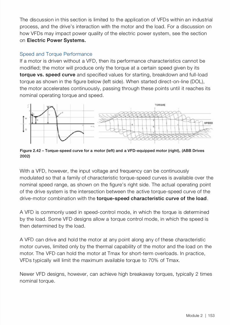
8/12/2019 Energy Efficiency Electronic Book Version 1548_PowerGenerationHandbook v1_1
http://slidepdf.com/reader/full/energy-efficiency-electronic-book-version-1548powergenerationhandbook-v11 155/361
The discussion in this section is limited to the application of VFDs within an industrialprocess, and the drive’s interaction with the motor and the load. For a discussion onhow VFDs may impact power quality of the electric power system, see the sectionon Electric Power Systems.
Speed and Torque PerformanceIf a motor is driven without a VFD, then its performance characteristics cannot bemodified; the motor will produce only the torque at a certain speed given by itstorque vs. speed curve and specified values for starting, breakdown and full-loadtorque as shown in the figure below (left side). When started direct-on-line (DOL),the motor accelerates continuously, passing through these points until it reaches itsnominal operating torque and speed.
Figure 2.42 – Torque-speed curve for a motor (left) and a VFD-equipped motor (right), (ABB Drives2002)
With a VFD, however, the input voltage and frequency can be continuouslymodulated so that a family of characteristic torque-speed curves is available over thenominal speed range, as shown on the figure’s right side. The actual operating pointof the drive system is the intersection between the active torque-speed curve of thedrive-motor combination with the torque-speed characteristic curve of the load .
A VFD is commonly used in speed-control mode, in which the torque is determinedby the load. Some VFD designs allow a torque control mode, in which the speed is
then determined by the load.
A VFD can drive and hold the motor at any point along any of these characteristicmotor curves, limited only by the thermal capability of the motor and the load on themotor. The VFD can hold the motor at Tmax for short-term overloads. In practice,
VFDs typically will limit the maximum available torque to 70% of Tmax.
Newer VFD designs, however, can achieve high breakaway torques, typically 2 timesnominal torque.
Module 2 | 153

8/12/2019 Energy Efficiency Electronic Book Version 1548_PowerGenerationHandbook v1_1
http://slidepdf.com/reader/full/energy-efficiency-electronic-book-version-1548powergenerationhandbook-v11 156/361
VFD Operating RegionsFor speeds below the nominal speed, the magnetic flux in the motor is constant.
At speeds above the nominal frequency/speed the motor operates in the ‘field-weakening’ range, in which magnetic flux density is sacrificed for higher speed. Themaximum torque of an induction motor is proportional to the square of the magneticflux. Below Ns the Tmax is constant; above Ns the Tmax decrease is inverselyproportional to the square of the frequency.
For example, a 100 hp, 460 V, 60 Hz, 1775 RPM (4 pole) motor supplied with 460 V, 75 Hz (6.134 V/Hz), would be limited to (60/75)2 = 64% torque at 125% speed(2218.75 RPM) = 100% power.
In most applications a VFD approach is chosen to provide different torque vs. speedperformance than would be possible for the motor by itself. This performance isusually matched to the load’s torque–speed performance curve. For example,constant torque over a wide range of speed is a common requirement for manyapplications. The figure below shows how voltage and speed control can achievetheoretical constant Tmax over the range of speed from zero to synchronous speed(n/ns =1.). At higher speeds, the weakening magnetic field causes torque to drop inquadratic fashion, known as the constant power region of operation.
VFD Performance & Efficiencies
Motors are developed and optimized to run at constant voltage and frequency andat full load. Adding another device, a VFD, cannot improve the combined efficiencyof the system operating at full load. In fact, the non-sinusoidal electrical output plusthe internal losses created by the VFD actually lower the combined efficiency at fullload by several percentage points, compared to the motor acting alone. (Competitek1996).
A VFD saves energy when it can modulate the motor power to match loads which
are less than 100% full load. Variable flow applications are obvious candidates, butconstant speed applications would benefit as their loads are seldom perfectly andforever matched to the rating of the motor. Many well-matched, constant-speedapplications could still profit from VFD soft start, power-factor correction and other
VFD Features .
Motor Current EstimationEstimating motor current is important for dimensioning a VFD, and can be done oncethe motor torque characteristic is known. The total current in a motor (I
m ) has active
(Iq ) and reactive (Id ) including magnetizing current components, as described in thesection on the power triangle . Only the active current component can producetorque; when torque is zero, so is the active current. The active current can always
154 | ABB Energy Efficiency Handbook

8/12/2019 Energy Efficiency Electronic Book Version 1548_PowerGenerationHandbook v1_1
http://slidepdf.com/reader/full/energy-efficiency-electronic-book-version-1548powergenerationhandbook-v11 157/361
be calculated by multiplying the total current by the power factor, also shown ascos(ϕ n ).
In the constant flux region (below field weakening point):
In the constant flux region the motor currents do not depend on speed. The activecurrent can be approximated as follows:
Ia = In x (T load /T n ) x cos(ϕ n )
Where: In = nominal (nameplate) current
At higher torque values motor current becomes nearly proportional to the torque. Agood approximation for total motor current at a given load is as follows:
Im = In x (T load /T n ) when T load is between 0.8 x T n and 0.7 x T max
For example: a 150 kW motor’s nominal current is 320 A at power factor 0.85.What are the approximate active and total currents at 120% torque, below the fieldweakening point? Using the approximation formulas from above:
Ia = 320 x 1.2 x 0.85 = 326 A
Im = 320 x 1.2 = 384 A
In the decreasing flux region (above field weakening point), the motor currentsdepend on speed. The active current can be approximated as follows:
Ia = In x (T load /T n ) x ( n/nn ) x cos(ϕ n ) = In x (Pload /P n ) x cos(ϕ n )
Where:
Pn = nominal (nameplate) power
Within a certain operating region the total motor current becomes proportional to therelative power.
Im = I
n x (T
load /T
n ) x ( n/n
n ) = = I
n x (P
load /P
n ) when T
load is between 0.8 x (n
n /n) and
0.7 x (nn /n)2 x T max
Module 2 | 155

8/12/2019 Energy Efficiency Electronic Book Version 1548_PowerGenerationHandbook v1_1
http://slidepdf.com/reader/full/energy-efficiency-electronic-book-version-1548powergenerationhandbook-v11 158/361
For example: a 150 kW motor’s nominal current is 320 A. How much current isneeded to maintain the 100% torque level at 1.3 times nominal speed (assume Tmax=3 x Tn)? Using the approximation formula above:
Im = 320 x 1.3 = 416 A
For additional motor power and torque formulas see the Motor and Drive Trainsection .
Drive EfficiencyEfficiency levels of MV AC drives vary from 95 to 99%, including the supplytransformer, power factor correction equipment and any harmonic filters. A typical
VFD efficiency curve stays relatively high (above 90%) and constant until about 20%of full load. At loads below 20% full load, the VFD efficiency drops to between 75%and 90%. This drop is partly because the losses in the drive electronics accountfor an increasing proportion of the input power. The extra protective circuits whichare often built-into modern VFDs, such as suppressors and line reactors, improvereliability but they come at a slight cost in drive efficiency (Liptak, 2005). Vendors of
VFDs may promote small drive efficiency margins over other vendors, but these aretiny compared to the efficiency gains of the entire drive power system, VFD, drivetrain and pump or fan. Engineering support, programmability and other factors willlikely play a more important role in total drivepower system efficiency, which is the
only valid basis for comparisons and design decisions.
VFD Harmonics A harmonic is a sinusoidal component of a periodic wave or quantity having afrequency that is an integral multiple of the fundamental frequency. Harmonics arecaused by the non-linear switching action of VFD inverter electronics. The rapid stepchanges in voltage levels found in most drive outputs, and especially in PWM drives,create flux harmonics and heating within the motor. Rotor heating from PWM drives
can range from 30% to over 300% more than with only 60Hz input power, dependingon the type of modulation control used (Competitek 1996).
High harmonic content coming from early frequency converters led to heatingof motor windings and the practice of de-rating the motor 5-10% for use with
VFDs. Modern VFD drives now output low levels of harmonic content andperform according to the detailed standards in IEEE 519 and NEMA MG1 Part 31specifications (or G5/3 n the UK); it is usually no longer necessary to de-rate a motorfor use with a VFD (US DoE, 2008).
Harmonics tend to be drawn from the supply network and may affect other electricalequipment. For a discussion of the energy impact of these supply-side harmonics,
156 | ABB Energy Efficiency Handbook

8/12/2019 Energy Efficiency Electronic Book Version 1548_PowerGenerationHandbook v1_1
http://slidepdf.com/reader/full/energy-efficiency-electronic-book-version-1548powergenerationhandbook-v11 159/361
and of ways to mitigate their effects, see the Electric Power Systems sectionHarmonics Mitigation .
VFD Application Design and Engineering After two decades on industrial service, VFDs have evolved to high levels of reliabilityand functionality. Early VFD pitfalls have been eliminated in modern VFD designs.On the motor side, early pitfalls encountered with VFD applications were related toharmonics and voltage spikes, which induced heating and led to motor damage.On the power side, early pitfalls with VFDs were line interference, power systemharmonics and poor power factor at low speeds.
VFD Trends Advancements in power electronics and usability are moving drives toward thestatus of a commodity item. In the past, all drives were considered ‘engineered’items which suppliers (such as ABB) would configure based on detailed applicationspecifications that the customer would put out to tender. Engineered drives withcustom capabilities may still be required for applications with special loadingprofiles, special environmental conditions, or where plant power supply issuessuch as harmonics and phase unbalance pose a particular challenge. Most driveshave features that handle these issues ‘out of the box’ for approximately 85% of allapplications (ABB Drives, 2006). All drives are available as separate devices, butoften ‘component’ drives are embedded in small-scale OEM equipment solutions
requiring speed control.
Although VFDs are becoming more of a commodity item, careful engineeringfollowing the guidelines below will help to address most of the problem areas and toachieve the expected efficiency improvements.
VFD Selection and Sizing The following sections provide an overview of the steps involved in dimensioning a
drive system. This overview focuses on energy efficiency aspects; for more completeguidelines see the full ABB Technical Guide No.7 for Dimensioning a Drive (ABBDrives 2002) upon which this section is based, or the NEMA Application Guide for
AC Adjustable Speed Drive Systems 2001, IEEE Paper No. PCIC-2001-7.
Select Drive Size & RatingStandard drives can be selected from the catalog and with some vendor assistance,based on inputs from the process, mechanical and electrical application engineers.
The requirements for each of the four main elements in the drivetrain system areshown in the figure below.
Module 2 | 157

8/12/2019 Energy Efficiency Electronic Book Version 1548_PowerGenerationHandbook v1_1
http://slidepdf.com/reader/full/energy-efficiency-electronic-book-version-1548powergenerationhandbook-v11 160/361
Figure 2.43 – Drive dimensioning procedure, (ABB Drives 2002)
The typical dimensioning steps for a drive and motor system are listed below. These steps apply mainly for variable torque applications, such as a pump or fan
application. Details and example calculations for each step are given in the ABB Technical Guide for Dimensioning of a Drive System, 2002.
Step 1: Check initial requirements and conditions of network and the load
− 1.1 Required voltage level (LV or MV) − 1.2 Required quadrant control (reversing, regeneration) − 1.3 Required power system capability (voltage/frequency/harmonics tolerance)
− 1.4 Required maximum application load (for example, fan or pump) power andspeed
Step 2: Choose the (or evaluate an existing) motor
158 | ABB Energy Efficiency Handbook

8/12/2019 Energy Efficiency Electronic Book Version 1548_PowerGenerationHandbook v1_1
http://slidepdf.com/reader/full/energy-efficiency-electronic-book-version-1548powergenerationhandbook-v11 161/361
Figure 2.44 – Motor loadability curves comparing 1) 2-pole and 2) 4-pole motors
− 2.1 Determine the required maximum load torque at full speed - narrowselection of motors
− 2.2 Check motor loadability. using torque profile curve, at the nominal speedand then over the required speed (rpm) operating range
− 2.3 Check for high application load torque starting conditions
− 2.4 Determine motor nominal torque and power, based on number of motorpoles − 2.5 Select a new (or approve an existing) motor; add a margin (from 10 to 30%,
depending on loading information certainty) so that power is available atmaximum speed.
Step 3: Choose a VFD and associated equipment
− 3.1 Determine type of load (cube law, constant power, constant torque,quadrant operation)
− 3.2 Determine total motor continuous current (Amps) at full speed − 3.3 Specify any special operating conditions and required IP (enclosure) class
Module 2 | 159
8/12/2019 Energy Efficiency Electronic Book Version 1548_PowerGenerationHandbook v1_1
http://slidepdf.com/reader/full/energy-efficiency-electronic-book-version-1548powergenerationhandbook-v11 162/361
− 3.4 Select a drive based on current estimation and vendor tables − 3.5 Specify drive cooling requirement based on drive selection, ambient
conditions − 3.6 Specify input transformer power rating − 3.7 Specify length and type of cabling between drive and motor
In Step 1, the application load (for example, the pump or fan) power rating atmaximum speed can be used to determine the necessary application torquerequirement using the power – torque formulas. The power supply network mustbe capable of providing nominal voltage (step 1.1). If the supply voltage is lowerthan nominal, the field weakening point shifts to a lower frequency and the availablemaximum torque of the motor is also reduced in the field weakening range (ABBDrives 2002).
In Step 2, the motor nominal values for power and torque are determined, basedon the application requirement (from step 2.1) and the motor model loadability data.
Then a motor selection can be made, or an existing motor is approved for a driveretrofit.
In Step 3, the motor total current is determined based on the nominal motor valuesin Step 2 and load torque in Step 1, and then a drive selection is made. A driveshould be dimensioned according to the continuous full load current requirement,
and not the horsepower requirement. The mechanical or process unit needs areusually supplied in terms of a motor load torque characteristic, from which motorcurrent is derived according to the motor current approximation formulas . Thesevalues are then compared to the converter’s limits to select the correct size andmodel. The motor’s nominal current may also be used as a first approximation forconverter dimensioning. Note that when a high-efficiency motor is specified in Step2, then a smaller drive might suffice due to the lower current requirements.
A common temptation in VFD sizing is to add a design margin to the VFD size. Thisis not usually necessary because in common practice the motor has already receiveda very high margin . The VFD is merely a conduit for motor power and thereforeadding a margin only for ‘process flexibility’ serves no purpose. An exception to thisrule is if there is possibility for the motor to exceed its full load amp rating (beyondservice factor margin). This situation may arise due to unforeseen changes inprocess flow densities, for example. In such cases, a higher drive rating is necessaryto avoid drive trips. Another exception is if the drive is to be located in warm ambientconditions, as may be the case in small industrial boiler applications (Plantsystems.com, 11/2008).
160 | ABB Energy Efficiency Handbook
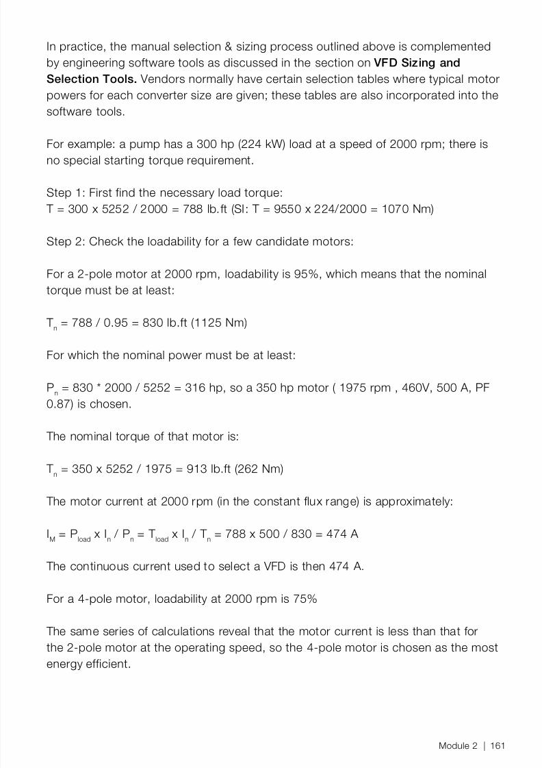
8/12/2019 Energy Efficiency Electronic Book Version 1548_PowerGenerationHandbook v1_1
http://slidepdf.com/reader/full/energy-efficiency-electronic-book-version-1548powergenerationhandbook-v11 163/361
In practice, the manual selection & sizing process outlined above is complementedby engineering software tools as discussed in the section on VFD Sizing andSelection Tools. Vendors normally have certain selection tables where typical motorpowers for each converter size are given; these tables are also incorporated into thesoftware tools.
For example: a pump has a 300 hp (224 kW) load at a speed of 2000 rpm; there isno special starting torque requirement.
Step 1: First find the necessary load torque: T = 300 x 5252 / 2000 = 788 lb.ft (SI: T = 9550 x 224/2000 = 1070 Nm)
Step 2: Check the loadability for a few candidate motors:
For a 2-pole motor at 2000 rpm, loadability is 95%, which means that the nominaltorque must be at least:
T n = 788 / 0.95 = 830 lb.ft (1125 Nm)
For which the nominal power must be at least:
Pn = 830 * 2000 / 5252 = 316 hp, so a 350 hp motor ( 1975 rpm , 460V, 500 A, PF
0.87) is chosen.
The nominal torque of that motor is:
T n = 350 x 5252 / 1975 = 913 lb.ft (262 Nm)
The motor current at 2000 rpm (in the constant flux range) is approximately:
IM = P load x In / P n = T load x In / T n = 788 x 500 / 830 = 474 A
The continuous current used to select a VFD is then 474 A.
For a 4-pole motor, loadability at 2000 rpm is 75%
The same series of calculations reveal that the motor current is less than that forthe 2-pole motor at the operating speed, so the 4-pole motor is chosen as the mostenergy efficient.
Module 2 | 161

8/12/2019 Energy Efficiency Electronic Book Version 1548_PowerGenerationHandbook v1_1
http://slidepdf.com/reader/full/energy-efficiency-electronic-book-version-1548powergenerationhandbook-v11 164/361
Voltage Level: Low-Voltage (LV) vs. Medium Voltage (MV) The selection process begins with selection of the voltage level. Low voltage ACdrives may be technically possible for certain power levels and their generally lowerprice may seem attractive. However, LV drives draw higher current for a given motorpower than for MV drives. For long cable lengths between motor and inverter, thelarger required cable diameter and cost will favor an MV drive option. Power systemcontrol and protection devices like contactors may be a limiting factor in high-power LV designs.
Converter voltage output ranges up to 4kV, which is sufficient for most standardLV and MV motors. For HV motors, however, a specially designed step-up outputtransformer is required. A standard transformer cannot be used due to variation infrequency, the harmonic distortion and the DC component existing during transientsin the output voltage of the frequency converter.
The selection of VFD voltage level is closely related to the selection of bus voltagelevels as described in the section on Power System Design and Engineering . For aretrofit, the availability of MV or LV busses is a decisive factor.
Quadrant Control, Converter Basic Type The converter technology largely determines the drive losses, and hence therequirement for cooling, the drive’s physical size, and reliability. The converter
selection also determines many aspects of the drive-plus-motor’s torque-speedperformance. Application requirements should be carefully considered in this step ofthe selection process. Special requirements for 4-quadrant control will also stronglyaffect the drive technology selection; see the VFD Types and Applications sectionfor the common application areas for various drive technologies.
Motor Capability – Harmonics Although it is usually no longer necessary to derate a motor for use with a modern
VFD, it is still good practice to check with the drive or motor suppliers as to whethera specific motor can tolerate the drive’s harmonic levels. Older and/or rewoundmotors may have reduced tolerance for the effects of harmonics.
A class of motors called ‘inverter duty’ (NEMA MG1 Part 31) offers a higherperformance standard to ensure compatibility with VFDs. Modern VFDs ,however,are designed to work within the tolerances of the ‘general purpose’ class of motors;this was not generally the case for older 6-step drive inverters.
Motor Capability – Retrofit SituationsModern VFD drives can be applied to many existing induction & synchronous motorsas part of a retrofit without de-rating 5-10% as was done previously. In addition to
162 | ABB Energy Efficiency Handbook

8/12/2019 Energy Efficiency Electronic Book Version 1548_PowerGenerationHandbook v1_1
http://slidepdf.com/reader/full/energy-efficiency-electronic-book-version-1548powergenerationhandbook-v11 165/361

8/12/2019 Energy Efficiency Electronic Book Version 1548_PowerGenerationHandbook v1_1
http://slidepdf.com/reader/full/energy-efficiency-electronic-book-version-1548powergenerationhandbook-v11 166/361
damage motor insulation, and are a particular concern in MV retrofit situations (ABBSwitzerland, MV Drives, 2002). Some preventive design tips for inverter-fed motorsare 1) use input and output reactive filters and 2) ensure that the grounding systemis well designed. According to one source, (Competitek 1996), PWM drives cannottolerate long cable lengths (longer than 500 m due to standing wave effects. It isimportant to consult with drive vendors and their expertise before specifying VFDswith long cabling to motors.
Radiated EMIRadiated EMI
3-Phases, Earth Variable cable length
MOTORConducted EMI
O u
t p u
t F i l t e r
V S D
I n p u
t F i l t e r
Conducted EMI
Figure 2.44 – EMI disturbance from VFD (shown as VSD above) cabling, (DeAlmeida, 2006)
Circulating currents can also be induced in the walls of metal conduits, even whenit contains balanced phases. A preventive design tip is to use non-metallic conduitmaterial, such as PVC (Competitek 1996).
Motor Capability - Resonance Issues The following issues may arise due to complex, dynamic interactions between the VFD drive-electric motor and pump (or fan) system. These unwanted dynamicsare usually eliminated for maintenance or reliability reasons, but they also degradesystem energy efficiency if allowed to continue at a level judged ’tolerable’ for theequipment. This phenomenon is also called ‘torque pulsation’ in some technicalsources.
− Structural Resonance. Resonance is a mechanical vibration phenomenonthat occurs when the VFD output frequency matches the one of the naturalfrequencies of the entire pump, piping, and mounting system. The strongvibrations at these particular frequencies are harmful to the motor and pumpequipment couplings, bearings and support structure.
− These resonances are usually designed-out of pumps and motor combinationsoperating at known constant speeds. In variable speed applications however, thewide variation in motor frequency may uncover new resonances, especially thoseresulting from fluid pressure pulsations. Pumping system authorities (US Doe,Hydraulic Institute, Europump) recommend the following techniques to predictand avoid resonance situations (US DoE, 2008):
− Simple hydraulic resonance calculations
164 | ABB Energy Efficiency Handbook

8/12/2019 Energy Efficiency Electronic Book Version 1548_PowerGenerationHandbook v1_1
http://slidepdf.com/reader/full/energy-efficiency-electronic-book-version-1548powergenerationhandbook-v11 167/361
− Passing frequency analysis − Using Finite Element Analysis to reveal structural resonance − Modal testing on the actual machines, via a vibration test
Modal testing involves using an electromagnetic shaker or impulse hammer to applya force that is measured by an accelerometer (Plantservices.com, 2008). In retrofitsituations, where motor hardware cannot be easily re-designed, the VFD can beprogrammed to avoid troublesome resonant frequencies, once they have beenidentified using the methods described above.
Starting Load Torque and Speed Issues A VFD provides many different loading options compared to the motor acting alone. As shown previously, a VFD can provide nearly constant torque over a widerange of speed, as shown in Curve1 in the figure below (for a 50Hz nominal inputfrequency). For applications with high but temporary starting torque requirements,then the VFD can produce torque following Curve 3 in the figure below. Vector drivesare particularly suitable for supplying high torque at low speeds.
Figure 2.45 - Motor torque performance curves possible with VFD control, (ABB Oy. Drives, 2002)
A heavier-duty VFD may be required for applications with high starting torquerequirements, or where there are high torque pulsations (Competitek 1996). TheNEMA Application Guide for AC Drives (2001) cautions that applications withstatic torques above 140% of full load torque may require an oversized drive and amotor with higher torque capacity . Vector drives are an alternative solution to thisapplication requirement.
Variable torque loads such as most pumps (and some fans) have low torques atlow starting speeds. Constant torque applications typically have higher startingtorque requirements than variable torque loads. High-inertia rotating machinery,
Module 2 | 165
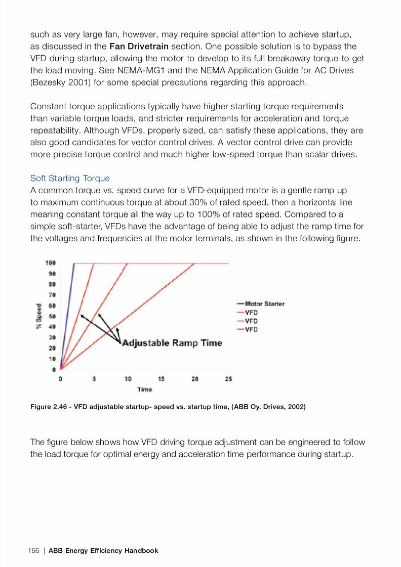
8/12/2019 Energy Efficiency Electronic Book Version 1548_PowerGenerationHandbook v1_1
http://slidepdf.com/reader/full/energy-efficiency-electronic-book-version-1548powergenerationhandbook-v11 168/361
such as very large fan, however, may require special attention to achieve startup,as discussed in the Fan Drivetrain section. One possible solution is to bypass the
VFD during startup, allowing the motor to develop to its full breakaway torque to getthe load moving. See NEMA-MG1 and the NEMA Application Guide for AC Drives(Bezesky 2001) for some special precautions regarding this approach.
Constant torque applications typically have higher starting torque requirementsthan variable torque loads, and stricter requirements for acceleration and torquerepeatability. Although VFDs, properly sized, can satisfy these applications, they arealso good candidates for vector control drives. A vector control drive can providemore precise torque control and much higher low-speed torque than scalar drives.
Soft Starting Torque A common torque vs. speed curve for a VFD-equipped motor is a gentle ramp upto maximum continuous torque at about 30% of rated speed, then a horizontal linemeaning constant torque all the way up to 100% of rated speed. Compared to asimple soft-starter, VFDs have the advantage of being able to adjust the ramp time forthe voltages and frequencies at the motor terminals, as shown in the following gure.
Figure 2.46 - VFD adjustable startup- speed vs. startup time, (ABB Oy. Drives, 2002)
The gure below shows how VFD driving torque adjustment can be engineered to followthe load torque for optimal energy and acceleration time performance during startup.
166 | ABB Energy Efficiency Handbook
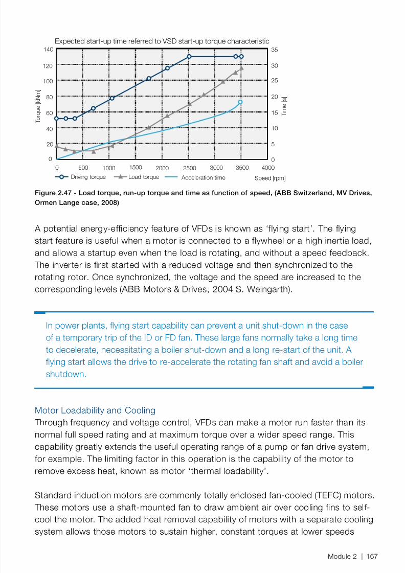
8/12/2019 Energy Efficiency Electronic Book Version 1548_PowerGenerationHandbook v1_1
http://slidepdf.com/reader/full/energy-efficiency-electronic-book-version-1548powergenerationhandbook-v11 169/361
Expected start-up time referred to VSD start-up torque characteristic
Acceleration time Speed [rpm]Load torqueDriving torque
140
120
100
80
60
40
20
00 500 1000 1500 2000 2500 3000 3500 4000
0
5
10
15
20
25
30
35
T o r q u e
[ k N m
]
T i m e [ s
]
Figure 2.47 - Load torque, run-up torque and time as function of speed, (ABB Switzerland, MV Drives,Ormen Lange case, 2008)
A potential energy-efficiency feature of VFDs is known as ‘flying start’. The flyingstart feature is useful when a motor is connected to a flywheel or a high inertia load,and allows a startup even when the load is rotating, and without a speed feedback.
The inverter is first started with a reduced voltage and then synchronized to therotating rotor. Once synchronized, the voltage and the speed are increased to thecorresponding levels (ABB Motors & Drives, 2004 S. Weingarth).
In power plants, ying start capability can prevent a unit shut-down in the caseof a temporary trip of the ID or FD fan. These large fans normally take a long timeto decelerate, necessitating a boiler shut-down and a long re-start of the unit. Aying start allows the drive to re-accelerate the rotating fan shaft and avoid a boilershutdown.
Motor Loadability and Cooling Through frequency and voltage control, VFDs can make a motor run faster than itsnormal full speed rating and at maximum torque over a wider speed range. Thiscapability greatly extends the useful operating range of a pump or fan drive system,for example. The limiting factor in this operation is the capability of the motor toremove excess heat, known as motor ‘thermal loadability’.
Standard induction motors are commonly totally enclosed fan-cooled (TEFC) motors. These motors use a shaft-mounted fan to draw ambient air over cooling fins to self-cool the motor. The added heat removal capability of motors with a separate coolingsystem allows those motors to sustain higher, constant torques at lower speeds
Module 2 | 167

8/12/2019 Energy Efficiency Electronic Book Version 1548_PowerGenerationHandbook v1_1
http://slidepdf.com/reader/full/energy-efficiency-electronic-book-version-1548powergenerationhandbook-v11 170/361
when equipped with a VFD. The effect of extra cooling is shown on the followingfigure. The following figure shows how an actual VFD can provide near-constanttorque from zero to nominal speed, if sufficient cooling is available to maintain aconstant nominal operation temperature for the motor; values with subscript ‘n’ arenominal values. Note that torque is limited in the field weakening range of operationregardless of cooling method.
Figure 2.48 – Standard induction motor loadability 1) without and 2) with separate cooling, (ABBDrives 2002)
With VFD speed and torque ‘overdrive’, a motor may be dimensioned accordingto its normal use, not for transient peak conditions, thus reducing motor size andinvestment cost. Where loading peaks are expected, however, it is important that theload, the VFD and the motor are compatible, otherwise the motor or the convertermay overheat and increase the risk of damage.
168 | ABB Energy Efficiency Handbook

8/12/2019 Energy Efficiency Electronic Book Version 1548_PowerGenerationHandbook v1_1
http://slidepdf.com/reader/full/energy-efficiency-electronic-book-version-1548powergenerationhandbook-v11 171/361
Figure 2.49 - Torque-speed curves with VSI-PWM VFD and 2 types of load, (based on deAlmeida,
2006)
This figure shows torque and power for a totally-enclosed fan-cooled (TEFC)induction motor fed by a VSI-PWM type VFD, assuming. Two typical load curves areshown; constant and quadratic (i.e. cube-law power load) torque. These loads canbe served by a normally-sized VFD. Loads with high starting or breakdown torquerequirements require more careful sizing and selection of the VFD .
Drive Loadability and Cooling IssuesEnergy losses in the VFD cubicle are a measure of the drive efficiency. For drivesaveraging 98% efficiency, therefore, the heat energy is 2% of the input power. Thisheat must be removed from the VFD, usually through forced cooling. It is importantto ensure sufficient drive module cooling and to include the drive fans and coolingsystem in a regular maintenance program.
Generally speaking, a frequency converter’s short term loadability is often morecritical than the motor’s. The motor thermal rise times are typically from 15 minutes(small motors) to several hours (big motors) depending on the motor size. Thefrequency converter’s thermal rise times (typically a few minutes) are given in theproduct manuals (ABB Drives 2002).
Proper application design and regular maintenance are the key to realizing drivesuppliers claims of mean-time-between-failure (MTBF) specification somewherebetween 20 and 100 years. Advances in technology however, are likely to prompt afacility to upgrade a drive within a shorter time frame. The life expectancy of the VFDconverter is generally directly related to the temperature of the internal components,especially the capacitors (US DoE, 2008).
Module 2 | 169

8/12/2019 Energy Efficiency Electronic Book Version 1548_PowerGenerationHandbook v1_1
http://slidepdf.com/reader/full/energy-efficiency-electronic-book-version-1548powergenerationhandbook-v11 172/361
Power System Capability A VFD and motor running at much lower than full speed have a lowered powerfactor. Drives with sufficient power factor correction capability are desirable inapplications which require long periods of low speed operation. Harmonics inducedby the VFD on the power supply network are one of the issues discussed in thePower Systems section.
Input Transformers VFDs in the MV range require input transformers to manage the connection to thepower system. These transformers perform several functions:
− They adjust power supply voltage to the levels required by the converter; mostsuppliers have drives that can be connected to 3.3 – 6.9 kV today, but manyplants have voltages that lie outside this range.
− They protect the motor and/or network from common mode voltages. − They provide isolation in case of faults; there is no physical (metallic) contact
between primary and secondary windings.
Modern VFDs have small ‘footprints’ and a flexible input transformer configuration. This configuration allows the large input transformer (See picture below) to be placedoutside the electrical room. The choice of VFD power electronics affects the flexibilityof the layout. For example, a 3-level VSI topology reduces the number of cables
between the input transformer and the converter (ABB Switzerland, MV Drives,2002). An input transformer that can be located outside the electrical room reducesthe size and cooling requirements for that room (ABB Switzerland, MV Drives, 2002).
170 | ABB Energy Efficiency Handbook

8/12/2019 Energy Efficiency Electronic Book Version 1548_PowerGenerationHandbook v1_1
http://slidepdf.com/reader/full/energy-efficiency-electronic-book-version-1548powergenerationhandbook-v11 173/361
Figure 2.50 – Photo of a large input isolation transformer, (ABB Drives, 2008)
Operating EnvironmentDue to the sensitivity of drive electronics, in retrofit situations the VFD hardwarecannot usually be placed in the same location as previous mechanical speedreduction equipment (US DoE, 2008). VFDs electronics are housed in an enclosurecalled a ‘cubicle’. Like most electronics, the VFD cannot normally tolerate corrosive,very humid or very hot ambient conditions. For this and other reasons related tocooling (see the section on Drive Cooling), the VFD cubicles are usually placed in
a separate ‘electrical’ room, usually together with low-voltage switchgear & motorcontrol centers. Typical dimensions for a large VFD cubicle are 9–16 ft long, 3 ftdeep and 6 ft high. VFD drives and switchgear can be housed in modular pre-fabricated units for easy site installation and limited civil engineering costs.
Figure 2.51 – Photo of a typical MV drive cubicle ABB Drives, 2008 (ACS-5000 Medium Voltage drive)
VFD Maintenance Availability (the inverse of failure rate) of a modern VFD is typically in the high 99+%range. VFDs provide online diagnostic information of the status of the drive and
Module 2 | 171

8/12/2019 Energy Efficiency Electronic Book Version 1548_PowerGenerationHandbook v1_1
http://slidepdf.com/reader/full/energy-efficiency-electronic-book-version-1548powergenerationhandbook-v11 174/361
motor. This information is accessible via open process industry communicationprotocols and can be used by pro-active maintenance programs to increase thereliability and the energy efficiency of the drive system. Basic values such as VFDinverter and motor temperatures, voltage, frequency, currents, operating hours andeven total number of motor revolutions are recorded and stored at high resolution.Derived values such as energy, torque and horsepower are also calculated andstored for performance improvement efforts such as plant energy efficiencyprograms. The VFD itself also continually performs automatic diagnostics usingthis information, for early fault detection. The average MTBF in months, in a typicalindustrial application such as pump flow control, is 32 months (ABB, Weingarth,
Automation World, 2004). This compares well with the MTBF of a control valve,which is 18 months. (ABB MV drives have an available optional DriveMonitor TM package, for use in modern asset management programs.)
VFD Cost and Technical CalculationsIn the early days of VFDs a small drive cost in the region of US$500 per kW.
Technology advances and economies of scale have brought the price down in theregion of $150 per kW, and the average hardware cost per hp decreases with thesize of the drive. Small to medium drives (100 to 500 hp) range from $200 to $150per hp, while larger drives (500 to 10,000 hp) will range from $100 to $75 per hp.
The total investment cost of a VFD are mainly hardware, engineering and installation
costs. The ‘total installed cost’ of a drive is typically more than double the hardwarecost for small to medium drives, and about 40% more for larger drives. A typical costof a 1,000 hp drive is $100 per hp (ABB Power Systems, 2009). The base cost ofsuch a large system, not including engineering, is about $100kUSD. The total cost istherefore around $185-200kUSD.
The installed cost of a VFD is small when compared to the application’s energysavings from speed control. An analysis of VSD economics by RMI in the Competitek
Drivepower Manual showed payback periods ranging from 4 years down to 1year for initial costs ranging from $750 to $175 per hp, in an industrial pumpingapplication. The handbook’s Case Studies section has a fully worked-out exampleof a flow-control retrofit showing payback and present value cost calculations.
Many of the VFD side benefits are not quantified in lifecycle cost (LCC) calculations. VFDs have many built-in motor protection and power quality functions that replacecostly dedicated equipment in new plant designs; these foregone costs should beconsidered in LCC analyses. Some indirect benefits also reduce the investmentcost; for example, the reduced current in VFD applications means that smaller-sizedelectric power system elements (breakers and cables) may be specified.
172 | ABB Energy Efficiency Handbook

8/12/2019 Energy Efficiency Electronic Book Version 1548_PowerGenerationHandbook v1_1
http://slidepdf.com/reader/full/energy-efficiency-electronic-book-version-1548powergenerationhandbook-v11 175/361

8/12/2019 Energy Efficiency Electronic Book Version 1548_PowerGenerationHandbook v1_1
http://slidepdf.com/reader/full/energy-efficiency-electronic-book-version-1548powergenerationhandbook-v11 176/361

8/12/2019 Energy Efficiency Electronic Book Version 1548_PowerGenerationHandbook v1_1
http://slidepdf.com/reader/full/energy-efficiency-electronic-book-version-1548powergenerationhandbook-v11 177/361
Module Summary This module provides general design & energy impact of the most commoncomponents of in-plant electrical power system, also known as ‘Electrical Balanceof Plant’ (EBoP). Most of the material in this section is applicable to all industrialelectrical power systems. The purpose of this section is to help identify areas ofcontrollable losses in medium and low-voltage (MV and LV) plant power systems andto provide some guidelines to mitigate those losses.
The information in this module may be generally applied to all industrial facilitiesindustries with large internal power distribution networks; industry-specific text isshown in alternate text, such as follows:
For power plants, the scope for this module begins at the generator busbar’sconnection to the auxiliary transformer(s), but also includes the power path
leading through the main step-up transformer. The relationships between electricpower system ‘balance of plant’ (EBoP) items are shown in the gure below.
Figure 3.1– Electrical balance of plant equipment in a fossil-fuel power station, ABB PowerSystems, 2008
Module 3Electric Power Systems for Auxilaries
Module 3 | 175

8/12/2019 Energy Efficiency Electronic Book Version 1548_PowerGenerationHandbook v1_1
http://slidepdf.com/reader/full/energy-efficiency-electronic-book-version-1548powergenerationhandbook-v11 178/361

8/12/2019 Energy Efficiency Electronic Book Version 1548_PowerGenerationHandbook v1_1
http://slidepdf.com/reader/full/energy-efficiency-electronic-book-version-1548powergenerationhandbook-v11 179/361
Power System – Overview The purpose of the in-plant power services is to supply electrical power to plant auxiliaryprocess loads, instruments and control systems. The criteria for delivery of this power are:
− Power quality: allow only tolerable small amounts of harmonics, spikes, sags andswells or phase voltage unbalance.
− Power factor: control the power factor at all levels of the plant to reduce thelosses associated with carrying reactive power.
− Power level and capacity: supply power to required capacity, at the voltagelevels needed, through efficient, right-sized transformers.
− Power protection & control: allow full automatic or manual control of powerdistribution to serve the needs of the loads, while protecting those loads and thepower system itself from harm.
− Power distribution & layout: carry power from the source to its destination at theload with minimal losses.
− Power reliability: supply all the above with high reliability
All of the above design criteria have a direct impact on plant energy efciency, which isthe focus of this module.
In a power plant, most of the auxiliary power demand, up to 80% of total auxiliary
load, is used by large MV electric motors that are typically connected to the mediumvoltage switchgears/switchyards supplied through unit auxiliary transformers.
Between 6 to 15% of gross electrical output can go to auxiliary power, dependingon the type of prime mover for large pumps and fans, the type of fossil fuel, andthe required environmental control systems.
Power System ConceptsElectrical Power There are three basic forms of electrical power:
Active power is the real power consumed by the electrical load, in which the electricenergy is transformed into other types like heat, light, mechanical, or chemical. Activepower is the power that can do useful work
Module 3 | 177

8/12/2019 Energy Efficiency Electronic Book Version 1548_PowerGenerationHandbook v1_1
http://slidepdf.com/reader/full/energy-efficiency-electronic-book-version-1548powergenerationhandbook-v11 180/361
Reactive power is the power required to bring electrical components to the status ofoperation when magnetization or induction is involved, as with generators, transformers,and motors. Though necessary for operation, reactive power does no useful work andsimply circulates within the network.
Apparent power is the angular sum of Active and Reactive powers derived from thefollowing formula:
S= (P2 + Q2 )1/2
Where:S = Apparent power (volt-amps)P = Active power (watts)Q = Reactive power (volt-amps reactive)
Power factor is the angular relationship between the Apparent power and the Activepower; this ‘phase’ angle is represented by the Greek letter ϕ , and the power factor isdened as the ratio P/S or cos( ϕ )
The following formulas describe power in 3-phase systems: Apparent power S = U x I Active power P = U x I x cos( ϕ )Reactive power Q = U x I x sin(ϕ )
Power factor (PF) cos(ϕ ) = P/S
Figure 3.2 – The power triangle diagram
Apparent Power SMeasured in VA
Reactive Power QMeasured in VAR
Active Power PMeasured in Watts
Phase angleφ
178 | ABB Energy Efficiency Handbook

8/12/2019 Energy Efficiency Electronic Book Version 1548_PowerGenerationHandbook v1_1
http://slidepdf.com/reader/full/energy-efficiency-electronic-book-version-1548powergenerationhandbook-v11 181/361
For a symmetrical 3-phase system, these same formulas can also be expressed asfollows:
S = 3 x U 1 x I1 = 3 1/2 x U x I1P = 3 x U 1 x I1 x cos(ϕ ) = 31/2 x U x I1 cos(ϕ )Q = 3 x U 1 x I1 x sin(ϕ ) = 31/2 x U x I1 sin(ϕ )
Where:U = rms value of the phase to phase voltageU1 = rms value of the phase to neutral voltageI1 = rms value of the phase current
The unit for all forms of power is the watt (W). The unit watt is also called ‘volt-ampere’(VA) when stating electric apparent power and ‘volt-ampere-reactive’ or simply Var (VAR)when stating reactive power.
Harmonic Power, not shown in the power triangle gure, is power which is dissipated athigher harmonic frequencies.
A harmonic is a sinusoidal component of a periodic wave having a frequency that is anintegral multiple of the fundamental frequency (i.e. 50 or 60 Hz). Harmonic Distortionfactor (DF) is dened as the ratio of the root-mean-square (RMS) of the harmoniccontent to the RMS value of the fundamental wave, expressed as a percent of the
fundamental.
The distortion factor (DF) is applicable to the denition of the total harmonic distortion(THD) for voltage harmonics and the total demand distortion (TDD) for currentharmonics.
The distortion factor (DF) is applicable to the denition of the total harmonic distortion(THD) for voltage harmonics and the total demand distortion (TDD) for currentharmonics.
Electrical Power Losses There are two basic kinds of losses in electric power systems:− Variable losses, also referred to as copper losses, occur mainly in lines
and cables, but also in the copper parts of all electrical devices, especiallytransformers and vary in proportion to the amount of current that is transmittedthrough the equipment.
100%*square of amplitude of fundamental
sum of squares of amplitudes of all harmonics=DF
Module 3 | 179
8/12/2019 Energy Efficiency Electronic Book Version 1548_PowerGenerationHandbook v1_1
http://slidepdf.com/reader/full/energy-efficiency-electronic-book-version-1548powergenerationhandbook-v11 182/361
− Fixed losses, also referred to as iron or ‘core’ losses, occur mainly in thegenerators/motors/transformer cores and do not vary according to current load,beyond the threshold required for energizing. (Leonardo Energy, 2008).
If harmonics are present, then iron losses in transformers will vary with the current, asdiscussed in the Transformer losses section, Effect of Harmonics.
It has to be noted that, not only do copper losses in electrical devices increase directpower consumption, but they also produce heat. To keep the device within thetolerable heat range, equipment shall be cooled either individually (e.g. fan or pump intransformers) or centrally by introducing HVAC (Heating, Ventilation and Air Conditioning)to the electrical enclosure or room. These additional cooling systems will furtherdecrease the overall net produced energy. Generated heat will affect the aging of theelectric components as well.
Power FactorLagging PF is due mainly to the reactive power demands of large inductive loadssuch as induction motors. Reactive power does no useful work, but all plant powersystem elements must nevertheless be sized to accommodate it. A ‘high’ PF system isconsidered to have values between 0.9 to 1.0, and ‘low’ PF systems have values lessthan 0.8 for in-plant power supply. The disadvantages of low power factor are:
− Increased losses: the current that carries reactive power leads to losses inelectrical devices such as transmissions, distributions and in transformers. TheseI2R losses are real power and reduce the overall efficiency of the system.
− Reduced capacity: generators, transformers and other power system equipmentcarrying reactive power have a consequently reduced capacity for carrying realpower.
− Increased maintenance: The heat, which accompanies these losses, often leads
to reliability and maintenance issues and decreased component lifetimes.− Reduced voltage regulation: low PF worsens systems voltage regulation of atransformer (RMI-Competitek,1996)
Most industrial customers, with the possible exception of utilities themselves, arepenalized by the electric utility for low plant PF. Industrial process plant PF typicallyranges from 0.87 to 0.95, but best practice calls for a 0.95 total PF (includingharmonics) and a fundamental PF greater than 0.97. Another design goal is to maintainhigh PF over the entire normal operating range of the equipment.
180 | ABB Energy Efficiency Handbook

8/12/2019 Energy Efficiency Electronic Book Version 1548_PowerGenerationHandbook v1_1
http://slidepdf.com/reader/full/energy-efficiency-electronic-book-version-1548powergenerationhandbook-v11 183/361

8/12/2019 Energy Efficiency Electronic Book Version 1548_PowerGenerationHandbook v1_1
http://slidepdf.com/reader/full/energy-efficiency-electronic-book-version-1548powergenerationhandbook-v11 184/361
Reactive Power CompensationPF correction which is matched and installed at the inductive source (a motor,a transformer or other inductive elements) has distinct advantages over centralcompensation. Correction at the source generally avoids problems with over-compensation, and no special switchgear and sophisticated switching or controldevices are required. The PF benefits are enjoyed by all equipment upstream fromthat point. Other considerations in approaching PF correction are listed below:
− PF control strategy should include power parameter monitoring at strategic, largeequipment points in the network. Voltage transducers on all phases should bespecified for these points, as these will also provide warning of voltage phaseunbalance (See section on Phase Voltage Unbalance for details)
− PF control should be considered together with harmonics, unbalance and otherpower quality issues. Some compensation solutions that employ capacitor/ inductor combinations are susceptible to damaging resonance at certain harmonicfrequencies.
− Modern active filtering technology offers solutions, which allow centralcompensation for these issues from a single package. (See section on PowerQuality-Harmonics , for details on active filters)
The amount of extra reactive power needed to compensate for inductive loads andtheir PF can be calculated from the reactive power balance formula:
Qk = P (tanϕn−tanϕ d)
Where:Qk = reactive power necessary for compensation; (kVAR)P = the load active power (kW)tanϕn = the non-compensated tangent valuetanϕd = the tangent value that should be achieved by the compensation.
Recall that ϕ is the phase angle and that PF = cos ϕ, so therefore ϕ = arcos (PF).
More detailed formulas and sample calculations for sizing of passive centralcompensation circuit elements are from www.leonardo-energy.org , under thesubject of ‘Centralized Reactive Power Compensation’
Motor Soft-Starting The power system is stressed by direct on-line (DOL) motor starts; large inductionmotor DOL startups draw 5 to 8 times the normal operating current for a sustainedperiod and at low power factor. Soft-starters typically reduce individual startupcurrents to only 1.5 to 2 times the operating current, improving PF during startup,but without speed control capability during normal operation. The reduced inrushcurrent reduces the heat load on the motor, allowing more frequent starts between
182 | ABB Energy Efficiency Handbook

8/12/2019 Energy Efficiency Electronic Book Version 1548_PowerGenerationHandbook v1_1
http://slidepdf.com/reader/full/energy-efficiency-electronic-book-version-1548powergenerationhandbook-v11 185/361

8/12/2019 Energy Efficiency Electronic Book Version 1548_PowerGenerationHandbook v1_1
http://slidepdf.com/reader/full/energy-efficiency-electronic-book-version-1548powergenerationhandbook-v11 186/361
network will change the VAR demand on the network, for example. To managechanging network power factor needs, utilities may install sets of capacitors andreactors which can be mechanically switched in or out of service. These devices areknown as mechanically switched capacitance (MSC) and reactance (MSR), and canbe operated in under a second.
Some dynamic network events, such as lightning strikes, short circuits, or otherfaults, require a much faster and more accurate compensation response bythe utility. Static VAR Compensators (SVCs) use the same power electronicstechnologies found in VFDs to switch in (or out) VAR-compensating elements as fastas 2 times per cycle. The term ‘static’ refers to the solid-state electronics’ lack ofmoving parts in this device when compared to mechanical (MSC or MSR) or rotatingdevices. SVCs are more expensive than the mechanical compensators, but theyare continuously controllable, offer much faster and more precise response, withoutregard for hysteresis in the load pattern. In practice, these two VAR compensationmethods are complementary; mechanical devices can switch in large steps, and theSVC can be used for fast and fine tuning of the compensation.
Figure 3.3 – SVC switches for reactance (left) and capacitance (right), (ABB Grid Systems,2009)
VAR compensators can be placed at any point in the electrical power system;near the generator source, in the grid, or near the large consumer loads. VARcompensators can increase the net real power output of the generator, but they arenot without small losses. These small losses can be further minimized by specifyingmore, smaller increments of capacitive and reactive elements, based on an LCCanalysis.
The following case material was provided by Brian Scott of ABB Grid Systems.
A generator with rated output of 695MVA is currently producing 625.5 MW. Theutility operator wishes to increase the real power output to 693 MW, an increaseof 67.5 or almost 11%. The PF requirements are from 0.9 leading to 0.95 lagging.
184 | ABB Energy Efficiency Handbook
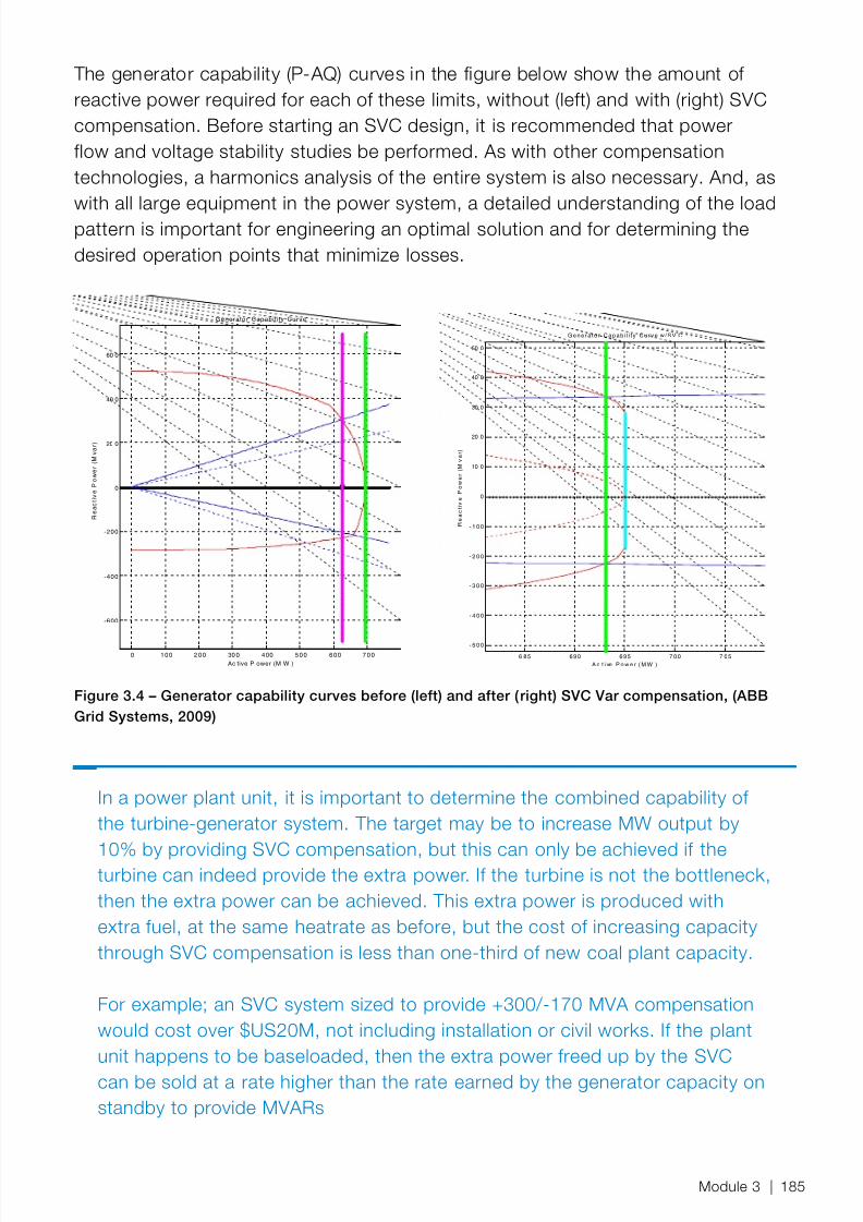
8/12/2019 Energy Efficiency Electronic Book Version 1548_PowerGenerationHandbook v1_1
http://slidepdf.com/reader/full/energy-efficiency-electronic-book-version-1548powergenerationhandbook-v11 187/361
The generator capability (P-AQ) curves in the figure below show the amount ofreactive power required for each of these limits, without (left) and with (right) SVCcompensation. Before starting an SVC design, it is recommended that powerflow and voltage stability studies be performed. As with other compensationtechnologies, a harmonics analysis of the entire system is also necessary. And, aswith all large equipment in the power system, a detailed understanding of the loadpattern is important for engineering an optimal solution and for determining thedesired operation points that minimize losses.
Figure 3.4 – Generator capability curves before (left) and after ( right) SVC Var compensation, (ABBGrid Systems, 2009)
0 1 0 0 2 0 0 30 0 4 00 5 0 0 6 0 0 7 0 0
-600
-400
-200
0
20 0
40 0
60 0
Ac tive P ower (M W )
R e a c
t i v e
P o w e r
( M v a r )
Generator Capabil i ty Curve
6 8 5 6 9 0 6 9 5 7 0 0 7 0 5
- 5 0 0
- 4 0 0
- 3 0 0
- 2 0 0
- 1 0 0
0
10 0
20 0
30 0
40 0
50 0
A c t i ve P o w e r ( M W )
R e a c
t i v e
P o w e r
( M v a r )
G e n e r a t o r C a p a b i l i t y C u r v e w / S V C
In a power plant unit, it is important to determine the combined capability ofthe turbine-generator system. The target may be to increase MW output by
10% by providing SVC compensation, but this can only be achieved if theturbine can indeed provide the extra power. If the turbine is not the bottleneck,then the extra power can be achieved. This extra power is produced withextra fuel, at the same heatrate as before, but the cost of increasing capacitythrough SVC compensation is less than one-third of new coal plant capacity.
For example; an SVC system sized to provide +300/-170 MVA compensationwould cost over $US20M, not including installation or civil works. If the plantunit happens to be baseloaded, then the extra power freed up by the SVCcan be sold at a rate higher than the rate earned by the generator capacity onstandby to provide MVARs
Module 3 | 185

8/12/2019 Energy Efficiency Electronic Book Version 1548_PowerGenerationHandbook v1_1
http://slidepdf.com/reader/full/energy-efficiency-electronic-book-version-1548powergenerationhandbook-v11 188/361
In one case where PF was increased from 0.8 to 0.95, the efficiency of theGSU transformer increased by 0.06% due to PF improvement alone. For stableoperation and other practical reasons, the PF at the generator cannot beincreased much past 0.95.
Active Rectifier Units on Motor Drives VFDs with an active front end (active rectifier unit - ARUs) can play an important rolein improving industrial plant active power generation capability and leading phaseoperation improvement. A VFD with active front end design gives the possibility tosupply reactive power (lead or lag) to the auxiliary power system to compensatethe reactive power needs of the remaining constant-speed motors and the reactivepower losses of auxiliary transformers.
InductionMotor
MCos
MV BUS
L
ARU DC-Link INU
Figure 3.5 – Schematic of VFD with active rectifier unit circuit, (ABB USCRC, 2008)
The reactive power compensation from ARUs is free-of-charge as long as theconverter operational point is within its P-Q circle diagram.
Figure 3.6 – P-Q diagram showing ARU capability, (ABB USCRC, 2008)
186 | ABB Energy Efficiency Handbook

8/12/2019 Energy Efficiency Electronic Book Version 1548_PowerGenerationHandbook v1_1
http://slidepdf.com/reader/full/energy-efficiency-electronic-book-version-1548powergenerationhandbook-v11 189/361
The benefits of ARU compensation functions are twofold 1) Full balancing thereactive power demand of all auxiliary loads and thus gives the possibility forthe generator to produce more active power, 2~3% of rated capacity while stillmaintaining the required external reactive power capability 2) Reactive powercompensation from ARUs can improve the plant leading phase operation capabilityand also plant auxiliary system operation performance under various disturbancessuch as suppressing transient over-voltage or under-voltage caused by generatorload rejection.
Power Quality – HarmonicsHarmonics ConceptsHarmonics are voltages and currents at frequencies higher or lower than the nominalfrequency (60Hz in the US, 50Hz in Europe). These frequencies are usually integermultiples of the nominal (‘fundamental’) frequency and are caused by devices thatdraw current in a non-linear fashion from the power source.
Typical nonlinear loads include rectifiers, Variable Frequency Drives (VFDs), andany other loads based on solid-state conversion. VFDs are a potential source ofharmonics due to their fast current switching action at frequencies higher than thefundamental. Transformers and reactors may also become nonlinear elements in apower system during overvoltage/saturation conditions. Chargers for batteries (in the
UPS system), for example, may also be a source of harmonics if these do not usethe recent switch mode/chopper technology. Harmonics may also be received fromother plants nearby, such as an aluminum smelter.
Power at harmonic frequencies does no useful work and causes equipment heating,interference and other undesirable effects. Electronics, including those onboardsome VFDs, are particularly sensitive to high levels of harmonics. The presence ofharmonics also decreases Power Factor , which is why engineers refer to ‘true’ PF in
systems with harmonic distortion.
Figure 3.7- Harmonics-induced damage, (ABB Kurt Schipman ,‘Active Filter Savings’, 2008)
Module 3 | 187

8/12/2019 Energy Efficiency Electronic Book Version 1548_PowerGenerationHandbook v1_1
http://slidepdf.com/reader/full/energy-efficiency-electronic-book-version-1548powergenerationhandbook-v11 190/361
Harmonic pollution may also cause kWh meters to give faulty readings; thesedevices are important for monitoring energy consumption.
Harmonics are said to ‘distort’ the pure 60Hz sinusoidal waveform that carries usefulpower from the source. The summary effect of these waveforms yields the TotalHarmonic Distortion (THD) measure.
Figure 3.8 – Graph of high harmonic content 50 Hz waveform, (ABB Kurt Schipman)
Figure 3.9 – Graph of harmonic current magnitudes of the above waveform, (ABB Kurt Schipman)
Although limits vary in different areas, the IEEE 519-1992 (USA), G5/4 (UK) standards
limit THDV ≤ 5% and limit for each harmonic component. The worldwide standard IEC61000-2-4 also limits THD. This limit is acceptable even for very sensitive loads. Thesestandards also provide detailed harmonics mitigation design guidelines.
VFD-Induced Harmonics ConceptsUnder ideal operating conditions, the current harmonics generated by a p-pulse line-commutated converter can be characterized by I h=I1 / h and h=pn± 1 (characteristicharmonics) where n = 1, 2, ... and p is an integral multiple of six. In cases of non-ideal conditions (e.g. unbalanced converter input voltage, unequal commutationreactance,..), other harmonics can emerge: even, triple, odd non-characteristic andnon-integral (inter-harmonics) harmonics belong to this group.
188 | ABB Energy Efficiency Handbook

8/12/2019 Energy Efficiency Electronic Book Version 1548_PowerGenerationHandbook v1_1
http://slidepdf.com/reader/full/energy-efficiency-electronic-book-version-1548powergenerationhandbook-v11 191/361

8/12/2019 Energy Efficiency Electronic Book Version 1548_PowerGenerationHandbook v1_1
http://slidepdf.com/reader/full/energy-efficiency-electronic-book-version-1548powergenerationhandbook-v11 192/361
Figure 3.10 – Passive filter performance vs. frequency, (ABB, Schipman ‘Active Filter Savings’, 2008)
Harmonics Mitigation With Active FiltersFor small and medium size loads, active filters, based on power electronic converterswith high switching frequency, may be a more attractive solution. The basic conceptis to put a switching inverter in parallel with the load that is injecting compensationcurrents at the harmonic frequencies. This approach is also known as a form ofStatic Synchronous Compensation (STATCOM).
LoadSupply
Active Filter
idistortion
Couplingsystem
icompensation
LoadSupply
Active Filter Active Filter
idistortionidistortion
Couplingsystem
icompensationicompensation
Figure 3.11 – Active filter with load schematic, (ABB, Schipman, 2008)
The advantages of parallel active filter topology are:
− Dimensioned for the compensation current only − Cannot be overloaded irrespective of the harmonic load increase over time − Does not directly affect the supply to the load
All commercial active filters on the LV market use parallel topology
Modern active filter technology is able to produce reactive power as well as mitigate,and in some cases, eliminate problems created by power system harmonics. Seesection on Power Factor and reactive power compensation for more details.
Active filters can perform the following Power Quality tasks: − Harmonic filtration up to high order − Reactive power compensation
190 | ABB Energy Efficiency Handbook
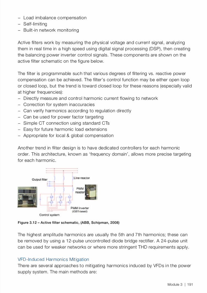
8/12/2019 Energy Efficiency Electronic Book Version 1548_PowerGenerationHandbook v1_1
http://slidepdf.com/reader/full/energy-efficiency-electronic-book-version-1548powergenerationhandbook-v11 193/361
− Load imbalance compensation − Self-limiting
− Built-in network monitoring
Active filters work by measuring the physical voltage and current signal, analyzingthem in real time in a high speed using digital signal processing (DSP), then creatingthe balancing power inverter control signals. These components are shown on theactive filter schematic on the figure below.
The filter is programmable such that various degrees of filtering vs. reactive powercompensation can be achieved. The filter’s control function may be either open loopor closed loop, but the trend is toward closed loop for these reasons (especially validat higher frequencies):
− Directly measure and control harmonic current flowing to network − Correction for system inaccuracies
− Can verify harmonics according to regulation directly − Can be used for power factor targeting − Simple CT connection using standard CTs
− Easy for future harmonic load extensions − Appropriate for local & global compensation
Another trend in filter design is to have dedicated controllers for each harmonic
order. This architecture, known as ‘frequency domain’, allows more precise targetingfor each harmonic.
Figure 3.12 – Active filter schematic, (ABB, Schipman, 2008)
The highest amplitude harmonics are usually the 5th and 7th harmonics; these canbe removed by using a 12-pulse uncontrolled diode bridge rectifier. A 24-pulse unitcan be used for weaker networks or where more stringent THD requirements apply.
VFD-Induced Harmonics Mitigation There are several approaches to mitigating harmonics induced by VFDs in the powersupply system. The main methods are:
Module 3 | 191
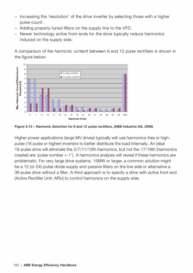
8/12/2019 Energy Efficiency Electronic Book Version 1548_PowerGenerationHandbook v1_1
http://slidepdf.com/reader/full/energy-efficiency-electronic-book-version-1548powergenerationhandbook-v11 194/361
− Increasing the ‘resolution’ of the drive inverter by selecting those with a higherpulse count .
− Adding properly tuned filters on the supply line to the VFD.− Newer technology active front-ends for the drive typically reduce harmonics
induced on the supply side.
A comparison of the harmonic content between 6 and 12 pulse rectifiers is shown inthe figure below:
Figure 3.13 – Harmonic distortion for 6 and 12 pulse rectifiers, (ABB Industrie AG, 2006)
Higher power applications (large MV drives) typically will use harmonics-free or high-
pulse (18 pulse or higher) inverters to better distribute the load internally. An ideal18-pulse drive will eliminate the 5/7/11/13th harmonics, but not the 17/19th (harmonicscreated are ‘pulse number +-1’). A harmonics analysis will reveal if these harmonics areproblematic. For very large drive systems, 15MW or larger, a common solution mightbe a 12 (or 24)-pulse diode supply and passive lters on the line side or alternative a36-pulse drive without a lter. A third approach is to specify a drive with active front end(Active Rectier Unit: ARU) to control harmonics on the supply-side.
192 | ABB Energy Efficiency Handbook
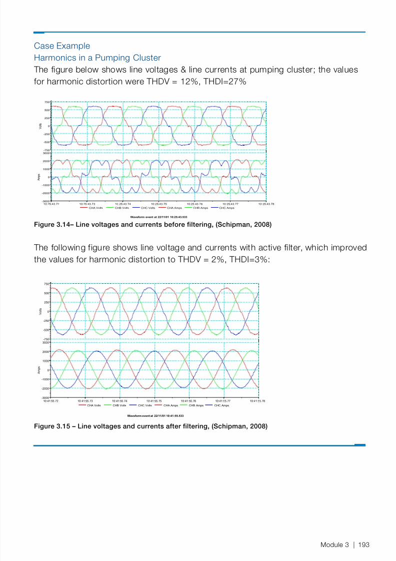
8/12/2019 Energy Efficiency Electronic Book Version 1548_PowerGenerationHandbook v1_1
http://slidepdf.com/reader/full/energy-efficiency-electronic-book-version-1548powergenerationhandbook-v11 195/361
Case ExampleHarmonics in a Pumping Cluster
The figure below shows line voltages & line currents at pumping cluster; the valuesfor harmonic distortion were THDV = 12%, THDI=27%
Waveform event at 22/11/01 10:25:43.533
CHA Volts CHB Volts CHC Volts CHA Amps CHB Amps CHC Amps
V o l t s
A m p s
10:25:43.72 10:25:43.73 10:25:43.74 10:25:43.75 10:25:43.76 10:25:43.77 10:25:43.78
-750
-500
-250
0
250
500
750
-3000
-2000
-1000
0
1000
2000
3000
Figure 3.14– Line voltages and currents before filtering, (Schipman, 2008)
The following figure shows line voltage and currents with active filter, which improvedthe values for harmonic distortion to THDV = 2%, THDI=3%:
Waveform event at 22/11/01 10:41:55.533
CHA Volts CHB Volts CHC Volts CHA Amps CHB Amps CHC Amps
V o l t s
A m p s
10:41:55.72 10:41:55.73 10:41:55.74 10:41:55.75 10:41:55.76 10:41:55.77 10:41:55.78
-750
-500
-250
0
250
500
750
-3000
-2000
-1000
0
1000
2000
3000
Figure 3.15 – Line voltages and currents after filtering, (Schipman, 2008)
Module 3 | 193

8/12/2019 Energy Efficiency Electronic Book Version 1548_PowerGenerationHandbook v1_1
http://slidepdf.com/reader/full/energy-efficiency-electronic-book-version-1548powergenerationhandbook-v11 196/361

8/12/2019 Energy Efficiency Electronic Book Version 1548_PowerGenerationHandbook v1_1
http://slidepdf.com/reader/full/energy-efficiency-electronic-book-version-1548powergenerationhandbook-v11 197/361
VFDs and other power electronics with built-in power factor controllers will thereforeact to reduce the applied voltage under these conditions to minimize losses in themotor.
In contrast to voltage variations, small frequency variations have little effect on motorenergy efficiencies.
Power Quality - Phase Voltage UnbalanceSources for this section are: ABB Power Systems, Canada and (Competitek, 1996)
Phase voltage unbalance can cause excessive rotor currents and damagingreversing torques in the motor. The combined effects of phase unbalance lead toincreased motor temperature, reduced net output torque, pulsations in speed &torque, increased mechanical stress on motor components and reduced motorefficiency.
Voltage Unbalance – Causes and EffectsNEMA defines voltage unbalance as % of maximum deviation of the line voltage fromthe average voltage.
For example, a 3-phase system with phase voltages of 466, 458, and 461:
The average voltage is : (466+458+461) = 461.7 The phase unbalance is therefore : (461.7-458)/461.7 = 0.8%
The main causes of sustained phase voltage imbalance are listed below: − unbalanced transformer windings − unequal impedances in distribution wiring − unbalance within the motor itself (rewound motors at higher risk) − single phase or unbalanced 3-phase loads which are unevenly distributed.
− failures in VFDs or PF correction equipment − single phase-to-ground faults or disconnection failures
Although rare in industrial process plant networks, just a 3.5% imbalance canincrease total motor losses by 20 to 25 percent. In a 90%-efficient motor this isequivalent to an increase in total power loss of 2.0 to 2.5 percentage points. Thedrop in motor efficiency due to phase voltage unbalance is greater at lower motorloadings, below 75%. At a 5% unbalance, the motor de-rating factor may be as largeas 75% of the nameplate horsepower. An unbalanced supply may have a disturbingor even damaging effect on motors, generators, polyphase converters, and otherequipment. The foremost concern with unbalanced voltage is overheating in three-phase induction motors. The percent current imbalance drawn by a motor may be
Module 3 | 195

8/12/2019 Energy Efficiency Electronic Book Version 1548_PowerGenerationHandbook v1_1
http://slidepdf.com/reader/full/energy-efficiency-electronic-book-version-1548powergenerationhandbook-v11 198/361
6 to 10 times the voltage imbalance, creating an increase in losses and in turn anincrease in motor temperature.
Mitigation through Design The US DoE recommends that unbalances greater than 1% lead to a de-rating ofthe motor. Under a condition of 5% voltage unbalance, the motor de-rating factormay be as large as 75% of the nameplate horsepower. An additional effect of voltageunbalance is that the locked rotor and breakdown torques will be decreased, andthe motor may no longer be adequate for its intended application. The above appliesspecifically to induction motors. Situations in which larger unbalanced voltages exist,or in which synchronous motors are supplied by unbalanced voltages, should bestated in the motor specifications (IEEE, 2007).
Downsized motors with correspondingly lower temperature ratings may be moreat risk of the overheating that follows sustained phase unbalance than a previouslyhighly oversized motor for the same load. The thermal margin of oversized motorsprevents motor failure but unfortunately also masks the cause of the reducedefficiency of the affected motors.
For an existing plant, the best practice is to balance phases as closely as possibleand to ensure that power protection devices monitor continuously for phaseunbalance exceeding 1% at motor terminals. Regular thermographic and vibration
monitoring will also reveal the signature symptoms of phase unbalance. In the designphase, the US DoE advice is to check electrical system single-line diagrams to verifythat single phase loads are evenly distributed across the phases. Designs that placeall receptacle loads on a single phase also risk phase unbalance, as this capacityvaries greatly or is seldom used.
Power System Control and Protection The function of power system control is to selectively connect power sources withconsumers, and to provide facility operators with information on the real-time status ofthe network. Power also control enables complex, automatic interlocking and energysequencing logic. As with DCS systems, modern power control has a distributedarchitecture, with separate units for control (the brains) and actuation (the muscle).
The control units execute the logic in a microcontroller unit, then send their outputsignal to contactors which perform the actual power switching. These contactors sendback status and health information to the control unit. Power control is distinct fromprotection in that the contactors, relays and other ‘switchgear’ in the power controlsystem cannot switch the very high currents during short-circuit; these situations arehandled by heavier-duty, fast acting protection devices.
196 | ABB Energy Efficiency Handbook

8/12/2019 Energy Efficiency Electronic Book Version 1548_PowerGenerationHandbook v1_1
http://slidepdf.com/reader/full/energy-efficiency-electronic-book-version-1548powergenerationhandbook-v11 199/361
Protection systems safeguard the motors, power system equipment, and humanstaff from damaging effects of short-circuits and ground faults. The equipmenttypically in need of protection are: generators, busbars, lines, and transformers.
The brains of protection systems are so-called ‘numerical relays’ which sense afault condition and then command a circuit breaker to interrupt one or all phasesof power; this is known as a trip . VFDs have many built-in protective functions toprotect the motor from abnormal power supply conditions.
Modern, microprocessor-based control and protection systems offer distinct energy-efficiency advantages over older, purely electro-mechanical devices. The abilityto execute more complex control logic, in close communication with the processcontrols running within the DCS, allows a higher degree of energy optimization thanpossible with electromechanical switching only. Load management schemes can beimplemented which balance supply and demand across parallel plant units in a waythat that minimizes losses and enhances power quality. Power control systemsalso enable complex unit-wide automatic startup and load shedding routines;these can conserve existing capacity and avoid energy-wasting trips, andlong or wasteful re-starts. The self-supervision capabilities of modern control andprotection devices further reduces the chances for an energy-wasting trip event.
Figure 3.16 – Automatic generator synchronizer device, (ABB Power Products 2006).
In power plants, the power control system can be programmed to ensure thatthe GSU, the auxiliary and the distribution transformers are not energized whennot in use.
Modern power control also enables integrated allocation optimization whenthere are multiple sources of power, as described in the section on Multi-LevelReal-Time Optimization.
Module 3 | 197

8/12/2019 Energy Efficiency Electronic Book Version 1548_PowerGenerationHandbook v1_1
http://slidepdf.com/reader/full/energy-efficiency-electronic-book-version-1548powergenerationhandbook-v11 200/361
Much of the design reference information available under the category of substationsalso applies to large industrial power supply systems.
Generator ControlIn power generation, an automatic synchronization device is recommended forparallel switching of generators with the power grid. The synchronizer brings therotation speed (frequency) and voltage of the generator to within the requiredtolerance range, using higher and lower commands to the turbine-generatorcontroller and the voltage controller (ABB Power Products 2006). Voltage, phaseangle and frequency are all dynamic quantities; the synchronizer ensures that thebreaker contacts touch at the instant when the phases are matching.
In power plants, the auxiliary power supply system typically has a high-speedtransfer system to ensure a secure supply of power to boiler drivepower; i.e.the BFW pump, circulating pump, and draft fans. In case of an interruptionin power, this switchover function provides power from an alternate, standbynetwork. This control function allows the unit to continue operating and avoidthe energy waste (and large opportunity cost) associated with a boiler trip.
Transformer Control
This section is adapted from the ABB Switchgear Manual, (ABB Power Products 2006):
Power control devices were once commonly used to operate the taps which changethe transformation ratio of a power transformer. This function serves to adapt thevoltage in case of load fluctuations, to distribute the load, to adjust active andreactive currents in interconnected systems. Although most modern transformers areequipped with automatic voltage regulation, transformers in parallel operation stillrequire tap change functionality to minimize the reactive current circulating between
transformers. Electric furnaces, rectifiers and other devices also rely on tap changecontrol for variation of their input voltage.
Efcient Power System Design and Engineering Achieving energy efficiency improvements in power system design is challenged bymany of the non-technical barriers outlined in the section Barriers by Stakeholder .
Those barriers most relevant to the plant electrical engineering discipline are:
198 | ABB Energy Efficiency Handbook

8/12/2019 Energy Efficiency Electronic Book Version 1548_PowerGenerationHandbook v1_1
http://slidepdf.com/reader/full/energy-efficiency-electronic-book-version-1548powergenerationhandbook-v11 201/361
− In a large power or process plant, electrical engineering (EE) is often the lastdiscipline to be engaged, after process, mechanical and controls. This leavesthe EE with little influence to practice efficient integrative design, since mostother aspects are now frozen. This of course, has a deleterious effect on theenergy efficiency of a plant, as virtually all of the internally consumed energypasses through the electrical system.
− The power system is also the first to be commissioned, which further restricts thetime that the EE can spend on conceptual studies described below.
− The trend away from turnkey projects and toward multiple suppliers fragments thedesign and communication, making integrative approaches more difficult.
− The vital role of power systems to all other plant equipment is the reason whycustomers often stipulate ‘liquidated damages’ in contracts with their suppliers.
This threat of very large opportunity cost from downtime is a subtle deterrenttoward newer designs with potentially significantly lower lifecycle costs.(opportunity costs are not as real as wasted energy costs, but often get the sameaccounting treatment)
In a retrofit situation involving increased electrification or the introduction of VFDs, itis good practice to re-examine the entire power system to ensure it is right-sized andstill capable of delivering high quality power at high reliability. For example, with achange in loading previous schemes for Power Factor (PF) compensation may needto be re-evaluated to avoid increased in-plant losses due to low PF or even for over-
correction in some cases.
Generating Station Power Systems The most common design of in-plant power systems is termed ‘unitconnected’, in which each generating unit has a self-contained networksupplied by that unit’s generator. The plant power system typically has its ownstep up and auxiliary transformers, plus one or more startup transformers.
Large loads are served directly from the MV switchgear, and the largest motorsare usually on a separate bus, where the voltage (during motor starts) may bepermitted to drop to a much lower level, say 80% (Black & Veatch 1996, p574)
In a typical generating station the nominal voltage ratings of the auxiliarybuses are usually 2.4 kV, 4.16 kV, 6.9 kV, or 13.8 kV. All these voltage levelsare referred to as medium voltage or MV. Stations in the 10-100MW rangemay have 2,400V. Most stations in the 75-500MW range use 4,160V as thebase auxiliary system voltage. For stations from 500MW to 1,000MW, it is notuncommon to have auxiliary bus voltages of 6,900V. Occasionally, some singlededicated loads such as BFPs in 10,000-15,000 hp (7.5 MW-11 MW) class aresupplied by a separate 13,800-V bus (Black & Veatch 1996). Bus design best
Module 3 | 199

8/12/2019 Energy Efficiency Electronic Book Version 1548_PowerGenerationHandbook v1_1
http://slidepdf.com/reader/full/energy-efficiency-electronic-book-version-1548powergenerationhandbook-v11 202/361
practice is to separate redundant loads (such as pairs of ID and FD fans), ondifferent buses. This leads to the common ‘double bus’ design illustrated in thesingle-line diagram figure below. Another best practice is to distribute the loadsequally among buses.
Figure 3.17 – Simplified single-line diagram for unit connected power system IEEE Std.666-2007,Design Guide for Power Stations
Figure 3.18 – Single-line diagram showing for a unit connected power system, (ABB EBoP/CRC)
200 | ABB Energy Efficiency Handbook

8/12/2019 Energy Efficiency Electronic Book Version 1548_PowerGenerationHandbook v1_1
http://slidepdf.com/reader/full/energy-efficiency-electronic-book-version-1548powergenerationhandbook-v11 203/361
Power System StudiesConceptual studies usually present the greatest opportunities to evaluate the impactof basic efficiency improving design changes, and to seek even greater energyefficiency improvements through rigorous analysis. The power quality conceptualstudies most relevant to energy efficiency are:
− Load analysis (especially of auxiliary loads) − Power flow, voltage selection and voltage drop calculations − Motor starting analysis − Harmonic analysis
Other typical power system project studies that have only an indirect impact onenergy efficiency are:
− Short-circuit analysis − Switching studies − Protection studies − Reliability analysis
Load List and AnalysisLoad analysis is the single most important power engineering step towardsincreasing energy efficiency. The starting point for design of the power system isto gather data about all the loads that the system will serve. This step includesnot just the nameplate data of those loads, but also their criticality, duty cycle,
seasonal variations and startup requirements. The sources of much of this dataare the mechanical and process design teams. This data is summarized in a ‘LoadList’ which becomes the main document interface between the mechanical/processand electrical disciplines or teams. Due to fragmentation of suppliers, assembling acomplete load list is not a simple task. Data from similar past projects can provide aguide, but only a guide, when actual load list information is lacking.
Load Analysis
Analysis of the load list should begin with quantifying the maximum operating load,given the actual loads and load factors. Using only the nameplate values will give agrossly inflated figure and load and lead to oversizing of the supply. A growth factormargin is recommended by the IEEE guidelines, but this may not apply in all cases.
The load analysis steps should also quantify the number and loading associated with VFDs. An obvious energy-saving step in load analysis is to reduce auxiliary levelsto the lowest possible realistic levels. Large or unusual loads also deserve specialattention at this stage. Medium voltage loads tend to be much better understoodand documented than low voltage (LV) loads. Attention to LV loading is important,however, as it may comprise up to 40% of the total in a typical industrial plant, with awide variation between industries.
Module 3 | 201

8/12/2019 Energy Efficiency Electronic Book Version 1548_PowerGenerationHandbook v1_1
http://slidepdf.com/reader/full/energy-efficiency-electronic-book-version-1548powergenerationhandbook-v11 204/361
Electrostatic precipitators (ESP) of the dry type operate by electrically chargingflue gas particles for collection on grounded plates. The charging electrodesare energized with 55 to 86 kVDC supplied by a transformer-rectifier (TR)supplied by a 480 VAC bus feeder. An ESP is a capacitive load. The TR is alsoequipped with controls to vary the voltage depending on current conditions, toachieve maximum voltage without arcing. (Babcock & Wilcox, 2005)
Current loads (kiloamps) can then be calculated from the loads in the load list. The electric power formulas at the start of this chapter and may be used tocalculate current load in transformers and synchronous generators. For inductionmotors direct-on-line, see the the handbook’s Motors section on motor powerformulas . For VFD=equipped motors, see that section’s formulas for motor currentestimation .
Power Flow and System VoltagesSystem voltage selection has an energy efficiency impact. Choosing a higher busvoltage where possible (for example 6,900V vs. 4,160V for auxiliary busses) willreduce ohmic losses due to the lower current levels relative to low voltage busses.Selecting MV rather than LV drives and motors will reduce ohmic losses in drive-power equipment. Motors and transformers rated at the higher voltage levelsgenerally offer higher efficiencies as well. Commercially available circuit breakers
are limited to interrupting a maximum of 3000A of short-circuit current. This currentlimitation may lead designers to split up busses and supply them from multiple,smaller transformers. Smaller transformers have lower efficiency than larger units.
Thus, higher bus voltages will allow the designer to specify fewer, larger transformerswhich will increase the overall efficiency of the system, and enjoy up front costsavings during equipment purchase.
Power flow and short-circuit analyses are required to ensure that voltages are
correctly selected during various power flow (both active & reactive) scenarios.
Startup Analysis (Motor Starting)Motors without soft starters draw many times their full load operating current duringtheir startup. High torque demands during startup will also increase the load onthe power system and may lead to over-sizing of components for these transientconditions, at the expense of lower continuous running efficiency. The electricaland mechanical/process engineers are encouraged to work together to find creativesolutions to make motor startup easier on the power system. For example, abypass valve could be opened during startup to temporarily relieve pressure, if thisis allowed by the process. Startup considerations are discussed in the Fan Startup
202 | ABB Energy Efficiency Handbook

8/12/2019 Energy Efficiency Electronic Book Version 1548_PowerGenerationHandbook v1_1
http://slidepdf.com/reader/full/energy-efficiency-electronic-book-version-1548powergenerationhandbook-v11 205/361

8/12/2019 Energy Efficiency Electronic Book Version 1548_PowerGenerationHandbook v1_1
http://slidepdf.com/reader/full/energy-efficiency-electronic-book-version-1548powergenerationhandbook-v11 206/361
If the drives don’t include internal reactance, or if many of them are only 6-pulse VFDs, then the system tolerance level drops to about 10%. If these thresholds areexceeded, then a formal harmonic analysis is recommended. If the level of excessharmonic content is high and many drives are involved, installation of an active filterwill likely be most appropriate; if only a small number of large drives are involved,then installing drives with active front-ends probably is the best solution. See thesection on Harmonics Mitigation for more details on passive and active filters.
Equipment Sizing and Bus DesignCorrect balancing of loads across buses will improve power quality and thus energyefficiency. In plants with multiple power sources, a correct balancing will also leadto optimal sizing of all power system components and reduced startup powerrequirements per bus.
A proper analysis will yield the optimum breaker and cable sizing; poor sizing ofcomponents here can have consequences for both energy efficiency and protectivefunctions. Undersized cables have higher losses, as discussed in the section onCable Selection & Sizing .
Contactors for BypassingSoft-starters are typically bypassed by a contactor (KB) as shown in the figurebelow when the motor has completed its startup. VFDs, however, are not normally
installed with such a bypass contactor for the full load condition. For large motors,specifying a contactor to bypass the VFD, which is not 100% efficient, may be costeffective. The feasibility of this design depends on the motor’s duty factor and theduration at continuous maximum load, and several other factors; see NEMA-MG1and the NEMA Application Guide for AC Drives (2001) for some special precautionsregarding this approach.
Softstarter
M3 -
Contactor KB
Contactor KL
Fuse
Contactor KB
Figure 3.19– Schematic of motor soft-starter on power system, (ABB Motors & Drives, 2007)
204 | ABB Energy Efficiency Handbook
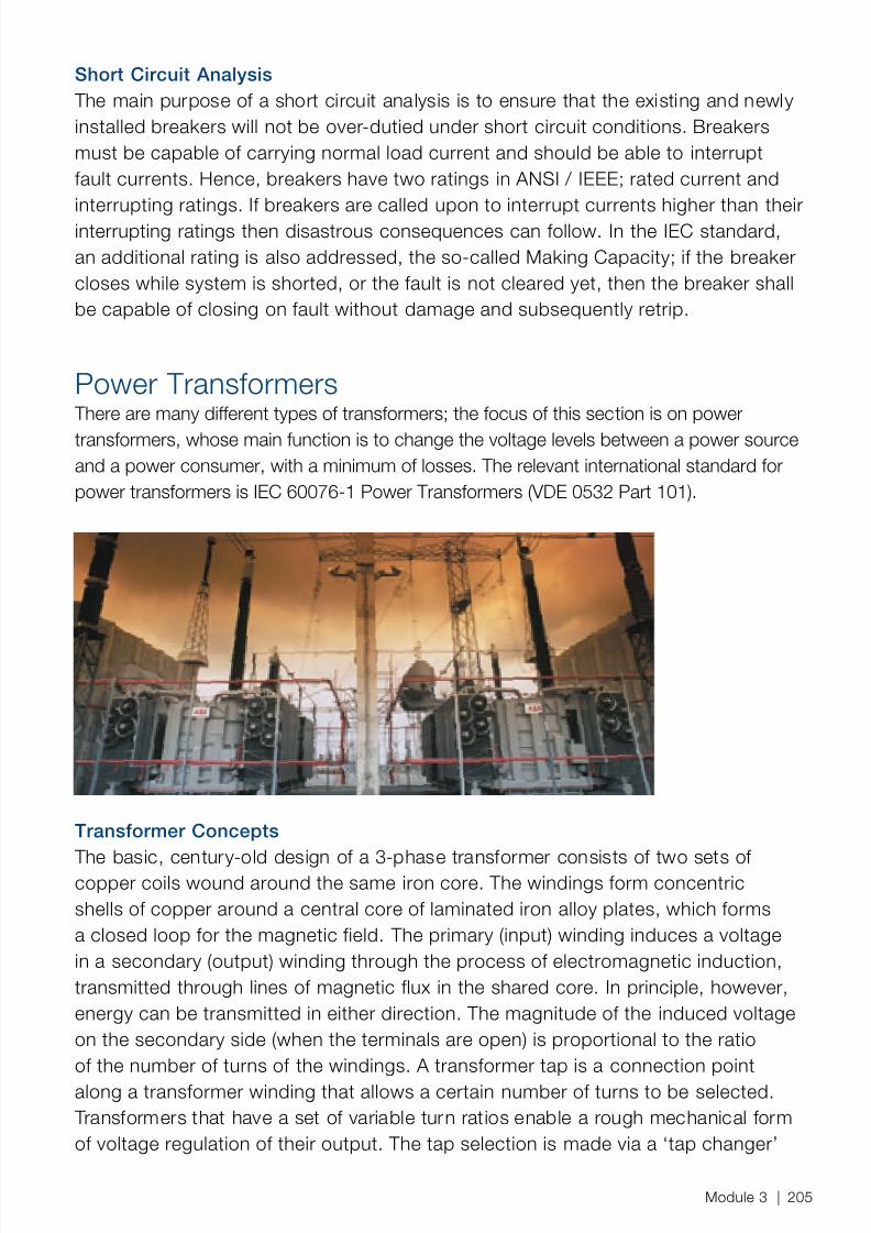
8/12/2019 Energy Efficiency Electronic Book Version 1548_PowerGenerationHandbook v1_1
http://slidepdf.com/reader/full/energy-efficiency-electronic-book-version-1548powergenerationhandbook-v11 207/361
Short Circuit Analysis The main purpose of a short circuit analysis is to ensure that the existing and newlyinstalled breakers will not be over-dutied under short circuit conditions. Breakersmust be capable of carrying normal load current and should be able to interruptfault currents. Hence, breakers have two ratings in ANSI / IEEE; rated current andinterrupting ratings. If breakers are called upon to interrupt currents higher than theirinterrupting ratings then disastrous consequences can follow. In the IEC standard,an additional rating is also addressed, the so-called Making Capacity; if the breakercloses while system is shorted, or the fault is not cleared yet, then the breaker shallbe capable of closing on fault without damage and subsequently retrip.
Power Transformers There are many different types of transformers; the focus of this section is on powertransformers, whose main function is to change the voltage levels between a power sourceand a power consumer, with a minimum of losses. The relevant international standard forpower transformers is IEC 60076-1 Power Transformers (VDE 0532 Part 101).
Transformer Concepts
The basic, century-old design of a 3-phase transformer consists of two sets ofcopper coils wound around the same iron core. The windings form concentricshells of copper around a central core of laminated iron alloy plates, which formsa closed loop for the magnetic field. The primary (input) winding induces a voltagein a secondary (output) winding through the process of electromagnetic induction,transmitted through lines of magnetic flux in the shared core. In principle, however,energy can be transmitted in either direction. The magnitude of the induced voltageon the secondary side (when the terminals are open) is proportional to the ratioof the number of turns of the windings. A transformer tap is a connection pointalong a transformer winding that allows a certain number of turns to be selected.
Transformers that have a set of variable turn ratios enable a rough mechanical formof voltage regulation of their output. The tap selection is made via a ‘tap changer’
Module 3 | 205

8/12/2019 Energy Efficiency Electronic Book Version 1548_PowerGenerationHandbook v1_1
http://slidepdf.com/reader/full/energy-efficiency-electronic-book-version-1548powergenerationhandbook-v11 208/361
mechanism. Modern power control offers other means of controlling transformervoltage, and tap-changing can then become an infrequent operation.
The power capacity (MVA rating) of a transformer depends on the size of thewindings and iron core, and also on the method for removing heat, as described inthe section on Transformer Cooling .
Generator Step Up Transformers - GSU ( also known as Unit Transformer – UT) These transformers take the voltage form the generator busbar MV level (10kVto 21kV) up to a higher (more economic) transmission voltage (HV) level, whichmay range from 110kV up to 800 kV. Limitations on the insulation design whichcan be achieved on rotating machinery prohibit the generator from producingHV without need of a step-up transformer (Fassbinder 1997).
The GSU must be matched to the generator so that the transformer can fullyutilize the generator’s active and reactive power capacities. The standardC57.116-1989 IEEE Guide for Transformers Directly Connected to Generatorsdescribes how these characteristics must be matched to the situation:
− Short-circuit impedance − Secondary (high) voltage rating
− Transformer MVA rating − Primary (low) voltage rating
Unit Auxiliary Transformers (UAT) The auxiliary power system can be supplied either from the generator bus orfrom the switchyard. If supplied from the generator, then one or more ‘stationservice’ startup transformers might also be required.
This additional startup hardware may increase the cost and complexity of thepower system, but the reliability of the system will increase. Voltage excursionsare also lower using power supply from the generator bus, and switchyarddisturbances are eliminated. (IEEE, 2007). Typically, two UATs are used forincreased reliability and reduce load and fault currents. The IEEE design guidealso suggests an alternative configuration which may provide an improvedbalance between capital costs, reliability and operating costs : a three-windingauxiliary transformer in lieu of two separate auxiliary transformers. (IEEE, 2007)
206 | ABB Energy Efficiency Handbook
8/12/2019 Energy Efficiency Electronic Book Version 1548_PowerGenerationHandbook v1_1
http://slidepdf.com/reader/full/energy-efficiency-electronic-book-version-1548powergenerationhandbook-v11 209/361
Station/Startup Transformers (SST) This transformer is used during unit startup and is fed from the MV switchyard.See the IEEE Std 666-2007 for details on the function and sizing of thistransformer.
In power plants with parallel units, the parallel units may share a single SST.
Transformer Losses & Efficiency The largest power transformers are “probably the most efficient machines devised byman” (Fassbinder 1997). Modern large GSU transformers can achieve efficiencies ofup to 99.75% at full load. Despite an impressive efficiency rating, there is still a largeincentive for improvement. The throughput of these large transformers can be upto 1000MVA, so even small, fractional percentage gains translate into MW of savedpower. Smaller transformers are less efficient (99.0% to 99.5%), but have a smallerthroughput. The incentive to seek improvements at this lower scale comes fromthe fact that most power consumers (at least in distribution networks) receive theirpower after it has passed through several transformers, which means that savings ofreduced loss-transformers are compounded.
Reduced-loss transformers lose energy in their 1) iron cores and 2) copper windings.
− In the core, losses occur mainly through hysteresis effects and I²R eddy currentscirculating within the iron core. Hysteresis refers to the lag between magneticflux and the magnetizing force and these losses increase with frequency. Eddycurrents are small induced currents running perpendicular to the direction of flux.
Taken together, these losses are known as no-load losses since they occur whenthe transformer is energized, and are present even when the secondary terminalsare open and under no load. These losses are sometimes referred to as core,magnetization or ‘iron’ losses.
− In the windings, losses occur due to ohmic resistance (I2
R losses) from the maincurrents flowing through the windings; these losses vary with the load on thetransformer and are therefore known as load losses or ‘copper’ losses. Someeddy current losses also occur in the windings; so the windings are kept tall andslim to reduce this eddy current circulation. The load loss is officially defined asthe active power consumed in a short-circuit test, where rated current of ratedfrequency is fed into one winding and another winding is short-circuited. This lossis also known as ‘impedance’ loss.
Loss values are often contractually guaranteed, and are determined at a certainreference temperature in the windings. Some typical penalties for non-compliancewith the agreed losses, as revealed during technical testing at the supplier’s plant,
Module 3 | 207

8/12/2019 Energy Efficiency Electronic Book Version 1548_PowerGenerationHandbook v1_1
http://slidepdf.com/reader/full/energy-efficiency-electronic-book-version-1548powergenerationhandbook-v11 210/361
are $1000 or more per kW of losses (usually iron losses only). This performanceguarantee is also sometimes known as a ‘loss evaluation’ agreement.
Estimating Transformer Losses Theoretically, a transformer has its highest efficiency at the load in which iron lossand copper losses are equal. Therefore the load at which the efficiency is highestcan be found from the following formula:
% optimum load = ( iron loss / copper loss) 1/2 x 100
This is about 57% of full load, and the curve is fairly flat for realistic core and loadloss values. Because transformer designs are conservative with respect to load, theactual highest efficiency point is usually found closer to 80% of the rated load.
Knowing the losses, the efficiency of a transformer can be calculated from the basicformula:
% efficiency = [ (input in Watts - total losses in watts) / (input in watts) ] x 100
In practice, the total losses are hard to measure for an existing transformer, so theno-load efficiency of a transformer is usually calculated as shown below. This no-load efficiency is useful for comparing different transformer types.
% efficiency = ( V x A out ) / ( V x A in )
Empirical data can be used to estimate the total percentage transformer losses (Pv),using the graph below for typical oil-immersed two-winding distribution transformersup to 40MVA rating, and the following formula:
Pv = P o + A 2Pk
Where: A = loading ratio, load kVA/rated kVA (S/S r )Io = percentage no-load currentPo = percentage no-load lossesPk = percentage impedance losses
208 | ABB Energy Efficiency Handbook

8/12/2019 Energy Efficiency Electronic Book Version 1548_PowerGenerationHandbook v1_1
http://slidepdf.com/reader/full/energy-efficiency-electronic-book-version-1548powergenerationhandbook-v11 211/361
Figure 3.20 – Transformer load-loss estimation curve, (ABB Power Products 2006)
The graph for the load losses P k has an upper limit for rated high voltage 123kV anda lower limit for rated high voltage 36kV.
For a 2.5 MVA transformer for 20/0.4 kV operating at half load (a= 0.5) and PF=0.8,the percentage no-load losses, as shown in the graph above are P 0 = 0.6%, and the
percentage impedance losses P k =1.0%. The percentage total transformer losses Pvare:
Pv = 0.6% + (0.25)(1) = 0.85%
In terms of real power, the total losses are = P v x S x PF:
Total losses = 0.85% x 2500 kVA x 0.8 = 1,700 kW
Combining the formula for total % losses with the definition of efficiency leads to thefollowing formula for Transformer Efficiency (Eff %) :
Eff = 100% - 100% x ( P o + a 2Pk ) / (a x S r x PF + P o )
Transformer losses are stated in MW, MVAR and MVA. The IEEE Std. C57.12.00 andIEEE Std. C57.12.01 [B8] provide the tolerances associated with the transformerlosses (IEEE 2007).
Module 3 | 209

8/12/2019 Energy Efficiency Electronic Book Version 1548_PowerGenerationHandbook v1_1
http://slidepdf.com/reader/full/energy-efficiency-electronic-book-version-1548powergenerationhandbook-v11 212/361
According to one power engineering industry guideline (Black & Veatch 1996),step-up transformer MVAR losses can be estimated by applying the followingmultipliers to the generator MVA rating.
kV (HV) Multiplier
69 0.09
115 0.10
138 0.11
161 0.12
230 0.13
345 0.14
500 0.17
Figure 3.21 – Multipliers (of MVA) to determine transformer MVAR losses, (Black & Veatch 1996)
The same source cites empirical data behind the following multiplier for transformerMW losses, which suggest that power transformers are on average 99.7% efficient:
MW losses = Generator MVA rating x 0.003
In a power plant, as an example of using these multipliers, one can start with agenerator rated at 500MW real power and 0.9 network PF, and a high-voltageside of 138kV.
− Calculate the generator MVA rating : 500/0.9 = 556.0 MVA − Calculate the transformer MW losses : 556 x 0.003 = 1.7 MW
− Calculate the transformer MVAR losses : 556 x 0.11 = 61.2MVAR
An underloaded transformer has a relatively larger core cross-section, thusreducing iron losses. If the transformer is too lightly loaded, however, the equivalentsecondary resistance will cause the winding and core losses to be unequal and theefficiency will be correspondingly lower (EC&M, 2000, M. Lamendola).
Power consumed by the transformer’s auxiliary forced-cooling system (fans andpumps) shall also be considered as the third source of losses for any calculation of
Total Loss in the transformer. These losses are harder to calculate, but will increasewith the %load and temperature as the cooling system tries to remove excess heat.
210 | ABB Energy Efficiency Handbook

8/12/2019 Energy Efficiency Electronic Book Version 1548_PowerGenerationHandbook v1_1
http://slidepdf.com/reader/full/energy-efficiency-electronic-book-version-1548powergenerationhandbook-v11 213/361

8/12/2019 Energy Efficiency Electronic Book Version 1548_PowerGenerationHandbook v1_1
http://slidepdf.com/reader/full/energy-efficiency-electronic-book-version-1548powergenerationhandbook-v11 214/361
Figure 3.22 – Transformer losses due to harmonics , Leonardo Energy,’Network Losses’ 2008
Harmonics losses can be reduced using the same methods described in theHarmonics Mitigation section.
Transformer Cooling There are 5 basic power transformer classes, based on how they dissipate internalheat from losses;
− “A” for dry-type transformers, in which core and windings are embedded in castresin. These transformers are used up to 20MVA and a maximum of 36kV.
− “O” for mineral (or other flammable) oil-immersed transformers, which have amaximum temperature below the oil flame point 300 oC.
− “K” for synthetic-oil immersed transformers, which have a higher maximumtemperature.
− “G” for gas cooling system with fire point > 300 oC − “W” for water cooled systems
Note that oil-immersion serves as both insulation and coolant, and is most common
on all large (>20MVA) transformers. There are several alternatives for removing theheat generated by losses, and these may be combined at different stages in thetransformer. For example, in oil immersed transformers, the cooling circuit collectshot oil at the top of the tank and returns cooled oil lower down on the side. Thecooling arrangement consists of two circuits, one inner and one outer. The innercircuit transfers heat from the hot transformer surfaces to the oil, and the outercircuit transfers the heat to a secondary cooling medium. IEC standards providedefinitions for the different types of oil immersed transformer cooling arrangements.
212 | ABB Energy Efficiency Handbook

8/12/2019 Energy Efficiency Electronic Book Version 1548_PowerGenerationHandbook v1_1
http://slidepdf.com/reader/full/energy-efficiency-electronic-book-version-1548powergenerationhandbook-v11 215/361
Code Inner circuit Outer circuit
ONAN Oil Natural Air Natural
ONAF Oil Natural Air Forced
OFNAN Oil Forced Air Natural
OFAF Oil Forced Air Forced
OFWF Oil Forced Water Forced
The transformer MVA power ratings are usually are stated to reflect different levels ofcooling. For example, the rating ONAN/ONAF1/ONAF2 may be 120/160/200. Theseratings show the maximum power rating depending on the level of cooling active.
At low loads, the ONAN circuits are sufficient; no forced cooling, hence no auxiliarylosses, are active.
Cooling has the effect of moving the operational power point lower down on thesaturation curve. The cooler the transformer, the more power and energy can bepassed through the transformer. On the other hand, power that is consumed by thecooling devices serves to effectively increase the transformer total losses.
Oil-filled transformers with pump circulation cooling systems are common, but thesehave higher losses and the higher parts count means reduced reliability compared tofan-cooled type units. The only advantage of pump-cooled systems is the reducedsize of the unit.
Some dry-type transformers, for example, Resi-block transformers, have a designthat can withstand extremely cold temperatures. These transformer types do notneed startup heaters, as oil-filled units do in such conditions, to achieve operatingtemperatures. From an energy perspective, transformers without need for startupheating save energy, provided that full load efficiencies are not reduced.
According to IEEE Std 666-2007 ‘An economic evaluation that considers theinitial cost of the transformer installed plus the evaluated cost of losses isused to determine the type of cooling, e.g., ONAN, ONAN/ONAF, ONAN/OFAFONAN/ONAF/OFAF. These transformers supply the unit auxiliary loads and areloaded a large portion of the time. Losses will consist mostly of load lossesand have a tendency to make an ONAN rating equal to normal load the mosteconomical.
The standards (IEC-3540) define the ‘hottest-spot’ temperature in the winding as thelimiting factor for loading & overloading limits, and provide a method for calculating
Module 3 | 213
8/12/2019 Energy Efficiency Electronic Book Version 1548_PowerGenerationHandbook v1_1
http://slidepdf.com/reader/full/energy-efficiency-electronic-book-version-1548powergenerationhandbook-v11 216/361
this temperature based on bottom or top oil temperature measurements and thegradient.
Transformer ConfigurationSome facilities specify separate power transformer units for each phase, usuallybased on the assumption that separate units offer increased reliability over combined3-phase units. Although this may have been true in the past, the reliability of 3-phasetransformers is now so high that it should no longer be the main reason to splitphases. Single phase transformers have lower energy efficiency than combinedphase units, are more expensive and require more auxiliary equipment whichcombined units can share between the phases. Additional reliability can be achievedthrough a bus design which includes a reserve transformer powered from anothersource, for example.
In power plants, the generator step-up unit (GSU) is 5 to 6 times more proneto failure than network transformers. This higher failure rate is due to themuch higher thermal and mechanical stresses experienced by these largetransformers. The average age of large power transformers in the US is now 39years (as of 2008). To maintain a slight edge in efficiency, but mainly to avoidthe costs of random failures, this fleet of 130,000 aging transformers shouldbe carefully monitored and screened for potential problems and eventual
replacement or refurbishment. ABB, for example, offers transformer monitoringsystems (TEC), and has a formal program offering (TRES) for fleetwideassessments of utility transformer condition, providing users with indicationswhere there is substiantially increased risk of failure for individual transformers.
Hartford Steam Boiler’s insurance division projects that the 2% annualfailure rate of the existing installed base will increase to 5% by the year2013. Most (43%) of these failures will be due to problems with the
winding insulation.
Selection & Sizing Transformer selection and kVA sizing is based on a thorough understanding of theloading that it must endure, and how this loading varies over the unit’s operatingregime during day, week, month and year; the unit’s complete duty cycle. As withelectrical motors, knowledge of startup loading demands is required. See sourcessuch as IEEE Design Guide (IEEE, 2007) for details on transformer sizing.
214 | ABB Energy Efficiency Handbook

8/12/2019 Energy Efficiency Electronic Book Version 1548_PowerGenerationHandbook v1_1
http://slidepdf.com/reader/full/energy-efficiency-electronic-book-version-1548powergenerationhandbook-v11 217/361
In power plants, the step-up transformer is downstream from the auxiliarytransformers, as shown in the simplified single-line diagrams from theprevious section. The MVA size of the step-up transformer can be estimatedby starting with the generator MVA size and then subtracting the auxiliarysystem transformers combined MVA ratings and the step-up transformer’s ownlosses, estimated from the multipliers in the section on Transformer Losses &Efficiency. Industry engineering guidelines (Black & Veatch 1996) recommendadding the MVA of one auxiliary transformer for the case when it is out ofservice. This extra capacity allows a design in which the generator step-uptransformer can supply the loads of the out-of-service auxiliary transformer.
The operational cost of this extra, but seldom-used capacity may be reducedby designs which can use some of the capacity of startup (SST) or reservetransformers in such situations.
Sizing of the unit auxiliary transformers follows the same procedure as anysubstation or industrial transformer, and is described in the sections below.
Problem of Over-sizingIn contrast to the design guidelines for motors and drives, an oversized transformeris actually somewhat more efficient than one operating at 100% capacity
Most improper selection and sizing are due to an incomplete load analysis . Even ifthe load analysis is complete and correct, there may still be a tendency to add toomany margins for electrical equipment, especially for power transformers and largemotors.
These margins may surpass 100% when the actual duty cycle is examined moreclosely, using historical data. Even if significant future load expansion is anticipated,
it is generally more economical to size the transformer with the necessary additionalhardware to allow higher capacity cooling to be added later, when it may be required(IEEE 2007).
A certain overload for a limited period of time is permissible. However, overloadingwhich leads to increased winding temperature above 221 ºF (105 ºC) in oil immersedtransformers increases the probability of bubbling in the cooling oil, which may leadto dielectric breakdown in the transformer. Aging of the oil will also be accelerated bystress due to overheating.
Module 3 | 215

8/12/2019 Energy Efficiency Electronic Book Version 1548_PowerGenerationHandbook v1_1
http://slidepdf.com/reader/full/energy-efficiency-electronic-book-version-1548powergenerationhandbook-v11 218/361
According to IEEE-666-2007, some plants require much higher startup powerthan others. A CCGT plant unit requires a large amount of power to bringthe GT to pull-in speed, after which the load requirements drop to a muchlower level. Coal-fired plant startup also requires more power during startup,due to high fan load inertias. In all cases, however, the startup for auxiliariesis relatively short and therefore the transformer can be safely loaded beyondits rating, as per the guidelines in IEEE Std. C57.91 [B13] and NEMA TR98,for short periods of time, instead of permanently oversizing the auxiliarytransformer.
According to the NEMA TR98 guide, an oil-filled transformer may carry 155%of its full load rating for up to 4 hours with only a small estimated loss of life.
Sizing Procedure for Motor Load The following simplified procedure assumes that the motor is the only load on thetransformer. Start with the rated current on the secondary side of the transformerand make this current equal to the continuous rated current of the motor. The nextstep is to determine the rated secondary voltage of the transformer. The ratedsecondary voltage according to standards (IEC 60076-1) is in the no-load condition.
The process and mechanical engineers must provide data needed to determine the
voltage and current during motor start-up, continuous and intermittent operation,and number of starts per hour. The Power Factor (PF) is also needed for thetransformer sizing, both during start-up and in continuous operation.
The short-circuit power of the source feeding the primary side of the transformer isalso a relevant parameter, especially when this value is low in relation to the powerrating of the motor. This may indicate that there will be a considerable drop in theapplied voltage from system to the primary side of the transformer during a motor
start. The transformer manufacturer might help with these issues, which are alsoimportant in sizing a transformer for a given motor in retrofit situations.
Case ExampleIn one power plant, the transient high startup power demand led to a grosslyoversized unit auxiliary transformer of 10MVA. This plant was also a pumpedstorage facility in which the generator was used as a motor for the water pump.
The transient high load was due to a 12,000hp (9 MW) starting motor, whichoperated for only 15 minutes each day, during startup rotation of the motor-generator when in pump mode. The transformer was sized to accommodate
216 | ABB Energy Efficiency Handbook
8/12/2019 Energy Efficiency Electronic Book Version 1548_PowerGenerationHandbook v1_1
http://slidepdf.com/reader/full/energy-efficiency-electronic-book-version-1548powergenerationhandbook-v11 219/361
this very high, but short-lived load, even though the normal auxiliary load wasless than 2MVA.
An improved design was `to specify a separate dedicated startup ‘pony’transformer which has a rating high enough for the temporary high load. Afterstartup was complete, this transformer could then be bypassed in favor of a2 MVA unit auxiliary transformer. This pony transformer could safely serve thehigh transient load with a rating much less than 10MVA, since the durationperiod is so short.
Sizing a power plant unit auxiliary transformer is based on normal andmaximum expected auxiliary loads, but with an eye to load profile and duration.
According to IEEE Std.666-2007 Design Guide, these auxiliary loads vary fordifferent types of plants such as for combined-cycle and coal-fired plants. For acombined-cycle plant, the starting load (particularly static type) to bring the gasturbine to firing speed is considerable, when compared to normal operatingload. Since the start duration is typically less than 30 min and is infrequent fora base load plant, temporary loading beyond nameplate per IEEE Std. C57.91[B13] in lieu of oversizing the auxiliary transformer would be a consideration forkilovolt ampere selection. It would be advisable to include this type of expectedloading duty in the transformer’s specification.
Transformer Retrofits The benefits of new transformer design can be gained at lower capital cost byselective replacement of certain elements, such as winding, core and coolingsystem, while retaining the existing tank and mounts. These replacements canincrease energy efficiency on old transformers without the need for additionalcivil and mechanical engineering needed to accommodate a new form factor. Acomponent retrofit may also have shorter lead times compared to a complete unit
especially for large power transformers. The decision to replace transformer internalsshould be addressed in the course of a plant power systems assessment. Thegreatest energy efficiency is gained by complete replacement of the old transformer,especially if the original transformer is over 50 years old. Advances in transformercore steel technology can substantially reduce core losses.
The following table shows the general benefits of reduced winding losses in newtransformers vs. old, and the range of capital costs involved for different transformercapacities.
Module 3 | 217

8/12/2019 Energy Efficiency Electronic Book Version 1548_PowerGenerationHandbook v1_1
http://slidepdf.com/reader/full/energy-efficiency-electronic-book-version-1548powergenerationhandbook-v11 220/361
MVA Size Range Price Range $/MVA % Losses(old) % Losses(new)
Large $5k-$10k 0.2 0.1
Medium $6k-$12k 0.5 0.2
Small $10k-$15k 0.6 0.3
Transformer Cost CalculationsLifecycle costing and accounting for operational costs is particularly important fortransformers due to their exceptionally long service life. The difference between thepurchase price of a standard transformer and an energy-efficient one is paid backseveral times over this lifespan.
This section is based on information from these sources: (ABB Ltd,Transformers,2007, Loss Capitalization & Optimum Transformer Design).
The manufacturing cost, hence purchase price, of a transformer increases withthe transformer mass. However, the cost of transformer losses decreases with thetransformer mass. The optimum transformer design or model is one which haslowest lifecycle cost (LCC) for the application.
As a first, very rough, approximation, the hardware cost alone of a new transformeris $10,000 per MVA (based on a medium-sized step-up power transformer). The
total installed cost (TIC) of transformers is large, due to the civil and installationcosts; these vary widely, but are at least double the cost of the hardware alone inmost cases. More specific rules regarding large power transformer costs is difficultdue to to the very high degree of customization in their design.
In LCC methods, the no-load loss is assumed to be present at its measuredreference value for the whole time the transformer is energized. The evaluation ofload loss is more complicated due to the variation of the load. From the section
on losses, Transformer Losses & Efficiency , the load loss varies with the squareof the load (I2R losses). Using the formulas from the section on Lifecycle CostingMethods , the no-load and load losses can be capitalized : the present value of theannual energy costs can then be calculated.
In the case a power plant GSU, it is normal practice to value the load losseshigher when the transformer is operating near its rated load, which is expectedin baseloaded plants.
218 | ABB Energy Efficiency Handbook

8/12/2019 Energy Efficiency Electronic Book Version 1548_PowerGenerationHandbook v1_1
http://slidepdf.com/reader/full/energy-efficiency-electronic-book-version-1548powergenerationhandbook-v11 221/361
Note that these simplified LCC methods do not take into account differencesbetween rated and service voltage, or the effects of any tap-changer settings.
Calculation CaseSample comparison of two 25MVA-rated unit auxiliary transformers, at 0.85 PF,at 99.3 and 99.7 % efficiency over 1 year:
Energy Savings = 25MVA x 0.85 x 8,000 hrs/yr x (0.997 – 0.993) = 680 MWhDollar Savings = 680 MWh x $60/MWh = $40,800/yr
Now applying LCC methods to determine the present value of the savings over20 years at 5% RoR:
PV = $40,800 x ((1 + 0.05)20 - 1 ) / 0.05(1 + 0.05)20PV = $508,500
Plant Power System Layout & Cabling The physical layout of the power system components and the length and diameter ofcables can be chosen to minimize losses. This challenge is similar to that of reducingfriction in a pumping system, where power is wasted in in friction through pipes,
valves and fittings.
Waste heat from transformer and VFD cooling systems may be used in processheating, or to seasonally augment the HVAC system, if the layout allows it and ifthere is good communication between the process, piping and electrical teams.For very large units, this recycling of heat may show a net lifecycle benefit to justifythe added hookup cost. At an early stage in plant (re)design, therefore, the processengineers should be encouraged to include the largest power system equipment in
their heat balances.
Cable Selection & SizingIn an electrical power system, power is wasted as losses in cables, switchgear andother current carrying devices, including control and protective circuits. Some usefuldesign guidelines to reduce such losses, adapted from (IEEE, 2007):
− Centrally locate the load center transformers, switchgears and LV MCCs to: − Reduce length of cable runs − Reduce losses and voltage drops
− Keep buses and taps as short as possible to: − Reduce distance between aux unit transformer and generator
Module 3 | 219

8/12/2019 Energy Efficiency Electronic Book Version 1548_PowerGenerationHandbook v1_1
http://slidepdf.com/reader/full/energy-efficiency-electronic-book-version-1548powergenerationhandbook-v11 222/361
− Increase cable diameter of smaller cables to one or max. two gauge higher toachieve multiple benefits:
− Lower ohmic losses − More cable of fewer different cable sizes reduces wastage during installation,
gets better terms such as Minimum Order Quantity. − Use VFDs to reduce average current to motor loads
− Saves on capital costs and losses in cabling
As with pumping systems, the main equipment is often laid out before theconnections between them are determined. Also analogous to pumping systems isthe unforunate design choice of smallest allowable diameter cables to reduce initialmaterial costs, at the expense of much larger lifetime operating costs.
Voltage Drop and Power LossFor cables and lines, the following formulas from ABB Switchgear Manual (2004)may be used to calculate line voltage drop and power loss in 3-phase systems,given the resistance of the line R L.
220 | ABB Energy Efficiency Handbook
8/12/2019 Energy Efficiency Electronic Book Version 1548_PowerGenerationHandbook v1_1
http://slidepdf.com/reader/full/energy-efficiency-electronic-book-version-1548powergenerationhandbook-v11 223/361
Cable Laying Method The cable laying method is an important aspect of cable layout and design. Thestandards call for a ‘derating factor’ to be applied to certain sub-optimal methods,such as vertical (wall) mounting and duct bank designs. See the ABB SwitchgearManual for more detailed guidelines and references on cable laying methods.
Busbar Design & SizingSome guidelines for copper busbar sizing: Increasing the cross section reducesenergy losses exponentially - doubling the conductor cross section area cuts theresistance in half and reduces the losses by 50%. The first few incremental sizeincreases above the minimum allowable will make a big difference in the loss, butthe cost of each increment increases while the return decreases. Selecting multiplebars in lieu of a single bus is another issue a design engineer has to consider forachieving a lower loss system.
In power plants, the currents in bus ducts between generator and step-uptransformer are very large and may cause circulating currents in the bus ductsthemselves. These currents reduce efficiency and may lead to overheating.Correct design of the termination of the bus duct at the transformer end canreduce these losses and the risk of overheating. (ABB Ltd,Transformers, 2007)
To reduce busbar losses, the step-up and unit auxiliary transformers should belocated as close as possible to the generator. (IEEE 2007) . According to (LeonardoEnergy , ‘Busbar Design’, 2008), the following procedure will improve the energyefficiency of busbar designs:
1. Select working and ambient temperatures2. Assume initial current density of 8 amps/mm2
3. Find appropriate size in standard range4. Calculate heat generated due to current5. Calculate heat loss at working temperature6. If 4>5, increase size and return to 47. When 4=<5, this is smallest possible size
Having calculated the size of the bar, there are three further considerations:
− voltage drop − short circuit current − skin effect - increases apparent resistance by reducing effective area - important
for thick busbars, high frequencies, harmonics generated by non-linear loads
Module 3 | 221

8/12/2019 Energy Efficiency Electronic Book Version 1548_PowerGenerationHandbook v1_1
http://slidepdf.com/reader/full/energy-efficiency-electronic-book-version-1548powergenerationhandbook-v11 224/361
Busbars are especially long-lived plant components, which gives their runningenergy costs more weight in lifecycle calculations. The figure below shows howthese energy costs decrease as cross-section of the busbar increases.
Figure 3.23 – Curves showing lifecycle cost for busbars, (Leonardo Energy , ‘Busbar Design’, 2008)
Power and Load ManagementPower Management Systems continuously monitor the configuration of the network
and can respond instantly to preserve capacity and power quality. PMS is typicallyused in industrial power systems to provide load-shedding, load balancing,synchronization and generator control functions.
In power plants with multiple generators, these industrial functions may also beapplied to ensure the most economical allocation of in-house loads to generators; akind of load dispatch or load sharing.
Even in single generator plants, a PMS can provide automatic non-essential loadshedding at very low loads to slightly improve heat rate. An intelligent PMS wouldalso be a useful addition to more radical energy designs requiring optimal use ofmultiple sources of auxiliary power, including renewable sources.
Suppliers of these systems, which are also referred to as Energy ManagementSystems or Electrical Control Systems (EMS,ECS) will soon be adding newcapabilities as new communication standards for electrical equipment (IEC -61850)are adopted by more equipment manufacturers and industries.
222 | ABB Energy Efficiency Handbook

8/12/2019 Energy Efficiency Electronic Book Version 1548_PowerGenerationHandbook v1_1
http://slidepdf.com/reader/full/energy-efficiency-electronic-book-version-1548powergenerationhandbook-v11 225/361
Power System Design and Analysis Tools There is a general lack of unified toolsets for modeling power systems for energyefficiency performance and calculating energy savings from different designalternatives. Some popular Schematic and design/drawing tools; elProCad,E3,eTAP, Innotec Comos, SmartPlant Electrical, and Auto-CAD Electrical. Some popularSystem / Network dynamic simulation tools; eTAP, MatLab/SimPower, PSSE,SKM, and EEDSA. Tools specifically for energy efficiency design are few and non-integrated with the big packages listed above.
Power System Maintenance A large transformer fails on average every 5-6 years, based on statistics for powergenerating plants (NERC GADS data, GAR Report 2006). The average opportunitycost per outage is 25,4GWh; so at 60kUSD per GWh this means $1.5MUSD peroutage. These opportunity costs hide the real loss of energy associated with anoutage. These losses are estimated in this handbook’s section on Efficiency &LifeCycle Cost Calculation .
It is common practice to manually inspect the step-up, startup and auxiliarytransformers once every three years (Burns & McDonnell 2007), and even morefrequently for older equipment.
Some useful power system preventive maintenance guidelines are in NFPA 70BRecommended Practice for Electrical Equipment Maintenance. For transformersspecifically, one can consult the ABB ‘Service Handbook for Power Transformers’.
On-Line Condition Monitoring & Control Transformer electronic control (as in ABB’s TEC) for modern transformers canprovide advance warning of degradation and eventual failure, and provide optimal
cooling control. The enhanced, real-time monitoring capability allows transformersto be overloaded when required, reducing the need to oversize the unit for thesetransient situations. Overload capability forecasts can be made, in which theestimated thermal aging is also taken into account. The monitoring software willcalculate the extent to which the transformer can be overloaded, and provide thefinancial impact of this overloading due to any extra aging of the insulation.
Modern transformers can be equipped with the monitoring and diagnostic functionscovering critical performance parameters shown in the figure below. Oldertransformers, which are most in need of improved monitoring and control, can beretrofitted with such a package.
Module 3 | 223

8/12/2019 Energy Efficiency Electronic Book Version 1548_PowerGenerationHandbook v1_1
http://slidepdf.com/reader/full/energy-efficiency-electronic-book-version-1548powergenerationhandbook-v11 226/361
Figure 3.24 – Transformer electronic control (TEC), ABB Transformers USA, 2006
Modern transformers use these data for hotspot calculation and for optimal controlof the cooling system. The optimal amount of cooling power will minimize lifecyclecosts. In an overloading situation, the controls will start the coolers earlier to avoid
premature ageing of the transformer. The controller also provides temperaturewarning and alarms; when a lower temperature limit is exceeded, then the TECcontrol will first issue a warning to operators. If temperature continues past thehigher limit, then an alarm is generated and a trip command will be sent to theprotection relay to isolate the transformer.
The extra data from a well-instrumented transformer can be used to perform anonline heat balance which can continuously calculate heat losses from different
sources, as shown in the figure below. These losses can be compared to a modelof the iron and copper losses at the current load level, providing another indicator ofperformance.
224 | ABB Energy Efficiency Handbook
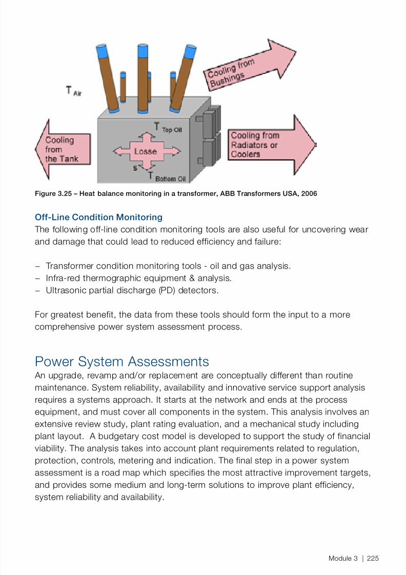
8/12/2019 Energy Efficiency Electronic Book Version 1548_PowerGenerationHandbook v1_1
http://slidepdf.com/reader/full/energy-efficiency-electronic-book-version-1548powergenerationhandbook-v11 227/361
Figure 3.25 – Heat balance monitoring in a transformer, ABB Transformers USA, 2006
Off-Line Condition Monitoring The following off-line condition monitoring tools are also useful for uncovering wearand damage that could lead to reduced efficiency and failure:
− Transformer condition monitoring tools - oil and gas analysis.− Infra-red thermographic equipment & analysis.− Ultrasonic partial discharge (PD) detectors.
For greatest benefit, the data from these tools should form the input to a morecomprehensive power system assessment process.
Power System Assessments An upgrade, revamp and/or replacement are conceptually different than routinemaintenance. System reliability, availability and innovative service support analysis
requires a systems approach. It starts at the network and ends at the processequipment, and must cover all components in the system. This analysis involves anextensive review study, plant rating evaluation, and a mechanical study includingplant layout. A budgetary cost model is developed to support the study of financialviability. The analysis takes into account plant requirements related to regulation,protection, controls, metering and indication. The final step in a power systemassessment is a road map which specifies the most attractive improvement targets,and provides some medium and long-term solutions to improve plant efficiency,system reliability and availability.
Module 3 | 225

8/12/2019 Energy Efficiency Electronic Book Version 1548_PowerGenerationHandbook v1_1
http://slidepdf.com/reader/full/energy-efficiency-electronic-book-version-1548powergenerationhandbook-v11 228/361
Power System Efciency Guidelines – SummaryDesign practices worth considering for improved energy efficiency in the powersystem are listed below:
− Select higher voltage levels for some buses (MV instead of LV).
− Use 3-phase transformers instead multiple single phase.
− Use large transformers instead of multiple, smaller ones; sharetransformers between units.
− Upgrade old transformers to achieve higher efficiency, improvedmonitoring
− Use PF correction, near the inductive sources where possible, to
approach 0.95 PF. − Use a generous cable laying method; avoid methods which lead to
cable derating.
− Consider a plant arrangement which reduces length of cable runs &voltage drops.
− Ensure that harmonics are well within tolerance.
− Understand motor duty, and size accordingly, following the guidelinesin Motor Sizing and Selection
− Ensure phase loads and voltages are balanced.
226 | ABB Energy Efficiency Handbook

8/12/2019 Energy Efficiency Electronic Book Version 1548_PowerGenerationHandbook v1_1
http://slidepdf.com/reader/full/energy-efficiency-electronic-book-version-1548powergenerationhandbook-v11 229/361
Module Summary This module describes the general design and energy impact of the plantinstrumentation, controls and optimization systems. While a detailed presentation ofall relevant automation concepts is beyond the scope of this handbook, this sectionexamines automation from an energy efficiency perspective and does not provideguidance on other, critical aspects of automation engineering such as interlock logic,emergency shutdown sequencing, or fault-tolerant design. For a more completeguide to all other aspects of automation design, see the standards and referencessections of this handbook.
The information in this module may also be generally applied to processindustries; industry-specific text is shown between rule lines.
Automation Concepts A process plant is a hierarchy of equipment & control systems: a combination ofhardware, software, people and operating procedures interrelated as shown in the
figure below.
Figure 4.1 – Levels of automation in an industrial plant
Instrumentation, control and optimization, collectively known as ‘automation’,encompass equipment, software and methods, ranging from field devices to plantmanagement. The main function of plant control and automation systems is toregulate various parts of the process, such that they operate at desired setpoints, toinitiate shutdown or trip action in case of problems, and to monitor key performanceparameters for continuous improvement. The ISA is a leading professional societyfor this relatively new field of engineering. Automation is one of the youngest
Module 4 Automation Systems
Module 4 | 227

8/12/2019 Energy Efficiency Electronic Book Version 1548_PowerGenerationHandbook v1_1
http://slidepdf.com/reader/full/energy-efficiency-electronic-book-version-1548powergenerationhandbook-v11 230/361
disciplines in engineering, and is growing rapidly as more sensors and intelligenceare embedded in common plant equipment.
Role of Automation in Energy Efciency Automation allows faster and more consistent response to changing load conditionscompared to open loop (or human in the loop) control methods. Automation alsoenables the process to operate in a more stable way, and thus can be safely operatedcloser to its constraints for optimum energy efciency. When a survey (US DoE, 2004)asked process plant professionals to identify the operational or process changes thatwould realize signicant energy savings, most of the responses involved one or moreautomation technologies.
The responses generally fall into these broad categories:
Control and Optimization: − Improved control of boilers, and other efficiency improvements through
optimization, modeling and equipment design. − Advanced control strategies such as model predictive control, improved
measurement devices− and sensors, multivariate data processing and analysis, better scheduling
optimization strategies
− Use of thermal optimization based on process integration technology (e.g., pinchtechnology): use of waste heat /use of waste heat recovery technologies.
Drive Power: − Optimized pumping & fan systems based on appropriately sized/specified
equipment and often relying on variable speed drives − Use of variable speed motors rather than throttling valves to control process flow
Management & Decision Support: − Use of information tools (advisory/monitoring) to improve decision making onthermal energy use
− Improved system-wide decision-support across the whole plant and groups ofplants
− Better management of power & electric loads − Regular and disciplined application of electrical and thermal energy assessment
tools
For process & industrial controls, end-users envision potential energy savingsranging from about 2% to 25%. Vendor estimates of the savings from plant-wide
228 | ABB Energy Efficency Handbook

8/12/2019 Energy Efficiency Electronic Book Version 1548_PowerGenerationHandbook v1_1
http://slidepdf.com/reader/full/energy-efficiency-electronic-book-version-1548powergenerationhandbook-v11 231/361
automation integration alone were on the order of 5% of the total energy, on averagefor all process industries (US DoE, 2004) .
Instruments and ActuatorsPlant automation and performance monitoring & improvement functions are alldependent on reliable plant data measurement and acquisition, and precisecontrollability of processes.
Figure 4.2– Pressure transmitter (left) and process analyzer (right). (ABB,2006)
Collectively known as ‘field devices’, anything that directly senses or controls
a process typically is categorized as an instrument, an analytical sensor, or anactuator. Instruments are sensors that obtain real-time measurements of basicprocess variables such as temperature, pressure and flow rate. These are sometimesalso referred to as transmitters and are typically used as inputs to fast-acting controlloops and interlocks. Actuators are output devices such as drives, valves anddampers that can either directly or indirectly modify measured process variables.
Process Instruments
The most common types of measuring devices (instruments) in a process or powerplant are; pressure sensors, temperature sensors, level sensors, and flow-meters. Additionally, control may require measurements of speed, current, voltage, chemicalcomposition or various physical properties, such as thickness, opacity, resistivity,etc. Accurate measurement is a requirement for process precision, as well asenergy-efficient control. Poorly chosen or located instruments will introduce lag andinstability, causing much energy-wasting corrective action or process instability.
According to the ISA, instruments should be installed as close as is practical to thesource of the measurement, with consideration being given to excessive vibrationand ambient temperature. Other common problems with process instruments aredrift, bias and lockup freezing. An instrumented that has drifted from its calibrationwill lead to off-setpoint control. Bias is when an instrument under or over reports a
Module 4 | 229

8/12/2019 Energy Efficiency Electronic Book Version 1548_PowerGenerationHandbook v1_1
http://slidepdf.com/reader/full/energy-efficiency-electronic-book-version-1548powergenerationhandbook-v11 232/361
measurement. Lockup, or freezing, is when an instrument continually transmits asingle value while the related process actually is varying.
These effects are particularly troubling if the instrument’s on-board diagnostics areunable to detect and report them to operators. ’Smart’ transmitters have fewersuch problems due to their continual diagnostic monitoring. These transmitters tendto be more accurate as well, and the extra signal processing allowing them to beturned down by a factor of 10 and still provide accurate measurement (ISA 2005).Smart transmitters should be specified as part of a broader strategy, which typicallyincludes an upgrade to fieldbus communication. Smart transmitters are currentlyavailable in three widely accepted varieties – HART, Profibus and FoundationFieldbus.
Performance monitoring, condition assessment, diagnostic tools, maintenancemanagement systems and asset lifecycle optimization rely on the data from smartinstruments and the automation system to provide in-depth information about theprocess, as well as the condition of the process equipment itself. This information isprovided in real-time, without the need for scheduled downtime or waiting for a plantshutdown to perform equipment inspections.
It is an energy efficiency design oversight to omit instruments altogether in certaincritical areas. The lack of accurate process data will hinder efforts at automatic
control and energy performance improvement.
In a power plant, steam flow measurements are essential to feedwater controland in a coordinated boiler-turbine control scheme described in CoordinatedBoiler-Turbine Control . Instead of direct flow measurement, however, thevalue is inferred from the HP turbine 1st stage pressure, which introduces lagand inaccuracy in the control systems.
In feedwater control, the specification of two additional sensors enabled the3-element control now common on sub-critical boilers. Lack of turndown inthese sensors, however, leads some units to fall back into less-stable and lessefficient single-element control at low loads. See Feedwater Flow Control fordetails.
Choice of sensing technology also has an impact on power plant controleffectiveness. Level sensors that are undesirably sensitive to density variationswill introduce errors unless corrected for with additional controls. Vibration andother effects may disturb some sensors used in condenser and de-aerator level
230 | ABB Energy Efficency Handbook
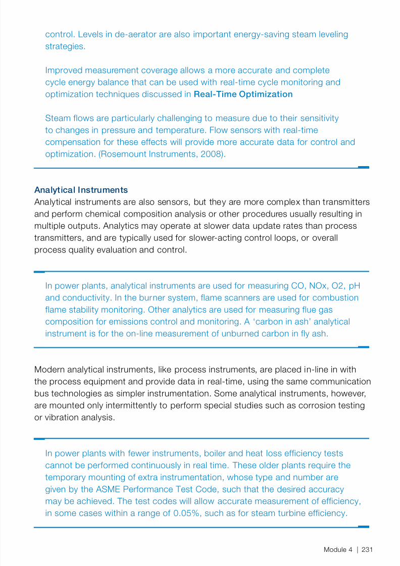
8/12/2019 Energy Efficiency Electronic Book Version 1548_PowerGenerationHandbook v1_1
http://slidepdf.com/reader/full/energy-efficiency-electronic-book-version-1548powergenerationhandbook-v11 233/361
control. Levels in de-aerator are also important energy-saving steam levelingstrategies.
Improved measurement coverage allows a more accurate and completecycle energy balance that can be used with real-time cycle monitoring andoptimization techniques discussed in Real-Time Optimization
Steam flows are particularly challenging to measure due to their sensitivityto changes in pressure and temperature. Flow sensors with real-timecompensation for these effects will provide more accurate data for control andoptimization. (Rosemount Instruments, 2008).
Analytical Instruments Analytical instruments are also sensors, but they are more complex than transmittersand perform chemical composition analysis or other procedures usually resulting inmultiple outputs. Analytics may operate at slower data update rates than processtransmitters, and are typically used for slower-acting control loops, or overallprocess quality evaluation and control.
In power plants, analytical instruments are used for measuring CO, NOx, O2, pH
and conductivity. In the burner system, flame scanners are used for combustionflame stability monitoring. Other analytics are used for measuring flue gascomposition for emissions control and monitoring. A ‘carbon in ash’ analyticalinstrument is for the on-line measurement of unburned carbon in fly ash.
Modern analytical instruments, like process instruments, are placed in-line in withthe process equipment and provide data in real-time, using the same communication
bus technologies as simpler instrumentation. Some analytical instruments, however,are mounted only intermittently to perform special studies such as corrosion testingor vibration analysis.
In power plants with fewer instruments, boiler and heat loss efficiency testscannot be performed continuously in real time. These older plants require thetemporary mounting of extra instrumentation, whose type and number aregiven by the ASME Performance Test Code, such that the desired accuracymay be achieved. The test codes will allow accurate measurement of efficiency,in some cases within a range of 0.05%, such as for steam turbine efficiency.
Module 4 | 231

8/12/2019 Energy Efficiency Electronic Book Version 1548_PowerGenerationHandbook v1_1
http://slidepdf.com/reader/full/energy-efficiency-electronic-book-version-1548powergenerationhandbook-v11 234/361
Process Actuators Actuators are devices that can directly act on the process through physicallydirecting gas and fluid flows. Some actuators typically found in a process or powerplants are; Dampers, Louvers, Inlet Guide Vanes, Servo valve position controllers,
Variable Frequency Drives, Solenoid (on-off) valves.
Actuators with significant deadband (hysteresis) will have poor control response,and non-linear actuators will require additional correction (linearization) to behavewell across their entire operating range. Also, a reduced range of action, such aslow turndown, can severely limit a unit’s energy performance at low loads. Anothercommon problem with process actuators is stiction, in which a large force is requiredto overcome static friction between two surfaces in contact.
Figure 4.3– Part-turn actuator for rotary movement of final control elements, (ABB PME120 brochure)
Control ValvesControl valves (CVs) are valves used for automatic control of fluid flow. Valve openingis controlled by a positioner that may be driven by an electric motor, hydraulic power,or by compressed air in response to a command from the control system.
Control valves that are oversized will operate in a nearly-closed state for most ofthe time. Oversized valves are hard to control and may cause instability during rapidchanges. Control valves are oversized as a result of the oversizing of constant-speed
upstream components, pumps and motors, as described in this handbook. Whenthe actual flows are much smaller than these components nominal operating points,then the CV must drop correspondingly more pressure by closing more fully. Asdescribed in the section on pump flow Throttling , the CV wastes energy that shouldnot have been input to start with. Speed control is the preferred method of flowcontrol, and eliminates the need for energy wasting throttling control valves.
CVs are mechanical devices that often operate under great fluid pressures and areprone to stiction in the valve stem and hysteresis. These effects will cause CV controlloops to oscillate and may lead to process instability. There are methods to measurestiction online, and techniques for tuning PID controllers where stiction is observedor suspected. CVs and other actuators are usually powered electrically, or from
232 | ABB Energy Efficency Handbook

8/12/2019 Energy Efficiency Electronic Book Version 1548_PowerGenerationHandbook v1_1
http://slidepdf.com/reader/full/energy-efficiency-electronic-book-version-1548powergenerationhandbook-v11 235/361

8/12/2019 Energy Efficiency Electronic Book Version 1548_PowerGenerationHandbook v1_1
http://slidepdf.com/reader/full/energy-efficiency-electronic-book-version-1548powergenerationhandbook-v11 236/361
trends, engaging in specific plant performance assessments or by doing a loopperformance analysis where set point, process value and control output froma controller are analyzed over a reasonable period of time (from several shifts,up to one month). Inaccurate or weak damper drives cause poor combustioncontrol response and can cost a plant in terms of poor load following, higherheat rate, slagging, carbon-in-ash, poor emissions control and unacceptableopacity variations.
The goal for improved damper control is to be able to remove processdeviations caused by draft-related variables (Furnace Pressure, NOX, excessO2 and so on), enabling operating points to move closer to ideal levels.Modern electric actuators make this possible by positioning the final controlelement down to within 0.1 percent of the driving control signal. Modernelectric actuators also have other operational advantages in addition toimproved damper control. Many advanced actuators have diagnostics for‘ watchdog ‘ functions that alert plant personnel before a serious problemdevelops, avoiding costly downtime. For example, the electric actuator canmonitor damper position, frequency of motor reversals, frequency of torquedelivered and actuator internal temperature. Monitoring these diagnostics andassociated alarms and alerts helps to ensure proactive instead of reactivemaintenance, as well as optimum air control and plant performance.
In many cases, accurate damper drives and controls alone will providesignificant improvements over legacy systems. See section Air Flow Controlfor Combustion for details on airflow control and alternatives to dampers forair flow control.
Sequential ControlSequential control (or sequential function chart- SFC) is a series of steps (or tasks)
which bring the process through a sequence of well-defined states. This type ofcontrol is commonly used during startup and shutdown procedures, or duringemergency (trip) action. SFC automates traditional checklists for these proceduresand is an important tool for plants with fewer experienced staff. Sequential controlhas the potential to speed up these procedures within safety limits, thus savingenergy and unproductive power generation. The intermediate states in the sequencecan be automatically monitored and operators receive alarms if an expected value isnot achieved. A sample SFC program, showing states and transitions between them,is shown in the figure below.
SFC programming, combined with the communication capabilities of intelligentMotor Control Centers (MCCs) can turn off motors when not required by the
234 | ABB Energy Efficency Handbook
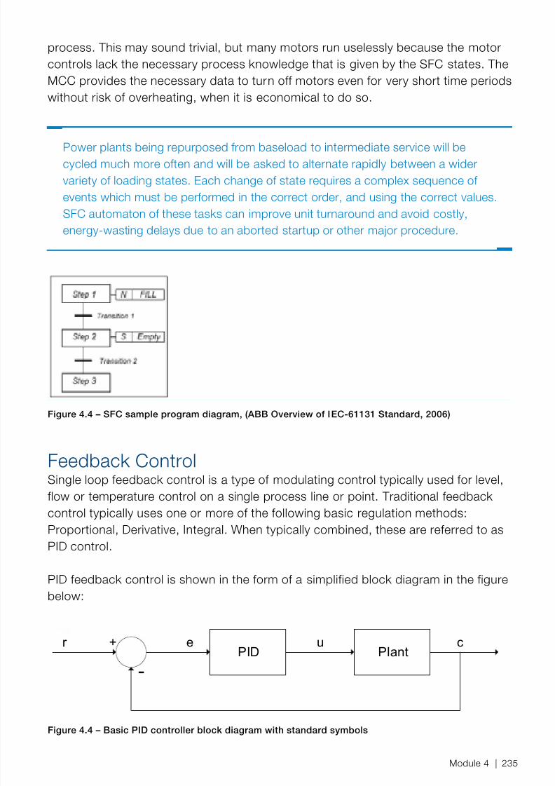
8/12/2019 Energy Efficiency Electronic Book Version 1548_PowerGenerationHandbook v1_1
http://slidepdf.com/reader/full/energy-efficiency-electronic-book-version-1548powergenerationhandbook-v11 237/361
process. This may sound trivial, but many motors run uselessly because the motorcontrols lack the necessary process knowledge that is given by the SFC states. TheMCC provides the necessary data to turn off motors even for very short time periodswithout risk of overheating, when it is economical to do so.
Power plants being repurposed from baseload to intermediate service will becycled much more often and will be asked to alternate rapidly between a widervariety of loading states. Each change of state requires a complex sequence ofevents which must be performed in the correct order, and using the correct values.SFC automaton of these tasks can improve unit turnaround and avoid costly,energy-wasting delays due to an aborted startup or other major procedure.
Figure 4.4 – SFC sample program diagram, (ABB Overview of IEC-61131 Standard, 2006)
Feedback ControlSingle loop feedback control is a type of modulating control typically used for level,flow or temperature control on a single process line or point. Traditional feedbackcontrol typically uses one or more of the following basic regulation methods:Proportional, Derivative, Integral. When typically combined, these are referred to as
PID control.
PID feedback control is shown in the form of a simplified block diagram in the figurebelow:
PID Plantr +
-
e u c
Figure 4.4 – Basic PID controller block diagram with standard symbols
Module 4 | 235

8/12/2019 Energy Efficiency Electronic Book Version 1548_PowerGenerationHandbook v1_1
http://slidepdf.com/reader/full/energy-efficiency-electronic-book-version-1548powergenerationhandbook-v11 238/361
Where, according to ISA terminology:
r = reference signal (also referred to as setpoint)e = error signal (r-c)u = PID controller output (also referred to as manipulated variable or control action)c = controlled output (also referred to as controlled variable)
The PID control loop compares the controlled output of the reference signal to getan error signal ‘e’. This signal is input to the actual controller, shown in the boxmarked ‘PID’ in the block diagram, which generates a corrective control signal to theactuator in the plant. The action is designed to drive the error signal to approximatelyzero, such that no further corrective control action is necessary,
A more detailed block diagram of a feedback control loop would show the additionaleffects introduced by the sensor and final control elements. Such a diagram wouldalso show the ‘disturbances’ which in most cases represent the varying load on theprocess.
The reference signal is also called the setpoint of the loop. Closed loop control actsto minimize the steady state error so that the output of the process returns to thedesired setpoint established by the operators. Unlike open-loop control, feedback
control can respond to any disturbance and return the process rapidly to setpoint,but only if the loop is properly tuned. If the underlying process parameters change,due to temperature or other effects, then the loop must be re-tuned.
Untuned loops may waste energy by demanding unnecessary auxiliarydrivepower and by allowing (or even causing) greater instability. According toindustry research (Matrikon, 2005), up to 75% of regulatory controls in a typical
process plant are under-performing. Many loops are incorrectly put into a fixedor “manual” mode, where the PID action has been defeated completely.
Manual mode control and loop instability will generally lead operators to useless efficient process setpoint values to avoid situations when the swingingoutput variable exceeds a critical limit. Stable automatic operation allowssustained and safe operation closer to optimal process and energy limits.
236 | ABB Energy Efficency Handbook

8/12/2019 Energy Efficiency Electronic Book Version 1548_PowerGenerationHandbook v1_1
http://slidepdf.com/reader/full/energy-efficiency-electronic-book-version-1548powergenerationhandbook-v11 239/361
Process CharacteristicsDesign and tuning of PID control loops requires an understanding of the physicalprocess under control. From a basic control standpoint, the process is characterizedby its gain, time constant, dead-time, and its degrees of freedom.
− Process gain (K) is the amount a process’ output changes in response to achange in input. Process gain can be separated into steady-state and dynamiccomponents. (ISA 2005). The product of process gain and controller gain is the‘loop gain’.
− Time constant (TC) describes the rapidity of the above response. After one TCthe output variable has reached 63.2% of its final value. More complex processesmay have multiple TCs.
− Dead time (DT) is the amount of time it takes for the above response to start afterthe input has changed. Transportation lag or thermal inertia are common sourcesof dead time.
− Degrees of Freedom (n) are the number of independent variables in the process,which is also the highest possible number of independently-acting controllers forthat process (ISA 2005). The degrees of freedom can be computed by taking thetotal number of process variables and subtracting the number of relationships(physical, chemical etc.) between them.
All the above process characteristics are important for correct loop design and
tuning, hence energy-efficient operation. Oscillations will result if the loop gain > 1.Response will be too slow if loop gain is very low. The controller gain must thereforebe chosen to provide a total loop gain of about 0.5 to achieve rapid yet stableperformance.
Feedforward ControlFeedback control responds only after a process disturbance has already causeda change in the output; it is blind to the original disturbance. In many cases,
this disturbance can be measured and even anticipated, as in the case of achange in process loading. Feedforward control uses this knowledge to computean appropriate control response, which is then summed with the output of aconventional PID controller as shown in the following block diagram.
Module 4 | 237

8/12/2019 Energy Efficiency Electronic Book Version 1548_PowerGenerationHandbook v1_1
http://slidepdf.com/reader/full/energy-efficiency-electronic-book-version-1548powergenerationhandbook-v11 240/361
PID Plantr +
-
e y
Disturbance
FeedforwardController
D(t)
++
+
+
Figure 4.5 – Feedforward controller block diagram
The feedforward response is based on a physical model of how the processresponds to the measured disturbance. The success of feedforward is dependenton the accuracy of this model, which is difficult to obtain and maintain. Even withan imperfect model, however, feedforward control combined with PID controlusually provides a faster and more stable response than PID method acting alone.
The feedforward controller corrects for 90% of the disturbance, while the PIDcontroller can rapidly and smoothly respond for the remaining 10%. (ISA 2005). Thefeedforward controller model can also provide lead-lag compensation for processdead-times, which would otherwise make a PID loop more difficult to tune.
The improved control response saves process energy and reduces waste, butfeedforward control has another energy benefit; reducing the load on the PIDcontroller by an order of magnitude. (ISA 2005), loops which use drivepower foractuation will use significantly less energy.
Cascading ControlIn cascading control, one PID is nested within another PID loop as shown in the
figure below. The outer (master) loop provides the setpoint for the inner (slave) loop.For cascade control to work, the inner loop must have a shorter time constant thanthe outer loop. One common example of cascading control is flow control, where theinner loop controls valve position and the outer loop controls for output temperature.
PID HeatExchanger
Outer loop
r +
-
FlowSystem
+
-Inner loop
PID
Figure 4.6 – Cascade feedback controller block diagram
238 | ABB Energy Efficency Handbook

8/12/2019 Energy Efficiency Electronic Book Version 1548_PowerGenerationHandbook v1_1
http://slidepdf.com/reader/full/energy-efficiency-electronic-book-version-1548powergenerationhandbook-v11 241/361
Cascade control allows the inner loop to correct quickly for inner loop disturbances,such as valve hysteresis, leaving the outer loop to respond more quickly to changesin the controlled variable.
Adaptive ControlIn adaptive control, also known as self-tuning or auto-tuning control, the PIDparameters themselves are automatically modified online to respond to the changingsensitivities of the process. In effect, the parameters which are normally fixed in a‘static’ PID controller become themselves variables in one or more feedback loops.Some self-tuning controllers operate in static mode most of the time, but will self-tune on request from an operator or after a fixed time interval.
Advanced Control and Optimization Advanced Control encompasses many methods for controlling and optimizing largersystems with multiple variables and with important constraints. This control leveltypically operates at slower rates than single loop control, but can still operate inreal-time.
Model-Based ControlModel-based control encompasses a variety of techniques using models togenerate a control response. These models may be either mechanistic or empirical.
Mechanistic models are based on physical principles (sometimes these modelsare called first principles), whereas empirical models use past data or black-box,mathematical approximations. The most common empirical technique models theprocess using a collection of step responses, each with its own coefficient(s).
The most widely used model-based technique uses a time-series model of the openloop response of the process. This series is the model’s calculated response to aseries of predicted control action values and disturbance values. An optimization
function then updates the control action value series to achieve minimal deviationfrom setpoint with limited control action. This sequence of control actions is referredto as a trajectory.
Model Predictive Control, or MPC, has multiple outputs, in contrast to feedbackcontrol methods, which output only a single control action in response to a changein the input measurement. MPC uses a form of feedback in which the estimationerror is used by the model to improve future estimations, as shown in the simplifiedblock diagram.
Module 4 | 239

8/12/2019 Energy Efficiency Electronic Book Version 1548_PowerGenerationHandbook v1_1
http://slidepdf.com/reader/full/energy-efficiency-electronic-book-version-1548powergenerationhandbook-v11 242/361
Figure 4.7 – MPC block diagram showing model and correction blocks
MPC is valuable in process situations of multiple variables with non-linear dynamicresponse, or where several control loops are interacting. The optimization function inMPC is well-suited to handling process constraints without decomposing them intosetpoints, as is the case with PID control. MPC is also useful in process situationswhere direct measurements are not possible, or cannot be made fast enough forconventional PID control to be applied.
MPC is typically used in a hierarchy of control, providing setpoints to the lower, PIDlevel of control as described in the section multi-level real-time optimization. MPCrequires more engineering effort, especially during the verification and commissioning
phases, compared to conventional control methods. Access to realistic or historicaldata is important for the model verification phase. Payback time for typical MPCinvestments is 6-12 months (Cybernetica, NFA Days Norway 2006). Some recentMPC projects, however, have netted impressive results, with paybacks of less thantwo months.
Inferential ControlInferential control (IC) is based on techniques such as inference engines or neural
networks. Such systems ‘learn’ from experience and can be used as a guideto operators. A properly designed and maintained IC system can absorb theaccumulated energy efficiency knowledge of experienced operators and showthe way to younger operators through complex and less frequent tasks, such asstartups/shutdowns and complex process transition procedures.
Linear Programming with Mixed Integer Programming (LP/MIP) The optimization layer uses linear programming technology (LP). LPs are commonoptimization tools used for planning and scheduling applications in many industries.
The LP minimizes an objective function (cost of fuel plus cost of purchasedelectricity), while adhering to many constraints. Some of the constraints are partof the plant model, representing mass and energy balances. Other constraints
240 | ABB Energy Efficency Handbook

8/12/2019 Energy Efficiency Electronic Book Version 1548_PowerGenerationHandbook v1_1
http://slidepdf.com/reader/full/energy-efficiency-electronic-book-version-1548powergenerationhandbook-v11 243/361
represent capacity limits, such as maximum fuel flow rates to boilers, and generatorconstraints (Pekka Immonen et al, Power Engineering, Nov.2008 ‘CoordinatedControl and Optimization of a Complex Industrial Power Plant’).
Multi-Level Real-Time Optimization This section is adapted from material by Pekka Immonen, which was first publishedin Power Engineering, Nov.2008 ‘Coordinated Control and Optimization of aComplex Industrial Power Plant’.
A multi-level approach (see Figure) uses real-time optimization (RTO), connected toadvanced process control (APC). At the top level, an optimization program monitorsthe current situation in the plant and gathers pricing data over the Internet to maketimely decisions about loading individual equipment in the plant. The optimizationprogram then dispatches these orders to an advanced control layer, which providescoordinated, decoupled control of pressure and power generation. The base controllevel modulates the actuators affecting the plant to maintain the measured processquantities at their setpoints.
Figure 4.8 – Multi-level real-time optimization, (Immonen, Coordinated Control and Optimization of aComplex Industrial Power Plant, 2008)
In industrial boiler systems, a multi-level approach uses LP to make theselection between the operating modes based on the fuel and power pricingsituation and the plant conditions. The selection cannot be made on pricinginformation alone. The equipment limits are higher priority and they must behonored for safety and equipment protection. The constraint set continuallyupdates as process conditions drift and available equipment varies withmaintenance schedules.
Module 4 | 241

8/12/2019 Energy Efficiency Electronic Book Version 1548_PowerGenerationHandbook v1_1
http://slidepdf.com/reader/full/energy-efficiency-electronic-book-version-1548powergenerationhandbook-v11 244/361
The advanced control system uses technology known as model predictivecontrol (MPC). MPC is a multivariable control algorithm. Like the LP, MPCuses a model, but it’s dynamic rather than steady-state. MPC runs at a muchhigher frequency than the LP, less than 10 seconds compared to 15 minutes.Using the model, the controller predicts the effects of moving multiple basecontrol setpoints: high pressure and low pressure boiler fuel setpoints, all threeextraction valves on all four turbines, all PRVs and all vent valves (a total of 28manipulated base control setpoints).
The algorithm is capable of providing smooth transitions, whether openingPRVs, closing vent valves or controlling the steam balance with LP boilerswhen the HP boilers are maximized. In case of large process upsets, the MPCuses all steam system components to help out, allowing temporary deviationsfrom their optimum targets. As the MPC is a multi-variable algorithm, all therequired operating modes are achieved with a single MPC configuration. Theoverall design is greatly simplified as there is no need for alternative DCSconfigurations or complex over-ride schemes at the base control layer forboiler-follow, turbine-follow, PRV and other such modes. The most immediatebenefit from the implementation of the new strategy was the greatly improvedprocess stability (Immonen, Coordinated Control and Optimization of aComplex Industrial Power Plant, 2008).
Process Model-Based Real-Time OptimizationProcess-model-based algorithms and advanced signal processing functions allowoperators to quickly identify under-performing equipment and take remedial actionon controllable losses. The advantage of model-based methods is their ability topredict plant performance for daily operations or long-term operational investmentssuch as retrofits or process improvements. These tools can be connected directlyto the process to run their models in real-time on actual plant data. The calculated
(expected) values can then be compared with the actual process values, as shown inthe following figure:
242 | ABB Energy Efficency Handbook

8/12/2019 Energy Efficiency Electronic Book Version 1548_PowerGenerationHandbook v1_1
http://slidepdf.com/reader/full/energy-efficiency-electronic-book-version-1548powergenerationhandbook-v11 245/361
Figure 4.9 – Simulation and monitoring with PowerCycle software, ( ABB Switzerland, Power Technol-ogy Systems, 2005, PowerCycle brochure)
These comparisons will reveal deviations from optimum energy efficiency, ascalculated in the process’ thermodynamic model. The resulting deviation data canbe used for early detection of equipment degradation of loop tuning problems. Theprocess thermodynamic model use by RTO is developed during the project design
phase using the methods described in section Modeling and Simulation Tools
Lifecycle Model-Based Real-Time Optimization The LCC methods described in Efficiency and Lifecycle Cost Calculations can beprogrammed to execute online and then input to one of the plant-wide optimizationengines described above.
Supervisory ControlSupervisory Control (SC) is the highest level, providing feedback for such plantmanagement tasks as economic optimization, decision support, performance monitoringand load scheduling. This level of control may have a rate of 15 minutes, hours or evendays. SC relies heavily on a Human Machine Interface (HMI) that can calculate and trendplant overall and equipment efciencies. SC functions also allows plant management tomonitor plant performance, identify root causes and correct problems.
In power plants, load dispatch commands are a semi-automated SC functionwhich is at the center of plant load control and operations.
Module 4 | 243
8/12/2019 Energy Efficiency Electronic Book Version 1548_PowerGenerationHandbook v1_1
http://slidepdf.com/reader/full/energy-efficiency-electronic-book-version-1548powergenerationhandbook-v11 246/361
Performance Monitoring SystemsPerformance Measurement Systems do not directly control the process, as theother systems described in this module. Performance Measurement Systems usehumans as the actuators by providing them with analysis functions and large amountof historical data. If performance measurement is used regularly and in a pro-activemanner by plant operators, then it becomes a very effective nearly-closed-loopsystem to optimize energy efficiency.
Performance Monitoring Concepts The plant unit historical data is collected from the plant’s instruments and stored inan integrated plant information management system (PIMS). Process data from allsources throughout the plant are collected and securely stored in the data server,where they can be analyzed further. The PIMS data repository, possibly coveringthe entire operating history of a plant in its archive, is an invaluable source ofinformation for efficient plant operation and maintenance. PIMS can offer a widerange of analysis and presentation tools. Among the basic tools are trend curvesfrom historical data on the operator station to monitor process behavior over timeand detect patterns.
In power plants the Performance Monitoring Systems (PM) will also calculateefficiency metrics of individual components such as air heater, condenser,
turbine, combustion, and emissions control equipment.
Convective Heat Exchanger PerformanceIn power plant, it is important to monitor the performance of superheater,reheater and economizer for convective heat exchange. The actualperformance value for each section is calculated by measuring water/steam-side heat absorption, and performing an iterative gas-side heat balance foreach individual section. Radiation heat transfer is taken into account for the
upper heat transfer sections. The clean surface performance is calculated foreach section using design information and an iterative gas-side heat balancefor each section. The ratio of the actual operating heat transfer rate to thepredicted clean heat transfer rate determines the conditions of each section.(ABB Switzerland, Power Technology Systems, Optimax Operations Products,2005)
Furnace Heat Transfer Performance An iterative heat balance calculation can also be applied to determine theperformance of furnace heat transfer areas. This calculation allows for heatabsorption in the roof and walls of the upper furnace, and the radiation heatfrom the lower furnace. These heat transfer performance calculations lead to
244 | ABB Energy Efficency Handbook

8/12/2019 Energy Efficiency Electronic Book Version 1548_PowerGenerationHandbook v1_1
http://slidepdf.com/reader/full/energy-efficiency-electronic-book-version-1548powergenerationhandbook-v11 247/361
a ‘cleanliness value’ that can guide soot-blowing operations (See section onsoot-blowing systems).
Air Heater PerformanceSimilar methods are used to calculate the air heater performance andcleanliness. The gas inlet temperatures at the air heater and other surfacescan also be calculated. Significant deviations can be indicative of large energylosses due to fouling or leakage.
Energy Efficiency Potential of Performance MonitoringIf the plant is properly instrumented, a PM system can be the key to a heat rateawareness and improvement program. Such a program uses benchmarks andkey performance indicators calculated and displayed on-line in trend charts bythe PM system. The success of a heat rate improvement program depends onan adequate assessment up-front, and management commitment throughout,to ensure that the recommendations are actually implemented. According toone example from EPRI, a PM system, together with a well-supported heatrate program, improved heat rate by 1.5 percent and the net capacity factorby 5.2 percent. Costs at that plant were also reduced by 2.3 percent. (PowerEngineering January, 2002, Douglas Smith)
A PM system is a very useful tool in plant heat rate improvement programs,but the historical data in the system must be reliable; this means that primaryprocess information is acquired by properly installed, calibrated and maintainedinstrumentation, as described in the section on Instruments and Actuators .
Condition Monitoring SystemsField devices, and process actuators in particular, will degrade in performance with
accumulated operating hours, number of cycles, or due to fouling and corrosioneffects. Catastrophic failures attract attention due to the large single opportunity costof a trip. The slower, less-visible accumulation of wasted energy due to degradedperformance may rival these costs over the lifetime of the unit. The energy cost ofa reliability related trip is described in the section on Energy Cost of a Trip for adiscussion on the energy cost of poor reliability.
Rotating MachineryDegradation or poor installation of the motor-coupling and bearings will reducedrivepower energy efficiency and lead to maintenance problems. Periodic inspectionand measurement helps, but online condition monitoring of rotating machinery willprovide earlier warning of impending efficiency problems. A Condition Monitoring
Module 4 | 245

8/12/2019 Energy Efficiency Electronic Book Version 1548_PowerGenerationHandbook v1_1
http://slidepdf.com/reader/full/energy-efficiency-electronic-book-version-1548powergenerationhandbook-v11 248/361
(CM) system monitors bearing vibration, eccentricity and axial rotor position onany type of rotating machinery. These data are integrated into the DCS to leveragethe CS logging, trending and operator alarms functionality. The types of rotatingmachinery deserving this form of condition monitoring are: turbines, feedpumps,fans, pumps, motors, gearboxes and compressors.
Condition Monitoring is distinguished from process monitoring through the useof models or other calculations to interpret the raw data and report on the actualcondition of the equipment. The large number of rotating machinery in a power plantwould make it difficult for operators to examine trends of each item. This type ofautomatic analysis is especially important for vibration data, which is a distributionof frequencies (a spectrum), which are both difficult and tedious for operators tointerpret. A CM system for vibration monitoring compares baseline spectral datato current spectral data; any changes in the data are matched to a rules basedalgorithm, which in turn determines the cause of the change. The result is actionableinformation in the form of specific fault diagnosis, fault severity and maintenancerecommendation.
In power plants: for large journal bearing machines like Main Turbines andBoiler Feed Pumps, these CM systems use Full Spectrum, Angle of theMajor Ellipse Axis and Aspect Ratio of the Ellipse for Orbit analysis plus
Shaft Centerline Position and Bearing Eccentricity. All these tools, along withcomparisons to user configured Threshold Values, combine to determine thecondition of the machine train, bearing by bearing.
Heat Exchanger Monitoring The status of heat exchanger performance can be monitored in real-time usingmeasurements of flowrate and temperatures (in and out) of each stream. These
data are used to calculate the overall heat transfer co-efficient (U), using thethermodynamic formula for heat transfer shown below.
Q = U x A x ΔT
Where:
Q = heat transferred (kcal/hr) A = area of heat exchanger (m²)ΔT = temperature difference between hot & cold sides (log C)
246 | ABB Energy Efficency Handbook

8/12/2019 Energy Efficiency Electronic Book Version 1548_PowerGenerationHandbook v1_1
http://slidepdf.com/reader/full/energy-efficiency-electronic-book-version-1548powergenerationhandbook-v11 249/361
All of these values are stored in a ‘process historian’ database and then continuouslyanalyzed using a fouling factor model. This model is simply an energy balancebetween the hot and cold streams within the exchanger. If the current overallco-efficient is 5% or more less than the model’s prediction (Rajan 2003), then amaintenance alert is triggered calling for proactive cleaning or problem investigation.
Control SystemsEvolution of Control SystemsControl systems have evolved from analog pneumatic controls to modernmicroprocessor-based systems. There are two main branches in this evolution;programmable logic controllers (PLCs) and Distributed Control Systems (DCS).PLCs are the simpler of the two, and are most suitable for machinery control andother areas of discrete manufacturing. A DCS is most suitable for processing thelarge number of analog input/output (I/O) in a large power or process plant, and aretherefore often referred to as ‘process control systems’ The term ‘distributed’ inDCS is meant to distinguish these from an earlier, more centralized control systemarchitecture centered around a process control computer. Another distinguishingfeature of DCS is their use of function blocks rather individual I/O ‘tags’ for easierprogrammability.
Distributed Control Systems (DCS)
− A DCS provides all of the background services needed for control, operation andmonitoring:
− Connections to various communication busses and networks − Controller CPUs and their associated I/O sub-systems − Human Machine Interface (HMI) for operator control, alarm and status indication − Historian services to log & store large volumes of real-time data
These DCS services can have a significant impact on plant energy efficiency. ADCS is the only equipment type that spans all the diverse plant units. The reach
of a modern DCS allows improved coordination and plant optimization strategies. Another source of DCS-related energy efficiency improvement comes with theinherent tighter control of modern digital control systems, especially when comparedwith legacy analog (e.g. pneumatic) control systems which may still live in the partsof some plants. ARC Advisory Group (Dedham, Mass) estimates there is $65 billionworth of control systems that are nearing the end of their useful life; at least a thirdof these systems are installed in North America, and most of them are more than 20years old.
Perhaps the most important benefit a DCS can provide to a plant’s energy efficiencyimprovement program comes from this: it is the only plant system which has such a
Module 4 | 247

8/12/2019 Energy Efficiency Electronic Book Version 1548_PowerGenerationHandbook v1_1
http://slidepdf.com/reader/full/energy-efficiency-electronic-book-version-1548powergenerationhandbook-v11 250/361
wide and rich interface to the operators and engineers. Thus, the DCS can leveragethe process knowledge in experienced plant personnel.
In power plants with antiquated analog control systems, a DCS upgradecan improve unit controls to provide 2-4% greater output and heat rateimprovements (ABB Power Systems, USA, 2007).
The improved perfomance monitoring and HMI capabilities of a modern DCSare an enabler for heat rate improvement programs which have been shown todeliver 1.5% improvement. See Energy Efficiency Potential of PerformanceMeasurement.
Figure 4.10 – Control room of ‘Jänschwalde 6x500 MW’ plant : Before (left) and after (right) aDCS modernization. Source: ABB Industrial IT for Power Plants.
Motor Control CentersMotor Control Centers, or MCCs, allow more intelligent, automatic control of the LVmotors and other LV loads. An MCC provides the centralized intelligence to control
the contactors providing power to these loads. In many plants, motors may runlonger than necessary because they have only manual control in the field. MCCsalso enable improved monitoring of motor health, which leads to improved energyefficiency of the motors through predictive maintenance. Most important of all, themodern MCCs communication technology allows rich motor operation, performanceand diagnostics data to be shared with the process control and load schedulingsystems running in the DCS. Good communications and integration lowers thethreshold for real-time energy management and optimization schemes:
− Intelligent load-shedding based on plant state, season, time of day − Feeder power allocation to most efficient or lowest CO2 power generating source
248 | ABB Energy Efficency Handbook

8/12/2019 Energy Efficiency Electronic Book Version 1548_PowerGenerationHandbook v1_1
http://slidepdf.com/reader/full/energy-efficiency-electronic-book-version-1548powergenerationhandbook-v11 251/361
− Optimization of duty cycle within all temperature constraints to eliminate or reduceparallel operation
Off-line energy efficiency improvement programs can also benefit from the increasedamount and variety of data available from MCCs and integrated with process data. .
In power plant engineering, MCCs are also referred to as Combination StarterPanels. MCC data can reveal hidden relationships between auxiliary powerconsumption and fuel supply composition.
Recent advances in MCC technology allow for increased communicationbetween MCC and the process control systems. This integration can allows aplant to startup and recover more quickly from a trip condition by coordinatingthe many LV motors with the needs of the process control system; manystartups are aborted because of an LV motor which did not start, a conditionwhich is more easy to anticipate and avoid with MCCs.
Figure 4.11 – Motor Control Center cabinet, and close-up of motor starter ‘drawer’ (ABB Oy, 2007)
Module 4 | 249

8/12/2019 Energy Efficiency Electronic Book Version 1548_PowerGenerationHandbook v1_1
http://slidepdf.com/reader/full/energy-efficiency-electronic-book-version-1548powergenerationhandbook-v11 252/361

8/12/2019 Energy Efficiency Electronic Book Version 1548_PowerGenerationHandbook v1_1
http://slidepdf.com/reader/full/energy-efficiency-electronic-book-version-1548powergenerationhandbook-v11 253/361
Automation System Design Guidelines – SummaryCoordinated design with other engineering disciplines is a necessity for a successfulautomation design. In simple terms, automation is about controlling for disturbances.In the case of pumps and fans, the first step is to investigate the demand for flowand to visit the process designers to see if it can be reduced. In automation, such aprocess design discussion is also recommended to see if the sources of disturbancecan be reduced at relatively low cost. Most of these principles are simply goodautomation design, but will lead to improved energy performance as well. Materialfor this section is from ISA 77 standards, ABB and Emerson process experts.
Some general principles to guide and inspire the automation engineer who seeks themost out of energy efficient designs:
Understand the process, then build and use models − Understand the process dynamics: degrees of freedom, gain, time constant and
especially its dead time.− Model the process to gain further understanding of its behavior and to tune your
designs, to get optimal setpoints, and to eventually train operators
Use a broad repertoire of control techniques to improve response − Use closed loop feedback instead of open loop control to keep the process at
setpoint and to correct for disturbances
− Understand how the process is disturbed using data and models, then usefeedforward control to improve response to that disturbance
− Use cascade control, with feedforward, to further improve control response torapidly changing loads, and to reduce effects of actuator non-linearity
− Use model-based control to optimize multiple variable processes, especially thoseprocesses with much non-linearity and dead-times.
Use smart, sensitive sensors to reduce dead-time, improve measurement
− Use digital, smart transmitters to improve accuracy, eliminate drift and benefitfrom onboard diagnostics. − Use multiple transmitters instead of only one, to increase the accuracy & reliability
of measurements.− Specify additional sensors required for the feedforward signals in your control
system strategy. − Locate sensors to decrease measurement lag, while still avoiding regions of
unstable measurement. − Specify controllers and IO systems with fast scan times to further reduce lags &
latencies
Module 4 | 251

8/12/2019 Energy Efficiency Electronic Book Version 1548_PowerGenerationHandbook v1_1
http://slidepdf.com/reader/full/energy-efficiency-electronic-book-version-1548powergenerationhandbook-v11 254/361

8/12/2019 Energy Efficiency Electronic Book Version 1548_PowerGenerationHandbook v1_1
http://slidepdf.com/reader/full/energy-efficiency-electronic-book-version-1548powergenerationhandbook-v11 255/361
Module Summary This module describes the energy efficiency aspect of the plant instrumentation,controls and optimization systems. A detailed presentation of all automation aspectsis beyond the scope of this handbook.
Gross Heat Rate and CapacityHeat rate is the thermal energy required to produce 1kw-hour of electrical power.Gross hear rate is the rating for gross power output from the generator terminals.Since some of the power is used to run internal plant processes, and is thusrouted back into the plant via the unit auxiliary transformer, then the remainderis delivered as salable power to the network. The thermal energy used to createthose deliverable kw-hours is termed net heat rate. The focus of previous handbooksections has been on reducing in-house auxiliary loads through more efficientelectrical and mechanical design. These approaches increased net plant capacity,and had their most direct effect on the net heat rate of the unit.
The focus of this module is on how automation can directly improve unit gross heatrate though control action on steam cycle parameters. These gains come fromreducing controllable losses, which result from operation of the cycle equipmentaway from the best efficiency points for given loads. Mitigating these ‘controllablelosses’ is the main contribution of automation to improving energy efficiency.Controllable losses tend to be higher than the cycle designers originally intendedbecause the plant seldom operates in steady state at its design point. Losses arecorrespondingly higher at lower loads and during periods of load disturbances.
Controllable losses worsen under conditions of equipment age, and poorimplementation or tuning of boiler controls.
This section examines automation from an energy efficiency perspective anddoes not provide guidance on other, critical aspects of automation engineeringsuch as safety interlock logic, emergency shutdown sequencing, human factorsengineering, or fault-tolerant design. For a more complete guide to all other aspectsof automation design see the standards and references sections of this handbook.
Module 5Power Plant Automation Systems
Module 5 | 253

8/12/2019 Energy Efficiency Electronic Book Version 1548_PowerGenerationHandbook v1_1
http://slidepdf.com/reader/full/energy-efficiency-electronic-book-version-1548powergenerationhandbook-v11 256/361
The information in this module section is specific to power generationindustries or process plants with on-site power plants. Many sections, however,are also broadly applicable to all industrial steam generation processes.
Power Plant Efciency Concepts An understanding of the basic thermodynamic principles of the steam cycle andthe basic principles of fossil-fuel combustion is essential to appreciate the actions ofplant automation systems. There are a number of ways to obtain the initial thermalenergy for the generation of steam, including the firing of oil, gas, waste & biomass.
The styles of boiler can vary, but typically there are only three main methods of firing:pulverized fuel with multilevel wall or corner burners, fluidized bed, or stoker-fed. Theprimary focus of the following discussion is the pulverized fuel boiler, as it currentlyrepresents the single largest component of the global generation fleet.
Pulverized Coal Combustion ConceptsPulverized fuel is mixed with preheated primary air and carried through multipleburners, where it is injected and ignited in the lower interior of the furnace. Draftand convection force the ignited fuel up through the active combustion zone, whichresembles a large fireball, where the vast majority of the available energy in the fuelis released. Ultimately, the desired combustion product is CO2 and some H2O,
indicating complete fuel component combustion. Undesired products include COfrom incomplete combustion, and NOX resulting from air-related and fuel-relatednitrogen sources combining with available O2 at high temperatures. Rapid and hotcombustion reduces CO to virtually nothing, but if it is too rapid and too hot, thenthermal NOX is produced to great excess. Other undesired combustion by-productsrequire some form of handling or mitigation, and include SOx (SO2, SO3, etc.), ash,carbon in ash, mercury and other heavy metal contaminants, radon, and unburnedhydrocarbons.
The rates and temperatures of combustion within the vertical combustion zonedetermine the production of both desired and undesired combustion products, butthey are not constant throughout the boiler. The combustion zones inside modernutility boilers occupy thousands of cubic yards. The size and firing rates of such largeboilers mean that fuel and air must enter the combustion zone from many locationsand at several levels within the boiler. Flows at each level need to be controlled toboth follow the load and optimally manage combustion.
254 | ABB Energy Efficiency Handbook

8/12/2019 Energy Efficiency Electronic Book Version 1548_PowerGenerationHandbook v1_1
http://slidepdf.com/reader/full/energy-efficiency-electronic-book-version-1548powergenerationhandbook-v11 257/361
8/12/2019 Energy Efficiency Electronic Book Version 1548_PowerGenerationHandbook v1_1
http://slidepdf.com/reader/full/energy-efficiency-electronic-book-version-1548powergenerationhandbook-v11 258/361
− Minimize the turbine extraction and exhaust steam pressures− Reduce flue gas exit temperature (FGET) down to a level which still prevents
condensation
The rules of thumb relating these parameters to thermal efficiency are given below,with an assumption of linearity within typical operating ranges:
− Boiler efficiency improves 1% for every 40 ºF (22 ºC) reduction in flue gas exittemperature., whose heat is recycled by the economizer and air heater. Ref(Babcock & Wilcox 2005)
− For a supercritical unit: each 50 ºF (28 ºC) increase in main steam temperatureincreases cycle efficiency by 1% (Babcock & Wilcox 2005)
− For a sub-critical unit: each 50 ºF (28 ºC) increase in main steam temperaturedecreases heatrate by 70 Btu (74 kJ) per kWh at full load, which corresponds toan increase in cycle efficiency of approximately 0.7% (EPRI report CS4554)
For a sub-critical unit: each 100 psi (690 kPa) increase in main steam pressuredecreases heatrate by 35 Btu (37 kJ) per kWh (i.e. about 1/3 of a percent) at full load(EPRI report CS-4554).
For a sub-critical unit: each 50º F (28 ºC) increase in reheat steam temperaturedecreases heatrate by 65 Btu (68 kJ) per kWh at full load (about 2/3 of a percent).
(EPRI report CS-4554)
− For a sub-critical unit: each 50 klb/hr (23 tonne/hr) reduction on reheat spray flowdecreases heatrate by 108 Btu (114 kJ) per kWh (about 1%) at full load. (EPRIreport CS-4554)
In industrial power generation situations and/or CHP plants, these additional systemparameters can be controlled for improved energy efficiency and lower operating
costs:
− Minimize the use of pressure reducing valves by-passing turbine generators− Optimize (minimize) the use of the steam vent valves− Optimize the mix between purchased power and own condensing− Increase the use of low cost fuels, decrease the use of expensive fuels
Energy Efficiency Potential of Power Plant Automation The energy efficiency potential of automation is summarized below, based on datafrom ABB, IEA CoalOnline and the US DoE:
− Faster plant start-up and shutdown by programming the plant-control sequences
256 | ABB Energy Efficiency Handbook

8/12/2019 Energy Efficiency Electronic Book Version 1548_PowerGenerationHandbook v1_1
http://slidepdf.com/reader/full/energy-efficiency-electronic-book-version-1548powergenerationhandbook-v11 259/361
− Higher availability by detecting and indicating the causes of impendingmalfunctions
− Greater thermal efficiency by reducing process variability and moving variable setpoints closer to the safe operating limits
− Reduced emissions by controlling the combustion process and downstreamemission-control technologies
− Lower maintenance costs by replacing pneumatic, electromechanical orelectronic/analogue devices
− A decrease in operational costs by reducing staff requirement: today’sdesigners are even striving for single-operator control of coal-fired power plants(Swanekamp, 1995)
Automation allows tighter integration between generator, turbine and boiler units,which can give significant energy benefits. Integrated (real-time) control betweenplant cycle equipment and between plant units is a particularly valuable techniqueto achieve energy savings in co-generation power plants or process plants thatproduce some of their own power and heat on-site (US DoE, 2004) p13. Retrofitsthat include biomass co-firing can also be made more economic by means of tighterintegration with the energy consuming units.
The average life of a modern automation system varies from 10 to 15 years for
PC-based systems and 15 to 20 years for proprietary distributed control systems. The cost of upgrading I&C in coal-fired plant is estimated to range from $1 to $6million (Ferrer, Green Strategies for Aging Coal Plants, 2008). This cost is relativelysmall when compared with some other steam plant upgrades of the power cycleequipment, which may cost up to 5 times as much. DCS vendors (ABB, Seimens,Emerson) claim heat rate improvements of 2-5 % can result from upgrading to amodern DCS and advanced control technologies. The improvement could be evenhigher if the energy saved from fewer trips were properly accounted for, and if
system-wide real-time optimization were included.
Module 5 | 257

8/12/2019 Energy Efficiency Electronic Book Version 1548_PowerGenerationHandbook v1_1
http://slidepdf.com/reader/full/energy-efficiency-electronic-book-version-1548powergenerationhandbook-v11 260/361
Figure 5.2 – Hierarchy of control in a fossil fuel plant, (ABB Solutions for Fossil Fuel Power Plants)
Power Plant Automation Standards and Best Practice The International Society for Automation (ISA) is the source of many useful andauthoritative standards on industrial instrumentation, controls and optimization. TheISA has formulated a collection of standards specifically for power plants: ISA SP 77Fossil Fuel Power Plant Standards
Power Plant Automation Systems Overview
The main automation systems in a steam power plant are listed below. Protectivesafety systems and most non-boiler service systems are out of scope of thishandbook.
Boiler-Turbine Control − Unit load control (Megawatt control) − Combustion/Firing rate control − Fuel Master, Fuel/Air Control
Excess Air ControlFD Fan Control, Furnace draft pressure(ID fan) controlFeedwater flow (drum level) control
− Gas flow distribution (gas recirculation) control − Turbine-generator control
Turbine Control valves − Superheat & reheat temperature control − Special monitoring:
Gas analysis : O2, CO Air flow, fuel flow
258 | ABB Energy Efficiency Handbook

8/12/2019 Energy Efficiency Electronic Book Version 1548_PowerGenerationHandbook v1_1
http://slidepdf.com/reader/full/energy-efficiency-electronic-book-version-1548powergenerationhandbook-v11 261/361
Burner Management − Boiler startup / shutdown system − Fuel management systems : pulverizer, PA fan control − Furnace monitoring: Flame stability
Emissions Control − NOx control − SO2 control − Special monitoring:
Particulate count in flue gas
Condenser & Condensate Controls − Condensate controls (Water level in de-aerator tank etc.) − Coolant controls (circulating water control, cooling tower control)
Fuel Preparation Systems
Soot-Blowing Systems
Water Treatment Systems
Additional plant-wide automation ‘systems’
− System-wide (multiple unit or ‘site’) optimization − Power Management System − Asset Management System − Motor Controls System
The interrelated set of boiler-turbine controls are shown in the figure below:
Figure 5.3 – Utility Boiler and Turbine Control System, ABB Power Systems, Application Guide,2008
Module 5 | 259

8/12/2019 Energy Efficiency Electronic Book Version 1548_PowerGenerationHandbook v1_1
http://slidepdf.com/reader/full/energy-efficiency-electronic-book-version-1548powergenerationhandbook-v11 262/361
Plant Operating Modes A power plant is usually designed for a certain operating mode. An operating modeis a combination of a plant’s duty-cycle and load response.
Duty Cycle A duty-cycle is a unit’s loading during a given time period. The typical unit dutycycles are:
− Base loading : unit operated at constant load 24 hrs/day, 7 days week.(nominally 8000 hrs/yr)
− Shift loading : unit operated at constant load during each 8-hour shift,reduced (banked) in-between
− Day/Night loading : unit operated at constant load during day, then banked orshutdown overnight
For a typical PC utility boiler, a cold restart after a complete shutdown may takebetween 6 to 12 hours. A unit operating in reduced or banked mode can be hot-started in a much shorter time. A ‘banked’ unit operates at much below its capacity,in anticipation of being dispatched to handle peak loads. This is sometimes referredto as ‘spinning reserve’.
Load Response
Load response is usually dominated by one of the following: − Frequency response: operated at nominal load (one of above) but modulated
to compensate for network frequency disturbances. In frequency response, theturbine governor responds immediately to the frequency drop that accompaniesan increase in end-user demand for electricity in the network.
− Load-following: a unit may be asked to operate anywhere between 30% and100% of its MCR as part of a load dispatch system, and where it may be requiredto change load at a rate of as much as 5% per minute (IEA Coal Online - 2, 2007).
In most response modes, the unit load demand is established by a remotedispatcher, part of a wide area networked load control system. Load-following is anincreasingly more common mode of operation in deregulated or liberalized markets,as shown by average availability figures in the region of 85% for sub-critical PCplants (IEA Coal Online - 2, 2007).
Flow Rates The plant’s operation may also be expressed in terms of main steam flow rates tothe high pressure turbine. Some important main steam flow rate terms are:
− Valves Wide Open (VWO) plus 5% - condition applies to units specified to run witha 5% overpressure
260 | ABB Energy Efficiency Handbook

8/12/2019 Energy Efficiency Electronic Book Version 1548_PowerGenerationHandbook v1_1
http://slidepdf.com/reader/full/energy-efficiency-electronic-book-version-1548powergenerationhandbook-v11 263/361
− Peak – the maximum capacity, which is used for sizing of all other systems,including auxiliaries. This flow is not maintained for long periods.
− Maximum Continuous Rating (MCR) – the steady-state maximum flow condition − Minimum flow – the minimum stable flow condition
Boiler-Turbine ControlBoiler vs. Turbine Following Modes
The boiler can store energy and supply it to the turbine-generator’s control valve at acertain ‘throttle’ pressure. The control valve regulates steam flow for initial responseto demand. In some turbine-generators, finer control is provided by a bank ofnozzles per turbine stage; at most, only 1 such nozzle will be throttled at any giventime. See the Turbine-Generator section for more description on turbine controlactuators and position control.
The boiler responds much more slowly to demand, through changes to fuel firingrate, due to its larger mass and thermal storage capacity. In boiler-following modethe turbine-generator provides megawatt control and the boiler catches up to restorethrottle pressure. In turbine-following mode the boiler provides the initial demandresponse by increasing firing rate and hence throttle pressure; the turbine-generatorfollows by adjusting its control valves to maintain throttle pressure. Boiler-followingmode is more responsive but less stable than turbine following mode, and puts more
thermal stresses on the turbine.
Constant Pressure vs. Sliding Pressure OperationIn the modes discussed above, the boiler (hence throttle) pressure is basically fixed.
The boiler is fired at a rate that will produce enough steam for the turbine to satisfyelectrical power demand. The turbine steam valve(s) are modulated to maintain aconstant pressure at the turbine inlet. Throttling of the turbine valve at lower loadswill reduce steam pressure and temperature downstream of the turbine inlet, which
reduces turbine efficiency.
In sliding-pressure operation, boiler pressure is allowed to vary with load, the steamturbine valves may be left open, and steam production is controlled by adjustingboiler pressure. The boiler must still be fired to produce the required the steam flowto satisfy demand. Sliding pressure operation is more efficient at lower loads, dueto lower first-stage turbine throttle losses (hence higher, and better controlled inlettemperatures) and reduced boiler feedwater pump power when compared to thehigher, fixed-pressure operation. The higher first-stage temperature also increasesreheat steam temperature at low load, which further reduced heat rate. Sliding(or variable) pressure operation, however, is slower to respond to demand - thetypical demand response rate is 50% of the rate under constant pressure operation.
Module 5 | 261

8/12/2019 Energy Efficiency Electronic Book Version 1548_PowerGenerationHandbook v1_1
http://slidepdf.com/reader/full/energy-efficiency-electronic-book-version-1548powergenerationhandbook-v11 264/361
(Babcock & Wilcox, 2005). Boiler thermal stresses are also greater in sliding-pressure operation, due to increased cycling of the boiler.
As a matter of practice in sliding-pressure operation, the turbine inlet valves aregenerally held at a constant position between 20% and 70% load; outside of thisrange, the unit is operated at constant pressure. Between 70 and 100% load, theoperating curves for the two modes are identical (ABB Inc. Plant Automation, 2006).
This level of throttling capability can provide reserve steam to meet sudden increasesfrom lower demand (IEA Coal Online - 2, 2007).
If rapid response to demand is required, one technique is to divert some steam fromfeedwater heating so that it can be instead expanded in the turbine to generatepower; the section on Condensate Controls and the Schwarze-Pump case discusssome of the efficiency trade-offs for this technique.
Another means of variable pressure control is by the use of large division valves in thesuperheater ow links (Black&Veatch 2008) . This method keeps the boiler operating athigher pressures and therefore does not benet from BFW pump power reduction.
Sliding pressure method is also suitable for once-through supercritical designs, wheremore rapid output changes can be achieved because of their lower thermal inertia.Once-through boilers can increase output by 5% per minute, compared with a typical
3% per minute for drum boilers (Luby, 2003, as cited in (IEA Coal Online - 2, 2007).
Case ExampleUnit C of the E.ON Scholven Power Plant, Germany
Figure 5.4 – ABB AG Power Technology Systems, 2006
The power produced in the Scholven power plant covers approximately 3% ofthe overall power demand in Germany, with gross output of 2,200MW.
262 | ABB Energy Efficiency Handbook

8/12/2019 Energy Efficiency Electronic Book Version 1548_PowerGenerationHandbook v1_1
http://slidepdf.com/reader/full/energy-efficiency-electronic-book-version-1548powergenerationhandbook-v11 265/361
Because of the new market situation, unit C, initially intended for base-loadoperation, is now being used in the medium load range. An inlet-pressure controlmode (the turbine controlling the pressure and thus supporting the boiler),plus natural and modied sliding-pressure modes with an adjustable degree ofturbine throttling (turbine or boiler following mode) needed to be implemented.In order to be able to follow the signal issued by the network controller, thecontrol concept must provide for frequent load ramps and load deltas with highload variation rates, without any equilibrium conditions during load reversals forsecondary control purposes.
The primary grid frequency control of the unit is responsible for the balancebetween the power generation and load consumption in the grid. The gridsecondary control (load-frequency control) is provided by a load dispatcher,which regulates the agreed load exchange between the interconnected powersupply partners and the overall grid.
Due to the complexity of the primary and secondary control tasks, a model-based unit control system (ABB’s MODAN) was chosen. The model uses thetwo main manipulated variables ‘fuel flow’ for the boiler and the ‘turbine controlvalve’ in a coordinated mode. This is done by considering internal dynamicmodels for live steam pressure and unit load. [If further control actions in thecondensate heating line are available, such as speed-controlled condensate
pumps or valves, the second unit control variant MODAKOND can be applied.]
This control strategy and operating mode has improved plant efficiency forprimary frequency control through reduced throttling of the turbine controlvalves. An added benefit has been reduced control activity which allow forsmoother operation of main components like pulverizers, FD and ID fans,thereby reducing plant operation costs. (This case text provided by ABB AG,Power Technology Systems, 2006)
Module 5 | 263

8/12/2019 Energy Efficiency Electronic Book Version 1548_PowerGenerationHandbook v1_1
http://slidepdf.com/reader/full/energy-efficiency-electronic-book-version-1548powergenerationhandbook-v11 266/361
Figure 5.5 – Boiler automation system for Scholven unit, ABB AG Power Technology Systems, 2006
Coordinated Boiler-Turbine ControlIn older plants, fuel flow control, boiler pressure and turbine steam flow control wereseparate control loops to accommodate either boiler or turbine following modes.
These base control loops acted independently, making it difficult to optimize the
process, and frequent operator intervention was required. During large processupsets it was difficult to maintain the steam conditions within acceptable limits,especially in multi-boiler and steam header plants. When large enough, such aprocess upset would result in a boiler trip.
Benefits of Coordinated ControlBoiler-turbine coordinated control combines the two control strategies by distributingsome demand responsibility to both boiler and turbine for improved overall response
and stability. The distribution of demand provides advantages similar to that of feed-forward control and reduces continuous interactions between these control loops;an advantage for precise load control in a wide-area load dispatch system (Babcock& Wilcox, 2005). Coordinated control can be used with either constant or slidingpressure operation.
Coordinated control is especially suited for load-following operation, wheremaintaining efficiency at low loads is important for a unit’s economic viability.
This operating mode responds well to load dispatcher signals which allocate moregeneration capacity to plants with higher efficiencies. Coordinated control provides
264 | ABB Energy Efficiency Handbook

8/12/2019 Energy Efficiency Electronic Book Version 1548_PowerGenerationHandbook v1_1
http://slidepdf.com/reader/full/energy-efficiency-electronic-book-version-1548powergenerationhandbook-v11 267/361
the operator with the flexibility to choose between base-loading and ramp-loading(load following). The control technology may be either model-based or usingfeedback loops. Feedback control is improved by using feedforward and adaptivetuning techniques. The increased stability of coordinated control allows the unit to beoperated closer to its optimum at base loads, and more efficiently under low loads.
The combined effect of coordinated control is a heat rate improvement of 4% to 7%(Ferrer, Small-Buck Change Yields Big-Bang Gain, 2007).
Pre-packaged controls in the turbine-generator equipment may not be able toparticipate in a coordinated control scheme. In such cases, it is recommended tosimply remove or bypass these controls in favor of a coordinating controller. Seethe Turbine-Generator section for more description on turbine controls.
Coordinated Control Demand DevelopmentIn coordinated control, a limited megawatt error signal offsets the throttle pressureerror, allowing the turbine to sustain initial megawatts until the boiler catches up.
A similar strategy provides the boiler demand signal. Adaptive tuning improves thecontroller’s sensitivity to different process time constants and for changes in energystorage after large load changes (ABB Inc. Plant Automation, 2006). Dynamicfunctions are used as the source of feedforward to overcome inertia in either turbineor boiler. The boiler feedforward may be a simple model using time delays.
For a description of model-based control, see the Scholven case text in thishandbook. For details on development of the unit load demand signals, see thereferences: (ABB Inc. Plant Automation, 2006; ABB Inc. Plant Automation, 2006)and (Babcock & Wilcox, 2005).
Combustion Control A combustion control system modulates the supply of fuel to the furnace andalso the amount of air supplied for combustion of that fuel to satisfy the demand
for energy. This fuel/air supply is also known as the firing rate, so this system issometimes referred to as ‘firing rate control’. The air/fuel ratio of a ‘typical’ boiler iscontrolled to within +/-2% of excess air (ISA 2005)
Fuel Control A typical PC boiler combustion (or firing rate) control system receives a demandsignal from the integrated boiler-turbine control system and trims it with error signalsfrom main steam temperature and feedwater flow. The resulting firing-rate demandis distributed to the subsidiary fuel flow control and air flow control via a ‘fuel-airmaster’ controller. The fuel flow control compares its demand signal to the total fuel
Module 5 | 265
8/12/2019 Energy Efficiency Electronic Book Version 1548_PowerGenerationHandbook v1_1
http://slidepdf.com/reader/full/energy-efficiency-electronic-book-version-1548powergenerationhandbook-v11 268/361
flow for all pulverizers. The resulting command signal is sent to the pulverizer’s groupmaster controller which applies the error signal in parallel to all pulverizers, alongwith a demanded air flow, which is PID-controlled on each pulverizer (Babcock &Wilcox, 2005).
Air Flow Control for Combustion This section is adapted from an article in Power Engineering by Richard Vesel(Vesel, 2007):(The drive power aspects of draft fans are discussed in the Drive Power- Fansections of this handbook.) Airflow control is essential to efficient and safecombustion process. Methods of airflow control vary with the basic boiler type;the descriptions in this section apply to a sub-critical, PC boiler design.
The basic combustion (primary and secondary) airflow control strategy is: the fuel-airmaster receives a boiler firing rate demand signal from which it calculates a total airdemand based on current fuel feed rates. The air flow demand is compared withactual flows summed from transmitters in the primary and secondary air streams.
This error signal is used by the secondary (FD) fan controller to adjust motor speedor the damper position to modulate the flow.
These final control elements must be accurately and speedily positioned for evenbasic control schemes to be effective. Inaccurate or weak damper drives cause poor
combustion control response and reduced efficiency. See the section on Process Actuators for more details on damper actuators. An opportunity to improve airflowcontrol method is when a plant must upgrade the main draft air driver systems withhigher power motors to make up for additional resistance from post-combustionflue gas processing (SCR and FGD among them) as described in the section onEmissions Controls . A plant can realize large energy benefits by controlling mainair flow with variable speed drives such as VFDs.
Air Flow Control for Draft ControlFurnace draft pressure control is a ‘housekeeping’ loop within combustion control. The ID fans serve to regulate furnace draft backpressure so that flue gasses can beexhausted at the correct flowrate. ID fans are controlled by a feedforward programbased on air flow demand, corrected by a furnace pressure deviation from setpoint.
Air Flow Control and Energy EfficiencyExcess O2, CO and NOx are the critical pieces of information needed to properlymanage combustion air flows. The solution that achieves and maintains essentiallycomplete combustion while minimizing production of NOx relies on the controlledfeeding of air into the combustion zone at various stages and in just the rightamounts. This promotes burning at temperatures high enough to consume all
266 | ABB Energy Efficiency Handbook
8/12/2019 Energy Efficiency Electronic Book Version 1548_PowerGenerationHandbook v1_1
http://slidepdf.com/reader/full/energy-efficiency-electronic-book-version-1548powergenerationhandbook-v11 269/361
available fuel, but low enough (that is, under 2,800 deg-F or 1550 deg-C) to avoidproduction of NOx in great quantities.
Other effects of this staged combustion process are: elevation of flue gastemperatures and higher temperatures in the upper interior, as well as the backpassof the boiler. Ash may reach fusion temperatures to form an especially tenacious slagon boiler tube surfaces. CO-rich ‘dark’ zones in the lower furnace can chemicallyattack boiler tubes, so ‘underfire air’ has been used to reduce this problem. Withthese various competing needs, the air balancing act within the boiler becomes evenmore delicate, more difficult to model and control, and harder to maintain underdynamic load conditions. Poor air control wastes fuel and degrades heat rate, bothof which increase costs.
The problems associated with outdated damper drives are described in Process Actuators . Plant owners can improve performance and reduce cost of ownershipby replacing traditional fan-motor-damper arrangements with fan-motor variablefrequency drive (VFD) system . A VFD provides variable speed control of a fanin response to a signal from a controller. Response times for VFD are a bit slowerthan direct damper control due to fan and motor inertia. However, if precise controlare used on trimming dampers, then optimal results can still be realized. Dampersare also increasingly important for control adjustments at speeds less than 33% ofmaximum (ISA 2005).
Automation Potential for Energy Efficient DesignEfficiency gains in combustion process have a direct impact on fuel costs (whichare 45-55% of the cost of the generated electricity- (IEA Coal Online - 2, 2007)) andplant heat rate. The thermal efficiencies of boilers are already high (up to 94%) and,according to the IEA’s Coal Online it ‘appears unlikely that further large gains in theefficiency of heat recovery from state-of-the-art PC boilers can occur’.
Such thermal efficiencies are calculated from steady-state mass and energybalances, however, they do not consider the detrimental effects of unstableoperation. Unstable firing rates will deter operators from keeping the boiler operatingnear its design constraints and optimum efficiency point.
Unstable boiler operation may occur after a retrofit to low NOx burners, orafter switching to different fuels. Other contributors to instability may be due touncorrected deadband or non-linearities in the throttle control valve(s). If the currentcontrol system gains are too high, then the response to load demands may also leadto swings in firing rate. One consequence of swinging between under- and over-firingis instability in the flue gas and thermal distributions within the furnace, leading topoor heat transfer at water wall tubing. Another disadvantage of unstable conditions
Module 5 | 267
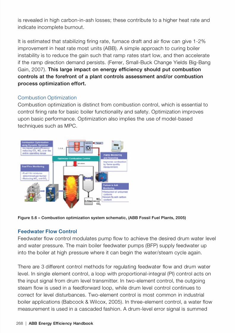
8/12/2019 Energy Efficiency Electronic Book Version 1548_PowerGenerationHandbook v1_1
http://slidepdf.com/reader/full/energy-efficiency-electronic-book-version-1548powergenerationhandbook-v11 270/361
is revealed in high carbon-in-ash losses; these contribute to a higher heat rate andindicate incomplete burnout.
It is estimated that stabilizing firing rate, furnace draft and air flow can give 1-2%improvement in heat rate most units (ABB). A simple approach to curing boilerinstability is to reduce the gain such that ramp rates start low, and then accelerateif the ramp direction demand persists. (Ferrer, Small-Buck Change Yields Big-BangGain, 2007). This large impact on energy efficiency should put combustioncontrols at the forefront of a plant controls assessment and/or combustionprocess optimization effort.
Combustion OptimizationCombustion optimization is distinct from combustion control, which is essential tocontrol firing rate for basic boiler functionality and safety. Optimization improvesupon basic performance. Optimization also implies the use of model-basedtechniques such as MPC.
Figure 5.6 – Combustion optimization system schematic, (ABB Fossil Fuel Plants, 2005)
Feedwater Flow ControlFeedwater flow control modulates pump flow to achieve the desired drum water leveland water pressure. The main boiler feedwater pumps (BFP) supply feedwater upinto the boiler at high pressure where it can begin the water/steam cycle again.
There are 3 different control methods for regulating feedwater flow and drum waterlevel. In single element control, a loop with proportional-integral (PI) control acts onthe input signal from drum level transmitter. In two-element control, the outgoingsteam flow is used in a feedforward loop, while drum level control continues tocorrect for level disturbances. Two-element control is most common in industrialboiler applications (Babcock & Wilcox, 2005). In three-element control, a water flowmeasurement is used in a cascaded fashion. A drum-level error signal is summed
268 | ABB Energy Efficiency Handbook

8/12/2019 Energy Efficiency Electronic Book Version 1548_PowerGenerationHandbook v1_1
http://slidepdf.com/reader/full/energy-efficiency-electronic-book-version-1548powergenerationhandbook-v11 271/361
with a steam flow feedforward signal to provide the feedwater demand. This demandis then compared with the water flow measurement to provide an error signal inputto the inner PI control loop. The more accurate feedwater flow control systemsalso use shrink-swell compensation to compensate for water density and volumechanges as temperature changes.
Demand for Auxiliary DrivepowerLarge demand for auxiliary drive power comes from the main and booster boilerfeedwater pumps (BFPs). The drive power aspects of the BFP are discussed in theDrivepower-Pump sections of this handbook. BFW pumping is a high-system headapplication for VSD speed control; a large part of the speed control range is used indeveloping pump head at low flow (ISA 2005). Benefits are therefore lower than inhigh-flow, low-head systems, but VSDs are still worthwhile in this application whencompared to throttling.
The ability of VFDs to provide over-speed capacity (within the service factor of themotor and pump) may be useful in boilers which are designed with extra margin foroverpressure operation. This extra capacity may be needed to supply peak loadingon hot summer days.
Another auxiliary load on many boiler designs comes from the relatively lower powerboiler recirculating pump, which moves water between drum and the boiler water
walls. This auxiliary load is eliminated in supercritical designs and in some HRSGdesigns which use natural circulation within the boiler.
Automation Potential for Energy Efficient DesignStable feedwater flow control allows the unit to operate closer to its design point formain steam pressure. For a sub-critical unit: each 100 psi increase in main steampressure decreases heatrate by 35 Btu per kWh at full load (EPRI report CS-4554).Steam pressure in a ‘typical’ boiler is normally controlled to within +/-1% of the
desired pressure (ISA 2005).
Case Example A feedwater pump use at a U.S. pulp and paper mill. As the peak load doesnot exceed 4,000 gpm (25 l/s), and two of the pumps can produce the requiredpressure at flow rates of 2,000 gpm (13 l/s) each, operating only two of thepumps would be sufficient.
The savings achievable from shutting down an extra feedwater pump are site-specic, depending on the pump size, the type of the drive (motor vs. turbine
Module 5 | 269
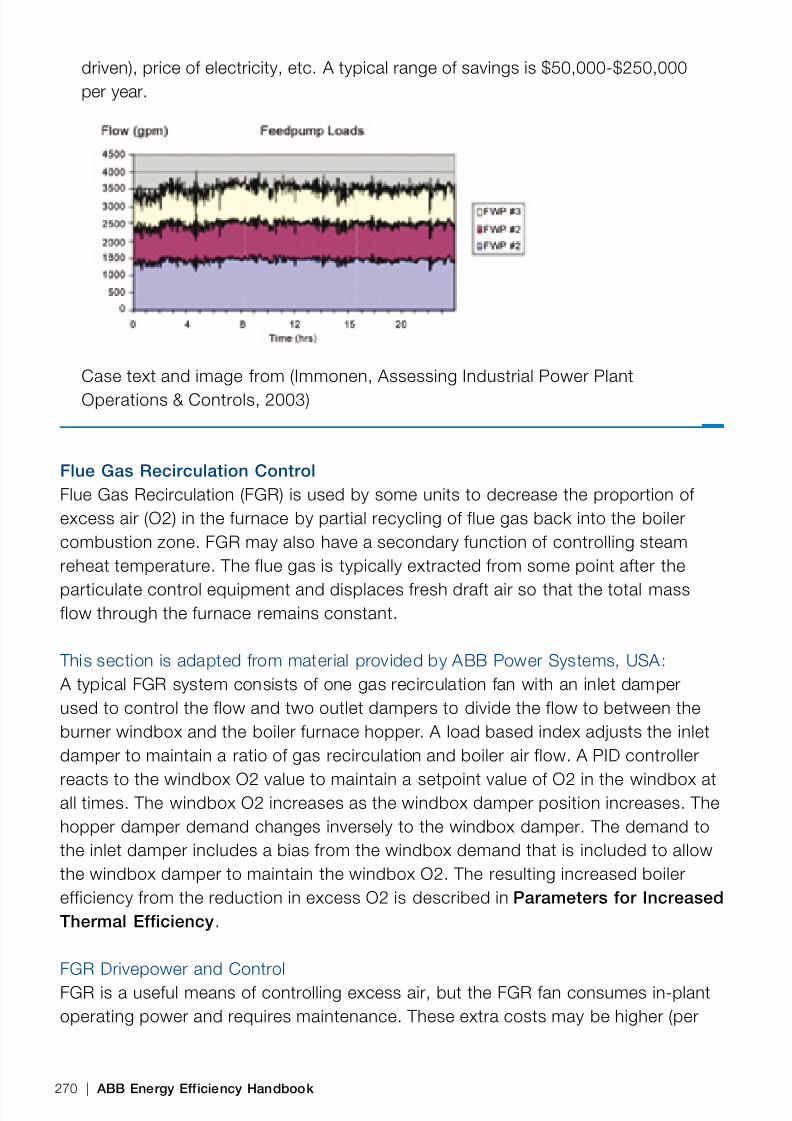
8/12/2019 Energy Efficiency Electronic Book Version 1548_PowerGenerationHandbook v1_1
http://slidepdf.com/reader/full/energy-efficiency-electronic-book-version-1548powergenerationhandbook-v11 272/361
driven), price of electricity, etc. A typical range of savings is $50,000-$250,000per year.
Case text and image from (Immonen, Assessing Industrial Power PlantOperations & Controls, 2003)
Flue Gas Recirculation ControlFlue Gas Recirculation (FGR) is used by some units to decrease the proportion ofexcess air (O2) in the furnace by partial recycling of flue gas back into the boilercombustion zone. FGR may also have a secondary function of controlling steamreheat temperature. The flue gas is typically extracted from some point after the
particulate control equipment and displaces fresh draft air so that the total massflow through the furnace remains constant.
This section is adapted from material provided by ABB Power Systems, USA: A typical FGR system consists of one gas recirculation fan with an inlet damperused to control the flow and two outlet dampers to divide the flow to between theburner windbox and the boiler furnace hopper. A load based index adjusts the inletdamper to maintain a ratio of gas recirculation and boiler air flow. A PID controller
reacts to the windbox O2 value to maintain a setpoint value of O2 in the windbox atall times. The windbox O2 increases as the windbox damper position increases. Thehopper damper demand changes inversely to the windbox damper. The demand tothe inlet damper includes a bias from the windbox demand that is included to allowthe windbox damper to maintain the windbox O2. The resulting increased boilerefficiency from the reduction in excess O2 is described in Parameters for IncreasedThermal Efficiency .
FGR Drivepower and ControlFGR is a useful means of controlling excess air, but the FGR fan consumes in-plantoperating power and requires maintenance. These extra costs may be higher (per
270 | ABB Energy Efficiency Handbook
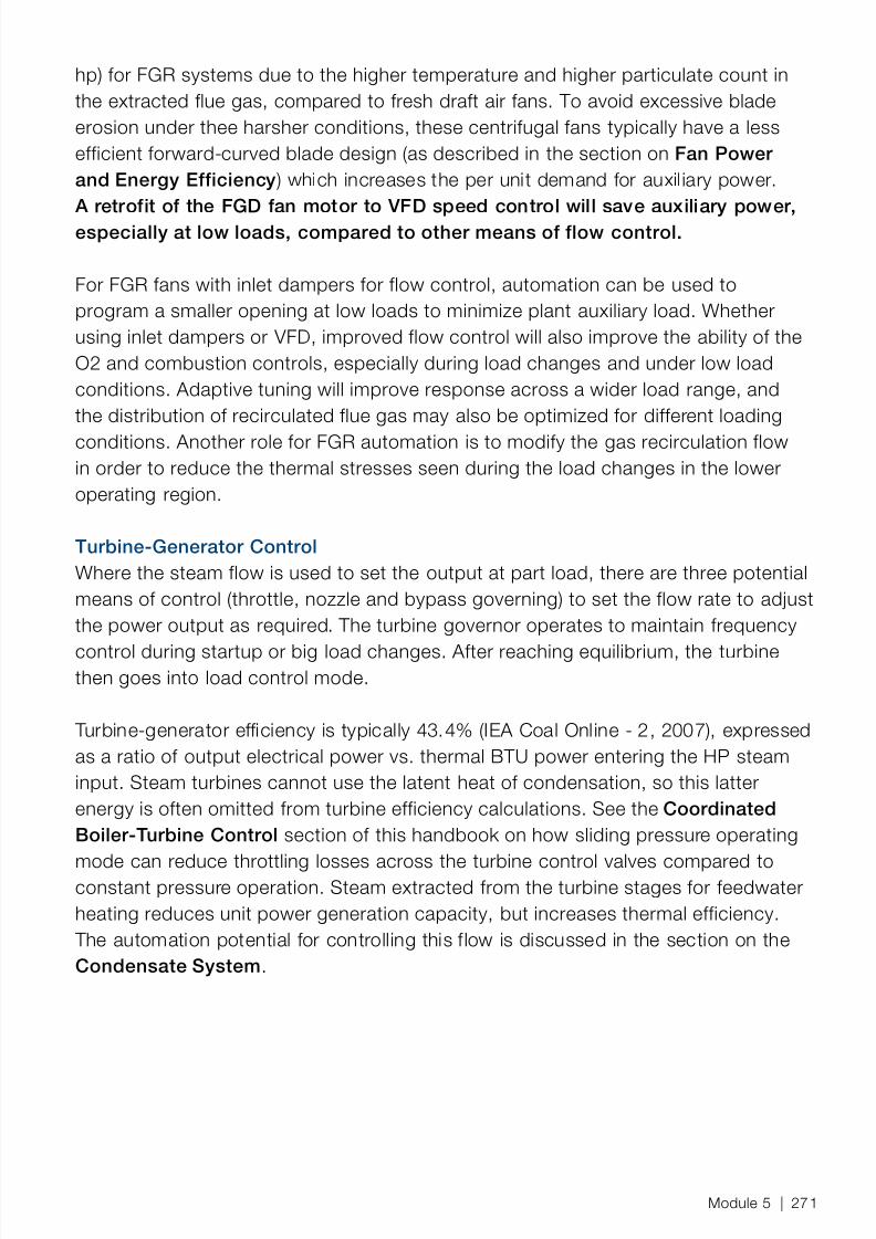
8/12/2019 Energy Efficiency Electronic Book Version 1548_PowerGenerationHandbook v1_1
http://slidepdf.com/reader/full/energy-efficiency-electronic-book-version-1548powergenerationhandbook-v11 273/361
hp) for FGR systems due to the higher temperature and higher particulate count inthe extracted flue gas, compared to fresh draft air fans. To avoid excessive bladeerosion under thee harsher conditions, these centrifugal fans typically have a lessefficient forward-curved blade design (as described in the section on Fan Powerand Energy Efficiency ) which increases the per unit demand for auxiliary power.
A retrofit of the FGD fan motor to VFD speed control will save auxiliary power,especially at low loads, compared to other means of flow control.
For FGR fans with inlet dampers for flow control, automation can be used toprogram a smaller opening at low loads to minimize plant auxiliary load. Whetherusing inlet dampers or VFD, improved flow control will also improve the ability of theO2 and combustion controls, especially during load changes and under low loadconditions. Adaptive tuning will improve response across a wider load range, andthe distribution of recirculated flue gas may also be optimized for different loadingconditions. Another role for FGR automation is to modify the gas recirculation flowin order to reduce the thermal stresses seen during the load changes in the loweroperating region.
Turbine-Generator ControlWhere the steam flow is used to set the output at part load, there are three potentialmeans of control (throttle, nozzle and bypass governing) to set the flow rate to adjustthe power output as required. The turbine governor operates to maintain frequency
control during startup or big load changes. After reaching equilibrium, the turbinethen goes into load control mode.
Turbine-generator efficiency is typically 43.4% (IEA Coal Online - 2, 2007), expressedas a ratio of output electrical power vs. thermal BTU power entering the HP steaminput. Steam turbines cannot use the latent heat of condensation, so this latterenergy is often omitted from turbine efficiency calculations. See the CoordinatedBoiler-Turbine Control section of this handbook on how sliding pressure operating
mode can reduce throttling losses across the turbine control valves compared toconstant pressure operation. Steam extracted from the turbine stages for feedwaterheating reduces unit power generation capacity, but increases thermal efficiency.
The automation potential for controlling this flow is discussed in the section on theCondensate System .
Module 5 | 271
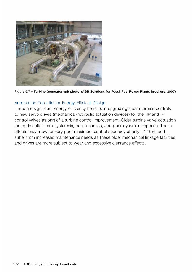
8/12/2019 Energy Efficiency Electronic Book Version 1548_PowerGenerationHandbook v1_1
http://slidepdf.com/reader/full/energy-efficiency-electronic-book-version-1548powergenerationhandbook-v11 274/361
Figure 5.7 – Turbine Generator unit photo, (ABB Solutions for Fossil Fuel Power Plants brochure, 2007)
Automation Potential for Energy Efficient Design There are significant energy efficiency benefits in upgrading steam turbine controlsto new servo drives (mechanical-hydraulic actuation devices) for the HP and IPcontrol valves as part of a turbine control improvement. Older turbine valve actuationmethods suffer from hysteresis, non-linearities, and poor dynamic response. Theseeffects may allow for very poor maximum control accuracy of only +/-10%, andsuffer from increased maintenance needs as these older mechanical linkage facilities
and drives are more subject to wear and excessive clearance effects.
272 | ABB Energy Efficiency Handbook

8/12/2019 Energy Efficiency Electronic Book Version 1548_PowerGenerationHandbook v1_1
http://slidepdf.com/reader/full/energy-efficiency-electronic-book-version-1548powergenerationhandbook-v11 275/361
Upgrading turbine valve servo drives and their controls can improve accuracy to+/-1%. Other advantages of the improved linearity and optimized positioningtimes are: improved dynamics, smoother operation, reduced throttling losses, andenhanced stability; the following case history describes the benefits in more detail.
Figure 5.8 – Upgraded turbine valve servo drive photo, (ABB Utilities GmbH, 2004)
Case ExampleUpgraded Turbine Components and Unit ControlsBlénod Power Plant Units 3 &4, EDF, France
The fossil-fueled units 3 & 4 of EDF’s CPT Blénod power plant are more than30 years old located at Pont a Mousson, Lorraine, France. The maximum netoutput of the plant is 265 MW.
Figure 5.9 – CPT Blénod Power Plant Units 3 &4, EDF, France
Module 5 | 273
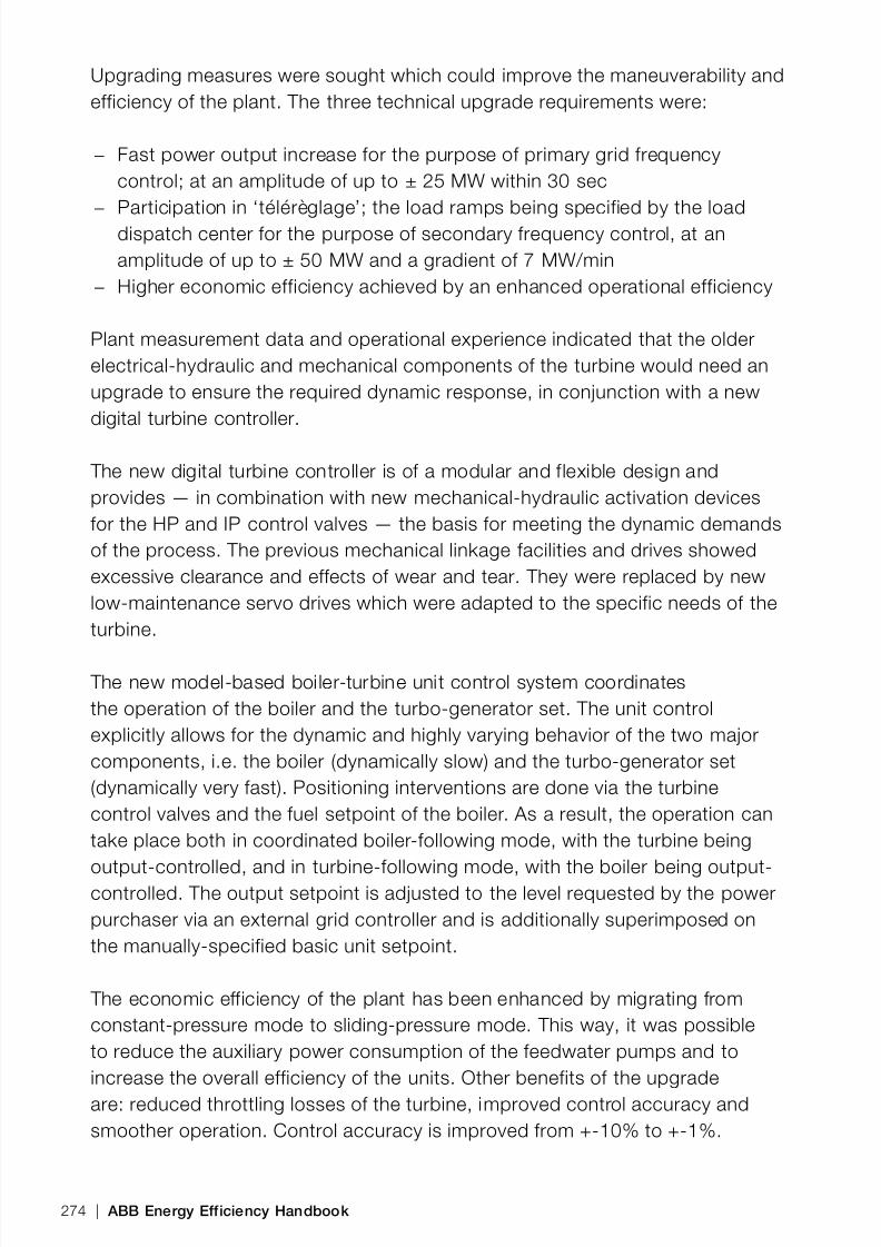
8/12/2019 Energy Efficiency Electronic Book Version 1548_PowerGenerationHandbook v1_1
http://slidepdf.com/reader/full/energy-efficiency-electronic-book-version-1548powergenerationhandbook-v11 276/361
Upgrading measures were sought which could improve the maneuverability andefficiency of the plant. The three technical upgrade requirements were:
− Fast power output increase for the purpose of primary grid frequencycontrol; at an amplitude of up to ± 25 MW within 30 sec
− Participation in ‘télérèglage’; the load ramps being specified by the loaddispatch center for the purpose of secondary frequency control, at anamplitude of up to ± 50 MW and a gradient of 7 MW/min
− Higher economic efficiency achieved by an enhanced operational efficiency
Plant measurement data and operational experience indicated that the olderelectrical-hydraulic and mechanical components of the turbine would need anupgrade to ensure the required dynamic response, in conjunction with a newdigital turbine controller.
The new digital turbine controller is of a modular and flexible design andprovides — in combination with new mechanical-hydraulic activation devicesfor the HP and IP control valves — the basis for meeting the dynamic demandsof the process. The previous mechanical linkage facilities and drives showedexcessive clearance and effects of wear and tear. They were replaced by newlow-maintenance servo drives which were adapted to the specific needs of theturbine.
The new model-based boiler-turbine unit control system coordinatesthe operation of the boiler and the turbo-generator set. The unit controlexplicitly allows for the dynamic and highly varying behavior of the two majorcomponents, i.e. the boiler (dynamically slow) and the turbo-generator set(dynamically very fast). Positioning interventions are done via the turbinecontrol valves and the fuel setpoint of the boiler. As a result, the operation cantake place both in coordinated boiler-following mode, with the turbine being
output-controlled, and in turbine-following mode, with the boiler being output-controlled. The output setpoint is adjusted to the level requested by the powerpurchaser via an external grid controller and is additionally superimposed onthe manually-specified basic unit setpoint.
The economic efficiency of the plant has been enhanced by migrating fromconstant-pressure mode to sliding-pressure mode. This way, it was possibleto reduce the auxiliary power consumption of the feedwater pumps and toincrease the overall efficiency of the units. Other benefits of the upgradeare: reduced throttling losses of the turbine, improved control accuracy andsmoother operation. Control accuracy is improved from +-10% to +-1%.
274 | ABB Energy Efficiency Handbook

8/12/2019 Energy Efficiency Electronic Book Version 1548_PowerGenerationHandbook v1_1
http://slidepdf.com/reader/full/energy-efficiency-electronic-book-version-1548powergenerationhandbook-v11 277/361
With these goals being accomplished, the plant can now demand higherprices when selling its electricity in the power market, as the price for providingsecondary-frequency power control is determined on the basis of the maximumpossible power amplitude and by the change gradient of the load ramp. Moreover,the plant is also able to participate in the European power market, although this isnot in-tended at present.
(Case text adapted from ABB Utilities GmbH, 2004 brochure on Upgrade ofBlénod Power Plant )
Excess Air ControlExcess air minimization is a frequently attempted efficiency improvement. Theobjective is clear, and the savings are easy to quantify in terms of fuel savings.Many successful implementations are currently in use, but significant room forimprovement exists. Note that excess air control is one of several other combustioncontrols; see the handbook section on Combustion Control for more details onother methods.
Excess Air Concepts A primary combustion quality measure is excess oxygen in the ue gas stream. Dueto imperfect mixing, the combustion process will require more than the chemical (i.e.
stoichiometric) amounts of air for efcient combustion. For a PC drum boiler, the excessair level at 50% load may be controlled to twice that at full load. (Black & Veatch, 1996)
Too little excess oxygen implies incomplete combustion, elevated levels of CO,unburned carbon and volatile hydrocarbons and the potential for loss on ignition(LOI). Too much excess oxygen means lowered efficiency due to unnecessary heatingof the unused components of the draft air stream, as well as excessive generation ofthermal NOX due to fast combustion in hot zones within the boiler. Between these
two extremes is a region of optimal performance shown in the following figure:
Module 5 | 275
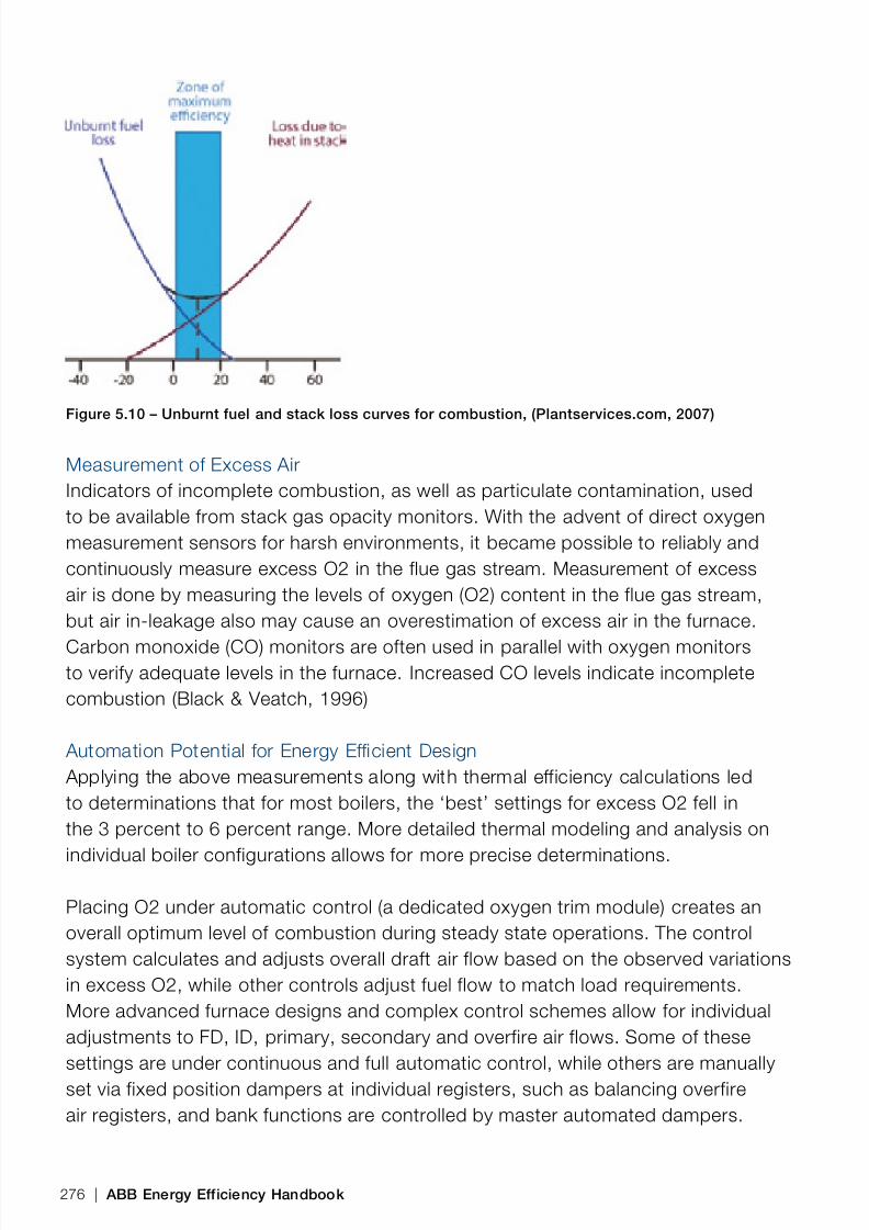
8/12/2019 Energy Efficiency Electronic Book Version 1548_PowerGenerationHandbook v1_1
http://slidepdf.com/reader/full/energy-efficiency-electronic-book-version-1548powergenerationhandbook-v11 278/361
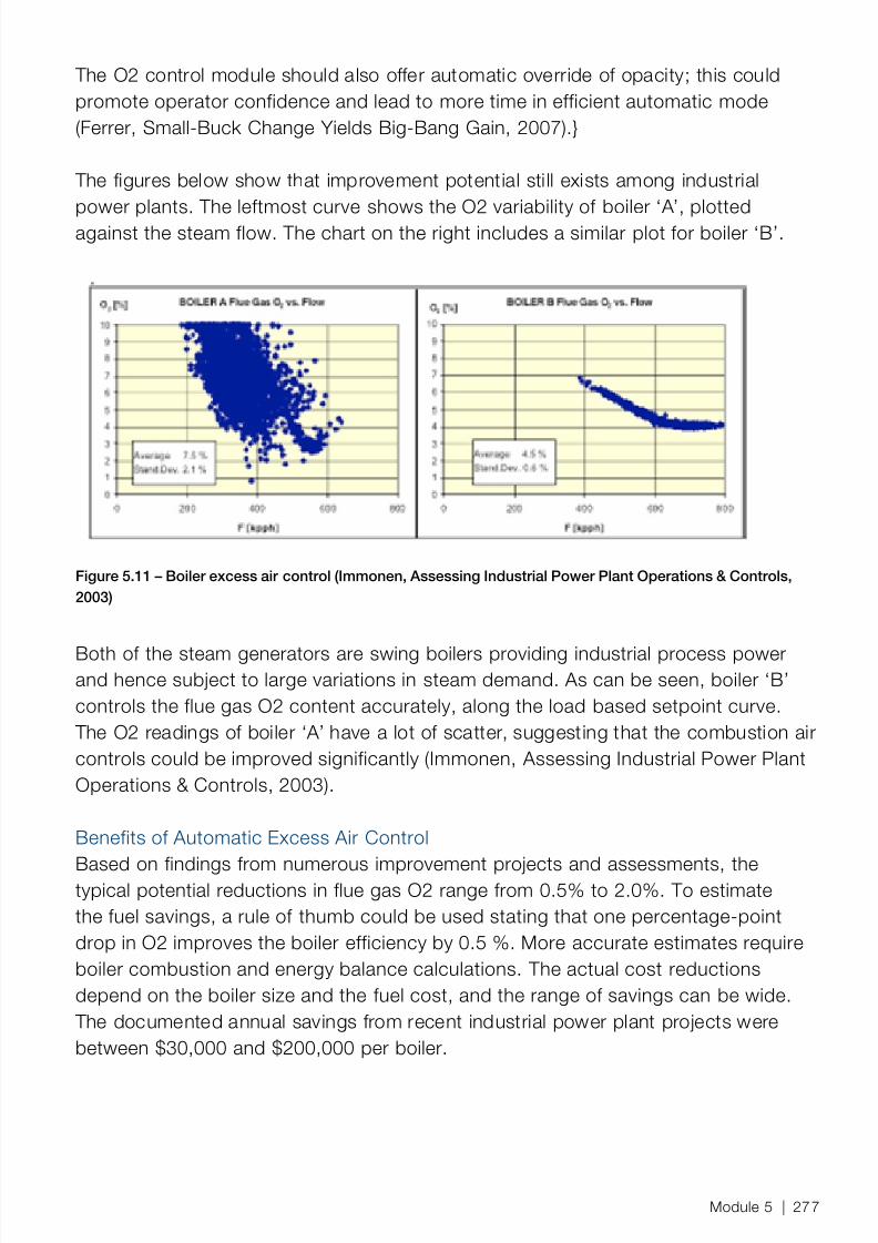
8/12/2019 Energy Efficiency Electronic Book Version 1548_PowerGenerationHandbook v1_1
http://slidepdf.com/reader/full/energy-efficiency-electronic-book-version-1548powergenerationhandbook-v11 279/361
The O2 control module should also offer automatic override of opacity; this couldpromote operator confidence and lead to more time in efficient automatic mode(Ferrer, Small-Buck Change Yields Big-Bang Gain, 2007).}
The figures below show that improvement potential still exists among industrialpower plants. The leftmost curve shows the O2 variability of boiler ‘A’, plottedagainst the steam flow. The chart on the right includes a similar plot for boiler ‘B’.
Figure 5.11 – Boiler excess air control (Immonen, Assessing Industrial Power Plant Operations & Controls,2003)
Both of the steam generators are swing boilers providing industrial process powerand hence subject to large variations in steam demand. As can be seen, boiler ‘B’controls the flue gas O2 content accurately, along the load based setpoint curve.
The O2 readings of boiler ‘A’ have a lot of scatter, suggesting that the combustion aircontrols could be improved significantly (Immonen, Assessing Industrial Power PlantOperations & Controls, 2003).
Benefits of Automatic Excess Air Control
Based on findings from numerous improvement projects and assessments, thetypical potential reductions in flue gas O2 range from 0.5% to 2.0%. To estimatethe fuel savings, a rule of thumb could be used stating that one percentage-pointdrop in O2 improves the boiler efficiency by 0.5 %. More accurate estimates requireboiler combustion and energy balance calculations. The actual cost reductionsdepend on the boiler size and the fuel cost, and the range of savings can be wide.
The documented annual savings from recent industrial power plant projects werebetween $30,000 and $200,000 per boiler.
Module 5 | 277

8/12/2019 Energy Efficiency Electronic Book Version 1548_PowerGenerationHandbook v1_1
http://slidepdf.com/reader/full/energy-efficiency-electronic-book-version-1548powergenerationhandbook-v11 280/361
Reduction of furnace excess air can yield a 3% to 5% improvement in heat rate insome older PC steam plants. These gains are typical for plants in which operatorsspend much time in manual control of air flow to avoid opacity excursions. Highopacity means that the exit gas exceeds limits on the total suspended particles (TSP).
Lower excess air can also provide other benefits. The induced draft fan capacityoften limits the combustion of other fuels such as waste or biomass. With excessair controls, the overall air demand is lower, so the waste fuel throughput may beincreased, thus decreasing expensive fossil fuel usage. The associated savings canexceed those from the efficiency improvements.
Steam Temperature Controls As firing rate and steam flow decrease from the design full-load conditions, the mainand reheat steam temperature tend to decrease, which results in reduced turbinecycle efficiency (according to Carnot cycle theory at the start of this module) For anacceptable efficiency across a wider range of loads, most boilers are designed tomaintain steam temperature over a specified load range. The ‘control point’ is thelowest point at which design temperature steam can be produced, typically 60% ofthe maximum continuous rating (MCR) (Black & Veatch 1996) p.192. Some boilerscannot achieve full superheat at lower loads, and in such cases the temperaturesmay not improve through better controls. By means of more accurate boiler steam
temperature control, it may be possible to reduce temperature variations, andthereby apply a higher temperature setpoint.
Higher steam temperatures have a signicant effect on heat rate by improving thefundamental thermodynamic efciency of the heat engine. These improvements arequantied in the section on Energy Efciency Potential of Power Plant Automation .
Steam Attemperation Concepts
This section is adapted from an ABB Application Guide, (ABB Inc. Plant Automation2006)
The primary means of controlling main steam temperature is by injecting feedwatersprays into the superheater line, known as ‘attemperation’. The attemperation water,which is 2-5% of the total steam flow, may come from the boiler feedwater pumpoutlet, or further downstream, just before the economizer inlet. The water is typicallysprayed prior to the secondary superheater, as shown in the figure below. From anenergy efficiency standpoint, attemperation would be more effective and requirelower flows if sprayed further downstream. The risk of water damage to the turbine,however, requires that water have time to mix and evaporate thoroughly beforeentering the turbine.
278 | ABB Energy Efficiency Handbook

8/12/2019 Energy Efficiency Electronic Book Version 1548_PowerGenerationHandbook v1_1
http://slidepdf.com/reader/full/energy-efficiency-electronic-book-version-1548powergenerationhandbook-v11 281/361
Figure 5.12 – Steam temperature control diagram, (ABB Inc. Plant Automation, 2006)
Attemperation flow may also be tapped directly from a special outlet within the mainfeedwater pump (IEA Coal Online - 2, 2007). Bypassing feedwater heating has anegative impact on cycle efficiency. See the Pump sections for discussion on thepump power requirements for these two alternatives.
Other means to control steam temperatures are; tilting burners away from thesuperheater tubes, using bypass dampers in the back-pass or convection portion ofthe unit (larger boilers that include these dampers can have 12 or more each of thesuperheat and reheat dampers), or using flue gas recirculation (FGR) to moderate
combustion. These methods are typically used for longer-term adjustment (Babcock& Wilcox 2005) compared to the quick action of spray attemperation to providecontrol of transients. Attemperation flows can be eliminated on supercritical boilersby controlling the firing rate to match the feedwater flow (IEA Coal Online - 2, 2007).
Advanced Steam Temperature ControlSteam temperature excursions are a result of an imbalance between the heat addedto the steam by the firing rate and the heat withdrawn, by the steam flow rate. An
advanced control strategy will control steam temperature for a drum boiler operatingin either constant or sliding pressure mode. Specific algorithms and techniques usedby the advanced control strategy include:
− The use of enthalpy calculations to determine the different SSH inlet temperatureset points when operating in a variable pressure mode.
− The use of anticipatory logic to account for changes in the boiler energy storage. − The use of an internal model controller (Smith Predictor) to accommodate for long
process time delays (dead time) and lags. − The use of adaptive tuning to provide controller sensitivity adjustment. − Advanced Model-Predictive controls can be applied, as part of an overall cycle
control optimization
Module 5 | 279

8/12/2019 Energy Efficiency Electronic Book Version 1548_PowerGenerationHandbook v1_1
http://slidepdf.com/reader/full/energy-efficiency-electronic-book-version-1548powergenerationhandbook-v11 282/361
Figure 5.13 - Advanced Steam Temperature control system logic, (ABB Inc. Plant Automation, 2006)
In units with bypass dampers for heat or re-heat temperature control, the accuracyof the control can be improved by using high-torque electric drives for positioning.One problem inherent with these particular dampers is their constant exposure tohigh-temperature corrosive gases and high levels of fly ash. In time, most of thesedampers experience increasing stiction and eventually will degrade into limitedrange of motion or completely frozen states. See the section Dampers and Louvers
for more details on these actuators. Upgrading to ‘intelligent’ drives with built-indiagnostic capability can provide an early warning of damper stiction problems andallow for proactive maintenance on the damper mechanism. Properly operatingsuperheat and reheat damper drives mitigate attemperator spray flows and ash buildup, in turn reducing both sootblowing and periodic maintenance in this section ofthe boiler. Both produce reductions in controllable losses, which improves plant heatrate (Vesel 2007).
Benefits of Advanced Steam Temperature Control The benefits of advanced steam temperature control are:
− Improved temperature control on process transients caused by changing load,sootblowing, starting and stopping of mills in service
− Improved steady state temperature control when operating under conditions ofreduced pressure, slagging.
− Faster ramp rate − Improved steam temperature control will also reduce the need for attemperation, which
improves plant heat rate. (Ferrer, Small-Buck Change Yields Big-Bang Gain, 2007).− Provides design flexibility to control main steam temperature on drum boilers in
either a fixed or variable pressure operation.
280 | ABB Energy Efficiency Handbook
8/12/2019 Energy Efficiency Electronic Book Version 1548_PowerGenerationHandbook v1_1
http://slidepdf.com/reader/full/energy-efficiency-electronic-book-version-1548powergenerationhandbook-v11 283/361
− Avoiding unscheduled outages for superheater tube failure
By means of more accurate boiler steam temperature control, it may be possibleto reduce temperature variations, and thereby apply a higher temperature setpoint.
The benefits of the higher temperature include increased generation of backpressurepower, better condensing power efficiency, and reduced steam use by the driveturbines, all due to the higher steam expansion work available in the turbines(Immonen, Assessing Industrial Power Plant Operations & Controls, 2003). Operatingwith higher energy content steam allows specific steam consumption to be reduced,with consequent reduction in auxiliary boiler feed pump power.
Case ExampleU.S. pulp and paper mill
An example of steam temperature increase potential is shown in Figure below(Immonen, Assessing Industrial Power Plant Operations & Controls, 2003). Thesteam temperature is shown as a function of the boiler load, to reveal possibleload dependency. As load dependent behavior is not obvious in the example,the temperature variations may be attributed to poor control. The standarddeviation of the temperature was found to be 8 °F (5 °C), while the averagetemperature was 34 °F (19 °C) below the design. Therefore, the operatorstended to maintain a safety margin of 4 times the standard deviation between
the maximum and the temperature setpoint.
By means of better control, the standard deviation could drop to one half,or 4 °F (2.3 °C). By using a commonly accepted safety margin of 3 timesthe standard deviation, the average temperature could be increased to 913°F. At this U.S. pulp and paper mill, savings were available from increasedbackpressure power generation, replacing approximately 0.8 MW of moreexpensive purchased power. While the annual savings here were approximately
$130,000, the range of savings can be wide, anywhere from $20,000 to$300,000 per year, or beyond, on relatively small power boiler systems.
Module 5 | 281

8/12/2019 Energy Efficiency Electronic Book Version 1548_PowerGenerationHandbook v1_1
http://slidepdf.com/reader/full/energy-efficiency-electronic-book-version-1548powergenerationhandbook-v11 284/361
Case text and figure provided by: (Immonen, Assessing Industrial Power PlantOperations & Controls, 2003)
The following calculation case quantifies some of the benefits of advanced steamtemperature control:
Calculation Case Advanced Steam Temperature Control System
This calculation assumes a 500 MW unit with an initial ramp rate of 5MW/min and amain steam temperature set point of 1000 ºF. The fuel savings realized from the initialassumptions are threefold: 1) increasing the main steam temperature set point toits design value of 1005 ºF thus, improving the unit heat rate 2) improving the ramprate to 10 MW/min thus, reducing the need to purchase power and 3) reducing thenumber of unscheduled boiler outages as the result of superheater tube leaks. Totalfuel savings in excess of $600,000.00 per year is possible with the Advanced Steam
Temperature Control System. The calculation of the fuel savings is as follows;
1. Increasing main steam temperature to design;Main Steam Temp Improvement: 5 °F (2.8 °C)Unit capacity: 500 MW @ 80% capacityFuel Cost: $1.75/MBTU (1MBTU = 1055 MJ)Main Steam Temp Dev Value: 1.5 BTU/(KWH °F)
Annual savings = (1.5 BTU/(KWH °F) x (5 °F) x (1.75 $/MBTU) x (500 mw x 0.8) x(24 HR/DAY) x (365 DAYS/YR) = $46,000/YR.
282 | ABB Energy Efficiency Handbook

8/12/2019 Energy Efficiency Electronic Book Version 1548_PowerGenerationHandbook v1_1
http://slidepdf.com/reader/full/energy-efficiency-electronic-book-version-1548powergenerationhandbook-v11 285/361
The following non-energy efficiency benefits are significant and are quantified below:2. Improving the unit ramp rate to 10 MW/min;MWHR/ramp: 18.75 MWHR/rampPurchase power penalty: $20/MWHRNumber of ramps per year: 250
Annual savings = (18.75 MWHR/ramp) x (250 ramp/YR) x (20 $/MWHR) = $93,750/YR
3. Avoiding unscheduled outages for superheater tube failure;Unit capacity: 500 MWPurchased power penalty: $20/MWHRUnit downtime per tube failure: 100 HRNumber of tube failure per year: 0.5
Annual savings = (500 MW) x ($20/MWHR) x (100HR) x (0.5/YR) = $500,000/YR.
Case text and values provided by: (Immonen, P., ABB Inc. Plant Automation, 2006)
Burner Management Systems The burner management system is mainly a protective system to ensure safeoperation, startup and shutdown of the burner equipment. Emergency shutdownoccurs when high levels of unburned combustibles are detected. Monitoring of theburner performance is by flame scanner, which measures the flame quality. These
systems are also collectively known as ‘boiler protection systems’.
Burner Controls The goal of burner controls is maximum burnout of pulverized coal, but withminimum NOX emissions. An advanced burner control system can initiate stagedcombustion, biased firing or fuel-nozzle tilt (in tangential firing) to adjust the furnaceexit gas temperature (FEGT) with load changes, varying fuels or in relation to thestate of the furnace wall (as in dirtiness). This allows the superheater or reheater
outlet steam temperature, or NOx production in the furnace, or both, to becontrolled. Although closely related to burner management, the Pulverizer Controlsare discussed in the Fuel Handling section.
Boiler Startup and Protection Automation systems using a nonlinear, model-based multi-variable controller canautomatically calculate optimum startup strategy for steam generators. The goalof startup optimization is to optimize fuel consumption and time during the boilerstartup process without exceeding the maximum thermal ratings of critical systemcomponents.
Module 5 | 283
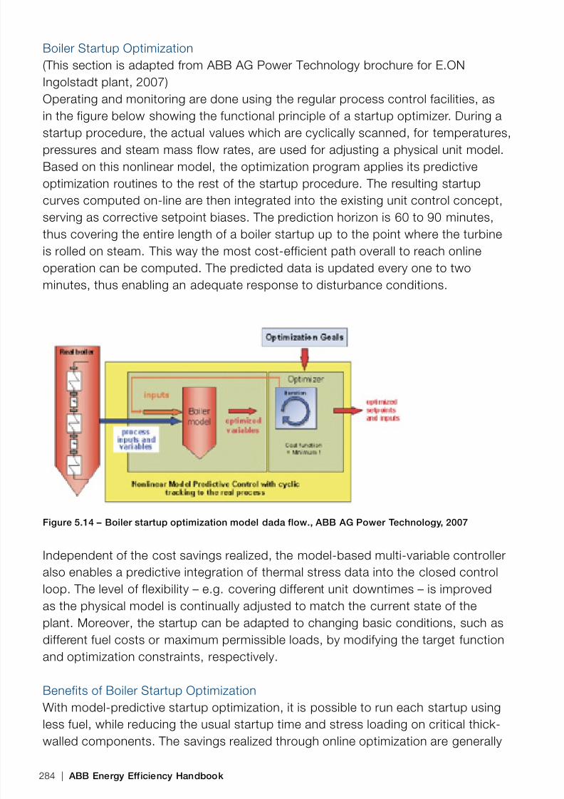
8/12/2019 Energy Efficiency Electronic Book Version 1548_PowerGenerationHandbook v1_1
http://slidepdf.com/reader/full/energy-efficiency-electronic-book-version-1548powergenerationhandbook-v11 286/361
Boiler Startup Optimization(This section is adapted from ABB AG Power Technology brochure for E.ONIngolstadt plant, 2007)Operating and monitoring are done using the regular process control facilities, asin the figure below showing the functional principle of a startup optimizer. During astartup procedure, the actual values which are cyclically scanned, for temperatures,pressures and steam mass flow rates, are used for adjusting a physical unit model.Based on this nonlinear model, the optimization program applies its predictiveoptimization routines to the rest of the startup procedure. The resulting startupcurves computed on-line are then integrated into the existing unit control concept,serving as corrective setpoint biases. The prediction horizon is 60 to 90 minutes,thus covering the entire length of a boiler startup up to the point where the turbineis rolled on steam. This way the most cost-efficient path overall to reach onlineoperation can be computed. The predicted data is updated every one to twominutes, thus enabling an adequate response to disturbance conditions.
Figure 5.14 – Boiler startup optimization model dada flow., ABB AG Power Technology, 2007
Independent of the cost savings realized, the model-based multi-variable controlleralso enables a predictive integration of thermal stress data into the closed controlloop. The level of flexibility – e.g. covering different unit downtimes – is improvedas the physical model is continually adjusted to match the current state of theplant. Moreover, the startup can be adapted to changing basic conditions, such asdifferent fuel costs or maximum permissible loads, by modifying the target functionand optimization constraints, respectively.
Benefits of Boiler Startup OptimizationWith model-predictive startup optimization, it is possible to run each startup usingless fuel, while reducing the usual startup time and stress loading on critical thick-walled components. The savings realized through online optimization are generally
284 | ABB Energy Efficiency Handbook

8/12/2019 Energy Efficiency Electronic Book Version 1548_PowerGenerationHandbook v1_1
http://slidepdf.com/reader/full/energy-efficiency-electronic-book-version-1548powergenerationhandbook-v11 287/361
within 10 to 20 percent of the normal costs of fuel and auxiliary power, for eachpower plant startup. Startup times can generally be reduced by increasing theloading of critical thick-walled components or by better exploiting the marginsthrough more homogenized thermal loading. Applying predictive startup optimizationin order to reduce the startup time is advisable if the permissible heat-up stressmargin is not fully exploited, or if the load is distributed unevenly during startup.
Energy efficiency improvements come from reduced startup fuel burned and/ or shorter startup times. Startup automation with optimization also leads to moreconsistent startups and lowers the risk of an aborted startup, with the consequentloss of input energy. Coal-fired power plants offer high additional savings potentials,provided that it is possible to shift from startup fuel to coal at an earlier point.
Energy savings accumulate for units in cycling duty. In particular, in the case offrequent brief standstills, when numerous startups are run under similar conditions,the spread of startup costs is obviously reduced. On average, the use of startupoptimization results in a significant reduction of startup costs. Even in the case ofbrief standstills, startup costs can be high, as a high live-steam temperature has tobe built up to approach the still high temperatures in the turbine. Taken together, theabove improvements increase efficiency by approximately 1% during startup, andalso decrease emissions values.
Case ExampleBoiler Startup Optimization
The figure below shows a comparison of two startup procedures in theIngolstadt power plant, unit 4: with BoilerMax (bold lines) and withoutBoilerMax (thin lines). The upper diagram shows the fuel quantity F_F and theHP bypass position Y_HPB. The diagram in the middle shows the live steamflow F_LS and the generator output P_Gen. The diagram at the bottom shows
the temperature differentials DT_SH4H and DT_SH5H occurring in HP headersof the two last superheater levels.
The diagrams show that it was possible to run a similar boiler startup while realizingan approximate 20% reduction of fuel consumption. Such fuel savings are possible,since the steam ow used for starting-up can be decreased by simultaneous andcoordinated reduction of the opening of the HP bypass station. In addition, thestartup time is slightly reduced.
Module 5 | 285

8/12/2019 Energy Efficiency Electronic Book Version 1548_PowerGenerationHandbook v1_1
http://slidepdf.com/reader/full/energy-efficiency-electronic-book-version-1548powergenerationhandbook-v11 288/361
Figure 5.15 – Comparison of two startups with model-based startup optimization. (shown in theheavier dashed and solid lines) and without (thinner lines) ABB AG Power Technology brochurefor E.ON Ingolstadt plant, 2007
Emissions ControlsEmissions Concepts
The flue gas contains particulates and other products of combustion which must becleaned to levels required by environmental regulations (in the USA, these are givenby the Clean Air Act Amendments, CAAA). Particulates are removed by electrostaticprecipitators (ESPs) or fabric filters.
Sulfur dioxide (SO2) is removed by one of the various ue gas desulphurization(FGD) processes. The wet scrubber process using limestone as the sorbent is themost widely used method. NOx production can be controlled in-furnace by low-NOxburners, air staging, and the use of a re-burn fuel in the upper part of the boiler. NOxcan also be removed by injection of ammonia or an ammonia- based compound intothe combustion products, with or without the use of a catalyst, processes known as
286 | ABB Energy Efficiency Handbook

8/12/2019 Energy Efficiency Electronic Book Version 1548_PowerGenerationHandbook v1_1
http://slidepdf.com/reader/full/energy-efficiency-electronic-book-version-1548powergenerationhandbook-v11 289/361
selective catalytic and non-catalytic reduction (SCR or SNCR) (IEA Coal Online - 2,2007).
Flue Gas Desulfurization (FGD)One way to limit extra auxiliary loads associated with FGD is to switch to fuels lowerin sulfur. The EPRI CQIM model described in the section on Fuel Handling Systems provides estimates for the amount of auxiliary power required for different coal types.
Methods to improve the contact between the limestone slurry and the flue gasimprove absorption will serve to reduce the auxiliary drivepower required forcirculating pumping. Innovative methods using open-spray tower absorbers mayreduce auxiliary loads by up to 1% of total generation (Sayer, 1995).
Seawater’s alkaline composition enables it to absorb SO2. Seawater FGD scrubbingmay be one of the lowest energy alternatives, where environmental agenciesgrant approval. ‘Most Recent Developments and Optimization Aspects for FGD
Technologies’ Dr. W. Schüttenhelm et al, Power-Gen Europe, Barcelona, Spain,May 25-27, 2004. Seawater FGD techniques eliminate the need for slurry injectionand recycle pumping. Dry FGD processes may offer lower auxiliary loads, but witha lower SO2 removal rate (Sayer, 1995). The gypsum or sulfuric acid byproducts ofFGD processes can be sold to other industries, which may change the cost-benefitcomparisons.
Figure 5.16 – Flow diagram of a typical supercritical PC plant with pollution control (cited in IEA CoalOnline - 2, 2007) Rousaki and Couch,2000)
NOx Emissions ReductionNOx emissions reduction technologies typically involve burner modifications anddo not directly add to the plant’s auxiliary loads. A NOx conversion which causesincreased boiler firing rate instability under upset conditions, however, may lead to a1-2% increase in heat rate (Ferrer, Small-Buck Change Yields Big-Bang Gain, 2007).
Module 5 | 287

8/12/2019 Energy Efficiency Electronic Book Version 1548_PowerGenerationHandbook v1_1
http://slidepdf.com/reader/full/energy-efficiency-electronic-book-version-1548powergenerationhandbook-v11 290/361
In units equipped with Selective Catalytic Reduction (SCR) equipment, NOx isabsorbed by ammonia within a reactor vessel located in the flue gas stream. Inaddition to reagent pumping drive-power, the pressure drop across the catalyticreactor requires greater ID fan power, bringing the total added SCR auxiliary loadto 1% to 1.5% of total generation capacity. The SCR equipment is typically locatedbetween the economizer and the air heater. However, in some designs the SCRvessel is located further downstream, after the electrostatic precipitator (ESP).
This configuration requires energy to reheat the saturated flue gas to the requiredreactor temperature, typically 600 ºF (316 ºC) (Babcock & Wilcox 2005). When thisenergy is provided from auxiliary power, it increases the total SCR system auxiliaryconsumption to values typically 2.5% of total generation (Sayer, 1995). Otherdesigns bypass some flue gas around the economizer to provide this energy, whichalso reduces the thermal efficiency of the unit.
Particulate Emissions ControlFuel ash and unburned carbon particles from coal and oil-fired plants are traditionallyremoved by electrostatic precipitator (ESP). ESPs have low pressure drop in theflue gas stream and use relatively low electrical power, but the size and powerrequirements increase as particle size decreases, giving an average auxiliary powerconsumption of 0.25% of total generation (Sayer, 1995). The alternative (andpossibly complementary) methods to ESPs, using fabric filters in ‘baghouses’, workswell at capturing fine particles but at the cost of a larger pressure drop and higher
fan power, bringing total auxiliary power to 0.35% of total generation. The fly ashcollected by these systems can be sold and used for more productive purposes thanlandfill, which may change the cost-benefit comparisons.
Drivepower Potential for Energy Efficient DesignEmissions control devices add pressure drops to the flue gas stream andsignificantly increase the requirement for ID fan power, often necessitating installationof a flue gas ID booster fan. Additional drivepower is needed for limestone
slurry-feed, absorbent circulation pumps and oxidation air compressors, and theelectrostatic precipitator is also represents an auxiliary electrical load. The proportionof plant generating capacity consumed by emissions control systems varies with thedegree of emissions reduction:
3% to 5% for reducing up to 90% of sulfur dioxide emissions from coal-fired plants
0.5% to 2.5% for reducing nitrogen oxide emissions up to 80% from all fossil-fired plants
0.5% to 1.5% for controlling particulate emissions from oil and coal-fired plants
The cumulative incremental power consumption for emissions control may be upto 9% of gross generating output (Sayer, 1995). The increased auxiliary load alsoincreases plant net heat rate and the amount of CO2 emitted per generated MWh.
288 | ABB Energy Efficiency Handbook

8/12/2019 Energy Efficiency Electronic Book Version 1548_PowerGenerationHandbook v1_1
http://slidepdf.com/reader/full/energy-efficiency-electronic-book-version-1548powergenerationhandbook-v11 291/361
Flow control through use of VFD speed control can reduce pump and fan auxiliarypower by 75% at low loads, and will correct for oversizing at full loads, reducingpower by 15%. Efficient motors and drive-trains can further reduce power by 5%.
A peaking plant that applies the suggested drivepower improvements cansubstantially reduce the unit auxiliary load.
{Note that gas-fired plants, on the other hand, may only require 1% of generatingoutput for reducing nitrogen oxides (C.P.Robie,P.A.Ireland, for EPRI, 1991), andnewly available low NOx combustors and burner tuning methodologies cancompletely eliminate post-combustion NOx treatments.}
Automation Potential for Energy Efficient Design A low-capital cost technology to complement low-NOx burners is improvedcombustion control. Using the automation techniques of co-coordinated boiler-turbine control and advanced realtime control of burners, air flow and gasrecirculation can reduce NOx emissions without any increase in auxiliary power.See the section on Excess Air Control for details on reducing NOx using controltechniques. Continuous monitoring of flue gas is vital for low-NOx burner orcombustion methods due to the risk of higher levels of unburned carbon and COemissions; see the section on Instruments and Actuators for more details onanalytical devices.
Automation for stabilizing firing rate after a low-NOX burner conversion can alsoreduce heat rate. Combustion Optimization Solutions (COS) use model-basedpredictive control techniques to reliably find the most suitable setpoints for improvingthe heat rate and reducing emissions like NOx. Every ton of NOx production thatis avoided during the combustion process, is eliminated from the cost of NOxmitigation or from offset credit purchase requirements. The value of this ranges from$1500 to $3500 per ton at current (2009) pricing.
Automation through intelligent flow control in open-spray FGD systems is animportant criterion for the effectiveness of the system. Particle capture in baghousesis directly related to the pressure drop; controlling this through fan speed mayincrease effectiveness over a wider operating range.
More advanced powering systems may also help improve the effectiveness of ESPsthrough variation of voltages and polarities. Further advantage may be gainedthrough coordinating ESP and fan flow control for optimum particulate removal atlowest power consumption. Precipitators and bag filters are not required to work atmaximum capacity when the plant works at partial load.
Module 5 | 289

8/12/2019 Energy Efficiency Electronic Book Version 1548_PowerGenerationHandbook v1_1
http://slidepdf.com/reader/full/energy-efficiency-electronic-book-version-1548powergenerationhandbook-v11 292/361
Automation allows these emissions control systems to be coordinated with theboiler-turbine controls. Feedforward and adaptive tuning will make the emissionssystems respond more intelligently to loads. Integration will allow these systemsto participate in plant wide optimization using model-based techniques, The multi-variable capability of model-based control allows the auxiliary ID or booster fan drivepower and steam extracted for cold-side SCR can be optimized together with thecombustion process, FD fan for any given plant load and coal quality.
Condenser Systems
Figure 5.17 – Condenser cooling system towers, (ABB Ltd., Power Generation Unit, 2006)
Condenser System ConceptsCondensing steam from the exhaust of the turbine into liquid allows it to beeconomically pumped to boiler pressure, at much lower energy than if it were stillin gas phase. Condensing returns the working fluid to the starting point on thethermodynamic cycle, and lowers the turbine exit back pressure and draws steamflow through the turbine. The coolant can be either water or air. Power generation inthe US uses 132,000-million gal/day (500 million m³/day) of freshwater – about 39%
of the country’s total freshwater usage. Approximately 98% of this water is for once-through cooling (OTC), and therefore is returned immediately to its source (PowerMagazine, R. Swanekamp, 2002).
Demand for Auxiliary DrivepowerDue to long-standing environmental regulations for thermal discharge which requirean exit temperature of the cooling water that is fairly near to the temperature of itssource, once-through cooling systems are no longer feasible. This restriction has ledto more closed-loop and air-cooled systems with forced draft towers. A revision toUS regulations is expected which may allow once-through cooling systems in somecases, and a substantial increase in cycle efficiency. In all cases, auxiliary power is
290 | ABB Energy Efficiency Handbook

8/12/2019 Energy Efficiency Electronic Book Version 1548_PowerGenerationHandbook v1_1
http://slidepdf.com/reader/full/energy-efficiency-electronic-book-version-1548powergenerationhandbook-v11 293/361
needed to drive pumps or fans to circulate the cooling media. The main auxiliarydrivepower loads are circulating water pumps and cooling tower pumps and fans.
In water-cooled systems, the amount of condenser cooling water required is approx.0.35 to 0.75 GPM (1.3 to 2.7 l/m) per kW of generating capacity. An approximatefigure for power required to circulate this water is 10hp (7500 W) per MW ofgenerating capacity.
In air-cooled condenser designs, the exhaust steam flows through finned tubesand ambient air is pushed through the fins with the help of a large fan. Air-cooledcondensers typically operate at a higher temperature than water-cooled versions,which reduces cycle efficiency. An approximated rule of thumb is that for every tendeg-F increase in condensor temperature, there is a 2% heat rate increase.
Drivepower Potential for Energy Efficient DesignLowering the temperature of the coolant will directly improve the plant heat rate. Thecondenser efficiency improvement potential is large, given that condensing ‘wastes’half of the input heat energy in the cycle.
Location is an important factor in the configuration of the condenser system, asis the design of the LP turbine and the condenser hardware. The condenser is theplant unit most affected by seasonal temperature variations, which have an impact
on the thermal efficiency of the entire cycle according to the rules of thumb inParameters for Increased Thermal Efficiency .
Applying the principles from the drivepower module will result in high-efficiency,speed-controlled cooling water pumps delivering cooling effect at a lower pumpingpower over a broader range of flow. The reduced auxiliary load will lower the netheat rate. The favorable economics of efficient circulation may prompt higher flowdesigns to deliver more cooling and therefore a reduced heat rate due to improved
thermodynamics.
Drivepower demands in air-cooled systems can be further reduced through useof high-efficiency components. Fans with aerodynamic improvements can give upto 80% savings and may be relatively easy to retrofit. Larger cooling tower cross-sections equipped with larger fans using Low Face Velocity (LFV) designs will usemuch less power, according to the fan affinity laws described in Fan Power andEnergy Efficiency.
Adding a micro-mist to the inlet air can provide additional evaporative coolingeffect, up to 15 ºF (8 ºC) in some industrial scale systems (RMI, 2007) High-quality,right-sized motors combined with VFD for flow control as described below can
Module 5 | 291
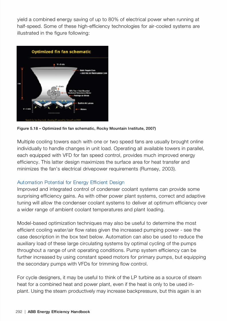
8/12/2019 Energy Efficiency Electronic Book Version 1548_PowerGenerationHandbook v1_1
http://slidepdf.com/reader/full/energy-efficiency-electronic-book-version-1548powergenerationhandbook-v11 294/361
yield a combined energy saving of up to 80% of electrical power when running athalf-speed. Some of these high-efficiency technologies for air-cooled systems areillustrated in the figure following:
Figure 5.18 – Optimized fin fan schematic, Rocky Mountain Institute, 2007)
Multiple cooling towers each with one or two speed fans are usually brought onlineindividually to handle changes in unit load. Operating all available towers in parallel,each equipped with VFD for fan speed control, provides much improved energyefficiency. This latter design maximizes the surface area for heat transfer and
minimizes the fan’s electrical drivepower requirements (Rumsey, 2003).
Automation Potential for Energy Efficient DesignImproved and integrated control of condenser coolant systems can provide somesurprising efficiency gains. As with other power plant systems, correct and adaptivetuning will allow the condenser coolant systems to deliver at optimum efficiency overa wider range of ambient coolant temperatures and plant loading.
Model-based optimization techniques may also be useful to determine the mostefficient cooling water/air flow rates given the increased pumping power - see thecase description in the box text below. Automation can also be used to reduce theauxiliary load of these large circulating systems by optimal cycling of the pumpsthroughout a range of unit operating conditions. Pump system efficiency can befurther increased by using constant speed motors for primary pumps, but equippingthe secondary pumps with VFDs for trimming flow control.
For cycle designers, it may be useful to think of the LP turbine as a source of steamheat for a combined heat and power plant, even if the heat is only to be used in-plant. Using the steam productively may increase backpressure, but this again is an
292 | ABB Energy Efficiency Handbook

8/12/2019 Energy Efficiency Electronic Book Version 1548_PowerGenerationHandbook v1_1
http://slidepdf.com/reader/full/energy-efficiency-electronic-book-version-1548powergenerationhandbook-v11 295/361
optimization problem that can be solved using the techniques described in previoussections. Some applications for in-plant CHP are the HVAC system, and fuel drying orpre-heating; these options are explored in the module on High Performance Design .
Case ExampleMaasvlakte 540 MWe coal-fired plant in the NetherlandsFor the Maasvlakte plant in the Netherlands, thermodynamic modeling showedthat there was a different optimum flow-rate depending on the temperatureof the cooling water (which varies at the plant’s location from 1°C to 20°C).
At 4°C, the optimum flow rate was 12.2 m/s, while at 20°C it was 18.8 m/s.Results from this modeling exercise were confirmed by actual plant data. Anaverage reduction in the condensor cooling-water temperature from 20°C to15°C at this plant reduced the heat rate by almost 1%.
(Case data from Kromhaut and others, 2001, and cited in (IEA Coal Online - 2,2007)
Automation’s monitoring functionality can be used to continually check thecondenser’s heat exchanger performance. The most-common causes of condenserinefficiency are: microbiological growth on the water side, scale formation on the
water side, tube pluggage by debris and air in-leakage on the steam side (Buecker,B. of Burns and McDonnell Engineering, Chemical Engineering; Vol. 102; Issue 4,
Apr 1995). Online monitoring, combined with modeling of these fouling phenomenacan be coupled with a pro-active treatment program to keep the condenser at peakdesign efficiency.
Condensate SystemCondensate System Concepts The purpose of this system is to collect the condensate (boiler feedwater) leaving thecondenser, remove non-condensable gases, raise its temperature through a seriesof feedwater heaters and then deliver it to the deaerator for additional heating andtemporary storage. From the deaerator, the feedwater goes to the boiler feed pumpwhere it is pumped up to near boiler drum pressure at the inlet of the economizer.
Increasing the boiler feedwater temperature effectively increases the uppertemperature of the thermodynamic cycle, raising the efficiency. Heating thefeedwater using steam extracted from the turbine stages is more thermodynamicallyefficient than using other nearby sources, such as fuel in the furnace. Up to 30% ofsteam may be extracted for this purpose, typically at a intermediate and high turbine
Module 5 | 293

8/12/2019 Energy Efficiency Electronic Book Version 1548_PowerGenerationHandbook v1_1
http://slidepdf.com/reader/full/energy-efficiency-electronic-book-version-1548powergenerationhandbook-v11 296/361
pressure stages. Designs with higher steam pressures allow a greater number ofextraction points and hence greater number of heaters in the ‘train’.
Demand for Auxiliary Drivepower This system’s main requirements for auxiliary drivepower come from the condensateand booster pumps. The relatively low-power vacuum pumps are not considered inthis discussion. The condensate pump is a low suction head extraction pump whichmust deliver sufficient discharge head to overcome pressure drops through severalfeedwater heaters. A booster pump is also sometimes used after the de-aeratorto raise pressure to a level sufficient for flow through the high-pressure feedwaterheaters. The power demand and control of the main boiler feedwater pump isdiscussed in the Feedwater control section.
Drivepower Potential for Energy Efficient Design The general case for efficient condensate pump drive power is made in section onPump Systems .
Automation Potential for Energy Efficient Design Although not strictly ‘auxiliary’ systems, the feedwater heaters (heat exchangers) andde-aerator’s energy efficiency could benefit from continuous monitoring at inlets andoutlets for early indication of plugging or fouling problems.
It is almost always more thermodynamically efficient to add another feedwaterheater; Welford and others (2002) cited a 0.15 percentage-point efficiency rise forthe whole unit through an increase of 20°C (36 ºF) in the final feedwater temperature.(IEA Coal Online - 2, 2007) Reliability and cost issues, however, often limit thetotal number of heaters; a total of 6-8 heaters is typical. For a small increment incost, the feedwater heater’s reliability can be increased by adding instrumentationand continuous on-line condition monitoring . Such extra reliability may favoran additional feedwater heater and be justified by the resulting increased cycle
efficiency. One new approach to feedwater heating involves the use of on-site solarequipment to provide thermal energy for feedwater heating during the days peakdemand hours.
The steam bypass valves can also benefit from condition monitoring. The enthalpydrop across these valve is large. Valve leakage can be detected by instrumentationon the downstream side of the bypass line. Similar monitoring can be installed onsteam traps in all bypass lines. Valve functionality can be continuously monitored forstiction and other control problems which lead to unnecessary loss of steam energy.In a poorly maintained system of steam traps, annual energy losses can easily reachsix figure costs.
294 | ABB Energy Efficiency Handbook

8/12/2019 Energy Efficiency Electronic Book Version 1548_PowerGenerationHandbook v1_1
http://slidepdf.com/reader/full/energy-efficiency-electronic-book-version-1548powergenerationhandbook-v11 297/361
The model-based optimization techniques developed for combined heat & power(CHP) systems may be applied to feedwater heater train and de-aerator system toachieve the optimal balance between use and production of steam, and allocationto the most efficient heaters (or other users). Such a control strategy could improvethe off-design performance of the system, especially at lower-load operation. Inindustrial boiler systems, the de-aerator and other components with an inventoryof steam or water may be used in a steam-leveling strategy to absorb processload swings and increase efficiency (Immonen, Assessing Industrial Power PlantOperations & Controls 2003).
In some units, peaking power supply is achieved by deliberately taking one ormore of the top feedwater heaters out of service (Babcock & Wilcox 2005). Thispractice allows more steam to pass through the turbine, but at a significant cycleenergy efficiency penalty. According to EPRI Report CS 4554, taking one top (high-pressure) feedwater out of service increases the heatrate by 94 BTU/kWh, whichcorresponds to a 1% drop in efficiency in a typical PC unit.
Sometimes efficiency is temporarily sacrificed for higher ramp rates, as described inthe following case text; the control strategy for faster ramping temporarily shuts offthe flow to one or more LP feedwater heaters. Operators must be made aware thatprotracted operation in this mode will significantly increase fuel cost and emissions.
Case ExampleSchwarze Pumpe, Power Plant, GermanySchwarze Pumpe in Germany provides an example of large, flexible PC unitswhere two 800 MWe supercritical lignite-fired boilers have been designed tooperate at sliding pressure to down to 40% output, with high rates of change,and short hot start-up times. A dynamic control system covers the whole plant,including firing and emissions control as well as the steam cycle. A 6% load
change per minute is achievable at Schwarze Pumpe with only minor effectson the main steam and hot reheat steam temperatures, and without turbinethrottling or using the storage capacity of the boiler.
Very rapid ramping (for example, by 50 MWe in seconds) requires the useof a degree of steam reserve and temporary changes in feedwater heating.
Temporarily diverting steam away from feedwater heating so that more passesthrough the later turbine stages will have a very negative effect on efficiency inthe short term, but this matters less than meeting demand over these transientperiods.
(Case text provided by IEA Coal Online – 2, 2007)
Module 5 | 295

8/12/2019 Energy Efficiency Electronic Book Version 1548_PowerGenerationHandbook v1_1
http://slidepdf.com/reader/full/energy-efficiency-electronic-book-version-1548powergenerationhandbook-v11 298/361
Fuel Handling Systems
Figure 5.19 – Coal pulverizer with motor, (ABB Motors, 2006)
Fuel Handling System ConceptsFuel handling involves all the processes needed to prepare the raw fuel for mixingwith air and injected into the furnace through burners for combustion. There is agreat variety of fuel handling methods, depending on the type of fossil fuel beingused. Coal is the most complex fossil fuel, with many compositional and hardnessvariations, and is this fuel which is the focus of most of this section. Also, because it
is a solid, mixing this fuel with air is more problematic compared to gaseous or liquidfuels (Black & Veatch 1996, p.182). The main preparation processes for coal arecrushing, drying, and milling, also known as pulverization.
Demand for Auxiliary Drivepower The main fuel handling demand for auxiliary power in coal plants come from crushersand pulverizers/millers, and the primary air system which heats and conveys the fuelto the burners. The CQIM Coal Quality Impact Model developed by Black & Veatch
for EPRI evaluates the total cost (not just delivered cost) due to alternative fuels.One of the 5 main CQIM impact areas is ‘Auxiliary Power Requirements’. Changes inauxiliary power are calculated for each fuel variant, and these are related to amountof lost generation and increased fuel burn rate. Note that the CQIM model includesdraft fan and other auxiliary loads in addition to those directly involved in coal fuelpreparation.
The heating value of coal is given in BTUs per pound, or kilojoules per kilogram(10000 Btu/lb = 23200 kJ/kg). Coal can range from 3500 Btu/lb (culm or wastecoal) to 15,000 Btu/lb for dry prime hard coal. Many auxiliary systems must stillrun and consume drivepower, regardless of the energy (BTU) content of the coal.
These systems include fuel handling, ash handling, draft fans and flue gas emissions
296 | ABB Energy Efficiency Handbook

8/12/2019 Energy Efficiency Electronic Book Version 1548_PowerGenerationHandbook v1_1
http://slidepdf.com/reader/full/energy-efficiency-electronic-book-version-1548powergenerationhandbook-v11 299/361
control equipment. Coal with lower heating values will therefore use a higherpercentage of auxiliary power for each unit of converted energy. Also, coals withhigher sulfur content will require increased auxiliary power to drive FGD processes.
Drivepower Potential for Energy Efficient Design The flow control design guidelines described in the drivepower module showed howspeed control is most efficient at less than full rated speeds. The ‘bypass’ methodfor speed control still used in some coal milling operations is therefore a candidatefor design improvement by applying VFDs for speed control.
Case ExampleMilling Applications: VFD drive instead of Bypass
In a boiler installation, 20 coal mills with a drive output of 710 kW each areused. A speed-controlled drive with a control coupling or with an AC driveis used to replace the bypass method. The possible saving with a controlcoupling is about 11 GWh and with an AC drive 23 GWh as shown below. (Fora description of bypass flow control, see Pump Flow Control Methods )
− Energy saving: 23,000 MWh/year− Reduction in CO2 emissions: 11,500 metric tonnes/year
− Better boiler control with fewer losses− Crushing wheels of the mills last longer− Payback period 2.5 years
(Case text from ABB Drives, 2007)
Pulverizer ApplicationsIn order to accommodate the larger range of operation asked of plants today, asdescribed in the section Plant Operating Modes , the designer should considerspecifying more, but smaller pulverizers rather than fewer, larger ones. The full loadfuel flow rates provided by the basic thermal balance will provide the upper limit ofcombined pulverizer capacity. A pulverizer’s capacity loss due to wear will consume
Module 5 | 297

8/12/2019 Energy Efficiency Electronic Book Version 1548_PowerGenerationHandbook v1_1
http://slidepdf.com/reader/full/energy-efficiency-electronic-book-version-1548powergenerationhandbook-v11 300/361
more power as grinding surfaces wear; this increase in power consumption should bepart of the sizing criteria for pulverizers. It is common practice to include primary airfan power consumption together with pulverizer power. When pulverizer wear is takeninto account, one industry estimate of combined power requirement is 22 kWh/ton(24kWh/metric ton) of coal for a load-following unit. (Babcock & Wilcox 2005).
When pulverizers operating at this capacity are in a typical older PC unit withheatrate of 10,000 BTU/kWh, fired on coal with a heating value of 10,000 BTU/lb,they will consume about 1% of the input fuel energy. This percentage increases withdecreasing coal heating value, increasing plant heat rate, and increasing moisturecontent of the coal.
Automation Potential for Energy Efficient Design Automation which can shut down one or more pulverizers for low load operationshould be coordinated with the combustion and steam temperature control systemsto avoid instability immediately after shutdown/startup. This simple automationmodification saves energy on units with larger boiler turndown, as is the case inunits which are being repurposed from baseload to dispatchable or load-followingduty. The automation of pulverizer operation within the combustion controlsystem, however, must accommodate the limited turndown capability of individualpulverizers, which can individually operate in stable fashion only down to about 50%of rated capacity’. (Black & Veatch 1996, p.182)
Another potential improvement is to enable online monitoring of the relative flow ofcoal in the pipes to individual pulverizers. This data can be used by the combustioncontrols to achieve better balancing of fuel flow to burners in the boiler burnerarray. Full closed loop combustion control, with coal-flow monitoring and and air/ fuel balancing of the the burner array is technically feasible and cost effective at thistime, but the industry is very slow to consider, adopt and apply this technology.
Sootblowing SystemsSootblowing System Concepts
Accumulation of ash and other products of combustion on the heat transfer surfaceswill reduce heat transfer and increase plant heat rate. Sootblowing systems typicallyuse steam or compressed air “cannons” to remove soot from boiler tube surfacesand structures. There are also mechanical vibration, and sonic soot remediationsystems which fall into this general category. Plants which have switched fromtheir design fuel to other, lower-quality fuels are particularly susceptible to moreash-related problems. If internal boiler combustion levels or distributions are notmanaged well, large fused-ash accumulations may form, which may eventually breakoff and fall, damaging boiler and tubes in the process.
298 | ABB Energy Efficiency Handbook

8/12/2019 Energy Efficiency Electronic Book Version 1548_PowerGenerationHandbook v1_1
http://slidepdf.com/reader/full/energy-efficiency-electronic-book-version-1548powergenerationhandbook-v11 301/361
Automation Potential for Energy Efficient DesignSoot-blowing automation can determine where and when to blow soot based uponchanges in heat transfer data. Precise control of soot-blowing will improve heattransfer and heat rate of the unit. Soot-blowing also has an indirect impact on energyefficiency in two ways: 1) Soot-blowing consumes power in the form of compressedair or steam 2) Soot-blowing causes sudden changes in heat-transfer which maydisturb main steam and reheat steam temperature control, causing swings in controlaction and increased attemperation use.
An automated soot-blowing system using closed-loop control will consume lesspower than traditional, open loop control based only on time intervals. A system thatis integrated with the rest of the DCS can use online measurement data to computeheat flux, which can then be used for feedback control. This control system couldbe further improved with MPC and thermodynamic models and direct readings fromstrain gauges (Whitworth, XCEL Energy, 2006)
Automation integration between soot-blowing and steam temperature controlsystems can reduce temperature instability and improve efficiency. When the soot-blowing system described above is ready to act, it can inform the steam temperaturecontrol system which may then take feed-forward compensation measures.
Ash Handling Systems Ash Handling System Concepts Ash-handling systems must transport the solid products of combustion, mostly ashand unburned carbon, from a hopper in the furnace floor.
Automation and Drivepower Potential for Energy Efficient DesignIn PC boilers, bottom ash removal systems consume electrical drivepower, but donot offer the potential for larger energy efficiency gains as the cube-law systems for
fluid and air flow.
Hot, yet unburned carbon in the solid combustion products (and possibly from flue-gas dust collection systems as well) may be reintroduced into the furnace to achievemore complete combustion. Further improvement can be gained by auxiliary systemscapable of separating the heavier carbon from the remaining lighter materials in theash mixture. A ‘carbon reinjection’ system can improve the efficiency of coal-firedboilers by 2% to 4% (Babcock & Wilcox 2005); this improvement is not in thermalefficiency, but calculated on the cost basis of primary coal input.
Module 5 | 299

8/12/2019 Energy Efficiency Electronic Book Version 1548_PowerGenerationHandbook v1_1
http://slidepdf.com/reader/full/energy-efficiency-electronic-book-version-1548powergenerationhandbook-v11 302/361
300 | ABB Energy Efficiency Handbook

8/12/2019 Energy Efficiency Electronic Book Version 1548_PowerGenerationHandbook v1_1
http://slidepdf.com/reader/full/energy-efficiency-electronic-book-version-1548powergenerationhandbook-v11 303/361
ABB Energy Efficient Handbook 301
Module Summary This module defines a base case plant unit and shows the cumulative effects ofdrivepower, electrical power system and automation system improvements. Capitalinvestment costs and operating costs are also estimated, for the purpose of alifecycle cost calculation. This case study will attempt to quantify the benefits inmany scales: efficiency/heatrate, ROI payback, fuel amount & cost, NOx & CO2costs, and power generated available for sale.
The information in this module section is specic to power generation industriesor process plants with on-site power houses. Many sections, however, are alsobroadly applicable to all industrial steam generation processes.
Causes of Energy Inefciency This section reviews the energy efficiency issues relating to auxiliary systems in an
‘average’ facility.
Power plants using pulverized coal fuel are averaging 30-35% efficiency,compared to 45% and higher for supercritical or combined cycle designs.
This very rough comparison provides some indicators as to where one shouldfocus energy efficiency efforts when confronted with an existing plant or whenevaluating alternatives to the ‘standard design’ of a new plant.
Changes in Available Technology − In older plants; the initial auxiliary designs are now outdated by advances in
controls and materials; VFDs for flow control, power electronics for power qualitymanagement, transformer designs with new materials, high efficiency motordesign, new materials etc.
− In older plants; lack of control integration between plant units, such as turbine-generator and the boiler control system leaves substantial opportunity forautomation improvements
Module 6Case Studies In Integrative Design

8/12/2019 Energy Efficiency Electronic Book Version 1548_PowerGenerationHandbook v1_1
http://slidepdf.com/reader/full/energy-efficiency-electronic-book-version-1548powergenerationhandbook-v11 304/361
Sub-Optimal Design and Engineering − Oversized pumps and fans waste energy in throttled operation or in low efficiency
operating regimes − Oversized motors and power supply equipment all operating at low efficiency − Process design & engineering decisions which unnecessarily increase drivepower
loads
Aging − As plants age they become less reliable and generally less efficient due to
corrosion, fouling, wear and other mechanical factors. Feed-water heater heatexchangers, cooling tower heat exchangers, and boiler tubes are all examples ofequipment prone to these mechanical factors.
− Steam losses through leaks, heat loss through boiler walls, and other energylosses through excessive attemperation, blowdown, or sootblowing.
− Loss or lack of experienced plant engineering and operations staff, loss or lack ofas-is plant documentation.
Changes in Operating Conditions − Changes in fuel supply from what boilers and burner systems were originally
designed for, leading to degraded performance. − Plants designed originally for base-load operation near their rated output now
operating below this capacity due to changes brought on by a deregulated and
competitive marketplace. Efficiency and response are reduced at lower loads.
Changes due to Environmental Retrofits − Addition of emissions control equipment such as precipitators, SO2 scrubbers
that restrict stack flow and require greater in-plant electric fan drive power. − Addition of cooling water environmental protection systems that increase the
demand for cooling medium flows and thus electric auxiliary drive power. − Retrofits, environmental and otherwise, without updating of unit controls, leading
to unsuitable control behavior and greater instability, especially boiler instability.
The cumulative negative effect of these causes can be witnessed in existing plant’soperation even without a benet of any formal assessment or extensive data analysis:
302 | ABB Energy Efficency Handbook

8/12/2019 Energy Efficiency Electronic Book Version 1548_PowerGenerationHandbook v1_1
http://slidepdf.com/reader/full/energy-efficiency-electronic-book-version-1548powergenerationhandbook-v11 305/361
Figure 6.1 –Common indicators of an energy-inefficient plant in operation
Energy Efciency Design AssessmentsUsing a systems approach known as ‘Integrative Design’, much of the plant processand mechanical design will be considered even though the scope of the retrofit maynot extend to the boiler or steam cycle (combustion, steam or water path) primary
equipment.
This methodology is a type of design assessment, rather than the morewidely known and applied ‘energy audit’ of an existing plant. The focus of thismethodology, however, is not on operating procedures or parameter adjustments:these are usually within reach of experienced plant managers. In very simplifiedterms, an energy audit seeks ways to reduce losses within the constraints of theplant design ‘as is’, whereas a design assessment uses heat and material balances
to provide a higher upper limit to the possible gains from a retrofit.
The Integrative Design methodology does have some steps in common with anoperational energy audit: in each, there is a data gathering phase, an analysis phase,a ranking of proposed changes, and then implementation. The ranking of proposeddesign changes is based on lifecycle cost calculations, tempered by a discussionof such important qualitative factors as compliance, availability and schedule.
The major differences between a typical energy audit and a design assessmentmethodology are listed in the table below.
Module 6 | 303

8/12/2019 Energy Efficiency Electronic Book Version 1548_PowerGenerationHandbook v1_1
http://slidepdf.com/reader/full/energy-efficiency-electronic-book-version-1548powergenerationhandbook-v11 306/361
Phase Energy Audit Design Assessment
Data gathering Mostly operational data
from historical databases,
strip charts or testing
Mostly design data ; P&ID drawings, flow sheets,
supplier performance data and kits, backed up
with operational data.
Analysis Efficiency calculations Heat and material balances, and comparison
with process models. Pressure drop calculations.
Component sizing calculations using iterative
approaches.
Proposals Procedural and small-scale
investment
Larger-scale design & equipment changes,
automation changes
Ranking Payback based on
short time horizon and
solely energy-saving
improvements
Payback based on longer time horizon and
including other non-energy improvements
Ultimate goal is to provide a utility with capacity
improvements without having to build new plants.
For power plants, the thermal analysis is the first step in the analysis, asthis will provide the basic combustion air, fuel, flue gas and feedwater flowrequirements (Babcock & Wilcox 2005). Based on these flows, the majorpressure drops may then be calculated, followed by the remaining pipe or ductresistance calculations.
See the section on Managing Energy Efficiency Improvement for a discussion ofmanaging both energy and design assessment efforts.
Integrative Design for Auxiliaries The energy efciency issues listed in the previous sections are complex and cut acrossmany plant systems. Integrative Design principles lend themselves well to improvingsteam plant designs. Some of the process areas where Integrative Design has been
successfully applied are: thermal integration, power systems, designing friction outof uid-handling systems, superefcient passive or heat-driven (absorption) cooling,superefcient drive systems and advanced controls. (Lovins, 2008).
Integrative Design takes advantage of the fact that efficiencies are multiplicativeand not simply additive. For a system with several components in series, such asan electrical drive, a motor, a pump, a pipe, and a valve, the efficiency of the wholesystem is the product of all the efficiencies as follows:
Esys = Edrive x Emotor x Epump x Evalve x Epipe
304 | ABB Energy Efficency Handbook
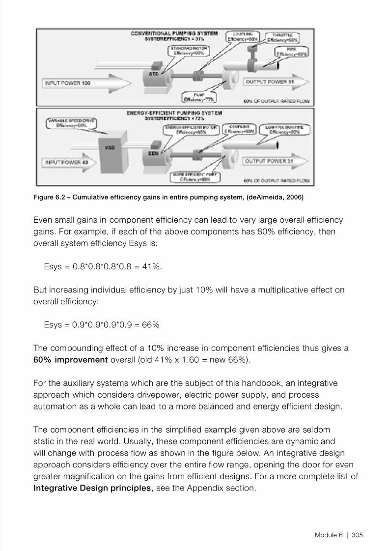
8/12/2019 Energy Efficiency Electronic Book Version 1548_PowerGenerationHandbook v1_1
http://slidepdf.com/reader/full/energy-efficiency-electronic-book-version-1548powergenerationhandbook-v11 307/361
Figure 6.2 – Cumulative efficiency gains in entire pumping system, (deAlmeida, 2006)
Even small gains in component efficiency can lead to very large overall efficiencygains. For example, if each of the above components has 80% efficiency, thenoverall system efficiency Esys is:
Esys = 0.8*0.8*0.8*0.8 = 41%.
But increasing individual efficiency by just 10% will have a multiplicative effect onoverall efficiency:
Esys = 0.9*0.9*0.9*0.9 = 66%
The compounding effect of a 10% increase in component efficiencies thus gives a60% improvement overall (old 41% x 1.60 = new 66%).
For the auxiliary systems which are the subject of this handbook, an integrativeapproach which considers drivepower, electric power supply, and processautomation as a whole can lead to a more balanced and energy efficient design.
The component efficiencies in the simplified example given above are seldomstatic in the real world. Usually, these component efficiencies are dynamic andwill change with process flow as shown in the figure below. An integrative designapproach considers efficiency over the entire flow range, opening the door for evengreater magnification on the gains from efficient designs. For a more complete list ofIntegrative Design principles , see the Appendix section.
Module 6 | 305

8/12/2019 Energy Efficiency Electronic Book Version 1548_PowerGenerationHandbook v1_1
http://slidepdf.com/reader/full/energy-efficiency-electronic-book-version-1548powergenerationhandbook-v11 308/361
Figure 6.3 – Typical efficiency vs. flow for drivepower components (ABB PumpSave User Manual 4.0)
Energy Efciency Design ImprovementsBase Case Unit
The base case used in this text is a 500MW (gross) single pulverized coal-red steamelectric utility power plant unit with a single, sub-critical, drum boiler sending steam toa single turbine. The base case plant is 25 years old and its design is representativeof the newer end of the eet of coal plants in the US. The target unit has previouslyundergone retrots for emissions control; low NOx burners and FGD systems.
The base case plant has old equipment for flow control and drive power, which willbe replaced by modern VFD flow control methods and higher efficiency motors andcouplings. The context for the activities in this module is a small to medium-sizedretrofit project. The cases are divided into smaller scopes than would be normal inretrofit project; this is for calculation purposes to show individual efficiency benefits.
Typically several activities would be combined in a larger retrofit project.
Change of Duty from Baseload to Intermediate
The target for this case study is a fixed-pressure unit designed for base-loading thatis converted to a variable pressure unit for intermediate (load-following) service andfor extended operation at lower loads, typically from 50% to 90% full rated load.
Efficiency Design Improvements The table below summarizes all the design improvements suitable for a plant ofthe stated type and project investment scope. The efficiency improvements areincremental and relate only to the direct effect of auxiliary design improvements.(For example, the effects of environmental or balanced draft conversions have anefficiency impact that is independent of how auxiliary design is executed). The non-auxiliary conversion or upgrade costs vary greatly with plant design and are omittedfrom the discussion.
306 | ABB Energy Efficency Handbook

8/12/2019 Energy Efficiency Electronic Book Version 1548_PowerGenerationHandbook v1_1
http://slidepdf.com/reader/full/energy-efficiency-electronic-book-version-1548powergenerationhandbook-v11 309/361
The design methods and recommendations for auxiliary and automation systemsdescribed in this module are largely applicable to many other fossil steam plantdesigns and situations as well. The table below lists all the proposed auxiliarydesigns for improved energy efficiency. The numbered proposals are singled out fordetailed description and benefits analysis in the following sections.
# Project or Case Scope Description & Benefits
1 VFDs for draft and FGD fan
flow control
Eliminate flow restricting control methods. May
be part of a balanced draft conversion. May also
include benefit of peak loading, previously limited
by fan capacity on hot days.
Upgrade sensors & actuators Retrofit electro-hydraulic(fturbine) , smart positioners for
dampers, louvers
Balanced draft conversion Proper furnace draft control using ID fans instead of FD
fans and speed control instead of dampers
2 VFDs for boiler, c irculating and
condensate pump flow control
Eliminate flow restricting control methods; may be
part of a feedwater heater upgrade
3 Motors & drive-trains upgrade Replace exist ing motor and drive-trains with right-sized,
higher efficiency equipment
DCS replacement for 20+ years
old system
Improved automatic and operator control response
4 Coordinated boiler-turbine
control, sliding pressureoperation
Coordinated boiler turbine control, use of feed-
forward techniques for rapid response. Improvedefficiency at low loads
Boiler startup optimization Less fuel, shorter time during startup
5 Advanced controls for steam
temperature control
Increase main steam temperature, reheat steam
temperature, and ramp rate
6 Stabilizing firing rate Improved heat rate, reduced need for attemperation.
1-2 % improvement in heat rate
7 Reduction of excess air Decrease the average flue gas O2 of the boilers
through improved airflow control.8 Improved Feedwater Pressure
& Level Control
General loop tuning Manual and adaptive tuning techniques
9 Electrical power system
upgrade
Power quality improvements, transformer right-sizing
and efficiency upgrade
Plant availability improvement Diagnostics, condition monitoring, asset management
Cooling tower retrofit Improve drivepower & controls related to condenser
systems
Environmental upgrade Improve drivepower & controls for FGD, precipitators,
catalytic conversion
Module 6 | 307
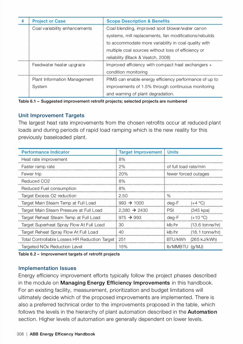
8/12/2019 Energy Efficiency Electronic Book Version 1548_PowerGenerationHandbook v1_1
http://slidepdf.com/reader/full/energy-efficiency-electronic-book-version-1548powergenerationhandbook-v11 310/361
# Project or Case Scope Description & Benefits
Coal variability enhancements Coal blending, improved soot blower/water canon
systems, mill replacements, fan modifications/rebuilds
to accommodate more variability in coal quality with
multiple coal sources without loss of efficiency or
reliability (Black & Veatch, 2008)
Feedwater heater upgrade Improved efficiency with compact heat exchangers +
condition monitoring
Plant Information Management
System
PIMS can enable energy efficiency performance of up to
improvements of 1.5% through continuous monitoring
and warning of plant degradation.
Table 6.1 – Suggested improvement retrofit projects; selected projects are numbered
Unit Improvement Targets The largest heat rate improvements from the chosen retrofits occur at reduced plantloads and during periods of rapid load ramping which is the new reality for thispreviously baseloaded plant.
Performance Indicator Target Improvement Units
Heat rate improvement 8%
Faster ramp rate 2% of full load rate/min
Fewer trip 20% fewer forced outages
Reduced CO2 8%Reduced Fuel consumption 8%
Target Excess O2 reduction 2.50 %
Target Main Steam Temp at Full Load 993 à 1000 deg-F (+4 ºC)
Target Main Steam Pressure at Full Load 2,380 à 2430 PSI (345 kpa)
Target Reheat Steam Temp at Full Load 975 à 993 deg-F (+10 ºC)
Target Superheat Spray Flow At Full Load 30 klb/hr (13.6 tonne/hr)
Target Reheat Spray Flow At Full Load 40 klb/hr (18.1 tonne/hr)
Total Controllable Losses HR Reduction Target 251 BTU/kWh (265 kJ/kWh) Targeted NOx Reduction Level 15% lb/MMBTU (g/MJ)
Table 6.2 – Improvement targets of retrofit projects
Implementation IssuesEnergy efficiency improvement efforts typically follow the project phases describedin the module on Managing Energy Efficiency Improvements in this handbook.For an existing facility, measurement, prioritization and budget limitations willultimately decide which of the proposed improvements are implemented. There isalso a preferred technical order to the improvements proposed in the table, whichfollows the levels in the hierarchy of plant automation described in the Automation section. Higher levels of automation are generally dependent on lower levels.
308 | ABB Energy Efficency Handbook

8/12/2019 Energy Efficiency Electronic Book Version 1548_PowerGenerationHandbook v1_1
http://slidepdf.com/reader/full/energy-efficiency-electronic-book-version-1548powergenerationhandbook-v11 311/361
− Upgrade sensors and actuators (especially electro-hydraulic and mechanicalcomponents)
− Upgrade motors and drives − Upgrade Distributed Control System (DCS) − Upgrade programmable control strategies − Upgrade programmable optimization routines − Upgrade plant unit operating manual & procedures
There are limitations to the possible efficiency gains in the context of auxiliarysystems redesign or retrofit. Some of the improvements discussed in the sectionon High Performance Energy Design , intended mainly for greenfield plant designs,could achieve 15% net heat rate reductions over older plant designs (from a nominal10200 Btu/kwh (10.8 MJ/kWh) down to 8700 Btu/kwh (9.2 MJ/kWh).
Base Case Plant Design and Performance Data As with operational energy audits, a design energy assessment starts with somedata identification and data gathering steps. Design data and documentation mustalso be collected, though, along with calculations/measurements of average heatrate at full and partial loads. Unit data was collected from the following sources:
− GE Handbook, H. Rustebakke, 1983
− Black & Veatch (Drbal,L et al.) Power Plant Engineering , 1995 − IEA CoalOnline , citing various data sources, 2008 − EPRI Field Test on VFD Retrofits, 1993 − ABB: Enel´s Torrevaldaliga Nord : 3 x 660MW units : increased net efficiency
from 39% to 45% with emission reductions: SO2/NOx/Dust from 400/200/50 to100/100/15 (mg/Nm3) , 2005
− ABB: Unit C of the E.ON Scholven Power Plant, 2008 − ABB: PC plant in China; 3 x 700 MW units. Energy performance data, before/after
VFDs, 2008
Module 6 | 309

8/12/2019 Energy Efficiency Electronic Book Version 1548_PowerGenerationHandbook v1_1
http://slidepdf.com/reader/full/energy-efficiency-electronic-book-version-1548powergenerationhandbook-v11 312/361
Plant Unit AssumptionsParameter Value Units SI Units
Average Unit Capacity for period 500 MWe
Assumed Annual Capacity Factor 70.0 %
Fuel HHV (typical) 8,895 BTU/lb 20.6 MJ/kg
0.00890 MBTU/lb
112.423 lb/MBTU
Fuel Cost $2.470 $/MMBTU
$0.0220 $/lb $0.048/kg
NOx Reduction Value $2,000 $/ton $2200/tonne
Fuel % Carbon 48.6 %
CO2 Reduction Value $5.00 $/ton $5.50/tonne
NOx (average for period) 0.210 lb/MBTU
Net Heat Rate (average for period) 10,211 BTU/kWh
Table 6.3 – Plant basic and automation parameters
Parameter Value Units SI Units
Operating hours per year (auxiliaries) 8000 hr
VFD investment cost $93 $/hp $125/kW
Induction motor investment cost $100 $/hp $135/kW
Cost of electricity when sold $0.05 $/kWh
Premium of in-plant electricity $0.007 $/kWh
Discount rate 5.0% %Service life remaining 20 years
Oversized motor efficiency penalty 0.1 %
Baseline annual generated energy 3,066,000,000 kWh
Baseline heat input 31,306,926 MMBtu 33 × 10 15 J
Cost of saved fuel $0.025 $/kWh
Table 6.4 – Drivepower parameters
Parameter Value Units SI Units Transformer investment cost 10,000 $/MVA
Average Power Output (70% of rating) 350 Mwe
Transformer Load losses $3,000 $/kW
Transformer Core losses $1,500 $/kW
SVC investment cost $50,000 $/MVAR
Table 6.5 – Transformer & SVC parameters
310 | ABB Energy Efficency Handbook

8/12/2019 Energy Efficiency Electronic Book Version 1548_PowerGenerationHandbook v1_1
http://slidepdf.com/reader/full/energy-efficiency-electronic-book-version-1548powergenerationhandbook-v11 313/361
% Full flow % Total Annual hrs Capacity factor %
100% 5 400 5%
90% 10 800 9%
80% 20 1600 16%
70% 25 2000 18%
60% 25 2000 15%
50% 10 800 5%
40% 5 400 2%
30% 0 0 0%
20% 0 0 0%
100 8000 70%
Table 6.6 – Operating profile for all auxiliaries
Load Name ID Rated
hp
In
use
Rated
Set hp
Control
method
Load
factor
Operat-
ing hp
%
Gross
Boiler feedwater
pump
BFW 14,000 2 28,000 Slip 0.81 22,680 4.8%
Condensate pump HW 2,250 1 2,250 Throttling 0.75 1,688 0.4%
Circulating water
pump
CW 3,400 2 6,800 Throttling 0.85 5,780 1.2%
Forced draft fan
(blower)
FD 2,250 2 4,500 Inlet vane 0.52 2,340 0.5%
Primary air fan PA 2,250 2 4,500 Inlet vane 0.49 2,205 0.5%
Induced draft fan ID 4,500 2 9,000 Inlet vane 0.78 7,020 1.5%
SUM ALL LARGE
MV motors
41,713
Boiler circulating
water pump
BCW 600 3 1,800 Throttling 0.82 1,476 0.3%
Service water
pump
SW 400 1 400 Throttling 0.82 328 0.1%
FGD slurry pump FGDS 600 1 600 Throttling 0.82 492 0.1%
Cooling tower fan CT 600 2 1,200 Inlet vane 0.82 984 0.2%
Pulverizers PV 450 5 2,250 Bypass 0.66 1,485 0.3%
Air compressor AIR 480 1 480 Bypass 1.66 797 0.2%
All other auxiliary
loads
AUX 4,300 1 4,300 N/A 0.53 2,279 0.5%
FGD booster fan FGD 6,500 1 6,500 Inlet vane 0.66 4,290 0.9%
TOTAL 66,480 54,171 11.5%
SCR circulating
pump
SCR 400 1 400 Throttling 0.82 328 0.1%
Table 6.7 – Auxiliary systems fan and pump drivepower
Module 6 | 311
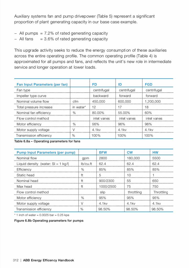
8/12/2019 Energy Efficiency Electronic Book Version 1548_PowerGenerationHandbook v1_1
http://slidepdf.com/reader/full/energy-efficiency-electronic-book-version-1548powergenerationhandbook-v11 314/361
Auxiliary systems fan and pump drivepower (Table 5) represent a significantproportion of plant generating capacity in our base case example.
− All pumps = 7.2% of rated generating capacity − All fans = 3.6% of rated generating capacity
This upgrade activity seeks to reduce the energy consumption of these auxiliariesacross the entire operating profile. The common operating profile (Table 4) isapproximated for all pumps and fans, and reflects the unit’s new role in intermediateservice and longer operation at lower loads.
Fan Input Parameters (per fan) FD ID FGD
Fan type centrifugal centrifugal centrifugal
Impeller type curve backward forward forward
Nominal volume flow cfm 450,000 600,000 1,200,000
Total pressure increase in water* 12 17 18
Nominal fan efficiency % 80.00% 55.00% 60%
Flow control method inlet vanes inlet vanes inlet vanes
Motor efficiency % 96% 96% 96%
Motor supply voltage V 4.1kv 4.1kv 4.1kv
Transmission efficiency % 100% 100% 100%
Table 6.8a – Operating parameters for fans
Pump Input Parameters (per pump) BFW CW HW
Nominal flow gpm 2800 180,000 5500
Liquid density (water: SI = 1 kg/l) lb/cu.ft 62.4 62.4 62.4
Efficiency % 85% 85% 85%
Static head ft 5 10 1
Nominal head ft 900/2300 55 650
Max head ft 1000/2500 75 750Flow control method slip throttling Throttling
Motor efficiency % 95% 95% 95%
Motor supply voltage V 4.1kv 4.1kv 4.1kv
Transmission efficiency % 98.50% 98.50% 98.50%
* 1 inch of water = 0.0025 bar = 0.25 kpa
Figure 6.8b Operating parameters for pumps
312 | ABB Energy Efficency Handbook

8/12/2019 Energy Efficiency Electronic Book Version 1548_PowerGenerationHandbook v1_1
http://slidepdf.com/reader/full/energy-efficiency-electronic-book-version-1548powergenerationhandbook-v11 315/361
Base Case Plant Improvement#1 Improved Fan Flow ControlIn the base case plant unit there are 2 FD fans, rated at 2250 hp (1680 kW) eachand 2 ID fans rated at 4500 hp (3357 kW) each, in parallel, all of centrifugal design,all using inlet guide vanes for flow control. On hot summer days, peak loading of theunit was limited by the FD fan capacity. A single FGD booster was later installed,rated at 6,500 hp (4850 kW).
Retrofit DescriptionIn the retrofit project, all fans were equipped with VFDs for speed control and theinlet vanes were locked in open position.
FD ID FGD
Number in operation # 2 2 1
Required input motor power;
rated, including 10% margin
hp 1065 3190 6184
Annual energy consumption
with existing flow control
kWh 3,472,721 10,403,631 20169878
Annual energy consumption
with VFD flow control
kWh 2,474,608 7,413,469 14372748
Annual energy saving kWh kWh 998,113 2,990,162 5,797,130
Efficiency gain % % 28.7% 28.7% 28.7%
Annual saved energy when sold $ $2,495 $7,475 $14,493 Annual saved fuel qty lbs 1,088,493 3,260,924 6,322,065
Annual saved fuel cost $ $23,915 $71,645 $138,900
Annual saved fuel cost
premium
$ $6,637 $19,885 $38,551
Annual heat input saving MMBTU/year 9,682 29,005 56,234
Annual CO2 reduction tons 970 2,905 5,633
Annual CO2 charge saving $ $4,849 $14,527 $28,165
Improvement in heat rate % 0.03% 0.10% 0.19% Annual saving TOTAL $ $37,897 $113,532 $220,108
Investment cost $ $99,045 $296,670 $575,112
Payback period years 2.4 2.4 2.4
Net Present Value $ $373,234 $1,118,190 $2,167,925
Divide lbs by 2.2 to get kg. Multiply MMBtu by 1055 to get MJ.
Table 6.9 – Main benefits analysis for fans, per fan
Module 6 | 313

8/12/2019 Energy Efficiency Electronic Book Version 1548_PowerGenerationHandbook v1_1
http://slidepdf.com/reader/full/energy-efficiency-electronic-book-version-1548powergenerationhandbook-v11 316/361
#2 Improved Pump Flow Control The boiler feedwater (BFW) pumping system in the base case plant unit has 2multi-stage, split-casing centrifugal BFW pumps each supplying 50% of the capacity.Each BFW pump is rated at 14,400 hp (10,740 kW). Control valve throttling wasoriginally used for flow control, then it was replaced by hydraulic slip-type couplingfor speed control some years ago.
The cooling water circulating water (CW) pump in the base case plant unit is a lowhead, high capacity axial design. There are 2 such pumps rated at 3217 hp (2400kW) which together consume approximately 0.8% of rated generating capacity forthe unit. The cooling system is closed loop and the pump is a vertical, wet pit type,and control valves are used for throttling flow control.
The condensate or hotwell (HW) pump in the base case plant unit is a single pumprated at 2144 hp (1600kW) and consumes approximately 0.1% of rated generatingcapacity for the unit. This pump is a 2-stage centrifugal design. An additional HWpump is installed for redundancy, but does not normally operate.
Retrofit Description The pumps were equipped with VFDs for speed control and the hydraulic couplingswere removed. Previous studies (by ABB, Black & Veatch, EPRI) have indicatedthat VFDs provide a 10% reduction in input electrical power compared to slip-type
couplings, even at 100% throttle ows. This advantage increases to 15% for owsbetween 50% and 75% of full throttle, which more closely reects the operating proleof the base case plant unit. See the section on Pump Flow Control for more detailson these ow control comparisons. The benets in the table below were calculatedusing the 15% improvement factor. If throttling were used for BFW pump ow control,then the advantage of using VFDs for ow control would vary from 10% at full throttleto 30% at half throttle ows. Note also that most simple tools for benets analysis arenot valid for large BFW pumps with multi-stage designs.
An alternative to retrofitting both CW pumps with VFDs is to retrofit only a singlepump and use automation to start/stop the other pump to reduce the plant auxiliaryload. The automation control logic could use the unit load and turbine back pressureas inputs.
314 | ABB Energy Efficency Handbook

8/12/2019 Energy Efficiency Electronic Book Version 1548_PowerGenerationHandbook v1_1
http://slidepdf.com/reader/full/energy-efficiency-electronic-book-version-1548powergenerationhandbook-v11 317/361
BFW CW HW
Number in operation # 2 2 1
Required input motor power;
rated, including 10% margin
hp 11,423 3240 1170
Annual energy consumption
with existing flow control
kWh 41,109,000 15,758,502 5,216,951
Annual energy consumption
with VFD flow control
kWh 34,942,500 7,372,117 2,716,618
Annual energy saving kWh kWh 6,166,500 8,386,385 2,500,333
Efficiency gain % % 15.0% 53.2% 47.9%
Annual saved energy when sold $ $15,416 $20,966 $6,251
Annual saved fuel qty lbs 6,724,882 9,145,779 2,726,740
Annual saved fuel cost $ $147,750 $200,939 $59,908
Annual saved fuel cost premium $ $41,007 $55,769 $16,627
Annual heat input saving MMBTU/year 59,817 81,351 24,254
Annual CO2 reduction tons 5,992 8,149 2,430
Annual CO2 charge saving $ $29,959 $40,744 $12,148
Improvement in heat rate % 0.20% 0.27% 0.08%
Annual saving TOTAL $ $234,133 $318,419 $94,934
Investment cost $ $1,062,293 $301,320 $108,810
Payback period years 4.5 1.0 1.2
Net Present Value $ $1,855,521 $3,666,885 $1,074,277
Divide lbs by 2.2 to get kg. Multiply MMBtu by 1055 to get MJ.Table 6.10 – Main benefits analysis for pumps, per pump
#3 High-Efficiency Motors & Drive-trainsRetrofit DescriptionExisting motors were replaced with high efficiency, low power-factor motors. Anyapplications with negative NPV (shown in red in the table below) would not beconsidered as candidates for this kind of retrofit.
Module 6 | 315

8/12/2019 Energy Efficiency Electronic Book Version 1548_PowerGenerationHandbook v1_1
http://slidepdf.com/reader/full/energy-efficiency-electronic-book-version-1548powergenerationhandbook-v11 318/361
Main Benefits AnalysisMotor & Drivetrain Improvement Motor
FD ID FGD
Existing motor rating (per unit) Hp 2,250 4,500 6,500
Existing motor efciency % 85.0% 85.0% 85.0%
Existing transmission efciency % 97.0% 97.0% 97.0%
New motor efciency % 96.5% 96.5% 96.5%
New transmission efciency % 99.0% 99.0% 99.0%
Oversized hp hp 1,185 1,310 316
Oversized % % 52.7% 29.1% 4.9%
Oversized motor efciency penalty % 5.3% 2.9% 0.5%
Annual energy saving kWh kWh 651,714 1,707,351 2,820,990
Efciency gain % % 18.8% 16.4% 14.0%
Annual saved energy when sold $ $1,629 $4,268 $7,052
Annual saved fuel qty lbs 710,727 1,861,954 3,076,433
Annual saved fuel cost $ $15,615 $40,908 $67,591
Annual saved fuel cost premium $ $4,562 $11,951 $19,747
Annual heat input saving MMBTU/year 6,321 16,562 27,364
Annual CO2 reduction tons 633 1,659 2,741
Annual CO2 charge saving $ $3,166 $8,295 $13,706
Improvement in heat rate % 0.02% 0.06% 0.09%
Annual saving TOTAL $ $24,973 $65,423 $108,096
Investment cost $ $106,500 $319,000 $618,400Payback period years 4.3 4.9 5.7
Net Present Value $204,719 $496,328 $728,715
Divide lbs by 2.2 to get kg. Multiply MMBtu by 1055 to get MJ.
Table 6.11 – Main motor and drivetrain benefits for fans, per motor
Motor & Drivetrain Improvement Per Unit -->
BFW CW HW
Existing motor rating (per unit) hp 14,000 3,400 2,250Existing motor efciency % 85.0% 85.0% 85.0%
Existing transmission efciency % 98.5% 97.0% 97.0%
New motor efciency % 96.5% 96.5% 96.5%
New transmission efciency % 99.0% 99.0% 99.0%
Oversized hp hp 2,578 160 1,080
Oversized % % 18.4% 4.7% 48.0%
Oversized motor efciency penalty % 1.8% 0.5% 4.8%
Annual energy saving kWh kWh 5,689,926 2,201,555 954,702
Efciency gain % % 13.8% 14.0% 18.3%
Annual saved energy when sold $ $14,225 $5,504 $2,387
Annual saved fuel qty lbs 6,205,154 2,400,908 1,041,151
316 | ABB Energy Efficency Handbook

8/12/2019 Energy Efficiency Electronic Book Version 1548_PowerGenerationHandbook v1_1
http://slidepdf.com/reader/full/energy-efficiency-electronic-book-version-1548powergenerationhandbook-v11 319/361
Motor & Drivetrain Improvement Per Unit -->
Annual saved fuel cost $ $136,331 $52,750 $22,875
Annual saved fuel cost premium $ $39,829 $15,411 $6,683
Annual heat input saving BTU/year 55,194,843,186 21,356,078,337 9,261,039,336
Annual CO2 reduction tons 5,529 2,139 928
Annual CO2 charge saving $ $27,644 $10,696 $4,638
Improvement in heat rate % 0.19% 0.07% 0.03%
Annual saving TOTAL $ $218,030 $84,360 $36,583
Investment cost $ $1,142,250 $324,000 $117,000
Payback period years 5.2 3.8 3.2
Divide lbs by 2.2 to get kg. Multiply MMBtu by 1055 to get MJ.
Table 6.12 – Main motor and drivetrain benefits for pumps , per motor
#4 Boiler Turbine Coordinated Controls and Sliding Pressure Operation This retrofit is worthwhile, but automation auxiliaries cannot claim all benefits due tosliding pressure mode; it is therefore excluded from the summary of benefits.
#5 Advanced Steam Temperature Control The existing control used the two parallel spray valves to control the final mainsuperheat (SH) steam temperature. The control strategy included two PID controllersin a cascade configuration. The outer PID calculated a setpoint for the average ofthe two attemperator outlet temperatures. A feedforward based on the unit load
demand was used as a valve demand reference. The system uses a single sprayvalve to control the final reheat (RH) steam temperature. A feedforward based on theunit load demand is used as a valve demand reference.
The sample data set, however, showed that the steam temperatures wereuncontrolled at the low or ramping loads, which degrades heatrate for the unit’snew role providing intermediate (load-following service. In the base case unit, thestandard deviation of the main steam temperature was found to be 8°F due to unstable
operation and control action. Operators typically maintained a safety margin of 3 to4 times the standard deviation between the maximum and the temperature setpoint(ABB, Immonen 2006) and this was reected in the average main steam temperature,which was 30 °F below the design point (1005°F), at 975 °F. Similar instability and loweraverage temperatures were observed for reheat temperatures as well.
Retrofit Description An advanced steam temperature control strategy was implemented to control steamtemperature for a drum boiler operating in either constant or sliding pressure mode:see the section on Advanced Seam Temperature Control for design details. Usingthese techniques, the standard deviation is more than halved to only 3°F, which
Module 6 | 317
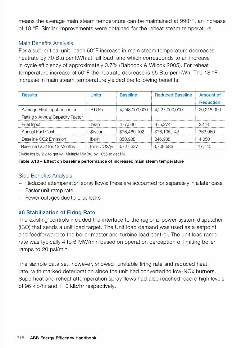
8/12/2019 Energy Efficiency Electronic Book Version 1548_PowerGenerationHandbook v1_1
http://slidepdf.com/reader/full/energy-efficiency-electronic-book-version-1548powergenerationhandbook-v11 320/361
means the average main steam temperature can be maintained at 993°F, an increaseof 18 °F. Similar improvements were obtained for the reheat steam temperature.
Main Benefits AnalysisFor a sub-critical unit: each 50°F increase in main steam temperature decreasesheatrate by 70 Btu per kWh at full load, and which corresponds to an increasein cycle efficiency of approximately 0.7% (Babcock & Wilcox 2005). For reheattemperature increase of 50°F the heatrate decrease is 65 Btu per kWh. The 18 °Fincrease in main steam temperature yielded the following benefits.
Results Units Baseline Reduced Baseline Amount of
Reduction
Average Heat Input based on
Rating x Annual Capacity Factor
BTU/h 4,248,000,000 4,227,000,000 20,218,000
Fuel Input lbs/h 477,546 475,274 2273
Annual Fuel Cost $/year $76,469,102 $76,105,142 363,960
Baseline CO2 Emission lbs/h 850,988 846,938 4,050
Baseline CO2 for 12 Months Tons CO2/yr 3,727,327 3,709,586 17,740
Divide lbs by 2.2 to get kg. Multiply MMBtu by 1055 to get MJ.
Table 6.13 – Effect on baseline performance of increased main steam temperature
Side Benefits Analysis
− Reduced attemperation spray ows: these are accounted for separately in a later case − Faster unit ramp rate − Fewer outages due to tube leaks
#6 Stabilization of Firing Rate The existing controls included the interface to the regional power system dispatcher(ISO) that sends a unit load target. The Unit load demand was used as a setpointand feedforward to the boiler master and turbine load control. The unit load ramp
rate was typically 4 to 6 MW/min based on operation perception of limiting boilerramps to 20 psi/min.
The sample data set, however, showed, unstable firing rate and reduced heatrate, with marked deterioration since the unit had converted to low-NOx burners.Superheat and reheat attemperation spray flows had also reached record high levelsof 96 klb/hr and 110 klb/hr respectively.
318 | ABB Energy Efficency Handbook

8/12/2019 Energy Efficiency Electronic Book Version 1548_PowerGenerationHandbook v1_1
http://slidepdf.com/reader/full/energy-efficiency-electronic-book-version-1548powergenerationhandbook-v11 321/361
Retrofit DescriptionIn conjunction with the controls retrofit, the response was re-programmed to beslower at start of a ramp, and greater acceleration is allowed when drum pressure isgreater than 1260 psig.
Main Benefits Analysis These modifications, in conjunction with the upgraded advanced steam temperaturecontrols, reduced instability and superheat and reheat attemperation spray flows to30 klb/hr and 40 klb/hr respectively, with the following estimated benefits:
Results Units Baseline Reduced Baseline Amount of
Reduction
Average Heat Input based
on Rating x Annual Capacity
Factor
BTU/h 4,247,776,000 4,178,413,824 69,362,176
Fuel Input lbs/h 477,546 469,749 7798
Annual Fuel Cost $/year $76,469,102 $75,220,434 $1,248,668
Baseline CO2 Emission lbs/h 850,988 837,092 13,896
Baseline CO2 for 12 Months Tons CO2/yr 3,727,327 3,666,463 60,864
Improvement in heat rate % 1.633%
Divide lbs by 2.2 to get kg. Multiply MMBtu by 1055 to get MJ.
Table 6.14 – Effect on baseline performance of decreased superheat and reheat attemperation flows
#7 Improved Airflow Control - Excess O2 ReductionPrior to all retrofits, two FD fans were used to control the boiler combustion air flowin the base case unit. The control response was adjusted based on whether one ortwo fans were in automatic service. The air flow control included the typical cross-limit by the fuel flow as described in the Combustion Control section. The sampledata set, however, showed a 0.5% variation in O2 at all loads, and worries aboutopacity excursions led to much manual control.
Retrofit DescriptionIn a control system retrot, a dedicated oxygen trim control module was installed toadjust the measured air ow as needed to keep the O2 at the load based setpoint.
The process variable is the lower of the two O2 analyzer inputs. The trim controlmodule also uses the more precise airow control provided by VFD-equipped FD and IDfans to achieve overall optimum levels of combustion, as described in Air Flow Controlfor Combustion . Furthermore, air heater seals were inspected and worn/broken oneswere replaced, to eliminate outside air leaks from entering the ue gas stream.
Module 6 | 319

8/12/2019 Energy Efficiency Electronic Book Version 1548_PowerGenerationHandbook v1_1
http://slidepdf.com/reader/full/energy-efficiency-electronic-book-version-1548powergenerationhandbook-v11 322/361
Main Benefits AnalysisImproved control and stability allowed full-time automatic control and an averagereduction in excess O2 from 3.7% to 2.5% and the following benefits. The first 0.5%of reduction came from the air heater seal replacements, and the net reduction from3.2% to 2.5% was obtained through the controls improvement:
Results Units Baseline Reduced
Baseline
Amount of
Reduction
Average Heat Input based on
Rating x Annual Capacity Factor
BTU/h 4,247,776,000 4,229,430,400 18,345,600
Fuel Input lbs/h 477,546 475,484 2062
Annual Fuel Cost $/year $76,469,102 $76,138,842 $330,260
Baseline CO2 Emission lbs/h 850,988 847,313 3,675
Baseline CO2 for 12 Months Tons CO2/yr 3,727,327 3,711,229 16,098
Divide lbs by 2.2 to get kg. Multiply MMBtu by 1055 to get MJ.
Table 6.15 – Effect on baseline performance of decreased excess oxygen
#8 Improved Feedwater Pressure & Level Control The base case unit’s drum level is regulated by two motor-driven Boiler Feedwater(BFW) pumps each with a variable speed (VFD) drive as a result of the retrofitdescribed in Improved Pump Flow Control . Single element-three elementcontrol strategy is employed for drum level control as described in Feedwater
Flow Control .
The unit’s transition to intermediate (load-following) service with higher ramp ratesand increased operation at lower loads, however, led to instability and lower averagemain steam pressure 2,436 psi compared to the design point at 2,500 psi whenoperating in constant pressure mode at higher loads.
Retrofit Description
The new control system uses shrink-swell compensation to maintain drum leveleven at the faster unit load ramp rates. Adaptive tuning is also employed to allowthe controllers to respond most accurately across the expanded load range.
Main Benefits Analysis The steam pressure standard deviation was reduced, allowing a higher averagepressure operation at 2,480 (an increase of 44 psi). For a sub-critical unit: each 100psi increase in main steam pressure decreases heatrate by 35 Btu per kWh at fullload (EPRI report CS-4554).
320 | ABB Energy Efficency Handbook

8/12/2019 Energy Efficiency Electronic Book Version 1548_PowerGenerationHandbook v1_1
http://slidepdf.com/reader/full/energy-efficiency-electronic-book-version-1548powergenerationhandbook-v11 323/361
Results Units Baseline Reduced
Baseline
Amount of
Reduction
Average Heat Input based
on Rating x Annual Capacity
Factor
BTU/h 4,247,776,000 4,241,369,600 6,406,400
Fuel Input lbs/h 477,546 476,826 720
Annual Fuel Cost $/year $76,469,102 $76,353,773 $115,329
Baseline CO2 Emission lbs/h 850,988 849,704 1,283
Baseline CO2 for 12 Months Tons CO2/yr 3,727,327 3,721,705 5,621
Divide lbs by 2.2 to get kg. Multiply MMBtu by 1055 to get MJ.
Table 6.16 – Effect on baseline performance of improved feedwater level & pressure control
#9 Electric Power System ImprovementUnit Transformers / Bus Gen Step-Up Aux 1A Aux 1B FGD Boost
Primary kV 19 19 19 19
Secondary kV 525 6.9 6.9 13.8
Rating MVA MVA 520 40 40 10
Existing PF N/A 0.91 0.85 0.85 0.85
Existing efciency at oper. pt. % 99.1% 97.2% 97.2% 97.2%
New PF N/A 0.94 0.9 0.9 0.9
New efciency % 99.7% 98.0% 98.0% 98.0%
Existing Reactive Power
(based on capcity factor)
MVAR 159.5 21.1 21.1 5.3
New Active Power MW 361.5 36.0 36.0 9.0
Change in Active Power MW 11.5 2.0 2.0 0.5
Cable type n/a 4x3C,
300mm
4x3C,
100mm
4x3C,
100mm
4x3C, 100mm
Cable length ft 150.0 700.0 700.0 700.0
Existing Total Power (based
on capacity factor)
MVA 384.6 40.0 40.0 10.0
Divide lbs by 2.2 to get kg. Multiply MMBtu by 1055 to get MJ.Table 6.17 – Power system improvements
The base case unit’s GSU and auxiliary transformers are old. The PF on thegenerator and plant network sides is relatively low.
Module 6 | 321
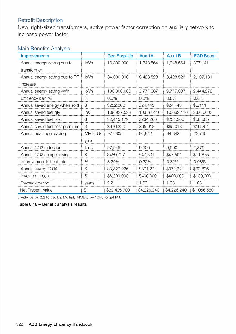
8/12/2019 Energy Efficiency Electronic Book Version 1548_PowerGenerationHandbook v1_1
http://slidepdf.com/reader/full/energy-efficiency-electronic-book-version-1548powergenerationhandbook-v11 324/361
Retrofit DescriptionNew, right-sized transformers, active power factor correction on auxiliary network toincrease power factor.
Main Benefits AnalysisImprovements Gen Step-Up Aux 1A Aux 1B FGD Boost
Annual energy saving due to
transformer
kWh 16,800,000 1,348,564 1,348,564 337,141
Annual energy saving due to PF
increase
kWh 84,000,000 8,428,523 8,428,523 2,107,131
Annual energy saving kWh kWh 100,800,000 9,777,087 9,777,087 2,444,272
Efciency gain % % 0.6% 0.8% 0.8% 0.8%
Annual saved energy when sold $ $252,000 $24,443 $24,443 $6,111
Annual saved fuel qty lbs 109,927,528 10,662,410 10,662,410 2,665,603
Annual saved fuel cost $ $2,415,179 $234,260 $234,260 $58,565
Annual saved fuel cost premium $ $670,320 $65,018 $65,018 $16,254
Annual heat input saving MMBTU/
year
977,805 94,842 94,842 23,710
Annual CO2 reduction tons 97,945 9,500 9,500 2,375
Annual CO2 charge saving $ $489,727 $47,501 $47,501 $11,875
Improvement in heat rate % 3.29% 0.32% 0.32% 0.08%
Annual saving TOTAL $ $3,827,226 $371,221 $371,221 $92,805
Investment cost $ $8,200,000 $400,000 $400,000 $100,000Payback period years 2.2 1.03 1.03 1.03
Net Present Value $ $39,495,700 $4,226,240 $4,226,240 $1,056,560
Divide lbs by 2.2 to get kg. Multiply MMBtu by 1055 to get MJ.
Table 6.18 – Benefit analysis results
322 | ABB Energy Efficency Handbook

8/12/2019 Energy Efficiency Electronic Book Version 1548_PowerGenerationHandbook v1_1
http://slidepdf.com/reader/full/energy-efficiency-electronic-book-version-1548powergenerationhandbook-v11 325/361

8/12/2019 Energy Efficiency Electronic Book Version 1548_PowerGenerationHandbook v1_1
http://slidepdf.com/reader/full/energy-efficiency-electronic-book-version-1548powergenerationhandbook-v11 326/361
Conclusion and Comments The cases were restricted to a single unit, but a true integrative design approachwould investigate possibilities for thermal and control integration with other unitsand even other nearby facilities. Integrated (real-time) control between plant unitsmay provide a relatively low-cost way to optimize production for energy. The basecase unit is analyzed in isolation, but environmental services for cooling or pumpedstorage may provide opportunities for improved auxiliary and cycle efficiency.
Software Tools for Energy Benefits Analysis The benefits analysis performed on the base case plant was aided by thespreadsheet tool: ABB Power Systems Valuation Tool, 2009.
Figure 6.4 – Screenshot of the ABB Power Systems Valuation Tool, Version 3, 2009
324 | ABB Energy Efficency Handbook

8/12/2019 Energy Efficiency Electronic Book Version 1548_PowerGenerationHandbook v1_1
http://slidepdf.com/reader/full/energy-efficiency-electronic-book-version-1548powergenerationhandbook-v11 327/361
Module Summary This module presents tools and methods for managing energy efficiency evaluationsand improvement efforts. This module provides methods for assessing energyperformance and for executing energy improvement design and engineering projects.
The information in this module may be generally applied to process industries;industry-specific text is shown in a shaded box.
Indicators of Energy InefciencyEnergy inefficient design is easier to see in an existing plant with an operating historythan in one that is still on the drawing board. The table and figure below show someindicators of ‘energy-inefficient’ design in an operating plant which may promptmanagers to take the next step toward an energy performance assessment.
Plant Characteristic StatusOverall design type far from current state of the art
Actual capacity significantly less than full design capacity
Age of the plant systems More than 17 years old
History of its major systems multiple, minor retrofits
Regulatory/energy price conditions in-plant power is priced at cost, and other
protective subsidies/regulations abound
Management of control, safety and pollution,
availability
no plant control strategy, patchwork
compliance, no pro-active reliability programNumber of trips many
Length of time in which major control loops are
in manual control
> 25%
Amount of operator tweaking, length and
amount of operator intervention in startups
Much operator intervention, manual control
Exceeds pollution/emission limits yes, often
Plant documentation not ‘as-built’ , with ‘as is’ murky
Quality and documentation of control logic not easily fathomable by anyone
Figure 7.1 – Indicators of energy project management problems
Module 7Managing Energy Efficiency Improvement
Module 7 | 325

8/12/2019 Energy Efficiency Electronic Book Version 1548_PowerGenerationHandbook v1_1
http://slidepdf.com/reader/full/energy-efficiency-electronic-book-version-1548powergenerationhandbook-v11 328/361
Energy Assessment ProcessesFull plant performance assessments are typically $50,000 to $90,000 and loopperformance analysis packages for a full plant can be implemented and monitoredfor as little as $50,000. Each can uncover costly control problems in air flows (andelsewhere) that can reach six or even seven figures a year, depending on plant sizeand the severity of the problem(s). At a 500 MW plant, for example, improving heatrate 1 percent can result in annual fuel savings exceeding $800,000.
Motor Energy Assessment A motor energy assessment must collect the following data from supplier and plantdocumentation, equipment strip charts, or DCS logging systems:
− Number of motors, their size, maintenance records− Duty cycle and load profile
− Input power from 3-phase wattmeter measurements − Number and type of throttled loads − Output power from process measurements − Efficiency: nameplate less 1% for each rewind
Plant Design & Modeling ToolsMany tools exist for engineers to calculate energy performance at the componentlevel, but fewer tools exist which take a wider, integrative view of the plant’s energyperformance. An example of the former are the US DoE calculation tools for Motor,Pump & Fan sizing and selection ; these are not for plant ‘design’, but are useful forsubsystem engineering.
Design Tools The greatest benefit to integrative energy design would come from integratingsome of the component calculations mentioned above into the leading plant designpackages. The design tools most relevant for engineers & designers today perform2D schematic and 3D design and some cost analysis. Engineers use design softwaretools to maintain a consistent view of the evolving design data and allow project
326 | ABB Energy Efficiency Handbook

8/12/2019 Energy Efficiency Electronic Book Version 1548_PowerGenerationHandbook v1_1
http://slidepdf.com/reader/full/energy-efficiency-electronic-book-version-1548powergenerationhandbook-v11 329/361
leaders to enforce some best practice workflow rules. Further benefits would begained if the cost-analysis functions could have built-in support for some of the mostcommon life cycle cost (LCC) energy calculations.
Integrated design tools make it easier to configure modeling and analysis toolsdescribed in the next section - the effort involved in collecting data from multipleincompatible tools can otherwise be as much effort as creating the model itself.
Modeling and Simulation ToolsModeling tools can perform the necessary energy and mass balances to give anintegrated view of the plant performance. Configuring and running such simulations,however, requires special training and is usually reserved for R&D or thermodynamicengineers who may not be part of a retrofit project team. As a result, the potential ofthese tools is not realized in many projects.
Ease of use is greatly increased by having a pre-built library of components whichcan be assembled according to the plant PFDs. One vendor, AspenTech, claimsthat their process engineering design tools can provide 5-20% energy saving due tobuilt-in energy pinch analysis, process simulation, and model-based cost analysis.Other modeling tools which have pre-built components and functionality for powerplant modeling are GE’s Gate Cycle and ABB’s PowerCycle packages. PowerCycleenables design of thermodynamic loops similar to a P&I scheme and to generate the
mathematical model automatically in the background. The tool has a comprehensivelibrary, which contains major plant components and its connections as well asmodules for control of variables and signal transmission.
Formal Energy Optimization MethodsSteam power plant modeling tools generally use one or more of the following formalenergy analysis methods:
− Exergy / Available Energy Analysis − Pinch Technology / Thermal Integration − Process Integration − Data envelopment analysis (DEA) − Stochastic-frontier method − Steam pricing
A description of these methods is beyond the scope of this handbook, but detailscan be found in some of the texts listed in the References section.
Module 7 | 327

8/12/2019 Energy Efficiency Electronic Book Version 1548_PowerGenerationHandbook v1_1
http://slidepdf.com/reader/full/energy-efficiency-electronic-book-version-1548powergenerationhandbook-v11 330/361
Importance of Design DocumentationGood retrofit or new-plant (greenfield) design begins with good input documentationwhich reflects the ‘as-is’ (and ‘as-built’) state of the plant. The two most importantdesign documents are the PFDs (Process Flow Diagrams) and the P&IDs (Piping andInstrumentation Drawing), examples of which are shown in the figures below.
Figure 7.2 – Sample PFD on left, Sample P&ID on right, (Wikipedia / Chemical Eng’g World)
A P&ID is a full diagrammatic representation of a process plant. Each piece ofequipment is shown along with its connectivity to other equipment. It may be
regarded as an enhanced process flow diagram that shows, in addition to theprocess itself, details such as control and instrumentation equipment, pump andpipe sizes etc. Each instrument / piece of equipment is shown by a symbol denotingits type (pump, sensor, valve etc.) and a unique identification number or tag fordifferentiation from others (Wikipedia / Chemical Eng’g World)
Large Capital Project Processes A glance at the section on ‘ Barriers to Energy Efficient Design’ shows thatfragmentation of disciplines and supply chain is a significant contributor toenergy deficient outcomes. The fragmentation of today’s complex projectsneeds ‘integrative’ project methods to achieve greater unity of design and moreopportunities for plant-wide energy efficiency measures. Another, kinder wordfor fragmentation is ‘componentization’ and it has led to improved equipmentperformance, but it has large hidden costs, especially in complex, large scaleprojects with life cycle costs far greater than the initial construction expense.
328 | ABB Energy Efficiency Handbook
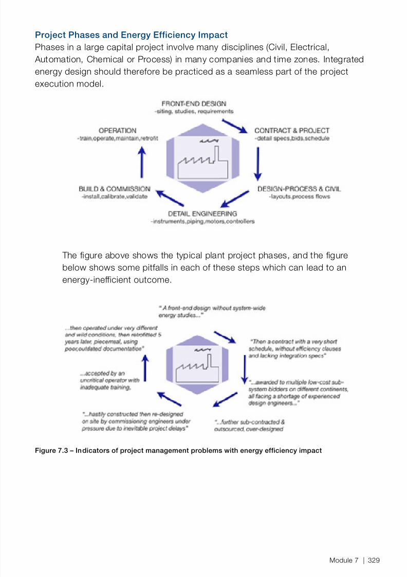
8/12/2019 Energy Efficiency Electronic Book Version 1548_PowerGenerationHandbook v1_1
http://slidepdf.com/reader/full/energy-efficiency-electronic-book-version-1548powergenerationhandbook-v11 331/361
Project Phases and Energy Efficiency ImpactPhases in a large capital project involve many disciplines (Civil, Electrical,
Automation, Chemical or Process) in many companies and time zones. Integratedenergy design should therefore be practiced as a seamless part of the projectexecution model.
The figure above shows the typical plant project phases, and the figurebelow shows some pitfalls in each of these steps which can lead to anenergy-inefficient outcome.
Figure 7.3 – Indicators of project management problems with energy efficiency impact
Module 7 | 329

8/12/2019 Energy Efficiency Electronic Book Version 1548_PowerGenerationHandbook v1_1
http://slidepdf.com/reader/full/energy-efficiency-electronic-book-version-1548powergenerationhandbook-v11 332/361
Integrated Approach to Energy Project ManagementFor project, bid and plant managers, the following project guidelines were inspired inpart by successful RMI design charrette methods. A design ‘charette’ is a technicalreview process which originated in the field of architecture. Some important pointsfor project managers to consider:
− Use lifecycle costing to fearlessly retire or retrofit energy-hogging assets, evenbefore they have been fully depreciated. Use a fair rate of return for energyperformance and re-consider the standard assumptions in your costing model.
− Budget time and money for front-end energy design studies. Recruit bestin-house designers, or get outside help, to study energy balances, sittingopportunities, renewable energy designs.
− Replace low-bid contract with multiple and specific energy performanceguarantees. Low-bid projects cut energy corners, use conservative designs.Stipulate energy performance, and agree on measurement.
− Use an agile project execution model which allows iteration on the originalrequirements. Avoid the ‘big freeze’ on the design before all important data is in.Use input to continuously iterate on the assumed requirements. Insist on earlysubmission of vendor information.
− Involve energy end-users as much as possible, in all project phases. Involve plantsite operators or others to represent the energy end-users. Show the PFDs andP&IDs to operators as early as possible.
− Appoint an energy steward to enforce energy standards in your project or plant,a senior person who will be as respected (and accountable) as safety experts aretoday.
− Appoint an interface manager to map & manage interfaces & ensure whole-design consistency. The interface manager ensures that disciplines, suppliers andoperations are communicating & using a common energy philosophy and designmodel of the evolving plant.
− Seek a single contractor and not multiple vendors where feasible. Give project,
and responsibility, to a firm with broad, multi-disciplinary experience; do notfracture design through ‘divide and conquer’ contracting. − Be energy critical during plant retrofit work acceptance. Don’t rush: ensure all
units work together under all loads – this is typically the last chance to holdsuppliers to their word.
Benefits of Integrated Project Management The up-front attention to real end-use demand will actually reduce the total numberof engineering hours, especially during the later project phases of when interfaces(i.e.: different sub-systems) must come together and be tested.
330 | ABB Energy Efficiency Handbook

8/12/2019 Energy Efficiency Electronic Book Version 1548_PowerGenerationHandbook v1_1
http://slidepdf.com/reader/full/energy-efficiency-electronic-book-version-1548powergenerationhandbook-v11 333/361
Figure 7.4 – Project hours reduction with a systems approach Honours,E.C. (2004) cited in (NaturalEdge Project, 2007)
Advantage of the Main Contractor Role The Main Automation and Main Electrical Contractor (MAC/MEC) project roles helpto tie together the design and implementation of diverse plant units to make plantoptimization interfacing easier. One function of these roles is to ensure that therequired signals and interfaces are present to allow integration and optimizationbetween sub-units and across the entire plant. Do not underestimate the importanceof clear and comprehensive documention, and rigorous communication and reviewof these signals and interfaces as part of project execution.
Module 7 | 331

8/12/2019 Energy Efficiency Electronic Book Version 1548_PowerGenerationHandbook v1_1
http://slidepdf.com/reader/full/energy-efficiency-electronic-book-version-1548powergenerationhandbook-v11 334/361

8/12/2019 Energy Efficiency Electronic Book Version 1548_PowerGenerationHandbook v1_1
http://slidepdf.com/reader/full/energy-efficiency-electronic-book-version-1548powergenerationhandbook-v11 335/361
Module 8High Performance Energy Design
Module Summary This module presents energy-efficiency designs and technical innovations whichmay be above the investment and risk thresholds of a modest retrofit project. Theconstraints of legacy equipment in retrofit projects also limit the potential to design-in large energy efficiency gains. A new plant or unit project, however, provides achance for the designer to use best-in-class equipment and methods across allsystems. In new projects, the energy targets can be ambitious and should aim forthe maximum allowed by the process thermodynamics.
The information in this module section is specific to power generation industriesor process plants with on-site power generation. Many sections, however, are alsobroadly applicable to all industrial steam generation processes.
Tunneling thru the Cost BarrierSolutions that apply Integrative Design principles on greenfield or large re-
development projects can achieve lower total-system capital costs in addition tolower total-system energy consumption compared to non-integrated designs. Anenergy effective design that has lower initial cost is much more likely to be approved.No net or marginal loss of service or quality is suffered in such a solution.
Auxiliaries in Best-Available-Technology PlantsSupercritical and Ultra-Supercritical Boilers
Supercritical boilers operate at pressures above the top point of the water-vapordome. These designs eliminate the drum, and water is in continuous phase changewithin the wall tubing. The higher operating steam parameters give this design higherefficiency than sub-critical boilers, and state of the art units have reached 47% ofLHV, some examples are Nordjyllandsværket in Denmark, and Haramachi No 2 andMisumi No.1 in Japan.
Although metallurgical advances are the main driver in SC or USC designs,modern, efficient auxiliaries are also key enablers. Control systems are one of thekey enablers of super-critical boilers that dominate new plant designs. By exactlymatching flow through the boiler tubing to the demands of the system, the controlsystem has eliminated the need for a water drum and allowed higher steam
Module 8 | 333

8/12/2019 Energy Efficiency Electronic Book Version 1548_PowerGenerationHandbook v1_1
http://slidepdf.com/reader/full/energy-efficiency-electronic-book-version-1548powergenerationhandbook-v11 336/361
parameters, lower system inertia, and much greater efficiency. Greater familiaritywith the capabilities of control system technology will help engineers to pushthe envelope even further to ultra-supercritical designs, achieving synergies withdevelopments in metallurgy.
The higher pressures of supercritical designs increase the auxiliary drive powerrequired by the boiler feedwater pumps. This extra power is worth the gain inthermodynamic efficiency - for otherwise similar configurations, the move fromhigh subcritical to low supercritical steam conditions is said to confer an efficiencyadvantage of approximately two percentage points (Weirich and Pietzonka, 1995).
Circulating Fluidized Bed (CFB) FurnacesIn CFB combustion designs, the fuel is spread over a deep wide area (the bed)and hot air is forced through the bed to supply combustion and to lift and separatethe individual fuel particles so that they behave like a fluid, In the context of CO2reduction, CFB can accommodate a wider variety of fuels, including biomass. CFBfurnaces can co-fire with up to 20% biomass (Ferrer, Green Strategies for Aging CoalPlants, 2008).
Auxiliary drivepower enters the picture through the fuel preparation required forhandling and feeding a variety of fuels, and also in higher-volume ash-removalsystems. This is balanced against the reduction in power required for fine
pulverization of the fuel, which is unnecessary in CFB boilers.
Waste to Energy A facility with CFB combustion may be equipped with recycling capacity for Refuse-Derived Fuel (RDF) and therefore qualify for more environmentally sustainable energyproduction. On-site processing of the RDF will require significant amounts of auxiliarypower, however.
Combined Cycle Gas TurbinesCCGT plants adds a Brayton gas turbine cycle ahead of the Rankine water-steamcycle to achieve even higher efficiencies. The exhaust from the gas turbine is asource of heat for the heat recovery steam generator (HRSG). Some PC steamplants may lend themselves to conversion to CCGT by installing gas fired gasturbines at site and use gas turbine exhaust heat to heat boiler feedwater. In suchcases both the coal fired boiler and the gas turbine are used at the same time. Thisconversion design is especially useful on coal fired boilers that were de-rated due toexcessive NOx or furnace slagging (Eng-Tips Power Generating Forum, Dave Fitz,2006).
334 | ABB Energy Efficiency Handbook

8/12/2019 Energy Efficiency Electronic Book Version 1548_PowerGenerationHandbook v1_1
http://slidepdf.com/reader/full/energy-efficiency-electronic-book-version-1548powergenerationhandbook-v11 337/361
Auxiliary electric drivepower is necessary for gas turbine startup and fuel pumpingrequirements, but auxiliary control can play an even larger role in energy efficientoperation of CCGT plants through optimal operation and allocation of the multiplesources and sinks for heat and power generation and consumption.
Integrated Gasification - Combined Cycle IGCC The IGCC process burns coal, but it begins with a low-oxygen gasification unit toproduce synthetic gas, which is then combusted in the gas turbine of a CCGT unit.IGCC plants have lower emissions of pollutants and higher efficiencies than PCsteam plants. IGCC is key to realizing the industry’s vision of ‘clean coal’, but somechallenges remain before plants can be scaled up to match the largest coal plantstoday. The capital cost of an IGCC plant is estimated to be 10-16% higher than a PCplant of similar capacity (Pew Center on Global Climate Change 2005). Recent pricevolatility in natural gas are delaying the anticipated trend toward IGCC plant types,as discussed in Trends in Steam Plant Designs and Efficiency . In one recentproject in Netherlands (ABB/Nuon), the gasifier converts coal and biomass intosyngas, which is used to fuel the combined-cycle units.
Significant new auxiliary drivepower is needed for coal slurry pumps and air/oxygencompressors, as well as an extra pumping of economized boiler feedwater to thesyngas cooler.
Gas-Gas Reheat for Flue Gas Desulfurization (FGD)Flue gas reheat after flue gas desulphurization (FGD) systems can scavangeadditional heat from the thermodynamic cycle if they use steam heating, ascommonly applied in the USA, but newer FGD systems have feed/effluent gas/gasheat-exchangers that avoid losses from this source (IEA Coal Online - 2 2007). Seethe section on Automation – Emissions Controls for details. This type FGD design,however, requires additional auxiliary speed control and automation.
Powering and Re-Powering with BiomassBiomass combustion is mainly carbon-neutral and should therefore be exempt fromany potential CO2 charges. Most power plants fired on PC can co-fire up to 4-5%biomass without significant degradation and without furnace re-design (Ferrer, GreenStrategies for Aging Coal Plants, 2008). The practical upper limit to co-firing withbiomass in existing PC plants may be as high as 20% (Pew Center on Global ClimateChange 2005), but at the expense of decreased efficiency. According to Robinsonand co-authors in their Assessment Potential of CO2 Reductions due to Biomass,2003, co-firing with 10% biomass can achieve carbon mitigation at a cost of $8-$27per metric ton CO2.
Module 8 | 335
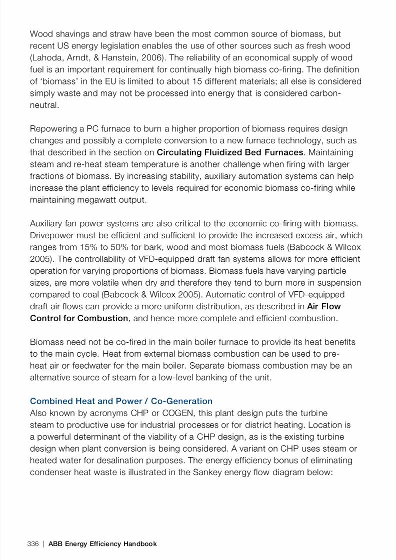
8/12/2019 Energy Efficiency Electronic Book Version 1548_PowerGenerationHandbook v1_1
http://slidepdf.com/reader/full/energy-efficiency-electronic-book-version-1548powergenerationhandbook-v11 338/361
Wood shavings and straw have been the most common source of biomass, butrecent US energy legislation enables the use of other sources such as fresh wood(Lahoda, Arndt, & Hanstein, 2006). The reliability of an economical supply of woodfuel is an important requirement for continually high biomass co-firing. The definitionof ‘biomass’ in the EU is limited to about 15 different materials; all else is consideredsimply waste and may not be processed into energy that is considered carbon-neutral.
Repowering a PC furnace to burn a higher proportion of biomass requires designchanges and possibly a complete conversion to a new furnace technology, such asthat described in the section on Circulating Fluidized Bed Furnaces . Maintainingsteam and re-heat steam temperature is another challenge when firing with largerfractions of biomass. By increasing stability, auxiliary automation systems can helpincrease the plant efficiency to levels required for economic biomass co-firing whilemaintaining megawatt output.
Auxiliary fan power systems are also critical to the economic co-firing with biomass.Drivepower must be efficient and sufficient to provide the increased excess air, whichranges from 15% to 50% for bark, wood and most biomass fuels (Babcock & Wilcox2005). The controllability of VFD-equipped draft fan systems allows for more efficientoperation for varying proportions of biomass. Biomass fuels have varying particlesizes, are more volatile when dry and therefore they tend to burn more in suspension
compared to coal (Babcock & Wilcox 2005). Automatic control of VFD-equippeddraft air flows can provide a more uniform distribution, as described in Air FlowControl for Combustion , and hence more complete and efficient combustion.
Biomass need not be co-fired in the main boiler furnace to provide its heat benefitsto the main cycle. Heat from external biomass combustion can be used to pre-heat air or feedwater for the main boiler. Separate biomass combustion may be analternative source of steam for a low-level banking of the unit.
Combined Heat and Power / Co-Generation Also known by acronyms CHP or COGEN, this plant design puts the turbinesteam to productive use for industrial processes or for district heating. Location isa powerful determinant of the viability of a CHP design, as is the existing turbinedesign when plant conversion is being considered. A variant on CHP uses steam orheated water for desalination purposes. The energy efficiency bonus of eliminatingcondenser heat waste is illustrated in the Sankey energy flow diagram below:
336 | ABB Energy Efficiency Handbook

8/12/2019 Energy Efficiency Electronic Book Version 1548_PowerGenerationHandbook v1_1
http://slidepdf.com/reader/full/energy-efficiency-electronic-book-version-1548powergenerationhandbook-v11 339/361
Figure 8.1 – Sankey energy flow diagram for CHP vs. conventional steam plant, Ref : ABB
The energy balance shows that the thermal efficiency of CHP plants is high (85%+)and approaches (and is ultimately limited by) the efficiency of the boiler itself. Afull accounting of all benefits of CHP to industrial users and society in general isavailable in ‘Small is Profitable’ (Lovins,A, 2006).
There is significant potential for CHP: as of 2008 only 9% of all electrical power
generation comes from co-generation plants (2008, US DoE).
Energy Storage SystemsPower plant units can operate continuously at their optimal efficiency design loadsif there is an economical way to store the produced energy for transmission at laterperiods of high demand. Another advantage of energy storage is that it displacesspinning reserve or ‘banked’ plants.
Pumped StorageLocations fortunate enough to have nearby volumes at higher elevations may usethese for energy storage. Drivepower from periods of low demand is used to pumpwater to the lake at higher elevation, from which hydro power can be generatedduring (peak) periods of higher demand.
Battery StorageBattery storage and inverter technology for energy storage (see case below) is aviable replacement for fossil fueled spinning reserve.
CondensingPower Plant
CHP
BoilerPlant
CHPFuel
PowerStation Fuel
(106)
165 100
Boiler Fuel(59)
Losses
Electricity
Heat Heat
Electricity
Losses
71
Losses
9
35
50
15
Module 8 | 337

8/12/2019 Energy Efficiency Electronic Book Version 1548_PowerGenerationHandbook v1_1
http://slidepdf.com/reader/full/energy-efficiency-electronic-book-version-1548powergenerationhandbook-v11 340/361
Case ExampleBattery Energy Storage SystemGolden Valley Electric Association in Fairbanks, Alaska contracted with ABB toconstruct a Battery Energy Storage System (BESS). The BESS will automatically pickup 26 megawatts of load for 15 minutes, or 40 MW for 7 minutes. The switch frompower line to battery and back to power line is seamless and goes unnoticed by thecustomers, so the prime function of the BESS is to provide spinning reserve in caseof power plant or transmission line equipment failure.
The two primary subsystems in BESS are the IGCT converter and the Ni-Cdbattery. The battery is the energy storage medium. The IGCT converter is theinterface between the DC battery voltage and the 60 Hz AC GVEA system voltage.
The converter transformers match the converter output to the 138 kV systemvoltage. The BESS can be programmed for the following modes: Spinning Reserve,
Automatic Scheduling, Support for Scheduled Load Increase, Automatic GenerationControl, Var Support, Power System Stabilizer and Charging.
Carbon Capture and Storage There are many technologies proposed for capturing then storing the CO2 releasedduring fossil fuels combustion. Post-combustion ammonia absorption is the nearestto market, and will require significant additional amounts of auxiliary drivepower forcirculation pumping, CO2 liquification, and high pressure pumping into permanent
storage locations, Optimization and automation of the CCS system will also playa key role in making this technology viable. However, current energy consumptionestimates for the new auxiliary systems required for CCS are from 25-35% of grossplant output. This implies that for every standard PC plant of a given size, say500MW net output, that is replace by a CCS plant, up to 40% more coal will have tobe consumed to get the same net electrical output. That is, three new SC units willhave the output of two old subcritical units.
Alternative Design Options These design options in the table below leverage existing technologies andapproaches to improve the energy productivity of traditional fossil-fired steam plants,but feasibility (shown as Risk vs. reward in the table) varies due to business ortechnical constraints in existing plant design.
338 | ABB Energy Efficiency Handbook

8/12/2019 Energy Efficiency Electronic Book Version 1548_PowerGenerationHandbook v1_1
http://slidepdf.com/reader/full/energy-efficiency-electronic-book-version-1548powergenerationhandbook-v11 341/361

8/12/2019 Energy Efficiency Electronic Book Version 1548_PowerGenerationHandbook v1_1
http://slidepdf.com/reader/full/energy-efficiency-electronic-book-version-1548powergenerationhandbook-v11 342/361
Smart Grid and Efficient Generation Technologies The Smart Grid begins with Efficient Generation
− Smart Grid, Smart Utility, and Efficient Generation are terms encompassing plantimprovements, renewable source power generation, load-flow management,automation, and systems integration. The term ‘smart grid’ refers to a wide rangeof technologies and operating procedures that will make today’s power systeminto one that is largely automated, applying greater intelligence to operate,monitor and even heal itself. The smart grid will use the same basic power deliveryinfrastructure in use today, but also will draw on advanced monitoring, control andcommunications technology.
− Widespread adoption of the converter technology used in VFDs will allow trainsand other vehicles to re-generate power during braking and supply it to thenetwork. This same technology also enables battery-powered vehicles anddistributed solar or wind generators to supply the grid..
Importance of Demand Side ManagementNo discussion of energy efficiency is complete without acknowledging the Khazoom-Brookes postulate (similar to the ‘rebound’ effect for end-use power consumption)in which a free market translates efficiency gains into a reduced price per energyservice. This then attracts increased demand for and investment in that energyservice, which leads to a net gain in absolute energy consumption. This postulate
is counterintuitive and its implications can be disturbing to well-meaning engineersdevoted to efficiency improvements. The postulate states that ‘energy efficiencyimprovements that, on the broadest considerations, are economically justified atthe micro-level, lead to higher levels of energy consumption at the macro-level.’
This discussion leads the reader beyond purely technical topics, but it may leadprogressive utility investors to also consider demand-side reduction strategies inconjunction with the plant efficiency measures proposed in this handbook.
Several utilities have committed large sums of capital to invest in demand-sidereduction activities, to the tune of hundreds of millions of dollars per organization. This is being facilitated in many states, led by California, which have decoupledtariffs, such that utilities are not going to lose revenue as a consequence of theirdemand-side reduction activities. This is an alternate means for a utility to avoiddisappearing reserves, while they anticipates a high cost of emitting CO2, or find itdifficult to impossible to locate and license new coal-fired generation facilities.
340 | ABB Energy Efficiency Handbook

8/12/2019 Energy Efficiency Electronic Book Version 1548_PowerGenerationHandbook v1_1
http://slidepdf.com/reader/full/energy-efficiency-electronic-book-version-1548powergenerationhandbook-v11 343/361
Appendix A Technical Symbols
The following tables of common electrotechnical symbols and SI units are from ISO31 and IEC 60027. This ISO standard 31 is being superseded by the harmonizedISO/IEC 80000 standard.
Mathematical Symbols for electrical quantities (general)Symbol Quantity SI unit
Q quantity of electricity, electric charge C
E electric field strength V/m
D electric flux density, electric displacement C/m²
U electric potential difference V
φ electric potential V
ε permittivity, dielectric constant, F/mεo electric field constant, ε o = 0.885419 · 10 -¹¹ F/m F/m
ε r relative permittivity 1
C electric capacitance F
I electric current intensity A
J electric current density A/m²
x, γ, σ specific electric conductivity S/mρ specific electric resistance Ω · m
G electric conductance S
R electric resistance Ω
θ electromotive force A
S apparent power W, (VA)
P active power W
Q reactive power W, (var)
φ phase displacement radϑ load angle radλ power factor, λ = PIS, λ cos φ ¹ ) 1δ los angle rad
d loss factor, d = tan δ ¹ ) 1
Z impedance Ω
Y admittance S
R resistance Ω
G conductance S
X reactance Ω
B susceptance S
R impedance angle, γ = arctan X/R rad
Table A.1 – Technical symbols (ABB Switchgear Manual, 2005)
Appendix A | 341

8/12/2019 Energy Efficiency Electronic Book Version 1548_PowerGenerationHandbook v1_1
http://slidepdf.com/reader/full/energy-efficiency-electronic-book-version-1548powergenerationhandbook-v11 344/361
Mathematical symbols for magnetic quantities (general)Symbol Quantity SI unit
ϕ magnetic flux Wb
B magnetic flux density T
H magnetic field strength A/m
V magnetomotive force A
μ permeability H/m
μ o absolute permeability, μ o = 4 π · 10 -7 · H/m H/m
μ r relative permeability 1
L inductance H
Lmn mutual inductance H
η efficiency 1
s slip 1
ρ number of pole-pairs 1
w, N number of turns 1
n tr (t) transformation ratio 1
m number of phases and conductors 1
k overvoltage factor 1
n ordinal number of a periodic component 1
g fundamental wave content 1
d harmonic content, distortion factor 1
k r resistance factor due to skin effect 1
¹ ) Valid only for sinusoidal voltage and current
Note: For US/English version of these symbols, see IEEE 280 Standard LetterSymbols for Quantities Used in Electrical Science and Electrical Engineering
342 | ABB Energy Efficiency Handbook

8/12/2019 Energy Efficiency Electronic Book Version 1548_PowerGenerationHandbook v1_1
http://slidepdf.com/reader/full/energy-efficiency-electronic-book-version-1548powergenerationhandbook-v11 345/361
Appendix BSteam Plant Cycle & Equipment
Thermodynamic Cycle The following diagrams and text are adapted from (IEA Coal Online - 2, 2007)
The proportion of the heat supplied that is converted into mechanical work isreferred to as the efficiency of the cycle. For the ideal engine, the efficiency is relatedto the initial and final temperatures of the system, as follows: h = (T1–T2)/T1 (1)where h is the efficiency and T1 and T2 are the upper and lower (initial and final)temperatures between which the engine operates, expressed in degrees Kelvin. Thelowest temperature in the steam-turbine cycle depends on the temperature of thecoolant water that cools the steam and condensate leaving the low-pressure outletof the turbine system. The idealized thermodynamic steam-water (Rankine) cycle,with superheating, is illustrated on the figures below. Pressure vs. Volume (right side)and Temperature vs. Entropy (left side)
Figure B.1 – Idealized Rankine cycle P-V and T-S diagrams, (IEA Coal Online - 2, 2007)
Sites with access to cold sea water can reach lower bottom-end temperatures in thecycle, and so achieve higher efficiencies. For an upper temperature of 600°C (typicalof a state-of-the-art supercritical turbine) and lower temperature of 20°C (typical forsea-water cooling at a North European coastal location), the theoretical maximumefficiency given by equation (1) is 66%. In practice, steam-cycle efficiencies aremuch lower, in the low 40s% for sub-critical boiler units.
Appendix B | 343

8/12/2019 Energy Efficiency Electronic Book Version 1548_PowerGenerationHandbook v1_1
http://slidepdf.com/reader/full/energy-efficiency-electronic-book-version-1548powergenerationhandbook-v11 346/361
Steam Cycle Equipment The main steam power plant physical units fall into these categories, with commonterminology:
− Furnace (‘Fire-side’) , incl. coal handling, burners and stack exhaust − Boiler (‘Water-side’) , (‘Steam path’) − Turbine (‘Steam path’) − Condenser (‘Water-path’) − Plant Auxiliary Systems
− Generator and electric power supply network (‘Electrical BoP’)
Figure B.2 – Steam cycle fluid flow and main equipment, ( IEA Coal Online - 2, 2007)
Cycle Operation A drum-type subcritical PC boiler takes the pressurized and preheated boilerfeedwater from around 250–260°C up to the evaporation point, then superheatsit to 540°C or above before sending to the high- pressure turbine. In the steamturbine, the steam is expanded while its energy is converted into mechanical workas it passes over static and moving blades within high-pressure (HP), intermediate-pressure (IP) and low-pressure (LP) turbines, which are usually compounded on toone shaft that drives the generator. .All large steam-turbine cycles incorporate reheat
of the intermediate-pressure steam from the high-pressure turbine exit, and multiplestages of feedwater pre-heating using steam extracted from the turbine to maximizeefficiency. Steam emerging from the LP turbines is condensed, then pumped back tothe boiler after pre-heating, thus completing the cycle
The thermal efficiency of state of-the-art PC plants is 45–47%, LHV (Lower Heating Value) basis, at cold sea-water cooling locations. Such plants use main steamconditions well into the supercritical range, with pressures approaching 30 MPa andtemperatures around 600°C Because of the degree of scope for achieving furtherefficiency improvements through moving to even higher steam conditions, materials-development programs are in progress in different parts of the world to reach them.
344 | ABB Energy Efficiency Handbook
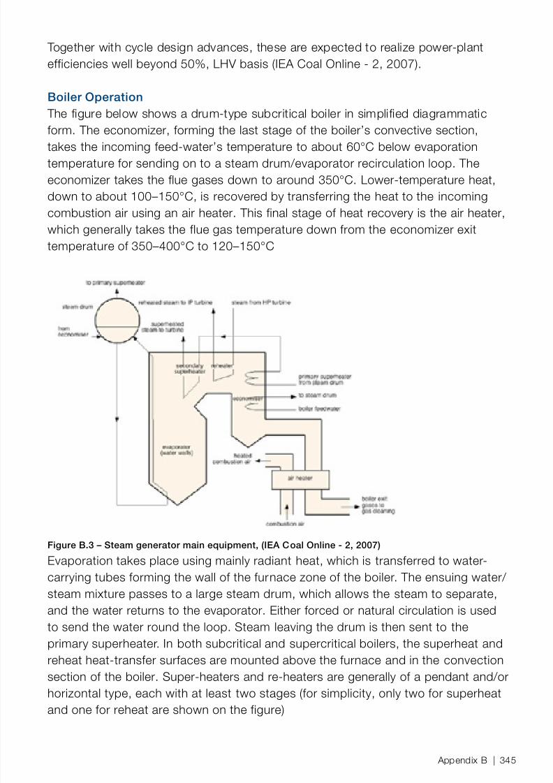
8/12/2019 Energy Efficiency Electronic Book Version 1548_PowerGenerationHandbook v1_1
http://slidepdf.com/reader/full/energy-efficiency-electronic-book-version-1548powergenerationhandbook-v11 347/361
Together with cycle design advances, these are expected to realize power-plantefficiencies well beyond 50%, LHV basis (IEA Coal Online - 2, 2007).
Boiler Operation The figure below shows a drum-type subcritical boiler in simplified diagrammaticform. The economizer, forming the last stage of the boiler’s convective section,takes the incoming feed-water’s temperature to about 60°C below evaporationtemperature for sending on to a steam drum/evaporator recirculation loop. Theeconomizer takes the flue gases down to around 350°C. Lower-temperature heat,down to about 100–150°C, is recovered by transferring the heat to the incomingcombustion air using an air heater. This final stage of heat recovery is the air heater,which generally takes the flue gas temperature down from the economizer exittemperature of 350–400°C to 120–150°C
Figure B.3 – Steam generator main equipment, (IEA Coal Online - 2, 2007)Evaporation takes place using mainly radiant heat, which is transferred to water-carrying tubes forming the wall of the furnace zone of the boiler. The ensuing water/ steam mixture passes to a large steam drum, which allows the steam to separate,and the water returns to the evaporator. Either forced or natural circulation is usedto send the water round the loop. Steam leaving the drum is then sent to theprimary superheater. In both subcritical and supercritical boilers, the superheat andreheat heat-transfer surfaces are mounted above the furnace and in the convectionsection of the boiler. Super-heaters and re-heaters are generally of a pendant and/orhorizontal type, each with at least two stages (for simplicity, only two for superheatand one for reheat are shown on the figure)
Appendix B | 345

8/12/2019 Energy Efficiency Electronic Book Version 1548_PowerGenerationHandbook v1_1
http://slidepdf.com/reader/full/energy-efficiency-electronic-book-version-1548powergenerationhandbook-v11 348/361
346 | ABB Energy Efficiency Handbook

8/12/2019 Energy Efficiency Electronic Book Version 1548_PowerGenerationHandbook v1_1
http://slidepdf.com/reader/full/energy-efficiency-electronic-book-version-1548powergenerationhandbook-v11 349/361
Appendix CIntegrative Design Principles
Integrative Design is founded on ‘Whole System Thinking’ principles. Theseprinciples also appear in the related fields of System Engineering, SustainabilityEngineering, Industrial Ecology, and meta-design. Integrative design principlesare reminders to engineers to look in the places where people, by nature, are notequipped to easily visualize. The four ‘corners’ which may hide design problems andopportunities are:
Hidden Quantity Reason why
Things that add up slowly, over time we tend to focus on the ‘now’, and less on the
far future
Things that multiply along a long path we tend to focus on the ‘here’ and less on the
route
Things at the edges we tend to focus on the center and less on the
periphery
Things in people’s heads we tend to focus on the objective, and less on
the subjective
Think Lifecyle: to see small things accumulating over a long timeChoose quality for reliability, over initial cost
Choose service over product
− Select high-efficiency and high-quality components,− The higher initial costs will be repaid in saved energy within a short period and
in reduced downtime over a long period... − Increased reliability has an direct energy efficiency benefit via reduced unstableor unproductive (ex: startup) operations
− Get fine control of your power input− Seek controllability in pumps, fans, burners so that you provide only the power
that the process needs, and no more than necessary
Think Bottom Up: to see things multiply along a long path in spaceReduce demand first, then size supplyReduce downstream loss first, then upstream
Appendix C | 347

8/12/2019 Energy Efficiency Electronic Book Version 1548_PowerGenerationHandbook v1_1
http://slidepdf.com/reader/full/energy-efficiency-electronic-book-version-1548powergenerationhandbook-v11 350/361
Bottom-up thinking moves in the opposite direction of the process flow of fluid, heator even of information & signals. ‘Start with what you need to have or deliver, thenwork back to supply’.
− Start downstream to design systems with lower capacity requirements − Reduce and rationalize end-use demand first : gather data to estimate the
REAL end-use loading, then work backward to the power source, reducinglosses along the way, Finally, size the supply according to the now-reducedloads
− Keep capacity design margins small − It will be cheaper to add extra capacity when requirements increase. Consider
a parallel standby unit instead of oversizing the main unit.
− Recover and re-use process energy − Use any means, mechanical or chemical, to retrieve what the process doesn’t
want...
Compounding over Time
Efficiencies compound upward along the flow path, and, because energy is anoperating cost, these savings also compound over time.
Compounding over Capital Cost
There is third major compounding effect, and that is the capital equipment cost. A reduction of downstream loads usually means that upstream supply equipmentcan be safely downsized, which also usually means lower installed costs. Take fulladvantage of this effect by doing a bottom-up energy assessment of the candidatedesigns when the plant is still on the drawing board, rather than waiting for a retrofit.
Think Interfaces: to see things at the edgesPut system before componentsPut application before equipment
− Practice good thermal integration − Connect sources with sinks, aspire to know and use all the available energy
(‘exergy’), including ambient energies...
− Harmonize the interfaces in both project and plant − In your project - between the disciplines & between suppliers. In the plant -
between diverse process units & between black-boxes.
348 | ABB Energy Efficiency Handbook

8/12/2019 Energy Efficiency Electronic Book Version 1548_PowerGenerationHandbook v1_1
http://slidepdf.com/reader/full/energy-efficiency-electronic-book-version-1548powergenerationhandbook-v11 351/361
− Instrument and monitor your power usage in real-time − Specify many, smart transmitters, placed so operators can see the process
eat your power across plant units: use data to trend & manage energy KPIs atplant level.
− Make models and use them to control and teach − In your project - to tune your design. In the plant - to enable real-time
advanced control to keep process stable & at constraint.
‘Interface busting’ is made more difficult in a world of highly componentized plantequipment. Component-based engineering comes with hidden costs, namely losingthe ability to optimize the whole system to its real energy constraints. This lostopportunity can be visualized as wasted volume when constructing a sphere of largeblocks vs. smaller ones. Integrated design guidelines insist that vendors providesmaller, less-specialized component units with richer physical & programmaticinterfaces. Avoid big isolated non-integrated feature-bloated and often moreexpensive components or systems, using this rule..
Think People & Process: to see how people think, feel and work togetherPut people before procedures & hardwarePut people in charge
− Put away the standard design - go for a walk − Ask for time to study alternatives, nature, and talk to operators of the last
‘standard design’ plant
− Use an agile project execution model− Involve operators or others to represent the energy end-users, iterate on the
assumed requirements
− Appoint an energy steward − An energy steward should be as respected as safety experts are today.
− Seek a single contractor, not multiple vendors − Give project, and responsibility, to a firm with broad, multi-disciplinary
experience. Do not fracture design through ‘divide and conquer’
Appendix C | 349

8/12/2019 Energy Efficiency Electronic Book Version 1548_PowerGenerationHandbook v1_1
http://slidepdf.com/reader/full/energy-efficiency-electronic-book-version-1548powergenerationhandbook-v11 352/361
350 | ABB Energy Efficiency Handbook

8/12/2019 Energy Efficiency Electronic Book Version 1548_PowerGenerationHandbook v1_1
http://slidepdf.com/reader/full/energy-efficiency-electronic-book-version-1548powergenerationhandbook-v11 353/361
References
− ABB AG, Power Technology Systems. “Unit C of the Scholven Power Plant Automated with System 800xA.” ABB Power Generation Solutions & Products.2006. http://library.abb.com/global/scot/scot221.nsf/veritydisplay/407efc39c6bf8878c125723d0037c852/$File/Unit%20C%20of%20the%20Scholven%20Power%20Plant%20F%20DEABB%201249%20%2006%20E.pdf (accessed Oct2008).
− ABB Drives. “Dimensioning a Drive: Technical Guide #7.” 2002. − ABB Drives. “Direct Torque Control: Technical Guide No.1.” 2002. − ABB Inc. “Effects of AC drives on Motor Insulation: Technical Guide #102.” 1998. − ABB Inc. Plant Automation. Application Guide - Steam Temperature Control. ABB,
2006. − ABB Inc. Plant Automation. Application Guide : Boiler-Turbine Coordinated
Control. ABB, 2006. − ABB Industry Oy. “Direct Torque Control, Technical Guide No. 1.” 1999. http://
www.abb-drives.com/StdDrives/RestrictedPages/Marketing/Documentation/files/ PRoducts/DTCTechGuide1.pdf.
− ABB Ltd,Transformers. ABB Transformer Handbook. 2007. − ABB Ltd., Power Generation Unit. “Power Generation Solutions & Products.”
Solutions for Fossil Fuel Power Plants. ABB. 2006. http://library.abb.com/global/ scot/scot221.nsf/veritydisplay/82660b404a03faa3c12571d300536bf1/$File/
ABB%20Solutions%20for%20FPP_S_DEABB%201297%2006%20E_23.pdf. − ABB Motors & Drives. “ABB Sustainability Guide #1.” ABB. Nov 2007. http://
search.abb.com/library/ABBLibrary.asp?DocumentID=3AFE68902037&LanguageCode=en&DocumentPartID=1&Action=Launch.
− —. “ABB Technical Application Paper: Three-phase asynchronous motors.” ABB.2007. www.abb.com. − ABB Oy. Drives. “100 Top Energy Saving AC Drive Tips.” ABB Drives. ABB. May
2006. − ABB Oy. Drives. Energy Efficiency Presentation, ABB Drives. Jan 9, 2008. − —. “Guide to Variable Speed Drives (Guide #4).” ABB. 2002. − —. “Using Variable Speed Drives in Pump Applications: Application Guide No.2.” ABB. 2006.
− ABB Power Products. Switchgear Manual. 2006. − ABB Switzerland, MV Drives. “Guide to Standard Medium Voltage Variable Speed
Drives.” ABB. 2002.
References | 351

8/12/2019 Energy Efficiency Electronic Book Version 1548_PowerGenerationHandbook v1_1
http://slidepdf.com/reader/full/energy-efficiency-electronic-book-version-1548powergenerationhandbook-v11 354/361
− ABB USCRC. “FEASIBILITY OF EBOP-ASD-Q CONTROL CONCEPT IN POWERPLANT.” Power Generation, Power Systems, 2008.
− Babcock & Wilcox. Steam - its generation and use. 41. Edited by J.B. Kitto andS.C.Stultz. 2005.
− Bezesky, David. “NEMA Application Guide for AC Adjustable Speed DriveSystems.” 2001.
− Black & Veatch. Power Plant Engineering. Edited by Larry Drbal. Springer, 1996. − Black&Veatch. Energy Solutions - Efficiency Improvements. Sept 2008. http://
www.bv.com/services/Climate_Change_Solutions/Energy/Efficiency.aspx. − Burns & McDonnell. “Minnkota Power Case Study.” 2007. − Carbon Monitoring for Action. Carbon Monitoring for Action. Sept 2008. http://
carma.org/plant (accessed Oct 2008). − Center for Global Development. Carbon Dioxide Emissions From Power
Plants Rated Worldwide. Nov 2007. http://www.sciencedaily.com/ releases/2007/11/071114163448.htm (accessed Oct 2008).
− Cmar, Greg. “”Pay Now or Pay Forever - The Design of Control SystemSoftware”.” Edited by Dr. Wayne C. Turner. Energy Engineering, Journal of the
AEE (Taylor & Francis) 105, no. 1 (2008): 46-56. − Competitek. COOLING - Competitek Technology Series. Vol. 2. RMI, 1995. − —. DRIVEPOWER - Competitek Technology Series. Vol. 4. RMI, 1996. − Eng-Tips Power Generating Forum. 2006+. http://www.eng-tips.com. − EPRI. “Lignite Coal Drying at Great River Energy.” 2005, 4.
− —. Retrofitting Utility Plant Motors for Adjustabel Speed - Field Test Program.EPRI, 1990.
− Fassbinder, Stefan. “Energy Efficiency and Loss Evaluation of Transformers.” Transformer Workshop at Friendship Palace. Beijing: Deutsches Kupfer-Institut,1997.
− Ferrer, Al. Green Strategies for Aging Coal Plants. July 2008. http://pepei.pennnet.com/display_article/335136/6/ARTCL/none/none/1/Green-Strategies-for-
Aging-Coal-Plants:-Alternatives,-Risks-&-Benefits/.
− —. “Small-Buck Change Yields Big-Bang Gain.” Power Engineering International.July 2007. http://pepei.pennnet.com/display_article/300905/6/ARTCL/none/ none/1/O&M-FEATURE:-Small-Buck-Change-Yields-Big-Bang-Gain/.
− GE Utility Division. Electric Utility Systems & Practices. Fourth. Edited by HomerM. Rustebakke. Wiley, 1983.
− Gielen, Dolf (IEA France). “Reducig Industrial Energy Use and CO2 Emssions.” April 2008. http://www.iea.org/Textbase/techno/etp/index.asp.
− Graus, W.H.J. “International comparison of energy efficiency of fossil powergeneration.” Energy Policy, March 2007: 3936-3951.
− Guffre, John. “Air Heater Losses Squander Big Bucks.” Power Magazine, Feb2007.
352 | ABB Energy Efficiency Handbook

8/12/2019 Energy Efficiency Electronic Book Version 1548_PowerGenerationHandbook v1_1
http://slidepdf.com/reader/full/energy-efficiency-electronic-book-version-1548powergenerationhandbook-v11 355/361
− IEA Coal Online - 1. Coal Combustion Technologies for a Competitive Market.2006. http://www.coalonline.org/site/coalonline/content/viewer?LogDocId=81494&PhyDocId=6092&filename=6092_195.html#.
− IEA Coal Online - 2. Coal Combustion Technology. 2007. http://www.coalonline.org/site/coalonline/content/Viewer/81996/6798/6798_1.html/Coal-combustion-technology#.
− IEEE. “IEEE Std 666-2007.” IEEE Design Guide for Electric Power GeneratingStations. 2007.
− Immonen, Pekka (ABB Inc.). “Assessing Industrial Power Plant Operations &Controls.” 13TH Annual Joint ISA POWID/EPRI Conference . 2003.
− —. “Coordinated Control and Optimization of a Complex Industrial Power Plant.”Power Engineering Magazine. November 2008. http://pepei.pennnet.com/display_article/346408/6/ARTCL/none/none/1/Coordinated-Control-and-Optimization-of-a-Complex-Industrial-Power-Plant/.
− International Energy Agency. “IEA World Energy Outlook 2006.” IEA. 2006. http:// www.worldenergyoutlook.org/2006.asp.
− ISA. Instrument Engineers’ Handbook: Vol2. Process Control and Optimization.Edited by Bela G. Liptak. Taylor & Francis, 2005.
− ISO. “INTERNATIONAL STANDARDS TO DEVELOP AND PROMOTE ENERGYEFFICIENCY AND RENEWABLE ENERGY SOURCES.” June 2007. http://www.iso.org/iso/hot_topics_energy.
− Johnson Controls. 2008. http://www.johnsoncontrols.com/publish/us/en/
sustainability/working_towards_a/the_bottom-line_benefits.html. − Kenney, W.F. Energy Conservation in the Process Industries. Academic Press,
1984. − Lahoda, J,, A. Arndt, and W. (Siemens) Hanstein. “BIOMASS LOOKING FOR
EFFICIENT UTILIZATION –THE REHEAT CONCEPT.” Siemens Power Generation.Siemens. 2006.
− Larsen, Chris. Generation Technologies Guidebook. Nov p.13, 2007. http://www.energycentral.com/centers/energybiz/detail_sourcebook.cfm?id=19.
− Lovins, Amory (Rocky Mountain Institute). Advanced Energy Efficinecy : Concepts& Practice. DVD. Stanford Univeristy, March 2007. − Lovins, Amory. “10xE Presentation to Irving Oil.” Presentation, RMI, 2008. − —. “Energy Strategy: The Road Not Taken.” Foreign Affairs, October 1976. − Lovins, Amory, and Paul Hawken. Natural Capitalism. Rocky Mountain Institute,
2000. − Mansfield, Scott. Engineering Design for Process Facilities. McGraw Hill Inc.,
1993. − Marc Hoffmann / Plant Engineering. June 15, 2008. http://www.plantengineering.
com/article/CA6568917.html?q=energy+efficiency. − Martin, Bob. “Energy Technology Investment Trends.” Rational Energy Network.
October 2004. http://www.rationalenergy.net/pdf/energy_trends.pdf.
References | 353

8/12/2019 Energy Efficiency Electronic Book Version 1548_PowerGenerationHandbook v1_1
http://slidepdf.com/reader/full/energy-efficiency-electronic-book-version-1548powergenerationhandbook-v11 356/361
− Masters, Gilbert M. Renewable & Efficient Electric Power Systems. 2004. − Natural Edge Project. “Natural Edge Project.” Natural Edge Project. Australian
Ministry of Environment. July 2007. http://www.naturaledgeproject.net/Whole_System_Design.aspx.
− Ordis, A.W. Modelling & Simuation of Power Generation Plants. Springer-Verlag,1994.
− Pew Center on Global Climate Change. US Electric Power Sector & GlobalClimate Change. 2005.
− Phillips, Jim. Power Factor and Harmonics for Utilities. Course text, T2G Technical Training Group, 2009.
− Rajan, G.G. Optimizing Energy Efficiencies in Industry. McGraw Hill, 2003. − Russsel, C. “Strategic Industrial Energy Efficiency.” Edited by Dr. Wayne C. Turner.
Energy Engineering (AEE) 102, no. 3 (2005). − Sayer, J.H. Energy-efficient air pollution controls for fossil-fueled plants: Technology assessment. New York State Energy Research and Development Authority, Albany, NY (United States), US DoE, 1995.
− Steve Ruddell, ABB Automation Ltd. UK. “Special Report: Motors and Drives.” ABB Review, 2005.
− Swanekamp, R. “Backfitting power plant control systems.” Power 139, no. 9(September 1995).
− Takahashi, P. Simple Solutions for Plaet Earth. Authorhouse, 2007. − Taylor, Dr Peter. “Energy Technologies for a Low Carbon Future.” IEA. IEA
Energy Policy Division Acting Head. July 2008. http://www.iea.org/textbase/ speech/2008/Taylor_ETP2008_CHP-DHC_Symposium.pdf.
− US DoE Best Practices. Oct 2008. http://www1.eere.energy.gov/industry/ bestpractices/tip_sheets_steam.html.
− US DoE. Energy Efficiency Assessment Study on Sensors & Automation. Nov2004. http://www1.eere.energy.gov/industry/sensors_automation/pdfs/doe_report.pdf.
− US DoE Sourcebook. “Improving Fan System Performance.” EERE Industrial
Technologies Program. 2006. http://www1.eere.energy.gov/industry/ bestpractices/pdfs/fan_sourcebook.pdf. − —. “Improving Pump System Performance.” EERE Industrial Technologies
Program. 2006. http://www1.eere.energy.gov/industry/bestpractices/pdfs/pump.pdf.
− US DoE. “Variable Speed Pumping : Guide to Successful Applications.” 2008. − Vesel, R. of ABB Inc. “Drive Technology Enables Combustion Optimization.”
Power Engineering, January 2007. − Whitworth, Seth (XCEL Energy). “DCS Integration for Intelligent Sootblowing.”
Energy Central Network. May 2006. http://topics.energycentral.com/centers/ gentech/library/detail_wp.cfm?wpid=102819.
354 | ABB Energy Efficiency Handbook

8/12/2019 Energy Efficiency Electronic Book Version 1548_PowerGenerationHandbook v1_1
http://slidepdf.com/reader/full/energy-efficiency-electronic-book-version-1548powergenerationhandbook-v11 357/361
− Wikipedia. Fossil Fuel Power Plants. Sept 30, 2008. http://en.wikipedia.org/wiki/ Fossil_fuel_power_plant (accessed Oct 2, 2008).
− —. Khazzoom-Brookes Postulate. Sept 25, 2008. http://en.wikipedia.org/wiki/ Khazzoom-Brookes_postulate.
− Woodruff, Everett B. Steam Plant Operation. Eighth. McGraw Hill, 2005. − World Energy Council. “Performance of Generating Plant.” World Energy Council
Publications. 2007. http://www.worldenergy.org/publications/1071.asp.
On-Line ResourcesSupplier Corporate Sites:
− ABB Inc., http://www.abb.com/energyefficiency − ABB Power Generation Solutions & Products has brochures, case studies
− Alstom Power, http://www.power.alstom.com/home/ − Info on power plant integration
− Siemens Power Generation, http://www.powergeneration.siemens.com − Pages & tech papers on steam power plants
− Honeywell ACS, Power Solutions, http://hpsweb.honeywell.com/Cultures/en-US/IndustrySolutions/Power
− Schneider Electric, http://www.criticalpowernow.com/ − White papers, efficiency calculators , but focus on low voltage
Engineering Services Corporate Sites:
− Foster-Wheeler Global Power Group , http://www.fwc.com/GlobalPowerGroup/ − Many good technical papers on CFB, biomass co-firing, materials
− Black & Veatch Energy , http://www.bv.com/markets/energy/ − Article on coal plant retrofits − www.bv.com/services/Climate_Change_Solutions/En ...
− GE Power, http://www.gepower.com/home/index.htm − Has design guides and handbooks, section on Clean Coal (IGCC)
− Bechtel Power, http://www.bechtel.com/power.html
− Has several project cases − Burns & Roe Power and Energy , http://www.roe.com/power_index.htm − Not much online
− KBR (Kellogg,Brown & Root) ,http://www.kbr.com/publications/coal.aspx − Articles on coal gasification
− Intergraph Process,Power & Marine , http://www.intergraph.com/ppm − 2D, 3D design software packages
− AspenTech , http://www.aspentech.com/ − Modeling and simulation software tools
− CH2M Hill,http://www.ch2m.com/corporate/services/sustainable_solutions − EPC with good energy efficiency credentials
References | 355

8/12/2019 Energy Efficiency Electronic Book Version 1548_PowerGenerationHandbook v1_1
http://slidepdf.com/reader/full/energy-efficiency-electronic-book-version-1548powergenerationhandbook-v11 358/361
− Arup, http://www.arup.com/ − EPC with good energy efficiency credentials, mostly built environment
− Rumsey Engineers, http://www.rumseyengineers.com/ − Specialist in energy efficiency engineering, mostly HVAC
− Southern Company, http://www.southerncompany.com/planetpower − One example of a utility with a progressive energy efficiency profile
Journals, Articles & News Sites: − Energy Central , http://www.energycentral.com/
− Have a large tech white paper library − Power Engineering International, http://pepei.pennnet.com/
− Good articles on steam plant efficiency, retrofits − Plant Engineering LIVE,http://www.plantengineering.com/
− Many white papers, links on ‘energy efficiency’ − Plant Systems, http://www.plantservices.com/
− Excellent VFD articles, sustainability links − Connecting Industry, http://www.connectingindustry.com/
− Section on energy management − International Journal of Energy Research
− http://www3.interscience.wiley.com/journal/3343/home
Academic Sites:
− The Natural Edge Project, http://www.naturaledgeproject.net − Course in whole system design, with pumping system case
− Engineering News Record, Power & Industrial, http://enr.construction.com/ infrastructure/power_industrial/default.asp
− Industry news − Energy Storm, http://www.energystorm.us/
− Citations, abstracts only − University of Pittsburgh, Mascaro Sustainability Initiative, http://www.
mascarocenter.pitt.edu/ − Mostly built environment, but some power infrastructure as well − Massachusetts Institute of Technology, Eng’g Systems Div. http://esd.mit.edu/ − NTNU Norway , http://www.ntnu.no/ − MIT’s Center for Engineering Systems Fundamentals , http://cesf.mit.edu/
− For schools : start when they are young!
356 | ABB Energy Efficiency Handbook

8/12/2019 Energy Efficiency Electronic Book Version 1548_PowerGenerationHandbook v1_1
http://slidepdf.com/reader/full/energy-efficiency-electronic-book-version-1548powergenerationhandbook-v11 359/361
Professional & Association Sites: − Motor Decisions Matter http://www.motorsmatter.org/
− Public awareness, Motor Planning Kit − Pump Systems Matter, http://www.pumpsystemsmatter.org/
− Great papers,tools,links − Air Movement and Control Association (AMCA) International, http://www.amca.
org/ − Non-profit supplier assoc.; has Best Practices for fan systems(US DoE
Sourcebook, 2006)(US DoE Sourcebook, 2006)
Industry and Expert Sites: − Electric Power Research Institute , http://my.epri.com
− Non-profit R&D and consulting organization, utility & industry funded − Eng-Tips Forums, http://www.eng-tips.com/
− Peek inside the daily work of practicing engineers − A great powergen engineering forum
− CR4 Engineering forum, http://cr4.globalspec.com/ − Large forums with hi quality posts
− Leonardo Energy, http://www.leonardo-energy.org − Global community of sustainable energy professionals − Have a slide library for energy educators, design guides on power quality…
− National Assoc. of Energy Service Companies, http://www.naesco.org/
− Demand side programs, but some relevant recommendations − The Design Futures Council, http://www.di.net/articles/archive/the_design_
futures_council/ − Mainly architectural design, but some good, general material
− Pew Center on Global Climate Change, http://www.pewclimate.org/ − Non-profit, non-partisan think tank
Authorities : US & International Sites:
− International Energy Agency (IAE) ,www.iae.org − Global data on coal applications − IEA Clean Coal Centre, http://www.iea-coal.org.uk
− Unbiased info on coal tech − IEA Coal Online,www.coalonline.org
− ISO, http://www.iso.org/iso/hot_topics_energy − Int’l standards organization, with emerging energy mgmt. standards
− World Energy Council , http://www.worldenergy.org/ − Pubs on power plant efficiency, energy policies…(World Energy Council, 2007)
− Consortium for Energy Efficiency (CEE) , http://www.cee1.org/
References | 357

8/12/2019 Energy Efficiency Electronic Book Version 1548_PowerGenerationHandbook v1_1
http://slidepdf.com/reader/full/energy-efficiency-electronic-book-version-1548powergenerationhandbook-v11 360/361
− US Dept. Of Energy, Energy Eff.& Renewable Energy, http://www1.eere.energy.gov/industry/
− Industrial Technologies Program − ISA Instruments and Automation society, http://isa.org/
− Standards and industry organization − IEEE Power & Energy Society, http://ieee.org/portal/site/pes
− Good links, active forums − IEEE Industry Applications Society, http://ewh.ieee.org/soc/ias/cms/ − National Academy of Engineering http://www.nae.edu
− Educating the Engineer of 2020: Adapting Engineering Education to the NewCentury
− American Assoc. of Eng’g Education (ASEE), http://www.asee.org/ − Accreditations, Prism magazine, Journal of Eng’g Education
− American Society of Heating, Refrigerating and Air-Conditioning Engineers(ASHRAE),http://www.ashrae.org/
− American Society of Mechanical Engineers, http://www.asme.org/ − EU Intelligent Energy programme : http://www.energypath.eu/
− For schools , high-schools
Revision History Ver Date Author Change Description
2.4 23.03.2009 RPM Torque vs speed info and calculations3.0 26.03.2009 RPM Added Arash Baebee comments to VFD section
3.1 12.04.2009 RWV Final Edit before layout
358 | ABB Energy Efficiency Handbook

8/12/2019 Energy Efficiency Electronic Book Version 1548_PowerGenerationHandbook v1_1
http://slidepdf.com/reader/full/energy-efficiency-electronic-book-version-1548powergenerationhandbook-v11 361/361


![Operator’s Manual - Hobbico, Inc.manuals.hobbico.com/dle/dleg0020-manual-v1_1.pdf · DLE-20 Operator’s Manual Specifications 20cc [1.2 cu. in.] 25. HP / 9,000rpm 1,700 rpm Electronic](https://static.fdocuments.net/doc/165x107/5b149de47f8b9a437c8de699/operators-manual-hobbico-inc-dle-20-operators-manual-specifications.jpg)


