Umeå Papers in Economic History No. 35 2008

Energy efficiency and Energy Demand: A Historical CGE Investigation on the Rebound Effect in the Swedish Economy 1957

Peter Vikström1

1 The Paper was written in 2004. Financial support from The Bank of Sweden Tercentenary Foundation and the Swedish Energy Agency (STEM) is gratefully acknowledged. Vikström is Director of Growth Analysis and Statistics at the Swedish Institute for Growth Policy Studies.

Umeå Papers in Economic History No. 35 2008

ISSN: 1653-7378

Abstract

The improvement in energy efficiency is one major strategy for fulfilling the goal concern-ing reduction in the emissions of greenhouse gases. However, the efficiency improvements at the micro or plant level are seldom fully realised on the macro level, which means that the use of energy and, subsequently, the reduction of greenhouse gases are not reduced in the same proportion on the aggregate level. The effect where energy efficiency improve-ments on the micro level are not realised to the full extent on the aggregate level is denoted the rebound effect in the literature and can under certain conditions be of significant mag-nitude.

The aim of this paper is to examine the rebound effect in historical perspective as a mecha-nism that can explain the appearance of the Swedish Environmental Kuznets Curve (EKC). From the basis of a simple EKC model incorporating technological change and preference change, it is argued that the rebound effect is an integrated part of the time path between chosen consumption bundles of good and bad outputs. It is also argued that the rebound effect and its impact on the EKC performance can be analysed using a CGE approach. This is exemplified in the paper by the implementation of a CGE model for the Swedish economy in 1957.

JEL classification: Q43.

Keywords: rebound effect, environmental Kuznets curve, computable general equilibrium, Sweden

1. Background

In the current debate concerning the global environmental problems, such as the green-house effects, energy use is of primary interest. As there is no real alternative to lowering the emissions of greenhouse gases such as CO2 besides using less energy, most of the taken environmental policy measures are aimed at using energy in a more efficient way. In the Kyoto-protocol, tradable permits and project based mechanisms such as the JI (joint Im-

3

plementation) and CDM (Clean Development Mechanism) are aimed at improving the efficiency in the use of energy.

However, the improvement of energy efficiency on the machinery or plant level is not re-sulting in the same reductions in energy intensities on the level of the aggregate economy. Increased energy efficiency on the plant level will make energy measured as effective en-ergy services relatively cheaper and therefore also creates increased demand for energy, given that the energy prices per physical quantity are kept at the same level. For instance, a machine that previously used a ton of oil for conducting a specific amount of work now only would need half a ton is the same as if the energy price measured as the price per en-ergy service unit would be halved. This would increase the demand for the now relatively cheaper oil input and there would be tendencies towards substitution with other inputs and production factors in the production process. Furthermore, this would also lead to that goods with high energy intensity would become relatively cheaper, which in turn would increase the demand for these goods from consumers. This would even further counteract the reductions in energy use made possible through the increase of energy efficiency on the plant level.

This effect, where the initial increase in energy efficiency is counteracted by various de-mand effects is known as the rebound effect or the Khazzoom-Brookes postulate (Saun-ders, 1992). Basically, the rebound effect makes the realised energy reductions on the macro levels to be less than what would be suggested by the increased energy efficiency on the micro level. The exact amount and the character of the rebound effect is dependent on the workings of the economy at hand and cannot be judged entirely a-priori. For instance, elasticities of substitution between energy and other production factors and demand elastic-ities for different types of goods are crucial in the determination of the rebound effect.

Even if the rebound effect can be seen as negative from the environmental perspective, since it counteracts and diminishes the effect of technical measures taken on the micro level, it is also positive since it translates technological improvements in energy efficiency into growth. This means that policy measures, such as taxes, taken with the aim of balanc-ing the rebound effect must be carefully designed in order not to destroy the preconditions for growth induced by increases in energy efficiency,

The general relation between technical change, energy use and economic growth has also been a central research area. One of the central issues is the research concerning the exis-tence of and explanations behind the so called Environmental Kuznets Curve or EKC. The EKC is a supposedly inverted U-shaped relationship between income level and environ-mental damages, such as harmful emissions. The EKC predicts that the environmental damages are low and then increases with growth and rising income levels. At a certain in-come level, environmental damages starts to decline as growth continues.

In the EKC-related research there is no consensus regarding the existence of the general EKC-relationships. For some countries and some pollutants, the EKC can be identified, while the general relationship is not supported by other observations. What may be more important, there is a lack of a consistent theoretical explanation for the EKC. Explanations covers the whole range of economic factors such as changes in output structure, foreign

4

trade effects and changing preferences and demand for environmental quality. However it is important to separate the fact that it is possible to trace a relationship between growth and different indicators of environmental quality on the one hand and on the other hand that there should exist a specific relationship in the form of an orthodox EKC. In this way it is possible to analyse the relation between growth, environment and technology using a broader perspective instead of only trying to find support for or against a specific relation-ship. Even if the EKC research to a large extent has been focused on contemporary cross section studies, research has also been directed towards historical EKC for single countries (Unruh and Moomaw, 1997, Lindmark, 2002).

The aim of this paper is to present a framework were the rebound effect can be used as part of the explanation of EKC-relationships in historical perspective. The aim is also to con-duct a preliminary historical study of the rebound effect in the Swedish long-term eco-nomic development. The empirical application in this paper should be seen as a pilot study and a test of the framework and not as an exhaustive study of the long-term EKC and its relation to the rebound effect.

The paper is organised as follows. In section 2 the rebound effect is described. Next, in section 3, a brief overview of theories of the EKC is presented, together with a plausible model for examining EKC relationships. In section 4 the rebound effect and the EKC model are integrated to a common framework. In section 5 and 6, the analytical use of the framework is illustrated using the evidence from a CGE model for Sweden in 1957. Fi-nally, section 7 concludes.

2. The rebound effect

Energy efficiency measures the amount of energy that is required to produce desired goods and services. In other words, energy efficiency is a parameter that depends on the state of technology and production methods. It is also related to the amount of energy used per unit of GDP, which is the same as the energy intensity of an economy. However, energy inten-sity also depends on other things than technical energy efficiency, such as consumer pref-erences and on other parameters such as climate and geography.

Improvements in energy efficiencies are often incorrectly connected with direct links to decreases in energy intensities at the aggregate level. An increase in energy efficiency can and normally does lower the energy intensity, but the relationship is not linear. The higher the level of aggregation, the more complex the relationship becomes. At the level of a sin-gle machine and a single unit of output, energy efficiency and energy intensity are identical concepts. On higher levels of aggregation, the rebound effect is additional to other autonomous influences of preferences, geography etc that drive in a wedge between changes in technical energy efficiency and energy intensities at a higher level of aggrega-tion. The rebound effect thus concerns changes induced by efficiency changes themselves, which reduce the impact of these technical improvements on energy intensity.

Various energy intensities, as well as the level of technological energy efficiency, are de-termined by preferences, the state of technology and the price of energy relative to other

5

production factors. According to standard theory, the relative prices between energy capital and labour will determine in competitive markets which technology that is selected. Higher energy prices will imply energy-saving technologies with higher shares of capital and la-bour. The actual response to changes in relative prices is dependent on the substitutability of energy with other production factors. Relative price changes can also induce technologi-cal development and not only substitution among existing technologies, thereby creating production possibilities that did not exist before. This means that changes in relative prices not only influence static combinations between factors but that these changes will also lead to research efforts for new technologies that in turn can lead to energy efficiency im-provements.

The increase in energy efficiency leads to an increased marginal productivity of energy. Furthermore, an increase in the efficiency of energy means that a greater number of energy services flow from each physical unit of energy. If the price per physical unit remains con-stant, this is the same as a prise decrease per energy service unit. It is now profitable to buy more energy services until the marginal productivity corresponds to the new lower price per energy service unit. Beside the size of the efficiency increase, this process is affected by how easy it is to integrate additional energy in the production process or by the elastic-ity of substitution.

In the process of adding energy services to the production process, the marginal productiv-ity of the other factors, capital and labour will be increased since each unit of capital and labour is now working with more efficiency units of energy than before. Even if the physi-cal amount of fuel may not have increased, more energy services is now used per unit of output than before. The process will continue until marginal productivities correspond again to factor prices. This is because the relative price of energy in terms of energy ser-vices has decreased. The result is that less of each factor is now needed to produce one unit of output, which is equivalent to an increase in GDP or the same as economic growth.

This process can be visualized using standard microeconomic isoquants, as shown in figure 1 (see for instance Layard and Walters, 1978).

6

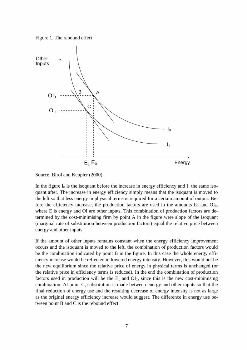
Figure 1. The rebound effect

I0

I1

Energy

OtherInputs

E1 E0

OI1

OI0AB

C

Source: Birol and Keppler (2000).

In the figure I0 is the isoquant before the increase in energy efficiency and I1 the same iso-quant after. The increase in energy efficiency simply means that the isoquant is moved to the left so that less energy in physical terms is required for a certain amount of output. Be-fore the efficiency increase, the production factors are used in the amounts E0 and OI0, where E is energy and OI are other inputs. This combination of production factors are de-termined by the cost-minimising firm by point A in the figure were slope of the isoquant (marginal rate of substitution between production factors) equal the relative price between energy and other inputs.

If the amount of other inputs remains constant when the energy efficiency improvement occurs and the isoquant is moved to the left, the combination of production factors would be the combination indicated by point B in the figure. In this case the whole energy effi-ciency increase would be reflected in lowered energy intensity. However, this would not be the new equilibrium since the relative price of energy in physical terms is unchanged (or the relative price in efficiency terms is reduced). In the end the combination of production factors used in production will be the E1 and OI1, since this is the new cost-minimising combination. At point C, substitution is made between energy and other inputs so that the final reduction of energy use and the resulting decrease of energy intensity is not as large as the original energy efficiency increase would suggest. The difference in energy use be-tween point B and C is the rebound effect.

7

The rebound effect is the increase in the use of energy services and eventually in energy due to the de facto lower price of energy measured in energy services or efficiency units. Furthermore, the size of the rebound effect depends on the elasticity of substitution be-tween energy and other factors, as well as on the elasticity of demand for the now cheaper final good. The higher the elasticity of substitution and the higher the elasticity of demand, the more the share of energy will increase after the energy efficiency improvement. An energy efficiency improvement will lead to an expansion of sectors with energy-intensive goods due to having lower relative costs. However, due to limited substitution possibilities both in production and demand, the overall energy intensity normally decreases after an energy efficiency increase. This means that rebound effect does not take away all of the potential profits from the efficiency improvements and expressed as a fraction of the po-tential gains in energy intensity, the rebound effect is between zero and one.

The size of the rebound effect cannot be determined on conceptual grounds alone. As long as there are possibilities for substitution, all that can be said is that the decrease in energy intensities will be less than the original increase in technical efficiency. Empirical esti-mates of the rebound effect usually ranges from zero to 0.5, which means that between 0 and 50% of the original efficiency increase is “taken back”.

From the aim of using energy efficiency improvements as a mean to achieve environ-mental policy goals such as the Kyoto protocol, the rebound effect can be seen as a nui-sance. The existence of the rebound effect makes it difficult in a growing economy to lower absolute energy consumption at unchanged prices per unit of energy. To achieve this would require rates of efficiency increases that accommodate both GDP growth and the rebound effect.

The rebound effect, however, cannot be seen as entirely negative. The existence of factor and product substitution indicates that the technical improvement has created new and bet-ter options to increase efficiency and consumer satisfaction. It is the rebound effect that transforms technical efficiency improvements into economic growth. This means that there is a trade-off between the contribution of an efficiency improvement to decreasing energy intensity and its contribution to economic growth.

In summary the total rebound effect is composed of three separate parts:

1. The price increase in energy services will lead to an increased use of energy in terms of energy services. This effect is dependent on the elasticity of substitution.

2. Due to the fall in real prices of energy services, products that use energy will be-come relatively cheaper. The more energy intensive, the cheaper it will be. This leads to readjustments between sectors, with energy intensive sectors gaining at the expense of less energy intensive ones. This effect depends on the elasticity of sub-stitution between products at the level of consumers and of the magnitude of the price changes.

3. There is also an additional effect due to the fact that the economic growth created by an energy efficiency improvement will in itself increase energy consumption by

8

some second-order fraction. This effect is relatively small due to the fact that en-ergy costs generally constitute less than 10 percent of GDP. In other words, if the rebound effect contributed to 1 percent to economic growth, only 0.1 percent of ad-ditional energy would be used.

The rebound effect increases with the level of aggregation and it should be expected that the rebound effect at the level of a single firm is less than at the sector or at the total econ-omy. This means that decreases in energy intensities at the national level is harder to achieve than decreases at the firm level.

In the discussion so far, the rebound effect has been discussed in the context that the rela-tive price of energy per physical unit is unchanged. A way of reducing the rebound effect would be to change the relative price of energy, for instance with an energy tax. In this way the various substitution effects that constitute the rebound effect would be counter-acted. For instance, in figure 1 the production factor combination could be kept at point B with a suitable change in relative prices, thereby balancing the rebound effect.

However, even if these price changes would diminish the rebound effect, it would also have negative effects on growth as it undermines the substitution possibilities that are im-portant for the growth process. From the policy perspective, this implies that various policy measures such as taxes must be used with care, so that as much of the efficiency improve-ments are translated into decreases in overall energy intensity and at the same time main-tain long-term economic growth.

3. The EKC

The hypothesis of the environmental Kuznets (EKC) curve predicts the existence of an inverted U-shape relationship between different environmental indicators and income per capita. One consequence of the hypothesis is that economic growth will eventually remedy the environmental impacts of the early stage of economic development and that growth will lead to further environmental improvements in the developed countries (Stern, 1998, p173). This means that growth is not a threat to the environment, but instead necessary in order to maintain and improve environmental quality (Meadows et al., 1992).

Those who argue in favour for the EKC hypothesis mean that at very low levels of activity environmental impacts are low, but as development proceeds resource use and waste gen-eration increase. At higher levels of development, structural change towards less resource-using industries and increased environmental awareness result in a gradual decline in envi-ronmental impacts. This positive view on the EKC theme was further promoted by the World Development Report in 1992 (IBRD, 1992).

The positive view on the relationship between growth and the environment have ques-tioned by a number of critics (Arrow et al, 1995 and Stern et al, 1996). The main argu-ments against the EKC are that much of the empirical evidence is weak and statistical techniques inappropriate, that the static relationship between rich and poor countries does

9

not necessarily tell us about the dynamics as countries experience growth, and that EKC relationships have been found for only a subset of environmental indicators.

Much of the literature on EKC is empirical, consisting mostly of cross-sectional studies. Maybe the first empirical EKC-study was the paper by Grossman and Krueger (1991), where they estimated EKC for SO2, dark matter and suspended particles, using a panel dataset from a number of locations in cities around the world. Each regression involves a cubic function of GDP per capita, together with various site related variables, a time trend and a trade intensity variable. Underlying the 1992 World Development Report was a study by Shafik and Bandyopadhyay (1992). They estimated EKC for ten different indica-tors, among others were ambient sulphur oxides, deforestation and carbon emissions. The EKC:s were estimated in the most general case using a logarithmic cubic polynomial in PPP GDP per capita. Other empirical studies on the EKC have followed, yielding different pictures of the EKC.

A useful theoretical starting point for analysing the EKC is the approach suggested by Kriström (1998) and Brännlund and Kriström (1998). In this approach, the technological production possibility frontier is matched against the utility maximising households in or-der to deduce the chosen mix between good and bad outputs (emissions etc) in the con-sumption bundle. The approach is depicted in figure 2

Figure 2. A model for the EKC

Goods

Bads(Energy use)

Q0

Q1

U0

U1

B1 B0

G0

G1

U1A

G1A

B1A

Source: Brännlund and Kriström (1998).

10

In figure 2, Q0 and Q1 are the production possibilities frontier (PPF) at time point 0 and 1, respectively. The PPF demonstrates the state of the production technology, or how the rela-tion is between good and bad outputs, at each time period. Technological change is re-flected in an outward shift of the PPF, as shown in figure 2. An outward shift indicates that more goods can be produced per unit of bad output.

The PPF is only half of the story, as it must be determined where on the PPF the mix be-tween goods and bads will be. This is determined by household preferences at each time period. The households have a set of indifference curves that determine the trade off be-tween good and bad outputs in the households’ preferences. The tangency point between the indifference curve and the PPF at each point in time will determine the actual combina-tion of good and bad outputs.

In figure 2, the tangency point yields the combination (G0,B0) for good and bad outputs. In time period 1, when technology and preferences change, a new tangency point or combina-tion of good and bad outputs is obtained. This new combination can result in more or less bad outputs produced in relation to the state in time point 0. In figure 2, the combination (G1,B1) indicates a situation where technological change and preferences have increased the production of good outputs as well as a reduction in bad outputs, B1<B0. However, the combination (G1A,B1A) reflects a situation where preferences are such that the bad outputs are expanded in relation to the case at time point 0 in order to achieve a further expansion of good outputs, G1A>G1.

It is these shifts in the PPF and preferences that make it possible to trace and analyse a spe-cific EKC. The model depicted in figure 2 allows both for an orthodox, inverted U-shaped EKC, as well as other time paths for the relation between income and emissions, or be-tween the production of goods and bads. For instance, the orthodox EKC predicts that ini-tially at low incomes the path is towards increasing bads, depicted as the shift from combi-nation (G0,B0) to combination (G1A,B1A) in figure 2. This indicates preferences more likely to prevail at low incomes where increases of good outputs are valued more than decreases in bad outputs. At higher incomes, the shift is instead from combination (G0,B0) and (G1,B1), which reflects a preference change towards valuing reductions in bad outputs rela-tively more than increases in good outputs. However, it must be emphasised that the ortho-dox EKC is only one of many possible time paths analysable using the model in figure 2. This makes the model a good starting point when analysing the relationship between growth and environmental impact without making a-priori adherements to specific func-tional forms.

4. The rebound and EKC – Parts of the same phenomenon?

Even if the rebound effect and the EKC can be treated as two separate issues, it is valuable from the analytical standpoint to see them as interrelated phenomena. This is most easily seen if technical change is examined. In the rebound case, technological change is mani-fested through energy efficiency increases, which is the same as that more goods can be produced with the same amount of energy inputs.

11

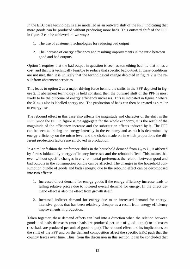
In the EKC case technology is also modelled as an outward shift of the PPF, indicating that more goods can be produced without producing more bads. This outward shift of the PPF in figure 2 can be achieved in two ways:

1. The use of abatement technologies for reducing bad output

2. The increase of energy efficiency and resulting improvements in the ratio between good and bad outputs

Option 1 requires that the bad output in question is seen as something bad, i.e that it has a cost, and that it is technically feasible to reduce that specific bad output. If these conditions are not met, then it is unlikely that the technological change depicted in figure 2 is the re-sult from abatement activities.

This leads to option 2 as a major driving force behind the shifts in the PPF depicted in fig-ure 2. If abatement technology is held constant, then the outward shift of the PPF is most likely to be the outcome of energy efficiency increases. This is indicated in figure 2 where the X-axis also is labelled energy use. The production of bads can then be treated as similar to energy use.

The rebound effect in this case also affects the magnitude and character of the shift in the PPF. Since the PPF in figure is the aggregate for the whole economy, it is the result of the magnitude of the efficiency increase and the substitution effects induced by it. The PPF can be seen as tracing the energy intensity in the economy and as such is determined by energy efficiency on the micro level and the choice made on in which proportions the dif-ferent production factors are employed in production.

In a similar fashion the preference shifts in the household demand from U0 to U1 is affected by forces initiated by energy efficiency increases and the rebound effect. This means that even without specific changes in environmental preferences the relation between good and bad outputs in the consumption bundle can be affected. The changes in the household con-sumption bundle of goods and bads (energy) due to the rebound effect can be decomposed into two effects:

1. Increased direct demand for energy goods if the energy efficiency increase leads to falling relative prices due to lowered overall demand for energy. In the direct de-mand effect is also the effect from growth itself.

2. Increased indirect demand for energy due to an increased demand for energy-intensive goods that has been relatively cheaper as a result from energy efficiency improvements in production.

Taken together, these demand effects can lead into a direction when the relation between goods and bads decreases (more bads are produced per unit of good output) or increases (less bads are produced per unit of good output). The rebound effect and its implications on the shift of the PPF and on the demand composition affect the specific EKC path that the country traces over time. Thus, from the discussion in this section it can be concluded that

12

the energy efficiency changes and the rebound effect can be integrated into the analysis of the EKC.

Furthermore, the change in the households demand for energy (bads) is dependent on two distinct factors. The first is the result of rational adaptation and welfare maximizing that is part of the rebound effect. The other factor is what from this perspective can be treated as an exogenous change in preferences This change is for instance the result of increased knowledge about the damages to environment, which leads to that households are demand-ing less bad outputs for a given amount of good output. Another factor in the exogenous preference shift is changes due to different income elasticities for good and bad outputs. As income increases, the demand for environmental quality is likely to increase relative to the demand for material goods. All in all, these preference changes are likely to lead to a cho-sen equilibrium point in the consumption of goods and bads that is different to the one pre-dicted by technical change and the rebound effect alone.

The change in the consumption bundle of good and bads between two points in time can be seen as the sum of different forces and these forces can be examined empirically using a CGE approach. However, before this can be done, the simple EKC model in figure 2 must be elaborated further, as shown in figure 3.

Figure 3. Decomposing the EKC

Goods

Bads(Energy use)

Q0

Q1

U0

U1S

B0C B0

G0

U1

G1

B1

ABC

D

G0C

E

B0B

Q1S

In figure 3, the shift of the PPF between Q0 and Q1 is assumed to be primarily the result of an increase in energy efficiency. If output of goods is held constant, this efficiency change would result in a reduction of bads from B0 to B0B. The rebound effect, however, will yield an increased demand for energy and subsequently a growth effect, resulting in a movement

13

from B to C. In point C output of goods has increased from G0 to G0, while there is still a reduction in bads (from B0 to B1). This point would also be the new equilibrium point in an economy without accumulation of production and changes in preferences.

One vital factor that is not explicitly treated in the EKC-model is the accumulation of pro-duction factors (labour and capital) and how this affects the path of the chosen combina-tions of goods and bads chosen. If factor accumulation is introduced into the sequence of events outlined in figure 3, this would result in a movement along the new PPF (Q1) until all factors are employed in production and allocated according to their marginal product, and assuming efficiency in production. During this process, when more labour and capital is utilised, the use of energy also increases, which in the end results in a new equilibrium at point D in the figure. At this equilibrium point, the output of goods has increased further, as well as the output of bads. The output of bads have increased compared to the original point since B1>B0. Thus the process so far shows the well-known positive relationship be-tween growth and energy use.

The next thing to consider also not explicitly treated in the basic EKC model outlined in section 3, is the effect of structural changes. In figure 2, the output of goods and bads is the aggregated output, which means that the relationship between good and bad output is de-pendent on the composition of the aggregated good output. If this composition or structure changes then the aggregate relationship between good and bad output will also be affected. In terms of the aggregated EKC-model, changes in structure will be revealed as another shift outwards of the PPF. If we assume that the aggregate level of output is held constant, this shift indicated as the shift from Q1 to Q1S will yield a new equilibrium point at E. At the equilibrium point the structure has changed towards less polluting or energy using goods, which indicates a preference shift towards less environmentally damaging produc-tion. The movement from D to E also captures exogenous changes in technology resulting in changed amounts of energy and the composition of energy commodities used that is not captured by estimated changes in energy efficiency. Pure efficiency changes in terms of heat content used per unit of output does not capture qualitative differences indicating that some technologies are only viable through the use of a specific energy commodity. For instance coal is no alternative to electricity when it comes to powering small engines or computers.

In summary, the EKC pattern for an economy can with the use of the process depicted in figure 3 can be decomposed into three parts:

1. A change in energy efficiency, which generates a rebound effect but generally moves in the direction of less bads and more goods.

2. A factor accumulation effect generating a movement along the PPF toward a direc-tion of more goods and more bads.

3. A structural change effect generated by changing preferences and other exogenous changes in technology not reflected in simple efficiency measures. These can work in all directions regarding the change of good and bad outputs, but in the case were the preference change are the results of increased knowledge about environmental

14

damages, it will work in the direction towards less bads and the same (or slightly reduced) level of goods.

Depending on the size of these three effects and how the importance of each effect changes over time, an EKC pattern for the economy can be traced over time. For instance, if the factor accumulation effect is large and the effects from structural change and efficiency improvement are small, a positive relationship between good and bad output can be seen. Likewise if the efficiency effect and structural change effect (due to changed preferences) are larger than the factor accumulation effect, then the relationship between goods and bads can be negative. It is important to remember, though, that the character of the rela-tionship cannot be judged a-priori, since it is an empirical question.

The three effects and the relative size of them at a specified point in time can empirically be investigated using a CGE-approach, where the starting point is a model calibrated to a benchmark time point (time point 0 in figure 3). It is possible to decompose the changes in goods and bads into the three effects outlined above through the use of counterfactual simulations based on historical changes of energy efficiency and factor accumulation. The only difficulty is how to observe the structural change effect using the fairly highly aggre-gation structure used in CGE-models. This problem can be solved if the structural change effect is treated as a residual effect between the observed change and the change estimated when the efficiency and factor accumulation effect is accounted for. Using the notation in figure 3, this means that the movement from A to C and from C to D can be simulated and the distance between D and E can be calculated as a residual between the aggregated actual historical change and the effects estimated in the simulations. In other words, the residual estimated this way can be treated as an estimate of the preference effect in the basic EKC-model. In the next two sections, an historical evaluation of these effects will be conducted, through the use of a static CGE model for the Swedish economy in 1957.

5. Evaluating the rebound effect: The Model

In this section the design of a static CGE model for the Swedish economy in 1957 is de-scribed. The description includes the general structure of the model and the data used for calibrating the model.

General model structure

The model used in this investigation is basically a multisectoral model for a small open economy. The use of this kind of model is not new to environmental analysis and examples of its use in the literature are for example Hill (2001), Harrison and Kriström (1998), and Böhringer and Rutherford (1997).

However, even if the basic model structure used in this article is similar to other models certain design features need to be decided upon if the model will be relevant to the investi-gation in this article. This concerns primarily the structure of production, the structure of demand and how substitution of production factors and changes in energy efficiency are handled in the model.

15

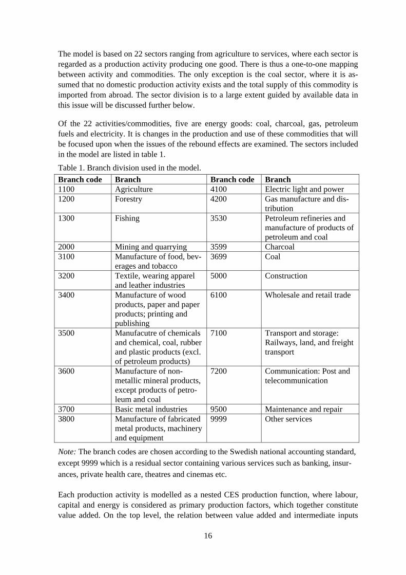
The model is based on 22 sectors ranging from agriculture to services, where each sector is regarded as a production activity producing one good. There is thus a one-to-one mapping between activity and commodities. The only exception is the coal sector, where it is as-sumed that no domestic production activity exists and the total supply of this commodity is imported from abroad. The sector division is to a large extent guided by available data in this issue will be discussed further below.

Of the 22 activities/commodities, five are energy goods: coal, charcoal, gas, petroleum fuels and electricity. It is changes in the production and use of these commodities that will be focused upon when the issues of the rebound effects are examined. The sectors included in the model are listed in table 1.

Table 1. Branch division used in the model. Branch code Branch Branch code Branch 1100 Agriculture 4100 Electric light and power 1200 Forestry 4200 Gas manufacture and dis-

tribution 1300 Fishing 3530 Petroleum refineries and

manufacture of products of petroleum and coal

2000 Mining and quarrying 3599 Charcoal 3100 Manufacture of food, bev-

erages and tobacco 3699

Coal

3200 Textile, wearing apparel and leather industries

5000 Construction

3400 Manufacture of wood products, paper and paper products; printing and publishing

6100 Wholesale and retail trade

3500 Manufacutre of chemicals and chemical, coal, rubber and plastic products (excl. of petroleum products)

7100 Transport and storage: Railways, land, and freight transport

3600 Manufacture of non-metallic mineral products, except products of petro-leum and coal

7200 Communication: Post and telecommunication

3700 Basic metal industries 9500 Maintenance and repair 3800 Manufacture of fabricated

metal products, machinery and equipment

9999 Other services

Note: The branch codes are chosen according to the Swedish national accounting standard, except 9999 which is a residual sector containing various services such as banking, insur-ances, private health care, theatres and cinemas etc.

Each production activity is modelled as a nested CES production function, where labour, capital and energy is considered as primary production factors, which together constitute value added. On the top level, the relation between value added and intermediate inputs

16

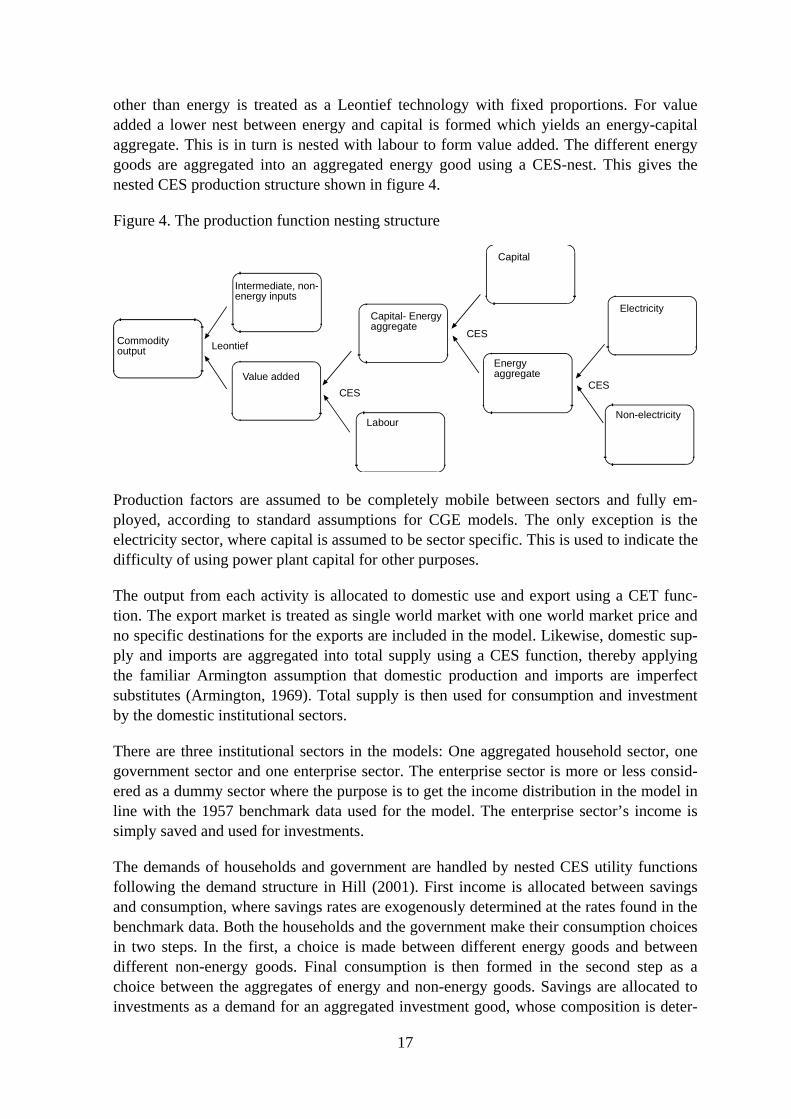
other than energy is treated as a Leontief technology with fixed proportions. For value added a lower nest between energy and capital is formed which yields an energy-capital aggregate. This is in turn is nested with labour to form value added. The different energy goods are aggregated into an aggregated energy good using a CES-nest. This gives the nested CES production structure shown in figure 4.

Figure 4. The production function nesting structure

Commodityoutput

Intermediate, non-energy inputs

Value added

Capital- Energyaggregate

Labour

CES

Capital

Energyaggregate

CES

Electricity

Non-electricity

CES

Leontief

Production factors are assumed to be completely mobile between sectors and fully em-ployed, according to standard assumptions for CGE models. The only exception is the electricity sector, where capital is assumed to be sector specific. This is used to indicate the difficulty of using power plant capital for other purposes.

The output from each activity is allocated to domestic use and export using a CET func-tion. The export market is treated as single world market with one world market price and no specific destinations for the exports are included in the model. Likewise, domestic sup-ply and imports are aggregated into total supply using a CES function, thereby applying the familiar Armington assumption that domestic production and imports are imperfect substitutes (Armington, 1969). Total supply is then used for consumption and investment by the domestic institutional sectors.

There are three institutional sectors in the models: One aggregated household sector, one government sector and one enterprise sector. The enterprise sector is more or less consid-ered as a dummy sector where the purpose is to get the income distribution in the model in line with the 1957 benchmark data used for the model. The enterprise sector’s income is simply saved and used for investments.

The demands of households and government are handled by nested CES utility functions following the demand structure in Hill (2001). First income is allocated between savings and consumption, where savings rates are exogenously determined at the rates found in the benchmark data. Both the households and the government make their consumption choices in two steps. In the first, a choice is made between different energy goods and between different non-energy goods. Final consumption is then formed in the second step as a choice between the aggregates of energy and non-energy goods. Savings are allocated to investments as a demand for an aggregated investment good, whose composition is deter-

17

mined by the benchmark data. Transfers and income taxes, as well as government demand are assumed to be exogenously determined and kept at the benchmark level.

Substitution possibilities

A key issue in model handling energy related issues is how to treat energy as a production factor. Specifically, how and to what extent is it possible to substitute between energy and other primary production factors such as labour and capital. The assumptions made on this issue guides the design of the production structure and what substitution elasticities to use in the model. As these assumptions affect the outcome from the model simulations, it is important to discuss suitable approaches to the issue of factor substitution.

The substitution problem has two aspects. First there is the substitution between different energy goods and, second, the substation between aggregate energy and other production factors. This problem has also a temporal dimension, as the substation possibilities are dif-ferent in the short and long term.

In the literature, the substitution between capital and energy is a major issue, and especially if capital and energy can be considered as substitutes or complements. As Vinals (1984) points out, the substitutability or complementarity issue is crucial in order to determine the direction of the adjustment of aggregate output following energy price changes. This means that this problem is important for this study as well since energy efficiency in-creases means that energy becomes cheaper in relation to its contribution to output.

In the literature there is no consensus regarding whether energy and capital are substitutes or if they are complements. For instance, Berndt and Wood (1979) found in their seminal study that energy and capital were complements, while others (Griffin and Gregory, 1976, Harris et al, 1993) have found that energy and capital are substitutes. Furthermore, Berndt and Wood tried to reconcile this issue by creating a framework were energy and capital are substitutes, if energy and capital is separated from the other inputs. This means that energy and capital form a nest of its own. Furthermore, this approach means that energy and capi-tal can be substitutes if the level of the energy-capital aggregate is held constant, but if the level of this aggregate is allowed to vary, then energy and capital are complements.

Thus it is important to consider the nesting structure of the production function when dis-cussing the substitution possibilities between capital and energy are complements. Even if there is an inner substitution elasticity between energy and capital in forming the energy-capital aggregate is greater than zero, indicating substation possibilities, the “outer” substi-tution elasticity on the output level may still be negative. Provided the value of the substi-tution elasticity between energy and capital is lower than the substitution elasticity between labour and the energy-capital aggregate, the outer elasticity can be negative (Bourge and Goulder, 1984).

Another substitution issue is the substitution between different kinds of energy goods. If the energy goods are treated according to their potential heat content, the substitution pos-sibilities can be considered as quite high. However, if a qualitative dimension is added the substitution possibilities between different energy goods becomes less clear, especially

18

when substitution between electricity and non-electricity energy goods is considered. It is simply not possible to fuel the TV set or the computer with any other energy good than electricity. For this investigation this means that it is important to distinguish between elec-tricity and non-electricity goods.

As reliable and clear-cut estimates of the substitution elasticities are hard to get, the normal procedure in CGE-modelling is to gather the available estimates from different sources and guesstimate the elasticities that cannot be found elsewhere. However, this approach would be unsatisfying when designing a historical CGE-model since the substitution possibilities is one aspect where the historical economy is likely to differ from the contemporary. Therefore, historical estimates for the manufacturing industry and its sub branches are made and used in the model. These estimates are based on translog cost functions and de-tails can be found in Vikström (2004b).

Data

The static model utilised in this article is calibrated using a benchmark social accounting matrix (SAM) for Sweden in 1957. This SAM is constructed from the results from the first official input-output study for the Swedish economy that were conducted in the 1960s (Höglund and Wering, 1964). This input-output study is very detailed in its general struc-ture, as it is based on 127 different commodities. However, the imports were not disaggre-gated at the same level and this is the reason behind the aggregation level used in this model. The data on the input-output structure is complemented with data from the Swedish national accounts on income distribution, transfers and savings for the institutional sectors. As often is the case when data from different sources are utilised, the resulting SAM is not perfectly balanced, i. e. row sums does not equal columns sums. Therefore, the cross-entropy approach to SAM balancing has been applied as suggested in Robinson, Cattaneo and Moataz, (2001), as it is more efficient and reliable than the common RAS approach to balancing a SAM. All details about the construction and balancing of the SAM can be found in Vikström (2004a).

In addition to the SAM, other data is needed in order to calibrate the model. Substitution elasticities for the CES production functions for the manufacturing industry branches (2000-3800, 9500) are collected as mentioned in the previous section from estimates of historical substitution elasticities in Vikström (2004b). Transformation elasticities for ex-port functions and the import substitution elasticities, as well as substitution elasticities for branches outside the manufacturing industry are based on contemporary estimates and col-lected from Hill (2001). The elasticities used in the model are summarized in table 2.

19

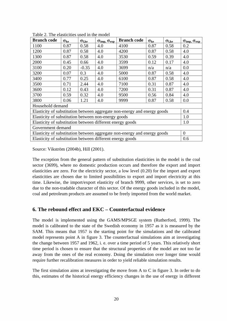
Table 2. The elasticities used in the model Branch code σke σl,ke σimp, σexp Branch code σke σl,ke σimp, σexp1100 0.87 0.58 4.0 4100 0.87 0.58 0.2 1200 0.87 0.58 4.0 4200 0.87 0.58 4.0 1300 0.87 0.58 4.0 3530 0.59 0.39 4.0 2000 0.45 0.66 4.0 3599 0.12 0.17 4.0 3100 0.20 -0.35 4.0 3699 n/a n/a 0.0 3200 0.07 0.3 4.0 5000 0.87 0.58 4.0 3400 0.77 0.25 4.0 6100 0.87 0.58 4.0 3500 0.71 2.44 4.0 7100 0.31 0.87 4.0 3600 0.12 0.43 4.0 7200 0.31 0.87 4.0 3700 0.59 0.32 4.0 9500 0.56 0.84 4.0 3800 0.06 1.21 4.0 9999 0.87 0.58 0.0 Household demand Elasticity of substitution between aggregate non-energy and energy goods 0.4 Elasticity of substitution between non-energy goods 1.0 Elasticity of substitution between different energy goods 1.0 Government demand Elasticity of substitution between aggregate non-energy and energy goods 0 Elasticity of substitution between different energy goods 0.6

Source: Vikström (2004b), Hill (2001).

The exception from the general pattern of substitution elasticities in the model is the coal sector (3699), where no domestic production occurs and therefore the export and import elasticities are zero. For the electricity sector, a low level (0.20) for the import and export elasticities are chosen due to limited possibilities to export and import electricity at this time. Likewise, the import/export elasticity of branch 9999, other services, is set to zero due to the non-tradable character of this sector. Of the energy goods included in the model, coal and petroleum products are assumed to be freely imported from the world market.

6. The rebound effect and EKC – Counterfactual evidence

The model is implemented using the GAMS/MPSGE system (Rutherford, 1999). The model is calibrated to the state of the Swedish economy in 1957 as it is measured by the SAM. This means that 1957 is the starting point for the simulations and the calibrated model represents point A in figure 3. The counterfactual simulations aim at investigating the change between 1957 and 1962, i. e. over a time period of 5 years. This relatively short time period is chosen to ensure that the structural properties of the model are not too far away from the ones of the real economy. Doing the simulation over longer time would require further recalibration measures in order to yield reliable simulation results.

The first simulation aims at investigating the move from A to C in figure 3. In order to do this, estimates of the historical energy efficiency changes in the use of energy in different

20

sectors must be known. Estimates for these are derived mainly from the Swedish industrial statistics.1 On average, the efficiency improvement is 15% between 1957 and 1962 and this is used for all sectors and energy commodities, excluding the energy producing sec-tors. For energy producing sectors, an efficiency improvement of 12% is assumed based on the evidence put forward by Kander (2002, p55) for the efficiency improvements in ther-mal power plants. Even if these estimates of efficiency improvement are not exact, they indicate the magnitude of the efficiency improvement. Another drawback with this crude measure is that the efficiency has been assumed to be equal for all energy commodities, which in reality probably is not the case. Obtaining exact efficiency improvement meas-ures separately for all energy commodities, however, would require a detailed study of its own.

Tracing the movement form A to C through changing the energy efficiency and holding other parameters and production factors in the model constant aims at capturing the re-bound effect existing in the Swedish economy during the 1950s. After running the simula-tion, the results reveal that GDP (good output) increases by 0,5% and energy use as input in production is reduced, on average, with 6%. The original efficiency increase of 15% percent is due to the rebound effect only reduced with 6% overall, indicating that the re-bound effect is around 0.6 which is fairly high when compared to contemporary estimates ranging 0 to 0.5 (Greening et al, 2000). The magnitude of the rebound effect indicates that only a minor part of the efficiency improvements were reproduced on the aggregate level. Total energy use is only reduced by 3% due to increased energy consumption by house-holds.

The next step in the simulation is to trace the movement from C to D, which requires that factor growth and ordinary TFP growth is added to the energy efficiency improvements. From the Swedish national accounts it can be deduced that the labour input grew 3% be-tween 1957 and 1962, while capital growth can be estimated to 20% during the same pe-riod. TFP growth in the industrial sector can be estimated to average 15% and for the other sectors in the economy, in the lack of precise estimated, TFP growth has been assumed to be 10% (Lindmark and Vikström, 2003). If TFP growth and factor growth is added to the model, the result is GDP growth of 21.3% and an increase of total energy use of 15.3% compared to 1957. Thus, the efficiency effect (the move from A to C) is counteracted by the factor accumulation effect (movement from C to D), resulting in an increase in energy use, as well as an increase in GDP.

Finally, it is time to asses whether the change between 1957 and 1962 also includes a structure effect due to changed preferences, as indicated as the movement from D to E in figure 3. As mentioned previously, it difficult to asses this effect directly in the model due to the fairly high aggregation level used. Many important structural changes are only pos-sibly to detect on a finer level of aggregation. However, it is possible to asses the existence of this effect if the simulation results are compared to the actual historical changes of GDP and energy use. These results are presented in table 3.

1 Energy efficiency is here defined as Value added in fixed prices per unit (MJ) of energy input. The

change in this efficiency measure is then used as raw proxy of energy efficiency improvement.

21

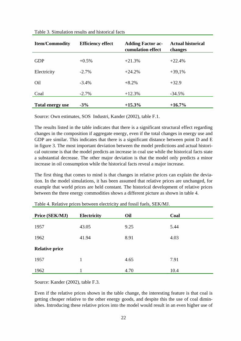
Table 3. Simulation results and historical facts

Item/Commodity Efficiency effect Adding Factor ac-cumulation effect

Actual historical changes

GDP +0.5% +21.3% +22.4%

Electricity -2.7% +24.2% +39,1%

Oil -3.4% +8.2% +32.9

Coal -2.7% +12.3% -34.5%

Total energy use -3% +15.3% +16.7%

Source: Own estimates, SOS Industri, Kander (2002), table F.1.

The results listed in the table indicates that there is a significant structural effect regarding changes in the composition if aggregate energy, even if the total changes in energy use and GDP are similar. This indicates that there is a significant distance between point D and E in figure 3. The most important deviation between the model predictions and actual histori-cal outcome is that the model predicts an increase in coal use while the historical facts state a substantial decrease. The other major deviation is that the model only predicts a minor increase in oil consumption while the historical facts reveal a major increase.

The first thing that comes to mind is that changes in relative prices can explain the devia-tion. In the model simulations, it has been assumed that relative prices are unchanged, for example that world prices are held constant. The historical development of relative prices between the three energy commodities shows a different picture as shown in table 4.

Table 4. Relative prices between electricity and fossil fuels, SEK/MJ.

Price (SEK/MJ) Electricity Oil Coal

1957 43.05 9.25 5.44

1962 41.94 8.91 4.03

Relative price

1957 1 4.65 7.91

1962 1 4.70 10.4

Source: Kander (2002), table F.3.

Even if the relative prices shown in the table change, the interesting feature is that coal is getting cheaper relative to the other energy goods, and despite this the use of coal dimin-ishes. Introducing these relative prices into the model would result in an even higher use of

22

coal. Likewise, the change in relative prices cannot explain the significant increase in oil use.

The conclusion is that the difference between the model simulation and the historical facts gives an estimate of the distance between point D and E in figure 3, reflecting changes in energy use not explained by changes in relative prices, captured by simple productivity or efficiency measures or by factor accumulation. Instead the explanation must be found in specific technology changes making the use of coal obsolete and in changes in preferences. However, explanations for the causes behind this structural effect would require extended investigation on the character of technical change and in changes in income elasticities for different commodities. This is outside the scope of this study and here it is sufficient to conclude that there exists a significant structural effect.

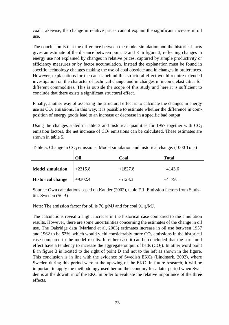
Finally, another way of assessing the structural effect is to calculate the changes in energy use as CO2 emissions. In this way, it is possible to estimate whether the difference in com-position of energy goods lead to an increase or decrease in a specific bad output.

Using the changes stated in table 3 and historical quantities for 1957 together with CO2 emission factors, the net increase of CO2 emissions can be calculated. These estimates are shown in table 5.

Table 5. Change in CO2 emissions. Model simulation and historical change. (1000 Tons)

Oil Coal Total

Model simulation +2315.8 +1827.8 +4143.6

Historical change +9302.4 -5123.3 +4179.1

Source: Own calculations based on Kander (2002), table F.1, Emission factors from Statis-tics Sweden (SCB)

Note: The emission factor for oil is 76 g/MJ and for coal 91 g/MJ.

The calculations reveal a slight increase in the historical case compared to the simulation results. However, there are some uncertainties concerning the estimates of the change in oil use. The Oakridge data (Marland et al, 2003) estimates increase in oil use between 1957 and 1962 to be 53%, which would yield considerably more CO2 emissions in the historical case compared to the model results. In either case it can be concluded that the structural effect have a tendency to increase the aggregate output of bads (CO2). In other word point E in figure 3 is located to the right of point D and not to the left as shown in the figure. This conclusion is in line with the evidence of Swedish EKCs (Lindmark, 2002), where Sweden during this period were at the upswing of the EKC. In future research, it will be important to apply the methodology used her on the economy for a later period when Swe-den is at the downturn of the EKC in order to evaluate the relative importance of the three effects.

23

7. Conclusions

The aim of this study has been to use the rebound effect as an analytical tool for analysing the Swedish historical economic performance in an EKC setting. The starting point has been that changes in energy efficiency and the related rebound effect can be incorporated in a basic EKC model that can be empirically investigated using a CGE approach. The ap-proach is illustrated through the use of a historical CGE-model calibrated to 1957.

Even if the approach is promising and the model simulations produce interesting results concerning changes in energy use in the 1950s in an EKC setting, the results must still be regarded as tentative. Further elaborations and research are necessary in order to provide conclusive results. It is foremost in three areas that further refinements of the approach are desirable.

First, there is a need to obtain further benchmarks to which the model can be calibrated. It is only in this way that changes over time of the relationship between goods and bads and its decomposition in an EKC setting can be made. After 1957, there exist a number of in-put-output investigations concerning the Swedish economy which can be used. It would be most important to apply the rebound-EKC approach outlined in this paper to a benchmark in the 1970s, which would allow for the comparison between the pre and post oil crisis properties of the economy. At the same time, though, it would also be desirable to obtain benchmarks before 1957, in order to get more insight into the historical performance of the Swedish economy in respect to energy use. This would require the establishment of fairly detailed historical input-output tables, which makes this a long-term research objective.

Second, the model itself could be more refined. At the present it is a fairly basic static model and more features could be introduced in order for the model to be more realistic. This concerns for instance the introduction of dynamics in the model and making it even-tually to a multi-period model where the growth paths can be followed more precisely. The introduction of dynamic properties would also imply that changes at the present treated as exogenous could be endogenised. This concerns for instance savings, investments and capital formation. Furthermore, the household demand function could be more refined so it more realistically reflects actual behaviour. However, such a refinement also requires some basic research regarding historical household behaviour, for instance the estimation of his-torical income elasticities. In the lack of such estimates, further refinements of the house-hold behaviour in the model would be meaningless, since it would be based on mere guesses about historical behaviour.

Third, the important structural effect that is obtained as a residual between the model simu-lations and the actual historical change must be investigated further so that it can be ex-plained properly. Leaving important factors behind the change in energy use explicitly unexplained in a residual cannot be seen as satisfactorily. This could be done for instance by elaborating the simulation scenarios further and incorporating further features into the model. Even if the residual from a model simulation cannot be seen as a satisfactory expla-nation, it cannot be neglected that the decomposition made through the use of model simu-

24

lations distinctly points out what needs to be explained. In other words, the residual pro-vides information on what needs to be explained, even if it cannot explain it by itself.

Even if the approach outlined in this paper still need further elaborations, it is clear that the integration of the rebound effect into a basic EKC model opens up for specific empirical investigations of what kinds of effects that to a large extent can explain changes in energy use and the relationship between the production of good and bad outputs. Since it is rea-sonable to use a CGE approach in the empirical research, fairly reliable estimates of the size and direction of these effects can be made.

References

Armington, P. (1969), A Theory of Demand for Products Distinguished by Place of Pro-duction, IMF Staff Papers, vol 16, pp159-178.

Arrow, K, Bolin, B, Costanza, R, Dasgupta, P, Folke, C, Holling, C. S, Jansson, B-O, Levin, S, Mäler, K-G, Perrings, C, and Pimentel (1995), Economic growth, carrying capac-ity, and the environment, Science, 268, pp520-521.

Berndt, E. R, and Wood, D. O. (1979), Engineering and Econometric Interpretations of Energy Capital Complementarity, American Economic Review, vol 69, June, pp342-354.

Birol, F, and Keppler, J. H. (2000), Prices, technology development and the rebound effect, Energy Policy, vol 28, pp457-469.

Böhringer, C, and Rutherford, T. F. (1996), Carbon Taxes with Exemptions in an Open Economy: A General Equilibrium Analysis of the German Tax Initiative, Journal of Envi-ronmental Economics and Management, pp189-203.

Bourges, A. M, and Goulder, L. H. (1984), Decomposing the impact of higher energy prices on log-term growth, in Scarf, H. E, and Shoven J. B. (eds), Applied Genereal Equi-librium Analysis, Cambridge University Press.

Brännlund, R, and Kriström, B. (1998), Miljöekonomi, Studentlitteratur: Lund.

Greening, L. A, Greene, D. L, and Difiglio, C. (2000), Energy efficiency and consumption – the rebound effect – a survey, Energy Policy, vol 28, p389-401.

Griffin, J. M, and Gregory, P. R. (1976), An Intercountry Translog Model of Energy Sub-stitution Responses, American Economic Review, vol 66, December, pp845-857.

Grossman, G. M, and Krueger, A. B. (1991), Environmental impacts of a North American Free Trade Agreement, NBER Working Paper 3914, NBER, Cambridge.

Harris, A, McAvinchey, I. D, and Yannopoulos, A. (1993), The Demand for Labour, Capi-tal, Fuels and Electricity: A Sectoral Model of the United Kingdom Economy, Journal of Economic Studies, vol 20, no 3, pp24-35.

25

Harrison, G. W, and Kriström, B. (1998), Carbon Emissions and the Economic Costs of Transport Policy in Sweden, in Roson, R, and Small, K. A. (eds), Environment and Trans-port in Economic Modelling, Amsterdam: Kluwer Academic Press.

Hill, M. (2001), Essays on Environmental Policy Analysis: Computable General Equilib-rium Approaches Applied to Sweden, diss. Stockholm School of Economics.

Höglund, B, and Werin, L. (1964), Input-output tabeller för Sverige år 1957, Stockholm.

IBRD (1992), World Development Report 1992: Development and the Environment, New York: Oxford University Press.

Kander, A. (2002), Economic growth, energy consumption and CO2 emissions in Sweden 1800-2000, diss, Lund studies in economic history, 19, Lund Univeristy.

Kriström, B. (1998), On a Clear Day, You Might See the Environmental Kuznets Curve, mimeo.

Layard, P. R. G, and Walters, A. A. (1978), Microeconomic Theory, McGraw-Hill, New York.

Lindmark, M. (2002), An EKC-pattern in historical perspective: carbon dioxide emissions, technology, fuel prices and growth in Sweden 1870–1997, Ecological Economics, vol 42, no 1-2, pp333-347.

Marland, G, Boden, T, Andres, R. L. (2003), Global, Regional, and National Fossil Fuel C02 Emissions. In Trends: A Compendium of Data on Global Change. Carbon Dioxide Information Analysis Center, Oak Ridge National Laboratory, U.S. Department of Energy, Oak Ridge, Tenn., U.S.A.

Meadows, D. H, Meadows, D: L, and Randers, J. (1992), Beyond the Limits: Global Col-lapse or a Sustainable Future, London: Earthscan.

Robinson, S, Cattaneo, A. and Moataz, E-S. (2001), Updating and Estimating a Social Ac-counting Matrix Using Cross Entropy Methods, Economic Systems Research, vol 13, no 1, p47-64.

Rutherford, T. F: (1999), Applied General Equilibrium Modeling Using MPSGE as a GAMS subsystem: An Overview of Modeling Framework and Syntax, Computational Economics, vol 14, p1-46.

Saunders, H. (1992), The Khazzoom-Brookes Postulate and Neoclassical Economic Growth, Energy Journal, vol 13, no 14, pp131-148.

Shafik, N, and Bandyopadhay, S. (1992), Economic growth and environmental quality: time series and cross-country evidence, Background paper for the World Development Report 1992, The World Bank, Washington DC.

26

Stern, D. I, Common, M. S, Barbier, E. B (1996), Economic Growth and environmental degradation: the environmental Kuznets curve and sustainable development, World Devel-opment, vol 24, pp1151-1160.

Stern, D. I. (1998), Progress on the environmental Kuznets curve?, Environment and De-velopment Economics, vol 3, no 2, pp173-196.

Unruh, G.C, and Moomaw, W. R. (1997), An alternative analysis of apparent EKC-type transtitions, Ecological Economics, vol 25, no 2, pp211-229.

Vikström, P. (2004a), A Social Accounting Matrix for Sweden in 1957, Umeå Papers in Economic History, no 27.

Vikström, P. (2004b), Capital-Energy Substitution in the Swedish Manufacturing Industry 1954-1965, mimeo.

Vinals, J. M. (1984), Energy-Capital Substitution, Wage Flexibility, and aggregate output supply, European Economic Review, vol 26, no 1-2, pp229-245.

27