Energy-Aware Server Provisioning and Load Dispatching forConnection-Intensive Internet Services

Gong Chen∗, Wenbo He?, Jie Liu†, Suman Nath†, Leonidas Rigas‡, Lin Xiao†, Feng Zhao†

∗Dept. of Statistics, University of California, Los Angeles, CA 90095?Dept. of Computer Science, University of Illinois, Urbana-Champaign, IL 61801

‡Microsoft †Research, One Microsoft Way, Redmond, WA 98052gchen@stat.ucla.edu, webohe@uiuc.edu

{liuj, sumann, leonr, lixiao, zhao}@microsoft.com

AbstractEnergy consumption in hosting Internet services is be-coming a pressing issue as these services scale up. Dy-namic server provisioning techniques are effective inturning off unnecessary servers to save energy. Suchtechniques, mostly studied for request-response services,face challenges in the context of connection servers thathost a large number of long-lived TCP connections. Inthis paper, we characterize unique properties, perfor-mance, and power models of connection servers, basedon a real data trace collected from the deployed WindowsLive Messenger. Using the models, we design serverprovisioning and load dispatching algorithms and studysubtle interactions between them. We show that our al-gorithms can save a significant amount of energy withoutsacrificing user experiences.

1 Introduction

Internet services such as search, web-mail, online chat-ting, and online gaming, have become part of people’severyday life. Such services are expected to scale well,to guarantee performance (e.g., small latency), and to behighly available. To achieve these goals, these servicesare typically deployed in clusters of massive number ofservers hosted in dedicated data centers. Each data cen-ter houses a large number of heterogeneous componentsfor computing, storage, and networking, together with aninfrastructure to distribute power and provide cooling.

Viewed from the outside, a data center is a “black box”that responds to a stream of requests from the Internet,while consuming power from the electrical grid and pro-ducing waste heat. As the demand on Internet servicesdrastically increases in recent years, the energy used bydata centers, directly related to the number of hostedservers and their workload, has been skyrocketing [8].In 2006, U.S. data centers consumed an estimated 61 bil-lion kilowatt-hours (kWh) of energy, enough to power5.8 million average US households.

Data center energy savings can come from a numberof places: on the hardware and facility side, e.g., by de-signing energy-efficient servers and data center infras-tructures, and on the software side, e.g., through resourcemanagement. In this paper, we take a software-basedapproach, consisting of two interdependent techniques:dynamic provisioning that dynamically turns on a mini-mum number of servers required to satisfy application-specific quality of service, and load dispatching that dis-tributes current load among the running machines. Ourapproach is motivated by two observations from real datasets collected from operating Internet services. First, thetotal load of a typical Internet service fluctuates over aday. For example, the fluctuation for the number of userslogged on to Windows Live Messenger can be about 40%of the peak load within a day. Similar patterns werefound in other studies [3, 20]. Second, an active server,even when it is kept idle, consumes a non-trivial amountof power (> 66% of the peak from our measurements,similar to other studies [9]). The first observation pro-vides us the opportunity to dynamically change the num-ber of active servers, while the second observation im-plies that shutting down machines during off-peak periodprovides maximum power savings.

Both dynamic provisioning and load dispatching havebeen extensively studied in literature [20, 3, 6]. How-ever, prior work studies them separately since the mainfoci were on request-response type of services, such asWeb serving. Simple Web server transactions are typi-cally short. There is no state to carry over when the totalnumber of servers changes. In that context, first the min-imum number of servers sufficient to handle the currentrequest rate is determined. After the required numberof servers are turned on, incoming requests are typicallydistributed evenly among them [3].

Many Internet services keep long-lived connections.For example, HTTP1.1 compatible web servers can op-tionally keep the TCP connection after returning the ini-tial web request in order to improve future response per-

NSDI ’08: 5th USENIX Symposium on Networked Systems Design and ImplementationUSENIX Association 337

formance. An extreme case is connection-oriented ser-vices like in instant messaging, video sharing, Internetgames, and virtual life applications, where users maybe continuously logged in for hours or even days. Fora connection server, the number of connections on aserver is an integral of its net login rate (gross login rateminus logout rate) over the time it has been on. Thepower consumption of the server is a function of manyfactors such as number of active connections and loginrate. Unlike request-response servers that serve short-lived transactions, long-lived connections in connectionservers present unique characteristics:

1. The capacity of a connection server is usually con-strained by both the rate at which it can accept newconnections and the total number of active connec-tions on the server. Moreover, the maximum toler-able connection rate is typically much smaller thanthe total number of active connections due to severalreasons such as expensive connection setup proce-dure and conservative SLA (Service Level Agree-ment) with back-end authentication services or userprofiles. This implies that when a new server isturned on, it cannot be fully utilized immediatelylike simple web servers. The load, in terms of howmany users it hosts, can only increase gradually.

2. If the number of server is under provisioned, new lo-gin requests will be rejected and users receive “ser-vice not available” (SNA) errors. When a connec-tion server with active users is turned off, users mayexperience a short period of disconnection, called“server initiated disconnections” (SID). When thishappens, the client software typically tries to recon-nect back, which may create an artificial surge onthe number of new connections, and generate un-necessary SNAs. Both errors should be avoided toperserve user experiences.

3. As we will see in Section 3.5, the energy costof maintaining a connection is orders of magni-tude smaller than processing a new connection re-quest. Thus, a provisioning algorithm that turns offa server with a large number of connections, whichin turn creates a large number of reconnections, maydefeat the purpose of energy saving.

Due to these unique properties, existing dynamic pro-visioning and load dispatching algorithms designed forrequest-response services may not work well with con-nection services. For example, consider a simple strategythat dynamically turns on or off servers based on currentnumber of users and then balances load among all ac-tive servers [3]. Since a connection server takes time,say T , to be fully utilized, provisioning X new serversbased on current users may not be sufficient. Note that

newly booted servers will require T time to take the tar-get load, and during this time the service will have fewerfully utilized servers than needed, causing poor service.Moreover, after time T of turning on X new servers,workload can significantly change, making these X newservers either insufficient or unnecessary. Consider, onthe other hand, that a server with N connections is turnedoff abruptly when the average connected users per serveris low. All those users will be disconnected. Sincemany disconnected clients will automatically re-login,currently available servers may not be able to handle thesurge. In short, a reactive provisioning system is verylikely to cause poor service or create instability. This canbe avoided by a proactive algorithm that takes the tran-sient behavior into account. For example, we can employa load prediction algorithm to turn on machines graduallybefore they are needed and to avoid turning on unneces-sary machines to cope with temporary spikes in load. Atthe same time, the provisioning algorithm needs to worktogether with load dispatching mechanism and anticipatethe side effect of changing server numbers. For example,if loads on servers are intentionally skewed, instead ofbalanced, to create “tail” servers with fewer live connec-tions, then turning off a tail server will not generate anybig surge to affect login patterns.

In this paper, we develop power saving techniquesfor connection services, and evaluate the techniques us-ing data traces from Windows Live Messenger (formerlyMSN Messenger), a popular instant messaging servicewith millions of users. We consider server provisioningand load dispatching in a single framework, and evaluatevarious load skewing techniques to trade off between en-ergy saving and quality of service. Although the problemis motivated by Messenger services, the results shouldapply to other connection-oriented services. The contri-butions of the paper are:

• We characterize performance, power, and user ex-perience models for Windows Live Messenger con-nection servers based on real data collected over aperiod of 45 days.

• We design a common provisioning framework thattrades off power saving and user experiences. Ittakes into account the server transient behavior andaccommodates various load dispatching algorithms.

• We design load skewing algorithms that allow sig-nificant amount of energy saving (up to 30%) with-out sacrificing user experiences, i.e., maintainingvery small number of SIDs.

The rest of paper is organized as follows. Section 2discusses related work. In Section 3, we give a briefoverview of the Messenger connection server behaviorand characterize connection server power, performance,

NSDI ’08: 5th USENIX Symposium on Networked Systems Design and Implementation USENIX Association338

and user experience models. We present the load pre-diction and server provisioning algorithms in Section 4,and load dispatching algorithms in Section 5. Using datatraces from deployed Internet services, we evaluate vari-ous algorithms and show the results in Section 6. Finally,we conclude the paper with discussions in Section 7.

2 Related Work

In modern CPUs, P-states and clock modulation mecha-nisms are available to control CPU power consumptionaccording to the load at any particular moment. Dy-namic Voltage/Frequency Scaling (DVFS) has been de-veloped as a standard technique to achieve power effi-ciency of processors [19, 13, 17]. DVFS is a power-ful adaptation mechanism, which adjusts power provi-sioning according to workload in computing systems.A control-based DVFS policy combined with requestbatching has been proposed in [7], which trades off sys-tem responsiveness to power saving and adopts a feed-back control framework to maintain a specified responsetime level. A DVFS policy is implemented in [21] on astand-alone Apache web server, which manages tasks tomeet soft real-time deadlines. Flautner et al. [10] adoptsperformance-setting algorithms for different workloadcharacteristics transparently, and implements the DVFSpolicy on per-task basis.

A lot of efforts have been made to address power ef-ficiency in data centers. In [11], Ganesh, et al. pro-posed a file system based solution to reduce disk arrayenergy consumption. The connection servers we studyin this paper have little disk IO load. Our focus ison provisioning entire servers. In [20], Pinheiro et al.presented a simple policy to turn cluster nodes on andoff dynamically. Chase et al. [3] allocated computingresources based on an economic approach, where ser-vices “bid” for resources as a function of required per-formance, and the system continuously monitors loadand allocates resources based on its utility. Heath etal. [14] studied Web service on-off strategies in the con-text of heterogeneous server types, although focusing ononly short transactions. Various other work using adap-tive policies to achieve power efficiency have been pro-posed. Abdelzaher et al. in [1] employed a Proportional-Integration (PI) controller for an Apache Web serverto control the assigned processes (or threads) and tomeet soft realtime latency requirements. Other workbased on feedback and/or optimal control theory includes[6, 5, 23, 22, 16, 15], which attempt to dynamically op-timize for energy, resources and operational costs whilemeeting performance-based SLAs.

In contrast to previous work, we consider and de-sign load dispatching and dynamic provisioning schemestogether since we observe that, in the context of con-

� � �� � � �� � �� � � � � � � �� � � � � � �� � � � � � � � � � � � � � �� � � � � � � � � � � � � � � � �� � � � � � � � � � � � � � �� � � � � � �� � � � � � � � � � � �� � � � � � � � � � � �� � � � � � � � � � � �

Figure 1: Connection service architecture.

nection servers, they have subtle interaction with eachother. These two components work together to controlpower consumption and performance levels. Moreover,we adopt forecast-based and hysteresis-based provision-ing to bear with slow rebooting of servers.

3 Connection Servers Background

Connection servers are essential for many Internet ser-vices. In this paper, we consider dedicated connectionservers, each of which runs only one connection serviceapplication. However, the discussion can be generalizedto servers hosting multiple services as well.

3.1 Connection ServiceFigure 1 shows an example of the front door architecturefor connection intensive Internet applications. Users,through dedicated clients, applets, or browser plug-ins,issue login requests to the service cloud. These login re-quests first reach a dispatch server (DS), which picks aconnection server (CS) and returns its IP address to theclient. The client then directly connects to the CS. TheCS authenticates the user and if succeeded, a live TCPconnection is maintained between the client and the CSuntil the client logs off. The TCP connection is usuallyused to update user status (e.g. on-line, busy, off-line,etc.) and to redirect further activities such as chattingand multimedia conferencing to other back-end servers.

At the application level, each CS is subject to two ma-jor constraints: the maximum login rate and the maxi-mum number of sockets it can host. The new user lo-gin rate L is defined as the number of new connectionrequests that a CS processes in a second. A limit onlogin rate Lmax is set to protect CS and other back-end services. For example, Messenger uses WindowsLive ID (a.k.a. Passport) service for user authentication.Since Live ID is also shared by other Microsoft and non-Microsoft applications, a service-level agreement (SLA)

NSDI ’08: 5th USENIX Symposium on Networked Systems Design and ImplementationUSENIX Association 339

0 20 40 60 80 100 120 140 160200

400

600

800

1000

1200

1400

Time in hours

Logi

n ra

te (p

er s

econ

d)

Login RateConnections

0

1

2

3

4

5

Num

ber o

f con

nect

ions

(milli

ons)

Figure 2: One week of load pattern (Monday to Sunday)from Windows Live Messenger connection servers

is set to bound the number of authentication requests thatMessenger can forward. In addition, a new user login isa CPU intensive operation on the CS, as we will showin Section 3.5. Having Lmax protects the CS from beingoverloaded or entering unsafe operation regions.

In terms of concurrent live TCP connections, a limitNmax is set on the total number of sockets for each CSfor two reasons: the memory constraints and the fault tol-erance concerns. Maintaining a TCP socket is relativelycheap for the CPU but requires a certain amount of mem-ory. At the same time, if a CS crashes, all its users willbe disconnected. As most users set their clients to auto-matically reconnect when disconnected, a large numberof new login requests will hit the servers. Since there is alimit on new login rate, not all reconnect requests can beprocessed in a short period of time, creating undesirableuser experiences.

3.2 Load PatternsPopular connection servers exhibit periodic load patternswith large fluctuation, similar to those reported in [6].

Figure 2 shows a pattern of the login rates and totalnumber of connections to the Messenger service over thecourse of a week. Only a subset of the data, scaled to 5million connections on 60 connection servers, is reportedhere. It is clear that the number of connections fluctu-ates over day and night times. In fact, for most days, theamount of fluctuation is about 40% of the correspond-ing peak load. Some geo-distributed services show evenlarger fluctuation. The login rates for the same time pe-riod are scaled similarly. It is worth noting that the loginrate is noisier than the connection count.

Since the total number of servers must be provisionedto handle peak load to guarantee service availability, itis a “overkill” when the load is low. If we can adaptserver resource utilization accordingly, we should be ableto save substantial energy. In addition, the smooth pat-tern indicates that the total number of connections is pre-dictable. In fact, if we look at the pattern over weeks, the

similarity is more significant. Since turning on serverstakes time, the prediction will help us act early.

3.3 Power ModelUnderstanding how power are consumed by connectionservers provides us insights on energy saving strategies.Connection servers are CPU, network, and memory in-tensive servers. There is almost no disk IO in normal op-eration, except occasional log writing. Since memory istypically pre-allocated to prevent run-time performancehit, the main contributor to the power consumption vari-ations of a server is the CPU utilization.

We measured power consumption of typical serverswhile changing the CPU utilization by using variableworkloads. Figure 3 shows the power consumption ontwo types of servers, where the horizontal axis indicatesthe average CPU utilization reported by the OS, and thevertical axis indicates the average power consumptionmeasured at the server power plug.

Sleep Idle 20% 40% 60% 80% 100%0

20

40

60

80

100

120

140

160

180

CPU Utilization

Powe

r Con

sump

tion (

Watts

)

Intel(R) 2CPU 2.4GHzIntel(R) 2CPU 3GHz

Figure 3: Power consumption v.s. CPU utilization

We observe two important facts. First, the power con-sumption increases almost linearly with CPU utilization,as reported in other studies [9]. Second, an idle serverconsumes up to 66% of the peak power, because evenwhen a server is not loaded with user tasks, the powerneeded to run the OS and to maintain hardware peripher-als, such as memory, disks, master board, PCI slots, andfans, is not negligible. Figure 3 implies that if we packconnections and login requests to a portion of servers,and keep the rest of servers hibernating (or shutting-down), we can achieve significant power savings. How-ever, the consolidation of login requests results in highutilization of those servers, which may downgrade per-formance and user experiences. Hence, it is important tounderstand the user experience model before we addresspower saving schemes for large-scale Internet service.

3.4 User ExperiencesIn the context of connection servers, we consider the fol-lowing factors as user experience metric.1. Service Not Available (SNA) Error. Service unavail-able is an error message returned to the client softwarewhen there is not enough resource to handle user login.

NSDI ’08: 5th USENIX Symposium on Networked Systems Design and Implementation USENIX Association340

This happens when DS cannot find a CS that can takethe new login request, or when a CS receives a login re-quest, it observes that its login rate or number of existingsockets exceeds corresponding limits.2. Server-Initiated Disconnection (SID). A disconnec-tion happens when a live user socket is terminated be-fore the user issues a log off request. This can be causedby network failures between the client and the server, byserver crash, or by the server sending a “reconnect” re-quest to the client. Since network failure and server crashare not controlled by the server software, we use server-initiated disconnection (SID) as the metric for short termuser experience degradation. SID is usually a part of con-nection server protocol, like MSNP [18], so that a servercan be shut down gracefully (for software update for ex-ample). SID can be handled transparently by the clientsoftware so that it is un-noticeable to users. Neverthe-less, some users, if they disable automated reconnect orare in active communication with their buddies, may ob-serve transient disconnections.3. Transaction Latency. Research on quality of ser-vices, e.g. [21, 6], often uses transaction delays as a met-ric for user experiences. However, after we examinedconnection server transactions, including user login, au-thentication, messaging redirection, etc., we observe nodirect correlation between transaction delays and serverload (in terms of CPU, number of connection, and loginrate). The reason is that connection services are not CPUbounded. The load of processing transactions is well un-der control when the number of connection and the loginrates are bounded. So, we will not consider transactiondelays as a quality of service metric in this paper.

From this architectural description, it is clear that theDS and its load dispatching algorithm play a critical rolein the shape of the load in connection servers. This moti-vates us to focus on the interaction between CS and DS,the provisioning algorithms and load dispatching algo-rithms to achieve power saving while maintaining userexperiences in terms of SNA and SID.

3.5 Performance ModelTo characterize the effect of load dispatching on serviceloads, it is important to understand the relationship be-tween application level parameters such as user login andphysical parameters such as CPU utilization and powerconsumption. In other words, we need to identify thevariables that significantly affect CPU and power. Thiswould enable us to control CPU usage and power con-sumption of the servers by controlling these variables.

We use a workload trace of Messenger service to iden-tify the key variables affecting CPU usage and power.The trace contains 32 different performance counterssuch as login rate, connection count, memory usage,CPU usage, connection failures, etc. of all production

residuals

Frequency

−5 0 5 10 15

01000

3000

5000

Figure 4: Residual distribution of performance model.

Messenger servers, over a period of 45 days. To keepthe data collection process lightweight, aggregated val-ues over 1 second are recorded every 30 seconds.

Given time series data of all available variables, weintend to identify important variables affecting the re-sponse variable (CPU utilization) and build a model ofthe response variable. Our statistical modeling method-ology includes various exploratory data analysis, bi-direction model selection, diagnostic procedures and per-formance validation. Readers can refer to our technicalreport [4] for details.

The final model obtained from our methodology is:

U = 2.84 × 10−4 · N + 0.549 · L − 0.820 (1)

where U denotes the estimate of the CPU utilizationpercentage—the conditional mean in linear models, N isthe number of active connections, and L is login rate. Forexample, given 70,000 connections and 15 new loginsper second, the model estimates the CPU utilization tobe 27.3%. The residual (error) distribution of this modelcan be seen from Figure 4. It shows that for 91.4% per-cent of cases, the observed values are within the rangefrom −5 to 5 of the estimates from the model. Refer-ring to the previous example, the actual CPU utilizationfalls in between 22.30 and 32.30 with probability 0.914.About 7.6% cases for which the model makes underesti-mation have larger residuals from 5 to 15. The remaining1% cases have residuals less than -5.

We use 2 weeks of data to train the model, and an-other 4 weeks for validation. The validation demon-strates that the distributions of testing errors are consis-tent with the distribution of training errors, concludingthat CPU usage (and hence power consumption) of Mes-senger servers can reasonably be modeled with login rate(L) and number of active connections (N ). Moreover,for a given maximum tolerable CPU utilization (definedby the Messenger operations group), the model also pro-vides Nmax and Lmax, maximum tolerable values for Nand L. Our provisioning and load dispatching algorithmstherefore consider only these two variables and try to en-sure that N < Nmax and L < Lmax, while minimizingtotal energy consumption.

NSDI ’08: 5th USENIX Symposium on Networked Systems Design and ImplementationUSENIX Association 341

4 Energy-Aware Server Provisioning

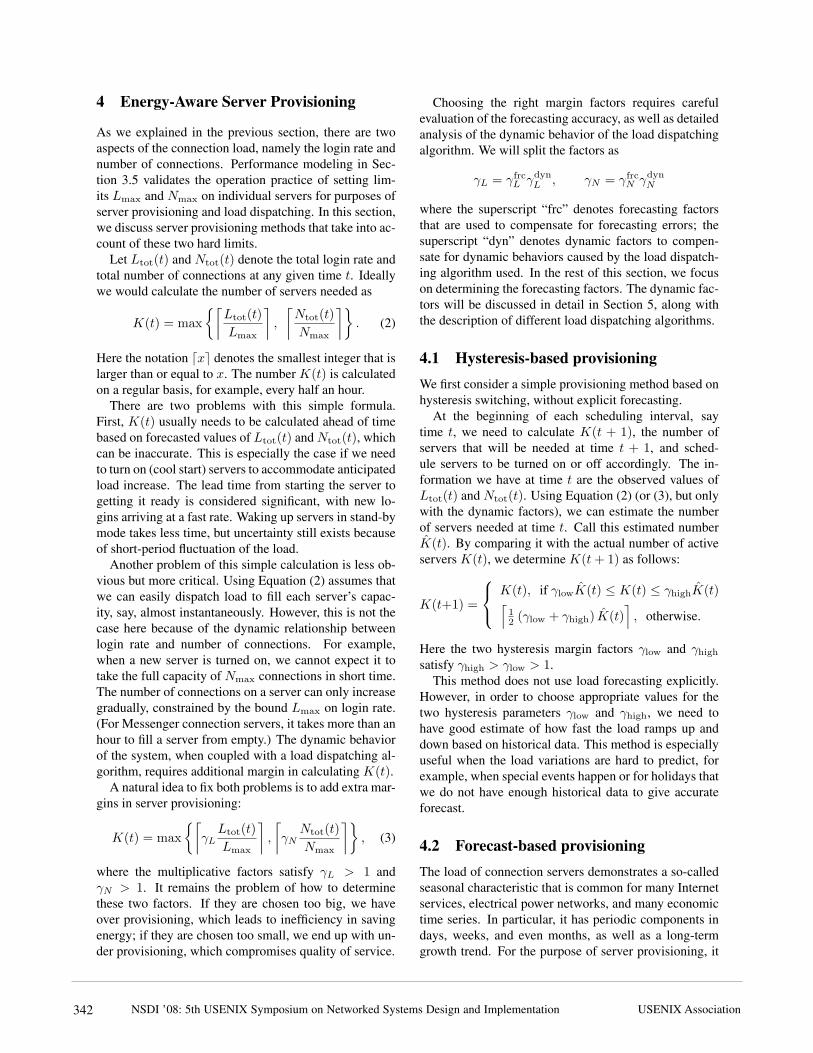
As we explained in the previous section, there are twoaspects of the connection load, namely the login rate andnumber of connections. Performance modeling in Sec-tion 3.5 validates the operation practice of setting lim-its Lmax and Nmax on individual servers for purposes ofserver provisioning and load dispatching. In this section,we discuss server provisioning methods that take into ac-count of these two hard limits.

Let Ltot(t) and Ntot(t) denote the total login rate andtotal number of connections at any given time t. Ideallywe would calculate the number of servers needed as

K(t) = max

{⌈

Ltot(t)

Lmax

⌉

,

⌈

Ntot(t)

Nmax

⌉}

. (2)

Here the notation dxe denotes the smallest integer that islarger than or equal to x. The number K(t) is calculatedon a regular basis, for example, every half an hour.

There are two problems with this simple formula.First, K(t) usually needs to be calculated ahead of timebased on forecasted values of Ltot(t) and Ntot(t), whichcan be inaccurate. This is especially the case if we needto turn on (cool start) servers to accommodate anticipatedload increase. The lead time from starting the server togetting it ready is considered significant, with new lo-gins arriving at a fast rate. Waking up servers in stand-bymode takes less time, but uncertainty still exists becauseof short-period fluctuation of the load.

Another problem of this simple calculation is less ob-vious but more critical. Using Equation (2) assumes thatwe can easily dispatch load to fill each server’s capac-ity, say, almost instantaneously. However, this is not thecase here because of the dynamic relationship betweenlogin rate and number of connections. For example,when a new server is turned on, we cannot expect it totake the full capacity of Nmax connections in short time.The number of connections on a server can only increasegradually, constrained by the bound Lmax on login rate.(For Messenger connection servers, it takes more than anhour to fill a server from empty.) The dynamic behaviorof the system, when coupled with a load dispatching al-gorithm, requires additional margin in calculating K(t).

A natural idea to fix both problems is to add extra mar-gins in server provisioning:

K(t) = max

{⌈

γL

Ltot(t)

Lmax

⌉

,

⌈

γN

Ntot(t)

Nmax

⌉}

, (3)

where the multiplicative factors satisfy γL > 1 andγN > 1. It remains the problem of how to determinethese two factors. If they are chosen too big, we haveover provisioning, which leads to inefficiency in savingenergy; if they are chosen too small, we end up with un-der provisioning, which compromises quality of service.

Choosing the right margin factors requires carefulevaluation of the forecasting accuracy, as well as detailedanalysis of the dynamic behavior of the load dispatchingalgorithm. We will split the factors as

γL = γfrcL γdyn

L , γN = γfrcN γdyn

N

where the superscript “frc” denotes forecasting factorsthat are used to compensate for forecasting errors; thesuperscript “dyn” denotes dynamic factors to compen-sate for dynamic behaviors caused by the load dispatch-ing algorithm used. In the rest of this section, we focuson determining the forecasting factors. The dynamic fac-tors will be discussed in detail in Section 5, along withthe description of different load dispatching algorithms.

4.1 Hysteresis-based provisioning

We first consider a simple provisioning method based onhysteresis switching, without explicit forecasting.

At the beginning of each scheduling interval, saytime t, we need to calculate K(t + 1), the number ofservers that will be needed at time t + 1, and sched-ule servers to be turned on or off accordingly. The in-formation we have at time t are the observed values ofLtot(t) and Ntot(t). Using Equation (2) (or (3), but onlywith the dynamic factors), we can estimate the numberof servers needed at time t. Call this estimated numberK(t). By comparing it with the actual number of activeservers K(t), we determine K(t + 1) as follows:

K(t+1) =

K(t), if γlowK(t) ≤ K(t) ≤ γhighK(t)⌈

12 (γlow + γhigh) K(t)

⌉

, otherwise.

Here the two hysteresis margin factors γlow and γhigh

satisfy γhigh > γlow > 1.This method does not use load forecasting explicitly.

However, in order to choose appropriate values for thetwo hysteresis parameters γlow and γhigh, we need tohave good estimate of how fast the load ramps up anddown based on historical data. This method is especiallyuseful when the load variations are hard to predict, forexample, when special events happen or for holidays thatwe do not have enough historical data to give accurateforecast.

4.2 Forecast-based provisioning

The load of connection servers demonstrates a so-calledseasonal characteristic that is common for many Internetservices, electrical power networks, and many economictime series. In particular, it has periodic components indays, weeks, and even months, as well as a long-termgrowth trend. For the purpose of server provisioning, it

NSDI ’08: 5th USENIX Symposium on Networked Systems Design and Implementation USENIX Association342

suffices to consider short-term load forecasting — fore-casting over a period from half an hour to several hours.(Midterm forecasting is for days and weeks, and long-term forecasting is for months and years.)

There is extensive literature on short-term load fore-casting of seasonal time series (see, e.g., [12, 2]). We de-rive a very simple and intuitive algorithm in Section 4.3,which works extremely well for the connection serverdata. To the best of our knowledge, it is a new additionto the literature of short-term load forecasting. On theother hand, however, the following discussion applies nomatter which forecasting algorithm is used, as long as itsassociated forecast factors are determined, as we will doin Section 4.3 for our algorithm.

If the forecasting algorithm anticipates increased loadLtot(t + 1) and Ntot(t + 1) at time t + 1, we can simplydetermine K(t+1), the number of servers needed, usingequation (3). The only thing we need to make sure is thatnew servers are turned on early enough to take the in-creased load. This usually is not a problem, for example,if we do forecasting over half an hour into the future.

More subtleties are involved in turning off servers. Ifthe forecasted load will decrease, we will need less num-ber of servers. Simply turning off one or more serversthat are fully loaded will cause a sudden burst of SIDs.When disconnected users try to re-login at almost thesame time, an artificial surge of login requests is created,which will stress the remaining active servers. Whenthe new login requests on the remaining servers exceedLmax, SNA errors will be generated.

A better alternative is to schedule draining before turn-ing a server off. More specifically, the dispatcher iden-tifies servers that have the least amount of connections,and schedules them to connect to other servers at a con-trolled much slower pace that will not generate any sig-nificant burden for remaining active servers.

In order to reduce the number of SIDs, we can alsostarve the servers (simply not feeding it any new logins)for a period of time before doing scheduled draining orshutting it down. For Messenger servers, the natural de-parture rate caused by normal user logoffs results in anexponential decay of the number of connections, with atime constant slightly less than an hour, meaning that thenumber of connections on a server decreases by half ev-ery hour. A two-hour starving time leads to number ofSIDs less than a quarter of that without starving. Thetrade-off is that adding starving time reduces efficiencyin saving energy.

4.3 Short-term load forecasting

Now we present our method for short-term load forecast-ing. Let y(t) be the stochastic periodic time series underconsideration, with a specified time unit. It can repre-

sent Ltot(t) or Ntot(t) measured at regular time inter-vals. Suppose the periodic component has a period of Ttime units. We express the value of y(t) in terms of allprevious measurements as

y(t) =n

∑

k=1

aky(t − kT ) +m

∑

j=1

bj∆y(t − j),

∆y(t − j) = y(t − j) −1

n

n∑

k=1

y(t − j − kT ).

There are two parts in the above model. The part withparameters ak does periodic prediction — it is an autore-gression model for the value of y over a period of T .The assumption is that the values of y at every T stepsare highly correlated. The part with parameters bj giveslocal adjustment, meaning that we also consider corre-lations between y(t) and the values immediately beforeit. The integers n and m are their orders, respectively.We call this a SPAR (Sparse Periodic Auto-Regression)model. It can be easily extended to one with multipleperiodic components.

For the examples we will consider, short-term fore-casting is done over half an hour, and we let the period Tbe a week, which leads to T = 7 × 24 × 2 = 168 sam-ples. In this case, the autoregression part (with parame-ters ak) of the SPAR model means, for example, the loadat 9am this Tuesday is highly correlated and can be wellpredicted from the loads at 9am of previous Tuesdays.The local adjustment part (with parameters bj) reflectsthe immediate trends predicted from values at 8:30am,8:00am, and so on, on the same day.

We have tried several models with different orders nand m, but found that the coefficients ak, bj are verysmall for k > 4 and j > 2, and ignoring them does notreduce the forecasting accuracy by much. So we choosethe orders n = 4 and m = 2 to do load forecasting inour examples. We used five weeks of data to estimate theparameters ak and bj (by solving a simple least-squaresfitting problem). Then we use these data and estimatedparameters to forecast loads for the following weeks.

Figure 5 shows the results of using this forecastingmodel. The figures show the forecasted values (every 30minutes) plotted against actually observations (measuredevery 30 seconds). Note that the observed login rates(measured every second and recorded every 30 seconds)appear to be very noisy and have lots of spikes. Usingthis model, we can reasonably forecast the smooth trendof the curve. The spikes are hard to predict, because theyare mostly caused by irregular server unavailability orcrashes that result in re-login bursts.

We computed the standard deviations of the relativeerrors (L(t) − L(t))/L(t) and (N(t) − N(t))/N(t):

σL = 0.039, σN = 0.006.

NSDI ’08: 5th USENIX Symposium on Networked Systems Design and ImplementationUSENIX Association 343

0 20 40 60 80 100 120 140 1602

2.5

3

3.5

4

4.5

5x 106

Observed valueForecasted value

Time (hours)

Ntot(t

)

(a) Number of connections over a week.

0 5 10 15 202

2.5

3

3.5

4

4.5

5x 106

Observed valueSPAR model forecast1st−derivative forecast

Time (hours)

Ntot(t

)

(b) Number of connections on Monday.

0 20 40 60 80 100 120 140 160200

300

400

500

600

700

800

900

1000

Observed valueForecasted value

Time (hours)

Ltot(t

)

(c) Login rates over a week.

0 5 10 15 20200

300

400

500

600

700

800

900

1000

Observed valueSPAR model forecast1st−derivative forecast

Time (hours)

Ltot(t

)(d) Login rates on Monday.

Figure 5: Short-term load forecasting.

We also compared it with some simple strategies forshort-term load forecasting without using periodic timeseries models. For example, one idea is to predict theload at the next observation point based on the first-orderderivative of the current load and the average load at theprevious observation point (e.g., Heath et al. [14]). Thisapproach leads to the standard deviations σL = 0.079and σN = 0.012, which are much worse than the resultsof our SPAR model (see Figure 5 (b) and (d)). We expectthat such simple heuristics would work well for smoothtrend and very short forecasting intervals. Here our timeseries can be very noisy (especially the login rates), and alonger forecasting interval is prefered because we do notwant to turn on and off servers too frequently. In particu-lar, the SPAR model will work reasonably well for fore-casting intervals of a couple of hours (and even longer),for which derivative-based heuristics will no longer makesense.

Given the standard deviations of the forecasting errorsusing the SPAR model, we can assign the forecasting fac-tors as

γfrcL = 1 + 3σL ≈ 1.12,

γfrcN = 1 + 3σN ≈ 1.02.

(4)

These forecast factors will be substituted into Equa-tion (3) to determine the number of servers required. Todo so, we also need to specify a load dispatching algo-rithm and its associated dynamic factors, which we ex-plain in the next section.

5 Load Dispatching Algorithms

In this section, we present algorithms that decide howlarge a share of the incoming login requests should begiven to each server. We describe two different typesof algorithms — load balancing and load skewing, anddetermine their corresponding dynamic factors γdyn

L andγdyn

N . These two algorithms lead to different load distri-butions on the active servers, and have different impli-cations in terms of energy saving and number of SIDs.In order to present them, we first need to establish a dy-namic model of the load-dispatching system.

5.1 Dynamic system modeling

We consider a discrete-time model, where t denotes timewith a specified unit. The time unit here is usually muchsmaller than the one used for load forecasting; for ex-ample, it is usually on the order of a few seconds. LetK(t) be the number of active servers during the intervalbetween time t and t + 1. Let Ni(t) denote the numberof connections on server i at time t, and Li(t) and Di(t)be the number of logins and departures, respectively, be-tween time t and t+1 (see Figure 5.1). The dynamics ofthe individual servers can be expressed as

Ni(t + 1) = Ni(t) + Li(t) − Di(t)

for i = 1, . . . ,K(t). This first-order difference equationcaptures the integration relationship between the login

NSDI ’08: 5th USENIX Symposium on Networked Systems Design and Implementation USENIX Association344

Ltot(t)

Li(t)

Ni(t)

Di(t)

1 2 i K(t)

load dispatcher

t t+1time

Ni(t) Ni(t+1)

Li(t), Di(t)

Figure 6: Load balancing of connection servers.

rates Li(t) and the number of connections Ni(t). Thenumber of departures Di(t) usually is a fraction of Ni(t),which varies a lot from time to time.

The job of the dispatcher is to dispatch the total incom-ing login request, Ltot(t), to the available K(t) servers.In other words, it determines Li(t) for each server i. Ingeneral, a dispatching algorithm can be expressed as

Li(t) = Ltot(t)pi(t), i = 1, . . . ,K(t)

where pi(t) is the portion or fraction of the total loginrequests assigned to the server i (with

∑

i pi(t) = 1). Fora randomized algorithm, pi(t) stands for the probabilitieswith which the dispatcher distributes the load.

5.2 Load balancing

Load balancing algorithms try to make the numbers ofconnections on the servers the same, or as close as possi-ble. The simple method of round-Robin load-balancing,i.e., always letting pi(t) = 1/K(t), apparently does notwork here. By setting a uniform login rates for all theservers, regardless of the fluctuations of departure rateson individual servers (an open-loop strategy), it leavesthe number of connections on the servers diverge with-out proper feedback control.

There are many ways to make load balancing work forsuch a system. For example, one effective heuristic is toapply round-Robin only to a fraction of the servers thathave relatively small number of connections. In this pa-per we describe a proportional load-balancing algorithm,where the dispatcher assigns the following portion of to-tal loads to server i:

pi(t) =1

K(t)+ α

(

1

K(t)−

Ni(t)

Ntot(t)

)

(5)

where α > 0 is a parameter that can be tuned to influ-ence the dynamic behavior of the system. Intuitively,this algorithm assigns larger portions to servers with rela-tively small number of connections, and smaller portionsto servers with relatively large number of connections.Using the fact Ntot(t) =

∑K(t)i=1 Ni(t), we always have

∑K(t)i=1 pi(t) = 1. However, we notice that pi(t) can be

negative. In this case, the dispatcher actually take loadoff from server i instead of assigning new load to it. Thiscan be done by either migrating connections internally,or by going through the loop of disconnecting some usersand automatic re-login onto other servers.

This algorithm leads to a very interesting property ofthe system: every server has the same closed-loop dy-namics, only with different initial conditions. All theservers will behave exactly the same as time goes on. Theonly exceptions are the newly turned-on servers whichhave zero initial number of connections. Turning offservers does not affect others if the load are reconnectedaccording to the same proportional rule in Equation (5).Detailed analysis of the properties of this algorithm isgiven in [4].

Now let’s examine carefully the effect of the param-eter α. For small values of α, the algorithm maintainsrelatively uniform login rates to all the servers, so it canbe very slow in driving the number of connections to uni-form. The extreme case of α = 0 (which is disallowedhere) would correspond to round-Robin. For large val-ues of α, the algorithm tries to drive the number of con-nections quickly to uniform, by relying on disparate lo-gin rates across servers. In terms of determining γdyn

L ,we note that the highest login rate is always assigned tonewly turned-on servers with Ni(t) = 0. In this case,pi(t) = (1 + α)/K(t). By requiring pi(t)Ltot(t) ≤Lmax, we obtain K(t) ≥ (1 + α)Ltot(t)/Lmax. Com-paring with Equation (3), we have γdyn

L = 1 + α.

The determination of γdynN is more involved. The de-

tails are omitted due to space constraints (but can befound in [4]). Here we simply list the two factors:

γdynL = 1 + α, γdyn

N =1 + α

r + α(6)

where r = mint Dtot(t)/Ltot(t), the minimum ratioamong any time t between Dtot(t) and Ltot(t) (the totaldepartures and total logins between time t and t + 1). Inpractice, r is estimated based on historical data.

In summary, tuning the parameter α allows us to trade-off the two terms appearing in the formula (3) for de-termining number of servers needed. Ideally, we shallchoose an α that makes the two terms approximatelyequal for typical ranges of Ltot(t) and Ntot(t), that is,makes the constraints tight simultaneously for both max-imum login rate and maximum number of connections.

NSDI ’08: 5th USENIX Symposium on Networked Systems Design and ImplementationUSENIX Association 345

5.3 Load skewing

The principle of load skewing is exactly the opposite ofload balancing. Here new login requests are routed tobusy servers as long as the servers can handle them. Thegoal is to maintain a small number of tail servers thathave small number of connections . When user loginrequests ramp up, these servers will be used as reserve tohandle login increases and surge, and give time for newservers to be turned on. When user login requests rampdown, these servers can be slowly drained and shut down.Since only tail servers are shut down, the number of SIDscan be greatly reduced, and no artificial surge of re-loginrequests or connection migrations will be created.

There are many possibilities to do load skewing. Herewe describe a very simple scheme. In addition to the hardbound Nmax on the number of connections a server cantake, we specify a target number of connections Ntgt,which is slightly smaller than Nmax. When dispatchingnew login requests, servers with loads that are smallerthan Ntgt and closest to Ntgt are given priority. Once aserver’s number of connections reaches Ntgt, it will notbe assigned new connections for a while, until it dropsagain below Ntgt due to gradual user departures.

More specifically, let 0 < ρ < 1 be a give parame-ter. At each time t, the dispatcher always distributes newconnections evenly (round-Robin) to a fraction ρ of allthe available servers. Let K(t) be the number of serversavailable, it will choose the dρK(t)e servers in the fol-lowing way. First, the dispatcher partitions the set ofservers {1, 2, . . . ,K(t)} into two subsets:

Ilow(t) = {i | Ni(t) < Ntgt}

Ihigh(t) = {i | Ni(t) ≥ Ntgt}

Then it chooses the top dρK(t)e servers (those with thehighest number of connections) in Ilow(t) . If the num-ber of servers in Ilow(t) is less than dρK(t)e, the dis-patcher has two choices. It can either distribute loadevenly only to servers in Ilow(t), or it can include thebottom dρK(t)e − |Ilow(t)| servers in Ihigh(t). In thesecond case, the number Ntgt is set further away fromNmax to avoid number of connections exceeding Nmax

(i.e., SNA errors) within a short time.This algorithm will lead to a skewed load distribution

across the available servers. Most of the active serversshould have number of connections close to Ntgt, excepta small number of tail servers. Let the desired number oftail servers be Ktail. The dynamic factors for this algo-rithm can be easily determined as

γdynL =

1

ρ, γdyn

N = 1 +Ktail

mint Ntot(t)/Ntgt. (7)

These factors can be substituted into equation (3) to cal-culate the number of servers needed K(t), where it can

be combined with either hysteresis-based or forecast-based server provisioning.

5.3.1 Reactive load skewing

The load skewing algorithm is especially suitable to re-duce the number of SIDs when turning off servers. Tobest utilize load skewing, we also develop a heuristiccalled reactive load skewing (RLS). In particular, it isa hysteresis rule to control the number of tail servers.For this purpose, we need to specify another numberNtail. Servers with number of connections less thanNtail are called tail servers. Let Ktail(t) be the num-ber of tail servers, and Klow < Khigh be two thresh-olds. If Ktail(t) < Klow, then d(Khigh − Klow)/2e −Ktail(t) servers are turned on. If Ktail(t) > Khigh, thenKtail(t) − Khigh servers are turned off. The tail servershave very low active connections, so turning off one oreven several of them will not create artificial reconnec-tion spike. This on-off policy is executed at the serverprovisioning time scale, for example, every half an hour.

6 Evaluations

In this section, we compare the performance of differ-ent provisioning and load dispatching algorithms throughsimulations based on real traffic traces.

6.1 Experimental setupWe simulate a cluster of 60 connection servers with realdata traces of total connected users and login rates ob-tained from production Messenger connection servers (asdescribed in Section 3.5). The data traces are scaled ac-cordingly to fit on 60 servers; see Figure 2. These 60servers are treated as one cluster with a single dispatcher.

The server power model is measured on an HP serverwith two dual-core 2.88GHz Xeon processors and 4Gmemory running Windows Server 2003. We approxi-mate server power consumption (in Watts) as

P =

{

150 + 0.75 × U, if active3, if stand-by

(8)

where U is the CPU utilization percentage from 0 to 100(see Figure 3). The CPU utilization is modeled using therelationship derived in Section 3.5, in particular equa-tion (1). CPU utilization is bounded within 5 to 100 per-cent when the server is active.

The limits on connected users and login rate are set byMessenger stress testing:

Nmax = 100, 000, Lmax = 70/sec.

Also through testing, the server’s wake-up delay, definedas the duration from a message is sent to wake up theserver till the server successfully joins the cluster, is 2

NSDI ’08: 5th USENIX Symposium on Networked Systems Design and Implementation USENIX Association346

minutes. The draining speed, defined as the number ofusers disconnected once a server decide to shut down, is100 connections per second. This implies that it takesabout 15 minutes to drain a fully loaded server.

6.2 Forecast vs. hysteresis provisioningWe first compare the performance of no provisioning,forecast-based and hysteresis-based provisioning, with acommon load balancing algorithm.

• No provisioning with load balancing (NB). NBuses all the 60 servers. It implements the load bal-ancing algorithm in Section 5.2 with α = 1.

• Forecast provisioning with load balancing (FB).FB uses the load balancing algorithm in Section 5.2with α = 1 and the load forecasting algorithm inSection 4.3. The number of servers K(t) are calcu-lated using equation (3) with the factors

γfrcL = 1.12, γfrc

N = 1.02 from equation (4),

γdynL = 2, γdyn

N = 1.05 from equation (6).

In calculating γdynN , we used the estimation r = 0.9

obtained from historical data.

• Hysteresis provisioning with load balancing(HB). HB uses the same load balancing algorithm,but with the hysteresis-based provisioning methodin Section 4.1. In calculating K(t), it uses the samedynamic factors as FB. There is no forecast factorsfor HB. Instead, we tried three pairs of hysteresismargins (γlow, γhigh):

(1.05, 1.10), (1.04, 1.08), (1.04, 1.06).

denoted as HB(5/10), HB(4/8) and HB(4/6).

The simulation results based on two days of real data(Monday and Tuesday in Figure 2) are listed in Table 1.The number of servers used are shown in Figure 7. Theseresults show that forecast-based provisioning leads toslightly more energy savings than hysteresis-based pro-visioning. With the hysteresis margins getting tight,the difference in energy savings becomes even smaller.However, this comes with a cost of service quality degra-dation, as shown by the increased numbers of SNA errorscaused by smaller hysteresis margins.

Algorithm Energy (kWh) Saving SNANB (α = 1) 478 — 0FB (α = 1) 331 30.8% 0HB(5/10) 344 28.0% 0HB(4/8) 341 28.6% 7,602HB(4/6) 338 29.2% 512,531

Table 1: Comparison of provisioning methods. Energysavings are reduced percentages with respect to NB.

0 8 16 24 32 40 4825

30

35

40

45

50

55

60

FB (α=1)HB(5/10)HB(4/8)

Time (hours)

Num

ber

ofac

tive

serv

ers

Figure 7: Number of servers used by FB and HB.

6.3 Load balancing vs. load skewing

In addition to energy saving, the number of SIDs is aanother important performance metric. We evaluate bothaspects on FB and the following algorithms:

• Forecast provisioning with load balancing andStarving (FBS). FBS uses the same parameters asFB, with the addition of a period of starving timebefore turning off servers. We denote the starvingtime by S. For example, S = 2 means starving fortwo hours before turning off.

• Forecast provisioning with load skewing (FS). FSuses the same forecast provisioning method as be-fore, combined with the load skewing algorithm inSection 5.3 with parameters ρ = 1/2 and Ntgt =98, 000. Its associated dynamic factors are obtainedfrom Equation (7): γdyn

L = 2 and γdynN = 1.2,

where Ktail = 6 is used in calculating γdynN .

• Forecast provisioning with load skewing andstarving (FSS). FSS uses the same algorithms andparameters as FS, with the addition of a starvingtime S hours before turning off servers.

• Reactive load skewing (RLS). RLS uses the loadskewing algorithm with the same ρ and Ntgt as FS.Instead of load forecasting, it uses the hysteresis on-off scheme in Section 5.3.1 with parameters Ntail =Nmax/10 = 10, 000, Klow = 2 and Khigh = 6.

Simulation results of some typical scenarios, labeledas (a),(b),(c),(d),(e),(f), are shown in Table 2 and Fig-ure 8. Comparing FBS with FB and FSS with FS, wesee that adding a two-hour starving time before turningoff servers leads to significant reduction in the number ofSIDs, and mild increase in energy consumption.

The results in Table 2 show a clear tradeoff betweenenergy consumption and number of SIDs. With the sameamount of starving time, load balancing uses less energybut generates more SIDs, and load skewing uses moreenergy but generates less SIDs. In particular, load skew-ing without starving has less number of SIDs than load

NSDI ’08: 5th USENIX Symposium on Networked Systems Design and ImplementationUSENIX Association 347

0 8 16 24 32 40 4825

30

35

40

45

50

55

60

(b) FB(c) FBS(f) RLS

Time (hours)

Num

ber

ofac

tive

serv

ers

(a) Number of servers used by FB, FBS and RLS.

0 8 16 24 32 40 4825

30

35

40

45

50

55

60

(b) FB(d) FS(e) FSS

Time (hours)

Num

ber

ofac

tive

serv

ers

(b) Number of servers used by FB, FS and FSS.

Figure 8: Number of servers by different algorithms.

balancing with starving for two hours. RLS with a rela-tively small Ntail (say around 10, 000) has less numberof SIDs even without starving. To give a better perspec-tive of the SID numbers, we note that the total number oflogins during these two days is over 100 millions (again,this is the number scaled to 60 servers).

6.3.1 Load profiles

To give more insight into different algorithms, we showtheir load profiles in Figure 9. Each vertical cut throughthe figures represents the load distribution (sorted num-ber of connections) across the 60 servers at a particulartime. For NB, all the loads are evenly distributed on the60 servers, so each vertical cut has uniform load distri-bution, and they vary together to follow the total loadpattern. Other algorithms use server provisioning to saveenergy, so each vertical cut has a drop to zero at the num-ber of servers they use. The contours of different numberof connections are plotted. The highest contour curvesshow the numbers of servers used (those with nonzeroconnections), cf. Figure 8.

For FB, the contour lines are very dense (sudden dropto zero), especially when the total load is ramping downand servers need to be turned off. This means serverswith almost full loads have to be turned off, which causeslots of SIDs. Adding starving time makes the contourlines of FBS sparser, which corresponds to reduced num-

Algorithms and Energy Saving NumberParameters (kWh) of SIDs

(a) NB 478 — 0(b) FB (α=1) 331 30.8% 3,711,680(c) FBS (α=1, S=2) 343 28.2% 799,120(d) FS (ρ=0.5) 367 23.3% 597,520(e) FSS (ρ=0.5, S=2) 381 20.2% 115,360(f) RLS (ρ=0.5, 375 21.5% 48,160

Ntail =10, 000)

Table 2: Comparison of load dispatching algorithms. Allalgorithms in this table have zero SNA errors.

ber of SIDs. Load skewing algorithms (FS, FSS andRLS) intentionally create tail servers, which makes thecontour lines much sparser. While they consume a bitmore energy, the number of SIDs are dramatically re-duced by turning off only tail servers.

6.3.2 Energy-SID tradeoffs

To unveil the complete picture of the energy-SID trade-offs, we did extensive simulation of different algorithmsby varying their key parameters.

Not all possible parameter variations give meaningfulresults. For example, if we choose ρ too small for FSSor RLS (e.g., ρ ≤ 0.4 for this particular data trace), sig-nificant amount of SNA errors will occur because smallρ limits the cluster’s capability of taking high login rates.The number of SNA errors will also increase signifi-cantly if we set Ntail ≥ 40, 000 in RLS. For fair com-parison, all scenarios shown in Figure 10 give less than1000 SNA errors (due to rare spikes in login rates).

For FBS, the three curves correspond to the param-eters α = 0.2, 1.0, and 3.0. Each curve is generatedby varying the starving time S from 0 to 8 hours, evalu-ated at every half-an-hour increment (labeled as crosses).Within the figure, it only shows parts of the curves to al-low better visualization of other curves. The right-mostcrosses on each curve correspond to S = 2 hours, andthe number of SIDs decreases as S increases.

For FSS, the three curves correspond to the parametersρ = 0.4, 0.5, 0.9. Each curve is generated by varying thestarving time S from 0 to 5 hours, evaluated at every halfan hour (labeled as triangles). For example, scenario (d)in Table 2 is the right-most symbol on the curve ρ = 0.5.The plots for FBS and FSS show that the number of SIDsroughly decreases by half for every hour of starving time(every two symbols on the curves).

For RLS, the three curves correspond to the param-eters ρ = 0.4, 0.5, and 0.6. Each curve is generatedby varying the threshold for tail servers Ntail from 1000to 40, 000 (labeled as circles). The number of SIDs in-creases as Ntail increases (the right-most circles are for

NSDI ’08: 5th USENIX Symposium on Networked Systems Design and Implementation USENIX Association348

0 8 16 24 32 40 48

10

20

30

40

50

60

100k

80k

60k

40k

20k

0k

Time (hours)

Sort

edse

rver

inde

x

(a) Load profile of NB (α = 1).

0 8 16 24 32 40 48

10

20

30

40

50

60

100k

80k

60k

40k

20k

0k

Time (hours)

Sort

edse

rver

inde

x

(b) Load profile of FB (α = 1).

0 8 16 24 32 40 48

10

20

30

40

50

60

100k

80k

60k

40k

20k

0k

Time (hours)

Sort

edse

rver

inde

x

(c) Load profile of FBS (α = 1, S = 2 hours).

0 8 16 24 32 40 48

10

20

30

40

50

60

100k

80k

60k

40k

20k

0k

Time (hours)

Sort

edse

rver

inde

x

(d) Load profile of FS (ρ = 0.5).

0 8 16 24 32 40 48

10

20

30

40

50

60

100k

80k

60k

40k

20k

0k

Time (hours)

Sort

edse

rver

inde

x

(e) Load profile of FSS (ρ = 0.5, S = 2 hours).

0 8 16 24 32 40 48

10

20

30

40

50

60

100k

80k

60k

40k

20k

0k

Time (hours)

Sort

edse

rver

inde

x

(f) Load profile of RLS (ρ = 0.5, Ntail = 10, 000).

Figure 9: Load profile of different server scheduling and load dispatching algorithms shown in Table 2.

Ntail=40, 000). Decreasing the threshold Ntail for RLSis roughly equivalent to increasing starving time S forFBS and FSS.

In Figure 10, points near the bottom-left corner havethe desired property of both low energy and low num-ber of SIDs. In this perspective, FSS can be completelydominated by both FBS and RLS if their parameters aretuned appropriately. For FBS, it takes a much longerstarving time than FSS to reach the same number ofSIDs, but the energy consumption can be much less if thevalue of α is chosen around 1.0. Between FBS and RLS,they have their own sweet spots of operation. For thisparticular data trace, FBS with α = 1 and 4 to 5 hours ofstarving time give excellent energy-SID tradeoff.

7 Discussions

From the simulation results in Section 6, we see thatwhile load skewing algorithms generate small number ofSIDs when turning off servers, they also maintain unnec-

0 2 4 6 8 10x 105

330

340

350

360

370

380

390

400

410

420

430

440

(c)

α=0.2

α=1.0

α=3.0

(d)

(e)

ρ=0.4ρ=0.5

ρ=0.9(f)

Number of SIDs

Ener

gy (K

WH)

ρ=0.4, 0.5, 0.6

FBSFSSRLS

(a)

(b)S=5 S=4

Figure 10: Energy-SID tradeoff of different algorithmswith key arameters varied. The particular scenarios(c),(d),(e),(f) listed in Table 2 are labeled with bold sym-bols. The scenarios (a) and (b) are out of scope of thisfigure, but their relative locations are pointed by arrows.

NSDI ’08: 5th USENIX Symposium on Networked Systems Design and ImplementationUSENIX Association 349

essary tail servers when the load ramps up. So a hybrid(switching) algorithm that employs load balancing whenload increases and load-skewing when load decreasesseems to be able to get the best energy-SID tradeoff. Thisis what the FBS algorithm tries to do with a long starvingtime, and its effectiveness is clearly seen in Figure 10. Ofcourse, there are regions in the energy-SID tradeoff planethat favor RLS more than FBS. This indicates that thereare still room to improve by explicitly switching betweenload balancing and load skewing, for example, when thetotal number of connections reaches the peak and startsto go down.

As mentioned in Section 3.4, SIDs can be handledtransparently by the client software so that they are un-noticeable to users, and the servers can be scheduled todrain slowly in order to avoid creating a surge of re-connection requests. The transitions can also be donethrough “controlled connection migration” (CCM) —to migrate the TCP connection endpoint state withoutbreaking it. Depending on the implementation details,CCM may also be a CPU- or networking-intensive activ-ity. The number of CCMs could be a performance metricsimilar to the number of SIDs, which we trade off withenergy saving. Depending on the cost of CCMs, theymight change the sweet spots on the energy-SID/CCMtradeoff plane. If the cost is low, due to a perfect connec-tion migration scheme, then we can be more aggressiveon energy saving. On the other hand, if the cost is high,we have to be more conservative, as in dealing with SIDs.We believe the analysis and algorithmic framework wedeveloped would still apply.

We end the discussions with some practical considera-tions of implementing the dynamic provisioning strategyat full scale. Implementing the core algorithms is rela-tively straightforward. However, we need to add somesafeguarding outer loops to ensure they work in theircomfort zone. For example, if the load-forecasting al-gorithm starts giving large prediction errors (e.g., whenthere is not enough historical data to produce accuratemodel for special periods such as holidays), we need toswitch to the more reactive hysteresis-based provision-ing algorithm. To take the best advantage of both loadbalancing and load skewing, we need a simple yet robustmechanism to detect the up and down trends in the totalload pattern. On the hardware side, frequently turning onand off servers may raise reliability concern. We want toavoid always turning on and off the same machines. Thisis where load prediction can help by looking ahead andavoiding short term decisions. A better solution is to ro-tate servers in and out of the active clusters deliberately.

Acknowledgments

We thank the Messenger team for their support, andJeremy Elson and Jon Howell for helpful discussions.

References[1] ABDELZAHER, T. F., SHIN, K. G., AND BHATTI, N. Performance guar-

antees for web server end-systems: A control-theoretical approach. IEEETrans. Parallel Distrib. Syst., 1 (2002), 80 – 96.

[2] BROCKWELL, P. J., AND DAVIS, R. A. Introduction to Time Series andForecasting, second ed. Springer, 2002.

[3] CHASE, J., ANDERSON, D., THAKAR, P., VAHDAT, A., AND DOYLE,R. Managing Energy and Server Resources in Hosting Centers. In SOSP(2001).

[4] CHEN, G., HE, W., LIU, J., NATH, S., RIGAS, L., XIAO, L., AND ZHAO,F. Energy-aware server provisioning and load dispatching for connection-intensive internet services. Tech. rep., Microsoft Research, 2007.

[5] CHEN, Y., DAS, A., QIN, W., SIVASUBRAMANIAM, A., WANG, Q., AND

GAUTAM, N. Managing server energy and operational costs in hostingcenters. In In Proceedings of the International Conference on Measurementand Modeling of Computer Systems (2005).

[6] DOYLE, R., CHASE, J., ASAD, O., JIN, W., AND VAHDAT, A. Model-Based Resource Provisioning in a Web Service Utility. In In Proceedings ofthe 4th USENIX Symposium on Internet Technologies and Systems (2003).

[7] ELNOZAHY, M., KISTLER, M., AND RAJAMONY, R. Energy conservationpolicies for web servers. In USITS (2003).

[8] EPA Report on Server and Data Center Energy Efficiency. U.S. Environ-mental Protection Agency, ENERGY STAR Program, 2007.

[9] FAN, X., WEBER, W.-D., AND BARROSO, L. A. Power Provisioning fora Warehouse-sized Computer. In ISCA (2007).

[10] FLAUTNER, K., AND MUDGE, T. Vertigo: Automatic Performance-Setting for Linux. In OSDI (2002).

[11] GANESH, L., WEATHERSPOON, H., BALAKRISHNAN, M., AND BIR-MAN, K. Optimizing power consumption in large scale storage systems.In Proceedings of the 11th USENIX Workshop on Hot Topics in OperatingSystems (HotOS ’07) (2007).

[12] GROSS, G., AND GALIANA, F. D. Short-term load forecasting. Proceed-ings of The IEEE 75, 12 (1987), 1558–1573.

[13] GRUNWALD, D., LEVIS, P., FARKAS, K. I., III, C. B. M., AND

NEUFELD, M. Policies for Dynamic Clock Scheduling. In OSDI (2000).

[14] HEATH, T., DINIZ, B., CARRERA, E. V., JR., W. M., AND BIANCHINI,R. Energy conservation in heterogeneous server clusters. In Proceedingsof ACM SIGPLAN Symposium on Principles and Practice of Parallel Pro-gramming (PPoPP) (2005).

[15] KANDASAMY, N., ABDELWAHED, S., AND HAYES, J. P. Self-optimization in computer systems via online control: Application to powermanagement. In IEEE International Conference on Autonomic ComputingICAC (2004).

[16] KUSIC, D., AND KANDASAMY, N. Risk-aware limited lookahead controlfor dynamic resource provisioning in enterprise computing systems. InIEEE International Conference on Autonomic Computing ICAC (2006).

[17] LORCH, J. R., AND SMITH, A. J. Improving Dynamic Voltage ScalingAlgorithms with PACE. In SIGMETRICS/Performance (2001).

[18] MSN protocol documentation. http://msnpiki.msnfanatic.com/.

[19] M.WEISER, B.WELCH, DEMERS, A. J., AND SHENKER, S. Schedulingfor Reduced CPU Energy. In OSDI (1994).

[20] PINHEIRO, E., BIANCHINI, R., CARRERA, E. V., AND HEATH, T. Dy-namic Cluster Reconfiguration for Power and Performance. In Proceed-ings of the Workshop on Compilers and Operating Systems for Low Power(2001).

[21] SHARMA, V., THOMAS, A., ABDELZAHER, T., SKADRON, K., AND LU,Z. Power aware QoS management in web servers. In IEEE RTSS (2003).

[22] WANG, M., KANDASAMY, N., GUEZ, A., AND KAM, M. Distributedcooperative control for adaptive performance management. IEEE InternetComputing 11, 1 (2007), 31–39.

[23] ZHU, Q., CHEN, Z., TAN, L., ZHOU, Y., KEETON, K., AND WILKES,J. Hibernator: Helping Disk Arrays Sleep Through the Winter. In SOSP(2005).

NSDI ’08: 5th USENIX Symposium on Networked Systems Design and Implementation USENIX Association350