1

Energy-Aware Scheduling with Quality of Surveillance Guarantee in Wireless Sensor Networks

Jaehoon Jeong, Sarah Sharafkandi and David H.C. Du

Dept. of Computer Science and Engineering, Univ. of Minnesota

International Conference on Mobile Computing and Networking

Dependability issues in wireless ad hoc networks and sensor networks, 2006

2

Outline

Introduction Related Work Problem Formulation Energy-Aware Sensor Scheduling Optimality of Sensor Scheduling QoSv-Guaranteed Sensor Scheduling Sensor Scheduling for Complex Roads Performance Evaluation Conclusion

3

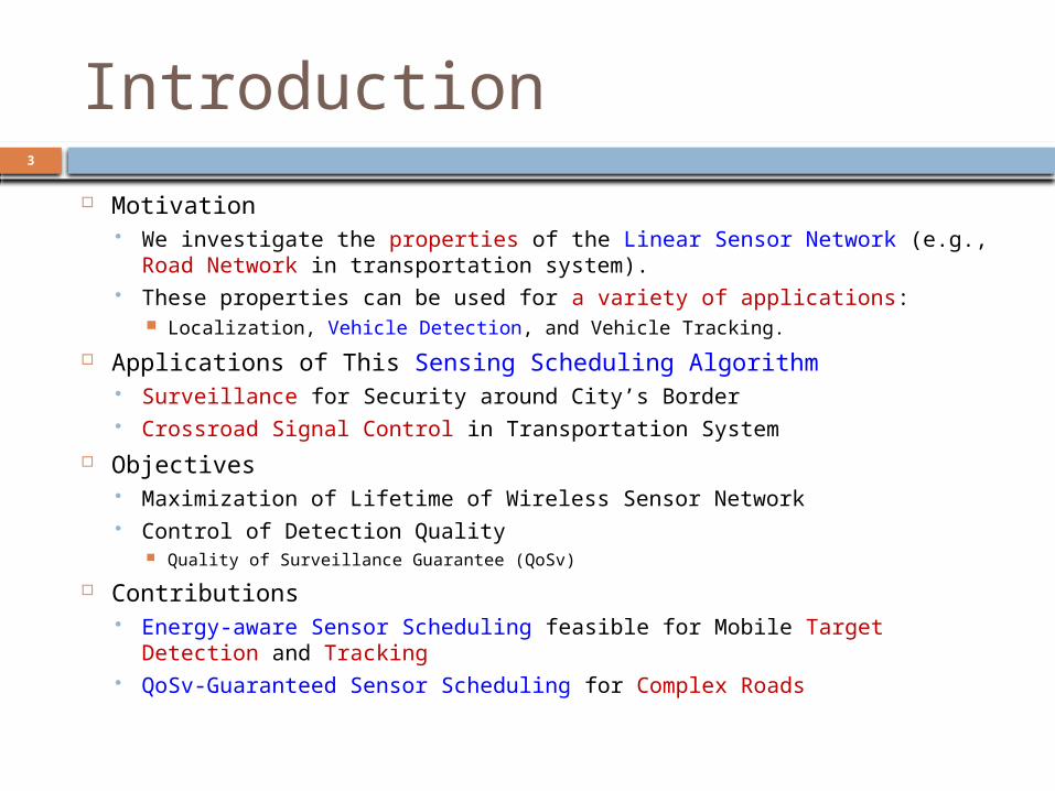
Introduction

Motivation We investigate the properties of the Linear Sensor Network (e.g., Road

Network in transportation system). These properties can be used for a variety of applications:

Localization, Vehicle Detection, and Vehicle Tracking.

Applications of This Sensing Scheduling Algorithm Surveillance for Security around City’s Border Crossroad Signal Control in Transportation System

Objectives Maximization of Lifetime of Wireless Sensor Network Control of Detection Quality

Quality of Surveillance Guarantee (QoSv)

Contributions Energy-aware Sensor Scheduling feasible for Mobile Target Detection and

Tracking QoSv-Guaranteed Sensor Scheduling for Complex Roads

4

Surveillance of City Border Roads (1)

Inner BoundaryCITY

Outer Boundary

5

Surveillance of City Border Roads (2)

Inner BoundaryCITY

Outer Boundary

S1

Road Segment

S2 S3 Sn. . . . .

Sensing Coverage

6

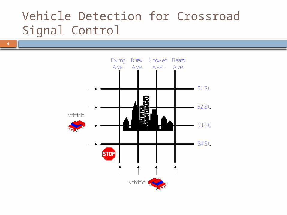
Vehicle Detection for Crossroad Signal Control

54 St.

53 St.

52 St.

51 St.

EwingAve.

DrewAve.

ChowenAve.

BeardAve.

vehicle

vehicle

7

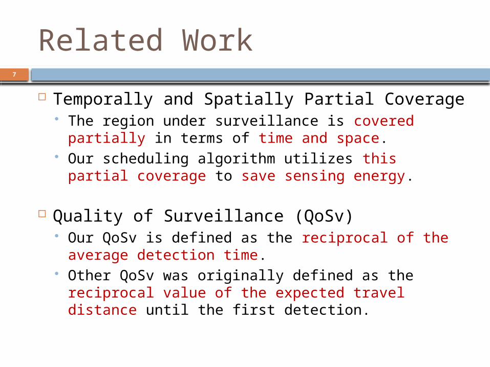
Related Work

Temporally and Spatially Partial Coverage The region under surveillance is covered partially in

terms of time and space. Our scheduling algorithm utilizes this partial

coverage to save sensing energy.

Quality of Surveillance (QoSv) Our QoSv is defined as the reciprocal of the

average detection time. Other QoSv was originally defined as the reciprocal

value of the expected travel distance until the first detection.

8

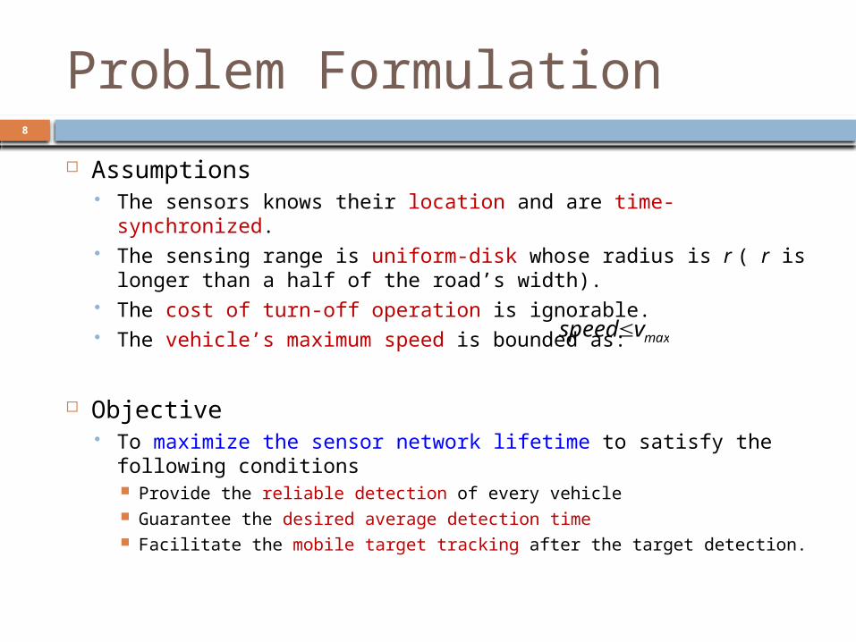
Problem Formulation

Assumptions The sensors knows their location and are time-synchronized. The sensing range is uniform-disk whose radius is r ( r is

longer than a half of the road’s width). The cost of turn-off operation is ignorable. The vehicle’s maximum speed is bounded as:

Objective To maximize the sensor network lifetime to satisfy the

following conditions Provide the reliable detection of every vehicle Guarantee the desired average detection time Facilitate the mobile target tracking after the target detection.

maxvspeed

9

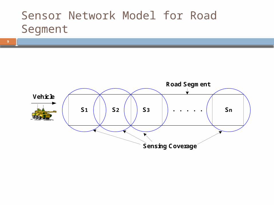
Sensor Network Model for Road Segment

S1

Road Segment

Vehicle

S2 S3 Sn. . . . .

Sensing Coverage

10

Key Idea to This Scheduling

How to have some sleeping time to save energy? We observe that the vehicle needs time l/v to pass

the road segment. Time l/v is the sleeping time for all the sensors on

the road segment.

S1

Road Segment Length = l

Vehicle

S2 S3 Sn. . . . .

Speed = v

11

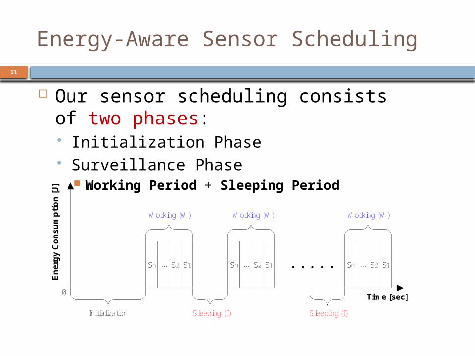
Energy-Aware Sensor Scheduling

Our sensor scheduling consists of two phases: Initialization Phase Surveillance Phase

Working Period + Sleeping Period

sn ... s2 s1

0

sn ... s2 s1

En

erg

y C

on

sum

pti

on

[J]

Time [sec]

Sleeping (I)Initialization

Working (W) Working (W)

. . . . . sn ... s2 s1

Working (W)

Sleeping (I)

12

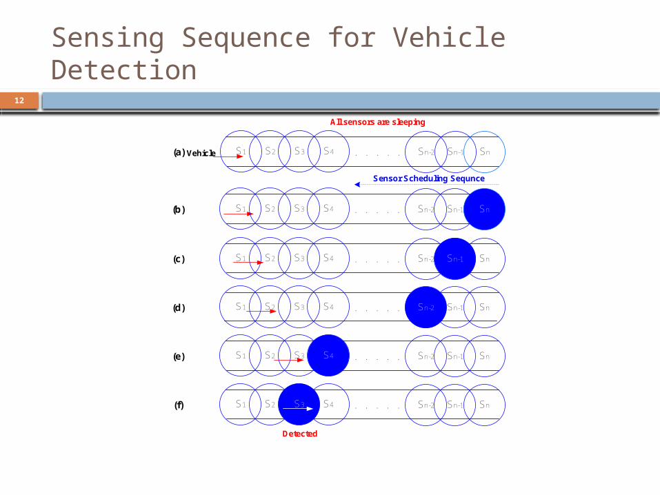
Sensing Sequence for Vehicle Detection

S1 . . . . .(b)

Sensor Scheduling Sequnce

S2 S3 S4 SnSn-1Sn-2

S1 . . . . .(c) S2 S3 S4 SnSn-1Sn-2

S1 . . . . .(d) S2 S3 S4 SnSn-1Sn-2

S1 . . . . .(e) S2 S3 S4 SnSn-1Sn-2

S1 . . . . .(f) S2 S3 S4 SnSn-1Sn-2

Detected

S1Vehicle . . . . .(a)

All sensors are sleeping

S2 S3 S4 SnSn-1Sn-2

13

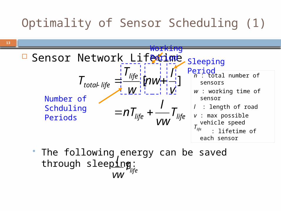
Optimality of Sensor Scheduling (1)

Sensor Network Lifetime

The following energy can be saved through sleeping:

Number of Schduling Periods

Working Period

Sleeping Period

lifelife

lifelifetotal

Tvw

lnT

v

lnw

w

TT

][

lifeTvw

l

n : total number of sensors

w : working time of sensor

l : length of road

v : max possible vehicle speed

: lifetime of each sensor

lifeT

14

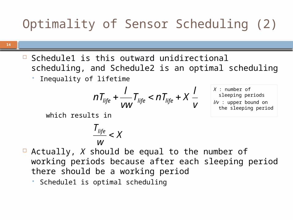
Optimality of Sensor Scheduling (2)

Schedule1 is this outward unidirectional scheduling, and Schedule2 is an optimal scheduling Inequality of lifetime

which results in

Actually, X should be equal to the number of working periods because after each sleeping period there should be a working period Schedule1 is optimal scheduling

v

lXnTT

vw

lnT lifelifelife

Xw

Tlife

X : number of sleeping periods

l/v : upper bound on the sleeping period

15

Considerations on Turn-On and Warming-UP Overheads

Each Sensor’s Lifetime without Sleeping

Sensor Network Lifetime through Sleeping

Case 1: Turn-On Overhead is greater than Sleeping benefit

Case 2: Turn-On Overhead is less than Sleeping benefit

w

EP

ET

ons

life

v

lnw

EwP

ET

onslifetotal

1 where

),(),(

n

Tb

v

lPnE

v

lbtminn

EPbtmin

E

v

lPnE

P

EEn

v

l

T

v

lw

sonons

sons

on

lifetotal

2)(

)(

ons

v

lsonlifetotal

EwP

PnEE

w

T

t : min time needed for each sensor to detect and transmit data

16

QoSv-Guaranteed Sensor Scheduling Average Detection Time for Constant Vehicle

Speed

Approximate Average Detection Time (ADT)

Average Detection Time for Bounded Vehicle Speed

lnwvvlnwv

vlwlnlvnwn

dEvlnw

vldE

vlnw

nwdE IW

2

122 322

v

lADT

2

max

minaa

max

minaa

v

v vItIvt

v

v vWtWvt

dvvpdEdE

dvvpdEdE

)(

)(

,

,

17

Determination of Scheduling Parameters

Scheduling (under sensing error) Parameters are Sensor Network Length (l)

Working Time (w)

Sleeping Time (s)where

m : the number of scanning per working periodPsuccess : the success probability of one scanning

S1

Sensor Network Length

Vehicle

S2 S3 Sn. . . . .

ADTvl 2

1

n

vlTw w

otherwise0

ifv

lPnEmwn

v

ls son

nsuccess pP

m11

18

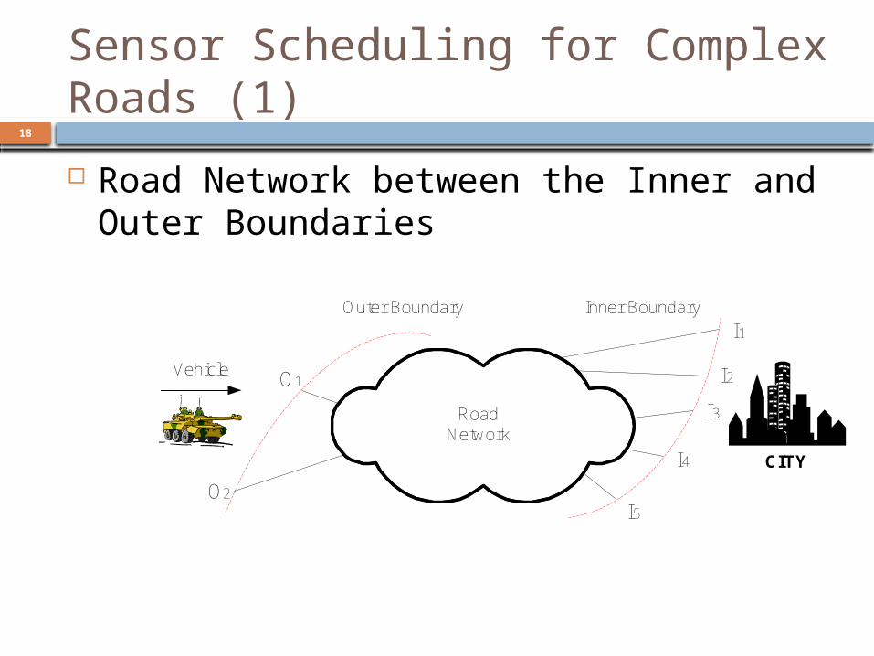
Sensor Scheduling for Complex Roads (1)

Road Network between the Inner and Outer Boundaries

O1

O2

I2

I3

I4

Outer Boundary Inner Boundary

I5

I1

Vehicle

CITY

Road

Network

19

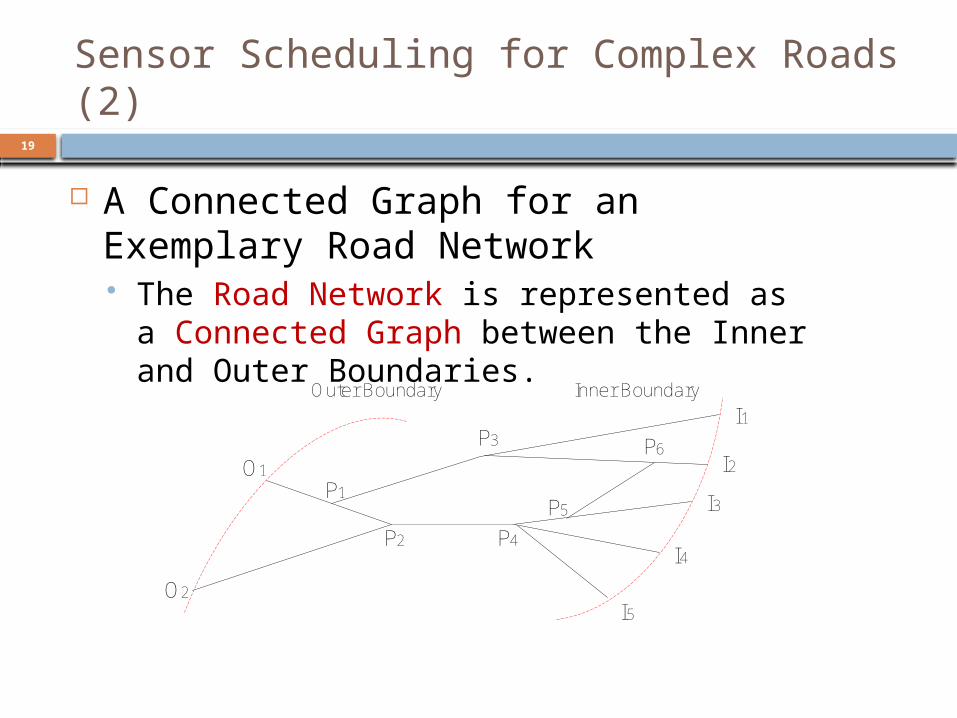
Sensor Scheduling for Complex Roads (2)

A Connected Graph for an Exemplary Road Network The Road Network is represented as a

Connected Graph between the Inner and Outer Boundaries.

O1

O2

I2

I3

I4

Outer Boundary Inner Boundary

I5

P1

P2

P3 P6

P5

P4

I1

20

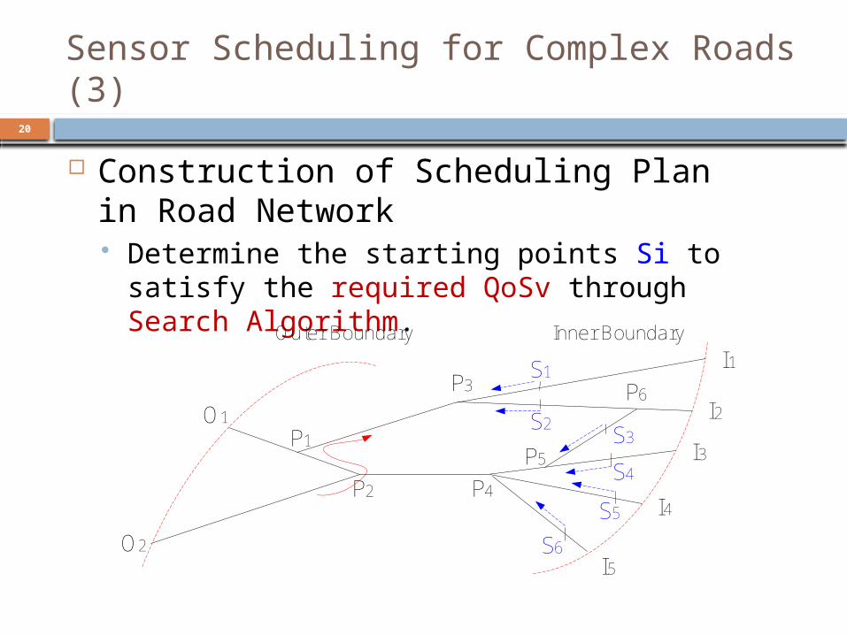
Sensor Scheduling for Complex Roads (3)

Construction of Scheduling Plan in Road Network Determine the starting points Si to satisfy

the required QoSv through Search Algorithm.

O1

O2

I2

I3

I4

Outer Boundary Inner Boundary

I5

P1

P2

P3 P6

P5

P4

I1S1

S2S3

S4

S6

S5

21

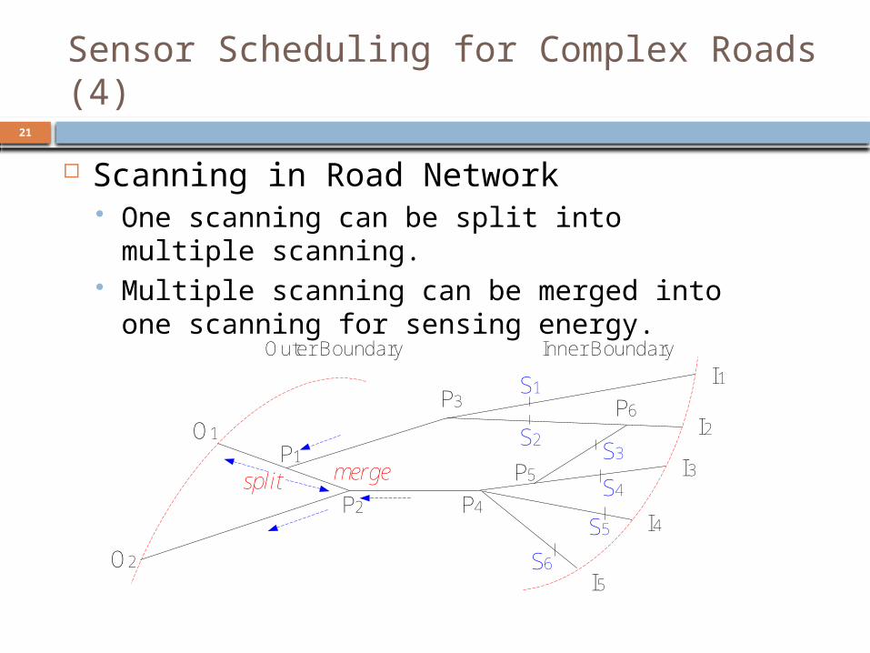
Sensor Scheduling for Complex Roads (4)

Scanning in Road Network One scanning can be split into multiple

scanning. Multiple scanning can be merged into one

scanning for sensing energy.

O1

O2

I2

I3

I4

Outer Boundary Inner Boundary

I5

P1

P2

P3 P6

P5

P4

I1S1

S2S3

S4

S6

S5

split merge

22

Performance Evaluation

Metrics Sensor Network Lifetime according to Working Time

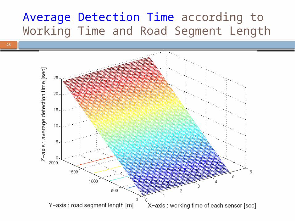
and Turn-on Energy Average Detection Time according to Working Time

and Road Segment Length (i.e., Sensor Network Length)

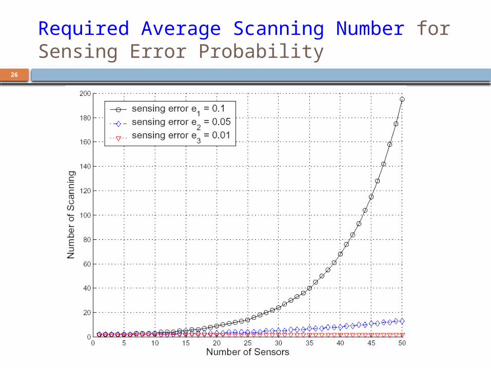
Required Average Scanning Number for Sensing Error Probability

Validation of Numerical Analysis We validated our numerical analysis of our

scheduling algorithm through simulation.

23

Environment for numerical analysis

road segment’s width is 20m, length is 2000m number of sensors is 100 total sensing energy in each sensor is 3600J,

can used continuously for 3600sec since sensing energy consumption rate is 1watts

working time per working period is in [0.1, 5] turn-on energy consumption is

{0,0.12,0.48,0.96}J vehicle’s max speed is 150km/h

24

Sensor Network Lifetime according to Working Time and Turn-on Energy

61036.0

25

Average Detection Time according to Working Time and Road Segment Length

26

Required Average Scanning Number for Sensing Error Probability

27

Conclusion

We proposed an Energy-Aware Scheduling Algorithm to satisfy the required QoSv in Linear Sensor Network. QoSv is defined as the reciprocal value of Average

Detection Time (ADT). Our Algorithm can be used for

Surveillance for City’s Border Roads, and Traffic Signal Control in Crossroads

Future Work Enhance the scheduling scheme when the sensors are

deployed randomly close to the roads Extend the scheme to two-dimensional open field