Energy and Buildings, 13 (1989) 127 - 138 127

Effects of Three Landscape Treatments on Residential Energy and Water Use in Tucson, Arizona*

E. GREGORY McPHERSOI~, JAMES R. SIMPSON** and MARGARET LIVINGSTON t

t School of Renewable Natural Resources, 325 Bio Sciences East, University of Arizona, Tucson, AZ 85721 and

**Department of Soil and Water Science, 439 Shantz, University of Arizona, Tucson, AZ 85721 (U.S.A.)

(Received July 7, 1988; accepted August 11, 1988; revised paper received September 29, 1988)

ABSTRACT

Vegetation can reduce the cooling loads o f buildings in hot arid climates by modi fy ing air temperature, solar heat gain, longwave heat gain, and heat loss by convection. How- ever, savings from reduced mechanical cool- ing may be of fset by increased irrigation

I water costs. In this study, three similar y - scale model buildings were constructed and surrounded with different landscapes: turf, rock mulch with a foundation planting o f shrubs, and rock mulch with no plants. Irriga- tion water use and electricity required to power the three room-sized air conditioners and interior lights were measured for two approximately week-long periods. Electrical energy consumed for air-conditioning by the rock model was 20 - 30% more than for the turf and shade models. Factors accounting for these differences in energy performance include dense shade that substantially re- duced solar heat gain for the shaded model, a 16% difference in longwave radiation flux between the rock and turf treatments, and a max imum drybulb depression o f 4 °C over the turf compared with the rock. Air-condi- tioning savings exceeded water costs for shade treatments that were simulated to receive moderate and low amounts o f irrigation water. These preliminary findings suggest that the localized effects o f vegetation on building

*Contribution to the Hatch project entitled "Im- pacts of Urban Forests in Arizona", University of Arizona Agricultural Experiment Station Journal, Series No. 5072.

microclimate may be more significant than boundary layer effects in hot arid regions.

INTRODUCTION

Trees and green spaces can ameliorate urban climate and enhance the attractiveness and livability of cities [1]. The importance of vegetation as a modifier of mesoclimate has been documented by numerous studies [2 - 4]. For instance, air temperatures in San Francisco's lush Golden Gate Park averaged 8 °C cooler than the less heavily vegetated neighborhoods adjacent to the park [5]. Meso- and microclimate changes can also reduce air-conditioning requirements in hot climates. Plants modify air temperature, solar heat gain, longwave heat gain, and heat loss by convection [6, 7]. Preliminary results f rom computer models showed that an addi- tional 25% increase in the urban tree cover saved 40% of annual cooling energy use for an average home in Sacramento, and 25% in Phoenix [8]. Computer simulations of irra- diance reductions for energy-efficient resi- dences in Tucson and Miami found that dense shade on all surfaces reduced annual cooling costs by $249 (53%) and $235 (54%), respectively [9]. These findings agree closely with results of other studies in warm climates [8, 10 - 12]. Cooling reductions are usually at tr ibuted to microscale phenomena, such as shade from a single tree, that reduce radiation and sensible heat loads near buildings. The cooling effects of evapotranspiration are thought to operate primarily at the mesoscale

0378-7788/89/$3.50 © Elsevier Sequoia/Printed in The Netherlands

128

because the cool air from a solitary tree is diluted and diffused by the large volume of warm air moving through the crown [6]. However, a recent study suggests that this form of latent heat loss may be more impor- tant at the microscale than commonly be- lieved [8].

In water-scarce regions like southern Ari- zona, the energy savings from reduced me- chanical cooling may be offset by increased irrigation water costs. Landscape irrigation accounts for 30 - 50% of the total annual residential water consumption in southern Arizona. Mature trees can require over 325 liters (100 gallons) of water a day to freely transpire in hot weather [13]. At current water prices it would cost about $0.20 a day to water such a tree. Some local governments have instituted water conservation landscape ordinances and incentives to comply with a state law aimed at eliminating groundwater overdraft by 2025 [14]. Most landscape ordinances in southern Arizona regulate the amount of tuff area and use of water-thirsty plants [15]. The City of Mesa, Arizona, offers a 25% landscape rebate ($231) on the residen- tial water development fee if at least 50% of the total landscaped area is covered with inorganic mulch (i.e., decomposed granite) and the majority of plants are low-water-use species [16]. Sometimes new landscapes are devoid of plant materials (Fig. 1), but home- owners are still eligible for the rebate. These "granitescapes" conserve water and reduce maintenance, but they also create hot arid microclimates that can increase building cool- ing requirements. For instance, the conversion of irrigated croplands to largely impervious urbanized landscapes in Phoenix, Arizona, has been associated with large increases in local temperatures and pan evaporation [ 17 ].

In summary, economic and social forces are compelling many residents and businesses to convert from lush to desert landscapes. Although these new landscapes conserve water, they may also increase space-cooling costs because of increased solar heat gain and warmer air temperatures. Reductions in vege- tation may be partially responsible for the growing urban heat islands in Phoenix and Tucson [18]. The primary objective of this s tudy was to quantify and compare energy and water consumption for representative landscapes in Tucson, Arizona. A secondary

Fig. 1. A typical "granitescape" in Tucson, AZ. Lawn and trees have been removed and replaced with rock to reduce water use and landscape maintenance.

objective was to ascertain the magnitude of localized effects of evapotranspirational cool- ing compared with mesoscale effects that have been reported in the literature. Three similar ¼-scale model buildings were surrounded with different landscapes: turf, rock mulch with a foundation planting of shrubs, and rock mulch with no plants. Electricity re- quired to power the three room-sized air conditioners and irrigation water consump- tion were measured during late summer, 1987. Benefits from shade and costs for irrigation water were calculated to determine the cost- effectiveness of each landscape treatment.

Energy transfer processes Replacing a lush landscape containing a

lawn, shrub foundation plantings, and shade trees with a "granitescape" (rock mulch with a few cacti) radically alters the transfer of energy between building and landscape. Changes in energy transfer processes that influ- ence building energy performance include:

(a) changes in solar heat gain due to shade and different albedos of turf and rock;

(2) changes in longwave heat balance due to different ground, building, and vegetation surface temperatures and emissivities, as well as view factor geometries;

(3) changes in drybulb temperature and conductive/convective heat gain due to evapo- transpiration by vegetation; and

(4) changes in air flow and the convective heat balance of a building due to vegetation.

This s tudy focused on assessing the relative importance of the first three processes.

Solar heat gain In ho t arid climates the benefits of shade

are substantial because solar radiation is the principal means of heat gain. When a building is shaded b y vegetation the active heat- absorbing surface is the leaf, which stores relatively little heat. Solar energy is converted to sensible heat that is transferred into the surrounding air, or latent heat that is released during transpiration. Field measurements [4, 11, 19 - 21] and computer simulations [7 - 10, 22] have documented that heat f low into a home and air-conditioning costs may be reduced by 30 - 50% as a result of shade.

Reflected solar heat gain of ten represents 10 - 30% of total solar gain. The albedos of landscape materials vary widely [23, 24]. The albedo of plant materials is generally some- what greater than for darker colored granite rock mulch. Hence, one possible advantage of the "granitescape" is reduced building heat gain from reflected solar radiation.

Longwave heat gain The surface temperature of a rocky desert

landscape can reach 70 °C or above, and this may result in emit ted longwave radiation that reaches 30 - 50% of total incoming radiation [25]. Outgoing radiation from a driveway was measured as 26% more than from a lawn in Weslaco, Texas [25]. Hence, increased out- going radiation from a "granitescape" in- creases the longwave flux to building surfaces. It also increases the sensible heat of air sur- rounding a building, compared to vegetated surfaces. Both effects increase the inside- outside temperature gradient and the rate of building heat gain.

Foundat ion plantings and overhanging trees will also retard building heat loss by obscuring the cool night sky [26]. Data suggest that reduced solar heat gains f rom tree shade out- weigh the effects of reduced heat loss at night [21].

Evapo transpiration Vaporization of moisture from well-irrigated

turfgrass can reduce air temperature at 2 m by as much as 7 °C compared to a dry soil surface [27]. The latent heat flux for an irri- gated lawn can exceed net radiation during the af ternoon and early evening [28]. Radiant energy and sensible heat from the surface atmosphere provide the energy required to

129

support large latent heat flux densities. In non-homogeneous urban areas, plant evapora- transpiration is enhanced by advection of sensible heat from drier surrounding surfaces [28 - 30]. In these "microoases" actual evapo- transpiration can markedly exceed the poten- tial value. Evaporative cooling from urban green-space can provide local amelioration from urban heat-island influences and reduce energy required for space cooling of residen- tial buildings [8, 28] . However, in Tucson this effect may not be as important as expected because deficit irrigation is common and vege- tat ion is seldom freely transpiring. Researchers have only recently begun to measure water use and evapotranspiration rates for landscape plants in the Southwest .

METHODS

Building characteristics Three similar ¼-scale-model residential-type

buildings were constructed at the University of Arizona Campus Agricultural Center in Tucson (Fig. 2). Models were centered in 15.3 m × 15.3 m plots, and sized so that small room-sized air conditioners would provide efficient cooling. With a few exceptions, the model buildings were designed to be similar to newly constructed homes in the area based on results of a local survey of new construc- tion [31]. Each building had 11 m 2 of floor area and the longest wall was oriented 16 de- grees east of true south to conform to the available space. East- and west-facing walls were 3 m long and n o r t h - a n d south-facing

i il iii !

i ii ii iiiii!!il iiiiiiii!i ,!? ii!i i i

Fig. 2. The ~-scale model buildings and landscape treatments: from foreground to background: turf, shade and rock.

130

wails were 3.7 m long. Exterior wood frame walls had an overall thermal transmittance value (U) of 0.49 W m -2 K -1 and were con- structed of plywood siding, sheathing, fiber- glass batt insulation, and drywall. The pitched roofs (18 °) were covered with asphalt shingles and had composite U-values of 1.78 W m -2 K -1 . The ceiling had a composite U-value of 0.2 W m -2 K -1 , and two layers of fiberglass insulation. Overhangs on the south and north sides were 19 cm long. The foundations were 10-cm standard-weight concrete slabs covered by carpets. Access to the inside of the models was through small doors in the north wails. Models were painted light gray.

Single-pane windows were centered in south-, east-, and west-facing walls. Glazing in the south wail represented 12% of that wall's total surface area, and east and west glazing represented 15% of each waifs surface area. Full-sized homes have similar ratios as these, but the absence of windows in the models' north walls resulted in a lower than normal ratio of total glazing to floor area (6.5%). Each window contained 0.23 m 2 of glazing with an estimated U-vaiue of 9 W m -2 K -1 . Windows could be opened for ventilatiori but remained closed during this study.

Building operating conditions Emerson room air conditioners (Model

8LJ9H) were set in the north-facing walls. The air conditioners had a rated coefficient of performance of 2.1 and a cooling capacity of 2345 W. A 300-watt light bulb was placed in the ceiling of each building to simulate internal heat gains from occupants, appliances, and lights. It operated 24 hours each day.

The amount of thermal mass placed inside each model related to the scaling factor, and this factor varied depending on the measure of interest. For linear calculations it was 1:4, for area it was 1:16, and for volume it was 1:64. Relatively greater thermal mass in the models compensated for their increased sur- face area (1:16) to volume (1:64) ratio com- pared to the full-sized building [32]. The interior heat capacity of the full-sized house was estimated by calculating the mass (kg) and specific heat (J/kg K) of typical materials such as walls, furniture, and appliances. The heat capacity of the model was 1/16 the heat capacity of the full-sized house, or 0.8 J K. This heat capacity was supplied in each model

by fifty, one-gallon plastic milk jars contain- ing a total of 189 liters of water.

Landscape treatments Three landscape treatments were installed

in early June, 1987 (Fig. 2). Each 15.3 m × 15.3 m plot surrounded a model. The first t reatment was a seeded Bermuda grass lawn. The turfgrass plot was irrigated dally from 03:00 to 04:00 with an automatic sprinkler system. The water application rate was mea- sured with catch-cans and found to be 1.27 cm per day, which is typical for this area. Turf was mowed weekly once established.

The second treatment consisted of 18 shrubs placed within 0.5 m of each exterior wall, and a 5-cm layer of dark red decom- posed granite spread over the remaining area. Five 0.9-m-tall hopbush shrubs (Dodonea viscosa 'Purpurea') were located 0.75 m apart opposite the east- and west-facing walls. Three slightly larger (1.2-m-tall) privet (Ligustrum lucidum) and two bottle brush (Callistemon citrinus) were placed 1.0 m apart opposite the south-facing wall. Three 1.2-m-taU olean- der (Nerium oleander) were spaced about 2 m apart opposite the north-facing wall.

Each wall of the shade model was photo- graphed to estimate irradiance reductions from the shrubs. Slides were projected on tracing paper and non-shaded areas outlined and measured with a planimeter. The mea- sured areas were summed and divided by the total wall area. The reciprocal of these values represented the fraction of irradiance blocked by shrubs for each wall. Irradiance reductions for the shaded model's walls (the roof was not shaded) were estimated as follows:

(1) south wall = 0.92 (2) west wall = 0.78 (3) east wall = 0.86 (4) north wall = 0.25.

Thus, these shrubs can be characterized as moderate-to-low water-use species casting relatively dense shade on the model's walls. The shrubs were irrigated two hours each night and one hour each day with drip irriga- tion on a separate valve from the turf. Approx- imately 16.4 liters were applied dally to each plant. This shrub irrigation rate was about four times the normal application rate because they remained in containers for much of the study [13].

The third t reatment consisted of a 0.5-cm layer of dark red decomposed granite wi thout vegetation. There was no irrigation. In subse- quent discussion we refer to landscape treat- ment effects for each model using the follow- ing terms: turf model, shade model, and rock model.

Data collection Interior and exterior air temperatures were

measured with Campbell Scientific Model 107 Temperature Probes and recorded every 15 min using Campbell Scientific CR21 Data Loggers. The outside temperature probes were located at a height of 0.7 m above the ground in full shade under the north over- hang of each model.

Hourly exterior wall, roof, and soil temper- atures were measured manually using an in- frared thermometer (Everest Interscience Model 110) from 06:00 to 21:00 on July 6, August 6, and October 2, 1987. We report data from October 2 because of warm tem- peratures and clear sky conditions on this day.

Additional microclimatic data collected at the s tudy site using a Campbell Scientific 21X data logger included:

(1) horizontal solar radiation (Star pyrano- meter);

(2) outside air temperature and relative humidi ty (Campbell Scientific Model 207 Temperature and Relative Humidi ty Probes);

(3) wind direction (Met-One Model 024A Sensor);

(4) wind speed (Met-One Model 014A Sensor), and

(5) net radiation (Micromet Systems Model Q3).

These data were supplemented with more extensive AZMET weather-station data col- lected 360 m from the site.

Energy and water use calculations Kilowatt-hour use in each model was con-

t inuously recorded and stored using a cali- brated Westinghouse watt-hour meter pro- vided by Tucson Electric Power Co. (TEP). We present hourly averages of electricity use from these data. Electricity costs were calcu- lated using TEP's 1987 residential price of $0.08 per kWh.

Water use was calculated based on measure- ments of actual application using catch-cans. Turf water use was calculated as 5% greater

1 3 1

than the amount applied to account for wind and evaporation losses. This correction was not applied to the drip-irrigated shrubs.

In addition to actual application rates, three simulated rates were used in subsequent analysis, for a total of five: two for turf and three for the shrubs. Water consumption rates for turf were based on (1) the actual applica- tion rate plus 5% (1.33 cm/day); and (2) a lower rate (0.58 cm/day average) based on the daffy mean AZMET reference evapotrans- piration (RET) for the study days. The RET rate is an index of potential evapotranspira- tion for well-watered rye grass 8 - 15 cm high. RET is calculated hourly using weather data located 360 m west of the s tudy site. A 0.80 crop coefficient was assumed for Bermuda grass because it is shorter and uses water more efficiently than rye grass [33].

The three application rates used for shrubs were:

(1) the actual application rate (16.3 1/plant per day);

(2) a lower rate typical of moderate water- use species (4.9 l/plant per day) [34]; and

(3) the lowest rate typical of low water-use species (2.2 1/plant/day)[34/.

Water costs were based on Tucson Water's 1987 summer block rates. Irrigation water was priced at $0.52/m 3 ($1.47/Ccf (hundred cubic feet)), the cost for water used in the block of 42 - 57 m 3 (15 - 20 Ccf).

RESULTS AND DISCUSSION

Building and equipment calibrations Initial experiments were conducted prior

to installation of the landscape treatments to test for similarity among models and cooling systems. The methods and findings of this pilot work are detailed in a technical report [32] and summarized below.

Inside air temperatures were compared prior to landscape t reatment installation to determine if the models were thermodynam- ically similar. We found a maximum inside temperature difference between models of +0.7 °C, with the mean differences being 0.18 + 0.23 °C and 0.38 + 0.17 °C between the rock and turf and the rock and shade models, respectively. Inside temperatures were not significantly different at the p = 0.5 level.

132

Pre-treatment environmental air and sur- face temperatures were compared to deter- mine if model microclimates were similar. There was a +1.0 °C outside temperature dif- ference across models. The pre-turf site was cooler than the other sites in early morning. This may be due to enhanced nocturnal heat loss from the loose loam soil compared to the compacted fill around the other two models. Statistical analysis showed no significant dif- ference among outside wall, roof, and ground surface temperatures measured manually with the IRT (p = 0.05).

The suitability of using meteorological data from the nearby AZMET weather station to describe conditions at the study site was tested using data collected for two warm clear-sky days (June 3 - 4) at both locations. Coefficients of determination (r 2) for the resulting regression analysis were greater than 0.90 except for relative humidity, which was r 2 = 0.86. Advection of moist air at the AZMET site was probably responsible for this difference.

Prior to landscape installation, the air con- ditioners were turned on and thermostats set and adjusted so that models were maintaining similar inside temperatures of 25.5 °C. An analysis of inside air temperature data indi- cated that temperatures deviated by less than +1 °C from 25.5 °C.

Manual readings from the kilowatt-hour meters were compared for five days prior to installation of landscape treatements to deter- mine if air conditioners were performing with similar efficiency. There was a 2 - 4% differ- ence in kWh use across models.

Analysis of electricity use during non- cooling periods showed that the total base load for models was a constant 0.38 kW due to the light bulb (0.30 kW) and fan inside the air conditioner (0.08 kW).

Results described above indicate that land- scape t reatment effects were primarily respon- sible for differences in electrical energy use across models.

Long- t e rm electrical use Electrical energy consumption was moni-

tored for each model for the period July 22 to October 14, 1987. Total electrical use (air- conditioning and lighting) for two approxi- mately week-long periods, when watt-hour meters and air-conditioning units were func-

0 . 9

0 . 8

0 . 7

kW 0 . 6

0 . 5

0.4

(a)

- -TuPf

--- Shade _ --

i I t I D-25 B-26 8-27 B-2O 8-29 8-30 8 -3 t 9 - t

Date

0 . 9 - - Tur'f ... Shade

O.D - - Rock

0.7

kN 0.6

0.5

0.4

0.3 ~ ~ t0-3 ~ ~ t t L t 10-t 10-2 10-4 t0-5 t0 -6 10-7 10-8

(b) Dot,

Fig. 3. Elec t r ica l u s e f o r t h e t h r ee mode l s .

40

35

30 Telm

(C) 25

20

15

(a) t I

8-25 6-26 0-27 L I I

• 8-28 8-29 Dote

I t i 8-30 8 -3 t u 9 - t 9-2

4 0 .

Tern 30.

(c) 25~

20.

t5,

io

(b)

I ) I i t

tO-t t0 -2 iO-3 i0-4 10-5

Date

I i i

t0 -6 10-7 t0-8

Fig. 4. Air t e m p e r a t u r e s m e a s u r e d a t t h e A Z M E T w e a t h e r s t a t i o n f o r t h e s t u d y per iods .

tioning properly, is plotted in Fig. 3. Total energy use for these periods and energy use as a percentage o f the rock-treatment energy use are found in Table 1. Comparisons were made of air-conditioning energy use by removing the 0.38 kW base load (Table 1). To aid in comparison, information on air temperature and solar radiation are included in Table 2 and Fig. 4. Radiation plots are not included

133

TABLE 1 Electrical and air-conditioning (AC) usage for August 25 to September 1 and October 1 - 8, 1987, for three land- scape treatments

Analysis August 25 - September 1 October 1 - October 8

Turf Shade Rock Turf Shade Rock

Total electrical (kWh) 104.2 102.4 111.9 100.3 AC electrical (kWh) 31.2 29.4 38.9 27.3 AC daily average (kWh) 3.9 3.7 4.9 3.4 AC savings from rock (kWh) 7.7 9.5 -- 11.8 AC percent savings (%) 19.8 24.3 - - 30.1

101.3 112.] 28.4 39.1

3.6 4 .9 10.7 27.5

TABLE 2 Average dally air temperature and solar radiation for August 25 to September 1 and October 1 - 8, 1987 (AZMET data)

Time Air Solar period temperature radiat ion

( ° c ) (MJ m - 2 )

8/25 - 9/1 27.4 22.4 10/1 - 10/8 25.7 20.3

since plots for successive days in each period were almost identical due to clear sky con- ditions.

Comparison of electrical use between treat- ments revealed that the tuf f and shade models had approximately the same energy use for the sample periods, while the rock-treatment model used 20 - 30% more energy for air- conditioning. For the earlier period, total solar radiation load measured on a horizontal surface was larger, and daily average energy consumption was greater. However, the differ- ence between peak loads for the rock and shade models was greater during early October than in late August (Fig. 3). This result may be due to increased solar heat gain because of a lower sun angle. At solar noon, the south- facing windows were almost entirely shaded by the overhangs on August 25, but only about 50% shaded on October 2.

Another possible explanation for this dif- ference in peak loads may be differences in nighttime temperature minimums and the magnitude of internal heat gain. Maximum air temperatures were within 2 - 3 °C for the two periods, while the minimums in October were lower by about 5 °C. This resulted in minimal air-conditioner operation for periods of one to four hours during the night for the

turf and shade models in October (Fig. 3). The effect is most pronounced for the turf t reatment. Nighttime minimum for tu f f mea- sured at 0.7 m height ranged up to 2 °C lower than for rock. These periods of air-conditioner shutdown in October reduced the air-condi- tioning load for turf and shade treatments with respect to rock compared to the August period (Table 1), when nighttime electrical loads were much closer in magnitude across treatments (Fig. 3). Assuming that this anal- ysis is correct, the large value of internal heat gain simulated by the 300 W light bulb may have biased the results by generating enough heat to require air-conditioner operating throughout the night. A smaller, more reason- able internal heat gain would result in air- conditioner shutdown during weather typical of August. This might result in closer agree- ment of tuff / rock and shade/rock percentages from August to October.

24-hour electr ical use Hourly measurements of microclimatic

variables were taken around each model on October 2 to better explain differences in electrical use for cooling. On October 2, ambient temperatures recorded at the nearby AZMET weather station ranged from 22 °C to 33 °C, and it was a cloudless day. Relative humidi ty averaged 56% from midnight to 11:00 and then dropped to about 10%, where it remained through midnight. Increased wind speed accompanied this midday weather change. The average wind speed changed from 1.3 m s -1 before 11:00 to 5.1 m s -1 from 11:00 to midnight.

The same energy-use trends noted for the two separate periods were" also evident for the October 2 data (Fig. 5). The rock model used 28% (1.35 kWh) and 29% (1.39 kWh)

134

0 . | .

0.7-

0.6-

kW

0 . 5

0.4

0.31 ;

-- Turf +Shade J

: : : : ; " ~ : : : : : ." " " : : " : " " I I 3 5 7 9 i i 13 f f i 17 [ 9 ~ D

- Hour Fig. 5. Electr ical use for t he th ree mode l s o n O c t obe r 2, 1987 .

more electricity for air-conditioning than the turf and shade models, respectively. The largest dayt ime percent differences in elec- trical use for cooling were 30% and 33% for the turf and rock models (at 14:00) and the shade and rock models (at 17: 00), respectively.

Solar heat gains Dense shade reduced solar heat gain on

windows and opaque wall surfaces of the shaded model. For example, at 08:00 there was a 24 °C difference between surface tempera- tures for shaded and unshaded east walls (shade and tuff models, Fig. 6). At 15:000 the peak west-wall temperature was 17 °C cooler for the shaded model than the rock model (Fig. 6). It should be noted that the shrubs effectively reduced both direct beam and diffuse radia- tion because they were immediately adjacent to the walls. Shrubs located further away from the wall would no t at tenuate as much diffuse or direct solar radiation. The diffuse compo- nent accounted for only 10% of the total in- coming shortwave radiation on October 2 (Table 3), but is relatively more important on c loudy days.

Reflected solar radiation accounted for 28% and 22% of the total incoming shortwave

~- +EWalI-TuPf -*-EWall-Sllade

m, --WWall-Turf m ~ -~HNall-Shade

TemP(c) m ~ ~ ÷ N N a l l - F l ° c k

H0ur Fig. 6. Temperatures of shaded and unshaded walls and the AZMET air temperature for October 2, 1987.

solar flux (209.7 MJ m -2) measured at the turf and rock sites, respectively (Table 3). Albedo for the tuf f ranged from 0.26 to 0.43, and values for the rock ranged from 0.21 to 0.30, with larger values occurring in the morning and afternoon for low sun angles. Hourly differences between the albedo of tuf f and rock ranged from 0.05 to 0.11. Differ- ences in albedo resulted in a maximum flux density difference of 43 W m -2 measured above and parallel to the ground (Fig. 7). A smaller difference in reflected solar heat gain is expected for vertical walls because only about half of the measured reflected radiation would strike the wall.

Longwave heat gains Landscape treatments affected ground sur-

face temperatures and outgoing radiation fluxes (as measured horizontally and above the tuff and rock on October 2). The surface temperature of the rock reached 45 °C and was as much as 14 °C warmer than the tuf f (Fig. 8). Average surface temperatures were 24.7 °C, 32.3 °C, and 31.6 °C for the tuff, shade, and rock treatments. The outgoing longwave radiation was 59% and 68% of the total incoming radiation for the tuf f and rock

T A B L E 3

Rad ia t i on ba lances for l andscape t r e a t m e n t s O c t obe r 2, 1987 - - h o r i z o n t a l sur face (MJ m -2 )

T r e a t m e n t Q Kdn D Kdn - - D Kup Lo* L i*

Tu r f 11 .64 20 .73 2.05 18 .65 5 .89 24 .23 22 .98 Rock 7 .48 20 .73 2 .05 18 .65 4.52 28 .05 23 .78

*Based o n m e a s u r e m e n t s t a k e n f r o m 0 6 : 0 0 to 2 1 : 0 0 . Q = ne t r ad ia t ion ; Kdn ffi i ncoming solar r ad ia t ion ; D = dif fuse r ad ia t ion ; Kdn - - D ffi i ncoming d i rec t b e a m solar; Kup = re f lec ted solar r ad ia t ion ; Lo ffi ou tgo ing longwave rad ia t ion ; L i = i ncoming longwave rad ia t ion .

135

H o u r 4 0 .

! $ S 7 | l i is iS 17 iS ~j, n

. ~ .~ ~ -q- KUp / rock Tell) W/N'2-~ ~ ÷ Lo (C)

. 4o l ~ _ . tu r f I

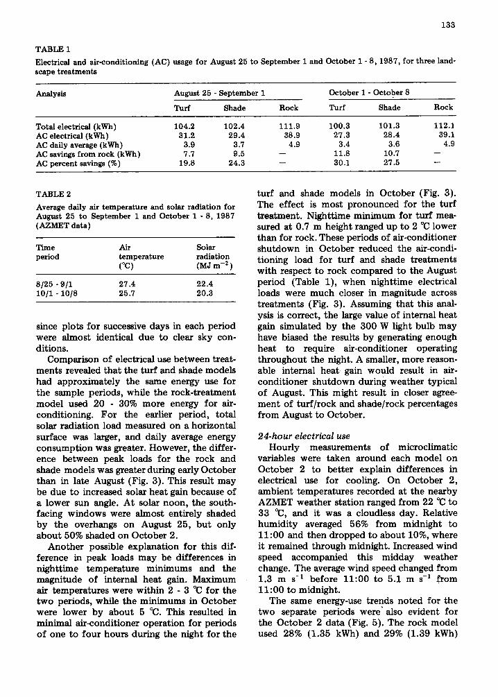
Fig. 7. Outgoing longwave radiation fluxes (Lo turf and Lo rock) and reflected solar radiation fluxes (/[up turf and Kup rock) for the turf and rock treatments on October 2, 1987.

Turf ~- Shade

J O . : : : : : : : : : " I I I I I I : : : : : " : $ U 7 9 l i 13 i s | 7 19 IU, 25

Hour Fig. 9. Outside air temperatures measured at 0.7 m and the AZMET air temperature on October 2, 1987.

45,

m, Telp (c) -.

CO.

6 ; ; ; ; ; : " " : " ~ I I I I 7 i l 9 10 I t ~ is 14 iS is 17 i s i s 10 P !

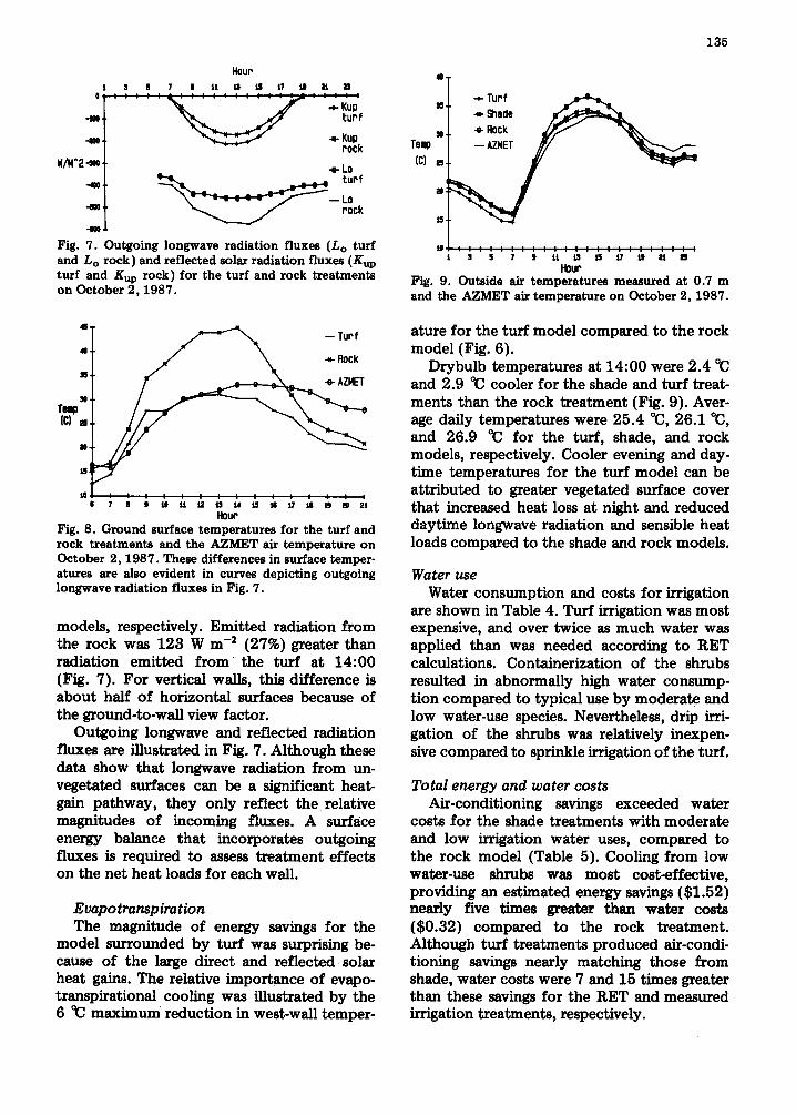
Hour Fig. 8. Ground surface temperatures for the turf and rock treatments and the AZMET air temperature on October 2, 1987. These differences in surface temper- atures are also evident in curves depicting outgoing longwave radiation fluxes in Fig. 7.

models, respectively. Emitted radiation from the rock was 123 W m -~ (27%) greater than radiation emitted f r o m the turf at 14:00 (Fig. 7). For vertical walls, this difference is about half of horizontal surfaces because of the ground-to-wall view factor.

Outgoing longwave and reflected radiation fluxes are illustrated in Fig. 7. Although these data show that longwave radiation from un- vegetated surfaces can be a significant heat- gain pathway, they only reflect the relative magnitudes of incoming fluxes. A surface energy balance that incorporates outgoing fluxes is required to assess treatment effects on the net heat loads for each wall.

Evapo transpiration The magnitude of energy savings for the

model surrounded by turf was surprising be- cause of the large direct and reflected solar heat gains. The relative importance of evapo- transpirational cooling was illustrated by the 6 °C maximum reduction in west-wall temper-

ature for the turf model compared to the rock model (Fig. 6).

Drybulb temperatures at 14:00 were 2.4 °C and 2.9 °C cooler for the shade and turf treat- ments than the rock treatment (Fig. 9). Aver- age daily temperatures were 25.4 °C, 26.1 °C, and 26.9 °C for the turf, shade, and rock models, respectively. Cooler evening and day- time temperatures for the turf model can be attributed to greater vegetated surface cover that increased heat loss at night and reduced daytime longwave radiation and sensible heat loads compared to the shade and rock models.

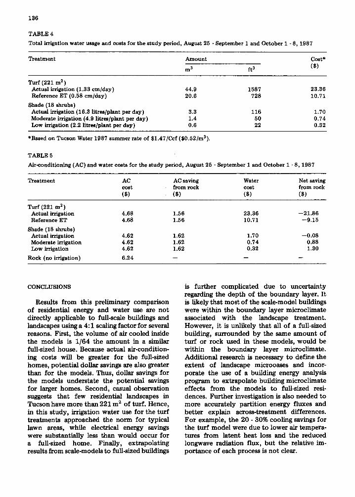
Water use Water consumption and costs for irrigation

are shown in Table 4. Turf irrigation was most expensive, and over twice as much water was applied than was needed according to RET calculations. Containerization of the shrubs resulted in abnormally high water consump- tion compared to typical use by moderate and low water-use species. Nevertheless, drip irri- gation of the shrubs was relatively inexpen- sive compared to sprinkle irrigation of the tuff.

Total energy and water costs Air-conditioning savings exceeded water

costs for the shade treatments with moderate and low irrigation water uses, compared to the rock model (Table 5). Cooling from low water-use shrubs was most cost~ffective, providing an estimated energy savings ($1.52) nearly five times greater than water costs ($0.32) compared to the rock treatment. Although turf treatments produced air-condi- tioning savings nearly matching those from shade, water costs were 7 and 15 times greater than these savings for the RET and measured irrigation treatments, respectively.

136

TABLE 4

Total irrigation water usage and costs for the study period, August 25 - September 1 and October 1 - 8, 1987

Treatment Amount

m 3 ft 3

Cost* ($)

Turf (221 m s) Actual irrigation (1.33 cm/day) Reference ET (0.58 cm/day)

Shade (18 shrubs) Actual irrigation (16.3 litres/plant per day) Moderate irrigation (4.9 litres/plant per day) Low irrigation (2.2 litrea/plant per day)

44.9 1587 23.36 20.6 728 10.71

3.3 116 1.70 1.4 50 0.74 0.6 22 0.32

*Based on Tucson Water 1987 summer rate of $1.47/Ccf ($0.52/m3).

TABLE 5

Air-conditioning (AC) and water costs for the study period, August 25 - September 1 and October 1 - 8, 1987

Treatment AC AC saving Water Net saving cost from rock cost from rock ($) ($) ($) ($)

Turf (221 m s) Actual irrigation 4.68 1.56 23.36 --21.86 Reference ET 4.68 1.56 10.71 --9.15

Shade (18 shrubs) Actual irrigation 4.62 1.62 1.70 --0.08 Moderate irrigation 4.62 1.62 0.74 0.88 Low irrigation 4.62 1.62 0.32 1.30

Rock (no irrigation) 6.24 -- -- --

CONCLUSIONS

Results f rom this preliminary comparison of residential energy and water use are not directly applicable to full-scale buildings and landscapes using a 4:1 scaling factor for several reasons. First, the volume of air cooled inside the models is 1/64 the amount in a similar full-sized house. Because actual air-condition- ing costs will be greater for the full-sized homes, potential dollar savings are also greater than for the models. Thus, dollar savings for the models understate the potential savings for larger homes. Second, casual observation suggests that few residential landscapes in Tucson have more than 221 m 2 of turf. Hence, in this study, irrigation water use for the turf treatments approached the norm for typical lawn areas, while electrical energy savings were substantially less than would occur for a full-sized home. Finally, extrapolating results from scale-models to full-sized buildings

is further complicated due to uncertainty regarding the depth of the boundary layer. It is likely that most of the scale-model buildings were within the boundary layer microclimate associated with the landscape treatment. However, it is unlikely that all of a full-sized building, surrounded by the same amount of turf or rock used in these models, would be within the boundary layer microclimate. Additional research is necessary to define the extent of landscape microoases and incor- porate the use of a building energy analysis program to extrapolate building microclimate effects from the models to full-sized resi- dences. Further investigation is also needed to more accurately partition energy fluxes and bet ter explain across-treatment differences. For example, the 20 - 30% cooling savings for the turf model were due to lower air tempera- tures from latent heat loss and the reduced longwave radiation flux, bu t the relative im- portance of each process is not clear.

137

Despite the shortcoming noted above, the results of this study are of value because few other studies have measured the effects of landscape treatments on building energy use in a controlled fashion. The results also show that longwave estimates should be improved. A surprising result of this study was the 16% difference between longwave radiation fluxes for the tuff and rock treatments. Currently, most building energy analysis models use simplifying assumptions to estimate net long- wave gain or loss to building walls, and this flux is least accurately estimated by urban climate models [35]. It may be desirable to incorporate an outside temperature correc- tion for the longwave component in building energy performance calculations. The temper- ature correction might result in more accurate performance estimates, especially in hot arid climates, where surface materials other than tuff often surround buildings.

Findings of this study also indicate that the localized effects of vegetation on building energy use can be as important as mesoscale effects on the urban heat island. The similar performance of models surrounded by tuff and shrubs was surprising, and suggests that evapotranspirational cooling is significant at the microscale. Huang and others [8] found a maximum drybulb depression in Phoenix of 2 °C for a 25% increase in canopy cover using an empirical evapotranspiration model. Their model assumed mixing of the entire boundary layer, and they noted that larger temperature reductions may exist within a building microclimate. A maximum drybulb depression of 4 °C found in this study sup- ports their hypothesis that localized effects may exceed their estimates because of uneven temperature distribution.

It appears that relatively small vegetated areas may have a substantial impact on build- ing microclimate. Each microoasis diverts radiant input from sensible to latent heat. This process is often accompanied by advec- tion of sensible heat from the roads, alleys, and other non-vegetated surfaces that define the border of each microoasis. Because hedges, patio walls, trees, and buildings reduce the convective diffusion of cool air, each micro- oasis may at times be like a bubble that par- tially bathes a building in cooler air. The cumulative effect of these semi-solitary micro- oases on neighborhood mesoclimate may be

less significant than their individual effects on building microclimates and energy perfor- mance.

Finally, information presented on potential energy/water savings is an important first step in the development of landscape design guide- lines that incorporate concern for conserva- tion of both resources. Savings found in this study are conservative estimates. Well-estab- lished tuff and shrubs would require less water than we applied. Potential savings associated with shade and evapotranspiration from trees were not investigated, but could be greater than we report for shrubs. Trees can shade roof as well as wall surfaces. Arid-adapted tree species require infrequent irrigation after establishment, especially if stormwater runoff is diverted from the roof and other impervious surfaces to planting areas. Designers and home- owners interested in conserving both water and energy should avoid "granitescapes", at least near the house, and instead use desert trees, shrubs, and vines to create cool and shady microoases around buildings. The role of tuff in desert landscapes is less clear. Many people find that lawns provide needed areas for play, cooling the air, and are aesthetically appealing. More studies are needed to deter- mine the optimum size and location for turf- grass areas in water-scarce regions.

ACKNOWLEDGEMENTS

The authors are indebted to Tucson Electric Power for their equipment and support. The project was supported in part by Argonne National Laboratory, Energy and Environ- mental Systems Division, and the U.S. Depart, ment of Energy.

REFERENCES

1 A. Bernatzky, The contribution of trees and green spaces to a town climate, Energy Build,, 5 (1982) 1 -10.

2 L. O. Myrup, .A numerical model of the urban heat island, J. Appl. Meteorol., 8 (1969) 908 - 918.

3 J. J. Flynn, Point pattern analysis and remote sensing techniques applied to explain the form of the urban heat island, Ph.D. Dissertation, College of Environmental Science and Forestry, State University of New York, Syracuse, 1979.

4 C. E. McGinn, The microclimate and energy use in suburban tree canopies, Ph.D. Dissertation, University of California, Davis, 1983.

1 3 8

5 F. S. Duckworth and J. S. Sandberg, The effects of cities upon horizontal and vertical tempera- ture gradients, Bull. Am. Meteoroiog. Soc., 35 (1954) 198 - 207.

6 B. A. Hutchison, F. G. Taylor, R. L. Wendt and the Critical Review Panel, Use of Vegetation to Ameliorate Building Microclimates: An Assess- ment of Energy Conservation Potentials, PubL No. 1913, Environmental Sciences Division, Oak Ridge National Laboratory, 1982.

7 H. Akbari, J. Huang and H. Taha, The Wind- Shielding and Shading Effects of Trees on Resi- dential Heating and Cooling Requirements, Tech- nical Report No. 24131, Lawrence Berkeley Laboratory, CA, 1987.

8 Y. J. Huang, H. Akbari, H. Taha and A. H. Rosen- feld, The potential of vegetation in reducing summer cooling loads in residential buildings, J. Climate Appl. Meteorol., 26 (1987) 1103 - 1116.

9 E. G. McPherson, L. P. Herrington and G. M. Heisler, Impacts of vegetation on residential heating and cooling, Energy Build., 12 (1988) 41 - 51.

10 D. E. Buffington, Economics of residential land- scaping for energy c o n s e r v a t i o n - - a statewide program, Proc. Florida State Horticultural Soc., 94 (1981) 208 - 216.

11 J. H. Parker, Landscaping to reduce the energy used in cooling buildings, J. Forestry, 81 (2) (1983) 8 2 - 84.

12 R. L. Thayer, Jr. and B. Maeda, Measuring street tree impact on solar performance: a five climate computer modeling study, J. Arboriculture, 11 (1) (1985) 1 - 12.

13 Water Conservation for Domestic Users, City of Tucson, Arizona.

14 Management goals for initial active management areas, Arizona Revised Statutes, 1980, Section 45 - 562.

15 Landscaping, Buffering and Screening Standards, and Landscape Design Manual, Pima County Zoning Code, Pima County, Arizona, 1985.

16 Bill Bates, Water Conservation Office, April 11, 1988, personal communication.

17 R. C. Bailing and S. W. Brazel, The impact of rapid urbanization on pan evaporation in Phoenix, Arizona, J. Climatology, 7 (1987) .593,597.

18 S. F. Kirby and W. D. Sellers, Cold air drainage and urban heating in Tucson, Arizona, J. Arizona- Nevada Academy of Sci., 22 (2) (1987)123 -128.

19 D. R. DeWalle, G. M. Heisler and R. E. Jacobs, Forest home sites influence heating and cooling energy, J. Forestry, 81 (1983) 84 - 88.

20 R. B. Deering, Effect of living shade on house temperatures, J. Forestry, 54 (1956) 399 - 400.

21 E. G. McPherson, The effects of orientation and shading from trees on inside and outside temper-

atures of model homes, Proc. International Pas- sive and Hybrid Cooling Conference, Newark, Delaware: American Section of ISES, 1981, pp. 369 - 373.

22 R. L. Thayer, Jr., J. A. Zanetto and B. Maeda, Modelling the effects of deciduous trees on thermal performance of solar and non-solar houses in Sacramento, California, Landscape J., 2 (2) (1983) 155 - 164.

23 T. R. Oke, Boundary Layer Climates, Halsted Press, London, 1978.

24 F. Wilmers, Variations of plant albedo due to latitude and altitude above sea level, Prog. Bio- meteorol., 3 (1984) 75 - 90.

25 P. R. Nixon, B. G. Goodier and W. A. Swanson, Midday surface temperatures and energy exchanges in a residential landscape, J. Rio Grande Horti- cultural Sot., 34 (1980) 89 - 48.

26 Microclimate, Architecture and Landscaping Relationships in an Arid Region: Phoenix, Ari- zona, Arizona State University, Center for Envi- ronmental Studies, Tempe, AZ, 1977.

27 A. Zangvil, A study of the effect of variable sur- face conditions on the outdoor heat stress using a mathematical model of the atmospheric bound- ary layer, Energy Build., 4 (1982) 285 - 288.

28 T. R. Oke, Advectively-assisted evapotranspira- tion from irrigated urban vegetation, Boundary LayerMeteorol., 17 (1979) 167 - 173.

29 P. Suckling, Energy balance microclimate of a suburban lawn, J. Appl. Meteorol., 19 (1980) 606 - 608.

30 B. D. Kalanda, T. R. Oke and D. L. Spittlehouse, Suburban energy balance estimates for Vancouver, B.C., using the Bowen ratio-energy balance ap- proach, J. Appl. Meteorol., 19 (1980) 791 -802.

31 Energy Simulation Specialists (ESS), Consumer Home Energy Rating System, Final report for the State of Arizona Office of Economic Planning And Development, Phoenix, Arizona, 1985.

32 E. G. McPherson, J. R. Simpson and M. Living- ston, Effects of Three Landscape Treatments on Energy and Water Use in Tucson, Arizona, Tech- nical report submitted to Argonne National Labo- ratory, 1988, 57 pp. (Available from the author, University of Arizona, Tucson. )

33 R. Snyder and W. O. Pruitt, Hourly ET calcula- tion, in California Irrigation Management Infor- mation System Final Report, Vol. 1, Land, Air, and Water Resources Papers No. 1013-,4, Univer- sity of California, Davis, CA, 1985.

34 Draft Management Plan, Second Management Period: 1990- 2000, Tucson Active Management Area, Arizona Department of Water Resources, Phoenix, AZ, 1988.

35 P. E. Todhunter and W. H. Terjung, Intercompari- son of three urban climate models, Boundary Layer Meteorol., 42 (1988) 181 - 205.