Energetics and dynamics of global integrals modeling ...heiko/veroeffentlichungen/filaments.pdf ·...
38
J. Math. Biol. DOI 10.1007/s00285-008-0227-6 Mathematical Biology Energetics and dynamics of global integrals modeling interaction between stiff filaments Philipp Reiter · Dieter Felix · Heiko von der Mosel · Wolfgang Alt Received: 22 April 2008 / Revised: 12 August 2008 © Springer-Verlag 2008 Abstract The attractive and spacing interaction between pairs of filaments via cross-linkers, e.g. myosin oligomers connecting actin filaments, is modeled by global integral kernels for negative binding energies between two intersecting stiff and long rods in a (projected) two-dimensional situation, for simplicity. Whereas maxima of the global energy functional represent intersection angles of ‘minimal contact’ between the filaments, minima are approached for energy values tending to −∞, represent- ing the two degenerate states of parallel and anti-parallel filament alignment. Stan- dard differential equations of negative gradient flow for such energy functionals show convergence of solutions to one of these degenerate equilibria in finite time, thus called ‘super-stable’ states. By considering energy variations under virtual rotation or translation of one filament with respect to the other, integral kernels for the result- ing local forces parallel and orthogonal to the filament are obtained. For the special modeling situation that these variations only activate ‘spring forces’ in direction of the cross-links, explicit formulas for total torque and translational forces are given and calculated for typical examples. Again, the two degenerate alignment states are locally ‘super-stable’ equilibria of the assumed over-damped dynamics, but also other stable states of orthogonal arrangement and different asymptotic behavior can occur. These phenomena become apparent if stochastic perturbations of the local force ker- nels are implemented as additive Gaussian noise induced by the cross-link binding Electronic supplementary material The online version of this article (doi:10.1007/s00285-008-0227-6) contains supplementary material, which is available to authorized users. P. Reiter · H. von der Mosel Institute of Mathematics, RWTH Aachen University, 52065 Aachen, Germany D. Felix · W. Alt (B ) Group of Theoretical Biology, IZMB, University of Bonn, 53012 Bonn, Germany e-mail: [email protected] 123
-
Upload
nguyenhuong -
Category
Documents
-
view
217 -
download
0
Transcript of Energetics and dynamics of global integrals modeling ...heiko/veroeffentlichungen/filaments.pdf ·...

J. Math. Biol.DOI 10.1007/s00285-008-0227-6 Mathematical Biology
Energetics and dynamics of global integrals modelinginteraction between stiff filaments
Philipp Reiter · Dieter Felix ·Heiko von der Mosel · Wolfgang Alt
Received: 22 April 2008 / Revised: 12 August 2008© Springer-Verlag 2008
Abstract The attractive and spacing interaction between pairs of filaments viacross-linkers, e.g. myosin oligomers connecting actin filaments, is modeled by globalintegral kernels for negative binding energies between two intersecting stiff and longrods in a (projected) two-dimensional situation, for simplicity. Whereas maxima of theglobal energy functional represent intersection angles of ‘minimal contact’ betweenthe filaments, minima are approached for energy values tending to −∞, represent-ing the two degenerate states of parallel and anti-parallel filament alignment. Stan-dard differential equations of negative gradient flow for such energy functionals showconvergence of solutions to one of these degenerate equilibria in finite time, thuscalled ‘super-stable’ states. By considering energy variations under virtual rotation ortranslation of one filament with respect to the other, integral kernels for the result-ing local forces parallel and orthogonal to the filament are obtained. For the specialmodeling situation that these variations only activate ‘spring forces’ in direction ofthe cross-links, explicit formulas for total torque and translational forces are givenand calculated for typical examples. Again, the two degenerate alignment states arelocally ‘super-stable’ equilibria of the assumed over-damped dynamics, but also otherstable states of orthogonal arrangement and different asymptotic behavior can occur.These phenomena become apparent if stochastic perturbations of the local force ker-nels are implemented as additive Gaussian noise induced by the cross-link binding
Electronic supplementary material The online version of this article(doi:10.1007/s00285-008-0227-6) contains supplementary material, which is available to authorized users.
P. Reiter · H. von der MoselInstitute of Mathematics, RWTH Aachen University, 52065 Aachen, Germany
D. Felix · W. Alt (B)Group of Theoretical Biology, IZMB, University of Bonn, 53012 Bonn, Germanye-mail: [email protected]
123

P. Reiter et al.
process with appropriate scaling. Then global filament dynamics is described by a cer-tain type of degenerate stochastic differential equations yielding asymptotic station-ary processes around the alignment states, which have generalized, namely bimodalGaussian distributions. Moreover, stochastic simulations reveal characteristic slidingbehavior as it is observed for myosin-mediated interaction between actin filaments.Finally, the forgoing explicit and asymptotic analysis as well as numerical simulationsare extended to the more realistic modeling situation with filaments of finite length.
Keywords Actin filaments · Polymer cross-linking · Myosin · Interaction energy ·Knot energies · Filament alignment · Torque · Stochastic differential equations ·Generalized Gauss distributions
Mathematics Subject Classification (2000) 57M25 · 65C30 · 74G65 · 82D60 ·92C10
1 Introduction
Contact avoidance of a closed curve in three-dimensional space (like a cyclicpolymer, for example, certain modified DNA strands) can be modeled by defininga global knot energy. According to [20, Def. 1.1], a real-valued functional on thespace of knots is called a knot energy, if it is bounded from below and self-repulsive,i.e. blows up on sequences of embedded curves converging to a curve with a self-intersection. A large family of knot energies may be represented by global integrals ofthe form
E =∫
∫
Hrep(γ (s)− γ (s), γ ′(s), γ ′(s)
)µ(s, s) . (1)
Here γ : I → ⊂ R3 denotes a suitable curve parametrization with arc length
coordinate s ∈ I := L ·S1, such that |γ ′(s)| = 1 and L is the curve length. Moreover,µ describes a certain measure on I × I as, for example, the simple product measureds · ds. The positive integral kernel, Hrep, describes the repulsive energy betweenpoints γ (s) and γ (s) distant along the curve (with s = s), growing to infinity whenthese two points approach each other. Thus, the global knot energy E models mutualrepulsion between different parts of the curve. Minimization of such energy functionalsmay lead to simple circles or, depending on the knot class, to so-called ‘ideal knots’,which represent states of maximal ‘distance’ or minimal ‘contact’ between curveparts [19,26,28]. Though existence and regularity of minimizers have been proven forcertain classes of knot energies [4,6,8,23,24,29], analytical treatment and a thoroughnumerical simulation of corresponding dynamical gradient flow systems are rare, see[5,9,15].
When considering the contrary case of mutual attraction between two, not neces-sarily closed curves and , the obvious idea is to just reverse the sign in the energyintegral (1) and define H = −Hrep as the integral kernel of a corresponding global
123

Energetics and dynamics of global integrals modeling
interaction energy
E = E , =∫
∫
H(γ (s)− γ (s), γ ′(s), γ ′(s)
)µ(s, s) . (2)
However, under the analogous conditions mentioned above for the repulsive kernels,minimization of this global interaction energy will occur for E → −∞, namely if thetwo curves tend to contact each other, so that locally the integrand H(z, θ, θ ) growstowards infinitely large negative values for a vanishing distance vector z = γ − γ . Formost of the used model kernels, the type of singularity that occurs in the contact limit,depends on the relation between the two local tangent vectors θ = γ ′ and θ = γ ′.In general, the dynamic properties of the resulting negative gradient flow for E in (2)would correspond to a reversed positive gradient flow for the repulsive knot energyErep in (1), and one might expect energy blow-up in finite time.
In the following prototypical case study we want to explain and quantitativelycharacterize such a blow-up behavior of global attraction energies and analyse theresulting stability properties under stochastic perturbations. For simplicity, we restrictour analysis to an idealized two-dimensional model of long and stiff polymer filamentsthat stay in close contact to each other (as approximately true for actin filaments incytoskeletal protein networks [2]). In our model, such filaments are represented bytwo straight (infinite) lines and ⊂ R
2 which (generically) always intersect: in areal 3D situation this constellation is approximately realized for two generically non-intersecting filaments by identifying the two parallel planes, each of which containsone of the two straight filaments, under the assumption that the distance dmin betweenthese planes does not change much and stays very small, so that we can consider the2D limit situation as dmin → 0 .
In particular, we investigate the dynamic interaction effects induced by mutualbinding of certain short and relatively stiff cross-linking polymers (e.g. α-actinindimers or myosin oligomers), which reveal thermal fluctuations at their two bindingsites but have a minimal cross-link length d, thereby serving, in a twofold manner,as ‘attractors’ and as ‘spacers’ between the filaments, cf. the illustrating sketch ofdifferent cross-linking geometries in Fig. 2 of [11]. Since then the integrand H(z, θ, θ )in model Eq. (2) has its support in the outer domain z ∈ R
2 : |z| = ρ ≥ d, thecontact singularity at zero distance between corresponding binding sites (i.e. ρ → 0)is avoided, but it is replaced by a new singularity appearing for filament alignment,namely when the two filament directions approach each other in a parallel or anti-parallel manner, i.e. for θ ∓ θ → 0.
In the first modeling Sect. 2, we derive, under quite general assumptions, simplemodel functions for interaction energies between such filament pairs and presentdegenerate ordinary differential equations for the corresponding negative gradient flowthat describes the relative rotation dynamics. By computing the variation of energywith respect to suitable variables, in Sect. 3, we derive expressions for the forces,which are locally exerted onto one filament via different actions of cross-linkers, andsupply degenerate ordinary differential equations for relative translations between twofilaments.
123

P. Reiter et al.
Fig. 1 Sketch of two straight, infinitely long filaments and with intersection angle ϕ. At each bindingsite of with distance s from the intersection point there can be at most two cross-link connections oflength ρ to the other filament, with binding angles α or α at , and corresponding angles α at
Then, by considering a further modeling and analysis step in Sect. 4, we discussconsistent models for stochastic force perturbations. These lead to a typical class ofdegenerate stochastic differential equations with additive Gaussian noise terms thathave certain scaling properties near the singularity.
Finally, in Sect. 5, we briefly discuss the more realistic model situation with stiff fil-aments of finite length, whereby the singularities in the dynamic differential equationsare smoothed in a specific manner.
2 Measures and energies for cross-link interactions
Let us consider two (infinitely long) oriented stiff filaments and in R2 pointing
into directions θ and θ ∈ S1, with uniquely defined intersection angle ϕ = (θ , θ)
satisfying cosϕ = θ · θ and sin ϕ = θ · θ⊥. Here we define the orientation of θ⊥by the convention (θ, θ⊥) = π
2 . As canonical arc length parameters let us choosethe signed distances s and s from the intersection point, so that any pair of positions(potential cross-linker binding sites) on the filaments is given by the points sθ and sθ ,with the contact vector z = sθ − sθ pointing from filament towards filament , seeFig. 1.
Since for actin filaments with typical lengths L 1 µm the binding sites for myosinare regularly spaced by 2.7 nm (cf. [16]), for example, we propose that in a justifiedcontinuum limit the binding sites for cross-linkers are continuously and uniformlydistributed along both filaments and that different cross-linkers do not conflict witheach other, so that we can take the simple product measure µ(s, s) = ds · ds inthe energy integral (2). Furthermore, assuming a quasi-stationary situation for givenintersection angle 0 < ϕ < π , we propose that binding probability and averaged
123
Energetics and dynamics of global integrals modeling
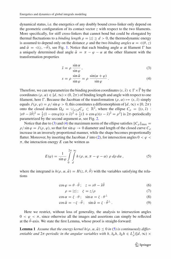
dynamical status, i.e. the energetics of any doubly bound cross-linker only depend onthe geometric configuration of its contact vector z with respect to the two filaments.More specifically, for stiff cross-linkers that cannot bend but could be elongated bythermal fluctuations to a binding length ρ = |z| ≥ d > 0, the thermodynamic energyis assumed to depend only on the distance ρ and the two binding angles α = (θ, z)and α = (z,−θ ), see Fig. 1. Notice that each binding angle α at filament hasa uniquely determined dual angle α = π − ϕ − α at the other filament with thetransformation properties
s = ρsin α
sin ϕ, (3)
s = ρsin α
sin ϕ= ρ
sin(α + ϕ)
sin ϕ. (4)
Therefore, we can reparametrize the binding position coordinates (s, s) ∈ × by thecoordinates (ρ, α) ∈ [d,∞)× (0, 2π) of binding length and angle with respect to onefilament, here . Because the Jacobian of the transformation (ρ, α) → (s, s) simplyequals J (ρ, ϕ) = ρ/ sin ϕ > 0, this constitutes a diffeomorphism of [d,∞)×[0, 2π)onto the closed domain d = ∪ρ≥dCρ ⊂ R
2, where the ellipse Cρ = (s, s) :|sθ − sθ |2 = 1
2 (1 − cosϕ)(s + s)2 + 12 (1 + cosϕ)(s − s)2 = ρ2 is 2π -periodically
parametrized by the second argument α, see Fig. 2.Notice that due to (3) and (4) the maximum norm of the ellipse satisfies ‖Cρ‖max =
ρ/ sin ϕ = J (ρ, ϕ), so that for sin ϕ → 0 diameter and length of the closed curve Cρincrease in an inversely proportional manner, while the shape becomes proportionallyflatter. Moreover, by inserting the Jacobian J into (2), for intersection angles 0 < ϕ <
π , the interaction energy E can be written as
E(ϕ) = 1
sin ϕ
2π∫
0
∞∫
d
h (ρ, α, π − ϕ − α) ρ dρ dα , (5)
where the integrand is h(ρ, α, α) = H(z, θ, θ ) with the variables satisfying the rela-tions
cosϕ = θ · θ ; z = sθ − sθ (6)
ρ = |z| ; ζ = z/ρ (7)
cosα = ζ · θ ; sin α = ζ · θ⊥ (8)
cos α = −ζ · θ ; sin α = ζ · θ⊥ . (9)
Here we restrict, without loss of generality, the analysis to intersection angles0 < ϕ < π , since otherwise all the images and assertions can simply be reflectedat the θ -axis. We state the first Lemma, whose proof is straight-forward:
Lemma 1 Assume that the energy kernel h(ρ, α, α) ≤ 0 in (5) is continuously differ-entiable and 2π -periodic in the angular variables with h, ∂αh, ∂αh ∈ L1
ρ([d,∞) ×
123

P. Reiter et al.
Fig. 2 Representation of possible cross-linker states in the (s, s) coordinate space with Cρ denoting allpairs of binding sites that are connected by a cross-link of length ρ. For minimal length ρ = d the bindingenergy k(ρ) in (17) has a negative jump representing the repulsive function of such cross-linkers on Cd ,thereby serving as ‘spacers’ between the filaments. As argued in the text, the ellipses become longer andflatter (around one of the two diagonals) for sin ϕ → 0. The marked interval [s−, s+] on the s-axis denotesthe binding sites on a shorter filament with finite length L = s+ −s−, intersecting a much longer filament, see Sect. 5
[0, 2π ]2), where g ∈ L1ρ means ρ · g ∈ L1. Further, let both integrals
h0 := −2π∫
0
∞∫
d
h (ρ, α, π − α) ρ dρ dα (10)
h1 := −2π∫
0
∞∫
d
h (ρ, α,−α) ρ dρ dα (11)
be positive. Then the energy functional E in (5) is continuously differentiable on theopen interval (0, π) with the following asymptotic behavior near the two singularboundary points ϕ∗ = 0 and π (with h = h0 or h1, respectively):
E(ϕ) = − h
sin ϕ+ O(1) , (12)
d E(ϕ)
dϕ= h cosϕ
sin2 ϕ+ O
(1
sin ϕ
). (13)
123

Energetics and dynamics of global integrals modeling
Proposition 1 (Degenerate negative gradient flow) According to Lemma 1 the twointersection angles ϕ∗ = 0 and π , representing parallel and anti-parallel orientationof the two filaments, respectively, are locally stable steady states of the negative gra-dient flow described by the standard differential equation with ‘relaxation rate’ λ > 0(and with notation ϕ(t) = dϕ(t)
dt ):
ϕ = −λ · d E(ϕ)
dϕ. (14)
This differential equation degenerates atϕ∗ = 0 andπ so that the asymptotic differencey = sin ϕ = |ϕ − ϕ∗| + O(|ϕ − ϕ∗|3) fulfills
y = −λh y−2 + O(y−1) . (15)
Thus, these so-called ‘super-stable’ steady states are reached in finite positive time t∗such that
y(t) ∼ [3λh(t∗ − t)
] 13 for t t∗ . (16)
We continue by specifying physically consistent models of the interaction energykernel h in (5). While neglecting any small bending of a cross-linking polymer, whichis approximately justified for myosin [16] and to a lesser degree also for α-actinin[30], we only consider thermal fluctuations of flexible binding chains at both endsand approximately describe the cross-link by a stochastically elongated linear springwith Hookian spring rate constant γ > 0 [ 1
ms ], but only for elongations ρ beyond afixed resting length d > 0. This so-called ‘half-spring’ model reflects the assumedcondition that simultaneous binding of a cross-linker to both filaments cannot occur ifthe spring is under compression. Since energy is consumed by binding, the resulting‘half-spring’ energy induced by such a doubly bound cross-linker can be written as anegative function of cross-link distance ρ with η = 2γ /β2, where β2[µm
ms ] measuresthe spring speed variance due to thermal excitations and where the appearing expo-nential function represents the stationary probability distribution of the correspondingstochastic process:
0 > − k(ρ) = − k0 · e− η2 [ρ−d]2+ for ρ ≥ d ,
(17)k(ρ) = 0 for ρ < d .
This energy distribution does not depend on the binding angles, it vanishes for lengthsρ < d, jumps to the minimal value −k0 at ρ = d and increases to zero with increasingspring elongation ρ → ∞, see Fig. 3. Then the action applied by a cross-linker ontothe filaments can be expressed by the ‘variational’ increment dk(ρ) = −k(ρ) ·µ f (ρ)
in distributional sense, with a scalar force distribution µ f given by
µ f (ρ) = η[ρ − d]+ dρ − δρ=d . (18)
123

P. Reiter et al.
0 0.5 1 1.5 2 2.5−3
−2.5
−2
−1.5
−1
−0.5
0
0.5
cross−link length: ρ
half−spring energy distribution
− k(ρ, ⋅ ⋅ )
Fig. 3 The negative spring energy −k due to cross-link binding according to an elastic ‘half-spring’ modelfor d = 1. (black curve): plot of −k(ρ) according to (17); (grey curves): plots of −k(ρ, α, α) in (27) forfixed r = r(α, α) = 0.2 yielding the lower energy curve and representing a spring in pre-tension, whereasthe upper curve for r = −0.2 represents pre-relaxation of the cross-link
Whereas the first term models the attractive force by an elongated Hooke spring,the negative δ-distribution represents the repulsive action by a cross-linker at mini-mal length, then serving as ‘spacer’ between the filaments. Typical rest length esti-mates reveal d ≈ 100 nm for α-actinin dimers and d 60 nm for myosin tetramers,see [11].
On the other hand, let us assume that the successive cross-link binding to one andthe other filament are independent of each other and do not depend on the actual springelongation ρ, but only on the two binding angles α and α (compare, for example, thepreferred binding ofα-actinin dimers to actin filaments [30]). Then the quasi-stationaryenergy configuration of such a filament pair can be quantified as follows:
Example A (Cross-link forces independent ofα and α). Suppose that the energy kernelh in (5) has a symmetric factorization
h(ρ, α, α) = − k(ρ, α, α) · q(α) · q(α) (19)
with a ‘half-spring’ cross-linker energy k(ρ, α, α) = k(ρ) only depending oncross-link length ρ as in (17) and an angle dependent binding strength q(α) > 0. Bydefining
123

Energetics and dynamics of global integrals modeling
k :=∞∫
d
k(ρ) ρ dρ = k0
η
1 + d
√ηπ
2
, (20)
the energy in (5) takes the explicit form, with k0 := π kq2
04 :
• (i) for α-independent binding, i.e. q(α) ≡ q02 :
E(ϕ) = −2 · k01
sin ϕ(21)
• (ii) for q(α) = q0 · sin2 α, or q(α) = q0 · cos2 α, modeling preferred binding atangles α ≈ ±π/2 or at α ≈ 0 and π , respectively (cf. Fig. 5a):
E(ϕ) = −k0
(3
sin ϕ− 2 sin ϕ
), (22)
d E(ϕ)
dϕ= k0 cosϕ
(3
sin2 ϕ+ 2
), (23)
• (iii) for q(α) = q0 · cos2(α2 ) = q02 (1 + cosα), modeling preferred binding at
angles α ≈ 0 and reduced binding at α ≈ π (cf. Fig. 5b):
E(ϕ) = −2 · k01 − 1
2 cosϕ
sin ϕ, (24)
d E(ϕ)
dϕ= 2 · k0
cosϕ − 12
sin2 ϕ. (25)
In the first two cases the energy E(ϕ) on the interval ]0, π [ is symmetric withmaximum at ϕ∗ = π/2 and with equally strong singularities of order 1
sin ϕ at ϕ∗ = 0and π , see Fig. 4a, while in the last case the asymmetric energy function attains itsmaximum at a lower intersection angle ϕ∗ = π
3 , with a relatively stronger singularityat ϕ∗ = π , see the dark curves in Fig. 4b.
Example B (Cross-link forces depending on α and α). In generalization of (17) letus assume that the ‘rest length’ ρ0 of the ‘half-spring’ representing a cross-link ofminimal length d, is not constantly equal to d but depends on the binding angles viaa function ρ0 = d − 1√
ηr with
r(α, α) =√π
2r0(cosα + cos α) , (26)
for example, see Fig. 5c. Here the two additive terms model the fact that, at each of thetwo cross-linker binding sites, acute local binding angles induce a pre-tension of thespring proportional to cosα > 0 or cos α > 0, respectively (see Fig. 3: lower curve),whereas in case of obtuse angles with negative cosine values, the same expressions
123

P. Reiter et al.
0 pi/2 pi−10
−8
−6
−4
−2
0
2
4
6
8
10− lambda * dE/dphi
0 pi/2 pi−10
−8
−6
−4
−2
0
2
4
6
8
10− lambda * dE/dphi
E1 (A)E2 (A)
E3 (A)E3 (B)
(a) (b)
Fig. 4 Plots of interaction energies E(ϕ) between two filaments (the negative concave curves) and of theirnegative gradient flow rates −λ · E ′(ϕ) (the monotone curves) according to a Eq. (21) in Example A(i) andEq. (22) in Example A(ii); to b Eq. (24) in Example A(iii) and Eq. (34) in Example B(iii)
model a pre-relaxation of the spring (see Fig. 3: upper curve). Indeed, for myosinII oligomers it is a well-known fact that their ‘heavy chain’ binding sites induce apre-stretching of the myosin ‘heads’ after binding to an actin filament, but only indirection of the so-called ‘barbed end’, which here is chosen to be the direction of thevectors θ and θ (for myosin see [10], for general models of molecular motor cross-linkssee [18]).
Due to the scaling factor 1/√η in front of the ‘relative rest length deviation’ r (26),
this is a dimensionless function, so that pre-tension/relaxation effects are maintainedfor increasingly stiff cross-linkers (i.e. large spring constant γ as, for example, γ ≈20 s−1 [17]). By substituting the rest length ρ0 into the spring energy function (17) andmultiplying it with a suitable stretching factor of order
√η, we obtain the following
(absolute value of the) modified energy function
kη(ρ, α, α) = √η κ e2
√2π
r(α,α)e− 12 (
√η[ρ−d]++r(α,α))
2for ρ ≥ d ,
(27)kη(ρ, α, α) = 0 for ρ < d .
123

Energetics and dynamics of global integrals modeling
In fact, its integral k, measuring the averaged potential energy of a single cross-link,is independent of the spring constant η:
k :=∞∫
d
kη(ρ, •, •) dρ
= κe2√
2π
r∞∫
0
e− 12 (r+r)
2dr
=√π
2κe2
√2π
r (1 − erfc(r)
), (28)
with erfc(r) :=√
2π
∫ r0 exp(− s2
2 )ds and erfc(∞) = 1. Whereas k only depends on
the two binding angles via r = r(α, α) in (26), the total spring energy in analogy to(20), namely
kη =∞∫
d
kη(ρ, •, •) ρ dρ
=(
d − r√η
)k + κ√
ηe− 1
2 r2+2√
2π
r, (29)
also depends on η, but converges towards d · k for η → ∞. Thus, with the analogousdefinition of the kernel h = hη (19), the total energy functional (5) for a filament paircan in general be computed as
Eη(ϕ) = − 1
sin ϕ
2π∫
0
kη(α, π − ϕ − α) · q(α) · q(π − ϕ − α) dα . (30)
However, in the limit η → ∞ of infinitely stiff cross-linkers, the original energydistribution kη(ρ, •, •) ρ dρ converges to the Dirac measure d · k δρ=d, so that theenergy functional E(ϕ) = E∞(ϕ) can be represented as a global integral (2) with thesingular kernel
H(z, θ, θ )µd(s, s) = −d · k(α, α) · q(α) · q(α) dα δρ=d . (31)
Here µd(s, s) describes the one-dimensional Hausdorff measure on the ellipse Cd =ρ = |z(s, s)| = d in the original (s, s)-coordinates according to (3) and (4), see alsoFig. 2.
In general, calculation of E(ϕ) as an explicit function of the intersection angle ϕ inclosed form is not possible, however, by approximating the error-function erfc in (28)
for small values of the pre-tension strength r0 in (26), we obtain e2√
2π
r(1−erfc(r)) =
(1 + 2√
2π
r + O(r2))(1 −√
2π
r + O(r2)) = 1 +√
2π
r + O(r2) and thus the simple
123

P. Reiter et al.
approximative kernel representation
k(α, α) =√π
2κ
(1 + r0(cosα + cos α)+ O(r2
0 )). (32)
Finally, under this assumption we derive the following explicit energy formulas, whichwe restrict to the two cases (i) and (iii) defined in Example A:
• (i) for α-independent binding, i.e. q(α) ≡ q02 :
E(ϕ) = −2 · κ0d
sin ϕ, (33)
with κ0 := (π2
) 32 κ
q202 , the same standard formula as in (21), and
• (iii) for q(α) = q02 (1 + cosα), modeling preferred binding at angles α ≈ 0 and
reduced binding at α ≈ π :
E(ϕ) = −2 · κ0d
sin ϕ
1 − 1
2cosϕ + r0(1 − cosϕ)
, (34)
d E(ϕ)
dϕ= 2 · κ0 d
(1 + r0) cosϕ − ( 12 + r0)
sin2 ϕ. (35)
In the last case the energy E(ϕ) is again an asymmetric function on ]0, π [ as inExample A(iii), attaining its maximum at an even smaller value ϕ∗ such that cosϕ∗ =12
1+2r01+r0
, which for small r0 is ϕ∗ = π3 − r0√
3+O(r2
0 ). See also the corresponding plotsin Fig. 4b.
3 Forces and dynamics induced by cross-linkers
In order to get insight into the physical mechanisms that lead to the singular behav-ior described in Proposition 1 and asserted in Examples A and B, we can extractthe effective forces exerted by cross-linker interactions with the aid of computingthe different variations of the energy functional E in (2) and (5) under changes in therelative position between the two filaments and . Assuming, for instance, that thelatter filament is fixed, then we can consider virtual translations of the other filament at a given binding position s in two orthogonal directions ζ and ζ⊥, i.e. in directionof the cross-linker contact vector z = ρ · ζ , see (6) and (7), and orthogonal to it. Thefirst variation (δζ ) means that the cross-linker length ρ is increased, say by dρ, whileboth binding angles α and α stay fixed. The other variation (δζ⊥) induces a rotationof the cross-linker around the fixed binding site s on such that the local turn, sayby dσ , of the lever (with constant length ρ) induces changes of both binding angles αand α by dα = −dα = 1/ρ dσ , since the sum α+ α = π − ϕ stays fixed due to puretranslation of the whole filament under constant ϕ. Thus, the force resulting fromvirtual spring length variations (δζ ) is the contracting or spacing spring force, whichin terms of the kernel h (19) can be written as
K f (s, s) = − ∂ρh(ρ, α, α) · ζ = ∂ρk(ρ, α, α) · q(α) · q(α) · ζ , (36)
123

Energetics and dynamics of global integrals modeling
Fig. 5 Symmetric model functions depending on the binding angles. Plotted over α and α are the product ofbinding strengths q(α) ·q(α) for a q(α) = q0 cos2 α and b q(α) = q0
2 (1+ cosα)with q0 = 1, and in c the
rescaled deviation of cross-linker rest length from the basal value d, namely r(α, α) =√π2 r0(cosα+cos α)
with r0 =√
2π
where the ‘unit cross-link vector’ is ζ = ζθ (α) = (cosα)θ+(sin α)θ⊥, cf. (7)–(9). Onthe other hand, from rotational variations (δζ⊥) we obtain the sum of two cross-linktorque forces
Kω(s, s) = − 1
ρ∂αh(ρ, α, α) · ζ⊥ , (37)
Kω(s, s) = 1
ρ∂αh(ρ, α, α) · ζ⊥ , (38)
so that the total force exerted by a cross-linker connection from the fixed binding site sat to the binding site s on is given by the following force kernel K : × → R
2:
K = K f + Kω + Kω . (39)
123
P. Reiter et al.
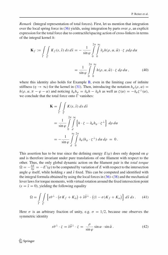
Remark (Integral representation of total forces). First, let us mention that integrationover the local spring force in (36) yields, using integration by parts over ρ, an explicitexpression for the total force due to contractile/spacing action of cross-linkers in termsof the integral kernel h:
K f :=∫
∫
K f (s, s) ds ds = − 1
sin ϕ
2π∫
0
∞∫
0
∂ρh(ρ, α, α) · ζ ρdρ dα
= 1
sin ϕ
2π∫
0
∞∫
0
h(ρ, α, α) · ζ dρ dα , (40)
where this identity also holds for Example B, even in the limiting case of infinitestiffness (η → ∞) for the kernel in (31). Then, introducing the notation hϕ(ρ, α) =h(ρ, α, π − ϕ − α) and noticing ∂αhϕ = ∂αh − ∂αh as well as ζ(α) = −∂αζ⊥(α),we conclude that the total force onto vanishes:
K =∫
∫
K (s, s) ds ds
= 1
sin ϕ
2π∫
0
∞∫
d
h · ζ − ∂αhϕ · ζ⊥
dρ dα
= − 1
sin ϕ
∞∫
d
2π∫
0
∂α(hϕ · ζ⊥) dα dρ = 0 .
This assertion has to be true since the defining energy E(ϕ) does only depend on ϕand is therefore invariant under pure translations of one filament with respect to theother. Thus, the only global dynamic action on the filament pair is the total torque = − δE
δϕ= −E ′(ϕ) to be computed by variation of E with respect to the intersection
angle ϕ itself, while holding s and s fixed. This can be computed and identified withthe integral formula obtained by using the local forces in (36)–(38) and the mechanicallever laws for torque moments, with virtual rotation around the fixed intersection point(s = s = 0), yielding the following equality
=∫
∫
sθ⊥ · (
σK f + Kω) + sθ⊥ · (
(1 − σ)K f + Kω)
ds ds . (41)
Here σ is an arbitrary fraction of unity, e.g. σ = 1/2, because one observes thesymmetric identity
sθ⊥ · ζ = sθ⊥ · ζ = ρ
sin ϕsin α · sin α . (42)
123

Energetics and dynamics of global integrals modeling
Thus, the resulting differential equation for temporal changes inϕ (see Proposition 3below) is the negative gradient flow (14). However, the local forces appearing in thetwo kernels Kω and Kω arise from variations (δζ⊥) that change the binding angles, sothat in the presented energy model they can be associated to resisting ‘torque’ forcesof cross-linkers that stay bound to actin filaments during the variation of bindingangles. Such a model (satisfying the gradient flow kinetics) could be relevant forphysical situations of steadily cross-linked molecules, whereas for the biophysicalsituation of ongoing dissociation and re-association of cross-linking polymers (asmyosin or α-actinin) on a microscale (of milliseconds or fractions of seconds [11])during slow filament motion on a macroscale (of several seconds), we have to modifythe model. Since for computing the virtual forces, only variations on an even fasterscale (e.g. fractions of milliseconds) are considered, we can assume that during thisshort time the cross-links stay bounded. Then due to the model interpretation of thebinding strengths, q(α) and q(α), these would not change, and the only remainingvariations are that of the spring energy k(ρ, α, α). Moreover, if we suppose that theangle-dependence of k (for the model in Example B) via the pre-tension/relaxationfunction r has been realized already during binding of the cross-link, then the onlyeffective variation that remains is the one in cross-linker length (δζ ). Thus, as localforce vector kernel we can take K = K f and assume Kω = Kω = 0. Splitting K intoits components parallel and orthogonal to the filament , namely K = K‖θ + K⊥θ⊥and using the relations (8) and (9) as well as (42), we obtain the following explicitformulas for the total torque and parallel and orthogonal force components expressedin (ρ, α, α)-coordinates:
Proposition 2 (Total torque and forces onto one filament) Assume that bound cross-links only apply forces to the filaments due to elongation of their ‘half-spring’ but notdue to bending or tilting of their binding angles, thus Kω = Kω = 0. Then under theassumption that filament is fixed, local variation of cross-linkers leads to the forcekernel K = K f in (36) yielding the following global torque and the parallel andorthogonal forces F‖ = ∫
∫
K‖(s, s) ds ds and F⊥ = ∫
∫
K⊥(s, s) ds ds ontofilament (again using integration by parts):
= − 1
sin2 ϕ
2π∫
0
∞∫
d
∂ρh(ρ, α, α) ρ2dρ sin α sin α dα
= 2
sin2 ϕ
2π∫
0
∞∫
d
h(ρ, α, α) ρ dρ sin α sin α dα (43)
F‖ = 1
sin ϕ
2π∫
0
∞∫
d
h(ρ, α, α) dρ cosα dα (44)
F⊥ = 1
sin ϕ
2π∫
0
∞∫
d
h(ρ, α, α) dρ sin α dα (45)
123

P. Reiter et al.
with the total translational force given by
K = K f = F‖ θ + F⊥θ⊥ . (46)
Before computing explicit expressions for , F‖ and F⊥ as functions of ϕ in specificexamples, let us write down the dynamical equations describing the resulting motionof one filament with respect to the other.
Proposition 3 (Over-damped dynamics of filament motion) Let us assume that onefilament, say , is held fixed and represented by the oriented x-axis, for instance.Then under the assumption of strong hydrodynamic friction relative to inertia, whichis clearly fulfilled for filament motion in highly viscous cytoplasm, the ‘over-damped’dynamics of the other filament, , is determined by the following force balance equa-tions for the three independent types of motion (rotation, parallel and orthogonaltranslation), where each of them can eventually have a different friction coefficient(λ−1):
dϕ
dt= λ , (47)
ds
dt= λ‖ F‖ , (48)
ds⊥
dt= λ⊥ F⊥ , (49)
with the torque and the other forces defined in (43)–(45). Let us remark that forfinite filaments the inverse friction coefficients λ could be assumed to depend on itslength L in a manner that λ⊥ = 2 · λ‖ ∼ L−1, but λ ∼ L−2, compare Sect. 5.
In general, the motion of is completely determined by the intersection coordinatex = R(t)with filament (the x-axis), the intersection angle ϕ = (t) and the signedsegment length s = S(t) between the intersection point (R(t), 0) and a freely chosenbut fixed point (X (t),Y (t)) on filament , e.g. the filament mass center, see Fig. 7dbelow. Thus we obtain the representation
X = R + S cos, Y = S sin, (50)
where the defining time-dependent variables, S, R satisfy the system of differentialequations (again for angles 0 < < π , without restriction of generality):
d
dt= λ () , (51)
d S
dt= λ‖ F‖()+ λ⊥
tanF⊥() , (52)
d R
dt= − λ⊥
sinF⊥() . (53)
123

Energetics and dynamics of global integrals modeling
The last Eq. (53) and the second term in Eq. (52) arise from orthogonal shifts offilament . Thus, for infinitely long filaments the ‘leading’ degenerate ODE (51)autonomously determines the dynamics of filament intersection angle (t), whereassubsequent integration of the other two, (t)-dependent Eqs. (52) and (53) yieldsthe relative position of one filament with respect to the other. For filaments of finitelength, the analogous ODE system turns out to be nonlinearly coupled in the first twovariables, see Sect. 5.
In order to characterize and visualize different types of filament dynamics for thevarious interaction models, we now compute the torque (ϕ) as well as the forceterms F‖(ϕ) and F⊥(ϕ) for the examples introduced in Sect. 2:
Example A (Cross-link forces only depending on ρ). With the conditions and defini-tions after Eq. (20) we can state:
• (i) and (ii) Since in these cases the force kernel h(ρ, α, π − ϕ − α) in (40)turns out to be an odd function of the periodic variable α, both integrated forcesF‖ and F⊥ vanish. Thus, for these models with symmetric interaction energyE(ϕ) = E(π − ϕ) the filament dynamics shows no translations, only rotationaround the fixed intersection point. In the standard case (i) we obtain the torque = −E ′(ϕ) for the energy in (21) and, thus, a resulting negative gradient flow.On the contrary, this does not hold for (ii), where in case of q(α) = q0 sin2 α wehave
(ϕ) = −k0 cosϕ
5
sin2 ϕ− 2
, (54)
and for q(α) = q0 cos2 α
(ϕ) = −k0 cosϕ
1
sin2 ϕ− 2
. (55)
Whereas in the first case the symmetric function(ϕ) is monotone increasing withthe unstable zero ϕ∗ = π/2, in the second case this orthogonal configuration isa stable equilibrium state with two additional unstable zeros at ϕ∗ = π/2 ± π/4,see the plots in Fig. 6a.
• (iii) With the asymmetric binding strength q(α) = q02 (1 + cosα) also the torque
function becomes asymmetric according to (43):
(ϕ) = −k0
2 cosϕ − 1
2
sin2 ϕ+ 1
, (56)
while the global forces according to (44) and (45) are
F‖(ϕ) = −2kη1 − cosϕ
sin ϕ, (57)
F⊥(ϕ) = −2kη , (58)
123

P. Reiter et al.
0 pi/2 pi−10
−8
−6
−4
−2
0
2
4
6
8
10Torque: Omega
0 pi/2 pi−10
−8
−6
−4
−2
0
2
4
6
8
10Torque: Omega
(A: q = sin2)
(A: q = cos2)
(A)(B)
(a) (b)
Fig. 6 Plots of the ϕ-dependent torque between two filaments (if one is fixed) according to a Eqs. (54)and (55) in Example A(ii) for the two indicated cross-link binding functions q(α): The case (sin2 α) ofpreferred orthogonal binding gives a torque similar to the negative gradient flow rate −λ · E ′(ϕ) with thesame convergence behavior as the standard function for Example A(i), see Fig. 4a, whereas the case (cos2 α)of preferred parallel binding of cross-linkers (see Fig. 5a) induces a non-monotone torque, with dynamicproperties totally different from the negative gradient flow: the orthogonal filament pair configuration is anasymptotically stable state; b torque plots according to (56) for Example A(iii) and (65) for Example B(iii).In addition, for both examples the parallel (lined) and orthogonal (dashed) force components are plotted
with kη = (π2 )32 k0√
η
q204 . Notice that the total orthogonal force onto the filament in
(58) is just a negative constant (for 0 < ϕ < π )!
Only for the last Example A(iii) the intersection point (R, 0) between the movingfilament and the fixed one changes due to parallel and orthogonal net forces, seeFig. 6b. Since there is a constant orthogonal ‘right-shift’ of the filament (to the rightside with respect to its orientation vector θ ) but a simultaneous parallel ‘back-draw’,at least for angles > 0, one cannot easily conclude, in which direction the filamentis translocated. Therefore, we have to study the ODE-System (51)–(53), which for
parameter values k0 = 2kη = 1 (equivalent to d +√
2πη
= 1) and inverse frictions
λ = 1, λ‖ = λ and λ⊥ = 2 · λ (all parameters and variables in dimensionlessunits) yields
123

Energetics and dynamics of global integrals modeling
d
dt= −
2 cos− 1
2
sin2+ 1
, (59)
d S
dt= −λ1 + cos
sin, (60)
d R
dt= 2 · λ 1
sin. (61)
According to Fig. 6b the intersection angle (t) generically converges to one of thetwo alignment states, where with (15) and (16) we obtain the following asymptoticbehavior:
At parallel alignment, see Fig. 7b, we have the rapid convergence(t)∼[t∗−t]1/3+
in finite time, so that by R(t) ∼ 2λ(t) ∼ −S(t) we obtain the corresponding conver-
gence R∗ − R(t) ∼ [t∗ − t]2/3+ ∼ (t)2. Thus, the intersection point R(t) increases
a bit, but gets stationary at a certain value R∗ even more rapidly than the intersectionangle. Since on this asymptotic order the sum (R + S)(t) ∼ R∗ + S∗ is already sta-tionary, the fixed point (marked in Fig. 7d) on the moving filament does perform analmost circular arc while approaching the fixed filament.
At antiparallel alignment, see Fig. 7a, we get the same asymptotic behavior for(t) = π −(t) and R(t), even with a bit stronger coefficient, but now the segmentlength S(t) ∼ S∗ on the moving filament is already stationary on the consideredasymptotic order, so that the increasing intersection point ‘draws’ the fixed point tothe right and its track is straightened to a line almost orthogonal to the fixed filament.For larger ‘translation mobility’ coefficient λ the fixed point is even translated to theright, meaning that the moving filament shows an asymptotic tendency to slide withrespect to the fixed one (see Fig. 7c). This only happens for near antiparallel alignment,since then most of the cross-links are bound with acute angles at both ends.
This is a clear asymmetric behavior, whose importance becomes even more apparentwhen stochastic perturbations are considered, see Sect. 4. Before doing this, we lookat the deterministic dynamic behavior in the other
Example B (Cross-link forces depending on α and α) With the conditions afterEq. (26), using the force representation in (40) for the singular measure (31) withthe simplified force kernel (32), we can state:
• (i) For constant binding strength q02 the force distribution kernel (for η → ∞) is
K f µd = − d
sin ϕ
√π
2κ
q20
4(1 − r0(cosα + cos α)) · ζ dα ,
so that the torque becomes
(ϕ) = −2κ0dcosϕ
sin2 ϕ= −E ′(ϕ) (62)
123

P. Reiter et al.
−8 −6 −4 −2 0 2
−4
−3
−2
−1
0
1
2
3
4
5
5
−4 −2 0 2 4 6 8 10−5
−4
−3
−2
−1
0
1
2
3
4
5
−8 −6 −4 −2 0 2 4−5
−5
−4
−3
−2
−1
0
1
2
3
4
−4 −2 0 2 4 6 8 10−5
−4
−3
−2
−1
0
1
2
3
4
5
(X,Y)
SR
(a) (b)
(c) (d)
Fig. 7 Plots of the filament dynamics according to the differential equations (51)–(53) for Examples A(iii)and B(iii) with the intersection angle (t) converging either to the antiparallel steady state π , see a and c,respectively, or to the parallel steady state 0, see b and d. As inverse friction coefficient we chose: a and bλ = 1; c and d λ = 3. Drawings of the moving filament (for simplicity of finite length) are performed fortime intervals with constant decrease in the intersection angle: the angular speed itself becomes infinitelyrapid according to |(t)| ∼ [t∗ − t]−2/3, see text for further discussion. On each filament a fixed pointwith coordinates (X, Y ) is marked
and the two force components
F‖(ϕ) = −κ0 r01 − cosϕ
sin ϕ(63)
F⊥(ϕ) = −κ0 r0 . (64)
Notice that these forces have exactly the same structure as in Example A(iii) above,but with a symmetric torque function as in the standard case A(i).
• (iii) For asymmetric binding as in Example A(iii) but with angle dependent forcewe analogously obtain
(ϕ) = −κ0
2d
(4 + r0(1 − cosϕ)2) · cosϕ − 1
sin2 ϕ+ 2(1 + r0)+ r0 cosϕ
(65)
and
F‖(ϕ) = − κ0
sin ϕ
(1 + r0 − 3
4r0 cosϕ
)(1 − cosϕ)+ r0
4sin2 ϕ
(66)
123

Energetics and dynamics of global integrals modeling
F⊥(ϕ) = − κ0
1 + 5
4r0 − r0
2cosϕ
. (67)
One can show that both force functions F‖ and F⊥ are negative and monotonedecreasing in the variable ϕ, see Fig. 6b.
According to the plots in Fig. 6b this last Example B(iii) modeling myosin actionbetween the two filaments, shows qualitatively the same behavior as the Example A(iii)with the same cross-linker binding strength function, namely preferred polar bind-ing in direction of the oriented filaments. Indeed, the asymptotic coefficients are abit larger and produce an even more rapid convergence during antiparallel align-ment and a stronger sliding effect near antiparallel alignment (see Fig. 7). Thus,the additional assumption of angle-dependent cross-linker force in (27) for Exam-ples B strengthens the asymmetric convergence behavior, which obviously is inducedalready by the assumed asymmetric cross-linker binding. Again, with additional sto-chastic noise introduced in the following section, these effects will become moreprominent.
4 Stochastic dynamics
So far the dynamic action of the cross-links was modeled in a mean field approximation,where with an assumed constant reservoir of cross-linking oligomers in solution theenergy integral kernel hϕ(ρ, α) = ρ
sin ϕ h(ρ, α, α) according to (5) measured the meanexpected density distribution of bound cross-linkers with respect to their length (ρ)and binding angle (α). Moreover, according to (36) the density of mean force locallyexerted by cross-linkers onto one filament could be expressed by the kernel Kϕ(ρ, α) =− ρ
sin ϕ ∂ρh(ρ, α, α) · ζ(α). Regarding that molecular association and dissociation ofcross-linkers are Poisson processes, then also the expected variance will be locallydistributed as proportional to hϕ . Thus, for any given intersection angle ϕ there isa constant b f measuring the noise amplitude (depending on temperature), so thatper infinitesimally small time step dt the local impulse increment density induced bycross-linkers, usually given by dt P = Kϕ dt , can now be written as a sum dt P =K detϕ dt + K stoch
ϕ dWt with a deterministic increment dt and a stochastic Wienerincrement dWt :
dt P(s, s) ds ds =(
−∂ρhρ
sin ϕdt + b f
√hρ
sin ϕdWt
)dρ dα · ζ . (68)
Then, computing the total impulse increment dt P = Kdet dt + Kstoch dWt accordingto the first integral representation in (40) we obtain stochastic integrals for each of thetwo force components of K = F‖θ + F⊥θ⊥ with the following properties:
Proposition 4 (Stochastic differential equations for filament motion) In the situationof Proposition 3, with stochastic noise introduced as described above, instead of(47)–(49) we obtain a system of degenerate stochastic differential equations (for any
123

P. Reiter et al.
2π -periodic ϕ)
dϕ = λ(
sign(sin ϕ)det (ϕ) dt + b(ϕ)| sin ϕ|− 32 dWt
), (69)
ds = λ‖(
F‖det (ϕ) dt + b‖(ϕ)| sin ϕ|− 1
2 dWt
), (70)
ds⊥ = λ⊥(
sign(sin ϕ) F⊥det (ϕ) dt + b⊥(ϕ)| sin ϕ|− 1
2 dWt
). (71)
Here the deterministic parts of torque and translation forces are given by the integralsdefined in (43)–(45), or by the computed formulas in Examples A and B of Sect. 3(as they are given for positive ϕ only). Moreover, the relative noise coefficients b#(ϕ)
depend continuously on cosϕ and sin ϕ, satisfying analogous integral representationsfor the variances of the stochastic torque and force components
b2 = | sin ϕ|3 Var(stoch) = b2
f
2π∫
0
∞∫
d
|h(ρ, α, α)|ρ3dρ (sin α sin α)2dα (72)
b2‖ = | sin ϕ| Var(F‖stoch) = b2
f
2π∫
0
∞∫
d
|h(ρ, α, α)| ρdρ cos2 α dα (73)
b2⊥ = | sin ϕ| Var(F⊥stoch) = b2
f
2π∫
0
∞∫
d
|h(ρ, α, α)| ρdρ sin2 α dα . (74)
Since the deterministic non-linearities degenerate likedet ∼ | sin ϕ|−2 and F#det ∼
| sin ϕ|−1, the stochastic increments in Eqs. (69)–(71) degenerate at a lower order. Inparticular, using the same notation as for the asymptotic deterministic equation (15),near the singularities ϕ∗ = 0 and π the leading stochastic equation (69) can asymp-totically be written as
dy = −a · |y|−m dt + b · |y|γ−m dWt (75)
with m = 2 and γ = 12 . This class of degenerate SDEs does not always lead to well
defined stationary processes:
Lemma 2 (Resolving power law singularities in SDEs) The degenerate SDE in (75)with m > 0 describes a nontrivial generalized Gauss process that is asymptoticallystationary only if the exponents satisfy the condition 0 < γ < m+1
2 . The stationaryprocess has the symmetric bimodal probability distribution
p(y) dy = pm · |y|me− 2aµb2 |y|µ
dy (76)
with µ = m + 1 − 2γ > 0 and a positive scaling factor pm, see Fig. 8b. Realizationsof the stationary process randomly switch between positive and negative values, with
123

Energetics and dynamics of global integrals modeling
0 0.5 1 1.5 2 2.5 3 3.5 4 4.5 5−1.5
−1
−0.5
0
0.5
1
1.5
(a)
0 200 400 600 800 1000−1.5
−1
−0.5
0
0.5
1
1.5
(b)
Fig. 8 Properties of the asymptotic process yt for the stochastic variable sint satisfying (75) withγ = 1
2 and m = 2. a Stochastic path (black) together with the path of the transformed variable zt = y3t
(grey), usually of lower absolute value; b empirical distribution of the yt values (histogram) and theoreticalprobability distribution according to (76): p(y) = 2ν
√ν/π y2 exp(−ν y2)with ν = a/b2, here a = 1 and
b = 0.3
super-exponentially long switching intervals (‘resting times’) and intermittent phasesof very fast oscillations, see Fig. 8a.
Proof Consider the transformed stochastic variable z = sign(y)|y|m+1 satisfying thefollowing non-continuous SDE, with a right-hand side that performs a negative jumpat zero, a so-called ‘negative sign-type’ SDE:
dz = −(m + 1)a · sign(z) dt + (m + 1)b · |z|β dWt (77)
with β = γm+1 > 0. Computation of the Kolmogorov forward equation reveals that
(77) possesses stationary solutions only if β < 1/2, with symmetric unimodal sta-tionary distribution p(z) ∼ exp(−ν|z|1−2β), where ν = a/
((m + 1)( 1
2 − β)b2).
While the deterministic solution without noise consists of straight lines reaching theabsorbing state zero in finite time, the stochastic realizations show weighted randomincrements with sufficiently strong perturbations of amplitude |z|β > √
z, which areable to drive the solution away from zero, fast enough to overcome the deterministicabsorption.
Applying the results of Lemma 2 to the original asymptotic differential equation (75)for the stochastic variable yt = sint , satisfying the condition 0 < γ = 1
2 <32 =
m+12 for m = 2, we conclude that the stochastic perturbations of order | sin ϕ|− 3
2 in(69) are not too strong, but strong enough to overcome the infinitely fast ‘attraction’to zero by the deterministic term dϕ/dt ∼ | sin ϕ|−2 and to induce a bimodal sta-tionary distribution, see the stochastic realization in Fig. 8. Interpreted in terms of thebiophysical model, this asymptotic result says that the more cross-linkers are activeto attract the two filaments towards alignment, with infinitely increasing speed forsint → 0, the more fluctuations of the stochastic binding process occur and disturbthe attraction, strongly enough to prevent complete alignment. Instead, the intersec-tion angle between the two filaments steadily fluctuates around zero, not in a Gaussianmanner as for regularly stable steady states, but with a generalized biomodal Gaussdistribution so that too small angles are avoided.
123

P. Reiter et al.
0 pi/2 pi
0
pi/2
pi
regularizing angular transformation
ψ
Λ
phi
Fig. 9 The regularizing periodic transformation ψ = ψ(ϕ) defined in (78) and the positive factor (ψ)appearing in the SDE (79), plotted as a function of ϕ with λ = 1
As a matter of luck and surprise, we even can find an explicit resolution of thesingularities for the 2π -periodic stochastic angle variablet satisfying the degenerateSDE (69), namely by transforming it into the 2π -periodic variable t = ψ(t )
according to
ψ(ϕ) = arctan
sin3 ϕ
cosϕ
, (78)
satisfying the ‘negative sign-type’ SDE
dψ = (ψ)(− sign(sinψ)ω(ψ) dt + b(ϕ)| sin ϕ| 1
2 dWt
). (79)
All the appearing parameter functions are bounded, particularly the ‘regularized’deterministic torque ω(ψ) = det (ϕ) sin2 ϕ and the positive function (ψ) =λ(cos2 ψ)(3+tan2 ϕ), where also the inverse transformation of (78) can be explicitlycalculated as
ϕ(ψ) = arctan
u+(tanψ)+ u−(tanψ)+ tanψ
3
, (80)
123

Energetics and dynamics of global integrals modeling
Fig. 10 Properties of the stochastic intersection angle dynamicst satisfying (69) for Example A(iii) withthe same parameters as in Fig. 7b and with equal noise coefficients b# = 0.5 (time step had been chosen asdt = 0.0005 comparable to 0.3 s provided the time unit is 10 min, which would roughly correspond to theused parameter values λ ∼ 1). a The stochastic path (black) is the last part of the longer time series plottedin c representing the stationary phase of small fluctuations around π , b empirical distribution of the tvalues for the stationary phase, c longer time series of the intersection anglet (black with tiny fluctuations)together with the other two stochastic variables determining the position of the moving filament, namely thesection length St (upper curve) and the x-value of the intersection point with the fixed filament Rt (lowercurve). The corresponding visualization of filament motion is depicted below in Fig. 12a and supplementaryMovie A12
u±(T ) =⎧⎨⎩v(T )±
√v(T )2 −
(T 2
9
)3⎫⎬⎭
13
, (81)
v(T ) = T
(1
2+ T 2
27
). (82)
Indeed, (78) is equivalent to a cubic equation for = tan ϕ, namely 3 = (1 +2) tanψ , whose appropriate solution branch is constructed above. Moreover, whereasat ϕ ≡ 0 mod (π) the transformation ψ(ϕ) ∼ z ∼ y3 ∼ sin3 ϕ locally resolves thesingularity just as z = z(y) does, see (15) and (77), at ϕ ≡ π
2 mod (π) the derivativefulfills ψ ′(ϕ) = 1, so that in a wide region between the singularities ψ resembles theidentical mapping, see Fig. 9.
Numerical solutions of the transformed ‘negative sign-type’ SDEs (77) and (79)with ‘negatively jumping’ right hand side at z = 0 or ψ ≡ 0 mod (π), respectively,
123

P. Reiter et al.
can now easily be performed by using the Euler–Marayuma discretization scheme, see[13]. We choose a sufficiently small constant step size, but apply an additional ‘freez-ing’ condition for the deterministic increment step, namely zdet (t +dt) = ε · z(t) ≈ 0if −dzdet/z(t) > dt , simulating the deterministic absorption at the singularity, whilethe stochastic increment is added without restriction. Plots of resulting stochastic sim-ulations in terms of the back-transformed solution path for the original degenerateSDEs (69) and (75) are shown in Figs. 8a and 10a, respectively.
Starting the simulated process near one of the stable singularities ϕ ≡ 0 mod (π),then, for a suitable small noise amplitude b f in the defining equation for the stochastictorque term (72), the transformed angle t , thus also the intersection angle t itself,very rarely leaves the attraction domain of this singular point, so that the distributionof resulting angles resembles that of the localized variable yt , compare Figs. 8b and10b. On the other hand, for larger noise amplitudes b f the stochastic angular path canswitch from one singularity to the other, depending on its stability measured by thevalue of ω(cosϕ, sin ϕ) for cosϕ = ±1.
Finally, let us apply the so far performed asymptotic and numerical analysis tothe full degenerate SDE system in (69)–(71) in order to visualize and interpret theresulting dynamics of interactive filament motion. For this we have to stochasticallyand numerically solve the ‘just integrating’ degenerate SDEs for st and s⊥
t , (70) and(71), which have additive Gaussian increments with noise amplitude proportional
to | sint |− 12 . Therefore the variance of these stochastic increments is bounded by
the expectation value E(| sint |−1) = O(1 + E(|yt |−1)) < ∞, because with theaid of (76) the probability distribution for the well-defined inverse process ut =(yt )
−1 can easily be calculated as p(u) ∼ u−4 exp(−ν u−2) having finite mean valueand variance. Thus, also the stochastic process t = (sint )
−1 is a well definedgeneralized Gaussian process so that, for example, the SDE for st in (70) is of the type
dst = a(t ) · |t | dt + b(t ) · √|t | dWt , (83)
being integrable and resulting in non-stationary stochastic solutions st . The same isvalid for solutions s⊥
t of (71). Numerically, these two stochastic differential equationsare simultaneously solved together with the solution of the degenerate SDE (79) fort , again using the Euler–Marayuma method, where also the deterministic incrementsdsdet and ds⊥
det are locked into the ‘freezing’ condition for the variablet . Notice that
near the singularities we have |t | ∼ |t |− 13 .
We can then visualize the stochastic motion of filament with respect to the fixedfilament by using the equations in (50) and calculating the increments of the definingvariables St and Rt in analogy to Eqs. (52) and (53), namely
d St = dst +t · cost ds⊥t , (84)
d Rt = −t ds⊥t . (85)
The pictures in Figs. 11 and 12 certify the asymptotic results obtained in the deter-ministic case and show that the effects already seen in Fig. 7 are clearly amplified byintroducing the weighted degenerate noise terms.
123

Energetics and dynamics of global integrals modeling
−8 −6 −4 −2 0 2 4 6 8 10
−4
−2
0
2
4
6
(a)
−8 −6 −4 −2 0 2 4 6 8 10−6
−4
−2
0
2
4
6
(b)
Fig. 11 Plots of the stochastic filament dynamics for Examples a A(iii) and b B(iii), where the intersectionangle(t) fluctuates around the parallel steady state 0. Parameters in the SDEs (69),(84),(85) are λ = 1,λ⊥/2 = λ‖ = 1.5 and equal noise amplitudes b# = 0.1. In contrast to the deterministic situation inFig. 7, the sequence of the moving filament (for simplicity drawn with finite length) is plotted for fixed timeintervals of length dtplot = 200 · dt with dt = 0.00001. The whole simulation period is 0.1 time units,comparable to about 1 min, so that snapshots of the continuously moving filament are performed everysecond, thus explaining the apparent ‘jumps’. See also the supplementary Movies A11 and B11
In particular, the stochastic fluctuations around parallel alignment reveal slightrotations of the filament without any translations parallel to the fixed filament: forExample A(iii) see Fig. 11a in comparison with Fig. 7b, and for Example B(iii) Fig. 11bin comparison with Fig. 7d, where the slight orthogonal drift in the deterministic caseobviously corresponds to stronger random drifts in the stochastic case.
Analogously, during antiparallel alignment the stochastic motion of the filamentagain reveals slight rotations, but now superimposed by a steady parallel sliding drift tothe right, which is less expressed in Example A(iii), see Fig. 12a and its deterministiccounterpart Fig. 7a, as compared to the stronger sliding in Example B(iii), see Fig. 12band its counterpart Fig. 7c.
Though these stochastic model simulations are performed for the idealized situationof two infinitely long stiff filaments, the asymptotic behavior around the singular statesof parallel and antiparallel alignment already reproduce the characteristic phenomenonof actin filament sliding, as it is experimentally observed and functionally effective in
123

P. Reiter et al.
−10 −5 0 5 10 15
−6
−4
−2
0
2
4
6 (a)
−10 −5 0 5 10 15
−6
−4
−2
0
2
4
6 (b)
Fig. 12 Plots of the stochastic filament dynamics for Examples a A(iii) and b B(iii) as in Fig. 11, but nowwith fluctuations around the anti-parallel steady state π , see also the Movies A12 and B12
muscle contraction and cellular stress fibers: When an extensive pool of phosphory-lated myosin II oligomers can cross-link two long actin filaments, they induce activesliding if and only if the two filaments are overlapping and oppositely oriented; thentheir filament tips (with the so-called ‘barbed ends’ anchored in the Z-lines or theplasma membrane) move towards each other so that, for instance, in a muscle cell thesarcomeres can eventually be contracted. The reason is that, as the model assump-tions suppose, myosin II dimers preferentially bind to an actin filament with its headoriented towards the ‘barbed end’, see the model in Example A(iii) and Fig. 5b, andthat under this condition they can also perform a stochastic power-stroke inducing apre-tension of their elastic ‘springs’ (between head and tail), see the additional modelassumptions in Example B(iii) and Fig. 5c.
We emphasize the difference between this ‘active’ dynamics and the simple negativegradient flow dynamics as shown by the symmetric model A(i). There, also duringstochastic motion of a filament pair, the mutual interaction energy always tends tothe (infinitely negative) energy minimum of alignment. In contrast, for the asymmet-ric ‘myosin-like’ models A(iii) and B(iii) the additional energy, which is fed intothe filament pair system due to preferential binding and hydrolysis-mediated activeforce application by the cross-linkers, induces the additional phenomenon of angle-dependent filament sliding, an ‘active’ effect that is superimposed onto the simplephysical law of energy minimization.
As already mentioned in Sect. 2, Fig. 2, the trace Cd of all possible cross-linkerstates of minimal length is an ellipse along one of the diagonals s = s or s =
123
Energetics and dynamics of global integrals modeling
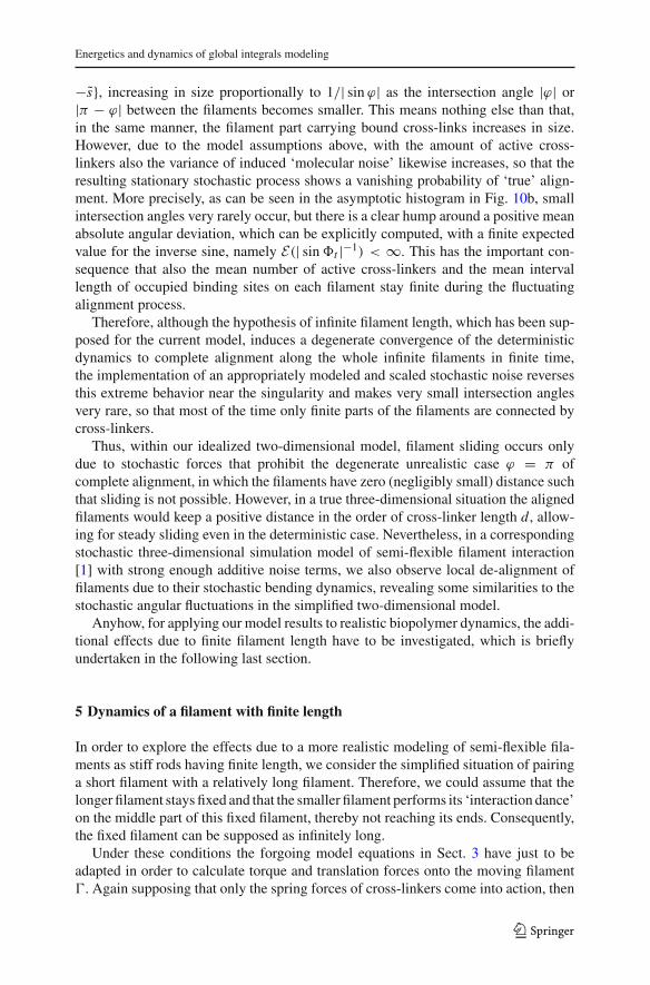
−s, increasing in size proportionally to 1/| sin ϕ| as the intersection angle |ϕ| or|π − ϕ| between the filaments becomes smaller. This means nothing else than that,in the same manner, the filament part carrying bound cross-links increases in size.However, due to the model assumptions above, with the amount of active cross-linkers also the variance of induced ‘molecular noise’ likewise increases, so that theresulting stationary stochastic process shows a vanishing probability of ‘true’ align-ment. More precisely, as can be seen in the asymptotic histogram in Fig. 10b, smallintersection angles very rarely occur, but there is a clear hump around a positive meanabsolute angular deviation, which can be explicitly computed, with a finite expectedvalue for the inverse sine, namely E(| sint |−1) < ∞. This has the important con-sequence that also the mean number of active cross-linkers and the mean intervallength of occupied binding sites on each filament stay finite during the fluctuatingalignment process.
Therefore, although the hypothesis of infinite filament length, which has been sup-posed for the current model, induces a degenerate convergence of the deterministicdynamics to complete alignment along the whole infinite filaments in finite time,the implementation of an appropriately modeled and scaled stochastic noise reversesthis extreme behavior near the singularity and makes very small intersection anglesvery rare, so that most of the time only finite parts of the filaments are connected bycross-linkers.
Thus, within our idealized two-dimensional model, filament sliding occurs onlydue to stochastic forces that prohibit the degenerate unrealistic case ϕ = π ofcomplete alignment, in which the filaments have zero (negligibly small) distance suchthat sliding is not possible. However, in a true three-dimensional situation the alignedfilaments would keep a positive distance in the order of cross-linker length d, allow-ing for steady sliding even in the deterministic case. Nevertheless, in a correspondingstochastic three-dimensional simulation model of semi-flexible filament interaction[1] with strong enough additive noise terms, we also observe local de-alignment offilaments due to their stochastic bending dynamics, revealing some similarities to thestochastic angular fluctuations in the simplified two-dimensional model.
Anyhow, for applying our model results to realistic biopolymer dynamics, the addi-tional effects due to finite filament length have to be investigated, which is brieflyundertaken in the following last section.
5 Dynamics of a filament with finite length
In order to explore the effects due to a more realistic modeling of semi-flexible fila-ments as stiff rods having finite length, we consider the simplified situation of pairinga short filament with a relatively long filament. Therefore, we could assume that thelonger filament stays fixed and that the smaller filament performs its ‘interaction dance’on the middle part of this fixed filament, thereby not reaching its ends. Consequently,the fixed filament can be supposed as infinitely long.
Under these conditions the forgoing model equations in Sect. 3 have just to beadapted in order to calculate torque and translation forces onto the moving filament. Again supposing that only the spring forces of cross-linkers come into action, then
123

P. Reiter et al.
under the simplifying assumption made in Example B, namely that the cross-linklength is approximately constant, ρ ≡ d, the measure valued version of the local forcekernel K f = K (s, s) can be used as it appears in (31) and (40). However, the integra-tion domain in the (s, s)-space is now restricted to those parts of the ellipse Cd whoses-values lie on the filament, see Fig. 2. Let us remind that s denotes the arc lengthon filament with s = 0 representing the intersection point with the other filament.Choosing the mass center as fixed point (X (t),Y (t)) on the moving filament, thenaccording to the terminology in (50) the variable S = S(t) denotes the s-value of thiscenter point, so that with finite filament length L the condition for s to represent anarbitrary point on the filament is
|s − S| ≤ L
2. (86)
Since the integration in all torque and force integrals is performed only on the curveCd , the relevant s-values representing occupied cross-link binding sites, see (4), satisfy
|s| =∣∣∣∣d · sin(ϕ + α)
sin ϕ
∣∣∣∣ ≤ d
sin ϕ, (87)
where we again restrict the derivation of this formula to the case 0 < ϕ < π . Forall these s-positions except the extreme ones, there are two angles α and α = π −2ϕ − α, under which cross-linkers can bind, see Figs. 1 and 2. Then the twofoldintegration domain is given by the intersection of both conditions (86) and (87) yieldings−(ϕ, S) ≤ s ≤ s+(ϕ, S) with
s±(ϕ, S) = ± min
(d
sin ϕ,
L
2± S
). (88)
Transformation into the α-parametrization, using the property
ds = cos(ϕ + α)d
sin ϕdα (89)
gives a well-determined integration domain α ∈ Aϕ,S and a ‘symmetry-map’α → α
with the property sin(ϕ + α) = sin(ϕ + α), so that both angles belong to the samebinding site s and that any of the integral representations with a kernel g = gϕ(α) asin Eqs. (43)–(45) can be written as a twofold integral over s, expressed by the sum oftwo integrands, namely gϕ(α) and gϕ(α):
d
sin ϕ
∫
Aϕ,S
gϕ(α) dα =s+(ϕ,S)∫
s−(ϕ,S)
gϕ(α)+ gϕ(α)
cos(ϕ + α)ds
= d
sin ϕ
r+(ϕ,S)∫
r−(ϕ,S)
gϕ(α)+ gϕ(α)√1 − r2
dr . (90)
123
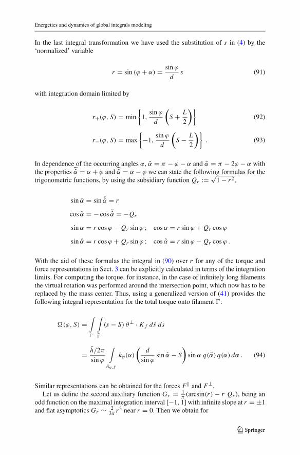
Energetics and dynamics of global integrals modeling
In the last integral transformation we have used the substitution of s in (4) by the‘normalized’ variable
r = sin (ϕ + α) = sin ϕ
ds (91)
with integration domain limited by
r+(ϕ, S) = min
1,
sin ϕ
d
(S + L
2
)(92)
r−(ϕ, S) = max
−1,
sin ϕ
d
(S − L
2
). (93)
In dependence of the occurring angles α, α = π − ϕ − α and α = π − 2ϕ − α withthe properties ˜α = α + ϕ and α = α − ϕ we can state the following formulas for thetrigonometric functions, by using the subsidiary function Qr := √
1 − r2,
sin α = sin ˜α = r
cos α = − cos ˜α = −Qr
sin α = r cosϕ − Qr sin ϕ ; cosα = r sin ϕ + Qr cosϕ
sin α = r cosϕ + Qr sin ϕ ; cos α = r sin ϕ − Qr cosϕ .
With the aid of these formulas the integral in (90) over r for any of the torque andforce representations in Sect. 3 can be explicitly calculated in terms of the integrationlimits. For computing the torque, for instance, in the case of infinitely long filamentsthe virtual rotation was performed around the intersection point, which now has to bereplaced by the mass center. Thus, using a generalized version of (41) provides thefollowing integral representation for the total torque onto filament :
(ϕ, S) =∫
∫
(s − S) θ⊥ · K f ds ds
= h/2π
sin ϕ
∫
Aϕ,S
kϕ(α)
(d
sin ϕsin α − S
)sin α q(α) q(α) dα . (94)
Similar representations can be obtained for the forces F‖ and F⊥.Let us define the second auxiliary function Gr = 1
π(arcsin(r) − r Qr ), being an
odd function on the maximal integration interval [−1, 1] with infinite slope at r = ±1and flat asymptotics Gr ∼ 2
3π r3 near r = 0. Then we obtain for
123

P. Reiter et al.
Example A(i) with infinitely stiff cross-linkers:
(ϕ, S) = −2κ0cosϕ
sin ϕ
(d
sin ϕ
1
2[Gr+(ϕ,S) − Gr−(ϕ,S)] − S
π[Qr−(ϕ,S) − Qr+(ϕ,S)]
),
F‖(ϕ, S) = −2κ0
π[Qr−(ϕ,S) − Qr+(ϕ,S)] ,
F⊥(ϕ, S) = −2κ0
π
1
tan ϕ[Qr−(ϕ,S) − Qr+(ϕ,S)] .
In general, the ODEs for the three dynamic variables(t), S(t) and R(t) can be takenas in (51)–(53), now with the nonlinearities also depending on S(t) and, clearly, on thelength L of the filament (including the inverse friction coefficients). The consequenceis that now the first two differential equations constitute a nonlinearly coupled ODEsystem:
d
dt= λ (, S) , (95)
d S
dt= λ FS(, S) := λ‖ F‖(, S)+ λ⊥
tanF⊥(, S) . (96)
The corresponding plots of the torque (ϕ, S) and ‘shift force’ FS(ϕ, S) aredepicted in Fig. 13. A nonzero shift force does only appear for larger values of |S|and small intersection angles (Fig. 13b), when cross-linkers only ‘pull’ at one sideof the finite filament. For discussing the more complex plot of the torque (Fig. 13a),we show its contour map in Fig. 14a and the section profile at S = 0 in Fig. 14b.The latter shows that pure rotational motion of the finite filament behaves similar asshown in Sect. 3, see Fig. 4a, but only as long as the intersection angle is so largethat the binding sites of active cross-linkers lie on the interior of the filament, namelyL · | sin| > 2d. As soon as the angle gets smaller, less cross-link combinations arepossible and the torque drastically falls to zero, but still linearly for sin φ → 0:
(ϕ, 0) ∼ − sign(sin ϕ)cosϕ
sin2 ϕmin1,GL·| sin ϕ|/2d
∼ −(
L
d
)3
cosϕ · sin ϕ .
This means that, due to the finite filament length, the two alignment states ϕ∗ = 0and π are no longer singular points for the filament dynamics, they rather are regu-lar asymptotically stable equilibria. Translated into the local analysis of the precedingsections, the corresponding ‘sign-type’ degenerate ODEs for zt ort are now smoothedin a specific manner, which is just induced by the model formulation for cross-linkaction.
The changed filament dynamics due to finite length becomes even more prominent,when the fixed filament is intersected by the moving one only for a small part at
123

Energetics and dynamics of global integrals modeling
Fig. 13 a (upper picture) The torque (ϕ, S) and b (lower picture) the ‘shift force’ FS(ϕ, S) for afinite moving filament of length L = 12 with cross-link length d = 1 using the model of the standardExample A(i). Parameters are as in Fig. 7b
its rear end, since then S(t) 0. As can be seen in Fig. 15 (and also in Fig. 14a,where the ((t), S(t)) trajectory is plotted into the contour diagram) the filament isslowly pulled towards the fixed filament, with S(t) slowly decreasing, but first theintersection angle gets wider, before finally the rapid rotational movement towardsantiparallel alignment takes place. In spite of the regularized singularity as discussedabove, the trajectory very rapidly reaches the asymptotic alignment state because of avery fast exponential decay.
Finally, most interesting is a combination of the results in Sects. 4 and 5, namelywhen implementing stochastic perturbations into the ODE-system (95) and (96) byexplicitly computing the corresponding noise amplitudes b#(ϕ, S) in analogy to (72)–(74). The properties of this full SDE system is currently explored and promises toreproduce some more interesting phenomena for short filament interaction.
123

P. Reiter et al.
phi
S
0.5 1 1.5 2 2.5 3
−10
−5
0
5
10
0 0.5 1 1.5 2 2.5 3−20
−15
−10
−5
0
5
10
15
20
phi
Ω( . ,0)
(a)
(b)
Fig. 14 a Contour lines of the torque (ϕ, S) together with a specific trajectory of Eqs. (95)–(96), andb profile of (ϕ, 0) for the situation when the intersection point is the mass center of the moving filament,see the text for comparison with the corresponding plot in Fig. 4a
6 Summary and further applications
The most important feature of the presented continuum model, for the interactionbetween stiff filaments, is the possibility to derive explicit local force kernels for avariety of applicable cross-linking mechanisms, which then can be used to calculatetorques and translational forces between the ‘rods’ as explicit global integrals depend-ing only on the geometric constellation. Clearly, this is valid only under the assumedhypothesis that there is a continuum of potential cross-link binding sites and a pseudo-stationary equilibrium in the Poisson process of binding and unbinding. However, notonly the mean binding strength in dependence of the geometric variables is condensedinto a deterministic model; also the stochastic fluctuations are modeled and simulatedaccording to an appropriate Gaussian noise kernel in the global integrals. Then, sto-chastic integration provides explicit variance expressions for the additive stochastictorques and forces, leading to a system of degenerate stochastic differential equations
123

Energetics and dynamics of global integrals modeling
−15 −10 −5 0 5
−4
−2
0
2
4
6
8
10
12
0 1 2 3 4 5 6−6
−4
−2
0
2
4
6Φ
t
Ψt
St
π − Rt
(a)
(b)
Fig. 15 Deterministic dynamics of a finite moving filament on a fixed infinite filament (the x-axis) formodel A(i) with parameters and conditions as in Fig. 13. In a (upper picture) the filament finally alignsantiparallelly, but the intersection angle π − t first increases towards π/2 while the filament is pulleddown, before the angle rapidly adjusts to alignment, see the dark curve in b (lower picture) and Movie A15.The convergence of t → π as well as of the two other variables St and Rt towards a steady state is notperformed in finite time: due to the smoothed function (see Fig. 14b) there remain tiny deviations thatare exponentially decreasing, though with a fast rate of order (L/d)3 = 123 in our case
(SDEs) for the filament variables (position and direction), which are coupled in therealistic case of filaments with finite length.
The idealized assumption of infinitely stiff filaments can approximately be appliedto actin filaments, whose length is small compared to the directional persistence lengthL pers ∼ 15 µm as estimated experimentally [7,21]. Thus for shorter filaments withL ≈ 1−5 µm the two-dimensional dynamics analysed and simulated in Sect. 5 shouldreflect typical properties of the observed stochastic pair interaction.
Clearly, our simplified model is restricted to situations, where the load forces ontoeach single cross-linker are so small ( 30pN ) that its conformational state and thedissociation rate of its actin binding site are not altered. Indeed, for higher forcesα-actinin and filamin dimers undergo subsequent steps of polymer unfolding, thuselastic relaxation, see [25,27].
123

P. Reiter et al.
Moreover, in the presented derivation of local force kernels we assume that thestiff cross-linkers (as e.g. myosin oligomers) apply forces only in direction of their‘connection vector’. However, many cross-linking polymers could be bent or twisted(as filamin, fascin or α-actinin) and thus could exert torque moments onto the attachedfilaments (see e.g. [22,30]). Under suitable model assumptions on the type and angulardependence of cross-linker micromechanics, analogous explicit kernels for the cor-responding forces (Kω and Kω in our notation) can then be derived. Obviously, theresulting degenerate differential equations could have different asymptotics and reveala variety of other convergence and fluctuation properties.
Finally, as described in Sect. 3, the temporal scaling of our model postulates arapid association and dissociation of cross-linkers at the actin binding sites, so thatcross-link connections between two filaments only stay for fractions of seconds or afew microseconds, while the parameter functions q(α) measure the angle-dependentassociation constants of the pseudo-stationary binding process. Thus, any filamentmotion with relative translational or angular speeds, v/L and , in the range below1/second will not experience any significant frictional resistance by cross-links, ratherby the dominating viscous drag forces appearing in the deterministic and stochasticdifferential equations. However, near the alignment singularity, sin ϕ = 0, at leastanalytically there appear infinitely large speeds, so that in a reasonable model exten-sion the frictional coefficients could be chosen as 1/λ(ϕ) ∼ 1 + εq0/| sin ϕ|, wherethe additional term would be proportional to the relative amount of bound cross-links.Then the slightly changed stochastic differential equation for ϕ would still be degen-erate (now with m = 1 in Lemma 2), but it would reveal a more smoothed fluctuationdynamics, thus better applicable to the observed filament behavior. Indeed, experi-mental observations with short actin filaments moving on a longer one that is fixedto a coated substrate, should be analysed under different myosin concentrations, inorder to test theoretical predictions similar to Sect. 5, now for the modified model.Moreover, a true model regularization resulting in bounded filament velocities maybe achieved by introducing friction terms that depend non-linearly on the angularspeed.
As one advantage of our simplified model we have demonstrated a thorough asymp-totic analysis around the singular states of parallel and antiparallel alignment, fromwhich some basic properties of the stochastic processes can be quantitatively extracted.Moreover, the presented regularization procedures are also used for consistent numer-ical procedures to simulate the degenerate stochastic dynamics, which reveals typicalproperties of actin filament sliding in the case that ‘contractile’ myosin oligomers actas cross-linkers.
As a further advantage, the explicitly computable (deterministic and stochastic)integrals could be easily used for more realistic worm-like-chain (WLC) models oflonger semi-flexible filaments, if just applied to all possible pair interactions betweenpiecewise straight segments of the discretized filaments. The resulting numerical algo-rithms, which reflect the approximative pseudo-stationary cross-linking process, couldwell compete with so far used ‘molecular dynamics’ simulations that uses multi-particle methods to represent individual cross-linkers (see e.g. [18]), particulary whenapplied to whole networks of interacting filaments as they currently are observed inexperiments, see [2], for instance.
123

Energetics and dynamics of global integrals modeling
Moreover, for the real three-dimensional biological system of semi-flexible actinfilaments, most of the two-dimensional dynamic properties presented here can be car-ried over and used as a basic description for more generalized interaction model: Thereis an additional degree of freedom not only in filament rotation and bending, but also inparametrizing the space angles of cross-link binding. Finally, we hope that an applica-tion of our approach, namely to derive explicit local interaction kernels from detailedmolecular mechanisms on a microscale, could give an input to the improvement ornew development of more physiological (than purely phenomenological) continuummodels for thermodynamical and fluid dynamical theories of polymer networks (seee.g. [3] or [12]), particularly for modeling and simulating the contractile actin-myosincytoskeleton in biological cells (see [14]).
Acknowledgments We thank the DFG for generously supporting this research, particularly within theSpecial Research Program (SFB 611) on Singular Phenomena and Scaling in Mathematical Models at BonnUniversity.
References
1. Bär D, Kuusela E, Alt W (2008) Interaction dynamics between pairs of semi-flexible filaments.University of Bonn (to appear)
2. Bendix PM, Weitz DA et al (2008) A quantitative analysis of contractility in active cytoskeletal proteinnetworks. Biophys J 94:3126–3136
3. Borukhov I, Bruinsma RF, Gelbart WM, Liu AJ (2005) Structural polymorphism of the cytoskeleton:a model of linker-assisted filament aggretation. Proc Natl Acad Sc USA 102:3673–3678
4. Blatt S, Reiter P (2006) Does finite knot energy lead to differentiability? Preprint no. 12. Institutfür Mathematik, RWTH Aachen. J Knot Theory Ramifications (to appear). http://www.instmath.rwth-aachen.de/→ preprints
5. Cantarella J, Piatek M, Rawdon E (2005) Visualizing the tightening of knots. In: VIS’05: Proceedingsof the 16th IEEE visualization. IEEE Computer Society, Washington, DC, pp 575–582
6. Freedman MH, He Z-X, Wang Z (1994) Möbius energy of knots and unknots. Ann Math (2) 139(1):1–50
7. Gittes F, Mickey B, Nettleton J, Howard J (1993) Flexural rigidity of microtubules and actin filamentsmeasured from thermal fluctuations in shape. J Cell Biology 120:923–934
8. Gonzalez O, Maddocks JH, Schuricht F, von der Mosel H (2002) Global curvature and self-contactof nonlinearly elastic curves and rods. Calc Var Partial Differ Equ 14(1):29–68
9. He Z-X (2000) The Euler-Lagrange equation and heat flow for the Möbius energy. Comm Pure ApplMath 53(4):399–431
10. Highsmith S (1999) Lever arm model for force generation by actin-myosin-ATP. Biochemistry 38:791–797
11. Janson LW, Taylor DL (1994) Actin-crosslinking protein regulation of filament movement in motilityassays: a theoretical model. Biophys J 67:973–982
12. Joanny JF, Jülicher F, Kruse K, Prost J (2007) Hydrodynamic theory for multicomponent active polargels. New J Phys 9:422
13. Kloeden PE, Platen E (1992) Numerical solution of stochastic differential equations. Springer, Berlin14. Koestler SA, Auinger S, Vinzenz M, Rottner K, Small JV (2008) Differentially oriented populations
of actin filaments generated in lamellipodia collaborate in pushing and pausing at the cell front. NatureCell Biol. doi:10.1038/ncb1692
15. Kusner RB, Sullivan JM (1998) Möbius-invariant knot energies. In [28], pp 315–35216. Liu X, Pollack GH (2004) Stepwise sliding of single actin and myosin filaments. Biophys J 86:353–35817. Lombardi V, Irving M et al (1995) Elastic distortion of myosin heads and repriming of the working
stroke in muscle. Nature 374:553–55518. Nédélec F (2002) Computer simulations reveal motor properties generating stable antiparallel micro-
tubule interaction. J Cell Biol 158:1005–1015
123

P. Reiter et al.
19. O’Hara J (1991) Energy of a knot. Topology 30(2):241–24720. O’Hara J (2003) Energy of knots and conformal geometry. Series on knots and everything, vol 33.
World Scientific Publishing Co. Inc., River Edge21. Ott A, Magnasco M, Simon A, Libchaber A (1993) Measurement of the persistence length of poly-
merized actin using fluorescence microscopy. Phys Rev E 48(3):1642–164622. Peletier O, Safinya CR et al (2003) Structure of actin cross-linkers withα-actinin: a network of bundels.
Phys Rev Lett 91(14):14810223. Reiter P (2004) Knotenenergien. Diploma Thesis, Math Inst Univ Bonn24. Reiter P (2008) Repulsive knot energies and pseudodifferential calculus. Ph.D. Thesis, RWTH Aachen
(to appear)25. Schwaiger I, Rief M et al (2004) A mechanical unfolding intermediate in an actin-crosslinking protein.
Nature Struct Mol Biol 11:81–8526. Schuricht F, von der Mosel H (2004) Characterization of ideal knots. Calc Var Partial Differ Equ
19:281–30527. Soncini M, Redaelli A et al (2007) Mechanical response and conformational changes of alpha-actinin
domains during unfolding: a molecular dynamics study. Biomech Model Biol 6:399–40728. Stasiak A, Katritch V, Kauffman LH (eds) (1998) Ideal knots. Series on knots and everything, vol 19.
World Scientific Publishing Co. Inc., River Edge29. Strzelecki P, von der Mosel H (2007) On rectifiable curves with L p-bounds on global curvature:
self-avoidance, regularity, and minimizing knots. Math Z 257:107–13030. Ylänne J, Scheffzek K, Young P, Saraste M (2001) Crystal structure of the α-actinin rod reveals an
extensive torsional twist. Structure 9:597–604
123