Endogenous Exchange Rate Fluctuations under the … Endogenous Exchange Rate Fluctuations under the...

This PDF is a selection from an out-of-print volume from the National Bureauof Economic Research

Volume Title: Macroeconomic Linkage: Savings, Exchange Rates, and CapitalFlows, NBER-EASE Volume 3

Volume Author/Editor: Takatoshi Ito and Anne Krueger, editors

Volume Publisher: University of Chicago Press

Volume ISBN: 0-226-38669-4

Volume URL: http://www.nber.org/books/ito_94-1

Conference Date: June 17-19, 1992

Publication Date: January 1994

Chapter Title: Endogenous Exchange Rate Fluctuations under the FlexibleExchange Rate Regime

Chapter Author: Shin-ichi Fukuda

Chapter URL: http://www.nber.org/chapters/c8533

Chapter pages in book: (p. 203 - 225)

8 Endogenous Exchange Rate Fluctuations under the Flexible Exchange Rate Regime Shin-ichi Fukuda

8.1 Introduction

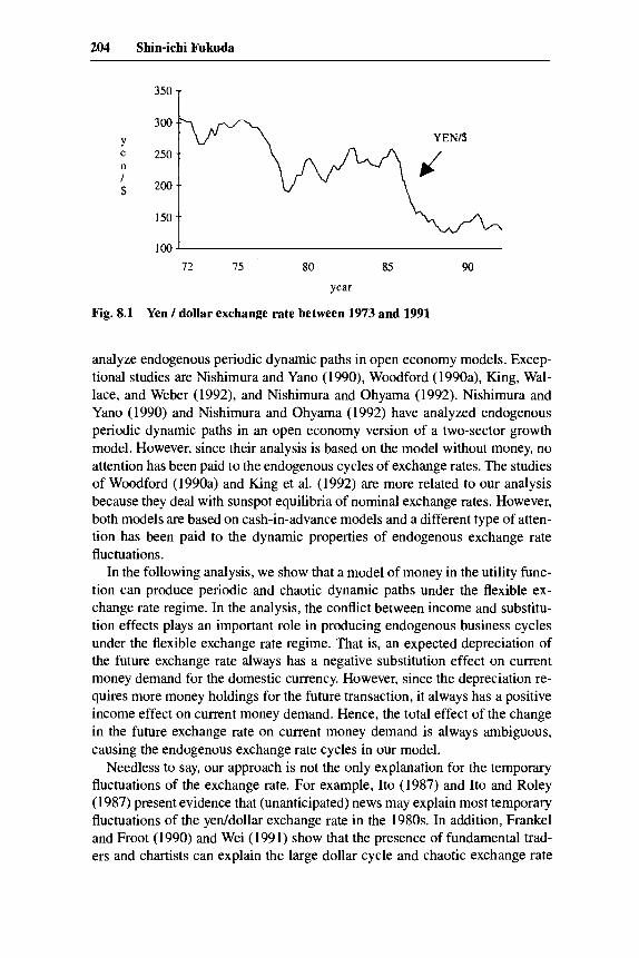
In the past two decades, we have experienced in the foreign exchange markets significant temporary fluctuations in the exchange rates of major currencies. For example, by plotting the movements of the yeddollar exchange rate after 1973, we can see a clear downward trend in this exchange rate in the long run. However, we can also see that the trend was not monotonic in the short run and that there were significant temporary fluctuations around the trend (see fig. 8.1). The purpose of this paper is to investigate why the exchange rate shows such significant temporary fluctuations. The model of the following analysis is based on a model of money in the utility function with liquidity-in- advance. Following Fukuda (1 990), we investigate the dynamic properties of a small open economy version of this monetary model.

The methodology used in the following analysis is an application of the theory of “chaos.” In the previous literature, Benhabib and Day (1982), Day (1982, 1983), and Stutzer (1980) are the first attempts to study chaotic phenomena in economic models. Authors such as Benhabib and Nishimura (1985) derive the competitive equilibrium cycles in a two-sector growth model, while authors such as Grandmont (1 985) characterize the chaotic phenomena in overlapping generations models. In addition, Matsuyama (1990, 1991) and Fukuda (1990) find that the model of money in the utility function can produce chaotic dynamic paths.’ However, throughout these studies there exist few attempts to

Shin-ichi Fukuda is associate professor of economics at the Institute of Economic Research, Hitotsubashi University.

The author would like to thank Michihiro Ohyama, Shang-Jin Wei, and other participants of the Third Annual East Asian Seminar on Economics for their helpful comments on an earlier draft of this paper. This research was supported by the Ministry of Education of Japan

I . See also Woodford (1988) for related issues.

203

204 Shin-ichi Fukuda

150 t 72 75 80 85 90

year

Fig. 8.1 Yen / dollar exchange rate between 1973 and 1991

analyze endogenous periodic dynamic paths in open economy models. Excep- tional studies are Nishimura and Yano (1990), Woodford (1990a), King, Wal- lace, and Weber (1992), and Nishimura and Ohyama (1992). Nishimura and Yano (1990) and Nishimura and Ohyama (1992) have analyzed endogenous periodic dynamic paths in an open economy version of a two-sector growth model. However, since their analysis is based on the model without money, no attention has been paid to the endogenous cycles of exchange rates. The studies of Woodford (1990a) and King et al. (1992) are more related to our analysis because they deal with sunspot equilibria of nominal exchange rates. However, both models are based on cash-in-advance models and a different type of attention has been paid to the dynamic properties of endogenous exchange rate fluctuations.

In the following analysis, we show that a model of money in the utility function can produce periodic and chaotic dynamic paths under the flexible exchange rate regime. In the analysis, the conflict between income and substitution effects plays an important role in producing endogenous business cycles under the flexible exchange rate regime. That is, an expected depreciation of the future exchange rate always has a negative substitution effect on current money demand for the domestic currency. However, since the depreciation requires more money holdings for the future transaction, it always has a positive income effect on current money demand. Hence, the total effect of the change in the future exchange rate on current money demand is always ambiguous, causing the endogenous exchange rate cycles in our model.

Needless to say, our approach is not the only explanation for the temporary fluctuations of the exchange rate. For example, Ito (1987) and Ito and Roley (1987) present evidence that (unanticipated) news may explain most temporary fluctuations of the yeddollar exchange rate in the 1980s. In addition, Frankel and Froot (1990) and Wei (1991) show that the presence of fundamental traders and chartists can explain the large dollar cycle and chaotic exchange rate

205 Endogenous Exchange Rate Fluctuations

movement in the 1980s. This paper does not deny the significance of these earlier studies. Instead, we try to present a supplementary explanation of some temporary fluctuations of exchange rates which these studies do not necessarily explain.

The paper is organized as follows. The next section presents a basic small open economy model of money in the utility function. Following Fukuda (1992), the dynamic properties of the model are analyzed under the flexible exchange rate regime in sections 8.3 and 8.4. Section 8.5 extends the model by introducing the endogenous labor supply. Section 8.6 shows that the fixed exchange rate regime may rule out the possibility of endogenous cycles in the economy. Section 8.7 interprets our results by using a phase diagram, and section 8.8 considers a welfare implication of our analysis. Section 8.9 summa- rizes our main results.

8.2 The Basic Model

The basic model of the following analysis is based on Fukuda (1992). We consider a small open economy inhabited by identical agents. Until section 8.5, we assume that there is a single, perishable, tradable consumption good in the economy. Each representative agent maximizes the following utility function:

where c, is consumption at period t, pr is the domestic price level at period t, M, is the amount of domestic currency at the beginning of period t, and p is a discount rate satisfying 0 < p < 1. For all c, > 0 and M / p , > 0, we assume that u and v are weakly concave and twice-continuously differentiable (i.e., u" 5 and v" 5 0) and are weakly increasing (i.e., u' 2 and v' 2 0).

The budget constraint of the representative agent is

where yr is exogenous income, T, is the lump-sum tax (or transfer if negative), r is the world real interest rate, and b, is the real amount of foreign bonds at period t.

In our representative agent model, the change in the real amount of foreign bonds is equal to the real amount of current account surplus. Furthermore, because of the law of one price, it holds that p , = ep* (i.e., the purchasing power parity condition) where p* is foreign price level and e, is the nominal exchange rate in terms of domestic currency. Since the model is a small open economy, world real interest rate, r; and foreign price, p*, are exogenously given in our model. In order to rule out extreme consumption behavior in the limit, we assume that world real interest rate, I; is constant and equal to the


rate of time preference of the representative agent, that is, P( 1 + r) = 1, in the following analysis.* We also normarize foreign price p* to be one.

Until section 8.5, we assume that exogenous income y, is constant over time (i.e., yr = y ) and is not storable. We also assume that government revenue through money creation is balanced by the exogenous change in the lump-sum transfer, Then, assuming an interior solution, the first-order conditions under perfect foresight are

(3)

(4) (1bJ u‘(c,) = P (W,+I) u’(c,+J + v’(q+I~P,+l) I. u’(c,) = P(1 + r) u’(c,+1)7

Since P( l + r) = 1, the monotonicity of u’(c,> implies that c, is constant over time. Furthermore, since p* = 1, the purchasing power parity condition leads to p , = e,. Hence, denoting the constant consumption level by c, the dynamic equation (4) is written as

( 5 ) lie, = P Wer+,) [ 1 + ( l / u r ( c ) ) vr(Mf+l/eI+l ) 1. Equation ( 5 ) determines the dynamic system in our model. By using this

equation, the following sections investigate whether nominal exchange rate and real money balances may show endogenous cycles under the flexible exchange rate regime. In considering periodic endogenous cycles, we define the iterates of a function h of a set X into itself by hl(x) = h(x) and h ( x ) =

h(h”(x)) for all integers i 2 2. We then define a periodic orbit (or a cycle) of period k of the backward perfect foresight map h by the sequence (x,+~, x , + ~ - ~ , . . . , x,) such that (i) x,,, is a fixed point of hk, i.e., xfik = hk( xr+J, and (ii)xf+k-l =h(x, , ,)#x,+,forall i= 1 , . . . , k - 1.

8.3 Endogenous Exchange Rate Cycles

Under the flexible exchange rate regime, the nominal money supply M , is exogenously determined by the monetary authority. In this paper, we consider the case in which the monetary authority keeps the growth rate of money supply constant as follows:

(6) M, = zM,-, for all t.

Then, (5) and (6) lead to

(7) m, = ( P M m,,, [ 1 + (11 u’(c)) v’(m,+J 1 , where m, = Mj e,.

The dynamic equation (7) determines the dynamic system of real money balances, m,, in our model under the flexible exchange rate regime. If we define

2. It is well known that lim,+= c, = 0 when p(1 + r) < 1 and lirn,+- c, = +- when p(1 + r ) > 1.


(8) f (m> = W z ) m + (11 ~ ’ ( c ) ) v’(m>l,

equation (7) implies that rn, can be written as a function of m,,, such that m, = f l m,+, ) under perfect foresight. That is, our system induces well-defined backward perfect foresight (b.p.f.) dynamics in which the expected future value determines its current value. This b.p.f. map is continuously differentiable.

In order to focus our attention on the well-defined dynamics, the following analysis assumes that z > p, lirnm+,f’(m) > 1, and lim,,++-f’(m) < 1 . Then, there exists a steady-state equilibrium of real money balances, m*, such that [ (z - p ) / p ] u’(c) = v’(m*) under the above assumptions. This steady-state equilibrium m* is a unique steady-state equilibrium if and only if limm,, mv’(m) > 0. When limm,, mv’(m) = 0, there is another steady-state equilibrium such that m, = 0. However, when m, = 0, the level of nominal exchange rate e, is infinite (i.e., the domestic currency has no value) because M, is finite.

In the following analysis, we investigate the possibility that the backward perfect foresight dynamics (7) may have period k 2 2 cycles and local sunspot equilibria even under some economically reasonable conditions. Under the assumption presented above, it is well known that a sufficient condition for period-two cycles and local sunspot equilibria in a one-dimensional map (7) is that I f ’ (m) I > 1 at m = m* (see, e.g., Grandmont 1985; Blanchard and Kahn 1980). By using this condition, Fukuda (1992) showed the following proposition.

Proposition: A sufficient condition for the existence of period-two cycles and local sunspot equilibria of real money balances is that

(9) - m* v”(m*) / v’(m*) > 2 [d(z - p)], where m* is the steady-state equilibrium such that v’(m*) = [ ( z - p) / p] ~ ’ ( c ) .

The proposition states that when the relative risk aversion of the utility on real money balances is large at the steady state m*, equilibrium real money balances may have period-two cycles and local sunspot equilibria. Further- more, since the nominal money supply is exogenously given, the proposition implies that the equilibrium nominal exchange rate may also have period-two cycles and local sunspot equilibria.

In general, our model of money in the utility function may have higher-order periodic and aperiodic cycles. However, without specifying the functional form of u and v it is difficult to find the existence of higher-order periodic and aperiodic cycles in our model. Hence, in the next section, we investigate numerically the existence of such higher-order periodic and aperiodic cycles for three specific classes of utility functions.

8.4 Examples

In this section, we investigate the existence of periodic and aperiodic cycles under the flexible exchange rate regime for specific utility functions. We consider the following three classes of utility functions:


(10)

(11)

v(m,) = m,l-R / (1 - R ) , where R > 0;

v(m,> = -(b12) (m, - k)2 , where b > 0, when m, < k, when m, 2 k; = 0,

(12)

The utility functions are, respectively, a member of the constant relative risk- aversion family, of the quadratic family, and of the constant absolute risk- aversion family. For each utility function, the dynamic equation (7) is written as

(13) m, = (BIZ) m,,, [1 + (Uu’(c)) m 3 ;

(14) m, = y m,,, (1 - 6 m,,,), when m,,, < k, when m,,, 2 k;

(15) m, = (P/z> m,,, [1 + (1/urW) exp(-a m,,,)l,

where y = (p/z)[l + (b/u’(c))k] and 6 = (b/u’(c))/[l + (b/u’(c)) k]. Hence, the proposition leads to the following corollary.

Corollary: A sufficient condition for the existence of period-two cycles and local sunspot equilibria under the flexible exchange rate regime is that (i) R > 2 [d(z - p)] in utility function (lo), (ii) (p/z)[l + (b/u’(c)k] > 3 under utility function ( l l ) , and (iii) log[(l/u’(c))(p/(z - p ) ) ] > 2[6(z - p ) ] under utility function (12).

The corollary implies that there exist period-two cycles and local sunspot equilibria under the flexible exchange rate regime (i) when z or R is large enough in utility function (lo), (ii) when parameter b, l/u’(c), or k is large enough in utility function ( l l ) , and (iii) when u’(c) is small enough in utility function (12). In fact, for parameter values satisfying the sufficiency conditions in the corollary, nominal exchange rate and real money balances may show very complicated dynamic paths around the steady-state equilibrium.

In figures 8.2-8.4, we describe these possibilities for given expected nominal exchange rates (or equivalently real money balances) at time I: In the figures, we depict the dynamics of nominal exchange rate and real money balances for the above three classes of utility functions. The dynamics clearly show that both nominal exchange rate and real money balances follow very complicated fluctuations around the steady-state equilibrium? In particular, although the expected nominal exchange rate at time T is very close to that of the steady state, the transition paths are very different and highly volatile.

8.5 Extensions

v(m,) = - (l/u) exp(-u mJ, where u > 0.

= (P/z> m,,,,

The results in the preceding sections were derived from a very simple small open economy model. Thus, in order to derive more realistic implications, the

3. Since the growth rate of money supply is positive (i.e,, z > 1). nominal exchange rates have trends to the depreciation in the figures.


(i) Exchange rate dynamics

I 0

TIME

( i i ) Dynamics of real money balances

T TIME

Fig. 8.2 The dynamics of exchange rate and real money balances under utility function (10) Notes: Parameter set : p = 0.9, z = 1.2, u' (c) = 1, R = 15, T = 30. Terminal values : rn, = 1 or 0.9.

model may need to be extended in several directions. We here extend the model by introducing the endogenous labor supply. We consider an economy in which each individual maximizes the following utility function:

m

u = c p' [U(C,> + ww,, ly/PJI, r=o

(16)

where L, is the amount of leisure at period t. We assume that the utility function w(L,m) satisfies the usual concave assumption. We also allow the possibility that the utilities of leisure and real money balances are not separable.

The budget constraint of the representative agent is

(17)

where Lo is the feasible labor hour and W, is real wage at period t.

b, = (1 + r) b,-, + W, (Lo - L,) - C, - M,+,/p, + Mjp, - T,,

Assuming a linear production function such that y , = L,, it holds that



0

- I 1

-3

TIME

(ii) Dynamics of real money balances

0.5 1 IIlT = 0.9

TIME

Fig. 8.3 The dynamics of exchange rate and real money balances under utility function (11) Notes: Parameter set : p = 0.9, z = 1.1, u'(c) = I , k = 1, b = 2, T = 30. Terminal values : mT =

0.8 or 0.9.

W, = 1 in equilibrium. Thus, since p(l + r) = 1 and p , = e,, the first-order conditions for an interior solution are

(18) u'(c,) = Uf(C,+J'

(19)

(20) Wt) ~'(c,) = P (l/e,+J [u'(c,+J + w2(Lr+l, m,+l)l.

Condition (19) states that L, can be written as a function of m,. Thus, defining a function cp such that L, = cp(m,) and substituting this function into (20), we obtain

wi(Lp mJ = w\(Lr+i, mr+i),

(21) (lie,) ~ ' ( c , ) = P (l/er+I) ur(cr+,) + *(mr+J 1 9



= 9

I 0

TIME

T 8 4 : : : : : : : : : : : : : : : : : : : : : : : : : : : :

0 TIME

Fig. 8.4 The dynamics of exchange rate and real money balances under utility function (12) Notes: Parameter set : p =0.9, z = 1.2, u'(c) = 0.0001, a = 1, T = 30. Terminal values : rn, =

10 or 9.

where W m f + J = w,(cp(m,), q+J Since condition (18) implies that c, is constant over time, the dynamic equa-

tion (21) is mathematically equivalent to the dynamic equation (7) if we re- place T(m,+J by v(mf+l). Hence, all results in earlier sections carry through. Thus, we can easily see that the nominal exchange rate and real money balances may have endogenous cycles in the model of endogenous labor supply. In addition, since L, is a function of m,, we can also see that labor supply may also fluctuate endogenously unless the utility function w(L, m) is separable in leisure and real money balances. Since the level of consumption is constant


over time, this implies the possibility that the current account may also fluctuate endogenously. This result is noteworthy because such endogenous cycles of the current account cannot be derived in the model of previous sections.

8.6 The Optimal Choice of Exchange Rate Regime

The question of optimal exchange rate regime is one of the most extensively debated topics in international macroeconomics. Traditionally, the debate was based mainly on Mundell-Fleming-type open macro models (see, e.g., Boyer 1978; Turnovsky 1984; Fukuda and Hamada 1988; Fukuda 1991). However, the analysis was limited because the models were not necessarily based on individuals’ maximizing behavior. In order to overcome this limitation, several authors have recently attempted to investigate the optimal exchange rate regime in models of money with individuals’ maximizing behavior. For example, Helpman (1981), Lucas (1982), and Aschauer and Greenwood (1983) have considered models of money with cash-in-advance constraint. They have shown that, without distortions, the choice of exchange rate regime has no real effect on resource allocation but that the existence of distortions introduces the possibility of real effects of exchange rate management. However, their anal- yses have focused mainly on resource allocation in the steady-state equilibrium and paid little attention to the transition path to the steady-state equilibrium. Hence, it is relatively unknown how the exchange rate regime affects the transition path to the steady-state equilibrium. This has been investigated by Fukuda (1992), however. He showed how the endogenous cycles under the flexible exchange rate regime will be ruled out under the fixed exchange rate regime. This section briefly reviews his main result by considering the dynamic property under the fixed exchange rate regime in our basic model.

Under the fixed exchange rate regime, nominal money supply M, is endogenously determined by the monetary authority to keep the nominal exchange rate e, constant. Hence, by noting that e, = e,,,, equation (5) can be written as

Since the left-hand side of equation (22) is constant over time, equation (22) implies that real money balances m, are constant over time. In particular, since the real money balances that satisfy (22) are equivalent to those of the steady state with constant money supply (i.e., z = l), real money balances stay at their steady-state equilibrium forever under the fixed exchange rate regime without changing the amount of money supply. This result is in marked contrast with that under the flexible exchange rate regime, because real balances under the flexible exchange rate regime may show endogenous fluctuations for some parameter set and terminal condition. That is, once the monetary authority can commit to fixing the exchange rate, real balances (and obviously nominal exchange rate) show no endogenous fluctuations for any parameter set.


One noteworthy point in the above result is that under the fixed exchange rate regime the monetary authority needs to make no intervention in the foreign exchange market to reduce the nominal exchange rate fluctuation. That is, once the initial values of exchange rate and money supply are given, the only necessary condition for the monetary authority to keep the fixed exchange rate regime is to make people believe that the monetary authority will endogenously determine nominal money supply M, to fix the nominal exchange rate e,. A crucial point is that, in our model of money in the utility function, periodic cycles or sunspot equilibria may arise when people’s expectations diverge from those of the steady-state equilibrium. Thus, once the commitment of the monetary authority to fixing the nominal exchange rate makes people’s expectations converge to those of the steady-state equilibrium, deviations of expectations from the steady-state equilibrium are ruled out under the fixed exchange rate regime.

8.7 Diagrammatic Explanation

In order to interpret the results in previous sections, it may be useful to illustrate them by drawing the locus of (7) in the plane (m,, m,+,). Figure 8.5 shows the locus of (7) under the utility function (1 1). When the parameter b is small (i.e., the curvature of the utility function is small), the curve is flat and the dynamic path of m, shows no cyclical fluctuation. However, when the parameter b is large (i.e., the curvature of the utility function is large), the curve is backward bending at some critical point p. That backward-bending curve arises reflects the conflict between intertemporal substitution and income effects. That is, an expected depreciation of the future exchange rate always has a negative substitution effect on current money demand the domestic currency (or a positive substitution effect on current demand for consumption). How- ever, since the depreciation requires more money holdings for future transactions, it always has a positive income effect on current money demand (or a negative income effect on current demand for consumption). Hence, the total effect of the change in the future exchange rate on current money demand is always ambiguous. This ambiguity through intertemporal substitution and income effects causes the business cycles that were obtained in the above proposition and its corollary.

The only case in which no endogenous fluctuation arises is when real money balances m, stay at the steady-state equilibrium forever. This special case does not necessarily happen under the flexible exchange rate regime because each individual does not necessarily expect real money balances to stay at the steady-state equilibrium forever. However, under the fixed exchange rate regime, the situation is different: the only self-fulfilling rational expectation is the expectation that the nominal exchange rate (and real money balances) will stay at the steady-state equilibrium forever. As a result, no endogenous fluctuation arises under the fixed exchange rate regime.


mt 0 I- mt+1

( i i ) the case that "b" is large

Fig. 8.5 The phase diagram under utility function (11)

8.8 A Welfare Implication

The results in preceding sections have an important welfare implication in determining the optimal exchange rate regime. As we explained in section 8.6, it is well known that if we simply compare the welfare properties of the steady- state equilibria in an economy with some distortions, the optimal exchange rate regime is the flexible exchange rate regime with appropriate money supply growth. In particular, we can show that, in our model of money in the utility function, the optimal rate of money growth is given by Friedman's (1969) rule: the rule which maintains a rate of money growth close to the rate of time preference (see Woodford [1990b] for its proof). However, as we have shown in previous sections, the equilibrium corresponding to a given rate of money growth (say, that specified by Friedman's rule) need not be unique. Since the


multiple equilibria are Pareto ranked, it also becomes very important to know under what exchange rate regime nonconvergent paths can be eliminated.

In the previous sections, we have shown that nonconvergent paths can be eliminated under the fixed exchange rate regime. Thus, although the optimal rate of money growth under the fixed exchange rate regime deviates from Friedman’s rule, the fixed exchange rate regime can lead to the second-best resource allocation in the sense that nonconvergent paths are eliminated. Of course, we may have the first-best resource allocation under the flexible exchange rate regime with Friedman’s rule as long as nonconvergent paths do not arise. However, as we have shown in the previous sections, endogenous periodic dynamic paths can arise even under Friedman’s rule. Hence, unless this possibility is ruled out, we may have the less desirable resource allocations of nonconvergent paths under Friedman’s rule.

8.9 Concluding Remarks

This paper investigated the dynamic properties in a small open economy model of money in the utility function. Following Fukuda (1990), we have shown that under a flexible exchange rate regime the nominal exchange rate and real money balances may have endogenous periodic dynamic paths for some parameter set and future expectations. We have also shown that if the labor supply is endogenous, the current account may also have endogenous dynamic paths.

Our theoretical results may present one answer to why the empirical relevance of existing classes of exchange rate theories is so poor (see, e.g., Meese and Rogoff [ 19831 which shows the poor out-of-sample forecasting perfor- m a n ~ e ) . ~ If a variable follows a chaotic path, its path would be extremely sensitive to the initial value and its forecast would be very difficult by usual statistical procedures. At the current stage, there is very little empirical evidence suggesting the presence of chaos in the exchange rate market. (An exceptional work is by Brock, Hsieh, and LeBaron [1991], which has applied the Brock- Dechert-Scheinkman statistic to the yeddollar exchange rate with four other major exchange rates.) However, further successful empirical studies may prove the potential importance of a chaotic model of exchange rate.

References

Aschauer, David, and Jeremy Greenwood. 1983. A further exploration in the theory of

Benhabib, Jess, and Richard H. Day. 1982. A characterization of erratic dynamics in exchange rate regimes. Journal of Political Economy 912365-75.

4. The following argument is based partly on comments by Shang-Jin Wei.


the overlapping generations model. Journal of Economic Dynamics and Control 4:37-55

Benhabib, Jess, and Kazuo Nishimura. 1985. Competitive equilibrium cycles. Journal of Economic Theory 35:284-306.

Blanchard, Olivier J., and Charles M. Kahn. 1980. The solution of linear difference models under rational expectations. Econometrica 48: 1305-1 1.

Boyer, Russell S. 1978. Optimal foreign exchange market intervention. Journal of Polit- ical Economy 86: 1045-55.

Brock, William A,, David A. Hsieh, and Blake LeBaron. 1991. Nonlinear dynamics, chaos, and instability: Statistical theory and economic evidence. Cambridge: MIT Press.

Day, Richard H. 1982. Irregular growth cycles. American Economic Review 72:406-14. . 1983. The emergence of chaos from classical economic growth. Quarterly

Journal of Economics 98:201-13. Frankel, Jeffrey, and Kenneth A. Froot. 1990. Chartists, fundamentalists, and trading in

the foreign exchange market. American Economic Review 80: 18 1-85. Friedman, Milton. 1969. The optimum quantity of money. In The optimum quantity of

money and other essays. Chicago: Aldine. Fukuda, Shin-ichi. 1990. The emergence of equilibrium cycles in a monetary economy

with a separable utility function. Discussion Paper no. 90-3, Yokohama National University.

. 1991. Exchange market intervention under multiple solutions. Journal of Eco- nomic Dynamics and Control 15:339-53.

. 1992. Endogenous exchange rate fluctuations and the desirable exchange rate regime. Discussion Paper no. 92-3, Yokohama National University.

Fukuda, Shin-ichi, and Koichi Hamada. 1988. Towards the implementations of desirable rules of monetary coordination and intervention. In Toward a world of economic stability, ed. Y. Suzuki and M. Okabe. Tokyo: University of Tokyo Press.

Grandmont, Jean-Michel. 1985. On endogenous competitive business cycles. Econo- metrica 53:995-1045.

Helpman, Elhanan. 1981. An exploration in the theory of exchange rate regimes. Jour- nal of Political Economy 892365-90.

Ito, Takatoshi. 1987. The Intra-daily exchange rate dynamics and monetary policies after the Group of Five agreement. Journal of the Japanese and International Econo- mies 1:275-98.

Ito, Takatoshi, and V. V. Roley. 1987. News from the U.S. and Japan: Which moves the yeddollar exchange rate? Journal of Monetary Economics 19:255-77.

King, Robert G., Neil Wallace, and Warren E. Weber. 1992. Nonfundamental uncer- tainty and exchange rates. Journal of International Economics 32233-108.

Lucas, Robert E., Jr. 1982. Interest rates and currency prices in a two-country world. Journal of Monetary Economics 10:335-60.

Matsuyama, Kiminori. 1990. Sunspot equilibria (rational bubbles) in a model of money-in-the-utility-function. Journal of Monetary Economics 25: 137-44.

. 1991. Endogenous price fluctuations in an optimizing model of a monetary economy. Econometrica 59: 1617-32.

Meese, Richard, and Kenneth Rogoff. 1983. Empirical exchange rate models of the seventies: Do they fit out of sample? Journal oflnternational Economics 14:3-24.

Nishimura, Kazuo, and Michihiro Ohyama. 1992. Dynamics of external debt and trade. Paper presented at Third Annual East Asian Seminar on Economics.

Nishimura, Kazuo, and Makoto Yano. 1990. Interlinkage in the endogenous real business cycles of international economies. Discussion Paper no. 90-8, Yokohama Na- tional University.


Stutzer, Michael J. 1980. Chaotic dynamics and bifurcation in a macro model. Journal of Economic Dynamics and Control 2:353-76.

Turnovsky, Stephen J. 1984. Exchange rate market intervention under alternative forms of exogenous disturbances. Journal of International Economics 17:279-97.

Wei, Shang-Jin. 1991. Price volatility without news about fundamentals. Economics Letters 37:453-58.

Woodford, Michael. 1988. Expectations, finance, and aggregate instability. In Finance constraints, expectations, and macroeconomics, ed. M. Kohn and S. C. Tsiang. New York: Oxford University Press.

. 1990a. Does competition between currencies lead to price level and exchange rate stability? NBER Working Paper no. 3341. Cambridge, Mass.: National Bureau of Economic Research.

. 1990b. The optimum quantity of money. In Handbook of monetary economics, ed. B. M. Friedman and E H. Hahn. Amsterdam: North-Holland.

Comment Michihiro Ohyama

This paper constructs a simple but very interesting model of a small open economy with representative agents optimizing under flexible and fixed exchange rates. It shows that under flexible exchange rates, the nominal exchange rate and real money balances may fluctuate periodically, whereas under fixed exchange rates the endogenous cycles of real money balances can be ruled out. In view of this result, the fixed exchange rate regime is said to be desirable in comparison with the flexible exchange rate regime, in the sense that the former eliminates nonconvergent adjustment paths that the latter may have to accom- modate.

The analysis of the model seems to be impeccable, and the results are neatly presented and summarized. Thus, all that I can do as a discussant is to recon- sider the assumptions of the model and present some comments on their implications.

Balanced Current Account

maximizing a utility function, The paper considers a small open economy with the representative agent

described in equation,, (1) in section 8.2. It is said that real money balances, M,/p,, held at the beginning of the period yield some utility since money re- duces the transaction cost of consumption. If the agent holds money solely for the purpose of reducing transaction cost, however, his or her utility function may not be separable into consumption and real money balance as is presently

Michihiro Ohyama is professor of economics at Keio University.


assumed. The present assumption seems to imply that the agent derives utility from holding money quite independently of his or her consumption of goods.

As is shown in the paper, this assumption of a separable utility function, coupled with another strong assumption that the agent’s rate of time preference is equal to the world interest rate, leads to the conclusion that optimal consumption is constant through time. Since output is constant, the budget constraint ( 2 ) implies that the economy’s current account is always balanced, with its trade account exhibiting a surplus or deficit corresponding to the interest payment arising from the initial (historically given) external debt. This seems to be an overly simplistic setup for a discussion of desirable exchange rate regime.

Needless to say, there are at least two distinct ways out of this trap. One is to modify the separability of the utility function, and the other is to modify the constancy of the rate of time preference. I hope that Fukuda gives some consideration to these modifications.

Transactions Money in Utility Function

The author seems to believe that money must enter the representative agent’s utility function along with consumption, separately or otherwise, as long as money is needed to reduce transactions cost. It seems to me, however, that the most direct and purest way of introducing money holding for transactions purposes in the present setup is simply to assume that the real money balance to be held at the beginning of each period is a function of the consumption planned for that period. Under this cash-in-advance approach, the other assumptions of the present model imply constancy of consumption and, therefore, of real money balance. Thus, fixed and flexible exchange rates become virtually indistinguishable.

Despite the interpretation of money in the utility function given in the present paper, I believe that it is necessary to go beyond the simple transactions motive of holding money if one is to investigate the relative desirability of flexible and fixed exchange rates. It may be one’s love for money, distinct from one’s need for consumption-the motive posited in the paper-or some speculative reason that motivates one’s holding money. Paul Krugman, a recent con- vert to the school of fixed exchange rate regime, argues convincingly in a recent paper that the fatal deficiency of the flexible exchange regime is its vulnerability to an attack of destabilizing speculation.

Some Questions

Finally, let me pose some questions regarding possible extensions of the model. First, the present paper assumes a small open economy facing the rate of interest and terms of trade given in the world. The international monetary system must be designed, however, to meet the needs of countries of compara- ble size, each with its own monetary authority. It is, therefore, desirable to


extend the present analysis to a model comprising at least two countries. The models of Matsuyama (1 991) and Fukuda (1990) cited in this paper may pro- vide useful departures.

Second, the fixed exchange rate regime discussed here must be distinguished from the adjustable-peg regime. The latter is vulnerable to speculative attack since the monetary authority’s commitment to fixing the exchange rate at a given level is inadequate. The real choice is often between the flexible exchange rate regime and the adjustable-peg regime rather than between the flexible exchange rate regime and the fixed exchange rate regime. Is it possible to construct a model of the adjustable-peg regime along the lines of the model in the present paper?

Third, toward the end of the paper, the author discusses the welfare implications of the present analysis. The discussion is, however, very brief and it is difficult for me to understand the welfare propositions asserted there. For in- stance, it is asserted that the fixed exchange rate regime can lead to the second- best resource allocation in the sense that nonconvergent paths are eliminated. It seems to me that the author has to expound on this and other welfare propositions in greater detail.

References

Fukuda, Shin-ichi. 1990. The emergence of equilibrium cycles in a monetary economy with a separable utility function. Discussion Paper no. 90-3, Yokohama National University.

Matsuyama, Kiminori. 1991. Endogenous price fluctuations in an optimizing model of a monetary economy. Econornetrica 59: 1617-32.

COmtneIlt Shang-Jin Wei

The central aspect of Shin-ichi Fukuda’s paper is an interesting demonstration that chaotic movement and sunspot equilibria of exchange rate can arise in a theoretic model. Building on this theoretical possibility of chaos, Fukuda then argues (mostly informally) that a flexible exchange rate system tends to yield lower welfare than a fixed rate regime.

Deriving chaos in an exchange rate model, by itself, is an interesting result. I will focus my comment on this aspect of the paper. Meese and Rogoff (1983) first challenged the empirical relevance of existing classes of exchange rate theories by showing their inferior out-of-sample forecasting performance relative to a simple atheoretical random-walk specification. Many people since then have tried alternative specifications or alternative estimation methods of

Shang-Jin Wei is assistant professor of public policy at the John F. Kennedy School of Govern- ment, Harvard University.


exchange rate models in an attempt to outperform the random-walk model. Almost all efforts have failed. It is important to note that the failure of economic models to outperform a random-walk specification does not establish that the (log) exchange rate follows a random walk. In fact, a direct test of the i i d . hypothesis for the change in the log exchange rate actually rejects such a null hypothesis (e.g., Brock, Hsieh, and LeBaron 1991).

A chaos model of exchange rate such as the Fukuda model could, in prin- ciple, explain these empirical findings. We know that if a variable (which is a well-defined function of other economic fundamentals) follows a chaotic path, its path would be extremely sensitive to the initial value (the so-called butterfly effect), Since the margin of error in measuring usual fundamental variables (e.g., GNP) is not low, we need not be surprised that exchange rate path seems not very forecastable by looking at these fundamentals, even if exchange rate theories have identified correctly that economic fundamentals that matter for exchange rate movement. Second, a deterministic chaos need not be distin- guishable from a stochastic (in particular, random-walk) series by usual statistical procedures.

If a chaos model of exchange rate has this appealing potential, how do we get chaos into a model? Fukuda chooses a representative agent approach with money-in-the-utility specification. What initially follows a chaotic path in his model is the domestic price level (and consequently real money balances). A key step to get chaos in the foreign exchange market is the assumption of purchasing power parity (PPP), so that chaos in the domestic price level can be transmitted into chaos in the exchange rate. However, many studies have shown that the PPP does not hold for the short horizons within which erratic exchange rate movement is thought to arise. In addition, a priori, one might think that exchange rates, or other asset prices, may be chaotic for certain time periods. But it appears to be stretching the point to believe domestic price level and real money balance to be erratic or chaotic.

More important, the role of the speculative market itself is missing in Fuku- da’s model. When people talk about erratic movement in the foreign exchange or any asset market, they have in mind more often than not some aspects of speculative trading itself as the amplifier or the source of short-term erratic fluctuation, which is not necessarily related to economic fundamentals. It seems desirable to have a model of chaotic exchange rate that builds upon speculative trading per se, without relying on the heavy assumption of the PPP.

In the next part of my comment, I will show in a very simple model that this can be done. The source of chaos in my model is the interaction of speculative activities among heterogeneous traders. Chaos is not present all the time, but it occurs for some parameter values. During the times when chaos does arise, the exchange rate movement can be very erratic, including having quantitative breaks even when the fundamentals do not fluctuate. The time path of exchange rate is extremely sensitive to the initial value (or the degree of its precision), which makes it virtually impossible to forecast exchange rates on the basis of


economic variables measured with errors. Finally, exchange rate can overreact to “insignificant” news.

Alternative Model Based on Interaction among Heterogenous Agents

This alternative model derives chaotic movement of exchange rate from interaction among heterogenous traders in the market. The presence of heterogenous traders in the foreign exchange market has been recognized before to have important implications. For example, the presence of fundamental traders and chartists has been argued as an explanation for the large dollar cycle in the 1980s (Frankel and Froot 1990).

In the following model, there are two classes of traders. The first class is informed fundamental traders, who believe in economic fundamentals and economic models and have some private but noisy information about the fundamentals. The second class is speculative chartists (similar to the noise trades in Black [ 19861 or Kyle [1985]). We could have a third class, uninformed fundamental traders, who would complicate the derivations without adding much new insight.

The Environment

To make the story as simple as possible, I will make some drastic assumptions. There are two types of assets. The first is a riskless domestic bond, whose one-period rate of interest is normalized to be zero. The second is a foreign bond, which also has a zero rate of interest when evaluated in the foreign currency. For simplicity, let domestic and foreign markets for foreign bonds be perfectly segregated (for example, a domestic U.S.-dollar bond market and a Euro-yen bond market. A Japanese ban on capital outflow prevents Japanese investors from investing in either of the two markets). Every informed fundamental trader is endowed with one unit of foreign bond, so the total supply of foreign bond in the market is equal to the number of informed traders, 0.

Informed Fundamental Traders

A representative fundamental trader has a negative exponential utility function with a constant coefficient of absolute risk aversion, 6. We assume that she has a two-period investment horizon (i.e., she will exit the foreign exchange market at the end of next period). She observes a noisy signal, i, about v, the ex post value of next-period exchange rate, v = S(t + 1):

(1) i = v + e ,

where e is a white noise variable. We assume that v and e are independently distributed, v has a normal distribution with mean zero and precision T”, and e is also a normal variate with mean zero and precision 7,. The informed trader’s information set contains all the past and present values if i’s, the past and present exchange rate, and the behavior rule of the chartists. However, since the


informed trader cares only about the value of her wealth at next period, the present value of i is the only relevant information for her. Let X ( t ) be her demand for foreign bonds. Since she is endowed with one unit of foreign bond, her demand for domestic bonds is [I - X(t)]S(t). where S(t) is the spot exchange rate at time t . More precisely, the informed fundamental trader solves the following problem:

( 2 )

subject to

(3)

max E{ -e-SW I i ( t ) ) ,

W = X( t ) v + [I - X(t)]S( t ) .

The solution to this problem is

(4)

where

X ( t ) = pi(t) - aS(t ) ,

(3)

Chartists

Let Z(t) be the chartists' collective demand for foreign bonds at time t. This demand is assumed to be proportional to the chartists' subjective expectation of the rate of return on the foreign bonds, denoted by RsetI+,. Let u(t) be the expectational error made by the chartists. Then,

and their demand for foreign bonds is

(7) 11.

The chartists here can also represent program traders, or any traders that use exogenous trading rules.

Equilibrium

An equilibrium in the model is defined to be a list {X( t ) , Z( t ) , S(t)}, such that X ( t ) maximizes the informed fundamental traders' expected utility, Z( t ) satisfies the chartists' trading rule, and S(t) clears the market (for foreign bonds).

Applying the definition of an equilibrium, we know that S(t) has to satisfy the following condition

(8) 0 X ( t ) + Z(t) = 0 .


With appropriate substitutions, the equilibrium exchange rate path can be characterized by

(9)

This seemingly simple first-order difference equation is, in fact, capable of generating chaotic movement for certain parameter values. To see this, let us first make a simple transformation. Define

on S(t) ru(t) - r + opi(t) -0 . Y(t) =

Then, equation (9) can be rewritten as

Y(t + 1) = CY(i,t) Y(t) [l - Y(t)l ,

where

(12) a(i,t) = [ru(t) - r + @pi(t) - @I2

rz[& + 1) - 11 + T@pi(t + 1) - I73 ’

Dynamics of nonlinear equations have been extensively studied recently. The above equation is one of the simplest nonlinear equations that can generate chaos. Let me summarize a relevant result.

Lemma (May 1976): Consider 1 < a(i,t) < 4. The behavior of equation (11) depends sensitively on the value of a(i):

(1) For 1 < cx < 3, the path of Y(t) converges to some fixed point. (2) Starting from CY = 3, the fixed point becomes unstable. (3) Starting from CY = 3.5700, the “chaotic” region begins. That is, the accu-

mulation of cycles of period 2” starts for some integer n. (4) Starting from CY = 3.6786, the first odd-period cycle appears. (5) Starting from a = 3.8284, cycles with period 3 appear. By Sarkovsky’s

theorem, this means that cycles with every integer period are present at the same time.

(6) For CY = 4.0000, the “chaotic” region ends. (7) There are stable cycles in the “chaotic” region.

This lemma shows that the time path Y(t) is extremely sensitive to the parameter values. Although chaos is not present at all times, the point is that it can occur for some parameter values.

Note that a(i, t) is a function of the information variable, i. This suggests two possibilities. First, for certain fixed values of i, say i(t + 1) = i(t) = some constant (so that there is no fluctuation in the information about fundamentals), the exchange rate could still be very volatile. As is well known from the chaos literature, the exchange rate path in (9) or (1 1) can have sudden quantitatively


large breaks, even with absolutely no shocks to the fundamentals to the market. Second, a slight change in the value of i(t + I ) , can dramatically change the dynamics of the exchange rate path. For example, consider a small change in the value of i(t + 1) that changes a from 3.56 to 3.58. For the original value of i(t + l), the exchange rate is nonchaotic. With this slight change in the news (or rumors) about the fundamentals, the exchange rate suddenly becomes erratic. Therefore, the exchange rate could appear to overreact to “insignificant” news.

What Do We Know Empirically?

Is there empirical evidence suggesting the presence of chaos in the exchange rate market? Since this is a conference on East Asian economies, let me first note that there are no chaotic movements in the bilateral exchange rates of any of the nine East Asian developing countries in terms of the U.S. dollar, since most of them either explicitly peg to or implicitly assign heavy weight in their currency basket to the dollar. The same can be said of many developing countries outside the Pacific region.

What about the yeddollar rate (or other exchange rates)? Empirical tests on this are very few. One exception is Brock, Hsieh, and LeBaron (1991), who have applied the Brock-Dechert-Scheinkman (BDS) statistic to the yeddollar rate together with four other major exchange rates. The result from the BDS test is consistent with both a low-dimensional chaos or stochastic nonlinear process. On the other hand, there is a lack of collaborative evidence in support of the chaos hypothesis. If attention is restricted to stochastic nonlinear models, they conclude that nonlinearity in variance is more plausible than nonlinearity in means.’

To summarize, a chaotic model of exchange rates has an appealing feature in its potential to explain the empirical failure of many earlier theoretical models of exchange rate determination. Such a chaotic model can be derived in a representative-agent macro model as in Fukuda or in a heterogenous-traders micro model as in this comment. Systematic empirical work is still needed in order to evaluate fully the empirical relevance of the chaos hypothesis of exchange rates.

References

Black, Fischer. 1986. Noise. Journal ofFinance 41 (July): 529-43. Brock, Williams A,, David A. Hsieh, and Blake LeBaron. 1991. Nonlinear dynamics,

chaos, and instability: Statistical theory and economic evidence. Cambridge: MIT Press.

1. A successful empirical model of nonlinear dependence in the variance of exchange rate (with no chaos) is Engle, Ito, and Lin (1990).


Engle, Robert, Takatoshi Ito, and Wen-Lin Lin. 1990. Meteor showers or heat waves? Heteroskedastic intra-daily volatility in the foreign exchange market. Econornetrica

Frankel, Jeffrey, and Kenneth Froot. 1990. “Chartists, fundamentalists, and trading in

Kyle, Albert. 1985. Continuous auctions and insider trading. Econornetrica

May, Robert. 1976. Simple mathematical models with very complicated dynamics. Na- ture 261:459-67.

Meese, Richard, and Kenneth Rogoff. 1983. Empirical exchange rate models of the seventies: Do they fit out of sample? Journal of International Economics 14:3-24.

Wei, Shang-Jin. 1991. Price volatility without news about fundamentals. Economics Letters 37:453-58.

58:525-42.

the foreign exchange market. American Economic Review 80 (May): 181-85.

53: 13 15-35.

Endogenous Exchange Rate Fluctuations under the … Endogenous Exchange Rate Fluctuations under the...

Documents

Transcript of Endogenous Exchange Rate Fluctuations under the … Endogenous Exchange Rate Fluctuations under the...