Lund University

School of economics and management

Department of Economics

Endogeneity and Specialization Theories ofOptimal Currency Areas: A Comparative

European Study

Second Year Master Thesis

Author:

Kristoffer Persson

Supervisor:

Fredrik NG Andersson

May 22, 2011

Abstract

In this thesis the group of European countries that signed the Maastricht treaty are inves-

tigated subject to the endogeneity aspect and the specialization effect of optimal currency

areas. The main method used is time series factor analysis for identification of a common

European business cycle. To give the analysis a firm basis the USA is compared with Euro-

pean countries during the 1970-2010 period. Furthermore, the group of European countries

are analyzed for the 1970-1993 and 1993-2010 periods separately. The results point in the

direction of the endogeneity aspect so far being the main aspect effecting the European coun-

tries. To further investigate the relationship between an occurrence of regional cycles in the

US the Krugman index of specialization is deployed for both the European countries and the

USA. This analysis together with the factor analysis implicates that the European countries

can expect a future dominance of the specialization effect.

Contents

1 Introduction 4

2 Theory 8

2.1 Optimal currency area . . . . . . . . . . . . . . . . . . . . . . . . . . . . . . 8

2.2 Specialization . . . . . . . . . . . . . . . . . . . . . . . . . . . . . . . . . . . 9

2.3 Endogeneity of currency areas . . . . . . . . . . . . . . . . . . . . . . . . . . 10

3 Analysis 11

3.1 Method . . . . . . . . . . . . . . . . . . . . . . . . . . . . . . . . . . . . . . 11

3.2 Data . . . . . . . . . . . . . . . . . . . . . . . . . . . . . . . . . . . . . . . . 13

3.2.1 Data treatment . . . . . . . . . . . . . . . . . . . . . . . . . . . . . . 13

3.2.2 European Business cycles 1970:Q1-2010:Q4 . . . . . . . . . . . . . . . 15

3.3 TSFA-results European countries 1970:Q1-1993:Q3 . . . . . . . . . . . . . . 20

3.4 TSFA-results for the European countries 1993:Q4-2010:Q4 . . . . . . . . . . 21

3.5 Analyzing the European case in the time domain . . . . . . . . . . . . . . . 23

3.6 TSFA results for US 1970:Q1-2010:Q4 . . . . . . . . . . . . . . . . . . . . . . 24

3.7 Analyzing the European case in the space domain . . . . . . . . . . . . . . . 27

3.8 Krugman index of specialization . . . . . . . . . . . . . . . . . . . . . . . . . 27

3.9 Analyzing the full picture . . . . . . . . . . . . . . . . . . . . . . . . . . . . 32

4 Conclusions 33

5 Appendix 35

6 References 48

1

List of Figures

3.1 The Finnish Business Cycle 1970-2010 . . . . . . . . . . . . . . . . . . . . . 15

3.2 The French Business Cycle 1970-2010 . . . . . . . . . . . . . . . . . . . . . . 15

3.3 The German Business Cycle 1970-2010 . . . . . . . . . . . . . . . . . . . . . 16

3.4 The Irish Business Cycle 1970-2010 . . . . . . . . . . . . . . . . . . . . . . . 16

3.5 The Italian Business Cycle 1970-2010 . . . . . . . . . . . . . . . . . . . . . . 17

3.6 The Dutch Business Cycle 1970-2010 . . . . . . . . . . . . . . . . . . . . . . 17

3.7 The Portuguese Business Cycle 1970-2010 . . . . . . . . . . . . . . . . . . . 18

3.8 The Spanish Business Cycle 1970-2010 . . . . . . . . . . . . . . . . . . . . . 18

3.9 The Greek Business Cycle 1970-2010 . . . . . . . . . . . . . . . . . . . . . . 19

3.10 The estimated European business cycle 1970:Q1-1993:Q3 . . . . . . . . . . . 21

3.11 The European estimated business cycle 1993Q4-2010:Q4 . . . . . . . . . . . 23

3.12 The estimated US national business cycle 1970:Q1-2010:Q4 . . . . . . . . . . 27

3.13 Mean level of specialization European countries 1993-2008 . . . . . . . . . . 29

3.14 Mean specialization US 1970-2008 . . . . . . . . . . . . . . . . . . . . . . . . 30

3.15 US specialization and communality of national cycle . . . . . . . . . . . . . . 31

2

List of Tables

3.1 CAIC-values for the European countries 1970:Q1-1993:Q3 . . . . . . . . . . . 20

3.2 TSFA European countries 1970:Q1-1993:Q3 . . . . . . . . . . . . . . . . . . 20

3.3 CAIC-values for the European countries 1993:Q3-2010:Q4 . . . . . . . . . . . 21

3.4 TSFA model for the European countries 1993:Q4-2010:Q4 . . . . . . . . . . . 22

3.5 Factor significances 1970:Q1-2010:Q4 . . . . . . . . . . . . . . . . . . . . . . 25

3.6 Specialization levels for the European countries 1993-2008 . . . . . . . . . . 28

3.7 Deviations from mean level of specialization . . . . . . . . . . . . . . . . . . 31

5.1 Communalities US 1970-2010 . . . . . . . . . . . . . . . . . . . . . . . . . . 36

5.2 Estimated Loadings US 1970-2010 . . . . . . . . . . . . . . . . . . . . . . . . 38

5.3 Krugman index of specialization USA . . . . . . . . . . . . . . . . . . . . . . 40

3

Chapter 1

Introduction

The European Monetary Union has for a long time been considered as an optimal currency

area. Economic events during the last four years have however revitalized this discussion.

The financial crisis has had a profound impact on the European monetary union and has

made it possible to view the economic evolution from the creation of the union as a full

business cycle. The union has also for the first time faced internal problems through the

substantial fiscal deficit of some of the member states. This opens the possibility of making a

proper effort of measuring the coherence of member states and the occurrence of a common

business cycle.

The economic motivation for having a common European currency clinches heavily on

the assumption that the EMU is an optimum currency area. Establishing whether the EMU

is such an area is therefore very important for a number of reasons. Firstly, it is important

for determining the future existence of the union. Secondly, it is important for determining

whether the union should be further expanded or not. Thirdly, it gives implications for policy

makers when making further decisions about the outline of the union.

Currency areas have for a long time been the target of economic interest. Especially the

different pros and cons of them have spurred many questions about when it is optimal to

form such unions and under what circumstances it is optimal to have one. This work starts

with Mundell (1961) who stated that periodic balance of payment crisis is unavoidable in a

system of pegged exchange rates. Moreover, systems of purely flexible exchange rates might

be suboptimal in areas who are candidates to be optimum currency areas (OCA). Groups

of nations that are candidates to be included into such an area must have high internal and

external common factor mobility. McKinnon (1963) continued the analysis further on the con-

cept of optimum currency areas and stressed the importance of intra-industry factor mobility.

4

Vaubel (1977) contributes to the optimum currency theory by attempting to answer a

set of questions regarding the suitability of the EC community (Germany, France, Italy,

Netherlands BENELUX, UK, Ireland and Denmark) as an OCA. The research points in the

direction of that the contemporary European community is indeed a candidate to be an

OCA and that the concept of OCA might be a dynamic one. Melvin (1985) suggests that

a currency substitution effect leads to a limitation of central banks ability to Independently

control the monetary supply. The main implication of the research is that France, Germany,

Italy and the UK are candidates to be an OCA but more for reason of currency substitution

than anything else. A public finance perspective on Europe as an OCA is proposed by Can-

zoneri & Rogers (1990). Their findings suggests that the EC, which is stylized by including

Italy and Germany, is likely to be an OCA if as long as they exhibit small valuation and

currency conversion costs, low public spending and a high degree of openness.

In addition theories that aim at describing what happens to countries’ business cycle

synchronization after the inception of a currency union have been developed. Krugman and

Venables (1996) develop a model of two imperfectly competitive industries located at differ-

ent geographical positions. The purpose is to investigate whether the European community

might experience agglomeration when entering a common currency area. This purely theo-

retical analysis points in the direction of agglomeration or specialization. In contrast, Frankel

and Rose (1998) investigate the relationship of intra currency union openness and intra in-

dustry trade. The main purpose of this is to investigate whether countries with strong trade

links tend to have more correlated business cycles. Findings on this type of relationship

suggests countries becoming better candidates for OCA membership after the inception of

the union. This effect is called the endogeneity aspect of currency unions. The results in

question are based on a panel regression for 30 industrialized countries.

Kose et al (2003) attempt to identify world-, region and country specific common business

cycles by the means of a dynamic factor model. The research implies that there indeed is an

underlying world factor that explains at least some part of all 60 included countries variation.

It also implies that regional factors play a role in some parts of the world. Bergman & Jonung

(2010) find support for the endogeneity aspect of currency unions when they measure busi-

ness cycle synchronization in Europe with special focus on the Scandinavian countries. They

base their conclusion on two factor model estimations for the Scandinavian currency union

and the EMU respectively. In a recent paper Willet et al (2010) analyze the endogeneity

aspect of the EMU from a political economy perspective. In this type of analysis focus is put

5

on trade flows, business cycle synchronization and structural reforms. The main method is

a simple correlation analysis along with a study of external trade ratios. When this type of

analysis is employed the conclusions differ somewhat from for example Bergman and Jonung

(2010) in the sense that the endogeneity aspect of the currency union is neither confirmed or

denied as the main force effecting the EMU countries after inception.

The aim of this thesis is to shed light upon whether the endogeneity aspect or the special-

ization effect of optimal currency areas has dominated since the inception of the Maastricht

treaty. More generally this means investigating whether the countries who signed the Maas-

tricht treaty and also later joined the EMU are moving towards or away from being an OCA.

The reason for including the seven Maastricht years leading up to the inception of the EMU

is that the Maastricht treaty forced the signing countries to converge in a number of OCA

criteria. The inception of the Maastricht treaty can therefore in some aspects be viewed as

the inception of the EMU albeit without the common currency.

The means by which the analysis will be carried out is through time series factor analysis

for measuring correlation and existence of common business cycles. This is in contrast to

simply measuring the correlation. The reason is that if a set of factors can be singled out

and we can conclude convergence then we can conclude both increase in correlation and the

presence of one or more underlying common business cycles. These can either represent the

total set of countries or a subset of them implying a regional factor. Such results are stronger

than only measuring the correlation between countries since countries can be correlated for

other reasons than direct economic integration.

Consider for example the case of two countries exporting a large portion of their pro-

duction to a third country. This might lead to correlation of the business cycle but not

necessarily to the existence of a common factor that steers the evolution of the two countries

business cycle. Therefore if there indeed exists one or more common business factors it will

be possible to draw firmer conclusion about the extent to which countries in the Maastricht

countries have integrated co-variant economies. In addition the degree of specialization will

be measured through employment of the Krugman Index of Specialization.

The time series factor analysis will span both over time and space. The time dimen-

sion will be analyzed by comparing the 1970-1992 period with the Maastricht (1993-2010)

period. The space dimension will be analyzed by comparing the Maastricht countries with

the US states for the 1970-2010 period. Similarly for the specialization index the US 1970-

6

2010 period will be compared with the EU 1993-2008 period. The reason for including the

US into the analysis is that it is widely regarded as a stable currency area that has been

around for many years which implies that it will give the analysis a good basis of comparison.

The uniqueness of this thesis stems mainly from the fact than an attempt is made to

measure both business cycle correlation by the means of factor analysis and level of special-

ization. Also the usage of the 2010 data adds relevance in relation to much research since it

includes the recent financial crisis.

The outline is as follows: In Chapter 2 the theoretical framework which this thesis builds

upon is outlined. Sub-sectionally in Chapter 3 the analysis starts with a review of the main

methods used. This is followed by a presentation of the data as well as a section on how

the data was treated before the main method was used. The Results are sub-sectionally

presented and analyzed. Finally in Chapter 4 some concluding remarks wrap up the thesis.

7

Chapter 2

Theory

2.1 Optimal currency area

The theory of optimal currency areas was developed with the Bretton Woods system of fixed

exchange rates still operational (Mongelli 2005:608). The man behind the idea, Mundell,

sets out to determine if it is optimal for all countries currencies to float freely or if there

exists such a concept as an optimal currency area. The optimal currency area as a concept

corresponds to a subset of all countries in the world for which a set of conditions are met.

Mudell is predominately focused on areas with a common currency where one central bank

controls the monetary supply (Mundell 1961:658).

At this point in time the Phillips curve still reigned unquestionably and Mundells primary

focus was to determine what size the currency area should have for there not to be frictions

of such an amplitude that one central bank would have to accept too large regional inflation

and too large regional unemployment at the same time (Mundell 1961:659). He argues that

flexible exchange rates are to prefer but only between regions that are optimal currency areas.

Countries that are good candidates for a currency area are defined as having:

• High factor mobility

• Price and wage flexibility

• Financial market integration

• Fiscal integration

• High political integration

• Diversification in production and consumption

8

• High degree of economic openness

• Similarities in inflation

The requirement for high factor mobility stems from the idea that if factor mobility is low

then flexible exchange rates fills the function of a compensation mechanism when the relative

real factor prices change. If the exchange rate is fixed or indeed there is a currency union

then factor mobility needs to be high because of the lack of such a compensation mechanism.

Also if the union experiences asymmetries in unemployment then mobility of labor needs to

be high in order to dampen effects of intra-regional drops in labor demand. The price and

wage flexibility is important from the perspective that when for example two countries are

in a currency union and exhibit high unemployment and high inflation then the process of

adjustment following the shock that put the countries in that position is made with less cost.

The reason for countries being financially integrated is that it reduces the need for ex-

change rate adjustments when interest rates differ due to shocks (Mongelli 2005:609). Di-

versification in production and consumption over all countries ensures that no country is

extra vulnerable to any specific types of shocks implying that business cycles will be similar

across countries (Mongelli 2005:610). The high degree of openness is mostly thought of as

being towards other member countries. Large intra union trade will cause spill over effects

synchronizing business cycles (Mongelli 2005:609). The similarities in inflation facilitates

that the common central bank can use effective monetary policy and that the terms of trade

between the member states remain stable over time which reduces the need for an adjustment

mechanism such as a flexible exchange rate (Mongelli 2005:610).

2.2 Specialization

The theory of specialization and OCA’s is based on the idea that different countries within

the union have different relative advantages for production of different goods. The main idea

is that when a currency area is started under such circumstances production will move to

countries that has relative advantages for production in different industries. This will lead

to specialization of industries relocating such that the industry portfolio of each country

becomes less diversified. This will lead to each country becoming more vulnerable to specific

shocks implying that a decrease of the homogeneity in the sensitivity of shocks across the

area will take place. All in all the theory of specialization suggests that a process of industry

specialization will take place when a currency union is started and that this process will lead

9

to less synchronized business cycles which in turn demands that labor mobility is high to

avoid within region unbalances in employment and inflation (Mongelli 2005:625).

2.3 Endogeneity of currency areas

In contrast to the theory of specialization the endogeneity aspect of a monetary union claims

that when a set of countries enter into a currency union they will become more synchronized.

The reason for this is that once they have committed to having one common currency they

have informally decided to become long-term partners in trade and political activities. This

commitment will facilitate foreign direct investment and reciprocal trade which in turn will

cause the business cycle to become more synchronized. This implies that countries need not

on forehand have synchronized business cycles for being candidates to enter in to a common

currency union. The real process of synchronization starts after the inception of such an

endeavor. Under this theory labor mobility does not need to be high, at least no to the same

extent as for the specialization theory (Frankel & Rose 1998:1010).

10

Chapter 3

Analysis

3.1 Method

The main idea behind factor analysis is that one can, from a set of observable variables, find

a set of common factors or latent variables. The factors govern the evolution of the observed

variables. This implies reducing the dimensions of the set of observable variables yi,t to the

a set of factors, ξk,t, such that k < i. The model is:

yi,t = α +Bξk,t + εt (3.1)

Where yi,t is the set of observable variables for country i and where ξk,t is the set of k

underlying factors or latent variables and B is the factor loadings on yi,t. The idiosyncratic

error term is represented by εt. In this specific case it is assumed that the underlying fac-

tors have some sort of dynamics but assumptions about such dynamics are not made. This

implies that fewer restrictions are imposed on the model as opposed to alternative meth-

ods such as Dynamic Factor Analysis (DFA) where the underlying factors on forehand have

to be explicitly modeled. Equation 3.1 is the same as for standard (cross-sectional) factor

analysis theory with the very important difference that observations are indexed with time.

This imposes some challenges to the model since time-series variables rarely are covariance

stationary (Gilbert & Meijer 2005:5).

Time series factor analysis (TSFA) assumes that the time series included in the model

are non-stationary integrated of order one so that the series show stationarity in its first

differences. In this thesis, all variables used for factor modeling are by definition stationary

I(0) so that differencing is not necessary. In this context the only assumption being made for

standard maximum likelihood estimation to be possible is that the series ξt and εt are serially

11

correlated but uncorrelated at t with zero means and constant covariances Γ and Ψ. In this

case the means and covariances of the observed series yt is: µy = α and Σy = BΓB′ + Ψ

(Gilber & Meijer 2005:6). Provided that these assumptions hold it is possible to consistently

estimate the factor loadings B and the error covariance Ω from the sample covariance through

the following equation:

Σ = BΓB′ + Ω (3.2)

Where

Ω =T∑t=1

εtε′t

T(3.3)

Here Ω is assumed to be diagonal and is identified if the following restriction is met:

(M − k)2 ≥M + k (3.4)

This restriction is known as the Ledermann bound where M stands for the number of

observable variables and k stands for the umber of factors. The Ledermann bound indicates

how many factors it is possible to estimate from the set of observable variables (Gilbert &

Meijer 2005:8). The likelihood estimator for the loadings B and the error covariances Ω is

found by minimizing the function (Gilbert & Meijer 2005:9):

L = log(detΣ) + tr(Σ−1Sy) (3.5)

The factor scores ξt, that is, the values of the underlying factors can be found by using

the Bartlett predictor. This method involves predicting the underlying factors from the set

of observed series yt, estimated loadings B and error covariance Ω through the expression

(Gilbert & Meijer 2005:12):

ξBt = (B′Ω−1B)−1B′Ω−1yt (3.6)

With estimators for factor loadings, factor correlations, and factor scores in place the

model can consistently be estimated. In order to determine the optimal number of factors to

include in the model the Consistent Akaike Information Criteria (CAIC) due to Bozdogan

(1987) will be used. The consistent AIC builds on the work by Akaike (1973) and is defined

as:

CAIC = −2log[L(θ)] +K[log(n) + 1] (3.7)

12

The model is selected by minimizing over the estimated CAIC values for different model

specifications. Here L(θ) is the log likelihood of the parameter vector and the entire first

term describes the lack of fit of the model in question. The second term is a penalty term

where more parsimonious models are preferred, here n is the sample size and K is the model

size. This measure is designed to avoid overparameterization by extending the penalty term

with the sample size as opposed to only the model size using standard AIC (Anderson et

al 1998:265). In the context of factor analysis the CAIC is used in combination with the

Ledermann bound to determine the optimal number of factors.

3.2 Data

The data that has been used for the TSFA-model is quarterly real-GDP for the European

countries from the OECD main economic indicators database. For the US no quarterly GDP

data was available for the entire 1970-2010 period on state level so employment data was

used as a proxy variable. The data on US employment was collected from the US Bureau

of Labor Statistics. For measuring the level of specialization data on yearly industry output

from the OECD STAN database was collected for the EU10 and for the US the data was

collected from the Bureau of Economic Activity (BEA). The industry data from the OECD

STAN database was somewhat more limited than the production data on the entire economy

from the OECD main indicators with data only available for the 1993-2008 period. Also the

data on Ireland was so scarce that the country was left out in the analysis.

3.2.1 Data treatment

Data on GDP and employment can be viewed as time series of the following composition:

Yt = Gt + Ct + St + It (3.8)

Where Gt is the growth trend or time trend, Ct is the cyclical component, St is a seasonal

component and It is an irregular component. For the European GDP data all series where

seasonally adjusted when collected which implies that the seasonal and irregular components

had been singled out and removed from the series Yt. The data on US employment was not

seasonally adjusted upon data collection and therefore the X12-ARIMA method of seasonal

adjustment1 was used for the entire dataset (see for example Granger (1978:35)). In order

to single out the cyclical component Ct the Hodrick-Prescott (HP) filter due to Hodrick and

1The calculations where made using a program supplied by the US Census Bureau

13

Prescott (1980,1996) was used. The method in question estimates the growth trend by min-

imizing the sum of the differences between Yt and Gt. In addition the smoothness of the

trend is controlled by a parameter λ. The resulting cyclical component Ct is by definition

mean-zero and stationary (Hodrick & Prescott 1996:3).

The HP-filter is a popular way of singling out the cyclical component in the research

community especially for business cycle theorists. At the same time some critiques have also

been proposed for the method which mainly focuses on 2 points. The first of these points

is that the HP-filter is not optimal at the endpoints of a series. This is due to the fact that

the series is a symmetric two-sided filter that looses optimality in the end- as well as start-

ing points of a series (Mise et al 2005:58). The second aspect of the critique points at the

possibility that it generates spurious cycles that could lead to wrong conclusions about how

short-term movements in macroeconomic data relates (Harvey & Jaeger 1993:246). Despite

this critique the method has withstood the test of time in a remarkably good way and is

likely to be used for the purpose of isolating the cyclical component of a time-series further

into the future (Ravn & Uhlig 2002:371).

For the reason of the HP-filter rendering spurious estimates at the endpoints of a dataset

the data on real GDP for the European countries and the data on employment for the US

was expanded exponentially at all start and end points of the dataset. The data on industry

production was limited to manufacturing industries following Midelfart-Knarvik et al (2000)

rendering a total of 38 industries for the 9 European countries included in the analysis. For

the US data on industry production the definitions are slightly different from the European

countries due to different data collecting agencies but a similar restriction as for the Euro-

pean countries was made. Estimation of the time series factor analysis and calculation of the

Krugman specialization index is made by use of the R software for statistical computing[2][3].

2The ”tsfa” package supplied by the Comprehensive R Archive Network and created by Paul Gilbert andEric Meijer was used for estimation of the factor models

3For most of the data treatment code was developed by the author in the GNU Regression and Economet-rics Library (GRETL). On a further note, the R code developed by the author for estimation and significancetesting of the factor models was embedded in GRETL-code

14

3.2.2 European Business cycles 1970:Q1-2010:Q4

Below the HP-filtered logarithmic real GDP series for the European countries are presented

graphically:

Figure 3.1: The Finnish Business Cycle 1970-2010

The Finnish business cycle varies in between -0,05 and 0,068 during the period. The volatility

in the output gap as measured by the standard deviation is 0,024. The series shows peaks in

the output gap at 1970, 1980 ,1990 and 2008. It shows dips at 1978, 1993 and 2008. The last

combination of peak and dip is most likely due to the recent financial crisis and its preceding

economic boom.

Figure 3.2: The French Business Cycle 1970-2010

The French business cycle varies in the interval of -0,03 and 0,03 with a standard deviation

of 0,011 which is considerably lower than for Finland. The series shows peaks in the output

gap at 1974, 1980, 1990, 2000 and around 2007. The main dips occur around 1975, 1987,

1994, 1997, 2003 and 2008. What is remarkable about the French output gap is that the dip

15

around 1975 which coincides with an oil shock of the 1970’s is more negative than the one

occurring at the time of the recent financial crisis.

Figure 3.3: The German Business Cycle 1970-2010

The German business cycle varies between -0,045 and 0,065 with a volatility of 0,017. It

shows peaks around 1971, 1979, 1991 and 2007. For Germany as for France the dip caused by

the oil shock in the 1970’s was more negative than the one caused by the recent financial crisis.

Figure 3.4: The Irish Business Cycle 1970-2010

The series describing the Irish business cycle is very smooth for the years 1970-1998

indicating that it might have been exponentially smoothened for the purpose of expanding

the dataset. For the same time period the volatility is quite low with the only real peak

at 1990. For the post 1998 period one large peak is observed just before the financial crisis

where the most substantial dip is observed. Over the entire period the series varies between

-0,06 and 0,075 with standard deviation 0,02.

16

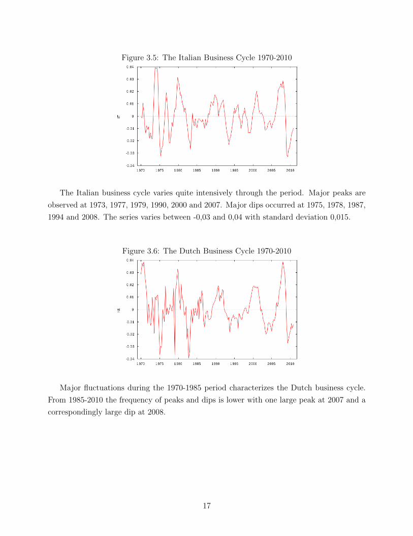
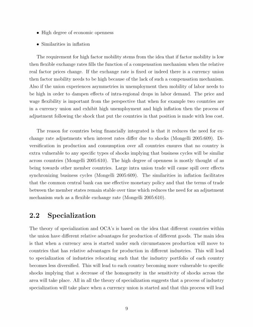
Figure 3.5: The Italian Business Cycle 1970-2010

The Italian business cycle varies quite intensively through the period. Major peaks are

observed at 1973, 1977, 1979, 1990, 2000 and 2007. Major dips occurred at 1975, 1978, 1987,

1994 and 2008. The series varies between -0,03 and 0,04 with standard deviation 0,015.

Figure 3.6: The Dutch Business Cycle 1970-2010

Major fluctuations during the 1970-1985 period characterizes the Dutch business cycle.

From 1985-2010 the frequency of peaks and dips is lower with one large peak at 2007 and a

correspondingly large dip at 2008.

17

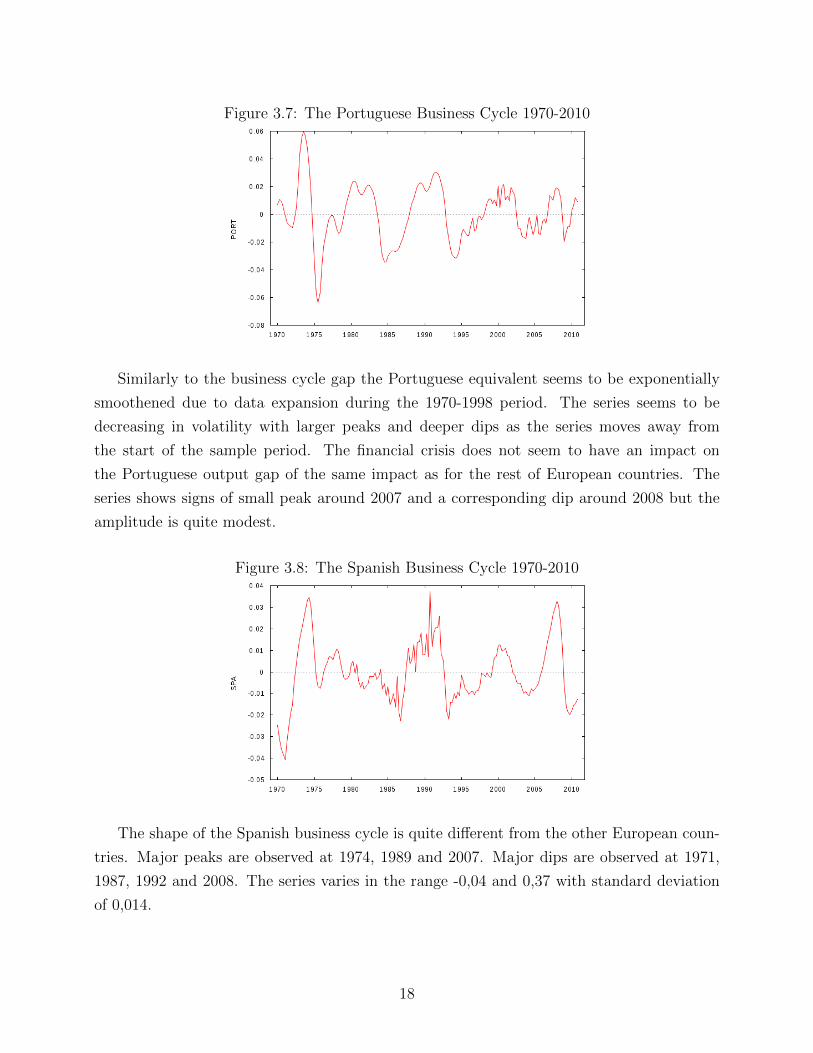
Figure 3.7: The Portuguese Business Cycle 1970-2010

Similarly to the business cycle gap the Portuguese equivalent seems to be exponentially

smoothened due to data expansion during the 1970-1998 period. The series seems to be

decreasing in volatility with larger peaks and deeper dips as the series moves away from

the start of the sample period. The financial crisis does not seem to have an impact on

the Portuguese output gap of the same impact as for the rest of European countries. The

series shows signs of small peak around 2007 and a corresponding dip around 2008 but the

amplitude is quite modest.

Figure 3.8: The Spanish Business Cycle 1970-2010

The shape of the Spanish business cycle is quite different from the other European coun-

tries. Major peaks are observed at 1974, 1989 and 2007. Major dips are observed at 1971,

1987, 1992 and 2008. The series varies in the range -0,04 and 0,37 with standard deviation

of 0,014.

18

Figure 3.9: The Greek Business Cycle 1970-2010

The Greek business cycle fluctuates heavily for most of the period. It exhibits a large dip

around 1975 and around 1990. What is most interesting about this series is the fact that the

financial crisis does not seem to be present at all. This is due to the fact that the HP-filter

has estimated the trend component as having a stark negative development for the 2005-2010

period. This leads to estimates of the cyclical component that is above the trend value and

therefore positive.

19

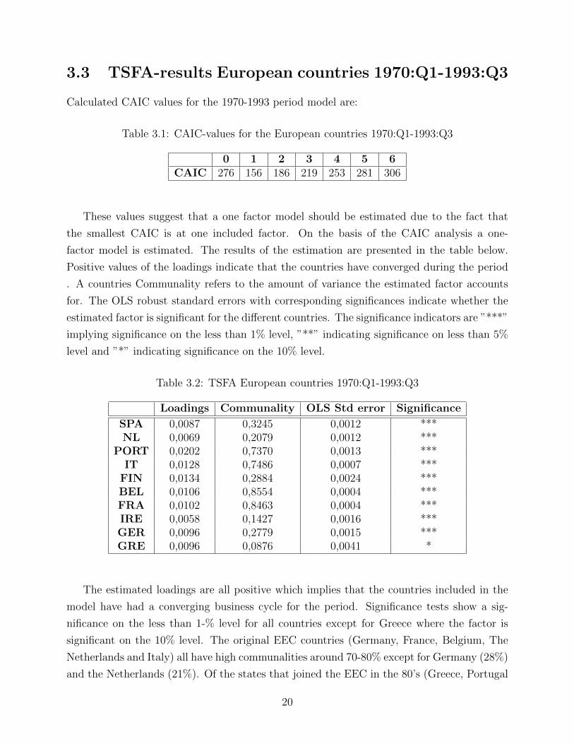
3.3 TSFA-results European countries 1970:Q1-1993:Q3

Calculated CAIC values for the 1970-1993 period model are:

Table 3.1: CAIC-values for the European countries 1970:Q1-1993:Q3

0 1 2 3 4 5 6CAIC 276 156 186 219 253 281 306

These values suggest that a one factor model should be estimated due to the fact that

the smallest CAIC is at one included factor. On the basis of the CAIC analysis a one-

factor model is estimated. The results of the estimation are presented in the table below.

Positive values of the loadings indicate that the countries have converged during the period

. A countries Communality refers to the amount of variance the estimated factor accounts

for. The OLS robust standard errors with corresponding significances indicate whether the

estimated factor is significant for the different countries. The significance indicators are ”***”

implying significance on the less than 1% level, ”**” indicating significance on less than 5%

level and ”*” indicating significance on the 10% level.

Table 3.2: TSFA European countries 1970:Q1-1993:Q3

Loadings Communality OLS Std error Significance

SPA 0,0087 0,3245 0,0012 ***NL 0,0069 0,2079 0,0012 ***

PORT 0,0202 0,7370 0,0013 ***IT 0,0128 0,7486 0,0007 ***

FIN 0,0134 0,2884 0,0024 ***BEL 0,0106 0,8554 0,0004 ***FRA 0,0102 0,8463 0,0004 ***IRE 0,0058 0,1427 0,0016 ***GER 0,0096 0,2779 0,0015 ***GRE 0,0096 0,0876 0,0041 *

The estimated loadings are all positive which implies that the countries included in the

model have had a converging business cycle for the period. Significance tests show a sig-

nificance on the less than 1-% level for all countries except for Greece where the factor is

significant on the 10% level. The original EEC countries (Germany, France, Belgium, The

Netherlands and Italy) all have high communalities around 70-80% except for Germany (28%)

and the Netherlands (21%). Of the states that joined the EEC in the 80’s (Greece, Portugal

20

and Spain) Portugal is the country with the highest communality at 74%. Interestingly Fin-

land who was not a member of the EEC for the entire period has a communality greater than

Germany, the Netherlands and Greece. Furthermore there seems to be a strong relationship

between the southern European countries and the estimated factor. All of the southern Eu-

ropean countries included in the analysis show a higher communality than the rest of the

countries with the exception of Greece. The mean communality for the total set of countries

was 45%. Below the estimated factor is plotted:

Figure 3.10: The estimated European business cycle 1970:Q1-1993:Q3

The European business cycle shows peaks at 1974, 1980 and 1989. Major dips occur at

1975, 1987 and 1993. The timing of both peaks ands dips agree quite well with the dips and

peaks of the individual countries business cycles (see pages 13-17).

3.4 TSFA-results for the European countries 1993:Q4-

2010:Q4

Calculated CAIC-values for different model specifications are:

Table 3.3: CAIC-values for the European countries 1993:Q3-2010:Q4

0 1 2 3 4 5 6CAIC 466 148 173 205 238 266 288

Once again the CAIC suggests the inclusion of one factor into the model. The 1 factor

model gave the following estimates of loadings and communalities:

21

Table 3.4: TSFA model for the European countries 1993:Q4-2010:Q4

Loadings Communality OLS Std error Significance

SPA 0,0117 0,9040 0,0006 ***NL 0,0139 0,9027 0,0006 ***

PORT 0,0091 0,4427 0,0010 ***IT 0,0123 0,8335 0,0006 ***

FIN 0,0204 0,8925 0,0007 ***BEL 0,0109 0,8873 0,0004 ***FRA 0,0101 0,9094 0,0003 ***IRE 0,0229 0,7926 0,0016 ***GER 0,0135 0,8584 0,0006 ***GRE 0,0009 0,0033 0,0025 -

The estimated loadings are also for this period all positive indicating convergance among

the countries. The communalities are for this period substantially larger for most countries

compared to the 1970-1993 period with the exception of Greece. The significanes are once

again indicating significance on the less than 1% level for all countries except Greece. Com-

munalities for the statistically significant countries range from around 0,44 (Portugal) to

0,91 (France). We can also see that Portugal has a lower communality for this period (0,44

compared to 0,74).

Ireland has a communality of 0,79 which is a very large increase from the 0,14 estimate

for the pre-Maastrich period. The fact that the factor is not significant for Greece is not

surprising. Greece had the lowest communality during the pre-Maastrich period and has

been effected differently than the other countries by the recent financial crisis. Furthermore

Spain shows a noteworthy increase in communality from 32% to 90%. Germany increase their

communality by 58% and Finland increase their communality by 60% which are remarkably

large increases. All in all the mean communality increased from 37% to 82%. The estimated

European business cycle is plotted below:

22

Figure 3.11: The European estimated business cycle 1993Q4-2010:Q4

The European business cycle exhibits peaks at 2001 and 2007. Dips are observed at 2003

and 2009. The 2009 dip is by far the most dramatic event during the period and is most

likely due to the recent financial crisis. The shape of the factor very much resembles that of

the individual countries who all where affected in a similar way by the financial crisis except

for Greece.

3.5 Analyzing the European case in the time domain

The results from the factor models for the pre- and post-Maastricht periods indicate an in-

crease in the European business cycle correlation. This is due to the fact that communalities

are in a broader sense substantially larger for the post-Maastricht period. The estimated

factor for the pre-Maastricht period showed large communalities for mainly southern Euro-

pean countries while the post-Maastricht period showed large communalities for countries

from both the northern and southern countries. There are however some exceptions such as

Portugal for whom the communality decreased for the post-Maastricht period and Greece for

whom the estimated factor was not significant. These countries where both hit very hard by

the financial crisis which could be the reason for the divergence. Furthermore, the fact that

the model selection criteria suggested one underlying factor as the optimal model specifica-

tion implies that there indeed exists one single underlying factor which is a powerful result.

All in all the results point in the direction of the endogeneity effect as being the major factor

effecting the countries since the Maastricht treaty.

23

3.6 TSFA results for US 1970:Q1-2010:Q4

For the US the CAIC suggests an inclusion of 4 factors. This is partially in line with what we

could expect and we can here assume that the second third and fourth factors are regional

cycles whereas the first one is a national cycle. The significances from the factor model can

be found on the preceding page, communalities and loadings can be found in the appendix.

24

Table 3.5: Factor significances 1970:Q1-2010:Q4

Factor 1 Factor 2 Factor 3 Factor 4Alabama*** Alabama*** Arizona*** Alaska**Alaska*** Alaska*** Arkansas*** Arizona**Arizona*** Arkansas*** Colorado*** Arkansas***Arkansas*** California*** Connecticut*** California***California*** Colorado*** Delaware** Colorado***Colorado*** Connecticut*** DOC** Connecticut***

Connecticut*** Delaware*** Florida** DOC***Delaware*** DOC* Hawaii*** Georgia***

DOC*** Florida** Idaho*** Hawaii***Florida*** Georgia*** Illinois* Illinois***Georgia*** Indiana*** Iowa* Indiana***Hawaii*** Iowa** Kansas*** Iowa***Idaho*** Kansas* Kentucky*** Kansas*Illinois*** Louisiana*** Louisiana*** Kentucky***Indiana*** Maine*** Maine*** Louisiana***

Iowa*** Maryland*** Massachussetts*** Maryland***Kansas*** Massachussetts*** Minnesota*** Massachussetts***

Kentucky*** Michigan*** Montana*** Michigan***Louisiana*** Missouri*** Nebraska*** Minnesota***

Maine*** Nebraska** Nevada*** Missouri**Maryland*** Nevada*** NH*** Montana**

Massachussetts*** NH*** NJ*** Nebraska***Michigan*** NJ*** NM*** Nevada***Minnesota*** NM*** NY*** NH***Missouri*** NC*** NC** NJ**Montana*** ND*** Ohio*** NM***Nebraska*** Ohio* Oklahoma*** NY***Nevada*** Oklahoma*** Oregon*** Ohio**

NH*** Oregon*** Pennsylvania*** Oklahoma***NJ*** Pennsylvania*** RI** Oregon***NM*** RI*** SD*** Pennsylvania***NY*** SC*** Tennesee*** RI***NC*** SD** Texas*** SC**ND*** Tennesee*** Utah*** Tennesee***

Ohio*** Texas*** Washington*** Texas***Oklahoma*** Utah*** Vermont** Washington***

Oregon*** Washington*** Wisconsin* Vermont*Pennsylvania*** Vermont*** Wyoming*** Virginia**

RI*** WV** Wisconsin***SC*** Virginia*** Wyoming***SD*** Wisconsin***

25

Tennesee*** Wyoming***Texas***Utah***Washington***Vermont***WV***Virginia***Wisconsin***Wyoming***

The estimated loadings show a positive sign for the first factor with the exception of

Alaska for which the estimated loading has a negative sign. This suggests that all states ex-

cept Alaska have converged with the national cycle for the period. For the second third and

fourth factors the estimated loadings have mixed signs which indicates mixed convergence

and also indicates that some of the factors might be insignificant for some states. In order to

further investigate whether some factors are insignificant a significance test was conducted

by running an OLS of each observed variable on each estimated factor. The results from the

significance tests are that the first factor is significant for all states. The second factor is

significant for 42 states, the third factor is significant for 38 states and the fourth for 40 states.

This does not give much information about what the factors represent and therefore it

seems more reasonable to look at the communalities. The variance that the respective factors

stands for are distributed quite unevenly between factors. From studying the table of vari-

ances it becomes clear that the first factor accounts for most of the variation in the observed

variables. The cases where the second, third or fourth factor stands more than 10% of the

variance are for factor 2: Alaska (23%) Louisiana (18%), Oklahoma (37%), Texas (35%) and

Wyoming (50%). These states are all large petroleum and gas producers and their respective

economies are therefore likely to be more sensitive to petroleum-specific shocks than the rest

of the country.

For the third factor the states with more than 10% explained variance are: Idaho (11%),

Kentucky (17%), Montana (11%), Oregon (13%) and Washington (15%). These states are all

located in the north west of the country except for Kentucky. In addition to the geographical

perspective these states also share industry structure with a large high-tech sector. For the

fourth factor the only state for which the factor could explain more than 10% was Hawaii

(26%). This indicates that the fourth factor may be an effect of autocorrelation in the

underlying factor since it is not plausible to assume that there exist a factor describing only

26

the Hawaiian economy. The first factor managed to account for more than 10% of the variance

for all states but Alaska. A graphical representation of the first factor can be viewed below:

Figure 3.12: The estimated US national business cycle 1970:Q1-2010:Q4

The US national business cycle shows peaks at 1974, 1980, 1985, 1990, 1994, 2001 and

2007. Major dips occur at 1971, 1975, 1983, 1987, 1992, 2003 and 2009. The dates of the

dips can for example be linked to the oil shocks in the 1970’s and 1980’s, the terrorist attacks

of the early 2000’s and finally the recent financial crisis.

3.7 Analyzing the European case in the space domain

The factor analysis results for the US 1970-2010 period are in contrast to the results for the

European countries. The way in which this materializes is mainly through the fact that there

appears to exist regional factors in the US economy. This result speaks for the specialization

effect of optimal currency areas since the second and third underlying factors can be viewed

as representing industry specific states. This implies that a stable currency union exhibits a

certain degree of specialization which leads to regional business cycle phenomenons. For the

European countries this means that there is likely to be an increasing specialization effect

that will make some regions less correlated with the main common factor or business cycle.

3.8 Krugman index of specialization

In order to investigate if a specialization process is already taking place among the European

countries the Krugman index of specialization will be deployed. The index takes a value

between 0 and 2 where 0 represents complete equality between countries and 2 represents

complete inequality of industry structure. This implies that a currency area with low degree

27

of specialization will display values close to zero and and one that has a high degree of

specialization will display values close to 2. The index is constructed as follows:

Ki(t) =∑k

abs(vki (t) − vki ) (3.9)

Where:

vi ≡ xki (t)/∑k

xki (t) (3.10)

Here xki is the output of country i in industry k. Furthermore:

vki ≡∑i 6=j

xki (t)/∑k

∑i 6=j

xki (t) (3.11)

So that equation (3.8) measures the sum over all industries k of the absolute deviance

of country i’s production from all other countries. (Midelfart-Knarvik et al 2000). The

index was calculated for EU countries except Ireland for the 1993-2008 period and gave the

following results:

Table 3.6: Specialization levels for the European countries 1993-2008BEL FIN FRA GER ITA NL PORT SPA GRE MEAN VAR

1993 0,30 0,46 0,18 0,35 0,29 0,44 0,59 0,27 0,68 0,39 0,0271994 0,31 0,47 0,17 0,31 0,30 0,43 0,57 0,25 0,68 0,39 0,0271995 0,32 0,55 0,16 0,30 0,31 0,43 0,53 0,24 0,69 0,39 0,0281996 0,32 0,54 0,18 0,30 0,30 0,43 0,53 0,24 0,66 0,39 0,0261997 0,33 0,57 0,18 0,30 0,31 0,42 0,51 0,25 0,69 0,40 0,0281998 0,32 0,61 0,18 0,30 0,31 0,40 0,52 0,24 0,71 0,40 0,0321999 0,31 0,64 0,19 0,32 0,31 0,42 0,52 0,24 0,71 0,41 0,0332000 0,33 0,68 0,19 0,33 0,32 0,44 0,50 0,24 0,70 0,42 0,0332001 0,33 0,63 0,20 0,34 0,34 0,45 0,51 0,23 0,70 0,41 0,0302002 0,35 0,63 0,20 0,35 0,34 0,47 0,51 0,23 0,65 0,42 0,0262003 0,36 0,62 0,20 0,36 0,35 0,47 0,49 0,23 0,64 0,41 0,0242004 0,37 0,63 0,20 0,37 0,34 0,48 0,48 0,25 0,63 0,42 0,0232005 0,41 0,64 0,21 0,38 0,34 0,50 0,47 0,24 0,61 0,42 0,0222006 0,43 0,62 0,21 0,37 0,34 0,51 0,46 0,24 0,63 0,42 0,0232007 0,45 0,62 0,22 0,38 0,33 0,53 0,44 0,23 0,63 0,43 0,0222008 0,47 0,59 0,23 0,40 0,32 0,55 0,42 0,24 0,62 0,43 0,021

0,36 0,60 0,19 0,34 0,32 0,46 0,50 0,24 0,66 0,41 0,027

For most of the countries the index value has increased since 1993. The exceptions are

Portugal, Spain and Greece who started at higher index values (0,59, 0,27 and 0,68 respec-

tively) than at the end pf the period (0,5, 0,24 and 0,66 respectively). The fact the level of

28

specialization for both Portugal and Greece has decreased during the period is in contrast to

the results from the factor analysis and suggests that the reason of the divergence of these

countries lies outside the specialization and/or endogeneity aspects of optimal currency areas.

Interestingly the two countries with the lowest degree of mean specialization, Spain (0,24)

and France (0,19) are also the countries who have the highest communalities in the factor

analysis for the 1993-2010 period. This result confirms the general theory of specialization.

In contrast Finland who has the second largest mean level of specialization also has the fourth

largest communality in the factor analysis. This result is not confirmatory of the special-

ization effect. Furthermore Finland has had the largest increase in specialization during the

period, a result that on its own speaks for the general theory of specialization. All in all the

results from the Krugman index of specialization are ambiguous with respect to confirming

the general theory of specialization. The mean series has increased for the period starting

at 0,356 and ending at 0,405. The variance has been quite stable for the period. Below the

mean series is plotted:

Figure 3.13: Mean level of specialization European countries 1993-2008

From studying the graph of the mean series it becomes clear that the European countries

have experienced a modest increase in specialization for the 1993-2008 period. The mean

value of specialization was quite stable for the first 4 years but has afterwards increased. All

in all the mean value of specialization increased with approximately 5% during the period.

For the US the 39 by 51 table analog to the EU table above is omitted but can be found

in the appendix. The mean value of specialization for the 1970-2008 period was 0,4727 with

average variance of 0,0486. Below the mean series of specialization is plotted:

29

Figure 3.14: Mean specialization US 1970-2008

The graph above does not show any clear sign of trending in any specific way with the

exception of 1970-1985 period where the average level of specialization decreased from around

0,51 to 0,45. After this the series has fluctuated a bit but shows no sign of trending in any

specific direction. This suggests that the US specialization process has leveled out which

confirms that the US is a stable currency area. The fact that the US has a mean value of

specialization that is quite close to the value for the European countries is somewhat contra-

dictory to the presence of regional factors.

This phenomenon can be explained by studying the variance (0,027 for the European

countries and 0,0486 for the US). The lager variance for the US implicates that some states

have levels of specialization which are quite distanced from the mean. The most obvious

cases of this in the direction of high degree of specialization are Alaska (0,9913), District

of Columbia (1,0002), Hawaii (0,9667), Louisiana (0,8154) and Wyoming (0,8050). On a

closer look these states are also highly correlated with the second and third estimated factors

from the time series factor analysis. To further illustrate the relationship between regional

factor and specialization a compilation of regional factor correlated states and their respective

deviation from the US mean of specialization is presented below:

30

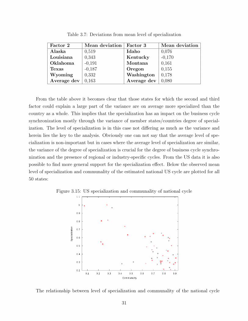
Table 3.7: Deviations from mean level of specialization

Factor 2 Mean deviation Factor 3 Mean deviationAlaska 0,519 Idaho 0,076Louisiana 0,343 Kentucky -0,170Oklahoma -0,191 Montana 0,161Texas -0,187 Oregon 0,155Wyoming 0,332 Washington 0,178Average dev 0,163 Average dev 0,080

From the table above it becomes clear that those states for which the second and third

factor could explain a large part of the variance are on average more specialized than the

country as a whole. This implies that the specialization has an impact on the business cycle

synchronization mostly through the variance of member states/countries degree of special-

ization. The level of specialization is in this case not differing as much as the variance and

herein lies the key to the analysis. Obviously one can not say that the average level of spe-

cialization is non-important but in cases where the average level of specialization are similar,

the variance of the degree of specialization is crucial for the degree of business cycle synchro-

nization and the presence of regional or industry-specific cycles. From the US data it is also

possible to find more general support for the specialization effect. Below the observed mean

level of specialization and communality of the estimated national US cycle are plotted for all

50 states:

Figure 3.15: US specialization and communality of national cycle

The relationship between level of specialization and communality of the national cycle

31

presented in the graph above seems to be negative. Most states are located in the bottom

right corner of the graph. Most of these observations are states with a combination of low

level of specialization and high level of communality. The states who are located in the

top left corner all have combinations of large level of specialization and low communalities.

The correlation between the variables is found to be equal to -0,67. The graph further

shows how a higher variance of specialization leads to a less homogeneous level of business

cycle synchronization. The analysis of the US specialization in combination with the factor

analysis carried out are unequivocal: a specialization process has taken place in the US and

the process in question is likely to have leveled out.

3.9 Analyzing the full picture

When combining both the factor analysis and the specialization analysis above it becomes

clear that the endogeneity aspect has been the dominating effect since 1993 for the Euro-

pean countries. The results that from the factor analysis seemed to contradict this i.e. the

lower degree of Portuguese communality and the lack of significance in the Greek case are

clearly not due to a specialization effect. For these cases it is more likely that other factors

have caused the divergence. One possible explanation is the soaring fiscal deficits of these

countries during the latter part of the last decade which have further affected the amplitude

of the recent financial crisis. The results from the US factor analysis together with the sub-

sequent specialization analysis suggests that the European countries can expect the degree

of specialization of individual countries to increase in the future. This result points in the

direction of an expected future dominance of the specialization effect.

32

Chapter 4

Conclusions

In this thesis the endogeneity and specialization aspects of optimal currency areas have been

evaluated. This has been done for the purpose of investigating which of the effects that has

dominated for a set of European countries since the inception of the Maastricht treaty in

1993. The currency areas which have been compared is the group of European countries who

signed the Maastricht treaty in 1992 and subsequently joined the EMU and the USA. The

results of the factor analysis suggests that there exists one single factor or business cycle

that explains much of the variation of the individual European countries business cycles.

Furthermore, the factor analysis suggested that the European countries have become more

synchronized since the Maastricht treaty. Simultaneously for the 1993-2008 period the aver-

age level of specialization has increased with a modest 5%.

These results were compared with the US for which the factor analysis resulted in 4 fac-

tors being estimated. The first is argued to be a national cycle, the second a petroleum

industry specific cycle and the third a regional north western cycle while the fourth factor

being recurrence of the first factor. The specialization analysis showed that the average US

level of specialization was quite close to the European countries albeit with a higher variance.

The higher variance was argued to be the reason for the presence of the non-national cycles

in the factor analysis.

In the background of the analysis of the full picture it is possible to conclude that the

endogeneity aspect of optimal currency areas has been the dominating effect for the Euro-

pean countries since the inception of the Maastricht treaty. It is however also possible to

conclude that the most likely future development is that the specialization effect will play a

more dominant role. This implies that the European countries are likely to experience some

divergence from the optimal currency area criteria until the specialization process levels out.

33

An interesting extension of the research would be to investigate to what extent the increase

in the European business cycle synchronization is due to an increase in the correlation of a

possibly global business cycle. This would contribute to making the analysis of the European

business cycle correlation more exact.

34

Chapter 5

Appendix

35

Table 5.1: Communalities US 1970-2010

Factor 1 Factor 2 Factor 3 Factor 4 Total

Alabama 0,9030209 0,0109077 0,0006696 0,0011253 0,9157235Alaska 0,0806698 0,2344754 0,0004851 0,0324530 0,3480833Arizona 0,8538954 0,0000211 0,0232273 0,0042282 0,8813720Arkansas 0,7878965 0,0491275 0,0110297 0,0231698 0,8712235California 0,8444216 0,0105376 0,0031900 0,0340959 0,8922451Colorado 0,8001428 0,0327851 0,0070563 0,0088078 0,8487919Connecticut 0,8014071 0,0053666 0,0574407 0,0603007 0,9245152Delaware 0,5073134 0,0174051 0,0270862 0,0030739 0,5548786DOC 0,3030103 0,0091463 0,0199256 0,0426108 0,3746930Florida 0,7872716 0,0058389 0,0137813 0,0003142 0,8072060Georgia 0,8837736 0,0228517 0,0002879 0,0201491 0,9270624Hawaii 0,3645972 0,0038700 0,0487400 0,2562522 0,6734593Idaho 0,7083138 0,0026105 0,1138142 0,0018925 0,8266310Illinois 0,8089738 0,0007780 0,0072081 0,0281719 0,8451317Indiana 0,8524756 0,0326663 0,0002148 0,0322263 0,9175830Iowa 0,7984734 0,0078900 0,0034301 0,0106043 0,8203977Kansas 0,7059470 0,0052008 0,0349791 0,0064994 0,7526262Kentucky 0,5210521 0,0004491 0,1662843 0,0393454 0,7271309Louisiana 0,3195708 0,1754119 0,0166623 0,0672783 0,5789234Maine 0,6566115 0,0885902 0,0712255 0,0017363 0,8181635Maryland 0,7640794 0,0102067 0,0004826 0,0914380 0,8662067Massachussetts 0,7584631 0,0306740 0,0779658 0,0165997 0,8837026Michigan 0,8082433 0,0207609 0,0047890 0,0389537 0,8727468Minnesota 0,8667256 0,0001448 0,0097864 0,0238140 0,9004708Missouri 0,8750530 0,0107640 0,0003990 0,0051838 0,8913998Montana 0,5083310 0,0064473 0,1056753 0,0296938 0,6501473Nebraska 0,7195240 0,0086971 0,0107331 0,0114462 0,7504004Nevada 0,7093168 0,0116689 0,0683562 0,0125522 0,8018941NH 0,7463842 0,0764182 0,0348510 0,0262449 0,8838984NJ 0,8443376 0,0302522 0,0488637 0,0027578 0,9262112NM 0,6901750 0,0307982 0,0555929 0,0810910 0,8576571NY 0,7947625 0,0000624 0,0613213 0,0294348 0,8855810NC 0,8641889 0,0420608 0,0019271 0,0031527 0,9113295ND 0,2615205 0,0308941 0,0069421 0,0148582 0,3142149Ohio 0,9166015 0,0009182 0,0055203 0,0038968 0,9269368Oklahoma 0,4186681 0,3654191 0,0459109 0,0071843 0,8371825Oregon 0,8073487 0,0075411 0,1337857 0,0038755 0,9525511Pennsylvania 0,8731011 0,0029149 0,0286545 0,0147729 0,9194434RI 0,7159975 0,0568303 0,0078194 0,0781646 0,8588118SC 0,8589676 0,0284727 0,0000638 0,0070147 0,8945189SD 0,6766230 0,0080329 0,0602636 0,0000264 0,7449459Tennesee 0,9027241 0,0307688 0,0079722 0,0232633 0,9647284Texas 0,6364201 0,3460229 0,0066337 0,0032488 0,9923254Utah 0,7505174 0,0678316 0,0354653 0,0000160 0,8538303Washington 0,7233140 0,0058411 0,1549942 0,0328077 0,9169570Vermont 0,7465941 0,0330058 0,0125974 0,0058178 0,7980151

36

WV 0,2425728 0,0140615 0,0000027 0,0006307 0,2572677Virginia 0,8494209 0,0339184 0,0000485 0,0054730 0,8888608Wisconsin 0,9206087 0,0039468 0,0027481 0,0082953 0,9355990Wyoming 0,2337766 0,4966216 0,0085213 0,0187487 0,7576683

37

Table 5.2: Estimated Loadings US 1970-2010

Factor 1 Factor 2 Factor 3 Factor 4

Alabama 0,008535 -0,000921 -0,000223 -0,000282Alaska -0,005605 0,009386 -0,000416 0,003328Arizona 0,012537 -0,000061 0,001980 0,000826Arkansas 0,008553 -0,002098 0,000969 -0,001373California 0,008515 0,000934 0,000501 0,001602Colorado 0,009141 0,001817 0,000822 -0,000898Connecticut 0,008070 -0,000649 -0,002069 0,002072Delaware 0,006178 -0,001124 0,001367 -0,000450DOC 0,003365 0,000574 0,000826 0,001181Florida 0,011448 -0,000968 0,001450 -0,000214Georgia 0,010303 -0,001627 0,000178 -0,001456Hawaii 0,004101 0,000415 0,001436 0,003218Idaho 0,009746 0,000581 0,003740 -0,000472Illinois 0,007729 0,000235 -0,000698 0,001350Indiana 0,011015 -0,002118 -0,000167 -0,002005Iowa 0,007273 -0,000710 0,000456 0,000785Kansas 0,007161 0,000604 0,001526 -0,000643Kentucky 0,008124 -0,000234 -0,004394 0,002090Louisiana 0,006046 0,004399 0,001322 -0,002597Maine 0,006905 -0,002491 -0,002178 -0,000332Maryland 0,006745 -0,000766 -0,000162 0,002184Massachussetts 0,008418 -0,001663 -0,002584 0,001166Michigan 0,011724 -0,001845 0,000864 -0,002409Minnesota 0,008254 -0,000105 0,000840 0,001281Missouri 0,007974 -0,000869 0,000163 -0,000574Montana 0,006003 -0,000664 0,002621 -0,001358Nebraska 0,006415 0,000693 0,000750 0,000757Nevada 0,011596 0,001461 0,003447 0,001444NH 0,010640 -0,003344 -0,002201 -0,001868NJ 0,007012 -0,001304 -0,001615 0,000375NM 0,006281 0,001303 0,001707 -0,002015NY 0,005974 0,000052 -0,001589 0,001076NC 0,010206 -0,002212 -0,000461 -0,000577ND 0,002795 0,000944 0,000436 0,000624Ohio 0,009584 -0,000298 -0,000712 0,000585Oklahoma 0,005474 0,005023 -0,001736 -0,000671Oregon 0,010393 -0,000987 0,004051 0,000674Pennsylvania 0,006653 0,000378 -0,001154 0,000810RI 0,009400 -0,002601 -0,000941 -0,002907SC 0,010946 -0,001957 -0,000090 -0,000926SD 0,006386 -0,000683 0,001825 -0,000037

38

Tennesee 0,010378 -0,001882 -0,000934 -0,001559Texas 0,007191 0,005208 -0,000703 -0,000481Utah 0,008126 0,002399 0,001691 0,000035Washington 0,007837 0,000692 0,003473 0,001562Vermont 0,007555 -0,001560 -0,000940 -0,000624WV 0,006263 0,001481 0,000020 -0,000299Virginia 0,007525 -0,001477 -0,000054 0,000565Wisconsin 0,008443 -0,000543 0,000442 0,000750Wyoming 0,006719 0,009619 -0,001228 -0,001781

39

Table 5.3: Krugman index of specialization USA

Alabama Alaska Arizona Arkansas California Colorado Connecticut1970 0,50 0,93 0,53 0,34 0,30 0,33 0,431971 0,47 0,90 0,52 0,32 0,28 0,30 0,381972 0,47 0,89 0,55 0,30 0,28 0,30 0,371973 0,46 0,86 0,53 0,29 0,27 0,29 0,391974 0,46 0,71 0,47 0,33 0,28 0,27 0,381975 0,48 0,87 0,54 0,32 0,28 0,32 0,411976 0,47 0,98 0,49 0,29 0,27 0,31 0,381977 0,44 1,03 0,50 0,29 0,27 0,30 0,391978 0,42 0,97 0,50 0,28 0,26 0,30 0,391979 0,43 0,96 0,49 0,29 0,28 0,30 0,391980 0,42 1,01 0,49 0,29 0,28 0,31 0,381981 0,44 0,91 0,49 0,30 0,33 0,33 0,381982 0,42 0,94 0,54 0,29 0,34 0,32 0,401983 0,42 1,01 0,51 0,28 0,33 0,32 0,401984 0,40 0,98 0,45 0,24 0,35 0,30 0,381985 0,41 0,94 0,47 0,21 0,36 0,31 0,381986 0,37 0,94 0,53 0,26 0,34 0,32 0,371987 0,37 0,96 0,53 0,28 0,34 0,31 0,351988 0,43 0,90 0,50 0,31 0,34 0,28 0,341989 0,39 0,94 0,53 0,32 0,33 0,28 0,361990 0,38 0,99 0,54 0,31 0,34 0,28 0,351991 0,39 1,00 0,60 0,29 0,32 0,32 0,381992 0,40 1,01 0,62 0,31 0,30 0,30 0,331993 0,39 0,97 0,63 0,32 0,29 0,33 0,311994 0,43 1,00 0,64 0,36 0,34 0,36 0,311995 0,40 1,00 0,66 0,33 0,34 0,35 0,311996 0,39 1,01 0,67 0,34 0,35 0,31 0,331997 0,37 1,10 0,75 0,29 0,37 0,35 0,431998 0,35 1,18 0,76 0,27 0,38 0,32 0,431999 0,30 1,11 0,77 0,28 0,39 0,32 0,402000 0,33 1,09 0,72 0,32 0,41 0,35 0,392001 0,31 1,07 0,79 0,32 0,35 0,29 0,452002 0,27 1,06 0,80 0,36 0,35 0,35 0,382003 0,26 1,08 0,86 0,40 0,30 0,33 0,412004 0,27 1,08 0,78 0,40 0,26 0,34 0,382005 0,31 1,04 0,73 0,40 0,29 0,29 0,402006 0,34 1,08 0,72 0,38 0,28 0,33 0,382007 0,32 1,06 0,65 0,34 0,28 0,34 0,382008 0,39 1,10 0,64 0,36 0,38 0,25 0,40

Mean 0,39 0,99 0,60 0,31 0,32 0,31 0,38

40

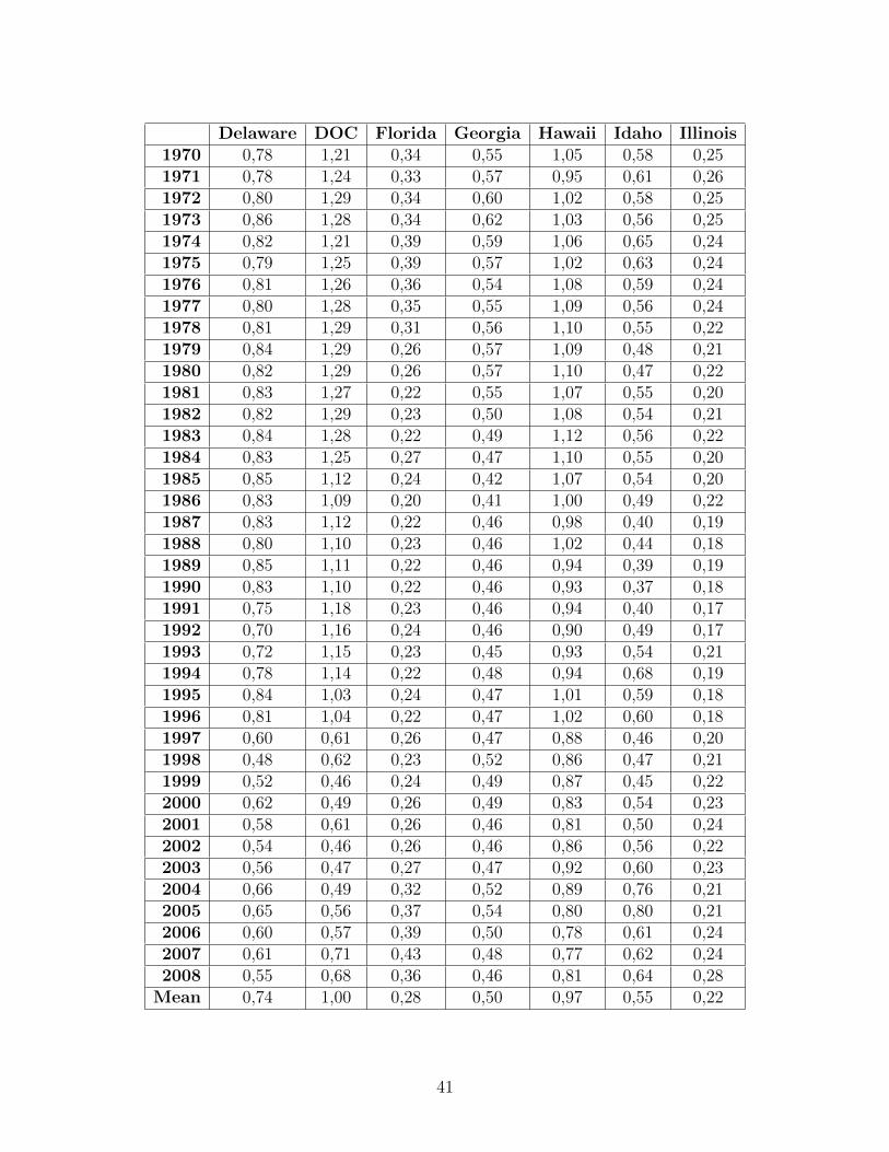
Delaware DOC Florida Georgia Hawaii Idaho Illinois1970 0,78 1,21 0,34 0,55 1,05 0,58 0,251971 0,78 1,24 0,33 0,57 0,95 0,61 0,261972 0,80 1,29 0,34 0,60 1,02 0,58 0,251973 0,86 1,28 0,34 0,62 1,03 0,56 0,251974 0,82 1,21 0,39 0,59 1,06 0,65 0,241975 0,79 1,25 0,39 0,57 1,02 0,63 0,241976 0,81 1,26 0,36 0,54 1,08 0,59 0,241977 0,80 1,28 0,35 0,55 1,09 0,56 0,241978 0,81 1,29 0,31 0,56 1,10 0,55 0,221979 0,84 1,29 0,26 0,57 1,09 0,48 0,211980 0,82 1,29 0,26 0,57 1,10 0,47 0,221981 0,83 1,27 0,22 0,55 1,07 0,55 0,201982 0,82 1,29 0,23 0,50 1,08 0,54 0,211983 0,84 1,28 0,22 0,49 1,12 0,56 0,221984 0,83 1,25 0,27 0,47 1,10 0,55 0,201985 0,85 1,12 0,24 0,42 1,07 0,54 0,201986 0,83 1,09 0,20 0,41 1,00 0,49 0,221987 0,83 1,12 0,22 0,46 0,98 0,40 0,191988 0,80 1,10 0,23 0,46 1,02 0,44 0,181989 0,85 1,11 0,22 0,46 0,94 0,39 0,191990 0,83 1,10 0,22 0,46 0,93 0,37 0,181991 0,75 1,18 0,23 0,46 0,94 0,40 0,171992 0,70 1,16 0,24 0,46 0,90 0,49 0,171993 0,72 1,15 0,23 0,45 0,93 0,54 0,211994 0,78 1,14 0,22 0,48 0,94 0,68 0,191995 0,84 1,03 0,24 0,47 1,01 0,59 0,181996 0,81 1,04 0,22 0,47 1,02 0,60 0,181997 0,60 0,61 0,26 0,47 0,88 0,46 0,201998 0,48 0,62 0,23 0,52 0,86 0,47 0,211999 0,52 0,46 0,24 0,49 0,87 0,45 0,222000 0,62 0,49 0,26 0,49 0,83 0,54 0,232001 0,58 0,61 0,26 0,46 0,81 0,50 0,242002 0,54 0,46 0,26 0,46 0,86 0,56 0,222003 0,56 0,47 0,27 0,47 0,92 0,60 0,232004 0,66 0,49 0,32 0,52 0,89 0,76 0,212005 0,65 0,56 0,37 0,54 0,80 0,80 0,212006 0,60 0,57 0,39 0,50 0,78 0,61 0,242007 0,61 0,71 0,43 0,48 0,77 0,62 0,242008 0,55 0,68 0,36 0,46 0,81 0,64 0,28

Mean 0,74 1,00 0,28 0,50 0,97 0,55 0,22

41

Indiana Iowa Kansas Kentucky Louisiana Maine Maryland1970 0,32 0,36 0,35 0,41 0,74 0,72 0,311971 0,36 0,32 0,32 0,40 0,75 0,67 0,291972 0,36 0,31 0,31 0,36 0,76 0,75 0,281973 0,37 0,32 0,32 0,34 0,73 0,75 0,251974 0,34 0,32 0,33 0,30 0,77 0,75 0,281975 0,36 0,33 0,34 0,28 0,76 0,77 0,281976 0,36 0,32 0,32 0,31 0,78 0,76 0,231977 0,36 0,33 0,29 0,33 0,76 0,76 0,241978 0,36 0,36 0,30 0,30 0,81 0,72 0,221979 0,34 0,35 0,32 0,30 0,77 0,70 0,231980 0,36 0,35 0,34 0,30 0,74 0,71 0,251981 0,34 0,31 0,33 0,32 0,66 0,67 0,271982 0,32 0,29 0,37 0,33 0,73 0,66 0,271983 0,32 0,27 0,33 0,31 0,73 0,59 0,291984 0,28 0,26 0,36 0,26 0,72 0,61 0,291985 0,30 0,24 0,36 0,28 0,79 0,57 0,301986 0,29 0,29 0,36 0,26 0,79 0,54 0,271987 0,28 0,28 0,37 0,26 0,87 0,59 0,251988 0,31 0,26 0,33 0,24 0,89 0,58 0,271989 0,30 0,30 0,34 0,25 0,87 0,57 0,271990 0,28 0,27 0,33 0,28 0,84 0,52 0,261991 0,33 0,25 0,34 0,28 0,80 0,52 0,271992 0,33 0,24 0,36 0,24 0,82 0,55 0,301993 0,35 0,23 0,36 0,24 0,85 0,58 0,271994 0,36 0,24 0,36 0,28 0,91 0,65 0,291995 0,38 0,24 0,37 0,31 0,84 0,61 0,301996 0,37 0,23 0,40 0,32 0,84 0,56 0,321997 0,34 0,32 0,37 0,33 0,80 0,61 0,251998 0,33 0,30 0,37 0,33 0,76 0,65 0,251999 0,35 0,30 0,37 0,34 0,82 0,64 0,292000 0,37 0,32 0,40 0,28 0,79 0,60 0,302001 0,38 0,30 0,39 0,28 0,72 0,52 0,302002 0,38 0,30 0,37 0,27 0,77 0,55 0,262003 0,41 0,33 0,33 0,32 0,91 0,49 0,272004 0,39 0,30 0,38 0,34 0,96 0,48 0,242005 0,39 0,34 0,25 0,32 1,08 0,46 0,272006 0,37 0,32 0,32 0,31 1,03 0,49 0,292007 0,37 0,33 0,36 0,29 0,93 0,52 0,362008 0,36 0,35 0,38 0,30 0,91 0,51 0,30

Mean 0,35 0,30 0,35 0,30 0,82 0,61 0,27

42

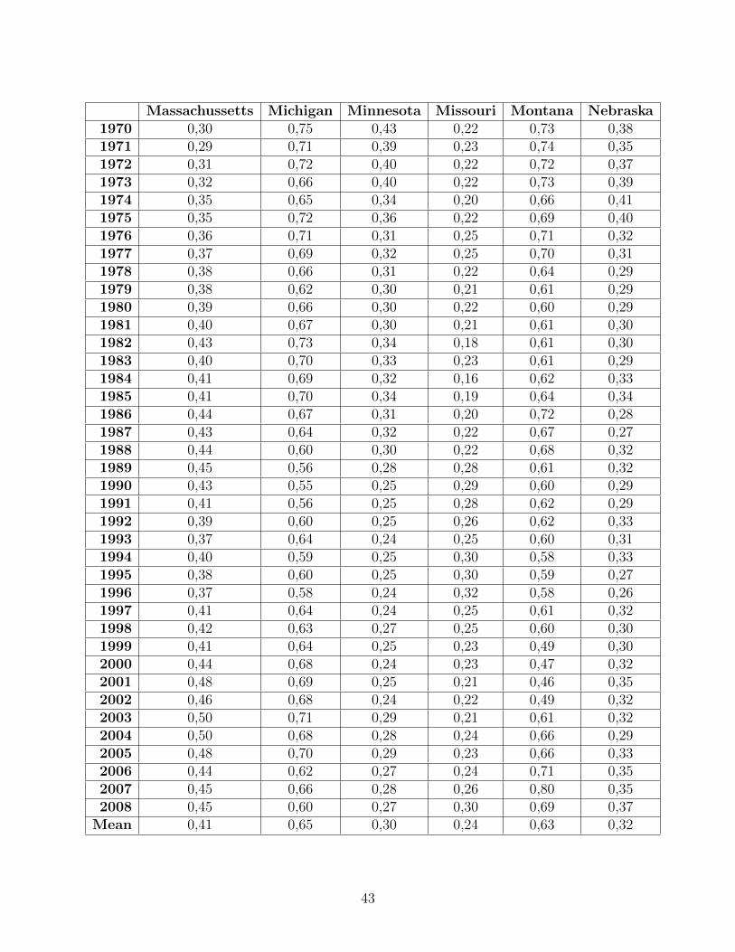
Massachussetts Michigan Minnesota Missouri Montana Nebraska1970 0,30 0,75 0,43 0,22 0,73 0,381971 0,29 0,71 0,39 0,23 0,74 0,351972 0,31 0,72 0,40 0,22 0,72 0,371973 0,32 0,66 0,40 0,22 0,73 0,391974 0,35 0,65 0,34 0,20 0,66 0,411975 0,35 0,72 0,36 0,22 0,69 0,401976 0,36 0,71 0,31 0,25 0,71 0,321977 0,37 0,69 0,32 0,25 0,70 0,311978 0,38 0,66 0,31 0,22 0,64 0,291979 0,38 0,62 0,30 0,21 0,61 0,291980 0,39 0,66 0,30 0,22 0,60 0,291981 0,40 0,67 0,30 0,21 0,61 0,301982 0,43 0,73 0,34 0,18 0,61 0,301983 0,40 0,70 0,33 0,23 0,61 0,291984 0,41 0,69 0,32 0,16 0,62 0,331985 0,41 0,70 0,34 0,19 0,64 0,341986 0,44 0,67 0,31 0,20 0,72 0,281987 0,43 0,64 0,32 0,22 0,67 0,271988 0,44 0,60 0,30 0,22 0,68 0,321989 0,45 0,56 0,28 0,28 0,61 0,321990 0,43 0,55 0,25 0,29 0,60 0,291991 0,41 0,56 0,25 0,28 0,62 0,291992 0,39 0,60 0,25 0,26 0,62 0,331993 0,37 0,64 0,24 0,25 0,60 0,311994 0,40 0,59 0,25 0,30 0,58 0,331995 0,38 0,60 0,25 0,30 0,59 0,271996 0,37 0,58 0,24 0,32 0,58 0,261997 0,41 0,64 0,24 0,25 0,61 0,321998 0,42 0,63 0,27 0,25 0,60 0,301999 0,41 0,64 0,25 0,23 0,49 0,302000 0,44 0,68 0,24 0,23 0,47 0,322001 0,48 0,69 0,25 0,21 0,46 0,352002 0,46 0,68 0,24 0,22 0,49 0,322003 0,50 0,71 0,29 0,21 0,61 0,322004 0,50 0,68 0,28 0,24 0,66 0,292005 0,48 0,70 0,29 0,23 0,66 0,332006 0,44 0,62 0,27 0,24 0,71 0,352007 0,45 0,66 0,28 0,26 0,80 0,352008 0,45 0,60 0,27 0,30 0,69 0,37

Mean 0,41 0,65 0,30 0,24 0,63 0,32

43

Nevada NH NJ NM NY NC ND Ohio1970 0,52 0,48 0,29 0,40 0,36 0,82 0,71 0,371971 0,42 0,44 0,31 0,38 0,36 0,78 0,68 0,381972 0,41 0,45 0,32 0,41 0,35 0,78 0,57 0,381973 0,41 0,42 0,33 0,41 0,34 0,77 0,59 0,381974 0,45 0,39 0,33 0,40 0,35 0,76 0,47 0,381975 0,44 0,40 0,36 0,39 0,34 0,74 0,51 0,361976 0,37 0,40 0,35 0,35 0,34 0,70 0,59 0,371977 0,35 0,44 0,37 0,34 0,34 0,70 0,54 0,371978 0,37 0,45 0,32 0,37 0,34 0,66 0,53 0,351979 0,36 0,45 0,29 0,29 0,32 0,64 0,54 0,321980 0,35 0,44 0,29 0,29 0,33 0,64 0,58 0,321981 0,35 0,45 0,33 0,32 0,33 0,62 0,61 0,301982 0,36 0,42 0,35 0,34 0,33 0,61 0,59 0,351983 0,35 0,46 0,33 0,30 0,34 0,56 0,62 0,341984 0,35 0,47 0,36 0,39 0,31 0,53 0,59 0,351985 0,34 0,47 0,38 0,42 0,33 0,52 0,57 0,341986 0,31 0,46 0,41 0,41 0,34 0,55 0,52 0,341987 0,33 0,45 0,39 0,38 0,33 0,54 0,44 0,341988 0,39 0,47 0,42 0,40 0,32 0,51 0,44 0,351989 0,38 0,43 0,45 0,43 0,32 0,52 0,45 0,321990 0,37 0,43 0,48 0,84 0,31 0,54 0,43 0,311991 0,40 0,46 0,49 0,92 0,32 0,55 0,38 0,341992 0,42 0,42 0,53 0,97 0,33 0,52 0,43 0,351993 0,46 0,45 0,53 1,01 0,35 0,52 0,44 0,341994 0,41 0,51 0,57 0,96 0,32 0,48 0,50 0,351995 0,41 0,52 0,63 0,95 0,34 0,51 0,49 0,321996 0,41 0,48 0,62 0,99 0,33 0,48 0,50 0,331997 0,45 0,57 0,60 1,03 0,26 0,52 0,55 0,381998 0,42 0,57 0,57 0,89 0,23 0,56 0,57 0,391999 0,38 0,47 0,59 0,91 0,25 0,53 0,57 0,372000 0,38 0,48 0,58 0,84 0,28 0,57 0,54 0,382001 0,36 0,45 0,58 0,69 0,24 0,59 0,45 0,342002 0,41 0,52 0,54 0,65 0,26 0,62 0,48 0,332003 0,48 0,53 0,54 0,79 0,28 0,61 0,48 0,352004 0,64 0,57 0,52 0,96 0,30 0,56 0,47 0,372005 0,66 0,56 0,50 0,92 0,28 0,54 0,54 0,382006 0,64 0,57 0,53 0,89 0,34 0,45 0,52 0,352007 0,70 0,57 0,52 0,73 0,29 0,47 0,46 0,342008 0,70 0,56 0,53 0,66 0,27 0,48 0,48 0,36

Mean 0,43 0,48 0,45 0,62 0,31 0,59 0,52 0,35

44

Oklahoma Oregon Pennsylvania RI SC SD Tennesee1970 0,28 0,61 0,23 0,37 0,77 0,64 0,391971 0,29 0,63 0,22 0,35 0,78 0,50 0,381972 0,26 0,68 0,22 0,36 0,78 0,50 0,381973 0,28 0,64 0,26 0,37 0,75 0,52 0,361974 0,30 0,58 0,28 0,43 0,70 0,51 0,391975 0,27 0,64 0,24 0,46 0,72 0,49 0,361976 0,26 0,66 0,19 0,44 0,70 0,44 0,381977 0,29 0,67 0,19 0,42 0,69 0,42 0,371978 0,26 0,64 0,19 0,43 0,68 0,45 0,351979 0,29 0,57 0,19 0,43 0,67 0,42 0,371980 0,31 0,52 0,18 0,45 0,68 0,43 0,381981 0,30 0,51 0,14 0,45 0,68 0,45 0,391982 0,29 0,58 0,15 0,44 0,65 0,45 0,341983 0,31 0,55 0,16 0,41 0,61 0,47 0,271984 0,30 0,54 0,15 0,48 0,61 0,41 0,321985 0,27 0,57 0,17 0,45 0,61 0,38 0,281986 0,26 0,53 0,15 0,47 0,56 0,43 0,261987 0,29 0,51 0,13 0,48 0,56 0,40 0,251988 0,27 0,52 0,13 0,48 0,57 0,40 0,261989 0,31 0,48 0,15 0,52 0,55 0,41 0,271990 0,28 0,46 0,17 0,50 0,57 0,42 0,271991 0,25 0,51 0,21 0,49 0,59 0,47 0,231992 0,21 0,59 0,20 0,46 0,56 0,58 0,241993 0,21 0,54 0,22 0,44 0,55 0,50 0,241994 0,24 0,59 0,17 0,45 0,55 0,55 0,231995 0,22 0,77 0,18 0,43 0,53 0,52 0,221996 0,21 0,75 0,21 0,42 0,51 0,51 0,231997 0,25 0,64 0,25 0,45 0,46 0,52 0,191998 0,31 0,66 0,25 0,45 0,45 0,51 0,181999 0,27 0,60 0,27 0,47 0,45 0,49 0,182000 0,26 0,60 0,27 0,46 0,46 0,59 0,182001 0,31 0,58 0,34 0,53 0,42 0,56 0,132002 0,35 0,61 0,34 0,52 0,35 0,70 0,162003 0,29 0,69 0,33 0,46 0,39 0,52 0,212004 0,33 0,82 0,24 0,57 0,35 0,54 0,192005 0,32 0,79 0,23 0,51 0,38 0,52 0,242006 0,32 0,87 0,20 0,45 0,38 0,50 0,262007 0,36 0,89 0,21 0,47 0,33 0,48 0,222008 0,34 0,88 0,19 0,46 0,34 0,47 0,23

Mean 0,28 0,63 0,21 0,45 0,56 0,49 0,28

45

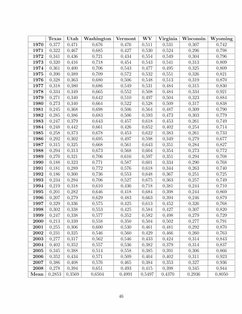
Texas Utah Washington Vermont WV Virginia Wisconsin Wyoming1970 0,377 0,471 0,676 0,476 0,511 0,531 0,307 0,7421971 0,322 0,467 0,685 0,427 0,530 0,524 0,296 0,7981972 0,341 0,436 0,721 0,434 0,554 0,549 0,304 0,7961973 0,320 0,416 0,718 0,454 0,543 0,541 0,313 0,8091974 0,361 0,400 0,706 0,543 0,477 0,495 0,325 0,8091975 0,390 0,389 0,709 0,572 0,532 0,551 0,326 0,8211976 0,328 0,363 0,680 0,506 0,548 0,513 0,319 0,8701977 0,318 0,380 0,686 0,549 0,531 0,484 0,315 0,8301978 0,334 0,349 0,665 0,552 0,508 0,484 0,334 0,9211979 0,271 0,340 0,642 0,510 0,497 0,504 0,323 0,8841980 0,273 0,340 0,664 0,522 0,528 0,509 0,317 0,8381981 0,245 0,368 0,698 0,506 0,564 0,487 0,309 0,7901982 0,285 0,386 0,683 0,506 0,593 0,473 0,303 0,7791983 0,247 0,379 0,643 0,457 0,618 0,453 0,261 0,7491984 0,248 0,442 0,661 0,426 0,652 0,402 0,254 0,7141985 0,258 0,373 0,678 0,453 0,622 0,383 0,261 0,7331986 0,292 0,302 0,695 0,497 0,598 0,349 0,279 0,6771987 0,315 0,325 0,668 0,561 0,643 0,351 0,284 0,8271988 0,294 0,313 0,673 0,568 0,604 0,354 0,273 0,7721989 0,270 0,321 0,706 0,616 0,597 0,351 0,294 0,7081990 0,188 0,323 0,771 0,587 0,601 0,334 0,290 0,7681991 0,181 0,289 0,772 0,576 0,618 0,344 0,263 0,7401992 0,186 0,300 0,736 0,553 0,648 0,367 0,251 0,7251993 0,234 0,294 0,706 0,527 0,675 0,363 0,257 0,7491994 0,219 0,318 0,610 0,436 0,718 0,381 0,244 0,7101995 0,201 0,282 0,646 0,418 0,684 0,398 0,244 0,8691996 0,207 0,279 0,629 0,483 0,663 0,394 0,246 0,8791997 0,329 0,336 0,575 0,425 0,613 0,452 0,326 0,7681998 0,302 0,338 0,553 0,425 0,584 0,427 0,307 0,8201999 0,247 0,338 0,577 0,352 0,582 0,498 0,279 0,7292000 0,213 0,339 0,558 0,350 0,504 0,502 0,277 0,7912001 0,255 0,306 0,600 0,530 0,461 0,481 0,292 0,8702002 0,231 0,325 0,546 0,560 0,429 0,466 0,260 0,7632003 0,277 0,317 0,562 0,546 0,433 0,424 0,314 0,8432004 0,402 0,352 0,557 0,536 0,382 0,379 0,314 0,8372005 0,345 0,388 0,514 0,558 0,385 0,391 0,306 0,8662006 0,352 0,434 0,571 0,509 0,404 0,402 0,311 0,9232007 0,386 0,408 0,576 0,465 0,384 0,353 0,327 0,9362008 0,278 0,394 0,651 0,493 0,415 0,398 0,345 0,944

Mean 0,2853 0,3569 0,6504 0,4991 0,5497 0,4370 0,2936 0,8050

46

Mean Variance1970 0,509 0,0491971 0,493 0,0491972 0,498 0,0531973 0,495 0,0521974 0,487 0,0451975 0,499 0,0481976 0,489 0,0551977 0,488 0,0561978 0,481 0,0571979 0,468 0,0551980 0,472 0,0551981 0,469 0,0521982 0,475 0,0531983 0,466 0,0551984 0,461 0,0521985 0,457 0,0481986 0,450 0,0461987 0,452 0,0491988 0,451 0,0471989 0,452 0,0451990 0,454 0,0501991 0,460 0,0531992 0,465 0,0531993 0,468 0,0531994 0,479 0,0541995 0,479 0,0561996 0,478 0,0561997 0,472 0,0421998 0,466 0,0421999 0,453 0,0402000 0,458 0,0372001 0,455 0,0372002 0,453 0,0362003 0,470 0,0422004 0,485 0,0482005 0,487 0,0472006 0,482 0,0442007 0,481 0,0422008 0,479 0,041

Mean 0,4727 0,0486

47

Chapter 6

References

Akaike, Hirotugu (1978) On the Likelihood of a Time Series Model Journal of the Royal

Statistical Society, Vol. 27, No. 3/4 pp. 217-235

Anderson, D. R. & Burnham, K. P. & White, G. C. (1998) Comparison of Akaike

information criterion and consistent Akaike information criterion for model selection

and statistical inference from capture-recapture studies Journal of Applied Statistics,

25: 2, 263-282

Bayoumi, Tamim & Eichengreen, Barry (1997) Ever closer to heaven? An optimum-

currency-area index for European countries European Economic Review vol. 41 pp.

761-770

Bergman, U. Michael & Jonung, Lars (2010) Business cycle synchronization in Europe

Evidence from the Scandinavian Currency Union European Commission Economic Pa-

pers 402

Canzoneri, Matthew B. & Rogers, Carol Ann Is the European Community an Opti-

mal Currency Area? Optimal Taxation Versus the Cost of Multiple Currencies The

American Economic Review, Vol. 80, No. 3 pp. 419-433

Frankel, effrey A. & Rose, Andrew K. The Endogeneity of the Optimum Currency Area

Criteria The Economic Journal, vol 108 pp. 1009-1025

Gilbert, Paul D. & Meijer, Eric (2005) Time Series Factor Analysis with an Application

to Measuring Money University of Groningen, Research School SOM Research Report

05F10

Granger, Clive W. J. (1978) Seasonality: Causation, Interpretation and Implications,

University of California, working paper

48

Harvey, A. C. & Jaeger, A. (1993) Detrending, Stylized Facts and the Business Cycle

Journal of Applied Econometrics, Vol. 8, No. 3 pp. 231-247

Hodrick, R.J., Prescott, E.C., (1997) Post-war US business cycles: An empirical inves-

tigation Journal of Money, Credit, and Banking 29, pp. 116

Krugman, Paul & Venables, Anthony J. (1996) Integration, specialization, and adjust-

ment European Economic Review 40 pp. 959-967

McKinnon, Ronald (2002) Optimum Currency Areas and the Economic experience Eco-

nomics of Transition Volume 10 (2) pp. 343364

McKinnon, Ronald I. (1963) Optimum Currency Areas the American Economic Review,

Vol. 53, No. 4 pp. 717-725

Mongelli, Paolo Francesco (2005) What is European Economic and Monetary Union

Telling us About the Properties of Optimum Currency Areas? JCMS 2005 Volume 43.

Number 3. pp. 607-35

Mundell, Robert A. (1961) A Theory of Optimum Currency Areas The American Eco-

nomic Review, Vol. 51, No. 4 pp. 657-665

Ravn, Morten O. & Uhlig, Harald (2002) On Adjusting the Hodrick-Prescott Filter for

the Frequency of Observations The Review of Economics and Statistics, Vol. 84, No. 2

pp. 371-376

Vaubel Roland (1978) Real Exchange-Rate Changes in the European Community Jour-

nal of International Economics vol. 8 pp. 319-339

Willett, Thomas D. & Permpoon, Orawan & Wihlborg, Clas (2010) Endogenous OCA

Analysis and the Early Euro Experience The World Economy, Blackwell pp. 851-872

49