ENDICONTI EMINARIO ATEMATICO - univie.ac.at · L. Bortoloni - P. Cermelli ... Andrea Bacciotti, who...
141
R ENDICONTI DEL S EMINARIO M ATEMATICO Universit` a e Politecnico di Torino Geometry, Continua and Microstuctures, I CONTENTS E. Binz - S. Pods - W. Schempp, Natural microstructures associated with singularity free gradient fields in three-space and quantization ..................... 1 E. Binz - D. Socolescu, Media with microstructures and thermodynamics from a mathe- matical point of view .................................. 17 L. Bortoloni - P. Cermelli, Statistically stored dislocations in rate-independent plasticity . 25 M. Braun, Compatibility conditions for discrete elastic structures .............. 37 M. Brocato - G. Capriz, Polycrystalline microstructure ................... 49 A. Carpinteri - B. Chiaia - P. Cornetti, A fractional calculus approach to the mechanics of fractal media ...................................... 57 S. Cleja-T ¸ igoiu, Anisotropic and dissipative finite elasto-plastic composite ......... 69 J. Engelbrecht - M. Vendelin, Microstructure described by hierarchical internal variables . 83 M. Epstein, Are continuous distributions of inhomogeneities in liquid crystals possible? .. 93 S. Forest - R. Parisot, Material crystal plasticity and deformation twinning ......... 99 J. F. Ganghoffer, New concepts in nonlocal continuum mechanics .............. 113 S. G¨ umbel - W. Muschik, GENERIC, an alternative formulation of nonequilibrium con- tinuum mechanics? ................................... 125 Volume 58, N. 1 2000
Transcript of ENDICONTI EMINARIO ATEMATICO - univie.ac.at · L. Bortoloni - P. Cermelli ... Andrea Bacciotti, who...

RENDICONTI
DEL SEMINARIO
MATEMATICO
Universita e Politecnico di Torino
Geometry, Continua and Microstuctures, I
CONTENTS
E. Binz - S. Pods - W. Schempp,Natural microstructures associated with singularity freegradient fields in three-space and quantization. . . . . . . . . . . . . . . . . . . . . 1
E. Binz - D. Socolescu,Media with microstructures and thermodynamics from a mathe-matical point of view . . . . . . . . . . . . . . . . . . . . . . . . . . . . . . . . . . 17
L. Bortoloni - P. Cermelli,Statistically stored dislocations in rate-independent plasticity . 25
M. Braun,Compatibility conditions for discrete elastic structures. . . . . . . . . . . . . . 37
M. Brocato - G. Capriz,Polycrystalline microstructure . . . . . . . . . . . . . . . . . . . 49
A. Carpinteri - B. Chiaia - P. Cornetti,A fractional calculus approach to the mechanics offractal media . . . . . . . . . . . . . . . . . . . . . . . . . . . . . . . . . . . . . . 57
S. Cleja-Tigoiu,Anisotropic and dissipative finite elasto-plastic composite . . . . . . . . . 69
J. Engelbrecht - M. Vendelin,Microstructure described by hierarchical internal variables . 83
M. Epstein,Are continuous distributions of inhomogeneities in liquidcrystals possible?. . 93
S. Forest - R. Parisot,Material crystal plasticity and deformation twinning. . . . . . . . . 99
J. F. Ganghoffer,New concepts in nonlocal continuum mechanics. . . . . . . . . . . . . . 113
S. Gumbel - W. Muschik,GENERIC, an alternative formulation of nonequilibrium con-tinuum mechanics?. . . . . . . . . . . . . . . . . . . . . . . . . . . . . . . . . . . 125
Volume 58, N. 1 2000

Preface
In 1997 Gerard Maugin organized the first International Seminar on “Geometry, Continuaand Microstructures” at the P. and M. Curie University in Paris. The success of the Seminarinduced the organizers to repeat it in Madrid (1998) and in Bad Herrenalb (1999). Hence, whenGerard Maugin asked me to organize the fourth edition of the Seminar in Turin, I accepted withpleasure and I am now honoured to present the proceedings of the 4th International Seminar ,which was held at the Department of Mathematics of the University of Turin from October 26th-28th, 2000.The proceedings of the meeting appear as a special issue of the Rendiconti del Seminario Matem-atico (Universita e Politecnico di Torino) and I am indebted to the Editor, Andrea Bacciotti, whogave me the opportunity to publish the papers in this journal.The meeting, as the previous ones, was successful and dense with scientific results, as demon-strated by the contents, the number of lectures, the 23 papers which fill two volumes of theproceedings as well as the high scientific level of participants (about 50 scientists and youngresearchers from many different countries of Europe, Israel, Canada, U.S.A, and Russia).The focus of the Seminar was the modelling of new phenomena incontinuum mechanics whichrequire the introduction of non-standard descriptors. Theframework is Rational Continuum Me-chanics which encompasses all descriptions of new phenomena from the macroscopic point ofview. Processes occurring at microscopic scales are then taken into account by suitable general-ized parameters. The introduction of these new descriptorshas enriched the classical framework,since they often take values in manifolds with non trivial topological and differential structure(i.e. liquid crystals) and the purpose of the Seminar was just to discuss and point out the variousproblems related to these topics.The lectures appearing in this volume provide an up-to-dateinsight of the state of the art and ofthe more recent evolution of research, with many new relevant results. Such evolution emergedclearly from the proceedings of the previous meetings and this volume represents a step alongthe way. In fact, a 5th International Seminar bearing the same title and focusing on the sametopics has been organized by Sanda Cleja-Tigoiu in Sinaia (Rumania) from Seprember 25th -28th, 2001 and will surely constitute a new milestone for future developments in this field ofresearch.
Acknowledgements.I am grateful to the members of the organizing committee (Manuelita Bonadies, Luca Bortoloni,Paolo Cermelli, Gianluca Gemelli, Maria Luisa Tonon) who made this meeting possible and suc-cessful and allowed this volume to be finished, notwithstanding some hindrances and difficulties.I would also like to thank:the Department of Mathematics of the University of Turin forproviding the meeting room, thefacilities and the necessary assistance;the University of Turin for the financial support;the M.U.R.S.T. for the funding provided through the research project COFIN 2000 “ModelliMatematici in Scienza dei Materiali”;the co-ordinator of this research project, Paolo Podio Guidugli, for his generosity.
Franco Pastrone

4th International Seminar on“Geometry, Continua & Microstructures”
Torino, 26-28 October 2000
List of partecipants
Gianluca AllemandiDipartimento di Matematica, Universita di TorinoVia Carlo Alberto 1010123, Torino, ItalyPhone: +39 0349 2694243e-mail:[email protected]
Albrecht BertramInstitut fur Mechanik Otto-von-Guericke, Universitat MagdeburgUniversitatsplatz 2D-39106 Magdeburg, GermanyPhone: +391 67 18062Fax: +391 67 12863e-mail:[email protected]
Ernst BinzFakultat fur Mathematik und Informatik, Universitat MannheimLehrstuhl fur Mathematik 1, D7, 27, Raum 404D-68131 Mannheim, GermanyPhone: +391 621 2925389Fax: +391 621 2925335e-mail:[email protected]
Luca BortoloniDipartimento di Matematica, Universita di BolognaPiazza di Porta San Donato 540127 Bologna, Italye-mail:[email protected]
Manfred BraunDepartment of Mechanics, University of Duisburg47048 Duisburg, GermanyPhone: +49 203 3793342Fax: +49 203 3792494e-mail:[email protected]
Gianfranco CaprizDipartimento di Matematica, Universita di PisaVia F. Buonarroti 5

viii
56126 Pisa, Italye-mail:[email protected]
Alberto CarpinteriDipartimento Ingegneria Strutturale e Geotecnica, Politecnico di TorinoCorso Duca degli Abruzzi 2410129 Torino, ItalyPhone: +39 011 5644850e-mail:[email protected]
Paolo CermelliDipartimento di Matematica, Universita di TorinoVia Carlo Alberto 1010123 Torino, Italye-mail:[email protected]
Bernardino ChiaiaDipartimento Ingegneria Strutturale e Geotecnica, Politecnico di TorinoCorso Duca degli Abruzzi 2410129 Torino, ItalyPhone: +39 011 5644866Fax: +39 011 5644899e-mail:[email protected]
Vincenzo CiancioDipartimento di Matematica, Universita di MessinaContrada Papardo, Salita Sperone 3198166 Messina, ItalyPhone: +39 090 6765061Fax: +39 090 393502e-mail:[email protected]
Sanda Cleja-TigoiuDepartment of Mechanics, Faculty of Mathematics, University of BucharestStr. Accademiei, 1470109 Bucharest, RomaniaPhone: 6755118e-mail:[email protected]
Fiammetta ConfortoDipartimento di Matematica, Universita di MessinaContrada Papardo, Salita Sperone 3198166 Messina, ItalyPhone: +39 090 6765063Fax: +39 090 393502e-mail:[email protected]

ix
Piero CornettiDipartimento Ingegneria Strutturale e Geotecnica, Politecnico di TorinoCorso Duca degli Abruzzi 2410129 Torino, ItalyPhone: +39 011 5644901e-mail:[email protected]
Antonio Di CarloDipartimento di Scienze dell’Ingegneria Civile, Facoltadi Ingegneria, Universita di Roma 3Via Corrado Segre 6000146 Roma, ItalyPhone: +39 06 55175002/3/4/5e-mail: [email protected]
Juri EngelbrechtDepartment of Mechanics and Applied Mathematics, Tallinn Technical UniversityAkadeemia tee, 2112618 Tallinn, EstoniaPhone: +37 26 442129Fax: +37 26 451805e-mail:[email protected]
Marcelo EpsteinDepartment of Mechanical and Manufacturing Engineering, University of CalgaryCalgary, Alberta T2N1 N4, CanadaPhone: 1-403-220-5791,Fax: 1-403-282-8406e-mail:[email protected] [email protected]
Samuel ForestEcole Nationale Superieure des Mines de ParisCentre des Materiaux / UMR 7633, B.P. 879100391003 Evry, FrancePhone: +33 1 60763051Fax: +33 1 60763150e-mail:[email protected]
Jean-Francois GanghofferLemta- Ensem2, Avenue de la Foret de Haye, B.P. 160- 54504Vandoeuvre Cedex, FrancePhone : +33 0383595530Fax : +33 0383595551e-mail:[email protected]
Sebastian GumbelInstitut fur theoretische Physik, Technische Universitaet BerlinSekretariat PN7-1, Hardenbergstrasse 36,
x
D-10623 Berlin, GermanyPhone: +49 030 31423000Fax: +49 030 31421130e-mail:[email protected]
Klaus HacklLehrstuhl fur Allgemeine MechanikRuhr-Universitat BochumD-44780 Bochum, GermanyPhone: +49 234 3226025Fax: +49 234 3214154e-mail:[email protected]
Heiko HerrmannInstitut fur Theoretische Physik, Technische Universit¨at BerlinSekretariat PN7-1, Hardenbergstrasse 36D-10623 Berlin, GermanyPhone: +49 030 31424443Fax: +49 030 31421130e-mail:[email protected]
Yordanka IvanovaInstitute of Mechanics and Biomechanics, B.A.S.Sofia, BulgariaPhone: +359 27131769e-mail:[email protected]
Akiko KatoInstitut fur theoretische Physik, Technische Universitaet BerlinSekretariat PN7-1, Hardenbergstrasse 36D-10623 Berlin, Germany,Phone: +49 030 31424443Fax: +49 030 31421130e-mail:[email protected]
Massimo MagnoGroupe Securite et Ecologie Chimiques, Ecole Nationale Superieure de Chimie de Mulhouse3, Rue Alfred WernerF-68093 Mulhouse Cedex, Francee-mail:[email protected]
Chi-Sing ManDepartment of Mathematics, University of Kentucky715 Patterson Office TowerLexington, KY 40506-0027, U.S.A.e-mail:[email protected] .edu

xi
Gerard A. MauginLaboratoire de Modalisation en Mecanique, Universite Pierre et Marie CurieCase 162, 8 rue du Capitaine Scott75015 Paris, FrancePhone: +33 144 275312, Fax: +33 144 275259e-mail:[email protected]
Marco MosconiIstituto di Scienza e Tecnica delle Costruzioni, Universita di AnconaVia Brecce Bianche, Monte d’Ago60131 Ancona, ItalyPhone: +39 0171 2204553Fax: +39 0171 2204576e-mail:[email protected]
Wolfgang MuschikInstitut fur Theoretyche Physik, Technische Universitat BerlinSekretariat PN7-1 , Hardenbergstrasse 36D-10623 Berlin, GermanyPhone: +49 030 31423765, Fax: +49 030 31421130e-mail:[email protected]
Rodolphe ParisotEcole Nationale Superieure des Mines de ParisCentre des Materiaux / UMR 7633, B.P. 879100391003 Evry, FrancePhone: +33 01 60763061Fax: +33 01 60763150e-mail:[email protected]
Alexey V. Porubovloffe Physico-Technical Institute of the Russian Academy of SciencesPolytechnicheskaya st., 26194021 Saint Petersburg, RussiaPhone: +7 812 2479352Fax: +7 812 2471017e-mail:[email protected]
Guy RodnayDepartment of Mechanical Engineering, Ben-Gurion University84105 Beer-Sheva, IsraelPhone: +972 54 665330Fax: +972 151 54 665330e-mail:[email protected]
Patrizia RogolinoDipartimento di Matematica, Universita di MessinaContrada Papardo, Salita Sperone 31

xii
98166 Messina, Italye-mail:[email protected]
Gunnar RuecknerInstitut fur Theoretische Physik, Technische Universit¨at BerlinSekretariat PN7-1, Hardenbergstrasse 36D-10623 Berlin, GermanyPhone: +49 030 31424443Fax: +49 030 31421130e-mail:[email protected]
Giuseppe SaccomandiDipartimento di Ingegneria dell’Innovazione, Universit`a di LecceVia Arnesano73100 Lecce, Italye-mail:[email protected]
Reuven SegevDepartment of Mechanical Engineering, Ben-Gurion UniversityP.O. Box 653,84105 Beer-Sheva, IsraelPhone: +972 7 6477108Fax: +972 7 6472813e-mail:[email protected]
Dan SocolescuFachbereich Mathematik, Universitat Kaiserslautern67663 Kaiserslautern, GermanyPhone: +49 631 2054032Fax: +49 631 2053052e-mail:[email protected]
Bob SvendsenDepartment of Mechanical Engineering, University of DormtundD-44221 Dormtund, Germany,Phone: +49 231 7552686Fax: +49 231 7552688e-mail:[email protected]
Carmine TrimarcoDipartimento Matematica Applicata “U. Dini”, Universitadi PisaVia Bonanno 25/BI-56126 Pisa, ItalyTel. +39 050 500065/56Fax: +39 050 49344e-mail:[email protected]

xiii
Robin TuckerDepartment of Physics, Lancaster UniversityLancaster LA1 4Y, UKPhone: +44 0152 4593610Fax: +44 0152 4844037e-mail:[email protected]
Varbinca ValevaInstitute of Mechanics and Biomechanics, B.A.S.ul Ac. Bonchev bl 41113 Sofia, Bulgaria

Rend. Sem. Mat. Univ. Pol. TorinoVol. 58, 1 (2000)Geom., Cont. and Micros., I
E. Binz - S. Pods - W. Schempp
NATURAL MICROSTRUCTURES ASSOCIATED WITH
SINGULARITY FREE GRADIENT FIELDS IN THREE-SPACE
AND QUANTIZATION
Abstract.Any singularity free vector fieldX defined on an open set in a three-dimen-
sional Euclidean space with curlX = 0 admits a complex line bundleFa with afibre-wise defined symplectic structure, a principal bundlePa and a Heisenberggroup bundleGa. For the non-vanishing constant vector fieldX the geometry ofPa defines for each frequency a Schrodinger representation ofany fibre of theHeisenberg group bundle and in turn a quantization procedure for homogeneousquadratic polynomials on the real line.
1. Introduction
In [2] we described microstructures on a deformable medium by a principal bundle on the bodymanifold. The microstructure at a point of the body manifoldis encoded by the fibre over it,i.e. the collection of all internal variables at the point. The structure group expresses the internalsymmetries.
In these notes we will show that each singularity free gradient field defined on an open setof the Euclidean space hides a natural microstructure. The structure group isU(1).
If the vector fieldX is a gradient field with a nowhere vanishing principal parta, say, thenthere are natural bundles overO such as a complex line bundleFa with a fibre-wise definedsymplectic formωa, a Heisenberg group bundleGa and a four-dimensional principal bundlePa
with structure groupU(1). (Fibres overO are indicated by a lower indexx.) For anyx ∈ O thefibre Fa
x is the orthogonal complement ofa(x) formed inE and encodes internal variables atx.It is, moreover, identified as a coadjoint orbit ofGa
x . The principal bundlePa, a subbundle ofthe fibre bundleFa, is equipped with a natural connection formαa, encoding the vector field interms of the geometry of the local level surfaces: The fieldX can be reconstructed fromαa. Thecollection of all internal variables provides all tangent vectors to all locally given level surfaces.The curvature�a of αa describes the geometry of the level surfaces of the gradientfield in termsof ωa and the Gaussian curvature.
There is a natural link between this sort of microstructure and quantum mechanics. Todemonstrate the mechanism we have in mind, the principal part a of the vector fieldX is assumedto be constant (for simplicity only). Thus the integral curves, i.e. the field lines, are straight lines.Fixing somex ∈ O and a solution curveβ passing throughx ∈ O, we consider the collection ofall geodesics on the restriction of the principal bundlePa to β. Each of these geodesics with thesame speed is called a periodic lift ofβ and passes through a common initial pointvx ∈ Pa
x , say.If the periodic lifts rotate in time, circular polarized waves are established. Hence the integral
1
2 E. Binz - S. Pods - W. Schempp
curveβ is accompanied by circular polarized waves onPa of arbitrarily given frequencies. Thiscollection of periodic lifts ofβ defines unitary representationsρν of the Heisenberg groupGa
x ,the Schrodinger representations (cf. [11] and [13]). The frequencies of the polarized wavescorrespond to the equivalence classes ofρν due to the theorem of Stone-von Neumann.
The automorphism group ofGax is the symplectic groupSp(Fa
x ) of the symplectic complexline Fa
x . Therefore, the representationρ1 of Gax yields a projective representation ofSp(Fa
x ),due to the theorem of Stone-von Neumann again. This projective representation is resolved toa unitary representationW of the metaplectic groupMp(Fa
x ) in the usual way. Its infinitesimalrepresentationdW of the Lie algebramp(Fa
x ) of Mp(Fax ) yields the quantization procedure for
all homogeneous quadratic polynomials defined on the real line. Of course, this is in analogy tothe quantization procedure emanating from the quadratic approximation in optics.
2. The complex line bundle associated with a singularity free gradient field in Euclideanspace
Let O be an open subset not containing the zero vector 0 in a three-dimensional orientedR-vector spaceE with scalar product< , >. The orientation on the Euclidean spaceE shall berepresented by the Euclidean volume formµE .
Our setting relies on a smooth, singularity free vector fieldX : O −→ O× E with principalparta : O −→ E, say. We shall frequently identifyX with its principal part.
Moreover, letH := R · e⊕ E be the skew field of quaternions wheree is the multiplicativeunit element. The scalar product< , > and the orientation onE extend to all ofH suchthat e ∈ H is a unit vector and the above splitting ofH is orthogonal. The unit sphereS3,i.e. Spin(E), is naturally isomorphic toSU(2) and coversSO(E) twice (cf. [8] and [9]).
Given anyx ∈ O, the orthogonal complementFax of a(x) ∈ E is a complex line as can be
seen from the following: LetCax ⊂ H be the orthogonal complement ofFa
x . Hence the field ofquaternionsH splits orthogonally into
(1) H = Cax ⊕ Fa
x .
As it is easily observed,
Cax = R · e⊕ R · a(x)
|a(x)|is a commutative subfield ofH naturally isomorphic toC due to
(a(x)
|a(x)|
)2= −e ∀ x ∈ O,
where| · | denotes the norm defined by< , >. This isomorphism shall be called
j ax : C −→ C
ax ;
it maps 1 toe and i to a(x)|a(x)| . The multiplicative group on the unit circle ofCa
x is denoted by
Uax (1). It is a subgroup ofSU(2) ⊂ H and hence a group of spins. Obviouslya(x) generates
the Lie algebra ofUax (1).
Fax is aCa
x-linear space under the (right) multiplication ofH and hence aC-linear space, acomplex line. Moreover,H is the Clifford algebra ofFa
x equipped with− < , > (cf. [9]).
The topological subspaceFa :=⋃
x∈O{x} × Fax of O × E is a C-vector subbundle of
O × E, if curl X = 0, as can easily be seen. In this caseFa is a complex line bundle (cf. [15]),

Natural microstructures 3
the complex line bundle associated withX. Let pra : Fa −→ O be its projection. Accordinglythere is a bundle of fieldsCa −→ O with fibreCa
x at eachx ∈ O. Clearly,
O × H = Ca × Fa
as vector bundles overO. Of course, the bundleFa −→ O can be regarded as the pull-back ofT S2 via the Gauss map assigninga(x)|a(x)| to anyx ∈ O.
We, therefore, assume that curlX = 0 from now on. Due to this assumption there is alocally given real-valued functionV , a potential ofa, such thata = grad V . Each (locallygiven) level surfaceSof V obviously satisfiesT S= Fa|S. HereFa|S =
⋃x∈S{x} × Fa
x . Each
fibre Fax of Fa is oriented by its Euclidean volume formi a(x)
|a(x)|µE := µE
(a(x)|a(x)| , . . . , . . .
). For
any level surface the scalar product yields a Riemannian metric gS on Sgiven by
gS(x; vx, wx) := < vx, wx > ∀ x ∈ O and ∀ vx, wx ∈ TxS.
For any vector fieldY on S, any x ∈ O and anyvx ∈ Tx S, the covariant derivative∇S ofLevi-Civita determined bygS satisfies
∇Svx
Y(x) = dY(x; vx)+ < Y(x),Wax (vx) > .
HereWax : Tx S −→ TxS is the Weingarten map ofS assigning to eachwx ∈ Tx S the vector
d a|a| (x;wx), the differential of a
|a| at x evaluated atwx . The Riemannian curvatureR of ∇S atanyx is expressed by the well-known equation of Gauss as
R(x; vx, wx .ux, yx) = < Wax (wx),ux > · < Wa
x (vx), yx >(2)
− < Wax (vx),ux > · < Wa
x (wx), yx >
for any choice of the vectorsvx, wx,ux, yx ∈ TxS.
A simple but fundamental observation in our setting is that each fibreFax ⊂ Fa carries a
natural symplectic structureωa defined by
ωa(x; h, k) := < h × a(x), k > = < h · a(x), k > ∀ h, k ∈ Fax ,
where× is the cross product, here being identical with the product in H. In the context ofFax as
a complex line we may write
ωa(x; h0, h1) = |a(x)|· < h0 · i, h1 > .
This is due to the fact thath anda(x) are perpendicular elements inE. The bundleFa is fibre-wise oriented by−ωa. In factωa extends on all ofE by setting
ωa(x; y, z) :=< y × a(x), z>
for all y, z ∈ E; it is not a symplectic structure onO, of course. Letκ(x) := detWax for all
x ∈ S, the Gaussian curvature ofS. Providedvx, wx is an orthonormal basis ofTx S, the relationbetween the Riemannian curvatureR andω is given by
R(x; vx, wx.ux, yx) = κ(x)
|a(x)| · ωa(x; ux, yx)
for everyx ∈ Sandux, yx ∈ Tx S= Fax .

4 E. Binz - S. Pods - W. Schempp
3. The natural principal bundle Pa associated withX
We recall that the singularity free vector fieldX on O has the formX = (id , a). LetPax ⊂ Fa
x
be the circle centred at zero with radius|a(x)|−12 for anyx ∈ O. Then
Pa :=⋃
x∈O
{x} × Pax
equipped with the topology induced byFa is a four-dimensional fibre-wise oriented submanifoldof Fa. It inherits its smooth fibre-wise orientation fromFa. Moreover,Pa is aU(1)-principalbundle.U(1) acts from the right on the fibrePa
x of Pa via j ax |U (1) : U(1) −→ Ua
x (1) for anyx ∈ O. This operation is fibre-wise orientation preserving. The reason for choosing the radius
of Pax to be|a(x)|−
12 will be made apparent below.
Both Fa andPa encode collections of internal variables overO and both are constructedout of X, of course. Clearly, the vector bundleFa is associated withPa.
The vector fieldX can be reconstructed out of the smooth, fibre-wise oriented principalbundlePa as follows: For eachx ∈ O the fibrePa
x is a circle in Fax centred at zero. The
orientation of this circle yields an orientation of the orthogonal complement ofFax formed in
E, the direction of the field atx. Hence|a(x)| is determined by the radius of the circlePax .
Therefore, the vector fieldX admits a characteristic geometric object, namely the smooth, fibre-wise oriented principal bundlePa on which all properties ofX can be reformulated in geometricterms. Vice versa, all geometric properties ofPa reflect characteristics ofa. The fibre-wiseorientation can be implemented in a more elegant way by introducing a connection form,αa,say, which is in fact much more powerful. This will be our nexttask. SincePa ⊂ O × E, anytangent vectorξ ∈ TvxP
a can be represented as a quadruple
ξ = (x, vx,h, ζvx ) ∈ O × E × E × E
for x ∈ O, vx ∈ Pax andh, ζvx ∈ E ⊂ H with the following restrictions, expressing the fact that
ξ is tangent toPa:Given a curveσ = (σ1, σ2) onPa with σ1(s) ∈ O andσ2(s) ∈ Pa
σ1(s)for all s, then
< σ2(s), a(σ1(s)) >= 0 and |σ2(s)|2 = 1
|a(σ1(s))|∀ s.
Eachζ ∈ TvxPa given byζ = ·
σ2 (0) is expressed as
ζ = r1 · a(x)
|a(x)| + r2 · vx
|vx | + r · vx × a(x)
|vx | · |a(x)|
with
r1 = − < Wax (vx),h > , r2 = −|vx |
2· d ln |a|(x; h)
and a free parameterr ∈ R. The Weingarten mapWax is of the form
da(x; k) = |a(x)| · Wax (k)+ a(x) · d ln |a|(x; k) ∀ x ∈ O , ∀ k ∈ E,
where we setWax (a(x)) = 0 for all x ∈ O. With these preparations we define the one-form
αa : TPa −→ R
Natural microstructures 5
for eachξ ∈ TPa with ξ = (x, vx,h, ζ ) to be
αa(vx, ξ) := < vx × a(x), ζ > .(3)
One easily shows thatαa is a connection form (cf. [10] and for the field theoretic aspect [1]). Tomatch the requirement of a connection form in this metric setting, the size of the radius ofPa
xis crucial for anyx ∈ O. The negative of the connection form onPa is in accordance with thesmooth fibre-wise orientation, of course.
Thus the principal bundlePa together with the connection formαa characterizes the vectorfield X, and vice versa. To determine the curvature�a which is defined to be the exteriorcovariant derivative ofαa, the horizontal bundles inTPa will be characterized. Givenvx ∈ Pa,the horizontal subspaceHorvx ⊂ TPa is defined by
Horvx := ker αa(vx; . . .).
A vectorξvx ∈ Horvx , being orthogonal tovx × a(x), has the form(x, vx,h, ζhor) ∈ O × E ×E × E whereh varies inO andζhor satisfies
ζhor = − < Wax (vx),h > · a(x)
|a(x)| − |vx |2
· d ln |a|(x; h) · vx
|vx | .
SinceTpra : Horvx −→ Tx O is an isomorphism for anyvx ∈ Pa, dim Horvx = 3 for allvx ∈ Pa and for allx ∈ O. The collectionHor ⊂ TPa of all horizontal subspaces in thetangent bundleTPa inherits a vector bundle structureTPa.
The exterior covariant derivativedhorαa is defined by
dhorαa(vx, ξ0, ξ1) := dαa(vx; ξhor0 , ξhor
1 )
for everyξ0, ξ1 ∈ TvxPa, vx ∈ Pa
x andx ∈ O.
The curvature�a := dhorαa of αa is sensitive in particular to the geometry of the (locallygiven) level surfaces, as is easily verified by using equation (2):
PROPOSITION1. Let X be a smooth, singularity free vector field on O with principal parta. The curvature�a of the connection formαa is
�a = κ
|a| · ωa
whereκ : O −→ R is the leaf-wise defined Gaussian curvature on the foliationof O givenby the collection of all level surfaces of the locally determined potential V . The curvature�a
vanishes along field lines of X.
The fact that the curvature�a vanishes along field lines plays a crucial role in our set-up.Itwill allow us to establish (on a simple model) the relation between the transmission of internalvariables along field lines ofX and the quantization of homogeneous quadratic polynomialsonthe real line.
4. Two examples
If we consider specific vector fields in these notes, we will concentrate on the two types presentedin more detail in this section. At first let us regard a constant vector fieldX on O ⊂ E\{0} with

6 E. Binz - S. Pods - W. Schempp
a principal part having the non-zero valuea ∈ E for all x ∈ O. Obviously the principal bundlePa is trivial, i.e.
Pa ∼= O × Ua(1).
Since an integral curveβ of X is a straight line segment parametrized by
β(t) = t · a + x0 with β(t0) = x0,
the restrictionPa|im β of Pa to the imageim β is a cylinder with radius|a|−12 .
As the second type of example of a principal bundlePa associated with a singularity freevector field let us consider a central symmetric fieldX = grad Vsol on E\{0} with the onlysingularity at the origin. The potentialVsol is given by
Vsol(x) := − m
|x| ∀ x ∈ O
wherem is a positive real. This potential governs planetary motions and hence gradVsol iscalled the solar field here. The principal parta of the gradient field is
grad Vsol(x) = − m
|x|2· x
|x| ∀ x ∈ E\{0}.(4)
For reasons of simplicity we illustrate from a longitudinalpoint of view the principal bundlePa
associated with the gradient field. An integral curveβ passing throughx at the timet0 = 1 is ofthe form
β(t) = −m · (3 · t − 2)13 · x for
2
3< t < ∞.(5)
Hence the (trivial) principal bundlePa|im β is a cone. The radiusr of a circlePax with x ∈ im β
is r = |x|√m
for all x ∈ O (cf. [12]).
5. Heisenberg group bundles associated with the singularity free vector field and curvesand the solar field
Associated with the(2+1)-splitting of the Euclidean spaceE caused by the vector fieldX thereis a natural Heisenberg group bundleGa with ωa as symplectic form. The bundleGa allows usto reconstructX as well. Heisenberg groups play a central role in signal theory (cf. [13], [14]).We essentially restrict us to the two types of examples presented in the previous section.
Givenx ∈ O, the vectora(x) 6= 0 determinesFax with the symplectic structureωa(x) and
Cax which decomposeH according to (1).
The submanifoldGax := |a(x)|−
12 · e · Ua
x (1) ⊕ Fax of H carries the Heisenberg group
structure the (non-commutative) multiplication of which is defined by
(z1 + h1) · (z2 + h2) := |a(x)|−12 · z1 · z2 · e
12 ·ωa(x;h1,h2)· a
|a| + h1 + h2(6)
for any twoz1, z2 ∈ |a(x)|−12 ·e·Ua
x (1) and any pairh1,h2 ∈ Fax (cf. [12]). The (commutative)
multiplication in the centre|a(x)|12 · e · Ua
x (1) of Gax is given by adding angles. The reason
the centre has radius|a(x)|−12 is the length scale onPa
x for any x ∈ O. The group bundle
Natural microstructures 7
∪x∈O{x}× |a(x)|−12 ·e·Ua
x (1), which is the collection of all centres, is associated withPa andforms a natural torus bundle together withPa. The collection
Ga :=⋃
x∈O
{x} × Gax
can be made into a group bundle which is associated with the principal bundlePa, too. ClearlyFa ⊂ Ga as fibre bundles. In the cases of a constant vector field and thesolar field the Heisen-berg group bundle along field lines is trivial.
In particular,a in (6) takes the values|a(x)|−12 = |a|−
12 and|a(x)|−
12 = |x|
m for all x ∈ Oin the cases of the constant vector field respectively the solar field.
The Lie algebraGax of Ga
x is
Gax := R · a
|a| ⊕ Fax
together with the operation[ϑ1 · a
|a| + h1, ϑ2 · a
|a| + h2
]:= ωa(x; h1,h2) · a
|a|
for any ϑ1, ϑ2 ∈ R and anyh1,h2 ∈ Fax . The exponential map expGa
x: Ga
x −→ Gax is
surjective. Obviously,X can be reconstructed from bothGa andGa. The coadjoint orbit ofAda∗
passing through< ϑ · a|a| + h1, .. >∈ Ga∗
x with ϑ 6= 0 isϑ · a|a| ⊕ Fa
x .
In this context we will study the solar field next (cf. [12]). At first let us see how it emanatesfrom Keppler’s laws of circular planetary motion. Supposeσ is a closed planetary orbit inE\{0}defined on all ofR; it lies in a planeFb′
, say, withb′ ∈ E\{0}, due to Keppler’s second law. Letσ be a circle of radiusr . It is generated by a one-parameter groupϕ in SO(Fb) with generatorb, say, yielding
ϕ(t) = et ·b ∀t ∈ R.
Henceϕ = b2 · ϕ = −|b|2 · ϕ.
This generator, a skew linear map inso(Fb), is identified with a vector inE in the obviousway. The invariant norms onso(Fb) are positive real multiples of the trace norm, and hence onso(Fb) the generator has a norm
||b||2 = −G′2 · tr b2 = G′2 · |b|2
for some positive real numberG′ and a fixed constant||b||.The time of revolutionT := 2π
|b| is determined by Keppler’s third law which states
T2 = r 3 · const.(7)
Thereforeς of ς := ϕ · x0 with |x0| = r has the form
ς = −||b||2G′2 · ς = −G · m
|ς |2· ς|ς |
with G′2 = G−1 · r 3 andm := ||b||2 as solar mass. This is the reason whyX with principalpart gradVsol here is called the solar field. Newton’s field of gravitation includes the mass ofthe planet, which is not involved here.

8 E. Binz - S. Pods - W. Schempp
Next let us point out a consequence of the comparison of the conePa|β embedded intoGax
for a fixedx ∈ im β, but shifted forward such that its vertex is in 0∈ E, with the coneCM ofa Minkowski metricga
M on Gax . The metricga
M relies on the following observation: Up to thechoice of a positive constantc, there is a natural Minkowski metric onH inherited from squaringany quaternionk = λ · e+ u with λ ∈ R andu ∈ E since thee-component(k2)e of k2 is
−(k2)e = (|u|2 − λ2) · e = (b2 · k2)e
with b ∈ S2. Introducing the positive constantc, the Minkowski metricgaM on Ga
x mentionedabove is pulled back toGa
x by the right multiplication with a|a| and reads
gaM (h1, h2) :=< u1,u2 > −c · λ1 · λ2
for anyhr ∈ Fa|a| represented byhr = λr · a
|a| + ur for r = 1,2. The respective interior angles
ϕa andϕCM which the meridians onP |im β andCM form with the axisR · x|x| satisfy
tanϕa = m− 12 and tanϕCM = 1
c,
and
m · c2 = G−1 · cot2 ϕa · cot2 ϕCM ,
providedm := mG . This is a geometric basis to derive within our settingE = m · c2 from special
relativity (cf. [12]).
Now we will study planetary motions in terms of Heisenberg algebras. In particular wewill deduce Keppler’s laws from the solar field by means of a holographic principle (we willmake this terminology precise below). To this end we first describe natural Heisenberg algebrasassociated with each time derivative of a smooth injective curveσ in O defined on an intervalI ⊂ R. For anyt ∈ I then-th derivativeσ (n)(t), assumed to be different from zero, defines aHeisenberg algebra bundleG(n) for n = 0,1 . . . with fibre
G(n)σ (t) := R · σ (n)(t)⊕ F(n)
σ (t)
whereF(n)σ (t) := σ (n)(t)⊥ (formed inE) with the symplectic structureω(n) defined by
ω(n)(σ (t);h1,h2) = < h1 × σ (n)(t),h2 > ∀h1, h2 ∈ F(n)σ (t).
HereF(n) is the complex line bundle alongim σ for which F(n)σ (t) := σ (n)(t)⊥ for eacht . The
two-formsω(n) are extended to all ofO by letting h1 andh2 vary also inR · σ (n)(t)|σ (n)(t)| for all
t ∈ I . The Heisenberg algebraG(n)σ (t) is naturally isomorphic toG(n)
σ (t0)for a givent0 ∈ I , anyt
and anyn for whichσ (n)(t) 6= 0.
As a subbundle ofF(n) we constructP(n) ⊂ F(n) which constitutes of the circlesP(n)σ (t) ⊂
F(n)σ (t) with radius|σ (n)(t)|−
12 . On F(n) the curveσ admits an analogueα(n) of the one-formαa
described in (3), determined by
α(n)(σ (t);h) = < σ(t)× σ (n)(t),h > ∀ h ∈ F(n)σ (t)

Natural microstructures 9
for any t . Since the Heisenberg algebra bundle evolves fromG(n)0 we may ask howα(n) evolves
alongσ , in particular forα(1). The evolution ofα(n) can be expressed in terms ofα(n) definedby
α(n)(σ (t);h) := d
dtα(n)(σ (t);h)− α(n)(σ (t),h)
= < σ(t)× σ (n+1)(t),h > ∀ h ∈ F(n)σ (t).
A slightly more informative form forα(1) is
α(1)(σ (t);h) = ω(2)(σ (t);σ(t),h) ∀ h ∈ F(1)σ (t).
Thus the evolution ofα(1) alongσ is governed by the Heisenberg algebrasG(2), yielding inparticular
α(1) = const. iff σ × σ = 0, meaning iσω(2) = 0.
Henceα(1) = const. is the analogue of Keppler’s second law. In this case the quaternionb :=σ × σ is constant and henceσ is in the planeF ⊂ E perpendicular tob. ThusR · b × Fb is aHeisenberg algebra with
ωb(h1,h2) :=< h1 × b, h2 > ∀ h1,h2 ∈ Fb
as symplectic form onFa. Hence the planetary motion can be described in only one Heisenbergalgebra, namely inGb, which is caused by the angular momentumb, of course. We haveσ =f · σ for some smooth real-valued functionf defined along a planetary motionσ , implying
ω(2) = f · |σ |2m · ωa. In caseσ is a circle, f is identical with the constant map with valuem|σ |2 ,
due to the third Kepplerian law (cf. equation (7)). This motivates us to set
G(2)σ (t) = Ga
σ(t) ∀t(8)
along any closed planetary motionσ which hence impliesω(2) = ωa alongσ . In turn oneobtains
σ (t) = gradVsol(σ (t)) ∀ t,(9)
a well-known equation from Newton implying Keppler’s laws.Equation (9) is derived from aholographic principle in the sense that equation (8) statesthat the oriented circle ofP2
σ(t) matches
the oriented circle ofPaσ(t) at anyt .
6. Horizontal and periodic lifts of β
Since, in general,�a 6= 0, the horizontal distribution inTPa does not need to be integrablealong level surfaces. However,�a vanishes along field lines and thus the horizontal distributionis integrable along these curves. Let us look atPa|β whereβ is a field line of the singularityfree vector fieldX.
A horizontal lift of β is a curveβhor in Horβ = kerαa which satisfiesTpraβhor = β
and obeys an initial condition inTPa|β . Hence there is a unique curveβhor passing throughvβ(t0) ∈ Pa
β(t0), say, called horizontal lift ofβ. In the case of a constant vector field or in the
10 E. Binz - S. Pods - W. Schempp
case of the solar field this is nothing else but a meridian of the cylinder respectively the conePa|β containingvβ(t0). Letβ(t0) = x for a fixedx ∈ O.
Obviously, a horizontal lift is a geodesic onPa|β equipped with the metricgHorβ , say,induced by the scalar product< , > on E.
At first let a be a non-vanishing constant. A curveγ onPa|β here is called a periodic liftof β throughvx iff it is of the form
γ (s) = βhor(s) · ep·s· a|a| ∈ Pa
β(s) ∀ s
wherep is a fixed real.
Clearly,γ is a horizontal lift throughvx iff γ = βhor, i.e. iff p = 0. In fact any periodiclift γ of β is a geodesic onPa|β . Henceγ is perpendicular toPa|β . Due to theU(1)-symmetryof Pa|β , a geodesicσ onPa|β is of the form
σ(s) = βhor(θ · s) · ep·θ ·s· a|a| ∀ s
as it is easily verified. Herep andθ denote reals.θ determines the speed of the geodesic. Thusσ andβ have accordant speeds ifθ = 1 (which will be assumed from now on), as can be easilyseen from
γ (0) = p · vx · a
|a| + βhor(0)
for t0 = 0. The real numberp determines the spatial frequency of the periodic liftγ due to2·πT = p
|vx | . The spatial frequency ofγ counts the number of revolutions aroundPa|β per unittime and is determined by theFa
x -componentp of the initial velocity due to theU(1)-symmetryof the cylinderPa|β . We refer top as a momentum.
For the solar fieldX(x) =(
x,− x|x|3
)with x ∈ O, let |x0| = 1 and let a parametrization of
the body of revolutionPa|β be given in Clairaut coordinates via the mapx : U → E defined by
x(u, v) := −m · (3v − 2)13 · r
(eu· a
|a|)
·(vx + a
|a|
)
on an open setU ⊂ R2. Herer is the representation ofUa|a| (1) ontoSO
(F
a|a|)
for anyx ∈ O.
Then a geodesicγ onPa|β takes the form
γ (s) = x(u(s), v(s)) = −m · (3v(s)− 2)13 · r
(eu(s)· a
|a|)
·(vx + a
|a|
)
where the functionsu andv are determined by
u(s) =√
2 · arctan
(s√2 d
+ c1
2 d
)+ c2(10)
and v(s) = ±1
3
((1√2
s + c1
)2+ d2
) 32
+ 2
3(11)
(cf. [12]) with s in an open intervalI ⊂ R containing 1. Herec1 andc2 are integration constantsdetermining the initial conditions. Since we are concernedwith a forward movement along the
Natural microstructures 11
channelR · a|a| , only the positive sign in (11) is of interest. The constantd fixes the slope of the
geodesic via
cosϑ = d√(1√2s + c1
)2+ d2
whereϑ is the constant angle between the geodesicγ , called periodic lift, again, and the parallelsgiven in Clairaut coordinates. This means thatd vanishes precisely for a meridian. A periodiclift γ is a horizontal lift ofβ iff γ is a meridian. Thus the parametrization of a meridian as ahorizontal liftβhor of an integral curveβ parametrized as in (5) has the form
βhor(t) = −m · (3t − 2)13 · vx
with βhor(1) = −m · vx as well asβ(1) = −m · x for 23 ≤ t < 1 and any initialvx ∈ Pa
β(1).
For the constant vector field from above, any periodic liftγ of β throughvx is uniquelydetermined by theUa(1)-valued map
s 7→ ep·s· a|a| ,
while for the solar field a periodic lift is characterized by
s 7→ eu(s)· a|a|
with u(s) as in (10). These two maps here are called an elementary periodic function respectivelyan elementary Clairaut map. Therefore, we can state:
PROPOSITION2. Let x = β(0). Under the hypothesis that a is a non-zero constant, thereis a one-to-one correspondence between all elementary periodic Ua(1)-valued functions and allperiodic lifts ofβ passing through a givenvx ∈ Pa
x . In case X is the solar field there is aone-to-one correspondence between all periodic lifts passing through a givenvx ∈ Pa
x and allelementary Clairaut maps.
An internal variable can be interpreted as a piece of information. Thus the fibresFax and
Pax can be regarded as a collection of pieces of information atx. The periodic lifts ofβ onPa|β
describe the evolution of information ofPa|β alongβ. This evolution can be further realized bya circular polarized wave: Let the lift rotate with frequency ν 6= 0. Then a pointw(s; t), say, onthis rotating lift is described by
w(s; t) = |vx | ·βhorvx
(s)
|βhorvx (s)|
· e2πν(t−p·s)· a|a| ∀s, t ∈ R, s 6= 0(12)
a circular polarized wave on the cylinder with1|p| as speed of the phase and|vx | as amplitude.
w travels alongR · a|a| , the channel of information. Clearly,Pa|im β is in O × E and not inE.
However,w could be coupled to the spaceE and could be a wave inE traveling alongβ, e.g. asan electric or magnetic field. More types of waves can be obtained by using the complex linebundleFa instead of the principal bundlePa, of course.

12 E. Binz - S. Pods - W. Schempp
7. Representation of the Heisenberg group associated with periodic lifts of β on Pa|β of aconstant vector field
Let a 6= 0 be constant onO andx ∈ im β a fixed vector. There is a unique periodic liftγ of βpassing throughvx = γ (0) with prescribed velocityγ (0). At first we will associate withγ (0) awell-defined unitary linear operator on a Hilbert space as follows.
The specification ofvx ∈ Pax turnsFa
x into a fieldFax isomorphic toC, since vx
|vx | ·C = Fax .
The real axis isR · vx|vx | and the imaginary one isR · vx
|vx | × a|a| . We rename these axes byq-axis
carried by the unit vectorqx and byp-axis carried by the unit vectorpx, respectively. Clearly,px = qx · j a
x (i ). Any h ∈ Fax is thus of the formh = (q, p). The Schwartz space of the real axis
and itsL2- completion are denoted byS(R,C) and L2(R,C), respectively. The Schrodingerrepresentationρx of Ga
x acts on each complex-valuedψ ∈ S(R,C) ⊂ L2(R,C) by
ρx(z + h)(ψ)(τ) := z · ep·τ ·i · e− 12 ·p·q·i · ψ(τ − q) ∀ τ ∈ R(13)
for all z + h ∈ Gax with h = (q, p) (cf. [11], [13] and [7]). Clearly,
−p · q · i = ωax((0, p), (q, 0)) · i and z = eϑ · a
|a|
for someϑ ∈ R. By the Stone-von Neumann theoremρx is irreducible (cf. [13] and [7]). Settingq = |vx |, for any p ∈ R, equation (13) turns into
ρx(z + (|vx |, p))(ψ)
(τ + |vx |
2
)= z · ep·τ ·i · ψ
(τ − |vx |
2
)∀ τ ∈ R.
Operators of this form generateρx(Gax), of course. In case 2πν with the frequencyν (justified
by (12)) is different from one, for eachp ∈ R equation (13) turns into
(14) ρν
(et · a
|a| + (|vx |, p))(ψ)
(τ + |vx |
2
)= e2πν·(t−p·τ )·i · ψ
(τ − |vx |
2
)
for everyτ, t ∈ R.
This shows that 2πν(t − p · s) in the exponent of the factore2πν(t−p·s)·i for s = τ ischaracteristic for the circular polarized wave described in (14) and determines the Schrodingerrepresentation. Thus the geometry on the collectionPa|β of all internal variables alongβ is
directly transfered to the Hilbert spaceL2(R,C) via the Schrodinger representation. Differentlyformulated, the Schrodinger representation has a geometric counterpart, namelyPa togetherwith its geometry, which is, for example, used for holography. The counterpart ofi in quantummechanics is the imaginary unita|a| ∈ H.
On the other hand theUax (1)-valued functionτ −→ e2πν(t−p·τ )· a
|a| entirely describes theperiodic lift γ , rotating with frequencyν and passing throughvx, as expressed in (13). Thus
the circular polarized wavew is characterized by the unitary linear transformationρν(et · a
|a| +(|vx |, p)) on L2(R,C). Due to the Stone-von Neumann theorem, the equivalence class ofρν isuniquely determined byν and vice versa. Therefore, we state:
THEOREM 1. Let a be a non-vanishing constant. Any periodic liftγ of β on Pa|β withinitial conditionsγ (0) = vx and momentum p is uniquely characterized by the unitary linear

Natural microstructures 13
transformationρx(1 + (|vx |, p)) of L2(R,C) with (1 + (|vx |, p)) ∈ Gax and vice versa. Thus
vx ∈ Pax determines a unitary representationρ on L2(R,C) characterizing the collection Cavx
of
all periodic lifts ofβ passing throughvx . The unitary linear transformationρν(et · a
|a| +(|vx |, p))of L2(R,C) characterizes the circular polarized wavew on Pa|im β with frequencyν 6= 0generated byγ and vice versa. The frequency determines the equivalence class ofρν .
As a consequence we have
COROLLARY 1. The Schrodinger representationρν of Gax describes the transport of any
piece of information(|vx |, p) ∈ T(vx,0)Pa|β along the field lineβ, with R · a
|a| as informationtransmission channel.
The mechanism by which each geodesic is associated with a Schrodinger representation asexpressed in theorem 1 is generalized for the solar field as follows (cf. [12]): Let O = E\{0}.Given im β of an integral curveβ, we consider the Heisenberg algebraR · a
|a| ⊕ Fa|a| equipped
with the symplectic structure determined bya|a| . Now let γ be a geodesic onPa|im β andψ ∈ S(R,C). Then the Schrodinger representationρsol of the solar field on the HeisenberggroupGa
x is given by
ρsol(z, x(s))(ψ)(τ)(s) := z · eu(s)·τ ·i · e− 12 ·u(s)·v(s)·i · ψ(τ − v(s))
for all s in the domain ofγ and anyτ ∈ R.
8. Periodic lifts of β on Pa|β , the metaplectic groupMp(Fax ) and quantization
Let ρx be given as in (13), meaning that Planck’s constant is set to one. Forvx ∈ Pax andγvx (0)
of a periodic liftγvx of β,
γvx (0) = γvx (0)Fa
x + βhorvx
(0)
is an orthogonal splitting of the velocity ofγvx at 0. Clearly, theFax -component ofγvx (0) is
γvx (0)Fa
x = p · px, wherep is the momentum. Thus the momenta of periodic lifts ofβ passingthroughvx are in a one-to-one correspondence with elements inTvxP
ax .
Therefore, the collectionCax of all periodic lifts of β on Pa|β is in a one-to-one corre-
spondence withTPax (being diffeomorphic to a cylinder) via a mapf : Ca
x −→ TPax , say.
Letj : TPa
x |β −→ Fax
be given byj := T j where j : Pax −→ Pa
x is the antipodal map. Thus
j (wx, λ) = j (w−x, λ) = λ
for every (wx, λ) ∈ TwxPax with wx ∈ Pa
x and λ ∈ R. Clearly, j is two-to-one. SettingFa
x = Fax \{0}, the map
j ◦ f : Cax −→ Fa
x
is two-to-one, turningCax into a two-fold covering ofFa
x . j ◦ f describes the correspondencebetween periodic lifts inCa
x and their momenta. The symplectic groupSp(Fax ) acts transitively
on Fax equipped withωa as symplectic structure. Therefore, the metaplectic groupMp(Fa
x ),which is the two-fold covering ofSp(Fa
x ), acts transitively onTPax .

14 E. Binz - S. Pods - W. Schempp
Thus givenu ∈ Fax , there is a smooth map
8 : Sp(Fax ) −→ Fa
x
given by8(A) := A(u) for all A ∈ Sp(Fax ). Since j ◦ f (uwx ) = j ◦ f (u wx ) for all uwx ∈
TPa|β(0), the map8 lifts smoothly to
8 : Mp(Fax ) −→ Ca
x
such that( j ◦ f ) ◦ 8 = pr ◦8
wherepr : Mp(Fax ) −→ Sp(Fa
x ) is the covering map. Clearly, the orbit ofMp(Fax ) on Ca
x isall of Ca
x , andMp(Fax ) acts onFa
x with a one-dimensional stabilizing group (cf. [14]). Now letus sketch the link between this observation and the quantization on R. Sp(Fa
x ) operates as anautomorphism group on the Heisenberg groupGa
x (leaving the centre fixed) via
A(z + h) = z + A(h) ∀ z + h ∈ Gax .
Any A ∈ Sp(Fax ) determines the irreducible unitary representationρA defined by
ρA(z + h) := ρx(z + A(h)) ∀ (z + h) ∈ Gax.
Due to the Stone-von Neumann theorem it must be equivalent toρx itself, meaning thatthere is an intertwining unitary operatorUA on L2(R,C), determined up to a complex number ofabsolute value one inCa
x , such thatρA = UA ◦ρ ◦U−1A andUA1 ◦UA2 = coc(A1, A2) ·UA1◦A2
for all A1, A2 ∈ Sp(Fax ). Here coc is a cocycle with valuecoc(A1, A2) ∈ C\{0}. Thus
U is a projective representation ofSp(Fax ) and hence lifts to a representationW of Mp(Fa
x ).Since the Lie algebra ofMp(Fa
x ) is isomorphic to the Poisson algebra of homogenous quadraticpolynomials,dW provides the quantization procedure of quadratic homogeneous polynomials onR and moreover describes the transport of information inPa along the field lineβ, as describedin [4].
References
[1] B INZ E., SNIATYCKI J. AND FISCHERH., The geometry of classical fields, MathematicalStudies154, North Holland 1988.
[2] B INZ E., DE LEON M. AND SOCOLESCUD., On a smooth geometric approach to thedynamics of media with microstructures, C.R. Acad. Sci. Paris326Serie II b (1998), 227–232.
[3] B INZ E. AND SCHEMPPW., Quantum teleportation and spin echo: a unitary symplecticspinor approach, in: “Aspects of complex analysis, differential geometry,mathematicalphysics and applications” (Eds. S. Dimiev and K. Sekigawa),World Scientific 1999, 314–365.
[4] B INZ E. AND SCHEMPPW., Vector fields in three-space, natural internal degrees of free-dom, signal transmission and quantization, Result. Math.37 (2000), 226–245.
[5] B INZ E. AND SCHEMPPW., Entanglement parataxy and cosmology, Proc. Leray Confer-ence, Kluwer Publishers, to appear.
Natural microstructures 15
[6] B INZ E. AND SCHEMPPW., Quantum systems: from macro systems to micro systems, theholographic technique, to appear.
[7] FOLLAND G. B.,Harmonic analysis in phase space, Princeton University Press 1989.
[8] GREUB W., Linear algebra, Springer Verlag 1975.
[9] GREUB W. Multilinear algebra, Springer Verlag 1978.
[10] GREUB W., HALPERIN S. AND VANSTONE R.,Connections, curvature and cohomology,Vol. II, Academic Press 1973.
[11] GUILLEMIN V. AND STERNBERGS.,Symplectic techniques in physics, Cambridge Uni-versity Press 1991.
[12] PODS S., Bildgebung durch klinische Magnetresonanztomographie, Diss. UniversitatMannheim, in preparation.
[13] SCHEMPPW. J., Harmonic analysis on the heisenberg nilpotent lie group with applica-tions to signal theory, Pitman Research Notes in Mathematics147, Longman Scientific &Technical 1986.
[14] SCHEMPP W. J., Magnetic resonance imaging, mathematical foundations andapplica-tions, Wiley-Liss 1998.
[15] SNIATYCKI J.,Geometric quantization and quantum mechanics, Applied Math. Series30,Springer-Verlag 1980.
AMS Subject Classification: 53D25, 43A65.
Ernst BINZ, Sonja PODSLehrstuhl fur Mathematik IUniversitat MannheimD-68131 Mannheim, GERMANYe-mail:[email protected]:[email protected]
Walter SCHEMPPLehrstuhl fur Mathematik IUniversitat SiegenD-57068 Siegen, GERMANYe-mail:[email protected]

16 E. Binz - S. Pods - W. Schempp

Rend. Sem. Mat. Univ. Pol. TorinoVol. 58, 1 (2000)Geom., Cont. and Micros., I
E. Binz - D. Socolescu
MEDIA WITH MICROSTRUCTURES AND
THERMODYNAMICS FROM A MATHEMATICAL
POINT OF VIEW
Abstract. Based on the notion of continua with microstructures we introduce thenotion of microstructures on discrete bodies. Using the analogy with of differentialforms on discrete media we develop the discrete virtual workand the thermody-namics in the sense of Caratheodory.
1. Continua with microstructures
Let B be a medium, i.e. a three dimensional compact, differentiable manifold with boundary. Inthe case of classical continuum mechanics this medium is thought to be moving and deforming inR3. A configuration is then a smooth embedding8 : B → R3. The configuration space is theneitherE(B,R3), the collection of all smooth embeddings fromB into R
3, a Frechet manifold,or, for physical reasons, a subset ofE(B,R3) which we denote bycon f (B,R3). This classicalsetting can be generalized to media with microstructures.
A mediumB with microstructure is thought as a medium whose points haveinternal degrees
of freedom. Such a medium was recently modelled by a specifiedprincipal bundlePπ→ B with
structure groupH, a compact Lie group ([3])
Accordingly the mediumB with microstructure is thought to be moving and deformingin the ambient spaceR3 with microstructure, which is modelled by another specifiedprincipal
bundleQω→ R3, with structure groupG, a Lie group containingH. A configuration is then a
smooth,H -equivariant, fibre preserving embedding8 : P → Q, i.e.
8(p, h) = 8(p) · h, ∀ p ∈ P, ∀ h ∈ H.
The configuration space is then eitherE(P,Q), i.e. the collection of all these configurations,or again for physical reasonsCon f(P,Q), a subset ofE(P,Q). Clearly any8 ∈ E(P,Q)determines some8 ∈ E(B,R3) by
8(π(p)) = ω(8(p)
), ∀ p ∈ P.
The mapπε : E(P,Q) → E(B,R3) given by
πε(8)(π(p)) = ω(8(p)), ∀ p ∈ P, ∀ 8 ∈ E(P,Q),
is not surjective in general. For the sake of simplicity we assume in the following thatπε issurjective. Given two configurations81, 82 in π−1
ε (8) ⊂ E(P,Q) for 8 ∈ E(B,R3), thereexists a smooth mapg : P → G, called gauge transformation, such that
81(p) = 82(p) · g(p), ∀ p ∈ P.
17

18 E. Binz - D. Socolescu
Moreover,g satisfies
g(p · h) = h−1 · g(p) · h, ∀ p ∈ P, ∀ h ∈ H.
The collectionGHP of all gauge transformationsg form a group, the so-called gauge group.
The gauge groupGHP is a smooth Frechet manifold. In factE(P,Q) is a principal bundle
overE(B,R3) with GHP as structure group.
2. Discrete systems with microstructures
In the following we show how the notion of media with microstructure dealed with above in thecontinuum case can be introduced in the discrete case. To this end we replace the body manifold,i.e. the mediumB, by a connected, two-dimensional polyhedronP. We denote the collection ofall verticesq of P by S0
P, the collection of all bounded edgese of P by S1P, and the collection
of all bounded facesf of P by S2P. We assume that:
i) every edgee ∈ S1P is directed, havinge− as initial ande+ as final vertex, and thereforeoriented,
ii) every face f ∈ S2P is plane starshaped with respect to a given barycenterB f and ori-ented. Morever,f is regarded as the plane cone over its boundary∂ f, formed with respectto B f . This cone inherits fromR2 a smooth linear parametrization along each ray joiningB f with the vertices off and with distinguished points of the edges belonging to∂ fand joining these vertices, as well as a picewise smooth, linear parametrization along theboundary∂ f of f, i.e. along the edges.
A configuration ofP is a map8 : P → R3 with the following defining properties:
i) j : S0P → R3 is an embedding;
ii) if any two verticesq1 andq2 in S0P are joined by some edgee in S1P, then the image8(e) is the edge joining8(q1) and8(q2);
iii) the image8( f ) of every face f in S2P, regarded as the plane cone over its boundary∂ f formed with respect toB f , is a cone inR3 over the corresponding boundary8(∂ f )formed with respect to8(B f );
iv) 8 preserves the orientation of every facef ∈ S2P and of every edgee ∈ S1P.
We denote byE(P,R3) the collection of all configurations8 of P, and bycon f(P,R3
)the
configuration space, which is eitherE(P,R3) or eventually a subset of it.
As in the continuum case we model the plyhedronP with microstructure by a principal
bundlePπ→ P with structure groupH , a compact Lie group, while the ambient spaceR
3 with
microstructure is modelled by another principal bundleQω→ R3 with structure groupG, a Lie
group containingH.
We note that we implement the interaction of internal variables by fixing a connection on
Pπ→ P, and this can be done by using an argument similar to that one in [4]. Clearly not every
closed, piecewise linear curve inP can be lifted to a closed, piecewise linear curve inP.
The configuration spaceCon f(P,Q) is a subset of the collectionE(P,Q) of smooth,H -equivariant, fibre preserving embeddings8 : P → Q.
Again Con f(P, Q) is a principal bundle overcon f(P,R3) or over some open subset of itwith GH
P as structure group.

Media with microstructures 19
3. The interaction form and its virtual work
Let us denote byF(S0P,R3) the collection of allR3-valued functions onS0P, by A(S1P,R3)
the collection of allR3-valued one-forms onP, i.e. of all mapsγ : S1P → R
3, and by
A2(
S2P,R3)
the collection of allR3-valued two-forms onP, i.e. of all mapsω : S2P → R3.
We note thatF(S0P,R3), A1S1P,R3) andA2(S2P,R3) are finite dimensionalR-vector spacesdue to the fact thatP has finitely many vertices, edges and faces. In all these vector spaces wecan present natural bases. Indeed, given anyz ∈ R3 and a fixed vertexq ∈ S0P, we definehz
q ∈ F(S0P,R3) as follows:
hzq(q
′) ={
z , if q = q′
0 , otherwise .
On the other hand, for a fixed edgee ∈ S1P respectively a fixed facef ∈ S2P, γ ze ∈
A1(S1P,R3) andωzf ∈ A2(S2P,R3) are given in the following way:
γ ze (e
′) ={
z , if e = e′ ,0 , otherwise ,
ωzf ( f ′) =
{z , if f = f ′ ,0 , otherwise .
If now {z1, z2, z3} is a base inR3, then
{hziq | q ∈ S0
P, i = 1,2, 3} ⊂ F(S0P,R3)
{γ zie | e ∈ S1
P, i = 1, 2, 3} ⊂ A1(S1P,R3)
and{ωzi
q | f ∈ S2P, i = 1, 2,3} ⊂ A2(S2
P,R3)
are the natural bases mentioned above.
Given now a scalar product〈·, ·〉 on R3, we define the scalar productG0,G1 andG2 onF(S0P,R3), A1(S1P,R3) and respectivelyA2(S2P,R3) by
G0(h1,h2) :=∑
q∈S0P
〈h1(q), h2(q)〉 , ∀ h1,h2 ∈ F(S0P,R3) ,
G1(γ1, γ2) :=∑
e∈S1P
〈γ1(e), γ2(e)〉 , ∀ γ1, γ2 ∈ A1(S1P,R3) ,
andG2(ω1, ω2) :=
∑
f ∈S2P
〈ω1( f ), ω2( f )〉 , ∀ ω1, ω2 ∈ A2(S2P,R3).
The differentialdh of anyh ∈ F(S0P,R3) is a one-form onP given by
dh(e) = h(e+)− h(e−) , ∀ e ∈ S1P ,
wheree− ande+ are the initial and the final vertex ofe.
The exterior differentiald : A1(S1P,R3) → A2(S2P,R3) applied to anyγ ∈ A1(S1P,R3)
is given bydγ ( f ) :=
∑
e∈∂ f
γ (e) , ∀ f ∈ S2P .

20 E. Binz - D. Socolescu
The exterior differentialdω for any two-formω on P vanishes. Associated withd and theabove scalar products are the divergence operators
δ : A2(S2P,R3) → A1(S1
P,R3)
andδ : A1(S1
P,R3) → F(S0P,R3) ,
respectively defined by the following equations
G1(δω, α) = G2(ω,dα) , ∀ ω ∈ A2(S2P,R3) and∀ α ∈ A1(S1P,R3) ,
andG0(δα,h) = G1(α,dh) , ∀ α ∈ A1(S1P,R3) and
∀ h ∈ F(S0P,R3) .
d ◦ d = 0 impliesδ ◦ δ = 0. Elements of the formdh in A1(S1P,R3) for anyh ∈ F(S0P,R3)
are called exact, while elements of the formδω in A1(S1P,R3) for anyω ∈ A2(S2
P,R3) arecalled coexact.The Laplacians10, 11 and12 on F(S0P,R3), A1(S1P,R3) and A2(S2P,R3) are respec-tively defined by
1i := δ ◦ d + d ◦ δ , i = 0, 1,2 .
Due to dimP = 2 these Laplacians, selfadjoint with respect toGi , i = 0, 1, 2 , simplify to10 = δ ◦ d on functions,11 = δ ◦ d + d ◦ δ on one-forms and12 = d ◦ δ on two-forms. Hencethere are the followingG0,G1- and respectivelyG2-orthogonal splittings, the so called Hodgesplittings [1]:
A0(S0P,R3) = δA1(S1P,R3)⊕ Harm0(S0P,R3) ,
A1(S1P,R3) = d F(S0P,R3)⊕ δA2(S2P,R3)⊕ Harm1(S1P,R3) ,
A2(S2P,R3) = d A1(S1P,R3)⊕ Harm2(S2P,R3) .
Here Harmi (Si P,R3) := Ker d ∩ Ker δ , i = 0,1, 2. Reformulated, this says thatβ ∈Harmi (Si P,R3) if 1i β = 0, i = 0,1, 2 ; we note thatβ ∈ Harm0(S0P,R3) is a constantfunction.
Letting H i (P,R3) be thei -th cohomology group ofP with coefficients inR3, we hencehave:
H i (P,R3)∼= Harmi (Si
P,R3) , i = 1, 2 .
Next we introduce the stress or interaction forms, which areconstitutive ingredients of thepolyhedronP. To this end we consider the interaction forces, i.e. vectors in R
3,which act up onany vertexq, along any edgee and any facef of P.
The collection of all these forces acting up on the vertices defines a configuration dependent
function α0(8) ∈ F(S0P,R3), where8 ∈ con f(P,R3
). Analogously the collection of all
the interaction forces acting up along the edges or along thefaces defines a one formα1(8) ∈A1(S1
P,R3) or a two-formα2(8) ∈ A2(S2P,R3) respectively. The virtual workAi (8) caused
respectively by any distortionγ i ∈ Ai (Si P,R3), i = 0, 1,2, is given by
Ai (8)(γ i ) = G i (αi (8), γ i ), i = 0,1, 2 .

Media with microstructures 21
However, it is important to point out that the total virtual workA(8) caused by a deforma-
tion of the polyhedronP is given only byA1(8)(γ 1)+A2(8)(ρ2), whereρ2 is the harmonic
part ofγ 2 ∈ A2(S2P,R3). In order to justify it we give the virtual worksAi (8)(γ i ), i = 1,2,in accordance with the Hodge splitting forαi (8) andγ i , i = 0, 1, 2, and with the definition ofthe divergence operatorsδ, the equivalent forms
G0(α0(8), δγ 1) = G1(dα0(8), γ 1),
G1(α1(8), γ 1) = G1(dβ0 + δω2 + ~1, γ 1)
= G0(β0, δγ 1)+ G2(ω2,dγ 1)+ G1(~1, ρ1)
G2(α0(8), δγ 1) = G2(dβ1 + ~2, γ 2) = G1(β1, δγ 2)+ G2(~2, ρ2),
Here the two terms
G1(~1, γ 1) = G1(~1,dh0 + dh2 + ρ1) = G1(~1, ρ1),
andG2(~2, γ 2) = G2(~2, dh1 + ρ2) = G2(~2, ρ2)
depend only on the topology of the polyhedronP.
Comparing now the different expressions for the virtual works we get
A1(8)(γ 1)
+ G2(~2, ρ2) = G0(α0(8), δγ 1)+ G2(α2(8),dγ 1)++ G1(~1, ρ1)+ G2(~2, ρ2),
α0(8) = δα1(8),
α1(8) = dα0(8)+ δα2(8)+ ρ1,
α2(8) = dα1(8)+ ρ2.
Moreover
10α0(8) = α0(8) ,
12α2(8)+ ~2 = α2(8) .
Accordingly, the total virtual work onP associated, as discussed above, withα0, α1 andα2
is given by
A(8)(γ 1, γ 2) := A1(8)(γ 1)+ A2(8)(ρ2)
= G1(α1(8),11γ1)+ G1(~1, ρ1)+ G2(~2, ρ2)
However, due to translational invariance
αi (8) = αi (d8), i = 0,1, 2 .
For this reason we letd8 vary in a smooth, compact and bounded manifoldK ⊂ dcon f(P,R3)
with non-empty interior. The virtual work onP has then the form
A(8)(γ 1, γ 2) = A(d8)(γ 1, γ 2)
for any d8 ∈ K and anyγ i ∈ Ai (Si P,R3). Sincedcon f(P,R3
)⊂ A1
(S1P,R3
)ac-
cording to the Hodge splitting is not open, not all elements in A1(
S1P,R3)
are tangent to

22 E. Binz - D. Socolescu
dcon f(P,R3
). Therefore,A is not a one-form onK ⊂ dcon f
(P,R3
), in general. To use the
formalism of differential forms, we need to extend the virtual workA to some compact bounded
submanifoldK1 ⊂ A1(
S1P,R3)
with K ⊂ K1- See [2] for details -
The one-formA(d8) needs not to be exact, in general. We decompose accordinglyA into
A(d8) = dI F +9.
This decomposition is the so called Neumann one, given by
divA = 1F, A(ξ) (ν(ξ)) = D(ξ)(ν(ξ))
for all ξ in the boundary∂K1 of K1. D is the Frechet derivative onA1(
S1P,R3), while ν
is the outward directed unit normal field on∂K 1. The differential opeatorsdiv and1 are the
divergence and respectively the Laplacian onA1(
S1P,R3).
4. Thermodynamical setting
This Neumann decomposition, combined with the idea of integrating factor of the heat, as pre-sented in [1], [6] and [7], yields a thermodynamical setting.
In order to do this let us remember first thatA1(
S1P,R3)
has according to the Hodge
splitting the decomposition
A1(
S1P,R3
)= d F
(S0
P,R3)
⊕ δA2(
S2P,R3
)⊕ Harm1
(S1
P,R3).
This fact implies the necessity of one additional coordinate function for the construction ofthe therodynamical setting. Accordingly we extendK1 to KR := K1 × R and pullA back toKR. The pull back is again denoted byA.
We follow now the argument in [2] and denote byU the additional coordinate function onKR : we set for the heat
H := dIU − A
where by dI we denote here the differential onKR.
Let now 1T be an integrating factor ofH ; i.e.
H = T dI S on KR,
whereS : KR → R is a smooth function ([2]). Next we introduce the free energyFKRby
settingFKR
:= U − T · S ,
yieldingA = dI FKR
− S dI T .
Both FKRand T depend on the tuple(ξ,U) ∈ KR. The one-formA on KR depends
trivially on U. We think of some dependence ofU on ξ, i.e. we think of a maps : K1 → R andrestrict the above decomposition ofA to the graph ofs. s is determined by the equation
FKR(ξ, s(ξ)) = F(ξ)+ F0,

Media with microstructures 23
∀ξ in some submanifoldsV of K1. We call F the free energy, too. Then
A = dI F +9 on K1,
where9 on V has the form
9(ξ)(γ ) = S(s(ξ)) · dI T(s(ξ)) ∀ξ ∈ V ⊂ K1 and∀γ ∈ A1(
S1P,R3
)
dI is here the differential onK1.
We have considered here the thermodynamical setting only inthe case of the virtual workdone onP. This can be easily generalized to the virtual work on the microstructure. To do thiswe define first the virtual work on the microstructure [4] and then we repeat the above argument.
References
[1] BAMBERG P. AND STERNBERGS., A course in mathematics for students of phisic, II,Cambridge University Press, Cambridge 1988.
[2] B INZ E.,On discrete media, their interaction forms and the origin ofnon-exactness of thevirtual work, in: “Symmetries in Science”, (Eds. B. Gruber and M. Ramek),Plenum Press,New York 1997, 47–61.
[3] B INZ E., DE LEON M. AND SOCOLESCUD., On a smooth geometric approach to thedynamics of media with microstructure, C.R. Acad. Sci. Paris326IIb (1998), 227–232.
[4] B INZ E., DE LEON M. AND SOCOLESCUD., Global dynamics of media with microstruc-ture, Extracta Math.142 (1999), 99–125.
[5] ECKMANN B., Harmonische Funktionen und Randwertaufgaben in einem Komplex, Com-ment. Math. Helv.172 (1944-45), 240–255.
[6] M AUGIN G.A., The thermomechanics of nonlinear irreversible behaviours, An introduc-tion, World Scientific, New Jersey 1998.
[7] STRAUMANN E.,Thermodynamik, Lecture Notes in Physics265, Springer, Berlin 1986.
AMS Subject Classification: 58F05, 73C50, 73Bxx, 80A10.
Ernst BINZFakultat fur Mathematik und InformatikUniversitat Mannheim68131 Mannheim, GERMANYe-mail:[email protected]
Dan SOCOLESCUFachbereich MathematikUniversitat Kaiserslautern67663 Kaiserslautern, GERMANYe-mail:[email protected]

24 E. Binz - D. Socolescu

Rend. Sem. Mat. Univ. Pol. TorinoVol. 58, 1 (2000)Geom., Cont. and Micros., I
L. Bortoloni - P. Cermelli ∗
STATISTICALLY STORED DISLOCATIONS IN
RATE-INDEPENDENT PLASTICITY
Abstract. Work hardening in crystalline materials is related to the accumulation ofstatistically stored dislocations in low-energy structures. We present here a modelwhich includes dislocation dynamics in the rate-independent setting for plasticity.Three basic physical features are taken into account: (i) the role of dislocationdensities in hardening; (ii) the relations between the slipvelocities and the mobilityof gliding dislocations; (iii)the energetics of self and mutual interactions betweendislocations. The model unifies a number of different approaches to the problempresented in literature. Reaction-diffusion equation with mobility depending onthe slip velocities are obtained for the evolution of the dislocations responsible ofhardening.
1. Introduction
Slip lines and slip bands on the surface of a plastically deformed crystal are due to complicatedphenomena which occur inside the crystal. When plastic deformation occurs, dislocations aregenerated : some of them move towards the crystal surface forming slip lines, others may bestored to harden the material and form more or less regular patterns ([1]-[16]). As reported inFleck et al. [1], “dislocations become stored for two reasons : they accumulate by trappingeach other in a random way or they are required for compatibledeformation of various partsof the crystal. The dislocation which trap each other randomly are referred to asstatisticallystored dislocations...gradients of plastic shear result in the storage ofgeometrically necessarydislocations”.
Taking into account both statistically stored dislocation(SSD) and geometrically necessarydislocations (GND), our purpose in this paper is to construct a model which is able, at least in thesimple case of single slip, to describe dislocations patterns. The basic idea here is to introducedislocation densities as independent variables in the framework of Gurtin’s theory of gradientplasticity [17].
Total dislocation densities have been introduced frequently in the literature, both to describehardening and the formation of patterns during plastic deformations ([18]-[26]).
In fact, materials scientists often describe hardening dueto dislocation accumulation bymeans of the so-called Kocks’ model (see [22]): the resistance to slipζ is assumed to depend onthe total dislocation density% through a relation of the form
ζ = ζ(%),
∗This paper has been completed with the support of the ItalianM.U.R.S.T. 1998-2000 research project“Modelli matematici per la scienza dei materiali”. We also wish to thank M.E. Gurtin, for his stimulatingcomments and suggestions.
25

26 L. Bortoloni - P. Cermelli
and the accumulation of dislocations during plastic slip evolves according to an ordinary differ-ential equation which can be rewritten in the form
(1)d%
dt= |ν|(ks
√% − kr %),
whereν is the resolved (plastic) shear strain rate andkr , ks are positive constants. In the righthand side of equation (1), the termks
√% represents dislocation storage and the termskr % repre-
sents dynamic recovery. An important consequence of this approach is immediately recognizableby equation (1): the dislocation rate% depends on the strain rate. Roughly, this means that dis-locations are less mobile when the material hardens.
The above approach does not take into account dislocation density gradients and thus, whilevery efficient for small strain rates, it does not allow to study spatial variations of the density.One of the first approaches tonon-local models, which should take into account both spatialand temporal variations of the dislocation density, is due to Holt [18], which obtains a Cahn-Hilliard equation for the total dislocation densities to describe patterning in a manner analogousto spinoidal decomposition in alloys. His model is based on afree energy density which takesinto account dislocation interactions through higher gradients of the dislocation density, in con-junction with a gradient-flow derivation of a balance equation for such densities.
Other authors, for instance Aifantis (see for example [23])and co-workers, model the com-plex phenomena due to dislocation interaction and annihilation by means of a reaction-diffusionsystem: in this approach two or more dislocation species areinvolved (e.g., mobile and immobiledislocations) and an evolution equation for each specie, say %(X, t), is postulated
(2)d%
dt= D1% + g(%)
whereg(%) is a source term describing creation and annihilation of dislocations (e.g.,g(%) =a% − b%2, with a andb phenomenological coefficients),D is a diffusive-like coefficient and1is the laplacian. Models like (2) may be used to describe various phenomena related to patternformation, but they do not include (plastic) strain rate effects of the type described by (1).
The main goal of our work is a unified model which includes all the basic features of themodels described above, i.e., the dependence of (plastic) shear rate on dislocation density rate,the non-locality, and finally a term describing work and soft-hardening.
Using consistently the assumption of rate-independence (see Gurtin [17]), we obtain anequation for the total edge dislocation density of the form
(3)d%
dt= |ν|
(ε1% − ∂ϕ
∂%
)
whereε may be interpreted as a diffusive coefficient andϕ(%) is a dislocation energy includingwork and soft-hardening behavior. Notice that equilibriumsolutions satisfy
(4) ε1% − ∂ϕ
∂%= 0.
Those solutions may correspond to low energy dislocations structures (LEDS, see Kuhlmann-Wilsdorf [2]), or patterns forming during fatigue, where dislocations arrange themselves in sucha way that their self and interaction energy are minimized, and their average density does notchange with time, even if plastic flow does occur andν 6= 0.

Statistically stored dislocations 27
If τ andζ(%) denote the resolved shear stress and the slip resistance respectively, then byregularization of the classical yield equationτ = (sgn ν)ζ(%), by lettingτ = (sgn ν)|ν|1/nζ(%)for a large positive integern, we obtain
(5) |ν| =( |τ |ζ(%)
)n.
By substitution ofν, as given by (5), into (3), we obtain the non linear parabolicdifferentialequation
(6)d%
dt=( |τ |ζ(%)
)n (ε1% − ∂ϕ
∂%
),
which can be solved if the resolved shear stressτ = τ(X, t) is known as a function of positionand time.
2. Kinematics
Consider a body identified with its reference configurationBR, a regular region inR3, and letX ∈ BR denote an arbitrary material point of the body. A motion of the body is a time-dependentone-to-one smooth mappingx = y(X, t). At each fixed timet , the deformation gradient is atensor field defined by
(7) F = Grad y
and consistent withdet F(X, t) > 0 for anyX in BR. A superposed dot denotes material timederivative so that, for instance,y is the velocity of the motion.
We assume that the classic elastic-plastic decomposition holds, i.e.,
(8) F = FeFp,
with Fe andFp the elastic and plastic gradients, consistent withJe = det Fe > 0 andJp =det Fp > 0. The usual interpretation of these tensors is thatFe represents stretching androtation of the atomic lattice embedded in the body, whileFp represents disarrangements due toslip of atomic planes.
We restrict attention toplastic slip shear deformation, i.e., deformations such that the de-composition (8) holds, withFe arbitrary and withFp of the form
(9) Fp = I + αs⊗ m, s · m = 0,
with I the identity inR3, s andm constant unit vectors andα = α(X, t). In (9), α may beinterpreted as slip rate on the slip plane, defined by the glide directionsand the slip-plane normalm. This plane is understood to be the only one active among all the available slip systems.
2.1. The geometrically necessary dislocation tensor
The presence of geometrically necessary dislocations in a crystal is usually described in terms ofBurgers vector, a notion strictly related to the incompatibility of the elastic deformation.
28 L. Bortoloni - P. Cermelli
DEFINITION 1. Let S be a surface in the deformed configuration, whose boundary ∂S is asmooth closed curve. The Burgers vector of∂S is defined as
b(∂S) =∫
∂SF−1
e dx
where dx is the line element of the circuit∂S. Stokes’ theorem implies that
b(∂S) =∫
S
(curl F−1
e
)Tnda,
wheren is the unit normal to the surface S andcurl and da are, respectively, the curl operatorwith respect to the pointx and the area element in the deformed configuration.
Sincecurl F−1e 6= 0 is necessary to have non null Burgers vectors, the tensorcurl F−1
eseems to be a candidate to measure geometrically necessary dislocations. As such, however, itsuffers some drawbacks: for example,curl F−1
e is not invariant under superposed compatibleelastic deformations; moreover, in view of applications togradient theories of plasticity, it shouldbe desirable to work in terms of a dislocation measure which can be expressed in terms of theplastic strain gradient also. In [27], Cermelli and Gurtin prove the existence of a dislocationtensor which satisfies both requirements above. We can rephrase their result as follows:
DEFINITION 2. Lety be a deformation andF = ∇y its deformation gradient. IfFe andFp
are smooth fields satisfying (8), then the identity1Jp
FpCurl Fp = JeF−1e curl F−1
e holds: we
define therefore the geometrically necessary dislocation tensor (GND tensor) as
(10) DG := 1
JpFpCurl Fp = JeF−1
e curl F−1e .
By (10), we have an alternative plastic and elastic representation ofDG. As pointed out in[27], in developing a constitutive theory “it would seem advantageous to use the representationof DG in terms ofFp, which characterizes defects, leavingFe to describe stretching and rotationof the lattice”. See [27] for an exhaustive discussion of thegeometrical dislocation tensor definedby (10).
For single slip plastic deformations (9), the GND tensor hasthe form
(11) DG = (∇α × m)⊗ s = sgs⊗ s+ egt ⊗ s
wheret = s× m and
(12) eg = ∇α · s, sg = −∇α · t.
The quantitieseg andsg can be interpreted as densities associated to geometrically necessaryedgeandscrewdislocations, respectively, with Burgers vector parallelto s.
2.2. The total dislocation tensor
Individual dislocations can be visualized by electron microscopy and their direction and Burgersvector can be determined experimentally. We thus assume that the microscopic arrangement ofdislocations at each point is characterized by scalar densities of edge end screw dislocations, forany given Burgers vector. More precisely, assuming that only dislocations with Burgers vectors

Statistically stored dislocations 29
are present, and their line direction is contained in the slip planem⊥, we introduce nonnegativefunctions
(13) e+ = e+(X, t), e− = e−(X, t), s+ = s+(X, t), s− = s−(X, t),
with the following interpretation :e+ ande− are the densities of dislocations with Burgers vectors and line directiont and−t respectively (edge dislocations);s+ and s− are the densities ofdislocations with Burgers vectorsand line directions and−s respectively (screw dislocations).
Noting that all the information on a given system of dislocations may be summarized in oneof the tensorial quantities (recall thate±, s± ≥ 0)
e+t ⊗ s, −e−t ⊗ s, s+s⊗ s, −s−s⊗ s,
we assume that the edge and screw densities above are relatedto the geometrically necessarydislocation tensor by a compatibility relation of the form
(14) DG = (e+ − e−)t ⊗ s+ (s+ − s−)s⊗ s
from which it follows that
e+ − e− = eg, s+ − s− = sg.
DEFINITION 3. Introducing the total edge and screw dislocation densities
e := e+ + e−, s := s+ + s−,
we define the total dislocation tensor by
(15) DS := e t ⊗ s+ s s⊗ s.
3. Dynamics
3.1. Standard forces and microforces
To describe the force systems associated to the motion of thebody, plastic deformation and theevolution of the total dislocation densities, we introducea tensor fieldS, vector fieldsbext, ξ, κeandκs, and scalar fields5, 5ext, Me, Mext
e , Ms andMexte , all functions of(X, t).
These fields correspond to three physically distinct sets offorces acting on the body.
The first force system is standard, and is given by the usual Piola-Kirchhoff stress tensorSand the body forcebext.
The second force system has been introduced by Gurtin in his theory of gradient plasticityof single crystals (see [17]), to describe forces that perform work associated to plastic slip. Thissystem consists in a vector microstressξ , a scalar internal microforce5, and a scalar externalmicroforce5ext.
The last set of forces is introduced to account for the dynamics of the total screw and edgedislocation densities. It consists of a vector forceκe, a scalar internal microforceMe, and ascalar external microforceMext
e for edge dislocations, and corresponding quantitiesκs, Ms andMext
s for screw dislocations.
A balance law is associated to each force system. We considerfirst the standard system(S,bext), which is governed by the classical force balances, in localform given by
(16) Div S+ bext = 0, SFT = FST,

30 L. Bortoloni - P. Cermelli
where we have omitted the inertial terms. To the second forcesystem(ξ,5,5ext), governingplastic slip, a corresponding microforce balance is associated (Gurtin, [17])
(17) Div ξ +5+5ext = 0.
Following Gurtin, [17] we shall see later that this relationreplaces the usual yield condition forthe single slip system under consideration.
In our theory two more balances must be introduced, in order to obtain a complete integrableset of equations once an adequate constitutive theory is developed. These new balances areassociated to the force systems(κe,5e,5
exte ) and(κs, 5s, 5
exts ), and are given in local form
by
Div κe + Me + Mexte = 0,
Div κs + Ms + Mexts = 0.(18)
Each of the above force system is characterized by the way it expends power on the rate ofchange of the corresponding microstructural field : precisely, we assume that the working of theforces on an arbitrary portionP of the body is
W(P) =∫
∂P(Sn · y + ξ · nα + κe · ne+ κs · ns)da
+∫
P(bext · y + α5ext + eMext
e + sMexts )dv.(19)
Notice that the microstressξ and the corresponding external force, expend power on the slipvelocity α, while the total dislocation forcesκe andκs expand power on the rate of change of thecorresponding dislocation densities.
We take the second law in the form of a dissipation inequality, stating that the time-derivativeof the free energy relative to an arbitrary subregionP of the body may not exceed the workingof the external forces acting onP , i.e.,
(20)d
dt
∫
Pψdv ≤ W(P)
whereψ is the free energy, density per unit volume in the reference configuration. Using thebalance equations, this inequality becomes, in local form,
(21) ψ ≤ Te · Fe + ξ · ∇α + κe · ∇e+ κs · ∇s + πα − Mee− Mss
where
(22) Te = SFTp π = τ −5, τ = S · (Fes⊗ m).
Notice thatτ is theresolved shear stresson the slip system under consideration.
3.2. Constitutive equations
Lettingσ = (Fe,e+,e−, s+, s−,∇e+,∇e−,∇s+,∇s−) andv = (α, e, s) we consider consti-tutive equations of the form
(23) ψ = ψ(σ ), Te = Te(σ ), ξ = ξ (σ ), κe = κe(σ ), κs = κs(σ )

Statistically stored dislocations 31
and
(24) π = π (σ, v), Me = Me(σ, v), Ms = Ms(σ, v).
Requiring the consistency of the constitutive equations with the dissipation inequality for anyprocess, we obtain by the classical Coleman-Noll procedurethe result that the constitutive func-tions above cannot depend on∇e+, ∇e−, ∇s+ and∇s−, but only on∇e and∇s, i.e., we canrewrite the constitutive relations (23) in terms of the list
σ ′ = (Fe,e+,e−, s+, s−,∇e,∇s)
or, equivalently,σ ′′ = (Fe,eg, sg,e, s,∇e,∇s).
Furthermore, the constitutive relations in (23) must satisy the requirements
(25)Te = ∂ψ
∂Fe, ξ = ∂ψ
∂egs+ ∂ψ
∂sgm × s,
κe = ∂ψ
∂∇e, κs = ∂ψ
∂∇s,
while the internal microforcesMe andMs decompose as
(26) Me = −Mdise − ∂ψ
∂e, Ms = −Mdis
s − ∂ψ
∂s
whereMdise , Mdis
s andπ must satisfy the residual dissipation inequality
(27) δ = πα + Mdise e+ Mdis
s s ≥ 0
for all processes(σ, v).
3.3. Rate independence
Notice that, under a time scale transformation defined byt → t/θ , θ > 0, the fieldsα, e andstransform according toα → θα, e → θ e ands → θ s. Following Gurtin, we assume that theconstitutive equations forMdis
e , Mdiss andπ are rate-independent, in the sense that they satisfy
Mdise (σ, v) = Mdis
e (σ, θv), Mdiss (σ, v) = Mdis
s (σ, θv), π(σ, v) = π(σ, θv),
for any(σ, v) and for allθ > 0.
4. A nonlinear model
For the applications presented in this paper, we choose a particular form of the free energyfunctionψ , namely
(28) ψ = ψe(Fe)+ ϕ(eg, sg,e, s)+ 1
2ε1|∇e|2 + 1
2ε2|∇s|2
whereψe andϕ are non-negative functions andε1 andε2 are positive constants.
32 L. Bortoloni - P. Cermelli
Moreover, we shall assume that the dissipative fieldsMdise , Mdis
s andπ are given by
Mdise (σ, v) = a(e, s)
e
|α| ,
Mdiss (σ, v) = b(e, s)
s
|α| ,(29)
π(σ, v) = ζ(e, s)sgn α,
wherea(e, s), b(e, s) andζ(e, s) are positive functions. This choice guarantees rate-independ-ence, and yields a dissipation density1 quadratic in the rates of change of the total dislocationdensities. Moreover, as we shall see, whenα = 0, equations (29)1 and (29)2 are well-defined.
Following Gurtin [17], the functionζ may be interpreted as theslip resistance. In [17], ζis introduced as internal variable, whose evolution is given by an ordinary differential equation,called thehardening equation, of the form
ζ = f (λ, α),
whereλ is a list possibly containing the fieldsFe, Fp, ∇Fp andζ . As shown in [17], whenrestricted by rate independence, the hardening equation becomes
(30) ζ = K (λ)|α|.
Our approach to hardening is substantially different from that based on internal variables: weassume in fact thatζ is given by a constitutive relation compatible with the dissipation inequalityand the hypothesis of rate independence. Therefore it is notnecessary to introduce the hardeningequationa priori, since, as shown below, it is a consequence of the constitutive choices (29)1and (29)2 for Mdis
e andMdiss .
To write explicitly the evolution equations for our model, we assume that no external forcesare present, and choose a cartesian coordinate system(X,Y, Z) in the reference configurationsuch that
(1,0, 0) = s× m (0, 1,0) = s (0,0, 1) = m.
The balance equations are then
1) the balances of linear and angular momentum
(31) Div
(∂ψe
∂FeF−T
p
)= 0, and
∂ψe
∂FeFT
e = Fe
(∂ψe
∂Fe
)T.
2) the yield equation
(32) τ = (sgn α)ζ − ∂2ϕ
∂e2g
∂2α
∂Y2+ 2
∂2ϕ
∂eg∂sg
∂2α
∂X∂Y− ∂2ϕ
∂s2g
∂2α
∂X2,
Notice that the yield condition is modified by the presence ofgeometrically necessarydislocations (we have used (12) to express the geometrically necessary dislocation den-sities in terms of the derivatives of the plastic slipα), which can be thought as inducingisotropic hardening-softening.
3) a reaction-diffusion system for the total dislocation densities
(33) e = |α|a
(ε11e− ∂ϕ
∂e
), s = |α|
b
(ε21s − ∂ϕ
∂s
).
Statistically stored dislocations 33
Notice that the dislocation mobility is proportional to themodulus of the slip velocityα.Henceforth, two characteristic features of dislocation dynamics are immediately recog-nizable from (33):
(i) one can have equilibrium configurations for edge dislocations, i.e.,
ε11e− ∂ϕ
∂e= 0
such thate = 0 and dislocations are ”locked” in low energy structures, but plasticflow does occur, and the slip velocity does not vanish:α 6= 0. A similar discussionapplies to screw densities.
(ii) if the material behaves elastically, so thatα = 0, then dislocations cannot move.
Besides, by derivations with respect the time of the constitutive relationζ(e, s) for theslip resistance, and using equations (33)1 and (33)2, we obtain a hardening equation
(34) ζ =[
1
a
∂ζ
∂e
(ε11e− ∂ϕ
∂e
)+ 1
b
∂ζ
∂s
(ε21s − ∂ϕ
∂s
)]|α|
which is a generalization of the classical equation (30).
5. One dimensional model
In this section we describe some simplifying assumptions which allow to reduce the reaction-diffusion system for the total dislocation densities, to a single one-dimensional equation for thetotal edge density.
ASSUMPTIONS
(i) We assume that the geometrically necessary dislocationdensities vanish, i.e.,
eg = sg = 0,
which implies thate+ = e−, s+ = s− and thus, by (12),α only depends on(Z, t) .
(ii) Screw dislocations densities are assumed to vanish identically, and the total edge disloca-tion densitye is constant on each slip plane, so thate depends only on(Z, t). Thuse isthe only non-vanishing dislocation density.
(iii) The resolved shear stressτ is assumed to be constant with respect to(X, t).
(iv) The constitutive relation for the slip resistance has the form
ζ(e) = ζ0 + c√
e
whereζ0 andc are positive constants. This relation is well known in the materials scienceliterature (cf. Livingston [4], Van Drunen and Saimoto [5],Staker and Holt [6]).
(v) We approximatesgn α for α 6= 0 by
|α|1nsgn α
with n large (viscoplastic regularization).
(vi) Assuming that the bodyB is an infinite layer between the planesZ = 0 andZ = L , wetake natural boundary conditions for the microstress associated to the total edge disloca-tion density,
∂e
∂Z
∣∣∣∣Z=0
= ∂e
∂Z
∣∣∣∣Z=L
= 0.

34 L. Bortoloni - P. Cermelli
5.1. A particular energy dislocation function
We further chooseϕ(e) in the form
(35) ϕ(e) = 1
4[e(e− em)]
2,
with em > 0 a constant. The functionϕ(e) is non-convex and non-negative with a local minimumat e = 0 ande = em and a local maximum ate = em/2.
5.2. The model
Assuming that the standard balance of momentum (31) is identically satisfied, the previous as-sumptions reduce the general model to the following two equations
(36) τ = (sgn α)|α|1/n(ζ0 + c√
e),
and
(37) e = 1
a|α|(ε1∂2e
∂Z2− e(e− em/2)(e− em)
).
Using (36), equation (37) becomes
(38) e = 1
a
( |τ |ζ0 + c
√e
)n(ε1∂2e
∂Z2− e(e− em/2)(e− em)
),
supplemented by the natural boundary conditions discussedabove. Equation (38), which isthe basic result of this work, is a non-linear partial differential equation which may be solvednumerically: a complete discussion of the behavior of the solutions to (38) will be publishedelsewhere.
References
[1] FLECK N. A., MULLER G. M., ASHBY M. F. AND HUTCHINSON J. W.,Strain gradientplasticity: theory and experiment, Acta metall. mater.42 (1994), 475–487.
[2] K UHLMANN -WILSDORFD., Modelling of plastic deformation via segmented voce curves,linked to characteristic LEDS’s which are generated by LEDStransformation betweenworkhardening stages, Phys. Stat. Sol.149(1995), 131–153.
[3] A SARO R. J.,Micromechanics of crystals and polycrystals, Advances in Applied Mechan-ics 23, Academic Press, 1983.
[4] L IVINGSTON J. D.,The density and distribution of dislocation in deformed copper crys-tals, Acta Met.10 (1962), 229–239.
[5] VAN DRUNEN G. AND SAIMOTO S.,Deformation and recovery of[001] oriented coppercrystals, Acta Met.19 (1971), 213–221.
[6] STAKER M. R. AND HOLT D. L., The dislocation cell size and dislocation density incopper deformed at temperatures between 25 and 700◦C, Acta Met.20 (1972), 567–579.
[7] HAASEN P.,Physical metallurgy, Cambridge University Press, 1996.

Statistically stored dislocations 35
[8] FERNANDESJ. V. AND SCHMITT J. H.,Dislocation microstructures in steel during deepdrawing, Phil. Magazine48 A (1983), 841–870.
[9] K UHLMANN -WILSDORFD., Theory of plastic deformation:-properties of low energy dis-location structures, Mater. Sci. Eng.113A (1989), 1–41.
[10] SWANN P. R.,Dislocation arrangements in face-centred cubic metals andalloys, in: “Theimpact of the transmission electron microscopy on theoriesof the strength of crystals” Pro-ceeding of the First Berkeley International Materials Conference, University of California,July 5-8, Berkeley 1961.
[11] NEUMANN P.,Low energy dislocation configurations: a possible key to theunderstandingof fatigue, Mat. Sci. Eng.81 (1986), 465-475.
[12] NABARRO F. R. N.,Theory of crystal dislocations, Clarendon Press, Oxford 1967.
[13] GLAZOV M., LLANES L. M. AND LAIRD C., Self-organized dislocation structures(SODS) in fatigue metals, Phys. Stat. Sol.149b (1995), 297–321.
[14] N. HANSEN AND HUGHES D. A., Analysis of large dislocation populations in deformedmetals, Phys. Stat. Sol.149b (1995), 155–171.
[15] ZAISER M. AND A IFANTIS E. C., Material instabilities and deformation patterning inplasticity, Recent Res. Devel. Metallurg. and Material Sci.3 (1999), 79–103.
[16] ORTIZ M. AND REPETTOE. A., Nonconvex energy minimization and dislocation struc-tures in ductile single crystals, J. Mech. Phys. Sol.47 (1999), 397–462.
[17] GURTIN M., On the plasticity of single crystal: free energy, microforces, plastic-straingradients, J. Mech. and Phys. Sol.48 (2000), 989–1036.
[18] HOLT L., Dislocation cell formation in metals, J. Appl. Phys.418 (1970), 3197–3201.
[19] KRATOCHVIL J., Plastic properties and internal stability of deformed metals, Czech. J.Phys.38B (1988), 421–424.
[20] KRATOCHVIL J., Dislocation pattern formation in metals, Revue Phys. Appl.23 (1988),419–429.
[21] SUN S., ADAMS B. L., SHET C., SAIGAL S. AND K ING W., Mesoscale investigation ofthe deformation field of an aluminium bicrystal, Scripta Materialia39 (1998), 501–508.
[22] KOCKS U. F., Laws for work-hardening and low-temperature creep, J. Eng. Mate. Tech.(1976), 76–85.
[23] A IFANTIS E. C.,Pattern formation in plasticity, Int. J. Engng Sci.33 (1995), 2161–2178.
[24] A IFANTIS E. C.,Gradient deformation models at Nano, Micro, and macro scales, J. Eng.Mater. Tech.121(1999), 189–202.
[25] A IFANTIS E. C.,The physics of plastic deformation, Inter. J. Plasticity3 (1987), 211–247.
[26] SALAZAR J. M., FOURNET R. AND BANAI N., Dislocation patterns from reaction-diffusion, Acta Metall. Mater.43 (1995), 1127–1134.
[27] CERMELLI P. AND GURTIN M., On the characterisation of geometrically necessary dis-locations in finite plasticity, J. Mech. Phys. Solids49 (2001), 1539–1568.

36 L. Bortoloni - P. Cermelli
AMS Subject Classification: 74C05, 74C15.
Luca BORTOLONIDipartimento di MatematicaUniversita di BolognaPiazza di Porta San Donato 540127 Bologna, ITALYe-mail:[email protected]
Paolo CERMELLIDipartimento di MatematicaUniversita di TorinoVia Carlo Alberto 1010123 Torino, ITALYe-mail:[email protected]

Rend. Sem. Mat. Univ. Pol. TorinoVol. 58, 1 (2000)Geom., Cont. and Micros., I
M. Braun
COMPATIBILITY CONDITIONS FOR DISCRETE
ELASTIC STRUCTURES
Abstract. The theory of plane, elastic trusses is reconsidered from the viewpointof the continuum theory of elastic media. A main difference between continuumand discrete theories is the following: In the continuous case all quantities aredeclared throughout the whole body, whereas in the discretecase each quantityhas its own “carrier”. In a truss, for instance, displacements and applied forces aredeclared in the nodes while strain and stress live in the members of the truss.
The paper deals with the proper formulation of compatibility conditions for atruss. They are derived along the same lines as St.-Venant’scompatibility condi-tions of plane elasticity, i. e. by stipulating that Cesaro’s integrals are path inde-pendent. Compatibility conditions can be formulated at each inner node of a truss,and they relate the strains of all members which constitute the rosette surroundingthe inner node.
1. Continuous and discrete elastic systems
Continuum theories are usually developed from physical models that are discrete in nature. Acontinuous distribution of dislocations, for instance, would hardly be conceivable, if we had nota clear idea of anisolateddislocation. Even the notion of stress as a distributed force followsthe example of a single force. Within the framework of a continuum theory, however, discretequantities appear as singularities and are formally less convenient to handle than their continuouscounterparts.
By the process ofhomogenizationthe underlying discrete ideas are transformed into a con-tinuum theory. The resulting partial differential equations do not admit closed-form solutions,in general. To solve them numerically adiscretizationprocess is invoked, which approximatesthe continuum by a discrete system. In this sense a continuumtheory is squeezed between theunderlying discretephysicalmodel and the discretenumericalapproximation.
The general structure of a physical theory should be perceptible independently of the dis-crete or continuum formulation. A balance equation, for instance, has a genuine physical mean-ing whether the model is continuous or discrete. The theory of a discrete elastic structure, be ita crystal lattice, a finite-element system or an elastic truss, should exhibit the same fundamen-tal laws as continuum elasticity theory. The general form ofthe fundamental equations can berepresented most suggestively by a so-called TONTI diagram [6, 7]. Figure 1 shows the TONTI
diagram of plane, linear elasticity theory. If we consider aplane,discreteelastic system, weshould encounter the same physical laws, although in a rather different formal garment.
This paper deals with the governing equations of plane, elastic trusses with special empha-size of the compatibility conditions, which are derived along the same lines as ST.-VENANT’scompatibility conditions of plane elasticity, i. e. by stipulating that CESARO’s integrals are path
37

38 M. Braun
independent.
The theory of plane, elastic trusses is reconsidered from the viewpoint of the continuumtheory of elastic media. Mathematically a truss is considered as an oriented 2-complex, onwhich displacement, strain, etc. are defined. In contrast tothe continuous body the mechanicalquantities in a truss are not available everywhere in the body, each quantity resides on its own“carrier”: Displacements and applied forces are declared in the nodes while strain and stress livein the members of the truss. It will be shown that the compatibility conditions are attached to“rosettes”, ı. e. inner nodes that are completely surrounded by triangles of truss members.
To consider trusses from the point of view of elasticity theory is not at all new. KLEIN
and WIEGHARDT [4] have presented such an exposition even in 1905, and they rely on earlierworks of MAXWELL and CREMONA. Meanwhile, however, trusses have become more a subjectof structural mechanics and the more theoretical aspects have been banned from textbooks. Asan exception a manuscript by RIEDER [5] should be mentioned, in which the cross-relationsbetween electrical and mechanical frameworks are studied in great detail.
2. Trusses
Mechanically a truss is a system of elasticmembersjoint to each other in hinges ornodeswithoutfriction. The truss is loaded by forces acting on the nodes only.
The appropriate mathematical model of a truss is a 1-complexconsisting of 0-simplexes(nodes) and 1-simplexes (members), which are “properly joined” [3]. The subsequent analysisgives rise to two extensions of this model, namely (i) each member is given an orientation, which
uuudisplacement
vector
Ei j = u(i, j )
EEEstrain tensor
ϑ = εikε j l Ei j ,kl
ϑ = 0disclination
densityϕ Airy’s stress
function
Ti j = εikε j l ϕ,kl
TTT stress tensor
Ti j , j + fi = 0
fff = 000volume forcedensity
Ti j = λEkkδi j + 2µEi j
Figure 1: Tonti diagram of plane linear elasticity

Compatibility conditions 39
0-simplex:node
��1-simplex:member
2-simplex:triangle
����
���
��
����
��
��
����
��
����
!
"#
$%&'
()
*+
,-
./01
1-Complex
2345
6789
:;<=
>?@A
BC
DE
FGHI
JK
LMNO
PQ
RS
TUVW
XY
Z[
\]
_a
Oriented 2-Complex
Figure 2: Plane truss as a geometric complex
may be prescribed arbitrarily, and (ii) the triangles or 2-simplexes formed by the members aretaken into account. Thus the mathematical model of a truss isextended to anoriented 2-complex(Figure 2). Only the non-oriented 1-complex is reproduced in hardware while the imposed ori-entation and the appended triangular patches are mere mathematical constructs which facilitatethe formulation of the theory.
Subsequently nodes will be designated by Latin lettersi, j , . . . while Greek lettersα,β, . . .denote the members. The connectivity of the truss is described by incidence numbers[α, k],which are defined as
[α, k] =
−1 if memberα starts at nodek,+1 if memberα ends at nodek,
0 else.
The distinction between start and end point of a member provides its orientation. The matrix ofall incidence numbers describes the topological structureof the truss.
The geometry may be specified by prescribing the position vectors xxxk of all nodes in theunloaded, stress-free state of the truss. The edge vector ofa memberα can then be representedby
(1) aaaα =∑
k
[α, k]xxxk,
where the summation index may run over all nodes, since the incidence numbers single outthe proper starting and terminating points, thus reducing the sum to a simple difference. Thedecomposition
aaaα = `αeeeα
yields the length α and the direction vectoreeeα of a member.

40 M. Braun
It has been tacitly assumed that there exists an unloaded, stress-free state of the truss. Incontinuum elasticity theory this corresponds to the assumption that the unloaded elastic bodyis free of initial stresses. In a more general setting one hasto start from the lengthsα of theundeformed members rather than from a given initial placement k 7→ xxxk of the nodes. Thisapproach within a nonlinear theory is indicated in [2].
3. Displacement and strain
When loads are applied to the truss, each nodek is displaced by a certain vectoruuuk from itsoriginal position. Thestrain or relative elongationε of a member due to displacementsuuu1 anduuu2 of its endpoints is
ε = 1
`eee ··· (uuu2 − uuu1),
if only linear terms are retained. Using again the incidencenumbers [α, k] the strainεα of anarbitrary memberα can be represented by
(2) εα = 1
`αeeeα ···
∑
k
[α, k]uuuk .
As in (1) above, the incidence numbers single out the end nodes of the member and the sumreduces to a simple difference.
Due to the nodal displacements each memberα undergoes also a rotationωα . Restrictionto linear approximation yields
ωα = 1
`αeeeα ∧
∑
k
[α, k]uuuk ,
where∧ denotes the outer product of two plane vectors. An approach starting from displace-ments does not need these rotations explicitly, since they do not enter the stress-strain relation.However, if the displacements have to be reconstructed fromgiven strains, the rotations areneeded as well.
��
��
`
eee
uuu1
uuu2
Figure 3: Elongation of a member
��i
PPPi
α
Fα
Figure 4: Equilibrium

Compatibility conditions 41
4. Equilibrium condition
Once the strain of a memberα is known, one obtains the transmitted force by HOOKE’s law
(3) Fα = (E A)αεα ,
whereE A denotes the axial rigidity of the member, i. e. the product ofYOUNG’s modulus andcross-sectional area.
At any nodei of the truss the applied external forcePPPi and the member forces acting onthat node must be in equilibrium (Figure 4). The force acted upon the node by the memberα is−[α, i ]Fαeeeα. Thus the equilibrium condition can be formulated as
(4)∑
α
[α, i ]Fαeeeα = PPPi .
The sum may be taken over all members of the truss, since the incidence numbers single out onlythose which start or end at nodei .
Combining the equilibrium condition (4), the constitutiveequation (3), and the definition ofstrain (2) yields the linear system of equations
∑
k
∑
α
[α, i ] [α, k](
E A
`eee⊗ eee
)
α
uuuk = PPPi ,
which is the discrete analogue of NAVIER ’s equations. In structural analysis the matrix of thissystem of equations would be called the global stiffness matrix of the truss. The three con-stituents of NAVIER ’s equations can be arranged in a TONTI diagram (Figure 5), which is stillincomplete, since the lower part with the compatibility condition and AIRY ’s stress function ismissing.
uuuknodal
displacements
εα = 1
`αeeeα ···
∑
k
[α, k] uuuk
εαmember
strainsFα
memberforces
∑
α
[α, i ]Fαeeeα = PPPi
PPPiexternalnodal forces
Fα = (E A)α εα
�
�
�
�
�
�
Figure 5: Tonti diagram (upper part) for an elastic truss
42 M. Braun
5. Compatibility in plane elasticity
Before developing the compatibility conditions for a trusswe shall first review the ST.-VENANT
compatibility condition of plane elasticity, which may be used as paradigm. Starting from apositionxxx0 with given displacement vector the whole displacement fieldhas to be reconstructedfrom the strain fieldEi j = u(i, j ). Integration along a curveC connectingxxx0 with an arbitrarypositionxxx yields the displacement components in terms of CESARO’s integral,
(5) ui (xxx) = ui (xxx0)+∫
C(Ei j + ωεi j )dx j ,
whereεi j denotes the two-dimensional permutation symbol. The rotation ω = 12(u2,1 − u1,2),
however, is still unknown and has to be reconstructed from the strain field too.
For the integral in (5) to be path independent the integrand has to satisfy the integrabilitycondition
(6) ai ≡ Ei j ,kεkj − ki = 0,
whereki = ω,i denotes the rotation gradient orstructural curvature[1]. Geometrically thismeans that the body is free of dislocations. On the other handthe rotation field itself can bereconstructed by another integral,
(7) ω(xxx) = ω(xxx0)+∫
Cki dxi .
For this integral to be path-independent the integrabilitycondition
(8) ϑ ≡ ki, j ε j i = 0
has to be satisfied, which means that the body is free of disclinations. Combining the two condi-tions (6) and (8) yields the ST.-VENANT compatibility condition
(9) εikε j l Ei j ,kl = 0,
which stipulates that both the dislocation and the disclination densities vanish.
The compatibility condition emerges from a two-stage process and combines two indepen-dent conditions. To unwrap this combination the geometric part of the TONTI diagram, Figure 1,has to be extended to show all the details, see Figure 6.
6. Compatibility condition for a plane truss
The displacement difference1uuu between the terminating nodes of a single member can be re-constructed from the strainε and the rotationω of that member. According to Figure 7 oneobtains
(10) 1uuu = εaaa + ωaaa∧,
where the vectoraaa is aligned with the member andaaa∧ denotes the vector obtained by rotationthrough+π/2.
The role of the pathC in CESARO’s integrals is adopted by an oriented 1-chain of trussmembers (Figure 9). A 1-chainC can be specified by incidence numbers

Compatibility conditions 43
[C, α] =
+1 if C containsα and has the same orientation,−1 if C containsα and has opposite orientation,
0 if C does not containα.
Extending (10) to an oriented 1-chainC yields the rotation difference
(11) 1uuuC =∑
α
[C, α](εαaaaα + ωαaaa∧α ).
This is the discrete analogue to CESARO’s first integral (5).
uuu
ω = 1
2ui, j ε j i
ω
ki = ω,i
kkk
ϑ = ki, j ε j i
ϑ = 0
Ei j = 1
2(ui, j + u j ,i )
EEE
ai = Ei j ,kεkj − ki
aaa = 000
displacement vector
rotation strain tensor
structuralcurvature
dislocationdensity
disclination density
St. Venant’scompatibility condition
Figure 6: Geometry of continuous deformation

44 M. Braun
The displacement difference (11) has to vanish for anyclosed1-chain, or 1-cycle,C. Thesimplest nontrivial 1-cycle is a triangle formed by three members. With the numbering andorientation as provided in Figure 10 the closing condition for this triangular 1-cycle reads
ε1aaa1 + ω1aaa∧1 + ε2aaa2 + ω2aaa∧
2 + ε3aaa3 + ω3aaa∧3 = 0.
Scalar multiplication by one of the edge vectors,aaa1 say, yields
ω2 − ω3 = 1
2A(ε1aaa1 + ε2aaa2 + ε3aaa3) ··· aaa1 ,
where 2A = aaa1 ∧ aaa2 = −aaa1 ∧ aaa3 is twice the area of the triangle. From elementary geometricconsiderations this can also be written as
(12) ω2 − ω3 = (ε1 − ε2) cotα3 + (ε1 − ε3) cotα2 ,
where the angles of the undeformed triangle are denoted as inFigure 10. Within each triangle therotation difference of two adjacent members can be computedfrom the strains in the membersof that triangle. This corresponds to the local integrability condition (6) of the continuum theory,which expresses the rotation gradient in terms of derivatives of the local strain field.
The simplest 1-chain, for which a rotation difference can bedefined, has length 2, it isformed by two adjacent members (Figure 8). An extended 1-chain may be decomposed into asequence of such elementary 1-chainsc. Thus the rotation difference of an arbitrary 1-chain is
1ωC =∑
c[C, c]1ωc
with appropriately defined incidence numbers [C, c]. Whereas the rotation difference1ωc isdefined for all pairsc of adjacent members, an explicit formula is available only,if these adja-cent members are complemented by a third member to a closed triangle. Therefore, in order toactually compute the rotation difference1ωC between the first and the last member of a con-nected 1-chainC, it has to be accompanied by an appropriate sequence of triangles, i. e. a 2-chain.Also the original 1-chainC must be extended by certain detours along the edges of the triangles(Figure 11).
For any 1-cycleC the rotation difference1ωC has to vanish,
(13)∑
c[C, c]1ωc = 0 if ∂C = ∅.
��
��
aaa
εaωa
1uuu
Figure 7: Single member
aaa 1
aaa2
��
ω1ω2
1ω = ω2 − ω1
Figure 8: Two members

Compatibility conditions 45
����
����
��
� ��
��
��
����
��
����
��
!
"#$%
&'
()
*+
,-./
01
23
C
Figure 9: Oriented 1-chain
45
67
67
aaa3
aaa1
aaa 2
α1
α2
α3
A
Figure 10: Triangle
8
888
8
8
9:9:
9:9:
9:9:
9:9:
9:
9:
9:
;
;
Figure 11: Chain of triangles
<=
<=
<=
<=
<=
2
4
6
2n
1
3
5
2n−1
α12
α23
α34
α45
α56
α2n,1
>?
Figure 12: Rosette
The shortest nontrivial 1-cycles are those surrounding an inner node of the truss (Figure 12).For each of these rosette-like substructures we can formulate an appropriate condition, whichcorresponds to the integrability condition (8) in the continuum case.
The closing condition for a rosette contains the differences 1ωc of successive members.By use of (12) these can be expressed in the strains of the members of the corresponding trian-gles. Using the numbering of members and angles indicated inFigure 12 one arrives at a singlecondition of the form
(14)n∑
i=1
(cotα2i−2
mod 2n,2i−1 + cotα2i−1,2i
)ε2i−1 =
n∑
i=1
(cotα2i−1,2i + cotα2i,2i+1
mod 2n
)ε2i .

46 M. Braun
��1
2
��
3
4��
5
6
��
�
�2n− 2
�
2n2n− 1
����
Figure 13: Regular rosette
����
����
��
13
5
7
2
4
6
8
Figure 14: Quadratic rosette
This is the analogue of ST.-VENANT’s compatibility condition for a truss. It is obtained bycombining the closing condition (13) for the rotations around a rosette with the closing condition(12) for the displacements around a triangle. For the truss to be stress-free in its unloaded statethe condition (14) is necessary but not sufficient, in general. If the 2-complex does not containany holes, the condition is also sufficient. The compatibility conditions are closely connectedwith the extended model of the truss as an oriented 2-complex, although the 2-simplexes are notmaterial parts of the truss.
In the special case of a regular rosette (Figure 13) all the anglesαi,i+1 are equal and cancelout. Thus the compatibility condition reduces to
n∑
i=1
ε2i−1 =n∑
i=1
ε2i .
The sum of the circumferential strains must be equal to the sum of the radial strains. The generalcompatibility condition (14) has a similar structure, withthe strains being affected by certaingeometrical weight factors. For a quadratic rosette the compatibility condition reads
ε1 + ε3 + ε5 + ε7 = ε2 + ε4 + ε6 + ε8 .
This equation can be interpreted as a discretization of ST.-VENANT’s compatibility condition(9).
7. Conclusion
The general structure of elasticity theory is not confined tothe continuum version, but holds alsofor discrete elastic systems such as trusses or finite-element models. A remarkable difference be-tween the theories of plane trusses and of elastic continua is the fact that in the continuous caseall quantities are declared throughout the whole body, whereas in the discrete case of the trusseach quantity has its own “carrier”: Displacements are declared in the nodes, strain and rota-tion are available in the members, rotation differences need pairs of members, and compatibilityconditions can be formulated for “rosettes”, ı. e. inner nodes that are completely surrounded bytriangles of truss members. In this sense the continuum theory could be regarded as “easier”,

Compatibility conditions 47
since all quantities are defined in each material point. A closer look shows, however, that thecontinuum theory can also provide different carriers for different quantities. This becomes mani-fest, if the mechanical quantities are described in terms ofdifferential forms rather than ordinaryfield functions.∗
The compatibility condition for a truss have been developedusing the same ideas as in thecontinuum. It rests upon the postulation that displacementand rotation can be represented bypath-independentintegrals or, in the discrete case, by path-independet finite sums. To generatelocalizedintegrability conditions in a continuum the integral around a closed path is transformedvia STOKES’s theorem into a surface integral, which must vanish identically. In the truss casethe local conditions are obtained by choosing the smallest nontrivial closed paths or 1-cycles,namely triangles for the displacements and rosettes for therotations.
The theory of trusses can be developed further and extended along these lines. The com-patibility condition should be complemented by its dual, the representation of member forcesby AIRY ’s stress function. This quantity has the same carrier as thecompatibility condition,i. e., it resides in the rosettes surrounding inner nodes of the truss. The generalization to threedimensions is more intricate, especially with respect to the closing condition for the rotationvector.
Quite interesting is the appropriate treatment of frame trusses, with members rigidly clampedto each other. A frame truss allows forcesand couplesto be applied to the nodes, and its mem-bers deform under extension,bending, andtorsion. In this case the corresponding continuumtheory has to include couple stresses. It might be interesting to compare the common features ofcontinuous and discrete couple-stress theories.
Also a nonlinear theory of trusses can be formulated from theparadigm of nonlinear elas-ticity theory. The concept of differentplacementsis easily transferred to a truss, and also theESHELBY stress tensor has its counterpart in the discrete case. A first attempt in this directionhas been made by the author in [2].
References
[1] A NTHONY K. H., Die Theorie der DisklinationenArchive for Rational Mechanics andAnalysis39 (1970), 43–88.
[2] BRAUN M., Continuous and discrete elastic structures, Proceedings of the EstonianAcademy of Sciences, Physics–Mathematics48 (1999), 174–188.
[3] CROOM F. H.Basic concepts of algebraic topology, Springer Verlag, New York HeidelbergBerlin 1978.
[4] K LEIN F. AND WIEGHARDT K. Uber Spannungsflachen und reziproke Diagramme, mitbesonderer Berucksichtigung der Maxwellschen Arbeiten, Archiv der Mathematik undPhysik III Reihe8 (1905), 1–10, 95–119.
[5] RIEDER G. Mechanik(Festigkeitslehre), Vorlesung an der RWTH Aachen 1978.
[6] TONTI E. On the mathematical structure of a large class of physical theories, Atti dellaAcademia Nazionale dei Lincei52 (1972), 48–56.
[7] TONTI E. The reason for analogies between physical theories, Applied Mathematics Mod-elling 1 (1976), 37–53 .
∗This aspect has been pointed out by Professor ANTONIO DI CARLO in the discussion of the paper atthe Torino seminar.

48 M. Braun
AMS Subject Classification: 74B99, 55U10.
Manfred BRAUNGerhard-Mercator-Universitat Duisburg,Institute of Mechatronics and System Dynamics47048 Duisburg, GERMANYe-mail:[email protected]

Rend. Sem. Mat. Univ. Pol. TorinoVol. 58, 1 (2000)Geom., Cont. and Micros., I
M. Brocato - G. Capriz∗
POLYCRYSTALLINE MICROSTRUCTURE
Abstract. Polycrystals are often modelled as Cosserat continua, the crystallo-graphic directions within single crystals being represented through elements ofSO(3). To address the problem of an overall representation of a polycrystallineaggregate, following the example of nematics, one may choose an appropriate em-bedding ofSO(3) in a linear space. Some possibilities are explored and a sugges-tion is made for such a choice.
1. Introduction
1.1. Orientation distribution in polycrystals
A polycrystal is a material body the elements of which comprise each a population of ‘specks’having the structure of a single perfect crystal. In the simplest instance all such crystallitesare of the same kind, i.e., any two of them can be superposed through a rigid displacement.Thus a reference crystallite can be chosen and a lattice orientation function can be assigned todescribe the polycrystal’s substructure. This approach isstandard in metallurgical analyses andthe problem of determining the orientation function is of industrial import.
The sketch above pertains to a particular range of observation scales. Actually no latticeat all can be defined within dislocations cores, while, observing metals at low temperature andat a scale significantly larger than the average dislocationspacing, a grain pattern appears. Thelattice orientation function is constant on regions of finite volume (the bulk of grains) and jumpsacross their boundaries.
When observations at a scale much larger than the largest grain size are involved no accountis taken of grain shapes and the polycrystal is described simply through an orientation distribu-tion function on the basis of probabilistic assumptions. The need arises for a global descriptionthrough a distribution of lattice orientations.
Thus when computations at a scale much larger than the largest grain size are involved, onemay wish to consider body elements which include many hundreds of grains and are charac-terised by a whole distribution of lattice orientations. The question arises as to the constitutivenature of the interactions between neighbouring body elements; it seems reasonable to start byassuming that these interactions depend on the first moment of the distribution and thus on some‘average’ orientation of the crystals within the material elements, and that these averages evolveaccording to general rules described by multifield theories, whereas evolutions of the orientationdistribution function deep within the element be describedon the basis of a multivariable theory(cf. [4, 5, 7, 8, 18]).
∗We thank our friend Fulvio Lazzeri for useful suggestions. This research is part of the programme“Modelli Matematici per la Scienza dei Materiali” of the Italian Ministero dell’Universita e della RicercaScientifica e Tecnologica.
49

50 M. Brocato - G. Capriz
In the case of polycrystals the manifoldM of ‘deep’ states,l’espace profondof [7], isa subset ofSO(3) (symmetry arguments may makeM a proper subgroup ofSO(3)) and, ateach pointx ∈ E , M is endowed with the structure of a probability space, so thateachµ ∈M is a random variable with probability density, say,γ (the orientation distribution function).Assuming that self-effects be weakly non-local inM, in the sense of [14], evolution equationsof general type can be found forγ , whereas interactions among neighbours inE occur throughsome kind of average overM based onγ .
To achieve that average a device, simple to use, could be invoked. Whitney’s theoremaffirms that a linear spaceS , of dimension 2m + 1, exists within which the manifoldM, ofdimensionm, can be embedded. The embedding is not unique and there are even cases wherethe embedding is feasible in a linear space of dimension lower than 2m + 1 (e.g.,SO(3), ofdimension 3, can be embedded in a 5-dimensional linear space). However the essential point isthatS exists and, in it, averages can be evaluated in a straightforward manner; they fall, generally,outside the imageM of M in S , and fill altogether the convex hullH of that image. WithinHcomplete disorder is represented by the average of a uniformdistribution onM.
1.2. General remarks on continuum models
The possible teaming up, for certain tasks, of a multifield and a multivariable theory has led oneof us to advance the remarks which follow [16]; we recall themhere because they are strictlyrelevant and give to our present proposal a very general setting.
Multifield theories are based on the classical space-timeE×T . Fieldsν : E×T → N (N amanifold of ‘substructures’) enrich the ‘natural’ classicdescription which invokes only bijectionsE → E at each instant. Interactions between elements are supposed to have short range inE ala Cauchy, though the nature of these interactions depends now, by duality arguments, on thegreater kinematic richness of the model.
Multivariable theories start from a wider representation of physical space, obtained byadding to standard placements inE a setM of ‘deep’ placementsµ. Interactions range nowbetween neighbours inE × M, but the duality is usually narrow. These theories take the com-ponentsµα of µ as extra independent variables beside the place variablex (and time if the caserequires). They introduce a distribution functionγ (µ, x) such thatγ (µ, x) dµ measures thefraction of fragments of the element atx having a value of the substructure falling within theinterval(µ, µ+ dµ).
In some current research contributions it is assumed that the evolution ofγ is totally dictatedby the internal state of each element and related to gradients in the variableµ in a sort of weaklynonlocal (onM) mode. Within the element spatial distances do not count, whereas it is easy tobelieve that two fragments with slightly different values of µ influence one another more thantwo fragments whose values are, in some measure, distant, irrespective of the exact locationof the two fragments within the element. The assumption of anexclusively internal dependencemay be sometimes a limiting factor, but this is not so critical in some problems for polycrystallinesolids where interelement effects due to spatial gradientsare modest, or occur mainly through theagency of macrostress; contrariwise, when studying nematics and hyperfluids [10], one perceiveseasily the depth of influence of certain constraining boundary conditions.
One way to fix the loophole: find somehow an average value ofµ over each element andimagine such average influenced by the averages in neighbouring elements in the same way ashappens in less deep theories where all fragments in an element lead to the same value of thesubstructural variable. Perhaps extract some ‘frame’ or background from the averages and, if ob-jectivity commands, describe the internal distributionsγ and their internal evolution against that

Polycrystalline microstructure 51
background. Judicious steps are always required to arrive at a proper and significant definition ofaverage. Previous embedding of the manifoldM in a linear spaceS of higher dimension is al-ways possible (in dimension 2m+1, by the already quoted theorem of Whitney); then calculationof averages is straightforward.
Actually reference toM, as a hypersurface inS , rather then to the intrinsic manifoldM, ifmanaged with care, makes many developments easier; correspondinglyS may take the place ofN , again if prudence is exercised to avoid breaches of objectivity. Known concepts and relationsmay be imported with advantage from available multifield theories.
Thus, for our present task, the matter of embeddingSO(3) in a linear space is an essentialprerequisite and becomes the core of our developments. To pave the way and make it evenmore evident, we pause to consider first the simpler, and in part already well established, case ofnematic liquid crystals.
2. The example of nematics
In the theory of nematic liquid crystalsM is the manifold of directions, hence of dimension 2.Whitney’s embedding can be realised in a linear space of dimension 5. Each direction is put firstinto one-to-one correspondence with the tensorn ⊗ n − 1
3 I , wheren is any one of the two unitvectors having the required direction andI is the identity. All those tensors belong to the linearspace (with dimension 5) of the symmetric traceless tensors; one of them, sayN, will be theaverage when the element contains molecules with varying degree of orientation. The principalaxes ofN provide the frame upon which details regarding the distribution of orientations can beassigned. Still, already the eigenvalues ofN + 1
3 I , call themλi determine two parameters whichdescribe essential traits of the distribution: the degree of prolation s (called also, by Ericksen,
degree of orientation) in[−1
2,1]:
s = 3
1
2
3∏
i=1
λi
1/3
and the degree of triaxiality in [0, 1]
β = 31/221/3
∣∣∣∣∣∣
3∏
i=1
(λi − λi+1
)∣∣∣∣∣∣
1/3
.
Perfect ordering corresponds to the valuess = 1, β = 0; ‘melting’ of the liquid crystal occurswhen both parameters vanish.
Many problems have been solved satisfactorily usingN as a substructural variable andwriting for it an appropriate evolution equation which involves the gradient ofN in physicalspace (for a partial analysis in this direction see [2] and [12]; a fuller study is in a forthcomingpaper by Biscari and Capriz).
However, if the details of the distribution of directionsγ (n) become relevant for specificproblems, then the following further steps must be taken. Anevolution equation forγ must beproposed, expressing its ‘conservation’ (the total ofγ overN must always equal to 1); here asuggestion of Muschik [3, 17] may be accepted though modifiedso as to admit also an influenceonγ of N and of the gross displacement gradientF .

52 M. Brocato - G. Capriz
Ultimately one comes to the equation
∂γ
∂τ+ divN (γ n)+ ( gradNγ ) · N + (gradFγ ) · F = 0 ,
where gradients enter along the manifoldsM andN . Actually if n ⊗ n, rather thann, hadbeen chosen as a variable, then divn would have been substituted by the appropriate surfacedivergence alongM in S .
The balance equation above, exhaustive though it be in very special cases, must be sup-plemented in general by a ‘deep’ balance equation, which, instatics, may express a minimalitycondition for the energy connected with a certain choice ofγ (N) and of its gradient onM.Alternatively, there may be steady states of deformation (e.g. of shearing) dominated by somesort of viscous action which must be itself balanced (for matching developments in the theory ofpolycrystals see [4, 6, 7, 9]).
3. Embedding ofSO(3) in R5
The so called ‘easy Whitney embedding theorem’ (cfr. [19]) proves thatSO(3) can, as anycompact (HausdorffCr ,2 ≤ r ≤ ∞) three dimensional manifold, be embedded inR
7, thoughembeddings into linear spaces of smaller dimension may be possible.
It has been proved thatSO(3) cannot be embedded intoR4 (cfr. [11]), while an embeddinginto R5 is known. The latter result can be shown through a chain of differentiable inclusions:SO(3) can be included intoS2 × S2 associating with each element of the orthogonal matrix anytwo column vectors of it:
c(1)1 c(2)1 c(3)1c(1)2 c(2)2 c(3)2c(1)3 c(2)3 c(3)3
∈ SO(3) → (c(1), c(2)) ∈ S2 × S2
One of the two unit 2-spheresS2 can be included into ]0,+∞[×R2:
c(2) ∈ S2 → (ξc(2)1 + ζ, ξc(2)2 , ξc(2)3 ) ∈]0,+∞[×R2 ,
with 0< ξ < ζ ; then
S2 × (]0,+∞[×R2) = (S2×]0,+∞[)× R
2 ≈ (R3 − {0})× R2 ⊂ R
5 .
Notice thatS2×]0,+∞[ is diffeomorphic toR3 − {0} as it can be shown, e.g., choosing coordi-nates(ϑ, φ) onS2 and taking the corresponding polar coordinatesc(1) = (sinφ cosϑ, sinφ sinϑ,cosφ) onR3 − {0}:
(ϑ, φ, ρ) ∈ S2×]0,+∞[→ (ρ sinφ cosϑ, ρ sinφ sinϑ, ρ cosφ) ∈ R3 − {0} .
We thus have the embedding:
[c(i )j
]∈ SO(3) →
(c(1)1 (ξc(2)1 + ζ ), c(1)2 (ξc(2)1 + ζ ), c(1)3 (ξc(2)1 + ζ ), ξc(2)2 , ξc(2)3 ) ∈ R5 .

Polycrystalline microstructure 53
It can be shown that the conditions‖c(1)‖ = 1 and‖c(2)‖ = 1, and the conditionc(1)·c(2) =0 correspond respectively to the equations (x ∈ R5):
(1)(‖x‖2 − ξ2 − ζ2)2 + 4ζ2(x2
4 + x25) = 4ξ2ζ2 ,
x1(‖x‖2 − ξ2 − ζ2)+ 2ζ(x2x4 + x3x5) = 0 .
4. Embedding a subgroup ofSO(3) into Sym0
The embedding recalled in Sect. 3 from texts in differentialgeometry does not appear to haveintrinsic character required on principle for its use in a physical theory; the appropriate alter-native is the introduction of a symmetric tensor of a specialclass to denote a particular latticeorientation.
We must emphasise, however, at the outset that application of the theorem to our physicalcontext will be legitimate only when a set of three mutually orthogonal directions (no arrow!),each endowed with a different characteristic length, existhaving an immediate physical signif-icance in the description of crystallites (e.g. the edges ofthe elementary cell if the crystallinesystem is orthorombic). Call{m(i ) | i ∈ {1,2, 3}}, ‖m(1)‖ < ‖m(2)‖ < ‖m(3)‖, the vectors rep-resenting a crystallite, their sign being immaterial to thephysical description of the crystallite,normalized to make
3∑
i=1
(m(i ))2 = 1 .
A polycrystal is a cluster of such crystallites, each uniquely identified through the properorthogonal tensorQ giving the rotation from a set of reference unit vectors{c(i )} to the crystal-lite’s unit vectors{m(i )/‖m(i )‖} modulus rotations ofπ about anyc(i ); call M ⊂ SO(3) thesubgroup of such rotations.
Now let us define the following map from the same set of crystallites to the linear space ofsymmetric tensors
S({m(i )}) =3∑
i=1
m(i ) ⊗ m(i ) ;
for all {m(i )} it is trS= 1, trS2 =∑3
i=1(m(i ))4, and detS =
∏3i=1(m
(i ))2.
There is a one to one differentiable map between the set of crystallites and the elements ofSymwhich verify the conditions listed above; in particular anytensorS verifying these condi-tions has three distinct eigenvalues(m(i ))2, with the corresponding eigenvectors parallel to thevectorsm(i ). The spectral decomposition of such a tensorS is thus
S({m(i )}) = QD2QT ,
whereD is the diagonal matrix
D :=
‖m(1)‖ 0 00 ‖m(2)‖ 00 0 ‖m(3)‖
.
Therefore
M ≈
S ∈ Sym
∣∣∣∣∣∣trS = 1, trS2 =
3∑
i=1
(m(i ))4, detS=3∏
i=1
(m(i ))2
,

54 M. Brocato - G. Capriz
and one can suggest the embedding in the affine space:
M ↪→ S ≡ {S ∈ Sym| trS= 1} .
REMARK 1. Chosen any reference the general element ofS is represented by
S=
x1 x5 x4x5 x2 x3x4 x3 1 − x1 − x2
,
i.e., by a mappingS → R5. The conditions trS2 =∑3
i=1(m(i ))4 and detS =
∏3i=1(m
(i ))2,can be written in coordinates (cfr. equations (1)):
‖x‖2 + x1x2 − x1 − x2 + 1 =∑3
i=1(m(i ))4 ,
(x1x2 − x25)(1 − x1 − x2)− x1x2
3 − x2x24 + 2x3x4x5 =
∏3i=1(m
(i ))2 ,
representing the imageM of M in S .
5. Conclusion
A distribution of orthorhombic crystals can be representedthrough the mean orientation definedas:
S :=∫
SO(3)γ (Q)S(Q)d(SO(3)) .
If the distribution is one of perfect order, with all crystals oriented as someQ, thenS = S(Q)has three distinct eigenvalues and the corresponding eigenvectors represent the axes of the crys-tallite. Contrariwise, if the disorder is complete, thenS is spherical and no preferred axis can beassigned to the average representation of the distributionof crystals. Intermediate conditions areclearly possible, with the axial optical properties of the aggregate corresponding to the numberof distinct eigenvalues ofS.
We have thus taken the first essential step for a convenient portrait of a polycrystal, a stepwhich opens the way for a rigourous connection between the theory of continua with microstruc-ture as displayed in [13] and the theory of ‘deep’ space proposed in [4] with direct metallurgicalapplications in mind.
References
[1] B ISCARI P., CAPRIZ G. AND V IRGA E., Biaxial nematic liquid crystal, in: “Boundary-value problems for partial differential equations and applications”, (Eds. C. Baiocchi andJ.L. Lions), Masson, Paris 1993.
[2] B ISCARI P. AND CAPRIZ G., Optical and statistical anisotropy in nematics, Rend. Acc.Lincei Matematica4 (1993), 307–313.
[3] BLENK S., EHRENTRAUT H. AND MUSCHIK W., A continuum theory for liquid crystalsdescribing different degrees of orientational order, Liquid Crystals14 4 (1993), 1221–1226.
[4] BROCATO M., Un modele thermo-mecanique de polycristal pour l’etudedes bandes decisaillement, Ph. D. Dissertation, ENPC, Paris 1994.
Polycrystalline microstructure 55
[5] BROCATO M., EHRLACHER A. AND TAMAGNY P.,Cinematica dei continui eterogenei,Atti XII Convegno Nazionale AIMETA, Napoli 1995, 105–110.
[6] BROCATO M., EHRLACHER A. AND TAMAGNY P.,A two dimensional polycrystal modelin a ‘deep’ space representation, Meccanica30 (1995), 641–663.
[7] BROCATOM., Un modele mecanique de polycristal, Presses de l’Ecole Nationale des Pontset Chaussees, Paris 1996.
[8] BROCATO M., EHRLACHER A. AND TAMAGNY P.,Focal-shift and polycristal models—from the continuum with microstructure to a deep continuum, Applied Sciences-EspeciallyMathematics, ZAMM - Z. Angew. Math. Mech.76 S4 (1996), 117–120.
[9] BROCATO M. AND A IFANTIS E. C., A theory of plasticity based on globalization ofmicroscopic constitutive assumptions, in: “Constitutive and damage modeling of inelasticdeformation and phase transformation” (Ed. A.S. Khan) Proc. of Plasticity’99, Cancun(Mexico), Neat Press, Fulton, Mariland USA 1999, 701–704.
[10] BROCATO M. AND CAPRIZ G., Spin fluids and hyperfluids, Rend. Dip. Mat. Univ. Pisa2000 and Atti XIV Convegno Nazionale AIMETA, Como (Italy), Oct. 1999, CD-ROM.
[11] BROGLIA F. AND LUMINATI D., Connected sum of compact analytic hypersurfaces, Ann.di Mat. Pura ed Appl.1734 (1997), 203–211.
[12] CALDERER M. C. AND L IU C., Poiseuille flow of nematic liquid crystals, The EringenSymposium dedicated to Pierre-Gilles de Gennes, Pullman, WA, 1998, Int. J. Engrg. Sci.38 9-10 (2000), 1007–1022.
[13] CAPRIZ G.,Continua with microstructure, Springer-Verlag, New York 1989.
[14] CAPRIZ G. AND GIOVINE P., Weakly non local effects in mechanics, Rend. Dip. Mat.Univ. Pisa 1999.
[15] CAPRIZ G.,Continua with substructure. Part I, Physical Mesomechanics3 4 (2000), 5–13.
[16] CAPRIZ G.,Continua with substructure. Part II, Physical Mesomechanics3 6 (2000), 37–48.
[17] EHRENTRAUT H., MUSCHIK W. AND PAPENFUSSC., Mesoscopically derived orienta-tion dynamics of liquid crystals, J. Non-Equilib. Thermodyn.22 (1997), 285–298.
[18] EHRLACHER A., TAMAGNY P. AND BROCATO M., Change of scale in media with mi-crostructure, in: “Geometry, Continua and Microstructure”’, (Ed. G. A. Maugin), Her-mann, Paris 1999, 131–143.
[19] MORRISW. HIRSCH, Differential topology, Springer-Verlag, New York 1976.
[20] TAMAGNY P., Les milieux a microstructure; approches par la methode des puissancesvirtuelles, Ph. D. Dissertation, ENPC, Paris 1996.
AMS Subject Classification: 74A30, 74A40, 74A60.
Maurizio BROCATOIEI-CNR, Area della Ricerca di Pisavia G. Moruzzi 156124 Pisa, ITALIAe-mail:[email protected]

56 M. Brocato - G. Capriz
Gianfranco CAPRIZDipartimento di MatematicaUniversita di Pisavia F. Buonarroti 556126 Pisa, ITALIAe-mail:[email protected]

Rend. Sem. Mat. Univ. Pol. TorinoVol. 58, 1 (2000)Geom., Cont. and Micros., I
A. Carpinteri - B. Chiaia - P. Cornetti ∗
A FRACTIONAL CALCULUS APPROACH TO THE
MECHANICS OF FRACTAL MEDIA
Abstract. Based on the experimental observation of the size effects onthe struc-tural behavior of heterogeneous material specimens, the fractal features of the mi-crostructure of such materials is rationally described. Once the fractal geometryof the microstructure is set, we can define the quantities characterizing the failureprocess of a disordered material (i.e. a fractal medium). These quantities showanomalous (non integer) physical dimensions. Our analysisallows a global ex-planation of the size effects affecting the cohesive law, i.e. the constitutive lawdescribing the tensile failure of heterogeneous materials. Moreover, a fractal co-hesive law which is a material property is put forward and itsvalidity is checkedby some experimental data. Then we propose new mathematicaloperators fromfractional calculus to handle the fractal quantities previously introduced. In thisway, the static and kinematic (fractional) differential equations of the model arepointed out. These equations form the basis of the mechanicsof fractal media. Inthis framework, the principle of virtual work is also obtained.
1. Introduction
In solid mechanics, with the termsize effectwe mean the dependence of one or more materialparameters on the size of the structure made by that material. In other words, we speak ofsize effect when geometrically similar structures show a different structural behavior. The firstobservations about size effect in solid mechanics date backto Galileo. For instance, in his“Discorsi e dimostrazioni matematiche intorno a due nuove scienze attenenti alla meccanica e imovimenti locali” (1638), he observed that the bones of small animals are more slender than thebones of big animals. In fact, increasing the size, the growth of the load prevails on the growth ofthe strength, since the first increases with the bulk, the latter with the area of the fracture surface.In the last century, fracture mechanics allowed a deeper insight in the size effect phenomenon.Nowadays, the most used model to describe damage localization in materials with disorderedmicrostructure (also called quasi-brittle materials) is the cohesive crack model, introduced byHillerborg et al. [1].
According to Hillerborg’s model, the material is characterized by a stress-strain relationship(σ -ε), valid for the undamaged zones, and by a stress-crack opening displacement relationship(σ -w, the cohesive law), describing how the stress decreases from its maximum valueσu to zeroas the distance between the crack lips increases from zero tothe critical displacementwc. Thearea below the cohesive law represents the energyGF spent to create the unit crack surface. Thecohesive crack model is able to simulate tests where high stress gradients are present, e.g. tests
∗Support by the EC-TMR contract N◦ ERBFMRXCT 960062 is gratefully acknowledged by the authors.Thanks are also due to the Italian Ministry of University andResearch (MURST).
57

58 A. Carpinteri - B. Chiaia - P. Cornetti
on pre-notched specimens; in particular, it captures the ductile-brittle transition occurring byincreasing the structural size. On the other hand, relevantscale effects are encountered alsoin uniaxial tensile tests on dog-bone shaped specimens [2, 3], where smaller stress gradientsare present. In this case size effects, which should be ascribed to the material rather than to thestress-intensification, can not be predicted by the cohesive crack model. In the following section,a scale-independent damage model is proposed which overcomes the drawbacks of the originalcohesive model, assuming that damage occurs within a band where it is spread in a fractal way.The fractal nature of the damage process allows us to explainthe size effects on tensile strength,fracture energy and critical displacement and, particularly, the rising of the cohesive law tailobserved in [3].
2. Damage mechanics of materials with heterogeneous microstructure
Let us start our investigation about materials with disordered microstructures analyzing the sizeeffect on their tensile strength. Recent experimental results about porous concrete microstructure[4] led us to believe that a consistent modelling of damage inconcrete can be achieved by assum-ing that the rarefied resisting sections in correspondence of the critical load can be representedby stochastic lacunar fractal sets with dimension 2− dσ (dσ ≥ 0). From fractal geometry, weknow that the area of lacunar sets is scale-dependent and tends to zero as the resolution increases.Finite measures can be obtained only with non-integer (fractal) dimensions. For the sake of sim-plicity, let us represent the specimen cross-section as a Sierpinski carpet built on the square ofsideb (fig. 1a). The fractal dimension of this planar domain is 1.893 (dσ = 0.107). The assump-tion of Euclidean domain characterizing the classical continuum theory states that the maximumload F is given by the product of the strengthσu times the nominal areaA0 = b2, whereas, inour model,F equals the product of the Hausdorff measureA∗ = b2−dσ of the Sierpinski carpettimes thefractal tensile strengthσ ∗
u [5]:
(1) F = σu A0 = σ ∗u A∗
whereσ ∗u presents the anomalous physical dimensions [F ][ L ]−(2−dσ ).
The fractal tensile strength is the true material constant,i.e., it is scale-invariant. From eqn (1)we obtain the scaling law for tensile strength:
(2) σu = σ ∗u b−dσ
i.e. a power law with negative exponent−dσ . Eqn (2) represents the negative size effect ontensile strength, experimentally revealed by several authors. Experimental and theoretical resultsallow us to affirm thatdσ can vary between the lower limit 0 - canonical dimensions forσ ∗
u andabsence of size effect on tensile strength - and the upper limit 1/2 - σ ∗
u with the dimensions of astress-intensity factor and maximum size effect on tensilestrength (as in the case of LEFM).
Turning now our attention from a single cross-section to thewhole damage zone, it can benoticed that damage is not localized onto a single section but is spread over a finite band wherethe damage distribution often presents fractal patterns. This is quite common in material sci-ence. For instance, in some metals, the so-called slip-lines develop with typical fractal patterns.Also fractal crack networks develop in dry clay or in old paintings under tensile stresses due toshrinkage. Thus, as representative of the damaged band, consider now the simplest structure, abar subjected to tension, where, at the maximum load, dilation strain tends to concentrate intodifferent softening regions, while the rest of the body undergoes elastic unloading. If, for thesake of simplicity, we assume that strain is localized onto cross-sections whose projections on

A fractional calculus approach 59
(c)εc* b
1–dεb
b
b
(a) (b)
0 b
w
z
Figure 1: Fractal localization: of the stress (a), of the strain (b), of the energy dissipa-tion (c).
the longitudinal axis are provided by a Cantor set, the displacement function at rupture can berepresented (fig. 1b) by a Cantor staircase graph (sometimescalled devil’s staircase). The straindefined in the classical manner is meaningless in the singular points, as it tends to diverge. Thisdrawback can be overcome introducing a fractal strain. Let 1−dε = 0.6391 be, for instance, thefractal dimension of the lacunar projection of the damaged sections (dε ≥ 0). According to thefractal measure of the damage line projection, the total elongation of the band at rupture must begiven by the product of the Hausdorff measureb(1−dε) of the Cantor set times thefractal criticalstrain ε∗c , while in the classical continuum theory it equals the product of the lengthb times thecritical strainεc:
(3) wc = εcb = ε∗cb(1−dε)
whereε∗c has the anomalous physical dimension [L ]dε . The fractal critical strain is the truematerial constant, i.e., it is the only scale-invariant parameter governing the kinematics of thefractal band. On the other hand, equation (3) states that thescaling of the critical displacement isdescribed by a power law with positive exponent 1−dε . The fractional exponentdε is intimatelyrelated to the degree of disorder in the mesoscopic damage process. Whendε varies from 0to 1, the kinematical control parameterε∗c moves from the canonical critical strainεc – [L ]0
– to the critical crack opening displacementwc – [L ]1. Therefore, whendε = 0 (diffuseddamage, ductile behavior), one obtains the classical response, i.e. collapse governed by the strainεc, independently of the bar length. In this case, continuum damage mechanics holds, and thecritical displacementwc is subjected to the maximum size effect (wc ∼ b). On the other hand,whendε = 1 (localization of damage onto a single section, brittle behavior) fracture mechanicsholds and the collapse is governed by the critical displacementwc, which is size-independent asin the cohesive model.
For what concerns the size effect upon the third parameter characterizing the cohesive law,i.e. the fracture energyGF , several experimental investigations have shown thatGF increaseswith the size of the specimen. This behavior can be explainedby assuming that, after the peakload, the energy is dissipated inside the damage band, i.e. over the infinite lacunar sectionswhere softening takes place (fig. 1a,b). Generalizing equations (2) and (3) to the whole softening

60 A. Carpinteri - B. Chiaia - P. Cornetti
regime, we getσ = σ ∗b−dσ andw = ε∗b(1−dε). These relationships can be considered aschanges of variables and applied to the integral definition of the fracture energy:
(4) GF =∫ wc
0σdw = b1−dε−dσ
∫ ε∗c
0σ ∗dε∗ = G∗
F b1−dε−dσ
Equation (4) highlights the effect of the structural size onthe fracture energy. On the other hand,since (fig. 1c) the damage process takes place over an invasive fractal domainA∗ (different fromthe lacunar one of equation (1)) with a dimension(2 + dG) larger than 2 (dG ≥ 0), we can alsoaffirm that the total energy expenditureW is equal to [4]:
W = GF A0 = G∗F A∗
whereG∗F is called thefractal fracture energyand presents the anomalous physical dimensions
[FL ][ L ]−(2+dG) and, as well asσ ∗u andε∗c , it is scale-independent. SinceA0 = b2 and A∗ =
b2+dG , the value ofdG is linked to the values ofdσ anddε :
(5) dσ + dε + dG = 1
where all the exponents are positive. Whiledε can get all the values inside the interval [0,1], dσanddG tend to be comprised between 0 and 1/2 (brownian disorder). Equation (5) states a strictrestriction to the maximum degree of disorder, confirming that the sum ofdσ anddG is alwayslower than 1, as previously asserted by Carpinteri through dimensional analysis arguments [5].
σu σu*
σ*σ
εu
ε εc
εc*0 0
(a) (b)
Figure 2: Fractal cohesive model.
It is interesting to note how, from equation (4), the fractalfracture energyG∗F can be ob-
tained as the area below the softening fractal stress-strain diagram (fig. 2b). During the softeningregime, i.e. when dissipation occurs,σ ∗ decreases from the maximum valueσ ∗
u to 0, whileε∗
grows from 0 toε∗c . In the meantime, the non-damaged parts of the bar undergo elastic unloading(fig. 2a). We call theσ ∗-ε∗ diagram the scale-independent orfractal cohesive law. Contrarilyto the classical cohesive law, which is experimentally sensitive to the structural size, this curveshould be an exclusive property of the material since it is able to capture the fractal nature of thedamage process.
Recently, van Mier et al. [3] accurately performed tensile tests on dog-bone shaped con-crete specimens over a wide scale range (1:32). They plottedthe cohesive law for specimensof different sizes and found that, increasing the specimen size, the peak of the curve decreases

A fractional calculus approach 61
whereas the tail rises. More in detail,wc increases more rapidly thanσu decreases, since, in themeantime, an increase of the area below the cohesive law, i.e. of the fracture energy, is observed.Thus, the fractal model consistently confirms the experimental trends ofσu, GF ,wc.
The model has been applied to the data obtained by Carpinteri& Ferro [2, 6] for tensile testson dog-bone shaped concrete specimens (fig. 3a) of various sizes under fixed boundary condi-tions. They interpreted the size effects on the tensile strength and the fracture energy by fractalgeometry. Fitting the experimental results, they found thevaluesdσ = 0.14 anddG = 0.38.Some of theσ -ε and theσ -w diagrams are reported in fig. 3b,c, wherew is the displacementlocalized in the damage band, obtained by subtracting, fromthe total one, the displacement dueto elastic and anelastic pre-peak deformation. Equation (5) yieldsdε = 0.48, so that the fractalcohesive laws can be represented in fig. 3d. As expected, all the curves related to the single sizestend to merge in a unique, scale-independent cohesive law. The overlapping of the cohesive lawsfor the different sizes proves the soundness of the fractal approach in the interpretation of thesize effects in concrete.
stre
ss (
N/m
m2)
localized displacement (µm)
fra
cta
l st
ress
(N
/mm
1.8
6)
fractal strain (mm/mm0.52)
strain
0
2
4
0 0.0008 0.0016
0
2
4
0 100 2000
4
8
0 0.005 0.01
stre
ss (
N/m
m2)
(a) (b)
(c) (d)
b = 50
b = 100
b = 50b = 100
b = 200
b = 200
3b
b4b
Figure 3: Tensile tests over dog-bone shaped concrete specimens (a): stress versusstrain plots (b), cohesive laws (c), fractal cohesive law (d).
3. Fractional calculus, local fractional calculus and fractal functions
The main characteristic of fractals is their irregularity over all the length scales. This irregularityis the reason of the non-integer dimensions of fractal sets and, unfortunately, it makes them verydifficult to handle analytically since the usual calculus isinadequate to describe such structuresand processes. Fractals are too irregular to have any smoothdifferentiable function defined onthem. Fractal functions do not possess first order derivative at any point. Therefore it is argued

62 A. Carpinteri - B. Chiaia - P. Cornetti
that a new calculus should be developed which includes intrinsically a fractal structure [7]. Re-cently, Kolwankar [8], based on fractional calculus, defined new mathematical operators - thelocal fractional derivative and the fractal integral - thatappear to be useful in the description offractal processes. It is important to emphasize that, what seems to be really interesting in study-ing fractals via fractional calculus, are the non-integer physical dimensions that arise dealingwith both fractional operators and fractal sets. Physically, this means to find the same scalinglaws both from an analytic and a geometric point of view.
Let’s start our analysis from the classical fractional calculus. While classical calculus treatsintegrals and derivatives of integer order, fractional calculus is the branch of mathematics thatdeals with the generalization of integrals and derivativesto all real (and even complex) orders.There are various definitions of fractional differintegraloperators not necessarily equivalent toeach other. A complete list of these definitions can be found in the fractional calculus treatises[9, 10, 11, 12]. These definitions have different origin. Themost frequently used definition of afractional integral of orderq (q > 0) is the Riemann-Liouville definition, which is a straightfor-ward generalization to non-integer values of Cauchy formula for repeated integration:
(6)d−q f (x)
[d(x − a)]−q = 1
0(q)
∫ x
a
f (y)
(x − y)1−qdy
From this formula, it appears logical to define the fractional derivative of ordern − 1 < q < n(n integer) as then-th integer derivative of the(n − q)-th fractional integral:
(7)dq f (x)
[d(x − a)]q= 1
0(n − q)
dn
dxn
∫ x
a
f (y)
(x − y)q+1−ndy
Once these definitions are given, it is natural to write differential equations in terms of suchquantities. In the last decade, many fractional differential equations have been proposed. Theyinclude relaxation equations, wave equations, diffusion equations, etc [13]. In these general-izations, one replaces the usual integer order time derivatives by fractional ones. In such way,by varying the order of derivation, it is possible to obtain acontinuous transition between com-pletely different models of the mathematical physics. Of course, whenq is not a positive integer,the fractional derivative (7) is a non-local operator sinceit depends on the lower integration limita. The chain rule, Leibniz rule, composition law and other properties have been studied forthe fractional derivatives [9]. Looking for a link between fractional calculus and fractals, it isworthwhile to cite the following scaling property (fora = 0):
dq f (bx)
[dx]q= bq dq f (bx)
[d(bx)]q
It means that the fractional differintegral operators are subjected to the same scaling power lawsthe quantities defined on fractal domains are subjected to (q being the fractal dimension). Forthe scaling property in the casea 6= 0, see [9].
More recently, another important result has been achieved concerning the maximum orderof fractional differentiability for non-classical differentiable functions. Let us explain this prop-erty for two kinds of functions: the Weierstrass function and the Cantor staircase. The first one iscontinuous but nowhere differentiable. The singularitiesare locally characterized by the Holderexponent, which is everywhere constant and equal to a certain value 0< s < 1. It is possibleto prove that the graph of this function is fractal with a box-counting dimension equal to 2− sand hence greater than 1. Although fractal, the Weierstrassfunction admits continuous fractionalderivatives of order lower thans. Hence, there is a direct relationship between the fractal dimen-sion of the graph and the maximum order of differentiability: the greater the fractal dimension,

A fractional calculus approach 63
the lower the differentiability. We have already encountered a Cantor staircase in Section 2.This kind of functions (fig. 1b) can be obtained [14] as the integral of a constant mass densityupon a lacunar fractal set belonging to the interval [0,1]. The result is a monotonic function thatgrows on a fractal support; elsewhere it is constant. The devil’s staircases are not fractal sincethey present a finite length; on the other hand, they have an infinite number of singular pointscharacterized by a Holder exponent equal to the fractal dimension of the support. Schellnhuber& Seyler [15] proved that the Cantor staircases admit continuous fractional derivatives of orderlower than the fractal dimension of the set where they grow.
From a physical point of view, some efforts have been spent toapply space fractional dif-ferential equations to the study of phenomena involving fractal distributions in space. Here wecan quote Giona & Roman [16], who proposed a fractional equation to describe diffusion onfractals, and Nonnenmacher [17], who showed that a class of Levy type processes satisfies anintegral equation of fractional order. This order is also the fractal dimension of the set visited bya random walker whose jump size distribution follows the given Levy distribution.
Recently, a new notion calledlocal fractional derivative(LFD) has been introduced withthe motivation of studying the local properties of fractal structures and processes [18]. The LFDdefinition is obtained from (7) introducing two “corrections” in order to avoid some physicallyundesirable features of the classical definition. In fact, if one wishes to analyze the local behaviorof a function, both the dependence on the lower limita and the fact that adding a constant toa function yields to a different fractional derivative should be avoided. This can be obtainedsubtracting from the function the value of the function at the point where we want to study thelocal scaling property and choosing as the lower limit that point itself. Therefore, restricting ourdiscussion to an orderq comprised between 0 and 1, the LFD is defined as the following limit(if it exists and is finite):
Dq f (y) = limx→y
dq[ f (x)− f (y)]
[d(x − y)]q, 0< q ≤ 1
In [18] it has been shown that the Weierstrass function is locally fractionally differentiableup to a critical orderα between 0 and 1. More precisely, the LFD is zero if the order islowerthanα, does not exist if greater, while exists and is finite only if equal toα. Thus the LFD showsa behavior analogous to the Hausdorff measure of a fractal set. Furthermore, the critical order isstrictly linked to the fractal properties of the function itself. In fact, Kolwankar & Gangal [18]showed that the critical order is equivalent to the local Holder exponent (which depends, as wehave seen, on the fractal dimension), by proving the following local fractional Taylor expansionof the function f (x) of orderq < 1 (for q > 1, see [19, 20]) forx → y:
(8) f (x) = f (y)+ Dq f (y)
0(q + 1)(x − y)q + Rq(x − y)
whereRq(x − y) is a remainder, negligible if compared with the other terms.Let us observethat the terms in the right hand side of equations (8) are nontrivial and finite only ifq is equalto the critical orderα. Moreover, forq = α, the fractional Taylor expansion (8) gives us thegeometrical interpretation of the LFD. Whenq is set equal to unity, one obtains from (8) theequation of a tangent. All the curves passing through the same point y with the same firstderivative have the same tangent. Analogously, all the curves with the same critical orderα andthe sameDα form an equivalence class modeled byxα . This is how it is possible to generalizethe geometric interpretation of derivatives in terms of “tangents”.
The solution of the simple differential equation df/dx = 1[0,x] gives the length of theinterval [0, x]. The solution is nothing but the integral of the unit function. Wishing to extend
64 A. Carpinteri - B. Chiaia - P. Cornetti
this idea to the computation of the measure of fractal sets, it can be seen immediately that thefractional integral (6) does not work as it fails to be additive because of its non-trivial kernel. Onthe other hand, Kolwankar [21] proved that a fractional measure of a fractal set can be obtainedthrough the inverse of the LFD defined as:
(9) aD−αb f (x) = lim
N→∞
N−1∑
i=0
f (x∗i )
d−α1dxi (x)[d(xi+1 − xi )
]−α
where [xi , xi+1], i = 0, . . . , N −1, x0 = a andxN = b, provide a partition of the interval [a, b]andx∗
i is some suitable point chosen in the subinterval [xi , xi+1], while 1dxi is the unit function
defined on the same subinterval. Kolwankar calledaD−αb f (x) the fractal integralof orderα of
f (x) over the interval [a, b]. The simple local fractional differential equationDα f (x) = g(x)has not a finite solution wheng(x) is constant and 0< α < 1. Interestingly, the solution existsif g(x) has a fractal support whose Hausdorff dimensiond is equal to the fractional order ofderivationα. Consider, for instance, the triadic Cantor setC, built on the interval [0,1], whosedimension isd = ln 2/ ln 3. Let 1C(x) be the function whose value is one in the points belongingto the Cantor set upon [0, 1], zero elsewhere. Therefore, the solution ofDα f (x) = 1C(x) whenα = d is f (x) = aD−α
b 1C(x). Applying (9) with x0 = 0 andxN = x and choosingx∗i to be
such that 1C(x∗i ) is maximum in the interval [xi , xi+1], one gets [17]:
(10) f (x) = 0D−αx 1C(x) = lim
N→∞
N−1∑
i=0
F iC(xi+1 − xi )
α
0(1 + α)= S(x)
0(1 + α)
whereF iC is a flag function that takes value 1 if the interval [xi , xi+1] contains a point of the
setC and 0 otherwise; henceS(x) is the Cantor (devil’s) staircase (fig. 1b). Moreover, equation(10) introduces the fractional measure of a fractal set we were looking for: for the Cantor setC it is defined asFα(C) = 0D−α
1 1C(x). In factFα(C) is infinite if α < d, and 0 ifα > d.
For α = d, we findFα(C) = 10(1+α) . This measure definition yields the same value of the
dimension predicted by the Hausdorff one, the difference being represented only by a differentvalue of the normalization constant.
Eventually, consider two continuous functionsf (x) and g(x) defined upon [a,b] with azero first derivative except at the points belonging to the same lacunar fractal setC where theypresent an Holder exponentα equal to the dimension of the fractal support (i.e.f (x) andg(x)are Cantor staircase type functions). Based on equation (8), it can be proved that, in the singularpointsx ∈ C, (i ) the product functionh(x) = f (x)g(x) has the same Holder exponentα unlessboth the factor functions have zero value; (i i ) the LFD of orderα of h(x) can be computed usingthe classical rule for the differentiation of the product:
(11) Dαh(x) = f (x)Dαg(x)+ g(x)Dα f (x)
Performing now, for both the sides of equation (11), a fractal integration of orderα upon [a, b]yields to the followingfractal integration by parts:
(12) aD−αb [ f (x)Dαg(x)] = [h(b)− h(a)] − aD−α
b [g(x)Dα f (x)]
which will be useful in the next section.
A fractional calculus approach 65
4. Kinematic and static equations for fractal media
As shown in the Sections 1 and 2, fractality plays a very important role in the mechanics of mate-rials with an heterogeneous microstructure. The aim of thisSection is to develop a model that, bythe local fractional operators introduced in Section 3, is able to capture intrinsically the fractalityof the material and, consequently, the size effects upon therelated physical quantities. Thus, letus start with a uniaxial model [22], hereafter calledfractal Cantor baraccording to Feder’s ter-minology [14]. Hence, consider a specimen of disordered material of lengthb. Suppose now toapply a tensile load in thez (axial) direction. As pointed out in Section 2, because of the fractallocalization of strain, the plot of the axial displacementw versusz is a Cantor staircase (fig. 1b).This plot corresponds to a strain field which is zero almost everywhere (corresponding to theinteger portions) except in an infinite number of points where it is singular (corresponding to thelocalized cracks). The displacement singularities can be characterized by the LFD of order equalto the fractal dimensionα = 1−dε of the domain of the singularities, the unique value for whichthe LFD is finite and different from zero (the critical value). This computation is equivalent toequation (3), passing from the global level to the local one.Therefore, we can define analyticallythe fractal strainε∗ as the LFD of the displacement:
(13) ε∗(z) = Dαw(z)
Let us observe that, in equation (13), the non-integer physical dimensions [L ]dε of ε∗ are in-troduced by the LFD, whilst in equation (3) they are a geometrical consequence of the fractaldimension of the localization domain.
Now let’s turn our attention to the differential equilibrium equation, when the fractal bar issubjected to an axial load. Consider again a fiber of the specimen and suppose that the body is inequilibrium,z = 0 andz = b being its extreme cross sections. We indicate withp∗(z) the axialload per unit of fractal length acting upon the fractal bar and with N(z) the axial force acting onthe generic cross section orthogonal to thez-axis. Take therefore into consideration a kinematicalfield (w, ε∗) satisfying equation (13) and a static field (N, p∗). The fractal integration by parts(12) can be interpreted as the principle of virtual work for the fractal bar. In fact, according tothe fractal nature of the material microstructure, the internal virtual work can be computed as thefractalα-integral of the product of the axial forceN times the fractal strainε∗ performed overthe interval [0, b], which, according to equations (13) and (12), is in its turnequal to:
(14) 0D−αb [N(z)ε∗(z)] = 0D−α
b [N(z)Dαw(z)] = [N(z)w(z)]z=bz=0 − 0D−α
b [w(z)DαN(z)]
Since the body is in equilibrium, the virtual work principleholds. Hence the right hand side ofequation (14) must be equal to the external virtual work. This is true if and only if:
(15) DαN(z) + p∗(z) = 0
which is the (fractional) static axial equation of the fractal bar. Observe the anomalous dimensionof the loadp∗, [F ][ L ]−(1−dε), since it considers forces acting on a fractal medium.
What has been done in the one-dimensional case can be formally extended in the three-dimensional case for a generic fractal medium [23]. As in theclassical continuum mechanics,one needs the introduction of the fractal stress{σ ∗} and fractal strain{ε∗} vectors to replace thecorresponding scalar quantities in equations (13) and (15). Denoting with{η} the displacementvector, the kinematic equations for a fractal medium can be expressed as:
(16) {ε∗} = [∂α ]{η}

66 A. Carpinteri - B. Chiaia - P. Cornetti
where [∂α ] is the kinematic fractional differential operator containing local fractional deriva-tives of orderα = 1 − dε . Equation (16) is the three-dimensional extension of equation (13).Analogously, equation (15) becomes:
(17) [∂α]T {σ ∗} = −{F∗}
where [∂α]T is the static fractional differential operator, transposed of the kinematic one and{F∗} is the vector of the forces per unit of fractal volume. From the physical dimension of thematrices at the first hand side of equation (17) and from the fundamental relationship (5) amongthe fractal exponents, it can be easily shown that{F∗} owns the following physical dimension:[F ][ L ]−(2+dG), where(2 + dG), comprised between 2 and 3, should now be seen as the fractaldimension of the fractal medium.
In order to get the expression of the principle of the virtualwork for a fractal medium,we need the extension to fractal domain of the Green theorem.This extension can be obtainedperforming a fractal integration of orderβ − α of both sides of equation(12):
(18) D−β�∗ [ f Dαg] = D−(β−α)
0∗ [ f gnx ] − D−β�∗ [gDα f ]
where nowDα is the LFD in thex-direction, nx is the x-component of the outward normalvector to the fractal boundary0∗ of the fractal body�∗. Other two scalar expressions can beobtained analogously to equation (18), just considering the LFDs in they andz-directions. Thuswe are now able to derive the expression of the principle of virtual work for fractal media. It issufficient to apply the extension of the Green theorem – equation (18) – substituting appropriatelyto the functionsf , g the components of the fractal stress{σ ∗} and displacement{η} vectors.Furthermore,α andβ are equal respectively to(1−dε) and(2+dG ). Thus for vector fields{σ ∗},{F∗} satisfying equation (17) (i.e. statically admissible) andvectors fields{ε∗}, {η} satisfyingequation (16) (i.e. kinematically admissible), it is possible to prove the validity of the followingequation:
(19)∫
�∗{F∗}T {η}d�∗ +
∫
0∗{p∗}T {η}d0∗ =
∫
�∗{σ ∗}T {ε∗}d�∗
which represents the principle of virtual work for a genericfractal medium and is the naturalextension of the classical continuum mechanics formulation of the principle. For the sake ofclarity, in equation (19) we used the classical symbol for the integrals; anyway they are fractalintegrals over fractal domains.{p∗} is the vector of the contact forces acting upon the (fractal)boundary of the fractal medium; it has the same physical dimension of the fractal stress, to whichit is related by the relation:
[N ]T {σ ∗} = {p∗}as naturally comes out in the proof of equation (19). [N ]T is defined at any dense point of theboundary as the cosine matrix of the outward normal vector tothe boundary of the initiator (see[14]) of the fractal set occupied by the body.
5. Conclusions
In this paper, the topologic framework for the mechanics of deformable fractal media has beenoutlined. Based on the experimental observations of the size effects on the parameters char-acterizing the cohesive law of materials with a disordered microstructure, the fractal quantitiescharacterizing the process of deformation have been pointed out. In the second part of the pa-per, new mathematical operators from fractional calculus have been applied to write the field

A fractional calculus approach 67
equations for solids with a fractal microstructure. It has been shown that the classical fractionalcalculus cannot be used to describe properly the deformations of fractal media. Instead, the localfractional operators, recently introduced by Kolwankar [8], can be successfully applied for ourpurposes. The static and kinematic equations for fractal media have been obtained. Moreover, theextension of the Green Theorem to fractal quantities and domains has been proposed, naturallyyielding the Principle of Virtual Work for fractal media. The next step should be the definition ofproper constitutive laws (e.g. elasticity) for fractal media. At this stage, only the formal structureof the static and kinematic equations has been outlined. Moreover, further analytical researchabout local fractional operators has to be carried out. Thus, engineering calculations may onlybe at an early stage. However, once these goals were achieved, boundary value problems onfractal sets could be solved, not only in principle, by meansof the Local Fractional Calculus.
References
[1] H ILLERBORG A., MODEER M. AND PETERSSONP. E.,Analysis of crack formation andcrack growth in concrete by means of fracture mechanics and finite elements, Cement andConcrete Research6 (1976), 773–782.
[2] CARPINTERI A. AND FERRO G., Size effects on tensile fracture properties: a unified ex-planation based on disorder and fractality of concrete microstructure, Materials and Struc-tures28 (1994), 563–571.
[3] VAN M IER J. G. M. AND VAN VLIET M. R. A., Effect of strain gradients on the sizeeffect of concrete in uniaxial tension, International Journal of Fracture94 (1999), 195–219.
[4] CARPINTERI A., CHIAIA B. AND INVERNIZZI S., Three-dimensional fractal analysisof concrete fracture at the meso-level, Theoretical and Applied Fracture Mechanics,31(1999), 163–172.
[5] CARPINTERI A., Fractal nature of material microstructure and size effectson apparentmechanical properties, Mechanics of Materials18 (1994), 89–101.
[6] CARPINTERI A. AND FERRO G., Scaling behaviour and dual renormalization of experi-mental tensile softening responses, Materials and Structures31 (19998), 303–309.
[7] CARPINTERI A. AND MAINARDI F., Fractals and fractional calculus, in: “Continuummechanics”, Springer Verlag, Wien 1997.
[8] K OLWANKAR K. M., Studies of fractal structures and processes using methods of frac-tional calculus, Ph. D. Thesis, University of Pune 1998.
[9] OLDHAM K. B. AND SPANIER J., The fractional calculus, Academic Press, New York1974.
[10] M ILLER K. S. AND ROSS B., An introduction to the fractional calculus and fractionaldifferential equations, Wiley, New York 1993.
[11] SAMKO S. G., KILBAS A. A. AND MARICHEV O. I.,Fractional integrals and derivatives:theory and applications, Gordon & Breach, Amsterdam 1993.
[12] PODLUBNY I., Fractional differential equations, Academic Press, San Diego 1999.
[13] MAINARDI F.,Fractional relaxation-oscillation and fractional diffusion-wave phenomena,Chaos, Solitons and Fractals7 (1996), 1461–1477.
[14] FEDER J.,Fractals, Plenum Press, New York 1988.

68 A. Carpinteri - B. Chiaia - P. Cornetti
[15] SCHELLNHUBER H. J. AND SEYLER A., Fractional differentiation of devil’s staircases,Physica191A (1992), 491–500.
[16] GIONA M. AND ROMAN H. E.,Fractional diffusion equation on fractals: one-dimensionalcase and asymptotic behavior, Journal of Physics25 A (1992), 2093–2105.
[17] NONNENMACHERT. F.,Fractional integral and differential equations for a classof Levy-type probability densities, Journal of Physics23A (1990), L697–L700.
[18] KOLWANKAR K. M. AND GANGAL A. D., Fractional differentiability of nowhere differ-entiable functions and dimensions, Chaos6 (1996), 505–523.
[19] KOLWANKAR K. M. AND GANGAL A. D., Holder exponents of irregular signals andlocal fractional derivatives, Pramana Journal of Physics48 (1997), 49–68.
[20] KOLWANKAR K. M. AND GANGAL A. D., Local fractional Fokker-Plank equation, Phys-ical Review Letters80 (1998), 214–217.
[21] KOLWANKAR K. M. AND GANGAL A. D., Local fractional calculus: a calculus for frac-tal space-time, in: “Proceedings of Fractals: theory and Applications in Engineering”,Springer, Delft 1999, 171–181.
[22] CARPINTERI A. AND CORNETTI P.,A fractional calculus approach to the description ofstress and strain localization in fractal media, Chaos Solitons and Fractals13 1 (2002),85–94.
[23] CARPINTERIA., CHIAIA B. AND CORNETTIP.,Static-kinematic duality and the principleof virtual work in the mechanics of fractal media, Computer Methods in Applied Mechanicsand Engineering1911-2 (2001), 3–19.
AMS Subject Classification: 26A33, 28A84, 74A30, 74R10.
Alberto CARPINTERI, Bernardino CHIAIA and Piero CORNETTIDipartimento di Ingegneria StrutturalePolitecnico di Torinocorso Duca degli Abruzzi 2410129 Torino, ITALIAe-mail:[email protected]:[email protected]:[email protected]

Rend. Sem. Mat. Univ. Pol. TorinoVol. 58, 1 (2000)Geom., Cont. and Micros., I
S. Cleja-Tigoiu∗
ANISOTROPIC AND DISSIPATIVE FINITE
ELASTO-PLASTIC COMPOSITE
Abstract. Here we propose a macroscopic model for elasto-plastic composite,characterized by an initial anisotropy, that can evolve during the large plastic de-formation. Application to transversely isotropic and orthotropic composites willbe also developed. The paper deals with anisotropic finite elasto-plastic6-models,which accounts for the dissipative nature of the plastic flow, within the constructiveframework of materials with relaxed configurations in internal variables. Here6stands for Mandel’s non-symmetric stress tensor,or the quasi-static Eshelby stress-tensor. The appropriate variational inequalities are derived, related rate quasi-staticboundary value problem, in our approach to composite materials.
1. Introduction
The continuum approach treats the composites as a single material with different properties indifferent directions. The macroscopic response will be transversely isotropic about the fiberdirection if there exists just one family of reinforced fibres and orthotropic if there are two fam-ilies. Spencer in [23] formulated yield conditions, flow rules and hardening rules for materialreinforced by one and two families of fibres, in small deformations plasticity theory. The yieldfunction is assumed to be not affected by a superposed tension in fibre direction. Spencer in[22] proposed the term of proportional hardening for the corresponding theory of isotropic hard-ening, for anisotropic plasticity. Rogers in [21] generalized Spencer’s results concerning fibrereinforced materials, assuming that the yield condition isunaffected by the superposition of anarbitrary hydrostatic pressure.
Experimental results performed on axially reinforced tubular specimens of boron alumini-um composite, under complex loading, reveal the large kinematic hardening effects, see [20]. In[26] the effect of shear on the compressive response and failure was investigated experimentallyfor an unidirectional composite. Here both axes of loading could be operated in either load ordisplacement control.
Here we propose a macroscopic model for elasto-plastic composite, characterized by an ini-tial anisotropy, that can evolve during the large plastic deformation. Applications to transverselyisotropic and orthotropic composites will be developed, based on the papers [5, 6], which gener-alized Spencer and Roger’s results.
The paper deals with anisotropic finite elasto-plastic6−models, which account for thedissipative nature of the plastic flow, within the constitutive framework of materials with relaxedconfigurations and internal variables, [1, 2]. Here6 stands for Mandel’s non-symmetric stresstensor, see [15], or the quasi-static Eshelby stress tensor, see [17, 18]. We shown in [9], that
∗This work was supported by ANSTI, Grant 5229, B1/1999.
69

70 S. Cleja-Tigoiu
there exist classes of6−models with hyperelastic properties, for which the dissipation postulate[7] can be equivalently imposed through the normality and convexity properties, despite of thenon-injectivity of the function which describes6 as dependent on elastic strain. Our dissipationpostulate extend to anisotropic materials the results obtained by [13, 14, 16, 24].
During the elasto-plastic deformation process, see experimental evidences in [26], the chan-ges in geometry and rotations of material elements cannot bedisregarded. Consequently, thefield equation and the boundary conditions at time t are properly formulated (see [11]) in termsof the rate of thenominalstress. The second objective of the paper is to derive an appropriatevariational inequality, related to the rate quasi-static boundary value problem and associatedwith a generic stage of the process in our approach to composite materials. Only when thedissipative nature of the plastic flow is considered, the variational inequality is caracterized bya bilinear form which becomes symmetric. In a forcomming paper a complete analysis of thebifurcation of the homogeneous deformation will be performed, as in Cleja-Tigoiu [4], basedon the variational inequality, under axial compressive stress. In our analyse it is not necessaryto make the assumptions either the fibres are uniformly inclined to the line of the loading by asmall angle, or the existence of a sinusoidal imperfection,which is uniformly distributed, as weremark here that the stability can be lost, during plastic deformation.
Further we shall use the following notations:
Lin, Lin+− the second order tensors and the elements with positive determinant;
V− the three dimensional vector space;
Sym, Skew, Sym+− symmetric, skew-symmetric and symmetric and positive definite tensors;
Ort+− all proper rotation of the orthogonal groupOrt;A · B := tr ABT− the scalar product ofA,B ∈ Lin;
As = 1
2(A +AT ) andAa = 1
2(A −AT )− the symmetrical and respectively skew- symmetrical
parts ofA ∈ Lin; I is the identity tensor;
ET− the transpose ofE− fourth order tensor, defined for allA,B ∈ Lin by
ET A · B := A · EB;u− represents the derivative with respect to time;∂G ϕ(G, α)− the partial derivative of thefunctionϕ(G, α) with respect toG;d 6(G)− the differential of the map6 at G;A · B := tr ABT− the scalar product ofA,B ∈ Lin; | A |=
√A · A ≡
√Ai j Ai j the modulus
of the second order tensor andAi j denote its Cartesian components;|E |4 =√∑
i j kl
E2i j kl denotes
the modulus of fourth order tensor andEi j kl are Cartesian components ofE;< z>= 1/2 (z+ | z |), ∀z ∈ R− the set of all real numbers;
ρ0, ρ, ρ are mass densities in initial, relaxed and actual configurations;
Q[α] := QαQT for α ∈ Lin, Q[α] := α for α ∈ R.
2. 6-models
We introduce now the constitutive framework of anisotropicelasto-plastic materials,6−modelsbeing included, see [8].
We fix a material pointX in the body, considered in the reference configurationk. For anarbitrary given motionχ , defined in a certain neighborhood ofX, let consider the deformation

Anisotropic and dissipative 71
gradientF(t) , det F(t) > 0, F(0) = I . We assume themultiplicative decompositionof thedeformation gradient into itselasticandplasticparts:
F(t) = E(t)P(t) where E(t) = ∇χ(X, t)K−1t , P(t) = K t K
−10(1)
based on the local, current configurationK t .
We denote byG = ET E the elastic strain, and byY = (P−1, α) the set of the irreversiblevariables, whereα represent the set of internal variables, scalars and tensors,5− symmetricPiola-Kirchhoff stress tensorK t , T− Cauchy stress tensor, related by
5
ρ= E−1 T
ρE−T
Theelastic type constitutivein term of6 is written under the form
6 := 6(G, α), 6(I , α) = 0,G−16(G, α) = 6T (G, α)G−1, ∀ G ∈ Sym+.
(2)
The value of the tensor function written in (2)2 gives the current value of5
ρ, taking into account
the relation between symmetric Piola-Kirchhoff and Mandel’s stress tensors
6 = G5
ρ
Therate independent evolution eqns.for P, α are expressed by
PP−1 = µ B(6, α), α = µ m(6,α),F(·, α) : D
F⊂ Lin −→ R≤0, and F(0, α) < 0,
µ ≥ 0, µ F = 0, and µ˙F = 0.
Material symmetry requirements(see [1, 3]). We assume that thepreexisting material symmetryis characterized bythe symmetry group gk ⊂ Ort+, that renders the material functions invariant
6(QGQT ,Q[α]) = Q6(G, α)QT , F(Q6QT ,Q[α]) = F(6,α),
B(Q6QT ,Q[α]) = QB(6, α)(Q)T , m(Q6QT ,Q[α]) = Q[m(G, α)]
for everyQ ∈ gk.
THEOREM1. Any6− model leads to a strain formulation of the elasto- plastic behaviourof the material with respect to the relaxed configurationK t . Also the material functions are gk−invariant.
The appropriate material functions in strain formulationsare related to the basic functionsfrom6−models through relationships of the type:
F(G, α) = F(6(G, α), α), B(G, α) = B(6(G, α), α), etc.
THEOREM2 (STRAIN FORMULATION IN THE INITIAL CONFIGURATION ).1. LetY := (P−1, α) characterizes the irreversible behaviour of the body, at the fixed materialpoint. The yield function in the reference configuration associated with the yield function inelastic strain is defined by
F(C,Y) := F(P−TCP−1, α) ≡ F(G, α) with Y ≡ (P−1, α)

72 S. Cleja-Tigoiu
as a consequence of (1).
2. The evolution in time ofY is governed by the solutions of Cauchy problem (see[1])
Y = − < β(t,Y) > Y(C(t),Y)H(F(C(t),Y))
β(t,C) = ∂CF(C(t),Y) · C(t)
∂YF(C,Y) · Y(C,Y) = 1 on F(C,Y) = 0
Y(0) = Y0
(3)
for a given strain history, denotedC ∈ Gs,
t ∈ [0,d] → C(t) ∈ Sym+, with C(t) = C(t) = FT (t)F(t).
HereH denotes the Heaviside function.
Basic assumptions:
I. There exists an unique solution of the Cauchy problem (3).
II. The smooth yield functionF is given in such way that
i) F : DF ⊂ Sym+ × Rn −→ R is of the classC1, and F(I , α) < 0 for all α;ii) for all fixed α ∈ pr2 DF− the projection on the space of internal variables, the set
{G ∈ Sym+ | F(G, α) ≤ 0}
is the closure of a non-empty, connected open set, i.e. if necessary we restrict the yield functionto the connected set that containsI ∈ pr1 DF ⊂ Sym+;
iii) for all α ∈ pr2DF the set{G ∈ Sym+ | F(G, α) = 0} defines aC1 differentialmanifold, called the current yield surface. Hence∂GF(G, α) 6= 0 on the yield surface.
THEOREM 3. The dissipation postulate, introduced in[7] is equivalent to the existence ofthe stress potential(I), together with the dissipation inequality(II ).
I. For all C ∈ Gs and for all t ∈ [0,1) there exist the smooth scalar valued functions,ϕ, σ,
related by
σ(C,Y(t)) = ϕ(P−T (t)CP−1(t), α(t)) ∀C ∈ U(Ct ) withU(Ct ) := {B ∈ Sym+ | F(B,Y(t)) ≤ 0}
the elastic range, at time t corresponding toC ∈ Gs. Here Ct is the restriction on[0, t ] of thegiven history.
The functionsϕ, σ, are stress potentials
5(t)
ρ(t)= 2 ∂Gϕ(G, α(t)),
T(t)ρ
= 2 F∂Cσ(C(t),Y(t))FT ,
G = P−T (t)C(t)P−1(t).(4)
II. The following equivalent dissipation inequalities
[∂Yσ(A,Y(t))− ∂Yσ(C(t),Y(t))] · Y(t) ≥ 0 and
(6(t)−6∗) · P(t)P−1(t)+ (a(t)− a∗)α(t) ≥ 0(5)

Anisotropic and dissipative 73
hold for all G,G∗ such thatF(G, α) = 0, F(G∗, α) ≤ 0, when the conjugated forces tointernal variables (see [10]) are considered
a(t) := −∂αϕ(G(t), α(t)), a∗ = −∂αϕ(G∗, α(t))
Here6(t),6∗ are calculated from (2) for the elastic strainsG(t) andG∗.
PROPOSITION1. When the dissipation inequality (5)2 is satisfied then modified flow rule
(∂G6(G, α))T [PP−1] = µ∂GF(G, α)+ ∂2
α Gϕ(G, α)[α](6)
withµ ≥ 0, holds. The dissipation inequality (5)1 imposes that
−∂Y [∂Cσ(C,Y)][ Y] = µ∂CF(C,Y) µ ≥ 0,(7)
for all C = C(t) on yield surfaceF(C,Y) = 0, for the fixedY = Y(t), with µ ≥ 0.
To end the discussion about the consequences of the dissipation postulate we recall the basicresult, similar to [13]:
THEOREM4. 1. At any regular point6 of the yield function in stress spaceF(6, α) = 0,but with6 = 6(G), the appropriate flow rule, i.e. the modified flow rule, takes the form
L p ≡ PP−1 = µ ∂6F(6, α)+ L p∗;L p∗ : (d 6(G))T (L p∗) = 0
(8)
3. Rate boundary value problem and variational inequalities
We derive the variational inequalities with respect to the actual and respectively initial config-urations, related to the rate quasi-static boundary value problem and associated with a genericstage of the process, at the timet . We use an appropriate procedure as in [19, 4] and differentmotion descriptions that can be found in [25].
Thenominal stresswith respect to the actual configuration at timet, or thenon-symmetricrelativePiola- Kirchhoff, is defined by
St (x, τ ) = (detFt (x, τ ))T(y, τ )(Ft (x, τ ))−T ,
withFt (x, τ ) = F(X, τ )(F(X, t))−1
the relative deformation gradient.Herex = χ(X, t), y = χ(X, τ ), or y = χt (x, τ ) ≡ χ(χ−1(x, t), τ )− the motion in the relativedescription. At timet we have
St (x, t) = T(x, t) and
St (x, t) ≡ ∂
∂τSt (x, τ ) |τ=t
= ρ(x, t)∂
∂τ(T(y, τ )ρ(y, τ )
) |τ=t −T(x, t)LT (x, t).
(9)
HereL (x, t) = ∇v(x, t) represents the velocity gradient, in spatial representation.
74 S. Cleja-Tigoiu
Let us consider a body, identified with� ⊂ R3 in the initial configuration, which undergoesthe finite elasto-plastic deformation and occupies the domain �τ = χ(�, τ) ⊂ R3, at timeτ.
Theequilibrium equationat timeτ, in terms of Cauchy stress tensorT(y, τ ) ∈ Sym
div T(y, τ )+ ρ(y, τ )b(y, τ ) = 0, in �τ
whereb are the body forces, can be equivalently expressed, with respect to the configuration attime t− taken as the reference configuration
div St (x, τ )+ ρ(x, t)bt (x, τ ) = 0 , with bt (x, τ ) = b(χt (x, τ ), τ )
St (x, τ )FTt (x, τ ) = Ft (x, τ )ST
t (x, τ )(10)
When the reference configuration is considered to be a natural one, we add the initial conditions
S0(X,0) = 0, F(X,0) = I , P(X,0) = I , α(X,0) = 0,
for everyX ∈ �0 and the following boundary conditions on∂�t :
St (x, τ )n(t) |01t = St (x, τ ) , (χt (x, τ )− x) |02t = Ut (x, τ )(11)
Here ∂�t ≡ 01t⋃02t denotes the boundary of the thredimensional domain�t , n(t) is the
unit external normal at01t , while χt (x, τ ) − x is the displacement vector with respect to theconfiguration at timet . St and Ut , the surface loading and the displacement vector are timedependent,τ, prescribed functions, with respect to the fixed at timet configuration.
The rate quasi-static boundary value problem at timet, involves the time differentiation, i.e.with respect toτ, of the equilibrium equations, (10),∀ x ∈ �t , and of the boundary condition(11), whenτ = t
div St (x, t)+ ρ(x, t)bt (x, t) = 0 ,
St (x, t)n(t) |01t =˙St(x, t),
v(x, t) |02t =˙Ut(x, t)
(12)
using the notationbt (x, t) for∂
∂τbt (x, τ |τ=t .
At a generic stage of the process the current values, i.e. at the timet, of F,T,Y, and the setof all material particles, in which the stress reached the current yield surface
�pt = χ(�p, t), with �p ≡ {X ∈ � | F(C(X, t),Y(X, t)) = 0}
are known for allx ∈ �t , with the current deformed domain�t also determined.
The set of kinematically admissible (at timet) velocity fields is denoted by
Vad(t) ≡ {v : �t −→ R3 | v |02t =˙Ut}.
and the set of all admissible plastic multiplier
M(t) ≡ {δ : �t −→ R≥0 | δ(x, t) = 0, if x ∈ �t\�pt ,
δ(x, t) ≥ 0, if x ∈ �pt }.

Anisotropic and dissipative 75
THEOREM5. At every time t the velocity field,v, and the equivalent plastic factorβ satisfythe following relationships
∫
�t
ρ{∇v
Tρ
· (∇w − ∇v)+ 4F∂2CCσ(C,Y)[F
T {∇v}sF]FT · ({∇w}s −
{∇v}s)}dx − 2∫
�pt
ρβ
hrF∂CF(C,Y)F
T · ({∇w}s − {∇v}s)dx =(13)
∫
�t
ρb · (w − v)dx +∫
02t
˙St · (w − v)da
and
−2∫
�pt
ρ
hr(δ − β) F∂CF(C,Y)F
T · ({∇v}s)dx +∫
�pt
ρ
hr(δ − β)βdx ≥ 0,(14)
which hold for every admissible vector fieldw ∈ Vad(t), and for all δ ∈ M(t).
Proof. In the theorem of virtual power, derived from the rate quasi-static equilibrium equation(12): ∫
�t
St · ∇wdx =∫
∂�t
Stn · wda +∫
�t
ρbt · wdx, ∀w ∈ Vad(t)
we substitute the rate of the nominal stress, at timet , calculated from (9), taking into account thepotentiality condition (4)2. First of all we calculate the differential with respect toτ of the righthand side in (4)2, in which we replaceFF−1 = L andC = 2FDFT , with D = Ls. Thus
∂
∂τ(Tρ) = 2LF∂Cσ(C,Y)F
T + 2F∂Cσ(C,Y)FT LT+
2F∂2CCσ(C,Y)[2FDFT ]FT + 2F(∂2
YCσ(C,Y)[Y])FT
(15)
in which we introduce the modified flow rule, (7), written under the form (see Remark 2)
∂2YCσ(C,Y)[Y] = −µ∂CF(C,Y),(16)
Hence the equality (13) follows at once from (9), (15)and (16).
In order to prove (14) we note thatµ ≥ 0 can be express either by the inequality
(µ− µ)˙F ≤ 0, ∀ µ ≥ 0, together with µ F = 0,(17)
or under its explicit dependence on the rate of strain:
µ = β
hr, with β = 2∂6F(6, α) · d6(G, α)[ET DE],
hr = 2∂6F(6, α) · d6(G, α)[{GB}s] − ∂αF(6, α) · m,
where the hardening parameterhr > 0. The time derivative ofF(6,α) with (2) is introduced in(17). Consequently, for allx ∈ �p
t we get
(µ− µ)(−µhr + 2∂6F(6,α) · d6(G, α)[ETDE]) ≤ 0.(18)

76 S. Cleja-Tigoiu
hr > 0. We can substituteµ and µ by β/hr and δ/hr . By integrating on�pt from (18) the
inequality (14) holds, when the equality
∂CF · A = ∂6F(6, α) · d6(G, α)[P−T AP−1]) , ∀ A ∈ Sym
is also used forA = FT DF.
Let us define the convex setK in the appropriate functional space of the solutionHad, by
K := {(w, δ) | w ∈ Vad(t), δ : � −→ R≥0},
andthe bilinear forms, in the appropriate spaceHab:
K [v,w] =∫
�t
ρ(∇v
Tρ
· ∇w + 4F∂2CCσ(C,Y)[F
T {∇v}sF]FT · {∇w}s)dx(19)
A[β, δ] =∫
�pt
ρ
hrβ δdx
B[δ, v] = −2∫
�pt
ρ
hrδ F∂CF(C,Y)F
T · {∇v}sdx
are defined∀ v,w ∈ Vad(t), ∀ δ, β : �t −→ R≥0.
As a consequence of (19) , (13) and (14) the below statement holds:
THEOREM6. Find U = (v, β) ∈ K , solution of the variational inequality,V.I.:
a[U,V − U] ≥ f [V − U] ∀ V ∈ K(20)
a[·, ·] is the bilinear and symmetric formdefined on Had
a[V,W] := K [v,w] + B[β,w] + B[δ, v] + A[β, δ]
defined∀ V = (v, β),W = (w, δ) and
f [V] :=∫
01t
˙St · vda +∫
�t
ρbt · vdx, 01t ⊂ ∂�t .(21)
REMARK 1. Under hypotheses: there existsHad− a Hilbert space, with the scalar productdenoted by·, the continuity of the bilinear form onHad, | a[V,U] |≤ co || V ||H || U ||H ,and of the linear functional from (21) then the existence ofQ− linear operator associated to thebilinear form:
a[U,V] = QU · V ∀ U,V ∈ Had.
The variational problemcan be equivalently formulated (see for instance Glowinski, Lions,Tremolieres [1976]): FindU ∈ Had such that
a[U,U − U] − f · (U − U)+8K (U)−8K (U) ≥ 0 ∀ U ∈ Had.
Here8K - the indicator function ofK , is zero on K , and infinity outside.

Anisotropic and dissipative 77
By using the subdifferential∂8K of the function8K the variational inequality becomes
−(QU − f) ∈ ∂8K (U)
We recall that thesubdifferentialof 8K is defined as the mapping onHad such that
∂8K (x) = {η ∈ H | 8K (y)−8K (x) ≥ η · (y − x) ∀ y ∈ H};
η ∈ ∂8K (x) are called subgradients of8K ( see [18]). The domain of∂8K coincides with
K , and ∂8K (x) = {0} when x belongs to the interior ofK .
PROPOSITION2. For linear elastic type constitutive equation, in the plastically deformedconfiguration, the following formula
4∂2CCσ(C,Y)[A] = P−1E [P−TAP−1]P−T , ∀ A ∈ Sym
follows.
In the case of small elastic strains
1 = 1
2(G − I) ' εe E = ReUe, where
Ue = I + εe, G = I + 2εe with | εe |≤ 1,
Re− elastic rotation, the following estimations
| ∇wTρ
· ∇w |≤| ∇w |2| E |4| εe |
4 | F∂2CCσ(C,Y)[F
T {∇w}sF]FT · {∇w}s | ≤ | ∇w |2| E |4hold.
In conclusion: in the case of small elastic strains the first terms in the bilinear formK [·, ·]can be neglected in the presence of the second one. Moreover,if the behavior of the body, withsmall elastic strain only, is elastic, which means thatβ = 0 in the solution of the variationalinequality, (20),then the bilinear forma[V,V] for V = (v, 0) is symmetric and positive definite.
In a similar manner, but starting from theequilibrium equationand thebalance equation ofmomentumwith respect to the initial configuration, expressed as
Div S+ b0 = 0, and SFT = FST , in � with
S := (detF)TF−T , S := ρ0FP−15
ρP−T
S− non-symmetric Piola- Kirchhoff stress tensor, whereb0 are the body forces, we can prove:
THEOREM 7. The formulation of the rate quasi- static boundary value problem, in theinitial configuration leads to the variational inequality:
Find (u, µ) ∈ V × M , such that∀(v, ν) ∈ V × M
K0[u, v − u] + B0[µ, v − u] = R[v − u],
B0[u, ν − µ] + A0[µ, ν − µ] ≥ 0(22)

78 S. Cleja-Tigoiu
where K0, B0, A0 denote the bilinear forms:
K0[v,w] =∫
�ρ0{∇vP−15
ρP−T · ∇w + E
p[{FT∇v}s] · {FT∇w}s}dX
B0[µ,w] = −2∫
�p
ρ0
hrµP−1(d 6)T [∂6F ]P−T · {FT∇w}sdX
A0[µ, ν] =∫
�p
ρ0
hrνµdX
The linear functional
R[v] =∫
01
F0 · vda +∫
�ρ0b0 · vdx,
represents the virtual power produced by the variation in time of the of the mass forceb0 and ofthe forces acting on the part01 of the boundary domain∂�, i.e. SN |01= F0.
Here we have introduced the elastic tensor with respect to the reference configurationEp
Ep[A] : = 4 P−1∂2
GGϕ[P−T AP−1]P−1
ϕ(G, α) = σ(C,Y) , G = P−T CP−1, Y = (P−1, α).
Here we denoted byV ≡ {v | v = U0 on02 ⊂ ∂�}, the set of admissible displacement rate(for a given functionU0 ), and byM, the set of admissible plastic factors.
REMARK 2. Note thatF = I +∇Xu, whereu(X, t) = χ(X, t)−X represents the displace-ment vector field andF = ∇X u, and the spatial representations of the bilinear form (19) are justrepresented in (22).
The plastic factorµ = β
hrwhich enter variational inequality is just the plastic factor which
characterizes the evolution of plastic deformation, via the modified flow rule (7). In order tojustify the above statement we recall the formula
∂CF = P−1∂GFP−T = P−1d6T [∂6F(6, α)]P−T ,
and from the modified flow rule (6) we found
d6T [ PP−1 − µ∂6F(6,α)] = 0.
On the other hand when we pass to the actual configuration we get
B0[µ, u] = B[µ, v]
for
u = ∂χ
∂ t(X, t) and v = ∂χ
∂ t(X, t) |x=χ−1(X,t)
the rate of the displacement vectoru andv represent the velocity at the material pointX in thematerial and the spatial representation.

Anisotropic and dissipative 79
4. Composite materials
We describe the composite materials within the framework of6-models, with the potentialitycondition and the modified flow rule.
The macroscopic response will be orthotropic if there are two families reinforced fibres. Inour model othotropic symmetry, characterized ( see [12]) bythe groupg6 ∈ Ort defined by
g6 := {Q ∈ Ort | Qni = ni , or Qni = −ni , i = 1, 2,3.}
where{n1, n2,n3} is the orthonormal basis of the symmetry directions.
For transverse isotropy we distinguish thesubgroups g1, g4, equivalently described in Liu[1983] by:
g1 ≡ {Q ∈ Ort | Qn1 = n1, QN1QT = N1}g4 ≡ {Q ∈ Ort | Q(n1 ⊗ n1)Q
T = n1 ⊗ n1}
whereN1 = n2 ⊗ n3 − n3 ⊗ n2, for {n1,n2, n3} an orthonormal basis, withn1− thesymmetrydirection. The general representation theorems of Liu [1983] and Wang[1970] for anisotropicand isotropic functions were consequently employed by [5],to describe the complete set of theconstitutive equations under the hypotheses formulated above. Here we give such kind of themodel.
The linear g4−transversely isotropic elasticconstitutive equation with five material param-eters, in tensorial representation is written with respectto plastically deformed configuration,K t ,
5
ρ= E(1) ≡ [a1n1 · n1 + ctr1](n1 ⊗ n1)+ (c1n1 · n1 + dtr1)I +
+ e[(n1 ⊗ n1)1+1(n1 ⊗ n1)] + f1
The last representation is written in terms of the attached isotropic fourth order elastic tensor,E,
such that∀ Q ∈ Ort . HereE is symmetric and positive definite.
The yield condition is generated via the formula (24) by the functionf orthotropic, i.e.dependent on fourteen material constant (or scalar functions invariant relative tog6 ), such that
f (6) := f (6s, 6a, (n1 ⊗ n1), (n2 ⊗ n2)) ≡≡ M((n1 ⊗ n1), (n2 ⊗ n2))6 ·6 == C1(6
s · I)2 + C26s ·6s + C3(6
a)2 · I ++ C4(6
s · I)(6s · (n1 ⊗ n1))+ C5(6s · I)(6s · (n2 ⊗ n2))+(23)
+ C66s · {6s(n1 ⊗ n1)}s + C76
s · {6s(n2 ⊗ n2)}s ++ C86
s · {(n1 ⊗ n1)6a}s + C96
s · {(n2 ⊗ n2)6a}s
+ C10[6s · (n1 ⊗ n1)]2 + C11[6s · (n2 ⊗ n2)]
2 ++ C12[6s · (n1 ⊗ n1)][6
s · (n2 ⊗ n2)] + C13(6a)2 · (n1 ⊗ n1)+
+ C14(6a)2 · (n2 ⊗ n2)
REMARK 3. When we consider the symmetrical case, that corresponds to small elasticstrains, i.e. when6s = 5,6a = 0 then the yield condition is given from (23) in whichC3 = C8 = C9 = C13 = C14 = 0.
80 S. Cleja-Tigoiu
The rate evolution equation for plastic deformation expressed by Mandel’s nine- dimen-sional flow rule, i.e. there is a particular representation of the modified flow rule given in (8),
PP−1 = µ∂6F(6, α, κ)
is associated to the orthotropic yield function, generatedby (23), which describe the proportionaland kinematic hardening given by
F(6, α, κ) ≡ f (6, κ)− 1 ≡M((n1 ⊗ n1), (n2 ⊗ n2), κ)6 ·6 − 1 = 0, 6 = 6 − α.
(24)
Here we put into evidence the possible dependence onκ of the yield function through the fourthorder tensorM.
We provide the constitutive relations for the plastic strain rate,Dp, as well as for the plasticspinW p, defined by
Dp = 1/2(L p + L pT), W p = 1/2(L p − L pT
), where L p = PP−1
For orthotropic material the plastic strain rate is given by
Dp = µ Np(6,α, κ, (n1 ⊗ n1), (n2 ⊗ n2))
with
Np = 2C1(6s · I)I + 2C26
s + C4[(6s · I)(n1 ⊗ n1)+(25)
+ (6s · n1 ⊗ n1)I ] + C5[(6
s · I)(n2 ⊗ n2)+ (6s · n2 ⊗ n2)I ] +
+ 2C6{6s(n1 ⊗ n1)}s + 2C7{6s
(n2 ⊗ n2)}s ++ C8{(n1 ⊗ n1)6
a}s + C9{(n2 ⊗ n2)6a}s +
+ 2C10(6s · (n1 ⊗ n1))(n1 ⊗ n1)+
+ 2C11(6s · (n2 ⊗ n2))(n2 ⊗ n2)+
+ 2C12[(6 · (n1 ⊗ n1))(n2 ⊗ n2)+ (6 · (n2 ⊗ n2))(n1 ⊗ n1)]
and the plastic spin is expressed under the form
W p = µ �p(6, α, κ,n1 ⊗ n1,n2 ⊗ n2) with
�p = −2C36a + C8{(n1 ⊗ n1)6
s}a + C9{(n2 ⊗ n2)6s}a−
−2C13{6a(n1 ⊗ n1)}a − 2C14{6
a(n2 ⊗ n2)}a
(26)
REMARK 4. W p involves the terms generated by the symmetric part of6, while Dp con-tains terms generated by the skew- symmetric part of6, with two coupling coefficientsC8,C9.
REMARK 5. In the case of6 ∈ Sym, i.e. for small elastic strainsandα ∈ Sym, directlyfrom (26) we derive the following expression fororthotropic plastic spin
W p = µ �p = µ {C8{(n1 ⊗ n1)6s}a + C9{(n2 ⊗ n2)6
s}a}(27)
But in this case, the yield condition (23) does not depend on the parameters which enter theexpression (27) of the plastic spin.

Anisotropic and dissipative 81
PROPOSITION3. From the orthotropic Mandel’s flow rule (26) the flow rule characterizingthe g4− transversely isotropic material is derived when C5 = C7 = C9 = C11 = C12 = 0, i.e.dependent on six material constants. The plastic spin is given by (25), in which C9 = C14 = 0,i.e. dependent on three constant only.
Evolution equation for internal variablecan be described, see [6], by some new generaliza-tion to finite deformation of Armstrong- Frederick hardening rule.
From the orthotrop representationg4− transversely isotropic case only can be obtained.Thus for plasticallyincompressiblematerial, i.e. ρ = ρ0, the representatio from [21] can beobtained by taking into account small deformation theory. The fibre-inextensible case given in[22] can be also derived from our general representation, when the appropriate yield constant ismuch grater then the others.
References
[1] CLEJA-TIGOIU S. AND SOOS E., Elastoplastic models with relaxed configurations andinternal state variables, Appl. Mech. Rev.43 (1990), 131–151.
[2] CLEJA-TIGOIU S.,Large elasto-plastic deformations of materials with relaxed configurations. I. Constitutive assumptions. II. Role of the complementary plastic factor, Int. J. Eng.Sci.28 (1990), 171–180, 273–284.
[3] CLEJA-TIGOIU S., Material symmetry of elastoplastic materials with relaxedconfigura-tions, Rev. Roum. Math. Pures Appl.34 (1989), 513–521.
[4] CLEJA-TIGOIU S.,Bifurcations of homogeneous deformations of the bar in finite elasto-plasticity, Eur. J. Mech. A, Solids34 (1986),761–786.
[5] CLEJA-TIGOIU S.,Nonlinear elasto-plastic deformations of transversely isotropic materi-als and plastic spin, Int. J. Engng. Sci.38 (2000), 737–763.
[6] CLEJA-TIGOIU S.,Orthotropic6− models in finite elasto-plasticy, Rev. Roumaine Math.Pures Appl.45 (2000), 219–227.
[7] CLEJA-TIGOIU S., Some remarks on dissipation postulate in anisotropic finiteelasto-plasticity, Technische Mechanik20 (2000), 183–193.
[8] CLEJA-TIGOIU S. AND MAUGIN G.A., Eshelby’s stress tensors in finite elastoplasticity,Acta Mech.139(2000), 231–249.
[9] CLEJA-TIGOIU S.,Consequences of the dissipative restrictions in finite anisotropic elasto-plasticity, Int. J. Plasticity, submitted.
[10] HALPHEN B. AND NGUYEN Q.S., Sur les materiaux standards generalises, J. deMecanique14 (1975), 39–63.
[11] HILL R., A general theory of uniqueness and stability in elastic- plastic solids, J. Mech.Phys. Solids6 (1958), 236–248.
[12] I-SHIH L IU, On the representations of anisotropic invariants, Int. J. Engng. Sci.40 (1982),1099–1109.
[13] LUBLINER J.,Normality rules in large-deformation plasticityMech. Mat.5 (1986), 29–34.
[14] LUCCHESI M. AND PODIO-GUIDUGLI P., Materials with elastic range. A theory with aview toward applications, Part II, Arch. Rat. Mech. Anal.110(1990), 9–42.
82 S. Cleja-Tigoiu
[15] MANDEL J.,Plasticite classique et viscoplasticite, CISM- Udine, Springer-Verlag, New-York 1972.
[16] MARIGO J.J.,Constitutive relations in plasticity, damage and fracturemechanics basedon a work property, Nuclear Eng.and Design114(1989), 249–272.
[17] MAUGIN G.A., Eshelby stress in elastoplasticity and fracture, Int. J. Plasticity10 (1994),393–408.
[18] MOREAU J.J.,Fonctionnelle convexes, Seminaire J. Lerray, College de France, Paris 1966.
[19] NGUYEN Q.S:,Some Remarks on Plastic Bifurcation, Eur. J. Mech. A, Solids13 (1994),485–500.
[20] NIGAM H., DVORAK G.J.AND BAHEI-EL -DIN,An experimental investigation of elastic-plastic behavior of a fibrous boron- aluminium composite: I.Matrix- dominant mode; II.Fiber-dominant mode, Int. J. Plasticity10 (1994), 23–48, 49–62.
[21] ROGERST.G., Plasticity of fibre-reinforced materials, in: “Continuum model in discretsystem” (Ed. G.A. Maugin), Vol.1, Longman 1990, 87–102.
[22] SPENCER A.J.M., Kinematic constraints, constitutive equations and failure rules foranisotropic materials, in: “Applications of tensor functions in solid mechanics”(Ed.J.P. Boehler), CISM Courses and Lecture Notes292, Springer 1987, 187–201.
[23] SPENCER A.J.M., Plasticity theory for fibre-reinforced composites, J. Eng. Math.29(1992), 107–118.
[24] SRINIVASA A.R., On the nature of the response functions in rate-independentplasticity,Int. J. Non-Linear Mech.32 (1997), 103–119.
[25] TRUESDELL C. AND NOLL W., The non-linear field theory of mechanics, in: “Handbuchder Phys., III/3”, (Ed. Fluge), Springer, Berlin - Gottingen - Heidelgerg 1965.
[26] VOGLER T.J., HSU S.Y. AND KYRIAKIDES S.,Composite failure under combined com-pression and shear. Int. J. Solids Struct.37 (2000), 1765–1791.
AMS Subject Classification: 74C15.
Sanda CLEJA-TIGOIUFaculty of MathematicsUniversity of BucharestStr. Academiei 1470109 Bucharest, ROMANIAe-mail:[email protected]

Rend. Sem. Mat. Univ. Pol. TorinoVol. 58, 1 (2000)Geom., Cont. and Micros., I
J. Engelbrecht - M. Vendelin∗
MICROSTRUCTURE DESCRIBED BY HIERARCHICAL
INTERNAL VARIABLES
Abstract. In this paper a clear distinction is made between the different scales andthe different processes in the microstructure which influence the dynamics at themacrolevel. In the first case the governing equation for wavepropagation is repre-sented by a hierarchy of waves. In the second case it has been shown, how usefulthe concept of internal variables is. The different processes can be best describedby a hierarchy of internal variables. An example of cardiac muscle contraction isbriefly described, demonstrating the dependence of the active stress on sliding themolecules and ion concentration involving the corresponding internal variables.
1. Introduction
Continuum mechanics is usually based on macroscopic concepts and quantities, such as energydensity, stress, strain, etc. However, materials (whatever their origin is) have usually a mi-crostructure because of inhomogeneities, pores, embeddedlayers, reinforcements, etc.. This listcan be prolonged but one is clear - the description of the behaviour of many materials should takeinto account both the macroscopic and microscopic properties, occuring at different length scalesand involving different physical effects. Within the framework of continuum mechanics, such abehaviour is best described by distinguishing macro stresses and microstresses with interactivemicroforces ([1], [2]). We feel however, that for materialswith complicated properties indicatedabove, one should start distinguishing clearly the observable and internal variables ([10], [13]).Although the formalism of internal variables is well known ([10], [13]), for the clarity sake werepeat here some basic concepts.
The observable variables are the usual macroscopic field quantities such as elastic strain, forexample. These variables are governed by conservation lawsand possess inertia. The internalstructure of the material (body, tissue, composite, etc.) is supposed to be described by internalvariables which are not observable and do not possess inertia. They should compensate ourlack of knowledge of the precise description of the microstructure. The formalism of internalvariables involves constructing of a dissipation potential D in parallel to the LagrangianL for theobservable variable. However, the governing equations of internal variables are kinetic equations(not hyperbolic) – see [10], [13].
The idea of using internal variables for describing dynamical processes in microstructuredmaterials has earlier been presented in [12], [4]. The problems become more complicated wheneither the scales or possible processes in materials are different and form a certain hierarchy. Thisbrings us directly to the idea of hierarchical internal variables that certainly need generalization
∗This study is supported by the Estonian Science Foundation.J.E. would like to thank Department ofMathematics, University of Turin, for the financial supportto attend the 4 th International seminar ”Geome-try, Continua & Microstructure” where the ideas of this paper were discussed.
83

84 J. Engelbrecht - M. Vendelin
of the existing formalism. An example and main concepts of hierarchical internal variables aregiven in [6], here a certain systematic approach is presented following by an example.
In Section 2 basic ideas of modelling are briefly described. The description involves contin-uum mechanics, internal variables and evolution equations- all needed for further presentation.More detailed description can, for example, be found in [3].Section 3 presents the central ide-ology of this paper. It makes clear distinction between different scales and different processes inthe microstructure. In the first case the result is a wave hierarchy, in the second case - a hierarchyof internal variables. In Section 4 an example is presented,illustrating the hierarchical internalvariables. The case study is based on the contraction of the cardiac muscle depending on the cellenergetics. Last Section 5 includes conclusions and open problems.
2. Basic modelling
2.1. Continuum mechanics
To be brief, we refer to [1], [2] for basic concepts for microstructured solids. For a bodyB ⊂ <3
with microstructure, an added fieldδ describes the mechanical characteristics of the microstruc-ture. The stress fields can be introduced after the definitionof the expended power in arbitraryprocesses [9], including a macroscopic (gross structure) stress and force, a microscopic (finestructure) stress and force, and an interaction force between the macro- and microstructures. In[2], this approach has been extended to include different microstructures at their characteristicscales. Then for arbitrary regionW in <3 with outward unit normalm we have for the actualpower50(W):
50(W) =∫
∂WTgm · vda+
∫
Wfg · vdv +5micro,1(W).
Herev is the velocity,Tg is the macroscopic stress, andfg is the macroscopic body force.Note that indexing has here and below been changed compared with [2]. The field5micro,1(W)
is the power expended by the microstructure. Further, the difference from the general theory [9]involves a sequence of microscopic processesdk, k = 2, 3, .... Now, we can magnify a smallregion ofW iteratively by magnificationsλk. At the first stage
5micro,1(W) =∫
∂W1
T1m · v1da+∫
W1
f1 · v1dv +5micro,2(W).
wherev1 = λv + d1 andT1 is the microscopic stress at this level. Further on,
5micro,2(W) =∫
∂W2
T2m · v2da+∫
W2
f2 · v2dv +5micro,3(W),
etc. (for details, see [2]. The general balance laws can now easily be rewritten in the referentialform.
2.2. Internal variables
The formalism of internal variables is presented in [10], [13]. Here we need point out justessentials for further analysis in Section 3. The behaviourof a system, i.e. dynamic state of abody involves description of observable state variablesχ (e.g. elastic strain and particle velocity)

Microstructure described 85
and a certain number of internal variablesα. The dependent variable(s) (e.g. the stress) must besimultaneously a function of both
σ = σ(χ, α)
which must be complemented by a governing equation forα:
(1) α = f (χ, α)+ g(χ, α)χ.
It is assumed that the strainε is split up in an elastic partεe and an ”anelastic” partε p:
ε = εe + ε p.
The free energy functionψ is assumed to be
ψ = ψ(εe, T;α,∇α)
whereT is temperature. The equations of motion are then easily derived. In addition, we needto concretize Eq (1). For that, a dissipation potentialD is postulated
D = D(σ, α, εe, T, α,∇α) > 0
possessing certain properties [10]. Then the governing Eq (1) for α is derived as
δψ
δα+ ∂D
∂α= 0.
As a rule, this equation is not hyperbolic.
2.3. Mathematical models
It is clear that mathematical models involving both observable and internal variables are of themixed (e.g. inertial-diffusive [10]) type. The general ideas for asymptotic analysis of suchsystems are presented in [4], [5]. To get an idea, the simplest 1D case could be described. Letan n-vectorU be the vector of the observable variables, a scalarw – the internal variable andX1 = X. Then the governing system is of the following form
(2) I∂U∂t
+ A1∂U∂X
+ εB11∂2U∂t∂X
+ h.o.t = H(U, w)
(3)∂w
∂t+ d11
∂2w
∂X2+ h.o.t = p(U, w)
where I is a unit matrix,A1(U, X), B11(U, X) are the matrices of parameters,H(U, w) andp(U, w) are the coupling vector and function, respectively,d11 is a constant andε a small pa-rameter while h.o.t stands for higher order terms (derivatives).
It is proposed [4], [5] to use conventional asymptotic approach for deriving the evolutionequation(s) for system (2), (3) (see [3]).

86 J. Engelbrecht - M. Vendelin
3. Types of models
Depending on the different length and time scales, the asymptotic governing equations derivedalong the ideas of Section 2, may have different character. Nevertheless, it is possible to distin-guish between the two types of governing equations.
Thefirst typeis based on structural hierarchy of a material (body) and strong dependence onlength scales within the material and of the excitation which are the leading factors. The simplestexample is just a material where macro- and microstructure are described by their own balancelaws [1], [9]. It means that the dynamic behaviour of the constituents is basically similar anddiffers in parameters.
Thesecond typeis based on process hierarchy in a material (body) where at various levelsvarious dynamical processes are of importance, all influencing the macrobehaviour. This isan example of the cardiac muscle [6] and characterized best by internal variables that form ahierarchy.
Below both types are briefly characterized.
3.1. Structural hierarchy and hierarchy of waves.
Many materials possess microstructure at various scales. On the other hand, it is widely knownthat dissipation and dispersion is different for various frequency scales. Hence, given the initialexcitation with a fixed frequency (wavelength), the response of the material depends actuallyon a certain underlying microstructure which is responsible for the governing physical effects.Actually, this could be just a case of macro- and microstructure, or then a case of several mi-crostructures. The outcome, i.e. the governing equation should certainly reflect this possiblechoice emphasized by certain input-dependent parameters.One could intuitively address theproblem asking a question, which material properties are more important: those characteristic tothe macrostructure or those characteristic to the microstructure of a certain level. It is clear thata single governing equation should have a certain hierarchyembedded into it.
Wave hierarchies are analysed by Whitham [15], showing the hierarchy of just two orders. Acase, demonstrating the wave hierarchy in dissipative solids, is analysed in [4]. For a dissipativemicrostructured solids where dissipation rates are different for macro- and microstructure, thefinal linearized governing equation in the dimensionless form is the following:
(4)∂
∂ξ
(∂u
∂τ− K1
∂2u
∂ξ2
)+ λ2
(L∂u
∂τ+ M
∂u
∂ξ− K2
∂2u
∂ξ2
)= 0.
whereu stands for the displacement gradient,τ andξ are the moving coordinates,K1, K2, L , Nare the constants andλ is the input-depending scale parameter. Equation (4) is derived fromthe conventional equations of motion in the reference form by using the asymptotic (reductiveperturbative) method (see, for example [3]). Forλ small, the influence of the microstructuremay be neglected and dissipation is governed by the constantK1, for λ large, the dissipation isgoverned by microstructural properties, i.e. byK2, while K1 6= K2.
Waves in dispersive solids (granular materials) where dissipation is neglected are analysedin [7]. In this case for scaled density fluctuationw the governing equation is
(5)∂2
∂ξ2
(∂w
∂τ+ w
∂w
∂ξ+ N1
∂3w
∂ξ3
)+ µ
(∂w
∂τ+ w
∂w
∂ξ+ N2
∂3w
∂ξ3
)= 0.

Microstructure described 87
whereN1, N2, µ are the coefficients. Contrary to the case (3.1), here dispersion is important and(5) represents actually a hierarchy of the Korteweg-de Vries equations. Intuitively, denoting byπ an operator for the Burger’s-type (dissipative) materials, Korteweg-de Vries-type (dispersive)materials, or both, the hierarchy of waves could be represented by
∑
mεm
∂n
∂ξn πm = 0
whereπm denotes the operator form-th scale andεm – a corresponding small parameter, ifany. Hence,π0 denotes the wave operator in the highest, i.e. in the macrolevel (c.f. Section2.1). The order of derivativesn(m) represents the order of coupling between various effects.As a conjecture, one could propose that dispersive effects are characterized byn = 2,4,... anddissipative effects – byn = 1,3,... (c.f. Eqs (4) and (5)).
3.2. Process hierarchy and hierarchical internal variables.
Beside the different scales, the embedded microstructuresare sometimes characterized by com-pletely different physical processes going on simultaneously. As said before, such processesare internal and governed by internal variables [10], [13].If now these processes are linked tothe macrobehaviour by a certain hierarchy then the corresponding internal variables form also ahierarchy. We use then notion of hierarchical internal variables [6].
In general terms, the idea of building up the mathematical model is the following [6]:1) a constitutive equation for a dependent variable, sayσ (i.e. stress, for example), depends onobservable variableχ and thefirst-levelinternal variableα
σ = σ(χ, α);
2) the evolution law forα is
(6) α = f (χ, α, β),
whereβ is the next,second-levelinternal variable influencingσ only through dynamics of thefirst-level internal variableα;3) the evolution law forβ is
(7) β = g(χ, α, β, γ ),
whereγ is again the next, now thethird-level internal variable, influencingσ only throughdynamics of the second level internal variableβ;4) the evolution law forγ is
(8) γ = h(χ, α, β, γ, ...),
etc.
Internal variablesα, β, γ, ... form a hierarchy reflecting the hierarchical processes in thematerial.
Consequently, the mathematical model of the macrobehaviour is governed by a system in-cluding several equations that can be of the various types. Note, however, that Eqs. (6), (7),(8) could also include gradients and then at least the governing system is composed by partialdifferential equation.

88 J. Engelbrecht - M. Vendelin
4. Example: cardiac muscle contraction
Here we refer to the fundamental treatises on cardiac performance [8], [16]. In terms of contin-uum mechanics, ventricles are thick-walled shells made of anisotropic fibres. These fibres havecomplicated microstructure and act as following. The muscle fibres are made up by the bunchesof smaller elements called myofibrils with a surrounding sarcotubular system. The main task ofmyofibrils is to convert metabolic energy into mechanical energy while the surrounding sarco-tubular system governs the behaviour ofCa2+ ions needed for activation. In sense of continuummechanics, these processes include the internal variablescompared to the observable macrovari-ables like strain. The stress in the muscle is the dependent variable and its constitutive law islinked to the observable variable and then the hierarchy of internal variables. Leaving aside thedetails of this extremely fascinating mechanism (the reader is referred to [6], [14]), we concen-trate here on the description of the mathematical model.
We assume, that the total (Cauchy) stress in the muscle can besplit up into two parts
σσσ = σσσ p + σσσa,
whereσσσ p andσσσa denote passive and active stress, respectively. The passive stress results fromthe elastic deformation of the tissue and can be calculated traditionally like
σσσ p = ∂ψ
∂εεεe ,
whereψ is the free energy andεεεe is the strain. Givenψ , the passive stress is easily calculated.The active stressσa is generated in myofibrils by activation and is directed parallel to the fibreorientation. Hence
σσσa = σaεεε1εεε1,
whereε1 is the unit vector showing the orientation. Now the complicated mechanism producingactive stress needs the more detailed description of the sequence of internal variables, which arethe main actors. At this structural level, myofibrils are thestarting point. A myofibril is com-posed of repeating units of myosin and actin filaments, called sarcomeres. The actin filament ismade of a double helix of actin molecules with troponin molecules localized in certain intervals.The myosin filament consists of myosin proteins with certainspatially localized meromyosinmolecules with heads resembling ”golf-clubs”. These headsare called cross-bridges. The excita-tion of a muscle is triggered by an action potential from the conducting system. This potential inits turn releasesCa2+ ions in the sarcotubular system which then activate the troponin moleculesso that they will be able to attach the heads of myosin molecules. This attaching means swiv-elling of myosin molecules that cause sliding the actin and myosin filaments against each other.As a result, active stress is created.
The mechanism briefly described above (for details see [6], [14] and the references therein)needs to be cast into a mathematical model.
We start here from the macrolevel down. The force on actin molecules (along the actinfilament) depends on the distancez between an attached cross-bridge and the nearest actin site.There are two states through the cycle, producing force. Denoting them byA and B, we maycalculate the corresponding forces by
FA = K A z, FB = KB z
whereK A, KB are elastic constants. Further we takeK A = KB = K . The total force over asarcomere of the lengthls depends on the number of crossbridges betweenz andz − dz in both
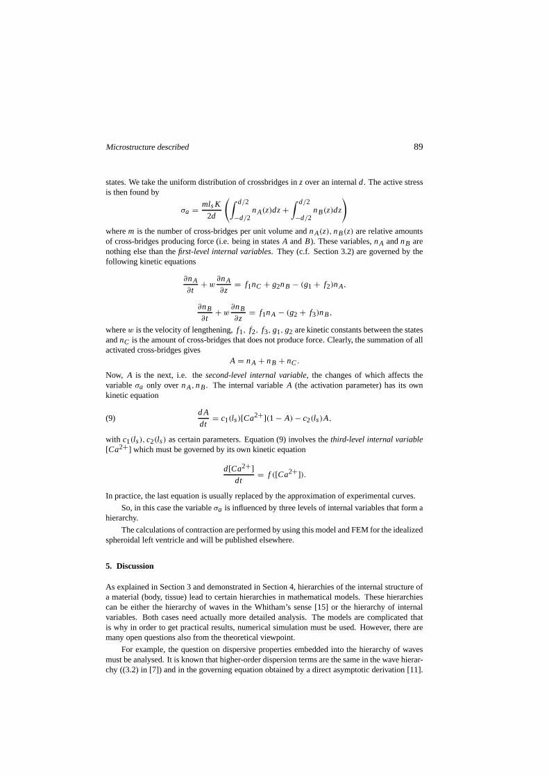
Microstructure described 89
states. We take the uniform distribution of crossbridges inz over an internald. The active stressis then found by
σa = mlsK
2d
(∫ d/2
−d/2nA(z)dz+
∫ d/2
−d/2nB(z)dz
)
wherem is the number of cross-bridges per unit volume andnA(z),nB(z) are relative amountsof cross-bridges producing force (i.e. being in statesA andB). These variables,nA andnB arenothing else than thefirst-level internal variables. They (c.f. Section 3.2) are governed by thefollowing kinetic equations
∂nA
∂t+ w
∂nA
∂z= f1nC + g2nB − (g1 + f2)nA,
∂nB
∂t+w
∂nB
∂z= f1nA − (g2 + f3)nB,
wherew is the velocity of lengthening,f1, f2, f3, g1, g2 are kinetic constants between the statesandnC is the amount of cross-bridges that does not produce force. Clearly, the summation of allactivated cross-bridges gives
A = nA + nB + nC .
Now, A is the next, i.e. thesecond-level internal variable, the changes of which affects thevariableσa only overnA,nB. The internal variableA (the activation parameter) has its ownkinetic equation
(9)d A
dt= c1(ls)[Ca2+](1 − A)− c2(ls)A,
with c1(ls), c2(ls) as certain parameters. Equation (9) involves thethird-level internal variable[Ca2+] which must be governed by its own kinetic equation
d[Ca2+]
dt= f ([Ca2+]).
In practice, the last equation is usually replaced by the approximation of experimental curves.
So, in this case the variableσa is influenced by three levels of internal variables that formahierarchy.
The calculations of contraction are performed by using thismodel and FEM for the idealizedspheroidal left ventricle and will be published elsewhere.
5. Discussion
As explained in Section 3 and demonstrated in Section 4, hierarchies of the internal structure ofa material (body, tissue) lead to certain hierarchies in mathematical models. These hierarchiescan be either the hierarchy of waves in the Whitham’s sense [15] or the hierarchy of internalvariables. Both cases need actually more detailed analysis. The models are complicated thatis why in order to get practical results, numerical simulation must be used. However, there aremany open questions also from the theoretical viewpoint.
For example, the question on dispersive properties embedded into the hierarchy of wavesmust be analysed. It is known that higher-order dispersion terms are the same in the wave hierar-chy ((3.2) in [7]) and in the governing equation obtained by adirect asymptotic derivation [11].

90 J. Engelbrecht - M. Vendelin
This certainly shows the correctness in leading terms but the properties of the wave hierarchy arenot clear.
For hierarchical internal variables the line of questions seems to be longer. The extra entropyflux k in the formalism of internal variables [10], [13] depends then also on internal variablesin a certain sequence that must be analysed. Open is the question, how to construct dissipativepotentialsDα,Dβ ,Dγ , ... corresponding to the each level of internal variables. It seems, that amore detailed formalism of internal variables might cast light over the formation of dissipativestructures.
References
[1] CAPRIZ G.,Continua with microstructure, Springer, New York 1989.
[2] CERMELLI P. AND PASTRONEF., Influence of a dissipative microstructure on wave prop-agation, in: “Nonlinear waves in solids”, (Eds. J.L. Wegner and F.R.Norwood), ASMEBook 1371995, 279–284.
[3] ENGELBRECHTJ.,Nonlinear wave dynamics: complexity and simplicity, 1997.
[4] ENGELBRECHTJ., CERMELLI P. AND PASTRONEF., Wave hierarchy in microstructuredsolids, in: “Geometry, continua and microstructure” (Ed. G.A. Maugin), Hermann Publ.,Paris 1999, 99–111.
[5] ENGELBRECHT J. AND MAUGIN G.A., Deformation waves in thermoelastic media andthe concept of internal variables, Arch. Appl. Mech.66 (1996), 200–207.
[6] ENGELBRECHTJ., VENDELIN M. AND MAUGIN G.A., Hierarchical internal variablesreflecting microstructural properties: application to cardiac muscle contraction, J. Non-Equilib. Thermodyn.25 (2000), 119–130.
[7] GIOVINE P. AND OLIVERI F., Dynamics and wave propagation in dilatant granular ma-terials, Meccanica30 (1995), 341–357.
[8] GLASS L., HUNTER .P, AND MCCULLOCH A., Theory of heart. Biomechanics, bio-physics, and nonlinear dynamics of cardiac function, Springer, New York 1991.
[9] GURTIN M.E. AND PODIO-GUIDUGLI P.,On the formulation of mechanical balance lawsfor structured continua, ZAMP 43 (1992), 181–190.
[10] MAUGIN G.A., Internal variables and dissipative structures, J. Non-Equilib. Thermodyn.15 (1990), 173–192.
[11] MAUGIN G.A., On some generalizations of Boussinesq and KdV systems, Proc. EstonianAcad. Sci. Phys. Math.44 (1995), 40–55.
[12] MAUGIN G.A. AND ENGELBRECHTJ.,A thermodynamical viewpoint on nerve pulse dy-namics, Proc. Estonian Acad. Sci. Phys. Math.19 (1994), 9–23.
[13] MAUGIN G.A. AND MUSCHIK W., Thermodynamics with internal variables, Ibid 19(1994), 217–249 (part I), 250–289 (part II).
[14] VENDELIN M., BOVENDEERD P.H.M., ARTS T., ENGELBRECHT J. AND VAN CAM -PEN D.H., Cardiac mechanoenergetics replicated by cross-bridge model, Annals Biomed.Eng.286 (2000), 629–640.
[15] WHITHAM G.B.,Linear and nonlinear waves, J. Wiley, New York 1974.
[16] ZIPES D.P. AND JALIFE J., Cardiac electrophysiology: from cell to bedside, Saunders,Philadelphia 1995.

Microstructure described 91
AMS Subject Classification: 35Q53, 74J30, 92C05.
Juri ENGELBRECHT, Marko VENDELINCentre for Nonlinear Studies, Institute of CyberneticsTallinn Technical UniversityAkadeemia tee 2112618 Tallinn, ESTONIAe-mail:[email protected]

92 J. Engelbrecht - M. Vendelin

Rend. Sem. Mat. Univ. Pol. TorinoVol. 58, 1 (2000)Geom., Cont. and Micros., I
M. Epstein∗
ARE CONTINUOUS DISTRIBUTIONS OF
INHOMOGENEITIES IN LIQUID CRYSTALS POSSIBLE?
Abstract. Within a theory of liquid-crystals-like materials based ona generalizedCosserat-type formulation, it is shown that continuous distributions of inhomo-geneities may exist at the microstructural level.
1. Introduction
In the conventional theories of liquid crystals, the free-energy density is assumed to be a functionof a spatial vector field and its spatial gradient. Starting from the pioneering work of Frank[6], various improvements were proposed by Leslie [9] and byEricksen [4] [5]. A differentpoint of view was advocated by Lee and Eringen [7] [8], as early as 1972, when considering aliquid criystal within the framework of the theory of materials with internal structure. The maindifference between these points of view is that the second approach emphasizes the dependenceof the constitutive equations on themappingsbetween vectors or tensor fields, rather than ontheir values alone. This mapping-dependence is essential not only for sustaining continuousdistributions of inhomogeneities, but also, as shown by Maugin and Trimarco [10], for the propersetting of a definition of Eshelby stresses. The general connection between these two aspects ofmaterial behaviour is described in [3].
2. The generalized Cosserat medium
A generalized Cosserat body(GCB) consists of the frame bundle of an ordinary bodyB. In otherwords, a GCB is a body plus the collection of all its local frames at each point. Denoting byX I
(I = 1, 2, 3) andxi (i = 1, 2,3) Cartesian coordinate systems for the bodyB and for physicalspace, respectively, a configuration of a GCB consists of thetwelve independent functions:
xi = xi (XJ )
H iI = H i
I (XJ )
whereH iI represents the mapping of the frames attached at pointXJ . It is important to stress
that the ordinary deformation gradientF iI = ∂xi
∂X I and the mappingH iI are of the same nature,
but represent two independent vector-dragging mechanisms.
A GCB is hyperelasticof the first grade if its material response can be completely charac-terized by a single scalar (“strain-energy”) function:
W = W(F iI , H i
I , H iI ,J ; XK )
∗Partially supported by the Natural Sciences and Engineering Research Council of Canada, and DGI-CYT (Spain) (Project PB97-1257).
93

94 M. Epstein
where comma subscripts denote partial derivatives. Under achange of reference configurationof the form
YA = YA(XJ )
H AI = H A
I (XJ )
where the indicesA, B,C are used for the new reference, the energy function changes to:
W = W′(F iA, H i
A, H iA,B; YC)
= W(F iAF A
I , H iAH A
I , H iA,B F B
J H AI + H i
AH AI ,J ; XK (YC))(1)
Notice the special form of the composition law for the derivatives of H iI .
Generalizing Noll’s idea of uniformity [11], by taking intoaccount the composition laws inEquation (1), one can show [1] [2] that in terms of an archetypal energy function
Wc = Wc(Fiα, H i
α, H iαβ )
where Greek indices are used for the archetype, a GCB isuniform (namely, it is made of “thesame material” at all points) if there exist three uniformity fields of tensorsPI
α(XJ ), QIα(X
J )
andRIαβ (X
J ) such that the equation
W(F iI , H i
I , H iI ,J ; XK ) = Wc(F
iI PI
α, H iI QI
α, H iI ,J PJ
βQIα + H i
I RIαβ )
is satisfied identically for all non-singularF iI andH i
I and for allH iI ,J . Homogeneity(global
or local) follows if, and only if, there exists a (global or local) reference configuration such thatthese fields become trivial.
3. The liquid-crystal-like model
We call aliquid-crystal-like model(LCM) a material whose internal structure can be representedby the deformation of one or more vector or tensor fields. Morespecifically, we say that a GCBis of the LCM type if a nowhere-zero material vector fieldD = D I EI and a material tensor fieldA = AI
JEI ⊗ EJ exist such that the energy density function depends on its arguments in thefollowing way:
(2) W = W(F iI , H i
I , H iI ,J ; XK ) = f (F i
I , H iI D I , H i
I ,J D I + H iI AI
J ; XK )
where we have used the letterf to denote the new functional dependence.
To clarify the rationale behind this definition, we considerfirst the particular case of a ref-erence configuration in whichD(X) constitutes a parallel unit vector field andA(X) vanishesidentically. We can then write (for that particular reference configuration, if it exists) that
W = f (F iI , H i
I D I , (H iI D I ),J ; XK )
This constitutive equation is unable to detect any difference between different deformations oftriads that happen to map the director into the same vector inspace. In other words, all thatmatters is the resulting vector and its gradient, just as in the “conventional” theory of liquidcrystals, and it is in this sense that Equation (2) constitutes a generalization. More importantly,when seen under this light, the tensorA no longer appears as an artificial construct, but as thenatural outcome of describing the manner in which the conventional archetype has been insertedin the body in a pointwise fashion.

Distributions of inhomogeneities 95
It is apparent that the particular form of the constitutive law adopted for an LCM mustentail certainminimal symmetries, namely, certain local changes of reference configuration thatare indistinguishable as far as the material response is concerned. In addition, an LCM may haveother non-generic symmetries, but here we are interested inderiving those symmetries that arealready inherent in the definition. Now, any symmetry of a GCBconsists of a triple{G, K , L}satisfying:
f (F iJ , H i
J DJ , H iM,N DM + H i
M AMN ; XK ) =
f (F iI GI
J , H iI K I
J DJ , (H iI ,J GJ
N K IM + H i
I L IM N )D
M + H iI K I
M AMN ; XK )
for all non-singularF iI andH i
I and for allH iI ,J . Since we are looking for minimal symme-
tries, namely, those stemming from the particular dependence assumed onH and its gradient,we setG equal to the identity. It then follows that the energy function will have the same valuesfor all K andL satisfying the following identities:
H iJ DJ = H i
I K IJ DJ
and
H iM,N DM + H i
M AMN = H i
I ,N K IM DM + H i
I L IM N DM + H i
I K IM AM
N
for all non-singularF iI and H i
I and for all H iI ,J . It follows immediately that the minimal
symmetries are those satisfying the following conditions:
(3) K IJ DJ = D I
and
(4) L IM N DM = (δ I
M − K IM )A
MN
The first condition is the obvious one: the energy function ata point remains invariant underany change of reference configuration which leaves the director at that point unchanged. Inother words, the matrixK has the director as an eigenvector corresponding to a unit eigenvalue.The second condition, on the other hand, is far from obvious and could not have been predictedexcept by means of the kinematically based method we have used. Note that in the particularcase in which the tensor fieldA is zero, the right-hand side of the second condition vanishes. Itis not difficult to show by a direct calculation that the collection of all the symmetries satisfyingthe above two conditions forms a groupGmin, which we will call theminimal symmetry groupof any LCM, under the multiplication law given by Equation (1).
Although not strictly necessary, we will adopt as theLCM archetypea point whose consti-tutive law is of the form
Wc = Wc(Fiα, H i
α, H iαβ ) = fc(F
iα, H i
αDα, H iαβ )
namely, we adoptAαβγ = 0 at the archetype. According to the general prescription for unifor-mity, then, fieldsPI
α(XK ), QIα(X
K ) andRIαβ (XK ) must exist such that:
W(F iI , H i
I , H iI ,J ; XK )
= Wc(FiI PI
α, H iI QI
α, H iI ,J PJ
βQIα + H i
I RIαβ )
= fc(FiI PI
α, H iI QI
αDα, (H iI ,J PJ
βQIα + H i
I RIαβ )D
α)

96 M. Epstein
It is a straightforward matter to verify that the resulting functionW has the requisite form:
W(F iI , H i
I , H iI ,J ; XK ) = f (F i
I , H iI D I , (H i
I ,J D I + H iI AI
J ))
whereD I = QI
αDα
andAI
J = RIαβ (P
−1)β J Dα
Indeed
fc(FiI PI
α, H iI QI
αDα, (H iI ,J PJ
βQIα + H i
I RIαβ )D
α)
= fc(FiI PI
α, H iI D I , PJ
β (HiI ,J D I + H i
I AIJ ))
= f (F iI , H i
I D I , H iI ,J D I + H i
I AIJ ; XK )
Under a change of reference configuration we know that the tensor fieldAIJ transforms to
AAB = (H A
I ,J D I + H AI AI
J)(F−1)J B
and we ask the question: does there exist a change of reference configuration leading to anidentically vanishingAA
B in an open neighbourhood of a point? It is not difficult to showthat asufficient condition for this local homogeneity requirement to take place is that:
AIJ = D I
,J
identically in that neighbourhood. Indeed, if that is the case, we can write:
AAB = (H A
I D I ),J(F−1)J B
Therefore, any change of reference configuration of the form
YA = YA(XK )
H AI = (Q−1)α I δ
Aα
will do the job. We conclude then that the local homogeneity of an LCM body is guaranteed, inaddition to the ordinary condition of homogeneity of the macromedium, by the equation
(5) AIJ = D I
,J
describing the compatibility of the liquid crystal superstructure. If, however, the underlyingmacromedium is homogeneous but condition (5) is violated, we have a genuine distribution ofinhomogeneities at the microstructural level. On the otherhand, it can be shown that the twoconditions taken together are not only sufficient, but also necessary, for local homogeneity ofan LCM uniform body whose symmetry group is minimal. This fact holds true even though theminimal symmetry group is continuous. More surprisingly, perhaps, the same conclusion holdseven when the macromedium is a genuine liquid, namely, when its symmetry group is the wholeunimodular group.
Assume that we have a reference configuration that is homogeneous as far as the underly-ing macromedium is concerned and in which the director field is unit and parallel. The onlysource of inhomogeneity left is, therefore, a smooth second-order tensor fieldA(X). By the po-lar decomposition theorem, this field can be seen geometrically as a field of ellipsoids, whose

Distributions of inhomogeneities 97
axes and eccentricities vary smoothly from point to point. In principle, then, we have a situationequivalent to that of a standard liquid crystal, except thatthe standard ellipsoids of orientationaldistribution are now replaced by the ellipsoids arising form the inhomogeneity of the microstruc-ture. These last ellipsoids are manifest, as already noted,even if the director field is perfectlyunitary and parallel! The typical optical patterns, whose beautiful curvy shapes have becomeassociated in popular imagination with liquid crystals, and usually explained as a manifestationof the variation of the mean orientational order of the molecules, could therefore be explainedequivalently by the presence of continuous distributions of inhomogeneities.
4. Concluding remarks
We have shown that, at least in principle, it is possible to formulate a theory of liquid-crystal-likeuniform bodies that admit continuous distributions of inhomogeneities. The main ingredient ofthis theory is the inclusion of maps, and derivatives thereof, between whole fibres of the princi-pal frame bundle of the underlying body. This stands in contrast with the conventional theory,which recognizes only the transformation of a single vectorfield and its derivative. Althoughthe treatment of a liquid crystal as some kind of generalizedCosserat body is not new, the wayin which a particular director field is made to enter the formulation is different from previousformulations. Instead of imposing a constitutive symmetryupon a standard Cosserat medium,we emphasize a kinematic motivation as a rationale for constraining the constitutive functionalto a particular form, and only then derive a-posteriori results for the minimal symmetry group.These results differ form the a-priori counterparts in [7] and [8] in the rather complicated sym-metry requirement for the microstructural component, a requirement that is absent in the a-prioristatement. But it is precisely this condition that allows for the existence of legitimate microstruc-tural inhomogeneities. Further mathematical details of the theory are now under investigation,including differential-geometric implications.
References
[1] EPSTEINM. AND DE LEON M., Homogeneity conditions for generalized Cosserat media,J. Elasticity43 (1996), 189–201.
[2] EPSTEINM. AND DE LEON M., Geometrical theory of uniform Cosserat media, J. Geom.Phys.26 (1998), 127–170.
[3] EPSTEINM. AND MAUGIN , G. A.,The energy-momentum tensor and material uniformityin finite elasticity, Acta Mech.83 (1990), 127–133.
[4] ERICKSEN J. L.,Anisotropic fluids, Arch. Rational Mech. Anal4 (1960), 231–237.
[5] ERICKSENJ. L.,Liquid crystals with variable degree of orientation, Arch. Rational Mech.Anal. 113(1991), 97–120.
[6] FRANK F. C.On the theory of liquid crystals, Discuss. Faraday Soc.25 (1958), 19–28.
[7] L EE J. D. AND ERINGEN A. C. Wave propagation in nematic liquid crystals, J. Chem.Phys.54 (1971), 5027–5034.
[8] L EE J. D. AND ERINGEN A. C. Continuum theory of smectic liquid crystals, J. Chem.Phys.58 (1973), 4203–4211.
[9] L ESLIE F. M. Some constitutive equations for liquid crystals, Arch. Rational Mech. Anal.28 (1968), 265–283.

98 M. Epstein
[10] MAUGIN G. A. AND TRIMARCO C. On material and physical forces in liquid crystals,Int. J. Engng. Sci.33 (1995), 1663–1678.
[11] NOLL W. Materially uniform simple bodies with inhomogeneities, Arch. Rational Mech.Anal. 27 (1967), 1–32.
AMS Subject Classification: 73B25, 53C10.
Marcelo EPSTEINDepartment of Mechanical and Manufacturing EngineeringUniversity of CalgaryCalgary, Alberta T2N 1N4, CANADAe-mail:[email protected]

Rend. Sem. Mat. Univ. Pol. TorinoVol. 58, 1 (2000)Geom., Cont. and Micros., I
S. Forest - R. Parisot∗
MATERIAL CRYSTAL PLASTICITY AND DEFORMATION
TWINNING
Abstract. In classical crystal plasticity, the lattice orientation is unchanged fromthe reference configuration to the local to the local intermediate is plastically de-formed configuration. Material plasticity corresponds to adifferent irreversibleprocess by which the lattice rotates together with materiallines between referenceand intermediate configurations. Deformation twinning is an example of mate-rial plasticity. A continuum model for mechanical twinningof single crystals ispresented in this work. Twin formation is regarded as an unstable localizationphenomenon, followed by twin front propagation. Finite element simulations areprovided showing the twinning and untwinning of a single crystal under cyclicloading, the development of twins at a crack tip, and lastly the formation of twinnetworks in a coating on an elastic substrate.
1. Material vs. dislocation-based crystal plasticity
The constitutive framework of anisotropic elastoplasticity has been settled by Mandel in [11]:it requires the definition of a tryad of directors attached toeach material point. In the case ofsingle crystal plasticity, the relative rotation rate of lattice directors with respect to material linesis derived in a unique way from the kinematics of plastic glide according toN slip systems. Aunique intermediate configuration can be defined for which the lattice orientation is the same asthe initial one. This results in a multiplicative decomposition of the deformation gradientF∼ intoelastic and plastic parts, as shown on figure 1a:
F∼ = E∼P∼, P∼P∼−1 =
N∑
s=1
γ sms ⊗ ns
where slip systems is described by the slip directionms and the normal to the slip planens,andγ s denotes the amount of associated slip. It follows that from the reference configuration tothe intermediate one, the lattice directions are left unchanged whereas the material lines rotateaccording to the rotation part in the polar decomposition ofP∼.
One can also imagine an irreversible deformation process bywhich the lattice directions ofthe crystal would simply follow the material lines. This is what we callmaterial crystal plasticity.It leads to the picture of figure 1b where the individual atomsundergo a uniform simple glide ina cooperative way. However this process is not so simple as itmay look since during the shearingthe lattice structure is changed usually going from a highlysymmetric class to a less symmetricone. Some critical shear amountγ0 may exist for which the crystal structure is retrieved withpossibly an orientation different from the initial one ([14]). Such a deformation process exists
∗The authors want to thank Prof. Andre Pineau for many discussions on twinning phenomena in zinc.
99

100 S. Forest - R. Parisot
in some crystals. It is referred to asdeformation twinning([2, 16]). The sequel of the paper isdevoted to the continuum modelling of this particular mode material crystal plasticity.
(a)
F
P E
(b)
Figure 1: Kinematics of crystal plasticity based on dislocation glide (a); homogeneousshearing of a lattice as an example of material crystal plasticity (b).
Figure 2: Twin network and four cleavage cracks in a large flatzinc grain coated on asteel sheet (grain size : 500µm).

Material cristal plasticity 101
2. Continuum modelling of deformation twinning
2.1. Elements of deformation twinning
Deformation twinning now is a well–known deformation mechanism in cubic and hexagonalcrystals. A modern and exhaustive account of the current knowledge from the crystallographic,metallurgical and mechanical point of view can be found in [3]. We will simply retain thefollowing features:
• the deformation of the twinned part of the crystal can be described by a homogeneousshearingγ0 in directionη1 and in the planeS;
• the crystal structure of the twin usually is the mirror imageof the parent crystal in thecrystallographic twin planeK1; K1 very often coincides with the plane of contact between thetwo crystals called composition plane which is neither rotated nor distorted; the direction inSundergoing only a rotation is calledη2 andK2 denotes the plane containingη2 and normal toS;
• in fact, a simple shear applied to atom positions, as distinct from lattice points, is notalways capable of producing all the atom movements which areneeded to form a twin: additionalreshuffleof some atoms of the unit cell is necessary, in particular in multiple lattices.
For simplicity, the present work is actually restricted to compound twins for which all el-ementsKi , ηi are rational ([10]). More specifically, the provided examples deal with pure zinchaving hexagonal closed–packed symmetry. Using classicalindex notations for this type of sym-metry ([2]), the twinning system of pure zinc is given by:
η1 =< 1011>, K1 = {1012}, η2 =< 1011>, K2 = {1012}, γ0 = 0.139
The lattice orientation relationship between the parent crystal and the twin in zinc are: a mirrorsymmetry inK1, or equivalently a rotation of angleπ aroundη1, a mirror symmetry in the planenormal toη1 or a rotation of angleπ around the normal toK1.
2.2. Elastoplastic model of twinning
Mechanical models for twinning are available from both microscopic and macroscopic points ofview. At the level of the cooperative behaviour of atoms, non–linear elasticity with a non–convexpotential has proved to be an efficient method to describe such a phase transition–like process([4, 19]). Indeedelastic twinningexists if there are no lattice friction forces opposing the motionof the dislocations at irregular interfaces. In this case, twins will run back when the appliedstress is removed. In calcite for instance, small twins nucleate by indentation and disappearwhen the load is removed ([10]). However, more generally twinning isnot reversibleand twinsremain in a crystal after it has been unloaded. The reason often is that accommodation hasoccurred by slip, relieving the stresses at the edge of the twin. Under these conditions, blunt twinplates with quite irregular interfaces are possible (figure2). That is why deformation twinningis modelled here as an elastoplastic process associated with dissipation. Such an approach hasalready been proposed to model at the macroscopic level the volume fraction of twins appearingin a polycrystalline volume element of metal deforming by both slip and twinning ([9, 18]). Wetackle here a different problem since the aim is to simulate the nucleation and propagation oftwins at the grain level.
The classical framework of crystal plasticity is now extended to incorporate the followingfeatures of twinning (figure 3):
• twin formation is modelled as an unstable plastic slip process according to classicaldislocation–based crystal plasticity;

102 S. Forest - R. Parisot
• as soon as a critical amount of shearγ = γ0 has been reached for the activated twinsystem, the orientation of the isoclinic intermediate configuration is changed switching from theinitial parent one to that of the associated twin.
The driving force for twinning is the resolved shear stressτ on the twin plane in the twinningdirection and the slip rate is computed using:
γ =< τ − τc
K>n, τc = τ0 + Q(1 − e−b(γ−E(γ /γ0)))
where the viscosity parametersK andn are chosen so that the resulting behaviour is as rate–independent as necessary.τ0 denotes the initial threshold for twinning and the hardening pa-rameterQ is taken negative. Such a softening behaviour makes twin nucleation an unstabledeformation mode associated with strain localization. Thefunction floorE(.) taking the integerpart of . is introduced so that the initial threshold is recovered once the local twinning processis finished. Contrary to the classical Schmid law in dislocation - based plasticity, the sign ofτplays a role since twinning is possible only in one specific direction : compression in directioncin zinc triggers deformation twinning, but not tension. Thechoice ofm andn is such thatτ, γandγ are positive when twinning occurs.
� � � � �� � � � �� � � � �� � � � �� � � � �� � � � �
� � � � �� � � � �� � � � �� � � � �� � � � �� � � � �
� � � � � �� � � � � �� � � � � �� � � � � �� � � � � �� � � � � �
� � � � � �� � � � � �� � � � � �� � � � � �� � � � � �� � � � � �
� � � � � �� � � � � �� � � � � �� � � � � �� � � � � �� � � � � �� � � � � �
� � � � � �� � � � � �� � � � � �� � � � � �� � � � � �� � � � � �� � � � � �
� � � � � � � �� � � � � � � �� � � � � � � �� � � � � � � �� � � � � � � �� � � � � � � �
� � � � � � � �� � � � � � � �� � � � � � � �� � � � � � � �� � � � � � � �� � � � � � � �
� � � � � � � �� � � � � � � �� � � � � � � �� � � � � � � �� � � � � � � �� � � � � � � �
initial orientation
associatedtwin
F
PE
Figure 3: Kinematics of twinning plasticity
2.3. Thermodynamic setting
The state variables of the system can be taken as the Green–Lagrange strain tensor with respectto the intermediate configuration]:
]1∼ = 1
2(E∼
T E∼ − 1∼)
and temperature. The free energyψ( ]1∼ , α) may also be a function of an internal variableα tobe specified. In the sequel, it is referred to the pure isothermal case. Only one twinning system
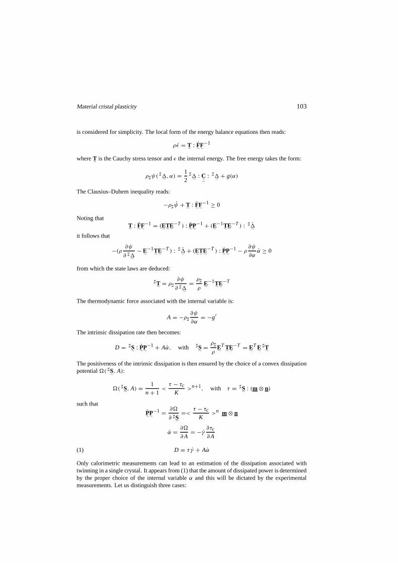
Material cristal plasticity 103
is considered for simplicity. The local form of the energy balance equations then reads:
ρε = T∼ : F∼F∼−1
whereT∼ is the Cauchy stress tensor andε the internal energy. The free energy takes the form:
ρ]ψ(]1∼ , α) = 1
2]1∼ : C∼∼
: ]1∼ + g(α)
The Clausius–Duhem inequality reads:
−ρ]ψ + T∼ : F∼F∼−1 ≥ 0
Noting thatT∼ : F∼F∼
−1 = (E∼T∼E∼−T ) : P∼P∼
−1 + (E∼−1T∼E∼
−T ) : ]1∼it follows that
−(ρ ∂ψ∂ ]1∼
− E∼−1T∼E∼
−T ) : ]1∼ + (E∼T∼E∼−T ) : P∼P∼
−1 − ρ∂ψ
∂αα ≥ 0
from which the state laws are deduced:
]T∼ = ρ]∂ψ
∂ ]1∼=ρ]
ρE∼
−1T∼E∼−T
The thermodynamic force associated with the internal variable is:
A = −ρ]∂ψ
∂α= −g′
The intrinsic dissipation rate then becomes:
D = ]S∼ : P∼P∼−1 + Aα, with ]S∼ =
ρ]
ρE∼
T T∼E∼−T = E∼
T E∼]T∼
The positiveness of the intrinsic dissipation is then ensured by the choice of a convex dissipationpotential�( ]S∼, A):
�( ]S∼, A) = 1
n + 1<τ − τc
K>n+1, with τ = ]S∼ : (m ⊗ n)
such that
P∼P∼−1 = ∂�
∂ ]S∼=< τ − τc
K>n m ⊗ n
α = ∂�
∂A= −γ ∂τc
∂A
(1) D = τ γ + Aα
Only calorimetric measurements can lead to an estimation ofthe dissipation associated withtwinning in a single crystal. It appears from (1) that the amount of dissipated power is determinedby the proper choice of the internal variableα and this will be dictated by the experimentalmeasurements. Let us distinguish three cases:

104 S. Forest - R. Parisot
• if no internal variable is introduced,D = τ γ so that the entire plastic power is dissipatedinto heat; it is positive for a proper choice ofm andn (such thatτ > 0 whenγ > 0), even if asoftening behaviour is introduced;
• if we takeg′ = τc = −A, thenα = γ and D = (τ − τc)γ which vanishes in the rate-independent case; accordingly, the entire plastic power isconsidered as irreversibly stored, likedislocation forest hardening in dislocation–glide plasticity;
• if we take τc = τ0 − A, i.e. g′ = −A = Q(1 − e−bγ ), thenα = γ and D =(τ − (τc − τ0))γ ' τ0γ in the quasi–rate–independent case; it is again positive since the twin-ning system orientation convention is such thatγ ≥ 0. This choice is classical in conventionalelastoviscoplasticity ([1]).
A much more fine tuning of the internal variable will be necessary in the case of twinning([17]) and is not undertaken here.
3. Finite element simulations of twinning in single crystals
The ability of the model to reproduce several experimental features of deformation twinningin single crystals is illustrated for three different situations. For that purpose, finite elementsimulations are provided based on classical nonlinear algorithms for the resolution of globalequilibrium and the local integration of the evolution equations.
3.1. Twinning and untwinning under cyclic loading
The main justification for choosing a softening stress-strain constitutive equation in the modelstems from the experimental results obtained by Price ([15]) on zinc whiskers deformed in ten-sion under a transmission electron microscope. He was able to observe and control the nucle-ation of a single twin and its propagation in the sample cross–section. The twin then thickensand invades the entire specimen. The load–displacement curve displays a sharp softening stageassociated with twin nucleation. The parameters of the model have been adjusted according tothis curve.
The simulation of a single crystal zinc plate oriented for plane single twinning in tensionis now considered. A geometrical defect is introduced to trigger strain localization that is in-terpreted here as twin nucleation. Indeed a deformation band appears and its orientation corre-sponds to that of a twin. Once the critical amount of shearγ0 is reached, the twin starts growing.Twin growths is the result of the motion of the localization front on one or both sides of the twinin the spirit of ([12]). The twin thickens and spreads over the entire specimen (figure 5a). Whenthe whole sample has twinned, the crystal behaves elastically in tension. The crystal can then beentirely untwinned if it is subsequently subjected to compression (figure 5b). It must be notedthat at the last deformation stage, a virgin crystal is obtained that can again twin in tension. Thisresults in the hysteresis loop shown in figure 4.
3.2. Twinning modes at a crack tip
Let us now consider a single crystalline Compact Tension specimen classically used in fracturemechanics. Thec–axis of the zinc crystal is normal to the crack plane and the initial crack growthdirection coincides with [0110]. It is recalled that twinning occurs in a specific directionη1 andnot in the opposite direction. A positive resolved shear stress in this direction is necessary fortwinning to become possible. The distribution of resolved shear stresses for the single considered
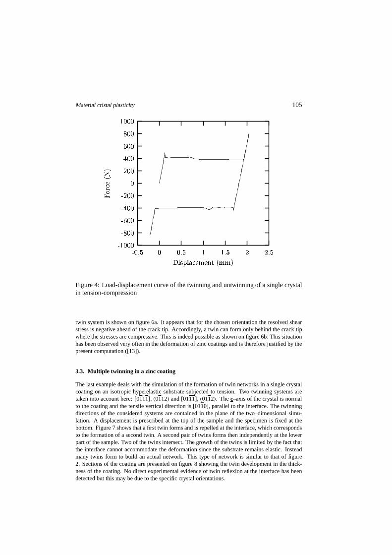
Material cristal plasticity 105
� ��� �� ��� � �� � �
�������
� ���� ���� ����� ��
����������� �����
�
� ���
�� ��
����
����
� ����
Figure 4: Load-displacement curve of the twinning and untwinning of a single crystalin tension-compression
twin system is shown on figure 6a. It appears that for the chosen orientation the resolved shearstress is negative ahead of the crack tip. Accordingly, a twin can form only behind the crack tipwhere the stresses are compressive. This is indeed possibleas shown on figure 6b. This situationhas been observed very often in the deformation of zinc coatings and is therefore justified by thepresent computation ([13]).
3.3. Multiple twinning in a zinc coating
The last example deals with the simulation of the formation of twin networks in a single crystalcoating on an isotropic hyperelastic substrate subjected to tension. Two twinning systems aretaken into account here: [0111], (0112) and [0111], (0112). Thec–axis of the crystal is normalto the coating and the tensile vertical direction is [0110], parallel to the interface. The twinningdirections of the considered systems are contained in the plane of the two–dimensional simu-lation. A displacement is prescribed at the top of the sampleand the specimen is fixed at thebottom. Figure 7 shows that a first twin forms and is repelled at the interface, which correspondsto the formation of a second twin. A second pair of twins formsthen independently at the lowerpart of the sample. Two of the twins intersect. The growth of the twins is limited by the fact thatthe interface cannot accommodate the deformation since thesubstrate remains elastic. Insteadmany twins form to build an actual network. This type of network is similar to that of figure2. Sections of the coating are presented on figure 8 showing the twin development in the thick-ness of the coating. No direct experimental evidence of twinreflexion at the interface has beendetected but this may be due to the specific crystal orientations.
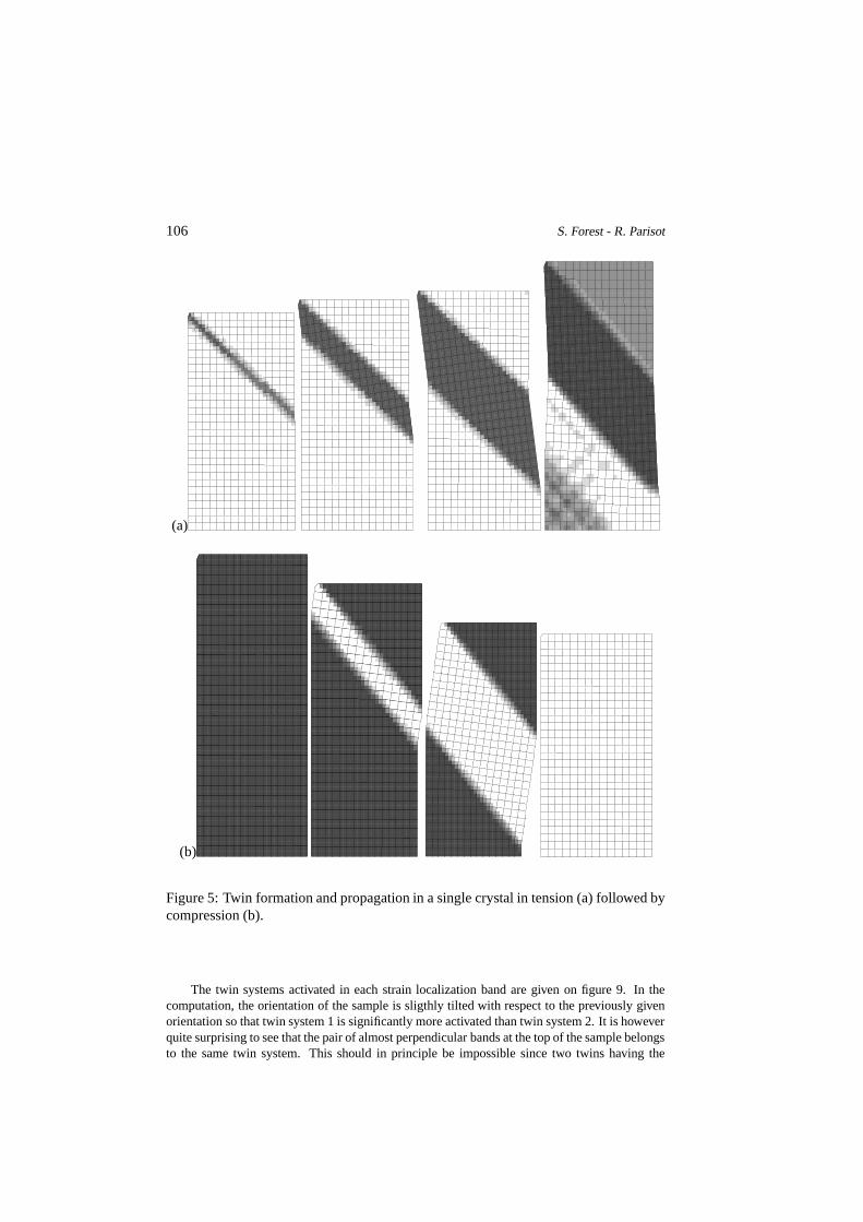
106 S. Forest - R. Parisot
(a)
(b)
Figure 5: Twin formation and propagation in a single crystalin tension (a) followed bycompression (b).
The twin systems activated in each strain localization bandare given on figure 9. In thecomputation, the orientation of the sample is sligthly tilted with respect to the previously givenorientation so that twin system 1 is significantly more activated than twin system 2. It is howeverquite surprising to see that the pair of almost perpendicular bands at the top of the sample belongsto the same twin system. This should in principle be impossible since two twins having the

Material cristal plasticity 107
(a) 0 28 55 83 110
(b)0 0.01 0.02 0.03 0.04 0.05 0.06 0.07 0.08 0.09 0.1
Figure 6: Twin formation at a cleavage crack tip : resolved shear stress distribution((a), in MPa) and equivalent plastic deformation field (b).

108 S. Forest - R. Parisot
Figure 7: Multiple twinning in a zinc coating: the first twin is repelled at the interfacecoating/substrate (left), multiple reflexion and formation lead to a network of twins inthe coating (right, only the coating is represented).
Figure 8: Section of the coating in the thickness showing theshape and orientation ofthe twins; the thickness of the coating is 10µm.
same twin plane should be parallel. These bands must be interpreted in fact as shear bands in asingle crystal undergoing single slip. Simple glide in the twinning direction has been artificiallyintroduced in the modelling to simulate twin formation. Twin formation has been interpretedas a strain localization phenomenon. In single slip, it is known that two localization planesare possible : slip bands lying in the slip plane but also kinkbands that are normal to the slipdirection ([5]). The last picture gives the distribution oflattice rotation with respect to the initialorientation before the twinned lattice has been reindexed.This information enables us in fact todistinguish the different types of bands : slip bands are usually associated with no lattice rotationwhereas kink banding induces lattice curvature. It appearsthat the first twin at the top is akinktwin and the second one a “slip twin”. A “kink twin” can be seen as a stacking of many paralleltwin lamellae. A severe limitation of the model is that such kink twins are usually not observedexperimentally.

Material cristal plasticity 109
(a) (b) (c) (d)
Figure 9: Structure of the twins in the coating : (a) equivalent plastic deformation, (b)twinning system 1, (c) twinning system 2, (d) lattice rotation before reindexing.
4. Discussion: The pros and the cons of the model
The proposed finite strain elastoplastic model of deformation twinning is able to account forseveral experimental features : twin formation and propagation in a single crystal, hysteresisloop associated with a twinning–untwinning process, arrowshape of twins at a cleavage cracktip and build–up of twin networks in a coating on a substrate.
Several important limitations remain however. One may for instance discuss the fact that atwinning criterion based on a critical resolved shear stress has been chosen. It is often recalledthat twin initiation is a nucleation (in contrast to propagation) controlled process. It can thereforebe affected for instance by prior dislocation glide so that it may be difficult to assign a criticalvalue τ0 to the twinning mechanism. Let us then admit thatτ0 is the critical resolved shearstress for twinning in a dislocation–free crystal like Price’s zinc whiskers. The effective twinnucleation stress can then decrease if dislocation glide has already taken place, according to asoftening law like:
τ = τ0 + Q2(1 − e−b2γslip)
whereQ2 is negative andγslip denotes the cumulative amount of prior dislocation glide.
Furthermore, deformation twinning is systematically associated with dislocation glide be-cause of the high local stresses arising for instance at the twin tip. This interaction has not beentaken into account yet, which leads to unrealistic local high stresses. Plastic slip can take placebefore twinning and the question to be solved is then : what happens to the obtained dislocation

110 S. Forest - R. Parisot
structure when it twins? How can prior slip activity affect further dislocation glide within thenewly formed twin? Mechanical metallurgy has already provided some answers that must beincorporated into continuum modelling.
Special attention should also be paid to the intersection oftwins that has occured in somesimulations.
A strong limitation has already been pointed out, namely theprediction of kink twins thatare not observed in practise. The elimination of such deformation modes is however possibleusing for instance Cosserat crystal plasticity ([6, 7]).
An alternative approach to deformation twinning is proposed in ([8]) based on minimizationprinciples. This global approach enables one to predict self–equilibrating structures that arefrequently observed. The difficulty then is the numerical exploration of all possible regionsand shapes where twinning can occur in order to finger out the most favourable configuration.The authors themselves plead for a Landau–Ginzburg or Cahn–Hilliard–type of modelling ofdisplacives phase transitions and deformation twinning. That is why an improvement of thepresent model could be the introduction of an order parameter, aiming at forbiding “interruptedtwins”, i.e. regions where crystal glide has begun but wherethe valueγ0 has not been reachedyet.
References
[1] CHABOCHE J. L., Thermodynamic formulation of constitutive equations and applicationto the viscoplasticity and viscoelasticity of metals and polymers, Int. J. Solids Structures34 (1997), 2239–2254.
[2] CHRISTIAN J. W., The theory of transformations in metals and alloys, Pergamon Press1965.
[3] CHRISTIAN J. W. AND MAHAJAN S., Deformation twinning, Progress in Materials Sci-ence39 (1995), 1-157.
[4] ERICKSEN J. L., Some phase transitions in crystals, Arch. Rat. Mech. Anal.73 (1980),99–124.
[5] FORESTS. AND CAILLETAUD G., Strain localization in single crystals: effect of bound-aries and interfaces, European Journal of Mechanics A-Solids14 (1995), 747–771.
[6] FOREST S., BARBE F. AND CAILLETAUD G., Cosserat modelling of size effects in themechanical behaviour of polycrystals and multiphase materials, Int. J. Solids Structures37 (2000), 7105–7126.
[7] FOREST S., Modeling slip, kink and shear banding in classical and generalized singlecrystal plasticityActa Materialia46 (1998), 3265–3281.
[8] I DESMAN A. V., L EVITAS V. I. AND STEIN E.,Structural changes in elastoplastic mate-rial: a unified finite-element approach to phase transformation, twinning and fracture, Int.J. Plasticity16 (2000), 893–949.
[9] K ALIDINDI S. R.,Incorporation of deformation twinning in crystal plasticity models, J.Mech. Phys. Solids46 (1998), 267–290.
[10] KELLY A. AND GROVES G. W., Crystallography and crystal defects, Longman, London1970.
[11] MANDEL J.,Equations constitutives et directeurs dans les milieux plastiques et viscoplas-tiques, Int. J. Solids Structures9 (1973), 725–740.

Material cristal plasticity 111
[12] MAUGIN G. A., On shock waves and phase-transition fronts in continua, ARI 50 (1998),141–150.
[13] PARISOT R., FORESTS., GOURGURESA. F. AND PINEAU A., Modelling the mechanicalbehaviour of a multicrystalline zinc coating on a galvanized steel sheet, ComputationalMaterials Science19 (2000), 189–204.
[14] PITTERI M., On the kinematics of mechanical twinning in crystals, Arch. Rat. Mech. Anal.58 (1985), 25–57.
[15] PRICE P. B., Nucleation and growth of twins in dislocation-free zinc, Proc. Roy. Soc.London260A (1961), 251–262.
[16] REED-HILL R. E., HIRTH J. P.AND ROGERSH. C.,Deformation twinning, MetallurgicalSociety Conferences25, Gordon and Breach Science Publishers 1964.
[17] SRINIVASA A. R., RAJAGOPAL K. R. AND AMSTRONG R. W., A phenomenologicalmodel of twinning based on dual reference structures, Acta Mater.46 (1998), 1235–1254.
[18] STAROSELSKYA. AND ANAND L., Inelastic deformation of polycrystalline f.c.c. materi-als by slip and twinning, J. Mech. Phys. Solids46 (1998), 671–696.
[19] TRUSKINOVSKY L. AND ZANZOTTO G., Ericksen’s bar revisited: energy wiggles, J.Mech. Phys. Solids44 (1996), 1371–1408.
AMS Subject Classification: 74C15, 74E10, 74Nxx.
Samuel FOREST, Rodolphe PARISOTEcole des Mines de Paris / CNRSCentre des Materiaux / UMR 7633, BP 8791003 Evry, FRANCEe-mail:[email protected]

112 S. Forest - R. Parisot

Rend. Sem. Mat. Univ. Pol. TorinoVol. 58, 1 (2000)Geom., Cont. and Micros., I
J. F. Ganghoffer
NEW CONCEPTS IN NONLOCAL CONTINUUM MECHANICS
Abstract. A new theoretical framework in nonlocal mechanics is defined, based onthe concept of influence functions between material points within the continuum.The traditional idea of a fixed and isotropic representativevolume is abandonedand the non-locality is introduced via an influence function, which defines a non-local interaction between material points. The general framework developed isexemplified by the description of damage as a scalar internalvariable : the localdamage rate at a given point can be expressed as a path integral involving the in-fluence functions and the values of the local rate of damage transported along eachpath. The properties satisfied by the influence function are first evidenced and theinfluence function is given an explicit expression, using a path integration tech-nique. The concept of a representative volume is further defined as an outcome ofthe stationarity of the internal entropy production with respect to the path. An im-plicit equation which defines the representative volume is formulated. The strengthof the nonlocal interaction is further incorporated into the space geometry, so thata metric characteristic of a Riemanian space is coupled to the internal variable dis-tribution. It appears that the curvature characterises thestrength of the nonlocalinteraction.
1. Introduction
Traditional continuum models in nonlocal mechanics usually rely on the assumption that thenonlocal variables are simply volume averages of the corresponding local variables over a fixedand isotropic representative volume element around the considered material point, see e.g. [1,2, 3, 4, 5]. Considerations based on micromechanical arguments however show that the sizeof the representative volume, i.e. the extension of the interaction shall depend on the localvariable distribution itself : in the work by Muhlhaus et al. ([6]), a Cosserat theory for granularmaterials is elaborated, starting from a particulate model. The model predicts that the shear bandthickness evolves with the shear strain. A micromechanicalargument for nonlocal damage hasbeen advanced in [2]: the strain-softening damage due to distributed cracking is modelled by aperiodic array of cracks. The results of the model show that the elastic part of the response shallbe local, whereas the damage recovered at the macro scale shall be nonlocal. Furthermore, thesize of the averaging region is determined by the crack spacing.
During loading of the cracked body, the increment of the stress along one crack is the sumof the average stress increment over the crack length and thecontributions of all other cracks :
(1) 1Si (x) =⟨1Si (x)
⟩+∫
V3i j (x, ξ)1Sj (ξ)dV(ξ).
The interactions of a set of microcracks cancel out over a short distance, and this in turn deter-mines the size of the representative volume. The kernel3(x, ξ) that determines the influence
113

114 J. F. Ganghoffer
between two cracks located at pointsx andξ depends on both the radial and angular variables,and evolves with the current crack distribution pattern. Thus, the form of the influence functionshall depend upon the distribution of the internal variables at each time / loading – step. The lastintegral is in fact a path integral, depending on the spatialdistribution of the cracks. The paththat do effectively contribute to the local stress increment on the left-hand side of (1) changeaccording to the evolution of the spatial pattern of cracks.
In Ganghoffer et al., a path integral formulation of the nonlocal interactions has been formu-lated, with damage as a focus. The scalar damage variable there represents the internal variable.The new concepts advanced therein can be considered as an attempt to model in a phenomeno-logical manner the nonlocal interactions between defects in a solid material. In this contribution,we only give the main thrust of the ideas developed in [7].
2. Path integral formulation of nonlocal mechanics
The formulation of nonlocal damage relies upon the thermodynamics of irreversi-ble processes;accordingly, a damage potential function is set up, with arguments the internal variables, namelythe local and the nonlocal damage. The consistency condition for the damage potential functionand its dependence upon the local and nonlocal damage imply an integro-differential equationfor the rate of the local damage, that can be recast into the general form
(2) d(x) = 1∫�
G1(x, y)dy
∫
�
G1(x, y)d(y)dy,
with G1(x, y) an influence function. Equality (2) is rewritten into the more compact form
(3) d(x) = G(x, y) ◦ d(y),
whereby the kernelG and the composition operator◦ are identified from the integral form in (2),i.e. (3) defines an integral operator having the kernel
G(x, y) = 1∫�
G1(x, y)dyG1(x, y).
When the kernelG(x, y) only depends on the difference(x − y) (e.g. in the form of the gaussian(3)), equality (2) gives the rate of damage as the convolution product of the kernel with the rateof damage. From now on, the starting point shall be the relation (2), in whichwe do not apriori know the kernel G(x, y). A path integration technique will then be used to determinetheexpression of this kernel.
Since the kernelG determines the evolution of the internal variable, it shallbe called thepropagatoras well. Properties satisfied by the kernelG are first evidenced. First note thatrelation (3) embodies an implicit definition ofG : elaborating (3) yields
(4) d(x) = G(x, y) ◦ G(y, z) ◦ d(z) = G(x, z) ◦ d(z)
and therefore, one has formally
(5) G(x, z) = G(x, y) ◦ G(y, z)
in which the composition operator means that one first propagates the influence fromx to y,and then fromy to z. Relation (5) is called theinclusion relationof an intermediate point. In

New concepts 115
its present form (4),G appears as a linear operator - acting on functionsf : R3 → R+ -and not depending on time (it only depends on the space variables). This is consistent with thefact that we shall only treat instantaneous quasi-static dissipative processes in this contribution(consideration of time-dependent or dynamic phenomena would involve a dependence of thekernelG on time as well). As a consequence, the inversion property for G reads as
(6) G(x, x) = Id = G(y, x) ◦ G(x, y) ⇒ G(x, y) = G(y, x)−1.
According to the elementary property satisfied byG :
(7) G(x, x) = Id,
we define the infinitesimal operatorB, such that
(8) G(x, x + dx) = Id + dx B(x).
Note that (8) has been set up as an exact relation, which meansthat B(x) includes virtually allpowers ofdx in the series expansion ofG(x, x +dx). SinceG(x, x+dx) connects two materialpointsx andy = x + dx which are in the same infinitesimal neighbourhood,G(x, x + dx) is infact the infinitesimal propagator and it is seen that the knowledge of the operatorB completelydeterminesG(x, x + dx). In the sequel, we shall formally evaluate the propagator between twopoints located at a finite distance from each other. This is done in a two steps procedure : first,the infinitesimal propagator is evaluated, and then a path integration technique shall be used toreconstruct the propagator for finitely distant points.
The operatorB is involved to derive a partial differential equation - p.d.e. - for G( . , . ).SinceG(x + dx, y) = G(x + dx, x) ◦ G(x, y) = (Id + B(x)dx) ◦ G(x, y) , one has the limit
limdx→0
G(x + dx, y)− G(x, y)
dx= B(x) ◦ G(x, y),
which implies
(9)∂G
∂x(x, y) = B(x) ◦ G(x, y).
From (3), one then obtains the p.d.e. for the local damage
∂d
∂x(x) = ∂G
∂x(x, y) ◦ d(y) = B(x).d(x)
with B(x) = G′(0). Equations (7) and (9) imply that the influence function is given by theintegral
G(x, y) = Id +∫
S(y,x)
B(z) ◦ G(z, y)dz
with S(x, y) a continuous path fromy to x, while the inversion rule (6) can be rewritten as
(10) dG(x, y) ◦ G−1(x, y) = B(x).dx
and one cannot integrate directly the left-hand side of thisequation.
An iterative solution of equation (10) is constructed, which renders the limit functionG(x, y) :=limn→∞ Gn(x, y) :
(11) G(x, y) = M
exp
∫
S(y,x)
B(z)dz

116 J. F. Ganghoffer
with M an operator, that orders the material points in space. Invariance by space translation -which can be easily deduced from (11) - results in the more specific form G(x, y) = G(x − y).
Assuming further that angular variations of the rate of damage are much smaller comparedto the radial variations, at least infinitesimally, we get
G(x, y = x + dx) = exp∫ x
ya2(x)(z − x)dz =(12)
= exp
[a2(x)
(z − x)2
2
]x
x+dx
=
= exp− k
[(y − x)
l (x)
]2
introducing a quantityl (x) as a function ofx, (such thata2(x) = −k/ l (x)2), which can bethought of as an internal length (it has the dimension of a length); k is a constant which dependson the dimension of space. Note that since expression (2.1312) is only valid for pointsx andysuch thaty − x = dx, the internal length depends on the distance (not on the orientation of thevectory−x if the isotropy assumption is kept) betweenx andy as well, thus we use the notationl (x, dist(x, y)) in the sequel.
In the second step of the procedure, the form (12) of the infinitesimal propagator is used toevaluate the propagator for arbitrary pointsx andy, now separated by a finite distance. Iteratingthe integral equation in (2) yields :
(13) d(x) = 1
C(x)
∫
�
G(x, y)
C(y)dy∫
�
G(y, z)d(z)dz = 1
C(x)
∫
�
G(x, z)d(z)dz
with the coefficients
C(x) :=∫
�
G(x, y)dy.
We next define the concept of path integral, and rewrite (13) as
(14) d(x) =∫
�
dy
∑
S[x,y]
∫
z∈S[x,y]
K (y, z)d(z)ds(z)
in which the functionK (y, z) is identified from (13) :
K (y, z) := G(x, y).G(y, z)
C(x)C(y)
which means that one propagates the intermediate pointz over all possible pathsS[x, y] joiningthe pointsx andy, fig.1. The summation done over all possible paths that join the pointsx andymeans that the variablez covers the whole space. A final summation is done so that the influenceis evaluated at all pointsy. Since a given path is in fact a line in space, the infinitesimal distanceelementds in (14) is given by the expression
(15) ds2 = gi j dxi dx j
which involves the metric tensor(gi j ) of the space. The co-ordinates of the generic point are
x1 = x; x2 = y; x3 = z, when the space is sustained by a set of basis vectors(ei )i . Thecoefficients of the metric in (15) are simply the inner products gi j = ei .ej .

New concepts 117
Next, the concept of sum over all paths is given a more precisemeaning, since we mustfirst characterise and label the paths in some systematic way. For that purpose, we make a spaceslicing, so that a continuous path from the end pointsx andz shall be decomposed inn discreteparts(z, z1, z2, ..., zn−1, x) of straight lines, having all the same sizeε :=
∥∥zi − zi−1∥∥ /n, fig.2.
Iterating the inclusion rule so as to include the influence ofall intermediate points, we get
G(x, z) =∫
�
G(x, zn−1)
C(zn−1)ds(zn−1)
∫
�
G(zn−1, zn−2)
C(zn−2)ds(zn−2)...
...
∫
�
G(z2, z1)
C(z1)
∫
�
G(z1, z)ds(z1)dy
which means that the effect ofz on x is propagated through the discrete path defined by the setof intermediate points(z1, z2, ..., zn−1), fig.2. In that way, a discretization of the propagatorG(x, y) is performed. Recall then the expression of the influence coefficient
G(zi , zi−1) = exp−k
{(zi − zi−1)
l (zi−1,dist(zi , zi−1))
}2.
We further assume that the length can be writtenl (zi−1,dist(zi , zi−1)) = l (ε.N), with N theunit vector that joinszi−1, zi , andε the length of the segment
[zi−1, zi
], supposed to be identical
for all segments. Restricting further to the isotropic assumption, the lengthl does not depend onthe vectorN, which justifies the notationl (ε). Furthermore, we suppose that we can locally finda system of co-ordinates such that the Riemannian space can be locally considered as Euclidean;as a consequence, since the infinitesimal lengthds is an invariant, the infinitesimal segmentsds(zp) are all equal to the Euclidean distance, i.e.ds(zp) = ds = dz, ∀p ∈ [0,n]. Sincenow all the segments have the same length, the internal length l (ε) remains constant. With theseassumptions, we evaluate the propagator fromz to z2, which is the nearest point afterz1:
G(z2, z) =∫
�
G(z2, z1).G(z1, z)
C(z1)dz1
=∫
�
exp−k[(z2 − z1)
2 + (z1 − z)2]/ l (2ε)2
∫�
exp−k(z − z1)2/ l (ε)2dz
dz1
in which the two lengthsl (ε) andl (2ε) are involved. We then use the following general equality,valid for any non zero real numbersa andb
∫exp
[a(x − x1)
2 + b(x − x2)2]
dx =( −π
a + b
)1/2exp
[ab
a + b(x1 − x2)
2]
to derive the expression
∫
�
exp−k(z − z1)2
l (ε)2dz1 ∼=
∫
]−∞,+∞[3
exp− kx2
l (ε)2dx =
√π
l (ε)√k,
replacing the volume occupied by the solid� by the infinite space ]−∞,+∞[. We thus obtain
G(z2, z) = lim infε→0
1√2
l (2ε)
l (2ε − ε)exp
[− k
2l (2ε)2(z − z2)
2]

118 J. F. Ganghoffer
which is nothing else than the influence coefficientG(z1, z) whenz1 is replaced byz2 andε by2ε (defining l (0) := 1). The integration overz1 has been performed over the whole space ofreels, i.e. over ]−∞,+∞[, whereas the solid occupies a finite volume in space : it is thoughthowever that this is a valid approximation when the length ofthe interactions is much smallerthan the global dimension of the body. Repeating this process then leads to
(16) G(x, z) = 1√2
lim infε→0
l (nε)
l ((n − 1)ε)exp
[− k
2l (nε)2(x − z)2
].
The continuous case in (16) is recovered when taking the limit of the discrete influence coeffi-cient in the following way : the length of the segments tends to zero, thusn → ∞, ε → 0,nε → dist(x, z), and the internal length becomesl (nε) → l (d(x, z)): we obtain the finalexpression
(17) G(x, z) = 1√2
exp[− k
2l (dist(x, z))2(x − z)2
].
When a more complete expansion of the functionB(x, z) is retained, we believe that a closedform of the kernelG(x, y) is much more difficult to derive. The nonlocal damage is furtherdefined as
d(x) := 1∫�
G(x, y)dy
∫
�
G(x, y)d(y)dy
using the kernel determined in (12).
The differences with the more traditional approaches, e.g.the nonlocal damage model in[2] are: the internal length is a function of both the material point considered, and on the dis-tance between the pointsx and y, whereas the traditional models assume it is a fixed, uniformquantity. In (17),l (x, y) is not defined, thus a complementary rule is still needed; this rule willbe elaborated in the next section. Note furthermore that in (13), the normalisation condition
∀y ∈ �, d(y) = 1 ⇒ ∀x ∈ �, d(x) = 1
is satisfied.
The path integral formulation can further be interpreted inthe following way : consider apath S joining x andz, and make a partition of the space� in all sets of possible such paths.Then, for a fixed pointy, the integral (14) can be formally expressed as a sum over allpossiblepaths of the damage rate convected along each path with an amplitude equal to the influencecoefficient K (x, z). The set of paths that effectively contribute to the damage rate at a givenpoint shall be selected from a thermodynamic criterion elaborated in the next section.
3. Selection rule for the path
We first rewrite formally the dissipation as an integral involving a product of - local - thermody-namic forcesFi and associated fluxesVi in the more condensed form
(18) φ = 1∫�
Gi (x, y)dy
∫
�
Fi (y).Vi (y)Gi (x, y)dy
in which the summation is intended over the indexi . A specific kernelGi (x, y) is associated toeach dissipative mechanism, and it has the form establishedin the previous section. Considering

New concepts 119
nonlocal damage coupled to elasticity, the fluxes are the rate of irreversible strain and the rate ofdamage (with a minus sign), and the associated thermodynamic forces are the local stress and thedamage driving force, respectively : according to (17), we can identify the force and the kernelassociated to the irreversible strain as
Fσ (y) := σ(y); Gσ (x, y) := δ(x − y)
and the force conjugated to the damage rate splits into a local contribution
F ld(y) := We(y); GF l
d:= δ(x − y),
and a nonlocal contributionFd(y) := β(1 − d(y)),
in which the kernelG(x, y) has the form defined in the previous section. We then perform thevariation of the integral in (18), considering thatx is a fixed point in space :
δφ = 1∫�
Gi (x, y)dy
∫
�
δ {Fi (y)Vi (y)Gi (x, y)} dy −(19)
−δ
{∫�
Gi (x, y)dy
}
[∫�
Gi (x, y)dy
]2
∫
�
{Fi (y)Vi (y)Gi (x, y)} dy.
We first work out the term∫�
δ {Fi (y)Vi (y)Gi (x, y)} dy , which is rewritten as the path integral
∫
�
δ {Fi (y)Vi (y)Gi (x, y)} dy =
∫
�
Fi (y)Vi (y)δ∑
z∈S[x,y]
∫
S[x,y]
Gi (x − z)Gi (z, y)
Ci (z)ds(z)
dy
where the summation (defined by the symbol∑
) is performed over all pathsS[x, y] that connectpointsx andy. The variation in (18), (19) is performed with the quantities at the extremal pointsx and y considered as fixed. Furthermore, in a first step, we considerthe metric of space as agiven quantity, at each point along any path.
As a matter of simplification, we set upS(z) := S[x, y]; the stationarity condition of theinternal entropy condition,δ(dSi
dt ) = 0 , is finally expressed into the condensed form [7]
∫
�
Gi (x, y)dy∫
y∈∂�
Fi (y)Vi (y)dy∑
S(z)
∫
γ∈∂S(z)
Gi (x, γ )Gi (γ, y)
Ci (γ )dγ
(20) −∫
y∈∂�
Gi (x, y)dy∫
�
{Fi (y)Vi (y)Gi (x, y)} dy = 0

120 J. F. Ganghoffer
which appears as a mixture of boundary and volume terms. Expression (20) is compacted as
(21)φ [∂Vr (x)]∫
∂�
G(x, y)dy= φ [�]∫�
G(x, y)dy
with self-explanatory notations. The left-hand side represents the average flux of internal en-tropy through the boundary of� (due to the normalisation coefficient 1/
∫∂�
Gi (x, y)dy), and
the right-hand side is the average internal entropy produced in the volume� (according to thenormalisation coefficient 1/
∫�
Gi (x, y)dy).
The concept of representative volume at the material pointx, Vr (x), arises from the set ofall pointsz enclosed within the volume delimited by the boundary∂S(z) in (4.9): equality (21)then defines implicitly the representative volume as the setof points interacting with the pointx, such that the internal entropy produced withinVr (x) is equilibrated by an equal and oppositeflux of internal entropy across the boundary∂Vr (x). Thus, we further rewrite (21) a
(22)φ [∂Vr (x)]∫
γ∈∂Vr (x)G(x, γ )dγ
= φ [Vr (x)]∫y∈Vr (x)
G(x, y)dy.
Since only the contribution to the dissipation due to non-local variables intervene in (21), equality(22) can be rewritten :
∫γ∈∂Vr (x)
{Fd(γ )Vd} exp
{−1
2
[k(x−γ )l(x,γ )
]2}
dγ
∫γ∈∂Vr (x)
exp
{−1
2
[k(x−γ )l(x,γ )
]2}
dγ=(23)
∫y∈Vr (x)
{Fd(y)Vd} exp
{−1
2
[k(x−y)l(x,y)
]2}
dy
∫y∈Vr (x)
exp
{−1
2
[k(x−γ )l(x,γ )
]2}
dy
with the non-local damage driving forceFd(y) defined at the beginning of previous section.
The concept of arepresentative volumeis then defined via the internal lengthl (x, dist(x, y))which connects the pointx - centre of the representative volume - and the pointy on its boundary,as the following set of points :
Vr (x) := {y ∈ �/dist(x, y) ≤ l (x, y)}
which is not necessarily a sphere. The internal length is an unknown that is determined fromequation (23).
The evaluation of the internal length at each time step is then done in a two-step uncoupledprocedure : in the first step, equation (23) is solved, using the value of the damage and rate ofdamage at previous time step. In the second step, the local and nonlocal damage variables areupdated, according to the return mapping algorithm described in [6].
4. Geometrisation of the interaction
The path selection rule has been obtained under the assumption that the metric(gi j ) of this spaceis given; in fact, the influence functionG(x, y) is a function of the metric, via the internal length.

New concepts 121
We want to reflect the fact that the forces responsible for thenonlocal interaction can be includedinto the geometry of the interaction, thus we envisage a situation in which the metric is coupledto the internal variable distribution.
As a matter of simplification, define the coefficients
Axy(z) := G(x, z)G(z, y)
C(z),
that intervene in equation (20). The coefficientAxy depends on the metric, and possibly onthe first order spatial gradient of the metric, thus we use thenotationAxy(gi j (z), gi j ,l (z)); thedifferential element of lengthds(z) involves the metric tensor according to the relation (15).Latin indices take their values in the set{1,2, 3}. We now perform the variation in the pathintegral (18) with respect to the metric, which gives the variation of the term
δ
∫
S[x,y]
Axy(gi j (z), gi j ,l (z))ds(z)
=
∫
S[x,y]
[δAxy(gi j (z), gi j ,l (z))+ Axyδds(z)
]ds(z).
We introduce the energy-momentum tensorTi j , see [8], defined as
Ti j :=∂Axy
∂gi j− ∂l (
∂Axy
∂(∂lgi j ))
and the Christoffel symbols
0ki j := 1
2gkm(g jm,l + gim, j − gi j ,m)
such that the covariant derivativeDu j of the contravariant vectoru := dx j
ds ej , locally tangent tothe path, expresses as
Du j := du j + 0jr t ur utds.
A set of elementary calculation [7] renders the variation
δ
{∫
S[x,y]Axy(gi j (z), gi j ,l (z))ds(z)
}=(24)
−∫
S[x,y]
[Tik,l + δil
Duk
dsAxy
]gikδx
l (z)ds(z).
Since the variationsδxl (z) in (24) are arbitrary, we get the following condition, validat eachpoint z ∈ S[x, y] :
(25)
(Tik,l + δil
Duk
DsAxy
)gi j = 0, ∀l .
Equation (25) is the sum of one term that contains the energy content of the nonlocal interaction(due to the energy-momentum tensor) and of a second term thataccounts for the geometric part
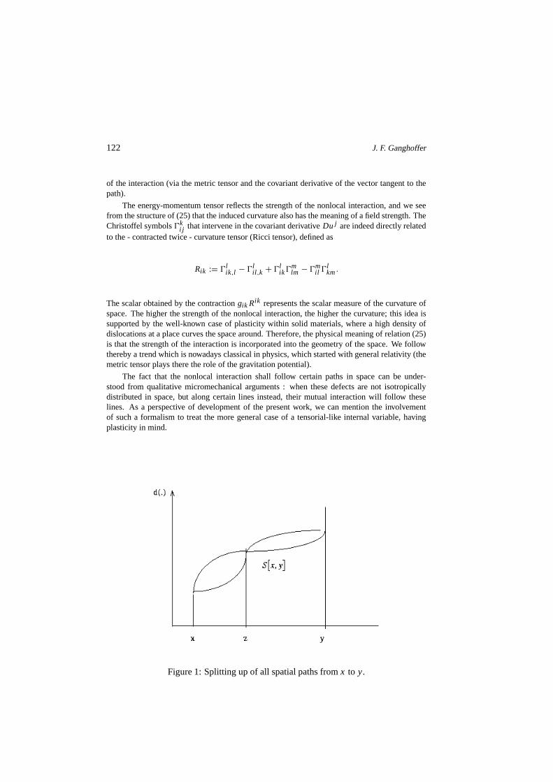
122 J. F. Ganghoffer
of the interaction (via the metric tensor and the covariant derivative of the vector tangent to thepath).
The energy-momentum tensor reflects the strength of the nonlocal interaction, and we seefrom the structure of (25) that the induced curvature also has the meaning of a field strength. TheChristoffel symbols0k
i j that intervene in the covariant derivativeDu j are indeed directly relatedto the - contracted twice - curvature tensor (Ricci tensor),defined as
Rik := 0lik,l − 0l
il ,k + 0lik0
mlm − 0m
il 0lkm.
The scalar obtained by the contractiongik Rik represents the scalar measure of the curvature ofspace. The higher the strength of the nonlocal interaction,the higher the curvature; this idea issupported by the well-known case of plasticity within solidmaterials, where a high density ofdislocations at a place curves the space around. Therefore,the physical meaning of relation (25)is that the strength of the interaction is incorporated intothe geometry of the space. We followthereby a trend which is nowadays classical in physics, which started with general relativity (themetric tensor plays there the role of the gravitation potential).
The fact that the nonlocal interaction shall follow certainpaths in space can be under-stood from qualitative micromechanical arguments : when these defects are not isotropicallydistributed in space, but along certain lines instead, their mutual interaction will follow theselines. As a perspective of development of the present work, we can mention the involvementof such a formalism to treat the more general case of a tensorial-like internal variable, havingplasticity in mind.
Figure 1: Splitting up of all spatial paths fromx to y.

New concepts 123
Figure 2: Space slicing. A continuous path fromd(x) to d(z) can be approximatedby a sequence of valuesd(z1),d(z2), . . . ,d(zn). This approximation becomes exact ifd(zi−1, zi ) → 0.
References
[1] DE BORST R., SLUYS L. J., MULHAUS H. B. AND PAMIN J., Fundamental issues infinite element analyses of localisation of deformation, Eng. Comp.10 (1993), 99–121.
[2] BAZANT Z. P. AND PIJAUDIER-CABOT G., Nonlocal damage theory, J. Eng Mech.113n. 10 (1987), 1512.
[3] BAZANT Z. P.AND PIJAUDIER-CABOT G.,Dynamic stability analysis with nonlocal dam-age, Computers and Structures293 (1988), 503.
[4] PIJAUDIER-CABOT G. AND BODE L., Localisation of damage in a nonlocal continuum,Mech. Res. Commun.192 (1992), 145.
[5] PIJAUDIER-CABOT G. AND BENALLAL A., Strain localisation and bifurcation in a non-local continuum, Int. J. Solids Struc.3013 (1993), 1761.
[6] M UHLHAUS H. B., VARDOULAKIS I., Geotechnique373 (1987), 271.
[7] GANGHOFFERJ. F.AND DE BORSTR., A new framework in nonlocal mechanics, Int. J.Engng Sci.38 (2000), 453–486.
AMS Subject Classification: 74A60, 74M25.
Jean-Francois GANGHOFFERLemta–Ensem2, Avenue de la Foret de HayeB.P. 160-54504Vandoeuvre Cedex, FRANCEe-mail:[email protected]

124 J. F. Ganghoffer

Rend. Sem. Mat. Univ. Pol. TorinoVol. 58, 1 (2000)Geom., Cont. and Micros., I
S. Gumbel - W. Muschik†
GENERIC∗, AN ALTERNATIVE FORMULATION OF
NONEQUILIBRIUM CONTINUUM MECHANICS?
Abstract.During the last 15 years a bracket formalism of dissipative continuum physics
has been developed which resulted in a formulation which is shortly denoted asGENERIC. GENERIC has been applied to different problems of continuum ther-modynamics, often in this way, that a well-known problem wasreformulated inGENERIC formalism. So in 1997 the GENERIC form of the equations of motionof a Navier-Stokes fluid was formulated. To learn some more about the GENERICprocedure we consider here a general 5-field theory of fluids.Usually GENERIC isformulated for an isolated system, but here we will discuss the facility to formulateGENERIC for an open system.
1. Introduction
The phenomenological theories of thermodynamics are divided into continuumtheoretical onesand into those of discrete systems. There is a variety of phenomenological non-equilibriumcontinuum theories which are similar, but differ in basic concepts [10]. These are the LinearIrreversible Thermodynamics [2], Rational and Extended Thermodynamics ([14] to [7]), Non-Classical Thermodynamics [9], and theories using evolution criteria [11] and variational prin-ciples [6]. These well-known thermodynamical theories arenow added by a special dissipativecontinuum procedure which was developped during the last 15years starting out with a bracketformalism originated by an extension of Hamiltonian mechanics [3]. One result of this bracketapproach is the GENERIC formalism [4, 5] which is totally different from the theories men-tioned above, but is claimed by its investigators to be generally valid for all discrete systemsalltheories in field formulation. In GENERIC the balance equations are generated by total energyand total entropy both acting as potentials and being only dependent on the wanted fields andnot on the state space. The GENERIC balances are splitted additively into a reversible and anirreversible part. Beyond the balance equations there are so-called degeneracy conditions whichare unknown in conventional, rational, and extended thermodynamics. Jacobi identities stem-ming from the antisymmetric bracket of the reversible part of the balance equations and callingto mind the Hamiltonian mechanics background of the GENERICformalism are also unknownin the other approaches [1].
The distinctions between GENERIC and the usual approach demand for a possibility tocompare them in a way as general as possible. Here a general 5-field formulation for fluidsis considered in GENERIC treatment. First of all we report ongeneral the GENERIC settingwhich is independent of special constitutive assumptions.Then we will extend the GENERIC
∗General Equation for the NonEquilibrium Reversible-Irreversible Coupling†Finacial support by the VISMAI Company, D-95085 Selb, Germany.
125

126 S. Gumbel - W. Muschik
formalism to open systems. The structure of GENERIC can be motivated by a microscopicfoundation [12],[13].
2. GENERIC setting
The fundamental structure of GENERIC is determined by six building blocks [3] to [12].
1. The set of the basic or wanted fieldsZ of the system which is presupposed to be open,
2. the total energyEtot(Z) of the open system and
3. its total entropyS(Z), as two global potentials which depend only of the basic fields
4. two, in general operator-valued matricesL(Z) and
5. the dissipation operatorM(Z) which depend on the state spaceZ which is not identicalto the basic fieldsZ,
6. the supply of the wanted fieldsfe wich is vanishing for an isolated system.
Theequations of motionof the basic fieldsZ have the special GENERIC form
∂t Z = L · δEtot
δZ+ M · δS
δZ+ fe,(1)
which always can be split into its reversible, its irreversible and its supply part
∂t Zrev := L · δEtot
δZ, ∂t Z irr := M · δS
δZ, ∂t Zsup := fe.(2)
Hereδ/δ is the functional derivative which maps global quantities to local ones, as we will seein the GENERIC treatment.
Beyond the equations of motion (1) the complementary degeneracy conditions
L · δS(Z)δZ
= 0, M · δEtot(Z)δZ
= 0(3)
are satisfied byL andM. Therefore the degeneracy conditions (3) describe the reversible-irreversible coupling which is meant in the name of GENERIC.The two contributions (3) to thetime evolution ofZ generated by the total energyEtot and by the total entropyS are called thereversible and irreversible contributions to dynamics, respectively.
General properties ofL andM are discussed easily in terms of two brackets, one is anti-symmetric, the other one symmetric
[ A, B] :=⟨δA
δZ,L · δB
δZ
⟩.= −[B, A] + 1
2(Orev(A, B)+ Orev(B, A)),
[ A, A] = Orev(A, A),(4)
{A, B} :=⟨δA
δZ,M · δB
δZ
⟩.= {B, A} + 1
2(Oirr (B, A)− Oirr (A, B)),(5)
{A, A} + Oirr (A, A)·≥ 0.(6)

GENERIC, an alternative formulation 127
Here〈 , 〉 denotes a scalar product, especially
⟨δA
δZ,L · δB
δZ
⟩:=∫
G
[δA
δZ· L · δB
δZ
]d3x,(7)
A andB are sufficiently regular and real-valued functionals onZ ,Orev is the reversible part, andOirr is the irreversible part of the flux through the surface of theVolumeG. From the setting (4)follows, thatL is antisymmetric, whereas we have to demand the symmetry ofM which cannotbe concluded from (5). Now we can express the degeneracy conditions (3) with the brackets, wefind
[S, Etot] − Orev(Etot, S) = 0, {Etot, S} + Oirr (Etot, S) = 0(8)
The antisymmetric bracket is presupposed to satisfy the Jacobi identity for closed systems, i.eall the surface terms vanish
[ A, [B,C]] + [B, [C, A]] + [C, [ A, B]].= 0.(9)
According to (1), (4) and (5) we can write the time evolution of A as
A =∫
a(Z) d3x, −→ δA
δZ= ∂a
∂Z,(10)
and because the system is an open one, we obtain
d
dtA =
∫∂ta(Z) d3x = [ A, Etot] + {A, S} +
∫∂a
∂Z· fe d3x.(11)
According to (11), (8), (4) and (5) we obtain the time rate of the total energy and that of the totalentropy of the isolated system
d
dtEtot = [Etot, Etot] + {Etot, S} +
∫∂etot
∂Z· fe d3x
= Orev(Etot, Etot)− Oirr (Etot, S)+∫∂etot
∂Z· fe d3x,(12)
d
dtS = [S, Etot] + {S, S} +
∫∂%s
∂Z· fe d3x
= Orev(Etot, S)+ {S, S} +∫∂%s
∂Z· fe d3x.(13)
with the entropy production
σ = {S, S} + Oirr (S, S) ≥ 0.
This inequality represents the second law of thermodynamics of an open system in global formu-lation, where the surface term represents the flux of the entropy through the surface of the system.It is also clear, that all the surface terms have to vanish, ifwe want to describe an isolated system.
To go on with the GENERIC treatment we now have to introduce constitutive assumptions,that means, we have to proceed beyond the general setting of GENERIC.

128 S. Gumbel - W. Muschik
3. GENERIC treatment
We consider an one-component simple fluid which is decribed by five basic fields: Mass density%, material velocityv, and specific internal energyε. Therefore is the set of the wanted fieldgiven by
(14) Z(x, t) = (%, p := %v, η := %ε)(x, t).
Then we can introduce the global potentials, as the total energy of the system
(15) Etot(Z) =∫ [
p2(x, t)2%(x, t)
+ η(x, t)
]d3x,
and the global entropy of the system is by setting a functional on Z
(16) S(Z) =∫%s(%,p, η) d3x.
More over, we know about a five field theorie, that the fields have to satisfy the following balanceequation for the wanted fields
reversible part irreversible part supply∂tρ = −∇ · ρv +0 +0∂t p = −∇ · pv − ∇ P +∇ · V +f∂tη = −∇ · ηv − P∇ · v +∇v : V − ∇ · q +r
(17)
whereP is the pressure,V is the traceless viscous pressure tensor,q is the heat flux density,f isthe supply of the momentum andr is the supply of the internal energy. We have also performeda split into a reversible and an irreversible part, respectively. But this is an unsolved problem inGENERIC, how to do the right split. Until now it is only possible to see that the split has beenfound correct, if the resulting entropy production is the right one. But for knowing the entropyproduction you have to treat the five field theory by another theory, for example by RationalThermodynamics and by exploiting the Liu-procedure [9].
3.1. State space
In 5-field theory the wanted basic fields (14) are those of a fluid and because we consider dissi-pative fluids, we choose as a state space one includes the gradients of the basic fields
Z+ := (%, η, v,∇%,∇η,∇v).(18)
Taking into account, that state spaces are spanned by objective quantities we have to change (18)into
Z := (%, η,∇%,∇η, (∇v)s).(19)
Here ()s is the symmetric part of a tensor. Because of (14) the constitutive quantities in thebalances (17) are
V = V(Z(x, t)), q(x, t) = Q(Z(x, t)).(20)
(21)
The viscous pressure tensor is symmetric
V(x, t) = V>(x, t),(22)
because we only consider fluids without internal spin.

GENERIC, an alternative formulation 129
3.2. Reversible part
Because in GENERIC the equations of motions for the basic fields (1) can be split into theirreversible and irreversible part (2), we start out with the reversible part of (1) which is as rep-resented in the first column in (17). The first step is that we have to calculate the functionalderivative from the global total energy (15). According to (14) the functional derivative in (2)1generates from (15) the local fields
(δEtot
δZ
)T
=(
−1
2v2(x, t), v(x, t), 1
),(23)
which inserted in (2)1 result in the reversible part of the equations of motion∂t%
∂tp∂tη
rev
= L ·
−12v2
v1
=
−∇ · (v%)−∇ · (vp)− ∇ P
−∇ · (vη)− P∇ · v
.(24)
These five equations are not sufficient to determine the 13 components of the antisymmetricL.Concerning the balances (17) this undetermination is not important, because all the differentLresult in the same balances. Concerning the degeneracy conditions (3)1 it is not evident that allthese differentL have the same kernel. On the other handL is also not determined by the kernelδS/δZ. The consequences of this undetermination ofL are not fully discussed up to now.
Now we can show, that one operator-valued matrix satisfying(24) is the following one
L = −
0 ∇%· 0%∇ [∇p + p∇]>· ∇ P + η∇0 (P∇ + ∇η)· 0
.(25)
The degeneracy conditions (3)1 are now used to determine the kernelδS/δZ of L. As alreadyremarked, it is not evident, that this kernel is unique. The global entropy of the system dependingonly onZ is given by (16) and the functional derivative ofSgenerates local quantities
(δS
δZ
)T=(∂(%s)
∂%=: − g
T(x, t),
∂(%s)
∂p(x, t),
∂(%s)
∂η=:
1
T(x, t)
).(26)
Here the usual abbreviationsspecific free enthalpy gandabsolute equilibrium temperature Tfor the derivatives of the entropy are introduced. The degeneracy condition (3)1 results in thefollowing equations
∂%s
∂p= 0,(27)
−%∇ g
T+ ∇ P
T+ η∇ 1
T= 0.(28)
As (27) shows, the GENERIC setting allows to derive that the entropy density does not dependon the velocityv. From (28) follows immediately by use of (26) and (27) that the followingequation yields
−%s = 1
T(%g − P − η)+ const −→(29)
−→ g = ε + P
%− T s , const= 0,(30)
because (30) is the definition of the specific free enthalpyg.
The exploitation of the reversible part of the GENERIC equations of motion (1) results in(25), (27), and (28). Now we investigate its irreversible part in the next section.
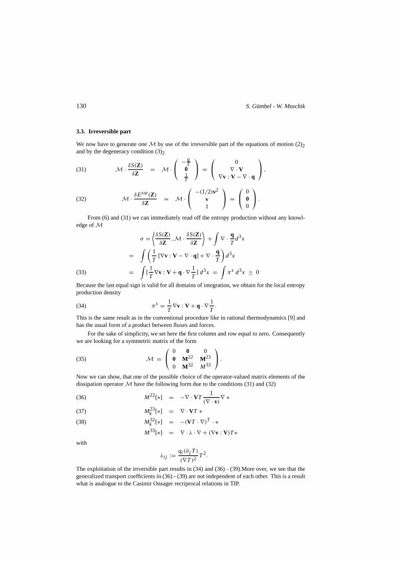
130 S. Gumbel - W. Muschik
3.3. Irreversible part
We now have to generate oneM by use of the irreversible part of the equations of motion (2)2and by the degeneracy condition (3)2
M · δS(Z)δZ
= M ·
− gT
01T
=
0∇ · V
∇v : V − ∇ · q
,(31)
M · δEtot(Z)δZ
= M ·
−(1/2)v2
v1
=
000
.(32)
From (6) and (31) we can immediately read off the entropy production without any knowl-edge ofM
σ =⟨δS(Z)δZ
,M · δS(Z)δZ
⟩+∫
∇ · qT
d3x
=∫ (
1
T[∇v : V − ∇ · q] + ∇ · q
T
)d3x
=∫
[1
T∇v : V + q · ∇ 1
T] d3x =
∫πs d3x ≥ 0(33)
Because the last equal sign is valid for all domains of integration, we obtain for the local entropyproduction density
πs = 1
T∇v : V + q · ∇ 1
T.(34)
This is the same result as in the conventional procedure likein rational thermodynamics [9] andhas the usual form of a product between fluxes and forces.
For the sake of simplicity, we set here the first column and rowequal to zero. Consequentlywe are looking for a symmetric matrix of the form
M =
0 0 00 M22 M23
0 M32 M33
.(35)
Now we can show, that one of the possible choice of the operator-valued matrix elements of thedissipation operatorM have the following form due to the conditions (31) and (32)
M22[∗] = −∇ · VT1
(∇ · v)∇ ∗(36)
M23k [∗] = ∇ · VT ∗(37)
M32k [∗] = −(VT · ∇)T · ∗(38)
M33[∗] = ∇ · λ · ∇ + (∇v : V)T∗with
λi j :=qi (∂ j T)
(∇T)2T2.
The exploitation of the irrversible part results in (34) and(36) - (39).More over, we see that thegeneralized transport coefficients in (36) - (39) are not independent of each other. This is a resultwhat is analogue to the Casimir Onsager recriprocal relations in TIP.

GENERIC, an alternative formulation 131
3.4. Balance equation for the global potentials
The last point, we have to discuss are the dynamic equations for both global potentials. Thesupply vector of the wanted fields is according to the last column in (15) is
fTe = (0, f, r ),(39)
and thus we get immediately from (13) using (29) and (33)
d
dtS(Z) = [S, Etot] + {S, S} +
∫∂%s
∂Z· fe d3x(40)
=∫ [
−∇ · v%s(Z)+ πs − ∇ · qT
+ r
T
]d3x.(41)
Similiar we get from (12) using (4), (5) and (3)2 the balance equation of the total energy
d
dtEtot(Z) = [Etot, Etot] + {Etot, S} +
∫∂etot
∂Z· fe d3x
=∫ {
−∇ · [(vetot(Z)+ vP)+ (VT · v − q)] + v · fe + r}
d3x
= W + Q(42)
with the work
W :=∫ [
−∇ · (vetot(Z)+ vP)+ ∇ · (VT · v)+ v · fe + r]
d3x(43)
and the heat exchange
Q :=∫
∇ · qd3x.(44)
4. Conclusion
An important statement of GENERIC is the fact, that the generalized transport coefficients of thedissipation operator are not independent. In GENERIC one derive a generalisation of Casimir-Onsager recriprocal relations. The structure of GENERIC provides, that the dissipation operatoris positive definit and thus that a closed system decays to equilibrium.
It is also possible to give a microscopic foundation of the GENERIC formalism [12], [13]which gives us a powerfull argument for the validity of this structure. But nevertheless, wehave the unsolved problem in GENERIC, that is a correct splitinto a reversible and an irre-versible part is not achieved up to now. Although it seems to be possible to transform the wholeGENERIC structure to open systems which was demonstrated here. Another important statementof GENERIC is, that we have to preassume local equilibrium, i.e the global potentials dependonly on the wanted fields.
References
[1] EDWARDS B. J. AND OTTINGER H. C., Time-structure invariance criteria for closureapproximation, Phys. Rev. E56 (1997), 4097.
132 S. Gumbel - W. Muschik
[2] DE GROOTS. R.AND MAZUR P.,Non-equilibrium thermodynamics, North-Holland, Am-sterdam 1963.
[3] GRMELA M., Bracket formulation of dissipative fluid mechanics equations, Phys. Lett. A102(1984), 335–358.
[4] GRMELA M. AND OTTINGER H. C., Dynamics and thermodynamics of complex fluids.Development of a general formalism, Phys. Rev. E56 (1997), 6620.
[5] GRMELA M. AND OTTINGER H. C., Dynamics and thermodynamics of complex fluids.Development of a general formalism, Phys. Rev. E56 (1997), 6633.
[6] GYARMATI I., Nonequilibrium thermodynamics (field theory and variational principles),Springer Verlag, Berlin 1970.
[7] JOU D., CASAS-V AZQUEZ V. AND LEBON G., Extended irreversible thermodynamics,Springer, Berlin 1996.
[8] M ULLER I. AND RUGGERIT., Extended Thermodynamics, Springer Tracts in Natural Phi-losophy37, Springer, Berlin 1993.
[9] M USCHIK W., Aspects of non-equilibrium thermodynamics, World Scientific, Singapore1990.
[10] MUSCHIK W., Fundamentals of nonequilibrium thermodynamics, in: “Non-equilibriumthermodynamics with applications to solids”, CISM Coursesand Lectures336 (sect. 1)Springer, Wien 1993.
[11] MUSCHIK W. AND PAPENFUSSC., An evolution criterion of nonequilibrium thermody-namics and its application to liquid crystals, Physica A201(1993), 515.
[12] OTTINGER H. C.,General projection operator formalism for the dynamics andthermody-namics of complex fluids, Phys. Rev. E57 (1998), 1416.
[13] OTTINGER H. C.,Derivation of a two-generator framework of nonequilibriumthermody-namics for quantum systems, Phys. Rev. E62 (2000), 4720.
[14] TRUESDELL C. AND TOUPIN R., The classical field theories, in: “Handbook of Physics,III/1”, Springer, Berlin 1960.
[15] WILMA NSKI K., Thermomechanics of continua, Springer, Berlin 1998.
AMS Subject Classification: 74A15.
Sebastian GUMBEL, Wolfgang MUSCHIKInstitut fur Theoretische PhysikTechnische Universitat BerlinSekretariat PN7-1 Hardenbergstrasse 36D-10623 Berlin, GERMANYe-mail:[email protected]:[email protected]