1

IPN Progress Report 42-189 • May 15, 2012

End-to-End Traffic Flow Modeling of the Integrated SCaN Network

Kar-Ming Cheung* and Douglas S. Abraham†

* Communications Architectures and Research Section. † Architecture, Strategic Planning, and System Engineering Section.

The research described in this publication was carried out by the Jet Propulsion Laboratory, California Institute of Technology, under a contract with the National Aeronautics and Space Administration. © 2012 California Institute of Technology. U.S. Government sponsorship acknowledged.

abstract. — In this article, we describe the analysis and simulation effort of the end-to-end traffic flow for the Integrated Space Communications and Navigation (SCaN) Network. Us-ing the network traffic derived for the 30-day period of July 2018 from the Space Commu-nications Mission Model (SCMM), we generate the wide-area network (WAN) bandwidths of the ground links for different architecture options of the Integrated SCaN Network. We also develop a new analytical scheme to model the traffic flow and buffering mechanism of a store-and-forward network. It is found that the WAN bandwidth of the Integrated SCaN Network is an important differentiator of different architecture options, as the recurring circuit costs of certain architecture options can be prohibitively high.

I. Introduction

Currently the National Aeronautics and Space Administration (NASA) communication infrastructure consists of three distinct networks — the Space Network (SN), the Near-Earth Network (NEN), and the Deep Space Network (DSN). The SN is composed of a number of geostationary Tracking and Data Relay Satellite System (TDRSS) satellites and the associated ground stations, and collectively they provide communications, data relay, and tracking ser-vices for low-Earth orbiting (LEO) satellites, human spaceflight, expendable launch vehicles (ELA), research aircraft, and scientific user missions. The NEN consists of both NASA-owned ground stations and those owned by international, commercial, and academic partners, and they provide communication and tracking services to user missions from LEO out to lunar orbit. The DSN consists of large-aperture and high-sensitivity tracking stations located in three longitudinally separated sites around Earth, and they provide continuous coverage to flight missions from Earth’s geostationary orbit (GEO) outward to the planets and other targets in the solar system. The communication and tracking data received by SN, NEN, and DSN are delivered to user missions over the data lines provided by the NASA Integrated Service Network (NISN) as well as the commercial terrestrial ground networks.

The SN, NEN, and DSN are managed by NASA’s Space Communications and Navigation (SCaN) Program. The SCaN Program system engineering (PSE) team is currently conduct-

2

ing a trade study on the Integrated Network Architecture (INA) under which the three networks will be re-architected into a single network. Depending on the degree of integra-tion, there can be an Integrated Network Operation Center (INOC) that provides allocated network management and service execution functions for the entire integrated network. It is expected that the shift from a distributed architecture to a unified one will promote stan-dardization and commonality among different network assets. This should in turn reduce the operational costs of NASA’s space communications and navigation infrastructure, and simplify the user missions’ interface to secure communications and navigation services. The goal of the study is to identify the architecture that provides that best value in terms of lower life cycle cost and risk, and higher technical performance.

The INA study examines two key aspects of the integrated network: a) Integrated Network Management (INM), and b) Integrated Service Execution (ISE). The INM provides mission users a set of standard network service management functions primarily implemented using Consultative Committee for Space Data Systems (CCSDS) service management standards. The ISE provides four standard categories of network services to flight missions — forward data delivery services, return data delivery services, radiometric services, and position and timing services.

There can be many options for ISE architecture based on the allocation of network signal processing and data delivery functions between the ground station sites (GSSs) and the INOC. Each ISE option depicts a different ground network topology. For the INA study, four ISE architecture options have been identified:

• ISE-1:SignalprocessingfunctionsatGSSsandthereisnoINOC.Processeddataproductsare sent from GSSs to Mission Operation Centers (MOCs).

• ISE-2:SignalprocessinguptolinklayeratGSSs,higher-layerprocessinganddatadeliv-ery at INOC.

• ISE-3:SignalprocessinguptoquantizedcodedsymbolsatGSSsthatarethensentontoINOC; link layer and higher processing and data delivery at INOC.

• ISE-4:Radiofrequency/intermediatefrequency(RF/IF)waveformsaresampledandquantizedatgroundstationsitesandsenttoINOC;allothersignalprocessinganddatadelivery performed at INOC.

One important consideration that differentiates among the ISE architecture options is the wide-areanetwork(WAN)bandwidthrequiredtoprovidedataflowforthereturndataservices among SCaN ground network assets as well as data delivery from SCaN to the user missions.TheWANbandwidthrequiredforeachISEoptionrepresentsasubstantialpor-tionofrecurringcost,andinsomecasesasignificanttechnicalrisk.ForISE-3andISE-4,the GSS–INOC links are bitstreams with no rate buffering,1 and WAN link sizes are driven by the instantaneous aggregated data rates. All other ground links (INOC–MOC links in ISE-3andISE-4,andalllinksinISE-1andISE-2)arestore-and-forwardlinks,andlinksizes

1ForISE-3andISE-4,theGSSgeneratesquantizedcodedsymbolsandRF/IFsamples,respectively,andhasnovisibilityinto the data content.

3

are driven by the combined effects of mission data rates, data types with different latency requirements,anddutycycles.

The purpose of this article is to describe the methodology that we use to model the end-to-end data flow of the ISE options. Since the return data services represent the bulk of the data flow,2 only the mission return links are considered. For the purpose of this study, we assume the following ground station configurations:

(1) The SN ground sites consist of the White Sands Ground Terminal (WSGT), Sec-ondary TDRS Ground Terminal (STGT), and the Guam Remote Ground Terminal (GRGT).

(2) The NEN ground sites only include the NASA-owned sites in the 2018 era, which includes the Wallops Flight Facility (WFF), McMurdo Ground Station (MGS), Alaska Satellite Facility (ASF), White Sands Complex (WSC), and Svalbard Ground Station (SGS).

(3) The DSN ground sites are located at Goldstone (United States), Canberra (Austra-lia), and Madrid (Spain).

(4) TheINOCisassumedtobelocatedatWhiteSands,NewMexico.3

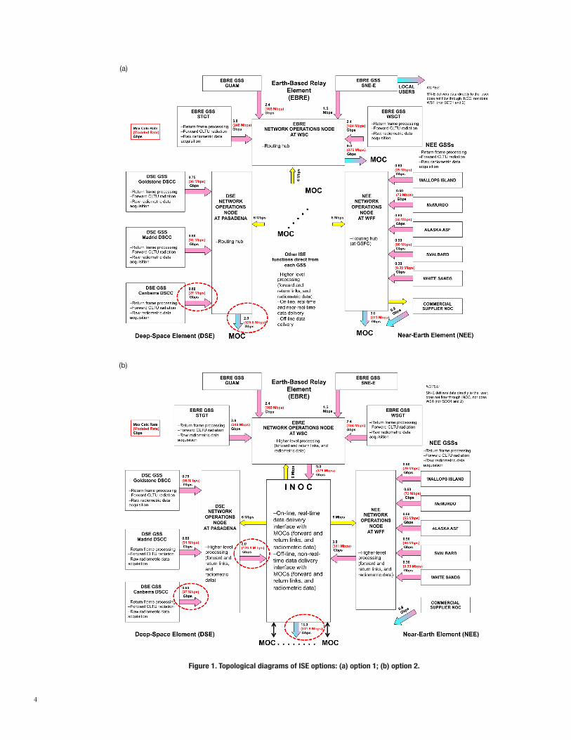
Based on the above assumptions, the topological diagrams of the four ISE options are shown in Figure 1.

The modeling of the end-to-end data flow of the Integrated SCaN Network consists of two main efforts:

(1) The modeling of NASA mission return data traffic as received by the SCaN network assets.

(2) The modeling of mission traffic data flow from the ground stations through the Integrated SCaN Network to the MOCs of user missions.

Figure 2 illustrates the process flow of the overall modeling effort. Based on the Space Communications Mission Model (SCMM), the mission traffic model generates the mission traffic for downlink passes4 from all NASA missions during the 31-day period in July 2018. The mission traffic is then fed into the network simulator, which provides additional mod-eling of the mission traffic characteristics and simulates the data flow through the network topology. This end-to-end data flow simulation provides bandwidth estimations for the GSS–INOC links and the INOC–MOC links for each of the ISE architecture options.

2Mannedmissionlinksareexceptionsastheforwardlinkscarryaudio/videodata.However,theyonlyrepresentasmallfraction of the total data flow of the SCaN network; thus, forward links are not architecture discriminators and are not considered.

3 The ground links between the GSSs at White Sands and the INOC are considered as a local-area network (LAN), and are not considered in the costing.

4 Each downlink pass is characterized by the start time, the end time, the data rate, and the coding scheme used.

4

Figure 1. Topological diagrams of ISE options: (a) option 1; (b) option 2.

(a)

(b)

5

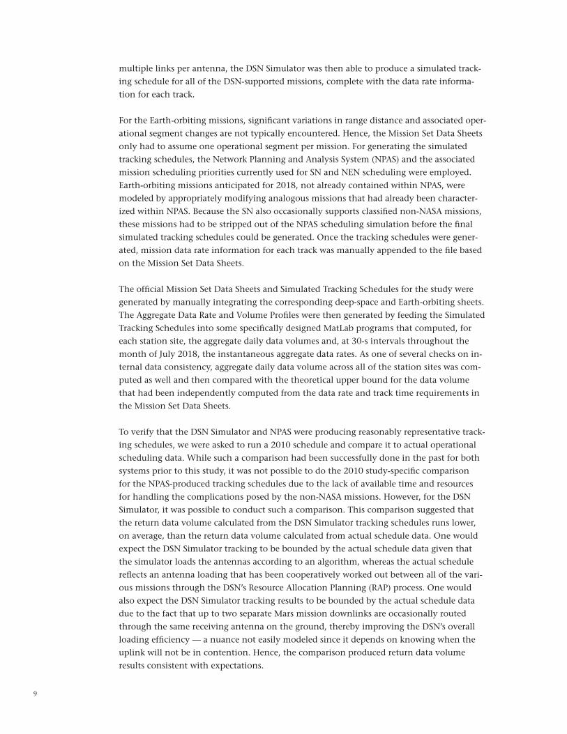
Figure 1 (continued). Topological diagrams of ISE options:

(c) option 3 — coded symbols; (d) option 4 — microwave/IF.

(d)

(c)

6

Figure 2. Process flow of the overall modeling effort.

Mission Traffic Model End-to-End Network Traffic Model

Four ISE Architecture Options

Era: 2018

Mission Scenarios: High, Nominal, Low

Mission Traffic Models: High, Nominal, Low for 2018

SCMM Set (SCMM, OTIE, MSAT, etc.) –Mission Models

Mission Data Type Model –Telemetry –Science –Audio –Video

SCaN Simulator –Network Model

Iterate with architec-ture reference design of each option.

Evaluate data flow and control loop issue of each option.

Quantify figures of merit with regard to the architecture reference design of each option.

The rest of the article is organized as follows: Section II describes the modeling of NASA mission traffic in detail. Section III discusses the modeling of mission traffic data types. Sec-tion IV describes the Integrated SCaN Network signal processing and data delivery model-ing.SectionVoutlinesthebandwidthestimationtechniquesforthestore-and-forwardfunctions of the Integrated SCaN Network. Section VI discusses the analysis and simulation results, and Section VII provides the concluding remarks.

II. SCMM-Derived Mission Traffic Modeling

A. Mission Traffic Model Overview

The Mission Traffic Model is essentially a compilation of Excel spreadsheets that provide a minute-by-minute model of all the downlink communications traffic projected to occur during the month of July 2018 between NASA-supported spacecraft and the receiving assets of the three networks. The model serves two purposes within the larger integrated network architecture study. First, it provides a representative aggregate data rate and data volume basis for modeling the number and sizes of the data “pipes” and associated data buffering andprocessingequipmentusedintheISEoptionreferencedesigns.Second,itprovidesrepresentative mission downlink traffic profiles for use in simulating each ISE option’s end-to-end network performance.

The Mission Traffic Model’s July 2018 projections are based on the missions for that time period characterized in the June 2, 2010, version of SCaN’s SCMM. In general, the SCMM’s content is synchronized with NASA’s latest Agency Mission Planning Manifest (AMPM), which is signed off by the Associate Administrator for each of the mission directorates. Mission specifics are derived from the flight programs and projects wherever possible. Where the SCMM contains generic placeholders (such as in the case of competitively bid missions), this information is derived by first using the latest NASA roadmaps and National Research Council’s Decadal Surveys to infer candidate missions. Then, the concept designs appropriate to these candidates are used to derive the mission specifics needed to model their contribution to the downlink communications traffic. Because many missions can expect to be extended beyond their prime science phase, historical mission extension data

7

are used to infer whether or not missions with prime science phases prior to 2018 are likely to still be active during the timeframe of interest.

Clearly, all of these projections are fraught with uncertainty and are subject to change. One need not look any further than the ongoing machinations between the Administra-tion and Congress regarding NASA’s future direction to see that this is the case. And, that is just one type of contributor to the uncertainty. Mission delays, cancellations, and failures can all impact the projected future mission set. Because the future is inherently uncertain and we cannot precisely predict which missions will actually be operating in 2018 and with what specific characteristics, we try to ensure that the Mission Traffic Model is repre-sentative by treating three cases: a base case, a high case, and a low case. The base case pos-tulates the 2018 missions to be as they are represented in the SCMM for that time period. The high case attempts to be more forward-looking, modifying the 2018 mission set to look like what might be supportable in 2028 — assuming the currently planned receiving assets. To achieve this, the 2018 mission data rates are tripled for all those missions not currently in operation. In addition, we assume double the number of spacecraft for each of the top three data volume contributors to each network. The low case postulates a much more pes-simistic scenario. The mission data rates remain the same as they are in the base case, and the top three data volume contributors to each network are deleted. A non–International Space Station human exploration test mission contained in the base case is also deleted in the low case.

While one can always postulate a higher high case, at triple the 2018 data rates, we lim-ited the high case to the “ragged edge” of what the currently planned receiving assets can support. When a mission is at more than a few tenths of an AU from Earth, megabit-per-second links become increasingly challenging due to the space losses associated with the large range distances. To make up for these losses on the ground-side, one has to assume a larger receiving area. This can be achieved by arraying up two or more antennas. But, ar-rayedantennasforonemissionleavefeweraperturesavailableforothermissions.Hence,ahigh case that fails to take this into account can actually cause the returned data volume in a higher high case to decrease relative to the base case. Even for the base case, we limit the amountofarrayable34-mantennastotwopermission—beyondthat,thedataratehasto decrease in the face of increasing link distance. For the high case we assume the same number of ground antennas per mission as for the base case — implying that the burden of tripling the data rate has to be borne entirely on the spacecraft-side via larger antennas, more powerful transmitters, etc. In the next analysis cycle, we plan to look at a higher high case where the receiving area on the ground is increased. For the SN-supported missions, spacecraft throughput capability becomes one of the primary barriers to such a case when the data rates significantly exceed the tripling used in this study. So, in the future analysis cycle, the higher high case might also involve postulating additional TDRS assets in space — assets with a higher data throughput capability.

Three types of Mission Traffic Model outputs serve as inputs to the End-to-End Traffic Model: Mission Set Data Sheets, Simulated Tracking Schedules, and Aggregate Data Volume and Rate Profiles. The Mission Set Data Sheets provide specific parameters for each mission. Theseparametersincludedatarate,forwarderror-correctioncodingscheme,frequency

8

band,andtrackingrequirements,aswellastheMOCtowhichthedataarebeingsent.Formissionswithuniqueoperationalsegments(e.g.,cruise,primescience,extendedrelayops,etc.), the above parameters are provided for each operational segment. A typical Mission Set Data Sheet runs about 115 lines, and three such sheets are generated for the study: one for the base case, one for the high case, and one for the low case.

TheSimulatedTrackingSchedulesprovideasimulatedsequenceofspacecraftcontacttimes,durations, and rates by station (i.e., receiving antenna) for each day within the timeframe of interest. This information, in combination with the Mission Set Data Sheet information, provides the end-to-end traffic simulation with the minute-by-minute data traffic through eachstationsite,whereitisheaded,whatitsfrequencybandassociationis,andwhatitscodingoverheadislikelytobe.AtypicalSimulatedTrackingSchedulerunsabout48,500lines, and three such sheets (base case, high case, and low case) are generated for the study.

The Aggregate Data Volume and Rate Profiles provide the aggregate daily data volumes and instantaneous aggregate information bit rates (into the antennas) by station site for the time frame of interest. The Aggregate Data Volume Profiles are derived from the Simulated Tracking Schedules and provide a useful basis for checking internal consistency between the Schedules and Mission Set Data Sheets. This is accomplished by generating an upper-bound data volume profile from each Mission Set Data Sheet (multiplying each mission’s dataratebyitstrackingtimerequirementsandthensummingacrossthemissions)andcomparing it with the data volume profile derived from the corresponding Simulated Track-ing Schedule. The Aggregate Data Volume Profiles also support sizing the station site data recorders in the ISE reference designs. Like the Aggregate Data Volume Profiles, the Rate Profiles are derived from the Simulated Tracking Schedule and specify the instantaneous ag-gregate information bit rate by station site for every 30-s interval all day long, each day, for the entire month of July. A typical Rate Profile runs about 86,500 lines and, as with all the other outputs, is generated for each of the base, high, and low cases. This output is particu-larly useful for sizing the data “pipes” for each of the ISE option reference designs and for providing a “sanity check” to the end-to-end traffic modeling.

B. Production of the Model Outputs

Slightly different approaches were used in generating the Mission Set Data Sheets and Sim-ulated Tracking Schedules pertaining to the deep-space mission customers than were used for those pertaining to the Earth-orbiting mission customers. Because deep-space missions tend to have multiple, inherently different operational segments that occur at significantly differentdistancesfromEarth,theirdataratesandantennatrackingrequirementschangefrom one operational segment to the next. So, for the missions being supported by the deep space element, substantial upfront work was necessary to identify and characterize each mission’s operational segments. This work included: (1) performing trajectory analyses to establish each mission’s range distance profile and help define the boundaries between operational segments, (2) running link budgets for each mission’s operational segments to determinetherequiredreceivingantennasforthestateddatarates,and(3)generatingeachmission’sspacecraftriseandsettimesrelativetotherequiredreceivingantennas.Allofthisinformation was fed into the DSN Simulator, as well as summarized in the mission set data sheets. With its ability to model and schedule evolving antenna architectures, arraying, and

9

multiple links per antenna, the DSN Simulator was then able to produce a simulated track-ing schedule for all of the DSN-supported missions, complete with the data rate informa-tion for each track.

For the Earth-orbiting missions, significant variations in range distance and associated oper-ationalsegmentchangesarenottypicallyencountered.Hence,theMissionSetDataSheetsonly had to assume one operational segment per mission. For generating the simulated tracking schedules, the Network Planning and Analysis System (NPAS) and the associated mission scheduling priorities currently used for SN and NEN scheduling were employed. Earth-orbiting missions anticipated for 2018, not already contained within NPAS, were modeled by appropriately modifying analogous missions that had already been character-ized within NPAS. Because the SN also occasionally supports classified non-NASA missions, these missions had to be stripped out of the NPAS scheduling simulation before the final simulated tracking schedules could be generated. Once the tracking schedules were gener-ated, mission data rate information for each track was manually appended to the file based on the Mission Set Data Sheets.

The official Mission Set Data Sheets and Simulated Tracking Schedules for the study were generated by manually integrating the corresponding deep-space and Earth-orbiting sheets. The Aggregate Data Rate and Volume Profiles were then generated by feeding the Simulated Tracking Schedules into some specifically designed MatLab programs that computed, for each station site, the aggregate daily data volumes and, at 30-s intervals throughout the month of July 2018, the instantaneous aggregate data rates. As one of several checks on in-ternal data consistency, aggregate daily data volume across all of the station sites was com-puted as well and then compared with the theoretical upper bound for the data volume thathadbeenindependentlycomputedfromthedatarateandtracktimerequirementsinthe Mission Set Data Sheets.

To verify that the DSN Simulator and NPAS were producing reasonably representative track-ing schedules, we were asked to run a 2010 schedule and compare it to actual operational scheduling data. While such a comparison had been successfully done in the past for both systems prior to this study, it was not possible to do the 2010 study-specific comparison for the NPAS-produced tracking schedules due to the lack of available time and resources forhandlingthecomplicationsposedbythenon-NASAmissions.However,fortheDSNSimulator, it was possible to conduct such a comparison. This comparison suggested that the return data volume calculated from the DSN Simulator tracking schedules runs lower, on average, than the return data volume calculated from actual schedule data. One would expect the DSN Simulator tracking to be bounded by the actual schedule data given that the simulator loads the antennas according to an algorithm, whereas the actual schedule reflects an antenna loading that has been cooperatively worked out between all of the vari-ous missions through the DSN’s Resource Allocation Planning (RAP) process. One would also expect the DSN Simulator tracking results to be bounded by the actual schedule data due to the fact that up to two separate Mars mission downlinks are occasionally routed through the same receiving antenna on the ground, thereby improving the DSN’s overall loading efficiency — a nuance not easily modeled since it depends on knowing when the uplinkwillnotbeincontention.Hence,thecomparisonproducedreturndatavolumeresults consistent with expectations.

10

C. Mission Traffic Model Summary Results

While the Mission Set Data Sheets, Simulated Tracking Schedules, and Aggregate Data Vol-ume and Rate Profiles emerging from the Mission Traffic Model provide vital inputs to the end-to-end traffic simulation, they also yield, at the summary level, some interesting direct observations.

Figure 3 conveys the first of these summary-level observations. Examination of the ag-gregate daily downlink volumes associated with the 2018 base case indicates a significant dichotomy between those of the DSN and those of the SN. This has to do primarily with the distance at which the missions are occurring. The DSN-supported missions generally occur at deep-space distances, far beyond GEO. The space losses over these vast distances make for very difficult communication links and, hence, constrain the achievable data rates to levels that only amount, in aggregate, to a couple of terabits (Tb) per day, on average. By contrast, the SN-supported missions occur relatively close to Earth, generally in LEO. The communication links are much easier and less constraining on the achievable data rate. Combined with moderate contact times, these higher data rates lead to aggregate return data volumes that run about 32 Tb per day, on average. NEN-supported missions also tend tooccurveryclosetoEarthand,hence,havehighachievabledatarates.However,theirview of the ground-based NEN stations is much shorter than the SN-supported missions’ view of the space-based SN “stations” (i.e., the TDRSS satellites). A NEN-supported space-craft may only be in view of a particular ground station for 10 min. So, the return data vol-umes will be much lower than those for the SN due to the reduced contact times. In short, the SN-supported missions tend to drive the aggregate daily data volumes.

DSN

35

30

25

20

15

10

5

0

SNNEN (Including Commercial Stations)

7/1/

2018

7/2/

2018

7/3/

2018

7/4/

2018

7/5/

2018

7/6/

2018

7/7/

2018

7/8/

2018

7/9/

2018

7/10

/201

87/

11/2

018

7/12

/201

87/

13/2

018

7/14

/201

87/

15/2

018

7/16

/201

87/

17/2

018

7/18

/201

87/

19/2

018

7/20

/201

87/

21/2

018

7/22

/201

87/

23/2

018

7/24

/201

87/

25/2

018

7/26

/201

87/

27/2

018

7/28

/201

87/

29/2

018

7/30

/201

8

Dat

a Vo

lum

e, T

b

Figure 3. Comparison of DSN, NEN, and SN aggregate daily downlink volumes.

11

Figure4comparestheaverageaggregatedailydownlinkvolumesbystationsiteandbycase(i.e., base, high, or low). The fact that the WSGT, STGT, and GRGT sites have some of the largest data volumes for the base case reaffirms the prior conclusion that the SN-supported missions tend to drive the aggregate daily data volumes. The comparison between the dif-ferent cases also suggests that the return data volume is generally two to three times larger for the high case than for the base case. This is consistent with the tripling of the future mission data rates for the highcase.However,notallofthestationsreflectthisduetothefact that return data volumes can also be driven by the contact times. For instance, STGT, in theSimulatedTrackingSchedule,supportstheHubbleSpaceTelescope(HST),adatavolumedriver.But,HSTdoesnotdownlinkatultra-highdatarates.Instead,itmakesuseoflongcontacttimes.Hence,thereturnvolumeratiobetweenthehigh case and base case for a given site depends on whether the mission return data volumes are more a function of the data rate or the contact time.

Alaska

Sate

llite F

acilit

y

Canber

ra, A

ustra

lia

Dongar

a, Aus

tralia

GRGT

Goldstone

, CA

Kiruna

, Swed

en

Mad

rid, S

pain

McM

urdo, A

ntarc

tica

North P

ole, A

laska

Poker F

lat, A

laska

STGT

Santia

go, Chil

e

South P

oint, H

awaii

Svalbard

, Norw

ay

WSGT

Wall

ops Isla

nd, V

irgini

a

Weih

eim, G

erman

y

Whit

e San

ds, New

Mex

ico

50

45

40

35

30

25

20

15

10

5

0

Dat

a Vo

lum

e, T

b

Base Case (Average) High Case (Average) Low Case (Average)

Figure 4. Comparison of aggregate daily downlink volumes by station site.

Figure 5 compares the maximum instantaneous aggregate downlink rates by station site and by case. So, the rates shown are the maximum seen when looking across the entire July 2018 period at 30-s intervals. These rates constitute one of the key determinants for sizing the data “pipes” in the ISE option reference designs, since they determine the maxi-mum throughput rate that the “pipes” have to accommodate. In this context, the high case results may be most relevant. Note that the two largest high-case station sites are not SN sites but, rather, NEN sites — commercial ones at that. This has to do with the fact that many of the missions driving data rates for the NEN sites are Earth remote-sensing satel-litesinpolarorbits.Hence,high-latitudesitestendtobekeyforthesemissions—asalsoevidenced by the large rates for the Alaska Satellite Facility and, in the case of the South-ernHemisphere,McMurdo.

12

Figure 5. Comparison of maximum instantaneous aggregate downlink rates by station site.

In the case of STGT, for this simulation, the base case actually ends up higher than the high case.ThisgoesbacktoourpriordiscussionregardingHST.Inthehigh case, in addition to tripling the data rates of the future missions, we double the number of spacecraft associated withthethreelargestdatavolumecontributorstoeachnetwork.HSTisoneofthosedatavolume contributors. But, because its data volume is driven by long contact times more thanhighdatarates,doublingthenumberofHSTsinthehigh case causes its contact times to dominate STGT availability while doing little to increase the aggregate instantaneous rate. So, the high case for this particular site in this simulation manifests a lower aggregate data rate than the base case.

One final observation on Figure 5 is that the DSN sites (Canberra, Goldstone, and Madrid) exhibit the largest “dynamic range” between the high case and the low case. This large disparity stems from the fact that the deep-space missions generally have low data rates due to their long link distances. The low case throws away each network’s top three data volume contributors — which, in the case of the DSN, are also its three highest data rate missions. The high case triples the data rates associated with the future missions and doubles the number of spacecraft associated with the top three data volume contributors — which, again, are the DSN’s three highest data rate missions. So, the cause of the high–low disparity is largely a function of the way these cases were designed relative to the very limited num-ber of high-rate missions characteristic of the DSN’s link-constrained customer base.

D. Mission Traffic Model Conclusions

To the extent that the Mission Traffic Model has attempted to incorporate mission data consistent with NASA’s latest plans, attempted to address the future’s inherent uncertainty

Alaska

Sate

llite F

acilit

y

Canber

ra, A

ustra

lia

Dongar

a, Aus

tralia

GRGT

Goldstone

, CA

Kiruna

, Swed

en

Mad

rid, S

pain

McM

urdo, A

ntarc

tica

North P

ole, A

laska

Poker F

lat, A

laska

STGT

Santia

go, Chil

e

South P

oint, H

awaii

Svalbard

, Norw

ay

WSGT

Wall

ops Isla

nd, V

irgini

a

Weih

eim, G

erman

y

Whit

e San

ds, New

Mex

ico

1200

1000

800

600

400

200

0

Dat

a Vo

lum

e, T

b

High Base Low

13

by adopting a high case and low case bounding approach to the base case, used comparative analysis of the model’s three types of output to check for internal consistency, attempted to calibrate the simulated schedules with actual schedule data, and provided the same model outputs for each ISE option being analyzed, it constitutes a reasonably representa-tive and consistent basis for estimating the number and size of the “data pipes” associated with each ISE option, as well as for modeling data traffic performance across those “pipes.” Examination of the aggregate daily data volumes and instantaneous aggregate information bit rates that emerge from the model yields four observations. First, the high case yields rates and volumes that tend to be two to three times higher than the base case. Second, NEN missions tend to drive instantaneous aggregate data rates. Third, SN missions tend to drive aggregate daily data volumes. And, fourth, DSN missions tend to have data rates that arelink-distanceconstrained—scalingtohigherdataratesrequiresarrayingreceivingas-sets, which can lead to asset contention with other missions.

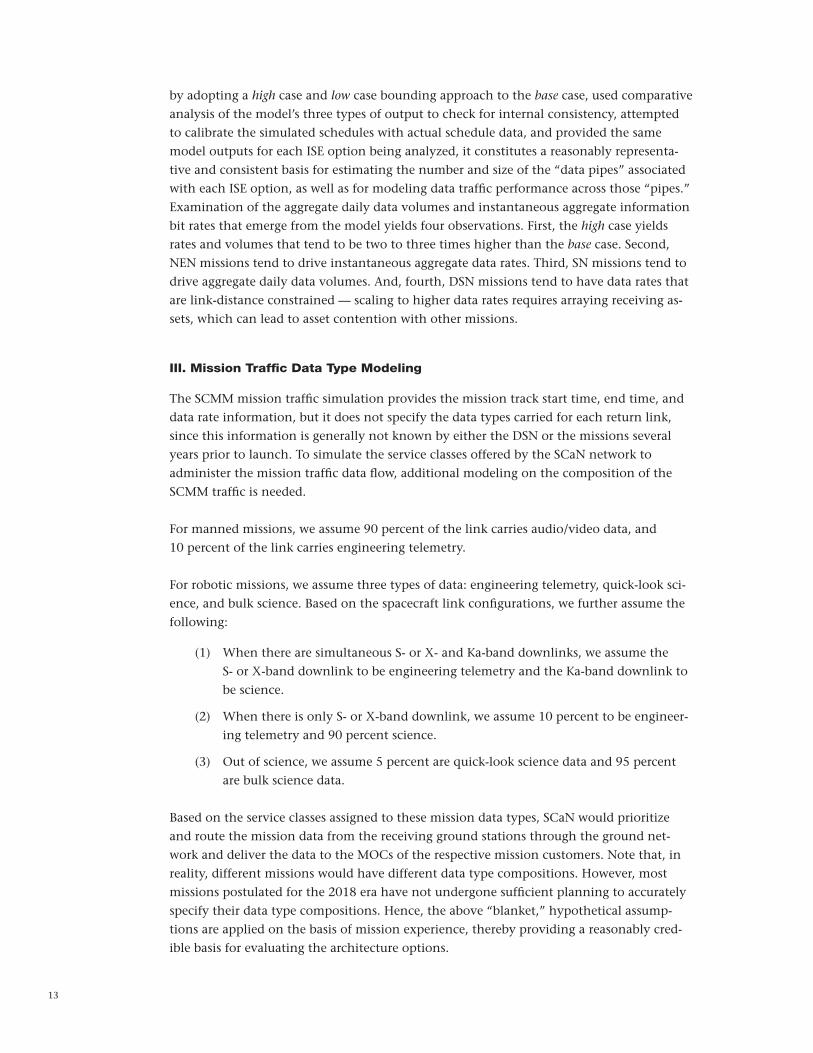
III. Mission Traffic Data Type Modeling

The SCMM mission traffic simulation provides the mission track start time, end time, and data rate information, but it does not specify the data types carried for each return link, since this information is generally not known by either the DSN or the missions several years prior to launch. To simulate the service classes offered by the SCaN network to administer the mission traffic data flow, additional modeling on the composition of the SCMM traffic is needed.

Formannedmissions,weassume90percentofthelinkcarriesaudio/videodata,and10 percent of the link carries engineering telemetry.

Forroboticmissions,weassumethreetypesofdata:engineeringtelemetry,quick-looksci-ence, and bulk science. Based on the spacecraft link configurations, we further assume the following:

(1) When there are simultaneous S- or X- and Ka-band downlinks, we assume the S- or X-band downlink to be engineering telemetry and the Ka-band downlink to be science.

(2) When there is only S- or X-band downlink, we assume 10 percent to be engineer-ing telemetry and 90 percent science.

(3) Outofscience,weassume5percentarequick-looksciencedataand95percentare bulk science data.

Based on the service classes assigned to these mission data types, SCaN would prioritize and route the mission data from the receiving ground stations through the ground net-work and deliver the data to the MOCs of the respective mission customers. Note that, in reality,differentmissionswouldhavedifferentdatatypecompositions.However,mostmissions postulated for the 2018 era have not undergone sufficient planning to accurately specifytheirdatatypecompositions.Hence,theabove“blanket,”hypotheticalassump-tions are applied on the basis of mission experience, thereby providing a reasonably cred-ible basis for evaluating the architecture options.

14

We have also considered the DSN’s science data types like very long baseline interferom-etry/delta-differentialone-wayranging(VLBI/DDOR), radar, and radio science. These DSN sciencedatatypesconsistofhigh-rateRF/IFsampleddata,buttheytypicallyhaverelaxeddatadeliveryrequirements(e.g.,off-linedelivery)exceptwhenusedtosupportspacecraft-critical events. In those cases, the real-time or near-real-time data delivery is planned far in advance to anticipate the situation. Thus, they are not ground-link bandwidth drivers and are not taken into account in this phase of the INA Study.

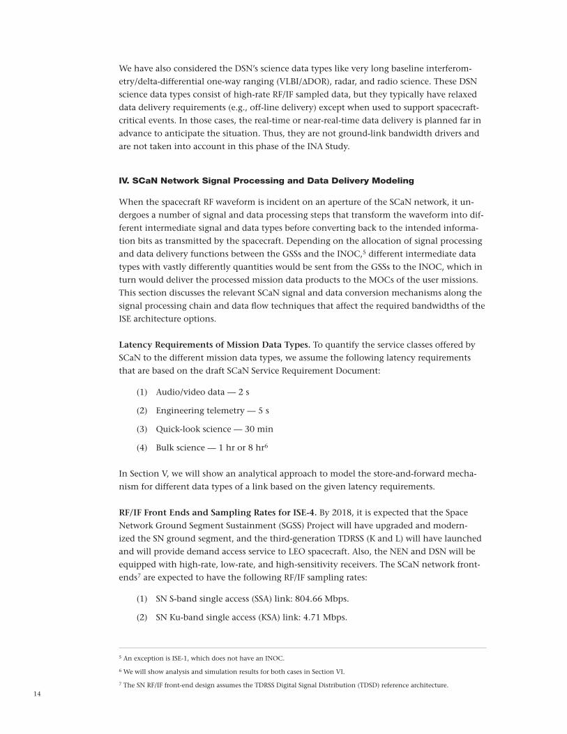
IV. SCaN Network Signal Processing and Data Delivery Modeling

When the spacecraft RF waveform is incident on an aperture of the SCaN network, it un-dergoes a number of signal and data processing steps that transform the waveform into dif-ferent intermediate signal and data types before converting back to the intended informa-tion bits as transmitted by the spacecraft. Depending on the allocation of signal processing and data delivery functions between the GSSs and the INOC,5 different intermediate data typeswithvastlydifferentlyquantitieswouldbesentfromtheGSSstotheINOC,whichinturn would deliver the processed mission data products to the MOCs of the user missions. This section discusses the relevant SCaN signal and data conversion mechanisms along the signalprocessingchainanddataflowtechniquesthataffecttherequiredbandwidthsoftheISE architecture options.

Latency Requirements of Mission Data Types.ToquantifytheserviceclassesofferedbySCaNtothedifferentmissiondatatypes,weassumethefollowinglatencyrequirementsthatarebasedonthedraftSCaNServiceRequirementDocument:

(1) Audio/videodata—2s

(2) Engineering telemetry — 5 s

(3) Quick-look science — 30 min

(4) Bulkscience—1hror8hr6

In Section V, we will show an analytical approach to model the store-and-forward mecha-nismfordifferentdatatypesofalinkbasedonthegivenlatencyrequirements.

RF/IF Front Ends and Sampling Rates for ISE-4. By 2018, it is expected that the Space Network Ground Segment Sustainment (SGSS) Project will have upgraded and modern-ized the SN ground segment, and the third-generation TDRSS (K and L) will have launched and will provide demand access service to LEO spacecraft. Also, the NEN and DSN will be equippedwithhigh-rate,low-rate,andhigh-sensitivityreceivers.TheSCaNnetworkfront-ends7areexpectedtohavethefollowingRF/IFsamplingrates:

(1) SNS-bandsingleaccess(SSA)link:804.66Mbps.

(2) SNKu-bandsingleaccess(KSA)link:4.71Mbps.

5 An exception is ISE-1, which does not have an INOC.

6 We will show analysis and simulation results for both cases in Section VI.

7TheSNRF/IFfront-enddesignassumestheTDRSSDigitalSignalDistribution(TDSD)referencearchitecture.

15

(3) SNKa-bandsingleaccess(KaSA)link:14.14Gbps.

(4) SN30elementsmultipleaccess(MA)(TDRSF3–F7,K,L):6.29Gbpsforonetofivemissions.

(5) SN MA space-based beam-forming (TDRS F8–F10): 201.17 Mbps per mission.

(6) NEN/DSNhigh-sensitivitylink(<1Mbps):1.28Gbps.

(7) NEN/DSNlow-ratelink(1–10Mbps):2.56Gbps.

(8) NEN/DSNhigh-ratelink(10Mbps–1.2Gbps):12.8Gbps.

Code Rates and Quantization Schemes for ISE-3. It is expected that each mission will specifytheerror-correctioncoding(ECC)schemesandtheirrespectivecoderates.However,many 2018 missions will not have decided on the coding schemes. For those missions, we use the following ECC assumptions:

(1) For DSN missions, we assume low-density parity-check (LDPC) code with rate Rc=1/2,codewordsizeCW=2048bits,andquantizationlevelQ=8bits.ForadatarateR,thecodedsymbolrate(includingquantization)is8×R/Rc = 16×R.

(2) For SN and NEN missions, we assume 50 percent of the missions will use rate 7/8LDPCcodeand50percentofthemissionswilluseconcatenatedcodes.Theaverage code rate Rc=0.58,theaveragecodewordlengthCW=4500bits,andtheaveragequantizationlevelQ=4bits.ForadatarateR,thecodedsymbolrate(includingquantization)is4×R/Rc = 6.9×R.

Network Delay Estimations. In the SCaN network signal processing chain and data de-livery process, various latency factors are introduced, and SCaN has to make sure that the overalllatencywillmeetthemissiondatadeliveryrequirements.Thefollowingarethekeylatency contributions in the SCaN end-to-end traffic flow:

(1) Store-and-forward delay. This is the buffering delay for a mission data type intro-duced at each network node according to the service class (priority) assigned to the data type. The SCaN network uses the store-and-forward mechanism to regulate the network data flow, to control the end-to-end delay and network resource utilization, and to ensure expedient delivery of mission data according totherespectivelatencyrequirements.Wewilldiscussthebandwidthestimationtechniquesofthestore-and-forwardlinksindetailinSectionV.

(2) Codeword buffering delay. We assume the codeword frame synchronization mecha-nismwillrequirethreecodeframestoacquireandtoconfirmframesync.LetRdenote the data rate. Thus, the codeword buffering delay for DSN missions and SN/NENmissionsare3×2048/Rand3×4500/R,respectively(inunitsofseconds).

(3) Frame buffering delay.WeassumeaSpaceLinkExtension(SLE)framesizeof10240,andframesynccanbeacquiredandconfirmedinoneframe.Thus,theframebufferingdelayis10240/R(inunitsofseconds).

(4) Ground transmission delay. From prior statistics for DSN data delivery over the NISN lines, we observe that the long-haul latency between DSN sites and JPL

16

Central is approximately two times the propagation delay. As ground transmission latency is a small fraction compared to the other delays, we use the crude estima-tion of two times propagation delay to model the ground transmission delay.

The emphasis of the current study is comparing the estimated network bandwidths of dif-ferent architecture options rather than understanding the latency behavior of the network. Thus, only the store-and-forward delay is taken into account for this phase of the study.

V. Leveling Scheme — Bandwidth Estimation Technique for a Store-and-Forward Link

Thetermstore-and-forwardreferstothetelecommunicationtechniqueinwhichdataaresent to an intermediate network node where the data are temporarily stored and sent at a later time to the final destination or to another intermediate node. Store-and-forward can be applied to both space-based networks that have intermittent connectivity and to ground-based networks with deterministic connectivity. For ground-based networks, the store-and-forward mechanism is used to regulate the network data flow and link resource utilization such that mission data types can be delivered to their MOCs without violating theirrespectivelatencyrequirements.

A high-level view of the store-and-forward mechanism is that for a communication pass thatconsistsofoneormoredatatypes,eachwithagivenlatencyrequirement,thestore-and-forward process spreads out each data type across a longer time horizon but without violatingthelatencyrequirement.

There are commercial off-the-shelf (COTS) network simulation tools like QualNet8 and Opnet,9 which provide high-fidelity bit-level simulation of data flow through a well-defined network10toevaluateprotocolperformanceandlatencybehavior.However,theseCOTStools are not suitable to estimate the bandwidths of the ISE architecture options for the fol-lowing reasons:

(1) The SCaN network is a large-scale network that supports tens of missions with an aggregate data rate of hundreds of Mbps at any time. Simulating the entire SCaN network at bit-level might be too computational- and memory-intensive for typi-cal COTS tools.

(2) The COTS tools are designed to perform direct simulation of the protocol perfor-mance and latency behavior for a given network configuration, and not to analyze thereverseproblemofsizingthenetworkforagivensetoflatencyrequirementsfor the various mission data types.

In light of the above challenges, we developed a new analytical approach, which we call the “leveling scheme,” to model the store-and-forward mechanism of the network data flow.

8ScalableNetworkTechnologies,http://www.scalable-networks.com/

9OpnetTechnologies,http://www.opnet.com/

10 Well-defined network refers to a network whose bandwidths between the nodes and storage capacities of the nodes are specified.

17

For the rest of this section, we will present a straightforward version of the leveling scheme that models the first-order behavior of the store-and-forward mechanism. This straightfor-

ward leveling scheme does not take into account the interactions among data types within a link nor between data types across the links at a network node, and is inherently subopti-mal.However,thissuboptimalestimationofbandwidthsprovidesaconservativeapproachto size the ISE architecture options, which is appropriate at this early stage of the SCaN INA study. An improved version of the leveling scheme takes into account the second-order behavior of the store-and-forward mechanism — the interactions among data types within a link.11 The improved leveling scheme is theoretically elegant, yet simple to implement, and more accurate than the straightforward leveling scheme. Both the straightforward and improvedlevelingschemesestimatethenetworkbandwidthsbasedonlatencyrequirementsofdatatypes,anddonotrequirethecomputationalandmemoryresourcestoperformbit-level simulations as the objective is not to analyze detailed protocol behavior and protocol overhead.

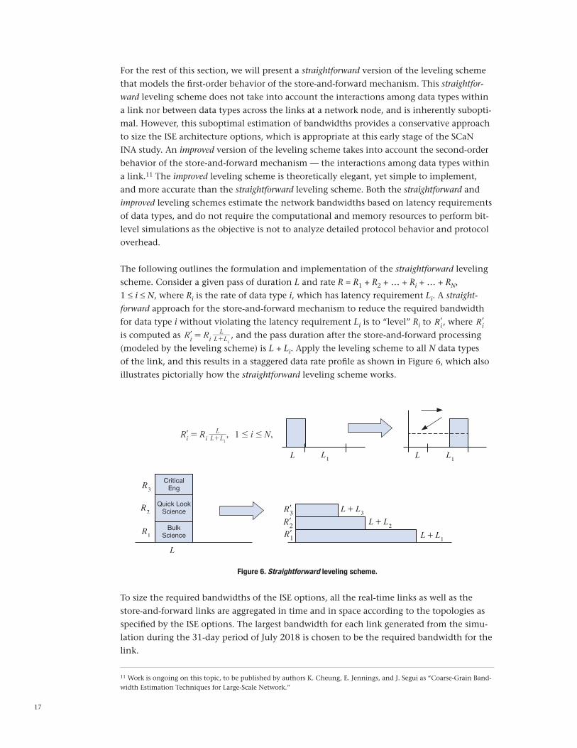
The following outlines the formulation and implementation of the straightforward leveling scheme. Consider a given pass of duration L and rate R = R1 + R2 + … + Ri + … + RN, 1 ≤ i ≤ N, where Ri is the rate of data type i,whichhaslatencyrequirementLi. A straight-

forwardapproachforthestore-and-forwardmechanismtoreducetherequiredbandwidthfor data type iwithoutviolatingthelatencyrequirementLi is to “level” Ri to lRi , where lRi is computed as R Ri L L

Li i= +l , and the pass duration after the store-and-forward processing

(modeled by the leveling scheme) is L + Li. Apply the leveling scheme to all N data types of the link, and this results in a staggered data rate profile as shown in Figure 6, which also illustrates pictorially how the straightforward leveling scheme works.

Figure 6. Straightforward leveling scheme.

TosizetherequiredbandwidthsoftheISEoptions,allthereal-timelinksaswellasthestore-and-forward links are aggregated in time and in space according to the topologies as specified by the ISE options. The largest bandwidth for each link generated from the simu-lationduringthe31-dayperiodofJuly2018ischosentobetherequiredbandwidthforthelink.

11 Work is ongoing on this topic, to be published by authors K. Cheung, E. Jennings, and J. Segui as “Coarse-Grain Band-widthEstimationTechniquesforLarge-ScaleNetwork.”

Critical Eng

Quick LookScience

BulkScience

, ,R R i N1i L LL

i i# #= +

l

L L1

L L1

L

R3

R2

R1

lR3lR2lR1

L + L3

L + L2

L + L1

18

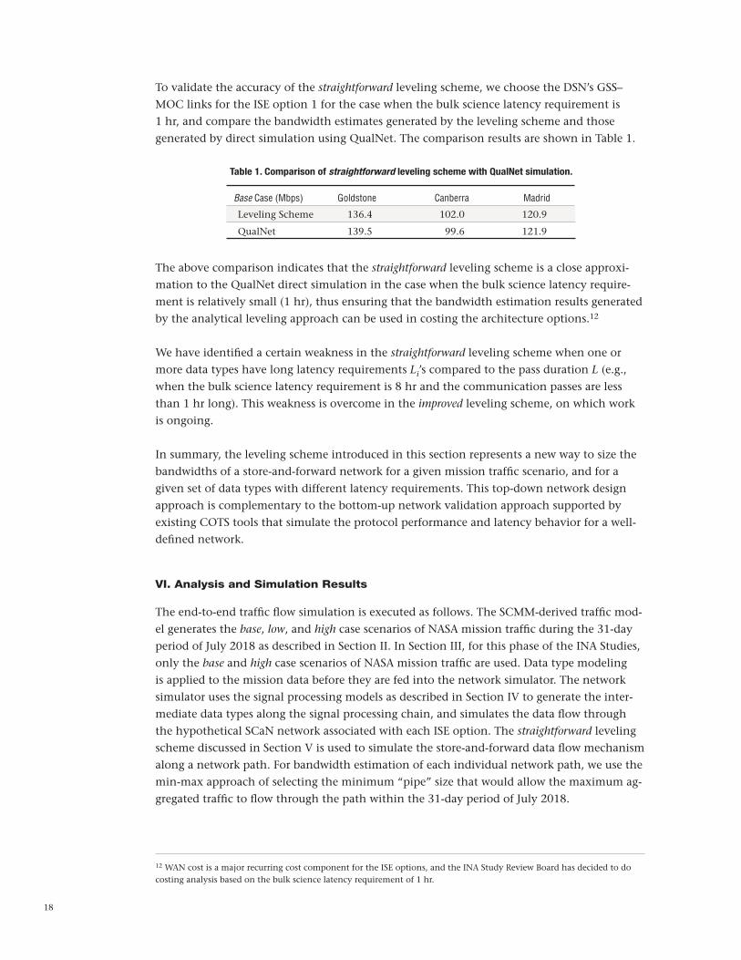
To validate the accuracy of the straightforward leveling scheme, we choose the DSN’s GSS–MOClinksfortheISEoption1forthecasewhenthebulksciencelatencyrequirementis1 hr, and compare the bandwidth estimates generated by the leveling scheme and those generated by direct simulation using QualNet. The comparison results are shown in Table 1.

Table 1. Comparison of straightforward leveling scheme with QualNet simulation.

Base Case (Mbps) Goldstone Canberra

LevelingScheme 136.4 102.0 120.9

QualNet 139.5 99.6 121.9

Madrid

The above comparison indicates that the straightforward leveling scheme is a close approxi-mationtotheQualNetdirectsimulationinthecasewhenthebulksciencelatencyrequire-ment is relatively small (1 hr), thus ensuring that the bandwidth estimation results generated by the analytical leveling approach can be used in costing the architecture options.12

We have identified a certain weakness in the straightforward leveling scheme when one or moredatatypeshavelonglatencyrequirementsLi’s compared to the pass duration L (e.g., whenthebulksciencelatencyrequirementis8hrandthecommunicationpassesarelessthan 1 hr long). This weakness is overcome in the improved leveling scheme, on which work is ongoing.

In summary, the leveling scheme introduced in this section represents a new way to size the bandwidths of a store-and-forward network for a given mission traffic scenario, and for a givensetofdatatypeswithdifferentlatencyrequirements.Thistop-downnetworkdesignapproach is complementary to the bottom-up network validation approach supported by existing COTS tools that simulate the protocol performance and latency behavior for a well-defined network.

VI. Analysis and Simulation Results

The end-to-end traffic flow simulation is executed as follows. The SCMM-derived traffic mod-el generates the base, low, and high case scenarios of NASA mission traffic during the 31-day period of July 2018 as described in Section II. In Section III, for this phase of the INA Studies, only the base and high case scenarios of NASA mission traffic are used. Data type modeling is applied to the mission data before they are fed into the network simulator. The network simulator uses the signal processing models as described in Section IV to generate the inter-mediate data types along the signal processing chain, and simulates the data flow through the hypothetical SCaN network associated with each ISE option. The straightforward leveling scheme discussed in Section V is used to simulate the store-and-forward data flow mechanism along a network path. For bandwidth estimation of each individual network path, we use the min-max approach of selecting the minimum “pipe” size that would allow the maximum ag-gregated traffic to flow through the path within the 31-day period of July 2018.

12 WAN cost is a major recurring cost component for the ISE options, and the INA Study Review Board has decided to do costinganalysisbasedonthebulksciencelatencyrequirementof1hr.

19

Using the above end-to-end traffic flow modeling, we estimate the link sizes of the network paths of the four ISE options for the base and high case scenarios, both for bulk science la-tencyrequirementsof1hrand8hr,respectively.TheaggregatedWANbandwidthsofthefour ISE options for both cases are given in Tables 2 and 3.

Table 2. Aggregated WAN bandwidths (Gbps) for bulk science latency of 1 hr.

Latency = 1 hr Option 4 Option 3

BaseCase 183.725 15.747 3.147 2.272

HighCase 209.909 43.628 8.673 6.238

Option 2a Option 1

Table 3. Aggregated WAN bandwidths (Gbps) for bulk science latency of 8 hr.

Latency = 8 hr Option 4 Option 3

Base Case 183.295 15.317 2.151 1.619

HighCase 208.627 42.346 6.235 4.195

Option 2a Option 1

The end-to-end traffic flow simulations reveal the following interesting facts:

(1) ForISE-3andISE-4,theGSS–INOClinksarereal-timebitstreamsandthelinksizesare driven by the instantaneous aggregated data rates.

(2) All other links are store-and-forward links, and the link sizes are driven by the combinedeffectsofmissiondatarates,datatypeswithdifferentlatencyrequire-ments, and duty cycles.

(3) ForISE-3andISE-4,theaggregatedWANbandwidthsareinsensitivetodatatypelatencyrequirementsastheirWANbandwidthsaredominatedbythereal-timeGSS–INOC links.

(4) ForISE-4withtwodifferentbulksciencelatencyrequirements,theaggregatedWAN bandwidths for the high-case are only 20 percent higher than those of the nominalcase.ThisisbecausetheISE-4WANbandwidthsaredominatedbyGSS–INOClinksthattransportRF/IFsamples,andareindependentofthedatarates.

(5) ForISE-3andISE-4,theaggregatedWANbandwidthsofthehigh case are approxi-mately three times as those of the base case. This is consistent with the fact that the high case consists of future mission data rates that are three times those of the base case.

(6) TheWANbandwidthsofISE-3andISE-4aremuchhigherthanthoseofISE-1andISE-2.

VII. Concluding Remarks

In this article, we described the traffic modeling, analysis, and simulation of the end-to-end traffic flow for the Integrated SCaN Network. These efforts generated the estimated bandwidthsrequiredtosupporttheJuly2018missiontrafficfordifferentIntegratedSCaNNetwork architecture options. At this preliminary phase of the study, when only high-level

20

information is available, we have made simplifying yet defensible assumptions on both the Mission Traffic Model and the SCaN signal processing and data delivery schemes in order to expedite the modeling and simulation. We have found that the recurring circuit costs of ISE-3andISE-4areprohibitivelyhigh,andtheISEoptionsaredownselectedtoISE-1andISE-2.

Acknowledgments

This research was supported by NASA’s Space Communication and Navigation (SCaN) Program. The authors would also like to thank the following contributors for their helpful discussion: L. Clare (JPL), E. Jennings (JPL), J. Segui (JPL), D. Morris (JPL), B. MacNeal (JPL), R.Tikijian(JPL),M.Schaub(GSFC/Honeywell),C.Schwartz(GSFC),D.Joesting(GSFC/Honeywell),F.Mathis(GSFC/Honeywell),W.Horne(GSFC),K.Bhasin(GRC),andR.Ku-nath (GRC).