EnablingTechnologies for the Internet of...

UNIVERSITÀ DI PISA

Enabling Technologies for the

Internet of Things (IoT)

Giuliano MANARA

Dipartimento di Ingegneria dell’Informazione

University of Pisa

Via G. Caruso 16, I-56122, Pisa, Italy

[email protected]

Giuliano Manara, Short Course «Enabling Technologies for IoT», Curitiba, October 27-28, 2016

UNIVERSITÀ DI PISA

� Introduction to the Internet of Things (IoT)

� Enabling technologies: RFID systems

� New design concepts for antennas

� Wireless Sensor Networks (WSN)

� Cyber Physical Systems (CPS)

� Future perspectives


UNIVERSITÀ DI PISA

4

More connected objects than people

Image Courtesy: : CISCO


UNIVERSITÀ DI PISAFrom radio to Internet of Things (IoT)


UNIVERSITÀ DI PISA

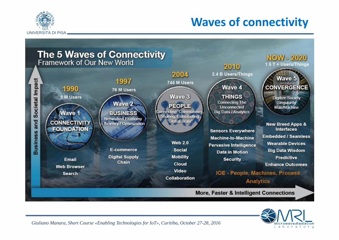
Waves of connectivity


UNIVERSITÀ DI PISA

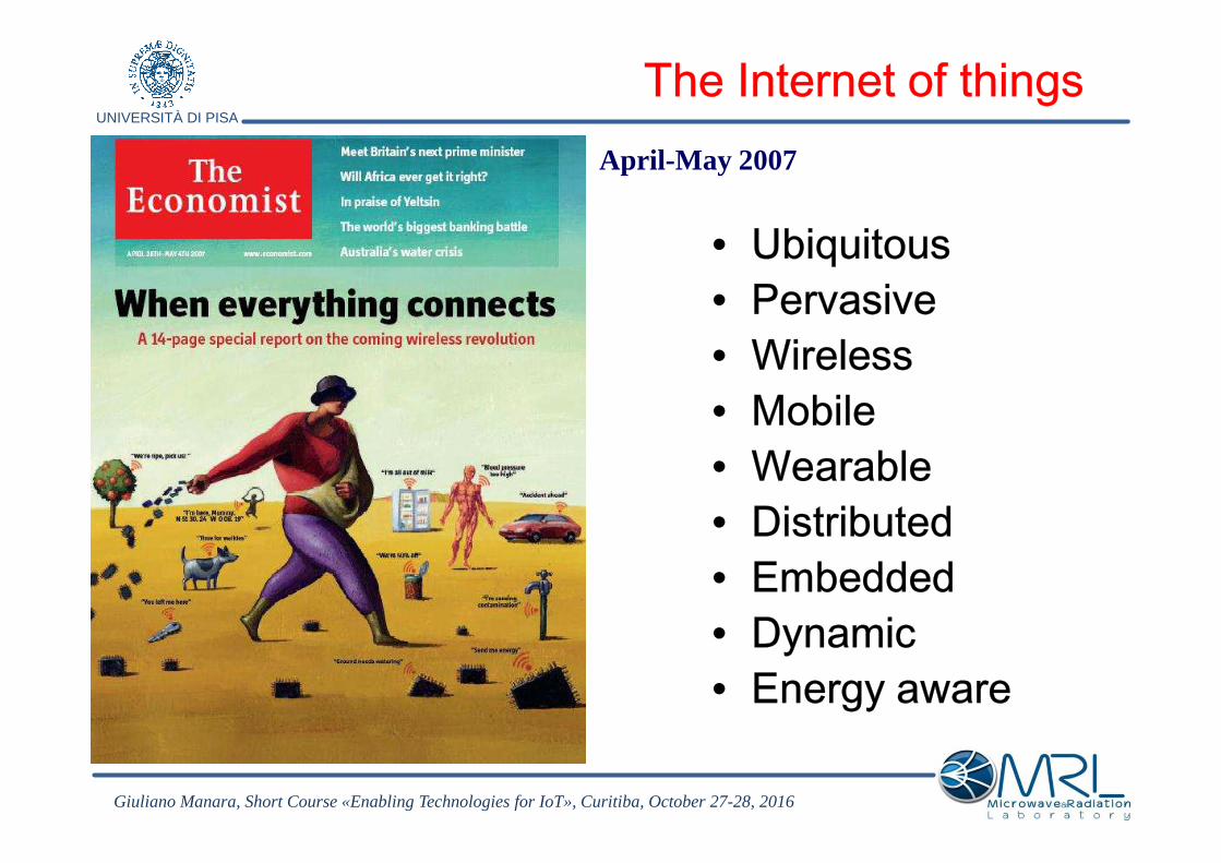
• Ubiquitous• Pervasive• Wireless• Mobile• Wearable• Distributed• Embedded• Dynamic• Energy aware

April-May 2007

The Internet of things


UNIVERSITÀ DI PISA








UNIVERSITÀ DI PISA

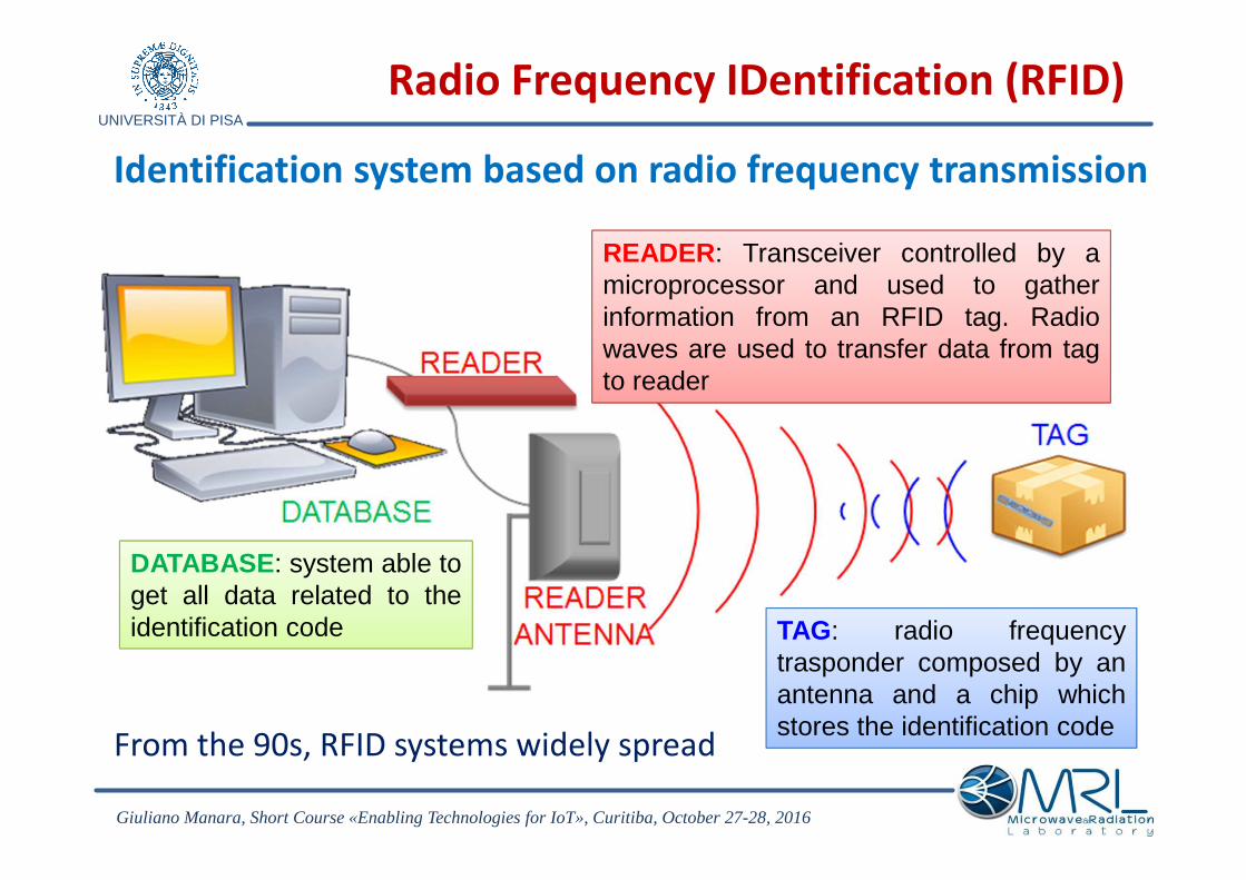
Radio Frequency IDentification (RFID)

Identification system based on radio frequency transmission

TAG: radio frequencytrasponder composed by anantenna and a chip whichstores the identification code

READER: Transceiver controlled by amicroprocessor and used to gatherinformation from an RFID tag. Radiowaves are used to transfer data from tagto reader

DATABASE: system able toget all data related to theidentification code

From the 90s, RFID systems widely spread


UNIVERSITÀ DI PISA

Basic operating principles of an RFID system


UNIVERSITÀ DI PISA

In 1999 at the Auto-ID Center of the Massachussets Institute ofTechnology, the EPC (Electronic Product Code) was born.

The barcode technology allows to item topology

identification

The EPC allows single item identification

01.0000A4F.001AD.000000001

HEADER

(8 bit)

EPC MANAGER

(28 bit)

SERIAL NUMBER

(36 bit)

OBJECT CLASS

(24 bit)

� HEADER defines the EPC length (from 64 to 256 bits).

� EPC MANAGER indicates tag producer

� OBJECT CLASS indicates tag topology

� SERIAL NUMBER indicates the unique identification number for each tag

Electronic Product Code


UNIVERSITÀ DI PISA

LF band (Low Frequency)120-145 KHz

� First employed band for RFID systemsApplications: animal tracking, asset tracking, access control

HF band (High Frequency)13.56 MHz

� Most employed and widespread band for RFID systemsApplications: smart cards, electronic documents, electronicmoney, baggage sorting

UHF band (Ultra-High Frequency)

Higher operativedistances with respectto other bands

medium860-950 MHz

� 865-870 MHz in Europe, 902-928 MHz in USA, 950 MHz inAsia

Applications: supply chain, items management

low(433-435 MHz)

� Band employed only in EuropeApplications: items management

high(2.4 GHz)

� Band crowded from other technologies (e.g. WiFi, Bluetooth,ZigBee)

Applications: items management

SHF band (Super High Frequency)(5.8 GHz)

Applications: telepass, ports

More recently RFID-UWB (Ultra Wide Band) systems in the 6-8.5 GHz band have reached increasing

attention.

Frequency bands

Depending on application, different frequency bands are employed:


UNIVERSITÀ DI PISA

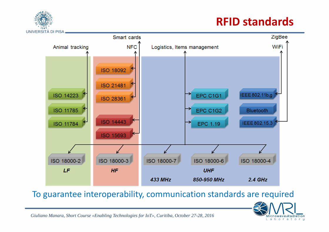
RFID standards

To guarantee interoperability, communication standards are required


UNIVERSITÀ DI PISA

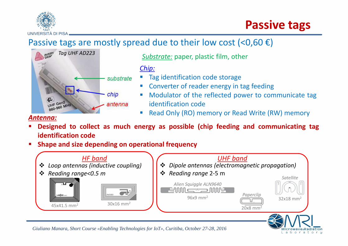
Passive tags are mostly spread due to their low cost (<0,60 €)

Chip:

� Tag identification code storage

� Converter of reader energy in tag feeding

� Modulator of the reflected power to communicate tag

identification code

� Read Only (RO) memory or Read Write (RW) memory

Passive tags

Antenna:

� Designed to collect as much energy as possible (chip feeding and communicating tag

identification code

� Shape and size depending on operational frequency

45x41.5 mm2 30x16 mm2

HF band� Loop antennas (inductive coupling)

� Reading range<0.5 m

UHF band� Dipole antennas (electromagnetic propagation)

� Reading range 2-5 m

96x9 mm2

Alien Squiggle ALN9640

32x18 mm2

Satellite

20x8 mm2

Paperclip

Tag UHF AD223Substrate: paper, plastic film, other


UNIVERSITÀ DI PISA

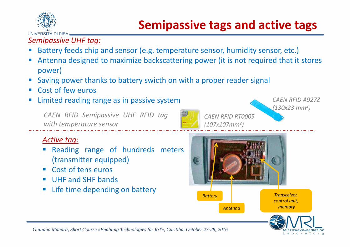
Semipassive UHF tag:

� Battery feeds chip and sensor (e.g. temperature sensor, humidity sensor, etc.)

� Antenna designed to maximize backscattering power (it is not required that it stores

power)

� Saving power thanks to battery swicth on with a proper reader signal

� Cost of few euros

� Limited reading range as in passive system

Semipassive tags and active tags

CAEN RFID RT0005

(107x107mm2)

CAEN RFID A927Z

(130x23 mm2)

CAEN RFID Semipassive UHF RFID tag

with temperature sensor

Active tag:

� Reading range of hundreds meters

(transmitter equipped)

� Cost of tens euros

� UHF and SHF bands

� Life time depending on battery

Antenna

Battery Transceiver,

control unit,

memory


UNIVERSITÀ DI PISA

Giuliano Manara, Workshop Internet das Coisas, Curitiba, 27/10/2016 – Instituto do Engenheria do Paranà (IEP)

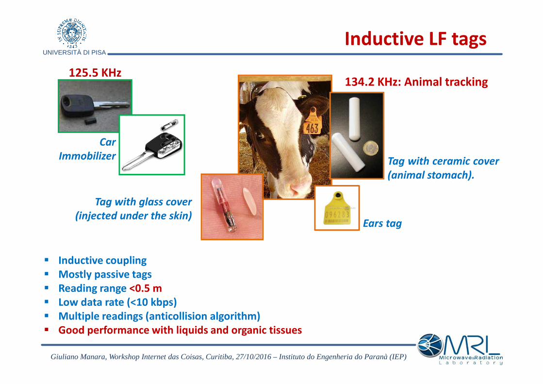
� Inductive coupling

� Mostly passive tags

� Reading range <0.5 m

� Low data rate (<10 kbps)

� Multiple readings (anticollision algorithm)

� Good performance with liquids and organic tissues

Car

Immobilizer

125.5 KHz

Inductive LF tags

134.2 KHz: Animal tracking

Tag with ceramic cover

(animal stomach).

Tag with glass cover

(injected under the skin)Ears tag

UNIVERSITÀ DI PISA

Smart labels

Baggage handling

Clothing

Logistics

Smart cards

Skypass

Credit cards

Inductive HF tags (13.56 MHz)

� Inductive coupling

� Mostly passive tags

� Reading range~1 m� Data rate up to 64 kbps

� Multiple readings (20-30 tag/s)

� Good performance with non-conducting liquids and organic tissues


UNIVERSITÀ DI PISA

Giuliano Manara, Workshop Internet das Coisas, Curitiba, 27/10/2016 – Instituto do Engenheria do Paranà (IEP)

System performance related to:• Tag antenna (loops number)• Reader antenna (loop sizes, loops number, maximum current)• Mutual positioning and mutual coupling among antennas• Tag Q-factor• Distance among antennas (available power at the tag side

proportional to 1/d6)

The variable magnetic field induces current on the tag antenna (electrical

transformer)

The tag communicates the

identification code by varying its

load impedance (load modulation).

distanza<λ

� Loop antennas typically employed

Inductive coupling

Many coils are required

(critical parameter)

UNIVERSITÀ DI PISA

� Electromagnetic propagation as in communication

systems

� Passive and active tags

� Reading range ~2-5 m

� Data rate up to 640 kbps

� Multiple readings (200 tag/s)

� Low performance in presence of liquids, organic tissues

and metals

Logistics

Metal tags

UHF tags


UNIVERSITÀ DI PISA

Frequencies employed within the UHF band are different from region to region

Passive tags have wideband design at the expence of performance

ERP=Effective

Radiated Power

(reference: ideal

dipole)

EIRP=Effective

Isotropic

Radiated Power

(reference:

isotropic

radiator)

2

2

1E EIRP

r∝

t tEIRP P G= ⋅

UHF tags

Interoperability problem


UNIVERSITÀ DI PISA

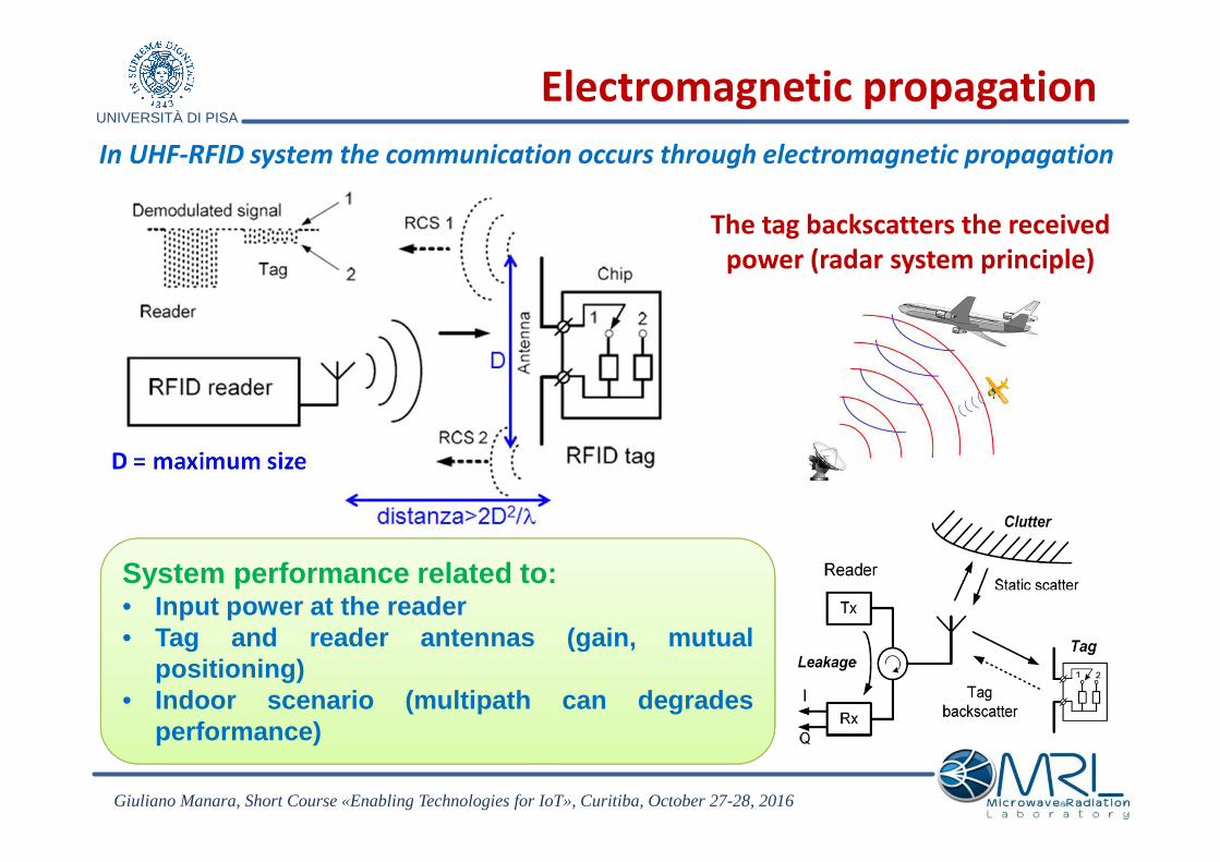
In UHF-RFID system the communication occurs through electromagnetic propagation

The tag backscatters the received

power (radar system principle)

D = maximum size

Electromagnetic propagation

System performance related to:• Input power at the reader• Tag and reader antennas (gain, mutual

positioning)• Indoor scenario (multipath can degrades

performance)


UNIVERSITÀ DI PISA

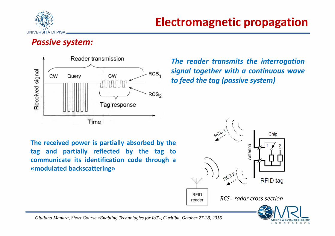
The received power is partially absorbed by the

tag and partially reflected by the tag to

communicate its identification code through a

«modulated backscattering»

RCS= radar cross section

Electromagnetic propagation

The reader transmits the interrogation

signal together with a continuous wave

to feed the tag (passive system)

Passive system:


UNIVERSITÀ DI PISA

• During tag backscattering, the chip works as switch and it

connects/disconnects the antenna to a specific load.

• Tipically two loads are used: an open circuit and a

complex conjiugate to the antenna impedance.

By varying the load impedance, the tag reflected

power changes (load modulation).

Modulated backscattering

Tag characterization as in radar system through the Radar Cross Section (RCS):

2 2 2

2b a

a c

P G RRCS

S Z Z

λσπ

= = =+

• Pb = tag backscattered power

• S= incident power density

• G = antenna gain

• Za = Ra+jXa = tag antenna impedance

• Zc = chip impedance

2 22

1 2 1 24

GRCS

λσ σ σ ρ ρ

π∆ = ∆ = − = −

1,21,2

1,2

*

*c a

c a

Z Z

Z Zρ

−=

+

The differential RCS is employed since the load impedance is variable:


UNIVERSITÀ DI PISA

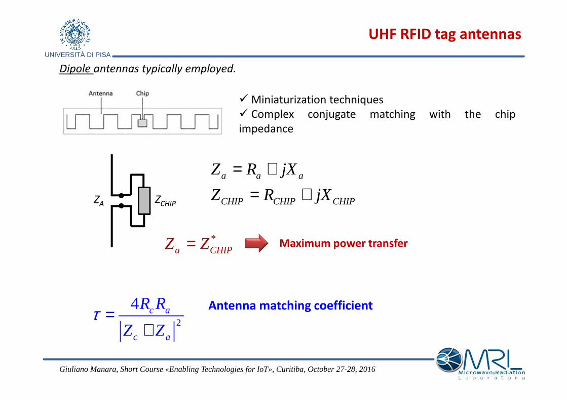
Dipole antennas typically employed.

� Miniaturization techniques

� Complex conjugate matching with the chip

impedance

*a CHIPZ Z= Maximum power transfer

ZCHIPZA

2

4 c a

c a

R R

Z Zτ =

+Antenna matching coefficient

a a a

CHIP CHIP CHIP

Z R jX

Z R jX

= += +

UHF RFID tag antennas


UNIVERSITÀ DI PISA

Read range� HF system (inductive coupling): highest performance with parallel tag antennas (i.e.

loops)

� UHF system (e.m. propagation): performance related to antennas radiation pattern

and polarization.Tag Alien Squiggle ALN9640 UHF

E E

Allignement not required

Positioning and Polarization

E E

Linearly polarized

The E vectors must be alligned

Linearly polarized

Linearly polarized

Circularly polarized


UNIVERSITÀ DI PISA








UNIVERSITÀ DI PISA

Antennas: some important items

• NEAR-FIELD FOCUSED ANTENNAS (NFFAs): CHARACTERISTIC PARAMETERS AND PROPERTIES

• BASIC DESIGN CRITERIA

• MICROWAVE NEAR-FIELD APPLICATIONS

• ADVANCED SYNTHESIS TECHNIQUES

• TECHNOLOGIES FOR NFF ANTENNAS: SOME EXAMPLES


UNIVERSITÀ DI PISA

Focusing: a well-known concept in optics

In Concentrating Photovoltaics (CPV), a large area of sunlight is focused onto the solar cell

….. burning ants or paper with a magnifier glass


UNIVERSITÀ DI PISA

From optics to mm-waves / THz regime

Focusing the electromagnetic field at a point in the antenna near-field region (the focalpoint) allows to increase the electromagnetic power density in a size-limited spotregion close to the antenna/array aperture.


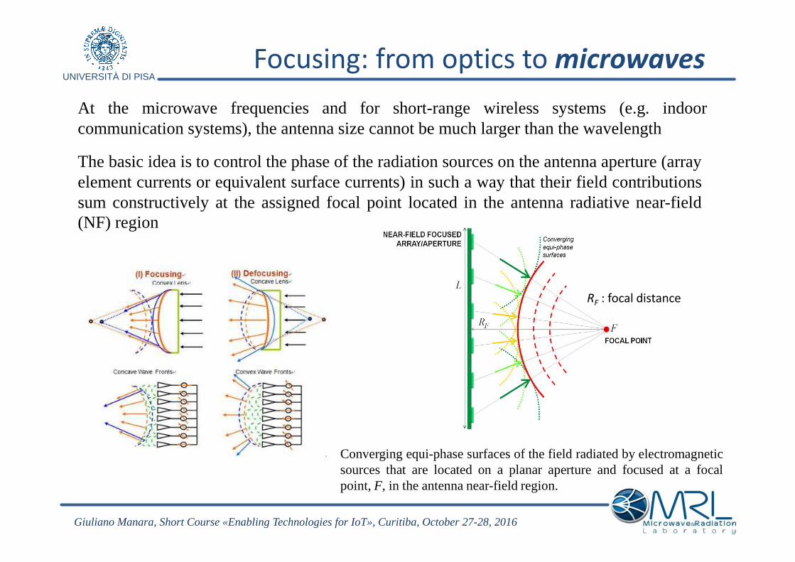
UNIVERSITÀ DI PISAFocusing: from optics to microwaves

The basic idea is to control the phase of the radiation sources on the antenna aperture (arrayelement currents or equivalent surface currents) in such a way that their field contributionssum constructively at the assigned focal point located in the antenna radiative near-field(NF) region

At the microwave frequencies and for short-range wireless systems (e.g.indoorcommunication systems), the antenna size cannot be much larger than the wavelength

Converging equi-phase surfaces of the field radiated by electromagneticsources that are located on a planar aperture and focused at afocalpoint,F, in the antenna near-field region.

RF : focal distance


UNIVERSITÀ DI PISA

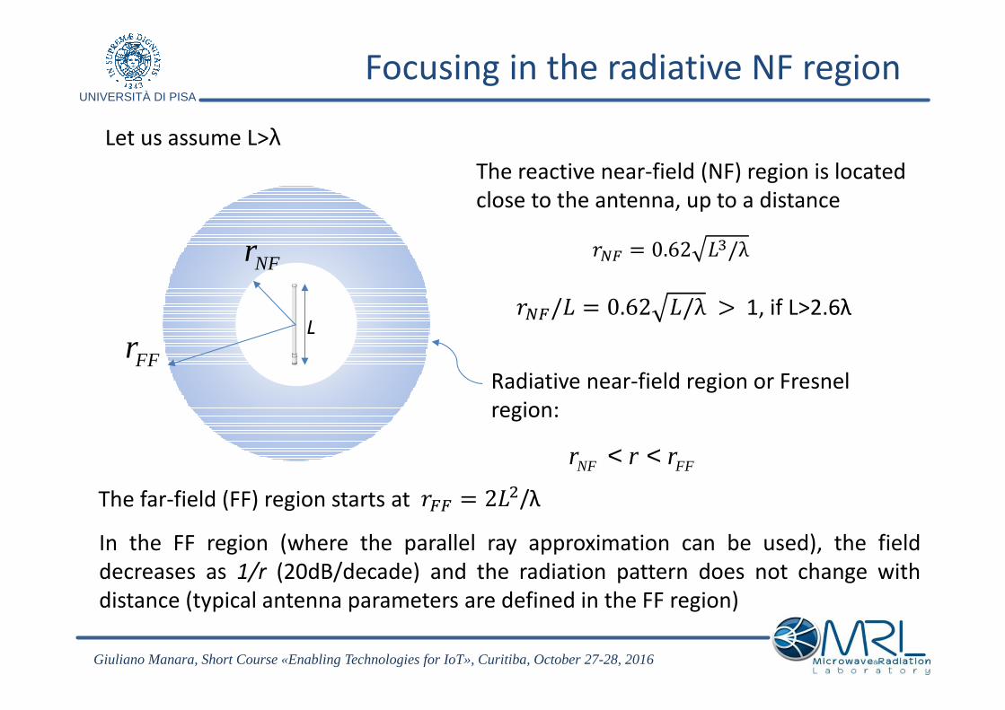
Focusing in the radiative NF region

Let us assume L>λ

L

FFr

NFr

NF FFr r r< <

Radiative near-field region or Fresnel

region:

The reactive near-field (NF) region is located

close to the antenna, up to a distance

The far-field (FF) region starts at

In the FF region (where the parallel ray approximation can be used), the field

decreases as 1/r (20dB/decade) and the radiation pattern does not change with

distance (typical antenna parameters are defined in the FF region)

�� = 0.62 /λ

��/ = 0.62 /λ > 1, if L>2.6λ

�� = 2�/λ


UNIVERSITÀ DI PISA

Why an array ?

• High gain

• Narrow HPBW

• Beamforming

What is an Antenna Array?


UNIVERSITÀ DI PISA

Let us consider two short dipoles oriented along the z-axis and aligned on the x-axis

Dipole 1 (x = d/2, y = 0, z = 0)

Dipole 2 (x = -d/2, y = 0, z = 0)

Due to the superposition effect:

1 2( ) ( ) ( )E P E P E P= +

0 0 ˆ( , , ) sin2 2

j rI LE r j e

rβζθ φ θ θ

λ−= ⋅ ⋅

If d, λ << r, r1, r2 (in order to ignore the near-field components), the electric field radiated by

a L-long short dipole fed with a current I0 toward a direction (θ,φ) at a distance r is

Two Short Dipoles


UNIVERSITÀ DI PISA

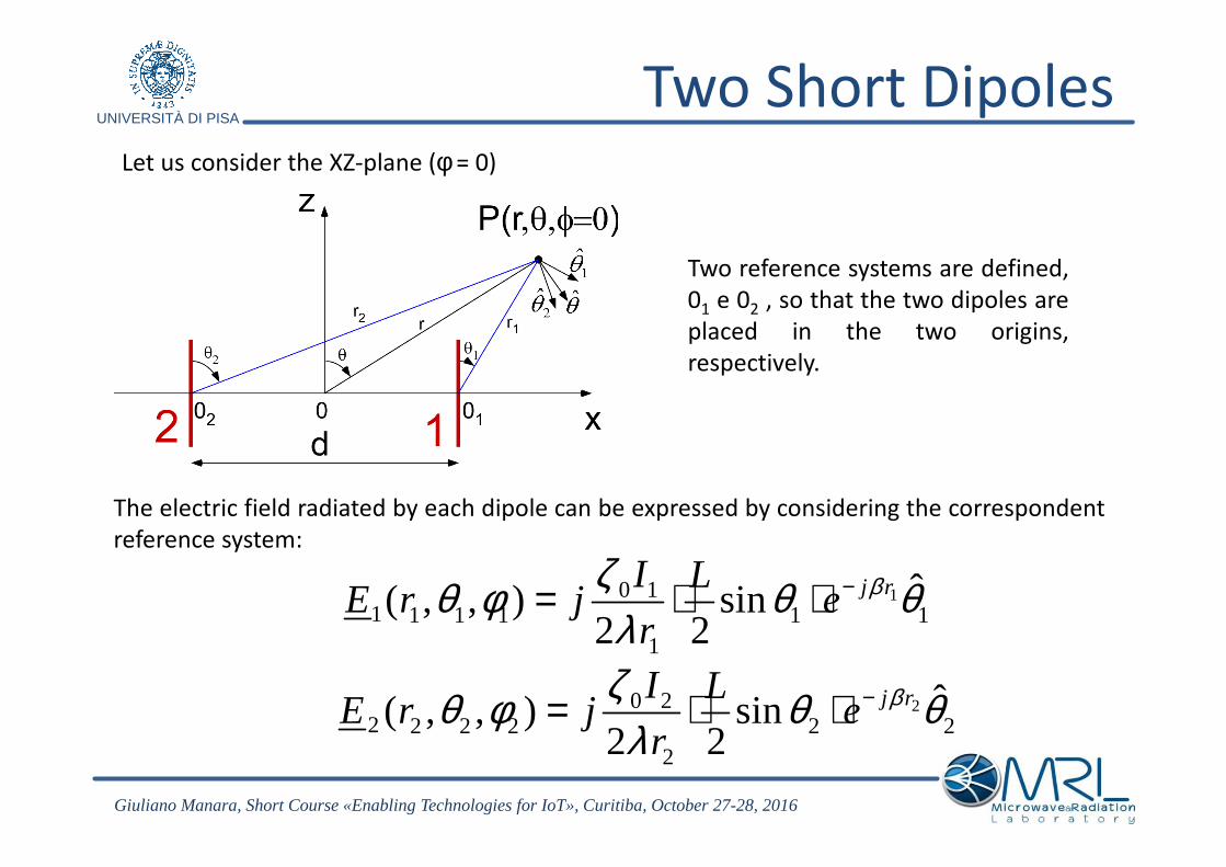
Let us consider the XZ-plane (φ = 0)

Two reference systems are defined,

01 e 02 , so that the two dipoles are

placed in the two origins,

respectively.

10 11 1 1 1 1 1

1

ˆ( , , ) sin2 2

j rI LE r j e

rβζθ φ θ θ

λ−= ⋅ ⋅

20 22 2 2 2 2 2

2

ˆ( , , ) sin2 2

j rI LE r j e

rβζθ φ θ θ

λ−= ⋅ ⋅

The electric field radiated by each dipole can be expressed by considering the correspondent

reference system:

Two Short Dipoles


UNIVERSITÀ DI PISA

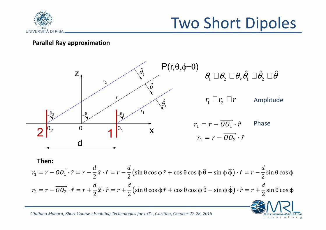
Parallel Ray approximation

Amplitude

1 2 1 2ˆ ˆ ˆ,θ θ θ θ θ θ≅ ≅ ≅ ≅

1 2r r r≅ ≅

Phase

Then:

Two Short Dipoles

�� = � − �� · �̂

�� = � − �� · �̂

�� = � − �� · �̂ = � −�

2�� · �̂ = � −

�

2sin θ cosϕ �̂ + cos θ cosϕθ − sinϕϕ! · �̂ = � −

�

2sin θ cosϕ

�� = � − �� · �̂ = � +�

2�� · �̂ = � +

�

2sin θ cosϕ �̂ + cos θ cosϕθ − sinϕϕ! · �̂ = � +

�

2sin θ cosϕ


UNIVERSITÀ DI PISA

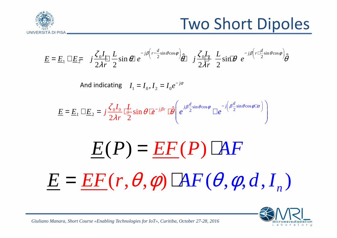
sin cos sin cos2 20 1 0 2

1 2ˆ ˆsin sin

2 2 2 2

d dj r j rI IL L

E E E j e j er r

β θ φ β θ φζ ζθ θ θ θλ λ

− − − + = + = ⋅ ⋅ + ⋅ ⋅

sin cossin cos

1 220 0 2ˆsin

2 2

ddj jr

j

eEI L

j eE Er

eβ θ φ αβ θ φβζ θ θ

λ

− + −

+

+ ⋅= =

⋅ ⋅

And indicating1 0 2 0, jI I I I e α−= =

(( )) EFE APP F= ⋅( , , ,( , ) ), nA dE FE r IF θ φθ φ= ⋅

Two Short Dipoles


UNIVERSITÀ DI PISA

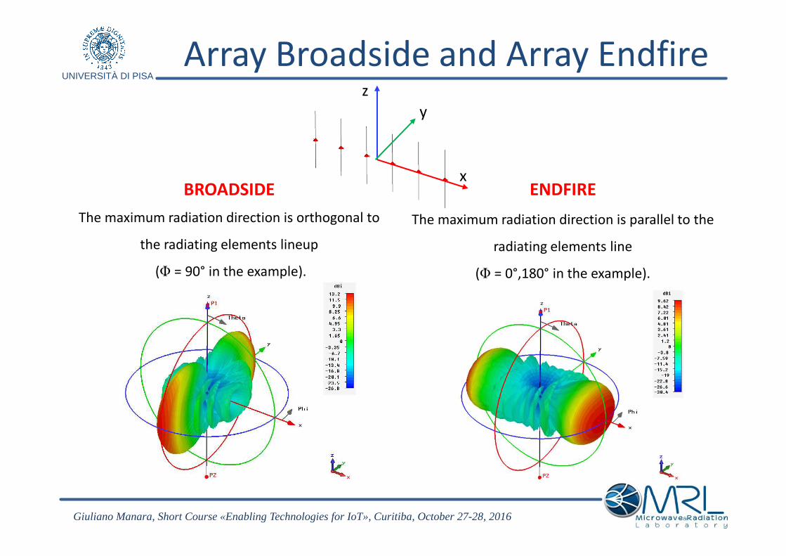
BROADSIDE ENDFIRE

z

y

x

The maximum radiation direction is orthogonal to

the radiating elements lineup

(Φ = 90° in the example).

The maximum radiation direction is parallel to the

radiating elements line

(Φ = 0°,180° in the example).

Array Broadside and Array Endfire


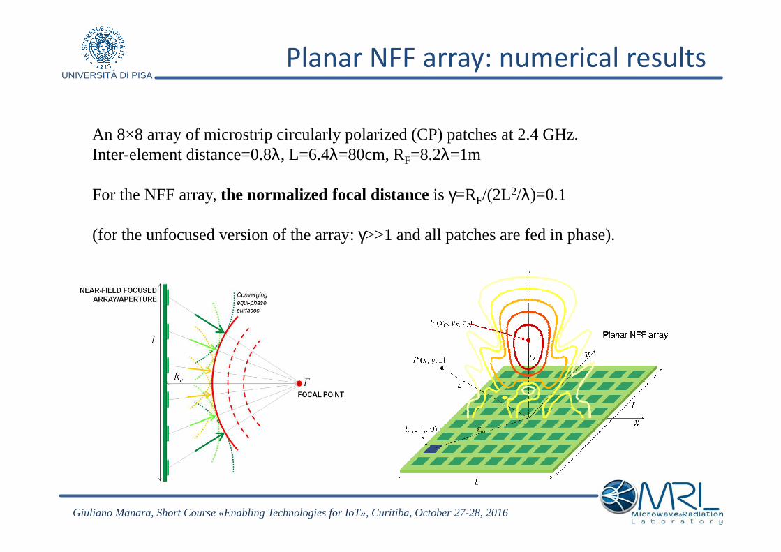
UNIVERSITÀ DI PISAPlanar NFF array: numerical results

An 8×8 array of microstrip circularly polarized (CP) patches at 2.4 GHz.Inter-element distance=0.8λ, L=6.4λ=80cm, RF=8.2λ=1m

For the NFF array,the normalized focal distance is γ=RF/(2L2/λ)=0.1

(for the unfocused version of the array:γ>>1 and all patches are fed in phase).


UNIVERSITÀ DI PISA

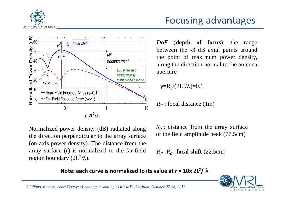
Focusing advantages

Note: each curve is normalized to its value at r = 10x 2L2/ λ

DoF (depth of focus): the rangebetween the -3 dB axial points aroundthe point of maximum power density,along the direction normal to the antennaaperture

RF : focal distance (1m)

R0 : distance from the array surfaceof the field amplitude peak (77.5cm)

RF -R0 : focal shift (22.5cm)

Normalized power density (dB) radiated alongthe direction perpendicular to the array surface(on-axis power density). The distance from thearray surface (r) is normalized to the far-fieldregion boundary (2L2/λ).

γ=RF/(2L2/λ)=0.1


UNIVERSITÀ DI PISA

Focusing advantages

Note: each curve is normalized to its maximum value in the near-field region.


UNIVERSITÀ DI PISA

Near-field at the focal plane (xy-plane at z=RF)

Near-FieldFocused (NFF) 8x8 arrayUnfocused 8x8 array(all patches are fed in phase)

The focus width, W, is defined as the -3 dB spot diameter at the focalplane.

For the NFF 8x8 microstrip array,W=14.7cm and the sidelobe level in thefocal plane is less than -15 dB.


UNIVERSITÀ DI PISA

Near-field at the transverse plane

For the NFF 8x8 microstrip array, W=14.7cm, and DoF=70.1cm

Near-FieldFocused (NFF) 8x8 arrayUnfocused 8x8 array(all patches are fed in phase)


UNIVERSITÀ DI PISAAntennas: Some Important Items

• NEAR-FIELD FOCUSED ANTENNAS (NFFAs): CHARACTERISTIC PARAMETERS AND PROPERTIES

• BASIC DESIGN CRITERIA

• MICROWAVE NEAR-FIELD APPLICATIONS

• ADVANCED SYNTHESIS TECHNIQUES

• TECHNOLOGIES FOR NFF ANTENNAS: EXAMPLES


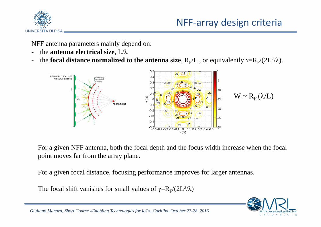
UNIVERSITÀ DI PISANFF-array design criteria

A. Buffi, P. Nepa, and G. Manara,“Design Criteria for Near-Field-FocusedPlanar Arrays”, IEEE Antennas andPropagationMagazine, February 2012

3D view of the normalized power density radiated by a NFF 8x8array of x-directed short dipoles (inter-element spacingd=0.8λ,L=Nd=6.4λ): NFF array withRF=8.2λ (left hand side) and far-fieldfocused array (right hand side)


UNIVERSITÀ DI PISA

NFF antenna parameters mainly depend on:- theantenna electrical size, L/λ- thefocal distance normalized to the antenna size, RF/L , or equivalentlyγ=RF/(2L2/λ).

For a given NFF antenna, both the focal depth and the focus width increase when the focal point moves far from the array plane.

For a given focal distance, focusing performance improves for larger antennas.

The focal shift vanishes for small values of γ=RF/(2L2/λ)

W ~ RF (λ/L)

NFF-array design criteria


UNIVERSITÀ DI PISA

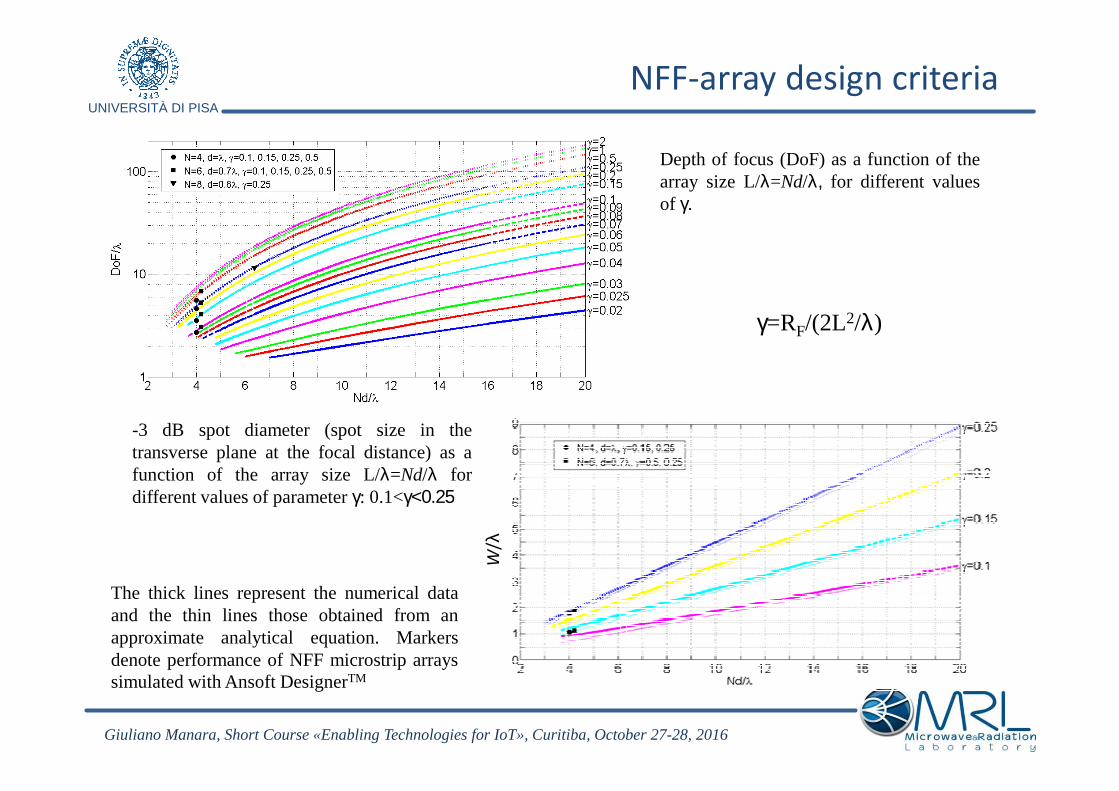
Depth of focus (DoF) as a function of thearray size L/λ=Nd/λ, for different valuesof γ.

-3 dB spot diameter (spot size in thetransverse plane at the focal distance) as afunction of the array size L/λ=Nd/λ fordifferent values of parameterγ: 0.1<γ<0.25.

W/λ

γ=RF/(2L2/λ)

The thick lines represent the numerical dataand the thin lines those obtained from anapproximate analytical equation. Markersdenote performance of NFF microstrip arrayssimulated with Ansoft DesignerTM

NFF-array design criteria


UNIVERSITÀ DI PISA

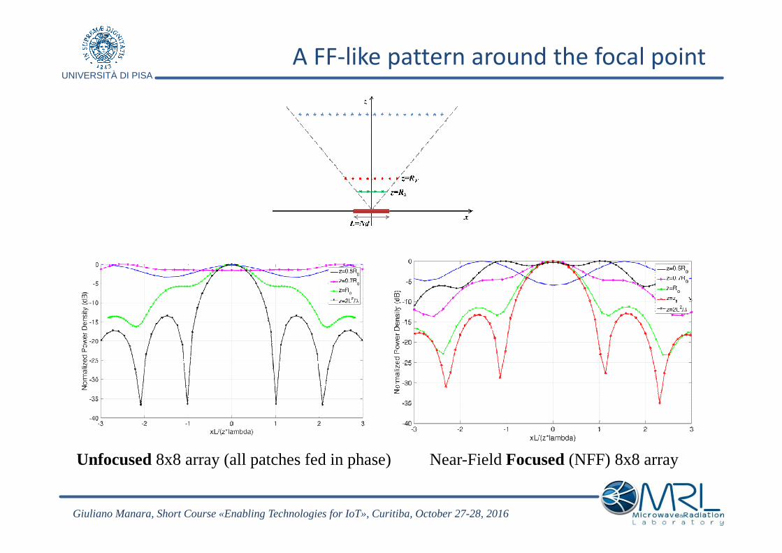
A FF-like pattern around the focal point

An 8×8 array of microstrip circularly polarized (CP) patches at 2.4 GHz.Inter-element distance=0.8λ, L=6.4λ=80cm, RF=8.2λ=1mFor the NFF array,the normalized focal distance is γ=RF/(2L2/λ)=0.1

The far-field radiation pattern of a conventional unfocused array can beachieved in the near-field region of the focused antenna


UNIVERSITÀ DI PISA

A FF-like pattern around the focal point

Near-FieldFocused (NFF) 8x8 arrayUnfocused 8x8 array (all patches fed in phase)


UNIVERSITÀ DI PISA

The conjugate-phase approach

2 /

01 1

( ) ( ) ( , )nj r rN N

nn n n nn n n

eE r C E r C E

r r

π λ

θ φ− −

= =

= =−∑ ∑

njn nC A e ϕ=

The source phase profile has to compensate for the phasedelay introduced by the path between each source pointon the antenna/array aperture and the targeted focal point

( ) ( ) 22 2 2 22 2 2ˆ2 ,F n n nn F n F n F F F Fr r x x y y z R r R r r

π π πϕλ λ λ

= + − = − + − + = + − ⋅

2 ( )/

01

( ) ( , )n F nj r r r rN

n n nn n

eE r A E

r r

π λ

θ φ− − − −

=

=−∑

The electric field at the generic observation point r:

At the focal point, all contributions sum in phase:

01

( ) ( , ) /N

F F nn n nn

E r r A E r rθ φ=

= = −∑

F nr r−


UNIVERSITÀ DI PISA

The quadratic phase approximation

F nr r−If the focal distance is enough larger than theantenna size (RF>L), the phase taperingrequired for focusing at the focal point can beapproximated by the sum of a linear phase shiftplus a quadratic term (Fresnel approximation)

( )2

2 2ˆ

2n

nn FF

rr r

R

π πϕλ λ

≈ − ⋅ +

The linear phase shift (first term at the right hand side) corresponds to thephaseexcitation required to point at the focal point direction when the focal pointis beyond the FF-region boundary (parallel ray approximation).

( , )F Fθ φ


UNIVERSITÀ DI PISA

The focal shift

2 ( )/

01

( ) ( , )n F nj r r r rN

n n nn n

eE r A E

r r

π λ

θ φ− − − −

=

=−∑

When moving from the focal point toward the antenna aperture, array contributions doesnot sum in phase anymore; on the other hand, the expected amplitude reduction isover-compensated by the fact that each element contribution exhibits a higher amplitude closeto the antenna aperture, as the spreading factor increases.1/ nr r−

γ=RF/(2L2/λ)


UNIVERSITÀ DI PISA

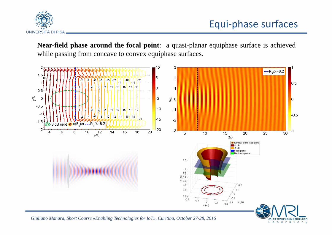
Equi-phase surfaces

Near-field phase around the focal point: a quasi-planar equiphase surface is achievedwhile passing from concave to convex equiphase surfaces.


UNIVERSITÀ DI PISAAcnowledgements

I want to aknowledge the precious support of my colleagues Prof.

Stefano Giordano, Prof. Paolo Nepa, Dr. Alice Buffi, Dr. Andrea

Michel in preparing this presentation.


EnablingTechnologies for the Internet of...

Documents

Transcript of EnablingTechnologies for the Internet of...