Enabling Photoemission Electron Microscopy in Liquids viaGraphene-Capped Microchannel ArraysHongxuan Guo,†,‡ Evgheni Strelcov,†,‡ Alexander Yulaev,†,‡,§ Jian Wang,∥ Narayana Appathurai,∥

Stephen Urquhart,⊥ John Vinson,# Subin Sahu,†,‡,∇ Michael Zwolak,† and Andrei Kolmakov*,†

†Center for Nanoscale Science and Technology, National Institute of Standards and Technology, Gaithersburg, Maryland 20899,United States‡Maryland NanoCenter, University of Maryland, College Park, Maryland 20742, United States§Department of Materials Science and Engineering, University of Maryland, College Park, Maryland 20742, United States∥Canadian Light Source, Saskatoon, Saskatchewan S7N 2V3, Canada⊥Department of Chemistry, University of Saskatchewan, Saskatoon, Saskatchewan S7N 5C9, Canada#Material Measurement Laboratory, National Institute of Standards and Technology, Gaithersburg, Maryland 20899, United States∇Department of Physics, Oregon State University, Corvallis, Oregon 97331, United States

*S Supporting Information

ABSTRACT: Photoelectron emission microscopy (PEEM) isa powerful tool to spectroscopically image dynamic surfaceprocesses at the nanoscale, but it is traditionally limited toultrahigh or moderate vacuum conditions. Here, we develop anovel graphene-capped multichannel array sample platform thatextends the capabilities of photoelectron spectromicroscopy toroutine liquid and atmospheric pressure studies with standardPEEM setups. Using this platform, we show that graphene hasonly a minor influence on the electronic structure of water inthe first few layers and thus will allow for the examination ofminimally perturbed aqueous-phase interfacial dynamics.Analogous to microarray screening technology in biomedicalresearch, our platform is highly suitable for applications intandem with large-scale data mining, pattern recognition, and combinatorial methods for spectro-temporal and spatiotemporalanalyses at solid−liquid interfaces. Applying Bayesian linear unmixing algorithm to X-ray induced water radiolysis process, wewere able to discriminate between different radiolysis scenarios and observe a metastable “wetting” intermediate water layerduring the late stages of bubble formation.

KEYWORDS: PEEM, liquids, graphene, XAS, data mining

Electron spectroscopy1,2 in liquids aims to boost ourunderstanding of the solid−liquid−gas interface relevant

to environmental,3 energy,4,5 catalysis,6 and biomedicalresearch.7 The pressure gap between the liquid or gaseoussample and the ultrahigh vacuum (UHV) partition of theexperimental setup (i.e., the electron energy analyzer) is usuallybridged via judiciously designed differentially pumped electronoptics8 in combination with advanced sample deliverysystems.9−12 Experimental challenges, however, delayed theapplication of the “photon-in electron-out” imaging techniquesto solid−liquid interfaces.Novel two-dimensional (2D) materials such as graphene

have recently enabled an alternative, truly atmospheric pressure,photon-in electron-out X-ray photoelectron spectroscopy(APXPS)13−17 via separation of the liquid or gaseous samplefrom UHV with a molecularly impermeable but yet electrontransparent membrane. The subnanometer thickness of these

membranes is smaller or comparable to electron’s inelasticmean free path (IMFP). Thus, the photoelectrons are able totraverse the membrane without significant attenuation whilepreserving their characteristic energies. The drastic reduction ofthe complexity of the experimental setup allowed the firstscanning photoelectron microscopy (SPEM) measurements tobe performed in liquid water through graphene-basedmembranes.14 However, focused X-ray beam raster scanningduring SPEM chemical mapping is relatively slow. Thisimpedes real-time or prolonged imaging of dynamic processesand decreases the lifetime of the membranes.18 Therefore, animplementation of the full field of view (FOV) PEEM imagingis advantageous due to reduced photon density at the sample

Received: October 25, 2016Revised: January 16, 2017Published: January 25, 2017

Letter

pubs.acs.org/NanoLett

© 2017 American Chemical Society 1034 DOI: 10.1021/acs.nanolett.6b04460Nano Lett. 2017, 17, 1034−1041

and acquisition at the video frame rate (see, e.g., Bauer19 andreferences therein). Though FOV photoelectron imaging of thedynamic processes and objects, such as working catalysts or livecells, in their native high pressure gaseous or liquid environ-ments was a long-standing scientific goal, the differentialpumping approach, so successful in APXPS, resulted only in≈10−1 Pa of near sample pressures so far when applied to thePEEM setup.20 The near-sample pressure value was limitedmainly by the reduced lifetime of the imaging detector andpossible discharge development between the sample and PEEMobjective lens. An approach, which surmounts these restric-tions, was proposed and tested in ref 21 and was based on anenvironmental cell consisting of two 100 to 200 nm thick Si3N4

membranes with a liquid layer of micrometer thickness inbetween.22 The PEEM images of liquid interior of the cell canonly be obtained within water soft X-ray transparency window(hν ≈ 285 to 532 eV) and in transmission mode. The Si3N4

membrane facing the PEEM objective lens was covered with athin gold photocathode to convert transmitted X-rays tophotoelectrons. These very first feasibility tests were, to the bestof our knowledge, the only PEEM measurements of hydratedsamples so far. On the other hand, prior PEEM research ofburied interfaces revealed that the ultraviolet (UV) excitedphotoelectrons can be recorded through SiO2 films from thedepths exceeding many IMFPs.23 Therefore, standard PEEMimaging in liquids and dense gases in principle can be feasibleusing photoelectrons, provided that UHV and high pressureenvironments are separated with a thin enough membrane. Thelatter possibility has been proven recently in an X-ray (X-PEEM) spectromicroscopy study of thermally inducedsegregation of nanobubbles at a graphene−Ir interface filledwith high pressure (≈GPa) noble gases.24

Here, we develop a novel, versatile microchannel array(MCA) platform that enables a wide range of photoelectronemission spectromicroscopies in liquids through a graphenemembrane using UV or soft X-rays. Unlike the case of theaforementioned PEEM “shadow” imaging of immersed objectsin the transmission mode, we were able to collect XASspectrotemporal data of dynamic processes at the graphene−liquid interface in operando and submicron spatial resolutionusing standard synchrotron-based PEEM equipment.

Multichannel Array Liquid Sample Platform for PEEM.PEEM at liquid−solid interfaces became possible as a result ofsuccessful development of a UHV compatible liquid sampleMCA platform proposed in ref 18. The details of the samplefabrication, liquid filling, and vacuum sealing can be found inthe Methods and Supporting Information. Briefly, liquid waterwas impregnated into the gold-coated silica matrix made of anordered array of ≈300 μm deep and ≈4 μm wide parallelchannels (Figure 1a). The top of the MCA was covered andisolated from the vacuum with an electron-transparentmembrane made of a bilayer graphene (BLG) stack (Figure 1b). The bottom of the sample was sealed with a water-immiscible sealant. The water-filling factor (the ratio betweenwater-filled and empty channels) is routinely in excess of 85%at the beginning of the experiment in UHV and slowly decayswith time. The lifetime of the liquid inside such a sampleusually exceeds a few hours and is limited mainly by thegraphene quality and interfacial diffusion of water molecules.The MCA sample containing thousands of water filled

microchannels and capped with BLG was illuminated withmonochromatic soft X-rays with an energy between 525 and560 eV, covering the O K-absorption edge (≈535 eV). Underthis excitation, fast photoelectrons and Auger electrons fromthe liquid that have the IMFP in excess of the thickness of the

Figure 1. Multichannel array sample design and experimental setup. (a) SEM (5 keV, color coded) image of water-filled graphene-cappedmicrochannel sample; the darker channels correspond to the graphene-capped but empty channels. Inset: water-filled 4 μm wide channel (SEM, 2keV). (b) The schematics of the PEEM and liquid cell setups. (c) PEEM images of the water filled MCA collected at different X-ray energies whilecrossing the O K-edge. (d) The resultant XAS spectra collected from different ROIs: water-filled (blue circle and spectrum) and empty (red circleand spectrum) channels. White squares mark the channels that exhibit the dynamic behavior. The spectra were normalized to incident X-rayintensity.

Nano Letters Letter

DOI: 10.1021/acs.nanolett.6b04460Nano Lett. 2017, 17, 1034−1041

1035

capping BLG membrane are able to escape into the vacuumwith only minor attenuation.25 These electrons constitute thetotal electron yield (TEY) that was used for spatially resolvedXAS of the liquid or for spectrally resolved PEEM imaging(Figure 1c,d). Water-containing areas have a sharp character-istic onset in the absorption cross-section around hν ≈ 535 eVand thus can be easily discriminated from the other substratematerials (graphene, Au) which have a flat photoemissionbackground across this energy range.Figure 1c shows a set of four PEEM images of the BLG-

capped water filled MCA recorded at different energies whilescanning across the O K edge. The contrast in these imagesoriginates from spatial variations of the local TEY from the Au-coated MCA matrix and the graphene-capped MCA channels.The graphene-capped channels can either be filled with liquidwater or be empty. A fraction of the channels does not have agraphene cap and these have the lowest signal in Figure 1c. Ascan be seen, the contrast between water-filled and emptychannels is miniscule below O−K absorption threshold at hν ≈535 eV and increases drastically above it. Such sequences ofPEEM images constitute a spatial X-ray absorption chemicalmap and specific regions of interest (ROI) can be designatedfor site-selective XAS. Figure 1d compares two such XASspectra collected from two ROIs: water filled (blue) and empty(red) channels. The empty channels show weak spectral featureat ∼532 eV characteristic of carbonyl group containinghydrocarbons.26 These contaminations have been previouslyobserved in XAS of ice and water27 and in our case can also bedue to poly(methyl methacrylate) (PMMA) residue at the BLGmembrane left after graphene transfer.28 On the other hand, thefilled channels demonstrate an XAS spectrum with pronouncedfeatures and a shape similar to liquid bulk water probed viaTEY or in transmission detection modes (see reviews29,30 andreferences therein). Such a spectrum is a result or transitionsfrom the strongly localized O 1s core level of water moleculesto unoccupied valence orbitals derived from the gas-phase 4a1and 2b2 states.31 The particular feature of these unoccupiedorbitals is their p character (due to the dipole selection rule)that results in their noticeable directionality and spatialextension far beyond the hydrogen atoms. Because hydrogenatoms participate in hydrogen bonding (H-bonding) in water,the XAS O K-edge spectra are very responsive to variations inelectronic and/or structural environment around the probedwater molecule. In good accordance with prior XAS works onliquid water,27,29 our PEEM-derived XAS spectrum in Figure 1d has a characteristic pre-edge (≈535 eV), main peak (≈537.5eV) features, and a postedge band around ≈541 eV. Thecommonly accepted interpretation of water XAS featuresassigns the prepeak and main band to the excitation of watermolecules with one broken (or largely distorted H-bond, a so-called single-donor (SD) molecule) while the postedge bandcorresponds to the molecular environment with strong H-bonds (double donor (DD) molecules) and increasedtetrahedrality.31

It is important to emphasize that the XAS spectrum in Figure1 originates from the first few layers of water at the graphene−water interface. This interfacial sensitivity of the through-membrane PEEM spectromicroscopy stems from the attenuat-ing role of the BLG layer, which has low transparency for slow,few electronvolts secondary electrons emitted from deeperwater layers.32 Therefore, the bulklike nature of our spectraindicates that interaction of interfacial water molecules withgraphene is very weak and neither the electronic nor the

geometrical structure are strongly affected by the graphene. Inaddition, the intensity ratio of the main bands and the absenceof the characteristic OH (≈526 eV) or H2O2 (≈533 eV)33

features in the water XAS spectrum indicate that the graphene−water interface is not accumulating radiolysis products underthe selected irradiation conditions. A previous XAS study ofinterfacial water in contact with gold34 revealed the significantsuppression of the pre-edge peak under similar experimentalconditions. Thus, graphene represents a model benchmarkmaterial to study interfacial water behavior with PEEM.

Modeling of the Graphene−Water Interface. To gaindeeper insight into these differences, we simulate graphene−water structures with all-atom molecular dynamics (MD)simulations and perform calculations of the oxygen K-edgeXAS, as described in the Methods and Supporting Information(SI). As shown in Figure 2a,b, the structure of the water about1 nm away from the graphene is already bulklike.

The presence of the graphene does, however, induce waterdensity oscillations (see Figure S2a in the SI) and results ininterfacial water losing about 30% of its hydrogen bonds(Figure S2b). The latter is reflected in the different proportionsof donating species of water near the graphene (Figure 2b).Despite these changes in interfacial H-bonding and density, thetheoretically computed XAS spectrum is similar to onecomputed for bulk water (Figure 2c). As with the experimentalresults, the characteristic pre-edge peak is present in bothspectra and of approximately the same relative magnitudecompared to the main peak. This is in stark contrast to theaforementioned XAS of liquid water near the gold surface,34

Figure 2. Water structure, hydrogen bonding, and theoretical XASspectrum. (a) A snapshot of the bilayer graphene-capped waterchannel from the MD simulations. The simulation is periodic in alldirections with the full unit cell shown in Figure S1a. (b) Density ofwater molecules with differing numbers of hydrogen bonds theydonate (DD = double donor, SD = single donor, and ND =nondonor) versus distance from the graphene sheet; panel a and bshare the same z-axis scale and alignment. The graphene induces adensity oscillation in the water, as well as a change in the relativepopulation of different donating species. (c) The oxygen K-edge XASspectrum for water at the graphene interface (green) and the spectrumfor bulk water (red) as a function of excitation energy. The bulk waterspectrum was y-offset for clarity. The presence of graphene does notsignificantly affect the spectrum of water. This is due to the weakgraphene−water interaction. The graphene surface reduces thenumber of hydrogen bonds but does not otherwise align watermolecules at the surface. Moreover, the core-hole screening by theBLG is not strong enough to suppress the pre-edge peak (as it doeswith gold). Thus, this peak, as well as the relative location of the mainpeak, is the same for bulk water and water at the graphene interface.The error bars of the XAS curves denote the variance of the meanacross different MD snapshots.

Nano Letters Letter

DOI: 10.1021/acs.nanolett.6b04460Nano Lett. 2017, 17, 1034−1041

1036

where it was found that the large increase in broken hydrogenbonds (expected to strengthen the pre-edge peak) is over-whelmed by the screening provided by the gold atoms. Thehighly effective screening of core holes created near the goldsurface weakens the core-hole potential, blue-shifting XASspectrum, and reducing the intensity of the lower-energy peaks(see Figure S3b). On the other hand, the BLG layer does notscreen the X-ray induced core hole appreciably and thus doesnot suppress the pre-edge peak. In total, for water near a BLGlayer, both the structural and electronic effects of the surface aresignificantly weaker than for water−gold interface, resulting inthe similarity of the interfacial and bulk water XAS. We furtherelaborate on these results in the SI.Spectrotemporal Evolution of Water upon X-ray

Irradiation. One of the methodological advantages offeredby our MCA sample platform is the ability to collect a statisticalpopulation of geometrically identical objects with variabletemporal and spectral behaviors. The latter allows for theefficient application of powerful data mining and patternrecognition methodologies. The variations in temporalevolution of water in water-filled channels inside the FOVcan already be seen from Figure 1 (e.g., in the channel framedwithin the square). The whole spectro-temporal three-dimen-sional PEEM data set cannot be directly visualized in 2D plots,and the examples similar to the above (Figure 1) necessarilyrequire dimensionality reduction via data compression. There-fore, to take advantage of the MCA sample platform and tolosslessly compress PEEM data sets, we have employed amultivariate statistical tool, Bayesian linear unmixing (BLU),that has been developed for analysis of hyperspectral imagingdata sets.35,36 The BLU algorithm reduces a 3D PEEM data setY(x,y,E) to a linear combination of position-independentcharacteristic spectra, S(E), with respective relative abundances,A(x,y): Y(x,y,E) = S(E)·A(x,y). Unlike other statistical toolsused for multidimensional data analysis, this methodincorporates several built-in constraints that allow for scientifi-cally meaningful interpretation of results. The spectrum at eachlocation, therefore, can be represented as a linear combinationof spectra of individual components in correspondingproportions. The number of spectral components must beprovided by the researcher and can be estimated using principalcomponent analysis (PCA) or via under- and oversamplingcriteria. A detailed description and testing of BLU against PCA,k-means, and other statistical methods can be found else-

where.36 The optimal number of components for the data setshown in Figure 1 was found to be 4 (for details, see SI).Figure 3 shows unmixing of a PEEM spectroscopic data set

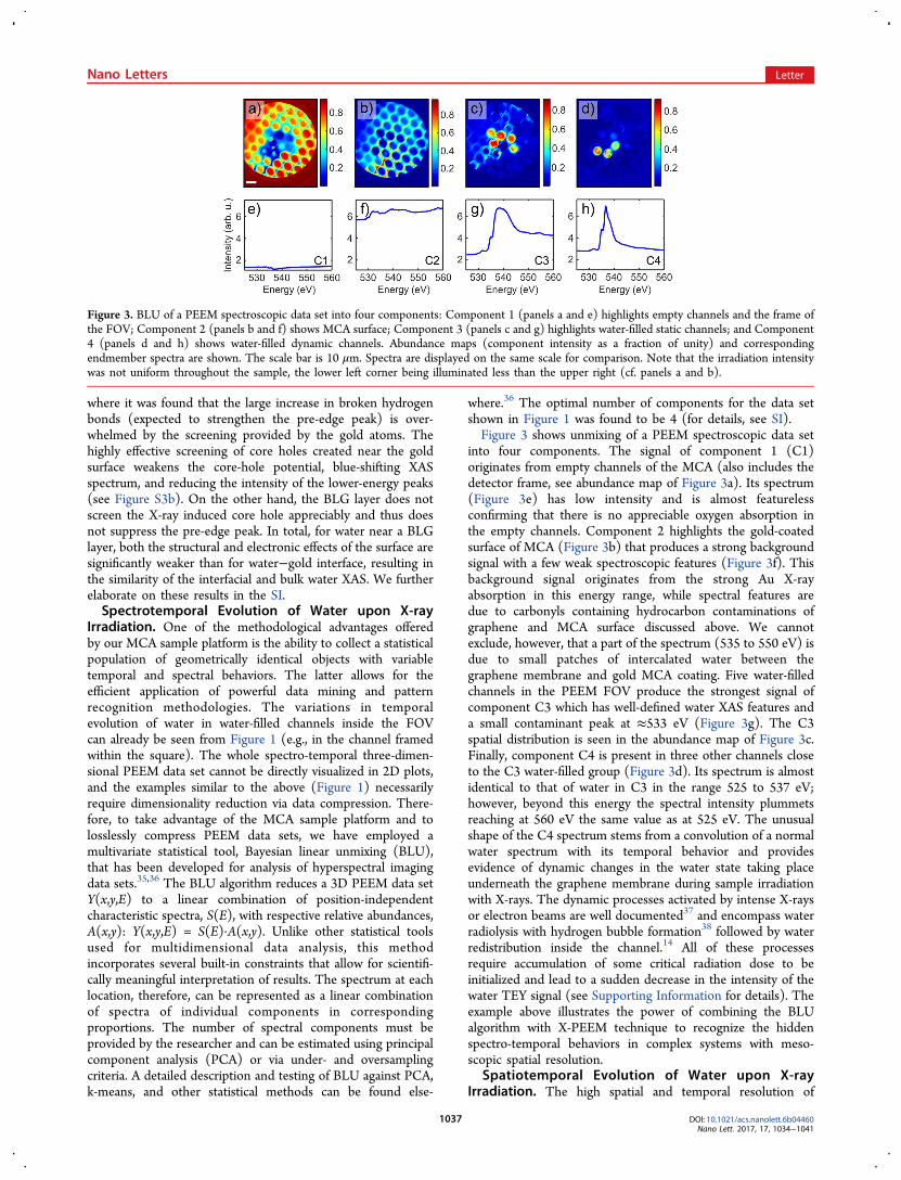
into four components. The signal of component 1 (C1)originates from empty channels of the MCA (also includes thedetector frame, see abundance map of Figure 3a). Its spectrum(Figure 3e) has low intensity and is almost featurelessconfirming that there is no appreciable oxygen absorption inthe empty channels. Component 2 highlights the gold-coatedsurface of MCA (Figure 3b) that produces a strong backgroundsignal with a few weak spectroscopic features (Figure 3f). Thisbackground signal originates from the strong Au X-rayabsorption in this energy range, while spectral features aredue to carbonyls containing hydrocarbon contaminations ofgraphene and MCA surface discussed above. We cannotexclude, however, that a part of the spectrum (535 to 550 eV) isdue to small patches of intercalated water between thegraphene membrane and gold MCA coating. Five water-filledchannels in the PEEM FOV produce the strongest signal ofcomponent C3 which has well-defined water XAS features anda small contaminant peak at ≈533 eV (Figure 3g). The C3spatial distribution is seen in the abundance map of Figure 3c.Finally, component C4 is present in three other channels closeto the C3 water-filled group (Figure 3d). Its spectrum is almostidentical to that of water in C3 in the range 525 to 537 eV;however, beyond this energy the spectral intensity plummetsreaching at 560 eV the same value as at 525 eV. The unusualshape of the C4 spectrum stems from a convolution of a normalwater spectrum with its temporal behavior and providesevidence of dynamic changes in the water state taking placeunderneath the graphene membrane during sample irradiationwith X-rays. The dynamic processes activated by intense X-raysor electron beams are well documented37 and encompass waterradiolysis with hydrogen bubble formation38 followed by waterredistribution inside the channel.14 All of these processesrequire accumulation of some critical radiation dose to beinitialized and lead to a sudden decrease in the intensity of thewater TEY signal (see Supporting Information for details). Theexample above illustrates the power of combining the BLUalgorithm with X-PEEM technique to recognize the hiddenspectro-temporal behaviors in complex systems with meso-scopic spatial resolution.

Spatiotemporal Evolution of Water upon X-rayIrradiation. The high spatial and temporal resolution of

Figure 3. BLU of a PEEM spectroscopic data set into four components: Component 1 (panels a and e) highlights empty channels and the frame ofthe FOV; Component 2 (panels b and f) shows MCA surface; Component 3 (panels c and g) highlights water-filled static channels; and Component4 (panels d and h) shows water-filled dynamic channels. Abundance maps (component intensity as a fraction of unity) and correspondingendmember spectra are shown. The scale bar is 10 μm. Spectra are displayed on the same scale for comparison. Note that the irradiation intensitywas not uniform throughout the sample, the lower left corner being illuminated less than the upper right (cf. panels a and b).

Nano Letters Letter

DOI: 10.1021/acs.nanolett.6b04460Nano Lett. 2017, 17, 1034−1041

1037

PEEM allows us to spectroscopically access particularities ofsoft X-rays induced radiolysis processes in water. In order toexplore the dynamics of interfacial water layer and facilitate theinterfacial bubble formation, we performed time-resolvedPEEM measurements by setting the X-rays excitation photonenergy at maximum of absorption (540 eV) and intensity (seemovie M1 in SI). The difference between the initial (t = 0 s)and final (t = 605 s) snapshots of the MCA graphene cappeddevice can be seen in Figure 4a,b, respectively. Initially, thedevice featured some graphene covered but empty channels(black circles in Figure 4a) and water-filled (light gray circles inFigure 4a) channels. During the first 605 s of sampleirradiation, many channels retained water, while others lostwater due to radiation induced interfacial bubble formation,evaporation or graphene disruption.The detailed spatiotemporal evolutions of TEY in corre-

sponding ROIs reveal three different groups of behavior. In thestrongly radiolysis-affected water-filled channels, the TEYdecreases, forming characteristic steplike drops (e.g., channels1 and 2 in Figure 4b,d). In the remaining channels, the TEYstays either nearly constant or even increases by the end of ameasurement cycle (channels 4 and 3 of Figure 4b,d). While anearly constant TEY indicates that radiolysis productseffectively diffuse away from the surface region in thesechannels, the increase of the TEY in some of the channels ispresumably evidence of the buildup of oxygen-rich radiolysisproducts (e.g., H2O2) near the graphene−water interface in thestrongly confined water volume and/or to graphene oxida-tion.39

We now discuss the water-filled channels that are stronglyaffected by radiolysis. The spatiotemporal map in Figure 4cindicates that TEY evolution is not uniform across the radius inthese particular channels. The center of these channels showsthe lowest TEY value first at an onset of TEY drop, and thenthe region of low TEY expanded radially over time until itencompassed the entire channel. This behavior is consistentwith radiation-induced bubble nucleation and growth under thegraphene membrane.14 The times at which the electron yielddrops and when it reaches the lowest value for a given channelvary widely across the ensemble (see Figure S5), which reflectsthe stochasticity in achieving the sufficient supersaturation ofH2 to form a bubble inside the irradiated channels. The TEYtemporal profiles recorded from the centers of channels 1 and 2of Figure 4b,d have very interesting particularities. The differentinitial intensity (I0) and the same final intensity (I2) can beexplained by different concentration of oxygen-containingspecies in the probing area and their nearly total absencewhen the bubble was formed. However, in many cases, the TEYintensity drop is not an instant but has a characteristicintermediate step (I1). Remarkably, the (I1) intensity(normalized to the local irradiation intensity) is nearly thesame for most of the observed channels. To explain such a“quantized” behavior of TEY intensity evolution, we invoke asimple water multilayer model (Figure 4e). The photons at 540eV energy and grazing angle 16° penetrate ∼500 nm deep intothe channels in our setup. We presume that Auger electronswith kinetic energies ∼500 eV dominate the PEEM TEYintensity due to larger electron attenuation depth withinwater−BLG stack compared to lower energy secondaryelectrons.32,40,41 We can, therefore, associate the initial TEYintensity (I0) of the water-filled channel with the PEEMprobing depth and the final intensity (I2) with the signaloriginating from empty channels covered with the graphene

membrane. On the basis of these ultimate values and usingstandard attenuation formulas,42 an estimate can be made (seeSI) of the number of monolayers N contributing to theintermediate step in the TEY intensity drop (I1, Figure 4d).The numerical value of N depends on the electron inelasticmean free path in water λw which has not been unequivocally

Figure 4. Spatiotemporal PEEM data analysis. (a,b) PEEM intensitymaps (in arb. units) of an MCA graphene-capped device as recordedin the initial state and 605 s later at an excitation energy of 540 eV.The temporal behavior of the PEEM signal from the channels can besubdivided into three categories: decreasing TEY intensity, increasingintensity, and constant signal intensity. (c) Contour plot map of thetime at which the signal intensity reached a value of 2.2 arb. units,showing how the signal drop started at the cell cores and expandedradially outward. (d) Intensity versus time curves averaged over thecentral region (500 nm × 500 nm) of channels indicated in panel (b)and displaying representative behaviors. The decrease in intensityproceeds discretely via formation of steps until the signal reaches thelevel of empty channels. The last step is most prominent and is clearlyvisible for channels 1 and 2. Channels 3 and 4 display fluctuation andincrease in intensity that reflect dynamic processes taking place inthem. (e) A schematic of the water−graphene interface model;synchrotron radiation penetrates through the graphene membrane (G)deep into the liquid water, generating photoelectrons, secondary, andAuger electrons. Low and intermediate energy electrons becomesignificantly attenuated by cumulative BLG and water layers. Only thefastest electrons with E ≈ 500 eV and IMFP λw = 2.5 nm (few waterlayers) contribute to the TEY PEEM signal. (f) Map of the number ofwater monolayers that correspond to step I1 (panel d) as estimatedfrom the water−graphene interface model. Dashed circle representsthe FOV. Channels 1 and 2 are the same as in panel b. Inset: 5 μm × 5μm screenshot of an SEM movie (2 keV primary energy, in-lenssecondary electron detector) of bubble formation inside the water-filled channel at the graphene−water interface. A peripheral multilayerthick liquid water rim surrounds the metastable intermediate I1 layer.Darkest areas correspond to the appeared patches of cleangraphene.The scale bars in all images are 10 μm.

Nano Letters Letter

DOI: 10.1021/acs.nanolett.6b04460Nano Lett. 2017, 17, 1034−1041

1038

determined yet for our experimental conditions.40,41,43

Assuming λw = 2.5 nm as a conservative water IMFP estimateand 0.25 nm as an effective thickness of a water monolayer,44

Figure 4f presents a map of the estimated number of waterlayers contributing to the I1-step. As can be seen, theintermediate I1 water state retains between 0.5 to 3 monolayersat the center of individual cells before it disappears completely.Although this number is only a rough estimate, it along withquantized behavior of the temporal TEY spectra suggests theexistence of a very thin homogeneous metastable water layer atthe surface of the graphene prior to complete evaporation.The supporting evidence for existence of this intermediate

water layer comes from imaging water-loaded MCA deviceswith scanning electron microscopy (SEM) that is also interfacesensitive and provides a higher spatial resolution than PEEM.The SI video M2 and inset in the Figure 4f demonstrate similarquantized behavior of water-related electron signal in one of theMCA channels. Despite the difference in radiation doses andimage formation mechanisms between the SEM and PEEM, thegeneral radiolysis-induced interfacial-water behavior inside thegraphene-covered microchannels appears to be quite similar.Though the previous reports indicate the formation of themetastable water layers under the confined or low temperatureconditions,45 the understanding of radiation-induced stabiliza-tion of water layer (for example, via dissociative adsorption atthe graphene surface46) requires further experiments withcontrolled vapor pressure inside the channels and graphenedefectiveness/cleanness. The correlation of this effect withradiation dose makes it plausible that beam-induced defectsformation and/or chemical modification of the graphene duringthe radiolysis process could be responsible for this “wetting”phenomenon.In summary, we developed a novel multichannel, graphene-

capped array platform that is UHV compatible and is able toretain liquid samples for hours. The latter, in conjunction withhigh electron transparency of the bilayer graphene, allow us toconduct spectromicroscopy studies of the graphene−waterinterface with high temporal resolution using standard PEEMinstrumentation. The shape of the oxygen K-edge XAS spectra,measured in TEY mode, was similar to bulk water. This resultreveals that bilayer graphene does not significantly distort theelectronic structure of water in the first few water layers. Ourtheoretical calculations indicate that this is due to very weakwater core-hole screening by the graphene and weak water−graphene interaction. Because the microarray comprises alattice of identical water-filled objects, it is suitable to use thisplatform in tandem with powerful data mining, patternrecognition, and combinatorial approaches for spectrotemporaland spatiotemporal analysis. Applying these algorithms to X-ray-induced processes, we were able to discriminate betweendifferent scenarios of water radiolysis and detect the appearanceof the metastable “wetting” water layer at the later stages ofbubble formation. Beam-induced processes, while being usefulto demonstrate the power of the aforementioned methods,have to be minimized in regular liquid interfaces studies. Thefollowing developments and approaches can be envisioned tomitigate the radiolytic effects (see also Supporting Informationfor details):(i) The future MCA designs have to be fluidic, thus the

radiolysis products can be rapidly removed from the excitationvolume.

(ii) Increasing the pressure inside the liquid cell will elevatethe hydrogen concertation threshold required for a bubbleformation.(iii) Working with harder X-rays is favorable to reduce the

generation probability and density of radiolysis products.We believe that our work opens up new avenues for

investigating electrochemical, catalytic, environmental andother phenomena in liquids using standard (X)PEEM, SPEM,XPS, and LEEM setups.

Methods. Liquid Cell Design, Graphene Transfer, Sealing.MCA is based on a commercial silica-based glass matrix usedfor the fabrication of the multichannel electron detectors.Before graphene transfer, the top surface of the MCA wasmetallized with Au (200 nm)/Cr (10 nm) film via sputtering.Monolayer graphene was CVD grown on the surface of acopper foil and coated with a PMMA sacrificial layer. The Cufoil was etched in 200 mol/m3 ammonium persulfate solution.The PMMA/graphene stack was then rinsed in deionized (DI)water and wet transferred onto a monolayer graphene oncopper foil. After drying and annealing of the PMMA/BLG/Custack, the metal foil was etched again and after DI water rinsingthe PMMA/BLG was transferred on to the Au surface of theMCA. After annealing, the PMMA was stripped off by acetone.The acetone was gradually substituted by isopropyl alcohol andthen by DI water at room temperature. In the last step, thewater-filled MCA sample was sealed from the back by UVcurable glue or liquid Ga. The latter approach provides acleaner graphene−water interface.

PEEM Setup. X-ray photoemission electron microscopy (X-PEEM) was conducted at the 10ID-1 SpectroMicroscopy (SM)Beamline of the Canadian Light Source (CLS), a 2.9 GeVsynchrotron. The beamline photon energy covers the rangefrom 130 to 2700 eV with an ∼1012 s−1 photon flux at the O K-edge (540 eV) and the beamline exit slit size set at 50 μm × 50μm. The plane grating monochromator (PGM) is able todeliver a spectral resolution of better than 0.1 eV in themeasured energy range, and the photon energy scale wascalibrated based on samples with known XAS features. Themonochromatic X-ray beam can be focused by an ellipsoidalmirror down to ≈20 μm spot and irradiated on the sample inPEEM at a grazing incidence angle of 16°. The sample is biasedat −20 kV with respect to PEEM objective. FOV image stacks(sequences) were acquired over a range of photon energies atthe O K-edge. The incident beam intensity was measured byrecording the photocurrent from an Au mesh located in theupstream part of the PEEM beamline and was used tonormalize the PEEM data acquired from the sample ROIs. X-PEEM data were analyzed by aXis2000 (http://unicorn.mcmaster.ca/aXis2000.html) and other routine image process-ing software packages.

Simulations. We ran all-atom MD simulations usingNAMD47 with a time step of 1 fs and periodic boundarycondition in all directions. The simulation cell consists of 200water molecules interfacing two parallel sheets of bi-layergraphene of cross-section 1.2 nm by 1.2 nm with 2 nm ofvacuum between them, as shown in Figure S1a. We use CAtype carbon from the CHARMM27 force field and rigid TIP 4pwater.48 Van der Waals and electrostatic interactions have acutoff 0.8 nm but we perform a full electrostatic calculationevery 4 fs via the particle-mesh Ewald (PME) method.49 To getthe production run structures, we minimize the energy of thesystem in 4 ps and then raise the temperature to 295 K inanother 4 ps. Then, we perform a 5 ns NPT (constant number

Nano Letters Letter

DOI: 10.1021/acs.nanolett.6b04460Nano Lett. 2017, 17, 1034−1041

1039

of particles, pressure, and temperature) equilibration using theNose−Hoover Langevin piston method50 to raise the pressureto 101 325 Pa (i.e., 1 atm), followed by 1 ns of NVT (constantnumber of particles, volume, and temperature) equilibration, togenerate the initial atomic configuration. The Langevindamping rate is 0.1 ps−1 on all atoms except the carbonatoms (which are fixed during the simulation). The finalproduction run is 0.5 ns NPT simulation starting with theequilibrated system from which 10 snapshots 50 ps apart weretaken for calculating the XAS.Using the structures from MD, we calculate the oxygen K-

edge XAS using the Bethe-Salpeter equation approachimplemented within the OCEAN code.51,52 Spectra werecalculated and averaged over two perpendicular X-ray polar-izations in the plane of the graphene. The MD simulation cellswere too large to carry out X-ray calculations, so each snapshotwas cut down to contain only a single BLG surface and the first128 water molecules placed within a 1.2 nm by 1.2 nm by 4.0nm box, leaving a vacuum layer of 0.8 nm between the carbonatoms and the periodic image of the water. To account for theshort electron inelastic mean free path, we average thecontributions of the first 48 oxygen atoms, constituting adepth of approximately 1.0 nm from the shallowest to deepestwater molecule below the surface. The bulk spectrum is theresult of 5 MD snapshots taken from a 226 water molecule cell.Data Processing. The BLU algorithm assumes that a 3D

data set Y(x,y,E) is a linear combination of position-independent endmembers, S(E), with respective relativeabundances, A(x,y), corrupted by additive Gaussian noise N:Y(x,y,E) = S(E)·A(x,y) + N. This method incorporates severalbuilt-in constraints that allow physical interpretation of results:the non-negativity (Si ≥ 0, Ai ≥ 0), full additivity and sum-to-one (∑Ai = 1) constraints for both the endmembers and theabundance coefficients. Because of non-negativity of theresulting endmembers S and normalization of abundances,the spectrum at each location can be represented as a linearcombination of spectra of individual components in corre-sponding proportions. The number of spectral componentsmust be provided by the researcher and can be estimated usingprincipal component analysis (PCA) or by under- andoversampling. To solve the blind unmixing problem, the BLUalgorithm estimates the initial projection of endmembers in adimensionality reduced subspace (PCA) via N-FINDR. Thelatter is a geometrical method that searches for a simplex ofmaximum volume that can be inscribed within the hyper-spectral data set using a simple nonlinear inversion. Theendmember abundance priors as well as noise variance priorsare then chosen by a multivariate Gaussian distribution, wherethe posterior distribution is calculated based on endmemberindependence using Markov Chain Monte Carlo. The lattergenerates asymptotically distributed samples probed by Gibbssampling strategy. The unmixing error was calculated as

= ∑ − ·∑x yError ( , )

Y x y E S E A x y

Y x y E

( ( , , ) ( ) ( , ))

( , , )E

E.

■ ASSOCIATED CONTENT

*S Supporting InformationThe Supporting Information is available free of charge on theACS Publications website at DOI: 10.1021/acs.nano-lett.6b04460.

Molecular dynamics simulations of water near graphene:comparison with Au interface, modeling of the oxygen K-

edge XAS spectra of water at graphene and goldinterfaces, details of BLU analysis, details on theformation of the “wetting layer” and supporting SEMstudies, AFM images of the MCA channels topography,estimation of the photon flux for X-rays induced bubbleformation (PDF)PEEM movie of the water dynamics at the grapheneinterface under 540 eV X-rays excitation (AVI)SEM movie of the electron beam induced bubbleformation and interfacial water dynamics (AVI)

■ AUTHOR INFORMATIONCorresponding Author*E-mail: andrei.kolmakov@nist.gov.ORCIDAndrei Kolmakov: 0000-0001-5299-4121Author ContributionsH.G., A.Y., and E.S. contributed to the project equally. H.G.and A.Y. made and tested the MCA-graphene liquid cells; A.K.and J.W. performed the measurements with N.A. and S.U.assisting; E.S. and A.K. performed analysis of the experimentaldata; S.U., J.V., S.S., and M.Z. performed theoreticalsimulations; A.K., E.S., M.Z., S.S. and J.V. cowrote themanuscript; A.K. conceived and supervised the project. Allauthors discussed the results and commented on the manu-script.NotesThe authors declare no competing financial interest.

■ ACKNOWLEDGMENTSH.G., E.S., A.Y., and S.S. acknowledge support under theCooperative Research Agreement between the University ofMaryland and the National Institute of Standards andTechnology Center for Nanoscale Science and Technology,Award 70NANB10H193, through the University of Maryland.The high quality graphene was kindly provided by I. Vlassiouk(ORNL, Oak Ridge, TN). PEEM measurements wereconducted at the Canadian Light Source (CLS) synchrotronradiation facility. The CLS is supported by the Natural Sciencesand Engineering Research Council of Canada, the NationalResearch Council Canada, the Canadian Institutes of HealthResearch, Government of Saskatchewan, Western EconomicDiversification Canada, and the University of Saskatchewan.A.K. and E.S. thank Professor A. Hitchcock (McMasterUniversity, Canada) and Dr. J. McClelland (CNST, NIST)for helpful insights on data processing and AFM instrumenta-tion.

■ REFERENCES(1) Siegbahn, H.; Siegbahn, K. J. Electron Spectrosc. Relat. Phenom.1973, 2 (3), 319−325.(2) Salmeron, M.; Schlogl, R. Surf. Sci. Rep. 2008, 63 (4), 169−199.(3) Ghosal, S.; Hemminger, J. C.; Bluhm, H.; Mun, B. S.;Hebenstreit, E. L.; Ketteler, G.; Ogletree, D. F.; Requejo, F. G.;Salmeron, M. Science 2005, 307 (5709), 563−566.(4) Zhang, C.; Grass, M. E.; McDaniel, A. H.; DeCaluwe, S. C.; ElGabaly, F.; Liu, Z.; McCarty, K. F.; Farrow, R. L.; Linne, M. A.;Hussain, Z. Nat. Mater. 2010, 9 (11), 944−949.(5) Favaro, M.; Jeong, B.; Ross, P. N.; Yano, J.; Hussain, Z.; Liu, Z.;Crumlin, E. J. Nat. Commun. 2016, 7, 12695.(6) Tao, F.; Dag, S.; Wang, L.-W.; Liu, Z.; Butcher, D. R.; Bluhm, H.;Salmeron, M.; Somorjai, G. A. Science 2010, 327 (5967), 850−853.

Nano Letters Letter

DOI: 10.1021/acs.nanolett.6b04460Nano Lett. 2017, 17, 1034−1041

1040

(7) Kirz, J.; Jacobsen, C.; Howells, M. Q. Rev. Biophys. 1995, 28 (01),33−130.(8) Ogletree, D. F.; Bluhm, H.; Lebedev, G.; Fadley, C. S.; Hussain,Z.; Salmeron, M. Rev. Sci. Instrum. 2002, 73 (11), 3872−3877.(9) Winter, B.; Faubel, M. Chem. Rev. 2006, 106 (4), 1176−1211.(10) Starr, D. E.; Wong, E. K.; Worsnop, D. R.; Wilson, K. R.; Bluhm,H. Phys. Chem. Chem. Phys. 2008, 10 (21), 3093−3098.(11) Crumlin, E. J.; Liu, Z.; Bluhm, H.; Yang, W.; Guo, J.; Hussain, Z.J. Electron Spectrosc. Relat. Phenom. 2015, 200, 264−273.(12) Siegbahn, H. J. Phys. Chem. 1985, 89 (6), 897−909.(13) Kolmakov, A.; Dikin, D. A.; Cote, L. J.; Huang, J.; Abyaneh, M.K.; Amati, M.; Gregoratti, L.; Gunther, S.; Kiskinova, M. Nat.Nanotechnol. 2011, 6 (10), 651−657.(14) Kraus, J.; Reichelt, R.; Gunther, S.; Gregoratti, L.; Amati, M.;Kiskinova, M.; Yulaev, A.; Vlassiouk, I.; Kolmakov, A. Nanoscale 2014,6 (23), 14394−14403.(15) Velasco-Velez, J. J.; Pfeifer, V.; Havecker, M.; Weatherup, R. S.;Arrigo, R.; Chuang, C. H.; Stotz, E.; Weinberg, G.; Salmeron, M.;Schlogl, R. Angew. Chem., Int. Ed. 2015, 54 (48), 14554−14558.(16) Weatherup, R. S.; Eren, B.; Hao, Y.; Bluhm, H.; Salmeron, M. B.J. Phys. Chem. Lett. 2016, 7 (9), 1622−1627.(17) Velasco-Velez, J.; Pfeifer, V.; Havecker, M.; Wang, R.; Centeno,A.; Zurutuza, A.; Algara-Siller, G.; Stotz, E.; Skorupska, K.; Teschner,D. Rev. Sci. Instrum. 2016, 87 (5), 053121.(18) Kolmakov, A.; Gregoratti, L.; Kiskinova, M.; Gunther, S. Top.Catal. 2016, 59 (5−7), 448−468.(19) Bauer, E. J. Electron Spectrosc. Relat. Phenom. 2012, 185 (10),314−322.(20) Spiel, C.; Vogel, D.; Suchorski, Y.; Drachsel, W.; Schlogl, R.;Rupprechter, G. Catal. Lett. 2011, 141 (5), 625−632.(21) De Stasio, G.; Gilbert, B.; Nelson, T.; Hansen, R.; Wallace, J.;Mercanti, D.; Capozi, M.; Baudat, P.; Perfetti, P.; Margaritondo, G.Rev. Sci. Instrum. 2000, 71 (1), 11−14.(22) Frazer, B.; Gilbert, B.; De Stasio, G. Rev. Sci. Instrum. 2002, 73(3), 1373−1375.(23) Ballarotto, V. W.; Breban, M.; Siegrist, K.; Phaneuf, R. J.;Williams, E. D. J. Vac. Sci. Technol., B: Microelectron. Process. Phenom.2002, 20 (6), 2514−2518.(24) Zamborlini, G.; Imam, M.; Patera, L. L.; Mentes, T. O.; Stojic,N. a.; Africh, C.; Sala, A.; Binggeli, N.; Comelli, G.; Locatelli, A. NanoLett. 2015, 15 (9), 6162−6169.(25) Frazer, B. H.; Gilbert, B.; Sonderegger, B. R.; De Stasio, G. Surf.Sci. 2003, 537 (1), 161−167.(26) Tinone, M. C.; Ueno, N.; Maruyama, J.; Kamiya, K.; Harada, Y.;Sekitani, T.; Tanaka, K. J. Electron Spectrosc. Relat. Phenom. 1996, 80,117−120.(27) Bluhm, H.; Ogletree, D. F.; Fadley, C. S.; Hussain, Z.; Salmeron,M. J. Phys.: Condens. Matter 2002, 14 (8), L227.(28) Lin, Y.-C.; Lu, C.-C.; Yeh, C.-H.; Jin, C.; Suenaga, K.; Chiu, P.-W. Nano Lett. 2012, 12 (1), 414−419.(29) Nilsson, A.; Nordlund, D.; Waluyo, I.; Huang, N.; Ogasawara,H.; Kaya, S.; Bergmann, U.; Naslund, L.-Å.; Ostrom, H.; Wernet, P. J.Electron Spectrosc. Relat. Phenom. 2010, 177 (2-3), 99−129.(30) Fransson, T.; Harada, Y.; Kosugi, N.; Besley, N. A.; Winter, B.;Rehr, J. J.; Pettersson, L. G.; Nilsson, A. Chem. Rev. 2016, 116, 7551.(31) Wernet, P.; Nordlund, D.; Bergmann, U.; Cavalleri, M.; Odelius,M.; Ogasawara, H.; Naslund, L.; Hirsch, T.; Ojamae, L.; Glatzel, P.Science 2004, 304 (5673), 995−999.(32) Frank, L.; Mikmekova, E.; Mullerova, I.; Lejeune, M. Appl. Phys.Lett. 2015, 106 (1), 013117.(33) Laffon, C.; L, S.; Bournel, F.; P, Ph; Parent, P.; Lacombe, S. J.Chem. Phys. 2006, 125 (20), 204714−204714.(34) Velasco-Velez, J.-J.; Wu, C. H.; Pascal, T. A.; Wan, L. F.; Guo, J.;Prendergast, D.; Salmeron, M. Science 2014, 346 (6211), 831−834.(35) Dobigeon, N.; Moussaoui, S.; Coulon, M.; Tourneret, J. Y.;Hero, A. O. IEEE Transactions on Signal Processing 2009, 57 (11),4355−4368.(36) Strelcov, E.; Belianinov, A.; Hsieh, Y.-H.; Jesse, S.; Baddorf, A.P.; Chu, Y.-H.; Kalinin, S. V. ACS Nano 2014, 8 (6), 6449−6457.

(37) Schneider, N. M.; Norton, M. M.; Mendel, B. J.; Grogan, J. M.;Ross, F. M.; Bau, H. H. J. Phys. Chem. C 2014, 118 (38), 22373−22382.(38) Grogan, J. M.; Schneider, N. M.; Ross, F. M.; Bau, H. H. NanoLett. 2014, 14 (1), 359−364.(39) Velasco-Velez, J.; Wu, C.; Wang, B.; Sun, Y.; Zhang, Y.; Guo, J.-H.; Salmeron, M. J. Phys. Chem. C 2014, 118 (44), 25456−25459.(40) Ottosson, N.; Faubel, M.; Bradforth, S. E.; Jungwirth, P.; Winter,B. J. Electron Spectrosc. Relat. Phenom. 2010, 177 (2−3), 60−70.(41) Thurmer, S.; Seidel, R.; Faubel, M.; Eberhardt, W.; Hemminger,J. C.; Bradforth, S. E.; Winter, B. Phys. Rev. Lett. 2013, 111 (17),173005.(42) Seah, M. P.; Briggs, D. Practical Surface Analysis: Auger and X-rayPhotoelectron Spectroscopy. John Wiley & Sons, 1990.(43) Shinotsuka, H.; Da, B.; Tanuma, S.; Yoshikawa, H.; Powell, C.J.; Penn, D. R. Surf. Interface Anal. 2016, DOI: 10.1002/sia.6123.(44) Israelachvili, J. N.; Pashley, R. M. Nature 1983, 306, 249.(45) Kimmel, G. A.; Matthiesen, J.; Baer, M.; Mundy, C. J.; Petrik, N.G.; Smith, R. S.; Dohnalek, Z.; Kay, B. D. J. Am. Chem. Soc. 2009, 131(35), 12838−12844.(46) Xu, Z.; Ao, Z.; Chu, D.; Younis, A.; Li, C. M.; Li, S. Sci. Rep.2014, 4, 6450.(47) Phillips, J. C.; Braun, R.; Wang, W.; Gumbart, J.; Tajkhorshid,E.; Villa, E.; Chipot, C.; Skeel, R. D.; Kale, L.; Schulten, K. J. Comput.Chem. 2005, 26 (16), 1781−1802.(48) Jorgensen, W. L.; Chandrasekhar, J.; Madura, J. D.; Impey, R.W.; Klein, M. L. J. Chem. Phys. 1983, 79 (2), 926−935.(49) Darden, T.; York, D.; Pedersen, L. J. Chem. Phys. 1993, 98 (12),10089−10092.(50) Martyna, G. J.; Tobias, D. J.; Klein, M. L. J. Chem. Phys. 1994,101 (5), 4177−4189.(51) Vinson, J.; Rehr, J.; Kas, J.; Shirley, E. Phys. Rev. B: Condens.Matter Mater. Phys. 2011, 83 (11), 115106.(52) Gilmore, K.; Vinson, J.; Shirley, E.; Prendergast, D.; Pemmaraju,C.; Kas, J.; Vila, F.; Rehr, J. Comput. Phys. Commun. 2015, 197, 109−117.

Nano Letters Letter

DOI: 10.1021/acs.nanolett.6b04460Nano Lett. 2017, 17, 1034−1041

1041

Enabling Photoemission Electron Microscopy in Liquids via Graphene-Capped Microchannel Arrays

Hongxuan Guo,1,2 Evgheni Strelcov,1,2 Alexander Yulaev,1,2,3 Jian Wang,4 Narayana Appathurai,4

Stephen Urquhart,5 John Vinson,6 Subin Sahu,1,2,7 Michael Zwolak,1 and Andrei Kolmakov1*

* Corresponding author: andrei.kolmakov@nist.gov.

1Center for Nanoscale Science and Technology, NIST, Gaithersburg, MD 20899

2Maryland NanoCenter, University of Maryland, College Park, MD 20742

3Department of Materials Science and Engineering, University of Maryland, College Park, MD 20742, USA

4Canadian Light Source, Saskatoon, SK S7N 2V3, Canada

5Department of Chemistry, University of Saskatchewan, Saskatoon, SK S7N 5C9, Canada

6Material Measurement Laboratory, NIST, Gaithersburg, MD 20899, USA

7Department of Physics, Oregon State University, Corvallis, OR 97331, USA

Supporting Information

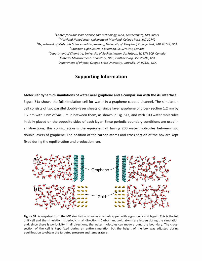
Molecular dynamics simulations of water near graphene and a comparison with the Au interface.

Figure S1a shows the full simulation cell for water in a graphene-capped channel. The simulation

cell consists of two parallel double-layer sheets of single layer graphene of cross- section 1.2 nm by

1.2 nm with 2 nm of vacuum in between them, as shown in Fig. S1a, and with 100 water molecules

initially placed on the opposite sides of each layer. Since periodic boundary conditions are used in

all directions, this configuration is the equivalent of having 200 water molecules between two

double layers of graphene. The position of the carbon atoms and cross-section of the box are kept

fixed during the equilibration and production run.

Figure S1. A snapshot from the MD simulation of water channel capped with a graphene and b gold. This is the full unit cell and the simulation is periodic in all directions. Carbon and gold atoms are frozen during the simulation and, since there is periodicity in all directions, the water molecules can move around the boundary. The cross-section of the cell is kept fixed during an entire simulation but the height of the box was adjusted during equilibration to obtain the targeted pressure and temperature.

We also perform MD simulations for gold-capped, water channels, see Fig.S1b. Here, the

simulation cell consists of two sheets of gold each of cross-section 1.24 nm by 1.24 nm separated

by 1.58 nm of vacuum on one side and 291 water molecules on the other. Each sheet has three

layers of gold atoms that are frozen during the simulation, where we use the (100) surface of the

face-centered cubic (fcc) structure. The parameters for the van der Waals interaction between gold

and water are from the Ref. 1. The remaining simulation details are the same as the graphene-

capped water channel. Our model does not take into account polarization of the metal due to

interaction with water. Individual water molecules can produce a significant image potential on

gold. For large numbers of water molecules, however, this image potential becomes insignificant

due to the averaging out of dipole orientations2. Other studies show that polarization does not

have a significant effect on interfacial water structure3. Since the dominant effect in gold is the

screening of the core hole, any small structural change due to polarization or other interactions will

not substantially change the XAS spectrum.

For determining whether two water molecules are hydrogen bonded, we use the criteria that

the oxygen-oxygen distance is less than 0.35 nm and the oxygen-oxygen-hydrogen angle is less than

35° (see Ref. 4). The molecules are counted as double donor (DD), single donor (SD), and non-donor

(ND) when the number of hydrogen atoms contributing to hydrogen bonds is two, one, and zero,

respectively (Figure S2).

Figure S2. a, Density profile for water adsorbed on graphene and gold as a function of distance from the interface. In both cases, oscillations are induced by the presence of the surface, with gold giving rise to slightly stronger oscillations than graphene; b, Hydrogen bonds per water molecule vs. distance, 𝑧, from the

graphene/gold surface. The number of hydrogen bonds rapidly approaches the bulk value away from the surface. Nearby the surface, however, the number of hydrogen bonds is depleted by about 25 %.

Oxygen K-edge XAS Calculations

The OCEAN code requires the one-electron wavefunctions of the ground-state system as an input for the

Bethe-Salpeter equation (BSE). For this we use density functional theory (DFT) within the local density

approximation as parameterized by Ceperley, Alder, Perdew, and Wang5. We make use of the

QuantumESPRESSO code6, and take advantage of an efficient k-point interpolation scheme7. The BSE

approach retains two electron-hole interaction terms in addition to the non-interacting DFT

Hamiltonian; the attractive direct and repulsive exchange. We calculate these explicitly using a

combination of a local and a real-space basis. A pseudopotential inversion scheme is necessary to

reconstruct the all-electron character of the DFT conduction-band states near the core hole5. Within the

BSE, the dielectric response of the system screens the direct interaction, for which we take the random

phase approximation coupled with a model dielectric function to capture the long-range response8.

Figure S3. The changes in the XAS water spectra with averaging over the first 16, 32, or 48 water molecules for both a water interfacing graphene and b water interfacing gold. While both become more bulk-like as further water molecules are included, the changes in the spectrum of the gold-interfacing water are much more dramatic. Spectra are y-offset for clarity of presentation.

We use an energy cut-off of 952 eV (70 Ryd.) for the DFT calculations and calculate DFT states at the

Gamma point. The k-point interpolation scheme expands this to a 2 × 2 × 2 k-point mesh for the x-ray

calculations. For the graphene surface we use a 1.2 nm by 1.2 nm by 4.0 nm box containing 128 water

molecules and 132 carbon atoms. For the gold this was changed to a 1.224 nm by 1.224 nm cross

section with 36 gold atoms. The screening calculation uses 9000 bands, covering a range of 100 eV

above the Fermi level. The BSE states include 5100 bands of which approximately 4456 (4390) were

unoccupied for the graphene (gold) surface cells – with a metallic surface layer not all k-points will have

the same number of occupied bands. The local basis for calculating the exchange and short-range

components of the direct interaction consists of four projectors per angular momentum channel for s-d

and three for f. The real-space basis is a regular 24 × 24 × 80 grid. The bulk cells contain 226 water

molecules within a 1.8 nm by 1.8 nm by 2.1287 nm box and the real-space basis is a 32 × 32 × 40 grid. All

other parameters are the same as for the cells with surfaces. The long-range part of the dielectric

response to the core-hole potential is calculated using a model dielectric function. For all three setups,

we used the bulk water dielectric constant of 1.8.

The reduced strength of the post-edge feature in the O K edge of water is commonly observed

in both the BSE calculations used here9 and the delta-SCF approach used in other work10. This is due to

the fact that the pre-edge and main-edge features (originating from 4a1 and 2b2 of isolated molecule)

are localized and therefore their relative intensities are highly sensitive to details of the potential. The

latter one depends sensitively on inaccuracies in screening of the core-hole potential.

Despite this, changes in the calculated spectra in response to changes in structure, from bulk

water to water on a surface, can be meaningfully compared to changes measured in experiment. In Fig

2c we show that, despite the structural changes due to the graphene bi-layer, the O K-edge XAS changes

only slightly compared to that of bulk water.

Details of the BLU analysis

As mentioned in the main text, the number of spectral components for BLU analysis must be

provided by the researcher and can be estimated using principal component analysis (PCA) or by under-

and oversampling. Figure S4 presents a case of oversampling: unmixing the PEEM spectral dataset of

Figure 3 (main text) into 6 components. As can be seen, the two new component arise due to the

splitting of C2 and C4 into two parts. The new component C2' (Fig. S4 b&h) is very similar to the old C2

both in its abundance map and its spectrum. The C2'' component (Fig. S4 c&i), though, is different, and

clearly unnecessary. Its average abundance across the map is only about 30 %, and its contribution to

the overall picture is higher than 70 % in only a few pixels. The endmember of the C2'' component (Fig.

S4i) has slanted shape with several tiny carbon and oxygen peaks. Overall, this component does not add

to the understanding of the sample’s behavior and should not be separated from C2'.

The C4'-C4'' pair, on the other hand, presents a much more physically meaningful picture

despite oversampling. These components highlight the core and peripheral sites of two water-filled

channels with prominent radiolysis. The difference between their spectra (Fig. S4 k&l) is perfectly clear

in the light of the main text explanations of the water redistribution and bubble formation processes.

The core of the cell is affected by bubble formation earlier than the periphery, and therefore the

spectrum of the peripheral component C4'' (Fig. S4l) is closer to the normal water spectrum (Fig. S4j),

than that of the core component C4' (Fig. S4k). The C4' spectrum plummets at 536.5 eV, whereas the

C4'' intensity drops later, at 337.7 eV. Since the bubble radial expansion is a gradual process, and BLU

considers data at every pixel as a linear combination of position-independent components, the total

number of independent components correctly describing a behavior of dynamic water channels should

be equal to the number of pixels in the cell radius. Yet, as shown in the main text, their behavior can be

understood by unmixing the dataset into only four components.

Figure S4. BLU of a PEEM spectroscopic dataset into 6 components: C1 - panels a & g empty channels and aperture; C2' - panels b & h MCA walls; C2'' - panels c & i weaker signal of MCA walls & contaminants; C3 - panels d & j water-filled static channels; C4' - panels e & k water-filled dynamic channels cores; and C4'' - panels f & l water-filled dynamic channels periphery. Abundance maps (component intensity as a fraction of unity) and

corresponding endmember spectra are shown. The scale bar is 10 µm. Spectra are displayed on the same scale for comparison.

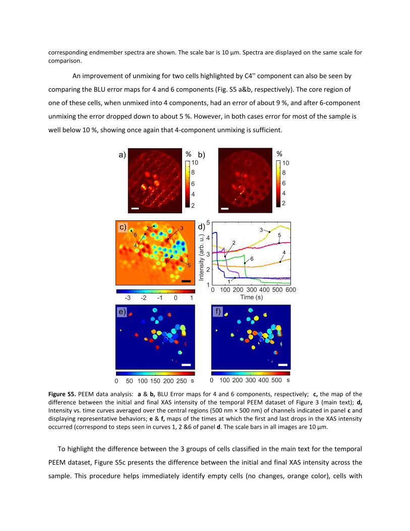
An improvement of unmixing for two cells highlighted by C4'' component can also be seen by

comparing the BLU error maps for 4 and 6 components (Fig. S5 a&b, respectively). The core region of

one of these cells, when unmixed into 4 components, had an error of about 9 %, and after 6-component

unmixing the error dropped down to about 5 %. However, in both cases error for most of the sample is

well below 10 %, showing once again that 4-component unmixing is sufficient.

Figure S5. PEEM data analysis: a & b, BLU Error maps for 4 and 6 components, respectively; c, the map of the difference between the initial and final XAS intensity of the temporal PEEM dataset of Figure 3 (main text); d, Intensity vs. time curves averaged over the central regions (500 nm × 500 nm) of channels indicated in panel c and displaying representative behaviors; e & f, maps of the times at which the first and last drops in the XAS intensity occurred (correspond to steps seen in curves 1, 2 &6 of panel d. The scale bars in all images are 10 µm.

To highlight the difference between the 3 groups of cells classified in the main text for the temporal

PEEM dataset, Figure S5c presents the difference between the initial and final XAS intensity across the

sample. This procedure helps immediately identify empty cells (no changes, orange color), cells with

increasing intensity (red color) and cells where the signal drops (blue color). For comparison, Figure S5d

also presents XAS intensity vs. time plots from several cells in panel c. Note that although the curve of

cell 6 has steps similar to those of cells 1 and 2, its final intensity is much lower. This is a consequence of

the cell 6 spatial position in the region of the sample where excitation irradiation is lower than in the

central regions, where cells 1 and 2 are located. When normalized to the local irradiation intensity, the

curves look similar and their final intensity values are very close.

Figures S5e and f also present spatial maps of times at which the first and last step-like drops in

intensity occurred. Despite the individual cells proximity to each other, they appear to behave

independent of one another, which suggests that they do not exchange liquid through the frontal or

backside MCA surface leakage.

In principle, the oxidation of the graphene membrane with radiolysis products (H2O2, OH˙, O˙) may

result in the loss of membrane integrity and water evaporation into the ambient vacuum. Such events

can be discriminated from the bubble formation cases by their lowest TEY intensity from the disrupted

channels.

The formation of the “wetting layer” and supporting SEM studies

Attenuation estimations

The ratio between the signal intensity produced by n monolayers of water to the intensity produced by

bulk water is given by:

, (1)

where h is the thickness of n water monolayers, and λw is the inelastic mean free path of electrons in

liquid water. Experimental intensities can be written as: and

, where α is the attenuation coefficient associated with the graphene membrane,

and Ig = I2 is the signal originating in the graphene. Thus, the number of water layers corresponding to

the I1 step is:

, (2)

where a = 0.25 nm was used as an effective thickness of a water monolayer. The numerical value of N

depends on the electron inelastic mean free path in water which has not been unequivocally

determined yet. 11,12 Assuming Auger electrons (Ek ≈ 500 eV)13 to be the fastest and dominant fraction in

𝐼𝑤𝑛

𝐼𝑤∞= 1 − 𝑒

−ℎ𝜆𝑤

𝐼0 = 𝐼𝑤∞ ∙ 𝛼 + 𝐼𝑔

𝐼1 = 𝐼𝑤𝑛 ∙ 𝛼 + 𝐼𝑔

𝑁 = −𝜆𝑤𝑎∙ 𝑙𝑛 (1 −

𝐼1 − 𝐼2𝐼0 − 𝐼2

)

the TEY signal having the largest inelastic mean free path, Figure 3f presents a map of the number of the

I1-step water layers calculated taking λw = 2.5 nm.

SEM experiments

Similar to x-rays, liquid water in the sealed micro-channel may undergo a radiolysis, with the formation

of bubbles, evaporation, re-condensation and extensive diffusion upon electron beam irradiation.

Figures S6a and S6b demonstrate SEM snapshots taken two seconds apart with several empty channels,

one of which is covered with graphene membrane, and a water-filled channel at the center. The SEM

signal intensity across the images can be classified into several regions having characteristic gray scale

regions: brightest MCA surface (1), darkest MCA channels with no graphene (2), regions with strong

water signal (3), pristine graphene membrane (4) and regions with weak water signal (5). Notice that the

pristine graphene membrane signal (4) has the same value both in the open empty channel and the

water-filled channel (Fig.S6 b). The water distribution within the central channel is very dynamic upon

electron beam irradiation, drastically changing over 2 seconds: patches of dry graphene not only

significantly grow in size, but also change shapes, merging into one large domain. The circular geometry

of the channel allowed us to introduce polar coordinates as shown in Figure S6a, to average SEM signal

over the polar angle and present it in the form of a 2D time-r-distance diagram in Figure S6c. This

diagram, as well as its sections shown in Figure S6d, clearly demonstrate the same „quantized“ behavior

of the water signal very similar to that we observed in the time-resolved PEEM data. Between the SEM

signal levels of the MPC walls (largest) and graphene (lowest), there are two spatially separate and

distinct levels of gray scale value, labeled as a “thick water“ and a “thin water“, that presumably

correspond to bulk water and one monolayer of water, respectively. Their spatial distribution is also

quite similar to that observed in the PEEM data, the “thick water“ towards the periphery and “thin

water“ covering the center part of graphene. The presented SEM images also imply the possible

existence of sub-monolayer water layers (in Fig. 3f (main text) cores of some channels contain 0.5 to 0.8

monolayers): an apparent sub-monolayer is a spatial mix of dry graphene regions and monolayer-

covered patches that PEEM cannot resolve spatially.

Figure S6. SEM imaging of MCA-G devices: a and b, images of an MCA-G region with a water-filled channel (center), several empty channels, and an empty channel with a suspended graphene membrane (right part of images) as captured 2 seconds apart during the water redistribution process (images taken from the video in SI). The signal intensity on the MCA wall (1) is 140 to 150 units, in empty channels (2) is 40 to 50 units, the thick water layer in the filled channel (3) is 120 to 130 units, the thin water layer in the filled channel (5) is 98 to 103 units, and on the empty graphene membrane (4) is 80 to 85 units; c, SEM intensity averaged over the full circle (angle θ in a) and plotted as a function of radius-vector (r in a) distance and time; d, Selected radial profiles from panel c for three different times showing signal strength for the MCA wall, graphene and two discrete water thicknesses formed during the redistribution process. The scale bars in a and b are 10 µm.

The channels topography

The topography of the graphene capped channels depends on a few factors: the media behind the

channel (empty, liquid, bubble) and residence time in vacuum. Figure S7 shows the shape of graphene

membrane in a water-filled, empty, and bubble containing channels as measured in AFM tapping (AC)

mode under vacuum conditions. Both topographic images and their cross-sections (Fig. S7 bottom raw)

imply that graphene is sufficiently strongly adhered to the liquid surface in the filled cell and takes a

concave shape with a typical stretch between 200 nm and 500 nm for this diameter of the channel. In

the empty channel the graphene membrane is flat, recessed ca. 150 nm lower than the MCA top plane.

The concave shape of the capped filled channel is a result of the leakage induced pressure drop inside

the channel from atmospheric (just after the channel sealing) to saturated vapor pressure (ca. 2 kPa)

when in vacuum.

Figure S7. AFM topographic images of MCA-G devices in vacuum: a water-filled channel a, an empty channel with suspended graphene membrane b; a filled channel with bubble formed under graphene c; The bottom row depicts the corresponding topographic profiles measured along the selected lines (top raw). Note that Height and Width axes are not on the same scale.

The detailed mechanisms of bubble formation under hydrophobic graphene is a subject of the ongoing

research. Based on our SEM and PEEM observations, the bubble formation in MCA platform is strongly

radiation dose dependent implying that radiolysis is a major mechanism. Briefly, when X-ray photons

with the energies of 540 eV (O K- absorption edge) irradiate water inside the channel under the grazing

angle, a high density of radicals is created within very thin (L ≈500 nm, soft X-ray 540 eV attenuation

length) water layer. The multiple reaction and recombination paths result in primary accumulation of

molecular hydrogen in this layer.14 Under conditions when the recombination reactions and runaway

diffusion of hydrogen are slower compared to its generation rate, concertation of hydrogen under the

graphene grows until the saturation concertation of hydrogen in water is achieved. The latter depends

on the pressure inside the channel. Oversaturation above this concertation causes stochastic formation

of a microbubble.

X-rays induced bubble formation thresholds

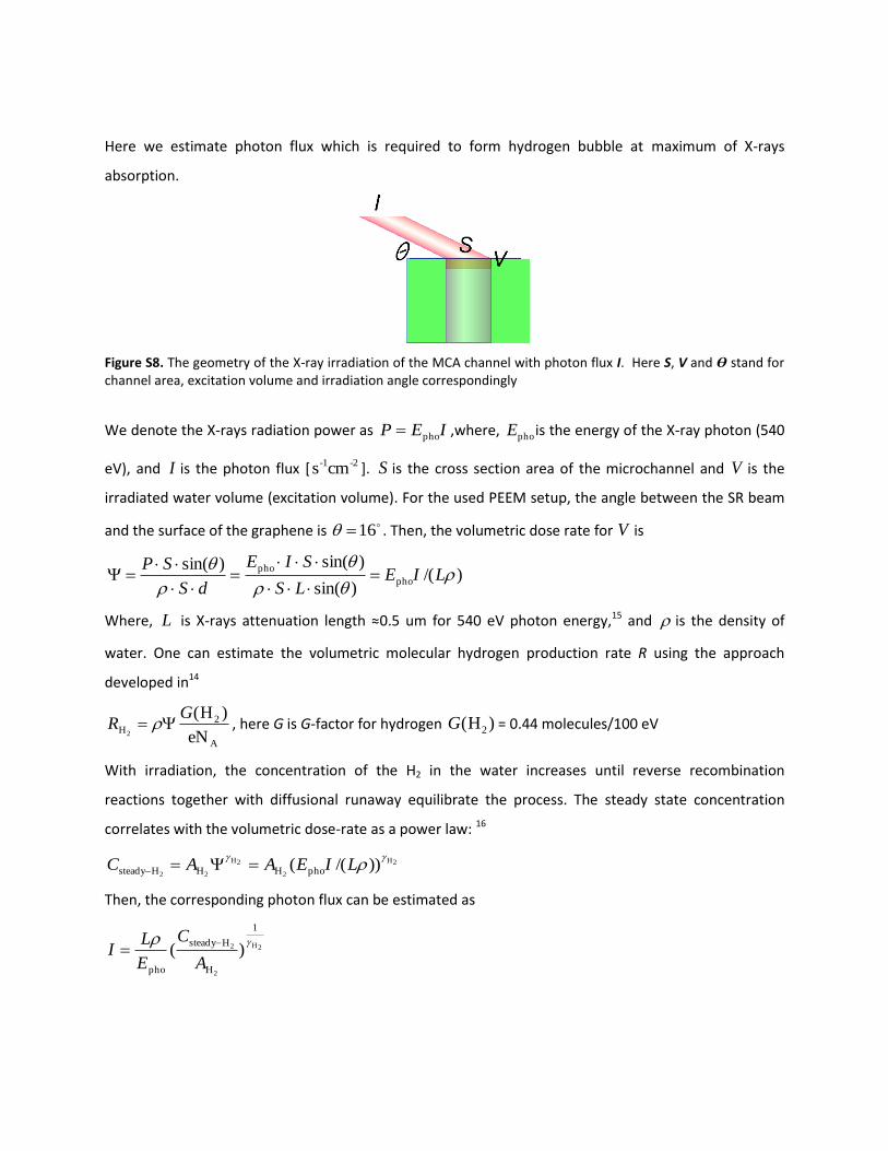
Here we estimate photon flux which is required to form hydrogen bubble at maximum of X-rays

absorption.

Figure S8. The geometry of the X-ray irradiation of the MCA channel with photon flux I. Here S, V and ϴ stand for channel area, excitation volume and irradiation angle correspondingly

We denote the X-rays radiation power as IEP pho ,where, phoE is the energy of the X-ray photon (540

eV), and I is the photon flux [ -2-1cms ]. S is the cross section area of the microchannel and V is the

irradiated water volume (excitation volume). For the used PEEM setup, the angle between the SR beam

and the surface of the graphene is 16 . Then, the volumetric dose rate for V is

)/()sin(

)sin()sin(pho

pho

LIE

LS

SIE

dS

SP

Where, L is X-rays attenuation length ≈0.5 um for 540 eV photon energy,15 and is the density of

water. One can estimate the volumetric molecular hydrogen production rate R using the approach

developed in14

A

2H

eN

)H(2

GR , here G is G-factor for hydrogen )H( 2G = 0.44 molecules/100 eV

With irradiation, the concentration of the H2 in the water increases until reverse recombination

reactions together with diffusional runaway equilibrate the process. The steady state concentration

correlates with the volumetric dose-rate as a power law: 16

2H

2

2H

22))/(( phoHHHsteady

LIEAAC

Then, the corresponding photon flux can be estimated as

2H

2

2

1

H

Hsteady

pho

)(

A

C

E

LI

The onset of a bubble formation via homogeneous nucleation requires very large supersaturation over

2HsteadyC and experimentally measured value is L

mmol 190~2Hh omogC .17 On the other hand,

heterogeneous nucleation of H2 at water-graphene interface may occur at any value below 2Hh omogC as

soon as 2HsteadyC exceeds the saturation concertation Csat of molecular hydrogen in water. 17

The latter, however, depends on the pressure inside the channel via Henry’s Law for H2 in water. We do

not know the pressure inside the channel exactly but for evaluation purposes can use two ultimate

values: saturated water vapor pressure (2 kPa) or atmospheric pressure (100 kPa).

Then, assuming Csat(2 kPa) ~ 2.1x 10-5

Lmol , and Csat(100 kPa) ~ 0.8x 10-3

Lmol

2H

2

-7

H (s/Gy)L

mol103.9~A , 44.0~

2H for water at PH 616 one can get:

2-111

kPa)2( cms107 I , 2-115

kPa)100( cms103 I This two numbers have to be compared to the

photon flux in our experiment: 2-11615

exp cms1010 I (depending on alignment) and to the flux

required for homogenous bubble nucleation:

2-120

hom cms108 ogI .

As can be seen, the radiolytic hydrogen bubbles can indeed be created under our experimental

conditions, and the presence of the graphene interface facilitates this process. To reduce the radiolytic

effects few procedures can be undertaken:

a) The channel’s design has to be fluidic thus the radiolysis products can be rapidly removed from

the excitation volume

b) The pressure inside the cell can be elevated to increase Csat

c) Working with harder X-rays with lower photo-absorption cross section.

References

1. Schravendijk, P.; van der Vegt, N.; Delle Site, L.; Kremer, K., Dual‐Scale Modeling of Benzene Adsorption onto Ni (111) and Au (111) Surfaces in Explicit Water. ChemPhysChem 2005, 6 (9), 1866-1871. 2. Shelley, J.; Patey, G.; Bérard, D.; Torrie, G., Modeling and structure of mercury-water interfaces. The Journal of chemical physics 1997, 107 (6), 2122-2141. 3. Kohlmeyer, A.; Witschel, W.; Spohr, E., Molecular dynamics simulations of water/metal and water/vacuum interfaces with a polarizable water model. Chemical physics 1996, 213 (1), 211-216.

4. Luzar, A., Resolving the hydrogen bond dynamics conundrum. The Journal of Chemical Physics 2000, 113 (23), 10663-10675. 5. Perdew, J. P.; Wang, Y., Pair-distribution function and its coupling-constant average for the spin-polarized electron gas. Physical Review B 1992, 46 (20), 12947. 6. Giannozzi, P.; Baroni, S.; Bonini, N.; Calandra, M.; Car, R.; Cavazzoni, C.; Ceresoli, D.; Chiarotti, G. L.; Cococcioni, M.; Dabo, I., QUANTUM ESPRESSO: a modular and open-source software project for quantum simulations of materials. Journal of physics: Condensed matter 2009, 21 (39), 395502. 7. (a) Prendergast, D.; Louie, S. G., Bloch-state-based interpolation: An efficient generalization of the Shirley approach to interpolating electronic structure. Physical Review B 2009, 80 (23), 235126; (b) Shirley, E. L., Optimal basis sets for detailed Brillouin-zone integrations. Physical Review B 1996, 54 (23), 16464. 8. Shirley, E. L., Local screening of a core hole: A real-space approach applied to hafnium oxide. Ultramicroscopy 2006, 106 (11), 986-993. 9. Vinson, J.; Kas, J. J.; Vila, F. D.; Rehr, J. J.; Shirley, E. L., Theoretical optical and x-ray spectra of liquid and solid H2O. Physical Review B 2012, 85 (4), 045101. 10. (a) Velasco-Velez, J.-J.; Wu, C. H.; Pascal, T. A.; Wan, L. F.; Guo, J.; Prendergast, D.; Salmeron, M., The structure of interfacial water on gold electrodes studied by x-ray absorption spectroscopy. Science 2014; (b) Prendergast, D.; Galli, G., X-Ray Absorption Spectra of Water from First Principles Calculations. Phys. Rev. Lett. 2006, 96 (21), 215502. 11. Nikjoo, H.; Uehara, S.; Emfietzoglou, D.; Brahme, A., Heavy charged particles in radiation biology and biophysics. New Journal of Physics 2008, 10 (7), 075006. 12. Ottosson, N.; Faubel, M.; Bradforth, S. E.; Jungwirth, P.; Winter, B., Photoelectron spectroscopy of liquid water and aqueous solution: Electron effective attenuation lengths and emission-angle anisotropy. Journal of Electron Spectroscopy and Related Phenomena 2010, 177 (2–3), 60-70. 13. Slavíček, P.; Kryzhevoi, N. V.; Aziz, E. F.; Winter, B., Relaxation Processes in Aqueous Systems upon X-ray Ionization: Entanglement of Electronic and Nuclear Dynamics. The Journal of Physical Chemistry Letters 2016, 7 (2), 234-243. 14. Grogan, J. M.; Schneider, N. M.; Ross, F. M.; Bau, H. H., Bubble and Pattern Formation in Liquid Induced by an Electron Beam. Nano Letters 2014, 14 (1), 359-364. 15. Technology, N. I. o. S. a., X-Ray Form Factor, Attenuation and Scattering Tables (version 2.1). Chantler, C.T., Olsen, K., Dragoset, R.A., Chang, J., Kishore, A.R., Kotochigova, S.A., and Zucker, D.S. : Gaithersburg, MD., 2005. 16. Joseph, J. M.; Seon Choi, B.; Yakabuskie, P.; Clara Wren, J., A Combined Experimental and Model Analysis on the Effect of pH and O2(aq) on Γ-radiolytically Produced H2 and H2O2. Radiat. Phys. Chem. 2008, 77. 17. Finkelstein, Y.; Tamir, A., Formation of Gas Bubbles in Supersaturated Solutions of Gases in Water. AIChE journal 1985, 31, 1409.