Knut H. Alfsen and Knut E. Rosendahl

Economic Damage of AirPollution

96/17 August 1996 Documents

Statistics NorwayResearch Department

Documents 96/17 • Statistics Norway, August 1996

Knut H. Alfsen and Knut E. Rosendahl

Economic Damage of AirPollution

Abstract:The paper considers available information on physical dose-response functions related to air pollutionand damage of human health and important materials. The dose-response functions are translated intoa form suitable for implementation in multi-sectoral computable general equilibrium models (CGEs) andsimulations are carried out illustrating the direct and indirect (allocation) costs of environmental damageto human health and materials on economic growth in Norway. The model is further supplementedwith a module relating the volume of road traffic to traffic accidents and their consequences on labourproductivity and public health expenditures.

Keywords: Air pollution, externalities, valuation.

JEL classification: Q25, H51, D62.

Address: Knut H. Alfsen, Statistics Norway, Research Department,P.O.Box 8131 Dep., N-0033 Oslo, Norway. E-mail: kha@ssb.no

Knut E. Rosendahl, Statistics Norway, Research Department,E-mail: ker@ssb.no

Economicactivity,emissions

GE model [Dispersiorimodel

Physical"7:1/44 effects on

health,• materials,

crops, etc.

rDose-responsefunctions

Concentration,exposure

J

Impacts on-70 economic

variables...

<<Translation

1 Introduction

Statistics Norway has previously made some tentative assessments of the cost of air pollution asso-ciated with damage to forests, fresh water lakes, human health and some important materials. Theassessments were mainly based on opinions obtained from expert panels together with empiricalstudies carried out in the U.S. in the 1970's, see Glomsrod and Rosland, 1988 [19], Brendemoenet al., 1992 (71 , Alfsen et aL, 1992 [3], Alfsen, 1993 [2], and Alfsen and Glomsrod, 1993 [5]. Theseassessments were linked to economic and emission forecasts generated by integrated economic,energy and emissions models, in order to study future development in air pollution damage andthe likely impacts of various policies (e.g. carbon taxes) on the level of the damage.

Lately a new consensus have emerged on some of the effects of air pollution on human health,and further studies have been carried out to measure the geographical distribution of buildingmaterials and the pollution induced corrosion of these materials. Based on this new knowledgeit is now possible to take some further steps in assessing the economic costs of air pollution.The main aim of this paper is to outline what we currently are doing in Statistics Norway onthe topic of health damage and damage to materials from excessive air pollution. This work isdocumented in detail (and - unfortunately - so far only in Norwegian) in Rosendahl (1996) [45],Glomsrod, Rosendahl and Hansen (1996) [18] and Glomsrod et al. (1996) [20]. The basis for thework is national and international studies on the physical effects of air pollution. We then convertthese estimates into forms suitable for inclusion in economy wide models, in order to capture notonly the direct cost of air pollution, but also the allocation or general equilibrium effects of thedamage. Economic activity in turn determines emission to air and hence pollution concentration.The effects of pollution then closes the circle, see figure 1.

Figure 1: Framework for environmental damage assessment

Only the "pure" economic costs of air pollution, i.e. the effect of air pollution on labour supplyand productivity, on public health expenditures and on maintenance and investments in capital,are considered. In addition we have included a module calculating the effects of road traffic on traf-fic accidents and their impact on labour productivity and public health expenditures (Glomsrod,Nesbakken and Aaserud, 1996 [17]). What is left out by this approach are the welfare effects (notcaptured by the market economy) of health damage due to air pollution and traffic accidents.Combined with the fact that we only cover a rather small fraction of the many economic effects ofair pollution, it is clear that the numbers we arrive at represents a considerable underestimate ofthe total cost of air pollution and the use of fossil fuels. Nevertheless, the numbers are of interestsince they provide a relatively secure or conservative lower limit to which policy makers and otherscan add their own judgement of the importance of welfare effects and other types of damage notcurrently well documented in the literature.

The paper is organised as follows (see table 1 and figure 1). In the first part, we consider theeffects of air pollution on human health. We start by describing the calculation of the relevantexposure of people to concentration of PM 10, NO2, 03, and 502. We then go on to discuss theeffects of this exposure on mortality and morbidity. These physical effects are then translated intoeconomic variables, like loss of working hours and public health expenditures. These relations are

3

implemented in a multi-sectoral general equilibrium model of the Norwegian economy in order toassess also the allocation costs of the induced health effects.

In the second part we follow a similar path for material damage of air pollution, now mainlyrelated to the exposure of various materials to SO2, but also to some extent covering the effects of03. The third part briefly describes the traffic accident module, while part four reports on somesimulations carried out with an integrated economy-energy-environment model with and withoutthe feedbacks described above.

Health Materials ScenariosEmissions PMio, NO2, 03, SO2 SO2, 03Exposure Population weigthed Material density weighted

Dose-response Mortality: -Short term Material loss Physical-Long term .L scenario

Morbidity: -RADs (MRADs) Economic life time-Resp. symptoms-COPD

Economic Labour supply Maintenance or"damage" Public expenditures replacement cost

( "Welfare")Effects Macro model implementation--+ Economic

cost of factor use, productivity—*emissions--+ economic effects

scenario

Table 1: namework for assessing environmental damage of air pollution

Part IHealth effects

2 Emissions

The polluting compounds considered for their effects on human health in this paper compriseparticulate matter (PM10), nitrogen dioxide (NO2), ozone (03), and sulphur dioxide (S02) 1 .

3 Exposure to air pollutants

There is disagreement and uncertainty about how to best measure the exposure of the populationto air pollution. Some argue for measuring mean concentration levels over certain periods, whileother measures the number of hours the concentration level is above a critical level. In moststudies of dose-response functions, mean concentration levels over one or a few days are employedin studies of acute health effects, while chronic effects are related to the mean concentrationlevel over semiannual or longer periods. In applied studies these measures are then convertedto annual mean concentration levels. This is possible given that the dose-response functions arelinear without any threshold levels. Most of the studies find this to be a reasonable approximationfor the effects and pollutants covered in this paper, and we will follow this custom here. Thereare, however, evidence in some cases (e.g. in the case of NO2 pollution) that shorter episodes withhigh concentration levels are of greater importance. In that case, our approach will underestimatethe effects of these episode related events.

Oslo is the capital and largest city in Norway, and population exposure to air pollutants istreated in a detailed manner for this region. A dispersion model (EPISODE developed by TheNorwegian Institute for Air Research — NILU) is used together with information on populationdensity to derive population weighted annual mean concentration levels for particulate matterin the form of PM10, i.e. particles with diameter less than 10 AM, and nitrogen dioxide (NO2)

1 The presentation relies heavily on Rosendahl (1996) [45] where more details and discussions of the variousassumptions used can be found.

4

(Walker, 1996 [55]). For other large population centres in Norway we have, in consultation withNILU and based on concentration measurements, extended the procedure to obtain the functionalrelationships reported in table 2 and 3. The urban areas covered represent some 30 per cent ofthe total population of Norway.

City Annual mean concentration of PM 10 () Level in 1992(a)

Oslo 4.2 -/T+5.3 -/F+3.7-/Km+4.0-/R+6 23.2Bergen 0.7•/T+7.0•/F+0.6•/Km+2.7-/R+4 15Trondheim 1.1 - iT + 7.9 - IF +1-0 ' -TKM + 2.0 - IR+ 3 15Stavanger 1.1 - /T + 5.2 - IF +1-0 ' IKM + 2.7 - IR+ 5 15Drammen 1.9 - /T + 5.4 - IF + 1.7 - IKM + 5.0 - IR+ 6 20Skien 1.3 -/T+ 7.5 -/F+1.2 -/Km+4.0-/R+6 20Porsgrunn 1.5 - /T + 7.2 - IF + 1.3 - /Km + 4.0 - IR+ 6 20Baerum 1.0-/T+2.1-/F+0.9•/Km+5.0•/R+6 15

Table 2: Person weighted mean annual concentration of PM 10 in 8 Norwegian cities.

City Annual mean concentration of NO2 () Level in 1992(7,77,3)

Oslo 14.6 - IT +2.1 - IF + 16.1 - l'Et + 13.2 46Bergen 11.8 - /T + 2.1 - /F + 16.1 - /B + 10.0 . 40llondheim 10.8 - /7- + 3.2 - /F + 13.0 - /B + 8.0 35Stavanger 6.9 • /T + 1.0 • /F + 16.1 - /B + 11.0 35Drammen 8.3 - /T + 0.5 - /F + 18.0 - /B + 13.2 40Skien 9.8 - /7, + 0.9 - /F + 16.1 - /B + 13.2 40Porsgrunn 2.9 - IT + 7.8 - IF + 16.1 - /B + 13.2 40Brum 3.4 - IT + 0.4 - IF + 18.0 - /B + 13.2 35

Table 3: Person weighted mean annual concentration of NO2 in 8 Norwegian cities.

In the tables, IT is an index of emissions from traffic, IF is an index of other local emissions,IKA1 is an index of the number of km driven (of relevance because of the use of studded tires inNorway), IR is an index of Norwegian regional emissions (e.g. outside Oslo), while Ig is an indexof the background concentration determined by foreign emissions. All indices take on the value of1 in the year 1992.

4 Dose-response functions: effects on health

Several human health related effects of air pollutants are considered in this paper: From mortality,through restricted activity days (RADs) and days with respiratory symptoms (RS) to chronicobstructive pulmonary diseases (COPD). The occurrence of these effects will sometimes lead tohospital admittance with associated costs, and often to a reduction in the productivity of thelabour force (depending among other things on the age structure of those affected). The generalstructure of the dose-response functions are as follows:

Mortality:

AD = 5 - AC. (1 )

Chronic obstructive pulmonary diseases:

ACOPD v - AC. (2)

COPDEffect on the number of days with respiratory symptoms and/or restricted activity days (RADs)

per year:

ALS = As • AC - P

(3 )

5

Effect on number of hospital admissions per year:

ALSH = 71H • AC • P (4)

Here D is the number of deaths per year and C designates the concentration of the relevantpollutants (measured in µg/m3) averaged over a relevant period. We will report both short term(acute) and long term effects. Of these, the short term effect is the better documented. COPD isthe number of new diagnoses of chronic obstructive pulmoray diseases. LS is the number of daysper year with respiratory symptoms or number of restricted activity days, and P is the numberof people exposed to the pollutants. LSH is the number of hospital admissions with respiratorysymptoms per year.

The parameters in the dose-response functions are taken from a number of studies. The mostcentral are Ostro (1987) [32], Ostro (1993) [341, Krupnick et al. (1990) [27], Pope (1991) [39] andAbbey et al. (1993) [1]. ORNL/RFF (1994) [30], Rowe et al. (1995) [47] and the EC (1994)[13] studies are also mainly based on these reports. Below, we will report on the dose-responsefunctions we have chosen and provide some brief remarks related to the specific parameter values.For further discussions and arguments for the particular choices, see Rosendahl (1996) [45]. Severalof the parameter values are highly uncertain. Therefore only a restricted subset of the relationsreported in this part of the paper will actually be implemented in the macroeconomic model. Wewill return to this in part four of the paper.

4.1 Particulate matter

Particulate matter comprise a large family of particles of varying sizes and chemical compositions.Studies of the health effects of air born particles have chosen to relate the observed effects todifferent measures of exposure, like for instance PM10 and PM2.5 (concentration of particles withdiameters smaller than 10 and 2.5 Am, respectively), TSP (total suspended particles - coveringall size fractions), sulfate and soot (the latter defined by the way it is measured - blackeningof filters). As already mentioned, the period of the measurements also varies, from a few hoursto several years. In the literature it is common practice to convert all of these measures to astandardized variable; annual mean concentration of PM3.0 measured in -1 2- . This is of course asimplification which introduce some additional uncertainty into the results, since the time profileand composition of particle pollution varies somewhat from place to place.

Table 4 provides the parameter values we employ in this paper together with references. Theuncertainty ranges (given in parenthesis) must be understood as very tentative. Usually they referto ±one standard deviation in the relevant studies.

Health effects of PMio Coefficient(per annual mean

concentrationof PMio(„,1))

Sources

Acute risk of death 0.96-10-3 Ostro (1993) [34](short term exposure) (0.63-1.30)-10-3

Risk of death 6.5-10-3 WHO (1995) [56](long term exposure) (4.6-9.1)-10-3

Annual number of restricted 57.5-10-3 Ostro (1987) [32]activity days (RADs) per person (36-90)-10-3 ORNL/RFF (1994) [30]

Annual number of days with 0.18 Krupnick et al. (1990) [27]respiratory symptoms per person (0.09-0.27) Ostro (1994) [35]

Annual hospital admittances with 36-10-6 Various studies, seerespiratory symptoms per person (12-102)•10-6 Rosendahl (1996) [45]

Risk for chronic obstructive 11.10-3 Abbey et al. (1993)pulmonary diseases (COPD) (5-17)-10-3 Rowe et al. (1995)

Table 4: Dose-response functions for particulate matter (PMio)•

6

Of all the health effects of air pollution, acute increase in mortality from particulate matter isprobably one of the best documented. Furthermore, there now seems to have emerged a consensuson the quantitative effect on mortality of short term exposure to particulate matter. Thereis evidence for claiming that it is the size of the particles, and not for instance the chemicalcomposition, that is usually of most importance for acute changes in mortality (Pope et al., 1992[40], Fairley, 1991 [14], Ostro, 1995 [36]). The people most affected by short term increases inexposure to particle pollution are elderly people (i.e. above approximately 65 years old) (see e.g.Schwartz and Dockery, 1992 [49]).

Far fewer studies have focused on the long term effects on mortality of exposure to particulatematter. The parameter in table 4 is taken from WHO (1995) [56] who refer to two cohort studies(Dockery et al., 1993 [10], and Pope et al., 1995 [41]). These studies find that the long term effectof exposure to particulate matter is from 5 to 10 times larger than the short term effects. Theresults are, however, more uncertain than the corresponding results for the short term effects.

It is important to interpret the mortality coefficients in table 4 correctly. The coefficients arerelated to changes in risk of death within for instance a period of one year due to changes in theconcentration of particulate matter. The actual number of deaths provoked by a change in theconcentration level will thus also depend on the time profile of mortality in the population.

The effects of exposure to particulate matter on the number of restricted activity days (RADs)have been studied by Ostro (Ostro 1983 [31], 1987 [32], 1990 [33], Ostro and Rothschild, 1989 [37]).According to ORNL/RFF (1994) [30], 62 per cent of the RADs represent lost working days, whilethe remaining are designated as minor restricted activity days (MRADs). These are assumed hereto reduce the labour productivity by 10 per cent.

Krupnick et al. (1990) [27] have carried out a study of the number of days with respiratorysymptoms as a function of exposure to particulate matter. The result, as reported by Ostro (1994)[35] and Rowe et al. (1995) [47], is given in table 4, however corrected for the number of RADs inorder to avoid double counting.

The dose-response function for number of hospital admittances as a function of exposure toparticulate matter reported in table 4, is based on a number of studies. These are discussed inmore detail in Rosendahl (1996) [45]. The final outcome is a dose-response function 3 times largerthan the function reported in Pope et al. (1991) [39].

Abbey et al. (1993) [1] reports significant correlations between the long term exposure toparticulate matter and the occurrence in the population of chronic bronchitis, asthma or emphy-sema, which are the three most common forms of chronic obstructive pulmonary diseases (COPD).The result, transformed to relations between PM 10 concentration and COPD, is given in table 4.These results are further corroborated by other studies (see Rosendahl, 1996 [45]). We note thatin principle there may be some overlap between short term and long term morbidity dose-responsefunctions. However, in the case of COPD, the main and strongly dominant effect is due to thelong term nature of the disease. Thus, the double counting of the acute effect represents only avery minor part of the total effect.

4.2 Nitrogen dioxide (NO2 )

In contrast to the case of particulate matter, relatively few epidemiological studies have foundany significant association between (outdoor) NO2 exposure and health effects. However, clinicaltrials and studies of indoor exposure to NO2 clearly indicates that such exposure is harmful.It is possible, however, that the main damage by NO2 is infficted by short term exposure tohigh concentration levels. This could explain why it may be difficult to obtain significant resultsfrom epidemiological studies which mainly relies on longer term mean concentration levels asexplanatory pollution related variable. In table 5 we list some dose-response functions found inthe literature.

Of particular interest is the study of hospital admittances due to asthma which was carriedout in Finland, a country with a similar climate to Norway. The results of this study is furtherconfirmed by another Finnish study (Rossi et al., 1993 [46]).

4.3 Sulphur dioxide (SO2)

Most studies of the health effects of SO2 have been carried out in areas with considerable higherconcentration levels than found in Norwegian cities, which have typical concentration levels of

7

Health effects of NO2 Coefficient(per annual mean

concentrationof NO2(.))

Sources

Risk for hospital admittancedue to asthma

Risk for hospital admittancedue to croup

Annual number of days withrespiratory symptoms per person

26-10-1

4.10-3

9.10-3(5-13)-10-3

Piink5. (1991) [44]

Schwartz et al. (1991) [48]

Schwartz and Zeger (1990) [50]

Table 5: Dose-response functions for NO2.

the order of 15 -15 or lower. Also, emissions of SO2 leads to the creation of sulphate in theatmosphere which properly belong to the group of small particles (PM2.5). In several studies theapparent health effects of SO2 disappear when particle concentrations are measured correctly. Itis thus unclear whether SO2 has any major independent health effects. Although we list somedose-response functions in table 6, we will not use them further on in this paper.

Health effect of SO2 Coefficient(per annual mean

concentrationof S02(4))

Sources

Risk of death

Annual number of days withrespiratory symptoms per person

480.10-6

10.10-3

Ostro (1994) [35],ORNL/RFF (1994) [30]

Ostro (1994) [35),ORNL/RFF (1994) [30]

Table 6: Dose-response functions for SO2.

4.4 Ozone (03)

Ozone is a so called secondary air pollutants which is created in a reaction between NO z , methane(CH4) and non-methane volatile organic compounds (NMVOC) in the atmosphere. Contraryto the situation in many other countries, the 0 3 concentration in Norway is mainly determinedby transboundary transport from the European continent. In fact, higher emissions of NO 2 inNorwegian cities is likely to reduce the concentration of 03 in the city centers, but increase thelevel somewhat in the surroundings. Since we in this paper are mainly concerned with the effectsrelated to Norwegian activities, we disregard at this stage the effects of 03 on health. However,table 7 reports some dose-response functions for ozone found in the literature.

The concentration level in the dose-response functions related to mortality refers to maximummean hourly level over a day, while the level in the function for MRADs, respiratory symptomsand hospital admittances refer to the annual mean of these concentration values. The coefficientfor MRADs is an average of the results found in the two refered studies.

4.5 Summary of dose-response function

Table 8 provides a summary of some of the parameters entering the dose-response functions forthe health effects of air pollution.

5 Transformation to economic variables - labour productiv-ity

The next step is to transform the physical information contained in the dose-response functionsto economic information on the direct costs associated with the various health effects. We do this

8

Health effects of 03 Coefficient(per mean

concentrationof 03(4))

Sources

Risk of death 75.10-6 EC (1994) [13],Kinney et al. (1994) [26]

Annual number of minor restrictedactivity days per person (MRADs)

12.10-3 Ostro and Rothschild (1989) [37],Portney and Mullahy (1986) [42]

Annual number of days withrespiratory symptoms per person

26.10-3 EC (1994) [13]

Annual hospital admittances withrespiratory symptoms per person

3.9-10-6 Thurston et al. (1992) [53]

Table 7: Dose-response functions for 03.

Health effects P1■410 NO2 SO2 03Acute mortality (5)COPD (v)RAD/MRAD (As)Resp. symptoms (As)Hosp. admittance (77H)

0.96-10°'11.10°3

57.5-10-3180.10-336.10°6

9.10-3

26.10°6

0.48-10°'

10.10-3

75.10°'

12.10°326-10-3

3.9-10°6

Table 8: Summary of parameters in dose-response functions for health effects.

for each pollutant in turn.

5.1 Particulate matter (PMio)

5.1.1 Mortality

People who die because of short term increases in the concentration of particulate matter, aremainly older people who do not participate in the labour force (Schwartz and Dockery, 1992 [49]as cited in Rowe et al., 1995 [47]). Also small children are suscestible to short term exposure toparticulate matter. This group represents, however, only a very minor part of all those who diesin Norway. For these reasons we will not assign an economic productivity loss to increased riskof mortality from short term exposure to particulate matter. We should not forget, however, theconsiderable welfare loss associated with this effect. We will briefly touch upon this issue later on.

The more recent studies of the effects of long term exposure to particulate matter on mortalityfind that also people in the labour force are affected. In a study by Dockery et al. (1993) [10], thepopulation between 25 and 74 years of age was divided into groups each covering a 5 year span.Job related exposure to dust and gases was identified and controlled for. In the study, the effect oflong term exposure was found to affect all ages more or less equally. Mostly, the mortality effectwas through lung cancer and respiratory diseases. Below, we illustrate how the information onphysical effects are translated into effects on some economic variables.

In Norway in 1993, 330 people died from malign tumors in the respiratory organs. Thisrepresented 3.6 per cent of all deaths in this year, and the mean age of this group was 57.6 years.Thus, they had on average 7.4 years left before retiring. In addition 1552 people in the 25-64 yearsage range died of diseases in the cardiovascular and respiratory systems, representing 56.4 per centof all deaths. Their mean age were 56.2 years, leaving 8.7 years to retirement. Combining thesetwo groups, we have 1882 deaths due to the illnesses mostly associated with particle pollutionwith an average time to go before retirement of 8.5 years. Dividing the number of hours workedin 1993 (2.87 billion) by the population in the age bracket from 20 to 70 years (2.70 million), wefind that the average numbers of hours worked per person in 1993 was 1061. This is probablya reasonable estimate of the annual hours worked for the age group we are most concerned with(55-65 years old).

Total hours of work loss because of the conditions mentioned above then amounts to (1882deaths) x (8.5 years to retirement) x (1061 hours worked per year per person) = 17 million hours.

9

Combined with the dose-response function in table 4, and taking into account that 60 per cent ofthe total number of deaths was related to the two classes of diseases mention above, and finallyassuming that only these conditions are affected by exposure particulate matter, we find thefollowing effect on hours worked due to changes in PM10 concentration:

AL = -17.10 6 • APMio = -187.10 3 - APMio - —6.5 - 10-3 P

0.6 B

(5)

where L is the numbers of hours worked, jits the fraction of the total population exposed toparticulate matter concentrations and APA40 is the change in the long run PM10 level measuredin Dividing by the number of hours worked in 1993 (2.87 billion) we can write this relation 2

as

AL= -65 - 10-6 - APM10• — (6)

Since there is considerable uncertainty to several of the steps in the above calculation, notleast with respect to the age structure of the mortality increase due to an increase in the PM 1 0concentration level, the final effect on the labour supply is also highly uncertain. For this reasonwe have at this stage decided against including this relation in the macroeconomic model.

5.1.2 Restricted activity days (RADs)

According to ORNL/RFF (1994) [30], 38 per cent of the restricted activity days are so calledminor restricted activity days (MRADs). In the same study the cost of a MRAD was estimated tosomewhat more than 4 of the wage. Given than this estimate also covers some welfare effects, weassume that the labour productivity loss associated with one MRAD is 10 per cent. The averageproductivity loss of RADs can then be calculated as (0.62 • 1 + 0.38 - 0.1) = 65.8 per cent. Wefurther assume that the RADs are uniformly distributed among working days and holidays. Inthe latter case we do not experience any effects on the labour productivity. According to thedose-response function for RADs (table 4), a unit increase in PM10 concentration increases theaverage number of RADs per year per person by 57.5-10-3 . Measured per day, this translates into57.5-103 = 0.16-10-3 . On a working day the productivity is, as mentioned, reduced by 65.8 per cent365for each RAD. Thus the effect of a unit increase in PM 10 concentration on labour productivity isgiven by 0.16-10-3 - 0.658 = 1.04 - 10-4 , i.e.

AL -104. 10-6 . APM10 - B-

•

(7)

5.1.3 Respiratory symptoms

The dose-response function for respiratory symptoms has already been adjusted to avoid overlapwith the occurrence of restricted activity days. Eskeland (1995) [12] assumes that each day withrespiratory symptoms leads to a loss of labour productivity of 6 per cent. Following the sameprocedure as in the previous paragraph, we then obtain

AL= -29.6 - 10-6 ARMio - B . (8)

5.1.4 Chronic obstructive pulmonary diseases (COPD)

This is the only chronic effect of long term exposure to particulate matter that we have included.We assume that the change in the occurrence of COPD (given by the dose-response function intable 4) leads to a proportional change in number of people on sick leaves 3 , number of people inrestitution programs and number of people permanently disabled with this diagnosis. From theNorwegian health authorities, we have obtained data on the money paid for, or the number of

2 1t is also possible, by use of Norwegian life tables, to transform the above results into reductions in expectedlength of life. The result is AFV = =o . 005694)APM10, where the upper (lower) coefficient refers to the female(male) part of the population and AFV is the change in expected life times measured in years due to changes inthe concentration level of PMio-

3 0nly sick leaves longer than 14 days are registered.

10

people in, the three categories by diagnosis in 1993 and 1994. Using the average hourly wage (sickleaves and restitution) and the average number of hours worked per person in the age group 20-70years (disableness), we obtain the following relations between changes in hours worked and thethree conditions of COPD patients

AL —242 - 10-9 - APM10 -

B due to sick leaves (9)

AL —1.34 10-6 - PM() - 75' due to restitution

AL —24.1 •• 10-6 - AP/1/10 •• due to disableness.

The study used for the underlying dose-response function (Abbey et al., 1993 [1]) was conductedover a ten years period. Thus, AP/Ulm is interpreted as changes in the ten years average PMioconcentration. A change in particle emissions today will therefore affect the labour force for thenext ten years.

5.2 Nitrogen dioxide (NO2)

The dose-response function for respiratory symptoms from NO2 exposure can be translated intoeffects on hours worked in a similar manner to the procedure applied to the PM io dose-responsefunction. The result is

ALL

= —1.51 .10`6 . LINO2 - - (10)

Here, ANO2 is the change in annual mean level of NO2 measured in . The NO2 concentrationlevel in Norwegian cities is approximately twice the level of PMio, which implies that the effect ofNO2 on the labour force is very much smaller than the corresponding effect of PM10. This makesthe problem of potential double counting of effects small.

5.3 Sulphur dioxide (SO2)

The dose-response function for days with respiratory symptoms is, as mentioned before, highlyuncertain. Nevertheless, we — for completeness — transform it in a manner similar to the aboveprocedure to obtain:

AL= —1.64 -10-6 AS02

5.4 Ozone (0 3 )

Although we will not utilize it further on, we — again for completness — list the effects of 0 3 onthe labour productivity. We have two relations. For minor restricted activity days (MRADs) wefind

ALL

= —3.4 - 10-6 • A 03 - , (12)

assuming a 10 per cent decrease in productivity for each MRAD. Respiratory symptoms areassumed to give a 6 per cent decrease in productivity, leading to the following relation for loss ofworking hours:

AL = —2.3 - 10-6 - ,A03 - (13)

11

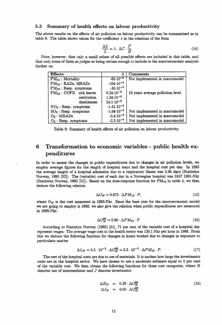
5.5 Summary of health effects on labour productivity

The above results on the effects of air pollution on labour productivity can be summarized as intable 9. The table shows values for the coefficient A in the relations of the form

AL= A - AC - —

B. (14)

Note, however, that only a small subset of all possible effects are included in this table, andthat only some of them as judges as being certain enough to include in the macroeconomic analysisfurther on.

Effects A CommentsPM10 : Mortality -65.10-6 Not implemented in macromodelPM10 : RADs, MRADs -104.10-6PM10 : Resp. symptoms -30.10-6PAID) : COPD sick leaves 0.24-10-6 10 years average pollution level

restitution 1.34-106disableness 24.1-10-6

NO2 : Resp. symptoms -1.51-10-6SO2 : Resp. symptoms -1.64-10-6 Not implemented in macromodel03 : MRADs -3.4-10-6 Not implemented in macromodel03 : Resp. symptoms -2.3-10-6 Not implemented in macromodel

Table 9: Summary of health effects of air pollution on labour productivity.

6 Transformation to economic variables - public health ex-penditures

In order to assess the changes in public expenditures due to changes in air pollution levels, weemploy average figures for the length of hospital stays and the hospital cost per day. In 1993the average length of a hospital admission due to a respiratory illness was 5.96 days (StatisticsNorway, 1995 [52]). The (variable) cost of each day in a Norwegian hospital was 3187 1991-Nkr(Statistics Norway, 1993 [51]). Based on the dose-response function for PM 10 in table 4, we thendeduce the following relation

LAOH = 0.675 - APAlio . P, (15)

where OH is the cost measured in 1993-Nkr. Since the base year for the macroeconomic modelwe are going to employ is 1988, we also give the relation when public expenditures are measuredin 1988-Nkr.

A081.13 = 0.60 - APMio • P. (16)

According to Statistics Norway (1993) [511, 71 per cent of the variable cost of a hospital dayrepresent wages. The average wage cost in the health sector was 130.1 Nkr per hour in 1988. Fromthis we deduce the following function for changes in hours worked due to changes in exposure toparticulate matter

ALH = 5.5 - 10-3 . A081 = 3.3 - 10-3 - AP/tfio . P. (17)

The rest of the hospital costs are due to use of materials. It is unclear how large the investmentscosts are in the hospital sector. We have chosen to use a moderate estimate equal to 5 per centof the variable cost. We then obtain the following functions for these cost categories, where Hdenotes use of intermediates and J denotes investments

AHH = 0.29 - A01.1§ ( 18)

AJH = 0.05 •A081.

12

If we assume that the increase in number of hospital days due to chronic obstructive pulmonarydisease (COPD) varies linearly with the occurrence of COPD, and combining this with the in-formation that in 1993 there were 28.3 hospital days per 1000 inhabitants with the diagnosis ofCOPD, we can deduce the following cost function related to COPD

DOS = 0.87 • APM10 • P. (19)

Here, APAlio is to be interpreted as change in the concentration level averaged over a 10 yearperiod.

Regarding hospital admittance due to asthma, we found a 1.5 per cent increase per unit increasein NO2 concentration (table 5). In 1993 there were on average 8.7 hospital days per 1000 peoplewith the diagnosis of bronchitic asthma. Following the same procedure as above, we obtain thefollowing cost function related to this diagnosis

A0819 = 0.37 - ANO2 • P. (20)

The effects on wage-, intermediates- and investment cost are as above (eq. 18).The coefficients for the air pollution induced variable costs in the public health sector

11081 = K• AC•P (21)

are summarized in table 10.

nPMio

Acute 0.60Chronic 0.87

NO2Asthma 0.37

Table 10: Summary of effects on the variable costs in the public health sector.

7 Welfare effects

All the health effects explored above of course have important welfare effects in addition to theeconomic losses incurred. To value these welfare effects is, however, extremely difficult (andperhaps even impossible). For illustrative purposes it may nevertheless be of interest to mentionsome monetary values in this connection, although we would warn against using these numbersuncritically in a decision making process. Rather one should then use the results on the physicaleffects contained in the dose-response functions.

There exist an estimate of the value of a statistical life developed in connection with trafficaccidents in Norway (Elvik, 1993 [11]) which is given as 10.5 million 1993-Nkr (approximatelyequal to 1.6 million US$). It may be discussed how relevant this value is for deaths due to airpollution, as for instance the age distribution of such deaths is very different from deaths due totraffic accidents. The value is, however, meant to capture only the welfare effects of the risk fordeaths. International studies seem often to use higher values, see e.g. Pearce (1995) [38]. Withthe dose-response function for mortality associated with short term exposure to PM 10, and witha general mortality rate in the population of 1.04 per cent, we get the following expression for thewelfare effects of PM10 mortality

AV = 105 - AP./tho • P, (22)

where V is measured in 1993-Nkr.We can also illustrate the welfare effect of higher risks for chronic respiratory diseases by noting

that Rowe et al. (1995) [47] is using an estimate of 210 000 1992-US$ based on willingness to paystudies. This corresponds to an amount approximately equal to 1.5 million 1994-Nkr.

13

Part IIMaterial damageMost materials placed in a polluted atmosphere will experience corrosion over and above whatwould occur in a (hypothetical) clean atmosphere. It is mainly the exposure to sulphur and ozonethat creates the damage, but also other compounds (e.g. NO z) may induce additional corrosion.Here we concentrate on the effects of SO2 and 03.

Pollution levels, climatic conditions and material densities all varies from region to regionand thus induce differences in corrosion rates and the cost of corrosion. We have chosen to treatconditions in Oslo in a very detailed manner, and used a cruder methodology for other urban areasin Norway. In Oslo, we have, through dispersion modelling, available information on air pollutionconcentration levels within a 500 x 500 m grid. Also, we know the coordinates, size and use of everybuilding in this area. From special surveys (to be discussed below), we know the typical materialcomposition of buildings employed for different purposes, and can thus deduce the distribution ofmaterial densities across the grids of Oslo. In other urban areas, the material densities are deducedfrom other types of statistics, such as manufacturing, agricultural, population and employmentstatistics.

8 Exposure to climate, SO2 and 03

The concentration of SO2 in the atmosphere is the sum of a background concentration level, Sb,and contributions from local emissions U

S = Sb e•U, (23)

where Sb is measured in e, U is local emissions of SO2 measured in metric tonnes, and e is aparameter relating emissions to concentration levels.

Ozone concentration in the city centres, where most of the material is concentrated, is generallya declining function of the NO2 concentration level (Kucera et al., 1995 [29]). We model the 03level in Oslo by the following function

O = 60.5 • e-o.o14-[NO21, (24)

where [NO2] is the concentration level measured in 5- . In other regions than Oslo, the ozone levelsare assumed constant and equal to typical observed values. Table 11 gives climatic conditions andconcentration levels of SO2 and 03 in the regions of Norway. The values for Oslo are from atypical grid site in the city. In the table, [SO2] and [03] are concentration levels of SO2 and 03,respectively, Tye is the time of wetness measured as the fraction of a year when relative humidityexceeds 80 per cent and the temperature is above 0°C, R is the amount of precipitation measured

in 71-1 and H+ is the acidity of the precipitation measured as 721 12-1--.+- rain.year 7 1

9 Exposed material

The amount of exposed material is based on a study by Kucera et al. (1993) [28]. The study, whichis the most comprehensive existing, surveyed in a detailed manner material densities of differenttypes of buildings in Praha, Stockholm and the Norwegian town Sarpsborg. These results havebeen extrapolated to national numbers for Sweden (Anderson, 1994 [61) and to Europe (Cowelland ApSimon, 1994 [9]). From these studies it is possible, together with national statistics andbuilding registers, to estimate the amount of materials in urban areas in Norway. Figure 2 showsthe result for Oslo. Glomsrod et al. (1996) [20] provides discussion of the methodology employedand detailed results for all Norwegian regions.

10 Material loss due to corrosion and the lifetime functions

Annual maintenance cost of materials (K) can be written

14

Regions , [SO2] (,-a5) ' {03} (ii.) 1-1± (92 ) RZr ) TwHalden 5 55 0.040 0.80 0.38Sarpsborg 16 50 0.032 0.88 0.39Fredrikstad 7 50 0.032 0.79 0.38Moss 5 55 0.032 0.81 0.40Bwrum 6 45 0.032 0.82 0.39Asker 5 45 0.032 0.94 0.41Oslo 15 30 0.025 0.60 0.32Drammen 6 43 0.032 0.95 0.34Porsgrunn 5 55 0.032 0.92 0.33Skien 14 55 0.032 0.85 0.33Bamble 3 53 0.032 0.87 0.33Kr.sand 3 54 0.040 1.38 0.49Stavanger 6 60 0.032 1.25 0.70Bergen 7 62 0.020 2.25 0.53Trondheim 5 55 0.008 0.93 0.41Troms0 2 55 0.010 1.03 0.24Urban south 3 55 0.031 1.03 0.42Urban north 2 55 0.010 1.03 0.24Rest of the country 1 40 0.031 1.03 0.42

Table 11: Climatic conditions and pollution levels in Norwegian regions. The values for Oslo arefrom a typical grid site in the city center.

20000

16000

16000

14000

12000

100:0

8000

6000

4000

2000

0 11:1 11feti

KIT* t

1 I. - I I I3. 3 7,3 ;147,3ctit " gE

I Cr. •

Figure 2: Materials in Oslo, 1000 m2 .

15

KM - P (25)

L

where M is the amount of material of a given type measured in m2 , P is the price of maintenanceor replacement measured in and L is the time period between maintenance or replacement.L is here also denoted the lifetime of the material.

The lifetime is a function of amount of material lost due to corrosion which in turn is dependenton the external environment, in particular the exposure to air pollution. Of particular importancein this respect is the exposure to sulphur dioxide (S02) and ozone (03). However, also climaticconditions play a role, in particular humidity, precipitation and the acidity of the precipitation.Extensive studies of material corrosion, as for instance summarized in Haagenrud and Henriksen(1995) [21], together with assumptions on when maintenance or replacement is necessary, makes itpossible to derive lifetime functions. It is found that a functional form of the following form givesa good fit to the experimental data (see Glomsrod et al., 1996 [18] for further documentation,references and discussions):

L (S, 0) = (b + c Tw - 0) S + d H± R + e

where a, b, c, d and e are material specific constants, S and 0 are concentration levels of 502 and03, respectively, measured in mq.. Tye , R and H+ have the same meanings as before. Table 12gives values for the constants in eq. 26 and also shows the types of materials covered.

Materials a b c d I eZink plated steel plate, replacement 30 0.0015 2.82 0.51Zink plated steel plate, maintenance 20 0.0015 2.82 0.51Zink plated steel wire 30 0.0015 2.82 0.51Zink plated steel profile 60 0.0015 2.82 0.51Zink plated steel, sealed 1000 0.155 38.6Zink plated steel, sealed and painted 1000 0.37 64.3Zink plated steel, painted 1000 0.803 84.5Painted steel 1000 1.37 108Copper roofing 100 0.00031 4.575 0.542Aluminium, sealed 1000 0.107 32.6Aluminium, sealed and painted 1000 0.37 64.3Plaster 1000 0.124 15.7Painted plaster 1000 0.278 19.9Painted/stained wood 1000 1.03 91.4Roofing paper 1000 0.327 48.9Brick If S < 10 Ag lm3 , then the lifetime is 70 years,

else 65 years.Concrete If S < 10129/m3 , then the lifetime is 50 years,

else 40 years.

Table 12: Constants in the lifetime function.

Of the materials listed in the table, zink plated sealed and painted steel, painted steel andsealed and painted aluminium are not included in the macroeconomic simulations presented laterin this paper.

11 The price of maintenance/replacement

Table 13 shows the maintenance or replacement costs employed in this study. The prices havebeen obtained by an informal survey of prices in the Oslo region in 1995.

12 The costs of corrosion

From the expression for the annual maintenance cost (eq. 25), the table 12 giving the lifetimefunctions and the prices in table 13, we can calculate the corrosion cost associated with air pollution

a (26)

16

Material Prices (9)Zink plated steel plate, replacement 275Zink plated steel plate, maintenance 150Zink plated steel wire 105Zink plated steel profile 300Zink plated steel, sealed 150Zink plated steel, painted 300Copper roofing 450Aluminium, sealed 150Aluminium, sealed and painted 150Plaster 350Painted/stained wood 80Roofing paper 160Painted plaster 250Brick 300Concrete 525

Table 13: Prices of maintenance or replacement exclusive of taxes. 1995-Nkr per m 2 .

levels above "natural" background levels (S6 , 06)

Kf = M - P 1

(27)[1,(;,0) L (Sb,0b)]

Marginal cost from changes in the concentration level of SO2 is then given by

arc b + c Tw - 0Ksa- --a7 =M-P (28)

a

while the marginal cost from changes in local emissions of SO2 is given by

ax b + c Tw - 0 Ku P (29)

8U a

Due to the linearity of the functions, the marginal costs are independent of concentrationand local emission levels. However, they depend on the interpretation of "local" or "natural"background, i.e. they depend on the parameter e in eq. 23.

Two interpretations are natural. One is that the background concentration is due to emissionsin all other regions than the one under consideration, e.g. including emissions in foreign countriesand in other domestic regions. Although this is perhaps the most natural interpretation, it isdifficult to make operational since we generally do not know the transport matrix aii between theregions used in this study. An alternative interpretation is to consider the background as that dueonly to foreign emissions. However, the concept of marginal costs then will have a rather specialmeaning since it in this case will reflect the increase in local costs due to a proportional increasein emissions in the whole of Norway.

Generally, we have that the concentration level in region i is determined by

Si = E aijUi sib tu ,-1-- aiiUi (30)jE{regions}

where Sii" is the background concentration due to foreign emissions and ST' i denotes the back-ground due to emissions in other regions of Norway. The element aii corresponds to the parametere above. We know Si and Sib'', while SIP' and aii are unknown. As a simplification we in thisstudy put SIPi equal to zero and determine aii = e by eq. 30:

b uE = (31)

Ui

By neglecting Siki , e is biased upwards by —&-7, and the marginal costs due to local emissionsoverestimated correspondingly. It should be noted, however, that SO2 is generally not transportedover long distances as such, and therefore the above approximation may not be too bad.

17

Table 14 gives the SO2 emission levels, estimated total corrosion costs due to these emissionsand the marginal costs associated with an increase in the emission of SO2 based on the data andformulas above.

Region Emission of SO2 1994(Metric tonnes SO2)

Cost(Mill. 1995-Nkr)

Marginal costsg2kr)

Halden 68_

1.77 - 26.17Sarpsborg 1 669 5.36 3.21ftedrikstad 885 2.41 2.73Moss 664 1.56 2.34Baerum 119 7.11 59.90Asker 62 2.57 41.28Oslo 1 051 74.40 70.81Drammen 74 3.84 51.65Porsgrunn 556 2.08 3.73Skien 229 13.15 57.49Bamble 24 0.48 19.91Kristiansand 1 008 2.13 2.12Stavanger 277 8.62 31.11Bergen 262 22.61 85.98Trondheim 674 9.23 13.70Tromso 108 0.80 7.48Urban south 17 886 34.76 1.94Urban north 5 798 3.56 0.61Rest of Norway 13 120 1.29 0.10Total 44 543 197:73 4.44 (averaged)

Table 14: Emissions, costs and marginal costs of material damage by regions.

It is seen from the table that the marginal costs varies widely between regions. This is notsurprisingly, given that Norway is a sparsely populated country where much of the most polluting(power intensive) industries are located in remote areas. The national average marginal cost of4.44 Nkr per kg SO2 reported in table 14, is somewhat high compared to results from other studies,see Calthrop and Pearce (1996) [8]. However, several studies in their sample show marginal costsup to 13 Nkr per kg S02.

Table 15 shows how the marginal costs are distributed by type of emission sources. Processemissions, i.e. emissions not related to stationary combustion of fossil fuels, account for more thanhalf of the total emissions in 1994, but are associated with only a quarter of the corrosion costs.This is due to the localisation of the power intensive industry in Norway in relatively remote areas.Emissions from mobile sources, mainly diesel powered automobiles, have the highest marginal cost.

Emissions1000 tonnes

CostsMill. 1995-Nkr

Marginal costsNkr/kg

Process 19.2 47.2 2.5Stationary 7.9 63.5 - 8.0Road 3.2 39.9 12.6Rail 0.1 0.4 5.1Airplanes 0.1 0.6 4.5Ships 13.4 41.9 . 3.1Other machinery 0.6 4.2 7.2

, Total/average 44.5 197.7 4.4

Table 15: 502 emissions by source type and material corrosion costs in 1994.

Based on the marginal cost information, it is also possible to calculate the gains obtainedover the 10 years period from 1985 to 1994 when Norway experienced strong reductions in SO2emissions. The result, excluding the allocation cost 4 associated with material damage, is given in

4 The allocation costs are calculated to have been 233 million 1994-Nkr in 1985 and 93 million Nkr in 1994, thus

18

table 16.

Emission of SO2(1000 metric tonnes)

Total costs(Mill. 1994 Nkr)

19851994

97.444.5

496198

Reduction 1985-1994 61.3 298

Table 16: Emissions and total material costs due to corrosion in 1985 and 1994.

Part IIITraffic accidentsEffects of a similar kind to those discussed above, but not directly associated with a deterioratedenvironment, are road traffic accidents. These are strongly correlated with the use of fossil fuels,and have predominantly effects on labour supply and productivity, and public health expenditures,given that we neglect welfare effects. Fridstrom and BjØrnskau (1989) [15j have carried out adetailed empirical study of possible explanatory variables for traffic accidents with person injuriesin Norway. Controlling for climatic variations, road standards, traffic density and special securitymeasures, they find that a 10 per cent increase in gasoline consumption leads to 8-9 per centincrease in traffic accidents with injuries. Moreover, they find that higher road standards withless traffic density increase the number of accidents with injuries. This finding is also supportedby an older Danish study (Vejdirektoratet, 1979 [54]). Thus there seems to be a trade off betweencongestion costs and the cost of injuries from traffic accidents. Here, we only consider the costsof accidents.

Table 17 gives some key numbers related to traffic accidents in Norway.

Persons affected Loss of man-years 1Traf6.c accidents 33 900

Deaths due to traffic accident(also in previous years)

332 7 254

Sick leaves first year after accident 1 350Sick leaves due to children's accidents 167Productivity loss due to trafficaccidents in the last 10 years

1 346

50 per cent disabled due to trafficaccidents in previous years

272 2 888

100 per cent disabled due to trafficaccidents in previous years

477 10 146

Total 23 151

Table 17: Some key annual numbers related to traffic accidents in Norway in 1990.

Loss of man-years due to people killed in the traffic is of the order of 7 000. The average age ofthose killed in the traffic is quite low; the length of the expected active participation in the workforce is 38 years for those killed. Sick leaves and productivity losses for those in work representeach about 1 300 man-years, while 13 000 man-years are lost each year due to varying degrees ofinvalidity following traffic accidents. Thus, over 23 000 man-years are lost each year due to trafficaccidents in Norway. The breakdown of traffic accidents according to seriousness, sick leaves anddisableness is described in Haukeland (1991) [23], while Hagen (1993) [22] has analysed the costsassociated with the various categories of person injuries from traffic accidents.

representing an additional annual saving of 104 million N kr.

19

13 Traffic accidents in a macroeconomic model

The effects of traffic accidents are implemented in the macroeconomic models of Statistics Norwayin the following manner.

Use of fuels (gasoline and diesel) are projected by the macroeconomic models. This is translatedto kilometer driven by the following formulas

KMG =mG . Gt - eect ,

(32)

KM") = mD - Dt - eept , (33)

where MG 'D are average number of kilometres driven per tonnes of gasoline and diesel, respectively,calibrated in the base year. The energy efficiency of vehicles increase by fixed annual rates OG ' D ,while G and D represent the demand for the two types of fuels. Traffic density (CONt) isdetermined by the ratio between kilometres driven and the total length of roads

KMG + KM?CONt = t

ROADSt (34)

The growth of the variable ROADS is exogenously determined as an exponentially decreasingfunction fitted to historical data from the period 1966 to 1993, and planned extensions for theperiod 1994-1997.

The number of persons injured in traffic accidents is modelled as follows:

S= K (Kmffy (Kmpy5 °ON: yr(35)

Here, K is a constant, while e6t represents a trend due to factors not covered in this analysis.A fraction of the number of people injured in traffic accidents are productive workers. Thusthe accidents leads to reduced supply or productivity of the labour force through sick leaves orpermanent losses due to deaths or disabilities.

The temporary loss of manpower is modelled as follows:

9

ALT = )37St--7 + (C + 6)(st — so)

(36)7=0

The first term on the right hand side represents productivity loss in year t due to traffic accidentsin the last 10 years. The last term represents loss due to own accidents and children's accidentsthis year.

Permanent loss of manpower due to deaths (ALn and invalidity (ALP) are given by

Luir =ri (St— So),

ALP = A (St-1 — So) • (38)

The permanent reduction in the labour force accumulates according to

= zuf + ALf + ALr 1 . (39)

Total reduction of the labour force in year t is calculated as the sum of temporary and perma-nent reductions:

ALt = ALT + ALT. (40)

We let the total treatment cost of traffic victims vary with number of victims. Thus, in themodel simulations the number of traffic accidents will influence on the otherwise exogenouslydetermined health service production level. The demand for input factors in the health sector isthen given by

Gi,t = (St — So) , i = labour, materials, capital. (41)

20

Glomsrod, Nesbakken and Aaserud (1996) [17] discuss and documents the coefficients appearingin the above equations.

Part IV

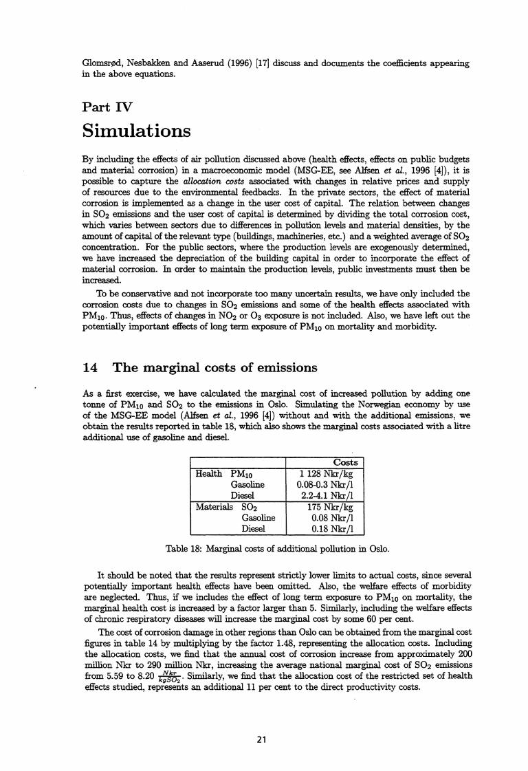
SimulationsBy including the effects of air pollution discussed above (health effects, effects on public budgetsand material corrosion) in a macroeconomic model (MSG-EE, see Alfsen et al., 1996 [4]), it ispossible to capture the allocation costs associated with changes in relative prices and supplyof resources due to the environmental feedbacks. In the private sectors, the effect of materialcorrosion is implemented as a change in the user cost of capital. The relation between changesin SO2 emissions and the user cost of capital is determined by dividing the total corrosion cost,which varies between sectors due to differences in pollution levels and material densities, by theamount of capital of the relevant type (buildings, machineries, etc.) and a weighted average of SO2concentration. For the public sectors, where the production levels are exogenously determined,we have increased the depreciation of the building capital in order to incorporate the effect ofmaterial corrosion. In order to maintain the production levels, public investments must then beincreased.

To be conservative and not incorporate too many uncertain results, we have only included thecorrosion costs due to changes in 502 emissions and some of the health effects associated withPM10. Thus, effects of changes in NO2 or 03 exposure is not included. Also, we have left out thepotentially important effects of long term exposure of PM10 on mortality and morbidity.

14 The marginal costs of emissions

As a first exercise, we have calculated the marginal cost of increased pollution by adding onetonne of PM 10 and 502 to the emissions in Oslo. Simulating the Norwegian economy by useof the MSG-EE model (Alfsen et al., 1996 [4]) without and with the additional emissions, weobtain the results reported in table 18, which also shows the marginal costs associated with a litreadditional use of gasoline and diesel.

CostsHealth PMio

GasolineDiesel

1 128 Nkr/kg0.08-0.3 Nkr/1

2.2-4.1 NIcrilMaterials SO2

GasolineDiesel

175 Nkr/kg0.08 Nkr/10.18 Nkr/1

Table 18: Marginal costs of additional pollution in Oslo.

It should be noted that the results represent strictly lower limits to actual costs, since severalpotentially important health effects have been omitted. Also, the welfare effects of morbidityare neglected. Thus, if we includes the effect of long term exposure to PM 10 on mortality, themarginal health cost is increased by a factor larger than 5. Similarly, including the welfare effectsof chronic respiratory diseases will increase the marginal cost by some 60 per cent.

The cost of corrosion damage in other regions than Oslo can be obtained from the marginal costfigures in table 14 by multiplying by the factor 1.48, representing the allocation costs. Includingthe allocation costs, we find that the annual cost of corrosion increase from approximately 200million Nkr to 290 million Nkr, increasing the average national marginal cost of 502 emissionsfrom 5.59 to 8.20 kNgsko% Similarly, we find that the allocation cost of the restricted set of healtheffects studied, represents an additional 11 per cent to the direct productivity costs.

21

1.4

1.3

1.2

1.1

1aoaD

..c!! 0.9

0.8

0.7

0.6

0.5

FM1 0

—0— SO2NOx

CO2

OD 0 CV d• CO CO 0 CV V' CO COCO 0) 0) 0) 0) 0) 0 0 0 0 0C) C) C) C) C) 0 0 0 0 0 0 0 0 0 0 0

11-• T T.- CV CV CV CV CV CV CV CV CV CV CV

0 CV 'Cr CCD CC) 0

15 Secondary benefits of a carbon tax

We have also studied the impacts of the environmental feedbacks described above on policy analysisof carbon taxation. The starting point is a reference path to year 2020 generated with the MSG-EE model without the environmental feedbacks. Without going into neither a detailed descriptionof the economic growth path, nor a discussion of the underlying model mechanisms, we note thatfrom an environmental point of view, the path is characterized by slightly falling PM 10, NOz andSO2 emission levels and increasing CO2 emission level, see figure 3.

Figure 3: Emissions of PM 10, NOT, SO2 and CO2 in the reference scenario. 1988=1.

With almost constant emission levels of local pollutants, the health and material corrosioncosts are also almost constant. Since we interpret the labour supply, depreciation rates, etc. inthe model as values where historical levels of health and material damage have been included,we will not see any effects of the environmental feedbacks in scenarios with more or less constantemission levels.

In order to study the effects of the feedbacks due to changes in emission levels, we haveanalysed an economic scenario where the current CO2 tax is increased gradually from 150 Nkrper tonnes CO2 (0.40 Nkr per litre oil) to 2 854 Nkr per tonnes CO2 (7.60 Nkr per litre oil)in 2020. The tax on labour is reduced correspondingly to make the tax reform revenue neutral.Note, however, that within the framework of the general equilibrium model MSG-EE, total laboursupply (disregarding the health effects) is exogenously given. The effects of the carbon tax onemission levels are reported in table 19.

Changes in 2020PM10 -6%NO2 -13%SO2 —31%

CO2 -35%

Table 19: Emission reductions in the tax scenario relative to the reference scenario in year 2020.

The relative low reduction in particle emission can be explained by the fact that household'suse of wood is an important source for these emissions in Norway. The comparatively strongeffect on SO2 emissions, is related to the fact that the power intensive industry in Norway is animportant contributor to these emissions, while at the same time contributing heavily to nationalCO2 emissions. Lower emission levels reduce the concentration levels correspondingly. Thus, thePM10 and NO2 concentrations in Oslo in year 2020 are reduced from 24.1 to 22.3 and 42.0 to

22

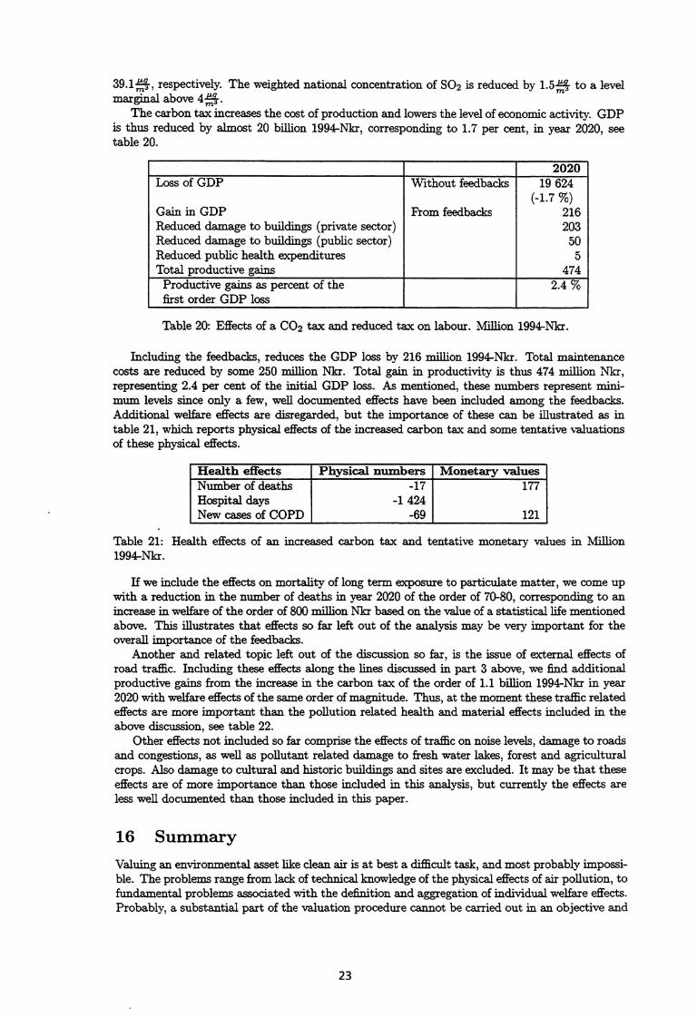
39.1 , respectively. The weighted national concentration of SO2 is reduced by 1.5 to a levelmarginal above 4 7.1%

The carbon tax increases the cost of production and lowers the level of economic activity. GDPis thus reduced by almost 20 billion 1994-Nkr, corresponding to 1.7 per cent, in year 2020, seetable 20.

2020Loss of GDP Without feedbacks 19 624

(-1.7 %)Gain in GDP From feedbacks 216Reduced damage to buildings (private sector) 203Reduced damage to buildings (public sector) 50Reduced public health expenditures 5Total productive gains 474

Productive gains as percent of thefirst order GDP loss

2.4 %

Table 20: Effects of a CO2 tax and reduced tax on labour. Million 1994-Nkr.

Including the feedbacks, reduces the GDP loss by 216 million 1994-Nkr. Total maintenancecosts are reduced by some 250 million Nkr. Total gain in productivity is thus 474 million Nkr,representing 2.4 per cent of the initial GDP loss. As mentioned, these numbers represent mini-mum levels since only a few, well documented effects have been included among the feedbacks.Additional welfare effects are disregarded, but the importance of these can be illustrated as intable 21, which reports physical effects of the increased carbon tax and some tentative valuationsof these physical effects.

Health effects Physical numbers Monetary valuesNumber of deathsHospital days

_ New cases of COPD

-17-1 424

-69

177

121

Table 21: Health effects of an increased carbon tax and tentative monetary values in Million1994-Nkr.

If we include the effects on mortality of long term exposure to particulate matter, we come upwith a reduction in the number of deaths in year 2020 of the order of 70-80, corresponding to anincrease in welfare of the order of 800 million Nkr based on the value of a statistical life mentionedabove. This illustrates that effects so far left out of the analysis may be very important for theoverall importance of the feedbacks.

Another and related topic left out of the discussion so far, is the issue of external effects ofroad traffic. Including these effects along the lines discussed in part 3 above, we find additionalproductive gains from the increase in the carbon tax of the order of 1.1 billion 1994-Nkr in year2020 with welfare effects of the same order of magnitude. Thus, at the moment these traffic relatedeffects are more important than the pollution related health and material effects included in theabove discussion, see table 22.

Other effects not included so far comprise the effects of traffic on noise levels, damage to roadsand congestions, as well as pollutant related damage to fresh water lakes, forest and agriculturalcrops. Also damage to cultural and historic buildings and sites are excluded. It may be that theseeffects are of more importance than those included in this analysis, but currently the effects areless well documented than those included in this paper.

16 Summary

Valuing an environmental asset like clean air is at best a difficult task, and most probably impossi-ble. The problems range from lack of technical knowledge of the physical effects of air pollution, tofundamental problems associated with the definition and aggregation of individual welfare effects.Probably, a substantial part of the valuation procedure cannot be carried out in an objective and

23

, 2020Reduced mortality from long term exposure to PMio 800Traffic accident related productivity effects 1 100Wellfare effects from pollution 300Wellfare effects from traffic accidents 1 000+

Total additonal gains 3 200+Additional gains as percentof the first order GDP loss

16 %+

Table 22: Additional and more uncertain benefits of a CO2 tax combined with a reduced tax onlabour in year 2020. Million 1994-Nkr.

value free manner and should be left to the political arena for decision. We are, however, ableto provide some well researched and objective input to the political process, and this paper is anattempt to document the state of the art in Norway in this regard.

The use of economy wide and disaggregated macroeconomic models in this process has severaladvantages. First, we are able to capture the macroeconomic allocation costs associated withthe productivity losses imposed on the economy by air pollution and road traffic. Second, themodel treats several air pollutants (and transport activities) and their effects on the economysimultaneously, thus providing a framework for assessing many of the cost components of severalpollutants at once. Third, the model allows us to assess the effects of not only environmentalcontrol policies directed at curbing the emission of one or a few pollutants, but also to assess moregeneral policies like for instance tax or trade policies. Finally, and perhaps special for Norway,the models are actively used by the policy makers. Thus, effects, linkages and results integratedin the models are taken note of in the policy making process.

Two aspects of the preliminary results reported in the paper are perhaps stricking. One is therelative smallness of the economic costs associated with air pollution in Norway. As noted manytimes, this is most probably due to the limited number of environmental effects we judge to bewell enough documented to form part of an objective knowledge base. The second aspect has theopposite "flavour" ; namely the seriousness of the physical impacts of air pollution. Thus, we findrelative large marginal corrosion cost of 502 emissions in several large cities in Norway. Thesecosts allows for far more stringent air pollution abatement policies than are in force today. Also,the number of deaths associated with short term exposure to particulate matter is probably wellabove what most people would have expected. That the people affected are old and unproductivein a limited economic sense, does not detract from the seriousness of the situation. This point is,of course, made even more important when one consider the possible effects of long term exposureto particulate matter and when we try to grasp the loss of welfare associated with all the healtheffects described in this paper. That we are unable to account for these effects in monetary terms,places a heavy responsibility on all of us as participants in the political processes.

24

References

[1] Abbey, D. E., F. Petersen, P. K. Mills and W. L. Beeson (1993): Long-term ambient concen-trations of total suspended particulates, ozone and sulphur dioxide and respiratory symptomsin a non-smoking population, Archives of Environmental Health 48, 33-46.

[2] Alfsen, K. H. (1993): Secondary benefits of reduced fossil fuel combustion, paper presented atSeminar on external effects in the utilization of renewable energy, The Technical Universityof Denmark, September 16., 1993.

[3] Alfsen, K. H., A. Brendemoen and S. Glomsrod (1992): Benefits of climate policies: Sometentative calculations, Discussion Paper 69, Statistics Norway, Oslo.

[4] Alfsen, K. H., T. Bye and E. HoImoy (eds.) (1996): MSG-EE: An applied general equilibriummodel for energy and environmental analyses, to appear in the series Social and EconomicStudies, Statistics Norway, Oslo.

[5] Alfsen, K. H. and S. Glomsrod (1993): Valuation of environmental benefits in Norway: Amodelling framework, Notater 93/28, Statistics Norway, Oslo.

[6] Anderson, B. (1994): Korrosjonskadekostnaden orsakad av svaveldioksid emissioner (Corro-sion costs due to sulphur emissions), Svenska railjOrakenskaper, Statistics Sweden, Stockholm.

[7] Brendemoen, A., S. Glomsrod and M. Aaserud (1992): Miljokostnader i makroperspektiv(Environmental damage in a macroeconomic perspective), Reports 92/17, Statistics Norway,Oslo.

[8] Calthrop, E., and D. Pearce (1996): Methodologies for calculating the damage to build-ings and materials: An overview, paper presented at the UN ECE Workshop on economicevaluation of air pollution abatement and damage to buildings including cultural heritage,Stockholm, 1996.

[9] Cowell, D., and H. ApSimon (1994): Estimating the cost of damage to buildings by acidi-fying pollution in Europe, UN ECE Workshop on economic evaluation of damage caused byacidifying pollutants, London May, 1994.

[10] Dockery, D. W., C. Arden Pope, Xiping Xu, J. D. Spengler, J. H. Ware, M. E. Fay, B. G.Ferris jr., and F. E: Speizer (1993): An association between air pollution and mortality in sixUS cities, New England Journal of Medicine 329, 1753-1759.

[11] Elvik, R. (1993): Økonomisk verdsetting av velferdstap ved trafikkulykker (Economic valuationof welfare losses from traffic accidents), TOI rapport 203/1993, Oslo.

[12] Eskeland, G. (1995): "The costs and benefits of an air pollution control strategy for Santiago,Chile" , in: Chile: Managing environmental problems: Economic analysis of selected issues,Report no. 13061-CH, World Bank, Washington, DC.

[13] EC (European Commission) (1994): DGXII (Joule programme) Externalities of fuel cycles;ExternE project, Report no. 2, Coal fuel cycle.

[14] Fairley, D. (1990): The relationship of daily mortality to suspended particulates in SantaClara County, 1980-1986, Environmental Health Perspectives 89, 159-168.

[15] Fridstrom, L. and T. BjØrnskau (1989): Trafikkulykkenes drivkrefter. En analyse av ulykkestal-lenes variasjon i tid og rom (The determinants of road traffic accidents in Norway. A combinedcross-sectional and time-series analysis), TOI report 39/1989, TOI, Oslo.

[16] Glomsrod, S. (1990): "Some macroeconomic consequences of emissions to air" , In: J. Fen-hann, H. Larsen, G. A. Mackenzie and R. B. Rasmussen (eds.): Environmental models:Emissions and consequences, Elsevier, Amsterdam.

[17] Glomsrod, S., R. Nesbakken and M. Aaserud (1996): Modelling impacts of traffic injuries onlabour supply and public health expenditures in a CGE model framework, to appear in theseries Reports, Statistics Norway, Oslo.

25

[18] Glomsrod, S., K. E. Rosendahl and A. C. Hansen (1996): Integrering av miljokostnader imakrookonomiske modeller (Integration of environmental costs in macroeconomic models), toappear in the series Reports, Statistics Norway, Oslo.

[19] Glomsrod, S. and A. Rosland (1988): Luftforurensning og materialskader: Sam-funnsokonomiske kostnader (Air pollution and material corrosion: Social costs), Reports88/31, Statistics Norway, Oslo

[20] Glomsrod, S., 0. Godal, J. F. Henriksen, S. Haagenrud og T. Skancke (1996): Luftforuren-sninger - effekter og verdier (LEVE): Materialkostnader pd bygninger og biter i Norge (Airpollution - impact and values: Material damage of buildings and cars in Norway), Report96:07, The Norwegian Pollution Control Authority (SFT), Oslo.

[21] Haagenrud, S. E., and J. F. Henriksen (1995): Luftforurensning - effekter og verdier (LEVE).Materialkorrosjon med vekt pd dose-responssammenhenger (Air pollution - impacts and values(LEVE). Corrosion of materials with emphasis on dose-response correlations), Report 95:22,The Norwegian Pollution Control Authority (SFT), Oslo.

[22] Hagen, K. E. (1993): Samfunnsokonomisk regnskapssystem for trafikkulykker og trafikksikker-hetstiltak (Economic accounting system for traffic accidents and safety measures), DOI report182/1993, TOI, Oslo.

[23] Haukeland, J. V. (1991): Velferdstap ved trafikkulykker (Welfare losses from traffic accidents),TOI report 92/1991, TOL Oslo.

[24] Kinney, P. L. and H. Ozkaynak (1991): Association of daily mortality and air pollution inLos Angeles County, Environmental Research 54, 99-120.

[25] Kinney, P. L. and H. Ozkaynak (1992): Associations between ozone and daily mortality inLos Angeles and New York City, American Review of Respiratory Disease 145, A95.

[26] Kinney, P. L., K. Ito and G. D. Thurston (1994): Daily mortality and air pollution in Los An-geles: An update, American Review of Respiratory and Critical Care Medicine Supplement,A660 (reference incomplete in EC (1994)).

[27] Krupnick, A. J., W. Harrington and B. Ostro (1990): Ambient ozone and acute health effects:Evidence from daily data, Journal of Environmental Economics and Management 18, 1-18.

[28] Kucera, V., J. F. Henriksen, D. Knotkova and C. SjOstriim (1993): Model for calculationof corrosion costs caused by air pollution and its application in three cities. Progress inunderstanding and prevention of corrosion, paper presented at the 10th European CorrosionCongress, Barcelona, July 1993

[29] Kucera, V., J. Tidblad, J. F. Henriksen, A. Bartonova, and A. A. Mikhailov (1995): Statisticalanalyses of 4 year materials exposures and acceptable deterioration and pollution levels,Korrosjonsinstitutet, Stockholm.

[30] ORNL/RFF (Oak Ridge National Laboratory and Resources for the Future) (1994): Exter-nal costs and benefits of fuel cycles: A study by the U.S. Department of Enenrgy and theCommission of the European Communities, Oak Ridge, TenneSsee.

[31] Ostro, B. (1983): The effects of air pollution on work loss and morbidity, Journal of Envi-ronmental Economics and Management 10, 371-382.

[32] Ostro, B. (1987): Air pollution and morbidity revisited: A specification test, Journal ofEnvironmental Economics and Management 14, 87-98.

[33] Ostro, B. (1990): Association between morbidity and alternative measures of particulatematter, Risk Analysis 10, 421-427.

[34] Ostro, B. (1993): The association of air pollution and mortality: Examining the case forinference, Archives of Environmental Health 48, 336-342.

26

[35] Ostro, B. (1994): Estimating the effects of air pollutants. A method with an application toJakarta, Working paper 1301, PRDPE Division, World Bank, Washington, D.C.

[36] Ostro, B. (1995): Addressing uncertainties in the quantitative estimation of air pollu-tion health effects, paper presented at the Workshop on the external costs of energy,EU/EEA/OECD, 30-31. January 1995.

[37] Ostro, B., and S. Rothschild (1989): Air pollution and acute respiratory morbidity: Anobservational study of multiple pollutants, Environmental Research 50, 238-247.

[38] Pearce, D. (1995): The development of externality adders in the United Kingdom, paperpresented at the Workshop on the external costs of energy, EU/IEA/OECD, 30.-31. January,1995.

[39] Pope, C. A. III (1991): Respiratory hospital admission associated with PM 10 pollution inUtah, Salt Lake and Cache Valleys, Archives of Environmental Health 46, 90-97.

[40] Pope, C. A. III, J. Schwartz and M. R. Ransom (1992): Daily mortality and PM10 pollutionin Utah, Salt Lake and Cache Valleys, Archives of Environmental Health 47, 211-217.

[41] Pope, C. A. III et al. (1995): Reference not given in WHO (1995).

[42] Portney, P., and J. Mullahy (1986): Urban air quality and acute respiratory disease, Journalof Urban Economics 20, 21-38.

[43] Portney, P., and J. Mullahy (1990): Urban air quality and chronic respiratory disease, Re-gional Science and Urban Economics 20, 407-418.

[44] POnka, A. (1991): Asthma and low level air pollution in Helsinki, Archives of EnvironmentalHealth 46, 262-270.

[45] Rosendahl, K. E. (1996): Helsevirkninger av luftforurensning og effekter pa Økonomisk ak-tivitet (Health effects of air pollution and effects on economic activity), Reports 96/8, Statis-tics Norway, Oslo.

[46] Rossi, 0. V. J., V. L. Kinnula, J. Tienari and E. Huhti (1993):* Association of severe asthmaattacks with weather, pollen, and air pollution, Thorax 48, 244-248.

[47] Rowe, R., L. Chestnut and C. Lang (1995): The New York environmental externalities coststudy: Summary of approaches and results, paper presented at the Workshop on the externalcosts of energy, EU/IEA/OECD, 30-31 January, 1995.

[48] Schwartz, J., C. Spix, H. E. Wichmann and E. Malin (1991): Air pollution and acute respi-ratory illness in five German communities, Environmental Research 56, 1-14.

[49] Schwartz, J. and D. W. Dockery (1992): Increased mortality in Philadelphia associated withdaily air pollution concentrations, American Review of Respiratory Diseases 145, 600-604.

[50] Schwartz, J. and S. Zeger (1990): Passive smoking, air pollution and acute respiratory symp-toms on a diary study of student nurses, American Review of Respiratory Diseases 141,62-67.

[51] Statistics Norway (1993): Helseinstitusjoner (Health institutions), Norwegian Official Statis-tics (NOS) C81, Statistics Norway, Oslo.

[52] Statistics Norway (1995): Pasientstatistikk 1993 (Pasient statistics 1993), Norwegian OfficialStatistics (NOS) C231, Statistics Norway, Oslo.

[53] Thurston, G. P., K. Ito, P. Kinney and M. Lippman (1992): A multi-year study of airpollution and respiratory hospital admissions in three New York state metropolitan areas:Results for 1988 and 1989 summer, Journal of Exposure and Environmental Epidemiology 2,429-450.

27

[54] Vejdirektoratet (1979): Undersogelse av uhelsmonsteret pa vejstrekninger der er blevetafiastet for traffic (Analysis of accidents on roads with reduced traffic), Okonomisk-statistiskavdeling, Vejdirektoratet, KObenhavn.

[55] Walker, S. E. (1996): Beregning av personvektet drsmiddelkonsentrasjon i Oslo av PM2.5,PM lo, og NO2, (Calculation of person weighted mean annual concentration of PM2.5, PMloand NO2 in Oslo), to appear in the series OR from NILU, Lillestrom.

[56] WHO (1995): Update and revision of the air quality guidelines for Europe, World HealthOrganization, Regional Office of Europe, Copenhagen.

28

Issued in the series Documents

94/1 H. Vennemo (1994): Welfare and the Environ-ment. Implications of a Recent Tax Reform inNorway

94/2 K.H. Alfsen (1994): Natural Resource Accountingand Analysis in Norway

94/3 0. Bjerkholt (1994): Ragnar Frisch 1895-1995

95/1 A.R. Swensen (1995): Simple Examples onSmoothing Macroeconomic Time Series

95/2 E. Gjelsvik, T. Johnsen, H.T. Mysen andA. Valdimarsson (1995): Energy Demand inIceland

95/3 C. Zhao, 0. Bjerkholt, T. Halvorsen andY. Zhu (1995): The Flow of Funds Accounts inChina

95/4 Nordic Indicator Group (1995): NordicEnvironmental Indicators. Draft document.English version with main points from commentsreceived

95/5 H.A. Gravningsmyhr (1995): Analysing Effects ofRemoving Survivors' Pensions, Using theMicrosimulation Model LOTTE

95/6 P. Boug (1995): User's Guide. The SEEM-modelVersion 2.0

95/7 E. Bowitz, N.O. Maehle, V.S. Sasmitawidjaja andS.B. Widoyono (1995): MEMLI — AnEnvironmental model for Indonesia. TechnicalDocumentation of data programs and procedures

95/8 K. H. Alfsen, T. Bye, S. Glomsod and H. Wiig(1995): Integrated Assessment of Soil Degradationand Economic Growth in Ghana

95/9 0. Bjerkholt (1995): Ragnar Frisch and theFoundation of the Econometric Society andEconometrica

95/10 P.J. Bjerve (1995): The Influence of RagnarFrisch on Macroeconomic Planning and Policy inNorway

96/1 D. Kolsrud (1996): Documentation of ComputerPrograms that Extend the SEEM Model andProvide a Link to the RAINS Model

96/2 E. Bowitz, V.S. Sasmitawidjaja and G. Sugiarto(1996): The Indonesian Economy and Emission ofCO2: An Analysis Based on the Environmental-Macroeconomic-Model MEMLI, 1990-2020

96/3 H.V. Swbo (1996): Use of GeographicalInformation Systems (GIS) in Statistics Norway

96/4 E. Berg (1996): Some Results from the Literatureon the Impact of Carbon Taxes on the PetroleumWealth

96/5 E.J. FlOttum (1996): Norwegian NationalAccounts — Documentation of the Compilationand Methods Applied. I General Description. IIGDP From the Output Approach

96/6 E.J. Flottum (1996): Norwegian NationalAccounts — Documentation of the Compilationand Methods Applied. III GDP by ExpenditureApproach. IV GDP by Income Approach

96/7 0. Bjerkholt, K.A. Brekke and R. Choudhury(1996): The Century Model - on the Long TermSustainability of the Saudi Arabian Economy

96/8 R. Choudhury (1996): The Century Model.Technical Documentation of Computer Programsand Procedures

96/9 R. Choudhury and K.A. Magnussen (1996): TheImplementation Model. Technical Documentationof Computer Programs and Procedures

96/10 R. Choudhury (1996): The Selection Model.Technical Documentation of Computer Programsand Procedures

96/11 R. Choudhury (1996): The 0M95 — An Oil Modelfor the Kingdom of Saudi Arabia. TechnicalDocumentation of Computer Programs andProcedures

96/12 K. Nyborg (1996): Environmental Valuation,Cost-Benefit Analysis and Policy Making: ASurvey

96/13 P.R. Johansen and K.A. Magnussen (1996): TheImplementation Model. A Macroeconomic Modelfor Saudi Arabia

96/14 A. Capplen and K. A. Magnussen (1996): TheSelection Model. A General Equilibrium Modelfor Saudi Arabia

96/15 P. Boug and L. Brubakk (1996): Impacts ofEconomic Integration on Energy Demand andCO2 emissions in Western Europe

96/16 J.K. Dagsvik (1996): Probabilistic Models forQualitative Choice Behavior: An Introduction

96/17 K.H. Alfsen and K.E. Rosendahl (1996):Economic Damage of Air Pollution

29

Documents

Statistics NorwayResearch DepartmentP.O.B. 8131 Dep.N-0033 Oslo

Tel.: + 47-22 86 45 00Fax: + 47-22 11 12 38

ISSN 0805-9411

OW Statistics Norway