ICS: Descriptors: English version Nondestructive testing - Ultrasonic examination - Part 6: Time-of-flight diffraction technique as a method for defect detection and sizing This draft European pre-standard is submitted to CEN members for formal Vote. It has been drawn up by the Technical Committee CEN/TC 138. CEN members shall make the ENV available at national level in an appropriate form promptly and announce its existence in the same way as for EN/HD. Existing conflicting national standards may be kept in force (in parallel to the ENV) until the final decision about the possible conversion of the ENV into an EN is reached. The lifetime of an ENV is first limited to three years. After two years the Secretary General shall take action by requesting members to send in comments an that ENV within six months. The comments received will be transmitted to the Technical Board for further action as follows: conversion into an EN after formal vote; or extension of the life of an ENV for another two years (once only); or replacement by a revised ENV approved in accordance with 7.2 and 7.3 of the CEN/CENELEC Internal Regulations Part 2; or withdrawal of the ENV; or assignment to a technical body of the task of assisting the Technical Board to reach any of the decisions listed above. CEN members are the national standards bodies of Austria, Belgium, Denmark, Finland, France, Germany, Greece, Iceland, Ireland, Italy, Luxembourg, Netherlands, Norway, Portugal, Spain, Sweden, Switzerland and United Kingdom. CEN European Committee for Standardization Comite Europaen de Normalisation Europaisches Komitee fur Normung

Contents Foreword 1 Scope 2 Normative references 3 Definitions and symbols 4 General 4.1 Principle of the technique 4.2 Requirements for surface condition and couplant 4.3 Materials and process type 5 Qualification and certification of personnel 6 Equipment requirements 6.1 Ultrasonic equipment and display 6.2 Ultrasonic probes 6.3. Scanning mechanisms 7 Equipment set-up procedures 7.1 General 7.2 Probe choice and probe separation 7.2.1 Probe selection 7.2.2 Probe separation 7.3 Time window setting 7.4 Sensitivity setting 7.5 Scan resolution setting 7.6 Setting of scanning speed 7.7 Checking system performance 8 Interpretation and analysis of data 8.1 Basic analysis of discontinuities 8.1.1 General 8.1.2 Characterization of discontinuities 8.1.3 Estimation of discontinuity position 8.1.4 Estimation of discontinuity length 8.1.5 Estimation of discontinuity depth and height 8.2 Detailed analysis of discontinuities 8.2.1 Additional scans 8.2.2 Additional algorithms 9 Detection and sizing in complex geometries 10 Limitations of the technique 10.1 Precision and resolution 10.2 Dead zones

11 TOFD examination without data recording 12 Examination procedure 13 Examination report Amex A (normative) Reference blocks

Foreword This European pre-standard has been prepared by CEN/TC 138 "Nondestructive examination" of which the secretariat is held by AFNOR. EN 583 "Nondestructive testing. Ultrasonic examination" consists of 6 parts : EN 583-1 Non-destructive testing - Ultrasonic examination - Part 1: General principles. EN 583-2 Non-destructive testing - Ultrasonic examination - Part 2: Sensitivity and range setting. EN 583-3 Non-destructive testing - Ultrasonic examination - Part 3: Transmission technique. EN 583-4 Non-destructive testing - Ultrasonic examination - Part 4: Examination for defects perpendicular to the surface. EN 583-5 Non-destructive testing - Ultrasonic examination - Part 5: Characterization and sizing of discontinuities. ENV 583-6 Nondestructive testing - Ultrasonic examination - Part 6: Time-of-flight diffraction technique as a method for defect detection and sizing (ENV). CEN/TC 138 approved this European pre-standard by resolution 170 during its meeting in Berlin 1995-10-26/27. According to the CEN/CENELEC Internal Regulations, the following countries are bound to annonce this European pre-standard.

1 Scope This European pre-standard defines the general principles for the application of the time-of-flight diffraction (TOFD) technique both detection and sizing of discontinuities in low alloyed car steel components. It could also be used for other types of materials, provided the application of the TOFD technique is performed with necessary consideration of geometry, acoustical properties of the materials, and the sensitivity of the examination. Although it is applicable, in general terms, to discontinuities in materials and applications covered by EN 583-1, it contains references to the application on welds. This approach has been chosen for reasons of clarity as to the ultrasonic probe positions and directions of scanning. Unless otherwise specified in the referencing documents, the minimum requirements of this pre-standard are applicable. Unless explicitly stated otherwise, this pre-standard is applicable to the following product classes as defined in EN 583-2:

- Class 1, without restrictions - Classes 2 and 3, restrictions will apply as stated in Clause 9.

The inspection of products of Classes 4 and 5 will require special procedures. These are addressed in Clause 9 as well. 2 Normative References This European pre-standard incorporates, by dated or undated references, provisions from other publications. These normative references are cited at the appropriate places in the text, and the publications are listed hereafter. For dated references, subsequent amendments to or revisions of any of these publications apply to this European pre-standard only when incorporated in it by amendment or revision. For undated references, the latest revision of the publication referred to applies. EN 473 Qualification and certification of NDT personnel - General principles EN 583-1 Nondestructive testing - Ultrasonic examination - Part 1: General principles EN 583-2 Nondestructive testing - Ultrasonic examination - Part 2: Sensitivity and range

setting EN 583-5 Nondestructive testing - Ultrasonic examination - Part 5: Characterization and

sizing of discontinuities EN 1330-4 Nondestructive testing - Terminology - Part 4: Terms used in ultrasonic welding EN -1 Ultrasonic examination - Characterization and verification of equipment used for

ultrasonic examination - Part 1: Flaw detectors (00138007) EN -2 Ultrasonic examination - Characterization and verification of equipment used for

ultrasonic examination - Part 2: Probes (00138058)

EN -3 Ultrasonic examination - Characterization and verification of equipment used for

ultrasonic examination - Part 3: Combined equipment (00138059) 3 Definitions and Symbols TOFD Time-of-Flight Diffraction

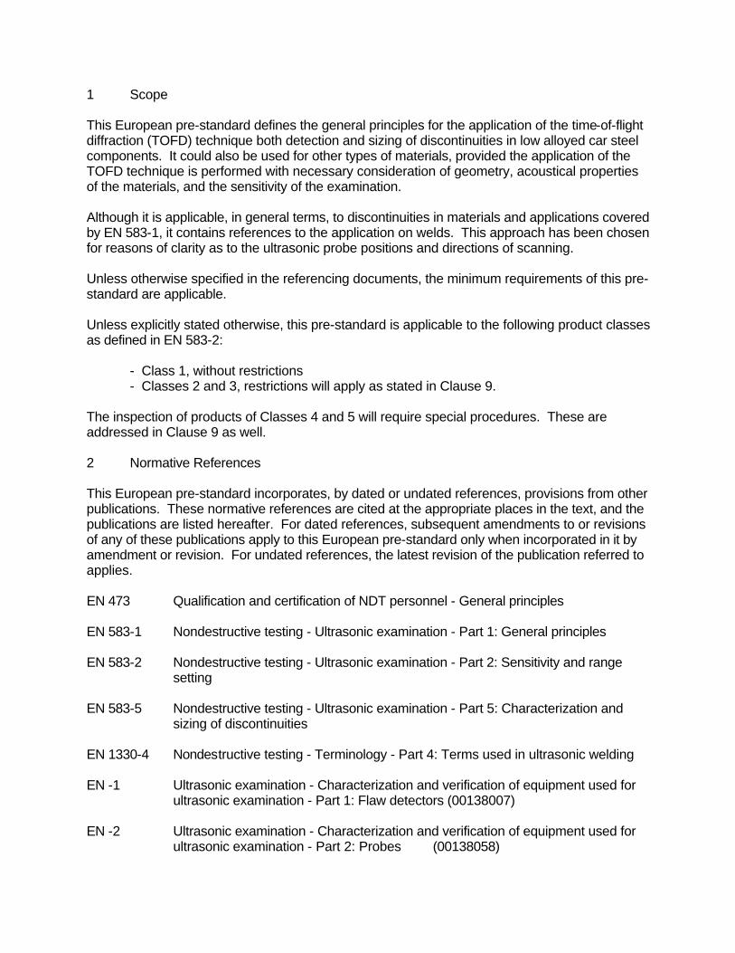
Figure 1: Coordinate definition x Coordinate parallel to the scanning surface, and parallel to a

predetermined reference line. In case of weld inspection this reference line should coincide with the weld. The origin of the axes may be defined as best suits the specimen under examination (see Figure 1)

∆x Discontinuity length y Coordinate parallel to the scanning surface, perpendicular to the

predetermined Reference 1 (see Figure 1) δy Error in lateral position z Coordinate perpendicular to the scanning surface (see Figure 1) ∆z Discontinuity height d Depth of a discontinuity tip below the scanning surface δd Error in depth Dds Scanning surface dead zone Ddw Backwall dead zone C Sound velocity δC Error in sound velocity R Spatial resolution

T Time-of-flight from the transmitter to the receiver ∆T Time-of-flight difference between the lateral wave and a second ultrasonic signal δT Error in time-of-flight Td Time-of-flight at depth d Tp Length (in time) of the acoustical pulse up to an amplitude of 10% of the

maximum Tw Time-of-flight of the backwall echo S Half the distance between the index points of two ultrasonic probes δS Error in half the probe separation W Wall thickness dead zone zone where indications may be obscured due to the presence of signals

of geometrical origin back wall dead zone Extra dead zone where signals may be obscured by the presence of the

backwall echo A-scan Display of the ultrasonic signal amplitude as a function of time S-scan Display of the time-of-flight of the ultrasonic signal as a function of probe

displacement Non-parallel scan Scan perpendicular to the ultrasonic beam direction (see Figure 4) Parallel scan Scan parallel to the ultrasonic beam direction (see Figure 5) 4 General 4.1 Principle of the Technique The TOFD technique relies on the interaction of ultrasonic waves with the tips of discontinuities. This interaction results in the emission of diffracted waves over a large angular range. Detection of the diffracted waves makes it possible to establish the presence of the discontinuity. The time-of-flight of the recorded signals is a direct measure for the depth of the discontinuity, thus enabling sizing of the defect. The dimension of the discontinuity is always determined from the time-of-flight of the diffracted signals. The signal amplitude is not used in size estimation.

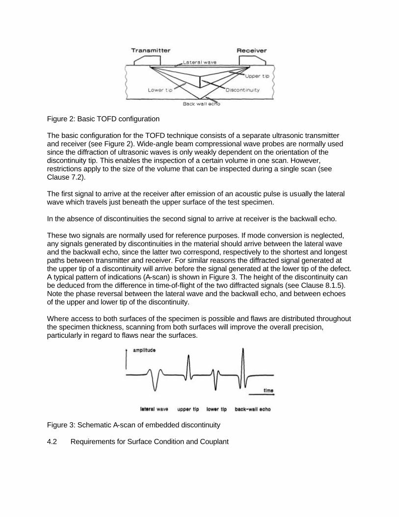
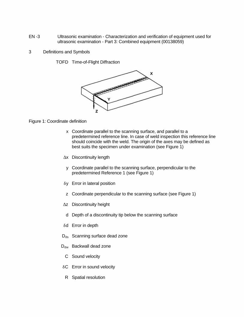
Figure 2: Basic TOFD configuration The basic configuration for the TOFD technique consists of a separate ultrasonic transmitter and receiver (see Figure 2). Wide-angle beam compressional wave probes are normally used since the diffraction of ultrasonic waves is only weakly dependent on the orientation of the discontinuity tip. This enables the inspection of a certain volume in one scan. However, restrictions apply to the size of the volume that can be inspected during a single scan (see Clause 7.2). The first signal to arrive at the receiver after emission of an acoustic pulse is usually the lateral wave which travels just beneath the upper surface of the test specimen. In the absence of discontinuities the second signal to arrive at receiver is the backwall echo. These two signals are normally used for reference purposes. If mode conversion is neglected, any signals generated by discontinuities in the material should arrive between the lateral wave and the backwall echo, since the latter two correspond, respectively to the shortest and longest paths between transmitter and receiver. For similar reasons the diffracted signal generated at the upper tip of a discontinuity will arrive before the signal generated at the lower tip of the defect. A typical pattern of indications (A-scan) is shown in Figure 3. The height of the discontinuity can be deduced from the difference in time-of-flight of the two diffracted signals (see Clause 8.1.5). Note the phase reversal between the lateral wave and the backwall echo, and between echoes of the upper and lower tip of the discontinuity. Where access to both surfaces of the specimen is possible and flaws are distributed throughout the specimen thickness, scanning from both surfaces will improve the overall precision, particularly in regard to flaws near the surfaces.

Figure 3: Schematic A-scan of embedded discontinuity 4.2 Requirements for Surface Condition and Couplant

Care shall be taken that the surface condition masts at least the requirements stated in Clause 8.1 of EN 583-1. Since the diffracted signals may be weak, the degradation of signal quality due to poor surface condition will have a severe impact on inspection reliability. Different coupling media can be used, but their type shall be compatible with the materials to be examined. Examples are water, possibly containing an agent (wetting, anti-freeze, corrosion inhibitor), contact paste, oil, grease, cellulose paste containing water, etc. The characteristics of the coupling medium shall remain constant throughout the examination. It shall be suitable for the temperature range in which it will be used. 4.3 Materials and Process Type Due to the relatively low signal amplitudes that are used in the TOFD technique, the method can be applied routinely on materials with relatively low levels of attenuation and scatter for ultrasonic waves. in general, application on unalloyed and low alloyed carbon steel components and welds is possible, but also on fine grained austenitic steals and aluminum. Coarse-grained materials and materials with significant anisotropy however, such as cast iron, austenitic weld materials and high-nickel alloys, will require additional validation and additional data processing. By mutual agreement, a representative test specimen with artificial and/or natural discontinuities can be used to confirm inspectability. Remember that diffraction characteristics of artificial defects can differ significantly from those of real defects. 5 Qualification and Certification of Personnel Personnel performing examinations with the TOFD technique shall, as a minimum, be qualified in accordance with EN 473, and shall have received additional training and examination on the use of the TOFD technique on the product classes to be tested, as specified in a written practice. 6 Equipment Requirements 6.1 Ultrasonic Equipment and Display Ultrasonic equipment used for the TOFD technique shall, as a minimum, comply with the requirements of prEN (00138007; 00138058, 00138059). In addition, the following requirements shall apply:

• The receiver bandwidth shall, as a minimum, range between 0, 5 and 2 times the Nominal probe frequency at -6 dB, unless specific materials and product classes require a larger bandwidth. Appropriate band filters can be used.

• The transmitting pulse can either be unipolar or bipolar. The rise time shall not

exceed 0.25 times the period corresponding to the nominal probe frequency.

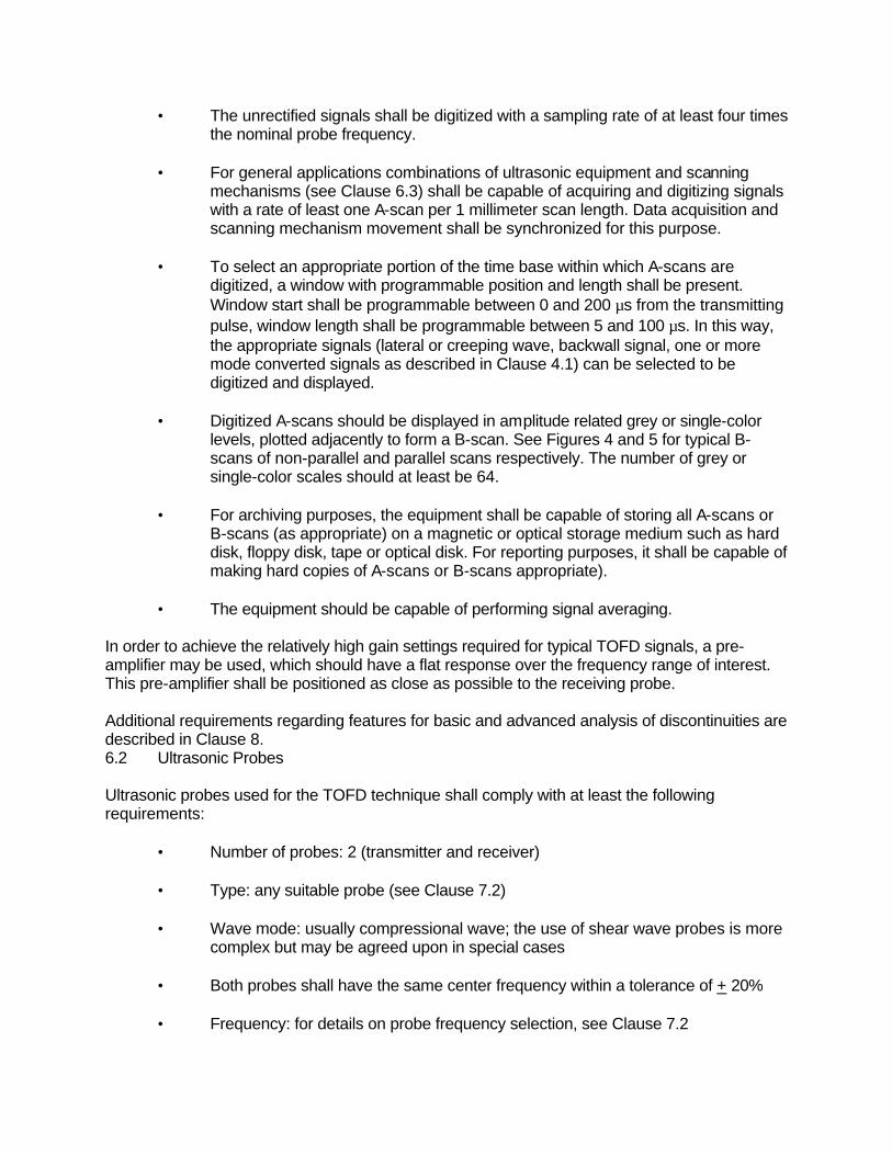
• The unrectified signals shall be digitized with a sampling rate of at least four times the nominal probe frequency.

• For general applications combinations of ultrasonic equipment and scanning

mechanisms (see Clause 6.3) shall be capable of acquiring and digitizing signals with a rate of least one A-scan per 1 millimeter scan length. Data acquisition and scanning mechanism movement shall be synchronized for this purpose.

• To select an appropriate portion of the time base within which A-scans are

digitized, a window with programmable position and length shall be present. Window start shall be programmable between 0 and 200 µs from the transmitting pulse, window length shall be programmable between 5 and 100 µs. In this way, the appropriate signals (lateral or creeping wave, backwall signal, one or more mode converted signals as described in Clause 4.1) can be selected to be digitized and displayed.

• Digitized A-scans should be displayed in amplitude related grey or single-color

levels, plotted adjacently to form a B-scan. See Figures 4 and 5 for typical B-scans of non-parallel and parallel scans respectively. The number of grey or single-color scales should at least be 64.

• For archiving purposes, the equipment shall be capable of storing all A-scans or

B-scans (as appropriate) on a magnetic or optical storage medium such as hard disk, floppy disk, tape or optical disk. For reporting purposes, it shall be capable of making hard copies of A-scans or B-scans appropriate).

• The equipment should be capable of performing signal averaging.

In order to achieve the relatively high gain settings required for typical TOFD signals, a pre-amplifier may be used, which should have a flat response over the frequency range of interest. This pre-amplifier shall be positioned as close as possible to the receiving probe. Additional requirements regarding features for basic and advanced analysis of discontinuities are described in Clause 8. 6.2 Ultrasonic Probes Ultrasonic probes used for the TOFD technique shall comply with at least the following requirements:

• Number of probes: 2 (transmitter and receiver)

• Type: any suitable probe (see Clause 7.2)

• Wave mode: usually compressional wave; the use of shear wave probes is more complex but may be agreed upon in special cases

• Both probes shall have the same center frequency within a tolerance of + 20%

• Frequency: for details on probe frequency selection, see Clause 7.2

• The pulse length of both the lateral wave and the backwall echo shall not exceed

two cycles, measured at 10% of the peak amplitude

• Pulse repetition rate shall be set such that no interference occurs between acoustical signals caused by successive transmission pulses.

Figure 4: Non-parallel scan, with the typical direction of probe displacement shown an the left, and the corresponding B-scan shown on the right 6.3 Scanning Mechanisms Scanning mechanisms shall be used to maintain a constant distance and alignment between the index points of the two probes. An additional function of scanner mechanisms is to provide the ultrasonic equipment with probe position information, in order to enable the generation of position-related B-scans. Information on probe position can be provided by means of e.g. incremental magnetic or optical encoders, or potentiometers. Scanning mechanisms in TOFD can either be motor or manually driven. They shall be guided by means of a suitable guiding mechanism (steel band, belt, automatic track following systems, guiding wheels). Guiding accuracy with respect to the center of a reference line (the center line of a weld) should be kept within a tolerance of ± 10% of the probe index point separation. 7 Equipment Set-Up Procedures 7.1 General Probe selection and probe configuration are important equipment set-up parameters. They largely determine the overall accuracy, the signal-to-noise ratio and the coverage of the region of interest of the TOFD technique.

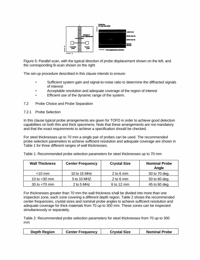
Figure 5: Parallel scan, with the typical direction of probe displacement shown on the left, and the corresponding B-scan shown on the right The set-up procedure described in this clause intends to ensure:

• Sufficient system gain and signal-to-noise ratio to determine the diffracted signals of interest

• Acceptable resolution and adequate coverage of the region of interest • Efficient use of the dynamic range of the system.

7.2 Probe Choice and Probe Separation 7.2.1 Probe Selection In this clause typical probe arrangements are given for TOFD in order to achieve good detection capabilities on both thin and thick specimens. Note that these arrangements are not mandatory and that the exact requirements to achieve a specification should be checked. For steel thicknesses up to 70 mm a single pair of probes can be used. The recommended probe selection parameters to achieve sufficient resolution and adequate coverage are shown in Table 1 for three different ranges of wall thicknesses. Table 1: Recommended probe selection parameters for steel thicknesses up to 70 mm

Wall Thickness Center Frequency Crystal Size Nominal Probe Angle

<10 mm 10 to 15 MHz 2 to 6 mm 50 to 70 deg. 10 to <30 mm 5 to 10 MHZ 2 to 6 mm 50 to 60 deg. 30 to <70 mm 2 to 5 MHz 6 to 12 mm 45 to 60 deg.

For thicknesses greater than 70 mm the wall thickness shall be divided into more than one inspection zone, each zone covering a different depth region. Table 2 shows the recommended center frequencies, crystal sizes and nominal probe angles to achieve sufficient resolution and adequate coverage for thick materials from 70 up to 300 mm. These zones can be inspected simultaneously or separately. Table 2: Recommended probe selection parameters for steel thicknesses from 70 up to 300 mm

Depth Region Center Frequency Crystal Size Nominal Probe

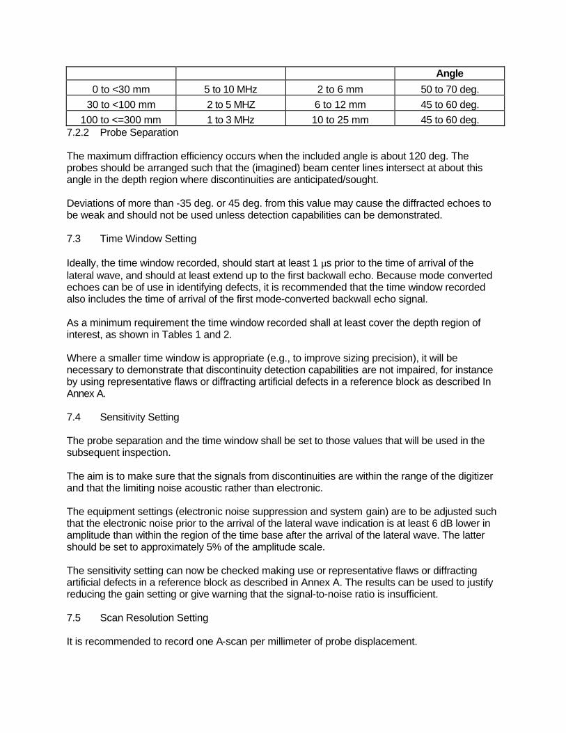
Angle

0 to <30 mm 5 to 10 MHz 2 to 6 mm 50 to 70 deg. 30 to <100 mm 2 to 5 MHZ 6 to 12 mm 45 to 60 deg.

100 to <=300 mm 1 to 3 MHz 10 to 25 mm 45 to 60 deg. 7.2.2 Probe Separation The maximum diffraction efficiency occurs when the included angle is about 120 deg. The probes should be arranged such that the (imagined) beam center lines intersect at about this angle in the depth region where discontinuities are anticipated/sought. Deviations of more than -35 deg. or 45 deg. from this value may cause the diffracted echoes to be weak and should not be used unless detection capabilities can be demonstrated. 7.3 Time Window Setting Ideally, the time window recorded, should start at least 1 µs prior to the time of arrival of the lateral wave, and should at least extend up to the first backwall echo. Because mode converted echoes can be of use in identifying defects, it is recommended that the time window recorded also includes the time of arrival of the first mode-converted backwall echo signal. As a minimum requirement the time window recorded shall at least cover the depth region of interest, as shown in Tables 1 and 2. Where a smaller time window is appropriate (e.g., to improve sizing precision), it will be necessary to demonstrate that discontinuity detection capabilities are not impaired, for instance by using representative flaws or diffracting artificial defects in a reference block as described In Annex A. 7.4 Sensitivity Setting The probe separation and the time window shall be set to those values that will be used in the subsequent inspection. The aim is to make sure that the signals from discontinuities are within the range of the digitizer and that the limiting noise acoustic rather than electronic. The equipment settings (electronic noise suppression and system gain) are to be adjusted such that the electronic noise prior to the arrival of the lateral wave indication is at least 6 dB lower in amplitude than within the region of the time base after the arrival of the lateral wave. The latter should be set to approximately 5% of the amplitude scale. The sensitivity setting can now be checked making use or representative flaws or diffracting artificial defects in a reference block as described in Annex A. The results can be used to justify reducing the gain setting or give warning that the signal-to-noise ratio is insufficient. 7.5 Scan Resolution Setting It is recommended to record one A-scan per millimeter of probe displacement.

7.6 Setting of Scanning Speed Scanning speed shall be selected such that it is compatible with the requirements of Clauses 7.3, 7.4, and 7.5. 7.7 Checking System Performance it is recommended that system performance is checked before and after an inspection by recording and comparing a limited number of representative A-scans. See also EN -3 (00138059). 8 Interpretation and Analysis of Data 8.1 Basic Analysis of Discontinuities 8.1.1 General Reporting or acceptance criteria shall be agreed upon by contracting parties prior to inspection. Discontinuities detected by TOFD shall be characterized by at least:

• Their position in the object (x- and y- coordinates) • Their length (∆x) • Their depth and height (z, ∆z) • Their type, limited to: ‘top surface breaking', 'bottom surface breaking' or

'embedded'. 8.1.2 Characterization of Discontinuities In order to characterize a discontinuity, the phase of the tip diffraction associated with this discontinuity shall be determined:

• A signal with the same apparent phase as the lateral wave shall be considered to originate from the lower tip of a discontinuity

• A signal with the same apparent phase as the backwall echo shall be considered

to originate either from an upper tip of a discontinuity or from a discontinuity with no measurable height.

If the signal-to-noise ratio is insufficient to allow the phase of the signal to be detected, these identifications are invalid. 8.1.2.1 Top Surface Breaking Discontinuities An indication consisting of a lower tip diffraction with an associated weakening (check for couplant loss) or interruption of the lateral wave shall be considered a top surface breaking discontinuity. Sometimes a slight shift of the lateral wave towards longer time-of-flight can be observed.

8.1.2.2 Bottom Surface Breaking Discontinuities An indication consisting of an upper tip diffraction with either associated shift of the backwall echo towards longer time-of-flight or an interruption (check for couplant loss) of the backwall echo shall be considered a bottom surface breaking discontinuity. 8.1.2.3 Embedded Discontinuities An indication consisting of both an upper tip and a lower tip diffraction shall be considered an embedded discontinuity. An indication consisting solely of an apparent upper tip diffraction with no associated indications in either lateral wave or backwall echo shall be considered a discontinuity with no height. Care must be taken however, because the indications in the lateral wave or backwall echo can be very weak, resulting in misinterpretation of the discontinuity. In case of doubt appropriate action shall be taken, either by performing multiple TOFO scans (see Clause 8.2.1) or by applying other techniques. In case further characterization is required, reference shall be made to Clause 8.2. In case of doubt about the interpretation of a defect, the worst possible interpretation shall be retained, until the interpretation can be verified. 8.1.3 Estimation of Discontinuity Position In general it will be sufficiently accurate to assume that the discontinuity is located on the intersection between the x, z-plane midway between the two ultrasonic probes and the y, z-plane through the center lines of the two probes. The time-of-flight of an indication generated by a discontinuity can also be used to estimate its position. The surface of constant time-of-flight theoretically is an ellipsoid centered around the index points of the ultrasonic probes. The exact determination of the position of the diffractor can only be achieved by at least two scans (see Clause 8.2.1). If a more accurate assessment of the position and/or orientation of the discontinuity is required, multiple TOFD scans (non-parallel and/or parallel) ill have to be performed. 8.1.4 Estimation of Discontinuity Length The estimation of the length of a discontinuity shall be made directly from the probe displacement of a nonparallel scan. In common with all ultrasonic techniques this record is likely to be elongated because of the finite width of the ultrasonic beam, resulting in conservative estimates of the discontinuity length. Indications with an apparent length of less than 1.5 times the size of the probe crystal used are too small to be sized, in length, by normal TOFD procedures but see Clause 8.2.2 for additional algorithms to determine discontinuity length. 8.1.5 Estimation of Discontinuity Depth and Height

It is assumed that the ultrasonic energy enters and leaves the specimen at the index points of the probes. In case the discontinuity is assumed to be midway between the two probes (see Clause 8.1.3), the depth of the defect is given by: d = [¼(CT2 = S2]½ (1) where: C is the sound velocity T is the time-of-flight of the tip diffraction signal

d is the depth of the tip of the discontinuity S is half the distance between the index points of the ultrasonic probes The time-of-flight of the ultrasonic signal inside the ultrasonic probes shall be subtracted before the calculation of the depth is made. Failure to do so will result in grave errors in the calculated depth. To avoid the errors that may arise from probe delay estimation the depth d shall be calculated, if possible, from the time-of-flight differences, ∆T, between the lateral wave and the diffracted pulse. Hence: d = ½ [(C∆T)2 + 4C∆T]½ (2) 8.1.5.1 Top Surface Breaking Discontinuities The height of a top surface breaking discontinuity is determined by the distance between the top surface and the depth of the lower tip diffraction signal. 8.1.5.2 Bottom Surface Breaking Discontinuities The height of a bottom surface breaking discontinuity is determined by the difference in depth between the upper tip diffraction and the bottom surface. 8.1.5.3 Embedded Discontinuities The height of an embedded discontinuity is determined by the difference in depth between the upper tip and lower tip diffraction. 8.2 Detailed Analysis of Discontinuities Detailed discontinuity analysis can be performed on discontinuities already detected by basic TOFD scans. In addition, the application of other NDT techniques can be considered in order to arrive at a more detailed characterization. The motivation for detailed discontinuity analysis can be:

• More accurate assessment of discontinuity length, depth, and height • Assessment of discontinuity orientation • Detailed estimation of discontinuity type.

The detailed discontinuity analysis involves performing additional scans with different probe angles, frequencies and/or probe separation. Also parallel scans can be performed. The detailed analysis can also involve the application of additional computer algorithms to analyze the data. 8.2.1 Additional Scans 8.2.1.1 Scans with Lower Test Frequency Scans with lower test frequencies can be performed if the signal-to-noise ratio is too low to permit detailed discontinuity analysis even with considerable averaging. In general this will be at the expense of an increased dead zone, and a decreased resolution. The equipment set-up parameters shall be optimized (see Clauses 6 and 7). 8.2.1.2 Scans with Higher Test Frequency Scans with higher test frequencies can be performed to obtain increased resolution, increased sizing accuracy and a reduced dead zone, at the expense of a reduced signal-to-noise ratio, due to increased grain noise. The equipment set-up parameters shall be optimized (see Clauses 6 and 7). 8.2.1.3 Scans with Reduced Probe Angle Scans with a reduced probe angle and an associated decreased probe separation can be performed to obtain increased resolution, increased sizing accuracy and a reduced dead zone at the expense of a smaller insonified volume of the specimen. The equipment set-up parameters shall be optimized (see Clauses 6 and 7). 8.2.1.4 Scans with Different Probe Offset In order to obtain the lateral position of the discontinuity (y-direction) and/or its orientation, either a parallel scan or an additional nonparallel scan with different probe offset can be made. The equipment set-up parameters shall be optimized (see Clauses 6 and 7). It shall be checked that the phase relationship of the signals observed in these scans is identical to the phase relationship in the initial scans. The surface of constant time-of-flight for a tip diffraction signal (locus curve) is an ellipsoid. If we consider only the y, z-plane through the probes, the ellipse describing a constant path is expressed by: CT = [d2 + (S - y)2]½ + [d2 + (S + y)2]½ (3) From this expression it is clear that a different offset of the diffractor from the center plane between the probes (i.e., a different y-value) will result in a different time-of-flight of the tip diffraction. Therefore the apparent depth of the discontinuity tip will change in scans with different probe positions.

The lateral position of a discontinuity tip (y-direction) can be determined directly from a parallel scan by the position of minimum apparent depth. A number of adjacent parallel scans at different x-coordinates will be required to find the position of real minimal depth of the discontinuity. Once the position and depth of both tips of a discontinuity are known its orientation can be determined from the axis through the two discontinuity-tips. In principle, two nonparallel scans, offset with respect to each other, also suffice for the accurate determination of discontinuity depth, length and orientation, provided that the overlap of the insonified volumes is sufficient. However, the determination of the position of the discontinuity tip from two nonparallel scans is less straightforward and will involve the drawing of locus curves by additional software, see Clause 8.2.2. Additional parallel scans may also be used to detect near-surface defects, that are poorly resolved because of the proximity of the lateral wave or the backwall echo. The apparent depth of the defect will change in each scan and this will enable resolving it from the lateral wave or the backwall echo. 8.2.2 Additional Algorithms Computer algorithms can be useful in analyzing the data recorded in a TOFD scan. For example:

• Curve fitting overlays for accurate determination of discontinuity length (see also Clause 8.1.4).

• Subtraction of lateral wave and/or backwall echo in order to detect indications

otherwise obscured due to interference (see Clause 10.2). If the surface is rough or pitted, the effectiveness of this technique should be demonstrated in trials.

• Linearization algorithms to linearize complete B-scans to accurately determine

the depth or the height of the discontinuity.

• Modeling algorithms enabling the drawing of locus curve and the analysis of mode converted signals. This can provide additional insight in the position, depth, and orientation of the discontinuity. Detailed understanding of the physics and modeling software are required.

The algorithms to be used in analyzing the data shall be agreed upon by the contracting parties prior to inspection. 9 Detection and Sizing in Complex Geometries For class 2 objects, if the surface between the two probes is flat, no further restrictions apply. Otherwise for class 2 objects and for all class 3 objects a modified inspection and interpretation procedure will be required to allow for the curvature of the object.

For class 4 and 5 objects special data processing techniques and operating conditions will apply. Computer algorithms will be useful in analyzing the data in these cases. To confirm discontinuity detection capabilities, the use of representative test specimens with natural flaws or artificial defects is strongly recommended in these cases as well. 10 Limitations of the Technique This clause considers the limitations of the TOFD technique and is equally applicable to basic TOFD detection as well as to TOFD sizing. The limits of achievable accuracy under normal conditions are defined and the influence of dead zones, which can effect detectability, is discussed. it is important to realize that the overall reliability of the technique is determined by a large number of contributing factors and the overall error will not be less than the combined errors discussed in this clause. Defects which are highly tilted or skewed, such as transverse cracks in nonparallel scans, are likely to be more difficult to detect and it is recommended that specific demonstrations of capability are carried out in such cases. In addition flaws which are not serious, such as point defects, have some ability to mimic more serious flaws such as cracks. Once again it is recommended that the ability to distinguish small cracks, is demonstrated, where appropriate. Demonstrations of capability can be specific to the inspection or can be referred back to other documented data. 10.1 Precision and Resolution A distinction should be made between precision and resolution. Precision is the degree to which the position of a reflector or diffractor can be determined, whereas resolution defines the degree to which closely spaced diffractors can be distinguished from one another. The precision of a TOFD measurement will be influenced by timing errors, errors in the sound velocity, probe separation errors, and errors in the assumed lateral position of an indication. Under normal circumstances the overall precision will be dominated by the latter. 10.1.1 Errors in the Lateral Position As stated in clause 8.1.3 of this standard, the lateral position of an indication is normally assumed to be midway between the two probes. In reality the indication will be located on an ellipse (Eq. 3). The error in depth (δd) due to the error in lateral position (δy) can be calculated by: δd = (C2T2 - 4S2)½ (δy2/C2T2)/[(0.25 - δy2/C2T2)½ (4) In principle, the lower edge of the acoustic beams determines δy. If no reliable information on the lower beam edge is available, δy = S shall be used. 10.1.2 Timing Errors

The limit of precision in the depth of an indication, due to timing errors (δT), can be estimated from: δd = C δT [d2 + S2]½/2d (5) where δd is the error in d. The timing error can be reduced by using a shorter pulse and/or a higher frequency. 10.1.3 Errors in Sound Velocity The limit of precision in the estimate of the depth of an indication, due to errors in the sound velocity (δc), is given by: δd = δC[d2 + S2 - S(d2 + S2)½]/Cd (6) This error is reduced if the probe separation is reduced. Independent calibration of the velocity by measurement of the delay of the backwall echo, with a known wall thickness, greatly reduces this error. 10.1.4 Errors in Probe Separation Errors in the distance between the index points (δS) will result in errors in depth measurement. The error in depth δd can be calculated by: δd = δS[(d2 + S2)½ - S]/d (7) it should be noted that errors in probe separation can arise from both measurement errors in the distance between the probes, as well as errors in the index point calibration. When the probe separation is smaller than twice the specimen thickness, the index point can no longer be considered a fixed point, but it becomes a function of depth. In this case, if accurate sizing is required, the depth measurement must be calibrated with the aid of a representative test specimen. 10.1.5 Spatial Resolution The spatial resolution (R) is a function of depth and can be calculated by: R = [C2(Td + Tp)2/4 - S2]½ - d (8) where Tp is the length of the acoustic pulse and Td is the time-of-flight at depth d. The resolution increases with increasing depth, and can be improved by decreasing the probe separation or the acoustic pulse length. 10.2 Dead Zones

Near the scanning surface there is a dead zone (Dds) due to presence of the lateral wave. Interference between the lateral wave and the discontinuity indication can obscure the indication. The depth of the so-called scanning surface dead zone is given by: Dds = [C2T2

p/4 + SCTp]½ (9) Near the, backwall there is also a dead zone (Ddw) due to presence of the backwall echo. The depth of the backwall dead zone is given by: Ddw = [C2(Tw + Tp)2/4 - S2]½ - W (10) where Tw is the time-of-flight of the backwall echo and W is the wall thickness. Both dead zones can be reduced by decreasing the probe separation or by using probes with shorter pulse length. 11 TOFD Examination Without Data Recording In manually applied TOFD, where interpretation is obtained directly from the A-scan, unrectified display of the signals shall be used. This form of the TOFD technique should only be used on product classes with simple geometries, and the equipment set-up shall comply with the requirements of Clauses 7.2, 7.3, and 7.4. In general it will not be possible to perform the detailed investigation of any response that is possible with recorded data. It will be more difficult to detect phase changes, slight changes in transit time and defect echoes close to the lateral wave. 12 Examination Procedure TOFD examination procedures shall comply with the requirements given in Clause 11 of EN 583-1, as applicable. Specific conditions of application and use of the TOFD technique will depend on the type of product examined and specific requirements, and will be described in written procedures. 13 Examination Report TOFD examination reports shall comply with the requirements given in Clause 12 of EN 583-1, as applicable. In addition, TOFD examination reports shall contain the following information:

• A description of the test specimen or reference block, if a test specimen or reference block has been used.

• Probe type, frequency, angle(s), separation and position with respect to a

reference line (e.g. weld center line).

• Plotted images (hard copies) of at least those locations where relevant indications have been detected. Details of equipment settings and method of setting test sensitivity.

Furthermore, all raw data recorded during the examination, stored on a magnetic or optical storage medium such as hard disk, floppy disk, tape or optical disk shall be kept for later reference. Annex A (normative) Reference Blocks The purpose of reference blocks is to set the system sensitivity correctly and to establish sufficient volumetric coverage. The minimum requirements of a reference block are the following:

a) It should be made of similar material as the object under inspection (e.g., with regard to sound velocity, grain noise, and surface condition);

b) The wall thickness shall be equal to or greater than the nominal wall thickness of

the object under inspection c) The width and the length of the scanning surface shall be adequate for probe

movement over the reference diffractors. Measurements shall be based on the diffracted signals from reference diffractors. These are either:

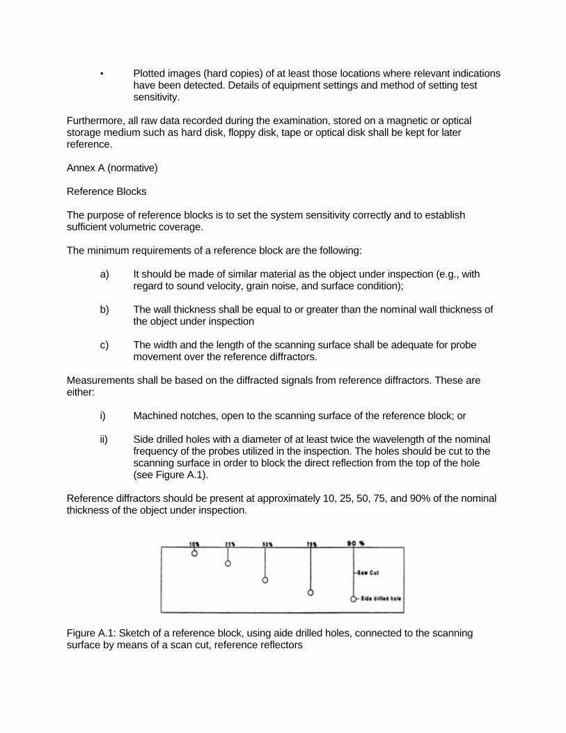
i) Machined notches, open to the scanning surface of the reference block; or ii) Side drilled holes with a diameter of at least twice the wavelength of the nominal

frequency of the probes utilized in the inspection. The holes should be cut to the scanning surface in order to block the direct reflection from the top of the hole (see Figure A.1).

Reference diffractors should be present at approximately 10, 25, 50, 75, and 90% of the nominal thickness of the object under inspection.

Figure A.1: Sketch of a reference block, using aide drilled holes, connected to the scanning surface by means of a scan cut, reference reflectors