EMPIRICAL TESTING FOR BUBBLES DURING THE INTER-WAR

EUROPEAN HYPERINFLATIONS

by

KAI-YINWOO

University of Stirling May, 2004

Thesis submitted for the degree of Doctor of Philosophy in Economics

Table of Contents

Abstract 111

Acknowledgement v

Chapter One Introduction

1.1 Purposes

1.2 Outline of the Thesis 5

Chapter Two Specifications and Solutions of the Cagan Model

2.1 Introduction 11

2.2

2.3

2.4

2.5

2.6

Specifications of the Cagan Model

Particular Solution

Homogenous Solution

General Solution

Summary

Table and Appendices

Chapter Three Structural Time Series Analysis of Data

3.1 Introduction

12

16

18

32

32

34

44

3.2 Statistical Specifications of Structural Time Series Model 45

3.3 Data Description and Structural Time Series Analysis of Data 48

3.4 Summary 55

Tables and Figures 56

Chapter Four Orthogonality Tests and Bubbles

4.1 Introduction

4.2 Literature Review

4.3

4.4

4.5

Procedures of Orthogonality Test and

Econometric Methodology

Estimation Periods and Empirical Results

Concluding Remarks

Figures and Tables

Appendix

72

73

81

90

95

97

107

Chapter Five Regime Switching and Bubbles

5.1 Introduction

5.2 Related Literature and Empirical Issues of Unit Root

Econometric Tests

5.3

5.4

5.5

5.6

Econometric Testing Procedure and Methodology

Monte Carlo Experiments

Estimation Periods and Empirical Results

Concluding Remarks

Tables

124

125

131

141

148

154

157

Appendices 164

Chapter Six Markov-switching Cointegration Test for Bubbles

6.1 Introduction 170

6.2 Econometric Methodology 171

6.3 Empirical Results 175

6.4 Concluding Remarks 179

Tables and Figures 181

Chapter Seven Summary and Conclusion 191

References 198

11

Abstract

In this thesis, I undertake an empirical search for the existence of price and

exchange rate bubbles during the inter-war European hyperinflations of Germany,

Hungary and Poland. Since the choice of an appropriate policy to control inflation

depends upon the true nature of the underlying process generating the inflation,

the existence or non-existence of inflationary bubbles has important policy

implications. If bubbles do exist, positive action will be required to counter the

public's self-fulfilling expectation of a price surge. Hyperinflationary episodes

have been chosen as my case study because of the dominant role that such

expectations play in price determination. In the literature, there are frequently

expressed concerns about empirical research into bubbles. The existence of model

misspecification and the nonlinear dynamics in the fundamentals under conditions

of regime switching may lead to spurious conclusions concerning the existence of

bubbles. Furthermore, some stochastic bubbles may display different collapsing

properties and consequently appear to be linearly stationary. Thus, the evidence

against the existence of bubbles may not be reliable. In my thesis, I attempt to

tackle the above empirical problems of testing for the existence of bubbles using

advances in testing procedures and methodologies. Since the number of bubble

solutions is infinite in the rational expectations framework, I adopt indirect tests,

iii

rather than direct tests, for the empirical study. From the findings of my empirical

research, the evidence for stationary specification errors and the nonlinearity of

the data series cannot be rejected, but the evidence for the existence of price and

exchange rate bubbles is rejected for all the countries under study. It leads to the

conclusion that the control of the inter-war European hyperinflations was

attributable to control of the fundamental processes, since the dynamics of prices

and exchange rates for these countries might not be driven by self-fulfilling

expectations.

iv

Acknowledgement

For the completion of this thesis, lowe a great deal to many people. I am

most indebted to my supervisors, Dr. Vue Ma and Prof. Bob Hart, who gave me

invaluable comments, encouragement and advice on the organization of this thesis.

I have also greatly appreciated the comments and advice on how to improve the

quality of my thesis from my internal and external examiners, Dr. Ron Shone, and

Prof. Martin Sola, respectively. I am also grateful to Dr. Hing-Lin Chan who

provided me with data sets, econometric packages and all other materials

necessary for my research work. His critical evaluations and suggestions on some

chapters of my thesis enlightened me very much.

In addition, I would like to express my sincere thanks to Chulsoo Kim and

Tom Engsted for their opinions, which were essential for an understanding of the

orthogonality tests and of the cointegration tests, when they were invited to attend

seminars in Hong Kong. I also appreciate Kyung-So 1m, Jeremy Piger and In

Choi, who sincerely sent me their own programs for my research works.

Moreover, I express my gratitude to Bruce Hansen, Chang-Jin Kim and Neil

Haldrup, who let practitioners download their Gauss codes for research uses. I am

grateful for Hans-Martin Krolzig, who let Ox users to download his Ox package,

MSVAR, for estimation of regime-switching models. Moreover, I benefited from

v

many members of the mailing lists of GAUSS, RATS and Ox, who had provided

me with codes, and solutions to the problems of econometric programming.

Without their help, many works of econometric estimation and simulation in my

thesis cannot be finished.

Besides, I feel thankful to Miss Susan Sprengeler and Ms. Gillian Gaston for

proofreading my thesis. Finally, my gratitude is extended to the Hong Kong Shue

Van College for granting me financial support for my studies.

Needless to say, all the errors and omissions that may remain are my sole

responsibility.

vi

CHAPTER ONE INTRODUCTION

1.1 Purposes

Price bubbles are defined as explosive processes of asset prices generated by

self-fulfilling expectations independently of market fundamentals. The existence of

bubbles represents a possible explanation for the deviation of asset prices from the

underlying fundamentals. There are many historical examples of incidents that

could be considered from the evidence as being self-fulfilling bubbles. Famous

classic cases include the tulip-mania in the Netherlands from 1634 to 1637, 'the

Mississippi bubble' in France in 1719-1720 and the contemporaneous and related

'South Sea bubbles' in Britain (Garber, 1989 and 1990). In addition, the US stock

market crashes of 1929, 1987 and 2000, the Asian stock market slump of 1997, as

well as the Japanese property market crash in the 1990s, are usually deemed as

recent examples of bubble bursts. Keynes (1936) considered that the stock prices in

the 1920s might not be governed by an objective view of fundamentals but by

"what average opinion expects average opinion to be". The study of bubbles has

attracted much research interest because bubble bursts will normally have negative

wealth effects and create economic confusion (Blanchard and Watson, 1982).

According to Kindleberger (1987), a bubble is defined loosely as a sharp rise in

price of an asset or a range of assets in a continuous process, with the initial rise

generating expectations of further rises and attracting new buyers, who are

generally speculators interested in profits from trading in the asset rather than its

use of earning capacity; the rise is usually followed by a reversal of expectations

and a subsequent sharp decline in price often resulting in financial crisis.

In the literature, general equilibrium arguments can be found about the

theoretical restrictions concerning the existence of bubbles and the effects of

bubbles on the economy. For instance, Tirole (1982) considers that rational bubbles

are ruled out when there exists a finite number of agents in the market. If the

number of agents is infinite, bubble existence will become possible (Tirole, 1985,

Weil, 1989). On the other hand, within a monetary framework, Obsteld and Rogoff

(1983) assert that price bubbles can be ruled out during hyperinflationary episodes

if the government guarantees a probable minimal redemption value for the currency

in units of capital. Nevertheless, the analysis in this thesis focuses on the empirical

examination of the existence of a bubble. This is because, while the existence of

bubbles cannot always be proven theoretically, it may be reasonable to rely upon

econometric methods to detect them.

2

Although the empirical search for evidence of bubbles has largely focused on

capital markets, I contend that the empirical investigation of inflationary bubbles is

equally important. Since the choice of an appropriate policy to reduce the inflation

rate may very much depend on the true nature of the underlying process generating

the inflation, the existence of inflationary bubbles has far-reaching policy

implications. If inflationary bubbles are not present in the observed price series,

then it is only necessary to take control of the market fundamentals, by such means

as the restrictive control of money supply growth and the reduction of fiscal deficits.

If, however, this inflation has a stubborn self-sustaining momentum and is thus

being driven by a bubble phenomenon, then positive action will be required to work

on the expectation mechanism to shock expectations off the speCUlative bubble

path (Funke et al. 1994). For instance, it would require the government to commit

itself to a change in its policies for controlling fiscal deficits and money growth in a

way that is sufficiently binding and convincing for them to be widely believed.

Further, since bubbles are associated with self-fulfilling prophecies, it is reasonable

to deduce that if bubbles do actually occur in the data, they are more likely to be

observed when the expected future market price is an important factor determining

the current market price level. During hyperinflation, expectation plays a dominant

role in the determination of the asset price. Hence, it is believed that 3

hyperinflationary episodes provide fascinating environments for the empirical

study of bubbles (Flood and Garber, 1980b). The classic examples include the

inter-war European hyperinflations of Germany, Hungary and Poland. Sargent

(1982) provides a detailed description of how the hyperinflation in these countries

was stopped. It has been found that the government authorities stopped inflation by

announcing a binding and credible policy regime change and at the same time

taking control of market fundamentals. Thus, the resulting control of inflation

cannot explain fully the true nature of the hyperinflation that occurred. It is

suggested that econometric methods could be used to test for the presence of

inflationary bubbles during these classic hyperinflationary episodes.

It is also to be noted that a floating exchange rate system was first

implemented in European countries during the 1920s following World War I.

According to Okina (1984), if price bubbles occur, and the purchasing power parity

is not violated, bubbles in the nominal exchange rate will also appear and are

reflected in the form of the price bubbles. The country's external competitiveness,

therefore, would not be adversely affected. On the other hand, when price bubbles

are not present but exchange rate bubbles do exist, the nominal exchange rate

bubbles are represented by an explosive deviation from the purchasing power parity,

4

and real exchange rate bubbles will appear as well. With the ups and pops of real

exchange rate fluctuations, the export sectors will suffer serious consequences and

will not recover quickly even when the bubbles finally burst. It is important,

therefore, to check for the presence of both price and exchange rate bubbles over

the same estimation periods.

The purpose ofthis thesis is to undertake empirical research into both the price

and exchange rate bubbles. I have chosen the inter-war European hyperinflations of

Germany, Hungary and Poland for my case study, because, the data series for both

prices and the free market exchange rates are available, and they have been widely

discussed in the literature.

1.2 Outline of the Thesis

The thesis is divided into seven chapters, which are structured as follows:

Chapter Two introduces specifications and solutions of the Cagan

hyperinflation models. Both the fundamental and bubble solutions of the Cagan

models under rational expectations will be derived. In the rational expectations

framework, the specification of a bubble process is related to an arbitrary

martingale. For any value of a bubble coefficient, there exists an infinite set of 5

bubble processes because there also exists an infinity of possible martingales with

respect to a given sequence of information sets. Some examples of theoretical

bubble specifications will be explored. In addition, several bursting bubble

specifications will be illustrated. Owing to the problems of multiple solutions,

indirect testing methodologies that do not require the specification of particular

forms of bubble are more appropriate and have been employed for identification of

bubbles.

Chapter Three provides a brief description of the data series for the inter-war

European hyperinflations of Germany, Hungary and Poland. In addition, since the

stochastic properties of the data series will affect the econometric methods to be

adopted and the economic interpretations of the empirical results in subsequent

chapters, I also investigate the stochastic properties of the observed variables.

Using structural time series modeling techniques, I extract the unobserved

structural components of the observed data variables and examine the integration

orders of the data on the basis of the specifications of the structural time series

components.

In the existing literature, three main concerns have been aired about the

empirical investigation of bubbles. First of all, most of the previous empirical 6

studies of bubbles have assumed at the outset that the models they use are correctly

specified. This means that if the models are in fact misspecified, this may be falsely

interpreted as evidence for the existence of bubbles. The bubble test is, however, a

joint test for both bubble existence and correct model specification. The evidence

for no bubbles implies that no bubbles are present and that the model under study is

correctly specified. Hence, the appropriate testing procedures and econometric

methods should be effective enough to separate model misspecification from the

evidence of bubbles. Secondly, there is a problem of observational equivalence

between expected future changes in economic fundamentals and bubbles. When the

Governments attempted to bring runaway inflation under control by enforcing

monetary reforms during the hyperinflationary episodes in the 1920s, the nonlinear

movements of price or exchange rate series that are caused by the possible regime

shifts in underlying fundamentals may often be misunderstood as representing a

bubble path. Thirdly, it is found that the stochastic bubble process, as illustrated in

Chapter Two, exhibits an explosive dynamic path over the expanding phase of the

bubble process only, but not over the whole sample period. Consequently, standard

econometric methods will be biased towards the rejection of bubble existence. In

subsequent chapters, I apply advances in econometric procedures and

methodologies to handle the above empirical issues of bubble detection in different 7

ways.

In Chapter Four, I design a set of orthogonality testing procedures for

empirical study, which can help separate tests on model specification from tests for

bubbles in a more rigorous manner. The orthogonality testing procedure is expected

to detect any kinds of bubble process that are not orthogonal to information sets. I

employ the fully modified econometric methodologies to conduct the orthogonality

tests, which are developed under the assumption of the linear data generation

process. Hence, I restrict the empirical analysis on pre-reform samples as has been

done in the previous literature. This chapter develops the ideas contained in my

work published in Progress in Economic Research (Chapter Two) and the

International Review of Economics and Finance.

In order to extend the empirical analysis to cover the excluded observations of

monetary reforms and to permit a comparison with the evidence for bubbles

contained in Chapter Four, in Chapter Five I employ the threshold cointegration

method for bubble detection. Since the threshold cointegration methodology can be

used to test simultaneously for the existence of nonstationary roots and for

threshold nonlinearity in two regimes, it is expected to be robust to the presence of

both a nonlinear switching process and a stochastic bubble. I also choose traditional 8

linear cointegration tests and the cointegrating RALS-ADF test for carrying out the

comparison study. Moreover, by conducting co integration analyses between the

real money balances and price changes, and subsequently between the real money

balances and money growth rate, the existence of a bubble can be separated from

the model misspecification. In addition, a comparison of the orthogonality tests and

the cointegration tests in detecting bubbles is made.

Further, while the regime-switching behaviour of market fundamentals

discussed in Chapter Five is restricted because it depends on an observed threshold

value, the switching process described in Chapter Six is specified to depend on

unobservable Markov-switching states generated by a first-order Markov chain.

The probability law that governs the Markov-switching states is more flexible in

that it allows the observed data to determine the specific form of the nonlinearities,

which are consistent with the sample information. Following the same

cointegration-testing procedure as in Chapter Five, I adopt the Markov-switching

cointegrating ADF method in Chapter Six, in order to simultaneously model the

Markovian regime shifts in underlying fundamentals and to test for bubble

existence. This method is considered to be effective in identifying nonstationary

dynamics from the stochastic bubbles.

9

Finally, Chapter Seven summarizes the major findings of the empirical

research, assesses the suitability of the econometric methods for carrying out tests

for the existence of bubbles, and contains the concluding remarks.

10

CHAPTER TWO SPECIFICA TIONS AND SOLUTIONS OF THE

CAGAN MODEL

2.1 Introduction

In this chapter, I will briefly describe the specifications of the Cagan model

under rational expectation in which the price and exchange rate series are expressed

in first-order linear difference equations. The particular and the homogenous

solutions to the Cagan model can then be derived. The particular or fundamental

solution characterizes a unique dynamic movement of an underlying fundamental

process. Several explicit representations of the fundamental solution will be

explored. The homogenous or bubble solution is non-unique III a rational

expectations framework. I attempt to specify some examples of bubble solution

with different dynamic properties. Also, several bursting bubble specifications will

be illustrated. It is concluded that the problems of multiple solutions make indirect

tests more attractive than direct tests for bubble detection. In addition, the general

solution, which is just the sum of particular and homogenous solutions, will be

discussed. Hence, the bubble paths are characterized as any deviations of the

general solution from the fundamental solution when the model is specified

correctly. The remainder of the chapter proceeds as follows: The specifications of

the Cagan's hyperinflation models will be explored in Section 2. Sections 3 and 4 II

explore the particular and homogenous solutions respectively. The general solution

is discussed in Section 5. A summary is offered in the final section. Proofs of some

equations are shown in the appendices.

2.2 Specifications of the Cagan Model

Money balances are held as a reserve of purchasing power for contingencies.

The desired real money balances depend upon several variables including real

wealth, real income, and the expected opportunity cost of holding money. The

expected cost of holding money refers to the difference between the expected

monetary return on holding cash balance and on substitutes of local currency. The

money return on cash balance is negligible and is usually assumed to be zero.

Therefore, to the extent that money is held as a substitute for financial assets, the

expected cost of holding money includes the expected interest rate and capital gain

yield of holding those financial assets. To the extent that money is held as

substitutes for non-perishable consumers' goods, the expected cost of holding

money is the expected rate of depreciation in the real value of money, or

equivalently, the rate of inflation. According to Cagan (1956), hyperinflation refers

to the rise in prices at a rate at least equal to 50% per month and only the expected

inflation rate accounts for the drastic fluctuations in real cash balances during 12

hyperinflation, with all other variables being considered to have minor effects on

desired cash balance. Cagan (1956) assumes the expectation mechanism to be

adaptive. Sargent and Wallace (1973), Sargent (1977) and Salemi and Sargent

(1979), however, introduce the rational expectation hypothesis of Muth (1961) to

the Cagan model. Mathematically, the linear form of the Cagan model under

rational expectations and instantaneous clearing in the money market is given as:

(2.1)

where M 1 is the natural logarithm of the money stock at time t, 1£1,1 is the natural

logarithm of the price level, E 1 (.) denotes the mathematical expectations operator

conditional on information set nt, cx.. is a constant, /31 is the semi-elasticity of real

money demand with respect to the expected inflation rate and u 1,1 refers to a

money demand disturbance term representing all deviations from the exact Cagan

model under rational expectations such as demand velocity shocks and all other

omitted real variables. Theoretically, the value of ~l should be negative because

money holders will substitute consumers' goods for money when the real value of

money is expected to fall or the expected inflation rate rises.

13

Since local currency loses its value very rapidly during hyperinflation,

foreign currency balances are often held in order to perform the functions of a

medium of exchange and a store of value. Even if foreign currencies are held

merely as a store of value, they are often converted back into domestic money and

then goods at a later time. Hence, the substitution between domestic money and

goods can occur, directly or indirectly, via foreign currencies (Moosa, 1999). Such

phenomenon of currency substitution is documented in Sargent (1982) for the

inter-war European hyperinflations. In light of this, it is appropriate to replace the

future inflation rate in Eq.(l) with the expected depreciation rate of domestic

currency to represent the cost of holding domestic money balance. 1 If I further

assume that the purchasing power parity (PPP) relationship holds and that all the

foreign money demand determinants, for example, foreign interest rates and

income levels, are assumed to be constant, the real money balance represented by

Eq.(2.1) can be alternatively expressed as:

(2.2)

I Frenkel (1977 and 1979) estimated the Cagan money demand using forward premium and

expected depreciation rate as a measure of expected cost of holding local currency during the

German hyperinflation.

14

where 1t2,t is the natural logarithm of the exchange rate measured as the value of

domestic currency per unit of foreign currency, ~1t2,t+l represents the exchange

rate change at time t+ 1, <X2 is an intercept, ~2 is the semi-elasticity of currency

substitution between domestic and foreign currency and u2,t is a measure of model

noise from the linear exact Cagan model under rational expectations that include all

the domestic and foreign money demand shocks and omitted real-side

determinants.

Re-arranging Eq. (2.1) and Eq. (2.2) in terms of 1t j ,t (j = 1,2) gives:

j = 1,2. (2.3)

Eq.(2.3) is expressed as a first-order dynamic linear difference equation with

rational expectations. The future expectation and the current variables are

determined simultaneously. The general solution of (2. 3) is the sum of a particular

solution and a homogenous solution.

15

2.3 Particular Solution

For sake of notional simplicity, I eliminate the subscript j in subsequent

equations. By recursively substituting forward for E, (1tI+I +i ) and using the law of

iterated expectations, I obtain:

When 1-f3-I< I, the transversality condition: f3 -1

. ( f3 Ji+1 ~lm -- Et(1tt+I+J = 0, ..... a> f3-1 (2.5)

is then satisfied. Under this circumstance, the solution of 1t1 is given by:

(2.6)

The expression of 1t{ represents a forward-looking particular solution or the

fundamental solution to the Cagan models (2.1) and (2.2) under rational

expectations, which is determined by the present discounted value of expected

levels of the market fundamentals, (Mt+i -u 1+i ), for all i ;S O. If the expectation

of (M, -u 1 ) grows at a constant rate g, the infinite sum, 1t{, will converge when

16

~ -1 1 2 (1+g) < - or g < 1- I·

~ ~

By assuming special stochastic processes for the sequence of M, and "t'

1t; can be written in explicit manners. Let's define X, as _1_M, or ~"t. 1-13 1-~

Gourieroux et al. (1982) considers the ARMA solutions of the Cagan model.

Assume that 1_13_1< 1 and X, admits an ARMA (p,q) representation, that 13 -1

is, qJ(L)X, = 9(L)l'l" where L is a lag operator, qJ(L) = 1- qJlL - ... - qJ plf,

9(L) = 1 + elL + ... + eqr and '11, is a white noise. Then, the present discounted

value of X,, i(_J3_)i E, (X,+i ) can be explicitly written as a unique stationary ;=0 J3-1

ARMA solution:

1 L b9(b)qJ(L) X {(L-b)[ - qJ(b)e(L)]} I'

(2.7)

where b is defined as ~ . J3 -1

However, many economic variables exhibit non stationarity. If X, follows

random walk with drift and linear time trend, that is, M, = J..l + rot + l'l/ then the

present discounted value of X I is written as: 3

2 In fact, it is similar to the case of the constant dividend growth model in which the growth rate of

dividend is no larger than the discount rate.

3 The steps of proof are shown in Appendix 2.1.

17

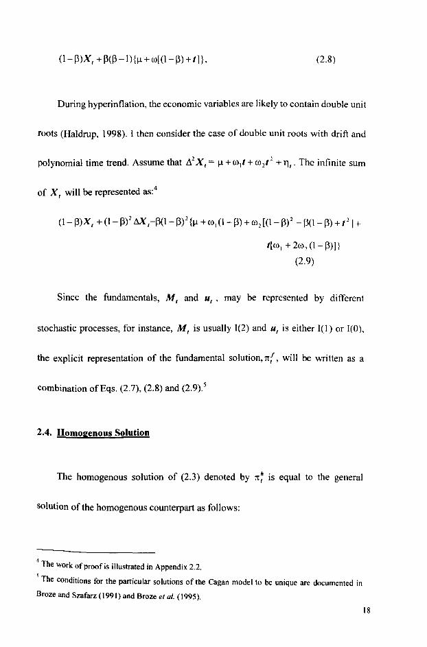
(l-\3)X, + \3(\3 -l){~ + w[(1-\3) + In, (2.8)

During hyperinflation, the economic variables are likely to contain double unit

roots (Haldrup, 1998). 1 then consider the case of double unit roots with drift and

polynomial time trend. Assume that /).2 X, = ~ + wll + W 2/2 + 11

" The infinite sum

of X, will be represented as:4

I[ WI + 2W2 (1 -\3) J}

(2.9)

Since the fundamentals, M, and u" may be represented by different

stochastic processes, for instance, M, is usually 1(2) and u, is either 1(1) or 1(0),

the explicit representation of the fundamental solution, n{, will be written as a

combination of Eqs. (2.7), (2.8) and (2.9).5

2.4. Homogenous Solution

The homogenous solution of (2.3) denoted by n: is equal to the general

solution of the homogenous counterpart as follows:

4 The work of proof is illustrated in Appendix 2.2.

5 The conditions for the particular solutions of the Cagan model to be unique are documented in

Broze and Szafarz (1991) and Broze et al. (1995).

18

h b1+iE (h ) 7t t = t 7tl+l+i , i ~ 0 (2.10)

Multiplying both sides ofEq.(2.10) by bt obtains:

bt h bt+1+iE (h ) 7tt = t 7tt+l+i , (2.11 )

Gourieroux et al. (1982) derive the homogenous solution, 7t;, by using the

martingale process. Let's define mt as bt 7t~, and the stochastic process of mt

satisfies the martingale property such that Et(mt ) = m" and Et (mt+;) = m" for

all i > O. The homogenous solution, 7t~, is represented in terms of the martingale

process:

(2.12)

Any arbitrary martingale process, m t , can be considered as a component of

7t;. It implies the existence of multiple solutions for the Cagan models under

. . E ( ") E (mt+! ) 1 (mt) h rational expectattons. Smce t 7tt+! = t bt+! = b b' were I b I < 1, the

stochastic process of 7t; follows a submartingale such that:

7th

E (7th )= _t > 7th t t+l b t· (2.13)

19

Therefore, 1t~ satisfies a bubble process that explodes in expected value and it

can be interpreted as a bubble solution,Bt . Also, when Eq. (2.11) and (2.12) are

substituted into the transversality condition of (2.5), it implies

Et(mt+1+i ) = mt = 0, for i- 00. Consequently, the transversality condition of(2.5)

implies the nonexistence of B t ·

The stochastic unit root process suggested by Granger and Swanson (1997)

can be generalized to the martingale process, mt

:

(2.14)

Suppose that x t - N (11 %' cr;). For an arbitrary A., the moment-generating

function of a normally distributed variable, x t , is given by E (exp( A.xt » =

exp(A.~x + 'xA?cr!). Hence, qt is represented by exp[A.xt -(A.~x + liA.2cr!)].

Dividing Eq.(2.l4) by btyields the following general bubble specification:

B = (qtBt-l) + ~ t b bt (2.1Sa)

(2.1Sb)

20

By restricting underlying parameters of bubble process given by (2.1Sb) such

as ')... and Il x' there are different theoretical bubble specifications with particular

stochastic properties to be derived (Salga, 1997). I illustrate them with further

modifications and refinements.

2.4.1. ')... = 0

Let's first assume that ')...= 0, the resulting bubble process will be obtained as

follows:

_ Bo Li=1 ro I=i --+=:.::.!..--b' b'

(2.16)

Since the above bubble process is driven by time only, it is known as pure

time-driven bubble process. As t- 00, the time-driven bubble must converge

toward infinity with I b I < 1 and its dynamics must then be asymptotically unstable.

In particular, if m, is a constant, the sequence of rot in Eq.(2.14) will become zero.

Consequently, Bt

is represented by !~ only, which is known as the deterministic

bubble.

21

2.4.2. A. *0 and Ilx + Ii A. a! = 0

If A. * 0 and Il x + Ii A. a! = 0, it then implies Ilx:1= 0 because A.

-21l --2 _x :1= o. The bubble process can be specified as:

ax

- 21l 0), B, = exp(--2 _x x, -In b) B'_I + l1"

ax (2. 17a)

Suppose that x, = w t - w t _1 = Ilx + Ext' where Ext ~ N (O,a!).

Replacing x t by w t - wt-\' substituting one period forward for Bt+1 and

re-arranging yield:6

-21l B t = exp[--2-X wt -(lnb)t]

ax (2.17b)

where In b < 0 since b < 1 or 13 < O.

Assume that wt represents a vector of underlying 1(1) fundamental variables

in the model. The stochastic bubble process of (2. 17b) thus depends upon both time

and the underlying fundamental process. Further, by recursively forward

substitution, W t = Wo + Il xt + L:~I E xt-j , the bubble process given by (2. 17b) can be

alternatively written as:

6 Appendix 2.3 proves the general specification of bubble when x t = W t - W tl .

22

(2.17c)

Given that L:=J E xt-i _ 0 as t- 00, B, will converge toward zero when t

- 2~x Ilx < In b < O. As a result, the dynamics of B, is asymptotically stable. The ax

divergent bubble process driven by the time component, exp[ -(In b )/], would be

- 211 somehow offset by the fundamental component, exp[--2 _x 11 x], to a certain

ax

degree. Hence, the inclusion of the fundamental-dependent component may help

stabilize bubble dynamics and exhibit more dynamic properties of the bubble

process (Ikeda and Shibata, 1992 and 1995).7

One special case is that 11" + ~ A cr! = 0 but A is restricted to be I, 11 x =

a 2

- -=- < 0, then the bubble process of (2.17a) and (2.17c) will be simplified to be: 2

B, = exp(x, -Inb) B'_J + :: (2.18a)

(2.18b)

7 Ikeda and Shibata (1992 and 1995) however derived the specifications of fundamental-dependent

bubbles in a continuous-time framework.

23

Similarly, the asymptotic dynamics of bubble process given by (2. 18b) depend

on the sign of (Il x -In b). If Il x <In b < 0 or exp(1l x) < b < 1, B t will converge

toward zero and is then asymptotically stable.

Let In b = (K + H) < 0, where K and H are arbitrary constants. Assume that A

* 0 and (Allx + Ii A2a~ + K) = 0 with A} and A 2 being the two characteristic roots.

Hence,

(2. 19a)

or B, = exp(A2 W, - Ht) (2.19b)

(2.20a)

(2.20b)

I first consider the case of Il x :t O. While Il x :t 0 and (Il: - 2a:K) = 0, then,

2 Il K = Il x

2 > 0, H must be negative. From (2.20a) and (2.20b), A) = 1..2 = - -+ The

2a x ax

bubble process of (2. 19a) and (2. 19b) will be written as:

24

B, = exp(-f.l; w, -Ht) ax

(22Ia)

(2.2Ib)

2 2

When - f.l; < H, which implies exp( - f.l x2 ) < b, the bubble process will ax 2a x

converge towards zero asymptotically.

On the other hand, when (f.l! -2a!K) *0, then it can be seen that AJ * A2 .

The bubble process of (2.19a) or (2.19b) or any linear combination of them still

satisfies the sub martingale process of (2.13). Let's define Al and A2 as two

arbitrary constants. The linear combination of bubble process (2.19a) and (2.19b) is

given as:

(2.22a) 8

(2.22b)

8 Appendix 2.4 provides the proof that the bubble solution (2.22a) can satisfy the submartingale

property.

25

2

In particular, while (Il~ -2a~K» 0, or K < Ilx2 ' then AI >A 2 and the A 2a x

values are real numbers. The stochastic stability of bubbles specified by (2.22b)

depends upon whether A;ll x < H or exp(A;llx + K) < b for all i = 1,2.

2

Moreover, if (Il~ -2a~K) < 0, or K > :x2 > 0, then H must be negative and ax

the A values contain imaginary numbers:

(2.23a)

(2.23b)

where ; is an imaginary number, ~ . Let's define hI = - ~ x , and h2 ax

[(2a2K-1l )1/2] x 2 x , so that AI' A2 = hI ± h2 i. The bubble process is specified as: 9

ax

(2.24a)

(2.24b)

Under this circumstance, the bubble process of (2.24a) and (2.24b) can exhibit

2 -Il~ cyclical patterns. While - 11 x < H < 0, or exp(--2 - + K) < b, the cyclical

a 2 a x x

9 Appendix 2.5 offers the detailed steps of proof.

26

dynamics of B t is asymptotically damped.

Now, I consider the case of Il x = O. When Il x = 0, then K must be negative

(-2a 2 K)1I2 (-2K) 112

since (Yz A?a! + K) = O. Also, AI = x 2 > 0, ax ax

(-2K)I!2 1..2 =- < O. The bubble process will be specified as:

ax

( 2K)1/2 (-2KY' 2

Bt

= AI exp[ - wt - Ht] + A z exp[ wt - HI] (2.2Sa) ax ax

(2.2Sb)

On condition that H > 0, the bubble process (2.2Sb) will converge towards

zero as I~ 00 .

Suppose that A * 0 and (All x + Yz AZa: + In b) = 0, the bubble process will be

purely driven by a fundamental process:

(2.26a)

or B t = exp(A 2 w t) (2.26b)

27

(2.27a)

(2.27b)

Given the fact that In b < 0, when ~ x 7= 0, it is impossible for (~: - 2cr: In b)

2 2

= 0 and (II 2 - 202 In b) < 0, which imply that In b = ~ x2 > 0 and In b > ~ > 0 "-x x 20 2cr 2

x x

respectively. The only possible case is given by (~: - 2cr: In b) > 0, or In b < 0

2

<~. Then, AI > A2 and the A values are real numbers. The specification of the 2cr2

x

bubble process will be written as:

(2.28a)

(2.28b)

The stochastic stability of bubbles specified by (2.28b) depends upon whether

A.II < 0 for all i = 1,2 . • ,.-x

(-20 2 Inb)1/2 (-2Inb)1/2 In case of J.l x = 0, then 1..1 = x = > 0 and

02 a x x

A2 - - (-2Inb)1/2 < 0 since In b must be negative. The bubble process is shown as: ax

28

(2.29a)

(2.29b)

The bubble process of (2.29b) must exhibit stable dynamics as t-~ 00 •

From the above, although all bubble processes are derived to explode in

expected values, they may converge towards zero as t --- 00 under certain

restrictions on parameters. The different examples of bubble specifications are

summarized in Table 2.1. The asymptotic stability of bubble process leads to

difficulties in bubble testing. Nevertheless, the numbers of observations are usually

not large during hyperinflationary episodes and consequently, such difficulties may

not be so serious in my subsequent empirical studies. 10

Other than the asymptotic dynamics of bubble, the bursting properties are the

main issues about the theoretical specifications of bubble solution. The

submartingale property of bubble process (2.13) can be further modified by the

inclusion of a probability that a bubble continues to grow (0:;;;;; n :;;;;; 1):

10 However, it may create serious problems of bubble detection in financial markets with long data

horizons.

29

= B, (2.30) b

where E,(Bt+IIG) and E,(B'+IIC) refer to the expected values of Bt+1 given the

regimes of bubble growth (G) and bubble collapse (C) respectively. I I

One particular example of a bubble process that is satisfied with the above

bursting bubble specification (2.30) is given as:

(2.3Ia)

(2.3Ib)

where E,(rot+l) = O.

The bubble process of (2.31 a) and (2.31 b) would occur with the probability of

IT in regime G and with the probability of (1- IT) in regime C respectively. They

represent a general version of the bursting bubbles suggested by Blanchard and

Watson (1982) who restricted the value of A in (2.31 a, b) to be zero. It is noted that

the expected value of the bubble in regime G, E,(Bt+IIG) = (bI1)-1 B" where

(bI1rl > b-I, and the bubble will collapse to zero expected value as it bursts,

E,(Bt+1 I C) = O.

II The probability, IT, can be a variable as a function of the size of bubble (Norden, 1996).

30

In addition, Evans (1991) suggests a periodically collapsing bubble

specification:

= exp[Axt +1 -(A.~x + ~A.2cr:)][00 +8 t+l n -lb-1(B, -oob)]+ :::11

for B, > K.

(2.32)

where both K and 00 > 0, St is an exogenous independently and identically

distributed Bernoulli process that takes the value of 1 with probability of n in

regime G and 0 with a probability of (1- n) in regime C. Since (B'_1 - oob) is

restricted to be positive, 00

must be smaller than (K b-1). 12

For B, ~ K, it implies that n = 1 and E,(B'+I) = B, . For B, > K, b

Et (Bt+l) is equal to ~' for any value of B t and the bubble process of Evans

(1991) can satisfy the submartingale property. It is found that the collapsing bubble

is strictly positive and never vanishes. Moreover, the size of bubble collapse or

explosion and the probability n are dependent upon the sizes of the bubble

12 The collapsing bubble is specified to be positive since if a bubble collapses to zero, it cannot

re-start (Diba and Grossman, I 988b).

31

compared to the value of K . Also, the bubble bursts partially in contrast to the total

bubble collapse of the bursting bubble of (2. 31).

2.5. General Solution

The general solution to the difference equation (2.3), denoted by 1t: , is equal

to the sum of particular and homogenous solutions, i.e. 1t{ + B t . The stochastic

process of 1t{ characterizes the long-run equilibrium path of 1tf ; on the other hand,

the movement of Bt characterizes the deviation of 1tf from 1t{. If the model

under study is correctly specified, the task of bubble testing consists in detecting

whether any movements of asset price deviate from the paths predicted by the

market fundamental solution.

2.6. Summary

I have specified two versions of the Cagan model under rational expectations,

in which the opportunity costs of holding money are measured by the expected

inflation rate and the expected depreciation rate of local currency respectively.

Hence, they will be used for the subsequent study of price and exchange rate

bubbles in this thesis. The general solution of the Cagan model is simply the sum of

fundamental and bubble solutions. The fundamental solutions can be expressed in 32

explicit representations dependent upon the assumed generating processes of the

underlying fundamentals. There exist arbitrary martingales in the bubble solution,

which is therefore non-unique in the rational expectations model. By restricting

parameters of the bubble solution, several examples of different theoretical bubble

specifications can be explored. Some exhibit asymptotic stability and some display

different switching behaviours under alternate regimes of explosion and collapse It

makes the indirect testing methodologies more attractive for bubble detection. In

subsequent chapters, I will conduct econometric studies to examine whether the

price or exchange rate series deviate from the particular solutions. Before doing so,

the first step is to examine the statistical properties of the relevant economic

variables in the next chapter so that I can adopt appropriate econometric procedures

and methods on the data set.

33

Table 2.1 Summary for different theoretical bubble specifications Parameter restrictions Equations Conditions for dynamic

stability A. =0 2.16 None

Il + li A. a2

= 0 x 2 x

J..l x*,O and A. *' 0 2.17a, b, c -21l x --2 -Il x < Inb < o. ax

a2 2.18a, b Ilx < In b < 0

J..l =-~< 0 and A. = 1 x 2

A. *0, and (A.J..lx + li A.2a~ + K) = 0, where In b = (K + H) < 0

J..lx *0 and 1..)=1..2 2.21a, b 2 -~<H

a 2 x

Il ... *0 and A.) * 1..2 2.22a,b A.;llx < H

Il ... *0 and 2.24a,b 2 -llx<H<O

1..1> 1.. 2= hi ± h2i a 2 x

Il x= 0 and A.) * 1..2 2.2Sa,b H>O

A. *0 and (A.J..l x + li A.2a! + lnb) = 0

Ilx *0 and A.) * 1..2 2.28a,b A.;llx <0

Il x = 0 and A.) * 1..2 2.29a,b Must be asymptotically stable

34

Appendix 2.1

Given that 1 b 1< 1, the presented discounted value of X, can be expressed as

follows:

'ibiE,(X,+J = X t +bE,(Xt+I)+b2E,(Xt+2)+b3Et(Xt+3)+'" i~O

'" = X t + L:lbiE,(M,+J+b 'LbiE,(X'+I+i)

i~O

= X t +_1_~", bi E (M .) 1- b 1 - b ~i=1 ' t+l

(A.2.1.1)

Suppose that tlX'+j = J.l+ro(t + j)+llt+j' the values of b i E,(AX,+;} are given as:

b" E (AX ) = b"J.l + b"rot + nb"ro I tH'

as n- 00

Hence, L:I bi E, (Mt+i) is equal to the sum of the following three components:

35

The value of each component is calculated as follows:

L "" bi - b!l L"" b i _ bmt 11_- mt--i=1 ,... I-b' i=1 I-b' L"" obi I Leo bi bm ,m=-- m=--

i=1 (I-b) H (l-b)2

(A2.12)

It is known that _1_ = 1- p, and _b_ = -p, then, from (A.2.1.1) and (A.2. 1.2), I I-b I-b

obtain:

= (1 - P)Xt + (1- P)[ -pJl- pmt - P(1- p)m]

= (1- P)Xt - p(1- P)[Jl + mt + (1- p)m]

= (I - P)X, + P(P -1){Jl + m[(l- P) + t]}

36

Appendix 2.2

Given that ,11,,2 X t+ j = ~ + 00] (I + j) + 00 2 (I + j)2 + llt+ j' the values of bi E t (fiX t+i )

are shown as:

b 2E t(fiXt+2) = b2AXt+] +b2~+b2oo](t+2)+b2OO2(t+2)2

= b 2 AXt + 2b2~ + b 2oo] (t + 1) + b2OO2 (t + 1)2 +

b 2oo] (I + 2) + b 2OO2 (I + 2)2

b3Et(AXt+3) b3AXt +3b3~+b3oo](t+I)+b3OO2(t+l)2 +b3oo](t+2)+

b3OO2 (t + 2)2 + b3oo] (t + 3) + b3OO2 (t + 3)2

b"Et(DXt+,,) = b"AXt +nb"~+b"0)1(t+l)+b"0)2(t+I)2 +

b"oo](t +2)+b"OO2(1 +2)2 + b"co l(t+3)+

b"co 2(t + 3)2 + .. +b"col(t + n) +b"co 2(t + n)2 as n~ 00

From the above, L:] b i Et (AXt+i) is equal to the sum of the following four

components:

37

The finite values of the above four components of :L:I b i E, (M'+i) are derived as

follows:

_1-L~ t(biO)I) + (bO)I +0+2)b 20)1 +(1+2+3)b3

0)1 + ... ) I-b ,~I

I bO) t + _I_~", ibiO) (1-b)2 I I-bL..i~1 I

1 bO) t (1-b)2 I

+ 1 ~"' biO) (1_b)2L..i=1 I

1 + bO)I (1-b)3 '

1 ~"' 2 . 1 L"'· 1 L"' 2 . -1 bL..i=lt (b'0)2) + -- ._ t(2ib')0)2 + -- ·_1(; )b'0)2 - I - b '-I (1- b) .-

t2bO) 2 I ",. 1~", .

(1-b)2 + (1-b)2 Lij(2b')0)2 + (1-b)2 L..i=I(2i-l)b'0)2

t 2b0)2 + t(2b)ro2 + b0)2 L"' 2biO) (1-b)2 (1- b)3 (1-b)3 i=1 2

t 2bO) 2 + t(2b)ro2 + b0)2 + b20)2 (A221) O-b)2 (1-b)3 0-b)4

38

OX)

From (A.2.1.1) and (A.2.21), the value of L bi E t (X t + i ) is equal to: i=-O

X t 1 M t b~ bro]t bro] t 2bro 2 t(2b)ro 2 --+-[-+ + + + + + l-b l-b l-b (I-b)2 (l-b)2 (I-b)3 (l-b)2 (I-b)3

bro 2 + b2ro 2]

(l-b)4

X t M t b ro] ro 2 (1 +b) b 2ro 2

= l-b + (l-b)2 + (l-b)3 [~+ (I-b) + (l-b)2 ]+ (l_b)3 [WI + (l_b)]t

bro 2 t 2

(1- b)3

= (1- J3)Xt + (1- J3)2 M t-J3(1- J3)2 {~+ ro] (1- J3) + ro 2[(1- J3)2 - J3(1- J3) + t 2] +

39

Appendix 2.3

Let x t = wt - wt _l • Substituting one period forward for B t +1 from the general

bubble specification (2.15), I obtain:

(A,~ x + ~ A,20: + In b)(t + 1) - (A,~ x + ~ A,

20: + In b)] Bt + :::i

=exp{A,wt+1 -(A,~x + ~A,20: +Inb)(t+l)-

Assume that {O) t} = 0 , then:

~ _ exp[A,wt+1 - A,(~x + Ji A,20: + In b)(t + I)]

Bt - exp[Awt -A(~x + JiA20! +Inb)(t)]

Hence, Bt = exp[A,wt - (A,~x + ~ A,20: + In b)t]. (A.2.3.1)

By imposing different parameter restrictions upon (A.2.3.1), I can obtain different

bubble specifications summarized in Table 2.1.

40

Appendix 2.4

Let's examine whether the linear combination of bubble process (2. 19a) and (2 19b)

or the bubble process (2.22a) can still satisfy the submartingale property such that

It is known that bE'_1 (B, ) = Et-J [exp(ln b )B, 1. By substituting the bubble process

(2.22a) into Et-J [exp(ln b)B,l ,I obtain:

Also, it is known that Et-J (q,Bt-J) = Et-J (exp[Ax, - (A.ll x + ~ A.2cr!)]B,_I)' By

substituting the bubble process (2.22a) into E'_I (exp[Ax, - (A.Il x + ~ A.2cr! )]Bt I)'

I find that Et-J (qtBt-l) is equal to:

E'_I {exp[A.I W, - 1..1 wt-J - (A.llx + Yz A.2cr!)]AI exp[A.1 wt-J - H(t -1)] +

exp[A.2w, -A. 2wt-J -(A. 2Ilx + ~A.2cr!)]A2exp[A.2wt-J -H(t-l)]}

41

Given the assumption that In b = K + H, and (A~x + Ii' A2cr~ + K) = 0, then

Et-j(qtBt_j) = Et_j{A j exp[AjW, -(\~x + li'A~cr: +K)-Ht+Inb]+

A2 exp[A2 wt -(A2~x + ~A/cr: +K)-Ht+Inh])

= E,_j{Aj exp[Ajw,-Ht+lnb]+ A 2 exp[A 2 wt -Ht+Inb]}

= bEt-I(Bt )

42

Appendix 2.5

AJ = hI + h2 i, and Az = hI - h2 i into (2.22a), I obtain:

B t = exp( -Ht}[A] exp(h] + hzi}wt + A z exp(h J - h2i}wt ]

= exp(h]wt -Ht}[A] exp(ih Zwt}+A2 exp(-lo2W t}]

= exp(h] wt - Ht){A] [cos(hz wt } + i sin(h z wt }]+

Az[cos(h 2 wt } - i sin(h z wt }]}

= exp(hJwt -Ht}[(A] +Az}cos(hZwt}+(AJ -Az}isin(hZwt }]

= exp(h] wt - Ht}[A3 cos(h 2wt } + A4 sin(h 2w t }].

where A3=AI+A2, ~ = (A1-A2}i

43

CHATPER THREE STRUCTURAL TIME SERIES ANALYSIS OF DATA

3.1 Introduction

In this chapter, I will provide a brief description of the data series for the three

inter-war European hyperinflations of Germany, Hungary and Poland. Also, since

the stochastic properties of economic variables affect the econometric methods

adopted for subsequent studies, I attempt a structural time series analysis to identify

the unobserved stochastic components of the observed data series. From the

reduced forms of the trend component, the integration orders of the data series can

be found. In addition, some evidence of regime changes in data generation can be

detected from the trend component or the slope of the trend. Such findings are

Important for empirical studies conducted in the subsequent chapters. This chapter

is structured as follows. Section 2 introduces the statistical specifications of the

unobserved components in a structural time series model. Section 3 discusses the

data sources, sample lengths and definitions of the variables under study. The

statistical and graphical analysis of the unobserved components will also be

presented. Section 4 summarizes the findings.

44

3.2. Statistical Specifications of Structural Time Series Model

Before taking the empirical testing in subsequent chapters, I try to examine the

stochastic properties of the economic variables under study. Using the structural

time series modeling techniques (Harvey, 1989), I attempt to decompose and

analyze the unobserved components of the observed data series. A univariate

structural time series model is formulated as:

(1- 'I'(L»Yot = Ilt +Yt + \lit +f:" 8 t -NID(O, a;), t = 1, ... , T.

(3.1)

where Yot is an observed time series variable, 'I'(L) = 1- 'I'lL - ... - '¥pLP where

'1'; is a parameter of a lagged value of Yot ; the elements Pt , Yt , 'l't and 8,

represent the unobserved trend, seasonal, cyclical and irregular components

respectively. 13

The trend is the long-run component in the series, which indicates the general

moving direction of the observed series under study. There are two parts to the

trend specified as:

13 A first-order autoregressive component and a vector of exogenous variables should also be

included in the univariate structural time series model (3.1), but they are not found in my empirical

results and thus are excluded here for simplicity.

45

Pt = P'-I + (,'

77 t -NID(O, a;),

(t -NID(O, at),

(3.2a)

(3.2b)

where f..l t is the level, which is the actual value of the trend, p, is the slope of the

trend. If a; and at are zero, f..lt and Pt will be fixed respectively.

Different properties of the level, slope and irregular component would result

in different specifications of the trend model. Let's illustrate them briefly. 14 When

both a; and a; are zero, then the trend specification given by:

f..l t = f..lt - I + PH ,

Pt = Pt-I + (" t;, -NID(O, a~),

(3.3a)

(3.3b)

is known as a second differencing model. When a; is not zero; the trend is known

as a smooth trend model. Also, in case where both a; and a~ are zero, the trend

model specified as:

IJ., = f..lH + PH + 77"

14 The details of the trend specifications are documented in Koopman et al. (2000).

(3.4a)

(3.4b)

46

is called random walk with a drift, or random walk if Pt = Pt-I = 0. While cr~ is

not zero, the trend component is known as the local level with a drift or the local

level, dependent upon whether Pt = Pt-l is different from zero.

The seasonal component may be based on the dummy variable form, or the

trigonometric formulation. Given that s refers to the number of seasonal

frequencies, the seasonal dummy is given by:

s-]

Y1 = L -YI-j + OJt ,

j=]

Moreover, the trigonometric seasonal formulation is:

(3.5)

OJ) ,-NID(O, a;' ). , ~

(3.6)

where Aj = 2jK / s refers to the frequency in radians, Y;,t is constructed to

estimate Yt .

On the other hand, the stochastic cycle is specified as follows:

47

where Itc is the frequency in radians, in the range 0 $; Itc :<=:; 1( , p is a damping

factor in the range 0 $; p:<=:; 1 and as in the trigonometric seasonal form (3.6), '1': I

is constructed to generate 'l't. The period of the cycle is equal to 21( / Itc'

All the disturbance terms of the structural components, and the irregular

component, {""t, ~t , OJt , OJ j,t, Kt , 8/ } are independent of one another. The inclusion of

the disturbance terms produces stochastic properties of the corresponding

unobserved components. The q-ratio is the ratio of the standard deviation of each

disturbance term to the standard deviation associated with the largest variance. The

q-ratio corresponding to a particular component is zero when that component is

deterministic or nonexistent.

3.3. Data Description and Structural Time Series Analysis of Data

The data from Germany, Hungary and Poland include money supply, price

index and exchange rate series. The money supply series are month-end data,

whereas the other series are monthly averages; I therefore fonow Abel et al. (1979)

in applying the geometric averaging method to make the money supply series

conform to the rest of the data. Also, all of the exchange rate series that are

originally quoted as the number of US cents per unit of local currency are

48

transformed in terms of the values of domestic currency per US dollar. The German

exchange rate series and all the data for Hungary and Poland are taken from Young

(1925), while the German money supply and price index are collected from

Tinbergen (1934). All series are transformed in logarithm.

The statistical treatment of the univariate structural time series model (3.1) is

based on the state space form. The values of the parameters and the unobserved

components are estimated using the maximum likelihood (ML) method with the

Kalman filter algorithms. Since the unobserved components are in general

stochastic, they can only be assessed by examining their behaviours throughout the

whole samples, not just at the end. The filtered and smoothed estimates of the

components will then be plotted to provide a guide as to whether the model is best

decomposed by the estimated components. The model can also be evaluated

through goodness-of-fit measures and diagnostic statistics.

For each country under study, the log level and the log difference of money

supply, price index and exchange rate series, as well as the log level of real money

balances in terms of both price and exchange rate series will be decomposed into

49

unobserved components for analysis. They are denoted by M, , 1t1." 1tz."

MI, , L\1tJ.t, L\1t 2." M, - 1tJ.t and M, - 1t 2., respectively.

3.3.1 Germany

The German data are collected from January 1920 to December 1923. Money

in circulation is employed to represent the money supply series, and the cost of

living index is used as a price index. The exchange rate figures are transformed

from US cents per German mark.

Table 3.1 reports the empirical results and Figures 3.1 to 3.8 show the

graphical components of the economic variables under study. From Table 3.1, all

observed series do not contain any lagged dependent variables and irregular

components, so that all of the '1'; and 8, are equal to zero. The trend component for

the series of M" 1tJ., and 1t2•1 follows a second differencing specification. From

the q-ratio and the seasonal test, both 1t1., and 1tv contain significant stochastic

dummy seasonal components. Further, M, contains a fixed seasonal and

1t1.t contains a nonzero stochastic cycle.

50

Furthermore, the trend component is a random walk with a fixed drift for the

series of ~1tI,t' ~1t2,t' M t - 1t I,t and M t -1t2,t as well as a random walk for the

series of ~t. The seasonals in M t , 1tI,t and 1t2,t remain in the structural

components of ~1t1 t' A1t2,! M t - 1tJ,t and M t -1t2,t· In addition, the stochastic

cycle contained in 1tI ,t is carried forward to A1t I,!.

[Table 3.1 to be inserted here]

From the figures of the structural components, the slopes of the trend for the

level series, M t , 1tI,t and 1t2,t, as well as the trend for A1tI,!, A1t2,t M t - 1t 1.t and

M t -1t2,t exhibit changes in moving direction toward the end of 1923. It signifies

the possible regime shifts in data generation.

[Figures 3. I to 3.8 to be inserted here]

3,3.2. Hungary

The Hungarian data sets starts from July 1921 to March 1925. The money

supply series includes notes in circulation and deposits. The price index numbers

from July 1921 through December 1923 represent retail prices based on 60

commodities. From December 1923 through March 1925, the figures of the price

51

index represent wholesale prices based on 52 commodities. The exchange rate data

are originally quoted as US cents per Hungarian crown.

The empirical results of the structural time series models are presented in

Table 3.2 with the components graphics plotted from Figures 3.9 to 3.16. All series

under study do not contain any seasonal components. The trend for M, and 7t", is

found to follow a second differencing specification, but given that the irregular

component is not zero, the trend for 7t2,1 is known as a smooth trend specification.

Moreover, there is one cyclical component found in M" 7t", and 7t2,1' The model

for the series of M" M, - 7t", and M, - 7t2" include lagged values of the

corresponding dependent variables.

The trend follows a random walk for the series of 1lM" d7t1,t , and M, - 7t", .

When the irregular components are nonzero, the trend models for the series of

M, - 7t2" and d7t2,1 are known as the local level and the local level with a fixed

slope respectively, dependent upon whether the fixed slope of the trend is existent

or not. Also, the stochastic cycles are carried forward to the series of 1lM" d7t1,t

and M, - 7t", from the series of M, and 7t"" but no cycle is found in the series of

52

[Table 3.2 to be inserted here]

The figures of the structural components indicate that the slopes of the trend

and the trend or the economic variables start to shift in the second half of 1923.

They all display some evidence of regime-switching behaviour in the observed data

series.

[Figures 3.19 to 3.16 to be inserted here]

3.3.3. Poland

The Polish data are collected from January 1921 to March 1924. The money

supply includes notes in circulation and the wholesale price index is chosen to

represent the price level. The exchange rate series is transformed from US cents per

Polish mark.

The empirical results of the structural models are shown in Table 3.3. As in the

case of Hungary, all observed series under study do not contain any seasonal

components. Only the model for the series of M, and tllf, include corresponding

lagged dependent variables.

53

The trend components for the senes of M t and x 2•t follow a second

differencing specification but the trend for Xu is a smooth trend in which the

irregular component exists. Moreover, x l •t and Xv contain a stochastic cycle,

which however cannot be found in M t ·

[Table 3.3 to be inserted here]

For the series of 1lM" L1xl.t , L1x 2,t, M, - XI" and M t - X2,t, the fixed slope

of the trend cannot be found. Also, the irregular components exist for the series of

L1x1,t and ~X2,t only. Hence, the trend model for the series of 1lM" M, -xu and

M t - X 2 , follows a random walk but it follows a local level for the series of

L1XJ,t and ~X2,t' Furthermore, the stochastic cycles remain in series of L1x l ,t ,

M, - XI,t and M, -X2,t but not in L1x2,t '

From the movements of the trend as well as the slope of trend for the time

series variables under study shown in Figures 3.17 to 3,24, some evidence of

structural changes is found in the data generation occurred in the late 1923.

[Figures 3,17 to 3,24 to be inserted here]

54

3.4. Summary

From the analysis of structural time series components, the cycles and

seasonals are found in some data series. More importantly, the trend for the levels

of money supply, price and exchange rate is composed of a fixed level with a

stochastic slope. From the reduced form of the structural time series models

(Harvey, 1989), the integration order of these level series is two; in other words,

they contain double unit roots. It is consistent with Haldrup (1998) that the

economic variables are likely to be 1(2) during hyperinflation. Also, the real money

balances, the first-differenced price and exchange rate series have a stochastic trend

with a fixed or zero slope, implying that these series contain a unit root. From the

figures of the structural components, it indicates possible regime changes in data

generation, resulting from monetary regime changes that will be further described

in Chapter Five and Chapter Six. IS Such findings of the stochastic properties play

an important role in the econometric methods adopted in subsequent chapters.

IS Due to the possible existence of structural breaks and nonlinearity in the raw data series, I do not

fOnnally conduct the writ root tests in this chapter. Nevertheless, I will conduct writ root tests in the

residuals of the Cagan money demand functions using nonlinear cointegration methodologies in

Chapter Five and Chapter Six.

55

Table 3.1 ML Estimation Results of the Structural Time Series Model for

Germany Variables M, 1t I,' 1t 2 ,1 l:!M, L11t I ,1 L11t 2,t M, -1t I "

Estimated standard deviation of disturbances [q-ratio]

a,., 0.5004 0.0460 0.4112 0.1837 -- -- --[1.0000] [0.0979] [0.8001 ] [1.0000]

a, 0.5024 0.2895 0.4506 -- - --[1.0000] [0.7189] [1.0000]

--

air 0.4026 0.4703 - 0.1139 --[1.0000]

-- --[ 1.0000J [0.6198]

aO) 0.0711 0.2958 0.1557 0.5139 0.1328 --[0.1767] [0.65641

--[0.3311] [1.0000] [0.7228]

M( -1t 2 ,1

0.2151 [ 1.0000]

--

--

0.2022 [0.9401]

Filtered estimates of final state vector at time T with the corresponding root mean square error (RMSE) in the brackets

J.iT 33.2690* 23.186* 29.373* 2.6041 * 1.1880* 3.4429* 6.0249* 4.5411* (0.4544) (1.0809) (0.5543) (0.2694) (0.3342) (0.4157) (0.2683) (0.1974)

PT 2.5691 * 1.7910* 3.5183* 0.0566 0.0377** 0.0861 -0.0731 ** -0.0691** (0.5701) (0.5297) (0.6051) (0.0789) (0.0158) (0.0659) (0.0301) (0.0343)

CPT 4.0166* 1.5518 -0.8133 --- -- -- --(2.7505) (2.2428) (0.4415)

YJ.T -0.8713** 0.6487 -0.2587 -0.2419 -2.0990 -2.8041 * 0.8982** 0.3066

* (2.6230) (0.5543) (0.2694) (2.2129) (0.4157) (0.4033) (0.1974) (0.4544) I

Y2,T -0.8839** 3.4688 2.6207* -0.0318 0.4432 3.6239* -0.6341 -1.6454* ~ (0.4325) (2.6711) (0.4200) (0.2617) (2.2157) (0.3267) (0.4062) (0.1577)

Y3,T -0.5708 4.2237 -0.8030*** 0.2899 1.2357 0.0011 -0.6560 0.6287* (0.4245) (2.7078) (0.4075) (0.2578) (2.2030) (0.3035) (0.4047) (0.1505)

Y4,T -0.0511 4.0646 -0.6008 0.4926*** 1.2808 0.1735 -0.2270 -0.1109 (0.4245) (2.7080) (0.4127) (0.2578) (2.2020) (0.3000) (0.4037) (0.1502)

Y 5,T 0.6133 3.3656 -0.7189 0.6334** 2.2227 0.1296 -0.8710** -0.3126** (0.4325) (2.6712) (0.4228) (0.2617) (2.2121) (0.2994) (0.4064) (0.1503)

Y6.T 0.6925 1.5230 -0.8964** 0.0442 2.0706 -0.2761 -0.5816 0.0287

(0.4544) (2.6257) _(0.4307) (0.2694) (2.2224) (0.2993) (0.4104) (0.1501)

Y7,T 0.6790 -0.7016 -0.6769 -0.0350 1.4104 -0.3992 -0.1708 0.2725***

(0.4557) (2.6248) (0.4309) (0.2773) (2.2268) (0.3001) (0.4124) (0.1507)

YS.T 0.5831 -2.7581 -0.2818 -0.1037 0.4452 -0.1219 0.0684 0.2427

(0.4495) (2.6712) (0.4260) (0.2825) (2.2149) (0.3018) (0.4094) (0.1518)

Y9,T 0.4370 -4.1619 -0.1315 -0.1403 -0.7557 -0.3371 0.4284 0.4940*

(0.4443) (2.7171) (0.4222) (0.2850) (2.1988) (0.3033) (0.4046) (0.1527)

YIO.T 0.1600 -4.4652 0.2009 -0.2576 -1.8780 -0.6201** 0.6170 0.3923**

(0.4443) (2.7170) (0.4226) (0.2850) (2.1988) (0.3038) (0.4045) (0.1530)

YII,T -0.2185 -3.4875 0.7738*** -0.3456 -2.1109 0.1295 0.5048 -0.1621 (0.4495) (2.6713) (0.4270) (0.2825) (2.2151) (0.3031 ) (0.4093) (0.1526)

Estimated parameters of cycle Variance 18.3227 8.0315 0.5105 -- -- -- --

p 0.9956 0.9861 0.9872 -- -- -- --Period (yr.) -- 0.9604 -- -- 0.9684 -- 0.9218

A, -- 0.5452 -- -- 0.5407 -- 0.5680 --Seasonal test (at time T)

%2(11) -- 21.5743** 421.345* I 34.9284* 514.924* 95.5476* 361.616* --

56

I

Goodness-of-fit measures and diagnostic checking SE 0.4175 0.7133 0.8542 0.4168 0.6535 0.8706 0.3613

R(l) 0.2022 0.l393 -0.0865 0.1710 0.0991 -0.1347 -0.0388 R(6) -0.0756 -0.0790 -0.0099 -0.0797 -0.0456 -0.0134 -0.0793 Q(4) 6.3655 3.8261 1.3000 6.6425 5.3202 1.4800 8.6160 Q(7) 6.8320 4.6983 3.1197 7.2309 5.6424 3.2953 9.0970

PEV 0.1743 0.5087 0.7297 0.1737 0.4271 0.7579 0.1305

R2 0.8634 0.6813 0.5699 0.2581 0.4060 0.5412 0.3166 d

AlC -1.1281 0.1337 0.3515 -1.1314 -0.0412 0.3894 -1.2267

BIC -0.5903 0.8370 0.9307 -0.5936 0.6621 0.9687 -0.5233

MaxlnL 7.1769 -4.6230 -7.8919 7.8000 -2.4095 -7.8991 16.6318

Notes:

1. A cycle component is not persistent throughout the series; a t-value is therefore not

appropriate.

2. SE is the standard error of the residuals of the estimated equations.

3. r(k) is the residual autocorrelation coefficient at lags (k).

4. Q(k) is the Box-Ljung Q statistics with degrees of freedom = k.

s. PEV is the prediction error variance.

6. R~ is a modified coefficient of determination based on the first difference of the

dependent variable.

7. AlC and BIC refer to the Akaike information criterion and Bayes information criterion

respectively.

8. Max In L is the maximum log-likelihood function.

9. *1**1*** Denotes the significance at the 1 %, 5%, and 10% level.

10. All computations are produced using the STAMP package written by Koopman,

et al. (2000).

57

0.3846 -0.0414 0.1283 3.5528 5.8950 0.1479 0.5676

-1.2443 -0.6651 15.6629

Figure 3.1 Structural Time Series Components of the German Money Supply

Level (Mt )

cl===L~og=of=m=o=ne~Y'~~~Pl~Y====== ______ -, 3Sr 35 1-- Trendl

30 30

2S 2S

20 20

IS 15

1921 1922 1923 1924 1921 1922 1923 1924

I sopel 1-- Souonall

4 ns

3

2 no

-0.5

1922 1923 1924

Figure 3.2 Structural Time Series Components of the German Consumer Price Level ( 1tlt )

1921 1922 1923 1924 1921 1922 1923 1924

.£fVWI 1921 1922 1923 1924

58

Figure 3.3 Structural Time Series Components of the German Exchange Rate (7t 2t )

Log of exchang rate Trend I ~~==~==~======~----~

20.

10

1921 1922 1923 1924

4~!~~=30~p=.o=r=T=r.n=d~! ______________ ~

3

2

1921 1922 1923 1924

20

10.

2

1921 1922 1923 1924 !- Dunmy Seasonal!

~=========-----------------

Figure 3.4. Structural Time Series Components of the Money Supply Growth

(1lM, ) for Germany

Log difference of money supply Trend! S.o.

2.5

~.-

0..0. ~ ~

1921 1922 1923 1924 !--Trendl

4

2

0. /"

~. ~ ~

1921 1922 1923 1924 !- Seasonal I

0.5

0.0.

59

Figure 3.5 Structural Time Series Components of the Price Change (L\1t lt ) for

Germany

Log difference of Erice Trend I I-Trendl

1.0

4

O.S

2

0.0

0

1921 1922 1923 1924 1921 1922 1923 1924

1- Cycl·1

2

0

1921 1922 1923 1924

Figure 3.6 Structural Time Series Components of the Exchange Rate Change (L\1tu) for Germany

I Log ciff .... nc. of.xch!l!lp ",I. - Trendl

::l 0.0_. 1:==. =~, I ..

~_-,1921 1922 1923 1924

1921 1922 1923 1924 I DlIDmy Souona! I

60

Figure 3.7. Structural Time Series Components of the Real Money Balance in

terms of Consumer Price (M t - 1t lt ) for Germany

t - Log of real money bdance in tenns of price - Trendl Trendl

9

8

7

6 7

6

1921 1922 1923 1921 1922 1923 1924

1921 1922 1923 1924 1921 1922 1923 1924

Figure 3.8. Structural Time Series Components of the Real Money Balance in

terms of Exchange Rate (M, -1t2t ) for Germany

1-Los of r_l money balance in term. of exchange rate - Trendl

6

4

1921 1922 1923 1924

I-Trendl

7

6

S

1_ SoBlOn.I~921

0

-1

1921 1922 1923 1924

61

Table 3.2 ML Estimation Results of the Structural Time Series Model For H ungary

Variables M t 7t1•t 7t2.t llMt .17t].t .17t 2.t M t -7t].t M t -7t2•t

Estimated standard deviation of disturbances [q-ratio] 0.0111 0.0473 0.0761 0.0905 0.1420

a" - - - [0.7274] [0.47011 [0.4713] [1.0000J 1[1.00001

a, 0.0150 0.0531 0.0393 - - - - -

[1.0000] [0.6997] 10.49321 0.0132 0.0759 0.0796 0.1520 0.1006 - 0.0716

a K] [0.8826] 11.0000] 11.00001 11.0000] [1.0000) [0.79171 -

0.0109 - - - -a K2 - - - [0.7142] 0.0667 - - 0.1615 - 0.0813

all - - [0.83721 [10000] [0.57241 Filtered estimates of final state vector at time T and the estimated coefficient of lagged dependent variable with the corresponding

RMSE in the brackets 5.5685· 14.571 • 6.5584· -0.0045 -0.0153 -0.0197 0.5336·

PT (0.9141) (0.1138) (0.1476) (0.0209) (0.0737) (0 1007) (0.1604)

PT 0.0086 -0.0227 -0.0424 - -0.0057

(0.0206) (0.0826) (0.0726) -

(00121 ) -

fPIT 0.0025 -0.0049 0.0133 0.0005 -0.0313 0.0254

(0.0178) (0.1138) (0.1379) _(0.02106) (0.0737) -

(0.0868)

fP2T - - - 0.0101 -(0.0201 )

- -

'P] 1.4445· - 0.7691· 0.5512· (0.0928)

-(0.1049)

- -(0.1249)

'1'2 -0.7987· -(0.0922)

- - - - -

Estimated parameters of the first cycle [second cycle]

Variance 0.0006 0.0200 0.0411 0.0012 0.0181 0.0130 -[0.0012]

P 0.8429 0.8438 0.9195 0.8979 0.6645 0.7783 -[0.9513]

Period (yr.) 0.4424 0.6942 0.8341 0.4674 0.5405 0.6661 -[0.8786]

Ac 1.1834 0.7542 0.6278 1.1202 0.9687 0.7861 [0.5960]

-

Goodness-of-fit measures and diagnostic checking SE 0.0321 0.1403 0.1767 0.0325 0.1382 0.1997 0.1322

R(I) 0.0203 0.1292 -0.0437 0.1149 0.0300 0.0886 0.0746

R(6) -0.0389 0.0606 0.0126 -0.0821 0.0500 -0.1706 0.0518

Q(4) 4.5138 3.7516 4.4654 6.3933 2.8203 7.1317 5.2419

Q(7) 6.7565 8.4173 6.2431 6.5268 5.6989 7.5821 8.3902

PEV 0.0010 0.0197 0.0312 0.0011 0.0191 0.0399 0.0175

R2 0.9191 0.3233 0.1630 0.6929 0.2383 0.2479 0.3192 d

AlC -6.5683 -3.7064 -3.1996 -6.4889 -3.7769 -3.0852 -3.8200

BIC -6.2873 -3.5057 -2.9587 -6.1645 -3.6147 -2.9636 -3.6173

Max InL 140.084 83.0573 72.6282 142.888 84.2527 63.6983 83.8088

Notes: 1. a ... ] and a ...

2 are the standard deviation of the disturbance terms of the first and the second

cycle respectively. 2. fPIT and fP2T are the final state of the first and the second cycle respectively. 3. Since money supply level contains a stochastic trend component, the standard statistical

inference of 'P] and 'P 2 is interpreted with care.

62

5.2435· (12454)

-

-

-0.4283· (0.1361)

-

-

-

-

-

0.1748

-0.0347

-0.2389

7.3353 -9.2621

0.0306 -0.0893 --3.3518

-3.2302 -71.9792 -

Figure 3.9 Structural Time Series Components of the Hungarian Money Supply Level (Mt )

1- Log ofmmey supPly 16

14

12

1922 1923 1- Slope of Trend 1

0.100

0.075

0.050

0.025

1922 1923

Trcnd plus lags of money suPJ,iyl I Trend I ~====~--------~.~

S.S

S.o

4.S

4.0

1922 1923 1924 1925

1 Cycle 1

1924 1925

Figure 3. 10 Structural Time Series Components of the Hungarian Composite Price Level ( 1t1t )

L~ ofCompooite Price - Trend! !-Trend! ----.-~-----

/' 14 14 /

12 12

10 10

1922 1923 1924 192s 1922 1923 1924 1925

1- Slope ofTrendl 1 Cycle!

0.3 0.2

0.2

0.1

-0.2 0.0

1922 1923 1924 1925 1922 1923 1924 1925

63

Figure 3. 11. Structural Time Series Components of the Hungarian Exchange Rate (1t 2, )

1922 1923 ..... ullrl

1924 1925

0.1

0.0

-0.1

1922 1923 1924 1925

Figure 3.12. Structural Time Series Components of the Money Supply Change (1lM, ) for Hungary

I LOll difference of m .... y oq>pIy 0.5

Trend pi .. lap ofloi citrerellOe ofmoney • ..,pyl I Trend I

0.4

0.3

0.2

0.1

1922 1923 1924 1_ Tlv: Fir'tCyclel

O.IOr=======---------~

0.05

1922 1923 1924 1925

0.075

0.050

O.OlS

0.000 r-------------~

1922 1923 1924 1925 1- Tlv: Secmd Cycle 1

o.OS

1922 1923 1924 1925

64

Figure 3.13. Structural Time Series Components of the Price Change (~1tII) for Hungary

'·"fl ... ",-.,,-,.,...,,~ -'-'I ::b::<-t0~ :~cl

1922 1923 1924 1925 r--~--:J TrOl,,1j

(13

(12

(11

(10 = 1922 1923 1924 1925

I-Cycle I

o.~

0.00

Figure 3.14. Structural Time Series Components ofthe Exchange Rate Change (~1t2t) for Hungary

1- Log difference of oxcbO!lJ!ll .. t. - Trend 1 :: Ul 1922 1923 1924 1925

(13~~~~-----------------------------------'

(12

(11

(10~-------------------------------------------~---=~--~

1922 1923 1924 1925

1- IIT."I,[ I 0.50

o.~

(100~~~~~--~~~--~-+~~=-~-~~~~~~~-~~~

-025

1923 1924 1925

65

Figure 3.15. Structural Time Series Components of the Real Money Balance in terms of Composite Price (M t -1t lt ) for Hungary

Log of real money balance m tennl of pnee Trend plus I. of real money balance in terms of J?!lCCl

;;t=?~/~/d 1924 1925

1922 1923 1924 1925

Figu~e 3.16. Structural Time Series Components of the Real Money Balance in terms of Exchange Rate (M, -1t 2,) for Hungary

I LOI of real money t:alance in term. of oxchanae rate - Trend plUl lap of real money balance 1Jl tennl of cxchlDlge rate I

:: -I 19Z2 1923 1924 1925

~1~~~Tr=~~~ ____________________________________________ ~?---, S.25 ,

S.OO

4.75

4.~

1923 1925

0.1 ,k~:;;;;;:;;.L-------------------;---------,

-0.1

1912 1923 1924 1925

66

Table 3.3 ML Estimation Results of the Structural Time Series Model for Poland

Variables M, 7tJ.t 7t2.t MI, ~7t1,t ~7t2.t M, -7tl,t

Estimated standard deviation of disturbances [q-ratio]

ey" -- 0.07877 0.0608 0.1068 0.1468 -- -- [0.4595] [1.0000] [1.0000J [0.4229]

ey, 0.0788 0.0629 0.0617 -- -- --[1.0000] [0.4925J . LO.32921

--

ey", 0.1278 0.1875 0.0675 -- 0.0861 --[1.0000]

--[1.0000] [0.4694] [0.5867]

eYE 0.0219 0.1438 0.2324 --[0.1712]

-- --[1.000Ql

--[l.OOOO]

M, -7t2.,

0.1159 [0.7036]

--

01648 [1.0000]

--

Filtered estimates of final state vector at time T and the estimated coefficient of lagged dependent variable with the corresponding RMSE in the brackets

Jlr 3.5694 19.385* 11.350* -0.2807** 0.4218* 0.2877** 0.2424 8.1719* (3.7453) (0.2447) (0.3109) (0.1360) (0.1122) (0.1406) (0.1538) (0.1899)

fiT -0.2807*** 0.4572* 0.4357* (0.1571) {0.1l56) (0.1218)

-- -- -- -- --

fPr -- -0.1282 0.0411 -0.3867 0.5860 0.5837 -- --(0.2191) (0.3109) (0.1127) (0.1538) (0.1899)

\!'i 0.8362* -- 0.8362* -- -- -- -- --(0.1889) (0.1889) Estimated parameters of cycle

Variance 0.1384 0.1528 0.0392 0.0905 0.1114 P 0.9392 0.8774 0.9400 0.9581 0.8696

Period (yr.) 0.9567 l.0921 0.9142 0.7999 0.9153

..tc -- 0.5473 0.4794 0.5727 0.6546 0.5720 -- --Goodness-of-fit measures and diagnostic checking

SE 0.0755 0.2104 0.2689 0.0766 0.2150 0.2880 0.1994 0.2399 R(l) 0.2588 -0.0226 -0.0386 0.2588 -0.0017 0.1144 0.1531 -0.0374 R(6) -0.1492 -0.0100 0.0763 -0.1492 -0.0156 -0.0038 0.0433 0.0508

Q(4) 4.4356 l.4354 4.8692 4.4356 l.9140 3.0416 4.3929 6.2058 Q(7) 5.9300 2.6137 6.5065 5.9300 3.0594 6.6827 6.2526 8.1936

PEV 0.0057 0.0443 0.0723 0.0059 0.0462 0.0829 0.0397 0.0576

R2 0.8936 0.4586 0.2024 0.3819 0.2135 0.2010 0.2749 0.1781 d

AlC -5.0049 -2.8100 -2.3703 -5.0286 -2.8113 -2.3845 -3.0149 -2.6442

BIC -4.8743 -2.5540 -2.1570 -4.9406 -2.5958 -2.2983 -2.8425 -2.4718

MaxlnL 87.2775 55.8956 46.9873 87.2775 55.6872 45.3099 58.4529 51.9073

See Notes to Table 3.1 and Table 3.2.

67

Figure 3.17. Structural Time Series Components of the Polish Money Supply Level (Mt )

Log of money supply Trend plus lags of money sqJply

20.0

_/~~j 17.5

15.0

125

1922 1923 1924 I-Trendl

t: ~ /J 1- s~. of Trendl

1922 1923 1924

0.25

0.00

..{l.25

1922 1923 1924

Figure 3.18. Structural Time Series Components of the Polish Wholesale Price Level ( 1tu)

Log of ,molaale price 1- Trend!

17.5 17.5

15.0 15.0

12.5 125

1923 1924 1921 1922 1923 1924 0.6 F.....::Sop=.. o:;;,f.:.T;;;ro;;;nd"----_______ ~ ,1===I=rr.~~~~~I ________ .___, 0.01,.

0.5

0.4

0.3

0.2 ..{l.01

0.1

1921 1922 1923 1924 1921 1922 1923 1924

68

Figure 3.19. Structural Time Series Components of the Polish Exchange Rate (7t 2t )

Log of exchange rate - Trendl I-Trendl

10.0 / 10.0

7.5 /1 7.5

/

5.0 5.0

2.S

1921 1922 1923 1924 1921 1922 1923 1924

I-So~ofTr.~ 1.0 I cycle I

(15

(14 0.5

(13

0.0 (12

(11 -0.5 ------~

1921 1922 1923 1924 1921 1922 1923 1924

Figure 3.20. Structural Time Series Components of the Money Supply Growth ( Mit ) for Poland

Lqjdiff""""",ofmonoy supply TrCOldplus Ias of log diffcn:nce ofmonoy supply I

0.75

o.~

0.25

1922 1923 1924

I-Trend/

-0.2

1922 1923 1924

69

Figure 3.21. Structural Time Series Components of the Price Change (L\1t lt ) for Poland

I-Trendl 1922

0.4

0.2

Figure 3.22. Structural Time Series Components of the Exchange Rate Change ( L\1t2t ) for Poland

1.0

0.5

0.50

0.25

0.50

0.25

Log dilTorenco of oxchanse rato - Trend I

I-Trendl 1922

1- Irregularl 1922

1923 1924

1923 1924

0.00 K---f----\-tL--\----;;.?---\-----::::,.---r~_\___+~~'---'\_-+-_\_+--+-_1

-0.25

1922 1923 1924

70

Figure 3.23. Structural Time Series Components of the Real Money Balance in terms of Wholesale Price (M t - 7t lt ) for Poland

/- Log of real money b:tlance In terms ofprice Trend)

1.5 I 1.0

0.5 ~

o.o~-------------------~~~-==--:.-=--

1923 1924

Figure 3.24. Structural Time Series Components of the Real Money Balance in terms of Exchange Rate (Mt -7t2t ) for Poland

1922 1923 1924

71

CHAPTER FOUR ORTHOGONALITY TESTS AND BUBBLES16

4.1 Introduction

This chapter starts the empirical testing of the presence of both price and

exchange rate bubbles during the three hyperinflations of Germany, Hungary and

Poland. Many previous studies have used the Cagan model to detect bubbles during

hyperinflation but most of them assume that the model they use is correctly specified.

The presence of model misspecification may be consequently interpreted as evidence

of bubbles. This chapter shows that it is possible to test model misspecification

separately from the presence of bubbles. I have designed a set of orthogonality tests

for conducting an empirical study of bubbles, which can be used to identify

specification errors and explosive bubbles. The set of orthogonality tests is an indirect

testing procedure that does not require specifying a particular form of bubble process.

Any bubbles oot orthogonal to particular information sets will be detected. The

problems of multiple bubble solutions io the framework of rational expectations

illustrated in Chapter Two make indirect tests look more attractive. Moreover, based

on the graphics of the structural time series components shown in Chapter Three,

there are possible regime changes in data generation for the three countries under

study. In order to avoid the problems of statistical inference caused by regime

changes, the final few months of hyperinflations are all truncated in the present

empirical work. The empirical results indicate the presence of misspecification in

exact Cagan's hyperinflation model under rational expectations but do not support the

evidence of price and exchange rate bubbles. The plan of this chapter is organized as

16 This chapter extends the ideas and empirical results in Woo and Chan (2001) and Woo, et a/ (2003)

72

follows: Section 2 reviews the related literature with critical evaluation. Section 3

discusses the procedures of orthogonality tests and the econometric methodology.

Sample periods of data and empirical results are reported in Section 4. The final

section concludes.

4.2 Literature Review

In the bubble-testing literature, many econometric methods have been

developed to carry out the analysis. I take a brief review of some of them, especially

those of currency bubble testing. 17 I mainly focus on the indirect tests here, which

rely on testing for the formulated null hypothesis of bubbles or no bubbles without

specifying a particular bubble process.

One early attempt of indirect tests is the variance bounds or variance inequality

test, which was first suggested by Shiller (1981), and LeRoy and Porter (1981) in

order to detect whether the fundamental solution or the present value relation alone is

valid to adequately characterize the actual asset prices. The variance bounds test is

based upon the mathematical property that the conditional expectation of any random

variable is less volatile than the variable itself. Hence, if the actual price ( 1t t ) is an

unbiased forecast of the corresponding perfect foresight analogue (1t;) represented

by the present discounted value of future underlying fundamentals up to the mth

period as m - 00, the variance of the perfect foresight price will constitute the upper

bound for the variance of actual price such that Yare 1t;) ;;;; Yare 1tt )· Violation of the

variance bounds implies the rejection of the fundamental solution. Since the violation

17 Camerer (1989) documents the detailed survey of bubble testing.

73

is attributable to the presence of an unobserved component with large variance, which

is usually considered as a bubble, rejection of the fundamental solution is equivalent

to the rejection of the no bubble hypothesis. However, there are some alternative

methodological problems that cause violation of the variance bounds test, even if the

fundamental solution is not rejected. According to Flavin (1983), the sample variance

of 7t will be estimated with downward bias when 7t, is positively autocorrelated and ,

the sample size is smaller than m periods. The sample variance of 7t; are however

estimated with a greater downward bias because 7t; is more strongly autocorrelated

than 1t" and the sample size must be smaller than m periods which are infinite under

the construction of 7t; . Hence, in finite samples, the variance bounds estimated from

sample variances may be reversed. Moreover, the population variances of 7t; and

1t, do not exist when both the underlying fundamentals and 7t, follow an integrated

process with infinite variance. Furthermore, if the sample's actual terminal price is

used to construct a measurable counterpart to 1t; as suggested by Shiller (1981), the

presence of bubbles will not cause violation of the variance bounds (Flood and

Hodrick, 1986).

West (l988b) derives another kind of variance inequality test to examine the

presence of bubbles. The inequality states that the variance of the innovations (or

forecast errors) to the expected present discounted value of fundamentals made with a

limited information set is larger than that based on the full information set. 18 For H,

to denote a limited information set, it IS noted that

18 The West's (1988b) inequality on innovation variance is considered to be a direct implication of the LeRoy-Porter inequality (see Cuthbertson, 1996, chapter 6).

74

lead to violation of the inequality if the bubbles are positively correlated with

fundamentals. Using West's (1988b) variance inequality test, West (1987b) examined

whether the standard monetary models were consistent with the 1974-84 variability

of the deutschemark exchange rate, and then provided evidence against speculative

exchange rate bubbles. Instead of the variance of tt t and 7t;, the variance bound test

of West (1988b) just requires estimating the variance of innovations, which are

stationary and assumed to be serially uncorrelated. Thus, West's (1988b) variance

bounds test does not appear to be subject to the small sample bias, the problem of

nonstationarity and the problems of the proxy for 7t;, which are all found in the

variance bounds of Shiller (1981) and LeRoy and Porter (1981). Nonetheless, all

kinds of variance bounds tests involve a joint hypothesis of correct model

specification and the absence of bubble solution. Violation of the variance bounds

may be caused by several possible alternatives other than the presence of bubble

solution, which include, for instance, the existence of time-varying discount rate,

irrationality of expectations or omission of fundamentals in the present value relation

under study. Then, the presence of model misspecification may be erroneously

interpreted as evidence of bubbles. 19

Moreover, it is expected that the bubble existence will cause some extremely

large price increases as they explode, and even larger price drops when they collapse,

so that the distribution of price changes is considered to have large kurtosis and

negative skewness if stochastic bubbles exist. Okina (1985) found large kurtosis for

19 Gilles and LeRoy (1991) and West (l988a) provide detailed surveys and critical evaluations of the variance bounds tests.

75

the short-term changes in exchange rates of the Canadian dollar, French franc,

deutschemark, Japanese yen and British pound during 1973-1980, which was

consistent with short-lived bubbles. Evans (1986) defined a bubble as a nonzero

median in the distribution of the excess return to holding foreign currency. He found

such a bubble in the British pound during 1981-1984. Furthermore, if bubbles grow

for a while and then burst afterwards, the excess return to holding the assets or simply

the asset price changes, will tend to be of the same sign while the bubble survives, and

then of a reverse sign when the bubble collapses. The total number of runs for the

existence of bubbles will be smaller than that for a random sequence of excess return

on assets (or asset price changes). The results of run tests conducted by Okina (1985)

were consistent with short-lived bubbles. Nevertheless, it is found that outliers and

non-zero median may be equally present in the fundamental components. Also, run

tests may not have high power against stochastic bubbles with alternate periods of

explosion and crash. Hence, the above tests for bubble existence are still

inconclusive.

Another approach for bubble testing is West's (1987a) specification test, which

examines whether two sets of parameter estimates differ significantly using the

Hausman's (1978) specification tests. The first set includes implied values of

parameters which are constructed using the Hansen and Sargent's (1980) formula

from the estimates of a pair of equations: one is the equation of an equilibrium

valuation model that admits a general solution20 and another is the ARIMA equation

generating the fundamental process. The second set is derived by a distributed lag

20 It is the arbitrage equation of stock price in West (1987a) that yields the discount rate, or the money demand equation in Casella (1989) that yields the elasticity of money demand with respect to expected inflation rate.

76

projection of asset price onto the underlying fundamental variables, which satisfies

the fundamental solution only. The point estimated parameters from the second set

would be asymptotically biased upwards when bubbles are present and result from an

overreaction to news about fundamentals, leading to significance of the Hausman's

(1978) test statistic. Apart from the correlation of the bubble with the fundamentals,

the bias may also be created by correlation of the bubble innovation with innovations

in any fundamental variables, or by the bubble's mean which may bias the estimate of

the intercept term (Flood and Hodrick, 1990). Therefore, West's (1987a) approach

can detect fundamental-dependent bubbles (Ikeda and Shibata, 1992 and 1995) or

intrinsic bubbles (Froot and Obsteld, 1991). Using West's (1987a) approach, Meese

(1986) found evidence of exchange rate bubbles for the deutschemark and British

pound over the period 1973-82. Casella (1989) independently developed the same

specification test as West (1987a), and examined the presence of price bubbles during

the 1920's German hyperinflation. The evidence of bubbles was found under the

restriction of exogenous money supply, whereas the presence of bubbles was rejected

if money supply process was assumed to be endogenous.

However, the distribution of the Hausman's (1978) test statistic may not be

consistent. That is, in the presence of bubbles, the asymptotic probability ofrejecting

the null hypothesis of no bubbles may not be unity, even if the two sets of parameter

estimates will be asymptotically different with probability one (West, 1987a). More

importantly, the actual size of the Hausman's (1978) test is likely to be larger than the

designated nominal level in small samples, leading to an incorrect rejection of the no

bubble hypothesis (Dezhbakhsh and Demirguc-Kunt, 1990). Furthermore,

conventional econometric methods may lead to spurious empirical results (Phillips,

77

1986) while they were used in regressions with nonstationary variables. In addition,

Casella (1989) imposed a random walk assumption on the money demand

disturbances. The random walk assumption implies a misspecification of the Cagan

model from the outset in sense of Engle and Granger (1987). If the assumption is

incorrect, misleading conclusions of bubbles will be reached.

Flood and Hodrick (1990) emphasized that the bubbles tests involve the joint

hypothesis of correct model specification and no bubbles. They provided a detailed

description of the model misspecification in West (l987a)?1 The presence of model

misspecification may be interpreted as evidence of bubbles. Durlauf and Hooker

(1994) and Hooker (2000) focus on this issue in the context of price bubbles during

the hyperinflationary episodes, and suggest a testing procedure that relies upon the

orthogonality properties of the flow and stock variables. Such approach was

originally designed to identify different sources of the violations of the fundamental

solution so as to avoid erroneous interpretation of model misspecification as evidence

of bubbles. Similar to West's (1987a) approach, the Durlauf-Hooker approach only

requires the bubbles under study to be correlated with information sets. Chen (1995

and 1999) employed the Durlauf-Hooker approach to test for model misspecification

and bubbles in the German, Canadian and the US stock markets from 1970 to 1993

and in the Taiwan's foreign exchange market from 1987 to 1995 respectively. The

results supported the evidence of model misspecification but rejected the presence of

bubbles in all cases. Woo, Chan and Lee (2001) employed this approach to test for

21 Similarly, Flood, Hodrick and Kaplan (1986) found that the Euler equation of stock price and dividend forecasting equation employed in West (1987a) for stock market bubble testing were seriously misspecified, leading to the false evidence of price bubbles.

78

price bubbles in the Hong Kong residential property markets and found the evidence

of bubbles in property market before 1997.

Despite the favourable ideas of the Durlauf-Hooker approach for detecting

bubbles, there are several drawbacks of the practical testing procedures that warrant

my attention. First, the works ofDurlaufand Hooker (1994) and Hooker (2000) make

restrictive parametric process assumptions on the unobservable money demand

disturbance of the Cagan model. They impose zero, random walk and AR( I)

assumptions on the money demand disturbance. This is undesirable because the

assumptions about the nature of the disturbance term may be made erroneously. More

seriously, specification errors may be caused by or enlarged by misspecification of

the generating process for the unobserved demand disturbance. Second, for the case

where both the flow and stock orthogonality conditions are rejected, it implies that

model misspecification is likely to be present but it is not certain whether bubbles

exist. As suggested by Durlauf and Hooker (1994) and Chen (1995 and 1999), unit

root tests are applied to the flow and stock variables for further analysis. 22 Ironically,

Durlauf and Hooker (1994) and Chen (1995) have ever critically evaluated the use of

unit root econometric methods in bubble testing. In fact, the Durlauf-Hooker

approach fails to determine whether the total model noise is caused by the existence

of a bubble or model misspecification or both when the two orthogonality conditions

are rejected, although the initiative of the Durlauf-Hooker approach is to separate

tests of model specification from tests for the presence of bubbles. Third, the

econometric analysis in literature was based on conventional regression methods

22 The unit root methodologies for bubble testing will be discussed in Chapter Five and Chapter Six. 79

developed for analyzing stationary variables. It therefore cannot yield valid

inferential statistics in regression models with nonstationary variables.

In view of the above drawbacks, my empirical work of bubble testing in this

chapter differs from that of the conventional Durlauf-Hooker approach in the

following aspects. In the first place, in contrast to Durlauf and Hooker (1994) and

Hooker (2000), I have decided not to impose any restrictive and arbitrary

assumptions on the parametric process of the money demand disturbance of the

Cagan model on the grounds that these assumptions may not be made correctly.

Instead, I propose to use the exact version of the Cagan model for conducting our

analysis. The advantage of using the exact Cagan model is that any deviations from

the model, including the nonzero demand disturbance of any parametric process, will

be captured by a model misspecification term?3 It, therefore, obviates the need to

impose any arbitrary and restrictive assumptions on the unobservable demand

disturbance. 24 Secondly, in the Durlauf-Hooker framework, the rejection of both the

flow and stock orthogonality conditions fails to test for the evidence of bubbles,

though it implies that model misspecification is likely to occur. I therefore suggest a

testing methodology that is revised from the original Durlauf-Hooker approach with

an aim to successfully detect the presence of bubbles when evidence of specification

error is found. Thirdly, I adopt the fully modified (FM) econometric techniques to

allow for nonstationary components of estimators. The purpose of using the FM

methods is to make semi parametric correction for the endogeneity and serial

23 Cagan model is a stochastic model so that a fundamental disturbance term is included in the model Hence, model misspecification refers to the omission of the disturbance term in the exact Cagan model Misspecification term, disturbance term and random error are the common terminologies and can be used interchangeably. 24 The assumption of zero disturbance term in the Cagan money demand model is then less arbitrary than the assumption made by Durlauf and Hooker (1994).

80

correlation bias, caused by nonstationarity of variables in the limit distribution of the

FM estimators (Phillips and Hansen, 1990)25 On the other hand, the FM inferential

statistics are employed for hypothesis testing. Since the sample sizes for all three

hyperinflation episodes under study are not large, I use finite-sample rather than

asymptotic critical values, generated from the Monte Carlo simulations for evaluating

our empirical results. Finally, my empirical study detects the presence of price and

exchange rate bubbles rather than price bubbles only.

4.3 Procedures of Orthogonality Test and Econometric Methodology

The models under study in this chapter are the exact version of the stochastic

Cagan models (2.1) and (2.2) specified in Chapter Two. The linear form ofthe exact

Cagan models under rational expectations for 7t1,t and 7t 2,t are shown as follows:

(4.1)

(4.2)

Re-arranging Esq.(4, 1) and (4.2) in terms of 7t i,t (j = 1,2) gives us the following

linear difference equations:

(J.. M ~. 1(. =_J ___ t_+_J_E (7t. ).

J,t ~j-l ~j-l ~j-l t J,t+I' j = 1,2. (4.3)

Since Eq.(4.3) is applicable to both price and exchange rate bubbles, we are able

to eliminate the subscript} in subsequent equations in order to make the presentation

25 A d' . ppen IX ~.1 provides a simulation study to compare the sampling performance of several FM

estimators III a finite sample.

81

neater. By recursively substituting forward for E t (7t t + l + i ) and using the law of

iterated expectations, I obtain:

. )i+1 I'" f3' . f3 1tt = -a+-L(-) Et(Mt+i)+hm(~ Et(1t t+ l + j )

1-(3 i=O f3 -1 1-)'" ,..,-1 (4.4).

Imposing the transversality condition, ~im(!-Ji+1 Et (1tt+I+J = 0, yields the ,->'" 1-'-1

fundamental solution, 7t[, in the following form:

1 "'(f3)i 1tf =-a+-~ - E (M .). t 1 - p to- f3 - 1 t t+,

(4.5)

Eq.(4.5) shows that the fundamental solution is determined by an infinite sum of

current and expected levels of money supply.

If the transversality condition is violated, then 1t{ in Eq. (4.5) is only a

particular solution. The homogenous or bubble solution, Bt

, satisfies the

submartingale property of Eq. (2 .13) in Chapter Two:

(4.6)

However, it is reasonable to expect that exact relationships do not generally hold

during hyperinflation. This is partly because some important fundamental variables,

such as income and real interest rate, have been omitted from the exact Cagan models

given in (4.1) and (4.2) and partly because measurement errors, expectations errors

82

i I

and deviations from the instantaneous PPP may occur Hence, it is useful to add a

misspecification term, St, to the general solution, 1[f, so that 7t( is decomposed into

the following unobserved components:

7t t == 7t: + St = 1t{ + B t + St· (47)

The misspecification term, St, represents that component of 1[, which cannot

be attributed to the exact Cagan models represented by Eqs.(4.1) and (4.2). The sum

of Bt

and St is defined as the total model noise.

The works of Durlauf and Hooker (1994) and Hooker (2000) employ flow and

stock variables to help detect the presence of model noise. To understand how these

variables are constructed, let me first introduce the perfect foresight solution, 1t; ,

which is defined as:

• 1 '" ( 13 )i 1[ =-a,+-- --

t 1-13 ~ /3 _ 1 M t +i · (4.8)

Since E(7t; lOt) = 7t{ , the relationship between the perfect foresight and

fundamental solutions_can be expressed as:

• - f V 7tt -1t t + t' (4.9)

where Vt denotes the rational expectations forecast errOT. By definition, Vt

is

orthogonal to 'Qt' Substituting VI into Eq. (4.7) obtains:

83

7t1 - 7t; = -VI + BI + SI . (4.10)

The implementation of the flow and stock tests requires the generation of the

flow and stock variables. By applying the forward quasi-difference operator,

<I>=-(l __ J3_ D l) to both sides ofEq. (4.10), I obtain the flow variable, RId as J3 -1 '

follows:

(4.11)

where rot+l denotes a bubble innovation in the dynamic process of Bt+l in Eq.(4.6),

which implies Et (ro t+l) = O. The stock variable, on the other hand, is simply equal to

7t1 -ref . The Durlauf-Hooker flow and stock tests are implemented by

projecting Rt+l and reI -ref, respectively, onto time-t information sets. When

applying these two tests, there are three possible outcomes. Firstly, if there is no

bubble and the model is correctly specified, the correlations of Rand 7t -ref 1+1 I I

with 01 will be statistically insignificant. Secondly, if a bubble is present and the

model is correctly specified, the ret -ref projection will be nonzero and the Rt+l

projection will be zero. Finally, if specification error is present, both the flow and

stock projections will be nonzero irrespective of whether a bubble exists or not. In

this situation, it is no longer possible to use the flow and stock tests to extract bubble

noise. 26 To solve this problem, I design a testing methodology to test for specification

26 Woo, Chan and Lee (2001) used an alternative procedure to extract the bubble noise even when misspecification exists, and the results supported the evidence of model misspecification and price bubbles in the Hong Kong property markets during 1980s and 1990s.

84

errors and bubbles, which is revised from the original Durlauf-Hooker framework in

such a way that the presence of bubbles can be detected in a more rigorous way,

especially when misspecification is found in the model.

My procedure begins with the analysis of the flow variable, Rt+ 1 . As shown in

P Eq. (4.11), Rt+l contains three elements; two of which, cj>(- Vt) and --O)t+1 , 13-1

involve time t+ 1 white noises. This implies that if St or $(St) is equal to zero, Rt+1

will be a white noise process because it is constituted merely of two white noise

components, which are orthogonal to 0t· On the other hand, if cj>(St) is nonzero,

Rt+l will not be a white noise and it can be represented by an ARIMA (p, d, q)

structure as follows: 27

(4.12)

noise. Since Rt+1 and cj>(St) share the same dynamic process, I can examine the

model misspecification by investigating the ARIMA process of Rt+I; notice that

since 8(L)1lt+l is an MA(q) process, 'J'(L)/ld (Rt+1 ) is orthogonal to 0t_q provided

that the values ofp, d and q are specified correctly.

27 For instance, if the nonzero S t is a white noise; then cj>( S t ) follows an MA (1) process and so is

Rt+I'

85

Taking the dth difference of ( 1t t - 1t;) in Eq. (4.7) and applying the

autoregressive operator '¥(L) to the resulting equation give

(413)

Sincel-~-I< 1 and E[<I>(~St)lnt] = E[~d(Rt+I)lnt], applying <1>-1 to both ~ -1

sides ofEq.(4.13) yields, in the limit,

(4.14)

It may be seen from Eq. (4.14)thatEt['¥(L)~d St] is orthogonal to 0t_q' Hence,

one can infer from Eq.(4.13) that, under the null hypothesis of no bubble,

qJ(L)~d(1tt -1t{) is orthogonal to 0t_q' This implies that if the projection of

'¥(L)~d (1t t -1t;) onto Ot_q is zero, I can reject the existence of a bubble. Clearly,

even if the total model noise is nonzero, it is still possible for us to check if a bubble

exists in the data.

The differences between the original Durlauf-Hooker approach and my

approach can be summarized in Table 4.1 and Table 4.2. Moreover, the practical

testing procedures of my orthogonality tests are shown in Fig. 4 .1.

[Table 4.1 and 4.2 to be inserted here]

[Figure 4. 1 to be inserted here]

86

From Figure 4.1, my testing procedures involve several major steps. The first

step is to estimate the values of the flow variable, RH1 . By substituting Eq. (4.8) into

Eq. (4.11), I can alternatively express Rt+1 as:

(4.15)

Using estimates of a and 13, I can construct Rt +1 from the residuals of Eq.

(4.15). To estimate Eq. (4.15), I propose to employ the FM version of the generalized

method of moment (GMM) (Kitamura and Phillips, 1997) with time-t information

sets used as instrumental variables. After obtaining the values of Rt+1 ' I can

investigate the dynamic process of the specification errors by examining the ARIMA

(p, d, q) structures of Rt+l . If Rt+l is white noise, i. e., p = d = q = 0, this implies that

<!I(St) or St is unlikely to exist. In this situation, I can proceed directly to extract the

bubble noise. However, if the process of Rt+l is not white noise, nonzero

specification error, S t , is likely to exist. This implies that the orthogonality condition

of the stationary components of the instruments and R.+l may be violated and

consequently, the estimation of Eq.(4.1S) may not be consistent. In view of this, I

propose to obtain the consistent estimators of the Cagan model. This can be achieved

by applying the operator '¥(L )~d to both sides of Eq. (4.15), which allows us to

obtain:

d a 13-1 d 13-1 d '¥(L)~ (Mt+I-1tt+1 -Mft+l)='¥(L)-+-'¥(L)~ (Mt-7tt)--'¥(L)~ Rt+1

13 13 ~ (4.16)

87

With time t-q information sets used as instruments, the estimated values of

'¥(L).1d (Rt+l) in Eq. (4.16) should be orthogonal to Otq. This orthogonality

property implies that the FM-GMM estimators for a and f3 would have a limit

theory that is normal for the 1(0) components with ~T consistency and mixed normal

for the 1(1) components with T consistency, where T stands for the number of usable

observations. The properties of asymptotic normality and consistency allow the

derivation of the FM-GMM t-ratio statistics to conduct hypotheses testing of the

parameters in Eq. (4.16). The orthogonality of 'P(L)Ad (Rt +1) can be examined by the

FM-GMM instrument validity test statistics (FM-GMM IV) or equivalently by

projecting 'P(L)Ad (Rt +1 ) onto time t-q information sets via the FM-OLS method

(Phillips, 1995a). The FM-OLS Wald statistics, WR, can be used to test for zero

coefficients in the projections. If the projections are statistically insignificant, this

implies that the values of 'P(L)Ad (Rl+l) and 0t_q are uncorrelated.

To carry out the analysis of bubble testing in the final step, I need to generate the

stock variable, ret -ref, which is equivalent to [(Mt -ref) - (Mt - ret)]. In contrast

to the method of Shiller (1981) adopted by Durlauf and Hooker (1994) and Hooker

(2000) to estimate 1t;, I employ the Hansen and Sargent's (1980) formula to

approximate the value of ( M t -ref )?8 The value of ( M t -ref) is estimated from the

following equation using the Hansen and Sargent's (1980) formula:

28 Shiller's (1981) method requires the imposition of truncation and terminal values on the infinite sum to estimate perfect foresight price. It then implies that the closer an agent gets to the terminal value, the less forward-looking he is. Also, as pointed out by Flood and Rodrick (1986), if the terminal value in the Shiller approximation contains a bubble, it will be exactly cancelled out in the construction of the perfect foresight price and the stock variable will never reveal the bubble. Hence, I choose to employ Hansen and Sargent's (1980) formula to estimate fundamental price.

88

~-1 1

(Mt -7t[) = a - C~=aiMlt-i + Lbi (Mt-i -7tH )] ( 4.17) i=O

where the coefficients ai

and bi in Eq. (4.11) are derivable from the consistent

FM-GMM estimator of ~ as well as the parameters C i, /;, g i and hi of the

following equations: 29

~ K

Mit =J..l+ :LciAM/-i + :LJ;(M/-i -7tH ), (4.1Sa) i~ i=1

1 ~-1

(Mt -7tt )=l1+ :Lgi(Mt - i -7tt _;) + 'L hiL1Mt-i' (4.1Sb) i~ i=O

Eq.(4.1Sa) is a money growth forecasting equation and Eq.(4.1Sb) describes the

autoregressive representation of real money balance in terms of lagged real money

balance and money growth rates. 30

As explained previously, I can check whether a bubble exists by projecting

'J'(L)6.d [(Mt -7t{)-(Mt -1t t )] onto time t-q information sets. I employ the

FM-OLS method to conduct the projections with the FM-Wald statistics, W'I!' being

used for hypothesis testing. If the null hypothesis is rejected, evidence of a bubble is

found. If not, the existence of a bubble is ruled out.

29 The estimates of fundamental real money balance may contain approximation errors when only a subset of full information is used to construct the fundamental variable. The approximation errors are considered as a kind of specification errors. 30 Chen (1995) describes the cross equation restrictions of (4.18a) and (4.18b) in greater detail.

89

4.4 Estimation Periods and Empirical Results

One issue that arises in studies of hyperinflation is the choice of estimation

sample, given that the European hyperinflations ended with a monetary refonn. The

possible regime changes in data generation caused by a monetary refonn during the

final months of the hyperinflations may result in coefficient instability and statistical

problems of inference. The common practice in literature is to truncate the final few

observations of the data. Hence, in the present study, the estimates and tests are

conducted on the pre-refonn samples (up to the months when the expectations of

monetary reform became significant). Then, the German data used for estimation

cover the periods from January 1920 up to June 1923, after which expectation of a

monetary reform began nonnegligible (Flood and Garber, 1980b). For Hungary, the

data sets include the periods from July 1921 to February 1924 with March 1924

identified as the reform date. The Polish data cover the period between January 1921

and December 1923 with the reform date taken as January 1924. The dates of

monetary reforms are quoted from Sargent (1982).

4.4. J Price bubbles

The results from the estimation of 0.1 and ~I as well as R1,t+1 in Eq. (4.15) are

reported in Table 4.3. The time t information sets used as instruments consist of

current and lagged ~ M t and ~ 1t1.t • As shown by the Phillips-Perron (1988) unit root

tests, the values of R1,t+1 are likely to be stationary, i.e., d == 0, for all the countries

under study. In addition, the FM-GMM instrument validity (FM-GMM IV) test

statistics indicate that the null hypotheses of the overidentifying restrictions are all

90

rejected, signifying the possible correlation of R1,t+1 and the stationary components

of instruments, i.e., time-t information sets. Therefore, the parameters reported in

Table 4.3 are not estimated consistently. This may be attributed to the presence of

non-zero specification errors in the Cagan model (4.1).

[Table 4.3 to be inserted here]

Since the values of R1,1+l are possibly correlated with the stationary components

of the time t information sets, it is necessary to examine the ARMA (p. q) structures

for R1,t+l' which are reported in Table 4.4. For Germany, and Poland, the dynamic

processes of R1,1+l with respect to all information sets are best represented by the

ARMA (0,1) and ARMA (0,4) models, respectively. For Hungary, the ARMA (0,2)

model fits the time series of R1,t+l best, except in two cases where the ARMA (1,2)

model is preferable. This implies that nonzero misspecification is likely to occur in

the exact Cagan model (4.1) for all the three countries. This corroborates results

reported by Engsted (1993) and Taylor (1991) who rejected the exact rational

expectations Cagan model and found strong evidence for the presence of stationary

specification errors. However, our result contradicts the random walk assumption on

money demand disturbances made by, for example, Flood and Garber (1980b),

Sargent and Wallace (1973), Sargent (1977), Salemi and Sargent (1979) as well as

Casella (1989). It also contradicts the findings of Goodfriend (1982), which

supported the exact rational expectations Cagan model for the same European

countries as are examined here. Goodfriend's (1982) results were based upon the

absence of serial correlation from the residuals of the Cagan model, but the

possibility of an MA process in the residuals was ignored. 91

[Table 4.4 to be inserted here]

Since nonzero specification errors are found for all three countries, I proceed to

step two in order to consistently estimate Eq.( 4.16), using time t-q information sets as

instruments. The empirical results of Eq. (4.16) are presented in Table 4.5. The

consistent estimation allows us to derive the FM-GMM t-ratio statistics for testing the

null hypotheses that ~ = 0 and (131-1):<:; I in Eq. (4.16), The t-ratio statistics show PI 131

that 131 's are negative for all countries and aI's are nonzero in most cases.

[Table 4.5 to be inserted here]

The requirement for consistency relies upon the assumption that the valid

instruments have been chosen in such a way that the estimated values

of\{J (L) RI,'+I are orthogonal to 0 ,_" From the FM -GMM IV statistics reported in

Table 4.5, the null hypothesis of over-identifying restrictions cannot be rejected.

However, as pointed out by Kitamura and Phillips (1997), the power properties of the

FM-GMM IV statistics in finite samples are not fully known. Equivalently, an

alternative way to confinn the evidence of orthogonality is to project \{J(L) RI.t+l

onto 0 with the FM-OLS Wald statistics, WR, being used to test for zero 1-, '

projections under the null. As the WR statistics in Table 4.6 show, I cannot reject the

null of zero projections for all three countries. Therefore, the estimations ofEq. (4.16)

are consistent. Based on these findings, I can proceed to the final step, which projects

the values of\{J(L) (1tl,t-1t{t) onto 0t_,' From the FM-OLS Wald statistics, W'f"

reported in Table 4.6, the null hypothesis of zero coefficients in the projections

cannot be rejected. I therefore conclude that evidence of price bubbles is not found in

92

the data for Gennany, Hungary and Poland. These no-bubble results concur with

those ofEngsted (1993, 1994). Hooker (2000) provided mixing evidence of flow and

stock tests in exact case, AR(l) case and random walk case together. Hooker (2003)

concluded that priors over the model cases could affect the interpretation of the

results, and he was more inclined to place more weight on the random walk case and

as contrary to the critical review from Engsted (2003), to view exact case results as

reflecting type II errors. In my opinion, such arguments mainly arise from the

puzzling evidence of flow and stock tests, produced by the Durlauf-Hooker testing

procedure.

[Table 4.6 to be inserted here]

4.4.2 Exchange rate bubbles

The testing procedures in exchange rate bubbles testing are exactly the same as

those for price bubbles. By estimating the values of (12 and ~2, I construct R 2,t+1 in Eq.

(4.15) using time-t infonnation sets as instruments. The instruments consist of current

and lagged tlM, and tl1t 2.,· In Table 4.7, the Phillips unit root t statistics show that

the values of R2

,t+1 for all countries are stationary, i.e., d = O. Also, the hypotheses of

the overidentifying restrictions are rejected for all three countries and the estimations

of (12 and ~2 in Eq. (4.15) are therefore unlikely to be consistent. This indicates that

specification errors in the Cagan model (4.2) may be non-zero.

[Table 4.7 to be inserted here]

As reported in Table 4.8, the parameters of the ARMA model for R 2,I+1 show

93

that the time series of R2,t+lare best represented by ARMA (0,1), ARMA (0,2) and

ARMA (0,4) for Germany, Hungary and Poland respectively. In other words, nonzero

stationary specification errors are contained in R 2,t+l' The results are different from

Engsted (1996), which supported the exact model for Germany.

[Table 4.8 to be inserted here]

Since nonzero specification errors are found in the data for all three countries, it

is necessary to initiate step two in order to obtain consistent estimates of U2 and P2. To

do that, I estimate Eq.(4.16) with Qt-q used as instruments, where q is set equal to 1,2

and 4 for Germany, Hungary, and Poland respectively. The FM-GMM t-ratio

statistics show that, for all three countries studied, the null hypothesis of~2 ~ 0 can be

generally rejected in favor of negative alternatives and the null hypothesis of U2 = 0

cannot be rejected in some cases.

[Table 4.9 to be inserted here]

To check if the parameters in Eq.(4.16) for all four countries are consistently

estimated, I rely on two types of statistics. The first are FM-GMM IV statistics. As

reported in Table 4.9, I cannot reject the overidentifying restrictions. The second are

FM-OLS Wald statistics, W R. As shown in Table 4.10, I cannot reject the zero

projections of \f'(L) R2,t+l onto Qt-q' Hence, both of these test statistics indicate that

the parameters in Table 4.9 are consistently estimated.

To check whether a bubble exists, I project the estimated values of

\f'(L)( 7t 2t -7tL) onto Qt-q' The FM-OLS Wald statistics, W'l" reported in Table 4.10,

94

cannot reject the null hypothesis of no bubble. This leads us to conclude that evidence

for exchange rate bubbles cannot be found for the four countries studied.

[Table 4.10 to be inserted here]

4.5 Concluding Remarks

In this chapter, I have proposed a testing procedure, which extends the original

Durlauf-Hooker framework for detecting the presence of specification errors, and

both price and exchange rate bubbles during the inter-war European hyperinflations

ofGennany, Hungary and Poland. I rely upon the FM-GMM instrument validity test

statistics and the ARIMA structures of the flow variables to detect the presence of

specification errors; stock variables can then be transformed in such a way that I can

differentiate between the presence of bubbles and model misspecification. My

empirical results show that evidence of nonzero stationary specification errors in the

exact Cagan models have been found, but that neither exchange rate nor price bubbles

are evident in the data ofthe countries under study. The results imply that the control

of hyperinflation only requires the control of the fundamental process. The dynamics

of price and exchange rate might not be driven by the self-fulfilling expectations for

the three inter-war European hyperinflations over the pre-reform samples.

The monetary reforms that occurred in the last few months of hyperinflations

might be the main reason for the possible nonlinear behaviours of time series, as

shown from the graphics of structural components in Chapter Three. The distribution

theory of the FM inferential statistics under the nonlinear process is however

unknown. The evidence for the absence of bubbles is therefore limited to the

95

pre-refonn observations. In subsequent chapters, I attempt several recent advances in

econometric techniques to study bubbles over the extended observations during

which monetary reforms were expected and even implemented, so that I can compare

the evidence for the existence of bubbles over different samples.

96

Table 4 1 Durlauf and Hooker's flow and stock tests . Flow test

(Checks whether R'+I ..L Qt-q )

Orthogonal Not orthogonal

Orthogonal No bubble and no Not applicable specification error.

Stock test (Checks whether Not orthogonal Bubbles exist and no Specification error

1t, -1t{ ..L n t•q ) specification error. exists; uncertain

about whether bubbles exist.

Table 4.2 The orthoeonality tests of model misspecification and bubbles.

Misspecification test

(Checks whether R'+I is white noise or

represented by an ARIMA (p, d, q) process)

White noise ARIMA process

Orthogonal No specification error; no Specification error Bubble test bubble. exists; no bubble.

(Checks whether 'l'(L)~d (1t, -1t; ) Not orthogonal No specification error; Specification error

bubbles exist. exists; bubbles exist. ..Ln t•q )

97

Figure 4.1 The Procedures of the Orthogonality Test

Step 1 Use the FM-GMM to

construct R'+!I

Step 2 Examine the ARIMA structure (p, d, q) of R,+!.

R,+! is not white noise.

Specification error exists, which implies that the GMM parameters of Eq. (15) are not consistently estimated.

Step 3 Construct qt(L)tf (R,+!)

using consistently estimated parameters, and test the hypothesis, H~ , that

qt(L)ild (RI+!) is orthogonal

to Q,-o

RejectH~ I \ notreject H~ The ARIMA The ARIMA structure of

R,+! is not specified correctly.

structure of

R,+! is specified correctly.

R,+! is white noise.

Specification error does not exist and the GMM parameters of Eq. (15) are consistently estimated.

Step 4 Generate the variable 'f'(L)ild (7t, -7t;) and then

test the hypothesis, H ~, that

\fI(L)ild (7t, -7t;) is

orthogonal to n,_q.

Bubble Bubble exists does

exist not

98

Table 4.3. Regression results of the Eq. (4.15):

Infonnation set UI 131 FM-GMMIV Phillips t (T) Phillips t (T-)

Gennany

0,,0'_1 9.3577 -3.4168 13.8468** -4.3746** -4.4592**

0,,···,°'-2 8.8299 -2.0035 21.1945** -4.0599** -4.3837**

0,,···,°'_3 8.9580 -2.8549 98.0218* -4.3261 ** -4.4827**

°1'···,°'_4 8.8513 -2.6081 195.5892* -4.2813** -4.4802**

0,,···,°'_5 9.1702 -4.0330 99.8418* -4.3820** -4.4170**

0,,···,°'_6 9.1871 -3.8724 105.8213** -4.3828** -4.4285**

Hungary O,,0t-] 1.0238 -3.1244 23.0409* -4.3910** -4.3972**

0" ... ,°'-2 1.61172 -4.6958 93.5012* -4.2998** -4.3044***

0" ... ,0'-3 1.5087 -5.1365 29.8987** -4.2638** -4.2678***

0" .. ·,°'-4 1.5744 -5.2658 50.2751 ** -4.2686** -4.2726***

0" ... ,°'_5 1.4569 -4.5001 158.8919* -4.3113**

0" .. ·,°'-6 1.3913 -3.9659 140.4584* -4.3437**

Poland

0,,···,°'-1 1.5141 -2.7767 8.3806 -4.6156*

0" .. ·,°'-2 1.9062 -8.0407 34.1663* -4.5614*

0" .. ·,°'_3 1.8195 -4.2307 35.5213** -4.6549*

0,,· .. ,°'-4 1.5976 -3.6010 86.9279* -4.6572*

0" .. ·,°'_5 1.8037 -4.4056 473.4988* -4.6520*

0,,···,°'_6 1.7964 -4.0199 608.1891* -4.6573*

Notes. (1) The number of usable observations for Germany, Hungary and Poland are 32, 30 and 28

respectively. (2) For Germany, the 5% simulated critical values ofFM-GMM IV statistics are 10.4536,20.0925,

27.4595, 39.7697, 55.6095, and 77.2497 with degrees of freedom = 2, 4, 6, 8, 10 and 12, respectively, while the corresponding 1% critical values are 15.8314, 29.5017, 38.3168, 55.8724,77.5442 and 110.3933.

(3) For Hungary, the 5% simulated critical values ofFM-GMM IV statistics are 11.1404,21.4183, 28.9268,42.6479,60.1887 and 86.8796 with degrees of freedom = 2, 4, 6, 8, 10 and 12, respectively, while the corresponding 1% simulated critical values 16.8410,31.8612,41.6750, 61.0027,88.6059 and 131.2547.

(4) For Poland, the 5% simulated critical values ofFM-GMM IV statistics are 11.7754,23.0888, 31.7244,47.1863,69.0410 and 102.2449 with degrees of freedom = 2, 4, 6, 8, 10 and 12, respectively, while the corresponding 1% critical values of FM-GMM IV statistics are 18.6293,33.4206,44.5272,67.3659, 104.6666 and 155.2173.

(5) The finite-sample fractiles of the FM inferential statistics are based on 20,000 Monte Carlo simulations.

(6) Phillips t(T) and Phillips t(T2) refer to the Phillips unit root t statistics with a linear trend and a quadratic trend respectively included in the Dickey-Fuller regression.

(7) The critical values for the Phillips' t statistics are obtained from Phillips and Ouliaris (1990). (8) */** Denote significance at the 1 %/5% levels, respectively.

-4.3160**

-4.3490*

-4.6244**

-4.5479**

-4.6114**

-4.6217**

-4.6081 **

-4.6515**

99

Table 4.4. The ARMA model for the flow variable RI 1+1 in Eq. (4.15).

Information set AR(l) MA(1) MA(2) MA(3) Ale Q(I) Q(G)

Germany

0,,°'_1 0.4744 -1.0274 1.2503 4.1200 - - --(0.1234)

0",,·,°'-2 0.5395 -1.0909 0.6491 2.9166 - -- --(0.1281)

0",,·,°'-3 0.3592 -1.2103 0.5281 2.4938 - -- --(0.1567)

0",,·,°'-4 0.3789 -1.2111 0.9125 1.8512 - -- -(0.1447)

0",,·,°'_5 0.3288 -1.1409 0.8885 2.7730 - -- --(0.1516)

0",,·,°'_6 0.3349 -1.1493 0.9484 2.9381 - -- --JO.1529)

Hungary

O,,0t-l 0.8689 -0.2367 -0.6625 -1.1993 1.4571 4.1370 (0.0680) (0.0870) -.to. 1283)

--

0",,·,°'_2 0.5020 -0.1678 -0.7255 -1.2636 0.2005 1.8599 {0.2141) (O.l02~ ~0.0860) --

0",,·,°'_3 -- 0.2862 -0.4351 -1.2780 1.9328 4.3979 (0.1413) JO. 1 8221 --

0",,·,°'_4 -- 0.1271 -0.6113 -1.3322 2.1137 5.7948 fO.l2941 (0.1448) --

0",,·,°'_5 0.2086 -0.5204 -1.3294 1.3074 3.0545 --(0.1140) (0.1330) --

0",,·,°'_6 0.3119 -0.4058 -1.3035 0.7092 1.8619 --LO.l68Ql LO.1834) --

Poland

MA(l) MA(2) MA(3) MA(4) Ale Q(l) Q(6) n"nt-l 0.2325 0.1297 0.2854 0.8359 -0.7178 2.7172 6.3102 (0.1292) (0.0542) fO.0649) (0.1440)

0",,·,°'-2 0.3427 0.3012 0.4096 0.79951 -0.2460 1.2914 4.3136 fO.1251) (0.0668) (0.047n (0.2024)

0",,·,°'_3 0.2134 0.1117 0.2596 0.8113 -0.5687 1.7832 5.1326 10.1253) (0.055~ lo.070~ JO.180~

0",,·,°'_4 0.2179 0.1150 0.2696 0.8235 -0.6253 2.1695 5.6755 fO.1250) (0.0575) (0.066~ (0.1723)

0",,·,°'-5 0.2154 0.1122 0.2579 0.8109 -0.5462 1.6943 4.9911 10.12631 10.05701 10.07 141 (0.1850)

0",,·,°'_6 0.2129 0.1124 0.2624 0.8137 -0.5916 1.9020 5.3051 -.to.1251) (0.0550) (0.0696) (0.1764)

Notes: (I) The figures in parentheses are Newey-West heteroskedasticity-and-autocorrelation

consistent standard errors. (2) Q(k) refers to Ljung-Box Q-statistics with degrees of freedom = k. (3) Ale refers to Akaike information criterion.

100

5R Table 4 . . egressIOn resu ts 0 fE (4 16) ~q.

Infonnation set UI FM-GMM PI

FM-GMM FM-GMM Phillips t (T) t(UI) t( (31) IV

Gennany

°'_1 8.9339** -2.6573 -3.8664** 2.5370 -- -4.3828**

°'_1,°'_2 8.9892* -3.8900 -3.4679* 3.6864 2.8954 -4.3766**

°'_1, .. ·,°'_3 8.9408* -15.0462 -3.2367* 14.6351 19.3396 -4.3651**

°'_1, .. ·,°'_4 8.9395* -13.3091 -3.3034* 13.0113 23.3083 -4.3692**

0'_1, .. ·,0, 5 9.0052* -10.0640 -3.3701 * 9.6698 17.1372 -4.3726**

0, I' ... ,0, 6 8.9654* -8.1694 -3.9361 * 7.8166 38.6320 -4.3827**

Hungary

°'-2 1.4520 -1.5232 -6.2455* 6.3502 -4.5927* --

0,_2, .. ·,0,-3 1.3861 * -5.7722 -4.0222** 2.8233 5.7219 -4.2213**

0'-2 , ... ,0'_4 1.5909* -7.4402 -4.8989* 3.7227 12.2932 -4.2883**

°'_2, ... ,° 1_ 5 1.5853* -4.9107 -5.5249** 2.7120 15.6025 -4.2555**

0,_2, ... ,° 1_ 6 1.5696* -5.8921 -5.1498* 3.2270 23.0465 -4.2747**

Poland

°'_4 1.4159* -6.7685 -2.6879* 4.8145 -4.6053* --

°'_4,°'_5 1.4163* -7.8364 -2.5260* 5.7759 5.6631 -4.5817*

°'_4,··,°'_6 1.4000* -16.4952 -2.6003* 9.9810 9.3812 -4.5933*

Notes: (1) The numbers of usable observations are same as those of Table 4.3. (2) For Germany, the 5% and 1% simulated critical values of the one-tailed FM-GMM t

statistics are 1.9712 and 2.8954, respectively, while the corresponding two-tailed FM-GMM t statistics are 2.3852 and 3.3076, respectively. The 5% simulated critical values ofFM-GMM IV statistics are 10.4536,20.0925,27.4595,39.7697 and 55.6095 with degrees of freedom = 2, 4, 6, 8 and 10, respectively.

(3) For Hungary, the 5% and 1% simulated critical values of the one-tailed FM-GMM t statistics are 2.0052 and 2.9569, respectively, while the corresponding two-tailed FM-GMM t statistics are 2.4287 and 3.3575 respectively. The 5% simulated critical values of FM-GMM IV statistics are 11.1404, 21.4183, 28.9268 and 42.6479 with degrees of freedom = 2, 4, 6 and 8, respectively.

(4) For Poland, the 5% and 1% simulated critical values of the one-tailed FM-GMM t statistics are 1.9979 and 3.0044 respectively, while the corresponding two-tailed FM-GMM t statistics are 2.4504 and 3.3802, respectively. The 5% simulated critical values ofFM-GMM IV statistics are 11.7754 and 23.0888 with degrees of freedom = 2 and 4 respectively.

(5) The finite-sample fractiles of the FM inferential statistics are based on 20,000 Monte Carlo simulations.

(6) Phillips t(T) and Phillips t(Tz) refer to the Phillips unit root t statistics with a linear trend and a quadratic trend respectively included in the Dickey-Fuller regression. The critical values are taken from Phillips and Ouliaris (1990).

(7) *1** Denote significance at the I %/5% levels, respectively.

101

Phillips t (T-)

-4.4289**

-4.4560**

-4.4694**

-4.4658**

-4.4620**

-4.4239**

-5.1002*

-4.2246**

-4.2927***

-4.2593***

-4.2788***

-4.6230**

-4.6192**

-4.6212**

Table 4.6. The FM-OLS Wald statistics for the projections of\f'(L) R1,'+1 and \f'(L)

(1t I ,-1t{,)

Infonnation set W R W~,

Gennany

°t-l 6.7109 6.8483

0t-t, Ot-2 11.4442 11.5981

Ot-1, 0t-2, 0'_3 22.3470 30.2699

0t-t, Ot-2, 0'_3' 0'-4 38.6098 37.7832

Ot-l, ... ,0'_5 40.2955 56.5292

Ot-t, ... ,0,_6 43.0040 101.1938

Hungary

Ot-2 5.9507 6.4725

Ot-2, 0'-3 20.9100 17.7286

Ot-2, 0'_3' 0'-4 12.6699 20.3563

Ot-2, 0'_3' 0'_4' 0'-5 32.1923 34.6593

Ot-2, . "'0'-6 47.8768 40.2012

Poland

°'_4 3.0237 3.2044

°'_4,°'_5 6.6163 18.7541

0'_4' 0'_5' 0'_6 22.5255 34.8514

Notes: (1) The numbers of usable observations are same as those of Table 4.3. (2) For Germany, the 5% simulated critical values of the FM-OLS Wald statistics are

10.5115,21.4149,35.9424,55.7938,86.2426 and 134.6337 with degrees of freedom = 2, 4,6,8, 10 and 12 respectively.

(3) For Hungary, the 5% simulated critical values of the FM-OLS Wald statistics are 10.8061,22.1647,38.0158,60.7450 and 98.4709 with degrees of freedom = 2,4,6, 8 and 10 respectively.

(4) For Poland, the 5% simulated critical values of the FM-OLS Wald statistics are 11.5412, 23.2997 and 41.1154 with degrees of freedom = 2,4 and 6 respectively.

102

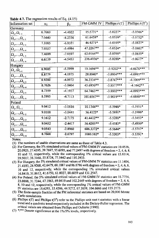
Table 4.7. The regression results ofEq. (4.15)

Infonnation set a2 Ih FM-GMMIV Phillips t (T) Phillips t (T2)

Gennany

0,.°'_1 6.7069 -4.4022 15.5731* -5.0227* -5.0566*

0,,···,°'_2 7.0440 -8.2336 61.6458* -5.0559* -5.0752*

0,,···,°'-3 7.1005 -6.8321 46.9271* -5.0599* -5.0827*

0,,···,°'-4 7.0357 -5.4984 47.2267** -5.0524* -5.0802*

0,,···,°'-5 7.4699 -7.0597 63.0164** -5.0598* -5.0819*

0" .... 0,_6 6.6139 -4.5453 236.4936* -5.0288* -5.0617*

Hungary

0,,°'-1 8.9685 -5.5999 10.1694** -3.9202** -4.0676***

0,,···,°'-2 8.8779 -4.1975 28.8040* -3.8804*** -4.0993***

0,,···,°'-3 8.9280 -4.0972 36.2334** -3.8747*** -4.1009***

0, ... ·'°'_4 8.7626 -3.8464 45.6930** -3.8577*** -4.1042**

°" .. ·.°'_5 8.7359 -4.1937 64.7463** -3.8802*** -4.0993***

0" .. ·,°'_6 8.5995 -4.7113 101.6567** -3.9019*** -4.0888***

Poland

O,.0t-l 9.0412 -3.0816 10.1344** -5.5948* -5.5951 *

°"""°'-2 9.0100 -3.0441 36.4123* -5.5891 * -5.5906*

°"""°'_3 9.1612 -2.7175 41.4412** -5.5288* -5.5453*

0" .... 0,_4 9.0452 -2.4417 56.4205** -5.4583* -5.4950*

0, .... ,0,_5 9.0543 -2.8960 686.3372* -5.5644* -5.5717*

°"""°'-6 8.7668 -2.6797 1080.582* -5.5203* -5.5391 *

Notes: (1) The numbers of usable observations are same as those of Table 4.3. (2) For Germany. the 5% simulated critical values ofFM-GMM IV statistics are 10.4536.

20.0925.27.4595.39.7697.55.6095. and 77.2497 with degrees of freedom = 2, 4, 6,8, 10 and 12. respectively. while the corresponding 1 % critical values are 15.8314, 29.5017.38.3168,55.8724, 77.5442 and 110.3933.

(3) For Hungary, the 5% simulated critical values ofFM-GMM IV statistics are 11.1404, 21.4183,28.9268.42.6479,60.1887 and 86.8796 with degrees of freedom = 2, 4, 6, 8, 10 and 12, respectively, while the corresponding 1 % simulated critical values 16.8410,31.8612,41.6750.61.0027,88.6059 and 131.2547.

(4) For Poland, the 5% simulated critical values ofFM-GMM IV statistics are 11.7754, 23.0888.31.7244,47.1863,69.0410 and 102.2449 with degrees of freedom = 2, 4, 6, 8. 10 and 12. respectively. while the corresponding 1 % critical values of FM -GMM IV statistics are 18.6293.33.4206,44.5272,67.3659, 104.6666 and 155.2173.

(5) The finite-sample fractiles of the FM inferential statistics are based on 20.000 Monte Carlo simulations.

(6) Phillips t(T) and Phillips t(Tz) refer to the Phillips unit root t statistics with a linear trend and a quadratic trend respectively included in the Dickey-Fuller regression. The critical values are obtained from Phillips and Ouliaris (1990).

(7) */** Denote significance at the 1 %/5% levels, respectively.

103

Table 4.8. The ARMA models for the flow variables R 2.,+1 in Eq. (4.15).

Infonnation set I MA{l) MA(2) I MA(3) MA(4) I Ale Q(I) \

Q(6)

Gennany

o,,°'_1 0.3282 0.1363 2.3002 8.9765 - - -

(0.1192)

°"""°'-2 0.3986 0.2776 1.9510 6.7939 - - -

(0.1470)

°"""°'_3 0.3279 0.1988 2.0933 7.7964 - - -

(0.l374)

°"""°'_4 0.2642 0.1305 2.2416 8.8674 - - -(0.1253)

0" .. ·,°'_5 0.2619 0.1607 1.8602 7.7095 - - -(0.1297)

o" .. ·,°'-6 0.3712 - 0.1733 2.5162 8.8768 (0.1258)

- -

Hungary

O"O,_t 0.5458 0.5675 -0.5790 0.8610 4.1379 (0.1128)

- -(0.1429)

0" ... ,0'-2 0.5450 0.5659 -0.6372 0.9059 4.1627 (0.1123) (0.1437)

- -

0" .. ·,°'_3 0.5469 0.5665 -0.6369 0.9190 4.1619 (0.1132) (0.1448)

- --

°"""°'_4 0.5451 0.5669 -0.6598 0.9131 4.1731 (0.1109)

- --(0.1419)

°"""°'-5 0.5458 0.5686 -0.6400 0.9073 4.1770 (0.1105) (0.1407)

- -

°"""°'_6 0.5552 0.5783 -0.5981 0.9334 4.1996 (0.1101) (0.1364)

- --Poland

O"Qt-J 0.0037 -0.1221 0.4759 0.6071 -0.4628 1.7421 4.7429 (0.1352) (0.0608) (0.0842 (0.0633)

°"""°'_2 -0.0035 -0.1209 0.4856 0.5940 -0.4589 1.8029 4.8382 (0.1669) (0.1108) (0.0746) (0.0746)

°"""°'_3 -0.0044 -0.1065 0.4248 0.6421 -0.5638 2.0156 4.9832 (0.1960) (0.0843) (0.0572) (0.O572)

°"""°'_4 0.0451 -0.1947 0.3842 0.7149 -0.6082 2.5710 5.6157 (0.2033) (0.0744) (0.0456) (0.0456)

0" ... ,01-5 -0.0026 -0.1016 0.4356 0.6341 -0.5066 1.8152 4.8106 (0.1731) (0.0929) (0.0689) (0.0689)

°"''''°'_6 0.0974 -0.1950 0.4117 0.7097 -0.4199 2.7309 5.5394 (0.2232) (0.0845) (0.1415) (0.1571)

Notes: (1) The figures in parentheses are Newey-West heteroskedasticity-and-autocorrelation

consistent standard errors. (2) Q(k) refers to Ljung-Box Q-statistics with degrees of freedom = k. (3) Ale refers to Akaike information criterion.

104

T bl 49Th a e .. It fE (4 16) e regressIOn resu s 0 ~q.

Information set (1.2 FM-GMM P2

FM-GMM FM-GMM Phillips I(T)

t(a2) t( (32) IV

Germany 0,_\ 7.2958** -2.7145 -6.4436** 2.4202 -5.0595* --

0,_\,0'_2 7.4149* -3.9739 -7.1355* 3.6500 5.2330 -5.0597*

0,_\,.··,°'_3 7.5052* -3.3792 -5.9558* 2.9761 14.3855 -5.0571 *

0,_\.···,°'_4 7.7457* -3.9792 -6.4084* 3.3432 13.4743 -5.0594*

O,-t. ... , Q,-5 7.8523* -4.6388 -7.5722* 3.7606 30.1904 -5.0586*

0,-1. ... ,0'_6 8.2020* -3.8777 -8.3767* 3.1127 33.4793 -5.0552*

Hungary

0'-2 8.9671 -0.9857 -5.2457* 5.6265 -- -4.8517*

0'-2, ... ,0'_3 9.5881 -0.6714 -9.8582* 6.2525 5.7191 -4.6606*

0'-2, .... , 0'-4 9.9925 -0.9952 -10.7494* 9.7029 11.6432 -4.6363*

0'_2,···,°'_5 9.7887 -1.3758 -8.3629* 10.8120 14.6191 -4.7096*

0'.2,···,°,_6 10.1638 -1.0045 -11.1344* 9.7322 20.7000 -4.6268*

Poland

°'_4 8.8654** -2.8554 -1.9017** 2.7416 -5.2403* --

°'_4,°'_5 8.8084* -5.2560 -1.6168* 5.0256 1.7582 -5.0619*

°'_4,··,°'_6 8.7760* -5.3281 -1.5409* 5.1112 5.8427 -5.0046*

Notes:

(1) The numbers of usable observations are same as those of Table 4.3. (2) For Germany, the 5% and 1% simulated critical values of the one-tailed FM-GMM t

statistics are 1.9712 and 2.8954, respectively, while the corresponding two-tailed FM-GMM t statistics are 2.3852 and 3.3076, respectively. The 5% simulated critical values ofFM-GMM N statistics are 10.4536,20.0925,27.4595,39.7697 and 55.6095 with degrees of freedom = 2, 4, 6, 8 and 10, respectively.

(3) For Hungary, the 5% and 1% simulated critical values of the one-tailed FM-GMM t statistics are 2.0052 and 2.9569, respectively, while the corresponding two-tailed FM-GMM t statistics are 2.4287 and 3.3575 respectively. The 5% simulated critical values of FM-GMM IV statistics are 11.l404, 21.4183, 28.9268 and 42.6479 with degrees of freedom = 2, 4, 6 and 8, respectively.

(4) For Poland, the 5% and 1% simulated critical values of the one-tailed FM-GMM t statistics are 1.9979 and 3.0044 respectively, while the corresponding two-tailed FM-GMM t statistics are 2.4504 and 3.3802, respectively. The 5% simulated critical values ofFM-GMM IV statistics are 11.7754 and 23.0888 with degrees of freedom = 2 and 4 respectively.

(5) The finite-sample fractiles of the FM inferential statistics are based on 20,000 Monte Carlo simulations.

(6) Phillips t(T) and Phillips t(Tz) refer to the Phillips unit root t statistics with a linear trend and a quadratic trend respectively included in the Dickey-Fuller regression. The critical values are taken from Phillips and Ouliaris (1990).

(7) *1** Denote significance at the 1%/5% levels, respectively.

Phillips I("r-)

-5.0835*

-5.0816* -5.0830*

-5.0835*

-5.0794*

-5.0742*

-4.8390**

-4.6998**

-4.6821 **

-4.7353**

-4.6752**

-5.3467*

-5.2272*

-5.1886*

105

Table 4.10. The FM-OLS Wald statistics for the projections oflJ'(L) R2,,+1 and lJ'(L)

(1t2t -1t{,)

Information set WR W'f' Germany Ot_1 0_7847 5.6989

Ot-I> 0t-2 8.1441 16.6208

Ot-I> 0t-2, 0'-3 28.2595 30.2699

Ot-I> Ot_2, 0'_3' 0'_4 38.5030 38.3649

Ot_I> ... ,0'_5 57.1144 28.8212

Ot-I> ""0'_6 47.5351 107.8442

Hungary

Ot-2 6_6078 6.2457

Ot-2,0,_3 12.0448 7.7946

Ot-2, 0,_3' 0'_4 18.6084 23.4400

Ot-2, 0'_3' 0'_4' 0'-5 44.4652 28.0724

Ot-2, ... ,0'_6 38.8802 60.7119

Poland

°'_4 2.0879 0.0937

0,_4,°'_5 8.8847 11.2366

0'_4' 0,_5' 0'_6 17.4438 11.4788

Notes: (I) The numbers of usable observations are same as those of Table 4.3. (2) For Germany, the 5% simulated critical values of the FM-OLS Wald statistics are

10.5115,21.4149,35_9424,55.7938,86.2426 and 134_6337 with degrees of freedom = 2, 4, 6, 8, 10 and 12 respectively.

(3) For Hungary, the 5% simulated critical values of the FM-OLS Wald statistics are 10_8061,22.1647,38.0158,60.7450 and 98.4709 with degrees of freedom = 2,4,6,8 and 10 respectively.

(4) For Poland, the 5% simulated critical values of the FM-OLS Wald statistics are 11.5412, 23.2997 and 41.1154 with degrees of freedom = 2,4 and 6 respectively.

106

Appendix 4.1

In this appendix, I conduct a simulation study to examine the sampling

performance of several FM estimators in a small sample. Other than the FM-OLS

and FM-GMM that are used in the bubble tests, I include FM-LAD and FM-GIVE

for comparison purposes. The FM-LAD is a FM version of the least absolute

deviation (LAD) method (Phillips, 1995b), which is a robust estimation method in

the presence of heavy-tailed errors in a nonstationary regression. FM-GIVE is a FM

extension of the generalized instrumental variable estimation (GIVE) method

(Kitamura and Phillips, 1997), which employs GLS transformation to data and

instruments in a nonstationary regression under the assumption of strictly

exogenous instruments.

The regression model used for data generation is shown as follows:

y, := a + Bx, + "D' a := O,B:= 1. t= l...T. (A.4.1)

and e 4 = 0.9. In other words, "DI is an MA( 4) process. x I is a 1(1) process and is a

linear combination of two processes, x al ' and x bl :

107

x, = CJ.Xa, + (l-a)xb, with a = 0.5 and (AA.2)

(A.4.3)

1 C /),xbl = [~ 2 Je21 +[ ~ 2 JUOI

(l+c) (l+c ) (A.4.4)

Llz is constructed by four first-differenced nonstationary instruments, Llz II , ,

Llz2t , Llz3, and Llz41 , which are generated in the following way:

Llz, = 0.25* Llzlt + 0.25* Llz2t + 0.25* Llz31 + 0.25* Llz41 + e31 , (A.4.5)

[ 0\ 0.7 0.5 -02]

mean = 0 and covariance = 1 0.4 -0.3 0.5 0.4 1 -0.3

-0.2 -0.3 0.6 1

where &i' = 0.8 * &//-1 + tiJ il 'd i = 1,2,3,4. It implies that the instruments Zi,

follow an ARIMA(1,1,0) process.

The residual terms, e, ={ ell' e2, ,e3, }', E, ={ E I , , E 2, ,E3, ,E 4, }' and tiJ , =

{ tiJ II ,tiJ 21 , tiJ 31 ,tiJ 41 } 'are uncorrelated with one another. From Eq.(AA.3) and

(A.4A), there is a feedback effect from Llz, to /),x, through /),xal; and from U OI to

108

t'J.xt

through t'J.xbt ' respectively. Hence, the instruments and the residual term are

correlated with the regressors separately but they are uncorrelated with each other.

Also, the parameter c controls the degree of association between L\x' at and rut as

well as between !'ubt and uot ' When c --* ex; , L\x'at and rut as well as L\x'bt and

Uot

become linearly dependent. When Icl = 1, the squared correlations between

them are equally 0.5. In the simulation study, the innovation terms,

distributions, which include standard normal distribution (N(O, 1 )), t distribution

with 2 degrees of freedom (t 2 ), stable distribution with the characteristic exponent

being equal to 1.5 (S <1=\.5 ),31 and standardized t 5 distribution with conditional

variance from an IGARCH(0.5,O.5) model such that E t = Z"tCft where ZOt ~ 15

(lGARCH(0.5,0.5)-ts). The values of cchosen for the simulation study are c = 1

and c=lOO. The sample size T is 40 and the number of Monte Carlo replications is

1000. The sampling performance of the FM estimators is indicated by the average

bias (BIAS.ve), the root mean square error (RMSE.ve), the quantiles (Qzs, Qso and

Q7S), interquantile ranges (Qw Qzs) and the concentration probabilities

A

(Pr( I b- b I~ k) where k is a constant. In order to examine the performance of the

31When the characteristic exponent of a stable distribution is below 2, the variance will be infinite.

The basic properties of stable distribution are described in McCulloch (1996).

109

FM estimators without the effect of the occasional outliers, I include the bias and

RMSE based on the results excluding 1 % in both tails, denoted by BIAS98 and

RMSE98 respectively.

The results of simulation study are reported from Table A.4.1 to Table A.4.16

below. It is noted that with respect to the estimated intercept terms (a), the mean

bias of the FM-GMM estimator is the most serious in cases where c =1 and the

distributions of innovations are non-normal, and where c=IOO and the innovations

are drawn from N(O,l) as well as IGARCH(O.5,O.5)-t5. For the rest of cases, the

mean bias ofthe FM-LAD estimator is however found to be the most serious. Also,

the dispersion of the FM-GMM estimator for the intercept, measured by the RMSE

and the interquantile range, is the largest in all cases and it is much larger than that

ofthe FM-OLS and FM-LAD estimators. From the concentration probabilities, the

FM-GMM estimator is unfavourably compared to other FM estimators, and the

probability that the absolute deviation of the FM-GMM estimator for the intercept

is smaller than 0.1 does not exceed 20%.

On the other hand, with respect to the I( 1) coefficient (B ), the mean bias of the

FM-GMM estimator is the lowest in most cases whereas the mean bias of the

FM-GIVE estimator is the most serious in all cases. Based upon the RMSE, 110

interquantile ranges and the concentration probabilities, the dispersion of the

FM-GIVE estimator for the 1(1) coefficient is the largest in all cases whereas the

dispersion of the FM-LAD estimator is the lowest in almost all cases. The

dispersion of the FM -GMM estimator for the 1(1) coefficient is slightly lower than

that of the FM-GIVE estimator under all circumstances and the dispersion of the

FM-OLS estimator is found to be slightly lower than that of the FM-LAD in some

cases.

In general, the overall performance of the FM-OLS and FM-LAD estimator

for intercepts and 1(1) coefficients are compared more favourably to that of the

FM-GMM and FM-GIVE estimators in a small sample of the present simulation

study whatever the values of c and the distributions ofthe innovations.

III

I

Table A.4.1. The simulation results of bias, RMSE, quantiles and interquantile range when c=1

and innovations are drawn from N(O,l)

Parameter Estimator BIASave RMSEave BIAS'8 RMSE,8 Q2S Qso Q7S Q7S- Q25 I a FM-OLS 0.0267 0.4773 0.0256 0.4143 -0.2253 0.0166 0.2770 0.5023

FM-LAD 0.0157 0.5436 0.0163 0.4774 -0.2857 0.0209 0.3161 0.6011

FM-GMM 0.0108 2.5481 -0.0012 0.8632 -0.4309 0.0199 0.4199 0.8508

FM-GIVE 0.0210 0.6547 0.0186 0.4942 -0.2372 0.0321 0.2679 0.5051

B FM-OLS -0.0270 0.1843 -0.0322 0.1390 -0.1164 -0.0302 0.0598 0.1762

FM-LAD 0.0364 0.1412 0.0365 0.1303 -0.0499 0.0311 0.1232 0.1731

FM-GMM 0.0186 0.4711 0.0099 0.2733 -0.1335 0.0099 0.1460 0.2795

FM-GIVE 0.1468 0.7060 0.1226 0.4095 -0.0795 0.0867 0.3088 0.3883 - -

112

Table A.4.2. The simulation results of bias, RMSE, quantiles and interquantile range when c=1

and innovations are drawn from t 2

Parameter Estimator BIAS.ve RMSE.ve BIAS98 RMS~ Qzs Qso Q7S Q7S- Q1S

a FM-OLS -0.0124 0.4929 -0.0133 0.4140 -0.2678 -0.0154 0.2422 0.5100

FM-LAD -0.1341 0.4870 -0.0160 0.3964 -0.2506 -0.0250 0.2239 0.4745

FM-GMM 0.0008 1.8249 0.0122 0.7763 -0.3817 -0.0050 0.3696 0.7513

FM-GIVE 0.0557 1.8284 -0.0014 0.4767 -0.2684 -0.0139 0.2434 0.5118

B FM-OLS -0.0277 0.1858 -0.0313 0.1383 -0.1165 -0.0295 0.0564 0.1729

FM-LAD 0.0315 0.1336 0.0307 0.1196 -0.0415 0.0249 0.0991 0.1406

FM-GMM -0.0109 0.4085 -0.0042 0.2509 -0.1214 0.0044 0.1355 0.2569

FM-GIVE 0.1122 0.8661 0.1297 0.4767 -0.0737 0.0983 0.2953 0.3690 ______ __ - - - - _ .. _______ - - _______ ~. I ___

113

Table A.4.3. The simulation results of bias, RMSE, quantiles and interquantile range when c=l

and innovations are drawn from S (1=1.5

Parameter Estimator BIAS ave RMSEave BIAS98 RMSE,s Q1S Qso Q75 Q7S- Q1S

a FM-OLS 0.0048 0.4712 0.0087 0.3910 -0.2344 0.0113 0.2614 0.4958

FM-LAD -0.0098 0.4923 -0.0042 0.3974 -0.2211 0.0163 0.2350 0.4561

FM-GMM 0.0108 1.0886 0.0212 0.7398 -0.3646 0.0201 0.3991 0.7637

FM-GIVE 0.0015 0.7217 0.0061 0.5196 -0.2650 -0.0022 0.2731 0.5381

B FM-OLS -0.0249 0.1589 -0.0275 0.1281 -0.1066 -0.0240 0.0530 0.1596

FM-LAD 0.0314 0.1217 0.0302 0.1078 -0.0340 0.0198 0.0892 0.1232

FM-GMM 0.0286 0.3337 0.0211 0.2216 -0.0952 0.0112 0.1457 0.2409

FM-GIVE 0.0823 0.9616 0.1073 0.5410 -0.0793 0.0796 0.2914 0.3707 - - -

I

114

Table A.4.4. The simulation results of bias, RMSE, quantiles and interquantile range when c=l

and innovations are drawn from IGARCH(0.5,0.5)-ts

Parameter Estimator BIASave RMSEave BIAS98 RMS~8 QZ5 Qso Q7S Q7S- Q2S

a FM-OLS 0.0111 0.5118 0.0065 0.4244 -0.2369 0.0036 0.2556 0.4925

FM-LAD 0.0205 0.5107 0.0185 0.4273 -0.2274 0.0109 0.2443 0.4717

FM-GMM 0.0983 2.4889 0.0199 0.7840 -0.3752 -0.0068 0.3783 0.7535

FM-GIVE 0.0024 0.7321 0.0132 0.5024 -0.2635 -0.0028 0.2715 0.5350

B FM-OLS -0.0213 0.1712 -0.0247 0.1367 -0.1162 -0.0236 0.0559 0.1721

FM-LAD 0.0351 0.1284 0.0340 0.1168 -0.0377 0.0235 0.1019 0.1396

FM-GMM 0.0171 0.4679 0.0227 0.2305 -0.1027 0.0083 0.1432 0.2459

FM-GIVE 0.1275 0.8040 0.1205 0.4485 -0.0627 0.0913 0.2947 0.3574 - - _.- _._-

115

Table A.4.5. The simulation results of concentration probabilities when c = I and

innovations are drawn from N(O,I) 1\

(Pr(1 b-b I~ k»

Parameter Estimator k ~ 0.1 k ~ 0.3 k ~ 0.5 k ~ 0.7 k ~ 0.9

a FM-OLS 0.2150 0.5790 0.7750 0.8790 0.9330

FM-LAD 0.1720 0.4960 0.7220 0.8400 0.9090

FM-GMM 0.1280 0.3700 0.5600 0.6820 0.7690

FM-GIVE 0.2130 0.5590 0.7490 0.8460 0.9020

B Estimator k ~ 0.01 k ~ 0.03 k :5 0.05 k ~ 0.07 k ~ 0.09

FM-OLS 0.0540 0.1690 0.2870 0.3970 0.4990

FM-LAD 0.0670 0.1940 0.2990 0.4060 0.5060

FM-GMM 0.0350 0.1180 0.1910 0.2710 0.3370

FM-GIVE 0.0320 0.0830 0.1450 0.2130 0.2710

Table A.4.6. The simulation results of concentration probabilities when c = 1 and

innovations are drawn from t 2

1\

(Pr(1 b-b I~ k))

Parameter Estimator k ~ 0.1 k :5 0.3 k :5 0.5 k ~ 0.7 k ~ 0.9

a FM-OLS 0.2020 0.5850 0.7840 0.8860 0.9330

FM-LAD 0.2180 0.5980 0.8140 0.9060 0.9430

FM-GMM 0.1340 0.4030 0.6120 0.7280 0.8050

FM-GIVE 0.2160 0.5700 0.7570 0.8560 0.9100

B Estimator k ~ 0.01 k:5 0.03 k:5 0.05 k :5 0.07 k :5 0.09

FM-OLS 0.0710 0.1840 0.3070 0.4260 0.5210

FM-LAD 0.0890 0.2300 0.3630 0.4900 0.5870

FM-GMM 0.0450 0.1430 0.2210 0.3020 0.3770

FM-GIVE 0.0290 0.0900 0.1490 0.2040 0.2600

116

Table A.4.7. The simulation results of concentration probabilities when c = 1 and

innovations are drawn from S a=1 5

A

(Pr(1 b-b I~ k»

Parameter Estimator k ~ 0.1 k ~ 0.3 k ~ 0.5 k ~ 0.7 k ~ 0.9

a FM-OLS 0.2020 0.5740 0.8060 0.9000 0.9480

FM-LAD 0.2210 0.6280 0.8080 0.8990 0.9440

FM-GMM 0.1590 0.4030 0.6170 0.7440 0.8210

FM-GIVE 0.2040 0.5460 0.7430 0.8450 0.8940

B Estimator k ~ 0.01 k ~ 0.03 k :S 0.05 k :S 0.07 k:S 0.09

FM-OLS 0.0810 0.2160 0.3310 0.4560 0.5430

FM-LAD 0.1080 0.2830 0.4210 0.5380 0.6460

FM-GMM 0.0540 0.1710 0.2440 0.3480 0.4190

FM-GIVE 0.0310 0.1010 0.1630 0.2260 0.2770

Table A.4.S. The simulation results of concentration probabilities when c = 1 and

innovations are drawn from IGARCH(0.5,0.5)-tj A

(PrO b- b I:S k»)

Parameter Estimator k :S 0.1 k:S 0.3 k ~ 0.5 k ~ 0.7 k ~ 0.9

a FM-OLS 0.2150 0.5730 0.7830 0.8790 0.9280

FM-LAD 0.2460 0.5890 0.7970 0.8780 0.9190

FM-GMM 0.1740 0.4140 0.5950 0.7230 0.8020

FM-GIVE 0.2130 0.5690 0.7520 0.8420 0.9060

Estimator k :S 0.01 k :S 0.03 k :S 0.05 k:S 0.07 k :S 0.09

B FM-OLS 0.0830 0.1920 0.3230 0.4150 0.4980

FM-LAD 0.0870 0.2490 0.3870 0.4840 0.5910

FM-GMM 0.0470 0.1330 0.2340 0.3130 0.3830

FM-GIVE 0.0260 0.0900 0.1570 0.2220 0.2930

117

Table A.4.9. The simulation results of bias, RMSE, quantiles and interquantile range when c=lOO

and innovations are drawn from N(O,l)

Parameter Estimator BIAS ave RMSEave BIAS98 RMSE,s Q2S Qso Q75 Q7S- QZ5 1

a FM-OLS -0.0215 0.4373 0.0199 0.3819 -0.1965 0.0181 0.2450 0.4415

FM-LAD 0.0106 0.5662 0.0105 0.4985 -0.2710 -0.0017 0.2978 0.5688

FM-GMM -0.0960 3.0643 0.0229 0.8358 -0.4191 0.0181 0.4143 0.8334

FM-GIVE 0.0320 0.6937 0.0200 0.5312 -0.2261 0.0199 0.2668 0.4929

B FM-OLS -0.0291 0.1199 -0.0301 0.1026 -0.0888 -0.0232 0.0345 0.1233

FM-LAD 0.0346 0.1124 0.0346 0.10277 -0.0308 0.0281 0.0961 0.1269

FM-GMM 0.0123 0.5044 0.0130 0.1938 -0.0909 0.01400 0.1208 0.2117

FM-GIVE 0.1115 0.5705 0.1170 0.3534 -0.0426 0.0757 0.2605 0.3031

118

Table A.4.10. The simulation results of bias, RMSE, quantiles and interquantile range when c=100

and innovations are drawn from t 2

Parameter Estimator MBiasave RMSEave Mbia898 RMS~8 Q1S Qso Q7S QWQ1S a FM-OLS -0.0039 0.4383 -0.0016 0.3758 -0.2261 -0.0060 0.2323 0.4584

FM-LAD -0.0181 0.5045 -0.0151 0.4136 -0.2381 -0.0247 0.2173 0.4554

FM-GMM 0.0123 0.9861 0.0035 0.7478 -0.3503 0.0047 0.3633 0.7136

FM-GIVE -0.0161 0.6357 -0.0186 0.5082 -0.2575 -0.0095 0.2412 0.4987

B FM-OLS -0.0314 0.1144 -0.0319 0.1035 -0.0946 -0.0300 0.0310 0.1256

FM-LAD 0.0268 0.1033 0.0262 0.0931 -0.0317 0.0206 0.0778 0.1095

FM-GMM 0.0020 0.2449 0.0009 0.1835 -0.0901 0.0035 0.0962 0.1863

FM-GIVE 0.1191 0.5282 0.1152 0.3419 -0.0356 0.0806 0.2524 0.2880 _ .. _.- -_ .. _- ~_._. __ . __ .- - - - - - - -

119

Table A.4.U. The simulation results of bias, RMSE, quantiles and interquantile range when c=100

and innovations are drawn from S a=LS

Parameter Estimator MBiasave RMSEave Mbia598 RMSE,s Q15 Q50 Q75 QWQ15 I a FM-OLS 0.0040 0.4884 0.0300 0.3988 -0.2325 0.0037 0.2333 0.4658 I

FM-LAD -0.0261 0.5216 -0.0210 0.4142 -0.2361 0.0074 0.2190 0.4551

FM-GMM -0.0135 0.9843 -0.0080 0.7751 -0.3270 0.0126 0.3379 0.6649

FM-GIVE -0.0181 0.8706 0.0019 0.4894 -0.2290 0.0162 0.2573 0.4863

B FM-OLS -0.0283 0.1117 -0.0288 0.0975 -0.0871 -0.0251 0.0283 0.1154

FM-LAD 0.0275 0.0985 0.0272 0.0870 -0.0241 0.0146 0.0725 0.0966

FM-GMM 0.0088 0.2310 0.01334 0.1740 -0.0705 0.0079 0.0997 0.1702

FM-GIVE 0.0884 1.0886 0.1124 0.3765 -0.0431 0.0618 0.2467 0.2898 - - - - -_. __ . __ .-

120

Table A.4.12. The simulation results of bias, RMSE, quantiles and interquantile range when c==lOO

and innovations are drawn from IGARCH(O.5,O.5)-ts Parameter Estimator MBiasave RMSEave Mbias98 RMS~8 Q2S Qso Q7S Q7S- Q1S

a FM-OLS 0.0070 0.4934 0.0092 0.4111 -0.2066 0.0047 0.2234 0.4300

FM-LAD 0.0237 0.5431 0.0260 0.4466 -0.2159 0.0148 0.2635 0.4794

FM-GMM 0.0481 1.5786 0.0640 0.8350 -0.3154 0.0107 0.3923 0.7077

FM-GIVE -0.0230 1.2535 0.0130 0.5396 -0.2482 0.0104 0.2784 0.5266

B FM-OLS -0.0262 0.1172 -0.0278 0.1018 -0.0907 -0.0256 0.0361 0.1267

FM-LAD 0.0297 0.1019 0.0285 0.0917 -0.0765 0.0201 0.0816 0.1581

FM-GMM 0.0385 0.4052 0.0269 0.1931 -0.0798 0.0081 0.1058 0.1856

FM-GIVE 0.0985 0.8456 0.1090 0.3546 -0.0479 0.0844 0.2360 0.2839 --- ----- - - - -- - --- - --- ----- --- - -- -- --

121

Table A.4.13. The simulation results of concentration probabilities when c = 100

and innovations are drawn from N(O,l) A

(Pr( 1 b- b 1$ k » Parameter Estimator k $ 0.1 k $ 0.3 k $ 0.5 k $ 0.7 k $ 0.9

a FM-OLS 0.2500 0.6050 0.7910 0.9050 0.9500

FM-LAD 0.2000 0.5220 0.7280 0.8290 0.8870

FM-GMM 0.1230 0.3850 0.5640 0.6950 0.7770

FM-GIVE 0.2130 0.5590 0.7490 0.8460 0.9020

B Estimator k $ 0.01 k $ 0.03 k $ 0.05 k $ 0.07 k $ 0.09

FM-OLS 0.0870 0.2580 0.4020 0.5250 0.6500

FM-LAD 0.0890 0.2550 0.3970 0.5200 0.6250

FM-GMM 0.0520 0.1360 0.2440 0.3510 0.4380

FM-GIVE 0.0430 0.1190 0.2040 0.2840 0.3490

Table A.4.14. The simulation results of concentration probabilities when c = 100

and innovations are drawn from t2 A

(Pr( I b- b 1$ k » Parameter Estimator k $ 0.1 k $ 0.3 k $ 0.5 k $ 0.7 k $ 0.9

a FM-OLS 0.2330 0.6290 0.8230 0.9020 0.9510

FM-LAD 0.2250 0.6170 0.8040 0.8930 0.9370

FM-GMM 0.1840 0.4430 0.6260 0.7480 0.8090

FM-GIVE 0.2230 0.5780 0.7540 0.8420 0.8930

B Estimator k $ 0.01 k $ 0.03 k $ 0.05 k $ 0.07 k $ 0.09

FM-OLS 0.0750 0.2420 0.3880 0.5230 0.6100

FM-LAD 0.2440 0.6200 0.8280 0.9250 0.9640

FM-GMM 0.0700 0.1910 0.2970 0.3940 0.4850

FM-GIVE 0.0380 0.1210 0.1970 0.2660 0.3390

122

Table A.4.1S. The simulation results of concentration probabilities when c = 100

and innovations are drawn from S a=L5

" (Pr(1 b-b I~ k»

Parameter Estimator k ~ 0.1 k ~ 0.3 k ~ 0.5 k ~ 0.7 k ~ 0.9

a FM-OLS 0.2260 0.6000 0.8070 0.9020 0.9440

FM-LAD 0.2510 0.6130 0.8050 0.8900 0.9310

FM-GMM 0.1560 0.4600 0.6530 0.7410 0.8040

FM-GIVE 0.2370 0.5770 0.7670 0.8550 0.9110

B Estimator k ~ 0.01 k ~ 0.03 k ~ 0.05 k ~ 0.07 k ~ 0.09

FM-OLS 0.1020 0.2700 0.4110 0.5300 0.6570

FM-LAD 0.1560 0.3520 0.5060 0.6380 0.7180

FM-GMM 0.0740 0.2060 0.3380 0.4430 0.5230

FM-GIVE 0.0520 0.1560 0.2460 0.3110 0.3750

Table A.4.16. The simulation results of concentration probabilities when c =:: 100

and innovations are drawn from IGARCH(0.5,0.5)-ts

" (Pr(1 b- b 1$ k))

Parameter Estimator k ~ 0.1 k ~ 0.3 k $ 0.5 k $ 0.7 k ~ 0.9

a FM-OLS 0.2520 0.6200 0.7980 0.8890 0.9360

FM-LAD 0.2380 0.5870 0.7830 0.8710 0.9110

FM-GMM 0.1740 0.4390 0.6190 0.7460 0.8200

FM-GIVE 0.2220 0.5400 0.7270 0.8290 0.8870

B Estimator k ~ 0.01 k ~ 0.03 k ~ 0.05 k ~ 0.07 k ~ 0.09

FM-OLS 0.0890 0.2420 0.4080 0.5340 0.6380

FM-LAD 0.0970 0.2890 0.4470 0.6040 0.7060

FM-GMM 0.0680 0.1770 0.3130 0.4060 0.4980

FM-GIVE 0.0410 0.1280 0.1930 0.2640 0.3350

123

CHAPTER FIVE REGIME SWITCHING AND BUBBLES

5.1 Introduction

The empirical study conducted in this chapter continues to examine the

presence of bubbles during the three inter-war European hyperinflations. It

nevertheless differs from the study in the last chapter in several aspects. First of all,

the Cagan models under study are stochastic, and the model specification errors are

captured by nonzero demand disturbances; moreover, the sample periods under

study are extended to cover the periods of monetary reform expected and

subsequently implemented, during which the data generating process and dynamic

equilibrium adjustment process may be nonlinear; finally, I adopt recent advances

in cointegration methodologies for the analysis and suggest that they are more

powerful under nonlinear dynamics than the conventional tests so as to provide

more reliable conclusions of bubbles. Evidence of nonlinear adjustment process is

found in almost all cases, but evidence of bubbles still cannot be supported in any

countries. The remainder of the chapter is set out as follows. Section 2 contains a

discussion of related literature and empirical issues of unit root econometric

methods in bubbles testing. Section 3 accounts for the cointegration methods

adopted in this chapter. Section 4 presents Monte Carlo evidence on the power and

124

size of the cointegration test statistics when the artificial data series exhibits

threshold stationarity and when periodically collapsing bubbles are present in the

data respectively. Data and empirical results are reported in section 5. The final

section concludes the major findings.

5.2 Related Literature and Empirical Issues of Unit Root Econometric Tests

The unit root econometric methods in the context of bubble testing were first

proposed by Hamilton and Whiteman (1985), Campbell and Shiller (1987), and

Diba and Grossman (1988a). They argue that if an asset price series contains

bubbles, it will grow faster than an integrated series. The unit root test will

therefore show that this kind of price series will remain nonstationary even though

it is taken a finite number of differences. Hamilton and Whiteman (1985) noted that

the presence of bubbles during the Gennan hyperinflation in the 1920's would

cause the price series to exhibit a higher order of integration than any of the

underlying fundamentals in a finite sample. They found that both series for price

and money contained two unit roots in the Gennan hyperinflation, and rejected the

existence of bubbles. For the same reason, the residuals obtained from the

projection of the asset price onto their underlying fundamentals will also be

nonstationary, which implies that it would not be possible to establish a 125

cointegrated relationship between the asset price and its underlying fundamental

process when a bubble exists. Meese (1986) found that over the period 1973-1982,

the exchange rate of the deutschemark was less stationary than market

fundamentals that included relative money supplies and relative real incomes. Then,

the null hypothesis that the deutschemark, Japanese yen and British pound did not

cointegrate with their corresponding fundamentals could not be rejected, signifying

the possible existence of bubbles in currency markets.

There are, however, several caveats that one may find in applying unit root

econometric methods to detect bubbles. First of all, taking a finite number of

differencing may make the explosive series appear stationary in small samples

(Durlauf and Hooker, 1994, Hall, et al. 1999). Furthermore, as emphasized by

Hamilton and Whiteman (1985) and, Diba and Grossman (1988), the

non-cointegration between asset prices and observable fundamentals may equally

result from the omission of nonstationary unobservable fundamentals. Under such

a circumstance, model misspecification may be erroneously interpreted as evidence

of bubbles.

In addition, the simulation conducted by Meese (1986) shows that the

nonlinear bursting bubbles of Blanchard and Watson (1982) may not exhibit 126

nonstationary behaviour discernible from the autocorrelation function. Later,

Evans (1991) finds that the conventional cointegration tests result in erroneous

rejection in favour of linearly stable alternatives when the simulated data series

contain periodically collapsing bubbles that display nonlinear explosive properties.

The size distortion is serious since the collapsing bubbles may appear in the form of

a stable linear autoregressive process especially when the probability of the bubble

collapse is high.

Finally, there is a problem of observational equivalence between expected

future changes in economic fundamentals and bubbles (Flood and Garber, 1980b,

Hamilton, 1986). Assume that there are two regimes of money supply process,

non-reform and reformed process. Expectation of reform refers to the possibility of

a shifting from non-reform regime of money growth process to a reformed regime

at some date. In periods prior to a given reform date, the expected inflation rate32 is

equal to the rate conditional on the regime of non-reform money supply process

plus a fraction of the "reform effect", which is defined as the difference between

reformed process and non-reformed process of money supply in the period

immediately following the reform (LaHaye, 1985). The value of the reform effect

32 From the Cagan model (2.2), the rate of inflation is equivalent in value to the rate of currency

depreciation through the PPP.

127

on the expected inflation rate is negative. Hence, while the expectation of monetary

reform occurred toward the end of hyperinflations, the expected inflation rate

would decline and the actual real money balance would increase. Furthermore,

after the reform was actually implemented, the real money balance and the

expected inflation rate would shift in response to the regime of reformed money

supply process. As a result, the expectation and the subsequent implementation of

monetary reforms might bring about regime shifting of real money balances,

money supply process and velocity of circulation (Evans, 1986, Flood and Garber,

1980a, Flood and Hodrick, 1986). 33 At the empirical level, the regime-switching

behaviours of these time series variables may lead to nonlinear error-correcting

dynamics in a cointegrated system. 34 To respond to this problem, the common

practice in the literature as mentioned in the last chapter has been to truncate the

final months of hyperinflations during which the expectations of monetary reform

began to take effect (for instance, Casella, 1989, Flood and Garber, 1980b, Engsted,

1993, 1996, Hooker, 2000, Woo, et al. 2003). However, the existence of bubble

33 In addition to the issue of monetary regime changes, asynunetric intervention rules, money

financing of perpetual government deficits, and the presence of transaction costs are other possible

economic justifications for non-linearity in a cointegrated system (Pippenger and Goering, 1993,

Peel and Speight, 1994, and Balke and Fomby, 1997).

34 The existence of nonlinear disequilibrium error will lead to nonlinear adjustment in the

error-correcting system (Balke and Fomby, 1997 and Granger and Siklos, 2001).

128

during the truncated observations cannot be precluded at a prior.

This chapter attempts to circumvent the above problems of bubble tests by

employing an alternative bubble testing strategy. In particular, I propose to apply a

sequential cointegration-testing procedure, as suggested by Engsted (1993), to

handle the problem of model misspecification. By conducting cointegration

analyses between the real money balance and expected price change, and

subsequently between the real money balance and the money growth rate, Engsted

(1993) argues that the existence of a bubble can be separated from the model

misspecification arising from omitted non-stationary fundamentals. In applying

this testing procedure, however, the econometric methodology chosen must be

robust to the presence of both a nonlinear dynamic process and a stochastic bubble

in order to avoid producing misleading cointegration results. In light of this, I

therefore suggest adopting the threshold autoregressive (TAR) unit root method of

Caner and Hansen (2001), which is designed to simultaneously test for unit root

and threshold nonlinearity so as to make it possible to distinguish threshold

stationarity from nonstationarity. The threshold cointegration methodology is

expected to have superior power to reject the null hypothesis of noncointegration

129

when the series under study are subject to nonlinear regime-switching behaviors. 35

Thus, the existence of a nonlinear process in the residuals of the money demand

models, which results from the agents' expectation of changes in market

fundamentals that are not observed by econometricians, will probably not be

identified as a nonstationary bubble path. Furthermore, since a stochastic bubble

can exhibit both nonstationary and stationary patterns during different phases of its

data generation process (Funke, et aI., 1994), the ability of the TAR method to

separate the series under study into different regimes makes it more likely to

identify the nonstationary dynamics of the collapsing bubbles in at least one regime.

Thus, the use of the TAR method in bubble detection is expected to produce less

serious size distortion than would the conventional tests. In order to investigate the

suitability ofthe TAR method for bubble detection, I compare, by means of Monte

Carlo experimentation, the relative empirical power and size performances of the

TAR method with those of some other cointegration tests that do not allow for

mUltiple regime shifts III the data generation process. I have chosen the

35 When the nonlinearity of the data generating process is deterministic at known dates, it is suggested that the

effects of deterministic shifts be captured by the inclusion of an appropriate set of intervention dummies in the

DF regression or vector error correction model (VECM). For instance, Woo (1999) employed the bootstrapped

algorithm of van Giersbergen (1996) to generate bootstrapped critical values of johansen's (\ 995) likelihood

ratio statistics when intercept dummies were added to the V AR model to capture the changes in parities of the

ERM currencies during 19805 and 19905.

130

conventional residual-based Augmented Dickey-Fuller (ADF) and the

Phillips-Ouliaris (1990) Z statistics, as well as the 1m's (1996, 2001)

residuals-augmented least square augmented Dickey-Fuller (RALS-ADF) t

statistic as comparison tests. The ADF and the class of Z statistics are among the

most popular co integration tests that have been used in the literature. 1m's (1996,

2001) method was adopted by Taylor and Peel (1998) for price bubble tests in the

US stock market and from the simulation study of Taylor and Peel (1998), the

RALS-ADF test has favourable power and size performance in detecting price

bubbles.

5.3 Econometric Testing Procedure and Methodology

I adopt the stochastic version ofthe Cagan models under rational expectations

in this chapter that are the same as those described in Chapter Two. For expositional

convenience, I re-write some of the equations in chapter two as necessary. Let's

re-write the Cagan models under rational expectations for 1t],/ and 1t 2,/ as follows:

(5.1)

(5.2)

131

where u l " and u2,t capture the model misspecification components in the exact

Cagan models (4.1) and (4.2) respectively.

By defining the rational expectation forecasting errors as 'tlj,,+1 = 6

'It . - E (6 'It. ) which are assumed to be serially uncorrelated, Eqs.(5.1) and J,I+I, J,I+I '

(5.2) can be re-written as:

M, -'It j,' = a j + ~ jt1.'It },,+I + ~j,,; j = 1, 2, (5.3)

For notional convenience, I eliminate the subscriptj in subsequent equations.

Re-arranging Eq. (5.1) and (5.2) in terms of 'It, and by recursively substituting

forward for E,(1rI+I+I) and using the law of iterated expectations, I obtain:

1 '" ( !3 )' .~ !3 )'+1 'It, =-a.+--L -- E,(M'+I-u'+I)+b -- E,('ltI+I+i ) (5.4) 1 -!3 i~O !3 - 1 1-+", !3 - 1

Imposing the non-bubble transversality condition, Fm -~- E, ('It 1+1+;) = 0, and ( )

i+1

,-+'" !3- 1

re-arranging terms yield:

132

The further re-arrangement of terms in Eq.(5.5) gives:

(M, -7t,)=a+J3M1, +(J3-1)~(J3~1}E,(~2M'+i)+(I~J3)~(J3~Ji E,(U'+i)·

(5.6)

Engsted (1993) proposes a set of sequential testing procedures to detect the

presence of B,. The procedure is conducted by comparing the cointegrating

relationship between M, -7t, and ~7tt+1 in Eq.(5.3) as well as between M, - 7t,

and ~, in Eq.(5.6). The Cagan models given by Eq.(5.3) represent a money

market equilibrium condition that admits a general solution. Therefore, provided

that ", is stationary, the Cagan models cannot be rejected even if B, exists.36 On

the other hand, the non-bubble transversality condition is imposed upon Eq.(S.6)

but not upon Eq.(S.3). Hence, Eq.(S.6) represents a fundamental solution only,

which can be rejected if B, is present in the price or exchange rate data. 37

Consequently, three possible outcomes may arise from the tests of these two

cointegrating relationships. First of all, if M, - 7t, cointegrates both ~7tt+1 and

36 It should be noted that the rational expectation forecasting error, '11).1+1 ' is a white noise by

definition.

37 The idea of Engsted (1993) is similar to that of West (1987a), which compares the differences of

parameters obtained from two sets of equations rather than the differences in their cointegrating

properties.

133

[).M t' it implies that "t is 1(0) and the presence of B, is less likely to occur.

Moreover, if M, -1t t only cointegrates with Ll1tt+l but not with LlM t , it indicates

that "t is 1(0) and B t may be present. However, if neither Ll1tt+l nor LlM t

cointegrates with M - 1t it indicates the fundamental failure of the Cagan t t'

models due to the presence of a nonstationary ", . Therefore, this testing procedure

can distinguish the existence of bubbles from the model misspecification caused by

omitted nonstationary fundamentals. For further investigating whether B, exists in

the final case, the model must have to be re-specified so that the omitted

nonstationary fundamental variables are included in the model.

One econometric method I choose to conduct the above cointegration-testing

procedure in this chapter is the residuals-based threshold cointegration test. By

applying the two-regime TAR unit root method of Caner and Hansen (2001) to the

OLS estimated residuals of Eq.(5.3) and (5.6),38 it can test for cointegration and

threshold nonlinearity simultaneously, which is considered to be ideal for threshold

cointegration analysis by Balke and Fomby (1997). The TAR regression can be

represented by the following equation:

38 As pointed out by Balke and Fomby (1997), the OLS estimates of a cointegration vector remain

superconsistency under certain conditions even though the disequilibrium error exhibits threshold

nonlinearity. Also, it is assumed to be constant in the threshold cointegration framework.

134

(5.7)

where Y, denotes the OLS residual of either Eq.(5.3) or (5.6); SI_I = (Y,_pl, t,

t.Y,_1 , ... , t.Y,_k )' is a vector of regressors in which t denotes a linear time trend, O;

= (Pi' C i' bi' 'l'U-I' ... ' 'I'/,t-k)' represents the slope parameters associated with

the corresponding regressors of SI_I. /(.) is an indicator function, Z,_I is the

observable threshold variable, 1...0 is a threshold value and e, is an i.i.d. error. In

practice, there are two possible ways to specify Z'_I' as either Yt-I - Yt-m-I or Yt-m-

Yt-m-I. which are known as long difference and lagged difference thresholds,

respectively. Although the particular specification for the threshold variable is not

essential, Zt-l must be strictly stationary and ergodic. Hence, the long difference

or lagged difference threshold specification is preferred to the lagged level of Yt

becauseYt is 1(1) under the nUll.39 The OLS estimate of AD is found by minimizing

02(1...0) in the unrestricted Eq.(5.7).

The sufficient conditions for the convergence of Yt in a two regime threshold

model require -2 < PI < 0 for i= 1,2 (Enders and Granger, 1998).40 Caner and

Hansen (2001) propose using a class of RT Wald statistics, which comprises the

39 Eq. (5.7) is alternatively known as momentum TAR model, first introduced by Enders and

Granger (1998), in which b.Yt-h rather thanYt_h is used as the threshold value.

40 As given in Chan and Tong (1985), there are less stringent conditions for stability of a first-order

threshold model. 135

one-sided (Rn) and two-sided (R2T) Wald statistics, which are expressed as t]2I(p]

< 0) + t22I(p2 < 0) and t12 + tl respectively, to test for the null hypothesis that PI =

P2 = o. The Rn and R2T Wald statistics can lead to a rejection of the null hypothesis

when Pi< 0 and Pi *0, respectively, for at least one i = 1,2. The distributions of

the Rr statistics are nonstandard and have to be approximated by bootstrapping. In

practice, there are two methods to carry out the bootstrapping. The first one is the

unidentified bootstrap that assumes no threshold effects on parameters in ej under

the null and the second is the identified bootstrap that imposes the restriction of

threshold effects. Caner and Hansen (2001), however, recommends the use of the

unidentified bootstrap to calculate the bootstrap p-values because the size

distortions of unit root test obtained by simulation from the identified bootstrap

method are substantially large. Other than the joint test statistics, there are two

individual t-ratio statistics, tl and t2, for PI and P2 respectively. Nevertheless, as

found in the simulation study of Caner and Hansen (2001), the power of the t-ratio

statistics associated with the lower absolute value of PI will substantially

deteriorate with an increase in I PI - P2 1 and I cI - c2 1. It is also found that even if the

series of y, is stationary in two regimes, the powers of the individual t-ratio

statistics are no larger than those of the RT Wald statistics. Following the lines of

argument by Granger and Siklos (2001), the RT Wald statistics are still useful when 136

the point estimates for Pi fall within the ranges of -2 and 0, V i, and especially

when there are threshold effects in coefficients.4] The evidence for the existence of

nonstationary roots in two regimes is rejected when the RT Wald statistics are

significant with all point estimates of PI and P2 lying between -2 and O.

On the other hand, the existence of threshold effects can be tested under the

null hypothesis of no threshold effect, i.e., 8] = 8 2• The Wald statistics, WT, for

examining this restriction is given by T (a~ / a 2( "-0) - 1), where T refers to the

number of usable observation and a~ IS the residual variances from OLS

estimation of the null linear model. The asymptotic distribution of WT depends

upon the presence of nonstationarity in Yt. Hence, Caner and Hansen (2001)

suggests the unconstrained and constrained bootstrapping approximations to the

asymptotic distribution ofWT; the former based upon the unrestrictive estimates of

parameters in Eq. (5.7) and the latter enforcing the restriction ofa unit root. Also,

the Wald statistics can be implemented to test for the equality of individual

coefficients of 8 across regimes.

41 Enders and Siklos (200 I) fmd that the F statistic for the null hypothesis of non-cointegration in

two regimes of a M-TAR model has more power than the individual t-ratio (t-rnax and t-min)

statistics in simulation experiments. Hence, they recommend the use of F statistic for conducting a

threshold cointegration test in cases where the point estimates of p; imply convergence for all i.

137

The other cointegration tests considered for comparing with the TAR RT

statistics include the conventional ADF and the Phillips-Ouliaris (1990) Z statistics,

as well as the 1m's (1996, 2001) RALS-ADF t statistic. While the ADF t statistic

corrects for serial correlation by adding lagged terms in the Dickey-Fuller (DF)

regression (Said and Dickey, 1984), the cointegrating Za and Zt statistics of

Phillips and Ouliaris (1990) employ the semi-parametric method to asymptotically

eliminate the bias caused by the weakly dependent and heterogeneously distributed

innovations of the DF regression. Consider the standard DF regression for the OLS

residual y, :

y, =OY'_I +e"" {e",} - i.i.d. (0, (1;,>. (5.8)

The Z a and Zt statistics are given as:

A T

Za= T(o-I)-(s2 -S;)(2r2 LY;_I)-\ (5.9) ,=\

(5.10)

2 _ 1· -IE["T]2 2 2 • . f 2 2 cr - ImT -+00 T 4.J'=1 e t • s. and s are consIstent estImates 0 cr e. and cr

138

T

respectively. The term (S2 -s~)(T-22>;_lr1 IS referred to as the serial 1=1

correlation correction factor. As argued by Perron and Ng (1996), the SIze

distortion will be serious in the semiparametric procedure of the unit root tests

when there are innovations of the DF regression with a moving average root close

On the other hand, the RALS-ADF t statistic introduced by 1m (1996, 2001), is

a variant of the Hansen's (1995) covariate ADF (CADF) statistic, which is

developed by including correlated stationary covariates into the ADF regression

with an aim to increase the power of the ADF unit root test. To illustrate the

working ofCADF, let's suppose that there exists an m-vector X"~ which is related to

the series, Yt, that is, the OLS residual ofEq.(5.3) or (5.6). Further suppose that X"~ is

1(1) and its differenced series, t::.Xt, is therefore 1(0). f).Xt is known as stationary

covariates of the following CADF regression:

(5.11)

42 Haldrup (1994 and 1998) recognize that the size distortion for the semiparametric double unit root

tests is serious in the presence of large negative MA errors in the DF regression. Appendix 5.1

presents a work of simulation study to examine the size distortion of the semiparametric double unit

root tests.

139

polynomial allowing for both leads and lags of the deviation of the covariates from

their expected means. The values of p, ql and q2 are chosen to make e, white noise.

For conducting the analysis, it is useful to define a variable, v" which equals

e(L)'(~, - ux ) + e,. Using this variable, I can further define the long-run squared

correlation between VI and e" denoted p2, as a~. I( a; a;), where a;. = f (v,e H ), k=O

<1; = fe,e'-k and <1; = fV,V'_k' and the variance ratio, denoted R2, as a;la;. k=O k=O

The value of p 2 lies between 0 and I, which measures the relative contribution of

~, to V,. As p2 approaches zero (unity), ~, tends to explain all (none of) the

movement in V,. Hence, the inclusion of Ax, in Eq.(5.11) leads to a smaller <1~,

which therefore increases the power of the ADF test statistic to reject the false null

hypothesis that 0 = O. The asymptotic critical values of the CADF statistic in the

context of unit root testing are dependent upon the values of p2 and are obtained in

Hansen (1995) from simulation. Using the same number of Monte Carlo

replications with the same length of sample as in Hansen (1995), the asymptotic

critical values of the co integrating CADF statistic are simulated and are reported in

Appendix 5.2. The asymptotic critical values are obtained from applying the CADF

to an OLS estimated residual of a regression. From Appendix 5.2, the critical

values for p2 = 1 are equal to those reported in Phillips and Ouliaris (1990). As the

140

values of p2 approach toward zero, the corresponding critical values (in absolute

terms) become smaller.

When the distribution of Vt exhibits strong skew and excess kurtosis, the

standardized third central moment of Vt will differ from zero, i.e. E, (v: - cr~) =

E [v (v 2 - cr 2)] "* ° and the standardized fourth central moment will exceed three, t t tv'

i.e. E,(V,4 -3cr:) = E,[v,(v; -3cr!v,)] "* 0, respectively. Based on these

observations, 1m (1996 and 2001) suggest that the appropriate choice of lu, be

[(V ,3 -30"~v,)' (V/ -O"~)']'. The tstatistic for 0= o is known as the RALS-ADF

t-ratio statistic, which will the be more robust to the presence of skew and kurtosis

in the distribution of the innovation term of the DF regression. The asymptotic

critical values of the RALS-ADF and the CADF test statistics are the same with the

2 same value of p .

5.4. Monte Carlo Experiments

In this section, I use Monte Carlo experiments to evaluate the power and size

properties of the above cointegration methodologies in a finite sample.

141

5.4a. Power test

To implement the power tests, 1 first need to generate an 1(0) cointegrating

regression residual with a two-regime threshold nonlinearity, which can be

obtained from the following data generating process oflength 45:

p/ = 0.5 F, + y" (5.12a)

Fo =Oand vl.t ~N(O,l), (5.l2b)

(5.12c)

be median of y, and e,~ N(O,I). Eq. (5.12a) represents a cointegrating regression

andy, is the residual of the Eq. (5.12a) with threshold effects. The empirical power

of the co integration tests is calculated by applying the test statistics to the estimated

residuals, y" which are obtained from regressing p/ on F, using the OLS method.

By specifying the threshold effects on y" 1 denote b..c = C2 - CI with 6.c being

varying among {0,I,3}; moreover, 1 vary P2 among {-O.l, -0.3, -0.5, -0.7} when PI

= -0.1, and vary P2 among {-0.05, -0.3, -0.5, -0.7} when PI = -0.3. Notice that the

threshold effect is absent when 6. c = 0 and PI = P2. The powers ofthe TAR Rr tests

are evaluated using the corresponding 5% bootstrapped critical values. On the other

hand, the corresponding finite-sample 5% critical values of the cointegrating ADF 142

and Z statistics are obtained from Phillips and Ouliaris (1990), and the critical

values of the cointegrating RALS-ADF test statistics are obtained from the

simulated 20,000 draws of length 45 from two I( 1) processes for Ut and F t , and

1\

applying the test statistics to the estimated residuals, U / ' from regressing p/ on Ft,

where p/ is constructed as follows:

p2 =Ft+ Ut / (5.12d)

where Ut = Ut- I + v2,/' U 0 = 0 and v2,/ ~ NCO,!)

In conducting the Monte Carlo study, the simulated series of p/ , p/ and F t

are demeaned and detrended using the OLS method. For each cointegration test,

1000 Monte Carlo replications were performed. From the results reported in Table

5.1, the TAR RT statistics have the greatest powers among other test statistics across

all parameterizations of PI and b. c. In addition, the power superiority of the TAR

RT statistics over other cointegration tests in the simulation study remains

unchanged even when there are no identified threshold effects, i.e. b. c = ° and PI =

P2 = -0.1 or = -0.3. By comparison, the power of the cointegrating RALS-ADF test

generally shrinks with an increase in b. c. Nevertheless, the RALS-ADF test still

performs much better than the classes of ADF and Z tests, though its power is

inferior to that of the TAR RT statistics especially whenb.c is large. On the other 143

hand, the class of ADF and Z statistics suffers noticeable power loss especially

when t:.. c is different from zero.43 The performance of the ADF and Z, tests are

somewhat better than that of the Za test. The rejection frequencies of Za fall to

about the 5% nominal size in 13 of the total of 24 cases that I conducted in the

experiment, and the rejection frequencies of the ADF and Z, are lower than 10%

in about 12 of the 24 cases.

[Table 5.1 to be inserted here]

5.4b. Size test

As pointed out by Evans (1991), the periodically collapsing bubbles may

appear to be stationary as well as nonstationary (both integrated and explosive).

This means that the statistical rejections of the noncointegration between asset

prices and underlying fundamentals may be attributable to size distortion rather

than the high power of the tests. Taylor and Peel (1998) thus argue that the

co integration methods chosen for bubble testing must have a relatively small size

distortion in accepting the non-cointegration null when the stochastic bubbles

43 Likewise, Pippenger and Goering (1993) produced unfavourable conclusions on the power of

standard DF statistics under the threshold process.

144

actually exist in the data.44 It is therefore necessary to assess the relative empirical

sizes of the above cointegration test statistics while the Evans' (1991) periodically

collapsing bubbles are present in the artificially generated data. The percentages of

rejection frequencies for the size test are calculated in the same way as for the

above power test, except the fact that y/ in Eq.(5.l2c) is now replaced by the

collapsing bubble, B" with the same parameterization as given in Evans (1991)

such that p/ = F, + B. 45

Table 5.2 presents the findings for the empirical sizes of all the cointegration

tests examined in the simulation experiment with different values of n, which

denote the probability that the collapsing bubble will continue, as illustrated in

Chapter Two. In general, the size distortions of the cointegration tests tend to

increase with the frequency of bubble collapses. In particular, when the bubble

process is almost deterministic with the value ofn approaching zero, the empirical

sizes would become much smaller. More specifically, when the value ofn does not

exceed 0.7, the classes of ADF and Z tests reject over 20%, and even up to about

44 It is different from Bohl (2003), which focuses upon the asymmetric adjustment of the M-TAR

model proposed by Enders and Siklos (200 I) in detecting periodically collapsing bubbles in the US

stock market.

45 The specification and the parameterisation of the Evans' (1991) periodically collapsing bubbles

were illustrated as Eq. (2.32) in Chapter Two.

145

80%. Therefore, the collapsing property of the bubble process makes it difficult for

these tests to identify a nonstationary root contained in the artificial series. When

the value ofD rises to 0.9 or above, the empirical rejection frequencies of the ADF

and the Z tests are found to fall below the 5% nominal size. As for the TAR RT tests,

they perform much better than the ADF and Z tests, especially when the simulated

bubble process exhibits a high frequency of periodic collapses. The TAR RT tests

reject no more than 14.5% for all values ofrr. Only in cases where the value of 0 is

equal to 0.9 or higher, are the rejection rates of the TAR RT statistics higher than

those of the ADF and Z statistics, but the empirical sizes of the TAR RT statistics

converges toward the 5% nominal level. As mentioned above, the threshold model

that is designed to separate the artificial data series into two separate regimes makes

it more capable of identifying the non-stationary dynamics of the collapsing

bubbles in at least one regime. In the simulation experiment, the number of times

that an explosive root is found in anyone regime ranges from about 56% to about

72% (unreported here) when the value ofrr rises from 0.2 to 0.95. Moreover, the

cointegrating RALS-ADF test performs the best in the size test. The rejection

frequencies of the RALS-ADF test are higher than those of the TAR RT tests when

D is not greater than 0.5, they however fall sharply to be the lowest as 0 exceed 0.5.

The rejection rates of the RALS-ADF test is even under-sized, that is, lower than 146

the 5% nominal size, while the value of n is greater than 0.625. Such findings of

favourable size performance for the RALS-ADF test are similar to those of Taylor

and Peel (1998) with a larger sample size. As mentioned in Section 4.2, the

existence of bursting bubbles may cause large kurtosis and excessive skewness in

the distribution of price changes. The RALS-ADF test based upon an estimator

originally designed to be robust to the presence of skewness and kurtosis, as argued

by Taylor and Peel (1998), may be less biased toward erroneous rejection of

noncointegration when the periodically bursting bubbles are present under the null.

To sum up, the power of the TAR RT tests is the highest among all the tests for

all parameterizations of Pi and b. c under the threshold stationary processes in the

finite sample that I have simulated. The power of the RALS-ADF test is reasonably

high enough to detect the nonlinear dynamics with the inclusion of stationary

covariates, although the RALS-ADF statistic is a linear cointegration test. On the

other hand, in the presence of periodically collapsing bubbles, all statistics under

study may falsely reject the null of noncointegration when n is low. As n is

lower than 0.5, the empirical sizes for the TAR RT tests are the lowest. As n

increases, the RALS-ADF test is more likely to accept the null of non co integration

than other cointegration test statistics.

147

[Table 5.2 to be inserted here]

5.5 Estimation Periods and Empirical Results

My sampled data for the three European hyperinflations in this chapter are

extended to cover the periods of monetary reforms that are truncated in literature

such as Engsted (1993, 1994 and 1996) and Taylor (1991). In other words, the

observation periods of the data in this chapter are the same as those used in Chapter

Three for the structural time series analysis.

5.5.1 Price bubbles

I first use the OLS method to estimate PI by regressing M t - 7t 1•t onto

Ll7t 1,l+l in Eq. (5.3), and by regressing M t - 7tl,t onto LlMt in Eq. (5.6). I then

implement the conventional ADF and Z tests of bubble existence and report all of

the results in Table 5.3. From this I learn that all the values of PI ofEqs (5.3) and

(5.6) are found to have the correct negative sign. In addition, the cointegrating ADF

and Z tests could not identify any cointegrated relationships between M t - 7t 1,t and

Ll7t 1,t+1 or between M t - 7t 1,t and 6.Mt for the three countries under study. In other

words, the classes of ADF and Z tests reject the validity of the Cagan model for the

sampled countries. 148

[Table 5.3 to be inserted here]

However, from the results of the cointegrating RALS-ADF tests presented in

Table 5.4, the RALS-ADF test statistics are all significant, thereby indicating that

the residuals, ult

ofEq.(5.3) and u lt ofEq.(5.6) are both stationary. The empirical

findings are interpreted against the evidence of price bubbles in all countries under

study. In addition, the values of p2 vary from 0.11 to 0.77. Therefore, the power of

the RALS-ADF test is likely to be increased by the inclusion of the stationary

covariates in the ADF regressions.

[Table 5.4 to be inserted here]

To extend the analysis, I repeat the bubble testing exercise but this time using

the residual-based threshold cointegration tests, which take into account a threshold

process with multiple regime shifts in the data series. The empirical results of this

test are reported in Table 5.5, which can be compared with those ofthe ADF, Z, and

RALS-ADF tests. As shown in Table 5.5, the point estimates of PI and P2 for the

regression of M t -1t I ,t on Ll1tI,1+1 , are all negative with significant Rr statistics.

Hence, the existence of nonstationary roots across two regimes in the money

demand equilibrium errors, U It , in Eq. (5.3) for the sample countries, are ruled out.

149

In addition, the significance of the WT statistics indicates that the equilibrium errors,

"It' exhibit threshold nonlinearity in all three countries, which are caused by the

regime shifting of one or more elements in Eli across their corresponding thresholds.

On the other hand, when the threshold cointegration tests are applied on the

regression of M, -1tI,' on AM" I obtain negative estimates of PI and P2 as well

as significant RT statistics, thereby implying that the residuals of Eq. (5.6) are

stationary for all the sampled countries. Therefore, given the fact that the

cointegrating relationships can be established for both Eqs (5.3) and (5.6), I do not

find any evidence of price bubbles in the data for all of the sampled hyperinflations.

It is also noted that the W T statistics for the joint threshold effects in the residuals of

Eq. (5.6) are significant for all the countries except Poland, where only W(t) is

significant at the 10% level. Hence, the evidence of threshold nonlinearity cannot

be rejected for the residuals of both Eqs (5.3) and (5.6).

[Table 5.5 to be inserted here]

From the above empirical results, I find that the TAR RT tests and the

RALS-ADF test consistently reject the null of non-cointegration, while the ADF

and Z tests accept the null. Based upon the finite-sampled power properties of the

cointegration tests considered in my simulation experiment, the frequent 150

acceptance of the noncointegration null for the classes of the ADF and Z tests are

likely to be caused by their low power characteristics in handling data series that

possibly display threshold nonlinear dynamics with multiple regime shifts. It is

important to note that when the final few observations of three hyperinflationary

episodes are truncated, Engsted (1993,1994) and Taylor (1991) could find evidence

of cointegrating relationships in Eqs.(5.3) or (5.6). Further, the Monte Carlo

findings of my size test show that the TAR RT tests and the RALS-ADF test are

more likely to accept the true null of non-co integration than the classes of ADF and

Z tests when the periodically cOllapsing bubbles are actually present. Consequently,

my empirical results of the tests do not point to the existence of collapsing bubbles.

5.5.2 Exchange rate bubble

I now tum to the exchange rate bubbles testing. The results of the ADF and Z

tests are presented in Table 5.6 The OLS estimates of P2 are all correctly signed.

The ADF and Z test statistics provide evidence of cointegration between M, - 7t 2.,

and D.7t 2.,+1 for Germany only. Moreover, the cointegration relationships between

M, -7t 2., and 1lM, for all three countries are rejected. Therefore, the classes of the

ADF and Z statistics provide some empirical evidence of exchange rate bubbles in

the German data. 151

[Table 5.6 to be inserted here]

However, it should be noted that the ADF and Z tests would be biased towards

the null of noncointegration when the data are subject to regime changes. To

investigate further, I apply the co integrating RALS-ADF test statistics to the

residuals ofEqs (5.3) and (5.6) again. I report the results of the test in Table 5.7,

which cannot reject the validity of the Cagan model and can provide evidence

against exchange rate bubbles in all sampled countries. Note that the values of p2

vary from 0.17 to 0.67, indicating an increase in power of the test that is made

possible by the inclusion of stationary covariates.

[Table 5.7 to be inserted here)

Finally, I apply the TAR unit root tests to the residuals ofEq. (5.3) and Eq. (5.6)

with the results presented in Table 5.8. I find that the point estimates of PI and P2

for the residuals ofEq. (5.3) are all negative and the RT statistics are significant. In

addition, the WT statistics are significant except in the case of Poland, indicating

that "2t exhibits threshold nonlinearity only for Hungary and Germany. Based on

the individual Wald statistics, I observe that the nonlinearity in the data for Hungary

is caused by the asymmetric values of PI and P2' whereas the nonlinear dynamics

152

for Germany are produced by the asymmetric changes in all the elements in Eli .. For

the estimation of Eq. (5.6), the results suggest that M, -7t 2" and 1lM, are

co integrated for all the sampled countries as indicated by the negative values of PI

and P2 as well as the significance of the RT statistics. The dynamics of the residuals

in the regression (5.6) are found to be nonlinear in the cases of Germany and

Hungary, as shown by the asymmetric values of PI and P2 • In the case of Poland,

however, the joint and individual hypotheses of threshold effects for the residuals

of Eq. (5.6) are all rejected.46

In conclusion, since the cointegrating relationships

are established for Eqs (5.3) and (5.6), these results do not suggest any evidence of

exchange rate bubbles in the data for the sampled hyperinflations. Also, the

dynamics of the equilibrium errors "I' ofEq. (5.3) and the residuals ofEq. (5.6),

generally display threshold nonlinearity in the data for all the sampled countries.

[Table 5.8 to be inserted here]

The findings of threshold effects in the data series leads me to conclude that

the frequent non-rejection of the ADF and Ztests is probably attributable to the low

46 As shown in the above Monte Carlo findings, the powers of the TAR RT statistics are still the

highest in a small sample even under unidentified threshold effects.

153

power property of these tests under nonlinear processes with multiple shifts.

Similar to the case of the price bubble tests, the results of the threshold

cointegration tests corroborate those of the RALS-ADF test. It is found that when

the final few observations of the German data were truncated, Engsted (1996) could

reject the evidence of the exchange rate bubble in Germany. Moreover, the overall

size distortion of the TAR RT tests and the RALS-ADF test from the Monte Carlo

simulation are found to be smaller than that of the class of the ADF and Z tests.

Thus, the empirical results that the null of noncointegration is rej ected by the TAR

RT tests and the RALS-ADF test while it is frequently accepted by the ADF and Z

tests can be interpreted as evidence that contradicts the existence of collapsing

bubbles in the data for all the three countries.

5.5 Concluding Remarks

In order to overcome the problems of identifying bubbles caused by

anticipation of changes in fundamentals, the common practice is to concentrate the

empirical tests on pre-reform samples. Using longer sample horizons, I attempt to

employ a threshold cointegration method together with some linear cointegration

test statistics for the further investigation of bubbles in this chapter. From the

findings of the Monte Carlo study, the power of the TAR RT tests is the highest in a 154

finite sample no matter whether there are threshold processes or not. The

RALS-ADF test gains substantial power improvement under the threshold

processes by the inclusion of stationary covariates in the ADF regression in finite

samples. The empirical results of the TAR RT concur with those of the RALS-ADF

test statistics and support the evidence of cointegrating relationships between real

money balance and expected inflation rate (or expected depreciation rate) as well as

real money balance and money growth rate for all countries of interest. Given the

fact that the orthogonality tests in Chapter Four reject the evidence of bubbles on

the pre-reform observations, the evidence against the existence of bubbles in

Chapter Five conclude that bubbles cannot be found on periods after the monetary

reforms as well. Furthermore, the evidence of threshold nonlinear processes cannot

be rejected in almost all cases for the countries under study. Hence, it is found that

the low power of the conventional cointegration tests in small samples under

nonlinear process is likely to produce a spurious conclusion of bubbles. Moreover,

the Monte Carlo findings show that in the presence of Evans' (1991) bubbles, the

TAR RT tests and the RALS-ADF test are more likely to accept the null of

noncointegration than the classes of ADF and Z statistics. The above empirical

results are obviously not consistent with the evidence for collapsing bubbles in the

hyperinflationary data for Germany, Hungary and Poland in the inter-war period. 155

However, the co integration-testing methodology has its own drawbacks for

bubble testing. For example, if an explosive bubble exists and the money supply is

endogenous, then the money supply and the price series may contain a common

explosive component. Real money balance may be stationary but the inflation rate,

the currency depreciation rate or the money growth is nonstationary. Consequently,

it may lead to misleading results. Given the fact that every econometric

methodology has its own limitations as well as advantages, it is then suggested to

adopt more than one method for the empirical study of bubbles. The orthogonality

methodology and the cointegration methodology should be complementary for

bubble testing. In fact, the two methodologies have their own specialties. The

former can exploit the high-frequency properties of the data whereas the latter

exploits the low-frequency properties (Engsted, 2003).

On the other hand, the switching processes so far have been restricted to

depend upon observable threshold values. Actually, threshold and Markov models

can be observationally equivalent (Carrasco, 2002). Thus, it is required to further

examine the evidence of bubbles when the regime-switching process of time series

variables is assumed to depend on unobservable Markov states. In the next chapter,

I carry out a Markov switching cointegration analysis to achieve the objective.

156

------ ---- - -------e- -- --.. ------ ----. ------ -e----- -- ------- ---. - -- ----- - -

PI =-0.1 I1c=O I1c=1 I1c=3

pz = -0.10 -0.30 -0.50 -0.70 -0.10 -0.30 -0.50 -0.70 -0.10 -0.30 -0.50 -0.70

RIT 30.20 45.90 72.80 91.00 30.00 35.50 52.70 75.60 29.00 29.60 35.00 41.30

RZT 29.30 44.30 70.50 90.00 29.30 33.70 50.80 74.30 28.10 29.00 33.30 40.20

RALS-ADF 25.60 38.60 53.20 66.00 20.20 21.00 24.60 33.40 24.00 20.40 20.50 18.70

ADF 9.10 15.30 29.70 48.00 5.70 5.50 7.40 15.90 8.80 6.40 6.80 5.60

Z" 5.80 10.40 21.60 40.30 2.50 2.20 4.50 11.20 4.80 3.20 3.20 3.20

Z, 10.30 18.10 33.70 54.40 7.00 7.30 10.00 18.10 9.90 7.40 8.00 7.00

PI =-0.3 I1c=O I1c=l I1c=3

P z = -0.050 -0.30 -0.50 -0.70 -0.050 -0.30 -0.50 -0.70 -0.050 -0.30 -0.50 -0.70

RIT 47.40 56.70 74.20 86.90 64.10 67.30 76.00 87.10 61.10 68.70 76.40 83.80

R2T 44.10 54.90 72.30 86.00 62.80 66.10 74.00 85.50 59.30 67.60 75.30 82.20

RALS-ADF 37.90 52.70 70.70 83.00 23.40 27.40 36.00 49.10 35.80 28.30 26.60 25.20

ADF 12.20 30.00 50.00 72.40 5.80 7.10 12.70 26.40 17.40 4.80 3.90 4.80

Z" 7.50 21.30 38.90 63.00 3.30 4.70 9.50 20.00 9.30 2.70 1.90 2.30

Z, 14.50 34.00 55.40 76.20 7.10 9.50 17.20 32.30 19.80 6.10 5.90 6.90 Notes: 1. Each entry is the percentage of instances in which the null hypothesis was correctly rejected. 2. The Monte Carlo study is based on 1,000 replications for each case, with the finite sample of 45.

157

Table 5.2. Percentage of rejection frequencies of non-cointegration in the

presence of periodically collapsing bubbles n RJT R2T RALS-ADF ADF Za Zt

0.20 12.17 11.50 46.10 49.90 48.80 52.60 0.40 11.87 11.63 43.60 71.80 72.50 73.70

0.50 13.60 13.30 40.70 78.10 75.80 79.50

0.60 14.43 14.14 9.50 72.40 55.60 76.20

0.625 14.14 13.71 5.60 65.10 45.10 69.90

0.65 12.29 11.86 3.30 56.00 36.80 62.00

0.70 12.70 12.60 0.80 37.00 21.70 42.60

0.80 7.80 7.90 0.30 10.10 4.90 13.60 0.90 4.00 4.00 0.00 2.10 1.50 2.50 0.95 4.30 4.20 0.80 1.20 1.20 1.50

Notes:

1. Each entry is the percentage of instances in which the null hypothesis was incorrectly

rejected.

2. The Monte Carlo study is based on 1000 replications for each case, with the finite sample

of45.

158

Table 5.3. Cointegrating ADF and Z tests for price bubbles Country UI PI ADF Za Zt

Cointegration test for the regression of M, - 1tI" on Ll1t I ,t+1

Gennany 8,3271 -0.6871 -2.1934 -18.5794 -2.0782

Hungary 0.8043 -1.0091 -1.9475 -8.8528 -2.0928

Poland 0.9500 -1.0635 -3.5561 -17.6590 -3,6762

Co integration test for the regression of M, -1t I " on LlM,

Gennany 8.3731 -0.9652 -3.4910 -20.8454 -3.5395

Hungary 1.1051 -3.3883 -3.0770 -9.1919 -2.1644

Poland 1.1947 -2.003 -3.2723 -13.8429 -2.7591

Notes:

1. For conducting the ADF and Z tests the data are demeaned and detrended by using the

OLSmethod.

2. The significance of the ADF and Z tests are based upon the critical values from Phillips

and Ouliaris (1990).

3. */**/*** denote significance at the 1 %/5%/1 0% levels, respectively.

Table 5.4. Cointegrating RALS-ADF test for price bubbles Country RALS-ADF[P] t( LlX",) p2 Rl Q(l) Q(6)

Cointegration test for the regression of M, - 1t1,t on Ll'1t t .1+1

Germany -3.6496[3]** (2.2286**,6.9937*) 0.2039 0.2153 0.7590 1.7591

Hungary -3.5117[3]* (-6.4991 *, -3.5032*) 0.1087 0.1354 1.3321 5.1044

Poland -4.8816[0]* (6.0132*) 0.5861 0.5157 0.2790 2.0401

Cointegration test for the regression of M, -1t I ., on LlM,

Germany -3.8575[3]** (-2.3619**,4.7527*) 0.3467 0.4129 0.1467 2.7035

Hungary -5.4648[3]* (1.3867, -3.6878*) 0.5495 0.2449 0.3422 2.7865

Poland -3.8267[1]** (-0.0582, 1.5024) 0.7751 0,8883 0.0434 2.9459

Notes:

1. The significance of the RALS-ADF tests depends upon the simulated finite-sample

critical values. The asymptotic critical values reported in appendix 4.1, however, lead to

the same results of significance.

2. R2 refers to the variance ratio defined in Hansen (1995).

3. t( LlX",) denotes t statistics for the coefficients of stationary covariates included in the

ADF regression.

4. Q(k) refers to Ljung-Box Q-statistics with degrees of freedom = k.

5. */**/***Denote significance at the 1 %/5%/1 0% levels, respectively.

159

Table 5.5. Threshold Cointegration test of price bubbles

Threshold cointegration test statistics for the regression of M t -1t I ,t on ~1tI,1+1

Country A[m] R2T RIT PI P2 Wr# Wee) Wet) W(Yt_l)

Germany -0.061[4] 85.8* 85,8* -1.0200 -1.6900 130* 2.8700 18.2** 4.39* (0.0092) (0.0000) (0.0000) (0.8370) (0.0464) (0.0020)

[0.1090]

6.5700 I Hungary 0.055[1 ] 22.0*** 22.0*** -0.9290 -0.2710 25.3 ** 12.2*** 19.1 * (0.0631) (0.0622) (0.0226) (0.0541) (0.0092) (0.1160) I

[0.0319] I

Poland -0.266[2] 21.8** 21.8** -0.8300 -0.6540 22.4** 4.9800 10.8** 0.2850 (0.0502) (0.0485) (0.0339) (0.3490) (0,0519) (0.7520)

rO.033'fl Threshold cointegration test statistics for the regression of M t -1t I ,t on AMt

Country A[m] R2T RIT PI P2 WT# Wee) Wet) W(Yt_l) ,----

Germany 0.087[1] 32.7** 32.7** -0.1380 -1.2800 59.4** 28.9** 31.9** 16.4** (0.0484) (0.0482) (0.0194) (0.0374) (0.0267) (0.0486)

[0.02641 ,

- -- -----

Hungary 0.162[4] 28.3** 28.3** -0.1270 -0.9840 26.2** 0.0044 0.9820 16.00* (0.0357) (0.0356) (0.0188) (0.9860) (0.6650) (0.0039)

[0.0362]

. (~i~f~)l Poland -0.046[2] 24.9** 24.9** -0.9900 -0.7690 12.2000 0.1320 8.08*** (0.0456) (0.0452) (0.2940) (0.9090) (0.0736)

--- -- ------ ---------,-- - -- --------- --- -------- --- ----- - ----- -----,[0.43~OL

160

Notes:

1. The number of usable observations for Germany, Hungary and Poland are 37, 42, and 37, respectively.

2. t.[m] denotes the value of threshold with delay number, m.

3. Wee), Wet), W( Y,_I ) and W(!:l Y'_I) refer to the Wald statistics to examine the hypothesis that the intercepts, the coefficients oflinear time trend, Yr-I and

!:l Yr- I respectively are equal between two regimes.

4. # the figure in the (.) denotes the unconstrained bootstrapped p value; whereas the figure in the [.] denotes the constrained bootstrapped p-value.

6. */**/***Denote significance at the 1 %/5%/10% levels, respectively.

5. Since the empirical results reject the null of unit root, the */**/*** refer to the significance to the unconstrained bootstrapped p value.

161

Table 5.6. Co integrating ADF and Z tests for exchange rate bubbles Country U2 ~2 ADF Za Z,

Cointegration test for the regression of M, -1t 2,1 on tm2.t+1

Germany 6.0429 -0.3154 -4.9178* -34.0155* -5.1365*

Hungary 8.3513 -0.8426 -2.7531 -12.0403 -2.7210

Poland 8.5968 -0.5950 -2.9242 -18.3954 -3.1626

Co integration test for the regression of MI -1t 2" on t}.M1

Germany 6.1433 -0.5996 -2.2389 -11.1121 -2.3384

Hungary 8.5766 -2.1281 -2.1803 -8.3965 -2.3195

Poland 8.8065 -1.4736 -2.2823 -11.9840 -2.4829

See notes to Table 5.3.

Table 5.7. Cointegrating RALS-ADF Test for exchange rate bubbles Country RALS-ADFfp] t(6x, ) p2 R2 Q(l) Q(6)

Cointegration test for the regression of M, -1t 2., on Ll1t 2.,+1

Germany -3.9711 [0]** (-4.8783*, 8.4394*) 0.4837 0.3788 0.6681 3.4756

Hungary -4.1294[0]* (-6.3331 *, -3.7160*) 0.1739 0.1757 0.5769 6.8238

Poland -4.7557[0]* (-2.540 1**, -1.2725) 0.6773 0.6667 0.0004 2.8828

Cointegration test for the regression of MI -1t21 on LlMI

Germany -3.9074[3]* (1.6479,3.1490*) 0.2846 0.1606 0.0046 4.7146

Hungary -3.7618[2]** (-0.2391,6.7937*) 0.5412 0.6136 0.5093 6.4561

Poland -5.1258[3]* (7.1830*) 0.1601 0.2777 0.5532 2.1798

See notes to Table 5.4.

162

Table 5.8 Threshold Cointegration test of exchange rate bubbles

Threshold cointegration test statistics for the regression of M, -1£2" on ~1£2,t+1

Country A[m] R2T RIT PI P2 WrfI Wee) Wet) W(Y,_I)

Germany OJ04[1] 4S.4* 4S.4* -1.9300 31.0** 27,6* 25,2* 15.6* (0.0039) (0.0039) -0.5100 (O.OIOS) (0.0027) (0.0032) (0.00S2)

[0.0254] Hungary 0.2S4[1 ] 2S.6** 2S.6** -1.5200 19.3*** 2.5S00 2.8600 17.0*

(0.0337) (0.0324) -0.1700 (0.0839) (0.5620) (0.4320) (0.006S) I [0.1210] I

Poland -0.350[2] 31.7* 31.7* -0.7410 11.900 1.3100 0.0156 5.25 (0.0060) (O.OOSS) -1.7600 (0.2890) (0.6770) (0.9470) (0.140)

rO.3IS0]

Threshold co integration test statistics for the regression of M, -1£2 t on ~,

Country A[m] R2T Rn PI P2 WT# Wee) Wet) W(Yt_l)

Germany 0.166[2] 33.3** 33.3* -0.4730 -1.7100 20.3000 1.4500 2.6800 7.45*** (0.0163) (0.0158) (0.1060) (0.7490) (0.5250) (O.069S) .

[0.21101 ---~-~--,

Hungary 0.325[3] 26.3*** 26.3*** -0.3620 -1.4200 \3.2000 7.0700 5.0500 9.6S** , (0.0699) (0.0692) (0.2060) (0.19S0) (0.2630) (0.0461) .

[0.3440] .. ... I Poland 0.42[2] 25.5*** 25.5*** -1.2200 -1.2S00 15.5000 0.0061 4.0S00 0.0106 (0.0504) (O.OSOI) (0.16S0) (0.9820) (0.3160) (0.948~)

---- --- - - -- - -- -- __ ___ __ -_ ____ _ ______ _~ ___ ~ __ @.llO()L ---- -- -- - ~---- ---

See notes to Table 5.5.

163

Appendix 5.1

Consider a regression of the generalized ADF form:

p-2

tJ,?y, = (al-l)Yt-I + (a2-1)ilYt-I + L4>l il2Yt-i +e, (A.S.I)

1=1

where Y, is a variable of interest, p is the autoregressive order of Y, and e, is an

II II

i.i.d innovation term. If Y, contains two unit roots, then a l = a2 = 1. Hence, it is

natural to test the joint hypothesis by a F-test. Haldrup (1994) documents the

advantages of a joint test for a double unit root over a sequential testing procedure of

Dickey and Pantula (1987).

Haldrup (1994) derives a semiparametric F test (H-F) to implement the joint

tests for double unit roots, which is an extension to the parametric F test ofHaza and

Fuller (1979). Moreover, a symmetrized version of (A.S.I) suggested by Sen and

Dickey (1987) is given as:

p-2

il2y, = (al-I)Yt-I + (a2-I)ilYH + L4>lil2Yt-I +e1t t=p+1, ... ,T. 1=1

(A.S.2)

il2y, = (al-I)Yt-I -(a2-I)ily, + ~4>lil2YI+; +e2, t = 3, ... ,T-p+2. ;=1

(A.S.3)

164

where ell and e2t refer to i.i.d. innovation terms. Likewise, a symmetrized joint test

A A for double unit roots is conducted by a F-test for a1 = a2 = 1. Shin and Kim (1999)

introduces a semiparametric F test (SK-F) based on the symmetric estimation of Sen

and Dickey (1987). The detailed survey of the 1(2) tests are documented in Haldrup

(1998).

When the semiparametric procedure is adopted, no augmentation through

lagged second differences, ,1)/ Y,±i ' in (AS.l), (AS.2) and (A.S.3) is required.

Nevertheless, Perron and Ng (1996) explain how these size distortions relate to the

kernel estimator of (12 in the semiparametric procedure of the Phillips and Perron

(1988) when there are innovations of the DF regression with an MA root close to -1.

Since the test statistics of Haldrup (1994) and Shin and Kim (1999) are derived with

an application of the semiparametric procedure of Phillips and Perron (1988), they

are likely to have a similar size distortion problem. In this appendix, I provide a size

test of the above two 1(2) tests when the data generating process is simulated as

1J,,2 Y, = (1 + 8)&, with &, - N(O,I) and 8 = -0.1, -0.2 , ... , -0.9. The number of

incorrect rejections is calculated using the finite-sample critical values obtained from

the Monte Carlo simulation with 8 = O.

165

The results of the empirical size are shown in Table A.5.1. The size distortion is

quite serious for the large negative MA roots (e) for both semiparametric 1(2) test. In

particular, when T=30, the size distortion of SK-F(C) is much lower than that of

H-F(C); whereas the incorrect rejection rate of the SK-F(T2) and SK-F(T) arc

generally larger than that ofH-F(T2) and H-F(T) respectively. When T increases to 50,

the semiparametric tests of Shin and Kim (1999) generally suffer from less serious

size distortions than that of Haldrup (1994) for any orders of the time polynomial in

fitted regressions. Therefore, symmetric estimators are likely to result in smaller size

distortion when T is large.

It is also noted that the size distortion of the SK-F(T2) is larger than that of the

SK-F(T), which is in turn more substantial than that ofthe SK-F(C). For the SK-F(C),

the percentage of incorrect rejection frequencies is around the 5% nominal size when

the absolute value of 9 is no larger than 0.4. It however rises sharply from less than

30% to over 60% when the absolute value of 9 increases from 0.8 to 0.9. On the

other hand, the size distortion of the H-F(C) is larger than that of the H-F(T2), which

is in tum more serious than that of the H-F(T) for most values of e. The percentage

of incorrect rejection frequencies for the tests of Haldrup (1994) is larger than the 5%

nominal size for all detrending specifications even when the absolute value of 0 is

166

0.1 only.

From the above, semiparametric tests of double unit root suffer from size

distortion in the presence of negative MA roots in the innovation terms of the OF

regression. Hence, I feel doubtful about adopting semiparametric double unit root test

methods to examine the stochastic properties of the relevant time series variables.

167

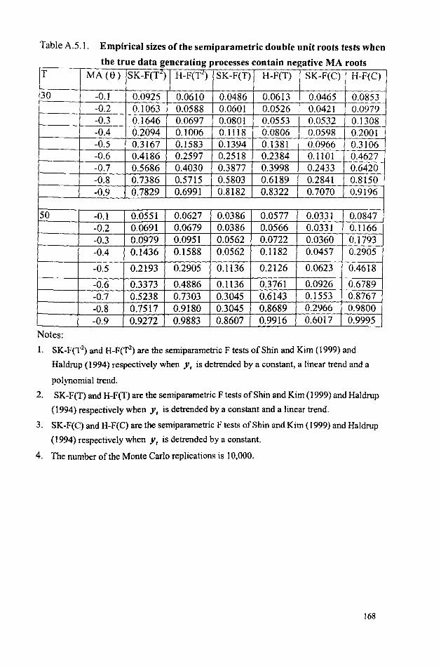
Table A.5.l. Empirical sizes of the semiparametric double unit roots tests when

the true data generating processes contain negative MA roots T MA(e) SK-F(T2) I H-F(TL) SK-F(T) H-F(T) SK-F(C) H-F(C)

30 -0.1 0.0925 0.0610 0.0486 0.0613 0.0465 0.0853 -0.2 0.1063 0.0588 0.0601 0.0526 0.0421 0.0979 -0.3 0.1646 0.0697 0.0801 0.0553 0.0532 0.1308 -0.4 0.2094 0.1006 0.1118 0.0806 0.0598 0.2001 -0.5 0.3167 0.1583 0.1394 0.1381 0.0966 0.3106 -0.6 0.4186 0.2597 0.2518 0.2384 O.llOl 0.4627 -0.7 0.5686 0.4030 0.3877 0.3998 0.2433 0.6420 -0.8 0.7386 0.5715 0.5803 0.6189 0.2841 0.8150 -0.9 0.7829 0.6991 0.8182 0.8322 0.7070 0.9196

50 -0.1 0.0551 0.0627 0.0386 0.0577 0.0331 0.0847 -0.2 0.0691 0.0679 0.0386 0.0566 0.0331 0.1166 -0.3 0.0979 0.0951 0.0562 0.0722 0.0360 0.1793 -0.4 0.1436 0.1588 0.0562 0.1182 0.0457 0.2905

-0.5 0.2193 0.2905 0.1136 0.2126 0.0623 0.4618

-0.6 0.3373 0.4886 0.1136 0.3761 0.0926 0.6789 -0.7 0.5238 0.7303 0.3045 0.6143 0.1553 0.8767 -0.8 0.7517 0.9180 0.3045 0.8689 0.2966 0.9800 -0.9 0.9272 0.9883 0.8607 0.9916 0.6017 0.9995

Notes:

1. SK-F(T2) and H_F(T2) are the semiparametric F tests of Shin and Kim (1999) and

Haldrup (1994) respectively when Y t is de trended by a constant, a linear trend and a

polynomial trend.

2. SK-F(T) and H-F(T) are the semiparametric F tests of Shin and Kim (1999) and HaJdrup

(1994) respectively when Y t is detrended by a constant and a linear trend.

3. SK-F(C) and H-F(C) are the semiparametric F tests of Shin and Kim (1999) and Haldrup

(1994) respectively when Y, is detrended by a constant.

4. The number of the Monte Carlo replications is 10,000.

168

Appendix 5.2

Table A5.2. Asymptotic critical values for cointegrating CADF t-statistics Standard Demeaned Detrended

2 1% 5% 10% 1% 5% 10% 1% 5% p

1.0 -2.4631 -2.7648 -3.3369 -3.9060 -3.3502 -3.0486 -4.3599 -3.7791 0.9 -3.3268 -2.7410 -2.4431 -3.8625 -3.3044 -2.9950 -4.2754 -3.7208

0.8 -3.3076 -2.7246 -2.4187 -3.8078 -3.2484 -2.9407 -4.2037 -3.6333

0.7 -3.2872 -2.7031 -2.3963 -3.7636 -3.1900 -2.8716 -4.1261 -3.5503

0.6 -3.2886 -2.6825 -2.3737 -3.7176 -3.1262 -2.8054 -4.0344 -3.4582

0.5 -3.2795 -2.6575 -2.3425 -3.6531 -3.0570 -2.7222 -3.9646 -3.3568

0.4 -3.2480 -2.6319 -2.3079 -3.6007 -2.9856 -2.6464 -3.8779 -3.2409 0.3 -3.2257 -2.6003 -2.2795 -2.5581 -2.9028 -2.5581 -3.7779 -3.1188

0.2 -3.1927 -2.5824 -2.2542 -3.4707 -2.8260 -2.4739 -3.6592 -2.9743

0.1 -3.1800 -2.5602 -2.2279 -3.3993 -2.7422 -2.3736 -3.5247 -2.8236

Notes:

1. The critical values were calculated from 60,000 draws generated from samples of sizes

1,000 with i.i.d. Gaussian innovations.

2. Parzen kernel is used and the bandwidth is calculated using the suggestion of Andrews

(1991).

169

10% -3.4962

-3.4195

-3.3358

-3.2443

-3.1422

-3.0343

-2.9147 -2.7822 -2.6298

-2.4575

CHAPTER SIX

6.1 Introduction

MARKOV-SWITCHING COINTEGRATION TEST

FOR BUBBLES

It is noted that the expectations and implementation of monetary reforms during

periods of hyperinflation might lead to regime changes in economic variables. Failure

to model the regime-shifting behaviour of time series may lead to biased conclusions

with respect to cointegration and the existence of bubbles. In the previous chapter,

threshold cointegration analysis was employed to model the switching processes that

are restricted to depend upon observable threshold values. However, threshold

nonlinearity and Markovian regime shifts may be observationally equivalent. In this

chapter, I will continue to use the same Cagan model specifications, and the testing

procedure of Engsted (1993), as in the previous chapter, to conduct the empirical

study of bubbles. The regime shifting behaviour of time series variables are,

alternatively, assumed to depend on unobservable states generated by a first-order

Markov chain, and I adopt the Markov-switching cointegration method for bubble

testing. The probability law that governs the Markov-switching regimes is

advantageous in that it is more flexible and allows the data to detennine the specific

fonn of nonlinearities that are consistent with the sample infonnation. The empirical

170

findings still do not support the evidence for bubbles but the Markovian

regime-switching behaviour can be identified. Also, inferences about the

probabilities of the unobservable states at each point in time can be made. The chapter

is structured as follows: Section 2 contains a discussion of the econometric

methodology; Section 3 reports the empirical results; concluding remarks are

contained in Section 4.

6.2. Econometric Methodology

Krolzig (1996, 1997), and Yao and Attali (2000) argue that a linear co integration

method is asymptotically valid to test for the number of cointegrating vectors in a

Markov error-correction model. However, Nelson et al. (2001), Psaradakis (2001)

and Cavaliere (2003) consider that the conventional unit root tests will result in

biased conclusions when the series under study exhibit Markov shifts. Hence,

Cavaliere (2003) suggests that unit root or cointegration tests be carried out using a

statistical method that allows for the Markov switching process.

In this chapter, I conduct the cointegration-testing procedure of Engsted (1993),

as illustrated in Chapter 5, for the identification of bubbles by sequentially applying

the MS-ADF unit root test of Hall et al. (1999) to the OLS residuals ofEqs (5.3) and

171

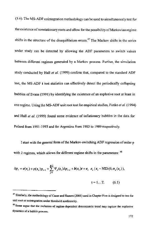
(5.6). The MS-ADF co integration methodology can be used to simultaneously test for

the existence of non stationary roots and allow for the possibility of Markovian regime

shifts in the structure of the disequilibrium errors.47 The Markov shifts in the series

under study can be detected by allowing the ADF parameters to switch values

between different regimes generated by a Markov process. Further, the simulation

study conducted by Hall et al. (1999) confinn that, compared to the standard ADF

test, the MS-ADF t test statistics can effectively detect the periodically collapsing

bubbles of Evans (1991) by identifying the existence of an explosive root at least in

one regime. Using the MS-ADF unit root test for empirical studies, Funke et al. (1994)

and Hall et a/. (1999) found some evidence of inflationary bubbles in the data for

Poland from 1991-1993 and for Argentina from 1983 to 1989 respectively.

I start with the general fonn of the Markov-switching ADF regression of order p

with 2 regimes, which allows for different regime shifts in the parameters: 48

L\y, = C(s,) + p(s,)Yt-l + I'I'j(s,)L\Yt-I +b(s,)t+e, e,ls,-NID(O,CJe(S,», )=1

t=l...T. (6.1)

47 Similarly. the methodology of Caner and Hansen (2001) used in Chapter Five is designed to test for

unit root or cointegration under threshold nonlinearity.

48 Some argue that the inclusion of regime-dependent deterministic trend may capture the explosive

dynamics of a bubble process.

172

where y, is an OLS residual ofEq. (5.3) or (5.6),49 is a white noise process with zero

mean and regime-switching standard deviation cr e (s,) . All parameters of the

autoregression, c(s,), p(s,), 'I' /s,), and crt (s,) are conditioned on a finite number

of stochastic unobservable Markov-switching state variable s, E {l,2} such that: 50

(6.2)

where Sl, takes on the value 1 when s, = i, and 0 otherwise, for i = 1,2.

The stochastic process generating the unobservable regimes is an ergodic

Markov chain governed by the transition probabilities, Pij= Pr [s, = j I S,_1 = i] with

2:;=1 PIj = 1 "t i, j E {1,2}. For an ergodic Markov chain, regime shifts are persistent

if Pij =1= Pu for some i =1= j, but not permanent if Pii =1= 1 "t i. The filtered probability of

2

S, = j, denoted by Pr[s, = j 10,], is equal to L Pr[s, = j, S,_1 = i I 0, J, conditional 1=1

on information up to time t, 0,. The smoothed probability of s, = j, denoted by

Pr[s, = j I Or], conditional on all the information in the sample, Or> and is

49 As pointed out by Yao and Attali (2000). the OLS estimates of a cointegration vector remain

superconsistent under regular conditions even though the disequilibrium error exhibits a

Markov-switching process. so I

n Hall et al. (1999). the Markov state s, is set to 0 or I. but in this chapter. s, is set to be 1 or 2

instead.

173

2

calculated by LPr[s, = j,st+1 = i I QT]' The Hamilton's (1989) filtering and the ;=1

Kim's (1994) smoothing algorithms are employed to make inferences about the

filtered and smoothed probabilities of the unobservable Markov regimes respectively.

An expectation-maximization (EM) algorithm for maximum likelihood estimation is

used to yield estimated parameters of the ADF regression (6.1).

The existence of non stationary roots is rejected when the two individual t-ratio

statistics, t\ and t2, reject the null hypothesis that PI ;;;; 0 against the alternative of Pi

< 0, for all i = 1 and 2.5\ In addition to the t-ratio statistics, I propose a Wald statistic

to test for the joint hypothesis that PI = P2 = 0 against the alternative of Pi =F 0 for

at least one i. When both the point estimates of PI and P2 lie in the open interval of

-2 and 0, the significance of the Wald statistic implies the rejection of the existence of

nonstationary roots across two regimes in the data series of interest. The associated

p-values ofthe Wald and t-ratio statistics are obtained via simulation.

On the other hand, the number of the Markov-switching regimes cannot be

tested using conventional testing approaches due to the presence of unidentified

nuisance parameters such as the transition probabilities under the null of linearity.

51 • The more ngorous stability conditions for a Markov-switching model are documented in Yao and

Attali (2000).

174

Hansen (1992, 1996) derived fonnal tests of Markov-switching nonlinearity, which

involve the approximation of the asymptotic distribution of the likelihood ratio (LR)

via simulation and evaluation of the likelihood function across a grid of different

values for the transition probabilities as well as for each state-dependent parameter.

This is, however, computationally demanding and time consuming. In practice,

Krolzig (2002) suggests the alternatives that include the upper bound of Davies (1977,

1987) for the significance level of the LR test statistics under nuisance parameters,52

and information criteria such as AIC, SC and HQ (see for example, Krolzig, et al.

2002 and Clarida, et al. 2003).

6.3 Empirical Results

The data and the sample periods in this section are identical to those in Chapter

Five. They include data series of price levels, money supply and exchange rates for

the inter-war European hyperinflations of Gennany, Hungary and Poland. In the

subsequent empirical studies, the estimation is conducted using the maximum

likelihood method with the expectation-maximization (EM) algorithm. The intercept

52 The Wald statistic for the joint hypothesis that the intercept terms are equal across two regimes is

valid (Krolzig, et.a/. 2002). Hence, if singular matrix occurs when the LR test is implemented, the

Waid statistic will be used instead.

175

tenus c(s,), standard deviation of error O"e (s,), and the coefficients b(s,), \I' j (s,) ,

and pes,), of the MS-ADF regression (6.1), can be made regime-dependent if the

corresponding upper bound LR test statistic of Davies (1977,1987) is significant. The

number of lag length, p, is chosen to make e, white noise. The p-values of the

MS-ADF Wald and t-ratio statistics are obtained via simulation. 53

6.3.1 Price bubbles

Table 6.1a contains the maximum likelihood estimates of the MS-ADF

regressions for the OLS residuals of Eq.(5.3), which are obtained from regressing

(M, -7t I.,) on ~7tI.t+1 • The estimation results show that all parameters of the

MS-ADF regression are made regime-dependent for all of the hyperinflations under

study, except the fact that the intercept term is regime-invariant for Germany. All the

point estimates of PI and P2 in two regimes are negative and the corresponding Wald

and t-ratio statistics are significant from the associated p-values. Hence, the results

favour the evidence of co integrating relationships between M, - 7tJ.t and ~7t1.t+1 •

Table 6.1 b presents the estimation results of the MS-ADF test for the OLS residuals

obtained from regressing (M, - 7t I,,) on 11M, . As shown in Table 6.2b, the

53 For some cases, I add a vector of regime-dependent stationary covariates into the MS-ADF

regressions to increase power as suggested in Hansen (1995).

176

intercepts of the MS-ADF regression are allowed to be regime-dependent for

Hungary only. The coefficients b(s,), \If j (s,), and p(s,) can vary across different

regimes for Germany and Poland. The standard deviation of e, can be

regime-dependent for Germany and Hungary. All point estimates of PI and P2 are

negative, and both the Wald and t-ratio statistics are significant. This signifies the

acceptance of the co integrated relationships of eM, -1t1.,) on 11M, . When

eM, -1t1,,) co integrates with ~1tI,t+l and 11M, the evidence for price bubbles in the

data, as suggested by Engsted (1993), is rejected.

[Table 6.1a and 6.1 b to be inserted here]

Figures 6.1 to 6.6 plot the filtered and smoothed probabilities of regime I for the

residuals of the regression of (M, -1tt,,) on ~1tl,t+l and of (M, -1t I,,) on 11M" from

which the Markovian regime shifts are found in the residuals of Eqs (5.3) and (5.6)

throughout the whole samples.

[Figure 6.1 and Figure 6.6 to be inserted here]

177

6.3.2 Exchange rate bubbles

The maximum likelihood estimates of the MS-ADF regressions for the OLS

residuals ofEq.(5.3) are obtained from regressing (M, -1t 2,,) on ~1t2,'+1 • The results

are presented in Table 6.2a. The intercept term of the MS-ADF regression is made

state-dependent for Germany and Hungary. The joint LR allows the coefficients

b(s,), \jJ J(s,), and p(s,), of the MS-ADF regression to switch between regimes for

Germany and Hungary. Also, the standard error of e, can be state-dependent for

Germany and Hungary. In other words, all the parameters of the MS-ADF regression

for Poland are restricted to be regime-independent and the t-ratio value of p is the

standard ADF t test statistic. For Germany and Hungary, the point estimates of PI

and P2 in two regimes are found to be negative and the MS-ADF Wald and t-ratio

statistics are significant. From the above, it can be concluded that there exists a

cointegrating relationship between (M, -1t 2,,) and ~1t2'1+1 for all of the countries

under study. Moreover, the results of the cointegrating tests applied to the OLS

residuals of Eq.(S.6) obtained from regressing (M, -1t 2,,) on ~, are presented in

Table 6.2b, For Germany, only the intercept ofthe MS-ADF regression is restricted to

be state-invariant; whereas for Poland, only the intercept can be made

regime-dependent. All the parameters of the MS-ADF regression are different across

178

regimes for Hungary. From the negative point estimates of PI and P2 with

significant Wald and t-ratio statistics, the existence of a cointegrated relationship

between (M, -7t2,,) and 11M, cannot be rejected. While (M, -7t z,,) cointegrates

with ~7t2,'+1 and with 11M" no nonstationary roots are found in the residuals of Eqs

(5.3) and (5.6) respectively. Hence, the evidence for an exchange rate bubble is

rejected in the data for all of the hyperinflations under study ..

[Table 6.2a and Table 6.2b to be inserted here]

The patterns of regime shifts can be seen from Figures 6.7 to 6.11 where the

filtered and smoothed probabilities of regime 1 for the residuals of the regression of

(M, -7t 2,') on ~7t2,'+1 and of (M, - 7t 2,,) on ~, , are plotted. The

regime-switching behaviours can be found throughout the whole estimation periods

for the countries under study.

[Figure 6.7 and Figure 6.11 to be inserted here]

6.4. Concluding Remarks

In this chapter, I have continued the cointegration tests to examine the bubble

existence using the co integrating Markov-switching ADF tests. The regime shifts in

179

the MS-ADF regression are allowed to depend on an unobservable state variable

governed by the Markov chain rather than on an observable threshold value. The

empirical results show that the evidence of Markovian regime shifts is found in the

cointegration residuals from the regression of M, -1t, and L\1t1+\ as well as M, - 1t,

and Mit. Also, the point estimates of Pi are all negative and the Wald and t-ratio

statistics are all significant. Hence, the evidence favours the MS cointegrating

relationship in both Eqs (5.3) and (5.6), and it rejects the presence of bubbles in any of

the countries under study.

180

Table 6.1a. MS Cointegrating ADF test for the regression of(M, - 7t u ) on ~7tI.t+ I

Country Gennany Hungary Poland Parameters Regime 1 I Regime 2 Regime 1 Regime 2 R~ime 11 R~ime 2

Intercept of the MS-ADF regression: c(s,) 0.2028*** 1.0282* 0.0918 1.0687* I 0.1634

(0.1072) (0.21 991 (0.0769) (0.0859) (0.1576) LR(c1 == c2 ) 0.0025# 18.4070* 8.7839**

[0.9599] 10.0004] [0.0323) Coefficients of the ADF regression:

b(s, ) -0.0046 -0.0294* -0.0508* -0.0006 -0.0495* -0.0021 (0.0037) (0.0053) (0.0078) (0.0021) (0.0026) (0.0069)

pes,) -0.2697 -l.5341 -0.8473 -0.2527 -0.7355 -0.6644

t(p(s, » -4.3517* -6.7925* -6.4622* -3.8816** -25.1221* -3.8598**

W (p(s,» 66.0191* 51.4814* 652.829*

Joint LR 51.0888* 25.6972* 12.1681 ** [0.0000] [0.0001] [0.0300)

Standard error of residuals

O"e(s,) 0.0695 0.9889 0.1200 0.1153 0.0370 I 0.2731

LR(0"1 == 0"2) 53.6782* 14.4253* 9.1883** [0.00001 [0.0024] [0.02691

Transition probability matrix: PII Pl2 0.8310 0.1690 0.4837 0.5173 0.4110 0.5890 P21 P22 0.6773 0.3227 0.1729 0.8271 0.1816 0.8184

Diagnostic checking AIC -0.0332 -0.3292 0.6719 HQ 0.1663 -0.1782 0.8250 SC 0.5386 0.0804 1.1208 Q(l2-p) 8.1515 7.9668 9.8592 Notes:

1. t(p(s, »and W (p(s, »refer to the MS-ADF t and Wald statistics respectively.

2. Joint LR refers to the joint LR linearity test for the coefficients \jJ I (s,). b(s,) and

pes,), of the MS-ADF regression.

3. # Denotes the Wald statistic, rather than the LR statistic, for linearity tests.

4. The figures in (.) are standard errors. The figures in [.] are the p-values for the

significance of the upper bound LR linearity tests.

5. AIC, HQ and SC refer to the Akaike, Schwarz, and Hannan and Quninn criterion

respectively.

6. Q(k) refers to Ljung-Box Q-statistics with degrees of freedom = k.

7. *1**1*** Denote significance at the J%, 5% and 10% level.

8. For the case of Gennany, the stationary covariates include ~27t2.H and ~l M, ,.

18l

Table 6.tb. MS Cointegrating ADF test for the regression of (M, -1tI,l) on 11M,

Country Germany Hungary Poland Parameters Regime 1 I Regime 2 Regime 1 I Regime 2 Regime 1 J Regime 2

Intercept of the ADF regression: c(s,) 0.6770* -0.1264**/ 0.1889* 0.1935*

(0.1069) (0.0499) (0.0477) (0.0164) LR(cl =c2 ) 0.0000# 11.2275** 0.0003#

[0.9932] [0.0106] [0.9855] Coefficients of the ADF regression:

\ill (s,) 0.5581 * -0.0385 0.6612* (0.0873) (0.0444) (0.1968)

\il2 (s,) 0.3992* 0.6127* (0.0452) (0.2025)

b(s, ) -0.0258* -0.0249* -0.0027** -0.0178* -0.0044* (0.0036) (0.0042) (0.0013) (0.0008) (0.0014)

pes,) -0.3968 -0.4378 -0.6259 -0.2293 -0.8422

t(p(s, » -5.0306* -4.4110* -8.5393* -7.9263* -5.6670*

W (p(s,» 33.5772* 72.9204* 87.431 *

Joint LR 50.4305* 9.4629 35.2855* [O.OOOOJ [0.2284] [O.OOOOJ

Standard error of residuals cr.(s,) 0.0562 0.1384 0.09442 0.0175 J 0.1200

LR(cr1 = (T2) 32.5865* 0.0232 19.4283* [0.0000] [0.87891 LO.00021

Transition probability matrix: PII PI2 0.5937 0.4063 0.8625 0.1375 0.4373 0.5627 P21 P22 0.5332 0.4668 0.0769 0.9231 0.2889 0.7111

Diagnostic checking AIC -0.8563 -0.9086 -0.7081 HQ -0.6568 -0.7873 -0.4804 SC -0.2786 -0.5777 -0.0211 Q(12-p) 13.2538 12.7802 10.8851 Notes:

1. For the cases of Germany and Poland, the stationary covariates include 112 M'_I' for

i=I,2, and 1l21t 2 H respectively.

2. Other notes to Table 6.1 a stilI apply.

182

Figure 6.1. Filtered and smoothed probabilities of regime 1 for the residuals of the

regression of (M, -1t I., )on ~1tI.t+1 in Germany

1.00 Probabilities ofRe ime I [~filteredl

0.75

0.50

0.25

Inl 1.00 Probabilities of Re 'me 1

[ .. srmothed I

0.75

0.50

1922 1923

Q~ i

1924

':::-:-'-~~~~~~~.l...-...~~~~~-'---'---L....~..J-~~J-\i~~~J Inl 1922 1923 1924

Figure 6.2. Filtered and smoothed probabilities of regime 1 for the residuals of the

regression of (M, -1tI.,) on ~1tI.'+1 in Hungary

1.00 Probabilities orR ime I [--Slteredl

0.75

0.25

I. 00 Probatli?it~ orltegime 1 [._- srmothed I

0.75

183

Figure 6.3. Filtered and smoothed probabilities of regime 1 for the residuals of the

regression of (M, - 7t 1.,) on ~7tI.t+1 in Poland

1.00 Probabilities ofR ·me 1 t filtered I ---T-··~'-

1\ I \

:~::'-------L-~~---"-----.L/ \/ __ \ 0.75

1924 1.00~==:==~~~~~ __________________ , __ ~

Figure 6.4. Filtered and smoothed probabilities of regime 1 for the residuals of the

regression of (M, -7tI.,)on flM, in Gennany

1.00 rF=P~ro~bab~i~lit~ies~o~f~R!'.!!!.!!·m~e...!.I ______________ ~'T [-filteredl

0.25

1.00 Probabilities of R . e 1 I ~-- -SlIDotbedl

0.75

0.50

1922

/ f I

. I \ i \ I

i' . J ,I I,

I /

/

.: \: ~------_______ --L_---'---"-____ .L._----.l.. __ _

1922 1923

1924

1924

184

Figure 6.5. Filtered and smoothed probabilities of regime I for the residuals of the

regression of (M, -1t I ,,)on t:.M, in Hungary

1.00 Probabilities ofRe ime 1 [_.- filtered I

0.75

0.50

0.25

1922 1.00 Probabilities ofR ime2

[ .. SITDothed I 0.75

0.50

0.25

1922

1923 1924

1923 1924

1925

1925

Figure 6.6. Filtered and smoothed probabilities of regime 1 for the residuals of the

regression of (M, -1tI,l)on AM, in Poland

1922 1.00 Probabilities ofRe 'me I

0.75 1\',"- SlTDothed>,~ I \

0.50 I, 1\ I 1\"

I I 0.25

1922 1924

185

Table6.2a Cointegrating MS-ADF test for the regression of(M -7t ) on L\7t , 2" 2,'+1

Country Getmany Hungary Poland Parameters Regime 1 I Regime 2 Resime 1 I Regime 2 Regime 11 Regime 2

Intercept of the ADF regression: c(s,) 2.1098** I 1.3878* -0.8864* I -0.0460 0.4547*

(0.7046) (0.3523) (0.0676) (0.0791) (0.1595) LR(c1 =c2 ) 9.2272** 65.0991 *# 3.6115

[0.0264J [O.OOOOJ [0.3066] Coefficients of the ADF regression:

lJI 1 (s,) -0.7453* 0.1874** (0.0956) (0.0738)

lJI2(S,) 0.2020** 0.2024* (0.0936) (0.0627)

b(s,) -0.0909* -0.0412* 0.0237* 0.0044*** -0.0217* (0.0191) (0.01 141 _LO.0018) (0.0023) (0.0070)

p(s,) -1.0375 -0.6391 -0.1768 -0.2710 -0.7360

t(p(s,» -6.8660* -5.1620* -4.0354** -3.8991** -4.5379*

W(p(s,) ) 73.8228* 32.1445* 20.6209*

Joint LR 33.0602* 44.9593* 6.6673 [0.0000] [0.0000] [0.5732]

Standard error of residuals

O',(s,) 0.4678 0.1119 0.0344 0.0849 0.3107

LR(O'I = 0'2) 22.7773* 6.7481*** 2.3391 [0.0000] [0.0804] [0.5051]

Transition probability matrix: Pll P12 0.7322 0.2678 0.1909 0.8091 P21 P22 0.1516 0.8484 0.3819 0.6181

Dil!8llostic checking AlC 0.8359 -0.6609 0.7222 HQ 1.0201 -0.3847 0.7836 SC 1.3637 0.1390 0.8981 Q(l2-p) 9.0479 11.7997 7.3214

Notes:

1. For the cases of Germany and Hungary, the stationary covariates are L\2 7t I,'_I' and

L\2 7t1 ,,_I' i = 1,2, respectively.

2. Other notes to Table 6.1 a still apply.

186

Table 6.2b. Cointegrating MS-ADF test for the regression of (M - 1t7 ) on AM I _.1 I

Country Gennany Hu~_ Poland Parameters Regime I /Regime 2 Regime 1 1 Regime 2 Regime 1 I Regime 2

Intercept of the ADF regression: c(s,) 0.8312* 0.1508* 1-0.4197* -0.3880* 1 0.0220

(0.] 875) (0.0453) (0.0879) (0.0667) (0.0548) LR(c) =c2 ) 0.0022# 32.1756*# 9.1718**

[0.9625] 10.00001 10.0271] Coefficients of the ADF regression:

'V\(s,) 1.7130* -0.4274* -0.5732* 0.3166* (0.2334) (0.0861) (0.0925) (0.1085)

b(s,) -0.0236* -0.0310* -0.0103* 0.0141 * 0.0029 (0.0070) (0.0059) (0.0018) (0.0026) (0.0023)

pes,) -0.5922 -0.3631 -0.2790 -0.4094 -0.7084

t(p(s,» -4.0692* -5.0590* -3.5969** -4.9534* -8.1681*

W(p(s,) ) 34.0088* 38.2115* 66.7179*

Joint LR 34.8726* 23.1208* 10.5068 [0.0000] [0.0068] JO.321 41

Standard error of residuals

cr~(s,) 0.2600 0.2276 0.0463 I 0.0824 0.1170

LR(cr) = 0"2) 25.9889* 12.0458* 0.0000# [0.0000] [0.007~1 [0.9973]

Transition probability matrix: PH Pl2 0.2778 0.7222 0.6893 0.3107 0.5628 0.4372 P21 P22 0.3094 0.6906 0.1540 0.8460 0.1811 0.8189

Diagnostic checking Ale 1.1407 -1.0614 0.0253 HQ 1.3095 -0.8179 0.1631 SC 1.6295 -0.3927 0.4293 Q(I2-p) 11.5172 10.3732 11.1613 Notes:

l. For the cases of Hungary and Poland, the stationary covariates are equally ~21t).H' i =

1,2.

2. Other notes to Table 6.1a still apply.

187

Figure 6.7. Filtered and smoothed probabilities of regime 1 for the residuals of the

regression of (M, -1t 2,/) on A1t 2,/+1 in Gennany

1.00 Probabilities ofRe ime 1 [~-- filteredj

1\ ;-=---0.75

0.50 \

0'25~L~_ ~~~J~~ 1921 1922 1923 1924

Probabilities of Regime 1 1.00 rr=====~~~=~~.-----------r~ ... ::::: .... 7' .. ---i---~----:"--­

stroothedl

0.75

0.50

0.25

/ /\ 19L2~1~==~~-----L~~19L~~'~~/~'~~~~~~~19L23~~'~~'~'~'~~~ 1924

Figure 6.8. Filtered and smoothed probabilities of regime 1 for the residuals of the

regression of (M, -1t 2,/) on L\1t 2,t+l in Hungary

188

Figure 6.9. Filtered and smoothed probabilities of regime 1 for the residuals of the

regression of (M, -1t 2,,) on tlM, in Germany

1.00 Probabilities~~me I L:::-,..:::_filt~ --------------------"~----------------,~-

:1, I

0.75

0.50

/' j / \ I

/~/ \1 / \j

0.25---

!

1922

r I \ i / \

i \ I \

I \ / 1\

I /

1923

/ /-J

1.00 LFP=ro"="bab",,,!:,:,il,:,:,:itl~·es~o~f~R"l!.!.'.im~e,...2c...-________________ ~i __ --:-______ --;------;-__ ~ [ sIIDolhed I !,

1924

i: 0.75

0.50

0.25

1922 1923 1924

Figure 6.10. Filtered and smoothed probabilities of regime 1 for the residuals of the

regression of (M, -1t 2,,) on tlM, in Hungary

1.00 rii~F~~~~------;;-r:::::-----r;----------

0.75

0.50

0.25

1924 1925

\

0.50

0.25'

1922 1923 1924 1925

189

Figure 6.11. Filtered and smoothed probabilities of regime 1 for the residuals ofthe

regression of (M, -1t 2 •1 ) on tlM, in Poland

075

050

0.25

1922 1.00 Probabilities of Regime I

[ slroolhed I

0.75

0.50

0.25

1922

/- \

/ 1923

1923

il '\

1924

1924

190

CHAPTER SEVEN SUMMARY and CONCLUSION

In this thesis, I have adopted several econometric methods to investigate for the

presence of price and exchange rate bubbles, using the inter-war European

hyperinflations of Germany, Hungary and Poland as a case study. This chapter

summarizes the major findings of the thesis and offers my concluding remarks.

In Chapter Two, two versions of the Cagan model under rational expectations

are specified. The general solution to the Cagan models is the sum ofthe fundamental

and bubble solutions. Dependent upon the assumed generating processes of the

driving fundamentals, several explicit representations of the fundamental solutions

are derived. In the rational expectations framework, the bubble solution contains an

arbitrary martingale process. Consequently, there exists an infinite set of bubble

processes for any value of a bubble coefficient. Several examples of theoretical

bubble specifications are explored by imposing parametric restrictions. Some ofthese

exhibit asymptotically dynamic stability, and some display different bursting

properties. The problem of non-uniqueness in the bubble solutions makes it difficult

to specify and test for every form of bubble. Hence, the general or indirect tests look

more attractive for empirical research, because they focus upon the statistical

191

properties of the data series used for bubble detection and do not require the

specification of a particular fonn of bubble process.

In Chapter Three, I carry out a structural time series analysis to decompose the

various structural time series components of the data over the full sample periods.

This facilitates the examination of the statistical properties and integration orders of

the relevant economic variables. It is found that the trend components for the data

series on the level of money supply, prices and exchange rates follow a second

differencing or a smooth trend specification. For the data series on real money

balances, money supply growth, inflation rates and currency depreciation rates, the

trend components follow a random walk or a local level representation. Some

evidence for seasonal or cyclical components is found in the data series. On the basis

of the reduced fonns of the structural time series models, the series of the different

levels are integrated at the order of two; and the other data series contain one unit root.

Such findings are important for the selection of the econometric methods to be

adopted for bubble testing in the thesis.

Some concern has been frequently expressed in the literature about the value of

empirical research into the existence of bubbles. It has been argued that model

misspecification and the process switching in fundamentals could lead to false 192

conclusions concerning the existence of bubbles. Furthermore, as illustrated in

Chapter Two, some stochastic bubbles may exhibit nonlinear explosive dynamics and

consequently appear to be linearly stationary. Under these circumstances,

conventional econometric methods may fail to test for the existence of bubbles even

if they actually occur in the data series. In this thesis, I have employed new

econometric procedures and methods to handle the above empirical problems of

bubble identification.

In Chapter Four, I propose a new testing procedure using orthogonality tests,

which is designed to effectively distinguish between bubbles and specification errors.

I rely upon the FM-GMM instrument validity test statistics and the ARIMA structures

of flow variables to detect the presence of specification errors. The stock variables are

transformed in such a way that I can differentiate between the presence of bubbles

and any model misspecification. Evidence for stationary specification errors in the

exact Cagan models can be found. Moreover, while the transformed stock variables

are orthogonal to the information sets in the FM regressions, both exchange rate and

price bubbles are rejected in the data for those European hyperinflations under study.

The results conclude that the control of inflation in those countries might only be

required to gain control of the fundamental process. This is because the dynamics of

193

prices and exchange rates might not be driven by the self-fulfilling expectations for

these countries. It is argued that the expectation and implementation of monetary

refonns that occurred in the final months of the sampled European hyperinflations

might lead to nonlinear behaviour by the underlying fundamental variables. The

distribution theory of the FM inferential statistics is developed, however, under the

assumption of linear data generation. Hence, the nonlinear movements of

fundamentals that display regime-switching behaviour may be misinterpreted as

indicating a bubble path. The usual practice in such cases is to truncate the estimation

periods under study, as was done in Chapter Four. The evidence for no bubbles given

in Chapter Four is therefore limited to the pre-refonn observations. The dilemma is

that by doing this, the ability to detect bubbles may be diminished even when bubbles

actually exist during the truncated observation periods. I suggest that advanced

cointegration-testing methodologies be used to further identify bubbles over the full

sample periods.

In Chapter Five, I employ a residual-based cointegrating TAR method to

investigate the evidence for bubbles over the full sample periods. I also choose the

conventional ADF and Z tests as well as the RALS-ADF test to carry out a

comparison study. From the Monte Carlo findings, the power of the TAR tests is

194

shown to be the highest no matter whether there are nonlinear threshold processes in

the data generation or not. The RALS-ADF test gains substantially in power when

using the threshold processes and it is made robust to the presence of non-normal

errors by the inclusion of stationary covariates in the ADF regression. The results of

the TAR and the RALS-ADF tests reject the evidence for the existence of bubbles,

but some evidence of threshold nonlinear processes is nevertheless found in the data

generation throughout the whole sample periods for all of the countries of interest.

The low power of the conventional ADF and Z tests under the nonlinear process is

likely to produce a spurious conclusion concerning the existence of bubbles. On the

other hand, it is argued that rejection of non-co integration may be attributable to a

serious size distortion when nonlinearly explosive bubbles are present. The Monte

Carlo findings, however, show that in the presence of periodically collapsing bubbles,

the TAR tests and the RALS-ADF test are more likely to accept the null of

non-cointegration than are cointegrating ADF and Z statistics. The empirical results

reported in Chapter Five are not consistent with the presence of collapsing bubbles in

the data.

The switching processes described in Chapter Five are assumed to depend upon

observable threshold values. Actually, the threshold model and the Markov model

195

can be observationally equivalent. Hence, in Chapter Six, I continue the cointegration

tests to test for bubble existence using the Markov-switching cointegration ADF tests.

The regime shifts in the Markov-switching ADF regression are allowed to depend on

an unobservable Markov state variable rather than on an observable threshold value.

The empirical results favour some evidence of Markov regime shifts in the data but

reject the evidence of bubbles for any of the European hyperinflations under study.

The co integration-testing methodology, however, has been criticized in the

literature as having its own drawbacks for bubble testing. Given the fact that every

econometric methodology has limitations as well as advantages, it is proposed that

more than one method be adopted for the empirical study of bubbles. The

orthogonality methodology and the cointegration methodology should be

complementary for this purpose. They each have their own specialties. The

orthogonality method can exploit the high-frequency properties of the data whereas

the cointegration method exploits the low-frequency properties.

From the above, it is apparent that it is necessary to select the appropriate

econometric procedures and methods for bubble testing, in order to handle the issues

of model misspecification, the regime-switching behaviour of fundamentals and the

nonlinear stochastic properties of bubbles. If any of these is ignored, misleading 196

conclusions concerning the existence of bubbles are likely to result. Although the

above econometric procedures and methods are useful for studying inflationary

bubbles, they can be equally applied to the investigation of asset price bubbles in

capital markets, and it is expected that this wiIl be tackled in future research work.

197

References:

1. Abel, A., Dornbusch, R., Huizinga, J. & Marcus, A. (1979). Money Demand

During Hyperinflation. Journal of Monetary Economics, 5, 97-lO4.

2. Andrews, D.W.K. (1991). Heteroskedasticity and Autocorrelation Consistent

Covariance Matrix Estimation. Econometrica, 59, 817-858.

3. Balke, N. and Fomby, T. (1997). Threshold Cointegration. International

Economic Review, 38,627-645.

4. Bhargava, A. (1986). On the Theory of Testing for Unit Roots in Observed Time

Series. Review of Economic Studies, 53, 369-384.

5. Blanchard, O. J. and Watson, M. W. (1982), "Bubbles, Rational Expectations,

and Financial Markets," in Paul Wachtel (eds.) Crisis in the Economic Financial

Structure, MA: Lexington Books.

6. Bohl, M. T. (2003), Periodically Collapsing Bubbles in the US Stock Market?

International Review of Economics and Finance, 12,358-397.

7. Broze, L., Gourieroux, C. and Szafarz, A. (1995). Solutions of Multivariate

Rational Expectations Models. Econometric Theory, 11, 229-257.

8. Broze, L. and A. Szafarz, (1991). The Econometric AnalYSis of Non-Uniqueness

in Rational Expectations Models, Amsterdam: North Holland.

9. Cagan, P. (1956). The Monetary Dynamics of Hyperinflation. In M. Friedman

(eds.), Studies in the Quantity Theory of Money. Chicago: University of Chicago

Press.

10. Camerer, C. (1989). Bubbles and Fads in Asset Prices. Journal of Economic

Surveys, 3, 3-41.

11. Campbell, J. Y. and Shiller, R. J. (1987). Co integration and Tests of Present Value

Models. Journal of Political Economy, 95, lO62-lO88.

198

12. Caner, M. and Hansen B. E. (2001). Threshold Autoregression with a Unit Root.

Econometrica, 69, 1555-1596.

13. Carrasco, M. (2002). Misspecified Structural Change, Threshold or

Markov-Switching

Models. Journal of Econometrics, vol. 109,239-273.

14. Casella, A. (1989). Testing for Rational Bubbles with Exogenous or Endogenous

Fundamentals: The German Hyperinflation Once More. Journal of Monetary

Economics, 24, 109-122.

15. Cavaliere, G. (2003). Asymptotics for Unit Root Tests under Markov

Regime-switching. Econometric Journal, 6, 193-216.

16. Chan, K. S. and Tong, H. (1985). On the Use of the Deterministic Lyapunov

Functions for the Egodicity of Stochastic Difference Equations. Advances in

Applied Probability, 17,666-678.

17. Chen, L. T. (1995). Essays on Testing for Speculative Bubbles in the Stock

Market. Monograph Series, No.65, The Institute of Economics, Academia

Sinica.

18. Chen, L. T. (1997). Misspecification Versus Bubbles in the Stock Market: The

Case for Time-varying Discount Rates. Academia Economic Papers, 25,

427-461.

19. Chen, L. T. (1999). Model Misspecification Versus Speculative Bubbles in the

Foreign Exchange Market: The Case of Taiwan's Effective Exchange Rate.

Taiwan Economic Review, 27, 43-68.

20. Clarida, R. R., Sarno, L., Talyor, M. P. and Valente, G. (2003). The

Out-or-Sample Success of Term structure Models as Exchange Rate Predicators:

A Step Beyond. Journal o/International Economics, 60, 61-83.

21. Cuthbertson, K. (1996). Quantitative Financial Economics. John Wiley & Sons.

199

22. Davies, R. B. (1977). Hypothesis Testing when a nuisance parameter is present

only under the Alternative. Biometrika, 64, 247-254.

23. Davies, R. B. (1987). Hypothesis Testing when a nuisance parameter is present

only under the Alternative. Biometrika, 74, 33-43.

24. Dezhbakhsh, H. and Demirguc-Kunt, A. (1990). On the Presence of Speculative

Bubbles in Stock Prices. Journal of Financial and Quantitative Analysis, 25,

101-112.

25. Diba, B. T., and H. I. Grossman (l988a). Explosive Rational Bubbles in Stock

Prices? American Economic Review, 78, 520-30.

26. Diba, B. T., and H. I. Grossman (1988b). Rational Inflationary Bubbles. Journal

of Monetary Economics, 21, 35-46.

27. Dickey, D.A. and Pantula, S. G. (1987). Detennining the Order of Differencing

in Autoregressive Processes. Journal of Business and Economic Statistics, 5,

455-461.

28. Durlauf, S. N. & Hooker, M. A. (1994), "Misspecification versus Bubbles in the

Cagan Hyperinflation Model," in C. Hargreaves (eds.), Non-stationary Time

Series AnalysiS and Cointegration. Oxford: Oxford University Press.

29. Enders, W. and Granger, C. W. J. (1998). Unit Root Tests and Asymmetric

Adjustment with an Example Using the Tenn Structure of Interest Rates. Journal

of Business and Economic Statistics, 16,304-311.

30. Enders, W. and Siklos, P. (2001). Cointegration and Threshold Adjustment.

Journal of Business and Economic Statistics, 19, 166-176.

31. Engle, R. F. and Granger, C. W. J. (1987). Cointegration and Error-correction:

Representation, Estimation and Testing. Econometrica, 55, 251-276.

32. Engsted, T. (1993). Cointegration and Cagan's model of Hyperinflation under

Rational Expectations. Journal of Money, Credit and Banking, 25, 350-360.

200

33. Engsted, T. (1994). The Classic European Hyperinflations Revisited: Testing the

Cagan Model Using a Cointegrated VAR Approach. Economica, 61, 331-341.

34. Engsted, T. (1996). The Monetary model of the Exchange Rate under

Hyperinflation: New Encouraging Evidence. Economics Letters, 51, 37-44.

35. Engsted, T. (2003). Misspecification versus Bubbles in Hyperinflation Data:

Comment. Journal of International Money and Finance, 22, 441-451.

36. Evans, G. E. (1986). A Test for Speculative Bubbles in the Sterling-Dollar

Exchange Rate: 1981-84. American Economic Review, 76, 621-636.

37. Evans, G. E. (1991). Pitfalls in Testing for Explosive Bubbles in Asset Prices.

American Economic Review, 81,922-930.

38. Flavin, M. (1983). Excess Volatility in the Financial Markets: A Reassessment of

the Empirical Evidence. Journal 0/ Political Economy, 91, 929-956.

39. Flood, R. P. and Garber, P. M. (1980a). An Economic Theory of Monetary

Reform. Journal 0/ Political Economy, 88, 24-58.

40. Flood, R. P. and Garber, P. M. (1980b). Market Fundamentals versus Price-Level

Bubbles: The First Tests. Journal o/Political Economy, 88, 745-770.

41. Flood, R. P. and Hodrick, R. J. (1986). Asset Price Volatility, Bubbles and

Process Switching. Journal o/Finance, 41,831-842.

42. Flood, R. P. and Rodrick, R. J. (1990). On Testing for Speculative Bubbles.

Journal o/Economic Perspectives, 4,85-101.

43. Flood, R. P., Rodrick, R. J. and Kaplan, P. (1986). An Evaluation of Recent

Evidence on Stock Market Bubbles. NBER Working Paper, No. 1971.

44. Frenkel, J. A. (1977). The Forward Exchange Rate, Expectations and the

Demand for Money: The German Hyperinflation. American Economic Review, 67,653-670.

201

45. Frenkel, J. A. (1979). Further Evidence on Expectations and the Demand for

Money During Gennan Hyperinflation. Journal of Monetary Economics, 5, 81-96.

46. Funke, M., Hall, S. and Sola, M. (1994). Rational Bubbles During Poland's

Hyperinflation: Implications and Empirical Evidence. European Economic

Review, 38, 1257-1276.

47. Garber, P. (1989). Tulipmania. Journal of Political Economy, 97, 535-560.

48. Garber, P. (1990). Famous First Bubbles. Journal of Economic Perspective, 4,

35-54.

49. Gilles, C. and LeRoy, S. F. (1991). Econometric Aspects of the Variance-Bounds

Tests: A Survey. Review of Financial Studies, 4, 753-791.

50. Granger, C. W. J. and Swanson, N. R. (1997). An Introduction to Stochastic

Unit-Root Process. Journal of Econometrics, 80, 35-62.

51. Goodfriend, M. S. (1982). An Alternate Method of Estimating the Cagan Money

Demand Function in Hyperinflation under Rational Expectations. Journal of

Monetary Economics, 9,43-57.

52. Gourieroux, C., Laffont, J.J. and Monfort, A. (1982). Rational Expectations in

Dynamic Linear Models: Analysis of the Solutions. Econometrica, 50, 409-425.

53. Haldrup, N. (1994). Semiparametric Tests for Double Unit Roots. Journal of

Business and Economic StatistiCS, 12, 109-122.

54. Haldrup, N. (1998). An Econometric Analysis of 1(2) Variables. Journal of

Economic Surveys, 12,595-650.

55. Hall, S. G., Psaradakis, Z. and Sola, M. (1999). Detecting Periodically

Collapsing Bubbles: A Markov-Switching Unit Root Test. Journal of Applied

Econometrics, 14, 143-154.

202

56. Hamilton, J. D. (1986). On Testing for Self-fulfilling Speculative Price Bubbles.

International Economic Review, 27,545-552.

57. Hamilton, J. D. (1989). A New Approach to the Economic Analysis of

NonstationaryTime Series and the Business Cycle, Econometrica, 57, 357-384.

58. Hamilton, J. D. and Whiteman, C. H. (1985). The Observable Implications of

Self-Fulfilling Expectations. Journal of Monetary Economics, 16, 353-373.

59. Hansen, B. E. (1995). Rethinking the Univariate Approach to Unit Root Testing.

Econometric Theory, 11, 1148-1171.

60. Hansen, L. P. & Sargent, T. J. (1980). Formulating and Estimating Dynamic

Linear Rational Expectations Models. Journal of Economic Dynamics and

Control,2,7-46.

61. Harvey, AC. (1989). Forecasting, Structural Time Series Models and Kalman

Filter. Cambridge University Press.

62. Hausman, J. A (1978). Specification Tests in Econometrics. Econometrica, 46,

1251-1271.

63. Haza, D. P. and Fuller, W. A. (1979). Estimation of Autoregressive Processes

with Unit Roots. The Annuals of Statistics, 7, 1106-1120.

64. Hooker, M. A. (2000). Misspecification versus Bubbles in Hyperinflation Data:

Monte Carlo and Interwar European Evidence. Journal of International Money

and Finance, 19, 583-600.

65. Ikeda, S. and Shibata, A. (1992). Fundamentals-dependent Bubbles in Stock

Prices. Journal of Monetary Economics, 30, 143-168.

66. Ikeda, S. and Shibata, A (1995). Fundamentals Uncertainty, Bubbles and

Exchange Rate Dynamics. Journal of International Economics, 38, 199-222.

67. 1m, K. S. (1996). Least Squares Approaches to Non-Normal Errors. DAE

working paper, No. 9603, University of Cambridge.

203

68. 1m, K.S. (2001). Unit Root Tests Using More Moment Conditions Than Least

Squares. Working paper, University of Central Florida.

69. Imrohoroglu, S. (1993). Testing for Sunspot Equilibria in the German

Hyperinflation. Journal of Economic Dynamics and Control, 17, 289-317.

70. Johansen, S. (1995). Likelihood Based Inference Cointegrated Vector

Autoregressive Models. Oxford University Press.

71. Keynes, J. M. (1936). The General Theory of Employment, Interest, and Money.

Macmillan.

72. Kim, C. J. (1994). Dynamic Linear Models with Marko-Switching, Journal of

Econometrics 60, 1-22.

73. Kindleberger, C. P. (1987). Bubbles. New Palsgrave Dictationary, Vol. 1,20-22.

74. Kitamura, Y. & Phillips, P. C. B. (1995). Efficient IV Estimation in

Nonstationary Regression: An Overview and Simulation Study. Econometric

Theory, 11, 1095-1130.

75. Kitamura, Y. & Phillips, P. C. B. (1997). Fully Modified IV, GIVE and GMM

Estimation with Possibly Non-stationary Regressors and Instruments. Journal of

Econometrics, 80, 85-123.

76. Kleidon, A. W. (1986). Variance Bounds Tests and Stock Price Valuation models.

Journal o/Political Economy, 94, 953-1001.

77. Koopman, S. J., Harvey, A. C., Doomik, J. A. and Shephard, N. (2000). STAMP:

Structural lime Series Analyser, Modeller and Predictor. Timberlake

Consultants Ltd.

78. Krolzig, H. M. (1996). Statistical Analysis of Co integrated VAR Processes with

Markovian Regime Shifts. SFB 373 Discussion Paper, 2511996, Humboldt

Universitat zu Berlin.

204

79. Krolzig, H. M. (1997). Markov Switching Vector Autoregression. Modelling.

Statistical Inference and Application to Business Cycle AnaZvsis. Berlin:

Springer.

80. Krolzig, H. M. (2002). Regime-Switching Models. Mirno, University of Oxford.

81. Krolzig, H. M., Marcellino, M. Mizon, G .. E. (2002). A Markov-switching

Vector equilibrium correction model of the UK Labour Market. Empirical

Economics, 27, 233-254.

82. LaHaye, L. (1985). Inflation and Currency Refonn. Journal of Political

Economy, 93, 537-560.

83. LeRoy, S. F. and Porter, R. D. (1981). The Present-Value Relation: Tests Based

on Implied Variance Bounds. Econometrica, 49,555-574.

84. McCulloch, 1. H. (1996), "Financial Applications of Stable Distributions," in G.

S. Maddala and C. R. Rao (eds.), Handbook of Statistics, Vol., 14, Elsevier,

pp.393-425.

85. Meese, R. (1986). Testing for Bubbles in Exchange Markets: A Case of

Sparkling Rates? Journal of Political Economy, 94,

86. Moosa, 1. A. (1999). Testing the Currency-Substitution Model under the Gennan

Hyperinflation. Journal of Economics, 70, 61-78.

87. Muth, J. F. (1961). Rational Expectations and the Theory of Price Movements.

Econometrica, 29, 315-335.

88. Nelson, C., Piger, J. and Zivot, E. (2001), Markov Regime Switching and

Unit-Root Tests. Journal of Business and Economic Statistics, 19,404-415.

89. Okina, K. (1984). Rational Expectation, Bubbles and Foreign Exchange Market.

Bank of Japan Monetary and Economic Studies, 2, 81-118.

90. Okina, K. (1985). Empirical Tests of Bubbles in the Foreign Exchange Market.

Bank of Japan Monetary and Economic Studies, 3, 1-45.

205

91. Peel, D. A. and Speight, A. E. H. (1994). Testing for Non-Linear Dependence in

Inter-War Exchange Rates. Weltwirtschaftliches Archiv, 130,391-417.

92. Perron, P. and Ng, S. (1996). Useful Modifications to some Unit Root Tests with

Dependent Errors and their Local Asymptotic Properties. Review of Economic

Studies, 63, 435-463.

93. Phillips, P.c.B. (1986). Understanding Spurious Regressions in Econometrics.

Journal of Econometrics, 33, 311-340.

94. Phillips, P. C. B. (I995a). Fully Modified Least Squares and Vector

Autoregressions. Econometrica. 63, 1023-78.

95. Phillips, P. C. B. (1995b). Robust Nonstationary Regression. Econometric

Theory. 11,912-951.

96. Phillips, P. C. B. & Hansen, B. E. (1990). Statistical Inference in Instrumental

Variables Regression with 1(1) Processes. Review of Economic Studies, 57,

99-125.

97. Phillips, P. C. B. & Ouliaris, S. (1990). Asymptotic Properties of Residual Based

Tests for Cointegration, Econometrica. 58, 165-193.

98. Phillips, P. C. B. and Perron, P. (1988). Testing for a Unit Root in Time Series

Regression. Biometrika, 75, 335-346.

99. Pippenger, M. K. and Goering, G. E. (1993). A Note on the Empirical Power of

Unit Root Tests under Threshold Processes. Oxford Bulletin of Economics and

Statistics, 55, 473-481.

100.Psaradakis, Z. (2001). Markov Level Shift and the Unit Root Hypothesis.

Econometrics Journal, 4, 226-42.

101.Salge, M. (1997). Rational Bubbles. Berlin: Springer.

206

102.Salemi, M.K. & Sargent, TJ., (1979). The Demand for Money during

Hyperinflation under Rational Expectations: II. International Economic Review,

20, 741-758.

103. Sargent, T. J. (1977). The Demand for Money during Hyperinflations under

Rational Expectations: 1. International Economic Review, 18,59-82.

104.Sargent, T. J. (1982), "The Ends of Four Big Inflations", in: Robert E. Hall (Ed.),

Inflation: Causes and Effects. Chicago University Press.

1OS.Sargent, T. J. and Wallace, N. (1973). Rational Expectations and the Dynamics of

Hyperinflation. International Economic ReView, 14, 328-S0.

1 06. Sen, D. L. and Dickey, D. A. (1987). Symmetric Test for Second Differencing in

univariate time series. Journal o/Business and Economic statistics, S, 463-473.

1 07. Shiller, R. J. (1981). Do Stock Prices Move Too Much to be Justified by

Subsequent Changes in Dividends? American Economic Review, LXXI, 421-36.

lOB.Shin, D. W. and Kim, H. J. (1999). Semiparametric Tests for Double Unit Roots

Based on Symmetric Estimators. Journal of Business and Economic Statistics,

17,67-73.

109.Taylor, M. P. (1991). The Hyperinflation Model of Money Demand Revisited.

Journalo/Money, Credit and Banking, 23, 327-3S1.

110.Taylor, M. P. and Peel, D. (1998). Periodically Collapsing Stock Price Bubbles:

A Robust Test. Economics Letters, 61, 221-228.

11 1. Tinbergen, J. (ed.) (1934). International Abstract o/Economic Statistics 1910-30.

London: International Conference of Economic Services.

112. Tirole, J. (1982). On the Possibility of Speculation under Rational expectations.

Econometrica, SO, 1163-1181.

113. Tirole, J.(198S). Asset Bubbles and Overlapping Generations. Econometrica, 53,

1499-1S28.

207

114.van Giersbergen, N.P.A. (1996). Bootstrapping the Trace Statistic in VAR

models: Monte Carlo Results and Applications. Oxford Bulletin of Economics

and Statistics, 58, 391-408.

115. Webb, S. B. (1985). Government Debt and Inflationary Expectations as

Determinants of the Money Supply in Gennany: 1919-23. Journal of Money,

Credit and Banking, 17,479-92.

116.Weil, P. (1989). Overlapping Families of Infinitely-lived Agents. Journal of

Public Economics, 38, 183-198.

117. West, K. D. (1987a). A Specification Test for Speculative Bubbles. Quarterly

Journal of Economics, 102, 553-580.

1I8.West, K. D. (1 987b). A Standard Monetary Model and the Variability of the

Deutschemark-Dollar Exchange Rate. Journal of Monetary Economics, 23,

57-76.

119.West, K. D. (I988a). Bubbles, Fads and Stock Price Volatility Tests: A Partial

Evaluation. Journal of Finance, xx, 639-656.

l20.West, K. D. (I 988b). Dividend Innovations and Stock Price Volatility.

Econometrica, 56, 37-61.

121.Woo, Kai-Yin (1999). Cointegration Analysis of the Intensity of the ERM

Currencies under the European Monetary System. Journal of International

Financial Markets, Institutions and Money, 9, 393-406.

I22.Woo, Kai-Yin and Chan, H. L. (2001), "Testingfor Model Misspecijication and

Bubbles Under the Chinese Hyperinflation", in Albert Travidze (Ed.), Progress

in Economics Research, Vol. 4, NOVA, pp.13-28.

123.Woo, Kai-Yin, Chan, H.L. and Lee, S.K. (2001). Detecting Rational Bubbles in

the Residential Housing Markets of Hong Kong. Economic Modelling, 18,

61-73.

208

124.Woo, Kai-Yin, Chan, H.L. and Lee, S.K. (2003). An Empirical Investigation of

Price and Exchange Rate Bubbles during the Interwar European Hyperinflations.

International Review o/Economics and Finance, 12,327-344.

125. Yao, J. F. and Attali, J. G. (2000). On Stability of Nonlinear Processes with

Markov Switching. Advances in Applied Probability, 32, 394-407.

126.Young, J.P. (1925). European Currency and Finance, Vol. 2. Washington, D.C:

U.S. Government Printing Office.

209