1

Empirical test on the Liquidity-adjusted Capital Asset Pricing

Model: Australian Evidence

Van Vu, Daniel Chai and Viet Do

Department of Accounting and Finance, Monash University

Preliminary Draft: Please do not quote or cite without permission. Comments welcome.

Abstract

This paper exams the Liquidity-adjusted Capital Asset Pricing Model (LCAPM) of

Acharya and Pederson (2005) in an Australian setting, spanning the period 1991 to 2009.

We find evidence that liquidity risks are related to the cross-section of Australian equity

returns. However, the performance of the LCAPM is sensitive to the choice of illiquidity

proxies. Overall, we find liquidity risks that arise from the co-movement of individual stock

liquidity with market liquidity and the co-movement of individual stock returns with

market liquidity are priced in the Australian market.

2

1. Introduction

Liquidity is an important aspect in financial markets because it facilitates better risk sharing

and trading efficiency. The seminal work of Amihud and Mendelson (1986) formalizes the

link between stock returns and stock liquidity. They suggest that investors with a longer

holding period require a higher compensation for illiquidity as reflected in the bid-ask

spread (the clientele effect). Over the years, there has been growing interest in the

importance of the relationship between stocks’ liquidity level and their returns.1 It is

important to note that different proxies for liquidity have been proposed in the literature.

The expanded focus on alternative proxies is largely in part due to that liquidity is a multi-

dimensional concept and it is doubtful that a single measure can capture all its aspects

(Kyle, 1985; Amihud, 2002).

Recently, the literature has shifted the focus from stocks’ liquidity level to their

liquidity risk in asset pricing tests. This is motivated by that investors are risk averse and

thus require a premium over variations in liquidity (Chordia et al., 2001). The extant

literature has documented a number of liquidity variations that are related to stock returns.

For instance, Chordia, Roll and Subrahmanyam (2000a) examine the co-movement

between individual stock liquidity and market-wide liquidity. The authors find evidence of

positive time-series stock liquidity co-variation suggesting that liquidity has common

underlying determinants. Pástor and Stambaugh (2003) find that the co-movement between

stock returns and market-wide liquidity is able to explain stock returns.

Acharya and Pederson (2005) propose a theoretical model, the Liquidity-adjusted

Capital Asset Pricing Model (LCAPM), that encompasses liquidity as a stock

characteristics as well as a source of various undiversifiable risks. In the LCAPM, the effect

of liquidity risk on stock return is reflected in three separate channels, namely (1) co-

1 For example, eearlier studies such as Eleswarapu and Reinganum (1993) and Brennan and Subrahmanyam

(1996) use bid-ask spreads and other microstructure variables to measure illiquidity. Later studies such as

Brennan, Chordia and Subrahmanyam (1998); Datar, Naik and Radcliffe (1998); Chordia, Subrahmanyam

and Anshuman (2001); Amihud (2002); Pástor and Stambaugh (2003); Lesmond (2005); Liu (2006); Bekaert,

Harvey and Lundbald (2007); and Keene and Peterson (2007) use proxies other than bid-ask spreads and

microstructure measures.

3

movement between individual stock liquidity and market-wide liquidity (Chordia et al.,

2000a); (2) co-movement between individual stock returns and market-wide liquidity

(Pástor and Stambaugh, 2003); (3) co-movement between individual stock liquidity and

market returns. In the LCAPM framework, increased expected return should be associated

with higher expected illiquidity costs and/or higher net liquidity risk. Lee (2011)

empirically test the LCAPM across international markets. Using the proportion of zero

daily returns as a proxy for illiquidity, the author finds evidence that liquidity risks are

priced independently of market risk in international markets. This suggests that liquidity

risks through different channels are important in explaining stock returns.

Given this backdrop, the central purpose of this study is to empirically exam the

LCAPM using stocks listed on the Australian Securities Exchange (ASX). The Australian

trading mechanism is different from that of the US market primarily because of the absence

of the market makers and the fact that public limit orders provide liquidity to the market

and establish the bid and ask prices. This characteristic produces a more transparent trading

environment in that market participants have the ability to observe recent trades. Brown and

Zhang (1997) also point out that markets that allow limit orders tend to have a lower

execution-price risk and have a higher level of liquidity. The order-driven setting of the

Australian market provides us an opportunity to further explore the well-documented

relationship between liquidity and stock returns. Accordingly, this study makes the

following contribution to the current literature. First, prior Australian studies that examine

the relationship between liquidity and stock returns have only focused on liquidity at a

stock level (as a stock characteristic).2 Further, asset pricing tests in prior studies are mainly

performed in the context of the Fama-French framework and involve the construction of

liquidity mimicking portfolio. In the current study, we take a step further and extend prior

2 The Australian liquidity literature can be traced back to early1980s. Beedles, Dodd and Officer (1988) note

that stock liquidity is one possible explanation for the size anomaly. The liquidity-return relationship is first

examined in Australia by Anderson, Clarkson and Moran (1997). The authors employ trading volume as the

liquidity proxy and find some evidence that trading volume is related to stock returns. Later studies on the

liquidity-return relationship include Chan and Faff (2003, 2005), Marshall and Young (2003), Marshall

(2006), and Limkriangkrai, Durand and Watson (2008). These existing Australian studies focus on the impact

of stocks’ liquidity level on returns and generally employ trading volume related measures as proxies for

liquidity.

4

Australian research by investigating the impact of liquidity risks on stock returns. This

would enrich the extant Australian asset pricing literature and provide new insights on the

importance of liquidity risk in stock returns. Second, we use five different illiquidity

proxies that capture different dimensions of liquidity in testing the LCAPM. As noted in

Stoll (2000), liquidity is a multifaceted concept which can be looked at from different

trading aspects and there has not been a single proxy that completely measures all aspects

of liquidity (Subrahmanyam, 2009). Furthermore, Goyenko, Holden and Trzcinka (2009)

demonstrate that even proxies designed to capture a certain dimension may not capture it

accurately. This raises the question of how the LCAPM performs when different illiquidity

measures are employed. The current research addresses this question by using illiquidity

proxies that represent different dimensions of liquidity.

The remainder of the paper is organised as follows. Section 2 introduces the

LCAPM and discusses the methodology and data sources. Section 3 introduces the

illiquidity proxies used in this study. Section 4 presents the empirical results and Section 5

concludes.

2. Research design and data

2.1 The Liquidity-adjusted Capital Asset Pricing Model

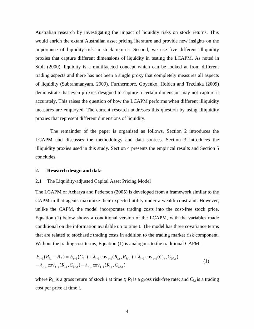
The LCAPM of Acharya and Pederson (2005) is developed from a framework similar to the

CAPM in that agents maximize their expected utility under a wealth constraint. However,

unlike the CAPM, the model incorporates trading costs into the cost-free stock price.

Equation (1) below shows a conditional version of the LCAPM, with the variables made

conditional on the information available up to time t. The model has three covariance terms

that are related to stochastic trading costs in addition to the trading market risk component.

Without the trading cost terms, Equation (1) is analogous to the traditional CAPM.

),(cov),(cov

),(cov),(cov)()(

,,11,,11

,,11,,11,1,1

tMtitttMtitt

tMtitttMtitttitftit

CRCR

CCRRCERRE

(1)

where Ri,t is a gross return of stock i at time t; Rf is a gross risk-free rate; and Ci,t is a trading

cost per price at time t.

5

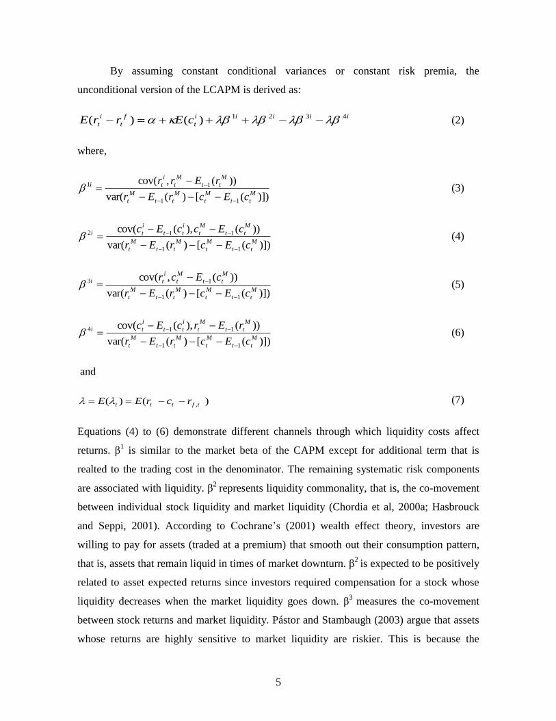
By assuming constant conditional variances or constant risk premia, the

unconditional version of the LCAPM is derived as:

iiiii

t

f

t

i

t cErrE 4321)()( (2)

where,

)])([)(var(

))(,cov(

11

11

M

tt

M

t

M

tt

M

t

M

tt

M

t

i

ti

cEcrEr

rErr

(3)

)])([)(var(

))(),(cov(

11

112

M

tt

M

t

M

tt

M

t

M

tt

M

t

i

tt

i

ti

cEcrEr

cEccEc

(4)

)])([)(var(

))(,cov(

11

13

M

tt

M

t

M

tt

M

t

M

tt

M

t

i

ti

cEcrEr

cEcr

(5)

)])([)(var(

))(),(cov(

11

114

M

tt

M

t

M

tt

M

t

M

tt

M

t

i

tt

i

ti

cEcrEr

rErcEc

(6)

and

)()( ,tfttt rcrEE (7)

Equations (4) to (6) demonstrate different channels through which liquidity costs affect

returns. β1 is similar to the market beta of the CAPM except for additional term that is

realted to the trading cost in the denominator. The remaining systematic risk components

are associated with liquidity. β2

represents liquidity commonality, that is, the co-movement

between individual stock liquidity and market liquidity (Chordia et al, 2000a; Hasbrouck

and Seppi, 2001). According to Cochrane’s (2001) wealth effect theory, investors are

willing to pay for assets (traded at a premium) that smooth out their consumption pattern,

that is, assets that remain liquid in times of market downturn. β2

is expected to be positively

related to asset expected returns since investors required compensation for a stock whose

liquidity decreases when the market liquidity goes down. β3

measures the co-movement

between stock returns and market liquidity. Pástor and Stambaugh (2003) argue that assets

whose returns are highly sensitive to market liquidity are riskier. This is because the

6

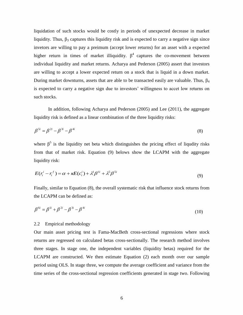
liquidation of such stocks would be costly in periods of unexpected decrease in market

liquidity. Thus, β3 captures this liquidity risk and is expected to carry a negative sign since

invetors are willing to pay a preimum (accept lower returns) for an asset with a expected

higher return in times of market illiquidity. β4

captures the co-movement between

individual liquidity and market returns. Acharya and Pederson (2005) assert that investors

are willing to accept a lower expected return on a stock that is liquid in a down market.

During market downturns, assets that are able to be transacted easily are valuable. Thus, β4

is expected to carry a negative sign due to investors’ willingness to accet low returns on

such stocks.

In addition, following Acharya and Pederson (2005) and Lee (2011), the aggregate

liquidity risk is defined as a linear combination of the three liquidity risks:

iiii 4325 (8)

where β5 is the liquidity net beta which distinguishes the pricing effect of liqudity risks

from that of market risk. Equation (9) belows show the LCAPM with the aggregate

liquidity risk:

iii

t

f

t

i

t cErrE 5511)()( (9)

Finally, similar to Equation (8), the overall systematic risk that influence stock returns from

the LCAPM can be defined as:

iiiii 43216 (10)

2.2 Empirical methodology

Our main asset pricing test is Fama-MacBeth cross-sectional regressions where stock

returns are regressed on calculated betas cross-sectionally. The research method involves

three stages. In stage one, the independent variables (liquidity betas) required for the

LCAPM are constructed. We then estimate Equation (2) each month over our sample

period using OLS. In stage three, we compute the average coefficient and variance from the

time series of the cross-sectional regression coefficients generated in stage two. Following

7

Fama-MacBeth (1973), we apply equal weight on all slope coefficients in estimating the

average coefficient.

In estimating liquidity betas for individual stocks, we follow the literature and

assign betas which are estimated at the portfolio level to individual stocks based on firm

size. This method reduces the noise which could be present when the betas are estimated at

the individual stock level (Fama and French, 1992) and is also in line with Acharya and

Pederson (2005) and Lee (2011). At the end of each year t, all available stocks are first

ranked based on their year-end market capitalization and then allocated into ten portfolios.3

Monthly equally-weighted returns on the ten portfolios are calculated from January to

December of year t+1.4 We also calculate aggregate illiquidity for the portfolios based on

different illiquidity measures. Since illiquidity has long memories5, we work with the

innovation in illiquidity rather than with the level of illiquidity in generating liquidity betas

in the LCAPM. This process is also to remove the “time effect” (Petersen, 2008) in our

empirical analysis. Following Pástor and Stambaugh (2003), Acharya and Pedersen (2005)

and Lee (2010), we transform each illiquidity measure through an autoregressive process,

as depicted in Equation (11)6:

3 Gharghori, Lee and Veeraraghavan (2009) point out the difficulty of Australian research in following U.S.

studies to form 25 portfolios. Since the Australian market is comprised of much fewer stocks, the

conventional 25 sorting would lead to the number of stocks per portfolio being too small. This would increase

variation in portfolio returns and reduce the accuracy of the results. 4 We have also run our analyses based on value-weighted portfolio returns. The results show that, in most

cases, the impact of liquidity risks on returns is weaker compared to the equally-weighted approach. Given

that the Australian market is characterized with a large number of small stocks, the finding suggests that

liquidity risk is playing a more crucial role for smaller stocks. This is consistent with the findings in Acharya

and Pedersen (2005). 5 Our unreported results show high autocorrelations in our equally-weighted market (portfolio) illiquidity.

Three illiquidity measures (out of five) exhibit significant (at the 1% level) first order autocorrelations.

Similar findings are also reported in Acharya and Pedersen (2005) and Lee (2011). 6 We run Equation (17) for each of our illiquidity measures. The number of lags is determined based on the

test of autocorrelation. We use both AR(2) and AR(3) to obtained innovations in illiquidity depending on the

lags.

8

i

t

i

xtx

i

t

i

t

i

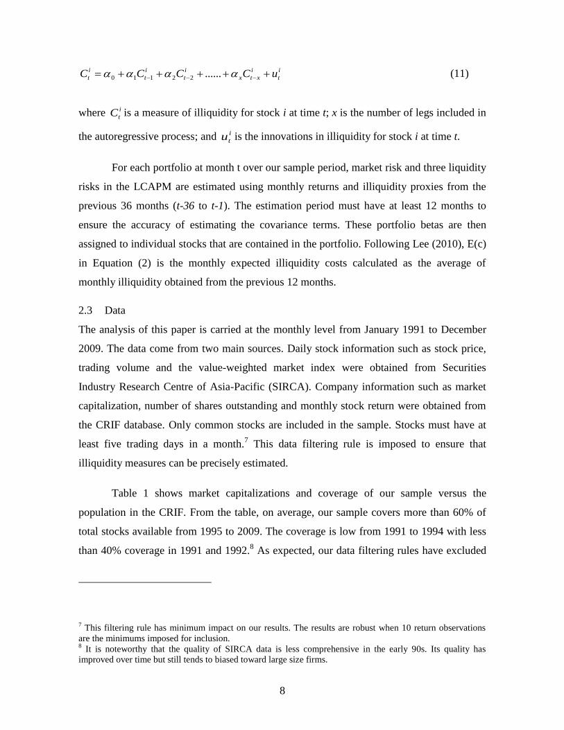
t uCCCC ......22110 (11)

where i

tC is a measure of illiquidity for stock i at time t; x is the number of legs included in

the autoregressive process; and i

tu is the innovations in illiquidity for stock i at time t.

For each portfolio at month t over our sample period, market risk and three liquidity

risks in the LCAPM are estimated using monthly returns and illiquidity proxies from the

previous 36 months (t-36 to t-1). The estimation period must have at least 12 months to

ensure the accuracy of estimating the covariance terms. These portfolio betas are then

assigned to individual stocks that are contained in the portfolio. Following Lee (2010), E(c)

in Equation (2) is the monthly expected illiquidity costs calculated as the average of

monthly illiquidity obtained from the previous 12 months.

2.3 Data

The analysis of this paper is carried at the monthly level from January 1991 to December

2009. The data come from two main sources. Daily stock information such as stock price,

trading volume and the value-weighted market index were obtained from Securities

Industry Research Centre of Asia-Pacific (SIRCA). Company information such as market

capitalization, number of shares outstanding and monthly stock return were obtained from

the CRIF database. Only common stocks are included in the sample. Stocks must have at

least five trading days in a month.7 This data filtering rule is imposed to ensure that

illiquidity measures can be precisely estimated.

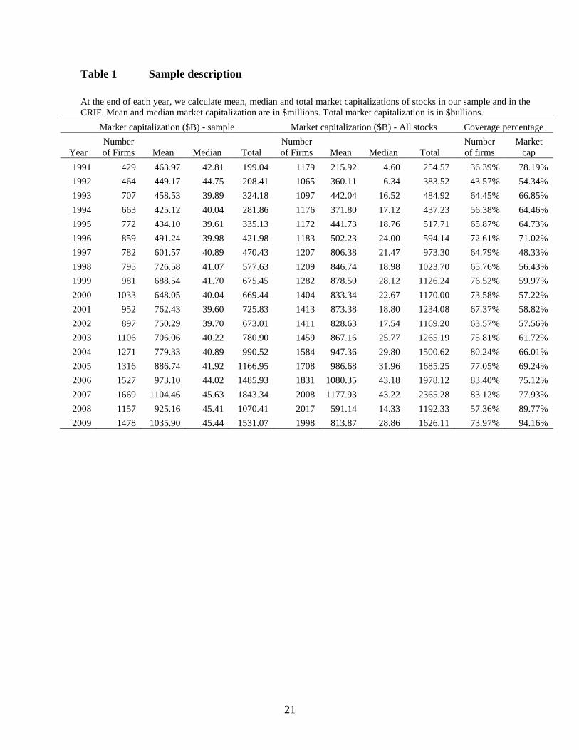
Table 1 shows market capitalizations and coverage of our sample versus the

population in the CRIF. From the table, on average, our sample covers more than 60% of

total stocks available from 1995 to 2009. The coverage is low from 1991 to 1994 with less

than 40% coverage in 1991 and 1992.8 As expected, our data filtering rules have excluded

7 This filtering rule has minimum impact on our results. The results are robust when 10 return observations

are the minimums imposed for inclusion. 8 It is noteworthy that the quality of SIRCA data is less comprehensive in the early 90s. Its quality has

improved over time but still tends to biased toward large size firms.

9

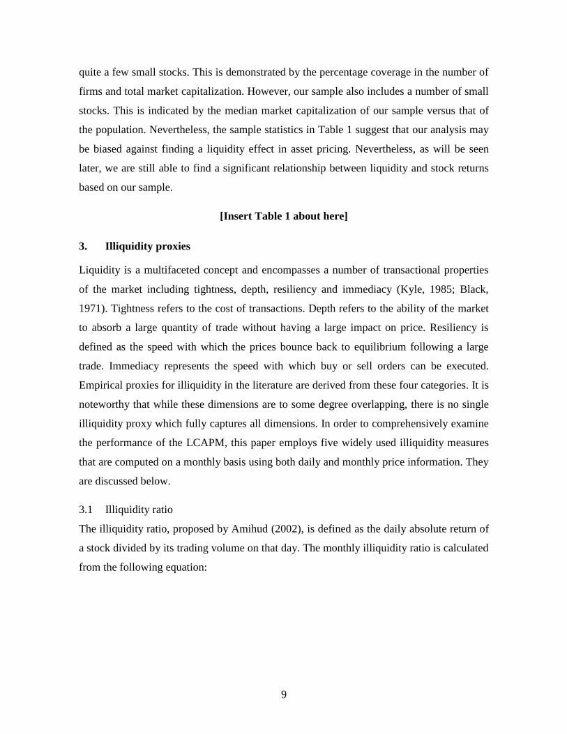
quite a few small stocks. This is demonstrated by the percentage coverage in the number of

firms and total market capitalization. However, our sample also includes a number of small

stocks. This is indicated by the median market capitalization of our sample versus that of

the population. Nevertheless, the sample statistics in Table 1 suggest that our analysis may

be biased against finding a liquidity effect in asset pricing. Nevertheless, as will be seen

later, we are still able to find a significant relationship between liquidity and stock returns

based on our sample.

[Insert Table 1 about here]

3. Illiquidity proxies

Liquidity is a multifaceted concept and encompasses a number of transactional properties

of the market including tightness, depth, resiliency and immediacy (Kyle, 1985; Black,

1971). Tightness refers to the cost of transactions. Depth refers to the ability of the market

to absorb a large quantity of trade without having a large impact on price. Resiliency is

defined as the speed with which the prices bounce back to equilibrium following a large

trade. Immediacy represents the speed with which buy or sell orders can be executed.

Empirical proxies for illiquidity in the literature are derived from these four categories. It is

noteworthy that while these dimensions are to some degree overlapping, there is no single

illiquidity proxy which fully captures all dimensions. In order to comprehensively examine

the performance of the LCAPM, this paper employs five widely used illiquidity measures

that are computed on a monthly basis using both daily and monthly price information. They

are discussed below.

3.1 Illiquidity ratio

The illiquidity ratio, proposed by Amihud (2002), is defined as the daily absolute return of

a stock divided by its trading volume on that day. The monthly illiquidity ratio is calculated

from the following equation:

10

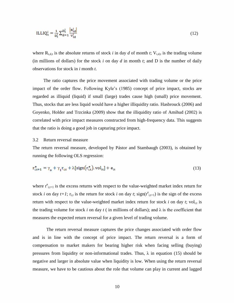
(12)

where Ri,d,t is the absolute returns of stock i in day d of month t; Vi,d,t is the trading volume

(in millions of dollars) for the stock i on day d in month t; and D is the number of daily

observations for stock in i month t.

The ratio captures the price movement associated with trading volume or the price

impact of the order flow. Following Kyle’s (1985) concept of price impact, stocks are

regarded as illiquid (liquid) if small (large) trades cause high (small) price movement.

Thus, stocks that are less liquid would have a higher illiquidity ratio. Hasbrouck (2006) and

Goyenko, Holder and Trzcinka (2009) show that the illiquidity ratio of Amihud (2002) is

correlated with price impact measures constructed from high-frequency data. This suggests

that the ratio is doing a good job in capturing price impact.

3.2 Return reversal measure

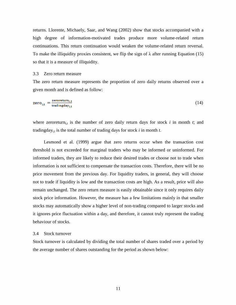
The return reversal measure, developed by Pástor and Stambaugh (2003), is obtained by

running the following OLS regression:

(13)

where rei,t+1 is the excess returns with respect to the value-weighted market index return for

stock i on day t+1; ri,t is the return for stock i on day t; sign(rei,t+1) is the sign of the excess

return with respect to the value-weighted market index return for stock i on day t; voli,t is

the trading volume for stock i on day t ( in millions of dollars); and λ is the coefficient that

measures the expected return reversal for a given level of trading volume.

The return reversal measure captures the price changes associated with order flow

and is in line with the concept of price impact. The return reversal is a form of

compensation to market makers for bearing higher risk when facing selling (buying)

pressures from liquidity or non-informational trades. Thus, λ in equation (15) should be

negative and larger in absolute value when liquidity is low. When using the return reversal

measure, we have to be cautious about the role that volume can play in current and lagged

11

returns. Llorente, Michaely, Saar, and Wang (2002) show that stocks accompanied with a

high degree of information-motivated trades produce more volume-related return

continuations. This return continuation would weaken the volume-related return reversal.

To make the illiquidity proxies consistent, we flip the sign of λ after running Equation (15)

so that it is a measure of illiquidity.

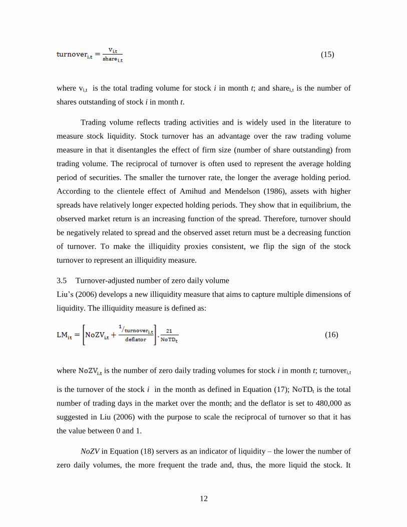
3.3 Zero return measure

The zero return measure represents the proportion of zero daily returns observed over a

given month and is defined as follow:

(14)

where zeroreturni,t is the number of zero daily return days for stock i in month t; and

tradingdayi,t is the total number of trading days for stock i in month t.

Lesmond et al. (1999) argue that zero returns occur when the transaction cost

threshold is not exceeded for marginal traders who may be informed or uninformed. For

informed traders, they are likely to reduce their desired trades or choose not to trade when

information is not sufficient to compensate the transaction costs. Therefore, there will be no

price movement from the previous day. For liquidity traders, in general, they will choose

not to trade if liquidity is low and the transaction costs are high. As a result, price will also

remain unchanged. The zero return measure is easily obtainable since it only requires daily

stock price information. However, the measure has a few limitations mainly in that smaller

stocks may automatically show a higher level of non-trading compared to larger stocks and

it ignores price fluctuation within a day, and therefore, it cannot truly represent the trading

behaviour of stocks.

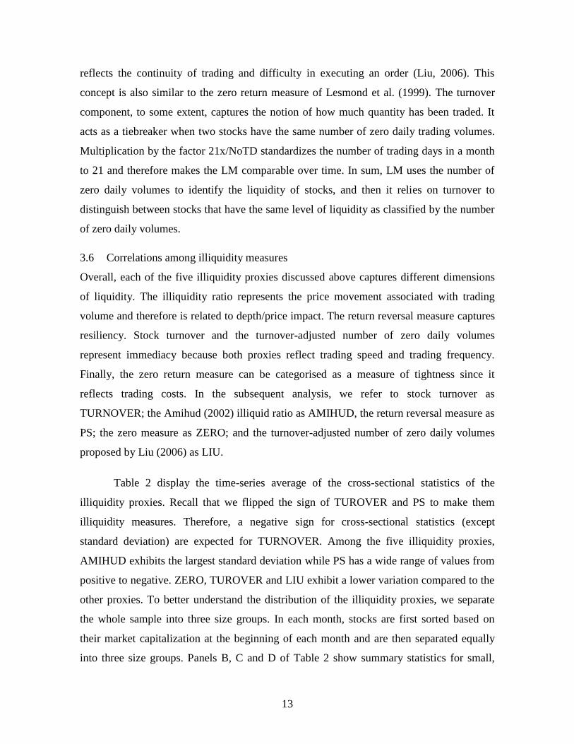
3.4 Stock turnover

Stock turnover is calculated by dividing the total number of shares traded over a period by

the average number of shares outstanding for the period as shown below:

12

(15)

where vi,t is the total trading volume for stock i in month t; and sharei,t is the number of

shares outstanding of stock i in month t.

Trading volume reflects trading activities and is widely used in the literature to

measure stock liquidity. Stock turnover has an advantage over the raw trading volume

measure in that it disentangles the effect of firm size (number of share outstanding) from

trading volume. The reciprocal of turnover is often used to represent the average holding

period of securities. The smaller the turnover rate, the longer the average holding period.

According to the clientele effect of Amihud and Mendelson (1986), assets with higher

spreads have relatively longer expected holding periods. They show that in equilibrium, the

observed market return is an increasing function of the spread. Therefore, turnover should

be negatively related to spread and the observed asset return must be a decreasing function

of turnover. To make the illiquidity proxies consistent, we flip the sign of the stock

turnover to represent an illiquidity measure.

3.5 Turnover-adjusted number of zero daily volume

Liu’s (2006) develops a new illiquidity measure that aims to capture multiple dimensions of

liquidity. The illiquidity measure is defined as:

(16)

where is the number of zero daily trading volumes for stock i in month t; turnoveri,t

is the turnover of the stock i in the month as defined in Equation (17); NoTDt is the total

number of trading days in the market over the month; and the deflator is set to 480,000 as

suggested in Liu (2006) with the purpose to scale the reciprocal of turnover so that it has

the value between 0 and 1.

NoZV in Equation (18) servers as an indicator of liquidity – the lower the number of

zero daily volumes, the more frequent the trade and, thus, the more liquid the stock. It

13

reflects the continuity of trading and difficulty in executing an order (Liu, 2006). This

concept is also similar to the zero return measure of Lesmond et al. (1999). The turnover

component, to some extent, captures the notion of how much quantity has been traded. It

acts as a tiebreaker when two stocks have the same number of zero daily trading volumes.

Multiplication by the factor 21x/NoTD standardizes the number of trading days in a month

to 21 and therefore makes the LM comparable over time. In sum, LM uses the number of

zero daily volumes to identify the liquidity of stocks, and then it relies on turnover to

distinguish between stocks that have the same level of liquidity as classified by the number

of zero daily volumes.

3.6 Correlations among illiquidity measures

Overall, each of the five illiquidity proxies discussed above captures different dimensions

of liquidity. The illiquidity ratio represents the price movement associated with trading

volume and therefore is related to depth/price impact. The return reversal measure captures

resiliency. Stock turnover and the turnover-adjusted number of zero daily volumes

represent immediacy because both proxies reflect trading speed and trading frequency.

Finally, the zero return measure can be categorised as a measure of tightness since it

reflects trading costs. In the subsequent analysis, we refer to stock turnover as

TURNOVER; the Amihud (2002) illiquid ratio as AMIHUD, the return reversal measure as

PS; the zero measure as ZERO; and the turnover-adjusted number of zero daily volumes

proposed by Liu (2006) as LIU.

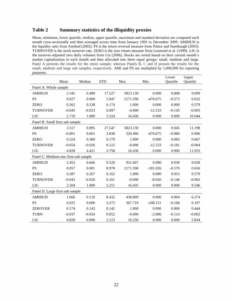
Table 2 display the time-series average of the cross-sectional statistics of the

illiquidity proxies. Recall that we flipped the sign of TUROVER and PS to make them

illiquidity measures. Therefore, a negative sign for cross-sectional statistics (except

standard deviation) are expected for TURNOVER. Among the five illiquidity proxies,

AMIHUD exhibits the largest standard deviation while PS has a wide range of values from

positive to negative. ZERO, TUROVER and LIU exhibit a lower variation compared to the

other proxies. To better understand the distribution of the illiquidity proxies, we separate

the whole sample into three size groups. In each month, stocks are first sorted based on

their market capitalization at the beginning of each month and are then separated equally

into three size groups. Panels B, C and D of Table 2 show summary statistics for small,

14

medium and large size firms, respectively. The mean value of AMIHUD, ZERO and LIU

decreases from small to large firms, which indicates that small firms are less liquid

compared to medium-size and large firms. This pattern is as expected since firm size is

related to illiquidity to certain degree. However, TURNOVER and PS exhibits a somewhat

different pattern. The mean value of TUROVER increases from small to large firms while

the median value is lowest in medium-size firms. The mean value of PS is also highest in

medium-size firms. This suggests that small and large firms may be traded more actively

(based on trading volume) than medium-size firms. The results may also be influenced by

the fact that small firms generally have a lower total number of shares outstanding and

hence, higher turnover rates are observed among small firms. Our findings are similar to

prior Australian studies such as Chai, Faff and Gharghori (2010) and Chan and Faff (2003).

Chan and Faff (2003) find that size is not correlated with stock turnover. Chai et al. (2010)

find that both stock turnover and the return reversal measure behave differently in relation

to trading characteristics compared to other liquidity proxies.

[Insert Table 2 about here]

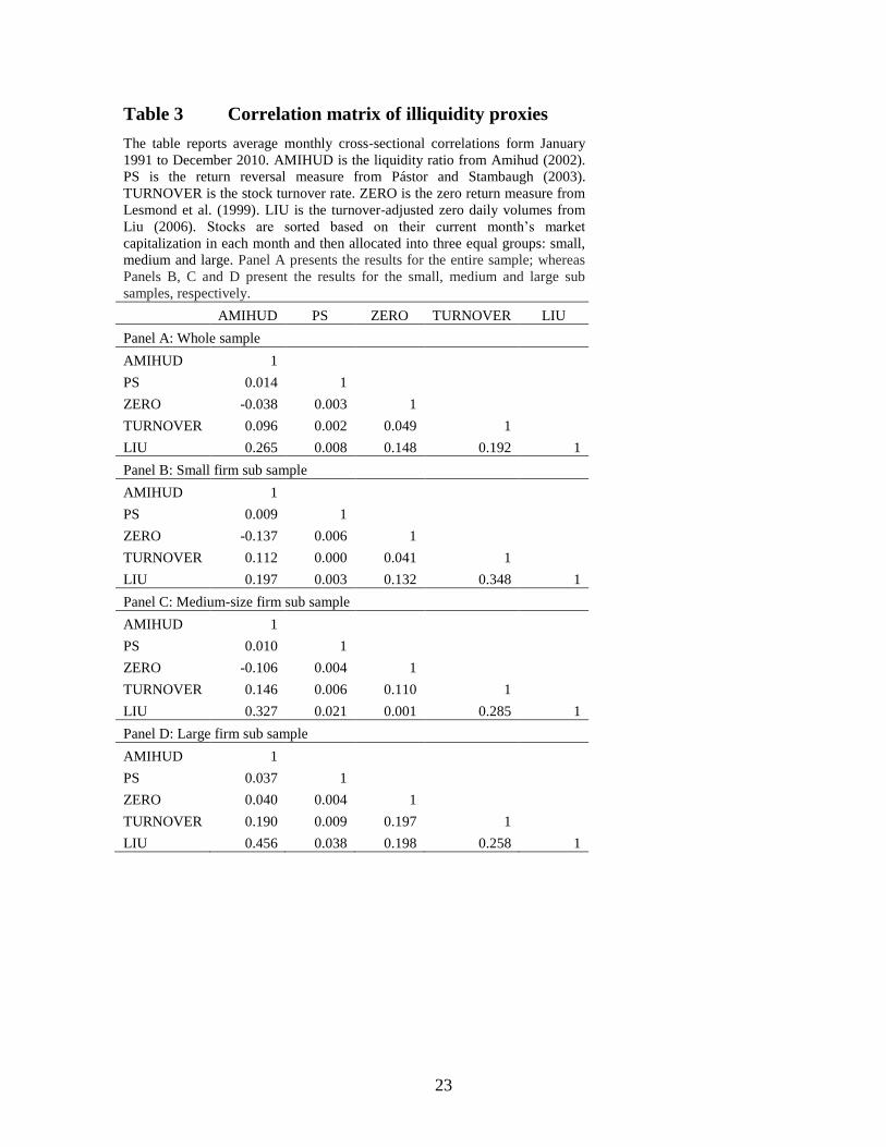
Table 3 reports the average monthly cross-sectional correlations between the

illiquidity proxies over our sample period. We also divide our sample into the three size

groups discussed above in order to understand the relationships among illiquidity proxies in

detail. Panel A displays the correlations for the full sample. The results show that the

correlations between illiquidity proxies are low in the cross-section expect for AMIHUD

with LIU. There are also weak correlations between LIU and ZERO, and LIU and

TURNOVER. Looking at correlations in the size groups (Panels B, C and D), the results

are generally consistent with the results in Panel A. Comparing across the size groups, the

correlations are stronger among illiquidity proxies for large firms. LIU exhibits stronger

correlations with AMIHUD, ZERO and TURNOVER; while TURNOVER is weakly

correlated with AMIHUD and ZERO. Overall, the results in Table 3 suggest that illiquidity

proxies which capture different trading aspects do not necessarily exhibit strong

correlations (Stoll, 2000). Furthermore, LIU tends to have better correlations with all the

other proxies. This finding is consistent with the intuition that LIU captures multiple

dimensions of liquidity.

15

[Insert Table 3 about here]

4. Empirical Results

4.1 Portfolio betas

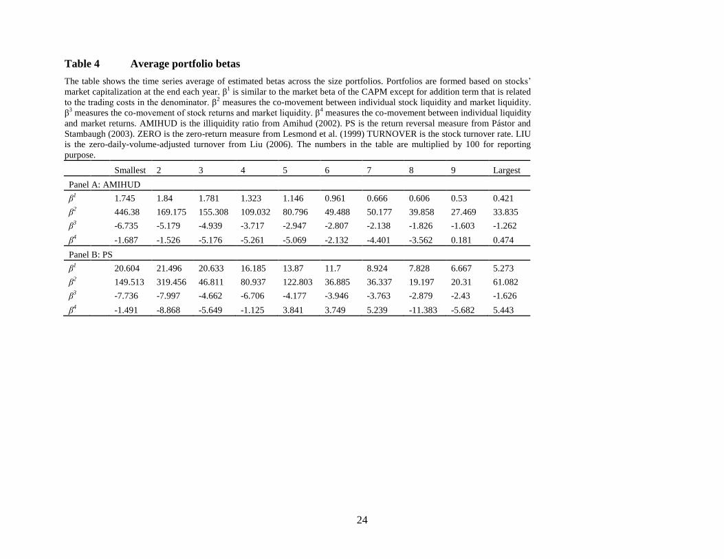
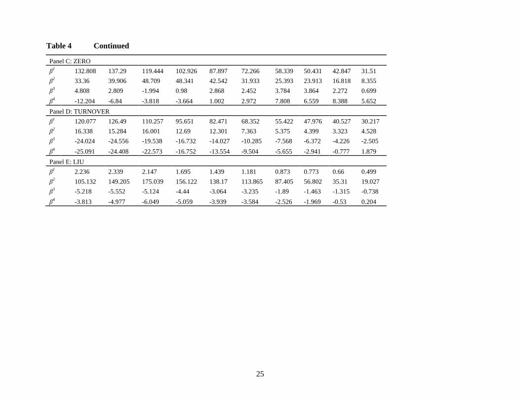
Table 4 demonstrates the time series average of estimated liquidity betas for each of the ten

size portfolios. In the framework of the LCAPM, illiquid stocks should have higher

liquidity risk. Thus, small size portfolios should have large values of β1

and β

2 and large

negative values of β3 and β

4. In Table 4, we see that the absolute values of β

1, β

2 and

β3decrase from small to large size portfolios and this inverse relationship is rather

monotonic across all our illiquidity measures. This indicates that illiquid stocks have higher

co-movement with the market illiquidity and higher return sensitivity to market illiquidity.

However, no monotonic relation is shown for β4. This is particularly the case for AMIHUD,

PS and ZERO. The results in Table 4 also suggest that β1, β

2 and β

3 are related to firm size.

In the subsequent section, we formally test the relationship between stock returns and

liquidity risks by using running cross-sectional regressions.

[Insert Table 4 about here]

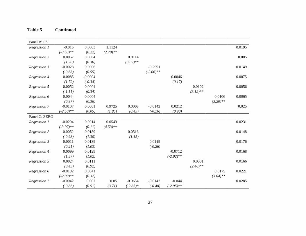
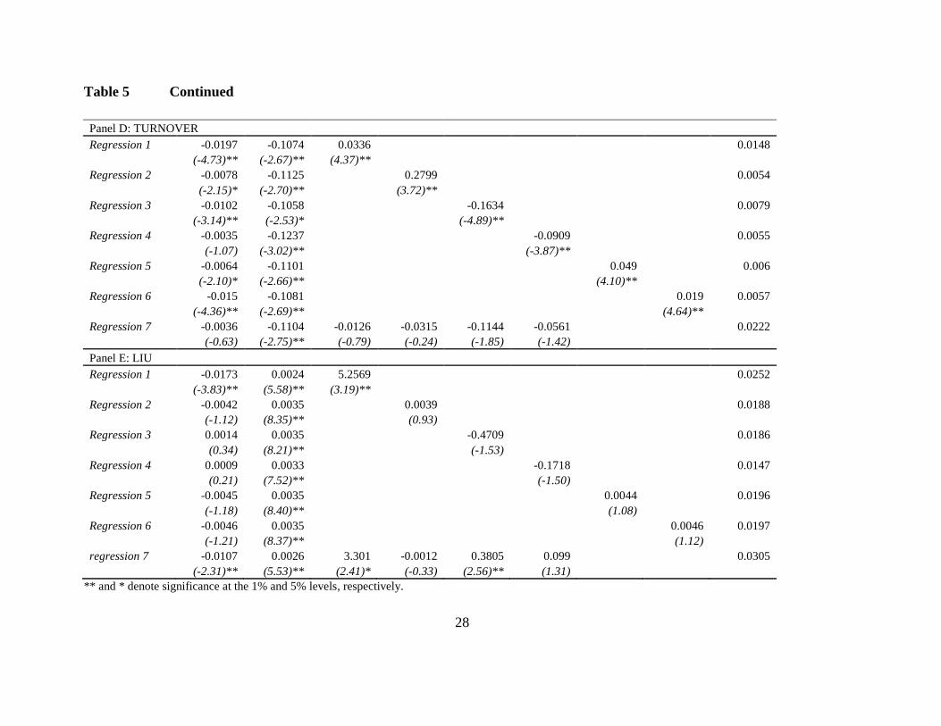
4.1 Stock returns and liquidity risk

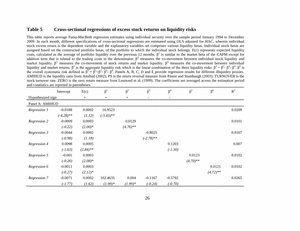
Table 5 displays the LCAPM results. In each month, we run cross-sectional regressions of

stocks returns on estimated liquidity betas. However, the correlations between the LCAPM

betas are high, indicating that our results are potentially subject to the multicollinearity

problem.9 This issue is also acknowledged in Acharya and Pedersen (2005) and Lee (2011).

Following Lee (2011), we run different regression specifications including univariate

regressions where stock returns are regressed on each individual liquidity beta (β1, β

2, β3

and β4) in order to alleviate the concern of multicollinearity. Moreover, we also use the net

beta to represent the combined liquidity risk (β5 and β

6) in the regressions.

9 For example, the correlations between β1 and β2 and between β1 and β3 for AMIHUD are, on average, 0.577

and 0.841 respectively. Tests for the Variance Inflation Factors (VIF) for these four betas are above 5 in

several regressions, suggesting that multicollinearity is a potential problem in the analysis. These results are

not reported but are available on request from the authors.

16

In the LCAPM framework, β1

and β

2 are expected to carry a positive sign and β

3 and

β4 are expected to carry a negative sign. We are also interested in the performance of net

liquidity betas (β5 and β

6) in explaining stock returns. The regression results for AMIHUD

(Panel A) and PS (Panel B) are similar, all betas are statistically significant (except β4) and

the sign of the coefficients are consistent with the expectations. The net betas, β5 and β

6, are

also statistically significant at the 1% level. This implies liquidity risk plays an important

role in explaining stock returns. However, the liquidity level E(c) is not related to stock

returns for PS.

Panel C displays results for ZERO. The sign of the liquidity betas are consistent

with the expectations; however, only β1 and β

4 are significant. The net liquidity betas, β

5

and β6

, are significantly related with stock returns. Similar to the results for PS, the liquidity

level E(c) shows no relationship with stock returns. The regression results for TURNOVER

(Panel D) and LIU (Panel E) exhibit somewhat interesting patterns. Compared to the results

for the other illiquidity proxies, the impact of liquidity risks on returns is strongest for

TURNOVER. All LCAPM betas are significant at the 1% level and have theoretically

correct signs for TURNOVER. However, the liquidity cost E(c) is significantly negatively

related with stocks returns, which contradicts to the expectations of the negative

relationship between return and illiquidity. This may be due to the relationship between

TURNOVER and size as observed in Table 3. In contrast to the other four proxies, none of

the liquidity-related risks (β2

to β6) is significant for LIU, although they all exhibit correct

signs. The explanatory power of liquidity on stock returns is mainly through liquidity level.

The liquidity cost E(c) is significantly positively related with stock returns. Thus, the

results for LIU suggest that liquidity level has a stronger impact on stock returns.

In summary, the regression results across different illiquidity proxies generally

support the LCAPM model. Our results indicate that the commonality beta (β2) is priced in

the Australian market. This finding is consistent with the concept of commonality in

liquidity (Chordia et al, 2000b) and is consistent with prior empirical studies such as

Chordia et al. (2001) and Lee (2010). Liquidity risk, β3, which is derived from the

sensitivity of the return to market liquidity, is also priced. This result also supports the

literature on the co-movement between stock liquidity and market returns (e.g., Pástor and

17

Stambaugh, 2003). However, we find that β4, which arise from the covariance of individual

stock liquidity with market returns, has a weaker impact on stock returns compared to that

of β2

and β3. Our findings are different to those documented in Acharya and Pedersen

(2005). In Acharya and Pedersen (2005), β4 tends to exhibit strongest explanatory power in

explaining returns compared to that of β2

and β3. Regarding the aggregate liquidity risks, we

find strong evidence that the liquidity net beta (β5) and aggregate beta (β6) are priced. This

indicates that the aggregate liquidity risk has a crucial impact on the cross section of

Australian stock returns. In sum, our findings support the LCAPM and the relationship

between stock returns and liquidity risks generally support those documented in the

literature across different illiquidity proxies.

[Insert Table 5 about here]

5. Conclusions

The role of liquidity in asset pricing has been well documented in the empirical finance

literature. The LCAPM proposed by Acharya and Pedersen (2005) is one of the few models

that allows us to explore the impact of various liquidity risks on stock returns. In this study,

we test the LCAPM in the Australian market using five different illiquidity proxies. The

effort is important as we are not only able to address the issue of measuring illiquidity, but

also able to compare the performance of the LCAPM across different illiquidity measures.

We find that the correlations among the employed illiquidity proxies are low in the

cross-section. This implies that they represent different dimensions of liquidity and a

certain type of trading behaviour. Stoll (2000) also notes that different illiquidity measures

need not be correlated for similar reasons. Consistent with the literature, we find that

liquidity risks are priced in the Australian market. Individual liquidity level, however,

exhibits a weaker relationship with stock returns. The performance of the LCAPM also

varies across different illiquidity measures. Among the identified liquidity risks, our results

indicate that the co-movements between individual stock liquidity and market liquidity and

between stock returns and market liquidity play important roles in explaining Australian

stock returns. The co-movement between stock liquidity and market returns also exhibit

18

some explanatory power but its impact is relatively weaker compared to other liquidity

risks.

Notably, we have been silent on the question of which illiquidity proxy performs

better in explaining stock returns. This research issue is beyond the scope of the current

study. Overall, our results support the LCAPM and highlight the importance of liquidity

risk in asset pricing tests.

19

References

Acharya, V. V., & Pedersen, L. H. (2005). Asset pricing with liquidity risk. Journal of

Financial Economics, 77(2), 375-410.

Amihud, Y. (2002). Illiquidity and stock returns: cross-section and time-series effects.

Journal of Financial Markets, 5(1), 31-56.

Amihud, Y., & Mendelson, H. (1986). Liquidity and stock returns. Financial Analysts

Journal, 42(3), 43-48.

Anderson, D., Clarkson, P. M., & Moran, S. A. (1997). The association between

information, liquidity, and two stock market anomalies, the size effect and

seasonalities in equity returns. Accounting Research Journal, 10(1), 6 - 20.

Atkins, A. B., & Dyl, E. A. (1997). Transactions costs and holding periods for common

stocks. Journal of Finance, 52(1), 309-325.

Beedles, W., Dodd, P., & Officer, R. (1988). Regularities in Australian share returns.

Australian Journal of Management, 13(1), 1-29.

Bekaert, G., Harvey, C. R., & Lundblad, C. (2007). Liquidity and expected returns: Lessons

from emerging markets. Review of Financial Studies, 20(6), 1783-1831.

Bhardwaj, R. K., & Brooks, L. D. (1993). Dual betas from bull and bear markets: Reversal

of the size effect. Journal of Financial Research, 16(4), 269.

Chai, D., Faff, R., & Gharghori, P. (2010). New evidence on the relation between stock

liquidity and measures of trading activity. International Review of Financial

Analysis, 19(3), 181-192.

Chan, H. W., & Faff, R. W. (2003). An investigation into the role of liquidity in asset

pricing: Australian evidence. Pacific-Basin Finance Journal, 11(5), 555-572.

Chan, H. W., & Faff, R. W. (2005). Asset pricing and the illiquidity premium. Financial

Review, 40(4), 429-458.

Chordia, T., Roll, R., & Subrahmanyam, A. (2000a). Co-movements in bid-ask spreads and

market depth. Financial Analysts Journal, 56(5), 23.

Chordia, T., Roll, R., & Subrahmanyam, A. (2000b). Commonality in liquidity. Journal of

Financial Economics, 56(1), 3-28.

Chordia, T., Subrahmanyam, A., Anshuman, V. R., Huang, R., Lewis, C., & Mad, A.

(2001). Trading activity and expected stock returns. Journal of Financial

Economics, 59, 3-32.

Cochrane, J. (2001). Asset Pricing. New Jersey: Princeton University Press.

Eleswarapu, V. R., & Reinganum, M. R. (1993). The seasonal behavior of the liquidity

premium in asset pricing. Journal of Financial Economics, 34(3), 373-386.

Fama, E. F., & MacBeth, J. (1973). Risk, return, and equilibrium: Empirical tests. Journal

of Political Economy, 81, 607-636.

Gharghori, P., Lee, R., & Veeraraghavan, M. (2009). Anomalies and stock returns:

Australian evidence. Accounting & Finance, 49(3), 555-576.

Goyenko, R. Y., Holden, C. W., & Trzcinka, C. A. (2009). Do liquidity measures measure

liquidity? Journal of Financial Economics, 92(2), 153-181.

Keene, M. A. (2004). A time-series approach to liquidity in asset pricing. The Florida State

University Florida.

Kyle, A. S. (1985). Continuous auctions and insider trading. Econometrica, 53(6), 1315-

1335.

20

Lee, K. H. (2011). The world price of liquidity risk. Journal of Financial Economics, 99(1),

136-161.

Lesmond, D. A. (2005). Liquidity of emerging markets. Journal of Financial Economics,

77(2), 411-452.

Lesmond, D. A., Ogden, J. P., & Trzcinka, C. A. (1999). A new estimate of transaction

costs. Review of Financial Studies, 12(5), 1113-1141.

Limkriangkrai, M., Durand, R. B., & Watson, I. (2008). Is liquidity the missing link?

Accounting and Finance 48, 829–845.

Liu, W. (2006). A liquidity-augmented capital asset pricing model. Journal of Financial

Economics, 82(3), 631-671.

Marshall, B. R. (2006). Liquidity and stock returns: Evidence from a pure order-driven

market using a new liquidity proxy. International Review of Financial Analysis,

15(1), 21-38.

Marshall, B. R., & Young, M. (2003). Liquidity and stock returns in pure order-driven

markets: evidence from the Australian stock market. International Review of

Financial Analysis, 12(2), 173-188.

Pástor, L. u., & Stambaugh, R. F. (2003). Liquidity risk and expected stock retums. Journal

of Political Economy, 111(3), 642-685.

Petersen, M. A. (2009). Estimating Standard Errors in Finance Panel Data Sets: Comparing

Approaches. Review of Financial Studies, 22(1), 435-480.

Stoll, H. R. (2000). Friction. Journal of Finance, 55(4), 1479-1514.

Subrahmanyam, A. (2009). The implications of liquidity and order flows for neoclassical

finance. Pacific-Basin Finance Journal, 17(5), 527-532.

21

Table 1 Sample description

At the end of each year, we calculate mean, median and total market capitalizations of stocks in our sample and in the

CRIF. Mean and median market capitalization are in $millions. Total market capitalization is in $bullions.

Market capitalization ($B) - sample Market capitalization ($B) - All stocks Coverage percentage

Year

Number

of Firms Mean Median Total

Number

of Firms Mean Median Total

Number

of firms

Market

cap

1991 429 463.97 42.81 199.04 1179 215.92 4.60 254.57 36.39% 78.19%

1992 464 449.17 44.75 208.41 1065 360.11 6.34 383.52 43.57% 54.34%

1993 707 458.53 39.89 324.18 1097 442.04 16.52 484.92 64.45% 66.85%

1994 663 425.12 40.04 281.86 1176 371.80 17.12 437.23 56.38% 64.46%

1995 772 434.10 39.61 335.13 1172 441.73 18.76 517.71 65.87% 64.73%

1996 859 491.24 39.98 421.98 1183 502.23 24.00 594.14 72.61% 71.02%

1997 782 601.57 40.89 470.43 1207 806.38 21.47 973.30 64.79% 48.33%

1998 795 726.58 41.07 577.63 1209 846.74 18.98 1023.70 65.76% 56.43%

1999 981 688.54 41.70 675.45 1282 878.50 28.12 1126.24 76.52% 59.97%

2000 1033 648.05 40.04 669.44 1404 833.34 22.67 1170.00 73.58% 57.22%

2001 952 762.43 39.60 725.83 1413 873.38 18.80 1234.08 67.37% 58.82%

2002 897 750.29 39.70 673.01 1411 828.63 17.54 1169.20 63.57% 57.56%

2003 1106 706.06 40.22 780.90 1459 867.16 25.77 1265.19 75.81% 61.72%

2004 1271 779.33 40.89 990.52 1584 947.36 29.80 1500.62 80.24% 66.01%

2005 1316 886.74 41.92 1166.95 1708 986.68 31.96 1685.25 77.05% 69.24%

2006 1527 973.10 44.02 1485.93 1831 1080.35 43.18 1978.12 83.40% 75.12%

2007 1669 1104.46 45.63 1843.34 2008 1177.93 43.22 2365.28 83.12% 77.93%

2008 1157 925.16 45.41 1070.41 2017 591.14 14.33 1192.33 57.36% 89.77%

2009 1478 1035.90 45.44 1531.07 1998 813.87 28.86 1626.11 73.97% 94.16%

22

Table 2 Summary statistics of the illiquidity proxies

Mean, minimum, lower quartile, median, upper quartile, maximum and standard deviation are computed each

month cross-sectionally and then averaged across time from January 1991 to December 2009. AMIHUD is

the liquidity ratio from Amihud (2002). PS is the return reversal measure from Pástor and Stambaugh (2003).

TURNOVER is the stock turnover rate. ZERO is the zero return measure from Lesmond et al. (1999). LIU is

the turnover-adjusted zero daily volumes from Liu (2006). Stocks are sorted based on their current month’s

market capitalization in each month and then allocated into three equal groups: small, medium and large.

Panel A presents the results for the entire sample; whereas Panels B, C and D present the results for the

small, medium and large sub samples, respectively. AMI and PS are multiplied by 1,000,000 for reporting

purposes.

Mean Median STD Max Min

Lower

Quartile

Upper

Quartile

Panel A: Whole sample

AMIHUD 2.545 0.489 17.527 5823.130 0.000 0.008 9.099

PS 0.027 0.000 5.947 2171.590 -470.675 -0.573 0.632

ZERO 0.262 0.238 0.174 1.000 0.000 0.000 0.579

TURNOVER -0.045 -0.023 0.097 -0.000 -12.533 -0.145 -0.003

LIU 2.719 1.000 3.524 16.436 0.000 0.000 10.044

Panel B: Small firm sub sample

AMIHUD 3.517 0.895 27.547 5823.130 0.000 0.045 11.198

PS -0.001 0.001 3.838 520.490 -470.675 -0.980 0.996

ZERO 0.324 0.300 0.179 1.000 0.000 0.083 0.667

TURNOVER -0.054 -0.026 0.122 -0.000 -12.533 -0.181 -0.004

LIU 4.828 4.421 3.758 16.436 0.000 0.000 11.053

Panel C: Medium-size firm sub sample

AMIHUD 2.452 0.666 9.520 931.847 0.000 0.030 9.028

PS 0.057 0.001 8.978 2171.590 -181.026 -0.570 0.656

ZERO 0.287 0.267 0.162 1.000 0.000 0.053 0.579

TURNOVER -0.043 -0.020 0.101 -0.000 -8.020 -0.146 -0.002

LIU 2.504 1.000 3.251 16.435 0.000 0.000 9.546

Panel D: Large firm sub sample

AMIHUD 1.666 0.110 8.432 438.809 0.000 0.004 6.274

PS 0.025 0.000 3.272 367.719 -248.151 -0.168 0.197

ZEROVER 0.174 0.143 0.142 1.000 0.000 0.000 0.444

TURN -0.037 -0.024 0.052 -0.000 -2.086 -0.114 -0.002

LIU 0.828 0.000 2.123 16.256 0.000 0.000 5.834

23

Table 3 Correlation matrix of illiquidity proxies

The table reports average monthly cross-sectional correlations form January

1991 to December 2010. AMIHUD is the liquidity ratio from Amihud (2002).

PS is the return reversal measure from Pástor and Stambaugh (2003).

TURNOVER is the stock turnover rate. ZERO is the zero return measure from

Lesmond et al. (1999). LIU is the turnover-adjusted zero daily volumes from

Liu (2006). Stocks are sorted based on their current month’s market

capitalization in each month and then allocated into three equal groups: small,

medium and large. Panel A presents the results for the entire sample; whereas

Panels B, C and D present the results for the small, medium and large sub

samples, respectively.

AMIHUD PS ZERO TURNOVER LIU

Panel A: Whole sample

AMIHUD 1

PS 0.014 1

ZERO -0.038 0.003 1

TURNOVER 0.096 0.002 0.049 1

LIU 0.265 0.008 0.148 0.192 1

Panel B: Small firm sub sample

AMIHUD 1

PS 0.009 1

ZERO -0.137 0.006 1

TURNOVER 0.112 0.000 0.041 1

LIU 0.197 0.003 0.132 0.348 1

Panel C: Medium-size firm sub sample

AMIHUD 1

PS 0.010 1

ZERO -0.106 0.004 1

TURNOVER 0.146 0.006 0.110 1

LIU 0.327 0.021 0.001 0.285 1

Panel D: Large firm sub sample

AMIHUD 1

PS 0.037 1

ZERO 0.040 0.004 1

TURNOVER 0.190 0.009 0.197 1

LIU 0.456 0.038 0.198 0.258 1

(11)

24

Table 4 Average portfolio betas

The table shows the time series average of estimated betas across the size portfolios. Portfolios are formed based on stocks’

market capitalization at the end each year. β1 is similar to the market beta of the CAPM except for addition term that is related

to the trading costs in the denominator. β2 measures the co-movement between individual stock liquidity and market liquidity.

β3 measures the co-movement of stock returns and market liquidity. β

4 measures the co-movement between individual liquidity

and market returns. AMIHUD is the illiquidity ratio from Amihud (2002). PS is the return reversal measure from Pástor and

Stambaugh (2003). ZERO is the zero-return measure from Lesmond et al. (1999) TURNOVER is the stock turnover rate. LIU

is the zero-daily-volume-adjusted turnover from Liu (2006). The numbers in the table are multiplied by 100 for reporting

purpose.

Smallest 2 3 4 5 6 7 8 9 Largest

Panel A: AMIHUD

β1

1.745 1.84 1.781 1.323 1.146 0.961 0.666 0.606 0.53 0.421

β2

446.38 169.175 155.308 109.032 80.796 49.488 50.177 39.858 27.469 33.835

β3

-6.735 -5.179 -4.939 -3.717 -2.947 -2.807 -2.138 -1.826 -1.603 -1.262

β4

-1.687 -1.526 -5.176 -5.261 -5.069 -2.132 -4.401 -3.562 0.181 0.474

Panel B: PS

β1

20.604 21.496 20.633 16.185 13.87 11.7 8.924 7.828 6.667 5.273

β2

149.513 319.456 46.811 80.937 122.803 36.885 36.337 19.197 20.31 61.082

β3

-7.736 -7.997 -4.662 -6.706 -4.177 -3.946 -3.763 -2.879 -2.43 -1.626

β4

-1.491 -8.868 -5.649 -1.125 3.841 3.749 5.239 -11.383 -5.682 5.443

25

Table 4 Continued

Panel C: ZERO

β1

132.808 137.29 119.444 102.926 87.897 72.266 58.339 50.431 42.847 31.51

β2

33.36 39.906 48.709 48.341 42.542 31.933 25.393 23.913 16.818 8.355

β3

4.808 2.809 -1.994 0.98 2.868 2.452 3.784 3.864 2.272 0.699

β4

-12.204 -6.84 -3.818 -3.664 1.002 2.972 7.808 6.559 8.388 5.652

Panel D: TURNOVER

β1

120.077 126.49 110.257 95.651 82.471 68.352 55.422 47.976 40.527 30.217

β2

16.338 15.284 16.001 12.69 12.301 7.363 5.375 4.399 3.323 4.528

β3

-24.024 -24.556 -19.538 -16.732 -14.027 -10.285 -7.568 -6.372 -4.226 -2.505

β4

-25.091 -24.408 -22.573 -16.752 -13.554 -9.504 -5.655 -2.941 -0.777 1.879

Panel E: LIU

β1

2.236 2.339 2.147 1.695 1.439 1.181 0.873 0.773 0.66 0.499

β2

105.132 149.205 175.039 156.122 138.17 113.865 87.405 56.802 35.31 19.027

β3

-5.218 -5.552 -5.124 -4.44 -3.064 -3.235 -1.89 -1.463 -1.315 -0.738

β4

-3.813 -4.977 -6.049 -5.059 -3.939 -3.584 -2.526 -1.969 -0.53 0.204

26

Table 5 Cross-sectional regressions of excess stock returns on liquidity risks

This table reports average Fama-MacBeth regression estimates using individual security over the sample period January 1994 to December

2009. In each month, different specifications of cross-sectional regressions are estimated using OLS adjusted for HAC, wherein individual

stock excess return is the dependent variable and the explanatory variables set comprises various liquidity betas. Individual stock betas are

assigned based on the constructed portfolio betas, of the portfolio to which the individual stock belongs. E(c) represents expected liquidity

costs, calculated as the average of portfolio liquidity over the previous 12 months. β1 is similar to the market beta of the CAPM except for

addition term that is related to the trading costs in the denominator. β2 measures the co-movement between individual stock liquidity and

market liquidity. β3 measures the co-movement of stock returns and market liquidity. β

4 measures the co-movement between individual

liquidity and market returns. β5 is the aggregate liquidity risk which is the linear combination of the three liquidity risks: β

5 = β

2- β

3- β

4. β

6 is

the overall systematic risk defined as β5

= β1+β

2- β

3- β

4. Panels A, B, C, D and E provide regression results for different illiquidity proxies.

AMIHUD is the liquidity ratio from Amihud (2002). PS is the return reversal measure from Pástor and Stambaugh (2003). TURNOVER is the

stock turnover rate. ZERO is the zero return measure from Lesmond et al. (1999). The coefficients are averaged across the estimation period

and t-statistics are reported in parentheses.

Intercept E(c) β1 β

2 β

3 β

4 β

5 β

6 R

2

Hypothesized sign + + + - -

Panel A: AMIHUD

Regression 1 -0.0188 0.0002 16.9523 0.0209

(-4.28)** (1.12) (-3.43)**

Regression 2 -0.0009 0.0003 0.0129 0.0101

(-0.22) (2.00)* (4.76)**

Regression 3 -0.0044 0.0002 -0.8025 0.0167

(-0.98) (1.18) (-2.78)**

Regression 4 0.0098 0.0005 0.1203 0.007

(-1.63) (2.84)** (-1.30)

Regression 5 -0.001 0.0003 0.0123 0.0102

(-0.26) (2.08)* (4.70)**

Regression 6 -0.0011 0.0003 0.0121 0.0102

(-0.27) (2.12)* (4.72)**

Regression 7 -0.0071 0.0002 102.4635 0.004 -0.1167 -0.5792 0.0265

(-1.77) (1.62) (1.99)* (1.99)* (-0.24) (-0.70)

27

Table 5 Continued

Panel B: PS

Regression 1 -0.015 0.0003 1.1124 0.0195

(-3.63)** (0.22) (2.70)**

Regression 2 0.0057 0.0004 0.0114 0.005

(1.20) (0.36) (3.02)**

Regression 3 -0.0028 0.0006 -0.2991 0.0149

(-0.63) (0.55) (-2.06)**

Regression 4 0.0085 -0.0004 0.0046 0.0075

(1.72) (-0.34) (0.17)

Regression 5 0.0052 0.0004 0.0102 0.0056

(-1.11) (0.34) (3.12)**

Regression 6 0.0044 0.0004 0.0106 0.0065

(0.97) (0.36) (3.20)**

Regression 7 -0.0107 0.0001 0.9725 0.0008 -0.0142 0.0212 0.025

(-2.50)** (0.05) (1.85) (0.45) (-0.16) (0.90)

Panel C: ZERO

Regression 1 -0.0204 0.0014 0.0543 0.0231

(-3.97)** (0.11) (4.53)**

Regression 2 -0.0052 0.0189 0.0516 0.0148

(-0.98) (1.30) (1.15)

Regression 3 0.0011 0.0139 -0.0119 0.0176

(0.21) (1.03) (-0.26)

Regression 4 0.0099 0.0129 -0.0712 0.0168

(1.57) (1.02) (-2.92)**

Regression 5 0.0024 0.0111 0.0301 0.0166

(0.45) (0.92) (2.40)**

Regression 6 -0.0102 0.0041 0.0175 0.0221

(-2.09)** (0.32) (3.64)**

Regression 7 -0.0042 0.007 0.05 -0.0634 -0.0142 -0.044 0.0285

(-0.86) (0.51) (3.71) (-2.35)* (-0.48) (-2.95)**

28

Table 5 Continued

Panel D: TURNOVER

Regression 1 -0.0197 -0.1074 0.0336 0.0148

(-4.73)** (-2.67)** (4.37)**

Regression 2 -0.0078 -0.1125 0.2799 0.0054

(-2.15)* (-2.70)** (3.72)**

Regression 3 -0.0102 -0.1058 -0.1634 0.0079

(-3.14)** (-2.53)* (-4.89)**

Regression 4 -0.0035 -0.1237 -0.0909 0.0055

(-1.07) (-3.02)** (-3.87)**

Regression 5 -0.0064 -0.1101 0.049 0.006

(-2.10)* (-2.66)** (4.10)**

Regression 6 -0.015 -0.1081 0.019 0.0057

(-4.36)** (-2.69)** (4.64)**

Regression 7 -0.0036 -0.1104 -0.0126 -0.0315 -0.1144 -0.0561 0.0222

(-0.63) (-2.75)** (-0.79) (-0.24) (-1.85) (-1.42)

Panel E: LIU

Regression 1 -0.0173 0.0024 5.2569 0.0252

(-3.83)** (5.58)** (3.19)**

Regression 2 -0.0042 0.0035 0.0039 0.0188

(-1.12) (8.35)** (0.93)

Regression 3 0.0014 0.0035 -0.4709 0.0186

(0.34) (8.21)** (-1.53)

Regression 4 0.0009 0.0033 -0.1718 0.0147

(0.21) (7.52)** (-1.50)

Regression 5 -0.0045 0.0035 0.0044 0.0196

(-1.18) (8.40)** (1.08)

Regression 6 -0.0046 0.0035 0.0046 0.0197

(-1.21) (8.37)** (1.12)

regression 7 -0.0107 0.0026 3.301 -0.0012 0.3805 0.099 0.0305

(-2.31)** (5.53)** (2.41)* (-0.33) (2.56)** (1.31)

** and * denote significance at the 1% and 5% levels, respectively.