water

Article

Empirical Sewer Water Quality Model for GeneratingInfluent Data for WWTP Modelling

Jeroen Langeveld 1,2,* , Petra Van Daal 2,3, Remy Schilperoort 1, Ingmar Nopens 4 ,Tony Flameling 5 and Stefan Weijers 5

1 Partners4UrbanWater, Javastraat 104a, Nijmegen 6524 MJ, The Netherlands;remy.schilperoort@urbanwater.nl

2 Section Sanitary Engineering, Department of Water Management, Delft University of Technology,P.O. Box 5048, Delft 2628 CD, The Netherlands; p.m.m.vandaal-rombouts@tudelft.nl

3 Witteveen+Bos, P.O. Box 233, Deventer 7400 AE, The Netherlands4 BIOMATH, Department of Mathematical Modelling, Statistics and Bioinformatics, Ghent University,

Coupure Links 653, Gent 9000, Belgium; Ingmar.nopens@ugent.be5 Waterschap De Dommel, P.O. Box 10.001, Boxtel 5280 DA, The Netherlands;

tflameling@dommel.nl (T.F.); sweijers@dommel.nl (S.W.)* Correspondence: j.g.langeveld@tudelft.nl; Tel.: + 31-6-1897-6283

Received: 30 March 2017; Accepted: 30 June 2017; Published: 5 July 2017

Abstract: Wastewater treatment plants (WWTP) typically have a service life of several decades.During this service life, external factors, such as changes in the effluent standards or the loadingof the WWTP may change, requiring WWTP performance to be optimized. WWTP modelling iswidely accepted as a means to assess and optimize WWTP performance. One of the challenges forWWTP modelling remains the prediction of water quality at the inlet of a WWTP. Recent applicationsof water quality sensors have resulted in long time series of WWTP influent quality, containingvaluable information on the response of influent quality to e.g., storm events. This allows thedevelopment of empirical models to predict influent quality. This paper proposes a new approachfor water quality modelling, which uses the measured hydraulic dynamics of the WWTP influentto derive the influent water quality. The model can also be based on simulated influent hydraulicsas input. Possible applications of the model are filling gaps in time series used as input for WWTPmodels or to assess the impact of measures such as real time control (RTC) on the performance ofwastewater systems.

Keywords: sewer system; empirical model; influent generator; influent modelling; gap filling

1. Introduction

Modelling of wastewater treatment plants (WWTPs) using activated sludge models (ASM)has become a standard in both industry and academia for a range of objectives, amongst othersWWTP design [1,2], operation [3], and control [4,5]. Especially the latter objective, developingcontrol strategies and assessing the performance of control strategies requires high frequency influentdata [6]. In a comprehensive review, [7] discussed the available approaches for generating influentdata. The approaches range from (1) data driven methods based on creating databases with monitoringand experimental data and derived models using the data; (2) very simple models based on harmonicfunctions; and (3) phenomenological models [8,9].

The data driven methods comprise two different approaches. The first method [10] uses pollutantrelease patterns derived from literature to generate dynamic influent data aggregating the punctualemissions from the database. The second method [11] interpolates available influent data at e.g., adaily timescale to e.g., hourly dynamics.

Water 2017, 9, 491; doi:10.3390/w9070491 www.mdpi.com/journal/water

Water 2017, 9, 491 2 of 18

The simple models based on harmonic functions are very well suited for the analyses of dryweather flow (DWF) situations, but less so for wet weather flow (WWF) situations [7].

The phenomenological models are the most detailed influent models, that can give aphenomenological representation of dynamics of WWTP influent, including diurnal patterns, weekend,seasonal, and holiday variations as well as rain events [7,8]. Despite being labelled as ‘promising’ [7],todays phenomenological models cannot adequately reproduce the dynamics in WWTP influentduring wet weather due to a relatively poor representation of the build-up and wash off of urbanpollutants. This is also true for the most recently published influent generator by [12], who use a mixof statistical and conceptual modelling techniques for synthetic generation of influent time series.

The limitations associated with the use of influent generators are not surprising given the stateof the art knowledge on the physical-chemical, biological and transport processes occurring in sewersystems [13–17]. Sediment transport especially is not very well understood and not very successfullyreproduced in deterministic sewer models. This is partly due to the fact that it is currently not possibleto get enough data on the initial sewer sediment conditions throughout an entire sewer network.It is interesting to note that the developers of influent generators, showing many similarities withsimplified or parsimonious sewer models [18,19], are facing the same issues as sewer modelers in thepast, i.e., how to incorporate the contribution of in-sewer stocks during storm events to the outflow ofsewers via either combined sewer overflow (CSO) or WWTP influent.

In order to overcome the limitations of deterministic sewer models, regression models havebeen proposed, which are validated against monitoring data. A recent successful example of thisapproach is given by [20], who developed an empirical model for storm water total suspended solids(TSS), event mean concentrations with rainfall depth, and antecedent dry weather period as inputvariables. These empirical relations, that are valid at a CSO or storm sewer outfall (SSO), however, arenot suitable for the prediction of WWTP influent quality, as these models do not predict the influentquality during DWF. For WWTP influent modelling, the empirical model described by [21], relates theinfluent concentration to the daily flows. A weak point of this approach is the impossibility to accountfor the dynamics during storm events. This is a major drawback, as storm events typically do not lasta full day.

Recent applications of water quality sensors have resulted in the availability of long time seriesof WWTP influent quantity and quality [22,23]. These time series contain a lot of information onthe response of influent quality to storm events and the contribution of in-sewer stocks to WWTPinfluent [24].

In this study, time series analysis is used to understand the dynamics of WWF related variationsin WWTP influent quality and to relate the variation in influent quality to influent hydraulics.This allowed the development of an empirical model based on understanding of the underlyingphysical processes.

The paper is organized as follows: first, the available data set of WWTP Eindhoven is described.Second, the model development and calibration method are presented. Next, the calibration results,model results and the transferability of the concept are presented, discussed, and finally, some foreseenapplications of the model are introduced.

2. Materials and Methods

2.1. System Description: The Dommel River IUWS

The Dommel river is relatively small and sensitive to loadings from CSOs and WWTP effluent.The river flows through the city of Eindhoven (the Netherlands) from the Belgian border (south)into the River Meuse (north). The Dommel receives discharges from the 750,000 people equivalent(PE) WWTP of Eindhoven and from over 200 CSOs in 10 municipalities. In summer time, the baseflow in the river just downstream of the WWTP comprises 50% of WWTP effluent, increasing to 90%during small storm events. The Dommel River does not yet meet the requirements of the European

Water 2017, 9, 491 3 of 18

Union Water Framework Directive (WFD) [25]. The water quality issues to be addressed are dissolvedoxygen (DO) depletion, ammonia peaks and seasonal average nutrient concentration levels [26,27].Earlier research within the KALLISTO project [18,25] demonstrated that the WWTP effluent is the mainsource for the toxic ammonia peaks in the Dommel river and that the ammonium peaks in the WWTPeffluent can be significantly reduced by applied integrated real time control (RTC). In [28], the useof RTC by activating in-sewer storage volume to reduce and delay the hydraulic peak loading of theWWTP during storm events has been shown to be an effective measure. Reference [29] introduced anew RTC concept: the smart buffer, which minimizes the peak load to the biology at WWTP Eindhovenby applying the aforementioned RTC combined with using only one of the three primary clarifiers(PC) during dry weather (DWF) and using the other two PCs only during storm events.

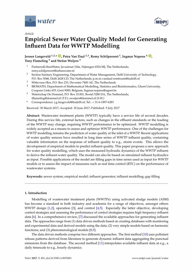
The 10 municipalities contributing to the WWTP influent are divided over three catchment areasthat are very different in size and character, each having a separate inflow to the WWTP (see Figure 1).Wastewater from Eindhoven Stad (ES, municipality of Eindhoven) accounts for approximately 50%(in practice ranging between 14,000 and 17,000 m3/h) of the hydraulic capacity and is dischargeddirectly to the WWTP. The other nine (much smaller) municipalities are each connected to one of thetwo wastewater transport mains, one to the north (Nuenen/Son or NS, 7 km in length) and one tothe south (Riool Zuid or RZ, 32 km in length), accounting for respectively 7% (3000 m3/h) and 43%(in practice ranging from 14,000 to 15,000 m3/h) of the hydraulic capacity. An elaborate description ofthe studied wastewater system can be found in [23].

Water 2017, 9, 491 3 of 18

oxygen (DO) depletion, ammonia peaks and seasonal average nutrient concentration levels [26,27]. Earlier research within the KALLISTO project [18,25] demonstrated that the WWTP effluent is the main source for the toxic ammonia peaks in the Dommel river and that the ammonium peaks in the WWTP effluent can be significantly reduced by applied integrated real time control (RTC). In [28], the use of RTC by activating in-sewer storage volume to reduce and delay the hydraulic peak loading of the WWTP during storm events has been shown to be an effective measure. Reference [29] introduced a new RTC concept: the smart buffer, which minimizes the peak load to the biology at WWTP Eindhoven by applying the aforementioned RTC combined with using only one of the three primary clarifiers (PC) during dry weather (DWF) and using the other two PCs only during storm events.

The 10 municipalities contributing to the WWTP influent are divided over three catchment areas that are very different in size and character, each having a separate inflow to the WWTP (see Figure 1). Wastewater from Eindhoven Stad (ES, municipality of Eindhoven) accounts for approximately 50% (in practice ranging between 14,000 and 17,000 m3/h) of the hydraulic capacity and is discharged directly to the WWTP. The other nine (much smaller) municipalities are each connected to one of the two wastewater transport mains, one to the north (Nuenen/Son or NS, 7 km in length) and one to the south (Riool Zuid or RZ, 32 km in length), accounting for respectively 7% (3000 m3/h) and 43% (in practice ranging from 14,000 to 15,000 m3/h) of the hydraulic capacity. An elaborate description of the studied wastewater system can be found in [23].

Figure 1. Wastewater system of Eindhoven (Left) and its receiving streams and schematic lay out of the wastewater system; (Right) Figure reproduced with permission from [23].

2.2. Monitoring Network and Data Validation

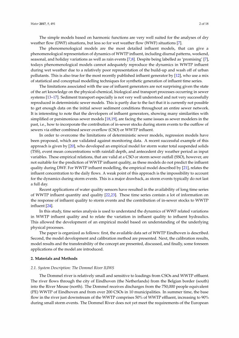
At each of the three inflows into the WWTP (locations ‘A’ in Figure 1 at the right) on-line spectroscopy sensors (UV-VIS) have been installed that measure equivalent concentration values of wastewater quality parameters: total suspended solids (TSS), chemical oxygen demand (COD), and filtered COD (CODf), i.e., the dissolved fraction of COD, at an interval of 2 min. In addition, flow is recorded every minute at these locations and ammonium (NH4, using Hach Lange Amtax sensors) at the Eindhoven Stad and Riool Zuid catchments. In this study, monitoring data for the year 2012 was used.

The monitoring data were validated manually, focusing on obtaining reliable data for calibration of wet weather flow processes. Figure 2 shows an example of data and their evaluation. After validation, only 38.5% of the data was considered to have an acceptable quality during the condition required. This percentage of data perceived ‘good enough’ after validation may seem relatively low.

0 3 6 9 kmN

ps Sonps Nederwetten

ps Gerwenps Nuenen

ps Mierlops Eeneind

Geldrop

ps Leende

ps Sterksel

Aalst

ps Waalre

Veldhoven

ps Wintelre

ps Knegsel

ps Steensel

ps Riethoven

ps WesterhovenBergeijk

Luijksgestel

ps Weebosch

ps Borkel

ps Eerselps Duizel Valkenswaard

wwtp Eindhoven

ps Heeze

wwtp Eindhovenfree flow conduitspressure mainspumping stationscontrol stationssludge proc. inst.

catchment area:Nuenen/SonEindhoven StadRiool-Zuid

sludge proc. inst.

cs Valkenswaard

cs de Merenps Aalst

cs rwzi

Closing section river

Figure 1. Wastewater system of Eindhoven (Left) and its receiving streams and schematic lay out ofthe wastewater system; (Right) Figure reproduced with permission from [23].

2.2. Monitoring Network and Data Validation

At each of the three inflows into the WWTP (locations ‘A’ in Figure 1 at the right) on-linespectroscopy sensors (UV-VIS) have been installed that measure equivalent concentration values ofwastewater quality parameters: total suspended solids (TSS), chemical oxygen demand (COD), andfiltered COD (CODf), i.e., the dissolved fraction of COD, at an interval of 2 min. In addition, flow isrecorded every minute at these locations and ammonium (NH4, using Hach Lange Amtax sensors)at the Eindhoven Stad and Riool Zuid catchments. In this study, monitoring data for the year 2012was used.

The monitoring data were validated manually, focusing on obtaining reliable data for calibration ofwet weather flow processes. Figure 2 shows an example of data and their evaluation. After validation,

Water 2017, 9, 491 4 of 18

only 38.5% of the data was considered to have an acceptable quality during the condition required.This percentage of data perceived ‘good enough’ after validation may seem relatively low. Duringearlier research projects (2007–2008) at WWTP Eindhoven on UV-VIS sensors, the percentage of ‘goodenough’ data after data validation ranged between 50% and 75%, despite very intensive maintenanceand surveillance [23] and without restrictions on the influent conditions. WWTP influent has shownto be a very difficult medium for water quality monitoring. The dataset after validation comprisesapproximately 30 storm events with good data for each calibration performed. In the model calibration,these events, including the antecedent dry day and several following dry days, were used. In Figure 2,and all other Figures, the data used for calibration is represented by the dark grey bullets, data notused for calibration with light grey bullets. An assessment of routine 24 h water quality samples ofWWTP influent showed that the DWF does not show a noticeable seasonal pattern.

Water 2017, 9, 491 4 of 18

During earlier research projects (2007–2008) at WWTP Eindhoven on UV-VIS sensors, the percentage of ‘good enough’ data after data validation ranged between 50% and 75%, despite very intensive maintenance and surveillance [23] and without restrictions on the influent conditions. WWTP influent has shown to be a very difficult medium for water quality monitoring. The dataset after validation comprises approximately 30 storm events with good data for each calibration performed. In the model calibration, these events, including the antecedent dry day and several following dry days, were used. In Figure 2, and all other Figures, the data used for calibration is represented by the dark grey bullets, data not used for calibration with light grey bullets. An assessment of routine 24 h water quality samples of WWTP influent showed that the DWF does not show a noticeable seasonal pattern.

Figure 2. Example of quality evaluation of monitoring data.

2.3. Data Analysis

In earlier work [16], a part of this data set was used to study the dynamics of wastewater composition. This resulted in well described typical diurnal patterns during DWF and typical dynamics during WWF (Figure 3).

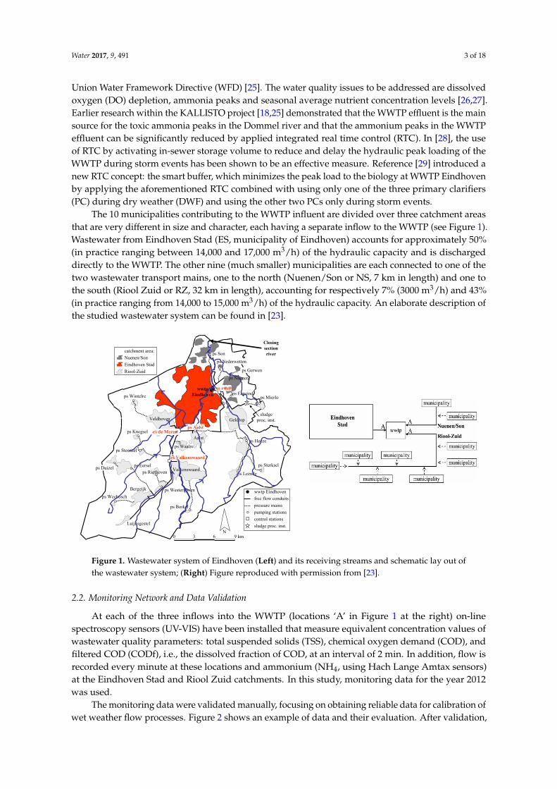
Figure 3. Wet weather flow (WWF) dynamics during the stages of a storm event on 12 June 2008 in Eindhoven Stad catchment.

Figure 2. Example of quality evaluation of monitoring data.

2.3. Data Analysis

In earlier work [16], a part of this data set was used to study the dynamics of wastewatercomposition. This resulted in well described typical diurnal patterns during DWF and typical dynamicsduring WWF (Figure 3).

Water 2017, 9, 491 4 of 18

During earlier research projects (2007–2008) at WWTP Eindhoven on UV-VIS sensors, the percentage of ‘good enough’ data after data validation ranged between 50% and 75%, despite very intensive maintenance and surveillance [23] and without restrictions on the influent conditions. WWTP influent has shown to be a very difficult medium for water quality monitoring. The dataset after validation comprises approximately 30 storm events with good data for each calibration performed. In the model calibration, these events, including the antecedent dry day and several following dry days, were used. In Figure 2, and all other Figures, the data used for calibration is represented by the dark grey bullets, data not used for calibration with light grey bullets. An assessment of routine 24 h water quality samples of WWTP influent showed that the DWF does not show a noticeable seasonal pattern.

Figure 2. Example of quality evaluation of monitoring data.

2.3. Data Analysis

In earlier work [16], a part of this data set was used to study the dynamics of wastewater composition. This resulted in well described typical diurnal patterns during DWF and typical dynamics during WWF (Figure 3).

Figure 3. Wet weather flow (WWF) dynamics during the stages of a storm event on 12 June 2008 in Eindhoven Stad catchment.

Figure 3. Wet weather flow (WWF) dynamics during the stages of a storm event on 12 June 2008 inEindhoven Stad catchment.

Water 2017, 9, 491 5 of 18

For WWF, it has been observed that the concentration levels of the wastewater show a typicalpattern during a storm event: a short period called ‘onset’ of the storm event, with an increasedconcentration level for particulate matter but not for dissolved matter, a longer period called ‘dilution’,where dilution of both dissolved and particulate matter takes place, and ‘recovery’, a period wheredissolved and particulate matter slowly return to DWF levels.

2.4. Model Development

The general idea behind the model development is that the measured hydraulic influent data,i.e., flow and water level in the influent pumping station, can be used to make a distinction betweenthe four patterns: DWF, onset of WWF, dilution during WWF and recovery after WWF. Each of thesepatterns is denoted as a system state, during which a certain relation between flow and concentrationlevel applies. This allows the incorporation of the contribution of in-sewer stocks on top of the mixingprocess between wastewater and stormwater. The latter is a common feature of influent models appliedto simulate both dry and wet periods, while explicitly accounting for the contribution of in-sewerstocks circumventing the relatively limited knowledge associated in sewer processes.

The water quality average dry weather diurnal pattern is the core of the model. As long as thesystem state is ‘DWF’, the average dry weather diurnal pattern based on monitoring data is used,together with the measured flow data. The average dry weather diurnal pattern has been derived fromflow monitoring data by averaging the monitoring data of 10 dry days over 5 min intervals with thesame timestamp.

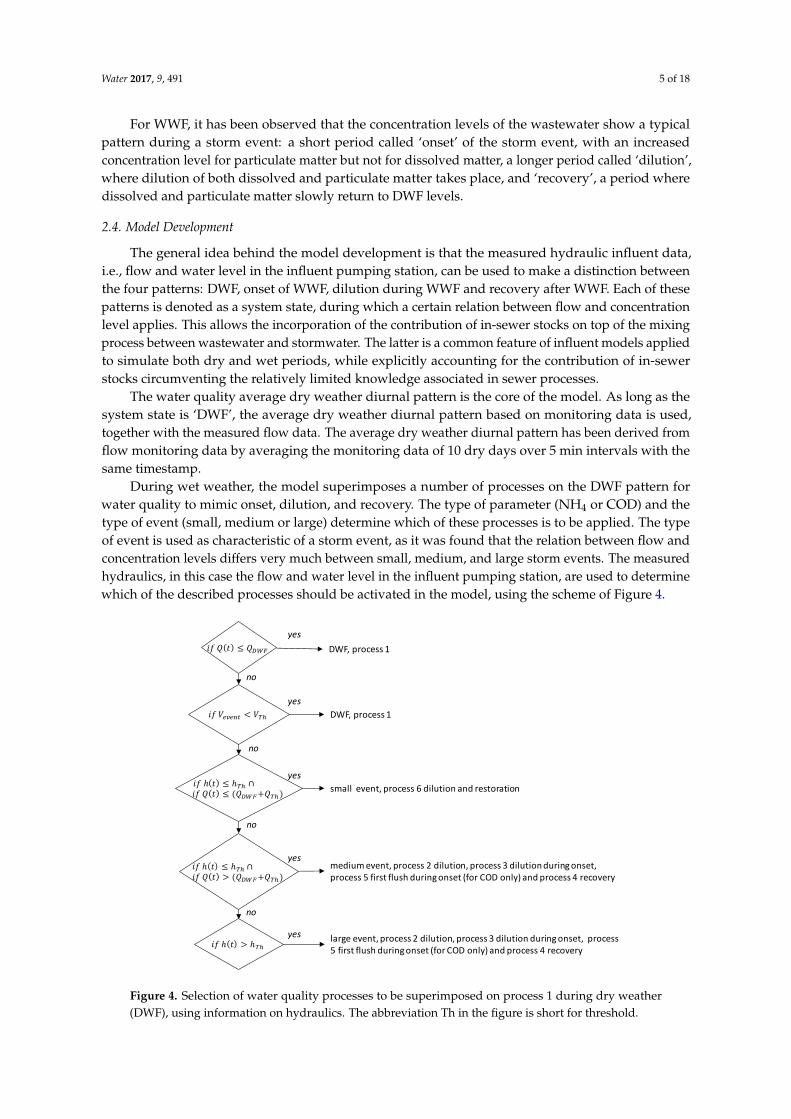
During wet weather, the model superimposes a number of processes on the DWF pattern forwater quality to mimic onset, dilution, and recovery. The type of parameter (NH4 or COD) and thetype of event (small, medium or large) determine which of these processes is to be applied. The typeof event is used as characteristic of a storm event, as it was found that the relation between flow andconcentration levels differs very much between small, medium, and large storm events. The measuredhydraulics, in this case the flow and water level in the influent pumping station, are used to determinewhich of the described processes should be activated in the model, using the scheme of Figure 4.

Water 2017, 9, 491 5 of 18

For WWF, it has been observed that the concentration levels of the wastewater show a typical pattern during a storm event: a short period called ‘onset’ of the storm event, with an increased concentration level for particulate matter but not for dissolved matter, a longer period called ‘dilution’, where dilution of both dissolved and particulate matter takes place, and ‘recovery’, a period where dissolved and particulate matter slowly return to DWF levels.

2.4. Model Development

The general idea behind the model development is that the measured hydraulic influent data, i.e., flow and water level in the influent pumping station, can be used to make a distinction between the four patterns: DWF, onset of WWF, dilution during WWF and recovery after WWF. Each of these patterns is denoted as a system state, during which a certain relation between flow and concentration level applies. This allows the incorporation of the contribution of in-sewer stocks on top of the mixing process between wastewater and stormwater. The latter is a common feature of influent models applied to simulate both dry and wet periods, while explicitly accounting for the contribution of in-sewer stocks circumventing the relatively limited knowledge associated in sewer processes.

The water quality average dry weather diurnal pattern is the core of the model. As long as the system state is ‘DWF’, the average dry weather diurnal pattern based on monitoring data is used, together with the measured flow data. The average dry weather diurnal pattern has been derived from flow monitoring data by averaging the monitoring data of 10 dry days over 5 min intervals with the same timestamp.

During wet weather, the model superimposes a number of processes on the DWF pattern for water quality to mimic onset, dilution, and recovery. The type of parameter (NH4 or COD) and the type of event (small, medium or large) determine which of these processes is to be applied. The type of event is used as characteristic of a storm event, as it was found that the relation between flow and concentration levels differs very much between small, medium, and large storm events. The measured hydraulics, in this case the flow and water level in the influent pumping station, are used to determine which of the described processes should be activated in the model, using the scheme of Figure 4.

Figure 4. Selection of water quality processes to be superimposed on process 1 during dry weather (DWF), using information on hydraulics. The abbreviation Th in the figure is short for threshold.

DWF, process 1yes

no

DWF, process 1

∩ small event, process 6 dilution and restoration

∩ medium event, process 2 dilution, process 3 dilution during onset, process 5 first flush during onset (for COD only) and process 4 recovery

large event, process 2 dilution, process 3 dilution during onset, process 5 first flush during onset (for COD only) and process 4 recovery

yes

no

yes

no

yes

no

yes

Figure 4. Selection of water quality processes to be superimposed on process 1 during dry weather(DWF), using information on hydraulics. The abbreviation Th in the figure is short for threshold.

Water 2017, 9, 491 6 of 18

As indicated in Figure 4, two conditions have to be met to change from DWF to WWF. The first isthat the upper limit for dry weather conditions (QDWF, set at the 95th percentile of the flow valuescollected during dry weather at a specific timestamp) has to be exceeded, the second that the volumeshould exceed a certain threshold (set at 5000 m3). The second condition is added to exclude apparentevents in the data caused by interference of the pump operation due to for example to maintenance.The value of 5000 m3, equivalent to the volume of 2 h of DWF, shown to be sufficient to filter flowvalues exceeding QDWF due to operational issues during DWF.

A small storm event is defined as an event for which the water level in the influent chamber doesnot rise above the DWF threshold value (set at 11.30 m AD) and the flow exceeds the 95 percentileDWF value with less than a threshold set at 4000 m3/h These events are very small storm events,where the inflow is less than 0.2 mm/h or 2 m3/ha). Medium events are defined as events where thewater level in the influent chamber does not exceed the DWF threshold value, but the flow exceeds the95 percentile DWF value with more than the threshold. These events are typically relatively small, lowintensity storm events, where the inflow is less than the available pumping capacity (which is equal toan interceptor capacity of 0.7 mm/h or 7 m3/ha). Large storm events are defined as events duringwhich not only flow increases, but also the water level in the influent pumping station increases abovethe DWF threshold value. This occurs only if the sewer system starts filling during bigger storm eventsexceeding the pumping capacity of the WWTP.

The processes applied in the model are:Process 1 the basic process for all parameters, is the DWF pattern for water quality. It is derived

from high-frequency monitoring data collected during multiple dry weather days, by averaging overthe same time stamps.

Process 2 mimics dilution and is based on the ratio between the actual flow (Qactual) and theupper limit for the flow during DWF at that time of the day at the location of the WWTP inlet works(QDWF). The wastewater concentration is calculated using Formula (1):

CWWF(t) = CDWF(t) (a1 QDWF(t)/Qactual(t) − a1 + 1) (1)

With CWWF = calculated concentration during wet weather, and CDWF = the concentration duringDWF conditions at that time of the day. The dilution factor a1 (-) is introduced to allow adjustment tothe dilution rate if necessary. A value of 1 for factor a1 indicates that the dilution is exactly inverse tothe increase in flow. A value of a1 smaller than 1 would impose an increase in pollutant loads duringthe event, which could be necessary to account for pollutant contributions originating from in-sewerstocks. A value of a1 larger than 1 would impose a decrease in pollutant loads during the event, whichcould be expected for a compound where in-sewer stocks are zero and a part of the pollutants wouldbe discharged via a CSO. For low dilution ratios, i.e., QDWF(t)/Qactual(t) being close to 1, the factor a1

has a limited influence, for higher dilution ratios, the factor a1 contributes to a larger extent.Process 3 accounts for dilution during the onset of storm events. Process 3 is described by a

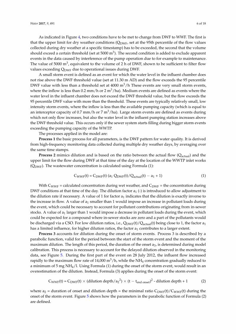
parabolic function, valid for the period between the start of the storm event and the moment of themaximum dilution. The length of this period, the duration of the onset a3, is determined during modelcalibration. This process is necessary to account for the delayed dilution observed in the monitoringdata, see Figure 5. During the first part of the event on 28 July 2012, the influent flow increasedrapidly to the maximum flow rate of 14,000 m3/h, while the NH4 concentration gradually reduced toa minimum of 5 mg NH4/l. Using Formula (1) during the onset of the storm event, would result in anoverestimation of the dilution. Instead, Formula (3) applies during the onset of the storm event:

CWWF(t) = CDWF(t) × (dilution depth/a22) × (t − tend onset)

2 - dilution depth + 1 (2)

where a2 = duration of onset and dilution depth = the minimal ratio CDWF(t)/CWWF(t) during theonset of the storm event. Figure 5 shows how the parameters in the parabolic function of Formula (2)are defined.

Water 2017, 9, 491 7 of 18Water 2017, 9, 491 7 of 18

Figure 5. Parameters of parabolic function that describes the delayed dilution of the quality parameters compared to the flow.

Process 4 reproduces restoration, which describes the gradual return of concentration values to DWF values after the storm event. Based on the analysis of the available data set, restoration can be assumed to be a linear process at rate a3 (mg/(L·s)) until the concentration returns to the DWF value. During the restoration phase, the concentration is calculated by:

CWWF(t + 1) = CWWF(t) (1 + a3) dt. (3)

Process 5 describes a first flush in concentration levels of particulate material (see Figure 3), it is thus not valid for soluble substances. This initial peak increases the concentrations during the first stage of storm events, before dilution becomes the dominant process. Process 5 is modeled as a triangle that causes an instant increase of the COD concentration of a4 mg/l at the onset of the event, decreasing with a fixed rate a5 (mg/(L·s)).

Process 6 regards dilution and restoration for small events. Process 6 describes the concentration profile as a fixed-shape triangle, where dilution takes place at a fixed rate a6 (mg/(L·s)) during x h and recovery at the same rate a6 (mg/L/s) during the next x h. In the case of Eindhoven Stad and Riool Zuid a duration of 13 h proved to be a good estimate of the duration of process 6.

2.5. Model Calibration

In this study the differential evolution adaptive metropolis (DREAM) algorithm is the method [30,31] applied to calibrate the parameters of the empirical model to find the minimal difference between the empirical model output and the monitoring data. The effectiveness of DREAM in water related model calibration has been demonstrated in many previous studies, e.g., [32–34].

Table 1 shows the model parameters, units and the searching range for the calibration procedure. The threshold values for selecting the type of event were derived during data analysis before the calibration of the model parameters and were consequently not included in the model calibration. Future users of the model on other catchments may include these parameters as part of the model calibration. For reasons of clarity, these parameters are listed here:

VTh: threshold value for making distinction between real storm events and irregularities in the DWF due to operational issues. In this study set at equivalent of 2 h of DWF.

QTh: threshold value to distinguish medium from small storm events. Set in this study at an equivalent of 0.2 mm/h of runoff.

hTh: threshold value to distinguish large from medium storm events. Set in this study at 0.30 m above the setpoint of the frequency controlled pumps.

x: duration of dilution and restoration for small events: Set in this study at 13 h.

Figure 5. Parameters of parabolic function that describes the delayed dilution of the quality parameterscompared to the flow.

Process 4 reproduces restoration, which describes the gradual return of concentration values toDWF values after the storm event. Based on the analysis of the available data set, restoration can beassumed to be a linear process at rate a3 (mg/(L·s)) until the concentration returns to the DWF value.During the restoration phase, the concentration is calculated by:

CWWF(t + 1) = CWWF(t) (1 + a3) dt. (3)

Process 5 describes a first flush in concentration levels of particulate material (see Figure 3), itis thus not valid for soluble substances. This initial peak increases the concentrations during thefirst stage of storm events, before dilution becomes the dominant process. Process 5 is modeled as atriangle that causes an instant increase of the COD concentration of a4 mg/l at the onset of the event,decreasing with a fixed rate a5 (mg/(L·s)).

Process 6 regards dilution and restoration for small events. Process 6 describes the concentrationprofile as a fixed-shape triangle, where dilution takes place at a fixed rate a6 (mg/(L·s)) during x h andrecovery at the same rate a6 (mg/L/s) during the next x h. In the case of Eindhoven Stad and RioolZuid a duration of 13 h proved to be a good estimate of the duration of process 6.

2.5. Model Calibration

In this study the differential evolution adaptive metropolis (DREAM) algorithm is themethod [30,31] applied to calibrate the parameters of the empirical model to find the minimal differencebetween the empirical model output and the monitoring data. The effectiveness of DREAM in waterrelated model calibration has been demonstrated in many previous studies, e.g., [32–34].

Table 1 shows the model parameters, units and the searching range for the calibration procedure.The threshold values for selecting the type of event were derived during data analysis before thecalibration of the model parameters and were consequently not included in the model calibration.Future users of the model on other catchments may include these parameters as part of the modelcalibration. For reasons of clarity, these parameters are listed here:

VTh: threshold value for making distinction between real storm events and irregularities in theDWF due to operational issues. In this study set at equivalent of 2 h of DWF.

QTh: threshold value to distinguish medium from small storm events. Set in this study at anequivalent of 0.2 mm/h of runoff.

hTh: threshold value to distinguish large from medium storm events. Set in this study at 0.30 mabove the setpoint of the frequency controlled pumps.

x: duration of dilution and restoration for small events: Set in this study at 13 h.

Water 2017, 9, 491 8 of 18

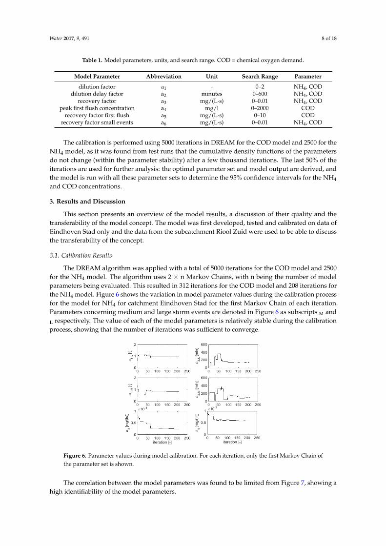
Table 1. Model parameters, units, and search range. COD = chemical oxygen demand.

Model Parameter Abbreviation Unit Search Range Parameter

dilution factor a1 - 0–2 NH4, CODdilution delay factor a2 minutes 0–600 NH4, COD

recovery factor a3 mg/(L·s) 0–0.01 NH4, CODpeak first flush concentration a4 mg/l 0–2000 COD

recovery factor first flush a5 mg/(L·s) 0–10 CODrecovery factor small events a6 mg/(L·s) 0–0.01 NH4, COD

The calibration is performed using 5000 iterations in DREAM for the COD model and 2500 for theNH4 model, as it was found from test runs that the cumulative density functions of the parametersdo not change (within the parameter stability) after a few thousand iterations. The last 50% of theiterations are used for further analysis: the optimal parameter set and model output are derived, andthe model is run with all these parameter sets to determine the 95% confidence intervals for the NH4

and COD concentrations.

3. Results and Discussion

This section presents an overview of the model results, a discussion of their quality and thetransferability of the model concept. The model was first developed, tested and calibrated on data ofEindhoven Stad only and the data from the subcatchment Riool Zuid were used to be able to discussthe transferability of the concept.

3.1. Calibration Results

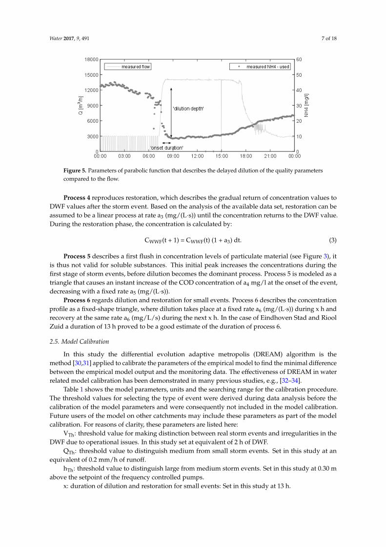
The DREAM algorithm was applied with a total of 5000 iterations for the COD model and 2500for the NH4 model. The algorithm uses 2 × n Markov Chains, with n being the number of modelparameters being evaluated. This resulted in 312 iterations for the COD model and 208 iterations forthe NH4 model. Figure 6 shows the variation in model parameter values during the calibration processfor the model for NH4 for catchment Eindhoven Stad for the first Markov Chain of each iteration.Parameters concerning medium and large storm events are denoted in Figure 6 as subscripts M and

L respectively. The value of each of the model parameters is relatively stable during the calibrationprocess, showing that the number of iterations was sufficient to converge.

Water 2017, 9, 491 8 of 18

Table 1. Model parameters, units, and search range. COD = chemical oxygen demand.

Model Parameter Abbreviation Unit Search Range Parameter dilution factor a1 - 0–2 NH4, COD

dilution delay factor a2 minutes 0–600 NH4, COD recovery factor a3 mg/(L·s) 0–0.01 NH4, COD

peak first flush concentration a4 mg/l 0–2000 COD recovery factor first flush a5 mg/(L·s) 0–10 COD

recovery factor small events a6 mg/(L·s) 0–0.01 NH4, COD

The calibration is performed using 5000 iterations in DREAM for the COD model and 2500 for the NH4 model, as it was found from test runs that the cumulative density functions of the parameters do not change (within the parameter stability) after a few thousand iterations. The last 50% of the iterations are used for further analysis: the optimal parameter set and model output are derived, and the model is run with all these parameter sets to determine the 95% confidence intervals for the NH4 and COD concentrations.

3. Results and Discussion

This section presents an overview of the model results, a discussion of their quality and the transferability of the model concept. The model was first developed, tested and calibrated on data of Eindhoven Stad only and the data from the subcatchment Riool Zuid were used to be able to discuss the transferability of the concept.

3.1. Calibration Results

The DREAM algorithm was applied with a total of 5000 iterations for the COD model and 2500 for the NH4 model. The algorithm uses 2 × n Markov Chains, with n being the number of model parameters being evaluated. This resulted in 312 iterations for the COD model and 208 iterations for the NH4 model. Figure 6 shows the variation in model parameter values during the calibration process for the model for NH4 for catchment Eindhoven Stad for the first Markov Chain of each iteration. Parameters concerning medium and large storm events are denoted in Figure 6 as subscripts M and L respectively. The value of each of the model parameters is relatively stable during the calibration process, showing that the number of iterations was sufficient to converge.

Figure 6. Parameter values during model calibration. For each iteration, only the first Markov Chain of the parameter set is shown.

The correlation between the model parameters was found to be limited from Figure 7, showing a high identifiability of the model parameters.

Figure 6. Parameter values during model calibration. For each iteration, only the first Markov Chain ofthe parameter set is shown.

The correlation between the model parameters was found to be limited from Figure 7, showing ahigh identifiability of the model parameters.

Water 2017, 9, 491 9 of 18Water 2017, 9, 491 9 of 18

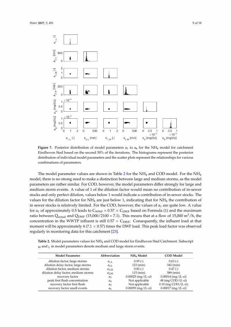
Figure 7. Posterior distribution of model parameters a1 to a6 for the NH4 model for catchment Eindhoven Stad based on the second 50% of the iterations. The histograms represent the posterior distribution of individual model parameters and the scatter plots represent the relationships for various combinations of parameters.

The model parameter values are shown in Table 2 for the NH4 and COD model. For the NH4 model, there is no strong need to make a distinction between large and medium storms, as the model parameters are rather similar. For COD, however, the model parameters differ strongly for large and medium storm events. A value of 1 of the dilution factor would mean no contribution of in-sewer stocks and only perfect dilution, values below 1 would indicate a contribution of in-sewer stocks. The values for the dilution factor for NH4 are just below 1, indicating that for NH4 the contribution of in sewer stocks is relatively limited. For the COD, however, the values of a1 are quite low. A value for a1 of approximately 0.5 leads to CWWF = 0.57 × CDWF based on Formula (1) and the maximum ratio between Qactual and QDWF (15,000/2100 = 7.1). This means that at a flow of 15,000 m3/h, the concentration in the WWTP influent is still 0.57 × CDWF. Consequently, the influent load at that moment will be approximately 4 (7.1 × 0.57) times the DWF load. This peak load factor was observed regularly in monitoring data for this catchment [23].

Table 2. Model parameters values for NH4 and COD model for Eindhoven Stad Catchment. Subscript M and L in model parameters denote medium and large storm events.

Model Parameter Abbreviation NH4 Model COD Model dilution factor, large storms a1,L 0.95 (-) 0.63 (-)

dilution delay factor, large storms a2,L 123 (min) 342 (min) dilution factor, medium storms a1,M 0.82 (-) 0.47 (-)

dilution delay factor, medium storms a2,M 115 (min) 589 (min) recovery factor a3 0.00025 (mg/(L·s)) 0.00014 (mg/(L·s))

peak first flush concentration a4 Not applicable 48 (mg COD/(L·s)) recovery factor first flush a5 Not applicable 0.19 (mg COD/(L·s))

recovery factor small events a6 0.00059 (mg/(L·s)) 0.00017 (mg/(L·s))

Figure 7. Posterior distribution of model parameters a1 to a6 for the NH4 model for catchmentEindhoven Stad based on the second 50% of the iterations. The histograms represent the posteriordistribution of individual model parameters and the scatter plots represent the relationships for variouscombinations of parameters.

The model parameter values are shown in Table 2 for the NH4 and COD model. For the NH4

model, there is no strong need to make a distinction between large and medium storms, as the modelparameters are rather similar. For COD, however, the model parameters differ strongly for large andmedium storm events. A value of 1 of the dilution factor would mean no contribution of in-sewerstocks and only perfect dilution, values below 1 would indicate a contribution of in-sewer stocks. Thevalues for the dilution factor for NH4 are just below 1, indicating that for NH4 the contribution ofin sewer stocks is relatively limited. For the COD, however, the values of a1 are quite low. A valuefor a1 of approximately 0.5 leads to CWWF = 0.57 × CDWF based on Formula (1) and the maximumratio between Qactual and QDWF (15,000/2100 = 7.1). This means that at a flow of 15,000 m3/h, theconcentration in the WWTP influent is still 0.57 × CDWF. Consequently, the influent load at thatmoment will be approximately 4 (7.1 × 0.57) times the DWF load. This peak load factor was observedregularly in monitoring data for this catchment [23].

Table 2. Model parameters values for NH4 and COD model for Eindhoven Stad Catchment. Subscript

M and L in model parameters denote medium and large storm events.

Model Parameter Abbreviation NH4 Model COD Model

dilution factor, large storms a1,L 0.95 (-) 0.63 (-)dilution delay factor, large storms a2,L 123 (min) 342 (min)

dilution factor, medium storms a1,M 0.82 (-) 0.47 (-)dilution delay factor, medium storms a2,M 115 (min) 589 (min)

recovery factor a3 0.00025 (mg/(L·s)) 0.00014 (mg/(L·s))peak first flush concentration a4 Not applicable 48 (mg COD/(L·s))

recovery factor first flush a5 Not applicable 0.19 (mg COD/(L·s))recovery factor small events a6 0.00059 (mg/(L·s)) 0.00017 (mg/(L·s))

Water 2017, 9, 491 10 of 18

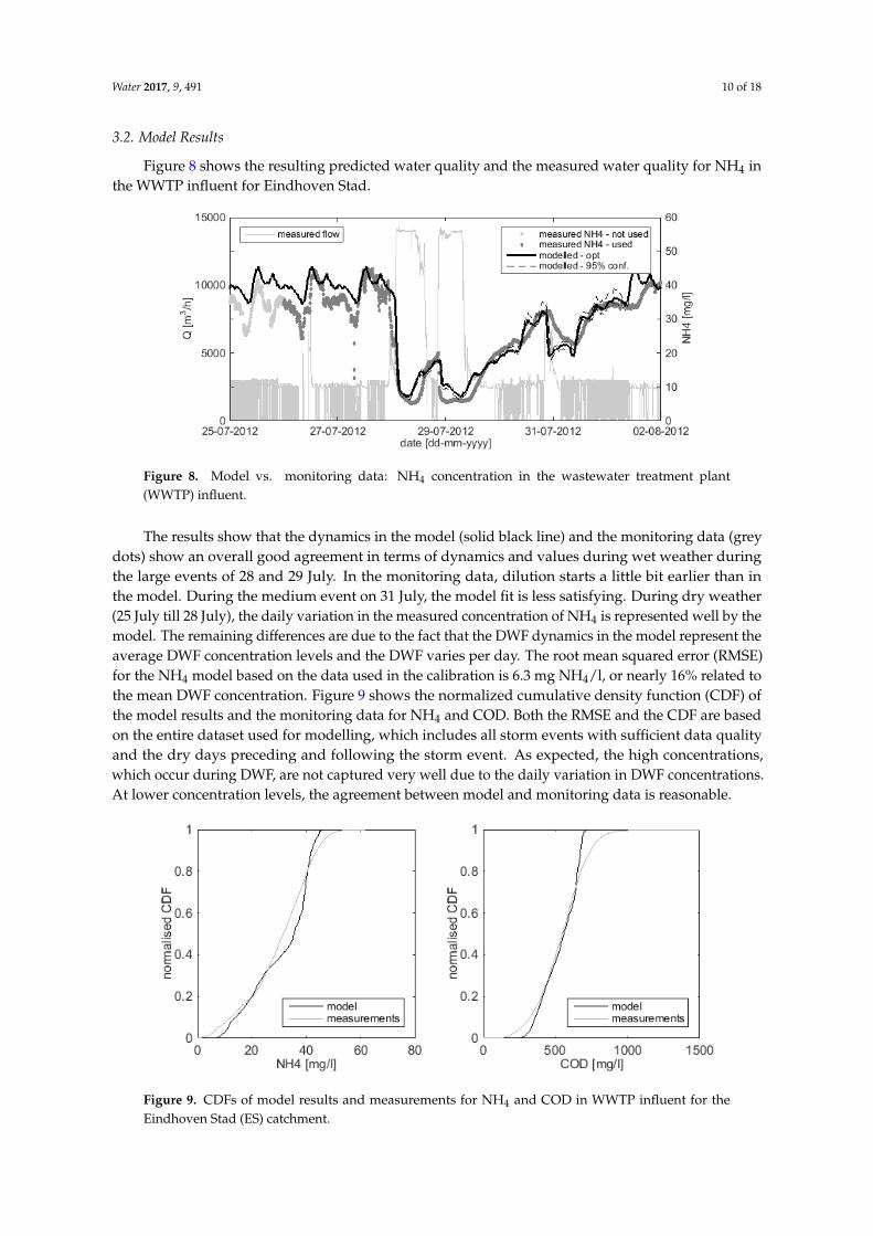
3.2. Model Results

Figure 8 shows the resulting predicted water quality and the measured water quality for NH4 inthe WWTP influent for Eindhoven Stad.

Water 2017, 9, 491 10 of 18

3.2. Model Results

Figure 8 shows the resulting predicted water quality and the measured water quality for NH4 in the WWTP influent for Eindhoven Stad.

Figure 8. Model vs. monitoring data: NH4 concentration in the wastewater treatment plant (WWTP) influent.

The results show that the dynamics in the model (solid black line) and the monitoring data (grey dots) show an overall good agreement in terms of dynamics and values during wet weather during the large events of 28 and 29 July. In the monitoring data, dilution starts a little bit earlier than in the model. During the medium event on 31 July, the model fit is less satisfying. During dry weather (25 July till 28 July), the daily variation in the measured concentration of NH4 is represented well by the model. The remaining differences are due to the fact that the DWF dynamics in the model represent the average DWF concentration levels and the DWF varies per day. The root mean squared error (RMSE) for the NH4 model based on the data used in the calibration is 6.3 mg NH4/l, or nearly 16% related to the mean DWF concentration. Figure 9 shows the normalized cumulative density function (CDF) of the model results and the monitoring data for NH4 and COD. Both the RMSE and the CDF are based on the entire dataset used for modelling, which includes all storm events with sufficient data quality and the dry days preceding and following the storm event. As expected, the high concentrations, which occur during DWF, are not captured very well due to the daily variation in DWF concentrations. At lower concentration levels, the agreement between model and monitoring data is reasonable.

Figure 9. CDFs of model results and measurements for NH4 and COD in WWTP influent for the Eindhoven Stad (ES) catchment.

Figure 8. Model vs. monitoring data: NH4 concentration in the wastewater treatment plant(WWTP) influent.

The results show that the dynamics in the model (solid black line) and the monitoring data (greydots) show an overall good agreement in terms of dynamics and values during wet weather duringthe large events of 28 and 29 July. In the monitoring data, dilution starts a little bit earlier than inthe model. During the medium event on 31 July, the model fit is less satisfying. During dry weather(25 July till 28 July), the daily variation in the measured concentration of NH4 is represented well by themodel. The remaining differences are due to the fact that the DWF dynamics in the model represent theaverage DWF concentration levels and the DWF varies per day. The root mean squared error (RMSE)for the NH4 model based on the data used in the calibration is 6.3 mg NH4/l, or nearly 16% related tothe mean DWF concentration. Figure 9 shows the normalized cumulative density function (CDF) ofthe model results and the monitoring data for NH4 and COD. Both the RMSE and the CDF are basedon the entire dataset used for modelling, which includes all storm events with sufficient data qualityand the dry days preceding and following the storm event. As expected, the high concentrations,which occur during DWF, are not captured very well due to the daily variation in DWF concentrations.At lower concentration levels, the agreement between model and monitoring data is reasonable.

Water 2017, 9, 491 10 of 18

3.2. Model Results

Figure 8 shows the resulting predicted water quality and the measured water quality for NH4 in the WWTP influent for Eindhoven Stad.

Figure 8. Model vs. monitoring data: NH4 concentration in the wastewater treatment plant (WWTP) influent.

The results show that the dynamics in the model (solid black line) and the monitoring data (grey dots) show an overall good agreement in terms of dynamics and values during wet weather during the large events of 28 and 29 July. In the monitoring data, dilution starts a little bit earlier than in the model. During the medium event on 31 July, the model fit is less satisfying. During dry weather (25 July till 28 July), the daily variation in the measured concentration of NH4 is represented well by the model. The remaining differences are due to the fact that the DWF dynamics in the model represent the average DWF concentration levels and the DWF varies per day. The root mean squared error (RMSE) for the NH4 model based on the data used in the calibration is 6.3 mg NH4/l, or nearly 16% related to the mean DWF concentration. Figure 9 shows the normalized cumulative density function (CDF) of the model results and the monitoring data for NH4 and COD. Both the RMSE and the CDF are based on the entire dataset used for modelling, which includes all storm events with sufficient data quality and the dry days preceding and following the storm event. As expected, the high concentrations, which occur during DWF, are not captured very well due to the daily variation in DWF concentrations. At lower concentration levels, the agreement between model and monitoring data is reasonable.

Figure 9. CDFs of model results and measurements for NH4 and COD in WWTP influent for the Eindhoven Stad (ES) catchment. Figure 9. CDFs of model results and measurements for NH4 and COD in WWTP influent for theEindhoven Stad (ES) catchment.

Water 2017, 9, 491 11 of 18

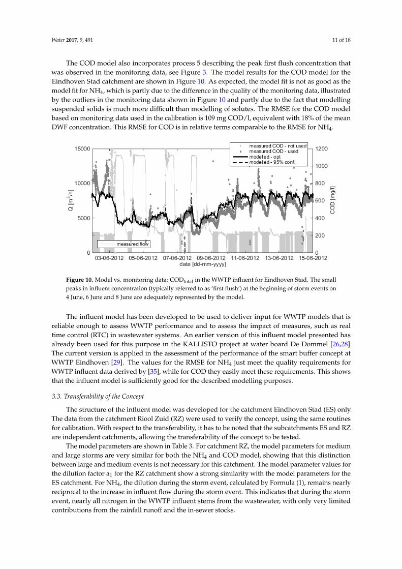
The COD model also incorporates process 5 describing the peak first flush concentration thatwas observed in the monitoring data, see Figure 3. The model results for the COD model for theEindhoven Stad catchment are shown in Figure 10. As expected, the model fit is not as good as themodel fit for NH4, which is partly due to the difference in the quality of the monitoring data, illustratedby the outliers in the monitoring data shown in Figure 10 and partly due to the fact that modellingsuspended solids is much more difficult than modelling of solutes. The RMSE for the COD modelbased on monitoring data used in the calibration is 109 mg COD/l, equivalent with 18% of the meanDWF concentration. This RMSE for COD is in relative terms comparable to the RMSE for NH4.

Water 2017, 9, 491 11 of 18

The COD model also incorporates process 5 describing the peak first flush concentration that was observed in the monitoring data, see Figure 3. The model results for the COD model for the Eindhoven Stad catchment are shown in Figure 10. As expected, the model fit is not as good as the model fit for NH4, which is partly due to the difference in the quality of the monitoring data, illustrated by the outliers in the monitoring data shown in Figure 10 and partly due to the fact that modelling suspended solids is much more difficult than modelling of solutes. The RMSE for the COD model based on monitoring data used in the calibration is 109 mg COD/l, equivalent with 18% of the mean DWF concentration. This RMSE for COD is in relative terms comparable to the RMSE for NH4.

Figure 10. Model vs. monitoring data: CODtotal in the WWTP influent for Eindhoven Stad. The small peaks in influent concentration (typically referred to as ‘first flush’) at the beginning of storm events on 4 June, 6 June and 8 June are adequately represented by the model.

The influent model has been developed to be used to deliver input for WWTP models that is reliable enough to assess WWTP performance and to assess the impact of measures, such as real time control (RTC) in wastewater systems. An earlier version of this influent model presented has already been used for this purpose in the KALLISTO project at water board De Dommel [26,28]. The current version is applied in the assessment of the performance of the smart buffer concept at WWTP Eindhoven [29]. The values for the RMSE for NH4 just meet the quality requirements for WWTP influent data derived by [35], while for COD they easily meet these requirements. This shows that the influent model is sufficiently good for the described modelling purposes.

3.3. Transferability of the Concept

The structure of the influent model was developed for the catchment Eindhoven Stad (ES) only. The data from the catchment Riool Zuid (RZ) were used to verify the concept, using the same routines for calibration. With respect to the transferability, it has to be noted that the subcatchments ES and RZ are independent catchments, allowing the transferability of the concept to be tested.

The model parameters are shown in Table 3. For catchment RZ, the model parameters for medium and large storms are very similar for both the NH4 and COD model, showing that this distinction between large and medium events is not necessary for this catchment. The model parameter values for the dilution factor a1 for the RZ catchment show a strong similarity with the model parameters for the ES catchment. For NH4, the dilution during the storm event, calculated by Formula (1), remains nearly reciprocal to the increase in influent flow during the storm event. This indicates that during the storm event, nearly all nitrogen in the WWTP influent stems from the wastewater, with only very limited contributions from the rainfall runoff and the in-sewer stocks.

Figure 10. Model vs. monitoring data: CODtotal in the WWTP influent for Eindhoven Stad. The smallpeaks in influent concentration (typically referred to as ‘first flush’) at the beginning of storm events on4 June, 6 June and 8 June are adequately represented by the model.

The influent model has been developed to be used to deliver input for WWTP models that isreliable enough to assess WWTP performance and to assess the impact of measures, such as realtime control (RTC) in wastewater systems. An earlier version of this influent model presented hasalready been used for this purpose in the KALLISTO project at water board De Dommel [26,28].The current version is applied in the assessment of the performance of the smart buffer concept atWWTP Eindhoven [29]. The values for the RMSE for NH4 just meet the quality requirements forWWTP influent data derived by [35], while for COD they easily meet these requirements. This showsthat the influent model is sufficiently good for the described modelling purposes.

3.3. Transferability of the Concept

The structure of the influent model was developed for the catchment Eindhoven Stad (ES) only.The data from the catchment Riool Zuid (RZ) were used to verify the concept, using the same routinesfor calibration. With respect to the transferability, it has to be noted that the subcatchments ES and RZare independent catchments, allowing the transferability of the concept to be tested.

The model parameters are shown in Table 3. For catchment RZ, the model parameters for mediumand large storms are very similar for both the NH4 and COD model, showing that this distinctionbetween large and medium events is not necessary for this catchment. The model parameter values forthe dilution factor a1 for the RZ catchment show a strong similarity with the model parameters for theES catchment. For NH4, the dilution during the storm event, calculated by Formula (1), remains nearlyreciprocal to the increase in influent flow during the storm event. This indicates that during the stormevent, nearly all nitrogen in the WWTP influent stems from the wastewater, with only very limitedcontributions from the rainfall runoff and the in-sewer stocks.

Water 2017, 9, 491 12 of 18

Table 3. Model parameters values for NH4 and COD model for Riool Zuid Catchment. Subscript M

and L in model parameters denote medium and large storm events.

Model Parameter Abbreviation NH4 Model COD Model

dilution factor, large storms a1,L 0.96 (-) 0.49 (-)dilution delay factor, large storms a2,L 373 (min) 590 (min)

dilution factor, medium storms a1,M 0.98 (-) 0.49 (-)dilution delay factor, medium storms a2,M 427 (min) 548 (min)

recovery factor a3 0.00033 (mg/(L·s)) 0.00034 (mg/(L·s))peak first flush concentration a4 Not applicable 60 (mg COD/(L·s))

recovery factor first flush a5 Not applicable 0.06 (mg COD/(L·s))recovery factor small events a6 0.00027 (mg/(L·s)) 0.00002 (mg/(L·s))

For the COD, the dilution factor of a1 of 0.49 results in COD concentration levels during the highflow period of storm events of between 250 and 300 mg COD/L and, as a consequence, high influentpeak loads. This additional load arriving via the influent at the WWTP during a storm event originatesmainly from the in-sewer stocks [15], given the fairly low COD concentration in Dutch stormwater of61 mg COD/L [36].

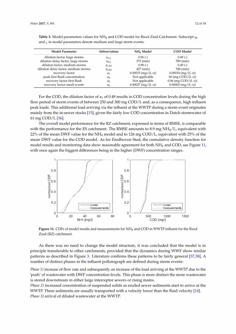
The overall model performance for the RZ catchment, expressed in terms of RMSE, is comparablewith the performance for the ES catchment. The RMSE amounts to 8.9 mg NH4/L, equivalent with22% of the mean DWF value for the NH4 model and to 126 mg COD/L, equivalent with 25% of themean DWF value for the COD model. As for Eindhoven Stad, the cumulative density function formodel results and monitoring data show reasonable agreement for both NH4 and COD, see Figure 11,with once again the biggest differences being in the higher (DWF) concentration ranges.

Water 2017, 9, 491 12 of 18

Table 3. Model parameters values for NH4 and COD model for Riool Zuid Catchment. Subscript M and L in model parameters denote medium and large storm events.

Model Parameter Abbreviation NH4 Model COD Modeldilution factor, large storms a1,L 0.96 (-) 0.49 (-)

dilution delay factor, large storms a2,L 373 (min) 590 (min) dilution factor, medium storms a1,M 0.98 (-) 0.49 (-) dilution delay factor, medium

storms a2,M 427 (min) 548 (min)

recovery factor a3 0.00033 (mg/(L·s)) 0.00034 (mg/(L·s)) peak first flush concentration a4 Not applicable 60 (mg COD/(L·s))

recovery factor first flush a5 Not applicable 0.06 (mg COD/(L·s)) recovery factor small events a6 0.00027 (mg/(L·s)) 0.00002 (mg/(L·s))

For the COD, the dilution factor of a1 of 0.49 results in COD concentration levels during the high flow period of storm events of between 250 and 300 mg COD/L and, as a consequence, high influent peak loads. This additional load arriving via the influent at the WWTP during a storm event originates mainly from the in-sewer stocks [15], given the fairly low COD concentration in Dutch stormwater of 61 mg COD/L [36].

The overall model performance for the RZ catchment, expressed in terms of RMSE, is comparable with the performance for the ES catchment. The RMSE amounts to 8.9 mg NH4/L, equivalent with 22% of the mean DWF value for the NH4 model and to 126 mg COD/L, equivalent with 25% of the mean DWF value for the COD model. As for Eindhoven Stad, the cumulative density function for model results and monitoring data show reasonable agreement for both NH4 and COD, see Figure 11, with once again the biggest differences being in the higher (DWF) concentration ranges.

Figure 11. CDFs of model results and measurements for NH4 and COD in WWTP influent for the Riool Zuid (RZ) catchment.

As there was no need to change the model structure, it was concluded that the model is in principle transferable to other catchments, provided that the dynamics during WWF show similar patterns as described in Figure 3. Literature confirms these patterns to be fairly general [37,38], A number of distinct phases in the influent pollutograph are defined during storm events:

Phase 1) increase of flow rate and subsequently an increase of the load arriving at the WWTP due to the ‘push’ of wastewater with DWF concentration levels. This phase is more distinct the more wastewater is stored downstream in either large interceptor sewers or rising mains. Phase 2) increased concentration of suspended solids as eroded sewer sediments start to arrive at the WWTP. These sediments are usually transported with a velocity lower than the fluid velocity [14]. Phase 3) arrival of diluted wastewater at the WWTP. Phase 4) return to DWF equilibrium. Equilibrium for dissolved compounds will be reached as soon as all remaining storm runoff has been transported (pumped) towards the WWTP. Reaching

Figure 11. CDFs of model results and measurements for NH4 and COD in WWTP influent for the RioolZuid (RZ) catchment.

As there was no need to change the model structure, it was concluded that the model is inprinciple transferable to other catchments, provided that the dynamics during WWF show similarpatterns as described in Figure 3. Literature confirms these patterns to be fairly general [37,38], Anumber of distinct phases in the influent pollutograph are defined during storm events:

Phase 1) increase of flow rate and subsequently an increase of the load arriving at the WWTP due to the‘push’ of wastewater with DWF concentration levels. This phase is more distinct the more wastewateris stored downstream in either large interceptor sewers or rising mains.Phase 2) increased concentration of suspended solids as eroded sewer sediments start to arrive at theWWTP. These sediments are usually transported with a velocity lower than the fluid velocity [14].Phase 3) arrival of diluted wastewater at the WWTP.

Water 2017, 9, 491 13 of 18

Phase 4) return to DWF equilibrium. Equilibrium for dissolved compounds will be reached as soon asall remaining storm runoff has been transported (pumped) towards the WWTP. Reaching equilibriumfor suspended solids may last longer since it takes time before all depressions within the sewer systemare filled again with sediment.

Phases 1 and 2 are both part of the onset of the storm event, phase 3 is similar to the dilutionstage, while phase 4 relates closely to the stage of recovery after the storm events. Despite the need offurther research on the transferability, the similarities in system dynamics strongly indicate a widerapplicability of the model then just for Eindhoven Stad and Riool Zuid.

The consistency in the dilution factors for NH4 and COD for Eindhoven Stad and Riool Zuid(with dilution factors for NH4 just a little smaller than 1, indicating a small contribution of in-sewerstocks and dilution factors for COD around 0.5, indicating a large contribution of in-sewer stocks)demonstrate that the empirical model is able to capture the contribution of in-sewer stocks duringthe dilution phase of the event adequately. This is an important benefit of the model compared withinfluent generators reviewed by [7]. The differences in model parameters related to the first flushand recovery after the event seem to be linked to the differences in lay out of the sewer system.Future research is necessary to further elaborate on the relation between parameter values and physicalcharacteristics of the catchment. The amount of in-sewer storage relative to the pumping capacity ofthe WWTP will likely be related to the length of the recovery period, as these characteristics determinethe emptying time of the sewer system, which will be related to the length of the recovery.

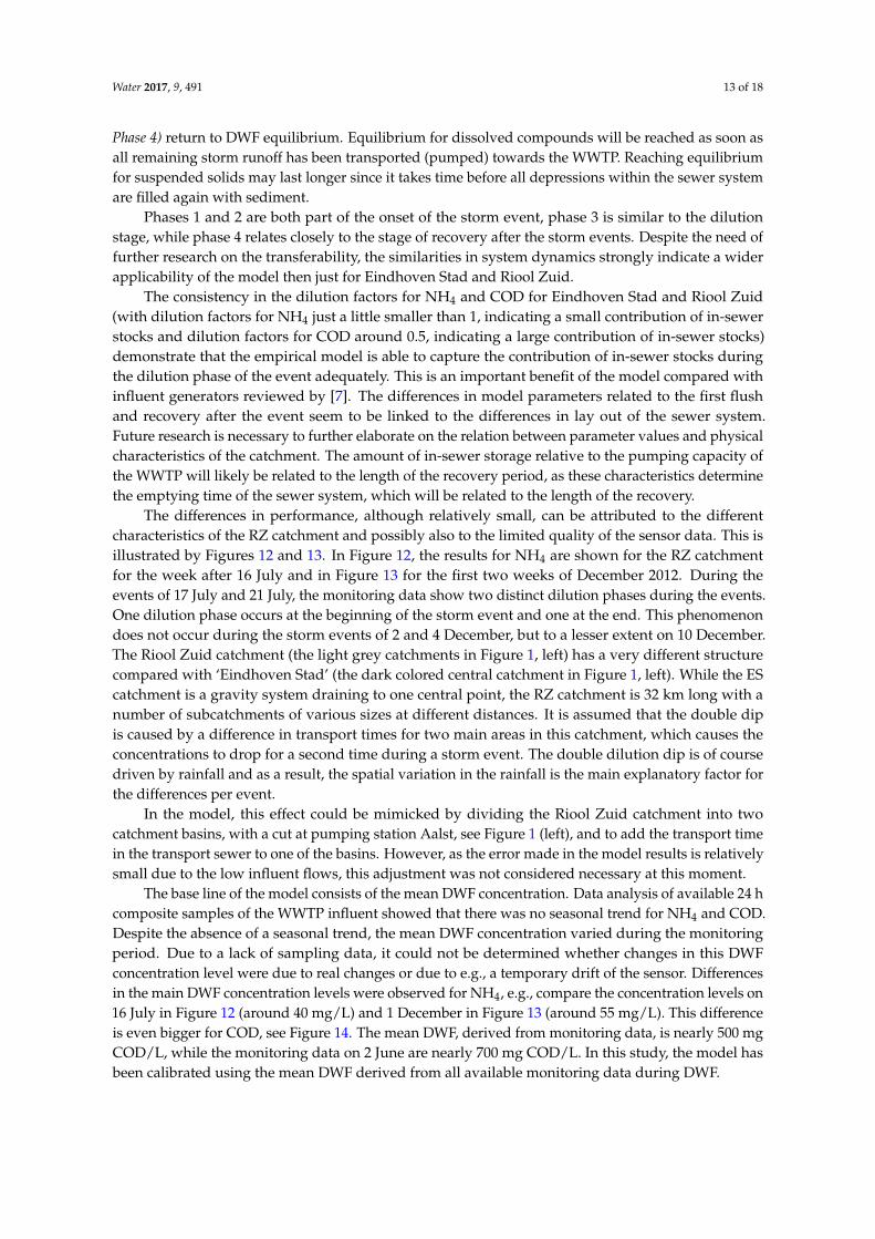
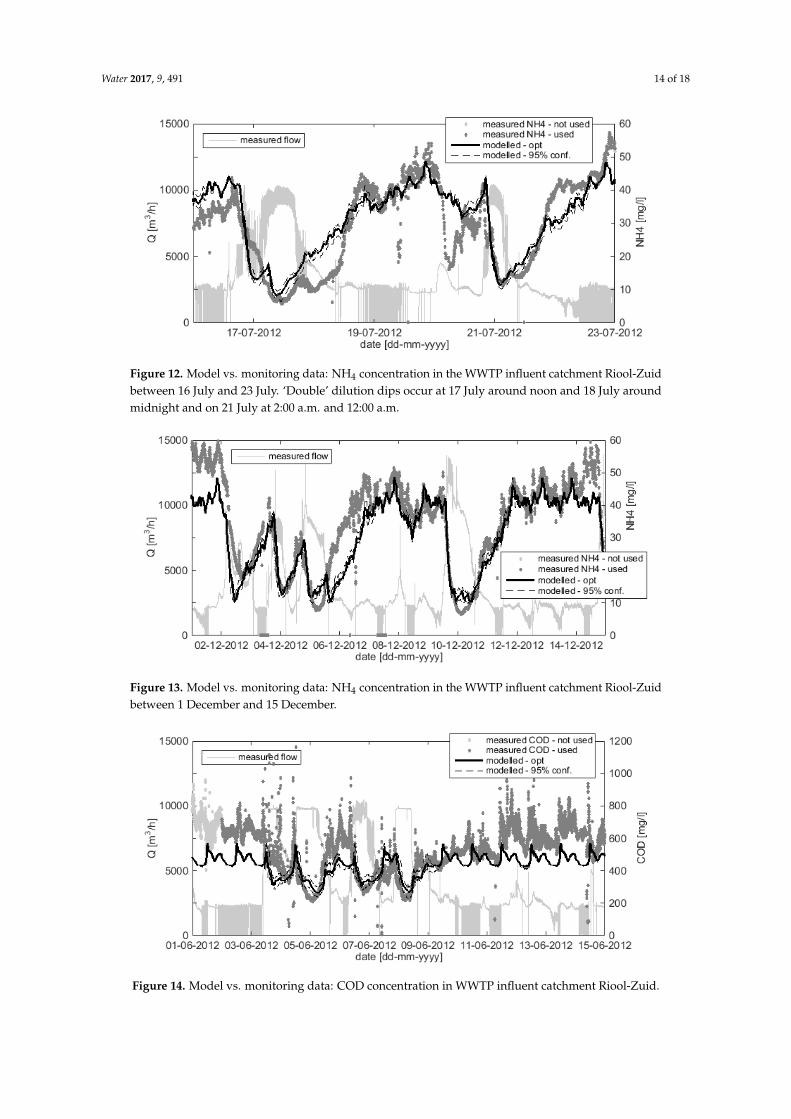
The differences in performance, although relatively small, can be attributed to the differentcharacteristics of the RZ catchment and possibly also to the limited quality of the sensor data. This isillustrated by Figures 12 and 13. In Figure 12, the results for NH4 are shown for the RZ catchmentfor the week after 16 July and in Figure 13 for the first two weeks of December 2012. During theevents of 17 July and 21 July, the monitoring data show two distinct dilution phases during the events.One dilution phase occurs at the beginning of the storm event and one at the end. This phenomenondoes not occur during the storm events of 2 and 4 December, but to a lesser extent on 10 December.The Riool Zuid catchment (the light grey catchments in Figure 1, left) has a very different structurecompared with ‘Eindhoven Stad’ (the dark colored central catchment in Figure 1, left). While the EScatchment is a gravity system draining to one central point, the RZ catchment is 32 km long with anumber of subcatchments of various sizes at different distances. It is assumed that the double dipis caused by a difference in transport times for two main areas in this catchment, which causes theconcentrations to drop for a second time during a storm event. The double dilution dip is of coursedriven by rainfall and as a result, the spatial variation in the rainfall is the main explanatory factor forthe differences per event.

In the model, this effect could be mimicked by dividing the Riool Zuid catchment into twocatchment basins, with a cut at pumping station Aalst, see Figure 1 (left), and to add the transport timein the transport sewer to one of the basins. However, as the error made in the model results is relativelysmall due to the low influent flows, this adjustment was not considered necessary at this moment.

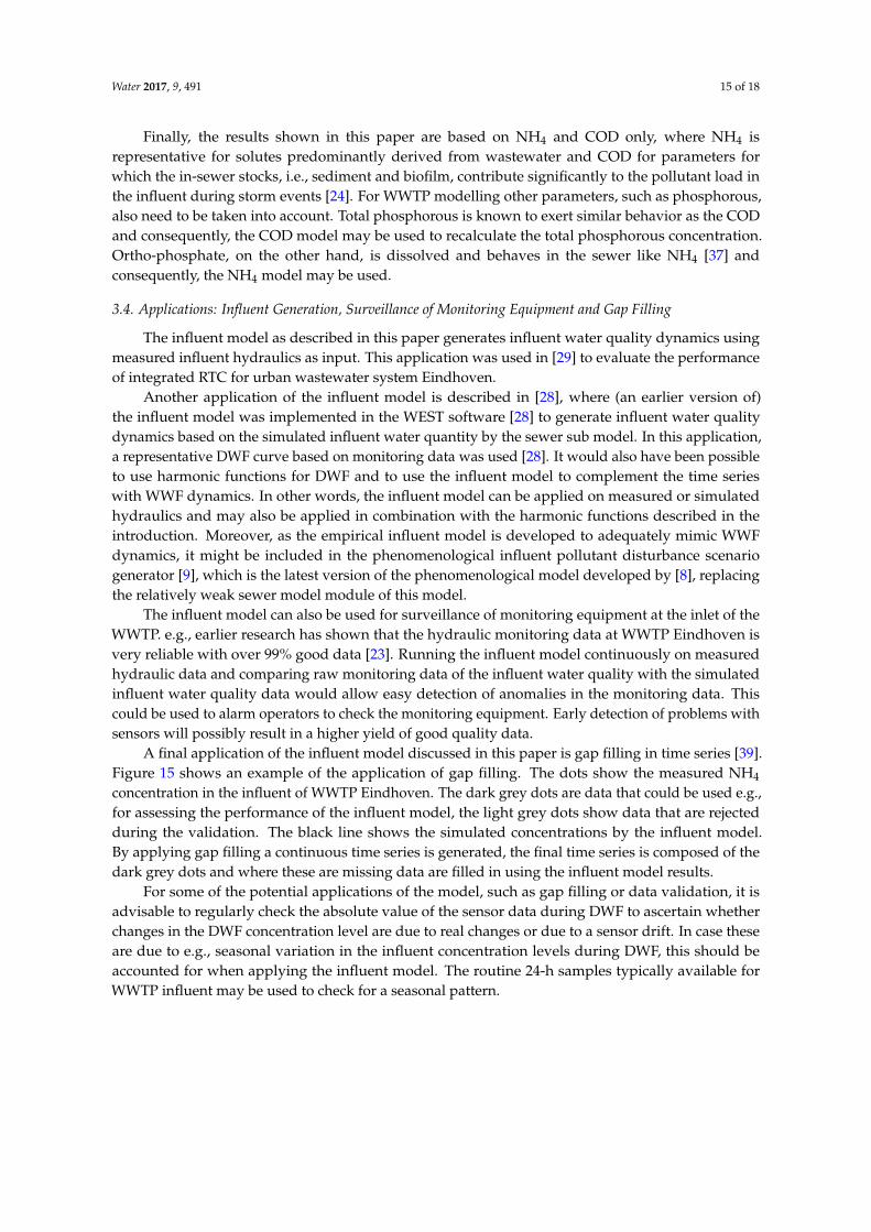
The base line of the model consists of the mean DWF concentration. Data analysis of available 24 hcomposite samples of the WWTP influent showed that there was no seasonal trend for NH4 and COD.Despite the absence of a seasonal trend, the mean DWF concentration varied during the monitoringperiod. Due to a lack of sampling data, it could not be determined whether changes in this DWFconcentration level were due to real changes or due to e.g., a temporary drift of the sensor. Differencesin the main DWF concentration levels were observed for NH4, e.g., compare the concentration levels on16 July in Figure 12 (around 40 mg/L) and 1 December in Figure 13 (around 55 mg/L). This differenceis even bigger for COD, see Figure 14. The mean DWF, derived from monitoring data, is nearly 500 mgCOD/L, while the monitoring data on 2 June are nearly 700 mg COD/L. In this study, the model hasbeen calibrated using the mean DWF derived from all available monitoring data during DWF.

Water 2017, 9, 491 14 of 18Water 2017, 9, 491 14 of 18

Figure 12. Model vs. monitoring data: NH4 concentration in the WWTP influent catchment Riool-Zuid between 16 July and 23 July. ‘Double’ dilution dips occur at 17 July around noon and 18 July around midnight and on 21 July at 2:00 a.m. and 12:00 a.m.

Figure 13. Model vs. monitoring data: NH4 concentration in the WWTP influent catchment Riool-Zuid between 1 December and 15 December.

Figure 14. Model vs. monitoring data: COD concentration in WWTP influent catchment Riool-Zuid.

Figure 12. Model vs. monitoring data: NH4 concentration in the WWTP influent catchment Riool-Zuidbetween 16 July and 23 July. ‘Double’ dilution dips occur at 17 July around noon and 18 July aroundmidnight and on 21 July at 2:00 a.m. and 12:00 a.m.

Water 2017, 9, 491 14 of 18

Figure 12. Model vs. monitoring data: NH4 concentration in the WWTP influent catchment Riool-Zuid between 16 July and 23 July. ‘Double’ dilution dips occur at 17 July around noon and 18 July around midnight and on 21 July at 2:00 a.m. and 12:00 a.m.

Figure 13. Model vs. monitoring data: NH4 concentration in the WWTP influent catchment Riool-Zuid between 1 December and 15 December.

Figure 14. Model vs. monitoring data: COD concentration in WWTP influent catchment Riool-Zuid.

Figure 13. Model vs. monitoring data: NH4 concentration in the WWTP influent catchment Riool-Zuidbetween 1 December and 15 December.

Water 2017, 9, 491 14 of 18

Figure 12. Model vs. monitoring data: NH4 concentration in the WWTP influent catchment Riool-Zuid between 16 July and 23 July. ‘Double’ dilution dips occur at 17 July around noon and 18 July around midnight and on 21 July at 2:00 a.m. and 12:00 a.m.

Figure 13. Model vs. monitoring data: NH4 concentration in the WWTP influent catchment Riool-Zuid between 1 December and 15 December.

Figure 14. Model vs. monitoring data: COD concentration in WWTP influent catchment Riool-Zuid. Figure 14. Model vs. monitoring data: COD concentration in WWTP influent catchment Riool-Zuid.

Water 2017, 9, 491 15 of 18

Finally, the results shown in this paper are based on NH4 and COD only, where NH4 isrepresentative for solutes predominantly derived from wastewater and COD for parameters forwhich the in-sewer stocks, i.e., sediment and biofilm, contribute significantly to the pollutant load inthe influent during storm events [24]. For WWTP modelling other parameters, such as phosphorous,also need to be taken into account. Total phosphorous is known to exert similar behavior as the CODand consequently, the COD model may be used to recalculate the total phosphorous concentration.Ortho-phosphate, on the other hand, is dissolved and behaves in the sewer like NH4 [37] andconsequently, the NH4 model may be used.

3.4. Applications: Influent Generation, Surveillance of Monitoring Equipment and Gap Filling

The influent model as described in this paper generates influent water quality dynamics usingmeasured influent hydraulics as input. This application was used in [29] to evaluate the performanceof integrated RTC for urban wastewater system Eindhoven.

Another application of the influent model is described in [28], where (an earlier version of)the influent model was implemented in the WEST software [28] to generate influent water qualitydynamics based on the simulated influent water quantity by the sewer sub model. In this application,a representative DWF curve based on monitoring data was used [28]. It would also have been possibleto use harmonic functions for DWF and to use the influent model to complement the time serieswith WWF dynamics. In other words, the influent model can be applied on measured or simulatedhydraulics and may also be applied in combination with the harmonic functions described in theintroduction. Moreover, as the empirical influent model is developed to adequately mimic WWFdynamics, it might be included in the phenomenological influent pollutant disturbance scenariogenerator [9], which is the latest version of the phenomenological model developed by [8], replacingthe relatively weak sewer model module of this model.

The influent model can also be used for surveillance of monitoring equipment at the inlet of theWWTP. e.g., earlier research has shown that the hydraulic monitoring data at WWTP Eindhoven isvery reliable with over 99% good data [23]. Running the influent model continuously on measuredhydraulic data and comparing raw monitoring data of the influent water quality with the simulatedinfluent water quality data would allow easy detection of anomalies in the monitoring data. Thiscould be used to alarm operators to check the monitoring equipment. Early detection of problems withsensors will possibly result in a higher yield of good quality data.

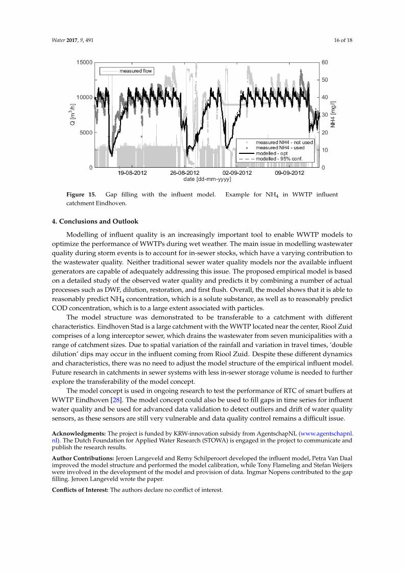
A final application of the influent model discussed in this paper is gap filling in time series [39].Figure 15 shows an example of the application of gap filling. The dots show the measured NH4

concentration in the influent of WWTP Eindhoven. The dark grey dots are data that could be used e.g.,for assessing the performance of the influent model, the light grey dots show data that are rejectedduring the validation. The black line shows the simulated concentrations by the influent model.By applying gap filling a continuous time series is generated, the final time series is composed of thedark grey dots and where these are missing data are filled in using the influent model results.

For some of the potential applications of the model, such as gap filling or data validation, it isadvisable to regularly check the absolute value of the sensor data during DWF to ascertain whetherchanges in the DWF concentration level are due to real changes or due to a sensor drift. In case theseare due to e.g., seasonal variation in the influent concentration levels during DWF, this should beaccounted for when applying the influent model. The routine 24-h samples typically available forWWTP influent may be used to check for a seasonal pattern.

Water 2017, 9, 491 16 of 18Water 2017, 9, 491 16 of 18

Figure 15. Gap filling with the influent model. Example for NH4 in WWTP influent catchment Eindhoven.

4. Conclusions and Outlook

Modelling of influent quality is an increasingly important tool to enable WWTP models to optimize the performance of WWTPs during wet weather. The main issue in modelling wastewater quality during storm events is to account for in-sewer stocks, which have a varying contribution to the wastewater quality. Neither traditional sewer water quality models nor the available influent generators are capable of adequately addressing this issue. The proposed empirical model is based on a detailed study of the observed water quality and predicts it by combining a number of actual processes such as DWF, dilution, restoration, and first flush. Overall, the model shows that it is able to reasonably predict NH4 concentration, which is a solute substance, as well as to reasonably predict COD concentration, which is to a large extent associated with particles.

The model structure was demonstrated to be transferable to a catchment with different characteristics. Eindhoven Stad is a large catchment with the WWTP located near the center, Riool Zuid comprises of a long interceptor sewer, which drains the wastewater from seven municipalities with a range of catchment sizes. Due to spatial variation of the rainfall and variation in travel times, ‘double dilution’ dips may occur in the influent coming from Riool Zuid. Despite these different dynamics and characteristics, there was no need to adjust the model structure of the empirical influent model. Future research in catchments in sewer systems with less in-sewer storage volume is needed to further explore the transferability of the model concept.

The model concept is used in ongoing research to test the performance of RTC of smart buffers at WWTP Eindhoven [28]. The model concept could also be used to fill gaps in time series for influent water quality and be used for advanced data validation to detect outliers and drift of water quality sensors, as these sensors are still very vulnerable and data quality control remains a difficult issue.

Acknowledgments: The project is funded by KRW-innovation subsidy from AgentschapNL (www.agentschapnl.nl). The Dutch Foundation for Applied Water Research (STOWA) is engaged in the project to communicate and publish the research results.

Author Contributions: Jeroen Langeveld and Remy Schilperoort developed the influent model, Petra Van Daal improved the model structure and performed the model calibration, while Tony Flameling and Stefan Weijers were involved in the development of the model and provision of data. Ingmar Nopens contributed to the gap filling. Jeroen Langeveld wrote the paper.

Conflicts of Interest: The authors declare no conflict of interest.

Figure 15. Gap filling with the influent model. Example for NH4 in WWTP influentcatchment Eindhoven.

4. Conclusions and Outlook

Modelling of influent quality is an increasingly important tool to enable WWTP models tooptimize the performance of WWTPs during wet weather. The main issue in modelling wastewaterquality during storm events is to account for in-sewer stocks, which have a varying contribution tothe wastewater quality. Neither traditional sewer water quality models nor the available influentgenerators are capable of adequately addressing this issue. The proposed empirical model is basedon a detailed study of the observed water quality and predicts it by combining a number of actualprocesses such as DWF, dilution, restoration, and first flush. Overall, the model shows that it is able toreasonably predict NH4 concentration, which is a solute substance, as well as to reasonably predictCOD concentration, which is to a large extent associated with particles.

The model structure was demonstrated to be transferable to a catchment with differentcharacteristics. Eindhoven Stad is a large catchment with the WWTP located near the center, Riool Zuidcomprises of a long interceptor sewer, which drains the wastewater from seven municipalities with arange of catchment sizes. Due to spatial variation of the rainfall and variation in travel times, ‘doubledilution’ dips may occur in the influent coming from Riool Zuid. Despite these different dynamicsand characteristics, there was no need to adjust the model structure of the empirical influent model.Future research in catchments in sewer systems with less in-sewer storage volume is needed to furtherexplore the transferability of the model concept.

The model concept is used in ongoing research to test the performance of RTC of smart buffers atWWTP Eindhoven [28]. The model concept could also be used to fill gaps in time series for influentwater quality and be used for advanced data validation to detect outliers and drift of water qualitysensors, as these sensors are still very vulnerable and data quality control remains a difficult issue.

Acknowledgments: The project is funded by KRW-innovation subsidy from AgentschapNL (www.agentschapnl.nl). The Dutch Foundation for Applied Water Research (STOWA) is engaged in the project to communicate andpublish the research results.

Author Contributions: Jeroen Langeveld and Remy Schilperoort developed the influent model, Petra Van Daalimproved the model structure and performed the model calibration, while Tony Flameling and Stefan Weijerswere involved in the development of the model and provision of data. Ingmar Nopens contributed to the gapfilling. Jeroen Langeveld wrote the paper.

Conflicts of Interest: The authors declare no conflict of interest.

Water 2017, 9, 491 17 of 18

References

1. Benedetti, L.; De Baets, B.; Nopens, I.; Vanrolleghem, P.A. Multi-criteria analysis of wastewater treatmentplant design and control scenarios under uncertainty. Environ. Model. Softw. 2010, 25, 616–621. [CrossRef]

2. Rieger, L.; Gillot, S.; Langergraber, G.; Ohtsuki, T.; Shaw, A.; Takács, I.; Winkler, S. Guidelines for UsingActivated Sludge Models. In IWA Scientific and Technical Report No. 22; IWA Publishing: London, UK, 2012.

3. Rodriguez-Roda, I.; Sànchez-Marrè, M.; Comas, J.; Baeza, J.; Colprim, J.; Lafuente, J.; Cortes, U.; Poch, M.A hybrid supervisory system to support WWTP operation: Implementation and validation. Water Sci. Technol.2002, 45, 289–297. [PubMed]

4. Flores-Alsina, X.; Rodríguez-Roda, I.; Sin, G.; Gernaey, K. Multi-criteria evaluation of wastewater treatmentplant control strategies under uncertainty. Water Res. 2008, 42, 4485–4497. [CrossRef] [PubMed]

5. Nopens, I.; Benedetti, L.; Jeppsson, U.; Pons, M.N.; Alex, J.; Copp, J.B.; Gernaey, K.V.; Rosen, C.; Steyer, J.P.;Vanrolleghem, P.A. Benchmark simulation model No 2: Finalisation of plant layout and default controlstrategy. Water Sci. Technol. 2010, 62, 1967–1974. [CrossRef] [PubMed]

6. Maruejouls, T.; Lessard, P.; Wipliez, B.; Pelletier, G.; Vanrolleghem, P.A. A phenomenological retention tankmodel using settling velocity distributions. Water Res. 2012, 46, 6857–6867. [CrossRef] [PubMed]

7. Martin, C.; Vanrolleghem, P.A. Analysing, completing, and generating influent data for WWTP modelling: Acritical review. Environ. Model. Softw. 2014, 60, 188–201. [CrossRef]

8. Gernaey, K.V.; Flores-Alsina, X.; Rosen, C.; Benedetti, L.; Jeppsson, U. Dynamic influent pollutant disturbancescenario generation using a phenomenological modelling approach. Environ. Model. Softw. 2011, 26,1255–1267. [CrossRef]

9. Flores-Alsina, X.; Saagi, R.; Lindblom, E.; Thirsing, C.; Thornberg, D.; Gernaey, K.V.; Jeppsson, U. Calibrationand validation of a phenomenological influent pollutant disturbance scenario generator using full-scale data.Water Res. 2014, 51, 172–185. [CrossRef] [PubMed]

10. De Keyser, W.; Gevaert, V.; Verdonck, F.; De Baets, B.; Benedetti, L. An emission time series generator forpollutant release modelling in urban areas. Environ. Model. Softw. 2010, 25, 554–561. [CrossRef]

11. Devisscher, M.; Ciacci, G.; Fé, L.; Benedetti, L.; Bixio, D.; Thoeye, C.; De Gueldre, G.; Marsili-Libelli, S.;Vanrolleghem, P.A. Estimating costs and benefits of advanced control for wastewater treatment plants—TheMAgIC methodology. Water Sci. Technol. 2006, 53, 215–223. [CrossRef] [PubMed]

12. Talebizadeh, M.; Belia, E.; Vanrolleghem, P.A. Influent generator for probabilistic modeling of nutrientremoval wastewater treatment plants. Environ. Model. Softw. 2016, 77, 32–49. [CrossRef]

13. Bertrand-Krajewski, J.-L. Stormwater pollutant loads modelling: Epistemological aspects and case studieson the influence of field data sets on calibration and verification. Water Sci. Technol. 2007, 55, 1–17. [CrossRef][PubMed]

14. Bertrand-Krajewski, J.-L.; Briat, P.; Scrivener, O. Sewer sediment production and transport modelling: Aliterature review. J. Hydraul. Res. 1993, 31, 435–460. [CrossRef]

15. Bertrand-Krajewski, J.-L.; Chebbo, G.; Saget, A. Distribution of pollutant mass vs volume in stormwaterdischarges and the first flush phenomenon. Water Res. 1998, 32, 2341–2356. [CrossRef]

16. Ashley, R.M.; Bertrand-Krajewski, J.L.; Hvitved-Jacobsen, T.; Verbanck, M. Solids in-Sewers; IWA Publishing:London, UK, 2004.

17. Ashley, R.M.; Hvitved-Jacobsen, T.; Bertrand-Krajewski, J.-L. Quo vadis sewer process modelling? Water Sci.Technol. 1999, 39, 9–22. [CrossRef]

18. Willems, P. Random number generator or sewer water quality model? Water Sci. Technol. 2006, 54, 387–394.[CrossRef] [PubMed]

19. Willems, P. Parsimonious model for combined sewer overflow pollution. J. Environ. Eng. 2010, 136, 316–325.[CrossRef]

20. Dembélé, A.; Bertrand-Krajewski, J.-L.; Becouze, C.; Barillon, B. A new empirical model for stormwater TSSevent mean concentrations (EMCs). Water Sci. Technol. 2011, 64, 1926–1934. [CrossRef] [PubMed]

21. Rousseau, D.; Verdonck, F.; Moerman, O.; Carrette, R.; Thoeye, C.; Meirlaen, J.; Vanrolleghem, P.A.Development of a risk assessment based technique for design/retrofitting of WWTPs. Water Sci. Technol.2001, 43, 287–294. [PubMed]

22. Gruber, G.; Winkler, S.; Pressl, A. Quantification of pollution loads from CSOs into surface water bodies bymeans of online techniques. Water Sci. Technol. 2004, 50, 73–80. [PubMed]

Water 2017, 9, 491 18 of 18

23. Schilperoort, R.P.S. Monitoring as a Tool for the Assessment of Wastewater Quality Dynamics. Ph.D. Thesis,Delft University of Technology, Delft, The Netherlands, 2011.

24. Schilperoort, R.P.S.; Dirksen, J.; Langeveld, J.G.; Clemens, F.H.L.R. Assessing characteristic time and spacescales of in-sewer processes by analysis of one year of continuous in-sewer monitoring data. Water Sci. Technol.2012, 66, 1614–1620. [CrossRef] [PubMed]

25. 2000/60/EC. Directive of the European Parliament and of the Council Establishing a Framework forCommunity Action in the Field of Water Policy (2000/60/EC). 23 October 2000. Available online: http://eur-lex.europa.eu (accessed on 3 July 2017).

26. Weijers, S.R.; de Jonge, J.; van Zanten, O.; Benedetti, L.; Langeveld, J.; Menkveld, H.W.; vanNieuwenhuijzen, A.F. KALLISTO: Cost Effective and Integrated Optimization of the Urban WastewaterSystem Eindhoven. Water Pract. Technol. 2012, 7. [CrossRef]

27. Benedetti, L.; Langeveld, J.; van Nieuwenhuijzen, A.F.; de Jonge, J.; de Klein, J.J.M.; de Flameling, T.;Nopens, I.; van Zanten, O.; Weijers, S. Cost-effective solutions for water quality improvement in theDommel River supported by sewer-WWTP-river integrated modelling. Water Sci. Technol. 2013, 68, 965–973.[CrossRef] [PubMed]

28. Langeveld, J.G.; Benedetti, L.; de Klein, J.J.M.; Nopens, I.; Amerlinck, Y.; van Nieuwenhuijzen, A.;Flameling, T.; van Zanten, O.; Weijers, S. Impact-based integrated real-time control for improvement of theDommel River water quality. Urban Water J. 2013, 10, 312–329. [CrossRef]

29. Daal-Rombouts, P.; van Benedetti, L.; de Jonge, J.; Weijers, S.; Langeveld, J. Performance evaluation of asmart buffer control at a wastewater treatment plant. Water Res. 2017. submit (under review).

30. Vrugt, J.A.; Ter Braak, C.J.F.; Clark, M.P.; Hyman, J.M.; Robinson, B.A. Treatment of input uncertaintyin hydrologic modeling: Doing hydrology backward with Markov chain Monte Carlo simulation.Water Resour. Res. 2008, 44, 1–15. [CrossRef]

31. Vrugt, J.A.; Ter Braak, C.J.F.; Gupta, H.V.; Robinson, B.A. Equifinality of formal (DREAM) and informal(GLUE) Bayesian approaches in hydrologic modeling? Stoch. Environ. Res. Risk Assess. 2009, 23, 1011–1026.[CrossRef]

32. Keating, E.H.; Doherty, J.; Vrugt, J.A.; Kang, Q. Optimization and uncertainty assessment of stronglynonlinear groundwater models with high parameter dimensionality. Water Resour. Res. 2010, 46, 1–8.[CrossRef]

33. Leonhardt, G.; Sun, S.; Rauch, W.; Bertrand-Krajewski, J.-L. Comparison of two model based approaches forareal rainfall estimation in urban hydrology. J. Hydrol. 2014, 511, 880–890. [CrossRef]

34. Van Daal-Rombouts, P.; Sun, S.; Langeveld, J.; Bertrand-Krajewski, J.-L.; Clemens, F. Design and performanceevaluation of a simplified dynamic model for combined sewer overflows in pumped sewer systems. J. Hydrol.2016, 538, 609–624. [CrossRef]

35. Langeveld, J.G.; Clemens, F.H.L.R.; Van Der Graaf, J.H.J.M. Interactions within the wastewater system:Requirements for sewer processes modelling. Water Sci. Technol. 2003, 47, 101–108. [PubMed]

36. Boogaard, F.; Lemmen, G. STOWA Stormwater Database: The Facts about the Quality of Stormwater Runoff ;STOWA 2007-21; STOWA: Amersfoort, The Netherlands, 2007. (In Dutch)

37. Krebs, P.; Merkel, K.; Kühn, V. Dynamic Changes in Wastewater Composition during Rain Runoff.In Proceedings of the 8ICUSD, Sydney, Australia, 30 August–3 September 1999; pp. 920–927.

38. Bruns, J.; von Regenwasserbehandlung, D.K.; bei Mischwasserzufluss, A. Stuttgarter Berichte zurSiedlungswasserwirtschaft; Bd. 151. (Stuttgart, Univ. Diss., 1998); Oldenbourg: München, Germany, 1999.

39. De Mulder, C.; Flameling, T.; Langeveld, J.; Amerlinck, Y.; Weijers, S.; Nopens, I. Automating the Raw Datato Model Input Process Using Flexible Open Source Tools. In Proceedings of the Frontiers InternationalConference on Wastewater Treatment, Palermo, Italy, 21–24 May 2017.

© 2017 by the authors. Licensee MDPI, Basel, Switzerland. This article is an open accessarticle distributed under the terms and conditions of the Creative Commons Attribution(CC BY) license (http://creativecommons.org/licenses/by/4.0/).