Empirical Evaluation of Workload ForecastingTechniques for Predictive Cloud Resource Scaling

In Kee Kim, Wei Wang, Yanjun Qi, and Marty HumphreyDepartment of Computer Science

University of Virginia{ik2sb, wwang}@virginia.edu, {yq2h, humphrey}@cs.virginia.edu

Abstract—Many predictive resource scaling approaches havebeen proposed to overcome the limitations of the conventionalreactive approaches most often used in clouds today. In general,due to the complexity of clouds, these reactive approaches wereoften forced to make significant limiting assumptions in eitherthe operating conditions/requirements or expected workloadpatterns. As such, it is extremely difficult for cloud users toknow which – if any – existing workload predictor will work bestfor their particular cloud activity, especially when consideringhighly-variable workload patterns, non-trivial billing models,variety of resources to add/subtract, etc. To solve this problem,we conduct comprehensive evaluations for a variety of workloadpredictors under real-world cloud configurations. The workloadpredictors cover four classes of 21 predictors: naive, regression,temporal, and non-temporal methods. We simulate a cloudapplication under four realistic workload patterns, two differentcloud billing models, and three different styles of predictivescaling. Our evaluation confirms that no workload predictoris universally best for all workload patterns, and shows thatPredictive Scaling-out + Predictive Scaling-in has the best costefficiency and the lowest job deadline miss rate in cloud resourcemanagement, on average providing 30% better cost efficiencyand 80% less job deadline miss rate compared to other styles ofpredictive scaling.

Index Terms—Predictive Cloud Resource Scaling; CloudWorkload Prediction; Job Arrival Time Prediction; PerformanceEvaluation;

I. INTRODUCTION

When and how to scale-out and scale-in a cloud applicationcan be one of the most difficult challenges for a cloud appli-cation designer/deployer. Fundamentally, basing this decisionon the current state of resources (e.g., VMs) for a given cloudapplication is usually simple and can be effective but is limiteddue to its reactive nature. For example, a standard use ofAmazon Web Services’ auto-scaling mechanism is to configureit to add more “worker VMs” when the average current CPUutilization stays above a certain threshold for a short periodtime. However, fluctuating or generally unpredictable work-load patterns can quickly eliminate any potential performanceor monetary improvements of such a policy/mechanism. Inother words, intuitively any changes to the cloud applicationsystem state/configuration assume that the near-past workloadwill continue for the near-future.

Next-generation scaling approaches attempt to move beyondthe limitations of such reactive systems by instead attempt-ing to predict the near-future workloads. In such systems,generally, there are two components. The workload predictor

functionality, and the resource scaling functionality, whichallocates/deallocates cloud resources and maps work requeststo specific resources. Over the past years, many studies haveproposed predictive scaling approaches [1–19]. In general, dueto the complexity of cloud environments, these approacheswere often forced to make significant limiting assumptionsin either the operating conditions/requirements or expectedworkload patterns. As such, it is extremely difficult for cloudusers to know which – if any – existing workload predictorwill work best for their particular cloud activity, especiallywhen considering highly-variable workload patterns, non-trivial billing models, variety of resources to add/subtract, etc.

The goal of this work is to comprehensively evaluateexisting cloud workload predictors, holistically, and often in abroader context than in the authors’ evaluation methodology.Because the most common metric to evaluate workload pre-dictors is accuracy for the future job arrivals, the first questionwe seek to answer is:

Question #1: Which existing workload predictor has thehighest accuracy for job arrival time prediction, when appliedfor different workload patterns?

After considering the workload predictor in isolation, weevaluate it in combination with the resource scaling compo-nent. Therefore, the second question we seek to answer is:

Question #2: Which existing workload predictor has thebest cost efficiency and deadline miss rate (which representsperformance and SLA requirements), when applied for differ-ent workload patterns, different scaling styles and differentpricing models?

Furthermore, some previous work employed predictivescaling-out, some employed predictive scaling-in, and someemployed both. Given these choices of applying predictivescaling, the third question we seek to answer is:

Question #3: Which style of predictive scaling (predictivescaling-out, predictive scaling-in, or both) achieves the bestcost and performance benefit for particular cloud configura-tions (e.g. billing model, job deadline)? And how much benefitcan be achieved?

To answer these questions, we conducted comprehensiveevaluations with a wide range of configurations of predictivecloud resource scaling using 15 existing workload predictors[5–19]. We also included 6 well-known machine learningpredictors that have not been used for the predictive scalingbefore. In total, we examined 21 predictors, covering naive,

1

regression, temporal (time series) and non-temporal methods.We used 24 randomly generated workloads covering fourcommon types of job arrival patterns [20, 21], which aregrowing, on/off, bursty and random. We also examined scalingoperations including RR (Scaling-out: Reactive + Scaling-in:Reactive), PR (Scaling-out: Predictive + Scaling-in: Reactive),RP (Scaling-out: Reactive + Scaling-in: Predictive) and PP(Scaling-out: Predictive + Scaling-in: Predictive). We alsoconsidered both hourly and minutely pricing models. In ourexperiments, each configuration then covered one workloadpredictor, one workload, one scaling operation and one billingmodel. As a result, more than 4K (21 ⇥ 24 ⇥ 4 ⇥ 2) config-urations were examined. We run each configuration using thePICS [22] simulators to evaluate each configuration’s cost anddeadline miss rate. We chose PICS because it can accuratelysimulate real public IaaS clouds in short amount of time.Without PICS, it is both timely and financially infeasible toconduct such extensive experiments on real IaaS clouds

Based on the experimental results, we successfully answerthe three questions posed previously. Here we summarize ourfindings and answers to each question:

To find the best workload predictor in terms of theaccuracy for diverse workload patterns (Question #1): theaccuracies of different workload predictors vary considerably.The best workload predictors in terms of statistical accuracyare usually orders of magnitudes more accurate than the worstones. However, no workload predictor is universally the bestfor all workload patterns. Each workload pattern has its ownbest workload predictor. We show the best workload predictorsfor each workload pattern in Section IV-A.

To find the best workload predictor in terms of cloudmetrics such as cost efficiency and SLA satisfaction (Ques-tion #2): the workload predictor with the highest accuracy isnot necessarily the best in terms of cost and deadline miss rate.Additionally, no workload predictor is universally the best forany workload pattern and billing model. However, we observethat the best predictor (in terms of cost and deadline miss rate)for a particular workload pattern is always one of the top3 most accurate predictors (in terms of statistical accuracy)of that workload pattern. We also show the best workloadpredictors for each workload pattern in terms of cloud metricsin Section IV-B.

To find the best style of predictive resource scalingin terms of providing the best cost and performancebenefits (Question #3): both predictive scaling-out (PR) andpredictive scaling-in/out (PP) significantly reduces cost anddeadline miss rate over purely reactive scaling (RR). However,predictive scaling-in (RP) performs similarly to RR. Overall,PP always provides the lowest cost and deadline miss ratefor all workload patterns and billing models. On average,PP provides 30% less cost and 80% less deadline miss ratecompared to RR or RP, and PP offers 14% less cost and 39%less deadline miss rate compared to PR.

A key finding from the answering those questions is thatusers, who want to design new algorithm for predictive re-source scaling, should consider top 3 workload predictors

depending on workload patterns, and use PP for their scal-ing operations in order to archive better cost efficiency anddeadline miss rate.

The contributions of this paper include:

• An extensive evaluation of 21 workload predictors fortheir accuracy to predict the future job arrival time.

• A comprehensive evaluation of workload predictors interms of cost and deadline miss rates. This evaluationconsiders various workload patterns, three styles of scal-ing operations, and two different billing models.

• Complete answers for the questions regarding what isthe best workload predictor and what is the best style forpredictive resource scaling operations.

The rest of this paper is organized as follows: Section IIdescribes workload predictors used in this work. Section IIIcontains the experimental design of this work. Section IV pro-vides evaluation results for all predictors. Section V containsrelated work and Section VI concludes this paper.

II. WORKLOAD PREDICTORS

We collect a total of 21 workload predictors via an extensivesurvey of previous research on predictive resource scaling.Each predictor is categorized into one of the following classes:1) naive, 2) regression, 3) temporal, and 4) non-temporal pre-dictor. The detailed description for all 21 workload predictorsis described in Table I.

1. Naive workload predictors: two types workload predic-tors are included in this class – mean and recent mean-based(kNN – k Nearest Neighbor) methods.

2. Regression-based workload predictors: the predictorsin this class can be split into category of global and localregressions. Each category can include linear (1-degree) orpolynomial (2 or more degrees) models. In total, we usesix regression-based predictors, which are global and localregression with linear, quadratic, and cubic models [23].

3. Temporal (Time-Series)-based Workload Predictors:there exist various temporal (time-series) methods for thefuture workload prediction because these predictors [5–15,18, 19, 24] are widely used to analyze workload patternsfor cloud computing as well as other domains of computersystems research. We use four categories of temporal models:ES (Exponential Smoothing), AR (Autoregressive), ARMA(Autoregressive and Moving Average), and ARIMA (Autore-gressive Integrated Moving Average) [1, 3, 8–15, 19].

4. Non-temporal Workload Predictors: the predictors inthis class have not been applied to the cloud resource scalingbefore. These predictors, however, have provided accurateprediction results within a deterministic amount of time. Weconsider several non-temporal approaches to predict the nextjob arrival time and select three categories of non-temporalprediction approaches: SVMs (Support Vector Machines),decision tree, and ensemble methods [23].

2

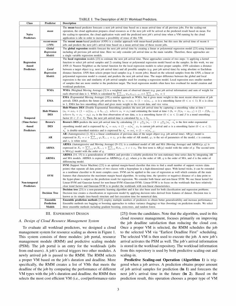
TABLE I: The Description of All 21 Workload Predictors.Class Predictor Description

The mean-based predictor forecasts a next job arrival time based on a mean arrival time of all previous jobs. For the scaling-outmean operation, the cloud application prepares cloud resources as if the next job will be arrived at the predicted result based on mean. For

Naive the scaling-in operation, the cloud application waits until the predicted next job’s arrival time when a VM running by the cloudPredictors application is idle in order to increase a possibility of reuse of this VM.

recent-mean The recent mean-based predictor (kNN) is a similar approach with mean-based predictor, but this uses the arrival time of recent k(kNN) jobs and predicts the next job’s arrival time based on a mean arrival time of those recent jobs.Global The global regression models forecast the next job arrival time by creating a linear or polynomial regression model [23] using features

Regression including all previous job arrival time. Here we only consider job arrival time as the main variable. Therefore, these approaches areModels a single variable regression models.

The local regression models [23] to estimate the next job arrival time. These approaches consist of two steps: 1) applying a kernelRegression function to select job arrival samples and 2) creating linear or polynomial regression model based on the samples. In this work, we use

-based kNN (k Nearest Neighbor) as the kernel function for the local regression models to select proper samples. kNN calculates a distancePredictors Local between a target object (e.g. next job arrival time) and all possible samples (e.g. past job arrival time) by using absolute or Euclidean

Regression distance function. kNN then selects proper local samples (e.g. k recent jobs). Based on the selected samples from the kNN, a linear orModels polynomial regression model is created, and predicts the next job arrival time. The major difference between the global and local

regression is the size and similarity of job arrival samples used for creating a regression model. Local regression uses smaller numberof samples that are more similar to the prediction target. The local regression models often have less overhead for model creation andworkload prediction.

WMA WMA (Weighted Moving Average) [3] is a weighted sum of observed dataset (e.g. past job arrival information) and sum of weight foreach observed data is 1. WMA is calculated by

Pkn=1 wnxt+1�n, s.t.

Pkn=1 wn = 1

EMA (Exponential Moving Average) [19] a similar approach as WMA, but it gives more weight to the most recent observation of jobEMA arrivals. EMA predicts the future job arrival time by st = ↵xt + (1 � ↵)st�1. ↵ is a smoothing factor (0 < ↵ < 1). If ↵ is close

to 1, EMA has less smoothing effect and gives more weight to the recent data, and vice versa.Holt-Winters DES (Double Exponential Smoothing) predicts the next job arrival time by capturing a smoothing value at time t

Holt-Winters (st = ↵xt + (1 � ↵)(st�1 + bt�1), where s1 = x1) and estimating the trend at time t (bt = �(st � st�1) + (1 � �)bt�1,

DES where b1 = x1 � x0). x0 is the first observation of raw data, ↵ is a smoothing factor (0 < ↵ < 1) and � is a trend smoothingTemporal factor (0 < � < 1). Then, the next job arrival time is calculated by st + bt.

(Time-Series) Brown’s Brown’s DES predicts the next job arrival time by calculating (2 + ↵1�↵ )s

0t � (1 + ↵

1�↵ )s00t . s

0t is the first order exponential

-based DES smoothing model and is expressed by s

0t = ↵xt + (1 � ↵)s

00t . xt is current job arrival and ↵ is a smoothing factor (0 < ↵ < 1).

Predictors s

00t is double-smoothed statistics and is expressed by s

00t = ↵s

0t + (1 � ↵)s

00t�1.

AR (Autoregressive) [1, 8] is a linear combination of previous data of the target object (e.g. job arrival time). AR(p) model isAR expressed in Xt = c +

Ppi=1 'iXt�1 + "t. p is the order of AR model, 'i is the set of parameters of the model, c is constant,

and "t is white noise.ARMA (Autoregressive and Moving Average) [9–13]. is a combined model of AR and MA (Moving Average) and ARMA(p, q) is

ARMA expressed in Xt =Pp

i=1 'iXt�1 +Pq

i=1 ✓i"t�i + c + "t. The first term is AR(p) model with the order of p. The second termis MA(q) model with the order of q.ARIMA [14, 15] is a generalization of ARMA and provides a reliable prediction for non-stationary time-series data by integrating AR

ARIMA and MA models. ARIMA is expressed as ARIMA(p, d, q), where p is the order of AR, q is the order of MA, and d is the order ofdifferencing model.SVM (Support Vector Machine) [23] is an optimal margin-based classifier that tries to find a small number of support vectors (datapoints) that separate all data points of two classes with a hyperplane in a high-dimensional space. With kernel tricks, it can be extendedas a nonlinear classifier to fit more complex cases. SVM can be applied to the case of regression as well which contains all the main

SVM features that characterize the maximum margin based algorithm. At testing time, the (positive or negative) distance of a data point tothe hyper-plane is output as the prediction result for regression. We consider both linear and non-linear SVM. We use linear kernel for

Non-temporal Linear-SVM and Gaussian kernel for non-linear-SVM (Gaussian-SVM). Linear-SVM is to focus on the workloads that have relativelyPredictors clear trend factors and Gaussian-SVM is to predict the workloads with non-linear characteristics.

Decision tree [23] is a non-parametric learning algorithm and it has also been used for both classification and regression problems.Decision Tree Decision tree creates a classification or regression model by applying decision rules derived from features of dataset. Decision tree is

known as its simple (tree-based) structure and fast execution time for numerical data.Ensemble Ensemble prediction methods [23] employ multiple numbers of predictors to obtain better generalizability and increase performance.Prediction Ensemble methods use bagging or boosting approaches to reduce variance (bagging) or bias (boosting) on prediction results. We select

Models three ensemble methods including gradient boosting, extra-trees, and random forest.

III. EXPERIMENT DESIGN

A. Design of Cloud Resource Management System

To evaluate all workload predictors, we designed a cloudmanagement system for resource scaling as shown in Figure 1.This system consists of three modules: job portal, resourcemanagement module (RMM) and predictive scaling module(PSM). The job portal is an entry for the workloads (jobsfrom end-users). A job’s arrival triggers two other modules. Anewly arrived job is passed to the RMM. The RMM selectsa proper VM based on the job’s duration and deadline. Morespecifically, the RMM creates a list of VMs that meets thedeadline of the job by comparing the performance of differentVM types with the job’s duration and deadline. the RMM thenselects the most cost efficient VM (i.e., cost/performance-ratio

[25]) from the candidates. Note that the algorithm, used in thiscloud resource management, focuses primarily on improvingthe job deadline satisfaction than reducing the cloud cost.Once a proper VM is selected, the RMM schedules the jobto the selected VM via “Earliest Deadline First” scheduling.The selected VM is then used to execute the job. A new job’sarrival activates the PSM as well. The job’s arrival informationis stored in the workload repository. The workload informationfrom this repository is used by both predictive scaling-out andscaling-in.

Predictive Scaling-out Operation (Algorithm 1) is trig-gered when a job arrives. A prediction obtains proper amountof job arrival samples for prediction (ln 1) and forecasts thenext job’s arrival time in the future (ln 2). Based on theprediction result, this operation chooses a proper type of VM

3

Job PortalJob (Duration, Deadline)

Workload Repository

Predictor for Scaling-Out Predictor for Scaling-In

Samples forPrediction

PredictionResult

Predictive Scaling Module

Job ArrivalInfo

Predictive Scaler

PredictiveScaling

Decision

Job

Job Queue

J J

J J J

J J J

Job Exe

Job Exe

Job Exe

Cloud Resource Management System

Resource Management Module(e.g. job scheduling, VM scaling,

and Management)

+/- VMs, Job Assign.

Cloud Infrastructure(e.g. AWS, Azure)

Workload

Fig. 1: Cloud Resource Management System with Predictive Scaling.

for the future job (ln 3) as explained in the previous paragraph(In Algorithm 1, we assume that the duration and deadlineof the future job are known). This operation selects a list ofcurrently running VMs to execute the next job (ln 4). If thelist is empty (ln 6), then a new VM will be created for thenext job (ln 7).

Algorithm 1 Predictive Scaling-OutRequire: A new job arrives1: samples get samples for prediction ()2: next job predict next job arrival (samples)3: vm type select proper vm type (next job)4: vm list current running vms (vm type)5:6: if vm list is empty then7: create vm (vm type, time to start)8: else9: do nothing ()

10: end if

Algorithm 2 Predictive Scaling-InRequire: vm is idle1: samples = get samples for prediction (vm)2: next job = predict next job arrival (samples)3:4: if next job arrival max startup delay then5: scale in time next billing boundary after next job arrival6: else7: scale in time this billing boundary8: end if9:

10: repeat11: if next job arrives then12: go to new job processing routine()13: end if14: until scale in time

15:16: terminate (vm)

Predictive Scaling-in Operation (Algorithm 2) is trig-gered when a VM is idle – no jobs in both processor andwork queue. The workload predictor for scaling-in operationestimates the next job arrival time to the idle VM (ln 1–2).Then we compare the predicted job arrival time with maximumVM startup delay [26]. If the job arrival time is smaller thanthe max startup delay, we choose to keep this VM for at leastmax startup delay time; otherwise, we choose to terminate thisVM (ln 4–8). The rationale behind this choice is explainedas follows. For any new job, starting a new VM for it takes(startup time + job duration) to execute it. However, if we useexisting idle VM, it takes (job arrival time + job duration)

# of

Job

Req

uest

s

Time

(a) Growing Pattern

# of

Job

Req

uest

s

Time

(b) On/Off Pattern

# of

Job

Req

uest

s

Time

(c) Bursty Pattern

# of

Job

Req

uest

s

Time

(d) Random Pattern

Fig. 2: Cloud Workload Patterns. X-axis means time and Y-axis meansthe number of requests (e.g. the number of jobs).

to execute it. Therefore, if job arrival time is smaller thanstartup time, it is faster and cheaper to use the existing VM;otherwise, it is cheaper to use new VM. Moreover, we chooseto terminate a VM only at nearest billing boundary, because wehave already paid for this billing cycle. If the next job arriveswithin the predicted time, the job is assigned/processed by thisVM (ln 12). If there is no more jobs until the predicted time,this VM is terminated (ln 16).

B. Cloud Workload PatternsWe generate synthetic workloads based on four cloud work-

load patterns (Figure 2). We create 6 workloads for eachworkload pattern with different mean and standard deviation ofjob arrival time/duration to reflect various and realistic cloudusage scenarios. The detail of each dataset is described inTable II. For the growing workload pattern, we first generatea quadratic base function and then apply Poisson distributionto randomize the arrival time of a particular job. The on/offworkload pattern has four active periods and three inactiveperiods. For the active periods of the on/off workload pattern,we use growing and declining quadratic functions. The burstyworkload pattern has 6 – 7 peak spikes periods and otherstable periods. To generate the random workload pattern, weuse Poisson distribution for the random job arrivals.

1This is job duration on smallest (worst performance) VM instance (smallEC2 instance [27] in our experiment design). By using the job duration anddeadline, the cloud resource management system (Section III-A) determinesa proper VM type that can meet deadline.

4

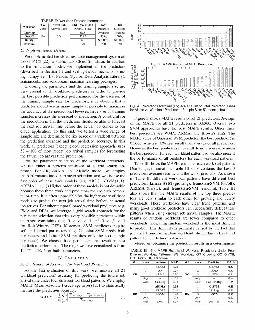
TABLE II: Workload Dataset Information.

Workload # ofJobs

Mean JobArrival Time

Std. Dev. of JobArrival Time

Job1

DurationJob

DeadlineGrowing 60.5 Average: Average:On/Off 10K 25s 375.5 450s, 500s,Bursty 35.3 Std.Dev.: Std.Dev.:

Random 270 270 250

C. Implementation DetailsWe implemented the cloud resource management system on

top of PICS [22], a Public IaaS Cloud Simulator. In additionto the simulation model, we implement all the predictors(described in Section II) and scaling-in/out mechanisms us-ing numpy ver. 1.8, Pandas (Python Data Analysis Library),statsmodels, and scikit-learn machine learning packages.

Choosing the parameters and the training sample size arevery crucial to all workload predictors in order to providethe best possible prediction performance. For the decision ofthe training sample size for predictors, it is obvious that apredictor should use as many sample as possible to maximizethe accuracy of the prediction. However, large size of trainingsamples increases the overhead of prediction. A constraint forthe prediction is that the predictors should be able to forecastthe next job arrival time before the actual job comes to ourcloud application. To this end, we tested a wide range ofsample size and determine the size based on a tradeoff betweenthe prediction overhead and the prediction accuracy. In thiswork, all predictors (except global regression approach) uses50 – 100 of most recent job arrival samples for forecastingthe future job arrival time prediction.

For the parameter selection of the workload predictors,we use either a performance-based or a grid search ap-proach. For AR, ARMA, and ARIMA model, we employthe performance-based parameter selection, and we choose thefirst order of these three models. (e.g. AR(1), ARMA(1, 1),ARIMA(1, 1, 1)) Higher-order of these models is not desirablebecause these three workload predictors require high compu-tation time. It is often impossible for the higher order of thesemodels to predict the next job arrival time before the actualjob arrives. For other temporal-based workload predictors (e.g.EMA and DES), we leverage a grid search approach for theparameter selection that tries every possible parameter withinits range constraints (e.g. 0 < ↵ < 1 and 0 < � < 1for Holt-Winters DES). Moreover, SVM predictors requiresoft and kernel parameters (e.g. Gaussian-SVM needs bothparameters and Linear-SVM requires only the soft marginparameter). We choose these parameters that result in bestprediction performance. The range we have considered is from10e�6 to 10e3 for both parameters.

IV. EVALUATION

A. Evaluation of Accuracy for Workload PredictorsAs the first evaluation of this work, we measure all 21

workload predictors’ accuracy for predicting the future jobarrival time under four different workload patterns. We employMAPE (Mean Absolute Percentage Error) [23] to statisticallymeasure the prediction accuracy.

MAPE =1n

nX

i=1

����Tactual,i � Tpredicted,i

Tactual,i

���� (1)

0 0.2 0.4 0.6 0.8

1 1.2 1.4 1.6

G-SVM

L-SVM

WM

AAR

MA

BRDES

AR RandForest

EMA

HW

DES

Ext.Trees

Loc.Lin.Reg

kNN

Lin.Reg

ARIM

A

Loc.CubicR

eg

CubicR

eg

GradBoost

Dec.Tree

Loc.Quad.R

eg

Quad.R

eg

Mean

MA

PE

Fig. 3: MAPE Results of All 21 Predictors.

10-1

100

101

102

103

kNN

WM

AEM

ABR

DES

Loc.Quad.R

eg

HW

DES

Loc.Cubic.R

eg

Loc.Lin.Reg

MEAN

L-SVM

G-SVM

Lin.Reg

Quad.R

eg

Dec.Tree

CubicR

eg

AR GradBoost

Ext.Tree

RandForest

ARIM

A

ARM

A

(Log S

cale

d)

Ove

rall

Pre

dic

tion O

verh

ead

(Unit:

Sec.

)

Fig. 4: Prediction Overhead (Log-scaled Sum of Total Prediction Time)for All the 21 Workload Predictors. (Sample Size: 50 recent jobs)

Figure 3 shows MAPE results of all 21 predictors. Averageof the MAPE for all 21 predictors is 0.6360. Overall, twoSVM approaches have the best MAPE results. Other threebest predictors are WMA, ARMA, and Brown’s DES. TheMAPE value of Gaussian-SVM predictor (the best predictor) is0.3665, which is 42% less result than average of all predictors.However, the best predictors in overall do not necessarily meanthe best predictor for each workload pattern, so we also presentthe performance of all predictors for each workload pattern.

Table III shows the MAPE results for each workload pattern.Due to page limitation, Table III only contains the best 3predictors, average results, and the worst predictor. As shownin Table II, different workload patterns have different bestpredictors: Linear-SVM (growing), Gaussian-SVM (on/off),ARIMA (bursty), and Gaussian-SVM (random). Table IIIalso shows that the MAPE results of the top three predic-tors are very similar to each other for growing and burstyworkloads. These workloads have clear trend patterns, andmany good workload predictors can successfully detect thesepatterns when using enough job arrival samples. The MAPEresults of random workload are lower compared to otherworkloads, indicating random workload is the most difficultto predict. This difficulty is primarily caused by the fact thatjob arrival times in random workloads do not have clear trendpattern for predictors to discover.

Moreover, obtaining the prediction results in a deterministic

TABLE III: The MAPE Results of Workload Predictors Under FourDifferent Workload Patterns. (WL: Workload, GR: Growing, OO: On/Off,BR: Bursty, RN: Random)

WL Rank Predictor MAPE WL Rank Predictor MAPE1 L-SVM 0.28 1 G-SVM 0.222 AR 0.29 2 ARMA 0.30

GR 3 ARMA 0.30 OO 3 L-SVM 0.44Avg. – 0.51 Avg. – 0.69Worst Qua.Reg 2.75 Worst Loc.Cub.Reg 1.25

1 ARIMA 0.38 1 G-SVM 0.452 BRDES 0.41 2 Lin.Reg 0.46

BR 3 L-SVM 0.43 RN 3 L-SVM 0.46Avg. – 0.75 Avg. – 0.52Worst mean 3.35 Worst Dec.Tree 0.62

5

0 20 40 60 80

100 120 140 160

Growing On/O Bursty Random

Norm

. Cos

t (%

)

37.6

50.1

38.2

44.0

37.9

38.3

50.2

38.1

41.8

44.7

42.8

42.6

42.9

42.8

43.1

43.6

43.6

43.3 61

.152

.352

.551

.753

.052

.253

.648

.753

.1

113.

611

4.1

114.

411

3.8

90.6

113.

811

3.6

113.

611

0.9

Lin.Reg.WMA

BRDESAR

ARMA

ARIMAG-SVML-SVM

Average

(a) Normalized Cost.

0 10 20 30 40 50 60 70 80

Growing On/O Bursty RandomNorm

. Dea

dlin

e M

iss R

ate

(%)

23.3

16.0

16.8

19.0

16.0

14.4

22.1

13.7

17.7

11.7

13.5

16.2

12.4

11.7

14.0

8.2

9.2

12.1 23

.616

.820

.619

.923

.715

.215

.417

.919

.1

54.9

48.2

54.6

47.8

48.8

48.9

47.3

48.8

49.9

Lin.Reg.WMA

BRDESAR

ARMA

ARIMAG-SVML-SVM

Average

(b) Normalized Job Deadline Miss Rate.

Fig. 5: Case #1 – Normalized Cost and Job Deadline Miss Rate of PR (Scaling-Out:Predictive + Scaling-In:Reactive) – Hourly Pricing Model.

0 20 40 60 80

100 120 140 160

Growing On/O Bursty Random

Norm

. Cos

t (%

)

107.

910

3.1

103.

510

3.9

103.

110

4.0

103.

510

4.7

104.

2

100.

198

.599

.098

.510

0.1

98.4

99.4

99.2

99.2

96.6

97.7

97.7

98.1

98.0

98.3

96.5

95.8

97.3 10

6.9

106.

810

5.9

106.

510

4.7

106.

710

6.2

106.

110

6.3

Lin.Reg.WMA

BRDESAR

ARMA

ARIMAG-SVML-SVM

Average

(a) Normalized Cost.

0 10 20 30 40 50 60 70 80

Growing On/O Bursty RandomNorm

. Dea

dlin

e M

iss R

ate

(%)

42.4

42.3

43.3

41.3

42.3

42.0

42.8

42.8

42.4

12.2

14.6

14.3

13.4

11.4

14.0

12.9

12.8

13.2

43.7

42.6

43.1

45.2

44.7

44.2

43.0

42.9

43.6 59

.459

.359

.259

.259

.159

.258

.659

.059

.1

Lin.Reg.WMA

BRDESAR

ARMA

ARIMAG-SVML-SVM

Average

(b) Normalized Job Deadline Miss Rate.

Fig. 6: Case #1 – Normalized Cost and Job Deadline Miss Rate of PR (Scaling-Out:Predictive + Scaling-In:Reactive) – Minutely Pricing Model.

amount of time is a critical issue for the predictive resourcescaling. We also measured computation overhead of predictors(Figure 4). kNN, WMA, and EMA are the fastest predictors.The overall prediction time for 10K jobs of these threepredictors are 0.48 (kNN), 0.96 (WMA), and 1.86 seconds(EMA). However, some temporal approaches (AR, ARMA,and ARIMA) and ensemble methods (extra trees, gradientboosting, and random forest) have longer prediction time. Thehighest overhead predictor is ARMA, which takes 6031.52seconds for 10K jobs.

B. Performance of Different Styles of Predictive Scaling

We measure the performance of four different styles ofscaling operations for cloud resource management:

• Baseline: RR (Scale-Out: Reactive + Scale-In: Reactive)• PR (Scale-Out: Predictive + Scale-In: Reactive)• RP (Scale-Out: Reactive + Scale-In: Predictive)• PP (Scale-Out: Predictive + Scale-In: Predictive)PR is the most common style of predictive scaling for cloud

application. PR predictively scales out cloud resources and

reactively scales in cloud resources. RP is another way ofpredictive scaling, and it uses a reactive way for scaling-outand a predictive approach for scaling-in. PP is a combinationof PR and RP, and it leverages a workload predictor for bothscaling-out and scaling-in operations. For this evaluation, weuse RR (Scaling-Out: Reactive + Scaling-In: Reactive) as abaseline. RR adds a new VM (scaling-out) when a new jobneeds an extra VM, and terminates an idle VM (scaling-in) atits billing boundary. (i.e., hourly bound or minutely bound).

Due to page limitation, we only show the results of the pre-dictive scaling operations with the most accurate 8 workloadpredictors from Section IV-A. These predictors are Linear-SVM, Gaussian-SVM, ARMA, AR, WMA, ARIMA, Brown’sDES, Linear regression, which cover the overall best 5 pre-dictors and the best 3 predictors for each workload pattern.

To evaluate the predictive scaling operations, we use twocommon cloud metrics (cost and job deadline miss rate) andtwo different billing models (hourly and minutely pricingmodel). Cost is to evaluate each scaling operations’ costefficiency, and job deadline miss rate represents the SLA-

6

0

50

100

150

200

Growing On/O Bursty Random

Norm

. Cos

t (%

)

100.

410

0.5

100.

610

0.5

100.

510

0.6

100.

510

0.4

100.

5

74.5

71.1

71.1

83.4

77.6

76.9

71.1

76.9

75.3

133.

513

3.9

138.

114

9.6

137.

413

7.6

133.

913

7.5

137.

7

77.6

77.6

77.5

77.7

77.6

77.6

77.6

77.5

77.6

Lin.Reg.WMA

BRDESAR

ARMA

ARIMAG-SVML-SVM

Average

(a) Normalized Cost.

0 20 40 60 80

100 120 140 160

Growing On/O Bursty RandomNorm

. Dea

dlin

e M

iss R

ate

(%)

98.9

99.6

99.2

99.9

99.4

99.3

99.1

98.5

99.2

99.6

98.7

99.5

99.1

97.6

99.2

99.7

98.5

99.0

99.9

100.

398

.410

1.3

97.5

97.4

99.5

99.4

99.2 99.5

99.3

100.

310

0.0

110.

899

.399

.599

.010

1.0

Lin.Reg.WMA

BRDESAR

ARMA

ARIMAG-SVML-SVM

Average

(b) Normalized Job Deadline Miss Rate.

Fig. 7: Case #2 – Normalized Cost and Job Deadline Miss Rate of RP (Scaling-Out:Reactive + Scaling-In:Predictive) – Hourly Pricing Model.

0 20 40 60 80

100 120 140 160 180

Growing On/O Bursty Random

Norm

. Cos

t (%

)

104.

410

6.8

108.

010

8.3

105.

410

7.4

104.

910

9.7

106.

9

122.

112

2.4

121.

212

3.3

120.

112

3.2

121.

412

0.7

121.

8

109.

010

9.0

107.

111

0.4

108.

310

9.1

108.

410

8.9

108.

4

85.3

85.9

85.9

90.1

89.2

85.4

85.9

85.9

86.7

Lin.Reg.WMA

BRDESAR

ARMA

ARIMAG-SVML-SVM

Average

(a) Normalized Cost.

0 20 40 60 80

100 120 140

Growing On/O Bursty RandomNorm

. Dea

dlin

e M

iss R

ate

(%)

98.9

99.3

99.5

99.2

99.4

99.0

98.9

100.

799

.5

99.3

99.2

99.2

99.9

99.5

99.3

99.4

99.2

99.5

99.2

99.3

99.2

99.3

99.6

99.3

100.

699

.099

.5

99.4

99.4

99.4

99.7

99.6

99.4

99.4

99.3

99.5 Lin.Reg.

WMABRDES

ARARMA

ARIMAG-SVML-SVM

Average

(b) Normalized Job Deadline Miss Rate.

Fig. 8: Case #2 – Normalized Cost and Job Deadline Miss Rate of RP (Scaling-Out:Reactive + Scaling-In:Predictive) – Minutely Pricing Model.

satisfaction requirement. We use two different billing mod-els for cloud infrastructure, because major commercial IaaSclouds employ either hourly (e.g. AWS) or minutely (e.g. MSAzure) pricing model. We also use four different workloadpatterns (growing, on/off, bursty, and random workload).

The goals of this evaluation are:

• Measuring the actual benefits from predictive scaling.• Determining the best style of predictive scaling.• Finding the best workload predictor for each workload

pattern in terms of cloud metrics.

Case #1 – PR (Scale-Out: Predictive + Scale-In: Reactive):Figure 5 shows a normalized cost and job deadline miss rate(all results are normalized to RR) of PR for hourly pricingmodel. The results show that PR can improve 47%–58% ofcost efficiency for growing, on/off, and bursty workloads.However, for random workload, PR has 11% of worse costefficiency over the baseline. In terms of job deadline miss rate,PR has 50%–88% of less job deadline miss rate over the RR(baseline). For the hourly pricing model, PR shows relativelypoor performance for random workload in both cost efficiency

and job deadline miss rate. This is because random workloadis harder to predict than the other workload patterns. We rankthe workload predictors for the PR based on the deadline missrate, because it is more important to ensure that jobs meet theirdeadlines. Only after the deadline requirements are met, ourcloud resource manager in Section III-A optimizes for costefficiency. The best workload predictors for PR are: Linear-SVM (13.7%) for growing, Gaussian-SVM (8.2%) for on/off,ARIMA (15.2%) for bursty, and Gaussian-SVM (47.3%) forrandom workload.

Figure 6 shows evaluation results of PR for minutely pricingmodel under four workload patterns. PR has similar cost effi-ciency with RR, but it has 41%–87% of less job deadline missrate than the baseline. Thus, PR provides better job deadlinesatisfaction without dramatically increasing cost. The reasonthat PR has similar cost efficiency with RR is that the minutelypricing model is designed to provide better cost efficiency thanhourly model to the user. So it is very hard to improve the costefficiency for the minutely pricing model even though we havea good predictor. The best workload predictors for RP with

7

0 10 20 30 40 50 60 70 80

Growing On/O Bursty Random

Norm

. Cos

t (%

)

32.6

32.0

32.1

30.2

33.1

30.1

30.0

30.3

31.3 33

.933

.235

.239

.334

.137

.734

.233

.835

.2

56.4

55.6

45.1

56.3

51.5

51.9

49.7

46.4

51.6

48.2

48.2

48.2

47.9

48.3

47.8

48.0

47.8

48.0 Lin.Reg.

WMABRDES

ARARMA

ARIMAG-SVML-SVM

Average

(a) Normalized Cost.

0

10

20

30

40

50

Growing On/O Bursty RandomNorm

. Dea

dlin

e M

iss R

ate

(%)

12.6

6.9

6.8

6.5

6.3

5.7

9.2

5.5

7.4

8.9

11.9

14.1

11.8

8.3

11.5

7.8

9.4

10.5

7.3

8.7

5.1

9.4

11.6

11.8

9.3

6.1

8.7

20.4

21.7

20.3

23.6

20.3

26.6

21.6

18.1

21.6 Lin.Reg.

WMABRDES

ARARMA

ARIMAG-SVML-SVM

Average

(b) Normalized Job Deadline Miss Rate.

Fig. 9: Case #3 – Normalized Cost and Job Deadline Miss Rate of PP (Scaling-Out:Predictive + Scaling-In:Predictive) – Hourly Pricing Model.

0 20 40 60 80

100 120 140

Growing On/O Bursty Random

Norm

. Cos

t (%

)

96.7

98.4

97.4

97.4

97.5

98.6

98.3

97.9

97.8

99.8

99.4

99.7

99.2

100.

499

.198

.799

.199

.4

92.3

94.1

94.6

96.2

97.3

95.8

94.1

93.5

94.7

85.9

86.1

88.7

94.0

88.5

89.4

90.2

88.6

88.9 Lin.Reg.

WMABRDES

ARARMA

ARIMAG-SVML-SVM

Average

(a) Normalized Cost.

0 10 20 30 40 50 60

Growing On/O Bursty RandomNorm

. Dea

dlin

e M

iss R

ate

(%)

30.9

28.3

27.9

27.5

28.9

28.1

29.4

27.9

28.6

12.5

14.5

14.3

12.9

11.4

14.5

12.9

12.5

13.2

29.6

30.9

19.7

32.9

36.5

33.0

31.2

27.2

30.1

39.8

39.8

39.6

39.8

40.5

39.6

39.5

39.8

39.8

Lin.Reg.WMA

BRDESAR

ARMA

ARIMAG-SVML-SVM

Average

(b) Normalized Job Deadline Miss Rate.

Fig. 10: Case #3 – Normalized Cost and Job Deadline Miss Rate of PP (Scaling-Out:Predictive + Scaling-In:Predictive) – Minutely Pricing Model.

minutely pricing model are: AR (41.3%) for growing, ARMA(11.4%) for on/off, WMA (42.6%) for bursty, and Gaussian-SVM (58.6%) for random workload.

Case #2 – RP (Scale-Out: Reactive + Scale-In: Predictive):Figure 7 and 8 show the evaluation results of RP for bothpricing models under four workload patterns. The resultsindicate that RP’s benefit to the cloud system is not as muchas the benefits from PR. The only benefit from the RP is theimproved cost efficiency (on/off and random workloads forhourly pricing model, random workload for minutely pricingmodel). The improvement of cost efficiency is 12%–25%, butit has no benefits for job deadline miss rate.

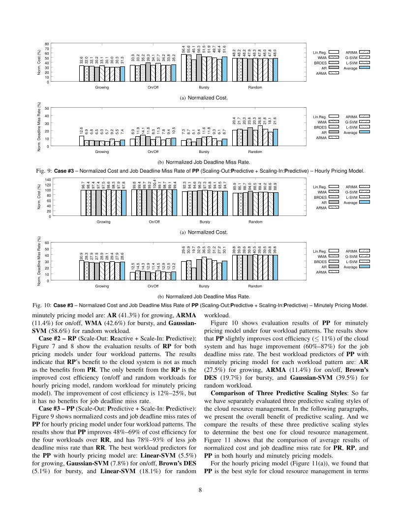
Case #3 – PP (Scale-Out: Predictive + Scale-In: Predictive):Figure 9 shows normalized costs and job deadline miss rates ofPP for hourly pricing model under four workload patterns. Theresults show that PP improves 48%–69% of cost efficiency forthe four workloads over RR, and has 78%–93% of less jobdeadline miss rate than RR. The best workload predictors forthe PP with hourly pricing model are: Linear-SVM (5.5%)for growing, Gaussian-SVM (7.8%) for on/off, Brown’s DES(5.1%) for bursty, and Linear-SVM (18.1%) for random

workload.Figure 10 shows evaluation results of PP for minutely

pricing model under four workload patterns. The results showthat PP slightly improves cost efficiency ( 11%) of the cloudsystem and has huge improvement (60%–87%) for the jobdeadline miss rate. The best workload predictors of PP withminutely pricing model for each workload pattern are: AR(27.5%) for growing, ARMA (11.4%) for on/off, Brown’sDES (19.7%) for bursty, and Gaussian-SVM (39.5%) forrandom workload.

Comparison of Three Predictive Scaling Styles: So farwe have separately evaluated three predictive scaling styles ofthe cloud resource management. In the following paragraphs,we present the overall benefit of predictive scaling. And wecompare the results of these three predictive scaling stylesto determine the best one for cloud resource management.Figure 11 shows that the comparison of average results ofnormalized cost and job deadline miss rate for PR, RP, andPP in both hourly and minutely pricing models.

For the hourly pricing model (Figure 11(a)), we found thatPP is the best style for cloud resource management in terms

8

0 0.2 0.4 0.6 0.8

1 1.2 1.4

PR RP PP

Norm

. Cos

t/DL

Miss

Rat

eNorm. Cost

Norm. DL Miss

(a) Hourly Pricing Model

0 0.2 0.4 0.6 0.8

1 1.2 1.4

PR RP PP

Norm

. Cos

t/DL

Miss

Rat

e

Norm. CostNorm. DL Miss

(b) Minutely Pricing Model

Fig. 11: Comparison of Average Results of Normalized Cost and JobDeadline Miss Rate of Three Scaling Styles (PR, RP, and PP).

0 0.5

1 1.5

2 2.5

3 3.5

PR RP PP

Norm

. VM

#/U

tils

Norm. # VMsNorm. VM Utils

(a) Hourly Pricing Model

0 0.2 0.4 0.6 0.8

1 1.2 1.4 1.6

PR RP PP

Norm

. VM

#/U

tils

Norm. # VMsNorm. VM Utils

(b) Minutely Pricing Model

Fig. 12: Comparison of VM Numbers/Utilization of Three Scaling Styles.

of better cost efficiency and less job deadline miss rate. PP’scost efficiency is 20% (compared to PR) and 56% (comparedto RP) better than other two approaches. Moreover, PP’sjob deadline miss rate is 13% (compared to PR) and 88%(compared to RP) lower than others. This result is interesting,because although predictive scaling-in does not improve costand deadline miss rate by itself (as shown in Case #2), itprovides considerable improvement for both metrics whencombined with predictive scaling-out. These results show thatpredictive scaling in/out approach (PP) (with a good workloadpredictor) helps to improve the performance of the cloudresource management.

For the minutely pricing model (Figure 11(b)), the jobdeadline miss rate of PP outperforms other two styles ofpredictive scaling operations. PP has 12% (compared to PR)and 72% (compared to RP) of less job deadline miss rate. PPalso improves cost efficiency over PR and RP. These resultssuggest PP can significantly reduce deadline miss rate withoutcost overhead.

To understand the reasons of 1) PP significantly improvescost efficiency (hourly pricing model) and deadline missrate (both pricing model) and 2) RP does not improve theperformance by itself, we analyze the number of created VMsand VM utilization of three styles. Figure 12 represents theVM numbers and utilization of three scaling styles for bothpricing models. For the both pricing models, PP creates theless number of VMs and has higher utilization than others. Thereasons that PP has high VM utilization and lower number ofcreated VMs are:

• Predictive scaling-out of PP uses more currently runningVMs for the (near) future jobs, and creates less VMs forthe (near) future jobs.

• Predictive scaling-in of PP keeps VMs alive for (further)future jobs, which further reduces the new VM creations,and increases the utilizations of existing VMs.

Moreover, the reason that RP cannot improve the cloudmetrics is related to reactive scaling-out of RP. Reactivescaling-out operation creates VMs when jobs actually arrive,so RP has to create better performance VMs (more expensiveVMs) in order to meet the jobs’ deadline. This is because RPhas no advance preparation for eliminating the overhead of theVM creation (e.g. startup delay). Also most of VMs shouldbe terminated after processing the current job because theyare not used for future jobs. So, predictive scaling-in of RPdoes not help in this case because most of VMs should bedestroyed.

V. RELATED WORK

A large body of work has been conducted for the predictivecloud resource management for dynamic workload patterns.There are two major branches in predictive resource manage-ment in the clouds. First branch is to focus on predicting thefuture resource usages (e.g. CPU, memory, and I/O) basedon past resource usage history [1–4, 28]. Second branch isa workload predictive approach for cloud resource manage-ment. More specifically, this branch focuses on predicting thefuture job arrival time by using various workload predictors.Our work is closer to the second branch because we haveevaluated prediction techniques for the future job arrivalsto the clouds. In order to predict the next job arrival time,previous works employ a variety of predictors. They appliedregression [16, 17, 29–31], time-series methods (e.g. ES [5–7, 18, 19], AR [8, 24], ARMA [9–13] and ARIMA [14, 15]) totheir cloud systems to effectively manage the cloud resources.Herbst et al [32] proposed WCF (Workload Classification andForecasting) framework, which is a self-adaptive approach forproactive resource management. However, the purpose of ourwork is different from the goal of previous works (proposinga new predictive scaling mechanism). We are more gearedtoward evaluating the performance of all existing predictiontechniques for cloud resource management (e.g. scaling) byemploying various/realistic workload patterns [20, 21], diversecloud configurations (e.g. billing model), and common per-formance metrics. Furthermore, we have concentrated on theevaluation of different styles of predictive scale operations:predictive scaling-out only, predictive scaling-in only, and bothpredictive scaling-in/out. Therefore, our goal is to determinethe best workload predictor for the cloud users’ specificworkload pattern and cloud configurations as well as the bestscaling style of the predictive scaling.

VI. CONCLUSION

In order to help the cloud users select the best workload pre-dictor, we comprehensively evaluated 21 workload predictorsusing statistical and cloud metrics. We then evaluated the pre-diction accuracy of all workload predictors, and cost/deadlinemiss rate of three following styles of predictive scaling underdiverse workload patterns and different cloud configurations.

• PR (Scale-Out: Predictive + Scale-In: Reactive)• RP (Scale-Out: Reactive + Scale-In: Predictive)• PP (Scale-Out: Predictive + Scale-In: Predictive)

9

We found that to design a new predictive cloud resourcescaling, the cloud users should consider top 3 workloadpredictors depending on their workload patterns, and use PPapproach for their scaling operations in order to maximize thescaling performance.

ACKNOWLEDGMENT

The authors would like to thank the anonymous reviewersfor their valuable comments and suggestions to improve thequality of this paper.

REFERENCES

[1] Peter A. Dinda and David R. O’Hallaron. Host Load Prediction usingLinear Models. Cluster Computing, 3(4):265–280, 2000.

[2] Zhenhuan Gong, Xiaohui Gu, and John Wilkes. PRESS: PRedictiveElastic ReSource Scaling for cloud systems. In International Conferenceon Network and Service Management (CNSM), 2010.

[3] Zhen Xiao, Weijia Song, and Qi Chen. Dynamic Resource AllocationUsing Virtual Machines for Cloud Computing Environment. IEEETransactions on Parallel and Distributed Systems, 24(6), 2013.

[4] Akindele A. Bankole and Samuel A. Ajila. Cloud Client PredictionModels for Cloud Resource Provisioning in a Multitier Web ApplicationEnvironment. In IEEE International Symposium on Service OrientedSystem Engineering (SOSE), 2013.

[5] Shuangcheng Niu, Jidong Zhai, Xiaosong Ma, Xiongchao Tang, andWenguang Chen. Cost-effective Cloud HPC Resource Provisioning byBuilding Semi-Elastic Virtual Clusters. In International Conference forHigh Performance Computing, Networking, Storage and Analysis (SC),2013.

[6] Ching Chuen Teck Mark, Dusit Niyato, and Tham Chen-Khong. Evo-lutionary Optimal Virtual Machine Placement and Demand Forecasterfor Cloud Computing. In IEEE International Conference on AdvancedInformation Networking and Applications (AINA), 2011.

[7] Haibo Mi, Huaimin Wang, Gang Yin, Yangfan Zhou, Dianxi Shi, andLin Yuan. Online Self-reconfiguration with Performance Guaranteefor Energy-efficient Large-scale Cloud Comp. Data Centers. In IEEEInternational Conference on Services Computing (SCC), 2010.

[8] Norman Bobroff, Andrzej Kochut, and Kirk Beaty. Dynamic Placementof Virtual Machines for Managing SLA Violations. In IFIP/IEEESymposium on Integrated Network and Service Management (IM), 2007.

[9] Nilabja Roy, Abhishek Dubey, and Aniruddha Gokhale. Efficient Au-toscaling in the Cloud using Predictive Models for Workload Forecast-ing. In IEEE International Conference on Cloud Computing (CLOUD),2011.

[10] Juan M. Tirado, Daniel Higuero, Florin Isaila, and Jesus Carretero.Predictive Data Grouping and Placement for Cloud-based Elastic ServerInfrastructures. In IEEE/ACM International Symposium on Cluster,Cloud and Grid Computing (CCGrid), 2011.

[11] Mohit Dhingra, J. Lakshmi, S. K. Nandy, Chiranjib Bhattacharyya, andK. Gopinath. Elastic Resources Framework in IaaS, preserving perfor-mance SLAs. In IEEE International Conference on Cloud Computing(CLOUD), 2013.

[12] Upendra Sharma, Prashant Shenoy, and Sambit Sahu. A Flexible ElasticControl Plane for Private Clouds. In ACM Cloud and AutonomicComputing Conference (CAC), 2013.

[13] Shun-Pun Li and Man-Hon Wong. Data Allocation in Scalable Dis-tributed Database Systems Based on Time Series Forecasting. In IEEEInternational Congress on Big Data (BigData Congress), 2013.

[14] Rodrigo N. Calheiros, Enayat Masoumi, Rajiv Ranjan, and RajkumarBuyy. Workload Prediction Using ARIMA Model and Its Impact onCloud Applications’ QoS. IEEE Transactions on Cloud Computing,3(4), 2015.

[15] Hong Xu Di Niu, Baochun Li, and Shuqiao Zhao. Quality-AssuredCloud Bandwidth Auto-Scaling for Video-on-Demand Applications. InIEEE International Conference on Computer Communications (INFO-COM), 2012.

[16] Peter Bodik, Rean Griffith, Charles Sutton, Armando Fox, MichaelJordan, and David Patterson. Statistical Machine Learning MakesAutomatic Control Practical for Internet Datacenters. In USENIXWorkshop on Hot Topics in Cloud Computing (HotCloud), 2009.

[17] Jingqi Yang, Chuanchang Liu, Yanlei Shang, Bo Cheng, Zexiang Mao,Chunhong Liu, Lisha Niu, and Junliang Chen. A Cost-aware Auto-scaling Approach Using the Workload Prediction in Service Clouds.Information Systems Frontiers, 16(1), 2014.

[18] Sou Koyano, Shingo Ata, Ikuo Oka, and Kazunari Inoue. A High-grained Traffic Prediction for Microseconds Power Control in Energy-aware Routers. In IEEE/ACM International Conference on Utility andCloud Computing (UCC), 2012.

[19] Prasad Saripalli, GVR Kiran, Ravi Shankar R, Harish Narware, and NitinBindal. Load Prediction and Hot Spot Detection Models for AutonomicCloud Computing. In IEEE International Conference on Utility andCloud Computing (UCC), 2011.

[20] Christoph Fehling et al. Cloud Computing Patterns: Fundamentals toDesign, Build, and Manage Cloud Applications. 2014.

[21] Workload Patterns for Cloud Computing. http://watdenkt.veenhof.nu/2010/07/13/workload-patterns-for-cloud-computing/.

[22] In Kee Kim, Wei Wang, and Marty Humphrey. PICS: A Public IaasCloud Simulator. In IEEE International Conference on Cloud Computing(CLOUD), 2015.

[23] Trevor Hastie, Robert Tibshirani, and Jerome Friedman. The Elementof Statistical Learning: Data Mining, Inference, and Prediction. 2011.

[24] Abhishek Chandra, Weibo Gong, and Prashant Shenoy. Dynamic Re-source Allocation for Shared Data Centers Using Online Measurements.In International Workshop on Quality of Service (IWQoS), 2003.

[25] In Kee Kim, Jacob Steele, Yanjun Qi, and Marty Humphrey. Comprehen-sive Elastic Resource Management to Ensure Predictable Performancefor Scientific Applications on Public IaaS Clouds. In IEEE/ACMInternational Conference on Utility and Cloud Computing (UCC), 2014.

[26] Ming Mao and Marty Humphrey. A Performance Study on the VMStartup Time in the Cloud. In IEEE International Conference on CloudComputing (CLOUD), 2012.

[27] Amazon Web Services. http://aws.amazon.com.[28] Zhiming Shen, Sethuraman Subbiah, Xiaohui Gu, and John Wilkes.

CloudScale: Elastic Resource Scaling for Multi-Tenant Cloud Systems.In ACM Symposium on Cloud Computing (SoCC), 2011.

[29] Waheed Iqbal, Matthew N. Dailey, David Carrera, and Paul Janecek.Adaptive Resource Provisioning for Read Intensive Multi-tier Applica-tions in the Cloud. Future Generation Computer Systems, 27(6), 2011.

[30] Sireesha Muppala, Xiaobo Zhou, and Liqiang Zhang. Regression BasedMulti-tier Resource Provisioning for Session Slowdown Guarantees.In IEEE International Performance Computing and CommunicationsConference (IPCCC), 2010.

[31] Sourav Dutta, Sankalp Gera, Akshat Verma, and Balaji Viswanathan.SmartScale: Automatic Application Scaling in Enterprise Clouds. InIEEE International Conference on Cloud Computing (CLOUD), 2012.

[32] Nikolas Roman Herbst, Nikolaus Huber, Samuel Kounev, and ErichAmrehn. Self-Adaptive Workload Classification and Forecasting forProactive Resource Provisioning. In ACM/SPEC International Confer-ence on Performance Engineering (ICPE), 2013.

10