Empirical Analysis of the Relation Between Social Spending and Economic...

A Thesis for the Degree of Master

Empirical Analysis of the Relation between Social

Spending and Economic Growth: Developing Countries

and OECD Members

By

Wonhyuk Cho

February 2009

Graduate School of Public Administration

Seoul National University

Korea

- 1 -

Abstract

Wonhyuk Cho

Graduate School of Public Administration

Seoul National University

Most previous empirical approaches examined the relationship between social spending

and economic growth only in developed countries or OECD member countries, and

show little or no efforts to compare the effects of social spending in developing

countries with those in developed or OECD member countries; however, developing

countries can be in very different social, economic, and institutional settings.

Therefore, we examined this relationship, drawing a comparison between the result of

developing countries and that of developed (or OECD member) and semi-developed

countries with the same data source, the IMF’s Government Finance Statistics data of 85

countries over the period from 1990 to 2007, using time-series cross-section regression

model.

We found that estimated coefficient on social spending is positive and statistically

significant in the sample of developing countries, while a significant negative

relationship between social spending and economic growth is observed in the sample of

developed countries. The results of this study can suggest that assumption of a tradeoff

between efficiency and equity could be not well applied in the developing countries.

- 2 -

Therefore, this finding can imply that we have to consider not only what to do but also

where to do, when we discuss the social spending effect and give policy advises to

developing countries.

Keywords: social spending, developing country, economic growth

Student Number: 2007-22288

- 3 -

Table of Contents

I. INTRODUCTION

II. WELFARE STATE MODELS AND DEVELOPMENT

III. EMPIRICAL STUDIES ON SOCIAL SPENDING

IV. MEOTHODOLOGY

1. Analytic Framework

2. Variables and Dataset

V. FINIDNGS AND DISCUSSION

1. Developing Countries

2. Developed Countries

3. Semi-Developed Countries

4. Discussion

VI. CONCLUSION

- 4 -

List of Tables and Figures

Tables

Table 1 Differences between Fixed Effect and Random Effect Models

Table 2 List of the Countries in the Sample

Table 3 Summary Statistics

Table 4 Result of Developing Country (Cash and Accrual Basis Combined)

Table 5 Result of Developing Country (Cash Basis)

Table 6 Result of Developing Country (Accrual Basis)

Table 7 Result of Developed Country (Cash and Accrual Basis Combined)

Table 8 Result of Developed Country (Cash Basis)

Table 9 Result of Developed Country (Accrual Basis)

Table 10 Result of Semi-Developed Country (Cash and Accrual Basis Combined)

Table 11 Result of Semi-Developed Country (Cash Basis)

Table 12 Result of Semi-Developed Country (Accrual Basis)

Figures

Figure 1 Welfare States in Developed and Developing Countries

- 5 -

I. INTRODUCTION

Although developmental welfare is not a new issue, social policy is now, partly

because of effort by neo-liberal economists, being vigorously discussed again in the

context of development (Midgley and Tang, 2001; Kwon, 2005; Mkandawire, 2001;

Hall and Midgley, 2004).

Neo-liberal economic theories argue that social expenditure does harm to the

economy and that spending on social policy should be reduced for the country’s

competitiveness. In practice, however, the programs based on this neo-liberal view seem

to have made the situation much worse in many developing countries during 1980s and

1990s; World Bank’s and International Monetary Foundation’s stabilization programs

such as austerity, privatization, and reduction of government social spending have

resulted in economic and social vulnerability (Cornia et al, 1987). Conditions of these

countries were worsened directly by rapidly rising food prices and elimination of basic

nutritional, educational, and health services, and indirectly by slowing growth and

increasing poverty (Cornia et al, 1987).

Lindert (2004, 2006) insisted that social spending does not negatively affect the

growth, showing some statistical and historical records, and criticized neo-liberal

economic theories as “theory-dependent bluffs.” Further, Kwon (2007) pointed out that

the developmental state in Korea, which considerably contributed to rapid economic

growth, conducted not only economic policy but also social policy as an overall

economic development strategy. Hort and Kuhnle (2000) argued that East Asian

countries adopted social welfare programs as policy instruments for economic growth,

- 6 -

and Goodman and White (1998) suggested that these East Asian welfare states’ social

policy aimed at goals such as subordinating welfare to economic efficiency and

discouraging dependence on the state.

In spite of many discussions and controversies about the impact of social spending

on economic growth, there has been relatively little attention to the empirical support for

the hypotheses mentioned above. Lindert (2006: 237) pointed out this lack of empirical

approach saying that “theory has gone into overdrive” in the issue of developmental

welfare with the widening gap between empirical record and a story, although theory

and fact are needed to be mixed in the right proportion. Even if there are growth studies

that tested effect of social spending, the data they used were, in most researches, that of

OECD members and not of developing countries. This means that there is a need to test

this relationship with samples covering developing countries. Further, previous studies

shows little or no efforts to compare the effects of social spending in developing

countries with those in developed or OECD member countries, although developing

countries can be in very different social, economic, and institutional settings. Therefore,

the objective of this study is to test the relationship between social spending and

economic growth with cross country panel data, and draw comparison between the

result of developing countries and that of developed countries.

- 7 -

II. WELFARE STATE MODELS AND DEVELOPMENT

Wilensky and Lebeaux (1958) preliminarily suggested the types of welfare states

with “residual” and “institutional” approaches to social welfare, reflecting different

thoughts in social policy and the role of the welfare state; their typology and its terms

have been widely used and often mentioned in social policy literature (Sainsbury, 2007;

Mishra, 1981; Bryson 1992; Graycar and Jamrozik, 1993, Esping-Andersen and Korpi,

1987). The residual approach of social welfare views that state assistance fills the gap

where the primary institutions, which are the “market” and the “family,” can not meet

the needs of a person or a family; that is, welfare states play a role when these

institutions have proved inadequate. Therefore, social welfare, according to this view,

should be kept minimal, temporary, requiring evidence of needs, and is only for the

disadvantaged. On the other hand, the institutional approach of welfare sees that welfare

is a dominant institution, so welfare states meet the needs of everyone and not just of the

disadvantaged. In other words, it views that the role of the state is to provide

comprehensive and universal social policy. In turn, the institutional view leads to higher

social spending, and universal programs for the benefit of all. By contrast, the residual

view leads to lower social spending, selective means-tested programs, and provision to

only those who are most in need.

Titmuss (1974) challenged the typology of Wilensky and Lebeaux, and elaborated it,

claiming that the residual and the institutional models appear simultaneously with the

third model that he named the “industrial achievement-performance model” of social

welfare; he also added “redistributive” to the definition of the institutional model. The

- 8 -

“industrial achievement-performance model” emphasizes social policies that are closely

related to performance in market economy, such as promoting higher productivity,

greater motivation, more work, and so on. Titmuss's own favorite is the “industrial

achievement-performance model” where the welfare policies become major integrative

tools for the society as a whole, providing universalistic responses to non-stigmatizing

needs in the direction of resource redistribution (Demerath, 1977).

Furniss and Tilton (1977) provided a typology of welfare state, based on the three

distinctive responses to the rise of advanced industrialization. First, they describe the

United States as a “positive state.” The fundamental goal of the positive state is to

protect property holders from the problems of unregulated market in capitalist society,

and from the influence of redistributive demands. Therefore, this type of state shows

strong opposition to social policies that are not directed by concerns of efficiency. They

suggested that the “positive states” depend on social insurance that is based on actuarial

principles. The second response to the rise of advanced industrialization is “social

security state” that United Kindom represents. This type of state is based on two

principles, which are the ‘maximalist full employment’ and the ‘guaranteed national

minimum.’ This means that the principle is clearly not ‘equality’ but ‘equality of

opportunity.’ The third response is the “social welfare state,” which Furniss and Tilton

sees Sweden as a representative example. The goals of this state are full employment

achieved by government-union cooperation, environmental planning, and solidaristic

wage settlements.

George and Wilding (1976) analyzed the ideological conflicts of the welfare state,

and suggested four types of thoughts; those are labeled as “anti-collectivism,” “reluctant

collectivism,” “Fabian socialism,”, and “Marxism.” These ideology types are based on

- 9 -

the analysis of representative thinkers (George, 1985); Milton Friedman, Hayek, and

Enoch Powell are the anti-collectivists; Crosland, Tawney, and Titmuss are the Fabian

socialists; and Strachey, Laski and Miliband are the Marxists. Their classification seems

to be a variation of attitudes towards the market economy, and this approach implies that

the values of capitalism and the ethic of welfare are, according to them, in conflict

(George, 1985; 34). “Anti-collectivists” advocate liberty and individualism, and think

that the pursuit of equality is incompatible with these values. They insist that market

mechanism is the most efficient means of resource allocation. “Reluctant collectivists”

have similar perception to the anti-collectivists, but have less faith in market economy.

They think that the unregulated capitalist economy can be inefficient in some way, and

does not necessarily produce a just distribution of resources. Therefore, state

intervention is justified, but it should be the minimum required to remove the

inefficiency and injustices generated by unregulated markets. Poverty, not inequality, is

the concern of the welfare state, and the provision of a minimum of income security and

essential services is their approach. “Fabian socialists” have a belief in equality, and also

have more positive attitude to state action than reluctant collectivists do. The

government plays an essential role not only in regulating but also in controlling,

directing and planning the economy, to maximize growth, justice and welfare.

“Marxists” regard the welfare state as inherently limited because it is rooted in a

capitalist class society. They think that socialist planned economy must replace the

capitalist market economy to achieve the goals of liberty, welfare and justice for all.

Esping-Andersen (1990) suggested three different types of welfare states, which

remains one of the most commonly used typologies of modern welfare states. He

identifies the process of decommodification of the wage earner in relation to theoretical

- 10 -

classification of advanced capitalist states. His welfare states types have a resemblance

to those by Titmuss; however, the difference is that Esping-Andersen identifies the

social, political, economic, and historical context that these types of welfare states

established in the countries, while Titmuss and others focus on the characteristics of

each welfare type. Esping-Andersen insisted that categorization of welfare states cannot

be based on the level of social spending, since not “all spending counts equally” and

“social spending per se was hardly ever at the centre of major political conflict”

(Esping-Andersen, 1990). He partly rejected the ‘working-class mobilization theory,’

saying that working-class mobilization is not a ‘single powerful causal force,’ but rather

in interaction with other factors such as the nature of class mobilization like union

structure, the opportunities of forming class-political coalition, and the historical legacy

of regime institutionalization. He also rejects the idea of an evolutionary development of

social reform starting with a liberal era, being displaced by a phase of social insurance

establishment, and approaching an era of comprehensive protection. Esping-Andersen’s

view is well represented by his expression that ‘politics not only matters, but is

decisive’; That is, the types of social policy were formed by the power constellations

during the stage of welfare states formation, and came from the different ideologies of

those political actors as they entered certain coalitions and compromised on certain

outcomes. Therefore, ‘three highly diverse regime-types’ were suggested, which were

organized around its own logic of organization, stratification, and societal integration.

Different historical forces were based on the origins of these types of welfare states, and

“qualitatively different developmental trajectories” were shown in them (Esping-

Andersen, 1990; 3).

Three regime-types categorized by Esping-Andersen are “liberal welfare state,”

- 11 -

“conservative and corporatist welfare state,” and “social democratic welfare state”; in

fact, Titmuss’s “residual,” “industrial achievement-performance,” and “'institutional

redistributive' welfare state are corresponding to Esping-Andersen’s ones. He suggests

that his typology categorizes social policies of the OECD countries according to

decommodification, stratification, and the private-public combination in pensions.

welfare markets. Decommodification is a key concept of Esping-Andersen's typology

that categorizes regime types, which denotes “the degree to which individuals, or

families, can uphold a socially acceptable standard of living independently of market

participation” or “the ease with which an average person can opt out of the market”

(Esping-Andersen, 1990: 37-49). The archetype of the liberal welfare state is the United

States, which has a low level of decommodification, profound dependence on minimal

means-tested benefits, and an extensive role of markets in the production of welfare. The

representative example of conservative and corporatist welfare state is the German

welfare state where a strong corporatist-statist legacy exists, characterized by

maintenance of the status quo, not redistributive, and distinct social insurance system

focused on preserving the traditional family. The prototype of social democratic welfare

state is Sweden, dominated by a high level of decommodification, citizenship-based

universal benefits, equal rights to have benefits and services, and a minor role of

markets in social policy.

Jones (1993) suggested that East Asian states such as Japan, Korea, Taiwan, Hong

Kong and Singapore would not qualify by Titmuss’s standard of welfare states or that of

Esping-Andersen, and rather have their own model. For example, she says that none of

them are committed to Titmuss’ institutional-redistributive model as the ultimate

objective, but it became barely possible to exclude any of them from this type, once a

- 12 -

more multicolored set of criteria in respect of a range of different types of welfare state

is allowed (Jones, 1993: 199). Further, she suggested that welfare capitalist typology by

Esping-Andersen is very much a “Western” one, and it only serves to establish “what the

tigers are not” (Jones, 1993). According to her, key of their welfare state model is the

Confucianism which has hierarch, duty, compliance, consensus, order, harmony, stability,

and staying in power. Kwon (1998) suggested four characteristics of the East Asian

welfare states on the basis of empirical and comparative research on the five countries

that Jones mentioned; first, the spending for social welfare is financed largely by

regulator, and quasi-governmental bodies, which is normally not state agencies, manage

the fund, except for Hong Kong; second, this financing made a fragmented welfare

system; third, the welfare system has a less redistributive characteristics than Western

welfare states, especially Singapore does; fourth, labor union and social democratic

parties have very limited influence on welfare policy compared to Western states.

Goodman and White (1998) suggested some strength of East Asian welfare model,

stemming from the characteristics listed above. This model subordinates welfare to

economic efficiency and growth, discouraging dependence on the state, promoting

private sources of welfare, and diverting the financial resources of social insurance to

investment in infrastructure. On the other hand, the East Asian welfare model has its

inevitable shortcoming due to its selective characteristics of the system, since social

policy programs covered mainly industrial workers, reinforcing socioeconomic

inequalities (Goodman and White, 1998; Kwon, 2007).

Rudra (2007) attempts to highlight systematic differences among the political

economies of the developing world, particularly with respect to their distribution

regimes, utilizing Esping-Andersen’s decomodification concept. He suggested that that

- 13 -

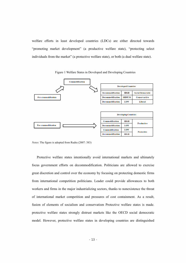
welfare efforts in least developed countries (LDCs) are either directed towards

“promoting market development” (a productive welfare state), “protecting select

individuals from the market” (a protective welfare state), or both (a dual welfare state).

Figure 1 Welfare States in Developed and Developing Countries

Notes: The figure is adopted from Rudra (2007: 383)

Protective welfare states intentionally avoid international markets and ultimately

focus government efforts on decommodification. Politicians are allowed to exercise

great discretion and control over the economy by focusing on protecting domestic firms

from international competition politicians. Leader could provide allowances to both

workers and firms in the major industrializing sectors, thanks to nonexistence the threat

of international market competition and pressures of cost containment. As a result,

fusion of elements of socialism and conservatism Protective welfare states is made.

protective welfare states strongly distrust markets like the OECD social democratic

model. However, protective welfare states in developing countries are distinguished

- 14 -

from both the social democratic and conservative welfare models in that highlighting on

decommodification occurred prior to proletarianization and, accordingly, social rights

have been directed towards a small clientele (Rudra, 2007).

In contrast, productive welfare states emphasize commodification, and originally

developed from systems which actively promoted participation in export markets.

Emphasis on cost containment is created by the goal of encouraging international

competitiveness of domestic firms, and governments are required to surrender some

control over the economy. The range of social welfare is much more restricted, as

leaders are constrained from pursuing worker benefits. Thereby, the liberal model by

Esping-Andersen shares certain components with Productive welfare states. In contrast

to its counterpart, this regime type holds close some of the nineteenth-century liberal

enthusiasm for the market and self-reliance (Rudra, 2007). The emphasis upon

strengthening the commodity status of labor in a globalizing economy is the

characteristics of productive welfare state that the liberal paradigm ultimately comes to

distinguish. Substantial level of public intervention aims to enhance international market

participation in productive welfare states. Social policies are constrained by this goal

and have to be implemented without hampering business activity. In contrast, the

proletarianization occurred gradually in the OECD countries over two centuries, and

state intervention was less required (Rudra, 2007).

- 15 -

III. EMPIRICAL STUDIES ON SOCIAL SPENDING

The studies on the research that question the relationship between social spending

and growth have resulted in mixed findings both theoretically and empirically.

Advocates of positive effect of social spending base their argument on that social

spending can (1) help build higher quality of human capital (2) reduce social conflict,

increasing the level of social cohesion of the country (3) allow laborers to adapt to

radically changing industrial structure and technology (4) and stabilize economy,

reducing inflation in boom days and creating effectual demand in economic depression

(Rodrick, 1999; Blank, 1994; Kohl, 1981; Abramovitz, 1981; Haveman, 1988).

Empirically, several studies found the positive relationship between social spending

and growth. Cashin (1994) showed that social security spending has a significant

positive impact on GDP per capita growth in the 23 developed countries using annual

data from 1971 to 1988 with OLS and IV method. Castles and Dowrick (1990) tested

the relationship between 18 OECD countries’ social spending (health and education

were excluded) and per capita GDP, and found a positive effect. They used pooled time-

series cross-section OLS method using data from 1971 to 1883. Korpi (1985) showed

that ILO social expenditure to GDP is positively associated with the real per capita GDP

in the 17 OECD countries during the period from 1950 to 1973. He used time series and

cross-section estimation by unweighted OLS measuring total effects and controlling for

the share of agricultural labor force. McCallum and Blais (1987) discovered a positive

relationship between OECD social security transfers to GDP and Real GDP of the

countries, using IV technique with controls for employment growth. They used 17

- 16 -

OECD countries with the period from 1960 to 1983. Castronova (2001) suggested that

social spending does not seem to lower per capita incomes, using panel data of 13

OECD countries from 1961 to 1991. Using simultaneous equation model with OECD

data, De Grauwe and Polan (2005) suggested that countries with high level of social

spending have high IMD and WEF competitiveness scores, and countries with well

developed social security systems do not necessarily face a trade-off between social

spending and competitiveness,. Baldacci et al (2004) found, using social spending panel

data in 120 developing countries from 1975 to 2000, that social spending on education

and health in developing countries is positively associated with the accumulation of

education and health capital, and education and health capital has positive impact on

higher economic growth; they insisted that spending on education and health has

positive “indirect impact on growth.”

On the other hand, some studies insist that social spending does harm economic

growth. They argue that social spending can (1) weaken the work incentive of recipients

or tax payers (2) reduce private savings that could be otherwise used in investment for

growth (3) increase dependence on government (4) expand shadow economy, making

distortion in resource allocation (Gilder, 1981; Murray, 1984; Feldstein, 1982; 1996;

Weede, 1986; Persson and Tabellini, 1994).

Some studies showed negative effect or statistically non-significant effect of social

spending on growth. Weede (1986, 1991) found that negative effect of social security

transfers over GDP on the OECD countries’ real GDP. He used pooled time series and

cross-section method with the period from 1960 to mid 1980s. Persson and Tabellini

(1994) included the social expenditure over GDP as one of the independent variables in

his growth model, and conducted a statistical test using the 13 OECD countries data

- 17 -

from 1960 to 1985. They used unweighted IV estimation method, and found negative

but non-significant coefficients in the relationship between social spending and growth.

Hansson and Henrekson (1994) found negative and significant effect of social security

transfers over GDP in 14 OECD countries in the sub-period from 1965 to 1982, and real

private output in 14 industries was the dependent variable. They used cross-country and

cross-industry OLS, controlling for investment and employment. Arjona et al (2003)

found that increased social protection expenditure is bad for economic growth, using

PMG and GMM-IV approaches with an annual sample of 21 OECD countries running

over the period 1970 to 1998. Landau (1985) suggested that transfer payment does not

exhibit statistically significant correlation with growth, using pooled time-series cross-

section method with 16 OECD countries’ data from 1952 to 1976. Carritte and

Willianison (1995) examined the effect of pension spending on economic growth based

on pooled time-series cross-section social indicator models for 18 developed countries

for the period between 1960 and 1988, and they found that the level of pension spending

does not have a substantial impact on economic growth for the period between 1960 and

1973, while a negative impact of pension spending was observed in the period between

1974 and 1988.

In the previous empirical approaches listed above, we can notice that there are some

rooms that are needed to be further examined. First of all, most previous studies tested

the relationship only in developed countries or OECD member countries, and there is

little attention to the effects in developing countries. In fact, the social spending effect

on economic development is somewhat more needed to be tested in developing

countries, because the social development and economic growth is a critically urgent

goal in those countries. Although there is a study by Baldacci et al (2004) that tries to

- 18 -

examine the relationship in developing country, it did not test the direct relationship

between social spending and economic growth. They examined the impact of social

spending on accumulation of education and health capital, and then linked this

accumulated human capital to increased per capita GDP. Although this finding has some

meaningful implications, we can very easily predict that more spending on education

and health will bring about more educational and health capital accumulated, and that

more educational and health capital accumulated will help economic development of the

country, which are tested in their study; that is, these two relationships are very likely to

be proved as positively related. However, what we are actually curious about is the

effect of social spending on overall economic performance of the country; public

spending affects not only the targeting objectives such as human capital accumulation

but also unexpected areas, resulting in some problems sometimes. Therefore, it is

meaningful to test direct relationship between social spending and economic growth in

developing countries. In addition to this, Baldacci et al (2004) did not include the

spending on social protection, but spending on social protection is very important issue

in social policy and economic growth.

Second, previous studies shows little or no efforts to compare the effects of social

spending in developing countries with those in developed or OECD member countries.

However, developing countries can be in very different social, economic, and

institutional settings, which means social spending that have positive or negative or no

impact in OECD countries can have different effects in developing countries. Therefore,

it is worthy to draw a comparison between the result of developing countries and that of

developed and semi-developed countries with the same data source, the IMF’s

Government Finance Statistics.

- 19 -

Third, there is a lack of empirical literatures using recent data; many studies used

data published before 1990. Therefore, it is necessary to look into recent phenomena.

This paper will use International Monetary Foundation’s Government Finance Statistics

which collected data from 1990 to 2007. Considering that many of previous studies used

OECD data, testing the relationship with other source can be also necessary for

robustness.

On the other hand, there could be a fundamental issue in spending approach that

social spending to GDP itself is problematic in measuring the welfare efforts by the

government (Esping-Andersen,1990). Therefore, it can be needed to observe specific

styles of social policy conducted in different countries such as active labor market policy.

However, there is lack of collected data, especially in developing countries, that this

specific policy differences are reflected. Further, even spending approach studies have

hardly dealt with developing countries. Therefore, this approach, which regards social

spending to GDP as proxy, is still meaningful in testing the effect in developing

countries and comparing the results, although we acknowledge that this approach can

have some limitation.

- 20 -

IV. MEOTHODOLOGY

1. Analytic Framework

This study tries to test the relationship between social spending and economic

growth with the endogenous growth model. By doing this, we will examine the

hypothesis that social spending can be instrumental in development. Following

regression will be estimated with time-series cross-section data.

∑=

++=p

k

itkitkit uXaY1

β

In the model, i is the country, t is the year and there are p explanatory, in which the

To test the relationship between social spending and economic growth, we used

time-series cross-sectional regression with error-components models. The time-series

cross-sectional regression deals with panel data sets that consist of time-series on each

of cross-section observation. Panel data creates variability, and provides more

informative results by eliminating the need for lengthy time series because we can use

the information available on the dynamic reactions of each subject (Kennedy 2003).

Further, time-series cross-section data can provide “more informative data, more

variability, less collinearity among variable, more degree of freedom and more

efficiency” by combining time-series observations on cross-sectional units (Gujarati,

2003: 637). Compared with either purely cross-sectional or purely time-series data,

time-series cross-sectional data has the ability to study dynamics of changes and to

model the differences, or heterogeneity, among subjects (Frees, 2004).

However, we have to consider several things that can make OLS biased in time-

- 21 -

series cross-section model (Oatley, 1999). For example, the time series component of

such data sets poses autocorrelation problem, and error terms may exhibit

heteroskedasticity both longitudinally and cross sectionally. Autocorrelation and

heteroskedasticity produce bias in standard error estimates, so lead to incorrect statistical

inferences. To deal with these problems, fixed effect model and random effect model can

be used (Gujarati, 2003); result of Hausman test will be considered in selection of these

models which can solve autocorrelation and heteroskedasticity problems.

Fixed effect model assumes that independent variable and error term is correlated,

while random effect model assumes that error term is independently and identically

distributed. Random effect model does not need to use dummy variable in the model, so

provides greater degree of freedom. However, there could be bias in estimation if

correlation between fixed effect and independent variable exists. Therefore, appropriate

model has to be decided based on Hausman test. If the null hypothesis that there is no

correlation between independent variable and error term is rejected through Hausman

test, fixed effect model is more appropriate. Random effect model can be used when the

null hypothesis is not rejected, which means that there is no such correlation.

The core difference between fixed and random effect models lies in the role of

dummies. If dummies are considered as a part of the intercept, this is a fixed effect

model. In a random effect model, the dummies act as an error term.

The fixed effect model examines group differences in intercepts, assuming the same

slopes and constant variance across groups. Fixed effect models use least squares

dummy variable (LSDV), within effect, and between effect estimation methods. Thus,

ordinary least squares (OLS) regressions with dummies, in fact, are fixed effect models.

The random effect model, by contrast, estimates variance components for groups and

- 22 -

error, assuming the same intercept and slopes. The difference among groups (or time

periods) lies in the variance of the error term. This model is estimated by generalized

least squares (GLS) when the Ω matrix, a variance structure among groups, is known.

The feasible generalized least squares (FGLS) method is used to estimate the variance

structure when Ω is not known. There are various estimation methods for FGLS

including maximum likelihood methods and simulations (Baltagi and Chang, 1994).

Fixed effects are tested by the incremental F test, while random effects are examined

by the Lagrange Multiplier (LM) test (Breusch and Pagan, 1980). If the null hypothesis

is not rejected, the pooled OLS regression is favored. The Hausman specification test

(Hausman, 1978) compares fixed effect and random effect models. Table 1 compares the

fixed effect and random effect models.

There are some missing observations in the data, thus we used method of Wansbeek

Table 1 Differences between Fixed Effect and Random Effect Models

Fixed Effect Model Random Effect Model

Functional Form itkitiit vXay +++= βµ )( )( itikitit vXay +++= µβ

Intercepts Varying across groups and/or

times Constant

Error Variances Constant Varying across groups and/or

times

Slopes Constant Constant

Estimation LSDV, within effect, between

effect GLS, FGLS

Hypothesis Test Incremental F test Breusch-Pagan LM test

Notes: itv is independent and identically distributed with zero means.

- 23 -

and Kapteyn (1989), which has been being widely used in estimation of the error-

components model with unbalanced data.

There are controversies on a reverse direction of causal relation between social

spending and country’s competitiveness. For example, we can imagine that countries

with a high level of economic growth can create extra income which, in turn, leads to a

higher demand for social spending, resulting in more generous social services. However,

De Grauwe and Polan (2005) investigated this reverse causality from competitiveness to

social spending, and found that this relationship is weak. In fact, more researches have

to be done to test the causality if someone wants to be able to say that country’s

competitiveness or level of economic growth can significantly affect social spending.

Therefore, we do not consider the reverse causality in the model, although we know and

acknowledge the potential risk of different causal relation.

2. Variables and Dataset

The independent variable, social spending, will be measured by the average rate of

central government’s expenditure on social protection, health, and education to GDP.

The reason that we used the average of these three items as one variable instead of

testing the effect of social protection, health, and education spending independently is

that spending on these items can be overlapped considerably and can also be correlated,

which can lead bias in the model itself or in the interpretation of the results. The

dependent variable, economic growth, will be measured by the annual GDP growth rate

of the countries. Social spending data, the average rate of the central government’s

- 24 -

expenditure on social protection, health, and education to GDP, is from the International

Monetary Foundation’s Government Finance Statistics.

Each country’s annual GDP growth rate is chosen as a dependent variable and the

GDP growth rate data that this study will use is from the World Development Indicator

by the World Bank.

Control variables include population growth rate, inflation rate, and tax rate. These

control variables were identified in the previous growth studies such as Easterly and

Rebel (1993), Davoodi and Zou (1998), and Andres and Hernando (1997). The

population growth rate, inflation rate, and Tax rate that this study uses are from the

World Development Indicator.

The data of this study includes 85 countries with annual observations from 1990 to

2007 which is sufficient for the time-series cross-sectional regression. In order to

analyze the differences stemming from social, economic, and institutional situations of

the countries, the 85 countries are categorized into three groups; developing countries,

semi-developed countries and developed countries. The GFS social spending data ware

collected on two accounting bases, cash basis and accrual basis, and some countries data

were reported on both basis. If we aggregate data without considering these two

different accounting bases, it can create some bias in cross-sectional dimension,

therefore, we separated country groups by each basis. However, due to the reduced

sample size, caused by this separation, there is a possibility of wrong explanation of

estimated results of regression in the groups with small sample size. To avoid this

problem, we did a regression not only with the data of each basis but also with the

aggregated data by combining cash basis data and accrual basis data, while

acknowledging possible bias.

- 25 -

Table 2 List of the Countries in the Sample

Category WB

Definition Accounting Country Name

Developing Countries

Low-income

Cash Basis Bangladesh, Burundi, Democratic Republic of Congo, Myanmar, Nepal, Pakistan, Tajikistan

Accrual Basis Madagascar

Lower-middle-income

Cash Basis Albania, Azerbaijan, Bhutan, Cameroon, Egypt, Georgia, India, Indonesia, Iran, Lesotho, Maldives, Moldova, Nicaragua, Syrian Arab Republic, Tunisia, Ukraine, Uruguay, Vanuatu (18)

Accrual Basis Bolivia, El Salvador, Thailand

Developed Countries

High-income OECD

Cash Basis Canada, Czech Republic, (Denmark), (Germany), (Hungary), (Ireland), Japan, Korea, (Netherlands), (Spain), (Sweden), Switzerland, United Kingdom, (United States)

Accrual Basis Australia, Austria, Belgium, (Denmark), Finland, France, (Germany), (Hungary), Iceland, (Ireland), Italy, Luxembourg, (Netherlands), New Zealand, Norway, Portugal, Slovak Republic, (Spain), (Sweden), (United States)

Semi-developed Countries

Upper-middle-income

Cash Basis Belarus, Brazil, Bulgaria, (Chile), Croatia, Jamaica, Kazakhstan, Latvia, Malaysia, Mauritius, Mexico, Panama, Russia, Seychelles, Venezuela

Accrual Basis (Chile), Argentina, Lithuania, Poland, Romania, South Africa

High-income Non-OECD

Cash Basis Bahrain, (Estonia), (Malta), Kuwait, Singapore, Slovenia, Trinidad and Tobago, United Arab Emirates

Accrual Basis Cyprus, (Estonia), Israel, (Malta)

Notes: Countries with the data collected on both cash and accrual basis are on parenthesis

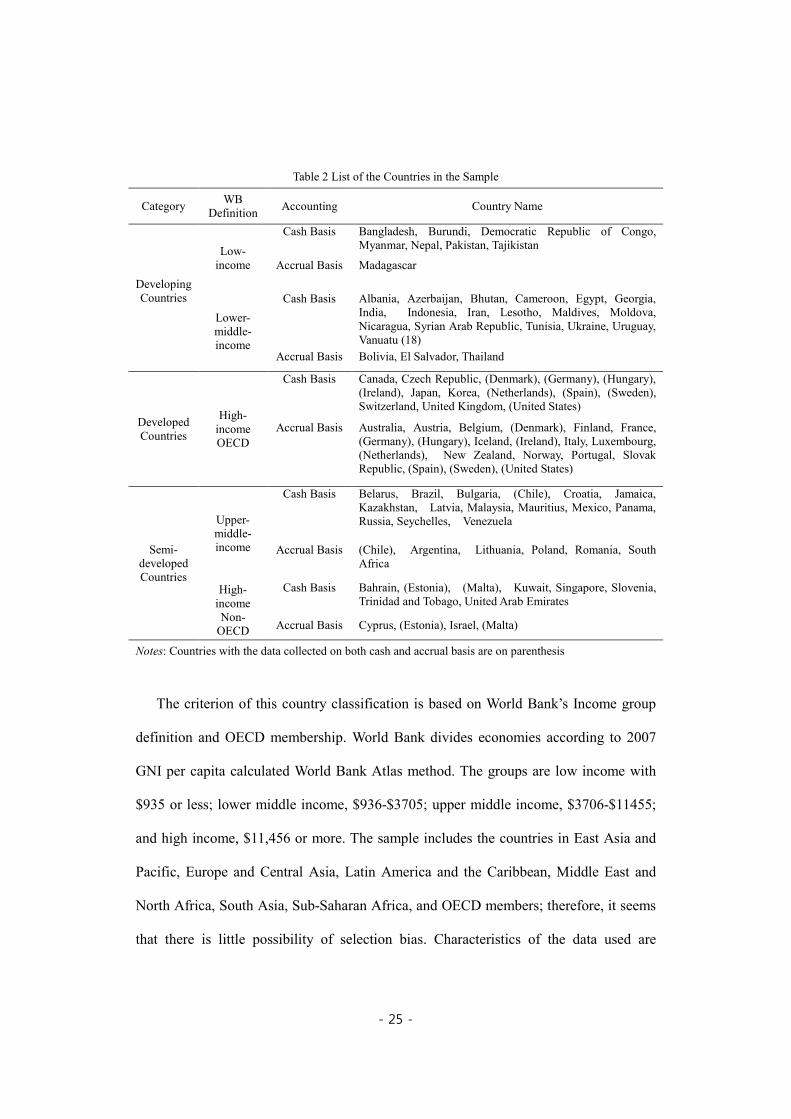
The criterion of this country classification is based on World Bank’s Income group

definition and OECD membership. World Bank divides economies according to 2007

GNI per capita calculated World Bank Atlas method. The groups are low income with

$935 or less; lower middle income, $936-$3705; upper middle income, $3706-$11455;

and high income, $11,456 or more. The sample includes the countries in East Asia and

Pacific, Europe and Central Asia, Latin America and the Caribbean, Middle East and

North Africa, South Asia, Sub-Saharan Africa, and OECD members; therefore, it seems

that there is little possibility of selection bias. Characteristics of the data used are

- 26 -

summarized in Table 3.

Table 3 Summary Statistics

Variable Mean Std. dev. Max Min

Developing Countries (Cash Basis)

GDP Growth Rate (%) 3.17 6.21 23.53 -30.90

Social Spending (%) 3.50 2.31 14.22 0.002

Population Growth Rate (%) 1.15 1.26 3.83 -5.81

Inflation Rate (%) 152.07 1197.9 26762.02 -2.87

Tax Rate (%) 23.03 10.30 57.20 2.99

Developing Countries

(Accrual Basis)

GDP Growth Rate (%) 4.04 2.10 9.19 1.14

Social Spending (%) 4.26 4.00 10.31 -12.67


Inflation Rate (%) 0.81 1.06 2.89 -1.49

Tax Rate (%) 22.47 6.15 32.95 7.99

Developed Countries (Cash Basis)

GDP Growth Rate (%) 3.49 3.70 33.99 -2.39

Social Spending (%) 6.26 4.76 23.36 0.91


Inflation Rate (%) 2.30 4.17 24.47 -17.14

Tax Rate (%) 29.32 9.07 58.71 8.37

Developed Countries

(Accrual Basis)

GDP Growth Rate (%) 7.77 1.97 11.73 3.77

Social Spending (%) 2.74 1.73 8.44 -0.18


Inflation Rate (%) 0.60 0.47 2.20 -0.11

Tax Rate (%) 36.90 6.88 50.41 17.49

Semi- Developed Countries (Cash Basis)

GDP Growth Rate (%) 4.69 3.24 14.43 -6.85

Social Spending (%) 3.39 2.16 7.60 0.87


Inflation Rate (%) 6.68 7.68 37.08 -7.05

Tax Rate (%) 29.57 7.34 42.61 15.90

Semi- Developed Countries

(Accrual Basis)

GDP Growth Rate (%) 6.04 2.04 9.05 3.04

Social Spending (%) 4.00 2.59 10.47 -0.94


Inflation Rate (%) 0.89 0.89 2.64 -0.40

Tax Rate (%) 35.24 4.38 41.92 25.67

- 27 -

V. FINIDNGS AND DISCUSSION

1. Developing Countries

Results of the relationship between social spending and growth in developing

countries, which are the cash and accrual basis combined, are shown in Table 4.

Hausman test rejects the null hypothesis that there is no correlation between

independent variable and error term, with m value of 11.91. This means that the

estimated coefficients in the random effect model could be biased due to the correlations.

Table 4 Result of Developing Country (Cash and Accrual Basis Combined)

Dependent Variable: GDP Growth Rate

Independent Variable Pooled OLS Fixed Effect Model Random Effect Model

Constant 4.5802*** (0.9304)

6.6940* (3.5763)

2.5379 (1.8262)

Social Spending -0.3388** (0.1668)

1.6356*** (0.4038)

0.7153** (0.2838)

Population Growth Rate -0.3811 (0.2771)

0.8528 (0.5274)

0.4409 (0.4273)

Inflation Rate -0.0003* (0.00018)

-0.0001 (0.0001)

-0.0002 (0.0001)

Tax Rate 0.0641 (0.0450)

-0.2325** (0.1154)

-0.0775 (0.0784)

R-Square 0.0429 0.4339 0.0337

Model Test F Value=2.62 (<.0356)

F Test for No Fixed Effects F Value=2.98 (<.0001)

Hausman Test for Random Effects m Value=17.42 (<.0016)

Number of Countries 29 29 29

Notes: Statistically significant at * the 0.1 level, ** the 0.05 level, *** the 0.01 level. Figures on parenthesis are standard errors.

- 28 -

In the fixed effect model, the result of F test for no fixed effect shows that the null

hypothesis, whish is that there are no fixed effects, is rejected with 2.98 F value,

meaning that the pooled OLS model could be also biased because of the existing fixed

effects. As a result, the fixed effect model, which is in the second column of the table

below, was proved to be appropriate in this regression.

The primary finding in the results is that the estimated coefficient on social spending

is positive and statistically significant at 0.01 significant levels. This finding provides

evidence that social spending in developing countries can positively contribute to

economic growth; it is not consistent with the neo-liberal economic theory. Concerning

other variables, tax rate is negatively related to economic growth at 0.05 level.

Table 5 reports the result of the regression in developing countries with cash basis

data. Hausman test for random effects shows, with the 16.24 m value, that independent

variable and error term are not uncorrelated, meaning that random effect model could be

biased. F Test for no fixed effects reject the null hypothesis that there are no fixed

effects, therefore, we have to choose fix effect model in estimation, which is in the

second column of the table.

The estimated coefficient on social spending is positive and significant at 0.01 levels.

This positive relationship is consistent with the result of cash and accrual basis data

combined. Tax rate also shows negative relationship in cash basis data of developing

countries at 0.1 level.

- 29 -

Regression results of developing countries data with accrual basis are displayed in

Table 6. Null hypothesis of no random effect is rejected by Hausman test, but F value of

the test for no fixed effect is not high enough to reject the null hypothesis.

However, we have to consider that the number of countries in this accrual basis data

of developing countries is just four which is very small, although panel data requires

less units in statistical estimation than those of only cross sectional data. In all

regressions of the other subsets in this study never show that the fixed effect model is

inappropriate, meaning that we can hardy believe this results of F test in very small

number of sample. Therefore, the results of this regression on accrual basis can be

Table 5 Result of Developing Country (Cash Basis)



Constant 4.6995*** (0.9487)

0.3124 (3.3435)

3.0964 (1.9424)

Social Spending -0.3191* (0.1711)

1.6131*** (0.3903)

0.8117*** (0.2900)

Population Growth Rate -0.3380 (0.2861)

0.8437 (0.5163)

0.5236 (0.4328)

Inflation Rate -0.0003** (0.00018)

-0.0001 (0.000179)

-0.0002 (0.000172)

Tax Rate 0.0542 (0.0462)

-0.1933* (0.1020)

-0.1174 (0.0807)

R-Square 0.0414 0.3843 0.0443



Hausman Test for Random Effects m Value=16.24 (<.0027)



- 30 -

incorrect due to the small sample, and are not meaningful.

In these regressions in developing countries, we can conclude that social spending,

overall, has positive relationship with growth in developing countries. That is, this

finding can provide evidence that social spending is instrumental in economic growth in

developing countries, which was partly examined in the study by Baldacci et al (2004);

however, this result shows direct positive relationship unlike the indirect impact tested

by Baldacci et al (2004).

Table 6 Result of Developing Country (Accrual Basis)



Constant -15.9047* (8.4045)

-19.2809 (39.6713)

-15.9047* (8.4046)


3.6014 (3.3854)

-3.1035** (1.2916)

Population Growth Rate 5.8721** (2.3863)

-18.9862 (32.2857)

5.8720** (2.3864)

Inflation Rate -0.8542*** (0.2699)

-0.9649** (0.2988)

-0.8542*** (0.2699)

Tax Rate 1.3957** (0.48234)

1.6279 (0.8643)

1.3957** (0.4823)

R-Square 0.5648 0.7217 0.5648



Hausman Test for Random Effects

m Value=5.14 (<.2735)



- 31 -

2. Developed Countries

Regression results in developed countries, cash and accrual basis data combined, are

presented in Table 7. The Hausman test for random effect Results test shows that there is

correlation between independent variable and error term, with m value of 5.90, which

means that the random effect model could be biased. The result of F test for no fixed

effect in the second column shows that the null hypothesis is rejected with 5.34 F value,

meaning that the existing fixed effects could make the pooled OLS biased. Therefore,

the fixed effect model in the second column of the table below is appropriate in

estimation.

Table 7 Result of Developed Country (Cash and Accrual Basis Combined)



Constant 3.0219*** (0.8433)

3.5934 (2.4631)

3.7710** (1.6467)


-0.4506** (0.2084)

-0.1793* (0.1077)

Population Growth Rate 0.3575 (0.3882)

0.1343 (0.6259)

0.1960 (0.5139)

Inflation Rate 0.0625 (0.0498)

-0.0766 (0.0554)

-0.0545 (0.0509)

Tax Rate 0.0215 (0.0282)

-0.0427 (0.0923)

0.0233 (0.0509)

R-Square 0.0494 0.4774 0.0192




m Value=5.90 (<.2066)



- 32 -

A statistically significant negative relationship between social spending and

economic growth is observed in the cash basis developed countries data at 0.05 level.

This result of negative relationship is a contrast to the results of developing countries.

Results of the regression in the cash basis data are reported in Table 8. Hausman test

rejects null hypothesis of uncorrelated error term, with m Value of 4.33, and F test for no

fixed effect presents that there are fixed effects. Therefore, the regression result of fix

effect model, which is in the second column of the table below, is favored. In the results

above, social spending shows no significant but negative coefficient.

Table 8 Result of Developed Country (Cash Basis)



Constant -1.3984 (1.95885)

4.1344 (4.0706)

4.0298 (3.2658)


-0.5621 (0.5466)

-0.1664 (0.1982)

Population Growth Rate 2.1370** (0.9490)

0.6706 (1.4711)

0.6133 (1.3007)


-0.1140 (0.0917)

-0.0749 (0.0846)

Tax Rate 0.1791** (0.0697)

-0.0754 (0.1748)

0.0167 (0.1086)

R-Square 0.1086 0.4800 0.0198




m Value=4.33 (<.3627)



- 33 -

Regression result of developed countries that accrual basis data are displayed in

Table 9. Hausman test for random effects rejects the null hypothesis that independent

variable and error term are uncorrelated, with m value of 7.51. This shows that the

estimation of the random effect model could be biased due to the correlations. The result

of F test for no fixed effect presents that the null hypothesis, whish is that there are no

fixed effects, is rejected with 7.00 F value. This means that the pooled OLS model could

be also biased because of the fixed effects. As a result, the fixed effect model, shown in

the second column of the table below, was proved to be appropriate in the estimation of

this regression.

Table 9 Result of Developed Country (Accrual Basis)



Constant 2.7993*** (0.9774)

4.9735** (2.0681)

5.4252*** (1.6408)

Social Spending -0.1185 (0.1031)

-1.1133*** (0.2237)

-0.4255*** (0.1578)


-1.1988** (0.5560)

-0.1317 (0.4068)


-0.0526 (0.0697)

-0.0376 (0.0553)

Tax Rate 0.0114 (0.0303)

0.1778* (0.0908)

0.0318 (0.0482)

R-Square 0.0695 0.5588 0.0575




m Value=7.51 (<.1113)



- 34 -

In the regression results above, social spending is negatively associated with growth

rate at 0.01 significant level, and this negative relationship is consistent with which is

consistent with the result of cash accrual basis combined data. Population growth rate

also shows negative relationship with growth rate at 0.05 level, while tax rate is

positively related to growth at 0.1 level.

3. Semi-Developed Countries

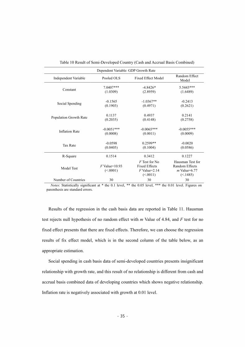
Results of relationship between spending and growth in semi-developed contries,

which are the cash and accrual basis data combined, are presented in Table 10. Hausman

test shows that independent variable and error term is not uncorrelated, with m value of

6.77. Therefore, the random effect model could be biased due to the correlations. The

result of F test for no fixed effect shows 2.14 of F value, and this value is enough to

reject the null hypothesis that there are no fixed effects. Consequently, fixed effect

model is found to be appropriate.

Social spending shows statistically significant and negative relationship in the

regression results at 0.05 level. Regarding other variables, inflation rate is negatively

associated with growth at 0.01, while tax rate is positively related at 0.05 level.

\

- 35 -

Results of the regression in the cash basis data are reported in Table 11. Hausman

test rejects null hypothesis of no random effect with m Value of 4.84, and F test for no

fixed effect presents that there are fixed effects. Therefore, we can choose the regression

results of fix effect model, which is in the second column of the table below, as an

appropriate estimation.

Social spending in cash basis data of semi-developed countries presents insignificant

relationship with growth rate, and this result of no relationship is different from cash and

accrual basis combined data of developing countries which shows negative relationship.

Inflation rate is negatively associated with growth at 0.01 level.

Table 10 Result of Semi-Developed Country (Cash and Accrual Basis Combined)



Constant 7.0407*** (1.0309)

-4.8426* (2.8959)

5.5443*** (1.6489)


-1.0367** (0.4971)

-0.2413 (0.2621)


0.4937 (0.4148)

0.2141 (0.2758)

Inflation Rate -0.0051*** (0.0008)

-0.0065*** (0.0011)

-0.0055*** (0.0009)

Tax Rate -0.0598 (0.0405)

0.2599** (0.1004)

-0.0020 (0.0586)

R-Square 0.1514 0.3412 0.1227




m Value=6.77 (<.1485)



- 36 -

Table 11 Result of Semi-Developed Country (Cash Basis)



Constant 6.9837*** (1.1572)

2.3992 (4.6774)

5.6548 (1.7303)


-0.7559 (0.5376)

-0.2875 (0.3167)


0.7900* (0.4527)

0.2439 (0.2924)

Inflation Rate -0.0050*** (0.0009)

-0.0058*** (0.0012)

-0.0055*** (0.0010)

Tax Rate -0.0578 (0.0463)

0.1437 (0.1160)

0.0011 (0.0622)

R-Square 0.1711 0.4398 0.1386




m Value=4.84 (<.3036)



Regression results of semi-developed countries data with accrual basis are displayed

in Table 12. Null hypothesis of no random effect is rejected by Hausman test, and F test

for no fixed effect presents that there are fixed effects. Therefore, the result of fix effect

model in the second column of the table below is chosen as an appropriate estimation.

In the result of semi-developed countries with accrual basis data, there is a

statistically significant relationship between social spending and growth rate at 0.01

level. Regarding other variables, inflation rate is negatively related at 0.01 level, while

tax rate shows positive coefficient at 0.05 level.

- 37 -

Table 12 Result of Semi-Developed Country (Accrual Basis)



Constant 9.6587*** (2.5765)

-4.2226 (5.9815)

8.1463 (5.9506)


-3.9798*** (1.0714)

-1.8475** (0.7485)

Population Growth Rate -1.3205*** (0.4903)

0.0268 (1.1077)

-0.8392 (0.9602)

Inflation Rate -0.2526*** (0.0836)

-0.5352*** (0.0958)

-0.4611*** (0.0932)

Tax Rate -0.0588 (0.0839)

0.6011** (0.2300)

0.2796 (0.1920)

R-Square 0.2606 0.6787 0.3760

Model Test F Value=4.32 (<0.0045)



m Value=2.79 (<0.5928)



4. Discussion

Gershenkron (1962) argued that different institutions were likely to be developed by

late industrializers in order to exploit their lateness or to catch up. In other words, the

much more active role of state can be played in the pioneer countries. Mkandawire

(2001) suggested that among the institutions adapted by such late industrializers were

those dealing with social policy, although it has rarely been explicitly theorized. Pierson

(1998) notes that “late starters” have tended to develop welfare state institutions earlier

in their own individual development and under more comprehensive terms of coverage

- 38 -

after 1923 except for the United States. That is, social policy served not only to ensure

national cohesion, which is often asserted of Bismarck’s welfare legislation, but also to

develop human capital that facilitated industrialization.

Further, Developmental Welfare theory is challenging the neo-liberal views on social

policy. The argument supporting the social policy is not defensive at all; it rather insists

that economic growth will be impeded if the social policy is retrenched (Midgley and

Tang, 2001). For example, Hall and Midgley (2004) insisted that important goal of

social policy is economic development and that social policy is what the government

should actively involve for economic development. Midgley (1995) defines social

development as “a process of planned social change designed to promote the well-being

of the population as a whole in conjunction with a dynamic process of economic

development.” Midgley and Tang (2001) pointed out that social expenditures in the form

of social investments do not detract from but contribute positively to economic

development.

In developing countries, there could be a situation that potential productive labor

forces in developing countries are not able to efficiently work or do some business,

because they have some health problems or are not well educated. In turn, productivity

is likely to be low due to the poor use of assets and less efficiency, and economic growth,

as a result, is becoming less competitive than they would have been otherwise (DFID,

2006). Social spending can improve health and education condition, and offer more

productive workforce. Social spending in developing country also can protect assets that

help people earn an income, encourage risk taking, and promote participation in the

labor market (DFID, 2006).

The regression results of this study can suggest that assumption of a tradeoff

- 39 -

between efficiency and equity could be not well applied in the developing countries.

Birdsall et al (1995) suggested that policies in East Asian countries which reduced

poverty and income inequality, such as emphasizing high-quality basic education and

augmenting labor demand, help stimulate economic growth in their developing period.

Furthermore, Rodrick (1999) argues that many countries’ experiences of a growth

collapse since the mid-1970s can be explained by domestic social conflicts. He showed

that divided societies (as measured by indicators of inequality, ethnic fragmentation, and

the like) and weak institutions of conflict management are the characteristics of the

countries who experienced the sharpest drops in growth after 1975 (Rodrick, 1999).

Persson and Tabellini (1994) also suggested that there is a significant and large negative

relation between inequality and growth using historical panel data and postwar cross

sections.

VI. CONCLUSION

This study examined the relationship between social spending and economic growth,

drawing a comparison between the result of developing countries and that of developed

(or OECD member) and semi-developed countries.

We found that estimated coefficient on social spending is positive and statistically

significant in the sample of developing countries. This result is a contrast with neo-

liberal economic theory. On the other hand, a significant negative relationship between

social spending and economic growth is observed in the sample of developed countries.

- 40 -

Lastly, the results of the regression in the sample of semi-developed countries show that

there is statistically significant and negative relationship, although there is also

insignificant negative coefficient in one regression of cash basis data.

This finding can imply that that assumption of a tradeoff between efficiency and

equity could be not well applied in the developing countries. Therefore, we have to

consider not only what to do but also where to do, when we discuss the social spending

effect and give policy advises to developing countries.

VII. REFERENCES

Abramovitz, M. (1982). Welfare Quandaries and Productivity Concerns. American

Economic Review, 71(1): 1-17.

Arjona, Roman and Ladaique, Maxime and Pearson, Mark. (2003). Growth, Inequality

and Social Protection. Canadian Public Policy/Analyse de Politiques, 29: 119-139.

Baldacci, Emanuele and Clements, Benedict and Gupta, Sanjeev and Cui1, Qiang.

(2004). Social Spending, Human Capital, and Growth in Developing Countries:

Implications for Achieving the MDGs. IMF Working Paper.

Baltagi, Badi H. and Chang, Young-Jae. (1994). Incomplete Panels: A Comparative

Study of Alternative Estimators for the Unbalanced One-way Error Component

Regression Model. Journal of Econometrics, 62(2): 67-89.

Blank, R. (1994). Social Protection Versus Economic Flexibility: Is There a Trade-Off.

- 41 -

Chicago: University of Chicago Press.

Birdsall, Nancy and Ross, David and Sabot, Richard. (1995). Inequality and Growth

Reconsidered: Lessons from East Asia. World Bank Economic Review, 9(3): 477-

508.

Breusch, T. S. and Pagan, A. R. (1980). The Lagrange Multiplier Test and its

Applications to Model Specification in Econometrics. Review of Economic

Studies, 47(1):239-253.

Bryson, L. (1992). Welfare and the State: Who Benefits? London: Macmillan.

Cashin, P. (1994). Government Spending, Taxes and Economic Growth. IMF Working

Paper WP/94/92.

Castles, F.G. and Dowrick, S. (1990). The Impact of Government Spending Levels on

Medium-Term Economic Growth in the OECD, 1960-85. Journal of Theoretical

Politics, 2: 173-204.

Castronova, Edward. (2001). Inequality and Income: The Mediating Effects of Social

Spending and Risk. Economics of Transition, 9(2): 395-415.

Cornia, Giovanni Andrea and Jolly, Richard and Stewart, Frances. (1987), Adjustment

with a Human Face, Oxford: Clarendon Press.

De Grauwe, Paul and Polan, Magdalena. (2005). Globalization and Social Spending.

Pacific Economic Review, 10(1): 105-123.

Demerath, N. J. III. (1977). Book Review: Social Policy. The American Journal of

Sociology, 82(5); 1105-1107.

DFID. (2006). Social Protection and Economic Growth in Poor Countries. DFID

practice paper. Social Protection Briefing Note Series No. 4.

Easterly, William and Rebelo, Sergio. (1993). Marginal Income Tax Rates and Economic

- 42 -

Growth in Developing Countries. European Economic Review, 37(2): 409-417.

Esping-Andersen, Gosta. (1990). The Three Worlds of Welfare Capitalism. Princeton, N.

J.: Princeton University Press.

Esping-Andersen, Gosta and Korpi, Walter. (1987). From Poor Relief to Institutional

Welfare States: The Development of Scandinavian Social Policy. in Erikson,

Robert et al (eds). The Scandinavian Model: Welfare States and Welfare Research.

Armonk, N.Y.: M.E. Sharpe.

Feldstein, Martin S. (1996). Social Security and Saving: New Time Series Evidence.

National Tax Journal, 49(2): 151-164.

Feldstein, Martin S. (1982). Social Security and Private Saving: Reply. The Journal of

Political Economy, 90(3): 630-642.

Frees, Edward W. (2004). Longitudinal and Panel Data: Analysis and Applications in

the Social Science. Cambridge University Press

Fuller, W.A. and Battese, G.E. (1974), Estimation of Linear Models with Crossed-Error

Structure, Journal of Econometrics, 2: 67-78.

Furniss, Norman and Tilton, Timothy. (1977). The Case for the Welfare State: From

Social Security to Social Equality. London: Indiana University Press.

Hausman, J. A. (1978). Specification Tests in Econometrics. Econometrica, 46(6): 1251-

1271.

George, Peter. (1985). Towards a Two-dimensional Analysis of Welfare Ideologies.

Social Policy & Administration, 19(1): 33-34.

George, Victor and Wilding, Paul. (1976). Ideology and Social Welfare. London:

Routledge & Kegal Paul.

Gershenkron, Alexander. (1962). Economic Backwardness in Historical Perspective.

- 43 -

Cambridge; Massachusetts: Harvard University Press.

Gilder, George. (1981). Wealth and Poverty. New York: Basic Books.

Goodman, R. and G. White. (1998). Welfare Orientalism and the Search for an East

Asian Welfare Model. in Goodman, R. and White G. and Kwon, H-J. (eds). The

East Asian Welfare Model: Welfare Orientalism and the State. London: Routledge.

Graycar, Adam and Jamrozik, Adam. (1993). How Australians Live: Social Policy in

Theory and Practice. South Melbourne: Macmillan Australia.

Gujarati, Damodar N. (2003). Basic Econometrics. Boston : McGraw Hill.

Hall, Anthony and Midgley, James. (2004). Social Policy for Development. London:

Sage.

Hansson, P. and Henrekson, M. (1994). A New Framework for Testing the Effect of

Government Spending on Growth and Productivity. Public Choice, 81: 381-401.

Haveman, R. (1988). Starting Even: An Equal Opportunity Program to Combat the

Nation's New Poverty. New York: Simon and Schuster.

Hort, S. and Kuhnle, S. (2000). The Coming of East and South-East Asian Welfare

States. Journal of European Social Policy, 10(2): 162–84.

Jones, C. (1993). The Pacific Challenge: Confucian Welfare States. In Jones, C. (ed.),

New Perspectives on the Welfare State in Europe. London: Routledge.

Kennedy, P. (2003). A Guide to Econometrics. The MIT Press, Cambridge,

Massachusetts.

Korpi, W. (1985). Economic Growth and the Welfare System: Leaky Bucket or

Irrigation System? European Sociological Review, 1: 97-118.

Kwon, Huck-ju. (1998). Democracy and the Politics of Social Policy: Comparative

analysis of social policy in East Asia. in Goodman, R. and White G. and Kwon, H.

- 44 -

J. (eds). The East Asian Welfare Model: Welfare Orientalism and the State.

London: Routledge.

Kwon, Huck-ju. (2005). Review Article: Social Policy and Development in Global

Context. Social Policy and Society, 4(4): 467–473.

Kwon, Huck-ju. (2007). Transforming the developmental welfare states in East Asia.

UN DESA Working Paper No. 40.

Landau, Daniel. (1985). Government Expenditure and Economic Growth in the

Developed Countries: 1952-76. Public Choice, 47: 459-477.

Lindert, Peter H. (2004). Growing Public: Social Spending and Economic Growth since

the Eighteenth Century. Cambridge University Press.

Lindert, Peter H. (2006). The Welfare State Is the Wrong Target: A Reply to Bergh. Econ

Journal Watch, 3(2): 236-250.

McCallum, J. and Blais, A. (1987). Government, Special Interest Groups and Economic

Growth. Public Choice, 54: 3-18.

Midgley, James. (1995). Social development: The developmental perspective in social

welfare. Thousand Oaks, CA, Sage Publications.

Midgley, James and Tang, Kwong-leung. (2001). Social policy, economic growth and

developmental welfare. International Journal of Social Welfare, 10: 244-252.

Mishra, Ramesh. (1981). Society and Social Policy: Theories and Practice of Welfare.

London: Macmillan.

Mkandawire, Thandika. (2001). Social Policy in a Development Context. Geneva:

United Nations Research Institute for Social Development

Murray, C. (1980). Losing Ground: American Social Policy, 1950-1980. New York:

Basic Books.

- 45 -

Oatley, Thomas. (1999). Central bank independence and inflation: Corporatism,

partisanship, and alternative indices of central bank independence. Public Choice,

98: 399–413.

Persson, T. and Tabellini, G. (1994). Is Inequality Harmful for Growth? American

Economic Review, 84(3): 600-621.

Pierson, Christopher. (1998). Beyond the Welfare State: The New Political Economy of

Welfare. London: Polity Press.

Rodrik, Dani. (1999). Where Did All the Growth Go? External Shocks, Social Conflict,

and Growth Collapses. Journal of Economic Growth, 4: 385–412.

Romer. Paul M. (1986). Increasing Returns and Long-Run Growth. The Journal of

Political Economy, 94(5): 1002-1037.

Rudra, Nita. (2007). Welfare States in Developing Countries: Unique or Universal? The

Journal of Politics, 69(2): 378-396.

Sainsbury, Diane. Analysing Welfare State Variations: The Merits and Limitations of

Models Based on the Residual–Institutional Distinction. Scandinavian Political

Studies, 14(1); 1-30.

Titmuss, Richard M. (1974). Social Policy: An Introduction. Edited by Abel-Smith, B.

and Titmuss, K. New York: Pantheon Books.

Wansbeek, Tom and Kapteyn, Arie. (1989), Estimation of the Error-Components Model

with Incomplete Panels, Journal of Econometrics, 41: 341-361.

Weede, E. (1986). Sectoral Reallocation, Distributional Coalitions and the Welfare State

as Determinants of Economic Growth Rates in OECD Countries. European

Journal of Political Research, 14: 501-19.

Weede, E. (1991). The Impact of State Power on Economic Growth Rates in OECD

- 46 -

Countries. Quality and Quantity, 25: 421-438

Wilensky, Harold. L. (2002). Rich Democracies: Political Economy, Public Policy, and

Performance. Berkeley: University of California Press.

Wilensky, Harold L. and Lebeaux, Charles N. (1958). Industrial Society and Social

Welfare. New York: Free Press.

- 47 -

국문 초록

사회지출과 경제 성장의 관계에 관한 실증연구

-개발도상국과 OECD국가 비교-

사회지출과 경제성장과의 관계에 관한 실증적인 연구는 그동안 OECD국가들을

대상으로 한 것이 대부분이었다. 즉, 사회지출이 경제성장에 미치는 영향에 대해서

개발도상국을 대상으로 한 연구나, 개발도상국과 OECD국가를 비교한 연구는 거의

없었다. 그러나 개발도상국은 사회적, 경제적, 그리고 제도적 환경에 있어 OECD국

가와는 매우 다르며, 이것은 같은 내용의 정책이나 공공지출일지라도 전혀 다른 결

과를 가져올 가능성이 많다는 것을 의미한다.

따라서 본 연구는 선진국, 중진국, 개발도상국으로 나누어 각각의 국가군에서

사회지출과 경제성장과의 관계를 통계적으로 검증하는 시도를 하였다. IMF의

Government Finance Statistics의 1990년부터 2007년까지 85개국의 패널 데이터를

활용하였고, error component 모형으로 time series cross section 회귀 분석을 하

였다.

그 결과 개발도상국 표본에서는 사회지출과 경제성장이 양의 상관관계를 갖는

것으로 나온 반면, 선진국에서는 음의 상관관계는 갖는 것으로 나왔다. 본 연구의 이

러한 결과는 효율성과 평등이 동시에 충족될 수 없다는 신자유주의적 이론이 개발도

상국에서는 잘 적용되지 않을 수 있다는 것을 의미한다. 그러므로 개발도상국의 사

회정책이나 개발 프로그램을 실행함에 있어 "무엇"을 할지와 더불어 "어디"에 "언제"

할 것인지 고려하는 것이 함께 필요하다는 함의를 이 연구를 통해 얻을 수 있다고

할 수 있다.

Empirical Analysis of the Relation Between Social Spending and Economic...

Documents

Transcript of Empirical Analysis of the Relation Between Social Spending and Economic...