Empirical Analysis of Countervailing Power in

Business-to-Business Bargaining

Walter Beckert∗

This version: May 2011.

Abstract

This paper provides a comprehensive econometric framework for the em-

pirical analysis of countervailing power. It encompasses the two main fea-

tures of pricing schemes in business-to-business relationships: nonlinear price

schedules and bargaining over rents. Disentangling them is critical to the em-

pirical identification of countervailing power. Testable predictions from the

theoretical analysis are delineated, and a pragmatic empirical methodology

is presented. It is readily implementable on the basis of transaction data,

routinely collected by antitrust authorities. The empirical framework is il-

lustrated using data from the UK brick industry. The paper emphasizes the

importance of controlling for endogeneity of volumes and for heterogeneity

across buyers and sellers.

JEL Classification: D43, L11, L12, L14, L42, C23, C78

Keywords: countervailing power, bargaining, nonlinear prices, transac-

tion panel data

∗I am grateful for helpful discussions with Ron Smith and Kate Collyer. I also benefitted

from comments by Richard Blundell, Sandeep Kapur, John Thanassoulis, Howard Smith and Mike

Whinston and various seminar audiences. I am indebted to executives of the UK brick industry

for letting me use their data. The views expressed in this paper are the sole responsibility of the

author. All errors are mine.

1

Correspondence: w.beckert@bbk.ac.uk, Walter Beckert, School of Eco-

nomics, Mathematics and Statistics, Birkbeck College, University of London,

Malet Street, London WC1E 7HX, UK.

1 Introduction

Countervailing power, often referred to as buyer power, is a paramount con-

cern in competition analysis. It is a line of inquiry in many competition

investigations focussing on business-to-business (B2B) dealings. Quintessen-

tial high profile examples are the relationships between supermarkets and

their suppliers.1 Another recent topical example is the relationship between

Chinese steel mills and Australian and Brazilian iron ore miners.2

At the center of many competition inquiries are often generic products,

e.g. groceries or raw materials. Then, the focus is on per unit prices, usually

obtained by antitrust bodies as revenue per unit sold. This price measure

typically constitutes a combination of the respective portion of a nonlinear

unit price schedule and a lump sum payment, e.g. a franchise fee, rebate, ret-

rospective quantity discounts or other incentive payment that is the outcome

of bargaining over joint surplus between buyer and supplier. Hence, one of the

primary difficulties in the analysis of buyer power on the basis of unit prices

is the important distinction between nonlinear pricing and the appropriation

of rents by means of bargaining.3

The conceptual contribution of this paper is a framework that connects

1On the European level, the European Commission considered buyer power issues in the German

- Austrian merger Rewe/Meinl (1999) and the French - Spanish merger Carrefour/Promodes (2000);

see also European Commission (1999). On the national level, see, for example, the recent market

inquiry into UK grocery retailing by the UK Competition Commission, in particular Provisional

Findings Appendix 8; the report can be downloaded from the Competition Commission website.2See Financial Times UK online, 09 July 2008. In spite of shipping costs per tonne from Brazil

being twice those from Australia, Brazilian and Australian miners receive the same freight-on-

board price. This is interpreted as a reflection of superior negotiating power of Brazilian miners

when bargaining with Chinese mills, given the size of Chinese demand for, and the limitations on

Australian miners’ capacity in the supply of, iron ore.3See also Bonnet et al. (2004) who investigate manufacturer-retailer relationships involving

nonlinear pricing. They present empirical tests of two-part tariffs with versus without retail price

maintenance embedded in a structural model of competition in differentiated product markets (e.g.

Berry (1994), Berry et al. (1995)) using market level data.

2

the analysis of countervailing power4 with the design of optimal nonlinear

pricing schemes, while at the same time incorporating bargaining over rents.

It thereby illuminates how buyer power is enhanced by the buyer’s ability

to switch between suppliers, and is constrained by the suppliers’ outside op-

tions and capacity; in particular, in contrast to Chipty and Snyder (1999),

Smith and Thanassoulis (2008) and some conventional wisdom, this paper

shows that, in the face of suppliers’ capacity constraints, buyer size may di-

minish buyer power. The theoretical model also offers supplier heterogeneity,

arising from idiosyncratic outside options, as a new explanation of equilib-

rium price dispersion; this line of argument is particularly pertinent to the

business-to-business context where traditional explanations in terms of im-

perfect information are implausible.5

The methodological contribution of the paper is a robust and practical

econometric methodology to identify countervailing power on the basis of B2B

transaction panel data. Such data are typically available in antitrust inquiries.

The proposed econometric approach is grounded in the theoretical framework

of B2B bargaining, highlights the importance of proper treatment of hetero-

geneity across bargains, and does not rely on complex identifying assumptions

or restrictions that are difficult to test. Instead, the econometric methodology

examines testable implications of the theory and thereby offers a robust route

to the empirical identification of countervailing power. Furthermore, it is easy

to implement and hence does not suffer from the typical barriers to diffusion

into applied competition analysis that many other methodologies are fraught

with. It is illustrated using data from a UK Competition Commission merger

inquiry in the brick manufacturing industry.

The paper proceeds as follows. After a brief review of the relevant antitrust

background, section 2 outlines the theoretical model that guides the analysis;

the section concludes with the main issues that an econometric analysis of

countervailing power has to confront and delineates implications for a robust

empirical strategy to identify countervailing power. Section 3 is devoted to

the empirical part of the paper. It presents the background for, and data used

4The notion of countervailing (buyer) power was coined by Galbraith (1952) and theoretically

developed in a dynamic setting by Snyder (1996).5The traditional view relates to retail prices and is articulated in Salop and Stiglitz (1977, 1982),

Reinganum (1979), Burdett and Judd (1983), Carlson and McAfee (1983), Hallagan and Joerding

(1985), Sorensen (2000) and the ensuing literature on equilibrium price dispersion.

3

in, the applied part of the paper, and it summarizes the empirical analysis.

Section 4 concludes.

1.1 Countervailing Power Analysis in Antitrust

The analysis of buyer power is often an integral part in antitrust inquiries. The

UK Competition Merger Guidelines (2003)6 consider buyer power in merger

assessment: Do buyers, either because of their size or commercial signifi-

cance to their suppliers, have the ability to prevent the exercise of market

power by suppliers? This ability, if present, is akin to Galbraith’ (1952) no-

tion of countervailing buyer power. The Competition Commission considers

such countervailing power as one potential mitigating factor, next to others

such as entry and switching costs, in the assessment of upstream mergers. In

the competition assessment in its market investigations (Competition Com-

mission Market Investigation Guidelines (2003)), it investigates the relative

importance to each other of each firm’s business with the counterparty; there

is an additional question whether any price reductions, obtained by virtue of

buyer power, are passed on to consumers. The guidelines enumerate several

factors that are viewed as potentially affecting buyers’ ability to constrain

suppliers: buyers’ ability to find alternative suppliers; the ease with which

buyers can switch suppliers; the extent to which buyers can credibly threaten

to set up their own supply arrangements, e.g. by backward integration or by

sponsoring entry; the extent to which buyers can impose costs on suppliers,

e.g. by delaying or stopping purchases or by transferring risk. It is worth

noting in this regard that a buyer’s size can cut both ways: while size en-

hances the significance of the buyer’s business vis-a-vis the supplier, it makes

switching more difficult when alternative suppliers’ capacities are constrained.

A prototypical buyer power analysis is the Competition Commission’s in-

vestigation as part of its inquiry into grocery retailing in the UK (2008). Based

on their size, pricing and margins, the Commission concluded that all large

retailers, wholesalers and buying groups have buyer power vis-a-vis their sup-

pliers. However, the Commission considered that their buyer power is offset

by market power of suppliers of branded goods; and that lower prices aris-

ing from buyer power in part are passed on to consumers. The Commission

6At the time of writing, the Competition Commission is drafting a revision of its guidelines.

4

substantiated these findings with an analysis of panel data, which for vari-

ous stock-keeping-units (SKUs) comprised yearly prices, volumes and some

cost information. The Commission’s methodology consisted of fixed-effects

regressions of unit prices on volumes.

The Commission’s analysis raises several questions. Panel data meth-

ods can capture unobserved heterogeneity. The analysis modelled SKU-level

idiosyncratic effects, but is this the appropriate level of heterogeneity? More-

over, does aggregation to annual data mask latent heterogeneity across time?

The analysis may also raise concerns about the treatment of volumes: If

business-to-business relationships involve bargaining over both volumes and

prices, then volumes should be treated as endogenous regressors. Furthermore,

the caveat about the ambiguous volume effect notwithstanding, the Commis-

sion’s analysis focussed on volume effects on prices as evidence of buyer power,

without attempting to quantify buyer’s ability to switch suppliers. But vol-

ume effects on unit prices might just reflect suppliers’ nonlinear pricing and

self-selection of buyers into the appropriate part of the tariff, irrespective of

buyer power. Hence, this type of reduced form analysis might be critiqued

along various dimensions, and it highlights that the treatment of potential

heterogeneity across buyers and suppliers, endogeneity of prices and volumes

and the distinction between nonlinear pricing and bargaining over rents are

the primary empirical challenges of the empirical analysis of buyer power.

1.2 Related Literature

Its growing importance and policy relevance notwithstanding, the academic

literature on buyer power is still relatively sparse. Inderst and Mazzarotto

(2006) survey its main theoretical strands to date, as they relate to sources

and consequences of, as well as policy responses to, buyer power of retailers

vis-a-vis manufacturers. With regard to applied work, the academic literature

offers very little towards a comprehensive, structural empirical framework for

the analysis of buyer power.7 Giulietti (2007) presents a reduced form anal-

7There is some early nonstructural work that provides empirical evidence supporting counter-

vailing buyer power; see Adelman (1959), Brooks (1973), Buzzell et al. (1975), Lustgarten (1975),

McGukin and Chen (1976), McKie (1950), Clevenger and Campbell (1977), Boulding and Staelin

(1990). Dobson and Waterson (1997) and von Ungern-Sternberg (1996) examine the effect on

countervailing power on consumer prices.

5

ysis of the Italian grocery retail sector, approximating suppliers’ bargaining

power by a concentration measure for the respective product level industry

they operate in. Chipty and Snyder’s (1999) approach exhibits more detailed

structural features. It provides an empirically testable condition - concavity

of the supplier’s revenue function - that needs to be satisfied for larger buyers,

e.g. arising from buyer mergers, to obtain lower transfer prices when bargain-

ing over surplus with their suppliers. This framework captures the anecdotal

view that larger buyers enjoy greater buyer power. It is useful when the analy-

sis focuses on revenues for bespoke goods or services; this is the case in Chipty

and Synder’s application of their model to the US cable television industry.

While Chipty and Snyder consider the case of an upstream monopoly, El-

lison and Snyder (2001) build on this approach and investigate the role of

substitution possibilities as a consequence of upstream competition. They fo-

cus on price differences in wholesale pharmaceutical markets between different

types of buyers, controlling for various institutional differences with regard to

drug administration.8 Recent work by Smith and Thanassoulis (2008) demon-

strates how upstream competition can endow large buyers with market power

by inducing supplier-level volume uncertainty.

Related work by Villas-Boas (2007) examines vertical relationships be-

tween manufacturers and retailers with limited data, when wholesale prices

for transactions between them are not observed; her objective is to indirectly

identify the strategic model appropriate for their interaction from demand

and cost estimates, with a particular focus on pricing models which feature

double marginalization.

8Drugs can be branded and subject to patent protection, branded and subject to generic com-

petitors, or generic and subject to some form of oligopolistic competition. Buyers such as HMOs

and hospitals have wider substitution possibilities through the use of restrictive formularies relative

to chain drugstores and independent drugstores. Ellison and Snyder (2001) empirically examine

the effects of different features of drugs on the difference in prices paid by various types of buyers.

Using cross-section data, their analysis cannot model unobserved heterogeneity across buyers. The

empirical analysis presented in this paper demonstrates that there exist circumstances in which

the conclusion about buyer power critically hinges on accounting for unobserved heterogeneity.

6

2 Theory

As a preamble to the theoretical section of the paper, it is worth emphasizing

at the outset that the theoretical framework outlined below is a stylized char-

acterization of business-to-business bargaining and not intended to capture

all the intricacies of business-to-business relationships. Instead, it is intended

to motivate the main issues that econometric analyses of buyer power have to

deal with. The empirical strategy proposed in this paper deliberately follows a

reduced form econometric approach that is informed by the structural model,

but does not suffer from the typical potential criticism of strong identifying

restrictions that structural approaches rely upon. The econometric approach

proposed here instead relies on testable implications that are robust across

more tightly specified structural models.

2.1 Multilateral Bargaining

To start, consider bilateral bargaining with complete information between a

single buyer and suppliers of an input to the buyer’s production technology.

Consider the following assumptions:

A1: The buyer’s production technology uses input q with revenue function

F (q) = qθ, θ ∈ (0, 1).

A2: The buyer faces a supplier whose payment schedule for the delivery of

q is given by C(q) = βqα, α, β ≥ 0. The supplier incurs zero cost of

production.

A3: The buyer maximizes profits F (q)−C(q); Nash bargaining over the joint

surplus between buyer and supplier induces the optimal price schedule

that the supplier presents to the buyer.

Proposition 1: Under assumptions A1-A3, the optimal nonlinear price

schedule is p(q) = q2θ−1.

Proof: Bargaining over surplus is the first stage of a two-stage game be-

tween the buyer and the supplier. On the second stage, given a price schedule

p(q) and associated payment schedule C(q) = p(q)q, the buyer chooses the

profit maximizing amount of inputs. This two-stage game is solved by back-

wards induction.

7

Maximizing the buyer’s profits π(q;α, β) = F (q)−C(q) = qθ − βqα over q

on the second stage yields optimal inputs q =(

θαβ

) 1α−θ

. The associated max-

imum profit is qθ−βqα =(

θαβ

) θα−θ −β

(θαβ

) αα−θ

=(

1β

) θα−θ ( θ

α

) αα−θ

(αθ − 1

)>

0, provided α > θ.

Following Stole and Zwiebel (1996), Nash bargaining on the first stage

induces the supplier to design the payment schedule such that the loss from

a breakdown in negotiations for both parties equate, i.e. the supplier chooses

α > θ and β > 0 that

π(q; α, β) =

(θ

αβ

) θα−θ

− β

(θ

αβ

) αα−θ

= β

(θ

αβ

) αα−θ

.

This implies that α = 2θ, while β is indeterminate, so without loss of genere-

ality β = 1. This implies the optimal price schedule p(q) = C(q)/q = βqα/q =

q2θ−1, and the buyer’s and supplier’s profits are(θα

) αα−θ = 1

4 . �.

Suppose now that the buyer faces two identical suppliers, i.e. there is

upstream competition and the buyer bargains multilaterally. The buyer will

find it optimal to source from both if the optimal payment schedule is convex,

i.e. α > 1. Therefore, consider the assumptions

A1’: The buyer’s production technology uses input q and induces the revenue

function F (q) = qθ, θ ∈(12 , 1

).

A2’: The buyer faces two identical suppliers whose payment schedule for the

delivery of q is given by C(q) = βqα, β ≥ 0, α > 1. The suppliers incur

zero cost of production.

A3’: The buyer maximizes profits; Nash bargaining over the joint surplus

between buyer and suppliers holding passive beliefs9 induces the optimal

price schedule that the supplier presents to the buyer.

Proposition 2: Under assumptions A1’, A2’ and A3’, upstream competi-

tion induces an optimal nonlinear price schedule p(q) that involves p(q) < p(q)

for all q > 0, where p(q) is given by Proposition 1.

9Cf. McAfee and Schwartz (1994); this assumption is maintained in Stole and Zwiebel and,

more generally, the literature on bargaining with multiple agents. It stipulates in this context

that in any bilateral bargaining situation between a buyer and a supplier, the parties hold the

belief that, should bargaining between them break down, the buyer reaches an efficient bargaining

outcome with the other supplier.

8

Proof: Since the marginal contribution to the buyer’s revenue from either

supplier is the same at an optimal input allocation, it must be that, with

convex payments, the buyer sources the same amount from both. Hence, on

the second stage, the supplier maximizes (2q)θ − 2βqα over q. This yields

optimal inputs q = 2θ−1α−θ

(θαβ

) 1α−θ

= 2θ−1α−θ q < q and 2q = 2

α−1α−θ q > q. This

implies associated maximum profits of π(q;α, β) = 2θ(α−1)α−θ π(q;α, β).

Consider the Nash bargaining stage where the buyer faces a supplier, hold-

ing passive beliefs. The supplier designs a price schedule with parameters α

and β such as to equate the loss to the buyer from breakdown with the sup-

plier’s loss of revenue, i.e.

2θ(α−1)α−θ π(q; α, β)− 1

4= β

(θ

αβ

) αα−θ

2(αθ−1)α−θ .

Suppose the supplier were to choose α = 2θ and β = 1, as in Proposition 1,

i.e. as if there were no upstream competition. Then, the buyer’s lost profits

(the LHS of the preceding equality) would be 14

(22θ−1 − 1

)> 0 if θ > 1

2 ,

while the supplier’s lost profits (the RHS of the preceding equality) would be142

2θ−1. Hence, the supplier has more to lose from a breakdown in bargaining

than the buyer and, therefore, has an incentive to offer better terms10, i.e.

α < α and β ≤ β. �Proposition 2 shows that upstream competition endows the buyer with

countervailing power vis-a-vis suppliers that permits to extract uniformly

more favorable terms from them. It follows as a corollary that the buyer’s

profits are increased by upstream competition. This inspires the definition of

countervailing buyer power in terms of equilibrium prices:

Definition: Consider a buyer who faces a nonlinear equilibrium price

schedule pi(q), q > 0, in the presence of an upstream monopoly of supplier

i. The buyer enjoys countervailing power if, in equilibrium, the supplier i

present the buyer with a nonlinear price schedule pi(q) < pi(q) for all q > 0.

Considering the equilibrium pay-off structure resulting from Proposition

2, by construction the pay-offs are balanced and efficient. Moreover, they

are individually fair, i.e. they exceed the individual non-cooperation pay offs;

10This can also be formally shown by noting that the derivative of the buyer’s loss with respect

to α and β at α and β is negative and dominated by the derivative of the supplier’s loss with

respect to the payment parameters at that point, so that the values α and β cannot be larger than

α and β.

9

symmetric, i.e. the equivalent suppliers receive the same pay-offs; additive

across bargains; and satisfy that a supplier who does not contribute to the joint

surplus receives a zero pay-off. The revenue or profit accruing to the supplier

therefore has the interpretation of the supplier’s Shapley value associated

with the cooperative game between the buyer and the two suppliers.11 Since

q < q, it follows that p(q)q < p(q)q. This inspires an equivalent definition of

countervailing buyer power in terms of Shapley values:

Definition: Consider supplier i’s Shapley value in the cooperative game

associated with the coalition including only i and the buyer, pi(qi)qi. The

buyer enjoys countervailing power if i’s Shapley value in the cooperative game

associated with the coalition including, inter alia, supplier i and the buyer,

pi(qi)qi, satisfies pi(qi)qi < pi(qi)qi.

It also follows as a corollary to the two preceding propositions that any

outside options the suppliers have, such as the selling to other buyers, enhances

their bargaining outcome, because such outside options reduce the loss they

incur in the event of a breakdown of bargaining.

A question that arises in the presence of upstream competition is whether

Bertrand style price competition would not drive prices below those predicted

by Proposition 2. While it is beyond the scope of this analysis to address

this concern in a more comprehensive framework, results due to Kreps and

Scheinkman (1983) suggest that, in industries where capacity is a strategic

variable, price competition subsequent to capacity choices yields Cournot com-

petition outcomes, with prices above marginal cost. In the kind of applications

that are envisaged for this theoretical investigation, capacity typically plays

an essential role, not least because it may well limit the extent to which the

buyer may be able to credibly threaten to divert demand away from a supplier.

To generalize this setup further, consider the case where the two suppli-

ers are heterogeneous, e.g. due to different outside options12. Consider the

following variant of the previous assumptions,

A2”: The buyer faces two heterogeneous suppliers whose payment schedules

11See Myerson (1980), Hart and Mas Colell (1989), Stole and Zwiebel (1996).12For example, this could be thought of as the buyer under consideration being located at the

midpoint of a Hotelling street connecting the two suppliers, and a second buyer being located on

the opposite side of the first supplier, say. The distance between supplier 1 and the second buyer

is then shorter than between the second buyer and supplier 2.

10

for the delivery of q are given by C(q) = βqα, β > 1, α > 2θ, and

supplier i’s outside option is given by (β − βδi)qα, i = {1, 2}, where

0 < δ1 < δ2 < 1.

A3”: The buyer maximizes profits; Nash bargaining over the joint surplus

between buyer and suppliers holding passive beliefs induces the optimal

price schedule that the supplier presents to the buyer, where suppliers

optimize β, taken α as given13

In this setup, supplier 1 has a more favorable outside option.

Proposition 3: Under assumption A1’, A2” and A3”, in an interior

equilibrium in which the buyer sources from both suppliers, assuming it exists,

the optimal nonlinear price schedule of supplier 1, p1(q), dominates the one

for supplier 2, p2(q), in the sense that p1(q) > p2(q) for all q > 0.

Remark: Lemma 1 in the Appendix establishes conditions under which a

dual-sourcing equilibrium exists.

Proof : At the second stage, the buyer maximizes (q1+q2)θ−β1q

α1 −β2q

α2 .

At the optimal input allocation (q1, q2), the marginal contribution of the two

suppliers to the buyer’s revenue must be the same, so that q2 = γq1, where

γ =(β2

β1

) 11−α

. Hence, the buyer maximizes (q1(1 + γ))θ − β1qα1 − β2(γq1)

α,

which yields

q1 =(1 + γ)

θα−θ

(β1 + γαβ2)1

α−θ

(θ

α

) 1α−θ

,

and the buyer’s profit is

π(q1;β1, β2) =(1 + γ)

θαα−θ

(β1 + γαβ2)θ

α−θ

[(θ

α

) θα−θ

−(θ

α

) αα−θ

].

=(1 + γ)

θαα−θ

(β1 + γαβ2)θ

α−θ

(θ

α

) αα−θ (α

θ− 1

).

Consider the Nash bargaining stage between the buyer and supplier 1,

assuming passive beliefs. If bargaining breaks down, then the buyer’s profit

reached with supplier 2 is π(q;α, β) =(

θαβ

) θα−θ − β

(θαβ

) αα−θ

, as in Propo-

13While this restricts the elasticity of the equilibrium payment schedules to be the same for

the heterogeneous suppliers, it allows for different levels in the schedules. This restriction is for

analytical convenience.

11

sition 1. Supplier 2’s profit, beyond 2’s outside option, is βδ2(

θαβ

) αα−θ

.14

Hence, supplier 2 will design a price schedule such as to equate this excess

profit with π(q;α, β), choosing β2 =(αθ − 1

) 11−δ2 > 1, i.e. ceteris paribus

the higher supplier 2’s outside option (the lower δ2), the less favorable the

terms offered to the buyer. The profit of the buyer under these terms is

π(q;β2) =(θα

) αα−θ

(αθ − 1

) θ(1−δ2)(α−θ) . Hence, when bargaining with the buyer,

supplier 1 will equate the loss to the buyer in the event of a breakdown,

∆π2(β1, β2, δ2) =

[(1 + γ)

θαα−θ

(β1 + γαβ2)θ

α−θ

(αθ− 1

)−

(αθ− 1

) θ(1−δ2)(α−θ)

](θ

α

) αα−θ

(1)

with supplier 1’s loss of revenue beyond the outside option,

s1(β1, β2, δ1) = βδ11

(1 + γ)θαα−θ

(β1 + γαβ2)θ

α−θ

(θ

α

) αα−θ

.

This implicitly defines supplier 1’s optimal design response to supplier 2,

b1(β2; δ1, δ2), as the solution of

∆π2(b1(β2; δ1, δ2), β2, δ2) = s1(b1(β2; δ1, δ2), β2, δ1).

Analogous considerations with regard to Nash bargaining between the buyer

and supplier 2 yield supplier 2’s optimal design response to supplier 1, b2(β1; δ1, δ2).

Suppose it were the case that β⋆ = b1(β⋆; δ1, δ2) = b2(β

⋆; δ1, δ2), so that

γ = 1, while δ1 < δ2. Then,

∆π1(β⋆; δ1, δ2) =

[(2α

2β⋆

) θα−θ (α

θ− 1

)−

(αθ− 1

) θ(1−δ2)(α−θ)

](θ

α

) αα−θ

∆π2(β⋆; δ1, δ2) =

[(2α

2β⋆

) θα−θ (α

θ− 1

)−

(αθ− 1

) θ(1−δ1)(α−θ)

](θ

α

) θα−θ

s1(β⋆; δ1, δ2) = (β⋆)δ1

(θ

α

) αα−θ

(2α

2β

) αα−θ

s2(β⋆; δ1, δ2) = (β⋆)δ2

(θ

α

) αα−θ

(2α

2β

) αα−θ

and δ1 < δ2 then implies that

∆π1(β⋆; δ1, δ2) > ∆π2(β

⋆; δ1, δ2)

s1(β⋆; δ1, δ2) > s2(β

⋆; δ1, δ2),

14This requires the implicit assumption that, once negotiations between the buyer and supplier

1 have broken down, the buyer will not re-start negotiations with supplier 1, so that supplier 2

effectively enjoys a monopoly position.

12

This implies that, under equal terms β⋆, the buyer loses more when negotia-

tions with supplier 1 break down than when they break down with supplier

2, even though supplier 1 enjoys the more favorable outside option. This in

turn, implies that, in equilibrium, supplier 1 chooses uniformly less favorable

terms relative to those implied by β⋆, while supplier 2 ameliorates the terms

offered to the buyer relative to β⋆, so that p1(q) = β⋆1q

α > β⋆2q

α for all q > 0,

where

β⋆1 = b1 (b2(β

⋆1 ; δ1, δ2); δ1, δ2)

β⋆2 = b2(β

⋆1 ; δ1, δ2) < β⋆

1 .

Note that, in equilibrium, it must be that β⋆2 > 1, since otherwise supplier

2’s outside option would be negative, implying a gain to the supplier from

breakdown of negotiations with the buyer. �Proposition 3 has the noteworthy corollary that supplier 2 may well ben-

efit from a very favorable outside option on the part of supplier 1, which

makes it easy for supplier 1 to walk away from negotiations with the buyer,

approximating the situation of a single supplier, as in Proposition 1. Since

β⋆1 > β⋆

2 and A1’ and A2” imply α > 1, it follows that q⋆2 = γ⋆q⋆1, where

γ⋆ =(β⋆2

β⋆1

) 1α−1

> 1 so that q⋆2 > q⋆1, for q⋆1 = (1+γ⋆)θ

α−θ

(β⋆1+γ⋆αβ⋆

2 )1

α−θ

(θα

) 1α−θ . There-

fore, the higher supplier 1’s outside option, the more aggressively he can afford

to price in equilibrium and, consequently, the more supplier 2 can sell and the

higher supplier 2’s revenues. Suppliers’ capacity constraints can naturally be

cast in this framework. A supplier operating at close to capacity does not

suffer much from a breakdown in negotiations with the buyer. With complete

information, this allows a competing supplier to price aggressively, essentially

earning the shadow value of the rival’s capacity constraint. The aforemen-

tioned example of equal freight-on-board iron ore prices paid by Chinese still

mills to Australian and Brazilian miners illustrates this case.

Furthermore, the proposition shows that supplier heterogeneity can induce

dispersion of nonlinear equilibrium prices. This is different from the expla-

nation of (retail) price dispersion as a consequence of incomplete information

and search costs, and it is a plausible alternative explanation especially in

the business-to-business bargaining context where search costs are typically

small, at least relative to the size and value of the transaction.

13

The ensemble of Propositions 1 - 3 implies another remarkable corollary.

It shows that, if the buyer and a supplier operate in geographically dispersed

markets and meet in several different local markets which exhibit different

levels of upstream competition, then this induces dispersion of nonlinear equi-

librium prices across their transactions, in the sense that the same buyer pays

different prices for the same quantity in different local markets. This is illus-

trated in the empirical section of the paper.

2.2 Implications for Empirical Strategy

Consider a generic equilibrium price schedule in B2B bargaining between sup-

plier i and buyer j of the form pij(qij ;µi, µj), where µi and µj parameterize

the supplier’s and buyer’s outside options. In particular, µj is a function of

buyer j’s access to alternative suppliers to supplier i. The preceding theoret-

ical results suggest the following properties of equilibrium price schedules in

B2B bargaining:

• Transaction volume qij is an endogenous right-hand-side variable.

• In the presence of upstream market power, equilibrium prices are non-

linear.

• In the presence of multi-sourcing, pij(q;µi, µj) is non-decreasing in q.

• Upstream market power operates through δi, in the sense that enhanced

outside options on the part of supplier i induce uniformly higher equi-

librium prices pij(q;µi, µj) for all q.

• Countervailing buyer power operates through µj , in the sense that greater

switching possibilities to alternative suppliers reduce the equilibrium

price schedule pij(q;µi, µj) uniformly for all q.

• To the extent that µi and µj are private information, they constitute

unobserved heterogeneity across buyers and suppliers.

These considerations suggest an econometric model for equilibrium prices

in B2B bargaining of the form

pijt = α+ µi + µj + βqijt + x′ijtθ + ϵijt,

where t indexes transactions between i and j, xijt is a vector of characteristics

of the respective transaction (other than volume and price), ϵijt is a residual

14

term, (α, β′, θ′) is a vector of parameters, and µi and µj are idiosyncratic

supplier and buyer effects, respectively. This model can be estimated using

transaction panel data, provided instruments for the endogenous regressor

qijt are available. Instruments that naturally suggest themselves are data on

transaction logistics such as delivery or transport arrangements, under the

identifying assumption that there is no bundling, or volumes of transactions

between i and j in non-overlapping geographic markets.

3 Empirical Analysis

3.1 Background and Data15

The data for the empirical part of this paper come from the UK brick in-

dustry. This sector has been the focus of a recent merger inquiry by the UK

competition authorities where the question of potential countervailing buyer

power was also investigated, as bricks are a relatively standardized product

and there are several manufacturers in the UK. There are four main suppli-

ers of bricks in the UK, and the data comprise their transactions with all

their UK customers in the period 2001 - 2006. Customers are construction

firms, or builders, and intermediaries, such as builders’ merchants and factors

(merchants specializing on bricks).

Each of the four brick manufacturers is involved in all stages of the brick

manufacturing process. This process starts from extracting clay from the soil

and processing it, including shaping it, and eventually burning the bricks in

large furnaces or kilns. As transportation costs are significant in this indus-

try, most manufacturing plants are close to clay deposits, and buyers favor

nearby manufacturing plants. Two main types of bricks emerge from these

processes: facing bricks, used as cladding material for the outside of buildings,

distinguishing the more expensive soft-mud brick from the more conventional

extruded variety; and engineering bricks, used to erect structures and accord-

ingly meeting special requirements with regard to load-bearing capacity and

water retention.

15The description of the industry background follows the UK Competition Commissions provi-

sional findings report onWienerberger Finance Service BV / Baggeridge Brick plc (2007), Appendix

C. The report is available from the Competition Commission website.

15

The industry has been experiencing some decline over the last decades.

Industry sources attribute this to reductions in the number of houses built,

the change in the housing mix from detached and semi-detached houses to

apartments, and different choices for structural and cladding materials, such

as timber, concrete blocks, steel and curtain walling (glass, laminates etc.).

With regard to the procurement of bricks, there are two primary channels.

One possibility is for buyers to purchase through framework agreements at

pre-determined prices. These agreements set out a matrix of prices and brick

specifications, including brick type and transport costs to different locations.

Prices can be quoted as ex-works or delivered prices. Buyers can thereby

negotiate the terms of the agreement, including retrospective rebates, poten-

tially on the basis of historic and prospective volumes. Eventually, once a

framework is agreed upon, there is, however, no firm commitment on the part

of the buyer, who can call off supplies according to the needs as they arise.

Builders’ merchants also use framework agreements, albeit typically with less

detailed specificity. Framework agreements are typically negotiated annually.

Alternatively, bricks can be purchased ad hoc at spot prices. Buyers may

still enjoy eventual retrospective rebates, and many buyers who sign frame-

work agreements may still buy ad hoc, e.g. when a manufacturer wishes to

sell off stock or a buyer experiences an unusual demand in terms of brick type,

location or volume. While the main manufacturers do have price lists, these

list prices do not apply to the bulk of bricks transactions.

The analysis presented here focuses on ex works prices per one thousand

bricks, i.e. net of transport costs, and also net of any rebates. Since the data

from one of the suppliers do not permit us to separate transport costs from

total transaction price, this supplier’s data have been excluded from most of

the analysis.

There are just below 7000 customers that purchased bricks from the four

suppliers over the six year period 2001 - 2006. Table 2 shows that there is a fair

amount of switching of these between the four suppliers. But often, suppliers

are able to make up the loss of customers by selling increased volume to those

customers who are retained, e.g. supplier 3 in the periods 2001 - 2002; or even

compensating for loss of volume by raising prices on the retained volume, e.g.

supplier 1 in the period 2005 - 2006. Hence, while Table 2 suggests that

buyers’ switching to and from suppliers is a salient feature of the UK brick

16

industry and hence provides the kind of conditions that potentially incubate

buyer power, it also provides some evidence that manufacturers’ may have

market power when setting prices.

Supplier 2001-02 2002-03 2003-04 2004-05 2005-06

Customers

Supplier 1 -0.061 0.017 0.015 -0.061 -0.045

Supplier 2 -0.119 0.099 -0.109 0.060 -0.100

Supplier 3 -0.208 0.0217 0.075 0.086 0.005

Volume

Supplier 1 0.046 0.046 -0.017 0.004 -0.029

Supplier 2 -0.197 0.363 -0.056 0.136 -0.0777

Supplier 3 0.001 0.030 0.010 -0.003 -0.079

Revenue

Supplier 1 0.084 0.113 0.044 0.006 0.0695

Supplier 2 -0.179 0.416 -0.011 0.181 -0.030

Supplier 3 0.030 0.088 0.039 0.050 -0.002

Table 2: Switching, relative to base year.

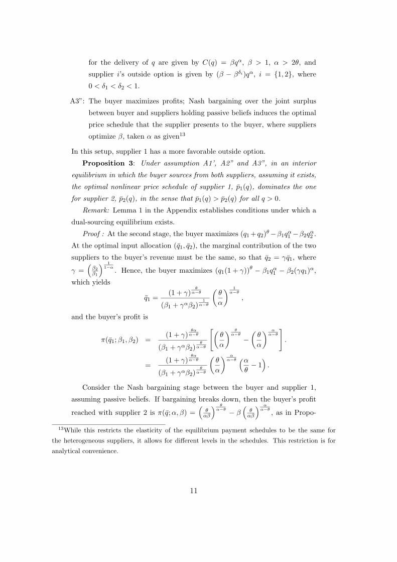
The data also provide an interesting illustration of price dispersion in the

absence of imperfect information. Figure 1 shows the price per 1000 bricks

paid by three national builders for a red multi brick16 for all deliveries to

their various construction sites in 2004. This brick is manufactured by one

of the four brick manufacturers, and each of this manufacturer’s competitors

produces an essentially equivalent brick. It is straightforward for buyers to

enquire about the costs of such substitutes for this red multi brick, so imper-

fect information does not rationalize the price dispersion in the data. The

theoretical results above suggest that different local competitive conditions

around the delivery sites are consistent with this pattern of prices. The con-

struction sites are in areas with locally distinct numbers of competitors, and

these may have different outside options, possibly as a consequence of their

capacity utilizations.

A brief description, definitions and summary statistics of the variables

used in the analysis are provided in an appendix.

16Here, “red” refers to the bricks color, and “multi” to its non-uniform color shading.

17

160

180

200

220

240

260

Pric

e pe

r 10

00 b

ricks

(G

BP

)

0 5000 10000 15000Volume (bricks)

Price per 1000 bricks (GBP) Price per 1000 bricks (GBP)Price per 1000 bricks (GBP)

Figure 1: Price dispersion for a red multi brick; 3 national builders, 2004.

18

3.2 Methodology and Results

The empirical methodology aims at uncovering the reduced form relationship

between brick price and various determinants of price. The specific focus

thereby is on the question whether buyers who have established a greater

number of contractual relationships in the period 2001-2006 - as an indication

of their switching possibilities - benefit from lower prices, on average. The

empirical analysis attempts to control for various characteristics of the trans-

action. First, there may be volume effects when price schedules are potentially

nonlinear. Second, as in this industry transport costs are significant, relative

to brick price, there may be distance effects: Buyers with construction or de-

livery sites that are more distant to the manufacturer’s plants may be given

discounts to capture their business. Third, the analysis controls for brick at-

tributes: On average, extruded bricks are cheaper than soft-mud bricks, and

similarly engineering bricks are cheaper than facing bricks.

In light of the foregoing theoretical analysis, transaction volume may be

endogenous. The analysis therefore, next to ordinary regressions, presents

results obtained from instrumenting volume. The decision to have the bricks

delivered is likely to be correlated with the transaction size, but, in the absence

of bundling, uncorrelated with the transaction price which is net of delivery

costs. Therefore, a variable indicating whether the transaction volume was

arranged to be delivered, as opposed to being picked up, is used as instrument

for volume, next to time trends captured by month and year. First stage

regressions are also in the appendix.

Moreover, as is now increasingly recognized in applied demand analysis,

heterogeneity across economic decision makers is an empirical regularity that

should be accounted for, if possible. Panel data permit to control for buyer

specific effects if they are present. Hence, the empirical analysis in addition

presents panel data estimators that exploit the entire richness of the data.

Table 3 presents the estimation results from different estimation method-

ologies.17 Two main conclusions emerge when comparing the columns of the

table. First, comparing standard with instrumental variables regressions, fail-

ure to instrument transaction volume induces a downward bias, in absolute

value, of the distance and multi-sourcing effects. The source of the bias is

17The various acronyms are: OLS - ordinary least squares; IV/2SLS - instrumental variables/2-

stage least squares; RE - random effects panel data estimator; BE - between effects estimator.

19

Priceper1k

bricks

OLS

IV/2SLS

RE

BE

IV,BE

OLS

IV/2SLS

RE

BE

IV,BE

Supplier2

--

--

--1

52.734⋆⋆⋆

-241.288⋆⋆⋆

-411.24

⋆⋆⋆

-313.102⋆⋆

-886.255⋆⋆⋆

--

--

-(2

0.247)

(20.704)

(113.323)

(148.138)

(163.588)

Supplier1

--

--

--1

61.075⋆⋆⋆

-161.075⋆⋆⋆

-327.710⋆⋆

-160.214

-926.606⋆⋆⋆

--

--

-(2

6.227)

(26.381)

(168.489)

(355.583)

(371.260)

week

0.541⋆⋆⋆

0.373⋆⋆⋆

0.574⋆⋆⋆

--

0.526⋆⋆⋆

0.356⋆⋆⋆

0.572⋆⋆⋆

--

(0.077)

(0.077)

(0.081)

--

(0.077)

(0.077)

(0.081)

--

Volu

me

-0.063⋆⋆⋆

0.007⋆

-0.072⋆⋆⋆

-0.183⋆⋆⋆

0.070⋆⋆

-0.061⋆⋆⋆

0.007⋆

-0.072⋆⋆⋆

-0.172⋆⋆⋆

0.104⋆⋆⋆

(0.002)

(0.004)

(0.002)

(0.018)

(0.034)

(0.002)

(0.004)

(0.002)

(0.019)

(0.036)

dista

nce

-0.380

-1.799⋆⋆⋆

-0.019

-0.916

-8.413⋆⋆⋆

-0.004

-1.195⋆⋆⋆

0.089

-0.253

-1.756

(0.390)

(0.396)

(0.469)

(2.758)

(2.921)

(0.413)

(0.418)

(0.475)

(4.492)

(4.566)

sourc

ing

-23.255⋆⋆⋆

-37.032⋆⋆⋆

-81.441

-35.913

-283.930⋆

47.655⋆⋆⋆

72.815⋆⋆⋆

89.001

68.183

114.837

(5.270)

(5.316)

(108.062)

(167.257)

(171.954)

(11.378)

(11.454)

(118.624)

(188.698)

(191.758)

extruded

-111.623⋆⋆⋆

-66.595⋆⋆⋆

-69.049⋆⋆⋆

-678.588⋆⋆⋆

-836.253⋆⋆⋆

-102.172⋆⋆⋆

-53.751⋆⋆⋆

-68.043⋆⋆⋆

-655.565⋆⋆⋆

-765.662⋆⋆⋆

(15.195)

(15.357)

(16.634)

(139.946)

(143.082)

(15.244)

(15.425)

(16.636)

(140.360)

(143.115)

engin

eering

-57.638

⋆⋆

-218.712⋆⋆⋆

-17.243

-55.923

-920.774⋆⋆⋆

-67.602⋆⋆

-227.878⋆⋆⋆

-17.890

-52.953

-932.777⋆⋆⋆

(27.181)

(28.228)

(29.890)

(292.519)

(312.150)

(27.207)

(28.287)

(29.892)

(293.035)

(313.542)

constant

794.751

⋆⋆⋆

423.487⋆⋆⋆

1009.102⋆⋆⋆

2054.644⋆⋆⋆

1458.645⋆⋆⋆

746.965⋆⋆⋆

365.962⋆⋆⋆

951.470⋆⋆⋆

1956.799⋆⋆⋆

1075.753⋆⋆⋆

(14.060)

(29.639)

(128.248)

(207.901)

(221.216)

(26.002)

(31.725)

(130.605)

(226.322)

(250.164)

Tab

le3:

Regressionresults;

stan

darderrors

inparenthesis;instruments

forVolume:

mon

th,year,

delivery

⋆sign

ificantat

10percentlevel

⋆⋆significantat

5percentlevel

⋆⋆⋆sign

ificantat

1percentlevel

20

likely to be that the size of the buyer business determines both prices and

volumes. Large transactions are generated by larger businesses that enter-

tain a larger number of supplier relationships, and these tend to get lower

prices. Also, large transactions entail higher transport costs, and in order to

secure such deals suppliers grant more significant discounts. Second, compar-

ing standard with panel data estimators, failure to account for heterogeneity

across buyers biases the empirical results of this analysis towards a finding

of buyer power, albeit only at the 10 percent level of statistical significance.

Controlling also for supplier specific effects eliminates any buyer power effect

reflected in negative coefficients on the sourcing variable and captures the

distance effects that were present in the first five specifications.18 Supplier

effects arise due to the different capacities and plant network configurations

of the three suppliers included in the analysis: Supplier 3 is by far the largest

supplier, with the largest number of plants and the widest geographic spread

of its plants.19 Hence, from a methodological point of view, accounting for

both endogeneity of transaction volume and heterogeneity of buyers appears

to be critical for the empirical identification of buyer power. Also, unit prices

increasing in volume are in line with the theory of multilateral bargaining

laid out in Section 2, and it is consistent with upstream market power in

this industry. Together with the finding that multi-sourcing does not induce

lower unit prices, this calls into question the Competition Commission’s con-

clusion that “larger buyers do have a degree of buyer power, [...] based on the

purchasing of large volumes [...] and their ability to multi-source”.20

4 Conclusions

This paper provides a comprehensive framework for the empirical analysis of

buyer power that is useful for practitioners, such as competition economists in

antitrust authorities. This framework encompasses the two main features of

pricing schemes in business-to-business relationships: nonlinear price sched-

18In light of the suppliers’ plant network configurations, the distance variable is highly correlated

with the suppliers’ capacities, measured by the number of plants they operate.19Appendix B provides further details on capacity. See also the Provisional Findings report

of the Competition Commission in the Wienerberger Finance Service BV / Baggeridge Brick plc

(2007) inquiry.20See Competition Commission, final report on the Wienerberger / Baggeridge inquiry (2007).

21

ules and bargaining over rents. Disentangling these two features is critical to

the empirical identification of buyer power. A structural theoretical model

investigates the principal determinants of optimal pricing schemes, with buy-

ers’ switching possibilities identified as the primary source of buyer power.

It forms the basis for the delineation of testable predictions that enable the

empirical identification of buyer power. The empirical part of the analysis

presents an illustration of the conceptual approach offered in this paper, for

the UK brick industry. It presents a reduced form methodology to estimate

the impact of buyers’ switching possibilities on prices. This methodology is

readily implementable on the basis of transaction data, as they are requested

routinely by antitrust authorities at the outset of their inquiries. The pa-

per emphasizes the importance to control for endogeneity of volumes and for

heterogeneity across buyers.

References

[1] Adelman, M.A. (1959): A& P: A Study in Price-Cost Behaviour and

Public Policy, Cambridge, MA: Harvard University Press

[2] Berry, S. (1994): “Estimating Discrete-Choice Models of Product Differ-

entiation”, Rand Journal of Economics, 25, 242-262

[3] Berry, S., Levinsohn, J. and A. Pakes (1995): “Automobile Prices in

Market Equilibrium”, Econometrica, 63, 841-890

[4] Bonnet, C., Dubois, P. and M Simioni (2004): “Two-Part Tariffs versus

Linear Pricing Between Manufacturers and Retailers: Empirical Tests on

Differentiated Products Markets, mimeo, University of Toulouse

[5] Boulding, W. and R. Staelin (1990): “Environment, Market Share and

Market Power”, Management Science, 36, 1160-1177

[6] Brooks, D.R. (1973): “Buyer Concentration: A Forgotten Element in

Market Structure Models”, Industrial Organization Review, 1, 151-163

[7] Burdett, K. and K.L. Judd (1983): “Equilibrium Price Dispersion”,

Econometrica, 51(4), 955-969

[8] Buzzell, R.D., Gale, B.T. and R.G.M. Sultan (1975): “Market Share - A

Key to Profitability”, Harvard Business Review, 53, 97-106

22

[9] Carlson, J.A. and R.P. McAfee (1983): “Discrete Equilibrium Price Dis-

persion”, Journal of Political Economy, 91(3), 480-484

[10] Chipty, T. and C.M. Snyder (1999): “The Role of Firm Size in Bliateral

Bargaining: A Study of the Cable Television Industry”, The Review of

Economics and Statistics, 81(2), 326-240

[11] Clevenger, T.C. and G.R. Campbell (1977): “Vertical Organization: A

Neglected Element in Market Structure - Performance Models”, Indus-

trial Organization Review, 5, 60-66

[12] Dobson, P.W. and M. Waterson (1997): “Countervailing Power and Con-

sumer Prices”, The Economic Journal, 107, 418-430

[13] Ellison, S.F. and C.F. Snyder (2001): “Countervailing Buyer Power in

Wholesale Pharmaceuticals”, mimeo, M.I.T.

[14] European Commission (1999): Buyer power and its impact on competi-

tion in the food retail distribution sector of the European Union, GD IV,

Brussels

[15] de Fontenay, C.C. and J.S. Gans (2004): “Can vertical intengration by a

monopolist harm consumer welfare?”, International Journal of Industrial

Organization, 22, 821-834

[16] Galbraith, J.K. (1952): American Capitalism. The Concept of Counter-

vailing Power. Boston: Houghton Mifflin

[17] Giulietti, M. (2007): “Buyer and seller power in grocery retailing: evi-

dence from Italy”, Revista de Economia del Rosario, 10(2), 109-125

[18] Hallagan, W. and W. Joerding (1985): “Equilibrium Price Dispersion”,

American Economic Review, 75(5), 1191-1194

[19] Hart, S. and A. Mas-Colell (1989): “Potential, Value, and Consistency”,

Econometrica, 57(3), 589-614

[20] Inderst, R. and N. Mazzarotto (2006): “Buyer Power: Sources, Conse-

quences, and Policy Responses”, mimeo

[21] Lustgarten, S.H. (1975): “The Impact of Buyer Concentration in Man-

ufacturing Industries”, The Review of Economics and Statistics, 57(1),

125-132

23

[22] McAfee P.R. and M. Schwartz (1994): “Opportunism in Multilateral

Vertical Contracting: Nondiscrimination, Excusivity, and Uniformity”,

American Economic Review, 84(1), 210-230

[23] McGukin, R. and H. Chen (1976): “Interactions between Buyer and

Seller Concentration: Nondiscrimination, Exclusivity, and Uniformity”,

Industrial Organization Review, 4, 123-132

[24] McKie, J.W. (1959): Tin Cans and Tin Plate, Cambridge, MA: Harvard

University Press

[25] Myserson, R.B. (1980): “Conference structures and fair allocation rules”,

International Journal of Game Theory, 9(3), 169-182

[26] Reinganum, J.F. (1979): “A Simple Model of Equilibrium Price Disper-

sion”, Journal of Political Economy, 87(4), 851-858

[27] Salop, S. and J. Stiglitz (1977): “Bargains and Ripoffs: A Model of Mo-

nopolistically Competitive Price Dispersion”, American Economic Re-

view, 44(3), 493-510 bibitemsalop2 Salop, S. and J. Stiglitz (1982): “The

Theory of Sales: A Simple Model of Equilibrium Price Dispersion with

Identical Agents”, American Economic Review, 72(5), 1121-1130

[28] Smith, H. and J. Thanassoulis (2008): “Upstream Competition and

Downstream Buyer Power”, mimeo, Oxford University

[29] Snyder, C.M. (1996): “A dynamic theory of countervailing power”,

RAND Journal of Economics, 27(4), 747-769

[30] Sorensen, A.T. (2000): “Equilibrium Price Dispersion in Retail Markets

for Prescription Drugs”, Journal of Political Economy, 108(4), 833-850

[31] Stole, L.A. and J. Zwiebel (1996): “Intra-Firm Bargaining under Non-

Binding Contracts”, Review of Economics Studies, 63(3), 375-410

[32] Ungern-Sternberg, Th.v. (1996): “Countervailing power revisited”, In-

ternational Journal of Industrial Organization, 14, 507-520

[33] Villas-Boas, S.B. (2007): “Vertical Relationships between Manufactur-

ers and Retailers: Inference with Limited Data”, Review of Economic

Studies, 74(2), 626-652

24

A Existence of Dual-Sourcing Equilibria

Consider equation (1). A dual-sourcing equilibrium requires that, for the op-

timal values of β1 and β2, ∆π1 and ∆π2 be positive. The more elastic the

suppliers’ price schedules are relative to the buyer’s revenue function, i.e. the

higher αθ , the more profitable dual-sourcing will be21. Similarly, the more fa-

vorable the suppliers’ outside options, i.e. the smaller max{δ1, δ2}, the more

the buyer benefits from dual-sourcing. The following result establishes that,

under adverse circumstances for the buyer, facing suppliers with sufficiently

favorable outside options, there exist ratios αθ that induce dual-sourcing equi-

libria.

Consider the following additional Assumption:

A4: max{δ1, δ2} < δ := exp(1)−1exp(1) .

Lemma 1: Under assumptions A1’, A2”,A3” and A4, a dual-sourcing

equilibrium exist.

Proof: It follows from equation (1) that the profit from dual-sourcing is

rising in αθ , while the profit from single-sourcing is falling as α

θ increases,

with the minimum occurring at αθ = 1 + exp(1). The value of δ that equates

θ(1−δ)(α−θ) = 1

(1−δ)(α/θ−1) at αθ = 1 + exp(1) with 1 is δ = exp(1)−1

exp(1) . So

min{∆π1,∆π2} > 0 provided max{δ1, δ2} < δ and (1+γ)θαα−θ

(β1+γαβ2)θ

α−θ

≥ 1.

Suppose β1 = β2 = β were a dual-sourcing equilibrium. Then, (1+γ)α

(β1+γαβ2)=

2α

2β ≥ 2α−1 > 1. Hence, if both suppliers had equal outside options, then

a dual-sourcing equilibrium exists. Now consider a slight improvement of

supplier 1’s outside option, say. This will slightly reduce the buyer’s gain from

dual-sourcing, or equivalently reduce the Shapley value accruing to supplier 1.

Similarly, a slight deterioration of supplier 2’s outside option, say, will slightly

improve the gain from dual sourcing. Since ∆πi, i = 1, 2, is continuous in βj ,

j = 1, 2, the necessary inequality for the existence of dual-sourcing equilibria

is preserved. �21Of course, if α

θ is very high, then production will no longer be profitable, so that a trivial

no-trade equilibrium arises.

25

B Data and Auxiliary Regressions

The data comprise roughly six hundred thousand individual contracts be-

tween UK buyers and the (three) manufacturers used in the analysis. Prices

per one thousand bricks are in GBP. Volume is measured in the number of

bricks. Distance is measured in kilometers between the manufacturing plant

and the construction or delivery site. The sourcing variable is the number of

manufacturers that the respective buyer entertains contractual relationships

with during the observation horizon 2001 - 2006. There are dummy variables

indicating whether the bricks of the respective transaction are of the extruded

(as opposed to soft mud) variety, whether they are engineering (as opposed

to facing) bricks, and whether the buyer chose to have the supplier arrange

the delivery or collected the bricks.

The following table provides summary statistics.

Variable Obs. Mean Std.Dev. Min Max

Price per 1k 637015 344.802 5093.57 0.0008306 3097000

Volume 637015 5991.746 3910.012 2 264000

sourcing 637015 2.567056 1.325533 1 4

distance 581112 4.089677 17.90908 0 341.3

extruded 637015 .6811441 .4660334 0 1

engineering 637015 .0723782 .2591133 0 1

delivery 637015 0.58792 .4922097 0 1

Table B1: Summary statistics.

Table B2 presents the first stage regression for the IV/2SLS estimation

results presented in Table 3.

26

Volume

month 2.639⋆⋆

(1.331)

year 105.661⋆⋆⋆

(16.219)

delivery 3620.443⋆⋆⋆

(8.843)

constant -211541.4 ⋆⋆⋆

(32446.6)

Table B2: First stage regression results.

⋆ significant at 10 percent level

⋆⋆ significant at 5 percent level

⋆⋆⋆ significant at 1 percent level

The four UK brick suppliers have different capacities. Suppliers 1 has 7

plants and supplier 2 has 20 plants. Supplier 3 is the largest supplier, with 23

plants and the largest geographic spread.22 For the three suppliers included

in the analysis, supplier 1 produced an average of 87.3 million bricks per year,

supplier 2 195.2 million and supplier 3 353.7 million bricks per year.

22This information is sourced from the Provisional Findings report of the Competition Commis-

sion.

27