Emerging market local currency bonds: diversification and - BIS

BIS Working Papers No 391

Emerging market local currency bonds: diversification and stability by Ken Miyajima, M S Mohanty and Tracy Chan

Monetary and Economic Department

November 2012

JEL classification: E43, F36, G12. Keywords: Currency mismatches, emerging market local currency bond, diversification benefit, safe asset, panel VAR

BIS Working Papers are written by members of the Monetary and Economic Department of the Bank for International Settlements, and from time to time by other economists, and are published by the Bank. The papers are on subjects of topical interest and are technical in character. The views expressed in them are those of their authors and not necessarily the views of the BIS.

This publication is available on the BIS website (www.bis.org).

© Bank for International Settlements 2012. All rights reserved. Brief excerpts may be reproduced or translated provided the source is stated.

ISSN 1020-0959 (print)

ISSN 1682-7678 (online)

http://www.bis.org/

iii

Emerging market local currency bonds:

diversification and stability

Ken Miyajima, M S Mohanty and Tracy Chan1

Abstract

Over the past three years, cross-border inflows into emerging market (EM) local currency bonds have surged. The returns on these bonds have moved more closely with those on international assets regarded as “safe”, particularly following the euro area debt crisis. This paper first demonstrates that domestic factors have tended to dictate the dynamics of the EM local currency government yield. The importance of local drivers has probably increased the potential diversification benefit, creating strong appetite for the asset class. Second, the paper confirms that EM local currency government yields have behaved more like safe haven yields since 2008: they have dropped, rather than increased, in response to worsening global risk sentiment. Yet EM local currency government yields could be susceptible to adverse external shocks: the yield dynamics have been affected by unsustainably low US Treasury yields. Moreover, the international role of EM local currency bonds depends crucially on the behaviour of exchange rates. Nevertheless, the further development of local currency bond markets should help strengthen the stability of the international monetary and financial system. JEL classification: E43, F36, G12. Keywords: Currency mismatches, emerging market local currency bond, diversification benefit, safe asset, panel VAR

1 Miyajima is Senior Economist at the Bank for International Settlements (BIS); Mohanty is Head of Emerging

Markets of the Monetary and Economic Department at the BIS; Chan is Research Analyst at the BIS. We thank Bernd Braasch, Gerard Caprio, Torsten Ehlers, Enisse Kharroubi, Előd Takáts, Philip Turner, Christian Upper, Fabrizio Zampolli and the participants at the Third International Workshop on Developing Local Currency Bond Markets in Emerging Market Economies and Developing Countries held at the Deutsche Bundesbank in November 2011 for comments. The views expressed in this paper are the authors’ own and not necessarily those of the BIS.

iv

Contents

1. Introduction ................................................................................................................... 1

2. Emerging market local currency bonds as an asset class? .......................................... 3

2.1 EM bond markets during the recent crisis ............................................................ 3

2.2 Diversification benefits from EM local currency government bonds ...................... 4

2.2.1 Is the performance determined by global or domestic factors? ................... 5

2.2.2 The role of the exchange rate ..................................................................... 6

3. Results from yield models ............................................................................................. 7

3.1 The model ............................................................................................................ 7

3.2 Econometric methodology and data ..................................................................... 8

3.3 Benchmark model ................................................................................................ 9

3.4 Expanded benchmark model ............................................................................. 12

3.4.1 Capital account openness (annual model) ................................................ 13

3.4.2 Currency mismatches (annual model) ....................................................... 13

3.4.3 Central bank financing needs (monthly model) ......................................... 14

3.5 Additional robustness checks ............................................................................. 14

3.5.1 Tests on endogeneity ............................................................................... 15

3.5.2 Using realised values ................................................................................ 15

4. Testing for resilience ................................................................................................... 17

4.1 A dynamic panel model ...................................................................................... 17

5. Conclusion and policy implications .............................................................................. 19

Annex Tables ....................................................................................................................... 21

1

1. Introduction

Historically, increased risk aversion in global financial markets has reduced capital flows into emerging market (EM) debt products. Yet, cross-border inflows into EM local currency bonds have surged over the past three years. The growing interest of foreign investors in EM debt could partly reflect the much discussed shortage of global safe assets2 (Caballero, Farhi and Gourinchas, 2008; and Gourinchas and Jeanne, 2012). In particular, since the beginning of the euro area debt crisis in 2010, the returns on EM local currency government bonds have moved closely with those on safe haven assets. At the same time, the recent surge has been accompanied by very low global interest rates and exceptional monetary easing by advanced economies that will almost certainly end at some point.

In this paper, we examine the factors behind the observed resilience of EM local currency government bonds. Does their recent performance represent a fundamental change in the characteristics of these assets? Do EM local currency bonds provide enough diversification benefits to be considered as a distinct and, possibly, safer asset class? Or, will the recent surge end in a crash, as has happened in previous episodes of crises in emerging market economies (EMEs) that followed monetary tightening in advanced economies?

The appeal of an asset depends on at least two crucial factors. First, from the point of view of portfolio diversification, the asset is more attractive when the return is determined by a set of idiosyncratic factors and less correlated with other asset returns. Second, the asset is more attractive when the volatility of returns is low, thereby allowing investors to anticipate the asset’s future returns with a lower degree of uncertainty. This suggests that, to be attractive as an investment proposition, not only should returns on EM bonds be determined more by domestic factors than global ones, but they must also be resilient to various shocks.3

Views about an international role for EM local currency bonds have varied widely. Some years ago, Eichengreen and Hausmann (1999) advanced the “original sin” hypothesis, which argues that EMEs lack the capacity to borrow in their own currencies, because international transactions are mostly denominated in currencies of a few advanced economies. Over the past decade, however, better macroeconomic policies and low inflation have made local currency paper more attractive in many EMEs for international investors.

The EMEs’ capacity to develop domestic bond markets has been clearly demonstrated. This has reflected changes in their domestic institutions, macroeconomic and monetary policies, market infrastructure and global financial integration (Classens et al, 2007; Gagnon, forthcoming; Goldstein and Turner, 2004; Montoro and Rojas-Suarez, 2012; and BIS, 2002; 2012a; 2012b). And this development has coincided with strong growth and better fiscal prospects in EMEs. There has been a steady increase in the foreign ownership of EM local currency bonds in the past decade.4 In addition, the local currency bonds of a number of EMEs are now included in the global bond indices.5 Echoing a positive view, the Committee

2 Following Gourinchas and Jeanne (2012), an asset is considered as “safe” when risks associated with credit,

market, inflation and exchange rate are low. 3 Yet, domestic factors are likely to be correlated with global factors to some extent, particularly in times of a

large global common shock. 4 For instance, at the beginning of the 2000s foreign investors accounted for less than 1% of the total stock of

local currency sovereign bonds in most EMEs (the exception was Hungary where this share was 47%). However, by 2010 this share had risen to 30% in Indonesia, 18–22% in Mexico and Malaysia, 14% in Brazil and 10% in Korea.

5 Domestic government bonds issued in five EMEs are currently included in the widely used Citigroup World Government Bond Index (WGBI), which consists of government bonds issued by 23 countries. These are Malaysia (included in 2007), Mexico (2010), Poland (2003), Singapore (2005), and South Africa (2012). The

2

on the Global Financial System (2007) argued that “…because local currency bonds represent attractive yield enhancement and diversification vehicles for foreign investors, further substantial growth seems likely in years ahead even if some cyclical reversal may occur”.

An important question is: what determines the diversification benefit from investing in EM assets. Some have argued that diversification benefits from assets denominated in local currencies depend crucially on the behaviour of the exchange rate (Burger and Warnock, 2007; and Turner, 2012). Others stress relative volatility. Because EM currencies tend to be more volatile than those of advanced economies, any diversification benefits from EM assets are likely to be small.

In examining the potential diversification role of EM local currency bond markets, we proceed in two stages. First, following Caporale and Williams (2002) and Gonzalez-Rozada and Yeyati (2008), we present a basic model to disentangle the effects of domestic and external factors on local currency government bond yields in EMEs, and then estimate it in a static panel framework. In the second stage, we use a dynamic panel VAR model to test whether these yields were resilient to shocks during the second half of the 2000s. These EM yields are modelled in local currency terms, assuming that expected exchange rate changes are reflected in interest rates. The model also considers determinants of exchange rates to capture the impact of exchange rates on EM domestic yields.

Compared to the way the literature sometimes uses capital flows as a proxy for EM asset performance, bond yields provide indirect evidence on how far EM bond markets have come up as an alternative asset class to compete with some of the advanced economy bond markets. It is also worth highlighting that our approach to some extent builds on the premise that EM domestic bond markets have matured, whereas the literature has focused on the capacity of EMEs to build domestic bond markets.6

Our results suggest that domestic factors – particularly monetary and fiscal policy – played a relatively more important role than global factors such as US bond yields and the VIX (which is the implied volatility of the S&P 500 stock index) in dictating local currency bond yields in EMEs over the past decade. And, these bond yields were quite resilient to both domestic and global shocks. These findings are robust to alternative specifications, different estimation periods and various endogeneity tests conducted in the paper. That said, US Treasury yields have been an important – if not dominant – determinant of EM local currency bond yields particularly during the recent global monetary easing cycle. This implies that the recent good performance of some EM bond markets is probably not sustainable. These findings have implications not only for the potential for EM local currency bonds to become a safe asset class but also for the exposure of EMEs to future financial shocks.

The rest of the paper is structured as follows. Section II discusses basic facts and findings in other studies about EM bonds as an asset class. Section III presents the theoretical model as well as the empirical results from a static panel framework. Using the Choleski decomposition strategy, Section IV examines the capacity of EM local currency government bonds to withstand shocks. The final section explores a few policy implications of the main findings.

market weights for most of the EMEs are in the range of 0.4–0.6%, comparable to those of Finland or Ireland, but much smaller than those of Japan or the US.

6 See, for instance, Eichengreen and Luengnaruemitchai (2006), Classens, Klingebiel and Schmukler (2007), and Mehl and Reynaud (2005).

3

Graph 1 Cumulative net inflows to mutual funds dedicated to emerging market bonds

In USD bn

Source: EPFR.

2. Emerging market local currency bonds as an asset class?

Global bond markets have seen large changes since the onset of the global financial crisis in 2008. As IMF (2011) notes, two, rather opposing, forces have influenced asset allocation by institutional investors. On the one hand, burned by large losses, these investors have become more sensitive to credit and liquidity risks than they were before the crisis. On the other hand, cyclical factors such as very low global interest rates may have tempted them to take on additional risks by going beyond their traditional asset classes. In this environment, EMEs that enjoy strong growth and balance sheet positions are seen as providing attractive investment opportunities to investors.

2.1 EM bond markets during the recent crisis Recent changes in investor behaviour have been accompanied by at least two major developments in EM bond markets. First, as Graph 1 shows, cross-border inflows into EM bond markets have risen rapidly since 2009. Prior to 2008, the cumulative inflows into mutual funds dedicated to EM bonds reached about $30 billion. Although the inflows collapsed following the 2008 Lehman crisis, they rebounded towards the end of 2009. In the following two and half years, these inflows rose at a dramatic rate, reaching some $120 billion by July 2012.

What is interesting to note is that a relatively large part of such inflows has been directed to bonds denominated in local currencies. Investor interest is growing in all types of EM bonds, irrespective of currency denomination. However, the share of local currency-denominated bonds in the total has risen from virtually zero in mid-2005 to almost half by the middle of 2012. Given the relatively small size of the EM corporate debt markets, a large share of the inflows has likely been directed to securities issued either by governments or central banks.

A second related development concerns the performance of these assets. Graph 2 shows total returns (interest income and capital gains) from EM local currency government bonds, as represented by the JP Morgan local currency government bond index, and those from US Treasury bonds. It also shows the VIX, a measure of global risk aversion. During 2003–07, a period of low global risk aversion, EM bonds fetched annual average returns of about 9%, significantly greater than the returns on US Treasuries of about 4%. Investors demanded a positive – and often substantial – premium for investing in EM local currency government bonds.

4

Graph 2 Annual returns on US Treasury and EM domestic government bonds and VIX

In per cent

1 US Treasury total return index USD. 2 GBI-EM broad traded total return index local currency.

Sources: Bloomberg; JPMorgan Chase; BIS staff calculations.

The performance of EM bonds deteriorated as risk sentiment worsened in the run-up to the 2008 crisis, but rebounded as early as the end of 2008. During the most recent period of high risk aversion related to the euro area debt crisis, returns on EM local currency government bonds almost converged with those on US Treasuries. The returns on these two assets have again diverged since the beginning of 2012, after the US Treasury returns dropped sharply, partly as tentative hopes that major central banks may act to help boost economic growth prompted investors to rotate out of US Treasury bonds.

The strong performance of the EM local currency government bonds also stands out when we look at their risk-adjusted returns, as measured by the ratio of median annual returns to volatility of returns (known as the Sharpe ratio). Graph 3 shows the Sharpe ratios for a range of assets during periods of high (2008–12) and low global risk aversion (2002–07). The y-axis shows the median returns and the x-axis standard deviation of returns; the size of the bubble represents the magnitude of the Sharpe ratio. The returns on all EM local currency assets are unadjusted for exchange rate changes, so that currency risks are assumed to be hedged by investors.

Compared with other asset classes, EM local currency government bonds have had one of the best Sharpe ratios in both good and bad times. During 2002–07, the Sharpe ratio of EM local currency government bonds was the highest (0.9), as their low returns were offset by the stability of the returns, followed by EM foreign currency government bonds in dollars and EM equities (all 0.5). It is interesting to note that, during 2008–12, when investors’ risk sentiment was weak, the Sharpe ratio of EM local currency government bonds (0.3) still continued to be the highest. Moreover, the dispersion of Sharpe ratios across asset classes rose, while those of oil and EM equities fell into negative territory.

2.2 Diversification benefits from EM local currency government bonds

The recent performance of EM local currency government bonds raises the question as to whether they can be an alternative to some of today’s advanced market bonds. We believe that the answer to this question depends on factors influencing their recent performance and the interaction of these factors with the exchange rate, which has a critical role to play in any diversification benefits from assets denominated in local currencies.

5

Graph 3 Cross-asset risk and returns, 2002–07 and 2008–12

Median (y-axis), standard deviation (x-axis), and Sharpe ratio (bubble size)

2002–07 2008–12

Note: DM equities = MSCI world price index in US dollar; EM domestic bond (USD, LC) = JP Morgan emerging market broad composite total return bond index in US dollar and local currency; EM equities = MSCI Emerging market price index in US dollar; EM external bond = JP Morgan EMBI global composite total return index in US dollar; Gold = Standard and Poors Goldman Sachs commodity gold total return index in US dollar; Oil = Standard and Poors Goldman Sachs commodity crude oil total return index in US dollar; US bond = Bank of America Merrill Lynch treasury master total return bond index in US dollar.

Sources: Datastream and BIS staff calculations.

2.2.1 Is the performance determined by global or domestic factors?

EM local currency government bonds would be less appealing to global investors if their performance were determined mainly by global factors. Global or common shocks can increase the correlation of asset returns, particularly during extreme events, reducing diversification benefits for investors. By contrast, to the extent that yields on these assets are determined by domestic growth and monetary conditions in EMEs, they could offer the much needed diversification opportunity to investors, just as when advanced economies’ sovereign debt are being downgraded because of their weak fiscal and growth prospects.

Past research has generally concluded that global shocks tend to have large effects on the returns of EM assets, although this finding has typically been based on the spreads on foreign currency sovereign debt (Eichengreen and Mody, 2000; IMF, 2004; and Gonzalez-Rozada and Yeyati, 2008). For instance, focusing on the period following the Russian default (2000–05), Gonzalez-Rozada and Yeyati (2008) show that about 50% of the long-run variability of EM foreign currency sovereign spreads were explained by two main factors, ie international risk appetite (as represented by the US corporate bond spreads) and international liquidity (as represented by US Treasury yields). Allowing for country-specific elasticity to global factors, these authors argue that the contribution increases to 80%.7

By contrast, there is very little systematic evidence to date regarding the determinants of EM local currency yields. The few studies that exist seem to confirm the view that domestic factors tend to have a larger impact than global factors. For instance, based on a quantity-of-flows model, IMF (2011) estimates that foreign inflows to EM bonds can be significantly

7 However, studies employing data for the post-2008 crisis period have found somewhat different results. For

instance, Bellas, Papaioannou and Petrova (2010) show that global liquidity has large effects on sovereign spreads only in the short run, while fundamental macroeconomic factors (eg external debt servicing capacity, fiscal and current balance) are relatively more important in the long term. Jaramillio and Tejada (2011) modify this result slightly, showing that EMEs that have recently reached an investment grade credit status have been able to reduce their sovereign spread by 5–10%. More broadly, Braasch (2012) discusses the importance of gaining a better understanding of factors behind international capital flows.

0

10

20

30

40

50

0 50 100 150 200

US bond

EM domestic bond (USD)

EM external bond

Gold

Oil

EM domestic bond (LC) DM equities

EM equities

-20

-10

0

10

20

30

40

0 50 100 150 200 250 300

EM domestic bond (LC)

EM domestic bond (USD) EM external bond

Gold

Oil

US bond

DM equities

EM equities

6

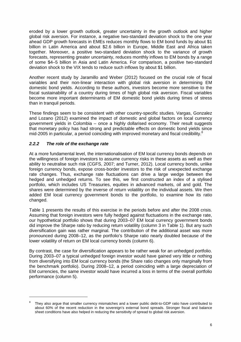
eroded by a lower growth outlook, greater uncertainty in the growth outlook and higher global risk aversion. For instance, a negative two-standard deviation shock to the one year ahead GDP growth forecasts in EMEs reduces monthly flows to EM bond funds by about $1 billion in Latin America and about $2.6 billion in Europe, Middle East and Africa taken together. Moreover, a positive two-standard deviation shock to the variance of growth forecasts, representing greater uncertainty, reduces monthly inflows to EM bonds by a range of some $4–5 billion in Asia and Latin America. For comparison, a positive two-standard deviation shock to the VIX tends to reduce such inflows by about $1 billion.

Another recent study by Jaramillo and Weber (2012) focused on the crucial role of fiscal variables and their non-linear interaction with global risk aversion in determining EM domestic bond yields. According to these authors, investors become more sensitive to the fiscal sustainability of a country during times of high global risk aversion. Fiscal variables become more important determinants of EM domestic bond yields during times of stress than in tranquil periods.

These findings seem to be consistent with other country-specific studies. Vargas, Gonzalez and Lozano (2012) examined the impact of domestic and global factors on local currency government yields in Colombia – once a highly dollarised economy. Their result suggests that monetary policy has had strong and predictable effects on domestic bond yields since mid-2005 in particular, a period coinciding with improved monetary and fiscal credibility.8

2.2.2 The role of the exchange rate

At a more fundamental level, the internationalisation of EM local currency bonds depends on the willingness of foreign investors to assume currency risks in these assets as well as their ability to neutralise such risk (CGFS, 2007; and Turner, 2012). Local currency bonds, unlike foreign currency bonds, expose cross-border investors to the risk of unexpected exchange rate changes. Thus, exchange rate fluctuations can drive a large wedge between the hedged and unhedged returns. To see this, we first constructed an index of a stylised portfolio, which includes US Treasuries, equities in advanced markets, oil and gold. The shares were determined by the inverse of return volatility on the individual assets. We then added EM local currency government bonds to the portfolio, to examine how its ratio changed.

Table 1 presents the results of this exercise in the periods before and after the 2008 crisis. Assuming that foreign investors were fully hedged against fluctuations in the exchange rate, our hypothetical portfolio shows that during 2003–07 EM local currency government bonds did improve the Sharpe ratio by reducing return volatility (column 3 in Table 1). But any such diversification gain was rather marginal. The contribution of the additional asset was more pronounced during 2008–12, as the portfolio’s Sharpe ratio nearly doubled because of the lower volatility of return on EM local currency bonds (column 6).

By contrast, the case for diversification appears to be rather weak for an unhedged portfolio. During 2003–07 a typical unhedged foreign investor would have gained very little or nothing from diversifying into EM local currency bonds (the Share ratio changes only marginally from the benchmark portfolio). During 2008–12, a period coinciding with a large depreciation of EM currencies, the same investor would have incurred a loss in terms of the overall portfolio performance (column 5).

8 They also argue that smaller currency mismatches and a lower public debt-to-GDP ratio have contributed to

about 60% of the recent reduction in the sovereign’s external bond spreads. Stronger fiscal and balance sheet conditions have also helped in reducing the sensitivity of spread to global risk aversion.

7

Table 1

Risk return characteristics of stylised portfolios

2003–07 2008–12

Benchmark Add EM local currency government bonds … Benchmark Add EM local currency

government bonds …

… with

currency risk

… without currency

risk

… with currency

risk

… without currency

risk

Average (=a) 8.9 10.2 8.9 8.3 8.3 7.9

Standard dev. (=b) 2.8 3.2 2.6 6.7 6.8 3.6

Sharpe ratio (=a/b) 3.14 3.19 3.35 1.23 1.21 2.23

Higher volatility of EM currencies can thus unwind the potential diversification benefits from EM local currency bonds. This has in a way remained the central concern underlying the “original sin” hypothesis. Turner (2012) argues that the capacity of these assets to preserve value (their so-called collateral capacity) can weaken significantly during a crisis. Burger and Warnock (2007) reach a similar conclusion by examining US investors’ behaviour, but argue that the source of exchange rate volatility matters more than volatility per se. If such volatility is due to macroeconomic factors, improved policies in EMEs can help reduce the problem.

3. Results from yield models

We now turn to an empirical investigation of the diversification hypothesis laid out in the previous section. To do this, we will attempt to disentangle the impact of domestic and global factors on the performance of EM local currency bonds in this section. In Section IV, using a dynamic model, we will examine the resilience of these markets to potential shocks.

3.1 The model

We write a model to help identify the effects of domestic and external factors on the EM local currency government yield i . To do this, we start from the model for the terms structure of bond yields operationalised by Caporale and Williams (2002), and expand on the variable representing the term premium in order to account more explicitly for additional risks faced by foreign investors:

)'()( ' zTzTii ds ++= (1)

where dsi is nominal domestic short rates, )(zT is the term premium faced by investors

generally as a function of a set of variables z, and )'(' zT is the additional term premium faced by foreign investors as a function of a set of variables z’. We characterise )'(' zT by starting from uncovered interest rate parity conditions. Here, the spread of the government yield in EMEs to the global safe yield *i is equated to the expected rate of depreciation of the local currency in EMEs.

t

t

ssEii ][)1()1( 1* +=+−+ (2)

8

This model can be extended to a version where a risk-averse global investor arbitrages “risky” government bonds in EMEs and a safe global asset. Following Gonzalez-Rozada and Yeyati (2008),

t

t

ssEqiqViq ][)1()1)(1( 1* +=−+−++− ϕ (3)

Where q is default probability, V is the recovery value, and ϕ is a parameter reflecting risk aversion. Assuming 0≅fqi ,

t

t

ssEVqii ][)1()1()1( 1* +=−−++−+ ϕ (4)

For reasonable parameter values, 0)1( <−−ϕV . For instance, a positive default probability q creates a wedge such that the expected rate of currency depreciation is smaller than the yield spread *ii − . Therefore, in some cases, a positive EM yield spread to a safe asset could be accompanied even by appreciation of the domestic currency in EMEs, thus supporting a carry trade strategy. By collecting terms,

t

t

ssEVqii ][)1( 1* ++−−−= ϕ (5)

From (1) and (5) above, the nominal government yield in EMEs can be written as follows.

)][),1(,),(,( 1*

t

tds s

sEVqizTifi +−−−= ϕ (6)

Thus, the domestic yield in EMEs is determined by the domestic short rate, the domestic term premia, the yield on a global safe asset, the country risk spread and the currency risk in EMEs. We conjecture that the first two terms are primarily dictated by domestic factors. The risk spread to a global safe asset could be affected by both domestic and external factors, so does the currency risk.

3.2 Econometric methodology and data Given the framework, we will now econometrically document the relative importance of the determinants of local currency government bond yields in EMEs using a set of domestic and external factors. First, we will estimate a static fixed-effect panel model to identify the key drivers of these yields:

ititiit xr εβα ++= (7)

where itr is the nominal local currency government yield in EMEs i at time t , itx is a vector of explanatory variables, and itε is residuals.

We focus on 11 EM domestic bond markets that are relatively well developed either in terms of size or investor diversity (with significant foreign participation in their markets). These are the markets of Brazil, Chile, Hungary, India, Indonesia, Korea, Malaysia, Mexico, Poland, South Africa and Turkey, which together account for the bulk of domestic bond universe in EMEs. We use monthly data starting from January 2000 and ending in December 2011.

Consistent with the literature, the yield on an international safe asset is represented by the yield on US 10-year Treasuries (us10). The assumption is that EM local currency government yields co-move with US yields – easy global liquidity conditions reduce the EM yield and vice versa. Global risk sentiment, which affects both country risk and currency risk,

9

is represented by the VIX index (vix). Turning to domestic factors, the domestic short-term interest rate represents the monetary policy stance. Indicators for GDP growth, inflation and the fiscal balance determine domestic term premia as well as country risk and currency risks emanating from domestic macroeconomic volatility.

A major empirical problem in estimating a reduced-form bond yield equation such as ours is the downward bias in coefficients arising from possible reverse causality from the left to the right side variables. As pointed out by Laubach (2009), bond yields and the fiscal balance may be negatively associated due to a common factor such as the business cycle, creating potential biases in the estimation. An economic slowdown may be associated with lower interest rates (through monetary easing) while at same time worsening the fiscal balance (through automatic stabilisers). We believe that this reverse causality is not unique to fiscal variables since growth and inflation can also be affected by bond yields through the same business cycle.

As Laubach argues, such an identification problem is difficult to resolve without a structural model but can be reduced by using forecast variables. The assumption is that fiscal deficits and other macroeconomic variables expected in years ahead are unlikely to be strongly correlated with the current state of the business cycle.9

We use monthly forecasts published by Consensus Economics for short rates (fcrate), GDP growth (fcgdp), inflation (fcinf) and fiscal balance to GDP (fcfisc).10 Forward rate agreements are also used to complement when short-rate forecasts are not available. As a robustness check, we estimate regressions using realised variables that broadly correspond to the individual forecast variables.11

We checked for possible non-stationarity problems in data that can lead to spurious correlations. A panel unit root test, reported in Table 2, revealed that all domestic variables and VIX are mostly stationary. However, as the test could not reject the null hypothesis that the US 10-year yield is not stationary, we also used de-trended US 10-year yields (us10_det) to check for robustness.

3.3 Benchmark model Table 3 presents the basic results of our fixed-effect, static panel model. Further details are provided in annex Table A1. The standard errors of the estimated coefficients are computed based on a robust procedure. Specifically, the sandwich estimator of Huber (1967) and White (1980) is computed while clustering observations by country à la Rogers (1993). Computed this way, the robust standard errors are larger than the ordinary ones, which is an indirect confirmation of the presence of heteroskedasticity and time dependence in the estimated residuals.

Turning to the results, the estimated coefficients broadly confirm the view that domestic yields in EMEs are determined by domestic factors. A 1 percentage point increase in short-rate expectations raises government yields by 89 basis points, while a 1 GDP percentage point improvement in the fiscal balance reduces government yields by 26 basis points. Interestingly, the US 10-year yield and the VIX are not significantly related to domestic yields.

9 An unpublished paper by Chadha, Turner and Zampolli uses a similar model for advanced economies. See

also Jaramillo and Weber (2012) for an application to EM bond markets. 10 When forecasts are reported for the current and following years, they are weighted to construct data with

comparable forecast horizons. 11 The policy rate, the economic risk rating index (which includes indicators of domestic fiscal conditions among

a few other macroeconomic indicators), industrial production and inflation.

10

Table 2

Unit root tests

Statistics P-value ADF regression average lags

yield -4.541 0.000 2.08

fcrate -3.736 0.000 1.92

fcinf -6.042 0.000 2.83

fcgdp -6.352 0.000 2.92

fcfisc -2.792 0.003 1.73

us10 2.544 0.995 7.00

vix -8.625 0.000 0.00

us10_det -5.601 0.000 3.00

cbfingap -0.456 0.324 2.00

cbfingap_det -1.778 0.038 2.08

prate -3.775 0.000 3.83

ip -8.738 0.000 4.67

inf -7.367 0.000 3.75

er -3.566 0.000 2.08

Note: Im-Pesaran-Shin unit root test. The null hypothesis is the variable contains unit roots. Lags for ADF regressions are chosen according to the AIC criterion. fcrate = one year ahead short-rate forecasts, fcinf = one year ahead inflation forecasts, fcgdp = one year ahead GDP growth forecasts, fcfisc = one year ahead forecasts of fiscal balance as a percentage of GDP, us10 = US 10 year yields, vix = VIX index, us10_det = detrended US 10 year yields, cbfingap = central bank financing gap defined as the excess of foreign exchange reserves above currency in circulation, as a percentage of M2, cbfingap_det = detrended central bank financing gap, prate = policy rate, ip = year-on-year industrial production, inf = year-on-year inflation, er = economic risk rating.

Surprisingly, the impact of GDP growth forecasts on bond yields is negative. This is counterintuitive in the sense that, in the long run, the interest rate should move in line with the economy’s growth rate. Our result is, nevertheless, consistent with earlier work.12 We infer that stronger GDP growth could reduce a country risk premium and attract capital flows, compressing domestic yields. In addition, higher GDP growth may predict higher future inflation, leading to ex-ante lower real interest rates. This is evident in our model from a small and statistically weak coefficient on inflation, implying that investors are not fully compensated for anticipated inflation.

To further assess the importance of the determinants, Table 4 reports the contribution to the mean and standard deviation of yield. The regression coefficients indicate the average response of yields to its determinants. They do not, however, reveal the full picture since the relative importance also depends on the evolution of each determinant during the sample period. To see this, the contribution is computed using the following formula.

12 Jaramillo and Weber (2012) estimate a similar model to explain domestic government yields in EMEs with

forecasts variables, and find a negative coefficient on GDP forecasts. Baldacci and Kumar (2010) attribute a negative coefficient on GDP growth to, other things being equal, a reduction in country risk premia, to the extent that higher tax revenues and less expenditure on the social safety net may reduce fiscal vulnerability.

11

Table 3

Impact of domestic and external factors on local currency government bond yields in EMEs

2000–11 2000–07 2008–11

Model 1 2 3

fcrate 0.894 0.846 0.830

(5.888) (10.548) (3.256)

fcinf 0.222 0.253 0.321

(1.257) (1.077) (1.059)

fcgdp -0.211 0.016 -0.198

(-1.902) (0.124) (-4.512)

fcfisc -0.257 -0.264 -0.369

(-2.264) (-2.436) (-2.889)

us10 0.319 0.370 0.598

(1.675) (1.751) (2.389)

vix 0.007 0.020 0.010

(0.702) (2.351) (0.669)

_cons -0.320 -1.712 -1.575

(-0.173) (-1.478) (-0.558)

N 1,255 782 473

r2_a 0.755 0.786 0.627

Note: t values are computed based on standard errors estimated with a robust procedure by clustering countries. See Table 2 for variable notations.

)/(

),/(

ijjj

ijjj ssµµδω

δη

=

= (8)

Where jj s,δ and jµ are the regression coefficients, standard deviation and mean of the

determinant j, respectively, while is and iµ are the standard deviation and mean of the dependent variable. As the Table shows, the contribution of short-rate forecasts was by far the largest, 0.79 and 0.84 in terms of mean and standard deviation. Although statistically insignificant, the US 10-year yields turn out to be the second largest contributor to mean of domestic bond yields. The contributions of GDP growth forecasts and fiscal balance forecast were relatively small. The contribution of VIX was the smallest, suggesting that external factors may have a large impact in the short run, but not systematically over the long run.

12

Table 4

Contribution to yield responses

2000–11 2000–07 2008–11

Mean Standard deviation Mean Standard

deviation Mean Standard deviation

Short-rate forecast 0.79 0.84 0.75 0.70 0.72 0.81

Inflation forecast 0.14 0.32 0.17 0.39 0.19 0.20

Growth forecast -0.10 0.09 0.01 0.00 -0.10 0.15

Fiscal balance forecast 0.09 0.16 0.08 0.15 0.14 0.28

US 10-year yield 0.16 0.08 0.20 0.05 0.24 0.15

VIX 0.02 0.01 0.04 0.03 0.04 0.04

As already noted, the recent crisis has led to important changes in the behaviour of international investors as well as in the global monetary and financial environment. Could this have changed the role of external factors? To see this, we split the estimation period into two windows, 2000–07 and 2008–11, which broadly correspond to before and after the onset of the global financial crisis in 2008 (see models 2 and 3 in Table 3). The coefficient on VIX is significant during 2000–07, but becomes insignificant during 2008–11, with its size falling by a half. This confirms our conjecture from the initial data review that the impact of global risk aversion on emerging debt markets has become significantly smaller over the past four years.

In contrast, the coefficient on the US 10-year yield is insignificant during the first subperiod, but becomes significant in the second subperiod, and, in addition, increased sharply from 0.37 to 0.60. This is in line with findings in other studies about the global effects of quantitative monetary policy easing by major central banks (see Chen et al., 2012).

The impact of monetary policy easing in advanced economies on EMEs seems to be expansionary and large. Focusing on the last two columns of Table 4, it is evident that global monetary factors do matter for EM local currency yields, with the contribution of US yields equal to a quarter of average EM local currency yields and about 15% of their standard deviation during 2008–11. The relative importance of domestic factors did decline during the recent global monetary cycle, but by very little.

The lack of stationarity in the US 10-year yield does not seem to affect our findings (models 4–6 in Table A1). Recall that statistical tests could not reject the null hypothesis that the US 10-year yield contains unit roots. When the variable is de-trended to remove unit roots, its coefficients change, but remain insignificant during 2000–11 and 2000–07. For 2008–11, the coefficient remains significant and comparable to that in the baseline model.

3.4 Expanded benchmark model In this subsection we expand the benchmark model in several directions. First, we assess whether the greater capital account openness of EMEs has amplified the impact of changes in global safe yields on EM local currency government yields. Second, in a bid to capture the perceived exchange rate risk identified as a key determinant of EM local currency yields, we add measures of currency mismatches to the model. Third, against the backdrop of a surge in official foreign exchange reserves across many EMEs, we estimate whether such a development has had a detectable impact on EM local currency yields. To accommodate the low frequency of data on currency mismatches and capital account openness, the monthly model is collapsed to an annual model.

13

3.4.1 Capital account openness (annual model) Capital account openness can be an important determinant of EM local currency yields. An extreme version of this hypothesis is perfect capital mobility enforcing the law of one price, so that global capital flows equalise interest rates across economies. The opposite case is financial autarky, where only domestic determinants matter for domestic interest rates. Several EMEs do maintain different degrees of capital control and some have reinstated them in recent years, but there is a general trend over the past decade towards greater openness in the capital account. This is likely to have at least two effects. First, to the extent that the domestic cost of capital is high, greater capital mobility, other things being equal, is likely to drive down domestic interest rates. Second, the more open is the capital account the greater are the arbitrage opportunities for investors, and hence the stronger is the effect of a given change in global interest rates on domestic interest rates.13

Exploiting the commonly-used Chinn-Ito index, we identified periods during which the degree of capital account openness is relatively high. This is done by constructing a dummy variable that takes a value of one (otherwise zero) for periods when the index values are equal to or above the second quartile. We also used the third quartile as a threshold for robustness. Apart from including a dummy on its own merit, to capture the impact of international arbitrage, we also interacted it with the US 10-year yield. Thus, the coefficient on the shift dummy is expected to be negative, while on the interaction term it is expected to be positive.

The results, shown in Table A2 (models 16–19), provide tentative evidence that greater capital account openness tends to reduce domestic interest rates. As expected the shift dummy is negative and significant in the model. However, we did not find evidence of greater international arbitrage, as the coefficients of the interaction terms (models 18 and 19) do not yield statistically significant coefficients, irrespective of the threshold of capital account openness.

The results also provide indirect evidence of the robustness of our initial findings. The inclusion of the capital account openness variable did not lead to major changes in the coefficient of domestic variables, nor did it change their statistical significance levels (models 16–19 in Table A2). It also did not alter the weak effect of the VIX on domestic yield. But the impact of the US treasury yield is now ambiguous, as the relevant coefficients are either close to zero or negative.

3.4.2 Currency mismatches (annual model)

Currency mismatches have traditionally been an important determinant of risk premia in EMEs. Their role in causing sudden changes in the interest rate has been well recognised.14 In the past, large currency mismatches and exchange rate depreciation have often interacted in a non-linear fashion, raising solvency risks for governments and corporations in EMEs. In addition, monetary policy had to focus on propping up the exchange rate rather than stabilising the economy. This was done by raising the policy rate, often in procyclical ways.

However, currency mismatches in many EMEs have fallen sharply since the beginning of the 2000s, as domestic bond markets have developed, and reliance on foreign currency debt has declined (Mehrotra, Miyajima and Villar, 2012). It is possible that such balance sheet improvements have dampened the response of bond yields to external variables, creating an upward bias in our estimates. We therefore included two alternative measures of currency mismatch in the model. The first is the share of foreign currency debt in total outstanding

13 In this respect, Peiris (2010) estimates the impact of foreign participation in determining long-term local

currency government bond yields and volatility in 10 EMEs during 2000–09, and finds that greater foreign participation tends to significantly reduce long-term government yields (and could dampen yield volatility).

14 See Turner (2012) and BIS (2012b) for a review.

14

debt, and the second is the net foreign currency liability position calculated as foreign currency liabilities minus foreign currency assets, as a share of exports.

Using these variables, a variant of our benchmark model provides tentative evidence that currency mismatches, especially when they are higher, tend to increase domestic yields. The coefficients on both foreign currency denominated debt (as a share of total debt) and net foreign currency denominated liabilities (as a share of exports) are positive and statistically significant during 2000–11 and 2000–07 (models 20–25 in Table A2). The coefficients became insignificant during 2008–11 as the size of currency mismatches fell, reducing the importance of these variables as a determinant of the risk premium. It is important to note that the inclusion of the foreign currency share of debt led to a slight increase in the negative coefficient of the VIX for the entire sample. In addition, for the first time, the coefficient became statistically significant in the model (model 20). There were no perceptible changes in the coefficients of either the US 10-year yield or the short-term interest rate and fiscal variables.

3.4.3 Central bank financing needs (monthly model) Over the past decade, many EM central banks have intervened in the foreign exchange market to resist or slow currency appreciation pressures. An implication of such intervention is that, as central banks accumulate foreign currency reserves, they issue their own securities to finance such assets. Some recent estimates suggest that the issuance of securities by EM central banks has increased sharply, constituting in several cases 10–35% of GDP in 2011.15 In principle, assuming imperfect substitutability of assets, such debt issuance should be accompanied by higher domestic bond yields. The relevant transmission mechanism is the risk premium, which rises following an increase in the relative supply of bonds. The impact is similar but opposite in sign to the large-scale bond purchase programmes by the US Federal Reserve and the Bank of England, whereby these central banks have attempted to reduce the supply of long-term government bonds to boost their prices (lower yields).

To correct for any potential bias in our estimates because of changes to the risk premium, we included a measure of the central banks’ financing gap in the model. Following Mohanty and Turner (2006), such a gap is represented by the excess of foreign exchange reserves above currency in circulation, as a percentage of M2. When this gap is positive central banks are required to issue bonds or use other methods of sterilisation to keep their monetary policy stance unaltered.

Our results indicate tentative evidence that higher central bank financing gaps may increase domestic yields (models 7–9 in Table A1). The estimated coefficient for the period of 2000–11 is not statistically significant, but does suggest that a 1 percentage point increase in the financing gap ratio leads to a 3 basis point increase in domestic government yields. Similarly, the coefficients for the two subperiods are positive but insignificant.

The coefficients on the other determinants remain broadly unchanged, except for those on the US 10-year yield, which become statistically significant and somewhat greater in size than those in the benchmark model. Moreover, as models 10–12 in Table A1 show, the message remains broadly unchanged after de-trending the indicator of financing gaps to remove potential unit roots identified in Table 2.

3.5 Additional robustness checks

As mentioned earlier, some of the explanatory variables could be endogenous in our model. Forecasts of the included macroeconomic variables could be affected by domestic yields,

15 See Filardo, Mohanty and Moreno (2012).

15

even though we suspect that such forecasts are probably reported during the month, little affected by the month-end values of domestic yields that are used in the analysis. Meanwhile, one may conjecture that the VIX index can be affected by domestic yields in EMEs particularly if the economy is relatively large and important for international financial markets and investors.

3.5.1 Tests on endogeneity We first test whether the explanatory variables are weakly exogenous to the dependent variable. For any explanatory variable to be endogenous, its weak exogeneity needs to be first rejected. In other words, the null hypothesis, that EM local currency government yields do not granger cause the individual explanatory variables, needs to be rejected. To do this, we rely on the block Wald exogeneity test to examine whether the lags of the dependent variable help explain the independent variables.

The results of this test are reported in Table A3. In some countries, the null hypothesis that EM local currency government yields do not granger cause the individual explanatory variables is rejected at the 1% and 5% levels. However, the results depend on the number of lags. In Poland, for example, forecasts of GDP growth and the fiscal balance could be endogenous at the 5% level when weak exogeneity is tested with 2 lags. However, the same test with 6 lags suggests all explanatory variables are exogenous.

Based on the granger test results, we estimated versions of the benchmark model to check the impact of potential endogeneity. In a first specification, we lagged forecasts variables by one period, but used the current VIX and US 10-year yields, as it was unclear whether lagging financial variables by one month would make sense. In a second specification, we used current values for all variables but excluded a few EMEs in which VIX and US 10-year yields were found to be potentially endogenous. These are Chile, Indonesia and Korea.16 The first three columns of Table A4 repeat the benchmark results using current forecasts, and include all EMEs. The next three columns (models 26–28) correspond to a model with lagged forecasts, but include all EMEs. The last three columns (models 29–31) use current forecasts, but exclude three EMEs where VIX and US 10-year yields could potentially be endogenous.

The results suggest that the benchmark findings are likely not biased by potential endogeneity issues. First, when forecast variables were lagged by one period, their coefficients remained broadly unchanged, even though their significance declined somewhat. Second, when the three EMEs are dropped, using current forecasts, the size and significance of the coefficients on VIX and US 10-year yield remained broadly unaltered. The sole exception was the fiscal balance forecasts whose coefficient became insignificant for the entire sample period even as it remained significant for the two subperiods.

3.5.2 Using realised values

To further check the robustness of the benchmark model, we re-estimated the model by replacing the four forecast variables with realised variables (Table A5, models 32–34). Specifically we used the policy rate, year-on-year inflation and year-on-year industrial production growth. Fiscal balance forecasts were replaced by the economic risk rating, a composite index measuring GDP per capita, GDP growth, inflation, the fiscal balance and the current account balance. The economic risk rating has been used in the literature to explain the external spread of sovereign bonds in EMEs (Comelli, 2012; Hartelius, 2006). When we tested for unit roots, the four realised variables were found to be stationary at the 1% level (Table 2).

16 The three EMEs are selected based on the block wald test results with different numbers of lags (2 and 6).

16

Table 5

Government and central bank domestic debt securities outstanding

Government and central bank domestic debt securities1 Bid-ask spread

In USD bn In basis points

2000 2010 2010

Emerging markets

Brazil 262 949 …

Chile 21 38 4.00

Hungary 17 65 40.00

India 112 608 1.00

Indonesia 51 91 …

Israel … … 4.70

Korea 114 475 1.00

Malaysia 28 141 …

Mexico 77 242 1.80

Poland 40 194 …

South Africa 49 128 2.50

Turkey 55 225 …

Advanced markets

Australia 70 345 …

Canada 433 1,046 0.53

Germany 596 1,724 0.44

Greece 87 159 1.55

Ireland 22 65 0.91

Italy 970 1,934 1.42

Japan 3,618 11,632 2.00

Portugal 33 115 3.44

Spain 268 629 0.68

United Kingdom 427 1,326 0.69

United States 4,106 11,839 0.38 1 See link for domestic debt securities methodology: http://www.bis.org/statistics/intfinstatsguide.pdf.

Sources: Bloomberg; Central bank questionnaire; 2012; BIS domestic debt securities statistics; BIS calculations.

The main message remained broadly similar with the alternative model. The monetary policy stance and the economic risk rating, together with the US 10-year yield, remain the major determinants of EM local currency government yields. To briefly document what has changed, first, industrial production was significant during 2000–07, but insignificant during 2008–12. This is the opposite of what we saw with GDP forecasts in the benchmark model. Second, the VIX lost significance during 2000–07, altering our original story that global risk

http://www.bis.org/statistics/intfinstatsguide.pdf

17

sentiment was a key determinant prior to 2008. However, the adjusted r-squared suggests that the benchmark model using forecast variables achieved a better fit and was thus probably superior. The adjusted r-squared for the alternative model dropped by up to 0.1.

4. Testing for resilience

An important aspect of a liquid bond market is its ability to absorb shocks without large price changes. Such resilience has direct implications for volatility of returns and thus the overall performance of an asset. In this respect, there is no parallel to the US and Japanese bond markets, with an outstanding stock of over $11 trillion at the end-2011, or for that matter the UK’s gilt and Germany’s bund markets. Because EM bond markets are relatively small, shocks can lead to potentially large volatility in returns.

Before testing this proposition empirically, it will be useful to briefly review the facts. For a comparative analysis of market depth, Table 5 provides information on size and liquidity in emerging and advanced bond markets. Although relatively small compared to large advanced markets, the outstanding stocks of sovereign securities issued by EM governments and central banks have increased sharply over the past decade, exceeding those of several other advanced markets (for instance, Australia and Spain). Brazil’s market capitalisation is close to $1 trillion – by far the largest among emerging bond markets – followed by India, Korea, Mexico, Turkey and Poland ($200–600 billion). In comparing markets and turnovers of different sizes, McCauley and Remolona (2000) found that liquid markets tended to have a minimum market size of $100–200 billion. Taking this as a guide, most EM local currency bond markets are now above this threshold with the exception of Chile, Hungary and Indonesia.17

The last column of Table 5 report the typical bid-ask spreads as a proxy for market liquidity. By this yardstick, many emerging bond markets lag behind the mature markets; nevertheless, some markets such as those of Korea, India and Mexico appear to be more developed than others. Yet turnovers are typically small in many EMEs. Recent reviews by the CGFS (2007) and Goswami and Sharma (2011) attribute poor liquidity in some of these markets to the lack of a diversified investor base and the underdevelopment of derivative markets.

4.1 A dynamic panel model How do various shocks affect the EM local currency government yields? To answer this question, we employ a panel-data vector auto-regression (panel VAR) model to study the effects of an initial shock. Such an approach combines the traditional VAR approach that treats all the variables in the system as endogenous and the panel-data approach that allows for unobserved individual heterogeneity. Expanding a standard VAR to a panel VAR, however, raises the question of how to deal with heterogeneities in a dynamic panel-data setup, since standard panel methods, such as fixed and random effects estimators, become inconsistent. A strand of work on the dynamic panel-data approach has used instrumental variables to address such issues.

We extend the static panel framework to a dynamic panel model in order to examine the dynamic response of the domestic yields to shocks to domestic and external factors. In a matrix form,

17 However, in many EMEs the tradable part of debt is generally smaller than the outstanding stock, which can

constrain investment opportunities for major players. The ratio varies from 22% in Brazil and India to 78% in Korea.

18

ititit uyLBBy ++= )(10 (9)

where ity is a vector of the included variables, 0B the deterministic component, )(L is a lag operator, and itu is residuals.

Following a standard identification strategy implicit in the Choleski decomposition, we order five variables according to the assumed degree of exogeneity such that the more “exogenous” variables impact the more “endogenous” variables in a sequential manner: VIX, the US 10-year yield, fiscal balance forecasts, short-rate forecasts and domestic government yields. Results were broadly similar when fiscal balance forecasts were replaced with GDP growth forecasts. To preserve degrees of freedom, while exploiting the lag structure, the lag length was set at two for all variables. To be able to assess how the impulse response changed over time, the model was estimated for two subperiods, 2000–07 and 2008–11.

The model was estimated using the pvar routine by Love and Ziccino (2006), which exploits a system-based GMM estimator as in Arellano and Bover (1995).18

Graph 4 shows the impulse response of domestic government yields to a shock in VIX, the US 10-year yield, and the policy rate. The response to fiscal balance forecasts was not significant and therefore not discussed.

The results suggest the characteristics of domestic government bonds in EMEs appear to have moved away from those of risk assets. During 2000–07, domestic bonds behaved as a risk asset, with their yields rising about 20 basis points in response to a 10 percentage point increase in the VIX. However, the impulse became statistically insignificant in less than a month, highlighting the transitory nature of a VIX shock. In contrast, EM local currency government bonds came closer to taking on the characteristics of safe assets during 2008–11. During the period, those yields dropped about 30 basis points, rather than rising, in reaction to a 10 percentage point increase in VIX.

The impact of the US 10-year yield appears to have become larger, but less durable, on impacts. During 2000–07, a 1 percentage point increase in the US 10-year yield lifted EM local currency government yields by 20–30 basis points, and the impulse remained statistically significant for three months. During 2008–11, the initial increase in EM yields in response to the same US yield shock was greater, exceeding 40 basis points. Meanwhile, the impulse turned statistically insignificant more quickly compared to the first subperiod, in little over a month. This can be attributed to the deeper domestic financial market, unwinding the impact of a given external shock more quickly.

Finally, the impact of an increase in short-rate forecasts remains broadly similar during the two subperiods. A 1 percentage point increase in short-rate forecasts lifts domestic yields by 40–50 basis points, and the impact remains statistically significant for six months or beyond in both cases. This seems to be consistent with the static panel results, in that domestic short rates are an important determinant of domestic government long yields during the two subperiods.

18 As the fixed effects are correlated with the regressors due to lags of the dependent variables, the mean-

differencing procedure commonly used to eliminate fixed effects would create biased coefficients. The orthogonality between transformed variables and lagged regressors is preserved by forward mean-differencing (the Helmert procedure in Arellano and Bover, 1995), which removes the mean of the future observations. Then, lagged regressors are used as instruments to estimate the coefficients by system GMM.

19

Graph 4 Panel VAR: response of the local currency government bond yield in EMEs to …

2000–07 2008–11

… a 10 percentage point increase in VIX

… a 1 percentage point increase in the US 10-year yield

… a 1 percentage point increase in domestic short-rate forecasts

Note: The x-axis shows the number of months, and the y-axis per cent. The results are based on panel-VAR regressions for 11 EMEs with 2 lags, using 200 iterations for errors.

Sources: Bloomberg; BIS calculations.

5. Conclusion and policy implications

This paper has highlighted the recent resilience of EM local currency government bonds against the backdrop of continued strains in the global financial markets. Foreign inflows to the asset class during the last few years have been strong, aided by improvements in the macroeconomic fundamentals of EMEs, particularly as those of advanced economies have deteriorated. In particular, the expansion of local bond markets in EMEs, and the associated reduction of currency mismatches, has created room for countercyclical domestic policy responses to adverse external shocks. Moreover, the awareness of global investors that many advanced market government bonds could expose them to credit risk, rather than just

20

duration risk, has helped widen investment mandates to previously unfamiliar EM credit products.

The potential diversification benefit has probably bolstered the strong appetite for EM local currency bonds. Specifically, our results suggest that the domestic short-term interest rate (which is anchored by domestic monetary policy) and the fiscal balance explained a large part of local currency bond yields, both before and after the crisis. Thus the greater monetary and fiscal policy credibility of EMEs is likely to be important for the further growth of local currency bond markets.

Of particular interest was the finding that the yields of EM local government bonds have behaved more like those of safe assets since 2008. Market participants have occasionally argued that EM bonds may have become a new source of safety, particularly against the backdrop of a shortage of safe assets from advanced economies. While the safe haven dimension of EM bonds remains debatable, this paper provides tentative evidence that, more recently, EM local government yields have tended to drop, rather than increase, in response to worsening global risk sentiment. This contrasts with their historical performance where worsening global risk sentiment was typically associated with a surge in domestic yields.

As the internationalisation of EM local currency government bonds is likely to continue, it will remain important to safeguard the policy space to respond to new adverse shocks. In addition to the search for safety, foreign inflows into EM local currency bonds have been driven by search for yield. Our results show that during the recent global monetary cycle, at least a quarter of the decline in domestic bond yields can be attributed to lower US Treasury yields. The implication is that any reversal in the exceptionally easy global monetary policies that prevail currently is likely to hit EM local currency bonds, and capital flows to EMEs more generally.

The international role for domestic bond markets in EMEs depends crucially on the behaviour of EM exchange rates. Our model did not directly include EM currencies, but considered several determinants of the exchange rates. It is natural for investors to hedge their anticipated currency exposures from investment. What matters are the unanticipated exchange rate changes. Exchange rate changes are often too abrupt and excessive in EMEs, which can adversely affect the international role of their assets. Yet a part of the volatility may be policy-related. To the extent that official currency market intervention in EMEs creates perceptions of exchange rate misalignment, these currencies may become more volatile in response to a new shock than otherwise. This suggests that greater exchange rate flexibility and deeper derivatives markets for hedging currency risk are essential in boosting domestic bond markets. This will reduce the vulnerability of EMEs to global financial volatility and increase their role in international financial markets.

The global policy implications are of potentially great significance, as successive G20 communiqués have underlined. The development of deep and liquid local currency bond markets would go a long way towards reducing the risks associated with mismatches in currency, maturity and capital structure that can hold back domestic fixed capital formation (Bush et al, 2011). This could help increase long-term capital formation at home, reducing the aggregate current account surplus in EMEs.

21

Annex Tables

Table A1

Impact of domestic and external factors on domestic government bond yields in EMEs

2000–11 2000–07 2008–11 2000–11 2000–07 2008–11

(benchmark specifications)

Model 1 2 3 4 5 6 fcrate 0.894 0.846 0.830 0.962 0.895 0.852 (5.888) (10.548) (3.256) (7.528) (11.849) (3.315) fcinf 0.222 0.253 0.321 0.168 0.223 0.354 (1.257) (1.077) (1.059) (1.007) (0.992) (1.038) fcgdp -0.211 0.016 -0.198 -0.209 0.064 -0.222 (-1.902) (0.124) (-4.512) (-1.991) (0.499) (-5.029) fcfisc -0.257 -0.264 -0.369 -0.251 -0.256 -0.343 (-2.264) (-2.436) (-2.889) (-2.272) (-1.932) (-2.769) us10 0.319 0.370 0.598 (1.675) (1.751) (2.389) vix 0.007 0.020 0.010 0.000 0.015 0.010 (0.702) (2.351) (0.669) (0.036) (2.222) (0.846) us10_det 0.123 -0.047 0.470 (0.952) (-0.297) (3.728) cbfingap cbfingap_det _cons -0.320 -1.712 -1.575 0.872 -0.380 0.221 (-0.173) (-1.478) (-0.558) (0.605) (-0.352 (0.092) N 1,255 782 473 1,255 782 473 r2_a 0.755 0.786 0.627 0.748 0.777 0.617


22

Table A1 continued

Impact of domestic and external factors on domestic government bond yields in EMEs

2000–11 2000–07 2008–11 2000–11 2000–07 2008–11

Model 7 8 9 10 11 12

fcrate 0.900 0.854 0.826 0.898 0.861 0.830 (6.543) (9.551) (3.346) (5.839) (9.611) (3.254) fcinf 0.216 0.240 0.363 0.230 0.228 0.305 (1.298) (1.056) (1.290) (1.357) (1.077) (1.033) fcgdp -0.214 0.002 -0.196 -0.205 -0.006 -0.198 (-2.254) (0.011) (-4.555) (-2.033) (-0.042) (-4.329) fcfisc -0.283 -0.266 -0.377 -0.267 -0.265 -0.365 (-2.998) (-2.501) (-3.087) (-2.575) (-2.546) (-2.979) us10 0.431 0.400 0.590 0.347 0.415 0.604 (3.075) (2.044) (2.287) (2.094) (2.240) (2.279) vix 0.009 0.021 0.009 0.007 0.020 0.010 (0.920) (2.546) (0.617) (0.731) (2.500) (0.686) us10_det cbfingap 0.028 0.008 0.016 (1.429) (0.976) (0.561) cbfingap_det 0.017 0.020 -0.005 (0.803) (1.367) (-0.217) _cons -1.332 -1.931 -2.036 -0.540 -1.807 -1.517 (-0.859) (-1.636) (-0.726) (-0.328) (-1.606) (-0.548) N 1,255 782 473 1,255 782 473

r2_a 0.765 0.787 0.629 0.757 0.788 0.627


23

Table A2

Impact of additional explanatory variables with annual frequency

Annual benchmark model Capital account openness

2000–11 2000–07 2008–11 2000–11

Model 13 14 15 16 17 18 19

fcrate 0.899 0.692 0.906 0.858 0.948 0.867 0.929 (4.215) (7.340) (3.000) (3.963) (4.206) (4.065) (4.317) fcinf 0.272 0.446 0.553 0.219 0.216 0.187 0.256 (1.273 (2.575) (1.106) (0.959) (0.914) (0.834) (1.126) fcgdp -0.307 -0.149 -0.198 -0.312 -0.315 -0.320 -0.315 (-2.263) (-0.918) (-1.086) (-2.181) (-1.979) (-2.262) (-2.073) fcfisc -0.297 -0.296 -0.599 -0.321 -0.348 -0.327 -0.338 (-2.343) (-2.285) (-2.936) (-2.495) (-2.641) (-2.441) (-2.413) us10 0.202 0.409 0.678 -0.001 0.036 -0.156 0.122 (0.621) (1.136) (1.265) (-0.003) (0.093) (-0.433) (0.410) vix -0.015 -0.008 0.018 -0.020 -0.023 -0.025 -0.020 (-1.129) (-0.471) (0.246) (-1.243) (-1.085) (-1.536) (-1.105)

fc1 fc2 const_ka2q -0.932 -2.065 (-1.434) (-1.604) const_ka3q -0.359 0.550 (-3.125) (0.347) slope_ka2q 0.270 (0.924) slope_ka3q -0.213 (-0.556)

_cons 0.638 -0.397 -4.310 2.551 1.385 3.414 0.950 (0.322) (-0.258) (-0.854) (0.926) (0.515) (1.326) (0.434)

N 113 69 44 109 109 109 109

r2_a 0.802 0.816 0.699 0.819 0.809 0.819 0.808

Note: t values are computed based on standard errors estimated with a robust procedure by clustering countries. fc1 = foreign currency share of total debt, fc2 = net foreign currency liabilities as a percentage of exports, const_ka2q (3q) = shift dummy taking a value of one when the Chin/Ito index is equal to or above the second (third) quartile, slope_ka2q (3q) = slope dummy taking a value of one when the Chin/Ito index is equal to or above the second (third) quartile. See Table 2 for other variable notations.

24

Table A2 continued

Impact of additional explanatory variables with annual frequency

Forex share of total debt Net forex liabilities to exports

2000–11 2000–07 2008–11 2000–11 2000–07 2008–11

Model 20 21 22 23 24 25

fcrate 0.861 0.739 0.777 0.875 0.658 0.893 (4.474) (8.100) (3.250) (3.482) (7.885) (3.562) fcinf 0.253 0.350 0.569 0.158 0.287 0.625 (1.407) (2.209) (1.314) (0.762) (2.256) (1.204) fcgdp -0.268 -0.152 -0.210 -0.233 -0.128 -0.274 (-3.183) (-0.869) (-1.393) (-2.420) (-0.722) (-1.176) fcfisc -0.365 -0.297 -0.581 -0.284 -0.252 -0.608 (-3.451) (-2.201) (-2.886) (-2.307) (-2.493) (-3.433) us10 0.261 0.344 0.726 0.192 0.292 0.914 (0.936) (0.955) (1.512) (0.587) (1.234) (1.988) vix -0.020 -0.010 0.008 -0.007 -0.008 -0.008 (-1.905) (-0.607) (0.099) (-0.547) (-0.550) (-0.095)

fc1 0.165 0.122 0.200 (6.744) (2.352) (1.030) fc2 0.016 0.026 -0.026 (3.358) (5.317) (-1.578) const_ka2q const_ka3q slope_ka2q slope_ka3q

_cons -2.020 -1.807 -6.571 1.024 1.315 -4.428 (-1.340) (-1.093) (-1.093) (0.539) (1.005) (-0.894)

N 113 69 44 113 69 44

r2_a 0.841 0.839 0.701 0.827 0.889 0.709

Note: t values are computed based on standard errors estimated with a robust procedure by clustering countries. fc1 = foreign currency share of total debt, fc2 = net foreign currency liabilities as a percentage of exports, const_ka2q (3q) = shift dummy taking a value of one when the Chin/Ito index is equal to or above the second (third) quartile, slope_ka2q (3q) = slope dummy taking a value of one when the Chin/Ito index is equal to or above the second (third) quartile. See Table 2 for other variable notations.

25

Table A3

Block exogeneity wald test

2 lags 6 lags

fcrate fcgdp fcfisc vix us10 fcrate fcgdp fcfisc vix us10

Brazil *** *** *** ***

Chile *** *** *** *** *** ***

Hungary ** *** **

India *** ***

Indonesia *** *** *** *** *** ***

Korea *** *** ** *** ** *** ***

Malaysia *** ***

Mexico *** *** *** ***

Poland ** **

South Africa *** *** ***

Turkey *** *** *** ***

*** (**) = reject the null that the line variable does not granger cause the column variable at the 1 per cent (5 per cent) level

26

Table A4

Robustness check for potential endogeneity of explanatory variables

Forecasts Current Lagged by 1 period Current

Countries All All Excl. Chile, Indonesia, Korea

(Benchmark specification)

2000–12 2000–07 2008–12 2000–12 2000–07 2008–12 2000–12 2000–07 2008–12

Model 1 2 3 25 26 27 28 29 30

fcrate 0.894 0.846 0.830 0.846 0.787 0.803 0.909 0.849 0.876

(5.888) (10.548) (3.256) (5.515) (12.296) (2.819) (6.001) (10.441) (3.595)

fcinf 0.222 0.253 0.321 0.209 0.246 0.219 0.226 0.252 0.386

(1.257 (1.077) (1.059) (1.030) (0.959) (0.605) (1.262) (1.056) (1.287)

fcgdp -0.211 0.016 -0.198 -0.179 -0.010 -0.134 -0.208 0.035 -0.186

(-1.902) (0.124) (-4.512) (-1.606) (-0.087) (-2.355) (-1.741) (0.268) (-2.756)

fcfisc -0.257 -0.264 -0.369 -0.232 -0.201 -0.357 -0.241 -0.296 -0.420

(-2.264) (-2.436) (-2.889) (-2.090) (-2.084) (-2.498) (-1.605) (-2.483) (-2.604)

us10 0.319 0.370 0.598 0.359 0.448 0.771 0.307 0.375 0.477

(1.675) (1.751) (2.389) (1.881) (2.094) (2.369) (1.573) (1.768) (1.936)

vix 0.007 0.020 0.010 0.007 0.022 0.011 0.009 0.019 0.014

(0.702) (2.351) (0.669) (0.675) (2.542) (0.795) (0.882) (2.111) (0.920)

_cons -0.320 -1.712 -1.575 -0.180 -1.377 -1.762 -0.481 -1.946 -2.266

(-0.173) (-1.478) (-0.558) (-0.098) (-1.411) (-0.558) (-0.246) (-1.624) (-0.763)

N 1,255 782 473 1,260 776 484 1,185 755 430

r2_a 0.755 0.786 0.627 0.709 0.737 0.565 0.765 0.788 0.658


27

Table A5

Robustness of the benchmark specification with realised variables

Benchmark specification Using realised variables

2000–11 2000–07 2008–11 2000–12 2000–07 2008–12

Model 1 2 3 31 32 33

fcrate 0.894 0.846 0.830

(5.888) (10.548) (3.256)

fcinf 0.222 0.253 0.321

(1.257) (1.077) (1.059)

fcgdp -0.211 0.016 -0.198

(-1.902) (0.124) (-4.512)

fcfisc -0.257 -0.264 -0.369

(-2.264) (-2.436) (-2.889)

prate 0.665 0.560 0.634

(4.556) (3.656) (2.804)

inf 0.017 0.051 -0.052

(0.273) (0.767) (-0.501)

ip 0.013 0.036 -0.002

(0.939) (2.478) (-0.148)

er -0.209 -0.317 -0.103

(-5.089) (-5.896) (-2.193)

us10 0.319 0.370 0.598 0.215 0.317 0.664

(1.675) (1.751) (2.389) (1.152) (0.945) (3.327)

vix 0.007 0.020 0.010 0.008 0.018 0.006

(0.702) (2.351) (0.669) (0.922) (1.090) (0.636)

_cons -0.320 -1.712 -1.575 10.054 13.857 5.634

(-0.173) (-1.478) (-0.558) (7.263) (5.718) (5.018)

N 1,255 782 473 1,574 915 659

r2_a 0.755 0.786 0.627 0.714 0.685 0.538


28

References

Arellano, M and O Bover (1995): “Another look at the instrumental variable estimation of error component models”, Journal of Econometrics, no 68, pp 29–51.

Baldacci, E, and M Kumar (2010): “Fiscal deficits, public debt, and sovereign bond yields”, IMF Working Papers, WP/10/184.

Bank for International Settlements (2002): “The development of bond markets in emerging economies”, BIS Papers, no 11, June.

——— (2012a): “Weathering financial crises: bond markets in Asia and the Pacific”, BIS Papers, no 63, January.

——— (2012b): “Fiscal policy, public debt and monetary policy in emerging market economies”, BIS Papers, no 67, October.

Bellas, D, M Papaioannou and I Petrova (2010): “Determinants of emerging market sovereign bond spreads: fundamentals vs financial stress”, IMF Working Papers, WP/10/281.

Braasch, B (2012): “Global monitoring of international capital flows”, Intereconomics, March, vol 47, no 2, pp 129–36.

Burger, J and F Warnock (2007): “Foreign participation in local currency bond markets”, Review of Financial Economics, no 16.

Bush, O, K Farrant and M Weight (2011): “Reform of the international monetary and financial system”, Bank of England Financial Stability Paper, no 13, December.

Caballero, R, E Farhi and P Gourinchas (2008): “An equilibrium model of global imbalances and low interest rates”, American Economic Review, no 98, no 1.

Caporale, G and G Williams (2002): “Long-term nominal interest rates and domestic fundamentals”, Review of Financial Economics, no 11, pp 119–30.

Chen, Q, A Filardo, D He and F Zhu (2012): “International spillovers of central bank balance sheet policies”, BIS Papers, no 66.

Claessens, S, D Klingebiel and S Schmukler (2007): “Government bonds in domestic and foreign currency: the role of institutional and macroeconomic factors”, Review of International Economics, no 15, no 2.

Comelli, F (2012): “Emerging market sovereign bond spreads: estimation and back-testing”, IMF Working Paper, 12/212, International Monetary Fund.

Committee on the Global Financial System (2007): “Financial stability and local currency bond markets”, CGFS Publications, no 28.

Eichengreen, B and A Mody (2000): “What explains changing spreads on emerging market debt?”, in S Edward (ed), Capital flows and the emerging economies: theory, evidence and controversies, University of Chicago.

Eichengreen, B and R Hausmann (1999): “Exchange rates and financial fragility” in New Challenges for Monetary Policy, Federal Reserve Kansas City.

Eichengreen, B and P Luengnaruemitchai (2006): “Why does not Asia have bigger bond markets?”, in Asian bond markets: issues and prospects, BIS Papers, no 30.

Filardo, A, M Mohanty and R Moreno (2012): “Central bank and government debt management: issues for monetary policy”, BIS papers, no 67.

Gagnon, J (forthcoming): “Currency and maturity mismatches in Asia”, Peterson Institute for International Economics, Washington.

Goldstein, M and P Turner (2004): “Controlling currency mismatches in emerging markets”, Institute for International Economics, Washington.

29

Gonzalez, R and E Levy Yeyati (2008): “Global factors and emerging market spreads”, The Economic Journal, no 118.

Goswami, M and S Sharma (2011): “The development of local debt markets in Asia”, IMF Working Paper, WP/11/132.

Gourinchas, P and O Jeanne (2012): “Global safe assets”, Paper prepared for the BIS research conference, Lucerne, June 20–21.

Hartelius, K (2006): Box 1.5 in the Global Financial Stability Report, April, pp 28–31, International Monetary Fund.

Huber, P (1967): “The behaviour of maximum likelihood estimates under non-standard conditions”, in Proceedings of the Fifth Berkeley Symposium on Mathematical Statistics and Probability, University of California Press, vol 1, pp 221–33.

International Monetary Fund (2004): “Determinants of the rally in emerging market debt – liquidity and fundamentals”, Global Financial Stability Report, April, Chapter 2.

International Monetary Fund (2011): “Long-term Investors and their asset allocations: where are they now?”, Global Financial Stability Report, September, Chapter 2.

Jaramillo, L and C Tejada (2011): “Sovereign credit rating and spreads in emerging markets: does investment grade matter?”, IMF Working Paper, WP/11/44.

Jaramillo, L and A Weber (2012): “Bond yields in emerging economies: it matters what state you are in”, IMF Working Paper, WP/12/198.

Laubach, T (2009): “New evidence on interest rate effects of budget deficits and debt”, Journal of the European Economic Association, no 7(4).

Love, I and L Ziccino (2006): “Financial development and dynamic investment behaviour: evidence from panel VAR”, Quarterly Review of Economics and Finance, no 46, pp 190–210.

McCauley, R and E Remolona (2000): “Size and liquidity in government bond markets”, BIS Quarterly Review, November.

Mehl, A and J Reynaud (2005): “The determinants of “domestic” original sin in emerging market economies”, ECB Working Paper Series, no 560.

Mehrotra, A, K Miyajima and A Villar (2012): “Development of domestic government bond markets in EMEs and their implications”, in Fiscal policy, public debt and monetary policy in emerging market economies, BIS papers, no, 67.

Mohanty, M and P Turner (2006): “Foreign exchange reserve accumulation in emerging markets: what are the domestic implications”, BIS Quarterly Review, September.

Montoro, C and L Rojas-Suarez (2012): “Credit in times of stress: lessons from Latin America”, BIS Quarterly Review, September.

Peiris, S (2010): “Foreign participation in emerging markets’ local currency bond markets”, IMF Working Papers, WP/10/88.

Rogers, W (1993): “Regression standard errors in clustered samples”, Stata Technical Bulletin, no 13, pp 19–23; reprinted in Stata Technical Bulletin Reprints, no 3, pp 88–94.

Turner, P (2012): “Weathering financial crisis: domestic bond markets in the EMEs”, in Weathering financial crises: bond markets in Asia and the Pacific, BIS Papers, no 63.

Vargas, H, A Gonzalez and I Lozano (2012): “Macroeconomic effects of structural fiscal policy changes in Colombia”, BIS Papers, no 67.

White, H (1980): “A heteroscedasticity-consistent covariance matrix estimator and a direct test for heteroscedasticity”, Econometrica, no 48, pp 817–30.

Emerging market local currency bonds: diversification and - BIS

Documents

Transcript of Emerging market local currency bonds: diversification and - BIS