Emergence of supersymmetry, gauge theory and string in

condensed matter systems

Lectures at TASI June, 2010

Sung-Sik Lee

Department of Physics & Astronomy, McMaster University,

Hamilton, Ontario L8S 4M1, Canada

(Dated: June 18, 2010)

Abstract

This is a set of lecture notes on the following topics :

1. Emergent supersymmetry[1]

2. Emergent gauge theory[2]

3. Critical spin liquid with Fermi surface[3]

4. Holographic description of quantum field theory[4]

1

I. INTRODUCTION

A variety of phenomena in condensed matter physics, ranging from metal to supercon-

ductivity can be understood based on simple Hamiltonians like the Hubbard model,

H = −∑

<i,j>

tijc†iσcjσ + U

∑

i

ni↑ni↓ −∑

i

µini. (1)

While it is easy to write, it is impossible to solve the Hamiltonian of interacting 1023 electrons

from the first principle calculation. The symmetry of the Hamiltonian is very low and there

is little kinematical constraint to rely on. Moreover, one can not disentangle a subsystem

from the rest to simplify the problem due to the interaction. Nonetheless, as one probes

the system at low energies, various dynamical constraints begin to emerge. This gives us a

chance to understand low energy physics more efficiently by focusing on low energy degrees of

freedom. Presumably, the full Hilbert space has a lot of local minima, and the system ‘flows’

to one of the minima in the low energy limit, depending on the details of the microscopic

Hamiltonian. Around each minimum, the geometrical and topological properties of the

low energy manifold determines the nature of low energy degrees of freedom. Quantum

fluctuations of the low energy degrees of freedom are governed by some low energy effective

theories which are rather insensitive to details of the Hamiltonian. The distinct set of

minima and the associated low energy effective theories characterize different phases of

matter (universality classes).

Condensed matter physicists have identified many different phases of matter, such as

Landau Fermi liquid, band insulator, superfluid, quantum Hall liquid, etc. Currently, the

list is growing, and new ways of characterizing different phases are being developed. However,

it is most likely that we’ve found only a small set of possible phases of matter, and there

are many new phases to be discovered.

There are some amazing aspects we need to appreciate. First, it is extremely hard to

predict to which phase a given Hamiltonian flows and what the low energy physics will look

like from the microscopic Hamiltonian. Sometimes, the microscopic Hamiltonian does not

give much clue over what emerges in the low energy limit. Who could have predicted that the

Hubbard model with impurities and defects has a phase called superconducting phase where

electric current can flow without any (not just small) resistivity? Second, low energy effective

theories in some phases or quantum critical points in condensed matter systems are strikingly

similar to what (we believe) describes the very vacuum of our universe[5, 6]. For example,

2

there exists a phase where the low energy effective theory has very high symmetry including

supersymmetry even though microscopic Hamiltonian breaks almost all symmetries except

for some discrete lattice symmetry and internal global symmetry. In some corner of the

landscape, gauge theory emerges as a low energy effective theory of the Hubbard model. In

some phases, there is no well-defined quasiparticle. Instead, some weakly coupled stringy

excitations emerge as low energy excitations. How is it possible that collective fluctuations of

electrons in solids have such striking similarities to the way the vacuum of our own universe

fluctuates. Is the universe made of a bunch of non-relativistic ‘electrons’ at very short

distance ? Perhaps it is simply that there are not too many good ideas that are available

to nature, and she has to recycle same ideas in different systems and different scales over

and over. In this lecture, we will consider some examples of such emergent phenomena

in condensed matter systems which are potentially interesting to both condensed matter

physicists and high energy physicists.

II. EMERGENT SUPERSYMMETRY

In spontaneous symmetry breaking, symmetry of microscopic model is broken at low ener-

gies as the ground state spontaneously choose a particular vacuum among degenerate vacua

which are connected by symmetry. In condensed matter systems, the opposite situation

often arises. Namely, new symmetry which is absent in microscopic Hamiltonian can arise

at low energies as the system dynamically organizes itself to show a pattern of fluctuations

which obey certain symmetry in the long distance limit. Sometimes, gapless excitations (or

ground state degeneracy) whose origins are not obvious from any microscopic symmetry can

be protected by emergent symmetries.

A. Emergence of (bosonic) space-time symmetry

Consider a rotor model in one-dimensional lattice,

Hb = −t∑

i

(ei(θi−θi+1) + h.c.) +U

2

∑

i

(ni − n)2, (2)

3

where θi (ni) is phase (number) of bosons at site i which satisfies [θi, nj] = iδij , and n is the

average density. For integer n, the long distance physics is captured by the 1+1D XY model

S = κ∫

dx2(∂µθ)2, (3)

where κ ∼√

t/U . Because θ is compact, instanton is allowed where the winding number

ν(t) =∫ L

0dx∂xθ(t, x) (4)

changes by 2π. Here we consider the periodic boundary condition : θ(t, 0) = θ(t, L). Phys-

ically, instanton describes quantum tunneling from a state with momentum k to a state

with momentum k + 2nπ/a with a the lattice spacing. This tunneling is allowed because

momentum needs to be conserved only modulo 2π/a due to the underlying lattice.

If κ >> 1, instantons are dynamically suppressed even though no symmetry prevent

them. In this case, the absolute value of momentum is conserved, not just in modulo 2π/a.

Since the state with momentum 2nπ/a does not mix with the state with zero momentum, it

arises as a well-defined excitations which becomes gapless excitation in the thermodynamic

limit. Note that this gapless excitation is not a Goldstone mode because the continuous

symmetry can not be broken in 1+1D even at T = 0. This gapless mode is a topological

excitation protected by the emergent conservation law. Within each topological sector, we

can treat θ as a non-compact variable and the low energy theory becomes a free theory.

If κ << 1, the potential energy dominates and bosons are localized, exhibiting gap. In

terms of the XY-model, instantons and anti-instantons proliferate, and the system can not

ignore the existence of lattice anymore.

Now let’s consider a two-dimensional lattice model where rotational symmetry emerges,

Hb = −t∑

<i,j>

(b†ibj + h.c.) − µ∑

i

b†ibi, (5)

where t is the hopping energy and µ is chemical potential. The energy spectrum is given by

Ek = −2t(cos kx + cos ky) − µ. (6)

The full spectrum respects only the 90 degree rotational symmetry. If the chemical potential

is tuned to the bottom of the band, the energy dispersion of low energy bosons become

Ek = tk2 +O(k4). (7)

4

In the low energy limit, higher order terms are irrelevant and the full rotational symmetry

emerges.

Besides the rotational symmetry, the full Lorentz symmetry can emerge. For example,

the low energy excitations of fermions at half filling on the honeycomb lattice are described

by the two copies of two-component Dirac fermions in 2+1 dimensions. As a result, the

full Lorentz symmetry emerges in the low energy limit alghouth the microscopic model has

only the six-fold rotational symmetry and the inversion symmetry. When there are gapless

excitations in the presence of Lorentz symmetry, usually the full conformal symmetry is

realized.

B. Emergent supersymmetry

Supersymmetry is a symmetry which relates bosons and fermions. Since bosons and

fermions have integer and half integer spins respectively in relativistic systems, supercharges

that map boson into fermion (or vice versa) have to carry half integer spin and supersym-

metry should be a part of space-time symmetry. Moreover, supersymmetry is the unique

non-trivial extention of the Poincare symmetry besides the conformal symmetry. Given

that all bosonic space-time symmetry can emerge in condensed matter systems, one can ask

whether supersymmetry can also emerge.

In 2D, it is known that supersymmetry can emerge from the dilute Ising model[7],

βH = −J∑

<i,j>

σiσj − µ∑

i

σ2i , (8)

where σ = ±1 represents a site with spin up or down, and σ = 0 represents a vacant

site. When µ is large, almost all sites are filled and the usual second order Ising transition

occurs as J is tuned. As µ is lowered, the second order transition terminates at a tricritical

point µ = µc and the phase transition becomes first order below µc. The tricritical point is

described by the Φ6-theory,

S =∫

d2x[(∂µΦ)2 + λ6Φ6] (9)

where Φ ∼< σ > describes the magnetic order parameter. Although there is no fermion in

this action, one can construct a fermion field ψ from a string of spins through the Jordan-

Wigner transformation. At the tricritical point, the scaling dimensions of Φ2 and ψ differ

5

exactly by 1/2. This is not an accident and these two fields form a multiplet under an

emergent supersymmetry. More generally, the operators which are even (odd) under the Z2

spin symmetry form the Neveu-Schwarz (Ramond) algebra. The dilute Ising model provides

deformations of the underlying superconformal theory within (−1)F = 1 sector, where F is

the fermion number.

To realize emergent supersymmetry in higher dimensions, it is desired to have an inter-

acting theory in the IR limit. Otherwise, RG flow of supersymmetry-breaking couplings

would stop below certain energy scale, and supersymmetry-breaking terms generically sur-

vive in the IR limit. It is hard to have free bosons and fermions which have same velocity

unless enforced by some exact microscopic symmetry. In this sense, 2+1D is a good (but

not exclusive) place to look for an emergent supersymmetry. In 3+1D, it has been suggested

that the N = 1 super Yang-Mills theory can emerge from a model of gauge boson and chiral

fermion in the adjoint representation[8]. If a subset of supersymmetry can be kept in lattice

models, a full supersymmetry can emerge rather naturally in the continuum[9]. Here, we

will consider a 2+1D lattice model where supersymmetry dynamically emerge at a critical

point without any lattice supersymmetry.

1. Model

The Hamiltonian is composed of three parts,

H = Hf +Hb +Hfb, (10)

where

Hf = −tf∑

<i,j>

(f †i fj + h.c.),

Hb = tb∑

<I,J>

(ei(θI−θJ ) + h.c.) +U

2

∑

I

n2I ,

Hfb = h0

∑

I

eiθI (fI+b1fI−b1 + fI−b2fI+b2 +

+fI−b1+b2fI+b1−b2) + h.c.. (11)

Here Hf describes spinless fermions with nearest neighbor hopping on the honeycomb lattice

at half filling; Hb describes bosons with nearest neighbor hopping and an on-site repulsion on

the triangular lattice which is dual to the honeycomb lattice; and Hfb couples the fermions

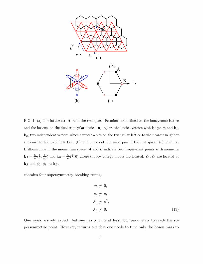
6

and bosons. The lattice structure is shown in Fig. 1 (a). fi is the fermion annihilation

operator and e−iθI , the lowering operator of nI which is conjugate to the angular variable

θI . i, j and I, J are site indices for the honeycomb and triangular lattices, respectively.

tf , tb > 0 are the hopping energies for the fermions and bosons, respectively and U is the

on-site boson repulsion energy. b1 and b2 are two independent vectors which connect a

site on the triangular lattice to the neighboring honeycomb lattice sites. h0 is the pairing

interaction strength associated with the process where two fermions in the f-wave channel

around a hexagon are paired and become a boson at the center of the hexagon, and vice

versa. In this sense, the boson can be regarded as a Cooper pair made of two spinless

fermions in the f-wave wavefunction. This model has a global U(1) symmetry under which

the fields transform as fi → fieiϕ and e−iθI → e−iθIei2ϕ.

In the low energy limit, there are two copies of Dirac fermions and two complex bosons.

One set of Dirac fermion and complex boson carries momentum kA, and the other set carries

momentum kB. The fermions are massless without any fine tuning, which is protected by

the time reversal symmetry and the inversion symmetry. The reason why we have two

complex bosons instead of one is that the boson kinetic energy is frustrated. Because tb > 0,

the boson kinetic energy is minimized when relative phases between neighboring bosons

become π. However, not all kinetic energy terms can be minimized due to the geometrical

frustration of the triangular lattice where bosons are defined. The best thing the bosons can

do to minimize the kinetic energy is to form a ‘spiral wave’ where the phase of bosons rotates

either by 120 or −120 degree around triangles. There are two such global configurations

and they carry the momenta kA and kB respectively. The low energy effective Lagrangian

becomes

L = i2∑

n=1

ψn

(

γ0∂τ + cf2∑

i=1

γi∂i

)

ψn

+2∑

n=1

[

|∂τφn|2 + c2b

2∑

i=1

|∂iφn|2 +m2|φn|2]

+λ1

2∑

n=1

|φn|4 + λ2|φ1|2|φ2|2

+h2∑

n=1

(

φ∗nψ

Tn εψn + c.c.

)

. (12)

Although there are same number of propagating bosons and fermions, this Lagrangian

7

1

2

x

y

(a)a

a

k

k

x

y

(c)(b)

b2

b1

B

A

FIG. 1: (a) The lattice structure in the real space. Fermions are defined on the honeycomb lattice

and the bosons, on the dual triangular lattice. a1, a2 are the lattice vectors with length a, and b1,

b2, two independent vectors which connect a site on the triangular lattice to the nearest neighbor

sites on the honeycomb lattice. (b) The phases of a fermion pair in the real space. (c) The first

Brillouin zone in the momentum space. A and B indicate two inequivalent points with momenta

kA = 2πa (1

3 ,1√3) and kB = 2π

a (23 , 0) where the low energy modes are located. ψ1, φ2 are located at

kA and ψ2, φ1, at kB .

contains four supersymmetry breaking terms,

m 6= 0,

cb 6= cf ,

λ1 6= h2,

λ2 6= 0. (13)

One would naively expect that one has to tune at least four parameters to reach the su-

persymmetric point. However, it turns out that one needs to tune only the boson mass to

8

realize supersymmetry.

2. RG flow

To control the theory, we consider the theory in 4−ǫ dimensions. We use the dimensional

regularization scheme where the number of fermion components and the traces of gamma

matrices are fixed.

The boson mass is a relevant (supersymmetry-breaking) perturbation and we tune it (by

hand) to zero. This amounts to tuning one microscopic parameter to reach the critical

point which separates the normal phase and the bose condensed phase. The one-loop beta

functions for the remaining couplings at the critical point is given by

dh

dl=

ǫ

2h− 1

(4πcf)2

(

2 +16c3f

cb(cf + cb)2

)

h3,

dλ1

dl= ǫλ1 −

1

(4π)2

(

20λ21 + λ2

2

c2b+

8h2λ1

c2f− 16h4

c2f

)

,

dλ2

dl= ǫλ2 −

1

(4π)2

(

4λ22 + 16λ1λ2

c2b+

8h2λ2

c2f

)

,

dcfdl

=32h2cf (cb − cf)

3(4π)2cb(cb + cf)2,

dcbdl

= −2h2cb(c2b − c2f)

(4πcbcf )2, (14)

where the logarithmic scaling parameter l increases in the infrared. The RG flow is shown

in Fig. 2.

The Gaussian (GA) fixed point, (h∗, λ∗1, λ∗2) = (0, 0, 0), the Wilson-Fisher (WF) fixed

point, (h∗, λ∗1, λ∗2) = (0, (4πcb)

2ǫ20

, 0), and the O(4) fixed point, (h∗, λ∗1, λ∗2) = (0, (4πcb)

2ǫ24

, (4πcb)2ǫ

12)

are all unstable upong turning on the pairing interaction h. If h is nonzero, the boson and

fermion velocities begin to flow as can be seen from the last two equations in Eq. (14).

Because the pairing interaction mixes the velocities of the boson and fermion, the difference

of the velocities exponentially flows to zero in the low-energy limit. With a nonzero h, the

system eventually flows to a stable fixed point,

(h∗, λ∗1, λ∗2) = (

√

(4π)2ǫ

12,(4π)2ǫ

12, 0). (15)

At this point, the theory becomes invariant under the supersymmetry transformation,

δξφn = −ψnξ, δξφ∗n = ξψn

9

(b)

b

cf

cb cf=

(a)

h

λ

λ

SUSY

2

1WFGA

c

FIG. 2: The schematic RG flows of (a) the velocities with h 6= 0 and (b) λ1, λ2 and h in the

subspace of m = 0. In (b), the solid lines represent the flow in the plane of (h, λ1) and the dashed

lines, the flow outside the plane.

δξψn = i/∂φ∗nξ −

h

2φ2nεξ

T, δξψn = iξ/∂φn −

h

2φ∗2n ξ

Tε,

(16)

where ξ is a two-component complex spinor. This theory corresponds to the N = 2 (four

supercharges) Wess-Zumino model with superpotential,

F = h(Φ31 + Φ3

2), (17)

where Φ1 and Φ2 are two chiral multiplets. Due to the emergent superconformal symmetry,

the one-loop anomalous scaling dimensions for the chiral primary fields φ and ψ,

ηφ = ηψ = ǫ/3 (18)

are exact.

Although the emergent supersymmetry has been obtained from a microscopic model

which has both fermions and bosons, one can view bosons as composite particles (Cooper

10

Normal phase

bt /U

Supersymmetric critical point

Bose condensed phase

FIG. 3: The superconformal theory describes the quantum critical point separating the normal

state and the f-wave superconducting (Bose condensed) state of spinless fermions in the honeycomb

lattice.

pairs) which emerge at low energies. This implies that supersymmetry can emerge from a

microscopic model which contains only fermions. Therefore, the N = 2 Wess-Zumino theory

with the cubic superpotential for two chiral multiplets can describe the second order quantum

phase transition of f-wave FFLO (Fulde-Ferrell-Larkin-Ovchinnikov) superconducting state

of spinless fermions on the honeycomb lattice at half filling (see Fig. 3).

III. EMERGENT GAUGE THEORY

Fractionalization is a phenomenon where a microscopic particle in many-body systems

decay into multiple modes each of which carry a fractional quantum number of the original

particle. In contrast to the more familiar phenomena where a composite particle breaks

into its constituent particles at high energies, fractionalization is a low energy collective

phenomenon where microscopic particles do not ‘really’ break into partons. Instead, many-

body correlations make it possible for parts of microscopic particles to emerge as deconfined

excitations in the low energy limit[10]. When fractionalization occurs, a gauge field emerges

as a collective excitation that mediates interaction between fractionalized excitations. In

this lecture, we are going to illustrate this phenomenon using a simple model.

A. Model

Consider a 4-dimensional Euclidean hypercubic lattice (with discretized time). At each

site on the lattice, there are boson fields eiθab

which carry one flavor index a and one anti-

flavor index b with a, b = 1, 2, ..., N . We impose contraints θab = −θba and eiθab

is anti-

particle of eiθba

. There are N(N − 1)/2 independent boson fields per site. In the following,

11

we will refer to these bosons as ‘mesons’. The action is

S = −t∑

<i,j>

∑

a,b

cos(

θabI − θabj)

−K∑

i

∑

a,b,c

cos(

θabi + θbci + θcai)

. (19)

Here the first term is the standard Euclidean kinetic energy of bosons and the second term is

the flavor conserving interactions between bosons. This model can be viewed as a low energy

effective theory of excitons in a multi-band insulator. But let’s forget about the ‘true UV

theory’ and take this model as our starting point. In this model, mesons are fundamental

particles.

B. Slave-particle theory

We are interested in the strong coupling limit (K >> 1). In this limit, the strong potential

imposes the dynamical constraints

θabi + θbci + θcai = 0 (20)

for every set of a, b, c. The constraints are satisfied on a (N − 1)-dimensional manifold in

(S1)N(N−1)/2 on each site. The low energy manifold is parameterized by

θabi = φai − φbi , (21)

where the new bosonic fields φa carry only one flavor quantum number contrary to the

meson fields. The new bosons are called slave-particles or partons. They are ‘enslaved’ to

each other because these partons can not escape out of mesons. Note that there is a local

U(1) redundancy in this parameterization and the low energy manifold is (S1)N/S1 not

(S1)N .

Within this low energy manifold, the potential energy can be dropped and the kinetic

energy becomes

S = −t∑

<i,j>

[

∑

a

ei(φai−φa

j)

] [

∑

b

e−i(φbi−φb

j)

]

. (22)

Since the kinetic energy is factorized in the flavor space, one can introduce a collective

dynamical field η ∼ ∑

b e−i(φb

i−φbj) using the Hubbard-Stratonovich transformation. Then the

12

effective action becomes

S = t∑

<i,j>

[

|ηij|2 − |ηij|∑

a

ei(φai−φa

j−aij) − c.c.

]

, (23)

where aij is the phase of the complex field ηij . Note that the full theory is invariant under

the U(1) gauge transformation

φai → φai + ϕi,

aij → aij + ϕi − ϕj . (24)

This theory is a compact U(1) lattice gauge theory coupled with N bosons with infinite

gauge coupling.

One might think that partons are always confined in this theory because the bare gauge

coupling is infinite. After all, mesons are fundamental particles and they can not break up!

This naive guess is only half correct. Indeed, mesons can never break into two particles

and partons should be always confined within mesons. However, this does not imply that

partons are always confined even in the long distance limit.

To see this, let us integrate out high energy fluctuations of φa to obtain an effective theory

with a cut-off Λ << 1/a where a is the lattice spacing. The fluctuations of partons generate

the Maxwell’s term (and all gauge invariant terms) in the low energy effective action,

S =∫

dx4

[

|(∂µ − iaµ)Φa|2 + V (Φa) +1

g2FµνF

µν + ...

]

, (25)

where Φa = eiφa

. Due to screening by N charged partons, the gauge coupling is renormalized

from infinity down to a finite value g2 ∼ 1/N . In the large N limit, the renormalized gauge

coupling can be made very small and the deconfinement (Coulomb) phase can arise as a

stable phase. Then gapless U(1) gauge boson (emergent photon) and fractionalized bosons

(partons) arise as low energy excitations.

C. World line picture

Although the above simple argument is very plausible, the relation between the ‘slave-

partons’ which are confined at short distance scales and the ‘liberated-partons’ which are

deconfined at long distance scales is rather obscure in this description. Moreover, it is not

entirely clear how partons can screen the gauge field in the first place if partons are always

13

ξ 2ξ 1

ξ 3

FIG. 4: Web of world lines.

confined within neutral mesons. In other words, one can question how one can integrate out

high energy fluctuations of partons reliably if they are subject to the infinitely strong gauge

coupling at high energies?

For this reason, it is useful to understand fractionalization purely in terms of original

mesons without introducing slave particles. Actually one can understand fractionalization

intuitively in terms of world lines of original mesons. The world line picture is not a quan-

titative description, but it is useful in that it provides a physical picture. In space-time,

world lines of mesons can be represented as double lines with two opposite arrows, where

each arrow carries a flavor current.

In the partition function, the simplest configuration is two overlapped loops with current

of flavor a moving in one direction and b in the other direction. General configurations

consist of a collection of connected webs made of boson world lines (world line web). Each

world line web defines closed surfaces as depicted in Fig. 4. Many such closed surfaces may

co-exist and interpenetrate each other. There are three different length scales in the world

line web. The shortest scale is the length of double line segment (ξ1) which corresponds to

the life time of a single exciton. This is order of the lattice scale in the strong coupling limit.

In other words, mesons quickly decay within a microscopic time scale due to the strong

interaction. The next scale is the typical size of single line loops (ξ2). This can be much

14

larger than ξ1 or the lattice scale even in the strong coupling limit. This is because a single

flavor a can switch as many partners as it wants during its life time before it meets with its

own anti-flavor a and decays into vacuum. In this case, we can view single lines as world

lines of emergent long-living excitations. The largest length scale is the size of the bubble

made of the web (ξ3). In general we have ξ1 < ξ2 < ξ3.

In the small t limit (which corresponds to limit of very massive mesons), all length scales

are of order of lattice scale. As t increases, mesons become lighter, and ξ2 and ξ3 increases.

However ξ1 remains always small in the strong coupling limit. If a ∼ ξ1 << ξ2 << ξ3 (which

can be achieved for a large but fixed N with a small tN) the closed surface of the world

line web is well-defined in the length scale ξ2 << x << ξ3. Thus the effective degrees of

freedom at this scale are fluctuating surface. The surface can be regarded as the world sheet

of oriented closed string. In the gauge theory picture the string corresponds to electric flux

line and the string tension, the gauge coupling. The gauge group should be U(1) due to the

orientedness of surfaces. The effective theory becomes a pure U(1) gauge theory. In this

scale, the world line web is very floppy and one obtains a weakly coupled pure gauge theory.

The transverse fluctuations of world line web corresponds to emergent gauge bosons.

For a finite ξ3, one eventually enters into the region where x >> ξ3 as one probes the

low energy limit. In this long distance limit, there are only small surfaces and the vacuum

is essentially empty. This corresponds to the confinement phase and ξ3 corresponds the

confining scale.

In the opposite limit, if we lower our length scale x to the scale comparable to ξ2, one

begins to notice holes on closed surfaces. One can interpret boundaries of the holes as world

lines of particles. These particles should be viewed as bosons because each contribution

adds up in the partition function without minus signs associated with single line loops. The

emergent bosons carry unit charge with respect to the emergent gauge field. This is because

world line web which corresponds to world sheet of one unit of electric flux line can end

on boundaries. Moreover, these bosons carry only one flavor quantum number due to the

fact that an anti-flavor b which always accompanies a flavor a is canceled by the flavor b

of nearby mesons. This is analogous to the situation where one can find a nonzero charge

density on a surface of a dielectric medium. Therefore in the scale x ∼ ξ2, the effective

degrees of freedom are gauge bosons coupled with N fractionalized bosons which carry only

one flavor quantum number.

15

In the shortest length scale x << ξ2, the single line loops look very large and these

fractionalized bosons look condensed. It corresponds to the Higgs phase of the gauge theory.

The crossover within the confinement phase become a real phase transition to a decon-

finement phase as ξ3 is made to diverge by making N larger with fixed tN . (A larger N

make the tension of world line web smaller through entropy contribution.) If ξ3 diverges

while ξ2 remains finite, the partons remain gapped but the gauge boson becomes gapless.

This is the Coulomb phase.

Although a parton is always bound with an anti-parton, it can propagate in space rather

freely by switching its partners repeatedly. (If you have too many girlfrieds or boyfriends,

you appear to be single in a long time scale although you are always with one girlfriend or

boyfriend at any moment.) As a result, partons can be effectively liberated and arise as

well-defined excitations in the Coulomb phase.

One may ask why one gets a weakly coupled gauge theory rather than some string theory.

One possible answer is that world line web is very dense in space-time in this case. They

constantly join and split, and their contact interactions are also important. It is hard to

imagine to have a well defined string in this strongly coupled soup of strings. This can be

viewed as a Lagrangian (or space-time) picture for the string-net condensation[11].

One can study different types of flavor preserving interactions. In particular, one can

obtain emergent fermionic excitations from the bosonic model if one introduces a quartic

interaction for mesons,

K4

∑

a,b,c,d

cos(θab + θbc + θcd + θda) (26)

instead of the cubic interaction. If K4 > 0, the interaction is frustrated and not all terms

in the potential energy can be minimized simultaneously. This frustration results in a

more degenerate low energy manifold and wavefunctions within the low energy manifold

acquires non-trivial sign structure, namely wavefunctions describing low energy excitations

are no longer positive definite. This non-trivial sign structure is responsible for the fermionic

statistics of emergent excitations. The emergent fermion can be also understood from the

world line picture where single line loops are endowed with minus signs in the partition

function due to the frustrated interaction. Then one should interpret single line loops as

world lines of fermions.

16

IV. CRITICAL SPIN LIQUID WITH FERMI SURFACE

A. From spin model to gauge theory

1. Slave-particle approach to spin-liquid states

Consider a system where spins are antiferromagnetically coupled in a two-dimensional

lattice,

H = J∑

<i,j>

~Si · ~Sj + ... (27)

Here we focus on models with spin 1/2. The antiferromagnetic coupling J > 0 favors

neighboring spins to align in anti-parallel direction. The dots denote higher order spin

interactions whose specific form is not important for the following discussion.

At sufficiently low temperatures T < J , spins usually order, spontaneously breaking the

SU(2) spin rotational symmetry. However, magnetic ordering can be avoided even at zero

temperature if there are strong quantum fluctuations. In systems which have small charge

gap, the ... terms induced by charge fluctuations cause strong quantum fluctuations of spins

(such as permutations of spins around plaquettes) which tend to disrupt magnetic ordering.

Quantum fluctuations are also enhanced by geometrical frustrations. Geometrical frustra-

tions arise when no spin configuration can minimize all interaction terms in the classical

Hamiltonian simultaneously. For example, three antiferromagnetic couplings on a triangle

can not be simultaneously minimized. Although magnetic order is absent, spins are usually

highly correlated and we refer to such correlated non-magnetic state as spin liquid[12] as

opposed to spin gas.

One way of describing spin liquid states is to use slave-particle approach. For example,

one decomposes a spin operator into fermion bilinear

~Si =∑

αβ

f †iα~σαβfiβ . (28)

Here fiα is a fermionic field which does not carry electromagnetic charge but carry only spin

1/2. For this reason, this particle is called ‘spinon’ This decomposition has the U(1) phase

redundancy. As a result, the theory for spinon has to be in the form of gauge theory. A

compact U(1) gauge theory coupled with spinons can be derived following a similar step

described in the previous lecture. Although the bare gauge coupling is infinite, the coupling

17

is renormalized to a finite value in the low energy limit. If deconfinement phase is stabilized,

spinons and the gauge field arise as low energy degrees of freedom.

Since there is spin 1/2 per each site, there is one spinon per site. Although there is no

bare kinetic term for spinons, they can propagate in space through the exchange interaction

: simutaneous flips of neighboring spins can be viewed as two spinons exchanging their

positions. As a result, spinons form a band, which then determines the low energy spectrum.

In non-bipartite lattice (a lattice which can not be divided into A and B sublattices, such

as the triangular lattice), the fermions generically form a fermi surface at half filling. In

this case, the low energy effective theory has a Fermi surface of spinons coupled with the

emergent U(1) gauge field[13, 14],

S =∫

d3x[

Ψ∗j(∂0 − ia0 − µF )Ψj

+1

2mΨ∗j(−i∇− a)2Ψj +

1

4g2fµνfµν

]

. (29)

Here Ψj is the fermion field with two flavors, j = 1, 2 (spin up and down) and aµ = (a0, a) is

the U(1) gauge field with µ = 0, 1, 2. µF is the chemical potential and g, the gauge coupling.

This is nothing but the QED3 with a nonzero chemical potential.

The zeroth order question one has to ask is the stability of the deconfinement phase.

Because of the presence of underlying lattice, the U(1) gauge field is compact. This allows

for instanton (or monopole) which describes an event localized in time where the flux of the

gauge field changes by 2π. It is known that if there is no gapless spinon, instantons always

proliferate in space-time, resulting in confinement. In this case, spin liquid states are not

stable and spinons are confined[15]. In the presence of gapless spinons, it is possible that

the gauge field is screened and instanton becomes irrelevant in the low energy limit. If this

happens, fractionalized phase is stable and spinons arise as low energy excitations.

If there are a large number of gapless spinons which have the relativistic dispersion,

instanton acquires a scaling dimension proportional to the number of flavors N . In the large

N limit, instanton is irrelevant at low energies and the fractionalized phase is stable[16].

In the presence of spinon Fermi surface, it turns out that the deconfinement phase can be

stable for any nonzero fermion flavor.

18

2. Stability of deconfinement phase in the presence of Fermi surface

To show that instanton is irrelevant in the presence of Fermi surface, we need the following

four ingredients.

First, one can describe low energy particle-hole excitations near the Fermi surface in

terms of an infinite copy of 1+1 dimensional fermions parameterized by the angle around

the Fermi surface[17]. In this angular representation, an instanton becomes a twist operator

which twists the boundary condition of the 1+1D fermions by π. In the presence of an

instanton, the fermions become anti-periodic around the origin in the 1+1D space-time.

This can be understood in the following way. At each point on the Fermi surface, the

Fermi velocity is perpendicular to the Femri surface. Fermions with a given Fermi velocity

explores a 1+1 dimensional subspace which is perpendicular to the x-y plane in 2+1D. Since

instanton is a source of 2π flux, the total flux of π penetrates through this plane. (Here we

are assuming that there is the rotational symmetry. But this argument can be generalized to

cases without the symmetry.) Therefore, a fermion moving in the plane encloses a flux close

to π as it is transported around the origin at a large distance. As a result, the boundary

condition of low energy fermion at each angle is twisted by π by instanton.

Second, the angle θ around the Fermi surface has a positive scaling dimension. As a result,

the angle is decompactified and runs from −∞ to ∞ in the low energy limit. In the low

energy limit, the gauge field becomes more and more ineffective in scattering fermions from

one momentum to another momentum along tangential directions to the Fermi surface.

This is because the momentum of the gauge field becomes much smaller than the Fermi

momentum. This amounts to saying that effective angular separation between two fixed

points on the Fermi surface grows in the low energy limit.

Third, the theory is local in the space of the decompactified angle. This is due to the

kinematic constraint of the curved Fermi surface. In the low energy limit, only those fermions

very close to the Fermi surface can be excited. Since gauge boson scatters one fermion

near the Fermi surface to another point near the Fermi surface, the momentum of gauge

boson is almost tangential to the Fermi surface where the fermions are located. Therefore,

fermions with a particular angle are significantly coupled only with those gauge field whose

momentum is tangential to the Fermi surface at the angle. This means that fermions with a

finite angular separation (except for those which are at the exact opposite side of the Fermi

19

x

τ

θ

π

P

P’

FIG. 5: ‘Time’-evolution of a quantum state defined on the surface of a pipe extended along the

angular direction, where a π-vortex is pierced through the pipe. Under the time-evolution, a point

on the surface P is mapped to a point on the surface P ′

.

surface) becomes essentially decoupled in the low energy limit because they are coupled only

with those gauge bosons whose momenta are separated in the momentum space.

Finally, instanton become a π vortex which is extended along the non-compact θ direction

in the theory written in the space of θ, τ and x, where x is a real space coordinate associated

with the radial momentum at each point on the Fermi surface. The vortex defines a quantum

state on the surface of a pipe P which is extended in the θ direction in the space of τ , x

and θ as is shown in Fig. 5. The scaling dimension of instanton corresponds to the ‘energy’

of this quantum state associated with the radial time evolution.

Because of the locality along the decompactified angular direction, the extended π-vortex

should have an infinite ‘energy’. This implies that the scaling dimension of the instanton

operator diverges and instanton remains strongly irrelevant. As a result, the deconfinement

phase can be stable.

B. Low energy effective theory

Having established that deconfinement phase is stable, we can treat the theory as a non-

compact U(1) gauge theory. Now, we are going to analyze the low energy effective theory

of Fermi surface coupled with the U(1) gauge field in 2+1D. Although we motivated this

theory in the context of spin liquid, the same theory often arises in other systems. More

20

k y

k x

FIG. 6: The parabolic Fermi surface of the model in Eq. (30). The shaded region includes negative

energy states.

importantly, the theory represents a class of typical non-Fermi liquid states which arise as a

result of coupling between Fermi surface and gapless bosons. Not surprisingly, many features

of this theory are shared by other non-Fermi liquid states in 2+1D.

In this system, there is no tunable parameter other than the number of fermion (vector)

flavors N . Given that the physically relevant theory (N = 2) is a strongly coupled theory,

it is natural to consider the theory with a large number of fermion flavors N . Naively one

would expect that the theory becomes classical in the large N limit. However, this intuition

based on relativistic field theories is incorrect in the presence of Fermi surface. Unlike those

theories where gapless excitations are located only at discrete set of points in the momentum

space, Fermi surface has an extended manifold of gapless points. The abundant low energy

excitations subject to the strong IR quantum fluctuations in 2+1D make the theory quite

nontrivial even in the large N limit.

In the low energy limit, fermions whose velocities are not parallel or anti-parallel to each

other are essentially decoupled. As a result, it is sufficient to consider local patches of Fermi

surface in the momentum space. The minimal model in parity symmetric systems is the

theory which includes an open patch of Fermi surface and one more patch whose Fermi

velocity is opposite to that of the former.

Here, we will focus on one patch in the momentum space. The one-patch theory is already

quite non-trivial and the full structure is yet to be understood. The two-patch theory has

yet another level of complications[24] over which we have much less theoretical control. The

action in the one-patch theory is

L =∑

j

ψ∗j (∂τ − ivx∂x − vy∂

2y)ψj

21

+e√N

∑

j

aψ∗jψj

+a[

−∂2τ − ∂2

x − ∂2y

]

a, (30)

where ψj is the fermion of flavor j = 1, 2, ..., N . We have chosen our k = 0 to be a point

on the Fermi surface where the Fermi velocity is parallel to the x-direction. vx is the Fermi

velocity and vy ∼ 1m

determines the curvature of the Fermi surface. The Fermi surface is on

vxkx+vyk2y = 0 as is shown in Fig. 6. This is a ‘chiral Fermi surface’ where the x-component

of Fermi velocity is always positive. This chirality is what makes the one-patch theory more

tractable compared to the two-patch theory. a is the transverse component of an emergent

U(1) gauge boson in the Coulomb gauge ∇ · a = 0. We ignore the temporal component of

the gauge field which is screened to a short range interaction. The transverse gauge field

is massless without a fine tuning due to an emergent U(1) symmetry associated with the

dynamical suppression of instantons. e is the coupling between fermions and the critical

boson.

In the one-loop order, gapless modes generate singular self energies. The one-loop quan-

tum effective action becomes

Γ =∑

j

∫

dk[

ic

Nsgn(k0)|k0|2/3 + ik0 + vxkx + vyk

2y

]

ψ∗j (k)ψj(k)

+∫

dk

[

γ|k0||ky|

+ k20 + k2

x + k2y

]

a∗(k)a(k)

+e√N

∑

j

∫

dkdq a(q)ψ∗j (k + q)ψj(k), (31)

where c and γ are constants of the order of 1. In the low energy limit, the leading terms of

the quantum effective action are invariant under the scale transformation,

k0 = b−1k′

0,

kx = b−2/3k′

x,

ky = b−1/3k′

y,

ψa(b−1k

′

0, b−2/3k

′

x, b−1/3k

′

y) = b4/3ψ′

a(k′

0, k′

x, k′

y). (32)

Dropping terms that are irrelevant under this scaling, we write the minimal action as

L =∑

j

ψ∗j (η∂τ − ivx∂x − vy∂

2y)ψj

+e√N

∑

j

aψ∗jψj + a(−∂2

y)a. (33)

22

The local time derivative term is also irrelevant, and η flows to zero in the low energy

limit. But we can not drop this term from the beginning. Otherwise, the theory becomes

completely local in time and there is no dynamics. The role of this irrelevant η-term is

to generate a non-trivial frequency dependent dynamics by maintaining the minimal causal

structure of the theory before it dies off in the low energy limit. In other words, the η-term

itself is irrelevant but it is crucial to generate marginal singular self energies. But once we

include the frequency dependent self energies, we can drop the η-term as far as we remember

that the non-local self energies are dynamically generated from the local Lagrangian.

The minimal action (33) has four marginal terms. On the other hand, there are five

parameters that set the scales of energy-momentum and the fields. Out of the five pa-

rameters, only four of them can modify the coefficients of the marginal terms because the

marginal terms remain invariant under the transformation (32). Using the remaining four

parameters, one can always rescale the coefficients of the marginal terms to arbitrary values.

Therefore, there is no dimensionless parameter in this theory except for the fermion flavor

N . In particular, the gauge coupling e can be always scaled away. This implies that the

theory with fixed N flows to a unique fixed point rather than a line of fixed point which has

exact marginal deformation. In the following, we will set vx = vy = e = 1.

1. Failure of a perturbative 1/N expansion

In the naive N counting, a vertex contributes N−1/2 and a fermion loop contributes N1.

In this counting, only the fermion RPA diagram is of the order of 1, and all other diagrams

are of higher order in 1/N . In the leading order, the propagators become

g0(k) =1

iηk0 + kx + k2y

,

D(k) =1

γ |k0||ky| + k2

y

. (34)

One can attempt to compute the full quantum effective action by including 1/N correc-

tions perturbatively. However, it turns out vertex functions which connect fermions on the

Fermi surface generically have strong IR singularity, which is cured only by loop corrections.

Therefore it is crucial to include the one-loop fermion self energy in the dressed fermion

23

propagator,

g(k) =1

iηk0 + i cN

sgn(k0)|k0|2/3 + kx + k2y

. (35)

Although the self energy has an additional factor of 1/N compared to the bare frequency

dependent term, the self energy dominates at sufficiently low energy k0 < 1/(ηN)3 for any

fixed N . Here it is important to take the low energy limit first before taking large N limit.

This is the correct order of limits to probe low energy physics in any physically relevant

systems with finite N .

The removal of IR singularity does not come without price. In the presence of the self

energy, the IR singularity is cut-off at a scale proportional to 1/N . As a result the IR

singularity is traded with a finite piece which has an additional positive power of N .

k + q

kl

k + l

l − q

p+ lq

p+ q

p

FIG. 7: A two-loop vertex correction.

For example, the two-loop vertex function ( Fig. 7 ) computed using the bare propagator

becomes

Γbare(p = 0, q) = −N−3/2

ηq1/30

f1(qy/q1/30 ) (36)

when both both p = 0 and p + q are on the Fermi surface. Here f1(t) is a non-singular

universal function which is independent of N and η. This diverges as q goes to zero with

fixed qy/q1/30 . With the dressed propagator, the IR singularity disappears but there exists

an enhancement factor of N ,

Γdressed(0, q) = −N−1/2f2(qy/q1/30 ), (37)

where f2(t) is a non-singular universal function. Note that this two-loop vertex correction

has the same order as the bare vertex, which signals a breakdown of perturbative 1/N

expansion. Similar enhancement factors arise in other diagrams as well.

24

2. Genus Expansion

There exists a simple way of understanding this enhancement factor in N systematically.

The reason why the enhancement factor arises is that the fermion propagator is not always

order of 1. For generic momentum away from the Fermi surface, the kinetic energy dominates

and the propagator is order of 1. On the other hand, when fermions are right on the

Fermi surface, the kinetic energy vanishes and there are only frequency dependent terms.

At sufficiently low frequencies, the non-local self energy dominates and the propagator is

enhanced to the order of N . In relativistic field theories, there are only discrete set of points

in the momentum space where the kinetic energy vanishes. Therefore the phase space in

which the fermion propagator becomes order of N is very limited. In the present case

with Fermi surface, there is one dimensional manifold of gapless points. Whenever fermions

hit the Fermi surface (and there are many ways to do that), the fermion propagator gets

enhanced to order of N . This is the basic reason why the naive N counting breaks down in

the presence of Fermi surface.

For a given diagram, say L-loop diagram, there are 2L integrations of internal momenta

kx and ky. In the 2L-dimensional space of internal momenta, in general there is a m-

dimensional sub-manifold on which all internal fermions can stay right on the Fermi surface

as long as external fermions are on the Fermi surface. We refer to this manifold as a ‘singular

manifold’. If we focus on the momentum integration near a generic point on the singular

manifold, it generically looks like

I ∼∫

dq1dq2...dqm

∫

dk1dk2...dk2L−mΠIfi=1

[

1

αijkj + i 1Nf(ωi)

]

. (38)

Here q1, q2, ..., qm are deviation of momenta from the point on the singualr manifold along the

directions tangential to the singular manifold. k1, k2, ..., k2L−m are momentum components

which are perpendicular to the singular manifold. If is the number of fermion propagators.

The key point is that the fermion propagators depend only on k’s but not on q’s because ki-

netic energy of fermions stay zero within the singular manifold. The tangential momenta q’s

parameterize exact zero modes of Fermi surface deformations where fermions on the Fermi

surface slide along the Fermi surface. If N is strictly infinite and we drop the frequency de-

pendent term in the self energy, the fermion propagators become singular whenever fermions

are on the Fermi surface. The m integrations along the tangential direction of the singular

manifold do not help to remove the IR singularity. Only 2L−m integrations of k momenta

25

(a) (b)

FIG. 8: The double line representations of (a) the 2-loop vertex correction and (b) the 3-loop

fermion self energy. Double lines represent propagators of the boson, and the single lines are the

propagators of the fermion. The number of single line loops (one in (a) and two in (b)) represents

the dimension of the singular manifold (see the text) on which all fermions remain on the Fermi

surface in the space of internal momenta.

lower the degree of IR singularity. After the integration over the all 2L momentum, the

remaining IR singularity is order of If − (2L − m). For any finite N , this IR singularity

is cut-off at a momentum proportional to 1/N . This means the resulting diagram has an

additional factor of N If−(2L−m) as compared to the naive N counting.

What determines the dimension of the singular manifold within which fermions always

remain on the Fermi surface? It turns out that the dimension of the singular manifold is

given by the number of closed loops when one draws boson propagators using double lines

and fermion propagators using single lines. First, we restrict momenta of all fermions to be

on the Fermi surface. A momentum kθ of fermion on the Fermi surface is represented by an

one-dimensional parameter θ. Then, a momentum of the boson q is decomposed into two

momenta on the Fermi surface as q = kθ − kθ′ , where both kθ and kθ′ are on the Fermi

surface. This decomposition is unique because there is only one way of choosing such kθ

and kθ′ near k = 0. As far as momentum conservation is concerned, one can view the boson

of momentum q as a composite particle made of a fermion of momentum kθ and a hole

of momentum kθ′ . For example, the two-loop vertex correction and the three-loop fermion

self energy correction can be drawn as Fig. 8 in this double line representation. In this

representation, each single line represents a momentum on the Fermi surface. Momenta in

the single lines that are connected to the external lines should be uniquely fixed to make

all fermions stay on the Fermi surface. On the other hand, momenta on the single lines

that form closed loops by themselves are unfixed. In other words, all fermions can stay on

26

the Fermi surface no matter what the value of the unfixed momentum component that runs

through the closed loop is. Since there is one closed loop in Fig. 8 (a), the dimension of the

singular manifold is 1 and the enhancement factor becomes N4−(4−1) = N for the two-loop

vertex correction. Likewise, the enhancement factor for the three-loop fermion self energy

becomes N5−(6−2) = N which makes the three-loop fermion self energy to have the same

power 1/N as the one-loop correction.

The enhancement factor is a direct consequence of the presence of infinitely many soft

modes associated with deformations of the Fermi surface. The extended Fermi surface

makes it possible for virtual particle-hole excitations to maneuver on the Fermi surface

without costing much energy. As a result, quantum fluctuations becomes strong when

external momenta are arranged in such a way that there are sufficiently many channels for

the virtual particle-hole excitations to remain on the Fermi surface. This makes higher order

processes to be important even in the large N limit. We note that this effect is absent in

relativistic quantum field theories where gapless modes exist only at discrete points in the

momentum space.

The net power in N for general Feynman diagrams becomes

N−V/2+Lf +

[

n+Ef+2Eb

2−2

]

, (39)

where n is the number of single line loop, Ef (Eb) is the number of external lines for fermion

(boson), and Lf is the number of fermion loop. Here [x] = x for non-negative x and [x] = 0

for negative x. For vacuum diagram, the N -counting depends only on the topology of the

Feynman diagram and it becomes

N−2g, (40)

where g is the genus of the 2d surface on which Feynman graph is drawn using the full double

line representation without any crossing. In the full double line representation, we draw not

only the boson propagator as a double line, but also the fermion propagator as a double line

where the additional line associated with a fermion loop corresponds to the flavor degree of

freedom which run from 1 to N . As a result, all planar diagrams are generically order of

N0. Some typical planar diagrams are shown in the following figures.

The above counting is based on the local consideration on the space of internal momenta

near the singular manifold. It turns out that planar diagrams precisely follow the counting

27

FIG. 9: A typical vacuum planar diagram which is of the order of N0.

FIG. 10: The full double line representation of the planar diagram shown in Fig. 9. The solid

double lines represent the boson propagator and double lines made of one solid and one dotted

lines represent fermion propagators. Loops of dotted lines are added to each fermion loops. In this

representation, there is a factor of N for each closed single line loop whether it is a loop made of

a solid or dotted line.

obtained from this local considerations. Some non-planar diagrams may deviate from this

local counting by some factor of logN . The full structure of non-planar diagrams are not

completely understood yet.

Power counting of diagrams with external lines can be easily obtained from the counting

of vacuum diagrams. The leading contributions come from the planar diagrams where the

genus of the underlying 2d surface is zero. In principle, there can be infinitely many diagrams

which are order ofN0 (N−1) for the boson (fermion) self energy and N−1/2 for the three-point

vertex function.

28

Because the one-patch theory is a chiral theory, there are strong kinematic constraints;

phase space for two right moving particles to scatter into is very limited. Using this, one can

actually can prove that all planar diagrams for boson self energy vanish beyond the one loop.

Moreover one can show that the beta function vanishes and fermions have no anomalous

scaling dimension to the leading order of N (the contributions of planar diagrams). However,

there are still infinitely many non-vanishing planar diagrams for the fermion self energy and

the vertex function.

Although the present theory has fermions with vector flavors, it behaves like a matrix

model in the large N limit. The reason why the genus expansion arises from this vector

model is that the angle around the Fermi surface plays the role of an additional flavor. In

the usual matrix model, N controls the genus expansion and the t’Hooft coupling λ controls

the loop expansion. One expects that a continuum world sheet description of string emerges

in a matrix model when both N and λ are large. In the present case, the effective ’t Hooft

coupling is order of 1. In other words, two diagrams with L-loops and (L + 1)-loops have

the same order of magnitude as far as they have same topology. This is because there is no

dimensionless parameter in the theory other than N as discussed earlier. With λ ∼ 1, the

theory is likely not in the regime where one can use a dual gravity description in a weakly

curved space-time. One may view the theory as a weakly coupled string theory in a highly

curved background.

If one includes two patches of Fermi surface, even non-planar diagrams are also important

due to UV divergence, and the genus expansion appears to break down[24]. It is yet to be

understood how Feynman diagrams are organized in this case.

V. HOLOGRAPHIC DESCRIPTION OF QUANTUM FIELD THEORY

Although the original AdS/CFT correspondence has been conjectured based on the su-

perstring theory, it is possible that the underlying holographic principle is more general and

a wider class of quantum field theories can be understood through holographic descriptions.

According to the holographic principle, the partition function of a D-dimensional theory can

be written as a partition function of a (D+1)-dimensional theory where the information on

the D-dimensional theory is encoded through boundary conditions as

Z[J(x)] =∫

Dφ(x)e−SD[φ]−

∫

dxJφ

29

=∫

D “J(x, z)”e−S(D+1)[J(x,z)]

∣

∣

∣

∣

J(x,0)=J(x),

(41)

where J(x, z) represent (D+1)-dimensional degrees of freedom. It is most likely that the

holographic description will be useful only for a certain class of quantum field theories.

Nevertheless, it would be still useful to develop a general prescription for the mapping. In

this lecture, we will develop a prescription to construct the bulk theory S(D+1)[J(x, z)] for

general quantum field theories SD[φ].

A. Toy-model : 0-dimensional scalar theory

To illustrate the basic idea, we first consider the simplest field theory : 0-dimensional

scalar theory. In zero dimension, the partition function is given by an ordinary integration,

Z[J ] =∫

dΦ e−S[Φ]. (42)

We consider an action S[Φ] = SM [Φ] + SJ [Φ] with

SM [Φ] = M2Φ2,

SJ [Φ] =∞∑

n=1

JnΦn. (43)

Here SM is the bare action with ‘mass’ M . SJ is a deformation with sources Jn. For

simplicity, we will consider deformations upto quartic order : Jn = 0 for n > 4. Here is the

prescription to construct a holographic theory.

• Step 1. Introduce an auxiliary field

We add an auxiliary field Φ with mass µ,

Z[J ] = µ∫

dΦdΦ e−(S[Φ]+µ2Φ2). (44)

Then, we find a new basis φ and φ

Φ = φ+ φ,

Φ = Aφ+Bφ, (45)

30

in such a way that the ‘low energy field’ φ has a mass M′

which is slightly larger than

the original mass M , and the ‘high energy field’ φ has a large mass m′

,

M′2 = M2e2αdz ,

m′2 =

M2

2αdz, (46)

where dz is an infinitesimally small parameter and α is a positive constant. Quantum

fluctuations for φ become slightly smaller than the original field Φ. The missing

quantum fluctuations are compensated by the high energy field φ. In terms of the new

variables, the partition function is written as

Z[J ] =

(

Mm′

M ′+MM

′

m′

)

∫

dφdφ e−(SJ [φ+φ]+M′2φ2+m

′2φ2). (47)

• Step 2. rescale the fields

To maintain the same form for the quadratic action, we rescale the fields as

φ→ e−αdzφ, φ→ e−αdzφ. (48)

Then the couplings are also rescaled to new values, Jn → jn = Jne−nαdz and m →m

′

e−αdz.

• Step 3. Expand the action in power of the low energy field

The new action becomes

Sj[φ+ φ] = Sj[φ] + (j1 + 2j2φ+ 3j3φ2 + 4j4φ

3)φ

+(j2 + 3j3φ+ 6j4φ2)φ2 + (j3 + 4j4φ)φ3 + j4φ

4. (49)

In the standard renormalization group (RG) procedure[26], one integrates out the high

energy field to obtain an effective action for the low energy field with renormalized

coupling constants. Here we take an alternative view and interpret the high energy

field φ as fluctuating sources for the low energy field. This means that the sources

for the low energy field can be regarded as dynamical fields instead of fixed coupling

constants.

• Step 4. Decouple low energy field and high energy field

31

We decouple the high energy field and the low energy field by introducing Hubbard-

Stratonovich fields Jn and Pn,

Z[J ] = m∫

dφdφΠ4n=1(dJndPn) e

−(S′

j+M2φ2+m2φ2), (50)

where

S′

j = Sj[φ]

+iP1J1 − iP1(j1 + 2j2φ+ 3j3φ2 + 4j4φ

3) + J1φ

+iP2J2 − iP2(j2 + 3j3φ+ 6j4φ2) + J2φ

2

+iP3J3 − iP3(j3 + 4j4φ) + J3φ3

+iP4J4 − iP4j4 + J4φ4. (51)

• Step 5. integrate out the high energy mode

We integrate out φ to the order of dz. The auxiliary fields P and J acquire non-trivial

action,

Z[J ] =∫

dφΠ4n=1(dJndPn) e

−(SJ [φ]+M2φ2+S(1)[J,P ]), (52)

where

S(1)[J, P ] =4∑

n=1

i(Jn − Jn + nαdzJn)Pn

+αdz

2M2(iJ1 + 2P1J2 + 3P2J3 + 4P3J4)

2. (53)

Here Jn = (Jn + Jn)/2. One would expect that Jn should be just Jn in the above

equation and there is another contribution coming from the quadratic action of the

high energy field. It turns out that the quadratic contribution can be included by

shifting Jn to Jn. One can explicitly check that the above action reproduces all

renormalized coupling to the order of dz if Pn and Jn are integrated out.

• Step 6. Repeat the steps 1-5 for the low energy field

If we keep applying the same procedure to the low energy field, the partition function

can be written as a functional integration over fluctuating sources and conjugate fields,

Z[J ] =∫

Π4n=1(DJnDPn) e

−S[J,P ], (54)

32

where

S[J, P ] =∫ ∞

0dz[

i(∂zJn + nαJn)Pn

+α

2M2(iJ1 + 2P1J2 + 3P2J3 + 4P3J4)

2]

. (55)

HereDJnDPn represent functional integrations over one dimensional fields Jn(z), Pn(z)

which are defined on the semi-infinite line [0,∞). The boundary value of Jn(z) is fixed

by the coupling constants of the original theory, Jn(0) = Jn. Pn(z) is the conjugate

field of Jn(z) which describes physical fluctuations of the operator φn. This can be

seen from the equations of motion for Jn.

The theory given by Eqs. (54) and (55), which is exactly dual to the original theory, is

an one-dimensional local quantum theory. The emergent dimension z corresponds to loga-

rithmic energy scale[27]. The parameter α determines the rate the energy scale is changed.

The partition function in Eq. (54) does not depend on the rate high energy modes are

eliminated as far as all modes are eventually eliminated. Moreover, at each step of mode

elimination, one could have chosen α differently. Therefore, α can be regarded as a function

of z. If one interprets z as ‘time’, it is natural to identify α(z) as the ‘lapse function’, that

is, α(z) =√

gzz(z), where gzz(z) is the metric. Then one can view Eqs. (54) and (55) as an

one-dimensional gravitational theory with matter fields Jn. This becomes more clear if we

write the Lagrangian as

L = Pn∂zJn − αH, (56)

whereH is the Hamiltonian (the reason whyH is not Hermitian in this case is that we started

from the Euclidean field theory). However, there is one important difference from the usual

gravitational theory. In the Hamiltonian formalism of gravity[28], the lapse function is a

Lagrangian multiplier which imposes the constraint H = 0. However, in Eq. (54), α is

not integrated over and the Hamiltonian constraint is not imposed. This is due to the

presence of the boundary at z = 0 which explicitly breaks the reparametrization symmetry.

In particular, the ‘proper time’ from z = 0 to z = ∞ given by

l =∫ ∞

0α(z)dz (57)

is a quantity of physical significance which measures the total warping factor. To reproduce

the original partition function in Eq. (42) from Eq. (54), one has to make sure that l = ∞

33

to include all modes in the infrared limit. Therefore, l should be fixed to be infinite. As a

result, one should not integrate over all possible α(z) some of which give different l. This

is the physical reason why the Hamiltonian constraint is not imposed in the present theory.

This theory is a gravitational theory with the fixed size along the z direction.

Although there are many fields in the bulk, i.e. Jn, Pn for each n, there is only one

propagating mode, and the remaining fields are non-dynamical in the sense they strictly

obey constraints imposed by their conjugate fields. This is not surprising because we started

with one dynamical field Φ. There is a freedom in choosing one independent field. In this

case, it is convenient to choose J3 as an independent field. If one eliminates all dependent

fields, one can obtain the local bulk action for one independent field.

B. D-dimensional O(N) vector theory

The same procedure can be generalized to D-dimensional field theory. For example, the

partition function for the D-dimensional O(N) vector model,

S[Φ] =∫

dxdy Φa(x)G−1M (x − y)Φa(y)

+∫

dx[

JaΦa + JabΦaΦb + JabcΦaΦbΦc + JabcdΦaΦbΦcΦd

+J ijab∂iΦa∂jΦb + J ij

abcΦa∂iΦb∂jΦc + J ijabcdΦaΦb∂iΦc∂jΦd

]

(58)

can be written as a (D + 1)-dimensional functional integration,

Z[J ] =∫

DJDP e−S[J,P ], (59)

where the bulk action is given by

S[J, P ] =∫

dxdz{

iPa(∂Ja −2 +D

2αJa) + iPab(∂Jab − 2αJab) + iPab,ij(∂J

ijab)

+iPabc(∂Jabc −6 −D

2αJabc) + iPabc,ij(∂J

ijabc −

2 − d

2αJ ijabc)

+iPabcd(∂Jabcd − (4 −D)αJabcd) + iPabcd,ij(∂Jijabcd − (2 − d)αJ ijabcd)

}

+14

∫

dxdydz{

αsa(x)G′

(x − y)sa(y)}

, (60)

with

sa =[

iJa + 2PbJab − 2∂j(Jijab∂iPb) + 3PbcJabc − ∂j(J

ijabc∂iPbc)

+ Pbc,ijJijabc + 4PbcdJabcd −

2

3∂j(J

ijabcd∂iPbcd) + 2J ijabcdPbcd,ij

]

, (61)

34

G′

(x) ≡ M∂MGM(x), and ∂ = ∂∂z

− α∑Di=1 xi

∂∂xi

. Here∫

dx and∫

dy are integrations on a

D-dimensional manifold MD, and G−1M (x) is the regularized kinetic energy with cut-off M .

The dual theory is given by the functional integrals of the source fields J and their

conjugate fields P in the (D+1)-dimensional space MD×[0,∞) with the boundary condition

J(x, z = 0) = J (x). If the D-dimensional manifold MD has a finite volume V , the volume

at scale z is given by V e−αDz.

One key difference from the 0-dimensional theory is that there exist bulk fields with

non-trivial spins. In Eq. (60), there are spin two fields which are coupled to the energy

momentum tensor at the boundary. In the presence of more general deformations in the

boundary theory, one needs to introduce fields with higher spins[29].

One can decompose the tensor sources into singlets and tranceless parts and take the large

N limit where saddle point solutions become exact for singlet fields. It would be natural

to integrate out all non-singlet fields and obtain an effective theory for single fields alone.

However, it turns out that the effective action for single fields become non-local in this O(N)

vector model. This is because there are light non-singlet fields in the bulk and integrating

over those soft modes generates non-local correlations for singlet fields. This means that we

should keep light non-singlet fields as ‘low energy degrees of freedom’ in the bulk description

if we want to use a local description.

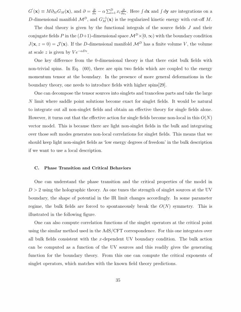
C. Phase Transition and Critical Behaviors

One can understand the phase transition and the critical properties of the model in

D > 2 using the holographic theory. As one tunes the strength of singlet sources at the UV

boundary, the shape of potential in the IR limit changes accordingly. In some parameter

regime, the bulk fields are forced to spontaneously break the O(N) symmetry. This is

illustrated in the following figure.

One can also compute correlation functions of the singlet operators at the critical point

using the similar method used in the AdS/CFT correspondence. For this one integrates over

all bulk fields consistent with the x-dependent UV boundary condition. The bulk action

can be computed as a function of the UV sources and this readily gives the generating

function for the boundary theory. From this one can compute the critical exponents of

singlet operators, which matches with the known field theory predictions.

35

J3a J3a

z z0 0

(a) (b)

FIG. 11: Saddle point configuration for a non-singlet source field J3a(z) (a) in the disordered phase

and (b) in the ordered phase. When J2 is sufficiently negative, a Mexican-hat potential at the

IR boundary drags J3a(z) away from J3a(z) = 0 in the bulk. At the critical point, J3a at the IR

boundary z = ∞ is more or less free to fluctuate, generating algebraic correlations between fields

inserted at the UV boundary z = 0.

VI. ACKNOWLEDGEMENT

I thank Andrey Chubukov, Guido Festuccia, Matthew Fisher, Sean Hartnoll, Michael

Hermele, Yong Baek Kim, Patrick Lee, Hong Liu, Max Metlitski, Lesik Motrunich, Joe

Polchinski, Subir Sachdev, T. Senthil and Xiao-Gang Wen for many illuminating discussions.

This work was supported by NSERC.

[1] S.-S. Lee, Phys. Rev. B 76, 075103 (2007).

[2] S.-S. Lee and P. A. Lee, Phys. Rev. B 72, 235104 (2005).

[3] S.-S. Lee, Phys. Rev. B 78, 085129 (2008); Phys. Rev. B 80, 165102 (2009).

[4] S.-S. Lee, Nucl. Phys. B 832, 567 (2010).

[5] X.-G. Wen, Quantum Field Theory of Many-body Systems: From the Origin of Sound to an

Origin of Light and Electrons (Oxford Graduate Texts).

[6] S. Sachdev, Quantum Phase Transitions, Cambridge University Press.

36

[7] D. Friedan, Z. Qui and S. Shenkar, Phys. Lett. B 151, 37 (1985).

[8] D. B. Kaplan, Phys. Lett. B 136, 162 (1984).

[9] S. Catterall, D. B. Kaplan and Mithat Unsal, arXiv: 0903.4881.

[10] P. W. Anderson, Science 235, 1196 (1987); P. Fazekas and P. W. Anderson, Philos. Mag. 30,

432 (1974).

[11] M. A. Levin and X.-G. Wen Phys. Rev. B 67, 245316 (2003); ibid. 71, 045110 (2005).

[12] For a more comprehensive review, see L. Balents, Nature 464, 199 (2010).

[13] O. I. Motrunich, Phys. Rev. B 72, 045105 (2005).

[14] S.-S. Lee and P. A. Lee, Phys. Rev. Lett. 95, 036403 (2005).

[15] A. M. Polyakov, Phys. Lett. B 59, 82 (1975); Nucl.Phys. B 120, 429 (1977).

[16] M. Hermele, T. Senthil, M. P. A. Fisher, P. A. Lee, N. Nagaosa and X.-G. Wen, Phys. Rev.

B 70, 214437 (2004).

[17] R. Shankar, Rev. Mod. Phys. 66, 129 (1994).

[18] P. A. Lee and N. Nagaosa, Phys. Rev. B 46 5621 (1992).

[19] J. Polchinski, Nucl. Phys. B 422, 617 (1994).

[20] Y. B. Kim, A. Furusaki, X.-G. Wen and P. A. Lee, Phys. Rev. B 50, 17917 (1994).

[21] C. Nayak and F. Wilczek, Nucl. Phys. B 417, 359 (1994); 430, 534 (1994).

[22] B. L. Altshuler, L. B. Ioffe and A. J. Millis, Phys. Rev. B 50, 14048 (1994).

[23] O. I. Motrunich and M. P. A. Fisher, Phys. Rev. B 75, 235116 (2007).

[24] M. Metlitski and S. Sachdev, arxiv:1001.1153.

[25] I.R. Klebanov and A.M. Polyakov, Phys. Lett. B 550, 213 (2002).

[26] J. Polchinski, Nucl. Phys. B 231, 269 (1984).

[27] J. de Boer, E. Verlinde and H. Verlinde, J. High Energy Phys. 08, 003 (2000).

[28] R. Arnowitt, S. Deser, and C. Misner, Phys. Rev. 116, 1322 (1959).

[29] M. A. Vasiliev, arXiv:hep-th/9910096.

37