EMC & OPTICS MANUAL CalStan 10 - RF Home
59
EMC & OPTICS MANUAL CalStan 10.0 RF Measurement Software 17.02.2011 Manual Version 1.6.1 Calstan Version 1.5.3
Transcript of EMC & OPTICS MANUAL CalStan 10 - RF Home
E M C & O P T I C S
MANUAL CalStan 10.0
RF Measurement Software
17.02.2011 Manual Version 1.6.1 Calstan Version 1.5.3

Notice Seibersdorf Labor GmbH reserves the right to make changes to any product described herein in order to improve function, design or for any other reason. Nothing contained herein shall constitute Seibersdorf Labor GmbH assuming any liability whatsoever arising out of the application or use of any product or circuit described herein. All graphs show typical data and not the measurement values of the individual product delivered with this manual. Seibersdorf Labor GmbH does not convey any license under its patent rights or the rights of others. © Copyright 2011 by Seibersdorf Labor GmbH. All Rights Reserved. No part of this document may be copied by any means without written permission from Seibersdorf Labor GmbH Contact Seibersdorf Labor GmbH EMC & Optics T +43(0) 50550-2882 | F +43(0) 50550-2881 [email protected] www.seibersdorf-rf.com VAT no.: ATU64767504, Company no. 319187v, DVR no. 4000728 Bank account: Erste Bank, sort code 20111, account no. 291-140-380-00
| CALSTAN 10.0 MANUAL SEIBERSDORF LABORATORIES 2

Table of Contents
1. INTRODUCTION................................................................................................................................ 5
2. SYSTEM REQUIREMENTS .............................................................................................................. 6
3. INSTALLATION AND UPDATE OF CALSTAN 10.0.......................................................................... 7
3.1. Installation .......................................................................................................................................... 7
3.2. Update.............................................................................................................................................. 10
4. QUICK START ................................................................................................................................. 12
5. CALSTAN 10.0 WORKSPACE ........................................................................................................ 13
6. MENU BAR ...................................................................................................................................... 15
6.1. File Menu.......................................................................................................................................... 15
6.2. Measurement Menu ......................................................................................................................... 16
6.3. Hardware Menu................................................................................................................................ 17
6.4. Tools Menu....................................................................................................................................... 17
6.5. Settings Menu .................................................................................................................................. 18
6.6. Help Menu ........................................................................................................................................ 18
7. CALSTAN 10.0 SETTINGS.............................................................................................................. 21
7.1. Measurement Settings ..................................................................................................................... 21
7.1.1. Frequency Step ................................................................................................................................ 21
7.1.2. Limit .................................................................................................................................................. 22
7.1.3. Factor files........................................................................................................................................ 23
7.2. Hardware Parameters ...................................................................................................................... 25
7.2.1. Instrument Parameters..................................................................................................................... 26
8. STARTING THE MEASUREMENT.................................................................................................. 28
9. RESULTS - MEASUREMENT DATA DISPLAY .............................................................................. 32
10. MEASUREMENT PLUG-INS ........................................................................................................... 34
10.1. Site VSWR ....................................................................................................................................... 34
10.1.1. Setup ................................................................................................................................................ 35
10.1.2. Using SPA1 Automatic Site VSWR Positioner................................................................................. 36
10.1.3. Measurement Procedure and Result Calculation ............................................................................ 37
10.1.4. Report Format .................................................................................................................................. 37
10.1.5. Literature .......................................................................................................................................... 38
10.2. NSA SAC (Semi-anechoic chambers) ............................................................................................. 39
10.2.1. Setup ................................................................................................................................................ 40
10.2.2. Measurement Procedure and Result Calculation ............................................................................ 40
10.2.3. Report Format .................................................................................................................................. 42
10.2.4. Literature .......................................................................................................................................... 43
10.3. NSA FAR (fully-anechoic rooms) ..................................................................................................... 44
10.3.1. Setup ................................................................................................................................................ 45
10.3.2. Measurement Procedure and Result Calculation ............................................................................ 45
10.3.3. Report Format .................................................................................................................................. 46
SEIBERSDORF LABORATORIES CALSTAN 10.0 MANUAL | 3

10.3.4. Literature .......................................................................................................................................... 47
10.4. Cableloss.......................................................................................................................................... 48
10.4.1. Setup ................................................................................................................................................ 49
10.4.2. Measurement Procedure and Result Calculation ............................................................................ 49
10.4.3. Report Format .................................................................................................................................. 50
10.5. Experimental Measurement ............................................................................................................. 51
10.5.1. Setup ................................................................................................................................................ 52
10.5.2. Measurement Procedure and Result Calculation ............................................................................ 53
10.5.3 Report Format...................................................................................................................................... 54
11. TROUBLESHOOTING ..................................................................................................................... 56
11.1. Device is detected as UNKNOWN although it supports *IDN? Query............................................. 56
11.2. Measurement fails with error message "error -420: Query unterminated INIT*OPC"...................... 56
11.3. Measurement fails with error message "error -108: Parameter not allowed” .................................. 56
12. FIGURES ......................................................................................................................................... 57
13. TABLES............................................................................................................................................ 58
ANNEX I. WARRANTY ............................................................................................................................... 59
| CALSTAN 10.0 MANUAL SEIBERSDORF LABORATORIES 4

1. INTRODUCTION CalStan 10.0 is a software tool for automation of radio frequency (RF) calibrations and measurements. The software controls the instruments via GPIB bus, reads the measurement values and computes the results. The purpose of the software is to perform calibrations and validations of equipments, such as antennas, cables, test sites and test setups. Every measurement type is implemented as a plug-in to the base application. This way the software can be extended to new functionalities. Similar approach is used by implementation of device drivers, so the support for new measurement equipment can be added on customer request. This manual describes in detail the usage of the software with currently available measurement types. Check at www.seibersdorf-rf.com/calstan for the latest version. What is New in CalStan 10.0? For up to date changes history go to http://www.seibersdorf-rf.com/calstan/updatenew/changelog.txt
SEIBERSDORF LABORATORIES CALSTAN 10.0 MANUAL | 5

2. SYSTEM REQUIREMENTS
Operating systems Windows XP SP3 Windows Vista
Minimum computer requirements 1500 MHz CPU 256 MB RAM 50 MB HDD
Additional hardware National Instruments GPIB card or GPIB-USB-HS interface
Installed software .NET framework version 3.5 (or higher) 1 National Instruments Runtime v4.3 2
Table 1: System Requirements A list of the supported measurement instruments can be found at our homepage http://www.seibersdorf-rf.com/calstan.
1 The .NET framework is part of Windows XP. You can download it from http://www.microsoft.com/downloads/details.aspx?familyid=333325FD-AE52-4E35-B531-508D977D32A6&displaylang=en. 2 National Instruments Runtime is usually shipped with the GPIB card and needs 260 MB of the hard-disc space. You can download it from http://ftp.ni.com/support/softlib/visa/NI-VISA/4.5/Windows/visa450full.exe.
| CALSTAN 10.0 MANUAL SEIBERSDORF LABORATORIES 6

3. INSTALLATION AND UPDATE OF CALSTAN 10.0 3.1. Installation The CalStan 10.0 software can be downloaded from our webpage http://www.seibersdorf-rf.com free of charge and installed on your local computer. After installation it runs with all its features but data saving is restricted if the user doesn’t possess a license for specific measurement types. The standard way of CalStan 10.0 distribution is to ship the software on an USB memory stick, which serves as a dongle at the same time. The dongle contains the license files for the user specific measurement types. If it is not connected to the PC the saving of data is disabled. Licenses for additional measurement types can be obtained later if desired. After executing the “setup.exe” file which was downloaded from our web or located on the USB memory stick, an installation dialog pops up.
Figure 1: Setup – Welcome dialog After clicking the “Next” button a window appears where the specific CalStan 10.0 components and types of measurements to install can be selected (Figure 2). By default all measurement types are selected. The input is finished by clicking “Next”.
SEIBERSDORF LABORATORIES CALSTAN 10.0 MANUAL | 7

Figure 2: Setup - Component selection dialog The destination folder for CalStan 10.0 has to be selected (Figure 3). To start the installation procedure, click the “Install” button, to go one step back to change the component selection press “Back” or “Cancel” to quit the installation.
Figure 3: Setup – Installation directory selection dialog
| CALSTAN 10.0 MANUAL SEIBERSDORF LABORATORIES 8
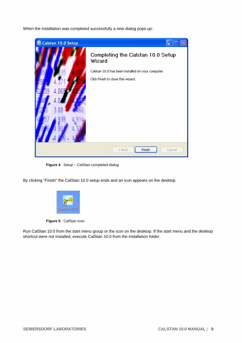
When the installation was completed successfully a new dialog pops up:
Figure 4: Setup – CalStan completed dialog By clicking “Finish” the CalStan 10.0 setup ends and an icon appears on the desktop.
Figure 5: CalStan Icon Run CalStan 10.0 from the start menu group or the icon on the desktop. If the start menu and the desktop shortcut were not installed, execute CalStan 10.0 from the installation folder.
SEIBERSDORF LABORATORIES CALSTAN 10.0 MANUAL | 9

3.2. Update By clicking the “Updates” menu entry an online updater application starts. This serves for keeping CalStan up to date. If an internet connection is available, the updater checks our remote server for newer versions of software components. This way the user can install new measurement types, new device drivers and get latest bug fixes. It is also possible to remove already installed components. Using the “Show components” combo box at top of the window, a list of all installed components can be shown (Figure 6) by choosing “All”.
Figure 6: Online application updater, showing all components By clicking the “Update” button, an update process starts (Figure 7). Before starting update, the CalStan application has to be closed manually. When the pop down menu in the “Action” column is opened a combo box with possible actions is shown: No change / Remove / Update. After the update is finished successfully CalStan is restarted automatically.
| CALSTAN 10.0 MANUAL SEIBERSDORF LABORATORIES 10
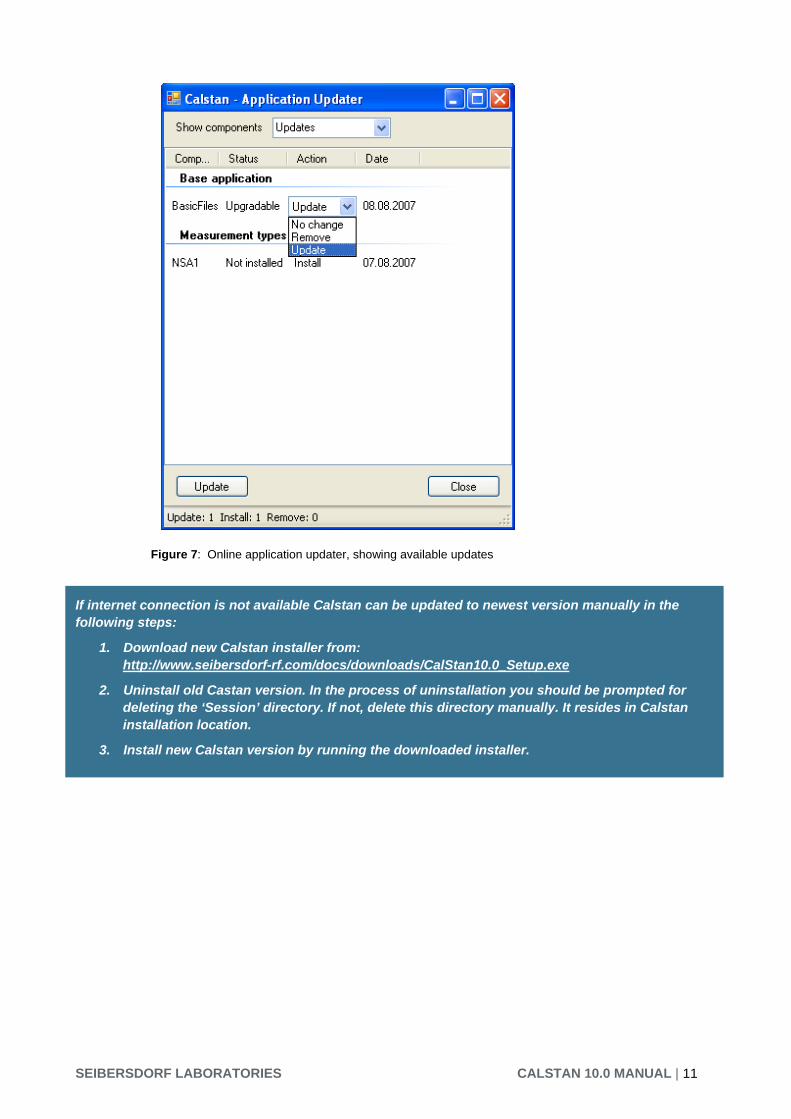
Figure 7: Online application updater, showing available updates
If internet connection is not available Calstan can be updated to newest version manually in the following steps:
1. Download new Calstan installer from: http://www.seibersdorf-rf.com/docs/downloads/CalStan10.0_Setup.exe
2. Uninstall old Castan version. In the process of uninstallation you should be prompted for deleting the ‘Session’ directory. If not, delete this directory manually. It resides in Calstan installation location.
3. Install new Calstan version by running the downloaded installer.
SEIBERSDORF LABORATORIES CALSTAN 10.0 MANUAL | 11

4. QUICK START In this chapter the typical steps to start a measurement campaign are described. Some measurement type may be more complex - but the basic procedure does not change.
1. To start a new measurement, choose the "File->New…" and select the desired measurement type.
2. Modify the parameters in the “Measurement settings” panel (in the bottom left part of the screen). Most common ones are the frequency range, frequency step and limit. If needed load some factor files (e.g. Dual Antenna Factor) or set the protective attenuator for use with special signal generator types (e.g. RefRad system).
3. Set your measurement devices and their parameters in the set of panels right of the “Measurement settings”. This may differ as specific measurement types use different device classes (Transmitters, Receivers, Masts, and Turntables). Most important of all is to set the right IEC address of the GPIB device, otherwise is not possible to connect to the instrument. To detect devices and their addresses automatically, go to “Hardware” menu and choose “Detect Devices”. If possible CalStan sets the proper device driver for connected devices, if not you have to choose driver manually from the driver list.
4. Run the measurement by clicking the “Start” button (lower left corner of the start measurement panel on the right side of the screen). If some settings are incorrect the software shows an info message with instructions.
5. To save the measurement go to “File->Save”.
| CALSTAN 10.0 MANUAL SEIBERSDORF LABORATORIES 12

5. CALSTAN 10.0 WORKSPACE The CalStan 10.0 main window (Figure 8) consists of three main parts:
A) Menu bar – shows main menu related to a currently opened measurement B) Measurement list bar – contains a list of currently opened measurements C) Measurement window – represents the currently opened (active) measurement
Figure 8: CalStan main window The measurement window can be divided into four sub areas:
1. Measurement display – shows the measurement data in a chart 2. Measurement settings – contain all measurement settings 3. Hardware settings – contain all device settings 4. Measurement control panel with the “Start” button – controls the measurement procedure 5. Chart legend – shows the legend of all measured traces
SEIBERSDORF LABORATORIES CALSTAN 10.0 MANUAL | 13

By clicking the button By clicking the button or , selected parts of the window can be maximized/minimized (Figure 9). Individual panels can also be maximized/minimized using the keyboard shortcuts: <Ctrl + Shift + L> for chart legend, <Ctrl + Shift + M> for measurement control panel and <Ctrl + Shift + S> for panel which contains the measurement and hardware settings.
Figure 9: Measurement window with measurement settings, hardware settings and chart legend panel minimized.
| CALSTAN 10.0 MANUAL SEIBERSDORF LABORATORIES 14

6. MENU BAR The menu bar is located at the top of the main window. It contains several menus which are described in the following. 6.1. File Menu Figure 10: The file menu
New Creates a new measurement.
Open Opens a previously saved measurement.
Save (disabled in demo mode)
Saves a measurement. The default file extension of the CalStan 10.0 measurement files is “.cmf”.
Save As (disabled in demo mode)
Saves a measurement with a user defined file name into an individual directory. The default file extension of the CalStan 10.0 measurement files is “.cmf”.
Import Imports a measurement from the previous, today’s obsolete version of CalStan v4.1. An extension of the imported file is not strictly specified. As the import function is measurement type specific, it is always related to the active measurement.
Exit Closes the CalStan software. User is asked if to save changes made to opened measurements or not. If changes are discarded measurement is closed automatically. If changes are saved or there were no changes made recently in opened measurements, Calstan exists and at the next startup all saved measurements are reloaded.
Table 2: File menu
SEIBERSDORF LABORATORIES CALSTAN 10.0 MANUAL | 15

6.2. Measurement Menu 6.2. Measurement Menu The measurement menu contains general options related to the active measurement. The measurement menu contains general options related to the active measurement.
Figure 11: The measurement menu Figure 11: The measurement menu
Measurement Info Opens a collection of general measurement information (Figure 12) in a dialog box. Some of the parameters are editable; others are locked as they are overtaken from measurement and hardware settings, indicated with the lock symbol.
Figure 12: Measurement info dialog box
Recalculate Results Recalculates the results of an active measurement. Results can be recalculated only if certain measurement specific conditions are fulfilled.
Unlock Settings Unlocks both the measurement and hardware setting.
Table 3: Measurement menu
| CALSTAN 10.0 MANUAL SEIBERSDORF LABORATORIES 16

6.3. Hardware Menu The hardware menu contains general options related to measurement devices used by CalStan. Figure 13: Hardware menu
Detect Devices Detects GPIB measurement instruments connected to the computer. If a detection procedure is successful, a dialog box with a list of devices pops up, showing information about device manufacturer, model and communication interface. After closing the device detection dialog box, the appropriate device drivers are selected in the hardware settings panel.
Table 4: Hardware menu 6.4. Tools Menu The tools menu contains various options applicable to an active measurement. Figure 14: Tools menu
Create Report (disabled in demo mode)
Creates the measurement report according to the active measurement procedure. The report is saved in MS Excel file format, in a user defined directory. In general the report contains measured data as well as computed results together with all settings used during the measurement. See specific measurement procedure for further details.
Export Height Scan Data
Saves the heights scan sweeps data in MS Excel file format. This function is available only in the measurement types which includes height scan.
Table 5: Tools menu
SEIBERSDORF LABORATORIES CALSTAN 10.0 MANUAL | 17

6.5. Settings Menu Overall application settings can be set in this menu. Figure 15: Settings menu
Language The program language can be selected; currently only English and German are available. English is the default language.
Table 6: Settings menu 6.6. Help Menu The help menu contains software related information, such as access to the manual and a list of installed components. From this menu is also possible to run the online updater. Figure 16: Help menu
| CALSTAN 10.0 MANUAL SEIBERSDORF LABORATORIES 18

Manual Opens the CalStan manual which is stored in pdf format (Adobe Acrobat Reader or other pdf reader application is needed).
Updates Software updates can be downloaded (see chapter 3.2).
Register Opens the registration form which is used for Calstan registration. By registering you provide us with your email address and Calstan version, so we can inform you about important updates.
Report Error If you encounter problem with our software, by this item you can generate special report file. Send us this file together with your problem description and we will provide you with our support.
Remote Support If problem occurs with a measurement performed by Calstan, we can provide you with online support directly at your computer running the measurement. All you need is the internet connection and if the “Ready to connect” icon appears at the bottom of the quick support dialog (Figure 17), by sending us the ID and Password you allow us to remotely control your computer and to examine the problem directly. This is necessary if there is some specific device error, which can’t be reproduced at our side. Figure 17: Quick support dialog for remote control
SEIBERSDORF LABORATORIES CALSTAN 10.0 MANUAL | 19

About Opens a dialog box which shows various information about the installed CalStan software including program version and a list of the installed measurements and device drivers (Figure 18). It also contains version changes history (Change Log) and system information.
Figure 18: Dialog boxes in the About dialog
Table 7: Help menu
| CALSTAN 10.0 MANUAL SEIBERSDORF LABORATORIES 20

7. CALSTAN 10.0 SETTINGS This section describes parameters used in most measurement procedures. 7.1. Measurement Settings The measurement setting panel is located in the lower left corner of the measurement window (Figure 9). It contains all measurement specific parameters such as frequency range or frequency steps and others. For measurements which involves height scan, the Height Receive Antenna parameters defines the mast movement. The start/stop heights and movement type (discrete or continuous). The height scan can be also disabled by setting the “Heightscan” parameter to “No”.
Figure 19: Measurement settings panel, for e.g. Site VSWR measurement
7.1.1. Frequency Step Measurements with CalStan 10.0 are done at discrete frequencies (frequency steps). The discrete measured points are displayed as a line plot in the measurement display window. Measurement results are only correct if the frequency resolution is high enough to cover any 'peaks' or 'resonances' within the measurement range. These frequency steps are defined in the “Frequency Step” dialog box which can be opened by clicking the folder icon in the related row of the measurement settings panel. In the “Frequency Step” dialog box (Figure 20) the frequency resolution of several frequency bands can be defined individually. The frequency bands must not overlap. Open the frequency step dialog box by clicking on the folder symbol. In the pop up window frequency steps can be edited, additional frequency steps can be inserted or existing ones deleted by right mouse click.
SEIBERSDORF LABORATORIES CALSTAN 10.0 MANUAL | 21

Figure 20: The „Frequency Step“ dialog The frequency steps can be loaded from or saved to a file using the “Open” and “Save” buttons. The frequency steps are classified as an interval dependent parameter; the “.par” file extension is used for this file type. The default frequency steps are recommended for most of the measurement procedures and can be restored by clicking the “Default” button.
7.1.2. Limit To determine if the measurement results fulfill a particular tolerance, limit boundaries are defined for specific frequency intervals. These intervals are specified in the “Limit” dialog box (Figure 21) which can be opened by clicking the folder icon in the related row of the measurement settings panel. When displaying the result chart, the limit data are displayed too. Figure 22 shows the situation when measurement results are not within the specified limit interval.
Figure 21: The „Limit“ dialog box
| CALSTAN 10.0 MANUAL SEIBERSDORF LABORATORIES 22

Figure 22: The limit boundaries in the measurement result chart
7.1.3. Factor files Some measurement types require various factor files to be set their measurement settings. This involves cable loss factor, transmit/receive antenna factors, dual antenna factors and others. By clicking the folder button in the measurement settings panel at the certain factor file parameter, factors file dialog pops up (see Figure 23). This dialog contains three tab pages:
1. Info page – displays description of the given factor measurement (see Figure 23) 2. Data page – shows factor data (see Figure 24) 3. Chart page – here the factor data chart is drawn (see Figure 25)
Figure 23: Factor file dialog – Info tab
SEIBERSDORF LABORATORIES CALSTAN 10.0 MANUAL | 23

At the bottom of the dialog the factor data from a CalStan 10.0 native format can be loaded by clicking the Open... button
Figure 24: Factor file dialog – Data tab Important! The combo box located above the Ok and Cancel buttons is used for setting of the proper results column which is intended to be used for results calculation later. This combo box is shown only if the distinction among more results contained in the factor data have to be made.
Figure 25: Factor file dialog – Chart tab
| CALSTAN 10.0 MANUAL SEIBERSDORF LABORATORIES 24

Another option is to import factor data from a text file. In the Info tab page the factor measurement description can be filled to available fields. Then switching to Data page and clicking the Import button a text file with “.data” file extension containing the physically measured values can be loaded. This can be for example tab-separated file exported from MS Excel spreadsheet (File->Save As... – Data Type = Tab-Separated values file).The exact format of the “.data” file is shown in separate dialog (Figure 26) if Help button is pressed.
Figure 26: Help dialog – Cable loss import file format. Factor file imported this way can be then saved in the Calstan 10 native format to make loading more convenient if needed next time. 7.2. Hardware Parameters The selection of measurement instruments and instrument settings is done in the respective hardware parameter dialogues. Every measurement type uses specific set of hardware. E.g. for Site VSWR procedure a transmitter, receiver, and optionally positioner is needed. NSA measurement above ground plane incorporates transmitter, receiver and antenna mast. If some of the devices are set to [None], then the device is not used in measurement procedure. In the case of NSA SAC it means, no height scan is performed. The parameters of the different measurement devices depend on the capabilities of the instrument. Network analyzers can be chosen in the receiver category. Choosing one automatically sets the transmitter type to [None] and it is not possible to set another transmitter unless the receiver is changed to a spectrum analyzer or test receiver.
SEIBERSDORF LABORATORIES CALSTAN 10.0 MANUAL | 25

7.2.1. Instrument Parameters The instrument parameters itself are explained on the example of a receiver. Figure 27: The hardware panel – device settings for Demo-Receiver To setup measurement device parameters in general, the panel displayed in Figure 27 is used (for every device type e.g. receiver, transmitter, etc. a panel exists). At the top of this panel a drop down list exists where the specific device can be selected. For illustration purposes the “Demo” receiver driver was used. The “Parameters” section of this table stores parameters which can be edited by clicking the value cells. The editing style of each parameter depends on its definition in the device driver which reflects capabilities of the device. For example some parameters are restricted to a certain list of values, which the drop down list represents. If a parameter has a range of valid values defined the entered value is checked. By holding the mouse cursor over the value the range of values is shown in a small tool tip (Figure 27). A value can be entered with a unit specification (e.g. kHz) otherwise the unit shown in the title is assumed. To communicate with an instrument the address parameter has to be set correctly. In case of GPIB devices, the IEC address is detected automatically if “Detect GPIB devices” from Hardware menu is used (see 6.3). For instruments connected via other interfaces (R232, Ethernet) the address have to be set manually. The “Device Info” of the hardware panel contains general information about the device such as manufacturer name, model type, frequency range etc. These values have only informative character and can not be edited as indicated by the small lock icon at end of the row. Important! Unit of the measured data values depend on the receiver hardware settings. If a receiver or spectrum analyzer is used the units are dBm. In the case of Network Analyzer data units depends on S-parameter. Setting it to S11/S22 read out data has no unit on the other hand S12/S21 configuration produces output in dB.
| CALSTAN 10.0 MANUAL SEIBERSDORF LABORATORIES 26

Some parameters can be set to the special parameter file (e.g. “Transmitter Parameters” or “Receiver Parameters”). This means that the parameter is frequency dependent and its value is set individually for specific frequency intervals via the parameter file (table). The parameter file can be accessed by clicking the yellow folder button located in the lower right corner of the panel (Figure 27).
Figure 28: Device parameter file dialog box. The parameter file (Figure 28) only contains the columns for parameters which are set to the “Parameter File” value. New rows can be inserted into the table via context menu “Insert” function. The list of values can be seen by holding the mouse cursor over the specific cell. Values can be entered with or without unit. If no unit is specified, the default unit is used, as listed in the column header.
SEIBERSDORF LABORATORIES CALSTAN 10.0 MANUAL | 27

8. STARTING THE MEASUREMENT Every measurement type contains the measurement control panel where the measurement configuration is set and the measurement is started from. For the sake of completeness all features of the measurement control panel are described in this chapter. As an example the panel from a Site VSWR measurement is shown. The layout is divided into two tabs. The “Positions” tab (Figure 29) in the upper part shows a table with a list of measurement positions. Its columns have the following meanings: 1. The name of the position - when clicked, the position is set active and is drawn in a bold line in the
chart. 2. The check box - indicator if the position’s data are displayed in the chart. 3. The finish status of the position – green hook means finished, orange circle marks partially finished
measurement and red cross means not finished at all.
Figure 29: Measurement control panel - Positions view
| CALSTAN 10.0 MANUAL SEIBERSDORF LABORATORIES 28

In the lower part of the “Positions” tab a graphic shows the layout of a currently active position (the “Layout” tab). With the radio buttons “Antenna left” and “Antenna right” the picture can be adjusted to show the antenna positioned left/right equal to the measurement set up. In the “Selection” tab (Figure 30) appropriate check boxes can be used for convenient selecting/deselecting specific measurement positions. This panel can also be accessed via context menu of the positions table.
Figure 30: A selection filter. The “Traces” tab (Figure 31) includes a table with a list of measurements finished at the active position. The columns have the following meaning: 1. Trace number 2. Comment – short text describing the measurement (user defined; after a second measurement of the
same measurement point, the input of a comment is requested) 3. Indicator (green dot) which trace is considered as the final (used for results computation – in some
measurement types whole results are recalculated if this is changed). To set a specific trace active use the context menu “Set as active” function.
SEIBERSDORF LABORATORIES CALSTAN 10.0 MANUAL | 29

Figure 31: Measurement control panel - Traces view By clicking the “Start” button of the measurement control panel the measurement procedure starts. If the demo receiver driver is used, a small dialog box pops up (Figure 32) and a mean value together with a deviation can be set. Then, the demo receiver driver generates a random data set with specified characteristics.
Figure 32: Demo measurement parameters If the measurement is started for the first time, the devices are initialized and a calibration dialog box appears (Figure 33).
Figure 33: Devices calibration dialog box.
| CALSTAN 10.0 MANUAL SEIBERSDORF LABORATORIES 30

At this point some manual settings on devices can be done before the measurement is started. After the “Ok” button is pressed the measurement starts immediately. The devices are initialized only once at the first start of current measurement. If you want to force re-initialization of a selected device due to a change of a parameter before next start, the “Force Ini” parameter has to be set to “Yes”. Changed parameters will then be sent to the devices. During the measurement the “Start” button is replaced by a “Stop” button. A progress bar is updated while the measurement is running. At the same time the measurement chart area is changed to the monitor display, which shows measurement data as they are read from the devices. At the very bottom of the measurement control panel a status panel indicates the number of already finished measurement positions to the total number of position to be measured.
Figure 34: Measurement progress bar To stop the measurements click the “Stop” button. The suspend measurement dialog box pops up (Figure 35) and all devices stop immediately. There are several options how to proceed further: 1. Stop the measurement and discard the data measured so far (since the start button was pressed).
Click the “Stop” button for this option. 2. Stop the measurement and preserve the data measured so far. Click the “Accept” button for this
option. 3. Resume the measurement – continues the measurement from the stop position. Click the “Resume”
button for this option.
Figure 35: Suspended measurement dialog box. During the measurement the data is displayed in the “Monitor” tab of the “Measurement display”. An acoustical signal indicates the end of the measurement.
SEIBERSDORF LABORATORIES CALSTAN 10.0 MANUAL | 31

9. RESULTS - MEASUREMENT DATA DISPLAY The results of the measurement are displayed in the ”Measurement display” in the “Results” tab. For the sake of completeness all tabs are described in this chapter. The first tab (“Monitor”) shows the actual measurement data during a measurement progress (Figure 36).
Figure 36: The monitor display (random data). The next tab marked as “Measurement” shows raw measurement data after a measurement is finished (Figure 37).
Figure 37: The measurement display and context menu in the legend tab for color selection.
| CALSTAN 10.0 MANUAL SEIBERSDORF LABORATORIES 32

Figure 38: The results display with data tab selected (random data) The “SiteVSWR” tab ( Figure 38) shows the calculated results for Site VSWR measurement and the specified limit boundaries. Some measurement procedures can have more than one result tab and can display various data. By using the radio buttons at the bottom of the chart area it is possible to switch between linear and logarithmic scale of the domain axis. The right part of the chart area is dedicated to display various data within the chart. The “Legend” tab (Figure 37) contains a list of displayed curves. With mouse right click on this panel a context menu can be accessed to change the color of the selected curves. Curves can be selected individually or a multi selection can be done by holding the “Shift” key. The color code can be randomized (“Random Color”) or selected from a color table which pops up by clicking the “Color…” menu entry. The “Data” tab ( Figure 38) holds a table of values displayed in the chart. The first column always contains the domain axis values (e.g. frequency) and the other column refers to the range axis values of the specific curve. Data from this table can be copied to the clipboard by selecting the appropriate rows/columns (hold “Shift” key for multi selection) and pressing “Ctrl+C” key combination. Then the data can be pasted (“Ctrl+V”) e.g. to MS Excel, for further processing. Additionally the data listed in the table can be sorted according to a specific column by clicking the column header.
SEIBERSDORF LABORATORIES CALSTAN 10.0 MANUAL | 33

10. MEASUREMENT PLUG-INS 10. MEASUREMENT PLUG-INS Different measurement procedures are described in this section. Different measurement procedures are described in this section. 10.1. Site VSWR 10.1. Site VSWR In CISPR 16-1-4 [1] a technique to validate fully anechoic rooms in the frequency range 1 – 18 GHz is described. This method is called Site VSWR. In CISPR 16-1-4 [1] a technique to validate fully anechoic rooms in the frequency range 1 – 18 GHz is described. This method is called Site VSWR. The POD Antenna and the POD Antenna Stand developed by Seibersdorf Laboratories are designed for this purpose. The software CalStan 10.0 controls measurement instruments (e.g. a network analyzer) to run the tests. Not all information required to perform a Site VSWR test is included in this manual but it gives guidance how to use the products.
The POD Antenna and the POD Antenna Stand developed by Seibersdorf Laboratories are designed for this purpose. The software CalStan 10.0 controls measurement instruments (e.g. a network analyzer) to run the tests. Not all information required to perform a Site VSWR test is included in this manual but it gives guidance how to use the products.
d
Measurement axis
Testvolume
F6 to F1
L6 to L1
R6 to R1
Antenna
h1
Top
floor absorbers
h2
a)
b)
max 30 cm
Front (h1)
C6 to C1
Center (C)
Front (h2)
Bottom
Figure 39: Location of test points for Site VSWR Figure 39: Location of test points for Site VSWR a) top view a) top view b) side view b) side view
| CALSTAN 10.0 MANUAL SEIBERSDORF LABORATORIES 34
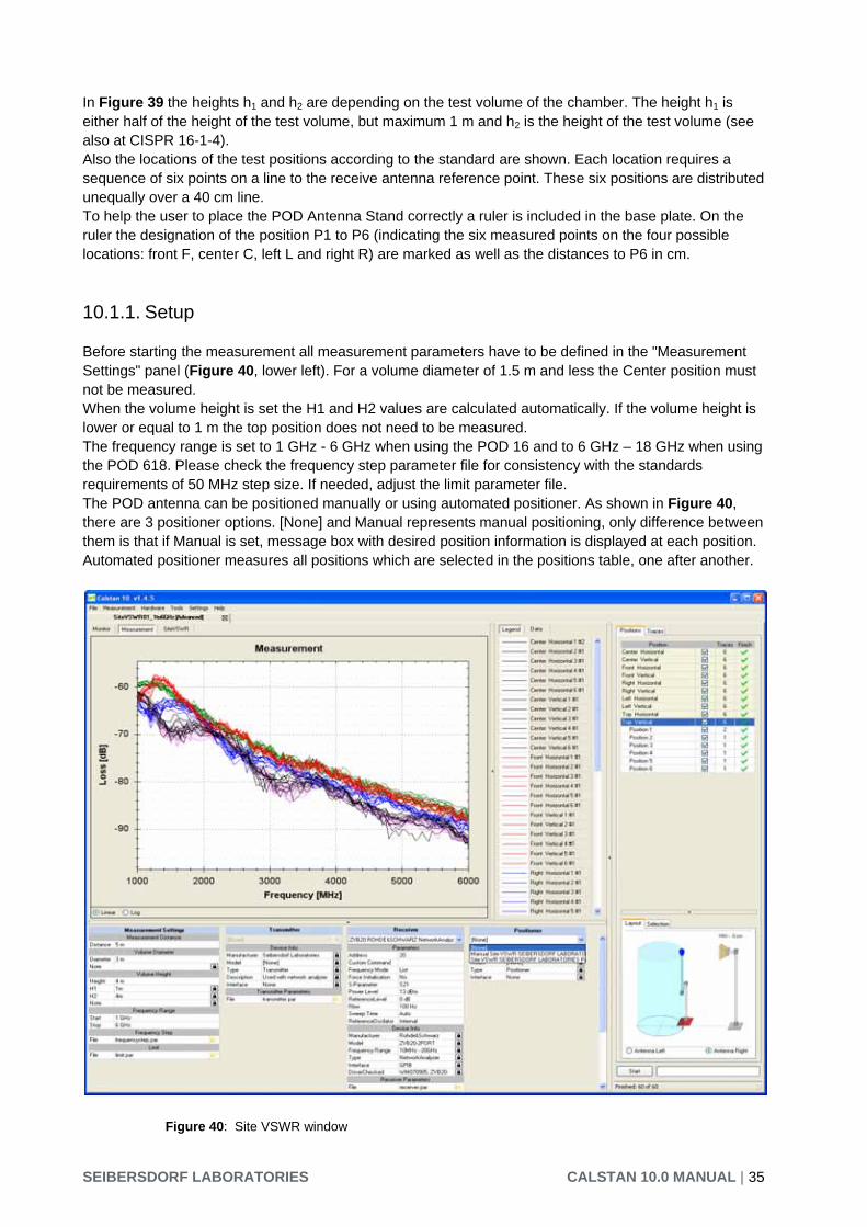
In Figure 39 the heights h1 and h2 are depending on the test volume of the chamber. The height h1 is either half of the height of the test volume, but maximum 1 m and h2 is the height of the test volume (see also at CISPR 16-1-4). Also the locations of the test positions according to the standard are shown. Each location requires a sequence of six points on a line to the receive antenna reference point. These six positions are distributed unequally over a 40 cm line. To help the user to place the POD Antenna Stand correctly a ruler is included in the base plate. On the ruler the designation of the position P1 to P6 (indicating the six measured points on the four possible locations: front F, center C, left L and right R) are marked as well as the distances to P6 in cm.
10.1.1. Setup Before starting the measurement all measurement parameters have to be defined in the "Measurement Settings" panel (Figure 40, lower left). For a volume diameter of 1.5 m and less the Center position must not be measured. When the volume height is set the H1 and H2 values are calculated automatically. If the volume height is lower or equal to 1 m the top position does not need to be measured. The frequency range is set to 1 GHz - 6 GHz when using the POD 16 and to 6 GHz – 18 GHz when using the POD 618. Please check the frequency step parameter file for consistency with the standards requirements of 50 MHz step size. If needed, adjust the limit parameter file. The POD antenna can be positioned manually or using automated positioner. As shown in Figure 40, there are 3 positioner options. [None] and Manual represents manual positioning, only difference between them is that if Manual is set, message box with desired position information is displayed at each position. Automated positioner measures all positions which are selected in the positions table, one after another.
Figure 40: Site VSWR window
SEIBERSDORF LABORATORIES CALSTAN 10.0 MANUAL | 35

10.1.2. Using SPA1 Automatic Site VSWR Positioner
Using the automatic positioner, the measurement procedure can be highly automated. By selecting more positions at once (Figure 41: Selecting multiple positions to be measured automatically) and clicking the start button, the positions are measured one after another as the positioner moves the antenna to appropriate distances. Figure 41: Selecting multiple positions to be measured automatically The specialized tool can be used for controlling the SPA1 positioner (e.g. for moving to the home position). This tool is executed by clicking the yellow icon in the device parameters panel (Figure 42: SPA1 Controller GUI). Figure 42: SPA1 Controller GUI
| CALSTAN 10.0 MANUAL SEIBERSDORF LABORATORIES 36

10.1.3. Measurement Procedure and Result Calculation The measurement campaign of the Site VSWR contains 60 measurements at maximum. Six positions (1-6) are measured at 5 locations (left, right, center, front, top) for 2 polarizations (horizontal, vertical). All six positions are depicted in the start measurement panel as shown in the right part of Figure 40. The results for a specific location e.g. center horizontal (index “A”) are calculated when the last of the appropriate six positions “i” is measured. This means, that if a user decides to re-measure one of the six already finished positions, the result is recalculated. If a user sets different traces of a position active, the result is also recalculated. The result for a specific location with index “A” is computed as follows: VSWR A = max (modifA,1, modifA,2, … , modifA,6) – min (modifA,1, modifA,2, … , modifA,6) where modifA,i = corrA,i + mesA,i with: corrA,6 = 20 * log10((D + 0.00)/D), corrA,5 = 20 * log10((D + 0.02)/D), corrA,4 = 20 * log10((D + 0.10)/D), corrA,3 = 20 * log10((D + 0.18)/D), corrA,2 = 20 * log10((D + 0.30)/D), corrA,1 = 20 * log10((D + 0.40)/D), mesA,i is a measured value at the specific location “A” in position “i” where D = d for front and top location, D = d + r for center location, D = sqrt((d +r )^2 + r^2) – 0.40 for right and left location, where “d” is a distance of the receiver antenna from the volume diameter and “r” is radius of the volume diameter (in meters).
10.1.4. Report Format As described in section 7.4 the measurement output can be exported to a MS Excel format. Figure 43 shows an Excel document containing several worksheets and Table 8 describes the content of the EXCEL file.
Result Data Shows results computed from measured data. First column contains frequency values, while the others hold values for specific measured locations. The column headers are shortened location names (“CH” -> Center Horizontal). As only two locations were measured, only data for Center Horizontal and Front Horizontal positions are present.
Measurement Data Include raw measurement data for every measured position.
SEIBERSDORF LABORATORIES CALSTAN 10.0 MANUAL | 37
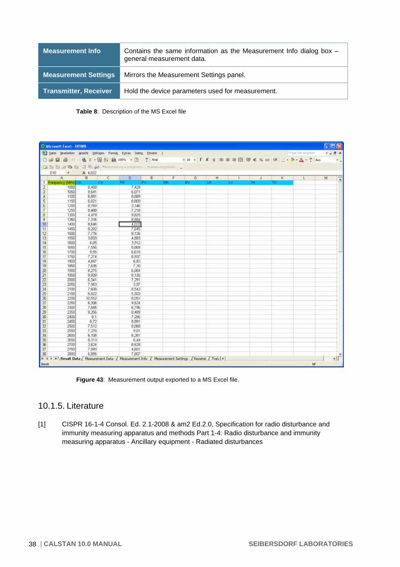
Measurement Info Contains the same information as the Measurement Info dialog box –general measurement data.
Measurement Settings Mirrors the Measurement Settings panel.
Transmitter, Receiver Hold the device parameters used for measurement.
Table 8: Description of the MS Excel file
Figure 43: Measurement output exported to a MS Excel file.
10.1.5. Literature [1] CISPR 16-1-4 Consol. Ed. 2.1-2008 & am2 Ed.2.0, Specification for radio disturbance and
immunity measuring apparatus and methods Part 1-4: Radio disturbance and immunity measuring apparatus - Ancillary equipment - Radiated disturbances
| CALSTAN 10.0 MANUAL SEIBERSDORF LABORATORIES 38

10.2. NSA SAC (Semi-anechoic chambers) 10.2. NSA SAC (Semi-anechoic chambers) Normalized site attenuation (NSA) measurements, in semi-anechoic chambers or on open area test sites, carried out with broadband antennas are implemented in CalStan 10.0 according to following standards: Normalized site attenuation (NSA) measurements, in semi-anechoic chambers or on open area test sites, carried out with broadband antennas are implemented in CalStan 10.0 according to following standards:
ANSI C63.4 ANSI C63.5 CISPR 16-1-4 Site Reference Method Arc Dual Antenna Factor Method
Table 9: List of NSA SAC standards. The measurement procedures described in the different standards are rather similar. Big differences can be found in the definition and application of the antenna factors. For all procedures the "volume method" has to be applied: This means that the transmit antenna connected to the signal generator has to be placed at 5 positions on the turntable. These positions are specified in the referenced documents. Furthermore the transmit antenna has to be operated in two heights and both polarizations. The receive antenna is kept co-polarized at constant horizontal distance and is always facing the transmit antenna. Transmission loss between transmit and receive antenna is measured according to the standard test procedure (height scan of the receiving antenna) for each frequency and polarization.
Figure 44: NSA SAC measurement window.
SEIBERSDORF LABORATORIES CALSTAN 10.0 MANUAL | 39 39

10.2.1. Setup Before starting the measurement all measurement parameters have to be defined in the "Measurement Settings" panel (Figure 44, lower left). 1. First of all, select measurement standard and load appropriate antenna factor file(s) for your transmit
and receive antennas. If the antenna factor is measured with a different frequency step, the data are interpolated (linear). Receive antenna and frequency range settings will be taken from this "antenna factor" file.
2. Choose the frequency range for the NSA measurement. 3. Adjust the frequency step table if needed. 4. Set the desired limit. 5. Set the protective attenuator (used for Vdirect measurement) or select the “none” option (double click
the cell and choose “none” from the drop down list). The protective attenuator value is added to the Vdirect measurement readout of the receiver. The Vdirect measurement value stored in CalStan 10.0 includes already the correction of the protective attenuator value.
6. Select appropriate devices and their parameters. To operate a specific device, the correct IEC (GPIB) address has to be set.
10.2.2. Measurement Procedure and Result Calculation 1. Measure Vdirect first. To do so select the “Direct” position in the positions table (Figure 44). Connect
the generator via the transmit cable and the receive cable to the receiver; two 10 dB attenuators shall be inserted. This configuration ensures that the cable loss of the receive cable is taken into account automatically. If the RefRad is used as generator, the enclosed 30 dB protective attenuator must be used within this measurement.
2. Then Vsite can be measured: Set up the antennas as required by the standard (distance, height, position, polarization). Connect the transmit antenna via one 10 dB attenuator and the transmit cable to the signal
generator. Connect the receive antenna to the other 10 dB attenuator and via the receive cable with the receiver.
Select the position in CalStan 10.0 and start the measurement. During the measurement the monitor display shows three traces:
blue: the ideal measurement data that would obtain zero dB NSA deviation black: the actual measurement data for the current antenna mast height red: the maxhold measurement data
When measuring in vertical polarization, make sure that the cable connected to the antenna does not affect the measured values. For best results we recommend to use a cable with ferrite rings (2 pieces every 10 cm) and the same cable layout of the receive antenna as used during the calibration of the antenna. Especially the distance between antenna and the vertical cable is important.
3. The NSA and the deviations from the NSA (DSA) are calculated automatically after each measured position according to the selected measurement standard (see Table 10). To show the results click the NSA or DSA tab in the chart area. If at least one result is shown, the limit-lines are displayed additionally. The NSA reference values need not to be specified separately. All theoretical factors are computed by CalStan 10.0 using the formulas given in the respective standards.
The results for specific position trace are always computed using the direct measurement trace which was set active at the time of that position trace measurement.
| CALSTAN 10.0 MANUAL SEIBERSDORF LABORATORIES 40

ANSI C63.4 [2] NSA = Vdir – Vsite – AFT – AFR
DSA = Theo - NSA
ANSI C63.5 [3] NSA = Vdir – Vsite – AFT – AFR – GSCF
DSA = Theo - NSA
CISPR 16-1-4 [1] NSA = Vdir – Vsite – AFT – AFR
DSA = Theo - NSA
EN 50147-2 [standard withdrawn] NSA = Vdir – Vsite – AFT – AFR
DSA = Theo - NSA
Site Reference Method [4] DSA = Vdir – Vsite – SAref
Arc Dual Antenna Factor Method [4] NSA = Vdir – Vsite – DAF
DSA = NSA - Theo
where
NSA – normalized site attenuation
DSA – deviation from normalized site attenuation
Theo - theoretical value of the site attenuation
Vdir – direct measurement 3
Vsite – values measured at the site
AFT – transmit antenna factor
AFR – receive antenna factor
GSCF – geometry specific correction factor
SAref – site reference
DAF – dual antenna factor
Table 10: NSA SAC results calculation for specific standards. The "dual antenna factor" represents the sum of the antenna factors of transmit and receive antenna, used with the measurement. It is recommended to use the dual antenna method, where the antenna pair is calibrated.
3 Important: The results are computed according to direct measurement trace that was active during the measurements. It means that you can re-measure the “direct” trace as often as required (e.g. temperature drift compensation) in between the “site” measurements.
SEIBERSDORF LABORATORIES CALSTAN 10.0 MANUAL | 41

10.2.3. Report Format 10.2.3. Report Format As described in section 7.4 the measurement output can be exported in a MS Excel format. In the picture below (Figure 45) you can see an Excel document containing several worksheets. As described in section 7.4 the measurement output can be exported in a MS Excel format. In the picture below (Figure 45) you can see an Excel document containing several worksheets.
Figure 45: Measurement output exported to a MS Excel file Figure 45: Measurement output exported to a MS Excel file
Measurement Info Contains general information about measurement from Measurement Info dialog box
V direct Vdirect measurement data for every measurement position.. When a protective attenuator is selected the attenuation is automatically corrected.
V site Vsite measurement data for every measured position
Transmit antenna factor Transmit antenna factor data for every measurement position. This sheet is present only if one of the measurement standards ANSI C63.4-2003, ANSI C63.5-2006, CISPR 16-1-4 ed.2–2007 or EN 50147-2, 1996 is used.
Receive antenna factor Receive antenna factor data for every measurement position. This sheet is present only if one of the measurement standards ANSI C63.4-2003, ANSI C63.5-2006, CISPR 16-1-4 ed.2–2007 or EN 50147-2, 1996 is used.
Site reference factor Site reference data for every measurement position. This sheet is present only if the Site reference method is used as a measurement standard.
| CALSTAN 10.0 MANUAL SEIBERSDORF LABORATORIES 42

Geometry specific correction factor
Geometry specific correction factor data for every measurement position. This sheet is present only if the ANSI C63.5-2006 is used as a measurement standard.
Dual antenna factor Dual antenna factor data for every measurement position. This sheet is present only if the Arc Dual Antenna Factor method is used as a measurement standard.
AN Measured NSA results computed from Vdirect, Vsite and antenna factor data. For some measurement standards the NSA is not computed, in that case this worksheet is not present.
AN Theoretical Contains theoretically computed data for specific position according to used measurement standard
Deviation DSA values computed as given in Fehler! Verweisquelle konnte nicht gefunden werden.
Limit Upper and lower limit data as set in the limit dialog
Protective Attenuator Protective attenuator data if used
Measurement Settings Measurement Settings panel content
Transmitter, Receiver, Mast
Holds the device parameters used for measurement
Table 11: Description of the MS Excel file
10.2.4. Literature [1] CISPR 16-1-4 Consol. Ed. 2.1-2008 & am2 Ed.2.0, Specification for radio disturbance and
immunity measuring apparatus and methods Part 1-4: Radio disturbance and immunity measuring apparatus - Ancillary equipment - Radiated disturbances
[2] ANSI C63.4-2003, American National Standard for Methods of Measurement of Radio-Noise Emissions from Low-Voltage Electrical and Electronic Equipment in the Range of 9 kHz to 40 GHz
[3] ANSI C63.5-2006, American National Standard Electromagnetic Compatibility–Radiated Emission Measurements in Electromagnetic Interference (EMI) Control–Calibration of Antennas (9 kHz to 40 GHz)
[4] W. Müllner, H. Garn: From NSA to Site-Reference Method for EMC Test Site Validation. IEEE EMC International Symposium, Montreal, Canada, August 13-17, 2001
SEIBERSDORF LABORATORIES CALSTAN 10.0 MANUAL | 43

10.3. NSA FAR (fully-anechoic rooms) 10.3. NSA FAR (fully-anechoic rooms) Normalized site attenuation (NSA) measurements in fully-anechoic chambers, carried out with broadband antennas are implemented in CalStan 10.0 according to following standards: Normalized site attenuation (NSA) measurements in fully-anechoic chambers, carried out with broadband antennas are implemented in CalStan 10.0 according to following standards:
CISPR 16-1-4 (Site reference)
CISPR 16-1-4 (NSA)
ARC Transmission Loss
Table 12: List of NSA FAR standards. Table 12: List of NSA FAR standards. The measurement procedures are described in detail in the standards. For all procedures the "volume method" has to be applied: The transmit antenna connected to the signal generator has to be placed at 5 positions in the test volume. These positions are specified in the referenced documents. Furthermore the transmit antenna has to be operated in two or three heights and both polarizations. The receive antenna is kept co-polarized at constant horizontal distance, is always facing the transmit antenna and sometimes even tilted depending on the chosen procedure. Transmission loss between transmit and receive antenna is measured according to the standard test procedure for each frequency and polarization.
The measurement procedures are described in detail in the standards. For all procedures the "volume method" has to be applied: The transmit antenna connected to the signal generator has to be placed at 5 positions in the test volume. These positions are specified in the referenced documents. Furthermore the transmit antenna has to be operated in two or three heights and both polarizations. The receive antenna is kept co-polarized at constant horizontal distance, is always facing the transmit antenna and sometimes even tilted depending on the chosen procedure. Transmission loss between transmit and receive antenna is measured according to the standard test procedure for each frequency and polarization.
Figure 46: NSA FAR measurement window (randomly generated measurement data). Figure 46: NSA FAR measurement window (randomly generated measurement data).
| CALSTAN 10.0 MANUAL SEIBERSDORF LABORATORIES 44

10.3.1. Setup Before starting the measurement all measurement parameters have to be defined in the "Measurement Settings" panel (Figure 46, lower left). 1. First of all select measurement standard and load appropriate antenna factor file(s) for your transmit
and receive antennas. If the antenna factor is measured with a different frequency step, the data are interpolated (linear). Receive antenna and frequency range settings will be taken from this "antenna factor" file.
2. Choose the frequency range for the NSA measurement. 3. Adjust the frequency step table if needed. 4. Set the desired limit. 5. Set the protective attenuator (used for Vdirect measurement) or select the “none” option (double click
the cell and choose “none” from the drop down list). The protective attenuator value is added to the Vdirect measurement readout of the receiver. The Vdirect measurement value stored in CalStan 10.0 includes already the correction of the protective attenuator value.
6. Select appropriate devices and their parameters. To operate a specific device, the correct IEC (GPIB) address has to be set.
10.3.2. Measurement Procedure and Result Calculation 1. Measure Vdirect first. To do so select the “Direct” position in the positions table (Figure 44). Connect
the generator via the transmit cable and the receive cable to the receiver; two 10 dB attenuators shall be inserted. This configuration ensures that the cable loss of the receive cable is taken into account automatically. If the RefRad is used as generator, the enclosed 30 dB protective attenuator must be used within this measurement.
2. Then Vsite can be measured:
Set up the antennas as required by the standard (distance, height, position, polarization). Connect the transmit antenna via one 10 dB attenuator and the transmit cable to the signal
generator. Connect the receive antenna to the other 10 dB attenuator and via the receive cable with the receiver.
Select the position in CalStan 10.0 and start the measurement. During the measurement the monitor display shows two traces:
blue: the ideal measurement data that would obtain zero dB NSA deviation black: the actual measurement data for the current antenna mast height
When measuring in vertical polarization, make sure that the cable connected to the antenna does not affect the measured values. For best results we recommend to use a cable with ferrite rings (2 pieces every 10 cm) and the same cable layout of the receive antenna as used during the calibration of the antenna. Especially the distance between antenna and the vertical cable is important.
3. The NSA and the deviations from the NSA (DSA) are calculated automatically after each measured position according to the selected measurement standard (see Table 13). To show the results click the NSA or DSA tab in the chart area. If at least one result is shown, the limit-lines are displayed additionally. The NSA reference values need not to be specified separately. All theoretical factors are computed by CalStan 10.0 using the formulas given in the respective standards.
The results for specific position trace are always computed using the direct measurement trace which was set active at the time of that position trace measurement.
SEIBERSDORF LABORATORIES CALSTAN 10.0 MANUAL | 45

CISPR 16-1-4 (Site reference) [1] DSA = SAref – Vdir - Vsite
CISPR 16-1-4 (NSA) [1] NSA = Vdir – Vsite – AFT – AFR DSA = NSA - Theo
ARC Transmission Loss DSA = SAref – Vdir - Vsite Where NSA – normalized site attenuation DSA – deviation from normalized site attenuation Theo - theoretical value of the site attenuation Vdir – direct measurement 4 Vsite – values measured at the site AFT – transmit antenna factor AFR – receive antenna factor SAref – site reference
Table 13: NSA FAR results calculation for specific standards.
10.3.3. Report Format As described in section 7.4 the measurement output can be exported in a MS Excel format. In the picture below (Figure 47) you can see an Excel document containing several worksheets.
Figure 47: Measurement output exported to a MS Excel file
4 Important: The results are computed according to direct measurement trace that was active during the measurements. It means that you can re-measure the “direct” trace as often as required (e.g. temperature drift compensation) in between the “site” measurements.
| CALSTAN 10.0 MANUAL SEIBERSDORF LABORATORIES 46
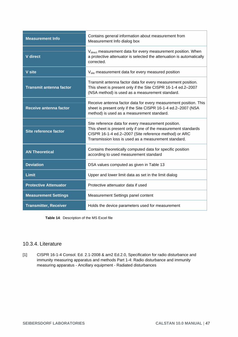
Measurement Info Contains general information about measurement from Measurement Info dialog box
V direct Vdirect measurement data for every measurement position. When a protective attenuator is selected the attenuation is automatically corrected.
V site Vsite measurement data for every measured position
Transmit antenna factor Transmit antenna factor data for every measurement position. This sheet is present only if the Site CISPR 16-1-4 ed.2–2007 (NSA method) is used as a measurement standard.
Receive antenna factor Receive antenna factor data for every measurement position. This sheet is present only if the Site CISPR 16-1-4 ed.2–2007 (NSA method) is used as a measurement standard.
Site reference factor
Site reference data for every measurement position. This sheet is present only if one of the measurement standards CISPR 16-1-4 ed.2–2007 (Site reference method) or ARC Transmission loss is used as a measurement standard.
AN Theoretical Contains theoretically computed data for specific position according to used measurement standard
Deviation DSA values computed as given in Table 13
Limit Upper and lower limit data as set in the limit dialog
Protective Attenuator Protective attenuator data if used
Measurement Settings Measurement Settings panel content
Transmitter, Receiver Holds the device parameters used for measurement
Table 14: Description of the MS Excel file
10.3.4. Literature [1] CISPR 16-1-4 Consol. Ed. 2.1-2008 & am2 Ed.2.0, Specification for radio disturbance and
immunity measuring apparatus and methods Part 1-4: Radio disturbance and immunity measuring apparatus - Ancillary equipment - Radiated disturbances
SEIBERSDORF LABORATORIES CALSTAN 10.0 MANUAL | 47

10.4. Cableloss This plug-in allows the measurement of attenuation of an EUT. The EUT can be a cable, an attenuator or any other coaxial device. By connecting the EUT between transmitter and receiver the attenuation is measured and evaluated with customer specific frequency resolution and range.
Figure 48: Cableloss measurement window.
| CALSTAN 10.0 MANUAL SEIBERSDORF LABORATORIES 48

10.4.1. Setup Before starting the measurement all measurement parameters have to be defined in the "Measurement Settings" panel (Figure 48, lower left). 1. Choose the frequency range. 2. Adjust the frequency step table if needed. 3. Set the protective attenuator (used for Vdirect measurement) or select the “none” option (double click
the cell and choose “none” from the drop down list). Generally the protective attenuator is required for conducted measurements with comb generators to protect the receiver from overload. In case of cable loss measurement with a comb generator it’s advised to use the protective attenuator for measurement of Vdirect and Vcable . In this case do NOT select a protective attenuator file here because it’s present in both measurements and has no effect on the measured attenuation. The protective attenuator value is added to the Vdirect measurement readout of the receiver. The Vdirect measurement value stored in CalStan 10.0 includes already the correction of the protective attenuator value. Vcable measurements are not influenced by the protective attenuator.
4. Select appropriate devices and their parameters. To operate a specific device, the correct IEC (GPIB) address has to be set.
10.4.2. Measurement Procedure and Result Calculation 1. Measure Vdirect. Select the “Direct” position in the positions table (Figure 44). Connect the generator
via the auxiliary cable to the receiver. This configuration ensures that the cable loss of the auxiliary cable is taken into account automatically. If you selected a protective attenuator in the measurement settings dialog you have to connect it now between transmitter and auxiliary cable. The measurement value stored in CalStan 10.0 is the receiver readout plus the protective attenuator value.
2. Measure Vcable: Connect the EUT between the auxiliary cable and the receiver. Make sure to remove the
protective attenuator when selected in the measurement settings. Select the position (e.g. Measurement 1) in CalStan 10.0 and start the measurement. During the measurement the monitor window shows the actual measurement data.
3. After the measurement is finished, results are calculated using the formula:
CL = Vdirect - Vcable where Vdirect – direct measurement value Vcable – measured value
4. At the beginning there are only two positions Direct and Measurement 1. By right mouse click context menu can be displayed and new measurement position added. Measurement position names can be edited by double clicking the name cell.
The results for specific position trace are always computed using the direct measurement trace which was set active at the time of that position trace measurement.
SEIBERSDORF LABORATORIES CALSTAN 10.0 MANUAL | 49

10.4.3. Report Format 10.4.3. Report Format As described in section 7.4 the measurement output can be exported in a MS Excel format. In the picture below (Figure 49) you can see an Excel document containing several worksheets. As described in section 7.4 the measurement output can be exported in a MS Excel format. In the picture below (Figure 49) you can see an Excel document containing several worksheets.
Figure 49: Measurement output exported to a MS Excel file
Figure 49: Measurement output exported to a MS Excel file
Measurement Info Contains general information about measurement from Measurement Info dialog box
V direct Vdirect measurement data for every measurement position. When a protective attenuator is selected the attenuation is corrected automatically.
V cable Vcable measurement data for every measured position
Attenuation Measurement results
Protective Attenuator Protective attenuator data if used
Measurement Settings Measurement Settings panel content
Transmitter, Receiver Holds the device parameters used for measurement
Table 15: Description of the MS Excel file
| CALSTAN 10.0 MANUAL SEIBERSDORF LABORATORIES 50
10.5. Experimental Measurement
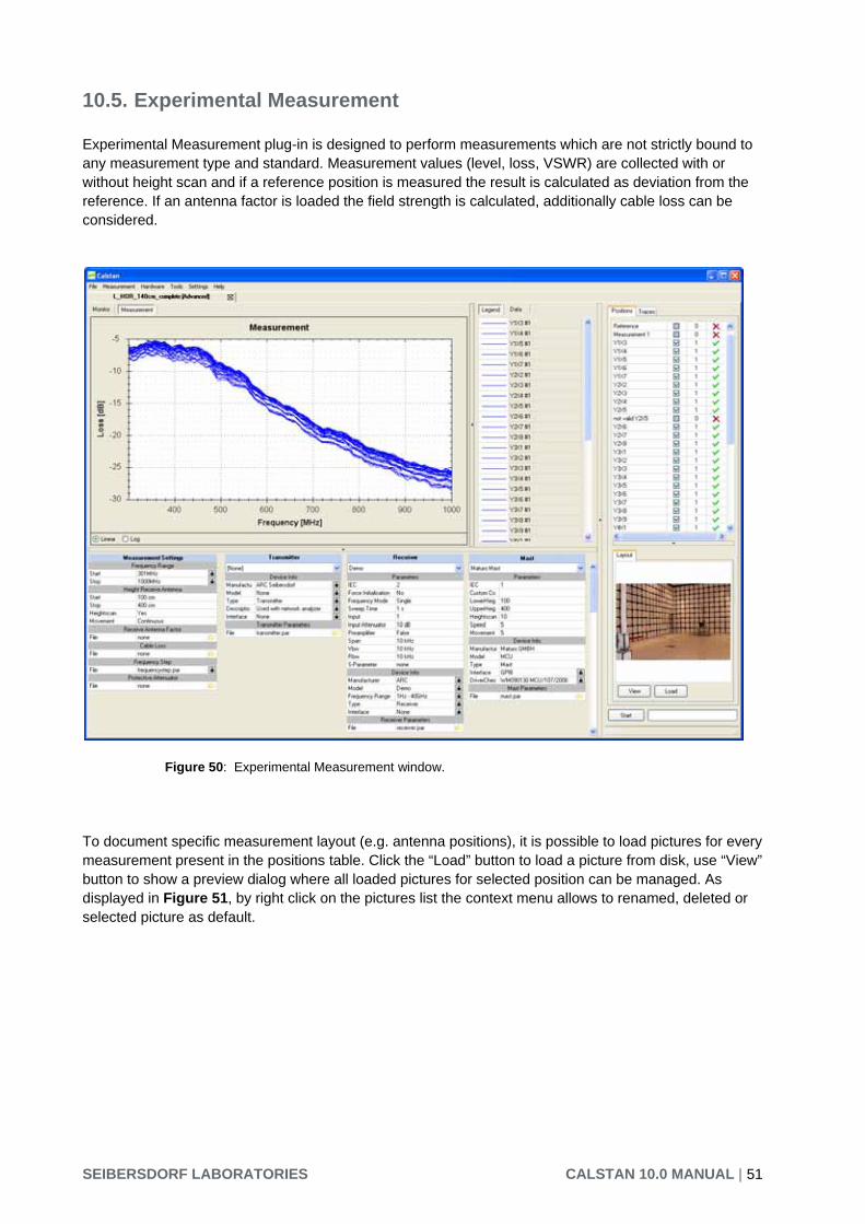
xperimental Measurement plug-in is designed to perform measurements which are not strictly bound to
o document specific measurement layout (e.g. antenna positions), it is possible to load pictures for every easurement present in the positions table. Click the “Load” button to load a picture from disk, use “View”
Eany measurement type and standard. Measurement values (level, loss, VSWR) are collected with or without height scan and if a reference position is measured the result is calculated as deviation from the reference. If an antenna factor is loaded the field strength is calculated, additionally cable loss can be considered.
Figure 50: Experimental Measurement window.
Tmbutton to show a preview dialog where all loaded pictures for selected position can be managed. As displayed in Figure 51, by right click on the pictures list the context menu allows to renamed, deleted or selected picture as default.
SEIBERSDORF LABORATORIES CALSTAN 10.0 MANUAL | 51

Figure 51: Assigning measurement layout picture.
10.5.1. Setup Before starting the measurement following measurement parameters have to be defined in the "Measurement Settings" panel (Figure 50, lower left). 1. Choose the frequency range. 2. Adjust the frequency step table if needed. 3. Set the receive antenna parameters to adjust height scan (see 7.1). 4. Set receiver antenna factor or cable loss factor file. Cable loss measurement performed by CalStan
can be also used here. Don’t forget to select correct result column from the combo box in the data tab as described in 7.1.3
5. Set the protective attenuator (used for Reference measurement only) or select the “none” option (double click the cell and choose “none” from the drop down list). Generally the protective attenuator is required for conducted measurements with comb generators to protect the receiver from overload. The protective attenuator value is added to the Reference measurement readout of the receiver and stored in CalStan 10.0. Other measurements are not influenced by the protective attenuator. See next section for more details.
6. Select appropriate devices and their parameters. To operate a specific device, the correct IEC (GPIB) address has to be set.
| CALSTAN 10.0 MANUAL SEIBERSDORF LABORATORIES 52

10.5.2. Measurement Procedure and Result Calculation In the experimental measurement there are two measurement types possible: 1. The reference measurement – this is represented by the “Reference” position at the top of the
positions table (see Figure 50). This measurement serves as reference according to which the results are computed. Protective attenuator data are added to measured values if their unit is dB or dBm. Unit of the receiver device readout is discussed in 7.2.1
2. The custom measurement – there is more-less unlimited number of measurements which can be performed. By right clicking the positions table and then choosing the “New Measurement” menu item from the pop upped context menu (see Figure 52) new row representing a custom measurement is added at the bottom of the list. Name of the measurement is set to current date by default, but can be changed anytime (context menu -> rename option). No protective attenuator data are added to the measured values.
Figure 52: Adding new measurement in the positions table When measurement is finished results are computed in the following way: 1. If receive antenna factor file is set and measurement data unit is dBm, the field strength is calculated
according to formula:
fs = ySite + 107 + afr + cl;
where: ySite: measured value [dBm]
afr: receive antenna factor value
cl: cable loss factor value (if available)
A “Field strength” chart tab is then added in the charts panel. 2. When custom measurement is finished and reference measurement is available. The difference of
reference measurement and the custom measurement is computed and displayed in separate “Deviation” tab in the charts panel.
The results for specific position trace are always computed using the direct measurement trace which was set active at the time of that position trace measurement.
SEIBERSDORF LABORATORIES CALSTAN 10.0 MANUAL | 53

10.5.3 Report Format As described in section 7.4 the measurement output can be exported in a MS Excel format. In the picture below (Figure 53) you can see an Excel document containing several worksheets.
Figure 53: Measurement output exported to a MS Excel file
| CALSTAN 10.0 MANUAL SEIBERSDORF LABORATORIES 54

Measurement Info Contains general information about measurement from Measurement Info dialog box
Measurements Measured data
Field Strength Computed field strength
Deviation Measurement results
Receive Antenna Factor* Receive antenna factor data
Cable loss* Cable loss data
Protective Attenuator* Protective attenuator data
Measurement Settings Measurement Settings panel content
Transmitter, Receiver, Mast Holds the device parameters used for measurement
* worksheets are added only if factor files are used
Table 16: Description of the MS Excel file
SEIBERSDORF LABORATORIES CALSTAN 10.0 MANUAL | 55

11. TROUBLESHOOTING 11.1. Device is detected as UNKNOWN although it supports *IDN?
Query. Possible reasons:
a) device responds with incompatible string. Correct string format is e.g. Rohde&Schwarz,ESU-40,100031/040,4.23 (manufacturer, model, serial number, firmware version)
b) device responds too slowly. In this case device has to be selected manually from the drivers list.
11.2. Measurement fails with error message "error -420: Query
unterminated INIT*OPC" Disable serial auto polling in the GPIB card properties
Figure 54: Disabling Serial Polling in the GPIB card configuration
11.3. Measurement fails with error message "error -108: Parameter not
allowed” This can be decimal separator problem in the device driver, try to change you regional settings to use “.” As decimal and “ ” as thousands separator. Please let us know about this problem.
| CALSTAN 10.0 MANUAL SEIBERSDORF LABORATORIES 56

12. FIGURES Figure 1: Setup – Welcome dialog.............................................................................................................. 7 Figure 2: Setup - Component selection dialog ........................................................................................... 8 Figure 3: Setup – Installation directory selection dialog ............................................................................. 8 Figure 4: Setup – CalStan completed dialog .............................................................................................. 9 Figure 5: CalStan Icon ................................................................................................................................ 9 Figure 6: Online application updater, showing all components ................................................................ 10 Figure 7: Online application updater, showing available updates ............................................................ 11 Figure 8: CalStan main window ................................................................................................................ 13 Figure 9: Measurement window with measurement settings, hardware settings and chart legend......... 14 Figure 10: The file menu........................................................................................................................... 15 Figure 11: The measurement menu ......................................................................................................... 16 Figure 12: Measurement info dialog box ................................................................................................... 16 Figure 13: Hardware menu ....................................................................................................................... 17 Figure 14: Tools menu.............................................................................................................................. 17 Figure 15: Settings menu.......................................................................................................................... 18 Figure 16: Help menu ............................................................................................................................... 18 Figure 17: Quick support dialog for remote control ................................................................................... 19 Figure 18: Dialog boxes in the About dialog.............................................................................................. 20 Figure 19: Measurement settings panel, for e.g. Site VSWR measurement............................................ 21 Figure 20: The „Frequency Step“ dialog................................................................................................... 22 Figure 21: The „Limit“ dialog box .............................................................................................................. 22 Figure 22: The limit boundaries in the measurement result chart ............................................................ 23 Figure 23: Factor file dialog – Info tab ...................................................................................................... 23 Figure 24: Factor file dialog – Data tab..................................................................................................... 24 Figure 25: Factor file dialog – Chart tab ................................................................................................... 24 Figure 26: Help dialog – Cable loss import file format.............................................................................. 25 Figure 27: The hardware panel – device settings for Demo-Receiver ..................................................... 26 Figure 28: Device parameter file dialog box. ............................................................................................ 27 Figure 29: Measurement control panel - Positions view........................................................................... 28 Figure 30: A selection filter. ...................................................................................................................... 29 Figure 31: Measurement control panel - Traces view .............................................................................. 30 Figure 32: Demo measurement parameters............................................................................................. 30 Figure 33: Devices calibration dialog box. ................................................................................................ 30 Figure 34: Measurement progress bar ..................................................................................................... 31 Figure 35: Suspended measurement dialog box...................................................................................... 31 Figure 36: The monitor display (random data). ........................................................................................ 32 Figure 37: The measurement display and context menu in the legend tab for color selection. ............... 32 Figure 38: The results display with data tab selected (random data)....................................................... 33 Figure 39: Location of test points for Site VSWR .................................................................................... 34 Figure 40: Site VSWR window.................................................................................................................. 35 Figure 41: Selecting multiple positions to be measured automatically..................................................... 36 Figure 42: SPA1 Controller GUI ............................................................................................................... 36 Figure 43: Measurement output exported to a MS Excel file. .................................................................. 38 Figure 44: NSA SAC measurement window............................................................................................. 39 Figure 45: Measurement output exported to a MS Excel file.................................................................... 42 Figure 46: NSA FAR measurement window (randomly generated measurement data). ......................... 44 Figure 47: Measurement output exported to a MS Excel file.................................................................... 46 Figure 48: Cableloss measurement window............................................................................................. 48 Figure 49: Measurement output exported to a MS Excel file.................................................................... 50 Figure 50: Experimental Measurement window. ...................................................................................... 51 Figure 51: Assigning measurement layout picture. .................................................................................. 52 Figure 52: Adding new measurement in the positions table..................................................................... 53
SEIBERSDORF LABORATORIES CALSTAN 10.0 MANUAL | 57

Figure 53: Measurement output exported to a MS Excel file.................................................................... 54 Figure 54: Disabling Serial Polling in the GPIB card configuration ........................................................... 56
13. TABLES Table 1: System Requirements................................................................................................................... 6 Table 2: File menu..................................................................................................................................... 15 Table 3: Measurement menu .................................................................................................................... 16 Table 4: Hardware menu .................................................................................................................... 17 Table 5: Tools menu.................................................................................................................................. 17 Table 6: Settings menu ............................................................................................................................. 18 Table 7: Help menu................................................................................................................................... 20 Table 8: Description of the MS Excel file .................................................................................................. 38 Table 9: List of NSA SAC standards. ........................................................................................................ 39 Table 10: NSA SAC results calculation for specific standards. ................................................................ 41 Table 11: Description of the MS Excel file ................................................................................................ 43 Table 12: List of NSA FAR standards. ...................................................................................................... 44 Table 13: NSA FAR results calculation for specific standards.................................................................. 46 Table 14: Description of the MS Excel file ................................................................................................ 47 Table 15: Description of the MS Excel file ................................................................................................ 50 Table 16: Description of the MS Excel file ................................................................................................ 55
| CALSTAN 10.0 MANUAL SEIBERSDORF LABORATORIES 58

ANNEX I. WARRANTY Seibersdorf Labor GmbH, hereinafter referred to as the Seller, warrants that standard Seibersdorf Laboratories products are free from defect in materials and workmanship for a period of two (2) years from the date of shipment. Standard Seibersdorf Laboratories products include the following: Antennas Cables Reference Radiators Software Antenna stands and positioners If the Buyer notifies the Seller of a defect within the warranty period, the Seller will, at the Seller’s option, either repair and/or replace products which prove to be defective during the warranty period. There will be no charge for warranty services performed at the location the Seller designates. The Buyer must, however, prepay inbound shipping costs and any duties or taxes. The Seller will pay outbound shipping cost for a carrier of the Seller’s choice, exclusive of any duties or taxes. This warranty does not apply to: Normal wear and tear of materials Consumable items such as fuses, batteries, etc. Products that have been improperly installed, maintained or used Products which have been operated outside the specifications Products which have been modified without authorization Calibration of products, unless necessitated by defects THIS WARRANTY IS EXCLUSIVE. NO OTHER WARRANTY, WRITTEN OR ORAL, IS EXPRESSED OR IMPLIED, INCLUDING BUT NOT LIMITED TO, THE IMPLIED WARRANTIES OF MERCHANTABILITY AND FITNESS FOR A PARTICULAR PURPOSE. THE REMEDIES PROVIDED BY THIS WARRANTY ARE THE BUYER’S SOLE AND EXCLUSIVE REMEDIES. IN NO EVENT IS THE SELLER LIABLE FOR ANY DAMAGES WHATSOEVER, INCLUDING BUT NOT LIMITED TO, DIRECT, INDIRECT, SPECIAL, INCIDENTAL, OR CONSEQUENTIAL DAMAGES, WHETHER BASED ON CONTRACT, TORT, OR ANY OTHER LEGAL THEORY.
SEIBERSDORF LABORATORIES CALSTAN 10.0 MANUAL | 59