
Embedded System Design || Modeling
63
Chapter 3 MODELING At the core of any design methodology are models at various steps of the flow. Models provide an abstract view of the design at any given time, representing certain aspects of reality while hiding others that are not relevant or not yet known. As such, design models at each level of abstraction provide the basis for applying analysis, synthesis or verification techniques. However, as discussed in previous chapters, tools for automation of these design processes beyond simulation can only be applied if models and corresponding abstraction levels are well-defined with clear and unambiguous semantics. In doing so, modeling concepts and techniques can have a large influence on the quality, accuracy and rapidity of results. Hence, modeling is concerned with defining the level and organization of detail to be represented, i.e., the objects, composition rules and, eventually, transformations, such that meaningful observations can be made, desired requirements are explicitly specified, and design automation tools can be applied. As explained in previous chapters, system behavior is generally described as a set of concurrent, hierarchical processes that operate on and exchange data via variables and channels. On the other hand, a system platform consists of a set of system components connected by a network of busses. Components in a platform realize system behavior by executing processes, storing variables and sending messages over channels. Hence, various components provide differ- ent aspects of system computation and communication, whether in software, hardware, or in a combination of both. In system modeling, we therefore need to develop models at varying levels of detail. Furthermore, we have to define models for each component as well as for the whole system. As discussed previously, different models are needed at different steps in the design process. There are abstract system models for application designers who must develop algorithms and verify that they will work correctly on the © Springer Science + Business Media, LLC 2009 D.D. Gajski et al., Embedded System Design: Modeling, Synthesis and Verification, DOI: 10.1007/978-1-4419-0504-8_3, 49
Transcript of Embedded System Design || Modeling

Chapter 3
MODELING
At the core of any design methodology are models at various steps of the flow.Models provide an abstract view of the design at any given time, representingcertain aspects of reality while hiding others that are not relevant or not yetknown. As such, design models at each level of abstraction provide the basis forapplying analysis, synthesis or verification techniques. However, as discussedin previous chapters, tools for automation of these design processes beyondsimulation can only be applied if models and corresponding abstraction levelsare well-defined with clear and unambiguous semantics. In doing so, modelingconcepts and techniques can have a large influence on the quality, accuracy andrapidity of results. Hence, modeling is concerned with defining the level andorganization of detail to be represented, i.e., the objects, composition rules and,eventually, transformations, such that meaningful observations can be made,desired requirements are explicitly specified, and design automation tools canbe applied.
As explained in previous chapters, system behavior is generally describedas a set of concurrent, hierarchical processes that operate on and exchange datavia variables and channels. On the other hand, a system platform consists of aset of system components connected by a network of busses. Components in aplatform realize system behavior by executing processes, storing variables andsending messages over channels. Hence, various components provide differ-ent aspects of system computation and communication, whether in software,hardware, or in a combination of both. In system modeling, we therefore needto develop models at varying levels of detail. Furthermore, we have to definemodels for each component as well as for the whole system.
As discussed previously, different models are needed at different steps inthe design process. There are abstract system models for application designerswho must develop algorithms and verify that they will work correctly on the
© Springer Science + Business Media, LLC 2009
D.D. Gajski et al., Embedded System Design: Modeling, Synthesis and Verification,DOI: 10.1007/978-1-4419-0504-8_3,
49

50 Modeling
platform under the given constraints. More detailed models are needed forsystem designers who must architect the platform The most detailed modelis needed for implementation designers who need to verify correctness of thesoftware and hardware implementation.
In this chapter, we will discuss concepts and techniques for modeling of sys-tems at various levels of abstraction. We first present Models of Computation(MoCs) and design languages, which together provide the foundation for defin-ing system behavior and models throughout the design flow. Based on thesegeneral principles, we then describe details of computation and communicationmodeling in the system components. The basic system component for compu-tation is a processor with functionality that can be separated into application,operating system, hardware abstraction and hardware layers. Communicationfunctionality can be modeled as stacks of network and protocol layers that areinserted into processors and CEs to realize drivers and interface hardware. Inthe end, we will show how these concepts and layers are combined into systemmodels for application, system, and implementation designers in the form ofa Specification Model (SM), a Transaction-Level Model (TLM) and a Cycle-Accurate Model (CAM), respectively.
3.1 MODELS OF COMPUTATIONA Model of Computation (MoC) is a generalized way of describing system
behavior in an abstract, conceptual form [130, 101, 117]. As a result, MoCsare the basis for both humans and automated tools to reason about behavior andthe requirements and constraints of computations to be performed. Typically,MoCs are represented in a formal manner, using, for example, mathematicalfunctions over domains, set-theoretical notations, or combinations thereof. Thisestablishes a well-defined semantics and allows formal techniques to be applied.Different MoCs can thereby have various degrees of supported features, com-plexity and expressive power. Hence, the analyzability and expressiveness ofbehavioral models is in the end determined by their underlying MoCs.
MoCs are generally based on a decomposition of behavior into pieces andtheir relationships in the form of well-defined objects and composition rules. Inthe process, MoCs are inherently tied to abstracted definitions of functionality,i.e., processing of data, and order, i.e., notions of time and concurrency. Modelsof time at higher levels of abstraction typically define a partial order in which arelative sequence of concurrent executions is only specified for a subset of theevents in the system, purely based on causality and inherent dependencies. Ina physical implementation at lower levels, by contrast, every event is attachedto a precise instant in real time, which imposes a total order on the execution ofthe system. To define the order, composition rules establish the dependencies

Models of Computation 51
between objects in the form of data and/or control flow. Examples at either endof the spectrum can include shared variables for unordered data flow or syn-chronization mechanisms such as events for data-less control flow and orderingonly.
Arguably the most common MoC is an imperative model, as realized bysequential programming languages such as C or C++. In an imperative MoC,behavior is described as a sequence of statements that operate on and changeprogram state. Imperative models can be graphically represented in the formof flow charts or activity diagrams [23]. Both statements and state can be de-composed into hierarchical structures using procedural or object-oriented pro-gramming methods. Statements communicate solely through manipulations ofshared memory. For that reason, statements are strictly ordered in time basedon the sequence in which they are defined. Note that modern compilation tech-niques can relax this requirement and extract concurrency or optimize the statespace by splitting imperative code into basic blocks and abstracting inter- andintra-block dependencies into CDFGs. In contrast, functional or logical pro-gramming models follow a declarative style and are directly based on variantsof a dataflow MoC (see Section 3.1.1 below) with ordering based on explicitdependencies only.
All imperative, functional or logical programming models describe the trans-formative aspects of systems as pure functionality that maps inputs to outputs.In embedded systems, however, time is usually a first-order property. Suchsystems are reactive in the sense that they continuously interact with their en-vironment. The relationship, relative ordering and interleaving of outputs andinputs is part of the definition of their behavior. Therefore, so-called syn-chronous languages [18] follow an approach where concurrency and orderingis explicitly specified in the code instead of relying on extracted or implicitscheduling of operations. Program statements are composed into concurrentblocks that communicate through signals to exchange sequences of values andevents. Furthermore, such languages divide the time model into a sequence ofdiscrete steps and mandate that all operations and events within each step hap-pen simultaneously and instantaneously, i.e., in zero time at the ticks of a set oflogical clocks. A conceptually discrete time model where all delays assumedto be zero establishes a total order and makes synchronous languages fullydeterministic, allowing for proofs of correctness. Examples of synchronouslanguages include Esterel [21], which follows an imperative style to defineblock behavior and is based on an underlying finite state machine MoC (seeSection 3.1.2). By contrast, Lustre [85] follows a functional (declarative) stylebased on a dataflow model (see Section 3.1.1) in which all blocks execute con-currently and in lockstep.
On top of basic, fine-grain programming models that are composed out ofobjects at the level of individual statements or operations, higher-level MoCs can
52 Modeling
be defined to reason about interactions between complete coarse-grain blocksof code. Such MoCs can be broadly subdivided into process-based and state-based models. Process-based models are data oriented and are typically used insystem behavioral models to describe desired application functionality. State-based models, on the other hand, focus on explicitly exposing and representingcontrol flow. They are used for control-dominated applications and for modelingof designs at the implementation level. Throughout the design flow, a variety ofsuch MoCs can then be used to describe designs. Note, however, that MoCs onlycapture behavioral aspects. Any system model will therefore have to combineMoCs with capabilities to represent structural aspects of the design as well.
3.1.1 PROCESS-BASED MODELSProcess-based MoCs represent computation as a set of concurrent processes.
Processes are internally described in an imperative form using sequential pro-gramming models. In other words, the overall system is modeled as a set ofblocks of code that execute in parallel and are generally independent of eachother. Thus, process-based MoCs focus on explicitly exposing available con-currency. They are untimed and ordering is only limited by data flow betweenprocesses as is the case, for example, in a producer-consumer type of relation-ship. As such, they are applicable for modeling of functionality at the input ofsystem design flows, specifically for streaming applications where interactionsare dominated by data dependencies.
Different process-based MoCs then vary in the semantics of communica-tion they support to exchange data and establish dependencies between pro-cesses. As realized by various operating systems (e.g., Posix threads [29]),languages (e.g., Java threads [79]) or parallel programming environments (e.g.,the Message Passing Interface, MPI [80]), general-purpose process models typ-ically support a broad set of Inter-Process Communication (IPC) mechanismswith universal semantics. Low-level and implementation-oriented thread-basedmodels are built on shared memory and shared variable semantics with the sub-sequent need for additional mechanisms (such as semaphores, mutexes or criti-cal sections) to explicitly synchronize accesses to shared resources [119]. Alter-natively, in message-passing models, each process has a separate local memoryspace and processes exchange blocks of data in a synchronous, rendezvous-style or asynchronous, queue-based fashion. In the synchronous case, messagesenders are always blocked until the receiver is ready to accept the data. In theasynchronous case, messages are buffered and senders may or may not block,depending on the buffer fill state.
Definitions of concurrency and communication in process-based models di-rectly translate into properties such as deadlocks and determinism. Deadlockscan arise if there is a circular dependency between two or more processes where

Models of Computation 53
each process holds an exclusive resource that the next one in the chain is wait-ing for. For example, a process might wait for a semaphore that is blockedby another process and vice versa. Deadlocks can be prevented or avoided bystatically ensuring that chains can never occur or by dynamically breaking themat runtime.
Determinism is related to the outputs of a model for a given set of inputs.If a model is deterministic, the same inputs will always produce the sameresults. By contrast, if a model is non-deterministic, its behavior is, for at leastsome inputs, undefined. Note that non-determinism is different from randombehavior. In the random case, different outputs will appear with a certainprobability, whereas non-determinism will not give any guarantees at all. Non-determinism makes it hard to ensure that the behavior is correct if a specific resultis desired. Especially during validation, it is generally not feasible to produceall possible outcomes. Randomized simulations can alleviate this problem yetstill not provide guarantees. A fully deterministic model, on the other hand,will guarantee results but might instead lead to overspecification. For example,truly concurrent processes have to be non-deterministic in the order in whichthey execute. This provides an implementation with the necessary degree offreedom to choose a specific schedule.
To cope with these issues and propose varying solutions, different process-based MoCs have been developed over the years. Depending on their rigor, themost common process-based models can be roughly subdivided into processnetworks, dataflow models and process calculi.
PROCESS NETWORKSSpecialized process-based MoCs have been proposed that provide deter-
ministic properties on a global scale while still allowing for non-deterministicexecution of individual processes. This is generally achieved by ensuring thatthe order of process execution cannot affect overall behavior of the system. Forexample, in a Kahn Process Network (KPN) [104], processes are only allowedto communicate via uni-directional and point-to-point asynchronous message-passing channels, where messages (also called tokens) can be of arbitrary type.Channels are unbounded, and as such, senders can never block. Conversely,receivers always block until a complete message is available. Since processescan only wait for a single channel and cannot check whether data is availablewithout blocking, they have to decide in each step whether to wait for a channeland which channel to wait for next. Therefore, the sequence of channel accessesis predetermined and processes cannot change their behavior depending on theorder in which data arrives on their inputs. Hence, the behavior of the overallsystem is deterministic and does not depend on the order in which processesare scheduled. Note that a KPN can have deadlocks but is defined to regularlyterminate on a global one when all processes are blocked while waiting for

54 Modeling
messages. Again, global deadlock and termination conditions do not dependon the chosen schedule.
P1 P3
P2 P4
FIGURE 3.1 Kahn Process Network (KPN) example
In a KPN, however, the chosen scheduling strategy will influence other prop-erties such as completeness or memory requirements. For example, Figure 3.1shows a simple KPN with two processes P1 and P2 producing data that is con-sumed by process P3. In addition, a fourth process P4 only depends on datafrom P2. In such a pure KPN model, processes are connected via unboundedFIFO queues with infinite buffers. Any KPN implementation, on the otherhand, must run within the limited physical memory of a real machine. In thisrespect, the order in which processes are executed will determine the amountof memory needed. For example, if processes are executed in a round-robinfashion but P1 and P2 produce tokens at a faster rate than they can be pro-cessed by P3 and P4, tokens will unnecessarily accumulate on the arcs. Thiscan be avoided by only running processes whenever their data is needed. Insuch demand-driven scheduling, arcs between processes are essentially treatedas synchronous message-passing channels with zero buffering. Note that thiscan create unnecessary backwards dependencies, which can potentially lead toartificial deadlocks.
Consider a variant in which P3 does not consume any tokens at all or isblocked in a local deadlock with another process. In this case, a demand-drivenscheduling would not execute P2, effectively blocking P4 and the independentstream in between them as well. In contrast, a data-driven scheduling runsprocesses whenever they are ready. It would keep P1, P2 and P4 running butwould also indefinitely accumulate tokens on the P1-P3 and P2-P3 arcs.
In general, KPNs are Turing complete and it is undecidable by any finitetime algorithm whether they terminate (halting problem) or can at least run inbounded memory. Not being able to determine if and in what order processeshave to be run when reaching full write buffers, any scheduling strategy mustchoose between a complete or a bounded execution. A complete executionruns processes as long as they are ready but might require unbounded mem-

Models of Computation 55
ory. A bounded execution imposes limits on buffer sizes and will block senderswhen reaching buffer limits. Thus, a bounded execution may be incomplete andmay potentially create artificial deadlocks leading to early termination. A data-driven scheduling algorithm prefers completeness and hence non-terminationover boundedness. A demand-driven scheduling prioritizes boundedness overcompleteness and even non-termination. In practice, hybrid approaches areemployed [154]. In Parks’ algorithm, processes are executed until buffers be-come full, gradually increasing buffer sizes whenever an artificial global dead-lock occurs. As such, the algorithm prefers non-terminating over bounded andbounded over complete execution. Note, however, that there are KPNs wherea complete, bounded schedule exists that neither algorithm will find [68].
DATAFLOWOverall, KPNs generally require both dynamic scheduling with runtime con-
text switching and dynamic memory allocation. For these reasons, their prac-tical and efficient realization is difficult to achieve. To improve on the short-comings of KPNs, extensions with restricted semantics have been developed.In a dataflow model, processes are broken down into atomic blocks of execu-tion, called actors. Avoiding the need for context switches in the middle ofprocesses, actors execute, or fire, once all their inputs are available. On everyexecution, an actor consumes the required number of tokens on all of its inputsand produces resulting tokens on all of its outputs. In the same way as KPNs,actors are connected into a network using unbounded, uni-directional FIFOswith tokens of arbitrary type. More formally, a dataflow network is a directedgraph where nodes are actors and edges are infinite queues. Dataflow networksare deterministic and have the same termination semantics as KPNs.
Dataflow models map well onto concepts of block diagrams with continuousstreaming of data from inputs to outputs. As a result, they are widely usedin the signal processing domain and as the basis for many commercial toolssuch as LabView [96] and Simulink [95]. However, in their general form,questions as to their schedulability, boundedness and completeness, remain. Forexample, termination due to deadlocks is typically not desired in these types ofapplications, yet non-termination cannot be analyzed or guaranteed. Therefore,variants of dataflow that further restrict semantics of atomic execution havebeen developed. For example, Synchronous Data Flow (SDF) [120] modelshave found widespread adoption. In an SDF graph, the number of tokensconsumed and produced by an actor per firing is constant and fixed. Hence,the amount of data flowing through the system is predetermined and can notdynamically change depending on, for example, elapsed time or received tokenvalues. Therefore, the graph can be statically scheduled in a fixed order. As aconsequence, statically scheduled SDF graphs are bounded and required buffer

56 Modeling
sizes are known before runtime. Note, however, that the choice of schedulemight still influence overall memory requirements.
a b c
d
1 1222
2
2
1
FIGURE 3.2 Synchronous Data Flow (SDF) example
Figure 3.2 shows an example of a simple SDF system with four actors, a, b,c and d. On every execution, actor a produces two tokens; actor b consumesthree tokens (one on the arc from a and two on the arc from d) and producestwo (on the arc for c); actor c consumes one of b’s tokens and sends a token tod; and finally, actor d both consumes and produces two tokens on each of itsinput and output arcs. Note that the graph is initialized by placing two tokenson the arc between c and d. Such initialization tokens are necessary to resolveany deadlocks that might exist in the raw graph, as is the case for this example.
To schedule such an SDF graph, we first determine the relative executionrates of actors by solving the system of linear equations relating production andconsumption rates on each arc. For the example shown in Figure 3.2, we getso-called balance equations
2a = b
2b = c
b = d
2d = c
which reduce to 4a = 2d = c = 2b. Picking the solution with the smallestrates, we have to execute c four times and b and d each two times for everyexecution of a. Note that if the system of linear equations is inconsistent andnot solvable other than by setting all rates to zero, the SDF graph can not bestatically scheduled and would otherwise (if scheduled dynamically) lead toaccumulation of tokens.
After computation of execution rates, we can determine a schedule to beexecuted periodically by simulating one iteration of the graph until its initialstate is reached again. Note that if a deadlock is reached during this process,initialization tokens (as described above) will have to be placed on some arcsfor a valid schedule to exist. Any scheduling and simulation algorithm can thenbe used to determine a firing order and many different schedules can usually begenerated for each graph. Schedules will vary in the sizes of buffers requiredduring their execution.

Models of Computation 57
For example, a simple list scheduling of Figure 3.2 could result in an actororder of adbccdbcc. This schedule will accumulate at any time a maximum of2 tokens on each arc for a total memory requirement of 8 token buffers. Bycontrast, a schedule of a(2db)(4c) would require a total of 12 token buffers, butwould potentially result in a smaller code size as the actors db and c are executedwithin local loops. In general, depending on code generation and compileroptimizations, a single-appearance schedule in which each actor invocationappears only once (such as the second one above) can lead to a reduction incode size, potentially at the expense of buffer requirements. All in all, SDFapproaches allow for efficient implementation of models in which dependenciesbetween blocks can be statically fixed.
PROCESS CALCULIA further restriction of dataflow models and a formalization of process-based
execution into a sound mathematical calculus framework is provided by mod-els such as Communicating Sequential Processes (CSP) [90] or the Calculusof Communicating Systems (CCS) [141]. As in a demand-driven schedul-ing of KPNs, communication between processes in such models is limited torendezvous-style, synchronous message-passing. Similar to the concept of amodel algebra introduced in Chapter 1, this strict semantics allows an algebraof processes to be developed based on a definition of corresponding objects,operations and axioms. Objects in a process algebra are processes {P,Q,...}and channels {a,b,...}. Operations are process compositions such as parallel(P ‖ Q), prefix/sequential (a → P ), or choice (P + Q) operators. Finally,axioms define basic truths such as indemnity (� ‖ P = P ) or commutativity(P + Q = Q + PorP ‖ Q = Q ‖ P ). Models can then be written as processalgebraic expressions and manipulated or compared, e.g., to prove equivalence,by successively applying axioms or derived theorems. Due to their rigoroussemantics, process calculi have been used as the basis for many parallel pro-gramming or design languages, among them OCCAM [121] or Handel-C [38],both of which are based on a CSP model.
In summary, process-based models have the general advantage of explicitlyexposing concurrency by focusing only on dependencies due to the flow ofdata through the system. Implementation-oriented solutions have the fewestrestrictions but also provide little to no guarantees or opportunities for analysisand optimization. At the other end, SDF models are statically fixed and can beimplemented very efficiently. Note that Data Flow Graphs (DFGs), as used, forexample, to represent dependencies in expressions or basic blocks of a CDFG,are further restricted variants of SDF in which graphs have to be both directedand acyclic, and actors representing operations are only allowed to produceand consume a single value per arc and firing. On the other hand, extended

58 Modeling
variants of SDF, such as Boolean [118] or Cyclo-Static Dataflow [22], relaxsome of the restrictions in order to become Turing complete or increase thescope. In between implementation-oriented and static models, KPNs and, toa more limited extend, process calculi provide even greater flexibility whilestill being at least partially analyzable (e.g., in terms of determinism) whenmodeling dynamic behavior, as found, for example, in many modern multimediaapplications.
3.1.2 STATE-BASED MODELSState-based models generally describe behavior in the form of states and
transitions between states. As such, they are primarily focused on an explicitrepresentation of the status of computation at any time, where a state is a snap-shot of the union of all memory and essentially reflects history. In addition,state-based models explicitly represent the flow of control as transitions be-tween different states Imperative models, flow charts and CDFGs, by contrast,only encode state implicitly (in the form of associated global variables).
State-based models were originally developed to describe the stepwise oper-ation of a machine in an abstracted, formalized manner. Specifically, they arealmost exclusively the basis for modeling of synchronous hardware down to acycle-by-cycle level. In addition, state-based models are often used to specifythe abstract behavior of control-dominated, reactive applications that are drivenby actions in response to events.
State-based models that represent computation are usually finite in the num-ber of states and transitions. As a result, they are not Turing complete. Yet, theyare powerful enough to describe large classes of computation. In addition, theirfinite nature makes them amendable to analysis and optimization through for-mal methods to check, for example, equivalence, minimization or reachabilityof states.
FINITE STATE MACHINESThe most fundamental model of computer science is a Finite State Machine
(FSM) or finite automaton. An FSM is formally defined as a quintuple
< S, I,O, f, h >
where S represents a set of states, I represents a set of inputs, O represents a setof outputs, and f and h are the next-state and output functions, respectively [62].The next state function f : S × I → S defines for every state and every inputthe transition to the next state of the FSM. An FSM is deterministic if there isone and only one next state for every input and state. On the other hand, anFSM is non-deterministic when f is a multivalued function. The output function
Models of Computation 59
h defines the output values of the FSM depending on the state and optionallyinput values. In a so-called Mealy FSM, the output function h : S × I → Ois transition-based and outputs are defined for every state and every input. Incontrast, a Moore FSM is state-based and the output function h : S → O doesnot depend on the inputs but only on the current state. Note that a Moore FSMis equivalent to a Mealy FSM in which incoming transitions for every state havethe same output. Therefore, a Mealy FSM can be converted into a Moore FSMby splitting states depending on the different outputs generated when enteringthe state.
An FSM can be efficiently stored in tabular form. However, FSM modelsquickly become too large to be processed by humans or tools and are usefulfor computations represented by several hundred states. On the software side,FSMs are often used as automata to recognize or represent language grammarsor regular expressions. On the hardware side, FSMs are used as abstractedrepresentations for analysis and optimization of sequential circuits that are im-plemented in the form of a state register, next state and output logic. In thiscase, FSM models are cycle-accurate and each state corresponds to one clockcycle.
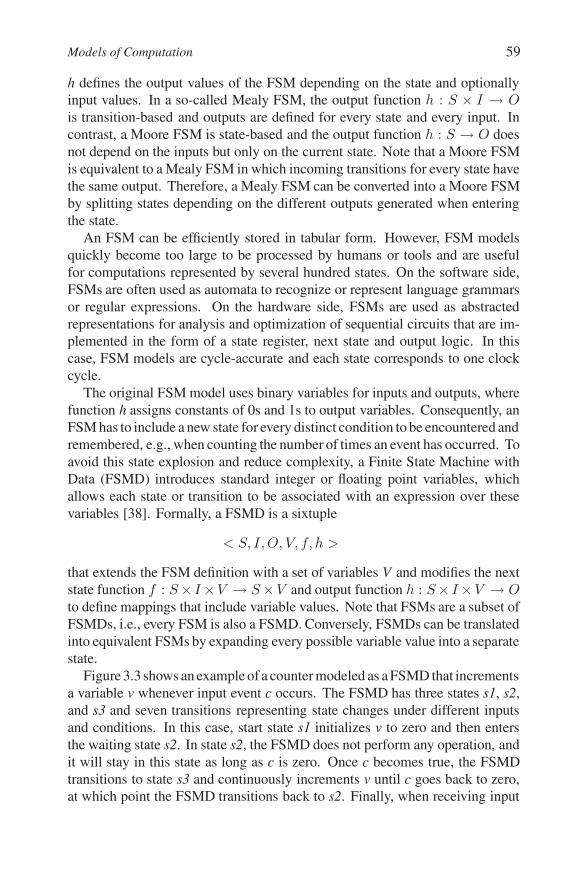
The original FSM model uses binary variables for inputs and outputs, wherefunction h assigns constants of 0s and 1s to output variables. Consequently, anFSM has to include a new state for every distinct condition to be encountered andremembered, e.g., when counting the number of times an event has occurred. Toavoid this state explosion and reduce complexity, a Finite State Machine withData (FSMD) introduces standard integer or floating point variables, whichallows each state or transition to be associated with an expression over thesevariables [38]. Formally, a FSMD is a sixtuple
< S, I,O, V, f, h >
that extends the FSM definition with a set of variables V and modifies the nextstate function f : S× I×V → S×V and output function h : S× I×V → Oto define mappings that include variable values. Note that FSMs are a subset ofFSMDs, i.e., every FSM is also a FSMD. Conversely, FSMDs can be translatedinto equivalent FSMs by expanding every possible variable value into a separatestate.
Figure 3.3 shows an example of a counter modeled as a FSMD that incrementsa variable v whenever input event c occurs. The FSMD has three states s1, s2,and s3 and seven transitions representing state changes under different inputsand conditions. In this case, start state s1 initializes v to zero and then entersthe waiting state s2. In state s2, the FSMD does not perform any operation, andit will stay in this state as long as c is zero. Once c becomes true, the FSMDtransitions to state s3 and continuously increments v until c goes back to zero,at which point the FSMD transitions back to s2. Finally, when receiving input

60 Modeling
s3s2
s1rr
c = 0 c = 1c = 1
c = 0
v : = 0
v : = v + 1
FIGURE 3.3 Finite State Machine with Data (FSMD) example
event r in either s2 or s3, the FSMD is reset and restarted by transitioning backto state s1. As is the case for most embedded, reactive systems, the FSMDexecutes indefinitely and does not terminate. In general, a state machine candeclare an explicit end state if it is meant to be embedded in a larger context.
The FSMD model is widely used to represent hardware implementationsof RTL processors consisting of a controller and a datapath [3]. In this case,each state executes in one clock cycle. States and transitions of the core FSMthereby describe the implementation of the controller. On the other hand,variables, expressions and conditions describe the operations performed by thedatapath in each cycle. In a similar manner, FSMDs can be used to provide astate-oriented view of imperative programming models. Transitions and statesdescribe the control flow of the program where each state computes a set ofexpressions corresponding to the statements in the code. Note that in this case,the FSMD are usually not cycle accurate since states can represent whole basicblocks that may require several clock cycles to execute. Furthermore, note thatimperative models are more vividly represented by a CDFG describing controland data dependencies between and within basic blocks, respectively.
HIERARCHICAL AND CONCURRENT STATE MACHINESHierarchy and concurrency are further mechanisms to manage complexity
of the state space. In a hierarchical state machine, states can be complex, so-called super states, which internally consist of a complete state machine each.Consequently, individual FSMDs are hierarchically composed into a so-calledSuper State FSMD (SFSMD). In an SFSMD, entering a super state is equivalentto entering the start state of the SFSMD contained within. Super states can beexited by defining an end state in the child SFSMD. Whenever a super statereaches it end state and exits, the parent SFSMD will transition to and entera specified other of its super states. As an alternative to explicit end states inchildren, a parent SFSMD can declare a transition between super states that willexit a child SFSMD whenever a specified condition becomes true, independentof which substate the child is in at that time. As such, hierarchy allows both

Models of Computation 61
to organize complexity and potentially reduce the number of transitions in thestate diagrams.
Concurrency allows complex state machines to be decomposed into mul-tiple, separate FSMDs running in parallel. Concurrent FSMDs can therebycommunicate through a set of shared signals, variables and events. Interactionsbetween state machines are usually based on a model that operates concurrent,communicating FSMDs in a synchronous, lock-step fashion. By ensuring thatFSMDs all transition and update or check signals at the same time, it can beguaranteed that they will not miss each other’s events and hence can safelyexchange information.
When combining both hierarchy and concurrency, so-called Hierarchical andConcurrent Finite State Machine (HCFSM) models emerge, such as the onespioneered in Harel’s graphical StateCharts language [86] and used for UnifiedModeling Language (UML) state diagrams [23]. In the original StateCharts,each hierarchical super state can be either a so-called AND- or OR-compositionof substates. OR states are used to describe regular hierarchy in which a parentstate is at any given time in either one (but only one) of its substates. In contrast,AND states describe a concurrent composition where being in a parent statemeans that the system is at the same time in all of its substates.
c / v : = v + 1
v : = 0
rs1
s
s2
s3
s4d / ed / e
FIGURE 3.4 Hierarchical, Concurrent Finite State Machine (HCFSM) example
Figure 3.4 shows an example of a HCFSM as a variation on the counterFSMD presented earlier in Figure 3.3. At the top level, the system is modeledas an OR composition that starts execution in initialization state s1. Uponreceiving the start signal s, the HCFSM enters the concurrent composition ofstate machines s2, s3 and s4. The left state machine starts in state s2 andessentially implements an edge detection that transitions between s2 and s3 andissues an event e depending on the presence or absence of event d. In parallel,s4 implements a simple counter that increments v on every occurrence of c. Atthe same time, the hierarchical combination of s2, s3 and s4 can be aborted byan event r that transitions from whatever state the combined super state is inback to the start state s1.
As discussed above, HCFMs execute concurrent state machines in a lock-step, synchronized fashion. Different HCFSM models can vary in the details

62 Modeling
of their semantics, specifically depending on when and for how long gener-ated events take effect. Introduced as a purely graphical notation, the originalStateCharts description did leave many of these issues open. As a result, awide variety of interpretations have been proposed over the years. Notably, thesemi-official semantics as realized by Harel’s own Statemate tool set follows anapproach in which events that are posted in one step are valid in and only in thenext step [87]. Together with additional rules about, among others, prioritiesof conflicting transitions, this makes Statemate models deterministic in theirexternally observable behavior.
Statemate thereby offers two different, so-called synchronous and asyn-chronous execution modes. In the synchronous mode, steps are executed atregular intervals, sampling all inputs, executing transitions and posting eventsfor the next interval in each. This corresponds directly to a hardware imple-mentation with a network of synchronous state machines connected in a Moorefashion. In the asynchronous mode, global steps can each consist of a sequenceof microsteps, where microsteps are assumed to execute in zero time. Externalinputs are only sampled at the beginning of each global cycle while internalevents are propagated through a chain of microsteps until the system stabilizesand no more events are generated. As long as there are no cyclic dependencies,this mode can emulate the propagation of signals among immediately reactiveMealy machines embedded within common, global clock cycles.
In the presence of combinatorial cycles, however, the sequence of microstepsmight never terminate. Worse, each microstep performs state updates, whichin turn might enable additional transitions in the next microstep, leading tosuperfluous or multiple transitions of state machines within each global step.Clearly, this behavior does not correspond to reality.
In all cases, none of the Statemate modes is strictly synchronous as requiredfor precise modeling of interconnected Mealy machines. As discussed previ-ously in the context of synchronous languages (at the beginning of Section 3.1),for models to be fully deterministic, events within each global cycle all have tooccur at the same instant and within zero time [18]. In that case, combinatorialcycles can lead to global inconsistencies or non-determinism. To deal withsuch issues, truly synchronous languages either generally reject models withcycles at compile time (e.g., as is the case for Lustre [85]) or require that aunique fixed-point solution exists in every global step (as realized, for example,in Esterel [21]). Likewise, note that strictly synchronous variants of HCFSMmodels have been developed by providing a dedicated synchronous interpre-tation (Argos [125]) or by using the StateCharts-like notation as a graphicalfrontend for Esterel (SyncCharts [6]).

Models of Computation 63
PROCESS STATE MACHINESTo avoid the need to maintain a global time, models exist that compose con-
current, communicating FSMDs asynchronously in the same manner as is donein process networks (see Section 3.1.1). This then requires more complex hand-shaking protocols or mechanisms such as message-passing in order for FSMDsto be able to communicate reliably. For example, while leaving many semanticdetails undefined, UML state diagrams [23] as yet another variant of HCFSMsare generally based on an unrestricted asynchronous execution model in whichconcurrent state machines must explicitly coordinate their execution throughevent queues wherever necessary, e.g., to synchronize accesses to shared vari-ables. As such, UML state diagrams are in the general case non-deterministic.However, their state-based nature allows other formal models, such as PetriNets [142], to be superimposed on such asynchronous HCFSMs. Similar toprocess calculi (see Section 3.1.1), state-oriented mathematical models likePetri Nets abstract away actual functionality and only focus on representing in-teractions and relationships necessary to analyze concurrency, synchronization,determinism and properties such as boundedness, reachability or liveness.
Combining synchronous and asynchronous approaches to concurrency, so-called Globally Asynchronous Locally Synchronous (GALS) models, such asCo-Design Finite State Machines (CFSMs) [11] have been proposed. GALSmodels maintain local clocks for FSMDs within each block yet allow dif-ferent blocks in the overall system to progress independently. Such modelsmatch the typical clock distribution in modern, complex system architectures.Nevertheless, at the leaves of the hierarchy, behavior is still described in animplementation-oriented form as clocked state machines communicating oversignals or wires.
Taking these ideas further, we can develop a sound combination of process-and state-based approaches by fully integrating concepts of process networks(see Section 3.1.1) into HCFSM models. For example, in a Program State Ma-chine Model (PSM) [63], leaves of the hierarchy contain complete asynchronousprocesses described in a sequential, imperative programming language. In theoriginal SpecSyn language, behavioral VHDL code was used as the basis fordescribing processes [185].
In a PSM model, such so-called program states can then be composed hier-archically following a HCFSM style. At each level, either a sequential state-machine or a concurrent but asynchronous composition of program states issupported. When entering a program state, execution either starts with the firststatement of the process code or, in the case of a superstate, by entering theset of start states in the same manner as a HCFSM. In contrast to HCFSMs,however, processes and hence program states have an explicit and clean notionof completion. Superstates can be exited in two ways: a so-called Transition-

64 Modeling
Immediately (TI) arc is equivalent to a transition in an HCFSM (such as r inFigure 3.4) that originates from the superstate to one of its siblings and canbe taken at any time, independent of the internal sub-state(s) the superstate isin. On the other hand, a Transition-On-Completion (TOC) arc is defined as atransition to a sibling of the superstate that is taken at the same time that thesubstates internally reach a declared end state. A leaf state completes wheneverits process exits (i.e., reaches its end or explicitly returns). Furthermore, theend state of a concurrent superstate is reached when all of its substates havecompleted.
As mentioned above, concurrent processes of a PSM run asynchronouslyto each other at any level. In the original SpecSyn model, processes can onlycommunicate through a set of basic shared variables, events and signals. Thus,models are generally non-deterministic and have to explicitly implement anyprotocols necessary to synchronize and coordinate process execution. As a re-sult, processes are generally a mix of computation and communication code. Toimprove on this situation, later extensions of the PSM model support the sepa-ration of communication from computation into distinct objects. For example,the SpecC model, while also being based on C instead of VHDL, introducedthe concepts of channels for encapsulation of communication and of clearlydefined interfaces as the boundary for separation of process from channel func-tionality [63].
SP P
c1P5
P3
P4
dP1
P2d
…c1.r ecei v e(d,e);a = 42;w h i l e (a<10 0 ){ b = b + a;i f (b > 50 )c = c + d;
el s ec = c + e;
a = c;}
c1.s en d(a);…
c2
FIGURE 3.5 Process State Machine (PSM) example
Figure 3.5 shows an example of an extended Process State Machine (PSM)model. At the leaves, the model consist of five processes, P1 through P5, thatare described in standard C or C++ form. As before, the system S starts byexecuting process P1 and, depending on input d, either transitions to processP2 or enters the concurrent superstate PP. Inside PP, the sequenc of process P3followed by P4 runs in parallel to process P5. Concurrent processes exchangedata by sending and receiving messages over channels c1 and c2. PP completesonce both P5 and P4 are finished executing. Upon completion of either P2 orPP, S enters its end state, which transparently follows to TOC arc of S to one

System Design Languages 65
of its siblings. Note that the example does not show any TI arcs, which werealready previously seen in Figure 3.4. Nevertheless, in contrast to plain HCFSMmodels, clean completion semantics of PSMs results in a well-defined modularcomposability.
In summary, PSM models provide a powerful combination of both process-based and state-based concepts. Asynchronous process networks provide ameans to describe dynamic, data-oriented application behavior limited only bythe flow of data and data dependencies across computations. On the other hand,concepts of states and transitions allow explicit modeling of reactive, control-oriented systems in addition to providing a representation of implementation is-sues such as program state, data storage, operation scheduling or cycle-accuratebehavior. At all levels, hierarchy and concurrency support organization andmanagement of complexity through separation of concerns. In addition, sep-aration of computation and communication supports further orthogonalizationof concerns and enables coarse-grain, asynchronous concurrency and flexibil-ity while still providing means, including libraries of message-passing or othercommunication channels, to maintain global determinism. All in all, combinedPSM-type models are able to support the complete system design process allthe way from specification of abstract system behavior down to cycle-accurateimplementation of hardware or software components.
3.2 SYSTEM DESIGN LANGUAGESIn order for a design to be simulated, analyzed and verified by the designer,
it needs to be represented in a formalized, machine-readable manner - that is,in some form of design language. Each design language carries very specificsyntax and semantics [55]. The syntax of a language defines its grammar asa set of valid strings over an alphabet. While design languages are typicallytextual, some have an optional or exclusively graphical syntax (e.g. a flow chartas a graphical representation of an imperative program or the purely graphicalStateCharts language). The semantics of a language subsequently defines themeaning of strings written in the language by mapping the syntax into an un-derlying semantic model, such as a mathematical domain [167] or an abstractstate machine model [158, 82].
A description of a design in such a design language is then called a designmodel. When referring to models, we need to distinguish between a designmodel as an instance of a syntactically valid description written in the language,the semantic model underlying a language, and an MoC that defines a formalclass of execution models where language-specific details such as data types andformats are abstracted away. For example, a MP3 decoder design model can bedescribed as an instance of a KPN MoC captured in the syntax and semantics

66 Modeling
of the SystemC language. Typically, the same MoC can be represented ina variety of languages. Conversely, the same design language can representdifferent MoCs if it has a broad, basic semantic model that other MoCs map to.For example, while differing in their concrete syntax and detailed semantics,sequential programming languages such as C or C++ all support an imperativeMoC, yet can also capture FSMs or FSMDs [184]. Note, however, that supportfor different MoCs in different languages varies, and specialized languages existthat are tied to a specific MoC, e.g., the graphical StateCharts language, whichdirectly realizes a HCFSM model.
3.2.1 NETLISTS AND SCHEMATICSOver the years, many new design languages have emerged to capture the
necessary and sufficient semantics at each new level of abstraction. Early on,one of the first concepts that was formally modeled and captured was the notionof a netlist. Netlist models are purely structural representations of the design asa set of components and their connectivity. As such, netlist models are the basisfor describing block diagrams used in early tools for computer-aided schematicentry and editing. Such schematic editors support simple automatic designrule checks to ensure, for example, that connections are only made betweencomponent ports that are compatible in terms of direction, signal and logiclevels. Hence, their main role is documentation of block diagrams to facilitatecommunication between different design teams.
Some of the first design languages were developed for description of netlistsat the gate level, such as the Electronic Design Interchange Format (EDIF).However, the concept of a netlist for structural representations is universal andhas been carried over into corresponding new languages at each level. Today, atthe system level, variants of the Extensible Markup Language (XML) are com-monly used to capture netlists of system platforms. For example, the SPIRITconsortium defines the IP-XACT standard [172] for XML-based exchange andassembly of system-level IP components.
3.2.2 HARDWARE-DESCRIPTION LANGUAGESAfter capturing netlists and schematics, interest arose in representing not only
the structure of designs but also their design behavior. By adding capabilitiesfor describing the behavior of every component in a netlist, languages gainedexecution semantics and could be simulated to validate the design. In orderto remain general, most widely used design languages are based on a verybasic discrete-event execution model. In a discrete event MoC, the system isrepresented as an ordered sequence of events where each event is a (value, tag)

System Design Languages 67
tuple that marks a change of state in the system at a certain point in simulatedtime [163]. Depending on the value and tag types supported by a specificlanguage, events can be used to model arbitrary state changes. For example, asignal is defined as a sequence of voltage changes on a wire.
On the one hand, many different designs objects and classes of MoCs can bemapped to such a universal event model and represented in a single languagewith a small set of basic primitives. On the other hand, as described in Chap-ter 1, while this expressibility might be desirable for simulation purposes, thereis a trade-off with the unambiguousness needed for analysis, synthesis and ver-ification, typically restricting corresponding use of such general languages to awell-defined subset with well-defined and unique interpretation.
In the early stages, these ideas were applied to the description of hardwareblocks at the gate level. Later on, they were transferred to the Register-TransferLevel (RTL). This resulted in the definition of so-called Hardware-DescriptionLanguages (HDLs) such as VHDL [7] or Verilog [180]. For example, at theRT level, the design is described as a microarchitecture consisting of functionaland storage units connected by wires. Each RT component, such as a register oran ALU, will eventually consist of logic gates, while its behavior is inherentlymodeled in the form of Boolean expressions. Since logic gates and consequentlyRT units respond to the signal changes at their inputs over time, a mechanism isneeded to indicate when inputs change and when this change propagates to theoutputs. Therefore, an event-driven execution behavior was added to triggerevaluation of a component on every input change and subsequently propagatethe new results to all components connected at the outputs. This process ofevent propagation and evaluation is repeatedly performed to simulate the designbehavior over time. All together, event-driven execution allowed for the firsttime to completely simulate a digital circuit in the computer.
For simulation of HDL models, a so-called discrete event simulator internallymaintains a logical simulated time and a queue of events ordered by their timestamps. In each simulation cycle, the simulator dequeues all events with thecurrent time stamp and triggers execution of processes waiting for those events.Each component in the design is thus associated with a process describing itsfunctionality. Once triggered, the process body is executed to compute internalstate changes and a set of new values on its output signals. The simulatorthen inserts the events generated by each process into its queue and advancestime to start the next simulation cycle. Note that to model delays, processescan post events at future points in time or can wait for time to advance in themiddle of their execution. Furthermore, in more recent languages, processescan dynamically change their sensitivity and wait for and post arbitrary eventsthroughout their execution. Hence, many HDLs can also model abstractedbehavior of process networks beyond simple components connected only bywires.

68 Modeling
3.2.3 SYSTEM-LEVEL DESIGN LANGUAGESAs we move to the system level, it becomes important not only to model
the hardware side of a design, but also parts of the system implemented insoftware. As a result, new languages have been developed that add capabilitiesto describe software in a native manner. Due to the large body of legacy code,a natural choice is to include software in the form of standard C code, eitherby combining C with an existing HDL (SystemVerilog [174]) or by addinghardware modeling capabilities to C or C++ through extensions (SpecC [65])or via libraries (SystemC [81]).
In all cases, and in the same way as previous HDLs, such System-LevelDesign Languages (SLDLs) are based on a discrete event driven executionmodel that supports necessary concepts for concurrency, hierarchy, timing andsynchronization. In addition, SLDLs are supplemented with support for rich,abstract data types, process- and state-based computation, and libraries of com-munication channels. For example, the SpecC language implements a PSMMoC with C-based processes composed hierarchically in an arbitrary parallel,pipelined, sequential or state machine fashion. Furthermore, SpecC introducedthe concept of native channels with a library providing, among others, message-passing, handshake, queue and semaphore type communication. SystemC, onthe other hand, started out as a C++-based HDL with parallel processes andsignals but later gained similar abstract channel concepts and libraries.
In addition, there are proprietary and standardized approaches that aim toprovide metalanguages for formally capturing heterogeneous models includingassociated requirements and constraints [12, 5]. In all cases, such SLDLs allowus to describe complete systems and their applications within a single frameworkall the way from abstract specification of high-level MoCs down to processorimplementations at the RT level.
3.3 SYSTEM MODELINGSystem design in general describes the process of going from a high-level
system specification of the desired functionality down to a system implemen-tation at the RT or instruction-set level. As outlined in Chapter 1, however,the semantic gap between specification and implementation is too large to beclosed in a single step. Following a top-down or meet-in-the-middle approach,the system design process is therefore broken into a series of smaller steps. Atthe core of this process are definitions of system models to represent and passdesign information from one step to the next.

System Modeling 69
Specification Model
I m plem entation Model
Model n
Model n+1
R efinem ent
O ptim . A lg or ith m
G U I
D B
...
...
D es ig n D ecis ions
FIGURE 3.6 System design and modeling flow
3.3.1 DESIGN PROCESSRealizing a Specify-Explore-Refine (SER) methodology based on model al-
gebra principles described in Chapter 1, a general design flow can be establishedin which an initial specification is gradually brought down to a final implementa-tion through successive, stepwise refinement of design models (Figure 3.6 [71]).In each design step, a refinement tool takes the input model and implements aset of design decisions in order to generate an output model at the next lowerlevel of abstraction. In the process, tools insert a new layer of computationand/or communication detail that reflects and represents the given decisions.For example, to implement communication between software and hardware,refinement tools generate drivers and interrupt handlers inside a model of theprocessor hardware.
Design decisions can thus come from the designer, typically entered in-teractively through a Graphical User Interface (GUI), or from an automatedalgorithm. In both cases, decisions are made to optimize a set of design met-rics, e.g., to simultaneously minimize system cost and area while not exceedinga maximum latency and power consumption. In general, both refinement anddecision-making can be manual or automated.

70 Modeling
Within such a design process, each system model at the same time documentsthe output of a design step and specifies the input to the next following stage.Hence, a model serves as both:
(a) A description of some aspect of reality such that one can reason about it, i.e.,a virtual prototype of already decided system details that allows validationof design decisions through simulation or analysis.
(b) A specification of the desired functionality to be implemented in furtherstages of the design process, i.e., a description of system features that stillneed to be build and decided.
Note that both cases are usually combined in a single model where differentparts of the model represent different aspects operated on by different tools.
From a documentation point of view, models have to be capable of capturingcomplex systems in all their relevant detail. Precise and complete representa-tions of implementation details have to be defined such that effects of designdecisions on design quality can be clearly observed, measured and/or predicted.At the system level, for example, virtual prototypes of the platform should allowsoftware to be developed before the actual hardware is available.
Models for simulation are thereby only a first step. In addition, modelsshould also enable formal methods to be applied for static analysis and verifi-cation of design properties, e.g., to guarantee response times in a hard real-timeenvironment. Especially also under the aspect of serving as a specification forfurther synthesis, models have to be defined with unambiguous semantics, suchthat application of corresponding tools becomes possible in the first place.
Combining documentation and specification aspects, each design model isan abstracted representation of a design instance. A model is associated with acorresponding abstraction level that defines the granularity of implementationdetail represented in the model. As design progresses, we gradually move downin the level of abstraction by adding more and more implementation detail. Dueto the lack of detail at higher levels, models simulate faster, but the accuracy ofresults is limited, typically resulting in a trade-off as we move up in abstraction.Therefore, the ideal design process should support a variety of levels withdifferent trade-offs, both to break the design flow into smaller steps and forefficient design space exploration. For example, in the early stages, designerswant to rapidly prune the design space of clearly infeasible solutions. As such,early models have to be fast but accurate only in relative, not absolute, terms.Then, as the design space continues to shrink, we can gradually afford to spendmore and more time on slower but increasingly accurate simulation until a finalsolution is confirmed.

System Modeling 71
3.3.2 ABSTRACTION LEVELSAs described in Chapter 1 and Chapter 2, there are four main abstraction
levels representing circuit, logic, processor and system levels. Within eachlevel, there are many different implementation details to be considered anddesign steps to be performed. This requires main abstraction levels to be dividedinto several intermediate levels and corresponding design models to be definedfor each. Specifically, in relation to system design we need to be concernedwith the implementation details within the upper system and processor levels.
Following the separation of computation and communication, we can firstand foremost distinguish between largely orthogonal computation and com-munication details [107, 72]. Both can range from purely functional, fullyuntimed descriptions down to cycle-accurate levels. On the communicationside, transaction-level approaches have recently become popular as an interme-diate approach for modeling of communication detail above the cycle-accuratelevel [31, 77, 109]. Similar concepts can also be applied on the computationside.
Computation
Commun
ication
A B
C
D F
Un-t i m e d
A p p r o x i m a t e -t i m e d
C y c l e -t i m e d
Un-t i m e d
A p p r o x i m a t e -t i m e d E
C y c l e -t i m e d A . S p e c i f i c a t i o n M o d e l ( S M )
B . T i m e d F u nc t i o na l M o d e lC . T r a ns a c t i o n-L e v e l M o d e l ( T L M )D . B u s C y c l e -A c c u r a t e M o d e l ( B C A M )E . C o m p u t a t i o n C y c l e -A c c u r a t e
M o d e l ( C C A M )F . C y c l e -A c c u r a t e M o d e l ( C A M )
FIGURE 3.7 Model granularities
Figure 3.7 [31] shows the range of granularities of computation and com-munication for various levels of abstraction. For example, a behavioral systemspecification at the origin of the graph (A) is untimed in both computation andcommunication with only a causal ordering between processes. Annotatingcomputation with execution models and estimated or measured delays resultsin a timed functional model (B). By also further refining communication down totiming-accurate bus transactions, we reach a Transaction-Level Model (TLM)of the system at point C. As such, a TLM includes timed models of computationand communication behavior for the processors in the system.

72 Modeling
Going into the design process at the processor level, Bus-Functional Mod-els (BFMs) of processors (which are assembled into a Bus Cycle-AccurateModel (BCAM) of the system) can be obtained by refining interfaces down tostate machines that drive and sample bus wires on a cycle-by-cycle basis (D).Alternatively, implementing only computation in the processors down to a mi-croarchitecture at the RT or timed instruction-set level, leads to a ComputationCycle-Accurate Model (CCAM), shown as point E in the graph. Finally, thecombined Cycle-Accurate Model (CAM) at the lowest level (F) is cycle-timedin both computation and communication.
As mentioned before, a methodology is defined as a set of models and trans-formations in between. A specific system design methodology is then estab-lished through the path that is taken to go from an untimed specification at pointA all the way to a final cycle-accurate implementation at point F. To that effect,the path taken determines the intermediate system models that are available, aswell as the amount, type and order of refinements to be performed throughoutthe design process. For example, in a general design methodology (see Chap-ter 1), design starts with a specification model (A) and progresses through anintermediate TLM (B) to reach the final CAM (F), where computation and com-munication refinement are performed together in two steps, at both the systemand processor levels.
3.4 PROCESSOR MODELINGOn the computation side, the basic system component is a processor. Com-
putation processes of the system behavioral model are mapped onto proces-sors, each of which runs a piece of the application code. Processor typescan range from programmable general-purposes processors over customizableApplication-Specific Integrated Processors (ASIPs) down to fully custom hard-ware units [184]. In the most complicated case of a software processor, we cantypically distinguish several layers of computation implementation (Figure 3.8).In the embedded case, the behavior of the system and hence of its componentsis not only defined by their functionality but also, of equal importance, by theirtiming. Thus, both aspects have to be considered throughout the design process.Since all of these layers significantly contribute to the functional or, more im-portantly, overall timing behavior of a processor, an accurate processor modelhas to include all of them [166, 24].
At the specification level, the application is modeled as a network of com-municating processes. Inside the processes, basic application algorithms aretypically described in an imperative programming language such as C. How-ever, application code in itself is untimed. To introduce the notion of time,information about execution delays on the given target processor has to be in-

Processor Modeling 73
serted into the code. This back-annotation can be performed at varying levelsof granularity. Such back-annotated application code then has to be augmentedwith a model of its execution environment such that effects of running the codeon a given platform are accurately described.
P1 P2
OSHW
DrvDrv I S RI S RH A L
p2.c
B u s Interrupts
FIGURE 3.8 Processor modeling layers
In the case of a software processor, as shown in Figure 3.8, application pro-cesses usually run on top of an operating system (OS), which provides dynamicscheduling and multi-tasking services. On the other end, application and OSsoftware has to run on top of the actual processor hardware, which realizes phys-ical bus interfaces and interrupts (including processor suspension and interrupttiming) for communication with the external world. In between, a hardwareabstraction layer (HAL) provides canonical interfaces, such as bus drivers andinterrupt service routines (ISRs) for accessing the processor hardware from thesoftware (i.e., application and OS) side.
Note that in general, all layers together determine the final execution orderand have a large influence on the overall timing behavior of the applicationrunning in the processor. Hence, models of all layers and their relevant detailsneed to be developed and integrated into the design process. To that effect,Figure 3.8 shows the most general case of a software processor with all layers.By contrast, models of other processors, such as custom hardware units, arederived as specialized versions of this general model by not including OS orhardware abstraction layers.
3.4.1 APPLICATION LAYERAs mentioned previously, at the highest application layer, computation func-
tionality running on a processor is generally described as a hierarchical set ofcommunicating processes. Processes at the leaves of the hierarchy encapsulatebasic algorithms, e.g., in the form of standard ANSI C code. Processes can becomposed hierarchically in an arbitrary serial-parallel fashion. Furthermore,processes communicate via shared variables, events or abstract channels pro-viding high-level, typed communication primitives such as message-passing,queues or semaphores.

74 Modeling
App
P2 C1
P1
P3C2
Logical time
5 1 00process P1() {
…w a i t f or( 5 );…
}
FIGURE 3.9 Application layer
For example, Figure 3.9 shows an application layer with three processesP1, P2 and P3, where P2 and P3 are spawned to run concurrently after P1 isfinished. During their execution, P2 and P3 exchange messages over channelsC1 and C2. Furthermore, P3 communicates with other processors in the systemthrough two external ports.
To provide the necessary concepts of concurrency, communication and tim-ing, such application descriptions are typically modeled in a C-based SLDLsuch as SystemC or SpecC. With such an application specification, the designeris essentially provided with a high-level, abstract model for programming thecomplete platform across different processors.
To achieve desirable high simulation speeds, the application model is ex-ecuted on the event-driven SLDL simulation kernel running natively on thesimulation host. In the process, application code is compiled into native hostinstructions to directly emulate its functional behavior using the fastest possi-ble host execution. In order to provide additional feedback about the timingbehavior, application processes have to be back-annotated with execution tim-ing, which models and simulates the delays of running application code on thechosen target processor in the final design (see Chapter 4).
As shown in Figure 3.9, back-annotation is performed by inserting wait-for-time statements into the code as supported by the timing model of the underlyingSLDL. Depending on the available data and the use case, such waitfor state-ments can be inserted at different levels of granularity ranging from basic blocksup to the level of functions or whole processes. Each option thereby results in aspecific speed/accuracy trade-off. For example, back-annotation at the functionor process level cannot represent dynamic effects of data-dependent control flowin the code. Instead, whole blocks of code are associated with a single, staticdelay number based on worst-case or average-case assumptions. On the otherhand, back-annotation at the basic block level accurately models control flowdependencies but is slower due to the larger number of waitfor statements tobe simulated.
There is a multitude of sources for obtaining execution delay numbers to beback-annotated into the application code. In general, delays can be acquired

Processor Modeling 75
either through estimation or measurement. Estimation of execution time is atopic that has been studied extensively with approaches that range from purelystatic, worst-case estimation techniques [194] to profiling-based solutions [31]that aim to deduce estimates from analysis or simulation of the source code,respectively. In terms of delay measurements, cycle counts for the code can begained by compiling the code for the target processor and tracing its executioneither on the real processor or in a corresponding timing-accurate ISS. Lastly,hybrid approaches exist that compile code down to an intermediate level inorder to apply analysis and estimation techniques at a level closer to the imple-mentation [93].
3.4.2 OPERATING SYSTEM LAYERIn the application layer, computation processes are modeled as running truly
concurrently. In reality, however, we have to assume that processors can onlyexecute a single thread of control or a limited number of threads at any giventime. With the operating system layer, the goal is therefore to introduce ac-curate representations of the scheduling of parallel processes on the inherentlysequential processors.
OSA p p
T a s kP2
C1
P1
T a s kP3C2
OS M o d e l
FIGURE 3.10 Operating system layer
As a first step, processes are grouped into tasks where all processes withina task are arranged in a fixed order according to a pre-defined static schedule.As shown in Figure 3.10, for example, processes P2 and P3 are converted intotasks with static scheduling combining all sub-processes into one sequentialpiece of code each. In a second step, remaining tasks are then considered tobe dynamically scheduled during runtime, typically by a Real-Time OperatingSystem (RTOS). To accurately reflect and specify these dynamic schedulingand RTOS effects and needs, an abstracted model of the RTOS is inserted intothe processor’s operating system layer [75]. In the process, tasks (e.g., P2and P3 in Figure 3.10) are refined to run on top of the OS model by insertingthe necessary OS calls for task management (creation and deletion), synchro-nization (event handling) and timing (delay modeling). In addition, existingapplication channels (e.g., C1 and C2, Figure 3.10) are refined into a model

76 Modeling
of Inter-Process Communication (IPC) that is properly integrated with the OSmodel by inserting appropriate OS calls for implementation of synchronization.
The operating system layer and OS model describe expected RTOS behavior,including the desired scheduling algorithm and scheduling parameters, both forvalidation during simulation as well as for further synthesis. To that effect, theconcept of OS modeling in general is based on the idea that at the specifica-tion level, as shown in Figure 3.11(a), processes are executed directly on theunderlying simulation kernel. Simulations run at native speeds but the concur-rency model of the simulator does not match the actual scheduling algorithmimplemented in the real RTOS.
Application
S L D L
C h anne ls
T1 T2
(a) Specification
Application
R TO SM od e l
C h anne ls
T1 T2
S L D L
(b) TLM
Application
I ns tr u ction S e t S im u lator
R T O S C om m . & S y nc. AP I
S L D L
(c) Implementation
FIGURE 3.11 Operating system modeling
To get accurate results, application software is therefore traditionally simu-lated in ISS models of processors instead (Figure 3.11(c)). For this purpose, theapplication code is cross-compiled for the target processor and linked againstthe real target RTOS libraries. The resulting final target binary is then executedby an ISS, which in turn can be integrated into an SLDL environment for co-simulation with the rest of the system [20, 70]. Such ISS approaches can bevery accurate, but as a result of their accuracy, can also be slow, especially ifmultiple processors have to be co-simulated together in a cycle by cycle fashion.
The goal of high-level RTOS modeling is thus to provide a solution thatcombines the speed of native application execution (Figure 3.11(a)) with theaccuracy of an ISS model (Figure 3.11(c)). Instead of running the real operatingsystem with all of its associated overhead, an abstracted RTOS model is insertedas an additional layer that sits between the application and the underlying sim-ulation kernel (Figure 3.11(b)). The OS model abstracts away unnecessaryimplementation details and focuses solely on modeling key concepts relatingto multi-tasking, preemption, interrupt handling and inter-process communi-cation and synchronization. As such, the RTOS model adds only a negligiblesimulation overhead. On the other hand, it provides accurate feedback about

Processor Modeling 77
all important OS effects early on in the design process and at a high level ofabstraction.
Internally, the OS model wraps around and replaces the underlying SLDLevent handling with its own primitives. As mentioned above, tasks and channelsare refined to call the equivalent OS model services and are not allowed to accessthe simulation kernel directly. Instead, the OS model selectively relays callsto the kernel, ensuring that at any given time only one task is active and allother tasks are blocked at the SLDL level. Whenever the OS model is called,either by a task, a channel or from an asynchronous event such as an interrupthandler, a re-scheduling and task switch is triggered. The OS model thenblocks the current task and selects, dispatches and releases a new task basedon its internally re-implemented scheduling algorithm. For example, an OSmodel that emulates a priority-based scheduling will block a low-priority taskcalling the OS if in the meantime a higher priority task has been activated byan asynchronous external interrupt. By replacing delay models (i.e., waitforstatements) with an appropriate wrapper, an OS model can therefore simulatetask preemption accurately within the granularity of the given back-annotation.
c1.recv()c1.s en d ()
Bus
b u s .recv()
P2 P3
S1
T i m e
t0
t1
t2t3
t5
t8
t6
t4
t7
t0
t1
t2
t3
t4
t5
t6
t7
t8
w a i t f o r() w a i t f o r()
w a i t f o r()
w a i t f o r()w a i t f o r()
w a i t f o r()
I n t
P1
w a i t f o r()
c1.recv()
c1.s en d ()
Bus
b u s .recv()
T a s k P2 T a s k P3
o s .w a i t f o r()
o s .w a i t f o r()
o s .w a i t f o r()
I n t
o s .w a i t f o r()
o s .w a i t f o r()
o s .w a i t f o r()
o s .w a i t f o r()
P1
C 1
S1
C 1
(a) Application (b) OS
FIGURE 3.12 Task scheduling

78 Modeling
Figure 3.12 shows the resulting execution schedules for the example previ-ously introduced in Figure 3.9 and Figure 3.10. Execution starts at time t0 withprocess P1, which in turn spawns processes P2 and P3 at time t1. In the un-scheduled case (Figure 3.12(a)), P2 and P3 are running truly concurrently andtheir simulated execution times overlap unless there is some causal dependencybetween them. For example, at time t2, process P3 is blocked and waits for amessage from P2, which arrives over channel C1 at time t3. Similarly, at timet4, P3 enters the bus driver to wait for external data from another processorin the system. At time t5, an external interrupt to signal availability of dataarrives. The corresponding interrupt service routine is executed and releases asemaphore S1 in the bus driver. The driver in turn receives the external dataand finally resumes execution of P3 at time t6. All throughout, P2, on the otherhand, runs continuously, uninterrupted by any of the events in the system.
Once the OS model has been inserted (Figure 3.12(a)), execution of tasks P2and P3 is interleaved according to the selected scheduling algorithm. In thisexample, priority-based scheduling is employed where task P3 has a higherpriority than task P2. Hence, P3 executes unless it is waiting on some event.P2 is switched in and can run only when P3 blocks on a call to C1 or the busdriver. Later, once C1 or S1 are released, P3 is reactivated, P2 is suspended,and execution switches back to P3 until P3 ends and P2 can finish its remainingexecution. All combined, the OS layer and OS model accurately reflect theexecution sequence and timing as realized and observed on the real processor,up to the significantly delayed end of execution at time t8. Note, however, thatthe task switch from P2 to P3 at time t6 does not happen directly upon releaseof S1 by the asynchronously triggered interrupt handler. In reality, the OSwould immediately preempt P2 to switch in the just reactivated high-prioritytask P3. In contrast, the OS model can only do so once P2’s waitfor expiresand simulation control returns to the OS. Thus, there is an inherent inaccuracy inmodeling preemption at higher levels as determined by the intrinsically coarsergranularity of the time model.
Finally, note that the OS model offers its services for task management, eventhandling, and delay modeling through a canonical API that is independent ofthe interface format of any specific target RTOS. This allows refinement andinsertion of corresponding API calls to be performed automatically. Further-more, during backend software synthesis (Chapter 5), such canonical API callscan then be automatically converted into calls to the actual API of the selectedtarget RTOS.
3.4.3 HARDWARE ABSTRACTION LAYERThe Hardware Abstraction Layer (HAL) provides the lowest level of func-
tionality that is implemented in software. As such, its border marks the bound-

Processor Modeling 79
ary between the processor hardware and the software running on top of it. Inother words, all layers thus far down to and including the HAL are implementedin software whereas all layers outside of the HAL are realized in hardware.Again, this is for the general case of a software processor. In the case of acustom hardware unit, neither HAL nor OS layers exist, and all functionality isimplemented in hardware.
Basic HAL templates are typically stored in the PE database, containing pre-defined functionality for abstracting access to the processor hardware into a setof canonical interfaces and services. For example, a HAL model in the databasewill include the hardware-specific driver code for transferring arbitrary blocksof bytes over the processor bus interface. Likewise, the HAL contains templatesof low-level interrupt handlers that are properly associated with correspondinghardware interrupt sources.
HALO SAp p
T a s kP2
C1
P1
T a s kP3C2
O S M o d e l
I n t A I n t B I n t C
U s r I n t 2U s r I n t 1
Drive
rDr
iver
I n t D
B u s T LMAc
cess
s a m p l e .s e n d (v1);
void s e n d (…) { i n t r . r e c e i ve ();b u s .m a s t e r W r i t e (0x A000,
&t m p , l e n );
}
FIGURE 3.13 Hardware abstraction layer
On top of the HAL templates stored in the database, models of the driversfor communication with the external world can then be developed and inserted.Details of these communication models will be described in Section 3.5. Ingeneral, as shown in Figure 3.13, models of the drivers are inserted into the OSlayer, where they are integrated with the rest of the processor model, i.e., the OSmodel and the low-level bus access code in the HAL. In the process, low-levelinterrupt handler templates in the HAL (e.g., IntA through IntC in Figure 3.13)are filled with required code. Furthermore, necessary user-level interrupt tasks(UsrInt1 and UsrInt2) are generated and registered with low-level handlers andthe OS model.
Together, these drivers describe the implementation of application channelcalls (such assend()or receive()) down to the level of external interrupts andbus read() or write() transactions. As a result, HAL models of processorsare connected by and communicate with each other through bus models at thelevel of individual interrupts and bus transactions. As mentioned previouslyand as will be described in more detail in Section 3.5, such bus TLMs provide

80 Modeling
an abstracted implementation of bus communication beyond individual pinsand wires.
3.4.4 HARDWARE LAYERWith the final hardware layer, an accurate model of the actual processor hard-
ware is included. The processor hardware model specifically captures detailsof physical bus interfaces and of interrupt handling behavior to suspend regularexecution and handle exceptions whenever an external interrupt is received.Note that in the HAL, interrupts are handled concurrently to the applicationand OS code, and the execution of interrupt handlers overlaps with those ofthe tasks. For example, Figure 3.14(a) shows the schedule of execution forthe HAL model from Figure 3.13. While tasks P1 and P2 are serialized andinterleaved by the OS model (see Section 3.4.2), the handler for interrupt IntCoccurring at time t1 is executed in parallel to the tasks. When finishing, the IntChandler releases a semaphore, which triggers a task switch from P1 to P2 inthe OS model until P2 blocks again and task P1 is resumed. In the end, overalltask execution finishes at time t2.
time
TP1
I n tC
t1 t2
TP2
t3
(a) HAL
time
TP1
I n tC
t1 t2
TP2
t3
(b) Hardware
FIGURE 3.14 Interrupt scheduling
In reality, however, the processor hardware interleaves interrupt processingwith execution of regular code. As shown in Figure 3.14(a), when the interruptoccurs at time t1, the processor hardware suspends execution of all tasks toexecute the IntC handler in its own context. Only after IntC is finished will thehardware resume task execution, at which point the OS can execute the interrupt-triggered switch from P1 to P2. As a result, end of task execution in the realprocessor is delayed until time t3 instead of t2. Since interrupt processing andthe interrupt load on the processor can therefore have a significant effect onoverall timing, corresponding models need to be included and considered in thedesign process [198].
For this purpose, the hardware layer as shown in Figure 3.15 adds a separatemodel of the processor’s hardware interrupt logic. When receiving an externalevent on one of its external interrupt ports (INTA through INTC, for the example

Processor Modeling 81
HWHA LO SA p p
T a s kP2
C1
P1
T a s kP3C2
O S M o d e l
Access
HWI n t
I n t A I n t B I n t C
U s r I n t 2U s r I n t 1
Driver
Driver
I n t D
B u s T L M
I N T AI N T BI N T CI N T D
FIGURE 3.15 Hardware layer
in Figure 3.15), the hardware interrupt logic suspends execution of the completeprocessor software including HAL, OS and application layers. Replicating theprocessor’s behavior for interrupt nesting and interrupt priorities, the interruptlogic then calls the appropriate interrupt handler (e.g. IntC in Figure 3.15). Thehandler in turn notifies a user-level interrupt task, e.g., UsrInt1 or UsrInt2, andreturns. Upon return of the interrupt handler, the HW interrupt logic resumesexecution of HAL, OS and application software, and the OS model re-schedulestasks such that interrupt-triggered high-priority jobs (e.g., UsrInt1 or UsrInt2)can potentially preempt any currently running task (e.g., P2 or P3).
Note that even though interrupt handlers behave in essentially the same fash-ion as high-priority tasks, scheduling strategies for tasks and interrupts in gen-eral are different, as is the case for a round-robin OS that runs in a processorwith prioritized interrupt sources. Therefore, interrupt handling behavior hasto be modeled separately. In essence, hardware and OS layers implement ahierarchal scheduler in which a primary interrupt scheduler in the hardwareexercises control over the secondary OS-internal task scheduler, each with itsown respective scheduling strategy that accurately represents reality.
Next to the core processor suspension functionality, the HW layer also in-cludes any interrupt controllers and other peripherals (e.g., timers) immediatelyassociated with the processor. The interrupt controller together with the suspen-sion logic then determines the overall interrupt behavior and interrupt schedul-ing strategy. If interrupt controllers are programmable, the HAL will includethe necessary code for setting up and properly associating interrupt handlerswith external interrupt sources according to user-selected parameters such aspriorities.

82 Modeling
In relation to its external bus interfaces, the hardware layer can provide twodifferent levels of communication detail. As in the case of the HAL, modelsof processor hardware at the transaction level communicate with each otherthrough abstracted models of busses and interrupts at a granularity of completetransactions, providing accurate feedback for fast simulation purposes. Onthe other hand, pin-accurate processor models are needed for integration intostructural system netlists and for further synthesis of hardware processors (seeChapter 6). A so-called Bus-Functional Model (BFM) therefore extends theprocessor hardware layer by including a cycle-accurate model of external busand interrupt protocols, accurately driving and sampling bus wires according tothe timing diagrams of the bus. More details about bus interface descriptionsat different levels can be found in Section 3.5. Note that, apart from theirexternal bus models, transaction-level and bus-functional models of processorsare equivalent.
TABLE 3.1 Processor models
OS HAL HW ISS
FeaturesTarget approx. c om pu tati on ti m i n gTas k m appi n g, d y n am i c s c h ed u l i n gTas k c om m u n i c ati on , s y n c h ron i z ati onI n terru pt h an d l ers , d ri v ersH W i n terru pt h an d l i n g, i n t. s c h ed u l i n gC y c l e-ac c u rate c om pu tati on
A ppl .
In summary (Table 3.1 [166]), a model of system computation as imple-mented by custom or standard processors can be constructed in a layer-basedfashion. With each layer, new features and aspects of computation behaviorare specified and can hence be observed. Basic algorithmic functionality, in-cluding execution timing, is modeled at the application layer. The operatingsystem layer adds dynamic scheduling and OS effects. At the hardware abstrac-tion layer, interrupt handlers and bus drivers for external communication areinserted. Finally, the hardware layer adds a model of the processor hardwareand interrupt logic.
In the end, a processor model at the hardware level provides a complete andfull-featured description of computation running in its execution environment.Transaction level versions of hardware processor models serve as a fast yetaccurate virtual prototypes for simulation in close to real time. Bus-functionalprocessor models, on the other hand, are structurally accurate for system inte-gration and hardware synthesis. As a reference, all such high-level processor

Communication Modeling 83
models are compared against a traditional bus-functional ISS model of the sameprocessor (see Chapter 5), which can be fully cycle accurate at the expense ofslow simulation speeds.
3.5 COMMUNICATION MODELINGCommunication needs and principles have been studied extensively in the
general-purpose networking community. The networking community early ondeveloped the ISO/OSI 7-layer model [98] to reason about networks and to serveas a guideline and outline of requirements and implementations. The modeldivides the functionality generally required to implement any network into sevendifferent layers. Layers are grouped and ordered based on orthogonality. Eachlayer defines the functionality implemented by it and the semantics supportedat its interface. Layers are stacked on top of each other and each layer providesservices to layers above by using services of the layer below. As such, the modelprovides a clear separation of concerns and allows for a structured process whendesigning new networks.
The ISO/OSI model has proven to be very valuable for reasoning about thedesign process in the networking world. Based on the observation that systemcommunication is not inherently different from any general-purpose commu-nication, we can adopt the ISO/OSI model as a basis for organizing systemcommunication functionality, the communication design process, and commu-nication modeling. In doing so, however, layers need to be tailored to specificsystem design requirements. For example, lower media access layers have tobe split in order to reflect the separation between functionality implementedin hardware and software. Furthermore, layering has to take into account thespecial features and restrictions of on-chip and off-chip busses employed in theembedded world. Note that in the context of this book, the term bus is usedbroadly in the sense that it can refer to a wide variety of physical communica-tion media, including, for example, serial, point-to-point or network-orientedbusses such as RS232, CAN, Ethernet or wireless protocols.
Table 3.2 [74] summarizes the results of this process. Next to related originalISO/OSI numbers, the table lists for each layer semantics provided at the in-terface to the layer above, functionality realized inside, and corresponding pro-cessor layers into which this functionality is eventually inserted. Note that pre-sentation, session, transport and network layers form the network-level driversthat are implemented next to the OS. Link, stream, and media access layers,on the other hand, are implemented as low-level drivers and interrupt handlersdirectly on top of the processor HAL. Finally, the protocol layer implementsthe actual physical bus interface in the processor hardware.

84 Modeling
TABLE 3.2 Communication layers
Layer Semantics Functionality Implementation OSI
Application Channels, variables Computation Application 7
Presentation End-to-end typedmessages
Data formatting OS 6
Session End-to-end untypedmessages
Synchronization,multiplexing
OS 5
Transport End-to-end datastreams
Packeting, flowcontrol
OS 4
Network End-to-end datapackets
Subnet bridging,routing
OS 3
Link Point-to-point logicallinks
Station typing,synchronization
Driver 2b
Stream Point-to-pointcontrol/data streams
Multiplexing,addressing
Driver 2b
Media access Shared medium bytestreams
Data slicing,arbitration
HAL 2a
Protocol Media (word/frame)transactions
Protocol timing Hardware 2a
Physical Pins, wires Driving, sampling Interconnect 1
Taken as a whole, Table 3.2 outlines the needs and requirements for imple-mentation of system communication. In order to support the design processfor arbitrary communication architectures, we need to develop models of allcommunication layers and their relevant functionality. Details of layers andsuch models will be discussed in the following sections.
It should be noted, however, that the ISO/OSI model was only ever intendedto aid in reasoning about communication stacks and their requirements. It wasnot meant to provide a reference for implementation of such functionality inthe same layered manner. Thus, while layers serve as a basis for developmentand organization of communication models, any implementation, and henceany further synthesis of models, should consider the complete stack as a sin-gle specification for possible merging of functionality and optimization acrosslayers.
3.5.1 APPLICATION LAYERAs discussed previously for the computation side, the application layer pro-
vides the designer with a high-level programming model for describing system

Communication Modeling 85
behavior. In this model communication semantics can vary widely in terms ofrequired or desired data and control flow. At the application level, a rich andpowerful set of high-level communication semantics should therefore be sup-ported. Typical examples of commonly used application-level communicationprimitives include:
(a) Pure events that establish one-way synchronization (i.e., control flow tran-sitions) but do not carry data.
(b) Shared variables, which only hold data and do not include any synchroniza-tion.
(c) Synchronous and asynchronous message-passing channels, which combinedata transfers with, respectively, two-way or one-way synchronization (con-trol flow). In the synchronous case, sender and receiver block until both areavailable to exchange data. In the asynchronous case, only the receiverside is blocking, waiting if necessary for data from the sender to becomeavailable. The sender, on the other hand, may or may not block. Asyn-chronous implementations can use buffers to decouple the sender from thereceiver, such that a sender is independent and will only block if no bufferspace is available. The amount of buffering, however, is implementation-dependent and, in general, no guarantees are made on the sender side. Notethat in an extreme case, asynchronous message-passing can be implementedsynchronously without any buffering.
(d) Queues as a special case of asynchronous message-passing with well-defined, fixed buffer sizes to implement and guarantee a specific queuedepth.
(e) Complex and user-defined channels with extended semantics, such assemaphores or mutexes widely used for advanced synchronization in thesoftware world.
In all cases, application designers expect communication primitives to provideguaranteed delivery. As such, all provided and supported primitives are assumedto be reliable, lossless and error-free. Communication design thus needs to en-sure that these primitives are implementable on any given target communicationarchitecture, even if underlying physical communication media are unreliable.
In general, a system specification can contain communication in the formof any of the application-level primitives described above. In contrast, actualimplementations of communication stacks can typically only support system-level communication using a canonical, restricted set of primitives. In the courseof mapping system behavior onto processors, the application layer thereforehas to translate all communication between system components into primitivessupported by the following design process.

86 Modeling
P1
P2
(a) Behavioral model
PE2
P2
B R c v
PE1
P1
B S n d
� �
(b) Synchronization
FIGURE 3.16 Application layer synchronization
To begin with, the application layer has to insert any necessary synchroniza-tion to guarantee that original execution semantics are preserved. Consider,for example, a system behavior in which two processes P1 and P2 are com-posed sequentially (Figure 3.16(a)). Mapping P1 and P2 to PE1 and PE2,respectively, results in them running in parallel on the inherently concurrentprocessors. Thus, the implicit sequential transition from P1 to P2 has to beconverted into explicit synchronization between the PEs. As shown in Fig-ure 3.16(b), an additional process BSnd on PE1 transfers control to PE2 bysending a message over a newly inserted channel C1 as soon as B1 finishes.Process BRcv on PE2, on the other hand, ensures that B2 does not start until thesynchronization message on C1 has been received and hence, as desired, untilB1 on PE1 has finished.
In addition to transitions, the system behavior might contain shared variablesbetween processes. If, as shown in Figure 3.17(a), two processes P1 and P2are mapped to different processors, storage represented by the shared variablev1 in between needs to be moved into local memories of one or more systemcomponents. In a distributed implementation (Figure 3.17(b)), a local copy of v1is created in each accessing PE. Local copies are kept synchronized by insertingmessages to exchange updated variable values at synchronization points. Forexample, in Figure 3.17(b), updates of v1 are merged into previously generatedsynchronization messages. Together with passing control from P1 on PE1 toP2 on PE2, BSnd and BRcv hence transfer any necessary updates of v1 viachannel C1.
In other implementations, variables are mapped specifically into a chosensingle PE. In a memory-mapped I/O implementation, variables are mappedinto the local memory of a processor, typically one of the processors access-ing the variable. For example, in Figure 3.17(c), v1 is mapped into the HWPE where it becomes a local register. A memory interface providing externalmethods for reading and writing the register is then created in the HW suchthat the CPU and other PEs can access v1 over the network. Alternatively, in a

Communication Modeling 87
P2P1 c1
v1
(a) Behavioral model
PE2
P2
B R c v
PE1
P1
B S n d
���v1
v1
(b) Distributed message-passing
HWC P U
P1 c1
v1
P2
(c) Memory-mapped I/O
HWC P U
P1 c1
M e mv1
P2
(d) Shared memory
FIGURE 3.17 Application layer storage
shared memory implementation (Figure 3.17(d)), v1 is mapped into a dedicatedmemory component. Again, the memory provides an interface for other PEs(i.e., CPU and HW ) to randomly access any variables stored inside.
Similar to shared variables, complex channels supported at the applicationlevel (such as queues, semaphores or mutexes) might have storage or com-putation requirements as part of their implementation. As such, they have tobe similarly resolved into basic channel primitives supported by the follow-ing design process. For example, Figure 3.18(a) shows two processes, P1 andP2, communicating through a queue channel, which requires both storage andcomputation to manage internal buffers and realize its external enqueuing anddequeueing functionality. As part of the application layer, such channels aretranslated into a client-server implementation. A separate server process is cre-ated to implement channel storage and functionality. Accesses to the channelby other client processes are translated into a Remote Procedure Call (RPC)to the server that emulates the original channel interface and semantics. Fig-ure 3.18(b) shows an example where the additional server process is mappedinto a dedicated, separate Queue hardware. Processes P1 and P2 in HW1 andHW2 then access the Queue via basic message-passing channels C1 and C2,respectively. On the other hand, the server process can be mapped into one ofthe accessing PEs instead. For example, in Figure 3.18(c), the queue process is

88 Modeling
CQueueP1 P2
(a) Behavioral model
QueueH W 1
C1P1
H W 2
P2C2
(b) Dedicated PE
HW1
C1
HW2
P2P1
(c) Local processes
FIGURE 3.18 Application layer channels
mapped into HW1, where it becomes an additional local process next to P1. Inthis case, the server communicates locally with P1 and accepts external requestsfor read accesses from P2 on HW2, again over a basic message-passing channelC1.
After resolving synchronization, storage and complex channel requirements,communication at the output of the application layer is reduced down to basicmessage-passing and memory access primitives. This canonical set of primi-tives can then be further implemented on a given target communication archi-tecture by the following layers of the communication stack.
3.5.2 PRESENTATION LAYERThe presentation layer is responsible for formatting of data and for conversion
of abstract datatypes found in the application into untyped blocks of bytes to betransferred over the network. Generally, data is stored in different layouts in thelocal memories of the different PEs. Layout of data items in a PE is dependenton the PE’s architecture and the target compiler/synthesizer used to translateapplication code into a PE-specific implementation. The data layout of a PE issufficiently described by the following parameters:

Communication Modeling 89
(a) Bitwidth of a machine character, i.e., of the smallest addressable unit.
(b) Size (in machine characters) of each basic/primitive datatype.
(c) Alignment (in machine characters) of each basic/primitive datatype.
(d) Endianess (little or big).
Given this information, the exact layout of data in the PE’s memory can bederived for all primitive or complex data types, such as arbitrary combinationsof structures and arrays.
When exchanging data over the network, a common format of the data on thenetwork has to be chosen for each pair of communicating partners. Similarly,a common layout of data in a shared memory accessed by two PEs has tobe defined. In general, the format of data on the network or in the memoryis equally defined by a set of character width, endianess, size and alignmentparameters.
The data layout on the network or in the memory can be the same as inboth, one or none of the involved PEs. If any network or memory parameteris different from the PE’s characteristics, the presentation layer has to performthe necessary conversion for all accesses. By contrast, the presentations layeris empty and data can be copied one-to-one only if all parameters are the same.
tAdslCardcardl i n e
tCardch ar i ds h o rt cu rP w rs h o rt m ax P w r
tL i n ei n t f e cC o u n t e rf l o at s n rs h o rt b i t R at e
4 21 5 23 7 5
04 5 .86 4 0
(a) Application data structure
byteid c u r P w r m a x P w r f e c C o u n t e r s n r b it R a t e
(b) Network byte stream
FIGURE 3.19 Presentation layer
Figure 3.19 shows an example of an application-level abstract data structure(Figure 3.19(a)) being marshaled into a stream of bytes to be transferred over thenetwork (Figure 3.19(b)). At the application level, the tAdslCard data structure

90 Modeling
consists of two members (card and line) which are of tCard and tLine type,each containing several items of basic character, integer and floating-point datatype. In the local PE memory, structures and their members are laid out toconform to PE parameters such as the requirement to align all items on wordor double-word boundaries. In contrast, on the network level, the presentationlayer transmits items byte by byte in the specified order and with given sizes(1 byte per char, 2 bytes per short and 4 bytes per int or float for this example),excluding in this case any empty bytes used for padding and alignment in thePE memory.
Note that the layout of data on the network or in memories can either beglobally defined for the whole system or adapted differently for each pair ofcommunicating PEs. In the former case, the layout can be optimized to re-duce overall data traffic globally. For example, traffic is minimized by settingalignment and size parameters such that no byte padding is performed and alldata types only occupy their minimally necessary space. In the latter case, thelayout can be matched individually to one or both of the PEs, simplifying orcompletely avoiding presentation layer implementations.
All in all, the presentation layer translates typed messages and memory ac-cesses between different endpoints at the application level into untyped mes-sages and byte-wise accesses to be implemented by the layers below.
3.5.3 SESSION LAYERIn general, the system application can define as many channels as desired
between any two endpoints. In order to reduce resource requirements in thefollowing layers, the session layer is responsible for merging groups of channelsinto sessions and multiplexing them over a reduced set of end-to-end transports.After data formatting performed by the presentation layer, messages are untypedand resulting byte streams can therefore be safely multiplexed over a singletransport channel. As such, the session layer is responsible for selecting theend-to-end channel used to transport messages of each application stream andto implement all the necessary means to separate and distinguish messages ofdifferent streams going over a single transport. Note that in the case of systemcommunication considered in this book, channel selection/merging is optionaland without loss of generality, the session layer can be skipped.
If two channels are accessed sequentially with a pre-defined, fixed and non-overlapping sequence of messages in both communication endpoints, they canbe merged unconditionally into a single stream. Figure 3.20(a), for example,shows a case where two sequential processes (P1 on the CPU and P2 in HW2)communicate over two channels, C1 and C2. Since processes can only ex-change messages over one channel at a time, the session layer merges themby simply connecting both ports on both processes to a single shared channel

Communication Modeling 91
CPU
C2
H W 1
P3 P4P1
C4
C3
H W 2
P2C1
(a) Application channels
HW1CPU
HW2
P3 P4P1
C4
C3
C4
����
C3
C4
P2C2
C3
C1
C2
C1
(b) Network transports
FIGURE 3.20 Session layer
C12 in between (Figure 3.20(a)). On both sides, message are then identified asoriginally belonging to either C1 or C2 simply by their order in the sequence ofmessages going back and forth over C12 (i.e., the first message always beingC1 and the second C2).
In the case of concurrently accessed channels, messages cannot be identifiedby their order in the stream. For example, in Figure 3.20, channels C3 andC4 are fed by two concurrent processes P3 and P4 in HW1. As a result,messages may arrive in any order or may even overlap on the CPU side. Hence,when transferred over a single channel, messages originating from C3 or C4cannot be directly distinguished. Instead, such concurrent channels can only bemerged if additional headers are prepended to each message in order to identifymessages belonging to different sources. In an embedded implementation,however, the additional overhead for handling and transmission of messageheaders is typically not justified and any such addressing realization is betterdeferred to lower layers (see Section 3.5.8).
In the end, the session layer handles the merging of channels by transmittingmessages from different sources over a reduced set of end-to-end streams such

92 Modeling
that overall complexities and resource requirements in implementation of laterlayers below will be minimized.
3.5.4 NETWORK LAYERThe network layer splits the overall network into smaller subnets where
different subnets can subsequently be implemented using different underlyingmedia. In order to connect subnets and route packets between them, the networklayer inserts additional Communication Elements (CEs) in between. In theprocess, the network layer transforms end-to-end transports of upper layersinto logical point-to-point links between individual stations forming the overallnetwork structure.
CPU
C2P1
H W
P2C1
(a) End-to-end transports
HW
P2C2
C1
C PU
P1C2
C1
L2A
L1A
CE L2B
L1B
(b) Point-to-point links
FIGURE 3.21 Network layer
For example, in Figure 3.21, end-to-end channels C1 and C2 between CPUand HW PEs (Figure 3.21(a)) are each split into two logical links, L1A/L1Band L2A/L2B, respectively. In between, a CE routes and translates betweenlinks such that subnets on either side can each be implemented over differentunderlying busses.
We can generally distinguish two types of CEs, transducers and bridges,depending on the layer at which their functionality is realized. As shown inFigure 3.22(a), a transducer operates according to a store-and-forward principle.It receives blocks of data on one side (PE1), temporarily stores them in aninternal buffer and does not send anything out on the other end (PE2) untilthe complete packet has been received and buffered. As a result, transducerssynchronize and exchange address and data items with each side separately.Thus, transducers break end-to-end transport paths presented to higher layers
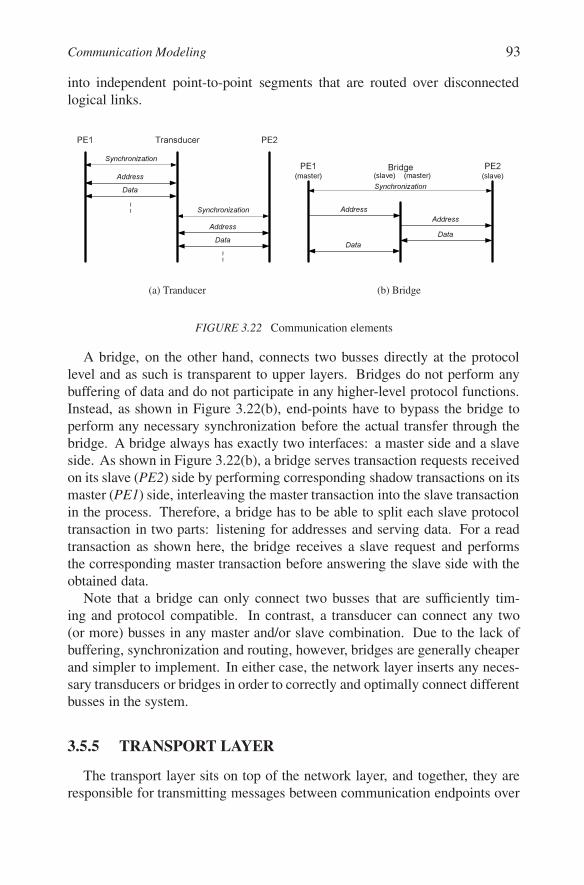
Communication Modeling 93
into independent point-to-point segments that are routed over disconnectedlogical links.
Transducer
AddressD a t a
AddressD a t a
P E 2P E 1
S y n c h ro n i z a t i o n
S y n c h ro n i z a t i o n
(a) Tranducer
Bridge
Address
D a t a
AddressD a t a
P E 2(s l a v e )
P E 1(m a s t e r )
S y n c h ro n i z a t i o n(s l a v e ) (m a s t e r )
(b) Bridge
FIGURE 3.22 Communication elements
A bridge, on the other hand, connects two busses directly at the protocollevel and as such is transparent to upper layers. Bridges do not perform anybuffering of data and do not participate in any higher-level protocol functions.Instead, as shown in Figure 3.22(b), end-points have to bypass the bridge toperform any necessary synchronization before the actual transfer through thebridge. A bridge always has exactly two interfaces: a master side and a slaveside. As shown in Figure 3.22(b), a bridge serves transaction requests receivedon its slave (PE2) side by performing corresponding shadow transactions on itsmaster (PE1) side, interleaving the master transaction into the slave transactionin the process. Therefore, a bridge has to be able to split each slave protocoltransaction in two parts: listening for addresses and serving data. For a readtransaction as shown here, the bridge receives a slave request and performsthe corresponding master transaction before answering the slave side with theobtained data.
Note that a bridge can only connect two busses that are sufficiently tim-ing and protocol compatible. In contrast, a transducer can connect any two(or more) busses in any master and/or slave combination. Due to the lack ofbuffering, synchronization and routing, however, bridges are generally cheaperand simpler to implement. In either case, the network layer inserts any neces-sary transducers or bridges in order to correctly and optimally connect differentbusses in the system.
3.5.5 TRANSPORT LAYERThe transport layer sits on top of the network layer, and together, they are
responsible for transmitting messages between communication endpoints over

94 Modeling
the network of logical links and CEs. Depending on the topology, the networkmight have to perform buffering of data in intermediate transducers. In orderto reduce the required sizes of these buffers, the transport layer splits largemessages into smaller chunks (packets). Packets get transferred one at a timefrom station to station, such that intermediate stations only have to buffer onepacket, rather than the whole message, at any time.
Part of the transport layer implementation is the selection of the maximumpacket size. In order to reduce buffer sizes, packets should be small. However,since the underlying layers will incur overhead (headers and synchronization)for each packet, there is a trade-off between buffer sizes and packet overhead.Packet sizes can be fixed or variable. In the fixed case, packets have to be paddedwith empty data if the message does not fill the last packet completely. In thecase of variable sizes, a header has to be prepended to the packet to indicatethe size of the payload. Note that no packeting is necessary if the packet sizeis bigger than the size of the largest message.
Since intermediate buffering in the network decouples endpoints and destroysany synchronicity, the transport layer also has to potentially restore any suchbidirectional end-to-end dependencies. If the application requires synchronousdata transfers and if there are buffers in the path between endpoints, the transportlayer will have to perform additional end-to-end synchronization by exchangingacknowledge messages at the end of each message.
Finally, in combination with the network layer, switching and routing ofpackets over the CEs in the network have to be implemented. Each transducer inthe network has to be able to determine which end-to-end path a certain packetbelongs to, either by allocating a dedicated incoming and outgoing link foreach separate end-to-end path, or by adding identifying headers with endpointaddresses to each packet. Based on the association with end-to-end paths, adecision can then be made in the transducers as to where to route each incomingpacket. If there is only one possible path between a pair of endpoints, routingis straightforward. In all other cases, packets can either be routed statically ordynamically using, respectively, a pre-determined, fixed route or a route that isdynamically computed during runtime based on information about the currentor estimated network status.
3.5.6 LINK LAYERThe link layer provides logical links for point-to-point packet transfers be-
tween adjacent (directly connected) stations of the network. For each packettransfer it can be observed that:
(a) One station is the sender and the other station is the receiver of the data.

Communication Modeling 95
(b) One station is the master (which actively initiates/controls the transfer) andthe other station is the slave (which passively waits and answers transferrequests).
Note that sender/receiver and master/slave designations for stations are inde-pendent of each other. Moreover, stations can have varying designations foreach transfer they perform, even between the same partners. For example, sta-tion often have to switch between sending and receiving. But stations can alsoswitch between master and slave mode. In the case of a typical master/slavebus, designations of stations as masters and/or slaves are fixed. By contrast,in node-based, network-oriented busses such as CAN, RS232 or Ethernet, astation is usually a master when actively sending and a slave when passivelyreceiving data. Master/slave behavior is thus coupled to the direction of thedata transfer.
ready?
t i m e
FIGURE 3.23 Link layer
Given these observations, the link layer is responsible for implementing syn-chronization from slaves to masters before performing the actual data transfersthrough lower layers (Figure 3.23). The link layer has to implement a mecha-nism to notify the master that the slave is ready before the master is allowed toinitiate the transfer. Note that if there are different logical sources of requests(e.g. multiple logical links from the same slave station), separate synchroniza-tion has to be implemented for each source such that the master can safelydetermine which request it is allowed to initiate.
If it is guaranteed that a slave will always be ready to answer requests, syn-chronization is not needed, as is the case for memories or memory-mappedI/O in hardware slaves (i.e., HW-internal registers mapped onto the bus, asseen in Figure 3.17(c), Section 3.5.1). A further exception is the case wherefull two-way synchronization is built into the low-level protocol, such as in anRS232 bus with hardware handshaking. In such cases, no explicit synchroniza-tion is necessary and the link layer is empty. In all other cases, a dedicatedsynchronization mechanism from slave to master becomes necessary.
In cases where two communication partners are fixed in terms of their mas-ter/slave assignments (e.g. HW/SW communication where CPUs can only bebus masters), the most efficient way of synchronizing the two partners is toinclude a separate, out-of-band connection between the components, purely forsynchronization purposes. Examples of separate signaling mechanisms fromslave to master include typical interrupts, which are, for example, supported bymost standard processors.

96 Modeling
PE1
Interrupthandler
Master I/O
intFlagS0
S1R/W D a t a
S e ti n t F l a g ?
PE2
Slave I/O
S0
S1R/W D a t a
T r a n s f e rr e q u e s t ?
G e n e r a t e i n t e r r u p t
B U S
(a) Dedicated interrupts
PE1Interrupthandler
Master I/O
intFlagS0
S1R/W D a t a
S e ti n t F l a g ?
PE2
Slave I/O
S0
S1R/W D a t a
T r a n s f e rr e q u e s t ?
G e n e r a t e i n t e r r u p t
B U S
rdyFlag
S e tRe a dr d y F l a g
(b) Shared interrupts
FIGURE 3.24 Link layer synchronization
In the simplest, most straightforward interrupt implementation, a dedicatedinterrupt connection is available for and assigned to each logical link betweencomponents. In this case, two components synchronize via an event on thededicated interrupt connection. As shown in Figure 3.24(a), on the slave side(PE2), the link layer implementation first sends the interrupt in state S0 beforeentering state S1 to wait (through the slave bus interface) for the data transfer tobe initiated and performed by the master. On the master side (PE1), a dedicatedinterrupt detection and handling logic running concurrently to the main threadcontinuously listens for events on the interrupt input and sets a local intFlag,indicating that the slave is ready whenever an interrupt is received. The linklayer in the master then always first waits (state S0) until the intFlag is set beforeresetting the flag and performing the actual data transfer (state S1) through itsbus mastering interface.

Communication Modeling 97
PE1
Master I/O
S0
S1R/W D a t a
r d y F l a g ?PE2
Slave I/O
S0
S1R/W D a t a
T r a n s f e rr e q u e s t ?
B U S
rdyFlag
S e tRe a dr d y F l a g
(c) Slave polling
PE1Master I/O
S0
S1R/W D a t a
r d y F l a g ?PE2
Slave I/O
S0
S1R/W D a t a
T r a n s f e rr e q u e s t ?
B U S
W r i t e r d y F l a g
Master I/O
Slave I/O
rdyFlag
(d) Flag in master
FIGURE 3.24 Link layer synchronization (con’t)
In cases where master/slave settings for communication partners are fixed butnot enough interrupt connections are available, interrupts can be shared acrossdifferent links. For example, Figure 3.24(b) shows a case where the samemaster interrupt input has multiple slave sources attached to it. Compared toan implementation with dedicated interrupts, each slave (e.g., PE2) has a localready flag. When sending an interrupt event in state S0, a slave always sets itslocal rdyFlag. In addition, the slave maps the rdyFlag onto the bus such thatits contents can be queried by the master. Whenever an event is received onthe master side (PE1), the interrupt handler reads and resets the ready flags ofall associated slaves to determine which slave(s) have waiting requests. Basedon these results, the interrupt handler then sets the corresponding local flag(s)in the master. Thus, any enabled link layer transitions from state S0 to S1 aretriggered as previously described for the case of dedicated interrupts.
98 Modeling
If no separate, out-of-band synchronization connections are available (or areotherwise used), synchronization can be implemented via polling of slaves, asshown in Figure 3.24(c). Similar to the shared interrupt implementation, eachslave (e.g., PE2) has a local rdyFlag that can be queried by the master and isset by the slave’s link layer (state S0) before each data transfer (state S1). Onthe master side (PE1), however, no concurrent interrupt handler is available.Instead, the master link layer has to periodically check (poll) the rdyFlag in theslave. The master can only enter state S1 and start the data transfer once the flaghas been set and the slave is ready. Note that polling is performed by readingthe flag in the slave over the normal data bus. While waiting for the slave tobecome ready, slave polling will therefore incur a constant bus load (and henceoverhead), as determined by the chosen polling period.
Finally, in cases where communicating components can switch between mas-ter and slave mode or have both types of bus interfaces, synchronization can beimplemented directly over the bus used for normal data transfers. As shown inFigure 3.24(d), synchronization is implemented by a slave-ready flag (rdyFlag)in the master (PE1) that can be written by the slave (PE2) over the inverted pairof bus interfaces. The link layer in the slave first sets (state S0) the flag in themaster by writing to it over the normal data bus. On the master side, the linklayer first waits for the flag to be set (state S0) before performing the actualtransfer (states S1 on both sides).
Note that the synchronization implementation in Figure 3.24(d) is specificallyrequired (and sufficient) for distributed, networked, and node-based busses,such as Ethernet or CAN, where no interrupts are available and where a mastercan not actively receive or request data. Such synchronization via master flagscan also be beneficial in cases of regular master/slave busses if communicationpartners already implement both types of interfaces. In contrast to an interrupt-based implementation, no specific interrupt detection and generation logic isnecessary. Furthermore, in contrast to polling, which introduces a regularlytriggered bus load, bus traffic overhead for synchronization is minimized.
In summary, using any of the available mechanisms to match applicationrequirements and target architecture capabilities, the link layer implements allsynchronization as it is necessary to realize logical links and packet transfersbetween master and slave stations in the network. As a result, the link layerseparates point-to-point packet transfers into control transactions for synchro-nization and data streams for implementation in lower layers.
3.5.7 STREAM LAYERThe stream layer is responsible for multiplexing of different data streams
going over an underlying shared medium. In order to merge multiple datasources, the stream layer has to be able to separate data packets from different

Communication Modeling 99
streams corresponding to different logical links mapped to the same medium.Data packets are separated by assigning them addresses, where different packetstreams carry different addresses. Note that packet transfers in the same streamare already separated in time and can hence share the same address. Based on apacket’s address, stream layer implementations on both sides can then internallydistribute the packet from the right source and to the right destination.
In the most straightforward case, each packet stream going over a sharedmedium/bus is assigned a unique physical bus address. Data transactions onthe shared medium carry the stream’s address to distinguish them from eachother. Note that a PE/CE might be assigned multiple addresses if there aremultiple concurrent and overlapping streams going in and out of it, either todifferent partners or even between the same pair of PEs/CEs.
In cases where there are not enough physical addresses available, the samephysical address can be shared among multiple concurrent packet transfers go-ing in and out of a PE/CE. At minimum, however, each pair of communicatingstations on a shared bus requires a different physical address. In order to distin-guish packets of different streams in case of shared physical addresses, a streamID has to be prefixed to the packet data and transferred as part of the packetheader.
All combined, resolution of addressing together with splitting of packet trans-fers into control and data transactions by the link layer results in unified streamsof control events and data blocks being exchanged between stations at the outputof the stream layer.
3.5.8 MEDIA ACCESS LAYERThe Media Access (MAC) layer is the first layer to provide an immediate
abstraction of the shared underlying medium. At its canonical interface, theMAC layer represents the underlying bus as a single, shared medium over whichpacket data in the form of untyped blocks of bytes can be transferred. Internally,the media access layer slices the data blocks into different transactions supportedby the underlying bus protocol. For example, Figure 3.25 shows the byte streamoriginally generated by the presentation layer (see Figure 3.19, Section 3.5.2)being split into bus word write transactions strictly two bytes at a time.
StoreWord StoreWord StoreWord StoreWord StoreWord StoreWord StoreWord StoreB y te
B y te s tre a m
B u s P ri m i ti v e s
FIGURE 3.25 Media access layer
The MAC layer is thus responsible for using available protocol transactions(e.g. burst modes) in an effective and optimal manner. Together with the pro-

100 Modeling
tocol, the media access layer also handles proper access control and locking(i.e., arbitration) to resolve and manage conflicting (overlapping) accesses tothe shared medium by different streams. In general, arbitration can be per-formed in either a centralized or distributed fashion. In the case of a centralizedscheme, additional arbiter components are part of the system busses and areinserted into the system architecture as part of the protocol layer implemen-tation. By contrast, in a distributed arbitration, bus protocol implementationscontain additional support for resolving conflicting accesses internally amongthemselves.
Note that while its interface to higher layers is canonical and independent ofthe underlying medium, the implementation of the media access layer dependsto a large extent on the actual protocol characteristics such as the data widthsand transaction types supported by the bus. As such, the MAC layer is the firstbus-specific layer. Hence, its interface separates and translates between target-dependent aspects in lower layers and application-specific code in higher layers.
3.5.9 PROTOCOL AND PHYSICAL LAYERSAt its interface to higher layers, the protocol layer provides services to trans-
fer groups of bits over the actual bus. The protocol layer thereby providessupport in the form of services or primitives for all transaction types supportedby the bus. Different transactions can thereby, for example, vary in the size ofwords or frames being transferred. The interface provided by the protocol layeris therefore highly dependent on the underlying bus in terms of number, types,semantics, and parameters of supported bus primitives.
time
Bus Arb. n+1 Bus Arb n+2Ad d r. C y c l e n-1 Ad d r. C y c l e n+1D a t a C y c l e n-2 D a t a C y c l e n-1
Bus Arbitration
D ataW rite C y c l eAd d re ssC y c l e
FIGURE 3.26 Protocol layer
Internally, the protocol layer implements the state machines to perform accesscontrol, synchronization and data transfers for each supported bus primitive ortransaction type. For example, Figure 3.26 shows how a bus write transaction isimplemented by a protocol layer state machine as a sequence of bus arbitration,address and data write cycles. Note that the protocol layer is typically storedin some bus database and is a direct implementation of the bus protocol asdescribed, for example, in the form of timing diagrams in the datasheet of abus.
Finally, the physical layer is responsible for the transmission of raw bits overa physical communication channel. It defines and implements the represen-

System Models 101
time
HGRANTHC NTRLHAD D RHW D ATAHRE AD Y
0x2 7 000000
HC L KHRE Q
Arbitration Cycle Ad d res s Cycle D ata Cycle
nonseq. w or d0xA 000 0000
0x2F00 9 8 01
FIGURE 3.27 Physical layer
tation of bits on the physical medium. In case of a typical bus, the physicallayer introduces the pins and wires of the bus and defines the correspondingvoltages and bit timing. For each protocol cycle, the physical layer then drivesand samples the wires correspondingly such that communication partners canexchange the selected bit values over a physical distance. For example, Fig-ure 3.27 shows the refinement of the general protocol layer state machine fromFigure 3.26 (in this case, for the example of an AMBA AHB bus [4]). Foreach arbitration, address or data cycle in the protocol layer, the physical layerperforms the required signal transitions on each wire of the bus. In a protocollayer arbitration cycle, the physical layer raises the HREQ request signal andsamples the HGRANT wire coming from the arbiter. Likewise, in the addressand data protocol cycles, the physical layer is reponsible for driving and sam-pling the HCNTL control and HADDR or HWDATA address or data wires ofthe bus, respectively.
On the whole, protocol and physical layers implement external interfacesused to connect system components together. Hence, in the process of insert-ing protocol and physical layers, the wiring of component ports to bus signalsis resolved, generating the final system netlist at the output of the overall com-munication design flow.
All together, organization of communication functionality into stacks of com-munication layers as described in the previous sections is the basis for develop-ing corresponding models of system communication. Layers are separated bywell-defined interfaces and each layer defines a set of features and aspects ofcommunication behavior that need to be modeled. Similar to processor layers(Section 3.4), a model of system communication can be constructed in a layer-based fashion. With each new layer, additional communication functionalityis described and specified, all the way from high-level application primitivesdown to bus transactions and eventually bus pins and wires.

102 Modeling
3.6 SYSTEM MODELSGiven the layering of computation and communication functionality de-
scribed in Section 3.4 and Section 3.5, we can construct a variety of systemmodels, depending on how many layers are implemented in the system compo-nents. As a result, we can define a new system model with each new computationor communication layer inserted into the design. In addition, we can constructmodels with only partial features of each layer or merge features of differentlayers and combine them in one model.
In general, as outlined throughout Section 3.4 and in Table 3.2, communica-tion layers are implemented inside matching computation layers depending onthe relationship and inherent dependencies of the former on services providedby the latter. For example, the link layer becomes part of the OS layer where itcan rely on interrupt servicing mechanisms provided by the OS and the HAL.Therefore, when constructing system models, communication layers are gener-ally inserted either after or together with the corresponding computation layersthat hold them.
Cycle Accurate ModelT ran s acti on L ev el ModelsS p eci f i cati on Model
7. A p p l i c at i o n6. P r e s e n t at i o n5. S e s s i o n4. T r an s p o r t3. N e t w o r k2b. L i n k + S t r e am2a. M e d i a A c c e s s2a. P r o t o c o l1. P h y s i c al
A d d r e s sD at a
C o n t r o l
T L M
MP
CAM
H W
A p p
O S
H A L
7. A p p l i c at i o n6. P r e s e n t at i o n5. S e s s i o n4. T r an s p o r t3. N e t w o r k2b. L i n k + S t r e am2a. M e d i a A c c e s s2a. P r o t o c o l1. P h y s i c al H W
O S
H A L
A p p
FIGURE 3.28 System models
As shown in Figure 3.28, we can generally distinguish three different classesof models needed for different types of designers: specification models forapplication programmers, Transaction-Level Models (TLMs) for system de-signers, and Cycle-Accurate Models (CAMs) for implementation designers.
Application designers define the system specification as system behaviordescribed in different MoCs, typically in some form of a hierarchical, sequen-

System Models 103
tial/parallel composition of processes communicating through abstract variablesand message-passing channels. The specification model then provides the ap-plication designer with feedback about the match between the desired behaviorand the requirements and restrictions imposed on a potential target platform interms of needed processors and memories.
System designers subsequently define the details of the system architectureand the implementation of the application on the platform. Application pro-cesses and variables are mapped to PEs and processes on different processorscommunicate with each other through channels mapped onto busses. Systemdesigners require models that allow them to validate corresponding design de-cisions by incorporating resulting layers of functionality. As previously shownin Table 3.2, the level of communication layers in the model thereby deter-mines the semantics of system communication required between components.Models for system designers are TLMs on an abstraction level above pins andwires. Depending on the number of layers inserted into components, a varietyof TLMs can be generated. With each new layer, component interfaces are re-fined to communicate through services usually provided by the next lower layer.Instead, however, components in a TLM communicate through system channelsthat provide equivalent interfaces, services and semantics. Such TLM channelsthereby describe communication between components in an abstracted form,encapsulating functionality of all layers that are not yet represented.
For example, in a TLM down to and including the network layer, individualstations in the network communicate by exchanging packets with their imme-diate neighbors over logical point-to-point links. On the other hand, a TLM atthe interface to the protocol layer will include models of bus channels at thegranularity of individual bus read/write transactions.
Finally, implementation designers define and validate the implementation ofcomponents at their microarchitecture level. Consequently, they need modelsthat are cycle-accurate. In a CAM, final protocol and physical layers are insertedand individual bus address, data and control signals, pins and wires are observ-able. Furthermore, hardware and software components are further refined downto cycle-accurate RTL or instruction-set descriptions, respectively.
3.6.1 SPECIFICATION MODELThe specification model describes the desried system functionality to be
implemented at the input of the system design process. As such, a specificationmodel is equivalent to a description of system behavior in a generic, process-and state-based MoC such as a PSM. For example, Figure 3.29 shows a simplespecification model with processes P1 and P2 that communicate via a set ofabstract, typed message-passing channels in between them.

104 Modeling
AbstractM P C h an n e l
AbstractM P C h an n e l
P2P1
FIGURE 3.29 Specification model
The specification model can be used by application designers to prove thevalidity, feasibility and requirements of the application behavior. Throughprofiling or other analysis, the specification model can provide initial feedbackabout basic implementation-independent characteristics. Such specificationmetrics can be used both to optimize the application and to drive the systemdesign and exploration process.
Furthermore, processes can be annotated with estimates of their executiontime or energy profile on a given set of target processor candidates. As such,the specification model can include initial performance, power consumption orother quality metrics of the application running on a potential target platform, allwith little to no additional overhead compared to a purely functional simulationof the application only. This provides application designers with early feedbackabout effects of application characteristics, such as the amount of availableparallelism, on target plaform capabilities and requirements, such as the numberand type of available processors.
All together, the specification model serves as the basis for developing ap-plications both in terms of their behavior as well as considering their overallimplementability at the very start of the system design and exploration process.
3.6.2 NETWORK TLMThe network TLM is the first model that reflects the overall topology of
the system architecture and the final communication network. The model is anetlist of PEs, memories and CEs connected by abstract, universal bus channels(Figure 3.30). In the network TLM, processes, variables and complex chan-nels of the system behavior are mapped onto PEs, memories and busses of thesystem platform. As a result, the network TLM contains application layers forboth computation and communication. Processes are grouped under applica-tion layers of processors according to the given mapping. Application layersof communication resolve synchronization, storage and complex channels be-tween processes down to the level of canonical primitives supported by lowerlayers.

System Models 105
Serial BusM P M o d el
P2
A p p lic at io nA p p .
M ast er BusM P M o d el
Slav e BusM P M o d elBrid g e
P resen t at io nSessio nT ran sp o rtN et w o rk
Drive
rP resen t at io nSessio nT ran sp o rtN et w o rkN et w o rk
T ran sd uc er
P1
A p p lic at io nA p p .
O S
C PU H W
H W
FIGURE 3.30 Network TLM
Application layers are then integrated into a network-level model of thecomputation and communication platform. OS layers of all software processorsare introduced. On the HW side, OS layers do not exist, and initial versions ofthe hardware layer are inserted instead. Finally, communication functionality isimplemented down to and including the network layer, inserting presentation,session, transport and network layers into the components. In the process,models of transducers that break the network into segments and route data areadded. Note that on the CPUs, inserted layers are integrated with the OS modelto become the drivers for implementation of reliable end-to-end communicationwith other processors.
Component models in the network TLM communicate via point-to-pointlogical links implemented over abstract, universal bus channels that each repre-sent one segment of the network. A universal bus channel provides services formultiple simultaneous packet transfers, blockwise memory accesses and eventnotifications. Using the channel, components within a segment can communi-cate by performing transfers with message-passing semantics. At its interface,the bus channel allows components to use an arbitrary number of logical ad-dresses in order to establish corresponding logical links and memory interfaceswith their neighbors.
Internally, the code in the universal channel is independent of the implemen-tation of the bus. Instead, it provides the functionality of link, stream, mediaaccess, protocol and physical layers in an abstract manner at a granularity ofblocks of data or events. The bus channel can include estimated timing for eachindividual transfer based on the bus bandwidth in relation to the size of the datablock. Since it is operating at a level of whole blocks, however, the universalbus channel cannot take into account effects of interleaving and scheduling ofoverlapping bus transfers as regulated in reality by arbitration on any underly-ing shared medium. Hence, the overall timing estimation within each networksegment and across the whole system is approximate. Yet, since bus traffic is

106 Modeling
simulated at a coarse granularity, the network TLM can provide rapid and earlyfeedback about network segmentation and resulting network traffic.
3.6.3 PROTOCOL TLM
Stream & M A C
N etw o rkLink
StreamM A C
L i n kStreamM A C
P1
A p p l i c ati o nA p p .P res en tati o nSes s i o nT ran s p o rtN etw o rk
Drive
r
L i n kStreamM A C
Drive
r
P2
A p p l i c ati o nA p p .P res en tati o nSes s i o nT ran s p o rtN etw o rkL i n kStreamM A C
I n terru p tT L M
Seri al B u sT L M
Sl av e B u sT L M
M as ter B u sT L M
H A L
C PU
O S
H W
H W
H WB r i d g e
T r a n s d u c e r
FIGURE 3.31 Protocol TLM
The protocol TLM provides an abstract, virtual prototype of the system thatmore accurately reflects the complete system computation and communicationstructure. The protocol TLM implements all application-specific functionalitydown to and including the HAL and MAC layers. It only abstracts away target-specific details of pre-defined hardware including protocol and physical layerbus interfaces. As shown in Figure 3.31, the protocol TLM adds link, streamand MAC layer implementations in each PE, memory, and CE. In the process,actual models of bridge CEs are introduced.
More specifically, on the CPUs, all drivers are generated on top of the MACinstance that, together with the HAL, is taken out of the PE database. Generateddrivers include interrupt handlers and interrupt tasks integrated into the OS.As shown previously in Figure 3.14(a), Section 3.4.4, the CPU in the protocolTLM can include a transaction-level model of the hardware layer that accuratelydescribes external interrupt scheduling and processor suspension.
Components in the protocol TLM communicate over bus channels that rep-resent and abstract the actual physical medium of each bus segment. Bus TLMchannels provide timed yet abstract implementations of all supported bus pro-tocol transactions, such as byte, word, double-word or burst reads and writes.As such, exact semantics and interfaces of bus TLM channels are specific to a

System Models 107
certain bus being modeled. Bus protocol channels can thereby model the knowntiming and effects of arbitration accurately at the level of individual transactions.In addition to bus channels, the TLM contains interrupt channels that abstractthe interrupt wires and interrupt detection and generation into event transfersused by the link layer for implementation of any necessary synchronization.
Since modeling of physical wires and signals imposes a heavy overhead inevent-driven simulation, the protocol TLM executes significantly faster thana corresponding BCAM (see Section 3.6.4 below). On the other hand, sinceall user-defined implementation detail is represented and all computation andcommunication parameters are known, the protocol TLM can provide accurateresults about all design decisions to the implementation designer. Hence, theprotocol TLM simulation provides fast and detailed measurable feedback aboutthe effects of each of the layer implementations in terms of bus traffic, interrupthandling overhead or processor load.
3.6.4 BUS CYCLE-ACCURATE MODEL (BCAM)
P1
ApplicationA p p .P r e s e ntationS e s s ionT r ans por tN e tw or k
Drive
r
L inkS tr e amM AC
Drive
r
H A L
C PU
O S
P r otocolP h y s icalH W
S tr e am & M ACP r otocolP h y s ical
P r otocolP h y s ical
B r i d g e
N e tw or kL inkS tr e amM AC
L inkS tr e amM AC
P r otocolP h y s ical
P r otocolP h y s ical
T r a n s d u c e r
P2
ApplicationA p p .P r e s e ntationS e s s ionT r ans por tN e tw or kL inkS tr e amM AC
H W
P r otocolP h y s icalH W
A d d r e s sD a t a
C o n t r o l
A d d r e s sD a t a
C o n t r o lS e r i a l
I n t e r r u p t
Arbiter
FIGURE 3.32 Bus Cycle-Accurate Model (BCAM)
The Bus Cycle-Accurate Model (BCAM) implements all layers of compu-tation and communication functionality in all PEs, memories and CEs of thesystem (Figure 3.32). Compared to the TLM, the BCAM includes additionalimplementations of protocol and optionally physical layers. As a result, theBCAM is structurally accurate and its components communicate via cycle-

108 Modeling
accurate descriptions of system busses and interrupt lines. As part of the busstructure, the BCAM can include additional bus components such as multiplex-ers, repeaters or arbiters. Note that depending on whether the physical layer isincluded, a BCAM may or may not be pin-accurate. In the pin-accurate version,the BCAM describes the complete system netlist as a set of blocks connected bysignals. Otherwise, physical layers are not included and components commu-nicate through transactions at the level of individual, abstracted address, dataand control cycles.
In contrast to other models, actual transitions and events on the busses canbe observed in the BCAM on the basis of individual bus cycles. Hence, theBCAM provides limited additional accuracy to model cycle-by-cycle behaviorneeded in cases of advanced busses with support for split transactions or for pre-emption of transfers by high-priority masters. Note, however, that the BCAMrequires significant additional overhead for simulation of individual events inevery cycle.
The BCAM is the basis for cycle-accurate implementation of components inthe backend hardware and software synthesis processes. In the BCAM, func-tionality of all layers is known. The BCAM therefore serves as a specificationfor implementation of all computation and communication in hardware and/orsoftware.
3.6.5 CYCLE-ACCURATE MODEL (CAM)
ProtocolISS
C P U
Ph y s i ca lH W
R T L
A d d r e s sD a t a
C o n t r o l
A d d r e s sD a t a
C o n t r o lSe r i a l
In t e r r u p t
Arbiter
C PU _C lk
B ri d g e _C lkB r i d g e
T_C lkT r a n s d u c e r
H W _C lkH W
I/F
H A LO SA p p .
Binary
FIGURE 3.33 Cycle-Accurate Model (CAM)
The Cycle-Accurate Model (CAM) is the result of the hardware and softwaresynthesis process in the backend (see Chapter 5 and Chapter 6) and hence thefinal result of the system design process. As shown in Figure 3.33, models of all

Summary 109
components in the system architecture are refined down to their cycle-accuraterepresentations. On the software side, behavioral CPU models in the BCAM arereplaced with ISS models that execute final binaries with target-specific objectcode for application, OS and HAL, including all drivers and interrupt handlers.ISS models are encapsulated in a wrapper that integrates the software simulatorinto the system by relaying all external bus and interrupt accesses throughcorresponding instances of protocol and physical layer hardware models.
On the hardware side, protocol and physical layers are replaced with cycle-accurate FSMs that drive and sample bus wires to implement all bus protocoltransactions. Upper layers, up to and including the application itself, on theother hand, are synthesized into corresponding FSMD models of their hard-ware implementation at the RT level. For external bus accesses, main FSMDscommunicate with bus interface FSMs through a register and signal interface.
Finally, bridge and transducer CEs are similarly synthesized into cycle-accurate state machine models. Bridges are realized as a product state ma-chine that translates between two protocols at the level of common bus cycles.Transducers, on the other hand, contain FSMs for each bus interface and a mainFSMD that implements queues and buffers for independent synchronizationand forwarding of data transfers between interfaces.
All in all, the CAM provides implementation designers with an environmentfor validation of component realizations at the RTL architecture level. In addi-tion, the CAM allows for a cycle-accurate simulation of the complete systemas a final signoff before further logic and physical synthesis.
3.7 SUMMARYIn this chapter we presented concepts and techniques for modeling of both
system computation and communication at various levels of detail. Startingwith the system behavior described in terms of different MoCs and capturedin a system design language, system functionality is gradually refined down toan implementation by inserting new layers of implementation detail with eachdesign step. In the process, processor and communication layers are combinedinto complete system models at different levels of abstraction. Each abstractionlevel thus includes different design decisions and provides validation of differentdesign metrics. All in all, the flow of well-defined system models provides thebasis for an automated design process with support for synthesis and verificationin each step.
As typical modeling results in Figure 3.34 show, we can generally observe atrade-off between simulation speed and accuracy of results when modeling sys-tems at varying levels of abstraction. The graphs here show both the simulationtimes (Figure 3.34(a)) and the average error in simulated frame delays (Fig-

110 Modeling
0.01
0.1
1
10
100
1000
10000
100000
Spec. TLM (Net) TLM (Prot) BCAM CAM
Sim
ulat
ion
Tim
e [s
] MP3JPEGGSM
(a) Simulation performance
0
5
10
15
20
25
Spec. TLM (Net) TLM (Prot) BCAM CAM
Aver
age
Erro
r [%
] MP3JPEGGSM
(b) Accuracy
FIGURE 3.34 Modeling results
ure 3.34(b)) obtained during validation of several realistic, industry-strengthdesign examples, such as an MP3 decoder, a JPEG encoder and a GSM voiceencoder/decoder for mobile phone applications. In all cases, results confirmthat simulation times generally increase exponentially while accuracy increaseslinearly, as more implementation detail is added with lower levels of abstraction.
A traditional CAM running cycle-accurate software ISSs next to hardwareRTL models is 100% cycle-accurate but slow. Note that ISS approaches existthat are significantly faster but provide only approximated or no timing [88,146]. On the other hand, a purely functional specification simulates at nativespeeds but with no accuracy. In between, TLMs at various levels supporttrade-offs between speed and accuracy. Specifically, a protocol TLM can beas accurate as a BCAM for systems that do not utilize busses with complexarbitration schemes such as preemption or split transactions. A network TLMcan provide the same accurate feedback only if there is no arbitration and busses

Summary 111
each have a single master only. In both cases, TLMs simulate at much higherspeeds compared to a BCAM or CAM.
As such, TLMs are ideal candidates for virtual prototyping of the designand corresponding rapid, early design space exploration. Complementing tra-ditional CAM simulations, a variety of TLMs at different levels of detail enablegradual pruning of the design space as design progresses from a specificationdown to its final implementation. In addition, note that simulations with anarbitrary combination of cycle-accurate or behavioral component models arepossible at both the protocol TLM and BCAM/CAM level. Such mixed-levelco-simulations allow for further speed and accuracy trade-offs by validatingstructural component implementations embedded in a fast behavioral simula-tion of the system environment.


![EE382N: Embedded System Design and Modelingusers.ece.utexas.edu/~gerstl/ee382n_f15/notes/lecture2.pdf · EE382N: Embedded System Design and Modeling ... [SpecC, SystemC, SystemVerilog]](https://static.fdocuments.net/doc/165x107/5b2d562e7f8b9ae16e8bba52/ee382n-embedded-system-design-and-gerstlee382nf15noteslecture2pdf-ee382n.jpg)

