Elena Konstantinova Lecture notes on some problems on Cayley ...
93
Elena Konstantinova Lecture notes on some problems on Cayley graphs (Zbirka Izbrana poglavja iz matematike, št. 10) Urednica zbirke: Petruša Miholič Izdala: Univerza na Primorskem Fakulteta za matematiko, naravoslovje in informacijske tehnologije Založila: Knjižnica za tehniko, medicino in naravoslovje – TeMeNa © TeMeNa, 2012 Vse pravice pridržane Koper, 2012 CIP - Kataložni zapis o publikaciji Narodna in univerzitetna knjižnica, Ljubljana 519.17 KONSTANTINOVA, Elena Lecture notes on some problems on Cayley graphs / Elena Konstantinova. - Koper : Knjižnica za tehniko, medicino in naravoslovje - TeMeNa, 2012. - (Zbirka Izbrana poglavja iz matematike ; št. 10) Dostopno tudi na: http://temena.famnit.upr.si/files/files/Lecture_Notes_2012.pdf ISBN 978-961-93076-1-8 ISBN 978-961-93076-2-5 (pdf) 262677248
Transcript of Elena Konstantinova Lecture notes on some problems on Cayley ...
Elena Konstantinova
Lecture notes on some problems on Cayley graphs
(Zbirka Izbrana poglavja iz matematike, št. 10)
Urednica zbirke: Petruša Miholič
Izdala:
Univerza na Primorskem
Fakulteta za matematiko, naravoslovje in informacijske tehnologije
Založila:
Knjižnica za tehniko, medicino in naravoslovje – TeMeNa
© TeMeNa, 2012
Vse pravice pridržane
Koper, 2012
CIP - Kataložni zapis o publikaciji
Narodna in univerzitetna knjižnica, Ljubljana
519.17
KONSTANTINOVA, Elena
Lecture notes on some problems on Cayley graphs / Elena Konstantinova. - Koper :
Knjižnica za tehniko, medicino in naravoslovje - TeMeNa, 2012. - (Zbirka Izbrana
poglavja iz matematike ; št. 10)
Dostopno tudi na: http://temena.famnit.upr.si/files/files/Lecture_Notes_2012.pdf
ISBN 978-961-93076-1-8
ISBN 978-961-93076-2-5 (pdf)
262677248
Lecture notes on some problems on Cayley graphs
Elena Konstantinova
Koper, 2012

2
Contents
1 Historical aspects 5
2 Definitions, basic properties and examples 7
2.1 Groups and graphs . . . . . . . . . . . . . . . . . . . . . . . . . . . . . . . 7
2.2 Symmetry and regularity of graphs . . . . . . . . . . . . . . . . . . . . . . 9
2.3 Examples . . . . . . . . . . . . . . . . . . . . . . . . . . . . . . . . . . . . 14
2.3.1 Some families of Cayley graphs . . . . . . . . . . . . . . . . . . . . 14
2.3.2 Hamming graph: distance–transitive Cayley graph . . . . . . . . . . 15
2.3.3 Johnson graph: distance–transitive not Cayley graph . . . . . . . . 16
2.3.4 Kneser graph: when it is a Cayley graph . . . . . . . . . . . . . . . 17
2.3.5 Cayley graphs on the symmetric group . . . . . . . . . . . . . . . . 18
3 Hamiltonicity of Cayley graphs 21
3.1 Hypercube graphs and a Gray code . . . . . . . . . . . . . . . . . . . . . . 21
3.2 Combinatorial conditions for Hamiltonicity . . . . . . . . . . . . . . . . . . 23
3.3 Lovasz and Babai conjectures . . . . . . . . . . . . . . . . . . . . . . . . . 26
3.4 Hamiltonicity of Cayley graphs on finite groups . . . . . . . . . . . . . . . 29
3.5 Hamiltonicity of Cayley graphs on the symmetric group . . . . . . . . . . . 31
3.6 Hamiltonicity of the Pancake graph . . . . . . . . . . . . . . . . . . . . . . 32
3.6.1 Hamiltonicity based on hierarchical structure . . . . . . . . . . . . . 33
3.6.2 The generating algorithm by Zaks . . . . . . . . . . . . . . . . . . . 35
3.7 Other cycles of the Pancake graph . . . . . . . . . . . . . . . . . . . . . . . 37
3.7.1 6–cycles of the Pancake graph . . . . . . . . . . . . . . . . . . . . . 39
3.7.2 7–cycles of the Pancake graph . . . . . . . . . . . . . . . . . . . . . 40
3.7.3 8–cycles of the Pancake graph . . . . . . . . . . . . . . . . . . . . . 44
4 The diameter problem 61
4.1 Diameter of Cayley graphs on abelian and non–abelian groups . . . . . . . 61
4.2 Pancake problem . . . . . . . . . . . . . . . . . . . . . . . . . . . . . . . . 63
4.2.1 An algorithm by Gates and Papadimitrou . . . . . . . . . . . . . . 64
4.2.2 Upper bound on the diameter of the Pancake graph . . . . . . . . . 68
4.2.3 Lower bound on the diameter of the Pancake graph . . . . . . . . . 70
4.2.4 Improved bounds by Heydari and Sudborough . . . . . . . . . . . . 73
4.2.5 Exact values on the diameter of the Pancake graph . . . . . . . . . 76
3

4 CONTENTS
4.3 Burnt Pancake problem . . . . . . . . . . . . . . . . . . . . . . . . . . . . . 76
4.4 Sorting by reversals . . . . . . . . . . . . . . . . . . . . . . . . . . . . . . . 77
5 Further reading 83
Bibliography 84
Chapter 1
Historical aspects
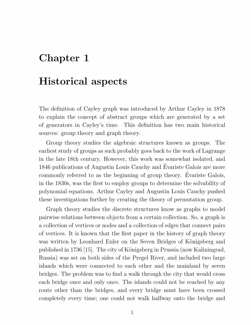
The definition of Cayley graph was introduced by Arthur Cayley in 1878
to explain the concept of abstract groups which are generated by a set
of generators in Cayley’s time. This definition has two main historical
sources: group theory and graph theory.
Group theory studies the algebraic structures known as groups. The
earliest study of groups as such probably goes back to the work of Lagrange
in the late 18th century. However, this work was somewhat isolated, and
1846 publications of Augustin Louis Cauchy and Evariste Galois are more
commonly referred to as the beginning of group theory. Evariste Galois,
in the 1830s, was the first to employ groups to determine the solvability of
polynomial equations. Arthur Cayley and Augustin Louis Cauchy pushed
these investigations further by creating the theory of permutation group.
Graph theory studies the discrete structures know as graphs to model
pairwise relations between objects from a certain collection. So, a graph is
a collection of vertices or nodes and a collection of edges that connect pairs
of vertices. It is known that the first paper in the history of graph theory
was written by Leonhard Euler on the Seven Bridges of Konigsberg and
published in 1736 [15]. The city of Konigsberg in Prussia (now Kaliningrad,
Russia) was set on both sides of the Pregel River, and included two large
islands which were connected to each other and the mainland by seven
bridges. The problem was to find a walk through the city that would cross
each bridge once and only once. The islands could not be reached by any
route other than the bridges, and every bridge must have been crossed
completely every time; one could not walk halfway onto the bridge and
5
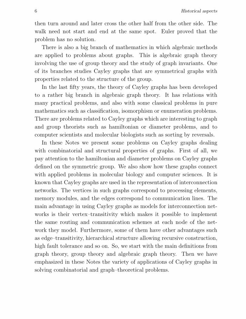
6 Historical aspects
then turn around and later cross the other half from the other side. The
walk need not start and end at the same spot. Euler proved that the
problem has no solution.
There is also a big branch of mathematics in which algebraic methods
are applied to problems about graphs. This is algebraic graph theory
involving the use of group theory and the study of graph invariants. One
of its branches studies Cayley graphs that are symmetrical graphs with
properties related to the structure of the group.
In the last fifty years, the theory of Cayley graphs has been developed
to a rather big branch in algebraic graph theory. It has relations with
many practical problems, and also with some classical problems in pure
mathematics such as classification, isomorphism or enumeration problems.
There are problems related to Cayley graphs which are interesting to graph
and group theorists such as hamiltonian or diameter problems, and to
computer scientists and molecular biologists such as sorting by reversals.
In these Notes we present some problems on Cayley graphs dealing
with combinatorial and structural properties of graphs. First of all, we
pay attention to the hamiltonian and diameter problems on Cayley graphs
defined on the symmetric group. We also show how these graphs connect
with applied problems in molecular biology and computer sciences. It is
known that Cayley graphs are used in the representation of interconnection
networks. The vertices in such graphs correspond to processing elements,
memory modules, and the edges correspond to communication lines. The
main advantage in using Cayley graphs as models for interconnection net-
works is their vertex–transitivity which makes it possible to implement
the same routing and communication schemes at each node of the net-
work they model. Furthermore, some of them have other advantages such
as edge–transitivity, hierarchical structure allowing recursive construction,
high fault tolerance and so on. So, we start with the main definitions from
graph theory, group theory and algebraic graph theory. Then we have
emphasized in these Notes the variety of applications of Cayley graphs in
solving combinatorial and graph–theoretical problems.
Chapter 2
Definitions, basic properties and
examples
In this section, basic definitions are given, notation is introduced and ex-
amples of graphs are presented. We also discuss some combinatorial and
structural properties of Cayley graphs that we will consider later. For
more definitions and details on graphs and groups we refer the reader to
the books [13, 14, 18, 59].
2.1 Groups and graphs
Let G be a finite group. The elements of a subset S of a group G are called
generators of G, and S is said to be a generating set, if every element of
G can be expressed as a finite product of generators. We will also say
that G is generated by S. The identity of a group G will be denoted by
e and the operation will be written as multiplication. A subset S of G is
identity free if e 6∈ S and it is symmetric (or closed under inverses) if s ∈ S
implies s−1 ∈ S. The last condition can be also denoted by S = S−1, where
S−1 = {s−1 : s ∈ S}.
A permutation π on the set X = {1, . . . , n} is a bijective mapping (i.e.
one–to–one and surjective) from X to X. We write a permutation π in
one–line notation as π = [π1, π2, . . . , πn] where πi = π(i) are the images of
the elements for every i ∈ {1, . . . , n}. We denote by Symn the group of all
permutations acting on the set {1, . . . , n}, also called the symmetric group.
The cardinality of the symmetric group Symn is defined by the number of
all its elements, that is |Symn| = n!. In particular, the symmetric group
7

8 Definitions, basic properties and examples
��
��
��
����
��
��
[213]
[231]
[312]
[132]
[321][123]
��
�� ��
��
��
��
[213] [231]
[321]
[312][132]
[123]
Sym3(T ) K3,3�
Symn is generated by transpositions swapping any two neighbors elements
of a permutations that is the generating set S = {(1, 2), (2, 3), ..., (n −
1, n)}. This set of generators is also known as the set of the (n−1) Coxeter
generators of Symn and it is an important instance in combinatorics of
Coxeter groups (for details see [16]).
Let S ⊂ G be the identity free and symmetric generating set of a finite
group G. In the Cayley graph Γ = Cay(G, S) = (V, E) vertices correspond
to the elements of the group, i.e. V = G, and edges correspond to mul-
tiplication on the right by generators, i.e. E = {{g, gs} : g ∈ G, s ∈ S}.
The identity free condition is imposed so that there are no loops in Γ. The
reason for the second condition is that an edge should be in the graph no
matter which end vertex is used. So when there is an edge from g to gs,
there is also an edge from gs to (gs)s−1 = g.
For example, if G is the symmetric group Sym3, and the generating set
S is presented by all transpositions from the set T = {(12), (23), (13)},
then the Cayley graph Sym3(T ) = Cay(Sym3, T ) is isomorphic to K3,3
(see Figure 1). Here Kp,q is the complete bipartite graph with p and q
vertices in the two parts, respectively.
Figure 1. The Cayley graph Sym3(T ) is isomorphic to K3,3
Let us note here that if the symmetry condition doesn’t hold in the
definition of the Cayley graph then we have the Cayley digraphs which are
not considered in these Lecture Notes.

2.2. SYMMETRY AND REGULARITY OF GRAPHS 9
�
�
�
�
�
�
�
�
�
�
�
�
�
�
�
�
�
�
�
�
�
�
�
� ����
��
��
��
��
��
��
u v
u′
v′
2.2 Symmetry and regularity of graphs
Let Γ = (V, E) be a finite simple graph. A graph Γ is said to be regular
of degree k, or k–regular if every vertex has degree k. A regular graph of
degree 3 is called cubic.
A permutation σ of the vertex set of a graph Γ is called an automorphism
provided that {u, v} is an edge of Γ if and only if {σ(u), σ(v)} is an edge
of Γ. A graph Γ is said to be vertex–transitive if for any two vertices u
and v of Γ, there is an automorphism σ of Γ satisfying σ(u) = v. Any
vertex–transitive graph is a regular graph. However, not every regular
graph is a vertex–transitive graph. For example, the Frucht graph is not
vertex–transitive (see Figure 1.) A graph Γ is said to be edge–transitive
if for any pair of edges x and y of Γ, there is an automorphism σ of Γ
that maps x into y. These symmetry properties require that every vertex
or every edge in a graph Γ looks the same and these two properties are not
interchangeable. A graph Γ presented in Figure 1 is vertex–transitive but
not edge–transitive since there is no an automorphism between edges {u, v}
and {u′, v′}. The complete bipartite graph Kp,q, p 6= q, is the example of
edge–transitive but not vertex–transitive graph.
Figure 2. The Frucht graph: regular but not vertex–transitive.
Graph Γ: vertex–transitive but not edge–transitive.
The Frucht graph Γ
10 Definitions, basic properties and examples
��
��������
����
��
��
�� ��
�� ��
��
��
��
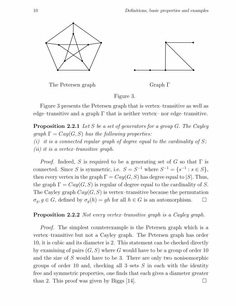
Figure 3.
The Petersen graph Graph Γ
Figure 3 presents the Petersen graph that is vertex–transitive as well as
edge–transitive and a graph Γ that is neither vertex– nor edge–transitive.
Proposition 2.2.1 Let S be a set of generators for a group G. The Cayley
graph Γ = Cay(G, S) has the following properties:
(i) it is a connected regular graph of degree equal to the cardinality of S;
(ii) it is a vertex–transitive graph.
Proof. Indeed, S is required to be a generating set of G so that Γ is
connected. Since S is symmetric, i.e. S = S−1 where S−1 = {s−1 : s ∈ S},
then every vertex in the graph Γ = Cay(G, S) has degree equal to |S|. Thus,
the graph Γ = Cay(G, S) is regular of degree equal to the cardinality of S.
The Cayley graph Cay(G, S) is vertex–transitive because the permutation
σg, g ∈ G, defined by σg(h) = gh for all h ∈ G is an automorphism. �
Proposition 2.2.2 Not every vertex–transitive graph is a Cayley graph.
Proof. The simplest counterexample is the Petersen graph which is a
vertex–transitive but not a Cayley graph. The Petersen graph has order
10, it is cubic and its diameter is 2. This statement can be checked directly
by examining of pairs (G, S) where G would have to be a group of order 10
and the size of S would have to be 3. There are only two nonisomorphic
groups of order 10 and, checking all 3–sets S in each with the identity
free and symmetric properties, one finds that each gives a diameter greater
than 2. This proof was given by Biggs [14]. �

2.2. SYMMETRY AND REGULARITY OF GRAPHS 11
v S1(v) Sd(v)S2(v)
a1
k 1 b1c2 b2
a2 ad
cd
Denote by d(u, v) the path distance between the vertices u and v in Γ,
and by d(Γ) = max{d(u, v) : u, v ∈ V } the diameter of Γ. In particular, in
a Cayley graph the diameter is the maximum, over g ∈ G, of the length of
a shortest expression for g as a product of generators. Let
Sr(v) = {u ∈ V (Γ) : d(v, u) = r} and Br(v) = {u ∈ V (Γ) : d(v, u) 6 r}
be the metric sphere and the metric ball of radius r centered at the vertex
v ∈ V (Γ), respectively. The vertices u ∈ Br(v) are r-neighbors of the
vertex v. For v ∈ V (Γ) we put ki(v) = |Si(v)| and for u ∈ Si(v) we set
ci(v, u) = |{x ∈ Si−1(v) : d(x, u) = 1}|,
ai(v, u) = |{x ∈ Si(v) : d(x, u) = 1}|,
bi(v, u) = |{x ∈ Si+1(v) : d(x, u) = 1}|.
From this a1(v, u) = a1(u, v) is the number of triangles over the edge {v, u}
and c2(v, u) is the number of common neighbors of v ∈ V and u ∈ S2(v). Let
λ = λ(Γ) = maxv∈V, u∈S1(v) a1(v, u) and µ = µ(Γ) = maxv∈V, u∈S2(v) c2(v, u).
A simple connected graph Γ is distance–regular if there are integers
bi, ci for i > 0 such that for any two vertices v and u at distance d(v, u) =
i there are precisely ci neighbors of u in Si−1(v) and bi neighbors of u
in Si+1(v). Evidently Γ is regular of valency k = b0, or k-regular. The
numbers ci, bi and ai = k − bi − ci, i = 0, . . . , d , where d = d(Γ) is the
diameter of Γ, are called the intersection numbers of Γ and the sequence
(b0, b1, . . . , bd−1; c1, c2, . . . , cd) is called the intersection array of Γ.
The schematic representation of the intersection array for a distance–
regular graph is given below:

12 Definitions, basic properties and examples
��
��
��
��
��
��
����
�� ��
��
��
uv
w
Figure 4. The cyclic 6–ladder L6
A k-regular simple graph Γ is strongly regular if there exist integers λ
and µ such that every adjacent pair of vertices has λ common neighbors,
and every nonadjacent pair of vertices has µ common neighbors. A simple
connected graph Γ is distance–transitive if, for any two arbitrary–chosen
pairs of vertices (v, u) and (v′, u′) at the same distance d(v, u) = d(v′, u′),
there is an automorphism σ of Γ satisfying σ(v) = v′ and σ(u) = u′.
Proposition 2.2.3 Any distance–transitive graph is vertex–transitive.
This statement is obvious (consider two vertices at distance 0). How-
ever, the converse is not true in general. There exist vertex–transitive
graphs that are not distance–transitive. For instance, the cyclic 6–ladder
L6 is clearly vertex–transitive - we can rotate and reflect it (see Figure 4).
However, it is not distance–transitive since there are two pairs of vertices
u, v and u, w at distance two, i.e. d(u, v) = d(u, w) = 2, such that there is
no automorphism that moves one pair of vertices into the other, as there
is only one path between vertices u, w, while there are two paths for the
vertices u, v.
The following graphs are distance–transitive: the complete graphs Kn;
the cycles Cn; the platonic graphs that are obtained from the five Pla-
tonic solids: their vertices and edges form distance–regular and distance–
transitive graphs as well with intersection arrays {3; 1} for tetrahedron,
{4, 1; 1, 4} for octahedron, {3, 2, 1; 1, 2, 3} for cube, {5, 2, 1; 1, 2, 5} for icosa-
hedron, {3, 2, 1, 1, 1; 1, 1, 1, 2, 3} for dodecahedron; and many others.
2.2. SYMMETRY AND REGULARITY OF GRAPHS 13
� �
�
�
� �
�
�
��
�� ��
��
����
��
��
��
�
�
��
�
�
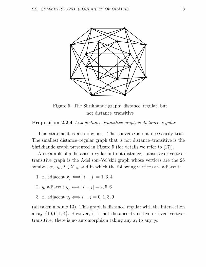
Figure 5. The Shrikhande graph: distance–regular, but
not distance–transitive
Proposition 2.2.4 Any distance–transitive graph is distance–regular.
This statement is also obvious. The converse is not necessarily true.
The smallest distance–regular graph that is not distance–transitive is the
Shrikhande graph presented in Figure 5 (for details we refer to [17]).
An example of a distance–regular but not distance–transitive or vertex–
transitive graph is the Adel’son–Vel’skii graph whose vertices are the 26
symbols xi, yi, i ∈ Z13, and in which the following vertices are adjacent:
1. xi adjacent xj ⇐⇒ |i− j| = 1, 3, 4
2. yi adjacent yj ⇐⇒ |i− j| = 2, 5, 6
3. xi adjacent yj ⇐⇒ i− j = 0, 1, 3, 9
(all taken modulo 13). This graph is distance–regular with the intersection
array {10, 6; 1, 4}. However, it is not distance–transitive or even vertex–
transitive: there is no automorphism taking any xi to any yi.
14 Definitions, basic properties and examples
2.3 Examples
2.3.1 Some families of Cayley graphs
The complete graph Kn is a Cayley graph on the additive group Zn of
integers modulo n with generating set of all non–zero elements of Zn.
The circulant is the Cayley graph Cay(Zn, S) where S ⊂ Zn is an arbitrary
generating set. The most prominent example is the cycle Cn.
The multidimensional torus Tn,k, n > 2 , k > 2 , is the cartesian product
of n cycles of length k. It has kn vertices of degree 2n and its diameter is
ndk2e. It is the Cayley graph of the group Znk that is the direct product of
Zk with itself n times, which is generated by 2n generators from the set
S = {(0, . . . , 0︸ ︷︷ ︸
i
, 1, 0, . . . , 0︸ ︷︷ ︸
n−i−1
), (0, . . . , 0︸ ︷︷ ︸
i
,−1, 0, . . . , 0︸ ︷︷ ︸
n−i−1
), 0 6 i 6 n− 1}.
The hypercube (or n-dimensional cube) Hn is the graph with vertex set
{x1x2 . . . xn : xi ∈ {0, 1}} in which two vertices (v1v2 . . . vn) and (u1u2 . . . un)
are adjacent if and only if vi = ui for all but one i , 1 6 i 6 n. It is a
distance–transitive graph with diameter and degree of n and can be con-
sidered as a particular case of torus, namely Tn,2, since it is the cartesian
product of n complete graphs K2. It is the Cayley graph on the group Zn2
with the generating set S = {(0, . . . , 0︸ ︷︷ ︸
i
, 1, 0, . . . , 0︸ ︷︷ ︸n−i−1
), 0 6 i 6 n− 1}.
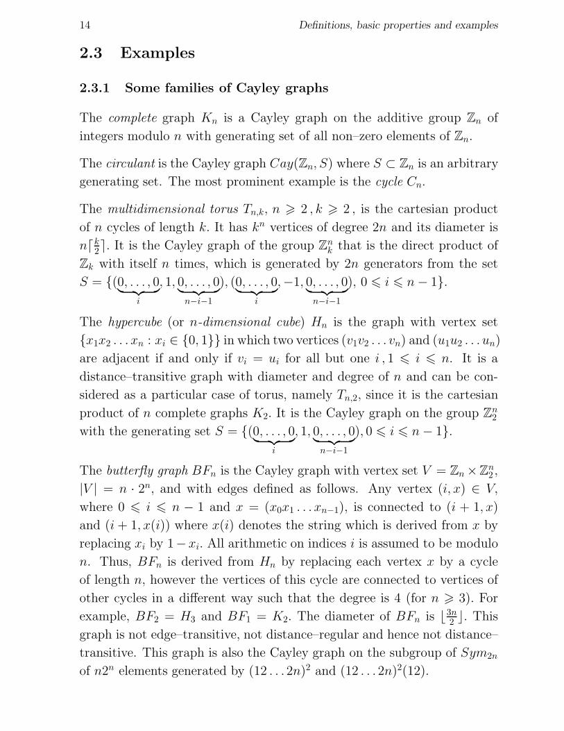
The butterfly graph BFn is the Cayley graph with vertex set V = Zn×Zn2 ,
|V | = n · 2n, and with edges defined as follows. Any vertex (i, x) ∈ V,
where 0 6 i 6 n − 1 and x = (x0x1 . . . xn−1), is connected to (i + 1, x)
and (i+ 1, x(i)) where x(i) denotes the string which is derived from x by
replacing xi by 1− xi. All arithmetic on indices i is assumed to be modulo
n. Thus, BFn is derived from Hn by replacing each vertex x by a cycle
of length n, however the vertices of this cycle are connected to vertices of
other cycles in a different way such that the degree is 4 (for n > 3). For
example, BF2 = H3 and BF1 = K2. The diameter of BFn is b3n2 c. This
graph is not edge–transitive, not distance–regular and hence not distance–
transitive. This graph is also the Cayley graph on the subgroup of Sym2n
of n2n elements generated by (12 . . . 2n)2 and (12 . . . 2n)2(12).

2.3. EXAMPLES 15
������
������
������
{2,0} {2,1} {2,2}
{1,0} {1,1} {1,2}
{0,0} {0,1} {0,2}
2.3.2 Hamming graph: distance–transitive Cayley graph
Let F nq be the Hamming space (where Fq is the field of q elements) consist-
ing of the qn vectors (or words) of length n over the alphabet {0, 1, ..., q−
1}, q > 2. This space is endowed with the Hamming distance d(x, y)
which equals to the number of coordinate positions in which x and y differ.
This space can be viewed as the Hamming graph Ln(q) with vertex set
given by the vector space F nq where {x, y} is an edge of Ln(q) if and only
if d(x, y) = 1. The Hamming graph Ln(q) is, equivalently, the cartesian
product of n complete graphs Kq. This graph has the following properties:
1. its diameter is n;
2. it is distance–transitive and Cayley graph;
3. it has intersection array given by bj = (n − j)(q − 1) and cj = j for
0 6 j 6 n.
Indeed, the Hamming graph is the Cayley graph on the additive group
F nq when we take the generating set S = {xei : x ∈ (Fq)
×, 1 6 i 6 n}
where (Fq)× is the cartesian product of Fq and ei = (0, ..., 0, 1, 0, ...0) are
the standard basis vectors of F nq .
For the particular case n = 2 the Hamming graph L2(q) is also known
as the lattice graph over Fq. This graph is strongly regular with parameters
|V (L2(q))| = q2, k = 2(q − 1), λ = q − 2, µ = 2. The lattice graph L2(3) is
presented in Figure 6.
Figure 6. The lattice graph L2(3)
16 Definitions, basic properties and examples
��
��
��
��
��
��
{1,2}
{1,4}{1,3}
{2,4}{2,3}
{3,4}
2.3.3 Johnson graph: distance–transitive not Cayley graph
The Johnson graph J(n,m) is defined on the vertex set of the m–element
subsets of an n–element set X. Two vertices are adjacent when they meet
in a (m − 1)–element set. On J(n,m) the Johnson distance is defined as
half the (even) Hamming distance, and two vertices x, y are joined by an
edge if and only if they are at Johnson distance one from each other. This
graph has the following properties:
1. its diameter d is min(m, n−m);
2. it is distance–transitive but not Cayley graph (for m > 2);
3. it has intersection array given by bj = (m− j)(n−m− j) and cj = j2
for 0 6 j 6 d.
Let us note that J(n, 1) ∼= Kn and it is a Cayley graph. In general, to
show that the Johnson graph is not a Cayley graph just take n or n − 1
congruent to 2(mod 4). Then(n2
)is odd, etc.
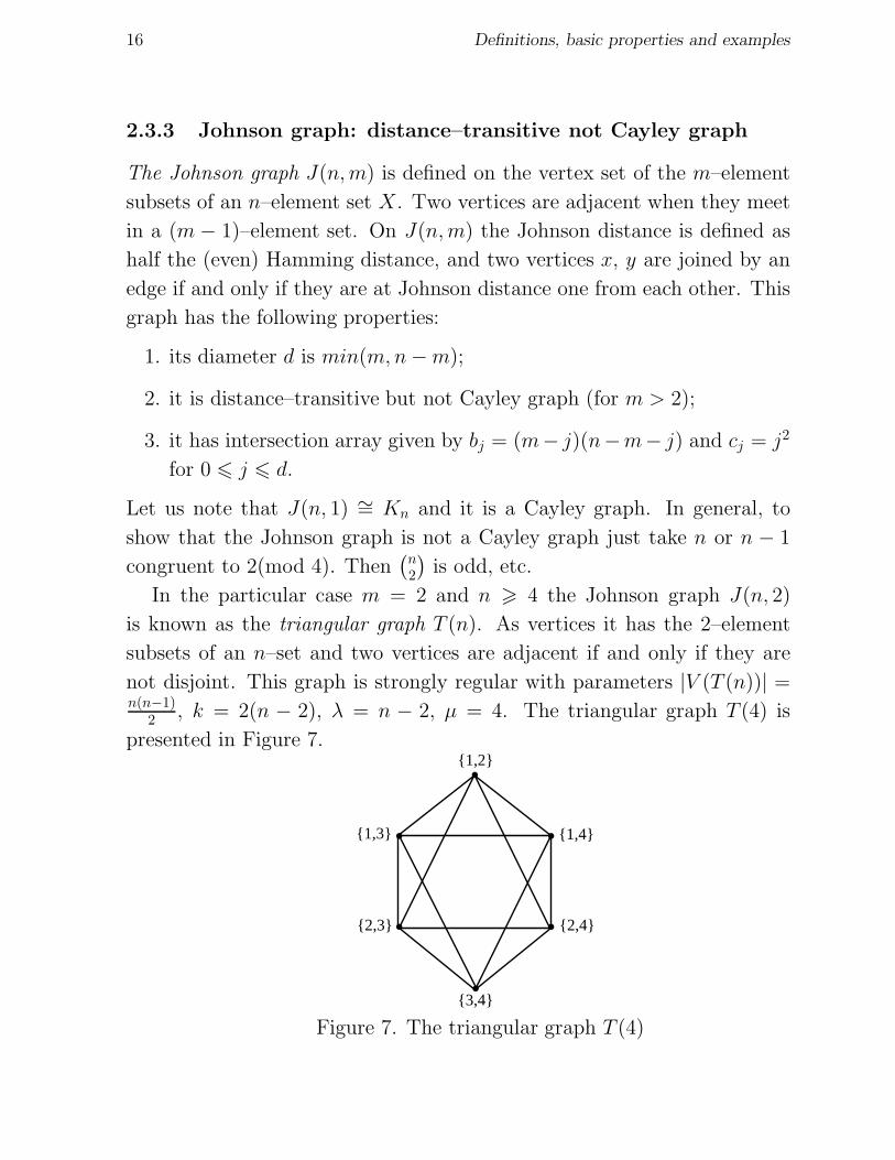
In the particular case m = 2 and n > 4 the Johnson graph J(n, 2)
is known as the triangular graph T (n). As vertices it has the 2–element
subsets of an n–set and two vertices are adjacent if and only if they are
not disjoint. This graph is strongly regular with parameters |V (T (n))| =n(n−1)
2 , k = 2(n − 2), λ = n − 2, µ = 4. The triangular graph T (4) is
presented in Figure 7.
Figure 7. The triangular graph T (4)
2.3. EXAMPLES 17
2.3.4 Kneser graph: when it is a Cayley graph
The Kneser graph K(n, k), k > 2, n > 2k + 1, is the graph whose vertices
correspond to the k-element subsets of a set of n elements, and where
two vertices are connected if and only if the two corresponding sets are
disjoint. The graph K(2n− 1, n− 1) is also referred as the odd graph On.
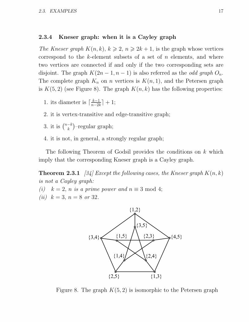
The complete graph Kn on n vertices is K(n, 1), and the Petersen graph
is K(5, 2) (see Figure 8). The graph K(n, k) has the following properties:
1. its diameter is d k−1n−2k
e+ 1;
2. it is vertex-transitive and edge-transitive graph;
3. it is(n−kk
)–regular graph;
4. it is not, in general, a strongly regular graph;
The following Theorem of Godsil provides the conditions on k which
imply that the corresponding Kneser graph is a Cayley graph.
Theorem 2.3.1 [34] Except the following cases, the Kneser graph K(n, k)
is not a Cayley graph:
(i) k = 2, n is a prime power and n ≡ 3 mod 4;
(ii) k = 3, n = 8 or 32.
Figure 8. The graph K(5, 2) is isomorphic to the Petersen graph
18 Definitions, basic properties and examples
2.3.5 Cayley graphs on the symmetric group
In this section we present Cayley graphs on the symmetric group Symn
that are applied in computer science, molecular biology and coding theory.
The Transposition graph Symn(T ) on Symn is generated by transposi-
tions from the set T = {ti,j ∈ Symn, 1 6 i < j 6 n}, where ti,j transposes
the ith and jth elements of a permutation when multiplied on the right.
The distance in this graph is defined as the least number of transposi-
tions transforming one permutation into another. The transposition graph
Symn(T ), n > 3, has the following properties:
1. it is a connected graph of order n! and diameter n− 1;
2. it is bipartite(n2
)–regular graph;
3. it has no subgraphs isomorphic to K2,4;
4. it is edge–transitive but not distance–regular and hence not distance–
transitive (for n > 3).
This graph arises in molecular biology for analysing transposons (genetic
transpositions) that are mutations transferring a chromosomal segment to
a new position on the same or another chromosome [69, 74]. It is also
considered in coding theory for solving a reconstruction problem [61].
The Bubble–sort graph Symn(t), n > 3, on Symn is generated by trans-
positions from the set t = {ti,i+1 ∈ Symn, 1 6 i < n}, where ti,i+1 are
2-cycles interchanging ith and (i + 1)th elements of a permutation when
multiplied on the right. This graph has the following properties:
1. it is a connected graph of order n! and diameter(n2
);
2. it is bipartite (n− 1)–regular graph;
3. it has no subgraphs isomorphic to K2,3;
4. it is edge–transitive but not distance–regular and hence not distance–
transitive (for n > 3).
This graph arises in computer science to represent interconnection net-
works [38] as well as in computer programming [57].
2.3. EXAMPLES 19
The Star graph Sn = Symn(st) on Symn is generated by transpositions
from the set st = {t1,i ∈ Symn, 1 < i 6 n} with the following properties:
1. it is a connected graph of order n! and diameter b3(n−1)2
c;
2. it is bipartite (n− 1)–regular graph;
3. it has no cycles of lengths 3,4,5,7;
4. it is edge–transitive but not distance–regular and hence not distance–
transitive (for n > 3).
This graph is one of the most investigated in the theory of intercon-
nection networks since many parallel algorithms are efficiently mapped on
this graph (see [1, 38, 58]). In [1] it is shown that the diameter of the Star
graph is b3(n−1)2 c. Moreover, it is claimed that when n is odd the diameter
becomes 3(n−1)2
and when n is even, 1 + 3(n−2)2
. This is shown by indicating
two permutations which require precisely these number of steps. When n
is odd the permutation π = [1, 3, 2, 5, 4, . . . , n, n−1] is considered. For any
swap, one and only one position other than the first is involved. Now it is
easily confirmed that to move 3 and 2 to their correct positions, at least
three swaps each involving the second and third position will be required.
Since there are (n−1)2 such pairs, the above diameter follows. Likewise, when
n is even, the permutation π = [2, 1, 4, 3, 6, 5, . . . , n, n − 1] is considered.
One can swap position 2 with one, but the remaining (n−2)2 pairs again each
require three. Thus, the indicated diameter again follows.
The Reversal graph Symn(R) is defined on Symn and generated by the
reversals from the set R = {ri,j ∈ Symn, 1 6 i < j 6 n} where a reversal
ri,j is the operation of reversing segments [i, j], 1 6 i < j 6 n, of a permu-
tation when multiplied on the right, i.e. [. . . , πi, πi+1, . . . , πj−1, πj, . . .]ri,j =
[. . . , πj, πj−1, . . . , πi+1, πi, . . .]. For n > 3 it has the following properties:
1. it is a connected graph of order n! and diameter n− 1;
2. it is(n2
)–regular graph;
3. it has no contain triangles nor subgraphs isomorphic to K2,4;
20 Definitions, basic properties and examples
4. it is not edge–transitive, not distance–regular and hence not distance–
transitive (for n > 3).
The reversal distance between two permutations in this graph, that is
the least number of reversals needed to transform one permutation into
another, corresponds to the reversal mutations in molecular biology. Re-
versal distance measures the amount of evolution that must have taken
place at the chromosome level, assuming evolution proceeded by inver-
sion. The analysis of genomes evolving by inversions leads to the combi-
natorial problem of sorting by reversals (for more details see Section 4.4).
This graph also appears in coding theory in solving a reconstruction prob-
lem [48, 49, 51].
The Pancake graph Pn = Cay(Symn, PR), n > 2, is the Cayley graph
on Symn with the generating set PR = {ri ∈ Symn, 2 6 i 6 n} of all
prefix–reversals ri reversing the order of any substring [1, i], 2 6 i 6 n, of a
permutation π when multiplied on the right, i.e. [π1 . . . πi πi+1 . . . πn] ri =
[πi . . . π1 πi+1 . . . πn]. For n > 3 this graph has the following properties:
1. it is a connected graph of order n!;
2. it is (n− 1)–regular graph;
3. it has no cycles of lengths 3,4,5,6;
4. it is not edge–transitive, not distance–regular and hence not distance–
transitive (for n > 4).
This graph is well known because of the combinatorial Pancake problem
which was posed in [27] as the problem of finding its diameter. The problem
is still open. Some upper and lower bounds [32, 39] as well as exact values
for 2 6 n 6 19 are known [4, 19]. One of the main difficulties in solving
this problem is a complicated cycle structure of the Pancake graph. As
it was shown in [42, 76], all cycles of length l, where 6 6 l 6 n!, can be
embedded in the Pancake graph Pn, n > 3. In particular, the graph is a
Hamiltonian [82]. We will discuss all these problems on the Pancake graph
in the next sections.
Chapter 3
Hamiltonicity of Cayley graphs
Let Γ = (V, E) be a connected graph where V = {v1, v2, . . . , vn}. A Hamil-
tonian cycle in Γ is a spanning cycle (v1, v2, . . . , vn, v1) and a Hamiltonian
path in Γ is a path (v1, v2, . . . , vn). We also say that a graph is Hamiltonian
if it contains a Hamiltonian cycle. The Hamiltonicity problem, that is to
check whether a graph is a Hamiltonian, was stated by Sir W.R. Hamil-
ton in the 1850s (see [36]). Studying the Hamiltonian property of graphs
is a favorite problem for graph and group theorists. Testing whether a
graph is Hamiltonian is an NP-complete problem [31]. Hamiltonian paths
and cycles naturally arise in computer science (see [58]), in the study of
word–hyperbolic groups and automatic groups (see [28]), and in combina-
torial designs (see [26]). For example, Hamiltonicity of the hypercube Qn
is connected to a Gray code that corresponds to a Hamiltonian cycle.
3.1 Hypercube graphs and a Gray code
A hypercube graph Qn = Ln(2) is a particular case of the Hamming
graph considered in Section 2.3.2. The hypercube graph Qn = Ln(2)
is a n–regular graph with 2n vertices presented by vectors of length n.
Two vertices are adjacent if and only if the corresponding vectors dif-
fer exactly in one position. The hypercube graph Qn is, equivalently,
the cartesian product of n two–vertex complete graphs K2. It is also
a Cayley graph on the finite additive group Zn2 with the generating set
S = {(0, . . . , 0︸ ︷︷ ︸
i
, 1, 0, . . . , 0︸ ︷︷ ︸n−i−1
), 0 6 i 6 n− 1}, where |S| = n.
It is well known fact that every hypercube graph Qn is Hamiltonian for
21
22 Hamiltonicity of Cayley graphs
n > 1, and any Hamiltonian cycle of a labeled hypercube graph defines a
Gray code [77]. More precisely there is a bijective correspondence between
the set of n–bit cyclic Gray codes and the set of Hamiltonian cycles in
the hypercube Qn. By the definition, the reflected binary code, also known
as Gray code after Frank Gray, is a binary numeral system where two
successive values differ in only one bit.
The Gray code list for n bits can be generated recursively from the list
for n− 1 bits by reflecting the list (i.e. listing the entries in reverse order),
concatenating the original list with the reversed list, prefixing the entries
in the original list with a binary 0, and then prefixing the entries in the
reflected list with a binary 1. For example, generating the n = 3 list from
the n = 2 list we have:
STEP 1.
2–bit list: 00, 01, 11, 10;
reflected : 10, 11, 01, 00;
STEP 2.
prefix old entries with 0 : 000, 001, 011, 010;
prefix new entries with 1: 110, 111, 101, 100;
STEP 3.
concatenated: 000, 001, 011, 010, 110, 111, 101, 100.
So, for n = 3 the Gray code can be also presented as:
000 001 011 010 | 110 111 101 100.
and for n = 4 the Gray code is presented as:
0000 0001 0011 0010 0110 0111 0101 0100 | 1100 1101 1111 1110 1010 1011 1001 1000.
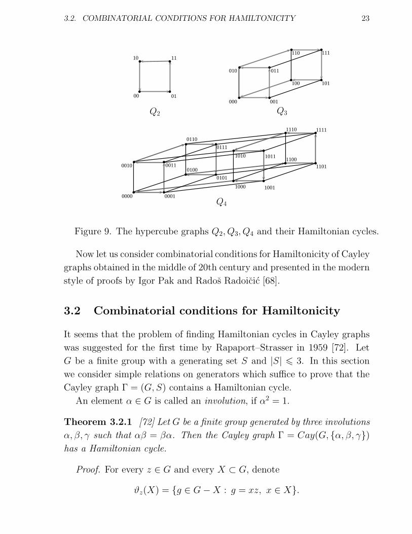
By the definition, the Gray codes define the set of vectors of the hypercube
graphs such that two successive vectors differ in only one bit. Hence, the
Gray codes correspond to the Hamiltonian path in the hypercube graphs.
Moreover, since the first and last vectors also differ in one position we
actually have the Hamiltonian cycles. The hypercube graphs Q2, Q3, Q4
and their Hamiltonian cycles are presented in Figure 9.
3.2. COMBINATORIAL CONDITIONS FOR HAMILTONICITY 23
����
����
10 11
00 01
����
����
010 011
000 001
����
����
110 111
100 101
Q2 Q3
����
����
0010 0011
0000 0001
����
����
0110
0111
0100
0101
����
����
1010 1011
1000 1001
����
����
1110 1111
11001101
Q4
Figure 9. The hypercube graphs Q2, Q3, Q4 and their Hamiltonian cycles.
Now let us consider combinatorial conditions for Hamiltonicity of Cayley
graphs obtained in the middle of 20th century and presented in the modern
style of proofs by Igor Pak and Rados Radoicic [68].
3.2 Combinatorial conditions for Hamiltonicity
It seems that the problem of finding Hamiltonian cycles in Cayley graphs
was suggested for the first time by Rapaport–Strasser in 1959 [72]. Let
G be a finite group with a generating set S and |S| 6 3. In this section
we consider simple relations on generators which suffice to prove that the
Cayley graph Γ = (G, S) contains a Hamiltonian cycle.
An element α ∈ G is called an involution, if α2 = 1.
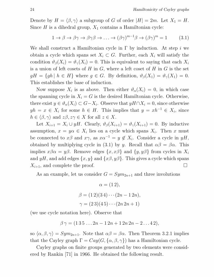
Theorem 3.2.1 [72] Let G be a finite group generated by three involutions
α, β, γ such that αβ = βα. Then the Cayley graph Γ = Cay(G, {α, β, γ})
has a Hamiltonian cycle.
Proof. For every z ∈ G and every X ⊂ G, denote
ϑz(X) = {g ∈ G−X : g = xz, x ∈ X}.
24 Hamiltonicity of Cayley graphs
Denote by H = 〈β, γ〉 a subgroup of G of order |H| = 2m. Let X1 = H.
Since H is a dihedral group, X1 contains a Hamiltonian cycle:
1 → β → βγ → βγβ → . . . → (βγ)m−1β → (βγ)m = 1 (3.1)
We shall construct a Hamiltonian cycle in Γ by induction. At step i we
obtain a cycle which spans set Xi ⊂ G. Further, each Xi will satisfy the
condition ϑβ(Xi) = ϑγ(Xi) = 0. This is equivalent to saying that each Xi
is a union of left cosets of H in G, where a left coset of H in G is the set
gH = {gh | h ∈ H} where g ∈ G. By definition, ϑβ(X1) = ϑγ(X1) = 0.
This establishes the base of induction.
Now suppose Xi is as above. Then either ϑα(Xi) = 0, in which case
the spanning cycle in Xi = G is the desired Hamiltonian cycle. Otherwise,
there exist y ∈ ϑα(Xi) ⊂ G−Xi. Observe that yH∩Xi = 0, since otherwise
yh = x ∈ Xi for some h ∈ H. This implies that y = xh−1 ∈ Xi, since
h ∈ 〈β, γ〉 and zβ, zγ ∈ X for all z ∈ X.
Let Xi+1 = Xi ∪ yH. Clearly, ϑβ(Xi+1) = ϑγ(Xi+1) = 0. By inductive
assumption, x = yα ∈ Xi lies on a cycle which spans Xi. Then x must
be connected to xβ and xγ, as xα−1 = y 6∈ Xi. Consider a cycle in yH,
obtained by multiplying cycle in (3.1) by y. Recall that αβ = βα. This
implies xβα = yβ. Remove edges {x, xβ} and {y, yβ} from cycles in Xi
and yH, and add edges {x, y} and {xβ, yβ}. This gives a cycle which spans
Xi+1, and complete the proof. �
As an example, let us consider G = Sym2n+1 and three involutions
α = (1 2),
β = (1 2)(3 4) · · · (2n− 1 2n),
γ = (2 3)(4 5) · · · (2n 2n+ 1)
(we use cycle notation here). Observe that
β γ = (1 3 5 . . . 2n− 1 2n+ 1 2n 2n− 2 . . . 4 2),
so 〈α, β, γ〉 = Sym2n+1. Note that αβ = βα. Then Theorem 3.2.1 implies
that the Cayley graph Γ = Cay(G, {α, β, γ}) has a Hamiltonian cycle.
Cayley graphs on finite groups generated by two elements were consid-
ered by Rankin [71] in 1966. He obtained the following result.

3.2. COMBINATORIAL CONDITIONS FOR HAMILTONICITY 25
Theorem 3.2.2 [71] Let G be a finite group generated by two elements
α, β such that (αβ)2 = 1. Then the Cayley graph Γ = Cay(G, {α, β}) has
a Hamiltonian cycle.
Proof. Again, we use the same inductive assumption as in Theorem 3.2.1.
Moreover, we need a new simple label condition. Let H = 〈β〉, X1 = H,
and assume that ϑα(Xi) = ϑα−1(Xi) = 0. We also assume, by induction,
that restriction of Γ to Xi contains an oriented Hamiltonian cycle Ci which
contains only labels β and α−1. We call these the label conditions.
The base of induction is obvious, namely ϑα(X1) = ϑα−1(X1) = 0.
For the step of induction, consider y = xα ∈ ϑα(Xi) − Xi. Note that
the edge oriented towards x ∈ Xi in Ci cannot have label α−1 (otherwise
it is {y, x} whereas y 6∈ Xi), nor labels α or β−1 (by the label conditions).
Therefore, this edge has the only remaining label β, and {xβ−1, x} ∈ Ci.
Now consider a cycle R on yH with labels β on all edges, and observe
that
x → xα = y → xαβ = yβ → xβ−1 = xαβα → x
is a square which connects R and Ci. Formally, let
Ci+1 = Ci ∪ R+ {x, y}+ {yβ, xβ−1} − {xβ−1, x} − {y, yβ}
and observe that Ci is a Hamiltonian cycle on Xi+1 = Xi ∪ yH. Let Ci+1
inherit the orientation from Ci and check that now Ci+1 satisfies the label
conditions with respect to the orientation.
In the case when y = xα−1 6∈ Xi, we consider the edge leaving x ∈ Xi
and proceed verbatim. If ϑα(Xi) = ϑα−1(Xi) = 0, we have Xi = G which
completes the proof. �
As an example, let us consider G = Symn, α = (1 2 . . . n), β =
(2 3 . . . n). Then αβ−1 = (1n) is an involution, and by Theorem 3.2.2
the Cayley graph Γ = Cay(G, {α, β}) has a Hamiltonian cycle.
The both theorems are presented here with respect to the proof given
by Pak and Radoicic [68]. In Section 3.4 we will use these proofs to show
the result by Pak and Radoicic on Hamiltonicity of Cayley graphs on finite
groups with a small generating set.
26 Hamiltonicity of Cayley graphs
3.3 Lovasz and Babai conjectures
There is a famous Hamiltonicity problem for vertex–transitive graphs which
was posed by Laszlo Lovasz in 1970 and well–known as follows.
Problem 3.3.1 Does every connected vertex–transitive graph with more
than two vertices have a Hamiltonian path?
To be more precisely he stated a research problem in [63] asking how
one can
“ ... construct a finite connected undirected graph which is sym-
metric and has no simple path containing all the vertices. A graph
is symmetric if for any two vertices x and y it has an automor-
phism mapping x onto y.
However, traditionally (see [24]) the problem is formulated in the posi-
tive and considered as the Lovasz conjecture that every vertex–transitive
graph has a Hamiltonian path.
There are only four vertex–transitive graphs on more than two ver-
tices which do not have a Hamiltonian cycle, and all of these graphs
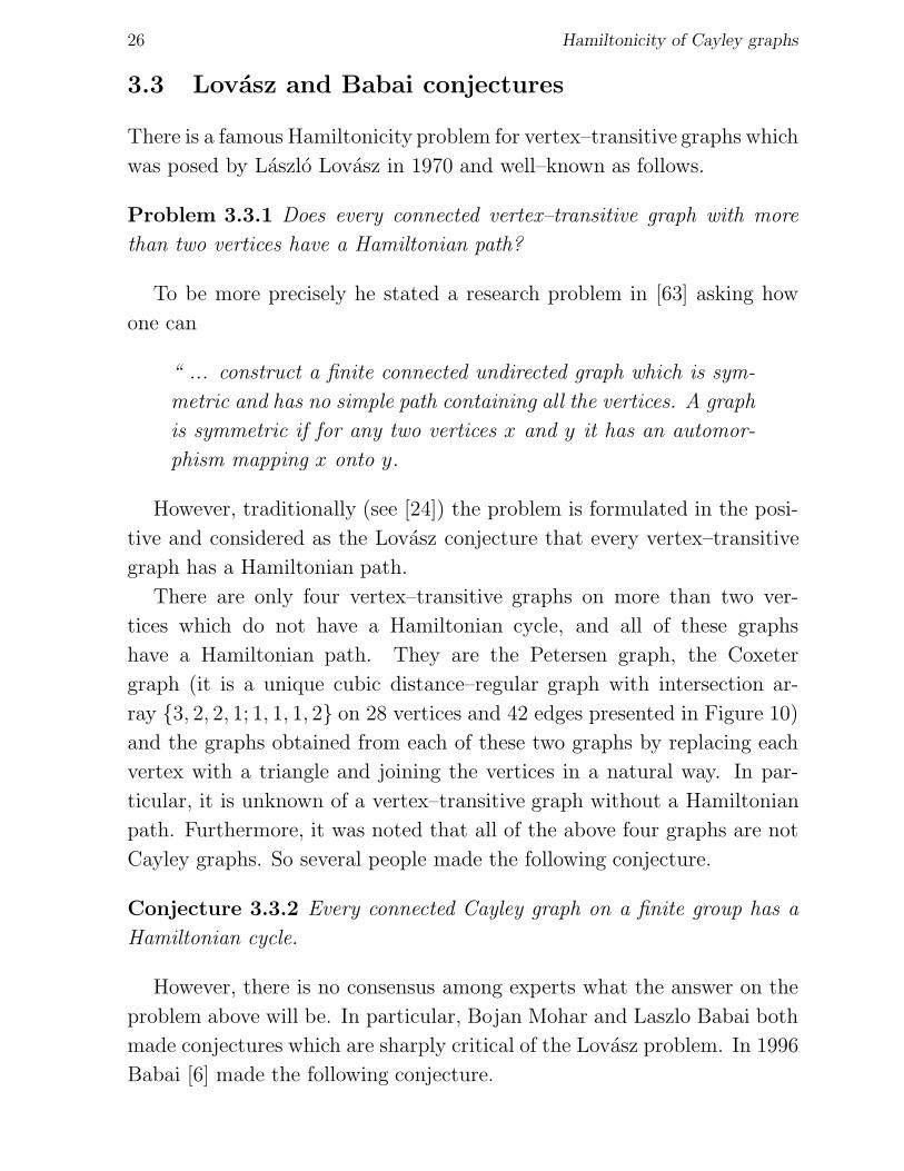
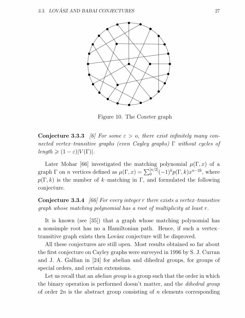
have a Hamiltonian path. They are the Petersen graph, the Coxeter
graph (it is a unique cubic distance–regular graph with intersection ar-
ray {3, 2, 2, 1; 1, 1, 1, 2} on 28 vertices and 42 edges presented in Figure 10)
and the graphs obtained from each of these two graphs by replacing each
vertex with a triangle and joining the vertices in a natural way. In par-
ticular, it is unknown of a vertex–transitive graph without a Hamiltonian
path. Furthermore, it was noted that all of the above four graphs are not
Cayley graphs. So several people made the following conjecture.
Conjecture 3.3.2 Every connected Cayley graph on a finite group has a
Hamiltonian cycle.
However, there is no consensus among experts what the answer on the
problem above will be. In particular, Bojan Mohar and Laszlo Babai both
made conjectures which are sharply critical of the Lovasz problem. In 1996
Babai [6] made the following conjecture.
3.3. LOVASZ AND BABAI CONJECTURES 27
��
�� ��
��
��
��
��
��
�� ��
����
��
��
��
��
��
��
����
��
��
��
��
��
����
��
��
Figure 10. The Coxeter graph
Conjecture 3.3.3 [6] For some ε > o, there exist infinitely many con-
nected vertex–transitive graphs (even Cayley graphs) Γ without cycles of
length > (1− ε)|V (Γ)|.
Later Mohar [66] investigated the matching polynomial µ(Γ, x) of a
graph Γ on n vertices defined as µ(Γ, x) =∑[n/2]
0 (−1)kp(Γ, k)xn−2k, where
p(Γ, k) is the number of k–matching in Γ, and formulated the following
conjecture.
Conjecture 3.3.4 [66] For every integer r there exists a vertex–transitive
graph whose matching polynomial has a root of multiplicity at least r.
It is known (see [35]) that a graph whose matching polynomial has
a nonsimple root has no a Hamiltonian path. Hence, if such a vertex–
transitive graph exists then Lovasz conjecture will be disproved.
All these conjectures are still open. Most results obtained so far about
the first conjecture on Cayley graphs were surveyed in 1996 by S. J. Curran
and J. A. Gallian in [24] for abelian and dihedral groups, for groups of
special orders, and certain extensions.
Let us recall that an abelian group is a group such that the order in which
the binary operation is performed doesn’t matter, and the dihedral group
of order 2n is the abstract group consisting of n elements corresponding

28 Hamiltonicity of Cayley graphs
to rotations of the polygon, and n corresponding to reflections. In 1983 it
was proved by Dragan Marusic [65] that this conjecture is true for abelian
groups.
Theorem 3.3.5 [65] A Cayley graph Γ = Cay(G, S) of an abelian group
G with at least three vertices contains a Hamiltonian cycle.
In 1989 Brian Alspach and Cun-Quan Zhang proved that every cubic
Cayley graph of a dihedral group is Hamiltonian [2]. A rare positive result
for all finite groups was obtained in 2009 by Pak and Radoicic [68].
Theorem 3.3.6 [68] Every finite group G of size |G| > 3 has a generating
set S of size |S| 6 log2 |G| such that the corresponding Cayley graph Γ =
Cay(G, S) has a Hamiltonian cycle.
This theorem shows that every finite group G has a Hamiltonian Cayley
graph with a generating set of small size. The bound on S is reached on
the group G = Zn2 for which the size of its smallest generating set is equal
to log2 |G|. For other groups the size of a generating set is much smaller.
For example, for all finite simple groups it is equal to two. This result can
be also considered as a corollary of the following natural conjecture.
Conjecture 3.3.7 [68] There exists ε > 0, such that for every finite
group G and every k > ε log2 |G|, the probability P (G, k) that the Cayley
graph Γ = Cay(G, S) with a random generating set S of size k contains a
Hamiltonian cycle, satisfies P (G, k) → 1 as |G| → ∞.
On one hand, this conjecture is much weaker then the Lovasz conjecture.
On the other hand, it also does not contradict the Babai conjecture. A
work by Michael Krivelevich and Benny Sudakov [56] shows that for every
ε > 0 a Cayley graph Γ = Cay(G, S) with large enough |G|, formed by
choosing a set S of ε log5 |G| random generators in a group G, is almost
surely Hamiltonian. Thus, they reduce the bound in Conjecture 3.3.7 down
to k > ε log5 |G|.
We present the proof of Theorem 3.3.6 in the next Section.

3.4. HAMILTONICITY OF CAYLEY GRAPHS ON FINITE GROUPS 29
3.4 Hamiltonicity of Cayley graphs on finite groups
Let G be a finite group of order n and H ⊂ G be a subgroup of G. Then
for g ∈ G the sets gH = {gh | h ∈ H} and Hg = {hg | h ∈ H} are left
and right cosets of H in G. A subgroup H of a group G is called a normal
subgroup (H CG) if the sets of left and right cosets of this subgroup in G
coincide, i.e. gH = Hg for any g ∈ G. A simple group is a nontrivial group
whose only normal subgroups are the trivial group and the group itself.
A factor group G/H of a group G with a normal subgroup H is called
the set of all cosets of H such that (aH)(bH) = (ab)H. A composition
series of a group G is a subnormal series such that
1 = H0 CH1 C . . .CHn = G,
with strict inclusions, where Hi is a maximal normal subgroup of Hi+1 for
all 0 6 i 6 n. Equivalently, a composition series is a subnormal series such
that each factor group Hi+1/Hi is simple. The factor groups are called
composition factors.
We need the following simple ”reduction lemma”.
Lemma 3.4.1 Let G be a finite group and let HCG be a normal subgroup.
Suppose S = S1 ∪ S2 is a generating set of G such that S1 ⊂ H generate
H, and projection S ′2 of S2 onto G/H generates G/H. Suppose both Γ1 =
Cay(H, S1) and Γ2 = Cay(G/H, S ′2) contain Hamiltonian paths. Then
Γ = Cay(G, S) also contains a Hamiltonian path.
Proof. Let Γ = Cay(G, S) be a Cayley graph which contains a Hamil-
tonian path. By vertex–transitivity of Γ one can arrange this path to start
at any vertex g ∈ G.
Let k = |G/H| and let g1 = 1 ∈ G. Consider a Hamiltonian path in the
Cayley graph Γ2 = Cay(G/H, S ′2) :
H → Hg1 → Hg2 → Hg3 → . . . → Hgk.
Now proceed by induction in a manner similar to that in the proof of
Theorem 3.2.1. Fix a Hamiltonian path in the cosetHg1 so that 1 ∈ G is its
starting point. Suppose h1g1 is its end point. Add an edge {h1g1, h1g2} ∈ Γ
and consider a Hamiltonian path in the cosetHg2 starting at h1g2. Suppose
30 Hamiltonicity of Cayley graphs
h2g2 is its end point. Repeat until the resulting path ends at hkgk. This
complete the construction and proves the Lemma. �
Let l(G) be the number of composition factors of G. Denote r(G) and
m(G) the number of abelian and non–abelian composition factors, respec-
tively. Clearly, l(G) = r(G) +m(G).
Theorem 3.4.2 Let G be a finite group and let r(G) andm(G) be as above.
Then there exists a generating set S of G with |S| 6 r(G) + 2m(G) such
that the corresponding Cayley graph Γ = Cay(G, S) contains a Hamiltonian
path.
Proof. It is a well known consequence from the classification of finite
simple group, that every non–abelian finite simple group can be generated
by two elements, one of which is an involution. Therefore, Theorem 3.2.2
is applicable, and every non–abelian finite simple group produces a gener-
ating set S, |S| = 2, such that the corresponding Cayley graph contains a
Hamiltonian cycle. If the group G is cyclic, a single generators suffices, of
course.
Now we use Lemma 3.4.1. Observe that in notation Lemma 3.4.1, any
generating set S ′2 of G/H can be lifted to S2 ⊂ G, so that S = S1 ∪ S2 is a
generating set of G. Therefore, if H and G/H have generating sets of size
k1 and k2, respectively, so that the corresponding Cayley graphs contain
Hamiltonian paths, then G contains such a generating set of size k1 + k2.
Now fix any composition series of a finite group G. By Lemma 3.4.1,
we can construct a generating set of size r(G) + 2m(G), so that the cor-
responding Cayley graph Γ = Cay(G, S) has a Hamiltonian path. This
completes the proof of Theorem. �
Now we are ready to prove Theorem 3.3.6.
Proof. We deduce it from Theorem 3.4.2. Fix a composition series of G.
Let r = r(G) and m = m(G). Denote by K1, . . . , Kr and L1, . . . , Lm the of
abelian and non–abelian composition factors of G, respectively. Since the
smallest simple non–abelian group A5 has order 60, then |Lj| > 60 > 4 for
any j ∈ {1, . . . , m}. We have:
2r+2m = 2r · 4m 6
r∏
i=1
|Ki| ·
m∏
j=1
|Li| = |G|.
3.5. HAMILTONICITY OF CAYLEY GRAPHS ON THE SYMMETRIC GROUP 31
Therefore, r(G) + 2m(G) 6 log2|G|, with the equality attained only for
G ∼= Zn2 . In the latter case, when n > 2, an elementary inductive argument
(or a Gray code (see Section 3.1)) gives a Hamiltonian cycle. In other
cases, one can add to a generating set, one extra element, which connects
the endpoints of a Hamiltonian path. This gives the desired Hamiltonian
cycle and completes the proof. �
3.5 Hamiltonicity of Cayley graphs on the symmetric
group
Some results for Cayley graphs on the symmetric group Symn generated
by transpositions are known. These graphs have been proposed as mod-
els for the design and analysis of interconnection networks (see [58, 38]).
Moreover, Hamiltonian paths in Cayley graphs on Symn provide an algo-
rithm for creating the elements of Symn from a particular generating set.
The following result was proved by Vladimir Kompel’makher and Vladimir
Liskovets [47] in 1975.
Theorem 3.5.1 [47] The graph Cay(Symn, S) is Hamiltonian whenever
S is a generating set for Symn consisting of transpositions.
This result was generalized by Tchuente [79] in 1982 as follows.
Theorem 3.5.2 [79] Let S be a generating set of transpositions for Symn.
Then there is a Hamiltonian path in the graph Cay(Symn, S) joining any
permutations of opposite parity.
Thus, by these statements Cayley graphs on the symmetric group Symn
generated by any sets of transpositions are Hamiltonian. Independently,
a number of results were shown for particular sets of generators based on
transpositions. In 1991 it was shown by Jung–Sing Jwo et al. in [41]
that the star graph Symn(st) is Hamiltonian, and by Jwo in [40] that the
bubble–sort graph Symn(t) is also Hamiltonian. Hamiltonian properties of
a Cayley graph generated by transpositions (l, 2), (l, · · · , n), (n, · · · , l) were
considered in 1993 by Robert C. Compton and S. Gill Williamson in [23].
They defined a doubly adjacent Gray code for the symmetric group Symn,

32 Hamiltonicity of Cayley graphs
gave a procedure for constructing such a Gray code and showed that this
code correspond to a Hamiltonian cycle in the corresponding Cayley graph
for n > 3.
Hamiltonicity of the Pancake graph Pn has been investigated indepen-
dently by Shmuel Zaks [82] in 1984, by Jwo [40] in 1991, by Arkady
Kanevsky and Chao Feng [42], by Jyh–Jian Sheu et al. [76] in 1999. As for a
work of Zaks, he didn’t consider the Pancake graph but he presented a new
algorithm for generation of permutation which exactly gives a Hamiltonian
cycle in this graph.
Theorem 3.5.3 The Pancake graph Pn is Hamiltonian for any n > 3.
In the next section we present two algorithms to generate a Hamiltonian
cycle in the Pancake graph.
3.6 Hamiltonicity of the Pancake graph
Let us recall that the Pancake graph Pn, n > 2, is the Cayley graph on
the symmetric group Symn of permutations π = [π1 π2 . . . πn], where πi =
π(i), 1 6 i 6 n, with the generating set PR = {ri ∈ Symn, 2 6 i 6 n} of
all prefix–reversals ri reversing the order of any substring [1, i], 2 6 i 6 n,
of a permutation π when multiplied on the right, i.e.
[π1 . . . πi πi+1 . . . πn] ri = [πi . . . π1 πi+1 . . . πn].
It is a connected vertex–transitive (n− 1)-regular graph of order n!.
Moreover, the Pancake graph Pn, n > 3, has a hierarchical structure
such that for any n > 3 it consists of n copies Pn−1(i), 1 6 i 6 n, where
the vertex set is presented by all permutations with a fixed element in the
last position:
V i = {[π1 . . . πn−1i], where πk ∈ {1, . . . , n}\{i}, 1 6 k 6 n− 1},
where |V i| = (n− 1)!, and the edge set is presented by the set:
Ei = {{[π1 . . . πn−1 i], [π1 . . . πn−1 i] rj}, 2 6 j 6 n− 1},
where |Ei| =(n−1)!(n−2)
2.
3.6. HAMILTONICITY OF THE PANCAKE GRAPH 33
[4321][1234]
[2134] [3421]
[2341][3214]
[4231]
[2431]
[3241]
[1324]
[2314]
[3142] [2413]
[1423]
[4123]
[2143]
[1243]
[4213]
[4312]
[3412]
[1342]
[4132]
[1432]
[3124]
[123]
[213]
[312]
[132]
[231]
[321]
P3
P4
r2r3
r4
r2
r3
r4
r2
r3
r4
r2
r3
r4
r2 r3
r4
r2
r3
r4
r2 r3
r4
r3 r2
r4
r3r2
r2r3
r4
r2
r3r2
r3
r2
r3
r2r3
r2
r3
P1
P2
[12] [21]
[1]
r2
��
��
��
��
��
��
����
��
��
��
�� ��
�� ��
�� ��
��
��
��
��
��
�� ��
��
��
��
��
�� ��
��
�� ��
��
r4
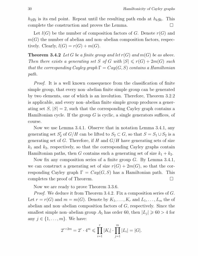
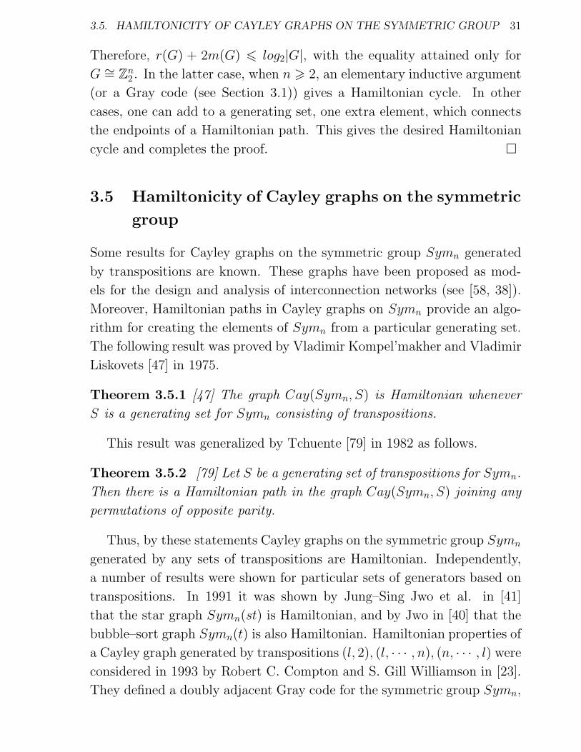
Figure 11. The hierarchical structure of P2, P3 and P4.
There are (n − 2)! external edges between any two copies Pn−1(i) and
Pn−1(j), i 6= j, presented as {[i π2 . . . πn−1 j], [j πn−1 . . . π2, i]}, where
[i π2 . . . πn−1 j] rn = [j πn−1 . . . π2 i].
These edges are defined by the generating element rn. The generating
elements rj, 2 6 j 6 n−1, define internal edges inside all n copies Pn−1(i),
1 6 i 6 n. The copies Pn−1(i) are also called (n− 1)–copies.
Figure 11 shows the hierarchical structure of P2, P3 and P4.
3.6.1 Hamiltonicity based on hierarchical structure
We shall construct a Hamiltonian cycle in the Pancake graph by induction
on the size k of the graph Pk, k > 3, with respect to the proof given in [76].
A similar approach was used also in[42].
When k = 3 then Pk∼= C6 which is a Hamiltonian with a cycle presented
34 Hamiltonicity of Cayley graphs
as follows:
[123]r2→ [213]
r3→ [312]r2→ [132]
r3→ [231]r2→ [321]
r3→ [123].
It is obvious that by removing one edge from this cycle we get a Hamilto-
nian path.
Now we suppose that we have a Hamiltonian cycle for k = n − 1. Let
us show that this is also true for k = n.
We construct a Hamiltonian cycleHn by using the hierarchical structure
of the graph. Since Pn is a vertex–transitive then without loss of generality
one can start with a vertex π1 = I = [1 2 . . . (n− 1)n] ∈ Pn−1(n).
By inductive assumption there is a Hamiltonian cycle Hnn−1 in a copy
Pn−1(n). We remove an edge {[1 2 . . . (n − 1)n], [(n− 1) . . . 2 1n]} from
Hnn−1 and denote a Hamiltonian path as Ln
n−1, where n represents a corre-
sponding (n− 1)–copy. A vertex π2 = [(n− 1) . . . 2 1n] in a copy Pn−1(n)
is connected to a vertex π3 = [n 1 2 . . . (n−2) (n−1)] by an external edge.
Moreover, by our inductive assumption there exists a Hamiltonian cycle in
a copy Pn−1(n−1). Then we remove an edge {[n 1 2 . . . (n−2) (n−1)], [(n−
2) . . . 1n (n− 1)]} from this Hamiltonian cycle and obtain a Hamiltonian
path Ln−1n−1. Again, a vertex π4 = [(n − 2) . . . 1n (n − 1)] is connected by
an external edge to a vertex π5 = [(n− 1)n 1 . . . (n− 3) (n− 2)] of a copy
Pn−1(n− 2) which also has, by inductive assumption, a Hamiltonian cycle.
Constructing a Hamiltonian path in this manner for all copies Pn−1(j),
1 6 j 6 n − 2, finally we have paths Ln−2n−1, . . . , L
1n−1 that are connected
to each other in sequence by an external edge. The last path L1n−1 ends
a vertex π2n = [n (n − 1) . . . 2 1], connected with a vertex π1 of a copy
Pn−1(n). Let us note that we started our construction with this copy.
Thus, by combining all these paths Lnn−1, L
n−1n−1, . . . , L
1n−1 with all exter-
nal edges between them, finally we obtain a Hamiltonian cycle Hn. This
completes a construction.
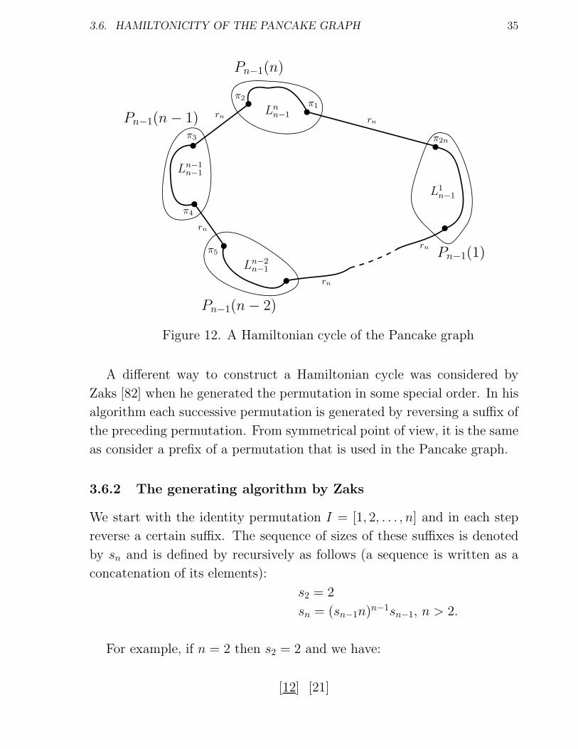
Figure 12 shows the way to construct a Hamiltonian cycle by the con-
struction above.
3.6. HAMILTONICITY OF THE PANCAKE GRAPH 35
��
��
��
��
��
��
��
��rn
rn
rn
rn
rn
π1
π2
π3
π4
π2n
Pn−1(n)
Pn−1(n − 1)
Pn−1(n − 2)
Pn−1(1)
Ln−1
n−1
Ln
n−1
L1
n−1
π5
Ln−2
n−1
Figure 12. A Hamiltonian cycle of the Pancake graph
A different way to construct a Hamiltonian cycle was considered by
Zaks [82] when he generated the permutation in some special order. In his
algorithm each successive permutation is generated by reversing a suffix of
the preceding permutation. From symmetrical point of view, it is the same
as consider a prefix of a permutation that is used in the Pancake graph.
3.6.2 The generating algorithm by Zaks
We start with the identity permutation I = [1, 2, . . . , n] and in each step
reverse a certain suffix. The sequence of sizes of these suffixes is denoted
by sn and is defined by recursively as follows (a sequence is written as a
concatenation of its elements):
s2 = 2
sn = (sn−1n)n−1sn−1, n > 2.
For example, if n = 2 then s2 = 2 and we have:
[12] [21]

36 Hamiltonicity of Cayley graphs
If n = 3 then s3 = 23232 and we have:
[123] [231] [312]
[132] [213] [321]
If n = 4 then s4 = 23232423232423232423232 and we have:
[1234] [2341] [3412] [4123]
[1243] [2314] [3421] [4132]
[1342] [2413] [3124] [4231]
[1324] [2431] [3142] [4213]
[1423] [2134] [3241] [4312]
[1432] [2143] [3214] [4321]
We prove validity of this generating algorithm by induction on n that,
starting with the permutation [1, 2, . . . , n] and applying the sequence sn of
suffix reversals, we generate all n! permutations ending with the permuta-
tion [n, n− 1, . . . , 1].
The assertion holds for n = 2. Assuming it holds for n − 1, we prove
it for n: sn starts with sn−1. Hence, starting with [1, 2, . . . , n] we first
generate the (n− 1)! permutations that start with 1 and, by the induction
assumption, the last one is [1, n, n − 1, . . . , 2]. The next element in sn is
n, hence the next permutation generated is [2, 3, . . . , n, 1]. The following
elements thus generated are all permutations starting with 2. Continuing
in this manner, we then generate the permutations starting with 3, . . . , n.
Moreover, because the first permutation starting with 2 ([2, 3, . . . , n, 1])
is obtained from the first permutation starting with 1 ([1, 2, . . . , n]) by
increasing each element by 1 (while n becomes 1), and because both the
permutations starting with 1 and whose starting with 2 are generated by
the sequence sn−1, therefore the last permutation starting with 2 is derived
from [1, n, n − 1, . . . , 2] (last permutation starting with 1) in the same
manner, namely, it is [2, 1, n, . . . , 3]. Continuing in this manner it is easy
to show that the first permutation starting with i, 1 < i 6 n, is [i, i +
1, . . . , n, 1, 2, . . . , i− 1] and the last one is [i, i− 1, . . . , 1, n, n− 1, . . . , i+1]
(it is [n, n− 1, . . . , 1] for i = n). The proof is thus complete.
3.7. OTHER CYCLES OF THE PANCAKE GRAPH 37
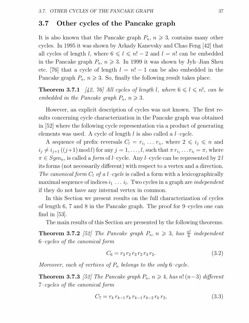
3.7 Other cycles of the Pancake graph
It is also known that the Pancake graph Pn, n > 3, contains many other
cycles. In 1995 it was shown by Arkady Kanevsky and Chao Feng [42] that
all cycles of length l, where 6 6 l 6 n! − 2 and l = n! can be embedded
in the Pancake graph Pn, n > 3. In 1999 it was shown by Jyh–Jian Sheu
etc. [76] that a cycle of length l = n! − 1 can be also embedded in the
Pancake graph Pn, n > 3. So, finally the following result takes place.
Theorem 3.7.1 [42, 76] All cycles of length l, where 6 6 l 6 n!, can be
embedded in the Pancake graph Pn, n > 3.
However, an explicit description of cycles was not known. The first re-
sults concerning cycle characterization in the Pancake graph was obtained
in [52] where the following cycle representation via a product of generating
elements was used. A cycle of length l is also called a l–cycle.
A sequence of prefix–reversals Cl = ri1 . . . ril, where 2 6 ij 6 n and
ij 6= ij+1 ((j+1)mod l) for any j = 1, . . . , l, such that π ri1 . . . ril = π, where
π ∈ Symn, is called a form of l–cycle. Any l–cycle can be represented by 2 l
its forms (not necessarily different) with respect to a vertex and a direction.
The canonical form Cl of a l–cycle is called a form with a lexicographically
maximal sequence of indices i1 . . . il. Two cycles in a graph are independent
if they do not have any internal vertex in common.
In this Section we present results on the full characterization of cycles
of length 6, 7 and 8 in the Pancake graph. The proof for 9–cycles one can
find in [53].
The main results of this Section are presented by the following theorems.
Theorem 3.7.2 [52] The Pancake graph Pn, n > 3, has n!6 independent
6–cycles of the canonical form
C6 = r3 r2 r3 r2 r3 r2. (3.2)
Moreover, each of vertices of Pn belongs to the only 6–cycle.
Theorem 3.7.3 [52] The Pancake graph Pn, n > 4, has n! (n−3) different
7–cycles of the canonical form
C7 = rk rk−1 rk rk−1 rk−2 rk r2, (3.3)
38 Hamiltonicity of Cayley graphs
where 4 6 k 6 n. Moreover, each of vertices of Pn belongs to 7 (n − 3)
different 7–cycles and there are n!8 6 N7 6
n!7 independent 7–cycles.
As one can see, the descriptions of 6–cycles and 7–cycles are not so
complicated. However, the situation is changed dramatically for 8–cycles
and 9–cycles.
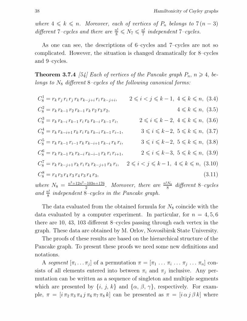
Theorem 3.7.4 [54] Each of vertices of the Pancake graph Pn, n > 4, be-
longs to N8 different 8–cycles of the following canonical forms:
C18 = rk rj ri rj rk rk−j+i ri rk−j+i, 2 6 i < j 6 k− 1, 4 6 k 6 n, (3.4)
C28 = rk rk−1 r2 rk−1 rk r2 r3 r2, 4 6 k 6 n, (3.5)
C38 = rk rk−i rk−1 ri rk rk−i rk−1 ri, 2 6 i 6 k − 2, 4 6 k 6 n, (3.6)
C48 = rk rk−i+1 rk ri rk rk−i rk−1 ri−1, 3 6 i 6 k−2, 5 6 k 6 n, (3.7)
C58 = rk rk−1 ri−1 rk rk−i+1 rk−i rk ri, 3 6 i 6 k−2, 5 6 k 6 n, (3.8)
C68 = rk rk−1 rk rk−i rk−i−1 rk ri ri+1, 2 6 i 6 k−3, 5 6 k 6 n, (3.9)
C78 = rk rk−j+1 rk ri rk rk−j+1 rk ri, 2 6 i < j 6 k− 1, 4 6 k 6 n, (3.10)
C88 = r4 r3 r4 r3 r4 r3 r4 r3, (3.11)
where N8 = n3+12n2−103n+1762 . Moreover, there are n!N8
8 different 8–cycles
and n!8 independent 8–cycles in the Pancake graph.
The data evaluated from the obtained formula for N8 coincide with the
data evaluated by a computer experiment. In particular, for n = 4, 5, 6
there are 10, 43, 103 different 8–cycles passing through each vertex in the
graph. These data are obtained by M. Orlov, Novosibirsk State University.
The proofs of these results are based on the hierarchical structure of the
Pancake graph. To present these proofs we need some new definitions and
notations.
A segment [πi . . . πj ] of a permutation π = [π1 . . . πi . . . πj . . . πn] con-
sists of all elements entered into between πi and πj inclusive. Any per-
mutation can be written as a sequence of singleton and multiple segments
which are presented by {i, j, k} and {α, β, γ}, respectively. For exam-
ple, π = [i π2 π3 π4 j π6 π7 π8 k] can be presented as π = [i α j β k] where

3.7. OTHER CYCLES OF THE PANCAKE GRAPH 39
α = [π2 π3 π4], β = [π6 π7 π8]. If α is the inversion of a segment α then
α = α. Let us denote the number of elements in a segment α as |α|. We
also put π = π rn and τ = τ rn.
Lemma 3.7.5 [52] Let two different permutations π and τ belong to one
and the same (n − 1)–copy of Pn, n > 3, and let d(π, τ) 6 2, then π, τ
belong to the different (n− 1)–copies of the graph.
Proof. Let π, τ ∈ Pn−1(i), 1 6 i 6 n. If d(π, τ) = 1 and if we put
π = [j α k β i] then τ = [k α j β i] where j 6= k 6= i. So π = [i β k α j],
τ = [i β j α k] which means that π, τ belong to the different copies Pn−1(j)
and Pn−1(k). If d(π, τ) = 2 then there is a permutation ω in Pn−1(i)
adjacent to π and τ . The permutations π and τ are obtained from ω by
multiplying on the different (not equal to rn) prefix–reversals on the right.
Thereby, the first elements of π and τ should be different hence π = π rnand τ = τ rn should be different, i.e. they belong to the different (n− 1)–
copies of Pn. �
3.7.1 6–cycles of the Pancake graph
In this section we present the proof of Theorem 3.7.2.
Proof. If n = 3 then P3∼= C6 and there is the only 6–cycle presented
as [123]r2→ [213]
r3→ [312]r2→ [132]
r3→ [231]r2→ [321]
r3→ [123] for which the
canonical form is C6 = r3 r2 r3 r2 r3 r2.
Let us show that there are no other forms of 6–cycles in Pn, n > 4.
First of all, we prove that a 6–cycle doesn’t appear on vertices of two
different (n − 1)–copies. Indeed, if π, τ ∈ Pn−1(i) and π, τ ∈ Pn−1(j)
then d(π, τ) 6= 1 and d(π, τ) 6= 2 by Lemma 3.7.5, and hence d(π, τ) >
3. Suppose that there is a 6–cycle containing vertices π, τ, π, τ . So, if
d(π, τ) = 3 then π, τ are adjacent in Pn−1(j) and by Lemma 3.7.5 vertices
π = π rn, τ = τ rn belong to the different (n − 1)–copies but this is not
true since π, τ ∈ Pn−1(i). If d(π, τ) = 4 then π = τ but this is not possible
since π 6= τ . Thus, a 6–cycle doesn’t appear on vertices of two different
(n− 1)–copies.
40 Hamiltonicity of Cayley graphs
Now let us prove that a 6–cycle doesn’t appear on vertices of three
different (n − 1)–copies. Let π, τ ∈ Pn−1(i), π 6= τ such that d(π, τ) 6 2
then by Lemma 3.7.5 vertices π, τ belong to the different (n − 1)–copies.
We consider two cases.
If d(π, τ) = 1 then vertices π, τ, π, τ might be belong to a 6–cycle if
and only if d(π, τ) = 3. Show that this is not true. Let π = [j α k β i]
then τ = [k α j β i] and π = [i β k α j] ∈ Pn−1(j), τ = [i β j α k] ∈ Pn−1(k).
The shortest path starting at π and belonging to Pn−1(k) should contain
vertices ω = [k β i α j] and ω = [j α i β k] ∈ Pn−1(k), i.e. d(π, ω) = 2.
It is evident that there is no a prefix–reversal transforming ω into τ , i.e.
d(ω, τ) 6= 1, and hence d(π, τ) 6= 3.
If d(π, τ) = 2 then vertices π, τ, π, τ might be belong to a 6–cycle if and
only if d(π, τ) = 2. However this is not possible since by Lemma 3.7.5
vertices π = π rn and τ = τ rn belong to the different (n−1)–copies. Thus,
a 6–cycle doesn’t appear on vertices of three different (n− 1)–copies.
It is also evident that a 6–cycle doesn’t appear on vertices of four and
more different (n − 1)–copies since there should be at least four external
edges as well as at least one edge in each of (n − 1)–copies so we have a
8–cycle.
Thus, there is the only canonical form, namely r3 r2 r3 r2 r3 r2, to describe
6–cycles in Pn, n > 3. These cycles are independent for n > 4 since prefix–
reversals ri, 4 6 i 6 n, define external edges for 6–cycles which means that
each of vertices of Pn belongs to the only 6–cycle. �
3.7.2 7–cycles of the Pancake graph
Proof. We prove Theorem 3.7.3 by the induction on the dimension k of
the Pancake graph Pk when k > 4. If k = 3 then there are no 7–cycles in
P3∼= C6. If k = 4 then Theorem says that each of vertices of P4 belongs to
7 different 7–cycles. Since Pn is a vertex–transitive graph then it is enough
to check this fact for any its vertex. In particular, all 7–cycles containing
the identity permutation [1234] are presented in the Table 1. They could
be found easily by considering the layer presentation of P4 with respect to
the identity permutation. The canonical form for all cycles presented in
Table 1 is C7 = r4 r3 r4 r3 r2 r4 r2 that corresponds to (3.3) when k = 4.

3.7. OTHER CYCLES OF THE PANCAKE GRAPH 41
vertex description prefix–reversal description
1 [1234]-[4321]-[2341]-[1432]-[3412]-[4312]-[2134] r4 r3 r4 r3 r2 r4 r22 [1234]-[3214]-[4123]-[2143]-[1243]-[3421]-[4321] r3 r4 r3 r2 r4 r2 r43 [1234]-[4321]-[2341]-[3241]-[1423]-[4123]-[3214] r4 r3 r2 r4 r2 r4 r34 [1234]-[3214]-[2314]-[4132]-[1432]-[2341]-[4321] r3 r2 r4 r2 r4 r3 r45 [1234]-[2134]-[4312]-[3412]-[2143]-[4123]-[3214] r2 r4 r2 r4 r3 r4 r36 [1234]-[4321]-[3421]-[1243]-[4213]-[3124]-[2134] r4 r2 r4 r3 r4 r3 r27 [1234]-[2134]-[4312]-[1342]-[2431]-[3421]-[4321] r2 r4 r3 r4 r3 r2 r4
Table 1. 7–cycles in P4 containing the identity permutation [1234].
Now we assume that Theorem is hold for k = n− 1 and prove that it is
hold also for k = n using the hierarchical structure of Pn. By the induction
assumption, any vertex of any (n − 1)–copy belongs to 7((n − 1) − 3) =
7(n−4) different 7–cycles of this copy. However, besides 7–cycles belonging
to one and the same (n − 1)–copy there may also be 7–cycles belonging
to the different (n− 1)–copies of the graph. The following three cases are
possible.
Case 1. Suppose that a sought 7–cycle C∗7 is formed on vertices from two
copies Pn−1(i) and Pn−1(j), 1 6 i 6= j 6 n, such that either two vertices
of C∗7 belong to a copy Pn−1(i) and other five vertices belong to a copy
Pn−1(j), or three vertices of C∗7 belong to a copy Pn−1(i) and other four
vertices belong to a copy Pn−1(j). In the both cases we have d(π, τ) 6 2 for
vertices π, τ ∈ Pn−1(i) belonging to C∗7 . Then by Lemma 3.7.5 vertices π, τ
belong to the different (n− 1)–copies that contradicts to our assumption.
Therefore, a 7–cycle does not occur in this case.
Case 2. Suppose that a sought 7–cycle C∗7 is formed on vertices from
three different (n − 1)–copies such that two vertices πi1, πi2 belong to
Pn−1(i), two vertices πj1 , πj2 belong to Pn−1(j), the other three vertices
πn1, πn2, πn3 belong to Pn−1(n), where 1 6 i < j 6 n (see Figure 13).
Let us describe a sought cycle. Since Pn is a vertex–transitive graph
then there is no loss of generality in taking πn2 = In = [α iβ j γ n], where
α = [1 . . . i − 1], β = [i+ 1 . . . j − 1], γ = [j + 1 . . . n− 1] and |α| = i − 1,
|β| = j − i− 1, |γ| = n− j − 1. By Lemma 3.7.5 vertices πn1 and πn3 are
adjacent to vertices from the different (n− 1)–copies Pn−1(i) and Pn−1(j),

42 Hamiltonicity of Cayley graphs
b
b
b
b
b
b
b
πn2
πn1πn3
πj1
πj2
πi2
πi1
Pn−1(j)
Pn−1(i)
Pn−1(n)
ri
rj
rn−j+ir
n−j+1
rn
rn
rn
Figure 13. Case 2 for the proof of Theorem 3.7.3
hence these vertices are presented as follows:
πn1 = πn2 ri = [i α β j γ n], where πn1
j = j,
πn3 = πn2 rj = [j β i α γ n], where πn3
j−i+1 = i.
Their adjacent vertices in copies Pn−1(i) and Pn−1(j) are presented as fol-
lows:
πi1 = πn1 rn = [n γ j β α i], where πi1n−j+1 = j,
πj1 = πn3 rn = [n γ α i β j], where πj1n−j+i = i.
A vertex πi2 should be adjacent to the vertex πi1 and to one of the vertices,
say πj2 , from the copy Pn−1(j):
πi2 = πi1 rn−j+1 = [j γ nβ α i], where πi21 = j.
On the other hand, a vertex πj2 should be adjacent to the vertex πj1.
Moreover, since it is also adjacent to πi2 hence πj2 has the following view:
πj2 = πj1 rn−j+i = [i α γ n β j], where πj21 = i.
By our assumption, the vertices πi2 and πj2 are incident to one and the same
external edge which means that a permutation π∗ = πi2 rn = [i α β n γ j]

3.7. OTHER CYCLES OF THE PANCAKE GRAPH 43
should coincide with the permutation πj2. This is possible only in the
case when segments β and γ are empty, i.e. |β| = j − i− 1 = 0 and |γ| =
n−j−1 = 0. From this we have j = n−1 and i = j−1 = n−2, and a 7–cycle
is presented as follows: πi1 r2→ πi2 rn→ πj2rn−1
−→ πj1 rn→ πn3rn−1
−→ πn2rn−2
−→ πn1rn→
πi1. Its canonical form C7 = rn rn−1 rn rn−1 rn−2 rn r2 coincide with (3.3)
when k = n.
Case 3. Suppose that a sought 7–cycle is formed on vertices from four
or more (n − 1)–copies. It follows from the hierarchical structure of the
graph that any its vertex is incident to the only external edge. So any
7–cycle in this graph should contain at least two vertices of one and the
same (n− 1)–copy and hence a 7–cycle does not occur in this assumption.
Thus, the only canonical form rn rn−1 rn rn−1 rn−2 rn r2 representing seven
cycles of the length seven and containing vertices from three different
(n − 1)–copies of the graph Pn is found. It is evident that any vertex
of Pn belongs to all these cycles. By the induction assumption, any vertex
of any (n − 1)–copy belongs to 7(n− 4) different 7–cycles from this copy.
Therefore, any vertex of Pn belongs to 7(n − 4) + 7 = 7(n − 3) different
7–cycles of the canonical form (3.3) that completes the proof on the main
fact of Theorem 3.7.3.
Since each of vertices belongs to 7 (n − 3) different 7–cycles and there
are n! vertices in Pn, hence there are n! 7 (n− 3) cycles of length 7. How-
ever, each cycle was enumerated seven times, so totally there are 7 (n− 3)
different 7–cycles.
It is also easy to show that there are three independent 7–cycles in P4.
For example, the following three 7–cycles are independent in P4:
C17 = [1234]− [2134]− [4312]− [1342]− [2431]− [3421]− [4321],
C27 = [3241]− [2341]− [1432]− [3412]− [2143]− [4123]− [1423],
C37 = [4213]− [2413]− [3142]− [4132]− [2314]− [1324]− [3124].
It follows from the hierarchical structure of Pn, n > 4, that there aren!24 copies of P4 and each of them has exactly three independent 7–cycles.
So, totally there are at least n!8 independent 7–cycles that gives the lower
bound. The upper bound is obtained in assumption that each of vertices
of Pn, n > 7, belongs to the only 7–cycle. �
44 Hamiltonicity of Cayley graphs
3.7.3 8–cycles of the Pancake graph
In this section we present the proof of Theorem 3.7.4 by using some ad-
ditional notations as well as technical Lemmas. We suggest that any
permutation can be written as a sequence of singleton and multiple seg-
ments which are presented by {i, j, p, q, k} and {α, β, γ, A,B, C}, respec-
tively. If π = [αβ], where α = [π1 π2 . . . πi] and β = [πi+1 . . . πn], then
π r|α| = [αβ], where |α| is the number of elements in a segment α, |α| > 2,
and α is the inversion of a segment α. It is obvious, that α = α.
An independent set D of vertices in a graph is called an efficient domi-
nating set if each vertex not inD is adjacent to exactly one vertex inD [25].
It is shown in [70] that Dp = {[p π2 . . . πn], πj ∈ {1, . . . , n}\{p}, 2 6 j 6
n}, |Dp| = (n−1)! , p = 1, . . . , n, are efficient dominating sets in Pn, n > 3.
Let us note that external edges of Pn, n > 3, are incident to vertices from
different efficient dominating sets of the Pancake graph.
The distance d = d(π, τ) between two vertices π, τ ∈ Pn is defined as the
least number of prefix–reversals transforming π into τ , i.e. π ri1 ri2 . . . rid =
τ .
The next lemma gives a full list of paths of length three between vertices
of one and the same efficient dominating set.
Lemma 3.7.6 Two permutations π, τ ∈ Dp, 1 6 p 6 n, are at the dis-
tance three from each other in Pn, n > 3, if and only if:
1) either τ = π rj ri rj, where 2 6 i < j 6 n, and permutations π, τ are
presented as:
π = [AB γ], τ = [AB γ]; (3.12)
2) or τ = π rj ri ri−j+1, where 2 6 j < i 6 n, and permutations π, τ are
presented as:
π = [pAB γ], τ = [pB Aγ]. (3.13)
Proof. We consider π ∈ Dp such that π = [p α q β k], πj = q. Let
us find other vertices from Dp being at the distance three from π. Let
π1 = π rj = [q α p β k], where π1j = p, 2 6 j 6 n. An application of a
prefix–reversal ri, 2 6 i 6 n, i 6= j, to the permutation π1 gives us the
following two cases.
3.7. OTHER CYCLES OF THE PANCAKE GRAPH 45
1) If i < j then π2 = π1 ri = [α2 q α1 p β k], where π2j = p, α = α1 α2 and
|α2| = i− 1, and an application of a prefix–reversals rj to the permutation
π2 gives us the permutation:
τ = π2 rj = [p α1 q α2 β k],
hence τ = π rj ri rj, and we get (3.12) by setting A = p α1, B = α2 q,
γ = β k in π and τ in this case.
2) If i > j then π2 = π1 ri = [β1 p α q β2 k], where π2i−j+1 = p, β = β1β2
and |β1| = i − j, and an application of a prefix–reversal ri−j+1 to the
permutation π2 gives us the permutation:
τ = π2 ri−j+1 = [p β1 α q β2 k],
hence τ = π rj ri ri−j+1, and we get (3.13) setting A = α q, B = β1, γ = β2 k
in π and τ in this case. �
Now we consider paths of length three between vertices of a given form
in the Pancake graph. To get these results we use the following fact: if for
given two vertices there is at least one path of length three (four) which
does not belong to a 7–cycle then there are no paths of length four (three)
between these vertices. This fact is based on the following lemma.
Lemma 3.7.7 If P is a path of length three (four) in Pn, n > 4, and
if there is no a 7–cycle containing P , then there is no another 7–cycles
containing any other path of length three (four).
Proof. Suppose there are two paths P and P ′ of length three (four)
between vertices π and τ such that there is no a 7–cycle containing P , and
there is a 7–cycle containing P ′. Since Pn has no 3– and 5–cycles, hence
there is a path of length four (three) between vertices π and τ which is dif-
ferent from P . Therefore, there is a 7–cycle containing P that contradicts
the conditions of the lemma. �
The next lemma gives us a description of paths of length three defined
on internal edges of the graph between vertices of given forms.
46 Hamiltonicity of Cayley graphs
Lemma 3.7.8 Let d(π, τ) = 3, then
1) if π = [γ1AB γ2] and τ = [γ1AB γ2], where either |γ1| > 2 and |A| > 2,
or |γ1| = 1 and |A| > 3, then there exists the only path of length three
between π and τ such that:
τ = π r|γ1|+|A| r|A| r|γ1|+|A|; (3.14)
2) if π = [γ1AB γ2] and τ = [γ1BAγ2], where |γ1| > 0, |A| > 1, |B| > 1,
then :
a) there is the only path of length three between π and τ :
τ = π r|γ1|+|A| r|γ1|+|A|+|B| r|γ1|+|B| (3.15)
provided that |γ1| = 1, and |A|, |B| 6= 1;
b) there are two paths of length three between π and τ :
τ = π r2 r3 r2 = π r3 r2 r3 (3.16)
provided that |γ1| = |A| = |B| = 1;
c) there is the only path of length three between π and τ :
τ = π r|A| r|A|+|B| r|B| (3.17)
provided that |γ1| = 0 and |A| > 2, |B| > 2.
Proof. 1) If π = [γ1AB γ2] and τ = [γ1AB γ2], then (3.14) is checked
by a direct verification:
π = [γ1AB γ2]r|γ1|+|A|
→ [Aγ1B γ2]r|A|→ [Aγ1B γ2]
r|γ1|+|A|
→ [γ1AB γ2] = τ.
Let us show that this path is the only path of length three between vertices
of given forms. Suppose that there is one more path of length three between
π and τ . Then these two paths should form a 6–cycle. However, by the
conditions of Lemma we have that either |γ1| > 2 and |A| > 2, or |γ1| = 1
and |A| > 3, hence, by Theorem 3.7.2 a 6–cycle does not exist between
given vertices. Therefore, a sought path is the only one in this case.
2) Let us consider π = [γ1AB γ2] and τ = [γ1BAγ2]. If |γ1| > 2,
|A| > 1, |B| > 1, then there is the following path of length four between
these vertices:
π = [γ1AB γ2]r|γ1|+|A|
→ [Aγ1B γ2]r|γ1|+|A|+|B|
→ [B γ1Aγ2]r|γ1|+|B|
→
3.7. OTHER CYCLES OF THE PANCAKE GRAPH 47
[γ1BAγ2]r|γ1|→ [γ1BAγ2] = τ. (3.18)
Suppose that there is also a path of length three between π and τ . This
means that these two paths should form a 7–cycle. Moreover, since |γ1| > 2,
|A| > 1 and |B| > 1 in this case, then a 7–cycle should consist of a
sequence of following prefix–reversals: r|γ1|+|A| r|γ1|+|A|+|B| r|γ1|+|B|r|γ1|. But
it is not possible by Theorem 3.7.3, so a 7–cycle does not exit. Hence, by
Lemma 3.7.7 there is no path of length three between vertices π and τ in
this case.
However, if we set |γ1| = 1 in (3.18) then there is a path of length three
between π and τ presented by (3.15):
τ = π r|γ1|+|A| r|γ1|+|A|+|B| r|γ1|+|B|.
Suppose that there is one more path of length three between π and τ . Then
these two paths should form a 6–cycle. By Theorem 3.7.2 it is possible only
in the case when |γ1| = |A| = |B| = 1 and this path can be presented as:
τ = π r|γ1|+|A|+|B| r|A|+|B| r|γ1|+|A|+|B| = π r3 r2 r3,
and another path, correspondingly, is presented as:
τ = π r|γ1|+|A| r|γ1|+|A|+|B| r|γ1|+|B| = π r2 r3 r2,
so we have got (3.16).
If we set |γ1| = 0 in (3.18) provided that |A| > 2, |B| > 2, then between
vertices π and τ there exists a path of length three presented by (3.17):
τ = π r|A| r|A|+|B| r|B|.
Suppose there is one more path of length three between π and τ . Then these
two paths should form a 6–cycle, but it is not possible by Theorem 3.7.2
since |A|+ |B| > 4. Let us note that if |A| = 1 and |B| = 1, then the path
presented above is transformed into an edge. This completes the proof of
the lemma. �
48 Hamiltonicity of Cayley graphs
Now we are ready to prove Theorem 3.7.4
Proof. In view of the hierarchical structure of the Pancake graph, when
we transit from Pn−1 to Pn then the number of cycles passing through one
and the same vertex will be increased due to new cycles formed on vertices
from (n−1)–copies, namely, a 8–cycle may have vertices belonging to two,
three or four (n− 1)–copies of the graph Pn.
Let us consider all possible vertex distributions among (n − 1)–copies
and find all descriptions of 8–cycles in Pn as well as their number.
Case 1: a 8–cycle has vertices from two (n− 1)–copies
Suppose that a 8–cycle is formed on vertices from two copies Pn−1(i)
and Pn−1(j), 1 6 i, j 6 n, i 6= j. There are three possibilities in this case.
(2 + 6)–situation. Suppose that two vertices of a sought 8–cycle be-
long to a copy Pn−1(i), and other six vertices belong to a copy Pn−1(j).
This means that a 8–cycle must have two external edge {[i α j], [j α i]} and
{[i β j], [j β i]}. Moreover, vertices π = [j α i] and τ = [j β i] from Pn−1(i)
should be connected by an internal edge, but it is not possible since both
permutations have one and the same first element. Therefore, a 8–cycle
does not occur in this situation.
(3 + 5)–situation. Suppose that three vertices of a sought 8–cycle belong
to a copy Pn−1(i), and other five vertices belong to a copy Pn−1(j). Then
a 8–cycle must have two external edges {[i α j], [j α i]} and {[i β j], [j β i]}.
Moreover, vertices π = [j α i] and τ = [j β i] from Pn−1(i) should be joined
by a path of a length two. This means that there exist two prefix–reversals
ri, rj, 2 6 i 6= j < n, such that π ri rj = τ . However, it is not possible since
permutations π and τ have one and the same first element. Therefore, a
8–cycle does not occur in this situation.
(4 + 4)–situation. Suppose that four vertices πk1, πk2 , πk3, πk4 of a sought
8–cycle belong to a copy Pn−1(k), and other four vertices πp1, πp2, πp3, πp4
belong to a copy Pn−1(p). Let us note that vertices πkl, l = 1, 2, 3, 4, should
form a path of length three whose endpoints πk1 and πk4 should be adja-
cent to vertices from Pn−1(p). This means that the equality πk11 = πk4
1 = p
should take place, and both vertices should belong to the efficient domi-
nating set Dp.

3.7. OTHER CYCLES OF THE PANCAKE GRAPH 49
�
�
�
πp2
πp1
πk1
Pn−1(k)
Pn−1(p)
rj
rn rn
πp3
ri
��
�
πk2 πk3
πk4rj
πp4� �
Case 1).
�
�
�
πp2
πp1
πk1
Pn−1(k)
Pn−1(p)
ri−j+1
rn rn
πp3
ri
��
�
πk2 πk3
πk4rj
πp4� �
Case 2).
Figure 14. (4 + 4)–situation
Let πk1 = [p α q β k], where πk11 = p, πk1
j = q, |α| = j−2, |β| = n− j−1.
Then by Lemma 3.7.6 a path of length three between vertices is presented
by the following two ways:
1) πk4 = πk1 rj ri rj, where 2 6 i < j 6 n− 1;
2) πk4 = πk1 rj ri ri−j+1, where 2 6 j < i 6 n− 1.
We consider both ways.
1) In the first way, a path of length three has the following form:
πk1 = [pαqβk]rj→ πk2 = [qαpβk]
ri→ πk3 = [α2qα1pβk]rj→ πk4 = [pα1qα2βk],
where πk2j = p; πk3
i = q, α = α1α2 and |α2| = i − 1 > 1; πk4n−j+i = q.
The endpoints πk1 , πk4 of the path of length three belonging to Pn−1(k)
are adjacent to vertices from Pn−1(p) which are presented as follows (see
Figure 14, Case 1):
πp1 = πk1 rn = [k β q α2 α1 p], where πp1n−j+1 = q,
πp4 = πk4 rn = [k β α2 q α1 p], where πp4n−i+j = q.
Let us describe a path of length three between vertices πp1 and πp4
belonging one and the same copy Pn−1(p). If γ1 = [k β], A = [q α2],
B = [α1], γ2 = [p], where |γ1| = |β| + 1 > 1, |A| > 2, |B| > 0, then
the permutations πp1, πp4 take forms [γ1AB γ2] and [γ1AB γ2], and by
Lemma 3.7.8 there is the only path of length three between them provided

50 Hamiltonicity of Cayley graphs
that |γ1| = |β|+1 = n− j > 1 and |A| = |α2|+1 = i > 2. Hence, a sought
8–cycle takes form:
C18 = rn−j+i ri rn−j+i rn rj ri rj rn, where 2 6 i < j 6 n− 1,
the canonical form of which correspond to the form (3.4) in Theorem 3.7.4
if we set n = k, where 4 6 k 6 n.
Moreover, if |γ1| = 1 and |A| = 2, then we have two different 8–cycles
of the following forms:
C28 = rn−1 r2 rn−1 rn r2 r3 r2 rn,
the canonical form of which corresponds to the form (3.5) in Theorem 3.7.4
if we put n = k, where 4 6 k 6 n, and rn−1 r2 rn−1 rn r3 r2 r3 rn, the
canonical form of which correspond to the obtained above form (3.4) if
we put i = 2, j = k − 1.
2) In the second way, a path of length three has the following form:
πk1 = [pαqβk]rj→ πk2 = [qαpβk]
ri→ πk3 = [β1pαqβ2 k]ri−j+1
→ πk4 = [pβ1αqβ2k],
where πk2j = p, πk3
i = q, β = β1β2, |β1| = i − j > 1 and |β2| = n − i − 1;
πk4i = q, and vertices from a copy Pn−1(p) that are adjacent to vertices
πk1, πk4 are presented as follows: (see Figure 14, Case 2):
πp1 = πk1 rn = [k β2 β1 q α p], where πp1n−j+1 = q,
πp4 = πk4 rn = [k β2 q α β1 p], where pip5n−i+1 = q.
Let us describe a path of length three between vertices πp1 and πp4
belonging one and the same copy Pn−1(p). If γ1 = [k β2], A = [β1], B =
[q α], [k] = [p], where |γ1| = |β2|+ 1 > 1, |A| = |β1| > 1, |B| = |α|+ 1 > 1,
then the permutations πp1, πp4 take forms [γ1AB k] and [γ1BAk], and by
Lemma 3.7.8 there is the only path of length three between them provided
that |γ1| = n − i = 1, |A| = |β1| = i − j > 1, |B| = |α| + 1 = j − 1 > 1,
which means that i = n− 1, and a sought 8–cycle takes a form:
C38 = rn rn−j rn−1 rj rn rn−j rn−1 rj, where 2 6 j 6 n− 2,
the canonical form of which corresponds to the form (3.6) in Theorem 3.7.4
if we set n = k and j = i. Let us note, that if |A| = |B| = 1 then we have

3.7. OTHER CYCLES OF THE PANCAKE GRAPH 51
�
�
�
�
πk2πk1
πj3
πj2
πi2
πi1
Pn−1(j)Pn−1(i)
Pn−1(k)
rj
rn−j+1
rn
rn
rn
�
πj4
πj1
�
�
�
Figure 15. (2 + 2 + 4)–situation
n = 4, j = 2, i = 3 and 8–cycles take forms r2 r3 r2 r4 r3 r2 r3 r4 and
r3 r2 r3 r4 r3 r2 r3 r4, that correspond to the obtained above forms (3.5) and
(3.4) when k = 4.
Thus, the case of two copies is considered and all 8–cycles occurring in
this case are found.
Case 2: a 8–cycle has vertices from three (n− 1)–copies
Suppose a 8–cycle is formed on vertices from copies Pn−1(i), Pn−1(j),
Pn−1(k), where 1 6 i 6= j 6= k 6 n. We have the following situations in
this case.
(2 + 2 + 4)–situation. Suppose two vertices πk1, πk2 of a sought 8–cycle
belong to a copy Pn−1(k), two vertices πi1, πi2 belong to a copy Pn−1(i),
and four vertices πjs, s = 1, . . . , 4, belong to a copy Pn−1(j) (see Figure 15).
Let us consider πk1 = [i α j β k], where α = [π2 . . . πj−1], |α| = j − 2, and
β = [πj+1 . . . πn−1], |β| = n− j−1. Since the vertex πk2 should be adjacent
to a vertex from a copy Pn−1(j), hence πk21 = j and we immediately have
πk2 = πk1 rj = [j α i β k], where πk2j = i.
The vertex πk2 must be joined by an external edge with the vertex πj1 ∈
Pn−1(j), hence
πj1 = πk2 rn = [k β i α j], where πj1n−j+1 = i.
52 Hamiltonicity of Cayley graphs
The vertex πk1 must be joined by an external edge with the vertex πi1 ∈
Pn−1(i), hence
πi1 = πk1 rn = [k β j α i], where πi1n−j+1 = j.
Since the vertex πi2 should be adjacent to a vertex from a copy Pn−1(j),
then πi21 = j and we immediately have
πi2 = πi1 rn−j+1 = [j β k α i], where πi2n−j+1 = k.
The vertex πi2 must be joined by an external edge with the vertex πj5 ∈
Pn−1(j), hence
πj4 = πi2 rn = [i α k β j], where πj4j = k.
Now we describe a path of length three between vertices πj1 and πj4 which
are differed in an order of segments [k β] and [i α]. This means they have
forms [γ1AB γ2] and [γ1BAγ2], where γ1 is empty, i.e. |γ1| = 0. Moreover,
A = [k β], B = [i α], γ2 = [j] and |A| = |β|+1 > 1, |B| = |α|+1 > 1. Then
by Lemma 3.7.8 between vertices πj1 and πj4 there exists path of length
three provided that |A| = n− j > 2 and |B| = j− 1 > 2. This means that
3 6 j 6 n− 2, where n > 5. Thus, a 8–cycle is presented as follows:
C48 = rn rn−j+1 rn rj−1 rn−1 rn−j rn rj, where 3 6 j 6 n− 2,
the canonical form of which corresponds to the form (3.7) in Theorem 3.7.4
if we set j = i and n = k, where 4 6 k 6 n.
(2 + 3 + 3)–situation. Suppose two vertices πk1, πk2 of a sought 8–cycle
belong to a copy Pn−1(k), three vertices πi1, πi2, πi3 belong to a copy
Pn−1(i), and three vertices πj1, πj2, πj3 belong to a copy Pn−1(j). We
consider πk1 = [iαjβk], where α = [π2 . . . πj−1], |α| = j − 2, and β =
[πj+1 . . . πn−1], |β| = n− j − 1. Vertices πk1 and πk2 should be adjacent to
vertices from different (n− 1)–copies, hence they are presented as follows:
πk2 = πk1 rj = [j α i β k], where πk2j = i.
The vertex πk1 must be joined by an external edge with a vertex πi1 ∈
Pn−1(i), hence
πi1 = πk1 rn = [k β j α i], where πi1n−j+1 = j.
3.7. OTHER CYCLES OF THE PANCAKE GRAPH 53
The vertex πk2 must be joined by an external edge with a vertex πj1 ∈
Pn−1(j), hence
πj1 = πk2 rn = [k β i α j], where πj1n−j+1 = i.
The vertex πi3 must be joined by an external edge with a vertex πj3 ∈
Pn−1(j), hence we have πi31 = j. Thus, vertices πi1 and πi3 should be joined
by a path of length two with the condition above. It can be obtained by
the following two ways:
πi1 = [k β j α i] → [β2 k β1 j α i] → [j β1 k β2 α i] = πi13, where |β2| 6= 0,
πi1 = [k β j α i] → [α2 j β k α1 i] → [j α2 β k α1 i] = πi23, where |α2| 6= 0.
From the other side, the vertex πj3 must be joined by an external edge
with a vertex πi3 ∈ Pn−1(i), hence we have πj31 = i. Thus, vertices πj1 and
πj3 should be joined by a path of length two with the condition above. It
can be obtained by the following two ways:
πj1 = [k β i α j] → [β2 k β1 i α j] → [i β1 k β2 α j] = πj13 , where |β2| 6= 0,
πj1 = [k β i α j] → [α1 i β k α2 j] → [i α1 β k α2 j] = πj23 , where |α1| 6= 0.
Let us note that vertices πi3 and πj3 should be joined by an external edge
rn which means that the order of segments in the permutations should be
reversed. An analysis of non–empty segments in these permutations shows
that external edges occur between the following vertices:
• πi13 and πj23 , when |α2| = 0 and |β1| = 0;
• πi23 and πj13 , when |α1| = 0 and |β1| = 0;
• πi23 and πj23 , when |β| = 0.
There is no an external edge between permutations πi13 and πj13 since they
have one and the same order of elements in the segment [k β2], where
|β2| 6= 0.
Thus, since |α| = j − 2, |β| = n− j − 1, then by taking into account an
external edge between πi13 and πj23 , where |α2| = 0 and |β1| = 0, we have
|α| > 1, |β| > 1, and a sought 8–cycle has a form:
C58 = rn rn−j rn−j+1 rn rj−1 rn−1 rn rj, where 3 6 j 6 n− 2, n > 5,
54 Hamiltonicity of Cayley graphs
the canonical form of which corresponds to the form (3.8) in Theorem 3.7.4
if we set n = k, where 5 6 k 6 n.
Moreover, by taking into account an external edge between πi23 and πj13 ,
where |α1| = 0 and |β1| = 0, we have |α| > 1, |β| > 1, and a sought 8–cycle
has a form rn rn−1 rj−1 rn rn−j+1 rn−j rn rj, where 3 6 j 6 n− 2, n > 5, the
canonical form of which corresponds to the form (3.8) if we set n = k,
where 5 6 k 6 n. And finally, by taking into account an external edge
between πi23 and πj23 , where |β| = 0, we have j = n − 1, |α1| = q > 1 and
|α2| = n− 3− q > 1, so we have one more 8–cycle presented as follows:
C68 = rn rn−q−1 rn−q−2 rn rq+1 rq+2 rn rn−1, where 1 6 q 6 n− 4, n > 5,
the canonical form of which corresponds to the form (3.9) if we put q = i−1
and n = k, where 5 6 k 6 n.
Thus, the case of three copies is considered and all 8–cycles occurring
in this case are found.
Case 3: a 8–cycle has vertices from four (n− 1)–copies
Suppose that a sought 8–cycle occurs on vertices πi1, πi2 ∈ Pn−1(i),
πj1, πj2 ∈ Pn−1(j), πk1, πk2 ∈ Pn−1(k), πn1, πn2 ∈ Pn−1(n), where 1 6 i 6=
j 6= k 6 n. Let us assume πn1 = [i α j β k γ n], where |α| > 0, |β| > 0,
|γ| > 0. There are two ways of distribution of vertices among four (n−1)–
copies.
1). Suppose that the vertex πn1 is adjacent to the vertex πi1, and the
vertex πn2 is adjacent to the vertex πj1. Then vertices πj1 and πn2 should
be presented as follows:
πi1 = πn1 rn = [n γ k β j α i], πn2 = πn1 r|α|+2 = [j α i β k γ n];
and hence the vertex πj1 which is adjacent to πn2 has the following form:
πj1 = πn2 rn = [n γ k β i α j].
The vertex πi2 should be joined by an external edge with the vertex πk1 ∈
Pn−1(k). This means that πi21 = k and we have:
πi2 = πi1 r|γ|+2 = [k γ n β j α i],

3.7. OTHER CYCLES OF THE PANCAKE GRAPH 55
and the vertex πj2 should be joined by an external edge with the vertex
πk2 ∈ Pn−1(k). This means that πj21 = k and we have:
πj2 = πj1 r|γ|+2 = [k γ n β i α j].
Vertices πi2 and πj2 should be joined by external edges with vertices πk1
and πk2, correspondingly:
πk1 = πi2 rn = [i α j β n γ k], πk2 = πj2 rn = [j α i β n γ k].
If a 8–cycle does exist then vertices πk1, πk2 should be incident to one
and the same internal edge which means that there should exist a prefix–
reversal transforming πk1 into πk2 . It is obvious that such a prefix–reversal
exist and it is r|α|+2. If we set |α| = i− 2, |β| = j − i− 1, |γ| = n− j − 1,
where 2 6 i < j < n, then a sought 8–cycle is presented as follows:
C78 = rn rn−j+1 rn ri rn rn−j+1 rn ri, where 2 6 i < j 6 n− 1,
the canonical form of which corresponds to the form (3.10) if we put n = k,
where 4 6 k 6 n.
2). Suppose that the vertex πn1 is adjacent to the vertex πi1, and the
vertex πn2 is adjacent to the vertex πk1 . Then vertices πi1 and πn2 should
be presented as follows:
πi1 = πn1 rn = [n γ k β j α i], πn2 = πn1 r|α|+|β|+3 = [k β j α i γ n];
and the vertex πk1 which is adjacent to πn2 has the following form:
πk1 = πn2 rn = [n γ i α j β k].
The vertex πi2 should be joined by an external edge with the vertex πj1 ∈
Pn−1(j). This means that πi21 = j and we have:
πi2 = πi1 r|β|+|γ|+3 = [j β k γ nα i],
and the vertex πk2 should be joined by an external edge with the vertex
πj2 ∈ Pn−1(j) which means that πk21 = j, hence we have;
πk2 = πk1 r|α|+|γ|+3 = [j α i γ n β k].

56 Hamiltonicity of Cayley graphs
Vertices πi2 and πk2 should be joined by external edges with vertices πj1
and πj2, correspondingly:
πj1 = πi2 rn = [i α n γ k β j], πj2 = πk2 rn = [k β n γ i α j].
In this case, an internal edge between vertices πj1 and πj2 does exist only
if |α| = |β| = |γ| = 0, which means that n = 4 and a sought 8–cycle takes
a form:
C88 = r4 r3 r4 r3 r4 r3 r4 r3,
presented as the form (3.11) in Theorem 3.7.4.
Thus, all canonical forms for 8–cycles in Pn, n > 4, are obtained.
Now we count the total number N8 of different 8–cycles passing through
a given vertex in the graph. We denote
N =8∑
i=1
NCi8,
where NCi8corresponds to the number of different 8–cycles described by
the canonical form C i8, 1 6 i 6 8, and passing through a given vertex.
Let us note that any canonical form of a l–cycle describes l cycles (not
necessarily different) for a given vertex. Among all canonical forms (3.4)–
(3.11), there is the only one, namely the form (3.8), which describes eight
different 8–cycles. In other cases, identical forms occur. For example,
from the canonical form C88 = r4r3r4r3r4r3r4r3 one can get two forms,
namely, r4r3r4r3r4r3r4r3 and r3r4r3r4r3r4r3r4 which are identical because
they describe one and the same 8–cycle. Thus, the canonical form C88 gives
the only 8–cycle, hence, NC88= 1.
Let us consider all other cases and find N .
The canonical form C18 = rkrjrirjrkrk−j+irirk−j+i, where 2 6 i < j 6
k − 1 and 4 6 k 6 n, gives identical forms of 8–cycles when j = k − j + i
such that: for a fixed k there are two identical forms for all j = k − j + i;
for fixed k and i there only two different forms for all j = k − j + i. So,
the number of different 8–cycles is one quarter of the total number forms
presented by the canonical form C18 :
NC18=
8
4
n−3∑
k=1
k∑
s=1
s = 2(n− 3) (n− 2) (n− 1)
6=
(n− 3) (n− 2) (n− 1)
3.

3.7. OTHER CYCLES OF THE PANCAKE GRAPH 57
For any form obtained from the canonical form C28 = rkrk−1r2rk−1rkr2r3r2,
where 4 6 k 6 n, there exist its reversed form which means that the num-
ber of different 8–cycles is half of the total number forms presented by the
canonical form C28 :
NC28=
8(n− 3)
4= 4(n− 3).
The canonical form C38 = rkrk−irk−1rirkrk−irk−1ri, where 2 6 i 6 k − 2
and 4 6 k 6 n, consists of two identical parts which means that it gives at
most four identical forms. Moreover, if k is even then for all i = k2 there
are only two different forms. We count numbers m1 and m2 of different
forms obtained from the canonical form C38 for all even 2s+ 2 6 n and all
odd 2s + 3 6 n, respectively. By taking into account identical forms we
have:
m1 = 4
n−2
2∑
s=1
s− 2(n
2− 1
)
=n(n− 2)
2− (n− 2) =
(n− 2)2
2,
m2 = 4
n−3
2∑
s=1
s =(n− 3)(n− 1)
2.
If n is even then NC38= (n−2)2
2+ ((n−1)−3)((n−1)−1)
2= (n − 2)(n− 3), and if
n is odd then NC38= (n−3)(n−1)
2 + ((n−1)−2)2
2 = (n− 2)(n− 3), hence for any
n > 4 we have
NC38= (n− 2)(n− 3).
Similar counts we use for the form C48 = rkrk−i+1rkrirkrk−irk−1ri−1,
where 2 6 i 6 k − 2 and 5 6 k 6 n, which gives identical forms of 8–
cycles when i = k− i+1, such that if k is odd then for all i = k+12 there are
only four different forms. By taking into account identical forms we count
the numbers m1 and m2 of different forms obtained from the canonical
form C48 for all even 2s+ 4 6 n and all odd 2s+ 3 6 n, correspondingly:
m1 = 8
n−4
2∑
s=1
s = (n− 2)(n− 4),
m2 = 8
n−3
2∑
s=1
s− 4
(n− 1
2− 1
)
= (n− 1)(n− 3)− 2(n− 3) = (n− 3)2.
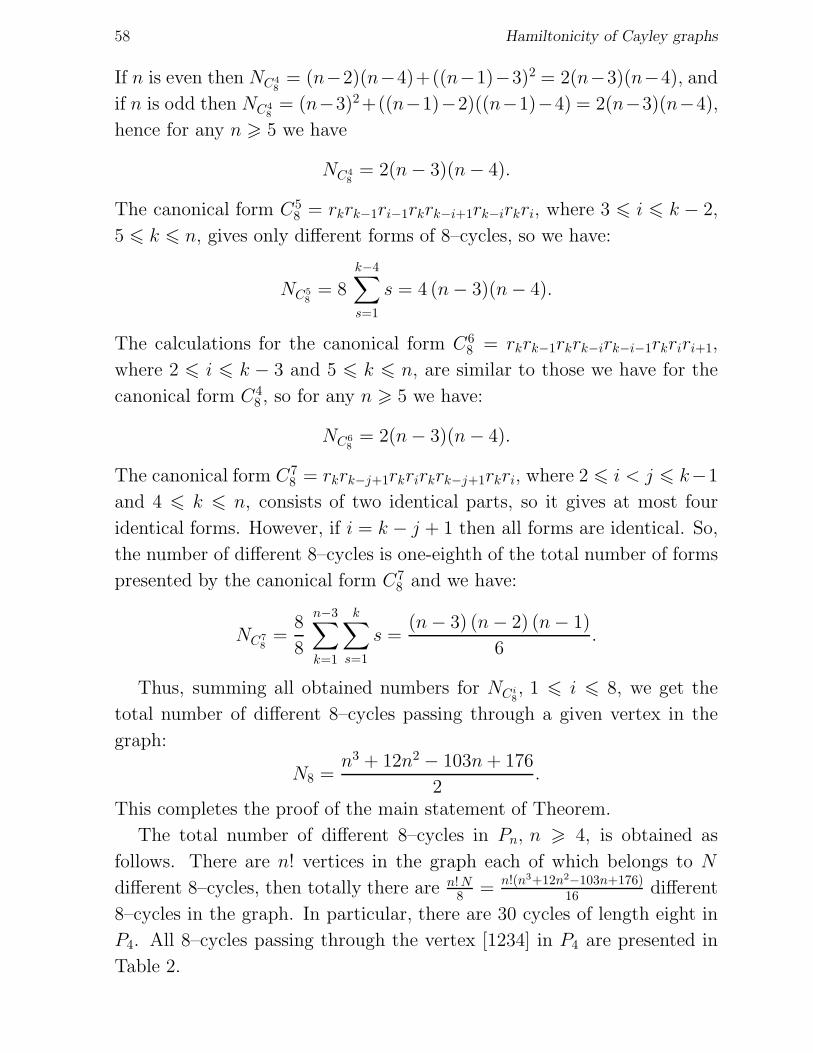
58 Hamiltonicity of Cayley graphs
If n is even then NC48= (n−2)(n−4)+((n−1)−3)2 = 2(n−3)(n−4), and
if n is odd then NC48= (n−3)2+((n−1)−2)((n−1)−4) = 2(n−3)(n−4),
hence for any n > 5 we have
NC48= 2(n− 3)(n− 4).
The canonical form C58 = rkrk−1ri−1rkrk−i+1rk−irkri, where 3 6 i 6 k − 2,
5 6 k 6 n, gives only different forms of 8–cycles, so we have:
NC58= 8
k−4∑
s=1
s = 4 (n− 3)(n− 4).
The calculations for the canonical form C68 = rkrk−1rkrk−irk−i−1rkriri+1,
where 2 6 i 6 k − 3 and 5 6 k 6 n, are similar to those we have for the
canonical form C48 , so for any n > 5 we have:
NC68= 2(n− 3)(n− 4).
The canonical form C78 = rkrk−j+1rkrirkrk−j+1rkri, where 2 6 i < j 6 k−1
and 4 6 k 6 n, consists of two identical parts, so it gives at most four
identical forms. However, if i = k − j + 1 then all forms are identical. So,
the number of different 8–cycles is one-eighth of the total number of forms
presented by the canonical form C78 and we have:
NC78=
8
8
n−3∑
k=1
k∑
s=1
s =(n− 3) (n− 2) (n− 1)
6.
Thus, summing all obtained numbers for NCi8, 1 6 i 6 8, we get the
total number of different 8–cycles passing through a given vertex in the
graph:
N8 =n3 + 12n2 − 103n+ 176
2.
This completes the proof of the main statement of Theorem.
The total number of different 8–cycles in Pn, n > 4, is obtained as
follows. There are n! vertices in the graph each of which belongs to N
different 8–cycles, then totally there are n!N8 = n!(n3+12n2−103n+176)
16 different
8–cycles in the graph. In particular, there are 30 cycles of length eight in
P4. All 8–cycles passing through the vertex [1234] in P4 are presented in
Table 2.
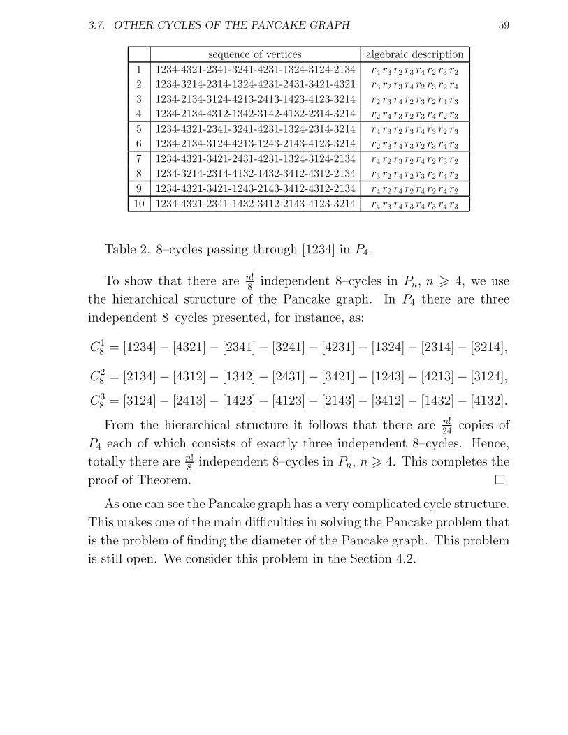
3.7. OTHER CYCLES OF THE PANCAKE GRAPH 59
sequence of vertices algebraic description
1 1234-4321-2341-3241-4231-1324-3124-2134 r4 r3 r2 r3 r4 r2 r3 r22 1234-3214-2314-1324-4231-2431-3421-4321 r3 r2 r3 r4 r2 r3 r2 r43 1234-2134-3124-4213-2413-1423-4123-3214 r2 r3 r4 r2 r3 r2 r4 r34 1234-2134-4312-1342-3142-4132-2314-3214 r2 r4 r3 r2 r3 r4 r2 r35 1234-4321-2341-3241-4231-1324-2314-3214 r4 r3 r2 r3 r4 r3 r2 r36 1234-2134-3124-4213-1243-2143-4123-3214 r2 r3 r4 r3 r2 r3 r4 r37 1234-4321-3421-2431-4231-1324-3124-2134 r4 r2 r3 r2 r4 r2 r3 r28 1234-3214-2314-4132-1432-3412-4312-2134 r3 r2 r4 r2 r3 r2 r4 r29 1234-4321-3421-1243-2143-3412-4312-2134 r4 r2 r4 r2 r4 r2 r4 r210 1234-4321-2341-1432-3412-2143-4123-3214 r4 r3 r4 r3 r4 r3 r4 r3
Table 2. 8–cycles passing through [1234] in P4.
To show that there are n!8 independent 8–cycles in Pn, n > 4, we use
the hierarchical structure of the Pancake graph. In P4 there are three
independent 8–cycles presented, for instance, as:
C18 = [1234]− [4321]− [2341]− [3241]− [4231]− [1324]− [2314]− [3214],
C28 = [2134]− [4312]− [1342]− [2431]− [3421]− [1243]− [4213]− [3124],
C38 = [3124]− [2413]− [1423]− [4123]− [2143]− [3412]− [1432]− [4132].
From the hierarchical structure it follows that there are n!24
copies of
P4 each of which consists of exactly three independent 8–cycles. Hence,
totally there are n!8 independent 8–cycles in Pn, n > 4. This completes the
proof of Theorem. �
As one can see the Pancake graph has a very complicated cycle structure.
This makes one of the main difficulties in solving the Pancake problem that
is the problem of finding the diameter of the Pancake graph. This problem
is still open. We consider this problem in the Section 4.2.

60 Hamiltonicity of Cayley graphs

Chapter 4
The diameter problem
Cayley graphs tend to have a number of other desirable properties as well,
including low diameter. There is the problem of establishing the diameter
of a Cayley graph Γ = Cay(G, S), that is the maximum, over g ∈ G, of the
length of a shortest expression for g as a product of generators. Computing
the diameter of an arbitrary Cayley graph over a set of generators is NP–
hard since the minimal word problem is known to be NP–hard in general.
This result was shown in 1981 by Shimon Even and Oded Goldreich in [29].
It is known, for instance, that it is the classic problem in the Rubik’s cube
puzzle. Recently it was announced [33] that every position of Rubik’s Cube
can be solved in twenty moves or less which represents the diameter of a
corresponding Cayley graph.
General upper and lower bounds are very difficult to obtain. Moreover,
there is a fundamental difference between Cayley graphs of abelian and
non–abelian groups.
4.1 Diameter of Cayley graphs on abelian and non–
abelian groups
Laszlo Babai et al. [7] have considered in 1989 the diameter of Cayley
graphs on non–abelian finite simple groups and the following result was
obtained.
Theorem 4.1.1 [7] Every non–abelian finite simple group G has a set of
6 7 generators such that the resulting Cayley graph has diameter O(log2 |G|).
61
62 The diameter problem
So, they have shown that each nonabelian simple group has a set of at
most seven generators that yields a Cayley graph with logarithmic diameter
(with constant factors). However, this property does not hold for Cayley
graphs of abelian groups as it was shown in 1993 by Fred Annexstein and
Marc Baumslag in [3]. They have found a lower bound on the diameter of
Cayley graphs on abelian groups. Let us recall, that in an abelian group
the result of applying the group operation to two group elements does not
depend on their order, i.e. for any g, h ∈ G we have gh = hg, and every
subgroup of an abelian group is normal.
By diam(Cay(G, S)) we denote the diameter of a Cayley graphCay(G, S)
on a group G with a generating set S. The result presented above is actu-
ally obtained for a Cayley digraph which means that there is no restrictions
for a generating set to be a symmetric or identity free.
Theorem 4.1.2 [3] Let G be an abelian group with a generating set S of
size r. The Cayley graph Cay(G, S) has the following diameter bound:
diam(Cay(G, S)) >1
e|G|1/r.
Proof. Suppose that G is an abelian group with a generating set S os
size r. Let n be the number of group elements that can be written as a
product of 6 d = diam(Cay(G, S)) elements from S. Since G is abelian,
n is at most equal to the number of ways d objects can be chosen from the
set of (r+ 1) objects with repetition allowed. The set of (r + 1) objects is
S⋃
e. The number of ways n is bounded as follows:
n 6
(r + d
d
)
=(r + d)!
r! d!6
(r + d)r
r!6
(r d)r
r!6 (ed)r.
Solving for d yields the given bound. �
We can get a tighter bound in the case r 6 |G|1/r 6 d. For then:
n 6
(r + d
d
)
=(r + d)!
r! d!6
(r + d)r
r!6
(2d)r
r!6
(2ed
r
)r
.
On the other hand, in 1988 it was conjectured by Laszlo Babai and Akos
Seress [9] for non–abelian groups that the diameter will always be small.
4.2. PANCAKE PROBLEM 63
Conjecture 4.1.3 [9] There exist a constant c such that for every non–
abelian finite simple group G, the diameter of every Cayley graph of G is
6 (log2 |G|)c.
If the conjecture is true, one would expect to find Cayley graphs of
these groups with small diameter. But this problem is open even for the
alternating groups An, consisting of all the even permutations of {1, . . . , n}.
The first step towards a solution this conjecture was made by Babai and
Seress [9] for the symmetric Symn and alternating An groups.
Theorem 4.1.4 [9] If G is either Symn or An then the diameter of every
Cayley graph of G is 6 exp((n lnn)(1/2)(1 + o(1))).
Even for simple examples the exact diameter is still unknown and there
are only bounds. For example, for the pancake graphs which are known
because of the open combinatorial Pancake problems.
4.2 Pancake problem
The original (unburnt) Pancake problem was posed in 1975 in the American
Mathematical Monthly by Jacob E. Goodman [27] writing under the name
”Harry Dweighter” (or ”Harried Waiter”) and it is stated as follows:
”The chef in our place is sloppy, and when he prepares a stack
of pancakes they come out all different sizes. Therefore, when I
deliver them to a customer, on the way to the table I rearrange
them (so that the smallest winds up on top, and so on, down
to the largest on the bottom) by grabbing several pancakes from
the top and flips them over, repeating this (varying the number
I flip) as many times as necessary. If there are n pancakes, what
is the maximum number of flips (as a function of n) that I will
ever have to use to rearrange them?”
It is clear that a stack of these n pancakes can be represented by a per-
mutation on n elements and the problem is to find the minimum number
of flips (prefix–reversals) needed to transform a permutation into the iden-
tity permutation. Clearly, this number of flips corresponds to the diameter
d(Pn) of the Pancake graph. There is the following open problem.
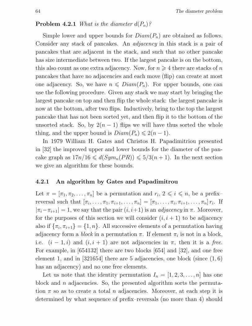
64 The diameter problem
Problem 4.2.1 What is the diameter d(Pn)?
Simple lower and upper bounds for Diam(Pn) are obtained as follows.
Consider any stack of pancakes. An adjacency in this stack is a pair of
pancakes that are adjacent in the stack, and such that no other pancake
has size intermediate between two. If the largest pancake is on the bottom,
this also count as one extra adjacency. Now, for n > 4 there are stacks of n
pancakes that have no adjacencies and each move (flip) can create at most
one adjacency. So, we have n 6 Diam(Pn). For upper bounds, one can
use the following procedure. Given any stack we may start by bringing the
largest pancake on top and then flip the whole stack: the largest pancake is
now at the bottom, after two flips. Inductively, bring to the top the largest
pancake that has not been sorted yet, and then flip it to the bottom of the
unsorted stack. So, by 2(n − 1) flips we will have thus sorted the whole
thing, and the upper bound is Diam(Pn) 6 2(n− 1).
In 1979 William H. Gates and Christos H. Papadimitriou presented
in [32] the improved upper and lower bounds for the diameter of the pan-
cake graph as 17n/16 6 d(Symn(PR)) 6 5/3(n+ 1). In the next section
we give an algorithm for these bounds.
4.2.1 An algorithm by Gates and Papadimitrou
Let π = [π1, π2, . . . , πn] be a permutation and ri, 2 6 i 6 n, be a prefix–
reversal such that [πi, . . . , π1, πi+1, . . . , πn] = [π1, . . . , πi, πi+1, . . . , πn] ri. If
|πi−πi+1| = 1, we say that the pair (i, i+1) is an adjacency in π. Moreover,
for the purposes of this section we will consider (i, i + 1) to be adjacency
also if {πi, πi+1} = {1, n}. All successive elements of a permutation having
adjacency form a block in a permutation π. If element πi is not in a block,
i.e. (i − 1, i) and (i, i + 1) are not adjacencies in π, then it is a free.
For example, in [654132] there are two blocks [654] and [32], and one free
element 1, and in [321654] there are 5 adjacencies, one block (since (1, 6)
has an adjacency) and no one free elements.
Let us note that the identity permutation In = [1, 2, 3, . . . , n] has one
block and n adjacencies. So, the presented algorithm sorts the permuta-
tion π so as to create a total n adjacencies. Moreover, at each step it is
determined by what sequence of prefix–reversals (no more than 4) should
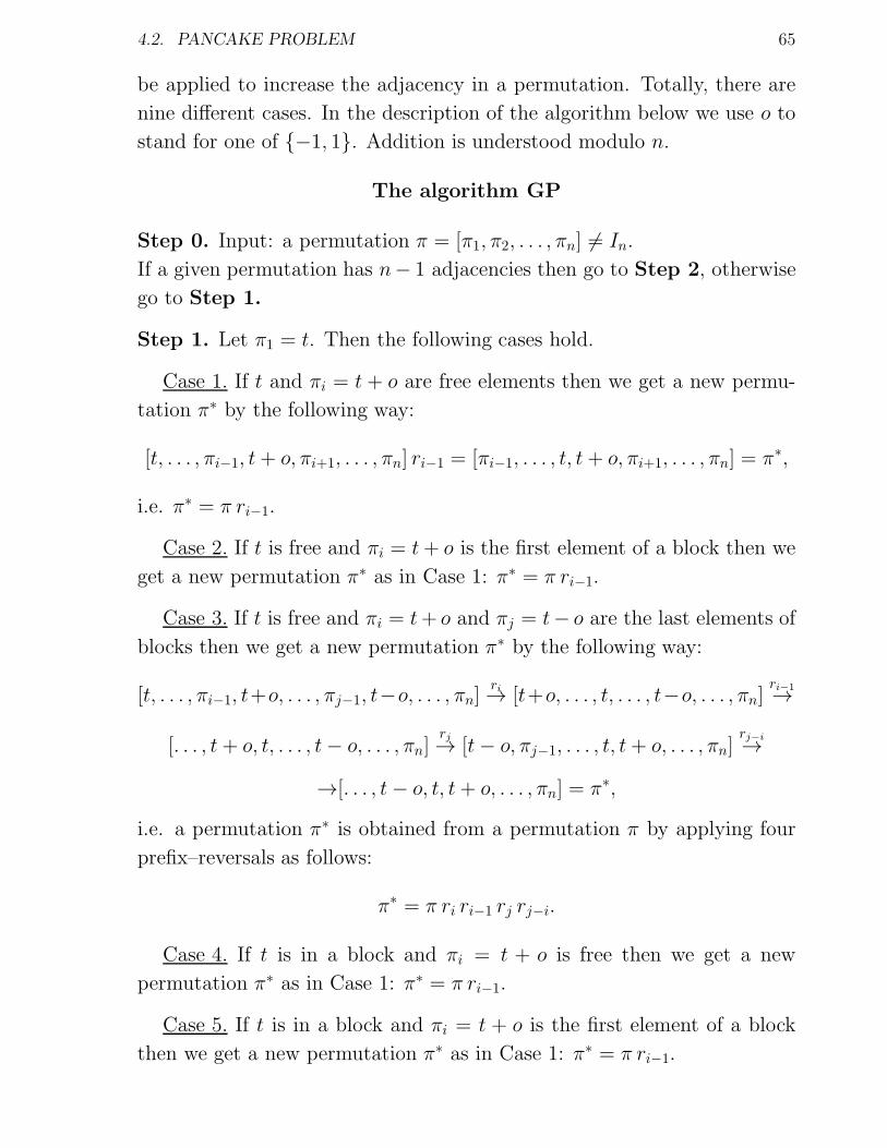
4.2. PANCAKE PROBLEM 65
be applied to increase the adjacency in a permutation. Totally, there are
nine different cases. In the description of the algorithm below we use o to
stand for one of {−1, 1}. Addition is understood modulo n.
The algorithm GP
Step 0. Input: a permutation π = [π1, π2, . . . , πn] 6= In.
If a given permutation has n− 1 adjacencies then go to Step 2, otherwise
go to Step 1.
Step 1. Let π1 = t. Then the following cases hold.
Case 1. If t and πi = t + o are free elements then we get a new permu-
tation π∗ by the following way:
[t, . . . , πi−1, t+ o, πi+1, . . . , πn] ri−1 = [πi−1, . . . , t, t+ o, πi+1, . . . , πn] = π∗,
i.e. π∗ = π ri−1.
Case 2. If t is free and πi = t+ o is the first element of a block then we
get a new permutation π∗ as in Case 1: π∗ = π ri−1.
Case 3. If t is free and πi = t+ o and πj = t− o are the last elements of
blocks then we get a new permutation π∗ by the following way:
[t, . . . , πi−1, t+o, . . . , πj−1, t−o, . . . , πn]ri→ [t+o, . . . , t, . . . , t−o, . . . , πn]
ri−1
→
[. . . , t+ o, t, . . . , t− o, . . . , πn]rj→ [t− o, πj−1, . . . , t, t+ o, . . . , πn]
rj−i
→
→[. . . , t− o, t, t+ o, . . . , πn] = π∗,
i.e. a permutation π∗ is obtained from a permutation π by applying four
prefix–reversals as follows:
π∗ = π ri ri−1 rj rj−i.
Case 4. If t is in a block and πi = t + o is free then we get a new
permutation π∗ as in Case 1: π∗ = π ri−1.
Case 5. If t is in a block and πi = t + o is the first element of a block
then we get a new permutation π∗ as in Case 1: π∗ = π ri−1.
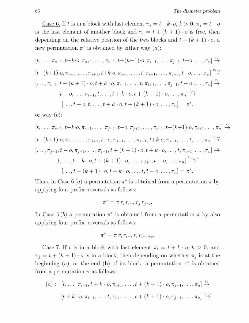
66 The diameter problem
Case 6. If t is in a block with last element πs = t+k ·o, k > 0, πj = t−o
is the last element of another block and πi = t + (k + 1) · o is free, then
depending on the relative position of the two blocks and t + (k + 1) · o, a
new permutation π∗ is obtained by either way (a):
[t, . . . , πs−1, t+k·o, πs+1, . . . , πi−1, t+(k+1)·o, πi+1, . . . , πj−1, t−o, . . . , πn]ri→
[t+(k+1)·o, πi−1, . . . , πs+1, t+k·o, πs−1, . . . , t, πi+1, . . . , πj−1, t−o, . . . , πn]ri−s→
[. . . , πi−1, t+ (k + 1) · o, t+ k · o, πs−1, . . . , t, πi+1, . . . , πj−1, t− o, . . . , πn]rj→
[t− o, . . . , πi+1, t, . . . , t+ k · o, t+ (k + 1) · o, . . . , πn]rj−i
→
[. . . , t− o, t, . . . , t+ k · o, t+ (k + 1) · o, . . . , πn] = π∗,
or way (b):
[t, . . . , πs−1, t+k·o, πs+1, . . . , πj−1, t−o, πj+1, . . . , πi−1, t+(k+1)·o, πi+1 . . . , πn]ri→
[t+(k+1)·o, πi−1, . . . , πj+1, t−o, πj−1, . . . , πs+1, t+k·o, πs−1, . . . , t, . . . , πn]ri−s→
[. . . , πj−1, t− o, πj+1, . . . , πi−1, t+ (k + 1) · o, t+ k · o, . . . , t, πi+1, . . . , πn]ri→
[t, . . . , t+ k · o, t+ (k + 1) · o, . . . , πj+1, t− o, . . . , πn]ri−j+s
→
[. . . , t+ (k + 1) · o, t+ k · o, . . . , t, t− o, . . . , πn] = π∗.
Thus, in Case 6 (a) a permutation π∗ is obtained from a permutation π by
applying four prefix–reversals as follows:
π∗ = π ri ri−s rj rj−i.
In Case 6 (b) a permutation π∗ is obtained from a permutation π by also
applying four prefix–reversals as follows:
π∗ = π ri ri−s ri ri−j+s.
Case 7. If t is in a block with last element πi = t + k · o, k > 0, and
πj = t + (k + 1) · o is in a block, then depending on whether πj is at the
beginning (a), or the end (b) of its block, a permutation π∗ is obtained
from a permutation π as follows:
(a) : [t, . . . , πi−1, t+ k · o, πi+1, . . . , t+ (k + 1) · o, πj+1, . . . , πn]ri→
[t+ k · o, πi−1, . . . , t, πi+1, . . . , t+ (k + 1) · o, πj+1, . . . , πn]rj−1
→
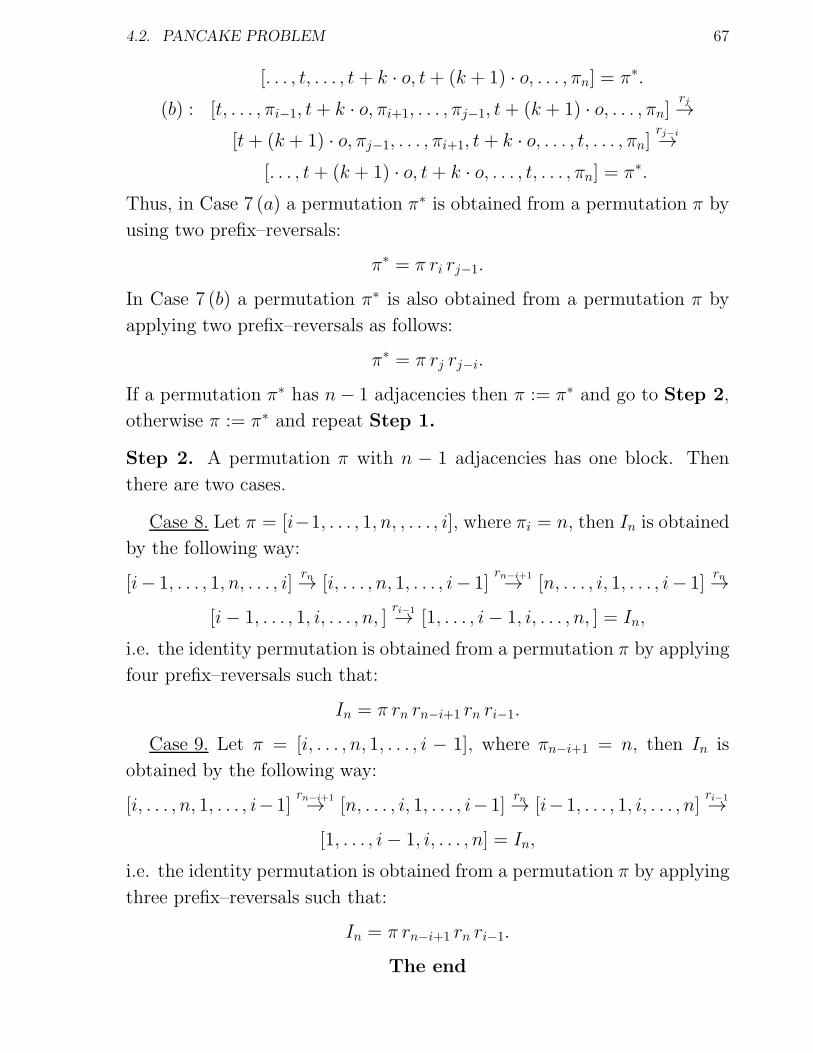
4.2. PANCAKE PROBLEM 67
[. . . , t, . . . , t+ k · o, t+ (k + 1) · o, . . . , πn] = π∗.
(b) : [t, . . . , πi−1, t+ k · o, πi+1, . . . , πj−1, t+ (k + 1) · o, . . . , πn]rj→
[t+ (k + 1) · o, πj−1, . . . , πi+1, t+ k · o, . . . , t, . . . , πn]rj−i
→
[. . . , t+ (k + 1) · o, t+ k · o, . . . , t, . . . , πn] = π∗.
Thus, in Case 7 (a) a permutation π∗ is obtained from a permutation π by
using two prefix–reversals:
π∗ = π ri rj−1.
In Case 7 (b) a permutation π∗ is also obtained from a permutation π by
applying two prefix–reversals as follows:
π∗ = π rj rj−i.
If a permutation π∗ has n− 1 adjacencies then π := π∗ and go to Step 2,
otherwise π := π∗ and repeat Step 1.
Step 2. A permutation π with n − 1 adjacencies has one block. Then
there are two cases.
Case 8. Let π = [i−1, . . . , 1, n, , . . . , i], where πi = n, then In is obtained
by the following way:
[i− 1, . . . , 1, n, . . . , i]rn→ [i, . . . , n, 1, . . . , i− 1]
rn−i+1
→ [n, . . . , i, 1, . . . , i− 1]rn→
[i− 1, . . . , 1, i, . . . , n, ]ri−1
→ [1, . . . , i− 1, i, . . . , n, ] = In,
i.e. the identity permutation is obtained from a permutation π by applying
four prefix–reversals such that:
In = π rn rn−i+1 rn ri−1.
Case 9. Let π = [i, . . . , n, 1, . . . , i − 1], where πn−i+1 = n, then In is
obtained by the following way:
[i, . . . , n, 1, . . . , i−1]rn−i+1
→ [n, . . . , i, 1, . . . , i−1]rn→ [i−1, . . . , 1, i, . . . , n]
ri−1
→
[1, . . . , i− 1, i, . . . , n] = In,
i.e. the identity permutation is obtained from a permutation π by applying
three prefix–reversals such that:
In = π rn−i+1 rn ri−1.
The end

68 The diameter problem
4.2.2 Upper bound on the diameter of the Pancake graph
Theorem 4.2.2 [32] Algorithm GP creates the identity permutation by at
most (5n+ 5)/3 prefix–reversals.
Proof. First, it is clear that if we have a permutation with less than
n− 1 adjacencies, one of the Cases 1–7 is applicable. Hence, the algorithm
does not halt unless (n−1) adjacencies have been created. Then one of the
Cases 8–9 is applicable to get the identity permutation with n adjacencies
and one block. Then the algorithm is finished. Obviously, the algorithm
will eventually halt, since at each execution of the main loop at least one
new adjacency is created and none are destroyed. It remains to prove that
it does so in no more than (5n+ 5)/3 prefix–reversals.
Call the action of Case i as action of a type i (or just action i). Let xi,
where i = 1, . . . , 9, denote the number of actions of type i performed by an
execution of the algorithm assuming that x3 = x6. Then the total number
z of prefix–reversals given by the Cases 1–7 are presented as follows:
z = x1 + x2 + 4x3 + x4 + x5 + 2x7,
where xi is multiplied by the number of prefix–reversals involved in the
corresponding case. Action 3 can be divided into four special cases, ac-
cording to what happens in the corresponding flipping that comes before
the last. The top of stack before the flipping and the element next to t− o
may either: 1) be non–adjacent; 2) from a new block; 3) merge a block
with a singleton; 4) merge two blocks. Accordingly, we distinguish among
these subcases by writing x3 = x31 + x32 + x33 + x34.
Now, since each action increases the number of adjacencies as indicated
in the table below, the total number of n− 1 adjacencies in the conclusion
of the Step 1 (Cases 1–7) of the algorithm is presented as:
n− 1 = a+ x1 + x2 + 2x31 + 3x32 + 3x33 + 3x34 + x4 + x5 + x7, (4.1)
where a is a number of adjacencies in a given permutation π,
Finally, if b is the number of blocks in a given permutation π then we
have
b+ x1 − x31 − x33 − 2x34 − x5 − x7 = 1, (4.2)
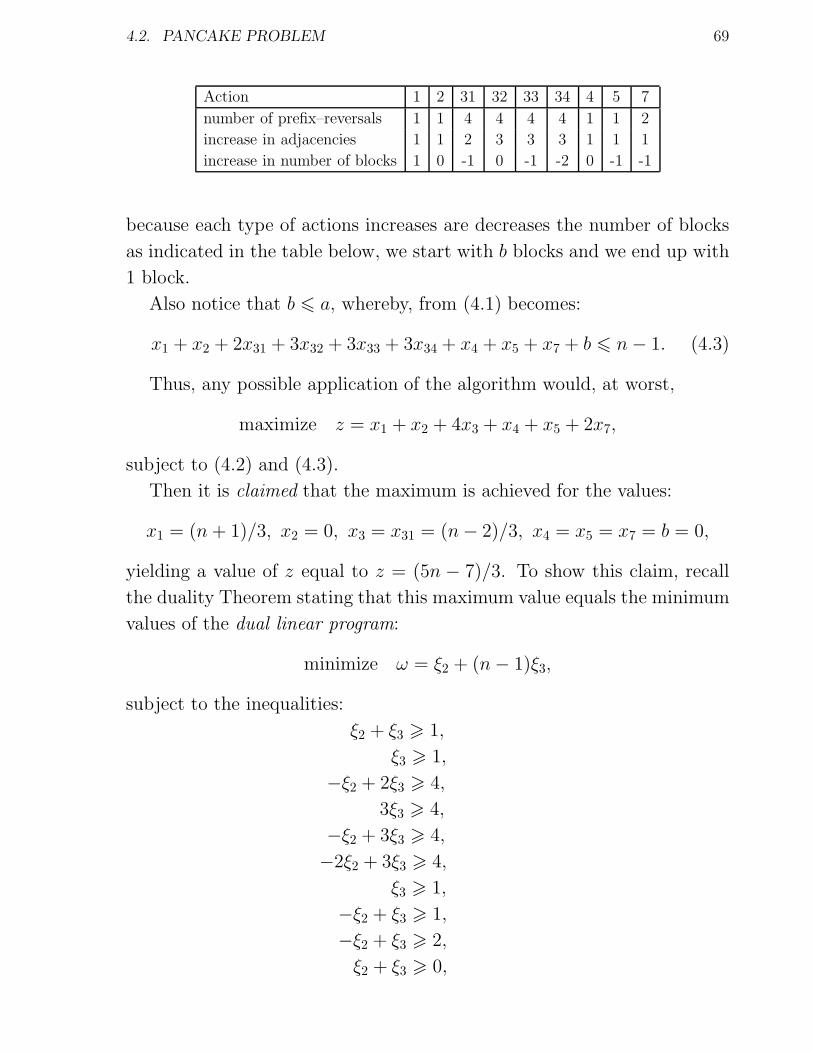
4.2. PANCAKE PROBLEM 69
Action 1 2 31 32 33 34 4 5 7
number of prefix–reversals 1 1 4 4 4 4 1 1 2
increase in adjacencies 1 1 2 3 3 3 1 1 1
increase in number of blocks 1 0 -1 0 -1 -2 0 -1 -1
because each type of actions increases are decreases the number of blocks
as indicated in the table below, we start with b blocks and we end up with
1 block.
Also notice that b 6 a, whereby, from (4.1) becomes:
x1 + x2 + 2x31 + 3x32 + 3x33 + 3x34 + x4 + x5 + x7 + b 6 n− 1. (4.3)
Thus, any possible application of the algorithm would, at worst,
maximize z = x1 + x2 + 4x3 + x4 + x5 + 2x7,
subject to (4.2) and (4.3).
Then it is claimed that the maximum is achieved for the values:
x1 = (n+ 1)/3, x2 = 0, x3 = x31 = (n− 2)/3, x4 = x5 = x7 = b = 0,
yielding a value of z equal to z = (5n − 7)/3. To show this claim, recall
the duality Theorem stating that this maximum value equals the minimum
values of the dual linear program:
minimize ω = ξ2 + (n− 1)ξ3,
subject to the inequalities:
ξ2 + ξ3 > 1,
ξ3 > 1,
−ξ2 + 2ξ3 > 4,
3ξ3 > 4,
−ξ2 + 3ξ3 > 4,
−2ξ2 + 3ξ3 > 4,
ξ3 > 1,
−ξ2 + ξ3 > 1,
−ξ2 + ξ3 > 2,
ξ2 + ξ3 > 0,
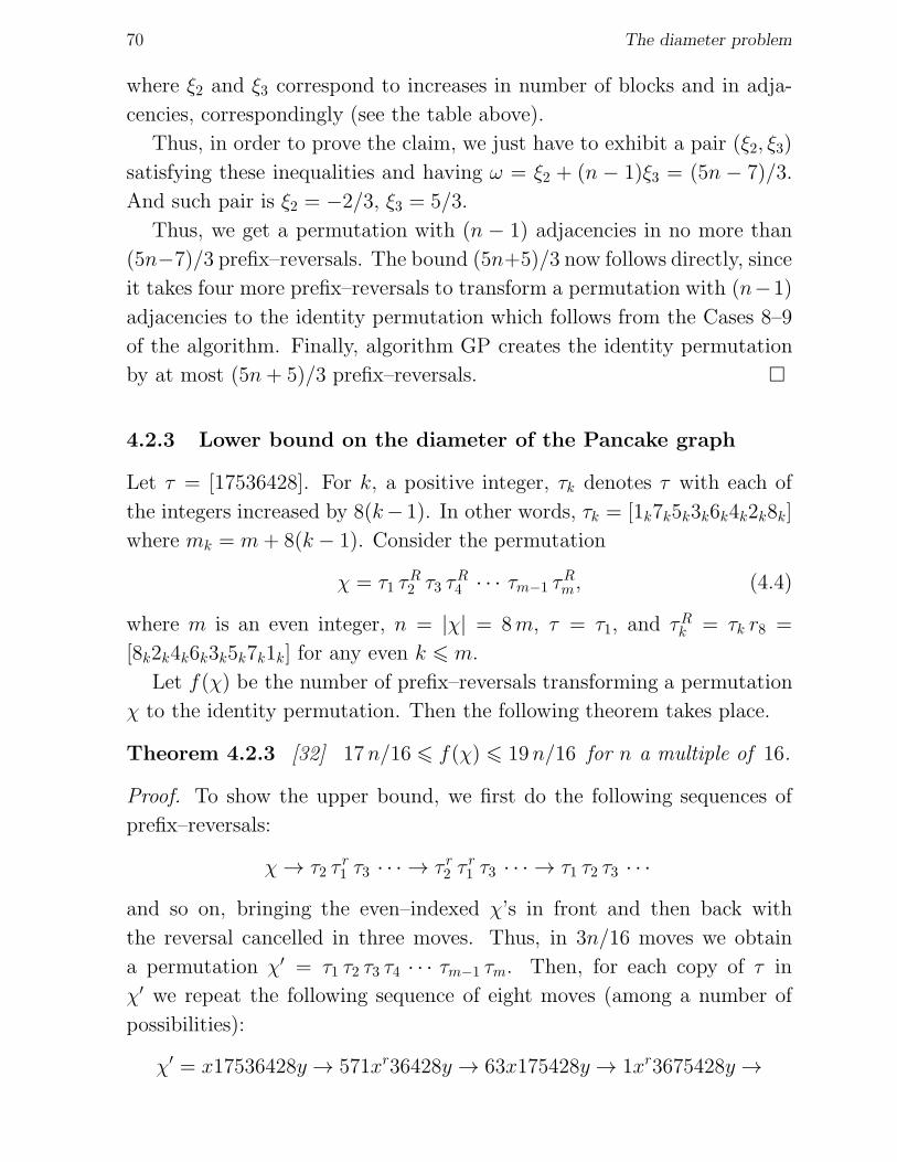
70 The diameter problem
where ξ2 and ξ3 correspond to increases in number of blocks and in adja-
cencies, correspondingly (see the table above).
Thus, in order to prove the claim, we just have to exhibit a pair (ξ2, ξ3)
satisfying these inequalities and having ω = ξ2 + (n − 1)ξ3 = (5n − 7)/3.
And such pair is ξ2 = −2/3, ξ3 = 5/3.
Thus, we get a permutation with (n − 1) adjacencies in no more than
(5n−7)/3 prefix–reversals. The bound (5n+5)/3 now follows directly, since
it takes four more prefix–reversals to transform a permutation with (n−1)
adjacencies to the identity permutation which follows from the Cases 8–9
of the algorithm. Finally, algorithm GP creates the identity permutation
by at most (5n+ 5)/3 prefix–reversals. �
4.2.3 Lower bound on the diameter of the Pancake graph
Let τ = [17536428]. For k, a positive integer, τk denotes τ with each of
the integers increased by 8(k− 1). In other words, τk = [1k7k5k3k6k4k2k8k]
where mk = m+ 8(k − 1). Consider the permutation
χ = τ1 τR2 τ3 τ
R4 · · · τm−1 τ
Rm, (4.4)
where m is an even integer, n = |χ| = 8m, τ = τ1, and τRk = τk r8 =
[8k2k4k6k3k5k7k1k] for any even k 6 m.
Let f(χ) be the number of prefix–reversals transforming a permutation
χ to the identity permutation. Then the following theorem takes place.
Theorem 4.2.3 [32] 17n/16 6 f(χ) 6 19n/16 for n a multiple of 16.
Proof. To show the upper bound, we first do the following sequences of
prefix–reversals:
χ → τ2 τr1 τ3 · · · → τ r2 τ
r1 τ3 · · · → τ1 τ2 τ3 · · ·
and so on, bringing the even–indexed χ’s in front and then back with
the reversal cancelled in three moves. Thus, in 3n/16 moves we obtain
a permutation χ′ = τ1 τ2 τ3 τ4 · · · τm−1 τm. Then, for each copy of τ in
χ′ we repeat the following sequence of eight moves (among a number of
possibilities):
χ′ = x17536428y → 571xr36428y → 63x175428y → 1xr3675428y →
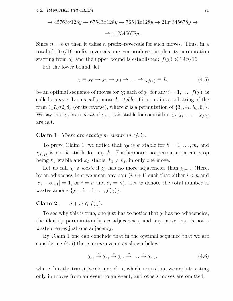
4.2. PANCAKE PROBLEM 71
→ 45763x128y → 67543x128y → 76543x128y → 21xr345678y →
→ x12345678y.
Since n = 8m then it takes n prefix–reversals for such moves. Thus, in a
total of 19n/16 prefix–reversals one can produce the identity permutation
starting from χ, and the upper bound is established: f(χ) 6 19n/16.
For the lower bound, let
χ ≡ χ0 → χ1 → χ2 → . . . → χf(χ) ≡ In (4.5)
be an optimal sequence of moves for χ; each of χi for any i = 1, . . . , f(χ), is
called a move. Let us call a move k–stable, if it contains a substring of the
form 1k7kσ2k8k (or its reverse), where σ is a permutation of {3k, 4k, 5k, 6k}.
We say that χi is an event, if χi−1 is k–stable for some k but χi, χi+1, . . . χf(χ)
are not.
Claim 1. There are exactly m events in (4.5).
To prove Claim 1, we notice that χ0 is k–stable for k = 1, . . . , m, and
χf(χ) is not k–stable for any k. Furthermore, no permutation can stop
being k1–stable and k2–stable, k1 6= k2, in only one move.
Let us call χi a waste if χi has no more adjacencies than χi−1. (Here,
by an adjacency in σ we mean any pair (i, i+1) such that either i < n and
|σi − σi+1| = 1, or i = n and σi = n). Let w denote the total number of
wastes among {χi : i = 1, . . . , f(χ)}.
Claim 2. n+ w 6 f(χ).
To see why this is true, one just has to notice that χ has no adjacencies,
the identity permutation has n adjacencies, and any move that is not a
waste creates just one adjacency.
By Claim 1 one can conclude that in the optimal sequence that we are
considering (4.5) there are m events as shown below:
χi1∗→ χi2
∗→ χi3
∗→ . . .
∗→ χim, (4.6)
where∗→ is the transitive closure of→, which means that we are interesting
only in moves from an event to an event, and others moves are omitted.
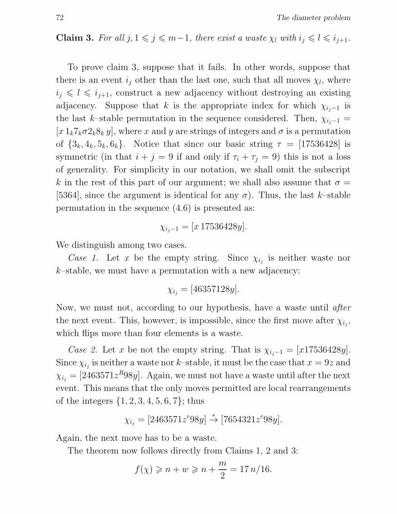
72 The diameter problem
Claim 3. For all j, 1 6 j 6 m−1, there exist a waste χl with ij 6 l 6 ij+1.
To prove claim 3, suppose that it fails. In other words, suppose that
there is an event ij other than the last one, such that all moves χl, where
ij 6 l 6 ij+1, construct a new adjacency without destroying an existing
adjacency. Suppose that k is the appropriate index for which χij−1 is
the last k–stable permutation in the sequence considered. Then, χij−1 =
[x 1k7kσ2k8k y], where x and y are strings of integers and σ is a permutation
of {3k, 4k, 5k, 6k}. Notice that since our basic string τ = [17536428] is
symmetric (in that i + j = 9 if and only if τi + τj = 9) this is not a loss
of generality. For simplicity in our notation, we shall omit the subscript
k in the rest of this part of our argument; we shall also assume that σ =
[5364], since the argument is identical for any σ). Thus, the last k–stable
permutation in the sequence (4.6) is presented as:
χij−1 = [x 17536428y].
We distinguish among two cases.
Case 1. Let x be the empty string. Since χij is neither waste nor
k–stable, we must have a permutation with a new adjacency:
χij = [46357128y].
Now, we must not, according to our hypothesis, have a waste until after
the next event. This, however, is impossible, since the first move after χij ,
which flips more than four elements is a waste.
Case 2. Let x be not the empty string. That is χij−1 = [x17536428y].
Since χij is neither a waste nor k–stable, it must be the case that x = 9z and
χij = [2463571zR98y]. Again, we must not have a waste until after the next
event. This means that the only moves permitted are local rearrangements
of the integers {1, 2, 3, 4, 5, 6, 7}; thus
χij = [2463571zr98y]∗→ [7654321zr98y].
Again, the next move has to be a waste.
The theorem now follows directly from Claims 1, 2 and 3:
f(χ) > n+ w > n+m
2= 17n/16.
4.2. PANCAKE PROBLEM 73
�
Thus, from this theorem we immediately have the following result.
Corollary 4.2.4 17n/16 6 diam(Pn) for n a multiple of 16.
4.2.4 Improved bounds by Heydari and Sudborough
Gates and Papadimitrou concluded in [32] that
”... slightly better lower bounds may be conceivably proved by
using different τ ′ - of length 7, say. However, we do not know
how the upper and lower bounds can be narrowed significantly.”
A lower bound was improved in 1997 by Heydari and Sudborough [39]
on the basic permutation ζ = [1753642]. Then as above for k, a positive
integer, ζk = [1k7k5k3k6k4k2k] where mk = m + 7(k − 1). Consider the
permutation
ϕn = ζ1 ζ2 · · · ζm, (4.7)
where m is an even integer, n = |ζ| = 7m, ζ = ζ1.
Let f(ϕn) be the number of prefix–reversals transforming a permutation
ϕn to the identity permutation. Then the following theorem takes place.
Theorem 4.2.5 [39] 15n/14 6 f(ϕn) for all n ≡ 0 (mod 14).
The proof is similar to that given by Gates and Papadimitrou in [32].
Proof. Let
ϕ ≡ ϕ0 → ϕ1 → . . . → ϕf(ϕn) ≡ In (4.8)
be an optimal sequence of moves for ϕn; each of ϕi, i = 1, . . . , f(ϕn), is
called a move. A move is called k–stable if it contains a substring of the
form
[1k7kσ2k8k] = [1k7kσ2k1k+1]
(or its reverse), where σ is a permutation of {3k, 4k, 5k, 6k}. (Assuming
that 8k = 1k+1, i.e., the (n + 1)th pancake, is in its correct place at the
bottom of the stack). We say that ϕi is an event if ϕi−1 is k–stable, for
some k, but ϕi, ϕi+1, . . . ϕf(ϕn) are not.
74 The diameter problem
Claim 1. There are exactly m events in (4.8).
To prove Claim 1, we notice that ϕ0 is k–stable for all k = 1, . . . , m,
and ϕf(ϕn) is not k–stable for any k. Furthermore, no permutation can stop
being k1–stable and k2–stable in only one move, k1 6= k2.
A waste is defined as above: ϕi is a waste if it has no more adjacencies
than ϕi−1. The total number of wastes among {ϕi : i = 1, . . . , f(ϕn)} is
denoted by w.
Claim 2. n+ w 6 f(ϕn).
To see why this is true, we just have to notice that ϕn has no adjacencies,
and the identity permutation In has n adjacencies, and any move that is
not a waste creates just one adjacency.
By Claim 1 we conclude that in the optimal sequence we consider (4.8)
there are m events as shown by:
ϕi1∗→ ϕi2
∗→ ϕi3
∗→ . . .
∗→ ϕim, (4.9)
where∗→ is the transitive closure of → as above.
Claim 3. For all j, 1 6 j 6 m−1, there exist a waste ϕl with ij 6 l 6 ij+1.
To prove Claim 3, suppose it were false. In other words, suppose that
these is an event ij other than the last one, such that all moves ϕl, ij 6 l 6
ij+1, construct a new adjacency without destroying an existing adjacency.
Suppose that k is the appropriate index for which ϕij−1 is the last k–stable
permutation in the sequence (4.8). Then
ϕij−1 = [x 1k7kσ2k8k y] = [x 1k7kσ2k1k+1 y],
where x and y are strings of integers and σ is a permutation of {3k, 4k, 5k, 6k}.
Notice that because the string ζ = [1k7k5k3k6k4k2k8k] is symmetric (in that
i + j = 9 if and only if ik + jk = 9 + 2(k − 1)7), this is without loss of
generality. For simplicity in our notation, we shall replace ik by simply i
in the rest of the argument; we shall also assume that σ = [5364] because
the argument is identical for any σ. Thus, the last k–stable permutation
in the sequence (4.8) is presented as:
ϕij−1 = [x 17536428y].

4.2. PANCAKE PROBLEM 75
We distinguish two cases.
Case 1. Let x be the empty string. Whereas ϕij is neither a waste nor
k–stable, we must have a permutation with a new adjacency:
ϕij = [46357128y].
Now, we must not, according our hypothesis, have a waste until after the
next event. This, however, is impossible, because the first move after ϕij
which flips more that four elements is a waste. Note that 8k = 1k+1 re-
mains fixed in any prefix–reversal of the four elements, and therefore all
such prefix–reversals do not change whether ϕij−1 contains (or does not
contain) the substring [1k+17k+1σ2k+18k+1] (or its reversal) for any σ. Also,
whereas 1k = 8k−1 is the first element in ϕij−1 and therefore quite appar-
ently is not next to 2k−1, the move ϕij−1 does not contain the substring
[8k−12k−1σ7k−11k−1] (or its reversal) for any σ. Whereas any prefix–reversal
of the first four elements will not create such a substring and break it, there
is no event created by such prefix–reversals that involves (k − 1)–stability
or (k + 1)–stability.
Case 2. Let x be not the empty substring. That is, ϕij−1 = [x17546428y].
Since ϕij is neither a waste nor k–stable, it must be the case that x = 9z
for some z and ϕij = [2463571zR98y]. Again, we must not have a waste
until after the next event. This means the only moves permitted are local
rearrangements of the integers {1, 2, 3, 4, 5, 6, 7}; thus
ϕij = [2463571zR98y]∗→ [7654321zr98y].
Again, the next move has to be a waste. Suppose that ϕij contains a
substring of the form [1k−17k−1σ2k−18k−1] for some σ. Recall that 8k−1 = 1k,
so each move involving a local permutation of the integers {1, 2, 3, 4, 5, 6, 7},
including the move ϕij = [2463571zr98y], does not change the status of
(k − 1)–stability. Similarly, for (k + 1)–stability, because the symbol 8k =
1k+1 remains fixed throughout.
Theorem 4.2.5 now follows directly from Claims 1, 2 and 3:
f(ϕn) > n+ w > n+m
2= 15n/14.
�
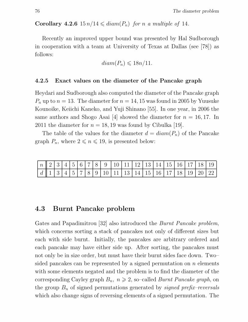
76 The diameter problem
Corollary 4.2.6 15n/14 6 diam(Pn) for n a multiple of 14.
Recently an improved upper bound was presented by Hal Sudborough
in cooperation with a team at University of Texas at Dallas (see [78]) as
follows:
diam(Pn) 6 18n/11.
4.2.5 Exact values on the diameter of the Pancake graph
Heydari and Sudborough also computed the diameter of the Pancake graph
Pn up to n = 13. The diameter for n = 14, 15 was found in 2005 by Yuusuke
Kounoike, Keiichi Kaneko, and Yuji Shinano [55]. In one year, in 2006 the
same authors and Shogo Asai [4] showed the diameter for n = 16, 17. In
2011 the diameter for n = 18, 19 was found by Cibulka [19].
The table of the values for the diameter d = diam(Pn) of the Pancake
graph Pn, where 2 6 n 6 19, is presented below:
n 2 3 4 5 6 7 8 9 10 11 12 13 14 15 16 17 18 19
d 1 3 4 5 7 8 9 10 11 13 14 15 16 17 18 19 20 22
4.3 Burnt Pancake problem
Gates and Papadimitrou [32] also introduced the Burnt Pancake problem,
which concerns sorting a stack of pancakes not only of different sizes but
each with side burnt. Initially, the pancakes are arbitrary ordered and
each pancake may have either side up. After sorting, the pancakes must
not only be in size order, but must have their burnt sides face down. Two–
sided pancakes can be represented by a signed permutation on n elements
with some elements negated and the problem is to find the diameter of the
corresponding Cayley graph Bn, n > 2, so–called Burnt Pancake graph, on
the group Bn of signed permutations generated by signed prefix–reversals
which also change signs of reversing elements of a signed permutation. The
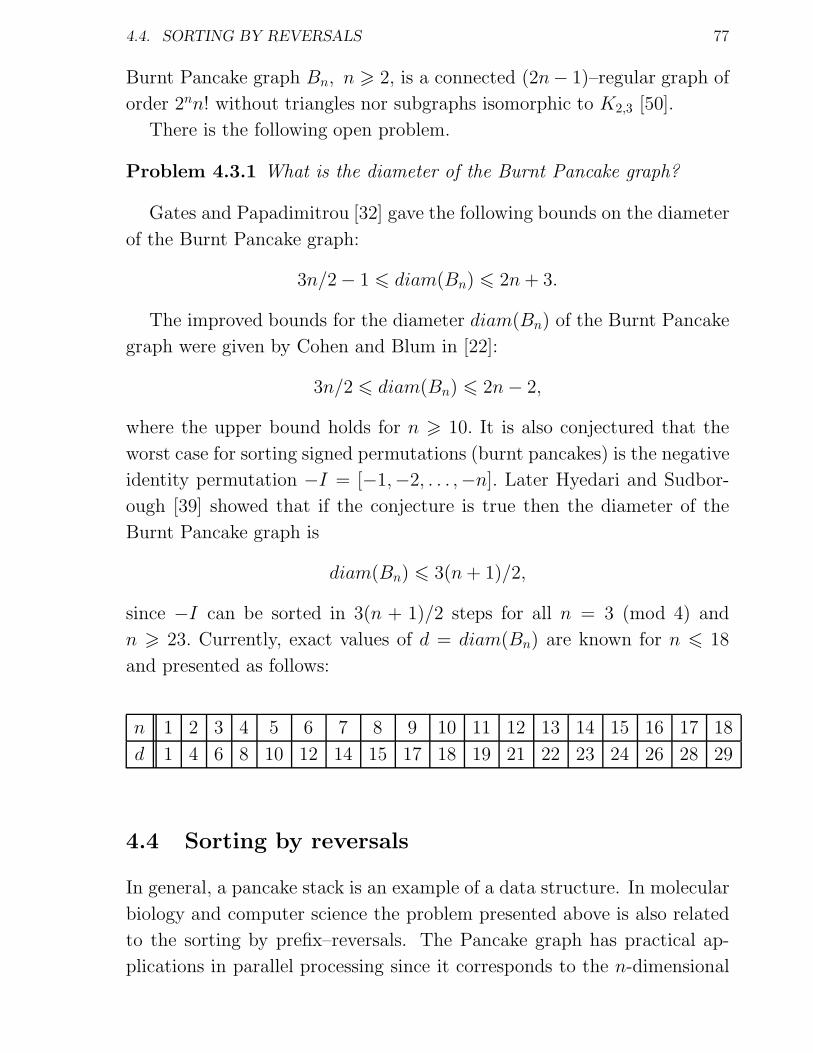
4.4. SORTING BY REVERSALS 77
Burnt Pancake graph Bn, n > 2, is a connected (2n− 1)–regular graph of
order 2nn! without triangles nor subgraphs isomorphic to K2,3 [50].
There is the following open problem.
Problem 4.3.1 What is the diameter of the Burnt Pancake graph?
Gates and Papadimitrou [32] gave the following bounds on the diameter
of the Burnt Pancake graph:
3n/2− 1 6 diam(Bn) 6 2n+ 3.
The improved bounds for the diameter diam(Bn) of the Burnt Pancake
graph were given by Cohen and Blum in [22]:
3n/2 6 diam(Bn) 6 2n− 2,
where the upper bound holds for n > 10. It is also conjectured that the
worst case for sorting signed permutations (burnt pancakes) is the negative
identity permutation −I = [−1,−2, . . . ,−n]. Later Hyedari and Sudbor-
ough [39] showed that if the conjecture is true then the diameter of the
Burnt Pancake graph is
diam(Bn) 6 3(n+ 1)/2,
since −I can be sorted in 3(n + 1)/2 steps for all n = 3 (mod 4) and
n > 23. Currently, exact values of d = diam(Bn) are known for n 6 18
and presented as follows:
n 1 2 3 4 5 6 7 8 9 10 11 12 13 14 15 16 17 18
d 1 4 6 8 10 12 14 15 17 18 19 21 22 23 24 26 28 29
4.4 Sorting by reversals
In general, a pancake stack is an example of a data structure. In molecular
biology and computer science the problem presented above is also related
to the sorting by prefix–reversals. The Pancake graph has practical ap-
plications in parallel processing since it corresponds to the n-dimensional

78 The diameter problem
pancake network such that this network has processors labeled with each
of the n! distinct permutations of length n. Two processors are connected
when the label of one is obtained from the other by some prefix–reversal.
The diameter of this network corresponds to the worst communication de-
lay for transmitting information in a system. The pancake sorting can
also provide an effective routing algorithm between processors. There is a
very nice survey by Marie–Claude Heydemann [38] about Cayley graphs
as interconnection networks, which can be recommended for more details.
Recent advances in genome identification have also brought to light
questions in molecular biology very similar to the Pancake problem. Dif-
ferences in genomes are usually explained by accumulated differences built
up in the genetic material due to random mutation and random mating. In
1986 another mechanism of evolution was discovered by Jeffrey D. Palmer
and Laura A. Herbon in [67]. Comparing two genomes one can often find
that these two genomes contain the same set of genes. But the order of
the genes is different in different genomes. For example, it was found that
both human X chromosome and mouse X chromosome contain eight genes
which are identical. In human, the genes are ordered as [4, 6, 1, 7, 2, 3, 5, 8]
and in mouse, they are ordered as [1, 2, 3, 4, 5, 6, 7, 8]. It was also found that
a set of genes in cabbage are ordered as [1,−5, 4,−3, 2] and in turnip, they
are ordered as [1, 2, 3, 4, 5.] The comparison of two genomes is significant
because it provides us some insight as to how far away genetically these
species are. If two genomes are similar to each other, they are genetically
close. This has inspired some molecular biologists to look at the mecha-
nisms which might shuffle the order of the genetic material. One way of
doing this is the prefix–reversals or just reversals. Analyzing the transfor-
mation from one species to another is analogous to the problem of finding
the shortest series of reversals to transform one into the other.
In the 1980’s it was shown that the difference in genomes is also ex-
plained by a small number of reversals which are the operations reversing
the order of a substring of a permutation. Reversal distance measures the
amount of evolution that must have taken place at the chromosome level,
assuming evolution proceeded by inversion. More precisely, a reversal ri,jis the operation of reversing segments [i, j], 1 6 i < j 6 n, of a permuta-
4.4. SORTING BY REVERSALS 79
tion when multiplied on the right, i.e. [. . . , πi, πi+1, . . . , πj−1, πj, . . .]ri,j =
[. . . , πj, πj−1, . . . , πi+1, πi, . . .]. The reversal distance d(π, τ) between two
permutations π and τ is the least number d of reversals needed to trans-
form π into τ, i.e., πri1,j1 . . . rid,jd = τ . The corresponding Cayley graph
defined on the symmetric group and generated by the reversals is called
the Reversal graph Symn(R). It was defined in Section 2.3.5 where some
its properties were also presented.
The problem of determining the smallest number of reversals required
to transform a given permutation into the identity permutation is called
sorting by reversals.
Mathematical analysis of the problem was initiated by David Sankoff [73]
in 1992, and then continued by another authors. There are two algorith-
mic subproblems. The first one is to find the reversal distance d(τ1, τ2)
between two permutations τ1 and τ2. Notice that the reversal distance be-
tween τ1 and τ2 is equal to the reversal distance between π = τ−12 τ1 and
the identity permutation In. It was shown by John Kececioglu and David
Sankoff [45] in 1995 as well as by Vineet Bafna and Pavel Pevzner [11] in
1996 that maxπ∈Symnd(π, In) = n − 1. The path distance in the Reversal
graph Symn(R) corresponds to the reversal distance between two permu-
tations. Hence, its diameter is n − 1, and the only permutations needing
these many reversals are the Gollan permutation γn and its inverse, where
the Gollan permutation, in one–line notation, is defined as follows
γn =
{
3, 1, 5, 2, 7, 4, . . . , n− 3, n− 5, n− 1, n− 4, n, n− 2, if n is even
3, 1, 5, 2, 7, 4, . . . , n− 6, n− 2, n− 5, n, n− 3, n− 1, if n is odd.
As it was shown above, the signed permutations are also used to repre-
sent genomes when a direction of genes is significant. These permutations
form the hyperoctahedral group Bn which is defined as the group of all per-
mutations πσ acting on the set {±1, . . . ,±n} such that πσ(−i) = −πσ(i)
for all i ∈ {1, . . . , n}. An element of Bn is a signed permutation, i.e. a
permutation with a sign attached to every entry and determined by two
pieces of information: |π(|i|)|, which permutes {1, . . . , n}, and the sign of
πσ(i) for 1 6 i 6 n. This gives a bijection between Bn and the wreath
product Z2 oSymn of the “sign–change” cyclic group Z2 with the symmetric
group Symn; thus |Bn| = 2nn!. We also use the compact one–line notation

80 The diameter problem
for a signed permutation πσ as [π1, π2, . . . , πi, . . . , πn], where a bar is writ-
ten over each element with a negative sign. A sign–change reversal rσi,j,
1 6 i 6 j 6 n, is the operation of reversing segments [i, j] of a signed
permutation πσ with flipping the signs of its elements, e.g.
[. . . , πi, πi+1, . . . , πj−1, πj, . . .]rσi,j = [. . . , πj, πj−1, . . . , πi+1, πi, . . .].
The reversal distance ρ(πσ, τσ) between two signed permutations πσ and
τσ is the least number ρ of sign–change reversals needed to transform πσ
into τσ, i.e., πσrσi1,j1 . . . rσid,jd
= τσ.
The Reversal graph Bn(Rσ) is defined on Bn and generated by the sign–
change reversals from the set Rσ = {rσi,j ∈ Bn, 1 6 i 6 j 6 n}. The
distance corresponds to the reversal distance between two signed permu-
tations. It is known [50] that the graph Bn(Rσ), n > 2, is a connected
(n+12
)-regular graph of order 2nn! without triangles nor subgraphs isomor-
phic to K2,3. It is not edge–transitive, not distance–regular and hence not
distance–transitive.
In the case of sorting by signed permutations, we have to find the
reversal distance ρ(τσ1 , τσ2 ) between two signed permutations τσ1 and τσ2 ,
or between πσ = (τσ2 )−1τσ1 and the positive identity permutation defined
as I+n = [+1, . . . ,+n]. It was shown by Knuth [57] in 1994 in Exercise
5.1.4–43 that at most n + 1 sign–change reversals are needed to sort any
signed permutation to the positive identity permutation, for all n > 3,
i.e. maxπσ∈Bnρ(πσ, I) = n + 1. The path distance in the Reversal graph
Bn(Rσ) corresponds to the reversal distance between two signed permuta-
tions. This means that its diameter is n+1 and the following permutations,
written in one–line notation, are at this maximum distance from the iden-
tity permutation I+n :
πσ =
{
+n,+(n− 1), . . . ,+1, if n is even,
+2,+1,+3,+n,+(n− 1), . . . ,+4, if n > 3 is odd.
In 2001, it was also shown by David Bader, Bernard Moret, and Mi
Yan [10] that the reversal distance could be calculated in linear time for
signed permutations.
The next subproblem here is how to reconstruct a sequence of reversals
which realizes the distance. Its solutions are far from unique. In 1994
4.4. SORTING BY REVERSALS 81
it was shown by John Kececioglu and David Sankoff [44] that the prob-
lem is NP–hard for the unsigned permutations. However, it is polynomial
for the signed permutations as it was shown by Sridhar Hannenhalli and
Pavel Pevzner [37] in 1999. The 1.5–approximation algorithm for sorting
unsigned permutations was presented by David Christie [21] in 1998. One
of the most effective algorithms that sort signed permutations by reversals
was presented by Haim Kaplan and Elad Verbin [43] in 2003.
An interesting problem related to sorting by reversals is the problem
of sorting by transpositions of long fragments which was considered by
Vineet Bafna and Pavel Pevzner [12] in 1998. Lower bounds on trans-
position distance between permutations are found and approximation al-
gorithms for sorting by transpositions are presented in this paper. Some
open problems in genome rearrangements are also discussed there. A nat-
ural generalization of sorting by transpositions is the problem of sorting by
block–interchanges which was considered by David Christie in his thesis
“Genome rearrangement problems” in 1998. In particular, he proved that
this problem in NP–hard. So, as one can see genome rearrangement prob-
lems have proved so interesting from a combinatorial point of view that
the field now belongs as much to mathematics as to biology.

82 The diameter problem
Chapter 5
Further reading
Classical problems on Cayley graphs such as classification, isomorphism
and enumeration of Cayley graphs were reviewed by Ming–Yao Xu [81]
in 1996 and Cai Heng Li [62] in 2002. The last article is devoted to sur-
veying results, open problems and methods based on deep group theory,
including the finite simple group classification, and on combinatorial tech-
niques. It contains 121 references on the topics. Very good survey articles
on the classification problems were written by Laszlo Babai [5] in 1981
as well as presented in the book on “Topics in Algebraic Graph Theory”
published in 2004 [13]. Isomorphisms of Cayley graphs were considered in
the older classic paper by Laszlo Babai and Peter Frankl [8] in 1978 and
in the modern handbook by Laszlo Babai [6] in 1996. Much more on the
combinatorics and groups, including the useful list of references on this
topic, is given in Peter Cameron’s IPM Lecture Notes [18] on “Combina-
torics and Groups” published in 2004 and in Adalbert Kerber’s book [46]
on “Algebraic Combinatorics via Finite Group Actions” published in 1991.
The questions concerning eigenvalues, expanders and random walks in Cay-
ley graphs (which not mentioned in these notes) were considered by Alex
Lubotzky [64] in 1995.
There are survey papers on hamiltonian problem for graphs, Cayley
graphs and digraphs, presented by Dave Witte and Joseph Gallian [80]
in 1984, Ronald Gould [36] in 1991 and Stephen Curran and Joseph Gal-
lian [24] in 1996. In the last paper the main results are chronicled and
some open problems and conjectures are included. These surveys also con-
tain some material on related topics such as hamiltonian decompositions,
83
84 Bibliography
hamiltonian–connected and pancyclic graphs and digraphs, as well as an
extensive bibliography of papers in the area. A short survey of various
results in hamiltonicity of Cayley graphs could be also found in the paper
by Igor Pak and Rados Radoicic [68].
To get more information about Cayley graphs in computer science, I
would like to recommend two surveys by Sheldon Akers and Balakrishnan
Krishnamurthy [1], and S. Lakshmivarahan, Jung–Sing Jwo and Sudar-
shan Dhall [58] written in 1989 and 1993, correspondingly. In these papers
some properties of Cayley graphs such as edge–transitivity (line symme-
try), hierarchical structure (allowing recursive construction), high fault
tolerance and so on, are discussed. Another good reference on this sub-
ject is the report by Marie-Claude Heydemann [38] on “Cayley Graphs as
Interconnection Networks” where routing problems including connectivity,
diameter and loads of routing are considered for Cayley graphs and for
some generalizations of Cayley graphs.
Some combinatorial problems arising in computational molecular bi-
ology have connections with classical combinatorial problems on Cayley
graphs. For more details on such applied problems, I recommend the books
by Pavel Pevzner [69] written in 2000 and the book on “Current Topics in
Computational Molecular Biology” [74] with a good chapter on “Genome
rearrangement” by David Sankoff and Nadia El–Mabrouk. There is also a
very nice course “Algorithms for Molecular Biology” by Ron Shamir pre-
sented at his homepage [75]. One more recently published book could be
also recommended for reading. This is “Combinatorics of Genome Re-
arrangements” by Guillaume Fertin, Anthony Labarre, Irena Rusu, Eric
Tannier and Stephane Vialette [30] published in 2009.
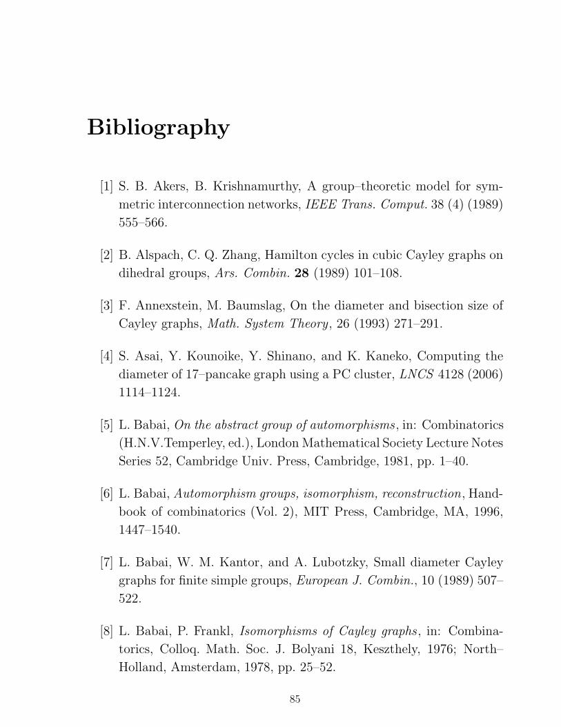
Bibliography
[1] S. B. Akers, B. Krishnamurthy, A group–theoretic model for sym-
metric interconnection networks, IEEE Trans. Comput. 38 (4) (1989)
555–566.
[2] B. Alspach, C. Q. Zhang, Hamilton cycles in cubic Cayley graphs on
dihedral groups, Ars. Combin. 28 (1989) 101–108.
[3] F. Annexstein, M. Baumslag, On the diameter and bisection size of
Cayley graphs, Math. System Theory , 26 (1993) 271–291.
[4] S. Asai, Y. Kounoike, Y. Shinano, and K. Kaneko, Computing the
diameter of 17–pancake graph using a PC cluster, LNCS 4128 (2006)
1114–1124.
[5] L. Babai, On the abstract group of automorphisms , in: Combinatorics
(H.N.V.Temperley, ed.), London Mathematical Society Lecture Notes
Series 52, Cambridge Univ. Press, Cambridge, 1981, pp. 1–40.
[6] L. Babai, Automorphism groups, isomorphism, reconstruction, Hand-
book of combinatorics (Vol. 2), MIT Press, Cambridge, MA, 1996,
1447–1540.
[7] L. Babai, W. M. Kantor, and A. Lubotzky, Small diameter Cayley
graphs for finite simple groups, European J. Combin., 10 (1989) 507–
522.
[8] L. Babai, P. Frankl, Isomorphisms of Cayley graphs , in: Combina-
torics, Colloq. Math. Soc. J. Bolyani 18, Keszthely, 1976; North–
Holland, Amsterdam, 1978, pp. 25–52.
85

86 BIBLIOGRAPHY
[9] L. Babai, A. Seress, On the diameter of Cayley graphs of the symmet-
ric group, Journal of Combinatorial Theory Series A, 49 (1) (1988)
175–179.
[10] D. Bader, B. M. E. Moret, and M. Yan, A linear–time algorithm for
computing inversion distance between signed permutations with an
experimental study, J. Comp. Biol., 8 (5) (2001) 483–492.
[11] V. Bafna, P. A. Pevzner, Genome rearrangments and sorting by re-
versals, SIAM Journal on Computing 25 (2) (1996) 272–289.
[12] V. Bafna, P. A. Pevzner, Sorting by transpositions, SIAM Journal
on Discrete Math. 11 (2) (1998) 224–240.
[13] L. W. Beineke, R. J. Wilson, and P. J. Cameron (Eds.), Topics in
algebraic graph theory , Series: Encyclopedia of mathematics and its
applications, Vol. 102, 2004.
[14] N. Biggs, Algebraic graph theory , Cambridge Mathematical Libray,
Cambridge University Press, Cambridge, second edition, 1993.
[15] N. Biggs, E. Lloyd, and R. Wilson, Graph Theory 1736–1936 , Oxford
University Press, 1986.
[16] A. Bjorner, F. Brenti, Combinatorics of Coxeter groups , Springer
Verlag, Heidelberg, New York, 2005.
[17] A. E. Brouwer, A. M. Cohen, and A. Neumaier, Distance–regular
graphs, Springer-Verlag, Berlin, Heidelberg, 1989.
[18] P. Cameron, Combinatorics and groups: Peter Cameron’s IPM Lec-
ture Notes , Lecture Notes Series 4, Institute for Studies in Theoretical
Physics and Mathematics, 2004.
[19] J. Cibulka, On average and highest number of flips in pancake sorting,
Theoretical Computer Science 412 (2011) 822–834.
[20] T. Chen, S. S. Skiena, Sorting with fixed–length reversals, Discrete
Applied Mathematics , 71 (1996) 269–295.
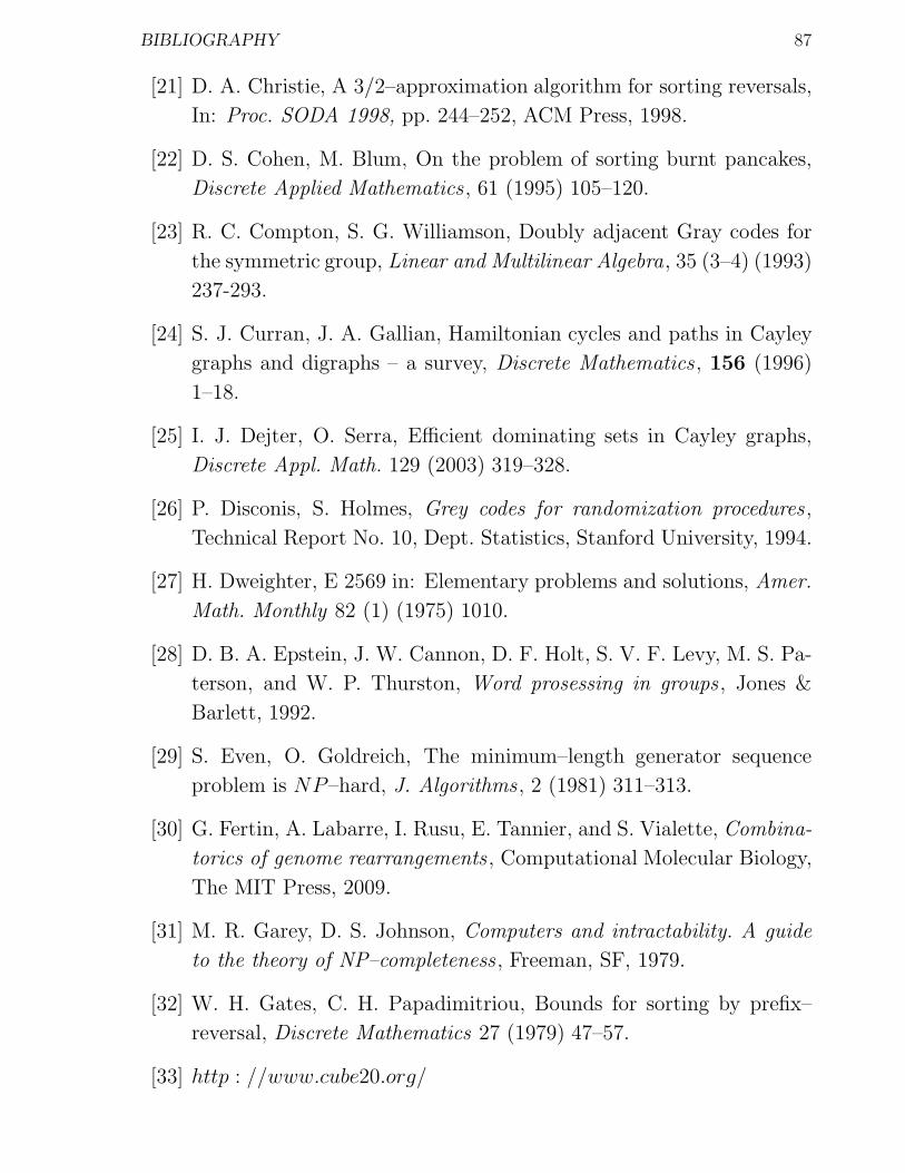
BIBLIOGRAPHY 87
[21] D. A. Christie, A 3/2–approximation algorithm for sorting reversals,
In: Proc. SODA 1998, pp. 244–252, ACM Press, 1998.
[22] D. S. Cohen, M. Blum, On the problem of sorting burnt pancakes,
Discrete Applied Mathematics , 61 (1995) 105–120.
[23] R. C. Compton, S. G. Williamson, Doubly adjacent Gray codes for
the symmetric group, Linear and Multilinear Algebra, 35 (3–4) (1993)
237-293.
[24] S. J. Curran, J. A. Gallian, Hamiltonian cycles and paths in Cayley
graphs and digraphs – a survey, Discrete Mathematics , 156 (1996)
1–18.
[25] I. J. Dejter, O. Serra, Efficient dominating sets in Cayley graphs,
Discrete Appl. Math. 129 (2003) 319–328.
[26] P. Disconis, S. Holmes, Grey codes for randomization procedures ,
Technical Report No. 10, Dept. Statistics, Stanford University, 1994.
[27] H. Dweighter, E 2569 in: Elementary problems and solutions, Amer.
Math. Monthly 82 (1) (1975) 1010.
[28] D. B. A. Epstein, J. W. Cannon, D. F. Holt, S. V. F. Levy, M. S. Pa-
terson, and W. P. Thurston, Word prosessing in groups , Jones &
Barlett, 1992.
[29] S. Even, O. Goldreich, The minimum–length generator sequence
problem is NP–hard, J. Algorithms , 2 (1981) 311–313.
[30] G. Fertin, A. Labarre, I. Rusu, E. Tannier, and S. Vialette, Combina-
torics of genome rearrangements , Computational Molecular Biology,
The MIT Press, 2009.
[31] M. R. Garey, D. S. Johnson, Computers and intractability. A guide
to the theory of NP–completeness , Freeman, SF, 1979.
[32] W. H. Gates, C. H. Papadimitriou, Bounds for sorting by prefix–
reversal, Discrete Mathematics 27 (1979) 47–57.
[33] http : //www.cube20.org/
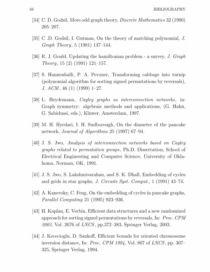
88 BIBLIOGRAPHY
[34] C. D. Godsil, More odd graph theory, Discrete Mathematics 32 (1980)
205–207.
[35] C .D. Godsil, I. Gutman, On the theory of matching polynomial, J.
Graph Theory , 5 (1981) 137–144.
[36] R. J. Gould, Updating the hamiltonian problem - a survey, J. Graph
Theory , 15 (2) (1991) 121–157.
[37] S. Hannenhalli, P. A. Pevzner, Transforming cabbage into turnip
(polynomial algorithm for sorting signed permutations by reversals),
J. ACM , 46 (1) (1999) 1–27.
[38] L. Heydemann, Cayley graphs as interconnection networks , in:
Graph symmetry: algebraic methods and applications, (G. Hahn,
G. Sabidussi, eds.), Kluwer, Amsterdam, 1997.
[39] M. H. Hyedari, I. H. Sudborough, On the diameter of the pancake
network, Journal of Algorithms 25 (1997) 67–94.
[40] J. S. Jwo, Analysis of interconnection networks based on Cayley
graphs related to permutation groups , Ph.D. Dissertation, School of
Electrical Engineering and Computer Science, University of Okla-
homa, Norman, OK, 1991.
[41] J. S. Jwo, S. Lakshmivarahan, and S. K. Dhall, Embedding of cycles
and grids in star graphs, J. Circuits Syst. Comput., 1 (1991) 43–74.
[42] A. Kanevsky, C. Feng, On the embedding of cycles in pancake graphs,
Parallel Computing 21 (1995) 923–936.
[43] H. Kaplan, E. Verbin, Efficient data structures and a new randomized
approach for sorting signed permutations by reversals, In: Proc. CPM
2003, Vol. 2676 of LNCS , pp.372–383, Springer Verlag, 2003.
[44] J. Kececioglu, D. Sankoff, Efficient bounds for oriented chromosome
inversion distance, In: Proc. CPM 1994, Vol. 807 of LNCS , pp. 307–
325, Springer Verlag, 1994.
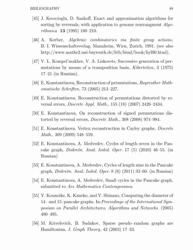
BIBLIOGRAPHY 89
[45] J. Kececioglu, D. Sankoff, Exact and approximation algorithms for
sorting by reversals, with application to genome rearrangment Algo-
rithmica 13 (1995) 180–210.
[46] A. Kerber, Algebraic combinatorics via finite group actions ,
B. I. Wissenschaftsverlag, Mannheim, Wien, Zurich, 1991. (see also
http://www.mathe2.uni-bayreuth.de/frib/html/book/hyl00.html).
[47] V. L. Kompel’makher, V. A. Liskovets, Successive generation of per-
mutations by means of a transposition basis, Kibertetica, 3 (1975)
17–21 (in Russian).
[48] E. Konstantinova, Reconstruction of permutations, Bayreuther Math-
ematische Schriften, 73 (2005) 213–227.
[49] E. Konstantinova, Reconstruction of permutations distorted by re-
versal errors, Discrete Appl. Math., 155 (18) (2007) 2426–2434.
[50] E. Konstantinova, On reconstruction of signed permutations dis-
torted by reversal errors, Discrete Math., 308 (2008) 974–984.
[51] E. Konstantinova, Vertex reconstruction in Cayley graphs, Discrete
Math., 309 (2009) 548–559.
[52] E. Konstantinova, A. Medvedev, Cycles of length seven in the Pan-
cake graph, Diskretn. Anal. Issled. Oper. 17 (5) (2010) 46–55. (in
Russian)
[53] E. Konstantinova, A. Medvedev, Cycles of length nine in the Pancake
graph, Diskretn. Anal. Issled. Oper. 8 (6) (2011) 33–60. (in Russian)
[54] E. Konstantinova, A. Medvedev, Small cycles in the Pancake graph,
submitted to Ars Mathematica Contemporanea.
[55] Y. Kounoike, K. Kaneko, and Y. Shinano, Computing the diameter of
14– and 15–pancake graphs. In:Proceedings of the International Sym-
posium on Parallel Architectures, Algorithms and Networks. (2005)
490–495.
[56] M. Krivelevich, B. Sudakov, Sparse pseudo–random graphs are
Hamiltonian, J. Graph Theory , 42 (2003) 17–33.

90 BIBLIOGRAPHY
[57] D. E. Knuth, Sorting and searching , Vol. 3 of The Art of Computer
Programming, Addison–Wesley, Reading, Massachusetts, second edi-
tion, 1998. p.72 and p.615.
[58] S. Lakshmivarahan, J. S. Jwo, and S. K. Dhall, Symmetry in inter-
connection networks based on Cayley graphs of permutation groups:
a survey, Parallel Comput. 19 (1993) 361–407.
[59] J. Lauri, R. Scapellato, Topics in graph automorphisms and recon-
struction, London Mathematical Society, Student Texts 54, Cam-
bridge University Press, 2003.
[60] F. T. Leighton, Introduction to parallel algorithms and architectures:
arrays, trees, hupercubes , Morgan Kaufmann Publishers, California,
1992.
[61] V. I. Levenshtein, J. Siemons, Error graphs and the reconstruction of
elements in groups, J. Comb. Theory, Ser. A 116 (4) (2009) 795–815.
[62] C. H. Li, On isomorphisms of finite Cayley graphs: a survey, Discrete
Mathematics , 256 (2002) 301–334.
[63] L. Lovasz, Problem 11 in: Combinatorial structures and their ap-
plications , (Proc. Calgary Internat. Conf., Calgary, Alberta, 1969),
Gordon and Breach, New York, 1970, pp. 243–246.
[64] A. Lubotzky, Cayley graphs: eigenvalues, expanders and random
walks, in: Surveys in combinatorics (P.Rowlinson, ed.), London
Mathematical Society Lecture Notes Series 218, Cambridge Univ.
Press, Cambridge, 1995, pp. 155–189.
[65] D. Marusic, Hamiltonian circuits in Cayley graphs, Discrete Mathe-
matics 46 (1983) 49–54.
[66] http://www.fmf.uni-lj.si/mohar/Problems/P6MatchingsVTGraphs.html
[67] J. D. Palmer, L. A. Herbon, Tricircular mitochondrial genomes of
brassica and Raphanus: reversal of repeat configurations by inver-
sion, Sequence alignment in molecular biology, Nucleid Acids Re-
search, 14 (1986) 9755–9764.

BIBLIOGRAPHY 91
[68] I. Pak, R. Radoicic, Hamiltonian paths in Cayley graphs, Discrete
Mathematics 309 (2009) 5501–5508.
[69] P. A. Pevzner, Computational molecular biology: an algorithmic ap-
proach, The MIT Press, Cambridge, MA, 2000.
[70] Ke Qiu, Optimal broadcasting algorithms for multiple messages
on the star and pancake graphs using minimum dominating sets,
Congress. Numerantium. 181 (2006) 33–39.
[71] R. A. Rankin, A campanological problem in group theory II, Proc.
Camb. Phyl. Soc. 62 (1966) 11–18.
[72] E. Rapaport–Strasser, Cayley color groups and Hamilton lines,
Scripta Math. 24 (1959) 51–58.
[73] D. Sankoff, Edit distance for genome comparison based on nonlocal
operations, In: Proc. CPM 1992, Vol. 644 of LNCS , pp. 121–135,
Springer Verlag, 1992.
[74] D. Sankoff, N. El–Mabrouk, Genome rearrangement , in: T. Jiang,
T. Smith, Y. Xu, M. Q. Zhang (Eds.), Current topics in computa-
tional molecular biology, MIT Press, 2002.
[75] R. Shamir, Algorithms for Molecular Biology: Course Archive,
http://www.cs.tau.ac.il/ rshamir/algmb.html.
[76] J. J. Sheu, J. J. M. Tan, L. H. Hsu, and M. Y. Lin, On the Cycle Em-
bedding of Pancake Graphs, Proceedings of 1999 National Computer
Symposium (1999) pp. C414–C419.
[77] S. Skiena, Hypercubes , In: Implementing Discrete Mathematics:
Combinatorics and Graph Theory with Mathematica, Reading, MA:
Addison–Wesley (1990) pp. 148–150.
[78] H. Sudborough, C. Chitturi, W. Fahle, A. Meng, L. Morales,
C. Shields, and W. Voit., An improved upper bound for the
pancake problem, Abstract of talks at a Tribute Workshop and
Festival to Honor Professor Dr. Neil D. Jones 25-26 August,
92 BIBLIOGRAPHY
2007 Lille Auditorium Datalogisk Institut, Kobenhavns Univer-
sitet Universitetsparken 1, Kobenhavn, Denmark, see: http://
www.diku.dk/forskning/topps/neilfest/abstract sudborough.html
[79] M. Tchuente, Generation of permutations by graphycal exchanges,
Ars Combin., 14 (1982) 115–122.
[80] D. Witte, J. A. Gallian, A survey: hamiltonian cycles in Cayley
graphs, Discrete Mathematics , 51 (1984) 293–304.
[81] M. Y. Xu, Some work on vertex-transitive graphs by Chinese mathe-
maticians , in: Group theory in China, Kluwer Academic Publishers,
Dordrecht, 1996, pp. 224–254.
[82] S. Zaks, A new algorithm for generation of permutations, BIT 24
(1984) 196–204.