Elements of Probability Theory - CAE Solutions Corporation14 Elements of Probability Theory The set...

Chapter 2

Elements of Probability Theory

2.1 Introduction

Whether referring to a storm’s intensity, an arrival time, or the success of a

decision, the word “probable,” or “likely,” has long been part of our language.

Most people have an appreciation for the impact of chance on the occurrence of

an event. In the last 350 years, the theory of probability has evolved to explain

the nature of chance and how it can be studied.

Probability theory is the formal study of events whose outcomes are uncertain.

Its origins trace to 17th-century gambling problems. Games that involved playing

cards, roulette wheels, and dice provided mathematicians with a host of interest-

ing problems. The solutions to many of these problems yielded the first principles

of modern probability theory. Today, probability theory is of fundamental impor-

tance in science, engineering, and business.

Engineering risk management aims to identify and manage events whose out-

comes are uncertain. In particular, its focus is on events that, if they occur, have

unwanted impacts or consequences to a project or program. The phrase “if they

occur” means these events are probabilistic in nature. Thus, understanding them

in the context of probability concepts is essential. This chapter presents an in-

troduction to these concepts and illustrates how they apply to managing risks in

engineering systems.

2.2 Interpretations and Axioms

We begin this discussion with the traditional look at dice. If a six-sided die is

tossed, there clearly are six possible outcomes for the number that appears on the

upturned face. These outcomes can be listed as elements in a set {1, 2, 3, 4, 5, 6}.

13

14 Elements of Probability Theory

The set of all possible outcomes of an experiment, such as tossing a six-sided die,

is called the sample space, which we will denote by �. The individual outcomes

of � are called sample points, which we will denote by ω.

An event is any subset of the sample space. An event is simple if it consists of

exactly one outcome. Simple events are also referred to as elementary events

or elementary outcomes. An event is compound if it consists of more than one

outcome. For instance, let A be the event an odd number appears and B be the

event an even number appears in a single toss of a die. These are compound events

that can be expressed by the sets A = {1, 3, 5} and B = {2, 4, 6}. Event A occurs

if and only if one of the outcomes in A occurs. The same is true for event B.

Seen in this discussion, events can be represented by sets. New events can be

constructed from given events according to the rules of set theory. The following

presents a brief review of set theory concepts.

Union. For any two events A and B of a sample space, the new event A ∪ B

(which reads A union B) consists of all outcomes either in A or in B or in both

A and B. The event A ∪ B occurs if either A or B occurs. To illustrate the union

of two events, consider the following: if A is the event an odd number appears in

the toss of a die and B is the event an even number appears, then the event A ∪ B

is the set {1, 2, 3, 4, 5, 6}, which is the sample space for this experiment.

Intersection. For any two events A and B of a sample space �, the new event

A ∩ B (which reads A intersection B) consists of all outcomes that are in both A

and in B. The event A ∩ B occurs only if both A and B occur. To illustrate the

intersection of two events, consider the following: if A is the event a 6 appears

in the toss of a die, B is the event an odd number appears, and C is the event

an even number appears, then the event A ∩ C is the simple event {6}; on the

other hand, the event A ∩ B contains no outcomes. Such an event is called the

null event. The null event is traditionally denoted by ∅. In general, if A ∩ B = ∅,

we say events A and B are mutually exclusive (disjoint). For notation conve-

nience, the intersection of two events A and B is sometimes written as AB, instead

of A ∩ B.

Complement. The complement of event A, denoted by Ac, consists of all out-

comes in the sample space � that are not in A. The event Ac occurs if and only

if A does not occur. The following illustrates the complement of an event. If C is

the event an even number appears in the toss of a die, then Cc is the event an odd

number appears.

2.2 Interpretations and Axioms 15

Subset. Event A is said to be a subset of event B if all the outcomes in A are also

contained in B. This is written as A ⊂ B.

In the preceding discussion, the sample space for the toss of a die was given by

� = {1, 2, 3, 4, 5, 6}. If we assume the die is fair, then any outcome in the sample

space is as likely to appear as any other. Given this, it is reasonable to conclude the

proportion of time each outcome is expected to occur is 1/6. Thus, the probability

of each simple event in the sample space is

P({1}) = P({2}) = P({3}) = P({4}) = P({5}) = P({6}) = 1

6

Similarly, suppose B is the event an odd number appears in a single toss of the

die. This compound event is given by the set B = {1, 3, 5}. Since there are three

ways event B can occur out of six possible, the probability of event B is

P(B) = 3

6= 1

2

The following presents a view of probability known as the equally likely inter-

pretation.

Equally Likely Interpretation. In this view, if a sample space � consists of

a finite number of outcomes n, which are all equally likely to occur, then the

probability of each simple event is 1/n. If an event A consists of m of these n

outcomes, then the probability of event A is

P(A) = m

n(2.1)

In the above, it is assumed the sample space consists of a finite number of outcomes

and all outcomes are equally likely to occur. What if the sample space is finite

but the outcomes are not equally likely? In these situations, probability might

be measured in terms of how frequently a particular outcome occurs when the

experiment is repeatedly performed under identical conditions. This leads to a

view of probability known as the frequency interpretation.

Frequency Interpretation. In this view, the probability of an event is the limiting

proportion of time the event occurs in a set of n repetitions of the experiment. In

particular, we write this as

P(A) = limn→∞

n(A)

n


where n(A) is the number of times in n repetitions of the experiment the event

A occurs. In this sense P(A) is the limiting frequency of event A. Probabilities

measured by the frequency interpretation are referred to as objective probabilities.

In many circumstances it is appropriate to work with objective probabilities.

However, there are limitations with this interpretation of probability. It restricts

events to those that can be subjected to repeated trials conducted under identical

conditions. Furthermore, it is not clear how many trials of an experiment are

needed to obtain an event’s limiting frequency.

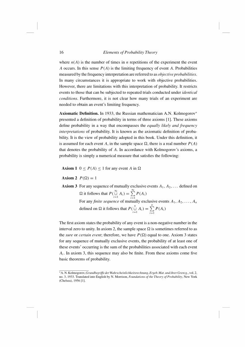
Axiomatic Definition. In 1933, the Russian mathematician A.N. Kolmogorov∗

presented a definition of probability in terms of three axioms [1]. These axioms

define probability in a way that encompasses the equally likely and frequency

interpretations of probability. It is known as the axiomatic definition of proba-

bility. It is the view of probability adopted in this book. Under this definition, it

is assumed for each event A, in the sample space �, there is a real number P(A)

that denotes the probability of A. In accordance with Kolmogorov’s axioms, a

probability is simply a numerical measure that satisfies the following:

Axiom 1 0 ≤ P(A) ≤ 1 for any event A in �

Axiom 2 P(�) = 1

Axiom 3 For any sequence of mutually exclusive events A1, A2, . . . defined on

� it follows that P(∞∪

i=1Ai ) =

∞∑i=1

P(Ai )

For any finite sequence of mutually exclusive events A1, A2, . . . , An

defined on � it follows that P(n∪

i=1Ai ) =

n∑i=1

P(Ai )

The first axiom states the probability of any event is a non-negative number in the

interval zero to unity. In axiom 2, the sample space � is sometimes referred to as

the sure or certain event; therefore, we have P(�) equal to one. Axiom 3 states

for any sequence of mutually exclusive events, the probability of at least one of

these events’ occurring is the sum of the probabilities associated with each event

Ai . In axiom 3, this sequence may also be finite. From these axioms come five

basic theorems of probability.

∗A. N. Kolmogorov, Grundbegriffe der Wahrscheinlichkeitsrechnung, Ergeb. Mat. und ihrer Grenzg., vol. 2,no. 3, 1933. Translated into English by N. Morrison, Foundations of the Theory of Probability, New York(Chelsea), 1956 [1].

2.2 Interpretations and Axioms 17

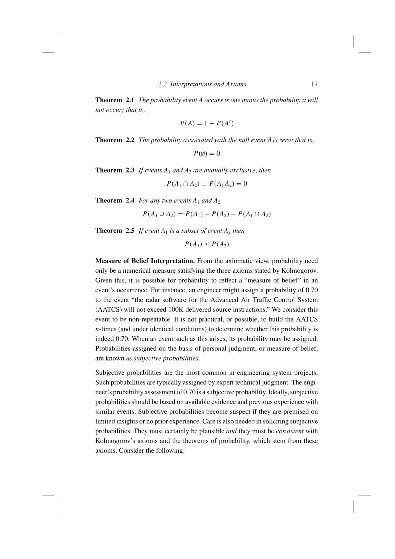
Theorem 2.1 The probability event A occurs is one minus the probability it will

not occur; that is,

P(A) = 1 − P(Ac)

Theorem 2.2 The probability associated with the null event ∅ is zero; that is,

P(∅) = 0

Theorem 2.3 If events A1 and A2 are mutually exclusive, then

P(A1 ∩ A2) ≡ P(A1 A2) = 0

Theorem 2.4 For any two events A1 and A2

P(A1 ∪ A2) = P(A1) + P(A2) − P(A1 ∩ A2)

Theorem 2.5 If event A1 is a subset of event A2 then

P(A1) ≤ P(A2)

Measure of Belief Interpretation. From the axiomatic view, probability need

only be a numerical measure satisfying the three axioms stated by Kolmogorov.

Given this, it is possible for probability to reflect a “measure of belief” in an

event’s occurrence. For instance, an engineer might assign a probability of 0.70

to the event “the radar software for the Advanced Air Traffic Control System

(AATCS) will not exceed 100K delivered source instructions.” We consider this

event to be non-repeatable. It is not practical, or possible, to build the AATCS

n-times (and under identical conditions) to determine whether this probability is

indeed 0.70. When an event such as this arises, its probability may be assigned.

Probabilities assigned on the basis of personal judgment, or measure of belief,

are known as subjective probabilities.

Subjective probabilities are the most common in engineering system projects.

Such probabilities are typically assigned by expert technical judgment. The engi-

neer’s probability assessment of 0.70 is a subjective probability. Ideally, subjective

probabilities should be based on available evidence and previous experience with

similar events. Subjective probabilities become suspect if they are premised on

limited insights or no prior experience. Care is also needed in soliciting subjective

probabilities. They must certainly be plausible and they must be consistent with

Kolmogorov’s axioms and the theorems of probability, which stem from these

axioms. Consider the following:


The XYZ Corporation has offers on two contracts A and B. Suppose the pro-

posal team made the following subjective probability assignments. The chance of

winning contract A is 40%, the chance of winning contract B is 20%, the chance

of winning contract A or contract B is 60%, and the chance of winning both

contract A and contract B is 10%. It turns out this set of probability assignments

is not consistent with the axioms and theorems of probability. Why is this?∗ If the

chance of winning contract B was changed to 30%, then this set of probability

assignments would be consistent.

Kolmogorov’s axioms, and the resulting theorems of probability, do not suggest

how to assign probabilities to events. Instead, they provide a way to verify that

probability assignments are consistent, whether these probabilities are objective

or subjective.

Risk versus Uncertainty. There is an important distinction between the terms risk

and uncertainty. Risk is the chance of loss or injury. In a situation that includes

favorable and unfavorable events, risk is the probability an unfavorable event

occurs. Uncertainty is the indefiniteness about the outcome of a situation. We

analyze uncertainty for the purpose of measuring risk. In systems engineering the

analysis might focus on measuring the risk of: (1) failing to achieve performance

objectives, (2) overrunning the budgeted cost, or (3) delivering the system too late

to meet user needs. Conducting the analysis often involves degrees of subjectivity.

This includes defining the events of concern and, when necessary, subjectively

specifying their occurrence probabilities. Given this, it is fair to ask whether it

is meaningful to apply rigorous mathematical procedures to such analyses. In a

speech before the 1955 Operations Research Society of America meeting, Charles

J. Hitch (RAND) addressed this question. He stated [2, 3]:

Systems analyses provide a framework which permits the judgment of

experts in many fields to be combined to yield results that transcend any

individual judgment. The systems analyst may have to be content with

better rather than optimal solutions; or with devising and costing sensible

methods of hedging; or merely with discovering critical sensitivities. We

tend to be worse, in an absolute sense, in applying analysis or scientific

method to broad context problems; but unaided intuition in such problems

is also much worse in the absolute sense. Let’s not deprive ourselves of any

useful tools, however short of perfection they may fail.

∗The answer can be seen from theorem 2.4.

2.3 Conditional Probability and Bayes’ Rule 19

2.3 Conditional Probability and Bayes’ Rule

In many circumstances, the probability of an event is conditioned on knowing

another event has taken place. Such a probability is known as a conditional proba-

bility. Conditional probabilities incorporate information about the occurrence of

another event. The conditional probability of event A given event B has occurred

is denoted by P(A |B) . If a pair of dice is tossed, then the probability the sum of

the toss is even is 1/2. This probability is known as a marginal or unconditional

probability.

How would this unconditional probability change (i.e., be conditioned) if it was

known the sum of the toss was a number less than 10? This is discussed in the

following example.

Example 2.1A pair of dice is tossed and the sum of the toss is a number less than 10. Given

this, compute the probability this sum is an even number.

SolutionSuppose we define events A and B as follows:

A: The sum of the toss is even

B: The sum of the toss is a number less than 10

The sample space � contains 36 possible outcomes; however, in this case we

want the subset of � containing only those outcomes whose toss yielded a sum

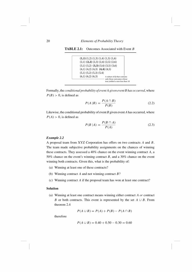
less than 10. This subset is shown in Table 2.1. It contains 30 outcomes. Within

Table 2.1, only 14 outcomes are associated with the event “the sum of the toss is

even given the sum of the toss is a number less than 10.”{(1, 1), (1, 3), (1, 5), (2, 2), (2, 4), (2, 6), (3, 1), (3, 3), (3, 5)

(4, 2), (4, 4), (5, 1), (5, 3), (6, 2)

}

Therefore, the probability of this event is P(A |B) = 14/30

In Example 2.1, observe that P(A |B) was obtained directly from a subset of the

sample space � and that P(A |B ) = 14/30 < P(A) = 1/2.

If A and B are events in the same sample space �, then P(A |B ) is the prob-

ability of event A within the subset of the sample space defined by event B.


TABLE 2.1: Outcomes Associated with Event B

(1,1) (1,2) (1,3) (1,4) (1,5) (1,6)

(2,1) (2,2) (2,3) (2,4) (2,5) (2,6)

(3,1) (3,2) (3,3) (3,4) (3,5) (3,6)

(4,1) (4,2) (4,3) (4,4) (4,5)

(5,1) (5,2) (5,3) (5,4)

(6,1) (6,2) (6,3) A subset of Ω that contains

only those outcomes whose

toss yielded a sum less than 10

Formally, the conditional probability of event A given event B has occurred, where

P(B) > 0, is defined as

P(A |B) = P(A ∩ B)

P(B)(2.2)

Likewise, the conditional probability of event B given event A has occurred, where

P(A) > 0, is defined as

P(B |A) = P(B ∩ A)

P(A)(2.3)

Example 2.2A proposal team from XYZ Corporation has offers on two contracts A and B.

The team made subjective probability assignments on the chances of winning

these contracts. They assessed a 40% chance on the event winning contract A, a

50% chance on the event’s winning contract B, and a 30% chance on the event

winning both contracts. Given this, what is the probability of:

(a) Winning at least one of these contracts?

(b) Winning contract A and not winning contract B?

(c) Winning contract A if the proposal team has won at least one contract?

Solution

(a) Winning at least one contract means winning either contract A or contract

B or both contracts. This event is represented by the set A ∪ B. From

theorem 2.4

P(A ∪ B) = P(A) + P(B) − P(A ∩ B)

therefore

P(A ∪ B) = 0.40 + 0.50 − 0.30 = 0.60


A

ABc AB AcB

B

P(A B)Ω

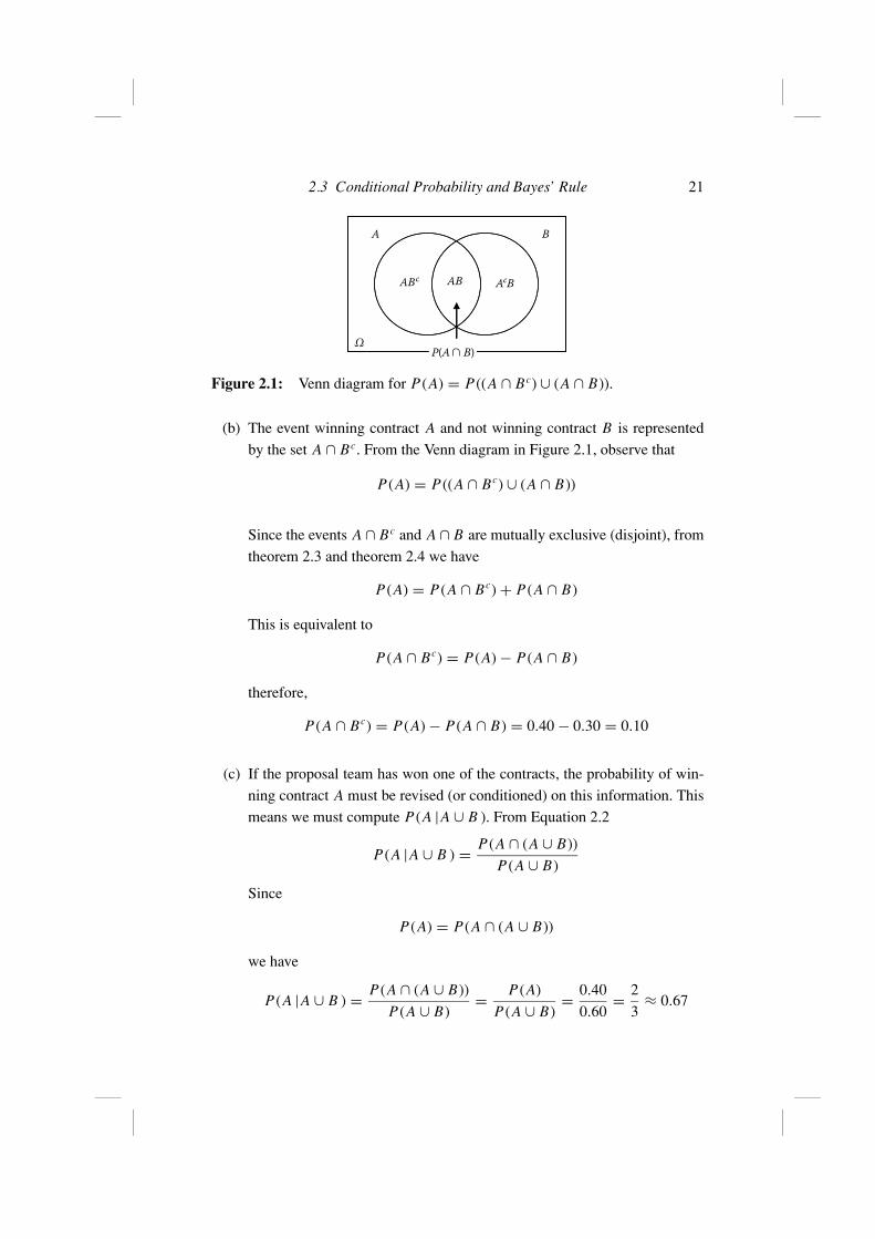
Figure 2.1: Venn diagram for P(A) = P((A ∩ Bc) ∪ (A ∩ B)).

(b) The event winning contract A and not winning contract B is represented

by the set A ∩ Bc. From the Venn diagram in Figure 2.1, observe that

P(A) = P((A ∩ Bc) ∪ (A ∩ B))

Since the events A ∩ Bc and A ∩ B are mutually exclusive (disjoint), from

theorem 2.3 and theorem 2.4 we have

P(A) = P(A ∩ Bc) + P(A ∩ B)

This is equivalent to

P(A ∩ Bc) = P(A) − P(A ∩ B)

therefore,

P(A ∩ Bc) = P(A) − P(A ∩ B) = 0.40 − 0.30 = 0.10

(c) If the proposal team has won one of the contracts, the probability of win-

ning contract A must be revised (or conditioned) on this information. This

means we must compute P(A |A ∪ B ). From Equation 2.2

P(A |A ∪ B ) = P(A ∩ (A ∪ B))

P(A ∪ B)

Since

P(A) = P(A ∩ (A ∪ B))

we have

P(A |A ∪ B ) = P(A ∩ (A ∪ B))

P(A ∪ B)= P(A)

P(A ∪ B)= 0.40

0.60= 2

3≈ 0.67


A consequence of conditional probability is obtained if we multiply Equations

2.2 and 2.3 by P(B) and P(A), respectively. This multiplication yields

P(A ∩ B) = P(B)P(A |B) = P(A)P(B |A) (2.4)

Equation 2.4 is known as the multiplication rule. The multiplication rule pro-

vides a way to express the probability of the intersection of two events in terms

of their conditional probabilities. An illustration of this rule is presented in

example 2.3.

Example 2.3A box contains memory chips of which 3 are defective and 97 are non-defective.

Two chips are drawn at random, one after the other, without replacement. Deter-

mine the probability:

(a) Both chips drawn are defective.

(b) The first chip is defective and the second chip is non-defective.

Solution

(a) Let A and B denote the event the first and second chips drawn from the box

are defective, respectively. From the multiplication rule, we have

P(A ∩ B) = P(A)P(B |A)

= P(1st chip defective) P(2nd chip defective|1st chip defective)

= 3

100

(2

99

)= 6

9900

(b) To determine the probability the first chip drawn is defective and the second

chip is non-defective, let C denote the event the second chip drawn is non-

defective. Thus,

P(A ∩ C) = P(AC) = P(A)P(C |A )

= P(1st chip defective) P(2nd chip nondefective|1st chip defective)

= 3

100

(97

99

)= 291

9900

In this example the sampling was performed without replacement. Suppose the

chips sampled were replaced; that is, the first chip selected was replaced before

the second chip was selected. In that case, the probability of a defective chip’s


being selected on the second drawing is independent of the outcome of the first

chip drawn. Specifically,

P(2nd chip defective) = P(1st chip defective) = 3/100

so

P(A ∩ B) = 3

100

(3

100

)= 9

10000

and

P(A ∩ C) = 3

100

(97

100

)= 291

10000

Independent Events

Two events A and B are said to be independent if and only if

P(A ∩ B) = P(A)P(B) (2.5)

and dependent otherwise. Events A1, A2, . . . , An are (mutually) independent if

and only if for every set of indices i1, i2, . . . , ik between 1 and n, inclusive,

P(Ai1 ∩ Ai2 ∩ . . . ∩ Aik ) = P(Ai1 )P(Ai2 ) . . . P(Aik ), (k = 2, . . . , n)

For instance, events A1, A2, and A3, are independent (or mutually independent)

if the following equations are satisfied

P(A1 ∩ A2 ∩ A3) = P(A1)P(A2)P(A3) (2.5a)

P(A1 ∩ A2) = P(A1)P(A2) (2.5b)

P(A1 ∩ A3) = P(A1)P(A3) (2.5c)

P(A2 ∩ A3) = P(A2)P(A3) (2.5d)

It is possible to have three events A1, A2, and A3 for which Equations 2.5b through

2.5d hold but Equation 2.5a does not hold. Mutual independence implies pairwise

independence, in the sense that Equations 2.5b through 2.5d hold, but the converse

is not true.


There is a close relationship between independent events and conditional proba-

bility. To see this, suppose events A and B are independent. This implies

P(AB) = P(A)P(B)

From this, Equations 2.2 and 2.3 become, respectively, P(A |B) = P(A) and

P(B |A) = P(B). Thus, when two events are independent the occurrence of one

event has no impact on the probability the other event occurs.

To illustrate the concept of independence, suppose a fair die is tossed. Let A be the

event an odd number appears. Let B be the event one of these numbers {2, 3, 5, 6}appears. From this,

P(A) = 1/2

and

P(B) = 2/3

Since A ∩ B is the event represented by the set {3, 5}, we can readily state

P(A∩ B) = 1/3. Therefore, P(A∩ B) = P(AB) = P(A)P(B) and we conclude

events A and B are independent.

Dependence can be illustratedby tossing two fair dice. Suppose A is the event

the sum of the toss is odd and B is the event the sum of the toss is even. Here,

P(A ∩ B) = 0 and P(A) and P(B) were each 1/2. Since P(A ∩ B) �= P(A)P(B)

we would conclude events A and B are dependent, in this case.

It is important not to confuse the meaning of independent events with mutually

exclusive events as shown in Figure 2.2. If events A and B are mutually exclusive,

the event A and B is empty; that is, A∩B = ∅. This implies P(A∩B) = P(∅) = 0.

If events A and B are independent with P(A) �= 0 and P(B) �= 0, then A and B

cannot be mutually exclusive since P(A ∩ B) = P(A)P(B) �= 0.

Bayes’ Rule

Suppose we have a collection of events Ai representing possible conjectures about

a topic. Furthermore, suppose we have some initial probabilities associated with

the “truth” of these conjectures. Bayes’ rule∗ provides a way to update (or revise)

initial probabilities when new information about these conjectures is evidenced.

∗Named in honor of Thomas Bayes (1702–1761), an English minister and mathematician.


A1 B

A1

A2 B

A3 = Ω

A3 B

A2 A1

B

A2

A3

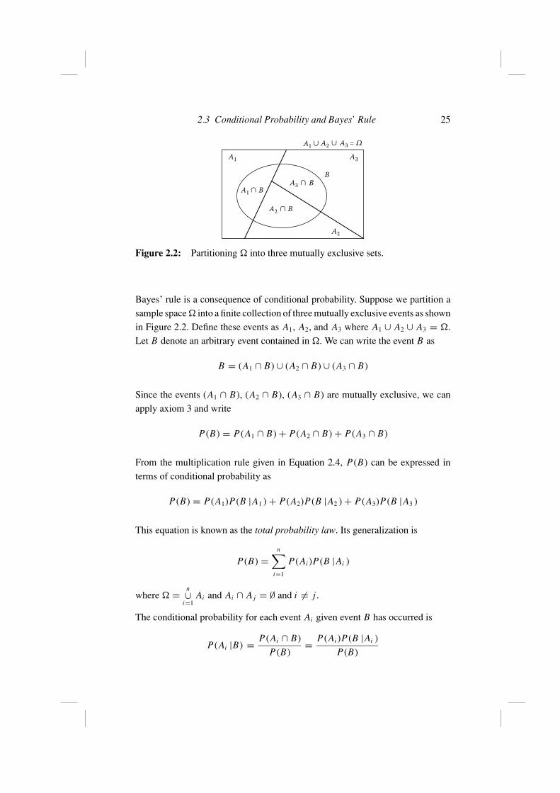
Figure 2.2: Partitioning � into three mutually exclusive sets.

Bayes’ rule is a consequence of conditional probability. Suppose we partition a

sample space � into a finite collection of three mutually exclusive events as shown

in Figure 2.2. Define these events as A1, A2, and A3 where A1 ∪ A2 ∪ A3 = �.

Let B denote an arbitrary event contained in �. We can write the event B as

B = (A1 ∩ B) ∪ (A2 ∩ B) ∪ (A3 ∩ B)

Since the events (A1 ∩ B), (A2 ∩ B), (A3 ∩ B) are mutually exclusive, we can

apply axiom 3 and write

P(B) = P(A1 ∩ B) + P(A2 ∩ B) + P(A3 ∩ B)

From the multiplication rule given in Equation 2.4, P(B) can be expressed in

terms of conditional probability as

P(B) = P(A1)P(B |A1 ) + P(A2)P(B |A2 ) + P(A3)P(B |A3 )

This equation is known as the total probability law. Its generalization is

P(B) =n∑

i=1

P(Ai )P(B |Ai )

where � = n∪i=1

Ai and Ai ∩ A j = ∅ and i �= j .

The conditional probability for each event Ai given event B has occurred is

P(Ai |B) = P(Ai ∩ B)

P(B)= P(Ai )P(B |Ai )

P(B)


When the total probability law is applied to this Equation we have

P(Ai |B) = P(Ai )P(B |Ai )n∑

i=1P(Ai )P(B |Ai )

(2.6)

Equation 2.6 is known as Bayes’ Rule.

Example 2.4The ChipyTech Corporation has three divisions, D1, D2, and D3, that each man-

ufacture a specific type of microprocessor chip. From the total annual output of

chips produced by the corporation, D1 manufactures 35%, D2 manufactures 20%,

and D3 manufactures 45%. Data collected from the quality control group indicate

1% of the chips from D1 are defective, 2% of the chips from D2 are defective,

and 3% of the chips from D3 are defective. Suppose a chip was randomly selected

from the total annual output produced and it was found to be defective. What is

the probability it was manufactured by D1? By D2? By D3?

SolutionLet Ai denote the event the selected chip was produced by division Di (i = 1, 2, 3).

Let B denote the event the selected chip is defective. To determine the probability

the defective chip was manufactured by Di we must compute the conditional

probability P(Ai |B) for i = 1, 2, 3. From the information provided, we have

P(A1) = 0.35, P(A2) = 0.20, and P(A3) = 0.45

P(B|Ai ) = 0.01, P(B|A2) = 0.02, P(B|A3) = 0.03

The total probability law and Bayes’ rule will be used to determine P(Ai |B) for

each i = 1, 2, and 3. Recall from Equation 2.9 that P(B) can be written as

P(B) = P(A1)P(B|A1) + P(A2)P(B|A2) + P(A3)P(B|A3)

P(B) = 0.35(0.01) + 0.20(0.02) + 0.45(0.03) = 0.021

and from Bayes’ rule we can write

P(Ai | B) = P(Ai )P(B |Ai )n∑

i=1P(Ai )P(B |Ai )

= P(Ai )P(B |Ai )

P(B)


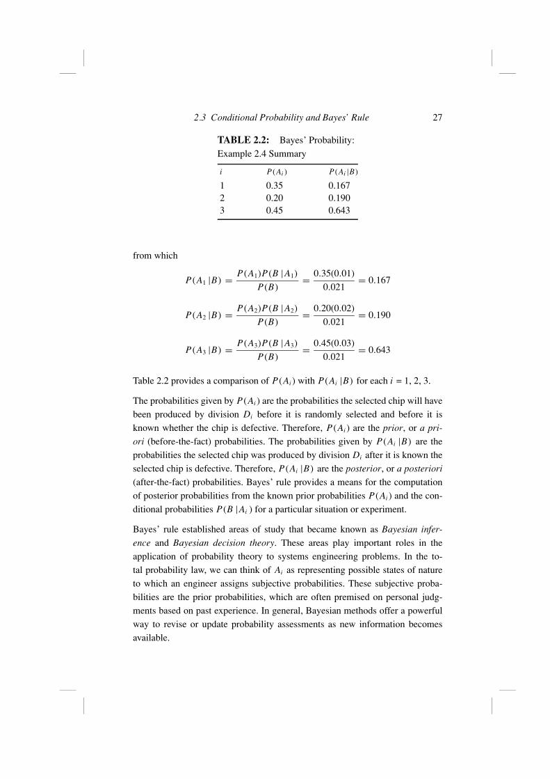
TABLE 2.2: Bayes’ Probability:

Example 2.4 Summary

i P(Ai ) P(Ai |B)

1 0.35 0.1672 0.20 0.1903 0.45 0.643

from which

P(A1 |B) = P(A1)P(B |A1)

P(B)= 0.35(0.01)

0.021= 0.167

P(A2 |B) = P(A2)P(B |A2)

P(B)= 0.20(0.02)

0.021= 0.190

P(A3 |B) = P(A3)P(B |A3)

P(B)= 0.45(0.03)

0.021= 0.643

Table 2.2 provides a comparison of P(Ai ) with P(Ai |B) for each i = 1, 2, 3.

The probabilities given by P(Ai ) are the probabilities the selected chip will have

been produced by division Di before it is randomly selected and before it is

known whether the chip is defective. Therefore, P(Ai ) are the prior, or a pri-

ori (before-the-fact) probabilities. The probabilities given by P(Ai |B) are the

probabilities the selected chip was produced by division Di after it is known the

selected chip is defective. Therefore, P(Ai |B) are the posterior, or a posteriori

(after-the-fact) probabilities. Bayes’ rule provides a means for the computation

of posterior probabilities from the known prior probabilities P(Ai ) and the con-

ditional probabilities P(B |Ai ) for a particular situation or experiment.

Bayes’ rule established areas of study that became known as Bayesian infer-

ence and Bayesian decision theory. These areas play important roles in the

application of probability theory to systems engineering problems. In the to-

tal probability law, we can think of Ai as representing possible states of nature

to which an engineer assigns subjective probabilities. These subjective proba-

bilities are the prior probabilities, which are often premised on personal judg-

ments based on past experience. In general, Bayesian methods offer a powerful

way to revise or update probability assessments as new information becomes

available.


2.4 Applications to Engineering Risk Management

Chapter 2 concludes with an expanded discussion of Bayes’ rule in terms of its

application to the analysis of risks in the engineering of systems. In addition, a

best-practice protocol for expressing risk in terms of its occurrence probability

and consequences is introduced.

2.4.1 Probability Inference — An Application of Bayes’ Rule

This discussion presents a technique known as Bayesian inference. Bayesian

inference is a way to examine how an initial belief in the truth of a hypothesis

H may change when evidence e relating to it is observed. This is done by an

application of Bayes’ rule, which we illustrate in the discussion below.

Suppose an engineering firm has been awarded a project to develop a software

application. Suppose a number of challenges are associated with this, among

them (1) staffing the project, (2) managing multiple development sites, and (3)

functional requirements that continue to evolve.

Given these challenges, suppose the project’s management team believes it has a

50% chance of completing the software development in accordance with the cus-

tomer’s planned schedule. From this, how might management use Bayes’ rule to

monitor whether the chance of completing the project on schedule is increasing

or decreasing?

As mentioned above, Bayesian inference is a procedure that takes evidence, ob-

servations, or indicators as they emerge and applies Bayes’ rule to infer the

truthfulness or falsity of a hypothesis in terms of its probability. In this case, the

hypothesis H is Project XYZ will experience significant delays in completing its

software development.

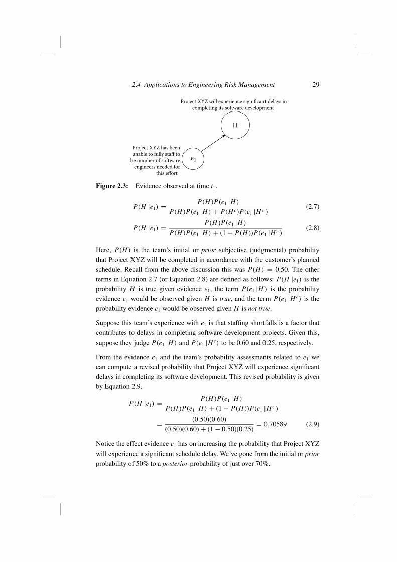
Suppose at time t1 the project’s management comes to recognize that project XYZ

has been unable to fully staff to the number of software engineers needed for this

effort. In Bayesian inference, we treat this as an observation or evidence that has

some bearing on the truthfulness of H . This is illustrated in Figure 2.3. Here, H is

the hypothesis “node” and e1 is the evidence node contributing to the truthfulness

of H .

Given the evidence-to-hypothesis relationship in Figure 2.3 we can form the

following equations from Bayes’ rule.

2.4 Applications to Engineering Risk Management 29

Project XYZ will experience significant delays in

completing its software development

Project XYZ has been

unable to fully staff to

the number of software

engineers needed for

this effort

H

e1

Figure 2.3: Evidence observed at time t1.

P(H |e1) = P(H )P(e1 |H )

P(H )P(e1 |H ) + P(H c)P(e1 |H c )(2.7)

P(H |e1) = P(H )P(e1 |H )

P(H )P(e1 |H ) + (1 − P(H ))P(e1 |H c )(2.8)

Here, P(H ) is the team’s initial or prior subjective (judgmental) probability

that Project XYZ will be completed in accordance with the customer’s planned

schedule. Recall from the above discussion this was P(H ) = 0.50. The other

terms in Equation 2.7 (or Equation 2.8) are defined as follows: P(H |e1) is the

probability H is true given evidence e1, the term P(e1 |H ) is the probability

evidence e1 would be observed given H is true, and the term P(e1 |H c) is the

probability evidence e1 would be observed given H is not true.

Suppose this team’s experience with e1 is that staffing shortfalls is a factor that

contributes to delays in completing software development projects. Given this,

suppose they judge P(e1 |H ) and P(e1 |H c) to be 0.60 and 0.25, respectively.

From the evidence e1 and the team’s probability assessments related to e1 we

can compute a revised probability that Project XYZ will experience significant

delays in completing its software development. This revised probability is given

by Equation 2.9.

P(H |e1) = P(H )P(e1 |H )

P(H )P(e1 |H ) + (1 − P(H ))P(e1 |H c )

= (0.50)(0.60)

(0.50)(0.60) + (1 − 0.50)(0.25)= 0.70589 (2.9)

Notice the effect evidence e1 has on increasing the probability that Project XYZ

will experience a significant schedule delay. We’ve gone from the initial or prior

probability of 50% to a posterior probability of just over 70%.


Project XYZ will experience significant delays in

completing its software development

Project XYZ has been

unable to fully staff to

the number of software

engineers needed for

this effort

Key software development

facilities are geographically

separated across different

time zones

Requirements for the

software’s operational

functionality continue to

change and evolve despite

best efforts to control the

baseline

H

e1

e2

e3

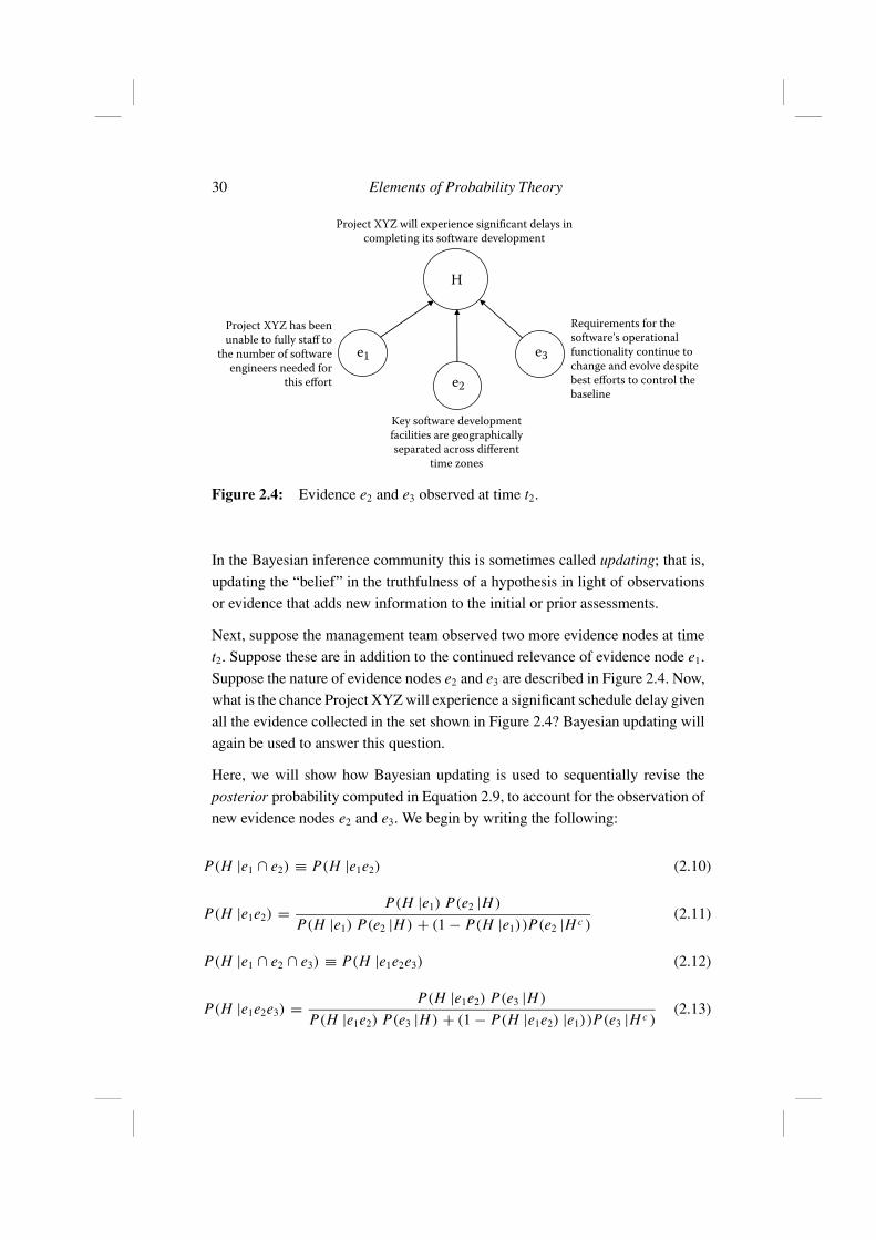
Figure 2.4: Evidence e2 and e3 observed at time t2.

In the Bayesian inference community this is sometimes called updating; that is,

updating the “belief” in the truthfulness of a hypothesis in light of observations

or evidence that adds new information to the initial or prior assessments.

Next, suppose the management team observed two more evidence nodes at time

t2. Suppose these are in addition to the continued relevance of evidence node e1.

Suppose the nature of evidence nodes e2 and e3 are described in Figure 2.4. Now,

what is the chance Project XYZ will experience a significant schedule delay given

all the evidence collected in the set shown in Figure 2.4? Bayesian updating will

again be used to answer this question.

Here, we will show how Bayesian updating is used to sequentially revise the

posterior probability computed in Equation 2.9, to account for the observation of

new evidence nodes e2 and e3. We begin by writing the following:

P(H |e1 ∩ e2) ≡ P(H |e1e2) (2.10)

P(H |e1e2) = P(H |e1) P(e2 |H )

P(H |e1) P(e2 |H ) + (1 − P(H |e1) )P(e2 |H c )(2.11)

P(H |e1 ∩ e2 ∩ e3) ≡ P(H |e1e2e3) (2.12)

P(H |e1e2e3) = P(H |e1e2) P(e3 |H )

P(H |e1e2) P(e3 |H ) + (1 − P(H |e1e2) |e1) )P(e3 |H c )(2.13)


0.00

0.25

0.50

0.75

1.00

Probability

Hypothesis is True

P(H e1e2) = 0.8276

P(H ) = 0.50

Initial or Prior “Belief”

That Hypothesis H isTrue

Updated Probability That Hypothesis

H is True, Given All Evidence

Observed-to-Date

Influence of Evidence Node ...

P(H e1e2e3) = 0.9785

P(H e1) = 0.7059

e1 e1 e2 e1 e2 e3

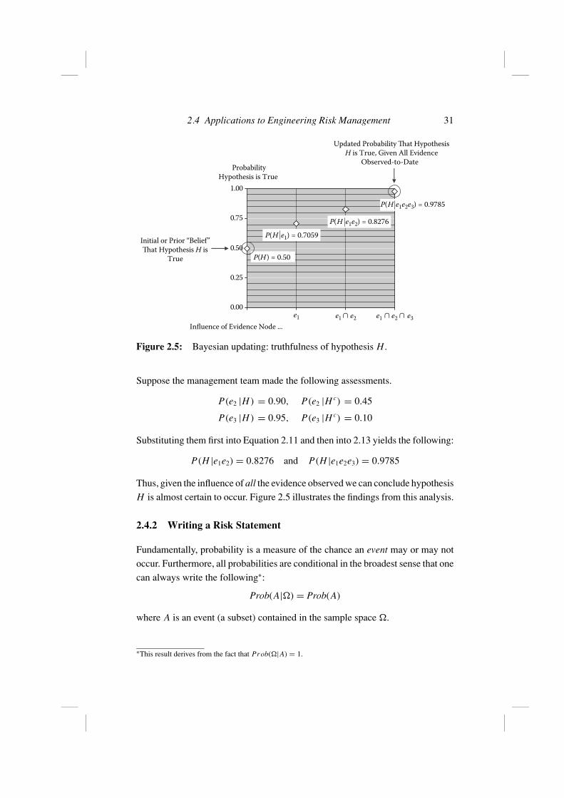
Figure 2.5: Bayesian updating: truthfulness of hypothesis H.

Suppose the management team made the following assessments.

P(e2 |H ) = 0.90, P(e2 |H c) = 0.45

P(e3 |H ) = 0.95, P(e3 |H c) = 0.10

Substituting them first into Equation 2.11 and then into 2.13 yields the following:

P(H |e1e2) = 0.8276 and P(H |e1e2e3) = 0.9785

Thus, given the influence of all the evidence observed we can conclude hypothesis

H is almost certain to occur. Figure 2.5 illustrates the findings from this analysis.

2.4.2 Writing a Risk Statement

Fundamentally, probability is a measure of the chance an event may or may not

occur. Furthermore, all probabilities are conditional in the broadest sense that one

can always write the following∗:

Prob(A|�) = Prob(A)

where A is an event (a subset) contained in the sample space �.

∗This result derives from the fact that Prob(�|A) = 1.


In a similar way, one can consider subjective or judgmental probabilities as con-

ditional probabilities. The conditioning event (or events) may be experience with

the occurrence of events known to have a bearing on the occurrence probability of

the future event. Conditioning events can also manifest themselves as evidence,

as discussed in the previous section on Bayesian inference.

Given these considerations, a “best practice” for expressing an identified risk is

to write it in a form known as the risk statement. A risk statement aims to provide

clarity and descriptive information about the identified risk so a reasoned and

defensible assessment can be made on the risk’s occurrence probability and its

areas of impact (if the risk event occurs).

A protocol for writing a risk statement is the Condition-If-Then construct. This

protocol applies in all risk management processes designed for any systems en-

gineering environment. It is a recognition that a risk event is, by its nature, a

probabilistic event and one that, if it occurs, has unwanted consequences.

What is the Condition-If-Then construct? The Condition reflects what is known

today. It is the root cause of the identified risk event. Thus, the Condition is an

event that has occurred, is presently occurring, or will occur with certainty. Risk

events are future events that may occur because of the Condition present. Below

is an illustration of this protocol.

Suppose we have the following two events. Define the Condition as event B and

the If as event A (the risk event)

B = {Current test plans are focused on the components of the subsystem

and not on the subsystem as a whole}A = {Subsystem will not be fully tested when integrated into the system for

full-up system-level testing}

The risk statement is the Condition-If part of the construct; specifically,

Risk Statement: {The subsystem will not be fully tested when integrated

into the system for full-up system-level testing, because current test plans

are focused on the components of the subsystem and not on the subsystem

as a whole.}


From the above, we see the Condition-If part of the construct is equivalent to a

probability event; formally, we can write

0 < P(A | B ) = α < 1

where α is the probability risk event A occurs given the conditioning event B (the

root cause event) has occurred. Why do you think P(A | B ) here is written as a

strict inequality?

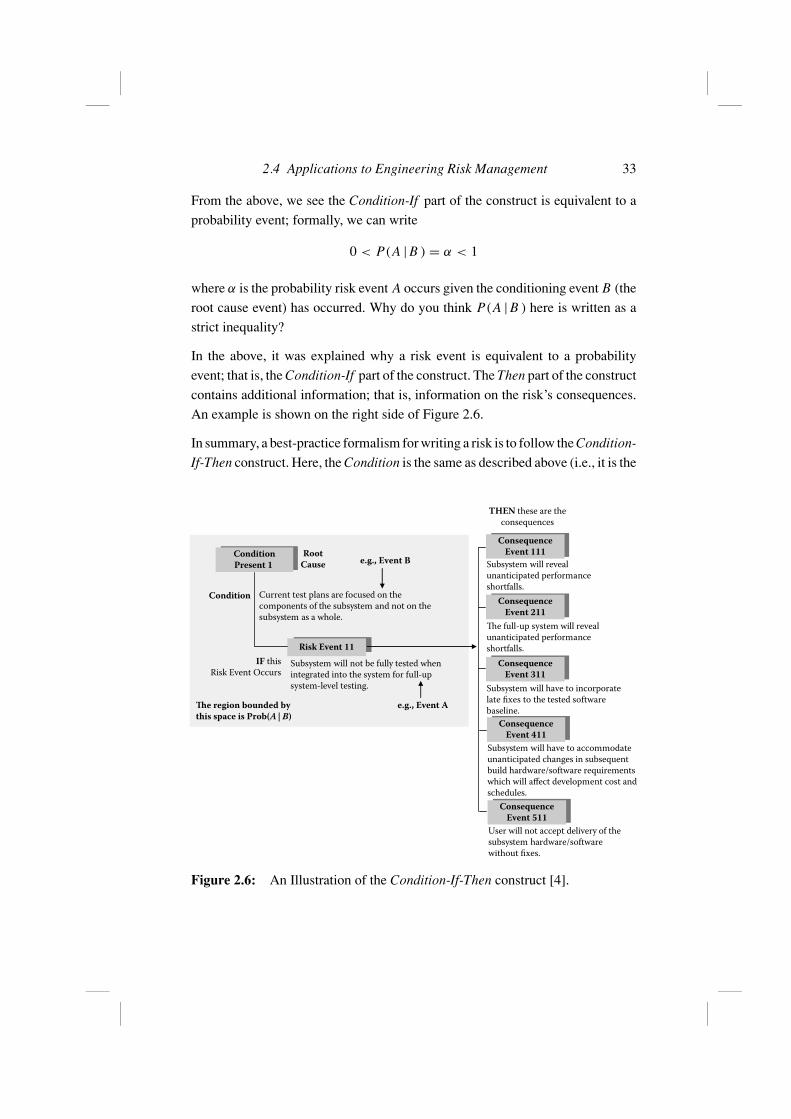
In the above, it was explained why a risk event is equivalent to a probability

event; that is, the Condition-If part of the construct. The Then part of the construct

contains additional information; that is, information on the risk’s consequences.

An example is shown on the right side of Figure 2.6.

In summary, a best-practice formalism for writing a risk is to follow the Condition-

If-Then construct. Here, the Condition is the same as described above (i.e., it is the

ConditionPresent 1

Risk Event 11Subsystem will not be fully tested when

integrated into the system for full-up

system-level testing.

ConsequenceEvent 111

Subsystem will reveal

unanticipated performance

shortfalls.


The full-up system will reveal

unanticipated performance

shortfalls.

Condition


Subsystem will have to incorporate

late fixes to the tested software

baseline.


Subsystem will have to accommodate

unanticipated changes in subsequent

build hardware/software requirements

which will affect development cost and

schedules.


User will not accept delivery of the

subsystem hardware/software

without fixes.

Current test plans are focused on the

components of the subsystem and not on the

subsystem as a whole.

IF this

Risk Event Occurs

THEN these are the

consequences

RootCause

The region bounded bythis space is Prob(A | B)

e.g., Event B

e.g., Event A

Figure 2.6: An Illustration of the Condition-If-Then construct [4].


root cause). The If is the associated risk event. The Then is the consequence, or set

of consequences, that will impact the engineering system project if the risk event

occurs. Figure 2.6 illustrates the Condition-If-Then construct for this example.

Questions and Exercises

1. State the interpretation of probability implied by the following:

(a) The probability a tail appears on the toss of a fair coin is 1/2.

(b) After recording the outcomes of 50 tosses of a fair coin, the probability

a tail appears is 0.54.

(c) It is with certainty the coin is fair.

(d) The probability is 60% that the stock market will close 500 points

above yesterday’s closing count.

(e) The design team believes there is less than a 5% chance the new

microchip will require more than 12,000 gates.

2. A sack contains 20 marbles exactly alike in size but different in color.

Suppose the sack contains 5 blue marbles, 3 green marbles, 7 red marbles,

2 yellow marbles, and 3 black marbles. Picking a single marble from the

sack and then replacing it, what is the probability of choosing the following:

(a) Blue marble? (b) Green marble? (c) Red marble?

(d) Yellow marble? (e) Black marble? (f) Non-blue marble

(g) Red or non-red marble?

3. If a fair coin is tossed, what is the probability of not obtaining a head? What

is the probability of the event: (a head or not a head)?

4. Suppose A is an event (a subset) contained in the sample space �. Given

this, are the following probability statements true or false, and why?

(a) P(A ∪ Ac) = 1 (b) P(A |� ) = P(A)

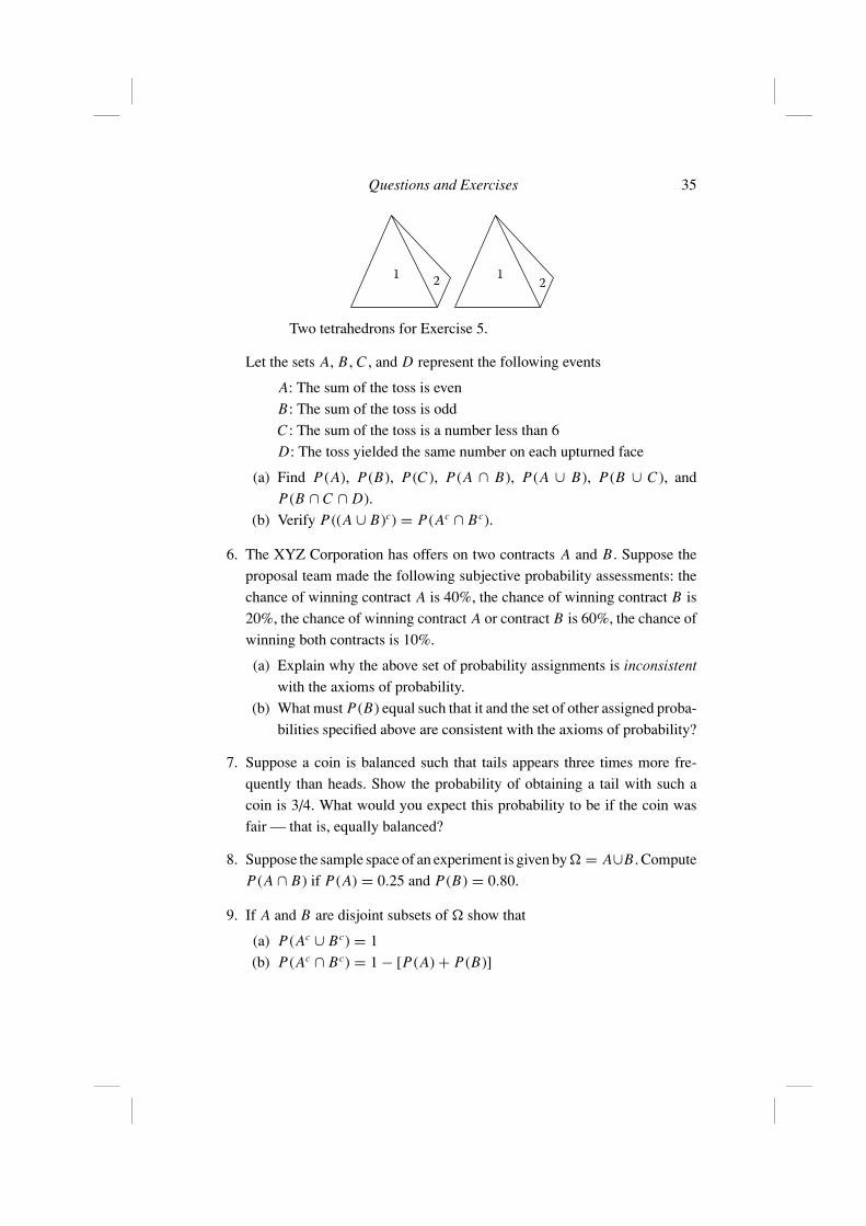
5. Suppose two tetrahedrons (4-sided polygons) are randomly tossed. Assum-

ing the tetrahedrons are weighted fair, determine the set of all possible

outcomes �. Assume each face is numbered 1, 2, 3, and 4.

Questions and Exercises 35

12

12

Two tetrahedrons for Exercise 5.

Let the sets A, B, C , and D represent the following events

A: The sum of the toss is even

B: The sum of the toss is odd

C : The sum of the toss is a number less than 6

D: The toss yielded the same number on each upturned face

(a) Find P(A), P(B), P(C), P(A ∩ B), P(A ∪ B), P(B ∪ C), and

P(B ∩ C ∩ D).

(b) Verify P((A ∪ B)c) = P(Ac ∩ Bc).

6. The XYZ Corporation has offers on two contracts A and B. Suppose the

proposal team made the following subjective probability assessments: the

chance of winning contract A is 40%, the chance of winning contract B is

20%, the chance of winning contract A or contract B is 60%, the chance of

winning both contracts is 10%.

(a) Explain why the above set of probability assignments is inconsistent

with the axioms of probability.

(b) What must P(B) equal such that it and the set of other assigned proba-

bilities specified above are consistent with the axioms of probability?

7. Suppose a coin is balanced such that tails appears three times more fre-

quently than heads. Show the probability of obtaining a tail with such a

coin is 3/4. What would you expect this probability to be if the coin was

fair — that is, equally balanced?

8. Suppose the sample space of an experiment is given by � = A∪B. Compute

P(A ∩ B) if P(A) = 0.25 and P(B) = 0.80.

9. If A and B are disjoint subsets of � show that

(a) P(Ac ∪ Bc) = 1

(b) P(Ac ∩ Bc) = 1 − [P(A) + P(B)]


10. Two missiles are launched. Suppose there is a 75% chance missile A hits

the target and a 90% chance missile B hits the target. If the probability

missile A hits the target is independent of the probability missile B hits the

target, determine the probability missile A or missile B hits the target. Find

the probability needed for missile A such that if the probability of missile

B’s hitting the target remains at 90%, the probability missile A or missile

B hits the target is 0.99.

11. Suppose A and B are independent events. Show that

(a) The events Ac and Bc are independent.

(b) The events A and Bc are independent.

(c) The events Ac and B are independent.

12. Suppose A and B are independent events with P(A) = 0.25 and P(B) =0.55. Determine the probability

(a) At least one event occurs.

(b) Event B occurs but event A does not occur.

13. Suppose A and B are independent events with P(A) = r and the probability

that at least A or B occurs is s. Show the only value for P(B) is the product

(s − r )(1 − r )−1.

14. At a local sweet shop, 10% of all customers buy ice cream, 2% buy fudge,

and 1% buy both ice cream and fudge. If a customer selected at random

bought fudge, what is the probability the customer bought an ice cream?

If a customer selected at random bought ice cream, what is the probability

the customer bought fudge?

15. For any two events A and B, show that P(A |A ∩ (A ∩ B)) = 1 .

16. A production lot contains 1000 microchips of which 10% are defective. Two

chips are successively drawn at random without replacement. Determine

the probability

(a) Both chips selected are non-defective.

(b) Both chips are defective.

(c) The first chip is defective and the second chip is non-defective.

(d) The first chip is non-defective and the second chip is defective.

Questions and Exercises 37

17. Suppose the sampling scheme in exercise 16 was with replacement, that is,

the first chip is returned to the lot before the second chip is drawn. Show

how the probabilities computed in exercise 16 change.

18. Spare power supply units for a communications terminal are provided to

the government from three different suppliers A1, A2, and A3. Suppose

30% come from A1, 20% come from A2, and 50% come from A3. Suppose

these units occasionally fail to perform according to their specifications and

the following has been observed: 2% of those supplied by A1 fail, 5% of

those supplied by A2 fail, and 3% of those supplied by A3 fail. What is the

probability any one of these units provided to the government will perform

without failure?

19. In a single day, ChipyTech Corporation’s manufacturing facility produces

10,000 microchips. Suppose machines A, B, and C individually produce

3000, 2500, and 4500 chips daily. The quality control group has determined

the output from machine A has yielded 35 defective chips, the output from

machine B has yielded 26 defective chips, and the output from machine C

has yielded 47 defective chips.

(a) If a chip was selected at random from the daily output, what is the

probability it is defective?

(b) What is the probability a randomly selected chip was produced by

machine A? By machine B? By machine C?

(c) Suppose a chip was randomly selected from the day’s production

of 10,000 microchips and it was found to be defective. What is the

probability it was produced by machine A? By machine B? By

machine C?

20. From section 2.4.1, show that Bayes’ rule is the basis for the equations

below.

(a) P(H |e1) = P(H )P(e1 |H )

P(H )P(e1 |H ) + (1 − P(H ))P(e1 |H c )

(b) P(H |e1e2) = P(H |e1) P(e2 |H )

P(H |e1) P(e2 |H ) + (1 − P(H |e1) )P(e2 |H c )

(c) P(H |e1e2e3) = P(H |e1e2) P(e3 |H )

P(H |e1e2) P(e3 |H ) + (1 − P(H |e1e2) |e1) )P(e3 |H c )

Elements of Probability Theory - CAE Solutions Corporation14 Elements of Probability Theory The set...

Documents

Transcript of Elements of Probability Theory - CAE Solutions Corporation14 Elements of Probability Theory The set...