Elements of Multiple Regression Analysis: Two

Independent Variables

Yong

Sept. 2010

Why Multiple Regression?

In real world, using only one predictor (IV) to interpret or predict a outcome variable (DV) is rare. Mostly, we need several IV’s.

Multiple regression (Pearson, 1908) is to investigate the relationship between several independent or predictor variables and a dependent or criterion variable.

The prediction equation in multiple regression

Y’ = predicted Y score a = intercept b1 … bk = regression coefficientsX1 … Xk = scores of IVs

With two IV’s:

Calculation of basic statistics 1

Calculation with two IV’s is similar to one IV. However, it is not hard but tedious.

We need knowledge of matrix operations to perform calculations with 3 or more IV’s.

Good news is that we can have the computer do the calculations!

Calculation of basic statistics 2

Calculation of basic statistics 3

Why calculations, as always?

Intercept (a) & regression coefficients (b’s) !

Brain exercise

Now, we have the regression line! What’s next? The predicted Y or Y’! Then what? Deviation due to regression ( ) and the

regression sum of squares ( ) . Deviation due to residuals ( ) and the

residual sum of squares ( ).

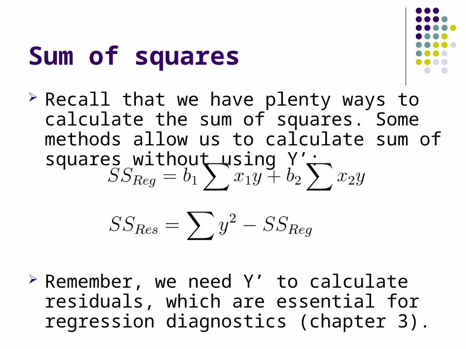
Sum of squares

Recall that we have plenty ways to calculate the sum of squares. Some methods allow us to calculate sum of squares without using Y’:

Remember, we need Y’ to calculate residuals, which are essential for regression diagnostics (chapter 3).

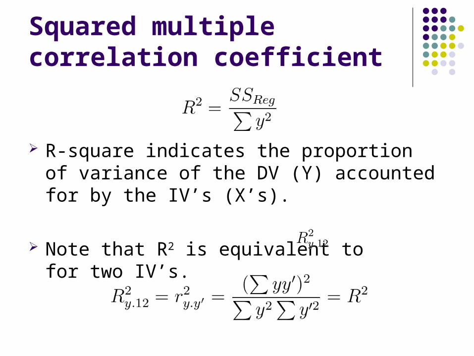
Squared multiple correlation coefficient

R-square indicates the proportion of variance of the DV (Y) accounted for by the IV’s (X’s).

Note that R2 is equivalent to for two IV’s.

Test of significance of R2

F test: if R2 is significantly different from 0.

Rule of thumb:We reject H0 when the calculated F is greater than the table (critical) value or the calculated probability is less than α.

significance level

fail to reject H0 reject H0

F critical Probability, p

Test of significance of individual b’s

T-test (mostly two-tailed, except that we can rule out one direction): if b is significantly different from 0.

Rule of thumb:We reject H0 when the absolute value of calculated T is greater than the table (critical) value or the calculated probability is less than α.

fail to reject H0

reject H0reject H0

Test of R2 vs. test of b

Test of R2 is equivalent to testing all the b’s simultaneously.

Test of a given b for significance is to determine whether it differs from 0 while controlling for the effects of the other IV’s.

For simple linear regression, they are equivalent ( ).

Confidence interval

Definition:

If an experiment was repeated many times, 100(1-α)% of these intervals would contain µ.

If the CI does not include 0, we reject H0 and conclude that the given regression coefficient significantly differs from 0.

Test of increments in proportion of variance accounted for (R2 change)

In multiple linear regression, we could test amount of R2 increases or decreases when a given IV or a set of variables are added to or deleted from the regression equation.

Test of increments in proportion of variance accounted for (R2 change)

The test is equivalent to testing significance of individual b if one IV is added to or deleted from the regression equation.

Note that the R2 change caused by a given IV or a set of IV’s depends on the order of addition or deletion.

Commonly used methods of adding or deleting variables

Enter: enter all IV’s at once in a single modelEnter: enter all IV’s at once in a single model Stepwise: enter IV’s one by one in several Stepwise: enter IV’s one by one in several

models commonly based on Rmodels commonly based on R22 Forward: enter IV’s one by one based on

strength of correlation with DV. Backward: enter all IV’s and delete weakest

one unless it significantly affects the model. Hierarchical: enter IV’s (one or more at a time) Hierarchical: enter IV’s (one or more at a time)

according to certain theoretical framework.according to certain theoretical framework.

Standardized regression coefficient (β, beta)

In SPSS (now PASW) output, we have something like this:

Is it a population parameter?

Standardized regression coefficient (β, beta)

Sample unstandardized regression coefficient (b) is the expected change in Y associated with one measurement unit change of in X.

Sample standardized regression coefficient (β) is the expected change in standard deviation of Y associated with a change of one standard deviation in X.

Standardized regression coefficient (β, beta)

The regression equation now is:

Note that the α disappears because standardized score for a constant is always 0.

β could be used to determine the relative contribution of individual IV to account for variance in DV.

What about the correlation coefficients (r’s)?

Later, we will discuss the correlation coefficients in details, mostly in chapter 7 (Statistical Control: Partial and Semipartial Correlation).

Remarks

Multiple regression is an upgraded version of simple linear regression and its interpretation is similar to simple linear regression.

We need emphasize on contributions of each individual IV’s.

To some extent, multiple IV’s have better explanation and prediction on the DV – it is not always true.