Struct Multidisc OptimDOI 10.1007/s00158-010-0495-9

RESEARCH PAPER

Element exchange method for topology optimization

Mohammad Rouhi · Masoud Rais-Rohani ·Thomas N. Williams

Received: 5 December 2008 / Revised: 22 January 2010 / Accepted: 27 January 2010c© Springer-Verlag 2010

Abstract This paper presents a stochastic direct searchmethod for topology optimization of continuum structures.In a systematic approach requiring repeated evaluations ofthe objective function, the element exchange method (EEM)eliminates the less influential solid elements by switchingthem into void elements and converts the more influentialvoid elements into solid resulting in an optimal 0–1 topol-ogy as the solution converges. For compliance minimizationproblems, the element strain energy is used as the principalcriterion for element exchange operation. A wider explo-ration of the design space is assured with the use of randomshuffle while a checkerboard control scheme is used fordetection and elimination of checkerboard regions. Throughthe solution of multiple two- and three-dimensional topol-ogy optimization problems, the general characteristics ofEEM are presented. Moreover, the solution accuracy andefficiency of EEM are compared with those based onexisting topology optimization methods.

Keywords Topology optimization · Element exchangemethod · EEM · Stochastic · Non-gradient · Binary

M. Rouhi · M. Rais-Rohani (B)Department of Aerospace Engineering, Mississippi State University,Mississippi State, MS 39762, USAe-mail: masoud@ae.msstate.edu

M. Rouhie-mail: rouhi@cavs.msstate.edu

M. Rouhi · M. Rais-Rohani · T. N. WilliamsCenter for Advanced Vehicular Systems, Mississippi State University,Mississippi State, MS 39762, USA

1 Introduction

Topology optimization of continuum structures is aimedat finding the optimum distribution of a specified vol-ume of material over a selected design domain that wouldpush a desired objective function toward its extreme value.Although optimum topology could be defined by such cri-teria as displacement or stress, it is commonly based onthe minimization of structural compliance or strain energyresulting in an optimal load path between the loading pointsand the structural supports.

Since the general topology optimization problem withbinary density function (i.e., ρ = 0 or 1) is ill-posed, var-ious methods have been developed to solve the modifiedproblem with a continuous density function (i.e., 0 <

ρ ≤ 1). For the most part, these methods have beenbased on relaxation through homogenization (Bendsoe andKikuchi 1988; Diaz and Bendsoe 1992), where the geome-try and orientation of anisotropic hole-in-cell microstructureare applied as continuous design variables, or with a con-tinuous density function, where the intermediate-densityelements are penalized (Bendsoe 1989; Zhou and Rozvany1991; Rozvany et al. 1992) to yield the desired 0–1 (void–solid) topology. Zhou and Rozvany (1991) showed thatthe use of non-optimal microstructures homogenized intoan anisotropic continuum introduces a penalty for perfo-rated (grey) regions into shape optimization. Their use ofan isotropic microstructure with a suitable penalty func-tion coupled with a gradient-based optimization approachresulted in the elimination of intermediate-density elementsin generalized shape optimization problems. As it came tobe known by its acronym SIMP (Rozvany et al. 1992), solidisotropic microstructure with penalty has become a popularapproach partly because of its accuracy and computational

M. Rouhi et al.

efficiency, as well as ease of integration with general-purpose finite element analysis (FEA) codes. Besides theexistence of multiple local minima, topology optimizationproblems can also suffer from mesh dependency and theformation of checkerboard regions. Some approaches tocombat the latter two problems have included the use ofheuristic mesh-independent filtering (Sigmund and Peterson1988), higher-order finite elements (Jog and Haber 1996),perimeter control (Haber et al. 1996), alternative density–stiffness interpolation schemes (Guo and Gu 2004), hyper-bolic sine functions for the intermediate densities (Bruns2005), and techniques for producing better topologies withsharper solid–void solutions having greater stiffness (Fuchset al. 2005) as well as less checkerboards (Zhou et al. 2001;Poulsen 2002; Pomezanski et al. 2005).

Research efforts in non-gradient based topology opti-mization have led to the development and applicationof such methods as simulated biological growth (SBG;Mattheck and Burkhardt 1990), particle swarm optimization(PSO; Fourie and Groenwold 2001), evolutionary structuraloptimization (ESO; Xie and Steven 1993), bidirectionalESO (BESO; Querin et al. 1998), and metamorphic devel-opment (MD; Liu et al. 2000). Some of these methods,together with other algorithms mimicking biological sys-tems such as genetic algorithms (GA; Goldberg 1989) andcellular automata (CA; Kita and Toyoda 1999), have alsobeen used in the solution of sizing and shape optimizationproblems. The use of binary design variables enables thesemethods to produce a black–white (solid–void) optimaltopology that excludes any gray (i.e., fuzzy or intermedi-ate density) regions without using penalization. Anotheradvantage of the stochastic direct search methods is theirnon-local search algorithms that can lead to a better solutionthan the local optimum in the vicinity of the initial designpoint. However, due to the need for a large number of func-tion evaluations for the multitude of candidate designs, thedirect search methods tend to be computationally inefficient(Fourie and Groenwold 2001; Werne 2006; Jakiela et al.2000; Mei et al. 2007). To remedy the checkerboard prob-lem, non-gradient based methods also resort to using mostlyheuristic schemes. Zhou and Rozvany (2001) discussedsome of the shortcomings of non-gradient based methodssuch as ESO, and more recently, Rozvany (2009) offereda detailed critical review of SIMP and ESO by examin-ing their mathematical foundations and highlighting theirdifferences in terms of solution accuracy and computationalefficiency.

In this paper, we introduce a new non-gradient basedtopology optimization method that has many of the sameadvantages and some of the shortcomings of the otherstochastic direct search methods but with noticeably bettercomputational efficiency. Named after the principal oper-ation in the topology optimization strategy, the element

exchange method (EEM) falls under the same category asBESO and GA due to the use of heuristic relationships, butit has certain features that are quite distinct from the othertwo methods. In the remaining portion of the paper, we pro-vide details of the EEM and describe the element exchangestrategy, checkerboard control procedure, convergence cri-teria, and the algorithmic parameters used in conjunctionwith different operations in EEM. The convergence prop-erties of EEM are illustrated along with a comparison toa known Michell truss structure. Moreover, the results forseveral two- and three-dimensional problems of varyingcomplexity are presented while making comparisons withthe solutions found using other methods as reported in theliterature.

2 General principle of element exchange

The general principle of element exchange for the case ofcompliance minimization is explained using a simple struc-tural system that is idealized by a combination of fourlinearly elastic springs and associated boundary conditionsas shown in Fig. 1. The total strain energy, Et stored in

(a)

(b)

Fig. 1 Spring system a before and b after element exchange operation

Element exchange method for topology optimization

the system is simply the sum of energy stored in individualsprings found as

Et =4∑

i=1

Ei = 1

2

4∑

i=1

Kiδ2i (1)

where Ei is the energy in the i th spring defined in terms ofthe corresponding stiffness, Ki and elongation, δi .

Assuming that only two springs can be used for min-imizing the strain energy of the system in this example,the problem becomes one of deciding which two springsto keep and which ones to eliminate. The two springs thatare kept create an optimal load path between the loadedand supported points of the system. For simplicity, a solidspring is assumed to have a stiffness of Ks while a voidspring has a stiffness of Kv = 0.001 Ks. Using the ini-tial distribution of springs shown in Fig. 1a and recognizingthat springs 1 and 2 are under equal axial force, elonga-tions of springs 1 through 4 can be shown to be: δ1 =

δ1,001 ≈ δ

1,000 ; δ2 = 1,0001,001δ ≈ δ; δ3 = δ4 = δ. Thus,

the substitution of appropriate values into (1) gives Et =Ks2

[1 × 10−6 + 1 × 10−3 + 1 × 100 + 1 × 10−3

]δ2 ≈

12 Ksδ

2 = 12

F2

Ks. Since spring 1 is a solid spring with the

lowest strain energy between the two solid springs, it willbe converted into a void spring in the next iteration whilespring 4—representing a void spring with the highest strainenergy between the two void springs—will be convertedinto a solid spring. Figure 1b shows the updated layout afterthe element exchange operation is performed. Now, the totalstrain energy stored in the system can be shown to be Et =Ks2

[2.5 × 10−4 + 2.5 × 10−4 + 1 × 100 + 1 × 100

]δ2 ≈

Ksδ2 = 1

4F2

Ks. While the number of solid springs is kept

constant, the total strain energy of the system is reduced by50%, signifying greater stiffness and smaller compliance.Hence, by identifying and switching the less influentialsolid spring into a void spring and the more influential voidspring into a solid spring, a better (more efficient) load pathis created.

By extending the problem to a continuum domain repre-sented by a finite element mesh, it would be possible to usethe element exchange as part of a more general algorithmand solution procedure for finding the optimal topology.

3 EEM algorithm

Here the EEM algorithm is discussed with focus on com-pliance minimization problems. With a continuum structurerepresented by a discretized domain of finite elements andassociated boundary conditions, the compliance minimiza-

tion problem is one of finding the optimal distribution ofsolid and void elements that would

min f (ρ) = uT Ku =M∑

j=1uT

j K j u j =M∑

j=12EEE j

s.t.M∑

j=1ρ j V j � V0

ρmin � ρ � 1.0

(2)

where f (ρ) represents the total strain energy, ρ the vec-tor of non-dimensional element densities treated as designvariables, u the vector of global generalized nodal displace-ments, K the global stiffness matrix, M the total numberof finite elements, with u j , K j and E j as the displace-ment vector, stiffness matrix and strain energy of the j thelement, respectively. With ρ j and Vj representing the non-dimensional density and volume of the j th element, theconstraint in (2) imposes an upper bound on the acceptablevolume fraction of solid elements in the design domain. Toavoid ill-conditioning of stiffness matrix, the void elementsare assumed to have a density equal to ρmin, with a verysmall positive value.

In EEM, stiffness of the j th element represented byE j is linearly related to its non-dimensional density (i.e.,E j = ρ j E , where E is the Young’s modulus of the solidmaterial), with ρ j treated as a discrete design variable ρ j ∈{ρmin, 1.0}, where ρmin = 0.001. For a uniformly dis-cretized domain of identical elements, the volume fractionconstraint in (2) becomes a strict equality that is satisfiedin every iteration. However, for non-uniform meshes, therecan be a small fluctuation of volume around the specifiedlimit, V0.

The EEM algorithm, as depicted by the flowchart inFig. 2 applies to both single- and multiple-load case prob-lems. Once the domain is discretized into a uniform finite-element mesh, the number of solid elements found asNs = MV0 is randomly distributed throughout the designdomain. If the mesh is non-uniform, then Ns would needto be adjusted accordingly to satisfy the specified volumefraction. All void elements are given a non-dimensionalmaterial density of 0.001. The EEM parameters and theirrecommended values appear later in the paper.

Because of the stochastic operations that occur atdifferent stages of EEM together with the fact that the initialdistribution is selected in random, EEM procedure can takedifferent solution paths for the same topology optimizationproblem. As will be shown later, if a problem has multi-ple local optima with nearly equal objective function values(Kutylowski 2002), then it is possible for the EEM solu-tion to converge to any one of these locations, which mayhave different solid–void material distributions. However,the randomly selected initial design and the stochastic oper-ations that occur at different stages of the solution process

M. Rouhi et al.

Fig. 2 Flowchart of EEM

make it more likely for EEM to find a better solution for amore general problem.

With the initial design domain and boundary conditionsspecified, a static FEA is performed to find the strain energydistribution among the elements as well as the total strainenergy of the structure as a whole. At the next step, a sub-set of solid elements with the lowest strain energy densityamongst the solid elements are converted into void elementswhile a volumetrically equivalent number of void elementswith the highest strain energy density amongst the void ele-ments are converted into solid elements such that the volumefraction remains fixed. In the case of a uniform mesh, allelements are geometrically identical; hence, volume frac-tion remains constant by simply setting the number of solidelements converted into voids and vice versa equal to eachother. On the other hand, if the mesh is non-uniform, thenfor the specified exchange volume the solid elements withthe lowest strain energy density are converted one by oneinto void, and similarly the void elements with the high-

est strain energy density are converted into solid until theexchange volume is balanced. Due to the use of discretedensity and variation in element geometry, it is possible toencounter a small difference in volume between the two setsof exchanged elements, which requires the relaxation of thevolume fraction constraint. Since the type of mesh used doesnot change the basic framework of EEM, henceforth, themesh is assumed to be uniform.

The new layout is analyzed for strain energy, andthe element exchange operation is repeated. This pro-cedure is continued for a specified number of iterationsbefore the checkerboard control (detection and elimination)operation is performed, with further details provided later inthe paper.

After completion of several iterations, a subset of thesolid elements are randomly scattered in the void regions.This so-called random shuf f le is similar to the mutationoperation in GA and serves a similar purpose in that itenhances the chance of finding a better solution to the topol-ogy optimization problem by exploring other regions ofthe design space. For a given design problem, the princi-pal operations (i.e., FEA, element exchange, checkerboardcontrol, and random shuffle) are repeated at different inter-vals until a convergence criterion is satisfied. As in the caseof the other stochastic methods, a limit is imposed on thenumber of iterations in order to stop the program when theselected convergence criterion is too tight.

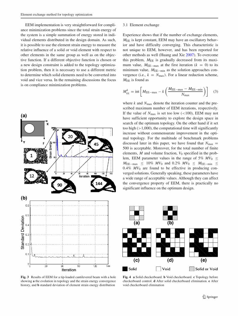
Figure 3a illustrates the evolution in topology from theinitial to optimum (minimum compliance) design point for atwo-dimensional domain using the EEM. Here, convergenceis defined as a nearly stationary topology with changes inthe strain energy below the specified threshold. The strainenergy history plot in Fig. 3a shows the general convergencepattern in EEM. The spikes that appear at different intervalsare mostly due to the random shuffle operation, althoughit is also possible to see an abrupt change in strain energyduring a routine element exchange operation.

In EEM, unlike ESO (Xie and Steven 1993; Querin et al.1998), void elements can be converted into solid and viceversa. Note that in EEM, the void elements have small butnonzero stiffness and density. Even if the initial randomdistribution of solid elements gives an appearance of a dis-continuous load path (infeasible topology), EEM graduallyconnects all the solid elements in its search for an opti-mum topology. Furthermore, in EEM the solid and voidelements participating in the conversion operation are notlimited to any specific region of the design domain as isthe case with BESO (Querin et al. 1998). These character-istics together with the random shuffle and overall topologyoptimization scheme help distinguish EEM from both ESOand BESO. The EEM algorithm is readily applicable to anytwo- or three-dimensional domain and boundary conditions,irrespective of its geometric or loading complexity.

Element exchange method for topology optimization

EEM implementation is very straightforward for compli-ance minimization problems since the total strain energy ofthe system is a simple summation of energy stored in indi-vidual elements distributed in the design domain. As such,it is possible to use the element strain energy to measure therelative influence of a solid or void element with respect toother elements in the same group as well as on the objec-tive function. If a different objective function is chosen ora new design constraint is added to the topology optimiza-tion problem, then it is necessary to use a different metricto determine which solid elements need to be converted intovoid and vice versa. In the remaining discussions the focusis on compliance minimization problems.

Fig. 3 Results of EEM for a tip-loaded cantilevered beam with a holeshowing a the evolution in topology and the strain energy convergencehistory, and b standard deviation of element strain energy distribution

3.1 Element exchange

Experience shows that if the number of exchange elements,MEE is kept constant, EEM may have an oscillatory behav-ior and have difficulty converging. This characteristic isnot unique to EEM, however, and has been reported forother methods as well (Huang and Xie 2007). To overcomethis problem, MEE is gradually decreased from its maxi-mum value, MEE−max at the first iteration (k = 0) to itsminimum value, MEE−min as the solution approaches con-vergence (i.e., k = Nmax). For a linear reduction scheme,MEE is found as

MkEE

= int

[MEE−max − k

(MEE−max − MEE−min

Nmax

)](3)

where k and Nmax denote the iteration counter and the pre-scribed maximum number of EEM iterations, respectively.If the value of Nmax is set too low (<100), EEM may nothave sufficient opportunity to explore the design space insearch of the optimum topology. On the other hand if it settoo high (>1,000), the computational time will significantlyincrease without commensurate improvement in the opti-mal topology. For the multitude of benchmark problemsdiscussed later in this paper, we have found that Nmax =500 is acceptable. Moreover, for the total number of finiteelements, M and volume fraction, V0 specified in the prob-lem, EEM parameter values in the range of 5% MV0 ≤MEE−max ≤ 10% MV0 and 0.2% MV0 ≤ MEE−min ≤0.4% MV0 are found to be effective in producing con-verged solutions. Generally speaking, these parameters havea wide range of acceptable values. Although they can affectthe convergence property of EEM, there is practically nosignificant influence on the optimum design.

Fig. 4 a Solid checkerboard. b Void checkerboard. c Topology beforecheckerboard control. d After solid checkerboard elimination. e Aftervoid checkerboard elimination

M. Rouhi et al.

3.2 Checkerboard control

Checkerboard patterns are generally undesirable anddepending on the topology optimization methodologyused, different strategies are employed to eliminate them(Sigmund and Peterson 1988; Zhou et al. 2001; Poulsen2002; Pomezanski et al. 2005). In EEM, a solid checker-board element is defined as a solid element whose edges areshared with void elements as shown in Fig. 4a, whereas avoid checkerboard element is the exact opposite as illus-trated in Fig. 4b. Whether the dashed elements shownin Fig. 4a and b are solid or void will not change thecheckerboard condition.

Since in EEM the initial topology is a random distribu-tion of solid elements per the specified volume fraction, itis natural to immediately encounter multiple checkerboardregions as shown in Fig. 3a. However, at the beginning, sev-eral element exchange iterations (NCI = 5–10% Nmax) areallowed to proceed before actively searching for checker-board patterns. To eliminate checkerboard regions, firstthe solid checkerboard elements are identified and con-verted into void elements as shown in Fig. 4c and d, andthen the void checkerboard elements are converted intosolid elements (Fig. 4d, e). The checkerboard search andelimination step is repeated every NCC = 1–5% Nmax

iterations. To maintain the specified volume fraction, thedifference between the numbers (volumes) of the switchedsolid and void elements is randomly redistributed in thedesign domain. It is possible for this random redistributionof the difference to result in the creation of small checker-board region(s). However, as EEM procedure is continued,these regions tend to gradually diminish before the finaltopology emerges. The checkerboard elimination procedurein EEM is heuristic and checkerboard elements are removedregardless of their impact on the overall compliance of thestructure.

It is important to note the interaction between checker-board and the mesh size. As shown in exact analytical solu-tions for Michell truss structures (Lewinski and Rozvany2008; Rozvany et al. 2006; Lewinski et al. 1994a), the opti-mal layout is one with many narrow connecting membersor branches. However, if the mesh is relatively coarse, theelements in some of these branches would have a pixilatedappearance and, hence, marked as checkerboard elementsto be eliminated. As will be shown in the example problemslater, there is a greater chance for EEM to produce a topol-ogy that approaches the analytical solution through meshrefinement.

Although the current checkerboard control algorithm isfairly effective, it does have some limitations in that it maynot recognize checkerboard patterns that do not perfectlymatch the models shown in Fig. 4a and b.

3.3 Random shuffle

Although both element exchange and checkerboard con-trol are effective tools in helping the EEM algorithm pushtoward the optimum topology, they are not sufficient. There-fore, an additional operation (i.e., random shuffle) is intro-duced. A random shuffle involves the selection of a subsetof solid elements and their redistribution in void regions ofthe domain. This action is analogous to the mutation oper-ation in GA (Goldberg 1989) or craziness in PSO (Fourieand Groenwold 2001), and is used for the same princi-pal reason, i.e., it helps prevent premature convergence orinsufficient exploration of the design domain in search ofoptimum design. While preserving the specified volumefraction, random shuffle can also help with convergence byalleviating the occasional back and forth oscillation (oscil-latory exchange) in a subset of elements from solid to voidback to solid in successive element exchange operations.Random shuffle will change the topology of the structureby introducing a random replacement of a group of solidelements thereby alleviating the oscillatory exchange. Theeffect of random shuffle on the solution is shown later inthe paper. Two things can generally happen as a result of therandom shuffle operation: (1) an abrupt change in stiffness(Rouhi and Rais-Rohani 2008) and total strain energy asshown by the spikes in Fig. 3a, and (2) creation of checker-board regions. However, neither one of these side effects isdetrimental as both are corrected by the element exchangeand checkerboard control operations of EEM.

Random shuffle is third in the sequence of operations inEEM and occurs at NRS = 2–10% Nmax iterations until theoptimal topology is found. The number of elements partici-pating in the random shuffle, MRS varies from its maximumvalue, MRS−max at the beginning (k = 0) to its minimumvalue, MRS−min as the solution approaches convergence.The value of MRS is found using the expression

MkRS

= int

[MRS−max − k

(MRS−max − MRS−min

Nmax

)](4)

where k and Nmax denote the iteration counter and the pre-scribed maximum number of EEM iterations, respectively.For the benchmark problems discussed later in this paper,MRS−max = MEE−max, MRS−min = MEE−min have beenfound to be effective in producing converged solutions.

3.4 Passive elements

Some continuum structures may contain solid and/or voidsub-regions whose geometry and locations cannot be alteredduring topology optimization. As a matter of convenienceand meshing simplicity, the permanent voids (or solids) may

Element exchange method for topology optimization

be included in the finite element mesh but represented by aseries of passive elements with ρ pi = ρmin (or ρ pi = 1.0)that will not be exchanged during the EEM solution pro-cess. The hole region in the structure shown in Fig. 3 wasmodeled using passive elements.

3.5 Convergence criteria

Increasing the number of iterations in EEM will usually leadto a more refined optimal topology but at the expense ofmore function calls (i.e., additional FE solutions). Besidesimposing a limit on the maximum number of iterations, twoadditional criteria are also used to establish a two-part con-vergence condition in EEM-based topology optimization.

The first convergence criterion considers the relativedifference in the element strain energy distributions in twoconsecutive elite topologies. Here, elite topology refers tothe topology with the lowest strain energy obtained prior tothe current iteration in the EEM procedure. Since it is pos-sible for two distinctly different topologies to have almostequal total strain energies (as noted in the SIMP basedresults in Fig. 5), it is necessary to compare the element

strain energy distribution, as represented by the vector∼E ,

for two consecutive elite topologies as∥∥∥

∼Ece − ∼

Epe

∥∥∥∥∥∥

∼Epe

∥∥∥≤ εE (5)

where subscripts “ce” and “pe” refer to the current and pre-vious elite topologies within Nmax iterations, respectively.

The second convergence criterion examines the densitydistribution in two consecutive elite topologies. The domain

topology is defined by vector∼D whose individual terms

have binary values depending on the solid (1) or void(0) property of the corresponding elements. Based on thisdefinition, the convergence criterion is defined as∥∥∥

∼Dce − ∼

Dpe

∥∥∥∥∥∥

∼Dpe

∥∥∥≤ εt (6)

Fig. 5 Two different topologieswith nearly identical strainenergy values

Figure 3a shows how the strain energy in EEM convergesto its minimum value for a cantilevered beam with a fixedhole. Strain energy starts from an extremely large valuebecause of the randomly distributed elements in the initialstep. However, after a few iterations, it reduces to roughlythe same order of magnitude as its minimum value. Thecontinuation of the element exchange will refine the topol-ogy toward its minimum strain energy as shown in Fig. 3a.Although there are occasional jumps in total strain energy(due to element exchange or random shuffle operation), theoverall trend shows a gradual convergence. It should benoted that similar spikes in the strain energy convergenceplots have also been observed when using BESO (Querinet al. 1998).

Figure 3b shows the plot of the standard deviation ofstrain energy in individual solid elements at different stagesof the solution process. The trend indicates that the strainenergy density field is approaching a more uniform state,resembling the fully stressed design in optimality criteria(Bendsoe and Sigmund 2002; Tanskanen 2002), as it makesthe most efficient use of available material in the designdomain.

Another point that needs to be mentioned here is that,in its current implementation, when EEM identifies anelite topology, no check is made whether any of the solidelements that were previously redistributed as a result ofrandom shuffle operation still remain in the void regions. Assuch, a few floating solid elements may appear as specks inthe void regions of the final topology in different exampleproblems. Since the few floating elements have no sig-nificant impact on the final topology, no attempt is madeto remove them in any of the presented solutions. Due tothe stochastic nature of EEM, another solution to the sameoptimization problem may show different floating elements.

4 Results for two-dimensional problems

Several benchmark problems are used to evaluate the per-formance of EEM and to compare its solutions with thoseobtained using some other methods. Each two-dimensionaldesign domain is defined according to nx, ny, V0 represent-ing the number of finite elements in the x and y directionsand the limit on volume fraction, respectively. Hereafter,strain energy refers to the non-dimensional strain energysince the nodal displacements and element stiffness are nor-malized with respect to element size and material Young’smodulus. The reported number of iterations (N) for theEEM results coincides with the number of FE analysesperformed in the solution process.

Since most of the computational time in each iteration,regardless of the method used, is spent on the compliance

M. Rouhi et al.

calculation via FEA, the total number of function calls(FE solutions) gives a fairly accurate measure of compu-tational efficiency. We purposefully avoided a time-basedcomparison because we did not want to improperly attributeinefficiencies in the implementation of FEA to that of thedifferent optimization algorithms considered. In EEM orSIMP, the required computational time is proportional tothe number of iterations whereas in population based meth-ods such as GA or PSO it is proportional to the number ofiterations times the population size.

4.1 Simply-supported beams

Model A1: Single mid-span force applied on top

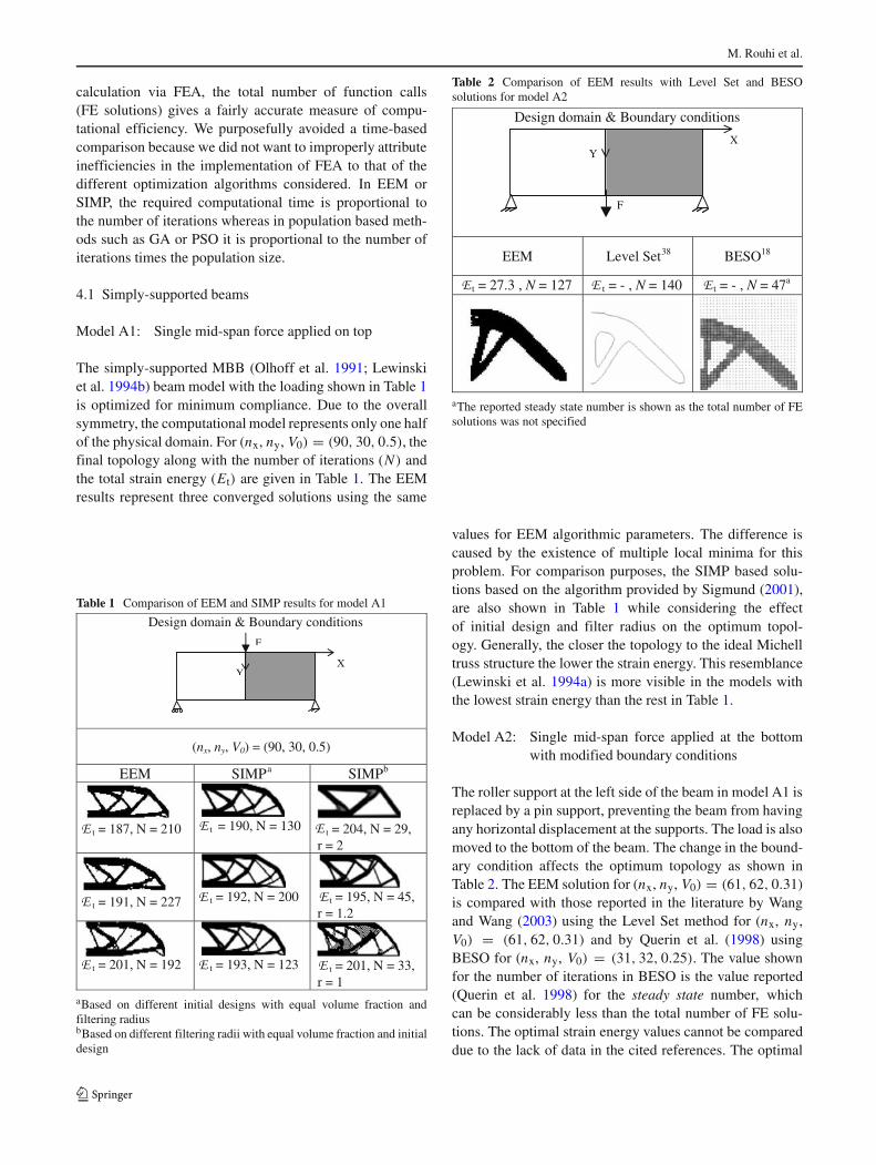
The simply-supported MBB (Olhoff et al. 1991; Lewinskiet al. 1994b) beam model with the loading shown in Table 1is optimized for minimum compliance. Due to the overallsymmetry, the computational model represents only one halfof the physical domain. For (nx, ny, V0) = (90, 30, 0.5), thefinal topology along with the number of iterations (N) andthe total strain energy (Et) are given in Table 1. The EEMresults represent three converged solutions using the same

Table 1 Comparison of EEM and SIMP results for model A1

Design domain & Boundary conditions

(nx, ny, V0) = (90, 30, 0.5)

EEM a SIMPb

t = 187, N = 210

t = 190, N = 130

t = 204, N = 29,

r = 2

t = 191, N = 227

t = 192, N = 200

t = 195, N = 45, r = 1.2

t = 201, N = 192

t = 193, N = 123

t = 201, N = 33, r = 1

F

YX

SIMP

aBased on different initial designs with equal volume fraction andfiltering radiusbBased on different filtering radii with equal volume fraction and initialdesign

Table 2 Comparison of EEM results with Level Set and BESOsolutions for model A2

Design domain & Boundary conditions

F

YX

EEM 38 BESO18

t = 27.3 , N = 127 t = - , N = 140 t = - , N = 47a

Level Set

aThe reported steady state number is shown as the total number of FEsolutions was not specified

values for EEM algorithmic parameters. The difference iscaused by the existence of multiple local minima for thisproblem. For comparison purposes, the SIMP based solu-tions based on the algorithm provided by Sigmund (2001),are also shown in Table 1 while considering the effectof initial design and filter radius on the optimum topol-ogy. Generally, the closer the topology to the ideal Michelltruss structure the lower the strain energy. This resemblance(Lewinski et al. 1994a) is more visible in the models withthe lowest strain energy than the rest in Table 1.

Model A2: Single mid-span force applied at the bottomwith modified boundary conditions

The roller support at the left side of the beam in model A1 isreplaced by a pin support, preventing the beam from havingany horizontal displacement at the supports. The load is alsomoved to the bottom of the beam. The change in the bound-ary condition affects the optimum topology as shown inTable 2. The EEM solution for (nx, ny, V0) = (61, 62, 0.31)

is compared with those reported in the literature by Wangand Wang (2003) using the Level Set method for (nx, ny,V0) = (61, 62, 0.31) and by Querin et al. (1998) usingBESO for (nx, ny, V0) = (31, 32, 0.25). The value shownfor the number of iterations in BESO is the value reported(Querin et al. 1998) for the steady state number, whichcan be considerably less than the total number of FE solu-tions. The optimal strain energy values cannot be compareddue to the lack of data in the cited references. The optimal

Element exchange method for topology optimization

Table 3 Comparison of EEM and SIMP results for model B1

Design domain & Boundary conditions

(nx, ny, V0) = (32, 20, 0.4)

EEM

t = 53.6 , N = 178 t = 57.4 , N = 71

(nx, ny, V0) = (64, 40, 0.4)

EEM SIMP

t = 57 , N = 174 t = 55.7 , N = 57

Y

X

F

SIMP

topologies are fairly similar with both EEM and BESO solu-tions showing one extra member than that in the Level Setsolution.

4.2 Cantilevered beams

Model B1: Single tip force applied at the bottom

Table 3 shows the beam model and loading condition alongwith the results of EEM and SIMP for two different meshsizes at the same volume fraction. In the case of the SIMP,the results are based on the filtering radius of 1.2. While theoptimal strain energy values are comparable, the total itera-tion numbers are different. As a result of mesh refinement,the optimal topology changes with minimal change in thefinal strain energy. By increasing the mesh size, both EEMand SIMP solutions move toward Michell truss topology.

At first, it appears counterintuitive for the more Michelllike structure (Lewinski et al. 1994a) associated with thefine-mesh solution of EEM to have a strain energy that ishigher than that of the coarse mesh. This does not imply thatthe fine-mesh solution is inferior. On the contrary, the appar-ent discrepancy can be explained by the fact that the FEAsolution (predicted strain energy) using the coarse mesh isnot as accurate as that for the fine mesh. If the optimal lay-out (ground elements) in each case were discretized so as toincrease the accuracy of post-optimum FEA solution, then

the more Michell like topology would have smaller strainenergy for the same volume fraction.

Model B2: Single tip force applied at mid height

The beam model and the corresponding topology optimiza-tion results are shown in Table 4. Two different meshdensities are used for EEM solutions at the same volumefraction. Both solutions show a fairly similar trend for mate-rial distribution, although the fine-mesh solution is moreaccurate. The results reported by Wang et al. (2006) basedon the enhanced GA approach are also shown in Table 4 forcomparison. Although the final geometry and strain energyvalues are nearly the same, the EEM solution converges 160times faster. Jakiela et al. (2000) state that, in general, GAbased solutions may require 10 to 100 times more func-tion evaluations than would be required by homogenizationbased solutions. It is notable that the number of functioncalls is in the order of the number of iterations multiplied bythe population size in both GA and PSO as will be shownlater.

A qualitative and quantitative comparison of the per-formance of EEM, enhanced GA and SIMP in findingthe optimum topology for this model is shown in Fig. 6.Although EEM is not as computationally efficient as SIMP,

Table 4 Comparison of EEM results with enhanced GA solution formodel B2

Design domain & Boundary conditions

Y

X

F

(nx, ny, V0) = (24, 12, 0.5)

EEM GA39

t = 66.1 , N = 150 t = 64.4 , N = 4x104

(nx, ny, V0) = (48, 24, 0.5)

EEM

t = 63.5 , N = 250

Enhanced

M. Rouhi et al.

(b)

(a)

(c)

Number of iteration

Com

plia

nce

Number of iteration

Com

plia

nce

Number of iteration

Com

plia

nce

Fig. 6 Compliance convergence history and final topology for aenhanced GA (Wang et al. 2006), b SIMP and c EEM

it is considerably more efficient than GA. It is also worthnoting that for GA the number of iterations times the pop-ulation size gives the total number of function calls (Wanget al. 2006).

Model B3: Model B2 with modified dimensions

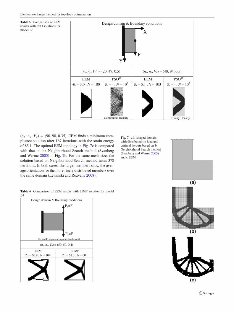
The dimensions of the cantilevered beam in model B2 aremodified such that the beam’s height is greater than itslength. In Table 5, the results of EEM for two different meshsizes are compared with the PSO based solutions reportedby Fourie and Groenwold (2001). While the topologies forthe fine mesh are nearly identical, the EEM optimum topol-ogy for the coarse mesh is better than that produced by PSO.Although PSO is a population-based method requiring mul-tiple FEA in every iteration, the results still show that theEEM solution can converge 10 to 1000 times faster thanPSO with no loss of accuracy.

Model B4: Multiple load cases

The cantilevered beam model in Table 6 is optimized fortwo separate load cases. In one load case, only force F1 isapplied at the tip whereas in the other only F2 is applied.Forces F1 and F2 have equal magnitudes and oppositedirections.

For EEM solution, the strain energy in each element isthe sum of that for each load case. As a result, the additiveform of the objective function is retained and the relation-ship between element strain energy and element exchangeoperation remains unchanged. Thus, the solid elements withthe lowest strain energy sum (from the two load cases com-bined) are converted into void elements whereas the voidelements with the highest strain energy sum are convertedinto solid elements.

The results for EEM and SIMP (with r = 1.2) are com-pared in Table 6. Because both F1 and F2 have equalmagnitudes, the structure tends to have a symmetric lay-out. The EEM and SIMP topologies have some distinctdifferences. The two horizontal (top and bottom) membersin SIMP solution appear as slanted in the EEM layout andthe vertical member in SIMP layout is absent in the EEMtopology. The dark specks seen in the EEM topology arethe residue or the floating elements from the last randomshuffle operation as discussed earlier in the paper.

4.3 L-shaped domain

Model C1: Distributed force applied along one boundary

An L-shaped domain with clamped boundary conditionsalong the top edge and a distributed force along the middlethird section of the right edge as shown in Fig. 7a is opti-mized for minimum compliance. For simplicity, the prob-lem is modeled as a square domain with elements located inthe upper right quadrant treated as passive elements. Using

Element exchange method for topology optimization

Table 5 Comparison of EEMresults with PSO solutions formodel B3

Design domain & Boundary conditions

Y

X

F

(nx, ny, V0) = (20, 47, 0.5) (nx, ny, V0) = (40, 94, 0.5)

EEM 16 EEM PSO16

t = 3.0 , N = 100 t = - , N = 105 t = 5.1 , N = 103 t = - , N = 103

Continuous Density

Binary Density

PSO

(nx, ny, V0) = (90, 90, 0.35), EEM finds a minimum com-pliance solution after 167 iterations with the strain energyof 85.1. The optimal EEM topology in Fig. 7c is comparedwith that of the Neighborhood Search method (Svanbergand Werme 2005) in Fig. 7b. For the same mesh size, thesolution based on Neighborhood Search method takes 378iterations. In both cases, the larger members show the aver-age orientation for the more finely distributed members overthe same domain (Lewinski and Rozvany 2008).

Table 6 Comparison of EEM results with SIMP solution for modelB4

Design domain & Boundary conditions

F1=F

F2=F

(F1 and F2 represent separate load cases)

(nx, ny, V0) = (50, 50, 0.4)

EEM

t = 60.9 , N = 104 t = 61.3 , N = 60

SIMP

Fig. 7 a L-shaped domainwith distributed tip load andoptimal layouts based on bNeighborhood Search method(Svanberg and Werme 2005)and c EEM

(a)

(b)

(c)

M. Rouhi et al.

Fig. 8 a L-shaped domain withsingle tip load and optimallayouts based on b exactanalytical solution (Lewinskiand Rozvany 2008). c EEMwith coarse mesh. d EEM withfine mesh

(a)

(b)

(c)

(d)

Model C2: Single tip force applied at the bottom

The problem is similar to that in model C1 except for theapplied load as shown in Fig. 8a. Here the EEM solutionsin Fig. 8c and d for (nx, ny, V0) = (90, 90, 0.35) and (nx,ny, V0) = (250, 250, 0.35), respectively, are compared tothe exact analytical solution (Lewinski and Rozvany 2008;Rozvany et al. 2006) in Fig. 8b. It should be noted that theunlimited number of bars in the analytical solutions wouldbe very difficult to capture in an FE solution with a limiteddiscretization, especially in this case where the boundaryconditions along the top edge are not exactly the same as

the analytical case. However, the trend captured in the EEMsolutions appears to be in reasonable agreement with theanalytical solution. Since there is some randomness in theEEM procedure, the number of lumped bars and their ori-entation may vary from one solution to another for the sameproblem.

5 Results for three-dimensional problems

Each three-dimensional design domain is defined accordingto nx, ny, nz, V0 values representing the number of finite ele-ments in the x , y, and z directions and the limit on volumefraction, respectively. As in the previous section, the EEMresults are compared with those reported in the literature.

5.1 Cubic domain

A cubic domain is simply supported at its four bottom cor-ners and is loaded by four concentrated vertical forces actingat the top surface as shown in Fig. 9a. Using the EEM proce-dure with (nx, ny, nz, V0) = (20, 20, 20, 0.08), the optimum

Fig. 9 a Design domain andboundary conditions withoptimum topology based onb Optimum Microstructures(Olhoff et al. 1998) and c EEM

(a)

(b)

(c)

Element exchange method for topology optimization

(a) (b)

(c) (d)

Fig. 10 a Design domain and boundary conditions with optimumtopology based on b EEM, V0 = 0.3, c EEM, V0 = 0.08 and d Opti-mum Microstructure (Olhoff et al. 1998), V0 = 0.3 (elements withdensities less than 0.5 filtered out)

topology in Fig. 9b is obtained after 178 iterations with astrain energy of 24.1. For comparison, the results obtainedby Olhoff et al. (1998) using the Optimum Microstructure(OM) method is shown in Fig. 9c. The gray regions in theFig. 9c imply intermediate density since the OM methoduses a continuous density function. Also, elements withdensity less than a threshold value are filtered out in the OMmethod to arrive at the final topology. Therefore, the finaltopology may not match the pre-specified volume fraction.

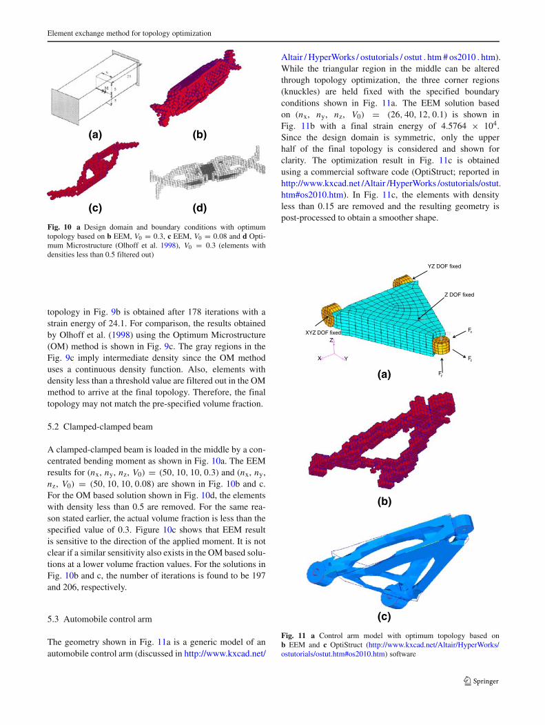
5.2 Clamped-clamped beam

A clamped-clamped beam is loaded in the middle by a con-centrated bending moment as shown in Fig. 10a. The EEMresults for (nx, ny, nz, V0) = (50, 10, 10, 0.3) and (nx, ny,nz, V0) = (50, 10, 10, 0.08) are shown in Fig. 10b and c.For the OM based solution shown in Fig. 10d, the elementswith density less than 0.5 are removed. For the same rea-son stated earlier, the actual volume fraction is less than thespecified value of 0.3. Figure 10c shows that EEM resultis sensitive to the direction of the applied moment. It is notclear if a similar sensitivity also exists in the OM based solu-tions at a lower volume fraction values. For the solutions inFig. 10b and c, the number of iterations is found to be 197and 206, respectively.

5.3 Automobile control arm

The geometry shown in Fig. 11a is a generic model of anautomobile control arm (discussed in http://www.kxcad.net/

Altair / HyperWorks / ostutorials / ostut . htm # os2010 . htm).While the triangular region in the middle can be alteredthrough topology optimization, the three corner regions(knuckles) are held fixed with the specified boundaryconditions shown in Fig. 11a. The EEM solution basedon (nx, ny, nz, V0) = (26, 40, 12, 0.1) is shown inFig. 11b with a final strain energy of 4.5764 × 104.Since the design domain is symmetric, only the upperhalf of the final topology is considered and shown forclarity. The optimization result in Fig. 11c is obtainedusing a commercial software code (OptiStruct; reported inhttp://www.kxcad.net /Altair /HyperWorks /ostutorials/ostut.htm#os2010.htm). In Fig. 11c, the elements with densityless than 0.15 are removed and the resulting geometry ispost-processed to obtain a smoother shape.

X

Z

Y

XYZ DOF fixed

YZ DOF fixed

Z DOF fixed

Fx

Fz

Fy(a)

(c)

(b)

Fig. 11 a Control arm model with optimum topology based onb EEM and c OptiStruct (http://www.kxcad.net/Altair/HyperWorks/ostutorials/ostut.htm#os2010.htm) software

M. Rouhi et al.

The possibility of sub-structuring the computationaldomain to reduce the number of FE calculations was inves-tigated in Rouhi and Rais-Rohani (2008). The idea was tolimit the FE analysis to the parts of the domain that partic-ipate in the element exchange operations. The participationof a large number of elements in different regions of thestructure in the various EEM operations showed that sucha sub-structuring may not be possible. The requirementfor a relatively large number of FE solutions is the maindrawback in all stochastic approaches including EEM.

6 Effects of special operations in EEM on the solution

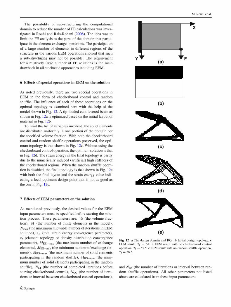
As noted previously, there are two special operations inEEM in the form of checkerboard control and randomshuffle. The influence of each of these operations on theoptimal topology is examined here with the help of themodel shown in Fig. 12. A tip-loaded cantilevered beam asshown in Fig. 12a is optimized based on the initial layout ofmaterial in Fig. 12b.

To limit the list of variables involved, the solid elementsare distributed uniformly in one portion of the domain perthe specified volume fraction. With both the checkerboardcontrol and random shuffle operations preserved, the opti-mum topology is that shown in Fig. 12c. Without using thecheckerboard control operation, the optimum solution is thatin Fig. 12d. The strain energy in the final topology is partlydue to the numerically induced (artificial) high stiffness ofthe checkerboard regions. When the random shuffle opera-tion is disabled, the final topology is that shown in Fig. 12ewith both the final layout and the strain energy value indi-cating a local optimum design point that is not as good asthe one in Fig. 12c.

7 Effects of EEM parameters on the solution

As mentioned previously, the desired values for the EEMinput parameters must be specified before starting the solu-tion process. These parameters are: V0 (the volume frac-tion), M (the number of finite elements in the model),Nmax (the maximum allowable number of iterations in EEMsolution), εE (total strain energy convergence parameter),εt (element topology or density distribution convergenceparameter), MEE−max (the maximum number of exchangeelements), MEE−min (the minimum number of exchange ele-ments), MRS−max (the maximum number of solid elementsparticipating in the random shuffle), MRS−min (the mini-mum number of solid elements participating in the randomshuffle), NCI (the number of completed iterations beforestarting checkerboard control), NCC (the number of itera-tions or interval between checkerboard control operations),

Y

X

F(a)

(b)

(c)

(d)

(e)

Fig. 12 a The design domain and BCs. b Initial design topology. cEEM result, Et = 54. d EEM result with no checkerboard controloperation, Et = 55.5. e EEM result with no random shuffle operation,Et = 58.5

and NRS (the number of iterations or interval between ran-dom shuffle operations). All other parameters not listedabove are calculated from these input parameters.

Element exchange method for topology optimization

The convergence parameters (Nmax, εE and εt) controlthe solution accuracy. Generally speaking, the EEM searchfor optimum topology becomes more rigorous by increas-ing the value of Nmax and decreasing the values of εE andεt at the expense of increased computational time. As withthe other stochastic methods, if Nmax is too small, EEMmay not be able to find an optimum solution. On the otherhand, if εE and εt are too small, convergence may be hardto achieve. As shown in Fig. 3, EEM finds the basic lay-out of the optimum topology in about 20 iterations with theremaining iterations devoted to refinement of the topology.However, when the design domain includes multiple localoptima, then it is possible for the topology to vary widelyduring the solution sequence.

Since element exchange is the main operation in EEM,the value selected for MEE is important. As notedpreviously, MEE cannot be treated as a constant and mustbe gradually reduced from its prescribed maximum value(MEE−max) at the very beginning to its imposed mini-mum (MEE−min) at the end. Based on the multitude ofproblems examined, choosing MEE−max ∼ 5–10% andMEE−min ∼ 0.2–0.4% of the solid elements (MV0) would beappropriate. Generally speaking, selecting a relatively largevalue for MEE−max will lead to the formation of the mainload path in the early stages of the optimization process.However, it may also reduce the computational efficiencydue to participation of a large number of elements inoscillatory exchange phenomenon discussed earlier. Like-wise, choosing a relatively small value for MEE−min makesthe solution easier to converge with a more refined finaltopology.

Similar to element exchange, the number of elements(MRS) and the interval (NRS) selected for random shuffleare crucial to the success of EEM. Equation (4) providesan acceptable reduction scheme for MRS in the rangeMRS−min ≤ MRS ≤ MRS−max. While starting with MRS =MRS−max widens the domain of exploration for optimumdesign (similar to a larger coefficient for the particle’s veloc-ity in PSO (Fourie and Groenwold 2001), it may reducethe computational efficiency by exchanging a large num-ber of elements in a random fashion. On the other hand,small MRS−min value helps with convergence while enhanc-ing the final topology. For problems with a large numberof solid elements (i.e., large volume fraction) or large MV0,EEM is less likely to get trapped in a loop (see Section IIIC)and the step size for random distribution can be increased toimprove the computational efficiency. Choosing NRS ≈ 2–5% Nmax is found to be sufficient to help EEM not to gettrapped in a local optimum while reducing the number ofelements involved in oscillatory exchange.

As shown in (3), a large value for Nmax decreases therate of reduction in MEE, which increases the number ofEEM iterations. Although it delays the finding of the final

topology, it makes entrapment in a local minimum lesslikely.

The value selected for NCI should provide sufficientopportunity for element exchange operation to improveupon the initial topology (random distribution of solid ele-ments), which may include many checkerboard regions.Similarly, NCC should not coincide directly with NRS, asrandom shuffle is likely to cause the creation of checker-board elements. Choosing NCI ≈ 5–10% Nmax and NCC ≈1% Nmax are found to be sufficient to allow both the ele-ment exchange and random shuffle operations to improvethe design before the accumulated checkerboard elementsare identified and eliminated by the checkerboard controlprocedure.

All of these parameters are flexible and reasonable devia-tions from the suggested values may not dramatically affectthe final results. The values selected for the EEM parame-ters in some of the example problems presented earlier areshown in the Appendix.

8 Concluding remarks

A stochastic direct search topology optimization methodcalled element exchange method (EEM) was presented withapplication to compliance minimization problems subject toa volume fraction constraint. The non-dimensional densityof each finite element was treated as a binary design vari-able (ρvoid = 0.001 and ρsolid = 1) with a linear elementdensity-stiffness relationship. The basic premise of the pro-posed method is that by systematically converting the lesscritical solid elements into void and the more critical voidelements into solid, an optimum topology will emerge. Theproper selection of EEM parameters assures convergence.However, depending on the selected mesh density and thedesired level of clarity in the final topology, the number ofiterations required for convergence may vary.

Through the solution of several two- and three-dimensional example problems for compliance minimiza-tion, the accuracy and efficiency of EEM were examinedand compared with different gradient based (e.g., SIMP)and non-gradient based (e.g., GA, EBSO) methods asreported in the literature. The results show that EEM isreasonably accurate in finding an optimum topology withclear solid-void layout of material in the design domain.As for computational efficiency, EEM is shown to be infe-rior to gradient based methods (e.g., SIMP) but superior tonon-gradient based methods such as GA and PSO.

Acknowledgments This material is based upon work supportedby the Department of Energy under Award Number DE-FC26-06NT42755. The authors are also grateful to Prof. Rozvany forvaluable discussions on topics related to topology optimization.

M. Rouhi et al.

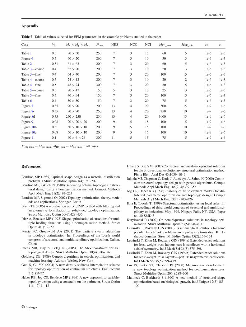
Table 7 Table of values selected for EEM parameters in the example problems studied in the paper

Case V0 Mx × My × Mz Nmax NRS NCC NCI MEE_max MEE_min εE εt

Table 1 0.5 90 × 30 250 7 3 15 60 5 1e-6 1e-3

Figure 6 0.5 60 × 20 260 7 3 10 30 3 1e-6 1e-3

Table 2 0.31 61 × 62 200 7 3 20 60 5 1e-6 1e-3

Table 3—coarse 0.4 32 × 20 200 7 3 10 20 3 1e-6 1e-3

Table 3—fine 0.4 64 × 40 200 7 3 20 100 5 1e-6 1e-3

Table 4—coarse 0.5 24 × 12 200 7 3 10 20 2 1e-6 1e-3

Table 4—fine 0.5 48 × 24 300 7 3 20 50 5 1e-6 1e-3

Table 5—coarse 0.5 20 × 47 150 5 3 10 25 3 1e-6 1e-3

Table 5—fine 0.5 40 × 94 150 7 3 20 100 5 1e-6 1e-3

Table 6 0.4 50 × 50 150 7 3 20 75 5 1e-6 1e-3

Figure 7 0.35 90 × 90 200 13 4 20 500 15 1e-9 1e-6

Figure 8c 0.35 90 × 90 250 13 4 20 250 10 1e-9 1e-6

Figure 8d 0.35 250 × 250 250 13 4 20 1000 15 1e-9 1e-6

Figure 9 0.08 20 × 20 × 20 200 9 5 15 100 5 1e-9 1e-6

Figure 10b 0.3 50 × 10 × 10 200 9 5 15 100 10 1e-9 1e-6

Figure 10c 0.08 50 × 10 × 10 200 9 5 15 100 10 1e-9 1e-6

Figure 11 0.1 40 × 6 × 26 300 11 5 15 75 5 1e-9 1e-6

MRS_max = MEE_max, MRS_min = MEE_min in all cases

Appendix

References

Bendsoe MP (1989) Optimal shape design as a material distributionproblem. J Struct Multidisc Optim 1(4):193–202

Bendsoe MP, Kikuchi N (1988) Generating optimal topologies in struc-tural design using a homogenization method. Comput MethodsAppl Mech Eng 71(2):197–224

Bendsoe MP, Sigmund O (2002) Topology optimization: theory, meth-ods and applications. Springer, Berlin

Bruns TE (2005) A reevaluation of the SIMP method with filtering andan alternative formulation for solid–void topology optimization.Struct Multidisc Optim 30(6):428–436

Diaz A, Bendsoe MP (1992) Shape optimization of structures for mul-tiple loading situations using a homogenization method. StructOptim 4(1):17–22

Fourie PC, Groenwold AA (2001) The particle swarm algorithmin topology optimization. In: Proceedings of the fourth worldcongress of structural and multidisciplinary optimization. Dalian,China

Fuchs MB, Jiny S, Peleg N (2005) The SRV constraint for 0/1topological design. Struct Multidisc Optim 30(4):320–326

Goldberg DE (1989) Genetic algorithms in search, optimization, andmachine learning. Addison-Wesley, New York

Guo X, Gu YX (2004) A new density-stiffness interpolation schemefor topology optimization of continuum structures. Eng Comput21(1):9–22

Haber RB, Jog CS, Bendsoe MP (1996) A new approach to variable-topology design using a constraint on the perimeter. Struct Optim11(1–2):11–12

Huang X, Xie YM (2007) Convergent and mesh-independent solutionsfor the bi-directional evolutionary structural optimization method.Finite Elem Anal Des 43:1039–1049

Jakiela MJ, Chapman C, Duda J, Adewuya A, Saitou K (2000) Contin-uum structural topology design with genetic algorithms. ComputMethods Appl Mech Eng 186(2–4):339–356

Jog CS, Haber RB (1996) Stability of finite element models for dis-tributed parameter optimization and topology design. ComputMethods Appl Mech Eng 130(3):203–226

Kita E, Toyoda T (1999) Structural optimization using local rules. In:Proceedings of third world congress of structural and multidisci-plinary optimization, May 1999, Niagara Falls, NY, USA. Paperno. 30-SMD-3

Kutylowski R (2002) On nonuniqueness solutions in topology opti-mization. Struct Multidisc Optim 23(5):398–403

Lewinski T, Rozvany GIN (2008) Exact analytical solutions for somepopular benchmark problems in topology optimization III: L-shaped domains. Struct Multidisc Optim 35(2):165–174

Lewinski T, Zhou M, Rozvany GIN (1994a) Extended exact solutionsfor least-weight truss layouts-part I: cantilever with a horizontalaxis of symmetry. Int J Mech Sci 36(5):375–398

Lewinski T, Zhou M, Rozvany GIN (1994b) Extended exact solutionsfor least-weight truss layouts—part II: unsymmetric cantilevers.Int J Mech Sci 36(5):399–419

Liu JS, Parks GT, Clarkson PJ (2000) Metamorphic development:a new topology optimization method for continuum structures.Struct Multidisc Optim 20(4):288–300

Mattheck C, Burkhardt S (1990) A new method of structural shapeoptimization based on biological growth. Int J Fatigue 12(3):185–190

Element exchange method for topology optimization

Mei YL, Wang XM, Cheng GD (2007) Binary discrete method oftopology optimization. Appl Math Mech 28(6):707–719

Olhoff N, Bendsoe MP, Rasmussen J (1991) On CAD integrated struc-tural topology and design optimization. Comput Methods ApplMech Eng 89:259–279

Olhoff N, Ronholt E, Scheel J (1998) Topology optimization of three-dimensional structures using optimum microstructures. StructOptim 16(1):1–18

Pomezanski V, Querin OM, Rozvany GIN (2005) CO-SIMP: extendedSIMP algorithm with direct corner contact control. StructMultidisc Optim 30:164–168

Poulsen TA (2002) A simple scheme to prevent checkerboard patternsand one-node connected hinges in topology optimization. StructMultidisc Optim 24:396–399

Querin OM, Steven GP, Xie YM (1998) Evolutionary structural opti-mization (ESO) using a bidirectional algorithm. Comput Struct15(8):1031–1048

Rouhi M, Rais-Rohani M (2008) Topology optimization of con-tinuum structures using element exchange method. In: 49thAIAA/ASME/ASCE/AHS/ASC structures, structural dynamics,and materials, 7–10 April 2008, Schaumburg, IL

Rozvany GIN (2009) A critical review of established methods in struc-tural topology optimization. Struct Multidisc Optim 37:217–237

Rozvany GIN, Zhou M, Birker T (1992) Generalized shape optimiza-tion without homogenization. Struct Optim 4:250–252

Rozvany GIN, Lewinski T, Querin OM, Logo J (2006) Quality con-trol in topology optimization using analytically derived bench-marks. In: 11th AIAA/ISSMO multidisciplinary analysis andoptimization conference, 6–8 September 2006, Portsmouth, VA

Sigmund O (2001) A 99 line topology optimization code written inMatlab. Struct Multidisc Optim 21(2):120–127

Sigmund O, Peterson J (1988) Numerical instabilities in topology opti-mization: a survey on procedures dealing with checkerboards,mesh-dependencies and local minima. Struct Optim 16(1):68–75

Svanberg K, Werme M (2005) A hierarchical neighborhood searchmethod for topology optimization. Struct Multidisc Optim29:325–340

Tanskanen P (2002) The evolutionary structural optimization method:theoretical aspects. Comput Methods Appl Mech Eng 191:5485–5498

Wang MY, Wang X (2003) Level set models for structural topologyoptimization. In: Proceedings of DETC’03, ASME 2003 designengineering technical conferences and ASME 2003 design engi-neering technical conferences and computers and information inengineering conference, 2–6 Sep. 2003, Chicago, IL

Wang SY, Tai K, Wang MY (2006) An enhanced genetic algorithmfor structural topology optimization. Int J Numer Methods Eng65(1):18–44

Werne M (2006) Globally optimal benchmark solutions to some small-scale discretized continuum topology optimization problems.Struct Multidisc Optim 32(3):259–262

Xie YM, Steven GP (1993) A simple evolutionary procedure forstructural optimization. Eng Comput 49(5):885–896

Zhou M, Rozvany GIN (1991) The COC algorithm, part II: topo-logical, geometry and generalized shape optimization. ComputMethods Appl Mech Eng 89(1–3):309–336

Zhou M, Rozvany GIN (2001) On the validity of ESO typemethods in topology optimization. Struct Multidisc Optim 21:80–83

Zhou M, Shyy YK, Thomas HL (2001) Checkerboard and minimummember size control in topology optimization. Struct MultidiscOptim 21:152–158