ELEG5481 SIGNAL PROCESSING OPTIMIZATION TECHNIQUES

ELEG5481 Signal Processing Optimization Techniques 0. Introduction

ELEG5481

SIGNAL PROCESSING OPTIMIZATION

TECHNIQUES

0. INTRODUCTION

Wing-Kin Ma, Dept. Electronic Eng., The Chinese University of Hong Kong 1


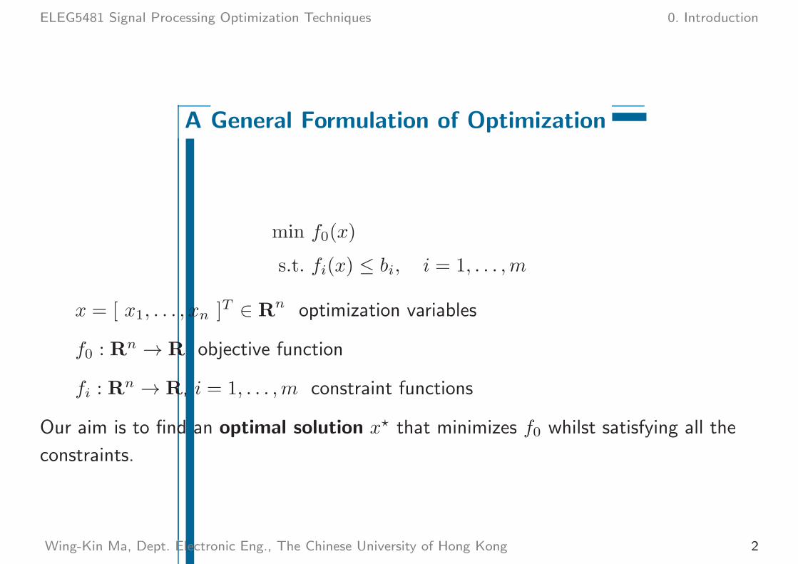
A General Formulation of Optimization

min f0(x)

s.t. fi(x) ≤ bi, i = 1, . . . ,m

x = [ x1, . . . , xn ]T ∈ Rn optimization variables

f0 : Rn → R objective function

fi : Rn → R, i = 1, . . . ,m constraint functions

Our aim is to find an optimal solution x⋆ that minimizes f0 whilst satisfying all the

constraints.



Why does optimization concern me?

• Optimization has found applications in a wide variety of areas such as finance,

statistics, and engineering, to name a few.

• In engineering, it plays a key role in solving or handling numerous (and sometimes

very hard) problems in control, circuit design, networks, signal processing, and

communications.

• It is an important enough topic that we should know at least a bit about it.



Example: Diet Problem

• xi is the quantity of food i.

• Each unit of food i has a cost of ci.

• One unit of food j contains an amount aij of nutrient i.

• We want nutrient i to be at least equal to bi.

• Problem: find the cheapest diet such that the minimum nutrient requirements are

fulfilled.

This problem can be formulated as:

minn∑

i=1

cixi

s.t.n∑

j=1

aijxj ≥ bi, i = 1, 2, . . . ,m

xi ≥ 0, i = 1, 2, . . . , n

This is a linear program.Wing-Kin Ma, Dept. Electronic Eng., The Chinese University of Hong Kong 4


Example: Chebychev Center

• Let a norm ball B(xc, r) = x | ‖xc − x‖2 ≤ r , & a polyhedron

P = x | aTi x ≤ bi, i = 1, . . . ,m .

• Problem: Find the largest ball inside a polyhedron P ; i.e., maxxc,r r, subject to

B(xc, r) ⊆ P .

xcr



Example: Optimal Power Assignment in Wireless Communications

• Consider a wireless comm. system with K transmitters & K receivers.

Transmitter 1

Receiver 1

Transmitter 2

Receiver 2

Transmitter 3

Receiver 3

• Receiver i is intended to receive information only from Transmitter i, & it sees the

other transmitters as interferers.



• The signal-to-interference-and-noise ratio (SINR) at receiver i

γi =Giipi

∑

j 6=iGijpj + σ2i

where

pi is the transmitter i power,

Gij is the path gain from transmitter j to receiver i,

σ2i is the noise power at receiver i.

• Problem: Maximize the weakest SINR subject to power constraints

0 ≤ pi ≤ pmax,i, where pmax,i is the max. allowable power of transmitter i.

maxpi∈[0,pmax,i]i=1,...,K

mini=1,...,K

Giipi∑

j 6=iGijpj + σ2i



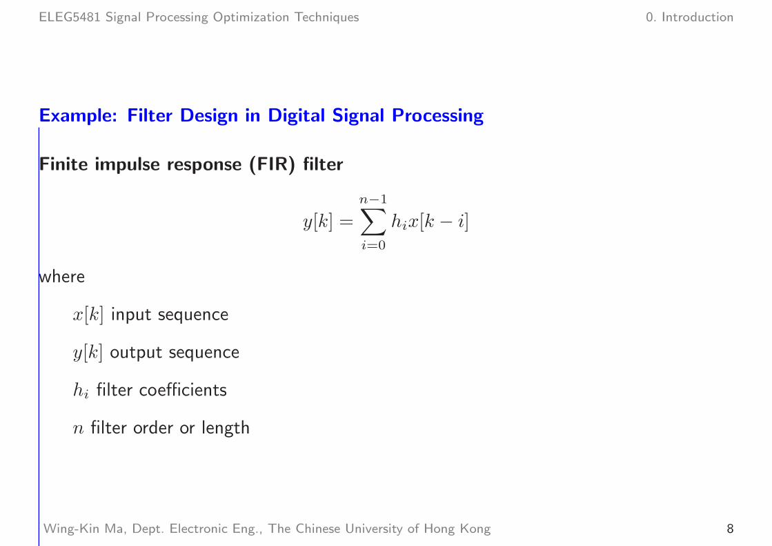
Example: Filter Design in Digital Signal Processing

Finite impulse response (FIR) filter

y[k] =n−1∑

i=0

hix[k − i]

where

x[k] input sequence

y[k] output sequence

hi filter coefficients

n filter order or length



Frequency response:

H(ω) =

n−1∑

i=0

hie−jωi

Problem: find h = [ h0, . . . , hn−1 ]T so that h and/or H satisfy/optimize certain given

specifications.

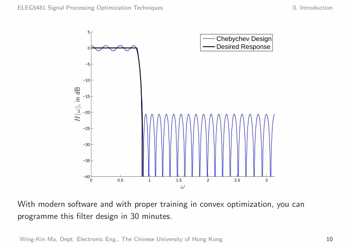
For example, the Chebychev design solves for

minh∈Rn

maxω∈[0,π]

∣∣H(ω)−Hdes(ω)

∣∣

given a desired freq. response Hdes(ω). This design minimizes the worst-case absolute

error between the desired and actual freq. responses.



0 0.5 1 1.5 2 2.5 3−40

−35

−30

−25

−20

−15

−10

−5

0

5

Chebychev DesignDesired Response

ω

H(ω),in

dB

With modern software and with proper training in convex optimization, you can

programme this filter design in 30 minutes.



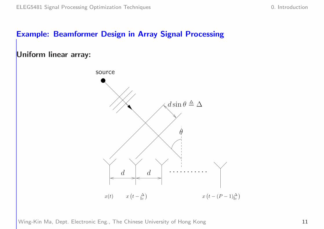
Example: Beamformer Design in Array Signal Processing

Uniform linear array:

source

θ

d sin θ , ∆

dd

x(t) x(t− ∆

c

)x(t− (P − 1)∆c

)



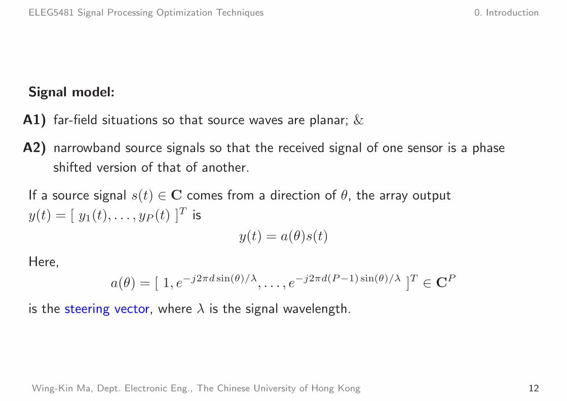
Signal model:

A1) far-field situations so that source waves are planar; &

A2) narrowband source signals so that the received signal of one sensor is a phase

shifted version of that of another.

If a source signal s(t) ∈ C comes from a direction of θ, the array output

y(t) = [ y1(t), . . . , yP (t) ]T is

y(t) = a(θ)s(t)

Here,

a(θ) = [ 1, e−j2πd sin(θ)/λ, . . . , e−j2πd(P−1) sin(θ)/λ ]T ∈ CP

is the steering vector, where λ is the signal wavelength.



Beamforming:

s(t) = wHy(t)

where w ∈ CP is a beamformer weight vector.

• Let θdes ∈ [−π2 ,

π2 ] be the desired direction.

• A simple beamformer is w = a(θdes), but it does not provide good sidelobe

suppression.

• Problem: find a w which minimizes sidelobe energy subject to a pass response to

θdes.



−80 −60 −40 −20 0 20 40 60 80−80

−70

−60

−50

−40

−30

−20

−10

0

10

Angle (Degree)

Mag

nitu

de (

dB)

Direction pattern of the conventional beamformer. θdes = 10; P = 20.



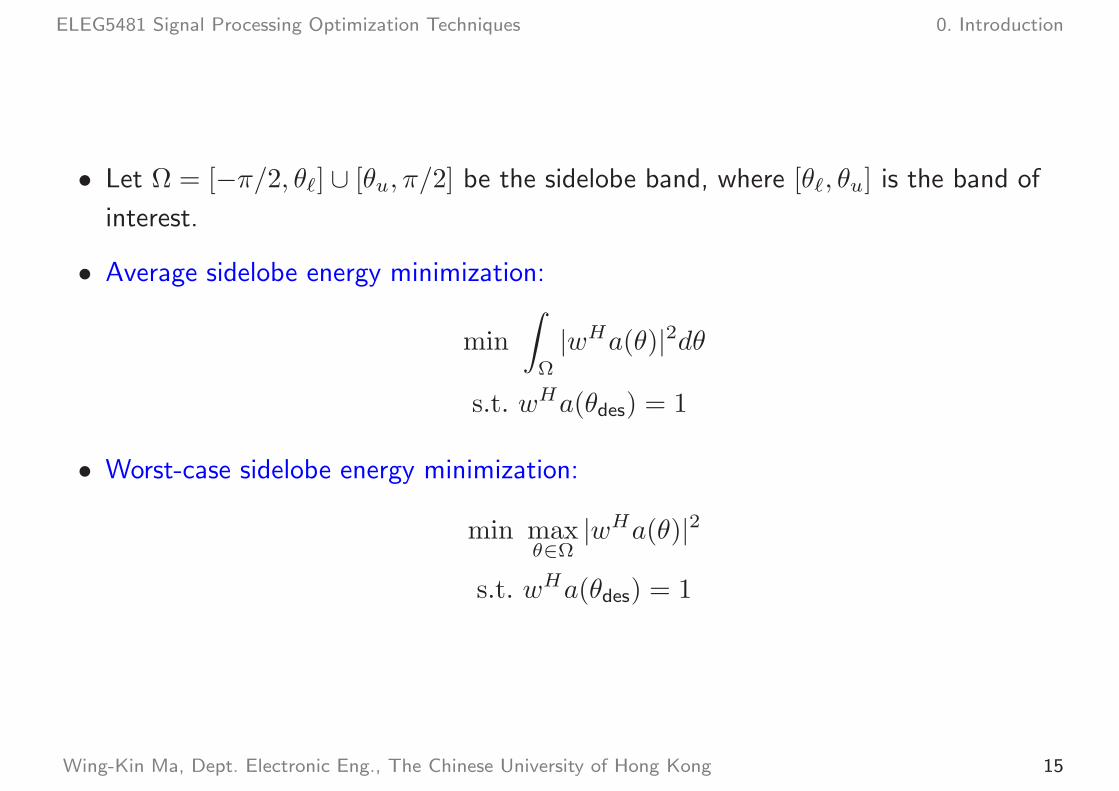
• Let Ω = [−π/2, θℓ] ∪ [θu, π/2] be the sidelobe band, where [θℓ, θu] is the band of

interest.

• Average sidelobe energy minimization:

min

∫

Ω

|wHa(θ)|2dθ

s.t. wHa(θdes) = 1

• Worst-case sidelobe energy minimization:

min maxθ∈Ω

|wHa(θ)|2

s.t. wHa(θdes) = 1



−80 −60 −40 −20 0 20 40 60 80−80

−70

−60

−50

−40

−30

−20

−10

0

10

Angle (Degree)

Mag

nitu

de (

dB)

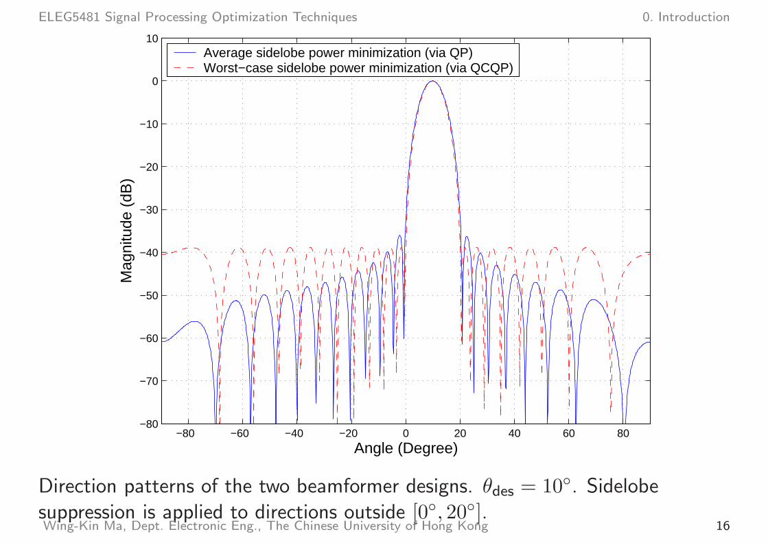
Average sidelobe power minimization (via QP)Worst−case sidelobe power minimization (via QCQP)

Direction patterns of the two beamformer designs. θdes = 10. Sidelobe

suppression is applied to directions outside [0, 20].Wing-Kin Ma, Dept. Electronic Eng., The Chinese University of Hong Kong 16


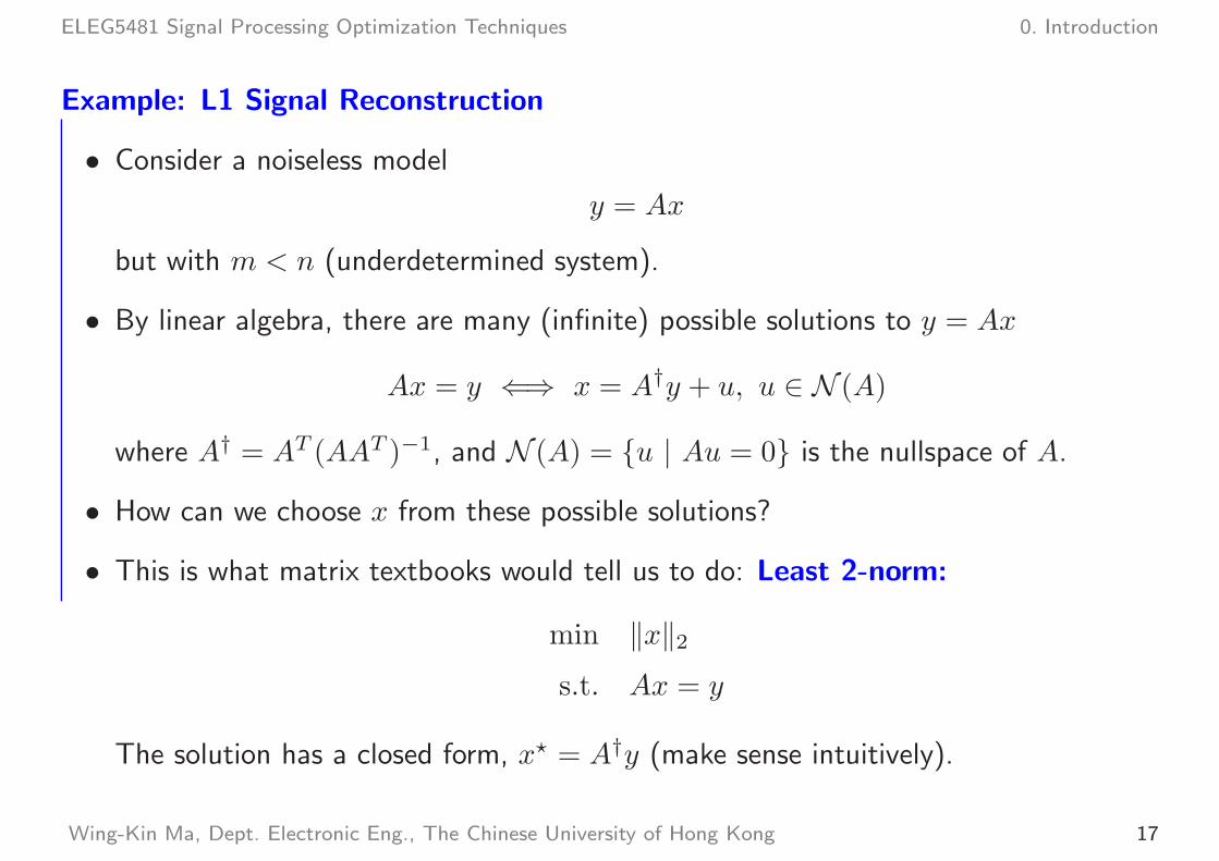
Example: L1 Signal Reconstruction

• Consider a noiseless model

y = Ax

but with m < n (underdetermined system).

• By linear algebra, there are many (infinite) possible solutions to y = Ax

Ax = y ⇐⇒ x = A†y + u, u ∈ N (A)

where A† = AT (AAT )−1, and N (A) = u | Au = 0 is the nullspace of A.

• How can we choose x from these possible solutions?

• This is what matrix textbooks would tell us to do: Least 2-norm:

min ‖x‖2

s.t. Ax = y

The solution has a closed form, x⋆ = A†y (make sense intuitively).



• Least 0-norm reconstruction:

min ‖x‖0

s.t. Ax = y

where ‖x‖0 counts the number of nonzero elements in x.

• Make sense for sparse signals; i.e., signals with many zeros.

• Can prove that if the no. of zeros in the actual x is sufficiently large compared to

the no. of measurements m, then 0-norm minimization leads to the ground truth.

• ‖ · ‖0 is not convex. In fact, 0-norm minimization poses a very hard problem.



• Least 1-norm reconstruction:

min ‖x‖1

s.t. Ax = y

• the ‘best’ convex approximation to 0-norm.

• can prove that under some assumptions, 1-norm minimization is able to approach

0-norm minimization (in some probabilistic sense).

• Currently a very hot topic (in the literature it is called compressive sensing)

• 1-norm minimization is an LP

min∑n

i=1 ti

s.t. Ax = y

−ti ≤ xi ≤ ti, i = 1, . . . , n



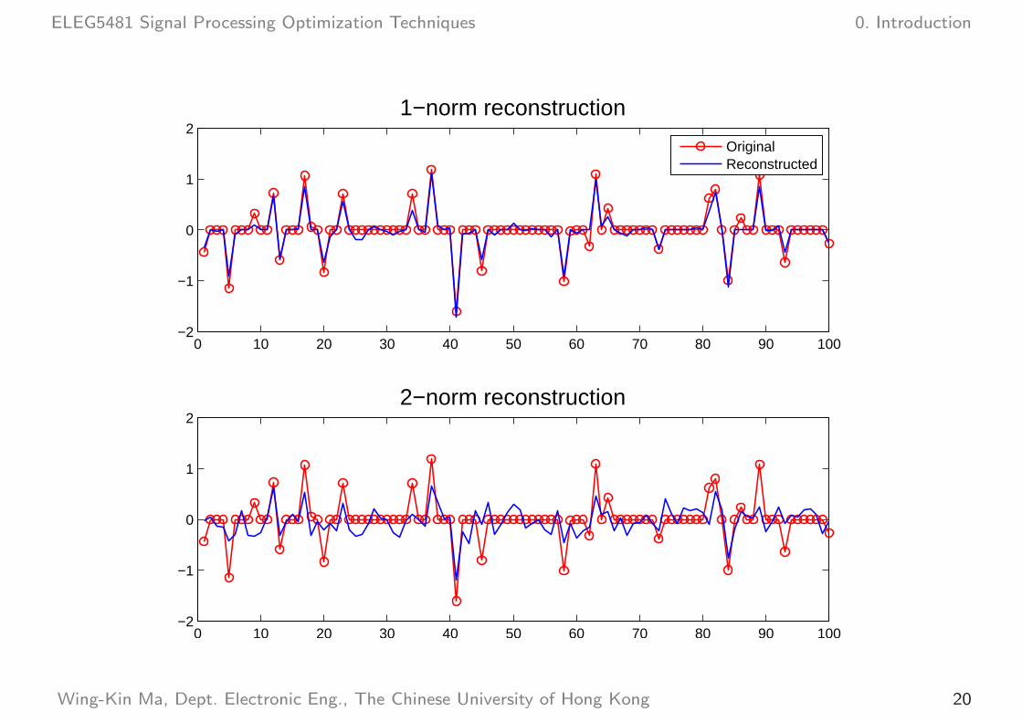
0 10 20 30 40 50 60 70 80 90 100−2

−1

0

1

21−norm reconstruction

OriginalReconstructed

0 10 20 30 40 50 60 70 80 90 100−2

−1

0

1

22−norm reconstruction



Solving optimization problems

• Given a general opt. problem, obtaining its optimal solution can be very hard.

• In the study of nonlinear programming (or nonlinear opt.), various numerical

algorithms have been developed to try to find the optimal solution. Some well

known examples are the gradient descent method, and the Newton method.

• These opt. algs. require an initial guess of the solution. Also, they may only

guarantee convergence to a locally optimal solution.



• There are also a variety of approaches for nonlinear opt., such as the heuristics

based approach (e.g., genetic algs., ant colony opt.), and the Monte-Carlo based

approach (e.g., simulated annealing). Again, convergence to a globally optimal

solution is not guaranteed.

• When an opt. problem is combinatorial (or discrete), the problem is generally much

harder to solve; study complexity theory for the details.

• There are certain problem classes that can be solved effectively, though.



There are problems for which the solutions can be analytically found:

Example: Least Squares (LS)

min ‖Ax− b‖22

• LS has a closed form solution x⋆ = (ATA)−1AT b.



Example: Entropy Maximization

• Let y be a r.v. drawn from y1, . . . , yn.

• Let pi = prob(y = yi).

• Problem: find a distribution pi such that the entropy of y is maximized.

max∑n

i=1 pi log(1/pi)

s.t. pi ≥ 0, i = 1, . . . , n∑n

i=1 pi = 1

• The solution is well known to be pi = 1/n for all i.



• Opt. problems that can be analytically solved are considered very special cases.

• Another problem class that can be effectively handled is that of the convex

optimization problems.

Example: Linear Programming (LP)

min cTx

s.t. aTi x ≤ bi, i = 1, . . . ,m

• no analytical formula for the solution

• efficient & reliable algorithms for finding the optimal solution exist.



Convex Optimization Problems

min f0(x)

s.t. fi(x) ≤ bi, i = 1, . . . ,m

in which the objective & constraint functions are convex:

fi(αx+ (1− α)y) ≤ αfi(x) + (1− α)fi(y)

for any x, y, and for any α ∈ [0, 1].



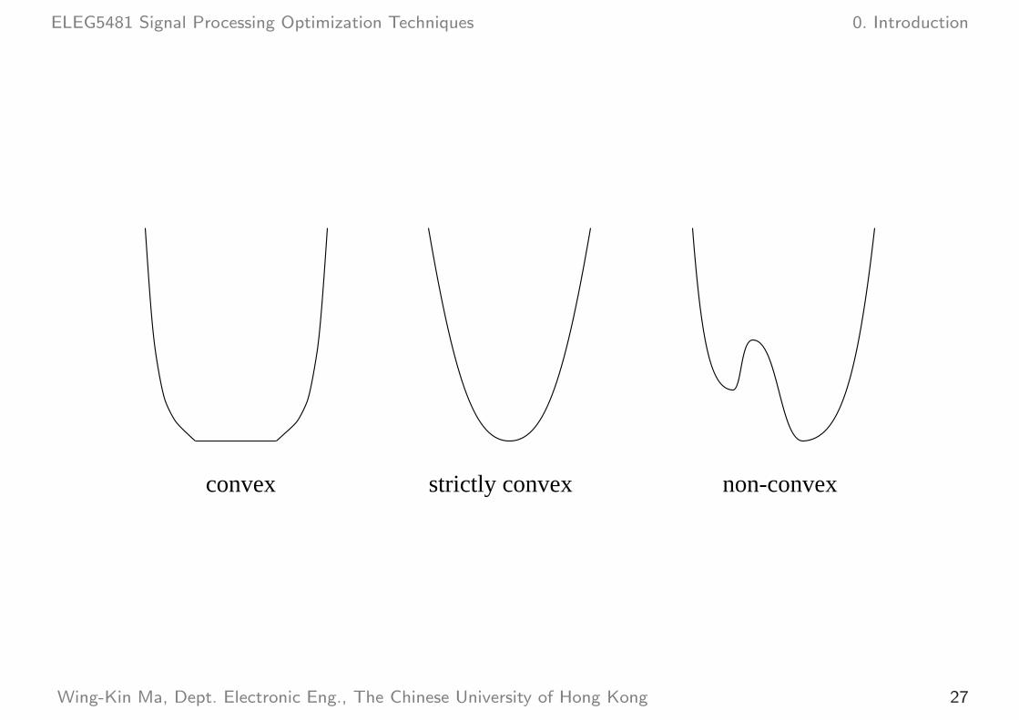
strictly convex non-convexconvex



Conic Problems

Conic optimization is a representative class of convex optimization problems.

min cTx

s.t. Ax = b,

x ∈ K

where K is a convex cone.

The well-known linear program is conic, where K = x ∈ Rn | xi ≥ 0, i = 1, . . . , n .



Second order cone program: K = x ∈ Rn+1 |√∑n

i=1 x2i ≤ xn+1 is the second

order cone.

Semidefinite program: K = X ∈ Rn×n | X is positive semidefinite (PSD) is the

set of PSD matrices.

−1

−0.5

0

0.5

1

−1

−0.5

0

0.5

10

0.2

0.4

0.6

0.8

1

x1

x2

x 3

(a) Second-order cone

0

0.5

1

−1

−0.5

0

0.5

10

0.2

0.4

0.6

0.8

1

x1

x2

x 3

(b) PSD cone



Merits of convex optimization

• Reliable and efficient algorithms exist for many convex opt. problems, especially

those under the conic opt. problem class.

• (Surprisingly) many problems can be converted to convex opt.

Role of convex optimization in nonconvex problems

• We can use convex opt. to approximate a nonconvex problem.

(Having a hard problem does not mean you should give up).

• We can use convex opt. to build a nonconvex opt. algorithm (subopt. per se).

– SQP, a general-purpose nonlinear opt. solver in MATLAB, may be seen as an

algorithm that uses convex opt. to sequentially process an opt. problem.



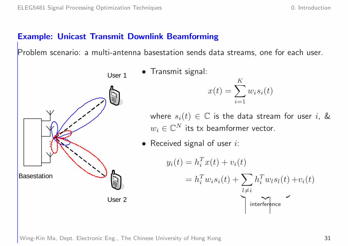
Example: Unicast Transmit Downlink Beamforming

Problem scenario: a multi-antenna basestation sends data streams, one for each user.

⋮

Basestation

User 1

User 2

• Transmit signal:

x(t) =

K∑

i=1

wisi(t)

where si(t) ∈ C is the data stream for user i, &

wi ∈ CN its tx beamformer vector.

• Received signal of user i:

yi(t) = hTi x(t) + vi(t)

= hTi wisi(t) +

∑

l 6=i

hTi wlsl(t)

︸︷︷︸

interference

+vi(t)



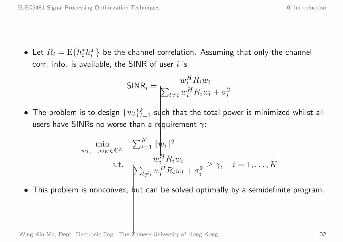
• Let Ri = Eh∗i h

Ti be the channel correlation. Assuming that only the channel

corr. info. is available, the SINR of user i is

SINRi =wH

i Riwi∑

l 6=iwHl Riwl + σ2

i

• The problem is to design wiki=1 such that the total power is minimized whilst all

users have SINRs no worse than a requirement γ:

minw1,...,wK∈CN

∑Ki=1 ‖wi‖

2

s.t.wH

i Riwi∑

l 6=iwHl Riwl + σ2

i

≥ γ, i = 1, . . . , K

• This problem is nonconvex, but can be solved optimally by a semidefinite program.



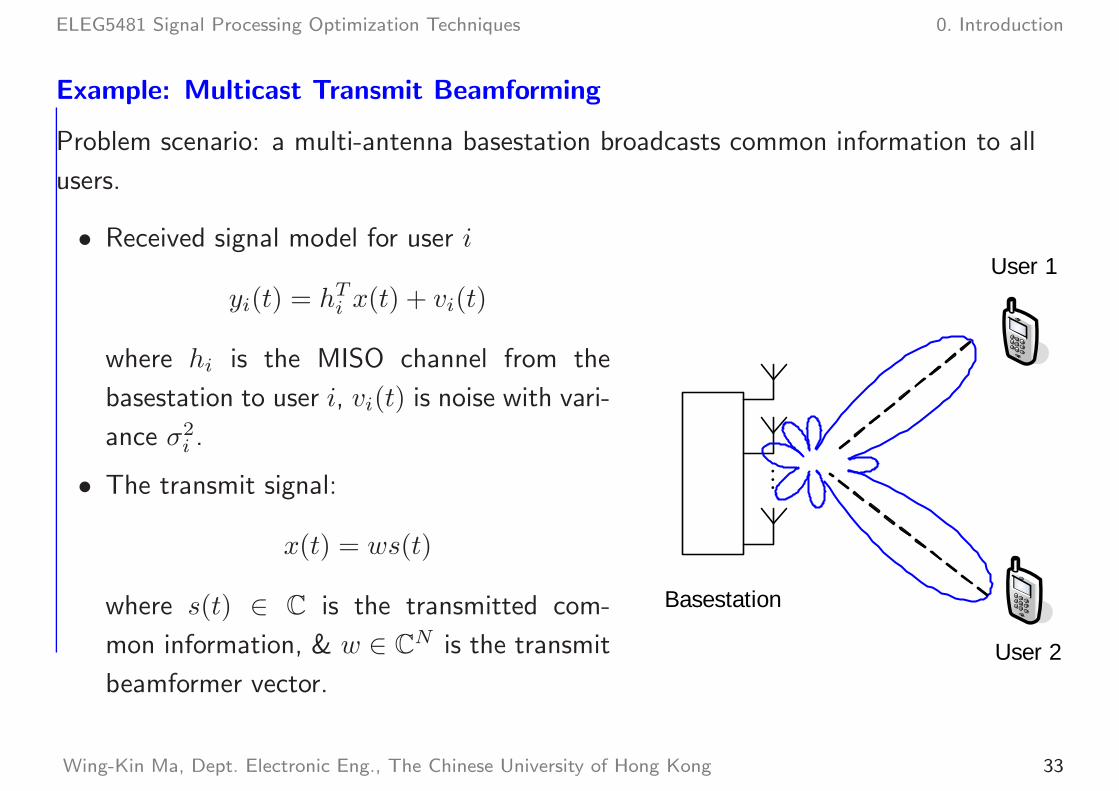
Example: Multicast Transmit Beamforming

Problem scenario: a multi-antenna basestation broadcasts common information to all

users.

• Received signal model for user i

yi(t) = hTi x(t) + vi(t)

where hi is the MISO channel from the

basestation to user i, vi(t) is noise with vari-

ance σ2i .

• The transmit signal:

x(t) = ws(t)

where s(t) ∈ C is the transmitted com-

mon information, & w ∈ CN is the transmit

beamformer vector.

⋮

Basestation

User 1

User 2



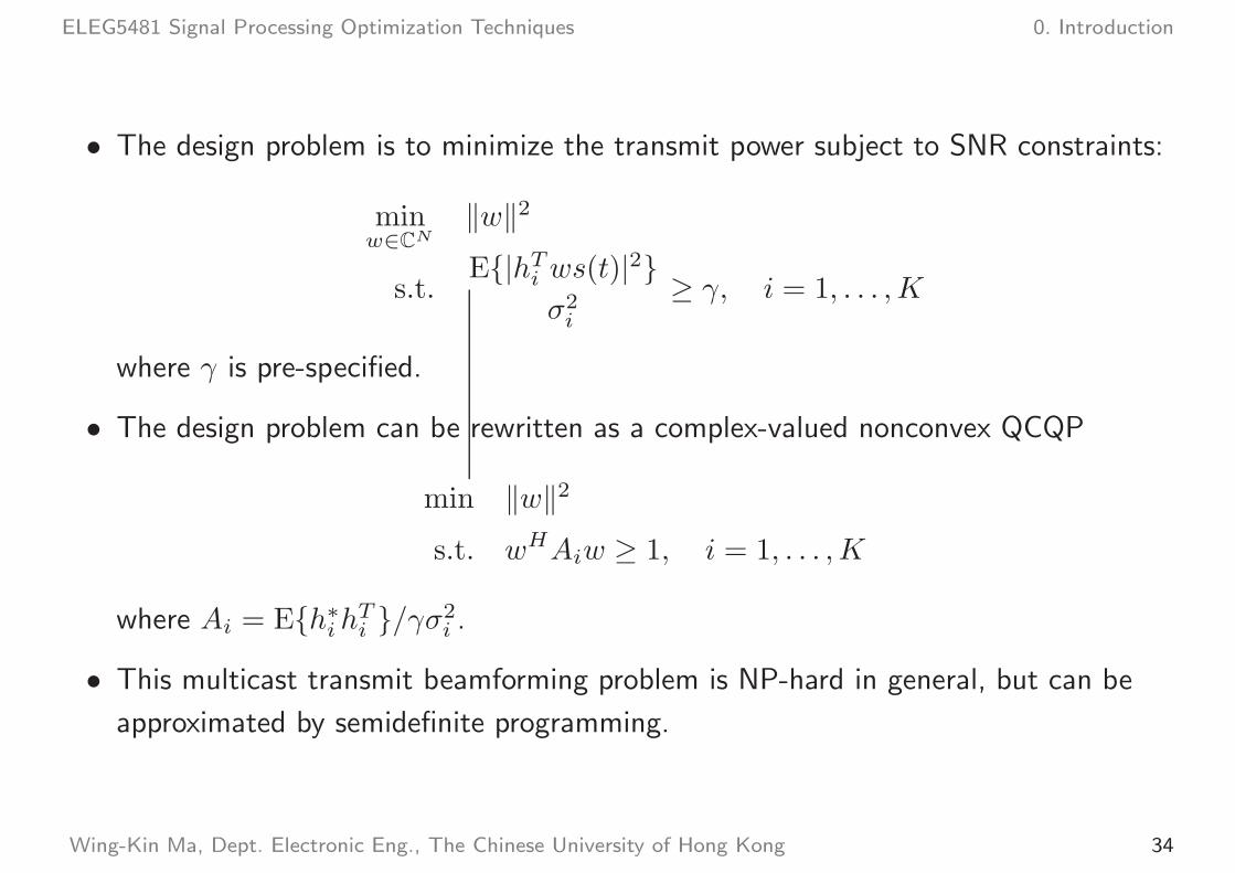
• The design problem is to minimize the transmit power subject to SNR constraints:

minw∈CN

‖w‖2

s.t.E|hT

i ws(t)|2

σ2i

≥ γ, i = 1, . . . , K

where γ is pre-specified.

• The design problem can be rewritten as a complex-valued nonconvex QCQP

min ‖w‖2

s.t. wHAiw ≥ 1, i = 1, . . . , K

where Ai = Eh∗i h

Ti /γσ

2i .

• This multicast transmit beamforming problem is NP-hard in general, but can be

approximated by semidefinite programming.



Example: MAXCUT

• Input: A graph G = (V,E) with weights wij for (i, j) ∈ E. Assume wij ≥ 0 and

wij = 0 if (i, j) /∈ E.

• Goal: Divide nodes into two parts so as to maximize the weight of the edges whose

nodes are in different parts.

w13

w14

w25

1

2

3

4

5



Let V = 1, 2, . . . , n without loss of generality. The MAXCUT problem takes the form

maxn∑

i=1

n∑

j=i+1

wij1− xixj

2

s.t. xi ∈ −1,+1, i = 1, . . . , n

Some remarks:

• MAXCUT is a combinatorial opt. problem.

• To find the optimal solution of MAXCUT is very hard.



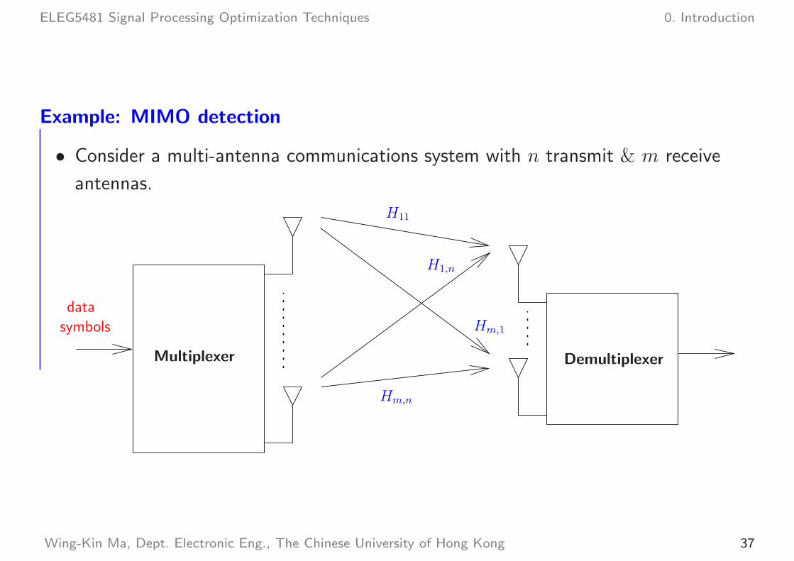
Example: MIMO detection

• Consider a multi-antenna communications system with n transmit & m receive

antennas.

data

symbols

Multiplexer Demultiplexer

H11

Hm,n

H1,n

Hm,1



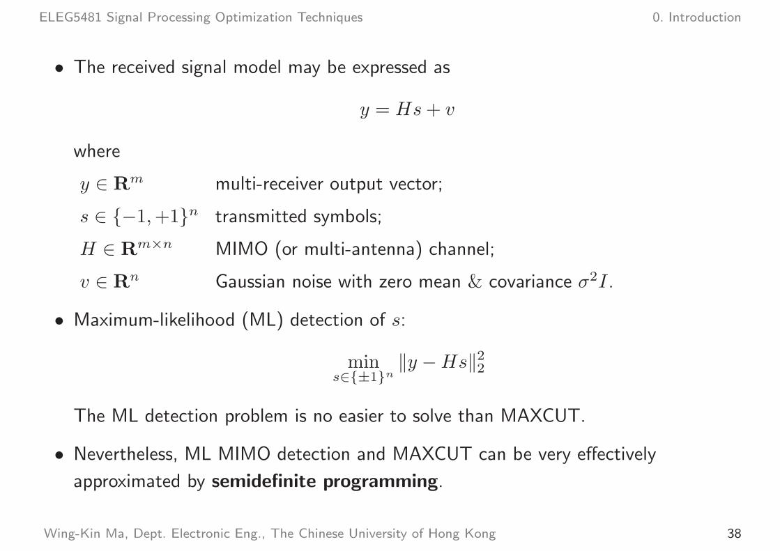
• The received signal model may be expressed as

y = Hs+ v

where

y ∈ Rm multi-receiver output vector;

s ∈ −1,+1n transmitted symbols;

H ∈ Rm×n MIMO (or multi-antenna) channel;

v ∈ Rn Gaussian noise with zero mean & covariance σ2I .

• Maximum-likelihood (ML) detection of s:

mins∈±1n

‖y −Hs‖22

The ML detection problem is no easier to solve than MAXCUT.

• Nevertheless, ML MIMO detection and MAXCUT can be very effectively

approximated by semidefinite programming.



Example: Sensor Network Localization

• Consider a sensor network where each node can communicate with the other nodes.

• Depending on applications, a sensor node may have no information on its position.

Anchors

Sensors



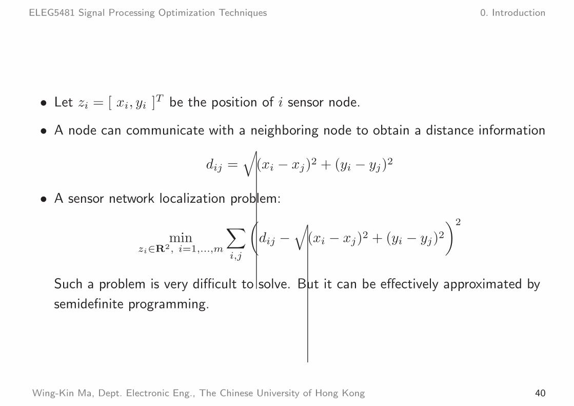
• Let zi = [ xi, yi ]T be the position of i sensor node.

• A node can communicate with a neighboring node to obtain a distance information

dij =√

(xi − xj)2 + (yi − yj)2

• A sensor network localization problem:

minzi∈R2, i=1,...,m

∑

i,j

(

dij −√

(xi − xj)2 + (yi − yj)2)2

Such a problem is very difficult to solve. But it can be effectively approximated by

semidefinite programming.



−0.5 −0.4 −0.3 −0.2 −0.1 0 0.1 0.2 0.3 0.4 0.5−0.5

−0.4

−0.3

−0.2

−0.1

0

0.1

0.2

0.3

0.4

0.5

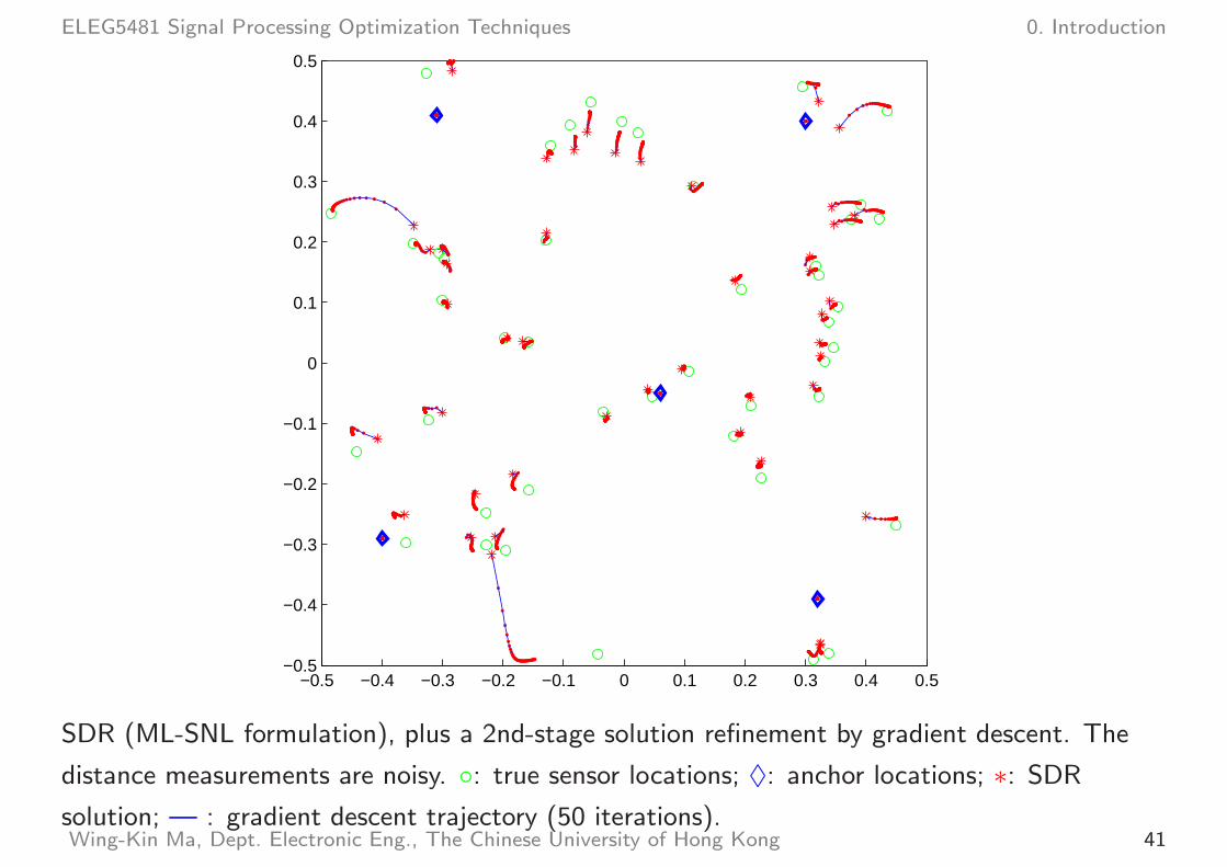
SDR (ML-SNL formulation), plus a 2nd-stage solution refinement by gradient descent. The

distance measurements are noisy. : true sensor locations; ♦: anchor locations; ∗: SDR

solution; — : gradient descent trajectory (50 iterations).Wing-Kin Ma, Dept. Electronic Eng., The Chinese University of Hong Kong 41


−0.5 −0.4 −0.3 −0.2 −0.1 0 0.1 0.2 0.3 0.4 0.5−0.5

−0.4

−0.3

−0.2

−0.1

0

0.1

0.2

0.3

0.4

0.5

Gradient descent ML-SNL with a random starting point. : true sensor locations; ♦: anchor

locations; — : gradient descent trajectory (50 iterations).Wing-Kin Ma, Dept. Electronic Eng., The Chinese University of Hong Kong 42


Course Outline

• Theory:

– linear algebra and matrix analysis

– convex sets and convex functions

– convex optimization, duality

– conic opt.: linear program, second-order cone program, semidefinite program

• Methods:

– interior-point methods (a brief overview)

– subgradient methods, first-order optimization

– nonconvex problems: optimization strategies based on convex or tractable opt.



• Applications:

– signal and image processing: optimization of digital filters, optimization of

beamforming in sensor array processing, sparse optimization and compressive

sensing

– signal estimation: signal recovery or regression via ℓp norm optimization

– pattern classification: support vector machine, large-margin nearest-neighbor

classification

– wireless communications: power allocation in wireless networks, MIMO transmit

optimization, mobile positioning and sensor network localization

– information theory: capacity optimization in Gaussian frequency-selective and

MIMO channels

– circuit: geometric program and circuit optimization

– distributed optimization, with applications to image processing and wireless

networks



Assessment Method

• Assignments, 20%.

• A written exam., 30%, in midterm. To make sure that you understand the basics.

• Project, 50%. Let you have hands-on experience with using opt. to solve signal

processing or engineering problems. Problems will be provided. You can also

propose problems related to your own research (subject to my approval).



Course Information

• Venue and Time: Every Wed, 19:00-22:00, ERB405

• Course website: http://dsp.ee.cuhk.edu.hk/eleg5481/

• My email: [email protected]



References

Textbook

S. Boyd & L. Vandenberghe, Convex Optimization, Cambridge Univ. Press, 2004.

Available online: http://www.stanford.edu/~boyd/cvxbook/

Other references

• D. P. Bertsekas, et. al, Convex Analysis and Optimization, Athenta Scientific, 2002.

• R. Fletcher, Practical Methods of Opt., John Wiley & Sons, 1987.

• http://www.stanford.edu/class/ee364/


ELEG5481 SIGNAL PROCESSING OPTIMIZATION TECHNIQUES

Documents

Transcript of ELEG5481 SIGNAL PROCESSING OPTIMIZATION TECHNIQUES