ELECTROSTATIC-PROBE MEASUREMENTS OF PLASMA PARAMETERS … · ELECTROSTATIC-PROBE MEASUREMENTS OF...
132
lr" NASA TECHNICAL NOTE ; Z ! J LOAN COPY RE1g= AFWL ( D O ~ P ~ - KIRTLAND AFE - 7 - r: P n * ;0 n rn 2 L ELECTROSTATIC-PROBE MEASUREMENTS OF PLASMA PARAMETERS FOR TWO REENTRY FLIGHT EXPERIMENTS AT 25 000 FEET PER SECOND Humj~ton, Vu. 23365 . ~ .- . NATIONAL AERONAUTICS AND SPACE ADMINISTRATION . WASHINGTON, D. c. . FEBRUAR.Y 1972 https://ntrs.nasa.gov/search.jsp?R=19720011555 2020-02-19T11:59:33+00:00Z
Transcript of ELECTROSTATIC-PROBE MEASUREMENTS OF PLASMA PARAMETERS … · ELECTROSTATIC-PROBE MEASUREMENTS OF...

l r "
N A S A TECHNICAL NOTE
;Z!J LOAN COPY RE1g=
AFWL ( D O ~ P ~ - KIRTLAND AFE -
7 -
r: P n * ;0 n rn 2 L
ELECTROSTATIC-PROBE MEASUREMENTS OF PLASMA PARAMETERS FOR TWO REENTRY FLIGHT EXPERIMENTS AT 25 000 FEET PER SECOND
Humj~ton, Vu. 23365
. ~ .- .
NATIONAL AERONAUTICS AND SPACE ADMINISTRATION . WASHINGTON, D. c. . FEBRUAR.Y 1972
https://ntrs.nasa.gov/search.jsp?R=19720011555 2020-02-19T11:59:33+00:00Z

TECH LIBRARY KAFB, NM
IlllIIl~~lIIIIu~llllllmUllHll 0133LbL
~~ ~
1. Report No. 3. Recipient's C a t a l o g No. 2. Government Accession No. . NASA TN D-6617
4. Title and Subtitle 5. Report Date ELECTROSTATIC-PROBE MEASUREMENTS O F PLASMA February 1972 PARAMETERS FOR TWO REENTRY FLIGHT EXPERIMENTS AT 25 000 FEET PER SECOND
6. Performing Organization Code
7. Author(s) 0. Performing Organization Report No.
W. Linwood Jones, Jr., and Aubrey E. Cross L-7984 10. Work Unit No.
9. Performing Organization Name and Address 115-21-01-01 NASA Langley Research Center Hampton, Va. 23365
11. Contract or Grant No.
13. Type of Report and Period Covered 12. Sponsoring Agency Name and Address Technical Note
National Aeronautics and Space Administration Washington, D.C. 20546
14. Sponsoring Agency Code
15. Supplementary Notes With appendix B by Lorraine F. Satchel1 and appendix C by William L. Weaver. Par t of the information presented herein was included in a dissertation, "Probe Mea-
surements of Electron Density Profiles During a Blunt-Body Reentry" by W. Linwood Jones, Jr., presented in partial fulfillment of the requirements for the degree of Doctor of Philosophy in Electrical Engineering, Virginia Polytechnic Institute and State University, Blacksburg, Virginia, June 1971.
16. Abstract Unique plasma diagnostic measurements at high altitudes from two geometrically simi-
lar blunt-body reentry spacecraft using electrostatic probe rakes are presented. The probes measured the positive-ion density profiles (shape and ma nitude) during the two flights. The
face in the aft flow field of the spacecraft over the altitude range of 85.3 to 53.3 km (280 000 probe measurements were made at eight discrete points 81 cm to 7 cm) from the vehicle sur-
to 175 000 ft) with measured densities of 108 to 1012 electrons/cm3, respectively. Maximum reentry velocity for each spacecraft was approximately 7620 meters/second (25 000 ft/sec).
In the first flight experiment, water was periodically injected into a flow field which was contaminated by ablation products from the spacecraft nose region. The nonablative nose of the second spacecraft thereby minimized flow-field contamination.
Comparisons of the probe-measured density profiles with theoretical calculations are presented with discussion as to the probable cause of significant disagreement. Also dis- cussed are the correlation of probe measurements with vehicle angle-of-attack motions and the good high-altitude agreement between electron densities inferred from the probe measure- ments, VHF antenna measurements, and microwave reflectometer diagnostic measurements.
~____
17. Key words (Suggested by Author(s) ) Reentry communications; plasma diagnostics; electrostatic (Langmuir) probes; blackout alleviation; microwave reflectometer; body I motions; electron concentration
18. Distribution Statement
Unclassified - Unlimited
~
19. Security Classif. (of this report) 22. Price' 21. NO. of Pages 20. Security Classif. (of this p a g e 1 Unclassified $3.00 129 Unclassified
For sale by the National Technical Information Service, Springfield, Virginia 22151


CONTENTS
Page SUMMARY . . . . . . . . . . . . . . . . . . . . . . . . . . . . . . . . . . . . . . . 1
INTRODUCTION . . . . . . . . . . . . . . . . . . . . . . . . . . . . . . . . . . . . 1
SYMBOLS . . . . . . . . . . . . . . . . . . . . . . . . . . . . . . . . . . . . . . . 2
EXPEFUMENT DESCRIPTION . . . . . . . . . . . . . . . . . . . . . . . . . . . . . 6 Flight Objectives . . . . . . . . . . . . . . . . . . . . . . . . . . . . . . . . . . 6 Launch Vehicles . . . . . . . . . . . . . . . . . . . . . . . . . . . . . . . . . . . 6 Payloads . . . . . . . . . . . . . . . . . . . . . . . . . . . . . . . . . . . . . . . 7 Electrostatic Probe System . . . . . . . . . . . . . . . . . . . . . . . . . . . . . 8 RAM C-I Water-Injection System . . . . . . . . . . . . . . . . . . . . . . . . . . 12 RAM C-11 Microwave Reflectometer System . . . . . . . . . . . . . . . . . . . . 12 VHF System . . . . . . . . . . . . . . . . . . . . . . . . . . . . . . . . . . . . . 13
ELECTROSTATIC PROBE THEORY . . . . . . . . . . . . . . . . . . . . . . . . . 13
FLIGHT DATA RESULTS AND DISCUSSION . . . . . . . . . . . . . . . . . . . . . 14 Measured Electrostatic Probe Ion Currents . . . . . . . . . . . . . . . . . . . . 14 Thermocouple Probe Results . . . . . . . . . . . . . . . . . . . . . . . . . . . . 15 Electron Densities Inferred by Electrostatic Probe . . . . . . . . . . . . . . . . 15 Effects of Ablation Impurities on Electron Density . . . . . . . . . . . . . . . . 16 Effects of Vehicle Angle-of-Attack Perturbations on Electron Density . . . . . . 16 Effects of Water Injection on Electron Density . . . . . . . . . . . . . . . . . . . 17 Microwave Reflectometer Measurements . . . . . . . . . . . . . . . . . . . . . 18 VHF Antenna Measurements . . . . . . . . . . . . . . . . . . . . . . . . . . . . 18 Comparison of Inferred Electron Densities for the RAM-C Flights . . . . . . . . 19 Comparison of Theoretical and Experimental Electron Density Profiles . . . . . 19
CONCLUSIONS . . . . . . . . . . . . . . . . . . . . . . . . . . . . . . . . . . . . . 21
APPENDIX A - ELECTROSTATIC PROBE THEORY . . . . . . . . . . . . . . . . 22 Flowing Plasmas . . . . . . . . . . . . . . . . . . . . . . . . . . . . . . . . . . 22 Directed Flow Parallel to Probe . . . . . . . . . . . . . . . . . . . . . . . . . . 23 Directed Flow Normal to Probe . . . . . . . . . . . . . . . . . . . . . . . . . . 26 Interpretation of RAM-C Fixed-Bias Electrostatic Probe Data . . . . . . . . . . 29 Sample Calculation . . . . . . . . . . . . . . . . . . . . . . . . . . . . . . . . . 29
APPENDIX B - ELECTROSTATIC-PROBE AUTOMATIC DATA REDUCTION PROCEDURE AND LISTINGS . . . . . . . . . . . . . . . . . . . . . . . . . . . . 31
.
iii
..
Page APPENDIX C . ANALYSIS OF SPACECRAFT MOTIONS AND WIND ANGLES . . . 56
Determination of Wind Angles . . . . . . . . . . . . . . . . . . . . . . . . . . . 56 Summary of Wind-Angle Analysis . . . . . . . . . . . . . . . . . . . . . . . . . 58
REFERENCES . . . . . . . . . . . . . . . . . . . . . . . . . . . . . . . . . . . . . 59
TABLES . . . . . . . . . . . . . . . . . . . . . . . . . . . . . . . . . . . . . . . . 62
FIGURES . . . . . . . . . . . . . . . . . . . . . . . . . . . . . . . . . . . . . . . 67
iv

ELECTROSTATIC-PROBE MEASUREMENTS OF PLASMA PARAMETERS
FOR TWO REENTRY FLIGHT EXPERIMENTS AT
25 ooo FEET PER SECOND*
By W. Linwood Jones, Jr., and Aubrey E. Cross Langley Research Center
SUMMARY
Unique plasma diagnostic measurements at high altitudes from two geometrically similar blunt-body reentry spacecraft using electrostatic probe rakes are presented. The probes measured the positive-ion density profiles (shape and magnitude) during the two flights. The probe measurements were made at eight discrete points (1 cm to 7 cm) from the vehicle surface in the aft flow field of the spacecraft over the altitude range of 85.3 to 53.3 km (280 000 to 175 000 ft) with measured densities of 108 to 10l2 electrons/cm3, respectively. Maximum reentry velocity for each spacecraft was approximately 7620 meters/second (25 000 ft/sec).
In the first flight experiment, water was periodically injected into a flow field which was contaminated by ablation products from the spacecraft nose region. The nonablative nose of the second spacecraft thereby minimized flow-field contamination.
Comparisons of the probe-measured density profiles with theoretical calculations are presented with discussion as to the probable cause of significant disagreement. Also discussed are the correlation of probe measurements with vehicle angle-of-attack motions and the good high-altitude agreement between electron densities inferred from the probe measurements, V H F antenna measurements, and microwave reflectometer diagnostic measurements.
INTRODUCTION
The plasma sheath (ionized gas) which envelops a spacecraft during entry into an atmosphere can disrupt radio communications and cause "radio blackout." This phenom- enon has received much attention (refs. 1 and 2) from both the U.S. Department of Defense and the National Aeronautics and Space Administration because of the serious problems
*Part of the information presented herein was included in a dissertation, "Probe Measurements of Electron Density Profiles During a Blunt-Body Reentry" by W. Linwood Jones, Jr., presented in partial fulfillment of the requirements for the degree of Doctor of Philosophy in Electrical Engineering, Virginia Polytechnic Institute and State University, Blacksburg, Virginia, June 1971.
~- . ~ . " ~

that it causes for mission planners. For instance, in manned flight missions there is a significant increase in the complexity of such onboard systems as navigation, guidance, and control due to the reduction of ground systems support during critical blackout peri- ods. In other instances, provisions for onboard data storage and delayed playback, or even a recoverable package, may be required for data retrieval after blackout. Also, terminal-phase systems such as altimeters, landing radars, homing devices, and elec- tronic countermeasures may be compromised for lack of real-time signal transmission. Consequently, a requirement exists for a fundamental understanding of the reentry plasma sheath and its interaction with spacecraft electromagnetic systems.
A project called "Radio Attenuation Measurements (RAM)" has been conducted at Langley Research Center where flow-field plasma characteristics and the resulting atten- uation of propagating electromagnetic waves have been investigated both experimentally and theoretically. (See ref. 3.) Experiments have been performed in both ground facili- ties and on reentry flights to determine radio-frequency plasma attenuation and flow- field electron density and collision-frequency distribution.
This report presents electron density profiles (absolute magnitude and shape) inferred from electrostatic probe measurements during two blunt-body reentries at 7620 meters/second (25 000 ft/sec). A rake of eight negatively biased probes, located near the aft section of each spacecraft, collected positive ion current out to a normal distance of 7 cm (2.75 in.) and over an altitude range of 85.3 km (280 000 f t j to 53.3 km (175 000 ft). In addition, inferred electron densities are presented from VHF antenna measurements during both flights and from microwave reflectometer measurements during the second flight. Comparisons are made between the experimentally derived electron densities and theoretically calculated values to assess the validity of present plasma flow-field models. Also the effects on electron density profiles of material injec tion (during the first flight) and spacecraft motions are discussed.
Also included in this report are a discussion of electrostatic probe theory in appen- dix A, a description of the probe-data-reduction procedure and a listing of RAM C-I and C-11 current and inferred density as a function of altitude and time for all probes in appen- dix B by Lorraine F. Satchell, and an analysis of spacecraft motions and wind angles in appendix C by William L. Weaver.
SYMBOLS
Values a r e given in both SI and U.S. Customary Units. The measurements and cal- culations in the text and appendix A were made in SI Units; those in appendixes B and C, in U.S. Customary Units.
2

A
An
a
D
current, amperes; also projected area of probe, cm2
accelerometer -measured accelerations (normal)
radius of probe sheath, Rp + d,, cm
accelerometer -measured accelerations due to aerodynamic force along Y-axis (tangential) and negative Z-axis (normal)
body nose diameter, cm
sheath thickness, cm
magnitude of electronic charge, 1.5921 X coulomb
ratio of modified potential energy to kinetic energy, - xP 1 + s2
lateral angular momentum
total angular momentum
roll angular momentum (about X-axis), Ixp
positive ion current collected by a probe, amperes
directed current into probe, nevf (2RpL), amperes
lateral moment of inertia, IY + Iz
normalized probe current, - I+ Ir
random ion current calculated for a probe, =(zsRpL), amperes
moments of inertia about spacecraft axes, kg-m
2
4
2
saturation positive ion current density, 0.4nev+, amperes-cm-2
Boltzmann's constant, 1.38044 X joule-K-'
3

L
4
L
M
Ne
n
RP ra
S
Te
V
V'
X
probe length, cm
angular impulse
ion mass, g
e lectron densi ty , e lectr~ns-cm-~
electron density, ele~trons-cm-~, or ion density, i ~ n s - c m - ~
rotation rates about X-axis (roll), Y-axis (pitch), and Z-axis (yaw), rad-sec'l
modified normalized probe current,
probe radius, cm
radius at which particles will just be collected, cm
ion speed ratio, - vf v+
mean electron temperature, K
probe potential, volts; also spacecraft velocity o r wind axis
absolute magnitude of applied probe bias, volts
initial energy of ion entering sheath, e kTe, joule -coulomb-'
plasma potential, volts
random thermal velocity of ions entering sheath, e, cm-sec-1
normal component of flow velocity, cm-sec- 1
flow velocity of ion f lux past probe, cm-sec- 1
spacecraft body-axis system
distance from nose along body axis, cm
4

AD
'b
VH
P
@
xP
distance from body along normal to body surface, cm
wind angles: angle of attack, sideslip angle, total wind angle, deg
ratio of probe-sheath radius to probe radius, Rp
permittivity of free space
absolute variation in total wind angle
inverted form of the Child-Langmuir 3/2-power law, vo1ts3/2 ampere
precession cone half-angle; also angle between flow velocity and probe axis, deg
Debye length, - EokTe 9 cm e2n
precession frequency of vector w2 about body axis
precession frequency of X-axis about angular momentum vector
charge density
angular coordinate for payload referenced to electrostatic probe rake, deg
normalized potential difference between probe and plasma, e(V - V,) kTe
lateral angular velocity, \lq2 + '2, rad-sec- 1
Subscripts:
cr cr i t ical
0 initial
An arrow over a symbol denotes a vector.
5

EXPERIMENT DESCRIPTION
Three flight experiments were conducted in the medium velocity (7620 meters/second (25 000 ft/sec)) reentry region to obtain quantitative measurements of plasma parameters about a hemisphere-cone body and to test radio-attenuation alleviation techniques. Only the first two flights are discussed herein, since the analysis of probe data for the third flight is incomplete. (Descriptions of the third flight and the preliminary probe results are found in refs. 4 and 5.) This section provides a brief description of the flight objec- tives, launch vehicles, and payload experiments. A description of the electrostatic probe system is given which includes the mechanical construction of the probe rake, the elec- tronic circuitry, characteristics of the circuit components, and data format. Also described briefly are other plasma diagnostic experiment systems onboard the respective payloads.
Flight Objectives
The primary objectives of the first flight (RAM C-I) were to test the effectiveness of water injection as an alleviation technique and to establish the operational system injection parameters (mass flow, penetration distance, and injection orifice size and loca- tion) necessary to achieve a required level of signal recovery. During this flight, electro- static probes were the principal diagnostic instrumentation for assessing the plasma alleviation. In the second flight (RAM C-11), the primary objective was to measure the electron density time and altitude histories at several locations along the spacecraft using microwave reflectometers and electrostatic probes. Flight details are discussed in ref- erence 6 for RAM C-I and in reference 7 for RAM C-11.
Launch Vehicles
Similar four-stage solid-fuel Scout vehicles were used to launch the RAM C-I and C-I1 payloads from the NASA Wallops Island Station in Virginia. The two Scout vehicles designated S-159 and S-168, ready for launching, are shown in the composite photograph of figure 1. Pertinent vehicle-payload identification and launch information are given in the following table:
Designztion Launch I
Rate I Time, GMT
S- 159 15:16:00 8-22-68 RAM C-I1 S-168 17:33:00 10- 19 -67 RAM C-I
6
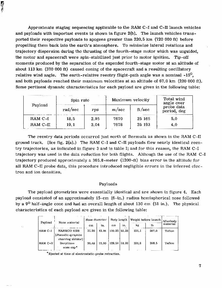
Approximate staging sequencing applicable to the RAM C-I and C-II launch vehicles and payloads with important events is shown in figure 2(b). The launch vehicles trans- ported their respective payloads to apogees greater than 220.5 km (720 000 f t ) before propelling them back into the earth's atmosphere. To minimize lateral rotations and trajectory dispersion during the thrusting of the fourth-stage motor which was unguided, the motor and spacecraft were spin-stabilized just prior to motor ignition. Tip-off moments produced by the separation of the expended fourth-stage motor at an altitude of about 113 km (370 000 ft) caused coning of the spacecraft and a resulting oscillatory relative wind angle. The earth-relative reentry flight-path angle was a nominal -15', and both payloads reached their maximum velocities at an altitude of 67.0 km (220 000 ft). Some pertinent dynamic characteristics for each payload are given in the following table:
~ "
Spin rate
period, deg probe data angle over . ~
Total wind Maximum velocity Payload
rad/sec ft/sec m/sec r P s ~~~ ~ "- .. .. ..
RAM C-I 5.0 25 165 7670 RAM C-I1 4.0 25 193 7678
~ ~ ~ . . . . ~-
The reentry data periods occurred just north of Bermuda as shown in the RAM C-I1 ground track. (See fig. 2(a).) The RAM C-I and C-11 payloads flew nearly identical reen- t r y trajectories, as indicated in figure 3 and in table I; and for this reason, the RAM C-I trajectory was used in the data reduction for both flights. Although the use of the RAM C-I trajectory produced approximately a 365.8-meter (1200-ft) bias error in the altitude for all RAM C-II probe data, this procedure introduced negligible errors in the inferred elec- tron and ion densities.
Payloads
The payload geometries were essentially identical and are shown in figure 4. Each payload consisted of an approximately 15-cm (6-in.) radius hemispherical nose followed by a go half-angle cone and had an overall length of about 130 cm (51 in.). The physical characteristics of each payload a r e given in the following table:
L- .
Nose material
.". ~~ ~ ~~
NARMCO 4028 (Phenolic-graphite
charring ablator) Beryllium
nose cap*
Nose diameter
cm
12.56 31.90
in.
30.48 12.00
Body length
cm
51.28 130.25
in. -~
~.
129.54 51.00
"I
~ ""1 materid
Weight before launch Afterbod)
"A I
121.1 Teflon 267.0
121.8 Teflon 268.5
*Ejected at time of electrostatic-probe retraction.
7

RAM C-I had a phenolic-graphite charring ablator on the hemispherical nose, whereas the nose of RAM C-I1 was covered by a beryllium-cap heat sink. Since RAM C-I was primarily a material-injection experiment, the ability to maintain the integrity of the injection orifices during the ablation period was mandatory; therefore, the phenolic- graphite material was selected. (See ref. 8; R A " C A designation is synonymous with RAM C-I.) An analysis of a sample of the NARMCO 4028 used to fabricate the heat shield showed that it contained about 1100 pg/g sodium. The analysis was incapable of detecting potassium, if present, at less than 3600 pg/g which means that the ablator could have con- tained up to 4700 pg/g of alkali. The beryllium nose cap and the teflon were found to be free of any significant amounts of alkaline impurities. For a sample of teflon, the analy- sis showed the alkali content to be less than 5 pg/g. Thus, during the RAM C-I reentry, the ablation of the nose fed easily ionizable alkali metals into the flow-field boundary layer. Since the primary objective of the RAM C-I1 flight was plasma flow-field diagnos- tics, the nonablative beryllium cap was selected to keep the flow field free of ablative con- taminants so that a comparison could be made of measured plasma characteristics with pure-air theoretical calculations. The beryllium cap was ejected at an altitude of 56.4 km (185 000 ft) prior to the surface melting, and thus exposed a teflon-covered nose. For both flights, the effects of teflon ablation from the afterbodies are believed to be negligible at altitudes above 56.4 km (185 000 f t ) (refs. 7 and 9) since the teflon had a low-alkali- metal contamination level; also, the ablation rates there were much less than those for the nose.
The location of the electrostatic and thermocouple probe rakes, the various radio- frequency antennas (diagnostic and instrumentation) on both payloads, and the water- injection orifices on the RAM C-I payload a r e shown in figure 5. Table II gives exact coordinate location and position of the various system sensors for both payloads.
Electrostatic Probe System
Design philosophy. - Realistic predictions of the electromagnetic wave attenuation to be experienced during atmospheric entry are dependent upon several factors, the fore- most of which is the physical nature of the plasma itself. The requirement for accurate knowledge of gas composition is more stringent for an analysis of this problem than for other reentry problems such as heat transfer or aerodynamic flow. The reason for this requirement is that the free electrons, which control the electrical conductivity of the gas, a r e a trace species and, as such, require a comprehensive nonequilibrium flow-field anal- ysis including finite-rate chemistry to determine the degree of gas ionization. For exam- ple, approximately 40 finite-rate chemical kinetic reactions involving 11 plasma species (free electrons, molecular and atomic ions, molecules, and atoms) must be considered in theoretical calculations of electron concentration. In addition, the dominant chemical kinetic process is dependent upon the velocity and body shape of the reentering spacecraft.
8

Moreover, calculations are more difficult to perform as one moves aft from the stagnation region because not only is a complete understanding of the local gas conditions required, but also of the entire gas history from the shock-entry point of each streamline to the location of interest.
The objective of the RAM-C electrostatic probe experiment for both flights was to determine experimentally the electron density profiles in the aft flow field in order to assess the validity of the theoretical calculations and to provide experimental data upon which to improve the analytical model used. The design of the RAM-C electrostatic probe system and the calibration testing in ground plasma facilities are discussed in detail in reference 4.
Configuration of electrostatic probe rakes on RAM C-I and C-11. - A photograph of the electrostatic probe rake is shown in figure 6(a); and the exterior configuration, a sec- tional view of the leading edge, and standoff dimensions of the ion collectors are shown in figure 6(b). Each of the iridium ion collectors extended 0.0254 cm (0.010 in.) beyond the wedge-shaped beryllium oxide leading edge of the rake. The two larger iridium pieces, one on each side of the rake, were electrically common and served as electron collectors. Iridium was chosen as the probe collector material because of its high melt- ing temperature, high electronic work function, and negligible oxidation property. The beryllium oxide leading-edge material was a high-temperature insulator which mechani- cally and electrically separated the ion collectors and the electron collectors. The beryllium oxide leading edge was a 60° wedge with a leading-edge radius of 0.0254 cm (0.010 in.) and was inclined at an angle of 45' with respect to the payload surface. The main body of the probe was constructed of a phenolic fiber-glass ablation material.
Probe circuitry.- A fixed bias of -5.0 volts, referenced to the electron collectors, was applied simultaneously to all ion collectors to attract positive ions. Figure 7 gives a schematic drawing of the probe electronic system on both the RAM C-I and RAM C-I1 payloads. As each probe continuously collected plasma current, the mechanical commu- tator sampled the voltage developed across the probe load resistors and calibrate resis- tors and fed the signals to the logarithmic amplifier at the rate of 300 samples per second. The voltage developed across the probe load resistor was converted by the logarithmic amplifier to drive a telemetry subcarrier oscillator. A photograph of typical flight com- ponents is shown in figure 8.
For the RAM C-I experiment, the output of the logarithmic amplifier was connected single-ended to the input of the subcarrier oscillator; whereas on the RAM C-11 experi- ment the output of the amplifier was connected to a differential-input subcarrier oscillator. This modification in the electronic system was made to correct an anomaly which occurred during the RAM C-I flight. The occurrence of the anomaly was ascertained during the onboard calibration of the logarithmic amplifier. The problem presented itself at an alti-
9

tude of about 67.0 km (220 000 ft) when the logarithmic amplifier output including all cal- ibrate levels unexpectedly went to zero. During water injection, the amplifier returned to normal operation; however, after the injection stopped, the output returned to zero. Approximately 3 seconds later at 61.0 km (200 000 ft), the amplifier returned to normal and continued so for the remainder of the flight. The anomaly was analyzed and it could be reproduced in the laboratory by connecting a -1.85-volt potential between the electron collector and the payload ground. It is surmised that during the flight the electron col- lectors and the spacecraft metallic skin assumed different floating potentials in the plasma. This condition caused the internal input diodes of the logarithmic amplifier to conduct and thereby reduced the amplifier output to zero. The differential connection used on the RAM C-11 system corrected the situation by effectively adding a large res is- tance (10 megohms) in series with this unwanted potential and thus prevented the diodes from conducting.
Logarithmic amplifier. - The solid-state logarithmic amplifier was developed spe - cifically for the electrostatic probe experiments. The device was a low-level input, adjustable high gain, chopper-stabilized dc amplifier which converted a differential high- impedance input into a differential low-impedance output. Figure 9(a) shows the dynamic (commutated at 300 samples/sec) input-output voltage characteristics of the amplifiers used for flight. As can be seen from the figure, the device provided an output propor- tional to the logarithm of the input voltage for greater than a three-decade range. The amplifier gain was adjusted so that the voltage developed by an input current from the probes of at least ampere, across the load resistor of 400 ohms, would be on the reasonably linear section of the characteristic curve. The maximum input current was
ampere and the minimum current value was determined by system noise (approxi- mately 5 X ampere for the RAM C-I experiment and 10-7 ampere for the RAM C-I1 experiment). The amplifier characteristics shown in figure 9(a) were obtained just prior to flight by calibrating the entire probe system as installed in the spacecraft. This cali- bration technique used a range of known resistances that were externally connected in sequence across the biased probe electrodes and thereby simulated a range of plasma currents. This calibration should not be confused with the onboard calibration the main purpose of which was to provide certain pulse levels in each data frame for automatic data reduction requirements.
Since the signal to the amplifier was commutated at 300 samples per second, good dynamic response was needed to reproduce the input accurately. Figure 9(b) shows a typical pulse-response curve of the amplifiers. With a delay time of less than 100 micro- seconds and rise and f a l l t imes of less than 75 microseconds each, the response was suf- ficient for data samples of approximately 3 milliseconds duration. For data-reduction purposes, only the center 50 percent of the pulse width was used.
10

Probe-experiment - "" characteristics and data format. - The format used for electro- static probe information from the logarithmic amplifier output, including currents from the probes and from the calibrates, is presented in figure 10. Shown in figure 10 is one complete data frame which has a duration of 100 milliseconds. There are five calibrate levels for each frame, which correspond to currents of 0.1, 1.0, 10.0, 100.0, and 1000.0 microamperes. Between the calibrate sequences are three consecutive samplings of the eight ion collectors. One profile measurement represents about 26.4 milliseconds or about 8 percent of a complete payload roll motion. The sampling rate of 300 samples per second was selected so that at least two data formats would be completed during the off time of the water-addition cycling system on RAM C-I. The same sampling rate was maintained for the RAM C-11 experiment.
Thermocouple probes.- On both of the RAM-C payloads, a rake of thermocouples was located diametrically opposite the electrostatic probe rake to monitor the tempera- ture of the leading edge. On RAM C-I, both the thermocouple and electrostatic probes were in line with the water-injection sites to insure similar heating environments. The external configuration of the thermocouple probe fin was the same as that of the electro- static probe fin and is shown in figure 11. Instead of electrodes, however, three thermo- couples were embedded 0.0635 to 0.1016 cm (0.025 to 0.040 in.) from the leading edge of the wedge. The thermocouples were platinum-platinum+13-percent-rhodium and were located 2, 4, and 6 cm (0.79, 1.57, and 2.36 in.) from the payload surface. The useful measurement range of the thermocouples w a s from 255 to 1977 K (Oo to 3100° F).
At elevated temperatures, the insulating properties of the beryllium oxide degraded, and unwanted leakage currents flowed between ion collectors and between ion and electron collectors. The thermocouple probe was used therefore to determine the altitude at which probe heating became significant. The electrical resistivity degradation affected the accuracy of the inferred electron density because the leakage currents added to the mea- sured plasma current and thereby caused a higher than actual electron density to be inferred. In reference 6, the electrostatic probe data were considered to be unusable in an absolute sense once the local probe temperature exceeded 811 K ( 1000° F). An improved analysis given in reference 4 estimated that the leakage current was on the order of 100 microamperes for a thermocouple temperature of 1366 K (2000O F). For both RA"C flights the inferred plasma density was greater than 10l1 electrons/cm3 when the local temperature for a given probe exceeded 1366 K; thus, the error in the inferred density at that point was less than a factor of two. For higher leading-edge temperatures, the leakage current probably exceeded the plasma current; therefore, above 1366 K the data were considered to be degraded for useful plasma-density inter- pretation purposes.
11

Retraction of probe rakes.- Although it was desirable to make electrostatic probe measurements over the entire blackout data period from 85.3 to 24.4 km (280 000 to 80 000 ft), certain restrictions were imposed. The high heating rates predicted for the intermediate altitude range from 61.0 to 30.5 km (200 000 to 100 000 f t ) would result in structural failure of the probes which could endanger the stability of the payload itself. Therefore, the rakes (electrostatic and thermocouple) were simultaneously retracted into the base region of the payload at a predetermined altitude by programer action. The RAM C-I rakes were retracted at an altitude of 53.6 km (176 000 ft). RAM C-11 probe retraction was initiated simultaneously with the beryllium cap ejection at 56.4 km (185 000 ft), but the effects of retraction on the inferred density were not noted until 55.9 km (183 400 ft).
RAM C-I Water-Injection System
During the RAM C-I flight, water was periodically injected into the flow field from the spacecraft nose to provide for electron density reductions in the peak attenuating layer of the flow field. The water was injected at varying flow rates with specific penetrations over an altitude range of 83.2 to 33.8 km (273 000 to 111 000 ft). The injection locations a re shown on the payload sketch in figure 5. Locations and positions of the nozzles are also given in table II. The electrostatic probe rake and two VHF slot antennas were located in line with the injection sites and were the principal diagnostic instrumentation for assessing the plasma alleviation.
The resultant programed variation of flow rates for the RAIV C-I experiment is given in table 111, with the altitude shown for the start of each pulse. Typical water flow- rate pulses are shown as a sequence of valve-on times. One complete injection cycle is shown and the cycles were repeated every 4 seconds. The valve-on times were 230 milli- seconds and the valves were opened at 0.5-second intervals. A more detailed description of the RAM C-I water-injection system can be found in reference 6.
RAM C-II Microwave Reflectometer System
A four-frequency microwave reflectometer system was used to infer the peak elec- tron density time and altitude histories about the RAM C-11 spacecraft. A plasma-density measurement range of three decades (1O1o to 1013 electrons/cm3) was provided by the reflectometer system. The microwave reflectometer technique used the reflectivity of the plasma to infer the electron density and phase measurements to infer the electron density profile shape. Microwave antennas for the four frequencies (L-, S-, X-, and Ka-bands) were located at each of the four body stations (except station 1, L-band excluded), for a total of 15 antennas (fig. 5). Antenna locations are listed in table II. Greater detail on the microwave reflectometer system may be found in reference 7 and in table II. 12

VHF System
It has been shown that significant pattern changes can occur for plasma-clad cylin- drical antennas when the electron density passes through the critical value. (See ref. 10.) These pattern changes are also accompanied by rapid changes in input impedance or input voltage standing wave ratio (VSWR). Received signal strength and onboard antenna VSWR were monitored during the RAM C-I and C-11 flights and were used to determine the occurrence of the VHF critical electron density. The antenna VSWR was monitored by onboard directional couplers, and the antenna patterns were reconstructed by use of the signal received from the spinning spacecraft. There were several ground, airborne, and shipborne receiving stations with different look angles; thus, patterns were obtained in several planes. The arrangement of receiving stations for RAM C-11 is shown in figure 2(a).
Two types of VHF antennas (cavity-backed slots and circumferential slot arrays) were used for the flights, as shown in figure 5. For the RAM C-I payload, two diametri- cally opposed, axially oriented, 259.7 -MHz cavity-backed slot antennas transmitted the real-time telemetry, and an aft-positioned circumferential slot array (ring) antenna transmitted the delayed-time telemetry. In comparison, on the RAM C-11 payload, the real-time and delayed-time telemetry systems utilized a pair of aft-located circumfer- ential slot arrays (ring antennas). The axially oriented slot antennas on RAM C-I were in line with the material-injection orifices and the electrostatic probes. The ring anten- nas for all payloads were just forward of the electrostatic probes. A more complete description of the VHF antennas on RAM C-I may be found in references 6 and 11 and in table IV.
ELECTROSTATIC PROBE THEORY
The RAM-C electrostatic probe measurements were interpreted by use of a free- molecular cylindrical probe theory modified to account for a directed-ion flux due to the plasma flow. This theory was developed by Scharfman (refs. 12 and 13) based on the works of Hok et al. and Smetana (refs. 14 and 15, respectively) and is summarized in appendix A.
The configuration of the RAM-C probe rake is such that in relation to the flowing plasma, each ion collector appears to be a cylindrical wire 0.0254 cm (0,010 in.) in diam- eter and 0.5385 cm (0.212 in.) long, which is inclined at an angle of 45O with respect to the plasma flow. Experimental programs were performed at Langley Research Center, Stanford Research Institute, and Cornel1 Aeronautical Laboratories to verify that the RAM-C electrostatic probe rake could be used to infer accurate localized ambient plasma electron densities. (See refs. 4, 13, 16, and 17.) Typical results from references 13 and 17 are shown in figure 12. The conclusion based on t h i s work is that free-stream electron density can be inferred within *20 percent by using the described theory for the
13

1lll1ll11llll Ill 1l11l111ll1l111111l1111l1l1l1l1 I I 1 I 1 I I I 1 I
RAM-C flight conditions for plasma densities from 1O1O to 10l1 electrons/cm3 and within a factor of two over the lo9 to 1013 electrons/cm3 range.
FLIGHT DATA RESULTS AND DISCUSSION
Measured Electrostatic Probe Ion Currents
Ion currents measured by each of the eight electrostatic probes onboard the RAM C-I and C-I1 flights are presented as a function of altitude from 85.3 to 53.3 km (280 000 to 175 000 f t ) in figures 13 and 14, respectively, and are listed in appendix B. (Altitudes for RAM C-II are too low by 0.3658 km (1200 ft).) In the figures, the measured probe-current data points are represented by the symbols which have been interconnected in order to show small variations clearly. Probes for both flights indicate an initial mea- surable current at an altitude of about 85.3 km (280 000 ft). Lowest measurable current for the probe electronic systems was about A. Likewise, system saturation current was 10-3 A.
Figures 13(a) to 13(d) show the currents measured by the electrostatic probes aboard RAM C-I. The effects of periodic water injection into the flow field can be seen as respective periods of greatly reduced measured currents for all eight probes. The anomaly period, discussed in an earlier section, occurred between 67.1 and 61.0 km (220 000 and 200 000 ft). The data shown in the figures during the anomaly period are considered to be valid since they were selected only when the onboard calibrates indicated normal amplifier operation. All data are valid after the anomaly period. The probes aboard RAM C-I were retracted at 53.6 km (176 000 f t ) from the aft-flow-field region into the payload base region. The probes continued to make measurements after retraction, but the analysis of these data is not presented in this report. Immediately after retrac- tion, the outermost probes still indicated system saturation current because of electrical degradation of the beryllium-oxide probe insulator induced by aerodynamic heating.
Figures 14(a) to 14(d) show the electrostatic-probe-measured ion currents for RAM C-11. Effects of retraction can be seen at about 55.5 km (182 000 f t ) in figures 14(a) to 14(c) as a steep dropoff of measured current. Again, the outermost probes of fig- ure 14(d) were still saturated immediately after retraction because of leakage current through the degraded probe insulator.
The small sinusoidal-type variation superimposed on the curves shown in figures 13 and 14 are variations in the plasma density due to spacecraft motion. These variations will be discussed in detail in a later section and in appendix C.
14

Thermocouple Probe Results
An accurate knowledge of the probe-rake leading-edge temperature during reentry was necessary for valid interpretation of the fixed-bias probe currents because at ther- mocouple temperatures greater than 1366 K (20000 F), the insulating properties of the dielectric wedge were degraded to the point that the inferred plasma densities were ques- tionable. Therefore, the first task in the data-reduction procedure was to examine the thermocouple data and to identify those probe data for which this threshold had been exceeded.
Measured thermocouple temperatures for both the RAM C-I and C-11 reentries are presented in figure 15. Overall, for corresponding thermocouples at identical altitudes, the temperatures of RAM C-I were less than those of RAM C-I1 most likely because of the cooling effects of water injection which can be seen on the RAM C-I curves. Water- injection cycles for RAM C-I are shown at the top of the figure. The RAM C-I and RAM C-11 data are presented in figure 16 as constant-temperature profiles of normal standoff distance y to a given temperature boundary plotted against altitude.
At any altitude, the temperature at any probe location on the leading edge may be determined from the intersection of a horizontal-probe location line, a vertical-altitude line, and a constant-temperature contour. When, for a given probe, this intersection occurs above the 1366 K (2000O F) contour, the interpretation of these data is questionable.
Electron Densities Inferred by Electrostatic Probe
By use of the probe interpretation discussed in appendix A, the collected ion cur- rents given in figures 13 and 14 were converted into respective ion (electron) densities for the two flights. (Flow-field calculations (ref. 9) indicate that positive-ion and electron densities are very nearly equal for the RAM-C trajectory.) The electron densities for RAM C-I a r e shown in figure 17 and for RAM C-11 in figure 18. The electron densities plotted against time and altitude are also tabulated for both flights in appendix B. The RAM C-I and RAM C-11 results after probe retraction should be disregarded since no temperature and velocity data are presently available to allow proper interpretation of the ion current.
Flow -field electron-density profiles (electron density plotted against standoff dis- tance y) were determined during both flights. Typical results are shown in figure 19 for selected altitudes during the RAM C-I flight where no water-injection effects were present and in figure 20 for similar altitudes on RAM C-II. The data represent the time-averaged electron density (averaged over one spacecraft revolution) at a given altitude for each probe, and the bars in figure 20 represent the peak-to-peak density change due to body
15

motions, to be discussed in a later section. The profiles for RAM C-I and RAM C-II flights are similar, although there was a slight difference in the absolute level at the specified altitudes. These differences are also observed in overlays of electron density plotted against altitude for RAM C-I and RAM C-I1 given in figure 21.
Effects of Ablation Impurities on Electron Density
Since the nose materials for the two RAM spacecraft were different (charring ablator for RAM C-I, nonablating heat sink for RAM C-11), a comparison can be made between contaminated and noncontaminated reentry plasma flow fields. The electron- density histories for RAM C-I and RAM C-I1 are superimposed for comparison in fig- ure 21. The electron density for RAM C-I is approximately a factor of 2 higher than that for RAM C-I1 for the altitude range of 85.3 to 73.2 km (280 000 to 240 000 ft). Below this altitude, RAM C-I1 results are slightly greater than those for RAM C-I, although the RAM C-I anomaly period and the effects of material addition make a quantitative com- parison less meaningful. The differences in measured electron density between these flights could be attributed to ablation product contamination effects because the payloads were nearly geometrically identical and they flew nearly identical trajectories. The RAM C-I charring phenolic-graphite nose fed easily ionizable alkali metals (sodium and potassium constituted approximately 1000 to 4000 pg/g in the virgin material) into the flow-field boundary layer, whereas the nonablating beryllium nose cap on RAM C-I1 did not contaminate the flow. For both spacecraft the teflon afterbody did ablate slightly; however, additional ionization was not probable because here the alkali metal content was kept below 5 ppm of teflon. A detailed discussion of alkali ablation product contamination of the RAM-C flow field is given in reference 9.
Effects of Vehicle Angle-of-Attack Perturbations on Electron Density
An analysis of the accelerometer data (appendix C) revealed that each payload underwent small angle-of-attack oscillations which produced variations in the ion current collected by all probes and variations in the microwave reflectometer measurements (RAM C-11). This effect is more clearly observed in the RAM C-I1 results (fig. 18) since these results are not disturbed by water injection. Variations in electron density at the probe station were produced because the payload was at an angle of attack (unsymmetrical flow field about payload) while spinning at 18.84 rad/sec (3 rps). When the payload expe- rienced a positive angle of attack (positive normal acceleration), the electrostatic probes were on the windward side of the payload and sensed a compression of the flow field. Conversely, for a negative angle of attack (negative normal acceleration), the probes sensed the leeward (less dense) side of the flow field.
16

A comparison of the RAM C-11 vehicle angle -of -attack motions (determined by accelerometer data) with electron density (inferred from electrostatic probe 1) is shown for the altitude region from 59.4 to 55.8 km (195 000 to 183 000 f t ) in figure 22. A s seen in the figure, small angle-of-attack motions produced peak-to-peak density fluctuations in the aft part of the flow field approaching a factor of three. The sizable density varia- tions close to the payload for relatively small changes in angle of attack can be one of the reasons that signal-attenuation models do not always accurately predict plasma-caused signal losses when normal zero angle-of-attack plasma profiles are used.
Effects of Water Injection on Electron Density
The effectiveness of water injection as a plasma alleviant in the RAM C-I flow field was assessed by means of two VHF slot antennas and the electrostatic probe rake located in line with the injection sites. The probe measurements provided an excellent means of determining injectant penetration distances as well as the resultant magnitudes of the suppressed plasma.
The amount of plasma suppression due to water injection on the RAM C-I plasma electron density is seen in figure 23. In the upper part of the figure, the water injection pulses are shown with varying magnitude. (Flow rates a r e given in table III.) Each pulse caused corresponding decreases in measured electron density. Cycle 1 (not shown in the figure) had no flow because of a slow fill rate in the lines. The very low flow rates of cycle 2 produced no detectable plasma alleviation for any of the probes. The larger flow ra tes of cycle 3, particularly the side-injection flow rates 3 and 4, caused appreciable electron-density reduction for all probes. Electron-density profiles for the various lat- eral injection flow ra tes of cycle 3 a r e shown in figure 24. Here, it is clearly seen that increasing flow rates are more effective in reducing electron density and in penetrating farther out into the flow. The electron-density profiles during stagnation injection (cycle 4, flow rate 5) are shown in figure 25 for selected altitudes over the 593 meter (1947 f t ) altitude range.
The probe electronic system anomaly occurred immediately after cycle 4, flow rate 6, and persisted through cycle 4, flow rate 4. For intervals during the periods of water injection, however, the amplifier returned to normal operation and allowed reliable probe measurements.
The effectiveness of the water-injection technique was assessed by comparing den- sity profiles with water injection against those without water for the same altitude range. Alleviation effects of water injection were noted by the ground stations on the signals received from all the onboard radio-frequency systems and good correlation was found between the probe electron-density profile changes and the observed attenuation changes of the signal strengths.

Microwave Reflectometer Measurements
The location and magnitude of the peak electron density inferred by the station 4 microwave reflectometers agree with the electron-density profiles inferred by the elec- trostatic probes for the RAM C-II flight. This good agreement lends credence to.both measurements since both measured and theoretical electron-density gradients along the aft payload surface are small (refs. 7 and 9, respectively).
The microwave phase data (fig. 35 of ref. 7) indicate that there was a strong density gradient between the payload surface and a normal distance into the flow of 1 to 2 cm. Beyond this distance the profile appeared to be nearly uniform for another several centimeters.
The magnitudes of the electron density inferred by the probes and microwaves are also strongly correlated as shown in the longitudinal profiles of peak electron density for constant altitude. (See fig. 26.) In figure 26, the time-averaged peak electron densities as indicated by the reflectometer are plotted against distance along the body, where zero on the abscissa corresponds to the payload nose. Also shown in the figure for purposes of comparison are the time-averaged electron densities (averaged over one body revolu- tion) for probes 1 and 8 (innermost and outermost probes, respectively). The bar on the probe data represents the peak-to-peak density fluctuation due to body motions.
VHF Antenna Measurements
The received VHF signal strengths (recorded at the Bermuda and U.S. Navy Ship (USNS) Twin Falls Victory stations) and the reflected power for the onboard antennas for RAM C-I are presented in figures 27 and 28 and for RAM C-11 in figure 29. The Bermuda station was located approximately broadside to the payload during the data period and the Twin Falls Victory station was directly down range. (See fig. 2(a).)
The peak electron density at a given antenna location was inferred from the region where the received signal strength ripple pattern (due to spinning payload) and the onboard antenna reflected power changed abruptly. In reference 10, these changes were shown to occur at the critical electron density; however, since the RAM-C experimental conditions were slightly different than those in reference 10, the peak electron density is estimated to be the critical value within a factor of two uncertainty.
For the RAM C-I records, the time period of interest is from 385 to 394 seconds. In the Bermuda 225.7-MHz record, the pattern ripple is about 30 dB prior to the cri t ical electron-density region (indicated by the arrows) which is in agreement with the measured free-space patterns in the equatorial plane. The ripple structure diminishes markedly in the critical electron-density region and then resumes as attenuation due to an overdense plasma occurs. The same sequential change was also noted by the Bermuda station in the 259.7-MHz antenna pattern ripple structure during a similar time frame.
18

A related change in the pattern ripple structure was also observed for both antennas in the signal received at the USNS Twiq Falls Victory station between 386 and 394 seconds. At 386 seconds, the plasma electron density over the antennas is negligible and the antenna pattern ripple is about *2 dB. Also the mean level of the signal received at the two f re - quencies is different by about 16 to 20 dB in absolute level. Both the magnitude of the pattern ripple and the absolute power levels agree very well with those predicted from the nose-on free-space absolute antenna patterns. During the time period from 390 to 392 seconds, the 225.7-MHz record experiences a 20-dB dip in the received signal level as the plasma goes through critical density. A similar but smaller signal-level dip also occurs at 259.7 MHz. The time of occurrence of these amplitude dips in the received nose-on signal closely correspond to the time period where a significant decrease in pat- tern ripple was observed from the broadside direction.
The records of reflected power to both the 225.7-MHz and the 259.7-MHz antennas are shown in the lower parts of figures 27 and 28. The sharp rise or increase in reflected power with the simultaneous occurrence of critical electron density over the antenna aper- ture corresponds to that altitude range where the pattern ripple changes were noted. For RAM C-11, nearly identical antenna effects were observed, as shown in figure 29.
Comparison of Inferred Electron Densities for the RAM-C Flights
The plasma diagnostic results for both flights a r e shown in figure 30 for the pur- pose of comparison. They include electron density as a function of altitude inferred from the RAM C-II electrostatic probes, RAM C-11 microwave reflectometers, and the RAM C-I and RAM C-I1 VHF antenna measurements. The data presented for electromagnetic tech- niques are time-averaged peak electron densities. The probe data represent the envelope of maximum to minimum values for all probes. All inferred densities are corrected for body location and are referred to the probe station by use of the appropriate longitudinal profile in figure 26.
Comparison of Theoretical and Experimental Electron Density Profiles
Calculated electron density profiles for the RAM-C flights were provided by the authors of reference 9. These calculations began with pressure distributions derived from equilibrium inviscid flow-field solutions for sphere-cone shapes. A nonequilibrium streamtube method provided temperature, density, and composition (including electron concentration). Streamline positions were determined by means of mass flow conserva- tion. An equilibrium thin boundary-layer solution was adapted for use with nonequilibrium edge conditions, and the combined viscous-inviscid solution was iterated to account for vorticity and displacement thickness. Inviscid streamline values were discarded upon entry into the boundary layer and were replaced by calculations based on conditions in the
19

boundary layer. The flow-field solutions described are not valid at altitudes above about 70.1 km (230 000 ft). It should be noted that ambipolar diffusion of the charged particles, which cannot be included in this treatment, was estimated in reference 9 to become an important influence at altitudes higher than 70.1 km (230 000 ft).
For RAM C-11 the clean-air assumption should have been valid down to 56.4 km (185 000 ft) where the beryllium nose cap was ejected, but for RAM C-I the flow field was contaminated by ablation products from the phenolic-graphite nose. For both bodies the teflon afterbody did ablate to some extent, but no additional ionization would result because the alkali metal content was kept below 5 ppm in the heat shield. There is, how- ever, an unanswered question concerning the reduction of the electron density due to the electrophilic action of teflon ablation products.
When the measured electron-density profiles shown in figures 19 and 20 were com- pared with the calculated profiles previously mentioned, the measured profiles were found to be lower and flatter than the calculated ones. Also the measurements appeared to extend to greater distances from the body surface than had been anticipated. A typical comparison is shown in figure 31 with the RAM C-II data bars representing the envelope of probe data (due to body motions). Comparison of the probe data with other available plasma flow-field calculations (ref. 18) also indicates this significant disagreement between experiment and theory in absolute magnitude and in shape of the electron-density profiles.
In an effort to resolve these differences above 71.0 km (233 000 ft), the effects of ambipolar diffusion were considered. Since the analytical model used a streamtube approach, the effects could not be handled directly; rather an ion diffusion correction factor was determined (ref. 9) which accounts for the reduction in the magnitude of the peak electron density. Unfortunately, no theoretical means is available for predicting the spreading of the electron-density profiles; conceptually, however, ambipolar diffusion should decrease the absolute magnitude of density and reduce its gradients.
The theoretical peak electron density and the RAM C-I and RAM C-11 envelopes of time-averaged inferred densities from probe 8 are shown in figure 32. The RAM C-I1 data should provide a better comparison with the "pure air" plasma calculations because the RAM C-I1 beryllium nose cap minimized flow-field contamination down to an altitude of 56.4 km (185 000 ft). At 85.3 km (280 000 ft) the inviscid calculation of peak electron density must be reduced by approximately two decades because of the ambipolar diffusion correction factor. This correction goes to zero near 70.1 km (230 000 ft), and below this altitude both the inviscid calculations and the inviscid calculations corrected for boundary layer yield identical results and according to reference 9 are believed to be correct. The good agreement between the inviscid calculations corrected for ambipolar diffusion and the experimental measurements above 70.1 km supports the hypothesis that ambipolar
20

diffusion is a principal mechanism for shaping the high-altitude electron-density profiles. The RAM C-11 electron densities from the inviscid calculations corrected for boundary layer, the microwave reflectometer measurements, and the electrostatic probe measure- ments are given for different body locations in figure 33. Although both the experimental and theoretical curves show a leveling of the electron density below 70.1 km (230 000 ft), the experimental values are greater. The electrostatic probe data envelope shown in the figure includes only those data that are below the 1366 K (20000 F) critical temperature. Although the probe data might be suspect below 70.1 km because of aerodynamic heating, the microwave reflectometer technique does not suffer from this effect.
CONCLUSIONS
Unique high-altitude electrostatic probe measurements have been made on the aft section of two high-velocity reentry spacecraft. Good agreement between the two RAM-C flight probe experiments with strong correlative data from microwave reflectometer and VHF antenna measurements support the following conclusions:
1. High-altitude (above 70 km (230 000 f t ) for RAM-C configurations) calculations of electron-density profiles using an inviscid streamtube approach corrected for boundary layer are inadequate and modifications including ambipolar diffusion effects are necessary.
2. Increases in ionization due to phenolic-graphite ablation products in the aft-flow- field boundary layer were no greater than a factor of two over an altitude range of 56.4 to 82.3 km (185 000 to 270 000 ft).
3. Small angle-of -attack motions produce significant peak-to-peak density fluctua- tions in the aft par ts of the flow field. These variations in electron-density profiles can be useful in qualitatively indicating vehicle angle of attack in the high altitudes where accelerometer data are limited.
4. The use of water addition into the flow field as a plasma alleviant is effective in reducing the electron density in the flow field and in alleviating radio blackout.
Langley Research Center, National Aeronautics and Space Administration,
Hampton, Va., December 20, 1971.
21
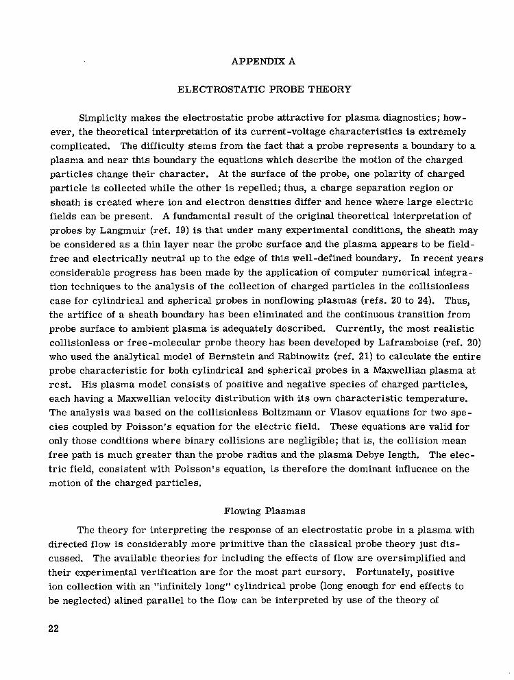
APPENDIX A
ELECTROSTATIC PROBE THEORY
Simplicity makes the electrostatic probe attractive for plasma diagnostics; how- ever, the theoretical interpretation of its current-voltage characteristics is extremely complicated. The difficulty stems from the fact that a probe represents a boundary to a plasma and near this boundary the equations which describe the motion of the charged particles change their character. At the surface of the probe, one polarity of charged particle is collected while the other is repelled; thus, a charge separation region or sheath is created where ion and electron densities differ and hence where large electric fields can be present. A fundamental result of the original theoretical interpretation of probes by Langmuir (ref. 19) is that under many experimental conditions, the sheath may be considered as a thin layer near the probe surface and the plasma appears to be field- f ree and electrically neutral up to the edge of this well-defined boundary. In recent years considerable progress has been made by the application of computer numerical integra- tion techniques to the analysis of the collection of charged particles in the collisionless case for cylindrical and spherical probes in nonflowing plasmas (refs. 20 to 24). Thus, the artifice of a sheath boundary has been eliminated and the continuous transition from probe surface to ambient plasma is adequately described. Currently, the most realistic collisionless or free-molecular probe theory has been developed by Laframboise (ref. 20) who used the analytical model of Bernstein and Rabinowitz (ref. 21) to calculate the entire probe characteristic for both cylindrical and spherical probes in a Maxwellian plasma at rest. His plasma model consists of positive and negative species of charged particles, each having a Maxwellian velocity distribution with its own characteristic temperature. The analysis was based on the collisionless Boltzmann or Vlasov equations for two spe- cies coupled by Poisson's equation for the electric field. These equations are valid for only those conditions where binary collisions are negligible; that is, the collision mean f ree path is much greater than the probe radius and the plasma Debye length. The elec- tric field, consistent with Poisson's equation, is therefore the dominant influence on the motion of the charged particles.
Flowing Plasmas
The theory for interpreting the response of an electrostatic probe in a plasma with directed flow is considerably more primitive than the classical probe theory just dis- cussed. The available theories for including the effects of flow are oversimplified and their experimental verification are for the most part cursory. Fortunately, positive ion collection with an "infinitely long" cylindrical probe (long enough for end effects to be neglected) alined parallel to the flow can be interpreted by use of the theory of
22

APPENDIX A - Continued
Laframboise for nonflowing plasmas. Also, for most experimental conditions, this theory should be applicable for electron collection with any probe orientation because the random velocity of electrons is usually large compared with the directed velocity of the flowing plasma. However, this theory is not applicable for the interpretation of posi- tive ion collection with a cylindrical probe of arbitrary orientation in a flowing plasma. In the following sections, an interpretation for cylindrical probes under these conditions by Scharfman (ref. 12), based on the works of Hok et al. (ref. 14) and Smetana (ref. 15), is presented.
Directed Flow Parallel to Probe
The ion current part of a cylindrical electrostatic probe characteristic has been numerically evaluated by Hok et al. (ref. 14) over a large range of ion densities and elec- tron temperatures for a nonflowing plasma which is also applicable to a plasma with the directed flow parallel to the axis of the probe. For the flowing plasma case, it is advan- tageous to use this theory because it can easily be modified to account for an arbitrary probe orientation. These results are shown graphically in figure 34 as the variation of the normalized current In with the normalized potential difference Xp between the probe and the plasma for selected values of ratio y of sheath radius a to probe radius Rp. The normalized current is the ratio of the current I+ collected by a probe to the random ion current I,. The random ion current is defined by Hok et al. to be the product of the saturation ion current density and the a rea of the probe and is given by
where
n
e
RP
L
v+
electron density or ion density
magnitude of electronic charge
probe radius
probe length
velocity of ions entering sheath
23

APPENDIX A - Continued
The velocity v+ is defined to be
8kTe v+ = /x
where
k Boltzmann's constant
Te mean electron temperature
M ion mass
It is to be noted that in equation (Al) the electron temperature Te is used rather than the ion temperature. This departure from the classical definition for the mean thermal speed is the result of incomplete shielding of the probe sheath. Thus, a total potential drop of order of magnitude kTe exists in the plasma and accelerates the ions into the probe sheath (ref. 25).
The normalized potential difference xP between the probe and the plasma is a dimensionless parameter defined as
xp = "(V - Vm) kTe
where
V probe potential
vc3 plasma potential
Before Hok's results (fig. 34) can be used to interpret experimental probe data, the ratio y of sheath to probe radii must be known. The ion sheath radius a is defined as
a = Rp +ds
where ds is the sheath thickness. For a planar probe geometry, the sheath thickness varies directly as the probe potential and inversely as the ion density and is given by
where AD is the Debye length and is defined as
24

APPENDIX A - Continued
where is the permittivity of free space.
The approximation of a planar solution for sheath thickness is applicable to cylin- drical probes only when the sheath thickness is small compared with the probe radius. When this is not the case, the ratio y of the from an inverted form of the Child-Langmuir current flow. This relation has been derived in figure 35 as y - 1 against 0 where 0
sheath to probe radius may be obtained 3/2-power law for space-charge-limited by Hok for cylindrical probes and is plotted is defined as
and
I+ measured probe current
V’ absolute magnitude of applied probe bias
To give more physical significance to the current collection curves shown in fig- ure 34, the following asymptotic cases are given:
Case I; thin sheath, y =: 1; X < -1: P
where Ji is the saturation positive ion current density for a collisionless Maxwellian plasma at rest and is given approximately by Bohm et al. (ref. 26) as
Ji = 0.4nev+ (A4)
Note that equation (A3) is independent of the applied probe bias.
Case II; moderate to thick sheaths, y > 1; large negative probe bias, xp << -y:
This current varies directly as the applied bias because of y.
25

APPENDIX A - Continued
Case III; extremely thick sheaths, y 7> Xp ; moderate negative probe bias, Xp < -2: I 1
In this region the current is approximately proportional to the square root of applied probe bias.
Directed Flow Normal to Probe
The effect of a normally directed ion flux (ions/unit area) on the current collected by free molecular cylindrical probes has been analyzed by several investigators. (See refs. 12, 15, 27, and 28.) If it is assumed that the flow does not distort the form of the ion sheath around the probe, the current density is the result of a superposition of random and directed ion fluxes (ref. 12). This effect is illustrated by figure 36, a curve of the normalized current In collected by a cylindrical probe not alined with the flow plotted against the ion speed ratio S. The speed ratio is defined as the normal component vf of the flow velocity vflow divided by the random thermal velocity v+
In figure 36 there are two asymptotes shown as dashed lines. The horizontal asymptote represents the value of current collected by a thin-sheathed (y = 1) probe in a nonflowing plasma and is equal to the random current 1, or to a normalized current of unity. The other asymptote represents the superposition of the random current Ir and a directed current Id. The directed current is
h = nevf 2R L = pvfA ( p )
where
P charge density
A projected area of probe
When the normal component of the flow velocity is small (S << l), the probe current is approximately that collected in a nonflowing plasma. For larger values of the normal component of flow velocity, that is, S > 3, the current collected by the probe approaches the value given in equation (A8).
When the ion sheath is not thin, that is, y > 1, the problem is more complicated because the ability of the relatively weak electrostatic potential field around the probe to
26

APPENDIX A - Continued
capture ions with increased inertial energy due to the flow is reduced. This problem was treated by Smetana (ref. 15) and the results are shown in figure 37.
Scharfman (ref. 12) gives the following qualitative explanation of Smetana's results: For the nonflowing plasma case (S = 0) with low values of applied bias xp > -1 and a large sheath thickness ( y >> l), the attraction of the probe's potential field is weak; con- sequently, most of the ions that enter the sheath orbit past the probe and are not collected. By using simple orbital theory, the radius ra at which particles will just be collected is
0
where
V probe potential
VO initial energy of ion entering sheath, kTe/e
Thus, the current is proportional to the flux (ions/unit area) entering the sheath at the radius ra and is proportionally given as
I+ nVo1/2Rp ( 1 +
In the limit of large applied potential xp << -1 , ( ) I+ V1/2Rp
When a directed velocity is included (S > 0), the flux is proportional to SVo 1/2 and the capture radius becomes
Thus, the effective capture radius for ions decreases while the flux increases. Therefore,
In the limit of large applied potentials << -S2), this relationship reduces to the same value as when S = 0; that is,
27

APPENDIX A - Continued
h-.the limit of large directed velocity (S >> l), In approaches S in value, and the cur- rent I+ is approximately given by equation (A8).
With this understanding of current collection under directed velocity conditions and with the asymptotic solutions for S = 0 and S >> 1, the works of Hok and Smetana can be combined by a transformation of the coordinates of figure 34. This result from Scharfman is replotted in figure 38 as the variation of R with H where
R = In
(1 + s 2 y 2
1 + s"
where
R modified normalized probe current
H ratio of modified potential energy to kinetic energy
The results presented in figure 38 can be readily used to infer positive ion density n by the following algorithm:
(1) Determine Te
(2) Measure the probe current I+ at V' volts below floating potential
(3) Calculate the normalized probe to plasma potential
xp = (E) + 5 * 0.5
(4) Calculate 0 by use of equation (A2)
(5) Obtain the appropriate value of y from figure 35
(6) Calculate v+ by using equation (Al)
(7) Calculate S by using equation (A")
(8) Calculate H by using equation (A10)
28

APPENDIX A - Continued
(9) Obtain the appropriate value of R from figure 38
(10) Calculate the positive ion density from
11 + S2RPev+RpL
Interpretation of RAM-C Fixed-Bias Electrostatic Probe Data
The configuration of the RAM-C electrostatic probe is shown in figure 6(b). In relation to the flowing plasma, each ion collector appears to be a cylindrical wire 0.0254 cm (0.010 in.) in diameter and 0.5385 cm (0.212 in.) long, which is inclined at an angle of 45' with respect to the plasma flow. To illustrate the data-reduction procedure, a sample calculation is presented.
Sample Calculation
The following factors are given in the sample calculation:
Altitude, km (ft) . . . . . . . . . . . . . . . . . . . . . . . . . . . . . . 76.2 (250 000) Ion collector . . . . . . . . . . . . . . . . . . . . . . . . . . . . . . . . . . . . . . . 8 Potential of probe below floating potential, V', volts . . . . . . . . . . . . . . . . . 5 Temperature, T, K . . . . . . . . . . . . . . . . . . . . . . . . . . . . . . . . . . 7500 Flow velocity, vfloW, km/sec (ft/sec) . . . . . . . . . . . . . . . . . . 5160 (16 930)
Ion mass (NO+), M y g . . . . . . . . . . . . . . . . . . . . . . . . . . . . 49.88 x Measured current, I+, pA . . . . . . . . . . . . . . . . . . . . . . . . . . . . . . . 50 Probe length, L, cm (in.) . . . . . . . . . . . . . . . . . . . . . . . 0.5385 (0.212) Probe radius, Rp, cm (in.) . . . . . . . . . . . . . . . . . . . . . . 0.0127 (0.005) Boltzmann constant, k, J/K . . . . . . . . . . . . . . . . . . . . . . . 1.38044 X 10⁻²³ Electronic charge, e, coulombs . . . . . . . . . . . . . . . . . . . . . 1.5921 x
For an altitude of 76.2 km (250 000 f t ) and ion collector 8, the temperature was calculated to be 7500 K. The electron temperature is assumed to be equal to the local gas tempera- ture. A plot of gas temperature as a function of altitude for the ion collector locations is shown in figure 39. These temperature data, as well as the flow velocity data given in figure 40, were generated by a nonequilibrium boundary-layer-corrected flow-field anal- ysis of the RAM C-I trajectory.
Angle between flow velocity and probe axis, 8, deg . . . . . . . . . . . . . . . . . 45
29

APPENDIX A - Concluded
The first factor to be calculated is the normalized potential difference between the probe and the plasma by using equation ( A l l )
x = * + 5 = 12.69 p kTe
Next, the ratio of ion sheath radius to probe radius y is estimated by using fig- ure 35 and equation (A2)
\ 3/2 5kTe
For a measured current of 50 PA, the value of 0 is 3.51 X lo7 volts 3/21 ampere. The corresponding ratio of sheath radius to probe radius y is 2.61.
The modified normalized probe current R is now determined. Figure 38 is a plot of R as a function of the ratio of modified potential energy to kinetic energy H (eq. (A10)) which is defined as
The velocity of ions entering the sheath v+ is calculated (eq. (Al)) to be
v+ = ($SI2 = 2.037 x lo5 cm/sec
The ion speed ratio S is (from eq. (A7))
s = ” Vf - Vflow sin e v+ v+
From equation (A7), S = 1.791 and thus the value of H is 3.015. The corresponding value of R is 1.93 from figure 38.
Solving for the density n yields
I+ = 3.21 X l o l o cm-3 = \ j z 1 3 f i e v + R p L
30

I
APPENDIX B
ELECTROSTATIC-PROBE AUTOMATIC DATA REDUCTION
PROCEDURE AND LISTINGS
By Lorraine F. Satchel1 Langley Research Center
This appendix outlines the method for inferring electron density from telemetry data for the RAM-C flight experiments. The theoretical interpretation used was that of Scharfman (based on the works of Smetana and Hok) as presented in appendix A. A flow chart that illustrates the data-reduction procedure follows:
Measured ca l ibra te
points
ADTRAN
\ ' Log amp output
voltage I I
Pref l ight ca l ibra te
w Calculated
Flow velocity and prof i les Punched
Payload t ra jectory Time against al t i tude I
Input current against output voltage 1
P r o b e theory
Computer p rogram
LPROBE
and alt i tude aga ins t t ime
CALCOMP Plots t ime
v P r o b e s
Telemetry signals containing the electrostatic probe data were recorded by ground receiving stations on magnetic tape. These data were in an analog-frequency-modulation form which consisted of subcarrier oscillator frequency deviations as a function of loga- rithmic amplifier output voltage. The format for this commutated probe data is given in figure 10. An analog-to-digital transcription made from magnetic telemetry tape data was converted to engineering units to be used as inputs to the probe theory computer program named LPROBE. LPROBE also required, as input data, theoretical flow-field velocities
31

APPENDIX B - Continued
and electron temperatures for each probe location, as functions of elapsed flight time and altitude, and preflight probe-electronic system calibration. Sufficient points from curves of these input data were tabulated and a second-order interpolation using FTLUP, a table look-up subroutine, provided the desired accuracy.
LPROBE was written in Fortran IV language for the Control Data 6000 series com- puter. The formats for the program inputs were flight time (FLTIME), delta time (DELTAT), synchronization code (ISYNC), and 24 channels of voltage and 24 channels of current. DNSTY was a subroutine with all tabular data listed internally. LPROBE pro- vided the data in the call sequence and DNSTY computed the electron density. The out- puts of LPROBE were CALCOMP plots (figs. 13, 14, 17, and 18) and/or tabulations of electron density (electrons/cm3) as a function of time for each probe.
Presented in this appendix are: a listing of the program, logarithmic amplifier calibrates (output voltage as a function of input current in microamperes) for the two flights, tables of computed gas temperatures (for altitudes in thousands of feet), flow velocity calculations (as a function of time) for each of the probes, and tabulations of computed electron density as a function of time for each of the probes for both RAM C-I and RAM C-LT.
C *CALL S E S i l E l \ i C E FOR SUf?ROl~TIbE DNSTY* LFS 2 5 0 C L F S 2 6 0 C Tf= iLECTRCV T tNFEQATUREpDZGREES KELVIh(CCMPUTED FRCC TABLES VS. T I Y E t L F S 2 7 0 c. L F S 2 9 0 C T I = I C A T F v P I F A T U R E l N f l T C I S E D - D U M P Y I N C 4 L L S T A T E M E N T ) L F S 290 C C F D ' 4 I L L ( D l d Y E T E P 1F PHPRE)= lC .O MILS
L F S 300 L F S 3 1 0
C C C C C C c C C
C c
C C
C c
C C C C C C C C C C C
C
L F S ' L Y l L L I L E h G T k CF P R O a F ) = 2 1 2 . 0 P I L L S L FS
L F S
L F S
L F S
L F S
L F S FLOVEL(FLDW-VELDClTYI Ilu V/SEC. (CCMPUTEC FPCF TARLES VS. T I M E ) L F S
L F S A'\1(rLECTRC:h: t E N S I T Y ) CCPPIJTEC U S I N G SLBROUTIhE D N S T Y . L F S
L F S Tt lEFF ARF A PRDBES-ZACH SAMPLES TPE DATA 3 T I C E S PER F L I G H T TIME. L FS S E E F I G l l R E 11 A h 9 T A B L E BELOW. LF S
4 V PCTEVTIAL CC I S MEASUrEC WITH RESPECT TC FLASMA pClTENTI4L. L F S
CC I C N SATUFPTICN CURFENTpMICRCAt'PS (CCMPUTEr V4CUES). LFS
h'41 I ( I C A M A S S ) = 2 d . O AUU L F S
4 t4GlORIENTATI@N ANGLE flF PRORE)=45.C DEGRFES C F - 7 8 5 3 9 8 2 6 R 4 D I A N S L F S
3 A T P ( 1 , 0 9 p 1 7 ) A P E PRC'OE 1 ( F T L U P U S E S CCRRECTED T I C E t T E M P l AND V F l l L F S D 4 T / 3 ( Z v I O p 1 6 ) ARC PROBE 2 ( F T L U P U S F S CORRECTED T ICEpTEHP2 A N 0 VF 2 l L F S 3 4 T A ( 3 9 1 1 p l C 1 ARE PRORE 3 ( F T L U P U S E S CC'RRECTED T IMFgTEMP3 AND V F 3 l L F S D 4 T A ( 4 p I ? v 2 C J ARE PR(36E 4 ( F T L U P USES CORRECTED TIk'EvTEMP4 AND V F 4 1 L F S 24TA(5 ,1?12 ! ) APE PliOAE 5 ( F T L U P LSES CFRRECTED T I W p T E M P 5 AND VF 5 ) L F S 34TA16 , /4 ,22J ARC PFfJRE 6 ( E T L l r P U S E S CORRECTEO TIP'E,TEMP6 AND V F 6 t L F S 0 4 T P ( 7 p 1 5 p 2 3 ) APE PRLlRE 7 ( F T L U P USFS CORRECTED T IMEvTEMP7 AND V F 7 ) L F S 0 4 T A l 9 p 1 5 v 2 4 ) A P E FRDRE R (FTLIJP bSES CORRECTED TIME,TEYPB AND V F S J L F S
L F S F E d L h ' ? ( 6 C @ ) L F S
L F S
3 2 0 33c 34c 3 5 0 360 37c 3 8 0 390 400 4 1 C 420 43c 44c 4 5 C 460 47@ 480 4 9 0 5 0 0 5 10 5 2 0 5 3 0 540 5 5 0 5 6 0 5 7 0
590 5ac
32

c
C C
C C
C. C
C c
C C C
c r, C C C
C C C
C C C
APPENDIX B - Continued
C I C E N S I C N V C L T S ~ 5 0 ~ ~ C U R ~ 5 0 ~ ~ T I Y E d / 4 0 ) r A L T d ~ 4 O ~ ~ A L T A ~ 4 O l ~ T E M P ~ 4 O ~ 8 ~ ~ T I M E ~ ~ 4 O L F S 600 1 ~ ~ A L T 8 ~ 4 C ~ ~ V F ~ 4 0 ~ 8 l ~ F L T 1 M E ~ 2 ~ 0 ~ ~ V f l L T A G E ~ 2 0 0 ~ 2 4 ~ ~ C U R ~ E ~ T ~ 2 0 0 ~ 2 4 ~ ~ L F S 610 1 I S Y N C ~ Z O O ~ ~ D € L T A T ~ 2 0 0 ~ ~ T I M E ~ 6 0 C ~ ~ C ~ R R ~ 6 O C ~ L F S 620
L F S 6 3 0
L F S 6 5 0
CALL CALCCMP LFS 67@ L F S 6 8 0
EQUIVALENCE (TIMEA,TIMEB),IALTA,ALTB) L F S 640
I N I T I A L I Z E PLOTTER. L F S 660
LSE PAPER 3 0 0 - SET PEN ON RIGHT MARGIR - SET ORIGIN. LFS 69@ CALL CALPLT(C.O,l.O*-31 LFS 700
L F S 710 PRINT CONSTANTS. L F S 7 2 0 S I Z E = o l L F S 7 3 C Z I 7 E O Z = S I Z E / 2 . 0 L F S 740 h = ( 6 . / 7 o ) * S I Z E L F S 7 5 0 Z I Z E D = S I Z E + S I Z E D Z L F S 760
LFS 770 CATA CCNSTANTS % C A Y O F P = K / F P S I L C N L F S 7 8 0 pDPILL= lC .O LFS 790 F L ” I L L = 2 1 2 . C L F S 8 0 0 A C I 1 = 2 8 o C C L F S 8 1 0 b N G = o 7 e 5 7 5 8 1 t L F S 820 E=5. J L F S 83@ CAYn?P=.OCOl38C54/1.6C?lO L F S 84G
L F S 8 5 0
P A M C - I AND 313 RPY C- I I l (DYN4MIC INPUT-@UTP(JT CURVES) LFS 870
1 FOFMAT(* l VCLTAGE CgRRENT LOG-AMP 814*/l L F S 89C
PEADTSTCRE AND k R I T E V’ILTAGE VS. CLRRENT F R C M L C G A M P C U R V E S ( 8 1 4 L F S 8 6 0
C R I T E ( 6 , l l L F S 880
L C 13 1 = 1 , 5 0 L F S 9 C O READ( 5 ,3 IVOLTS( I ) ,CUR( I ) L F S 910
3 FSRMAT(tF10.3 I L F S 9 2 0 k R I T E ( ~ , 3 I V O L T S ( I I , C ~ R ( I I L F S S30
1 3 CONT IrJUE LFS 9 4 0 L F S 950
P E A D , S T n R E PhO kiR I T E T I M E AND ALT ITUOE LS. TEMPEPATURE ( 1 THRtI R I L F S 96C (CCMPUTED ELECTROY O R G A S TEMPERATURE A S A FUNCTION OF ALT ITUDE LFS 970 FOR ELECTROSTATIC PROBE LOCATICNS O N PAM C - I AND R 4 M C - 1 1 ) L F S 98C
L F S 9 9 0 k R I T E ( 6 , l l I L F S 1 G O C
11 FORMAT (*1 TIME ALT TEMP1 TEYP2 TEMP3 TEMLFS 1010 1F4 TEPP6 TEPP7 TEMP8* / I L F S 1020
co 20 I = 1 , 4 C L F S 1 0 3 0 P E A D ( 5 ~ 1 2 l T I M E A ( I I , A L T A ( I l r ( T E M P ( I , J ~ , J = I v ~ I LFS 1 6 4 0
1 2 F O R M A T ( 2 F @ . 1 , 8 F 8 0 3 1 L F S 1 0 5 0 W R I T E ~ 6 ~ 1 3 ~ T 1 ~ E A ~ 1 ~ , A L T A o r ( T E M P ( I 1 J ~ , ~ T E M P ~ 1 , ~ l ~ J = 1 ~ ~ ~ L F S l O O C
2 3 CCNT I N U E L F S 1040 CFS 1 0 9 0
1 3 F O R M A T ~ 2 F 1 0 ~ 1 ~ 8 F 1 0 ~ 3 l L F S 1 0 7 0
READtSTORE AND WRITE TIME AND A L T I T U D E VS. FLOW VELOCITY ( 1 THRU 8 L F S 1100 ) (COYPUTEE VFLDCITY AS A FUNCTION OF P L T I T U D E I . L F S 1110 k R I T E ( 6 . 2 1 ) L F S 1 1 2 0
2 1 F O R M A T ( * l T I M E A L T VF 1 VF2 VF3 VLFS 113C 1 F 4 VF 5 V F 6 V F 7 V F 8 * / I L F S 1 1 4 0 CO 3 3 I = l r 4 0 L F S 1 1 5 C R E A D ( 5 ~ l Z ) T I M E B ( I l ~ A L T B ( I ) ( ( V F ( I , J ~ ~ J ~ 1 ~ 6 ~ L F S l l 6 C ~ R I T E ( ~ ~ ~ ~ ~ T I M E B ( I ~ , A L T B ( I ~ ~ ~ V F ( I I J ) , J I ~ J ~ ~ ~ ~ ~ L F S 1 1 7 0
30 CCNT I NUE L F S 1 1 8 @ L F S 1190
READ AND STORE DATA FRCY FLIGHTS (RAY C - I RFEL 2140’20 AND RAY C I I L F S 1200 REEL 3146261 . CFS 1210 I=1 L F S 1 2 2 0
69 R E A D ( 8 I F L T I M E ( I ~ ~ I S Y N C ( I l ~ D E L T A T ( I I ~ ~ V O L T A ~ E ~ I ~ J ~ ~ J ~ l ~ 2 4 I ~ ~ C ~ J ~ R ~ ~ T L F S 1 2 3 0 l ( I * J ) , J = 1 , 2 4 1 L F S 1 2 4 0
I F ( E O F , 8 ) 7 5 , 6 5 L F S 1 2 5 0 L F S ? 2 t @ L F S 1 2 7 C
6 5 I=I+l GO TO 6 0
33

APPENDIX B - Continued
75 REWIND 8 L F S 1 2 9 0 CALL E V I C T ( S L T A P E 8 ) L F S 1 2 9 @ I P T S = I L F S 130@
C L F S 1 3 1 C C CCHPUTE DPTA B Y PROBES L F S 1 3 2 0 '
C O 30C I P R O B E = l r 8 L F S 1 3 3 0 C L F S 1 3 4 0 C kEADINGS FOR DATA L F S 1 3 5 0
hPTS=O L F S 1360 h R I T E ( 6 r 7 6 1 L F S 1 3 7 0
7 6 F O R M A T ( * l P R O B E D I M E T E R = 1 0 M I L S PRORE LENGTH=ZlZ M I L S L J N MASLFS 13BC 1 5 = 2 8 ACU ORIENTATION ANGLE=.78539816 RACIANS* / ) L F S 1 3 9 0
k R I T E ( 6 r 7 7 ) L F S 1 4 0 0
l b T U P E f - V E L O C I T Y A V TIWE ELECTRON ONSTY L f l G ( V 3 ) * l L F S 1 4 2 0 7 7 F O R M A T ( * O P R O B E FL TIPE SYNC V O L T A G E C U R R E N T A L T I T ~ E T E Y P E R L F S 1 4 1 c
IF ( I PROBE. EQ. 1 I GO TO A 1 L F S 1 4 3 0 IF(IPROBE.EQ.2IGO TO 82 L F S 1 4 4 C I F ( IPROBE.EO. 3 i G G T O 83 L F S 1 4 5 C IF(IPROBE.EO.4)GG TO 84 LFS 146 '2 I F ( IPROBEoEQ.5)GO TO 85 L F S 1 4 7 0 IF( IPFCRE.EQ.6IGO TO 85 L F S 148@ I F ( IPROBE. EO. 7 ) GO TO 8 7 L F S 1 4 9 0 IF( IPROBEoEOo8)GO TO 83 L F S 1 5 0 C
91 P l = l L F S 1 5 1 0 C 2 = 1 7 L F S 1 5 2 0 hC=-11 LFS 153C GO TO 9 0 L F S 1 5 4 0
A2 P 1 = 2 L F S 1 5 5 0 C 2 = 1 8 L F S 1 5 6 0 hC=- 12 LFS 157 '2 G O T O 9 0 L F S 1 5 8 0
9 3 V 1 = 3 L F S 1 5 9 C P 2 = 1 ? L F S l6nO h 0 = - 1 3 L F S 1 6 1 C GC T O 9 0 L F S 1 6 2 0
3 4 F 1 = 4 L F S 1 6 3 0 C 2 = 2 0 L F S 1 6 4 0 F C = - ? 4 L F S 1650 G O T O 9 0 L F S 1 6 6 0
35 C l = 5 L F S 167C P 2 = 2 1 L F S 1 6 8 ' 2 NO=-15 L F S 1 6 9 c tC TO 90 L F S 1 7 0 0
36 V l = 6 L F S 1 7 1 C c 2 = 2 2 L F S 1720 h O = - 1 6 L F S 1 7 3 C GO TO 9G L F S 1 7 4 0
3 7 P l = 7 L F S 1 ' 7 5 0 P 2 = 2 3 L F S 1 7 h C h 0 = - 1 7 L F S 1 7 7 n GC TEI 90 LFS 17PO
8 3 P l = E L F S 1 7 9 0 E 2 = 2 4 L F S 1800 h O = - 1 8 L F S 1 8 1 C
C L F S 1 8 2 0 C 7 1 I S A DUMMY Ih; CALL STATEMERT T n SIJRROUT I Y E CNSTY. L F S 1 8 3 C
9 J T I = 1 . 3 L F S 1 8 4 0 I S = 1 L F S l 8 5 C CC 133 I = l r I P T S L.FS 1R6C I F ( I S Y N C ( I I . E a . 1 ) G O T O LOC LFS 187Q l F ( I S Y h ' C ( I I . E O . Z ) G O T O l o @ L F S 1 9 e c
J J = J L F S !9CC
I F ( V O L T A G E ( I , J I . G T . ( ~ . ~ ~ ~ ) I G O T O s e L F S 1 9 2 0
CO 9 9 J = M l r M Z r B L F S 1 8 9 0
I F ( V ~ L T A G E ( I r J ) . L T . ( - . C 8 0 ) ) G C T f l 9 8 LFS 191C

APPENDIX B - Continued
I F ( C U R R E N T ( I ~ J ) o L T o ( o l O O ) ~ G O T O 9 8 L F S 1 9 3 0 I F ~ C U R R E N T I I I J ) O G T . ( ~ O O O O ~ ) G O TO S 9 L F S 1 9 4 0 IF(LEGVAR(VOLTAGE(I,J1)198r91,98,91,98 L F S 1 9 5 0
3 1 IF(LEGVAR(CURRENT( 1 . J ) 1 1 G 8 r 9 2 1 S 8 L F S 1 9 6 0 9 2 A T I C E = F L T I b l E ( I ) + ( F L O A T ( J J ) ~ * D E L T A T ( I I L F S 1 9 7 0
1 F ( A T I M E . G T . ( 4 0 6 0 0 0 0 ) ) G 0 TO 5 8 L F S 1 9 8 0 k P T S = N P T S + I L F S 1 9 9 0 T I M E ( N P T S I = A T I M E L F S 2 0 0 0 CALL F T L U P ~ A T I M E ~ A L T ~ ~ T ~ O , T I M E B I A L T B ) L F S 2 0 1 0 P L T = A L T * 1 0 0 0 o L F S 2 0 2 0 CC=CURREPlT ( I 9 J 1 L F S 2 0 3 0 C U R R ( N P T S I = C U R R E N T ( I ( J I L F S 2 0 4 0 CALL F T L U P ( A T I M E , T E , 2 , 4 0 , T I M E A , T E M P ( l , I P P C E € ) ~ L F S 2 0 5 0 TE=TE*1000 . LFS 2060 AV=E+5.O*C-AY@EP*TE LFS 2 0 7 0
FLCVEL=FLCVEL* l@CO. LFS 2090
h 3 ( N P T S I = A L O G l O ( A N ) L F S 2 1 1 0 ~ R I T E ( ~ ~ ~ ~ ~ I P R O B E ~ J ~ F L T I M € ~ I ~ ~ I S Y ~ C ~ I ~ ~ V C L ~ A ~ E ~ I ~ J ~ ~ C C ~ A L T ~ T E T L F S 2 1 2 0
L F L O V E L , A V I T I M E ( N P T S ) ~ A N I N ~ ~ N P T S ) L F S 2 1 3 0 96 F O R M A T ~ I 2 ~ 1 4 ~ F 9 ~ 3 ~ I 5 1 2 F 1 0 . 3 r F 1 0 . l l i F 1 3 ~ 3 ~ F l O o l ~ ~ F l 3 o 3 ~ F l O o 3 ~ F @ ~ 3 ~ E l 6 o 6 ~ F l 2 o 6 ~ LFS 214C
CALL F T L U P ( A T I M E ~ F L O V E L ~ 2 ~ 4 O ~ T I M E B ~ V F ( l ~ I P R O B E 1 ~ LFS 2080
CALL D h S T Y ( T E , T I , P D M I L L , P L ~ I L L , C C , A V , A M I I , A ~ G , F L O V € L , A N ) LFS 2 1 O C
KPTS=NPTS LFS 2150 I F ( M O C ( N P T S * 4 0 1 ) 5 E 9 5 7 9 3 8 L F S 2 1 6 0
S7 W R I T E ( b r 7 5 ) L F S 2 1 7 0 h R I T E ( 6 . 7 7 ) L F S 2 1 8 0
9 3 C C h T I N U E 103 CCNTINUE
L F S 2 1 9 0 L F S 2 2 0 0
C L F S 2 2 1 @ L F S 2 2 2 0
C CCALE C A T A TI? RF PLOTTED LFS 2230 00 1 1 0 I = I , N P T S L F S 2 2 4 0 lICE( I ) = T I M E ( 1 ) - 3 8 6 0 C L F S 2 2 5 0 h 3 ( I ) = ( N 3 ( 1 ) - 7 0 0 ) ~ 2 0 5 L F S 2 2 6 0 C U R R ( I ~ = ( 1 o O + A L O G 1 0 ( C U K R o l ) n Z . 5 L F S 2 2 7 0
1 1 3 CChTINUE LFS 2280 C L F S 2 2 9 0 C PLCT T I M E VS. ELECTRCN DENSITY ( N 3 ) AkD T I W E V S o CURRENT ( C l I R R ) . L F S 2 3 0 0
GO 2 0 0 I P L ~ J T = 1 , 2 L F S 2 3 1 0 C L F S 2 3 2 0 C C R A W X-AXIS A N D LPGRID LFS 2330
CALL A X E S ( O o C ~ @ ~ G ~ O o O ~ 2 1 o @ ~ 3 8 6 ~ ~ l o G ~ l o @ ~ ~ 5 ~ ~ ~ T I ~ € ~ S E C ~ ~ o l 5 ~ ~ 9 t L F S 2 3 4 0 CALL L f l G R I D ~ 2 1 ~ 0 ~ 2 0 S ~ ~ l r 6 ~ ~ 0 C ~ l ~ 0 ~ ~ 2 )
C L F S 2 3 5 0 L F S 2 3 6 0
C GENERPL I C E h T I F I C A T I C N OF Y - A X I S L F S 2 3 7 0 CALL CPLPLT(OoOv15 .0 ,2 ) LFS 2380 CALL CALPLT(C.3 rOo '3 ,3 ) LFS 2390 CALL Y O T A T E ( - . 3 , O o O T S I Z E , 6 H P ~ O ~ E ,S1).0,6) L F S 2 4 0 G
hPTS=KPTS
hPROBE=IPRORE LFS 241@ XPROYE=NPROBE L F S 2 4 2 0 CALL h U ~ R E R ~ ~ ~ 3 ~ ~ 0 o O + ~ 5 o O * ~ ~ ~ ~ S I Z E ~ X P P ~ R E I S O . O ~ ~ I ~ L F S 2 4 3 0 CALL NCTATE(-.75,0o,SIZE,7HRAM C - P ~ 9 0 o C , 7 1 L F S 2 4 4 0 I F I I P L 3 T o E Q o 2 ) G C I T O 1 4 3 L F S 2 4 5 0 CALL N C T A T € ( - . ~ , ~ ~ ~ , ~ ~ ~ , A ~ ~ E L E C T ~ O ~ , ~ O O O ~ @ ) L F S 2 4 6 C CALL N O T A T E ( - ~ ~ , ~ ~ ~ , O ~ S ~ ~ H D E ~ S I T Y ~ ~ O ~ C ~ ~ ) L F S 2 4 7 0
C C T I M E V S o h 3 L F S 2 4 9 0
L F S 2 4 8 0
na IZC I = 1 , R p T s L F S 2 5 0 0 CALL F~TPLT(TIMF(I),N3(I)tNOIISl L F S 2 5 1 C
1 2 3 CONT I NUE CC T O 19C
C C T I M E V S o CURRENT
LFS 2 5 2 0 LFS 2 5 3 0 L F S 2 5 4 0 LFS 2 5 5 0
LFS 2 5 7 0 L F S 2 5 8 C LFS 2 5 9 0 LFS 2 6 0 @
1 4 0 C A L L N C T A T E ( - . ~ ~ ? ~ ~ ~ ~ ~ ~ ~ ~ ~ C L J R R E N T I ~ O ~ C ~ ~ ) L F S 2 5 6 0 C O l a 0 I = l , N P T S CALL PNTPLT(TIME(IIrC~IRR(1)tNOrIS)
1 30 CENT I NUE C
35

APPENDM B - Continued
C COVE T C NEW PLOTTING AREA L F S 2 6 1 0 L F S 2 6 2 0 L F S 2 6 3 0 L F S 2 6 4 0 L F S 2 6 5 C L F S 2 6 6 0 L F S 2 6 7 0 L F S 2 6 8 C L F S 2 6 9 0 L F S 2 7 0 8 L F S 2 7 1 @ L F S 2 7 2 0 L F S 2 7 3 0 L F S 2 7 4 0 L F S 2 7 5 0 L F S 2 7 6 0 L F S 2 7 7 0 L F S 7 7 8 9 L F S 2 7 9 C L F S 2 8 0 0 L F S 2 8 1 C L F S 2 0 2 C L F S 2 8 3 9 LFS 2 8 4 0 LFS 2 R 5 C LFS 2 R t 3 LFS 2R7C L F S 2 R R C L F S 2 8 9 0 L F S 2 9 0 C L F S 2 9 1 C L F S 2920 L F S 2 9 3 @ L F S 2 9 4 0 L F S 2 9 5 0 L F S 2 9 6 0 L F S 2970 L F S 2 9 8 0 C F S 2 9 9 0 L F S 3@0C L F S 3010 L F S 3 0 2 0 LFS 3330 L F S 3 0 4 0 LFS 3C5P LFS 3 O C O LFS 307C L F S 300@ L F S 3 0 9 0 LFS 3100 L F S -3110
LFS 3130 L F S 3 1 4 0 LFS 315C L F S 3 1 6 0 L F S ? 1 7 C LFS ? l e @ L F S 3 1 9 0 LFS 32OC L F S 2210 L F S 3 2 2 0 LFS 3230 LFS ? 2 4 C LFS 3 2 5 0
L F S 3 1 2 0
36

APPENDIX B - Continued
PRE-FLIGHT CALIBRATION OF LOGARITHMIC AMPLIFIERS
RAM c- I Logarithmic amplifier, serial number 814
VOLTAGE
-.060 -.OB0
" 0 4 0 0.000
- 0 5 5 - 1 5 0 .305 - 4 0 0 .545
7 0 0 - 8 5 0
1.055 1.210 1.300
1.600 1.480
1.710
1.900 1.800
2.10c 1 9 9 0
2.250 2.300 2.385 2.500 2.635
3.065 2. 8 G G
3.300 3.460 3.6CO 3.750
4.COO 3.9CG
4.200 4.325 4.400
4.60G 4.530
4.700 4.755 4.800 4.900 5.0CC 5.c55 5.100 5.170
3.200
5.200
CURREHT
- 5 7 0 .loo . t 5 5 .754 . e 3 0
1.020 .922
1.C85 1.175 1.260
1.480
1.725 1. t25
1.S80
2.450 2.185
2.655 3.030 3.4CO 3.89G 4. E10 5.220 6.010 7.640
10.490
24.960 20.700
28.600
36.600 33.400
49.500 58.5CO 65.500 8C.5CO 52.7CO
134.500 133.000
226.0CO 162.5CO
274.OCO 302.000 392.0CO 505.COO 579.000 626.000 717.0CO 770 . C C O
1 340
13.800
RAM c-I1 Logarithmic amplifier, serial number 813
VOLTAGE
" 1 3 6 0.000
- 0 9 0 ~ 2 4 3 .455 - 7 8 0 .925
1.375 1.540 1.725
1.115
1.825 1.950 2.025
2.215 2.310
2.500 2.375
2.651 2.6C5
2.715
2.810 2.765
2.865 2.905 2.940 2.980 3 -040
3.230 3.175
3.3313 3.430 3.535 3.725
4.C30 3.880
4.110 4.170 4.185 4.190
4.265 4.225
4.330
4.520 4.483
4.615 4.770
2.140
3.130
CURRENT
.loo .298 - 3 7 0 .450 - 5 8 0
7 9 0 e 7 2 0
e 7 0 - 9 9 0
1.090 1 240 1.340
1 e 600 1.480
1.8c0 2.0c0 2.3GC 2.550
4.000 3.200
4.50C 5.200 6.0c0 7.0c0 e . 5CO
10.000 11.030 12.500 14.50C
21.0so 18.5CO
23.5CO 28.500
43. C O O 34.000
53.0CC 65.COO
3 0 . OCO 79. O C O
100. OCO
105.030 132.000
1zc.oco 140.000 18O.OCO 277.000 310.000
550.000 3 S O . O C O
5.264 1COC.COO 5.023 lCOO.OC0
37

W 03
RAM C-I AND C-I1 COhlF'vIED GAS TEWERATURES FOR PROBES 1 - 8
T I M E
3 86.5 387.0 387.5 388.0 3 88 .5 389.0 389.5 390. 0 390.5 391.0 391. 5 392.0 392.5 393.0 393.5 394.0 394.5 395.0 395.5 396.0 396.5 397.0 397.5 398.0 398.5 399.0 399.5 400.0 400.5 401.0 401.5 402.0 402.5 403.0 403. 5 404.0 404.5 405.0 405 5 406.0
ALT
3CZm 6 299. 2 295.9 2S2.6 289.4 2E6m 1 282.8 279.6 276.3 273.0 269.8 266. 5 263.3 260.0 256.8 253.5 250.3 247.0 243.7 240.4 237.1 233.9 230.6 227.3 224.1 2 20.8 217.6 214.3 211.0 2C7.7 2C4.7 2G1. 1 157.9 194.6 191.4 188.1 184.9 181.6 178.3 175.1
TEMP1
5.870 5.760 5.660 5.570 5.470 5.380 5.280 5.190 5.100 5.000 4.900 4.810 4.700 4.6CO 4.510 4.400 4.310 4.200 4.100 4.000 3. 890 3.800 3.680 3.580 3.480 3.380 3.270 3.180 3.070 2.970 2.870 2.760 2.660 2.550 2.460 2. 350 2.240 2.140 2.040 1.940
T E M P 2
7.060 7.030 6.990 6.970 6.920 6.880 6.830 6.780 6.720 6.660 6.580 6.510 6.430 6 .330 6.230 6 . 130 6.030 5.910 5.780 5.660 5.520 5.360 5.200 5.040 4. 860 4.660 4.460 4.260 4.020 3.770 3.530 3.250 2.960 2.640 2.350 1.990 1.580 1.250
8920 0 6 1 0
TEPP3
8.530 8.500 8.460 8.400 8.360 8.270 8.200 8.120 8.050 7.940 7.840 7.720 7.620 7.49C 7.370 7.230 7.080 6.920 6.750 6.67C 6.380 6. 180 5.970 5.77c 5.530 5.280 5.020 4.76G 4.460 4.140 3.830 3.480 3. 110
.2 .73c 2.980 1.990 1.580 1.250
- 9 2 0 8610
TEMP4
9.900 9. e50 9.760 9m66C 9.56C 9.450 5. 320 9.190 8.060 8.9CO 8.750 8.590 8.440 8.26C 8.C7C 7.870 7.69C 7.480 7.260 7m04C 6.810 6.550 6.300 6.050 5.77C 5.510 5.230 4.950 4.660 4.370 4.090 3.720 3.500 3. 2 10 2.95C 2.660 2.36C 2.100 1.840 1.600
T E M P 5
10.630 10.570 10. 490 10.420 10. 340 10.250 10. 150 10.030
9. 850 9.650 9.440 9.22 c 9 .010 8.770 8.530 8.280 8.050 7.760 7.500 7.22 0 6.930 6.640 6.340 6.070 5.820 5.550 5.300 5.050 4.770 4.490 4.250 3.980 3. 750 3.480 3.270 3.030 2.820 2.610 2.360 2.120
TEMP6
11. 160 11.120 11.060 10.990 L 0. 900 10. 800 10.680 10. 570 10.460 10.250 10.050
9.760 9. 470 9.120 8.800 8.470 8.180 7.860 7.540 7.230 6.920 6.630 6.350 6.070 5.820 5.550 5.300 5.020 4.800 4.560 4.320 4.110 3.900 3.690 3.490 3.290 3. LOO 2.910 2.750 2.570
TEMP7
11.690 11.670 11.630 11.560 11. 460 11.350 11.210 11.110 11.070 1Cm 850 10.660 10.300
9.930 9.100 8.610 8.200 7.870 7 .540 7.230 6.940 6.670 6.360 6.150 5.920 5.710 5.460 5.240 5.020
. 4.800 4.560 4.320 4.110 3.900 3.690 3.490 3.290 3.100 2.910 2.750 2.570
TEMP8
12.220 12.220 12.200 12.130 12.020 11.900 11.740 11.650 11.550 11.450 11. 270 10.840
So e50 8. 920 8.3 80 7.930 7.580 7.240 6.920 6.630 6.360 6.050 5. e40 5.620 5.400 5.160 4.940 4.7 20 4.500 4. 2 8 0 4.080 3.860 3. t 50 3.430 3.270 '3.030 2.820 2.590 2.420 2.2co

BAY C-I AND C-I1 COWLTED FLOW VELOCITY FOR PROBES 1 - 8
V F 1
0 8 5 0 0 845
8 4 0 0 8 3 0 0 825 0 820 0 8 1 8 0 8 1 5 0 8 1 0 0 808
805 . 8G4 0810 e830 0 850 0880 0910 0950
1.000 1.050 1.120
10 260 1.320 1 0 4 1 0 10 500 1 0 6 0 0 1.700 1.800 1.930 2.c50 i. 1 7 0 20 290 2.420 20 530 2.640 2 0 7 6 0 2.880 20 9 9 0 30 110
1.180
VF4
10 240 1 0 3 4 0 1 0 4 5 0 1 0 5 6 0 1 0 6 6 C 1.77C 1.870 1.980 2.080 2.190 2.3OC 2 0 4 0 0 2.500 2.570 2.630 2.71C 2.790 2.880 2.980 3.100 3.220 3036C 3.510 3.67C 30 840 4.C30 4.230 4.46C 4.7CO 4.97C 5.250 5.5 80 5.7tC 5.87C 5.95C 6oC30 6.090 6.130 6.170 6.200
V F 5
1.310 1.440 1.600 1.730 1.880 2.010 2.150 2 0 310 2.430 20 570 2.720 20 850 2.980 3.070 3.160 30 260 30 370 30 4 8 0 3.610 3.730 30 880 4.010 40 1 8 0 40 340 40 52 0 40 72 0 4.90 0 50 090 5.310 50 540 5.770 6.020 60 1 5 0 6.230 60 290 6c 350 6.400 60 440 6 0 4 8 0 60 500
a 3 d;
W W

APPENDIX B - Continued TABULATIONS OF CURRENT AND INFERRED ELECTRON DENSITY FOR
RAM C-I, PROBE 1
40

APPENDIX B - Continued
L
4 1
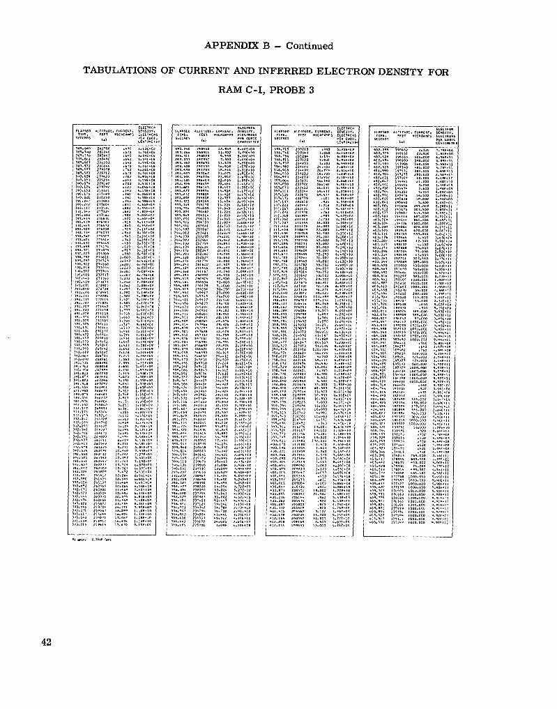
APPENDIX B - Continued
TABULATIONS OF' CURRENT AND INFERRED ELECTRON DENSITY FOR
RAlM C-I, PROBE 3
42

43

APPENDIX B - Continued
TABULATIONS OF CURRENT AND INFERRED ELECTRON DENSITY FOR
RAM C-I, PROBE 5
44

APPENDIX B - Continued
TABULATIONS OF CURRENT AND INFERRED ELECTRON DENSITY FOR
RAM C-I, PROBE 6
45

APPENDIX B - Continued
TABULATIONS OF CURRENT AND INFERRED ELECTRON DENSITY FOR
RAM C-I, PROBE 7
L
r, rr. . ,
46

APPENDIX B - Continued
TABULATIONS OF CURREN,T AND INFERRED ELECTRON DENSITY FOR
RAM C-I, PROBE 8
47
I

APPEIV.DE B - Continued
TABULATIONS OF CURRENT AND INFERRED ELECTRON DENSITY FOR
RAM C-II, PROBE 1
t
48

APPENDIX B - Continued
TABULATIONS OF CURRENT AND INFERRED ELECTRON DENSITY FOR
RAM C-11, PROBE 2
49

50
APPENDIX B - Continued
TABULATIONS OF CURRENT AND INFERRED ELECTRON DENSITY FOR
RAM C-II, PROBE 3

APPENDIX B - Continued
TABULATIONS OF CURRENT AND INFERRED ELECTRON DENSITY FOR
RAM C-II, PROBE 4
51

APPENDIX B - Continued
TABULATIONS OF CURRENT AND INFERRED ELECTRON DENSITY FOR
RAM C-11, PROBE 5
52

APPENDIX B - Continued
TABULATIONS OF CURRENT AND INFERRED ELECTRON DENSITY FOR
RAM C-II, PROBE 6
53

APPENDIX B - Continued
TABULATIONS OF CURRENT AND INFERRED ELECTRON DENSITY FOR
RAM C-It, PROBE 7
54

APPENDIX B - Concluded
TABULATIONS OF CURRENT AND INFERRED ELECTRON DENSITY FOR
RAM C-11, PROBE 8
55

APPENDIX C
ANALYSIS OF SPACECRAFT MOTIONS AND WIND ANGLES
By William L. Weaver Langley Research Center
The spacecraft axis system employed and its relation to the wind axis are illustrated in figure 41.
The rate gyro data show coning of the RAM C-I and C-11 spacecraft after separation of the expended fourth-stage motors, but the very low dynamic pressures and resulting low accelerations did not permit accurate determinations of the spacecraft wind angles from accelerometer data. Coning of the spacecraft was also indicated by the cyclic vari- ations in the electrostatic probe-measured electron densities observed during both flights. Figure 42 shows the correlation of measured normal aerodynamic acceleration with vari- ations in electron densities measured by probe 1 on RAM C-11 during the last few seconds before probe-rake retraction. Figure 43 shows that the electrostatic probe rake was in the same plane as the measured normal acceleration, and thus the correlation of figure 42 suggests that the cyclic variations in measured electron densities were due to displace- ments of the probe rake from the wind axis in the angle-of-attack (a) plane. The varia- tions were generally symmetrical; this symmetry further suggest that the average value of the electron densities corresponded to the zero-angle-of-attack case.
Determination of Wind Angles
Prior to separation of the fourth-stage motors, the RAM C-I and C-II spacecraft had roll momenta only with the X-axes fixed in direction. The separation impulses pro- duced uniform coning (precession) of the X-axes about the total angular momentum vec- tors. The motion is illustrated in figure 44, and the equations which describe it a r e
L = IZWZ
IZWl tme=- IXP
Ixp 1 VH = I~ COS e 2.rr
56

APPENDIX C - Continued
Values computed by these equations for both flights are given in table V. The preflight- measured moments of inertia and the flight-measured rotation rates are given in table VI. It can be seen from figures 4 1 and 44 that for the case of vo = 0 (X-axes initially alined with velocity vectors), the total wind angles will describe the cones of half-angle 8. Thus the absolute change in the total wind angle (I AT() is given by 2 8.
the angular motions of a rigid body was employed. At about 380 seconds, short-duration (0.01 second) angular impulses were applied; these impulses produced matchups of the gyro-measured lateral rotation rates. Total wind angle was set to zero q0 = 0). Fig- ure 45 shows the comparisons of the measured and program-computed spacecraft rotation rates. The required impulses were
To study the spacecraft motions further, a computer-programed set of equations for
(
L = 3.93 N-m-sec (2.9 lb-ft-sec) (RAM C-I)
L = 3.25 N-m-sec (2.4 lb-ft-sec) (RAM C-II)
These values are in good agreement with the impulses computed by equation (Cl). (See table V.) Figure 45 shows that both the magnitudes and frequencies of the rotation rates are closely matched. The frequencies are identical with the values of vb given in table V.
Figure 46 shows the histories of the program-computed values of the wind angles for the computer runs which produced the matchup in rotation rates. These values are not the actual histories of the in-flight wind angles. They do represent the characteris- tic trends, and the frequencies and absolute variations in the angles should closely approx- imate those in flight. Note that the maximum values of 77 a r e twice the values of the cone angles 8 in table V and that the frequencies of r] are identical to those listed for vH in table V. The component wind angles (a,@) are seen to have variations approxi- mately equal to *28 because the spacecraft is rolling on the surface of the precession cone as illustrated in figure 44. If it is assumed that the velocity vectors were alined with the spacecraft X-axes at stage separations, the variations in 77 were
O Z ~ 5 5 0 (for RAM C-I)
05r]Z40 (for RAM C-11)
and the peak-to-peak variations in the component wind angles were
a,p = *5O (for RAM C-I)
a!,p = *40 (for RAM C-11)
57

APPENDIX C - Concluded
Summary of Wind-Angle Analysis
Cyclic changes in the measured electron densities were shown to be due to the displacements of the electrostatic probe from the wind axis in the angle-of-attack (a!) plane. Peak-to-peak variations in the densities were produced by variations in angle of attack of a! = *5O (for RAM C-I) and a! = *4O (for RAM C-II). The symmetry of the density variation suggests that the average values corresponded to the case where a! = 0.

REFERENCES
1. Bachynski, M. P.: Electromagnetic Wave Penetration of Reentry Plasma Sheaths. Radio Sci., J. Res. NBS, vol. 69D, no. 2, Feb. 1965, pp. 147-154.
2. Anon.: Proceedings of the NASA Conference on Communicating Through Plasmas of Atmospheric Entry and Rocket Exhaust. NASA SP-52, 1964.
3. Akey, Norman D.: Overview of RAM Reentry Measurement Program. The Entry Plasma Sheath and Its Effects on Space Vehicle Electromagnetic Systems, Vol. I, NASA SP-252, 1970, pp. 19-31.
4. Jones, William Linwood, Jr.: Probe Measurements of Electron Density Profiles During a Blunt-Body Reentry. Ph. D. Thesis, Virginia Polytechnic Inst. & State Univ., June 1971.
5. Jones, W. Linwood, Jr.; and Cross, Aubrey E.: Electrostatic Probe Measurements of Plasma Surrounding Three 25 000 Foot Per Second Reentry Flight Experiments. The Entry Plasma Sheath and Its Effects on Space Vehicle Electromagnetic Systems, Vol. I, NASA SP-252, 1970, pp. 109-136.
6. Akey, Norman D.; and Cross, Aubrey E. (With appendix A by Thomas G. Campbell; appendix B by Fred B. Beck; and appendix C by W. Linwood Jones, Jr.): Radio Blackout Alleviation and Plasma Diagnostic Results From a 25 000 Foot P e r Second Blunt-Body Reentry. NASA TN D-5615, 1970.
7. Grantham, William L.: Flight Results of a 25 000-Foot-Per-Second Reentry Experi- ment Using Microwave Reflectometers To Measure Plasma Electron Density and Standoff Distance. NASA TN D-6062, 1970.
8. Sutton, Kenneth; Zoby, Ernest V.; and Butler, David H.: An Evaluation Test of a Full- Scale Replica of the RA”CA Flight Heat Shield in a Rocket-Engine Exhaust. NASA TM X-1841, 1969.
9. Schexnayder, Charles J., Jr.; Huber, Paul W.; and Evans, John S.: Calculation of Electron Concentration for a Blunt Body at Orbital Speeds and Comparison With Experimental Data. NASA T N D-6294, 1971.
10. Swift, C. T.; Gooderum, P. B.; and Castellow, S. L., Jr.: Experimental Investigation of a Plasma Covered, Axially Slotted Cylinder Antenna. IEEE Trans. Antennas Propagation, vol. AP-17, no. ‘5, Sept. 1969, pp. 598-605.
11. Croswell, William F.; and Jones, W. Linwood, Jr.: Effects of Reentry Plasma on RAM C-I VHF Telemetry Antennas. The Entry Plasma Sheath and Its Effects on Space Vehicle Electromagnetic Systems, Vol. I, NASA SP-252, 1970, pp. 183-201.
59

12. Scharfman, W. E.: The Use of Langmuir Probes To Determine the Electron Density Surrounding Re-Entry Vehicles. SRI Project 5034 (Contract NAS 1-3942), Stanford Res. Inst., June 1965.
13. Scharfman, W. E.; and Bredfeldt, H. R.: Use of the Langmuir Probe To Determine the Electron Density and Temperature Surrounding Re-Entry Vehicles. SRI Project 5771 (Contract NAS 1-4872), Stanford Res. Inst., Dec. 1966. (Available as NASA CR-66275.)
14. Hok, Gunnar; Spencer, N. W.; Reifman, A.; and DOW, W. G.: Dynamic Probe Measure- ments in the Ionosphere. AFCRC TN-58-616, U.S. Air Force, Nov. 1958.
15. Smetana, Frederick 0.: On the Current Collected by a Charged Circular Cylinder Immersed in a Two-Dimensional Rarefied Plasma Stream. Rarefied Gas Dynamics, Vol. 11, J. A. Laurmann, ed., Academic Press, Inc., 1963, pp. 65-91.
16. Dunn, Michael G.: Laboratory Measurements of Electron Density and Electron Tem- perature With RAM Flight Probes. The Entry Plasma Sheath and Its Effect on Space Vehicle Electromagnetic Systems, Vol. I, NASA SP-252, 1970, pp. 261-276.
17. Dunn, Michael G.: Experimental Plasma Studies. NASA CR-1958, 1972.
18. Webb, H., Jr.; Dresser, H.; Korkan, K.; and Raparelli, R.: Theoretical Flow Field Calculations for Project RAM. NASA CR-1308, 1969.
19. Suits, C. Guy; and Way, Harold E., eds.: The Collected Works of Irving Langmuir. Vol. 4 - Electrical Discharge. Pergamon Press, Inc., c.1961.
20. Laframboise, James G.: Theory of Spherical and Cylindrical Langmuir Probes in a Collisionless, Maxwellian Plasma at Rest. Rep. No. 100, Inst. Aerosp. Studies, Univ. of Toronto, June 1966. (Available from DDC as AD 634 596.)
21. Bernstein, Ira B.; and Rabinowitz, Irving N.: Theory of Electrostatic Probes in a Low-Density Plasma. Phys. Fluids, vol. 2, no. 2, Mar.-Apr. 1959, pp. 112-121.
22. Allen, J . E.; Boyd, R. L. F.; and Reynolds, P.: The Collection of Positive Ions by a Probe Immersed in a Plasma. Proc. Phys. SOC., vol. 70, pt. 3, no. 447B, Mar. 1, 1957, pp. 297-304.
23. Lam, S. H.: The Langmuir Probe in a Collisionless Plasma. AFOSR 64-0353, U.S. Air Force, Mar. 1964. (Available from DDC as AD 434 342.)
24. Chen, Francis F.: Numerical Computations for Ion Probe Characteristics in a Colli- sionless Plasma. MATT-252 (Contract AT(30-1)-1238), Plasma Phys. Lab., Princeton Univ., Feb. 1964.
25. Chen, Francis F.: Electric Probes. Plasma Diagnostic Techniques, Richard H. Huddlestone and Stanley L. Leonard, eds., Academic Press, 1965, pp. 113-200.
60

26. Bohm, David.; Burhop, E. H. S.; and Massey, H. S. W.: The Use of Probes for Plasma Exploration in Strong Magnetic Fields. The Characteristics of Electrical Dis- charges in Magnetic Fields, A. Guthrie and R. K. Wakerling, eds., McGraw-Hill Book CO., hc., 1949, pp. 13-76.
27. Sonin, A. A.: The Behaviour of Free Molecular Cylindrical Langmuir Probes in Super- sonic Flows, and Their Application to the Study of the Blunt Body Stagnation Layer. UTIAS Rep. No. 109, Univ. of Toronto, Aug. 1965.
28. Hoegy, W. R.; and Brace, L. H.: The Dumbbell Electrostatic Ionosphere Probe: Theo- retical Aspects. Rep. JS-1 (Contracts AF 19(604)6124, DA-20-018-509-ORD-103, and NASw-139), College Eng., Univ. Michigan, Sept. 1961.
61

TABLE I.- ALTITUDE, VELOCITY, AND TIME OF RAM C-I AND RAM C-II* REENTRY TRAJECTORIES
I Altitude
km
152.4 150.9 149.4 147.8 146.3 144.8 143.2 141.7 140.2 138.7
137.2 135.6 134.1 132.6 131.1 129.5 128.0 '
126.5 125.0 123.4 1
121.9 1
120.4 118.9 : 117.3 : 115.8 : 114.3 : 112.8 : 111.2 : 109.7 : 108.2 : 106.7 c 105.2 103.6 102.1 : 100.6 2 99.1 : 97.5 3 96.0 3 94.5 3 93.0 3
91.4 3 89.9 2 88.4 2 86.9 2 85.3 2 83.8 2 82.3 2
ft
500 X 103 495 490 485 480 475 470 465 460 455
450 445 440 435 430 42 5 420 415 4 10
105
400 395 390 385 380 375 3 70 365 360 I55
150 345 140 135 130 125 120 115 110 105
;oo :95 :90 85 80 75 70 65 60 I__
Velocity - m/sec
70 12 7095 7183 7277 7366 7460 7527 7564 7580 7579
7578 7580 7587 7590 7596 7597 7594 7594 7591 7602
7609 76 14 7611 7610 7610 7612 7616 7617 7619 7622
7626 7629 7627 7629 763 1 7628 7628 7633 7640 76 50
7649 7646 7642 7645 7649 765 1 7649 7649 7654
__
~
~
ft/sec
23 00' 23 271 23 567 23 87: 24 16Z 24 47f 24 696 24 81E 24 872 24 866
24 863 24 872 24 892 24 902 24 920 24 926 24 916 24 914 24 924 24 941
24 965 24 982 24 971 24 967 24 969 24 913 24 986 24 991 24 996 25 008
25 019 25 029 25 024 25 031 25 037 25 026 25 025 25 042 25 065
" . .
25 098
35 094 15 087 15 074 15 082 15 095 15 103 !5 094 !5 096 !5 113 ___
1 _____ Time from
lift-off, sec
355.98 356.83 357.64 358.42 359.19 359.98 360.77 361.57 362.34 363.11
363.81 364.64 365.40 366.18 366.95 367.13 368.49 369.25 310.00 370.75
371.52 372.30 373.08 373.85 374.61 375.37 376.14 376.92 377.70 378.47
379.23 379.99 380.75 381.52 382.29 383.01 383.86 384.63 385.39 386.14
386.88 387.64 388.40 389.17 389.93 390.70 391.46 392.23 393.00
-~ . - 1 r - km
77.7 76.2 74.7 73.2 71.6 70.1 68.6 61.0 65.5 64.0
62.5 61.0 59.4 57.9 56.4 54.9 53.3 51.8 50.3 48.8
47.2 45.7 44.2 42.7 41.4 39.6 38.1 36.6 35.0 33.5
32.0 30.5 29.0 27.4 25.9 24.4 12.9 31.3 19.8 18.3
16.8 15.2 13.7 12.2 10.7 9.1 7.6 6.1
-
__
Altitude
ft
255 X 103 2 50 245 240 235 230 225 220 215 2 10
205 200 195 190 185 180 175 170 165 160
155 150 145 140 135 130 125 120 115 I10
LO 5 too 95 90 85 80 75 70 65 60
55 50 45 40 35 30 25 20
_ _ ~ Velocity -
m/sec
7657 766 1 7670 7664 7660 7662 7665 7670 7668 7664
7657 7651 7655 7653 7643 7640 7630 7623 7610 7596
7568 7544 7517 7477 7432 7363 7279 7182 7072 6938
6759 6539 6232 5938 5555 5089 4552 3945 3238 2438
1739 1049 581 271 220 239 227 276
__
"~
__ ft/sec
25 121 25 135 25 164 25 143 25 131 25 139 25 148 25 165 25 156 25 145
25 123 25 102 25 115 25 108 25 076 25 064 25 034 25 009 24 967 24 923
24 829 24 752 24 663 24 532 24 384 24 157 23 882 23 563 23 202 22 763
22 176 21 455 20 446 19 483 18 226 16 697 14 935 12 942 10 624
". -
8 ooa 5 706 3 441 1 906
890 72 1 185 744 907
" -
"~
Time fron lift-off,
sec
393.77 394.54 395.30 396.07 396.83 397.59 398.36 399.13 399.89 400.65
401.41 402.18 402.94 403.11 404.48 405.25 406.02 406.79 407.56 408.32
409.09 409.86 410.64 411.42 412.20 412.99 413.80 414.61 415.43 416.26
417.12 418.00 418.91 419.81 420.87 421.96 423.16 424.51 426.12 428.22
430.88 434.69 440.26 448.98 459.34 467.88 475.40 484.45
-~
~ -~
*For time correlation purposes, between the times of 386.88 and 406.79 seconds, the C-lI spacecraft was 365.8 m (1200 ft) higher in altitude than listed in the table with a velocity of approximately 18 m/sec (60 ft/sec) greater than the value listed.
62

TABLE IL- POSITION OF FUNCTIONAL PARTS ON THE RAM C-I AND C-II PAYLOADS
RAM c-II
RAM c-I
RAM C-I
RAM c-II
RAM c-I I
RAM C-I
RAM C-II
RAM c-II
RAM C-I
RAM c-II
"" ~~ ~ ~~
Antenna
S-band open-ended guide (3344 M H z ) X-band conical horn (10 044 MHz) %-band conical horn (35 000 MHz) L-band open-ended guide (1116 M H z ) S-band open-ended guide (3344 MHz) X-band conical horn (10 044 MHz) &-band conical horn (35 000 MHz) L-band open-ended guide (1116 MHz) S-band open-ended guide (3344 MHz) X-band conical horn (10 044 MHz) Ka-band conical horn (35 000 MHz)
VHF axial cavity-backed slot (259.7 MHz) VHF axial cavity-backed slot (259.7 MHz)
X-band rectangular horn (9210 MHz) X-band rectangular horn (9210 MHz) X-band rectangular horn (9210 MHz) X-band rectangular horn (9210 MHz)
X-band rectangular horn (9210 MHz) X-band rectangular horn (9210 MHz) X-band rectangular horn (9210 MHz) X-band rectangular horn (9210 MHz)
VHF circumferential-slot array (259.7 MHz)
VHF circumferential-slot array (225.7 MHz)
L-band open-ended guide (1116 MHz) S-band open-ended guide (3344 MHz) X-band conical horn (10 044 MHz) Ka-band conical horn (35 000 MHz)
C-band rectangular horn (5800 MHz)
C-band rectangular horn (5700 MHz)
VHF circumferential-slot array (225.7 M H z ) - "~ ~" .. -
Probe rake
Electrostatic Thermocouple
RAM c-II Electrostatic
- ~. Thermocouple
a Center-line location of parts. - ~ ~
0 15.2 15.2
p~
" ~ ~~
4.6 4.6 4.6 23.1 23.1 23.1 23.1 70.1 70.1 70.1 70.1
75.2 75.2
82.8 82.8 82.8 82.8
80.5 80.5 80.5 80.5
97.5
109.2
106.2 106.2 106.2 106.2
106.7
118.4
114.8 ~" -~ 1
0 6.0 6.0
-__ 1.8 1.8 1.8 9.1 9.1 9.1 9.1 27.6 27.6 27.6 27.6
29.6 29.6
32.6 32.6 32.6 32.6
31.7 31.7 31.7 31.7
38.4
43.0
41.8 41.8 41.8 41.8
42.0
46.6
45.2
-~
123.4 pi! 123.4
123.4 48.6 123.4
~ ~ ~~~
-" 0
180 O I :ti 90 330 210 195 15
285 227 195 15
285 105
0 180
60 150 240 330
15 105 195 285 "_ "_ 195 15
285 105
32
30 "_
0.15 .15 .15 .76 .76 .76 .76 2.30 2.30 2.30 2.30
2.36 2.36
2.60 2.60 2.60 2.60
2.65 2.65 2.65 2.65
3.20
3.42
3.48 3.48 3.48 3.48
3.50
3.71
3.76
0 180
0 180
3.87 3.87
4.05 4.05
bNose diameter D is 31.90 cm (12.56 in.) for RAM C-I; nose diameter D is 30.48 cm (12.00 in.) for RAM C-IL
63

TABLE m.- RAM C-I TYPICAL INJECTION CYCLE AND FLOW RATE HJSTORY
__ Stagnation injection +
Valve number 3 -
2 L 6 E 5 s u 7
7
5
I I I I I I I 0 1.0 2.0 3.0 4.0
Time from start of cycle, sec
"~
Valve l o r - T 7 1 Flow rate I Altitude -r Valve for - Flow rate I Altitude 1 ""
Side njectic
- ." kg/=
0 0 0 0 0 0 0
0 0
" . ~ .
"
.014
.004
.018
.045 .068
0.009 .032 .064 .027 .064 .181 299
0.018 .054 .lo9 .036 .095 .249 .404
- "
""
. ."
i t -
""
Ib/sec km
0 0 0 0
0 0 0
0 85.( 0 84.c .03 83.: ,01 82.C .04 81.C .10 8O.C .15 79.1
0.02 71.1 .Ol 76.1 .14 75.1 .06 14.1
.40 -14 173.1 72.1
.66 171.1 0.04 69.1 .12 68.1 .24 61.1 .08 66.1 21 65.1 .55 64.1 .89 63.1
. .
"_ -
- - . . . . -
- .. . - . -
. . -. - , -.
3tagnai injecti,
jtagnatic injectio~ njectio~
Side &/set ~
0.023 .068 .I27 .045 .lo9 295 .458
0.021 .082 .163 .059 .145 .408 .644
0.032 .lo4 .195 .068 .159 .444 .703
3.036 .lo9 .195 .068 .159 I
__
"_
.. -
1 1
b/sec ft km
0.05 61.1
184 202 56.1 .65 187 462 57.1 .24 190 724 58.1 .lo 193 982 59.1 2 8 197 236 60.1 . I5 200 490
1.01 55.2 180 943
0.06 53.2 114 451 .18 52.2 171 212 .36 51.2 161 968 .13 50.2 164 722 .32
158 199 48.2 .90 161 466 49.2
1.42 47.2 154 937
0.07 45.2 148 484 2 3 44.3 145 267 .43 43.3 142 058 . I 5 42.3 138 864 .35 41.4 135 684 .98 40.4 132 511 1.55 39.5 129 532
0.08 37.5 123 137 .24 36.6 120 058 .43 35.7 117 010 .I5 34.1 113 981 .35 33.8 110 986
)
I
5 6 I
5 6 7
5 6 7
~
5 6 7
78 908
73 027 69 115 65 866 62 616 59 363
19 598 16 328 13 048 39 771 36 486 33 '205
!3 442 !O 185
3 635 0 348 I 054 ""
1 2 3 4 _ _
1 2 3 4
1 2 3 4
. . . . . . .
1 2 3 4
. .- . -.
I 2 3 4 ". "
T 5 6 7
_. . I
64

payload Purpose
RAM C-I Real-time telemetry RAM c- I I
RAM c-11
RAM C-11
RAM C-11 Reflectometer experiment
TABLE IV.- RAM C-I AND RAM C-II RADIO-FREQUENCY SYSTEMS
Frequency Transmi t te r
Antenna type Approximate Body location,
Band X/D Modulation RF power, MHz Remarks
wat ts
VHF
but delayed by onboard tape loop 3.76 FM 5 Circumferent ia l -s lot array 225.7 VHF Same data as red - t ime t e l eme t ry , 3.42 FM 5 Circumferent ia l - s lo t a r ray 225.7 VHF
""""""""""""""- 3.20 FM 5 Circumferent ia l -s lot array 259.7 VHF T w o slots, diametrically opposed 2.36 FM 5 Axial cavity-backed slots 259.7
for approximately 45 sec
C
Four horns, 900 spacing 2.65 PPM 500 peak Rectangular horn 9 210 X Four horns, 90° spacing 2.60 PPM 500 peak Rectangular-horn array 9 210 X
3.50 Pulse 800 peak Rectangular horn 5 800 C 3.71 Pulse 900 peak Rectangular horn 5 700
L 1 116 T-fed slot 0.1 .cw
Station number 3; x/D of 2.30 0.15, 0.76, 2.30, and 3.48 CW .1 Conical horn 10 044 X Station number 2; x/D of 0.76 0.15, 0.76, 2.30, and 3.48 CW .I Open-ended waveguide 3 344 S Station number 1; x / D of 0.15 _" , 0.76, 2.30, and 3.48
K, 35 000 Conical horn .1 CW 0.15, 0.76, 2.30, and 3.48 Station number 4; x/D of 3.48
""""""""_""""""" """""""""""""~""

TABLE V.- COMPUTED VALUES OF IMPULSE, PRECESSION CONE ANGLE, AND
PRECESSION FREQUENCIES (EQS. (Cl) TO (C4))
Flight VH, V b’ N-m-sec lb-ft-sec Hz Hz
c-I I c-I1 I 3.7
~ 3.2
2.7
2.3
2.48 0.704 2.25 1 2.00 I .800 1 2.25 I
TABLE VI.- PREFLIGHT-MEASURED SPACECRAFT MOMENTS OF INERTIA*
AND FLIGHT-MEASURED ROTATION RATES
IX IZ IY Flight w 2 9 P,
kg-m2 rad/sec rad/sec slug-ft2 kg-mz slug-ft kg - m2 slug-ft2
c -I .175 19.1 13.22 17.92 13.32 18.06 3.45 4.68 c -11 0,190 18.5 14.50 19.66 14.24 19.31 3.41 4.62
I * Moments of inertia constant during data period.

L-71-7172 (a) S-159; RAM C-I. (b) S-168; RAM C-II.
Figure 1.- Launch vehicles.
67
L

40
al U
c,
c, -1
.-
30
800 70' 60'
& Launch l lops s i te
L a t i o n Launch s i t e NASA Wallops ;3-%\ USA Reentry region data
Station . L
Bermuda@
0 Aircraft B Ship
BUSNS Range Recover
I ONASA 438 twin NASA 4 3 2 0 4 I Fal ls Vic
250
200 -
E 150 -
0)
cr -rl cr
n
100-
50 -
0-
(a) RAM C-I1 ground track.
~- 4
er
tory
31
.OO
00
800 x 103 3d ignition
600 -
0 100 200 300 400 500 600 700
I I I I I I I I I I I I I 1 Range from Wallops Island, i n t . n . m i .
0 100 200 300 400 500 600 700 800 900 1000 1100 1200 1300 Range from Wallops Island, km
(b) RAM C-I and C-11 flight events.
Figure 2.- Ground track and flight events.
68

25 x 10 500 x r
7[ 6 20
5
1
0 f 0
100
25c 0
201
10
Events
0 RAM C-I
0 RAM c-I1
Velocity
d c-I
Time from lift-off, sec
Figure 3 . - Reentry trajectories.
I

130.25 cm
1
Phenolic-graphite charring ablator Nose radius 15.95 cm
Microwave reflectometer antennas
Beryllium heat sink Nose radius 15.24 cm
129.54 cm
L-71-7173 (a) RAM C-I. (b) RAM C-II.
Figure 4.- Payload configurations shown with fourth-stage engines and separation motors.
70

C-band horn
circumferenti
Thermocouple probe rake stagnation orifices orifices telemetry horns
(a) RAM C-I.
Beryllium heat sink
-Electrostatic probe rake
C-band horn
.a1 slot
S circumferential slot
circumferential slot
Reflectometer diagnostic antennas are designated L. S, X and K,. Thermocouple probe rake
horns
(b) RAM C-II.
Figure 5. - Electrostatic probe and radio-frequency antenna locations.
71

L-67-5814 (a) Photograph of rake.
Figure 6.- Electrostatic probe rake.
72

0 radius-, 0.0127 cm (.005 i n . )
Leading-edge d e t a i l Iridium i o n collectors
Payload surface
collector
Ion Standoff distance, 1 coliector cm I i n .
I
0.96 1 .84 2.70 3.58 4.46 5.34 6.20 7.08
0.378 .724
1.062 1.408 1.754 2.102 2.438 2.790
(b) Detail sketch of rake. Collection area of each ion collector was 0.0420 cm2 (0.006 in2).
Figure 6.- Concluded.

E l e c t r o n c o l l e c t o r s
Bias supply 5 volts
Figure 7.- Circuit diagram for electrostatic probe system.

Elec t ros ta t ic p robe : Mechanica l rake commutator
Logarithmic a m p l i f i e r
Subcarr'ier o s c i l l a t o r
Bias supply
. .
L-70-8365.1 Figure 8.- Major components of electrostatic probe system.

1
10
10
Input , v o l t s
10
10
1u 0 1 2 3 4 + - ou tpu t , vo l t s
(a) Dynamic input-output curves.
k p u l s e w i d t h Center SOgL o f
n L I 5
Delay tim Rise time F a l l time
I " 0 1 2 3 4
Time, mil l iseconds
(b) Typical pulse-response curve.
Figure 9. - Electrical characteristics of logarithmic amplifiers.
76

. Ful l ." 1
T y p i c a l , b e f o r e d a t a
p e r i o d
Z a l i b . pu l se :
- Time
T y p i c a l , d u r i n g d a t a
p e r i o d
I
Palib- pulses
100 m s 1 Figure 10.- Electrostatic probe data format.

L-71-7150
(a) Photograph of rake.
L e a d i n g - e d g e d e t a i l
Thermocouple S t a n d o f f d i s t a n c e , y cm I i n . ..
" ~ ~ ~~ -
I 1 2 3
0.788 1.576 2.364
i s t
(b) Rake configuration. Thermocouple distance from leading edge for RAM C-I was 0.0635 cm (0.025 in.) and for RAM C-II, the distance was 0.1016 cm (0.040 in.).
Figure 11.- Thermocouple probe rake.
78

Ne. probe
Ne, microwave
0.1- 1010 1
I 1 I I I I l l I 1 I 1 1 1 1 - 4 ' - T Stanford Research Insti tute
- -
&
( r e f . 13) I Cornell Aeronautical Laboratories- ( r e f . 171 11
-
1 1011
11 1012
Ne, microwave
Figure 12.- Ratio of electron densities inferred from probes and from microwave data as a function of electron density inferred from microwave data.

:tion
,tion
"
390 395 400 Elapsed time, sec
405
I I I I 1 I I I 1 I 280 260 240 220 200 180 X Ib3
Altitude, ft
I I I 1 85 80 75 70 65 60 55
Altitude, km
(a) Electrostatic probes 1 and 2.
Figure 13.- Ion current measurements from electrostatic probes on RAM C-I flight experiment.
80

. t ion
t i o n
"
390 395 400 Elapsed time, sec
405
I I I I I I I I I I I I
I'~I I I 1 I ~~
280 260 240 220 200 180 x ;OB
A l t i t u d e , f t
85 80 75 70 65 60 55 Alt i tude, km
(b) Electrostatic probes 3 and 4.
- Figure 13. - Continued.
81

4 :tion
E H 0
"
390 395 400 E l a p s e d t i m e , s e c
405
I I I I I "
I I I I ~ ~ ".I I 280 260 240 220 200 180 x lo3
A l t i t u d e , f t
85 80 75 70 65 60 55 A l t i t u d e , km
(c) Electrostatic probes 5 and 6.
Figure 13.- Continued.
82
I

t ion
"
390 395 400 Elapsed time, sec
405
l l l l l l " 280 260 240 220 200 180 x 103
A l t i t u d e , f t
I I I I I I 85
~ ~
80 75 7 0 65 60 55 A l t i t u d e , km
(d) Electrostatic probes 7 and 8.
.tion
Figure 13.- Concluded.
83
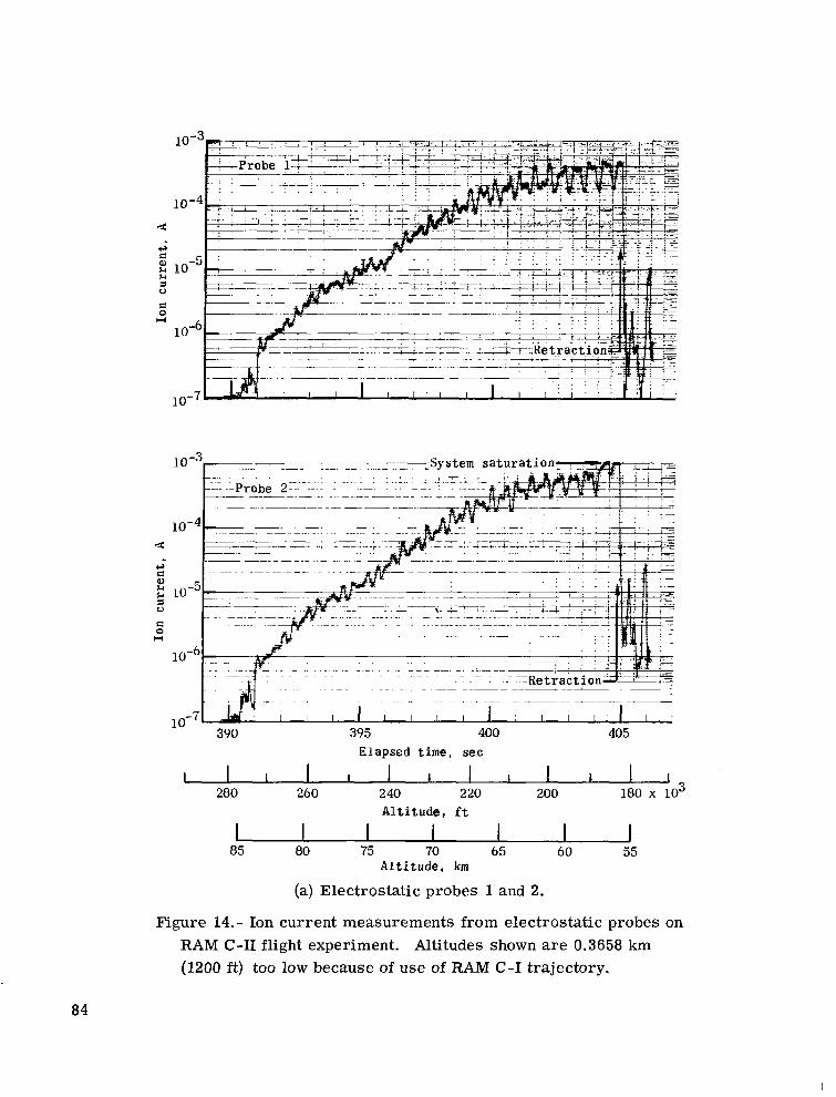
I I I I I 1 I 1 I I I I
I I I I I I I
280 260 2 40 220 200 180 x :03 Altitude, ft
85 80 75 70 65 60 55 A l t i t u d e , km
(a) Electrostatic probes 1 and 2.
Figure 14.- Ion current measurements from electrostatic probes on RAM C-11 flight experiment. Altitudes shown are 0.3658 km (1200 ft) too low because of use of RAM C-I trajectory.
84
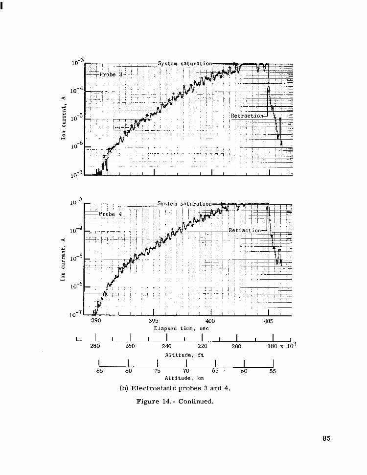
1 o - ~
1 0 8
10"
10"
s H 0
10"
10-
I 1 -1" I I I I I I I I I I
I I~ I I I I I
280 260 240 220 200 180 x 103 A l t i t u d e , f t
85 80 75 70 65 . 60 55 A l t i t u d e , km
(b) Electrostatic probes 3 and 4.
Figure 14.- Continued.
85

390 395 400 E l a p s e d time, sec
405
1- 280 260 240 2 20 200 180 x 103
A l t i t u d e , f t
I I I I I I 85 80 75 70 6 5 6 0 55
A l t i t u d e , km (c) Electrostatic probes 5 and 6.
Figure 14. - Continued.
86

E H 0
6:
1 o - ~
lo-<
10-f e
C
H 0
1 d t
. . . . ~. ~-
.-L"l"l"LL" 1 I I I I I I
390 395 400 405 Elapsed time, sec
A 1 ~I" I I I I I I I I 280 260 240 220 200 180 x lo3
Altitude, ft
I " 1 I I I I 1 85 80 75 70 65 60 55
Altitude, km
(d) Electrostatic probes 7 and 8.
Figure 14. - Concluded.
87
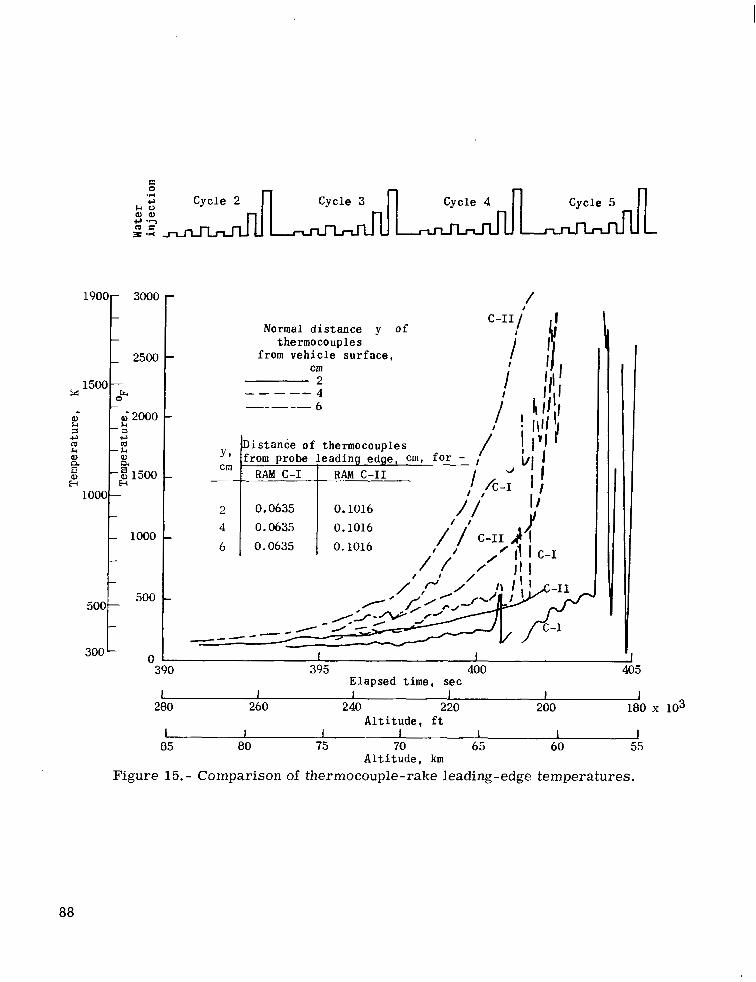
1900- 3000 -
-
- 2500
* -k 1500
0 - a k S c, Q
-I
m m Q k - k
a a (u
E H Fl
2000
Q - 2 1500
1000 -
- - 1000
-
I-
5001 500
Normal distance y of thermocouples
from vehicle surface, Cm
2 4 "-"
Y1
cm
2 4
6
I I i
6 I Iistance o f thermocouples from probe
RAM C-I
0.0635
0.0635
0.0635
0.1016 I / 0.1016 0.1016 /'j C
I /
-11 #44 / /' /' It I
' 11 I c-I
395 400 Elapsed time, sec
405
I I I I I 280 260 240 220 200 m'o x 103
Altitude, f t
85 80 75 70 65 60 55 Altitude, km
Figure 15. - Comparison of thermocouple-rake leading-edge temperatures.
88
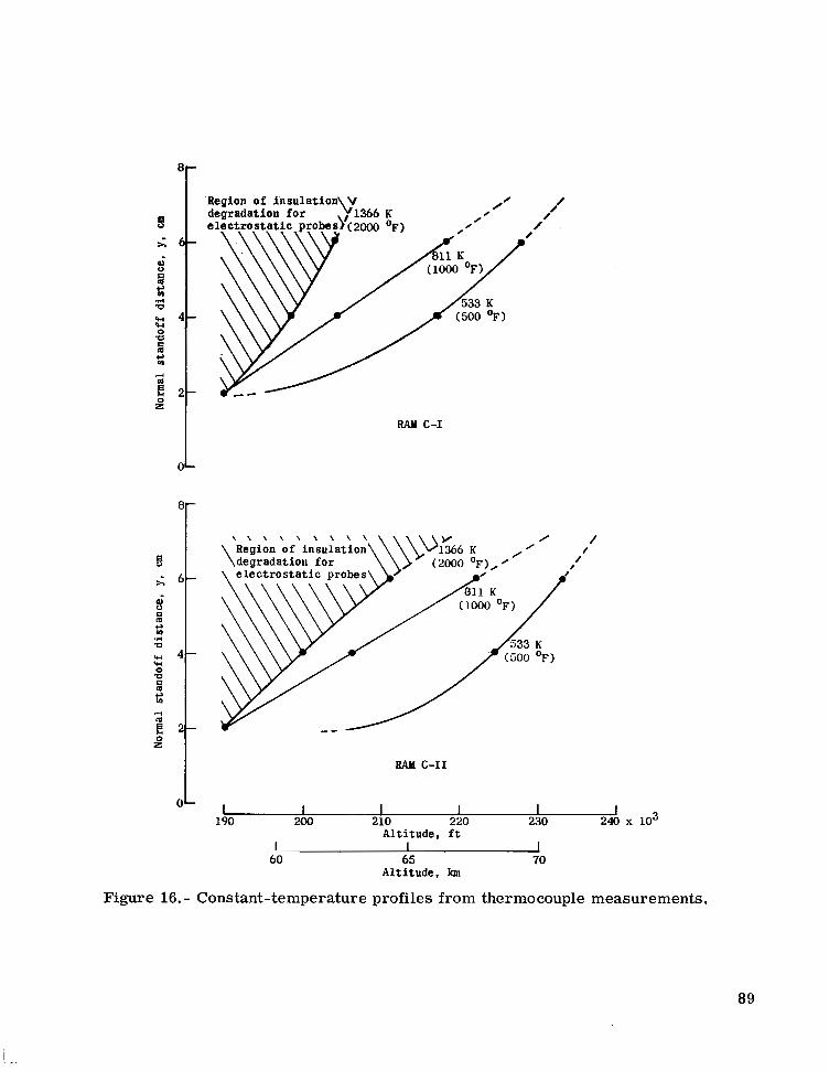
/ degradation for 1 1
0 /
RAN c-I
/ /
/
BAY c-I1
I I I 1 I
1 1
190 200 210 220 230 2 2 x 10³
L Altitude, ft
60 65 70 Altitude. km
Figure 16. - Constant-temperature profiles from thermocouple measurements.
89

c t i o n
lction
390 395 400 Elapsed time, sec
405
'$1 A l t i t u d e , f t
85 80 75 70 65 60 55 A l t i t u d e , km
(a) Electrostatic probes 1 and 2.
Figure 17.- Electron density of RAM C-I flow field at standoff distances y ranging between 1 and 7 cm as inferred from electrostatic probe measurements.
90

.ion
Elapsed time, sec
I I I I I I I I I I 280 260 240 220 200
Altitude, f t
I I I I I I I 85 ' 80 75 70 65 60 55
(b) Electrostatic probes 3 and 4.
Figure 17.- Continued.
Altitude, km
91

. n
ction
"
390 395 400 Elapsed time, sec
405
I I I I I I I 1 1 I 1 280 260 240 220 200
Altitude, f t
1 I I I I 1 I 85 80 75 70 65 60 55
A l t i t u d e , km
(c) Electrostatic probes 5 and 6.
Figure 17. - Continued.
92

.tion
"
390 395 400 405 Elapsed time, sec
I" -1.. ~ I 1 I I I 1 I I I I 280 260 240 220 200 180 x 103
Altitude, ft
85 80 75 70 65 60 55 Altitude, km
I I I I I I
(d) Electrostatic probes 7 and 8.
Figure 17. - Concluded.
93

I I I I I I I 85 80 75 70 65 60 55
A l t i t u d e , km
(a) Electrostatic probes 1 and 2.
Figure 18.- Electron density of RAM C-11 flow field at standoff distances y ranging between 1 and 7 cm as inferred from electrostatic probe measurements. Altitudes shown are 0.3658 km (1200 ft) too low because of use of RAM C-I trajectory.
94

I I I I I I I 85 80 75 70 65 60 55
Altitude, km
(b) Electrostatic probes 3 and 4.
Figure 18. - Continued.
95

E 0 h c,
z 1of w 4
IO'
I I I I I 1 I I I I I
I I I I
280 260 240 220 200 180 x 103 Altitude, f t
85 80 75 70 65 60 55 Altitude, km
( c ) Electrostatic probes 5 and 6.
Figure 18. - Continued.
96

:'Pro'be 8, . . " . . .
. . .
. .
. .
. y. :
.rl VI E al U
E
I I I I I 85 80 75 70 65 60 55 -~
A l t i t u d e , km
(d) Electrostatic probes 7 and 8.
Figure 18.- Concluded.
97

. . _. .. . . . . ... . - . . . . . .. .-
0 1 2 3 4 5 7 8
Standoff distance, y, crn
Figure 19.- Measured time-average electron density profiles for RAM C-I at selected altitudes during no water injection.
98

System saturation
t T
Alt i tude Kilometers Feet
0 80.8 265 000 0 76.2 250 000 0 71 .0 233 000 A 61.0 200 000
1 Excursion due t o body motion
I I I I I I t I 1 2 3 4 5 6 7 8
Standof f d i s tance , y , cm
Figure 20.- Measured time-average electron density profiles for RAM C-II at four altitudes.
99

r u al Z 107 1 Probe 1 ; y = 0.96 cm
N r
H 107 Probe 3; y = 2.70 cm
w 2Ao 2Ao 260 2:o 2Ao Ibo x 103
Alt i tude, f t
> 85 80 75 70 65 60 55
Alt i tude, km
L Probe 2; y = 1.84 cm
1 Probe 4; y = 3.58 cm
28Lo 2Ao 260 2bo llgo x 103 - Alti tude, f t
85 80 75 70 65 60 55 Alt i tude, km
(a) Probes 1 to 4.
Figure 21.- Comparison of measured electron densities for individual probes on RAM C-I and C-II. Altitudes for RAM C-I1 data are 0.3658 km (1200 ft) too low because of use of RAM C-I trajectory.

107 Probe 5; y = 4.46 cm I I I I 1
Probe 6 ; y = 5.34 cm I I I I I
r ." "IY'
i 85 80 75 70 65 60 55
Alti tude, km 85 80 75 70 65 60 55
Alti tude, km
(b) Probes 5 to 8.
Figure 21. - Concluded.

r Approximate bow shock
.
,, E l e c t r o s t a t i c
F l i g h t p a t h
"I'=. E l e c t r o s t a t i c
--e-- Normal a c c e l e r a t i o n , An
- E l e c t r o n d e n s i t y , Ne X O h m w * X
Probe 1 , RAM C - I 1 + P s -k $ E
U Q ) o n w M 0
O.!! 1 0 $a Q) O u m
s w m.c c,
iJ - w w m o M
a s o m aril In-
A m
- E O w 2
Figure 22.
probe rake
403 ~~
404 Time, sec
405
I I 195 190
A l t i t u d e , ft I I I 1
59 58 57 56 A l t i t u d e , km
Correlation of RAM C-II fixed-bias electrostatic probe measurements with spacecraft angle-of -attack motions.
102

0
1071 Probe 3
l0"i
IIIIII 280 260 240 220 200 180 x lo3
Altitude, ft
I ~ U 85 80 75 70 65 60 55
Altitude, krn
n, Cycle 2 3 4 5
I" 280 260 240 220 200 180 X lo3
Altitude, ft - a5 80 75 70 65 60 55
Altitude, km
Figure 23.- Effects of water injection on electron density as inferred by RAM C-I electrostatic probes.
103

Altitude Kilometers Feet
b 73.981 242 720 v 72.832 238 949 0 70.702 232 223 0 71.881 235 829
Mean level of pre- and post-injection period for cycle 3
I I 1 I 0 1 2 3 4 5 6 7 8
Standoff distance, y . cm
Figure 24.- RAM C-I electron-density distribution profiles during side injection portion of cycle 3.
104

I
Time, Altitude
sec Km F t
398.10 69.095 226 690
398.25 68.799 225 717 398.20 68.897 226 041
398.28 68.739 225 523 398.35 68.601 225 068
e 8 398.40 68.502 224 743
Standoff distance, y , cm
Figure 25. - Effect of stagnation injection at flow rate 5 of cycle 4 on RAM C-I electron density distribution profiles at various altitudes.
105

ooOA Reflectometer measurements
I probe E l e c t r o s t a t i c
I Excursion due t o body motion 1 measurements
Probe 1 OM+ Probe 8
-r
Alt i tude , km ( f t )
( 200 000)
Distance along payload, inches L I I I I I
0 .25 0.50 0.75 1.00 1.25 Distance along payload, meters
Figure 26.- RAM C-11 longitudinal profiles of inferred peak electron density for constant altitudes.
106

30
20 Bermuda s t a t i o n ,
LCP- I
30 20
Bermuda s t a t i o n ,
40
10
Twin Fa l l s V ic tory s ta t ion , LC!?
6.0
4.0
Spacecraft antenna L I I l l I I l l l I
385 390 395 Elapsed time, sec
A l t i t u d e , f t
1 310 290 270 ' 250 x 103
I I 95 90 85 80 75
A l t i t u d e , km
Figure 27.- Effects of RAM C-I reentry plasma on 225.7 MHz telemetry antenna. LCP, left circular polarization; RCP, right circular polarization.
107
L

50
30 20
30 20
10
LCP. I
Bermuda s t a t i o n RCG 1
T w i n F a l l s V i c t o r y s t a t i o n , LCP k "1 __J" I Ne,cr r e g i o n
1.0 S p a c e c r a f t a n t e n n a
I I I I I I I I I I 385 3 90 395
I I I E l a p s e d t i m e , s e c
310 290 270 ' 250 x 103 A l t i t u d e , f t
I 95 90 85 80 75
A l t i t u d e , km
Figure 28.- Effects of RAM C-I reentry plasma on 259.7 MHz telemetry antenna. LCP, left circular polarization; RCP, right circular polarization.
108

E .n m
s I m 2 -120 cl Bermuda s t a t i o n . LCP ro
m
al 3 0 r.
5 . 0
:-I 2.0
1 .0
0 Spacecraft antenna
11111111111 335 390 395
Elapsed t ime, sec - 310 290 270 250 X 103
Alt i tude . it
A l t i t u d e , k m
P 9
Figure 29.- Effects of RAM C-II reentry plasma on 225.7 MHz telemetry antenna. LCP, left circular polarization; RCP, right circular polarization.
109

0 C-11 r e f l e c t o m e t e r , s t a . 3" C-11 r e f l e c t o m e t e r , s t a . 4"
C-I and C - I 1 225.74" ring* -1 C-I 259.7-MHz s l o t "
* Data co r rec t ed t o p robe body s t a t i o n
l08L I I I I I 160 180 200 2 20 240 260
A l t i t u d e , f t
1 I 1 I I 1 2 50 55 60 65 70 75 80 85
A l t i t u d e , km
Figure 30.- Comparison of inferred electron densities.
110

Standoff distance, y , cm
Figure 31.- Comparison of RAM C-II electrostatic probe measured data with theoretical electron density profiles.
111
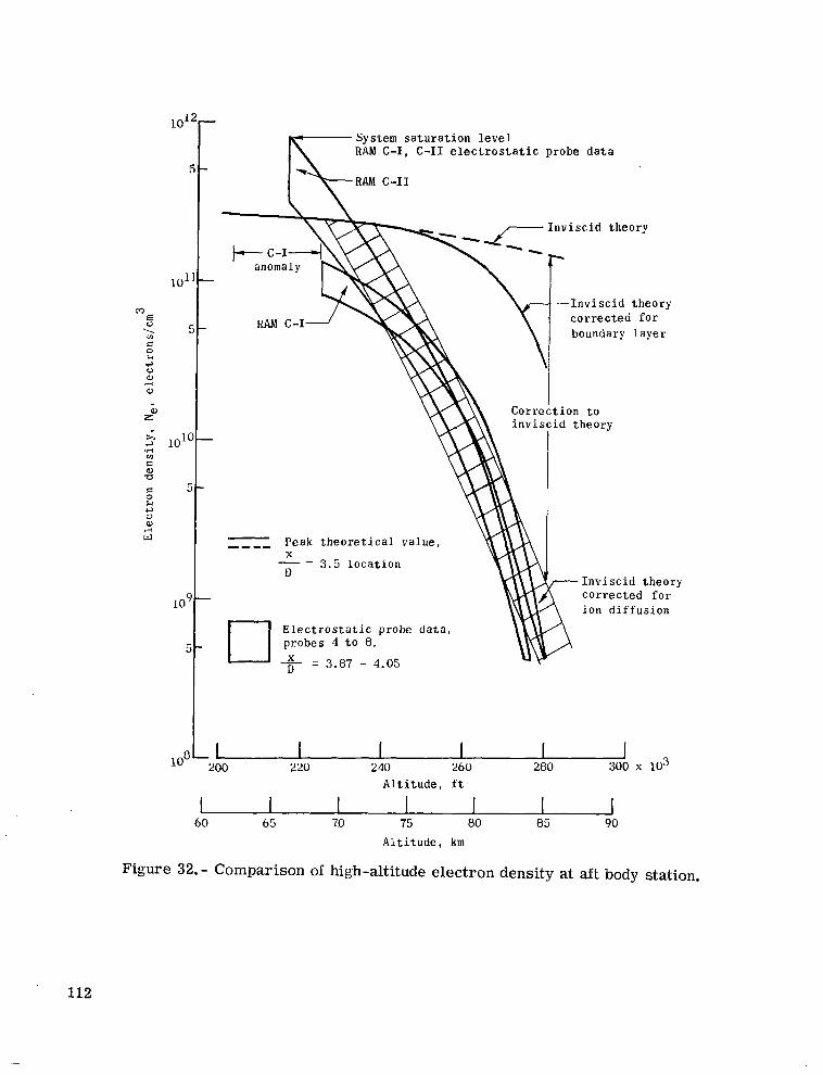
10.
10’
10
lof
Sys tem sa tu ra t ion l eve l RAM C-I, C - I 1 e l e c t r o s t a t i c p r o b e d a t a
- - < I n v i s c i d t h e o r y
anomaly f RAM C-I J‘
I n v i s c i d t h e o r y c o r r e c t e d f o r boundary layer
C o r r e c t i o n t o i n v i s c i d t h e o r y
I
- - - ” P e a k t h e o r e t i c a l v a l u e , x - D ” 3 . 5 l o c a t i o n
E l e c t r o s t a t i c p r o b e d a t a , p robes 4 t o 8,
= 3.87 - 4.05
I n v i s c i d t h e o r y Cor rec t ed fo r i o n d i f f u s i o n
I I I I I 200 220 240 260 280
A l t i t u d e , f t
I I 1 I I 1 60 65 79 75 80 85 90
A l t i t u d e , km
Figure 32.- Comparison of high-altitude electron density at aft body station.
112

T T D a t a f a i r i n g
I E lec t ros ta t ic p robe da ta , mean value of probes 1 t o 8
Reflectometer data , s ta t ion 4 (ba r s r ep resen t 2 f a c t o r o f 2 error) I - Theory, s ta t ion 4
0
w Payload
1 n9 1 I Reflectometer s ta t ion qJ t E l e c t r o s t a t i c probe rake
A l t i t u d e , f t I I I I I
50 60 70 80 90 A l t i t u d e , km
Figure 33. - Comparison of RAM C-I1 plasma diagnostic measurements with theoretical calculations.

-. 1 - 1 - 10 - 100 - 1000
*P
Figure 34.- Variation of normalized probe current with normalized potential difference between probe and plasma for range of y.

Y -
Figure 35. - Inverted form of space-charge-limited diode equation.
115

10-1
Figure 36. - Normalized current I,
100 S
collected by a probe perpendicular to the directed velocity as a function of the ratio S of directed to random veloc- ity. Dashed lines indicate asymptotes.
116

In
2O t 10 - s = 10 I
a - - 6 - -
4 - . s = 3 -
2 - s = 1
E
1 - 0.01 - 0.1
7 = 100
Results f o r 7 = 30 are ident ic ; except f o r S = 30
; = 0.3
I I I I 1111 I I I I I I I I I I I I I I l l - 1.0 - 10
I
xP
Figure 37.- Variation of normalized current with dimensionless probe potential for various speed ratios at y = 100.

R
-J 40
.1 1 10 100 1000
H
Figure 38.- Normalized probe current R as a function of the ratio of modified potential energy to the kinetic energy H for various values of y.

10"
collector Ion
0 1 D 2 0 3 A 4 h 5 0 6
0 8 n 7
-~ " q . x
l -
O b A 0 I I I I I
200 2 20 240 260 280 Altitude, ft
I I I I I I I 1 55 6 0 6 5 70 75 80 85 90
Altitude, km
Altitude, ft I I I I I I I 1
55 6 0 6 5 70 75 80 85 90 Altitude, km
Figure 39. - Computed gas temperature as a function of altitude for electrostatic probe locations.
119

K 10 5 -
I I I I I I 180 200 220 240 260 280
A l t i t u d e , f t
I I I I I I I 1 55 60 65 70 75 80 85 90
Altitude, km
Figure 40. - Computed flow velocity as a function of altitude for electrostatic probe locations.
120

$ z (a) Illustration of body rotations.
\
(b) Illustration of orientation with wind axis.
Figure 41. - Spacecraft axis sy'stem.
12 1

I I
Electron density Ne; probe 1
an ””_
7 x 10l1 i-
A - 6- 5- 4
3-
2- Probe rake retraction I I I I - 403 4 04 405
Time, sec I I I I
200 195 190 185
L I I I I I 60 59 58 57 56 55 km
Altitude
Figure 42.- Correlation of measured electron densities with measured normal acceleration on RAM C-II.
122

+all i'"
Looking forward (into paper)
J-Aerodynamic shock - " "
Wind axis V
-Electrostatic probe rake
Figure 43.- Locations of probe rakes relative to axes systems.

. .. ." . . . . . - .. .. ._ . . "" ."
c
"
center of mass
of X-axis
Initial direction of X-axis
Figure 44. - Spacecraft precession in force-free space.
124

+ Gyro-measured - Computed
380.0 380.4 380.8 381.2 381.6 382.0 Time, sec
(a) RAM C-I.
380.0 380.4 380.8 381.2 381.6 382.0
Time, sec
(b) RAM C-II.
Figure 45.- Comparisons of gyro-measured spacecraft rotation rates with computed rotation rates.
125
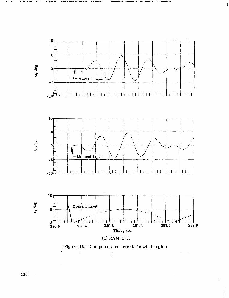
I I 1 II I I 1 IIIII I 1 I1 I I 11111111 11111111111111111111 1111111 1 1 1 1 111 I111111111 1111.111111111111 I 1111111 I1 I 111 11- I I I I1 .I- I111
M W .. U
M W a
380.0 380.4 380.8 381.2 381.6 382.0 Time, sec
(a) RAM C-I.
Figure 46. - Computed characteristic wind angles.
126

W M a c? ..
M W P
r ..
Time, sec
(b) RAM C-II.
Figure 46. - Concluded.
I
127