Electrospun Nanofiber Yarns for Nanofluidic Applications

Clemson UniversityTigerPrints

All Dissertations Dissertations

8-2013

Electrospun Nanofiber Yarns for NanofluidicApplicationsChen-Chih TsaiClemson University

Follow this and additional works at: https://tigerprints.clemson.edu/all_dissertations

Part of the Materials Science and Engineering Commons

This Dissertation is brought to you for free and open access by the Dissertations at TigerPrints. It has been accepted for inclusion in All Dissertations byan authorized administrator of TigerPrints. For more information, please contact [email protected].

Recommended CitationTsai, Chen-Chih, "Electrospun Nanofiber Yarns for Nanofluidic Applications" (2013). All Dissertations. 1609.https://tigerprints.clemson.edu/all_dissertations/1609

https://tigerprints.clemson.edu?utm_source=tigerprints.clemson.edu%2Fall_dissertations%2F1609&utm_medium=PDF&utm_campaign=PDFCoverPages

https://tigerprints.clemson.edu/all_dissertations?utm_source=tigerprints.clemson.edu%2Fall_dissertations%2F1609&utm_medium=PDF&utm_campaign=PDFCoverPages

https://tigerprints.clemson.edu/dissertations?utm_source=tigerprints.clemson.edu%2Fall_dissertations%2F1609&utm_medium=PDF&utm_campaign=PDFCoverPages

https://tigerprints.clemson.edu/all_dissertations?utm_source=tigerprints.clemson.edu%2Fall_dissertations%2F1609&utm_medium=PDF&utm_campaign=PDFCoverPages

http://network.bepress.com/hgg/discipline/285?utm_source=tigerprints.clemson.edu%2Fall_dissertations%2F1609&utm_medium=PDF&utm_campaign=PDFCoverPages

https://tigerprints.clemson.edu/all_dissertations/1609?utm_source=tigerprints.clemson.edu%2Fall_dissertations%2F1609&utm_medium=PDF&utm_campaign=PDFCoverPages

mailto:[email protected]

i

ELECTROSPUN NANOFIBER YARNS FOR NANOFLUIDIC APPLICATIONS

A Dissertation

Presented to

the Graduate School of

Clemson University

In Partial Fulfillment

of the Requirements for the Degree

Doctor of Philosophy

Materials Science and Engineering

by

Chen-Chih Tsai

August 2013

Accepted by:

Dr. Konstantin G. Kornev, Committee Chair

Dr. Igor Luzinov

Dr. Douglas E. Hirt

Dr. Gary C. Lickfield

Dr. Fei Peng

ii

ABSTRACT

This dissertation is centered on the development and characterization of

electrospun nanofiber probes. These probes are envisioned to act like sponges, drawing

up fluids from microcapillaries, small organisms, and, ideally, from a single cell. Thus,

the probe performance significantly depends on the materials ability to readily absorb

liquids. Electrospun nanofibers gained much attention in recent decades, and have been

applied in biomedical, textile, filtration, and military applications. However, most

nanofibers are produced in the form of randomly deposited non-woven fiber mats.

Recently, different electrospinning setups have been proposed to control alignment of

electrospun nanofibers. However, reproducibility of the mechanical and transport

properties of electrospun nanofiber yarns is difficult to achieve. Before this study, there

were no reports demonstrating that the electrospun yarns have reproducible transport and

mechanical properties. For the probe applications, one needs to have yarns with identical

characteristics. The absorption properties of probes are of the main concern. These

challenges are addressed in this thesis, and the experimental protocol and characterization

methods are developed to study electrospun nanofiber yarns.

A modified electrospinning setup was built which enables control of the

properties of electrospun yarns. A library of e-spinnable polymers was generated and the

polymers successfully electrospun into yarns. A unique technique for characterization of

yarn permeability was developed. The produced electrospun yarns have permeabilities

spanning two orders of magnitude (10-14

~10-12

m2). The yarns made from porous fibers

iii

can significantly increase the absorption rate. The produced yarns have been applied for

diagnosis of sickle cell disease. Using the experimental protocol developed for

characterization of yarn permeability, the permeability of a butterfly proboscis was

examined for the first time. The electrospun yarns and methods of characterization

developed in this study will find many applications.

iv

DEDICATION

This dissertation is dedicated to my family. Your constant love, support, and

encouragement have guided and helped me during my PhD studies. I would like to thank

you all for your prayers and support.

v

ACKNOWLEDGMENTS

This dissertation could not have been completed without the help of many

individuals. First of all, I would like to thank my advisor, Dr. Konstantin G. Kornev, for

his support, guidance, and patience during my PhD study. He shared with me not only the

excitement of research but also advised me in many other sides of my life. His guidance

has provided me with a broad knowledge in the field of porous materials. I am also very

grateful to my committee members, Dr. Igor Luzinov, Dr. Douglas E. Hirt, Dr. Gary C.

Lickfield, and Dr. Fei Peng for their critical comments and valuable suggestions for the

research.

Many thanks to all past and current group members for their help, suggestions,

and encouragements during my graduate study: especially, Yu Gu and Dr. Daria

Monaenkova in the development of Matlab® codes. Also, I would like to acknowledge

the help of undergraduate students, Edgar White, Joseph Howe, and Kara Phillips. I

would like to extend thanks to the MSE staff, particularly Kim Ivey, James Lowe,

Stanley Justice, and Robbie Nicholson, for helping me learn many tricks of analytical

polymer and textile chemistry and engineering.

I enjoyed the time spent with Dr. David Lukas and Dr. Petr Mikes from Technical

University of Liberec, Czech Republic. These conversations enriched my knowledge in

electrospinning. I would like to extend special acknowledgements to Dr. Alexey Aprelev

from Drexel University for the collaboration on the development of new application of the

electrospun nanofiber yarns for diagnosis of the sickle cells disease. Dr. Peter Adler, Dr.

vi

Charles E. Beard, and Daniel Hasegawa from the Department of Entomology of Clemson

University helped me to understand anatomy of butterfly proboscis and fruitful discussions

with them led to the development of an experimental protocol for characterization of

permeability of butterfly proboscis.

I have no words to express my gratefulness to my dearest parents, Chun-Pao Tsai

and Shien-Nu Wu. They are the greatest parents in the World. Thank you for everything

that you give me. The greatest thanks are to my wife, Li-Ching Pan, who is always on my

side supporting and encouraging me. I also need to thank our lovely son, Lucas Tsai, for

providing a lot of fun, setting the deeper meaning of life, and hope for the future.

vii

TABLE OF CONTENTS

Page

TITLE PAGE ....................................................................................................................... i

ABSTRACT ........................................................................................................................ ii

DEDICATION ................................................................................................................... iv

ACKNOWLEDGEMENTS .................................................................................................v

LIST OF FIGURES .......................................................................................................... xii

LIST OF TABLES ........................................................................................................... xxi

CHAPTER

1 INTRODUCTION ....................................................................................................... 1

1.1 History......................................................................................................................1

1.2 Electrospinning Equipment ......................................................................................1

1.3 Factors Affecting Electrospining .............................................................................3

1.4 Electrospinning Design ............................................................................................5

1.4.1 Fiber Collectors ................................................................................................5

1.4.2 Tools for Manipulation of Electric Field .........................................................6

1.4.3 Solution Delivery Systems ...............................................................................7

1.5 Nanofibers with Surface Porosity ............................................................................8

1.5.1 Extraction of a Component from Bicomponent Nanofibers ............................9

1.5.2 Phase Separation during Electrospinning ........................................................9

1.6 References ..............................................................................................................11

2 REVIEW OF BASIC PHYSICAL PHENOMENA USED FOR

CHARACTERIZATION OF NANOFIBER YARNS .............................................. 15

2.1 Surface Tension .....................................................................................................15

2.2 Curved Interfaces. The Young-Laplace Equation .................................................17

2.3 Wetting of Surfaces and Young’s Equation...........................................................18

2.4 Capillarity ..............................................................................................................20

2.5 Flow of Viscous Fluids through Tube-like and Slit-like Conduits ........................23

2.6 Lucas-Washburn Equation of Spontaneous Uptake of Liquids by Capillaries ......25

viii

Table of Contents (Continued)

Page

2.7 Porosity ..................................................................................................................27

2.8 Darcy’s Law and Permeability...............................................................................29

2.9 Yarn Flexibility ......................................................................................................32

2.9.1 Strain in a Bent Yarn......................................................................................32

2.9.2 Stress in a Bent Yarn......................................................................................33

2.9.3 Bending Moment ...........................................................................................34

2.10 References ..............................................................................................................35

3 FABRICATION OF YARNS FROM ELECTRSPUN FIBERS .............................. 38

3.1 Introduction ............................................................................................................38

3.2 Modified Electrospinning Setup ............................................................................39

3.3 Electric Field between Needle and Two-Arm Collector........................................40

3.4 Fabrication of Yarns from Electrospun Fibers .......................................................42

3.5 Process of Yarn Formation ....................................................................................43

3.6 A Library of Materials ...........................................................................................48

3.7 Analysis of Electrospun Nanofiber Yarns .............................................................50

3.7.1 Yarn Diameters ..............................................................................................50

3.7.2 Elasticity ........................................................................................................52

3.7.3 Yarn Flexibility ..............................................................................................55

3.8 Methods and Materials ...........................................................................................57

3.8.1 Polymer Solution Preparation ........................................................................57

3.8.2 Porosity (ε) .....................................................................................................57

3.9 Conclusions ............................................................................................................58

3.10 References ..............................................................................................................58

4 PERMEABILITY OF ELECTROSPUN FIBER YARNS........................................ 60

4.1 Introduction ............................................................................................................60

4.2 Experimental Setup ................................................................................................64

4.3 Data Acquisition ....................................................................................................65

ix


Page

4.4 Model of Fluid Uptake by a Yarn-In-A-Tube Composite Conduit .......................67

4.4.1 The Liquid Discharge through the Yarn (Q1) ................................................67

4.4.2 The Liquid Discharge through the Capillary (Q2) .........................................68

4.4.3 Meniscus Motion through Capillary ..............................................................69

4.4.4 Engineering Parameters of Yarns ..................................................................70

4.4.5 The Effect of Parameter α on Capillary Rise Kinetics ...................................72

4.5 Results ....................................................................................................................73

4.5.1 Analysis of Experimental Data ......................................................................73

4.5.2 Reproducible Permeability.............................................................................76

4.6 Methods and Materials ...........................................................................................77

4.6.1 Polymer Solution Preparation ........................................................................77

4.6.2 Yarn Formation ..............................................................................................78

4.6.3 SEM Characterization ....................................................................................78

4.6.4 Surface Tension .............................................................................................79

4.6.5 Jurin Length (Zc) ............................................................................................79

4.6.6 Porosity (ε) .....................................................................................................79

4.6.7 Reynolds Number (Re) ..................................................................................80

4.7 Conclusions ............................................................................................................81

4.8 References ..............................................................................................................82

5 WETTING PROPERTIES OF ELECTROSPUN YARNS ...................................... 83

5.1 Introduction ............................................................................................................83

5.2 Wettability of CA, PMMA, and CA/PMMA Films ...............................................85

5.2.1 Preparation of CA, PMMA, and CA/PMMA Films ......................................85

5.2.2 Contact Angles of CA, PMMA, and CA/PMMA Films ................................85

5.3 Wettability of CA/PMMA Electrospun Yarns .......................................................87

5.3.1 Experiments on Upward Yarn Wicking .........................................................88

5.3.2 Analysis of Experimental Data ......................................................................90

x


Page

5.3.3 The Pore Size of the CA/PMMA Yarns ........................................................92

5.3.4 Discussions ....................................................................................................93

5.4 Conclusions ............................................................................................................94

5.5 Methods..................................................................................................................95

5.5.1 SEM Characterization ....................................................................................95

5.5.2 Volume Ratio of Each Component on the Fiber (f) .......................................95

5.5.3 Measurements of Surface Tension (σ) ...........................................................95

5.6 References ..............................................................................................................96

6 NANOPOROUS ARTIFICIAL PROBOSCIS FOR PROBING MINUTE AMOUNT

OF LIQUIDS ............................................................................................................. 99

6.1 Introduction ............................................................................................................99

6.2 Fabrication of Artificial Proboscis .......................................................................102

6.3 Experimental ........................................................................................................103

6.3.1 Fiber Porosity ...............................................................................................103

6.3.2 Absorbency of Artificial Proboscises ..........................................................105

6.4 Kinetics of Drop Absorption into Yarns with Double Porosity ...........................107

6.5 Mechanism of Strong Wicking ............................................................................110

6.6 Deployment and Manipulation of the Artificial Proboscis with Electric and

Magnetic Fields ....................................................................................................113

6.7 Methods and Materials .........................................................................................115

6.7.1 Probe Manufacturing ...................................................................................115

6.7.2 Fiber Porosity ...............................................................................................117

6.7.3 Analysis of Pore Size Distribution ...............................................................118

6.7.4 Probe Characterization by Fourier Transform Infrared Spectroscopy .........118

6.7.5 Swelling Properties: PVDF/PEO Films .......................................................120

6.8 Conclusions ..........................................................................................................122

6.9 References ............................................................................................................123

xi


Page

7 APPLICATIONS OF WICK-IN-A-TUBE SYSTEM............................................. 128

7.1 Introduction ..........................................................................................................128

7.2 Materials and Methods .........................................................................................131

7.2.1 Proboscis Permeability.................................................................................131

7.2.2 Preparation of Proboscises ...........................................................................134

7.3 Experiment Design...............................................................................................135

7.3.1 Data Acquisition ..........................................................................................136

7.3.2 Interpretation of Wicking Experiments .......................................................137

7.3.3 Measurements of Surface Tension (σ) .........................................................143

7.3.4 Determining Jurin length (Zc) of a Capillary Tube ......................................144

7.4 Results ..................................................................................................................144

7.4.1 Suction Pump Pressure ................................................................................146

7.5 Discussions ..........................................................................................................147

7.5.1 Drinking Straw Catastrophe .........................................................................147

7.6 References ............................................................................................................148

8 CONCLUSION ....................................................................................................... 151

APPENDICES ................................................................................................................ 153

A Preliminary Results of Applications of Electrospun Yarns for Diagnosis of

Sickle Cell Disease ..............................................................................................154

A.1 Experimental ................................................................................................155

A.2 Results: Permeability of Oxy and Deoxy Solution ..................................... 158

A.3 Experimental Observation .......................................................................... 160

A.4 Conclusions ..................................................................................................162

A.5 Reference .....................................................................................................162

xii

LIST OF FIGURES

Figure Page

1.1. A schematic diagram of typical electrospinning setup. (A) syringe with

polymer solution, (B) metal needle. (C) high voltage supply. (D) grounded

collector. (E) syringe pump......................................................................................2

1.2. (A) A schematic of electrospinning setup to produce uniaxially aligned

nanofibers [28]. The collector consisted of two pieces of conductive silicon

stripes which were separated by a gap. (B) The electric field vectors were

calculated in the region between the needle and the collector. The arrows

indicate the direction of the electrostatic field lines ................................................7

1.3. Multiple jets produced by cleft-like spinnerets (material: polyvinyl alcohol) .........8

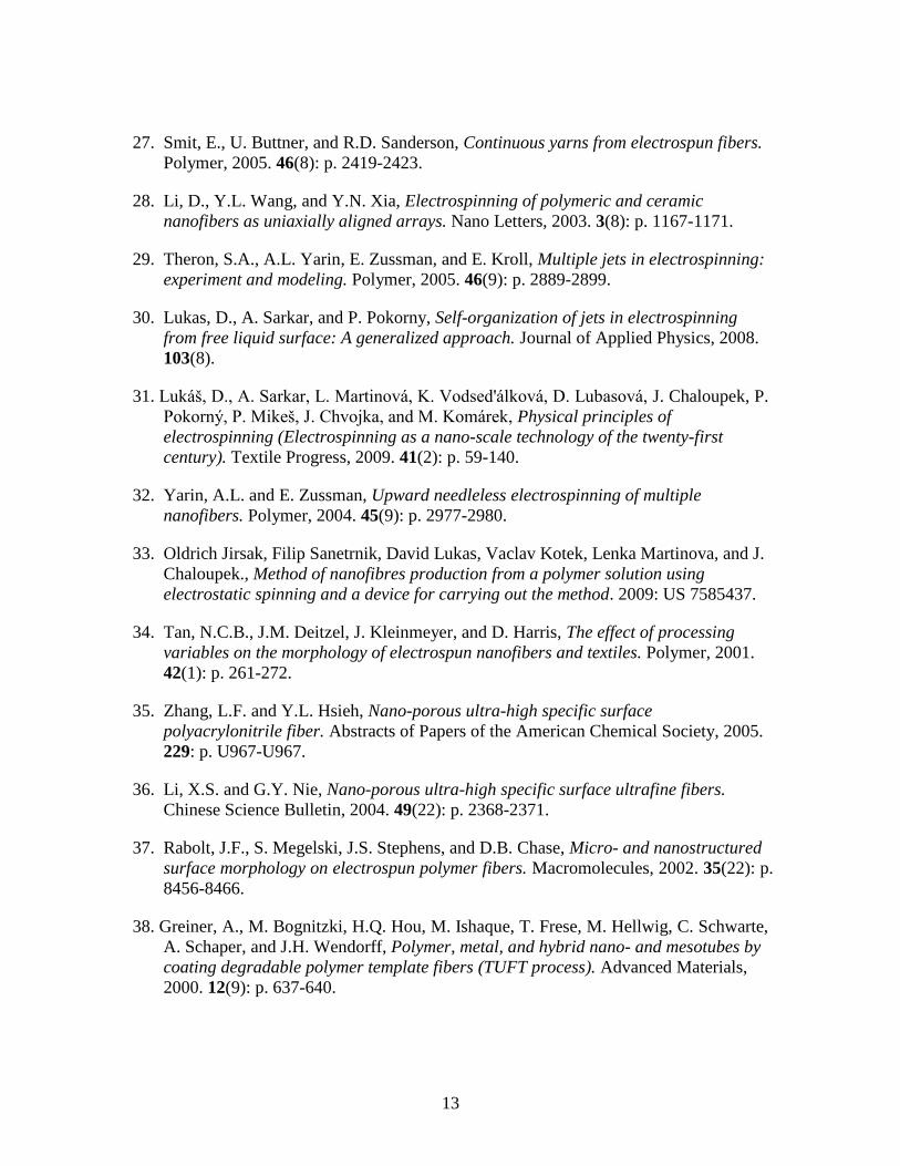
2.1. The concept of surface tension. A soap film is stretched on a wire frame with

one side attached to a movable wire. .....................................................................15

2.2. Two principle radii of curvature of an arbitrarily curved surface ..........................17

2.3. Illustration of the wettability of solid surfaces by a given liquid: (a) Forces

acting at the contact line. (b) Good wetting, (c) Poor wetting. ..............................19

2.4. (a) The concept of Jurin height: the height of the liquid column is inversely

proportional to the capillary radius. (b) A geometrical construction helping to

relate the contact angle θ with the capillary radius r. ............................................20

2.5. Jurin height of different liquids at different capillary radii. Assuming the

contact angle θ = 0°. ..............................................................................................21

2.6. Schematic of liquid flow in a cylindrical tube. ......................................................23

2.7. Schematic of liquid flow in a slit. ..........................................................................25

2.8. A schematic of cross-section of a yarn consisting of close-packed cylindrical

fibers of equal radii ................................................................................................28

2.9. Schematics of the Kozeny-Carman’s approach for the permeability evaluation

of a granular bed. (a) the granular bed is made of spherical particles with

diameter d, (b) the pores are built by a system of cylindrical tubes (diameter

D). ..........................................................................................................................30

xiii

List of Figures (Continued)

Figure Page

2.10. (a) Schematic of a curved yarn. The radius of curvature of the bow R is

assumed to be much greater than the yarn diameter. (b) The distribution of

tensile stress across the yarn ..................................................................................33

3.1. (A) A schematic diagram of modified electrospinning setup [9]. (a) syringe

with polymer solution, (b) metal needle, (c) syringe pump, (d) high voltage

supply. (e) grounded collector with four bars. (f) motor. (B) Schematic

diagram of the twisting device to produce yarns. The inset is the magnified

brush. ......................................................................................................................40

3.2. The perspective view of electric field in the region between the needle and

two-arm collector. The red arrows denote the direction of the electrostatic

field, and different colors in the plane correspond to different potentials

specified in the vertical bar. The needle is charged to 10 kV and the bars are

grounded ................................................................................................................41

3.3. Steps of yarn formation: (a) Ordered nanofibers forming a band on the two-

arm collector. (b) Gathering nanofibers with the brushes moving along the

electrodes rails. (c) Yarn formed after 120 twists. (d) Removal of the yarn

using a scissors. (e) The produced yarn .................................................................43

3.4. Process of yarn formation by rotating the brushes in opposite directions. (a)

Fibers were collected as a cylindrical shell. (b) Upon twisting the shell, two

cones were developed. These cones met at a singular point, a yarn nucleus. (c)

Formation of yarn of length L at moment t. (d) The produced yarn. A ruler on

the bottom of each image was used as a reference scale to calculate the yarn

length......................................................................................................................44

3.5. (a) Comparison of yarn formation rates for 13 cm and 10 cm gaps. The error

bars correspond to the standard deviations. (b) The yarn length-cone angle

curve of 13 cm gap and 10 cm gap. .......................................................................45

xiv


Figure Page

3.6. (a) Schematic diagram of the geometry of the twisting device. (b) The

theoretical relation between cone angle and yarn length calculated from Eq.

(3.2) corresponding to the experimental range yarn lengths. .................................47

3.7. The theoretical relation between cone angle and yarn length calculated from

Eq. (3.2). ................................................................................................................48

3.8. The SEM (FESEM-Hitachi 4800) micrographs of electrospun CA/PMMA

yarns produced by the proposed method. ..............................................................50

3.9. (a) The average diameters of CA/PMMA, PAN/PMMA, and PVDF/PEO

yarns prepared by electrospinning one hour and application of 12 tpcm twists.

The blue columns correspond to CA/PMMA yarns, the red columns

correspond to PAN/PMMA yarns, and the green columns correspond to

PVDF/PEO yarns. The error bars are the standard deviations. (b) The average

diameters of PVDF/PEO yarns produced from the different collection times

and number of twists applied to the yarns. ............................................................51

3.10. Schematic of the U-shaped frame. .........................................................................54

3.11. The experimental stress-strain curves of CA/PMMA, PAN/PMMA, and

PVDF/PEO yarns. The inset presenting the linear stress-strain behavior, were

used to calculate the Young’s moduli. ...................................................................55

4.1. Fluid flow through a porous cylinder of length L is described by Darcy’s law

( ) ( )a bQ A k P P L . Q is the volumetric flow rate, A is the sample cross-

sectional area through which the liquid is flowing, and the pressure gradient is

expressed as ∇P = (Pb - Pa)/L. ...............................................................................61

xv


Figure Page

4.2. (a) A schematic of the experimental setup showing the principle of operation

of Cahn DCA-322 Analyzer. A capillary tube with embedded yarn is

connected to the balance arm through a hook. The weight of the absorbed

liquid is measured by the balance arm as the meniscus crawls up the capillary

bore. (b) The position of liquid meniscus before and after wicking

experiments. Scale bar is 2 mm. (c) An example of measurement of Jurin

length (Zc) which is shown as the white arrow. .....................................................65

4.3. A typical experimental curve showing force changes at different steps: a steep

jump of the blue line allows one to define the ZDOI point. The stage was

moving until the immersed part reached 0.1 mm (green line), then we waited

for 5 minutes (purple line), and started collecting the change of water weight

for 50 minutes (red line). .......................................................................................67

4.4. The normalized liquid front position (L*) versus the normalized time (t

*) for

the different values of parameter α. t* = t/t0, L

* = L/Zc. .........................................72

4.5. The dimensionless meniscus position (L*) versus dimensionless time (t

*) in the

yarn-in-a-tube conduit. The black solid lines represent the fitting curves. ............73

4.6. A summary of permeabilities and porosities of different materials. The y axis

of permeability is represented in logarithmic scale, and error bars are the

standard deviations.................................................................................................75

4.7. The SEM micrographs of electrospun fiber yarns: (A) CA/PMMA/PEO, fiber

diameters Df ~ 6μm, (B) PVDF/PEO, fiber diameters Df ~ 2μm, (C)

CA/PMMA, fiber diameters Df ~ 1μm, and (d) PAN, fiber diameters Df ~

0.6μm. (e) The corresponding relation between the interfiber distance (d) and

fiber diameter (Df). .................................................................................................76

4.8. The permeability of four electrospun CA/PMMA nanofiber yarns. The y axis

is presented in the logarithmic scale and error bars correspond to the standard

deviations. ..............................................................................................................77

xvi


Figure Page

4.9. The Reynolds number versus time for hexadecane: η = 3.03 mPa·s, ρ = 773

kg/m3. .....................................................................................................................81

5.1. SEM micrographs of CA/PMMA films, scale bar is 200 µm. ...............................87

5.2. A schematic of the experimental setup showing the principle of operation of

Cahn DCA-322 Analyzer. A hook with the plasticine sealed yarn is connected

to the balance arm. The weight of the absorbed liquid is measured by the

balance arm. ...........................................................................................................89

5.3. A typical experimental curve showing force changes at different steps: a steep

jump of the blue line allows one to define the ZDOI point. The change of

liquid weight was collected for 5 minutes (red line)..............................................90

5.4. An experimental curve showing the wetting front position as a function of

square-root-of-time. The black dashed line represents the fit which can be

used for the description of the wicking kinetics when the time t > t0. ...................91

5.5. The wetting front position as a function of square-root-of-time for hexadecane

and DI water. The black lines correspond to the Lucas-Washburn prediction. .....92

5.6. SEM micrographs of CA/PMMA yarns, scale bar is 1 µm. ..................................94

6.1. (A) Butterfly drawing sugar solution from paper towel. The dorsal side of the

proboscis is pushed toward the porous surface, (B) The legulae (arrow),

looking like a fence at the dorsal side of the proboscis. The liquid wicks into

the food canal through the nanopores formed by two nearest legulae. ................100

6.2. SEM images of the electrospun PVDF/PEO fibers. (A) Solid non-porous

fibers, (B) Porous fibers, (C) The cross-section of PVDF/PEO yarns. The

black areas in the insert show the pores in an undisturbed spot after the yarn

cutting. This area suggests that the porosity is close to 10%. .............................103

xvii


Figure Page

6.3. (a) Comparative absorption kinetics of hexadecane and TBP droplets on yarns

made of porous PVDF/PEO fibers. A is the yarn cross-section, V0 is the initial

drop volume, and V is the drop volume at time t. The insert is the schematic

used for modeling of drop penetration into yarn. The front position is shown

by the black arrow. (b) A series of pictures illustrating the absorption kinetics

of hexadecane droplet into the PVDF/PEO yarn made of nanoporous fibers.

An 80-µm copper wire with a hexadecane droplet of the same initial volume

was used as the reference. Scale bar: 500μm. (c) Comparative absorption

kinetics of hexadecane droplets by yarns made of porous and non-porous

fibers. The error bar corresponds to the highest standard deviation in the

experiments. .........................................................................................................106

6.4. A schematic illustrates that the liquid flow through a yarn and a porous fiber.

Subscripts y and f correspond to yarn and fiber, respectively. .............................108

6.5. The pore size distribution of electrospun nanoporous PVDF/PEO fibers. The

blue column shows the frequency of appearance of a fiber with a certain

diameter. The numbers above the red columns show the cumulative pore

diameter, which approaches the average pore diameter of 98 nm. ......................113

6.6. (A) Butterfly with a proboscis searching for food. (B) A schematic of yarn

manipulation with electric field generated by two vertical electrodes. (C)

Artificial proboscis made of PVDF/PEO fibers absorbing a TBP droplet. Two

electrodes are positioned from the sides and are not shown here. The solid

black fiber on the left is the artificial proboscis; the gray fiber on the right is a

nylon yarn. The scale bar is 2 mm. ......................................................................115

6.7. Absorption of a TBP droplet by the artificial proboscis made of PVDF/PEO

fibers with embedded superparamagnetic nanoparticles. The proboscis was

manipulated with a magnetic field. The scale bar is 2 mm ..................................115

xviii


Figure Page

6.8. (A) FTIR spectra of PVDF pellet, dip-coated PVDF–PEO film, and

electrospun PVDF–PEO fiber. (B) β/α ratios for PVDF pellets, PVDF–PEO

film and electrospun PVDF–PEO fibers, suggesting that the electrospun fibers

contain greater amount of ferroelectric crystals. ..................................................119

6.9. The blue line refers to the thickness of glass slide (1 mm) and the red line

refers to the total thickness of PVDF/PEO film plus the glass slide. (a) without

soaking in TBP and (B) after soaking 120 minutes in TBP. ................................122

6.10. The swelling ratio versus different soaking time in HEX and TBP. ...................122

7.1. Scanning electron micrographs. (A) Single galea of the monarch proboscis. (B)

Dorsal legulae. (C) Proboscis tip showing slit between opposing galeae............131

7.2. (A) Schematic of experiment showing the operation principle of the Cahn

DSA-322. A capillary tube with the proboscis is connected to the balance arm

through a hook. An oil droplet closes the rectangular vessel, preventing water

evaporation and allowing the tube to move freely through the hole. Water

moves from the reservoir to the tube by capillary action. The weight of the

wicking water column is measured by the balance arm as the meniscus moves

up the bore of the capillary tube. (B) Closed vessel after 1 hour of saturation

with water vapor. The proboscis is suspended above the water. (C) The same

vessel at the moment when the proboscis tip touches the water. (D) Example

of measurement of Jurin length (Zc), shown by the white arrow. ........................133

7.3. Typical experimental curve showing force changes at different steps of

proboscis movement. A steep jump of the blue line allowed the ZDOI point to

be defined. The proboscis was immersed further into the water for 0.1 mm

(green line). After 1 minute (purple line), the change of water weight for 60

minutes was collected (red line). .........................................................................137

xix


Figure Page

7.4 A schematic of a food canal model. Symbols: proboscis length Lp, drinking

region length H, food canal radius Rp, drinking region radius at truncated tip

R0, and taper angle φ. The scale bar is 100 μm....................................................139

7.5. The experimental curve of dimensionless meniscus position (L*) versus

dimensionless time (t*) for a butterfly proboscis acquired by the DCA-322

analyzer. The blue hollow dots are the experimental data, and the solid black

line is the fitting curve. ........................................................................................145

7.6. Average radii (± standard deviation) of the food canal at the tip of the drinking

region R0 and average length of the drinking region H of proboscises from 6

monarch butterflies. .............................................................................................145

7.7. The pressure produced by the butterfly’s cibarial pump, using parameters

from Table 7.2. PH = pressure at the end of the drinking region, Pp = pressure

in the cibarial pump, Pt = pressure in the cibarial pump in the tube model of

the proboscis when the tube radius Rp did not change along the proboscis. ........147

A.1. An example of experimental frames showing the meniscus of Deoxy RBCs

moving inside a 500 µm capillary. .....................................................................1566

A.2. Meniscus dynamics in 500 μm diameter capillary tube of (a) Oxy and (b)

Deoxy solutions. The blue dashed lines represent the theoretical results. ...........157

A.3. (a) The typical curves of dimensionless meniscus position (L*) versus

dimensionless time (t*) for Oxy and Deoxy solutions. The black solid lines

represent the fitting curves. (b) A summary of permeability of Oxy and Deoxy

solutions. ..............................................................................................................159

A.4. (a) Dimensionless meniscus position (L*) versus dimensionless time (t

*) for

CA/PMMA/PEO and CA/PMMA/PEO with PVA. The black solid lines

represent the fitting curves. (b) The permeability of CA/PMMA/PEO and

CA/PMMA/PEO with PVA yarns. The y axis of permeability is presented in

logarithmic scale. The error bars are the standard deviations. .............................161

xx


Figure Page

A.5. The SEM micrographs of (a-b) CA/PMMA/PEO, (c-d) CA/PMMA/PEO with

PVA. (a) and (c) represent the side view of yarn, and (b) and (d) represent the

cross-sectional view of the yarn. The images confirm that the interfiber space

was filled with PVA polymer, and the interfiber distance and porosity

decrease. ...............................................................................................................161

xxi

LIST OF TABLES

Table Page

1.1. Illustration of the variables which should be taken into consideration. ...................3

2.1. Values of surface tension of different liquids at temperature of 20 °C. ................16

2.2. Values of capillary length of different liquids. Surface tensions are taken from

Ref. [2], and densities are taken from material safety data sheet (MSDS). ...........22

3.1. The list of polymers which can be used for yarn formation with the proposed

device. ....................................................................................................................49

3.2. Summary of elastic properties of CA/PMMA, PAN/PMMA, and PVDF/PEO

yarns. The data present the average ± standard deviations. ...................................54

3.3. Summary of flexibility of CA/PMMA, PAN/PMMA, and PVDF/PEO yarns.

The data present the average ± standard deviations. ..............................................56

4.1. A summary of parameter α, permeability ky, interfiber distance d, and fiber

diameter Df of different materials. .........................................................................75

5.1. Liquid properties and contact angles of liquids on CA, PMMA, and

CA/PMMA films. ..................................................................................................86

6.1. Properties of probed liquids. ................................................................................107

7.1. Radius of the proboscis opening at the tip and the length of the tapered part of

the food canal of monarch butterfly proboscises. ................................................146

7.2. Parameters of the monarch proboscis and properties of model nectars ...............146

A.1. The characteristics of yarns used in experiments with blood cells. .....................158

1

CHAPTER ONE

1INTRODUCTION

The electrospinning methods for fiber formation are first introduced, and the

electrospinning setups and key parameters affecting the produced fibers are discussed.

1.1 History

The first patent showing the drawing of the electrospinning equipment was traced

back to John Cooley in 1902 [1]. He filed another similar patent regarding

electrospinning a year later in 1903 [2]. During 1934-1944, Anton Formhals made

significant contributions to the development of electrospinning for the production of

artificial threads using high electric field [3]. In the mid-1990s, nanofiber production has

become a prominent research field. The most important research in this field has been

conducted by the Reneker group at the University of Akron [4, 5] and the Rutledge group

at MIT [6-9]. They have demonstrated that many organic polymers could be electrospun

into nanofibers, and characterized these electrospun fibers. Since then, the publications

on electrospinning on the Web of Science are increasing exponentially every year.

1.2 Electrospinning Equipment

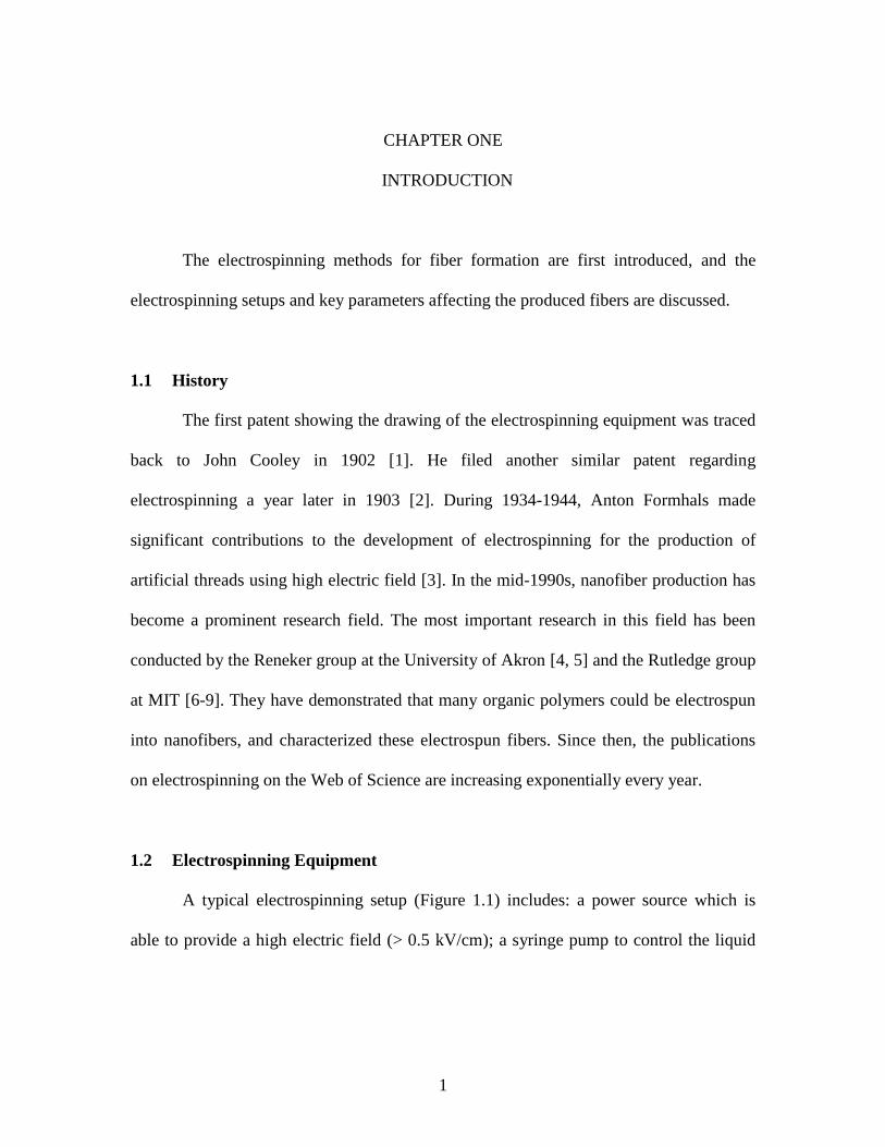
A typical electrospinning setup (Figure 1.1) includes: a power source which is

able to provide a high electric field (> 0.5 kV/cm); a syringe pump to control the liquid

http://en.wikipedia.org/wiki/Nanofiber

2

flow rate; a capillary (such as a metal needle or a pipette); and an electrode working as a

fiber collector.

Figure 1.1. A schematic diagram of typical electrospinning setup. (A) syringe with

polymer solution, (B) metal needle. (C) high voltage supply. (D) grounded collector. (E)

syringe pump.

In the electrospinning process, a polymer solution is extruded through a spinneret

(usually a metallic needle) forming a droplet at the tip. When an electric field is applied

to the polymer solution, it pulls the droplet to form a conical meniscus which is called the

Taylor cone [10, 11]. As soon as the repulsive electrostatic forces between the charges on

the drop surface overcome its surface tension, a jet is ejected from the drop. On its way to

the collector, the jet vigorously bends and spontaneously twists [6, 7]. This type of

movement and additional spiraling and ballooning of the whipping jet leads to significant

increase of its length and hence decrease of the jet diameter [12]. Simultaneously, the

solvent evaporates during this motion, leaving only solid polymer residues on the

collector.

3

1.3 Factors Affecting Electrospining

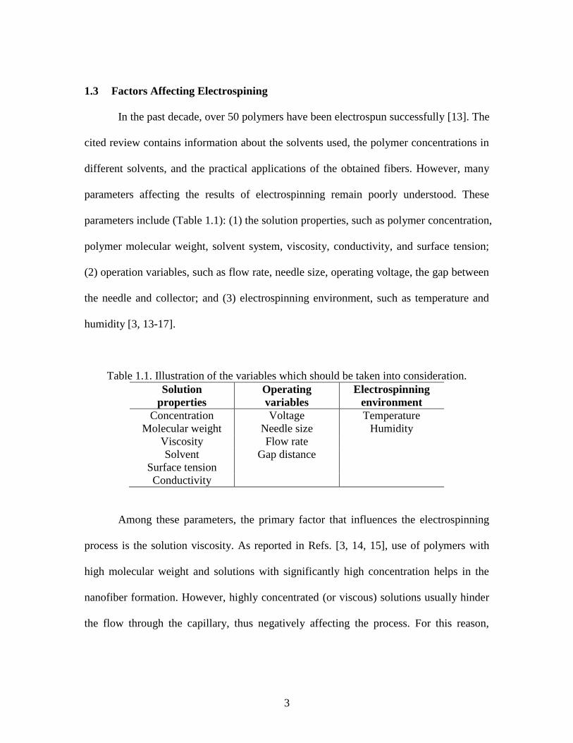
In the past decade, over 50 polymers have been electrospun successfully [13]. The

cited review contains information about the solvents used, the polymer concentrations in

different solvents, and the practical applications of the obtained fibers. However, many

parameters affecting the results of electrospinning remain poorly understood. These

parameters include (Table 1.1): (1) the solution properties, such as polymer concentration,

polymer molecular weight, solvent system, viscosity, conductivity, and surface tension;

(2) operation variables, such as flow rate, needle size, operating voltage, the gap between

the needle and collector; and (3) electrospinning environment, such as temperature and

humidity [3, 13-17].

Table 1.1. Illustration of the variables which should be taken into consideration.

Solution

properties

Operating

variables

Electrospinning

environment

Concentration Voltage Temperature

Molecular weight Needle size Humidity

Viscosity Flow rate

Solvent Gap distance

Surface tension

Conductivity

Among these parameters, the primary factor that influences the electrospinning

process is the solution viscosity. As reported in Refs. [3, 14, 15], use of polymers with

high molecular weight and solutions with significantly high concentration helps in the

nanofiber formation. However, highly concentrated (or viscous) solutions usually hinder

the flow through the capillary, thus negatively affecting the process. For this reason,

4

finding an optimal range of polymer concentrations is considered the most important step

for successful electrospinning of nanofibers.

Another important factor is the applied voltage. As mentioned previously, a jet

can be produced if, and only if, the applied electrostatic force overcomes the droplet

surface tension. At lower voltage, a pendant drop, usually sitting at the needle tip, cannot

be detached from the tip. It is known [12, 18] that the fibers cannot be formed below a

certain voltage because the repulsive force of the charged solution cannot overcome the

solution surface tension. In addition, although fibers can be electrospun above a critical

voltage, they will usually contain bead defects. Surface tension tries to minimize specific

surface area by changing jets into spheres. On the contrary, an excess electrical charge

tries to increase the surface area which results in thinner jets. Therefore, high surface

tension liquids tend to form beads; decreasing the surface tension can make the beads

disappear. These results show that the applied voltage should be optimized to produce

defect-free fibers.

However, no theory exists that can take all factors into account and predict the

fiber size. When the solution viscosity is increased, the number of beads on fibers and

bead size increase as well. As the gap between the needle and collector increases, the jets

become thinner. To successfully fabricate a thin and fine jet, it is important to find a

balance of the abovementioned parameters.

5

1.4 Electrospinning Design

The focus of research in textile technology has recently shifted toward the design

of electrospinning instruments to fabricate nanofibers with various fibrous assemblies

[19-21]. In the Ramakrishna-Teo report [19], designs of different parts of electrospinning

setups were reviewed and divided into three main groups: (1) fiber collectors; (2) tools

for manipulation of electric field; and (3) solution delivery systems. These designs were

compared and the advantages and disadvantages were listed.

1.4.1 Fiber Collectors

Several research groups have reported that it is possible to obtain aligned fibers

by using a rapidly rotating collector [22-24]. Matthews et al. [22] proved that the rotating

speed of a drum has influence on the degree of alignment of electrospun collagen fibers.

As the rotating speed was less than 500 rpm, the randomly deposited collagen fibers were

created on the collector. However, when the rotating speed was increased to 4,500 rpm

(approximately 1.4 m/s at the surface of the drum), the collagen fibers exhibited good

alignment along the rotation direction. Kim et al [25] concluded that the mechanical

properties of the electrospun PET nonwovens strongly depended on the linear velocity of

drum. They reported that the Young’s modulus, yield stress, and tensile strength of the

electrospun PET nonwovens increased with increasing the linear velocity of the drum up

to 30 m/min; however, the same parameters decreased when the linear velocity of the

drum was set above 45 m/min. Another study by Zussman et al showed that the necking

of the electrospun fibers can occur at high enough rotation speed [26]. Therefore, the

6

rotating speed and the fiber orientation are closely linked and have a significant influence

on the material properties.

Unlike the conventional electrospinning device with a solid collector, Smit et al

[27] proposed to deposit electrospun fibers in a water (non-solvent) bath; this method

provided a continuous yarn, which was collected on a rotating drum. After examining the

SEM micrographs, these yarns showed that the electrospun fibers were aligned in the

direction of the yarn axis. Although the electrospun fibers were randomly deposited on

the water surface as a nonwoven web, the web was successfully converted into yarns.

Three materials, poly(vinyl acetate), poly(vinylidene fluoride), and polyacrylonitrile,

were successfully fabricated using this method. However, some defects on fibers such as

beads and fiber loops were detected in the images [27]. No further studies were carried

out to determine the yarn properties.

1.4.2 Tools for Manipulation of Electric Field

Li et al. [28] reported that the fibers can be aligned when two electrode collectors

were placed parallel to each other. The advantage of this configuration is that it is easy to

set up, and it allows formation of highly aligned fibers, which are easily transferable to

another substrate. However, the main disadvantage is that the length of the aligned fibers

is limited by the gap distance. At a wider gap, the electrospun fibers may not deposited

across the gap or the fibers may break, especially if the fiber diameter is small. Another

drawback is that the fibers lack the alignment when more fibers are deposited between

7

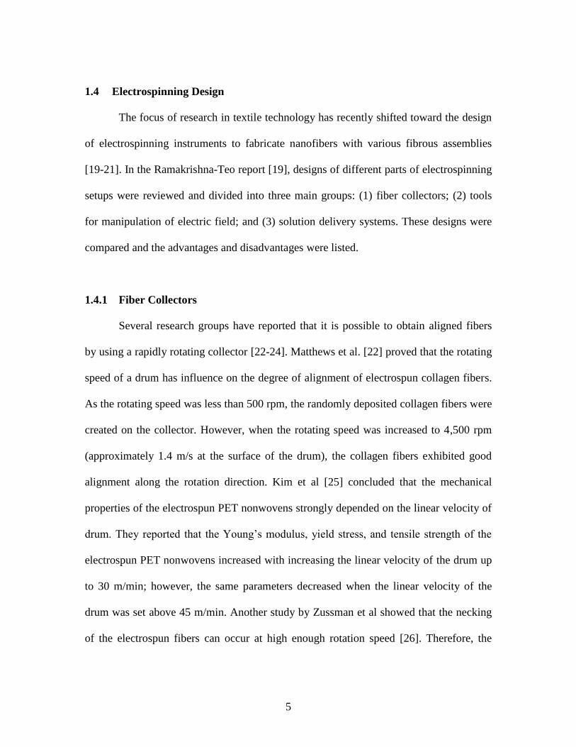
the parallel electrodes [19]. This is probably due to the accumulation of residual charges

on the deposited fibers which changes the desired electric field profile.

Figure 1.2. (A) A schematic of electrospinning setup to produce uniaxially aligned

nanofibers [28]. The collector consisted of two pieces of conductive silicon stripes which

were separated by a gap. (B) The electric field vectors were calculated in the region

between the needle and the collector. The arrows indicate the direction of the electrostatic

field lines [28].

1.4.3 Solution Delivery Systems

A major limitation of industrial applications of electrospinning is the rate of fiber

production which is very much lower than the current fiber spinning technology can

provide. A straightforward method of increasing the yield of electrospinning is by

increasing the number of spinnerets used in the process [19]. However, the presence of

adjacent spinnerets may influence the mutual Coulombic interactions, causing jet

whipping [29].

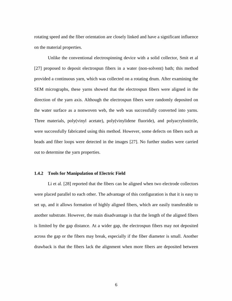
Another approach to increase the productivity is using free liquid surface to

produce numerous jets during electrospinning. This is called the needleless

electrospinning [30, 31]. The idea and its initial implementation was reported by Yarin

and Zussman [32]. They applied a strong magnetic field on a magnetic liquid to produce

8

many spikes. The spikes became field concentrators and generated multiple jets. Jirsak et

al. [33] observed the formation of multiple jets from a free liquid surface covering a

slowly rotating horizontal cylinder. The multiple jets emanating from a free surface can

be explained by the Larmor-Tonks-Frenkel instability [30, 33]. The success of the

method was subsequently commercialized by Elmarco Company under the brand name of

NanospiderTM

.

Figure 1.3. Multiple jets produced by cleft-like spinnerets (material: polyvinyl alcohol)

[30].

1.5 Nanofibers with Surface Porosity

The major advantage of nanofibers is the high specific surface area needed in

many applications, such as catalysis, filtration, and sensor technology. The surface area

per unit mass in fiber mats increases as the average fiber diameter is reduced. The fiber

diameter, generally, decreases when the concentration of polymer in solution decreases.

However, as described before, there is a limiting concentration below which the solution

cannot be spun into fibers [34]. In order to significantly increase the surface area of

nanofibers, several approaches to modify the surface morphology of nanofibers have

been discussed in the literature over recent years [35, 36].

9

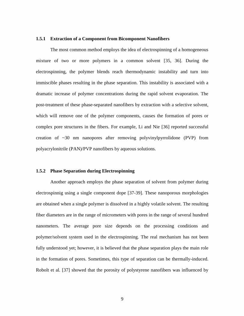
1.5.1 Extraction of a Component from Bicomponent Nanofibers

The most common method employs the idea of electrospinning of a homogeneous

mixture of two or more polymers in a common solvent [35, 36]. During the

electrospinning, the polymer blends reach thermodynamic instability and turn into

immiscible phases resulting in the phase separation. This instability is associated with a

dramatic increase of polymer concentrations during the rapid solvent evaporation. The

post-treatment of these phase-separated nanofibers by extraction with a selective solvent,

which will remove one of the polymer components, causes the formation of pores or

complex pore structures in the fibers. For example, Li and Nie [36] reported successful

creation of ~30 nm nanopores after removing polyvinylpyrrolidone (PVP) from

polyacrylonitrile (PAN)/PVP nanofibers by aqueous solutions.

1.5.2 Phase Separation during Electrospinning

Another approach employs the phase separation of solvent from polymer during

electrospinnig using a single component dope [37-39]. These nanoporous morphologies

are obtained when a single polymer is dissolved in a highly volatile solvent. The resulting

fiber diameters are in the range of micrometers with pores in the range of several hundred

nanometers. The average pore size depends on the processing conditions and

polymer/solvent system used in the electrospinning. The real mechanism has not been

fully understood yet; however, it is believed that the phase separation plays the main role

in the formation of pores. Sometimes, this type of separation can be thermally-induced.

Robolt et al. [37] showed that the porosity of polystyrene nanofibers was influenced by

10

the solvent mixture of dimethyl formamide/tetrahydrofuran (DMF/THF). The porosity

was reduced when the content of less volatile DMF was increased, and finally produced a

smooth surface morphology.

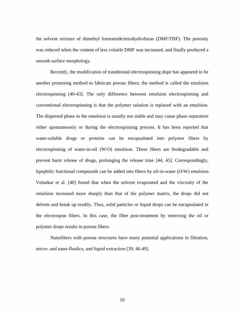
Recently, the modification of tranditional electrospinning dope has appeared to be

another promising method to fabricate porous fibers; the method is called the emulsion

electrospinning [40-43]. The only difference between emulsion electrospinning and

conventional electrospinning is that the polymer solution is replaced with an emulsion.

The dispersed phase in the emulsion is usually not stable and may cause phase separation

either spontaneously or during the electrospinning process. It has been reported that

water-soluble drugs or proteins can be encapsulated into polymer fibers by

electrospinning of water-in-oil (W/O) emulsion. These fibers are biodegradable and

prevent burst release of drugs, prolonging the release time [44, 45]. Correspondingly,

lipophilic functional compounds can be added into fibers by oil-in-water (O/W) emulsion.

Velankar et al. [40] found that when the solvent evaporated and the viscosity of the

emulsion increased more sharply than that of the polymer matrix, the drops did not

deform and break up readily. Thus, solid particles or liquid drops can be encapsulated in

the electrospun fibers. In this case, the fiber post-treatment by removing the oil or

polymer drops results in porous fibers.

Nanofibers with porous structures have many potential applications in filtration,

micro- and nano-fluidics, and liquid extraction [39, 46-49].

11

1.6 References

1. Cooley, J.F., Apparatus for electrically dispersing fluids. 1902: US 692631.

2. Cooley, J.F., Electrical method of dispersing fluids. 1903: US 745276.

3. Andrady, A.L., Science and technology of polymer nanofibers. 2008, Hoboken, N.J.:

Wiley. xix, 403 p.

4. Doshi, J. and D.H. Reneker, Electrospinning process and applications of electrospun

fibers. Journal of Electrostatics, 1995. 35(2–3): p. 151-160.

5. Reneker, D.H. and I. Chun, Nanometer diameter fibres of polymer, produced by

electrospinning. Nanotechnology, 1996. 7(3): p. 216-223.

6. Shin, Y.M., M.M. Hohman, M.P. Brenner, and G.C. Rutledge, Experimental

characterization of electrospinning: the electrically forced jet and instabilities.

Polymer, 2001. 42(25): p. 09955-09967.

7. Shin, Y.M., M.M. Hohman, M.P. Brenner, and G.C. Rutledge, Electrospinning: A

whipping fluid jet generates submicron polymer fibers. Applied Physics Letters,

2001. 78(8): p. 1149-1151.

8. Hohman, M.M., M. Shin, G. Rutledge, and M.P. Brenner, Electrospinning and

electrically forced jets. I. Stability theory. Physics of Fluids, 2001. 13(8): p. 2201-

2220.

9. Hohman, M.M., M. Shin, G. Rutledge, and M.P. Brenner, Electrospinning and

electrically forced jets. II. Applications. Physics of Fluids, 2001. 13(8): p. 2221-2236.

10. Taylor, G., Disintegration of Water Drops in an Electric Field. Proceedings of the

Royal Society of London. Series A. Mathematical and Physical Sciences, 1964.

280(1382): p. 383-397.

11. Taylor, G., The Coalescence of Closely Spaced Drops when they are at Different

Electric Potentials. Proceedings of the Royal Society of London. Series A.

Mathematical and Physical Sciences, 1968. 306(1487): p. 423-434.

12. Rutledge, G.C. and S.V. Fridrikh, Formation of fibers by electrospinning. Advanced

Drug Delivery Reviews, 2007. 59(14): p. 1384-1391.

13. Huang, Z.M., Y.Z. Zhang, M. Kotaki, and S. Ramakrishna, A review on polymer

nanofibers by electrospinning and their applications in nanocomposites. Composites

Science and Technology, 2003. 63(15): p. 2223-2253.

12

14. Weiss, J., C. Kriegel, A. Arrechi, K. Kit, and D.J. McClements, Fabrication,

functionalization, and application of electrospun biopolymer nanofibers. Critical

Reviews in Food Science and Nutrition, 2008. 48(8): p. 775-797.

15. Mikos, A.G., Q.P. Pham, and U. Sharma, Electrospinning of polymeric nanofibers

for tissue engineering applications: A review. Tissue Engineering, 2006. 12(5): p.

1197-1211.

16. Thompson, C.J., G.G. Chase, A.L. Yarin, and D.H. Reneker, Effects of parameters

on nanofiber diameter determined from electrospinning model. Polymer, 2007.

48(23): p. 6913-6922.

17. Theron, S.A., E. Zussman, and A.L. Yarin, Experimental investigation of the

governing parameters in the electrospinning of polymer solutions. Polymer, 2004.

45(6): p. 2017-2030.

18. Reneker, D.H. and A.L. Yarin, Electrospinning jets and polymer nanofibers.

Polymer, 2008. 49(10): p. 2387-2425.

19. Ramakrishna, S. and W.E. Teo, A review on electrospinning design and nanofibre

assemblies. Nanotechnology, 2006. 17(14): p. R89-R106.

20. Nayak, R., R. Padhye, I. Kyratzis, Y.B. Truong, and L. Arnold, Recent advances in

nanofibre fabrication techniques. Textile Research Journal, 2012. 82(2): p. 129-147.

21. Park, S., K. Park, H. Yoon, J. Son, T. Min, and G. Kim, Apparatus for preparing

electrospun nanofibers: designing an electrospinning process for nanofiber

fabrication. Polymer International, 2007. 56(11): p. 1361-1366.

22. Matthews, J.A., G.E. Wnek, D.G. Simpson, and G.L. Bowlin, Electrospinning of

collagen nanofibers. Biomacromolecules, 2002. 3(2): p. 232-238.

23. Kameoka, J., R. Orth, Y.N. Yang, D. Czaplewski, R. Mathers, G.W. Coates, and H.G.

Craighead, A scanning tip electrospinning source for deposition of oriented

nanofibres. Nanotechnology, 2003. 14(10): p. 1124-1129.

24. Moon, S. and R.J. Farris, How is it possible to produce highly oriented yarns of

electrospun fibers? Polymer Engineering and Science, 2007. 47(10): p. 1530-1535.

25. Kim, K.W., K.H. Lee, M.S. Khil, Y.S. Ho, and H.Y. Kim, The effect of molecular

weight and the linear velocity of drum surface on the properties of electrospun

poly(ethylene terephthalate) nonwovens. Fibers and Polymers, 2004. 5(2): p. 122-127.

26. Zussman, E., D. Rittel, and A.L. Yarin, Failure modes of electrospun nanofibers.

Applied Physics Letters, 2003. 82(22): p. 3958-3960.

13

27. Smit, E., U. Buttner, and R.D. Sanderson, Continuous yarns from electrospun fibers.

Polymer, 2005. 46(8): p. 2419-2423.

28. Li, D., Y.L. Wang, and Y.N. Xia, Electrospinning of polymeric and ceramic

nanofibers as uniaxially aligned arrays. Nano Letters, 2003. 3(8): p. 1167-1171.

29. Theron, S.A., A.L. Yarin, E. Zussman, and E. Kroll, Multiple jets in electrospinning:

experiment and modeling. Polymer, 2005. 46(9): p. 2889-2899.

30. Lukas, D., A. Sarkar, and P. Pokorny, Self-organization of jets in electrospinning

from free liquid surface: A generalized approach. Journal of Applied Physics, 2008.

103(8).

31. Lukáš, D., A. Sarkar, L. Martinová, K. Vodsed'álková, D. Lubasová, J. Chaloupek, P.

Pokorný, P. Mikeš, J. Chvojka, and M. Komárek, Physical principles of

electrospinning (Electrospinning as a nano-scale technology of the twenty-first

century). Textile Progress, 2009. 41(2): p. 59-140.

32. Yarin, A.L. and E. Zussman, Upward needleless electrospinning of multiple

nanofibers. Polymer, 2004. 45(9): p. 2977-2980.

33. Oldrich Jirsak, Filip Sanetrnik, David Lukas, Vaclav Kotek, Lenka Martinova, and J.

Chaloupek., Method of nanofibres production from a polymer solution using

electrostatic spinning and a device for carrying out the method. 2009: US 7585437.

34. Tan, N.C.B., J.M. Deitzel, J. Kleinmeyer, and D. Harris, The effect of processing

variables on the morphology of electrospun nanofibers and textiles. Polymer, 2001.

42(1): p. 261-272.

35. Zhang, L.F. and Y.L. Hsieh, Nano-porous ultra-high specific surface

polyacrylonitrile fiber. Abstracts of Papers of the American Chemical Society, 2005.

229: p. U967-U967.

36. Li, X.S. and G.Y. Nie, Nano-porous ultra-high specific surface ultrafine fibers.

Chinese Science Bulletin, 2004. 49(22): p. 2368-2371.

37. Rabolt, J.F., S. Megelski, J.S. Stephens, and D.B. Chase, Micro- and nanostructured

surface morphology on electrospun polymer fibers. Macromolecules, 2002. 35(22): p.

8456-8466.

38. Greiner, A., M. Bognitzki, H.Q. Hou, M. Ishaque, T. Frese, M. Hellwig, C. Schwarte,

A. Schaper, and J.H. Wendorff, Polymer, metal, and hybrid nano- and mesotubes by

coating degradable polymer template fibers (TUFT process). Advanced Materials,

2000. 12(9): p. 637-640.

14

39. Uyar, T. and A. Celebioglu, Electrospun porous cellulose acetate fibers from volatile

solvent mixture. Materials Letters, 2011. 65(14): p. 2291-2294.

40. Velankar, S.S., M. Angeles, and H.L. Cheng, Emulsion electrospinning: composite

fibers from drop breakup during electrospinning. Polymers for Advanced

Technologies, 2008. 19(7): p. 728-733.

41. Agarwal, S. and A. Greiner, On the way to clean and safe electrospinning-green

electrospinning: emulsion and suspension electrospinning. Polymers for Advanced

Technologies, 2011. 22(3): p. 372-378.

42. Shastri, V.P., J.C. Sy, and A.S. Klemm, Emulsion as a Means of Controlling

Electrospinning of Polymers. Advanced Materials, 2009. 21(18): p. 1814-1819.

43. Chen, H., J. Di, N. Wang, H. Dong, J. Wu, Y. Zhao, J. Yu, and L. Jiang, Fabrication

of hierarchically porous inorganic nanofibers by a general microemulsion

electrospinning approach. Small, 2011. 7(13): p. 1779-83.

44. Jing, X.B., X.L. Xu, L.X. Yang, X.Y. Xu, X. Wang, X.S. Chen, Q.Z. Liang, and J.

Zeng, Ultrafine medicated fibers electrospun from W/O emulsions. Journal of

Controlled Release, 2005. 108(1): p. 33-42.

45. Weiss, J., C. Kriegel, K.A. Kit, and D.J. McClements, Nanofibers as Carrier Systems

for Antimicrobial Microemulsions. Part I: Fabrication and Characterization.

Langmuir, 2009. 25(2): p. 1154-1161.

46. Zhao, L.M., H.K. Lee, and R.E. Majors, The Use of Hollow Fibers in Liquid-Phase

Microextraction. Lc Gc North America, 2010. 28(8): p. 580-+.

47. Lee, J.Y., H.K. Lee, K.E. Rasmussen, and S. Pedersen-Bjergaard, Environmental and

bioanalytical applications of hollow fiber membrane liquid-phase microextraction: A

review. Analytica Chimica Acta, 2008. 624(2): p. 253-268.

48. Lee, I.H., J.Y. Park, and B.W. Han, Preparation of electrospun porous ethyl

cellulose fiber by THF/DMAc binary solvent system. Journal of Industrial and

Engineering Chemistry, 2007. 13(6): p. 1002-1008.

49. Whitesides, G.M., The origins and the future of microfluidics. Nature, 2006.

442(7101): p. 368-373.

15

CHAPTER TWO

2REVIEW OF BASIC PHYSICAL PHENOMENA USED FOR

CHARACTERIZATION OF NANOFIBER YARNS

2.1 Surface Tension

From the macroscopic point of view, the transition layer separating two phases of

materials can be considered as an infinitely thin membrane. Consider a soap film

stretched on a wire frame with one side attached to a movable wire as shown

schematically in Figure 2.1. Setting the movable wire free, one observes that this wire

slides toward the film [1]. These experiments with soap films suggest that both surfaces

of soap film are held under some tension. Therefore, a flat fluid/fluid interface is not

stable but it tends to decrease its surface area. If the force acting per unit length of the

soap film is denoted by σ one can measure this force by applying different weight W to

the movable wire. It appears that the wire can sit in equilibrium only at a certain weight

which is equal to W = 2σL, where L is the wire length. This experiment shows that the

surface tension of the soap film is constant and it does not depend on the surface

deformation.

Figure 2.1. The concept of surface tension. A soap film is stretched on a wire frame with

one side attached to a movable wire.

16

This concept appears to be applicable for any fluid/fluid interfaces, not

necessarily soap films [1]. In order to characterize these interfaces, one can introduce a

constant interfacial tension σ acting parallel to the surface separating two dissimilar fluids.

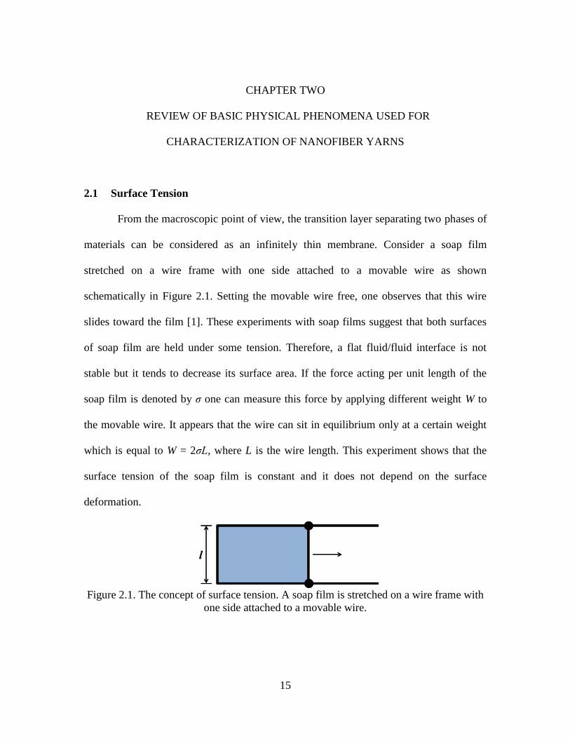
In the SI units, the surface tension is measured in Newtons per meter (N/m). Table 2.1

lists the values of surface tension of different liquids at 20 °C in mN/m [2].

Table 2.1. Values of surface tension of different liquids at temperature of 20 °C [2].

Liquid Surface tension (N/m) Liquid Surface tension (N/m)

Water 72.8×10-3

cis-Decalin 32.2×10-3

Glycerol 64×10-3

Hexadecane 27.47×10-3

Formamide 58×10-3

Hexane 18.4×10-3

Ethylene glycol 48×10-3

Methanol 22.5×10-3

Diiodomethane 50.8×10-3

Ethanol 22.4×10-3

The concept of surface tension can be put into a thermodynamic framework by

considering an elementary act of formation of a new surface as an attachment of a

“frozen” liquid platelet of infinitesimally small thickness and area dxdy with the surface

energy per unit area . Placing a single elementary platelet at an empty spot, one changes

the surface energy by dU = dxdy. To keep this platelet in equilibrium, one needs to

apply the force dF = dy. The work done by this force to support the platelet of width dx

is equal to dA = dxdF. Therefore, the energy budget is written as dU = dA, leading to the

identity = . In this derivation, we assumed that the material does not deform during

the creation of a new surface as if it were built from the Lego bricks.

17

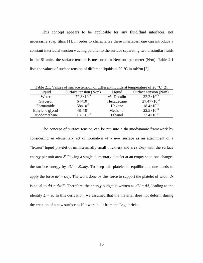
2.2 Curved Interfaces. The Young-Laplace Equation

When the interface is curved, any elementary block containing the interface will

result in a free body diagram where the normal components of the surface tension are not

necessarily balanced (Figure 2.2). This misbalance leads to a pressure jump ΔP across the

interface.

Figure 2.2. Two principle radii of curvature of an arbitrarily curved surface [1].

Let us consider a spherical soap bubble of radius r. The gas inside the bubble is

held under an excess pressure ΔP measured relative to the reference atmospheric pressure.

The force acting per unit length of the soap film equals to σ. The balance of forces acting

on the cross-section of the hemi-sphere reads σ × 2πr = ΔP × πr2. Therefore the excess

pressure in a spherical bubble is equal to ΔP = 2σ/r. In the case of a cylindrical bubble of

the same radius r and length L, one can consider a cross-section along the cylinder

through its axis. The balance of forces acting on this cross-section is expressed as σ × 2L

= ΔP × 2Lr. Therefore the excess pressure is ΔP = σ/r.

One can approach this problem from the energetic standpoint. Consider a

spherical droplet of radius r. The droplet has the surface energy 4πr2σ. If the radius is

18

decreased by dr, the surface energy is decreased by 8πrσdr. In order to support this

change of the droplet radius, one needs to do the work ΔP4πr2dr. Thus, the energy budget

reads ΔP4πr2dr = 8πrσdr resulting in the same equation ΔP = 2σ/r with the surface

tension twice smaller than that of a soap film having two surfaces. Using the same

arguments, one can estimate the pressure difference across the interface of a liquid

cylinder with radius r and length L. In this case, the energy budget reads ΔP2πrLdr =

2πσLdr leading to twice smaller pressure difference ΔP = σ/r.

In the general case, the pressure discontinuity across any curved surface with two

principal radii of curvatures r1 and r2 (Figure 2.2) is expressed as [1]:

1 2

1 1( )Pr r

. (2.1)

This is the Young-Laplace law, qualitatively described by Thomas Young in 1805

[3] and mathematically derived by Pierre-Simon Laplace in 1806 [4].

2.3 Wetting of Surfaces and Young’s Equation

According to the IUPAC definition, wetting is a process by which an interface

separating a solid from a gas is replaced by an interface separating the same solid from a

liquid. Whether a liquid spreads over a given surface or not depends on the values of the

surface tensions at liquid/solid, solid/gas and liquid/gas interfaces. In the cases when a

liquid drop assumes a shape of a spherical cap on the solid surface the drop profile is

completely specified by the contact angle, a physicochemical characteristic of the three

dissimilar solid/liquid/gas phases meeting at a contact line. The contact angle is

19

introduced as an angle at which the fluid/fluid interface meets a solid surface. For

example, if one fluid is a gas, the balance of forces acting at the contact line in the plane

parallel to the solid surface reads (Figure 2.3a) [5]:

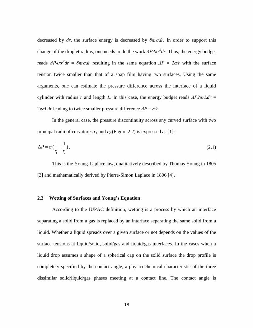
coslv sv sl , (2.2)

where σlv, σsv, and σsl are the surface tensions of liquid/gas, solid/gas, and solid/liquid,

respectively. Eq. (2.2) is the Young’s equation connecting the contact angle θ with the

surface tensions of constituent phases.

Figure 2.3. Illustration of the wettability of solid surfaces by a given liquid: (a) Forces

acting at the contact line. (b) Good wetting, (c) Poor wetting.

Good wetting assumes that the contact angle formed by a droplet is acute. The

material is considered poorly wettable if the drop beads on the surface forming the

contact angle greater than 90⁰. A useful parameter for determining the surface wettability

is the spreading coefficient S defined as [6, 7]:

( )sv sl lvS . (2.3)

If S > 0, the liquid spreads completely on a solid surface (complete wetting). If S

< 0, the liquid does not totally wet a solid surface and forms a droplet on the surface

(partial wetting).

20

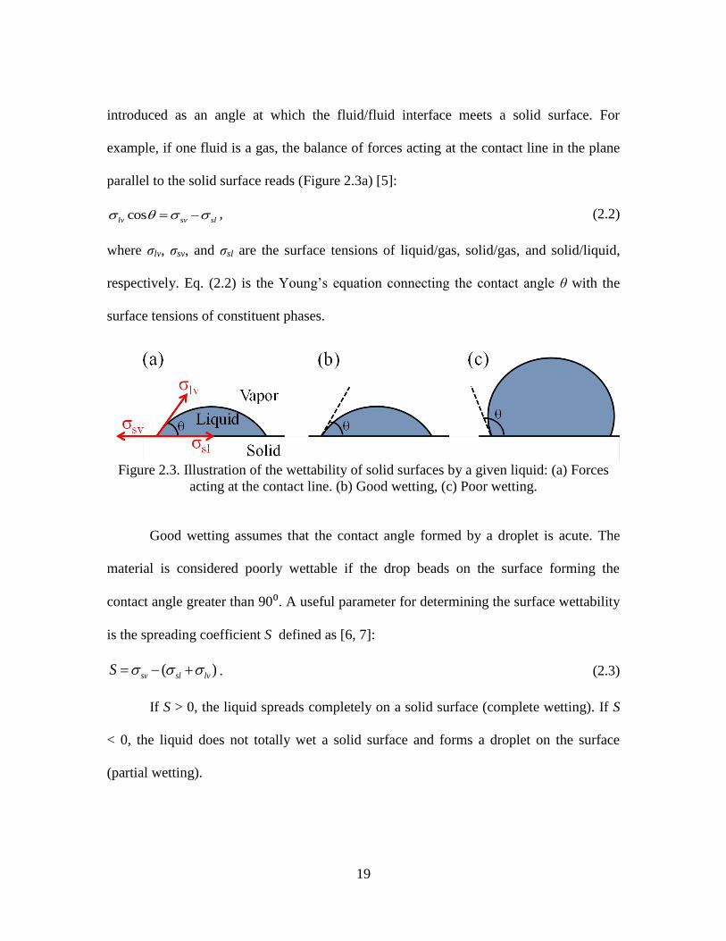
2.4 Capillarity

Capillarity is a general term describing a broad class of phenomena associated

with formation of liquid menisci. In many cases, capillarity is associated with the ability

of a liquid to spontaneous flow into narrow spaces as can be found in numerous examples

in our daily life. When a tube of a small radius is brought in contact with a wetting liquid,

the liquid spontaneously invades the tube and rises up until it reaches some limiting

height. In circular tubes, the liquid meniscus has a spherical shape. Figure 2.4b shows a

schematic of meniscus of radius R in a capillary tube of radius r. Meniscus meets the tube

wall at the contact angle θ. Thus, according to the Young-Laplace law, the pressure under

meniscus Pl is expressed as Pl = Pa - 2/R, or

2 cos /l aP P r , (2.4)

where Pa is the atmospheric pressure above the meniscus.

Figure 2.4. (a) The concept of Jurin height: the height of the liquid column is inversely

proportional to the capillary radius. (b) A geometrical construction helping to relate the

contact angle θ with the capillary radius r.

21

The pressure at the capillary entrance is equal to the atmospheric pressure Pa.

When the liquid reaches the maximum equilibrium height Zc, according to hydrostatics,

the pressure under meniscus is equal to:

l a cP P gZ , (2.5)

where g is the acceleration due to gravity, and ρ is the liquid density.

Substituting Eq. (2.4) into Eq. (2.5), one can find the equilibrium height of the

liquid column, the so-called Jurin height [1, 8]:

2 cos / ( )cZ gr . (2.6)

The lower the contact angle, the higher the liquid column. The Jurin height is

large for capillaries of small diameter (Figure 2.4a).

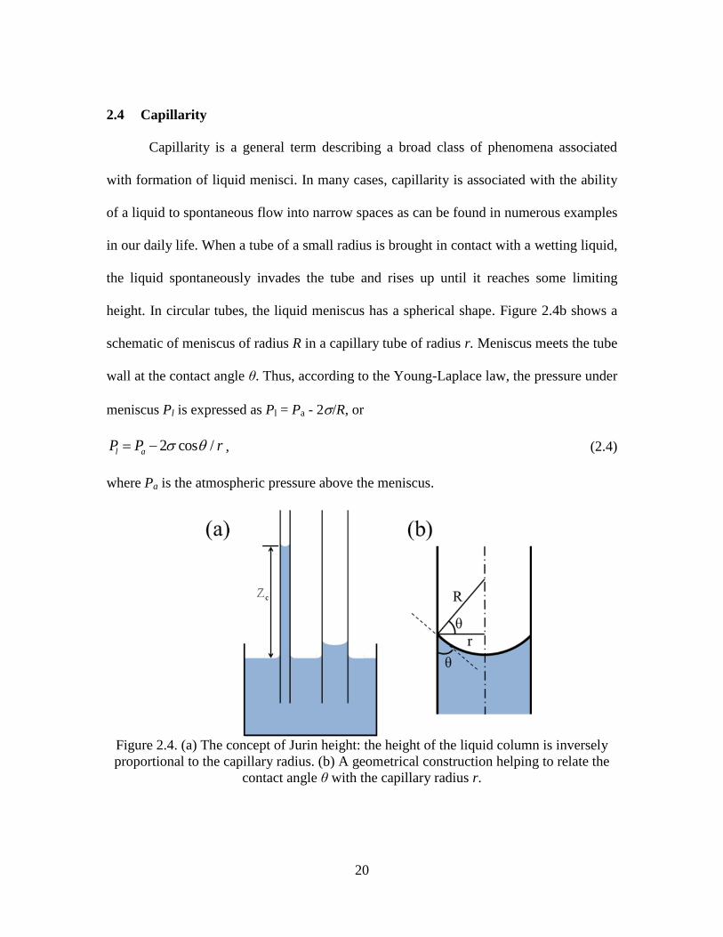
Figure 2.5. Jurin height of different liquids at different capillary radii. Assuming the

contact angle θ = 0°.

The Jurin height is graphed in Figure 2.5 for different liquids and capillary radii.

For example, water reaches 15 meters in a 2 μm diameter capillary (θ = 0⁰) while in a

22

200 μm diameter capillary it rises only 15 centimeters (θ = 0⁰) above the free water

surface of the reservoir (Figure 2.5).

There exists a characteristic capillary length, denoted by κ, specifying the

condition when gravity becomes important and the associated hydrostatic pressure ~ρgκ

becomes comparable with the capillary pressure ~σ/κ. Balancing these pressures, one

obtains:

g . (2.7)

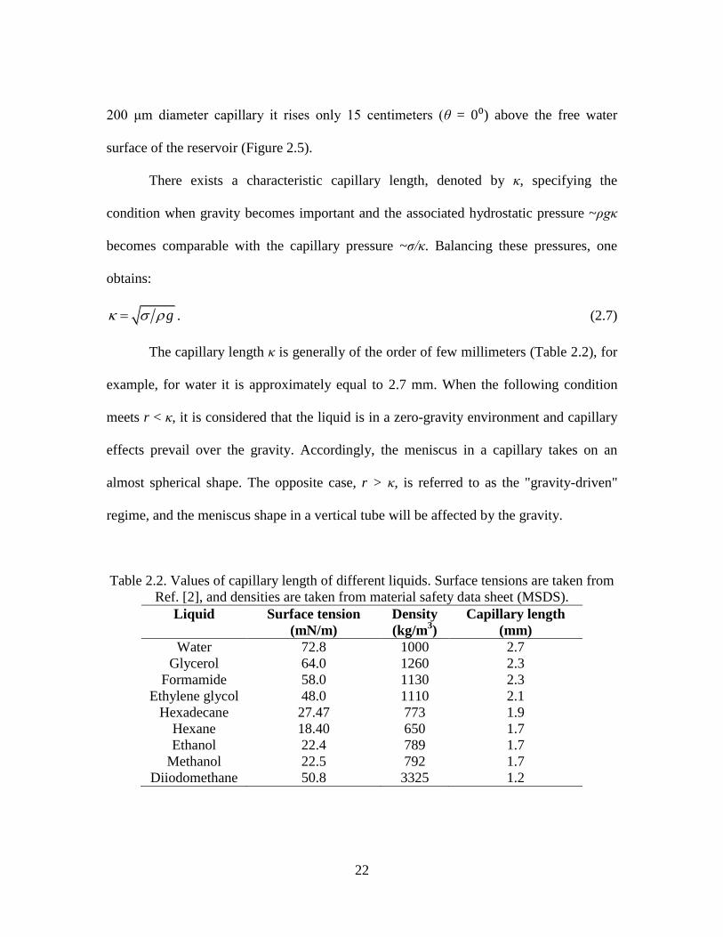
The capillary length κ is generally of the order of few millimeters (Table 2.2), for

example, for water it is approximately equal to 2.7 mm. When the following condition

meets r < κ, it is considered that the liquid is in a zero-gravity environment and capillary

effects prevail over the gravity. Accordingly, the meniscus in a capillary takes on an

almost spherical shape. The opposite case, r > κ, is referred to as the "gravity-driven"

regime, and the meniscus shape in a vertical tube will be affected by the gravity.

Table 2.2. Values of capillary length of different liquids. Surface tensions are taken from

Ref. [2], and densities are taken from material safety data sheet (MSDS).

Liquid Surface tension

(mN/m)

Density

(kg/m3)

Capillary length

(mm)

Water 72.8 1000 2.7

Glycerol 64.0 1260 2.3

Formamide 58.0 1130 2.3

Ethylene glycol 48.0 1110 2.1

Hexadecane 27.47 773 1.9

Hexane 18.40 650 1.7

Ethanol 22.4 789 1.7

Methanol 22.5 792 1.7

Diiodomethane 50.8 3325 1.2

23

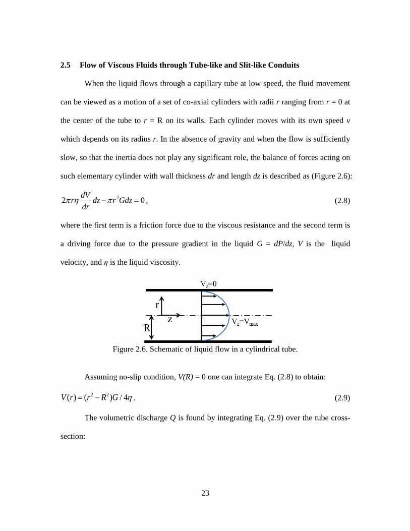
2.5 Flow of Viscous Fluids through Tube-like and Slit-like Conduits

When the liquid flows through a capillary tube at low speed, the fluid movement

can be viewed as a motion of a set of co-axial cylinders with radii r ranging from r = 0 at

the center of the tube to r = R on its walls. Each cylinder moves with its own speed v

which depends on its radius r. In the absence of gravity and when the flow is sufficiently

slow, so that the inertia does not play any significant role, the balance of forces acting on

such elementary cylinder with wall thickness dr and length dz is described as (Figure 2.6):

22 0dV

r dz r Gdzdr

, (2.8)

where the first term is a friction force due to the viscous resistance and the second term is

a driving force due to the pressure gradient in the liquid G = dP/dz, V is the liquid

velocity, and η is the liquid viscosity.

Figure 2.6. Schematic of liquid flow in a cylindrical tube.

Assuming no-slip condition, V(R) = 0 one can integrate Eq. (2.8) to obtain:

2 2( ) ( ) / 4V r r R G . (2.9)

The volumetric discharge Q is found by integrating Eq. (2.9) over the tube cross-

section:

24

4

0

28

RR G

Q Vrdr

. (2.10)

This is the well-known Hagen-Poiseuille equation for the laminar flows in

cylindrical tubes [1]. The mean velocity is defined as:

22

2

0

2/ ( )

8

RR G

q Q R VrdrR

, (2.11)

and it appears that the mean velocity is proportional to the square of tube radius.

The same approach is used to find the liquid discharge through a slit of thickness

H. Assume that the liquid is viscous and incompressible and the flow through the slit with

width W is laminar and unidirectional. The force balance for elementary volume of

thickness dx and length dz is described as (Figure 2.7):

0dV

W dz xWGdzdx

, (2.12)

where the first term is the friction force due to the viscous resistance and the second term

is the pressure gradient term G = dP/dz.

Assuming no-slip condition, V(H/2) = 0, the liquid velocity at any point x can be

obtained by integrating Eq. (2.12):

22( ) ( ) / 2

4

HV x x G . (2.13)

The volumetric discharge Q is:

/2 3

/212

H

H

WH GQ W Vdx

. (2.14)

And the mean velocity is:

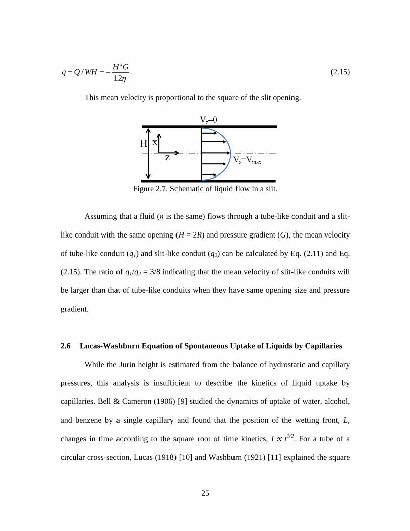
25

2

/12

H Gq Q WH

. (2.15)

This mean velocity is proportional to the square of the slit opening.

Figure 2.7. Schematic of liquid flow in a slit.

Assuming that a fluid (η is the same) flows through a tube-like conduit and a slit-

like conduit with the same opening (H = 2R) and pressure gradient (G), the mean velocity

of tube-like conduit (q1) and slit-like conduit (q2) can be calculated by Eq. (2.11) and Eq.

(2.15). The ratio of q1/q2 = 3/8 indicating that the mean velocity of slit-like conduits will

be larger than that of tube-like conduits when they have same opening size and pressure

gradient.

2.6 Lucas-Washburn Equation of Spontaneous Uptake of Liquids by Capillaries

While the Jurin height is estimated from the balance of hydrostatic and capillary

pressures, this analysis is insufficient to describe the kinetics of liquid uptake by

capillaries. Bell & Cameron (1906) [9] studied the dynamics of uptake of water, alcohol,

and benzene by a single capillary and found that the position of the wetting front, L,

changes in time according to the square root of time kinetics, L∝ t1/2

. For a tube of a

circular cross-section, Lucas (1918) [10] and Washburn (1921) [11] explained the square

26

root of time kinetics by balancing the wetting force with the gravitation force and

Poiseuille friction force (Figure 2.6).

The solution of Lucas-Washburn equation neglecting gravity is described here.

Assuming that the liquid is incompressible and the flow discharge is constant along the

tube ∂Q/∂z = 0, it follows from Eq. (2.10) that the pressure in the liquid is a linear

function of the front position, d2P/dz

2 = 0 or P(z) = az + b. When the tube is immersed in

a liquid reservoir, the pressure in the liquid equals to the atmospheric pressure P(0) = P1.

Taking this pressure P1 as the reference pressure, the first boundary condition reads P(0)

= P1 = 0. At the moving front, z = L(t), the pressure in the liquid is equal to the capillary

pressure P2 = -Pc = -2σcosθ/R . Therefore, the constants a and b are specified and the

pressure distribution in the liquid column reads:

2 11( )

P PP z z P

L

. (2.16)

The flow discharge through a tube is expressed as:

Q = πR2dL/dt. (2.17)

Substituting Eq. (2.16) and Eq. (2.17) into Eq. (2.10), one finds:

2

2 1

8

P PdL R

dt L

. (2.18)

Eq. (2.18) can be integrated using the initial condition L(0) = 0 to give:

cos( )

2

RtL t

. (2.19)

For a slit, this equation is written as [where P2 = -Pc = -2σcosθ/H]:

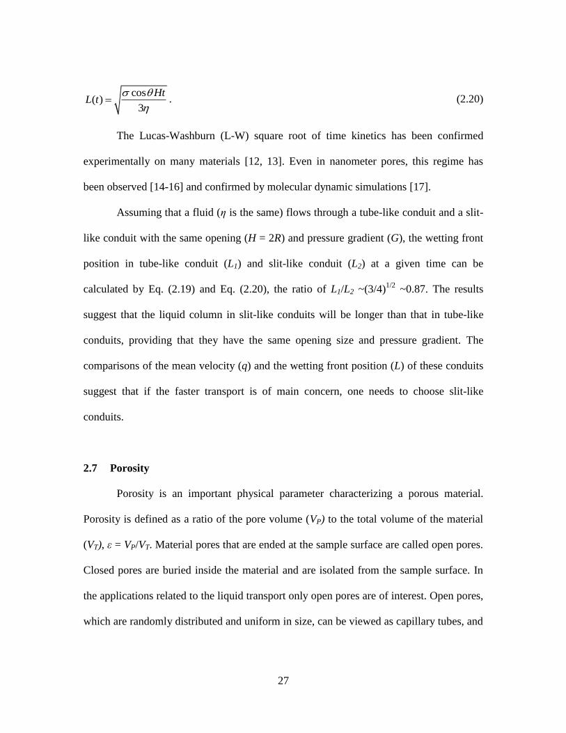
27

cos( )

3

HtL t

. (2.20)

The Lucas-Washburn (L-W) square root of time kinetics has been confirmed

experimentally on many materials [12, 13]. Even in nanometer pores, this regime has

been observed [14-16] and confirmed by molecular dynamic simulations [17].

Assuming that a fluid (η is the same) flows through a tube-like conduit and a slit-

like conduit with the same opening (H = 2R) and pressure gradient (G), the wetting front

position in tube-like conduit (L1) and slit-like conduit (L2) at a given time can be

calculated by Eq. (2.19) and Eq. (2.20), the ratio of L1/L2 ~(3/4)1/2

~0.87. The results

suggest that the liquid column in slit-like conduits will be longer than that in tube-like

conduits, providing that they have the same opening size and pressure gradient. The

comparisons of the mean velocity (q) and the wetting front position (L) of these conduits

suggest that if the faster transport is of main concern, one needs to choose slit-like

conduits.

2.7 Porosity

Porosity is an important physical parameter characterizing a porous material.

Porosity is defined as a ratio of the pore volume (VP) to the total volume of the material

(VT), ε = VP/VT. Material pores that are ended at the sample surface are called open pores.

Closed pores are buried inside the material and are isolated from the sample surface. In

the applications related to the liquid transport only open pores are of interest. Open pores,

which are randomly distributed and uniform in size, can be viewed as capillary tubes, and

28

the porous material can be modeled as a bundle of capillaries. In textile materials, the

three main components of the material porosity are: (1) intrafiber porosity (formed by

voids within the fibers); (2) interfiber porosity (formed by voids between fibers in the

yarns), and (3) interyarn porosity (formed by voids between yams). All pores are open

pores and the yarn/fabric can be considered as a bundle of capillary tubes with different

effective diameters.

Assuming that the yarn cross-section is made of identical cylinders which are

closely packed, forming a hexagonal elementary cell (Figure 2.8), the porosity is

estimated as [18]:

2

2

( 3 / 2)0.093

3

R

R

. (2.21)

If yarn is saturated with a liquid, the liquid can be trapped in the interfiber space

in the middle of the yarn as well as in the space between fibers on the surface of the yarn

(as shown by the dotted line in Figure 2.8). Therefore, the yarn porosity defined as ε =

VP/VT, should be always larger than that obtained from Eq. (2.21).

Figure 2.8. A schematic of cross-section of a yarn consisting of close-packed cylindrical

fibers of equal radii [18].

29

2.8 Darcy’s Law and Permeability

The description of fluid flow through a porous medium usually relies on Darcy’s

law, which states that the flow rate q is proportional to the pressure gradient ∇ driving

the flow and inversely proportional to the dynamic viscosity of the liquid η. Darcy’s law

was derived by the French engineer, Henry Darcy (1856). Darcy analyzed experimental

observations of the flow of water through sand filters. Darcy’s law is written as [1, 13]:

Q kq P

A , (2.22)

where Q is the volumetric flow rate, A is the cross-sectional area, and k is the

permeability of the porous media.

The structure of Eq. (2.22) is very similar to the structure of equations for the

mean velocity through cylindrical tubes and slits. If the porous material is made of

cylindrical tubes, Eq. (2.11) equals to Eq. (2.22) with k = R2/8. In the case of slits, Eq.

(2.15) equals to Eq. (2.22), and k = H2/12. These simple models of porous materials

suggest that the permeability is proportional to the square of pore opening, k ~ R2.

The permeability k can be considered as an ability of a porous material to

transport fluids through it. It significantly depends on the intersections between pores or

geometrical structure of the medium. This parameter received great attention from

materials scientists and engineers (Kozeny & Carman, Sheidegger, Dulien [13, 19-21]).

In particular, Kozeny and Carman derived a very useful relation between the materials

porosity and permeability considering the packed beads as a bundle of capillary tubes [20,

30

21]. They postulated that the total internal surface area and the total internal volume are

equal to the particle surface area and to the pore volume, respectively (Figure 2.9).

Figure 2.9. Schematics of the Kozeny-Carman’s approach for the permeability evaluation

of a granular bed. (a) the granular bed is made of spherical particles with diameter d, (b)

the pores are built by a system of cylindrical tubes (diameter D).

The volume of particles (Vp) can be expressed as:

3

6

p

p

N dV

, (2.23)

where Np is the number of particles and d is the diameter of spherical particles.

Considering an elementary volume (Ve) with porosity (ε), the volume of particles

(Vp) can be also expressed as Vp = Ve(1 − ε), and the elementary volume (Ve) and total

pore volume (Vpore) are expressed as:

3

6(1 )

p

e

N dV

, (2.24)

3

6(1 )

p

pore e

N dV V

. (2.25)

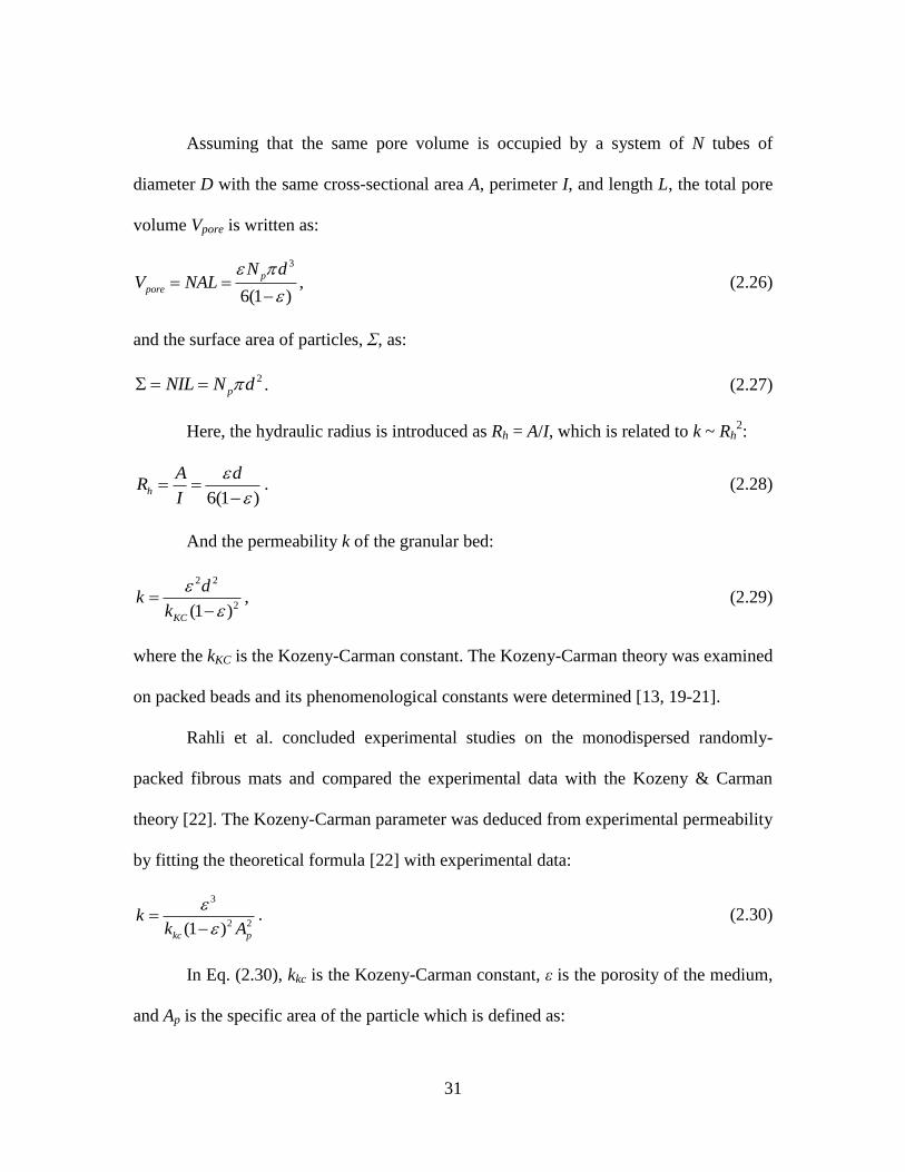
31

Assuming that the same pore volume is occupied by a system of N tubes of

diameter D with the same cross-sectional area A, perimeter I, and length L, the total pore

volume Vpore is written as:

3

6(1 )

p

pore

N dV NAL

, (2.26)

and the surface area of particles, Σ, as:

2

pNIL N d . (2.27)

Here, the hydraulic radius is introduced as Rh = A/I, which is related to k ~ Rh2:

6(1 )h

A dR

I

. (2.28)

And the permeability k of the granular bed:

2 2

2(1 )KC

dk

k

, (2.29)

where the kKC is the Kozeny-Carman constant. The Kozeny-Carman theory was examined

on packed beads and its phenomenological constants were determined [13, 19-21].

Rahli et al. concluded experimental studies on the monodispersed randomly-

packed fibrous mats and compared the experimental data with the Kozeny & Carman

theory [22]. The Kozeny-Carman parameter was deduced from experimental permeability

by fitting the theoretical formula [22] with experimental data:

3

2 2(1 )kc p

kk A

. (2.30)

In Eq. (2.30), kkc is the Kozeny-Carman constant, ε is the porosity of the medium,

and Ap is the specific area of the particle which is defined as:

32

2(2 1)p

ARA

ARd

, (2.31)

where AR is the fiber aspect ratio (L/d), which is calculated by dividing fiber length (L)

by its diameter (d).

2.9 Yarn Flexibility

The Bernoulli-Euler theory of beam bending is typically employed to describe

mechanics of fiber and yarn bending. This theory has two basic assumptions:

1. The material is isotropic and obeys the linear Hooke’s law of elasticity. These

properties remain unchanged during deformations;

2. The flat transverse planes of element (xy) in the unloaded beam will still be flat in the

bent beam.

These assumptions are adequate for metals and glasses but hardly applicable for

yarns. Internal structure of the nanofiber yarns is poorly understood; hence the Bernoulli-

Euler beam theory has to be applied with a precaution. However, the estimates of the

yarn flexibility based on the data on tensile experiments are worth to have. These

estimates will provide a good benchmark to evaluate the yarn flexibility relative to

existing textile materials.

2.9.1 Strain in a Bent Yarn

Consider a yarn bent in a loop of radius R as shown in Figure 2.10a. The bowed

fiber lies in the xy-plane. The bending moments M are applied to the fiber ends and one

needs to find a relation between the bending moments M and the fiber radius R. Bending

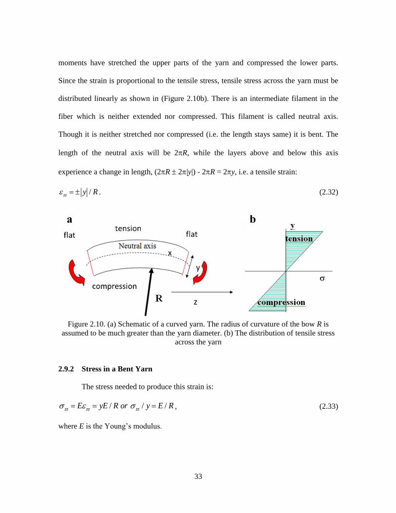
33

moments have stretched the upper parts of the yarn and compressed the lower parts.

Since the strain is proportional to the tensile stress, tensile stress across the yarn must be

distributed linearly as shown in (Figure 2.10b). There is an intermediate filament in the

fiber which is neither extended nor compressed. This filament is called neutral axis.

Though it is neither stretched nor compressed (i.e. the length stays same) it is bent. The

length of the neutral axis will be 2R, while the layers above and below this axis

experience a change in length, (2R 2|y|) - 2R = 2y, i.e. a tensile strain:

/zz y R . (2.32)

Figure 2.10. (a) Schematic of a curved yarn. The radius of curvature of the bow R is

assumed to be much greater than the yarn diameter. (b) The distribution of tensile stress

across the yarn

2.9.2 Stress in a Bent Yarn

The stress needed to produce this strain is:

/ / /zz zz zzE yE R or y E R , (2.33)

where E is the Young’s modulus.

34

This relation holds true for any point along the yarn, even if it is bent in a more

complicated shape, provided that R = R(s), i.e. the local radius depends on the arclength s.

Due to the second assumption, if the transverse planes are to remain flat, the total force

acting on this cross-section should be zero. Therefore, the force distribution shown in

Figure 2.10 should give no resultant force. The tensile force acting on the infinitesimal

slice with the cross sectional area dA is written as:

zzdF dA . (2.34)

The total force is 0zzdF dA , or using Eq. (2.33) which gives:

0zz

ydA E dA

R . (2.35)

This equation serves for specification of the neutral axis and the quantity

yI ydA is called the first moment of inertia.

2.9.3 Bending Moment

Consider the force moment as a resultant of the stress distribution of Eq. (2.33). In

any fiber cross-section perpendicular to the loop plane and neutral axis, the force moment

is written as:

zzdM y dA . (2.36)

Substituting Eq. (2.33) into Eq. (2.36), one obtains:

2 /dM Ey dA R . (2.37)

Integrating Eq. (2.37), one finds the Bernoulli-Euler result:

35

/M EI R (2.38)

where 2I y dA is the second moment of inertia. Hence, the bending moment has the

right dimension [M] = [N/m2] [m

4] / [m] = [N*m].

The product EI is called flexural rigidity and shows the yarn ability to resist

bending. Consider a solid fiber with a circular cross-section and radius R,. Placing the

origin of coordinates at the fiber center line (x = 0, y = 0), one has y = rsinθ, x = rcosθ,

and dA = rdrdθ. The second moment of inertia is calculated as:

2

2 2 4

0 0

sin / 4

R

I r rdrd R

. (2.39)

In the case of a yarn with a circular cross-section with the radius Ry and porosity ε,

the elemental area occupied by the solid material is written as dA = (1 - ε)rdrdθ:

2

2 2 4

0 0

sin (1 ) (1 ) / 4

yR

y yI r rdrd R

. (2.40)

2.10 References

1. Adamson, A.W. and A.P. Gast. Physical chemistry of surfaces. 1997.

2. Van Oss, C.J., Interfacial Forces in Aqueous Media. 1994: Marcel Dekker.

3. Young, T., An Essay on the Cohesion of Fluids. Philosophical Transactions of the

Royal Society of London, 1805. 95: p. 65-87.

4. de LaPlace, P.S., Supplément au Xe livre du Traité de mécanique céleste. 1806:

Courcier.

5. Berthier, J., Microdrops and Digital Microfluidics. 2008: William Andrew

Publishing.

36

6. Gennes, P.-G.d., F. Brochard-Wyart, and D. Quéré, Capillarity and wetting

phenomena : drops, bubbles, pearls, waves. 2004, New York: Springer.

7. Starov, V.M., M.G. Velarde, and C.J. Radke, Wetting And Spreading Dynamics.

2007: CRC PressINC.

8. Jurin, J., An Account of Some Experiments Shown before the Royal Society; With an

Enquiry into the Cause of the Ascent and Suspension of Water in Capillary Tubes. By

James Jurin, M. D. and R. Soc. S. Philosophical Transactions, 1717. 30(351-363): p.

739-747.

9. Bell, J.M. and F.K. Cameron, The Flow of Liquids through Capillary Spaces. The

Journal of Physical Chemistry, 1905. 10(8): p. 658-674.

10. Lucas, R., Ueber das Zeitgesetz des Kapillaren Aufstiegs von Flussigkeiten. Kolloid-

Z., 1918. 23: p. 15-22.

11. Washburn, E.W., The Dynamics of Capillary Flow. Physical Review, 1921. 17(3): p.

273.

12. Fisher, L.R. and P.D. Lark, Experimental-study of the Washburn equation for liquid

flow in very fine capillaries. Journal of Colloid and Interface Science, 1979. 69(3): p.

486-492.

13. Scheidegger, A.E., The physics of flow through porous media. 1957: University of

Toronto Press.

14. Neimark, A.V., S. Ruetsch, K.G. Kornev, P.I. Ravikovitch, P. Poulin, S. Badaire, and

M. Maugey, Hierarchical Pore Structure and Wetting Properties of Single Wall

Carbon Nanotube Fibers. Nano Letters, 2003. 3(3): p. 419-423.

15. Callegari, G., I. Tyomkin, K.G. Kornev, A.V. Neimark, and Y.L. Hsieh, Absorption

and transport properties of ultra-fine cellulose webs. Journal of Colloid and Interface

Science, 2011. 353(1): p. 290-293.

16. Tsai, C.C., P. Mikes, T. Andrukh, E. White, D. Monaenkova, O. Burtovyy, R.

Burtovyy, B. Rubin, D. Lukas, I. Luzinov, J.R. Owens, and K.G. Kornev,

Nanoporous artificial proboscis for probing minute amount of liquids. Nanoscale,

2011. 3(11): p. 4685-4695.

17. Martic, G., F. Gentner, D. Seveno, D. Coulon, J. De Coninck, and T.D. Blake, A

molecular dynamics simulation of capillary imbibition. Langmuir, 2002. 18(21): p.

7971-7976.

18. Raheel, M., Modern Textile Characterization Mthds. 1996: Marcel Dekker.

37

19. Dullien, F.A.L., Porous media: fluid transport and pore structure. 1992: Academic

Press.

20. Carman, P.C., Fluid flow through granular beds. Transactions of the Institution of

Chemical Engineers, 1937. 15: p. 150-166.

21. Kozeny, J., Ueber kapillare Leitung des Wassers im Boden. Sitzungsberichte

Akademie der Wissenschaften, Wien, 1927. 136: p. 271-306.

22. Rahli, O., L. Tadrist, M. Miscevic, and R. Santini, Fluid Flow Through Randomly

Packed Monodisperse Fibers: The Kozeny-Carman Parameter Analysis. Journal of

Fluids Engineering, 1997. 119(1): p. 188-192.

38

CHAPTER THREE

3FABRICATION OF YARNS FROM ELECTRSPUN FIBERS

A modified electrospinning setup was constructed. This setup enabled control

of the properties of electrospun yarns. A library of e-spinnable polymers was

generated and the polymers successfully electrospun into yarns. The breaking

strength, elongation at break, and Young’s modulus of these yarns were studied.

The electrospun yarns appeared to be much more flexible than traditional textile

fibers and yarns.

3.1 Introduction

Although several groups have developed different techniques to produce

nanofiber yarns, none of them demonstrated that the resulting yarns had the repeatable

transport and mechanical properties [1-7]. Precision control of these properties, however,

is critical for the performance of the probes. In this chapter, the development of an

industrially scalable method of yarn formation that provides reproducible mechanical

characteristics to these yarns was discussed. A home-made electrospinning collector and

a twisting device were developed in this study, and used for the yarn formation. The

electric field between the needle and two arm collector was simulated using COMSOL

software which explained the enhancement of fiber alignment between two conductive

parallel plates. The process of yarn formation was recorded using a high speed camera

(MotionPro X3, IDT Inc.) at 1,000 frames per second (fps), and the yarn length and cone

39

angle changing with time were studied. A geometric structure of twisting device was

created and the theoretical relation between the yarn length and cone angle was

calculated by this model. The theoretical calculations explained the experimental

observations. A library of polymers that can be successfully electrospun into yarns were

created. The SEM micrographs showed that fibers in a yarn are highly oriented after

twisting. The produced yarns were very uniform in diameter, eg. for 200 μm diameter

yarns, the standard deviations were about 5 μm. We also examined the tensile properties

of yarns using the stress-strain curves obtained on Instron machine. The results exhibited

that the yarns produced following the same experimental protocol had repeatable

breaking stress, elongation at break, and Young’s modulus. Yarns made from different

polymers exhibited different tensile stress–strain behavior suggesting that these

electrospun fiber yarns can be used in different applications.

3.2 Modified Electrospinning Setup

As presented in the literature review in chapter one, different spinning collectors

and different configurations of electric field have been employed to obtain aligned fibers.

However, prior to this work, there were no industrially scalable methods to form

nanofiber yarns. The proposed protocol consists of two steps: in the first step, one needs

to prepare an array of oriented fibers, which can be gathered in the second step by using a

special device. The proposed technique takes advantage of the most popular method of

formation of ordered fiber arrays suggested by Li et al. [8] where the fiber orientation is

significantly improved by making the target electrode from unipolar parallel bars.

40

A home-made collection and twisting device for the yarn formation was

developed by modifying the traditional electrospinnning setup [9]. The stationary

grounded collector (Figure 1.1) was replaced by a rotating disk with four aluminum bars

(Figure 3.1A). During electrospinning process, the aligned fibers are collected between

each pair of bars. The distance between each pair of bars can be adjusted. In this setup,

the interbar distance can be changed from 10 to 30 cm in order to control the yarn length.

In the second step, a special twisting device (Figure 3.1B) is used to collect and then twist

the aligned nanofibers into a yarn. The twisting device has two main functions: one is to

collect fibers from each pair of bars; the other one is to twist fibers into a yarn.

Figure 3.1. (A) A schematic diagram of modified electrospinning setup [9]. (a) syringe

with polymer solution, (b) metal needle, (c) syringe pump, (d) high voltage supply. (e)

grounded collector with four bars. (f) motor. (B) Schematic diagram of the twisting

device to produce yarns. The inset is the magnified brush.

3.3 Electric Field between Needle and Two-Arm Collector

The electric field between the needle and two-arm collector was calculated using

41

COMSOL

modeling software1. The needle was charged to 10 kV, the distance between

needle and two-arm collector was 30 cm, the gap between two arms was 20 cm, and the

collector was grounded. As shown in Figure 3.2, the red arrows represent the direction of

the electrostatic field, and different colors in the plane correspond to different potentials

specified in the vertical bar.

Figure 3.2. The perspective view of electric field in the region between the needle and

two-arm collector. The red arrows denote the direction of the electrostatic field, and

different colors in the plane correspond to different potentials specified in the vertical bar.

The needle is charged to 10 kV and the bars are grounded [9].

As demonstrated in Figure 3.2, the electric field near the plates is almost two-

dimensional. Since both plates are kept at the same voltage, the electric field lines branch

out from a singular line, which divides the interplate gap in half. Near the two charged

plates, the electric field vector E has opposite directions. Therefore, if two identical

charges q are situated in different halves of the interplate gap, they will be pushed by the

force F = qE toward different plates. For the jet, this specific electrode geometry works

as a natural stretching device. As a charged jet approaches the electrodes and is about to

1 I acknowledge Dr. Binyamin Rubin for his help in the simulation of the electric field distribution.

42

land in between, the electric force pulls the jet in different directions. Because the

nanofibers are charged, they repel each other. As a result, the nanofibers align

perpendicularly to the plates and do not touch each other.

3.4 Fabrication of Yarns from Electrospun Fibers

The oriented fibers were collected on the rotating disk with four aluminum bars as

shown in Figure 3.3a. In order to collect the fibers and twist them into a yarn, a special

twisting device was designed and produced. This twisting device consists of two circular

wire brushes mounted co-axially and attached to two miniature DC motors. The two arms

of the collector support the rolled brushes (Figure 3.3b). The fibers are gathered as a

fibrous cylindrical shell attached from its ends to the brushes. The same device is used to

form yarns by spinning the brushes in opposite directions: the brushes twist the fibrous

shell to a predetermined density, thus forming a yarn (Figure 3.3c). The twisting device

allows one to control the yarn diameter and its compactness by changing the total number

of revolutions of the brushes. After twisting, the yarn was cut off as a single piece (Figure

3.3d). Using this method, we formed yarns from different materials. By controlling the

electrospinning parameters, such as flow rate, polymer concentration, distance between

needle and collector etc., one can form a densely-packed or loosely-packed yarn by

controlling the electrospinning time and number of twists applied to a yarn.

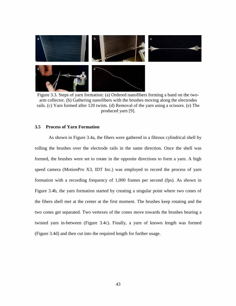
43

Figure 3.3. Steps of yarn formation: (a) Ordered nanofibers forming a band on the two-

arm collector. (b) Gathering nanofibers with the brushes moving along the electrodes

rails. (c) Yarn formed after 120 twists. (d) Removal of the yarn using a scissors. (e) The

produced yarn [9].

3.5 Process of Yarn Formation

As shown in Figure 3.4a, the fibers were gathered in a fibrous cylindrical shell by

rolling the brushes over the electrode rails in the same direction. Once the shell was

formed, the brushes were set to rotate in the opposite directions to form a yarn. A high

speed camera (MotionPro X3, IDT Inc.) was employed to record the process of yarn

formation with a recording frequency of 1,000 frames per second (fps). As shown in

Figure 3.4b, the yarn formation started by creating a singular point where two cones of

the fibers shell met at the center at the first moment. The brushes keep rotating and the

two cones get separated. Two vertexes of the cones move towards the brushes bearing a

twisted yarn in-between (Figure 3.4c). Finally, a yarn of known length was formed

(Figure 3.4d) and then cut into the required length for further usage.

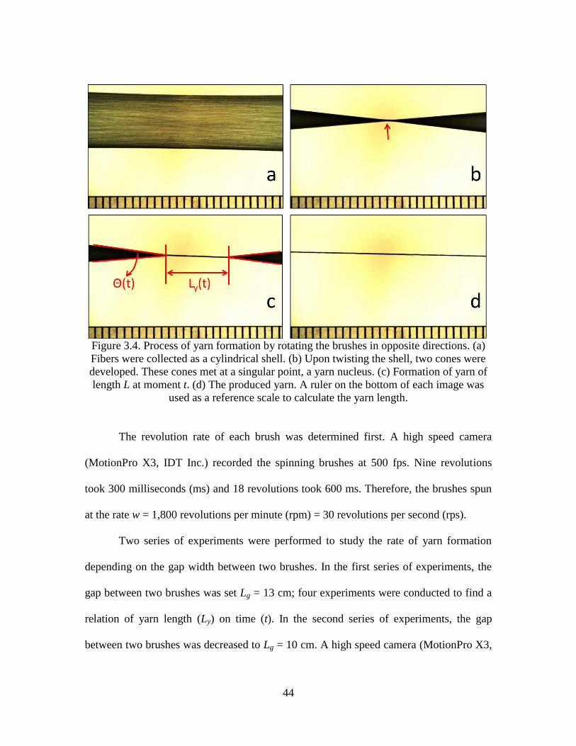
44

Figure 3.4. Process of yarn formation by rotating the brushes in opposite directions. (a)

Fibers were collected as a cylindrical shell. (b) Upon twisting the shell, two cones were

developed. These cones met at a singular point, a yarn nucleus. (c) Formation of yarn of

length L at moment t. (d) The produced yarn. A ruler on the bottom of each image was

used as a reference scale to calculate the yarn length.

The revolution rate of each brush was determined first. A high speed camera

(MotionPro X3, IDT Inc.) recorded the spinning brushes at 500 fps. Nine revolutions

took 300 milliseconds (ms) and 18 revolutions took 600 ms. Therefore, the brushes spun

at the rate w = 1,800 revolutions per minute (rpm) = 30 revolutions per second (rps).

Two series of experiments were performed to study the rate of yarn formation

depending on the gap width between two brushes. In the first series of experiments, the

gap between two brushes was set Lg = 13 cm; four experiments were conducted to find a

relation of yarn length (Ly) on time (t). In the second series of experiments, the gap

between two brushes was decreased to Lg = 10 cm. A high speed camera (MotionPro X3,

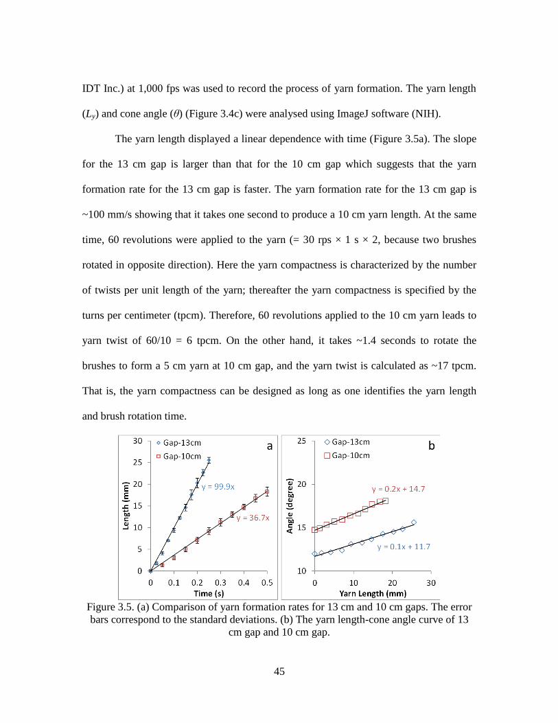
45

IDT Inc.) at 1,000 fps was used to record the process of yarn formation. The yarn length

(Ly) and cone angle (θ) (Figure 3.4c) were analysed using ImageJ software (NIH).

The yarn length displayed a linear dependence with time (Figure 3.5a). The slope

for the 13 cm gap is larger than that for the 10 cm gap which suggests that the yarn

formation rate for the 13 cm gap is faster. The yarn formation rate for the 13 cm gap is

~100 mm/s showing that it takes one second to produce a 10 cm yarn length. At the same

time, 60 revolutions were applied to the yarn (= 30 rps × 1 s × 2, because two brushes

rotated in opposite direction). Here the yarn compactness is characterized by the number

of twists per unit length of the yarn; thereafter the yarn compactness is specified by the

turns per centimeter (tpcm). Therefore, 60 revolutions applied to the 10 cm yarn leads to

yarn twist of 60/10 = 6 tpcm. On the other hand, it takes ~1.4 seconds to rotate the

brushes to form a 5 cm yarn at 10 cm gap, and the yarn twist is calculated as ~17 tpcm.

That is, the yarn compactness can be designed as long as one identifies the yarn length

and brush rotation time.

Figure 3.5. (a) Comparison of yarn formation rates for 13 cm and 10 cm gaps. The error

bars correspond to the standard deviations. (b) The yarn length-cone angle curve of 13

cm gap and 10 cm gap.

46

The cone angles were also studied and shown in Figure 3.5b. Since the diameter

of brush is constant, the longer the gap between two brushes, the smaller the initial cone

angle (Figure 3.5b). When the yarn length (Ly) is getting longer, the cone endpoints

approach the two brushes causing an increase in cone angles. The cone angles, however,

do not increase significantly, not greater than ~3 degrees, following a linear dependence

with the yarn length (Figure 3.5b).

A schematic diagram (Figure 3.6a) shows the geometry of the twisting device and

two cones creating a yarn “nucleus” at the center. With the notations shown in Figure

3.6a, where the diameter of brush is D, the gap width is Lg, and the cone angle is θ, the

equation relating the cone angle with the geometrical parameters of the yarn twisting

device is written as:

/ 2tan( )

2 ( ) / 2 ( )g y g y

D D

L L L L

, (3.1)

where Ly(t) is the yarn length which is a time-dependent function.

Solving Eq. (3.1) for θ, we obtain:

12 tan ( )g y

D

L L

. (3.2)

That is, the relation between the cone angle and yarn length can be established as

long as the diameter of brush (D) and the gap distance between two brushes (Lg) are

known. Giving the experimental parameters: D = 1.4 cm and Lg = 13 cm (or 10 cm), the

yarn length-cone angle curve corresponding to the experimental parameters was created

(Figure 3.6b). Comparing Figure 3.5b and Figure 3.6b, one concludes that the

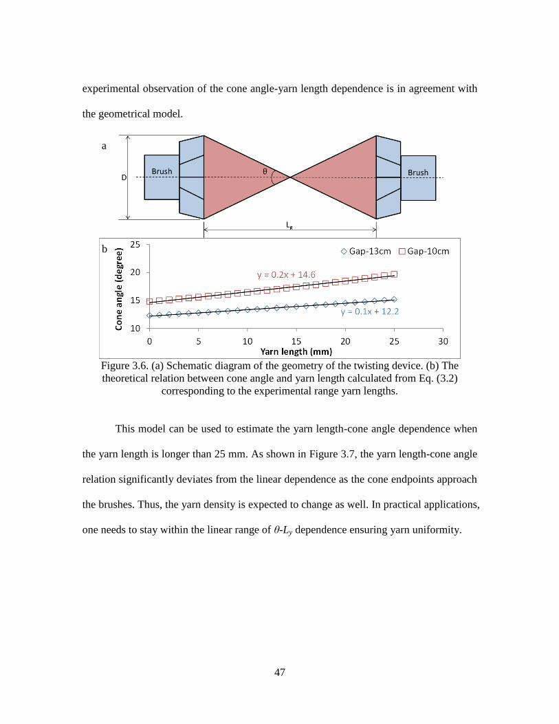
47

experimental observation of the cone angle-yarn length dependence is in agreement with

the geometrical model.

Figure 3.6. (a) Schematic diagram of the geometry of the twisting device. (b) The

theoretical relation between cone angle and yarn length calculated from Eq. (3.2)

corresponding to the experimental range yarn lengths.

This model can be used to estimate the yarn length-cone angle dependence when

the yarn length is longer than 25 mm. As shown in Figure 3.7, the yarn length-cone angle

relation significantly deviates from the linear dependence as the cone endpoints approach

the brushes. Thus, the yarn density is expected to change as well. In practical applications,

one needs to stay within the linear range of θ-Ly dependence ensuring yarn uniformity.

a

b

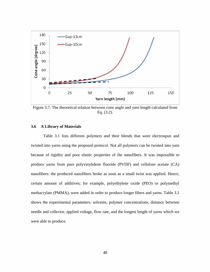
48

Figure 3.7. The theoretical relation between cone angle and yarn length calculated from

Eq. (3.2).

3.6 A Library of Materials

Table 3.1 lists different polymers and their blends that were electrospun and

twisted into yarns using the proposed protocol. Not all polymers can be twisted into yarn

because of rigidity and poor elastic properties of the nanofibers. It was impossible to

produce yarns from pure polyvinylidene fluoride (PVDF) and cellulose acetate (CA)

nanofibers: the produced nanofibers broke as soon as a small twist was applied. Hence,

certain amount of additives; for example, polyethylene oxide (PEO) or polymethyl

methacrylate (PMMA), were added in order to produce longer fibers and yarns. Table 3.1

shows the experimental parameters: solvents, polymer concentrations, distance between

needle and collector, applied voltage, flow rate, and the longest length of yarns which we

were able to produce.

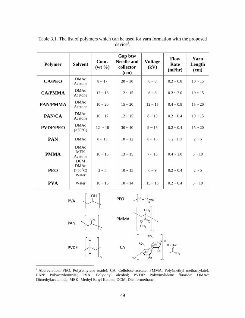
49

Table 3.1. The list of polymers which can be used for yarn formation with the proposed

device2.

2 Abbreviation: PEO: Poly(ethylene oxide); CA: Cellulose acetate; PMMA: Poly(methyl methacrylate);

PAN: Polyacrylonitrile; PVA: Polyvinyl alcohol; PVDF: Polyvinylidene fluoride; DMAc:

Dimethylacetamide; MEK: Methyl Ethyl Ketone; DCM: Dichlormethane.

PVDF

PVA

PAN

PEO

CA

PMMA

Polymer Solvent Conc.

(wt %)

Gap btw

Needle and

collector

(cm)

Voltage

(kV)

Flow

Rate

(ml/hr)

Yarn

Length

(cm)

CA/PEO DMAc

Acetone 8 ~ 17 20 ~ 30 6 ~ 8 0.2 ~ 0.8 10 ~ 15

CA/PMMA DMAc

Acetone 12 ~ 16 12 ~ 15 6 ~ 8 0.2 ~ 2.0 10 ~ 15

PAN/PMMA DMAc

Acetone 10 ~ 20 15 ~ 20 12 ~ 15 0.4 ~ 0.8 15 ~ 20

PAN/CA DMAc

Acetone 10 ~ 17 12 ~ 15 8 ~ 10 0.2 ~ 0.4 10 ~ 15

PVDF/PEO DMAc

(>50⁰C) 12 ~ 18 30 ~ 40 9 ~ 13 0.2 ~ 0.4 15 ~ 20

PAN DMAc 8 ~ 15 10 ~ 12 8 ~ 15 0.2 ~1.0 2 ~ 5

PMMA

DMAc

MEK

Acetone

DCM

10 ~ 16 13 ~ 15 7 ~ 15 0.4 ~ 1.0 5 ~ 10

PEO DMAc

(>50⁰C)

Water

2 ~ 5 10 ~ 15 6 ~ 9 0.2 ~ 0.4 2 ~ 5

PVA Water 10 ~ 16 10 ~ 14 15 ~ 18 0.2 ~ 0.4 5 ~ 10

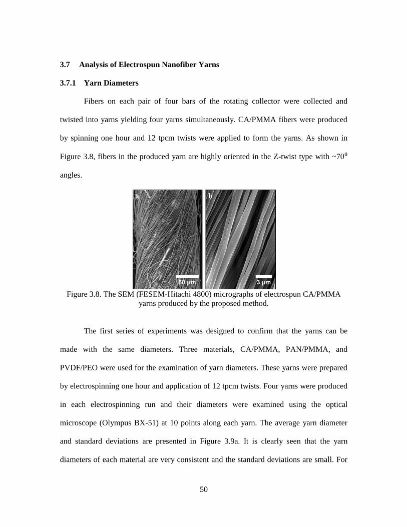
50

3.7 Analysis of Electrospun Nanofiber Yarns

3.7.1 Yarn Diameters

Fibers on each pair of four bars of the rotating collector were collected and

twisted into yarns yielding four yarns simultaneously. CA/PMMA fibers were produced

by spinning one hour and 12 tpcm twists were applied to form the yarns. As shown in

Figure 3.8, fibers in the produced yarn are highly oriented in the Z-twist type with ~70⁰

angles.

Figure 3.8. The SEM (FESEM-Hitachi 4800) micrographs of electrospun CA/PMMA

yarns produced by the proposed method.

The first series of experiments was designed to confirm that the yarns can be

made with the same diameters. Three materials, CA/PMMA, PAN/PMMA, and

PVDF/PEO were used for the examination of yarn diameters. These yarns were prepared

by electrospinning one hour and application of 12 tpcm twists. Four yarns were produced

in each electrospinning run and their diameters were examined using the optical

microscope (Olympus BX-51) at 10 points along each yarn. The average yarn diameter

and standard deviations are presented in Figure 3.9a. It is clearly seen that the yarn

diameters of each material are very consistent and the standard deviations are small. For

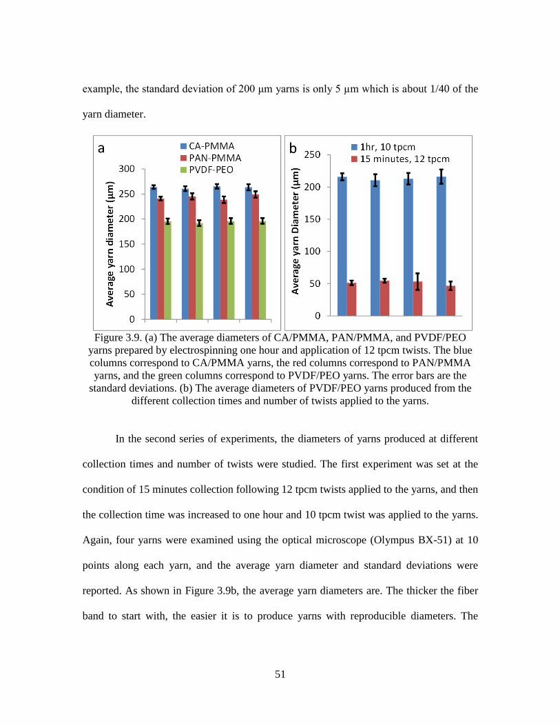
51

example, the standard deviation of 200 μm yarns is only 5 µm which is about 1/40 of the

yarn diameter.

Figure 3.9. (a) The average diameters of CA/PMMA, PAN/PMMA, and PVDF/PEO

yarns prepared by electrospinning one hour and application of 12 tpcm twists. The blue

columns correspond to CA/PMMA yarns, the red columns correspond to PAN/PMMA

yarns, and the green columns correspond to PVDF/PEO yarns. The error bars are the

standard deviations. (b) The average diameters of PVDF/PEO yarns produced from the

different collection times and number of twists applied to the yarns.

In the second series of experiments, the diameters of yarns produced at different

collection times and number of twists were studied. The first experiment was set at the

condition of 15 minutes collection following 12 tpcm twists applied to the yarns, and then

the collection time was increased to one hour and 10 tpcm twist was applied to the yarns.

Again, four yarns were examined using the optical microscope (Olympus BX-51) at 10

points along each yarn, and the average yarn diameter and standard deviations were

reported. As shown in Figure 3.9b, the average yarn diameters are. The thicker the fiber

band to start with, the easier it is to produce yarns with reproducible diameters. The

52

thinnest reproducible yarns were 20 m in diameter. These results show that the proposed

device is able to fabricate yarns with controlled properties.

3.7.2 Elasticity

The tensile stress-strain test is the simplest mechanical test providing the Young’s

modulus of the material, and the strength characteristics of the yarns. Tensile stress-strain

characteristics are determined by monitoring the force and the yarn elongation. The

Young’s modulus is usually defined at small strains where the stress-strain curve is

approximately linear.

The stress σ is defined as:

0

F

A , (3.3)

where F is the force applied perpendicularly to the specimen cross-section and A0 is the

original cross-sectional area of the yarn before loading. Typical units of stress are

megapascals, MPa (SI), or pounds force per square inch, psi.

The definition of strain ε is:

0

0

il l l

l l

, (3.4)

where l0 is the original yarn length before loading and li is the yarn length under the load,

and Δl is the yarn extension. The strain is unitless. It is common to express strain in

percent:

0

0

(%) 100 100il l l

l l

. (3.5)

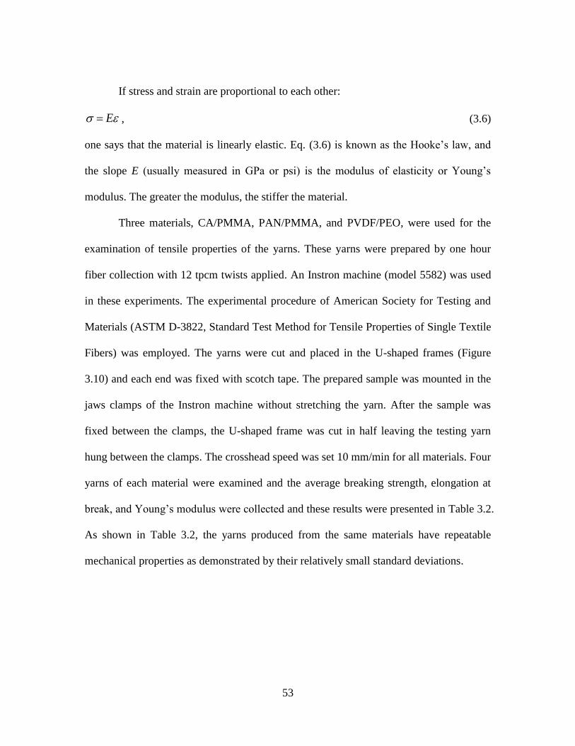
53

If stress and strain are proportional to each other:

E , (3.6)

one says that the material is linearly elastic. Eq. (3.6) is known as the Hooke’s law, and

the slope E (usually measured in GPa or psi) is the modulus of elasticity or Young’s

modulus. The greater the modulus, the stiffer the material.

Three materials, CA/PMMA, PAN/PMMA, and PVDF/PEO, were used for the

examination of tensile properties of the yarns. These yarns were prepared by one hour

fiber collection with 12 tpcm twists applied. An Instron machine (model 5582) was used

in these experiments. The experimental procedure of American Society for Testing and

Materials (ASTM D-3822, Standard Test Method for Tensile Properties of Single Textile

Fibers) was employed. The yarns were cut and placed in the U-shaped frames (Figure

3.10) and each end was fixed with scotch tape. The prepared sample was mounted in the

jaws clamps of the Instron machine without stretching the yarn. After the sample was

fixed between the clamps, the U-shaped frame was cut in half leaving the testing yarn

hung between the clamps. The crosshead speed was set 10 mm/min for all materials. Four

yarns of each material were examined and the average breaking strength, elongation at

break, and Young’s modulus were collected and these results were presented in Table 3.2.

As shown in Table 3.2, the yarns produced from the same materials have repeatable

mechanical properties as demonstrated by their relatively small standard deviations.

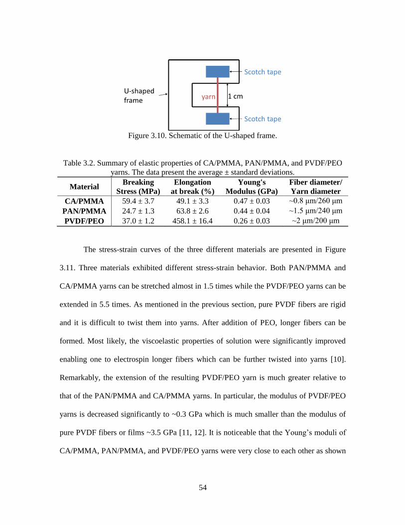
54

Figure 3.10. Schematic of the U-shaped frame.

Table 3.2. Summary of elastic properties of CA/PMMA, PAN/PMMA, and PVDF/PEO

yarns. The data present the average ± standard deviations.

Material Breaking

Stress (MPa)

Elongation

at break (%)

Young's

Modulus (GPa)

Fiber diameter/

Yarn diameter

CA/PMMA 59.4 ± 3.7 49.1 ± 3.3 0.47 ± 0.03 ~0.8 μm/260 μm

PAN/PMMA 24.7 ± 1.3 63.8 ± 2.6 0.44 ± 0.04 ~1.5 μm/240 μm

PVDF/PEO 37.0 ± 1.2 458.1 ± 16.4 0.26 ± 0.03 ~2 μm/200 μm

The stress-strain curves of the three different materials are presented in Figure

3.11. Three materials exhibited different stress-strain behavior. Both PAN/PMMA and

CA/PMMA yarns can be stretched almost in 1.5 times while the PVDF/PEO yarns can be

extended in 5.5 times. As mentioned in the previous section, pure PVDF fibers are rigid

and it is difficult to twist them into yarns. After addition of PEO, longer fibers can be

formed. Most likely, the viscoelastic properties of solution were significantly improved

enabling one to electrospin longer fibers which can be further twisted into yarns [10].

Remarkably, the extension of the resulting PVDF/PEO yarn is much greater relative to

that of the PAN/PMMA and CA/PMMA yarns. In particular, the modulus of PVDF/PEO

yarns is decreased significantly to ~0.3 GPa which is much smaller than the modulus of

pure PVDF fibers or films ~3.5 GPa [11, 12]. It is noticeable that the Young’s moduli of

CA/PMMA, PAN/PMMA, and PVDF/PEO yarns were very close to each other as shown

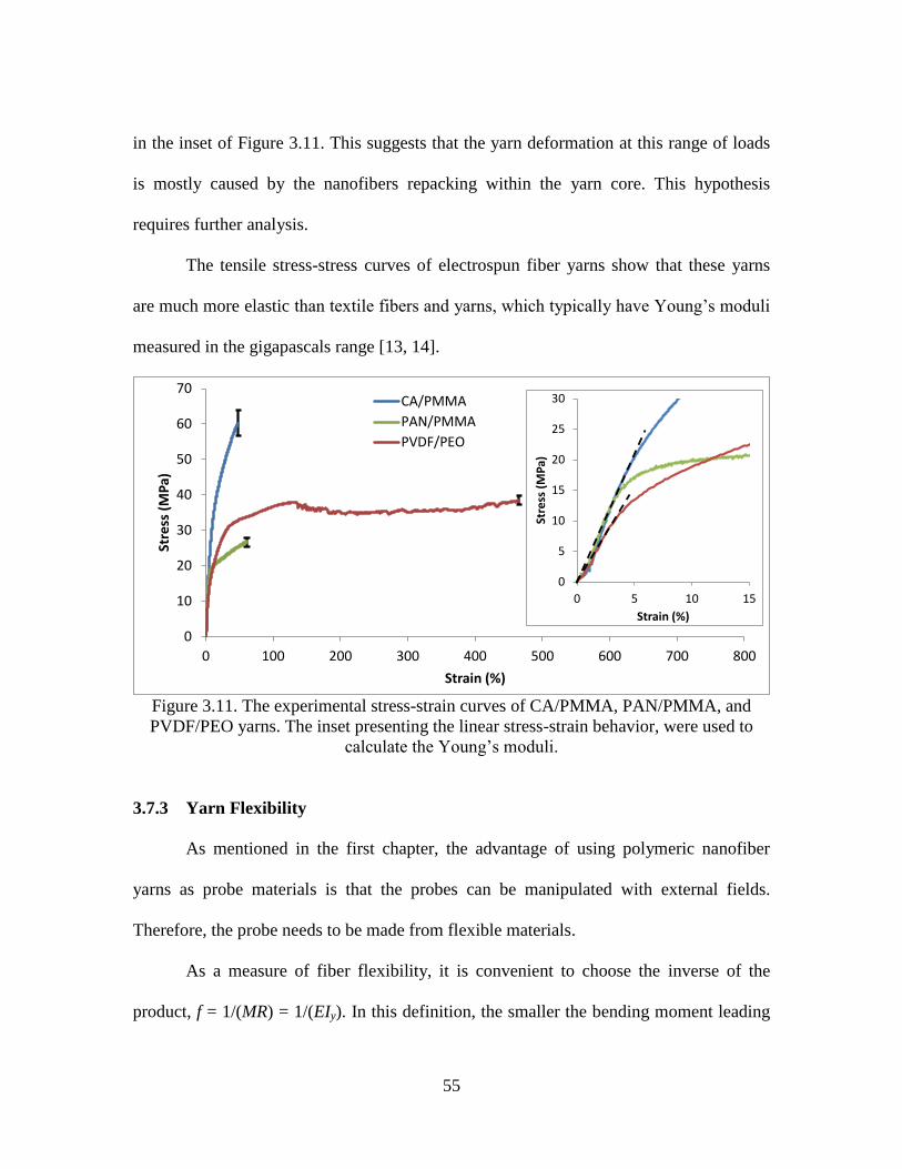
55

in the inset of Figure 3.11. This suggests that the yarn deformation at this range of loads

is mostly caused by the nanofibers repacking within the yarn core. This hypothesis

requires further analysis.

The tensile stress-stress curves of electrospun fiber yarns show that these yarns

are much more elastic than textile fibers and yarns, which typically have Young’s moduli

measured in the gigapascals range [13, 14].

Figure 3.11. The experimental stress-strain curves of CA/PMMA, PAN/PMMA, and

PVDF/PEO yarns. The inset presenting the linear stress-strain behavior, were used to

calculate the Young’s moduli.

3.7.3 Yarn Flexibility

As mentioned in the first chapter, the advantage of using polymeric nanofiber

yarns as probe materials is that the probes can be manipulated with external fields.

Therefore, the probe needs to be made from flexible materials.

As a measure of fiber flexibility, it is convenient to choose the inverse of the

product, f = 1/(MR) = 1/(EIy). In this definition, the smaller the bending moment leading

0

10

20

30

40

50

60

70

0 100 200 300 400 500 600 700 800

Stre

ss (

MP

a)

Strain (%)

CA/PMMA

PAN/PMMA

PVDF/PEO

0

5

10

15

20

25

30

0 5 10 15

Stre

ss (

MP

a)

Strain (%)

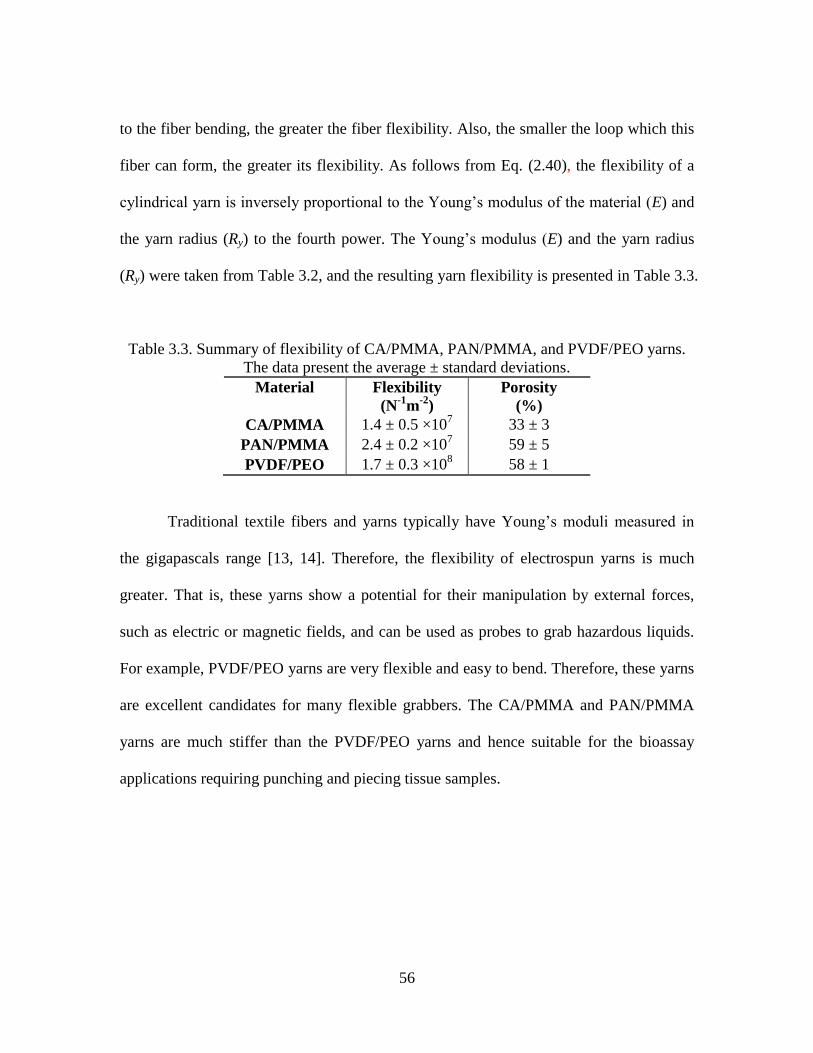
56

to the fiber bending, the greater the fiber flexibility. Also, the smaller the loop which this

fiber can form, the greater its flexibility. As follows from Eq. (2.40), the flexibility of a

cylindrical yarn is inversely proportional to the Young’s modulus of the material (E) and

the yarn radius (Ry) to the fourth power. The Young’s modulus (E) and the yarn radius

(Ry) were taken from Table 3.2, and the resulting yarn flexibility is presented in Table 3.3.

Table 3.3. Summary of flexibility of CA/PMMA, PAN/PMMA, and PVDF/PEO yarns.

The data present the average ± standard deviations.

Material Flexibility

(N-1

m-2

)

Porosity

(%)

CA/PMMA 1.4 ± 0.5 ×107 33 ± 3

PAN/PMMA 2.4 ± 0.2 ×107 59 ± 5

PVDF/PEO 1.7 ± 0.3 ×108 58 ± 1

Traditional textile fibers and yarns typically have Young’s moduli measured in

the gigapascals range [13, 14]. Therefore, the flexibility of electrospun yarns is much

greater. That is, these yarns show a potential for their manipulation by external forces,

such as electric or magnetic fields, and can be used as probes to grab hazardous liquids.

For example, PVDF/PEO yarns are very flexible and easy to bend. Therefore, these yarns

are excellent candidates for many flexible grabbers. The CA/PMMA and PAN/PMMA

yarns are much stiffer than the PVDF/PEO yarns and hence suitable for the bioassay

applications requiring punching and piecing tissue samples.

57

3.8 Methods and Materials

3.8.1 Polymer Solution Preparation

Polyacrylonitrile (PAN, MW=150 kDa), Polyethylene oxide (PEO, MW=1000

kDa), Cellulose acetate3 (CA, MW: ~37 kDa), Polymethyl methacrylate (PMMA, MW:

~996 kDa) were obtained from Sigma-Aldrich. Polyvinylidene fluoride (PVDF) was

purchased from Goodfellow. Dimethylacetamide (DMAc) was purchased from Alfa

Aesar. All chemicals were used as received without further purification. DMAc was used

as a solvent to prepare polymer solutions: a. 12.28 wt% CA/PMMA mixture with the

CA/PMMA ratio = 5:2 (by weight); b. 19.35 wt% PAN/PMMA mixture with the

PNA/PMMA ratio = 1:1; c. 18.03 wt% PVDF/PEO mixtures with the PVDF/PEO ratio =

10:1 (by weight).

3.8.2 Porosity (ε)

The porosity of different materials was estimated by the formula ε = (mw-md) /

(ρVy), where mw is the mass of wet yarn, md is the mass of dry yarn, ρ is the liquid density,

and Vy is the yarn volume. The yarn volume was calculated as Vy = πRy2Ly, where Ry is

the radius of yarn which was measured by the optical microscope Olympus BX-51, and

Ly is the length of the yarn. The yarn was placed vertically with one end sealed with

plasticine and another end submersed in hexadecane. The mass change was measured by

Cahn DCA-322 DCA analyzer. The porosity was examined on three samples for each

material.

3 The CA is actually cellulose diacetate with a degree of substitution (DS) of approximate 2.3.

58

3.9 Conclusions

A technique to fabricate electrospun fiber yarns was successfully developed by

industrially scalable methods using a modified collector and a twisting device. Various

polymer fibers were electrospun into ordered bands and subsequently twisted into yarns.

The process of yarn formation was studied and compared with a geometrical model; the

time dependence of the yarn length and cone angle was in agreement with theoretical

calculations. The fibers in the produced yarns appeared oriented after twisting. The yarns

produced were very uniform. The tensile properties of yarns were examined by Instron

machine The measured mechanical characteristics of the yarns were very repeatable. The

yarns appeared much more flexible comparing with the textile fibers and yarns. The

results suggest that these electrospun yarns may have various applications in micro- and

nano-mechanical devices. For example, to probe, one needs fibers flexible enable to

penetrate capillaries and small pores; and PVDF/PEO yarns are the best candidates. For

piercing tissue and for biopsy, one needs stiff materials preventing deformation during

punching and piercing. Thus, CA/PMMA and PAN/PMMA yarns are the best candidates

for these applications.

3.10 References

1. Lin, T., Nanofibers - production, properties and functional applications. 2011:

InTech. 458 p.



3. Ali, U., Y.Q. Zhou, X.G. Wang, and T. Lin, Direct electrospinning of highly twisted,

continuous nanofiber yarns. Journal of the Textile Institute, 2012. 103(1): p. 80-88.

59

4. Dabirian, F., S.A.H. Ravandi, R.H. Sanatgar, and J.P. Hinestroza, Manufacturing of

Twisted Continuous PAN Nanofiber Yarn by Electrospinning Process. Fibers and

Polymers, 2011. 12(5): p. 610-615.


Polymer, 2005. 46(8): p. 2419-2423.

6. Zhou, F.L. and R.H. Gong, Manufacturing technologies of polymeric nanofibres and

nanofibre yarns. Polymer International, 2008. 57(6): p. 837-845.

7. Usman Ali, Y.Z., Xungai Wang, and Tong Lin, Electrospinning of Continuous

Nanofiber Bundles and Twisted Nanofiber Yarns, Nanofibers - Production,

Properties and Functional Applications, Dr. Tong Lin. 2011: InTech.

8. Li, D., Y.L. Wang, and Y.N. Xia, Electrospinning of polymeric and ceramic

nanofibers as uniaxially aligned arrays. Nano Letters, 2003. 3(8): p. 1167-1171.




2011. 3(11): p. 4685-4695.

10. Bazilevsky, A.V., K.G. Kornev, A.N. Rozhkov, and A.V. Neimark, Spontaneous

absorption of viscous and viscoelastic fluids by capillaries and porous substrates.

Journal of Colloid and Interface Science, 2003. 262(1): p. 16-24.

11. Du, C., B. Zhu, and Y. Xu, Hard elasticity of poly(vinylidene fluoride) fibers. Journal

of Materials Science, 2005. 40(4): p. 1035-1036.

12. Vinogradov, A. and F. Holloway, Electro-mechanical properties of the piezoelectric

polymer PVDF. Ferroelectrics, 1999. 226(1): p. 169-181.

13. Hongu, T., G.O. Phillips, and M. Takigami, New millenium fibers. 2005, Cambridge,

England: Woodhead Publishing Ltd.

14. Lee, S.M., Handbook of Composite Reinforcements. 1992: Wiley.

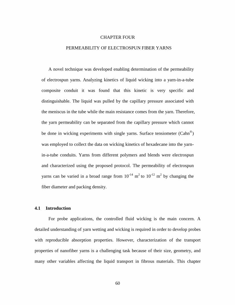
60

CHAPTER FOUR

4PERMEABILITY OF ELECTROSPUN FIBER YARNS

A novel technique was developed enabling determination of the permeability

of electrospun yarns. Analyzing kinetics of liquid wicking into a yarn-in-a-tube

composite conduit it was found that this kinetic is very specific and

distinguishable. The liquid was pulled by the capillary pressure associated with

the meniscus in the tube while the main resistance comes from the yarn. Therefore,

the yarn permeability can be separated from the capillary pressure which cannot

be done in wicking experiments with single yarns. Surface tensiometer (Cahn

)

was employed to collect the data on wicking kinetics of hexadecane into the yarn-

in-a-tube conduits. Yarns from different polymers and blends were electrospun

and characterized using the proposed protocol. The permeability of electrospun

yarns can be varied in a broad range from 10-14

m2

to 10-12

m2 by changing the

fiber diameter and packing density.

4.1 Introduction

For probe applications, the controlled fluid wicking is the main concern. A

detailed understanding of yarn wetting and wicking is required in order to develop probes

with reproducible absorption properties. However, characterization of the transport

properties of nanofiber yarns is a challenging task because of their size, geometry, and

many other variables affecting the liquid transport in fibrous materials. This chapter

61

discusses the characterization of transport properties of nanofiber yarns in terms of their

permeability, which is the main factor affecting the fluid flow in a porous material. The

permeability k can be considered as an characteristic of a porous material to transport

fluids through it. Fluid flow through a porous medium can be described by Darcy’s law

(Figure 4.1), which relates the filtration velocity, q, with the pressure gradient, ∇ , and

dynamic viscosity of the liquid, η [1, 2]:

Q kq P

A , (4.1)

where Q is the volumetric flow rate, A is the sample cross-sectional area through which

the liquid is flowing, and k is the permeability of the porous medium. Figure 4.1

represents a schematic of fluid flow through a porous cylinder.

Figure 4.1. Fluid flow through a porous cylinder of length L is described by Darcy’s law

( ) ( )a bQ A k P P L . Q is the volumetric flow rate, A is the sample cross-sectional

area through which the liquid is flowing, and the pressure gradient is expressed as ∇P =

(Pb - Pa)/L.

Nanofiber yarns are attractive candidates for probing of different liquids because

they generate very high capillary pressure. In order to illustrate great potential of

nanofiber yarns, consider a simple yarn model as a fiber bundle. Making this model even

62

simpler, the interfiber channel is assumed cylindrical with radius R. Then the capillary

pressure generated by a liquid meniscus is estimated as (see Chapter 2, Eq. (2.4)):

2 cos /cP R , (4.2)

where σ is the surface tension of the liquid/air interface and θ is the contact angle that the

meniscus makes with the channel wall. Therefore, when the yarn is dipped into a liquid,

the meniscus at the wetting front pulls the liquid from the reservoir by creating a pressure

drop Pc.

Combining Eq. (4.1) and Eq. (4.2), and expressing the volumetric flow rate as the

velocity of the wetting front Q = εAdL/dt, we obtain:

2 cosckPdL k

dt L LR

, (4.3)

where L is the wetting front position at time t and ε is the porosity of the yarn.

Eq. (4.3) can be immediately integrated to give the well-known Lucas-Washburn

law [3, 4]:

2 cos2ckP k

L t tR

. (4.4)

As follows from Eq. (4.4), in order to interpret the experimental L(t) dependency,

one needs to know porosity ε, capillary pressure Pc, and permeability of the given yarn k.

Conventional wicking experiments cannot independently provide the capillary pressure

and permeability because these parameters cannot be separated in Eq. (4.4). Available

experimental techniques assume dealing with large samples. In addition to their small

size, nanofiber yarns pose another challenge: the capillary pressure created by the yarns

63

becomes very high, making the analysis of the Jurin length problematic [5]. For example,

a water column is supposed to reach 15 meters in a 2 μm diameter pore (Figure 2.5)

indicating that the Jurin experiment cannot be used for characterization of these yarns.

Recent progress in the electrospinning of nanofibers and nanofiber yarns calls for

development of new characterization methods of their analyses.

This challenge is addressed by developing a novel technique enabling

determination of the permeability of nanofiber yarns without knowing its capillary

pressure. If one embeds the nanofiber yarn in a capillary letting a piece of yarn to stick

out of the capillary, the yarn and capillary will work as a complex conduit with a

composite permeability. This permeability can be directly evaluated from the same

capillary rise experiment: one needs to fill the yarn with the liquid and let meniscus to

propagate through the capillary. Meniscus position is determined by the yarn

permeability ky (ky = r2/8, where r is the capillary radius [1, 6]). The driving force for the

capillary rise is the wetting force, Fw = 2πrσcosθ, where θ is the contact angle that

meniscus makes with the capillary wall. Thus, the driving force can be separated from the

yarn permeability.

An engineering model was developed to describe this wicking experiment. The

model leads to the Lucas-Washburn equation with the modified permeability. The model

reveals interesting kinetics specific for the yarn-in-a-tube system allowing extraction of

the yarn permeability directly from the wicking experiments. An experimental setup

utilizing the capability of a Cahn surface tensiometer was developed. Different nanofiber

yarns were electrospun and their permeabilities were measured using the proposed theory

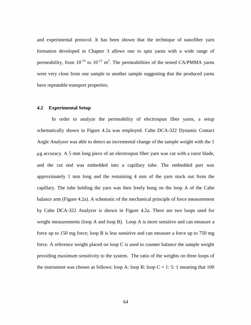
64

and experimental protocol. It has been shown that the technique of nanofiber yarn

formation developed in Chapter 3 allows one to spin yarns with a wide range of

permeability, from 10-14

to 10-12

m2. The permeabilities of the tested CA/PMMA yarns

were very close from one sample to another sample suggesting that the produced yarns

have repeatable transport properties.

4.2 Experimental Setup

In order to analyze the permeability of electrospun fiber yarns, a setup

schematically shown in Figure 4.2a was employed. Cahn DCA-322 Dynamic Contact

Angle Analyzer was able to detect an incremental change of the sample weight with the 1

g accuracy. A 5 mm long piece of an electrospun fiber yarn was cut with a razor blade,

and the cut end was embedded into a capillary tube. The embedded part was

approximately 1 mm long and the remaining 4 mm of the yarn stuck out from the

capillary. The tube holding the yarn was then freely hung on the loop A of the Cahn

balance arm (Figure 4.2a). A schematic of the mechanical principle of force measurement

by Cahn DCA-322 Analyzer is shown in Figure 4.2a. There are two loops used for

weight measurements (loop A and loop B). Loop A is more sensitive and can measure a

force up to 150 mg force; loop B is less sensitive and can measure a force up to 750 mg

force. A reference weight placed on loop C is used to counter balance the sample weight

providing maximum sensitivity to the system. The ratio of the weights on three loops of

the instrument was chosen as follows: loop A: loop B: loop C = 1: 5: 1 meaning that 100

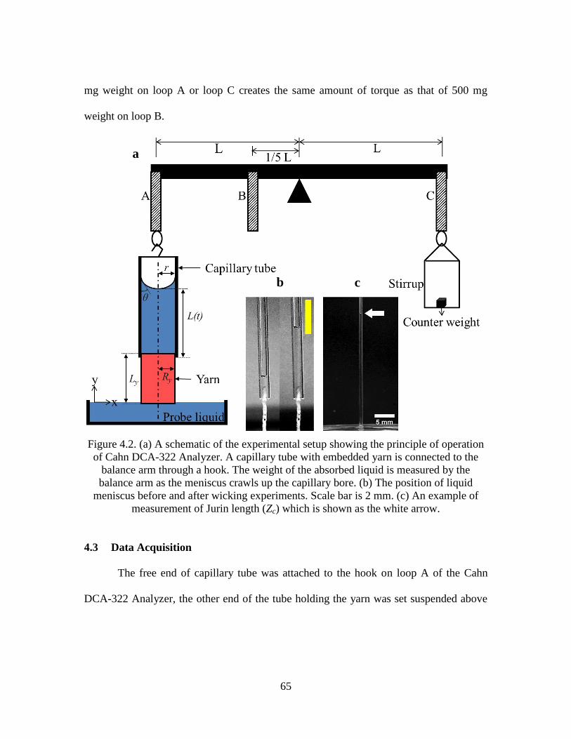
65

mg weight on loop A or loop C creates the same amount of torque as that of 500 mg

weight on loop B.

Figure 4.2. (a) A schematic of the experimental setup showing the principle of operation

of Cahn DCA-322 Analyzer. A capillary tube with embedded yarn is connected to the

balance arm through a hook. The weight of the absorbed liquid is measured by the

balance arm as the meniscus crawls up the capillary bore. (b) The position of liquid

meniscus before and after wicking experiments. Scale bar is 2 mm. (c) An example of

measurement of Jurin length (Zc) which is shown as the white arrow.

4.3 Data Acquisition

The free end of capillary tube was attached to the hook on loop A of the Cahn

DCA-322 Analyzer, the other end of the tube holding the yarn was set suspended above

a

b c

66

the free liquid surface. The stage with the liquid container moving up at the speed of 200

µm per second, the free end of the yarn was brought to in contact with the liquid surface.

A special function of Cahn DCA-322 analyzer software, called the Zero Depth of

Immersion (ZDOI), can set the starting moment of weight measurements. The ZDOI

point was chosen as the moment the end of yarn first touched the liquid surface. This was

experimentally found by setting a minimum force threshold at the Fmin = 500 µgf level.

With this choice of the ZDOI point, the stage with the liquid kept moving up if the

measured force was less than 500 μgf. The balance was first zeroed, and the force was

kept at the zero level when the stage was moved up (Figure 4.3). When the yarn touched

the liquid surface, the force jumped up reflecting the action of the wetting force (red

arrow in Figure 4.3) which appeared significantly larger than the ZDOI threshold [7].

When the yarn first touched the liquid surface and the measured force became greater

than Fmin, the stage continued to raise up 0.1 mm with 200 µm/sec speed to confirm that

the yarn was immersed in liquid. A negative slope in Figure 4.3 is associated with the

immersion process and it is caused by the increase of the buoyancy and viscous friction

forces at the meniscus when the yarn gets immersed into liquid [7]. Then, the stage

position was fixed. Stabilization of the entire setup required five minutes; then the force

change was acquired for the next 50 minutes, red line in Figure 4.3.

67

Figure 4.3. A typical experimental curve showing force changes at different steps: a steep

jump of the blue line allows one to define the ZDOI point. The stage was moving until

the immersed part reached 0.1 mm (green line), then we waited for 5 minutes (purple

line), and started collecting the change of water weight for 50 minutes (red line).

After the stage position was fixed, a meniscus was observed inside the capillary

(Figure 4.2b) and all incremental changes of force detected by the analyzer were

attributed to the incremental change of weight of the liquid column invading the tube due

to capillary action.

4.4 Model of Fluid Uptake by a Yarn-In-A-Tube Composite Conduit

4.4.1 The Liquid Discharge through the Yarn (Q1)

The center of Cartesian coordinates is taken at the liquid surface with the y-axis

pointing upwards (Figure 4.2). The flow is assumed one-dimensional with non-zero

velocity component directed along the yarn and capillary axes. It is convenient to

introduce a flow potential as the sum of the pressure in liquid, P(y), at the position y,

and hydrostatic pressure due to weight of the liquid column:

( )P y gy , (4.5)

68

where ρ is the liquid density and g is acceleration due to gravity.

In this definition, the pressure at the liquid surface is zero and the potential is zero

as well. Therefore, Darcy’s law is written through the flow potential as Q = -

(kyA/η)(∂/∂y), where ky is the permeability of the yarn, η is the liquid viscosity, ∂/∂y is

the potential gradient taken along the yarn, and A = πRy2 is the cross-sectional area of the

yarn of radius Ry.

The liquid is assumed not volatile (eg. Hexadecane, vapor pressure: 1 mmHg @

105°C), hence, the mass conservation equation reads Qy/y = 2y/y

2 = 0. Integrating

this equation, one obtains the linear distribution of the potential along the liquid column,

y ay b , where a and b are time-dependent functions that can be found from the

boundary conditions. The boundary conditions state that the pressure at the liquid surface,

y = 0, is equal to zero, hence b = 0. At the embedded end of the yarn y = Ly,

y y yP gL aL . From this equation, it follows that ( )y y ya P gL L . With the

obtained constants, the liquid discharge through the yarn is expressed as:

2

1 ( )y y y y

y

R k P gLQ

L

. (4.6)

4.4.2 The Liquid Discharge through the Capillary (Q2)

The flow of the liquid column through the capillary can be described by the

Hagen–Poiseuille law [6] which is written in Darcy’s form as 2 / /c cQ k A y

with kc = r2/8. Subscript “c” refers to the capillary. Once again, using the mass

69

conservation equation, we obtain Qc/y = 2c/y

2 = 0. Integrating this equation, one

infers the linear distribution of the potential along the liquid column, c cy d , where

c and d are time-dependent functions that can be found from the boundary conditions.

The boundary conditions state that the pressure at the embedded end of yarn must be

equal to the pressure in the liquid column at the same position y = Ly. Therefore,

y y yP gL cL d . At the wetting front y = L(t), the pressure is below atmospheric

pressure and the jump is equal to capillary pressure Pc. From this equation it follows that

cP gL cL d . From these two boundary conditions it follows that

( [ ]) / [ ]y c y yc P P g L L L L and ( [ ]) / [ ]y y y c y y yd P gL P P g L L L L L .

With the obtained constants, the liquid discharge through the capillary is expressed as:

4

2 / ( [ ]) / [ ]8

c y c y y

rQ k A c P P g L L L L

. (4.7)

4.4.3 Meniscus Motion through Capillary

The liquid discharge through the capillary is the same as that given by Eq. (4.7).

Once again, the conservation of mass requires the following equality Q1 = Q2,

2 4

( ) ( [ ]) / [ ]8

y y y y

y c y y

y

R k P gL rP P g L L L L

L

. (4.8)

Solving Eq. (4.8) for Py, we can express pressure Py through the meniscus

position L(t):

70

4

2

2 44

8( ) 8 ( )( )

8( )

y y y y

y c y

y y

y y

r

L L gR k L LP P g L L

R k rr

L L L

. (4.9)

Plugging Eq. (4.9) into Eq. (4.7) and expressing its left hand side through the

meniscus velocity Q2 = πr2dL/dt, we obtain the basic equation describing kinetics of

meniscus propagation through the capillary:

2

4

2

8

8

c

y

y

y y

P gLdL r

r LdtL L

R k

. (4.10)

4.4.4 Engineering Parameters of Yarns

Eq. (4.10) contains many geometrical and physical parameters. This equation can

be significantly simplified by introducing dimensionless variables. In order to see this, we

normalize the meniscus position by the Jurin length Zc which is defined as the maximum

possible height of the liquid column coexisting with the liquid reservoir [5], Zc = Pc/ρg

=2σcosθ/(ρgr). The time in Eq. (4.10) is convenient to normalize by the following

characteristic time:

0 2 2 2 2

8 8c cZ Pt

gr g r

. (4.11)

71

This time is approximately equal to the time required for a liquid meniscus to

reach the Jurin height. As seen from Eq. (4.11), this time depends on fluid viscosity .

With this normalization, L* = L/Zc, t

* = t/t0, Eq. (4.10) is rewritten as:

* *

* *

1dL L

dt L

, (4.12)

where

4

28

y y

c y y c

r L L

Z R k Z . (4.13)

If the yarn length is much smaller than the Jurin length (Ly << Zc), the effect of

gravity, the second term on the right-hand side of Eq. (4.13), can be neglected, and Eq.

(4.13) is simplified as:

4

28

y

c y y

r L

Z R k . (4.14)

Eq. (4.12) is a familiar Lucas-Washburn equation describing capillary rise in the

tubes [3, 4], which has the solution:

* * *(1 ) ln(1 )L L t . (4.15)

Thus, using the introduced normalization, one can interpret the experimental data

in a much easier way by first measuring the Jurin length Zc then calculating the

characteristic time t0 and then fitting the experimental curve L*(t

*) adjusting parameter α.

After determination of this parameter α, the permeability of the yarn is calculated as:

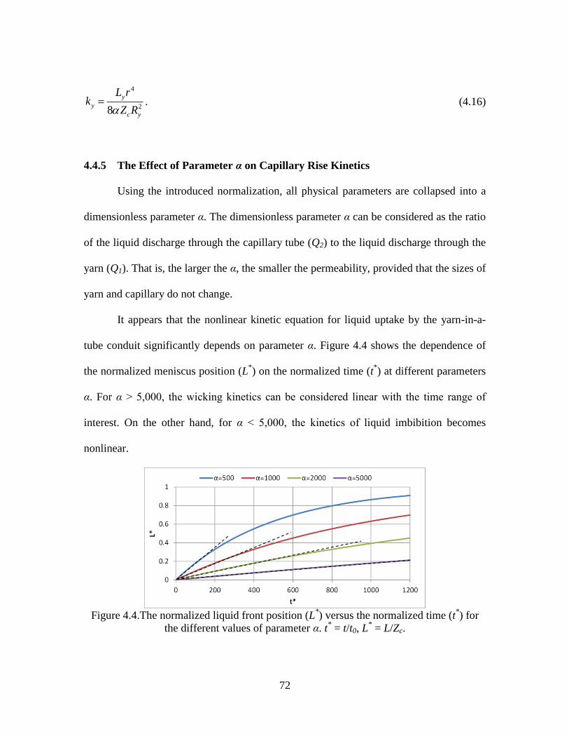
72

4

28

y

y

c y

L rk

Z R . (4.16)

4.4.5 The Effect of Parameter α on Capillary Rise Kinetics

Using the introduced normalization, all physical parameters are collapsed into a

dimensionless parameter α. The dimensionless parameter α can be considered as the ratio

of the liquid discharge through the capillary tube (Q2) to the liquid discharge through the

yarn (Q1). That is, the larger the α, the smaller the permeability, provided that the sizes of

yarn and capillary do not change.

It appears that the nonlinear kinetic equation for liquid uptake by the yarn-in-a-

tube conduit significantly depends on parameter α. Figure 4.4 shows the dependence of

the normalized meniscus position (L*) on the normalized time (t

*) at different parameters

α. For α ˃ 5,000, the wicking kinetics can be considered linear with the time range of

interest. On the other hand, for α ˂ 5,000, the kinetics of liquid imbibition becomes

nonlinear.

Figure 4.4.The normalized liquid front position (L

*) versus the normalized time (t

*) for

the different values of parameter α. t* = t/t0, L

* = L/Zc.

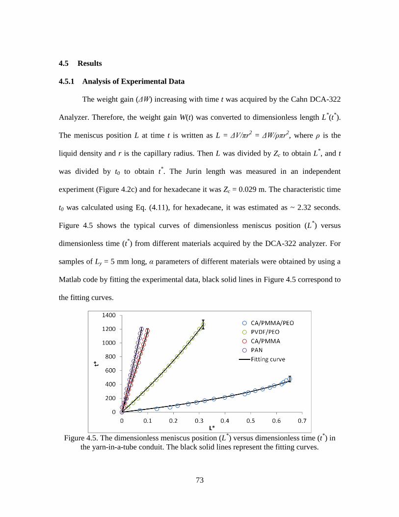
73

4.5 Results

4.5.1 Analysis of Experimental Data

The weight gain (ΔW) increasing with time t was acquired by the Cahn DCA-322

Analyzer. Therefore, the weight gain W(t) was converted to dimensionless length L*(t

*).

The meniscus position L at time t is written as L = ΔV/πr2 = ΔW/ρπr

2, where ρ is the

liquid density and r is the capillary radius. Then L was divided by Zc to obtain L*, and t

was divided by t0 to obtain t*. The Jurin length was measured in an independent

experiment (Figure 4.2c) and for hexadecane it was Zc = 0.029 m. The characteristic time

t0 was calculated using Eq. (4.11), for hexadecane, it was estimated as ~ 2.32 seconds.

Figure 4.5 shows the typical curves of dimensionless meniscus position (L*) versus

dimensionless time (t*) from different materials acquired by the DCA-322 analyzer. For

samples of Ly = 5 mm long, α parameters of different materials were obtained by using a

Matlab code by fitting the experimental data, black solid lines in Figure 4.5 correspond to

the fitting curves.

Figure 4.5. The dimensionless meniscus position (L

*) versus dimensionless time (t

*) in

the yarn-in-a-tube conduit. The black solid lines represent the fitting curves.

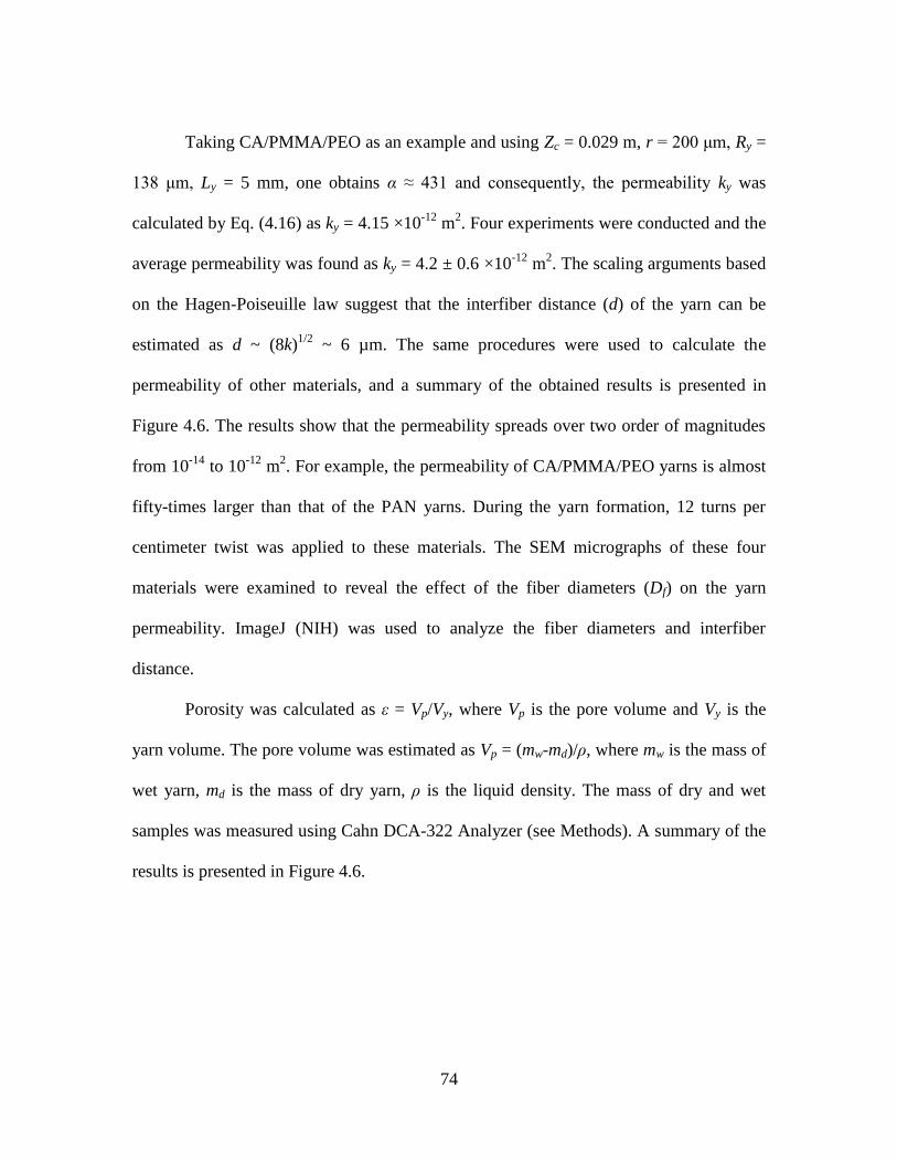
74

Taking CA/PMMA/PEO as an example and using Zc = 0.029 m, r = 200 μm, Ry =

138 μm, Ly = 5 mm, one obtains α ≈ 431 and consequently, the permeability ky was

calculated by Eq. (4.16) as ky = 4.15 ×10-12

m2. Four experiments were conducted and the

average permeability was found as ky = 4.2 ± 0.6 ×10-12

m2. The scaling arguments based

on the Hagen-Poiseuille law suggest that the interfiber distance (d) of the yarn can be

estimated as d ~ (8k)1/2

~ 6 µm. The same procedures were used to calculate the

permeability of other materials, and a summary of the obtained results is presented in

Figure 4.6. The results show that the permeability spreads over two order of magnitudes

from 10-14

to 10-12

m2. For example, the permeability of CA/PMMA/PEO yarns is almost

fifty-times larger than that of the PAN yarns. During the yarn formation, 12 turns per

centimeter twist was applied to these materials. The SEM micrographs of these four

materials were examined to reveal the effect of the fiber diameters (Df) on the yarn

permeability. ImageJ (NIH) was used to analyze the fiber diameters and interfiber

distance.

Porosity was calculated as ε = Vp/Vy, where Vp is the pore volume and Vy is the

yarn volume. The pore volume was estimated as Vp = (mw-md)/ρ, where mw is the mass of

wet yarn, md is the mass of dry yarn, ρ is the liquid density. The mass of dry and wet

samples was measured using Cahn DCA-322 Analyzer (see Methods). A summary of the

results is presented in Figure 4.6.

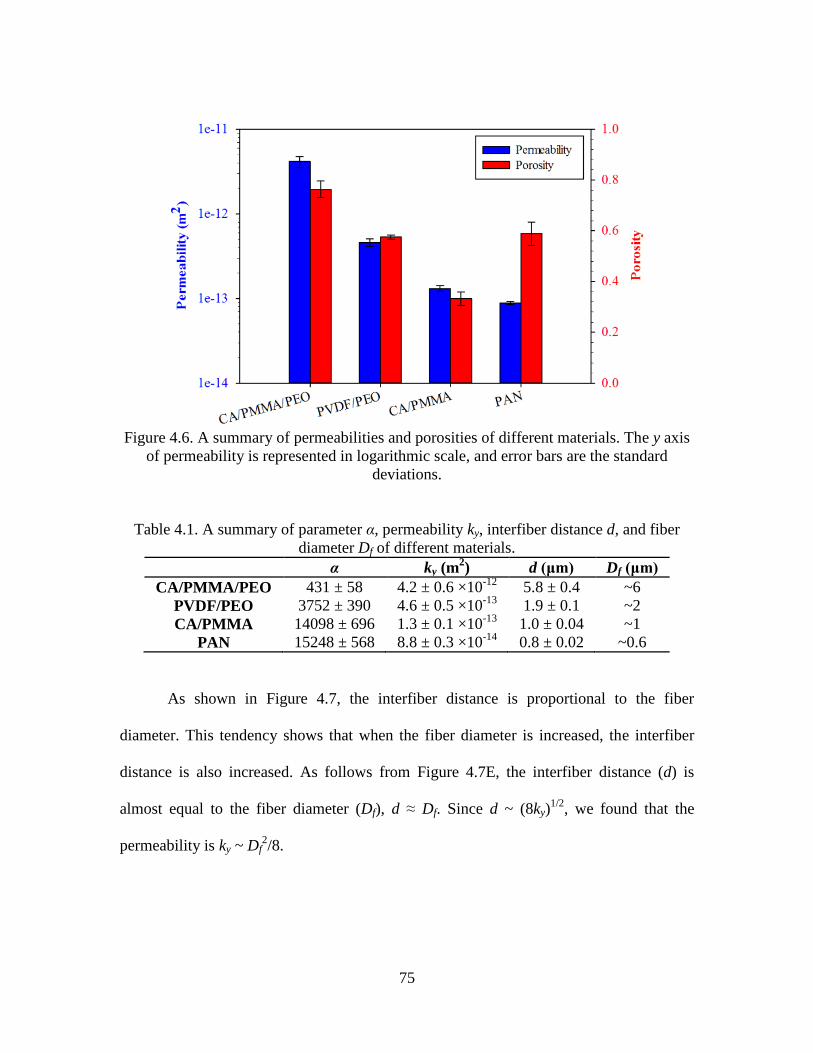
75

Figure 4.6. A summary of permeabilities and porosities of different materials. The y axis

of permeability is represented in logarithmic scale, and error bars are the standard

deviations.

Table 4.1. A summary of parameter α, permeability ky, interfiber distance d, and fiber

diameter Df of different materials.

α ky (m2) d (μm) Df (μm)

CA/PMMA/PEO 431 ± 58 4.2 ± 0.6 ×10-12

5.8 ± 0.4 ~6

PVDF/PEO 3752 ± 390 4.6 ± 0.5 ×10-13

1.9 ± 0.1 ~2

CA/PMMA 14098 ± 696 1.3 ± 0.1 ×10-13

1.0 ± 0.04 ~1

PAN 15248 ± 568 8.8 ± 0.3 ×10-14

0.8 ± 0.02 ~0.6

As shown in Figure 4.7, the interfiber distance is proportional to the fiber

diameter. This tendency shows that when the fiber diameter is increased, the interfiber

distance is also increased. As follows from Figure 4.7E, the interfiber distance (d) is

almost equal to the fiber diameter (Df), d ≈ Df. Since d ~ (8ky)1/2

, we found that the

permeability is ky ~ Df2/8.

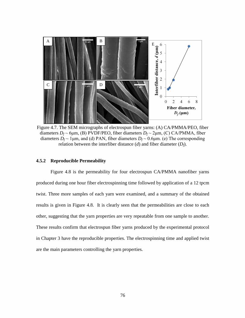
76

Figure 4.7. The SEM micrographs of electrospun fiber yarns: (A) CA/PMMA/PEO, fiber

diameters Df ~ 6μm, (B) PVDF/PEO, fiber diameters Df ~ 2μm, (C) CA/PMMA, fiber

diameters Df ~ 1μm, and (d) PAN, fiber diameters Df ~ 0.6μm. (e) The corresponding

relation between the interfiber distance (d) and fiber diameter (Df).

4.5.2 Reproducible Permeability

Figure 4.8 is the permeability for four electrospun CA/PMMA nanofiber yarns

produced during one hour fiber electrospinning time followed by application of a 12 tpcm

twist. Three more samples of each yarn were examined, and a summary of the obtained

results is given in Figure 4.8. It is clearly seen that the permeabilities are close to each

other, suggesting that the yarn properties are very repeatable from one sample to another.

These results confirm that electrospun fiber yarns produced by the experimental protocol

in Chapter 3 have the reproducible properties. The electrospinning time and applied twist

are the main parameters controlling the yarn properties.

A

B

C D

E

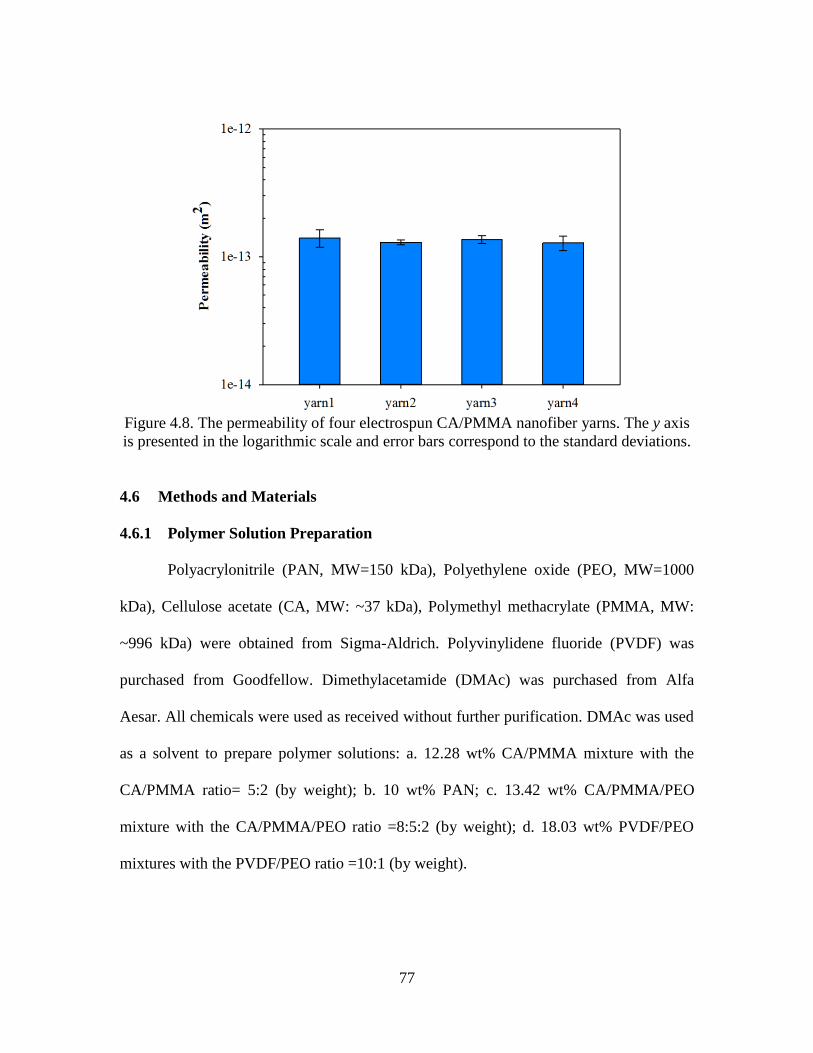
77

Figure 4.8. The permeability of four electrospun CA/PMMA nanofiber yarns. The y axis

is presented in the logarithmic scale and error bars correspond to the standard deviations.


4.6.1 Polymer Solution Preparation

Polyacrylonitrile (PAN, MW=150 kDa), Polyethylene oxide (PEO, MW=1000

kDa), Cellulose acetate (CA, MW: ~37 kDa), Polymethyl methacrylate (PMMA, MW:

~996 kDa) were obtained from Sigma-Aldrich. Polyvinylidene fluoride (PVDF) was

purchased from Goodfellow. Dimethylacetamide (DMAc) was purchased from Alfa

Aesar. All chemicals were used as received without further purification. DMAc was used

as a solvent to prepare polymer solutions: a. 12.28 wt% CA/PMMA mixture with the

CA/PMMA ratio= 5:2 (by weight); b. 10 wt% PAN; c. 13.42 wt% CA/PMMA/PEO

mixture with the CA/PMMA/PEO ratio =8:5:2 (by weight); d. 18.03 wt% PVDF/PEO

mixtures with the PVDF/PEO ratio =10:1 (by weight).

78

4.6.2 Yarn Formation

The yarns were formed by using the method of Tsai et. al. [8]. The prepared

polymer solutions were placed in a 10 mL syringe. A syringe pump (New Era Pump

System, NE-300) was used to control the flow rate. A home-made rotating mandrel with

four alumina bars separated from each other by 20 cm was used as a fiber collector [8]. A

high voltage power supply (Glassman High Voltage, Inc.) was connected to the syringe

through a stainless-steel needle (Gauge 20, EXEL). The needle was placed 15 cm apart

from the nearest face of the collector. A positive voltage was applied to the needle until

the Taylor cone was produced. When the nanofibers were collected on the mandrel, a

home-made collecting and twisting device to form yarns was employed [8]. The twisting

device consists of two circular wire brushes with the ¾ inches diameter each, mounted

co-axially on the holder [8]. 12 turns per centimeter (tpcm) twist was applied to the yarns.

It has been demonstrated the electrospinning time and number of twists are the main

parameters controlling the yarn properties (diameter, porosity, and permeability) [8].

4.6.3 SEM Characterization

The surface morphology of the CA/PMMA, PAN, PVDF/PEO, and

CA/PMMA/PEO fibers and yarns were examined with a Hitachi Field Emission scanning

electron microscope (FESEM-Hitachi 4800). The samples were sputter-coated with a few

nanometer thickness of gold prior to SEM examination.

79

4.6.4 Surface Tension

The surface tension of hexadecane was measured using Wilhelmy Plate method

using Cahn DCA-322 DCA analyzer. A platinum wire with a 250 μm diameter was used

as the standard probe. The platinum wire was cleaned with ethanol and an oxidizing

flame to heat it to red-hot. The Wilhelmy equation F= σP was used to evaluate the

surface tension, where F is the measured force, σ is the surface tension of the liquid, P is

the perimeter of the wire. Hexadecane was examined three times and gave the surface

tension σ = 23.5 ± 0.2 mN/m.

4.6.5 Jurin Length (Zc)

To use the dimensionless parameters L* and t

*, one needs to know the Jurin length

(Zc). The Jurin length of Hexadecane (η = 3.03 cp, ρ = 773 kg/m3) was determined by

measuring the equilibrium height of liquid column in the capillary tube. A glass capillary

tube with 200 μm in radius (r) was used in these experiments. Three experiments were

conducted and the average Jurin length was measured as Zc = 0.029 ± 0.0003 m. The

characteristic time t0 was calculated using Eq. (4.11), t0 = 2.32 seconds.

4.6.6 Porosity (ε)

The porosity of different materials was estimated by the formula ε = (mw-md) /

(ρVy), where mw is the mass of wet yarn, md is the mass of dry yarn, ρ is the liquid density,

and Vy is the yarn volume. The yarn volume was calculated as Vy = πRy2Ly, where Ry is

the radius of yarn which was measured by the optical microscope Olympus BX-51, and

80

Ly is the length of the yarn. The yarn was placed vertically with one end sealed with

plasticine and another end submersed in hexadecane. The mass change was measured by

Cahn DCA-322 DCA analyzer. The porosity was examined on three samples for each

material.

4.6.7 Reynolds Number (Re)

The Hagen-Poiseuille equation was used to describe the liquid flow in a

cylindrical tube. The assumptions are the fluid is viscous and incompressible, and the

flow is laminar. For a flow in a pipe or tube, the Reynolds number is defined as:

ReD

, (4.17)

where ρ is the liquid density, v is the mean liquid velocity, D is the hydraulic diameter of

the pipe, and η is the liquid viscosity.

The Reynolds number is a dimensionless parameter and represents the ratio of

inertial forces to viscous forces. High values of the parameter indicate that the viscous

forces are small and the flow is controlled by inertia. In the opposite case, the flow is

controlled by viscosity. Darcy’s law requires that the flow at the level of pores must be

laminar and Reynolds numbers must be small.

In order to check the validity of the Hagen-Poiseuille equation used in our system,

the Reynolds number (Re) was calculated using experimental parameters. Eq. (4.17)

expresses the kinetics of meniscus propagation through the capillary, and the meniscus

velocity was taken as the liquid velocity dL/dt in the Eq. (4.10). The Reynolds number

http://en.wikipedia.org/wiki/Hydraulic_diameter

81

becomes a time dependent function. The Reynolds numbers for the different materials

were calculated and are summarized in Figure 4.9. As shown in Figure 4.9, the

assumption of laminar flow in our system is valid.

Figure 4.9. The Reynolds number versus time for hexadecane: η = 3.03 mPa·s, ρ = 773

kg/m3.

4.7 Conclusions

A characterization technique was developed enabling to specify the permeability

of electrospun yarns using wicking experiments on complex conduits made of yarn-in-a-

tube pairs. This method takes advantage of the distinctive capillary pressure produced by

the meniscus in a tube; this pressure is significantly different from the capillary pressure

produced by menisci in the pores of the yarn. Therefore, the driving capillary pressure

does not depend on the pore size and can be measured independently using the Jurin

capillary rise technique. A mathematical model describing the kinetics of wicking of

wetting liquids into yarn-in-a-tube conduit was developed and used for interpretation of

82

experiments. Yarns from CA/PMMA, PAN, PVDF/PEO, and CA/PMMA/PEO were

electrospun and characterized using the proposed technique. The produced yarns showed

permeability spinning two orders of magnitude (10-14

~10-12

m2).

4.8 References

1. Scheidegger, A.E., The physics of flow through porous media. 1957: University of

Toronto Press.

2. Adamson, A.W. and A.P. Gast. Physical chemistry of surfaces. 1997.

3. Lucas, R., Ueber das Zeitgesetz des kapillaren Aufstiegs von Flussigkeiten. Kolloid

Zeitschrift, 1918. 23: p. 15-22.

4. Washburn, E., The Dynamics of Capillary Flow. Phys. Rev. Physical Review, 1921.

17(3): p. 273-283.

5. Jurin, J., An account of some experiments shown before the Royal Society; with an

enquiry into the cause of the ascent and suspension of water in capillary tubes.

Philosophical Transactions of the Royal Society, 1917-1919. 30(351-363): p. 739-

747.

6. Adamson, A.W. and A.P. Gast, Physical chemistry of surfaces. 1997, New York:

Wiley.

7. Miller, B., L.S. Penn, and S. Hedvat, Wetting force measurements on single fibers.

Colloids and Surfaces, 1983. 6(1): p. 49-61.




2011. 3(11): p. 4685-4695.

83

CHAPTER FIVE

5WETTING PROPERTIES OF ELECTROSPUN YARNS

Wetting properties of CA/PMMA yarns and their constituent films were

studied in this chapter. The contact angles of flat films were measured by the

sessile drop technique while the contact angles of electrospun yarns were

characterized by the capillary rise method. The contact angles extracted from

wicking experiments were close to the contact angles on the flat CA and PMMA

films. The surface of CA/PMMA fibers was very smooth with roughness

measured in nanometers. Therefore, as expected the contact angle in the yarn is

very close to that on flat surface of CA or PMMA. On the contrary, the surface

morphology of microfibers formed from the polymer blends is drastically

different from that of the films: the films were rough while the microfibers were

smooth. This resulted in distinct wetting properties of yarns and films made of the

same materials.

5.1 Introduction

Recently, nanofibers have attracted great attention as promising materials for

building different constructs and nanodevices [1-3]. Nanofibers can be made porous or

hollow and can be bundled and twisted into yarns [1-4]. Because of their flexibility and

porosity, nanofiber yarns and webs show great potential for probing and scanning tissues.

The wettability of electrospun yarns is the essential requirement for the fiber-based

84

probes [5]. The material wettability depends on the surface energy of the material, which

is evaluated by analyzing the contact angle using different probe liquids [6-9]. For a flat

and smooth solid surface, the sessile drop technique is traditionally used to examine the

contact angle. However, the determination of the contact angle on fibrous materials

becomes a challenging task. The apparent contact angle significantly depends on the

surface roughness [10, 11]. In addition, the liquid droplet may rapidly penetrate into the

fiber structure making the sessile drop measurement questionable.

One straightforward method to overcome these problems is to use the capillary

rise method. The contact angle can be obtained from the analysis of the wicking kinetics

[12-16]. Owing to the complex fibrous structure of electrospun yarns, the contact angle of

flat polymer films was first studied. The upward wicking of hexadecane and water into

yarns was then analyzed. The Cahn surface tensiometer was employed for these studies.

The water contact angle of CA/PMMA yarns was ~74° which was close to water contact

angle on flat CA or PMMA films (~ 71 - 72°). In contrast, the surface morphology of the

CA/PMMA films was very rough: one observed bumps and valleys. The water contact

angle on CA/PMMA films was measured to be ~63°. However, the electrospun

CA/PMMA fibers appeared smooth, no defects were noticed. The wicking experiments

on yarns made of CA/PMMA fibers led to the conclusion that the contact angles of these

fibers is very close to those measured on the films made from CA and PMMA.

85

5.2 Wettability of CA, PMMA, and CA/PMMA Films

5.2.1 Preparation of CA, PMMA, and CA/PMMA Films

The surface wettability is usually characterized by measuring the contact angle of

a liquid on a solid surface. For a flat and smooth solid surface, the most common method

is the sessile drop technique. The 10 wt% CA, 10 wt% PMMA, and 12.28 wt%

CA/PMMA solutions were independently prepared for the CA, PMMA, and CA/PMMA

films, respectively. The CA to PMMA ratio of CA/PMMA solution was prepared the

same as the solutions prepared for the electropinning of CA/PMMA fibers. A 1,200 rpm

speed was set on the spin coater (Headway Research Inc., MP-101) to make uniform

films by rotating for 30 seconds. Glass slides (Corning Inc., 2947-3x1) were used as the

coating substrates. The prepared films were dried overnight at room temperature in the

hood and then dried at room temperature under vacuum (approximately 10 mmHg

pressure) for 4 hours.

5.2.2 Contact Angles of CA, PMMA, and CA/PMMA Films

Hexadecane (HEX) and deionized water (Water) were chosen for the wettability

experiments. HEX was chosen as a standard non-polar hydrocarbon solvent, and Water

was chosen as the standard polar solvent. The measurements were done at room

temperature using the sessile drop method: equilibration time was ~ 20 seconds. Results

were recorded on the Contact Angle Measuring instrument (Krüss, FM40MK2 Easydrop)

using the DSA software. Contact angles for each sample were measured at least five

droplets, and the average values were reported. The contact angles of HEX on the CA

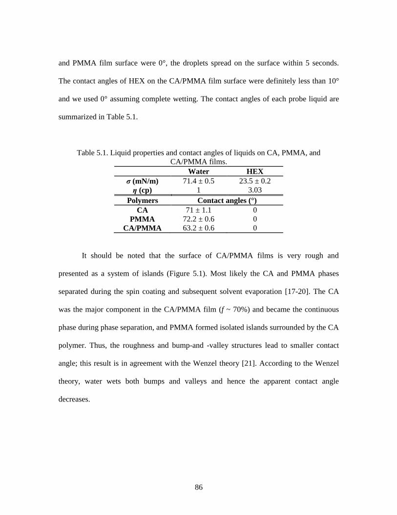
86

and PMMA film surface were 0°, the droplets spread on the surface within 5 seconds.

The contact angles of HEX on the CA/PMMA film surface were definitely less than 10°

and we used 0° assuming complete wetting. The contact angles of each probe liquid are

summarized in Table 5.1.

Table 5.1. Liquid properties and contact angles of liquids on CA, PMMA, and

CA/PMMA films.

Water HEX

σ (mN/m) 71.4 ± 0.5 23.5 ± 0.2

η (cp) 1 3.03

Polymers Contact angles (°)

CA 71 ± 1.1 0

PMMA 72.2 ± 0.6 0

CA/PMMA 63.2 ± 0.6 0

It should be noted that the surface of CA/PMMA films is very rough and

presented as a system of islands (Figure 5.1). Most likely the CA and PMMA phases

separated during the spin coating and subsequent solvent evaporation [17-20]. The CA

was the major component in the CA/PMMA film (f ~ 70%) and became the continuous

phase during phase separation, and PMMA formed isolated islands surrounded by the CA

polymer. Thus, the roughness and bump-and -valley structures lead to smaller contact

angle; this result is in agreement with the Wenzel theory [21]. According to the Wenzel

theory, water wets both bumps and valleys and hence the apparent contact angle

decreases.

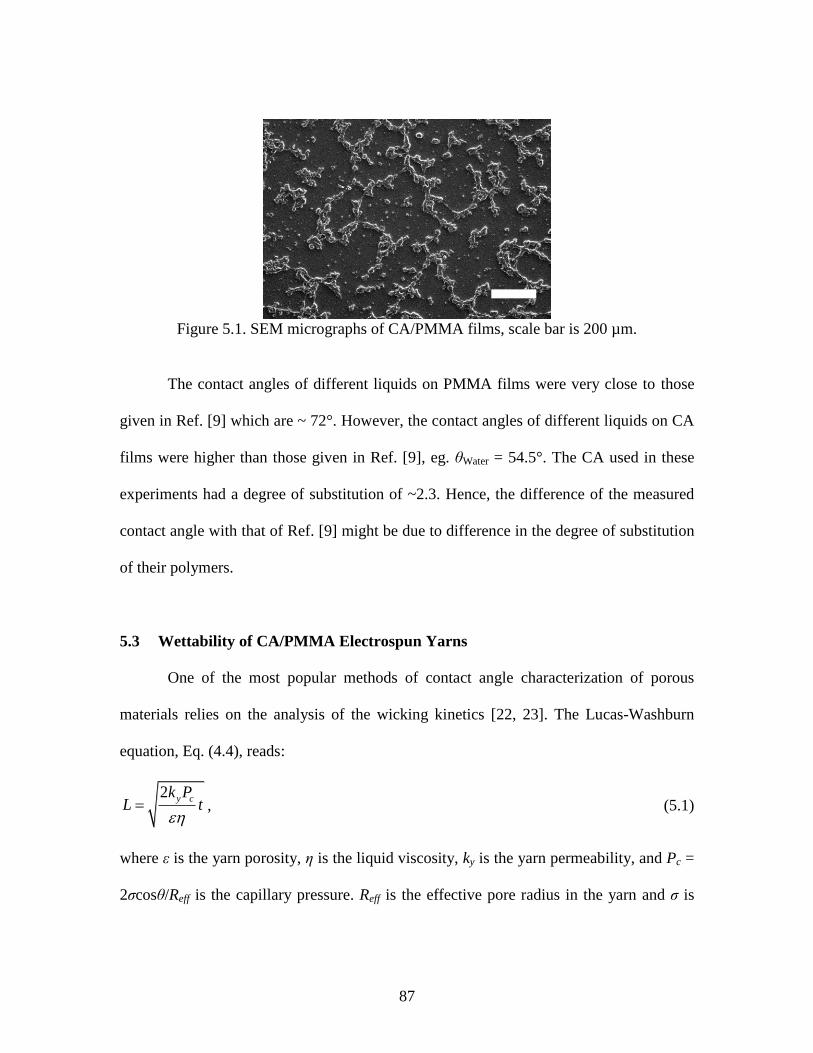
87

Figure 5.1. SEM micrographs of CA/PMMA films, scale bar is 200 µm.

The contact angles of different liquids on PMMA films were very close to those

given in Ref. [9] which are ~ 72°. However, the contact angles of different liquids on CA

films were higher than those given in Ref. [9], eg. θWater = 54.5°. The CA used in these

experiments had a degree of substitution of ~2.3. Hence, the difference of the measured

contact angle with that of Ref. [9] might be due to difference in the degree of substitution

of their polymers.

5.3 Wettability of CA/PMMA Electrospun Yarns

One of the most popular methods of contact angle characterization of porous

materials relies on the analysis of the wicking kinetics [22, 23]. The Lucas-Washburn

equation, Eq. (4.4), reads:

2 y ck PL t

, (5.1)

where ε is the yarn porosity, η is the liquid viscosity, ky is the yarn permeability, and Pc =

2σcosθ/Reff is the capillary pressure. Reff is the effective pore radius in the yarn and σ is

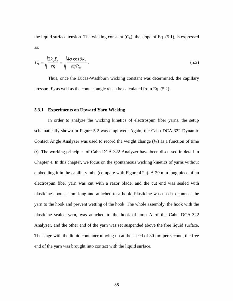
88

the liquid surface tension. The wicking constant (CL), the slope of Eq. (5.1), is expressed

as:

2 4 cosy c y

L

eff

k P kC

R

. (5.2)

Thus, once the Lucas-Washburn wicking constant was determined, the capillary

pressure Pc as well as the contact angle θ can be calculated from Eq. (5.2).

5.3.1 Experiments on Upward Yarn Wicking

In order to analyze the wicking kinetics of electrospun fiber yarns, the setup

schematically shown in Figure 5.2 was employed. Again, the Cahn DCA-322 Dynamic

Contact Angle Analyzer was used to record the weight change (W) as a function of time

(t). The working principles of Cahn DCA-322 Analyzer have been discussed in detail in

Chapter 4. In this chapter, we focus on the spontaneous wicking kinetics of yarns without

embedding it in the capillary tube (compare with Figure 4.2a). A 20 mm long piece of an

electrospun fiber yarn was cut with a razor blade, and the cut end was sealed with

plasticine about 2 mm long and attached to a hook. Plasticine was used to connect the

yarn to the hook and prevent wetting of the hook. The whole assembly, the hook with the

plasticine sealed yarn, was attached to the hook of loop A of the Cahn DCA-322

Analyzer, and the other end of the yarn was set suspended above the free liquid surface.

The stage with the liquid container moving up at the speed of 80 µm per second, the free

end of the yarn was brought into contact with the liquid surface.

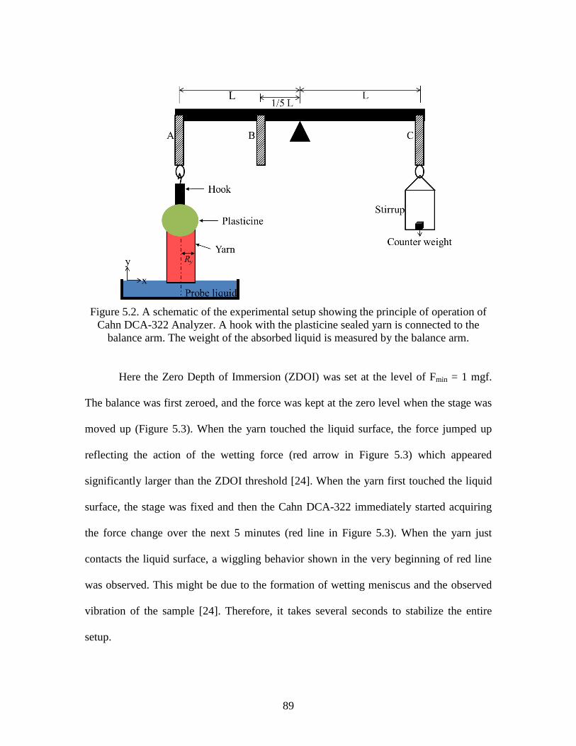
89

Figure 5.2. A schematic of the experimental setup showing the principle of operation of

Cahn DCA-322 Analyzer. A hook with the plasticine sealed yarn is connected to the

balance arm. The weight of the absorbed liquid is measured by the balance arm.

Here the Zero Depth of Immersion (ZDOI) was set at the level of Fmin = 1 mgf.

The balance was first zeroed, and the force was kept at the zero level when the stage was

moved up (Figure 5.3). When the yarn touched the liquid surface, the force jumped up

reflecting the action of the wetting force (red arrow in Figure 5.3) which appeared

significantly larger than the ZDOI threshold [24]. When the yarn first touched the liquid

surface, the stage was fixed and then the Cahn DCA-322 immediately started acquiring

the force change over the next 5 minutes (red line in Figure 5.3). When the yarn just

contacts the liquid surface, a wiggling behavior shown in the very beginning of red line

was observed. This might be due to the formation of wetting meniscus and the observed

vibration of the sample [24]. Therefore, it takes several seconds to stabilize the entire

setup.

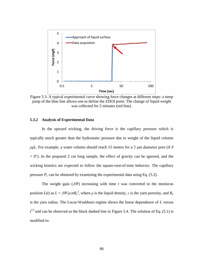
90

Figure 5.3. A typical experimental curve showing force changes at different steps: a steep

jump of the blue line allows one to define the ZDOI point. The change of liquid weight

was collected for 5 minutes (red line).

5.3.2 Analysis of Experimental Data

In the upward wicking, the driving force is the capillary pressure which is

typically much greater than the hydrostatic pressure due to weight of the liquid column

ρgL. For example, a water column should reach 15 meters for a 2 μm diameter pore (if θ

= 0°). In the prepared 2 cm long sample, the effect of gravity can be ignored, and the

wicking kinetics are expected to follow the square-root-of-time behavior. The capillary

pressure Pc can be obtained by examining the experimental data using Eq. (5.2).

The weight gain (ΔW) increasing with time t was converted to the meniscus

position L(t) as L = ΔW/ρεπRy2, where ρ is the liquid density, ε is the yarn porosity, and Ry

is the yarn radius. The Lucas-Washburn regime shows the linear dependence of L versus

t1/2

and can be observed as the black dashed line in Figure 5.4. The solution of Eq. (5.1) is

modified to:

0

1

2

3

4

5

0.5 5 50 500

Forc

e (

mgf

)

Time (sec)

Approach of liquid surface

Data acquistion

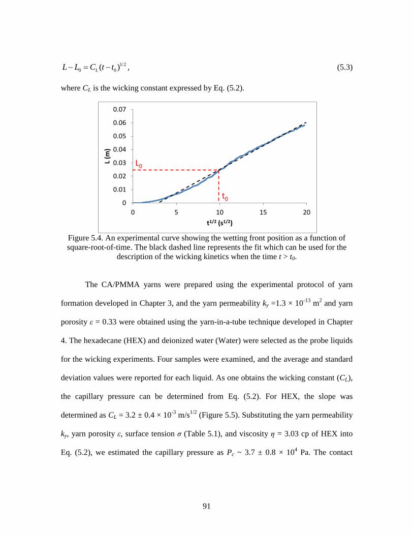
91

1/2

0 0( )LL L C t t , (5.3)

where CL is the wicking constant expressed by Eq. (5.2).

Figure 5.4. An experimental curve showing the wetting front position as a function of

square-root-of-time. The black dashed line represents the fit which can be used for the

description of the wicking kinetics when the time t > t0.

The CA/PMMA yarns were prepared using the experimental protocol of yarn

formation developed in Chapter 3, and the yarn permeability ky =1.3 × 10-13

m2 and yarn

porosity ε = 0.33 were obtained using the yarn-in-a-tube technique developed in Chapter

4. The hexadecane (HEX) and deionized water (Water) were selected as the probe liquids

for the wicking experiments. Four samples were examined, and the average and standard

deviation values were reported for each liquid. As one obtains the wicking constant (CL),

the capillary pressure can be determined from Eq. (5.2). For HEX, the slope was

determined as CL = 3.2 ± 0.4 × 10-3

m/s1/2

(Figure 5.5). Substituting the yarn permeability

ky, yarn porosity ε, surface tension σ (Table 5.1), and viscosity η = 3.03 cp of HEX into

Eq. (5.2), we estimated the capillary pressure as Pc ~ 3.7 ± 0.8 × 104 Pa. The contact

0

0.01

0.02

0.03

0.04

0.05

0.06

0.07

0 5 10 15 20

L (m

)

t1/2 (s1/2)

t0

L0

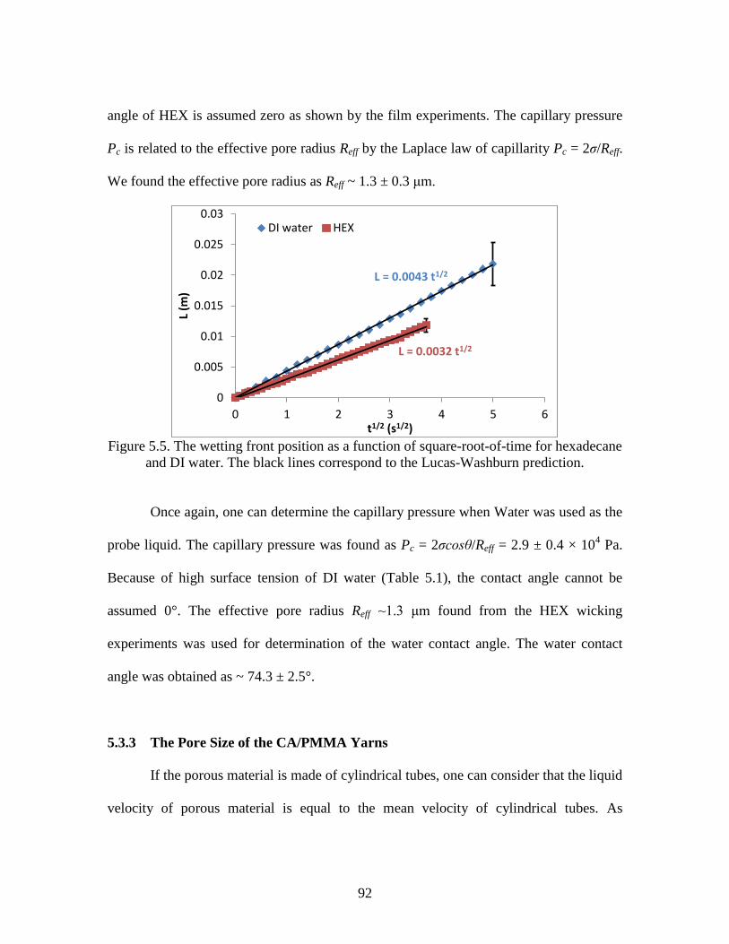
92

angle of HEX is assumed zero as shown by the film experiments. The capillary pressure

Pc is related to the effective pore radius Reff by the Laplace law of capillarity Pc = 2σ/Reff.

We found the effective pore radius as Reff ~ 1.3 ± 0.3 μm.

Figure 5.5. The wetting front position as a function of square-root-of-time for hexadecane

and DI water. The black lines correspond to the Lucas-Washburn prediction.

Once again, one can determine the capillary pressure when Water was used as the

probe liquid. The capillary pressure was found as Pc = 2σcosθ/Reff = 2.9 ± 0.4 × 104 Pa.

Because of high surface tension of DI water (Table 5.1), the contact angle cannot be

assumed 0°. The effective pore radius Reff ~1.3 μm found from the HEX wicking

experiments was used for determination of the water contact angle. The water contact

angle was obtained as ~ 74.3 ± 2.5°.

5.3.3 The Pore Size of the CA/PMMA Yarns

If the porous material is made of cylindrical tubes, one can consider that the liquid

velocity of porous material is equal to the mean velocity of cylindrical tubes. As

L = 0.0043 t1/2

L = 0.0032 t1/2

0

0.005

0.01

0.015

0.02

0.025

0.03

0 1 2 3 4 5 6

L (m

)

t1/2 (s1/2)

DI water HEX

93

described in Chapter 2, the scaling arguments show that ky = Rp2/8, where Rp is the pore

radius. This model of porous materials suggests that the yarn permeability is proportional

to the square of pore opening Rp. The radius Rp was found as Rp = (8ky)1/2

= (8×1.3×10-

13)1/2

~ 1 μm, which is close to Reff ~ 1.3 μm determined by wicking experiments. Thus,

this analysis allows one to assume that the transport pores and capillary pressure pores

are the same. For this pore radius, the Jurin height Zc of HEX will be ~ 5 m, which is

much larger than the prepared yarn length, 2 cm, and the initial assumption of negligible

gravity is valid for the capillary rise experiments.

5.3.4 Discussions

The contact angles extracted from wicking experiments on CA and PMMA yarns

(~74°) were close to the contact angles measured on flat CA and PMMA films (~71-72°).

The surface morphology of the CA/PMMA yarns was examined using a scanning

electron microscope. As shown in Figure 5.6, the surface of CA/PMMA fibers was very

smooth with roughness measured in nanometers. Therefore, as expected the contact angle

in the yarn is very close to that on flat surface of CA or PMMA.

Comparing Figure 5.1 and Figure 5.6, the surface morphology of microfiber in the

yarns is extremely different from that of the films. This leads to distinct wetting

properties of yarns and films made of same CA/PMMA blends.

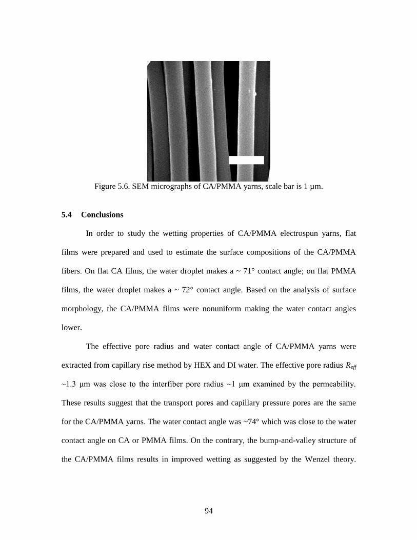
94

Figure 5.6. SEM micrographs of CA/PMMA yarns, scale bar is 1 µm.

5.4 Conclusions

In order to study the wetting properties of CA/PMMA electrospun yarns, flat

films were prepared and used to estimate the surface compositions of the CA/PMMA

fibers. On flat CA films, the water droplet makes a ~ 71° contact angle; on flat PMMA

films, the water droplet makes a ~ 72° contact angle. Based on the analysis of surface

morphology, the CA/PMMA films were nonuniform making the water contact angles

lower.

The effective pore radius and water contact angle of CA/PMMA yarns were

extracted from capillary rise method by HEX and DI water. The effective pore radius Reff

~1.3 μm was close to the interfiber pore radius ~1 μm examined by the permeability.

These results suggest that the transport pores and capillary pressure pores are the same

for the CA/PMMA yarns. The water contact angle was ~74° which was close to the water

contact angle on CA or PMMA films. On the contrary, the bump-and-valley structure of

the CA/PMMA films results in improved wetting as suggested by the Wenzel theory.

95

Thus, the different surface morphology leads to distinct wetting properties of yarns and

films made of CA/PMMA blends.

5.5 Methods

5.5.1 SEM Characterization

The surface morphology of the CA/PMMA fibers and films were examined with a

Hitachi Field Emission scanning electron microscope (FESEM-Hitachi 4800). The

samples were sputter-coated with a few nanometer thickness of gold prior to SEM

examination.

5.5.2 Volume Ratio of Each Component on the Fiber (f)

Assuming that the solvent was totally evaporated and only solid polymers left in

the fiber, the volume ratio of each component (fi) can be calculated as:

( )

i ii

i i

mf

m

(5.4)

where mi is the mass of each component in the fiber and ρi is the density of each

component in the fiber. Giving the experimental compositions of CA/PMMA solution,

the volume ratio of CA on the fiber is f1 ~ 0.7.

5.5.3 Measurements of Surface Tension (σ)

The surface tension of hexadecane and deionized water was measured using the

Wilhelmy method with a Cahn DCA-322 [25]. A platinum wire with a 250 μm diameter

96

was used as the standard probe [24]. The wire was cleaned with ethanol and heated to

red-hot with an oxidizing flame. The Wilhelmy equation F= σPcosθ was used, where F is

the wetting force, σ is the surface tension of the probe liquid, P is the perimeter of the

probe, and θ is the contact angle. We assumed that the contact angle is θ = 0° or cosθ = 1

because of the high surface energy of the platinum. Hexadecane and deionized water

were measured three times, yielding an average surface tension of HEX = 23.5 ± 0.2

mN/m and Water = 71.4 ± 0.5 mN/m, respectively.

5.6 References


Polymer, 2008. 49(10): p. 2387-2425.



3. Dzenis, Y., Structural Nanocomposites. Science, 2008. 319(5862): p. 419-420.






2011. 3(11): p. 4685-4695.

6. Wu, S., Calculation of interfacial tension in polymer systems. Journal of Polymer

Science Part C: Polymer Symposia, 1971. 34(1): p. 19-30.

7. Fowkes, F.M., Attractive forces at interfaces. Industrial & Engineering Chemistry,

1964. 56(12): p. 40-52.

8. Owens, D.K. and R.C. Wendt, Estimation of the surface free energy of polymers.

Journal of Applied Polymer Science, 1969. 13(8): p. 1741-1747.

9. Van Oss, C.J., Interfacial Forces in Aqueous Media. 1994: Marcel Dekker.

97

10. Cassie, A.B.D. and S. Baxter, Wettability of porous surfaces. Transactions of the

Faraday Society, 1944. 40: p. 546-551.

11. Baxter, S. and A.B.D. Cassie, 8—The water repellency of fabrics and a new water

repellency test. Journal of the Textile Institute Transactions, 1945. 36(4): p. T67-T90.

12. Kissa, E., Wetting and Wicking. Textile Research Journal, 1996. 66(10): p. 660-668.

13. Perwuelz, A., P. Mondon, and C. Caze, Experimental Study of Capillary Flow in

Yarns. Textile Research Journal, 2000. 70(4): p. 333-339.

14. Brugnara, M., E. Degasperi, C. Della Volpe, D. Maniglio, A. Penati, and S. Siboni,

Wettability of porous materials. II. Can we obtain the contact angle from the

Washburn equation. Contact Angle, Wettability and Adhesion, 2006. 4(143-164): p.

192.



Science, 2011. 353(1): p. 290-293.

16. Nyoni, A.B. and D. Brook, Wicking mechanisms in yarns-the key to fabric wicking

performance. Journal of the Textile Institute, 2006. 97(2): p. 119-128.

17. Lee, W.H., D. Kwak, J.E. Anthony, H.S. Lee, H.H. Choi, D.H. Kim, S.G. Lee, and K.

Cho, The Influence of the Solvent Evaporation Rate on the Phase Separation and

Electrical Performances of Soluble Acene-Polymer Blend Semiconductors.

Advanced Functional Materials, 2012. 22(2): p. 267-281.

18. Heriot, S.Y. and R.A.L. Jones, An interfacial instability in a transient wetting layer

leads to lateral phase separation in thin spin-cast polymer-blend films. Nature

Materials, 2005. 4(10): p. 782-786.

19. DalnokiVeress, K., J.A. Forrest, J.R. Stevens, and J.R. Dutcher, Phase separation

morphology of spin-coated polymer blend thin films. Physica A, 1997. 239(1-3): p.

87-94.

20. Liu, T., R. Ozisik, and R.W. Siegel, Phase separation and surface morphology of

spin-coated films of polyetherimide/polycaprolactone immiscible polymer blends.

Thin Solid Films, 2007. 515(5): p. 2965-2973.

21. Wenzel, R.N., Surface Roughness and Contact Angle. The Journal of Physical and

Colloid Chemistry, 1949. 53(9): p. 1466-1467.


Zeitschrift, 1918. 23: p. 15-22.

98


17(3): p. 273-283.




Wiley.

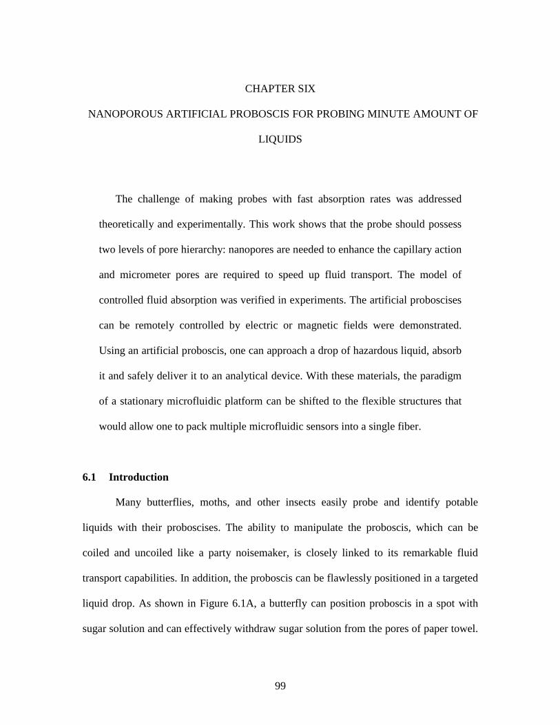
99

CHAPTER SIX

6NANOPOROUS ARTIFICIAL PROBOSCIS FOR PROBING MINUTE AMOUNT OF

LIQUIDS

The challenge of making probes with fast absorption rates was addressed

theoretically and experimentally. This work shows that the probe should possess

two levels of pore hierarchy: nanopores are needed to enhance the capillary action

and micrometer pores are required to speed up fluid transport. The model of

controlled fluid absorption was verified in experiments. The artificial proboscises

can be remotely controlled by electric or magnetic fields were demonstrated.

Using an artificial proboscis, one can approach a drop of hazardous liquid, absorb

it and safely deliver it to an analytical device. With these materials, the paradigm

of a stationary microfluidic platform can be shifted to the flexible structures that

would allow one to pack multiple microfluidic sensors into a single fiber.

6.1 Introduction

Many butterflies, moths, and other insects easily probe and identify potable

liquids with their proboscises. The ability to manipulate the proboscis, which can be

coiled and uncoiled like a party noisemaker, is closely linked to its remarkable fluid

transport capabilities. In addition, the proboscis can be flawlessly positioned in a targeted

liquid drop. As shown in Figure 6.1A, a butterfly can position proboscis in a spot with

sugar solution and can effectively withdraw sugar solution from the pores of paper towel.

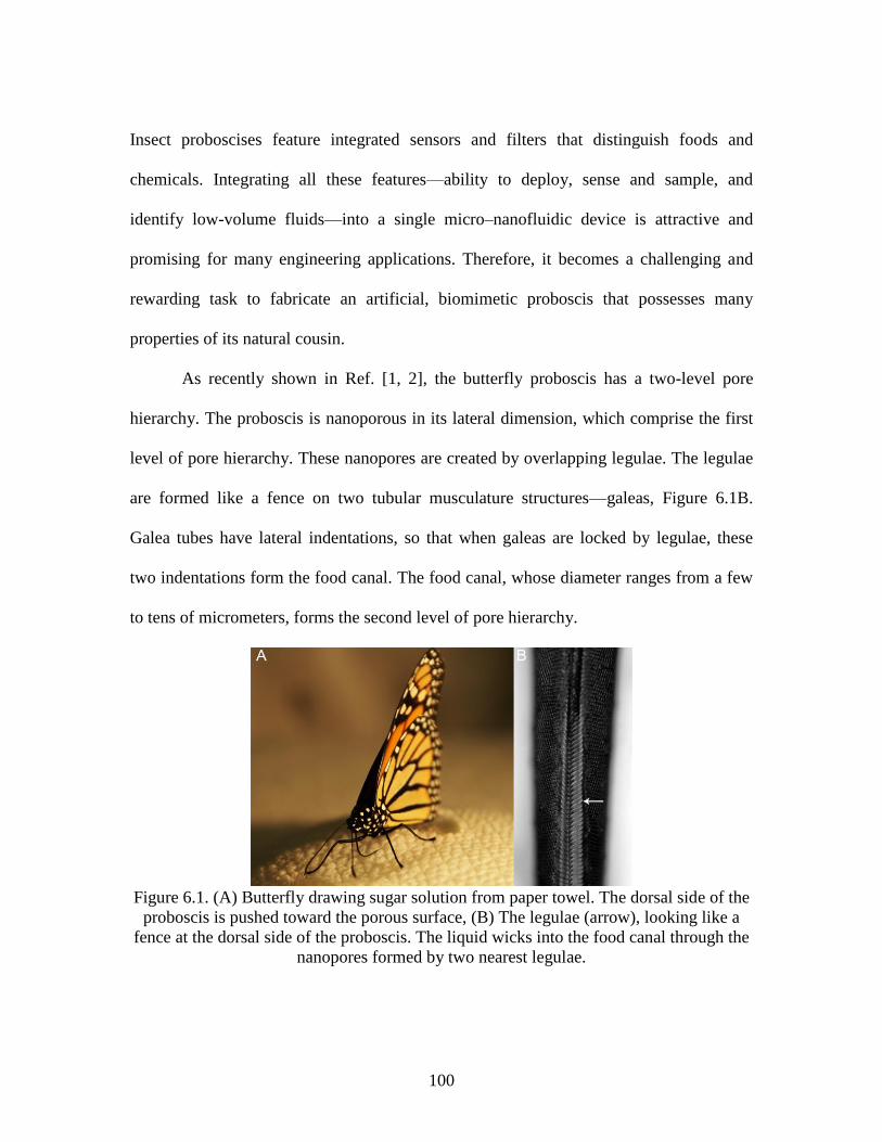
100

Insect proboscises feature integrated sensors and filters that distinguish foods and

chemicals. Integrating all these features—ability to deploy, sense and sample, and

identify low-volume fluids—into a single micro–nanofluidic device is attractive and

promising for many engineering applications. Therefore, it becomes a challenging and

rewarding task to fabricate an artificial, biomimetic proboscis that possesses many

properties of its natural cousin.

As recently shown in Ref. [1, 2], the butterfly proboscis has a two-level pore

hierarchy. The proboscis is nanoporous in its lateral dimension, which comprise the first

level of pore hierarchy. These nanopores are created by overlapping legulae. The legulae

are formed like a fence on two tubular musculature structures—galeas, Figure 6.1B.

Galea tubes have lateral indentations, so that when galeas are locked by legulae, these

two indentations form the food canal. The food canal, whose diameter ranges from a few

to tens of micrometers, forms the second level of pore hierarchy.

Figure 6.1. (A) Butterfly drawing sugar solution from paper towel. The dorsal side of the

proboscis is pushed toward the porous surface, (B) The legulae (arrow), looking like a

fence at the dorsal side of the proboscis. The liquid wicks into the food canal through the

nanopores formed by two nearest legulae.

101

In this chapter, a method of fabrication of nanoporous flexible probes which work

as artificial proboscises is described. The challenge of making probes with fast absorption

rates and good retention capacity was addressed theoretically and experimentally. The

probe material requires at least a double porosity with nanometer pores that provide

strong capillary action, and micrometer pores that provide rapid wicking. The model of

controlled fluid absorption was verified in experiments. Materials and design strategies

were focused on making artificial proboscises that feature an unprecedented flexibility,

deployability, and absorptive capacity.

Recently, electrospun nanofibers have gained considerable attention as building

blocks for various constructs and nanodevices [3-7]. Nanofibers can be made porous and

hollow, and can be bundled and twisted into yarns. These materials constitute a broad

class of flexible, lightweight structures that can be utilized in many applications dealing

with liquid handling and manipulation [8-11]. Precision control of these properties,

however, is critical for performance of the probe design. As an illustration of robustness

of the proposed method, an artificial proboscis was made from polyvinylidene fluoride

(PVDF) fibers. PVDF is well-known for its chemical inertness and thermal stability due

to the presence of -CF2- groups [4, 6]. Another advantageous PVDF property is that the

C2H2F2 molecular units of the polymer chains possess large dipole moments. These

dipoles point from the electronegative fluorine to the electropositive hydrogen. Under

certain solidification conditions, the dipoles form ordered structures that make the

material ferroelectric [12-20]. Hence, the produced probes can be manipulated with

electric fields to grab and absorb droplets of hazardous liquids. The PVDF fibers can be

102

made porous by adding a removable polymer to the dope prior to electrospinning. The

probes made of these nanoporous fibers do exhibit an increased rate of liquid absorption.

The artificial proboscises can be remotely controlled with electric or magnetic

fields. Using an artificial proboscis, one can approach a drop of hazardous liquid, absorb

it and safely deliver it to an analytical device. With these materials, the paradigm of a

stationary microfluidic platform can be shifted to the flexible structures that would allow

one to pack multiple microfluidic sensors into a single fiber.

Artificial proboscises made of nanofibers with the proposed pore structure will

find many applications as active elements in nanofluidic devices, chemical and

biomedical sensors, forensic probes, and in many other fields where probing minute

amounts of liquids is a crucial step of material processing and analysis.

6.2 Fabrication of Artificial Proboscis

The proposed yarn formation protocol developed in Chapter 3 was used to

fabricate yarns from PVDF/PEO blends. The electrospinning parameters, such as flow

rate, applied voltage, and gap between the needle and collector, are given in Table 3.1.

The morphological structure of the PVDF/PEO nanofiber surfaces and yarns was

examined with a Field Emission Scanning Electron Microscope (FESEM, Hitachi 4800)

and shown in Figure 6.2. The solid nonporous fibers and porous fibers were fabricated

during winter and summer, respectively. The temperature and relative humidity (RH) in

the hood were measured using a hygrometer (Fisher Scientific, S/N: 80614641). It was

observed that the RH was 50-65 % during summer while the RH was 25-35 % during

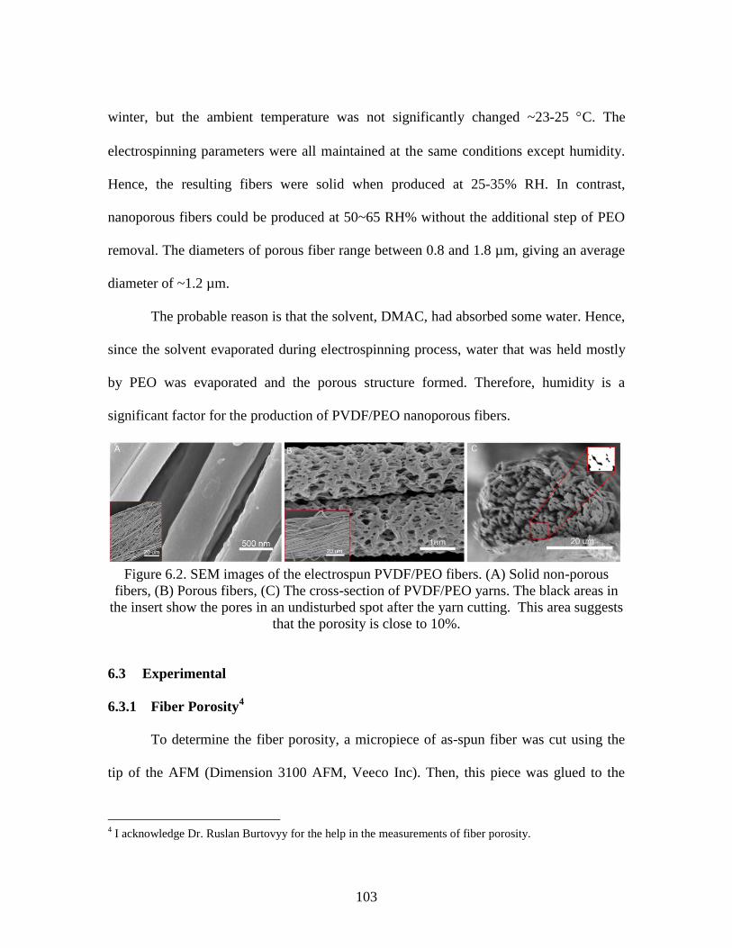
103

winter, but the ambient temperature was not significantly changed ~23-25 C. The

electrospinning parameters were all maintained at the same conditions except humidity.

Hence, the resulting fibers were solid when produced at 25-35% RH. In contrast,

nanoporous fibers could be produced at 50~65 RH% without the additional step of PEO

removal. The diameters of porous fiber range between 0.8 and 1.8 µm, giving an average

diameter of ~1.2 µm.

The probable reason is that the solvent, DMAC, had absorbed some water. Hence,

since the solvent evaporated during electrospinning process, water that was held mostly

by PEO was evaporated and the porous structure formed. Therefore, humidity is a

significant factor for the production of PVDF/PEO nanoporous fibers.

Figure 6.2. SEM images of the electrospun PVDF/PEO fibers. (A) Solid non-porous

fibers, (B) Porous fibers, (C) The cross-section of PVDF/PEO yarns. The black areas in

the insert show the pores in an undisturbed spot after the yarn cutting. This area suggests

that the porosity is close to 10%.

6.3 Experimental

6.3.1 Fiber Porosity4

To determine the fiber porosity, a micropiece of as-spun fiber was cut using the

tip of the AFM (Dimension 3100 AFM, Veeco Inc). Then, this piece was glued to the

4 I acknowledge Dr. Ruslan Burtovyy for the help in the measurements of fiber porosity.

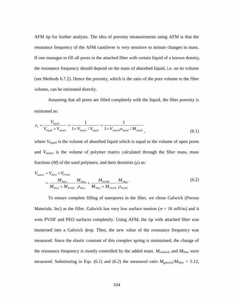
104

AFM tip for further analysis. The idea of porosity measurements using AFM is that the

resonance frequency of the AFM cantilever is very sensitive to minute changes in mass.

If one manages to fill all pores in the attached fiber with certain liquid of a known density,

the resonance frequency should depend on the mass of absorbed liquid, i.e. on its volume

(see Methods 6.7.2). Hence the porosity, which is the ratio of the pore volume to the fiber

volume, can be estimated directly.

Assuming that all pores are filled completely with the liquid, the fiber porosity is

estimated as:

liquid

f

liquid matrix matrix liquid matrix liquid liquid

1 1

1 / 1 /

V

V V V V V M

, (6.1)

where Vliquid is the volume of absorbed liquid which is equal to the volume of open pores

and Vmatrix is the volume of polymer matrix calculated through the fiber mass, mass

fractions (M) of the used polymers, and their densities (ρ) as:

matrix PEO PVDF

PEO fiber PVDF fiber

PEO PVDF PEO PEO PVDF PVDF

V V V

M M M M

M M M M

. (6.2)

To ensure complete filling of nanopores in the fiber, we chose Galwick (Porous

Materials, Inc) as the filler. Galwick has very low surface tension ( = 16 mN/m) and it

wets PVDF and PEO surfaces completely. Using AFM, the tip with attached fiber was

immersed into a Galwick drop. Then, the new value of the resonance frequency was

measured. Since the elastic constant of this complex spring is maintained, the change of

the resonance frequency is mostly controlled by the added mass. MGalwick and Mfiber were

measured. Substituting in Eqs. (6.1) and (6.2) the measured ratio Mgalwick/Mfiber = 5.12,

105

and the given values MPEO/MPVDF = 0.1, ρGalwick = 1.82 g/cm3, ρPVDF = 1.76 g/cm

3,

ρPEO=1.13 g/cm3, we estimated the porosity of single fibers as εf = 0.82. This high

porosity suggests that even a single fiber appears to be a good candidate for design of

nanoprobes enabling one to collect and retain liquids in pores. When the fibers are

twisted in the yarn, thus forming large micropores between them, one expects that the

transport properties of yarns will be significantly enhanced.

6.3.2 Absorbency of Artificial Proboscises

Porous and nonporous PVDF/PEO fiber yarns were prepared using the

experimental protocol of yarn formation developed in Chapter 3. In a first series of

experiments, the wicking properties of the produced yarns were studied. Droplets of

wetting nonvolatile liquids, hexadecane (HEX) and tributyl phosphate (TBP), Table 6.1,

were used for the evaluation of wicking properties of the yarns. These liquids were

chosen as simulants of hazardous liquids [21-27]. Droplets with initial volume V0 were

deposited on yarns, as shown in Figure 6.3b. The drop volume V(t) was defined at each

increment of time t by fitting the drop profile with Carrol’s unduloid5 [28, 29], an

analytical solution of the Laplace equation of capillarity that describes the drop shape as a

function of its volume. Figure 6.3b shows a sequence of pictures of a HEX droplet during

its absorption by the yarn. To confirm that the droplet does not evaporate during

absorption experiment, but gets absorbed by the yarn, a reference HEX droplet was

5 I acknowledge Yu Gu and Dr. Monaenkova for their help in the development of Matlab

® codes for the

droplet volume analysis.

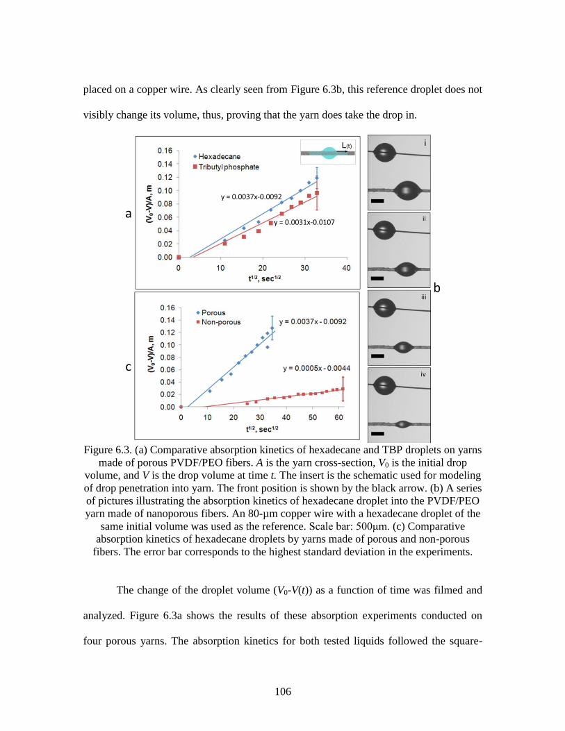
106

placed on a copper wire. As clearly seen from Figure 6.3b, this reference droplet does not

visibly change its volume, thus, proving that the yarn does take the drop in.

Figure 6.3. (a) Comparative absorption kinetics of hexadecane and TBP droplets on yarns

made of porous PVDF/PEO fibers. A is the yarn cross-section, V0 is the initial drop

volume, and V is the drop volume at time t. The insert is the schematic used for modeling

of drop penetration into yarn. The front position is shown by the black arrow. (b) A series

of pictures illustrating the absorption kinetics of hexadecane droplet into the PVDF/PEO

yarn made of nanoporous fibers. An 80-µm copper wire with a hexadecane droplet of the

same initial volume was used as the reference. Scale bar: 500μm. (c) Comparative

absorption kinetics of hexadecane droplets by yarns made of porous and non-porous

fibers. The error bar corresponds to the highest standard deviation in the experiments.

The change of the droplet volume (V0-V(t)) as a function of time was filmed and

analyzed. Figure 6.3a shows the results of these absorption experiments conducted on

four porous yarns. The absorption kinetics for both tested liquids followed the square-

107

root-of-time law, also known as the Lucas–Washburn law [30, 31]. The slope of the

fitting lines in Figure 6.3a, or wicking constants are close to each other (HEX: 0.0037

m/s1/2

; TBP: 0.0031 m/s1/2

). The results suggest that the yarn properties are very

repeatable from one sample to another and that the given similarity is not just a chance

event, but an expected consequence of the similarity of liquid properties, Table 6.1.

Table 6.1. Properties of probed liquids.

Property at

(20°C-25°C)

Tributyl phosphate

(TBP)

n-Hexadecane

(HEX)

Color Colorless Colorless

Molecular formula

(Molecular Weight)

C12H27O4P

(Mw: 266.31)

C16H34

(Mw: 226.24)

Viscosity (mPa∙s) 3.80 3.03

Surface tension (mN/m) 27 ± 0.1 23.5 ± 0.2

Density (g/cm3) 0.97 0.773

Vapor Pressure (mm Hg) 27 @ 178 °C 1 @ 105⁰C

In a second series of experiments, with three porous and three non-porous yarns,

the absorption properties of yarns made of solid non-porous fibers are much different

from those of porous fibers were presented. As demonstrated in Figure 6.3c, the wicking

constant of yarns made of solid nonporous fibers (0.0005 m/s1/2

) is at least 7 times

smaller than that of porous fibers (0.0037 m/s1/2

), It is, therefore, important to understand

the mechanism of significant enhancement of the wicking properties provided by the

nanoporous fibers in the yarn.

6.4 Kinetics of Drop Absorption into Yarns with Double Porosity

When the dimensions of pores in a material are measured in nanometers, the rate

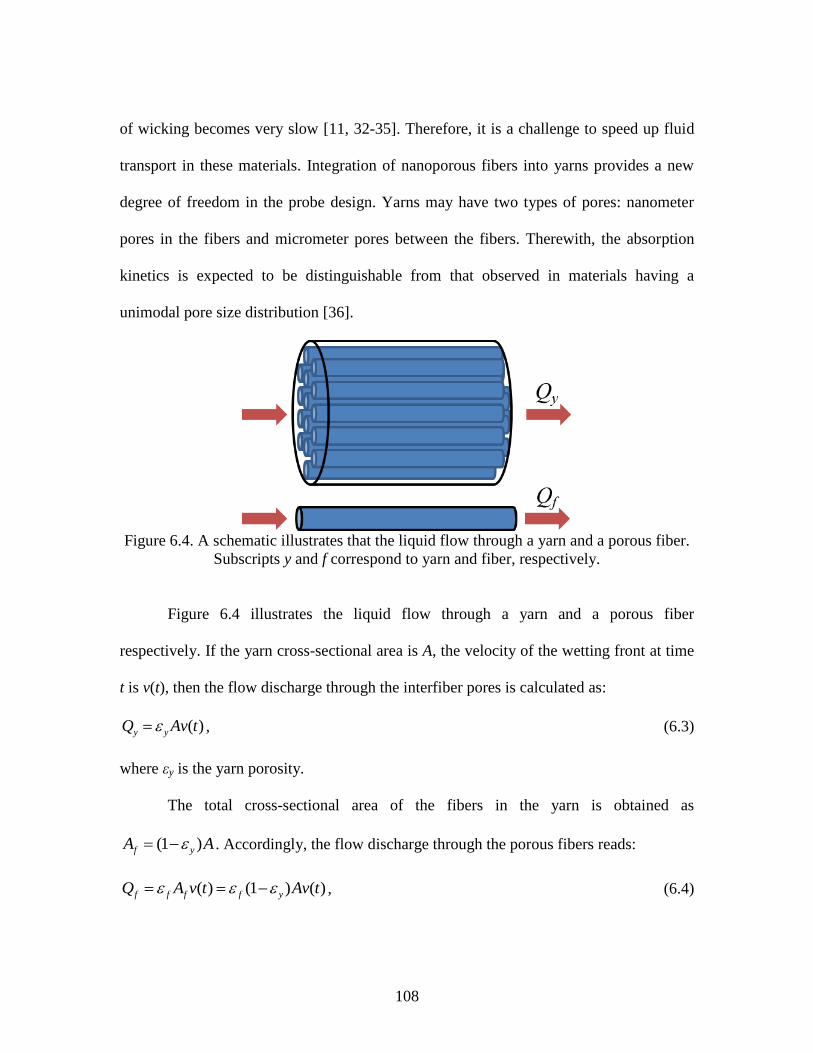
108

of wicking becomes very slow [11, 32-35]. Therefore, it is a challenge to speed up fluid

transport in these materials. Integration of nanoporous fibers into yarns provides a new

degree of freedom in the probe design. Yarns may have two types of pores: nanometer

pores in the fibers and micrometer pores between the fibers. Therewith, the absorption

kinetics is expected to be distinguishable from that observed in materials having a

unimodal pore size distribution [36].

Figure 6.4. A schematic illustrates that the liquid flow through a yarn and a porous fiber.

Subscripts y and f correspond to yarn and fiber, respectively.

Figure 6.4 illustrates the liquid flow through a yarn and a porous fiber

respectively. If the yarn cross-sectional area is A, the velocity of the wetting front at time

t is v(t), then the flow discharge through the interfiber pores is calculated as:

( )y yQ Av t , (6.3)

where εy is the yarn porosity.

The total cross-sectional area of the fibers in the yarn is obtained as

(1 )f yA A . Accordingly, the flow discharge through the porous fibers reads:

( ) (1 ) ( )f f f f yQ A v t Av t , (6.4)

109

where εf is the fiber porosity.

Applying Darcy’s law, the yarn permeability ky corresponds to the permeability of

yarn made of nonporous fibers:

y

y

k A PQ

x

, (6.5)

where η is the liquid viscosity and ∂P/∂x is the pressure gradient assuming the x-axis

along the fiber.

The discharge only through the fibers is written as:

( )f f

f

k A PQ

x

, (6.6)

where kf is the permeability of a single porous fiber.

Hence, the mass balance Qy + Qf is expressed as:

[ (1 )] ( ) [ (1 )]y f y y f y

A PAv t k k

x

. (6.7)

The liquid is assumed not volatile (eg. Hexadecane, vapor pressure: 1 mmHg @

105°C), hence, the mass conservation equation reads ∂(Qy+Qf)/∂x = ∂2P/∂x

2 = 0.

Integrating this equation, one obtains the linear distribution of the potential along the

liquid column, P(x) = ax + b, where a and b are time-dependent functions that can be

found from the boundary conditions. For further analysis it is sufficient to consider only

one half of the drop and place the center of coordinate at the contact line. Hence, taking

atmospheric pressure for the reference, the first boundary condition reads P(0) = 0. The

second boundary condition is formulated at the wetting front x = L(t). There, the capillary

pressure is built by the pores between fibers, P(L) = − Pc. These two boundary conditions

110

specify the pressure gradient ∂P/∂x = − Pc/L(t). Substituting this pressure gradient and

noticing that at the wetting front v(t) = dL/dt into Eq. (6.7), one can obtain an ordinary

differential equation:

[ (1 )]

[ (1 )]

y f y c

y f y

k k PdL

dt L

. (6.8)

Integrating Eq. (6.8) once to give:

[ (1 )]2

[ (1 )]

y f yc

y f y

k kPL t

. (6.9)

The front position L(t) can be expressed through the incremental change of

droplet volume as: (V(t) - V0 )/A = 2[εy + εf(1 - εy)]L(t), where the factor two accounts for

two wetting fronts. Solving this equation for L(t) and substituting it to Eq. (6.9), we

obtain:

1/20 tw

V VC t

A

, (6.10)

where Cw is the slop or wicking constant which is expressed as 2 2w eff cC k P and

[ (1 )][ (1 )]eff y f y y f yk k k .

6.5 Mechanism of Strong Wicking

Nanoporous materials are superior absorbers due to their ability to generate

extremely high capillary pressure [37]. The suction capillary pressure of a porous

material is estimated by the Laplace formula as Pc ~2σcos/Rp, where σ is the liquid

surface tension, is the contact angle, and Rp is a characteristic radius of pores in the

111

material [37, 38]. Hence, by decreasing the pore radius down to nanometers, one can

significantly increase the driving force for the liquid wicking. On the other hand, doing so,

one makes nanoporous materials even less permeable. Therefore, it is instructive to

analyze a condition in which the interfiber spacing would provide sufficient permeability

to the yarn, yet nanoporous fibers would increase the driving force for wicking.

Eq. (6.10) is a familiar definition of the Lucas–Washburn wicking constant Cw

with the effective permeability keff. Capillary pressure Pc and effective permeability keff

include all effects caused by nanopores in the fibers. As known from the physics of flow

through porous media, the permeability is proportional to the square of the pore radius

[38]. Therefore, the yarn permeability is typically much greater than the fiber

permeability, ky >> kf. In this limit, the wicking constant is represented in a form

convenient for comparison with the experiment:

22 [ (1 )]

c y

w y f y

P kC

. (6.11)

Porous fibers increase the capillary pressure, Pc ∝ but decrease the

permeability, kf ∝ . As follows from Eq. (6.11), when the porous fibers are twisted in a

yarn, the permeability increases, yet the capillary pressure stays the same. As a result, the

wicking constant increases; the smaller the pore size in each fiber, the greater is the

wicking constant.

As seen from Figure 6.2C, where the porosity of a spot not affected by the yarn

cutting was analyzed, the fibers in the yarn are closely packed. It is therefore plausible to

assume that the fibers form a hexagonal elementary cell. Then the yarn porosity is

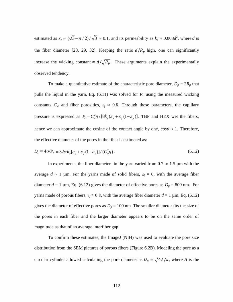
112

estimated as y ( 3 / 2) / 3 0.1, and its permeability as ky 0.008d2, where

d is

the fiber diameter [28, 29, 32]. Keeping the ratio high, one can significantly

increase the wicking constant ∝ √ . These arguments explain the experimentally

observed tendency.

To make a quantitative estimate of the characteristic pore diameter, Dp = 2Rp that

pulls the liquid in the yarn, Eq. (6.11) was solved for Pc using the measured wicking

constants Cw and fiber porosities, εf ≈ 0.8. Through these parameters, the capillary

pressure is expressed as 2 / [8 ( (1 )]c w y y f yP C k . TBP and HEX wet the fibers,

hence we can approximate the cosine of the contact angle by one, cos ≈ 1. Therefore,

the effective diameter of the pores in the fiber is estimated as:

Dp ≈ 4/Pc 232 [ (1 )] / ( )y y f y wk C . (6.12)

In experiments, the fiber diameters in the yarn varied from 0.7 to 1.5 µm with the

average d ~ 1 µm. For the yarns made of solid fibers, εf = 0, with the average fiber

diameter d = 1 µm, Eq. (6.12) gives the diameter of effective pores as Dp = 800 nm. For

yarns made of porous fibers, εf ≈ 0.8, with the average fiber diameter d = 1 µm, Eq. (6.12)

gives the diameter of effective pores as Dp = 100 nm. The smaller diameter fits the size of

the pores in each fiber and the larger diameter appears to be on the same order of

magnitude as that of an average interfiber gap.

To confirm these estimates, the ImageJ (NIH) was used to evaluate the pore size

distribution from the SEM pictures of porous fibers (Figure 6.2B). Modeling the pore as a

circular cylinder allowed calculating the pore diameter as √ , where A is the

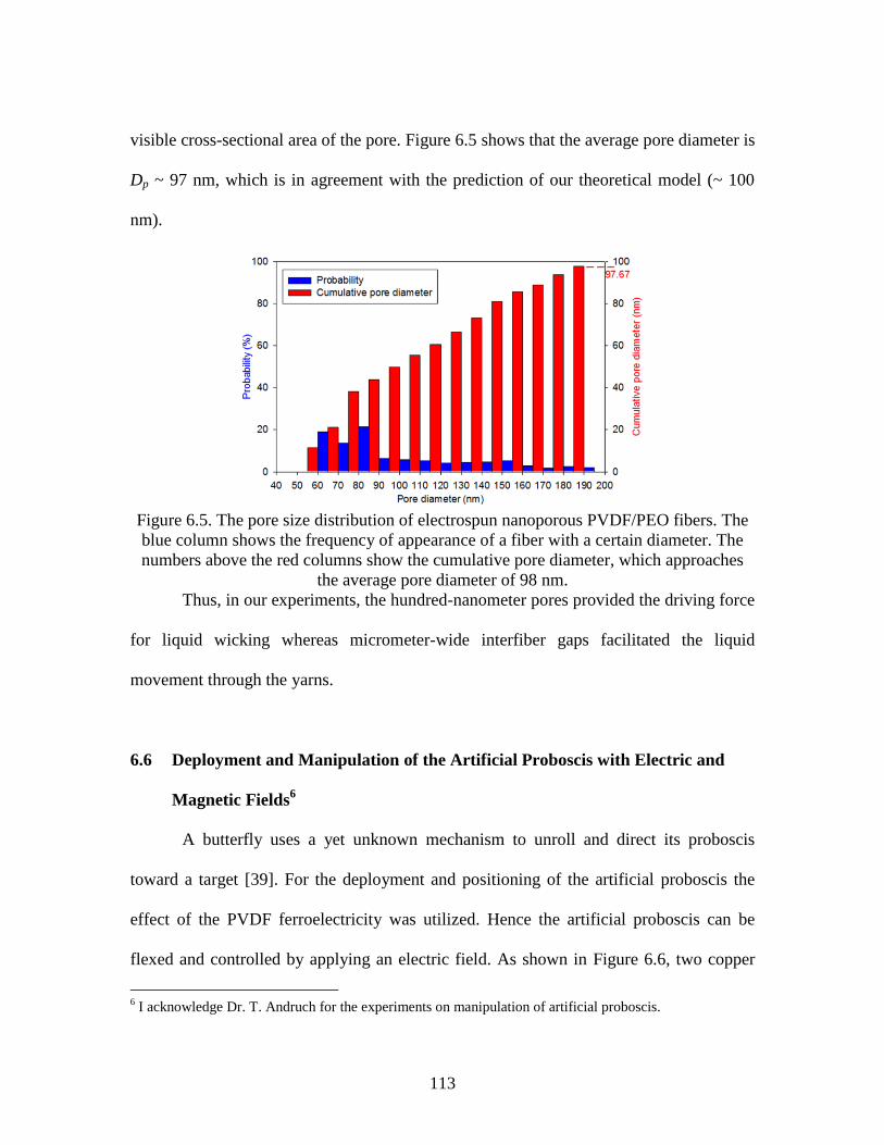
113

visible cross-sectional area of the pore. Figure 6.5 shows that the average pore diameter is

Dp ~ 97 nm, which is in agreement with the prediction of our theoretical model (~ 100

nm).

Figure 6.5. The pore size distribution of electrospun nanoporous PVDF/PEO fibers. The

blue column shows the frequency of appearance of a fiber with a certain diameter. The

numbers above the red columns show the cumulative pore diameter, which approaches

the average pore diameter of 98 nm.

Thus, in our experiments, the hundred-nanometer pores provided the driving force

for liquid wicking whereas micrometer-wide interfiber gaps facilitated the liquid

movement through the yarns.

6.6 Deployment and Manipulation of the Artificial Proboscis with Electric and

Magnetic Fields6

A butterfly uses a yet unknown mechanism to unroll and direct its proboscis

toward a target [39]. For the deployment and positioning of the artificial proboscis the

effect of the PVDF ferroelectricity was utilized. Hence the artificial proboscis can be

flexed and controlled by applying an electric field. As shown in Figure 6.6, two copper

6 I acknowledge Dr. T. Andruch for the experiments on manipulation of artificial proboscis.

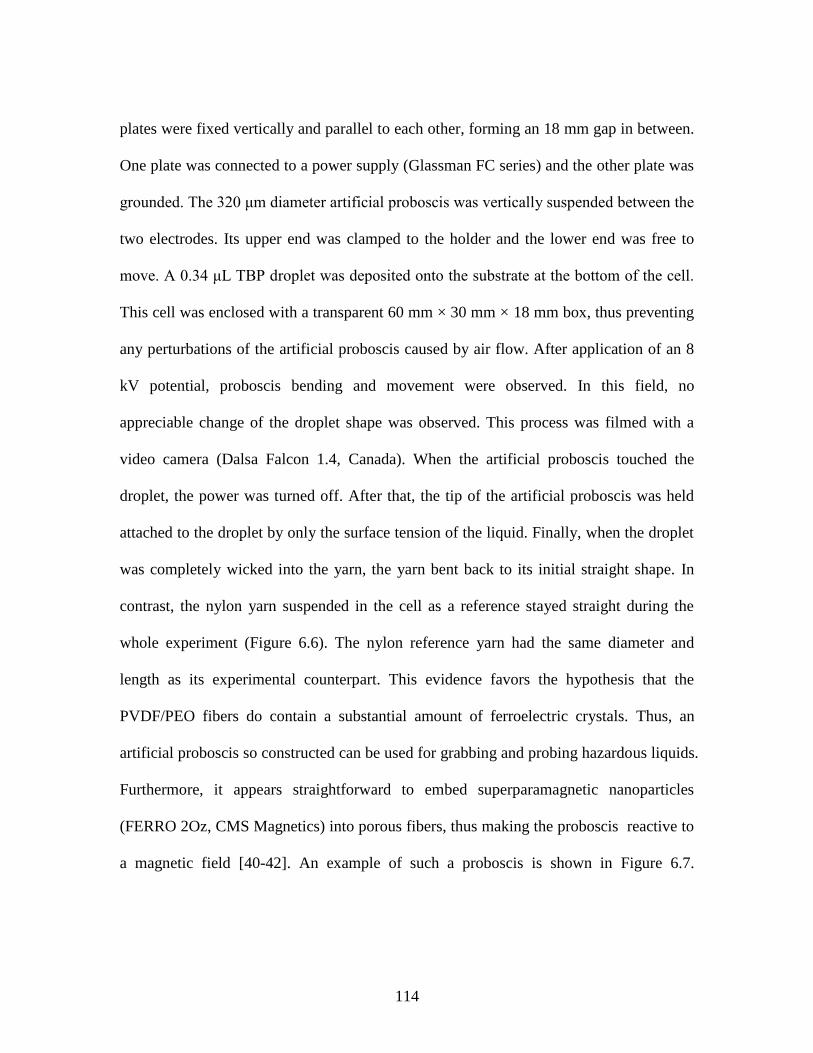
114

plates were fixed vertically and parallel to each other, forming an 18 mm gap in between.

One plate was connected to a power supply (Glassman FC series) and the other plate was

grounded. The 320 μm diameter artificial proboscis was vertically suspended between the

two electrodes. Its upper end was clamped to the holder and the lower end was free to

move. A 0.34 μL TBP droplet was deposited onto the substrate at the bottom of the cell.

This cell was enclosed with a transparent 60 mm × 30 mm × 18 mm box, thus preventing

any perturbations of the artificial proboscis caused by air flow. After application of an 8

kV potential, proboscis bending and movement were observed. In this field, no

appreciable change of the droplet shape was observed. This process was filmed with a

video camera (Dalsa Falcon 1.4, Canada). When the artificial proboscis touched the

droplet, the power was turned off. After that, the tip of the artificial proboscis was held

attached to the droplet by only the surface tension of the liquid. Finally, when the droplet

was completely wicked into the yarn, the yarn bent back to its initial straight shape. In

contrast, the nylon yarn suspended in the cell as a reference stayed straight during the

whole experiment (Figure 6.6). The nylon reference yarn had the same diameter and

length as its experimental counterpart. This evidence favors the hypothesis that the

PVDF/PEO fibers do contain a substantial amount of ferroelectric crystals. Thus, an

artificial proboscis so constructed can be used for grabbing and probing hazardous liquids.

Furthermore, it appears straightforward to embed superparamagnetic nanoparticles

(FERRO 2Oz, CMS Magnetics) into porous fibers, thus making the proboscis reactive to

a magnetic field [40-42]. An example of such a proboscis is shown in Figure 6.7.

115

Magnetically actuated artificial proboscises are attractive candidates for probing aqueous

solutions, blood or any biofluids that do not interfere with the magnetic field.

Figure 6.6. (A) Butterfly with a proboscis searching for food. (B) A schematic of yarn

manipulation with electric field generated by two vertical electrodes. (C) Artificial

proboscis made of PVDF/PEO fibers absorbing a TBP droplet. Two electrodes are

positioned from the sides and are not shown here. The solid black fiber on the left is the

artificial proboscis; the gray fiber on the right is a nylon yarn. The scale bar is 2 mm.

Figure 6.7. Absorption of a TBP droplet by the artificial proboscis made of PVDF/PEO

fibers with embedded superparamagnetic nanoparticles. The proboscis was manipulated

with a magnetic field. The scale bar is 2 mm


6.7.1 Probe Manufacturing

Two grams of PVDF (Goodfellow Corporation) and 0.2 g PEO (Mw=1,000 kDa,

Sigma–Aldrich) were dissolved in 10 g dimethylacetamide (DMAc, Spectrum) at 55 C.

116

All chemicals were used as received without further purification. The prepared polymer

solution was placed in a 10 mL syringe. A flexible syringe heater (Watlow, EHG SL10)

was attached to the syringe to maintain the temperature at 55 C. The syringe with its

heater was placed on the syringe pump (New Era Pump System, NE-300). A rotating

mandrel with four aluminum bars separated from each other by 20 cm was used as a fiber

collector. A high-voltage power supply (Glassman High Voltage, Inc.) was connected to

the syringe through a stainless-steel needle (Gauge 20, EXEL) and a 35-cm wide gap

separated the needle end from the nearest face of the mandrel. The flow rate was

controlled at 0.2 mL/hr. A positive voltage varying between 8–10 kV was applied to the

needle until a fiber jet and Taylor cone were produced. A second high-voltage power

supply was attached to the collector and a negative charge of 1 kV was applied. The

device for fiber collection consists of two ¾ -inch diameter circular wire brushes,

mounted co-axially and each attached to a miniature DC motor. The same device was

used to form yarns by spinning the brushes in the opposite directions. The number of

revolutions and the rate of twisting was controlled with totalizer counters (Crouzet 2108)

and optical reflection sensors (OPTEC Technology OPB704WZ) operating in the infrared

range of light, thus avoiding any interference with other devices. Solid non-porous fibers

were obtained at 25-35% RH while porous fibers were obtained at 65% RH even without

PEO removal Fibers were prepared at ambient temperature, 23-25 C.

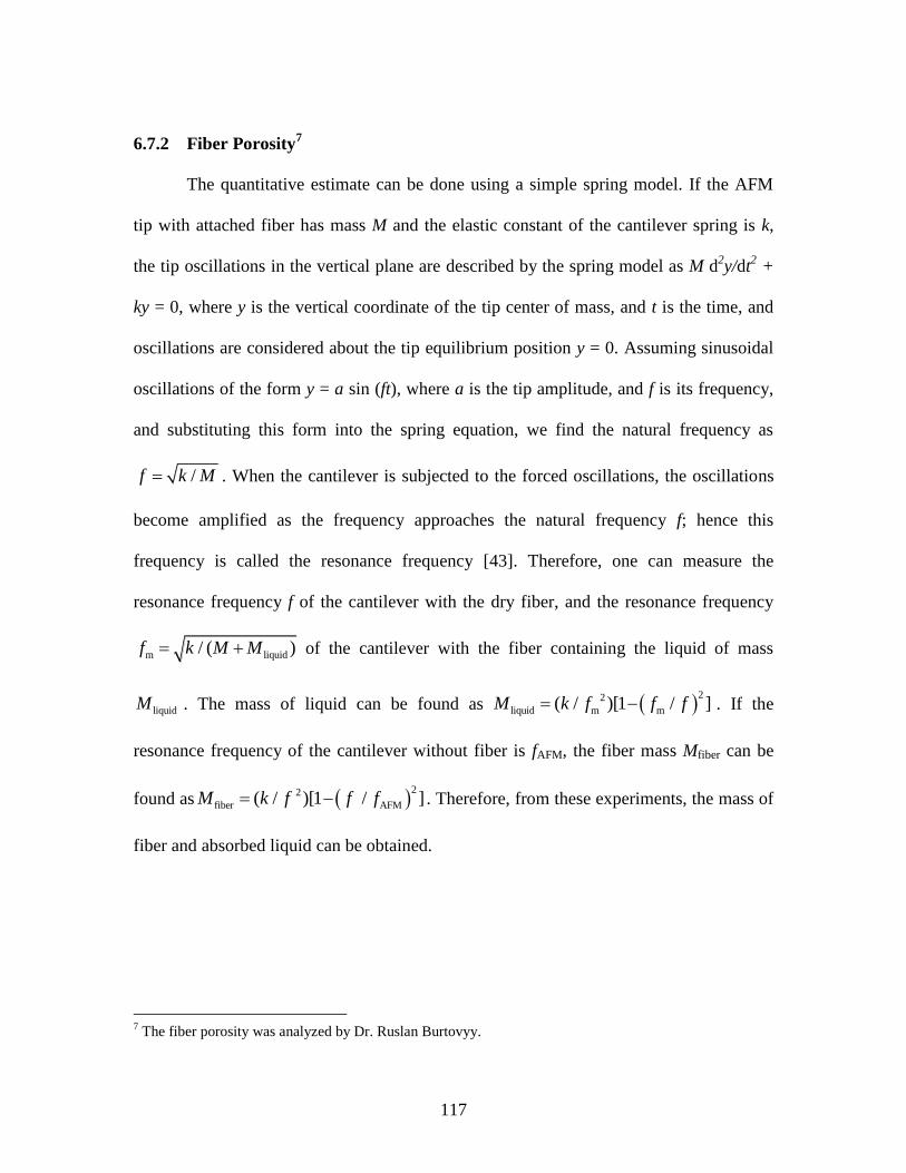
117

6.7.2 Fiber Porosity7

The quantitative estimate can be done using a simple spring model. If the AFM

tip with attached fiber has mass M and the elastic constant of the cantilever spring is k,

the tip oscillations in the vertical plane are described by the spring model as M d2y/dt

2 +

ky = 0, where y is the vertical coordinate of the tip center of mass, and t is the time, and

oscillations are considered about the tip equilibrium position y = 0. Assuming sinusoidal

oscillations of the form y = a sin (ft), where a is the tip amplitude, and f is its frequency,

and substituting this form into the spring equation, we find the natural frequency as

/f k M . When the cantilever is subjected to the forced oscillations, the oscillations

become amplified as the frequency approaches the natural frequency f; hence this

frequency is called the resonance frequency [43]. Therefore, one can measure the

resonance frequency f of the cantilever with the dry fiber, and the resonance frequency

m liquid/ ( )f k M M of the cantilever with the fiber containing the liquid of mass

liquidM . The mass of liquid can be found as 22

liquid m m( / )[1 / ]M k f f f . If the

resonance frequency of the cantilever without fiber is fAFM, the fiber mass Mfiber can be

found as 22

fiber AFM( / )[1 / ]M k f f f . Therefore, from these experiments, the mass of

fiber and absorbed liquid can be obtained.

7 The fiber porosity was analyzed by Dr. Ruslan Burtovyy.

118

6.7.3 Analysis of Pore Size Distribution

The pore size distribution was analyzed by using ImageJ software (NIH). The

images from Figure 6.2B were cropped into several 2 µm × 1 m pieces and the number of

pores in each picture was calculated. ImageJ also provides the pore area. To estimate the

pore diameter, we assumed that all pores were made of circular cylinders with diameter d.

Figure 6.5 shows that most pores had the diameters in the range of 60 ~ 80 nm. The

average diameter was calculated from Dp = Σ fi*di, where f is the probability to find the

diameter di, and subscript i corresponds to the site at which the pore diameter was

measured within the prescribed range from 50 to 190 nm.

6.7.4 Probe Characterization by Fourier Transform Infrared Spectroscopy (FT-IR)

FT-IR spectra of the electrospun nanofiber yarns were measured on Nicolet 550

Magna-IR spectrometer in the 400-1000 cm-1

range. Figure 6.8A shows three different IR

spectra of PVDF pellets, PVDF/PEO films obtained by dip coating of glass slides, and

electrospun PVDF/PEO fibers. The C2H2F2 molecular unit cells in the PVDF chain have

net dipole moments, pointing the electronegative fluorine the hydrogen, and can

crystallize forming different phases with different dipole orientations [44]. It is known

that β-phase mostly consists of CF2-CH2 dipoles oriented in the same directions, i.e., this

phase is ferroelectric. In another phase, called α-phase, the dipoles are counter directed or

form clusters with zero net moment, i.e., this phase is not ferroelectric. β- and α-phases

can be distinguished by their spectral characteristics: absorption bands of the β-phase are

situated at 509 and 840 cm-1

and absorption bands of the α-phase appear at 530, 614, 762,

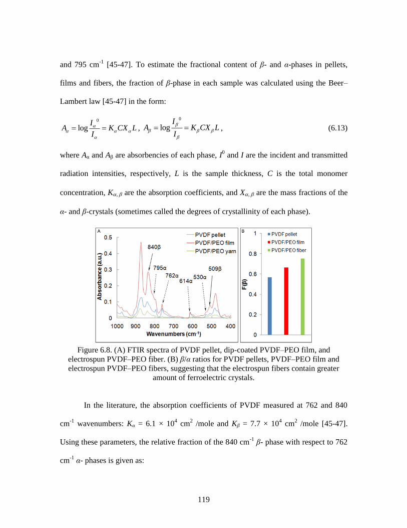
119

and 795 cm-1

[45-47]. To estimate the fractional content of β- and α-phases in pellets,

films and fibers, the fraction of β-phase in each sample was calculated using the Beer–

Lambert law [45-47] in the form:

0

logI

A K CX LI

,

0

logI

A K CX LI

, (6.13)

where Aα and Aβ are absorbencies of each phase, I0 and I are the incident and transmitted

radiation intensities, respectively, L is the sample thickness, C is the total monomer

concentration, K, are the absorption coefficients, and X, are the mass fractions of the

α- and β-crystals (sometimes called the degrees of crystallinity of each phase).

Figure 6.8. (A) FTIR spectra of PVDF pellet, dip-coated PVDF–PEO film, and

electrospun PVDF–PEO fiber. (B) β/α ratios for PVDF pellets, PVDF–PEO film and

electrospun PVDF–PEO fibers, suggesting that the electrospun fibers contain greater

amount of ferroelectric crystals.

In the literature, the absorption coefficients of PVDF measured at 762 and 840

cm-1

wavenumbers: Kα = 6.1 × 104 cm

2 /mole and Kβ = 7.7 × 10

4 cm

2 /mole [45-47].

Using these parameters, the relative fraction of the 840 cm-1

β- phase with respect to 762

cm-1

α- phases is given as:

120

( )( / ) 1.26

X A AF

X X K K A A A A

. (6.14)

The results are presented in Figure 6.8B. In the electrospun PVDF/PEO fibers, the

fraction of β-crystals appears greater than that found in the PVDF pellets. Quantitatively,

about 30% increase of the β-crystals was observed in electrospun fibers. It has been

shown that the α or γ phases can be converted in the ferroelectric β-phase by application

of a strong electric field [45] or by fiber or film drawing [48]. In electrospinning, both

these mechanisms may play important role in the enrichment of electrospun fibers with

the β-phase.

This analysis, however, does not provide any information about the direction of

the polarization vector in the fibers. One can assume that the polarization vectors in

crystallites are randomly oriented, because the external field changed frequently owing to

the mandrel rotation as well as because of flipping of the field directions between each

pair of charged arms.

6.7.5 Swelling Properties: PVDF/PEO Films

To confirm that the liquid is wicked into the pores but not absorbed by the PVDF

fiber itself, a series of experiments was conducted on films of the same composition. A

dip coater (MTI Corporation, HWTL-01) with a temperature chamber for controlling the

internal temperature was used to make uniform films. The temperature was set at 55 ⁰C.

Glass slides (Corning Inc., 2947-3x1) were used as the coating substrates. The pulling

speed was maintained at 78 mm/min. The films were dried in the chamber for 10 minutes,

121

then overnight at room temperature in a fume hood, and finally under vacuum at room

temperature for 4 hours.

The thickness of prepared PVDF/PEO films was measured before soaking them in

the liquids (HEX and TBP). A digital timer was used to record the soaking time. Every 5

minutes, the film was taken off from the liquids and an extra liquid was removed from

the film surface. Then an image was taken by a camera. After that, the film was put back

in the liquid and time was counted continuously. The film thickness at different time

moments was measured by the ImageJ (NIH) software. The brightness and contrast were

adjusted to make the film thickness measurable. The thickness δ of the PVDF/PEO film

was defined as δ = (A2 − A1)/2 (Figure 6.9), where A1 is the thickness of a glass slide (1

mm) and A2 is the total thickness of the PVDF/PEO film plus the glass slide. Ten points

were measured along the film and the average and standard deviations of film thickness

were presented in Figure 6.10. The swelling ratio is defined as (δt - δ0)/δ0, where δt is the

film thickness at time t and δ0 is the initial film thickness. As shown in Figure 6.10, the

swelling ratio is less than 5% after 20 minutes soaking. This time is on the same order as

that of the time of wicking of HEX and TBP droplets. We confirmed that at time

increments shorter than the time of droplet disappearance, which is typically approximate

20 min, swelling of PVDF/PEO films is not significant, less than 5%. Therefore, one can

safely neglect the swelling effect and interpret the experiments based on physical flow

phenomena.

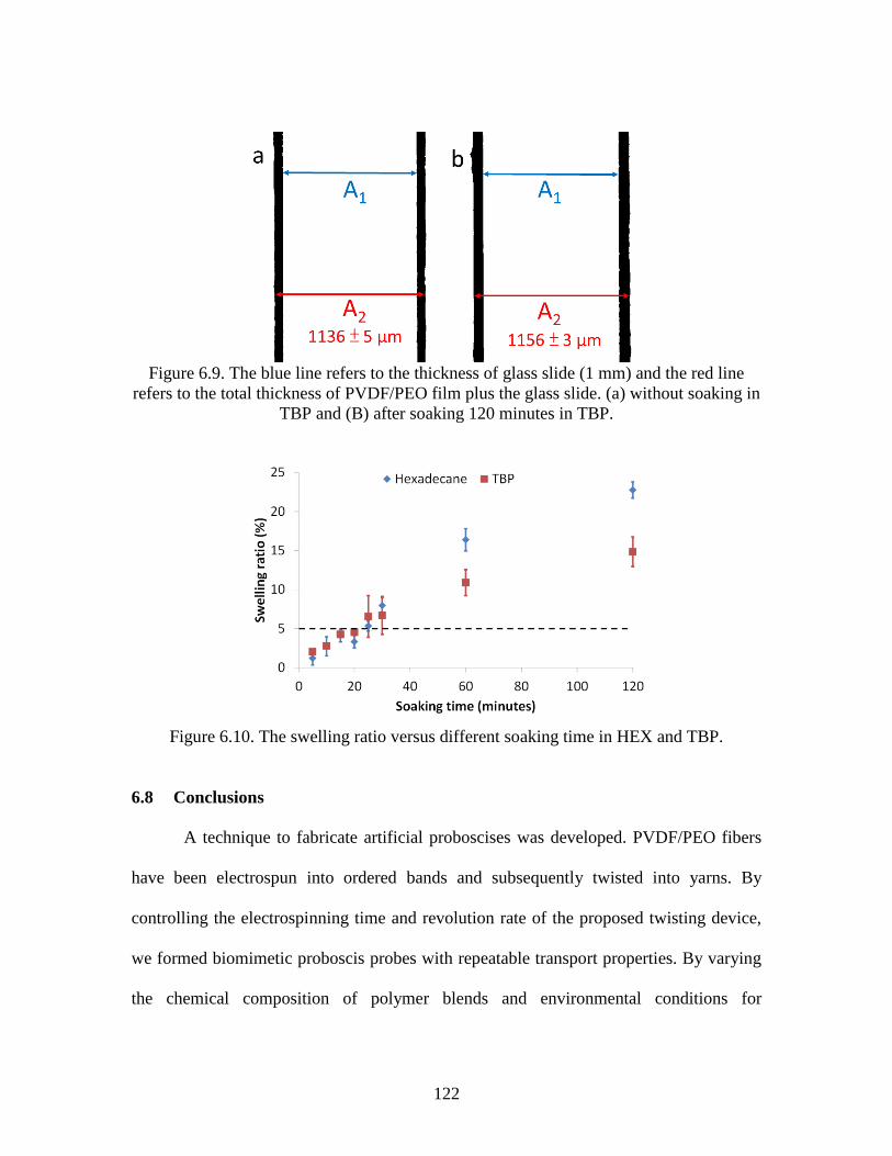
122

Figure 6.9. The blue line refers to the thickness of glass slide (1 mm) and the red line

refers to the total thickness of PVDF/PEO film plus the glass slide. (a) without soaking in

TBP and (B) after soaking 120 minutes in TBP.

Figure 6.10. The swelling ratio versus different soaking time in HEX and TBP.

6.8 Conclusions

A technique to fabricate artificial proboscises was developed. PVDF/PEO fibers

have been electrospun into ordered bands and subsequently twisted into yarns. By

controlling the electrospinning time and revolution rate of the proposed twisting device,

we formed biomimetic proboscis probes with repeatable transport properties. By varying

the chemical composition of polymer blends and environmental conditions for

123

electrospinning, we achieved porosities as high as 82% for single fibers. As predicted

theoretically, and proven experimentally, the absorption rate of the probes can be

significantly increased if one designs the probes to have double porosity composed of

micro- and nanopores. Depending on the application, the probe can be made ferroelectric

or magnetic. Further, owing to the ferroelectric and magnetic properties of the probes

produced in this work, these probes can function as artificial proboscises and can be

manipulated remotely. Commercially available microfluidic devices are typically

monolithic stationary platforms with multiple channels to which the liquid is delivered

either by a pipette or by a pump. One should mention that the produced materials swell in

hours after a TBP or hexadecane droplet gets inside. Thus, these probes can be used as

sensors as well. This work has the potential to embed multiple sensing devices in a single

fiber and make the probing device in the form of an artificial octopus with many different

microarms probing and analyzing the substrate in different places simultaneously. The

fiber-based flexible platform here developed opens up many opportunities for probing

and manipulating hazardous liquids, extracting biofluids from microorganisms or

secretory glands, or operating on single cells.

6.9 References

1. Kornev, K.G., D. Monaenkova, C. Yore, C. Klipowics, E. Edmond, V. Sa, and T.

Andrukh. Buttefly proboscis as a biomicrofluidic system. in 2008 AICHE Annular

Meeting, November 16-21. 2008. Philadelphia, PA AICHE.

2. Monaenkova, D., M.S. Lehnert, T. Andrukh, C.E. Beard, B. Rubin, A. Tokarev, W.K.

Lee, P.H. Adler, and K.G. Kornev, Butterfly proboscis: combining a drinking straw

with a nanosponge facilitated diversification of feeding habits. Journal of the Royal

Society Interface, 2012. 9(69): p. 720-726.

124

3. Reneker, D.H., A.L. Yarin, E. Zussman, and H. Xu, Electrospinning of nanofibers

from polymer solutions and melts, in Advances in Applied Mechanics, Vol 41. 2007.

p. 43-195.


Polymer, 2008. 49(10): p. 2387-2425.

5. Dzenis, Y., Materials science - Structural nanocomposites. Science, 2008. 319(5862):

p. 419-420.



7. Fang, J., H.T. Niu, T. Lin, and X.G. Wang, Applications of electrospun nanofibers.

Chinese Science Bulletin, 2008. 53(15): p. 2265-2286.

8. Janle, E.M. and J.E. Sojka, Use of ultrafiltration probes in sheep to collect interstitial

fluid for measurement of calcium and magnesium. Contemporary Topics in

Laboratory Animal Science, 2000. 39(6): p. 47-50.

9. Huang, C.M., C.C. Wang, M. Kawai, S. Barnes, and C.A. Elmets, In vivo protein

sampling using capillary ultrafiltration semi-permeable hollow fiber and protein

identification via mass spectrometry-based proteomics. Journal of Chromatography

A, 2006. 1109(2): p. 144-151.

10. Reukov, V., A. Vertegel, O. Burtovyy, K.G. Kornev, and I. Luzinov, Fabrication of

nanocoated fibers for self-diagnosis of bacterial vaginosis Materials Science and

Engineeering C, 2008.

11. Monaenkova, D. and K.G. Kornev, Elastocapillarity: Stress transfer through fibrous

probes in wicking experiments. Journal of Colloid and Interface Science, 2010.

348(1): p. 240-249.

12. Dabirian, F. and S.A.H. Ravandi, Novel Method for Nanofibre Yarn Production

Using Two Differently Charged Nozzles. Fibres & Textiles in Eastern Europe, 2009.

17(3): p. 45-47.

13. Afifi, A.M., S. Nakano, H. Yamane, and Y. Kimura, Electrospinning of Continuous

Aligning Yarns with a 'Funnel' Target. Macromolecular Materials and Engineering,

2010. 295(7): p. 660-665.

14. Zhang, K., X.F. Wang, Y. Yang, L.L. Wang, M.F. Zhu, B.S. Hsiao, and B. Chu,

Aligned and Molecularly Oriented Semihollow Ultrafine Polymer Fiber Yarns by a

Facile Method. Journal of Polymer Science Part B-Polymer Physics, 2010. 48(10): p.

1118-1125.

125

15. Bazbouz, M.B. and G.K. Stylios, Novel mechanism for spinning continuous twisted

composite nanofiber yarns. European Polymer Journal, 2008. 44(1): p. 1-12.

16. Mondal, A., R. Borah, A. Mukherjee, S. Basu, M. Jassal, and A.K. Agrawal,

Electrospun self-assembled nanofiber yarns. Journal of Applied Polymer Science,

2008. 110(1): p. 603-607.

17. Zhou, F.L. and R.H. Gong, Manufacturing technologies of polymeric nanofibres and

nanofibre yarns. Polymer International, 2008. 57(6): p. 837-845.

18. Moon, S. and R.J. Farris, How is it possible to produce highly oriented yarns of

electrospun fibers? Polymer Engineering and Science, 2007. 47(10): p. 1530-1535.


Polymer, 2005. 46(8): p. 2419-2423.

20. Teo, W.E. and S. Ramakrishna, A review on electrospinning design and nanofibre


21. Adu-Wusu, K. and N.M. Hassan, Evaluating the effects of tributyl phosphate (TBP)

and normal paraffin hydrocarbon (NPH) in simulated low-activity waste solution on

ion exchange. Separation Science and Technology, 2005. 40(1-3): p. 463-482.

22. Carrera, J.A., E. Munoz, E. Bringas, M.F. San Roman, and I. Ortiz, Influence of

operation variables on the recovery of zinc from spent pickling effluents using the

emulsion pertraction technology. Desalination, 2009. 245(1-3): p. 675-679.

23. Kumbasar, R.A., Separation and concentration of cobalt from aqueous thiocyanate

solutions containing cobalt-nickel by emulsion liquid membranes using TBP as

extractant. Journal of Membrane Science, 2009. 338(1-2): p. 182-188.

24. Kumbasar, R.A., Selective extraction of chromium (VI) from multicomponent acidic

solutions by emulsion liquid membranes using tributhylphosphate as carrier. Journal

of Hazardous Materials, 2010. 178(1-3): p. 875-882.

25. Messikh, N., M.H. Samar, and L. Messikh, Neural network analysis of liquid-liquid

extraction of phenol from wastewater using TBP solvent. Desalination, 2007. 208(1-

3): p. 42-48.

26. Ortiz, I., E. Bringas, M.F. San Roman, and A.M. Urtiaga, Selective separation of zinc

and iron from spent pickling solutions by membrane-based solvent extraction:

Process viability. Separation Science and Technology, 2004. 39(10): p. 2441-2455.

126

27. Zhao, L.F., D.J. Fei, Y.G. Dang, X.L. Zhou, and J.L. Xiao, Studies on the extraction

of chromium(III) by emulsion liquid membrane. Journal of Hazardous Materials,

2010. 178(1-3): p. 130-135.

28. Carroll, B.J., The Accurate Measurement of Contact Angle, Phase Contact Areas,

Drop Volume, and La Place Excess Pressure in Drop-Fiber Systems. Journal of

Colloid and Interface Science, 1976. 57(3): p. 488-95.

29. Chen, X.M., K.G. Kornev, Y.K. Kamath, and A.V. Neimark, The wicking kinetics of

liquid droplets into yarns. Textile Research Journal, 2001. 71(10): p. 862-869.


Zeitschrift, 1918. 23: p. 15-22.

31. Washburn, E.W., The dynamics of capillary flow. Physical Review, 1921. 17: p. 273-

283.

32. Neimark, A.V., S. Ruetsch, K.G. Kornev, P.I. Ravikovitch, P. Poulin, S. Badaire, and

M. Maugey, Hierarchical Pore Structure and Wetting Properties of Single Wall

Carbon Nanotube Fibers. Nano Letters, 2003. 3(3): p. 419-423.

33. Raravikar, N.R., L.S. Schadler, A. Vijayaraghavan, Y.P. Zhao, B.Q. Wei, and P.M.

Ajayan, Synthesis and characterization of thickness-aligned carbon nanotube-

polymer composite films. Chemistry of Materials, 2005. 17(5): p. 974-983.



Science, 2011. 353(1): p. 290-293.

35. Kornev, K.G., X. Ren, and Y. Dzenis, Controlling Liquid Release by Compressing

Electrospun Nanowebs. Journal of Engineered Fibers and Fabrics, 2009. 4(3): p. 14-

23.

36. Alimov, M.M. and K.G. Kornev, Impregnation of liquids into a laminated porous

material with a high permeability contrast. Physics of Fluids, 2007. 19(10): p.

102108

37. Rouquerol, F., J. Rouquerol, and K. Sing, Adsorption by powders and porous solids.

1999, New York: Academic Press. 467.

38. Scheidegger, A.E., The physics of flow through porous media. 3rd ed. 1974, Toronto:

University of Toronto.

127

39. Eastham, L.E.S. and Y.E.E. Eassa, The feeding mechanism of the butterfly Pieris

brassicae L. Philosophical Transactions of the Royal Society of London. Series B,

Biological Sciences, 1955. 239(659): p. 1-43.

40. Korneva, G., H.H. Ye, Y. Gogotsi, D. Halverson, G. Friedman, J.C. Bradley, and

K.G. Kornev, Carbon nanotubes loaded with magnetic particles. Nano Letters, 2005.

5(5): p. 879-884.

41. Kornev, K.G., D. Halverson, G. Korneva, Y. Gogotsi, and G. Fridman,

Magnetostatic interactions between carbon nanotubes filled with magnetic

nanoparticles. Applied Physics Letters, 2008. 92: p. 233117.

42. Freedman, J.R., D. Mattia, G. Korneva, Y. Gogotsi, G. Friedman, and A.K.

Fontecchio, Magnetically assembled carbon nanotube tipped pipettes. Applied

Physics Letters, 2007. 90(10).

43. Landau, L.D. and E.M. Lifshitz, Theory of elasticity. 2nd ed. 1970, New York:

Pergamon.

44. Poulsen, M. and S. Ducharme, Why Ferroelectric Polyvinylidene Fluoride is Special.

Ieee Transactions on Dielectrics and Electrical Insulation, 2010. 17(4): p. 1028-1035.

45. Andrew, J.S. and D.R. Clarke, Effect of electrospinning on the ferroelectric phase

content of polyvinylidene difluoride fibers. Langmuir, 2008. 24(3): p. 670-672.

46. Gregorio, R. and M. Cestari, Effect of Crystallization Temperature on the Crystalline

Phase Content and Morphology of Poly(Vinylidene Fluoride). Journal of Polymer

Science Part B-Polymer Physics, 1994. 32(5): p. 859-870.

47. Bormashenko, Y., R. Pogreb, O. Stanevsky, and E. Bormashenko, Vibrational

spectrum of PVDF and its interpretation. Polymer Testing, 2004. 23(7): p. 791-796.

48. Hsu, T.C. and P.H. Geil, Deformation and transformation mechanisms of

poly(vinylidene fluoride) (PVF2). Journal of Materials Science, 1989. 24(4): p. 1219-

1232.

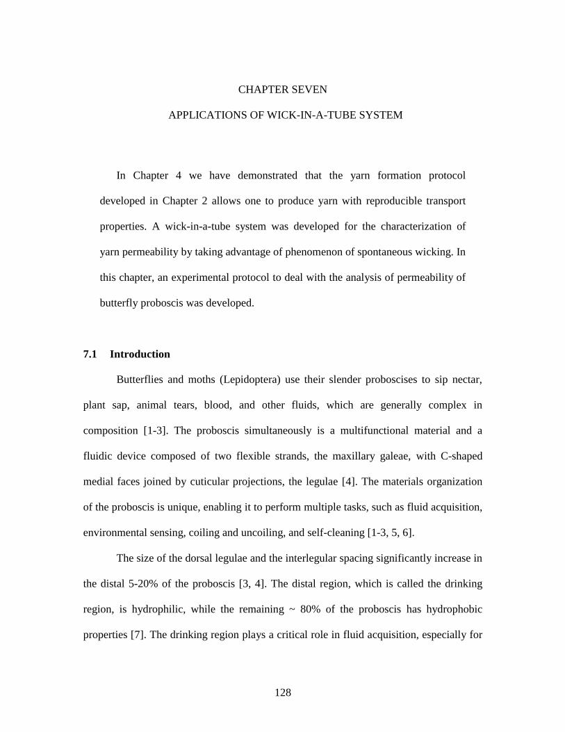
128

CHAPTER SEVEN

7APPLICATIONS OF WICK-IN-A-TUBE SYSTEM

In Chapter 4 we have demonstrated that the yarn formation protocol

developed in Chapter 2 allows one to produce yarn with reproducible transport

properties. A wick-in-a-tube system was developed for the characterization of

yarn permeability by taking advantage of phenomenon of spontaneous wicking. In

this chapter, an experimental protocol to deal with the analysis of permeability of

butterfly proboscis was developed.

7.1 Introduction

Butterflies and moths (Lepidoptera) use their slender proboscises to sip nectar,

plant sap, animal tears, blood, and other fluids, which are generally complex in

composition [1-3]. The proboscis simultaneously is a multifunctional material and a

fluidic device composed of two flexible strands, the maxillary galeae, with C-shaped

medial faces joined by cuticular projections, the legulae [4]. The materials organization

of the proboscis is unique, enabling it to perform multiple tasks, such as fluid acquisition,

environmental sensing, coiling and uncoiling, and self-cleaning [1-3, 5, 6].

The size of the dorsal legulae and the interlegular spacing significantly increase in

the distal 5-20% of the proboscis [3, 4]. The distal region, which is called the drinking

region, is hydrophilic, while the remaining ~ 80% of the proboscis has hydrophobic

properties [7]. The drinking region plays a critical role in fluid acquisition, especially for

129

feeding on porous materials such as rotten fruits and tree sap. It has been shown [4, 8]

that submicron pores (interlegular spaces) in the proboscis provide strong capillary action

favoring the uptake of fluid droplets and films [9] and facilitating fluid withdrawal from

pores [4]. Lepidoptera feed on porous materials, such as rotten fruits, and it proboscis

typically has a brushlike extension of chemosensilla, which aids fluid uptake [4, 10].

Extant members of ancient lepidopteran lineages also have brushy proboscises [11],

suggesting that capillarity had an early selective advantage, perhaps in exploiting limited

moisture and sugary exudates [12, 13]. Evolutionary diversification of siphonate

Lepidoptera, including those with comparatively smooth proboscises capable of reaching

pools of nectar in floral tubes, was associated with the radiation of flowering plants [9,

13].

The mechanism by which Lepidoptera acquire fluid from a pool has been debated

[6, 14-16]. The drinking-straw model, based on the Hagen-Poiseuille equation [17], was

proposed to explain a relation between the observed flow rate and the pressure drop

required from the suction pump, with flow rate decreasing as proboscis length increases

[6, 18, 19]. This model is useful for crude estimates of the effects of food-canal diameter

and fluid viscosity on the feeding efficiency and energetic requirements [6, 18], but faces

problems when attempting to interpret experimental observations on the uptake of thick

fluids [16]. The Hagen-Poiseuille model [6] of the fluid flow through a cylindrical tube

cannot be directly applied to the butterfly proboscis because it is not a circular cylinder.

The proboscis tip historically has been viewed as sealed [15, 20], notwithstanding

the analogy to a drinking straw. As revealed by X-ray tomography [4], however, the food

130

canal converges apically to a microscopic slit-like opening. A second structural problem

for the drinking-straw model is the distal taper of the food canal [4, 21]. A tapered food

canal increases viscous friction [22] significantly restricting fluid uptake. Optimizing

uptake from liquid films and droplets versus pools is, therefore, contradictory; a small

lumen enhances capillarity [4], whereas a large lumen enhances flow [6, 17].

To test the hypothesis that the proboscis can function as a Hagen-Poiseuille straw,

the permeability and flow in the drinking region were tested. The experimental data did

not fit the drinking-straw model, and a new model was proposed. The pressure

differential that would be required, based on our data, is greater than one atmosphere;

thus, a vacuum pump could not function. To account for this paradox, we suggest that the

butterfly can adjust the apical opening and the taper of the food canal by slightly splaying

open the galeae at the distal tip to reduce the pressure differential when feeding on thick

fluids. A second behavioral feature also could adjust the fluid-pressure differential by

changing the size of the interlegular pores and apical opening. The ability to slide the

galeae past one another in antiparallel movements [23] is well-documented for moths that

pierce animal and plant tissues [24]; it is also common in nectar and other pool-feeding

Lepidoptera and can serve to adjust the pressure differential.

131

Figure 7.1. Scanning electron micrographs. (A) Single galea of the monarch proboscis. (B)

Dorsal legulae. (C) Proboscis tip showing slit between opposing galeae.

7.2 Materials and Methods

7.2.1 Proboscis Permeability

The ability of a conduit or porous material to transport fluid at the fixed pressure

gradient P/l is characterized by the materials parameter called “permeability” [25, 26],

denoted here as k. Permeability enters the problem via Darcy’s law [25, 26], which states

that the flow discharge Q through each proboscis cross-sectional area A and thickness l is

written as Q = (kA/η)(P/l), where η is the liquid viscosity and P is the pressure

differential. In particular, if the proboscis is modeled as a cylindrical tube of radius R, the

permeability k is derived from the Hagen–Poiseuille law as k = R2/8 [17]. For a more

complex geometry, the material parameter k can be obtained by directly measuring the

total flow rate Q and pressure gradient and by knowing the proboscis cross-sectional area

and viscosity of the liquid.

A B

C

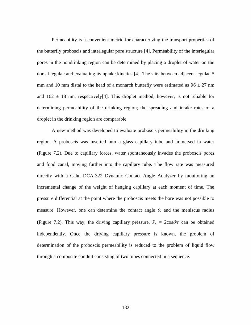
132

Permeability is a convenient metric for characterizing the transport properties of

the butterfly proboscis and interlegular pore structure [4]. Permeability of the interlegular

pores in the nondrinking region can be determined by placing a droplet of water on the

dorsal legulae and evaluating its uptake kinetics [4]. The slits between adjacent legulae 5

mm and 10 mm distal to the head of a monarch butterfly were estimated as 96 ± 27 nm

and 162 ± 18 nm, respectively[4]. This droplet method, however, is not reliable for

determining permeability of the drinking region; the spreading and intake rates of a

droplet in the drinking region are comparable.

A new method was developed to evaluate proboscis permeability in the drinking

region. A proboscis was inserted into a glass capillary tube and immersed in water

(Figure 7.2). Due to capillary forces, water spontaneously invades the proboscis pores

and food canal, moving further into the capillary tube. The flow rate was measured

directly with a Cahn DCA-322 Dynamic Contact Angle Analyzer by monitoring an

incremental change of the weight of hanging capillary at each moment of time. The

pressure differential at the point where the proboscis meets the bore was not possible to

measure. However, one can determine the contact angle , and the meniscus radius

(Figure 7.2). This way, the driving capillary pressure, Pc = 2cos/r can be obtained

independently. Once the driving capillary pressure is known, the problem of

determination of the proboscis permeability is reduced to the problem of liquid flow

through a composite conduit consisting of two tubes connected in a sequence.

133

Figure 7.2. (A) Schematic of experiment showing the operation principle of the Cahn

DSA-322. A capillary tube with the proboscis is connected to the balance arm through a

hook. An oil droplet closes the rectangular vessel, preventing water evaporation and

allowing the tube to move freely through the hole. Water moves from the reservoir to the

tube by capillary action. The weight of the wicking water column is measured by the

balance arm as the meniscus moves up the bore of the capillary tube. (B) Closed vessel

after 1 hour of saturation with water vapor. The proboscis is suspended above the water.

(C) The same vessel at the moment when the proboscis tip touches the water. (D)

Example of measurement of Jurin length (Zc), shown by the white arrow.

When such a conduit has a fixed length and the pressure differential is applied to

the ends of this conduit, the problem appears similar to the Cohn-Rashevsky problem of

design of some parts of the cardiovascular system [27-29]. In the case of moving

meniscus, the length of the liquid column changes with time and one needs to change the

Cohn-Rashevsky model. The corresponding mathematical analysis is presented in the

A

134

Appendix. A more realistic model of tapered food canal was used and analyzed the

straight cylinder model as the limiting case. In each tube of the complex conduit the flow

was assumed to follow the Hagen–Poiseuille law and the conservation of mass and the

pressure continuity were used as the boundary conditions at the point where the proboscis

meets the capillary. As follows from this model, the permeability of the capillary tube

could be separated from the permeability of the proboscis.

7.2.2 Preparation of Proboscises8

Proboscises of monarch butterflies (Danaus plexippus L.) for scanning electron

microscopy were straightened with crisscrossed pins on foam, dehydrated through an

ethanol series (80-100%), dried in hexamethyldisilazane, mounted with double-sided

conductive adhesive tape on aluminum stubs, and sputter coated with platinum for 3

minutes. Imaging was done with a Hitachi TM3000 (Hitachi High Technologies America

Inc., Alpharetta, GA, USA) at 15KV, composite image mode, and full vacuum.

Coiled proboscises of 6 monarch butterflies were soaked in deionized water for 12

hours to soften and uncoil. They were straightened several millimeters at a time and fixed

in position with pins every 2 hours. Straightened proboscises were examined with an

optical microscope to confirm that the galeae did not separate apically and to measure the

diameter.

8 The SEM micrographs were taken by Dr. Charles Beard.

135

7.3 Experiment Design

To analyze the permeability of the proboscis, the Cahn DCA-322 was used. This

instrument allows one to detect incremental changes in the sample weight with 1 g

accuracy (Figure 7.2A). A 5 mm long piece of each straightened proboscis was cut

proximal to its tip, and the cut end was inserted into a capillary tube. The inserted portion

was approximate 3 mm long; the remaining (distal) 2 mm, which included the drinking

region, protruded from the capillary tube. The tube with the proboscis was placed in a

rectangular vessel (Polystyrene, 12.5 mm × 12.5 mm × 45 mm, BRAND), and capped

(Cuvette cap square, Fisher Scientific). A 3 mm diameter hole in the cap was punched,

allowing the capillary tube to hang freely in the container, but permitting the Cahn

balance arm to connect to it (Figure 7.2A). The tip of the proboscis was suspended above

the water, without touching it (Figure 7.2B). A drop of motor oil (Castrol, SAE 5W-30)

was used to seal the space between the hole edges and external wall of the tube,

preventing evaporation and serving as a lubricant to enable the tube to move during

wicking experiments. The tip of the proboscis was brought in contact with the water by

raising the stage with the water vessel at 20 µm per second (Figure 7.2C). From the

control experiments, we found that the trapped air bubble separating the top of the sealed

vessel from the water surface required about 1 hour to reach full saturation with the water

vapor (99 %RH) when the water filled the vessel up to Z = 30 mm height.

A schematic of the mechanical principle of force measurement by the Cahn DCA-

322 is shown in Figure 7.2A. Two loops were used for force measurements (loop A and

loop B). Loop A was more sensitive and could measure a force up to 1.5 mN; loop B was

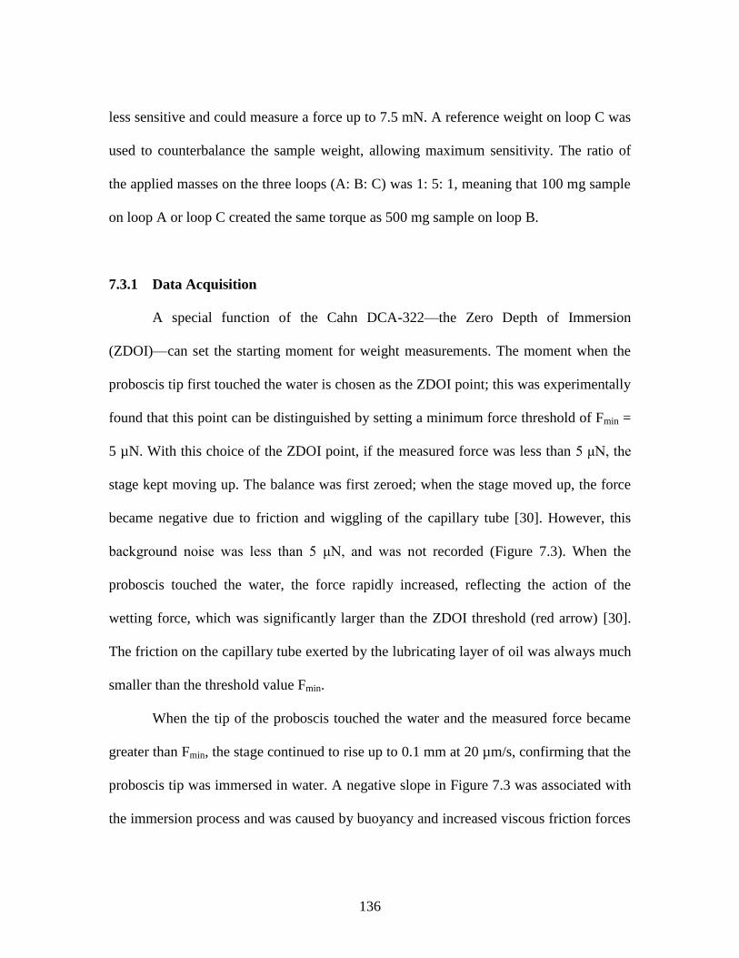
136

less sensitive and could measure a force up to 7.5 mN. A reference weight on loop C was

used to counterbalance the sample weight, allowing maximum sensitivity. The ratio of

the applied masses on the three loops (A: B: C) was 1: 5: 1, meaning that 100 mg sample

on loop A or loop C created the same torque as 500 mg sample on loop B.

7.3.1 Data Acquisition

A special function of the Cahn DCA-322—the Zero Depth of Immersion

(ZDOI)—can set the starting moment for weight measurements. The moment when the

proboscis tip first touched the water is chosen as the ZDOI point; this was experimentally

found that this point can be distinguished by setting a minimum force threshold of Fmin =

5 µN. With this choice of the ZDOI point, if the measured force was less than 5 μN, the

stage kept moving up. The balance was first zeroed; when the stage moved up, the force

became negative due to friction and wiggling of the capillary tube [30]. However, this

background noise was less than 5 μN, and was not recorded (Figure 7.3). When the

proboscis touched the water, the force rapidly increased, reflecting the action of the

wetting force, which was significantly larger than the ZDOI threshold (red arrow) [30].

The friction on the capillary tube exerted by the lubricating layer of oil was always much

smaller than the threshold value Fmin.

When the tip of the proboscis touched the water and the measured force became

greater than Fmin, the stage continued to rise up to 0.1 mm at 20 µm/s, confirming that the

proboscis tip was immersed in water. A negative slope in Figure 7.3 was associated with

the immersion process and was caused by buoyancy and increased viscous friction forces

137

at the meniscus when the proboscis became immersed [30]. The stage then was stopped.

One minute was waited to stabilize the entire setup, and began acquiring the force change

for the next 60 minutes (red line, Figure 7.3). After the stage was stopped, a meniscus

inside the capillary tube was observed, and all incremental changes of force detected by

the analyzer were attributed to the incremental change of weight of the water column

invading the tube due to capillary action.

Figure 7.3. Typical experimental curve showing force changes at different steps of

proboscis movement. A steep jump of the blue line allowed the ZDOI point to be defined.

The proboscis was immersed further into the water for 0.1 mm (green line). After 1

minute (purple line), the change of water weight for 60 minutes was collected (red line).

7.3.2 Interpretation of Wicking Experiments

The center of Cartesian coordinates was taken at the water surface, with the y-axis

pointing upward. The flow potential,, was introduced as the sum of the pressure in

water P(y) at position y and hydrostatic pressure due to weight of the liquid column:

, (7.1)

-5

0

5

10

15

20

0.5 5 50 500 5000

Forc

e (μ

N)

Time (sec)

Approach of water surfacce

Dipping proboscis into water

Establishment of stable wicking flow

Data acquisition

( )P y gy

138

where ρ is water density and g is acceleration due to gravity. In this definition, the

pressure at the water surface is zero and the potential is zero. Thus, Darcy’s law is written

through the flow potential as Q = - kpA/η(∂/∂y), where kp is the permeability of the

proboscis, η is the liquid viscosity, and ∂/∂y is the potential gradient along the proboscis.

With this definition of permeability, the material parameter kp could be obtained by

measuring the total flow rate (Q) and the potential gradient and by knowing the proboscis

cross-sectional area and viscosity of liquid used in our experiments. In the experiment,

the flow rate was measured directly using the Cahn DSA-322, but the potential gradient

was not defined. Therefore, data interpretation required additional information regarding

the fluid flow. Below, a model was set up allowing us to extract the permeability from the

experiment data.

7.3.2.1 Liquid discharge through the drinking region of the food canal (QH)

The cross-sectional area in the drinking region of the food canal, A, changes from

the tip to the proximal end of the drinking region. The shape of the food canal in the

drinking region was assumed conical (Figure 7.4). The radius of the food canal at the

submerged tip is denoted by R0, and the radius of the food canal at the proximal end of

the drinking region is denoted by Rp. Introducing the cone angle φ, the radius of food

canal at position y from the tip is expressed as R(y) = R0 + y tanφ. Using the Hagen–

Poiseuille law and assuming that the taper angle is small, the permeability of the drinking

region of the food canal is approximated as kH = (R0 + ytanφ)2/8. Accordingly, the water

discharge through a cross-sectional area A(y) is expressed as:

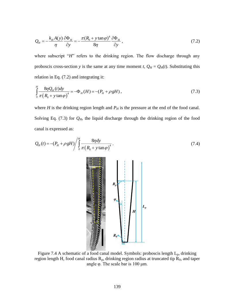
139

, (7.2)

where subscript “H” refers to the drinking region. The flow discharge through any

proboscis cross-section y is the same at any time moment t, QH = QH(t). Substituting this

relation in Eq. (7.2) and integrating it:

, (7.3)

where H is the drinking region length and PH is the pressure at the end of the food canal.

Solving Eq. (7.3) for QH, the liquid discharge through the drinking region of the food

canal is expressed as:

4

0 0

8( ) ( )

tan

H

H H

dyQ t P gH

R y

. (7.4)

Figure 7.4 A schematic of a food canal model. Symbols: proboscis length Lp, drinking

region length H, food canal radius Rp, drinking region radius at truncated tip R0, and taper

angle φ. The scale bar is 100 μm.

4

0( tan )( )

8

H H HH

R yk A yQ

y y

4

0 0

8 ( )( ) ( )

tan

H

HH H

Q t dyH P gH

R y

140

7.3.2.2 Liquid discharge through the nondrinking region of the food canal (Qp)

Above the drinking region, y > H, the cone angle φ of the food canal becomes

small, Figure 7.4, and the food canal in the non-drinking region is modeled by a straight

cylindrical tube with radius, Rp. Therefore, the flow of the liquid column can be described

by the Hagen–Poiseuille law [31] written in Darcy’s form as

with kp = Rp2/8. Subscript “p” refers to the nondrinking region of the food canal. Using

the mass conservation equation, we obtain Qp/y = 2p/y

2 = 0. Integrating this

equation, the linear distribution of the potential along the liquid column, ,

can be inferred, where c and d are time-dependent functions that can be found from the

boundary conditions. The boundary conditions state that the pressure at the end of the

drinking region of the food canal y = H must be equal to the pressure in the water column

at the same position y = H. Therefore, . At the inserted end of the

food canal y = Lp, the pressure is written as . From these two

boundary conditions, it follows that and

. With the obtained constants, the

liquid discharge through the rest of the food canal is expressed as:

4

/ ( [ ]) / [ ]8

p

p p p H p p

RQ k A a P P g L H L H

. (7.5)

The pressure at the end of the drinking region of the food canal, PH, can be related

using the conservation of mass, QH = Qp:

/ /p p pQ k A y

p cy d

HP gH cH d

p p pP gL cL d

( [ ]) / [ ]p H p pc P P g L H L H

( ( )) / ( )p p p H p pd P gL P P g L H H L L

141

4

4

0 0

8( ) ( [ ]) / [ ]

8tan

Hp

H p H p p

RdyP gH P P g L H L H

R y

. (7.6)

Taking the integral and using the definition Rp = R0 + H tan φ, the pressure PH is

expressed as:

p p

H

BP gB L H gAHP

A B

, (7.7)

where we introduce the constants:

A = 3tanφR03Rp

3/(Rp

3- R0

3) and B = Rp

4/(Lp-H). (7.8)

These constants contain the structural parameters of the proboscis. Plugging Eq.

(7.7) into Eq. (7.4), the liquid discharge through the nondrinking region of the food canal

is expressed as:

( )

8p p p

ABQ P gL

A B

. (7.9)

7.3.2.3 Meniscus motion through the capillary tube and related water discharge

(Qc)

Liquid discharge through the capillary tube is the same as that given by Eq. (7.4).

Conservation of mass requires the following equality Qp = Qc, where the flow rate

through the capillary is given by the Hagen–Poiseuille law with the pressure at one end y

= Lp being Pp and at the other end, i.e. at the meniscus position y = Lp + L(t), being Pc:

4

( ) ( [ ]) [ ]8 8

p p p c p p

AB rP gL P P g L L L L

A B

. (7.10)

Solving this equation for Pp one finds:

142

4 4

4

1( )

( )

pcp p

p p

p

gABLr P grP L L

AB r L L L L A B

A B L L

. (7.11)

Plugging Eq. (7.11) into Eq. (7.4) and expressing its left side through the

meniscus velocity Qc = πr2dL/dt, the basic equation describing the kinetics of meniscus

propagation through the complex conduit consisting of the proboscis and capillary tube is

expressed as:

2

48

c

p

P gLdL r

r A BdtL L

AB

. (7.12)

7.3.2.4 Engineering Parameters of the Butterfly Proboscis

The kinetics of meniscus propagation depends on the structural parameters of the

butterfly proboscis indirectly, but through certain dimensionless complexes. To visualize

this, the meniscus position is normalized by the Jurin length, Zc, and the time in Eq. (7.12)

by the following characteristic time:

0 2 2 2 2

8 8c cZ Pt

gr g r

. (7.13)

This time is approximately equal to the time required for a liquid meniscus to

reach the Jurin length.

With this normalization, L* = L/Zc, t* = t/t0, Eq. (7.12) is rewritten as:

* *

* *

1dL L

dt L

, (7.14)

where

143

4

p

c c

Lr A B

ABZ Z

. (7.15)

If the proboscis length is much smaller than the Jurin length (Lp << Zc), the effect

of gravity, the second term on the right side of Eq. (7.15), can be neglected, and Eq. (7.15)

is simplified as:

4

c

r A B

ABZ

. (7.16)

Eq. (7.14) is the familiar Lucas-Washburn equation describing capillary rise in

tubes [32, 33], which has the solution:

* * *(1 ) ln(1 )L L t . (7.17)

Thus, using the introduced normalization, we can interpret the experiment data in

an easier way by measuring the Jurin length Zc, calculating the characteristic time t0, and

then fitting the experimental curve L*(t

*), by adjusting parameter . After determination

of this parameter, the length of the drinking region is calculated as:

4 0cAB Z r A B or

3 4 3 4

0 0

4 2 2 3 4

0 0

3 3

3

p c p p

p p p o

R R Z R R LH

R r R R R R R r

. (7.18)

7.3.3 Measurements of Surface Tension (σ)

The surface tension of deionized water was measured using the Wilhelmy method

with a Cahn DCA-322 [31]. A platinum wire with a 250 μm diameter was used as the

standard probe [30]. The wire was cleaned with ethanol and heated to red-hot with an

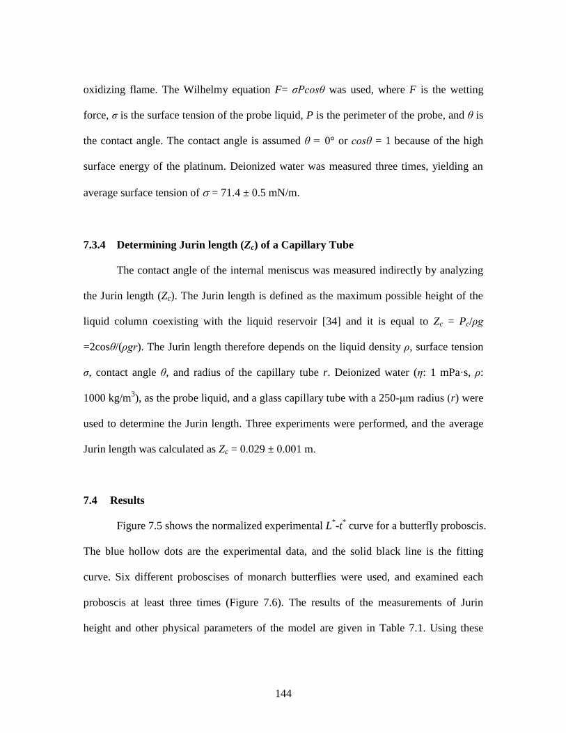
144

oxidizing flame. The Wilhelmy equation F= σPcosθ was used, where F is the wetting

force, σ is the surface tension of the probe liquid, P is the perimeter of the probe, and θ is

the contact angle. The contact angle is assumed θ = 0° or cosθ = 1 because of the high

surface energy of the platinum. Deionized water was measured three times, yielding an

average surface tension of = 71.4 ± 0.5 mN/m.

7.3.4 Determining Jurin length (Zc) of a Capillary Tube

The contact angle of the internal meniscus was measured indirectly by analyzing

the Jurin length (Zc). The Jurin length is defined as the maximum possible height of the

liquid column coexisting with the liquid reservoir [34] and it is equal to Zc = Pc/ρg

=2cosθ/(ρgr). The Jurin length therefore depends on the liquid density ρ, surface tension

σ, contact angle θ, and radius of the capillary tube r. Deionized water (η: 1 mPa·s, ρ:

1000 kg/m3), as the probe liquid, and a glass capillary tube with a 250-μm radius (r) were

used to determine the Jurin length. Three experiments were performed, and the average

Jurin length was calculated as Zc = 0.029 ± 0.001 m.

7.4 Results

Figure 7.5 shows the normalized experimental L*-t

* curve for a butterfly proboscis.

The blue hollow dots are the experimental data, and the solid black line is the fitting

curve. Six different proboscises of monarch butterflies were used, and examined each

proboscis at least three times (Figure 7.6). The results of the measurements of Jurin

height and other physical parameters of the model are given in Table 7.1. Using these

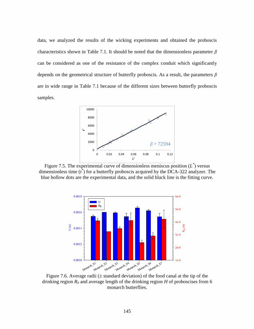
145

data, we analyzed the results of the wicking experiments and obtained the proboscis

characteristics shown in Table 7.1. It should be noted that the dimensionless parameter β

can be considered as one of the resistance of the complex conduit which significantly

depends on the geometrical structure of butterfly proboscis. As a result, the parameters β

are in wide range in Table 7.1 because of the different sizes between butterfly proboscis

samples.

Figure 7.5. The experimental curve of dimensionless meniscus position (L

*) versus

dimensionless time (t*) for a butterfly proboscis acquired by the DCA-322 analyzer. The

blue hollow dots are the experimental data, and the solid black line is the fitting curve.

Figure 7.6. Average radii (± standard deviation) of the food canal at the tip of the

drinking region R0 and average length of the drinking region H of proboscises from 6

monarch butterflies.

0

2000

4000

6000

8000

10000

0 0.02 0.04 0.06 0.08 0.1 0.12

t*

L*

β = 72594

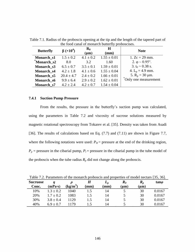
146

Table 7.1. Radius of the proboscis opening at the tip and the length of the tapered part of

the food canal of monarch butterfly proboscises.

Butterfly β (×104)

R0

(μm)

H

(mm) Note

Monarch_s1 1.5 ± 0.2 4.1 ± 0.2 1.55 ± 0.01 1. Zc = 29 mm.

2. φ ~ 0.95°.

3. t0 ~ 0.38 s.

4. Lp = 4.9 mm.

5. Rp = 30 μm. *Only one measurement

*Monarch_s2 8.0 3.2 1.60

Monarch_s3 6.5 ± 0.7 3.5 ± 0.1 1.59 ± 0.01

Monarch_s4 4.2 ± 1.8 4.1 ± 0.6 1.55 ± 0.04

Monarch_s5 20.4 ± 4.7 2.4 ± 0.2 1.66 ± 0.01

Monarch_s6 9.9 ± 6.4 2.9 ± 0.2 1.62 ± 0.01

Monarch_s7 4.2 ± 2.4 4.2 ± 0.7 1.54 ± 0.04

7.4.1 Suction Pump Pressure

From the results, the pressure in the butterfly’s suction pump was calculated,

using the parameters in Table 7.2 and viscosity of sucrose solutions measured by

magnetic rotational spectroscopy from Tokarev et al. [35]. Density was taken from Asadi

[36]. The results of calculations based on Eq. (7.7) and (7.11) are shown in Figure 7.7,

where the following notations were used: PH = pressure at the end of the drinking region,

Pp = pressure in the cibarial pump, Pt = pressure in the cibarial pump in the tube model of

the proboscis when the tube radius Rp did not change along the proboscis.

Table 7.2. Parameters of the monarch proboscis and properties of model nectars [35, 36].

Sucruose

Conc.

η

(mPa∙s)

ρ

(kg/m3)

H

(mm)

Lp

(mm)

R0

(μm)

Rp

(μm)

tanφ

10% 1.3 ± 0.2 1040 1.5 14 5 30 0.0167

20% 1.7 ± 0.2 1083 1.5 14 5 30 0.0167

30% 3.8 ± 0.4 1129 1.5 14 5 30 0.0167

40% 6.9 ± 0.7 1179 1.5 14 5 30 0.0167

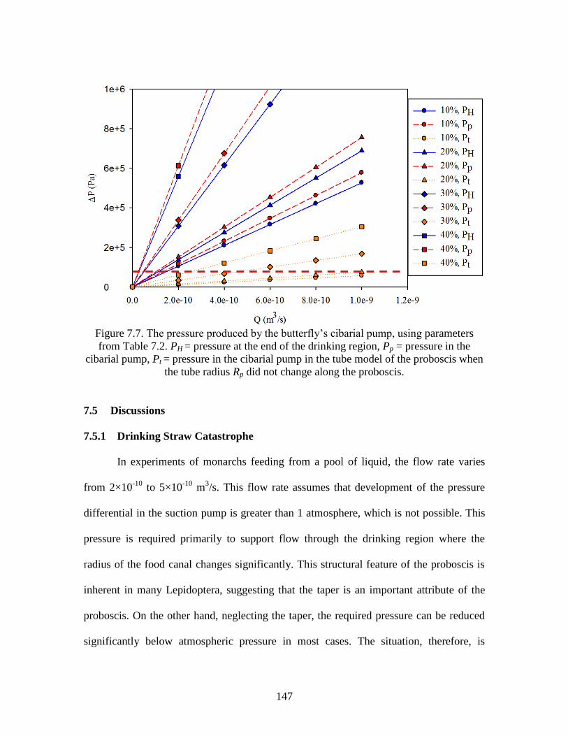
147

Figure 7.7. The pressure produced by the butterfly’s cibarial pump, using parameters

from Table 7.2. PH = pressure at the end of the drinking region, Pp = pressure in the

cibarial pump, Pt = pressure in the cibarial pump in the tube model of the proboscis when

the tube radius Rp did not change along the proboscis.

7.5 Discussions

7.5.1 Drinking Straw Catastrophe

In experiments of monarchs feeding from a pool of liquid, the flow rate varies

from 2×10-10

to 5×10-10

m3/s. This flow rate assumes that development of the pressure

differential in the suction pump is greater than 1 atmosphere, which is not possible. This

pressure is required primarily to support flow through the drinking region where the

radius of the food canal changes significantly. This structural feature of the proboscis is

inherent in many Lepidoptera, suggesting that the taper is an important attribute of the

proboscis. On the other hand, neglecting the taper, the required pressure can be reduced

significantly below atmospheric pressure in most cases. The situation, therefore, is

148

paradoxical: If structural features of the proboscis is taken into account, the required

pressure skyrockets, while a simplistic drinking-straw model that ignores the structural

features allows the pressure catastrophe to be avoided. Accordingly, the strategy of fluid

acquisition by butterflies is more complex, and that the butterfly strategy allows high

pressure differentials to be avoided.

7.6 References

1. Wigglesworth, V.B., The life of insects. 3rd edition ed. 1972, New York: Weidenfeld

and Nicolson. 359.

2. Snodgrass, R.E., The caterpillar and the butterfly. Smithson Misc. Coll., 1961.

143(6): p. 1-51.

3. Krenn, H.W., Feeding Mechanisms of Adult Lepidoptera: Structure, Function, and

Evolution of the Mouthparts. Annual Review of Entomology, 2010. 55: p. 307-327.

4. Monaenkova, D., M.S. Lehnert, T. Andrukh, C.E. Beard, B. Rubin, A. Tokarev, W.K.

Lee, P.H. Adler, and K.G. Kornev, Butterfly proboscis: combining a drinking straw

with a nanosponge facilitated diversification of feeding habits. Journal of the Royal

Society Interface, 2012. 9(69): p. 720-726.

5. Eastham, L.E.S. and Y.E.E. Eassa, The feeding mechanism of the butterfly Pieris

brassicae L. Philosophical Transactions of the Royal Society of London. Series B,

Biological Sciences, 1955. 239(659): p. 1-43.

6. Kingsolver, J.G. and T.L. Daniel, Mechanics of food handling by fluid-feeding

insects, in Regulatory mechanisms in insect feeding, R.F. Chapman and G. de Boer,

Editors. 1995, Springer: New York. p. 32-74.

7. Lehnert, M.S., D. Monaenkova, T. Andrukh, C.E. Beard, P.H. Adler, and K.G.

Kornev, Hydrophobic–hydrophilic dichotomy of the butterfly proboscis. Journal of

the Royal Society Interface, 2013. 10(85).




2011. 3(11): p. 4685-4695.

149

9. Barth, F.G., Insects and Flowers: The Biology of a Partnership. 2nd ed. 1991,

Princeton, NJ: Princeton University Press

10. Knopp, M.C.N. and H.W. Krenn, Efficiency of fruit juice feeding in Morpho peleides

(Nymphalidae, Lepidoptera). Journal of Insect Behavior, 2003. 16(1): p. 67-77.

11. Krenn, H.W. and N.P. Kristensen, Early evolution of the proboscis of Lepidoptera:

external morphology of the galea in basal glossatan moths, with remarks on the

origin of the pilifers. Zoologischer Anzeiger, 2000. 239: p. 179-196.

12. Kristensen, N.P., Studies on the morphology and systematics of primitive lepidoptera

insecta. Steenstrupia, 1984. 10(5): p. 141-191.

13. Grimaldi, D.a.M.S.E., Evolution of the Insects. 2005: Cambridge University Press.

14. Borrell, B.J., Mechanics of nectar feeding in the orchid bee Euglossa imperialis:

pressure, viscosity and flow. Journal of Experimental Biology, 2006. 209(24): p.

4901-4907.

15. Borrell, B.J. and H.W. Krenn, Nectar Feeding in Long-Proboscid Insects, in Ecology

and Biomechanics: A Mechanical Approach to the Ecology of Animals and Plants A.

Herrel, T. Speck, and N.P. Rowe, Editors. 2006, CRC: Boca Roton. p. 185-205.

16. Lehane, M.J., The Biology of Blood-Sucking in Insects. 2nd ed. 2005, New York:

Cambridge University Press.

17. Vogel, S., Comparative Biomechanics: Life's Physical World 2003, Princeton, NJ:

Princeton University Press 582.

18. Kingsolver, J.G., Butterfly engineering. Scientific American, 1985. 253 (2): p. 106-

114.

19. Kingsolver, J.G. and T.L. Daniel, Mechanics and energetics of nectar feeding in

butterflies. Journal of Theoretical Biology, 1979. 76(2): p. 167-&.

20. Krenn, H.W., J.D. Plant, and N.U. Szucsich, Mouthparts of flower-visiting insects.

Arthropod Structure & Development, 2005. 34(1): p. 1-40.

21. Krenn, H.W. and N. Muhlberger, Groundplan anatomy of the proboscis of butterflies

(Papilionoidea, lepidoptera). Zoologischer Anzeiger, 2002. 241(4): p. 369-380.

22. Batchelor, G.K., An introduction to fluid dynamics. 2000, New York: Cambridge

University Press.

23. Krenn, H.W., Proboscis assembly in butterflies (Lepidoptera) - a once in a lifetime

sequence of events. European Journal of Entomology, 1997. 94(4): p. 495-501.

150

24. Buttiker, W., H.W. Krenn, and J.F. Putterill, The proboscis of eye-frequenting and

piercing Lepidoptera (Insecta). Zoomorphology, 1996. 116(2): p. 77-83.

25. Dullien, F.A.L., Porous Media. Fluid Transport and Pore Structure 1991, New York:

Academic Press.

26. Scheidegger, A.E., The physics of flow through porous media. 3rd ed. 1974, Toronto:

University of Toronto.

27. Cohn, D.L., Optimal systems: I. The vascular system. Cohn. The Bulletin of

Mathematical Biophysics, 1954. 16(1): p. 59 - 74.

28. Cohn, D.L., Optimal systems: II. The vascular system. . The Bulletin of

Mathematical Biophysics, 1955. 17(3): p. 219 - 227.

29. Rashevsky, N., Mathematical Biophysics. 3rd Ed ed. Vol. Vol. II. 1960, New York:

Dover Publications, Inc. 462.




Wiley.


Zeitschrift, 1918. 23: p. 15-22.


17(3): p. 273-283.

34. Jurin, J., An account of some experiments shown before the Royal Society; with an

enquiry into the cause of the ascent and suspension of water in capillary tubes.

Philosophical Transactions of the Royal Society, 1917-1919. 30(351-363): p. 739-

747.

35. Tokarev, A., B. Kaufman, Y. Gu, T. Andrukh, P.H. Adler, and K.G. Kornev,

Probing viscosity of nanoliter droplets of butterfly saliva by magnetic rotational

spectroscopy. Applied Physics Letters, 2013. 102(3).

36. Asadi, M., Tables A.1 in Beet-Sugar Handbook. 2005, John Wiley & Sons, Inc. p.

779-801.

151

CHAPTER EIGHT

8CONCLUSION

1. A technique was developed to fabricate electrospun fiber yarn using a modified

collector and twisting device. Different polymers and polymer blends were electrospun

and collected. Fibers were twisted using a twisting device consisting of two co-axially

mounted brushes. This design allowed control of the yarn diameter and compactness.

The yarns produced were very uniform. These yarns had reproducible breaking stress,

elongation at break, and Young’s modulus. The modified electrospinning setup is a

promising tool to fabricate yarns with reproducible properties.

2. The wick-in-a-tube technique was developed to enable determination of the

permeability of electrospun yarns by taking advantage of wicking phenomenon. Yarns

from different polymers were electrospun and characterized. The wicking kinetics in

the wick-in-a-tube composite conduit was studied and the permeability was extracted

from the modified Lucas-Washburn equation. The permeability of electrospun yarns

demonstrated a two orders of magnitude range, from 10-14

m2 to 10

-12 m

2, by

alternation of the fiber diameter and packing density.

3. Wetting properties of CA/PMMA yarns and their constituent films were studied. The

contact angles on flat films were measured by the sessile drop technique while the

contact angles on electrospun yarns were characterized by the capillary rise method.

152

The contact angles extracted from wicking experiments were close to the contact

angles on the flat CA and PMMA films. The surface of microfibers made from

polymer blends was smooth in while the surface of films made of the same blends was

rough. This led to distinct wetting properties of yarns and films.

4. The challenge of making probes with fast absorption rates was addressed theoretically

showing that the probe should possess two levels of pore hierarchy: nanopores are

needed to enhance the capillary action and micrometer pores are required to speed up

fluid transport. This model was verified in experiments. The yarns made of

nanoporous fibers had faster wicking rates than those made of solid fibers. The

nanopores caused strong suction and the micropores provided fast flow. It was shown

that the artificial proboscises can be remotely controlled with electric or magnetic

fields. Using an artificial proboscis, one can approach a drop of hazardous liquid,

absorb it and safely deliver it to an analytical device.

5. The permeability of Monarch butterfly proboscises was characterized using the

developed wick-in-a-tube technique. The experimental results did not fit the drinking-

straw model, and a new model was proposed. Based on the experimental data, it was

demonstrated that to drink fluids butterflies have to apply a pressure differential

greater than one atmosphere.

153

APPENDICES

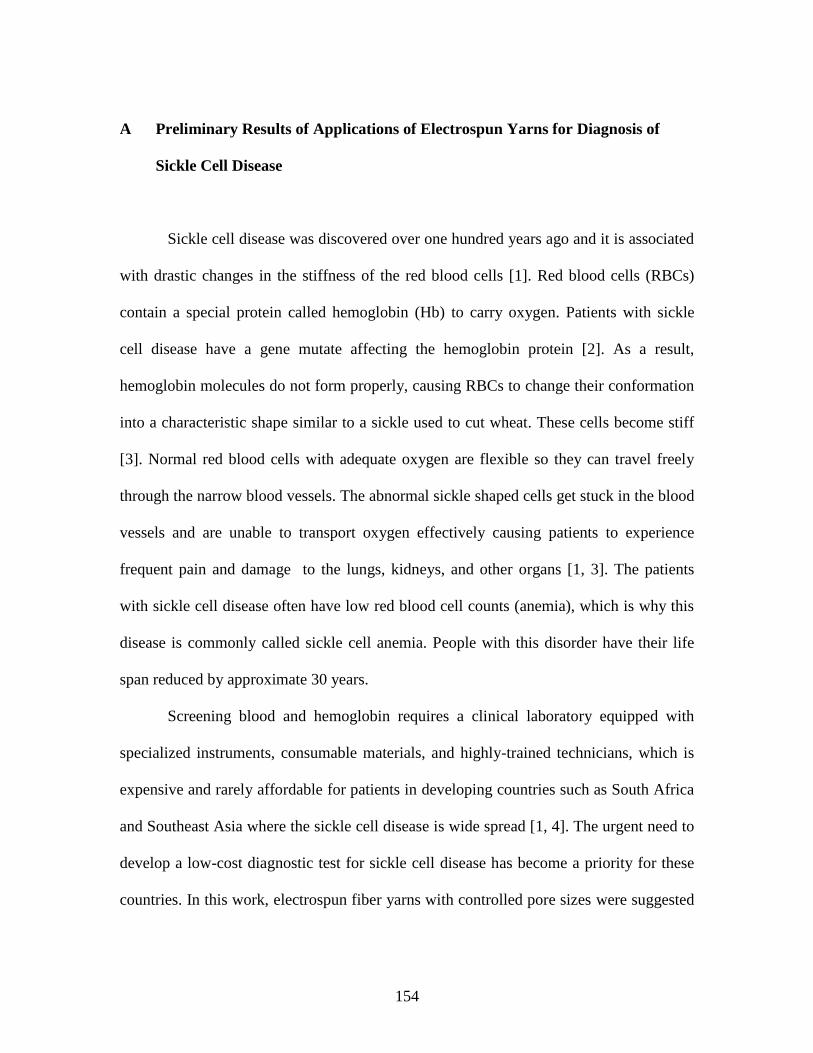
154

A Preliminary Results of Applications of Electrospun Yarns for Diagnosis of

Sickle Cell Disease

Sickle cell disease was discovered over one hundred years ago and it is associated

with drastic changes in the stiffness of the red blood cells [1]. Red blood cells (RBCs)

contain a special protein called hemoglobin (Hb) to carry oxygen. Patients with sickle

cell disease have a gene mutate affecting the hemoglobin protein [2]. As a result,

hemoglobin molecules do not form properly, causing RBCs to change their conformation

into a characteristic shape similar to a sickle used to cut wheat. These cells become stiff

[3]. Normal red blood cells with adequate oxygen are flexible so they can travel freely

through the narrow blood vessels. The abnormal sickle shaped cells get stuck in the blood

vessels and are unable to transport oxygen effectively causing patients to experience

frequent pain and damage to the lungs, kidneys, and other organs [1, 3]. The patients

with sickle cell disease often have low red blood cell counts (anemia), which is why this

disease is commonly called sickle cell anemia. People with this disorder have their life

span reduced by approximate 30 years.

Screening blood and hemoglobin requires a clinical laboratory equipped with

specialized instruments, consumable materials, and highly-trained technicians, which is

expensive and rarely affordable for patients in developing countries such as South Africa

and Southeast Asia where the sickle cell disease is wide spread [1, 4]. The urgent need to

develop a low-cost diagnostic test for sickle cell disease has become a priority for these

countries. In this work, electrospun fiber yarns with controlled pore sizes were suggested

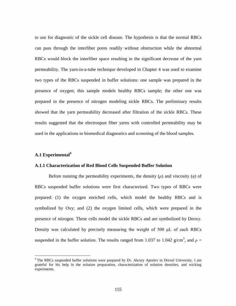
155

to use for diagnostic of the sickle cell disease. The hypothesis is that the normal RBCs

can pass through the interfiber pores readily without obstruction while the abnormal

RBCs would block the interfiber space resulting in the significant decrease of the yarn

permeability. The yarn-in-a-tube technique developed in Chapter 4 was used to examine

two types of the RBCs suspended in buffer solutions: one sample was prepared in the

presence of oxygen; this sample models healthy RBCs sample; the other one was

prepared in the presence of nitrogen modeling sickle RBCs. The preliminary results

showed that the yarn permeability decreased after filtration of the sickle RBCs. These

results suggested that the electrospun fiber yarns with controlled permeability may be

used in the applications to biomedical diagnostics and screening of the blood samples.

A.1 Experimental9

A.1.1 Characterization of Red Blood Cells Suspended Buffer Solution

Before running the permeability experiments, the density (ρ) and viscosity (η) of

RBCs suspended buffer solutions were first characterized. Two types of RBCs were

prepared: (1) the oxygen enriched cells, which model the healthy RBCs and is

symbolized by Oxy; and (2) the oxygen limited cells, which were prepared in the

presence of nitrogen. These cells model the sickle RBCs and are symbolized by Deoxy.

Density was calculated by precisely measuring the weight of 500 μL of each RBCs

suspended in the buffer solution. The results ranged from 1.037 to 1.042 g/cm3, and ρ =

9 The RBCs suspended buffer solutions were prepared by Dr. Alexey Aprelev in Drexel University. I am

grateful for his help in the solution preparation, characterization of solution densities, and wicking

experiments.

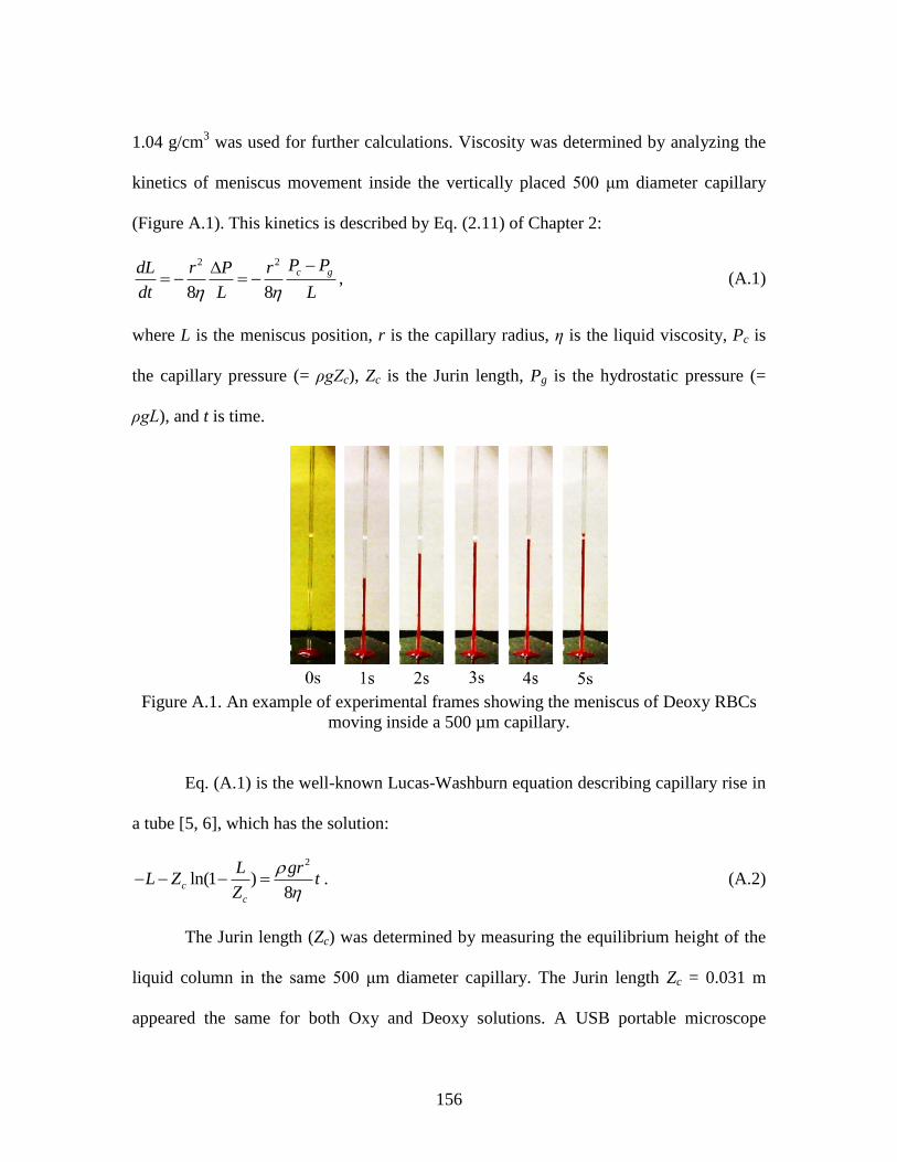
156

1.04 g/cm3 was used for further calculations. Viscosity was determined by analyzing the

kinetics of meniscus movement inside the vertically placed 500 μm diameter capillary

(Figure A.1). This kinetics is described by Eq. (2.11) of Chapter 2:

2 2

8 8

c gP PdL r P r

dt L L

, (A.1)

where L is the meniscus position, r is the capillary radius, η is the liquid viscosity, Pc is

the capillary pressure (= ρgZc), Zc is the Jurin length, Pg is the hydrostatic pressure (=

ρgL), and t is time.

Figure A.1. An example of experimental frames showing the meniscus of Deoxy RBCs

moving inside a 500 µm capillary.

Eq. (A.1) is the well-known Lucas-Washburn equation describing capillary rise in

a tube [5, 6], which has the solution:

2

ln(1 )8

c

c

L grL Z t

Z

. (A.2)

The Jurin length (Zc) was determined by measuring the equilibrium height of the

liquid column in the same 500 μm diameter capillary. The Jurin length Zc = 0.031 m

appeared the same for both Oxy and Deoxy solutions. A USB portable microscope

157

(B003+ Multi-function, Shenzhen D&F Co.) with recording frequency of one frame per

second (fps) was used to determine the position of liquid meniscus L(t). Figure A.2 shows

the curves of meniscus position (L) versus time (t) for Oxy and Deoxy solutions. The

viscosities of Oxy and Deoxy solutions were obtained by using a Matlab code to fit the

experimental data and the blue dashed lines corresponded to the theoretical model. As

one obtains the fitting parameter ρgr2/(8η), one can calculate the viscosity. The viscosity

of Oxy solution was calculated as ηo = 10.9 cp and the viscosity of Deoxy was calculated

as ηd = 6.8 cp.

Figure A.2. Meniscus dynamics in 500 μm diameter capillary tube of (a) Oxy and (b)

Deoxy solutions. The blue dashed lines represent the theoretical results.

A.1.2 Preparation of Yarns with Different Interfiber Space

Cellulose acetate (CA) and poly(methyl methacrylate) (PMMA) were dissolved in

Dimethylacetamide (DMAc) with the CA/PMMA ratio = 1:1 (by weight) to prepare

solutions of different polymer concentrations: 15wt%, 20wt%, and 25wt%. These

solutions were individually electrospun to produce fibers. Fibers were collected and

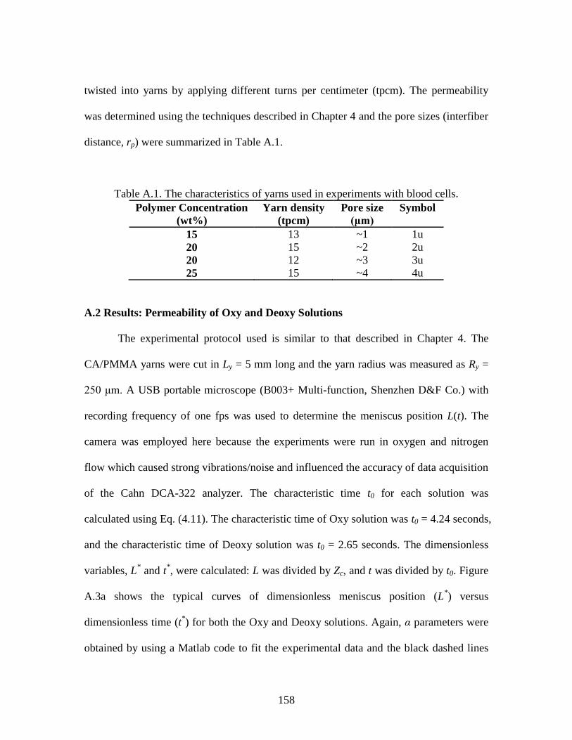
158

twisted into yarns by applying different turns per centimeter (tpcm). The permeability

was determined using the techniques described in Chapter 4 and the pore sizes (interfiber

distance, rp) were summarized in Table A.1.

Table A.1. The characteristics of yarns used in experiments with blood cells.

Polymer Concentration

(wt%)

Yarn density

(tpcm)

Pore size

(μm)

Symbol

15 13 ~1 1u

20 15 ~2 2u

20 12 ~3 3u

25 15 ~4 4u

A.2 Results: Permeability of Oxy and Deoxy Solutions

The experimental protocol used is similar to that described in Chapter 4. The

CA/PMMA yarns were cut in Ly = 5 mm long and the yarn radius was measured as Ry =

250 μm. A USB portable microscope (B003+ Multi-function, Shenzhen D&F Co.) with

recording frequency of one fps was used to determine the meniscus position L(t). The

camera was employed here because the experiments were run in oxygen and nitrogen

flow which caused strong vibrations/noise and influenced the accuracy of data acquisition

of the Cahn DCA-322 analyzer. The characteristic time t0 for each solution was

calculated using Eq. (4.11). The characteristic time of Oxy solution was t0 = 4.24 seconds,

and the characteristic time of Deoxy solution was t0 = 2.65 seconds. The dimensionless

variables, L* and t

*, were calculated: L was divided by Zc, and t was divided by t0. Figure

A.3a shows the typical curves of dimensionless meniscus position (L*) versus

dimensionless time (t*) for both the Oxy and Deoxy solutions. Again, α parameters were

obtained by using a Matlab code to fit the experimental data and the black dashed lines

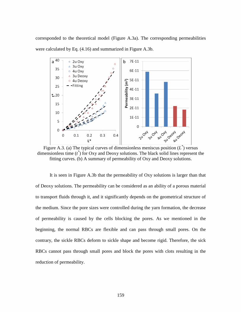
159

corresponded to the theoretical model (Figure A.3a). The corresponding permeabilities

were calculated by Eq. (4.16) and summarized in Figure A.3b.

Figure A.3. (a) The typical curves of dimensionless meniscus position (L

*) versus

dimensionless time (t*) for Oxy and Deoxy solutions. The black solid lines represent the

fitting curves. (b) A summary of permeability of Oxy and Deoxy solutions.

It is seen in Figure A.3b that the permeability of Oxy solutions is larger than that

of Deoxy solutions. The permeability can be considered as an ability of a porous material

to transport fluids through it, and it significantly depends on the geometrical structure of

the medium. Since the pore sizes were controlled during the yarn formation, the decrease

of permeability is caused by the cells blocking the pores. As we mentioned in the

beginning, the normal RBCs are flexible and can pass through small pores. On the

contrary, the sickle RBCs deform to sickle shape and become rigid. Therefore, the sick

RBCs cannot pass through small pores and block the pores with clots resulting in the

reduction of permeability.

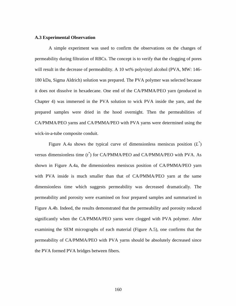
160

A.3 Experimental Observation

A simple experiment was used to confirm the observations on the changes of

permeability during filtration of RBCs. The concept is to verify that the clogging of pores

will result in the decrease of permeability. A 10 wt% polyvinyl alcohol (PVA, MW: 146-

180 kDa, Sigma Aldrich) solution was prepared. The PVA polymer was selected because

it does not dissolve in hexadecane. One end of the CA/PMMA/PEO yarn (produced in

Chapter 4) was immersed in the PVA solution to wick PVA inside the yarn, and the

prepared samples were dried in the hood overnight. Then the permeabilities of

CA/PMMA/PEO yarns and CA/PMMA/PEO with PVA yarns were determined using the

wick-in-a-tube composite conduit.

Figure A.4a shows the typical curve of dimensionless meniscus position (L*)

versus dimensionless time (t*) for CA/PMMA/PEO and CA/PMMA/PEO with PVA. As

shown in Figure A.4a, the dimensionless meniscus position of CA/PMMA/PEO yarn

with PVA inside is much smaller than that of CA/PMMA/PEO yarn at the same

dimensionless time which suggests permeability was decreased dramatically. The

permeability and porosity were examined on four prepared samples and summarized in

Figure A.4b. Indeed, the results demonstrated that the permeability and porosity reduced

significantly when the CA/PMMA/PEO yarns were clogged with PVA polymer. After

examining the SEM micrographs of each material (Figure A.5), one confirms that the

permeability of CA/PMMA/PEO with PVA yarns should be absolutely decreased since

the PVA formed PVA bridges between fibers.

161

Figure A.4. (a) Dimensionless meniscus position (L

*) versus dimensionless time (t

*) for

CA/PMMA/PEO and CA/PMMA/PEO with PVA. The black solid lines represent the

fitting curves. (b) The permeability of CA/PMMA/PEO and CA/PMMA/PEO with PVA

yarns. The y axis of permeability is presented in logarithmic scale. The error bars are the

standard deviations.

Figure A.5. The SEM micrographs of (a-b) CA/PMMA/PEO, (c-d) CA/PMMA/PEO with

PVA. (a) and (c) represent the side view of yarn, and (b) and (d) represent the cross-

sectional view of the yarn. The images confirm that the interfiber space was filled with

PVA polymer, and the interfiber distance and porosity decrease.

a

c d

b 10 μm

162

A.4 Conclusions

The yarn-in-a-tube technique was proposed to diagnose the sickle cell disease.

The yarn permeability was decreased after filtering of the sick RBCs solutions; the cells

blocked some pores in the yarns. These results suggested that the electrospun fiber yarns

with controlled permeability may be used for micro- or nanofluidic applications requiring

separation and filtration of particles and emulsions.

A.5 Reference

1. Jones, P., Sickle Cell Disease. 2008: Chelsea House Publishers.

2. Orkin, S.H. and D.R. Higgs, MEDICINE Sickle Cell Disease at 100 Years. Science,

2010. 329(5989): p. 291-292.

3. Schechter, A.N., Hemoglobin research and the origins of molecular medicine. Blood,

2008. 112(10): p. 3927-3938.

4. Weatherall, D.J. and J.B. Clegg, Inherited haemoglobin disorders: an increasing

global health problem. Bulletin of the World Health Organization, 2001. 79(8): p.

704-712.


Zeitschrift, 1918. 23: p. 15-22.


17(3): p. 273-283.

Electrospun Nanofiber Yarns for Nanofluidic Applications

Documents

Transcript of Electrospun Nanofiber Yarns for Nanofluidic Applications