Electronic Sound Reinforcement of Rooms/Auditoriums · sound reinforcement equipment can make...

UIUC Physics 406 Acoustical Physics of Music

Professor Steven Errede, Department of Physics, University of Illinois at Urbana-Champaign, Illinois

2002 - 2017. All rights reserved.

- 1 -

Electronic Sound Reinforcement of Rooms/Auditoriums

As we saw in the EASE Examples lecture notes, especially these days, with all the sophisticated, state-of-the-art/high-tech electronic sound reinforcement equipment that is readily available on the market, that there are many situations where the judicious use of electronic sound reinforcement equipment can make significant improvements in, or beneficially enhance the acoustic properties of places used for live musical entertainment, lecture halls, churches, auditoriums and concert halls, etc.

Depending on the individual/specific need(s) of the room, electronic reinforcement of sound can be in the form of either the direct, early or reverberant sound, however, usually it is the direct sound that is often in most need of reinforcement. In “dry” auditoriums, the reverberant sound can be reinforced, thereby increasing the reverberation time and hence the “liveliness” of the room. On the other hand, if excessive reverberation time or background noise interferes with clarity of speech in lecture halls and/or church settings, selective reinforcement of the direct sound over a selected range of frequencies can improve the situation in such rooms, but it also must be kept in mind that electronic reinforcement of direct sound likely will also increase the reverberant sound level(s) of such rooms.

We can characterize sound sources in a room not only by their acoustic power, P (Watts) emitted at the source, but also by their directivity factor, Q (dimensionless). In general, both the sound power P and the directivity factor Q of a sound source will vary with frequency f, i.e. P P f and Q Q f .

The sound power level LPwr logarithmically compares the acoustic power of the source, P to a reference acoustic power level, e.g. Po 1012 Watts, thus: 1010log Pwr oL P P dB .

Note that the average source power of a human speaking at a conversational level is typically 5~ 10 P Watts , which corresponds to a sound power level: 5 12

1010log 10 10 ~ 70 PwrL dB .

The directivity factor, Q is defined as the ratio of the sound intensity at a distance r in front of a source to the sound intensity averaged over all directions, the same distance r from the source:

,

ˆQ I r rz I r

, where: 2

14, 0 0

cosI r I r d d

For a point sound source that radiates equal amounts of sound uniformly in all directions, Q = 1 (solid angle subtended by the point sound source = 4/Q = 4 steradians).

If this same point sound source is placed e.g. in the middle/center of a floor, far away from the walls, then Q = 2 (solid angle subtended by point sound source = 4/Q = 2 steradians).

If this point sound source is instead placed e.g. in the middle of a wall-floor or ceiling- wall junction, then Q = 4 (solid angle subtended by point sound source = 4/Q = steradians).

If this point sound source is placed in a corner of a room, e.g. where the floor and two walls meet, then Q = 8 (solid angle subtended by point sound source = 4/Q = /2 steradians).




- 2 -

The sound pressure level 2 210 1010 log = 20log p o oSPL r L r p r p p r p dB

and/or sound intensity level 1010log I oSIL r L r I r I dB depend on the power P and

directivity factor Q of the sound source, the separation distance r from the sound source, and the strength of the reflected sound.

In a free-field situation (i.e. far away from any reflecting and/or confining/constricting surfaces), since 2

oI p c , we have shown that, to within ~ 0.1 dB:

2 210 10 1010log 10log = 20log I o p o oSIL L I I SPL L p p p p dB :

The free-field sound intensity directly in front of, and at a distance r away from a sound source having sound power P (Watts) and directivity factor Q associated with it is:

22

4ff

QPI r Watts m

r

Using the above formulae, it is a straightforward algebraic exercise (please work it out!!!) to show that the free-field sound pressure level directly in front of this sound source is:

21010log 4 direct

direct p PwrSPL r L r L Q r dB

Sound Fields:

In analogy to the concept of an electric field distributed in 3-D space in electromagnetism, in acoustical physics we characterize the distribution of sound in 3-D space as a sound field.

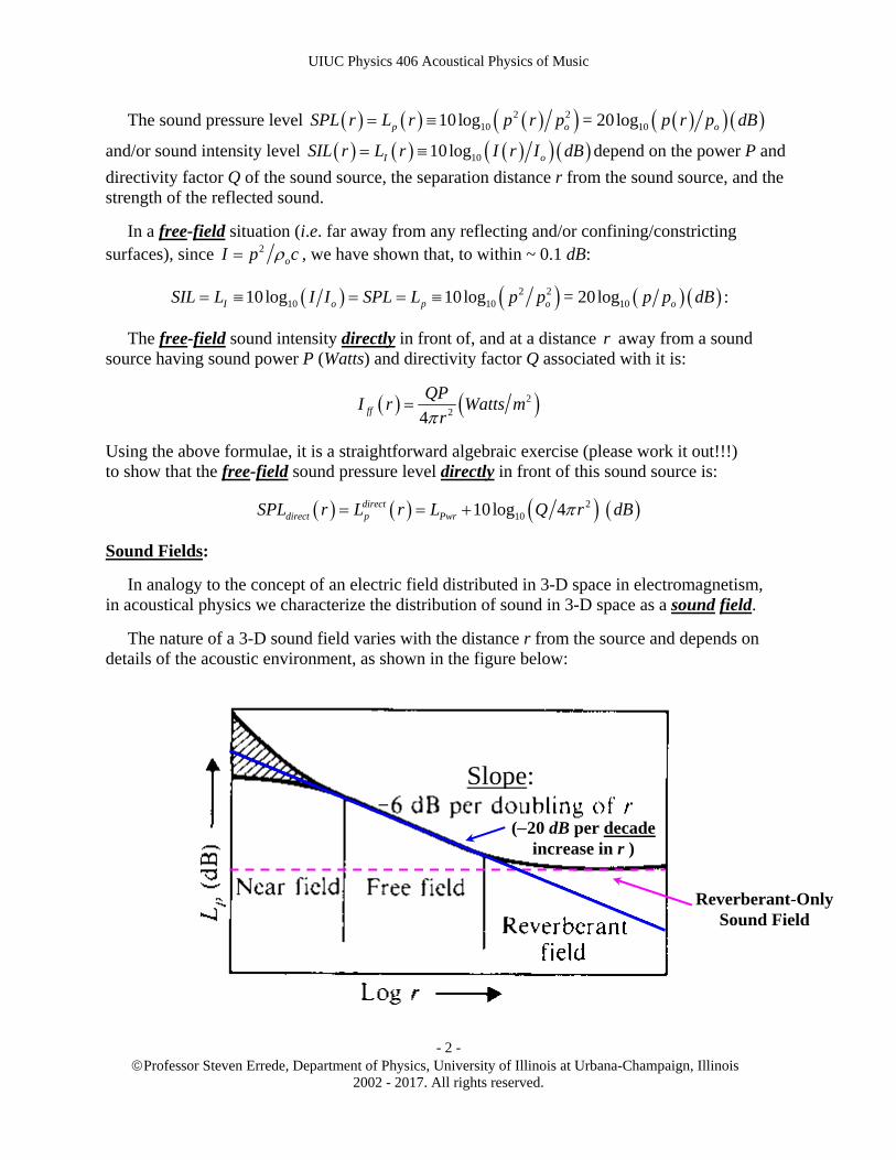
The nature of a 3-D sound field varies with the distance r from the source and depends on details of the acoustic environment, as shown in the figure below:

Reverberant-Only Sound Field

(20 dB per decade increase in r )

Slope:




- 3 -

As a function of distance r from the source, the sound field consists of three basic regions:

a.) The near field (when , r QD ) depends on the detailed geometrical nature of the sound

source, its diameter D and directivity factor Q, and wavelength of the sound. Some parts of the sound source may radiate more strongly/intensely than others.

b.) The free field (when , r QD ) is such that the sound pressure ffp r and sound

intensity ffI r vary as ~ 1 r and 2~ 1 r , respectively, such that the free-field sound

pressure level and/or sound intensity level ffff pSPL r L r = ff

ff ISIL r L r decreases

6 dB for each doubling of r (20 dB for each order-of-magnitude increase in r).

c.) The reverberant field (when , r QD ) is such that in the steady-state, the sound

pressure rvbp r , sound intensity rvbI r associated solely with the reverberant/reflected

sound (i.e. excluding the direct sound from the sound source itself) are independent of position, i.e. rvb rvb

only only

p r p constant , rvb rvbI r I constant and thus the corresponding

reverberant-only sound pressure level/sound intensity level

rvb rvbonly only

rvb p rvb Ionly only

SPL r L r SIL r L r constant .

In an enclosed space – e.g. some kind of room, auditorium, etc. in the steady-state, these physical quantities associated with the reverberant-only sound field depend on the detailed nature of the absorption properties of the various surfaces in the room, as well as on the acoustic/sound power P of the sound source. If the total absorption of the room is characterized by an effective/equivalent hole in the room of area A (as in the Sabine formula), the sound pressure level/sound intensity level in the reverberant-only sound field is:

10

410log

rvb rvbonly only

rvb p rvb I Pwronly only

SPL r L r SIL r L r L dBA

Note that the in the steady-state, the reverberant-only sound pressure level/sound intensity level in the reverberant field region is independent of listener location/position r in the room, and note also that it diverges logarithmically as the absorption, A 0.

Combining both the direct and reverberant-only sound fields (assuming no correlations between the two), the combined sound pressure level/sound intensity level in the reverberant-

field region , r QD is:

10 2

410log

4rvb rvb

direct p rvb I Pwrrvb

QSPL r L r SIL r L r L dB

r A

Note again that the in the steady-state, the combined direct + reverberant sound in the reverberant-field region is such that the associated sound pressure level/sound intensity level also diverges (logarithmically) as the absorption, A 0.

Note further that this acoustic situation has many similarities/parallels to that associated with a source emitting electromagnetic waves into a rectangular cavity with partially-absorbing walls.




- 4 -

Example:

An auditorium has dimensions 203010 m and an average absorption coefficient 0.15a . A speaker standing with his/her back in proximity to a wall of the room, located ~ in the center of this wall radiates 510 P Watts of power with a directivity factor Q = 4. Since A Sa , then:

20.15 2 20 30 2 20 10 2 30 10 330 A Sa m (n.b. this A-value is a very

small absorption for a room this room will be extremely reverberant/extremely “live”).

Directly in front of the speaker, at a distance 5 r m away from the speaker, the sound pressure level associated with the direct + reverberant sound will be:

10 2

57

10 10 10 10212

45 5 10log

4

10 4 4 10 log 10log 10log 10 10log 0.0261

10 3304 5

70 15.84 54.16

directdirect p Pwr

rvb

QSPL r m L r m L dB

r A

dB

The steady-state reverberant-only sound pressure level (n.b. independent of location in the room) will be:

710 10 10

4 410log 10log 10 10log 70 19.16 50.84

330rvb Pwronly

SPL L dBA

As long as the noise level in the room is not too large, the speaker can be heard by a listener located 5 m away, directly in front of the speaker. However note that the direct vs. reverberant-only sound pressure levels as this location in the room differ only by ~ 3.3 dB!

If the above calculations are repeated for a listener located 30 m away from the speaker, again directly in front of him/her (e.g. at the very back of the room), 30 ~ 35 directSPL r m dB ,

which is 16 dB below the reverberant-only sound pressure level – thus the listener at the very back of the room will have an extremely tough time hearing/clearly understanding the speaker due to the (strong) reverberant nature of this “live” room. Thus, electronic reinforcement of sound in this portion of the room/auditorium would significantly improve the quality of the sound listeners hear there...

Percentage Articulation Loss for Consonants (%ALCONS):

Speech intelligibility studies carried out in the Netherlands in the early 1970’s (please see/read e.g. V.M.A. Peutz, “Articulation Loss of Consonants as a Criterion for Speech Transmission in a Room”, J. Audio Eng. Soc. 19, p. 915, 1971) have enabled us to develop mathematical formulae quantifying the percentage loss of consonants, from direct measurements of the percentage of sounds incorrectly identified e.g. by good, average and poor listeners:

2 2

60200% crit

r TALCONS r D k

QV




- 5 -

where r = source - listener separation distance (m), critD = a critical distance (m), beyond which

the articulation loss remains constant, 60T = reverberation time (s), Q = directivity factor,

V = room volume (m3) and k is a constant associated with each listener, associated with his/her intrinsic listening inability. The listener inability constant ranges from k = 1.5% for the best listener to k = 12.5% for the poorest listener, with k = 7.0% for an average listener.

The critical distance, critD beyond which the articulation loss remains constant is given by the

formula: 600.2121 critD QV T m .

The %ALCONS in this region is given by: 60% 9critALCONS r D T k .

At critr D : 2 2

6060

200% 9crit

crit

D TALCONS r D k T k

QV

60 60

90.2121

200crit

QV QVD

T T

For skilled speakers and listeners, a %ALCONS of ~ 25-30% as calculated from these formulas may be acceptable, but only because human speech includes a fair amount of redundancy. Undoubtably, a %ALCONS of ~ 25-30% also causes a fair amount of momentary/ transitory distraction/loss of concentration on the part of the listener, ultimately resulting in loss of retention by the listener of what is being said by the speaker… Thus, it is a much better strategy to reduce the %ALCONS to the ~ 10-15% level.

Example:

Using the above room example, determine the %ALCONS for the room, assuming k = 7% for an average listener, but here, for simplicity, we assume a directivity factor of Q = 1 for the speaker.

Using the Sabine formula, the reverberation time for this room is:

60 0.161 0.161 6000 330 2.93 T V A s .

The %ALCONS for the room for an average listener is:

2 22 2260

200 2.9200% 7% 0.2856 7%

6000crit

rr TALCONS r D k r

V

For an average listener located at a distance of r = 5 m from the speaker:

% 5 14.14%ALCONS r m .

The critical distance for the room is: 600.2121 0.2121 6000 2.9 9.6 critD V T m .

Beyond the critical distance, 60% 9 9 2.9 7 33.35%critALCONS r D T k , which is

clearly excessive. In order to keep this to % 15%critALCONS r D , e.g. the reverberation

time of the room would need to be reduced to 60 0.9 T s , e.g. by increasing A (i.e. adding

significant amounts of sound-absorbing material to the room), or using sound reinforcement.




- 6 -

If the main problem with sound intelligibility is room noise, if it cannot be reduced (or is not easy or is extremely costly for it to be reduced), speech intelligibility can be improved significantly in this situation by simply improving the signal/noise ratio via electronic sound reinforcement techniques, raising the sound pressure level by at least 25 dB over the background noise level, for all listeners (if possible). Speech clarity/speech intelligibility only needs sound reinforcement in the mid-range frequencies, i.e. frequencies in the 500 4000 f Hz range.

If, however the main problem is associated with a poor ratio of direct to reverberant-only sound (often found e.g. in the centuries-old cathedrals of Europe), a sound reinforcement system should use loudspeakers with high Q-directivity factors to solve this problem – otherwise, both the reverberant-only and direct sound will be reinforced, thus not improving the S/N ratio.

Sound Power Considerations For A Listening Room:

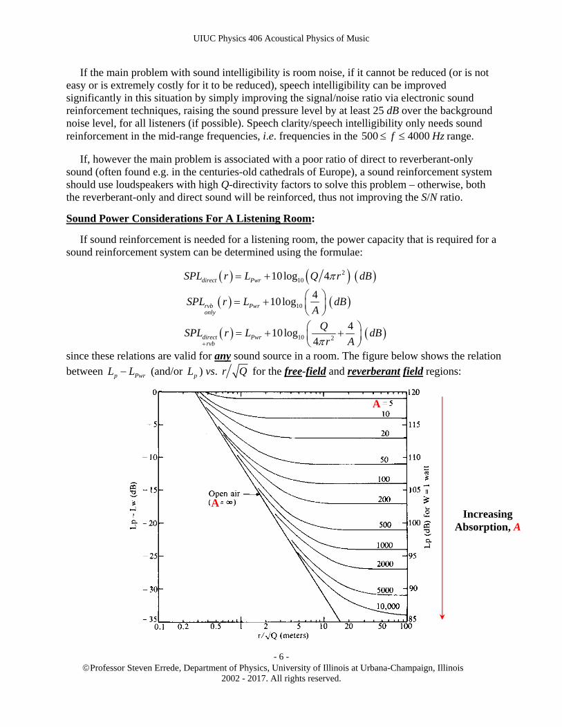
If sound reinforcement is needed for a listening room, the power capacity that is required for a sound reinforcement system can be determined using the formulae:

21010 log 4 direct PwrSPL r L Q r dB

10

410log rvb Pwr

only

SPL r L dBA

10 2

410log

4direct Pwrrvb

QSPL r L dB

r A

since these relations are valid for any sound source in a room. The figure below shows the relation

between p PwrL L (and/or pL ) vs. r Q for the free-field and reverberant field regions:

Increasing Absorption, A

A

A




- 7 -

For speech, SPL’s of 65-70 dB are usually adequate, provided this is at least 25 dB above the room noise level.

For music, which spans a wide range of genre’s and dynamic range, typically peak levels of 90-100 dB (or more) may be required. However, e.g. for rock music, 110-120 dB peaks are not uncommon…

Example:

The acoustical power, Pac needed to achieve a reverberant-field sound pressure level of

SPL = 100 rvbonlypL dB in a room with total absorption A = 500 m2 can be determined using the

above graph (and/or the use of the formula 10

410log

rvbonly

rvb p Pwronly

SPL L L dBA

).

When 10 r Q m (i.e. the reverberant-field region, for A = 500 m2), we see from the above

graph/formula that: 10 10 10

4 410log 10log 10log 0.008 21

500

rvbonlyp pwrL L dB

A

or: 21 100 21 121 rvbonly

pwr pL L dB dB .

Since 1010 log 121 Pwr ac oL P P dB , then 1010 log 121ac oP P 10log 12.1ac oP P

10log 12.110 10ac oP P Thus: 12.1 12.1 12.0 0.110 10 10 10 1.26 ac oP P AcousticWatts RMS .

If the loudspeaker(s) that are to be used for sound reinforcement in this room each have an efficiency of e.g. spkr = 1.26% for conversion of electrical energy into acoustical energy, then since ac spkr elP P , the electrical power Pel required for the amplifier used in the electronic sound

reinforcement system for this room needs to be 1.26 1.26% 100.0 el ac spkrP P Watts RMS .

Placement/Location of Loudspeakers In a Listening Room:

In designing a sound system for a listening room, the placement/location of the loudspeakers in the room is one of the most important factors to take into consideration in order to achieve the best coverage, clarity and intelligibility over the listening area. Sound reinforcement systems often use a large single sound source, or a number of small sound sources judiciously distributed throughout the listening room.

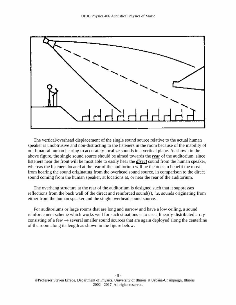
In most auditoriums (i.e. large listening rooms), single sound sources are preferred, because they preserve the best spatial pattern of the sound field. A single sound source generally consists of an array, or cluster of loudspeakers, each with directivity factor Q selected (and spatially oriented) to give the best overall sound coverage for the audience. From direct experience with installation and the use of such sound reinforcement systems in auditoriums/large rooms, the {strongly!} preferred solution is the use of a single sound source, located along the centerline of the room, near the front, placed over/above the speaker’s head, as shown in the figure below:




- 8 -

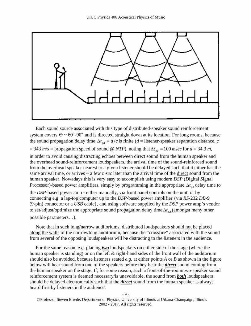
The vertical/overhead displacement of the single sound source relative to the actual human speaker is unobtrusive and non-distracting to the listeners in the room because of the inability of our binaural human hearing to accurately localize sounds in a vertical plane. As shown in the above figure, the single sound source should be aimed towards the rear of the auditorium, since listeners near the front will be most able to easily hear the direct sound from the human speaker, whereas the listeners located at the rear of the auditorium will be the ones to benefit the most from hearing the sound originating from the overhead sound source, in comparison to the direct sound coming from the human speaker, at locations at, or near the rear of the auditorium. The overhang structure at the rear of the auditorium is designed such that it suppresses reflections from the back wall of the direct and reinforced sound(s), i.e. sounds originating from either from the human speaker and the single overhead sound source. For auditoriums or large rooms that are long and narrow and have a low ceiling, a sound reinforcement scheme which works well for such situations is to use a linearly-distributed array consisting of a few several smaller sound sources that are again deployed along the centerline of the room along its length as shown in the figure below:




- 9 -

Each sound source associated with this type of distributed-speaker sound reinforcement system covers o o~ 60 -90 and is directed straight down at its location. For long rooms, because the sound propagation delay time pdt d c is finite (d = listener-speaker separation distance, c

= 343 m/s = propagation speed of sound @ NTP), noting that 100 pdt msec for d = 34.3 m,

in order to avoid causing distracting echoes between direct sound from the human speaker and the overhead sound-reinforcement loudspeakers, the arrival time of the sound-reinforced sound from the overhead speaker nearest to a given listener should be delayed such that it either has the same arrival time, or arrives ~ a few msec later than the arrival time of the direct sound from the human speaker. Nowadays this is very easy to accomplish using modern DSP (Digital Signal Processor)-based power amplifiers, simply by programming in the appropriate pdt delay time to

the DSP-based power amp - either manually, via front panel controls on the unit, or by connecting e.g. a lap-top computer up to the DSP-based power amplifier {via RS-232 DB-9 (9-pin) connector or a USB cable}, and using software supplied by the DSP power amp’s vendor to set/adjust/optimize the appropriate sound propagation delay time pdt (amongst many other

possible parameters…).

Note that in such long/narrow auditoriums, distributed loudspeakers should not be placed along the walls of the narrow/long auditorium, because the “crossfire” associated with the sound from several of the opposing loudspeakers will be distracting to the listeners in the audience.

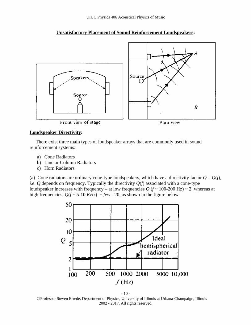
For the same reason, e.g. placing two loudspeakers on either side of the stage (where the human speaker is standing) or on the left & right-hand sides of the front wall of the auditorium should also be avoided, because listeners seated e.g. at either points A or B as shown in the figure below will hear sound from one of the speakers before they hear the direct sound coming from the human speaker on the stage. If, for some reason, such a front-of-the-room/two-speaker sound reinforcement system is deemed necessary/is unavoidable, the sound from both loudspeakers should be delayed electronically such that the direct sound from the human speaker is always heard first by listeners in the audience.




- 10 -

Unsatisfactory Placement of Sound Reinforcement Loudspeakers:

Loudspeaker Directivity:

There exist three main types of loudspeaker arrays that are commonly used in sound reinforcement systems:

a) Cone Radiators b) Line or Column Radiators c) Horn Radiators

(a) Cone radiators are ordinary cone-type loudspeakers, which have a directivity factor Q = Q(f), i.e. Q depends on frequency. Typically the directivity Q(f) associated with a cone-type loudspeaker increases with frequency – at low frequencies Q (f ~ 100-200 Hz) ~ 2, whereas at high frequencies, Q(f ~ 5-10 KHz) ~ few - 20, as shown in the figure below.




- 11 -

When the wavelength of the sound is much larger than the diameter of the cone D – i.e. >> D, sound radiation in the forward hemisphere is fairly uniform. Even directly backwards, for such loudspeakers in fully-sealed enclosures, the sound level in the backwards direction is typically only 10-15 dB less than in the forward direction for such low frequencies. At higher frequencies, when ~ D (and for < D), the sound radiation is increasingly concentrated into the forward direction, along the loudspeaker axis.

The angular response of a loudspeaker can be calculated from first-principles of acoustics, for example, simplifying/modeling a loudspeaker as a circular piston of radius a, the far-field RMS pressure amplitude angular response can be shown to be: 1 sin sinop p J ka ka where

op is the on-axis RMS pressure amplitude, 1J x is the ordinary Bessel function of the first kind

of order 1, and the wavenumber 2k . Real speakers are much more complicated than a simple piston, but can be simulated on a computer, thus angular response predictions for real speakers can be obtained in this manner, via numerical methods/simulations on a computer…

The angular response of a cone-type loudspeaker, measured at various frequencies (e.g. 1/3 octave intervals) is commonly given by loudspeaker manufacturers in a series of polar plots, where the radial distance on such plots is given in dB units, typically 6 dB per radial division, as shown in the figure below for an EV S-152 Two-Way 200W PA loudspeaker cabinet:




- 12 -

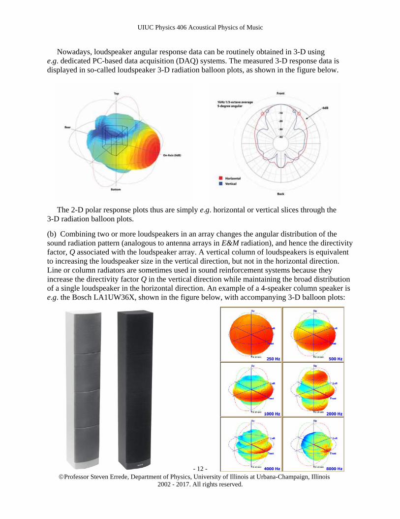
Nowadays, loudspeaker angular response data can be routinely obtained in 3-D using e.g. dedicated PC-based data acquisition (DAQ) systems. The measured 3-D response data is displayed in so-called loudspeaker 3-D radiation balloon plots, as shown in the figure below.

The 2-D polar response plots thus are simply e.g. horizontal or vertical slices through the 3-D radiation balloon plots.

(b) Combining two or more loudspeakers in an array changes the angular distribution of the sound radiation pattern (analogous to antenna arrays in E&M radiation), and hence the directivity factor, Q associated with the loudspeaker array. A vertical column of loudspeakers is equivalent to increasing the loudspeaker size in the vertical direction, but not in the horizontal direction. Line or column radiators are sometimes used in sound reinforcement systems because they increase the directivity factor Q in the vertical direction while maintaining the broad distribution of a single loudspeaker in the horizontal direction. An example of a 4-speaker column speaker is e.g. the Bosch LA1UW36X, shown in the figure below, with accompanying 3-D balloon plots:




- 13 -

(c) Horn-type loudspeakers, as shown in the figure on the right, are intrinsically more efficient than cone-speakers in converting electrical energy into acoustical energy, because the design of the so-called compression driver for the horn, is simpler and more compact than that for a cone loudspeaker. The horn radiator acts as a sound transformer, adiabatically converting the high pressure sound field at the compression driver at the throat of the horn to that of low pressure at the bell of the horn.

Horns can also be designed to have greater directivity factors Q than cone-type loudspeakers, however they can also be designed to have constant directivity, independent of frequency. Their main disadvantage is size. For example, in order to achieive a smooth response down to f ~ 100 Hz, a horn needs to have a surface area of at least ~ 8 ft2. Thus, large horns are not often used for low frequencies; most of the time smaller ones are e.g. used in 2-, 3- or 4-way speaker systems, where e.g. a passive cross-over network is used to route the amplifier’s signal in the low, medium and high frequency bands to the woofer, midrange horn and tweeter, respectively in a 3-way loudspeaker system.

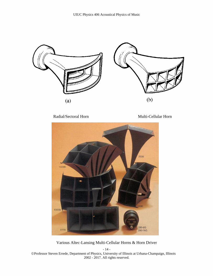
Horns are named conical, exponential, hyperbolic, Bessel, etc. according to the way in which their area expands with distance from the compression driver, as shown in the figure on the right. Note that such horn shapes also appear in the classic wind instruments – e.g. trumpet, French horn, clarinet, saxophone, etc! The two horn designs that are in common use today are the multi-cellular horn and the radial / sectoral horn. The radial/sectoral horn uniformly controls the sound projection angle, and has straight sides on two boundaries and curved sides on the other boundaries, as shown in figure (a) below. The multi-cellular horn consists of several exponential horns with axis passing through a common point, as shown in figure (b) below. At lower frequencies, the multi-cellular horn radiates as a single unit, whereas at higher frequencies, each cell of the multi-cellular horn radiates its own narrow beam, its angular width decreasing with increasing frequency.




- 14 -

Radial/Sectoral Horn Multi-Cellular Horn

Various Altec-Lansing Multi-Cellular Horns & Horn Driver




- 15 -

Constant Directivity Horns:

A horn provides more sound pressure level (SPL) at a given listening area by increasing the directivity of the sound towards the listener. There is more sound at the listening area, and less sound outside of that area. By analogy, think of focusing a beam of light (e.g. from a flashlight). A widely focused beam spreads the light around, thus the intensity at any given point is reduced. However, a narrowly focused beam provides much more light intensity at the center, and much less in the surrounding area. Properly designed horns can also act as a waveguide that actually serves to spread higher frequency sounds out in a much more consistent manner than would otherwise happen. Round horns and radial horns tend to change their angles of spread {their directivity, measured by the directivity factor, Q(f)} as the frequency f changes. This means that high frequencies might be more highly directed and therefore sound louder to someone in a central location than to someone else outside of the center (but still within the horn's low-frequency area of enhancement). To cope with this problem, the constant directivity (CD) horn was invented.

The design goal of the CD horn was to provide the same SPL at all frequencies within the designed coverage angles. The term "Constant Directivity" is actually trademark of ElectroVoice but has become somewhat of a catch-all phrase to describe constant-beamwidth horns.

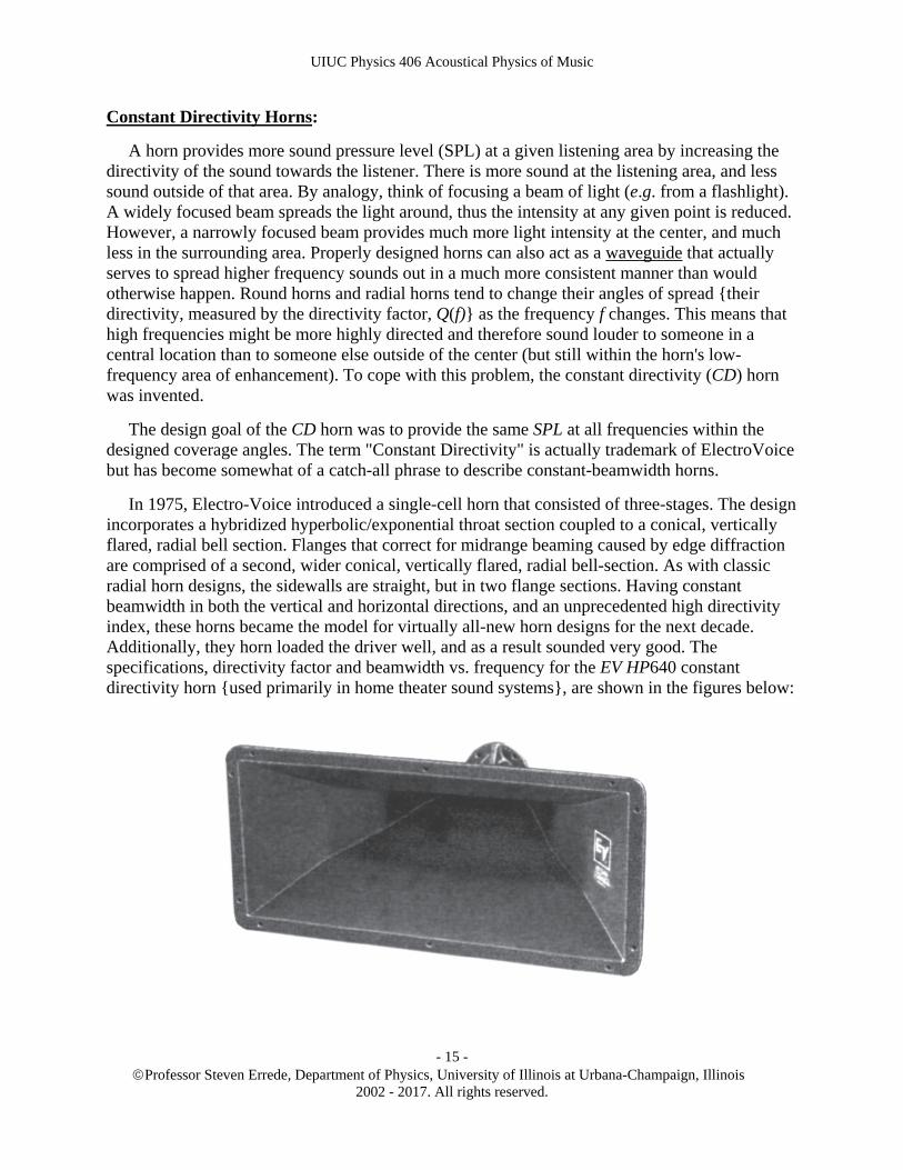
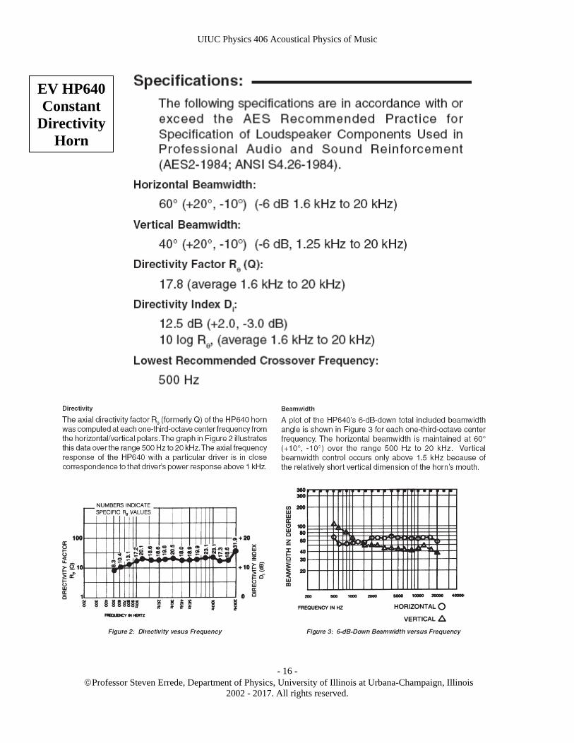
In 1975, Electro-Voice introduced a single-cell horn that consisted of three-stages. The design incorporates a hybridized hyperbolic/exponential throat section coupled to a conical, vertically flared, radial bell section. Flanges that correct for midrange beaming caused by edge diffraction are comprised of a second, wider conical, vertically flared, radial bell-section. As with classic radial horn designs, the sidewalls are straight, but in two flange sections. Having constant beamwidth in both the vertical and horizontal directions, and an unprecedented high directivity index, these horns became the model for virtually all-new horn designs for the next decade. Additionally, they horn loaded the driver well, and as a result sounded very good. The specifications, directivity factor and beamwidth vs. frequency for the EV HP640 constant directivity horn {used primarily in home theater sound systems}, are shown in the figures below:




- 16 -

EV HP640 Constant

Directivity Horn




- 17 -

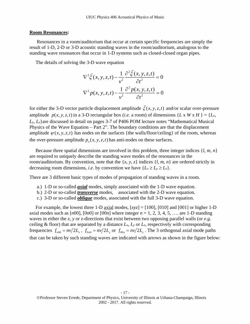
Room Resonances:

Resonances in a room/auditorium that occur at certain specific frequencies are simply the result of 1-D, 2-D or 3-D acoustic standing waves in the room/auditorium, analogous to the standing wave resonances that occur in 1-D systems such as closed-closed organ pipes.

The details of solving the 3-D wave equation

for either the 3-D vector particle displacement amplitude ( , , , )x y z t

and/or scalar over-pressure amplitude ( , , , )p x y z t in a 3-D rectangular box (i.e. a room) of dimensions {L x W x H } = {Lx, Ly, Lz}are discussed in detail on pages 3-7 of P406 POM lecture notes “Mathematical Musical Physics of the Wave Equation – Part 2”. The boundary conditions are that the displacement amplitude ( , , , )x y z t has nodes on the surfaces {the walls/floor/ceiling} of the room, whereas

the over-pressure amplitude ( , , , )op x y z t has anti-nodes on these surfaces.

Because three spatial dimensions are involved in this problem, three integer indices {l, m, n} are required to uniquely describe the standing wave modes of the resonances in the room/auditorium. By convention, note that the {x, y, z} indices {l, m, n} are ordered strictly in decreasing room dimensions, i.e. by convention we have {Lx Ly Lz}.

There are 3 different basic types of modes of propagation of standing waves in a room.

a.) 1-D or so-called axial modes, simply associated with the 1-D wave equation. b.) 2-D or so-called transverse modes, associated with the 2-D wave equation. c.) 3-D or so-called oblique modes, associated with the full 3-D wave equation.

For example, the lowest three 1-D axial modes, [xyz] = [100], [010] and [001] or higher 1-D axial modes such as [n00], [0n0] or [00n] where integer n = 1, 2, 3, 4, 5, …. are 1-D standing waves in either the x, y or z-directions that exist between two opposing parallel walls (or e.g. ceiling & floor) that are separated by a distance Lx, Ly or Lz, respectively with corresponding frequencies 00 2n xf nv L , 0 0 2n yf nv L or 00 2n zf nv L . The 3 orthogonal axial mode paths

that can be taken by such standing waves are indicated with arrows as shown in the figure below:

22

2 2

22

2 2

1 ( , , , )( , , , ) 0

1 ( , , , )( , , , ) 0

x y z tx y z t

v t

p x y z tp x y z t

v t




- 18 -

Thus, the 1-D axial modes are1-D standing waves in a 3-D room. The wavelength of 1-D axial mode standing waves is e.g. 00 2n xL n for the x-direction, etc. The pressure amplitude for the

200 axial mode, with 200 xL is shown in the figure below (note the pressure anti-nodes on the

opposing walls) {n.b. see also 3-D box mode demos on the P406 POM software web-page}:




- 19 -

1-D Axial Mode Particle Displacement 010 and Pressure 010p Plots:






- 20 -

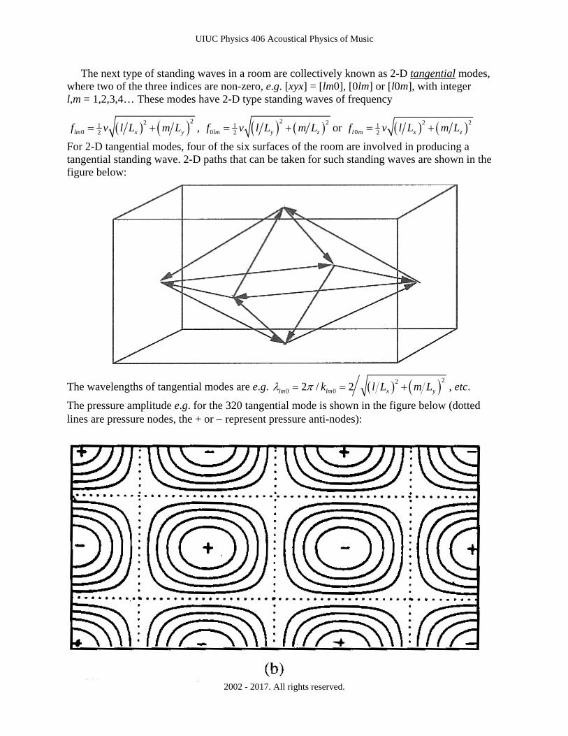
The next type of standing waves in a room are collectively known as 2-D tangential modes, where two of the three indices are non-zero, e.g. [xyx] = [lm0], [0lm] or [l0m], with integer l,m = 1,2,3,4… These modes have 2-D type standing waves of frequency

2210 2lm x yf v l L m L , 2 21

0 2lm y zf v l L m L or 2 210 2l m x zf v l L m L

For 2-D tangential modes, four of the six surfaces of the room are involved in producing a tangential standing wave. 2-D paths that can be taken for such standing waves are shown in the figure below:

The wavelengths of tangential modes are e.g. 22

0 02 / 2lm lm x yk l L m L , etc.

The pressure amplitude e.g. for the 320 tangential mode is shown in the figure below (dotted lines are pressure nodes, the + or represent pressure anti-nodes):




- 21 -

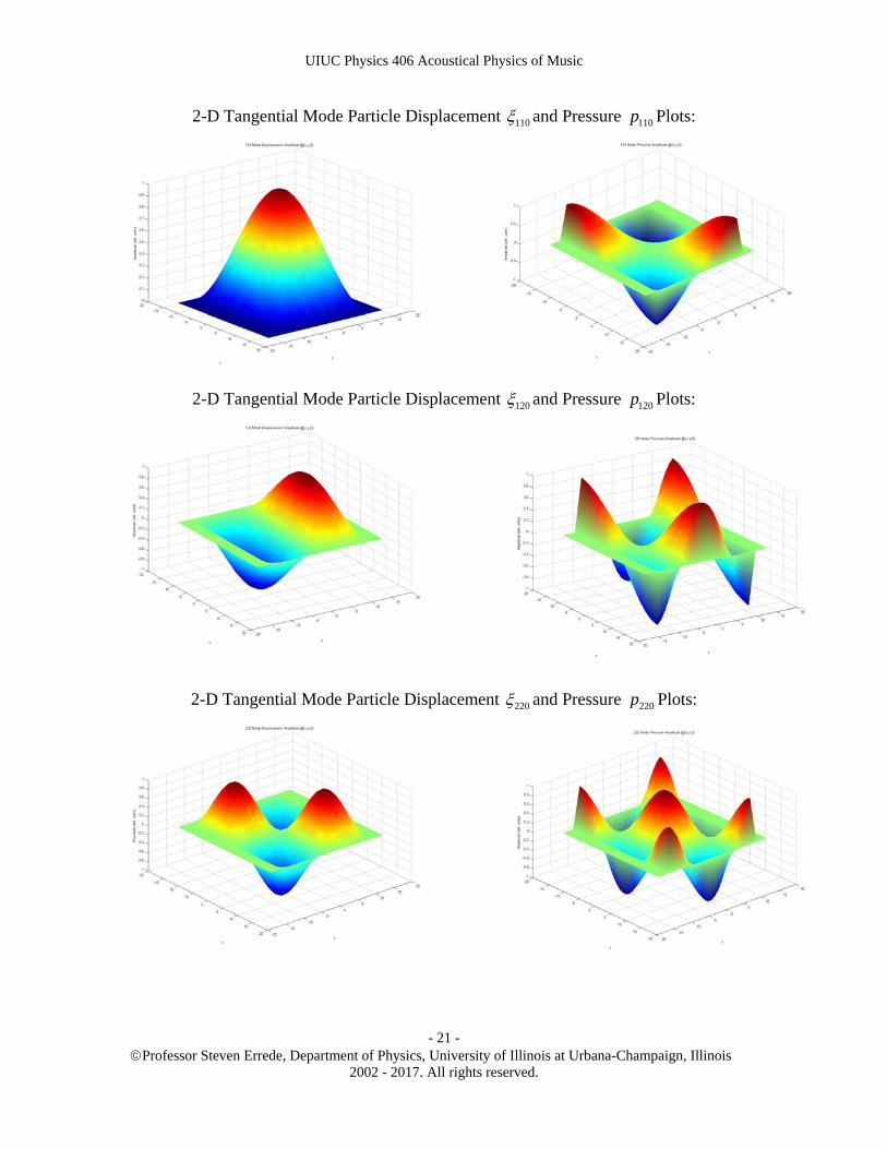
2-D Tangential Mode Particle Displacement 110 and Pressure 110p Plots:






- 22 -

The third type of standing wave in a room are known as 3-D oblique modes, in which all six surfaces of the room are involved in producing standing waves, one such path is shown in the figure below:

For oblique modes, none of the [xyz] = [lmn] indices are zero, and hence the eigen-frequencies associated with oblique modes are given by the full 3-D formula

22 212lmn x y zf v l L m L n L with wavelength for the 3-D oblique modes of

22 22lmn x y zl L m L n L .

The 3-D longitudinal displacement amplitudes for the oblique-mode resonances in this room / auditorium are of the form:

whereas the 3-D over-pressure amplitude for oblique-mode resonances in this room/auditorium are of the form:

( , , , ) ( , , ) ( ) ( ) ( ) ( ) ( )

( , , , ) sin( )sin( ) sin( )

( , , , ) sin( ) sin( )sin( )

, , 1,

lmn lmn

lmn lmn

lmn lmn lmn l m n lmn

i tlmn lmn l m n

i tlmn lmn x y z

x y z t U x y z T t X x Y y Z z T t

x y z t A k x k y k z e

x y z t A l x L m y L n z L e

l m n

( , , , ) ( , , ) ( ) ( ) ( ) ( ) ( )

( , , , ) cos( ) cos( ) cos( )

( , , , ) cos( ) cos( ) cos( )

, , 1,

lmn lmn

lmn lmn

lmn lmn lmn l m n lmn

i tlmn lmn l m n

i tlmn lmn x y z

p x y z t V x y z T t F x G y H z T t

p x y z t C k x k y k z e

p x y z t C l x L m y L n z L e

l m n




- 23 -

The characteristic, or so-called eigen-frequencies, eigen-wavelengths, eigen-energy densities associated with 1-D axial, 2-D transverse and fully 3-D oblique modes of acoustic standing waves in a room can be “generically” written as:

The 1-D axial modes have the lowest frequency and/or energy; the {1,0,0} axial mode is the lowest, the next lowest is the {0,1,0} axial mode, the next lowest is the {0,0,1} axial mode.

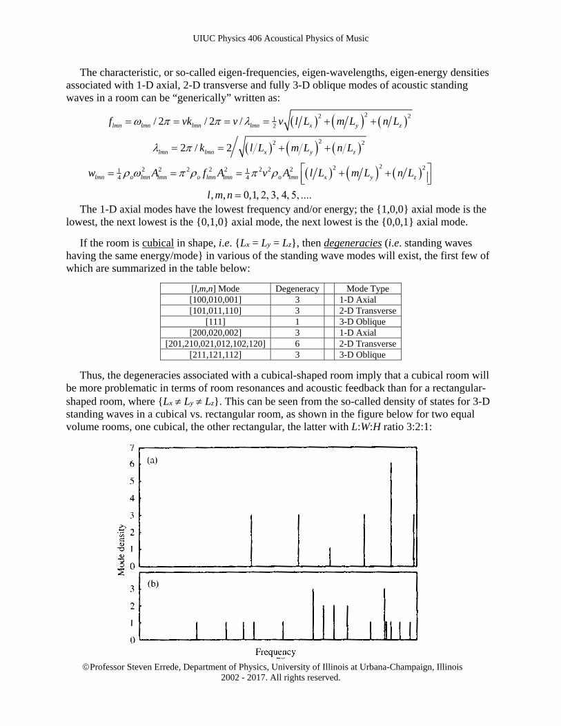
If the room is cubical in shape, i.e. {Lx = Ly = Lz}, then degeneracies (i.e. standing waves having the same energy/mode} in various of the standing wave modes will exist, the first few of which are summarized in the table below:

[l,m,n] Mode Degeneracy Mode Type [100,010,001] 3 1-D Axial [101,011,110] 3 2-D Transverse

[111] 1 3-D Oblique [200,020,002] 3 1-D Axial

[201,210,021,012,102,120] 6 2-D Transverse [211,121,112] 3 3-D Oblique

Thus, the degeneracies associated with a cubical-shaped room imply that a cubical room will be more problematic in terms of room resonances and acoustic feedback than for a rectangular-shaped room, where {Lx Ly Lz}. This can be seen from the so-called density of states for 3-D standing waves in a cubical vs. rectangular room, as shown in the figure below for two equal volume rooms, one cubical, the other rectangular, the latter with L:W:H ratio 3:2:1:

22 212

22 2

22 22 2 2 2 2 2 2 21 14 4

/ 2 / 2 /

2 / 2

, , 0,1,

lmn lmn lmn lmn x y z

lmn lmn x y z

lmn o lmn lmn o lmn lmn o lmn x y z

f vk v v l L m L n L

k l L m L n L

w A f A v A l L m L n L

l m n




- 24 -

It can be seen from the above figure that rectangular rooms are acoustically preferable to cubical rooms, for this reason. Room with e.g. a L:W:H dimensions in the ratio of 5:3:2 are noted for their smooth response in this regard, because it avoids the degeneracies associated with having two (or all 3) of the room dimensions being equal to each other. Other non-integral ratios will also work well; one famous, often-used ratio, not just for rooms/auditoriums, but also e.g.

speaker enclosures, is the so-called golden ratio 1.618 : 1 : 0.618 (= 5 1 2 :1: 5 1 2 ),

which fascinated the ancient greek mathematicians – e.g. Pythagoras and Euclid, as well as Fibonacci, Kepler, and more recently, Roger Penrose with his mathematical development of quasi-crystals and Penrose tiles… Note also that in the figure above, the 3-D room resonances/room modes are not infinitely sharp – each resonance at a given frequency lmnf will in fact have a finite, frequency-dependent

width lmn lmnf f associated with it, due to the frequency-dependent nature of the absorption,

A(f) of the room, and for the lowest modes, which are 1-D axial and/or 2-D tangential in nature, the A(f)’s associated with specific opposing walls for these low-mode standing waves.

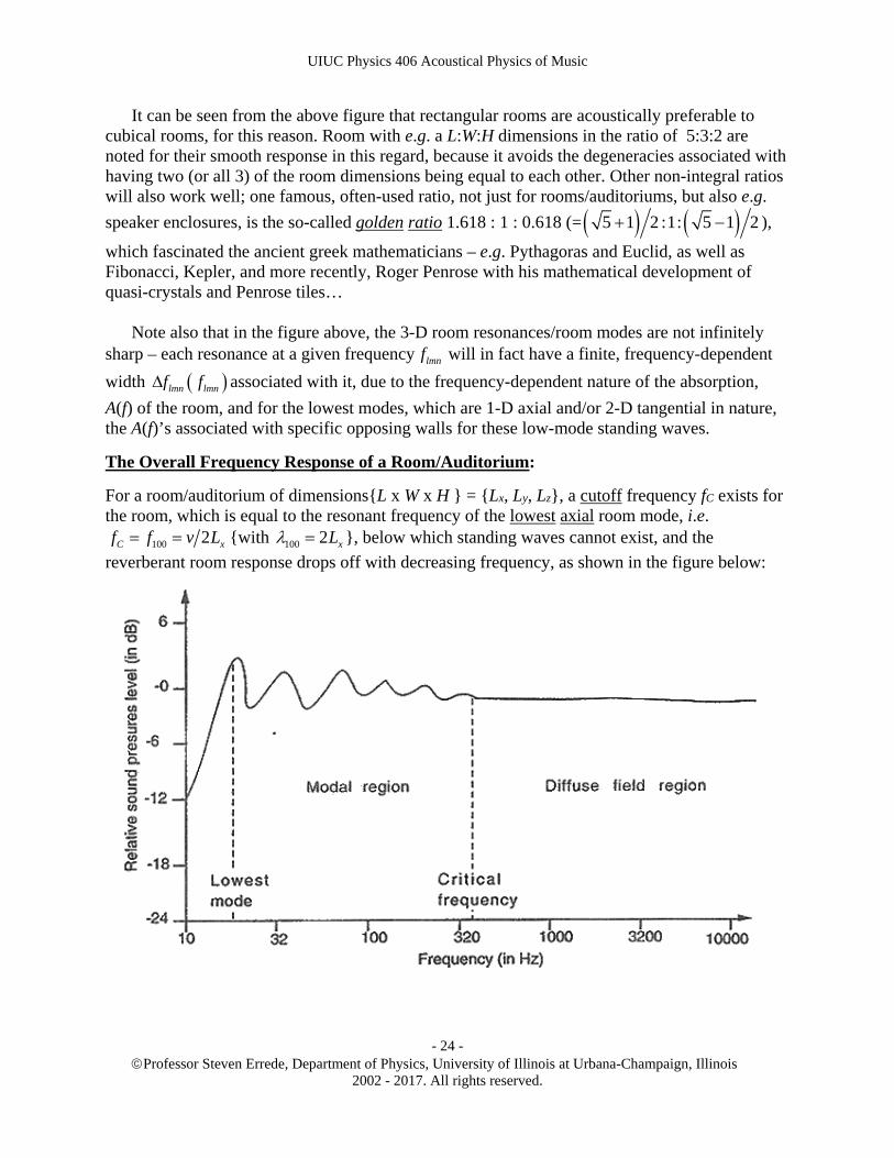
The Overall Frequency Response of a Room/Auditorium:

For a room/auditorium of dimensions{L x W x H } = {Lx, Ly, Lz}, a cutoff frequency fC exists for the room, which is equal to the resonant frequency of the lowest axial room mode, i.e.

100 2C xf f v L {with 100 2 xL }, below which standing waves cannot exist, and the

reverberant room response drops off with decreasing frequency, as shown in the figure below:




- 25 -

The critical frequency of a room fcrit occurs where different [lmn] modes first begin to overlap each other. Above fcrit, the reverberant nature of the room is such that the energy density is uniform throughout the room, i.e. everywhere within the volume of the room acts as a diffuse sound source {for the reverberant field}. The frequency region between C critf f f is the so-

called modal region, which is dominated by discrete axial, tangential and/or oblique standing wave modes, well-separated from each other in both frequency and also in 3-D space.

For concert halls, auditoriums, etc. the spatial dimensions of such large rooms ideally should be such that fcrit < lowest frequency to be played/reproduced in the room, i.e. the frequencies of all music is in the reverberant/diffuse field region of the above graph. For small rooms, because of the smaller room dimensions, the criterion that fcrit < lowest frequency to be played / reproduced in the room is almost impossible to achieve; however at least fcrit should be below some particularly desirable portion of the audio frequency spectrum, if at all possible. Acoustic Feedback – And How to Avoid It:

Almost all of us have at some time or another been in an auditorium or a musical venue using a PA system where a live performance of music, or a speech has been disrupted by problems associated with acoustic feedback – i.e. loud howls, squeals or whines at certain frequencies. Acoustic feedback is actually one specific example of the more generic process known as positive feedback, which, when sufficiently large, can cause an amplifier (or more generically, a system) to act as an oscillator. Acoustical feedback in a sound system occurs when a microphone at a particular location in the room/auditorium picks up a sound output from a loudspeaker and sends the picked-up signal back to the amplifier, where it is re-amplified, output again to the loudspeaker, which then gets picked up again by the microphone, etc. This process is shown schematically in the figure below:




- 26 -

If the overall gain of this mic-amp-loudspeaker feedback loop is Gtot > 1 and the phase of the mic signal is such that it constructively adds to this feedback process, then acoustic feedback will occur. The electrical gain of the sound system Gel must be greater than the acoustical pressure loss Gac ~ 1/r between the loudspeaker and the {pressure} microphone, since 1tot el acG G G

for acoustic feedback to occur.

If the overall gain is just below 1, on the verge of oscillation at one or more frequencies, acoustic feedback can still cause speech/music to sound tinny/weird due to long decay times at those frequencies.

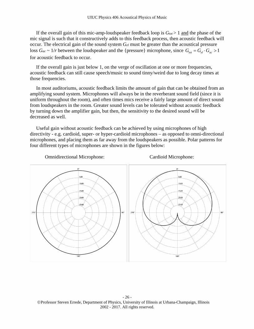
In most auditoriums, acoustic feedback limits the amount of gain that can be obtained from an amplifying sound system. Microphones will always be in the reverberant sound field (since it is uniform throughout the room), and often times mics receive a fairly large amount of direct sound from loudspeakers in the room. Greater sound levels can be tolerated without acoustic feedback by turning down the amplifier gain, but then, the sensitivity to the desired sound will be decreased as well. Useful gain without acoustic feedback can be achieved by using microphones of high directivity - e.g. cardioid, super- or hyper-cardioid microphones – as opposed to omni-directional microphones, and placing them as far away from the loudspeakers as possible. Polar patterns for four different types of microphones are shown in the figures below:

Omnidirectional Microphone: Cardioid Microphone:




- 27 -

Hypercardioid Microphone: Shotgun-Type Microphone:

Pictures of four different types of microphones are shown in the figures below:

Behringer ECM8000 Reference Mic Shure SM-58 Cardioid Dynamic Mic: Neumann U87 Condenser Mic: {Omnidirectional Electret Mic} {Popular vocals mic for live music} {Venerable recording studio mic}




- 28 -

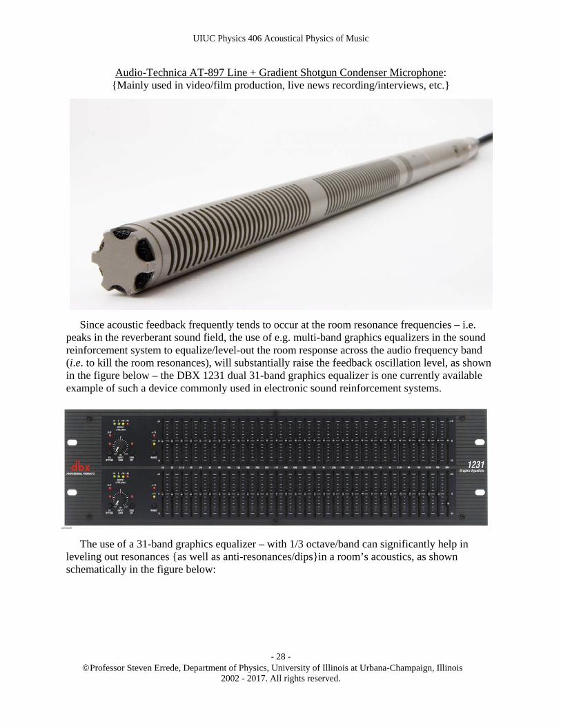
Audio-Technica AT-897 Line + Gradient Shotgun Condenser Microphone: {Mainly used in video/film production, live news recording/interviews, etc.}

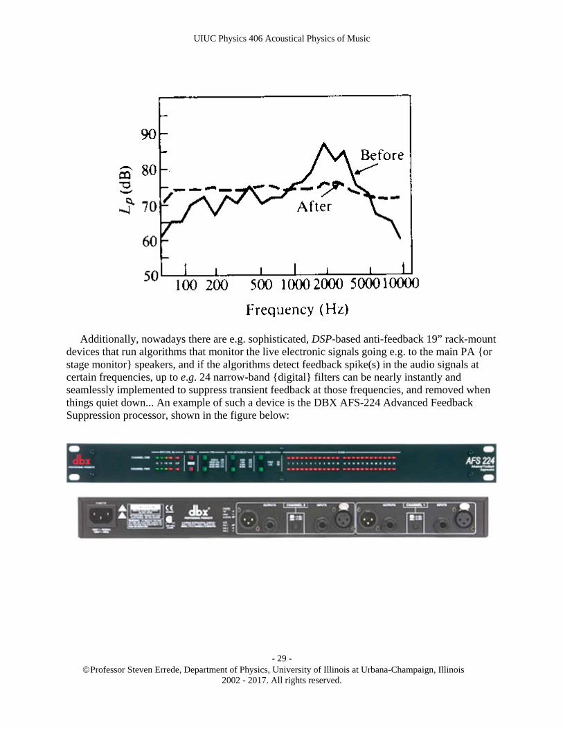
Since acoustic feedback frequently tends to occur at the room resonance frequencies – i.e. peaks in the reverberant sound field, the use of e.g. multi-band graphics equalizers in the sound reinforcement system to equalize/level-out the room response across the audio frequency band (i.e. to kill the room resonances), will substantially raise the feedback oscillation level, as shown in the figure below – the DBX 1231 dual 31-band graphics equalizer is one currently available example of such a device commonly used in electronic sound reinforcement systems.

The use of a 31-band graphics equalizer – with 1/3 octave/band can significantly help in leveling out resonances {as well as anti-resonances/dips}in a room’s acoustics, as shown schematically in the figure below:




- 29 -

Additionally, nowadays there are e.g. sophisticated, DSP-based anti-feedback 19” rack-mount devices that run algorithms that monitor the live electronic signals going e.g. to the main PA {or stage monitor} speakers, and if the algorithms detect feedback spike(s) in the audio signals at certain frequencies, up to e.g. 24 narrow-band {digital} filters can be nearly instantly and seamlessly implemented to suppress transient feedback at those frequencies, and removed when things quiet down... An example of such a device is the DBX AFS-224 Advanced Feedback Suppression processor, shown in the figure below:




- 30 -

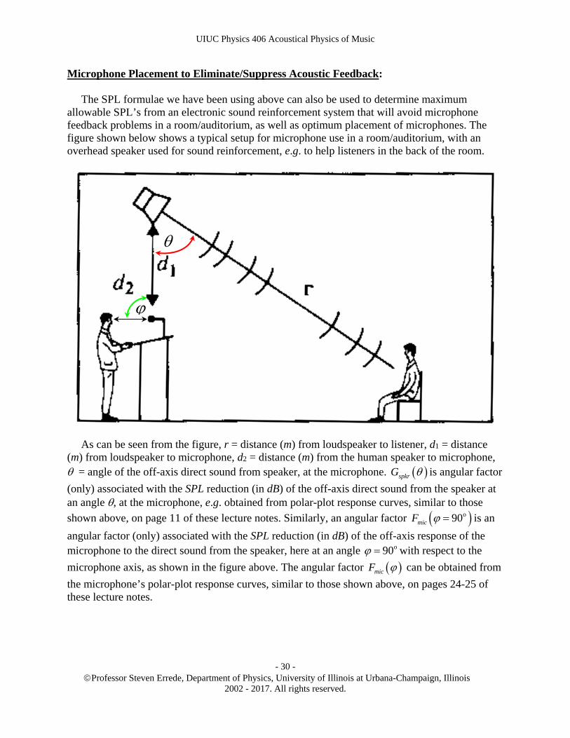
Microphone Placement to Eliminate/Suppress Acoustic Feedback: The SPL formulae we have been using above can also be used to determine maximum allowable SPL’s from an electronic sound reinforcement system that will avoid microphone feedback problems in a room/auditorium, as well as optimum placement of microphones. The figure shown below shows a typical setup for microphone use in a room/auditorium, with an overhead speaker used for sound reinforcement, e.g. to help listeners in the back of the room.

As can be seen from the figure, r = distance (m) from loudspeaker to listener, d1 = distance (m) from loudspeaker to microphone, d2 = distance (m) from the human speaker to microphone, = angle of the off-axis direct sound from speaker, at the microphone. spkrG is angular factor

(only) associated with the SPL reduction (in dB) of the off-axis direct sound from the speaker at an angle , at the microphone, e.g. obtained from polar-plot response curves, similar to those

shown above, on page 11 of these lecture notes. Similarly, an angular factor o90micF is an

angular factor (only) associated with the SPL reduction (in dB) of the off-axis response of the microphone to the direct sound from the speaker, here at an angle o90 with respect to the

microphone axis, as shown in the figure above. The angular factor micF can be obtained from

the microphone’s polar-plot response curves, similar to those shown above, on pages 24-25 of these lecture notes.




- 31 -

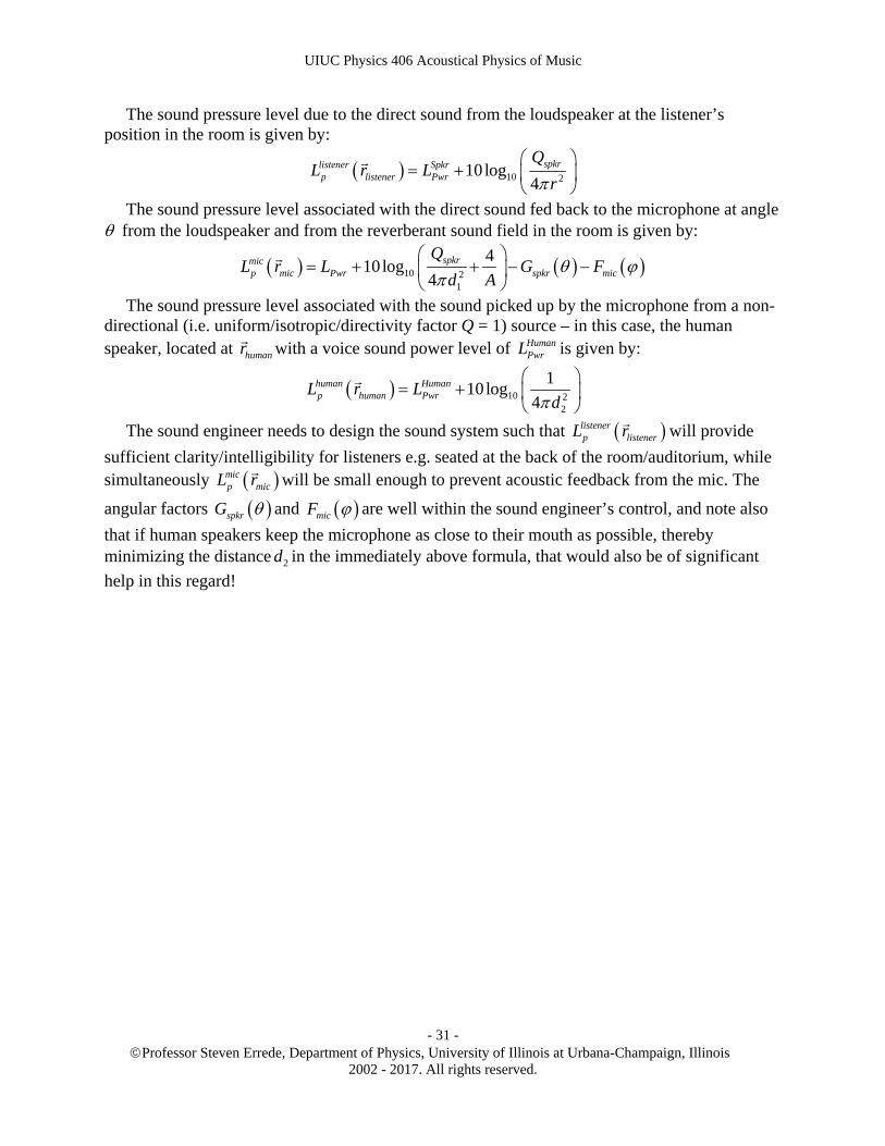
The sound pressure level due to the direct sound from the loudspeaker at the listener’s position in the room is given by:

10 210 log

4spkrlistener Spkr

p listener Pwr

QL r L

r

The sound pressure level associated with the direct sound fed back to the microphone at angle from the loudspeaker and from the reverberant sound field in the room is given by:

10 21

410log

4spkrmic

p mic Pwr spkr mic

QL r L G F

d A

The sound pressure level associated with the sound picked up by the microphone from a non-directional (i.e. uniform/isotropic/directivity factor Q = 1) source – in this case, the human speaker, located at humanr

with a voice sound power level of Human

PwrL is given by:

10 22

110log

4human Humanp human PwrL r L

d

The sound engineer needs to design the sound system such that listenerp listenerL r

will provide

sufficient clarity/intelligibility for listeners e.g. seated at the back of the room/auditorium, while simultaneously mic

p micL r

will be small enough to prevent acoustic feedback from the mic. The

angular factors spkrG and micF are well within the sound engineer’s control, and note also

that if human speakers keep the microphone as close to their mouth as possible, thereby minimizing the distance 2d in the immediately above formula, that would also be of significant

help in this regard!




- 32 -

Legal Disclaimer and Copyright Notice:

Legal Disclaimer:

The author specifically disclaims legal responsibility for any loss of profit, or any consequential, incidental, and/or other damages resulting from the mis-use of information contained in this document. The author has made every effort possible to ensure that the information contained in this document is factually and technically accurate and correct.

Copyright Notice:

The contents of this document are protected under both United States of America and International Copyright Laws. No portion of this document may be reproduced in any manner for commercial use without prior written permission from the author of this document. The author grants permission for the use of information contained in this document for private, non-commercial purposes only.

Electronic Sound Reinforcement of Rooms/Auditoriums · sound reinforcement equipment can make...

Documents

Transcript of Electronic Sound Reinforcement of Rooms/Auditoriums · sound reinforcement equipment can make...