Unit IV

ELECTRONIC MEASUREMENTS

Signal generators

Signal generators can be used to test frequency responses of loudspeakers. They are also a

useful way of testing a Finite Impulse Response (FIR) and Infinite Impulse Response (IIR) filters

without the need of an external signal source.

Function Generator

A function generator is a signal source that has the capability of producing different types of

waveforms as its output signal. The most common output waveforms are sine-waves, triangular

waves, square waves, and saw tooth waves. The frequencies of such waveforms may be adjusted

from a fraction of a hertz to several hundred kHz.

Actually the function generators are very versatile instruments as they are capable of

producing a wide variety of waveforms and frequencies. In fact, each of the waveform they

generate is particularly suitable for a different group of applications. The uses of sinusoidal outputs

and square-wave outputs have already been described in the earlier Arts. The triangular-wave and

saw tooth wave outputs of function generators are commonly used for those applications which

need a signal that increases (or reduces) at a specific linear rate. They are also used in driving

sweep oscillators in oscilloscopes and the X-axis of X-Y recorders.

Many function generators are also capable of generating two different waveforms

simultaneously (from different output terminals, of course). This can be a useful feature when two

generated signals are required for particular application. For instance, by providing a square wave

for linearity measurements in an audio-system, a simultaneous saw tooth output may be used to

drive the horizontal deflection amplifier of an oscilloscope, providing a visual display of the

measurement result. For another example, a triangular-wave and a sine-wave of equal frequencies

can be produced simultaneously. If the zero crossings of both the waves are made to occur at the

same time, a linearly varying waveform is available which can be started at the point of zero phase

of a sine-wave.

Another important feature of some function generators is their capability of phase-locking

to an external signal source. One function generator may be used to phase lock a second function

generator and the two output signals can be displaced in phase by an adjustable amount. In

addition, one function generator may be phase locked to a harmonic of the sine-wave of another

function generator. By adjustment of the phase and the amplitude of the harmonics, almost any

waveform may be produced by the summation of the fundamental frequency generated by one

function generator and the harmonic generated by the other function generator. The function

generator can also be phase locked to an accurate frequency standard, and all its output waveforms

will have the same frequency, stability, and accuracy as the standard.

The block diagram of a function generator is given in Figure. In this instrument the

frequency is controlled by varying the magnitude of current that drives the integrator. This

instrument provides different types of waveforms (such as sinusoidal, triangular and square waves)

as its output signal with a frequency range of 0.01 Hz to 100 kHz.

The frequency controlled voltage regulates two current supply sources. Current supply

source 1 supplies constant current to the integrator whose output voltage rises linearly with time.

An increase or decrease in the current increases or reduces the slope of the output voltage and thus

controls the frequency.

The voltage comparator multivibrator changes state at a predetermined maximum level, of

the integrator output voltage. This change cuts-off the current supply from supply source 1 and

switches to the supply source 2. The current supply source 2 supplies a reverse current to the

integrator so that its output drops linearly with time. When the output attains a predetermined level,

the voltage comparator again changes state and switches on the current supply source. The output

of the integrator is a triangular wave whose frequency depends on the current supplied by the

constant current supply sources. The comparator output provides a square wave of the same

frequency as output. The resistance diode network changes the slope of the triangular wave as its

amplitude changes and produces a sinusoidal wave with less than 1% distortion.

RF signal Generators

A typical radio frequency signal generator contains, in addition to the necessary power

supply, three main sections; an oscillator circuit, a modulator, and an output control circuit. The

internal modulator modulates the radiofrequency signal of the oscillator. In addition, most RF

generators are provided with connections through which an external source of modulation of any

desired waveform may be applied to the generated signal. Metal shielding surrounds the unit to

prevent the entrance of signals from the oscillator into the circuit under test by means other

than through the output circuit of the generator.

Block diagram of RF signal generator

A block diagram of a representative RF signal generator is shown in Figure. The function of

the oscillator stage is to produce a signal which can be accurately set in frequency at any point in

the range of the generator. The type of oscillator circuit used depends on the range of the

frequencies for which the generator is designed. In low frequency signal generators, the

resonating circuit consists of a group of coils combined with a variable capacitor.

One of the coils has a selector switch attached to the capacitor to provide an LC circuit that

has the correct range of resonant frequencies. The function of the modulating circuit is to produce

audio (or video) voltage which can be superimposed on the RF signal produced by the oscillator.

The modulating signal may be provided by an audio oscillator within the generator, or it may be

derived from an external source. In some signal generators, either of these methods of modulation

may be used. In addition, a means of disabling the modulator section is used whereby the pure un-

modulated signal from the oscillator can be used when it is desired.

The type of modulation used depends on the application of the particular signal

generator. The modulating voltage may be either a sine wave, a square wave, or pulse of varying

duration. In some specialized generators, provision is made for pulse modulation in which the RF

signal can be pulsed over a wide range of repetition rates and at various pulse widths.

Sweep Generators

The working of a sweep-frequency generator is explained in the article below. The working

and block diagram of an electronically tuned sweep frequency generator and its different

parameters are also explained.

A sweep frequency generator is a type of signal generator that is used to generate a

sinusoidal output. Such an output will have its frequency automatically varied or swept between

two selected frequencies. One complete cycle of the frequency variation is called a sweep.

Depending on the design of a particular instrument, either linear or logarithmic variations can be

introduced to the frequency rate. However, over the entire frequency range of the sweep, the

amplitude of the signal output is designed to remain constant.

Sweep-frequency generators are primarily used for measuring the responses of amplifiers,

filters, and electrical components over various frequency bands. The frequency range of a sweep-

frequency generator usually extends over three bands, 0.001 Hz – 100 kHz (low frequency to

audio), 100 kHz – 1,500 MHz (RF range), and 1-200 GHz (microwave range). It is really a hectic

task to know the performance of measurement of bandwidth over a wide frequency range with a

manually tuned oscillator. By using a sweep-frequency generator, a sinusoidal signal that is

automatically swept between two chosen frequencies can be applied to the circuit under test and its

response against frequency can be displayed on an oscilloscope or X-Y recorder.

Thus the measurement time and effort is considerably reduced. Sweep generators may also

be employed for checking and repairing of amplifiers used in TV and radar receivers.

The block diagram of an electronically tuned sweep frequency generator is shown in the

figure.

Electronically Tuned sweep generator

The most important component of a sweep-frequency generator is the master oscillator. It is

mostly an RF type and has many operating ranges which are selected by a range switch. Either

mechanical or electronic variations can be brought to the frequency of the output signal of the

signal generator. In the case of mechanically varied models, a motor driven capacitor is used to

tune the of the output signal of the master oscillator.

In the case of electronically tuned models, two frequencies are used. One will be a constant

frequency that is produced by the master oscillator. The other will be a varying frequency signal,

which is produced by another oscillator, called the voltage controlled oscillator (VCO). The VCO

contains an element whose capacitance depends upon the voltage applied across it. This element is

used to vary the frequency of the sinusoidal output of the VCO. A special electronic device called a

mixer is then used to combine the output of VCO and the output of the master oscillator. When

both the signals are combined, the resulting output will be sinusoidal, and its frequency will depend

on the difference of frequencies of the output signals of the master oscillator and VCO. For

example, if the master oscillator frequency is fixed at 10.00 MHz and the variable frequency is

varied between 10.01 MHz to 35 MHz, the mixer will give sinusoidal output whose frequency is

swept from 10 KHz to 25 MHz.

Adjustments can be brought to the sweep rates in a sweep frequency generator and it

normally can be varied from 100 to 0.01 seconds per sweep. The X-axis of an oscilloscope or X-Y

recorder can be easily driven synchronously with a voltage that varies linearly or logarithmically.

In the electronically tuned sweep generators, the same voltage which drives the VCO serves as this

voltage.

Wave Analyzer

The analysis of electrical signals is used in many applications. The different instruments

which are used for signal analysis are wave analyzers, distortion analyzers, spectrum analyzers,

audio analyzers and modulation analyzers. All signal analysis instruments measure the basic

frequency properties of a signal, but they use different techniques to do so.

A wave analyzer is a voltmeter which can be accurately tuned to measure the amplitude of a

single frequency, within a band of about 10 Hz – 40 MHz. It is well known that any periodic

waveform can be represented as the sum of a d.c component and a series of sinusoidal harmonics.

Analysis of a waveform consists of determination of the values of amplitude, frequency, and

sometime phase angle of the harmonic components. Graphical and mathematical methods may be

used for the purpose but these methods are quite laborious. The analysis of a complex waveform

can be done by electrical means using a band pass filter network to single out the various harmonic

components. Networks of these types pass a narrow band of frequency and provide a high degree of

attenuation to all other frequencies.

A wave analyzer, in fact, is an instrument designed to measure relative amplitudes of single

frequency Components in a complex waveform. Basically, the instrument acts as a frequency

selective voltmeter which is tuned to the frequency of one signal while rejecting all other signal

components. The desired frequency is selected by a frequency calibrated dial to the point of

maximum amplitude. The amplitude is indicated either by a suitable voltmeter or a CRO.

Wave analyzers have very important applications in the following fields

1) Electrical measurements

2) Sound measurements and

3) Vibration measurements.

The wave analyzers are applied industrially in the field of reduction of sound and vibrations

generated by rotating electrical machines and apparatus. The source of noise and vibrations is first

identified by wave analyzers before it can be reduced or eliminated. A fine spectrum analysis with

the wave analyzer shows various discrete frequencies and resonances that can be related to the

motion of machines. Once, these sources of sound and vibrations are detected with the help of wave

analyzers, ways and means can be found to eliminate them.

There are two types of wave analysers, depending upon the frequency ranges used,

(i) Frequency Selective wave analyser and

(ii) Heterodyne wave analyser.

Frequency selective Wave analyzer

The wave analyzer consists of a very narrow pass-band filter section which can Be tuned to

a particular frequency within the audible frequency range(20Hz to 20 KHz)). The block diagram of

a wave analyzer is as shown in fig.

The complex wave to be analyzed is passed through an adjustable attenuator which serves

as a range multiplier and permits a large range of signal amplitudes to be analyzed without loading

the amplifier. The output of the attenuator is then fed to a selective amplifier, which amplifies the

selected frequency. The driver amplifier applies the attenuated input signal to a high-Q active filter.

This high-Q filter is a low pass filter which allows the frequency which is selected to pass and

reject all others. The magnitude of this selected frequency is indicated by the meter and the filter

section identifies the frequency of the component. The filter circuit consists of a cascaded RC

resonant circuit and amplifiers. For selecting the frequency range, the capacitors generally used are

of the closed tolerance polystyrene type and the resistances used are precision potentiometers. The

capacitors are used for range changing and the potentiometer is used to change the frequency

within the selected pass-band, Hence this wave analyzer is also called a Frequency selective

voltmeter. The entire AF range is covered in decade steps by switching capacitors in the RC section

The selected signal output from the final amplifier stage is applied to the meter circuit and

to an unturned buffer amplifier. The main function of the buffer amplifier is to drive output devices,

such as recorders or electronics counters. The meter has several voltage ranges as well as decibel

scales marked on it. It is driven by an average reading rectifier type detector. The wave analyzer

must have extremely low input distortion, undetectable by the analyzer itself. The band width of the

instrument is very narrow typically about 1% of the selective band given by the following response

characteristics shows in fig.

Heterodyne Wave Analyzer

Analysis of the waveform means determination of the values of amplitude, frequency and

sometime phase angle of the harmonic components. A wave analyser is an instrument designed to

measure relative amplitude of signal frequency components in a complex waveform .basically a

wave instruments acts as a frequency selective voltmeter which is tuned to the frequency of one

signal while rejecting all other signal components.

It is well known that any periodic waveform can be represented as the sum of a d.c.

component and a series of sinusoidal harmonics. Analysis of a waveform consists of determination

of the values of amplitude, frequency, and sometime phase angle of the harmonic components.

Graphical and mathematical methods may be used for the purpose but these methods are quite

laborious. The analysis of a complex waveform can be done by electrical means using a band pass

filter network to single out the various harmonic components. Networks of these types pass a

narrow band of frequency and provide a high degree of attenuation to all other frequencies.

A wave analyzer, in fact, is an instrument designed to measure relative amplitudes of single

frequency components in a complex waveform. Basically, the instrument acts as a frequency

selective voltmeter which is used to the frequency of one signal while rejecting all other signal

components. The desired frequency is selected by a frequency calibrated dial to the point of

maximum amplitude. The amplitude is indicated either by a suitable voltmeter or CRO.

This instrument is used in the MHz range. The input signal to be analysed is heterodyned to a

higher IF by an internal local oscillator. Tuning the local oscillator shifts various signal frequency

components into the pass band of the IF amplifier. The output of the IF amplifier is rectified and is

applied to the metering circuit. The instrument using the heterodyning principle is called

a heterodyning tuned voltmeter.

The block schematic of the wave analyser using the heterodyning principle is shown in fig.

above. The operating frequency range of this instrument is from 10 kHz to 18 MHz in 18

overlapping bands selected by the frequency range control of the local oscillator. The bandwidth is

controlled by an active filter and can be selected at 200, 1000, and 3000 Hz.

Application of wave analyzer

1. Electrical measurements

2. Sound measurements

3. Vibration measurements.

In industries there are heavy machineries which produce a lot of sound and

vibrations, it is very important to determine the amount of sound and vibrations because if it

exceeds the permissible level it would create a number of problems. The source of noise and

vibrations is first identified by wave analyzer and then it is reduced by further circuitry.

Harmonic Distortion Analyzers

Harmonic Distortion

When we give a sinusoidal signal input to any electronic instrument there should be output

in sinusoidal form, but generally the output is not exactly the replica of input, because of various

types of distortion that my occur.

Distortion is occur due to inherent non-linear characteristics of different components used in

electronic circuit. Nonlinear behavior of electronic component introduces harmonics in the output

waveform and the resultant distortion is often referred as harmonic distortion.

Types of Harmonic Distortion

1) Frequency Distortion

This type of distortion occurs in amplifiers because of amplification factor of amplifier is

different for different frequencies.

2) Amplitude Distortion

It occurs because amplifier introduces harmonic of fundamental of input frequency.

Harmonics always generates distortion in amplitude. E.g. when amplifiers are overdriven it clips

the waveform.

3) Phase Distortion

This distortion occurs due to energy storage elements in the system which causes the output

signal to be displaced in phase with the input signal. Signals with different frequencies will be

shifted by different phase angles.

4) Intermodulation Distortion

This type of distortion occurs as a consequence of interaction or heterodyning of two

frequencies, giving an output which is sum or difference of the two original frequencies.

5) Cross-Over Distortion

This type of distortion occurs in push-pull amplifiers on account of incorrect boas levels as

shown in figure.

Total Harmonic Distortion (THD)

In a measurement system noise is read in addition to harmonics and the total waveform

consisting of harmonics, noise and fundamental is measured instead of fundamental alone

Distortion analyzer measures the total harmonic power present in the test wave rather than

the distortion caused by each component. The simplest method is to suppress the fundamental

frequency by means of a high pass filter whose cut off frequency is a little above the fundamental

frequency. This high pass allows only the harmonics to pass and the total harmonic distortion can

then be measured. Other types of harmonic distortion analyzers based on fundamental suppression

are as follows.

Employing a Resonance Bridge

The bridge shown in fig 3.1 is balanced for the fundamental frequency, i.e. L and C are tuned to the

fundamental frequency. The bridge is unbalanced for the harmonics, i.e. only harmonic power will

be available at the output terminal and can be measured. If the fundamental frequency is changed,

the bridge must be balanced again. If L and C are fixed components, then this method is suitable

only when the test wave has a fixed frequency. Indicators can be thermocouples or square law

VTVMs. This indicates the rms value of all harmonics. When a continuous adjustment of the

fundamental frequency is desifrequency is desired a Wien bridge arrangement is used as shown in

fig.

Wien’s Bridge Method

The bridge is balanced for the fundamental frequency. The fundamental energy is dissipated in the

bridge circuit elements. Only the harmonic components reach the output terminals .The harmonic

distortion output can then be measured with a meter. For balance at the fundamental frequency

C1=C2=C, R1=R2=R, R3=2R4.

Bridged T-Network Method

Referring to the fig the L and C’s are tuned to the fundamental frequency, and R is adjusted

to bypass fundamental frequency. The tank circuit being tuned to the fundamental frequency, the

fundamental energy will circulate in the tank and is bypassed by the resistance. Only harmonic

components will reach the output terminals and the distorted output can be measured by the meter.

The Q of the resonant circuit must be at least 3-5. One way of using a bridge T-network is given in

Fig. 3.4 The switch S is first connected to point A so that the attenuator is excluded and the bridge

T-network is adjusted for full suppression of the fundamental frequency, i.e. Minimum output

indicates that the bridged Tnetwork is tuned to the fundamental frequency and that fundamental

frequencies is fully suppressed.

The switch is next connected to terminal B, i.e. the bridge T- network is excluded.

Attenuation is adjusted until the same reading is obtained on the meter. The attenuator reading

indicates the total rams distortion. Distortion measurement can also be obtained by means of a

wave analyzer, knowing the amplitude and the frequency of each component, the harmonic

distortion can be calculated. However, distortion meters based on fundamental suppression are

simpler to design and less expensive than wave analyzers. The advantage is that give only the total

distortion and not the amplitude of individual distortion components.

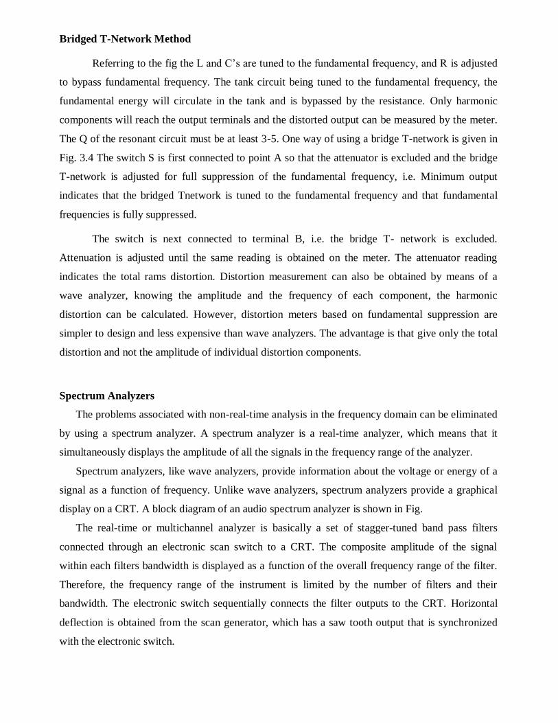
Spectrum Analyzers

The problems associated with non-real-time analysis in the frequency domain can be eliminated

by using a spectrum analyzer. A spectrum analyzer is a real-time analyzer, which means that it

simultaneously displays the amplitude of all the signals in the frequency range of the analyzer.

Spectrum analyzers, like wave analyzers, provide information about the voltage or energy of a

signal as a function of frequency. Unlike wave analyzers, spectrum analyzers provide a graphical

display on a CRT. A block diagram of an audio spectrum analyzer is shown in Fig.

The real-time or multichannel analyzer is basically a set of stagger-tuned band pass filters

connected through an electronic scan switch to a CRT. The composite amplitude of the signal

within each filters bandwidth is displayed as a function of the overall frequency range of the filter.

Therefore, the frequency range of the instrument is limited by the number of filters and their

bandwidth. The electronic switch sequentially connects the filter outputs to the CRT. Horizontal

deflection is obtained from the scan generator, which has a saw tooth output that is synchronized

with the electronic switch.

Block diagram of an audio spectrum analyzer

Such analyzers are usually restricted to audio-frequency applications and may employ

as many as 32 filters. The bandwidth of each filter is generally made very narrow for good

resolution.

The relationship between a time-domain presentation on the CRT of an oscilloscope

and a frequency-domain presentation on the CRT of a spectrum analyzer is shown in the three-

dimensional drawing in Fig.

Three dimensional relationships between time, frequency and amplitude

After the waveform is applied to the amplifier, it got amplified further directly to the

distortion analyzer which measures the total harmonic distortion. In the field of microwave

communications, in which pulsed oscillators are widely used one. Spectrum analyzers are an

important tool. They also find wide application in analyzing the performance of AM and FM

transmitters. Spectrum analyzers and Fourier analyzers are widely used in applications requiring

very low frequencies in the fields of biomedical electronics, geological surveying and

oceanography. They are also used in analyzing air and water pollution.

DC Voltmeter

The DC voltmeter mainly consists of a dc amplifier apart from the attenuator, as shown in

Figure

Block diagram of DC voltmeter

DC voltmeters can be divided into two categories.

1. Direct coupled amplifier DC Voltmeter.

2. Chopper type DC Voltmeter.

Direct coupled amplifier DC voltmeter

This type of voltmeter is very common because of its low cost. This instrument is

used only to measure voltages of the order of milli-volts owing to limited amplifier gain. The

circuit diagram for a direct coupled amplifier dc voltmeter using cascaded transistors is shown in

Figure 1.4. An attenuator is used in input stage to select voltage range. A transistor is a current

controlled device so resistance is inserted in series with the transistor Q1 to select the voltage

range. It can be seen from figure that sensitivity of voltmeter is 200 kilo ohms/volt neglecting

small resistance offered by transistor Q1. Other values of range selecting resistors are so chosen

that sensitivity remains same for all the ranges. So current drawn from the circuit is only 5micro

Ampere.

Two transistors in cascaded connections are used instead of using a single transistor

for amplification in order to increase the sensitivity of the circuit. Transistors Q1 and Q2 are

taken complement to each other and are directly coupled to minimize the number of components

in the circuit. They form a direct coupled amplifier. A variable resistance R is put in the circuit

for zero adjustment of the PMMC. It controls the bucking current from the supply E to buck out

the quiescent current. The draw-back of such a voltmeter is that it has to work under specified

ambient temperature to get the required accuracy otherwise excessive drift problem occurs

during operation.

DC Voltmeter using FET

Direct coupled amplifier DC voltmeter using FET

Another circuit diagram of a direct coupled amplifier dc voltmeter using FET in input

stage is shown in Figure 1.6. In this voltmeter, voltage to be measured is firstly attenuated with

range selector switch to keep the input voltage of amplifier within its level. FET is used in the

input stage of amplifier because of its high input impedance so that is does not load the circuit of

which voltage is to be measured and it also keeps the sensitivity of voltmeter very high. As FET

is a voltage controlled device so resistance network of attenuator is put in shunt in the circuit.

Transistors Q2 and Q3 form the direct coupled dc amplifier whose output is finally supplied to

PMMC meter. When, transistors work within their operating region, then the deflection of meter

remains proportional to the applied input voltage. This voltmeter can be used for measurement of

voltages of the order of milli-volts because of sufficient gain of amplifier.

Apart from having high input impedance, this circuit has another advan-tage that

when input voltage exceeds its limit, amplifier gets saturated which limits the current passing

through the PMMC meter. So meter does not burn out.

Chopper Type DC Voltmeter

The simple block diagram of the chopper fed DC voltmeter is shown in Figure

Block diagram of chopper type DC Voltmeter

Chopper type dc amplifier is used in highly sensitive dc electronic volt-meters. Its

block diagram is shown in Figure 1.7. Firstly dc input voltage is converted into ac voltage by

chopper modulator and then it is supplied to an ac amplifier, Output of amplifier is then

demodulated to a dc voltage proportional to the original input voltage. Modulator chopper and

demodulator chopper act in anti-synchronism. Chopper system may be either mechanical or

electronic.

Circuit diagram of an electronic chopper employing photo diodes is shown in Figure 1.8.

Photo diodes change its resistance under different illumination conditions; this property of photo

diode is used in chopper amplifier. Its resistance changes from the order of few mega-ohms to few

hundred ohms when it is illuminated by a light source in the dark place.

Two neon lamps are used in this circuit which is supplied by an oscillator for alternate

half cycles. Two photo diodes are used in input stage which acts as half-wave modulators

because of its alternate switching action by the neon lamps at the frequency of oscillator.

Output of chopper modulator is a square wave voltage (proportional to the input

signal) which is supplied to the ac amplifier through a capacitor. Amplified output is again

passed through a capacitor and then fed to chopper demodulator. Capacitor is used to remove dc

drift from the signal. Chopper demodulator gives a dc output voltage (proportional to the input

voltage) which is passed through the low pass filter to remove any residual ac component. Now

this dc output voltage is supplied to the PMMC meter for measurement of input voltage.

In chopper amplifier dc voltmeter, input impedance is of the order of hundred mega-

ohms and it has sensitivity of one micro-volt per scale division.

AC Voltmeter

Sometimes signal is firstly amplified by ac amplifier and then rectified before supplying it

to dc meter, as shown in Figure 1.9. In the former case the advantage is of economical amplifiers

and the arrangement is usually used in low priced voltmeters.

Broadly ac voltmeters can be divided into three categories.

1. Average reading AC voltmeters using vacuum tube diode

2. Average reading AC voltmeters using semiconductor diode

3. Peak reading AC voltmeter

AC voltmeter using vacuum tube diode

Normally ac voltmeters are average responding type and the meter is calibrated in terms

of rms values for a sine wave. Since most of the voltage measurements involve sinusoidal

waveform so this method of measuring rms value of ac voltages works satisfactorily and is less

expensive than true rms responding voltmeters. However, in case of measurement of non-

sinusoidal waveform voltage, this meter will give high or low reading depending on the form

factor of the waveform of the voltage to be measured.

The circuit diagram for an average reading voltmeter using a vacuum tube diode is shown

in Figure. The arrangement requires a vacuum tube diode, an high resistance (of the order of 105

Q) R and PMMC instrument, all connected in series, as shown in fig. Resistance R is used to

limit the current and make the plate

The linear plate characteristics are essential in order to make the current directly

proportional to voltage. Also because of high series resistance R, plate resistance of vacuum tube

diode becomes negligible and therefore variations in plate resistance do not cause non-linearity in

voltage-current characteristics. Thus the scale of PMMC instrument is uniform and independent

of variations of tube plate resistance. Voltage across the high resistance is fed to dc amplifier and

output of the amplifier is fed to PMMC instrument. Circuit diagram of an average reading ac

voltmeter using semi-conductor diode is shown in Figure. The diode conducts during the positive

half cycle and does not conduct during the -ve half cycle, as shown in figure.

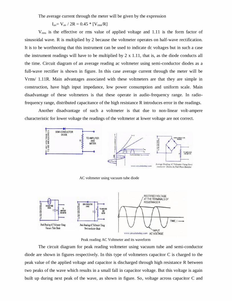
The average current through the meter will be given by the expression

Iav= Vav / 2R = 0.45 * [Vrms/R]

Vrms is the effective or rms value of applied voltage and 1.11 is the form factor of

sinusoidal wave. R is multiplied by 2 because the voltmeter operates on half-wave rectification.

It is to be worthnoting that this instrument can be used to indicate dc voltages but in such a case

the instrument readings will have to be multiplied by 2 x 1.11, that is, as the diode conducts all

the time. Circuit diagram of an average reading ac voltmeter using semi-conductor diodes as a

full-wave rectifier is shown in figure. In this case average current through the meter will be

Vrms/ 1.11R. Main advantages associated with these voltmeters are that they are simple in

construction, have high input impedance, low power consumption and uniform scale. Main

disadvantage of these voltmeters is that these operate in audio-frequency range. In radio-

frequency range, distributed capacitance of the high resistance R introduces error in the readings.

Another disadvantage of such a voltmeter is that due to non-linear volt-ampere

characteristic for lower voltage the readings of the voltmeter at lower voltage are not correct.

AC voltmeter using vacuum tube diode

Peak reading AC Voltmeter and its waveform

The circuit diagram for peak reading voltmeter using vacuum tube and semi-conductor

diode are shown in figures respectively. In this type of voltmeters capacitor C is charged to the

peak value of the applied voltage and capacitor is discharged through high resistance R between

two peaks of the wave which results in a small fall in capacitor voltage. But this voltage is again

built up during next peak of the wave, as shown in figure. So, voltage across capacitor C and

resistance R remains almost constant and equal to peak value of the applied voltage.

Either the average voltage across R or the average current through R, can be used to

indicate the peak value of applied voltage. In case the vacuum tube diode (or semi-conductor

diode), series resistance R shunted by capacitance C and PMMC are connected in series across

the source of unknown voltage, and the current through the PMMC will indicate the peak value

of applied voltage.

In case, the circuit shown in figure making use of rectifying diode, series resistance R, dc

amplifier and PMMC is employed, the average voltage across R will indicate the peak value of

applied voltage. The high value input resistance also gives more linear relationship between peak

applied voltage and the instrument indication. Also the performance of the diode with inputs

consisting of pulses and modulated waves is improved.

The dc amplifier associated with the diode rectifier should be provided with stabilizing

means in order to prevent drift in the indication of the output meter. Usually a voltage regulated

supply combined with a compensating circuit is used.

The use of high series resistance R, associated with dc amplifier, no doubt results in a

high input resistance but at the same time it implies that an applied voltage of sufficient

amplitude is required so that the system acts as a peak voltage device. The main disadvantage of

this system is with regards to measurement of low voltage. If the applied voltage is too small,

then there is a flow of some current throughout the cycle of the voltage because of high velocity

of emission of electrons, and the input resistance may be a few hundred ohms and it defeats the

very purpose with which electronic instruments are used.

Digital Voltmeters

Voltmeter is an electrical measuring instrument which is used to measure potential

difference between two points. The voltage to be measured may be AC or DC. Two types of

voltmeters are available for the purpose of voltage measurement i.e. analog and digital. Analog

voltmeters generally contain a dial with a needle moving over it according to the measur and hence

displaying the value of the same. With the passage of time analog voltmeters are replaced by

digital voltmeters due to the same advantages associated with digital systems. Although analog

voltmeters are not fully replaced by digital voltmeters, still there are many places where analog

voltmeters are preferred over digital voltmeters. Digital voltmeters display the value of AC or DC

voltage being measured directly as discrete numerical instead of a pointer deflection on a

continuous scale as in analog instruments.

Advantages Associated with Digital Voltmeters

Read out of DVMs is easy as it eliminates observational errors in measurement committed

by operators.

Error on account of parallax and approximation is entirely eliminated.

Reading can be taken very fast.

Output can be fed to memory devices for storage and future computations.

Versatile and accurate

Compact and cheap

Low power requirements

Portability increased

Working Principle of Digital Voltmeter

The block diagram of a simple digital voltmeter is shown in the figure. Explanation of

various blocks Input signal: It is basically the signal i.e. voltage to be measured. Pulse generator:

Actually it is a voltage source. It uses digital, analog or both techniques to generate a rectangular

pulse. The width and frequency of the rectangular pulse is controlled by the digital circuitry inside

the generator while amplitude and rise & fall time is controlled by analog circuitry. AND gate: It

gives high output only when both the inputs are high. When a train pulse is fed to it along with

rectangular pulse, it provides us an output having train pulses with duration as same as the

rectangular pulse from the pulse generator.

Train pulse

Rectangular pulse

Output of AND gate

NOT gate: It inverts the output of AND gate.

Output of NOT gate

Decimal Display: It counts the numbers of impulses and hence the duration and display the value

of voltage on LED or LCD display after calibrating it.

The working of a digital voltmeter as follows:

Unknown voltage signal is fed to the pulse generator which generates a pulse whose width

is proportional to the input signal.

Output of pulse generator is fed to one leg of the AND gate.

The input signal to the other leg of the AND gate is a train of pulses.

Output of AND gate is positive triggered train of duration same as the width of the pulse

generated by the pulse generator.

This positive triggered train is fed to the inverter which converts it into a negative triggered

train.

Output of the inverter is fed to a counter which counts the number of triggers in the

duration which is proportional to the input signal i.e. voltage under measurement.

Thus, counter can be calibrated to indicate voltage in volts directly.

Working of digital voltmeter is nothing but an analog to digital converter which converts an analog

signal into a train of pulses, the number of which is proportional to the input signal. So a digital

voltmeter can be made by using any one of the A/D conversion methods.

On the basis of A/D conversion method used digital voltmeters can be classified as:

Ramp type digital voltmeter

Integrating type voltmeter

Potentiometric type digital voltmeters

Successive approximation type digital voltmeter

Continuous balance type digital voltmeter

Now-a-days digital voltmeters are also replaced by digital millimeters due to its multitasking

feature i.e. it can be used for measuring current, voltage and resistance. But still there are some

fields where separated digital voltmeters are being used.

Ramp Type Digital Voltmeter

The operating principle of a ramp type digital voltmeter is to measure the time that a linear

ramp voltage takes to change from level of input voltage to zero voltage (or vice versa).

This time interval is measured with an electronic time interval counter and the count is displayed as

a number of digits on electronic indicating tubes of the output readout of the voltmeter. The

conversion of a voltage value of a time interval is shown in the timing diagram of Fig.

At the start of measurement a ramp voltage is initiated.

• A negative going ramp is shown in Fig. but a positive going ramp may also be used.

• The ramp voltage value is continuously compared with the voltage being measured (unknown

voltage).

• At the instant the value of ramp voltage is equal to that of unknown voltage.

• The ramp voltage continues to decrease till it reaches ground level (zero voltage).

• At this instant another comparator called ground comparator generates. a pulse and closes the

gate.

• The time elapsed between opening and closing of the gate is t as indicated in Fig.

• During this time interval pulses from a clock pulse generator pass through the gate and are

counted and displayed.

• The decimal number as indicated by the readout is a measure of the value of input voltage.

• The sample rate multivibrator determines the rate at which the measurement cycles are

initiated.

• The sample rate circuit provides an initiating pulse for the ramp generator to start its next

ramp voltage.

• At the same time it sends a pulse to the counters which set all of them to 0.

• This momentarily removes the digital display of the readout.

Integrating type voltmeter

This class of voltmeter is used to measure the average value of applied input voltage in a

wide range. In opposite of integrating type voltmeter in case of ramp type voltmeter sampling of

input voltage in done at the ending of the whole process. As the name suggests an integrating

circuit is used in this case that performs the function of converting voltage to its equivalent

frequency i.e. it works as voltage to frequency converter. It behaves as a feedback system and tends

to decide the rate at which pulses are formed in correspondence to quantity of voltage feed at input

section. Voltage to frequency conversion merely means to generate a train of pulses such that it

frequency is dependent upon the magnitude of instantaneous voltage applied in this way an parent

of variations in voltage is copies into an equivalent pattern of variations in frequency. After

formation of a pulse train it is counted that how man pulse the present in fixed interval of time with

help of a suitable electronic circuit. As is discussed that thus obtained pulse train has frequency

whose value at any instance depends upon the corresponding value of input voltage thus there

exists a relation between pulse train and input voltage that is used further to recover the original

value of input voltage.

The most important part of this whole system is integrator section which is nothing but an

operational amplifier that produces an output voltage whose value can be given by a relation

depending upon input voltage Ei. The relation is given by

Eo=-Ei.t/RC.

Where, Eo is output voltage obtained at integrator while Ei is input voltage.

When Ei is made to remain constant Eo tends to change in its magnitude according to time

such that Eo is always 180 degree out of phase i.e. having opposite polarity. By the graphical

analysis it is seen that if input attains a shape of straight line horizontal to X-axis then its

corresponding output comes to have a shape of straight line having declination with X-axis.

As soon as a constant input voltage is applied to integrator circuit a corresponding output is

obtained whose value increase with time representing a straight line with a slope depending upon

magnitude of input voltage. This rising voltage is applied to a level detector section that further

sends a pulse to pulse generator circuit when a particular level of voltage is encountered by it.

Functioning of level detector can be understood by considering it as voltage comparator. Integrator

and level detector works together in such a way that output voltage from integrator is kept

comparing with a fixed reference level, as soon as it reaches that level it generates the massaging

pulse. Consequence of this pulse is that it triggers pulse generator gate that make the pulse

generated at clock oscillator of fixed frequency to leave from pulse generator. This pulse generator

is nothing but a Schmitt trigger.

Now this pulse, having polarity opposite to that of input with even greater magnitude which

is further applied to integrator. This results into the total input to integrator with reversed polarity.

And consequence of this opposite polarity inputs makes the output of integrator having downward

slope. And as soon as output from integrator drops down a level detector circuit switches off the

pulse generator gate and now no pulse is generated from clock oscillator. Once after passing of the

pulse from pulse generator the input is reset to previous value and also makes output of integrator

to increase again and the whole procedure is repeated again and again. This repetition results in

formation of a saw tooth waveform whose frequency is function of magnitude of input voltage.

Thus frequency of thus produces signal makes it possible to find out the value of input voltage

applied.

Potentiometric Type Digital Voltmeter

A potentiometric type of DVM employs voltage comparison technique. In this DVM the

unknown voltage is compared with reference voltage whose value is fixed by the setting of the

calibrated potentiometer.

• The potentiometer setting is changed to obtain balance (i.e. null conditions).

• When null conditions are obtained the value of the unknown voltage, is indicated by the

dial setting of the potentiometer.

• In potentiometric type DVMs, the balance is not obtained manually but is arrived at

automatically.

• Thus, this DVM is in fact a self- balancing potentiometer.

• The potentiometric DVM is provided with a readout which displays the voltage being

measured.

The block diagram of basic circuit of a potentiometric DVM is shown.

• The unknown voltage is filtered and attenuated to suitable level.

• This input voltage is applied to a comparator (also known as error detector).

• This error detector may be chopper.

• The reference voltage is obtained from a fixed voltage source.

• This voltage is applied to a potentiometer.

• The value of the feedback voltage depends up the position of the sliding contact.

• The feedback voltage is also applied to the comparator.

• The unknown voltage and the feedback voltages are compared in the comparator.

• The output voltage of the comparator is the difference of the above two voltages.

• The difference of voltage is called the error signal.

• The error signal is amplified and is fed to a potentiometer adjustment device, which moves

the sliding contact of the potentiometer.

• This magnitude by which the sliding contact moves depends upon the magnitude of the error

signal.

• The direction of movement of slider depends upon whether the feedback voltage is larger or

the input voltage is larger.

• The sliding contact moves to such a place where the feedback voltage equals the unknown

voltage.

• In that case, there will not be any error voltage and hence there will be no input to the device

adjusting the position of the sliding contact and therefore it (sliding contact) will come to rest.

• The position of the potentiometer adjustment device at this point is indicated in numerical

form on the digital readout device associated with it.

Since the position at which no voltage appears at potentiometer adjustment device is the one

where the unknown voltage equals the feedback voltage, the reading of readout device indicates the

value of unknown voltage.

Successive approximation type digital voltmeter

The development of A/D converters has progressed in a quest to reduce the conversion

time. The successive approximation type ADC aims at approximating the analogue signal to be

digitized by trying only one bit at a time. Work process of Successive Approximation Type ADC is

different. The process of A/D conversion by this technique can be illustrated with the help of an

example. Let us take a four-bit successive approximation type ADC.

Initially, the counter is reset to all 0s. The conversion process begins with the MSB being

set by the start pulse. That is, the flip-flop representing the MSB is set. The counter output is

converted into an equivalent analogue signal and then compared with the analogue signal to be

digitized. A decision is then taken as to whether the MSB is to be left in (i.e. the flip-flop

representing the MSB is to remain set) or whether it is to be taken out (i.e. the flip-flop is to be

reset) when the first clock pulse sets the second MSB. Once the second MSB is set, again a

comparison is made and a decision taken as to whether or not the second MSB is to remain set

when the subsequent clock pulse sets the third MSB.

The process continues until we go down to the LSB. Note that, every time we make a

comparison, we tend to narrow down the difference between the analogue signal to be digitized and

the analogue signal representing the counter count. Refer to the operational diagram of Fig. 12.33.

It is clear from the diagram that, to reach any count from 0000 to 1111, the converter requires four

clock cycles. In general, the number of clock cycles required for each conversion will be n for an n-

bit A/D converter of this type.

The above Fig shows a block schematic representation of a successive approximation type ADC.

Since only one flip-flop (in the counter) is operated upon at one time, a ring counter, which is

nothing but a circulating register (a serial shift register with the outputs Q and Q of the last flip-flop

connected to the J and K inputs respectively of the first flip-flop), is used to do the job. Referring to

Fig the dark lines show the sequence in which the counter arrives at the desired count, assuming

that 1001 is the desired count. This type of A/D converter is much faster than the counter-type A/D

converter previously discussed. In an n-bit converter, the counter-type A/D converter on average

would require 2n−1 clock cycles for each conversion, whereas a successive approximation type

converter requires only n clock cycles. That is, an eight-bit A/D converter of this type operating on

a 1 MHz clock has a conversion time of 8 s.

Conversion time of Successive Approximation ADC

By observing above 3 bit example it is illustrated for a 3 bit ADC the conversion time will be 3

clock pulses. Then; N bit Successive Approximation ADC conversion time = 3T (T- clock pulse).

So to avoid aliasing effect the next sample of input signal should be taken after 3 clock pulses.

Important note on Successive Approximation ADC

In Counter type or digital ramp type ADC the time taken for conversion depends on the

magnitude of the input, but in SAR the conversion time is independent of the magnitude of the

input sampled value.

Advantages of Successive Approximation ADC

Speed is high compared to counter type ADC.

Good ratio of speed to power.

Compact design compared to Flash Type and it is inexpensive.

Disadvantages of Successive Approximation ADC

Cost is high because of SAR

Complexity in design.

Applications

The SAR ADC will used widely data acquisition techniques at the sampling rates higher

than 10KHz.

Continuous Balance or servo Balance DVM

The basic Block diagram is shown in figure. The input voltage applied to mechanical

chopper comparator, the other side being connected to the variable arm of a precision

potentiometer. The output of chopper comparator which is driven by the line voltage at the line

frequency rate is a square wave signal whose amplitude is a function of the difference in voltages

connected to the opposite side of the chopper. The square wave signal is amplified and fed to a

power amplifier and the amplified square wave difference signal drives the arm of the

potentiometer in the direction needed to make the difference voltage zero. The servo motor also

drives the mechanical readout which is an indication of the magnitude of the input voltage. This

DVM uses the principle of balancing instead of sampling because of mechanical movement. The

average reading time is 2sec.

Electronic Multimeters

It is one of the most versatile general purpose instruments capable of measuring dc and ac

voltages as well as current and resistances. The solid-state electronic multimeter generally consists

of the following elements.

1. A balanced bridge dc amplifier and a PMMC meter.

2. An attenuator in input stage to select the proper voltage range.

3. A rectifier for converting of an ac input voltage to proportionate dc value.

4. An internal battery and additional circuitry for providing the capability of resistance

measurement.

5. A function switch for selecting various measurement functions of the meter such as

voltage, current or resistance.

In addition, the instrument is usually provided with a built-in power supply for operation on

ac mains and, in most cases, one or more batteries for operation as a portable test instrument.

The schematic diagram of a balanced-bridge dc amplifier using two field effect transistors

(FETs) is given in figure. It is to be noted that two FETs used in circuit should be reasonably well

matched for current gain to ensure circuit thermal stability. The two FETs and the source resistors

Rx and R2, together with zero adjust control resistor R3, constitute a bridge circuit. The PMMC

meter is connected between the source terminals of the FETs, representing two opposite corners of

the bridge.

In the absence of input signal, the gate terminals of the FETs are at ground potential and the

transistors operate under identical quiescent conditions. Ideally no current should flow through the

PMMC movement but in practice, on account of some mismatch between the two FETs and slight

tolerance differences in the values of various resistors a current does flow and causes the meter

movement to deflect from zero position. This current is reduced zero by the adjust control resistor

R3. Now the bridge is balanced. With a positive input signal applied to the gate of input transistor

T1 its drain current creases causing the voltage at the source terminal to rise. The resulting

unbalance between the two transistors T1 and T2 source voltages is shown by the meter movement,

whose scale is calibrated in terms of the magnitude of the applied input voltage. The maximum

voltage that can be applied to the gate of input transistor T1 is determined by its operating range,

which is usually of the order of a few volts. The range of the bridge can easily be extended by

employing an input attenuator or a range switch, as illustrated in figure.

The unknown dc input voltage is applied through a large resistor in the probe body to a

resistive voltage divider. Thus, with the range switch in the 3-V position as illustrated, the voltage

at the gate of the input transistor T1 is developed across 8 MQ resistor of the total resistance of 11.3

MQ and the circuit is so arranged that the PMMC meter gives full scale deflection with 3 V applied

to the tip of the probe. With the range switch in 1,200 V position, the gate voltage is developed

across 20 kilo ohm of the total divider resistance of 11.3 Mega ohms and an input voltage of 1,200

V will he required to cause the full-scale meter deflection.

When the multimeter’s function switch is placed in the OHM position, the unknown resistor

is connected in series with an internal battery, and the PMMC meter simply measure the voltage

drop across it (unknown resistor, Rx).

A typical circuit is given in figure. In the given circuit, a separate divider network,

employed only for the measurement of resistance, provides a number of different resistance ranges.

With the unknown resistor Rx connected to the OHM terminals of the multimeter, the battery

supplies current through one of the range resistors and the unknown resistor to ground. Voltage

drop across unknown resistor Rx, Vx is applied to the input of the bridge amplifier and the PMMC

movement deflects. Since the voltage drop across Rx is directly proportional to its resistance, the

meter scale can be calibrated in terms of Kilo ohm.

The worth noting point is that this instrument indicates increasing resistance from left to

right whereas the conventional meter, indicates increasing resistance from right to left. This is

because the electronic multimeter reads a large resistance as a higher voltage, whereas the

conventional multimeter indicates a higher resistance as a smaller current.

DIGITAL MULTIMETER

It is a common & important laboratory instrument. It is used to measure AC/DC voltage,

AC/DC current and resistance with digital display. It gives digital display, which is very accurate. It

has an advantage of very high input resistance. It also provides over ranging indicator.

How digital multimeter works?

The block diagram of DMM is given below. The working of each block to measure different types

of electrical quantities is as follows.

All multimeters on a broad scale use the same process to sample the quantity under

measurement

How to measure resistance?

Connect an unknown resistor across its input probes. Keep rotary switch in the position-

1 (refer block diagram above). The proportional current flows through the resistor, from constant

current source. According to Ohm’s law voltage is produced across it. This voltage is directly

proportional to its resistance. This voltage is buffered and fed to A-D converter, to get digital

display in Ohms.

How to measure AC voltage?

Connect an unknown AC voltage across the input probes. Keep rotary switch in position-2.

The voltage is attenuated, if it is above the selected range and then rectified to convert it into

proportional DC voltage. It is then fed to A-D converter to get the digital display in Volts.

How to measure AC current?

Current is indirectly measured by converting it into proportional voltage. Connect an

unknown AC current across input probes. Keep the switch in position-3. The current is converted

into voltage proportionally with the help of I-V converter and then rectified. Now the voltage in

terms of AC current is fed to A-D converter to get digital display in Amperes.

How to measure DC current?

The DC current is also measured indirectly. Connect an unknown DC current across input

probes. Keep the switch in position-4. The current is converted into voltage proportionally with the

help of I-V converter. Now the voltage in terms of DC current is fed to A-D converter to get the

digital display in Amperes.

How to measure DC voltage?

Connect an unknown DC voltage across input probes. Keep the switch in position-5. The

voltage is attenuated, if it is above the selected range and then directly fed to A-D converter to get

the digital display in Volts.

Digital multimeter finds wide range of applications in the measurements of different

electrical quantities. Remember that a meter capable of checking for voltage, current, and resistance

is called a multimeter.

Remember that while measuring voltage, the DMM is connected in parallel. To measure

voltage at a point in the circuit, first confirm the type of voltage, whether it is AC or DC. Also

confirm the range of voltage (it is better to start with higher voltage range).

Now connect black probe of DMM to negative terminal of circuit power supply and then

connect the RED probe to the point where you want to measure the voltage. Be careful not to touch

the bare probe tip anywhere else in the circuit otherwise there may be the problem of short circuit,

etc.

Remember that while measuring current, the DMM is connected in series. To measure

current flowing through a circuit or wire, first confirm the type of current, whether it is AC or DC.

Also confirm the range of current (it is better to start with higher current range).

Now connect red and black probes at random in the circuit, to measure the current. Be

careful about the connections between the circuit terminals and the probes. They should be tight,

otherwise, there will be “makes” and “breaks” during measurement, which may lead to produce

errors.

To measure the unknown resistance: If you are measuring the unknown value of a resistor

already connected in a working circuit, then first of all, switch off the power supply and disconnect

the resistor from the circuit.

This is very important, because if you measure the resistance without disconnecting it from

the circuit, the voltage drop across it may damage the DMM permanently.

Now connect it across the probes keeping the DMM in resistance range. Fix the higher

range first, say 10MΩ. Then reduce the range, until you get correct readout.

Remember that the multimeter has practically no resistance between its leads. This is

essential during continuity testing, in particular. It is intended to allow electrons to flow through the

meter with the least possible difficulty.

For example, while checking the continuity of a small piece of copper wire, its practical

resistance should be zero. If the probe resistance were greater than zero, the meter would add extra

resistance in the circuit and would display some errors during continuity testing and would also

affect the current.

The elements of DMM

The former topic of DMM covered its fundamental concept. However the commercial

DMM is more advanced and packed with many features. It has more precision also. Remember that

any DMM internally works as digital voltmeter.

That is, any quantity under measurement is first converted into proportional DC voltage and

then measured. For example:

When we measure resistance, a constant current passes through the unknown resistance and

proportional voltage is produced, which is then buffered, sampled and fed to the counter.

When we measure current, it is converted into proportional voltage first. Then it is sampled and

fed to the counter to obtain the equivalent reading in relevant unit.

Thus, every time the DMM converts the quantity under measurement into proportional DC

voltage first and then the relevant reading is displayed. Now we shall understand the necessity and

basic working of different blocks or elements used in DMM, as follows:

Attenuator: The commercial DMM has a rotary switch used selecting proper range with many

steps in it. Now suppose the DMM is put in voltage range to measure AC or DC voltage. When

unknown voltage is connected across its probes, first of all, it is checked for its magnitude within

the specified range.

If voltage is high, then it is attenuated proportionally. The attenuator is a ladder of high

wattage resistors, as shown in following figure. It has number of steps for attenuation from several

volts to kilovolts. To select a particular range for measuring voltage, first switch to higher range.

If the resolution of the reading is less, then only you can switch over to successive lower

range.

Range selector arrangement using resistor ladder

The process of sampling & gating: Once the input voltage under measurement is converted into

DC voltage, it is further processed and sampled into a series of digital pulses, as shown below.

When unknown voltage is connected, at the start of measurement, the ramp voltage is

initiated at point „a‟. It is a negative going sawtooth voltage. The ramp voltage is constantly

compared with unknown voltage. When magnitude of unknown voltage becomes equal to ramp

voltage, at point „b‟, at that instant the input comparator produces START pulse, and the gate is

opened.

So digital pulses are fed to the counter and the counting is initiated. During this, the ramp

voltage further falls. As it reaches to zero, at point „c‟, the ground comparator produces STOP pulse

and the gate is closed. So the digital pulses are disconnected from input of counter. The counting

stops and result is displayed.

Current to voltage conversion: This circuit is built around special type of operational amplifier. A

typical circuit of current to voltage converter is given in following circuit. We shall understand how

it converts current into proportional voltage.

According to the theory of operational amplifiers, the output voltage of the circuit is given by the

equation, as follows:

(Vo/Vi) = -(Rf/Ri) ………… ∴ Vo = -(Vi/R1).Rf

However as V1=0, V1=V2

(Vi/R1) = Iin and ∴ Vo = -(Iin.Rf)

So if we replace the Vi and R1 combination by a current source Iin of as shown in the above

circuit, then the output voltage Vo becomes proportional to the input current Iin. Thus, we can say

that the input current is converted into proportional output voltage.

In addition to the additional measurement capabilities, DMMs also offer flexibility in the way

measurements are made. Again this is achieved because of the additional capabilities provided by

the digital electronics circuitry contained within the digital multimeter. Many instruments will offer

two additional capabilities:

Auto-range: This facility enables the correct range of the digital multimeter to be selected

so that the most significant digits are shown, i.e. a four-digit DMM would automatically

select an appropriate range to display 1.234 mV instead of 0.012 V. Additionally it also

prevent overloading, by ensuring that a volts range is selected instead of a millivolts range.

Digital multimeters that incorporate an auto-range facility usually include a facility to

'freeze' the meter to a particular range. This prevents a measurement that might be on the

border between two ranges causing the meter to frequently change its range which can be

very distracting.

Auto-polarity: This is a very convenient facility that comes into action for direct current

and voltage readings. It shows if the voltage of current being measured is positive (i.e. it is

in the same sense as the meter connections) or negative (i.e. opposite polarity to meter

connections). Analogue meters did not have this facility and the meter would deflect

backwards and the meter leads would have to be reversed to correctly take the reading.

Automatic Functions

Various automatic functions in digital instruments are Automatic Polarity Indication, Automatic

Ranging and Auto zeroing.

Automatic polarity indication

The information obtained by ADC is responsible for the polarity indication. For the integrating

ADCs, only the polarity of the integrated signal is of importance. The polarity should be measured

at the end of the integration period as shown in the fig. the integration period is measured by

counting the pulses. The last count or some of the last counts can be used to atart the polarity

measurement. The output of the integrator is then used to set the polarity flip-flop, the output of

which is stored in the memory until the next measurement is done.

Automatic Ranging

Consider 31/2 digit display on which the maximum reading possible is 1999. i.e the value

greater than 1999 have to be reduced by a factor of 10, before it can be displayed. Thus if the

display is less than 0200, the instrument should be automatically switched to a range which is more

sensitive while if display is higher than 1999 then the next less sensitive range must be

automatically selected. Practically the lower limit is taken much lower than 0200. Thus by selecting

lower limit much lower than 0200 overlapping of the ranges is achieved. The overlapping ranges

make sure that all the values are displayed in the same range. This overlapping range is shown in

fig.

The design of the automatic ranging system is shown in fig. The ADC counter contains

some information. If this count is less than 170, a control pulse for down ranging is produced. If

this is more than 1999 units, control pulse for up ranging is produced. The up/down counters

reacts to this information, at the moment when clock pulse is applied. The new information is

used to set the range relays via the decoder. At the same time as per the requirement of new

range the decimal point is also changed. If more than one range step is to be made several

measuring periods are necessary to reach the final result. The clock pulses and hence automatic

ranging can be nhibited by a manual range hold command, by a signal that exceeds the

maximum range and by reaching the most sensitive range.

Auto zeroing

Zero had so long been set manually, especially for analog meter. Autozeroing is a facility

incorporated with ADC as a part of the instrument. The zero is measured before measurement of

each parameter and the zero error stored as an analog signal. An auto zeroing system is shown in

figure.

At the start, switches S3, S4 and S5 are closed for a very short period say 0.05 second.

Switch S4 connects output of the comparator to capacitor C switch S3 grounds the circuit input and

switch S5 puts integrator time constant to effective zero, although a very short time constant does

exist. Capacitor C will be charged by the offset voltages of the three stages indicated – amplifier,

integrator and comparator. With switches now opened and switch S1 closed for measurement. The

offset voltage stored in the capacitor being the effective zero, the error is algebraically subtracted

for the zero error correction.

FREQUENCY COUNTER

Digital frequency counters are widely used items of test equipment within the electronics

industry for measuring the frequency of repetitive signals. In particular, digital frequency counters

are used for radio frequency (RF) measurements where it is important to test or measure the precise

frequency of a particular signal. These frequency counter is commonly found as general purpose

laboratory test equipment.

Frequency counters are test equipment that operate by counting events within a set period or

discovering what a period is by counting a number of precisely timed events. The time periods

within which events are counted, or the precisely timed events can be generated using a highly

stable quartz crystal oscillator. This may even be oven controlled, and in this way a very accurate

reference is obtained.

To look at the way in which a frequency counter works, it is necessary to describe the two

approaches separately. The two approaches may be termed direct counting and reciprocal counting.

Direct counting

Those digital frequency counters that use a direct counting approach count the number of

times the input signal crosses a given trigger voltage (and in a given direction, e.g. moving from

negative to positive) in a given time. This time is known as the gate time

Basic frequency counter block diagram

Within the basic counter there are several main blocks:

Input: When the signal enters the frequency counter it enters the input amplifier where the

signal is converted into a logic rectangular wave for processing within the digital circuitry

in the rest of the counter. Normally this stage contains a Schmitt trigger circuit so that noise

does not cause spurious edges that would give rise to additional pulses that would be

counted. Trigger levels and sensitivity are controlled within this area of the frequency

counter.

Accurate time-base / clock: In order to create the various gate / timing signals within the

frequency counter an accurate timebase or clock is required. This is typically is a crystal

oscillator and in high quality test instruments it will be an oven controlled crystal oscillator.

In many instruments, there will be the capability to use a better quality external oscillator,

or to use the frequency counter oscillator for other instruments. This is also beneficial when

it is necessary to lock a number of instruments to the same standard.

Decade dividers and flip-flop: The clock oscillator is used to provide an accurately timed

gate signal that will allow through pulses from the incoming signal. This is generated

fromth e clock by dividing the clock signal by decade dividers and then feeding this into a

flip flop to give the enabling pulse for the main gate

Gate: The precisely timed gate enabling signal from the clock is applied to one input of a

gate and the other has a train of pulses from the incoming signal. The resultant output from

the gate is a series of pulses for a precise amount of time. For example if the incoming

signal was at 1 MHz and the gate was opened for 1 second, then 1 million pulses would be

allowed through.

Counter/ latch: The counter takes the incoming pulses from the gate. It has a set of divide-

by-10 stages (number equal to the number of display digits minus 1). Each stage divides by

ten and therefore as they are chained the first stage is the input divided by ten, the next is

the input divided by 10 x 10, and so forth. These counter outputs are then used to drive the

display.

In order to hold the output in place while the figures are being displayed, the output is

latched. Typically the latch will hold the last result while the counter is counting a new

reading. In this way the display will remain static until a new result can be displayed at

which point the latch will be updated and the new reading presented to the display.

Display: The display takes the output from the latch and displays it in a normal readable

format. LCD, or LED displays are the most common. There is a digit for each decade the

counter can display. Obviously other relevant information may be displayed on the display

as well.

It is important that the gate time is accurately generated. This is done by having a highly

accurate frequency source within the frequency counter. Typically these will operate at a frequency

of 10 MHz and this needs to be divided to give the required gate time. Figures of 0.01, 0.1, 1, and

10 seconds may be selected. The shorter times obviously enable the display to be refreshed more

often, but against this the count accuracy is less.

The reason that the gate time determines the resolution of the frequency counter is that it can

normally only count complete cycles, as each crossing represents a cycle. This a gate time of one

second will enable frequency resolutions of 1 Hz to be gained, and a ten second gate time will

enable resolutions down to 0.1 Hz. It is worth noting that the measurement resolution is a not a

percentage of the measurement, but instead it is fixed amount relating only to the gate time.

Reciprocal frequency counters

Another method of measuring the frequency of a signal is to measure the period for one

cycle of the waveform and then take the reciprocal of this. Although this approach is slightly more

expensive to implement than direct counting and it is not as widely used, it does have some

advantages. The main one is that it always will always display the same number of digits of

resolution regardless of the input frequency. As a result, reciprocal frequency counters are specified

in terms of the number of digits for a given gate time, e.g. 10 digits per second. In view of this it

can be seen that reciprocal counters give a higher resolution at low frequencies. At 1 kHz, a direct

counter gives a resolution of 1 Hz (4 digits). A 10 digit/second reciprocal counter gives a resolution

of 10 digits.The other advantage is that these counters can make very fast readings. A reciprocal

counter will give 1 mHz resolution in 1 ms, whereas a direct counter takes a second to give a

reading with a resolution of 1 Hz.

Digital frequency counters are an essential item of test equipment for any accurate

measurements of frequency. RF frequency counters may be used in development, production,

repair or maintenance. Of the two types, the direct frequency counter is the most common. In fact

some digital frequency counters may be bought for a particularly low cost as a result of the high

levels of integration that are now available. Even small handheld digital frequency counters are

available. However RF frequency counters with much higher levels of performance tend to be

contained in larger cases. Often they will require highly accurate crystal oven oscillators to provide

the very accurate gate times required. Nevertheless these digital frequency counters still represent

very good value.

Measurement of Frequency and Time Intervel

The conventional counter is a digital electronic device which measures the frequency of an

input signal. It may also have been designed to perform related basic measurements including the

period of the input signal, ratio of the frequency of two input signals, time interval between two

events and totalizing a specific group of events.

Frequency Measurement

The frequency, f, of repetitive signals may be defined by the number of cycles of that signal

per unit of time. It may be represented by the equation: f = n / t (1) where n is the number of cycles

of the repetitive signal that occurs in time interval, t. If t = 1 second, then the frequency is

expressed as n cycles per second or n Hertz. As suggested by equation (1), the frequency, f, of a

repetitive signal is measured by the conventional counter by counting the number of cycles, n, and

dividing it by the time interval, t. The basic block diagram of the counter in its frequency mode of

measurement is shown in Figure.

The input signal is initially conditioned to a form that is compatible with the internal

circuitry of the counter. The conditioned signal appearing at the door of the main gate is a pulse

train where each pulse corresponds to one cycle or event of the input signal. With the main gate

open, pulses are allowed to pass through and get totalized by the counting register. The time

between the opening to the closing of the main gate or gate time is controlled by the Time Base.

From equation (1), it is apparent that the accuracy of the frequency measurement is dependent on

the accuracy in which t is determined. Consequently, most counters employ crystal oscillators with

frequencies such as 1, 5 or 10 MHz as the basic time base element.

The Time Base Divider takes the time base oscillator signal as its input and provides as an

output a pulse train whose frequency is variable in decade steps made selectable by the Gate Time

switch. The time, t, of equation (1) or gate time is determined by the period of the selected pulse

train emanating from the time base dividers. The number of pulses totaled by the counting register

for the selected gate time yields the frequency of the input signal. The frequency counted is

displayed on a visual numerical readout. For example, if the number of pulses totaled by the

counting register is 50,000, and the selected gate time is one second, the frequency of the input

signal is 50,000 Hertz.

Time Interval Measurement

The basic block diagram of the conventional counter in its time interval mode of

measurement is shown in Figure 4. The main gate is now controlled by two independent inputs, the

START input, which opens the gate, and the STOP input which closes it. Clock pulses from the

dividers are accumulated for the time duration for which the gate is open. The accumulated count

gives the time interval between the START event and the STOP event. Sometimes the time interval

may be for signal of different voltage levels such as th shown in Figure 5. The input conditioning

circuit must be able to generate the START pulse at the 0.5V amplitude point, and the STOP pulse

at the 1.5V amplitude point.