Electronic Lecture Notes DATA STRUCTURES AND ALGORITHMS · 2019-09-18 · Electronic Lecture Notes...
293
Electronic Lecture Notes DATA STRUCTURES AND ALGORITHMS 15 8 14 9 17 21 35 26 5 12 24 14 26 65 16 21 18 Singly linked list Binary search tree Digraph Graph Binomial tree Array of pointers Skip list 3 7 9 12 6 19 21 25 26 NIL A E D C B Y. NARAHARI Computer Science and Automation Indian Institute of Science Bangalore - 560 012 August 2000
Transcript of Electronic Lecture Notes DATA STRUCTURES AND ALGORITHMS · 2019-09-18 · Electronic Lecture Notes...
Electronic Lecture Notes
DATA STRUCTURES
AND ALGORITHMS
15
8
14
9 17
21
35
26
5
12
24 14
2665 16
21
18
Singly linked list
Binary search tree Digraph
Graph
Binomial treeArray of pointers
Skip list
3 79
12
6
19 21
25
26
NIL
A E
DC
B
Y. NARAHARIComputer Science and Automation
Indian Institute of ScienceBangalore - 560 012
August 2000
Preface
As a subject, Data Structures and Algorithms has always fascinated me and it was apleasure teaching this course to the Master’s students at the Indian Institute of Sciencefor six times in the last seven years. While teaching this course, I had prepared some notes,designed some programming assignments, and compiled what I thought were interestingproblems. In April-95, Professor Srikant and I offered a course on Data Structures to theITI engineers and followed it up with a more intensive AICTE-sponsored course on ObjectOriented Programming and Data Structures in November-95. On both these occasions,I had prepared some lecture notes and course material. There was then a desire to puttogether a complete set of notes and I even toyed with the idea of writing the idealbook on DSA for Indian university students (later abandoned). Finally, encouraged byProfessor Mrutyunjaya, past Chairman, CCE, Professor Pandyan, current Chairman-CCE, and Prof. K.R. Ramakrishnan (QIP co-ordinator, CCE), and supported by someCCE funding, I embarked on the project of preparing a Web-enabled Lecture Notes.
At the outset, let me say this does not pretend to be a textbook on the subject, thoughit does have some ingredients like examples, problems, proofs, programming assignments,etc. The lecture notes offers an adequate exposure at theoretical and practical level toimportant data structures and algorithms. It is safe to say the level of contents will liesomewhere between an undergraduate course in Data Structures and a graduate coursein Algorithms. Since I have taught these topics to M.E. students with a non-CS back-ground, I believe the lecture notes is at that level. By implication, this lecture notes willbe suitable for second year or third year B.E./B. Tech students of Computer Science andfor second year M.C.A. students. It is also useful to working software professionals and se-rious programmers to gain a sound understanding of commonly used data structures andalgorithm design techniques. Familiarity with C programming is assumed from all readers.
OUTLINE
The Lecture Notes is organized into eleven chapters. Besides the subject matter, eachchapter includes a list of problems and a list of programming projects. Also, each chapterconcludes with a list of references for further reading and exploration of the subject.
ii
1. Introduction 2. Lists3. Dictionaries 4. Binary Trees5. Balanced Trees 6. Priority Queues7. Directed Graphs 8. Undirected Graphs9. Sorting Methods 10. NP-Completeness11. References
Most of the material (including some figures, examples, and problems) is either sourcedor adapted from classical textbooks on the subject. However about 10 percent of thematerial has been presented in a way different from any of the available sources. Theprimary sources include the following six textbooks.
1. A. V. Aho, J. E. Hopcroft, and J. D. Ullman. Data Structures and Algorithms.Addison-Wesley, Reading, Massachusetts, 1983.
2. Gilles Brassard and Paul Bratley. Fundamentals of Algorithmics . Prentice-Hall,1996. Indian Edition published by Prentice Hall of India, 1998.
3. T. H. Cormen, C. E. Leiserson, and R. L. Rivest. Introduction to Algorithms. TheMIT Press and McGraw-Hill Book Company, Cambridge, Massachusetts, 1990.
4. D. E. Knuth. Fundamental Algorithms (The Art of Computer Programming: Vol-ume 1). Second Edition, Narosa Publishing House, New Delhi, 1985.
5. R. L. Kruse. Data Structures and Program Design in C . Prentice Hall of India, NewDelhi, 1994.
6. A. Weiss. Data Structures and Algorithms in C++. Addison-Wesley, Reading,Massachusetts, 1994.
Two topics that have been covered implicitly rather than in the form of independentchapters are: Algorithm Analysis Techniques (such as recurrence relations) and AlgorithmDesign Techniques (such as greedy strategy, dynamic programming, divide and conquer,backtracking, local search, etc.). Two topics which have not been covered adequatelyare: Memory management Techniques and Garbage Collection, and Secondary StorageAlgorithms. Pointers to excellent sources for these topics are provided at appropriateplaces.
ACKNOWLEDGEMENTS
I should first acknowledge six generations of students at IISc who went through the courseand gave valuable inputs. Some of them even solved and latexed the solutions of manyproblems. The following students have enthusiastically and uncomplainingly supportedme as teaching assistants. They certainly deserve a special mention:
Jan-Apr 1992 R.Venugopal, Somyabrata BhattacharyaAug-Dec 1993 R. Venugopal, G. Phanendra BabuAug-Dec 1994 S.R. Prakash, Rajalakshmi Iyer, N.S. Narayana Swamy, L.M. KhanAug-Dec 1995 S.R. Prakash, N. Gokulmuthu, V.S. Anil Kumar, G. Suthindran,
K.S. RaghunathAug-Dec 1998 Manimaran, Ashes Ganguly, Arun, Rileen Sinha, Dhiman GhoshAug-Dec 1999 M. Bharat Kumar, R. Sai Anand, K. Sriram, Chintan Amrit
My special thanks to Professor N. Viswanadham for his encouragement. I shall like tothank Dr. Ashok Subramanian for clarifying many technical subtleties in the subject atvarious points. Many thanks to Professors V.V.S. Sarma, U.R. Prasad, V. Rajaraman,D.K. Subramanian, Y.N. Srikant, Priti Shankar, S.V. Rangaswamy, M. Narasimha Murty,C.E. Veni Madhavan, and Vijay Chandru for their encouragement. Thanks also to Dr. B.Shekar for his interest. Special thanks to Professor Kruse for sending me all the materialhe could on this subject.
More than 200 problems have been listed as exercises in the individual chapters of thislecture notes. Many of these problems have been freely borrowed or adapted from varioussources, including the textbooks listed above and the question papers set by colleagues.I would like to acknowledge the help received in this respect.
The Latexing of this document was done near flawlessly by Renugopal first and then byMrs Mary. The figures were done with good care by Amit Garde, Arghya Mukherjee, MrsMary, and Chandra Sekhar. My thanks to all of them. Numerous students at CSA havegone through drafts at various points and provided valuable feedback.
Behind any of my efforts of this kind, there are two personalities whose blessings formthe inspirational force. The first is my divine Mother, who is no more but whose powerfulpersonality continues to be a divine driving force. The second is my revered Father whois the light of my life. He continues to guide me like a beacon. Of course, I simply cannotforget the love and affection of Padmasri and Naganand and all members of my extendedfamily, which is like a distributed yet tightly coupled enterprise.
There are bound to be numerous typographical/logical/grammatical/stylistic errors inthis the first draft. I urge the readers to unearth as many as possible and to intimateto me on the email ([email protected]). Any suggestions/comments/criticism on anyaspect of this lecture notes are most welcome.
Y. NARAHARI
Electronic Enterprises LaboratoryDepartment of Computer Science and AutomationIndian Institute of Science, Bangalore
Contents
Preface ii
1 Introduction 11.1 Some Definitions . . . . . . . . . . . . . . . . . . . . . . . . . . . . . . . . 1
1.1.1 Four Fundamental Data Structures . . . . . . . . . . . . . . . . . . 31.2 Complexity of Algorithms . . . . . . . . . . . . . . . . . . . . . . . . . . . 3
1.2.1 Big Oh Notation . . . . . . . . . . . . . . . . . . . . . . . . . . . . 41.2.2 Examples . . . . . . . . . . . . . . . . . . . . . . . . . . . . . . . . 41.2.3 An Example: Complexity of Mergesort . . . . . . . . . . . . . . . . 51.2.4 Role of the Constant . . . . . . . . . . . . . . . . . . . . . . . . . . 71.2.5 Worst Case, Average Case, and Amortized Complexity . . . . . . . 71.2.6 Big Omega and Big Theta Notations . . . . . . . . . . . . . . . . . 81.2.7 An Example: . . . . . . . . . . . . . . . . . . . . . . . . . . . . . . 9
1.3 To Probe Further . . . . . . . . . . . . . . . . . . . . . . . . . . . . . . . . 91.4 Problems . . . . . . . . . . . . . . . . . . . . . . . . . . . . . . . . . . . . . 10
2 Lists 132.1 List Abstract Data Type . . . . . . . . . . . . . . . . . . . . . . . . . . . . 13
2.1.1 A Program with List ADT . . . . . . . . . . . . . . . . . . . . . . . 152.2 Implementation of Lists . . . . . . . . . . . . . . . . . . . . . . . . . . . . 16
2.2.1 Array Implementation of Lists . . . . . . . . . . . . . . . . . . . . . 162.2.2 Pointer Implementation of Lists . . . . . . . . . . . . . . . . . . . . 182.2.3 Doubly Linked List Implementation . . . . . . . . . . . . . . . . . . 19
2.3 Stacks . . . . . . . . . . . . . . . . . . . . . . . . . . . . . . . . . . . . . . 202.4 Queues . . . . . . . . . . . . . . . . . . . . . . . . . . . . . . . . . . . . . . 24
2.4.1 Pointer Implementation . . . . . . . . . . . . . . . . . . . . . . . . 242.4.2 Circular Array Implementation . . . . . . . . . . . . . . . . . . . . 252.4.3 Circular Linked List Implementation . . . . . . . . . . . . . . . . . 25
2.5 To Probe Further . . . . . . . . . . . . . . . . . . . . . . . . . . . . . . . . 262.6 Problems . . . . . . . . . . . . . . . . . . . . . . . . . . . . . . . . . . . . . 272.7 Programming Assignments . . . . . . . . . . . . . . . . . . . . . . . . . . . 29
2.7.1 Sparse Matrix Package . . . . . . . . . . . . . . . . . . . . . . . . . 292.7.2 Polynomial Arithmetic . . . . . . . . . . . . . . . . . . . . . . . . . 292.7.3 Skip Lists . . . . . . . . . . . . . . . . . . . . . . . . . . . . . . . . 29
v
2.7.4 Buddy Systems of Memory Allocation . . . . . . . . . . . . . . . . 29
3 Dictionaries 313.1 Sets . . . . . . . . . . . . . . . . . . . . . . . . . . . . . . . . . . . . . . . 313.2 Dictionaries . . . . . . . . . . . . . . . . . . . . . . . . . . . . . . . . . . . 323.3 Hash Tables . . . . . . . . . . . . . . . . . . . . . . . . . . . . . . . . . . . 33
3.3.1 Open Hashing . . . . . . . . . . . . . . . . . . . . . . . . . . . . . . 343.4 Closed Hashing . . . . . . . . . . . . . . . . . . . . . . . . . . . . . . . . . 36
3.4.1 Rehashing Methods . . . . . . . . . . . . . . . . . . . . . . . . . . . 373.4.2 An Example: . . . . . . . . . . . . . . . . . . . . . . . . . . . . . . 383.4.3 Another Example: . . . . . . . . . . . . . . . . . . . . . . . . . . . 40
3.5 Hashing Functions . . . . . . . . . . . . . . . . . . . . . . . . . . . . . . . 403.5.1 Division Method . . . . . . . . . . . . . . . . . . . . . . . . . . . . 423.5.2 Multiplication Method . . . . . . . . . . . . . . . . . . . . . . . . . 423.5.3 Universal Hashing . . . . . . . . . . . . . . . . . . . . . . . . . . . . 43
3.6 Analysis of Closed Hashing . . . . . . . . . . . . . . . . . . . . . . . . . . 443.6.1 Result 1: Unsuccessful Search . . . . . . . . . . . . . . . . . . . . . 443.6.2 Result 2: Insertion . . . . . . . . . . . . . . . . . . . . . . . . . . . 463.6.3 Result 3: Successful Search . . . . . . . . . . . . . . . . . . . . . . . 463.6.4 Result 4: Deletion . . . . . . . . . . . . . . . . . . . . . . . . . . . 47
3.7 Hash Table Restructuring . . . . . . . . . . . . . . . . . . . . . . . . . . . 483.8 Skip Lists . . . . . . . . . . . . . . . . . . . . . . . . . . . . . . . . . . . . 49
3.8.1 Initialization: . . . . . . . . . . . . . . . . . . . . . . . . . . . . . . 523.9 Analysis of Skip Lists . . . . . . . . . . . . . . . . . . . . . . . . . . . . . . 55
3.9.1 Analysis of Expected Search Cost . . . . . . . . . . . . . . . . . . . 563.10 To Probe Further . . . . . . . . . . . . . . . . . . . . . . . . . . . . . . . . 593.11 Problems . . . . . . . . . . . . . . . . . . . . . . . . . . . . . . . . . . . . . 603.12 Programming Assignments . . . . . . . . . . . . . . . . . . . . . . . . . . . 62
3.12.1 Hashing: Experimental Analysis . . . . . . . . . . . . . . . . . . . . 623.12.2 Skip Lists: Experimental Analysis . . . . . . . . . . . . . . . . . . . 65
4 Binary Trees 664.1 Introduction . . . . . . . . . . . . . . . . . . . . . . . . . . . . . . . . . . . 66
4.1.1 Definitions . . . . . . . . . . . . . . . . . . . . . . . . . . . . . . . 664.1.2 Preorder, Inorder, Postorder . . . . . . . . . . . . . . . . . . . . . . 684.1.3 The Tree ADT . . . . . . . . . . . . . . . . . . . . . . . . . . . . . 694.1.4 Data Structures for Tree Representation . . . . . . . . . . . . . . . 69
4.2 Binary Trees . . . . . . . . . . . . . . . . . . . . . . . . . . . . . . . . . . . 704.3 An Application of Binary Trees: Huffman Code Construction . . . . . . . . 74
4.3.1 Implementation . . . . . . . . . . . . . . . . . . . . . . . . . . . . . 774.3.2 Sketch of Huffman Tree Construction . . . . . . . . . . . . . . . . . 78
4.4 Binary Search Tree . . . . . . . . . . . . . . . . . . . . . . . . . . . . . . . 824.4.1 Average Case Analysis of BST Operations . . . . . . . . . . . . . . 85
4.5 Splay Trees . . . . . . . . . . . . . . . . . . . . . . . . . . . . . . . . . . . 88
4.5.1 Search, Insert, Delete in Bottom-up Splaying . . . . . . . . . . . . . 934.6 Amortized Algorithm Analysis . . . . . . . . . . . . . . . . . . . . . . . . . 94
4.6.1 Example of Sorting . . . . . . . . . . . . . . . . . . . . . . . . . . . 944.6.2 Example of Tree Traversal (Inorder) . . . . . . . . . . . . . . . . . 954.6.3 Credit Balance . . . . . . . . . . . . . . . . . . . . . . . . . . . . . 954.6.4 Example of Incrementing Binary Integers . . . . . . . . . . . . . . . 974.6.5 Amortized Analysis of Splaying . . . . . . . . . . . . . . . . . . . . 97
4.7 To Probe Further . . . . . . . . . . . . . . . . . . . . . . . . . . . . . . . . 1034.8 Problems . . . . . . . . . . . . . . . . . . . . . . . . . . . . . . . . . . . . . 104
4.8.1 General Trees . . . . . . . . . . . . . . . . . . . . . . . . . . . . . . 1044.8.2 Binary Search Trees . . . . . . . . . . . . . . . . . . . . . . . . . . 1054.8.3 Splay Trees . . . . . . . . . . . . . . . . . . . . . . . . . . . . . . . 107
4.9 Programming Assignments . . . . . . . . . . . . . . . . . . . . . . . . . . . 1084.9.1 Huffman Coding . . . . . . . . . . . . . . . . . . . . . . . . . . . . 1084.9.2 Comparison of Hash Tables and Binary Search Trees . . . . . . . . 1084.9.3 Comparison of Skip Lists and Splay Trees . . . . . . . . . . . . . . 110
5 Balanced Trees 1125.1 AVL Trees . . . . . . . . . . . . . . . . . . . . . . . . . . . . . . . . . . . . 112
5.1.1 Maximum Height of an AVL Tree . . . . . . . . . . . . . . . . . . . 1135.1.2 AVL Trees: Insertions and Deletions . . . . . . . . . . . . . . . . . 115
5.2 Red-Black Trees . . . . . . . . . . . . . . . . . . . . . . . . . . . . . . . . . 1205.2.1 Height of a Red-Black Tree . . . . . . . . . . . . . . . . . . . . . . 1215.2.2 Red-Black Trees: Insertions . . . . . . . . . . . . . . . . . . . . . . 1245.2.3 Red-Black Trees: Deletion . . . . . . . . . . . . . . . . . . . . . . . 126
5.3 2-3 Trees . . . . . . . . . . . . . . . . . . . . . . . . . . . . . . . . . . . . . 1325.3.1 2-3 Trees: Insertion . . . . . . . . . . . . . . . . . . . . . . . . . . . 1335.3.2 2-3 Trees: Deletion . . . . . . . . . . . . . . . . . . . . . . . . . . . 136
5.4 B-Trees . . . . . . . . . . . . . . . . . . . . . . . . . . . . . . . . . . . . . 1375.4.1 Definition of B-Trees . . . . . . . . . . . . . . . . . . . . . . . . . . 1375.4.2 Complexity of B-tree Operations . . . . . . . . . . . . . . . . . . . 1385.4.3 B-Trees: Insertion . . . . . . . . . . . . . . . . . . . . . . . . . . . . 1405.4.4 B-Trees: Deletion . . . . . . . . . . . . . . . . . . . . . . . . . . . . 1415.4.5 Variants of B-Trees . . . . . . . . . . . . . . . . . . . . . . . . . . . 142
5.5 To Probe Further . . . . . . . . . . . . . . . . . . . . . . . . . . . . . . . . 1435.6 Problems . . . . . . . . . . . . . . . . . . . . . . . . . . . . . . . . . . . . . 145
5.6.1 AVL Trees . . . . . . . . . . . . . . . . . . . . . . . . . . . . . . . . 1455.6.2 Red-Black Trees . . . . . . . . . . . . . . . . . . . . . . . . . . . . . 1455.6.3 2-3 Trees and B-Trees . . . . . . . . . . . . . . . . . . . . . . . . . 146
5.7 Programming Assignments . . . . . . . . . . . . . . . . . . . . . . . . . . . 1475.7.1 Red-Black Trees and Splay Trees . . . . . . . . . . . . . . . . . . . 1475.7.2 Skip Lists and Binary search Trees . . . . . . . . . . . . . . . . . . 1495.7.3 Multiway Search Trees and B-Trees . . . . . . . . . . . . . . . . . . 149
6 Priority Queues 1516.1 Binary Heaps . . . . . . . . . . . . . . . . . . . . . . . . . . . . . . . . . . 151
6.1.1 Implementation of Insert and Deletemin . . . . . . . . . . . . . . . 1536.1.2 Creating Heap . . . . . . . . . . . . . . . . . . . . . . . . . . . . . . 154
6.2 Binomial Queues . . . . . . . . . . . . . . . . . . . . . . . . . . . . . . . . 1576.2.1 Binomial Queue Operations . . . . . . . . . . . . . . . . . . . . . . 1586.2.2 Binomial Amortized Analysis . . . . . . . . . . . . . . . . . . . . . 1646.2.3 Lazy Binomial Queues . . . . . . . . . . . . . . . . . . . . . . . . . 167
6.3 To Probe Further . . . . . . . . . . . . . . . . . . . . . . . . . . . . . . . . 1686.4 Problems . . . . . . . . . . . . . . . . . . . . . . . . . . . . . . . . . . . . . 1696.5 Programming Assignments . . . . . . . . . . . . . . . . . . . . . . . . . . . 170
6.5.1 Discrete Event Simulation . . . . . . . . . . . . . . . . . . . . . . . 170
7 Directed Graphs 1717.1 Directed Graphs . . . . . . . . . . . . . . . . . . . . . . . . . . . . . . . . . 171
7.1.1 Data Structures for Graph Representation . . . . . . . . . . . . . . 1727.2 Shortest Paths Problem . . . . . . . . . . . . . . . . . . . . . . . . . . . . 174
7.2.1 Single Source Shortest Paths Problem: Dijkstra’s Algorithm . . . . 1747.2.2 Dynamic Programming Algorithm . . . . . . . . . . . . . . . . . . 1797.2.3 All Pairs Shortest Paths Problem: Floyd’s Algorithm . . . . . . . . 182
7.3 Warshall’s Algorithm . . . . . . . . . . . . . . . . . . . . . . . . . . . . . . 1857.4 Depth First Search and Breadth First Search . . . . . . . . . . . . . . . . . 186
7.4.1 Breadth First Search . . . . . . . . . . . . . . . . . . . . . . . . . . 1887.5 Directed Acyclic Graphs . . . . . . . . . . . . . . . . . . . . . . . . . . . . 190
7.5.1 Test for Acyclicity . . . . . . . . . . . . . . . . . . . . . . . . . . . 1907.5.2 Topological Sort . . . . . . . . . . . . . . . . . . . . . . . . . . . . . 1917.5.3 Strong Components . . . . . . . . . . . . . . . . . . . . . . . . . . . 193
7.6 To Probe Further . . . . . . . . . . . . . . . . . . . . . . . . . . . . . . . . 1967.7 Problems . . . . . . . . . . . . . . . . . . . . . . . . . . . . . . . . . . . . . 1987.8 Programming Assignments . . . . . . . . . . . . . . . . . . . . . . . . . . . 199
7.8.1 Implementation of Dijkstra’s Algorithm Using Binary Heaps andBinomial Queues . . . . . . . . . . . . . . . . . . . . . . . . . . . . 199
7.8.2 Strong Components . . . . . . . . . . . . . . . . . . . . . . . . . . . 200
8 Undirected Graphs 2018.1 Some Definitions . . . . . . . . . . . . . . . . . . . . . . . . . . . . . . . . 2018.2 Depth First and Breadth First Search . . . . . . . . . . . . . . . . . . . . . 203
8.2.1 Breadth-first search of undirected graph . . . . . . . . . . . . . . . 2048.3 Minimum-Cost Spanning Trees . . . . . . . . . . . . . . . . . . . . . . . . 204
8.3.1 MST Property . . . . . . . . . . . . . . . . . . . . . . . . . . . . . . 2058.3.2 Prim’s Algorithm . . . . . . . . . . . . . . . . . . . . . . . . . . . . 2098.3.3 Kruskal’s Algorithm . . . . . . . . . . . . . . . . . . . . . . . . . . 212
8.4 Traveling Salesman Problem . . . . . . . . . . . . . . . . . . . . . . . . . . 2178.4.1 A Greedy Algorithm for TSP . . . . . . . . . . . . . . . . . . . . . 218
8.4.2 Optimal Solution for TSP using Branch and Bound . . . . . . . . . 2208.5 To Probe Further . . . . . . . . . . . . . . . . . . . . . . . . . . . . . . . . 2258.6 Problems . . . . . . . . . . . . . . . . . . . . . . . . . . . . . . . . . . . . . 2268.7 Programming Assignments . . . . . . . . . . . . . . . . . . . . . . . . . . . 227
8.7.1 Implementation of Some Graph Algorithms . . . . . . . . . . . . . . 2278.7.2 Traveling Salesman Problem . . . . . . . . . . . . . . . . . . . . . . 228
9 Sorting Methods 2299.1 Bubble Sort . . . . . . . . . . . . . . . . . . . . . . . . . . . . . . . . . . . 2309.2 Insertion Sort . . . . . . . . . . . . . . . . . . . . . . . . . . . . . . . . . . 2319.3 Selection Sort . . . . . . . . . . . . . . . . . . . . . . . . . . . . . . . . . . 2329.4 Shellsort . . . . . . . . . . . . . . . . . . . . . . . . . . . . . . . . . . . . . 2339.5 Heap Sort . . . . . . . . . . . . . . . . . . . . . . . . . . . . . . . . . . . . 2349.6 Quick Sort . . . . . . . . . . . . . . . . . . . . . . . . . . . . . . . . . . . . 237
9.6.1 Algorithm: . . . . . . . . . . . . . . . . . . . . . . . . . . . . . . . 2379.6.2 Algorithm for Partitioning . . . . . . . . . . . . . . . . . . . . . . . 2389.6.3 Quicksort: Average Case Analysis . . . . . . . . . . . . . . . . . . . 239
9.7 Order Statistics . . . . . . . . . . . . . . . . . . . . . . . . . . . . . . . . . 2429.7.1 Algorithm 1 . . . . . . . . . . . . . . . . . . . . . . . . . . . . . . . 2429.7.2 Algorithm 2 . . . . . . . . . . . . . . . . . . . . . . . . . . . . . . . 2439.7.3 Algorithm 3 . . . . . . . . . . . . . . . . . . . . . . . . . . . . . . . 243
9.8 Lower Bound on Complexity for Sorting Methods . . . . . . . . . . . . . . 2469.8.1 Result 1: Lower Bound on Worst Case Complexity . . . . . . . . . 2479.8.2 Result 2: Lower Bound on Average Case Complexity . . . . . . . . 249
9.9 Radix Sorting . . . . . . . . . . . . . . . . . . . . . . . . . . . . . . . . . . 2509.10 Merge Sort . . . . . . . . . . . . . . . . . . . . . . . . . . . . . . . . . . . . 2559.11 To Probe Further . . . . . . . . . . . . . . . . . . . . . . . . . . . . . . . . 2599.12 Problems . . . . . . . . . . . . . . . . . . . . . . . . . . . . . . . . . . . . . 2619.13 Programming Assignments . . . . . . . . . . . . . . . . . . . . . . . . . . . 263
9.13.1 Heap Sort and Quicksort . . . . . . . . . . . . . . . . . . . . . . . . 263
10 Introduction to NP-Completeness 26410.1 Importance of NP-Completeness . . . . . . . . . . . . . . . . . . . . . . . . 26410.2 Optimization Problems and Decision Problems . . . . . . . . . . . . . . . 26510.3 Examples of some Intractable Problems . . . . . . . . . . . . . . . . . . . . 266
10.3.1 Traveling Salesman Problem . . . . . . . . . . . . . . . . . . . . . . 26610.3.2 Subset Sum . . . . . . . . . . . . . . . . . . . . . . . . . . . . . . . 26710.3.3 Knapsack Problem . . . . . . . . . . . . . . . . . . . . . . . . . . . 26710.3.4 Bin Packing . . . . . . . . . . . . . . . . . . . . . . . . . . . . . . . 26710.3.5 Job Shop Scheduling . . . . . . . . . . . . . . . . . . . . . . . . . . 26810.3.6 Satisfiability . . . . . . . . . . . . . . . . . . . . . . . . . . . . . . . 268
10.4 The Classes P and NP . . . . . . . . . . . . . . . . . . . . . . . . . . . . . 26910.5 NP-Complete Problems . . . . . . . . . . . . . . . . . . . . . . . . . . . . . 270
10.5.1 NP-Hardness and NP-Completeness . . . . . . . . . . . . . . . . . . 270
10.6 To Probe Further . . . . . . . . . . . . . . . . . . . . . . . . . . . . . . . . 27210.7 Problems . . . . . . . . . . . . . . . . . . . . . . . . . . . . . . . . . . . . . 273
11 References 27411.1 Primary Sources for this Lecture Notes . . . . . . . . . . . . . . . . . . . . 27411.2 Useful Books . . . . . . . . . . . . . . . . . . . . . . . . . . . . . . . . . . 27511.3 Original Research Papers and Survey Articles . . . . . . . . . . . . . . . . 276
List of Figures
1.1 Growth rates of some functions . . . . . . . . . . . . . . . . . . . . . . . . 6
2.1 A singly linked list . . . . . . . . . . . . . . . . . . . . . . . . . . . . . . . 182.2 Insertion in a singly linked list . . . . . . . . . . . . . . . . . . . . . . . . . 192.3 Deletion in a singly linked list . . . . . . . . . . . . . . . . . . . . . . . . . 202.4 A doubly linked list . . . . . . . . . . . . . . . . . . . . . . . . . . . . . . . 202.5 An array implementation for the stack ADT . . . . . . . . . . . . . . . . . 212.6 A linked list implementation of the stack ADT . . . . . . . . . . . . . . . 212.7 Push operation in a linked stack . . . . . . . . . . . . . . . . . . . . . . . . 232.8 Pop operation on a linked stack . . . . . . . . . . . . . . . . . . . . . . . . 232.9 Queue implementation using pointers . . . . . . . . . . . . . . . . . . . . . 242.10 Circular array implementation of a queue . . . . . . . . . . . . . . . . . . . 252.11 Circular linked list implementation of a queue . . . . . . . . . . . . . . . . 26
3.1 Collision resolution by chaining . . . . . . . . . . . . . . . . . . . . . . . . 353.2 Open hashing: An example . . . . . . . . . . . . . . . . . . . . . . . . . . 353.3 Performance of closed hashing . . . . . . . . . . . . . . . . . . . . . . . . . 483.4 A singly linked list . . . . . . . . . . . . . . . . . . . . . . . . . . . . . . . 493.5 Every other node has an additional pointer . . . . . . . . . . . . . . . . . . 503.6 Every second node has a pointer two ahead of it . . . . . . . . . . . . . . . 503.7 Every (2i)th node has a pointer to a node (2i) nodes ahead (i = 1, 2, ...) . . 503.8 A skip list . . . . . . . . . . . . . . . . . . . . . . . . . . . . . . . . . . . . 513.9 A skip list . . . . . . . . . . . . . . . . . . . . . . . . . . . . . . . . . . . . 53
4.1 Recursive structure of a tree . . . . . . . . . . . . . . . . . . . . . . . . . . 674.2 Example of a general tree . . . . . . . . . . . . . . . . . . . . . . . . . . . 694.3 A tree with i subtrees . . . . . . . . . . . . . . . . . . . . . . . . . . . . . . 704.4 Examples of binary trees . . . . . . . . . . . . . . . . . . . . . . . . . . . . 714.5 Level by level numbering of a binary tree . . . . . . . . . . . . . . . . . . . 714.6 Examples of complete, incomplete binary trees . . . . . . . . . . . . . . . . 724.7 Binary tree traversals . . . . . . . . . . . . . . . . . . . . . . . . . . . . . . 734.8 Code 1 and Code 2 . . . . . . . . . . . . . . . . . . . . . . . . . . . . . . . 764.9 An example of Huffman algorithm . . . . . . . . . . . . . . . . . . . . . . . 774.10 Initial state of data structures . . . . . . . . . . . . . . . . . . . . . . . . . 784.11 Step 1 . . . . . . . . . . . . . . . . . . . . . . . . . . . . . . . . . . . . . . 79
xi
4.12 Step 2 and Step 3 . . . . . . . . . . . . . . . . . . . . . . . . . . . . . . . . 804.13 Step 4 and Step 5 . . . . . . . . . . . . . . . . . . . . . . . . . . . . . . . . 814.14 An example of a binary search tree . . . . . . . . . . . . . . . . . . . . . . 834.15 Deletion in binary search trees: An example . . . . . . . . . . . . . . . . . 844.16 A typical binary search tree with n elements . . . . . . . . . . . . . . . . . 864.17 Zig rotation and zag rotation . . . . . . . . . . . . . . . . . . . . . . . . . 904.18 Zig-zag rotation . . . . . . . . . . . . . . . . . . . . . . . . . . . . . . . . . 904.19 Zag-zig rotation . . . . . . . . . . . . . . . . . . . . . . . . . . . . . . . . . 904.20 Zig-zig and zag-zag rotations . . . . . . . . . . . . . . . . . . . . . . . . . . 904.21 Two successive right rotations . . . . . . . . . . . . . . . . . . . . . . . . . 914.22 An example of splaying . . . . . . . . . . . . . . . . . . . . . . . . . . . . . 924.23 An example of searching in splay trees . . . . . . . . . . . . . . . . . . . . 934.24 An example of an insert in a splay tree . . . . . . . . . . . . . . . . . . . . 944.25 An example of a delete in a splay tree . . . . . . . . . . . . . . . . . . . . . 954.26 A zig-zig at the ith splaying step . . . . . . . . . . . . . . . . . . . . . . . 99
5.1 Examples of AVL trees . . . . . . . . . . . . . . . . . . . . . . . . . . . . . 1135.2 An AVL tree with height h . . . . . . . . . . . . . . . . . . . . . . . . . . . 1145.3 Fibonacci trees . . . . . . . . . . . . . . . . . . . . . . . . . . . . . . . . . 1155.4 Rotations in a binary search tree . . . . . . . . . . . . . . . . . . . . . . . 1155.5 Insertion in AVL trees: Scenario D . . . . . . . . . . . . . . . . . . . . . . 1175.6 Insertion in AVL trees: Scenario C . . . . . . . . . . . . . . . . . . . . . . 1185.7 Deletion in AVL trees: Scenario 1 . . . . . . . . . . . . . . . . . . . . . . . 1185.8 Deletion in AVL trees: Scenario 2 . . . . . . . . . . . . . . . . . . . . . . . 1195.9 A red-black tree with black height 2 . . . . . . . . . . . . . . . . . . . . . . 1215.10 Examples of red-black trees . . . . . . . . . . . . . . . . . . . . . . . . . . 1225.11 A simple red-black tree . . . . . . . . . . . . . . . . . . . . . . . . . . . . . 1235.12 Rotations in a red-black tree . . . . . . . . . . . . . . . . . . . . . . . . . . 1245.13 Insertion in RB trees: Different scenarios . . . . . . . . . . . . . . . . . . . 1255.14 Insertion in red-black trees: Example 1 . . . . . . . . . . . . . . . . . . . . 1265.15 Insertion in red-black trees: Example 2 . . . . . . . . . . . . . . . . . . . . 1275.16 Deletion in RB trees: Situation 1 . . . . . . . . . . . . . . . . . . . . . . . 1285.17 Deletion in red-black trees: Situation 2 . . . . . . . . . . . . . . . . . . . . 1285.18 Deletion in red-black trees: Situation 3 . . . . . . . . . . . . . . . . . . . . 1285.19 Deletion in red-black trees: Situation 4 . . . . . . . . . . . . . . . . . . . . 1285.20 Deletion in red-black trees: Situation 5 . . . . . . . . . . . . . . . . . . . . 1285.21 Deletion in red-black trees: Example 1 . . . . . . . . . . . . . . . . . . . . 1295.22 Deletion in red-black trees: Example 2 . . . . . . . . . . . . . . . . . . . . 1305.23 An example of a 2-3 tree . . . . . . . . . . . . . . . . . . . . . . . . . . . . 1335.24 Insertion in 2-3 trees: An example . . . . . . . . . . . . . . . . . . . . . . . 1345.25 Deletion in 2-3 trees: An Example . . . . . . . . . . . . . . . . . . . . . . . 1355.26 An example of a B-tree . . . . . . . . . . . . . . . . . . . . . . . . . . . . . 1385.27 Insertion and deletion in B-trees: An example . . . . . . . . . . . . . . . . 139
6.1 An example of a heap and its array representation . . . . . . . . . . . . . . 1526.2 Insertion into a heap . . . . . . . . . . . . . . . . . . . . . . . . . . . . . . 1546.3 Deletemin . . . . . . . . . . . . . . . . . . . . . . . . . . . . . . . . . . . . 1556.4 Creation of heap . . . . . . . . . . . . . . . . . . . . . . . . . . . . . . . . 1566.5 Examples of Binomial Trees . . . . . . . . . . . . . . . . . . . . . . . . . . 1576.6 A binomial queue H1 with six elements . . . . . . . . . . . . . . . . . . . . 1586.7 Examples of Merging . . . . . . . . . . . . . . . . . . . . . . . . . . . . . . 1606.8 Merge of H1 and H2 . . . . . . . . . . . . . . . . . . . . . . . . . . . . . . 1616.9 Examples of Inserts . . . . . . . . . . . . . . . . . . . . . . . . . . . . . . . 1626.10 Merges of H
′
and H′′
. . . . . . . . . . . . . . . . . . . . . . . . . . . . . . 163
7.1 A digraph with 4 vertices and 5 arcs . . . . . . . . . . . . . . . . . . . . . 1727.2 Adjacency list representation of the digraph . . . . . . . . . . . . . . . . . 1737.3 Adjacency list using cursors . . . . . . . . . . . . . . . . . . . . . . . . . . 1737.4 The shortest path to v cannot visit x . . . . . . . . . . . . . . . . . . . . . 1767.5 A digraph example for Dijkstra’s algorithm . . . . . . . . . . . . . . . . . . 1777.6 Principle of dynamic programming . . . . . . . . . . . . . . . . . . . . . . 1807.7 An example digraph to illustrate dynamic programming . . . . . . . . . . . 1817.8 Principle of Floyd’s algorithm . . . . . . . . . . . . . . . . . . . . . . . . . 1837.9 A digraph example for Floyd’s algorithm . . . . . . . . . . . . . . . . . . . 1847.10 Depth first search of a digraph . . . . . . . . . . . . . . . . . . . . . . . . . 1877.11 Breadth-first search of the digraph in Figure 7.11 . . . . . . . . . . . . . . 1897.12 Examples of directed acyclic graphs . . . . . . . . . . . . . . . . . . . . . . 1907.13 A cycle in a digraph . . . . . . . . . . . . . . . . . . . . . . . . . . . . . . 1907.14 A digraph example for topological sort . . . . . . . . . . . . . . . . . . . . 1927.15 Strong components of a digraph . . . . . . . . . . . . . . . . . . . . . . . . 1937.16 Step 1 in the strong components algorithm . . . . . . . . . . . . . . . . . . 1947.17 Step 3 in the strong components algorithm . . . . . . . . . . . . . . . . . . 195
8.1 Examples of undirected graphs . . . . . . . . . . . . . . . . . . . . . . . . . 2028.2 Depth-first search of an undirected graph . . . . . . . . . . . . . . . . . . . 2038.3 Breadth-first search of an undirected graph . . . . . . . . . . . . . . . . . . 2048.4 Spanning trees in a connected graph . . . . . . . . . . . . . . . . . . . . . 2058.5 An illustration of MST property . . . . . . . . . . . . . . . . . . . . . . . . 2068.6 Construction of a minimal spanning tree . . . . . . . . . . . . . . . . . . . 2068.7 An example graph for finding an MST . . . . . . . . . . . . . . . . . . . . 2078.8 A spanning tree in the above graph, with cost 26 . . . . . . . . . . . . . . 2078.9 Another spanning tree, but with cost 22 . . . . . . . . . . . . . . . . . . . 2088.10 Illustration of MST Lemma . . . . . . . . . . . . . . . . . . . . . . . . . . 2088.11 Illustration of Prim’s algorithm . . . . . . . . . . . . . . . . . . . . . . . . 2118.12 An example graph for illustrating Prim’s algorithm . . . . . . . . . . . . . 2118.13 An illustration of Kruskal’s algorithm . . . . . . . . . . . . . . . . . . . . . 2158.14 A six-city TSP and some tours . . . . . . . . . . . . . . . . . . . . . . . . . 2188.15 An intermediate stage in the construction of a TSP tour . . . . . . . . . . 219
8.16 A TSP tour for the six-city problem . . . . . . . . . . . . . . . . . . . . . . 2208.17 Example of a complete graph with five vertices . . . . . . . . . . . . . . . . 2228.18 A solution tree for a TSP instance . . . . . . . . . . . . . . . . . . . . . . . 2238.19 Branch and bound applied to a TSP instance . . . . . . . . . . . . . . . . 224
9.1 Example of a heap . . . . . . . . . . . . . . . . . . . . . . . . . . . . . . . 2359.2 Illustration of some heap operations . . . . . . . . . . . . . . . . . . . . . . 2369.3 Quicksort applied to a list of 10 elements . . . . . . . . . . . . . . . . . . . 2399.4 A decision tree scenario . . . . . . . . . . . . . . . . . . . . . . . . . . . . . 2479.5 Decision tree for a 3-element insertion sort . . . . . . . . . . . . . . . . . . 2479.6 Two possibilities for a counterexample with fewest nodes . . . . . . . . . . 249
Chapter 1
Introduction
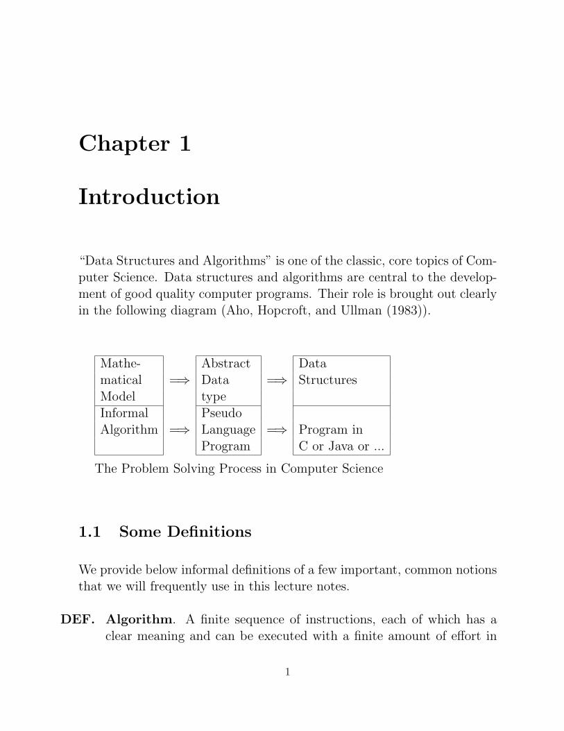
“Data Structures and Algorithms” is one of the classic, core topics of Com-puter Science. Data structures and algorithms are central to the develop-ment of good quality computer programs. Their role is brought out clearlyin the following diagram (Aho, Hopcroft, and Ullman (1983)).
Mathe- Abstract Datamatical =⇒ Data =⇒ StructuresModel typeInformal PseudoAlgorithm =⇒ Language =⇒ Program in
Program C or Java or ...
The Problem Solving Process in Computer Science
1.1 Some Definitions
We provide below informal definitions of a few important, common notionsthat we will frequently use in this lecture notes.
DEF. Algorithm. A finite sequence of instructions, each of which has aclear meaning and can be executed with a finite amount of effort in
1
Chapter 1. Introduction 2
finite time.
• whatever the input values, an algorithm will definitely terminate afterexecuting a finite number of instructions.
DEF. Data Type. Data type of a variable is the set of values that thevariable may assume.
Basic data types in C :
• int char float double
Basic data types in Pascal:
• integer real char boolean
DEF. Abstract Data Type (ADT): An ADT is a set of elements with acollection of well defined operations.
– The operations can take as operands not only instances of theADT but other types of operands or instances of other ADTs.
– Similarly results need not be instances of the ADT
– At least one operand or the result is of the ADT type in question.
Object-oriented languages such as C++ and Java provide explicit supportfor expressing ADTs by means of classes.
Examples of ADTs include list, stack, queue, set, tree, graph, etc.
DEF. Data Structures: An implementation of an ADT is a translationinto statements of a programming language,
– the declarations that define a variable to be of that ADT type
– the operations defined on the ADT (using procedures of the pro-gramming language)
Chapter 1. Introduction 3
An ADT implementation chooses a data structure to represent the ADT.Each data structure is built up from the basic data types of the underlyingprogramming language using the available data structuring facilities, suchas arrays, records (structures in C), pointers, files, sets, etc.
Example: A “Queue” is an ADT which can be defined as a sequence ofelements with operations such as null(Q), empty(Q), enqueue(x, Q), anddequeue(Q). This can be implemented using data structures such as
– array
– singly linked list
– doubly linked list
– circular array
1.1.1 Four Fundamental Data Structures
The following four data structures are used ubiquitously in the descriptionof algorithms and serve as basic building blocks for realizing more complexdata structures.
• Sequences (also called as lists)
• Dictionaries
• Priority Queues
• Graphs
Dictionaries and priority queues can be classified under a broader cate-gory called dynamic sets . Also, binary and general trees are very popularbuilding blocks for implementing dictionaries and priority queues.
1.2 Complexity of Algorithms
It is very convenient to classify algorithms based on the relative amountof time or relative amount of space they require and specify the growth of
Chapter 1. Introduction 4
time /space requirements as a function of the input size. Thus, we havethe notions of:
– Time Complexity: Running time of the program as a function ofthe size of input
– Space Complexity: Amount of computer memory required duringthe program execution, as a function of the input size
1.2.1 Big Oh Notation
– A convenient way of describing the growth rate of a function and hencethe time complexity of an algorithm.
Let n be the size of the input and f(n), g(n) be positive functions of n.
DEF. Big Oh. f(n) is O(g(n)) if and only if there exists a real, positiveconstant C and a positive integer n0 such that
f(n) ≤ Cg(n) ∀ n ≥ n0
• Note that O(g(n)) is a class of functions.
• The ”Oh” notation specifies asymptotic upper bounds
• O(1) refers to constant time. O(n) indicates linear time; O(nk) (kfixed) refers to polynomial time; O(log n) is called logarithmic time;O(2n) refers to exponential time, etc.
1.2.2 Examples
• Let f(n) = n2 + n + 5. Then
– f(n) is O(n2)
– f(n) is O(n3)
– f(n) is not O(n)
• Let f(n) = 3n
Chapter 1. Introduction 5
– f(n) is O(4n)
– f(n) is not O(2n)
• If f1(n) is O(g1(n)) and f2(n) is O(g2(n)), then
– f1(n) + f2(n) is O(max(g1(n), g2(n)))
1.2.3 An Example: Complexity of Mergesort
Mergesort is a divide and conquer algorithm, as outlined below. Note thatthe function mergesort calls itself recursively . Let us try to determine thetime complexity of this algorithm.
list mergesort (list L, int n);
if (n = = 1)
return (L)
else Split L into two halves L1 and L2 ;
return (merge (mergesort (L1,n2), (mergesort (L2,
n2))
Let T(n) be the running time of Mergesort on an input list of size n.Then,
T (n) ≤ C1 (if n = 1) (C1 is a constant)
≤ 2 T
(
n
2
)
︸ ︷︷ ︸
two recursive calls
+ C2n︸ ︷︷ ︸
cost of merging
(if n > 1)
If n = 2k for some k, it can be shown that
T (n) ≤ 2kT (1) + C2k2k
That is, T (n) is O(n log n).
Chapter 1. Introduction 6
100n
5nn /22n 3
2
n
T(n)
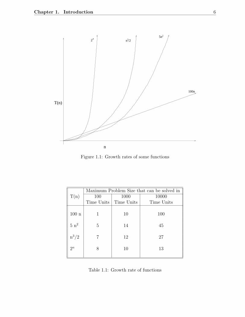
Figure 1.1: Growth rates of some functions
Maximum Problem Size that can be solved inT(n) 100 1000 10000
Time Units Time Units Time Units
100 n 1 10 100
5 n2 5 14 45
n3/2 7 12 27
2n 8 10 13
Table 1.1: Growth rate of functions
Chapter 1. Introduction 7
1.2.4 Role of the Constant
The constant C that appears in the definition of the asymptotic upperbounds is very important. It depends on the algorithm, machine, compiler,etc. It is to be noted that the big ”Oh” notation gives only asymptoticcomplexity. As such, a polynomial time algorithm with a large value of theconstant may turn out to be much less efficient than an exponential timealgorithm (with a small constant) for the range of interest of the inputvalues. See Figure 1.1 and also Table 1.1.
1.2.5 Worst Case, Average Case, and Amortized Complexity
• Worst case Running Time: The behavior of the algorithm withrespect to the worst possible case of the input instance. The worst-caserunning time of an algorithm is an upper bound on the running timefor any input. Knowing it gives us a guarantee that the algorithm willnever take any longer. There is no need to make an educated guessabout the running time.
• Average case Running Time: The expected behavior when theinput is randomly drawn from a given distribution. The average-caserunning time of an algorithm is an estimate of the running time for an”average” input. Computation of average-case running time entailsknowing all possible input sequences, the probability distribution ofoccurrence of these sequences, and the running times for the individualsequences. Often it is assumed that all inputs of a given size areequally likely.
• Amortized Running Time Here the time required to perform asequence of (related) operations is averaged over all the operationsperformed. Amortized analysis can be used to show that the averagecost of an operation is small, if one averages over a sequence of opera-tions, even though a simple operation might be expensive. Amortizedanalysis guarantees the average performance of each operation in theworst case.
Chapter 1. Introduction 8
1. For example, consider the problem of finding the minimum element ina list of elements.
Worst case = O(n)
Average case = O(n)
2. Quick sort
Worst case = O(n2)
Average case = O(n log n)
3. Merge Sort, Heap Sort
Worst case = O(n log n)
Average case = O(n log n)
4. Bubble sort
Worst case = O(n2)
Average case = O(n2)
5. Binary Search Tree: Search for an element
Worst case = O(n)
Average case = O(log n)
1.2.6 Big Omega and Big Theta Notations
The Ω notation specifies asymptotic lower bounds.
DEF. Big Omega. f(n) is said to be Ω(g(n)) if ∃ a positive real constantC and a positive integer n0 such that
f(n) ≥ Cg(n) ∀ n ≥ n0
An Alternative Definition : f(n) is said to be Ω(g(n)) iff ∃ a positive realconstant C such that
f(n) ≥ Cg(n) for infinitely many values of n.
Chapter 1. Introduction 9
The Θ notation describes asymptotic tight bounds.
DEF. Big Theta. f(n) is Θ(g(n)) iff ∃ positive real constants C1 and C2
and a positive integer n0, such that
C1g(n) ≤ f(n) ≤ C2g(n) ∀ n ≥ n0
1.2.7 An Example:
Let f(n) = 2n2 + 4n + 10. f(n) is O(n2). For,
f(n) ≤ 3n2 ∀ n ≥ 6
Thus, C = 3 and n0 = 6
Also,
f(n) ≤ 4n2 ∀ n ≥ 4
Thus, C = 4 and n0 = 4
f(n) is O(n3)
In fact, if f(n) is O(nk) for some k, it is O(nh) for h > k
f(n) is not O(n).
Suppose ∃ a constant C such that
2n2 + 4n + 10 ≤ Cn ∀n ≥ n0
This can be easily seen to lead to a contradiction. Thus, we have that:
f(n) is Ω(n2) and f(n) is Θ(n2)
1.3 To Probe Further
The following books provide an excellent treatment of the topics discussedin this chapter. The readers should also study two other key topics: (1)Recursion; (2) Recurrence Relations, from these sources.
Chapter 1. Introduction 10
1. Alfred V Aho, John E. Hopcroft, and Jeffrey D Ullman. Data Struc-tures and Algorithms . Addison-Wesley, 1983.
2. Gilles Brassard and Paul Bratley. Fundamentals of Algorithmics .Prentice-Hall, 1996. Indian Edition published by Prentice Hall ofIndia, 1998.
3. Thomas H. Cormen, Charles E. Leiserson, and Donald L. Rivest. In-troduction to Algorithms . The MIT Electrical Engineering and Com-puter Science Series, 1990. Indian Edition published in 1999.
4. Mark Allen Weiss. Data Structures and Algorithm Analysis in C++.Benjamin-Cummings, 1994. Indian Edition published in 1998.
5. R.L. Graham, D.E. Knuth, and O. Patashnik. Concrete Mathematics .Addison-wesley, Reading, 1990. Indian Edition published by Addison-Wesley Longman, 1998.
1.4 Problems
1. Assuming that n is a power of 2, express the output of the following program interms of n.
int mystery (int n)
int x=2, count=0;
while (x < n) x *=2; count++
return count;
2. Show that the following statements are true:
(a) n(n−1)2
is O(n2)
(b) max(n3, 10n2) is O(n3)
(c)∑n
i=1 ik is O(nk+1) and Ω(nk+1), for integer k
(d) If p(x) is any kth degree polynomial with a positive leading coefficient, thenp(n) is O(nk) and Ω(nk).
3. Which function grows faster?
(a) nlog n; (log n)n
Chapter 1. Introduction 11
(b) log nk; (log n)k
(c) nlog log log n; (log n)!
(d) nn; n!.
4. If f1(n) is O(g1(n)) and f2(n) is O(g2(n)) where f1 and f2 are positive functions ofn, show that the function f1(n) + f2(n) is O(max(g1(n), g2(n))).
5. If f1(n) is O(g1(n)) and f2(n) is O(g2(n)) where f1 and f2 are positive functions of n,state whether each statement below is true or false. If the statement is true(false),give a proof(counter-example).
(a) The function |f1(n) − f2(n)| is O(min(g1(n), g2(n))).
(b) The function |f1(n) − f2(n)| is O(max(g1(n), g2(n))).
6. Prove or disprove: If f(n) is a positive function of n, then f(n) is O(f(n2)).
7. The running times of an algorithm A and a competing algorithm A′
are describedby the recurrences
T (n) = 3T (n
2) + n; T
′
(n) = aT′
(n
4) + n
respectively. Assuming T (1) = T′
(1) = 1, and n = 4k for some positive integer k,determine the values of a for which A
′
is asymptotically faster than A.
8. Solve the following recurrences, where T (1) = 1 and T (n) for n ≥ 2 satisfies:
(a) T (n) = 3T (n2) + n
(b) T (n) = 3T (n2) + n2
(c) T (n) = 3T (n2) + n3
(d) T (n) = 4T (n3) + n
(e) T (n) = 4T (n3) + n2
(f) T (n) = 4T (n3) + n3
(g) T (n) = T (n2) + 1
(h) T (n) = 2T (n2) + log n
(i) T (n) = 2T (n2) + n2
(j) T (n) = 2T (n − 1) + 1
(k) T (n) = 2T (n − 1) + n
9. Show that the function T (n) defined by T (1) = 1 and
T (n) = T (n − 1) +1
n
for n ≥ 2 has the complexity O(log n).
Chapter 1. Introduction 12
10. Prove or disprove: f(3**n) is O(f(2**n))
11. Solve the following recurrence relation:
T (n) ≤ cn +2
n − 1
n−1∑
i=1
T (i)
where c is a constant, n ≥ 2, and T (2) is known to be a constant c1.
Chapter 2
Lists
A list, also called a sequence, is a container that stores elements in a certainlinear order, which is imposed by the operations performed. The basic op-erations supported are retrieving, inserting, and removing an element givenits position. Special types of lists include stacks and queues, where inser-tions and deletions can be done only at the head or the tail of the sequence.The basic realization of sequences is by means of arrays and linked lists.
2.1 List Abstract Data Type
A list is a sequence of zero or more elements of a given type
a1, a2, . . . , an (n ≥ 0)
• n : length of the list• a1 : first element of the list• an : last element of the list• n = 0 : empty list• elements can be linearly ordered according to their position in the list
We say ai precedes ai+1, ai+1 follows ai, and ai is at position i
Let us assume the following:
13
Chapter 2. Lists 14
L : list of objects of type element typex : an object of this typep : of type positionEND(L) : a function that returns the position following the
last position in the list L
Define the following operations:
1. Insert (x, p, L)
• Insert x at position p in list L
• If p = END(L), insert x at the end
• If L does not have position p, result is undefined
2. Locate (x, L)
• returns position of x on L
• returns END(L) if x does not appear
3. Retrieve (p, L)
• returns element at position p on L
• undefined if p does not exist or p = END(L)
4. Delete (p, L)
• delete element at position p in L
• undefined if p = END(L) or does not exist
5. Next (p, L)
• returns the position immediately following position p
6. Prev (p, L)
• returns the position previous to p
7. Makenull (L)
• causes L to become an empty list and returns position END(L)
Chapter 2. Lists 15
8. First (L)
• returns the first position on L
9. Printlist (L)
• print the elements of L in order of occurrence
2.1.1 A Program with List ADT
A program given below is independent of which data structure is used toimplement the list ADT. This is an example of the notion of encapsulationin object oriented programming.
Purpose:
To eliminate all duplicates from a list
Given:
1. Elements of list L are of element type
2. function same (x, y), where x and y are of element type, returns trueif x and y are same, false otherwise
3. p and q are of type position
p : current position in L
q : moves ahead to find equal elements
Pseudocode in C:
p = first (L) ;
while (p! = end(L)) q = next(p, L) ;
while (q! = end(L)) if (same (retrieve (p,L), retrieve (q, L))))
Chapter 2. Lists 16
delete (q,L);
else
q = next (q, L) ;
p = next (p, L) ;
2.2 Implementation of Lists
Many implementations are possible. Popular ones include:
1. Arrays
2. Pointers (singly linked, doubly linked, etc.)
3. Cursors (arrays with integer pointers)
2.2.1 Array Implementation of Lists
• Here, elements of list are stored in the (contiguous) cells of an array.
• List is a structure with two members.
member 1 : an array of elements
member 2 : last — indicates position of the last element of the list
Position is of type integer and has the range 0 to maxlength–1
# define maxlength 1000
typedef int elementtype; /∗ elements are integers ∗/typedef struct list–tag
elementtype elements [maxlength];
int last;
list–type;
Chapter 2. Lists 17
end(L)
int end (list–type ∗ℓp)
return (ℓp → last + 1)
Insert (x, p,L)
void insert (elementtype x ; int p ; list–type ∗ℓp) ;
int v; /∗ running position ∗/if (ℓp → last >= maxlength–1)
error (“list is full”)
elseif ((p < 0) || (p > ℓp → last + 1))
error (position does not exist)
else
for (q = ℓp → last ; q <= p, q−−)
ℓp → elements [q + 1] = ℓp → elements [q] ;
ℓp → last = ℓp → last + 1 ;
ℓp → elements [p] = x
Delete (p, L)
void delete (int p ; list–type ∗ℓp)
int q ; /∗ running position ∗/if ((p > ℓp → last) || (p < 0))
error (“position does not exist”)
else /∗ shift elements ∗/ ℓp → last −− ;
for (q = p ; q <= ℓp → last; q ++)
ℓp → elements [q] = ℓp → elements [q+1]
Chapter 2. Lists 18
header
null
a a a1 2 n
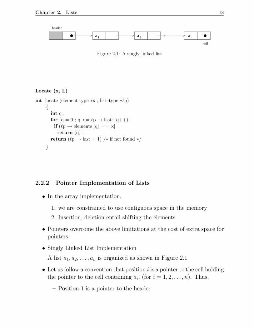
Figure 2.1: A singly linked list
Locate (x, L)
int locate (element type ∗x ; list–type ∗ℓp)
int q ;
for (q = 0 ; q <= ℓp → last ; q++)
if (ℓp → elements [q] = = x]
return (q) ;
return (ℓp → last + 1) /∗ if not found ∗/
2.2.2 Pointer Implementation of Lists
• In the array implementation,
1. we are constrained to use contiguous space in the memory
2. Insertion, deletion entail shifting the elements
• Pointers overcome the above limitations at the cost of extra space forpointers.
• Singly Linked List Implementation
A list a1, a2, . . . , an is organized as shown in Figure 2.1
• Let us follow a convention that position i is a pointer to the cell holdingthe pointer to the cell containing ai, (for i = 1, 2, . . . , n). Thus,
– Position 1 is a pointer to the header
Chapter 2. Lists 19
Before Insertion
After Insertion
a b
p
p
a b
x
//broken
temp
Figure 2.2: Insertion in a singly linked list
– End (L) is a pointer to the last cell of list L
• If position of ai is simply a pointer to the cell holding ai, then
– Position 1 will be the address in the header
– end (L) will be a null pointer
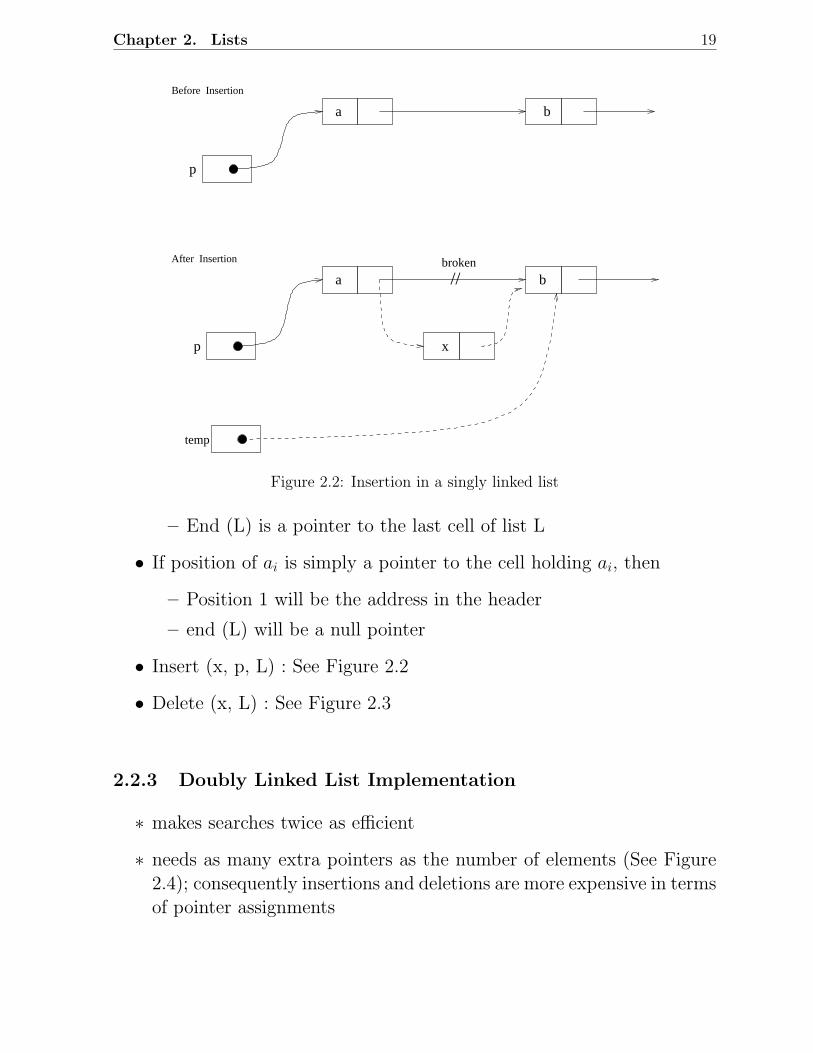
• Insert (x, p, L) : See Figure 2.2
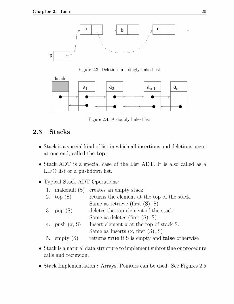
• Delete (x, L) : See Figure 2.3
2.2.3 Doubly Linked List Implementation
∗ makes searches twice as efficient
∗ needs as many extra pointers as the number of elements (See Figure2.4); consequently insertions and deletions are more expensive in termsof pointer assignments
Chapter 2. Lists 20
p
a b c
Figure 2.3: Deletion in a singly linked list
a a a a1 2 nn-1
header
Figure 2.4: A doubly linked list
2.3 Stacks
• Stack is a special kind of list in which all insertions and deletions occurat one end, called the top.
• Stack ADT is a special case of the List ADT. It is also called as aLIFO list or a pushdown list.
• Typical Stack ADT Operations:
1. makenull (S) creates an empty stack2. top (S) returns the element at the top of the stack.
Same as retrieve (first (S), S)3. pop (S) deletes the top element of the stack
Same as deletes (first (S), S)4. push (x, S) Insert element x at the top of stack S.
Same as Inserts (x, first (S), S)5. empty (S) returns true if S is empty and false otherwise
• Stack is a natural data structure to implement subroutine or procedurecalls and recursion.
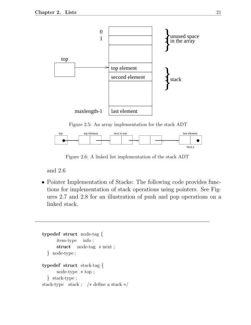
• Stack Implementation : Arrays, Pointers can be used. See Figures 2.5
Chapter 2. Lists 21
01
maxlength-1
top element
second element
last element
top
unused spacein the array
stack
Figure 2.5: An array implementation for the stack ADT
top top element next to top last element
NULL
Figure 2.6: A linked list implementation of the stack ADT
and 2.6
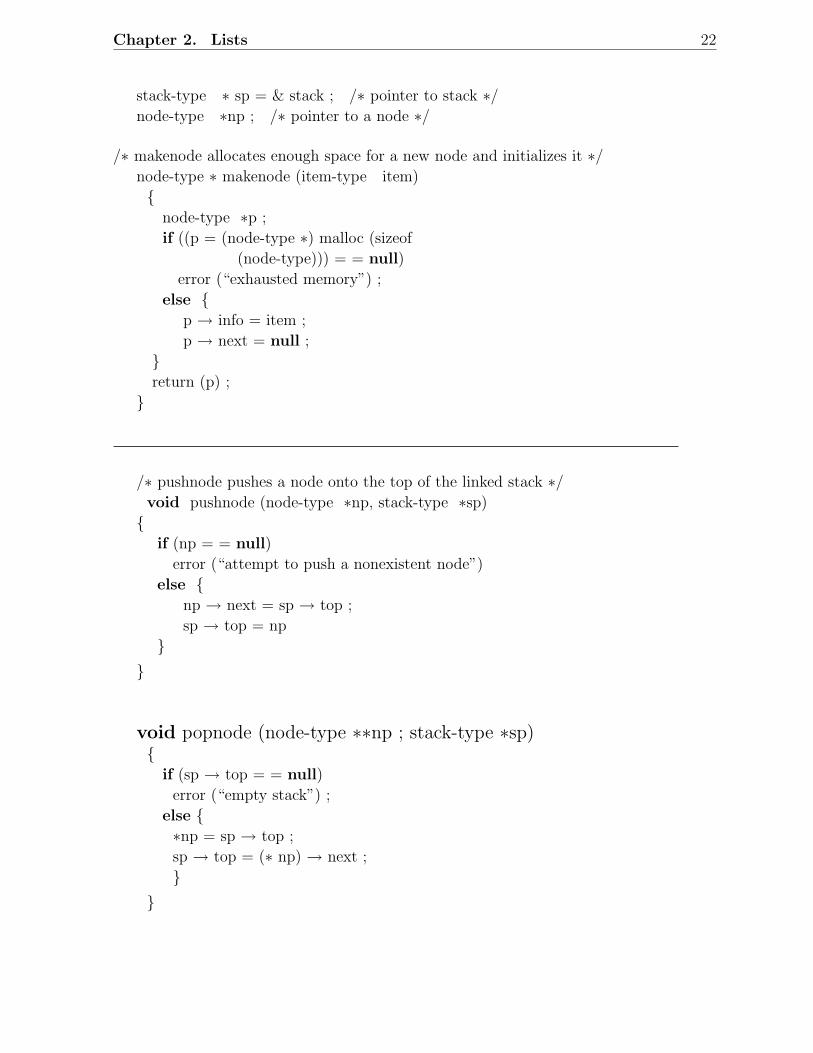
• Pointer Implementation of Stacks: The following code provides func-tions for implementation of stack operations using pointers. See Fig-ures 2.7 and 2.8 for an illustration of push and pop operations on alinked stack.
typedef struct node-tag item-type info ;
struct node-tag ∗ next ;
node-type ;
typedef struct stack-tag node-type ∗ top ;
stack-type ;
stack-type stack ; /∗ define a stack ∗/
Chapter 2. Lists 22
stack-type ∗ sp = & stack ; /∗ pointer to stack ∗/node-type ∗np ; /∗ pointer to a node ∗/
/∗ makenode allocates enough space for a new node and initializes it ∗/node-type ∗ makenode (item-type item)
node-type ∗p ;
if ((p = (node-type ∗) malloc (sizeof
(node-type))) = = null)
error (“exhausted memory”) ;
else p → info = item ;
p → next = null ;
return (p) ;
/∗ pushnode pushes a node onto the top of the linked stack ∗/void pushnode (node-type ∗np, stack-type ∗sp)
if (np = = null)
error (“attempt to push a nonexistent node”)
else np → next = sp → top ;
sp → top = np
void popnode (node-type ∗∗np ; stack-type ∗sp)
if (sp → top = = null)
error (“empty stack”) ;
else ∗np = sp → top ;
sp → top = (∗ np) → next ;
Chapter 2. Lists 23
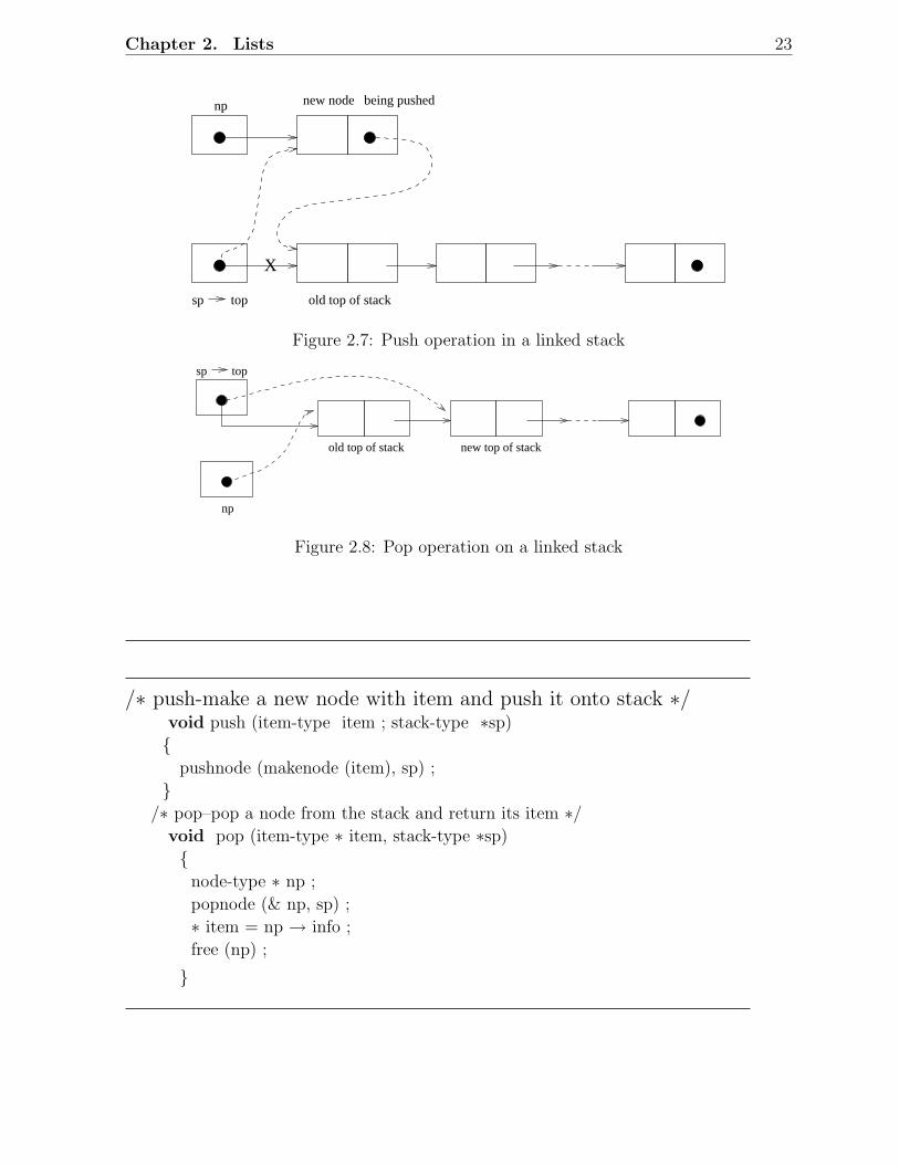
being pushednp
sp top old top of stack
new node
X
Figure 2.7: Push operation in a linked stack
sp top
old top of stack
np
new top of stack
Figure 2.8: Pop operation on a linked stack
/∗ push-make a new node with item and push it onto stack ∗/void push (item-type item ; stack-type ∗sp)
pushnode (makenode (item), sp) ;
/∗ pop–pop a node from the stack and return its item ∗/
void pop (item-type ∗ item, stack-type ∗sp)
node-type ∗ np ;
popnode (& np, sp) ;
∗ item = np → info ;
free (np) ;
Chapter 2. Lists 24
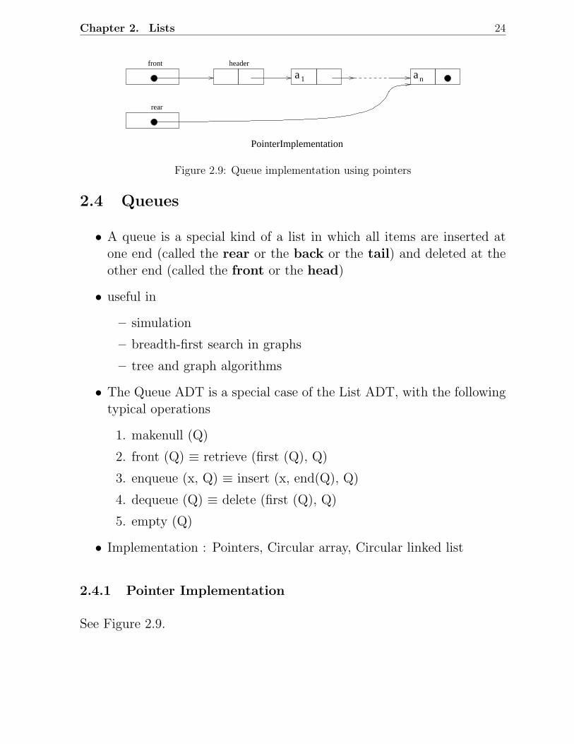
a a n
headerfront
rear
PointerImplementation
1
Figure 2.9: Queue implementation using pointers
2.4 Queues
• A queue is a special kind of a list in which all items are inserted atone end (called the rear or the back or the tail) and deleted at theother end (called the front or the head)
• useful in
– simulation
– breadth-first search in graphs
– tree and graph algorithms
• The Queue ADT is a special case of the List ADT, with the followingtypical operations
1. makenull (Q)
2. front (Q) ≡ retrieve (first (Q), Q)
3. enqueue (x, Q) ≡ insert (x, end(Q), Q)
4. dequeue (Q) ≡ delete (first (Q), Q)
5. empty (Q)
• Implementation : Pointers, Circular array, Circular linked list
2.4.1 Pointer Implementation
See Figure 2.9.
Chapter 2. Lists 25
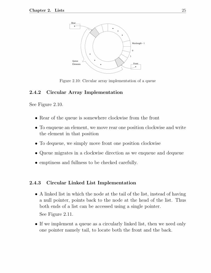
Maxlength - 1
0
1
Front
Rear
Queue
Elements
Figure 2.10: Circular array implementation of a queue
2.4.2 Circular Array Implementation
See Figure 2.10.
• Rear of the queue is somewhere clockwise from the front
• To enqueue an element, we move rear one position clockwise and writethe element in that position
• To dequeue, we simply move front one position clockwise
• Queue migrates in a clockwise direction as we enqueue and dequeue
• emptiness and fullness to be checked carefully.
2.4.3 Circular Linked List Implementation
• A linked list in which the node at the tail of the list, instead of havinga null pointer, points back to the node at the head of the list. Thusboth ends of a list can be accessed using a single pointer.
See Figure 2.11.
• If we implement a queue as a circularly linked list, then we need onlyone pointer namely tail, to locate both the front and the back.
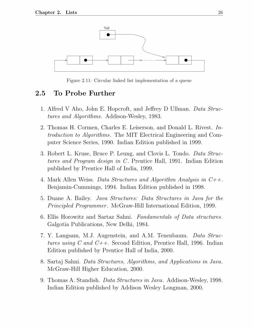
Chapter 2. Lists 26
Tail
Figure 2.11: Circular linked list implementation of a queue
2.5 To Probe Further
1. Alfred V Aho, John E. Hopcroft, and Jeffrey D Ullman. Data Struc-tures and Algorithms . Addison-Wesley, 1983.
2. Thomas H. Cormen, Charles E. Leiserson, and Donald L. Rivest. In-troduction to Algorithms . The MIT Electrical Engineering and Com-puter Science Series, 1990. Indian Edition published in 1999.
3. Robert L. Kruse, Bruce P. Leung, and Clovis L. Tondo. Data Struc-tures and Program design in C . Prentice Hall, 1991. Indian Editionpublished by Prentice Hall of India, 1999.
4. Mark Allen Weiss. Data Structures and Algorithm Analysis in C++.Benjamin-Cummings, 1994. Indian Edition published in 1998.
5. Duane A. Bailey. Java Structures: Data Structures in Java for thePrincipled Programmer . McGraw-Hill International Edition, 1999.
6. Ellis Horowitz and Sartaz Sahni. Fundamentals of Data structures .Galgotia Publications, New Delhi, 1984.
7. Y. Langsam, M.J. Augenstein, and A.M. Tenenbaum. Data Struc-tures using C and C++. Second Edition, Prentice Hall, 1996. IndianEdition published by Prentice Hall of India, 2000.
8. Sartaj Sahni. Data Structures, Algorithms, and Applications in Java.McGraw-Hill Higher Education, 2000.
9. Thomas A. Standish. Data Structures in Java. Addison-Wesley, 1998.Indian Edition published by Addison Wesley Longman, 2000.
Chapter 2. Lists 27
2.6 Problems
1. A linked list has exactly n nodes. The elements in these nodes are selected fromthe set 0, 1, . . . , n. There are no duplicates in the list. Design an O(n) worst casetime algorithm to find which one of the elements from the above set is missing inthe given linked list.
2. Write a procedure that will reverse a linked list while traversing it only once. At theconclusion, each node should point to the node that was previously its predecessor:the head should point to the node that was formerly at the end, and the node thatwas formerly first should have a null link.
3. How would one implement a queue if the elements that are to be placed on thequeue are arbitrary length strings? How long does it take to enqueue a string?
4. Let A be an array of size n, containing positive or negative integers, with A[1] <A[2] < . . . < A[n]. Design an efficient algorithm (should be more efficient thanO(n)) to find an i such that A[i] = i provided such an i exists. What is the worstcase computational complexity of your algorithm ?
5. Consider an array of size n. Sketch an O(n) algorithm to shift all items in the arrayk places cyclically counterclockwise. You are allowed to use only one extra locationto implement swapping of items.
6. In some operating systems, the least recently used (LRU) algorithm is used for pagereplacement. The implementation of such an algorithm will involve the followingoperations on a collection of nodes.
• use a node.
• replace the LRU node by a new node.
Suggest a good data structure for implementing such a collection of nodes.
7. A queue Q contains the items a1, a2, . . . , an, in that order with a1 at the front and an
at the back. It is required to transfer these items on to a stack S (initially empty) sothat a1 is at the top of the stack and the order of all other items is preserved. Usingenqueue and dequeue operations for the queue and push and pop operations for thestack, outline an efficient O(n) algorithm to accomplish the above task, using onlya constant amount of additional storage.
8. A queue is set up in a circular array C[0..n−1] with front and rear defined as usual.Assume that n−1 locations in the array are available for storing the elements (withthe other element being used to detect full/empty condition). Derive a formula forthe number of elements in the queue in terms of rear , front , and n.
9. Let p1p2 . . . pn be a stack-realizable permutation of 12 . . . n. Show that there do notexist indices i < j < k such that pj < pk < pi.
Chapter 2. Lists 28
10. Write recursive algorithms for the following problems:
(a) Compute the number of combinations of n objects taken m at a time.
(b) Reverse a linked list.
(c) Reverse an array.
(d) Binary search on an array of size n.
(e) Compute gcd of two numbers n and m.
11. Consider the following recursive definition:
g(i, j) = i (j = 1) (2.1)
g(i, j) = j (i = 1) (2.2)
g(i, j) = g(i − 1, j) + g(i, j − 1) else (2.3)
Design an O(mn) iterative algorithm to compute g(m,n) where m and n are positiveintegers.
12. Consider polynomials of the form:
p(x) = c1xe1 + c2x
e2 . . . c1xen ;
where e1 > e2 . . . > en ≥ 0. Such polynomials can be represented by a linked listsin which each cell has 3 fields: one for the coefficient, one for the exponent, and onepointing to the next cell. Write procedures for
(a) differentiating,
(b) integrating,
(c) adding,
(d) multiplying
such polynomials. What is the running time of these procedures as a function ofthe number of terms in the polynomials?
13. Suppose the numbers 1, 2, 3, 4, 5 and 6 arrive in an input stream in that order.Which of the following sequences can be realized as the output of (1) stack, and (2)double ended queue?
a) 1 2 3 4 5 6
b) 6 5 4 3 2 1
c) 2 4 3 6 5 1
d) 1 5 2 4 3 6
e) 1 3 5 2 4 6
Chapter 2. Lists 29
2.7 Programming Assignments
2.7.1 Sparse Matrix Package
As you might already know, sparse matrices are those in which most of the elementsare zero (that is, the number of non-zero elements is very small). Linked lists are veryuseful in representing sparse matrices, since they eliminate the need to represent zeroentries in the matrix. Implement a package that facilitates efficient addition, subtraction,multiplication, and other important arithmetic operations on sparse matrices, using linkedlist representation of those.
2.7.2 Polynomial Arithmetic
Polynomials involving real variables and real-valued coefficients can also be representedefficiently through linked lists. Assuming single variable polynomials, design a suitablelinked list representation for polynomials and develop a package that implements variouspolynomial operations such as addition, subtraction, multiplication, and division.
2.7.3 Skip Lists
A skip list is an efficient linked list-based data structure that attempts to implementbinary search on linked lists. Read the following paper: William Pugh. Skip Lists: Aprobabilistic alternative to balanced trees. Communications of the ACM , Volume 33,Number 6, pp. 668-676, 1990. Also read the section on Skip Lists in Chapter 4 of thislecture notes. Develop programs to implement search, insert, and delete operations inskip lists.
2.7.4 Buddy Systems of Memory Allocation
The objective of this assignment is to compare the performance of the exponential andthe Fibonacci buddy systems of memory allocation. For more details on buddy systems,refer to the book: Donald E Knuth. Fundamental Algorithms , Volume 1 of The Artof Computer Programming, Addison-Wesley, 1968, Second Edition, 1973. Consider anexponential buddy system with the following allowable block sizes: 8, 16, 32, 64, 128,512, 1024, 2048, and 4096. Let the allowable block sizes for the Fibonacci system be 8,13, 21, 34, 55, 89, 144, 233, 377, 610, 987, 1597, 2594, and 4191. Your tasks are thefollowing.
1. Generate a random sequence of allocations and liberations. Start with an emptymemory and carry out a sequence of allocations first, so that the memory becomes
Chapter 2. Lists 30
adequately committed. Now generate a sequence of allocations and liberations in-terleaved randomly. You may try with 100 or 200 or even 1000 such allocations andliberations. While generating the memory sizes requested for allocations, you mayuse a reasonable distribution. For example, one typical scenario is:
Range of block size Probability
8–100: 0.1100–500: 0.5500–1000: 0.21000–2000: 0.12000-4191: 0.1
2. Simulate the memory allocations and liberations for the above random sequences.At various intermediate points, print out the detailed state of the memory, indicatingthe allocated portions, available portions, and the i-lists. Use recursive algorithmsfor allocations and liberations. It would be excellent if you implement very generalallocation and liberation algorithms, that will work for any arbitrary order buddysystem.
3. Compute the following performance measures for each random sequence:
• Average fragmentation.
• Total number of splits.
• Total number of merges.
• Average size of all linked lists used in maintaining the available block informa-tion.
• Number of blocks that cannot be combined with buddies.
• Number of contiguous blocks that are not buddies.
4. Repeat the experiments for several random sequences and print out the averageperformance measures. You may like to repeat the experimentation on differentdistributions of request sizes.
Chapter 3
Dictionaries
A dictionary is a container of elements from a totally ordered universe thatsupports the basic operations of inserting/deleting elements and searchingfor a given element. In this chapter, we present hash tables which providean efficient implicit realization of a dictionary. Efficient explicit implemen-tations include binary search trees and balanced search trees. These aretreated in detail in Chapter 4. First, we introduce the abstract data typeSet which includes dictionaries, priority queues, etc. as subclasses.
3.1 Sets
• A set is a collection of well defined elements. The members of a setare all different.
• A set ADT can be defined to comprise the following operations:
1. Union (A, B, C)
2. Intersection (A, B, C)
3. Difference (A, B, C)
4. Merge (A, B, C)
5. Find (x)
6. Member (x, A) or Search (x, A)
7. Makenull (A)
31
Chapter 3. Dictionaries 32
8. Equal (A, B)
9. Assign (A, B)
10. Insert (x, A)
11. Delete (x, A)
12. Min (A) (if A is an ordered set)
• Set implementation: Possible data structures include:
– Bit Vector
– Array
– Linked List
∗ Unsorted
∗ Sorted
3.2 Dictionaries
• A dictionary is a dynamic set ADT with the operations:
1. Makenull (D)
2. Insert (x, D)
3. Delete (x, D)
4. Search (x, D)
• Useful in implementing symbol tables, text retrieval systems, databasesystems, page mapping tables, etc.
• Implementation:
1. Fixed Length arrays
2. Linked lists : sorted, unsorted, skip-lists
3. Hash Tables : open, closed
4. Trees
– Binary Search Trees (BSTs)
Chapter 3. Dictionaries 33
– Balanced BSTs
∗ AVL Trees
∗ Red-Black Trees
– Splay Trees
– Multiway Search Trees
∗ 2-3 Trees
∗ B Trees
– Tries
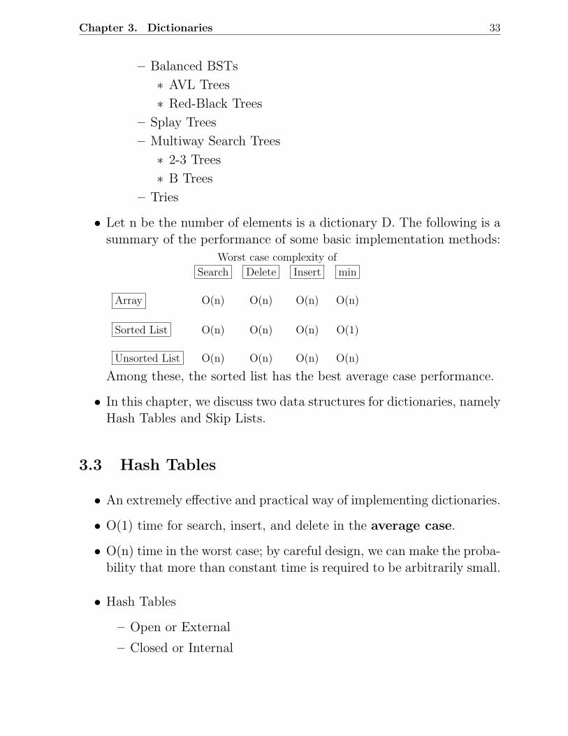
• Let n be the number of elements is a dictionary D. The following is asummary of the performance of some basic implementation methods:
Worst case complexity of
Search Delete Insert min
Array O(n) O(n) O(n) O(n)
Sorted List O(n) O(n) O(n) O(1)
Unsorted List O(n) O(n) O(n) O(n)
Among these, the sorted list has the best average case performance.
• In this chapter, we discuss two data structures for dictionaries, namelyHash Tables and Skip Lists.
3.3 Hash Tables
• An extremely effective and practical way of implementing dictionaries.
• O(1) time for search, insert, and delete in the average case.
• O(n) time in the worst case; by careful design, we can make the proba-bility that more than constant time is required to be arbitrarily small.
• Hash Tables
– Open or External
– Closed or Internal
Chapter 3. Dictionaries 34
3.3.1 Open Hashing
Let:
• U be the universe of keys:
– integers
– character strings
– complex bit patterns
• B the set of hash values (also called the buckets or bins). Let B =0, 1, . . . , m − 1 where m > 0 is a positive integer.
A hash function h : U → B associates buckets (hash values) to keys.
Two main issues:
1. Collisions
If x1 and x2 are two different keys, it is possible that h(x1) = h(x2).This is called a collision. Collision resolution is the most importantissue in hash table implementations.
2. Hash Functions
Choosing a hash function that minimizes the number of collisions andalso hashes uniformly is another critical issue.
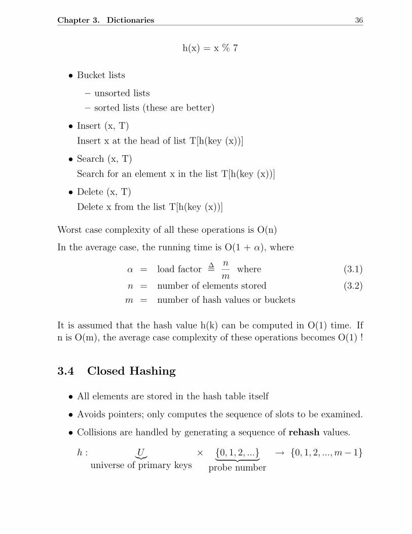
Collision Resolution by Chaining
• Put all the elements that hash to the same value in a linked list. SeeFigure 3.1.
Example:
See Figure 3.2. Consider the keys 0, 1, 4, 9, 16, 25, 36, 49, 64, 81, 100. Letthe hash function be:
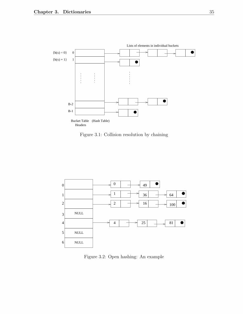
Chapter 3. Dictionaries 35
0
1
B-2
B-1
h(x) = 0
h(x) = 1
Lists of elements in individual buckets
Bucket Table (Hash Table)Headers
Figure 3.1: Collision resolution by chaining
NULL
NULL
NULL
0
2
3
4
5
6
1
0
1
4
49
36
16
25 81
100
64
2
Figure 3.2: Open hashing: An example
Chapter 3. Dictionaries 36
h(x) = x % 7
• Bucket lists
– unsorted lists
– sorted lists (these are better)
• Insert (x, T)
Insert x at the head of list T[h(key (x))]
• Search (x, T)
Search for an element x in the list T[h(key (x))]
• Delete (x, T)
Delete x from the list T[h(key (x))]
Worst case complexity of all these operations is O(n)
In the average case, the running time is O(1 + α), where
α = load factor ∆=n
mwhere (3.1)
n = number of elements stored (3.2)
m = number of hash values or buckets
It is assumed that the hash value h(k) can be computed in O(1) time. Ifn is O(m), the average case complexity of these operations becomes O(1) !
3.4 Closed Hashing
• All elements are stored in the hash table itself
• Avoids pointers; only computes the sequence of slots to be examined.
• Collisions are handled by generating a sequence of rehash values.
h : U︸︷︷︸
universe of primary keys
× 0, 1, 2, ...︸ ︷︷ ︸
probe number
→ 0, 1, 2, ..., m− 1
Chapter 3. Dictionaries 37
• Given a key x, it has a hash value h(x,0) and a set of rehash values
h(x, 1), h(x,2), . . . , h(x, m-1)
• We require that for every key x, the probe sequence
< h(x,0), h(x, 1), h(x,2), . . . , h(x, m-1)>
be a permutation of <0, 1, ..., m-1>.
This ensures that every hash table position is eventually consideredas a slot for storing a record with a key value x.
Search (x, T)
• Search will continue until you find the element x (successful search)or an empty slot (unsuccessful search).
Delete (x, T)
• No delete if the search is unsuccessful.
• If the search is successful, then put the label DELETED (different froman empty slot).
Insert (x, T)
• No need to insert if the search is successful.
• If the search is unsuccessful, insert at the first position with a DELETED
tag.
3.4.1 Rehashing Methods
Denote h(x, 0) by simply h(x).
1. Linear probingh(x, i) = (h(x) + i) mod m
Chapter 3. Dictionaries 38
2. Quadratic Probing
h(x, i) = (h(x) + C1i + C2i2) mod m
where C1 and C2 are constants.
3. Double Hashing
h(x, i) = (h(x) + i h′(x))︸ ︷︷ ︸
anotherhashfunction
mod m
A Comparison of Rehashing Methods
Linear Probing m distinct probe Primary clustering
sequences
Quadratic Probing m distinct probe No primary clustering;
sequences but secondary clustering
Double Hashing m2 distinct probe No primary clustering
sequences No secondary clustering
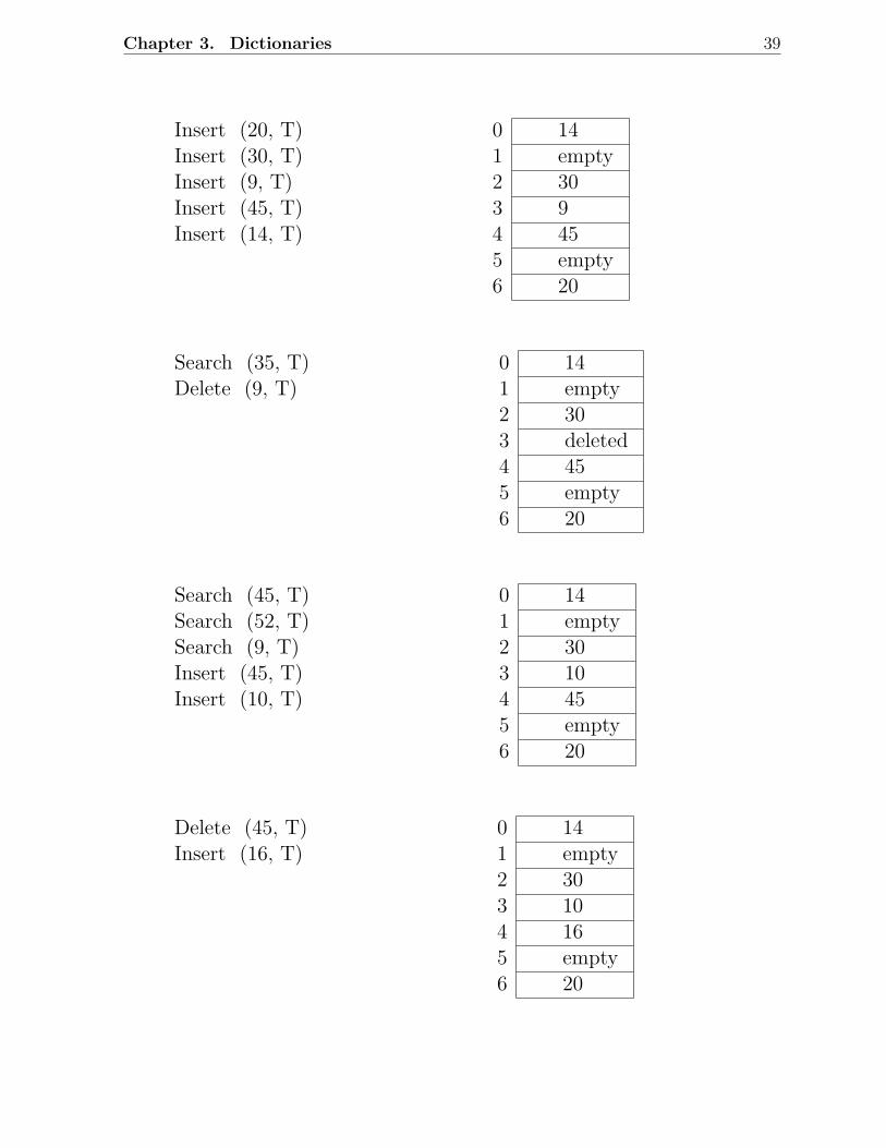
3.4.2 An Example:
Assume linear probing with the following hashing and rehashing functions:
h(x, 0) = x%7h(x, i) = (h(x, 0) + i)%7
Start with an empty table.
Chapter 3. Dictionaries 39
Insert (20, T) 0 14Insert (30, T) 1 emptyInsert (9, T) 2 30Insert (45, T) 3 9Insert (14, T) 4 45
5 empty6 20
Search (35, T) 0 14Delete (9, T) 1 empty
2 303 deleted4 455 empty6 20
Search (45, T) 0 14Search (52, T) 1 emptySearch (9, T) 2 30Insert (45, T) 3 10Insert (10, T) 4 45
5 empty6 20
Delete (45, T) 0 14Insert (16, T) 1 empty
2 303 104 165 empty6 20
Chapter 3. Dictionaries 40
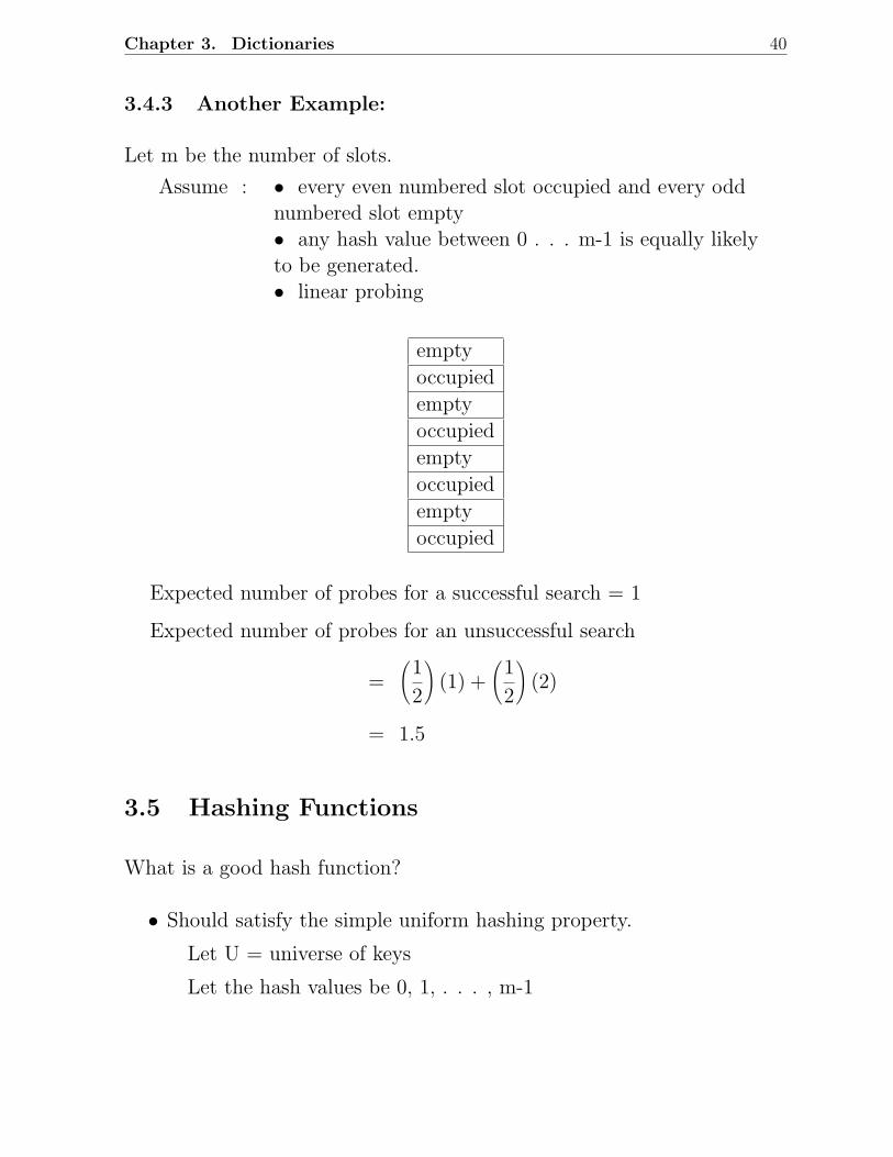
3.4.3 Another Example:
Let m be the number of slots.
Assume : • every even numbered slot occupied and every oddnumbered slot empty• any hash value between 0 . . . m-1 is equally likelyto be generated.• linear probing
empty
occupied
empty
occupied
empty
occupied
empty
occupied
Expected number of probes for a successful search = 1
Expected number of probes for an unsuccessful search
=
(
1
2
)
(1) +
(
1
2
)
(2)
= 1.5
3.5 Hashing Functions
What is a good hash function?
• Should satisfy the simple uniform hashing property.
Let U = universe of keys
Let the hash values be 0, 1, . . . , m-1
Chapter 3. Dictionaries 41
Let us assume that each key is drawn independently from U accordingto a probability distribution P. i.e., for k ∈ U
P (k) = Probability that k is drawn
Then simple uniform hashing requires that
∑
k:h(k)=j
P (k) =1
mfor each j = 0, 1, . . . , m − 1
that is, each bucket is equally likely to be occupied.
• Example of a hash function that satisfies simple uniform hashing prop-erty:
Suppose the keys are known to be random real numbers k indepen-dently and uniformly distributed in the range [0,1).
h(k) = ⌊km⌋
satisfies the simple uniform hashing property.
Qualitative information about P is often useful in the design process.For example, consider a compiler’s symbol table in which the keys arearbitrary character strings representing identifiers in a program. It iscommon for closely related symbols, say pt, pts, ptt, to appear in thesame program. A good hash function would minimize the chance thatsuch variants hash to the same slot.
• A common approach is to derive a hash value in a way that is expectedto be independent of any patterns that might exist in the data.
– The division method computes the hash value as the remainderwhen the key is divided by a prime number. Unless that prime issomehow related to patterns in the distribution P , this methodgives good results.
Chapter 3. Dictionaries 42
3.5.1 Division Method
• A key is mapped into one of m slots using the function
h(k) = k mod m
• Requires only a single division, hence fast
• m should not be :
– a power of 2, since if m = 2p, then h(k) is just the p lowest orderbits of k
– a power of 10, since then the hash function does not depend onall the decimal digits of k
– 2p − 1. If k is a character string interpreted in radix 2p, twostrings that are identical except for a transposition of two adjacentcharacters will hash to the same value.
• Good values for m
– primes not too close to exact powers of 2.
3.5.2 Multiplication Method
There are two steps:
1. Multiply the key k by a constant A in the range 0 < A < 1 and extractthe fractional part of kA
2. Multiply this fractional part by m and take the floor.
h(k) = ⌊m(kA mod 1)⌋
where
kA mod 1 = kA − ⌊kA⌋h(k) = ⌊m(kA − ⌊kA⌋)⌋
Chapter 3. Dictionaries 43
• Advantage of the method is that the value of m is not critical. Wetypically choose it to be a power of 2:
m = 2p
for some integer p so that we can then easily implement the functionon most computers as follows:
Suppose the word size = w. Assume that k fits into a single word.First multiply k by the w-bit integer ⌊A.2w⌋. The result is a 2w - bitvalue
r12w + r0
where r1 is the high order word of the product and r0 is the low orderword of the product. The desired p-bit hash value consists of the pmost significant bits of r0.
• Works practically with any value of A, but works better with somevalues than the others. The optimal choice depends on the character-istics of the data being hashed. Knuth recommends
A ≃√
5 − 1
2= 0.6180339887 . . . (Golden Ratio)
3.5.3 Universal Hashing
This involves choosing a hash function randomly in a way that is indepen-dent of the keys that are actually going to be stored. We select the hashfunction at random from a carefully designed class of functions.
• Let Φ be a finite collection of hash functions that map a given universeU of keys into the range 0, 1, 2, . . . , m − 1.
• Φ is called universal if for each pair of distinct keys x, y ∈ U , thenumber of hash functions h ∈ Φ for which h(x) = h(y) is preciselyequal to
|Φ|m
Chapter 3. Dictionaries 44
• With a function randomly chosen from Φ, the chance of a collisionbetween x and y where x 6= y is exactly 1
m .
Example of a universal class of hash functions:
Let table size m be prime. Decompose a key x into r +1 bytes. (i.e.,characters or fixed-width binary strings). Thus
x = (x0, x1, . . . , xr)
Assume that the maximum value of a byte to be less than m.
Let a = (a0, a1, . . . , ar) denote a sequence of r + 1 elements chosenrandomly from the set 0, 1, . . . , m− 1. Define a hash function ha ∈ Φ by
ha(x) =r∑
i=0
aixi mod m
With this definition, Φ =⊔
aha can be shown to be universal. Note thatit has mr+1 members.
3.6 Analysis of Closed Hashing
Load factor α
α ∆=n
m=
# of elements stored the table
total # of elements in the table
Assume uniform hashing. In this scheme, the probe sequence
< h(k, 0), . . . , h(k, m − 1) >
for each key k is equally likely to be any permutation of< 0, 1, . . . , m − 1 >
3.6.1 Result 1: Unsuccessful Search
• The expected number of probes in an unsuccessful search ≤ 11−α
Chapter 3. Dictionaries 45
Proof: In an unsuccessful search, every probe but the last accessesan occupied slot that does not contain the desired key and the lastslot probed is empty.
Let the random variable X denote the number of occupied slots probedbefore hitting an empty slot. X can take values 0, 1, . . . , n. It is easyto see that the expected number of probes in an unsuccessful searchis 1 + E[X].
pi = P exactly i probes access occupied slots, for i = 0, 1, 2, . . .
for i > n, pi = 0 since we can find at most n occupied slots.
Thus the expected number of probes
= 1 +n∑
i=0
ipi (∗)
To evaluate (*), define
qi = Pat least i probes access occupied slots
and use the identity:n∑
i=0
ipi =n∑
i=1
qi
To compute qi, we proceed as follows:
q1 =n
m
since the probability that the first probe accesses an occupied slot isn/m.
With uniform hashing, a second probe, if necessary, is to one of theremaining m − 1 unprobed slots, n − 1 of which are occupied. Thus
q2 =
(
n
m
) (
n − 1
m − 1
)
since we make a second probe only if the first probe accesses an occu-pied slot.
Chapter 3. Dictionaries 46
In general,
qi =
(
n
m
) (
n − 1
m − 1
)
· · ·(
n − i + 1
m − i + 1
)
≤(
n
m
)i
= αi sincen − j
m − j≤ n
m
Thus the expected number of probes in an unsuccessful search
= 1 +n∑
i=o
ipi
≤ 1 + α + α2 + · · ·=
1
1 − α
• Intuitive Interpretation of the above:
One probe is always made, with probability approximately α a secondprobe is needed, with probability approximately α2 a third probe isneeded, and so on.
3.6.2 Result 2: Insertion
• Insertion of an element requires at most 11−α probes on average.
• Proof is obvious because inserting a key requires an unsuccessful searchfollowed by a placement of the key in the first empty slot found.
3.6.3 Result 3: Successful Search
• The expected number of probes in a successful search is at most
1
αln
1
1 − α+
1
α
assuming that each key in the table is equally likely to be searchedfor.
A search for a key k follows the same probe sequence as was followedwhen the element with key k was inserted. Thus, if k was the (i+1)th
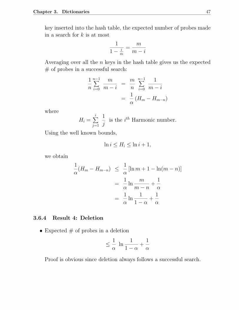
Chapter 3. Dictionaries 47
key inserted into the hash table, the expected number of probes madein a search for k is at most
1
1 − im
=m
m − i
Averaging over all the n keys in the hash table gives us the expected# of probes in a successful search:
1
n
n−1∑
i=0
m
m − i=
m
n
n−1∑
i=0
1
m − i
=1
α(Hm − Hm−n)
where
Hi =i∑
j=1
1
jis the ith Harmonic number.
Using the well known bounds,
ln i ≤ Hi ≤ ln i + 1,
we obtain
1
α(Hm − Hm−n) ≤ 1
α[ln m + 1 − ln(m − n)]
=1
αln
m
m − n+
1
α
=1
αln
1
1 − α+
1
α
3.6.4 Result 4: Deletion
• Expected # of probes in a deletion
≤ 1
αln
1
1 − α+
1
α
Proof is obvious since deletion always follows a successful search.
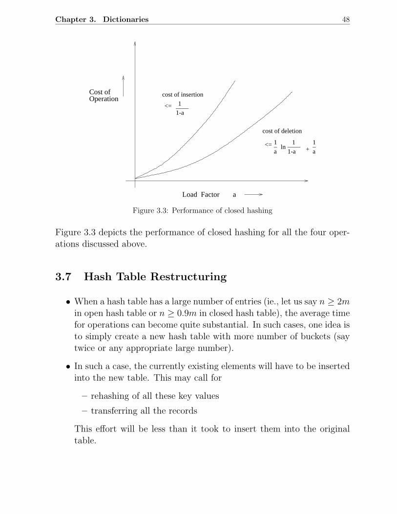
Chapter 3. Dictionaries 48
Load Factor a
Cost ofOperation
cost of insertion
<= 1____1-a
cost of deletion
<= 1_a
ln 1____
1-a + 1_a
Figure 3.3: Performance of closed hashing
Figure 3.3 depicts the performance of closed hashing for all the four oper-ations discussed above.
3.7 Hash Table Restructuring
• When a hash table has a large number of entries (ie., let us say n ≥ 2min open hash table or n ≥ 0.9m in closed hash table), the average timefor operations can become quite substantial. In such cases, one idea isto simply create a new hash table with more number of buckets (saytwice or any appropriate large number).
• In such a case, the currently existing elements will have to be insertedinto the new table. This may call for
– rehashing of all these key values
– transferring all the records
This effort will be less than it took to insert them into the originaltable.
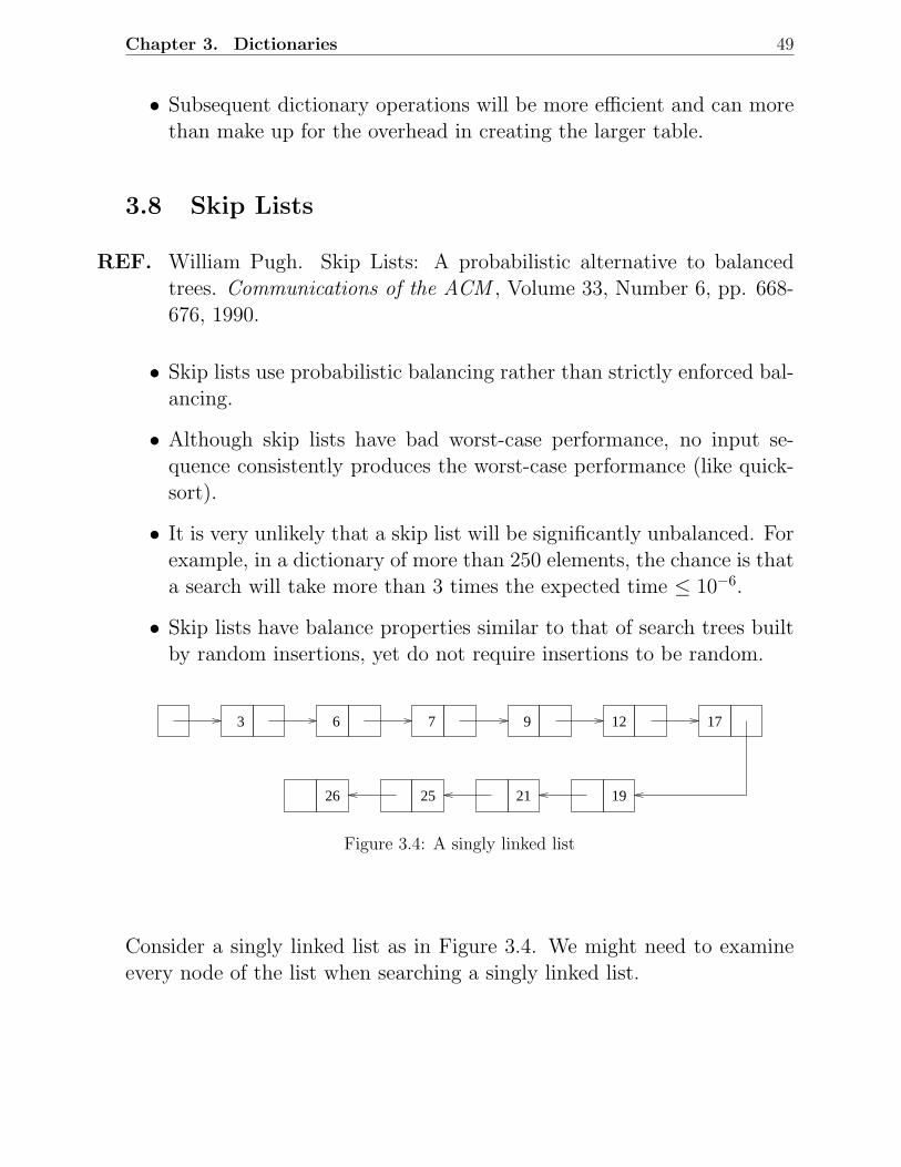
Chapter 3. Dictionaries 49
• Subsequent dictionary operations will be more efficient and can morethan make up for the overhead in creating the larger table.
3.8 Skip Lists
REF. William Pugh. Skip Lists: A probabilistic alternative to balancedtrees. Communications of the ACM , Volume 33, Number 6, pp. 668-676, 1990.
• Skip lists use probabilistic balancing rather than strictly enforced bal-ancing.
• Although skip lists have bad worst-case performance, no input se-quence consistently produces the worst-case performance (like quick-sort).
• It is very unlikely that a skip list will be significantly unbalanced. Forexample, in a dictionary of more than 250 elements, the chance is thata search will take more than 3 times the expected time ≤ 10−6.
• Skip lists have balance properties similar to that of search trees builtby random insertions, yet do not require insertions to be random.
3 6 7 9 12 17
26 25 21 19
Figure 3.4: A singly linked list
Consider a singly linked list as in Figure 3.4. We might need to examineevery node of the list when searching a singly linked list.
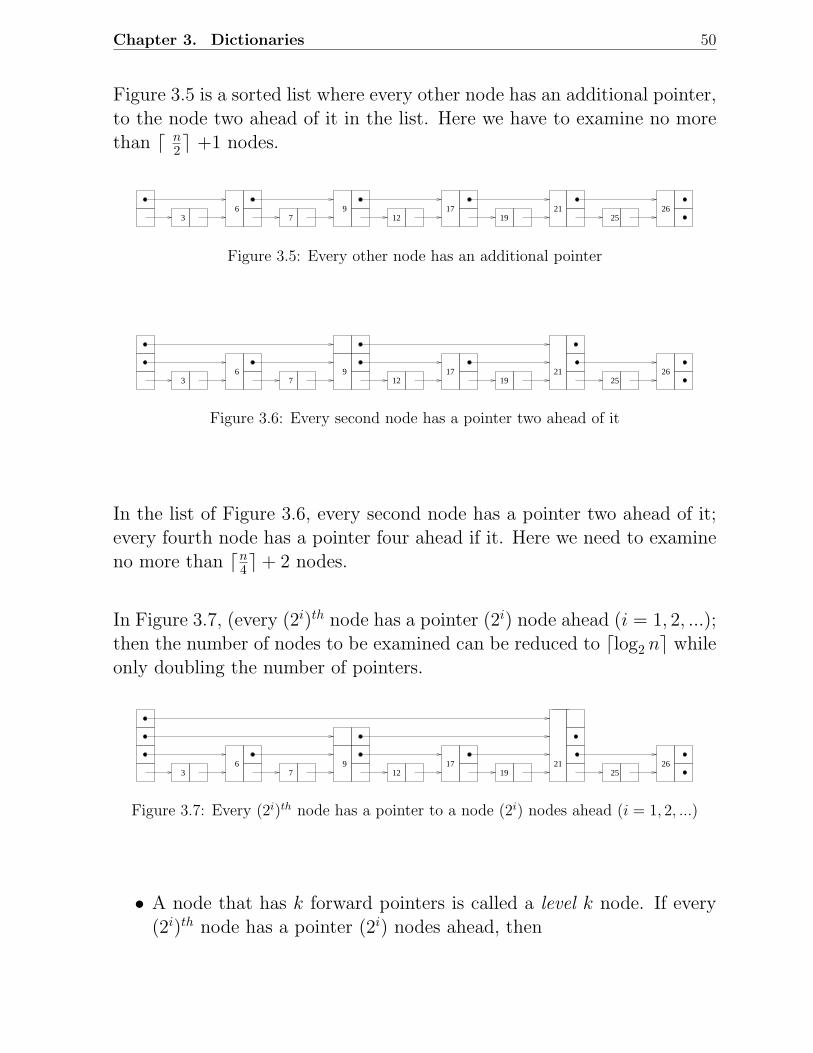
Chapter 3. Dictionaries 50
Figure 3.5 is a sorted list where every other node has an additional pointer,to the node two ahead of it in the list. Here we have to examine no morethan ⌈ n
2⌉ +1 nodes.
63 7
912
1719
2125
26
Figure 3.5: Every other node has an additional pointer
63 7
912
1719 25
2621
Figure 3.6: Every second node has a pointer two ahead of it
In the list of Figure 3.6, every second node has a pointer two ahead of it;every fourth node has a pointer four ahead if it. Here we need to examineno more than ⌈n
4⌉ + 2 nodes.
In Figure 3.7, (every (2i)th node has a pointer (2i) node ahead (i = 1, 2, ...);then the number of nodes to be examined can be reduced to ⌈log2 n⌉ whileonly doubling the number of pointers.
63 7
912
1719 25
2621
Figure 3.7: Every (2i)th node has a pointer to a node (2i) nodes ahead (i = 1, 2, ...)
• A node that has k forward pointers is called a level k node. If every(2i)th node has a pointer (2i) nodes ahead, then
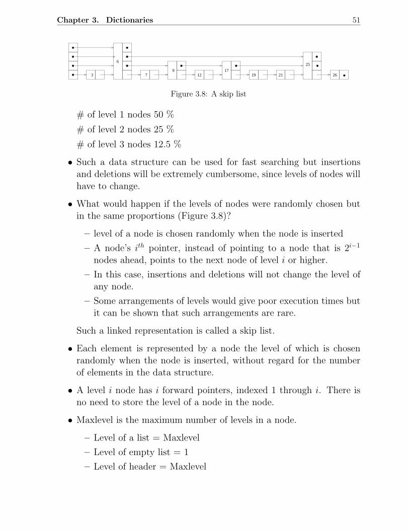
Chapter 3. Dictionaries 51
3 79
1217
19
6
21
25
26
Figure 3.8: A skip list
# of level 1 nodes 50 %
# of level 2 nodes 25 %
# of level 3 nodes 12.5 %
• Such a data structure can be used for fast searching but insertionsand deletions will be extremely cumbersome, since levels of nodes willhave to change.
• What would happen if the levels of nodes were randomly chosen butin the same proportions (Figure 3.8)?
– level of a node is chosen randomly when the node is inserted
– A node’s ith pointer, instead of pointing to a node that is 2i−1
nodes ahead, points to the next node of level i or higher.
– In this case, insertions and deletions will not change the level ofany node.
– Some arrangements of levels would give poor execution times butit can be shown that such arrangements are rare.
Such a linked representation is called a skip list.
• Each element is represented by a node the level of which is chosenrandomly when the node is inserted, without regard for the numberof elements in the data structure.
• A level i node has i forward pointers, indexed 1 through i. There isno need to store the level of a node in the node.
• Maxlevel is the maximum number of levels in a node.
– Level of a list = Maxlevel
– Level of empty list = 1
– Level of header = Maxlevel
Chapter 3. Dictionaries 52
3.8.1 Initialization:
An element NIL is allocated and given a key greater than any legal key.All levels of all lists are terminated with NIL. A new list is initialized sothat the level of list = maxlevel and all forward pointers of the list’s headerpoint to NIL
Search:
We search for an element by traversing forward pointers that do not over-shoot the node containing the element being searched for. When no moreprogress can be made at the current level of forward pointers, the searchmoves down to the next level. When we can make no more progress at level1, we must be immediately in front of the node that contains the desiredelement (if it is in the list).
Insertion and Deletion:
• Insertion and deletion are through search and splice
• update [i] contains a pointer to the rightmost node of level i or higherthat is to the left of the location of insertion or deletion.
• If an insertion generates a node with a level greater than the previousmaximum level, we update the maximum level and initialize appro-priate portions of update list.
• After a deletion, we check to see if we have deleted the maximum levelelement of the list and if so, decrease the maximum level of the list.
• Figure 3.9 provides an example of Insert and Delete. The pseudocodefor Insert and Delete is shown below.
search (list, searchkey);
x = list → header;
for (i = list → level; i ≥ 1; i – –)
while (x → forward[i] → key < searchkey)
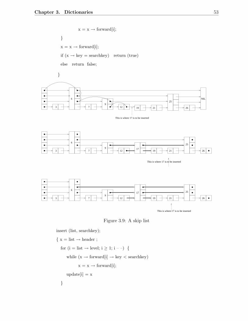
Chapter 3. Dictionaries 53
x = x → forward[i];
x = x → forward[i];
if (x → key = searchkey) return (true)
else return false;
3 79
12
6
3 79
12
6
19 21
25
26
This is where 17 is to be inserted
NIL
This is where 17 is to be inserted
1719 21 26
3 79
12
6
This is where 17 is to be inserted
25
17
19 21 26
25
Figure 3.9: A skip list
insert (list, searchkey);
x = list → header ;
for (i = list → level; i ≥ 1; i – –)
while (x → forward[i] → key < searchkey)
x = x → forward[i];
update[i] = x
Chapter 3. Dictionaries 54
x = x → forward[1];
if (x → key = searchkey) return (“key already present”)
else
newLevel = randomLevel();
if newLevel > list → level
for (i = list → level + 1; i ≤ newLevel; i ++ )
update[i] = list → header;
x = makenode(newLevel, searchkey);
for (i = 1, i ≤ newLevel; i++)
x → forward[i] = update[i] → forward[i];
update[i] → forward[i] = x
delete (list, searchkey);
x = list → header ;
for (i = list → level; i ≥ 1; i – )
while (x → forward[i] → key < searchkey)
x = x → forward[i];
update[i] = x
x = x → forward[1];
if (x → key = searchkey)
for (i = 1; i ≤ list → level; i ++)
if (update[i] → forward[i] 6= x)
break;
if (update[i] → forward[i] = x → forward[i];
free(x)
Chapter 3. Dictionaries 55
While (( list → 1) &&
(list → header → forward [list+level] = NIL))
list → level = list → level - 1
3.9 Analysis of Skip Lists
In a skiplist of 16 elements, we may have
• 9 elements at level 1
• 3 elements at level 2
• 3 elements at level 3
• 1 element at level 6
• One important question is:Where do we start our search? Analysis shows we should start fromlevel L(n) where
L(n) = log2 n
In general if p is the probability fraction,
L(n) = log 1
pn
where p is the fraction of the nodes with level i pointers which alsohave level (i + 1) pointers.
• However, starting at the highest level does not alter the efficiency ina significant way.
• Another important question to ask is:What should be MaxLevel? A good choice is
MaxLevel = L(N) = log 1
pN
where N is an upperbound on the number of elements is a skiplist.
Chapter 3. Dictionaries 56
• Complexity of search, delete, insert is dominated by the time requiredto search for the appropriate element. This in turn is proportional tothe length of the search path. This is determined by the pattern inwhich elements with different levels appear as we traverse the list.
• Insert and delete involve additional cost proportional to the level ofthe node being inserted or deleted.
3.9.1 Analysis of Expected Search Cost
We analyze the search path backwards, traveling up and to the left. Wepretend as if the level of a node is being determined only when it is observedwhile backtracking the search path.
1. From level 1, we rise to level L(n)
2. We move leftward
3. We climb from L(n) to maxLevel.
At a particular point in the climb, we are at the ith forward pointer ofa node x and we have no knowledge about the levels of nodes to the leftof x or about the level of x (other than that the level of x must be ≥ i ).See situation (a) in figure.
• Assume “x′′ is not the header.
• If level of x is i, then we are in situation (b). If level of x is > i, weare in situation (c).
• Prob we are in situation cA = p
• Each time we are in situation c, we climb up one level.
LetC(k) = expected length of a search path that
climbs up k levels in an infinite list.
Chapter 3. Dictionaries 57
Then:C(0) = 0C(k) = p cost in situation c
(1 − p) cost in situation b
We get
C(k) = p 1 + C(k − 1) + (1 − p)1 + C(k)C(k) = 1
p + C(k − 1)
C(k) = kp
Our assumption that the list is infinite is pessimistic.
When we bump into the header in our backward climb, we simply climb itup without performing any leftward (horizontal) movements.
This gives us an upperbound of
L(n) − 1
p
On the expected length of a path that climbs up from level 1 to level L(n)in a list of n elements. (because L(n) − 1 level are being climbed).
The rest of the journey includes
1. leftward movements, the number of which is bounded by the numberof elements of level L(n) or higher. his has an expected value = 1
p
2. We also move upwards from level L(n) to the maximum level in thelist.
p maximum level in the list > k= 1 − (1 − pk)n
≤ npk
Chapter 3. Dictionaries 58
p an element has a level > k = pk
=⇒ p an element has level ≤ k = 1 − pk
=⇒ p all n elements have level ≤ k = (1 − pk)n
=⇒ p at least one element has level ≥ k = 1 − (1 − pk)n
Expected maximum level ≤ npk
=⇒ Expected maximum level ≤ L(n) + 11−p
Putting our results together, we get:
Total expected cost to climb out of a list on n elements
≤ L(n)p + 1
p which is O(log n).
We can also compute the probability if the actual cost of a search exceedsexpected cost by more than a specified ratio.
Examples
1. p = 12 ; n = 256
p search will take longer than 3 times the expected cost = 106
2. p = 12 ; n = 4096
p search will take longer than 2 times the expected cost = 104
3. p = 12 ; n = 1024
p search will take longer than 3 times = 1018
How do we choose p ?
• Decreasing p increases variability of running times.
• p = 12 ; generation of random level can be done from a stream of
random bits.
Chapter 3. Dictionaries 59
• Decreasing p decreases # of pointers per node.
• Overheads are related to L(n) rather than L(n)p .
• p = 14 is probably the best choice, unless variability of running times
is an issue.
3.10 To Probe Further
1. Alfred V Aho, John E. Hopcroft, and Jeffrey D Ullman. Data Struc-tures and Algorithms . Addison-Wesley, 1983.
2. Thomas H. Cormen, Charles E. Leiserson, and Donald L. Rivest. In-troduction to Algorithms . The MIT Electrical Engineering and Com-puter Science Series, 1990. Indian Edition published in 1999.
3. Donald E Knuth. Fundamental Algorithms , Volume 1 of The Artof Computer Programming, Addison-Wesley, 1968, Second Edition,1973.
4. Robert L. Kruse, Bruce P. Leung, and Clovis L. Tondo. Data Struc-tures and Program design in C . Prentice Hall, 1991. Indian Editionpublished by Prentice Hall of India, 1999.
5. Mark Allen Weiss. Data Structures and Algorithm Analysis in C++.Benjamin-Cummings, 1994. Indian Edition published in 1998.
6. Ellis Horowitz, Sartaz Sahni, and Rajasekaran. Fundamentals of Com-puter Algorithms . W.H. Freeman and Company, 1998. Indian Editionpublished by Galgotia Publications, 2000.
7. Donald E. Knuth. Sorting and Searching , Volume 3 of The Art ofComputer Programming, Addison-Wesley, 1973.
8. Donald E Knuth. Seminumerical Algorithms . Volume 2 of The Artof Computer Programming, Addison-Wesley, 1969, Second Edition,1981.
Chapter 3. Dictionaries 60
9. Y. Langsam, M.J. Augenstein, and A.M. Tenenbaum. Data Struc-tures using C and C++. Second Edition, Prentice Hall, 1996. IndianEdition published by Prentice Hall of India, 2000.
10. Kurt Mehlhorn. Sorting and Searching. Volume 1 of Data Structuresand Algorithms. Springer-Verlag, 1984.
11. William Pugh. Skip Lists: A probabilistic alternative to balancedtrees. Communications of the ACM , Volume 33, Number 6, pp. 668-676, 1990.
3.11 Problems
1. Consider inserting the keys 10, 22, 31, 4, 15, 28, 17, 88, 59 into a closed hash tableof length m = 11 using the primary hashing function h(k) = k mod m. Illustratethe result of inserting these keys using
(a) Linear probing.
(b) Quadratic probing with hi(k) = (h(k) + i + 3i2) mod m.
(c) Double hashing with rehashing function hi(k) = (h(k) + i(1 + k mod (m −1)) mod m.
2. A closed hash table of size m is used to store n items, where n ≤ m/2.
(a) Assuming uniform hashing, show that for i = 1, 2, . . . , n, the probability thatthe ith insertion requires strictly more than k probes is at most 2−k.
(b) Show that for i = 1, 2, . . . , n, the probability that the ith insertion requiresmore than 2 log n probes is at most n−2.
3. Consider a closed hash table with 2n buckets (n > 0), employing the hash functionh(x) = x mod 2n. Which of the following rehash strategies would you prefer andwhy?
(a) Strategy 1: hi(x) = (h(x) + i) mod 2n.
(b) Strategy 2: hi(x) = (h(x) + 2i) mod 2n.
4. Given a set of a maximum of 52 names of 5 characters each and that not morethan two names start with the same character, is it possible to find a closed hashingfunction that operates on a hash table of size 56? Each element of the hash tablecan be a string of 5 characters. The hashing function should provide for membershiptest in at most 3 time units. Either exhibit such a hashing function or provide acounter-example. Assume that only upper case alphabetic characters are used in
Chapter 3. Dictionaries 61
names and that the hashing function can be computed in one time unit. Comparisonof strings also takes one time unit.
5. Consider all two character names with each character being from the set A,B,C,D,E, F,G,H, I, JDesign an efficient hashing function such that there would be no collisions on inser-tion. Assume a hash table of size 115.
6. Suppose that we are given a key k to search for in a closed hash table with positions0, 1, . . . ,m − 1, where m is known to be a power of 2. Let h be a hash function.Consider the following search scheme:
1. Compute i = h(k) and set j = 0.
2. Probe in position i. Terminate if the required item is found or that position isempty.
3. Set j = (j + 1) mod m and i = (i + j) mod m. Return to Step 2.
Answer the following questions and justify your answers.
a. Does the algorithm examine every table position in the worst case?
b. Is this linear probing or quadratic probing or double hashing or none?
c. What is the distinct number of probe sequences?
7. Given a skip list of 16 elements, compute the (best case) minimum number of probesrequired for an unsuccessful search in each case below:
(a) All nodes in the list are level 4 nodes
(b) There are 14 nodes of level 1 and 2 nodes of level 3
(c) There is one level 4 node, one level 3 node, and the rest are level 1 nodes
8. The following results have been experimentally observed by William Pugh in hisCACM article on skip lists, while comparing the average case performance of skiplists, splay trees, non-recursive AVL trees, and recursive 2-3 trees. Provide anintuitive justification for each of these:
(a) The non-recursive AVL tree has the least average case complexity for a dictio-nary search operation
(b) The skip list outperforms all other data structures for insertions and deletions
(c) Splay trees perform better than 2-3 trees for insertions
Chapter 3. Dictionaries 62
3.12 Programming Assignments
3.12.1 Hashing: Experimental Analysis
The objective of this assignment is to compare the performance of different hash tableorganizations, hashing methods, and collision resolution techniques.
Generation of Keys
Assume that your keys are character strings of length 10 obtained by scanning a C pro-gram. Call these as tokens. Define a token as any string that appears between successiveoccurrences of a forbidden character, where the forbidden set of characters is given by:
F = !, ”, #, %, &, (, ), ∗, +,−, ., /, :, ; , <,>, =, ?, [, ], , , , |, backslash, comma, space
Exceptions to the above rule are:
• Ignore anything that appears as comment (that is between /* and */)
• Ignore anything that appears between double quotes
That is, in the above two cases, the character strings are not to be taken as tokens.If a string has less than 10 characters, make it up to 10 characters by including anappropriate number of trailing *’s. On the other hand, if the current string has morethan 10 characters, truncate it to have the first ten characters only.
From the individual character strings (from now on called as tokens), generate apositive integer (from now on called as keys) by summing up the ASCII values of thecharacters in the particular token. Use this integer key in the hashing functions. However,remember that the original token is a character string and this is the one to be stored inthe hash table.
Hash Table Methods to be Evaluated
As discussed in the class, the following eleven schemes are to be evaluated.
1. Open with division method for hashing and unsorted lists for chaining
2. Open with division method for hashing and sorted lists for chaining
Chapter 3. Dictionaries 63
3. Open with multiplication method for hashing and unsorted lists for chaining
4. Open with multiplication method for hashing and sorted lists for chaining
5. Closed with simple coalesced hashing
6. Closed with linear probing
7. Closed with quadratic probing
8. Closed with double hashing
9. Closed with linear probing and Knuth-Amble method (Keys with same hash valueappear in descending order)
10. Closed with quadratic probing and Knuth-Amble method
11. Closed with double hashing and Knuth-Amble method
Hashing Functions
For the sake of uniformity, use the following hashing functions only. In the following, mis the hash table size (that is, the possible hash values are, 0, 1, . . . ,m − 1), and x is aninteger key.
1. Division Methodh(x) = x mod m
2. Multiplication Method
h(x) = Floor(m ∗ Fraction(k ∗ x))
where k =
√(5)−1
2, the Golden Ratio.
3. Linear Probing
h(x, i) = (h(x, 0) + i) mod m; i = 0, . . . ,m − 1
4. Quadratic Probing
h(x, i) = (h(x, 0) + i + i2) mod m; i = 0, . . . ,m − 1
5. Double Hashing
Use the division method for h(x) and the multiplication method for h′
(x).
Chapter 3. Dictionaries 64
Inputs to the Program
The possible inputs to the program are:
• m: Hash table size. Several values could be given here and the experiments areto be repeated for all values specified. If nothing is specified, assume all primarynumbers between 7 and 97.
• n: The initial number of insertions to be made for setting up a hash table with aparticular load factor.
• M : This is a subset of the set 1, 2, . . . , 11 indicating the set of methods to beinvestigated.
• I: This is a decimal number from which a ternary string is to be generated (namelythe radix-3 representation of I). In this representation, assume that a 0 representsthe search operation, a 1 represents the insert operation, and a 2 represents thedelete operation.
• A C program, from which the tokens are to be picked up for setting up and experi-menting with the hash table.
What should the Program Do?
1. For each element of M and for each value of m, do the following.
2. Scan the given C program and as you scan, insert the first n tokens scanned intoan initially empty hash table.
3. Now scan the rest of the C program token by token, searching for it or inserting itor deleting it, as dictated by the radix-3 representation of I. Note that the mostsignificant bit (tigit?) is to be considered first while doing this and you proceedfrom left to right in the radix-3 representation. For each individual operation, keeptrack of the number of probes.
4. Compute the average number of probes for a typical successful search, unsuccessfulsearch, insert, and delete.
5. Repeat Steps 2, 3, and 4 for each value of M and each value of m.
6. For each individual method investigated, obtain a table that lists the average numberof probes for the four cases for various values of m. The table entries can be of thefollowing format:
Hash table size Average Number of Probes forUsearch Ssearch Insert Delete
Chapter 3. Dictionaries 65
7. For each individual value of m, obtain a table that lists the average number ofprobes for various methods. The table entries can be of the following format:
Hash table method Average Number of Probes forUsearch Ssearch Insert Delete
3.12.2 Skip Lists: Experimental Analysis
Implement skip list data structure. Analyze the efficiency of search, insert, and delete operations
on randomly generated inputs. Carefully take into account all the tradeoffs involved in designing
and implementing skip lists. Validate the experimental results with those given in the article
by William Pugh (Skip Lists: A probabilistic alternative to balanced trees. Communications
of the ACM , Volume 33, Number 6, pp. 668-676, 1990). Design and carry out experiments to
compare the performance of skip lists with that of hash tables.
Chapter 4
Binary Trees
4.1 Introduction
Trees are very useful and important abstractions in Computer Science.They are ideally suited to representing hierarchical relationships amongelements in a universe. Efficient implementations of abstract data typessuch as dictionaries and priority queues are invariably in terms of binaryor general trees.
4.1.1 Definitions
We shall first present some definitions and then introduce the Tree ADT.
• Tree:
1. A single node is a tree and this node is the root of the tree.
2. Suppose r is a node and T1, T2, . . . , Tk are trees with roots r1, r2, . . . , rk,respectively, then we can construct a new tree whose root is r andT1, T2, . . . , Tk are the subtrees of the root. The nodes r1, r2, . . . , rk
are called the children of r.
See Figure 4.1. Often, it is convenient to include among trees, thenull tree, which is a tree with no nodes.
66
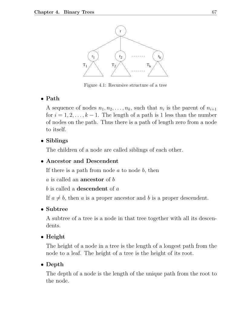
Chapter 4. Binary Trees 67
r
2r
1 TkT
1r kr
T2
Figure 4.1: Recursive structure of a tree
• Path
A sequence of nodes n1, n2, . . . , nk, such that ni is the parent of ni+1
for i = 1, 2, . . . , k − 1. The length of a path is 1 less than the numberof nodes on the path. Thus there is a path of length zero from a nodeto itself.
• Siblings
The children of a node are called siblings of each other.
• Ancestor and Descendent
If there is a path from node a to node b, then
a is called an ancestor of b
b is called a descendent of a
If a 6= b, then a is a proper ancestor and b is a proper descendent.
• Subtree
A subtree of a tree is a node in that tree together with all its descen-dents.
• Height
The height of a node in a tree is the length of a longest path from thenode to a leaf. The height of a tree is the height of its root.
• Depth
The depth of a node is the length of the unique path from the root tothe node.
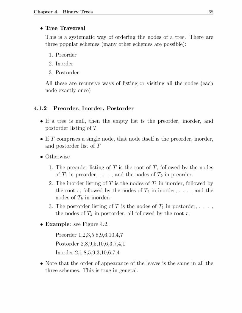
Chapter 4. Binary Trees 68
• Tree Traversal
This is a systematic way of ordering the nodes of a tree. There arethree popular schemes (many other schemes are possible):
1. Preorder
2. Inorder
3. Postorder
All these are recursive ways of listing or visiting all the nodes (eachnode exactly once)
4.1.2 Preorder, Inorder, Postorder
• If a tree is null, then the empty list is the preorder, inorder, andpostorder listing of T
• If T comprises a single node, that node itself is the preorder, inorder,and postorder list of T
• Otherwise
1. The preorder listing of T is the root of T , followed by the nodesof T1 in preorder, . . . , and the nodes of Tk in preorder.
2. The inorder listing of T is the nodes of T1 in inorder, followed bythe root r, followed by the nodes of T2 in inorder, . . . , and thenodes of Tk in inorder.
3. The postorder listing of T is the nodes of T1 in postorder, . . . ,the nodes of Tk in postorder, all followed by the root r.
• Example: see Figure 4.2.
Preorder 1,2,3,5,8,9,6,10,4,7
Postorder 2,8,9,5,10,6,3,7,4,1
Inorder 2,1,8,5,9,3,10,6,7,4
• Note that the order of appearance of the leaves is the same in all thethree schemes. This is true in general.
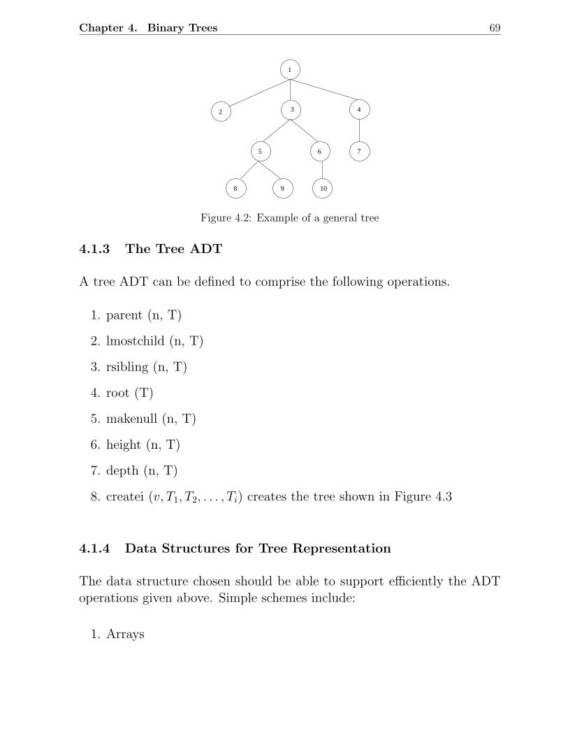
Chapter 4. Binary Trees 69
3
1
2
5
9 10
6
4
7
8
Figure 4.2: Example of a general tree
4.1.3 The Tree ADT
A tree ADT can be defined to comprise the following operations.
1. parent (n, T)
2. lmostchild (n, T)
3. rsibling (n, T)
4. root (T)
5. makenull (n, T)
6. height (n, T)
7. depth (n, T)
8. createi (v, T1, T2, . . . , Ti) creates the tree shown in Figure 4.3
4.1.4 Data Structures for Tree Representation
The data structure chosen should be able to support efficiently the ADToperations given above. Simple schemes include:
1. Arrays
Chapter 4. Binary Trees 70
V
1T 2T iT
Figure 4.3: A tree with i subtrees
2. Lists of children
3. Leftmost child-right sibling representation
For a detailed discussion of data structures to support Tree ADT opera-tions, refer to the book by Aho, Hopcroft, and Ullman (1983).
4.2 Binary Trees
Definition: A binary tree is either empty or consists of a node called theroot together with two binary trees called the left subtree and the rightsubtree.
• If h = height of a binary tree,
max # of leaves = 2h
max # of nodes = 2h+1 − 1
• A binary tree with height h and 2h+1 − 1 nodes (or 2h leaves) is calleda full binary tree
• Figure 4.4 shows several examples of binary trees.
• The nodes of a binary tree can be numbered in a natural way, levelby level, left to right. For example, see Figure 4.5.
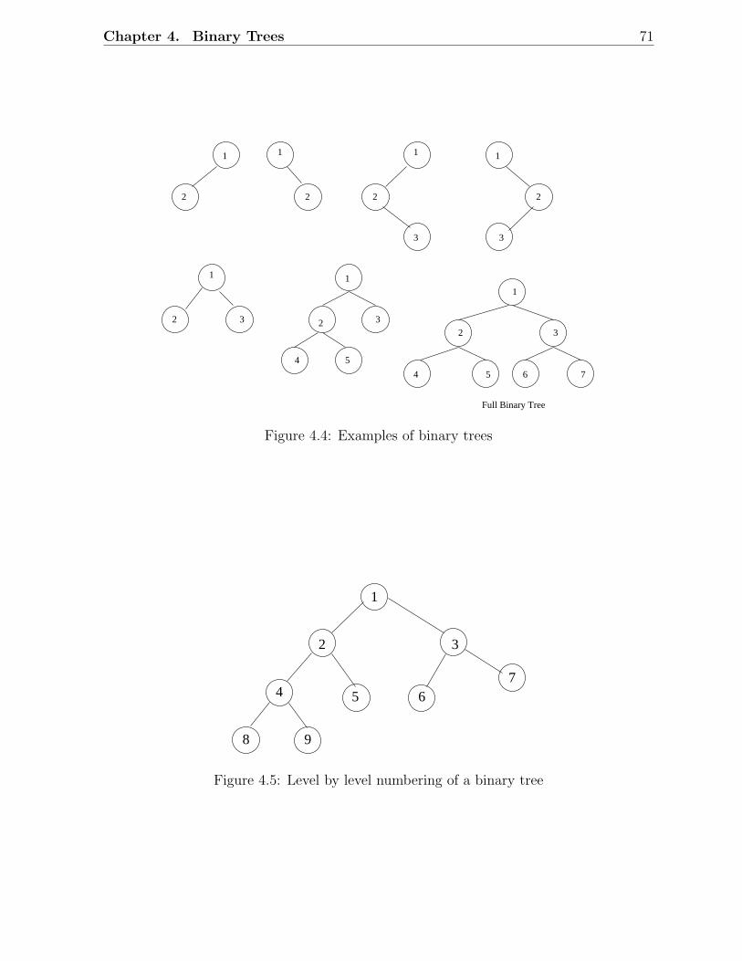
Chapter 4. Binary Trees 71
1
2
3
4 5
6 7
Full Binary Tree
1 1 1
1 1
1
2 2 2
2 22
3
3 3
3
4 5
Figure 4.4: Examples of binary trees
1
2
5
98
4
3
76
Figure 4.5: Level by level numbering of a binary tree
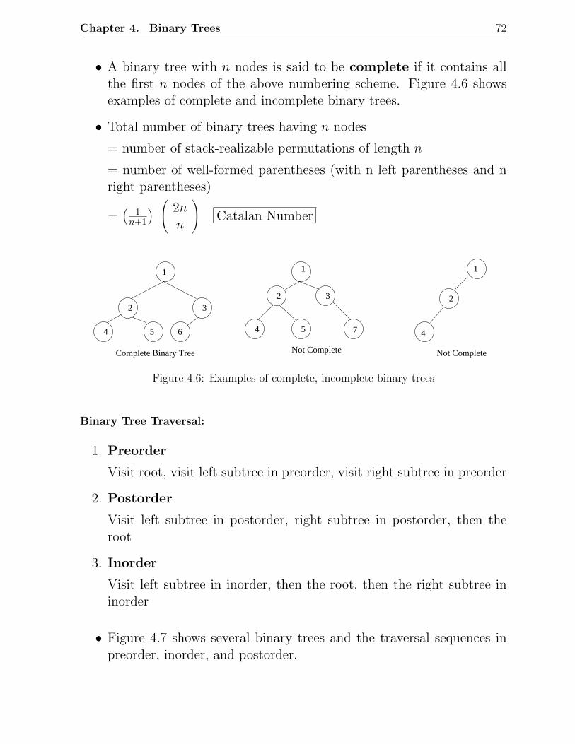
Chapter 4. Binary Trees 72
• A binary tree with n nodes is said to be complete if it contains allthe first n nodes of the above numbering scheme. Figure 4.6 showsexamples of complete and incomplete binary trees.
• Total number of binary trees having n nodes
= number of stack-realizable permutations of length n
= number of well-formed parentheses (with n left parentheses and nright parentheses)
=(
1n+1
)
2nn
Catalan Number
7
1
2 3
5 64
Complete Binary Tree
1 1
2 23
4 5
Not Complete
4
Not Complete
Figure 4.6: Examples of complete, incomplete binary trees
Binary Tree Traversal:
1. Preorder
Visit root, visit left subtree in preorder, visit right subtree in preorder
2. Postorder
Visit left subtree in postorder, right subtree in postorder, then theroot
3. Inorder
Visit left subtree in inorder, then the root, then the right subtree ininorder
• Figure 4.7 shows several binary trees and the traversal sequences inpreorder, inorder, and postorder.
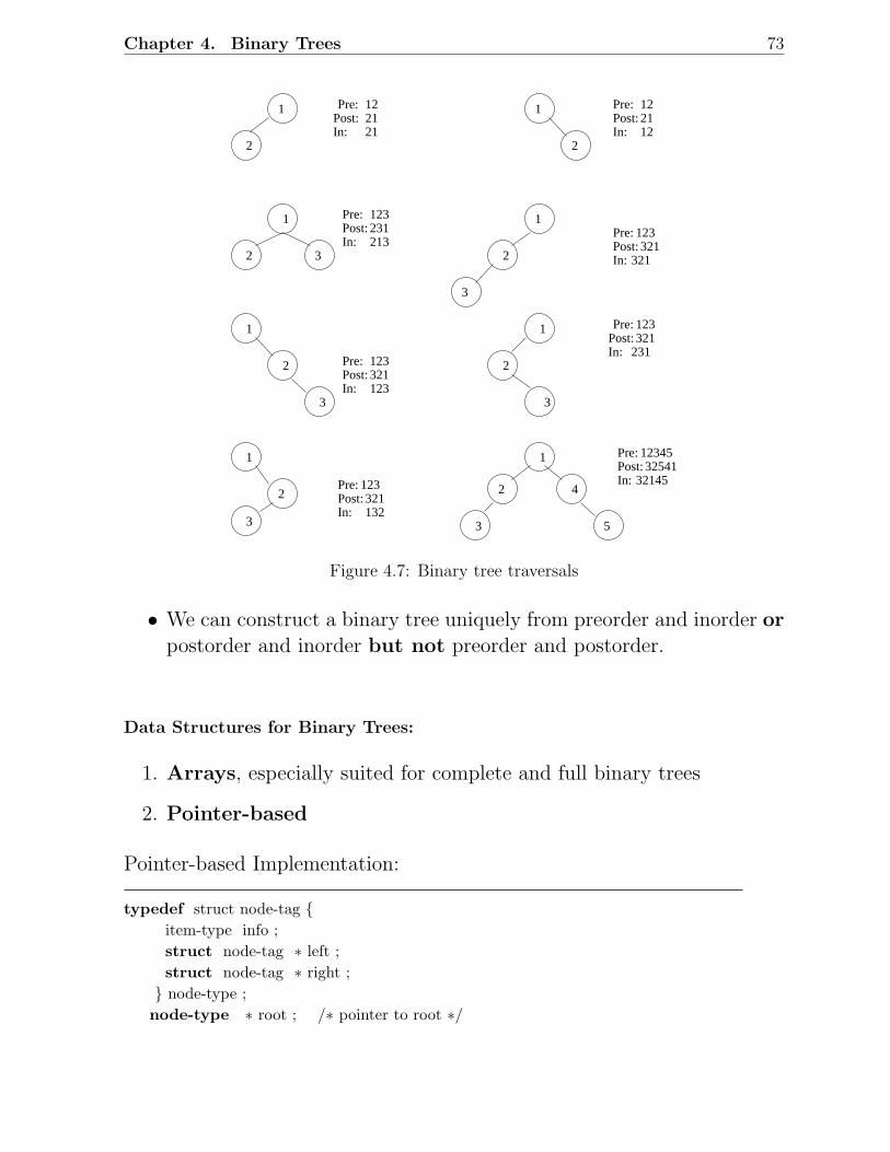
Chapter 4. Binary Trees 73
1
2
3
3 5
1
2
1
2 2
2
2 2
2
1
1 1
1 1
3
3 3
3
4
Pre:
Pre:
Pre:
Pre: Pre:
Pre:
Pre:
Pre:
Post:
Post:
Post:
Post:
Post:
Post:
Post:
Post:
In:
In:
In:
In:
In:
In:
In:
In:
1221
231213
123
321
132
1234532541
32145
212112
12
123321
321
123
123
123321
123321
231
Figure 4.7: Binary tree traversals
• We can construct a binary tree uniquely from preorder and inorder orpostorder and inorder but not preorder and postorder.
Data Structures for Binary Trees:
1. Arrays, especially suited for complete and full binary trees
2. Pointer-based
Pointer-based Implementation:
typedef struct node-tag item-type info ;
struct node-tag ∗ left ;
struct node-tag ∗ right ;
node-type ;
node-type ∗ root ; /∗ pointer to root ∗/
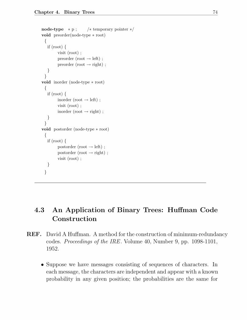
Chapter 4. Binary Trees 74
node-type ∗ p ; /∗ temporary pointer ∗/void preorder(node-type ∗ root)
if (root)
visit (root) ;
preorder (root → left) ;
preorder (root → right) ;
void inorder (node-type ∗ root)
if (root)
inorder (root → left) ;
visit (root) ;
inorder (root → right) ;
void postorder (node-type ∗ root)
if (root)
postorder (root → left) ;
postorder (root → right) ;
visit (root) ;
4.3 An Application of Binary Trees: Huffman Code
Construction
REF. David A Huffman. A method for the construction of minimum-redundancycodes. Proceedings of the IRE . Volume 40, Number 9, pp. 1098-1101,1952.
• Suppose we have messages consisting of sequences of characters. Ineach message, the characters are independent and appear with a knownprobability in any given position; the probabilities are the same for
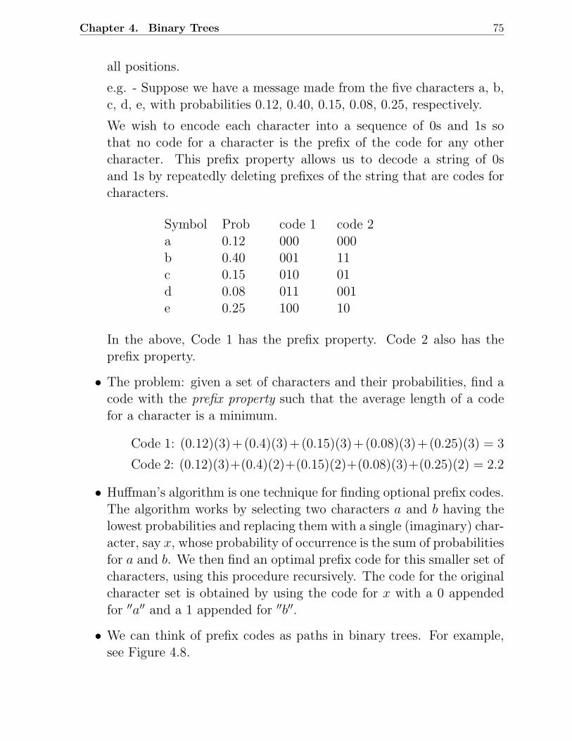
Chapter 4. Binary Trees 75
all positions.
e.g. - Suppose we have a message made from the five characters a, b,c, d, e, with probabilities 0.12, 0.40, 0.15, 0.08, 0.25, respectively.
We wish to encode each character into a sequence of 0s and 1s sothat no code for a character is the prefix of the code for any othercharacter. This prefix property allows us to decode a string of 0sand 1s by repeatedly deleting prefixes of the string that are codes forcharacters.
Symbol Prob code 1 code 2a 0.12 000 000b 0.40 001 11c 0.15 010 01d 0.08 011 001e 0.25 100 10
In the above, Code 1 has the prefix property. Code 2 also has theprefix property.
• The problem: given a set of characters and their probabilities, find acode with the prefix property such that the average length of a codefor a character is a minimum.
Code 1: (0.12)(3)+(0.4)(3)+(0.15)(3)+(0.08)(3)+(0.25)(3) = 3
Code 2: (0.12)(3)+(0.4)(2)+(0.15)(2)+(0.08)(3)+(0.25)(2) = 2.2
• Huffman’s algorithm is one technique for finding optional prefix codes.The algorithm works by selecting two characters a and b having thelowest probabilities and replacing them with a single (imaginary) char-acter, say x, whose probability of occurrence is the sum of probabilitiesfor a and b. We then find an optimal prefix code for this smaller set ofcharacters, using this procedure recursively. The code for the originalcharacter set is obtained by using the code for x with a 0 appendedfor ′′a′′ and a 1 appended for ′′b′′.
• We can think of prefix codes as paths in binary trees. For example,see Figure 4.8.
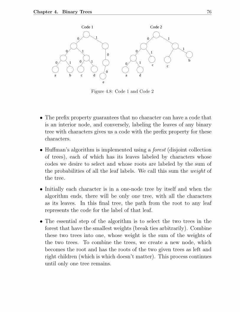
Chapter 4. Binary Trees 76
a b c d
e
0
00
0
0 1
1
10
1
Code 1
a d
c c
b1
1
1
1
0
0
0
Code 2
Figure 4.8: Code 1 and Code 2
• The prefix property guarantees that no character can have a code thatis an interior node, and conversely, labeling the leaves of any binarytree with characters gives us a code with the prefix property for thesecharacters.
• Huffman’s algorithm is implemented using a forest (disjoint collectionof trees), each of which has its leaves labeled by characters whosecodes we desire to select and whose roots are labeled by the sum ofthe probabilities of all the leaf labels. We call this sum the weight ofthe tree.
• Initially each character is in a one-node tree by itself and when thealgorithm ends, there will be only one tree, with all the charactersas its leaves. In this final tree, the path from the root to any leafrepresents the code for the label of that leaf.
• The essential step of the algorithm is to select the two trees in theforest that have the smallest weights (break ties arbitrarily). Combinethese two trees into one, whose weight is the sum of the weights ofthe two trees. To combine the trees, we create a new node, whichbecomes the root and has the roots of the two given trees as left andright children (which is which doesn’t matter). This process continuesuntil only one tree remains.
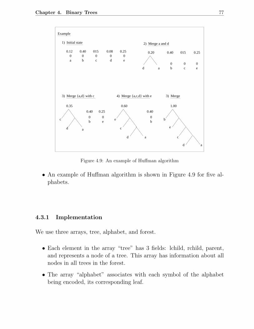
Chapter 4. Binary Trees 77
Example
0.12 0.40 015 0.08 0.250 0 00a b c d
0e
1) Initial state
1.00
3) Merge
ad
c
b
e
0.20
d a b c
0.40 015 0.25
e0 0 0
2) Merge a and d
0.60
4) Merge a,c,d with e
ad
c
e
0.40
0b
0.35
b0 0
3) Merge a,d with c
a
c
d
0.40
e
0.25
Figure 4.9: An example of Huffman algorithm
• An example of Huffman algorithm is shown in Figure 4.9 for five al-phabets.
4.3.1 Implementation
We use three arrays, tree, alphabet, and forest.
• Each element in the array “tree” has 3 fields: lchild, rchild, parent,and represents a node of a tree. This array has information about allnodes in all trees in the forest.
• The array “alphabet” associates with each symbol of the alphabetbeing encoded, its corresponding leaf.
Chapter 4. Binary Trees 78
1
2
3
4
5
.12
.40
.15
.08
.25
1
2
3
4
5
weight root
Forest
1
2
3
4
5
.12
.40
.15
.08
.25
1
2
3
4
5
a
c
d
e
b
1 0 0
0
0
0
00
0
0
00
0
0
0
0
lchild rchild parent
2
3
4
5
(Dynamic)(Dynamic) (Static)
Alphabet
Shrinks grows
as many elements as the numberof trees in the forest currently
as many elements as the numberof nodes in all the current trees of the forest
Figure 4.10: Initial state of data structures
• The array “forest” represents the collection of all trees. Initial valuesof these arrays are shown as follows:
• Figure 4.10 shows the above three data structures for our example.
4.3.2 Sketch of Huffman Tree Construction
1. while (there is more than one tree in the forest) do
2. i = index of tree in forest with smallest weight ;
3. j = index of tree in forest with second smallest weight ;
4. create a new node with
lchild = forest [i].root ;
rchild = forest [j].root ;
5. replace tree i in forest by a tree with root as new node, with
weight = forest [i] → weight + forest[j] → weight ;
6. delete tree j from forest
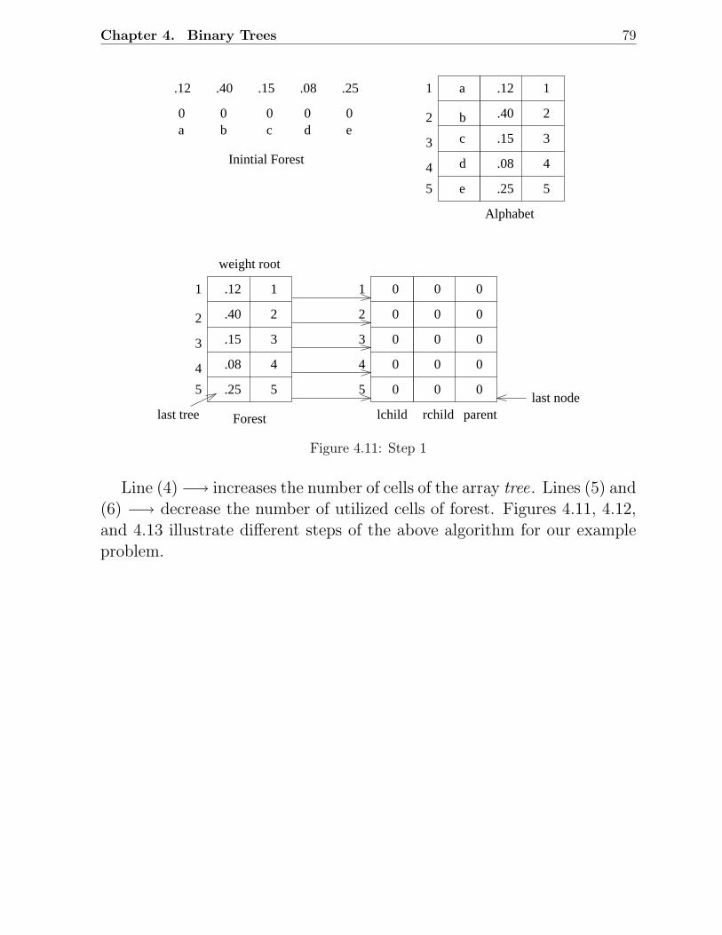
Chapter 4. Binary Trees 79
1
2
3
4
5
.12
.40
.15
.08
.25
1
2
3
4
5
1 0 0
0
0
0
00
0
0
00
0
0
0
0
lchild rchild parent
2
3
4
5
weight root
last treelast node
.12 .40 .15 .08 .25 1
2
3
4
5
.12
.40
.15
.08
.25
1
2
3
4
5
a
c
d
e
b0 0 0 00c d eba
Inintial Forest
Forest
Alphabet
Figure 4.11: Step 1
Line (4) −→ increases the number of cells of the array tree. Lines (5) and(6) −→ decrease the number of utilized cells of forest. Figures 4.11, 4.12,and 4.13 illustrate different steps of the above algorithm for our exampleproblem.
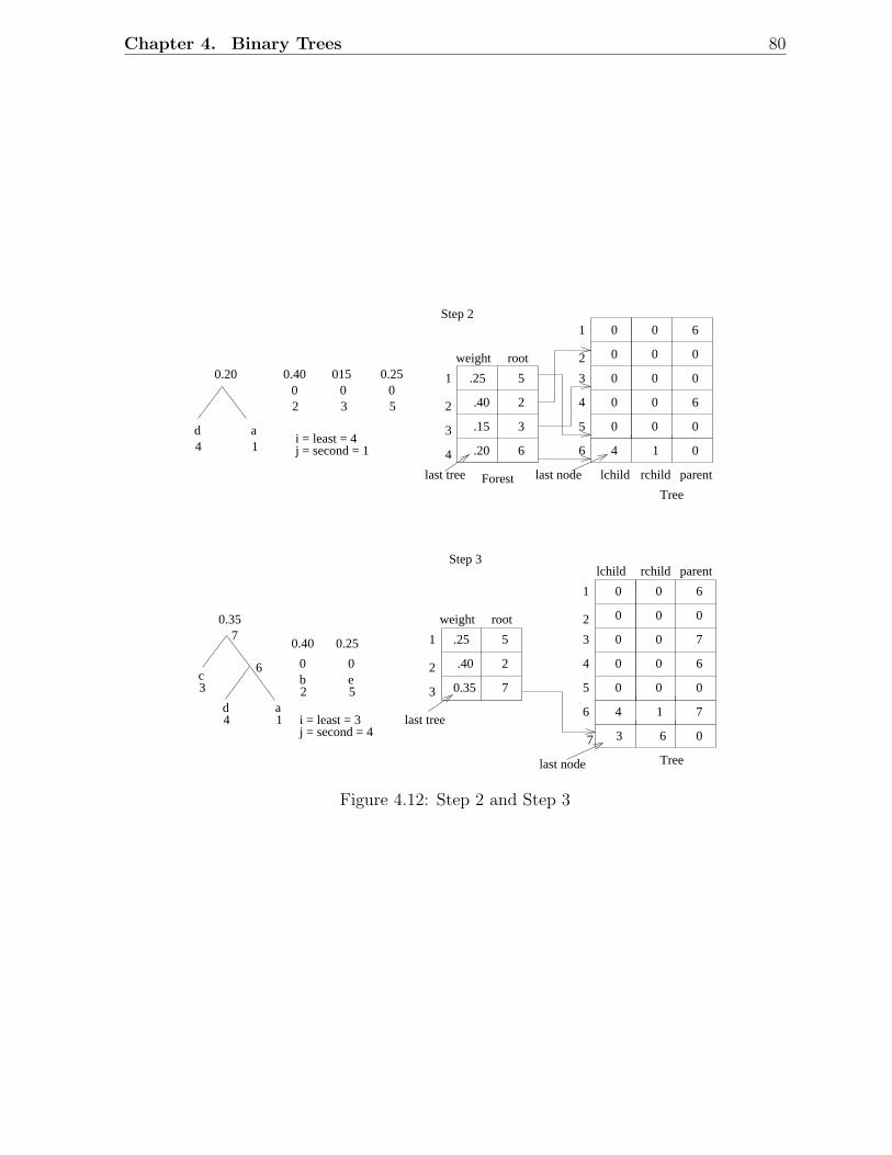
Chapter 4. Binary Trees 80
1
2
3
.40 2
7
.25 5
weight root
b0 0
a
0.40
e
0.25
c
d4 1
3
6
70.35
2 5
i = least = 3j = second = 4
0.35
last tree
1
5
0 6
0
7
6
00
0
0
00
0
0
0
0
4 1 7
2
3
6
lchild rchild parent
0637
last node Tree
Step 3
Step 2
0.20
d a
0.40 015 0.25
4 1
0 0 02 3 5
i = least = 4j = second = 1
last node
1
2
3
4
.40
.15
.20
2
3
6
.25 5
Forestlast tree
weight root
1
5
0 6
0
0
6
00
0
0
00
0
0
0
0
4 1 0
lchild rchild parent
2
3
6
Tree
4
4
Figure 4.12: Step 2 and Step 3
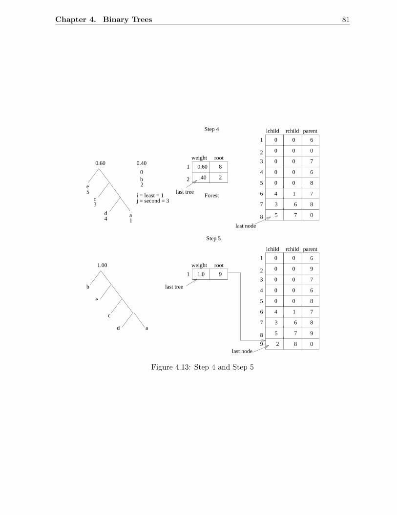
Chapter 4. Binary Trees 81
1
5
0 6
0
7
6
0
0
0
00
0
0
0
0
4 1 7
2
3
6
lchild rchild parent
63
4
7
8
last node
8
8
075
b0
0.40
2
0.60
d
c
a
i = least = 1j = second = 3
Step 4
4 1
5e
3
Step 5
1.00
ad
c
b
e
1 9
weight root
1.0
1
5
0 6
7
6
0
0
0
00
0
0
0
0
4 1 7
2
3
6
lchild rchild parent
63
4
7
8
8
8
75
1
2 .40
8
weight root
0.60
last tree
2
Forest
last tree
9last node
2 8 0
9
9
Figure 4.13: Step 4 and Step 5
Chapter 4. Binary Trees 82
4.4 Binary Search Tree
• A prominent data structure used in many systems programming ap-plications for representing and managing dynamic sets.
• Average case complexity of Search, Insert, and Delete Operations isO(log n), where n is the number of nodes in the tree.
• DEF: A binary tree in which the nodes are labeled with elements ofan ordered dynamic set and the following BST property is satisfied:all elements stored in the left subtree of any node x are less than theelement stored at x and all elements stored in the right subtree of xare greater than the element at x.
• An Example: Figure 4.14 shows a binary search tree. Notice thatthis tree is obtained by inserting the values 13, 3, 4, 12, 14, 10, 5, 1,8, 2, 7, 9, 11, 6, 18 in that order, starting from an empty tree.
• Note that inorder traversal of a binary search tree always gives asorted sequence of the values. This is a direct consequence of the BSTproperty. This provides a way of sorting a given sequence of keys:first, create a BST with these keys and then do an inorder traversalof the BST so created.
• Note that the highest valued element in a BST can be found by travers-ing from the root in the right direction all along until a node with noright link is found (we can call that the rightmost element in the BST).
• The lowest valued element in a BST can be found by traversing fromthe root in the left direction all along until a node with no left link isfound (we can call that the leftmost element in the BST).
• Search is straightforward in a BST. Start with the root and keepmoving left or right using the BST property. If the key we are seekingis present, this search procedure will lead us to the key. If the key isnot present, we end up in a null link.
• Insertion in a BST is also a straightforward operation. If we needto insert an element x, we first search for x. If x is present, there is
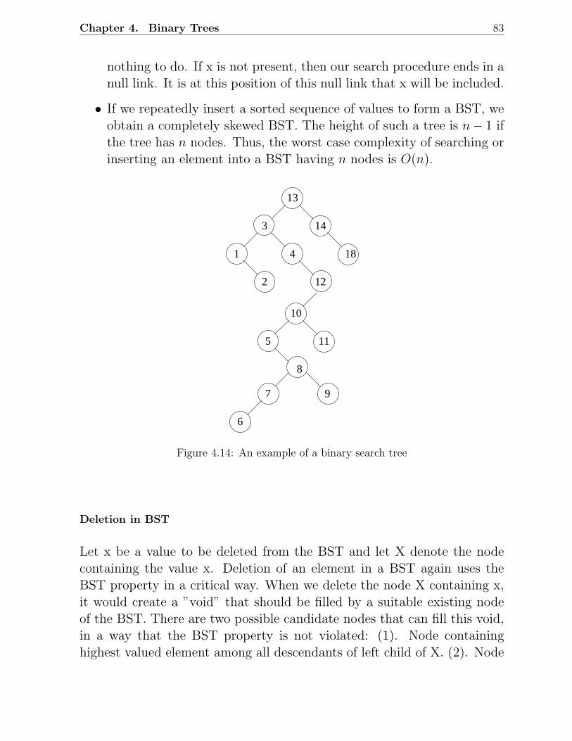
Chapter 4. Binary Trees 83
nothing to do. If x is not present, then our search procedure ends in anull link. It is at this position of this null link that x will be included.
• If we repeatedly insert a sorted sequence of values to form a BST, weobtain a completely skewed BST. The height of such a tree is n− 1 ifthe tree has n nodes. Thus, the worst case complexity of searching orinserting an element into a BST having n nodes is O(n).
122
10
5 11
8
7
6
9
18
13
143
41
Figure 4.14: An example of a binary search tree
Deletion in BST
Let x be a value to be deleted from the BST and let X denote the nodecontaining the value x. Deletion of an element in a BST again uses theBST property in a critical way. When we delete the node X containing x,it would create a ”void” that should be filled by a suitable existing nodeof the BST. There are two possible candidate nodes that can fill this void,in a way that the BST property is not violated: (1). Node containinghighest valued element among all descendants of left child of X. (2). Node
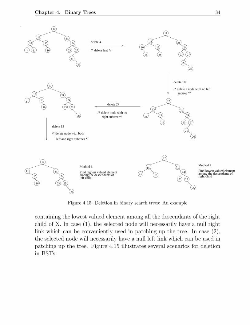
Chapter 4. Binary Trees 84
delete 4
/* delete leaf */
delete 10
/* delete a node with no left subtree */
delete 27
/* delete node with noright subtree */
delete 13
/* delete node with both
left and right subtrees */
Method 1.
Find highest valued elementamong the descendants ofleft child
Find lowest valued element
Method 2
among the descendants ofright child
17
13 21
15 2410
4 11 16 23 27
25
26
17
13 21
15 24
16 23
11
25
26
17
21
15 24
16 23 25
26
11
17
13 21
15 24
16 23 27
25
26
11
17
21
24
23 25
26
15
1611
17
13 21
15 2410
11 16 23 27
25
26
Figure 4.15: Deletion in binary search trees: An example
containing the lowest valued element among all the descendants of the rightchild of X. In case (1), the selected node will necessarily have a null rightlink which can be conveniently used in patching up the tree. In case (2),the selected node will necessarily have a null left link which can be used inpatching up the tree. Figure 4.15 illustrates several scenarios for deletionin BSTs.
Chapter 4. Binary Trees 85
4.4.1 Average Case Analysis of BST Operations
RESULT
If we insert n random elements into an initially empty BST, then theaverage path length from the root to a node is O(log n)
• Note that the BST is formed by insertions only. Obviously the treeso formed need not be complete.
• We shall assume that all orders of n inserted elements are equallylikely. This means that any of the n! permutations is equally likely tobe the sequence of keys inserted.
LetP(n) = average path length in a BST with n nodes
(average number of nodes on the path from the rootto a node, not necessarily a leaf)
Leta = first element inserted. This will be the root of
the BST. Also this is equally likely to be the first, second. . . , ith, . . . , or nth in the sorted order of then elements.
Note that P(0) = 0 and P(1) = 1. Consider a fixed i, 0 ≤ i ≤ n − 1. If ielements are less than a, the BST will look like in Figure 4.16.
• Since all orders for the i small elements are equally likely and likewisefor the (n − i − 1) larger elements,
Average path length in the
– left subtree = P(i)
– right subtree = P(n − i − 1)
• For a fixed i, let us compute the average path length of the above tree.
Number of probes if the element a is being sought = 1
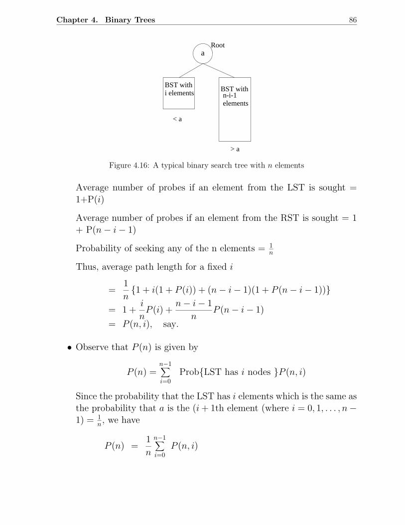
Chapter 4. Binary Trees 86
a
n-i-1elements
< a
> a
BST withi elements
BST with
Root
Figure 4.16: A typical binary search tree with n elements
Average number of probes if an element from the LST is sought =1+P(i)
Average number of probes if an element from the RST is sought = 1+ P(n − i − 1)
Probability of seeking any of the n elements = 1n
Thus, average path length for a fixed i
=1
n1 + i(1 + P (i)) + (n − i − 1)(1 + P (n − i − 1))
= 1 +i
nP (i) +
n − i − 1
nP (n − i − 1)
= P (n, i), say.
• Observe that P (n) is given by
P (n) =n−1∑
i=0
ProbLST has i nodes P (n, i)
Since the probability that the LST has i elements which is the same asthe probability that a is the (i + 1th element (where i = 0, 1, . . . , n −1) = 1
n , we have
P (n) =1
n
n−1∑
i=0
P (n, i)
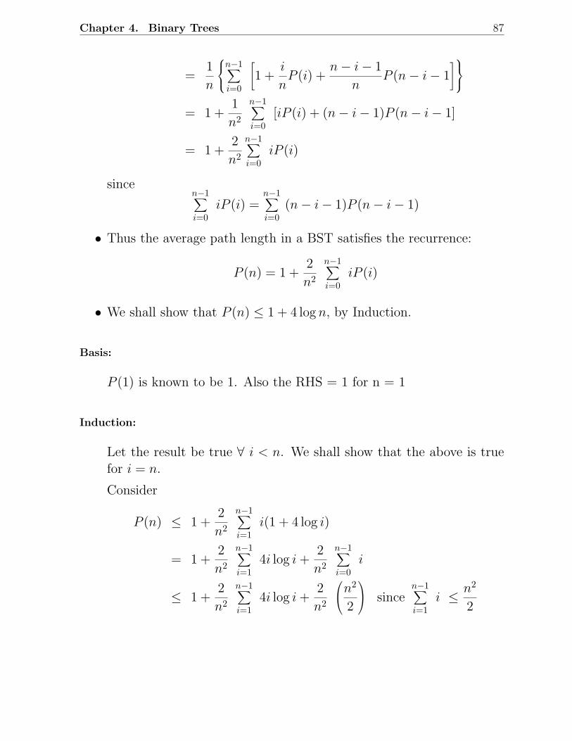
Chapter 4. Binary Trees 87
=1
n
n−1∑
i=0
[
1 +i
nP (i) +
n − i − 1
nP (n − i − 1
]
= 1 +1
n2
n−1∑
i=0
[iP (i) + (n − i − 1)P (n − i − 1]
= 1 +2
n2
n−1∑
i=0
iP (i)
sincen−1∑
i=0
iP (i) =n−1∑
i=0
(n − i − 1)P (n − i − 1)
• Thus the average path length in a BST satisfies the recurrence:
P (n) = 1 +2
n2
n−1∑
i=0
iP (i)
• We shall show that P (n) ≤ 1 + 4 log n, by Induction.
Basis:
P (1) is known to be 1. Also the RHS = 1 for n = 1
Induction:
Let the result be true ∀ i < n. We shall show that the above is truefor i = n.
Consider
P (n) ≤ 1 +2
n2
n−1∑
i=1
i(1 + 4 log i)
= 1 +2
n2
n−1∑
i=1
4i log i +2
n2
n−1∑
i=0
i
≤ 1 +2
n2
n−1∑
i=1
4i log i +2
n2
n2
2
sincen−1∑
i=1
i ≤ n2
2
Chapter 4. Binary Trees 88
Thus
P (n) ≤ 2 +8
n2
n−1∑
i=1
i log i
Now
n−1∑
i=1
i log i =⌈n
2⌉−1
∑
i=1
i log i +n−1∑
i=⌈n2⌉
i log i
≤⌈n
2⌉−1
∑
i=1
i logn
2+
n−1∑
i=⌈n2⌉
i log n
≤ n2
8log
n
2+
3n2
8log n
=n2
2log n − n2
8
Therefore
P (n) ≤ 2 +8
n2
n2
2log−n2
8
= 1 + 4 log n
A more careful analysis can be done and it can be shown that
P (n) ≤ 1 + 1.4 log n
4.5 Splay Trees
REF. Daniel D Sleator and Robert E. Tarjan. Self-adjusting binary searchtrees. Journal of the ACM , Volume 32, Number 3, pp. 652-686, 1985.
REF. Robert E. Tarjan. Amortized computational complexity. SIAM Jour-nal on Algebraic and Discrete Methods , Volume 6, Number 2, pp.306-318, 1985.
• These are binary search trees which are self-adjusting in the followingway:
Every time we access a node of the tree, whether for retrieval or in-sertion or deletion, we perform radical surgery on the tree, resulting
Chapter 4. Binary Trees 89
in the newly accessed node becoming the root of the modified tree.This surgery will ensure that nodes that are frequently accessed willnever drift too far away from the root whereas inactive nodes will getpushed away farther from the root.
• Amortized complexity
– Splay trees can become highly unbalanced so that a single accessto a node of the tree can be quite expensive.
– However, over a long sequence of accesses, the few expensive casesare averaged in with many inexpensive cases to obtain good per-formance.
• Does not need heights or balance factors as in AVL trees and coloursas in Red-Black trees.
• The surgery on the tree is done using rotations, also called as splayingsteps. There are six different splaying steps.
1. Zig Rotation (Right Rotation)
2. Zag Rotation (Left Rotation)
3. Zig-Zag (Zig followed by Zag)
4. Zag-Zig (Zag followed by Zig)
5. Zig-Zig
6. Zag-Zag
• Consider the path going from the root down to the accessed node.
– Each time we move left going down this path, we say we “zig”and each time we move right, we say we “zag.”
• Zig Rotation and Zag Rotation
– Note that a zig rotation is the same as a right rotation whereasthe zag step is the left rotation.
– See Figure 4.17.
• Zig-Zag
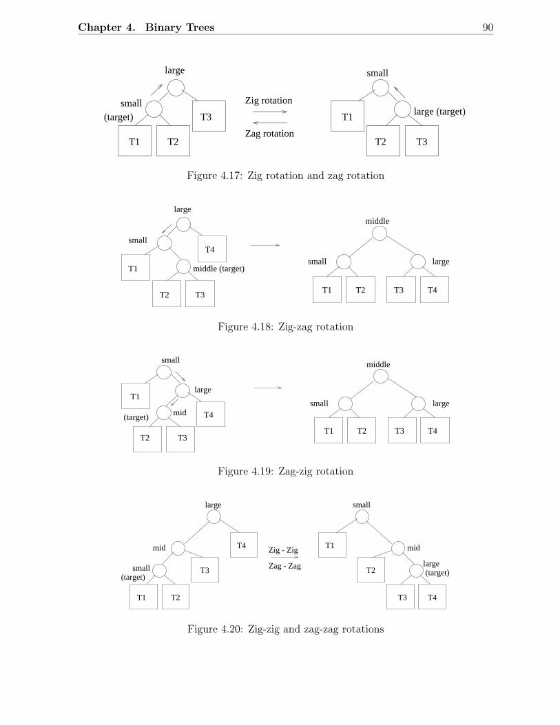
Chapter 4. Binary Trees 90
large small
large (target)small
(target)
T1 T2
T3
Zig rotation
Zag rotation
T1
T2 T3
Figure 4.17: Zig rotation and zag rotation
large
small
middle (target) T1
T2 T3
T4
T3 T4
small
middle
large
T1 T2
Figure 4.18: Zig-zag rotation
T3 T4
small
middle
large
small
large
T4
T1
T2 T3
(target) mid
T1 T2
Figure 4.19: Zag-zig rotation
T3
T2
T2
T3T1
T4
large
mid T1
T4
small
large(target)
mid
small(target)
Zag - Zag
Zig - Zig
Figure 4.20: Zig-zig and zag-zag rotations
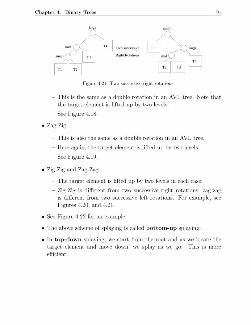
Chapter 4. Binary Trees 91
T3
T2T1
T4
large
mid
small
Two successive
Right Rotations
T1
small
T4
T3T2
mid
large
Figure 4.21: Two successive right rotations
– This is the same as a double rotation in an AVL tree. Note thatthe target element is lifted up by two levels.
– See Figure 4.18.
• Zag-Zig
– This is also the same as a double rotation in an AVL tree.
– Here again, the target element is lifted up by two levels.
– See Figure 4.19.
• Zig-Zig and Zag-Zag
– The target element is lifted up by two levels in each case.
– Zig-Zig is different from two successive right rotations; zag-zagis different from two successive left rotations. For example, seeFigures 4.20, and 4.21.
• See Figure 4.22 for an example
• The above scheme of splaying is called bottom-up splaying.
• In top-down splaying, we start from the root and as we locate thetarget element and move down, we splay as we go. This is moreefficient.
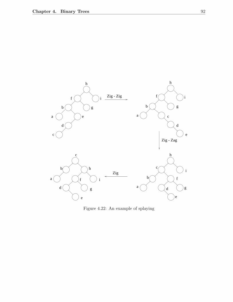
Chapter 4. Binary Trees 92
h
a
b
c
d
e
f
g
i
a
b
c
d
e
f
g
h
i
c
a
b
h
i
f
d
e
g
a
b
c
h
i
g
f
d
e
Zig - Zag
Zig - Zig
Zig
Figure 4.22: An example of splaying
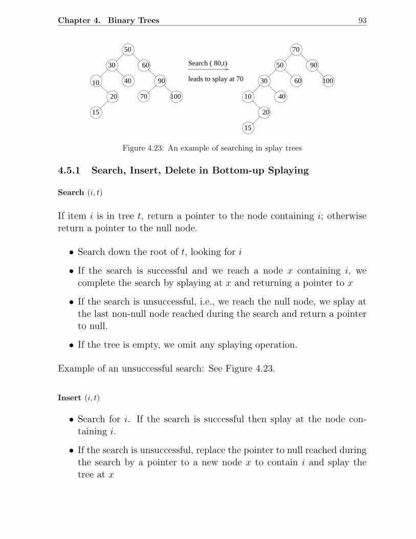
Chapter 4. Binary Trees 93
30
10
Search ( 80,t)
leads to splay at 70
50
60
90
1007020
15
40
70
50
30
10
20
15
40
60
90
100
Figure 4.23: An example of searching in splay trees
4.5.1 Search, Insert, Delete in Bottom-up Splaying
Search (i, t)
If item i is in tree t, return a pointer to the node containing i; otherwisereturn a pointer to the null node.
• Search down the root of t, looking for i
• If the search is successful and we reach a node x containing i, wecomplete the search by splaying at x and returning a pointer to x
• If the search is unsuccessful, i.e., we reach the null node, we splay atthe last non-null node reached during the search and return a pointerto null.
• If the tree is empty, we omit any splaying operation.
Example of an unsuccessful search: See Figure 4.23.
Insert (i, t)
• Search for i. If the search is successful then splay at the node con-taining i.
• If the search is unsuccessful, replace the pointer to null reached duringthe search by a pointer to a new node x to contain i and splay thetree at x
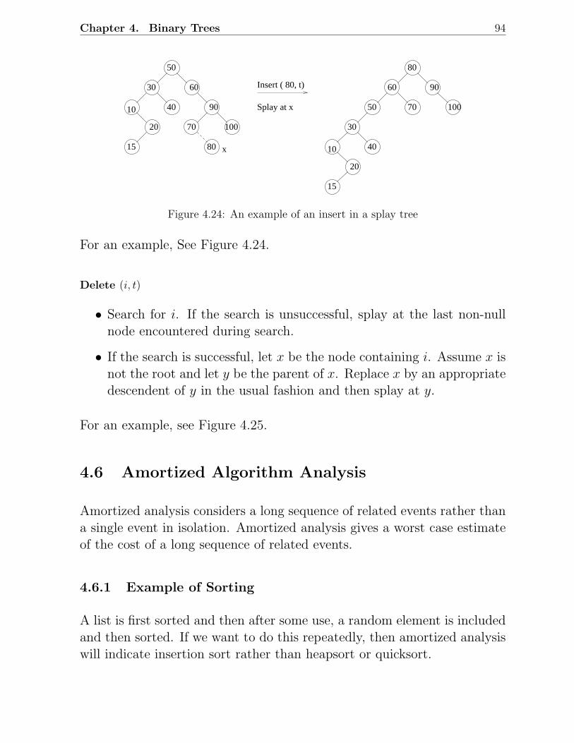
Chapter 4. Binary Trees 94
100
30
10
50
20
15
40
90
70
80
60Insert ( 80, t)
Splay at x
80 x
30
10
50
60
90
1007020
15
40
Figure 4.24: An example of an insert in a splay tree
For an example, See Figure 4.24.
Delete (i, t)
• Search for i. If the search is unsuccessful, splay at the last non-nullnode encountered during search.
• If the search is successful, let x be the node containing i. Assume x isnot the root and let y be the parent of x. Replace x by an appropriatedescendent of y in the usual fashion and then splay at y.
For an example, see Figure 4.25.
4.6 Amortized Algorithm Analysis
Amortized analysis considers a long sequence of related events rather thana single event in isolation. Amortized analysis gives a worst case estimateof the cost of a long sequence of related events.
4.6.1 Example of Sorting
A list is first sorted and then after some use, a random element is includedand then sorted. If we want to do this repeatedly, then amortized analysiswill indicate insertion sort rather than heapsort or quicksort.
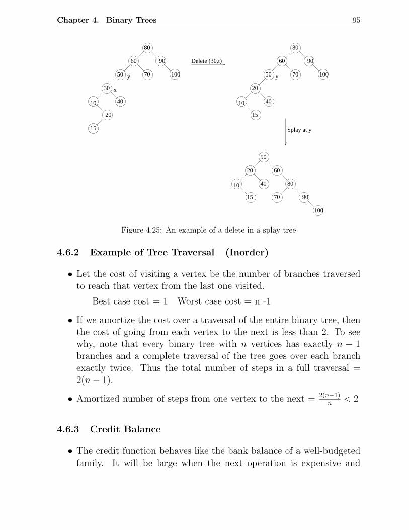
Chapter 4. Binary Trees 95
60Delete (30,t)
Splay at y
x
y y100
30
10
50
20
15
40
90
70
80
60
100
90
80
70
10
50
40
20
15
60
10
50
40
20
15
100
90
70
80
Figure 4.25: An example of a delete in a splay tree
4.6.2 Example of Tree Traversal (Inorder)
• Let the cost of visiting a vertex be the number of branches traversedto reach that vertex from the last one visited.
Best case cost = 1 Worst case cost = n -1
• If we amortize the cost over a traversal of the entire binary tree, thenthe cost of going from each vertex to the next is less than 2. To seewhy, note that every binary tree with n vertices has exactly n − 1branches and a complete traversal of the tree goes over each branchexactly twice. Thus the total number of steps in a full traversal =2(n − 1).
• Amortized number of steps from one vertex to the next = 2(n−1)n < 2
4.6.3 Credit Balance
• The credit function behaves like the bank balance of a well-budgetedfamily. It will be large when the next operation is expensive and
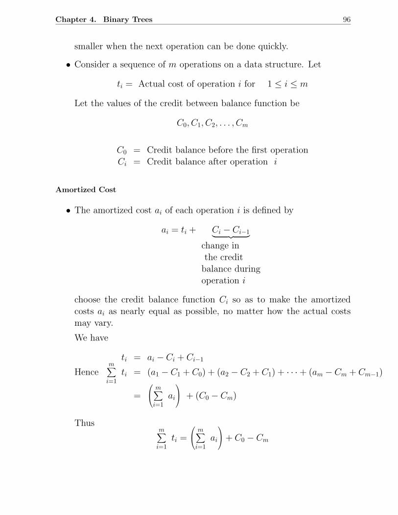
Chapter 4. Binary Trees 96
smaller when the next operation can be done quickly.
• Consider a sequence of m operations on a data structure. Let
ti = Actual cost of operation i for 1 ≤ i ≤ m
Let the values of the credit between balance function be
C0, C1, C2, . . . , Cm
C0 = Credit balance before the first operationCi = Credit balance after operation i
Amortized Cost
• The amortized cost ai of each operation i is defined by
ai = ti + Ci − Ci−1︸ ︷︷ ︸
change inthe credit
balance duringoperation i
choose the credit balance function Ci so as to make the amortizedcosts ai as nearly equal as possible, no matter how the actual costsmay vary.
We have
ti = ai − Ci + Ci−1
Hencem∑
i=1
ti = (a1 − C1 + C0) + (a2 − C2 + C1) + · · · + (am − Cm + Cm−1)
=
m∑
i=1
ai
+ (C0 − Cm)
Thusm∑
i=1
ti =
m∑
i=1
ai
+ C0 − Cm
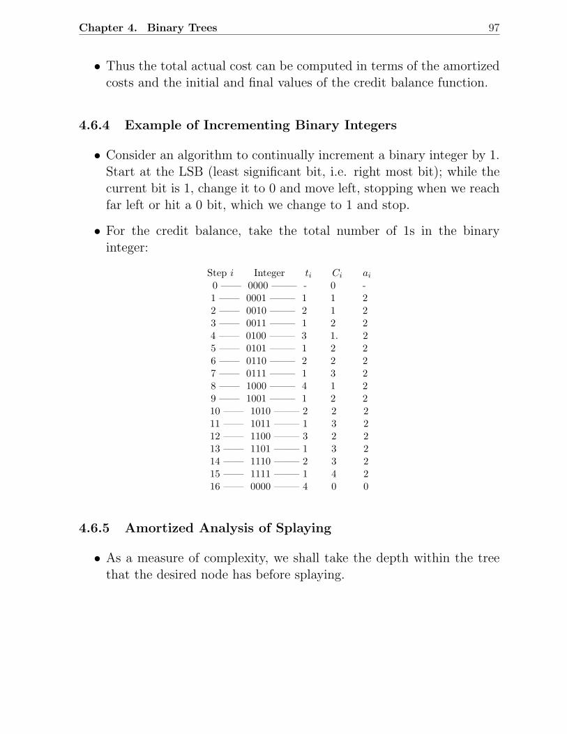
Chapter 4. Binary Trees 97
• Thus the total actual cost can be computed in terms of the amortizedcosts and the initial and final values of the credit balance function.
4.6.4 Example of Incrementing Binary Integers
• Consider an algorithm to continually increment a binary integer by 1.Start at the LSB (least significant bit, i.e. right most bit); while thecurrent bit is 1, change it to 0 and move left, stopping when we reachfar left or hit a 0 bit, which we change to 1 and stop.
• For the credit balance, take the total number of 1s in the binaryinteger:
Step i Integer ti Ci ai
0 —— 0000 ——– - 0 -1 —— 0001 ——– 1 1 22 —— 0010 ——– 2 1 23 —— 0011 ——– 1 2 24 —— 0100 ——– 3 1. 25 —— 0101 ——– 1 2 26 —— 0110 ——– 2 2 27 —— 0111 ——– 1 3 28 —— 1000 ——– 4 1 29 —— 1001 ——– 1 2 210 —— 1010 ——– 2 2 211 —— 1011 ——– 1 3 212 —— 1100 ——– 3 2 213 —— 1101 ——– 1 3 214 —— 1110 ——– 2 3 215 —— 1111 ——– 1 4 216 —— 0000 ——– 4 0 0
4.6.5 Amortized Analysis of Splaying
• As a measure of complexity, we shall take the depth within the treethat the desired node has before splaying.
Chapter 4. Binary Trees 98
T : BST on which we are performing a splayinsertion or retrieval
Ti : tree T as it has been transformed afterstep i of the splaying process, with T0 = T
x : any node in Ti
Ti(x) : subtree of Ti with root x|Ti(x)| : number of nodes of Ti(x)
• We consider bottom-up splaying at a node x, so that x begins some-where in the tree T but after m splaying steps, ends up as the root ofT .
• Rank
For each step i of the splaying process and each vertex x ∈ T , wedefine rank at step i of x to be
ri(x) = log |Ti(x)|︸ ︷︷ ︸
height ofTi(x) if it
were completelybalanced.
• Portion out the credit balance of the tree among all its vertices byrequiring the following credit invariant to hold:
For every node x of T and after every step i of splaying, node x hascredit equal to its rank ri(x).
• Define the total credit balance for the tree as
Ci =∑
x∈Ti
ri(x)
• If the tree is empty or contains only one node, then its credit balanceis 0. As the tree grows, its credit balance increases. The credit balanceshould reflect the work needed to build the tree.
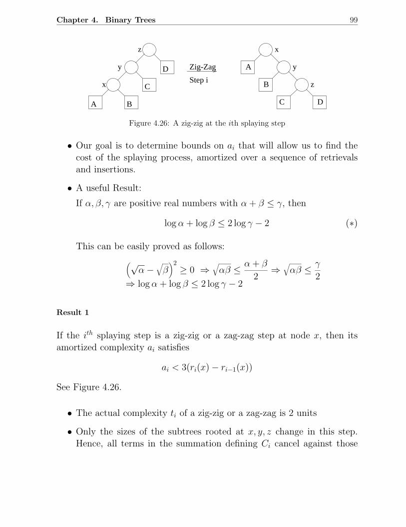
Chapter 4. Binary Trees 99
x
y
z
A B
C
D Zig-Zag
Step i
x
y
z
A
B
C D
Figure 4.26: A zig-zig at the ith splaying step
• Our goal is to determine bounds on ai that will allow us to find thecost of the splaying process, amortized over a sequence of retrievalsand insertions.
• A useful Result:
If α, β, γ are positive real numbers with α + β ≤ γ, then
log α + log β ≤ 2 log γ − 2 (∗)
This can be easily proved as follows:
(√α −
√
β)2
≥ 0 ⇒√
αβ ≤ α + β
2⇒
√
αβ ≤ γ
2⇒ log α + log β ≤ 2 log γ − 2
Result 1
If the ith splaying step is a zig-zig or a zag-zag step at node x, then itsamortized complexity ai satisfies
ai < 3(ri(x) − ri−1(x))
See Figure 4.26.
• The actual complexity ti of a zig-zig or a zag-zag is 2 units
• Only the sizes of the subtrees rooted at x, y, z change in this step.Hence, all terms in the summation defining Ci cancel against those
Chapter 4. Binary Trees 100
for Ci−1 except those indicated below
ai = ti + Ci − Ci−1
= 2 + ri(x) + ri(y) + ri(z)−ri−1(x) − ri−1(y) + ri−1(z)
= 2 + ri(y) + ri(z) − ri−1(x) − ri−1(y) (•)
Since |Ti(x)| = |Ti−1(z)| as the subtree rooted at z before the splaying stephas the same size as that rooted at x after the step.
Let
α = |Ti−1(x)|, β = |Ti(z)|, and γ = |Ti(x)|. Then observe that α+β ≤ γ.This is because
Ti−1(x) contains components x, A, B
Ti(z) contains components z, C, DTi(x) contains all these components (plus y besides).
Thus by (∗)ri−1(x) + ri(z) ≤ 2ri(x) − 2
⇒ 2ri(x) − ri−1(x) − ri(z) − 2 ≥ 0
Adding this to (•), we get
ai ≤ 2ri(x) − 2ri−1(x) + ri(y) − ri−1(y)
Before step i, y is the parent of x so that
|Ti−1(y)| > |Ti−1(x)|
After step i, x is the parent of y so that
|Ti(x)| > |Ti(y)|
Taking logarithms we have
ri−1(y) > ri−1(x) and ri(x) > ri(y)
Chapter 4. Binary Trees 101
Thus we obtainai < 3ri(x) − 3ri−1(x)
Similarly, we can show Results 2 and 3 below:
Result 2
If the ith splaying step is a zig-zag or zag-zig at node x, then its amortizedcomplexity ai satisfies
ai < 2(ri(x) − ri−1(x))
Result 3
If the ith splaying step is a zig or a zag, then
ai < 1 + (ri(x) − ri−1(x))
Result 4
The total amortized cost over all the splaying steps can be computed byadding the costs of all the splay steps. If there are k such steps, only thelast can be a zig or zag and the others are all zig-zag or zig-zag or zag-zigor zag-zag. Since (∗) provides the weaker bound, we get,
k∑
i=1
ai =k−1∑
i=1
ai + ak
≤k−1∑
i−1
3(ri(x) − ri−1(x)) + (1 + 3rk(x) − 3rk−1(x))
= 1 + 3rk(x) − 3r0(x)
≤ 1 + 3rk(x)
= 1 + 3 log n
Chapter 4. Binary Trees 102
Thus the amortized cost of an insertion or retrieval with splaying in aBST with n nodes does not exceed 1 + 3 log n upward moves of the targetnode in the tree.
Result 5
Now consider a long sequence of m splay insertions or retrievals. We seekto compute the actual cost of all these m operations.
Let Tj and Aj be the actual cost and amortized cost of the jth opera-tion, where j = 1, 2, . . . , m, now represents a typical insertion or retrievaloperation.
We havem∑
j=1
Tj =
m∑
j=1
Aj
+ CO − Cm
If the tree never has more than n nodes, then C0 and Cm lie between 0 andlog n, so that
C0 − Cm ≤ log n
Also we know that
Aj ≤ 1 + 3 log n for j = 1, 2, . . . , m
Thus the above becomes
m∑
j=1
Tj = m(1 + 3 log n) + log n
The above gives the total actual time of m insertions or retrievals on atree that never has more than n nodes.
This gives O(log n) actual running time for each operation.
Chapter 4. Binary Trees 103
4.7 To Probe Further
1. Alfred V Aho, John E. Hopcroft, and Jeffrey D Ullman. Data Struc-tures and Algorithms . Addison-Wesley, 1983.
2. Gilles Brassard and Paul Bratley. Fundamentals of Algorithmics .Prentice-Hall, 1996. Indian Edition published by Prentice Hall ofIndia, 1998.
3. Thomas H. Cormen, Charles E. Leiserson, and Donald L. Rivest. In-troduction to Algorithms . The MIT Electrical Engineering and Com-puter Science Series, 1990. Indian Edition published in 1999.
4. Donald E Knuth. Fundamental Algorithms , Volume 1 of The Artof Computer Programming, Addison-Wesley, 1968, Second Edition,1973.
5. Robert L. Kruse, Bruce P. Leung, and Clovis L. Tondo. Data Struc-tures and Program design in C . Prentice Hall, 1991. Indian Editionpublished by Prentice Hall of India, 1999.
6. Mark Allen Weiss. Data Structures and Algorithm Analysis in C++.Benjamin-Cummings, 1994. Indian Edition published in 1998.
7. Duane A. Bailey. Java Structures: Data Structures in Java for thePrincipled Programmer . McGraw-Hill International Edition, 1999.
8. Ellis Horowitz and Sartaz Sahni. Fundamentals of Data structures .Galgotia Publications, New Delhi, 1984.
9. Donald E Knuth. Seminumerical Algorithms . Volume 2 of The Artof Computer Programming, Addison-Wesley, 1969, Second Edition,1981.
10. Donald E. Knuth. Sorting and Searching , Volume 3 of The Art ofComputer Programming, Addison-Wesley, 1973.
11. Y. Langsam, M.J. Augenstein, and A.M. Tenenbaum. Data Struc-tures using C and C++. Second Edition, Prentice Hall, 1996. IndianEdition published by Prentice Hall of India, 2000.
Chapter 4. Binary Trees 104
12. Kurt Mehlhorn. Sorting and Searching. Volume 1 of Data Structuresand Algorithms. Springer-Verlag, 1984.
13. Sataj Sahni. Data Structures, Algorithms, and Applications in Java.McGraw-Hill Higher Education, 2000.
14. Thomas A. Standish. Data Structures in Java. Addison-Wesley, 1998.Indian Edition published by Addison Wesley Longman, 2000.
15. Nicklaus Wirth. Data Structures + Algorithms = Programs. Prentice-Hall, Englewood Cliffs. 1975.
16. David A Huffman. A method for the construction of minimum-redundancycodes. Proceedings of the IRE Volume 40, Number 9, pp. 1098-1101,1952.
17. Daniel D Sleator and Robert E. Tarjan. Self-adjusting binary searchtrees. Journal of the ACM , Volume 32, Number 3, pp 652-686, 1985.
18. Robert E. Tarjan. Amortized computational complexity. SIAM Jour-nal on Algebraic and Discrete Methods , Volume 6, Number 2, pp.306-318, 1985.
4.8 Problems
4.8.1 General Trees
1. Show in any binary tree that the number of leaves is one more than the number ofnodes of degree two.
2. The degree of a node in a tree is the number of children the node has. If a tree hasn1 nodes of degree 1, n2 nodes of degree 2, ..., nm nodes of degree m, compute thenumber of leaves in the tree in terms of n1, n2, . . . , nm.
3. Show that if T is a k-ary tree with n nodes, each having a fixed size, then nk+1−nof the nk link fields are null links (n ≥ 1).
4. Provide an efficient O(n) time algorithm to determine the height of a tree containingn nodes, represented using parent links. You may build any other supporting datastructures, if needed.
Chapter 4. Binary Trees 105
5. Associate a weight w(x) = 2−d with each leaf x of depth d in a binary tree T . Showthat
∑
x
w(x) ≤ 1
where the sum is taken over all leaves x in T .
6. Consider a complete binary tree with an odd number of nodes. Let n be the numberof internal nodes (non-leaves) in the tree. Define the internal path length, I, as thesum, taken over all the internal nodes of the tree, of the depth of each node. Likewise,define the external pathlength, E, as the sum, taken over all the leaves of the tree,of the depth of each leaf. Show that E = I + 2n.
7. What is the optimal Huffman code for the following set of frequencies, based on thefirst 8 Fibonacci numbers?
a b c d e f g h1 1 2 3 5 8 13 21
Write down the resulting Huffman tree. Can you generalize your answer to find theoptimal code when the frequencies are the first n Fibonacci numbers?
4.8.2 Binary Search Trees
1. Suppose that we have numbers between 1 and 1000 in a binary search tree and wantto search for the number 363. Which of the following sequences could not be thesequence of nodes examined?
(a) 2, 252, 401, 398, 330, 344, 397, 363.
(b) 924, 220, 911, 244, 898, 258, 362, 363.
(c) 925, 202, 911, 240, 912, 245, 363.
(d) 2, 399, 387, 219, 266, 382, 381, 278, 363.
(e) 935, 278, 347, 621, 299, 392, 358, 363.
2. In a binary search tree, given a key x, define successor(x) as the key which isthe successor of x in the sorted order determined by an inorder tree walk. Definepredecessor(x) similarly. Explain how, given x, its successor and predecessor maybe found.
3. A binary search tree is constructed by inserting the key values 1, 2, 3, 4, 5, 6, 7in some order specified by a permutation of 1, . . ., 7, into an initially empty tree.Which of these permutations will lead to a complete binary search tree ( 1 node atlevel 1, 2 nodes at level 2, and 4 nodes at level 3)?
Chapter 4. Binary Trees 106
4. Suppose that the search for key k in a binary search tree ends up in a leaf. Considerthree sets: A, the keys to the left of the search path; B, the keys on the search path;and C, the keys to the right of the search path. Investigate if the following is true:a ≤ b ≤ c ∀ a ∈ A; b ∈ B; c ∈ C. Give a proof or a counter-example as the casemay be.
5. Is the operation of deletion in a binary search tree commutative in the sense thatdeleting x and then y from a binary search tree leaves the same tree as deleting yand then x? Argue why it is so or give a counter-example.
6. Devise an algorithm that takes two values, a and b such that a ≤ b, and visits allkeys x in a BST such that a ≤ x ≤ b. The running time of your algorithm shouldbe O(N +log n), where N is the number of keys visited and n is the number of keysin the tree.
7. A random binary search tree having n nodes, where n = 2k − 1, for some positiveinteger k, is to be reorganized into a perfectly balanced binary search tree. Outlinean efficient algorithm for this task. The algorithm should not use any memorylocations other than those already used by the random binary search tree.
8. Consider three keys, k1, k2, k3, such that k1 < k2 < k3. A binary search tree isconstructed with these three keys. Depending on the order in which the keys areinserted, five different binary search trees are possible.
(a) Write down the five binary search trees.
(b) Let p, q, r be the probabilities of probing for k1, k2, k3, respectively in the givenbinary search trees (p+q+r = 1). Compute the average number of comparisons(or probes) on a successful search for each of the above five binary search trees.
(c) Define the optimum binary search tree as the one for which the average numberof comparisons on a successful search is minimum. Determine the range ofvalues of p, q, r, for which the completely balanced search tree is the optimumsearch tree.
9. Given a set of 31 names, each containing 10 uppercase alphabets, we wish to set upa data structure that would lead to efficient average case performance of successfuland unsuccessful searches on this set. It is known that not more than 5 names startwith the same alphabet. Also, assume that successful and unsuccessful searches areequally likely and that in the event of a successful search, it is equally likely thatany of the 31 names was searched for. The two likely choices for the data structureare:
• A closed hash table with 130 locations where each location can accommodateone name.
• A full binary search tree of height 4, where each of the 31 nodes contains aname and lexicographic ordering is used to set up the BST.
Chapter 4. Binary Trees 107
Answer the following questions:
(a) What is the hashing function you would use for the closed hash table?
(b) Assume that the computation of the hash function above takes the same timeas comparing two given names. Now, compute the average case running timeof a search operation using the hash table. Ignore the time for setting up thehash table.
(c) Compute the average case running time of a search operation using the BST.Ignore the time for setting up the BST.
4.8.3 Splay Trees
1. Complete the proof of the following lemmas in the amortized analysis of splay trees:
(a) If the ith splaying step is a zig-zag step or a zag-zig step at node x, then itsamortized complexity ai satisfies ai ≤ 2(ri(x) − ri−1(x)).
(b) If the ith splaying step is a zig step or a zag step at node x, then its amortizedcomplexity ai satisfies ai ≤ 1 + (ri(x) − ri−1(x)).
2. Define a rank function r(x) for the nodes of any binary tree as follows: If x is theroot, then r(x) = 0; If x is the left child of y, then r(x) = r(y) − 1; If x is the rightchild of y, then r(x) = r(y)+1. Define the credit balance of a tree during a traversalto be the rank of the node being visited. For several binary trees, determine theranks at each node and prepare a table showing the actual cost, credit balance, andamortized cost (in edges traversed) of each step of an inorder traversal.
3. Generalize the amortized analysis for incrementing four digit binary integers to ndigit binary integers.
4. A sequence of n operations is performed on a data structure. The ith operationcosts i if i is an exact power of 2, and 1 otherwise. Use a suitable credit functionand compute the amortized cost per operation.
5. Keys 1, 2, . . . , n are inserted in that order into an empty splay tree, using splayinsertions. What will be the resulting tree? Also write down the splay tree thatresults when the key n is deleted, using splay deletion.
6. Consider a sequence of m accesses (search operations) to an n-node splay tree. Showthat the total running time of this sequence of operations is O((m + n) log n + m).
Chapter 4. Binary Trees 108
4.9 Programming Assignments
4.9.1 Huffman Coding
1. Problem: Given a set of alphabets and their relative frequencies, find the Huffmanbinary code using binary trees and an optimal ternary code using ternary trees.
2. Reading: Read pages 94-102 of ”Data Structures and Algorithms” by Aho, Hopcroft,and Ullman.
3. Input: The number of alphabets and relative frequencies of those, for example,
8 .2 .02 .3 .05 .03 .15 .22 .03
Assume the alphabets as 1, 2, 3, ..., without loss of generality.
4. Output: For each alphabet, print the Huffman binary code and an optimal ternarycode. Also print the average length of code.
5. Data structures: For binary trees, use the data structures suggested by Aho,Hopcroft, and Ullman. For ternary trees, use similar data structures based onleftmostchild-right sibling representation with nodes organized into cellspace.
6. Programming language: Use C or C++or Java. Best practices in programmingshould be adhered to.
4.9.2 Comparison of Hash Tables and Binary Search Trees
The objective of this assignment is to compare the performance of open hash tables, closedhash tables, and binary search trees in implementing search, insert, and delete operationsin dynamic sets. You can initially implement using C but the intent is to use C++ andobject-oriented principles.
Generation of Keys
Assume that your keys are character strings of length 10 obtained by scanning a textfile. Call these as tokens. Define a token as any string that appears between successiveoccurrences of a forbidden character, where the forbidden set of characters is given by:
F = comma, period, space
If a string has less than 10 characters, make it up into a string of exactly 10 characters byincluding an appropriate number of trailing *’s. On the other hand, if the current stringhas more than 10 characters, truncate it to have the first ten characters only.
Chapter 4. Binary Trees 109
From the individual character strings (from now on called as tokens), generate apositive integer (from now on called as keys) by summing up the ASCII values of thecharacters in the particular token. Use this integer key in the hashing functions. However,remember that the original token is a character string and this is the one to be stored inthe data structure.
Methods to be Evaluated
The following four schemes are to be evaluated.
1. Open hashing with multiplication method for hashing and unsorted lists for chaining
2. Open hashing with multiplication method for hashing and sorted lists for chaining
3. Closed hashing with linear probing
4. Binary search trees
Hashing Functions
For the sake of uniformity, use the following hashing functions only. In the following, mis the hash table size (that is, the possible hash values are, 0, 1, . . . ,m − 1), and x is aninteger key.
1. Multiplication Method
h(x) = Floor(m ∗ Fraction(k ∗ x))
where k =
√(5)−1
2, the Golden Ratio.
2. Linear Probing
h(x, i) = (h(x, 0) + i) mod m; i = 0, . . . ,m − 1
Inputs to the Program
The possible inputs to the program are:
• m: Hash table size. Several values could be given here and the experiments are tobe repeated for all values specified. This input has no significance for binary searchtrees.
Chapter 4. Binary Trees 110
• n: The initial number of insertions of distinct strings to be made for setting up adata structure.
• M : This is a subset of the set 1, 2, 3, 4 indicating the set of methods to be inves-tigated.
• I: This is a decimal number from which a ternary string is to be generated (namelythe radix-3 representation of I). In this representation, assume that a 0 representsthe search operation, a 1 represents the insert operation, and a 2 represents thedelete operation.
• A text file, from which the tokens are to be picked up for setting up and experi-menting with the data structure
What should the Program Do?
1. For each element of M and for each value of m, do the following.
2. Scan the given text file and as you scan, insert the first n distinct strings scannedinto an initially empty data structure.
3. Now scan the rest of the text file token by token, searching for it or inserting itor deleting it, as dictated by the radix-3 representation of I. Note that the mostsignificant digit is to be considered first while doing this and you proceed from leftto right in the radix-3 representation. For each individual operation, keep track ofthe number of probes.
4. Compute the average number of probes for a typical successful search, unsuccessfulsearch, insert, and delete.
4.9.3 Comparison of Skip Lists and Splay Trees
The objective of this assignment is to compare the performance of splay trees and skiplists in implementing search, insert, and delete operations in dictionaries. The context isprovided by symbol table operations in a C compiler.
What is Required?
Assume that your keys are identifiers in a C program (strings that are different fromspecial symbols). Use LEX to design a scanner (lexical analyzer) that will scan the Cprogram and split it into a set of identifiers. Each identifier is a regular expression. Callthese identifiers as tokens from henceforth. The tokens are to be put it into a symboltable. The following two data structures are to be evaluated.
1. Splay trees with bottom-up splaying
Chapter 4. Binary Trees 111
2. Skip lists
Inputs to the Program
The inputs to the program are:
• A C program of sufficient size
• n: The initial number of insertions of distinct tokens to be carried out to set up abase data structure.
What should the Program Do?
Do the following steps for splay tree (skip list):
1. Scan the given C program and as you scan, insert the first n distinct tokens into aninitially empty data structure.
2. Now scan the rest of the C program token by token, inserting or deleting the token,by tossing a fair coin. For each individual operation, keep track of the number ofprobes and number of rotations (if applicable). Count the number of elementaryoperations for each insert or delete (comparisons, assignments of pointers, etc.)
3. Compute the average number of elementary operations for insert and delete.
Programming Language
C++ or Java is recommended. A serious attempt should be made to use ideas of data
abstraction, encapsulation, modularity, inheritance, and polymorphism.
Chapter 5
Balanced Trees
5.1 AVL Trees
Also called as: Height Balanced Binary Search Trees.
REF. G.M. Adel’son-Vel’skii and E.M. Landis. An algorithm for the or-ganization of information. Soviet Mathematics Monthly Volume 3,pp.1259-1263, 1962.
Search, Insertion, and Deletion can be implemented in worst case O(log n)time
Definition
An AVL tree is a binary search tree in which
1. the heights of the right subtree and left subtree of the root differ byat most 1
2. the left subtree and the right subtree are themselves AVL trees
3. A node is said to be
112
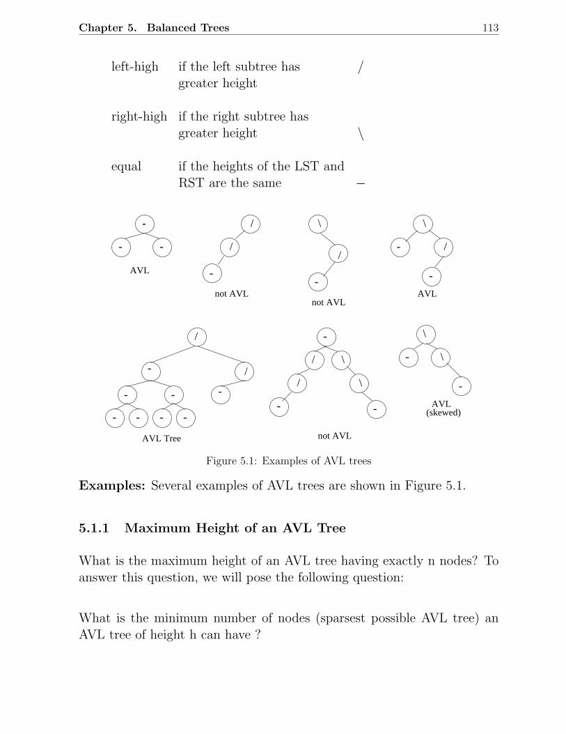
Chapter 5. Balanced Trees 113
left-high if the left subtree has /greater height
right-high if the right subtree hasgreater height \
equal if the heights of the LST andRST are the same −
AVL
AVLnot AVLnot AVL
not AVLAVL Tree
AVL(skewed)
-
-- -
- - - -
/
/
-
- -
-
/
/
-
/
\
-
-
/
\
-
-
\
\
-
-
-
/
/
\
\
Figure 5.1: Examples of AVL trees
Examples: Several examples of AVL trees are shown in Figure 5.1.
5.1.1 Maximum Height of an AVL Tree
What is the maximum height of an AVL tree having exactly n nodes? Toanswer this question, we will pose the following question:
What is the minimum number of nodes (sparsest possible AVL tree) anAVL tree of height h can have ?
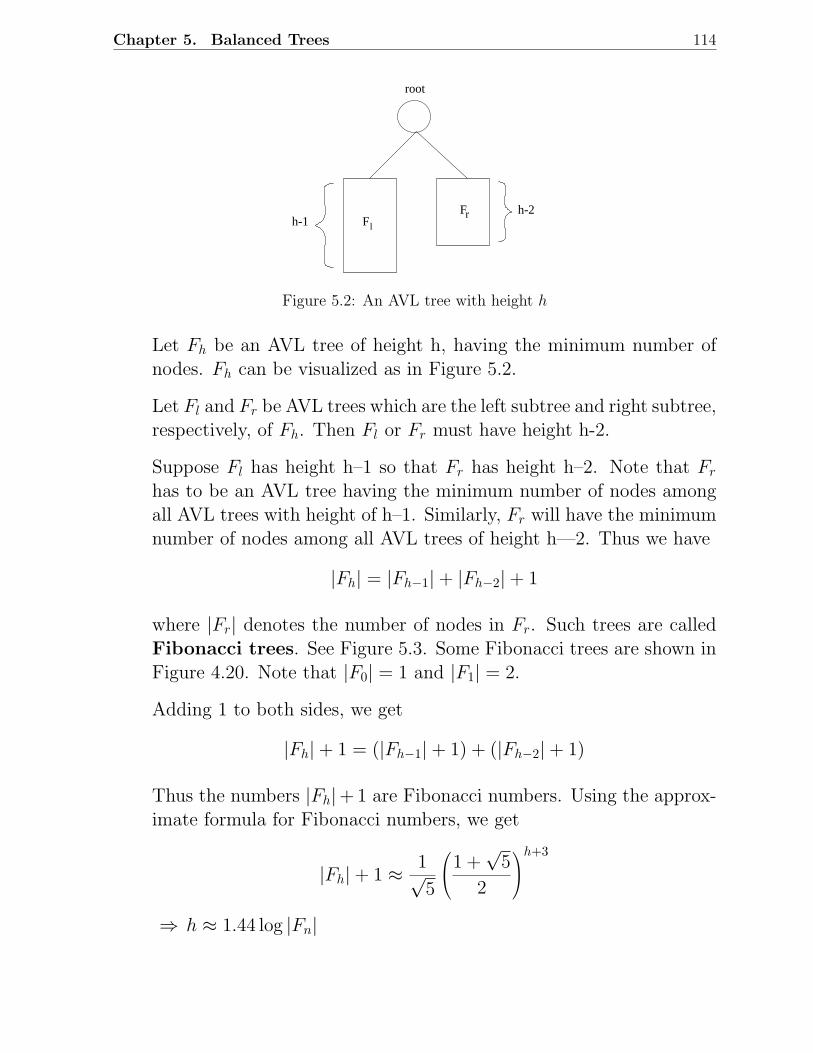
Chapter 5. Balanced Trees 114
lFF
root
h-2h-1
r
Figure 5.2: An AVL tree with height h
Let Fh be an AVL tree of height h, having the minimum number ofnodes. Fh can be visualized as in Figure 5.2.
Let Fl and Fr be AVL trees which are the left subtree and right subtree,respectively, of Fh. Then Fl or Fr must have height h-2.
Suppose Fl has height h–1 so that Fr has height h–2. Note that Fr
has to be an AVL tree having the minimum number of nodes amongall AVL trees with height of h–1. Similarly, Fr will have the minimumnumber of nodes among all AVL trees of height h—2. Thus we have
|Fh| = |Fh−1| + |Fh−2| + 1
where |Fr| denotes the number of nodes in Fr. Such trees are calledFibonacci trees. See Figure 5.3. Some Fibonacci trees are shown inFigure 4.20. Note that |F0| = 1 and |F1| = 2.
Adding 1 to both sides, we get
|Fh| + 1 = (|Fh−1| + 1) + (|Fh−2| + 1)
Thus the numbers |Fh|+ 1 are Fibonacci numbers. Using the approx-imate formula for Fibonacci numbers, we get
|Fh| + 1 ≈ 1√5
1 +
√5
2
h+3
⇒ h ≈ 1.44 log |Fn|
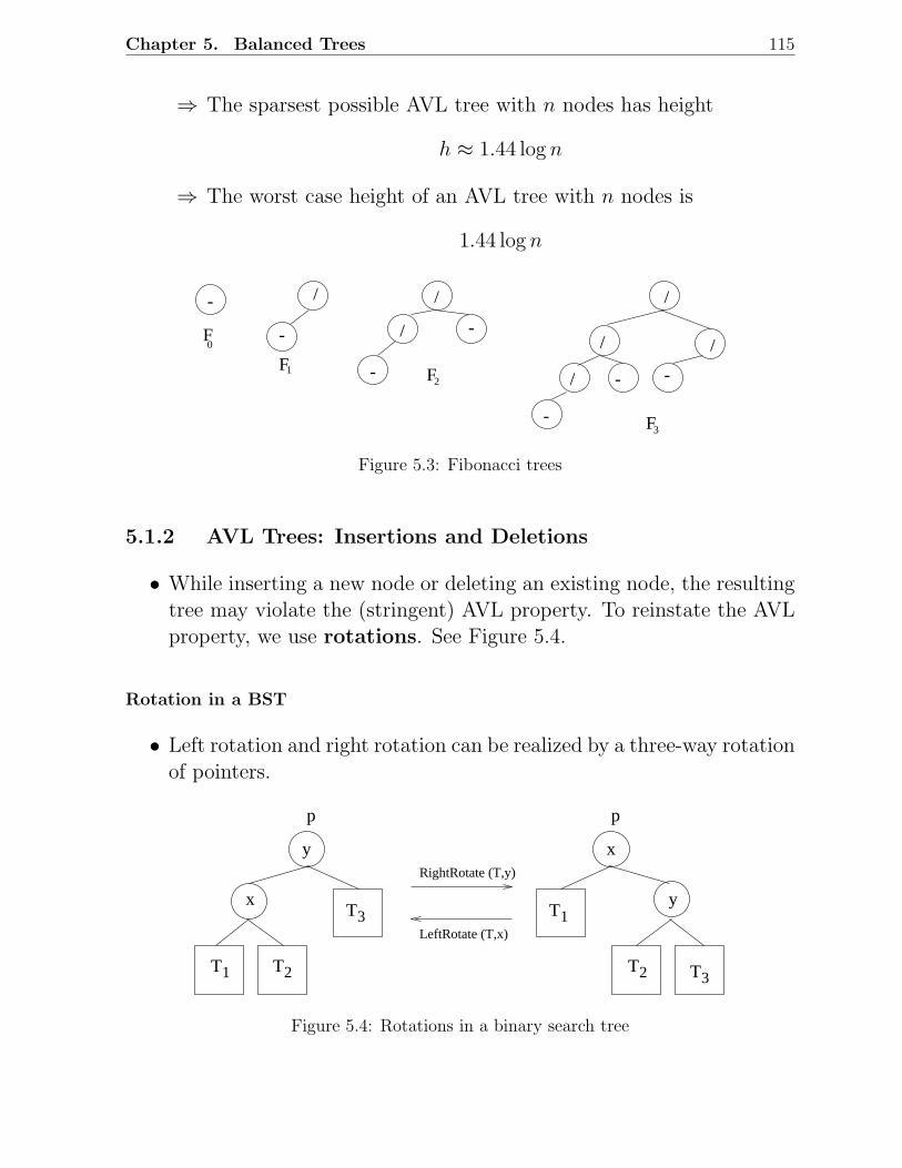
Chapter 5. Balanced Trees 115
⇒ The sparsest possible AVL tree with n nodes has height
h ≈ 1.44 log n
⇒ The worst case height of an AVL tree with n nodes is
1.44 log n
-
F0
-
/
F1 -
-
/
/
F2
-
- -
/
/
/
/
F3
Figure 5.3: Fibonacci trees
5.1.2 AVL Trees: Insertions and Deletions
• While inserting a new node or deleting an existing node, the resultingtree may violate the (stringent) AVL property. To reinstate the AVLproperty, we use rotations. See Figure 5.4.
Rotation in a BST
• Left rotation and right rotation can be realized by a three-way rotationof pointers.
1T 2
3T 1T
2T3TT
x
yx
y
pp
RightRotate (T,y)
LeftRotate (T,x)
Figure 5.4: Rotations in a binary search tree
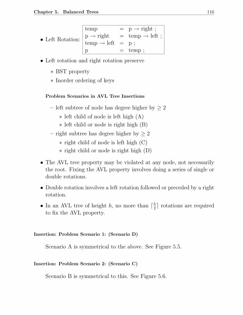
Chapter 5. Balanced Trees 116
• Left Rotation:
temp = p → right ;p → right = temp → left ;temp → left = p ;p = temp ;
• Left rotation and right rotation preserve
∗ BST property
∗ Inorder ordering of keys
Problem Scenarios in AVL Tree Insertions
– left subtree of node has degree higher by ≥ 2
∗ left child of node is left high (A)
∗ left child or node is right high (B)
– right subtree has degree higher by ≥ 2
∗ right child of node is left high (C)
∗ right child or node is right high (D)
• The AVL tree property may be violated at any node, not necessarilythe root. Fixing the AVL property involves doing a series of single ordouble rotations.
• Double rotation involves a left rotation followed or preceded by a rightrotation.
• In an AVL tree of height h, no more than ⌈h2⌉ rotations are required
to fix the AVL property.
Insertion: Problem Scenario 1: (Scenario D)
Scenario A is symmetrical to the above. See Figure 5.5.
Insertion: Problem Scenario 2: (Scenario C)
Scenario B is symmetrical to this. See Figure 5.6.
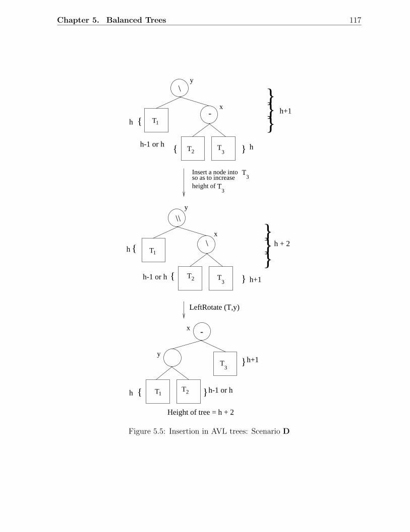
Chapter 5. Balanced Trees 117
T3
T3
T1
T2T
3
T1
T2 T3
T2
T3
Insert a node intoso as to increaseheight of
LeftRotate (T,y)
\
-
y
x
h
hh-1 or h
h+1
y
x
\\
\
h+1h-1 or h
h + 2h
x
y
h h-1 or h
h+1
-
Height of tree = h + 2
T1
Figure 5.5: Insertion in AVL trees: Scenario D
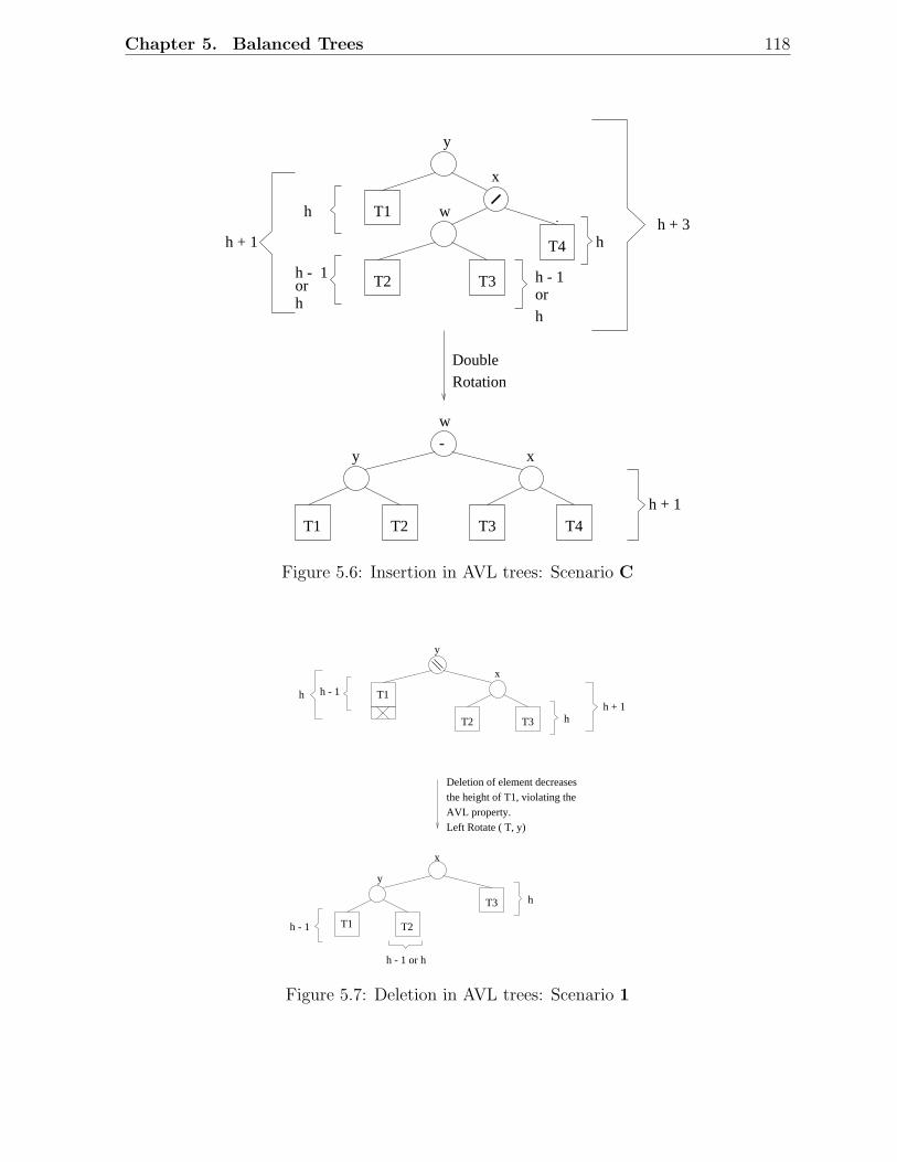
Chapter 5. Balanced Trees 118
h
h - 1orh
h
h - 1orh
x
wT1
T2 T3
T4h + 3
w
y x-
T1 T2 T3 T4h + 1
DoubleRotation
y
h + 1
Figure 5.6: Insertion in AVL trees: Scenario C
x
T2
T1h + 1
y
h - 1h
hT3
h
h - 1
x
y
T1 T2
T3
h - 1 or h
Deletion of element decreasesthe height of T1, violating theAVL property. Left Rotate ( T, y)
Figure 5.7: Deletion in AVL trees: Scenario 1
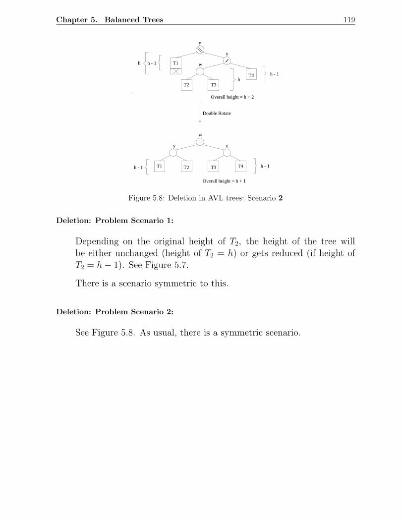
Chapter 5. Balanced Trees 119
x
T1
y
h
h - 1
y
T1 T2
T2 T3h
h - 1
w
T4
h - 1
Overall height = h + 2
Double Rotate
T3 T4
x
w
h - 1
Overall height = h + 1
Figure 5.8: Deletion in AVL trees: Scenario 2
Deletion: Problem Scenario 1:
Depending on the original height of T2, the height of the tree willbe either unchanged (height of T2 = h) or gets reduced (if height ofT2 = h − 1). See Figure 5.7.
There is a scenario symmetric to this.
Deletion: Problem Scenario 2:
See Figure 5.8. As usual, there is a symmetric scenario.
Chapter 5. Balanced Trees 120
5.2 Red-Black Trees
• Binary search trees where no path from the root to a leaf is more thantwice as long as any other path from the root to a leaf.
REF. R. Bayer. Symmetric binary B-trees: Data Structures and mainte-nance algorithms, Acta Informatica, Volume 1, pp.290-306, 1972.
Definition
A BST is called an RBT if it satisfies the following four properties.
1. Every node is either red or black
2. Every leaf is black (Missing node property)
3. If a node is red, then both its children are black
(RED constraint)
4. Every simple path from a node to a descendent leaf contains the samenumber of black nodes
(BLACK constraint)
Black-Height of a Node
• Number of black nodes on any path from, but not including a node xto a leaf is called the black height of x and is denoted by bh(x).
• Black height of an RBT is the black height of its root.
• Each node of a red black tree contains the following fields.
colour key left right parent
• If a child of a node does not exist, the corresponding pointer field willbe NULL and these are regarded as leaves.
• Only the internal nodes will have key values associated with them.
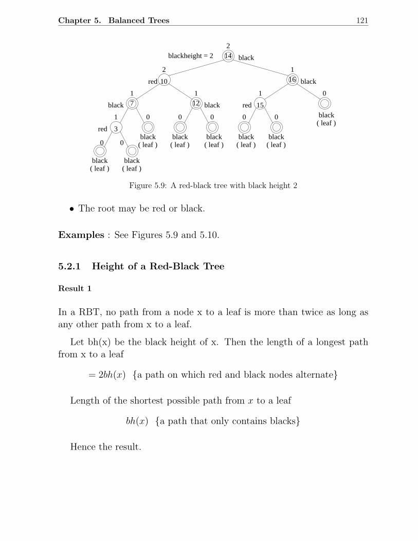
Chapter 5. Balanced Trees 121
3
7 15
10
12
16
14
blackblackblackblackblack
blackblack
black
black
black
black
red
red
redblack
( leaf )
( leaf )( leaf )( leaf )( leaf )( leaf )
( leaf ) ( leaf )
0 0
0 0 0 0 0
0
1
1 1
2
1
1
2blackheight = 2
Figure 5.9: A red-black tree with black height 2
• The root may be red or black.
Examples : See Figures 5.9 and 5.10.
5.2.1 Height of a Red-Black Tree
Result 1
In a RBT, no path from a node x to a leaf is more than twice as long asany other path from x to a leaf.
Let bh(x) be the black height of x. Then the length of a longest pathfrom x to a leaf
= 2bh(x) a path on which red and black nodes alternate
Length of the shortest possible path from x to a leaf
bh(x) a path that only contains blacks
Hence the result.
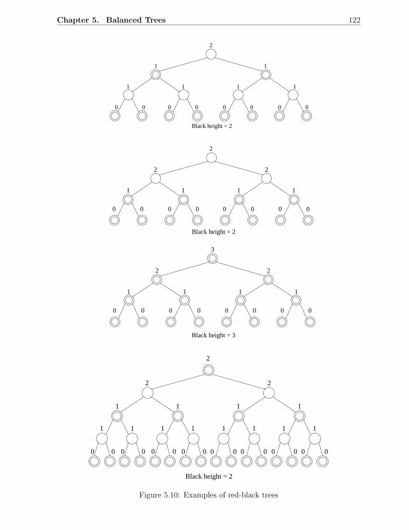
Chapter 5. Balanced Trees 122
0 0 0 0 0 0 0 0
1 1 1 1
11
2
2
Black height = 2
Black height = 2
1 1 1 1
0 0 0 0 0 0 0 0
2 2
Black height = 3
1 1 1 1
0 0 0 0 0 0 0 0
2 2
3
0 0 0 0 0 0 0 0 0 0 0 0 0 0 0 0
1 1 1 1 1 1 1 1
1111
2 2
2
Black height = 2
Figure 5.10: Examples of red-black trees
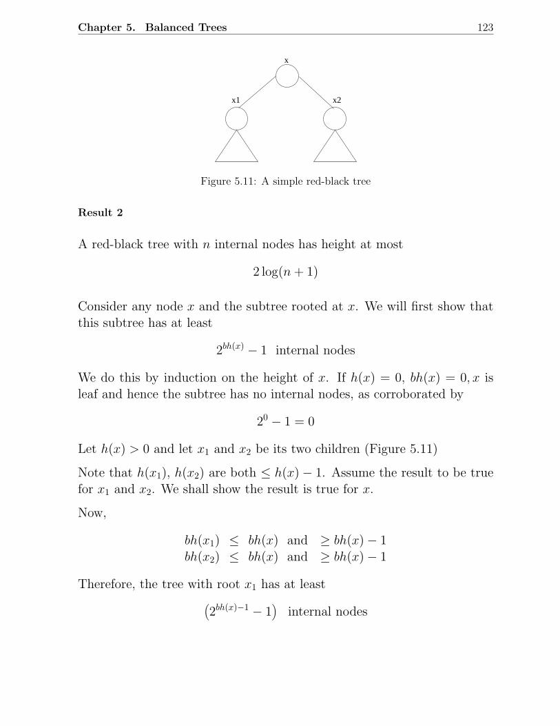
Chapter 5. Balanced Trees 123
x
x2x1
Figure 5.11: A simple red-black tree
Result 2
A red-black tree with n internal nodes has height at most
2 log(n + 1)
Consider any node x and the subtree rooted at x. We will first show thatthis subtree has at least
2bh(x) − 1 internal nodes
We do this by induction on the height of x. If h(x) = 0, bh(x) = 0, x isleaf and hence the subtree has no internal nodes, as corroborated by
20 − 1 = 0
Let h(x) > 0 and let x1 and x2 be its two children (Figure 5.11)
Note that h(x1), h(x2) are both ≤ h(x) − 1. Assume the result to be truefor x1 and x2. We shall show the result is true for x.
Now,
bh(x1) ≤ bh(x) and ≥ bh(x) − 1bh(x2) ≤ bh(x) and ≥ bh(x) − 1
Therefore, the tree with root x1 has at least(
2bh(x)−1 − 1)
internal nodes
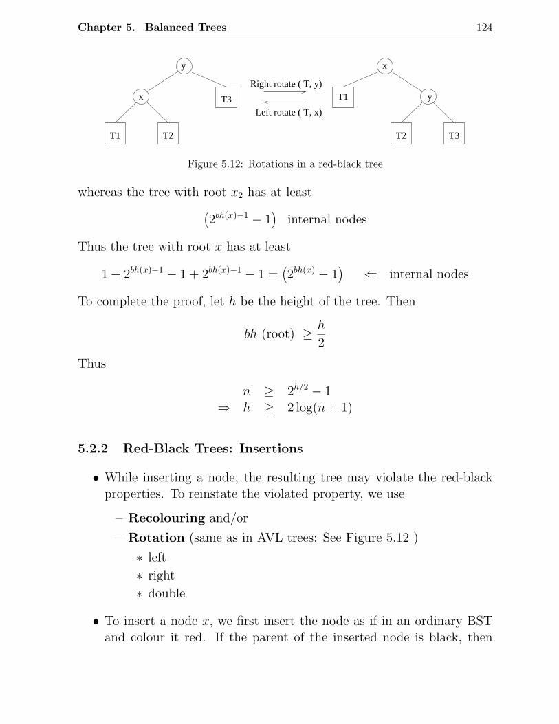
Chapter 5. Balanced Trees 124
T1 T2
T3 x
y x
yT1
T2 T3
Right rotate ( T, y)
Left rotate ( T, x)
Figure 5.12: Rotations in a red-black tree
whereas the tree with root x2 has at least(
2bh(x)−1 − 1)
internal nodes
Thus the tree with root x has at least
1 + 2bh(x)−1 − 1 + 2bh(x)−1 − 1 =(
2bh(x) − 1)
⇐ internal nodes
To complete the proof, let h be the height of the tree. Then
bh (root) ≥ h
2
Thus
n ≥ 2h/2 − 1⇒ h ≥ 2 log(n + 1)
5.2.2 Red-Black Trees: Insertions
• While inserting a node, the resulting tree may violate the red-blackproperties. To reinstate the violated property, we use
– Recolouring and/or
– Rotation (same as in AVL trees: See Figure 5.12 )
∗ left
∗ right
∗ double
• To insert a node x, we first insert the node as if in an ordinary BSTand colour it red. If the parent of the inserted node is black, then
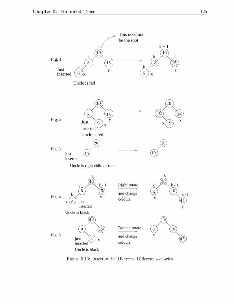
Chapter 5. Balanced Trees 125
Right rotate
and changecolours
10
8 15
9
10
15
8
9
8
10
15
15
10
8
6
6
k
k - 1k
k
x
Uncle is black
y
k
k
k - 1
k -1 x
y
10 10
20 20
Uncle is right child of root
Fig. 5
Fig. 4
Fig. 3
Just
insertedx
y
Uncle is red
10
8
9
15y
x
15
9
8
10
Uncle is red
insertedJust
x xy y
k
k
k k + 1
kk
k 8
10
15 15
10
8
6 6
This need notbe the root
Fig. 1
Fig. 2
Double rotate
and change
coloursx
x
Uncle is black
justinserted
justinserted
justinserted
Figure 5.13: Insertion in RB trees: Different scenarios
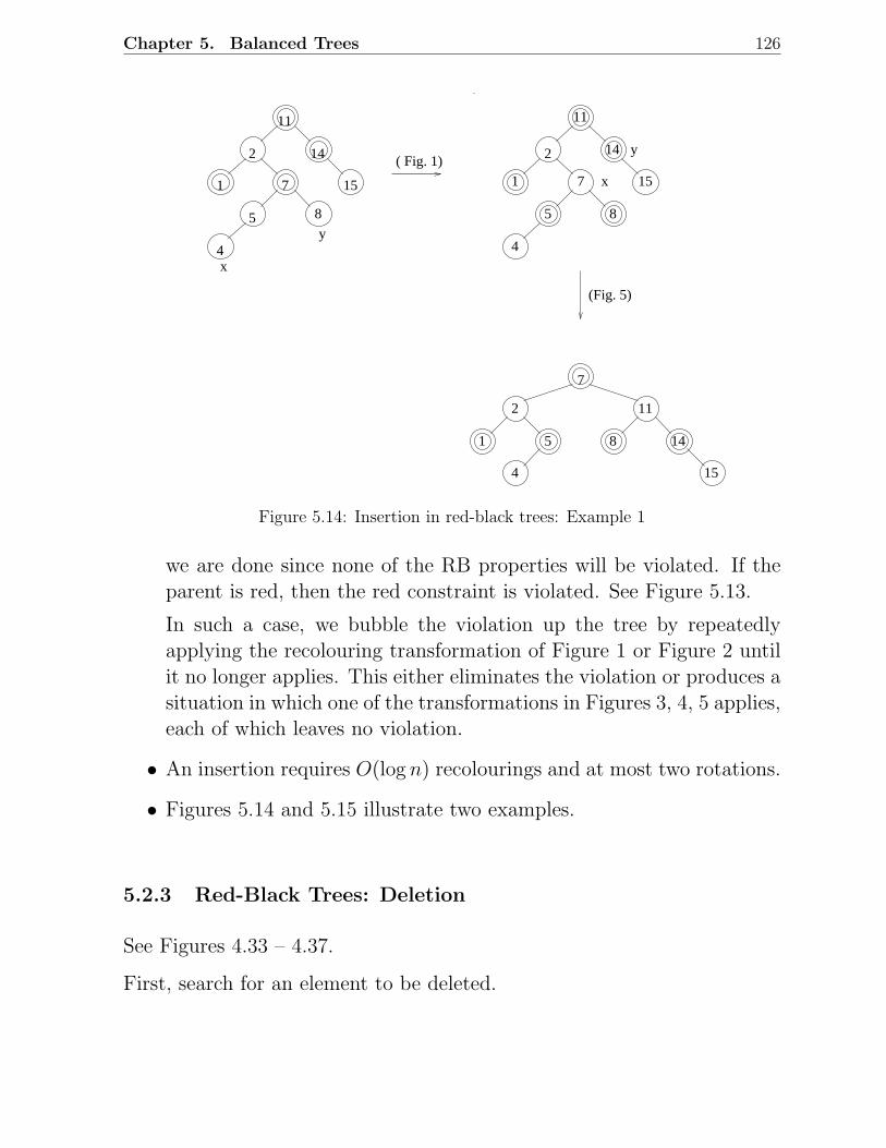
Chapter 5. Balanced Trees 126
x
y4
5
7
8
1
2
11
14
15
( Fig. 1)
(Fig. 5)
11
2 14
1571
5 8
4
x
y
7
11
14
15
2
5
4
1 8
Figure 5.14: Insertion in red-black trees: Example 1
we are done since none of the RB properties will be violated. If theparent is red, then the red constraint is violated. See Figure 5.13.
In such a case, we bubble the violation up the tree by repeatedlyapplying the recolouring transformation of Figure 1 or Figure 2 untilit no longer applies. This either eliminates the violation or produces asituation in which one of the transformations in Figures 3, 4, 5 applies,each of which leaves no violation.
• An insertion requires O(log n) recolourings and at most two rotations.
• Figures 5.14 and 5.15 illustrate two examples.
5.2.3 Red-Black Trees: Deletion
See Figures 4.33 – 4.37.
First, search for an element to be deleted.
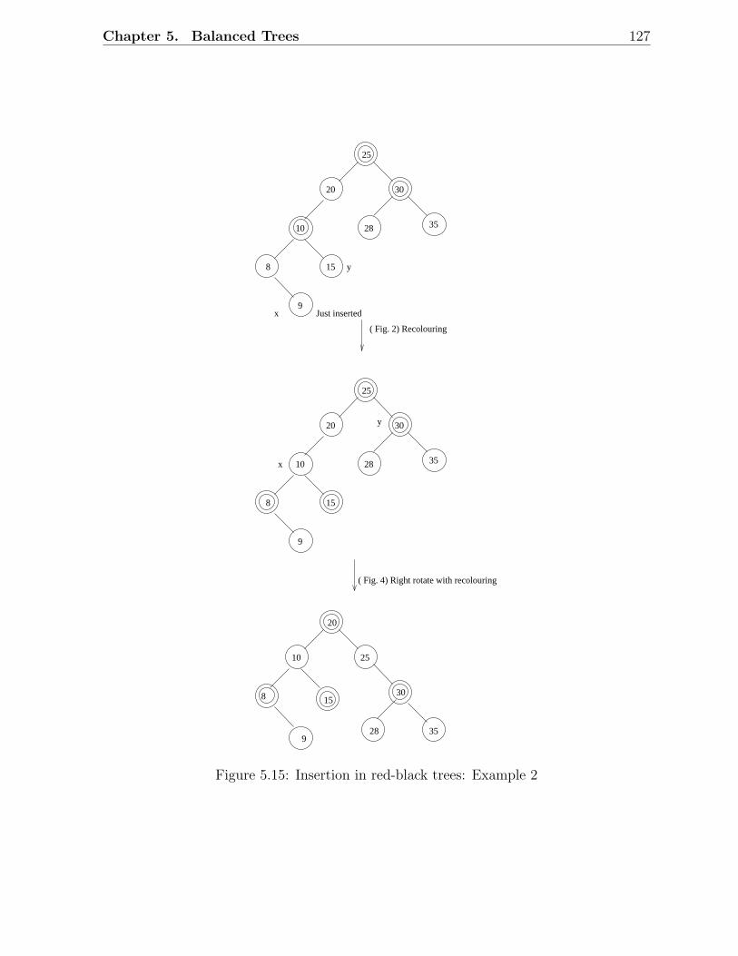
Chapter 5. Balanced Trees 127
( Fig. 2) Recolouring
( Fig. 4) Right rotate with recolouring
25
20 30
28 35 10
15 8
9Just inserted
y
x
25
20 30
28 35 10
15 8
9
x
y
15
25
30
3528 9
20
8
10
Figure 5.15: Insertion in red-black trees: Example 2
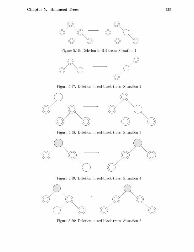
Chapter 5. Balanced Trees 128
Figure 5.16: Deletion in RB trees: Situation 1
Figure 5.17: Deletion in red-black trees: Situation 2
Figure 5.18: Deletion in red-black trees: Situation 3
Figure 5.19: Deletion in red-black trees: Situation 4
Figure 5.20: Deletion in red-black trees: Situation 5
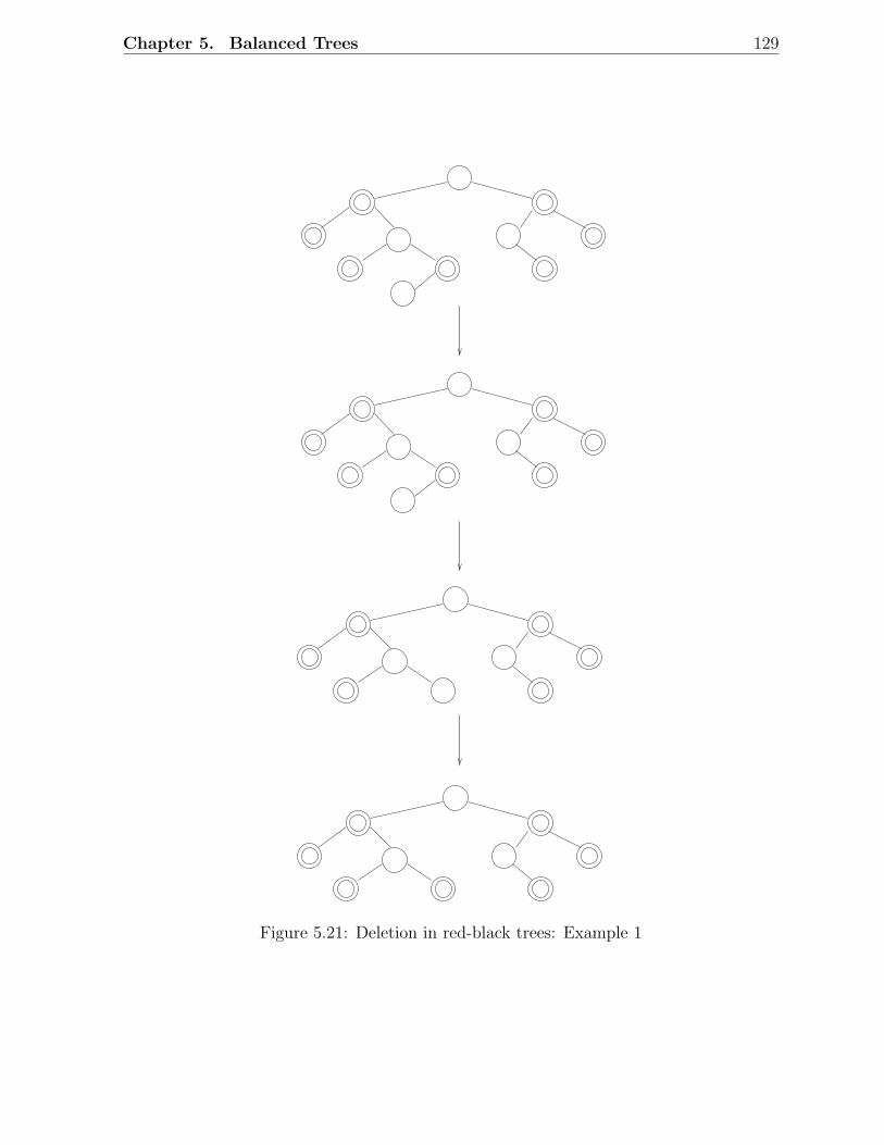
Chapter 5. Balanced Trees 129
Figure 5.21: Deletion in red-black trees: Example 1
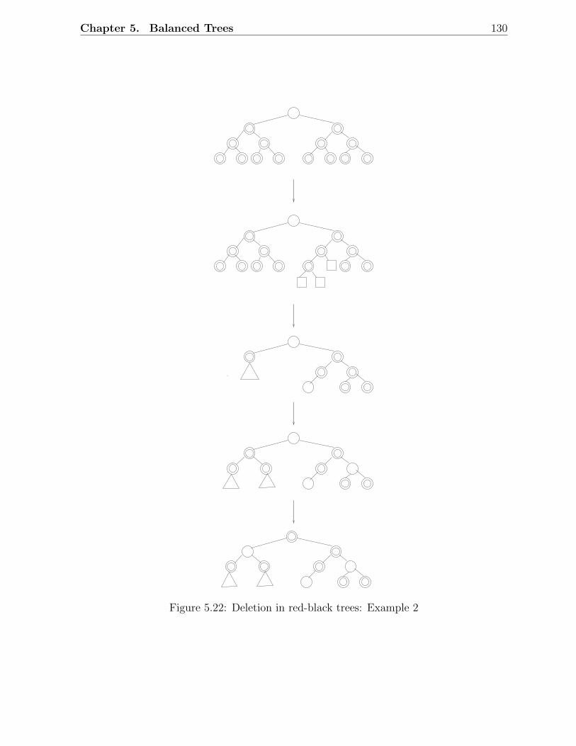
Chapter 5. Balanced Trees 130
Figure 5.22: Deletion in red-black trees: Example 2
Chapter 5. Balanced Trees 131
• If the element to be deleted is in a node with only left child, swap thisnode with the one containing the largest element in the left subtree.(This node has no right child).
• If the element to be deleted is in a node with only right child, swapthis node with the one containing the smallest element in the rightsubtree (This node has no left child).
• If the element to be deleted is in a node with both a left child and aright child, then swap in any of the above two ways.
While swapping, swap only the keys but not the colours.
• The item to be deleted is now in a node having only a left child oronly a right child. Replace this node with its sole child. This mayviolate red constraint or black constraint. Violation of red constraintcan be easily fixed.
• If the deleted node is block, the black constraint is violated. Theremoval of a black node y causes any path that contained y to haveone fewer black node.
• Two cases arise:
1. The replacing node is red, in which case we merely colour it blackto make up for the loss of one black node.
2. The replacing node is black.
In this case, we “bubble” the “shortness” up the tree by repeatedlyapplying the recolouring transformation of Figure 5.16 until it nolonger applies.
Then we perform the transformation in Figure 5.17 if it applies, fol-lowed if necessary by one application of Figure 5.18, Figure 5.19, orFigure 5.20.
• RB-deletion requires O(log n) recolourings and at most 3 rotations.
• See Figures 5.21 and 5.22 for two examples.
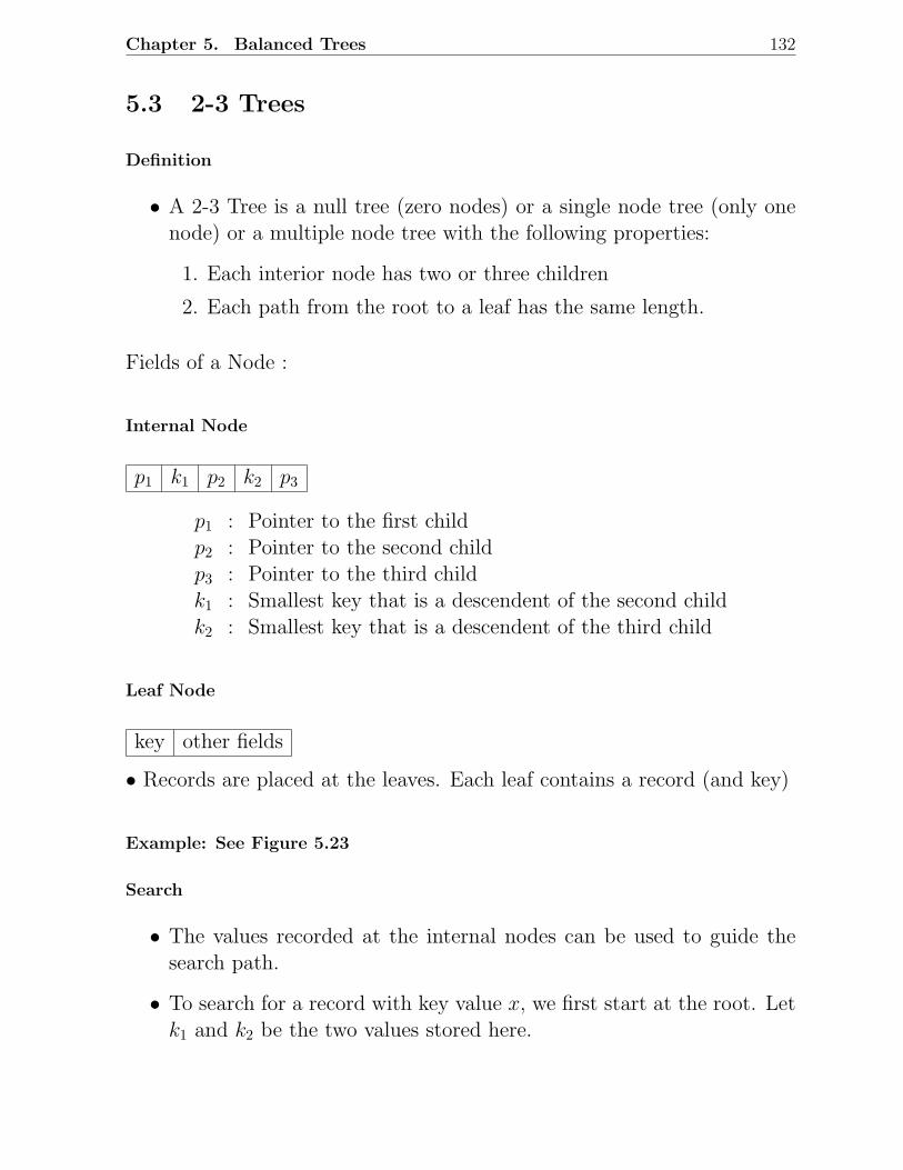
Chapter 5. Balanced Trees 132
5.3 2-3 Trees
Definition
• A 2-3 Tree is a null tree (zero nodes) or a single node tree (only onenode) or a multiple node tree with the following properties:
1. Each interior node has two or three children
2. Each path from the root to a leaf has the same length.
Fields of a Node :
Internal Node
p1 k1 p2 k2 p3
p1 : Pointer to the first childp2 : Pointer to the second childp3 : Pointer to the third childk1 : Smallest key that is a descendent of the second childk2 : Smallest key that is a descendent of the third child
Leaf Node
key other fields
• Records are placed at the leaves. Each leaf contains a record (and key)
Example: See Figure 5.23
Search
• The values recorded at the internal nodes can be used to guide thesearch path.
• To search for a record with key value x, we first start at the root. Letk1 and k2 be the two values stored here.
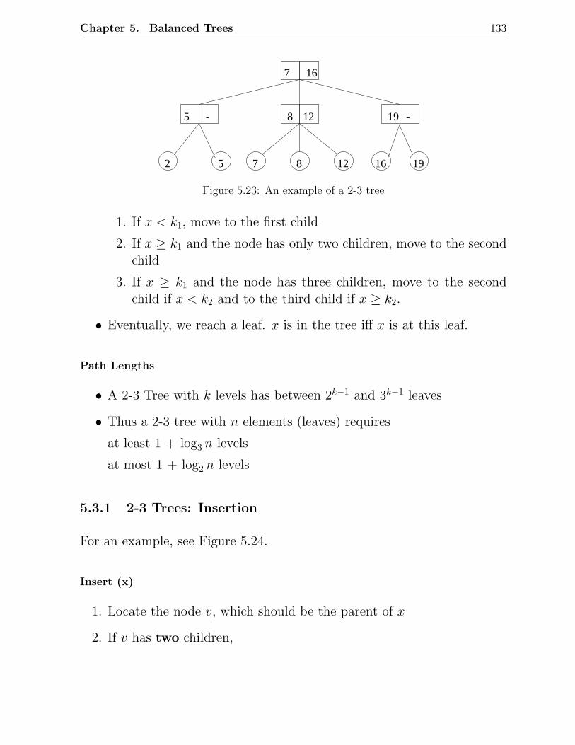
Chapter 5. Balanced Trees 133
7 16
5 - 8 12 19 -
2 5 7 8 12 16 19
Figure 5.23: An example of a 2-3 tree
1. If x < k1, move to the first child
2. If x ≥ k1 and the node has only two children, move to the secondchild
3. If x ≥ k1 and the node has three children, move to the secondchild if x < k2 and to the third child if x ≥ k2.
• Eventually, we reach a leaf. x is in the tree iff x is at this leaf.
Path Lengths
• A 2-3 Tree with k levels has between 2k−1 and 3k−1 leaves
• Thus a 2-3 tree with n elements (leaves) requires
at least 1 + log3 n levels
at most 1 + log2 n levels
5.3.1 2-3 Trees: Insertion
For an example, see Figure 5.24.
Insert (x)
1. Locate the node v, which should be the parent of x
2. If v has two children,
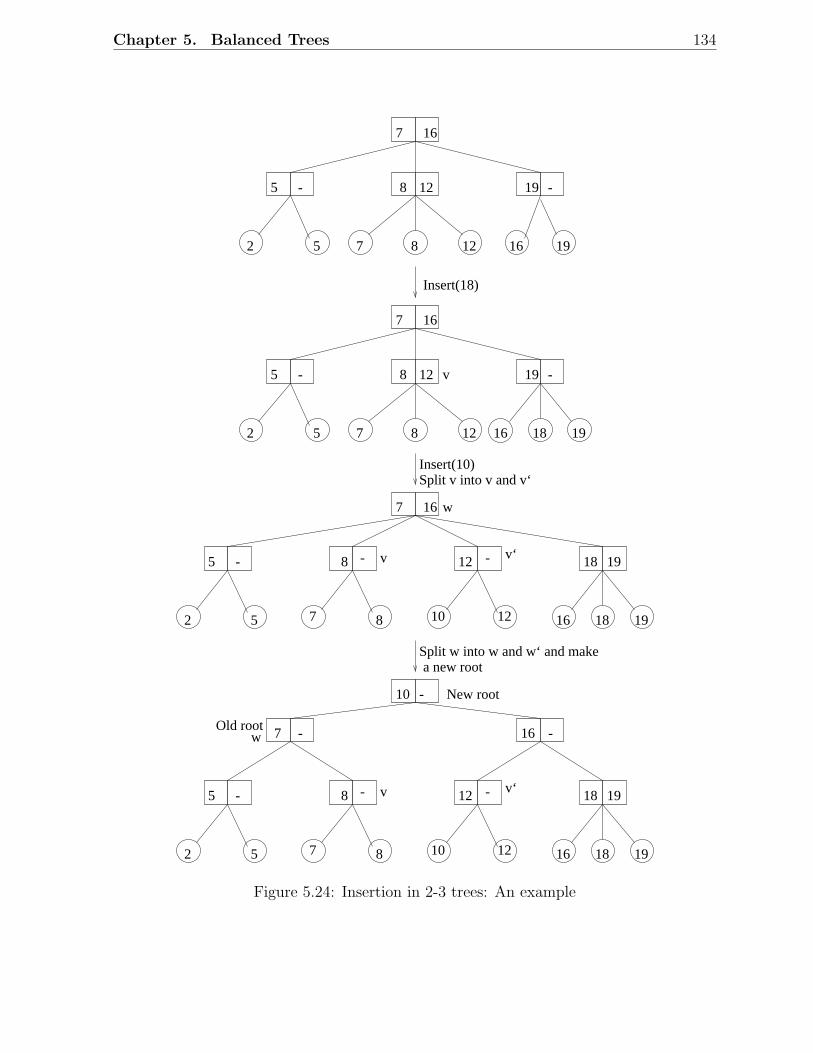
Chapter 5. Balanced Trees 134
5 -
5 -
2 5
8 -
7 8
v 12 -
10 12
v‘
16 18 19
1918
v
7 16
8 - 12
16 18 19
-
7 8 10 12
w
v v‘ 1918
- - 7 16w
10 - New root
Old root
Insert(18)
Insert(10)Split v into v and v‘
Split w into w and w‘ and makea new root
7 16
5 - 8 12 19 -
2 5 7 8 12 16 18 19
2 5
7 16
5 - 8 12 19 -
2 5 7 8 12 16 19
Figure 5.24: Insertion in 2-3 trees: An example
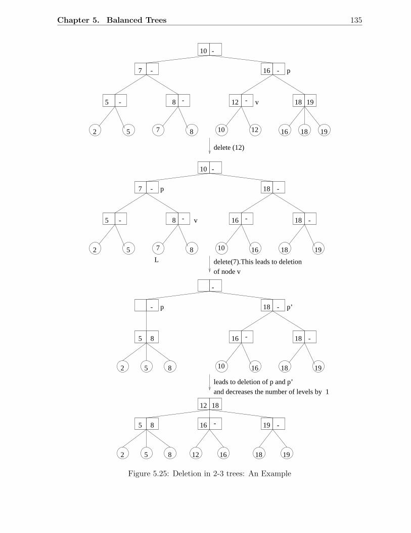
Chapter 5. Balanced Trees 135
5 -
5 -
p
delete (12)
-
10
16 18 -
16 18 19
5 8
of node vdelete(7).This leads to deletion
--
12 18
5 8 16 19
12 16 18 19
leads to deletion of p and p’and decreases the number of levels by 1
- - 7
10 -
8 -
7 8
-
10
18
16 18 -
16 18 19
p
v
L 2 5
- -
-
18p p’
2 5 8
2 5 8
- - 7 16
10 -
8 -
7 8
12 -
10 12
v
2 5 16 18 19
1918
Figure 5.25: Deletion in 2-3 trees: An Example
Chapter 5. Balanced Trees 136
• make x another child of v and place it in the proper order
• adjust k1 and k2 at node v to reflect the new situation
3. If v has three children,
• split v into two nodes v and v′. Make the two smallest amongfour children stay with v and assign the other two as children ofv′.
• Recursively insert v′ among the children of w where
w = parent of v
• The recursive insertion can proceed all the way up to the root,making it necessary to split the root. In this case, create a newroot, thus increasing the number of levels by 1.
5.3.2 2-3 Trees: Deletion
Delete (x)
1. Locate the leaf L containing x and let v be the parent of L
2. Delete L. This may leave v with only one child. If v is the root, deletev and let its lone child become the new root. This reduces the numberof levels by 1. If v is not the root, let
p = parent of v
If p has a child with 3 children, transfer an appropriate one to v
if this child is adjacent (sibling) to v.
If children of p adjacent to v have only two children, transfer thelone child of v to an adjacent sibling of v and delete v.
– If p now has only one child, repeat recursively with p in placeof v. The recursion can ripple all the way up to the root,leading to a decrease in the number of levels.
Example: See Figure 5.25.
Chapter 5. Balanced Trees 137
5.4 B-Trees
• Generalization of 2-3 Trees
• Multi-way search tree, very well suited for external storage
• Standard organization for indices in database systems
• Balanced tree, which achieves minimization of disk accesses in databaseretrieval applications.
REF R. Bayer. Symmetric binary B-trees: Data Structures and mainte-nance algorithms. Acta Informatica, Volume 1, pp.290-306, 1972.
REF R. Bayer and E.M. McCreight. Organization and maintenance of largeordered indexes. Acta Informatica, Volume 1, Number 3, pp. 173-189,1972.
REF D. Comer. The ubiquitous B-tree. ACM Computing Surveys , Volume11, Number 2, pp 121-137, 1979.
5.4.1 Definition of B-Trees
A B-tree of order m is an m-ary search tree with the following properties:
• The root is either a leaf or has at least two children
• Each node, except for the root and the leaves, has between ⌈m/2⌉ andm children
• Each path from the root to a leaf has the same length.
• The root, each internal node, and each leaf is typically a disk block.
• Each internal node has up to (m−1) key values and up to m pointers(to children)
• The records are typically stored in leaves (in some organizations, theyare also stored in internal nodes)
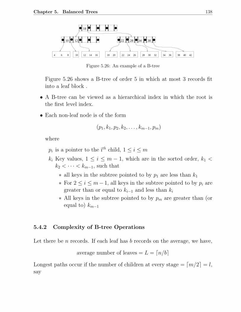
Chapter 5. Balanced Trees 138
18
10 12 22 28 34 38
4 6 8 10 12 14 16 18 20 22 24 26 28 30 32 34 36 38 40 42
Figure 5.26: An example of a B-tree
Figure 5.26 shows a B-tree of order 5 in which at most 3 records fitinto a leaf block .
• A B-tree can be viewed as a hierarchical index in which the root isthe first level index.
• Each non-leaf node is of the form
(p1, k1, p2, k2, . . . , km−1, pm)
where
pi is a pointer to the ith child, 1 ≤ i ≤ m
ki Key values, 1 ≤ i ≤ m − 1, which are in the sorted order, k1 <
k2 < · · · < km−1, such that
∗ all keys in the subtree pointed to by p1 are less than k1
∗ For 2 ≤ i ≤ m− 1, all keys in the subtree pointed to by pi aregreater than or equal to ki−1 and less than ki
∗ All keys in the subtree pointed to by pm are greater than (orequal to) km−1
5.4.2 Complexity of B-tree Operations
Let there be n records. If each leaf has b records on the average, we have,
average number of leaves = L = ⌈n/b⌉
Longest paths occur if the number of children at every stage = ⌈m/2⌉ = l,say
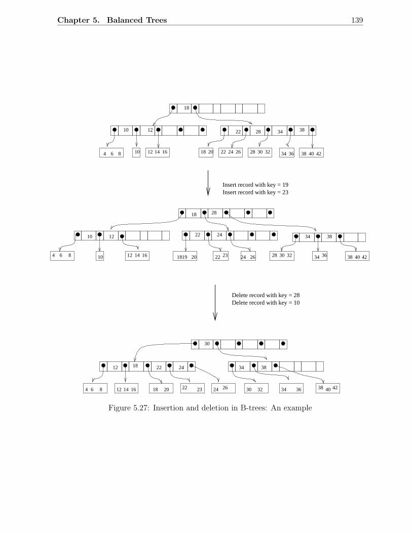
Chapter 5. Balanced Trees 139
38 40 42
4 6 8 10 12 14 16 1819 20 22 23 24 26 28 30 32 34 36 38 40 42
Insert record with key = 19Insert record with key = 23
Delete record with key = 28Delete record with key = 10
30
12 18 22 24 34 38
4 6 8 12 14 16 18 20 22 23 24 26 30 32 34 36
18 28
10 12 22 24 34 38
18
10 12 22 28 34 38
4 6 10 12 14 168 2818 20 22 24 26 30 32 34 3836 40 42
Figure 5.27: Insertion and deletion in B-trees: An example
Chapter 5. Balanced Trees 140
Average number of nodes that are parents of leaves = Ll
Average number of nodes that are second level parents
=
(
L
l
) /
l =L
l2
If h is the level of the leaves, we have
L
lh−1≥ 1
or h ≤ logl Li.e., h ≤ log⌈m/2⌉⌈n/b⌉
If n = 106 records (1 million records), b = 10, and m = 100, we have
h ≤ 3.9
5.4.3 B-Trees: Insertion
Insert (r, x)
Insert a record r with key value = x
• Locate the leaf L at which r should belong.
• If there is room for r in L,
– Insert r into L in the proper order.
– Note that no modifications are necessary to the ancestors of L.
• If there is no room for r in L,
– request the file system for a new block L′ and move the last halfof the records from L to L′, inserting r into its proper place in Lor L′.
Let
P = parent of L
k′ = smallest key value in L′
Chapter 5. Balanced Trees 141
ℓ′ = pointer to L′
Insert k′ and ℓ′ in P (recursively)
– If P already has m pointers, insertion of k′ and ℓ′ into P willcause P to be split and will necessitate an insertion of a key anda pointer in the parent of P .
– The recursive scheme can ripple all the way up to the root causingthe root to be split, in which case
∗ Create a new root with the two halves of the old root as itstwo children. This
· increases the number of levels
· is the only situation where a node has fewer than ⌈m/2⌉children.
Example: See Figure 5.27.
5.4.4 B-Trees: Deletion
Delete (r, x)
Delete a record r with key value = x
• Locate the leaf L containing r
• Remove r from L.
Case 1: L does not become empty after deletion
– if r is not the first record in L, then there is no need to fix thekey values at higher levels.
– If r is the first record in L, then
– if L is not the first child of its parent P , then set the key valuein P ’s entry for L to be the new first key value in L
– if L is the first child of P , the key of r is not recorded inP ; locate the lowest ancestor A of P such that L is not theleftmost descendent of A and set the appropriate key value inA.
Chapter 5. Balanced Trees 142
Case 2: L becomes empty after deletion of r
– Return L to the file system
– Adjust the keys and pointers in P (parent of L) to reflect theremoval of L
– If the number of children of P now < ⌈m/2⌉, examine the node P ′
immediately to the left or the right. If P ′ has at least 1 + ⌈m/2⌉children, distribute the keys and pointers in P and P ′ evenlybetween P and P ′.
– Modify the key values for P and P ′ in the parent of P
– If necessary, ripple the effects to as many ancestors of P asare affected.
– If the number of children of P ′ is exactly ⌈m/2⌉, we combineP and P ′ into a single node with 2⌈m/2⌉ -1 children. Thenremove the key and pointer to P ′ from the parent for P ′. If theeffects of deletion ripple all the way back to the root, combinethe only two children of the root. The resulting combinednode is the new root and the old root is returned to the filesystem. The number of levels decreases by 1.
See Figure 5.27 for an example.
5.4.5 Variants of B-Trees
B+-Trees
• Internal nodes contain the indices to the records corresponding to thekey values k1, k2, . . . , km stored at the internal node. This obviates theneed for repeating these key values and associated indices at the leaflevel.
• More efficient than B-Trees in the case of successful searches.
Chapter 5. Balanced Trees 143
B∗-Trees
• The minimum number of children at each internal node (except theroot) is
⌈
2m
3
⌉
• Pathlengths are smaller for obvious reasons
• Insertions and deletions are more complex.
5.5 To Probe Further
1. Alfred V Aho, John E. Hopcroft, and Jeffrey D Ullman. Data Struc-tures and Algorithms . Addison-Wesley, 1983.
2. Gilles Brassard and Paul Bratley. Fundamentals of Algorithmics .Prentice-Hall, 1996. Indian Edition published by Prentice Hall ofIndia, 1998.
3. Thomas H. Cormen, Charles E. Leiserson, and Donald L. Rivest. In-troduction to Algorithms . The MIT Electrical Engineering and Com-puter Science Series, 1990. Indian Edition published in 1999.
4. Robert L. Kruse, Bruce P. Leung, and Clovis L. Tondo. Data Struc-tures and Program design in C . Prentice Hall, 1991. Indian Editionpublished by Prentice Hall of India, 1999.
5. Mark Allen Weiss. Data Structures and Algorithm Analysis in C++.Benjamin-Cummings, 1994. Indian Edition published in 1998.
6. Duane A. Bailey. Java Structures: Data Structures in Java for thePrincipled Programmer . McGraw-Hill International Edition, 1999.
7. Donald E. Knuth. Sorting and Searching , Volume 3 of The Art ofComputer Programming, Addison-Wesley, 1973.
8. Y. Langsam, M.J. Augenstein, and A.M. Tenenbaum. Data Struc-tures using C and C++. Second Edition, Prentice Hall, 1996. IndianEdition published by Prentice Hall of India, 2000.
Chapter 5. Balanced Trees 144
9. Kurt Mehlhorn. Sorting and Searching. Volume 1 of Data Structuresand Algorithms. Springer-Verlag, 1984.
10. Sartaj Sahni. Data Structures, Algorithms, and Applications in Java.McGraw-Hill Higher Education, 2000.
11. Thomas A. Standish. Data Structures in Java. Addison-Wesley, 1998.Indian Edition published by Addison Wesley Longman, 2000.
12. Nicklaus Wirth. Data Structures + Algorithms = Programs. Prentice-Hall, Englewood Cliffs. 1975.
13. G.M. Adel’son-Vel’skii and E.M. Landis. An algorithm for the or-ganization of information. Soviet Mathematics Monthly , Volume 3,pp.1259-1263, 1962.
14. R. Bayer. Symmetric binary B-trees: Data Structures and mainte-nance algorithms, Acta Informatica, Volume 1, pp.290-306, 1972.
15. R. Bayer and E.M. McCreight. Organization and maintenance of largeordered indexes. Acta Informatica, Volume 1, Number 3, pp. 173-189,1972.
16. D. Comer. The ubiquitous B-tree. ACM Computing Surveys , Volume11, Number 2, pp 121-137, 1979.
17. William Pugh. Skip Lists: A probabilistic alternative to balancedtrees. Communications of the ACM , Volume 33, Number 6, pp. 668-676, 1990.
18. Daniel D Sleator and Robert E. Tarjan. Self-adjusting binary searchtrees. Journal of the ACM , Volume 32, Number 3, pp 652-686, 1985.
19. Robert E. Tarjan. Amortized computational complexity. SIAM Jour-nal on Algebraic and Discrete Methods , Volume 6, Number 2, pp.306-318, 1985.
Chapter 5. Balanced Trees 145
5.6 Problems
5.6.1 AVL Trees
1. Draw all possible binary search trees containing the key values 1, 2, 3, 4. Which ofthese are AVL trees?
2. In each of the following, insert the keys in the order shown, to build them into AVLtrees.
(a) A, Z, B, Y, C, X, D, W, E, V, F.
(b) A, B, C, D, E, F, G, H, I, J, K, L.
(c) A, V, L, T, R, E, I, S, O, K.
In each case, do the following:
(a) Delete each of the the keys inserted in LIFO order (last key inserted is firstdeleted).
(b) Delete each of the keys inserted in FIFO order (first key inserted is firstdeleted).
3. An AVL tree is constructed by inserting the key values 1, 2, 3, 4, 5 in some orderspecified by a permutation of 1, 2, 3, 4, 5, into an initially empty tree. For whichof these permutations is there no need to do any rotations at any stage during theinsertions?
4. Show that the number of (single or double) rotations done in deleting a key froman AVL tree cannot exceed half the height of the tree.
5.6.2 Red-Black Trees
1. Show that any arbitrary n-node binary tree can be transformed into any otherarbitrary n-node binary tree using O(n) rotations.
2. Draw the complete binary search tree of height 3 on the keys 1, 2, · · · , 15. Add theNIL leaves and colour the nodes in three different ways such that the black-heightsof the resulting red-black trees are 2, 3, and 4.
3. Show the red-black trees that result after successively inserting the keys 41, 38, 31,12, 19, 8 into an initially empty red-black tree. Now show the RB trees that resultfrom the successive deletion of the keys in the order 8, 12, 19, 31, 31, 38, 41.
4. Suppose that a node x is inserted into an RB tree and then immediately deleted. Isthe resulting RB tree the same as the initial RB tree? Justify your answer.
Chapter 5. Balanced Trees 146
5. Construct the RB-trees that result by repeated insertions in each of the followingcases, starting from an initially empty tree.
(a) 1, 2, . . . , 15
(b) 8, 4, 12, 6, 14, 2, 10, 7, 11, 5, 9, 3, 8, 1, 15
(c) 1, 2, 3, 4, 5, 6, 7, 15, 14, 13, 12, 11, 10, 9, 8
5.6.3 2-3 Trees and B-Trees
1. For a 2-3 tree with n leaves, compute the following:
(a) Minimum height
(b) Maximum height
2. For a 2-3 tree with height h, compute the following:
(a) Minimum number of leaves
(b) Maximum number of leaves
3. What are the minimum and maximum numbers of internal nodes a B-tree of orderm and height h (ie. (h + 1) levels) may have?
4. Suppose we insert the keys 1,2, ..., in ascending order into an initially empty 2-3tree. Which key would cause the leaves to be at level 4 for the first time? (Assumethat the root is at level 1). Write down the resulting 2-3 tree.
5. Devise an algorithm to find the kth largest element in a
(a) 2-3 tree.
(b) B-tree.
6. Suppose that the keys 1, 2, . . . , 20, are inserted in that order into a B-tree withm = 2. How many internal nodes does the final B-tree have? Show the final B-tree.Compare this with a binary search tree for the same sequence of inserted elements.Assume that each leaf block can only store one record.
7. Suppose that the keys 1, 2, . . . , 20, are inserted in that order into a B-tree withm = 4. How many internal nodes does the final B-tree have? Show the final B-tree.Compare this with a 4-way search tree for the same sequence of inserted elements.Assume that each leaf block can only store one record.
8. Given a B-tree, explain how to find
(a) the minimum key inserted.
(b) predecessor of a given key stored.
Chapter 5. Balanced Trees 147
(c) successor of a given key stored.
9. Suppose we have a file of one million records where each record takes 100 bytes.Blocks are 1000 bytes long and a pointer to a block takes 4 bytes. Also each keyvalue needs two bytes. Devise a B-tree organization for this file.
10. Design a B-tree organization if it is required to contain at least one billion keysbut is constrained to have a height of 4 (ie. 5 levels). Assume that the number ofrecords for each leaf block is 16.
11. Compute the smallest number of keys, which when inserted in an appropriate orderwill force a B-tree of order 5 to have exactly m levels (root at level 1 and leaves atlevel m).
12. A B∗-tree is a B-tree in which each interior node is at least 2/3 full (rather thanhalf full). How do the algorithms for search and delete change for a B∗-tree? Whatwould be the advantages and disadvantages of B∗-trees compared to B-trees?
13. Assume that it takes a + bm milliseconds to read a block containing a node of anm-ary search tree. Assume that it takes c + d log2 m milliseconds to process eachnode in internal memory. If there are n nodes in the tree, compute the total timetaken to find a given record in the tree.
14. Suppose that disk hardware allows us to choose the size of a disk block arbitrarily,but that the time it takes to read the disk block is a+bt, where a and b are specifiedconstants and t is the degree of a B-tree that uses blocks of the selected size (i.e.each disk block contains (t−1) key values and t pointers). Assume that a total of Nrecords are stored in the B-tree database, with each disk block storing one record.
(a) Compute the minimum number of disk blocks required by the above B-treeorganization, including the blocks for storing the records.
(b) Assuming that any record is equally likely to be searched for, estimate the totalaverage disk block reading time for accessing a record.
(c) How do you choose t so as to minimize the total average disk block readingtime?
5.7 Programming Assignments
5.7.1 Red-Black Trees and Splay Trees
This assignment involves the implementation of searches, insertions, and deletions inred-black trees and splay trees, and evaluating the performance of each data structurein several scenarios. The intent is to show that these trees are better than ordinary(unbalanced) binary search trees and also to compare red-black trees with splay trees.
Chapter 5. Balanced Trees 148
Generation of Keys
Assume that your keys are character strings of length 10 obtained by scanning a C pro-gram (identical to Programming assignment 1). If a string has less than 10 characters,make it up to 10 characters by including an appropriate number of trailing *’s. On theother hand, if the current string has more than 10 characters, truncate it to have the firstten characters only.
Inputs to the Program
The possible inputs to the program are:
• n: The initial number of insertions of distinct strings to be made for setting up aninitial search tree (RBT or ST).
• I: This is a decimal number from which a ternary string is to be generated (namelythe radix-3 representation of I). In this representation, assume that a 0 representsthe search operation, a 1 represents the insert operation, and a 2 represents thedelete operation.
• N : Number of operations to be performed on the data structure.
• A C program, from which the tokens are to be picked up for setting up and experi-menting with the search trees.
What should the Program Do?
1. Scan the given C program and as you scan, insert the first n distinct strings scannedinto an initial search tree (BST or RBT or ST).
2. For each individual operation, keep track of:
• Number of probes (comparison of two strings of 10 characters each)
• Number of pointer assignments (a single rotation involves three pointer assign-ments)
• Number of single rotations and number of double rotations (in the case ofRBTs and STs)
• Examining or changing the colour (in a red-black tree)
Now, compute for the BST, RBT, and ST so created, the following:
• Height of the search tree
Chapter 5. Balanced Trees 149
• Total number of probes for all the operations
• Average number of probes (averaged over all the operations) for a typical suc-cessful search, unsuccessful search, insert, and delete.
• Total number of pointer assignments
• Total number of single rotations (in the case of RBTs and STs)
• Total number of double rotations (in the case of RBTs and STs)
• Total number of each type of splaying steps (Zig, Zag, Zig-zig, Zig-zag, Zag-zig,Zag-zag) in the case of STs
• Total number of recolourings in the case of RBTs
3. Scan the rest of the C program token by token, searching for it or inserting it ordeleting it, as dictated by the radix-3 representation of I and its permutations. Youare to carry out a total of N operations.
4. Repeat Step 2 to evaluate the trees over the N operations.
5.7.2 Skip Lists and Binary search Trees
The paper by William Pugh ( Skip Lists: A probabilistic alternative to balanced trees.Communications of the ACM , Volume 33, Number 6, pp. 668-676, 1990) compares theperformance of skip lists with AVL trees, splay trees, and 2-3 trees. Implement all thesedata structures, design experiments on these data structures, and verify the results pre-sented in that article.
5.7.3 Multiway Search Trees and B-Trees
The objective of this assignment is to implement insertions and deletions in multi-waysearch trees and B-trees , and evaluate their performance. Three scenarios are considered:insertions alone; deletions alone; and insertions and deletions interleaved randomly.
• Scenario 1 – Insertions only:Generate a random permutation of n numbers, say a1, a2, . . . , an. Insert these ele-ments into an initially empty data structure. This process will result in a multi-waysearch tree and a B-tree, each with n nodes. The order of the tree to be constructed,m, is given as an input. Note that a binary search tree is a multi-way search treewith m = 2, whereas a 2-3 tree is a B-tree with m = 3. Also the number of recordsper leaf is also to be specified as part of the input. Choose a small number, say 2or 3, here.
• Scenario 2 – Deletions only:Start with the tree constructed in Scenario 1 and delete the n elements, one by one,in the following orders:
Chapter 5. Balanced Trees 150
– In the order of insertion
– In the reversed order of insertion
– In a random order
• Scenario 3 – Interleaved Insertion and Deletions:Start with the tree constructed in Scenario 1 and do a series of randomly interleavedinsertions and deletions. Assume that insertions and deletions are equally likely.Assume that elements currently in the tree and elements not currently in the treeare generated with equal probabilities.
The performance measures are the following:
• Average height of the tree. You should compute it for both MST and BT in all thethree scenarios. Also, you should be able to compute the respective heights at anyintermediate stage. It should be possible to break execution at any desired pointand track the probe sequence for a desired operation.
• Average number of probes required for insertions and deletions. This can be com-puted for each type of tree in each of the three scenarios.
Repeat the above experiment for several random sequences to obtain better and more
credible performance estimates. You will get bonus marks if you implement B∗-trees also.
Chapter 6
Priority Queues
A Priority queue is an important abstract data type in Computer Sci-ence. Major operations supported by priority queues are INSERT andDELETEMIN. They find extensive use in
• implementing schedulers in OS, and distributed systems
• representing event lists in discrete event simulation
• implementing numerous graph algorithms efficiently
• selecting kth largest or kth smallest elements in lists (order statisticsproblems)
• sorting applications
Simple ways of implementing a priority queue include:
• Linked list – sorted and unsorted
• Binary search tree
6.1 Binary Heaps
Heaps (occasionally called as partially ordered trees) are a very populardata structure for implementing priority queues.
151
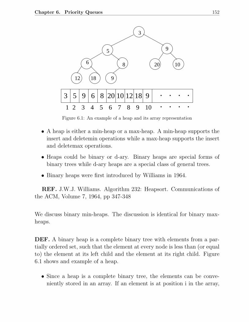
Chapter 6. Priority Queues 152
3 5 9 6 8 20 10 12 18 9 . . . .
4 5 6 7 8 9 101 2 3 . . . .
3
5 9
6 8 10
12 18 9
20
Figure 6.1: An example of a heap and its array representation
• A heap is either a min-heap or a max-heap. A min-heap supports theinsert and deletemin operations while a max-heap supports the insertand deletemax operations.
• Heaps could be binary or d-ary. Binary heaps are special forms ofbinary trees while d-ary heaps are a special class of general trees.
• Binary heaps were first introduced by Williams in 1964.
REF. J.W.J. Williams. Algorithm 232: Heapsort. Communications ofthe ACM, Volume 7, 1964, pp 347-348
We discuss binary min-heaps. The discussion is identical for binary max-heaps.
DEF. A binary heap is a complete binary tree with elements from a par-tially ordered set, such that the element at every node is less than (or equalto) the element at its left child and the element at its right child. Figure6.1 shows and example of a heap.
• Since a heap is a complete binary tree, the elements can be conve-niently stored in an array. If an element is at position i in the array,
Chapter 6. Priority Queues 153
then the left child will be in position 2i and the right child will be inposition 2i + 1. By the same token, a non-root element at position iwill have its parent at position ⌊ i
2 ⌋
• Because of its structure, a heap with height k will have between 2k
and 2k+1 − 1 elements. Therefore a heap with n elements will haveheight = ⌊log2 n ⌋
• Because of the heap property, the minimum element will always bepresent at the root of the heap. Thus the findmin operation will haveworst-case O (1) running time.
6.1.1 Implementation of Insert and Deletemin
Insert
To insert an element say x, into the heap with n elements, we first create ahole in position (n+1) and see if the heap property is violated by puttingx into the hole. If the heap property is not violated, then we have foundthe correct position for x. Otherwise, we “push-up” or “percolate-up” xuntil the heap property is restored. To do this, we slide the element that isin the hole’s parent node into the hole, thus bubbling the hole up towardthe root. We continue this process until x can be placed in the whole. SeeFigure 6.2 for an example.
Worstcase complexity of insert is O (h) where h is the height of the heap.Thus insertions are O (log n) where n is the number of elements in the heap.
Deletemin
When the minimum is deleted, a hole is created at the root level. Sincethe heap now has one less element and the heap is a complete binary tree,the element in the least position is to be relocated. This we first do byplacing the last element in the hole created at the root. This will leave theheap property possibly violated at the root level. We now “push-down” or“percolate-down” the hole at the root until the violation of heap propertyis stopped. While pushing down the hole, it is important to slide it down
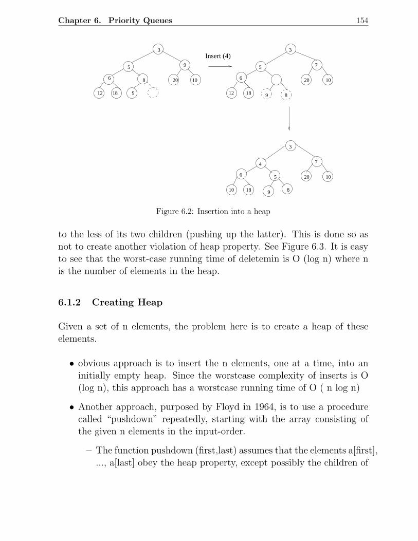
Chapter 6. Priority Queues 154
Insert (4)3
5 9
6 8 10
12 18 9
3
5 7
20 10
18
4 7
6
10 18
20
12
6
20 10
3
89
89
5
Figure 6.2: Insertion into a heap
to the less of its two children (pushing up the latter). This is done so asnot to create another violation of heap property. See Figure 6.3. It is easyto see that the worst-case running time of deletemin is O (log n) where nis the number of elements in the heap.
6.1.2 Creating Heap
Given a set of n elements, the problem here is to create a heap of theseelements.
• obvious approach is to insert the n elements, one at a time, into aninitially empty heap. Since the worstcase complexity of inserts is O(log n), this approach has a worstcase running time of O ( n log n)
• Another approach, purposed by Floyd in 1964, is to use a procedurecalled “pushdown” repeatedly, starting with the array consisting ofthe given n elements in the input-order.
– The function pushdown (first,last) assumes that the elements a[first],..., a[last] obey the heap property, except possibly the children of
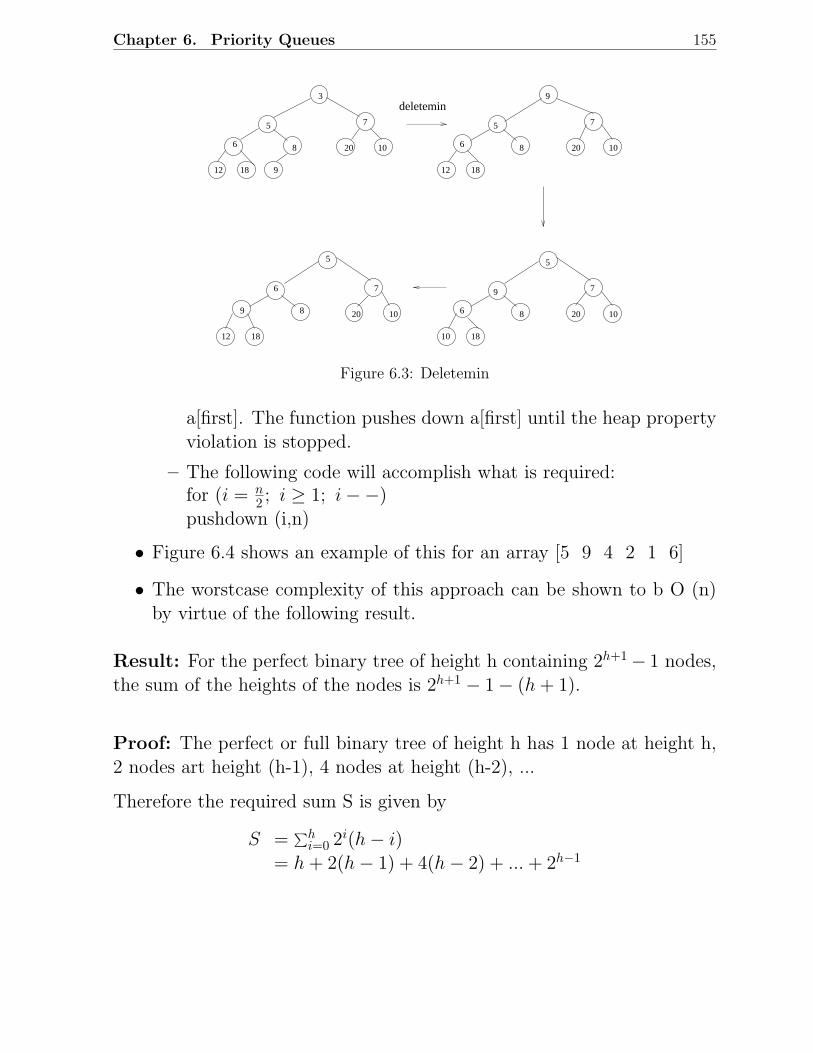
Chapter 6. Priority Queues 155
deletemin3
5
6 8 10
12 18 9
9
5 7
8 20 10
18
9 7
6 8
10 18
5
6 7
9 208 10
12 18
20
12
6
20 10
5
7
Figure 6.3: Deletemin
a[first]. The function pushes down a[first] until the heap propertyviolation is stopped.
– The following code will accomplish what is required:for (i = n
2 ; i ≥ 1; i −−)pushdown (i,n)
• Figure 6.4 shows an example of this for an array [5 9 4 2 1 6]
• The worstcase complexity of this approach can be shown to b O (n)by virtue of the following result.
Result: For the perfect binary tree of height h containing 2h+1 − 1 nodes,the sum of the heights of the nodes is 2h+1 − 1 − (h + 1).
Proof: The perfect or full binary tree of height h has 1 node at height h,2 nodes art height (h-1), 4 nodes at height (h-2), ...
Therefore the required sum S is given by
S =∑h
i=0 2i(h − i)= h + 2(h − 1) + 4(h − 2) + ... + 2h−1
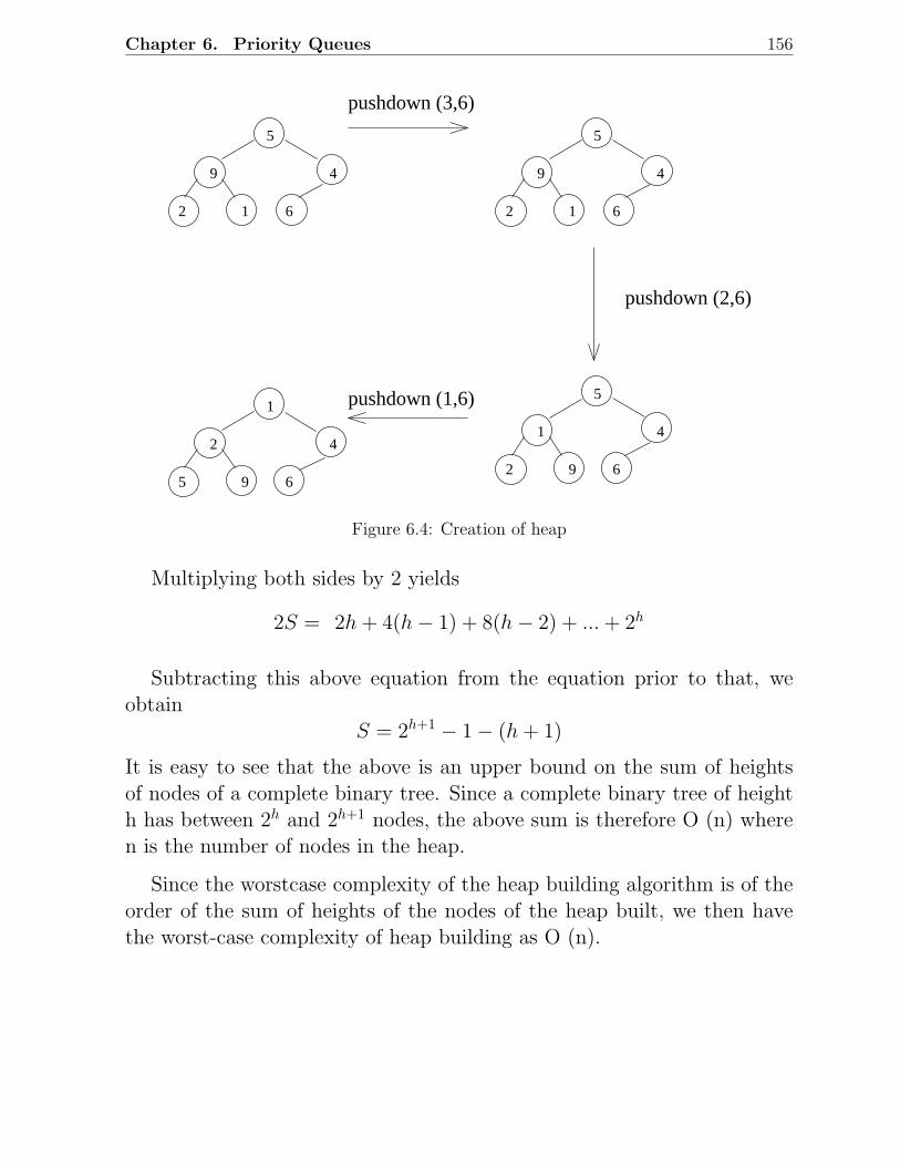
Chapter 6. Priority Queues 156
pushdown (3,6)
pushdown (1,6)
pushdown (2,6)
1
5
2
9
5
2
1
9
5
2
9
1 6
5
2
9
1 6
4 4
44
66
Figure 6.4: Creation of heap
Multiplying both sides by 2 yields
2S = 2h + 4(h − 1) + 8(h − 2) + ... + 2h
Subtracting this above equation from the equation prior to that, weobtain
S = 2h+1 − 1 − (h + 1)
It is easy to see that the above is an upper bound on the sum of heightsof nodes of a complete binary tree. Since a complete binary tree of heighth has between 2h and 2h+1 nodes, the above sum is therefore O (n) wheren is the number of nodes in the heap.
Since the worstcase complexity of the heap building algorithm is of theorder of the sum of heights of the nodes of the heap built, we then havethe worst-case complexity of heap building as O (n).
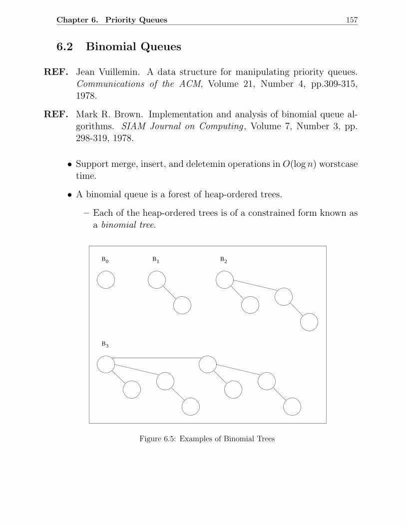
Chapter 6. Priority Queues 157
6.2 Binomial Queues
REF. Jean Vuillemin. A data structure for manipulating priority queues.Communications of the ACM, Volume 21, Number 4, pp.309-315,1978.
REF. Mark R. Brown. Implementation and analysis of binomial queue al-gorithms. SIAM Journal on Computing , Volume 7, Number 3, pp.298-319, 1978.
• Support merge, insert, and deletemin operations in O(log n) worstcasetime.
• A binomial queue is a forest of heap-ordered trees.
– Each of the heap-ordered trees is of a constrained form known asa binomial tree.
B 3
B 0 B 1 B 2
Figure 6.5: Examples of Binomial Trees
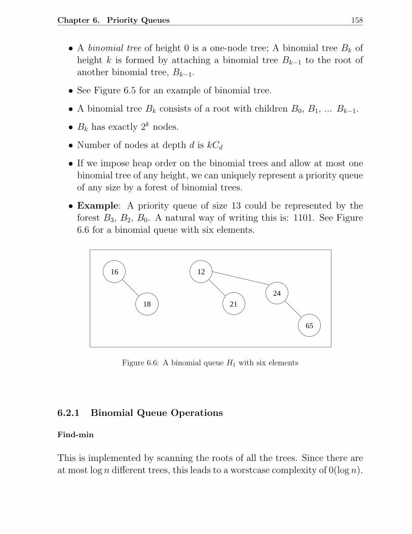
Chapter 6. Priority Queues 158
• A binomial tree of height 0 is a one-node tree; A binomial tree Bk ofheight k is formed by attaching a binomial tree Bk−1 to the root ofanother binomial tree, Bk−1.
• See Figure 6.5 for an example of binomial tree.
• A binomial tree Bk consists of a root with children B0, B1, ... Bk−1.
• Bk has exactly 2k nodes.
• Number of nodes at depth d is kCd
• If we impose heap order on the binomial trees and allow at most onebinomial tree of any height, we can uniquely represent a priority queueof any size by a forest of binomial trees.
• Example: A priority queue of size 13 could be represented by theforest B3, B2, B0. A natural way of writing this is: 1101. See Figure6.6 for a binomial queue with six elements.
16
18
12
21
24
65
Figure 6.6: A binomial queue H1 with six elements
6.2.1 Binomial Queue Operations
Find-min
This is implemented by scanning the roots of all the trees. Since there areat most log n different trees, this leads to a worstcase complexity of 0(log n).
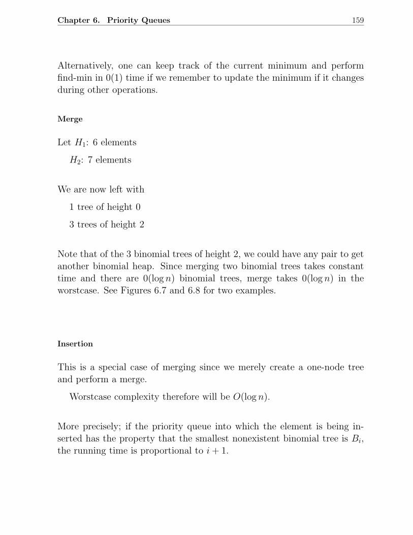
Chapter 6. Priority Queues 159
Alternatively, one can keep track of the current minimum and performfind-min in 0(1) time if we remember to update the minimum if it changesduring other operations.
Merge
Let H1: 6 elements
H2: 7 elements
We are now left with
1 tree of height 0
3 trees of height 2
Note that of the 3 binomial trees of height 2, we could have any pair to getanother binomial heap. Since merging two binomial trees takes constanttime and there are 0(log n) binomial trees, merge takes 0(log n) in theworstcase. See Figures 6.7 and 6.8 for two examples.
Insertion
This is a special case of merging since we merely create a one-node treeand perform a merge.
Worstcase complexity therefore will be O(log n).
More precisely; if the priority queue into which the element is being in-serted has the property that the smallest nonexistent binomial tree is Bi,the running time is proportional to i + 1.
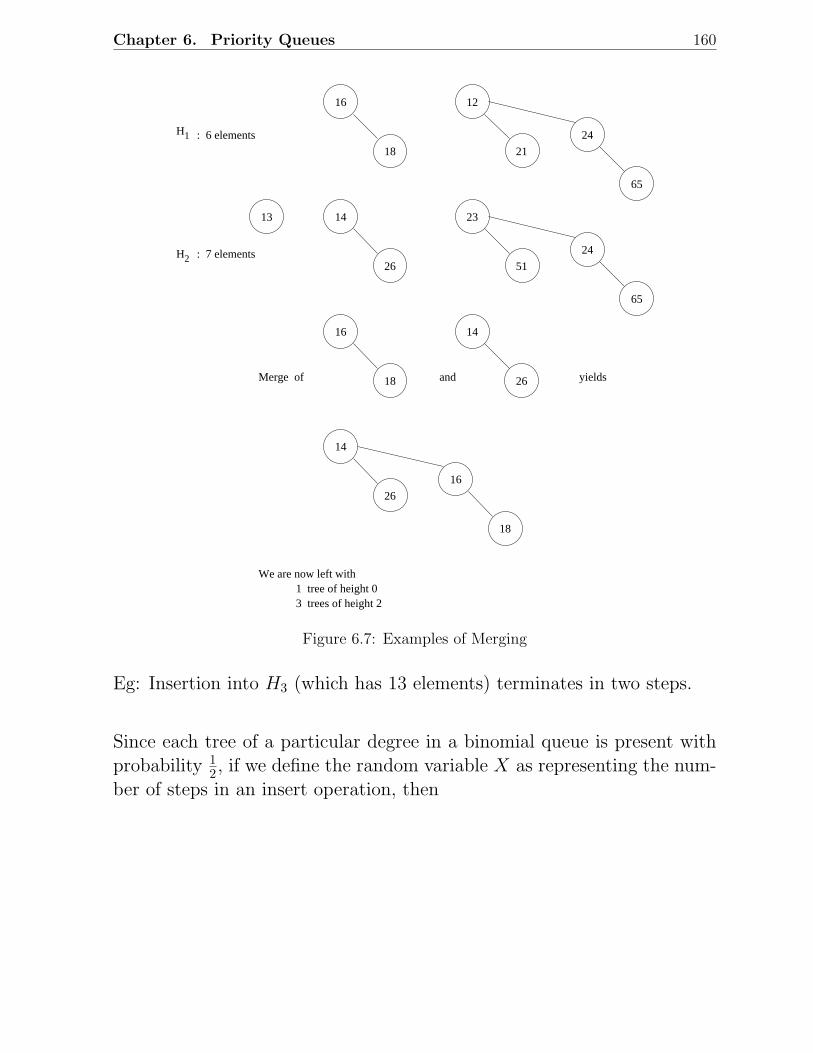
Chapter 6. Priority Queues 160
14
26
23
24
65
51
13
2 : 7 elementsH
16
18 21
24
65
12
H1 : 6 elements
14
26
16
18Merge of and yields
26
16
18
14
We are now left with 1 tree of height 0 3 trees of height 2
Figure 6.7: Examples of Merging
Eg: Insertion into H3 (which has 13 elements) terminates in two steps.
Since each tree of a particular degree in a binomial queue is present withprobability 1
2 , if we define the random variable X as representing the num-ber of steps in an insert operation, then
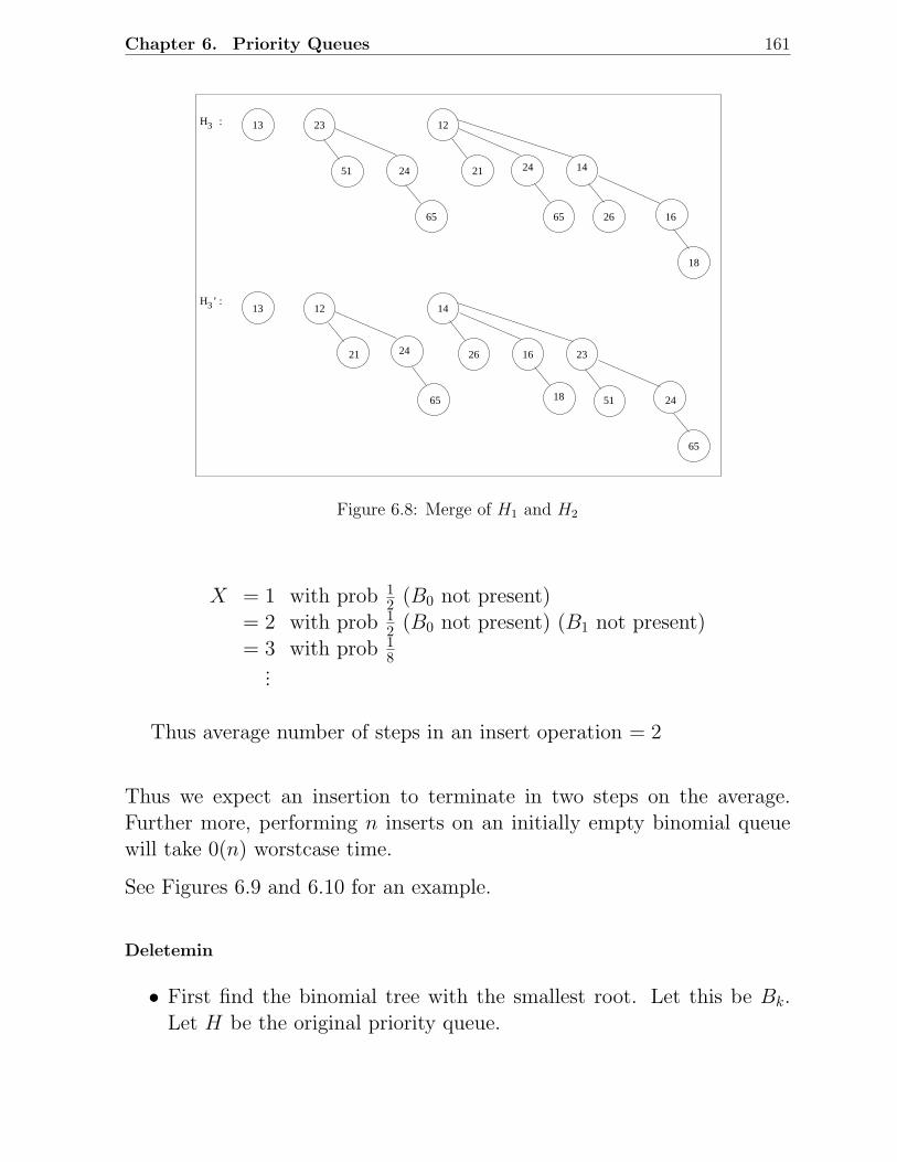
Chapter 6. Priority Queues 161
H3 : 13
12
65
2421
65
24
26
14
16
18
14
26
12
24
23
51
65
21
23
51
18
16
24
65
13H ’ : 3
Figure 6.8: Merge of H1 and H2
X = 1 with prob 12 (B0 not present)
= 2 with prob 12 (B0 not present) (B1 not present)
= 3 with prob 18
...
Thus average number of steps in an insert operation = 2
Thus we expect an insertion to terminate in two steps on the average.Further more, performing n inserts on an initially empty binomial queuewill take 0(n) worstcase time.
See Figures 6.9 and 6.10 for an example.
Deletemin
• First find the binomial tree with the smallest root. Let this be Bk.Let H be the original priority queue.
Chapter 6. Priority Queues 162
Inser (5)
3
5
5
10
+
6 3
5
=
6
10
3
5
3
5
10
Inser (3)
Inser (10)
Inser (6)
18
6
10
3
5
Inser (18)
Inser (14) 14
18 6
10
3
5
6
3
5
14
18
2Inser (2)
18 5
314
6
100
10
Inser (100) 2 10
Figure 6.9: Examples of Inserts
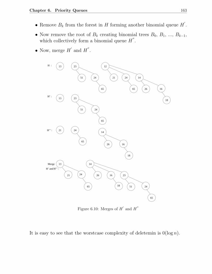
Chapter 6. Priority Queues 163
• Remove Bk from the forest in H forming another binomial queue H′
.
• Now remove the root of Bk creating binomial trees B0, B1, ..., Bk−1,which collectively form a binomial queue H
′′
.
• Now, merge H′
and H′′
.
13
21
1223
51
65 26
18
16
24
65
1424
65
24
24
23
51
65
13
26
18
16
14
65
2421 16
18
14
26 23
51 24
65
H’ :
H :
H’’ :
Merge
21
13
H’’ :H’ and
Figure 6.10: Merges of H′
and H′′
It is easy to see that the worstcase complexity of deletemin is 0(log n).
Chapter 6. Priority Queues 164
Implementation of a Binomial Queue
• deletemin operation requires ability to find all subtrees of the root.Thus children of each node should be available (say a linked list)
• deletemin requires that the children be ordered by the size of theirsubtrees.
• we need to make sure it is easy to merge tress. Two binomial trees canbe merged only if they have the same size, hence the size of the treemust be stored in the root. While merging, one of the trees becomesthe last child of the other, so we should keep track of the last child ofeach node. A good data structure to use is a circular doubly linkedlist what each node is of the following form:
data first left right rank No. ofchild sibling sibling children
6.2.2 Binomial Amortized Analysis
Amortized Analysis of Merge
• To merge two binomial queues, an operation similar to addition ofbinary integers is performed:
At any stage, we may have zero, one, two, or three Bk trees,depending on whether or not the two priority queues contain aBk tree and whether or not a Bk tree is carried over from theprevious step.
∗ if there is zero or more Bk tree, it is placed as a tree in theresulting binomial queue.
∗ If there are two, they are merged into a Bk+1 tree and carriedover
∗ If there are three, one is retained and other two merged.
Chapter 6. Priority Queues 165
Result 1:
• A binomial queue of n elements can be built by n successive insertionsin 0(n) time.
• Brute force AnalysisDefine the cost of each insertions to be
– 1 time unit + an extra unit for each linking stepThus the total will be n units plus the total number of linkingsteps.
– The 1st, 3rd, ... and each odd-numbered step requires no linkingsteps since there is no B0 present.
– A quarter of the insertions require only one linking step: 2nd, 6th,10, ...
– One eighth of insertions require two linking steps.
We could do all this and bound the number of linking steps by n.
The above analysis will not help when we try to analyze a sequenceof operations that include more than just insertions.
• Amortized Analysis
Consider the result of an insertion.
– If there is no B0 tree, then the insertion costs one time unit. Theresult of insertion is that there is now a B0 tree and the forest hasone more tree.
– If there is a B0 tree but not B1 tree, then insertion costs 2 timeunits. The new forest will have a B1 tree but not a B0 tree. Thusnumber of trees in the forest is unchanged.
– An insertion that costs 3 time units will create a B2 tree butdestroy a B0 and B1, yielding one less tree in the forest.
– In general, an insertion that costs c units results in a net increaseof 2 − c trees. Since
∗ a Bc−1 tree is created
Chapter 6. Priority Queues 166
∗ all Bi trees, 0 ≤ i ≤ c − 1 are removed.
Thus expensive insertions remove trees and cheap insertions createtrees.
Let ti = cost of ith insertionci = no. of trees in forest after ith insertion
We havec0 = 0ti + (ci − ci−1) = 2
Result 2:
• The amortized running times of Insert, Delete-min, and Merge are0(1), 0(log n), and 0(log n) respectively.
Potential function = # of trees in the queue
To prove this result we choose:
• Insertion
ti = actual cost of ith insertionci = no. of trees in forest after ith
ai = ti + (ci − ci−1)ai = 2 ∀ i∑n
i=1 ti =∑n
i=1 ai − (cn − c0)= 2n − (cn − c0)
As long as (cn − c0) is positive, we are done.
In any case (cn − c0) is bounded by log n if we start with an emptytree.
• Merge:
Assume that the two queues to be merged have n1 and n2 nodes withT1 and T2 trees. Let n = n1+ n2. Actual time to perform merge isgiven by:
Chapter 6. Priority Queues 167
ti = 0(log n1 + log n2)= 0(max(log n1, log n2)= 0(log n)
(ci − ci−1) is at most (log n) since there can be at most (log n) treesafter merge.
• Deletemin:The analysis here follows the same argument as for merge.
6.2.3 Lazy Binomial Queues
Binomial queues in which merging is done lazily.
Here, to merge two binomial queues, we simply concatenate the two listsof binomial trees. In the resulting forest, there may be several trees of thesame size.
Because of the lazy merge, merge and insert are both worstcase 0(1) time.
• Deletemin:
– Convert lazy binomial queue into a standard binomial queue
– Do deletemin as in standard queue.
Fibonacci Heaps
Fibonacci heap supports all basic heap operations in 0(1) amortized time,with the exception of deletemin and delete which take 0(log n) amortizedtime.
Fibonacci heaps generalize binomial queues by adding two new concepts:
Chapter 6. Priority Queues 168
• A different implementation of decrease-key
• Lazy merging: Two heaps are merged only when it is required.
It can be shown in a Fibonacci heap that any node of rank r ≥ 1 has atleast Fr+1 descendents.
6.3 To Probe Further
1. Alfred V Aho, John E. Hopcroft, and Jeffrey D Ullman. Data Struc-tures and Algorithms . Addison-Wesley, 1983.
2. Gilles Brassard and Paul Bratley. Fundamentals of Algorithmics .Prentice-Hall, 1996. Indian Edition published by Prentice Hall ofIndia, 1998.
3. Thomas H. Cormen, Charles E. Leiserson, and Donald L. Rivest. In-troduction to Algorithms . The MIT Electrical Engineering and Com-puter Science Series, 1990. Indian Edition published in 1999.
4. Mark Allen Weiss. Data Structures and Algorithm Analysis in C++.Benjamin-Cummings, 1994. Indian Edition published in 1998.
5. Ellis Horowitz, Sartaz Sahni, and Rajasekaran. Fundamentals of Com-puter Algorithms . W.H. Freeman and Company, 1998. Indian Editionpublished by Galgotia Publications, 2000.
6. Y. Langsam, M.J. Augenstein, and A.M. Tenenbaum. Data Structuresusing C and C++. Second Edition, Prentice Hall, 1996.XS IndianEdition published by Prentice Hall of India, 2000.
7. Sataj Sahni. Data Structures, Algorithms, and Applications in Java.McGraw-Hill Higher Education, 2000.
8. Thomas A. Standish. Data Structures in Java. Addison-Wesley, 1998.Indian Edition published by Addison Wesley Longman, 2000.
9. Mark R. Brown. Implementation and analysis of binomial queue al-gorithms. SIAM Journal on Computing, Volume 7, Number 3, pp.298-319, 1978.
Chapter 6. Priority Queues 169
10. Michael L. Fredman and Robert E. Tarjan. Fibonacci heaps and theiruses in improved network optimization algorithms. Journal of theACM , Volume 34, Number 3, pp. 596-615, 1987.
11. Robert W. Floyd. Algorithm 245 (TreeSort). Communications of theACM , Volume 7, pp.701, 1964.
12. Jean Vuillemin. A data structure for manipulating priority queues.Communications of the ACM, Volume 21, Number 4, pp.309-315,1978.
13. J.W.J. Williams. Algorithm 232 (Heapsort). Communications of theACM , Volume 7, pp.347-348, 1964.
6.4 Problems
1. Show the result of inserting 10, 5, 1, 17, 20, 15, 6, 4, 2, one at a time, into an initiallyempty binary heap. For the same input, show the result of building the heap by the lineartime algorithm discussed.
2. Design an algorithm to find all nodes less than some value, x, in a binary heap. Youralgorithm should run in O (m), worst-case time, where m is the number of nodes output.
3. A min-max heap is a data structure that supports both deletemin and deletemax in O (log n) worst-case time. The structure is identical to a binary heap, but the heap orderproperty is that, for any node x, at even depth, the key stored at x is the smallest in itssubtree, and for any node x at odd depth, the key stored at x is the largest in its subtree.
(a) How do we find minimum and maximum elements
(b) Present an algorithm to insert a new node into the min-max heap
(c) Give an algorithm to perform deletemin and deletemax
4. Prove that a binomial tree Bk has binomial trees B0, B1, . . . , Bk−1 as children of the root.
5. Prove that a binomial tree of height k has stackrel(k)(d) nodes at depth d.
6. Present an algorithm to insert m nodes into a binomial queue of n elements in O(m+log n)worst-case time. Prove your bound.
7. It is required to increment the value of the roots of all binomial trees in a binomial queue.What is the worst-case running time of this in terms of the number of elements in thebinomial queue.
Chapter 6. Priority Queues 170
8. Design an algorithm to search for an element in a binary heap. What is the worst-casecomplexity of your algorithm. Can you use the heap property to speedup the searchprocess?
9. Prove that a binomial queue with n items has at most log n binomial trees, the largest ofwhich contains 2log n items.
10. How do you implement the following operations in a binary heap?
• Decrease the key at some position
• Increase the key at some position
• Remove element at some position
11. What is the worstcase complexity of each problem below, given a binomial queue with nelements? Explain with reason or example in each case.
(a) Find the second smallest element
(b) Find the second largest element
12. Consider lazy binomial queues where the merge operation is lazy and it is left to thedeletemin operation to convert the lazy binomial queue into a binomial queue in standardform. Obviously, the merge operation is O(1), but the deletemin operation is not worstcase O(log n) anymore. However, show that deletemin is still O(log n) in amortized time.
6.5 Programming Assignments
6.5.1 Discrete Event Simulation
Priority queues provide a natural dats structure to use in event list maintenance in discrete eventsimulations. The objective of this assignment is to develop event list algorithms using priorityqueues and use these as a component in a discrete event simulation package. Singly linked listsare commonly used in implementing event lists. One can use binary heaps and binomial queuesfor better performance.
Write a simulation package for a discrete event system (with a large number of events) and
compare the performance of naive linked lists, binary heaps, and binomial queues in event list
related aspects of the simulation.
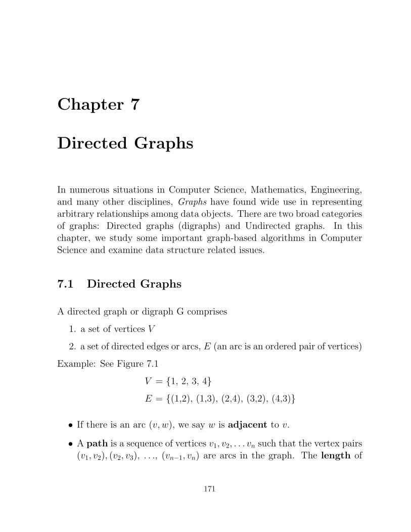
Chapter 7
Directed Graphs
In numerous situations in Computer Science, Mathematics, Engineering,and many other disciplines, Graphs have found wide use in representingarbitrary relationships among data objects. There are two broad categoriesof graphs: Directed graphs (digraphs) and Undirected graphs. In thischapter, we study some important graph-based algorithms in ComputerScience and examine data structure related issues.
7.1 Directed Graphs
A directed graph or digraph G comprises
1. a set of vertices V
2. a set of directed edges or arcs, E (an arc is an ordered pair of vertices)
Example: See Figure 7.1
V = 1, 2, 3, 4E = (1,2), (1,3), (2,4), (3,2), (4,3)
• If there is an arc (v, w), we say w is adjacent to v.
• A path is a sequence of vertices v1, v2, . . . vn such that the vertex pairs(v1, v2), (v2, v3), . . ., (vn−1, vn) are arcs in the graph. The length of
171
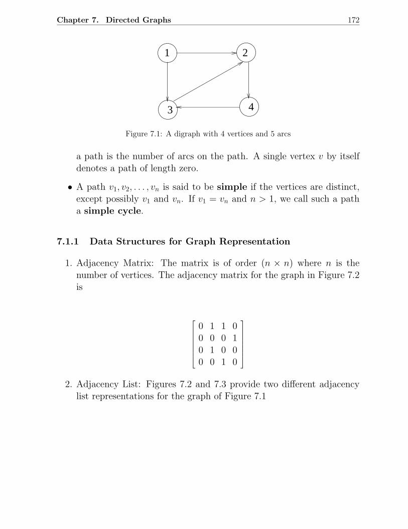
Chapter 7. Directed Graphs 172
3 4
1 2
Figure 7.1: A digraph with 4 vertices and 5 arcs
a path is the number of arcs on the path. A single vertex v by itselfdenotes a path of length zero.
• A path v1, v2, . . . , vn is said to be simple if the vertices are distinct,except possibly v1 and vn. If v1 = vn and n > 1, we call such a patha simple cycle.
7.1.1 Data Structures for Graph Representation
1. Adjacency Matrix: The matrix is of order (n × n) where n is thenumber of vertices. The adjacency matrix for the graph in Figure 7.2is
0 1 1 00 0 0 10 1 0 00 0 1 0
2. Adjacency List: Figures 7.2 and 7.3 provide two different adjacencylist representations for the graph of Figure 7.1
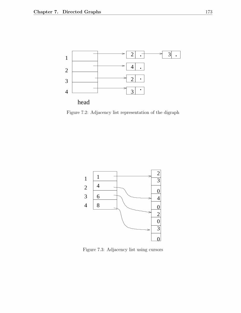
Chapter 7. Directed Graphs 173
1
2
3
4
2
2
3
3.
.
.
.
.
4
head
Figure 7.2: Adjacency list representation of the digraph
1
2
4
3
4
8
1
604
020
0
32
3
Figure 7.3: Adjacency list using cursors
Chapter 7. Directed Graphs 174
7.2 Shortest Paths Problem
Given : A digraph G = (V, E) in which each arc has a non-negativecost and one vertex is designated as the source.
Problem : To determine the cost of the shortest path from the sourceto every other vertex in V (where the length of a path isjust the sum of the costs of the arcs on the path).
7.2.1 Single Source Shortest Paths Problem: Dijkstra’s Algo-rithm
REF. E.W. Dijkstra. A note on two problems in connection with graphs.Numerische Mathematik , Volume 1, pp. 269-271, 1959.
• Greedy algorithm
• It works by maintaining a set S of “special” vertices whose shortestdistance from the source is already known. At each step, a “non-special” vertex is absorbed into S.
• The absorption of an element of V − S into S is done by a greedystrategy.
• The following provides the steps of the algorithm.
Let
V = 1, 2, . . . , n and source = 1 (7.1)
C[i, j] = Cost of the arc (i, j) if the arc (i, j) exists; otherwise ∞
S= 1 ;for (i = 2; i < n; i++)
D[i] = C[1,i];
Chapter 7. Directed Graphs 175
for (i=1; i < = n-1; i++)
choose a vertex w ∈ V–S such that D[w] is a minimum;
S = S ∪ w ;for each vertex v ∈ V–S
D[v] = min (D[v], D[w] + C[w, v])
• The above algorithm gives the costs of the shortest paths from sourcevertex to every other vertex.
• The actual shortest paths can also be constructed by modifying theabove algorithm.
Theorem: Dijkstra’s algorithm finds the shortest paths from a singlesource to all other nodes of a weighted digraph with positive weights.
Proof: Let V = 1, 2, ..., n and 1 be the source vertex. We use mathematicalinduction to show that
(a) If a node i (6= 1) ∈ S, then D[i] gives the length of the shortest pathfrom the source to i.
(b) if a node i /∈ S, then D[i] gives the length of the shortest special pathfrom the source to i.
Basis: Initially S = 1 and hence (a) is vacuously true. For i ∈ S, the onlyspecial path from the source is the direct edge if present from source to iand D is initialized accordingly. Hence (b) is also true.
Induction for condition (a)
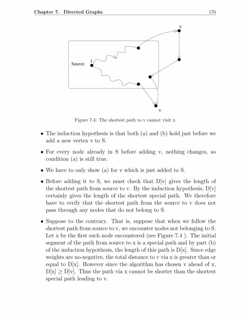
Chapter 7. Directed Graphs 176
Source1
x
v
Figure 7.4: The shortest path to v cannot visit x
• The induction hypothesis is that both (a) and (b) hold just before weadd a new vertex v to S.
• For every node already in S before adding v, nothing changes, socondition (a) is still true.
• We have to only show (a) for v which is just added to S.
• Before adding it to S, we must check that D[v] gives the length ofthe shortest path from source to v. By the induction hypothesis, D[v]certainly gives the length of the shortest special path. We thereforehave to verify that the shortest path from the source to v does notpass through any nodes that do not belong to S.
• Suppose to the contrary. That is, suppose that when we follow theshortest path from source to v, we encounter nodes not belonging to S.Let x be the first such node encountered (see Figure 7.4 ). The initialsegment of the path from source to x is a special path and by part (b)of the induction hypothesis, the length of this path is D[x]. Since edgeweights are no-negative, the total distance to v via x is greater than orequal to D[x]. However since the algorithm has chosen v ahead of x,D[x] ≥ D[v]. Thus the path via x cannot be shorter than the shortestspecial path leading to v.
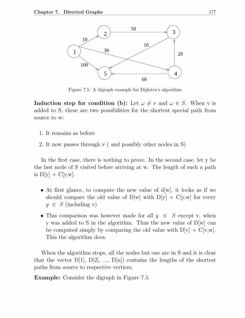
Chapter 7. Directed Graphs 177
1
2 3
45
10
50
20
10
60
100
30
Figure 7.5: A digraph example for Dijkstra’s algorithm
Induction step for condition (b): Let ω 6= v and ω ∈ S. When v isadded to S, these are two possibilities for the shortest special path fromsource to w:
1. It remains as before
2. It now passes through v ( and possibly other nodes in S)
In the first case, there is nothing to prove. In the second case, let y bethe last node of S visited before arriving at w. The length of such a pathis D[y] + C[y,w].
• At first glance, to compute the new value of d[w], it looks as if weshould compare the old value of D[w] with D[y] + C[y,w] for everyy ∈ S (including v)
• This comparison was however made for all y ∈ S except v, wheny was added to S in the algorithm. Thus the new value of D[w] canbe computed simply by comparing the old value with D[v] + C[v,w].This the algorithm does.
When the algorithm stops, all the nodes but one are in S and it is clearthat the vector D[1], D[2], ..., D[n]) contains the lengths of the shortestpaths from source to respective vertices.
Example: Consider the digraph in Figure 7.5.
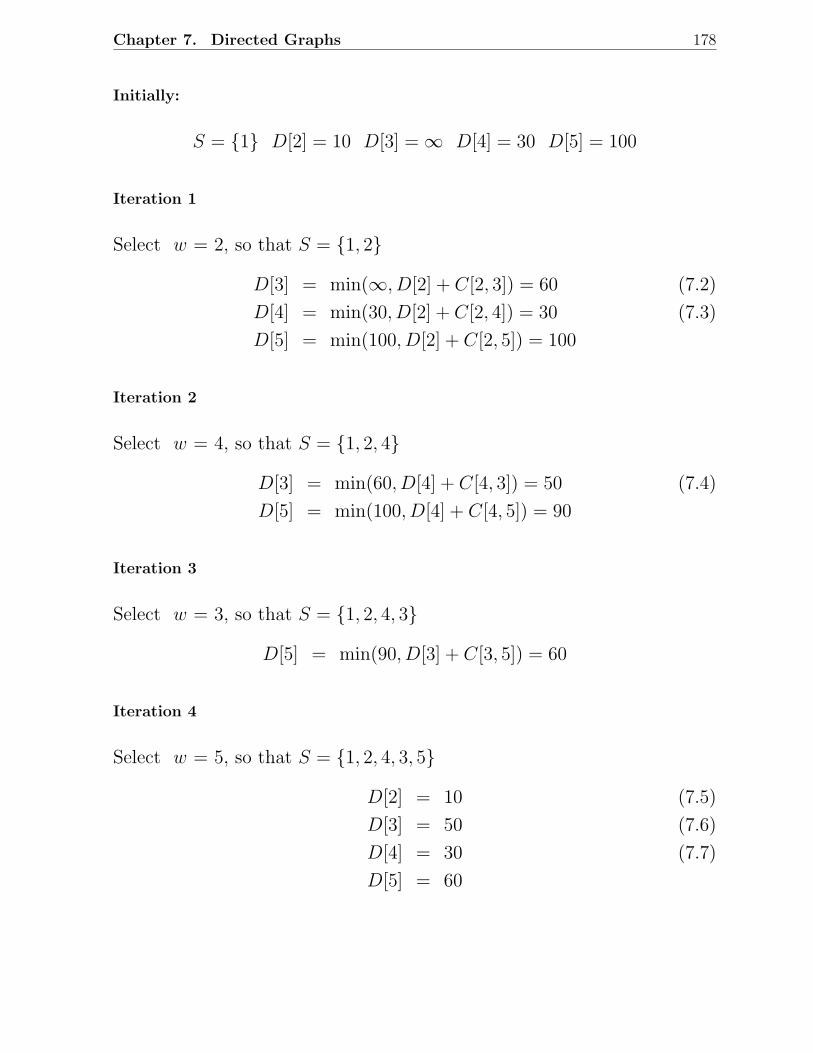
Chapter 7. Directed Graphs 178
Initially:
S = 1 D[2] = 10 D[3] = ∞ D[4] = 30 D[5] = 100
Iteration 1
Select w = 2, so that S = 1, 2
D[3] = min(∞, D[2] + C[2, 3]) = 60 (7.2)
D[4] = min(30, D[2] + C[2, 4]) = 30 (7.3)
D[5] = min(100, D[2] + C[2, 5]) = 100
Iteration 2
Select w = 4, so that S = 1, 2, 4
D[3] = min(60, D[4] + C[4, 3]) = 50 (7.4)
D[5] = min(100, D[4] + C[4, 5]) = 90
Iteration 3
Select w = 3, so that S = 1, 2, 4, 3
D[5] = min(90, D[3] + C[3, 5]) = 60
Iteration 4
Select w = 5, so that S = 1, 2, 4, 3, 5
D[2] = 10 (7.5)
D[3] = 50 (7.6)
D[4] = 30 (7.7)
D[5] = 60
Chapter 7. Directed Graphs 179
Complexity of Dijkstra’s Algorithm
With adjacency matrix representation, the running time is O(n2) By us-ing an adjacency list representation and a partially ordered tree datastructure for organizing the set V − S, the complexity can be shown to be
O(e log n)
where e is the number of edges and n is the number of vertices in thedigraph.
7.2.2 Dynamic Programming Algorithm
REF. Richard Bellman. Dynamic Programming . Princeton University Press,1957.
REF. Richard Bellman. On a routing problem. Quarterly of Applied Math-ematics , Volume 16, Number 1, pp. 87-90, 1958.
Consider a directed acyclic graph (digraph without cycles) with non-negative weights on the directed arcs.
Given a destination vertex z, the problem is to find a shortest cost pathfrom each vertex of the digraph. See Figure 7.6.
Let
C(i, j) = Cost of the directed arc from vertex i to
vertex j (∞ in case there is no link) (7.8)
J(i) = Optimal cost of a path from vertex i, to the (7.9)
destination vertex z
J(i) Satisfies :J(z) = 0
and if the optimal path from i to z traverses the link (i, j) then
J(i) = C(i, j) + J(j)
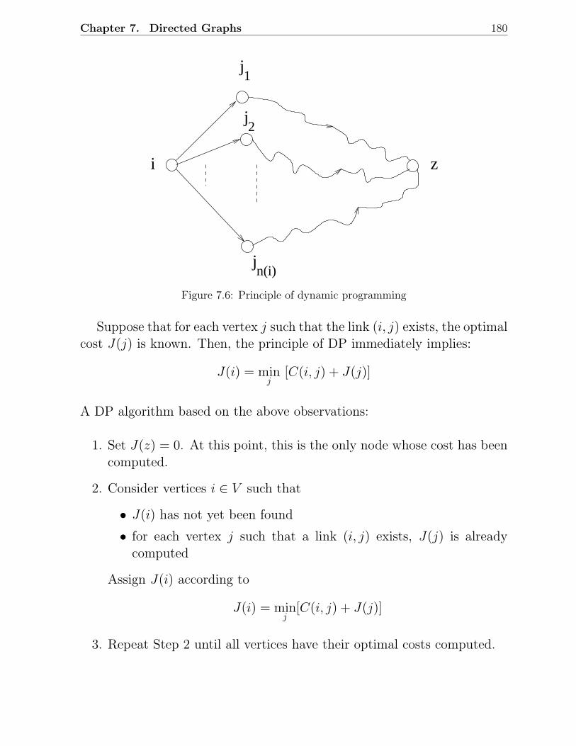
Chapter 7. Directed Graphs 180
i z
1
2
n(i)j
j
j
Figure 7.6: Principle of dynamic programming
Suppose that for each vertex j such that the link (i, j) exists, the optimalcost J(j) is known. Then, the principle of DP immediately implies:
J(i) = minj
[C(i, j) + J(j)]
A DP algorithm based on the above observations:
1. Set J(z) = 0. At this point, this is the only node whose cost has beencomputed.
2. Consider vertices i ∈ V such that
• J(i) has not yet been found
• for each vertex j such that a link (i, j) exists, J(j) is alreadycomputed
Assign J(i) according to
J(i) = minj
[C(i, j) + J(j)]
3. Repeat Step 2 until all vertices have their optimal costs computed.
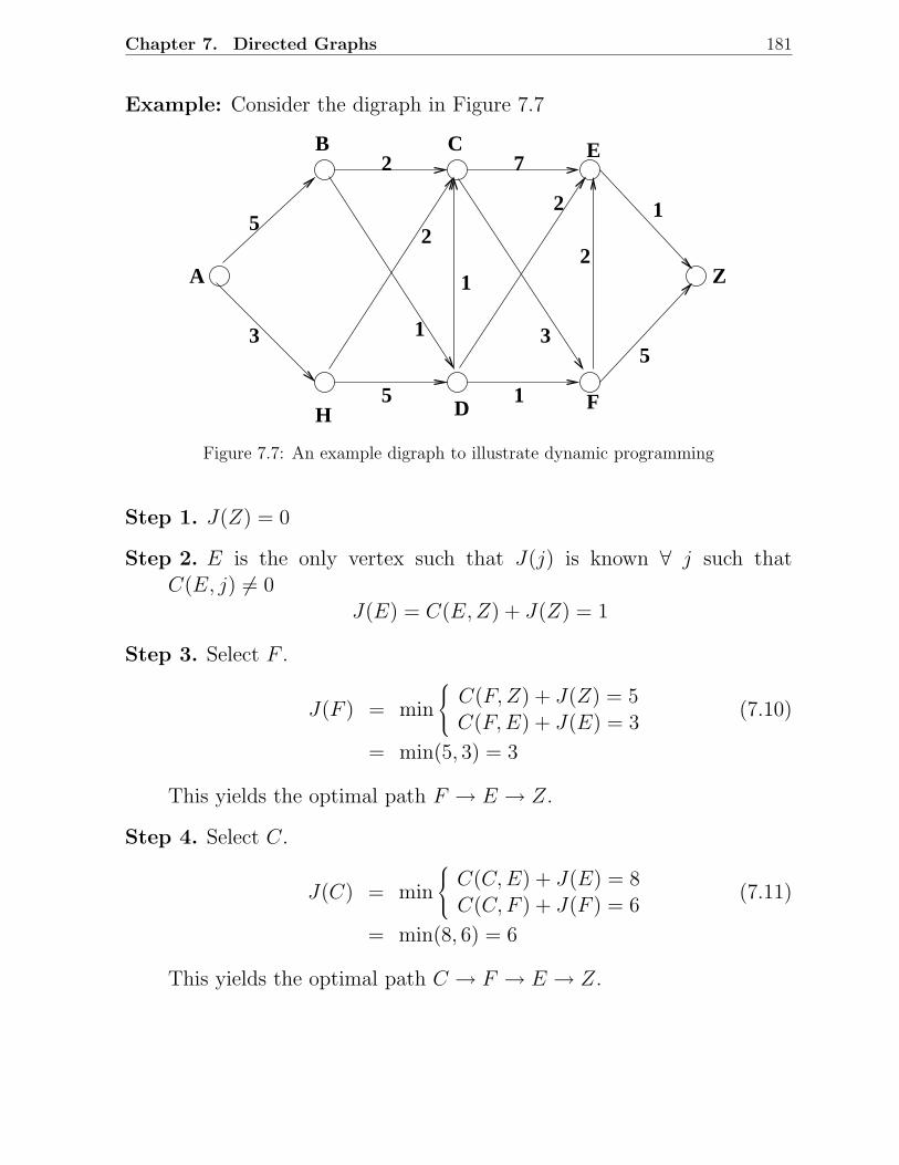
Chapter 7. Directed Graphs 181
Example: Consider the digraph in Figure 7.7
B C E
H D F
A Z
5
2 7
1
5
5 1
21
2
3 1 3
2
Figure 7.7: An example digraph to illustrate dynamic programming
Step 1. J(Z) = 0
Step 2. E is the only vertex such that J(j) is known ∀ j such thatC(E, j) 6= 0
J(E) = C(E, Z) + J(Z) = 1
Step 3. Select F .
J(F ) = min
C(F, Z) + J(Z) = 5C(F, E) + J(E) = 3
(7.10)
= min(5, 3) = 3
This yields the optimal path F → E → Z.
Step 4. Select C.
J(C) = min
C(C, E) + J(E) = 8C(C, F ) + J(F ) = 6
(7.11)
= min(8, 6) = 6
This yields the optimal path C → F → E → Z.
Chapter 7. Directed Graphs 182
Step 5. Select D
J(D) = min
C(D, C) + J(C) = 7C(D, E) + J(E) = 3 = 3C(D, F ) + J(F ) = 4
This yields the optimal path D → E → Z....
Eventually, we get all the optimal paths and all the optimal costs.
Complexity of the Algorithm
• It is easy to see that the algorithm has a worst case complexity ofO(n2), where n is the number of vertices.
• Limitation of the algorithm
– doesn’t work if there are cycles in the digraph.
7.2.3 All Pairs Shortest Paths Problem: Floyd’s Algorithm
REF. Robert W Floyd. Algorithm 97 (Shortest Path). Communications ofthe ACM , Volume 5, Number 6, pp. 345, 1962.
Given : A digraph G = (V, E) in which each arc v → w has
a nonnegative cost C[v, w]
To find : For each ordered pair of vertices (v, w), the smallest
length of any path from v to w
Floyd’s Algorithm
• This is an O(n3) algorithm, where n is the number of vertices in thedigraph.
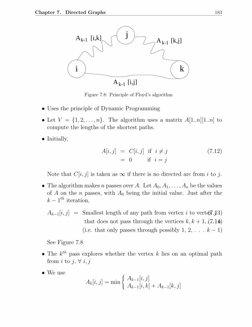
Chapter 7. Directed Graphs 183
i
[i,k]Ak-1
A k-1
[k,j]A k-1
[i,j]
j
k
Figure 7.8: Principle of Floyd’s algorithm
• Uses the principle of Dynamic Programming
• Let V = 1, 2, . . . , n. The algorithm uses a matrix A[1..n][1..n] tocompute the lengths of the shortest paths.
• Initially,
A[i, j] = C[i, j] if i 6= j (7.12)
= 0 if i = j
Note that C[i, j] is taken as ∞ if there is no directed arc from i to j.
• The algorithm makes n passes over A. Let A0, A1, . . . , An be the valuesof A on the n passes, with A0 being the initial value. Just after thek − 1th iteration,
Ak−1[i, j] = Smallest length of any path from vertex i to vertex j(7.13)
that does not pass through the vertices k, k + 1, . . . , n(7.14)
(i.e. that only passes through possibly 1, 2, . . . k − 1)
See Figure 7.8
• The kth pass explores whether the vertex k lies on an optimal pathfrom i to j, ∀ i, j
• We use
Ak[i, j] = min
Ak−1[i, j]Ak−1[i, k] + Ak−1[k, j]
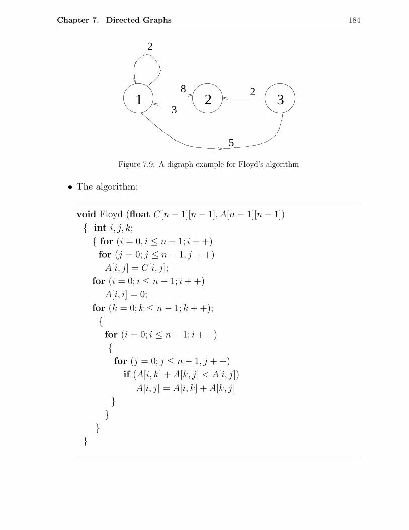
Chapter 7. Directed Graphs 184
2
8
3
2
5
1 2 3
Figure 7.9: A digraph example for Floyd’s algorithm
• The algorithm:
void Floyd (float C[n − 1][n − 1], A[n − 1][n − 1])
int i, j, k;
for (i = 0, i ≤ n − 1; i + +)
for (j = 0; j ≤ n − 1, j + +)
A[i, j] = C[i, j];
for (i = 0; i ≤ n − 1; i + +)
A[i, i] = 0;
for (k = 0; k ≤ n − 1; k + +);
for (i = 0; i ≤ n − 1; i + +)
for (j = 0; j ≤ n − 1, j + +)
if (A[i, k] + A[k, j] < A[i, j])
A[i, j] = A[i, k] + A[k, j]
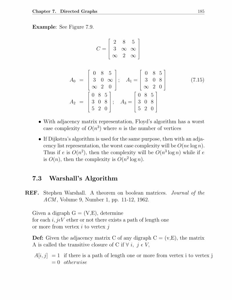
Chapter 7. Directed Graphs 185
Example: See Figure 7.9.
C =
2 8 53 ∞ ∞∞ 2 ∞
A0 =
0 8 53 0 ∞∞ 2 0
; A1 =
0 8 53 0 8∞ 2 0
(7.15)
A2 =
0 8 53 0 85 2 0
; A3 =
0 8 53 0 85 2 0
• With adjacency matrix representation, Floyd’s algorithm has a worstcase complexity of O(n3) where n is the number of vertices
• If Dijkstra’s algorithm is used for the same purpose, then with an adja-cency list representation, the worst case complexity will be O(ne log n).Thus if e is O(n2), then the complexity will be O(n3 log n) while if e
is O(n), then the complexity is O(n2 log n).
7.3 Warshall’s Algorithm
REF. Stephen Warshall. A theorem on boolean matrices. Journal of theACM , Volume 9, Number 1, pp. 11-12, 1962.
Given a digraph G = (V,E), determinefor each i, jǫV ether or not there exists a path of length oneor more from vertex i to vertex j
Def: Given the adjacency matrix C of any digraph C = (v,E), the matrixA is called the transitive closure of C if ∀ i, j ǫ V,
A[i, j] = 1 if there is a path of length one or more from vertex i to vertex j= 0 otherwise
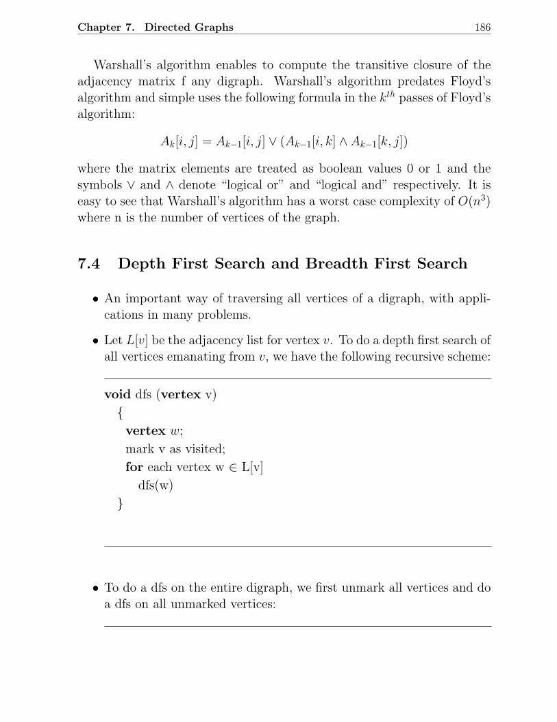
Chapter 7. Directed Graphs 186
Warshall’s algorithm enables to compute the transitive closure of theadjacency matrix f any digraph. Warshall’s algorithm predates Floyd’salgorithm and simple uses the following formula in the kth passes of Floyd’salgorithm:
Ak[i, j] = Ak−1[i, j] ∨ (Ak−1[i, k] ∧ Ak−1[k, j])
where the matrix elements are treated as boolean values 0 or 1 and thesymbols ∨ and ∧ denote “logical or” and “logical and” respectively. It iseasy to see that Warshall’s algorithm has a worst case complexity of O(n3)where n is the number of vertices of the graph.
7.4 Depth First Search and Breadth First Search
• An important way of traversing all vertices of a digraph, with appli-cations in many problems.
• Let L[v] be the adjacency list for vertex v. To do a depth first search ofall vertices emanating from v, we have the following recursive scheme:
void dfs (vertex v)
vertex w;
mark v as visited;
for each vertex w ∈ L[v]
dfs(w)
• To do a dfs on the entire digraph, we first unmark all vertices and doa dfs on all unmarked vertices:
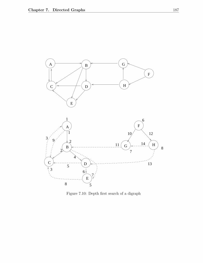
Chapter 7. Directed Graphs 187
A B
C D
E
F
G
H
10
7
A
B
C D
E
F
G H
1
2
2
4
3
8 5
1
11
7
148
12
6
13
93
56
Figure 7.10: Depth first search of a digraph
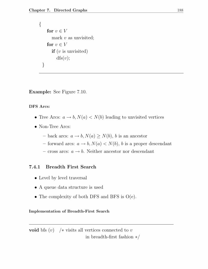
Chapter 7. Directed Graphs 188
for v ∈ V
mark v as unvisited;
for v ∈ V
if (v is unvisited)
dfs(v);
Example: See Figure 7.10.
DFS Arcs:
• Tree Arcs: a → b, N(a) < N(b) leading to unvisited vertices
• Non-Tree Arcs:
– back arcs: a → b, N(a) ≥ N(b), b is an ancestor
– forward arcs: a → b, N(a) < N(b), b is a proper descendant
– cross arcs: a → b. Neither ancestor nor descendant
7.4.1 Breadth First Search
• Level by level traversal
• A queue data structure is used
• The complexity of both DFS and BFS is O(e).
Implementation of Breadth-First Search
void bfs (v) /∗ visits all vertices connected to v
in breadth-first fashion ∗/
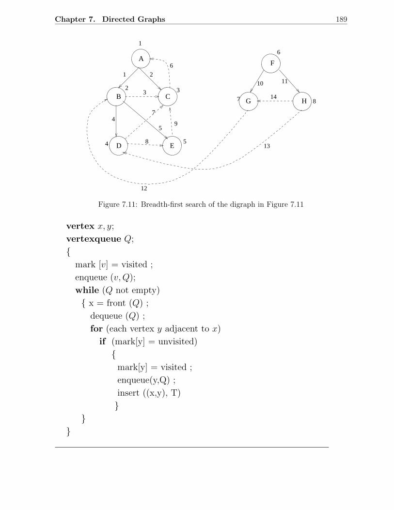
Chapter 7. Directed Graphs 189
14
1
1 2
3 3
54
4
2
7 8
6A
B C
D E
F
G H
6
7
8
59
10 11
12
13
Figure 7.11: Breadth-first search of the digraph in Figure 7.11
vertex x, y;
vertexqueue Q;
mark [v] = visited ;
enqueue (v, Q);
while (Q not empty)
x = front (Q) ;
dequeue (Q) ;
for (each vertex y adjacent to x)
if (mark[y] = unvisited)
mark[y] = visited ;
enqueue(y,Q) ;
insert ((x,y), T)
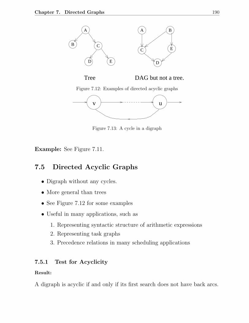
Chapter 7. Directed Graphs 190
A
C
ED
BC E
D
BA
Tree DAG but not a tree.
Figure 7.12: Examples of directed acyclic graphs
v u
Figure 7.13: A cycle in a digraph
Example: See Figure 7.11.
7.5 Directed Acyclic Graphs
• Digraph without any cycles.
• More general than trees
• See Figure 7.12 for some examples
• Useful in many applications, such as
1. Representing syntactic structure of arithmetic expressions
2. Representing task graphs
3. Precedence relations in many scheduling applications
7.5.1 Test for Acyclicity
Result:
A digraph is acyclic if and only if its first search does not have back arcs.
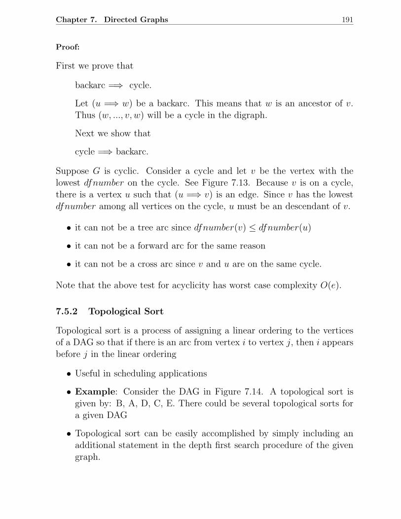
Chapter 7. Directed Graphs 191
Proof:
First we prove that
backarc =⇒ cycle.
Let (u =⇒ w) be a backarc. This means that w is an ancestor of v.Thus (w, ..., v, w) will be a cycle in the digraph.
Next we show that
cycle =⇒ backarc.
Suppose G is cyclic. Consider a cycle and let v be the vertex with thelowest dfnumber on the cycle. See Figure 7.13. Because v is on a cycle,there is a vertex u such that (u =⇒ v) is an edge. Since v has the lowestdfnumber among all vertices on the cycle, u must be an descendant of v.
• it can not be a tree arc since dfnumber(v) ≤ dfnumber(u)
• it can not be a forward arc for the same reason
• it can not be a cross arc since v and u are on the same cycle.
Note that the above test for acyclicity has worst case complexity O(e).
7.5.2 Topological Sort
Topological sort is a process of assigning a linear ordering to the verticesof a DAG so that if there is an arc from vertex i to vertex j, then i appearsbefore j in the linear ordering
• Useful in scheduling applications
• Example: Consider the DAG in Figure 7.14. A topological sort isgiven by: B, A, D, C, E. There could be several topological sorts fora given DAG
• Topological sort can be easily accomplished by simply including anadditional statement in the depth first search procedure of the givengraph.
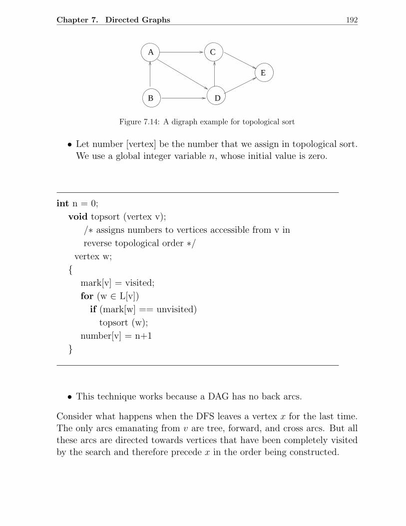
Chapter 7. Directed Graphs 192
A
B
C
D
E
Figure 7.14: A digraph example for topological sort
• Let number [vertex] be the number that we assign in topological sort.We use a global integer variable n, whose initial value is zero.
int n = 0;
void topsort (vertex v);
/∗ assigns numbers to vertices accessible from v in
reverse topological order ∗/vertex w;
mark[v] = visited;
for (w ∈ L[v])
if (mark[w] == unvisited)
topsort (w);
number[v] = n+1
• This technique works because a DAG has no back arcs.
Consider what happens when the DFS leaves a vertex x for the last time.The only arcs emanating from v are tree, forward, and cross arcs. But allthese arcs are directed towards vertices that have been completely visitedby the search and therefore precede x in the order being constructed.
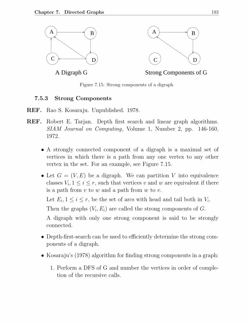
Chapter 7. Directed Graphs 193
A AB B
C CD D
A Digraph G Strong Components of G
Figure 7.15: Strong components of a digraph
7.5.3 Strong Components
REF. Rao S. Kosaraju. Unpublished. 1978.
REF. Robert E. Tarjan. Depth first search and linear graph algorithms.SIAM Journal on Computing , Volume 1, Number 2, pp. 146-160,1972.
• A strongly connected component of a digraph is a maximal set ofvertices in which there is a path from any one vertex to any othervertex in the set. For an example, see Figure 7.15.
• Let G = (V, E) be a digraph. We can partition V into equivalenceclasses Vi, 1 ≤ i ≤ r, such that vertices v and w are equivalent if thereis a path from v to w and a path from w to v.
Let Ei, 1 ≤ i ≤ r, be the set of arcs with head and tail both in Vi.
Then the graphs (Vi, Ei) are called the strong components of G.
A digraph with only one strong component is said to be stronglyconnected.
• Depth-first-search can be used to efficiently determine the strong com-ponents of a digraph.
• Kosaraju’s (1978) algorithm for finding strong components in a graph:
1. Perform a DFS of G and number the vertices in order of comple-tion of the recursive calls.
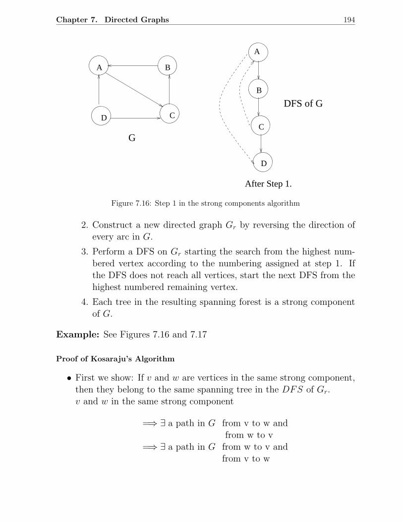
Chapter 7. Directed Graphs 194
A B
CD
A
B
D
CG
DFS of G
After Step 1.
Figure 7.16: Step 1 in the strong components algorithm
2. Construct a new directed graph Gr by reversing the direction ofevery arc in G.
3. Perform a DFS on Gr starting the search from the highest num-bered vertex according to the numbering assigned at step 1. Ifthe DFS does not reach all vertices, start the next DFS from thehighest numbered remaining vertex.
4. Each tree in the resulting spanning forest is a strong componentof G.
Example: See Figures 7.16 and 7.17
Proof of Kosaraju’s Algorithm
• First we show: If v and w are vertices in the same strong component,then they belong to the same spanning tree in the DFS of Gr.v and w in the same strong component
=⇒ ∃ a path in G from v to w andfrom w to v
=⇒ ∃ a path in G from w to v andfrom v to w
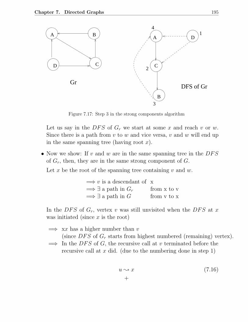
Chapter 7. Directed Graphs 195
A B
CD C
B
A D1
2
3
4
GrDFS of Gr
Figure 7.17: Step 3 in the strong components algorithm
Let us say in the DFS of Gr we start at some x and reach v or w.Since there is a path from v to w and vice versa, v and w will end upin the same spanning tree (having root x).
• Now we show: If v and w are in the same spanning tree in the DFS
of Gr, then, they are in the same strong component of G.
Let x be the root of the spanning tree containing v and w.
=⇒ v is a descendant of x=⇒ ∃ a path in Gr from x to v=⇒ ∃ a path in G from v to x
In the DFS of Gr, vertex v was still unvisited when the DFS at xwas initiated (since x is the root)
=⇒ xx has a higher number than v(since DFS of Gr starts from highest numbered (remaining) vertex).
=⇒ In the DFS of G, the recursive call at v terminated before therecursive call at x did. (due to the numbering done in step 1)
u ; x (7.16)
+
Chapter 7. Directed Graphs 196
Recursive call at v terminates before that of x in G (7.17)
In the DFS of G, there are two possibilities.
1) Search of v occurs before x (7.18)
2) Search of x occurs before v (7.19)
(1), (3) =⇒ DFS of v ... invokes DFS of x back to v.
=⇒ search at x would start and end before the search starts at v ends.=⇒ recursive call at v terminates after the call at x contradicts (2).
=⇒ search of x occurs before v.(4), (2) =⇒ v is visited during the search of x.
=⇒ v is descendant of x.=⇒ ∃ a path from x to v.
=⇒ x and v are in the same strong component.
Similarly, x and w are in the same strong component.=⇒ Similarly, v and w are in the same strong component.
7.6 To Probe Further
1. Alfred V Aho, John E. Hopcroft, and Jeffrey D Ullman. Data Struc-tures and Algorithms . Addison-Wesley, 1983.
2. Gilles Brassard and Paul Bratley. Fundamentals of Algorithmics .Prentice-Hall, 1996. Indian Edition published by Prentice Hall ofIndia, 1998.
3. Thomas H. Cormen, Charles E. Leiserson, and Donald L. Rivest. In-troduction to Algorithms . The MIT Electrical Engineering and Com-puter Science Series, 1990. Indian Edition published in 1999.
4. Mark Allen Weiss. Data Structures and Algorithm Analysis in C++.Benjamin-Cummings, 1994. Indian Edition published in 1998.
5. Alfred V Aho, John E. Hopcroft, and Jeffrey D Ullman. The Design
Chapter 7. Directed Graphs 197
and Analysis of Computer Algorithms , Addison-Wesley, 1974.
6. Sara Baase and Allen Van Gelder. Computer Algorithms: Introductionto Design and Analysis . Addison-Wesley, Third Edition, 2000. IndianEdition published by Pearson Education Asia, 2000.
7. Richard Bellman. Dynamic Programming . Princeton University Press,1957.
8. Gilles Brassard and Paul Bratley. Algorithmics : Theory and Practice.Prentice-Hall, 1988.
9. Ellis Horowitz, Sartaz Sahni, and Rajasekaran. Fundamentals of Com-puter Algorithms . W.H. Freeman and Company, 1998. Indian Editionpublished by Galgotia Publications, 2000.
10. Kurt Mehlhorn. Graph Algorithms and NP-Completeness . Volume 2of Data Structures and Algorithms , Springer-Verlag, 1984.
11. Robert Sedgewick. Algorithms. Addison-Wesley, Second Edition,1988.
12. Nicklaus Wirth. Data Structures + Algorithms = Programs. Prentice-Hall, Englewood Cliffs. 1975.
13. Richard Bellman. On a routing problem. Quarterly of Applied Math-ematics . Volume 16, Number 1, pp. 87–90, 1958.
14. E.W. Dijkstra. A note on two problems in connection with graphs.Numerische Mathematik , Volume 1, pp 269-271, 1959.
15. Jack Edmonds. Paths, trees, and flowers. Canadian Journal of Math-ematics , Volume 17, pp 449-467, 1965.
16. Robert W Floyd. Algorithm 97 (Shortest Path). Communications ofthe ACM , Volume 5, Number 6, pp. 345, 1962.
17. John E Hopcroft and Robert E. Tarjan. Efficient algorithms for graphmanipulation. Communications of the ACM , Volume 16, Number 6pp.372-378, 1973.
Chapter 7. Directed Graphs 198
18. Robert E. Tarjan. Depth first search and linear graph algorithms.SIAM Journal on Computing , Volume 1, Number 2, pp.146-160, 1972.
19. Stephen Warshall. A theorem on boolean matrices. Journal of theACM , Volume 9, Number 1, pp.11-12, 1962.
7.7 Problems
1. Give a simple example of a directed graph with negative-weight edges for whichDijkstra’s algorithm produces incorrect answers. Why doesn’t the proof of Dijkstra’salgorithm go through when negative-weight edges are allowed?
2. Give an example of a four node directed graph with some negative-weight edgesfor which Dijkstra’s algorithm produces incorrect answers. Also, give an exampleof a four node directed graph with some negative-weight edges for which Dijkstra’salgorithm always produces correct answers. In either case, justify your answer.
3. Explain how to modify Dijkstra’s algorithm so that if there is more than one mini-mum path from source to a destination vertex, then a path with the fewest numberof edges is chosen.
4. Suppose that in implementing Dijkstra’s shortest path algorithm, one uses an AVLtree rather than a partially ordered tree for representing the dynamic set of non-special vertices. What will be the worst case complexity of the algorithm if anadjacency list representation is used for the digraph? Would you still prefer thepartially ordered tree implementation?
5. We are given a directed graph G = (V,E) on which each edge (u, v) ∈ E has anassociated value r(u, v), which is a real number in the range 0 ≤ r(u, v) ≤ 1 thatrepresents the reliability of a communication channel from vertex u to vertex v. Weinterpret r(u, v) as the probability that the channel from u to v will not fail, andwe assume that these probabilities are independent. Give an efficient algorithm tofind the most reliable path between two vertices.
6. Write a program to find the longest path in a directed acyclic graph. What is thecomplexity of the algorithm?
7. Describe a mathematical model for the following scheduling problem: Given tasksT1, T2, . . . , Tn, which require time t1, t2, . . . , tn to complete, and a set of constraints,each of the form Tj must be completed prior to the start of Ti, find the minimumtime necessary to complete all the tasks assuming unlimited number of processorsto be available.
Chapter 7. Directed Graphs 199
8. In a depth-first search of a directed graph G = (V,E), define d(v) as the timestampwhen v is visited for the first time and f(v) the timestamp when the search finishesexamining the adjacency list of v. Show that an edge (u, v) ∈ E is
(a) a tree edge or forward edge if and only if d[u] < d[v] < f [v] < f [u].
(b) a back edge if and only if d[v] < d[u] < f [u] < f [v].
(c) a cross edge if and only if d[v] < f [v] < d[u] < f [u].
9. An Euler Tour of a connected, directed graph G = (V,E) is a cycle that traverseseach edge of G exactly once, although it may visit a vertex more than once.
(a) Show that G has an Euler tour if and only if indegree(v) = outdegree(v)∀v ∈ V .
(b) Describe an O(e) algorithm to find an Euler tour of G if one exists, where e isthe number of edges.
10. Design an efficient algorithm to determine whether a given DAG is a tree.
11. Let G= (V, E) be a digraph. Define a relation R on V such that uRv if and only if uand v lie on a common (not necessarily simple) cycle. Prove that R is an equivalencerelation on V.
7.8 Programming Assignments
7.8.1 Implementation of Dijkstra’s Algorithm Using Binary Heapsand Binomial Queues
The objective of this assignment is to compare the performance of binary heaps and bino-mial queues in implementing the single source shortest path algorithm of Dijkstra, whichcomputes the costs and paths of the shortest cost paths from a source vertex to everyother vertex in a labeled digraph with non-negative weights. Note that the dynamic setV − S is implemented using binary heaps or binomial queues.
Input graph
The graph that is input to the algorithm is either through a simple text file or is generatedrandomly. In the first case, assume the input to be in the following format:
• Line 1: Number of vertices in the graph
• Line 2: Source vertex (an integer between 1 and n, where n is the number of vertices
• Line 3: List of immediate neighbours of Node 1 with the weights on associated arcs
• Line 4: List of immediate neighbours of Vertex 2 with the weights on associatedarcs
Chapter 7. Directed Graphs 200
• etc · · ·
In the second case, to generate a random digraph, assume three inputs:
1. Number of vertices, n
2. Average degree of a node
3. Range of (integer) weights to be randomly generated for the directed arcs
Choose an appropriate data structure for the graph.
What is to be done ?
Implement Dijkstra’s algorithm, using binary heaps and using binomial queues. Make sureto use the standard array data structure for binary heaps and an efficient, appropriate datastructure for binomial queues (for example, look at the book by Alan Weiss). Attemptto do it in C++ but C is also good enough. As usual, special care should be takento structure your program according to best practices in software engineering: use ofgood abstractions, smart algorithms, discipline in coding, documentation, provision forexceptions (for example, negative weights should be detected immediately; errors in inputshould be flagged asap; etc.).
For the input graph and the source vertex, print the following:
• shortest cost path to each vertex and the cost of this shortest path
• Execution times of the program with binary heaps and binomial queues
• Total number of heap operations executed with binary heaps and binomial queues(this includes: probes, swaps, link traversals, etc.)
7.8.2 Strong Components
Finding strong components of a given digraph is an important practical problem. You have
studied Kosaraju’s algorithm for this purpose. There are other algorithms available in the
literature for determining the strong components. Many of the references lister earlier can be
consulted for this. Implement Kosaraju’s and at least one other algorithm for determining strong
components and compare the performance of the two algorithms.
Chapter 8
Undirected Graphs
8.1 Some Definitions
• G = (V, E)
Each edge is an unordered pair of vertices
• v and w are adjacent if (v, w) or equivalently (w, v) is an edge. Theedge (v, w) is incident upon the vertices v and w.
• A path is a sequence of vertices v1, v2, . . . , vn, such that (vi, vi+1) is anedge for 1 ≤ i < n. A path is simple if all vertices on it are distinct,except possibly v1 and vn. The path has length n− 1 and connects v1
and vn.
• A graph is connected if every pair of vertices is connected.
• A subgraph G′ = (V ′, E ′) of a graph G = (V, E) is a graph such that
1. V ′ ⊆ V
2. E ′ contains some edges (u, v) of E such that both u and v are inV ′
If E ′ contains all edges (u, v) ∈ E for which u, v ∈ V ′, the subgraphG′ is called an induced subgraph.
• A connected component of a graph is an induced subgraph which isconnected and which is not a proper subgraph of any other connectedsubgraph of G (i.e., maximal connected induced subgraph).
201
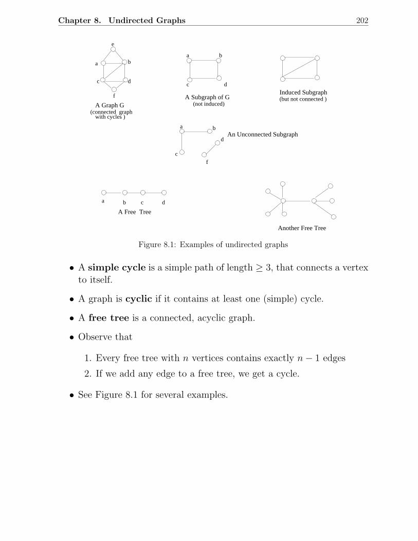
Chapter 8. Undirected Graphs 202
e
b
d
f
c
aa b
c d
A Graph GA Subgraph of G
(not induced)
Induced Subgraph(but not connected )
(connected graphwith cycles )
a b c d
A Free Tree
b
c
d
f
aAn Unconnected Subgraph
Another Free Tree
Figure 8.1: Examples of undirected graphs
• A simple cycle is a simple path of length ≥ 3, that connects a vertexto itself.
• A graph is cyclic if it contains at least one (simple) cycle.
• A free tree is a connected, acyclic graph.
• Observe that
1. Every free tree with n vertices contains exactly n − 1 edges
2. If we add any edge to a free tree, we get a cycle.
• See Figure 8.1 for several examples.
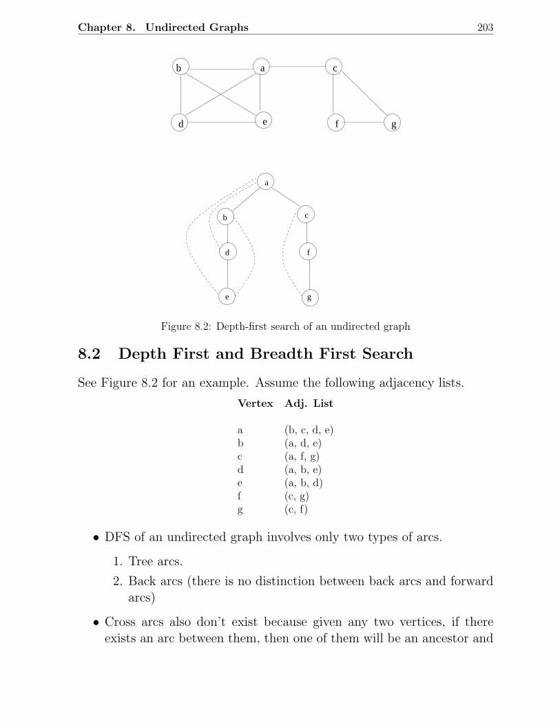
Chapter 8. Undirected Graphs 203
b a
e
c
f gd
a
b
d
e
c
f
g
Figure 8.2: Depth-first search of an undirected graph
8.2 Depth First and Breadth First Search
See Figure 8.2 for an example. Assume the following adjacency lists.
Vertex Adj. List
a (b, c, d, e)b (a, d, e)c (a, f, g)d (a, b, e)e (a, b, d)f (c, g)g (c, f)
• DFS of an undirected graph involves only two types of arcs.
1. Tree arcs.
2. Back arcs (there is no distinction between back arcs and forwardarcs)
• Cross arcs also don’t exist because given any two vertices, if thereexists an arc between them, then one of them will be an ancestor and
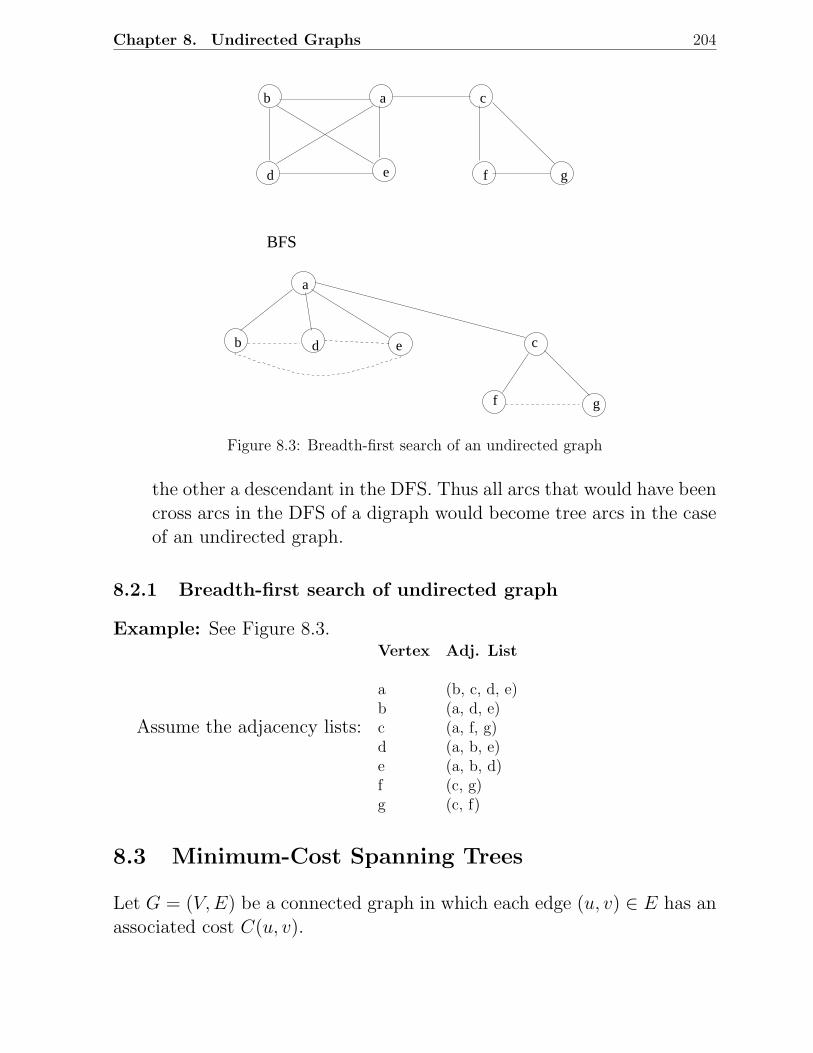
Chapter 8. Undirected Graphs 204
b a
e
c
f gd
a
b d e c
f g
BFS
Figure 8.3: Breadth-first search of an undirected graph
the other a descendant in the DFS. Thus all arcs that would have beencross arcs in the DFS of a digraph would become tree arcs in the caseof an undirected graph.
8.2.1 Breadth-first search of undirected graph
Example: See Figure 8.3.
Assume the adjacency lists:
Vertex Adj. List
a (b, c, d, e)b (a, d, e)c (a, f, g)d (a, b, e)e (a, b, d)f (c, g)g (c, f)
8.3 Minimum-Cost Spanning Trees
Let G = (V, E) be a connected graph in which each edge (u, v) ∈ E has anassociated cost C(u, v).
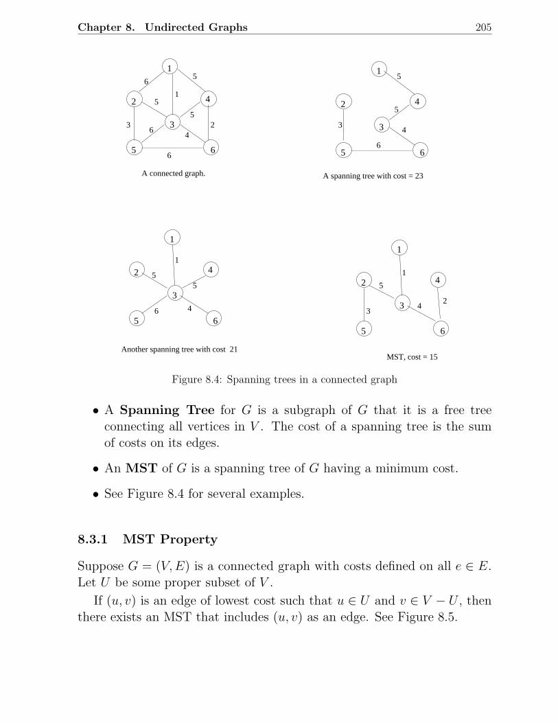
Chapter 8. Undirected Graphs 205
1
3
2 4
5 6
1
3
2 4
5 6
1
3
2 4
5 6
1
3
2 4
5 6
65
2
6
3
51
5
46
5
5
4
6
3
1
5
46
5 1
24
5
3
A connected graph. A spanning tree with cost = 23
Another spanning tree with cost 21MST, cost = 15
Figure 8.4: Spanning trees in a connected graph
• A Spanning Tree for G is a subgraph of G that it is a free treeconnecting all vertices in V . The cost of a spanning tree is the sumof costs on its edges.
• An MST of G is a spanning tree of G having a minimum cost.
• See Figure 8.4 for several examples.
8.3.1 MST Property
Suppose G = (V, E) is a connected graph with costs defined on all e ∈ E.Let U be some proper subset of V .
If (u, v) is an edge of lowest cost such that u ∈ U and v ∈ V − U , thenthere exists an MST that includes (u, v) as an edge. See Figure 8.5.
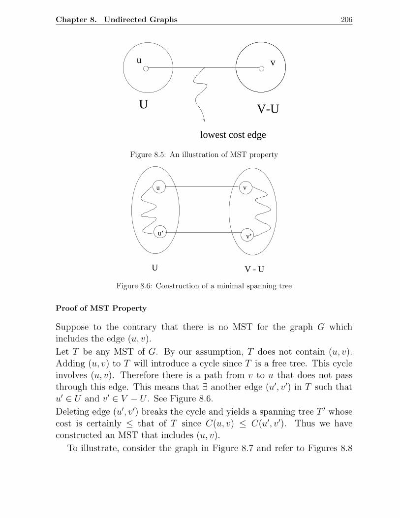
Chapter 8. Undirected Graphs 206
lowest cost edge
u v
U V-U
Figure 8.5: An illustration of MST property
U V - U
u
u’
v
v’
Figure 8.6: Construction of a minimal spanning tree
Proof of MST Property
Suppose to the contrary that there is no MST for the graph G whichincludes the edge (u, v).
Let T be any MST of G. By our assumption, T does not contain (u, v).Adding (u, v) to T will introduce a cycle since T is a free tree. This cycleinvolves (u, v). Therefore there is a path from v to u that does not passthrough this edge. This means that ∃ another edge (u′, v′) in T such thatu′ ∈ U and v′ ∈ V − U . See Figure 8.6.
Deleting edge (u′, v′) breaks the cycle and yields a spanning tree T ′ whosecost is certainly ≤ that of T since C(u, v) ≤ C(u′, v′). Thus we haveconstructed an MST that includes (u, v).
To illustrate, consider the graph in Figure 8.7 and refer to Figures 8.8
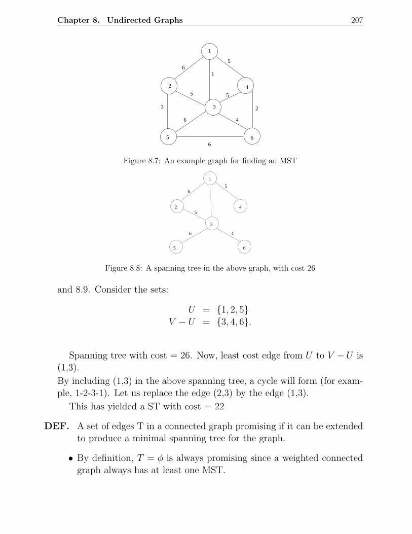
Chapter 8. Undirected Graphs 207
65
6 4
4
6
5
3
1
5
2
65
2
3
1
Figure 8.7: An example graph for finding an MST
65
6 4
1
3
42
5 6
5
Figure 8.8: A spanning tree in the above graph, with cost 26
and 8.9. Consider the sets:
U = 1, 2, 5V − U = 3, 4, 6.
Spanning tree with cost = 26. Now, least cost edge from U to V −U is(1,3).
By including (1,3) in the above spanning tree, a cycle will form (for exam-ple, 1-2-3-1). Let us replace the edge (2,3) by the edge (1,3).
This has yielded a ST with cost = 22
DEF. A set of edges T in a connected graph promising if it can be extendedto produce a minimal spanning tree for the graph.
• By definition, T = φ is always promising since a weighted connectedgraph always has at least one MST.
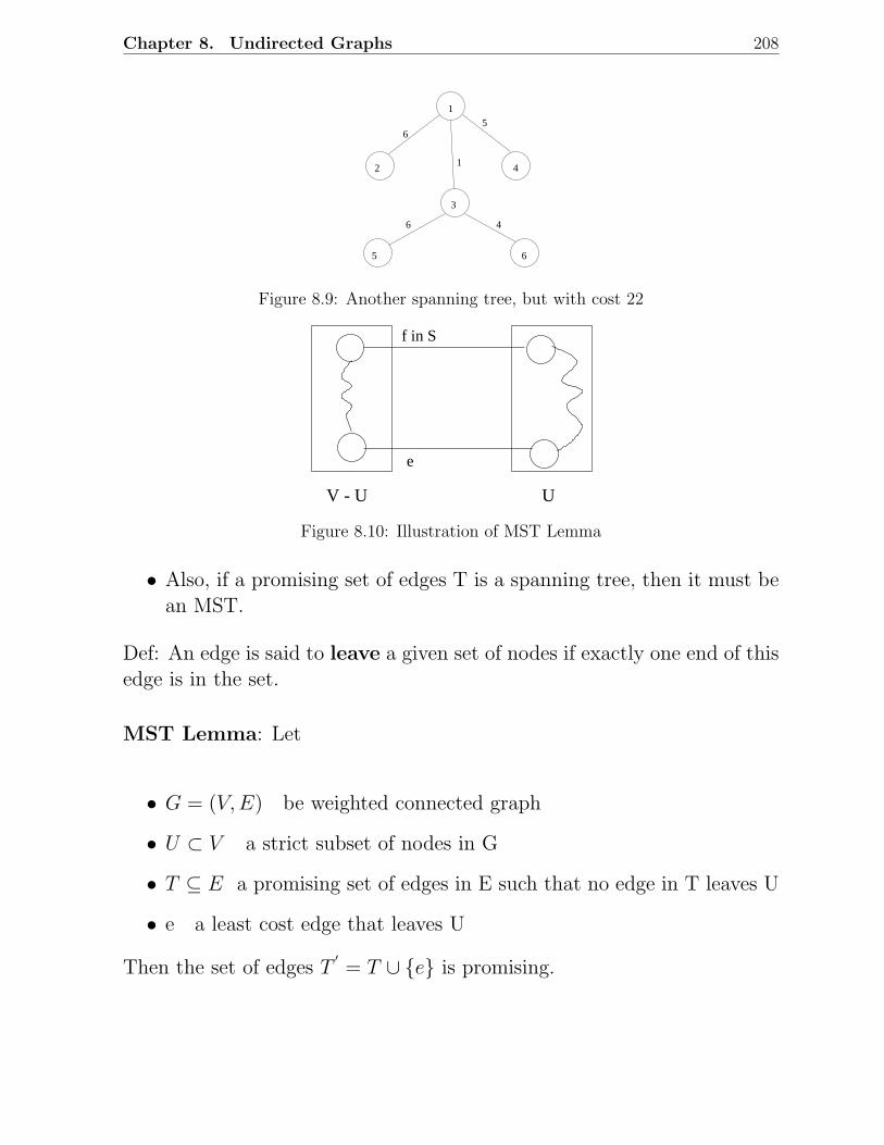
Chapter 8. Undirected Graphs 208
65
1
6 4
1
3
42
5 6
Figure 8.9: Another spanning tree, but with cost 22
e
f in S
UV - U
Figure 8.10: Illustration of MST Lemma
• Also, if a promising set of edges T is a spanning tree, then it must bean MST.
Def: An edge is said to leave a given set of nodes if exactly one end of thisedge is in the set.
MST Lemma: Let
• G = (V, E) be weighted connected graph
• U ⊂ V a strict subset of nodes in G
• T ⊆ E a promising set of edges in E such that no edge in T leaves U
• e a least cost edge that leaves U
Then the set of edges T′
= T ∪ e is promising.
Chapter 8. Undirected Graphs 209
Proof
Since T is promising, it can be extended to obtain an MST, says S. Ife ∈ S, there is nothing to prove.
If e ∈ S, then we add edge e to S, we create exactly one cycle (since Sis a spanning tree). In this cycle, since e leaves U there exists at least oneother edge, f say, that also leaves U (otherwise the cycle could not close).See Figure 8.10.
If we now remove f, the cycle disappears and we obtain a new tree R thatspans G.
Note that R = (S ∪ e) − f
Also note that weight of e ≤ weight of f since e is a least cost edge leavingU.
Therefore R is also an MST and it includes edge e. Furthermore T ⊆ R
and so can be extended to the MST R. Thus T is a promising set of edges.
8.3.2 Prim’s Algorithm
This algorithm is directly based on the MST property. Assume that V =1, 2, . . . , n.
REF. R.C. Prim. Shortest connection networks and some generalizations.Bell System Technical Journal , Volume 36, pp. 1389-1401, 1957.
T = φ;
U = 1 ;while (U 6= V )
let (u, v) be the lowest cost edge
such that u ∈ U and v ∈ V − U ;
Chapter 8. Undirected Graphs 210
T = T ∪ (u, v)U = U ∪ v
• See Figure 8.11 for an example.
• O(n2) algorithm.
Proof of Correctness of Prim’s Algorithm
Theorem: Prim’s algorithm finds a minimum spanning tree.
Proof: Let G = (V,E) be a weighted, connected graph. Let T be theedge set that is grown in Prim’s algorithm. The proof is by mathematicalinduction on the number of edges in T and using the MST Lemma.
Basis: The empty set φ is promising since a connected, weighted graphalways has at least one MST.
Induction Step: Assume that T is promising just before the algorithmadds a new edge e = (u,v). Let U be the set of nodes grown in Prim’salgorithm. Then all three conditions in the MST Lemma are satisfied andtherefore T U e is also promising.
When the algorithm stops, U includes all vertices of the graph and henceT is a spanning tree. Since T is also promising, it will be a MST.
Implementation of Prim’s Algorithm
Use two arrays, closest and lowcost.
• For i ∈ V − U , closest[i] gives the vertex in U that is closest to i
• For i ∈ V − U , lowcost[i] gives the cost of the edge (i, closest(i))
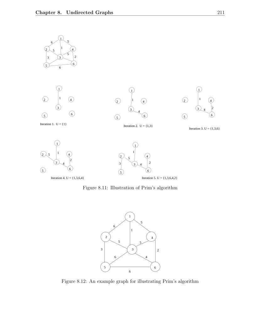
Chapter 8. Undirected Graphs 211
1
2 4
3
5 6
1
2 4
3
5 6
1
2 4
3
5 6
1
2 4
3
5 6
1
2 4
3
5 6
1
2 4
3
5 6
56
15
5
6
23
1 1
4
1
4 2
1
42
51
5
3 4 2
Iteration 1. U = 1 Iteration 2. U = 1,3Iteration 3. U = 1,3,6
Iteration 4. U = 1,3,6,4 Iteration 5. U = 1,3,6,4,2
Figure 8.11: Illustration of Prim’s algorithm
65
6 4
4
6
5
3
1
5
2
65
2
3
1
Figure 8.12: An example graph for illustrating Prim’s algorithm
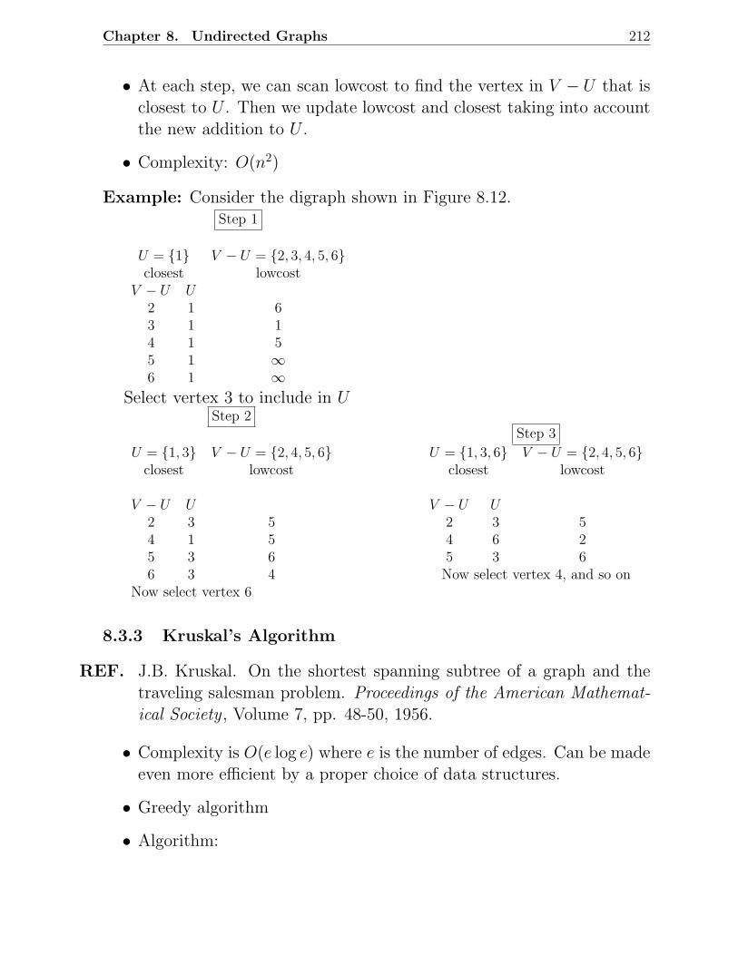
Chapter 8. Undirected Graphs 212
• At each step, we can scan lowcost to find the vertex in V − U that isclosest to U . Then we update lowcost and closest taking into accountthe new addition to U .
• Complexity: O(n2)
Example: Consider the digraph shown in Figure 8.12.Step 1
U = 1 V − U = 2, 3, 4, 5, 6closest lowcost
V − U U2 1 63 1 14 1 55 1 ∞6 1 ∞
Select vertex 3 to include in UStep 2
U = 1, 3 V − U = 2, 4, 5, 6closest lowcost
V − U U2 3 54 1 55 3 66 3 4
Now select vertex 6
Step 3
U = 1, 3, 6 V − U = 2, 4, 5, 6closest lowcost
V − U U2 3 54 6 25 3 6Now select vertex 4, and so on
8.3.3 Kruskal’s Algorithm
REF. J.B. Kruskal. On the shortest spanning subtree of a graph and thetraveling salesman problem. Proceedings of the American Mathemat-ical Society , Volume 7, pp. 48-50, 1956.
• Complexity is O(e log e) where e is the number of edges. Can be madeeven more efficient by a proper choice of data structures.
• Greedy algorithm
• Algorithm:
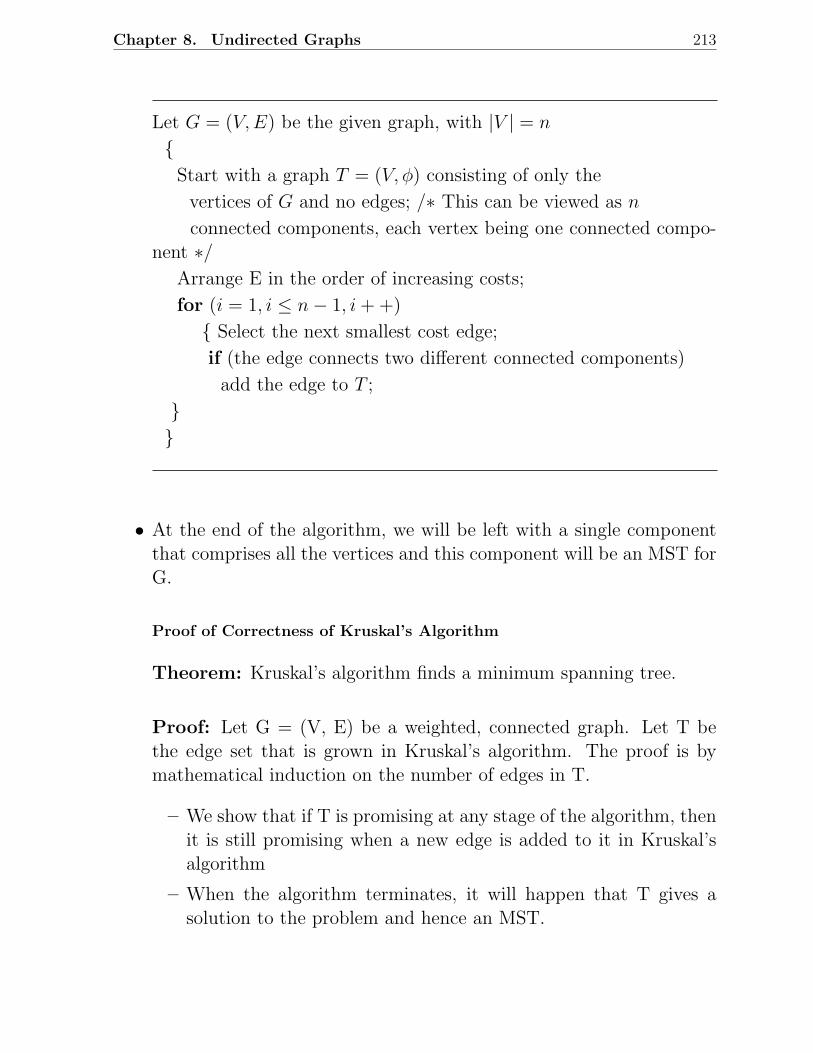
Chapter 8. Undirected Graphs 213
Let G = (V, E) be the given graph, with |V | = n
Start with a graph T = (V, φ) consisting of only the
vertices of G and no edges; /∗ This can be viewed as n
connected components, each vertex being one connected compo-nent ∗/
Arrange E in the order of increasing costs;
for (i = 1, i ≤ n − 1, i + +)
Select the next smallest cost edge;
if (the edge connects two different connected components)
add the edge to T ;
• At the end of the algorithm, we will be left with a single componentthat comprises all the vertices and this component will be an MST forG.
Proof of Correctness of Kruskal’s Algorithm
Theorem: Kruskal’s algorithm finds a minimum spanning tree.
Proof: Let G = (V, E) be a weighted, connected graph. Let T bethe edge set that is grown in Kruskal’s algorithm. The proof is bymathematical induction on the number of edges in T.
– We show that if T is promising at any stage of the algorithm, thenit is still promising when a new edge is added to it in Kruskal’salgorithm
– When the algorithm terminates, it will happen that T gives asolution to the problem and hence an MST.
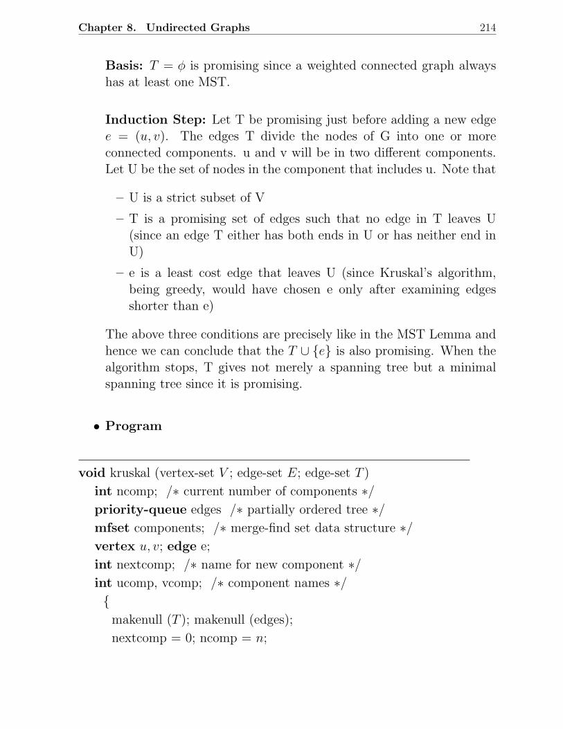
Chapter 8. Undirected Graphs 214
Basis: T = φ is promising since a weighted connected graph alwayshas at least one MST.
Induction Step: Let T be promising just before adding a new edgee = (u, v). The edges T divide the nodes of G into one or moreconnected components. u and v will be in two different components.Let U be the set of nodes in the component that includes u. Note that
– U is a strict subset of V
– T is a promising set of edges such that no edge in T leaves U(since an edge T either has both ends in U or has neither end inU)
– e is a least cost edge that leaves U (since Kruskal’s algorithm,being greedy, would have chosen e only after examining edgesshorter than e)
The above three conditions are precisely like in the MST Lemma andhence we can conclude that the T ∪ e is also promising. When thealgorithm stops, T gives not merely a spanning tree but a minimalspanning tree since it is promising.
• Program
void kruskal (vertex-set V ; edge-set E; edge-set T )
int ncomp; /∗ current number of components ∗/priority-queue edges /∗ partially ordered tree ∗/mfset components; /∗ merge-find set data structure ∗/vertex u, v; edge e;
int nextcomp; /∗ name for new component ∗/int ucomp, vcomp; /∗ component names ∗/
makenull (T ); makenull (edges);
nextcomp = 0; ncomp = n;
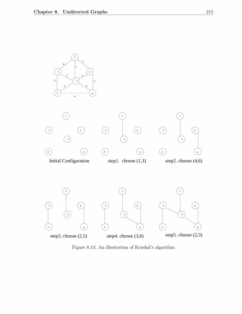
Chapter 8. Undirected Graphs 215
65
6 4
6
5
3
1
5
2
65
2
3
1
4
65
2
3
1
4
65
2
3
1
4
65
2
3
1
4
Initial Configuration step1. choose (1,3) step2. choose (4,6)
65
2
3
1
4
65
2
3
1
4
65
2
3
1
4
step3. choose (2,5) step4. choose (3,6) step5. choose (2,3)
Figure 8.13: An illustration of Kruskal’s algorithm
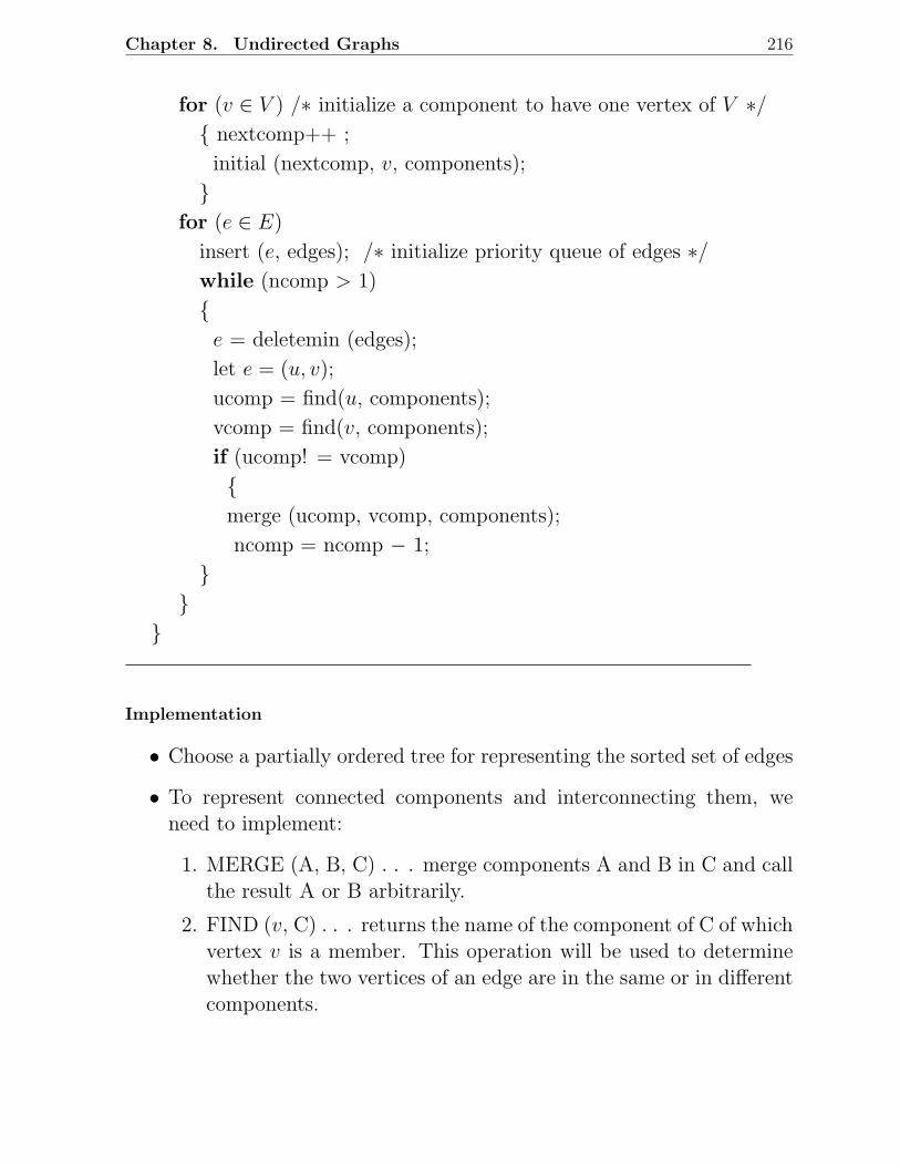
Chapter 8. Undirected Graphs 216
for (v ∈ V ) /∗ initialize a component to have one vertex of V ∗/ nextcomp++ ;
initial (nextcomp, v, components);
for (e ∈ E)
insert (e, edges); /∗ initialize priority queue of edges ∗/while (ncomp > 1)
e = deletemin (edges);
let e = (u, v);
ucomp = find(u, components);
vcomp = find(v, components);
if (ucomp! = vcomp)
merge (ucomp, vcomp, components);
ncomp = ncomp − 1;
Implementation
• Choose a partially ordered tree for representing the sorted set of edges
• To represent connected components and interconnecting them, weneed to implement:
1. MERGE (A, B, C) . . . merge components A and B in C and callthe result A or B arbitrarily.
2. FIND (v, C) . . . returns the name of the component of C of whichvertex v is a member. This operation will be used to determinewhether the two vertices of an edge are in the same or in differentcomponents.
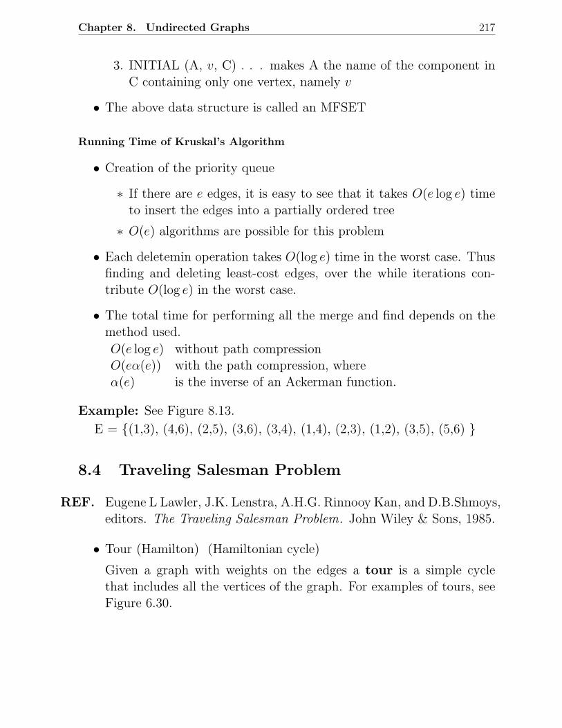
Chapter 8. Undirected Graphs 217
3. INITIAL (A, v, C) . . . makes A the name of the component inC containing only one vertex, namely v
• The above data structure is called an MFSET
Running Time of Kruskal’s Algorithm
• Creation of the priority queue
∗ If there are e edges, it is easy to see that it takes O(e log e) timeto insert the edges into a partially ordered tree
∗ O(e) algorithms are possible for this problem
• Each deletemin operation takes O(log e) time in the worst case. Thusfinding and deleting least-cost edges, over the while iterations con-tribute O(log e) in the worst case.
• The total time for performing all the merge and find depends on themethod used.
O(e log e) without path compressionO(eα(e)) with the path compression, whereα(e) is the inverse of an Ackerman function.
Example: See Figure 8.13.
E = (1,3), (4,6), (2,5), (3,6), (3,4), (1,4), (2,3), (1,2), (3,5), (5,6)
8.4 Traveling Salesman Problem
REF. Eugene L Lawler, J.K. Lenstra, A.H.G. Rinnooy Kan, and D.B.Shmoys,editors. The Traveling Salesman Problem. John Wiley & Sons, 1985.
• Tour (Hamilton) (Hamiltonian cycle)
Given a graph with weights on the edges a tour is a simple cyclethat includes all the vertices of the graph. For examples of tours, seeFigure 6.30.
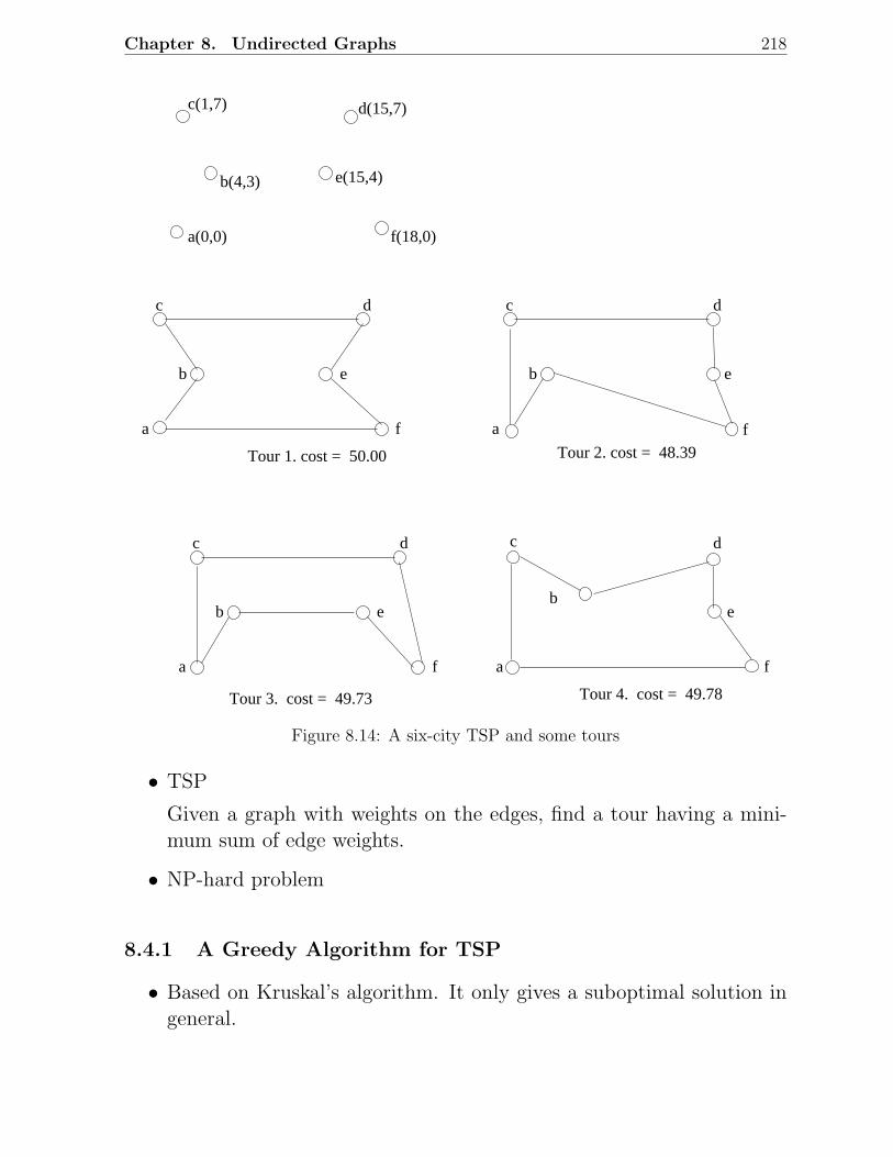
Chapter 8. Undirected Graphs 218
b(4,3)
c(1,7) d(15,7)
f(18,0)
e(15,4)
a(0,0)
Tour 1. cost = 50.00
f
e
c d
b
a
a f
e
c d
b
a
c
b
d
f
e
Tour 2. cost = 48.39
a
c
be
d
f
Tour 4. cost = 49.78Tour 3. cost = 49.73
Figure 8.14: A six-city TSP and some tours
• TSP
Given a graph with weights on the edges, find a tour having a mini-mum sum of edge weights.
• NP-hard problem
8.4.1 A Greedy Algorithm for TSP
• Based on Kruskal’s algorithm. It only gives a suboptimal solution ingeneral.
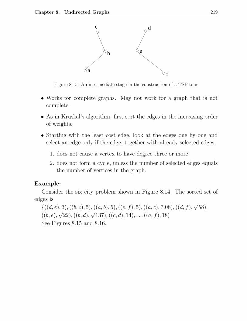
Chapter 8. Undirected Graphs 219
a
b
c d
e
f
Figure 8.15: An intermediate stage in the construction of a TSP tour
• Works for complete graphs. May not work for a graph that is notcomplete.
• As in Kruskal’s algorithm, first sort the edges in the increasing orderof weights.
• Starting with the least cost edge, look at the edges one by one andselect an edge only if the edge, together with already selected edges,
1. does not cause a vertex to have degree three or more
2. does not form a cycle, unless the number of selected edges equalsthe number of vertices in the graph.
Example:
Consider the six city problem shown in Figure 8.14. The sorted set ofedges is
((d, e), 3), ((b, c), 5), ((a, b), 5), ((e, f), 5), ((a, c), 7.08), ((d, f),√
58),
((b, e),√
22), ((b, d),√
137), ((c, d), 14), . . . ((a, f), 18)
See Figures 8.15 and 8.16.
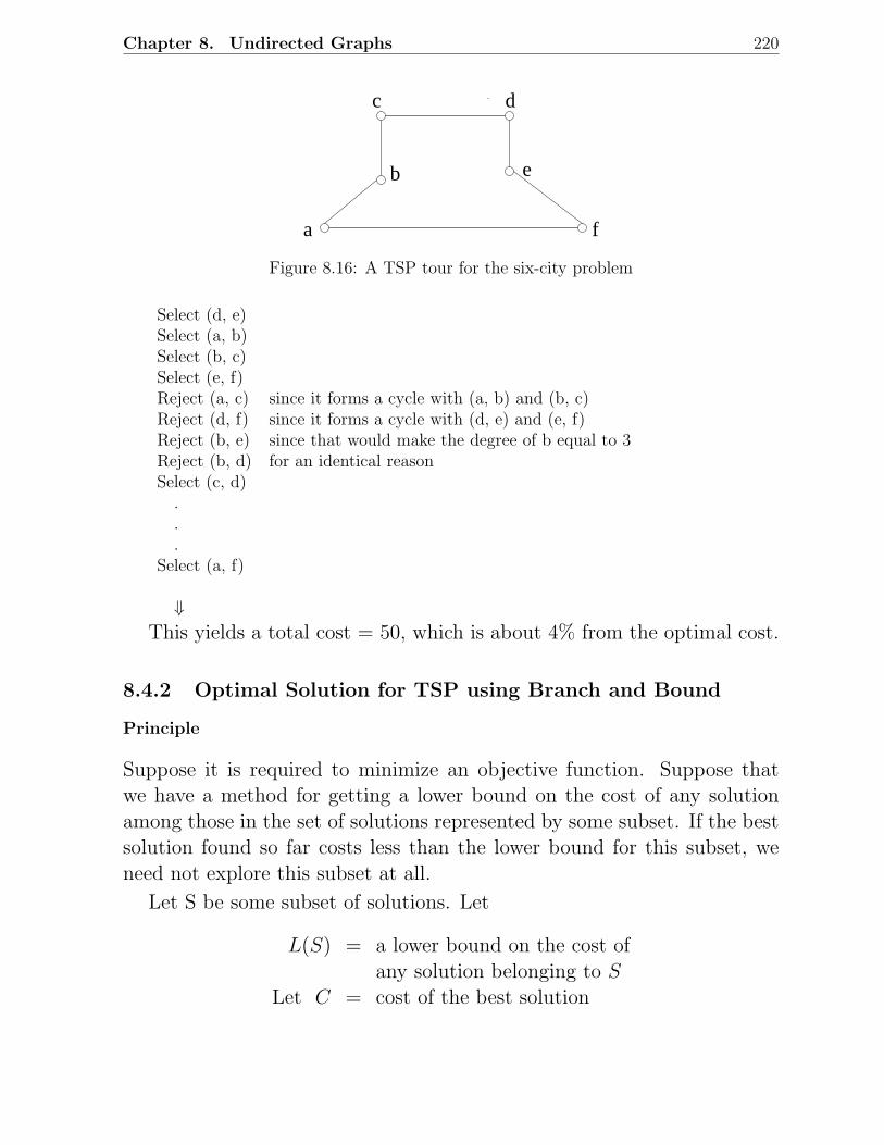
Chapter 8. Undirected Graphs 220
fa
dc
e b
Figure 8.16: A TSP tour for the six-city problem
Select (d, e)Select (a, b)Select (b, c)Select (e, f)Reject (a, c) since it forms a cycle with (a, b) and (b, c)Reject (d, f) since it forms a cycle with (d, e) and (e, f)Reject (b, e) since that would make the degree of b equal to 3Reject (b, d) for an identical reasonSelect (c, d)
.
.
.Select (a, f)
⇓This yields a total cost = 50, which is about 4% from the optimal cost.
8.4.2 Optimal Solution for TSP using Branch and Bound
Principle
Suppose it is required to minimize an objective function. Suppose thatwe have a method for getting a lower bound on the cost of any solutionamong those in the set of solutions represented by some subset. If the bestsolution found so far costs less than the lower bound for this subset, weneed not explore this subset at all.
Let S be some subset of solutions. Let
L(S) = a lower bound on the cost ofany solution belonging to S
Let C = cost of the best solution
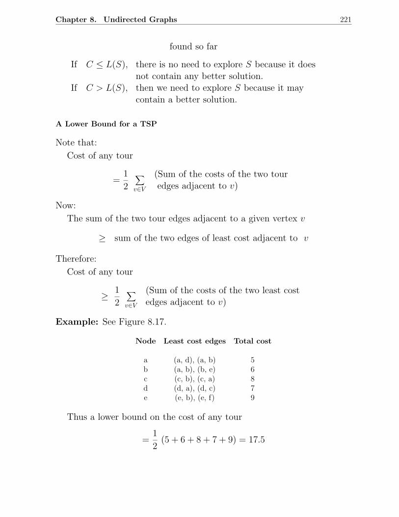
Chapter 8. Undirected Graphs 221
found so far
If C ≤ L(S), there is no need to explore S because it doesnot contain any better solution.
If C > L(S), then we need to explore S because it maycontain a better solution.
A Lower Bound for a TSP
Note that:
Cost of any tour
=1
2
∑
v∈V
(Sum of the costs of the two touredges adjacent to v)
Now:
The sum of the two tour edges adjacent to a given vertex v
≥ sum of the two edges of least cost adjacent to v
Therefore:
Cost of any tour
≥ 1
2
∑
v∈V
(Sum of the costs of the two least costedges adjacent to v)
Example: See Figure 8.17.
Node Least cost edges Total cost
a (a, d), (a, b) 5b (a, b), (b, e) 6c (c, b), (c, a) 8d (d, a), (d, c) 7e (e, b), (e, f) 9
Thus a lower bound on the cost of any tour
=1
2(5 + 6 + 8 + 7 + 9) = 17.5
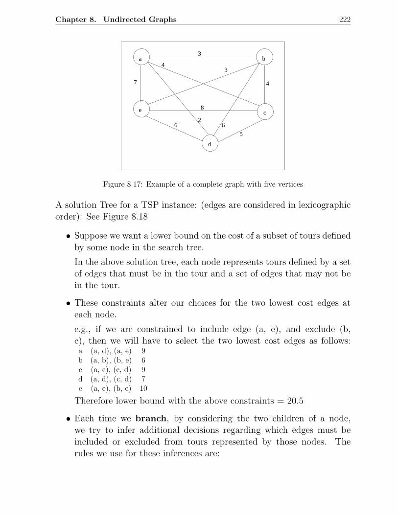
Chapter 8. Undirected Graphs 222
a b
e
d
c
3
4
43
7
8
62
6
5
Figure 8.17: Example of a complete graph with five vertices
A solution Tree for a TSP instance: (edges are considered in lexicographicorder): See Figure 8.18
• Suppose we want a lower bound on the cost of a subset of tours definedby some node in the search tree.
In the above solution tree, each node represents tours defined by a setof edges that must be in the tour and a set of edges that may not bein the tour.
• These constraints alter our choices for the two lowest cost edges ateach node.
e.g., if we are constrained to include edge (a, e), and exclude (b,c), then we will have to select the two lowest cost edges as follows:a (a, d), (a, e) 9b (a, b), (b, e) 6c (a, c), (c, d) 9d (a, d), (c, d) 7e (a, e), (b, e) 10
Therefore lower bound with the above constraints = 20.5
• Each time we branch, by considering the two children of a node,we try to infer additional decisions regarding which edges must beincluded or excluded from tours represented by those nodes. Therules we use for these inferences are:
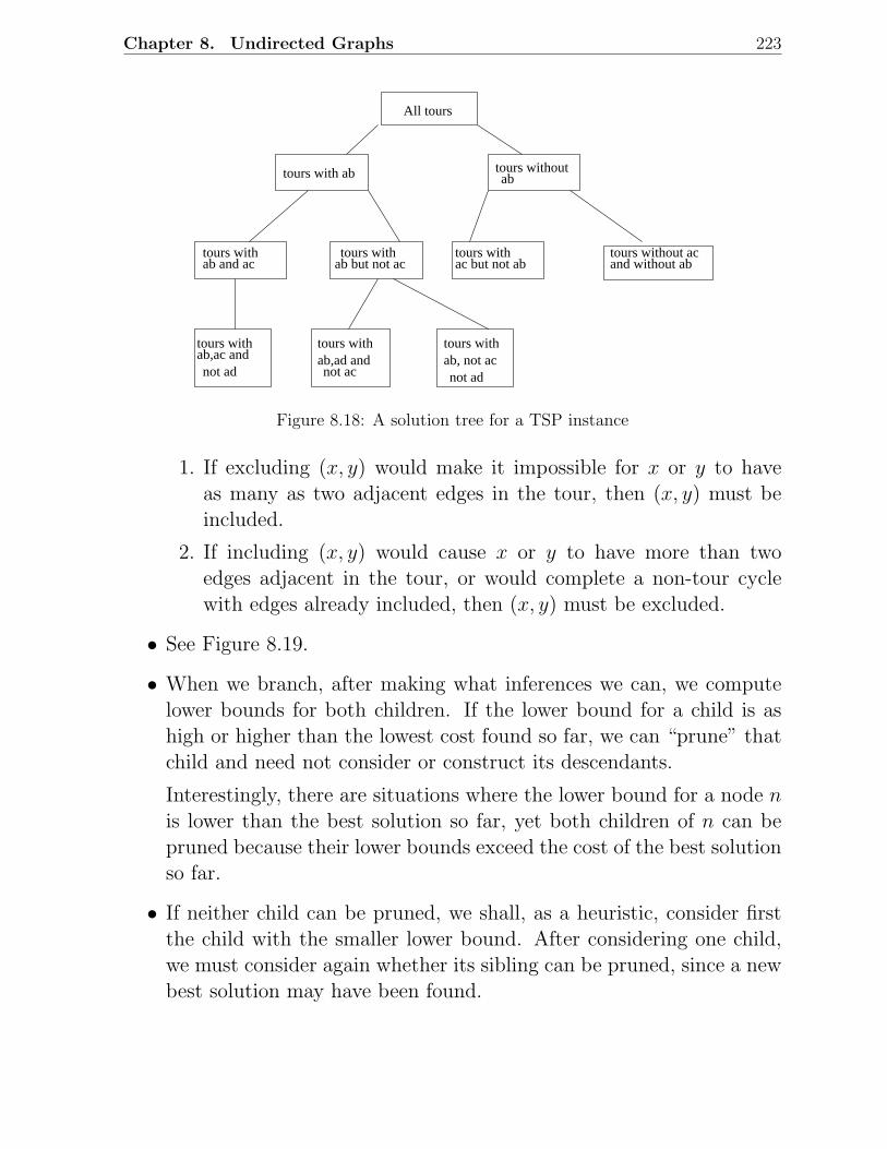
Chapter 8. Undirected Graphs 223
All tours
tours with ab tours withoutab
tours withab and ac
tours withab but not ac
tours with ac but not ab
tours without ac and without ab
tours with tours with tours with ab,ac andnot ad
ab,ad andnot ac
ab, not acnot ad
Figure 8.18: A solution tree for a TSP instance
1. If excluding (x, y) would make it impossible for x or y to haveas many as two adjacent edges in the tour, then (x, y) must beincluded.
2. If including (x, y) would cause x or y to have more than twoedges adjacent in the tour, or would complete a non-tour cyclewith edges already included, then (x, y) must be excluded.
• See Figure 8.19.
• When we branch, after making what inferences we can, we computelower bounds for both children. If the lower bound for a child is ashigh or higher than the lowest cost found so far, we can “prune” thatchild and need not consider or construct its descendants.
Interestingly, there are situations where the lower bound for a node n
is lower than the best solution so far, yet both children of n can bepruned because their lower bounds exceed the cost of the best solutionso far.
• If neither child can be pruned, we shall, as a heuristic, consider firstthe child with the smaller lower bound. After considering one child,we must consider again whether its sibling can be pruned, since a newbest solution may have been found.
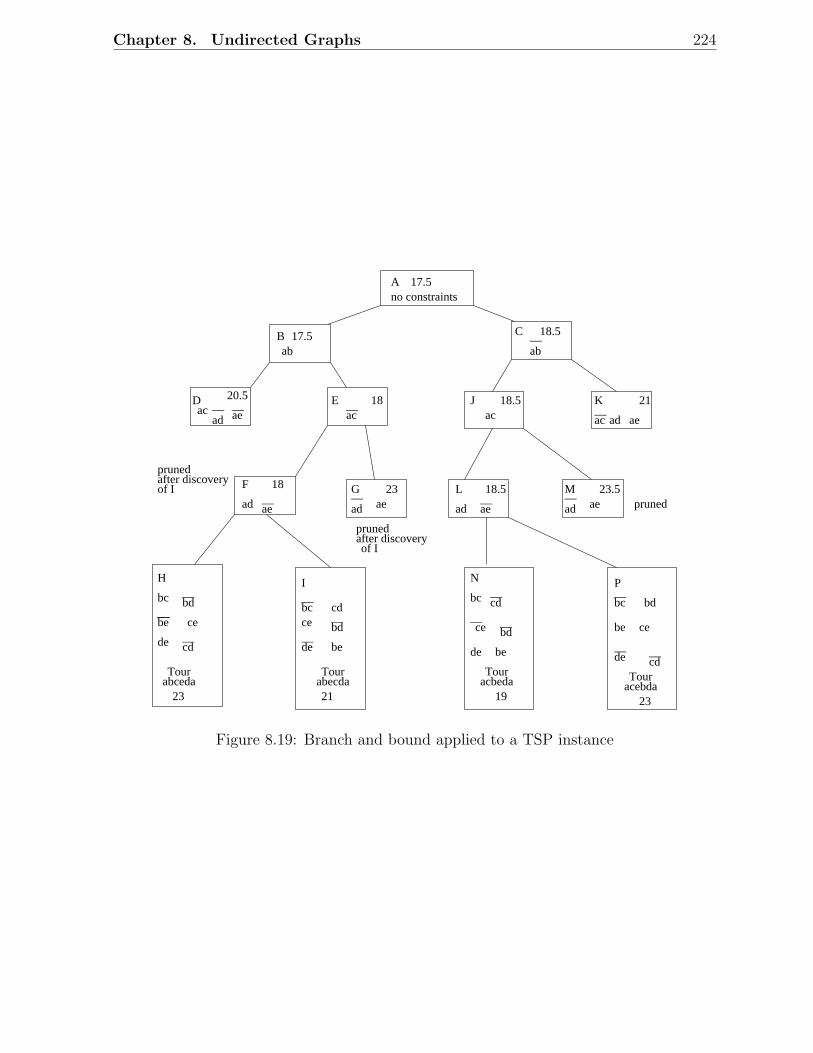
Chapter 8. Undirected Graphs 224
ad__
ae__
ab__
ac__
ad__
ae__
ad__
bd__
be____
cd__
bc__
bd__
de__
cd__
ce__
bd__
bc__
de__
cd__
no constraintsA
B C
D E
F G
H I
J K
L M
N P
17.5
17.5 18.5
20.5 18 18.5 21
18 23 18.5 23.5
ac
ab
ac ad ae
ad ae ad ae
bc
ce
de
Tour
cdce
be
Tour
bc
de be
Tour
bd
be ce
Tourabceda abecda acbeda acebda23 21 19 23
pruned
pruned
pruned
after discovery
after discovery
of I
of I
ae__
ac__
Figure 8.19: Branch and bound applied to a TSP instance
Chapter 8. Undirected Graphs 225
8.5 To Probe Further
1. Alfred V Aho, John E. Hopcroft, and Jeffrey D Ullman. Data Struc-tures and Algorithms . Addison-Wesley, 1983.
2. Gilles Brassard and Paul Bratley. Fundamentals of Algorithmics .Prentice-Hall, 1996. Indian Edition published by Prentice Hall ofIndia, 1998.
3. Thomas H. Cormen, Charles E. Leiserson, and Donald L. Rivest. In-troduction to Algorithms . The MIT Electrical Engineering and Com-puter Science Series, 1990. Indian Edition published in 1999.
4. Mark Allen Weiss. Data Structures and Algorithm Analysis in C++.Benjamin-Cummings, 1994. Indian Edition published in 1998.
5. Alfred V Aho, John E. Hopcroft, and Jeffrey D Ullman. The Designand Analysis of Computer Algorithms , Addison-Wesley, 1974.
6. Sara Baase and Allen Van Gelder. Computer Algorithms: Introductionto Design and Analysis . Addison-Wesley, Third Edition, 2000. IndianEdition published by Pearson Education Asia, 2000.
7. Ellis Horowitz, Sartaz Sahni, and Rajasekaran. Fundamentals of Com-puter Algorithms . W.H. Freeman and Company, 1998. Indian Editionpublished by Galgotia Publications, 2000.
8. Eugene L Lawler, J.K. Lenstra, A.H.G. Rinnooy Kan, and D.B.Shmoys,editors. The Traveling Salesman Problem. John Wiley & Sons, 1985.
9. Kurt Mehlhorn. Graph Algorithms and NP-Completeness . Volume 2of Data Structures and Algorithms , Springer-Verlag, 1984.
10. Robert Sedgewick. Algorithms. Addison-Wesley, Second Edition,1988.
11. Jack Edmonds. Paths, trees, and flowers. Canadian Journal of Math-ematics , Volume 17, pp 449-467, 1965.
Chapter 8. Undirected Graphs 226
12. John E Hopcroft and Robert E. Tarjan. Efficient algorithms for graphmanipulation. Communications of the ACM , Volume 16, Number 6pp.372-378, 1973.
13. J.B. Kruskal. On the shortest spanning subtree of a graph and thetraveling salesman problem. Proceedings of the American Mathemat-ical Society , Volume 7, pp 48-50, 1956.
14. R.C. Prim. Shortest connection networks and some generalizations.Bell System Technical Journal , Volume 36, pp.1389-1401, 1957.
15. Robert E. Tarjan. Depth first search and linear graph algorithms.SIAM Journal on Computing , Volume 1, Number 2, pp.146-160, 1972.
8.6 Problems
1. Consider an undirected graph G=(V, E), with n vertices. Show how a one dimen-
sional array of length n(n−1)2
can be used to represent G.
2. Give an algorithm that determines whether or not a given undirected graph G =(V,E) contains a cycle. The algorithm should run in O(|V|) time independent of|E|.
3. Design an algorithm to enumerate all simple cycles of a graph. How many suchcycles can there be? What is the time complexity of the algorithm?
4. Let (u, v) be a minimum-weight edge in a graph G. Show that (u, v) belongs tosome minimum spanning tree of G.
5. Let e be maximum-weight edge on some cycle of G = (V,E). Prove that there is aminimum spanning tree of G′ = (V,E − e) that is also a minimum spanning treeof G.
6. For an undirected graph G with n vertices and e edges, show that∑n
i=1 di = 2ewhere di is the degree of vertex i (number of edges incident on vertex i).
7. The diameter of a tree T = (V,E) is defined by maxu,v∈V δ(u, v) where δ(u, v) isthe shortest-path distance from vertex u to vertex v. Give an efficient algorithm tocompute the diameter of a tree, and analyze the running time of the algorithm.
8. An Eulerian walk in an undirected graph is a path that starts and ends at the samevertex, traversing every edge in the graph exactly once. Prove that in order for sucha path to exist, all nodes must have even degree.
Chapter 8. Undirected Graphs 227
9. Two binary trees T1 and T2 are said to be isomorphic if T1 can be transformedinto T2 by swapping left and right children of (some of the) nodes in T1. Design anefficient algorithm to decide id two given trees are isomorphic. What is the timecomplexity of your algorithm?
8.7 Programming Assignments
8.7.1 Implementation of Some Graph Algorithms
This assignment involves five problems.
1. Generate a connected graph with n vertices and a certain number of edges, decidedby an average degree d of each vertex. The connected graph generated should haveseveral spanning trees and several Hamiltonian paths . Also, generate random costsfor all the edges.
2. Find a minimum cost spanning tree (MST) for the above graph, using an efficientimplementation of Prim’s algorithm. Compute the execution time of this program.
3. Find an MST using Kruskal’s algorithm. In the implementation, use the heap datastructure to organize the set of edges and the MFSET data structure to implementunion’s and find’s. Compare the execution time with that of Prim’s algorithm.
4. Find a second best MST by extending the Kruskal’s algorithm, using the followingproperty: If T is an MST, then there exist an edge (u, v) ∈ T and an edge (x, y) 6∈ Tsuch that (T − (u, v))U(x, y) is a second best MST.
5. Find a Hamiltonian path using a greedy strategy based on Kruskal’s algorithm.You can compare the cost of this path to that of a minimal cost Hamiltonian path(found by exhaustive enumeration) for values of n up to 10. In fact, you can do alittle better by using the branch and bound method to compute the minimal costHamiltonian path.
6. Provide examples of connected graphs for situations specified below. If an examplecannot exist for the situation, provide reasons.
(a) A graph in which a maximum cost edge is a part of every MST in the graph
(b) A graph in which a maximum cost edge is never a part of any MST
(c) A graph in which a least cost edge is not a part of any MST
7. Let T be a minimum spanning tree of a connected graph G. Prove that there existedges (u, v) ∈ T and (x, y) 6∈ T such that T − (u, v) ∪ (x, y) is a second-bestminimum spanning tree of G.
Chapter 8. Undirected Graphs 228
8.7.2 Traveling Salesman Problem
This assignment involves implementing the following five problems.
1. Generate a complete graph with n vertices and random costs for all the edges. Letthe costs be positive integers uniformly distributed between 1 and 100.
2. Find a minimum cost spanning tree (MST) for the above graph, using an efficientimplementation of Prim’s algorithm. Compute the running time of this program.
3. Find an MST using Kruskal’s algorithm. In the implementation, use the partiallyordered tree data structure to organize the set of edges and the MFSET data struc-ture to implement union’s and find’s. Compare the running time with that of Prim’salgorithm.
4. Find a Hamiltonian path using a greedy strategy based on Kruskal’s algorithm.
5. Find an optimal Hamiltonian path for the above graph using the branch and boundmethodology.
It should be possible to input any desired graph and carry out steps 2, 3, 4, and 5 above.
Assume the following input format: Let the set of vertices be V = 1, . . . , n Then the
input file would be: n, Cost of edge (1, 2), . . ., Cost of edge (1, n), Cost of edge (2, 3), . . .,
Cost of edge (2, n), Cost of edge (3, 4), . . ., Cost of edge (n − 1, n).
Chapter 9
Sorting Methods
The function of sorting or ordering a list of objects according to some linearorder is so fundamental that it is ubiquitous in engineering applications inall disciplines. There are two broad categories of sorting methods: Inter-nal sorting takes place in the main memory, where we can take advantageof the random access nature of the main memory; External sorting isnecessary when the number and size of objects are prohibitive to be ac-commodated in the main memory.
The Problem:
• Given records r1, r2, . . . , rn, with key values k1, k2, . . . , kn, produce therecords in the order
ri1, ri2, . . . , rin,
such thatki1 ≤ ki2 ≤ . . . ≤ kin
• The complexity of a sorting algorithm can be measured in terms of
∗ number of algorithm steps to sort n records
∗ number of comparisons between keys (appropriate when the keysare long character strings)
∗ number of times records must be moved (appropriate when recordsize is large)
• Any sorting algorithm that uses comparisons of keys needs at leastO(n log n) time to accomplish the sorting.
229
Chapter 9. Sorting Methods 230
Sorting Methods
Internal External(In memory) Appropriate for secondary storage
quick sortheap sort mergesortbubble sort radix sortinsertion sort polyphase sortselection sortshell sort
9.1 Bubble Sort
Let a[1], a[2], . . . , a[n] be n records to be sorted on a key field “key”. Inbubble sort, records with low keys (light records) bubble up to the top.
for (i = 1; i <= n − 1; i + +)
for (j = n; j >= i + 1; j −−)
if (a[j].key < a[j − 1].key)
swap the records a[j] and a[j − 1]
At the end of the (i − 1)st iteration, we have
a[1] . . . a[i − 1]︸ ︷︷ ︸
sorted as in thefinal order
a[i] . . . a[n]︸ ︷︷ ︸
unsorted
In the ith iteration, the ith lowest key bubbles up to the ith position and
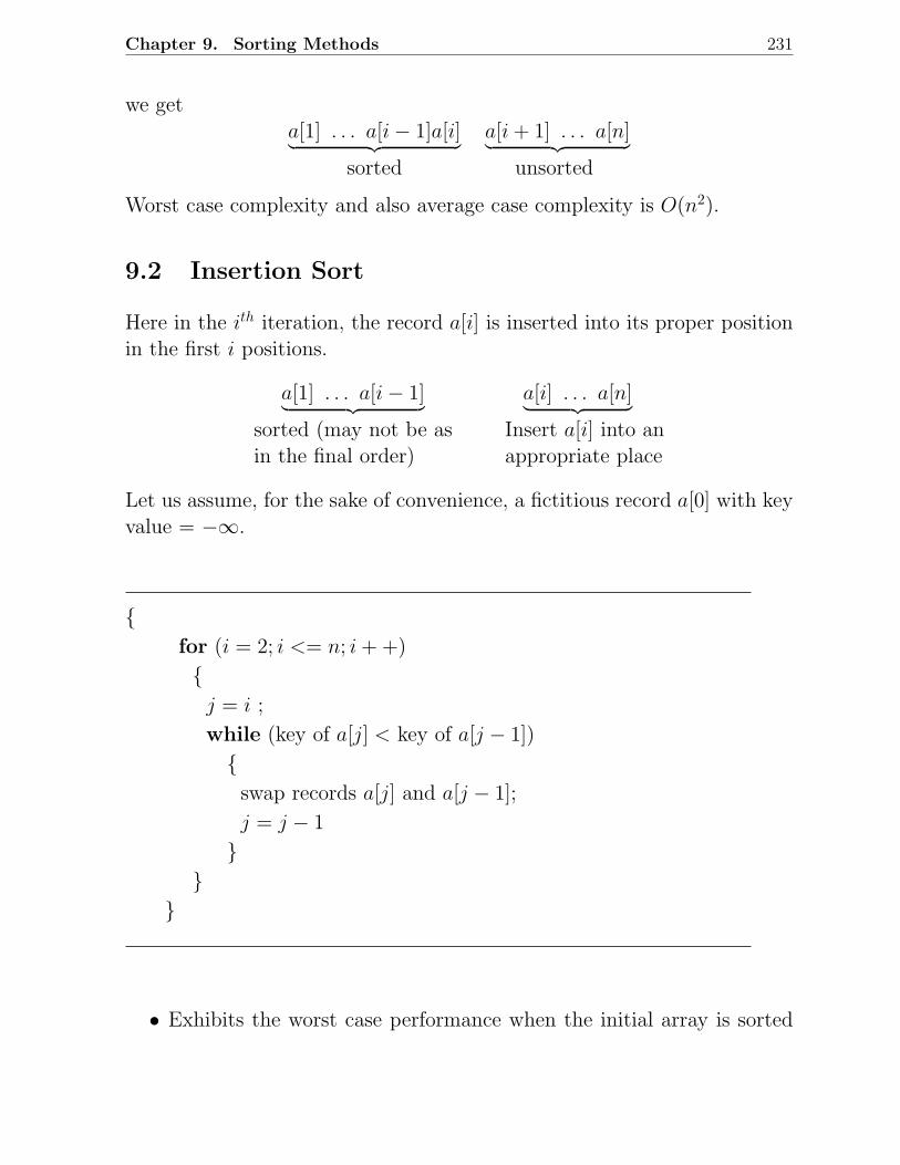
Chapter 9. Sorting Methods 231
we geta[1] . . . a[i − 1]a[i]︸ ︷︷ ︸
sorted
a[i + 1] . . . a[n]︸ ︷︷ ︸
unsorted
Worst case complexity and also average case complexity is O(n2).
9.2 Insertion Sort
Here in the ith iteration, the record a[i] is inserted into its proper positionin the first i positions.
a[1] . . . a[i − 1]︸ ︷︷ ︸
sorted (may not be asin the final order)
a[i] . . . a[n]︸ ︷︷ ︸
Insert a[i] into anappropriate place
Let us assume, for the sake of convenience, a fictitious record a[0] with keyvalue = −∞.
for (i = 2; i <= n; i + +)
j = i ;
while (key of a[j] < key of a[j − 1])
swap records a[j] and a[j − 1];
j = j − 1
• Exhibits the worst case performance when the initial array is sorted
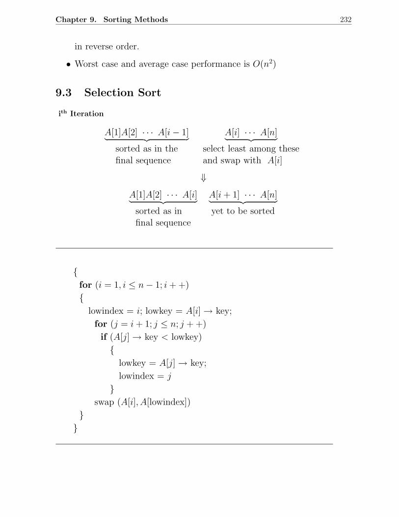
Chapter 9. Sorting Methods 232
in reverse order.
• Worst case and average case performance is O(n2)
9.3 Selection Sort
ith Iteration
A[1]A[2] · · · A[i − 1]︸ ︷︷ ︸
sorted as in thefinal sequence
A[i] · · · A[n]︸ ︷︷ ︸
select least among theseand swap with A[i]
⇓A[1]A[2] · · · A[i]︸ ︷︷ ︸
sorted as infinal sequence
A[i + 1] · · · A[n]︸ ︷︷ ︸
yet to be sorted
for (i = 1, i ≤ n − 1; i + +)
lowindex = i; lowkey = A[i] → key;
for (j = i + 1; j ≤ n; j + +)
if (A[j] → key < lowkey)
lowkey = A[j] → key;
lowindex = j
swap (A[i], A[lowindex])
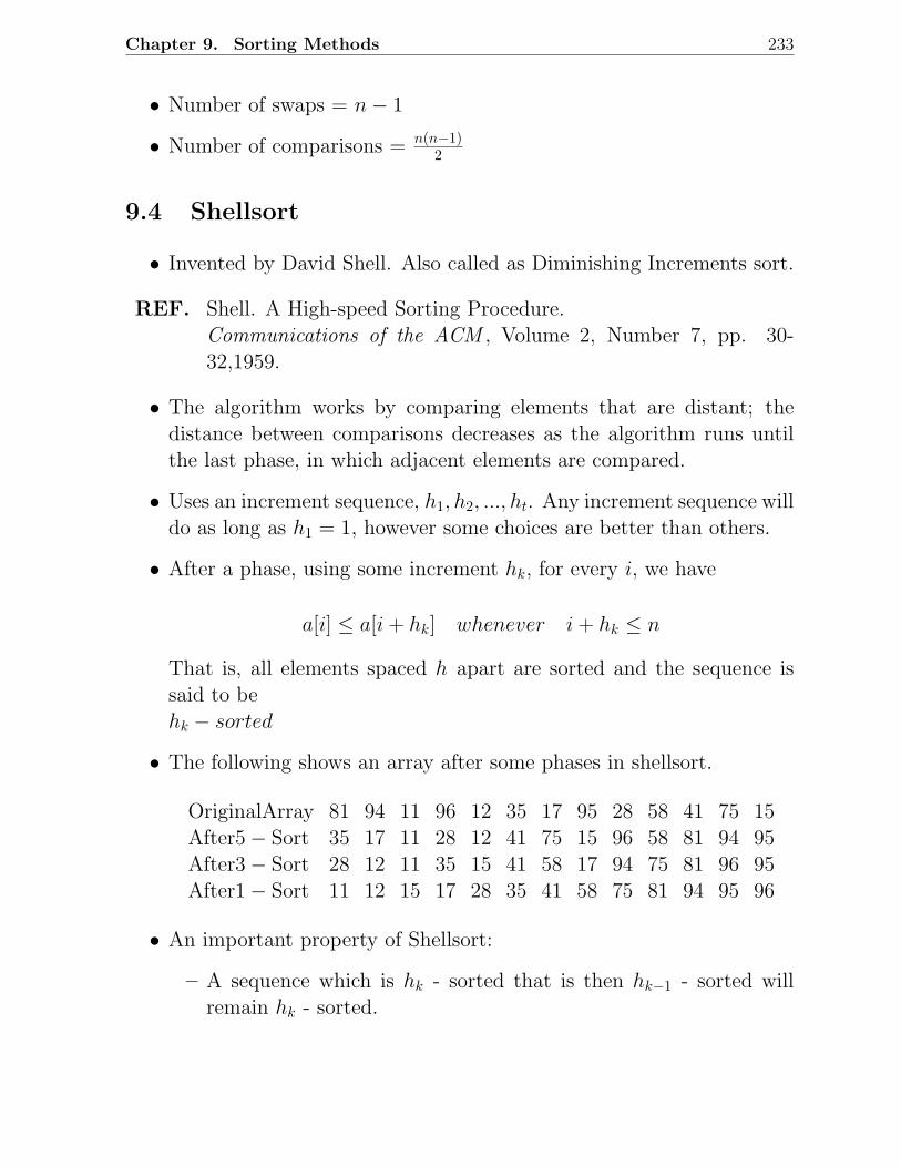
Chapter 9. Sorting Methods 233
• Number of swaps = n − 1
• Number of comparisons = n(n−1)2
9.4 Shellsort
• Invented by David Shell. Also called as Diminishing Increments sort.
REF. Shell. A High-speed Sorting Procedure.Communications of the ACM , Volume 2, Number 7, pp. 30-32,1959.
• The algorithm works by comparing elements that are distant; thedistance between comparisons decreases as the algorithm runs untilthe last phase, in which adjacent elements are compared.
• Uses an increment sequence, h1, h2, ..., ht. Any increment sequence willdo as long as h1 = 1, however some choices are better than others.
• After a phase, using some increment hk, for every i, we have
a[i] ≤ a[i + hk] whenever i + hk ≤ n
That is, all elements spaced h apart are sorted and the sequence issaid to behk − sorted
• The following shows an array after some phases in shellsort.
OriginalArray 81 94 11 96 12 35 17 95 28 58 41 75 15After5 − Sort 35 17 11 28 12 41 75 15 96 58 81 94 95After3 − Sort 28 12 11 35 15 41 58 17 94 75 81 96 95After1 − Sort 11 12 15 17 28 35 41 58 75 81 94 95 96
• An important property of Shellsort:
– A sequence which is hk - sorted that is then hk−1 - sorted willremain hk - sorted.
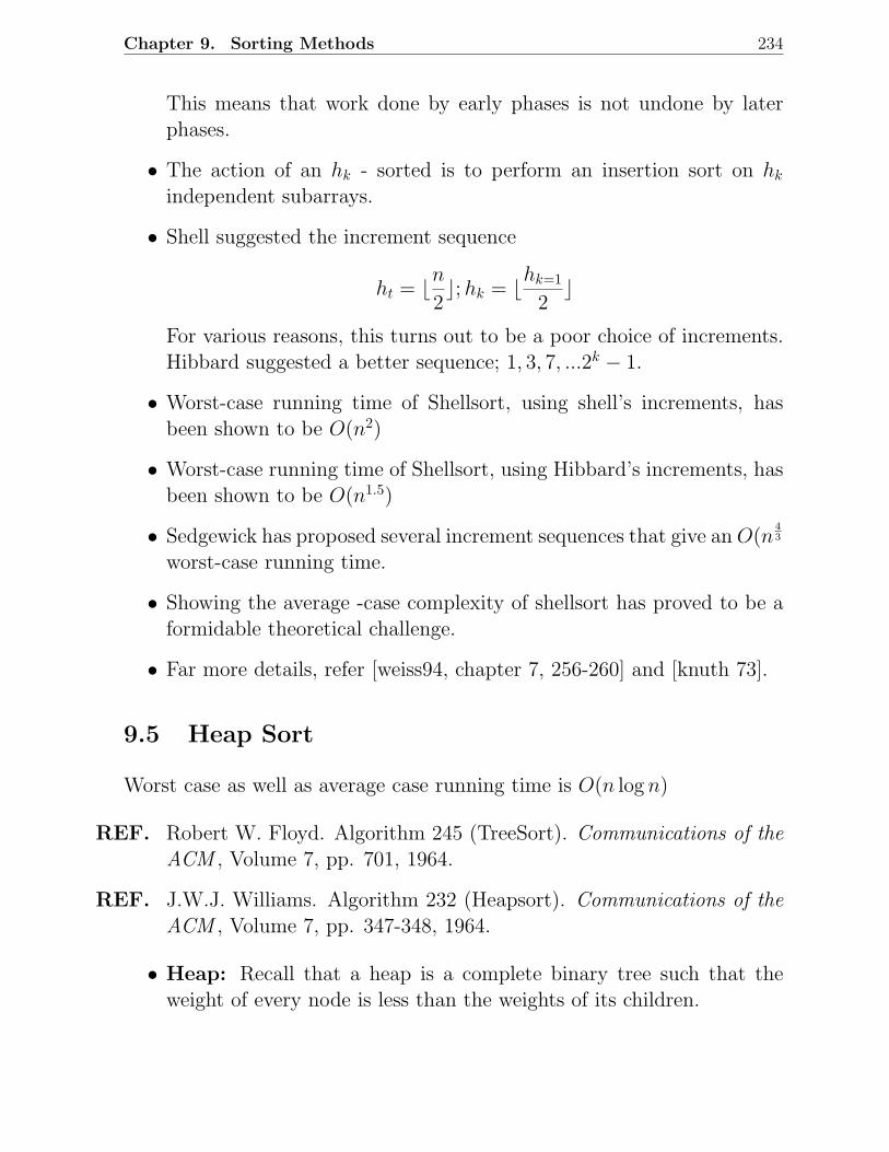
Chapter 9. Sorting Methods 234
This means that work done by early phases is not undone by laterphases.
• The action of an hk - sorted is to perform an insertion sort on hk
independent subarrays.
• Shell suggested the increment sequence
ht = ⌊n2⌋; hk = ⌊hk=1
2⌋
For various reasons, this turns out to be a poor choice of increments.Hibbard suggested a better sequence; 1, 3, 7, ...2k − 1.
• Worst-case running time of Shellsort, using shell’s increments, hasbeen shown to be O(n2)
• Worst-case running time of Shellsort, using Hibbard’s increments, hasbeen shown to be O(n1.5)
• Sedgewick has proposed several increment sequences that give an O(n4
3
worst-case running time.
• Showing the average -case complexity of shellsort has proved to be aformidable theoretical challenge.
• Far more details, refer [weiss94, chapter 7, 256-260] and [knuth 73].
9.5 Heap Sort
Worst case as well as average case running time is O(n log n)
REF. Robert W. Floyd. Algorithm 245 (TreeSort). Communications of theACM , Volume 7, pp. 701, 1964.
REF. J.W.J. Williams. Algorithm 232 (Heapsort). Communications of theACM , Volume 7, pp. 347-348, 1964.
• Heap: Recall that a heap is a complete binary tree such that theweight of every node is less than the weights of its children.
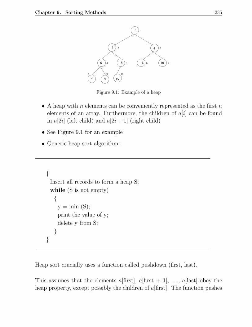
Chapter 9. Sorting Methods 235
1
2 4
6 8 16 10
7 9 15
1
2 3
4 5 6 7
8 9 10
Figure 9.1: Example of a heap
• A heap with n elements can be conveniently represented as the first nelements of an array. Furthermore, the children of a[i] can be foundin a[2i] (left child) and a[2i + 1] (right child)
• See Figure 9.1 for an example
• Generic heap sort algorithm:
Insert all records to form a heap S;
while (S is not empty)
y = min (S);
print the value of y;
delete y from S;
Heap sort crucially uses a function called pushdown (first, last).
This assumes that the elements a[first], a[first + 1], . . ., a[last] obey theheap property, except possibly the children of a[first]. The function pushes
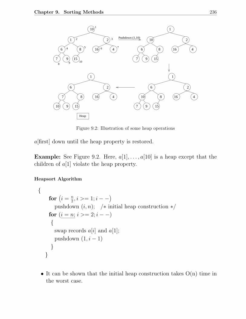
Chapter 9. Sorting Methods 236
10
1 2
6 8 16 4
7 9 15
1
2 3
4 5 6 7
8 9 10
1
10 2
6 8 16 4
7 9 15
1
6 2
10 8 16 4
7 9 15
1
6 2
7 8 16 4
10 9 15
Pushdown (1,10)
Heap
Figure 9.2: Illustration of some heap operations
a[first] down until the heap property is restored.
Example: See Figure 9.2. Here, a[1], . . . , a[10] is a heap except that thechildren of a[1] violate the heap property.
Heapsort Algorithm
for
(
i = n2 , i >= 1; i −−
)
pushdown (i, n); /∗ initial heap construction ∗/for (i = n; i >= 2; i −−)
swap records a[i] and a[1];
pushdown (1, i − 1)
• It can be shown that the initial heap construction takes O(n) time inthe worst case.
Chapter 9. Sorting Methods 237
• The sorting portion takes worst case O(n log n) time.
• Heap sort can also be used for computing order statistics, ie., kth
lowest in a list of records.
9.6 Quick Sort
REF. C.A.R. Hoare. Algorithm 63 (Partition) and Algorithm 65 (find).Communications of the ACM , Volume 4, Number 7, pp. 321-322,1961.
REF. C.A.R. Hoare. Quicksort. The Computer Journal , Volume 5, Number1, pp. 10-15, 1962.
REF. Robert Sedgewick. Implementing quicksort programs. Communica-tions of the ACM , Volume 21, Number 10, pp. 847-857, 1978.
• Divide and conquer algorithm designed by CAR Hoare in 1962.
• Worst case O(n2) time, but average case O(n log n) time. Better av-erage case performance than heap sort.
9.6.1 Algorithm:
To sort the records a[i], a[i + 1], . . . , a[j], in place.
quicksort (i, j)
if (a[i] · · · a[j] contain at least two distinct keys)
let v be the larger of the first two distinct keys;
Partition a[i] · · · a[j] so that for some k between i + 1 and j,
a[i] · · · a[k − 1] all have keys < v, and
a[k] · · · a[j] all have keys ≥ v;
quicksort (i, k − 1);
quicksort (k, j);
Chapter 9. Sorting Methods 238
a[i] · · · a[k − 1]︸ ︷︷ ︸
keys <v
a[k] · · · a[j]︸ ︷︷ ︸
keys ≥v
v is called the pivot. It could be any element such that the resultingpartition desirably has two equal sized groups.
9.6.2 Algorithm for Partitioning
int partition (int i; int j; key-type pivot);
/∗ partitions the elements a[k] · · · a[j],
wrt the pivot and returns the position k ∗/
int ℓ, r;
ℓ = i; /∗ ℓ starts from left end ∗/r = j; /∗ r starts from right end ∗/do
swap the records a[ℓ] and a[r];
while (a[ℓ] . key < pivot)
ℓ = ℓ + 1;
while (a[r] . key ≥ pivot)
r = r − 1;
while (ℓ ≤ r);
return (ℓ);
• For an example, see Figure 9.3.
• Worst case arises when the input is already sorted: O(n2)
• Average case : O(n log n)
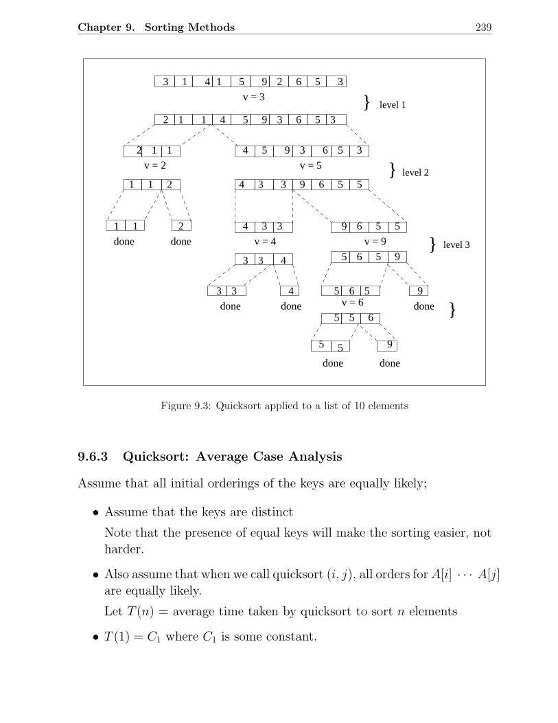
Chapter 9. Sorting Methods 239
3 3
3 3
3 3
3 3
3 3
3 3
3 3
1 1
1 1
1 1
1 1
1 1
2
2
2
2
2
4
4
4
4
4
4
4
5 5
5 5
5 5
5 5
5 5
5 5
5 5
5 5
5 5
6
6
6
6
6
6
6
6
9
9
9
9
9
9
9
9
done done
done done
done done
done
v = 3
v = 4 v = 9
v = 6
v = 5v = 2
level 1
level 2
level 3
Figure 9.3: Quicksort applied to a list of 10 elements
9.6.3 Quicksort: Average Case Analysis
Assume that all initial orderings of the keys are equally likely;
• Assume that the keys are distinct
Note that the presence of equal keys will make the sorting easier, notharder.
• Also assume that when we call quicksort (i, j), all orders for A[i] · · · A[j]are equally likely.
Let T (n) = average time taken by quicksort to sort n elements
• T (1) = C1 where C1 is some constant.
Chapter 9. Sorting Methods 240
• Recall that the pivot is the larger of the first two elements.
• When n > 1, quicksort splits the subarray, taking C2n time, where C2
is another constant.
Also, since the pivot is the larger of the first two elements, left groups tendto be larger than the right groups.
The left group can have i elements where i = 1, 2, . . . , n − 1, since the leftgroup has at least one element and the right group also has at least oneelement.
Let us fix i and try to compute the probability:
P left group has i elements
Now, left group has i elements
⇒ pivot must be the (i + 1)st element among the n elements
If the pivot is in position 1, then the element in position 2 is one of the ismaller elements and vice-versa.
P Position 1 contains one of the i smaller elements
=
(
i
n − 1
) (
1
n
)
Similarly,
P Position 2 contains one of the i smaller elements
=
(
1
n
) (
i
n − 1
)
Therefore,
P left group has i elements
=2i
n(n − 1)
This leads to
Chapter 9. Sorting Methods 241
T (n) ≤ C2n +n−1∑
i=1
2i
n(n − 1)T (i) + T (n − i)
Usingn−1∑
i=1
f(i) =n−1∑
i=1
f(n − i),
we get
T (n) ≤ C2n +1
n − 1
n−1∑
i=1
T (i) + T (n − i)
The above expression is in the form it would have been if we had picked atruly random pivot at each step.
The above simplifies to:
T (n) ≤ C2n +2
n − 1
n−1∑
i=1
T (i)
The above is the recurrence that one would get if all sizes between 1 andn − 1 for the left group were equally likely. Thus picking the larger of thetwo elements doesn’t really affect the size distribution.
We shall guess the solution
T (n) ≤ Cn log n
for some constant C and prove its correctness using induction.
Basis:
n = 2 ⇒ Cn log n = 2C
which is correct.
Induction Step:
Assume T (i) ≤ Ci log i ∀ i < n.
T (n) ≤ C2n +2C
n − 1
n−1∑
i=1
i log i
Chapter 9. Sorting Methods 242
≤ C2n +2C
n − 1
n/2∑
i=1
i log i +2C
n − 1
n−1∑
i=n2+1
i log i
≤ C2n +2C
n − 1
n/2∑
i=1
i logn
2+
2C
n − 1
n−1∑
i=n2+1
i log n
≤ C2n + Cn log n − Cn
4− Cn
2(n − 1), after simplification
Picking C ≥ 4C2, we have,
C2n − Cn
4≥ 0
Thus T (n) is O(n log n)
9.7 Order Statistics
• Given a list of n records, and an integer k, find the record whose keyis the kth in the sorted order of keys.
• Note that
K = 1 corresponds to finding the minimumK = n corresponds to finding the maximum
K =n
2corresponds to finding the median
9.7.1 Algorithm 1
One can arrange the n keys into a heap and pick the kth largest in k steps,where each step takes logarithmic time in the number of elements of theheap.
Since the construction of initial heap can be accomplished in worst caseO(n) time, the worst case complexity of this algorithm is:
O(n + k log n)
Therefore if k ≤ nlog n or k ≥ n
log n , the above algorithm will have O(n) worstcase complexity.
Chapter 9. Sorting Methods 243
9.7.2 Algorithm 2
Variation of quicksort.
Select (i, j, k) /∗ finds the kth element among A[i] · · · A[j] ∗/
pick a pivot element v;
partition A[i] · · · A[j] so as to get
A[i] · · · A[m − 1] with keys < v and
A[m] · · · A[j] with keys ≥ v;
if (k ≤ m − 1)
Select (i, m − 1, k)
else
Select (m, j, k − m + i)
• Worst case complexity of the above algorithm is O(n2) (as in quick-sort).
• Average Case:
– Note that select calls itself only once at a time whereas quicksortcalled itself twice each time.
– On an average, select calls itself on a subarray half as long as thesubarray. To be conservative, suppose that each call of select is
on an array(
910
)ththe size on previous call. Then,
T (n) ≤ Cn + T
(
9n
10
)
which can be shown to be O(n).
9.7.3 Algorithm 3
Worst case linear time algorithm due to
Blum, Floyd, Pratt, Rivest, Tarzan.
Chapter 9. Sorting Methods 244
REF. Manuel Blum, Robert W. Floyd, Vaughan Pratt, Ronald L Rivest, andRobert E. Tarjan. Time bounds for selection. Journal of Computerand System Sciences , Volume 7, Number 4, pp. 448-461, 1973.
• This is also a variation of quicksort and the main idea is to find a goodpivot.
• Assume that all the elements are distinct. The algorithm works oth-erwise too.
1. Divide the n elements into groups of 5 leaving aside between 0 and 4elements that cannot be placed in a group.
Sort each group of 5 elements by any algorithm and take the middleelement from each group. This yields
⌊n/5⌋ medians.
2. Use the SELECT algorithm to find the median of these ⌊n/5⌋ ele-ments. Choose this median as the pivot.
• Note that this pivot is in position ⌊n+510 ⌋
• Also, the pivot exceeds ⌊n−510 ⌋ of the middle elements and each of
these middle elements exceeds two elements. Thus, the pivot exceedsat least
3⌊n − 5
10⌋ elements.
Also, by a similar argument, the pivot is less than at least
3⌊n − 5
10⌋ elements.
• If n ≥ 75,
3⌊n − 5
10⌋ ≥ 3⌊70
10⌋ = 21 >
75
4In other words,
n ≥ 75 ⇒ 3
[
n + 5
10
]
≥ n
4
This would mean that, if n ≥ 75, the pivot is greater than at least n4
elements and less than at least n4 elements. Consequently, when we
Chapter 9. Sorting Methods 245
partition an array with this pivot, the kth element is isolated to withina range of at most 3n
4 of the elements.
Implementation
keytype select (int i, j, k);
/∗ returns key of the kth largest element among A[i] · · · A[j] ∗/if ((j − i) < 75)
find the kth largest by some simple algorithm
else for (m = 0; m ≤ (j − i − 4)/5; m + +)
find the third element among A[i+5 ∗m] · · · A[i+5 ∗m+4]
and swap it with A[i + m];
pivot = select (i, (j − i − 4)/5, (j − i − 4)/10)
m = partition (i, j, pivot);
if (k ≤ m − i)
return (select (i, m − 1, k))
else
return (select (m, j, (k − (m − i)))
The worst case complexity of the above algorithm can be described by
T (n) ≤ C1 if n ≤ 75
≤ C2n + T
(
n
5
)
+ T
(
3n
4
)
if n > 75
Let us guess the solution T (n) = Cn for n > 75. For n ≥ 75, assume
Chapter 9. Sorting Methods 246
T (m) ≤ Cm for m < n. Then
T (n) ≤ C2n +
(
Cn
5
)
+
(
3Cn
4
)
≤ C2n +19
20Cn
Thus T (n) is O(n).
• Instead of groups of 5, let us say we choose groups of 7. It is easy toshow that the worst case complexity is again O(n). In general, anysize of the groups that ensures the sum of the two arguments of T (.)to be less than n will yield O(n) worst case complexity.
9.8 Lower Bound on Complexity for Sorting Meth-
ods
Result 1
The worst case complexity of any sorting algorithm that only uses keycomparisons is
Ω(n log n)
Result 2
The average case complexity of any sorting algorithm that only uses keycomparisons is
Ω(n log n)
The above results are proved using a Decision Tree which is a binarytree in which the nodes represent the status of the algorithm after makingsome comparisons.
Consider a node x in a decision tree and let y be its left child and z itsright child. See Figure 9.4.
Basically, y represents a state consisting of the information known at x
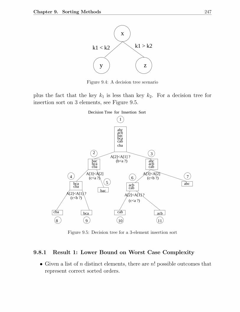
Chapter 9. Sorting Methods 247
k1 < k2 k1 > k2
z
x
y
Figure 9.4: A decision tree scenario
plus the fact that the key k1 is less than key k2. For a decision tree forinsertion sort on 3 elements, see Figure 9.5.
abcacbbacbcacabcba
bacbcacba
abcacbcab
bcacba
cba bca
bac
cab acb
abcacbcab
A[2]<A[1] ?(b<a ?)
A[3]<A[2](c<a ?)
A[2]<A[1] ?(c<b ?)
A[2]<A[1] ?
(c<a ?)
A[3]<A[2](c<b ?)
Decision Tree for Insertion Sort
1
2 3
4
5 6 7
8 9 10 11
Figure 9.5: Decision tree for a 3-element insertion sort
9.8.1 Result 1: Lower Bound on Worst Case Complexity
• Given a list of n distinct elements, there are n! possible outcomes thatrepresent correct sorted orders.
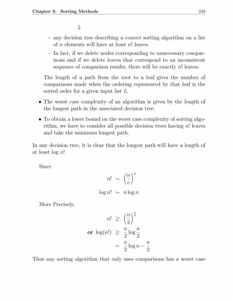
Chapter 9. Sorting Methods 248
⇓
– any decision tree describing a correct sorting algorithm on a listof n elements will have at least n! leaves.
– In fact, if we delete nodes corresponding to unnecessary compar-isons and if we delete leaves that correspond to an inconsistentsequence of comparison results, there will be exactly n! leaves.
The length of a path from the root to a leaf gives the number ofcomparisons made when the ordering represented by that leaf is thesorted order for a given input list L.
• The worst case complexity of an algorithm is given by the length ofthe longest path in the associated decision tree.
• To obtain a lower bound on the worst case complexity of sorting algo-rithm, we have to consider all possible decision trees having n! leavesand take the minimum longest path.
In any decision tree, it is clear that the longest path will have a length ofat least log n!
Since
n! ∼(
n
e
)n
log n! ∼ n log n
More Precisely,
n! ≥(
n
2
)n2
or log(n!) ≥ n
2log
n
2
=n
2log n − n
2
Thus any sorting algorithm that only uses comparisons has a worst case
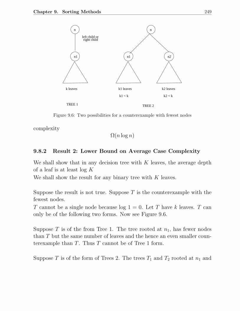
Chapter 9. Sorting Methods 249
k leaves k1 leaves k2 leaves
k1 < k k2 < k
TREE 1 TREE 2
n
n1 n1 n2
n
left child or right child
Figure 9.6: Two possibilities for a counterexample with fewest nodes
complexityΩ(n log n)
9.8.2 Result 2: Lower Bound on Average Case Complexity
We shall show that in any decision tree with K leaves, the average depthof a leaf is at least log K
We shall show the result for any binary tree with K leaves.
Suppose the result is not true. Suppose T is the counterexample with thefewest nodes.
T cannot be a single node because log 1 = 0. Let T have k leaves. T canonly be of the following two forms. Now see Figure 9.6.
Suppose T is of the from Tree 1. The tree rooted at n1, has fewer nodesthan T but the same number of leaves and the hence an even smaller coun-terexample than T . Thus T cannot be of Tree 1 form.
Suppose T is of the form of Trees 2. The trees T1 and T2 rooted at n1 and
Chapter 9. Sorting Methods 250
n2 are smaller than T and therefore the
Average depth of T1 ≥ log k1
Average depth of T2 ≥ log k2
Thus the average depth of T
≥ k1
k1 + k2log k1 +
k2
k1 + k2log k2 + 1
=k1
klog k1 +
k2
klog k2 +
(
k1
k+
k2
k
)
=1
k(k1 log 2k1 + k2 log 2k2)
≥ log k
since the minimum value ofthe above is attained atk1 = k2 giving the value k
This contradicts the premise that the average depth of T is < log k.
Thus T cannot be of the form of Tree 2.
Thus in any decision tree with n! leaves, the average path length to a leafis at least
log(n!) ∼ O(n log n)
9.9 Radix Sorting
• Here we use some special information about the keys and design sort-ing algorithms which beat the O(n log n) lower bound for comparison-based sorting methods.
• Consider sorting n integers in the range 0 to n2 - 1. We do it in twophases.
Phase 1: We use n bins, one for each of the integers 0, 1, · · · , n − 1. We
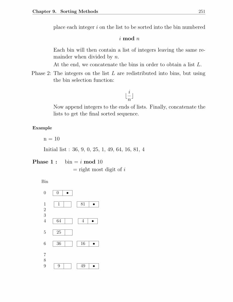
Chapter 9. Sorting Methods 251
place each integer i on the list to be sorted into the bin numbered
i mod n
Each bin will then contain a list of integers leaving the same re-mainder when divided by n.
At the end, we concatenate the bins in order to obtain a list L.
Phase 2: The integers on the list L are redistributed into bins, but usingthe bin selection function:
⌊ i
n⌋
Now append integers to the ends of lists. Finally, concatenate thelists to get the final sorted sequence.
Example
n = 10
Initial list : 36, 9, 0, 25, 1, 49, 64, 16, 81, 4
Phase 1 : bin = i mod 10
= right most digit of i
Bin
0 0 •
1 1 81 •234 64 4 •
5 25
6 36 16 •
789 9 49 •
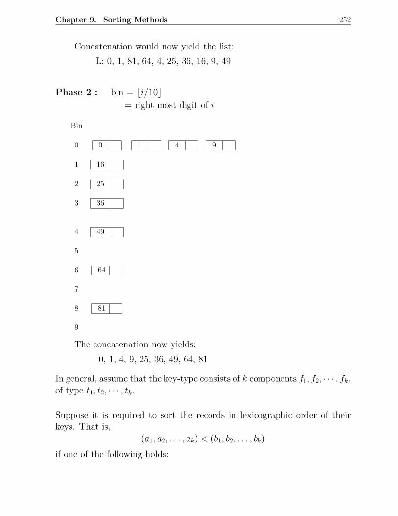
Chapter 9. Sorting Methods 252
Concatenation would now yield the list:
L: 0, 1, 81, 64, 4, 25, 36, 16, 9, 49
Phase 2 : bin = ⌊i/10⌋= right most digit of i
Bin
0 0 1 4 9
1 16
2 25
3 36
4 49
5
6 64
7
8 81
9
The concatenation now yields:
0, 1, 4, 9, 25, 36, 49, 64, 81
In general, assume that the key-type consists of k components f1, f2, · · · , fk,of type t1, t2, · · · , tk.
Suppose it is required to sort the records in lexicographic order of theirkeys. That is,
(a1, a2, . . . , ak) < (b1, b2, . . . , bk)
if one of the following holds:
Chapter 9. Sorting Methods 253
1. a1 < b1
2. a1 = b1; a2 < b2
3. a1 = b1; a2 = b2; a3 < b3
.
.
.k. a1 = b1; . . . ; ak−1 = bk−1; ak < bk
Radix sort proceeds in the following way.
First binsort all records first on fk, the least significant digit, then concate-nate the bins lowest value first.
Then binsort the above concatenated list on fk−1 and then concatenate thebins lowest value first.
In general, after binsorting on fk, fk−1, . . . , fi, the records will appear inlexicographic order if the key consisted of only the fields fi, . . . , fk.
void radixsort;
/ ∗ Sorts a list A of n records with keys consisting of fields
f1, . . . , fk of types t1, . . . , tk. The function uses k
arrays B1, . . . , Bk of type array [ti] of list-type, i = 1, . . . , k,
where list-type is a linked list of records ∗/for (i = k; i ≥ 1; i −−)
for (each value v of type ti)
make Bi[v] empty; /∗ clear bins ∗/for (each value r on list A)
move r from A onto the end of bin Bi[v],
where v is the value of the field fi of the key of r;
for (each value v of type ti from lowest to highest)
concatenate Bi[v] onto the end of A
Chapter 9. Sorting Methods 254
• Elements to be sorted are presented in the form of a linked list obvi-ating the need for copying a record. We just move records from onelist to another.
• For concatenation to be done quickly, we need pointers to the end oflists.
Complexity of Radix Sort
• Inner loop 1 takes O(si) time where si = number of different valuesof type ti
• Inner loop 2 takes O(n) time
• Inner loop 3 times O(si) time
Thus the total time
=k∑
i=1
O(si + n)
= O
kn +k∑
i=1
si
= O
n +k∑
i=1
si
assuming k to be a constant
• For example, if keys are integers in the range 0 to nk − 1, then we canview the integers as radix −n integers each k digits long. Then ti hasrange 0 · · · n − 1 for 1 ≤ i ≤ k.
Thus si = n and total running time is O(n)
• similarly, if keys are character strings of length k, for constant k, thensi = 128 (say) for i = 1, . . . , k and again we get the total running timeas O(n).
Chapter 9. Sorting Methods 255
9.10 Merge Sort
• Divide and conquer algorithm
• O(n log n) worst case performance
• Useful in external sorting applications.
Algorithm
list-type mergesort (list-type L; int n)
if (n = 1)
return (L)
else split L into two halves L1 and L2;
return (merge (mergesort(
L1,n2
)
, mergesort(
L2,n2
))
Let T (n) be the running time of mergesort on a list of size n. Then.
T (n) ≤ C1 (n = 1)
≤ 2T
(
n
2
)
︸ ︷︷ ︸
divideandconquer
+ C2n︸ ︷︷ ︸
merge(n > 1)
It can be shown that T (n) is O(n log n).
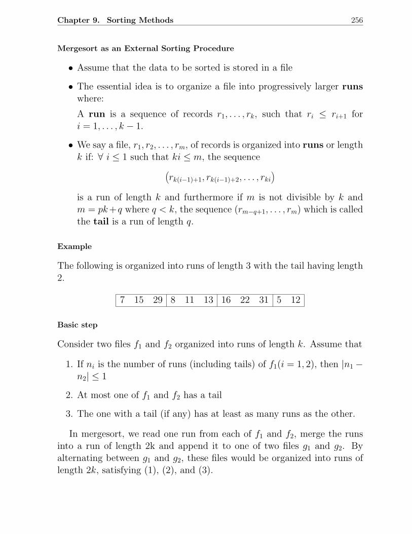
Chapter 9. Sorting Methods 256
Mergesort as an External Sorting Procedure
• Assume that the data to be sorted is stored in a file
• The essential idea is to organize a file into progressively larger runswhere:
A run is a sequence of records r1, . . . , rk, such that ri ≤ ri+1 fori = 1, . . . , k − 1.
• We say a file, r1, r2, . . . , rm, of records is organized into runs or lengthk if: ∀ i ≤ 1 such that ki ≤ m, the sequence
(
rk(i−1)+1, rk(i−1)+2, . . . , rki
)
is a run of length k and furthermore if m is not divisible by k andm = pk+q where q < k, the sequence (rm−q+1, . . . , rm) which is calledthe tail is a run of length q.
Example
The following is organized into runs of length 3 with the tail having length2.
7 15 29 8 11 13 16 22 31 5 12
Basic step
Consider two files f1 and f2 organized into runs of length k. Assume that
1. If ni is the number of runs (including tails) of f1(i = 1, 2), then |n1 −n2| ≤ 1
2. At most one of f1 and f2 has a tail
3. The one with a tail (if any) has at least as many runs as the other.
In mergesort, we read one run from each of f1 and f2, merge the runsinto a run of length 2k and append it to one of two files g1 and g2. Byalternating between g1 and g2, these files would be organized into runs oflength 2k, satisfying (1), (2), and (3).
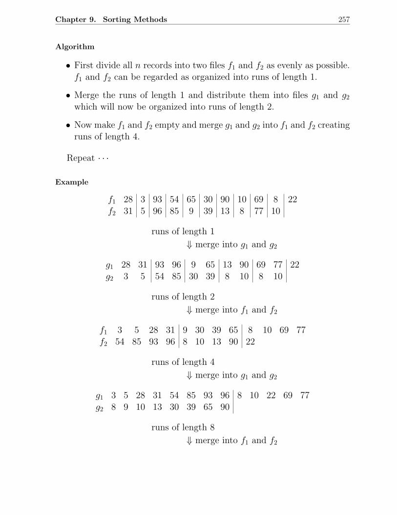
Chapter 9. Sorting Methods 257
Algorithm
• First divide all n records into two files f1 and f2 as evenly as possible.f1 and f2 can be regarded as organized into runs of length 1.
• Merge the runs of length 1 and distribute them into files g1 and g2
which will now be organized into runs of length 2.
• Now make f1 and f2 empty and merge g1 and g2 into f1 and f2 creatingruns of length 4.
Repeat · · ·
Example
f1 28 3 93 54 65 30 90 10 69 8 22f2 31 5 96 85 9 39 13 8 77 10
runs of length 1
⇓ merge into g1 and g2
g1 28 31 93 96 9 65 13 90 69 77 22g2 3 5 54 85 30 39 8 10 8 10
runs of length 2
⇓ merge into f1 and f2
f1 3 5 28 31 9 30 39 65 8 10 69 77f2 54 85 93 96 8 10 13 90 22
runs of length 4
⇓ merge into g1 and g2
g1 3 5 28 31 54 85 93 96 8 10 22 69 77g2 8 9 10 13 30 39 65 90
runs of length 8
⇓ merge into f1 and f2
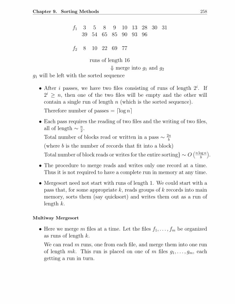
Chapter 9. Sorting Methods 258
f1 3 5 8 9 10 13 28 30 3139 54 65 85 90 93 96
f2 8 10 22 69 77
runs of length 16
⇓ merge into g1 and g2
g1 will be left with the sorted sequence
• After i passes, we have two files consisting of runs of length 2i. If2i ≥ n, then one of the two files will be empty and the other willcontain a single run of length n (which is the sorted sequence).
Therefore number of passes = ⌈log n⌉
• Each pass requires the reading of two files and the writing of two files,all of length ∼ n
2 .
Total number of blocks read or written in a pass ∼ 2nb
(where b is the number of records that fit into a block)
Total number of block reads or writes for the entire sorting ∼ O(
n log nb
)
.
• The procedure to merge reads and writes only one record at a time.Thus it is not required to have a complete run in memory at any time.
• Mergesort need not start with runs of length 1. We could start with apass that, for some appropriate k, reads groups of k records into mainmemory, sorts them (say quicksort) and writes them out as a run oflength k.
Multiway Mergesort
• Here we merge m files at a time. Let the files f1, . . . , fm be organizedas runs of length k.
We can read m runs, one from each file, and merge them into one runof length mk. This run is placed on one of m files g1, . . . , gm, eachgetting a run in turn.
Chapter 9. Sorting Methods 259
• The merging process will involve each time selecting the minimumamong m currently smallest unselected records from each file.
By using a priority queue that supports insert and delete in logarith-mic time (e.g., partially ordered tree), the process can be accomplishedin O(log m) time.
• Number of passes - ⌈logm n⌉Effort in each pass = O(n log2 m)overall complexity ∼ O(n log2 m. logm n)
• Advantages
• We save by a factor of log2 m, the number of times we read eachrecord
• We can process data O(m) times faster with m disk units.
9.11 To Probe Further
1. Alfred V Aho, John E. Hopcroft, and Jeffrey D Ullman. Data Struc-tures and Algorithms . Addison-Wesley, 1983.
2. Gilles Brassard and Paul Bratley. Fundamentals of Algorithmics .Prentice-Hall, 1996. Indian Edition published by Prentice Hall ofIndia, 1998.
3. Thomas H. Cormen, Charles E. Leiserson, and Donald L. Rivest. In-troduction to Algorithms . The MIT Electrical Engineering and Com-puter Science Series, 1990. Indian Edition published in 1999.
4. Mark Allen Weiss. Data Structures and Algorithm Analysis in C++.Benjamin-Cummings, 1994. Indian Edition published in 1998.
5. Alfred V Aho, John E. Hopcroft, and Jeffrey D Ullman. The Designand Analysis of Computer Algorithms , Addison-Wesley, 1974.
6. Sara Baase and Allen Van Gelder. Computer Algorithms: Introductionto Design and Analysis . Addison-Wesley, Third Edition, 2000. IndianEdition published by Pearson Education Asia, 2000.
Chapter 9. Sorting Methods 260
7. Ellis Horowitz, Sartaz Sahni, and Rajasekaran. Fundamentals of Com-puter Algorithms . W.H. Freeman and Company, 1998. Indian Editionpublished by Galgotia Publications, 2000.
8. Donald E Knuth. Fundamental Algorithms , Volume 1 of The Artof Computer Programming, Addison-Wesley, 1968, Second Edition,1973.
9. Donald E. Knuth. Sorting and Searching , Volume 3 of The Art ofComputer Programming, Addison-Wesley, 1973.
10. Y. Langsam, M.J. Augenstein, and A.M. Tenenbaum. Data Struc-tures using C and C++. Second Edition, Prentice Hall, 1996. IndianEdition published by Prentice Hall of India, 2000.
11. Kurt Mehlhorn. Sorting and Searching. Volume 1 of Data Structuresand Algorithms. Springer-Verlag, 1984.
12. Nicklaus Wirth. Data Structures + Algorithms = Programs. Prentice-Hall, Englewood Cliffs. 1975.
13. Manuel Blum, Robert W. Floyd, Vaughan Pratt, Ronald L Rivest, andRobert E. Tarjan. Time bounds for selection. Journal of Computerand System Sciences , Volume 7, Number 4, pp.448-461, 1973.
14. Robert W. Floyd. Algorithm 245 (TreeSort). Communications of theACM , Volume 7, pp.701, 1964.
15. C.A.R. Hoare. Algorithm 63 (Partition) and Algorithm 65 (find).Communications of the ACM , Volume 4, Number 7, pp 321-322, 1961.
16. C.A.R. Hoare. Quicksort. The Computer Journal , Volume 5, Number1, pp.10-15, 1962.
17. Robert Sedgewick. Implementing quicksort programs. Communica-tions of the ACM , Volume 21, Number 10, pp.847-857, 1978.
18. Shell. A High-speed Sorting Procedure. Communications of the ACM ,Volume 2, Number 7, pp. 30-32,1959.
Chapter 9. Sorting Methods 261
9.12 Problems
1. Consider the following sorting methods: Bubble sort, Insertion Sort, Selection sort,Shell sort, Merge sort, Quick sort, and Heap sort.
• Sort the following keys using each of the above methods:22, 36, 6, 79, 26, 45, 2, 13, 31, 62, 10, 79, 33, 11, 62, 26
• A sorting algorithm is said to be stable if it preserves the original order ofrecords with equal keys. Which of the above methods are stable?
• Suppose you are to sort a list L comprising a sorted list followed by a fewrandom elements. Which of the above sorting methods would you prefer andwhy?
2. Show that if k is the smallest integer greater than or equal to n+ log2 n− 2, k com-parisons are necessary and sufficient to find the largest and second largest elementsof a set of n distinct elements.
3. Design an algorithm to find the two smallest elements in an array of length n. Canthis be done in fewer than 2n − 3 comparisons?
4. Show how to find the minimum and maximum elements in an array using only(2n − 3) comparisons, where n is the size of the array.
5. Show that any sorting algorithm that moves elements only one position at a timemust have time complexity Ω(n2).
6. Design an efficient algorithm to find all duplicates in a list of n elements.
7. Find a sorting method for four keys that is optimal in the sense of doing the smallestpossible number of key comparisons in the worst case. Find how many comparisonsyour algorithm does in the average case.
8. Suppose we have a set of words, i.e., strings of the letters a–z, whose total lengthis n. Show how to sort these in O(n) time. Note that if the maximum length ofa word is constant, then bin sort will work. However, you must consider the casewhere some of the words are very long.
9. Suppose we have a sorted array of strings s1, . . . , sn. Write an algorithm to determinewhether a given string x is a member of this sequence. What is the time complexityof your algorithm as a function of n and the length of x?
10. Design an algorithm that will arrange a contiguous list of real numbers so that allthe items with negative keys will come first, then those with nonnegative keys. Thefinal list need not be sorted.
11. Design an algorithm that will rearrange a list of integers as described in each casebelow.
Chapter 9. Sorting Methods 262
• All even integers come before all odd integers.
• Either all the integers in even-numbered positions will be even or all integersin the odd-numbered positions will be odd. First, prove that one or the otherof these goals can be achieved, although it may not be possible to achieve bothgoals at the same time.
12. Suppose that the splits at every level of quicksort are in the proportion 1− α to α,where 0 < α ≤ 1
2and α is a constant. Show that the minimum depth of a leaf in
the recursion tree of quicksort is approximately − log n
log αand the maximum depth is
approximately − log n
log(1−α). (Ignore the integer round off).
13. Recall the algorithm Select(i, j, k) that finds the kth element in the sorted order ofthe elements a[i], a[i + 1], ..., a[j]. Choose the pivot as follows. Divide the elementsinto groups of 3 (leaving aside between 0 and 2 elements that cannot be placed ina group), sort each group, and take the middle element from each group; a total ofsay, p, middle elements will result. Choose the median of these p elements as thepivot. Let T (n) be the time taken by a call to Select on n elements. Write down anappropriate recurrence relation for T (n). Is T (n), O(n)?
14. In the above problem, choose the pivot as follows. Divide the elements into groupsof 7, leaving aside between 0 and 6 elements that cannot be placed in a group. Sorteach group and take the middle element from each group. Choose the median ofthese middle elements as the pivot.
Let T (n) be the time taken by a call to select on n elements. Write down anappropriate recurrence for T (n) and show that it is O(n).
15. A d-ary heap is like a binary heap, but in stead of two children, nodes have dchildren.
• How would you represent a d-ary heap in an array?
• What is the height of a d-ary heap of n elements in terms of n and d?
• Give an efficient implementation of deletemin and insert operations and analyzethe running time in terms of d and n.
16. Consider constructing a heap by first forming a complete binary tree and then re-peatedly applying the pushdown procedure. What input permutations of (1, 2, 3, 4, 5)are transformed into (1, 2, 4, 3, 5) by this process?
17. Give a permutation of 1, 2, . . . , 8, which when input to the quicksort algorithm willproduce the best possible performance of the quicksort algorithm (assume that thelarger of the first two keys is selected as the pivot for partitioning).
18. Suppose we have an array of n data records such that the key of each record hasthe value 0 or 1. Outline a worst case linear time algorithm to sort these recordsin place, using only an additional amount of storage equal to that of one record. Isyour algorithm stable? Justify.
Chapter 9. Sorting Methods 263
19. Outline an O(n log k) algorithm to merge k sorted lists into a single sorted list,where n is the total number of elements in all the input lists.
20. Outline an efficient algorithm, using the binomial queue data structure to mergek sorted lists into a single sorted list. What is the worst-case complexity of youralgorithm (in terms of k and n), if n is the total number of elements in all the inputlists.
21. Suppose we have an array of n data records such that the key of each record hasthe value 0, 1, or 2. Outline a worst case linear time algorithm to sort these recordsin place, using only an additional amount of storage equal to that of one record. Isyour algorithm stable? Justify.
22. Write down a decision tree for sorting three elements a, b, c using bubble sort , withproper annotations on the nodes and edges of the tree.
9.13 Programming Assignments
9.13.1 Heap Sort and Quicksort
Implement heapsort and quicksort. Design and carry out an experiment to compare their average
case complexities.

Chapter 10
Introduction to NP-Completeness
10.1 Importance of NP-Completeness
Most algorithms we have studied so far have polynomial-time runningtimes. According to Cormen, Leiserson, and Rivest, polynomial-time algo-rithms can be considered tractable for the following reasons.
(1) Although a problem which has a running time of say O(n20) or O(n100)can be called intractable, there are very few practical problems withsuch orders of polynomial complexity.
(2) For reasonable models of computation, a problem that can be solvedin polynomial time in one model can also be solved in polynomial timeon another.
(3) The class of polynomial-time solvable problems has nice closure prop-erties (since polynomials are closed under addition, multiplication,etc.)
The class of NP-complete (Non-deterministic polynomial time complete)problems is a very important and interesting class of problems in ComputerScience. The interest surrounding this class of problems can be attributedto the following reasons.
1. No polynomial-time algorithm has yet been discovered for any NP-complete problem; at the same time no NP-complete problem hasbeen shown to have a super polynomial-time (for example exponentialtime) lower bound.
264
Chapter 10. Introduction to NP-Completeness 265
2. If a polynomial-time algorithm is discovered for even one NP-completeproblem, then all NP-complete problems will be solvable in polynomial-time.
It is believed (but so far no proof is available) that NP-complete problemsdo not have polynomial-time algorithms and therefore are intractable. Thebasis for this belief is the second fact above, namely that if any singleNP-complete problem can be solved in polynomial time, then every NP-complete problem has a polynomial-time algorithm. Given the wide rangeof NP-complete problems that have been discovered to date, it will besensational if all of them could be solved in polynomial time.
It is important to know the rudiments of NP-completeness for anyoneto design ”sound” algorithms for problems. If one can establish a problemas NP-complete, there is strong reason to believe that it is intractable.We would then do better by trying to design a good approximation al-gorithm rather than searching endlessly seeking an exact solution. Anexample of this is the TSP (Traveling Salesman Problem), which has beenshown to be intractable. A practical strategy to solve TSP therefore wouldbe to design a good approximation algorithm. This is what we did inChapter 8, where we used a variation of Kruskal’s minimal spanning treealgorithm to approximately solve the TSP. Another important reason tohave good familiarity with NP-completeness is many natural interestingand innocuous-looking problems that on the surface seem no harder thansorting or searching, are in fact NP-complete.
10.2 Optimization Problems and Decision Problems
NP-completeness has been studied in the framework of decision problems .Most problems are not decision problems, but optimization problems (wheresome value needs to be minimized or maximized). In order to apply thetheory of NP-completeness to optimization problems, we must recast themas decision problems. We provide an example of how an optimization prob-lem can be transformed into a decision problem.
Example: Consider the problem SHORTEST-PATH that finds a short-est path between two given vertices in an unweighted, undirected graph
Chapter 10. Introduction to NP-Completeness 266
G = (V, E). An instance of SHORTEST-PATH consists of a particulargraph and two vertices of that graph. A solution is a sequence of verticesin the graph, with perhaps an empty sequence denoting that no path exists.Thus the problem SHORTEST-PATH is a relation that associates each in-stance of a graph and two vertices with a solution (namely a shortest pathin this case). Note that a given instance may have no solution, exactly onesolution, or multiple solutions.
A decision problem PATH related to the SHORTEST-PATH problemabove is : Given a graph G = (V, E), two vertices u, v ∈ V , and a non-negative integer k, does a path exist in G between u and v whose lengthis at most k ?
Note that the decision problem PATH is one way of casting the orig-inal optimization problem as a decision problem. We have done this byimposing a bound on the value to be optimized. This is a popular way oftransforming an optimization problem into a decision problem.
If an optimization problem is easy then its related decision problem iseasy as well. Similarly, if we can provide evidence that a decision problemis hard, we also provide evidence that its related optimization problem ishard.
10.3 Examples of some Intractable Problems
10.3.1 Traveling Salesman Problem
A Hamiltonian cycle in an undirected graph is a simple cycle that passesthrough every vertex exactly once.
Optimization Problem: Given a complete, weighted graph, find a minimum-weight Hamiltonian Cycle.
Decision Problem: Given a complete, weighted graph and an integer k,does there exist a Hamiltonian cycle with total weight at most k.
Chapter 10. Introduction to NP-Completeness 267
10.3.2 Subset Sum
The input is a positive integer C and n objects whose sizes are positiveintegers s1, s2, . . . , sn.
Optimization Problem: Among all subsets of objects with sum at mostC, what is the largest subset sum?
Decision Problem: Is there a subset of objects whose sizes add up toexactly C?
10.3.3 Knapsack Problem
This is a generalization of the subset sum problem. Consider a knapsackof capacity C where C is a positive integer and n objects with positiveinteger sizes s1, s2, . . . , sn and positive integer profits p1, p2, . . . , pn.
Optimization Problem: Find the largest total profit of any subset ofthe objects that fits in the knapsack.
Decision Problem: Given k, is there a subset of the objects that fits inthe knapsack and has total profit at least k?
10.3.4 Bin Packing
Suppose we have unlimited number of bins each of unit capacity and nobjects with sizes s1, s2, . . . , sn where the sizes si(i = 1, . . . , n) are rationalnumbers in the range 0 < si ≤ 1.
Optimization Problem: Determine the smallest number of bins intowhich the objects can be packed and find an optimal packing.
Decision Problem: Given an integer k, do the objects fit in k bins?
Chapter 10. Introduction to NP-Completeness 268
10.3.5 Job Shop Scheduling
Suppose there are n jobs, J1, J2, . . . , Jn to be processed one at a time innon-preemptive fashion. Let the processing time be t1, t2, . . . , tn and thedue dates be d1, d2, . . . , dn. A schedule for the jobs is a permutation π of1, 2, . . . , n. Job Ji(i = 1, . . . , n) will incur a penalty of pi(i = 1, . . . , n)if it misses the due-date in the given schedule π. If processed within thedue-date, the penalty is taken as zero. The processing times, due-dates,and penalties are all positive integers. The penalty of a schedule is thesum of penalties incurred by jobs processed according to that schedule.
Optimization Problem: Determine the minimum possible penalty fora schedule and find an (optimal) schedule that achieves the minimumpenalty.
Decision Problem: Given a non-negative integer k, does there exist aschedule with penalty at most k?
10.3.6 Satisfiability
A propositional variable is one that can be assigned the value true or false.A literal is a propositional variable or its negation. A clause is a sequenceof literals separated by the logical OR operator. A propositional formulais said to be in conjunctive normal form (CNF) if it consists of a sequenceof clauses separated by the logical AND operator. For example,
(p ∨ q ∨ s) ∧ (q ∨ r) ∧ (p ∨ q ∨ r ∨ s)
A truth assignment for a set of propositional variables is an assignment oftrue or false value to each propositional variable. A truth assignment issaid to satisfy a formula if it makes the value of the formula true.
3-SAT (Decision Problem): Given a CNF formula in which each clauseis permitted to contain at most three literals, is there a truth assignmentto its variables that satisfies it?
Chapter 10. Introduction to NP-Completeness 269
10.4 The Classes P and NP
An algorithm is said to be polynomially bounded if its worst-case complex-ity is bounded by a polynomial function of the input size. A problem is saidto be polynomially bounded if there is a polynomially bounded algorithmfor it.
P is the class of all decision problems that are polynomially bounded.The implication is that a decision problem X ∈ P can be solved in polyno-mial time on a deterministic computation model (such as a deterministicTuring machine).
NP represents the class of decision problems which can be solved inpolynomial time by a non-deterministic model of computation. That is,a decision problem X ∈ NP can be solved in polynomial-time on a non-deterministic computation model (such as a non-deterministic Turing ma-chine). A non-deterministic model can make the right guesses on everymove and race towards the solution much faster than a deterministic model.
A deterministic machine, at each point in time, executes an instruction.Depending on the outcome of executing the instruction, it then executessome next instruction, which is unique. A non-deterministic machine onthe other hand has a choice of next steps. It is free to choose any that itwishes. For example, it can always choose a next step that leads to thebest solution for the problem. A non-deterministic machine thus has thepower of extremely good, optimal guessing.
As an example, let us consider the decision version of TSP: Given acomplete, weighted graph and an integer k, does there exist a Hamiltoniancycle with total weight at most k?
A smart non-deterministic algorithm for the above problem starts witha vertex, guesses the correct edge to choose, proceeds to the next vertex,guesses the correct edge to choose there, etc. and in polynomial time dis-covers a Hamiltonian cycle of least cost and provides an answer to theabove problem. This is the power of non-determinism. A deterministic al-gorithm here will have no choice but take super-polynomial time to answerthe above question.
Another way of viewing the above is that given a candidate Hamiltoniancycle (call it certificate), one can verify in polynomial time whether the
Chapter 10. Introduction to NP-Completeness 270
answer to the above question is YES or NO. Thus to check if a problem isin NP, it is enough to prove in polynomial time that any YES instance iscorrect. We do not have to worry about NO instances since the programalways makes the right choice.
It is easy to show that P ⊆ NP. However, it is unknown whether P= NP. In fact, this question is perhaps the most celebrated of all openproblems in Computer Science.
10.5 NP-Complete Problems
The definition of NP-completeness is based on reducibility of problems.Suppose we wish to solve a problem X and we already have an algorithmfor solving another problem Y. Suppose we have a function T that takesan input x for X and produces T(x), an input for Y such that the correctanswer for X on x is yes if and only if the correct answer for Y on T(x) isyes. Then by composing T and the algorithm for y, we have an algorithmfor X.
• If the function T itself can be computed in polynomially boundedtime, we say X is polynomially reducible to Y and we write X ≤ p Y.
• If X is polynomially reducible to Y, then the implication is that Y isat least as hard to solve as X. i.e. X is no harder to solve than Y.
• It is easy to see that
X ≤p Y and Y ∈ P implies X ∈ P.
10.5.1 NP-Hardness and NP-Completeness
A decision problem Y is said to be NP-hard if X ≤p Y ∀ X ∈ NP. AnNP-hard problem Y is said to be NP-complete if Y ∈ NP. NPC is thestandard notation for the class of all NP-complete problems.
• Informally, an NP-hard problem is a problem that is at least as hardas any problem in NP. If, further, the problem also belongs to NP,it would become NP-complete.
Chapter 10. Introduction to NP-Completeness 271
• It can be easily proved that if any NP-complete problem is in P,then NP = P. Similarly, if any problem in NP is not polynomial-time solvable, then no NP-complete problem will be polynomial-timesolvable. Thus NP-completeness is at the crux of deciding whether ornot NP = P.
• Using the above definition of NP-completeness to show that a givendecision problem, say Y, is NP-complete will call for proving polyno-mial reducibility of each problem in NP to the problem Y. This isimpractical since the class NP already has a large number of mem-ber problems and will continuously grow as researchers discover newmembers of NP.
• A more practical way of proving NP-completeness of a decision prob-lem Y is to discover a problem X ∈ NPC such that X ≤p Y. Since Xis NP-complete and ≤p is a transitive relationship, the above wouldmean that Z ≤p Y ∀ Z ∈ NP. Furthermore if Y ∈ NP, then Y isNP-complete.
The above is the standard technique used for showing the NP-hardnessor NP-completeness of a given decision problem. For example, allthe decision problems given in Section 10.2 can be shown to be NP-complete by the above technique.
• An interesting question is: how was the first member of NPC found?Stephen Cook showed the NP-completeness of the problem 3-SAT bydirectly proving that X ≤p 3-SAT ∀ X ∈ NP.
• If a problem is NP-complete, it does not mean that all hopes are lost.If the actual input sizes are small, an algorithm with, say, exponentialrunning time may be acceptable. On the other hand, it may stillbe possible to obtain near-optimal solutions in polynomial-time. Suchan algorithm that returns near-optimal solutions (in polynomial time)is called an approximation algorithm. Using Kruskal’s algorithm toobtain a suboptimal solution to the TSP (see Chapter 8) is an exampleof this.
Chapter 10. Introduction to NP-Completeness 272
10.6 To Probe Further
This chapter has presented a first level introduction to the notion of NP-completeness. We have consciously avoided a technical discussion of thetopics since that would be the subject of a more advanced course. For a rig-orous treatment of the subject, you should consult the following references.
The following book is a classic source on the theory of NP-completenessand also contains a catalogue of NP-complete problems discovered until1979.
REF. M.R. Garey and D.S. Johnson. Computers and Intractability : AGuide to the Theory of NP-completeness. W.H. Freeman, 1979.
The class P was first introduced by Cobham in 1964,
REF. Alan Cobham. The intrinsic computational difficulty of functions.Proceedings of the 1964 Congress for Logic, Methodology, and Philos-ophy of Sciences, North-Holland, 1964, pp.24-30.
The class P was also independently introduced in 1965 by Edmonds, whoalso conjectured P 6= NP for the first time.
REF. Jack Edmonds. Paths, trees, and flowers. Canadian Journal of Math-ematics, Volume 17, 1965, pp. 449-467.
The notion of NP-completeness was first proposed in 1971 by Stephen Cookwho also gave the first NP-completeness proof for 3-SAT.
REF. Stephen Cook. The complexity of theorem proving procedures. Pro-ceedings of the Third Annual ACM Symposium on Theory of Com-puting, 1971, pp. 151-158.
The technique of polynomial reductions was introduced in 1972 by Karp,who also demonstrated a rich variety of NP-complete problems.
REF. Richard M Karp. Reducibility among combinatorial problems. InComplexity of computer computations, edited by R.E. Miller and J.WThather, Plenum Press, 1972 pp. 85-103.
Chapter 10. Introduction to NP-Completeness 273
This chapter has liberally drawn from the material presented in twobooks: Chapter 36 of the book by Cormen, Leiserson, and Rivest andChapter 13 of the book by Sara Baase and Allen Van Gelder. These twobooks are a rich source of NP-complete problems and NP-completenessproofs.
10.7 Problems
1. Show that an algorithm that makes at most a constant number of calls to polynomial-timesubroutines runs in polynomial time, but that a polynomial number of calls to polynomial-time subroutines may result in an exponential-time algorithm.
2. A Hamiltonian path in a graph is a simple path that visits every vertex exactly once.Show that the decision problem of determining whether or not there is a Hamiltonianpath from a given vertex u to another given vertex v belongs to NP
3. Show that the ≤p relation is a transitive relation on the set of problems.
4. Given an undirected graph, the Hamiltonian cycle problem determines whether a graphhas a Hamiltonian cycle. Given that the Hamiltonian cycle problem for undirected graphsis NP-Complete, what can you say about the Hamiltonian cycle problem for directedgraphs? Provide reasons for your answer.
Chapter 11
References
11.1 Primary Sources for this Lecture Notes
1. Alfred V Aho, John E. Hopcroft, and Jeffrey D Ullman. Data Struc-tures and Algorithms . Addison-Wesley, 1983.
2. Gilles Brassard and Paul Bratley. Fundamentals of Algorithmics .Prentice-Hall, 1996. Indian Edition published by Prentice Hall ofIndia, 1998.
3. Thomas H. Cormen, Charles E. Leiserson, and Donald L. Rivest. In-troduction to Algorithms . The MIT Electrical Engineering and Com-puter Science Series, 1990. Indian Edition published in 1999.
4. Donald E Knuth. Fundamental Algorithms , Volume 1 of The Artof Computer Programming, Addison-Wesley, 1968, Second Edition,1973.
5. Robert L. Kruse, Bruce P. Leung, and Clovis L. Tondo. Data Struc-tures and Program design in C . Prentice Hall, 1991. Indian Editionpublished by Prentice Hall of India, 1999.
6. Mark Allen Weiss. Data Structures and Algorithm Analysis in C++.Benjamin-Cummings, 1994. Indian Edition published in 1998.
274
Chapter 11. References 275
11.2 Useful Books
1. Alfred V Aho, John E. Hopcroft, and Jeffrey D Ullman. The Designand Analysis of Computer Algorithms , Addison-Wesley, 1974.
2. Sara Baase and Allen Van Gelder. Computer Algorithms: Introductionto Design and Analysis . Addison-Wesley, Third Edition, 2000. IndianEdition published by Pearson Education Asia, 2000.
3. Duane A. Bailey. Java Structures: Data Structures in Java for thePrincipled Programmer . McGraw-Hill International Edition, 1999.
4. Richard Bellman. Dynamic Programming . Princeton University Press,1957.
5. Jon L. Bentley. Writing Efficient Programs , Prentice-Hall, 1982.
6. Jon L. Bentley. Programming Pearls , Addison-Wesley, 1986.
7. Jon L. Bentley. More Programming Pearls , Addison-Wesley, 1988.
8. Gilles Brassard and Paul Bratley. Algorithmics : Theory and Practice.Prentice-Hall, 1988.
9. Michael R. Garey and David S Johnson. Computers and Intractability:A Guide to Theory of NP-Completeness . W.H. Freeman, 1979.
10. R.L. Graham, D.E. Knuth, and O. Patashnik. Concrete Mathematics .Addison-wesley, Reading, 1990. Indian Edition published by Addison-Wesley Longman, 1998.
11. Ellis Horowitz and Sartaz Sahni. Fundamentals of Data structures .Galgotia Publications, New Delhi, 1984.
12. Ellis Horowitz, Sartaz Sahni, and Rajasekaran. Fundamentals of Com-puter Algorithms . W.H. Freeman and Company, 1998. Indian Editionpublished by Galgotia Publications, 2000.
13. Donald E Knuth. Fundamental Algorithms , Volume 1 of The Artof Computer Programming, Addison-Wesley, 1968, Second Edition,1973.
Chapter 11. References 276
14. Donald E Knuth. Seminumerical Algorithms . Volume 2 of The Artof Computer Programming, Addison-Wesley, 1969, Second Edition,1981.
15. Donald E. Knuth. Sorting and Searching , Volume 3 of The Art ofComputer Programming, Addison-Wesley, 1973.
16. Y. Langsam, M.J. Augenstein, and A.M. Tenenbaum. Data Struc-tures using C and C++. Second Edition, Prentice Hall, 1996. IndianEdition published by Prentice Hall of India, 2000.
17. Eugene L Lawler, J.K. Lenstra, A.H.G. Rinnooy Kan, and D.B.Shmoys,editors. The Traveling Salesman Problem. John Wiley & Sons, 1985.
18. Kurt Mehlhorn. Sorting and Searching. Volume 1 of Data Structuresand Algorithms. Springer-Verlag, 1984.
19. Kurt Mehlhorn. Graph Algorithms and NP-Completeness . Volume 2of Data Structures and Algorithms , Springer-Verlag, 1984.
20. Kurt Mehlhorn. Multidimensional Searching and Computational Ge-ometry . Volume 3 of Data Structures and Algorithms , Springer-Verlag,1984.
21. Sartaj Sahni. Data Structures, Algorithms, and Applications in Java.McGraw-Hill Higher Education, 2000.
22. Robert Sedgewick. Algorithms. Addison-Wesley, Second Edition,1988.
23. Thomas A. Standish. Data Structures in Java. Addison-Wesley, 1998.Indian Edition published by Addison Wesley Longman, 2000.
24. Nicklaus Wirth. Data Structures + Algorithms = Programs. Prentice-Hall, Englewood Cliffs. 1975.
11.3 Original Research Papers and Survey Articles
1. G.M. Adel’son-Vel’skii and E.M. Landis. An algorithm for the or-ganization of information. Soviet Mathematics Monthly , Volume 3,pp.1259-1263, 1962.
Chapter 11. References 277
2. R. Bayer. Symmetric binary B-trees: Data Structures and mainte-nance algorithms, Acta Informatica, Volume 1, pp.290-306, 1972.
3. R. Bayer and E.M. McCreight. Organization and maintenance of largeordered indexes. Acta Informatica, Volume 1, Number 3, pp. 173-189,1972.
4. Richard Bellman. On a routing problem. Quarterly of Applied Math-ematics . Volume 16, Number 1, pp. 87–90, 1958.
5. Manuel Blum, Robert W. Floyd, Vaughan Pratt, Ronald L Rivest, andRobert E. Tarjan. Time bounds for selection. Journal of Computerand System Sciences , Volume 7, Number 4, pp.448-461, 1973.
6. Mark R. Brown. Implementation and analysis of binomial queue al-gorithms. SIAM Journal on Computing, Volume 7, Number 3, pp.298-319, 1978.
7. Alan Cobham. The intrinsic computational difficulty of functions.In Proceedings of the 1964 Congress for Logic, Methodology, and thePhilosophy of Science, pages 24-30, North-Holland, 1964.
8. D. Comer. The ubiquitous B-tree. ACM Computing Surveys , Volume11, Number 2, pp 121-137, 1979.
9. Stephen Cook. The complexity of theorem proving procedures. InProceedings of the Third Annual ACM Symposium on Theory of Com-puting , pages 151-158, 1971.
10. E.W. Dijkstra. A note on two problems in connection with graphs.Numerische Mathematik , Volume 1, pp 269-271, 1959.
11. Jack Edmonds. Paths, trees, and flowers. Canadian Journal of Math-ematics , Volume 17, pp 449-467, 1965.
12. Robert W Floyd. Algorithm 97 (Shortest Path). Communications ofthe ACM , Volume 5, Number 6, pp. 345, 1962.
13. Robert W. Floyd. Algorithm 245 (TreeSort). Communications of theACM , Volume 7, pp.701, 1964.
Chapter 11. References 278
14. Michael L. Fredman and Robert E. Tarjan. Fibonacci heaps and theiruses in improved network optimization algorithms. Journal of theACM , Volume 34, Number 3, pp. 596-615, 1987.
15. C.A.R. Hoare. Algorithm 63 (Partition) and Algorithm 65 (find).Communications of the ACM , Volume 4, Number 7, pp 321-322, 1961.
16. C.A.R. Hoare. Quicksort. The Computer Journal , Volume 5, Number1, pp.10-15, 1962.
17. John E Hopcroft and Robert E. Tarjan. Efficient algorithms for graphmanipulation. Communications of the ACM , Volume 16, Number 6pp.372-378, 1973.
18. David A Huffman. A method for the construction of minimum-redundancycodes. Proceedings of the IRE Volume 40, Number 9, pp. 1098-1101,1952.
19. Richard M. Karp. Reducibility among combinatorial problems. InRaymond E. Miller and James W. Thatcher, editors, Complexity ofComputer Computations . pages 85-103, Plenum Press, 1972.
20. J.B. Kruskal. On the shortest spanning subtree of a graph and thetraveling salesman problem. Proceedings of the American Mathemat-ical Society , Volume 7, pp 48-50, 1956.
21. R.C. Prim. Shortest connection networks and some generalizations.Bell System Technical Journal , Volume 36, pp.1389-1401, 1957.
22. William Pugh. Skip Lists: A probabilistic alternative to balancedtrees. Communications of the ACM , Volume 33, Number 6, pp. 668-676, 1990.
23. Robert Sedgewick. Implementing quicksort programs. Communica-tions of the ACM , Volume 21, Number 10, pp.847-857, 1978.
24. Daniel D Sleator and Robert E. Tarjan. Self-adjusting binary searchtrees. Journal of the ACM , Volume 32, Number 3, pp 652-686, 1985.
25. Robert E. Tarjan. Depth first search and linear graph algorithms.SIAM Journal on Computing , Volume 1, Number 2, pp.146-160, 1972.
Chapter 11. References 279
26. Robert E. Tarjan. Amortized computational complexity. SIAM Jour-nal on Algebraic and Discrete Methods , Volume 6, Number 2, pp.306-318, 1985.
27. Jean Vuillemin. A data structure for manipulating priority queues.Communications of the ACM, Volume 21, Number 4, pp.309-315,1978.
28. Stephen Warshall. A theorem on boolean matrices. Journal of theACM , Volume 9, Number 1, pp.11-12, 1962.
29. J.W.J. Williams. Algorithm 232 (Heapsort). Communications of theACM , Volume 7, pp.347-348, 1964.