Electronic Associates, Inc. - ntrs.nasa.gov · Electronic Associates, Inc. August 20, 1991 ABSTRACT...
58
Electronic Associates, Inc. 185 Monmouth Parkway, West Long Branch, N. J. 07764 (908) 229-1100 Final Report NASA Contract NAS5-30905 Construction of a Parallel Processor for Simulating Manipulators and Other Mechanical Systems. Electronic Associates, Inc. August 20, 1991 ABSTRACT This report summarizes the results of NASA Contract NAS5-30905, awarded under Phase 2 of the SBIR Program, for a demonstration of the feasibility of a new high-speed parallel simulation processor, called the RTA (Real-Time Accelerator). The principal goals were met, and EAI is now proceeding with Phase 3: development of a commercial product. This product is scheduled for commercial introduction in the second quarter of 1992. CONTENTS 1. INTRODUCTION 2. GOALS OF THE PHASE 2 PROJECT 3. RESULTS OF THE PHASE 2 PROJECT 4. USER' S GUIDE TO THE PROTOTYPE RTA 5. ANALYSIS OF AN RTA BENCHMARK 6. CONCLUSIONS 2 2 3 10 35 57 George Hannauer Principal Investigator ack Budelman ice President, Product Engineering (NASA-CR-191327) CONSTRUCTION OF A N94-32482 PARALLEL PROCESSOR FOR SIMULATING MANIPULATORS AND OTHER MECHANICAL SYSTEMS Final Report, Apr. 1990 - Unclas Aug. 1991 (Electronic Associates) 58 p G3/62 0010553 https://ntrs.nasa.gov/search.jsp?R=19940027976 2020-03-27T14:20:57+00:00Z
Transcript of Electronic Associates, Inc. - ntrs.nasa.gov · Electronic Associates, Inc. August 20, 1991 ABSTRACT...

Electronic Associates, Inc.185 Monmouth Parkway, West Long Branch, N. J. 07764 (908) 229-1100
Final ReportNASA Contract NAS5-30905
Construction of a Parallel Processorfor Simulating Manipulators
and Other Mechanical Systems.
Electronic Associates, Inc.August 20, 1991
ABSTRACT
This report summarizes the results of NASA Contract NAS5-30905, awarded under Phase 2 of theSBIR Program, for a demonstration of the feasibility of a new high-speed parallel simulation processor,called the RTA (Real-Time Accelerator). The principal goals were met, and EAI is now proceeding withPhase 3: development of a commercial product. This product is scheduled for commercial introductionin the second quarter of 1992.
CONTENTS
1. INTRODUCTION2. GOALS OF THE PHASE 2 PROJECT3. RESULTS OF THE PHASE 2 PROJECT4. USER' S GUIDE TO THE PROTOTYPE RTA5. ANALYSIS OF AN RTA BENCHMARK6. CONCLUSIONS
223
103557
George HannauerPrincipal Investigator
ack Budelmanice President, Product Engineering
(NASA-CR-191327) CONSTRUCTION OF A N94-32482PARALLEL PROCESSOR FOR SIMULATINGMANIPULATORS AND OTHER MECHANICALSYSTEMS Final Report, Apr. 1990 - UnclasAug. 1991 (Electronic Associates)58 p
G3/62 0010553
https://ntrs.nasa.gov/search.jsp?R=19940027976 2020-03-27T14:20:57+00:00Z

Electronic Associates. Inc.185 Monmouth Parkway, West Long Branch, N. J. 07764 (908) 229-1100
1. INTRODUCTION
For over 35 years, EAI has been designing and building the world's fastest simulation machines.Initially they were analog; later, hybrid. Several years ago, the company undertook a feasibility study todetermine what performance could be achieved with a new simulation system, based on an analog-typearchitecture, but implemented digitally. The result is the RTA.
Theoretical analysis and manual simulation led to the conclusion that such a system would be ten toone hundred times faster than existing machines for the vast majority of the target simulationapplications, at considerably less cost.
In 1990, under NASA Contract NAS5-30905, EAI began work on a prototype hardware system anda Continuous System Simulation Language (CSSL) compiler, to verify the design concepts. Thatcontract effort is now complete. It meets or exceeds all its major goals. For the last several months, ithas been outperforming other machines in hardware, as well as on paper.
The Applications Base
The starting point for the study was a set of benchmark applications that were used to evaluate thedesign. These included a six-degree-of-freedom missile launch simulation and a small, but very stiff,chemical kinetics application, both taken from our customer files. To these, we added severalapplications in robotics, furnished by NASA. These applications were chosen to be a representativesample of the ones that our customers have been running on our simulation computers for the past 35years. They share the following characteristics:
They are all applications in Continuous Systems Simulation—mathematically speaking, initial-valueproblems in ordinary differential equations. They typically require high speed, but only moderateaccuracy (a few percent at several hundred Hertz). They are often stiff (a wide range of eigenvalues),and usually include hardware in the loop, necessitating real-time operation. Most contain switchingtransients (discontinuities), so that a full set of logical, relational, and switching operations must bemade available and efficiently implemented.
We have run over a dozen benchmarks on the prototype hardware, including several that were not inthe original set. These additional applications, brought to us by potential customers after the studybegan, provided an important control. If the system had shown a great speed advantage for the originalbenchmarks, and a small advantage or none at all for the new ones, it would mean that the design hadbeen too strongly "tailored" to the specific examples, and was not robust enough for general-purposeuse. What was hoped, of course, was that the system would exhibit essentially the same competitiveadvantage for the new benchmarks as for the original ones, verifying that the latter had been selected

Electronic Associates, Inc.185 Monmouth Parkway, West Long Branch, N. J. 07764 (908) 229-1100
well. This hope has been realized, as the results in section 3 below clearly show.
2. GOALS OF THE PHASE 2 PROJECT
The goals of phase 2 of this study are succinctly summarized in the Technical Abstract of the Phase 2proposal summary:
"The objective of Phase 2 is to verify the Real-Time Accelerator (RTA) concept andthe timing estimates by building a prototype. EAI plans to build such a prototype andrun several simulations on it, verifying both the programmability and the speed of theproposed system. It is expected that the prototype will fulfill its expectations of atenfold-to-hundredfold speedup over conventional computers. If so, EAI plans topursue sources of non-Government venture capital to develop it as a commercialproduct."
This report describes the results of the Phase 2, including the running of the benchmarks, the speedcomparisons with conventional machines, and EAI's future development plans.
3. RESULTS OF THE PHASE 2 PROJECT
The major goals, as spelled out in the previous section, have been accomplished:
• The prototype RTA system has been developed and is being shipped to NASA, as per contract.Section 4 of this report provides a user's guide for the programming and operation of this prototypesystem.
• All three applications have been programmed and successfully run. The execution times metexpectations: the RTA runs these applications ten to one hundred times faster than currently availablemachines.
• EAI has obtained non-government funding for the third phase of this project: the development of acommercial product
3.1 Description of Benchmarks.
The Phase 2 proposal listed three benchmark applications to be run as part of the evaluation. All havebeen programmed and run, and the source files and executable files are provided on the disk shippedwith the prototype system. The three benchmarks include a chemical engineering application, anaerospace application, and a robotics application:

Electronic Associates, Inc.185 Monmouth Parkway, West Long Branch, N. J. 07764 (908) 229-1100
Armstrong Cork: A small, but very stiff, chemical kinetics application, obtained from theArmstrong Cork Corporation.
Spinning Missile: A six-degree-of-freedom simulation of the boost phase of a spin-stabilizedmissile, obtained from the U.S. Army Missile Command, Redstone Arsenal, Huntsville, Alabama.
Robot: A four-degree-of-freedom simulation of a robotic manipulator arm, obtained fromNASA, Goddard Space Flight Center, Greenbelt, Maryland., in conjunction with Dr. Roger Chen,University of Maryland.
All three of these benchmarks have been successfully run, and the resulting RTA programs areprovided in both source and executable form on the disk to be delivered with the prototype system infulfillment of the contract. In addition, seven other benchmarks, not part of the original set, have beenrun, and are included on the prototype disk. The benchmarks provided are listed by filename below:
SHENG: A simulation of the space shuttle main rocket engine, furnished by NASA MannedSpaceflight Center, Huntsville, Alabama. This application has a large function generation require-ment—thirty functions of one variable, and three functions of two variables. It is the largest benchmarkof the ten, both in terms of the number of computations required for a derivative evaluation, and interms of frame time.
Since functions of two variables were not included in the original project plan, additional softwareeffort (not charged to the project) was required to develop the necessary algorithms to run the shuttleengine. The macros for functions of two variables, and for unequally-spaced breakpoint search, areincluded in the macro libraries on the disk shipped with the prototype.
SPMIS: The Spinning Missile benchmark, described earlier.
ARM: The Armstrong Cork chemical benchmark, described earlier.
BOUNCE: A simulation of semi-elastic collisions—the classical "bouncing ball" problem. Whilesmall, this application demonstrates an important capability: the use of mode-controlled integrators.
CHAOS: A simple model of long-term weather cycles, illustrating extreme sensitivity to initialconditions, proposed by Lorentz of MIT.
VCO: A Voltage-Controlled Oscillator. This is simply an oscillator with a variable frequency, set (inthis example) to sweep over a five-to-one range of frequencies. The resulting solution, displayed on an

Electronic Associates, Inc.185 Monmouth Parkway, West Long Branch, N. J. 07764 (908) 229-1100
oscilloscope, exhibits very good accuracy for a real-time frequency sweep from 1 to 5 kHz., with novisible amplitude growth or decay over six cycles of oscillation. When speeded up to sweep from 2 to10 kHz., there is a barely noticeable amplitude growth. Even over a frequency range from 4 to 20kHz., the amplitude growth is only a few percent over six cycles. The solution compares favorablywith analog results.
DPEND: A simulation of a Double Pendulum. This simulation is described in detail in the Phase 1final report, and the description is repeated as Section 5 of the present report. It is complex enough toexemplify the inherent coupling and nonlinear characteristics of manipulator dynamics, yet simpleenough to be analyzed in detail. At 76 lines of source code, it is the largest simulation ever scheduledmanually on the RTA. The manual schedule, produced before any software was developed,corresponds very closely with the results actually obtained with the compiler's scheduling algorithm.
ROBOT: The four-degree-of-freedom robot arm, provided by NASA, Goddard as one of theoriginal benchmark set. It is the second largest benchmark, after the shuttle engine.
HTTRA and MUTSU. Two nuclear reactor simulations, requiring a very wide range of values tobe accurately represented.
3.2 Evaluation of RTA Performance.
The key questions to be resolved during this study were:1) Can the RTA solve the problems and generate correct answers?2) Can the compiler generate an efficient RTA schedule from a high-level sourceprogram, without burdening the user with the details of the machine's architecture?3) How fast will the resulting program run on the RTA?4) How does the RTA speed compare with other machines?
The answer to the first question is "Yes." All ten benchmarks (the original three and seven additionalones) have been run on the hardware, and the results compared with solutions obtained on othersystems. The "other systems" used for comparison include several conventional digital computersrunning FORTRAN and CSSL, and analog/hybrid computers. In all cases, the RTA results were insubstantial agreement with the results obtained by other means.
The answer to the second question is also "Yes." The programs were all written in CSSL, andcompiled and run using a scheduling compiler developed on this project. The program does not requiredetailed knowledge of the details of the machine's architecture; in fact, the program is essentially alisting of the model equations. Section 5 provides an analysis of one of these benchmarks, including acomplete source listing and a description of the detailed schedule.

Electronic Associates. Inc.185 Monmouth Parkway, West Long Branch, N. J. 07764 (908) 229-1100
As for speed, the RTA is, as expected, ten to 100 times faster than currently available machines. Thebenchmark results are summarized in the following table:
BENCH-MARK
SHENGSPMISARMBOUNCECHAOSVCODPENDROBOTHTTRAMUTSU
CRITICALPATH LIMIT
(CYCLES)
22012525202515
1152956550
RESOURCELIMIT
(CYCLES)
9543395020271898
609346109
COMPILERSCHEDULE
(CYCLES)
101535451222819
128615347110
EFFIC-IENCY
(%)
94.095.898.090.996.494.789.899.099.799.1
FRAMETIME
(usec.)
61.0025.804.753.202.852.408.10
33.4527.8010.40
Table 3.1 Results of RTA Benchmark Compilation and Scheduling
This table not only gives the "bottom line" speed results (the last column) but also information aboutthe performance of the scheduling compiler. The statistics in this table are automatically generated bythe compiler and made available on the listing file.
Although in normal operation, the user is concerned only with the last column (which determines thesolution speed), the other information was useful during this project for evaluating compiler perform-ance, and thus allowing the compiler to be "tuned" for efficiency. The meaning of the terms is asfollows:
The critical path limit is the number of cycles required to perform the longest path of dependent cal-culations in the derivative evaluation program for a given application. Since each computation in thiscritical path depends on the result of its predecessor, there is no way that any of these computations canbe performed in parallel. Hence the derivative evaluation must take at least this many cycles ofcomputer time, even if an unlimited number of processors were available.
The resource limit is, roughly, the total amount of computation to be performed divided by thenumber of processors available. It represents the minimum amount of time to perform the derivative

D Electronic Associates, Inc.185 Monmouth Parkway, West Long Branch, N. J. 07764 (908) 229-1100
evaluation with a given number of processors, even if there were no dependency constraints, so that allcomputations were allowed to proceed in parallel. The "total amount of computation" is calculated by analgorithm that is sophisticated enough to recognize that different computations take different amounts oftime, and that different computations may require different types of processors. With a given number ofprocessors, the derivative evaluation must take at least this much time, and might take longer.
Both the resource limit and the critical path limit establish lower bounds on the amount of timerequired for a given derivative evaluation. The critical path limit is established by concentrating on thedata dependencies and ignoring resource constraints—assuming an unbounded number of processors.The resource limit ignores the data dependencies and concentrates on the amount of computation to beperformed and the number of processors available. The larger of these two times provides an absolutelower bound—no program can perform the derivative evaluation in less time than this.
As an example, consider the Armstrong Cork benchmark. Its critical path limit, according to Table3.1, is 25 cycles, meaning that there is at least one chain of dependent calculations that takes this long.There is assumed to be only one processor available. There are 44 operations to be performed, all ofwhich are one-cycle operations, requiring a total of 44 cycles for computation. The scheduler adds 6cycles of overhead to this to allow for the pipeline latency, and reports the resource limit as 50 cycles. Iftwo processors had been available, the resource limit would have been 28 cycles (44/2 + 6). With threeprocessors, the resource limit would have been 21 cycles (44/3 + 6, rounded up to the next higherinteger).
With one processor, the computation must take at least max(25, 50) = 50 cycles. With two pro-cessors, it must take at least max(25, 28) = 28 cycles, and with three processors, it must take at leastmax(25, 21) = 25. If these values can, in fact, be attained, it is clear that a second processor wouldspeed up the Armstrong Cork program by almost a factor of two, whereas a third processor wouldprovide relatively little additional speedup, since the 25-cycle critical path limit dominates.
The actual schedule performs the derivative evaluation in 51 cycles, only one more than the theoret-ical limit. Thus the efficiency of the scheduler is at least 50/51, or about 98%. (It might, in fact, evenbe 100% in this example, since 51 cycles might actually be necessary. All we know for sure is that atleast 50 are necessary.) Thus, this algorithm tends to underestimate the scheduler's efficiencysomewhat. However, since the estimated efficiency is very high for all cases, there is little to be gainedin improving either the accuracy of the estimate or the efficiency itself. The estimated efficiencies rangefrom 89.8% (for the double pendulum) to 99.7% (for the HTTRA reactor). The median efficiency is96.1%.
Multiplying the compiler-generated schedule length (in machine cycles) by 50 nanoseconds (theprototype RTA uses a 20 MHz. clock) gives the amount of time required for derivative evaluation. Tothis, the compiler adds the time required to update the integrators and other state variables, to get thetotal frame time in the last column.

Electronic Associates. Inc.185 Monmouth Parkway, West Long Branch, N. J. 07764 (908) 229-1100
3.3 Comparison of RTA Performance with Existing Machines.
The results in the last section clearly establish that the scheduling compiler is capable of generatingan efficient program from a high-level source program. Both the RTA hardware and software areadequate to the task. But how fast is the RTA in comparison with other available machines? Does it liveup to its promise?
Table 3-2 compares the results obtained on the Spinning Missile benchmark with results obtained onseveral other systems. The times given are for one frame (i.e. one complete evaluation of all theequations, using a single-pass integration method such as Euler or second-order Adams/ Bashforth). Ascan be seen from the table, the RTA exhibits a speed advantage ranging from about 7 to 1 (over theCray) to more than 200 to 1 (over the Motorola).
System Frame Time Frames/sec.
RTA 25.8 usec. 39,000
CrayY-MP 175 usec. 5,700
Intel i-860 430 usec. 2,300Encore 2040 1.0msec. 1,000Encore 32/87 1.7msec. 600Motorola 68040 2.0 msec. 500Motorola 68030 5.8msec. 171
Table 3.2. Results of the Six-DOF Missile Simulation
It should be noted that the list includes systems that are much more expensive than the RTA, as wellas systems using the latest technology—in fact, several of the systems represented in this table werenot available at the beginning of this project; they became available after the project was well underway. (Test results are also available for a number of slower machines, including the IBM PC/AT andthe VAX 11/780, but only the six fastest machines are shown for this application).
Comparisons have also been made with other applications on several other machines, including theInmos Transputer, the IBM Powerstation, and the SPARC 2 RISC processor. The results for allapplications and all machines to date support the following conclusions:
• The prototype RTA, including its associated software developed on this project, outperforms allother machines currently available on all tested applications.

D Electronic Associates, Inc.185 Monmouth Parkway, West Long Branch, N. J. 07764 (908) 229-1100
• The Cray Y-MP (or, in some cases, the X-MP) is in second place for all applications for which aCray was available. The RTA is from two to ten times faster than the Cray (The factor of two applied tothe Armstrong Cork application, which is quite small. The factor of 5 to 10 is more typical for largeapplications, since, as noted before, the RTA gets more efficient as the application gets larger.) Notethat the Cray sells for 15 to 25 million dollars.
• The RTA is over ten times as fast as any tested machine other than the Cray.
It is clear from the above summary that the project has been successful: the RTA meets its goals ofspeed, power, and programmability.

Electronic Associates. Inc.185 Monmouth Parkway, West Long Branch, N. J. 07764 (908) 229-1100
4. USER'S GUIDE TO THE PROTOTYPE RTA
This section contains a description of the prototype RTA user interface. The user interacts with theRTA hardware through several pieces of software: the macro expander, the compiler, libraries, linker,and command processor. Material in this section is adapted from the original software specification asset out in the first quarterly report for the Phase 2 project. Where major differences exist between whatwas proposed and what was actually implemented, they are flagged.
4.1. OVERVIEW OF THE SOURCE LANGUAGE
The Phase 2 NASA SBIR project is a feasibility demonstration, not a product development project.Consequently, the compiler is a rudimentary one—prototype software for prototype hardware.
EAI is currently enhancing the compiler into a full commercial version. For the commercial versionof the RTA, we will extend the prototype software with a pretranslator, performing equation reductionand other syntactic functions to simplify the user's input task. The current version of the compiler wasdesigned to be easy to implement, and close enough to the hardware to allow full utilization of itscapabilities.
The input language accepts two types of source statements: equations and directives.
4.1.1. Equations
An equation has the formOUTPUT LIST = OPERATOR NAME(INPUT LIST)
where "OUTPUT LIST" is a list of variable names, defining the output(s) of some operation. Mostoperators have a single output, but multiple outputs are allowed. If there are several outputs, theirnames are separated by commas. Each variable in an RTA program must appear on the left hand side ofexactly one source equation. This equation is called the defining equation for that variable.
"INPUT LIST" is a list of names, similar to "OUTPUT LIST," but somewhat more general. Namesin the input list can be either variable names or constant names. In addition, some operators allowsigned names in the input list.
"OPERATOR NAME" is the name of an operator defining the relation between the input(s) and theoutput(s). From the implementation point of view, there are three types of operators: hardwareoperators, compiler-supported operators, and macro operators. These operators are described in detailin Sections 4.2, 4.3, and 4.4, respectively, of this report.
10

D Electronic Associates, Inc.185 Monmouth Parkway, West Long Branch, N. J. 07764 (908) 229-1100
Examples of equations include
W = SUM(X, Y), which defines W as X + YQ = SUM(X, -Y), which defines Q as X - YS, C = SCOS(THETA), which defines S as SIN(THETA), and C as COS(THETA)Y = INTEG(YDOT, YO), which defines Y as the integral of YDOT with initial condition YO.
4.1.2 Directives
A directive is any source statement that doesn't fit into the equation form described in the previous
section. All directives begin with an @ sign or a dollar sign1, followed by the name of the directive.After the directive name comes a (possibly empty) list of arguments, separated by commas. The numberof arguments and their meaning depend on the directive. Examples of directives include
$CON, A = 32.5, B = 97, C = -28
which defines three constants and gives them values.
$ ARRAY, =, ALPHA ,11, 0, 20
which defines ALPHA as an ARRAY. There are 11 values, equally spaced, ranging from 0 to 20. Afull list of directives is given in Section 4.5. of this report.
The syntax for equations and directives is chosen to make the parsing task especially simple. Inparticular, the first character in a statement tells the parser immediately whether the statement is adeclaration or an equation. This eliminates the need for "backtracking'' in the parser.
4.2. HARDWARE OPERATORS
This section lists all the operators in the initial release of the compiler which are supported directly bythe hardware. It does not include every opcode of the floating-point chip, since many of those are notmeaningful for simulation applications. In particular, the RTA does not use denormalized variables,wrapped variables, or unsigned integers, so all opcodes referring to these data types are unused.
Furthermore, there are a few operators that do not correspond directly to 8847 opcodes. Inparticular, MIN, MAX, and the various comparison operators (see 4.2.2.3 and 4.2.2.4) are supportedby EAI-added hardware.
1The original design allowed only a dollar sign, but the compiler was modified to accept either, so as to
allow it to work smoothly with the macro processor, which has a different use for the dollar sign.
11

Electronic Associates. Inc.185 Monmouth Parkway, West Long Branch, N. J. 07764 (908) 229-1100
Most of the hardware operators are binary (they have two inputs), but several are unary (one input).No hardware operators have more than two inputs, but there are many multi-input operators in software(see Section 4.3.2). These are reduced by the software to two-input operators2.
4.2.1 Unary Operators
4.2.1.1. Conversion Operators
FLOAT(X) is the result of integer-to-floating conversion.ENT(X) is the integer part of X. Any fractional part is discarded. Thus INT(7.95) = 7.NINT(X) is the nearest integer to X. Thus NINT(7.95) = 8.
On the 8847 chip, INT and MINT are implemented with the same opcode, but different roundingmodes.
4.2.1.2. Negation Operators
As we will see below, there are many sign options associated with the binary operators. In mostcases, one can get a negated sum or product in a single operation, so that there is comparatively littleneed for unary negation operators. Still, they are necessary for a few cases, and are directly supportedby the hardware.
NEG(X) is -X. Floating-point negation. Only the sign bit is changed.INEG(X) is -X. Integer negation (two's complement).COMP(X) is the logical complement Every bit complemented.
4.2.1.3. Other Operators
SQRT(X) is the square root of X (floating-point).ISQRT(X) is the integer square root. Probably not useful in simulation, but included for
completeness.ABS(X) is the Absolute value of X (floating point).
Note there is no IABS operator, since the hardware does not provide this as a single operation. Itcan, of course, be obtained with the comparison and switch operators.
2Two operators—SWITCH and LIMIT, are implemented in hardware, but treated as macros by the
prototype compiler to keep the software simple. The commercial version of the software will be modified to
take advantage of them.
12

Electronic Associates. Inc.185 Monmouth Parkway, West Long Branch, N. J. 07764 (908) 229-1100
4.2.2 Binary Operators
4.2.2.1. Floating-point Arithmetic
SUM(X, Y)is X + YASUM(X, Y) is |X+Y|MUL(X, Y) is X*YDIV(X, Y) is X/Y
These operations allow signed inputs. Signs may be either "+" or "-" (if omitted, the sign is taken tobe "+" by default). Thus SUM(X, -Y) is X - Y, and MUL(-X, Y) is (-X)*Y. For logical variables, -Xmeans "NOT X."
4.2.2.2. Integer Arithmetic
ISUM(X,Y) is X + YISUB(X,Y) is X - YIMUL(X,Y) is X*YIDIV(X,Y) is X/Y
In the above four cases, X and Y are both integers. Note no signs are allowed, because the 8847chip does not support signed integer operations with a single instruction. If you want -X*Y (X and Yintegers), you cannot simply write W = IMUL(-X,Y). But you can get the desired result by writing aseparate equation, introducing a new variable:
W = INEG(Q)Q = MUL(X,Y)
Note also that X-Y is written as ISUB(X,Y), and not ISUM(X,-Y), since signed inputs are notallowed.
4.2.2.3. Floating-point Comparison
Comparison of two numbers (either floating-point or integer) produces a logical output. Logicalvalues are represented by 32-bit words whose bits are all equal. If the word is all 1's, it represents thevalue TRUE; if it's all O's, it represents the value FALSE.
Note that this is not the same as the convention used in the C language, where any nonzero value istaken as TRUE. The reason for the "all bits alike" representation of logical values is that it allows theuse of bitwise AND and OR operations to perform logical selection. For more details, see thediscussion of the SWITCH function.
13

Electronic Associates. Inc.185 Monmouth Parkway, West Long Branch, N. J. 07764 (908) 229-1100
GT(X,Y)is TRUE (all 1's) if X>Y; FALSE (all O's) otherwise.Similarly, we have LT (less than), GE, and LE.
These operators are derived from the COMPARE operator in the floating-point chip, augmented byPALs at the chip's data output to provide the 32-bit result when the instruction is one of thecomparisons.
All floating point compare operators allow signed arguments, since the floating-point chip'sCOMPARE operator supports them. For example, GT(X, -Y) is TRUE if and only if X > -Y.
4.2.2.4. Integer Comparison
These operators have the same names as the corresponding floating-point operators, with an Iappended at the beginning. Thus the operators are IGT, ILT, IGE, and ILE. They have the obviousmeanings. No signs are allowed, because the hardware does not support signed integer comparison.
4.2.2.5. Logical Operators
AND(X,Y) is the bitwise AND of the 32-bit words X and Y.OR(X,Y) is the bitwise logical OR.XOR(X,Y) is the bitwise exclusive OR. Each bit is true if and only if the corresponding bits in X
and Y are different.
4.2.2.6. Shift Operators
SLL(X, Y) means Shift Left Logical. Y must be an integer in the range 0 to 31. X can be any type ofvariable: integer, logical, or floating point. The result is the value of X, shifted Y bits to the left. Thevacated positions on the right are filled with O's.
SRL(X,Y) means Shift Right Logical. Just like SLL, except that the shift is to the right. Vacatedpositions on the left are filled with O's.
SRA(X,Y) means Shift Right Arithmetic. The sign bit stays put, the other bits are shifted right, andvacated positions are filled with copies of the sign.
IMPLEMENTATION NOTE: The tables in the TI manual for the 8847 chip classify these shiftoperators as "one-input" operators (presumably because the first argument is thought of as a "data"input and the second merely as a "control" input). This means that bit 15 in the instruction word must beset to 1 (which normally means a single input) for the shifts to work. But two pieces of data have to be
14

D Electronic Associates, Inc.185 Monmouth Parkway, West Long Branch, N. J. 07764 (908) 229-1100
brought to the input pins, so the compiler treats them as binary operators.
4.3. COMPILER-SUPPORTED OPERATORS
The compiler treats all operators in the previous section in essentially the same way. The input(s) arebrought to the input terminals of the chip, and several cycles later (depending on the latency of theoperation) the result appears at the output terminals. This section deals with those operators that require"special handling" by the compiler. They come in four categories: state operators, multi-input operators,I/O operators, and data memory operators.
4.3.1. State Operators
A state variable is a variable that is defined by specifying two things: an initial value (sometimescalled the "initial condition" for the variable) and a rule about how that variable changes as thecomputation progresses. State variables are distinguished from algebraic variables, which are definedby explicit expressions as functions of the values of other variables.
The best-known type of state variable is the integrator output. In fact, in ACSL, the integrator is theonly type of state variable allowed (a limitation that makes ACSL programming unnecessarilycumbersome). Other state variables that have proved useful in simulation include flip/flops, track/storeunits, counters, etc.
For each type of state variable, the compiler must allocate storage for its current value, its initialvalue, and other values necessary to compute the necessary changes. In the case of a flip/flop, this isthe previous value; in the case of an integrator, it's the derivative (and possibly other information,depending on the integration method used).
Since each type of state variable requires different compiler code, it is desirable to keep the numberof distinct types of state to a minimum, to keep the compiler simple. The current compiler design usesonly three types. One of these types (the EVtPL operator for algebraic loops) is not needed to run thebenchmarks, and was not implemented on this project It will be included in the commercial version ofthe compiler. All three state operators are described in this report, but the description of the IMPLoperator omits some details in the interest of brevity.
15
Electronic Associates. Inc.185 Monmouth Parkway, West Long Branch, N. J. 07764 (908) 229-1100
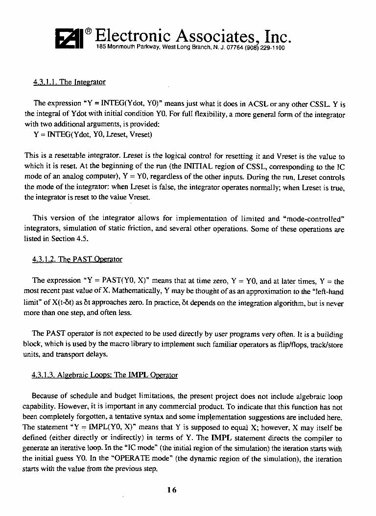
4.3.1.1. The Integrator
The expression "Y = INTEG(Ydot, YO)" means just what it does in ACSL or any other CSSL. Y isthe integral of Ydot with initial condition YO. For full flexibility, a more general form of the integratorwith two additional arguments, is provided:
Y = INTEG(Ydot, YO, Lreset, Vreset)
This is a resettable integrator. Lreset is the logical control for resetting it and Vreset is the value towhich it is reset. At the beginning of the run (the INITIAL region of CSSL, corresponding to the 1Cmode of an analog computer), Y = YO, regardless of the other inputs. During the run, Lreset controlsthe mode of the integrator: when Lreset is false, the integrator operates normally; when Lreset is true,the integrator is reset to the value Vreset.
This version of the integrator allows for implementation of limited and "mode-controlled"integrators, simulation of static friction, and several other operations. Some of these operations arelisted in Section 4.5.
4.3.1.2. The PAST Operator
The expression "Y = PAST(YO, X)" means that at time zero, Y = YO, and at later times, Y = themost recent past value of X. Mathematically, Y may be thought of as an approximation to the "left-hand
limit" of X(t-6t) as 6t approaches zero. In practice, 5t depends on the integration algorithm, but is nevermore than one step, and often less.
The PAST operator is not expected to be used directly by user programs very often. It is a buildingblock, which is used by the macro library to implement such familiar operators as flip/flops, track/storeunits, and transport delays.
4.3.1.3. Algebraic Loops: The IMPL Operator
Because of schedule and budget limitations, the present project does not include algebraic loopcapability. However, it is important in any commercial product. To indicate that this function has notbeen completely forgotten, a tentative syntax and some implementation suggestions are included here.The statement "Y = IMPL(YO, X)" means that Y is supposed to equal X; however, X may itself bedefined (either directly or indirectly) in terms of Y. The IMPL statement directs the compiler togenerate an iterative loop. In the "1C mode" (the initial region of the simulation) the iteration starts withthe initial guess YO. In the "OPERATE mode" (the dynamic region of the simulation), the iterationstarts with the value from the previous step.
16

D Electronic Associates. Inc.185 Monmouth Parkway, West Long Branch, N. J. 07764 (908) 229-1100
Iteration proceeds until the difference between Y and X is sufficiently small, or until a predeterminednumber of iterations is performed, whichever happens first. The error tolerance, as well as themaximum number of iterations, should be user-definable. This requires additional syntax, either in theform of additional arguments to the IMPL function, or additional directives. Such specification isoutside the scope of this project.
4.3.2. Multi-input Operators
In simulation applications, sums of more than two terms, and products of more than two factors, arefairly common. Since the hardware adds and/or multiplies only two things at a time, it is necessary tobreak these operations down into two-input hardware operators.
In the interest of execution speed, this operation is performed by the scheduling compiler, not by thepretranslator. For example, the simple three-input expression "W = SUM(X, Y, Z)" could bedecomposed in three different ways:
W = (X+Y)+Z. Combine X and Y, then combine the result with Z.W = X+(Y+Z). Combine Y and Z, then combine the result with X.W = (X+Z)+Y. Combine X and Z, then combine the result with Y.
For a four-input sum, there are 15 different ways of reducing it to two-input sums. The differentmethods do not all take the same amount of execution time, and, in fact, any one of the possibilitiesmight be optimal, depending on the amount of computation needed to generate the various inputs.
For example, suppose X and Z are state variables (whose values are available at the beginning of thestep) and Y is an algebraic variable that results from a long sequence of computations. In this case, thelast decomposition (X+Z)+Y is better than either of the others, since it allows one of the additions to beperformed immediately. With the other two, no part of the computation can be performed until Ybecomes available.
Using either of the alternatives would lengthen the critical path, and increase the likelihood of "datastalling." i.e. having one or more processors idle because the necessary input values are not available.
While the hardware directly supports only two inputs for a summer or multiplier, the compiler allowsup to 120 inputs (more than anyone is likely to want to write in a single input statement). Thebreakdown into two-input operations is performed during the scheduling process.
17

Electronic Associates, Inc.185 Monmouth Parkway, West Long Branch, N. J. 07764 (908) 229-1100
The operators that allow multiple inputs are the following: SUM, ASUM, MUL, ISUM, IMUL,AND, OR, and XOR. These are all commutative and associative operations.
4.3.3 Data Memory Operator (and Directive)
The Data Memory is indexed, and supports indexed fetches and stores. An indexed fetch is simplyan operator, in that it deter-mines a value (on the left-hand side of an equation) which depends on theinput argument on the right. The basic form is
Y = FETCH(I, A, Offset)or simplyY = FETCH(I, A)
where I is an integer variable, A is an array, and Offset is an integer constant. The. value of Y is thevalue of A(Offset+I), i.e. the contents of the data memory at the address (I+Offset+address of A). Whatmakes this different from an ordinary operator is that the second argument is an array. To the scheduler,FETCH looks like a unary operator, since I is the only dynamically changing value. The constant sum(Address of A + Offset) is represented by the address in the Data Memory instruction word, and I is inan index register.
Note that I and Offset are not interchangeable. Of the three arguments, only the first may be variable.If Offset is omitted, it is taken as zero, so that FETCH(I, A) means A(I), i.e. the contents of the datamemory at the address (I + Address of A).
In addition to the FETCH operator, there is the STORE directive. This has the form of a directive,not an operator, because there is no equal sign and no output value (see Section 4.5). The form is
$STORE, X, I, A, Offsetwhich means that the value of X is to be stored at the location A(I+Offset), i.e. the location whoseaddress is I + (address of A) + Offset.
It is not expected that the user will use FETCH or STORE directly in source code very often.However, they are used by system macros to support function generation, transport delay, and datalogging.
18

Electronic Associates. Inc.185 Monmouth Parkway, West Long Branch, N. J. 07764 (908) 229-1100
4.3.4 I/O Operator (and Directive)
I/O, like memory, requires one operator and one directive. The operator is EN:Y =
means that Y is the value that is available on input channel #17. What this means in detail is veryinstallation-dependent. It might be coming from an ADC or from some digital sensor, or from anotherdigital device. (On the prototype, no real-time input is included, so the IN operator is not needed).
The directive is OUT:$OUT, X, 12
directs the compiler to feed the value of X to output channel #12. Again, what is actually connected toeach output is installation-dependent. The NASA project includes four DAC channels for displaypurposes, so that the $OUT directive can have values of 0, 1, 2, or 3 for its second argument.
4.4. MACRO OPERATORS
Macros work like subroutines, except that instead of generating one copy of a program and linking toit, the compiler generates a complete copy of the macro program each time the macro is called. Notonly does this eliminate subroutine linkage overhead, but it also allows for overlapped execution, sincethe macro expansion is just a collection of hardware operations which can be run in parallel with otheroperations in the simulation model.
The original plan for the prototype was for macro expansion to be done manually, to avoid the effortof developing a macro expander on this project. The macro library is in text form, and the programmerwanting to use a macro would copy its entire expansion into the source file and use a text editor tosubstitute names to prevent clashes and connect the expanded macro with the rest of the simulationmodel. This is tedious, but adequate for demonstrating the hardware feasibility.
However, during the project, a macro expander became available, which had been developed onanother project. This was incorporated into the prototype software, which both saved developmenteffort and allowed a much larger range of benchmark applications to be programmed.
The following list of macro operators includes all that are needed for running the benchmarks on thisproject, and several that are not All the macros originally planned have been implemented, as well as afew others (notably the function of two variables and the unequally-spaced breakpoint search).
19

Electronic Associates, Inc.185 Monmouth Parkway, West Long Branch, N. J. 07764 (908) 229-1100
4.4.1 Flip/Flops
A flip/flop has two logical inputs S and R, and one logical output Y. There are three forms offlip/flop:
Y = SFLOP(YO, S, R)Y = RFLOP(YO, S, R)Y = TFLOP(YO, S, R)
In the INITIAL region, Y = YO. In the DYNAMIC region, S and R may be thought of as"command" inputs which tell the flip/flop what to do next. If S and R are both FALSE, then Y keeps itsold value. If S is true and R is false, then Y is SET, i.e. its new value is TRUE. If S is false and R isTRUE, then Y is RESET (its new value is FALSE).
The three types of flip/flop are distinguished by what they do in the fourth case (S and R both true).In this case, the SFLOP Sets, the RFLOP Resets, and the JFLOP Triggers or Joggles (its outputchanges). All three types of flip/flop are implemented with the PAST operator. Section 4.6 shows theimplementation in more detail.
4.4.2. Switches
The basic switch operator has three arguments:W = SWITCH(L, X, Y)
In this statement, L must be a logical variable, and X and Y can be of any type, but they must be thesame type. If L is true, then W is X; otherwise, it is Y. To remember the order of the arguments, thinkof this equation as "If L, then X, else Y."
In the special case where the third argument is zero, the SWITCH operator may be replaced by thehardware AND operator. This is why the values "all O's" and "all 1's" were chosen for defining logicalvalues. The SWITCH operator is implemented in the macro library as
SWITCH(L, X, Y) = OR( AND(L, X), AND(-L, Y)).Remember that the AND operator accepts signed inputs, and -L means NOT L. The calculation of
AND(-L, Y) is a single hardware operation.
4.4.3. Mathematical Functions
The usual math functions available in most programming languages are supported. A slight change isthe fact that individual SIN and COS functions are replaced by the SCOS macro that delivers both
20
Electronic Associates, Inc.185 Monmouth Parkway, West Long Branch, N. J. 07764 (908) 229-1100
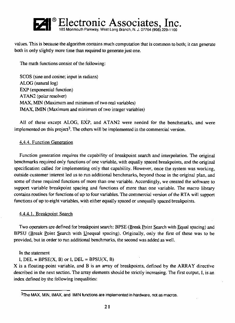
values. This is because the algorithm contains much computation that is common to both; it can generateboth in only slightly more time than required to generate just one.
The math functions consist of the following:
SCOS (sine and cosine; input in radians)ALOG (natural log)EXP (exponential function)ATAN2 (polar resolver)MAX, NUN (Maximum and minimum of two real variables)IMAX, IMIN (Maximum and minimum of two integer variables)
All of these except ALOG, EXP, and ATAN2 were needed for the benchmarks, and wereimplemented on this project3. The others will be implemented in the commercial version.
4.4.4. Function Generation
Function generation requires the capability of breakpoint search and interpolation. The originalbenchmarks required only functions of one variable, with equally spaced breakpoints, and the originalspecification called for implementing only that capability. However, once the system was working,outside customer interest led us to run additional benchmarks, beyond those in the original plan, andsome of these required functions of more than one variable. Accordingly, we created the software tosupport variable breakpoint spacing and functions of more than one variable. The macro librarycontains routines for functions of up to four variables. The commercial version of the RTA will supportfunctions of up to eight variables, with either equally spaced or unequally spaced breakpoints.
4.4.4.1. Breakpoint Search
Two operators are defined for breakpoint search: BPSE (Break Point Search with Equal spacing) andBPSU (Break Point Search with Unequal spacing). Originally, only the first of these was to beprovided, but in order to run additional benchmarks, the second was added as well.
In the statementI, DEL = BPSE(X, B) or I, DEL = BPSU(X, B)
X is a floating-point variable, and B is an array of breakpoints, defined by the ARRAY directivedescribed in the next section. The array elements should be strictly increasing. The first output, I, is anindex defined by the following inequalities:
3The MAX, M1N, IMAX, and IMIN functions are implemented in hardware, not as macros.
21

D Electronic Associates. Inc.185 Monmouth Parkway, West Long Branch, N. J. 07764 (908) 229-1100
If X< B(l), then 1 = 0If B ( 1 ) < X < B(2), then 1=1If B ( 2 ) < X < B(3), then 1 = 2
If B(N-2) < X < B(N-l), then I = N-2If X> B(N-l), thenI = N-l
Note that in general, we have B(I) < X < B(I+1), except that if X is out of range, i.e. X < B(0) or X> B(N), the value of I is limited to the range [0, N-l], since we don't want to address an array outsideits defined boundaries.
For BPSE (equal spacing), the value of I is calculated by subtraction, multiplication, and float-to-fixconversion. The IMAX and IMIN operators are used to assure that I remains always in the desiredrange [0, N-l], even if X gets out of range.
For BPSU, a binary search is used, to minimize the number of comparisons required. In this case,no MAX and/or MIN operators are needed to keep the value of I within range4.
The second argument, DEL, is defined as [X-B(I)]/[B(I+1)-B(I)]. As X varies between B(I) andB(I+1), DEL varies from 0 to 1. For equally-spaced breakpoints, the calculation requires amultiplication and an integer-to-floating-point conversion. For unequally-spaced breakpoints, it alsorequires two fetches from an indexed array, in which the previously-calculated reciprocals of theinterval lengths—values of 1/[B(I+1)-B(I)]—are stored.
4.4.4.2. Interpolation
The INTERP operator, defined asINTERP(DEL, A, B) = A + DEL*(B-A)
can be used for the actual function generation. Note that INTERP has the value A if DEL = 0, and B ifDEL = 1. This operator applies to for both single-variable and multi-variable functions. For functionsof one variable, the function value is given by
FUN1V(I, DEL, FV) = INTERP(DEL, FETCH(I, FV), FETCH(I, FV, 1))where I and DEL are obtained from the input X using the BPSE or BPSU operators defined in theprevious section, and FV is the array of function values. Note that the two fetches are from adjacentlocations in memory.
4lnstead of a single BPSU macro, the actual implementation uses several macros: BPS3, BPS5, BPS9,
BPS17, and BPS33. In any given application, use BPSn, where n is the smallest number > the number ofbreakpoints in the array.
22

Electronic Associates, Inc.185 Monmouth Parkway, West Long Branch, N. J. 07764 (908) 229-1100
Original plans called for the FUN IV macro to be expressed in terms of the INTERP macro, but thecurrent version of the macro expander does not support nested macros, so FUN IV is expressed interms of basic operators. Analogous macros FUN2V, FUN3V, and FUN4V are also provided in themacro library.
4.4.5 Other Operators
The other operators in the original specification are DIFF, FDIFF, BIDIFF, BCKLSH, DBLINT,LIMIT, LIMPOS, LIMNEG, LIMDSfT, DELAY, and ZHOLD. All these operators are described in theSIMSTAR manual, except for FDIFF (falling-edge differentiator) and LIMPOS and LIMNEG (positiveand negative limits). All these have been implemented, and are included in the macro library.
FDIFF(X) is equivalent to DIFF(-X), i.e. it produces a pulse when X becomes FALSE.LIMPOS (X) is equal to X when X is positive, and zero otherwise. LIMNEG(X) is equal to X when Xis negative and zero otherwise.
4.4.6 New Operators
Several other operators, which were not included in the original specification, turned out to beuseful, and were implemented. They are included in the macro library. These include INCMOD,PEAK, VALLEY, MAT4, SOLVE4, and ROTATE.
The INCMOD macro increments an integer modulo another integer. In the macro callI = INCMOD(IO, N)
I is incremented modulo N. Initially, I = 10. On every frame, I is incremented by 1 until it reaches N-l.When I = N-l, the next increment "wraps around" to zero. This macro is useful in in maintaining apointer to a circular buffer for transport delay and data logging.
The PEAK macro picks the maximum of its input over all time. Y = PEAK(YO, X) means thatinitially, Y = YO, and on each succeeding step, Y is replaced by MAX(Y, X). If YO is chosen to equalXO, as is usually the case, then Y = MAX[X(t)], the maximum being over all previous time. Y is thepeak value of X. Similarly, VALLEY(YO, X) tracks the minimum value of X.
MAT4 applies a 4-by-4 "matrix" to a 4-dimensional "vector." The result is a four-dimensional"vector." The arguments are actually scalars; each "vector" consists of four explicitly-named scalars,and the "matrix"consists of sixteen scalars. The format is
Yl, Y2, Y3, Y4 = MAT4(M11, M12, M13, M14, M21, ...M44, XI, X2, X3, X4.
23
® Electronic Associates. Inc.185 Monmouth Parkway, West Long Branch, N. J. 07764 (908) 229-1100
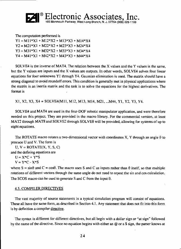
The computation performed isYl = Ml 1*X1 + M12*X2 + M13*X3 + M14*X4Y2 = M21*X1 + M22*X2 + M23*X3 + M24*X4Y3 = M31*X1 + M32*X2 + M33*X3 + M34*X4Y4 = M41*X1 + M42*X2 + M43*X3 + M44*X4
SOLVE4 is the inverse of MAT4. The relation between the X values and the Y values is the same,but the Y values are inputs and the X values are outputs. In other words, SOLVE4 solves four linearequations for four unknowns Yl through Y4. Gaussian elimination is used. The matrix should have astrong diagonal to avoid roundoff errors. This condition is generally met in physical applications wherethe matrix is an inertia matrix and the task is to solve the equations for the highest derivatives. Theformat is
XI, X2, X3, X4 = SOLVE4(M11, M12, M13, M14, M21, ...M44, Yl, Y2, Y3, Y4.
SOLVE4 and MAT4 are used in the four-DOF robotic manipulator application, and were thereforeneeded on this project. They are provided in the macro library. For the commercial version, at leastMAT2 through MATS and SOLVE2 through SOLVES will be provided, allowing for systems of up toeight equations.
The ROTATE macro rotates a two-dimensional vector with coordinates X, Y through an angle 0 toprocuce U and V. The form is
U, V = ROTATE(X, Y, S, C)and the defining equations are
U = X*C + Y*SV = Y*C - X*S
where S = sin0 and C = cos6. The macro uses S and C as inputs rather than 6 itself, so that multiplerotations of different vectors through the same angle do not need to repeat the sin and cos calculation.
The SCOS macro can be used to generate S and C from the input 0.
4.5. COMPILER DIRECTIVES
The vast majority of source statements in a typical simulation program will consist of equations.These all have the same form, as described in Section 4.1. Any statement that does not fit into this formis by definition a compiler directive.
The syntax is different for different directives, but all begin with a dollar sign or "at sign" followedby the name of the directive. Since no equation begins with either an @ or a $ sign, the parser knows at
24

D Electronic Associates, Inc.185 Monmouth Parkway, West Long Branch, N. J. 07764 (908) 229-1100
once if a particular statement is a directive, and the next word tells it which directive. This eliminates theneed for backtracking in the parser, since there is never any ambiguity as to whether a source statementis a directive or an equation.
4.5.1 Type Directives
There are three data types: Integer, Floating Point, and Logical. In typical applications, the vastmajority of variables and constants are floating point. Therefore, this is the default (unlike the defaultassumption of "integer" for C functions or the FORTRAN initial-letter default). Hence the only typedeclarations necessary are INTEGER and LOGICAL. They are abbreviated by their first three letters.
For example, the declarations$INT, X, Y, Z$LOG, A, B, C
declare X, Y, and Z to be integers and A, B, and C to be logical. Every variable or constant that iseither integer or logical should be declared before its first use; otherwise, it will be assumed real(floating-point).
4.5.2. Defining Constants: The CON Directive
The CON directive is used to tell the compiler that a certain name refers to a constant, and to give theconstant a value. Constants of any data type are allowed, but if they are not real, they must be specifiedbefore the $CON directive. For example, the declaration
$CON, A = 5.0, B = 2.34, C = .FALSE., I = 5declares values for four constants. A and B are automatically REAL, but I and C must be declared INTand LOG respectively.
4.5.3. Structure Directives
Structure declarations declare the beginning and end of structural blocks, such as the INITIAL,DYNAMIC, and TERMINAL blocks. The directives
$INITstatements in initial region$ENDINIT
delineate the beginning and end of the INITIAL region. This is a block of code that is simply copied toa file (the .INI file), and later compiled and linked with the rest of the setup and runtime program thatruns on the host. It is executed at the beginning of each new run. On the prototype system, the INI fileis generated, but not compiled and linked. The user must perform this task manually. The commercialsystem will provide for the automatic compiling and linking of this file.
25

® Electronic Associates. Inc.185 Monmouth Parkway, West Long Branch, N. J. 07764 (908) 229-1100
Similarly, the directivesDERIVstatements in derivative region$ENDDERTV
delineate the beginning and end of the derivative section, which contains the user's model. Only onederivative section is allowed for the prototype system, so these directives are not necessary.
Within the derivative section, there should be a either a $DONE directive or a SRUNTTME directive,to terminate the run. The $DONE directive has the form
$DONE, name of logical variable.The logical variable must be defined by an equation in the derivative section, and represents a conditionfor terminating the run.
The SRUNTIME directive has the form $RUNTIME, real constant. For example, the directive$RUNTIME, 10
means "run the simulation until TIME > 10 seconds".
Both RUNTIME and DONE directives may be used in the same program; the run will then terminatewhen the DONE signal becomes true or after ten seconds, whichever happens first.
The directives$TERMstatements in terminal region$ENDTERM
delineate the beginning and end of the terminal section, which, like the initial section, consists of codethat is simply copied to a file and later linked with the rest of the host program.
The directive$END
(note nothing written after the "END") signifies the end of the source file. It is not really necessary,since the compiler will interpret end-of-file as meaning the end of the source program, but it serves toreassure a human reader that the "tail end" of the source file has not been inadvertently deleted.
4.5.4. I/O and Data Memory Directives
These are the STORE and OUT directives. They have already been described in Sections 4.3.3 and4.3.4. They are directives, rather than equations, since they do not conform to the equation syntax: theyhave no equal sign and generate no output values.
26

® Electronic Associates. Inc.185 Monmouth Parkway, West Long Branch, N. J. 07764 (908) 229-1100
4.5.5. The ARRAY Directive
This directive is used to tell the compiler that a specific name refers to an array, to dimension thearray, and (optionally) to fill it with initial values. In simulation, arrays are used mostly for functiongeneration, and can be either breakpoint arrays or function value arrays. Such arrays are normally"read-only," that is, they are not changed by the running program.
Applications like transport delay and function storage and playback require that arrays be updateddynamically. The FETCH operator and the STORE directive allow for both reading and writing arraysat run time.
The ARRAY directive has three forms, depending on the type of array.
4.5.5.1 Filled Arrays.
Filled arrays, used for function generation, are filled at load time with data from a file. The format is$ARRAY, F, name, size
where the "F" means that this is a filled array, "name" is the name of the array, and "size" is a literalinteger constant.
The compiler uses the name internally to identify functions which use it in the source program. Italso passes the name along to the linker, which looks for a file in the current directory with the samename, and the extension .TXT. This is the data file used to fill the array at load time.
The size of the array is the number of values it contains. The corresponding data file must containthis many values, in text form, separated by spaces.
4.5.5.2. Blank Arrays.
Blank arrays are not filled from a file at load time, but may be (optionally) initialized with a valuebefore each run. They are used for transport delay and data logging. The general form is
$ARRAY, B, name, size [.initial value]The "B" tells the compiler that this is a blank array. The name and size have the same meaning asbefore, but no file of data values is needed. If the initial value is included, then the array will be filledwith that value before each run. This is the case for arrays used in transport delay. If no initial value isprovided, the array is not initialized before each run; this is the case for arrays used for data logging.
The initial value, if provided, must be a parameter name, not a literal constant.5
5This restriction will be removed in the commercial version, which will allow either a named parameter or a
literal constant.
27

® Electronic Associates, Inc.185 Monmouth Parkway, West Long Branch, N. J. 07764 (908) 229-1100
4.5.5.3. Equally-spaced Arrays.
The directive$ARRAY, =, name, size, min, max
declares an array of equally-spaced values, generally used as a breakpoint array for function generation.This array does not actually exist as a set of equally-spaced values in the data memory. Instead, themin, max, and size arguments are used to perform a breakpoint "search" by arithmetic calculations andfloat-to-flxed conversion. The min, max, and size arguments must be literal integer constants.
Examples:$ARRAY, =, ALPHA, 11, 0, 20
This example was given in Section 4.1.2. It defines the array ALPHA to have 11 values 0, 2, 4, 6, 8,10, 12, 14, 16, 18,and 20. Note that the number of values in the array is one more than the number ofintervals. For ten intervals, each of length 2.0, we need eleven data points.
$ARRAY, F, BETA, 5defines BETA as an array of five values (four intervals), unequally spaced. The breakpoint values willbe found in a disk file named "BETA.TXT."
$ARRAY, B, GAMMA, 100, Adefines GAMMA as an array of 100 values, and generates code that copies the constant A into everyarray location before each run. If the last argument were omitted, the array would not be initialized.
4.5.6. The ALARM and VAR Directives
The original software plan included an ALARM directive, to allow for program-generated detectionof exceptional conditions, and a VAR directive, to allow the user to rename the independent variable(the default name is "TIME"). These were not implemented on this project due to lack of time, but theywill be included in the commercial version.
4.6 OVER AT T. SOFTWARE DATAFLOW
Figure 4.1 is an overall software block diagram, showing data flow for the entire prototype RTAprogramming system. This diagram shows five executable host programs: MACRO, PHASE1,PHASE2, SLINK, and CMD.
Each program reads one or more files and each program (except for CMD) writes one or more files.In normal use, the programs are executed in succession, under the control of a batch file.
The compilation and linking process creates a large number of intermediate files on the disk, as
28

D Electronic Associates, Inc.185 Monmouth Parkway, West Long Branch, N. J. 07764 (908) 229-1100
described below. To avoid confusion, it is strongly recommended that all files related to a particularsimulation model (i.e.the source file and all necessary function generator data files) be placed in asingle directory devoted to that particular simulation model. All intermediate files generated by theprocess will be placed in that directory. This practice prevents any directory from getting cluttered upwith many files relating to different simulations. The benchmark applications provided on the prototypedisk are structured in this manner.
The executable files (the compiler, linker, etc. as described below) are system files that are placed onthe disk in the directory \RTA\SYSTEM. They are not associated with any particular simulation, so allsimulations need to access them. This may be done very simply by putting the \RTA\SYSTEMdirectory in the PATH variable, so that DOS can fine the executable files.
The starting point is a source file containing the equations and directives describing the model. Thissource file should have a name without a DOS extension (referred to simply as "name" in the figure).All files created during compilation, linking, and execution will have this same name with differentextensions, (e.g. NAME.MAC, NAME.EXP etc.) .The macro expander reads the equations and looksup the operator name for each equation in a table of "built-in" RTA operators (see Sections 4.2 and4.3). If an operator is not in that list, the macro expander scans the list of macro operators in the macrofile(s). If the operator is found in one of the macro files, the macro expander copies the entire body ofthe macro into the source file, with appropriate name substitutions.
29

Electronic Associates. Inc.185 Monmouth Parkway, West Long Branch, N. J. 07764 (908) 229-1100
EXPAND MACROS
name »i MALrnUj * name.iviAL; — (Rename) — > name.EXP
Source File MACRO Expanded File Expanded File
EXPANDER
COMPILE ^^
name.EXP {p HAS El) — > name.PAR -
Expanded PARSERX^Hle \ name.INI
\name.TRI
LINK /-* name.lM
/name.ouii *i SLINK r * namo.Aivi
LINKER \ :^-» name.DM
name.lM — \ COMMAND
X f£Hnnmn YM \\ P IUI n 1 ' '
= / T
name.DM — ^msm^
D 1 1 Kln LI Iv j . -. n«JFRie;{- (V""TERMINAL
-**^ | name.LIS
Listing File
-^(PHASE2)— » name.SCH
SCHED- \ ScheduledULER \ Program
name.TR2
>^
RTAy Image
Files
/
^ t^TA ==JDISPLAYDWARE ^ — >
Figure 4.1 Dataflow in a Typical RTA Compilation.
30

Electronic Associates, Inc.185 Monmouth Parkway, West Long Branch, N. J. 07764 (908) 229-1100
To illustrate the macro expansion function, suppose the following line occurs in the source file:TFLOP(P, PO, XPOS, XNEG)6
The operator TFLOP (Trigger flop or Toggle flop) is not built into the hardware or the compiler, but itis found in the macro library. The macro library contains the following definition:
MACRO TFLOP(Y, YO, S, R)MACRO RENAME TEMPI, TEMP2, YNEXTTEMPI = AND(S, -Y)TEMP2 = AND(-R, Y)YNEXT = OR(TEMP1, TEMP2)Y = PAST(YO, YNEXT)
MACRO END
This definition corresponds to the following truth table:
S R TEMPI TEMP2 Ynext0 0 0 Y Y0 1 0 0 01 0 -Y Y 11 1 -Y 0 -Y
which shows that the operator responds correctly to all possible combinations of inputs. (Rememberthat "-Y" means NOT Y.)
The macro expander replaces the original source line with a complete copy of the macro definition(minus the header and terminator lines). In the copying process, Y is replaced by P, YO by PO, S byXPOS, and R by XNEG. The dummy names TEMPI, TEMP2, and YNEXT are replaced with namesgenerated by the macro expander. Different names are generated for each use of the TFLOP macro. Asa result, the original use of TFLOP is replaced by
ZZ34 = AND(XPOS, -P)ZZ35 = AND(-XNEG, P)ZZ36 = OR(ZZ34, ZZ35)P = PAST(PO? ZZ36)
Names beginning with ZZ are reserved for system use, and should not be used in the sourceprogram. In this example, the macro expander substitutes the names ZZ34, ZZ35, and ZZ36 for the
6The prototype software insists on this form, with the macro name first. The commercial version will also
allow the more natural form, with the output first: P = TFLOP(PO, XPOS, XNEG).
31

Electronic Associates, Inc.185 Monmouth Parkway, West Long Branch, N. J. 07764 (908) 229-1100
dummy names TEMPI, TEMP2, and YNEXT in the macro definition. This example assumes, ofcourse, that the last macro-assigned name was ZZ33. If the next macro encountered after this one isanother use of TFLOP, this new use of the TFLOP macro will have the names ZZ37, ZZ38, and ZZ39for its internal variables.
Thus, each equation in the file produced by the macro expander has a single operator which isdirectly supported either by the hardware or by the compiler. The macro expander output has the samename as the input file, but with the extension .MAC. The compiler expects an input file with theextension .EXP (EXPanded file). This file may be created by renaming the .MAC file. For programsthat don't use the macro library, the user can save a step by starting with the name.EXP file andbypassing the macro expander entirely.
The scheduling compiler consists of two phases: PHASE1 is the parser, which simply reads thesource file and applies a lexical analysis and some bookkeeping chores to turn the source representationinto an internal set of tables defining, for each variable, what its generating equation is (i.e., what theoperands and the operator are).
The output of the parser is the file name.PAR, which is fed into PHASE2: the scheduler. Thisprogram contains the heuristic scheduling algorithm which decides, for each variable, when (on whichclock cycle) and where (on which processor) it is to be generated. The resulting schedule is written intothe name.SCH file. The compiler also generates the name.INI file, which contains the initial region (thecode to be executed at the bebinning of each run). In the commercial version, this file will be compiledand linked with the rest of the program to set automatically all parameters that depend on otherparameters. At present, the user must print out this file and perform the computations manually.
The other files created by the compiler are the listing file, name.LIS, and the trace files, name.TRland name.TR2. The listing file contains a copy of all source statements, except that blanks andcomments are removed, and statement numbers added to facilitate error tracing. It also contains errormessages, a brief summary of the utilization of the various operators, and the frame time. Any errormessages detected in the input source file are immediately flagged, with indicators pointing directly tothe offending text.
The trace files are of interest only to those who know the internal structure of the compiler (i.e. theywere used for debugging the compiler itself, rather than the user's source program). Since thegeneration of these files takes considerable time (in many cases, more time than the actual compilation),they are made optional. By default, no trace files are generated. If a "T" flag is used on the commandline invoking the PHASE1 or PHASE2 part of the compiler, the trace file will be generated. Without theflag, no trace file will be generated, and the compilation will be faster.
32

Electronic Associates, Inc.185 Monmouth Parkway, West Long Branch, N. J. 07764 (908) 229-1100
The linker, SLINK, reads the scheduler output file name.SCH, resolves memory references, andgenerates the executable RTA program. This program consists of several files called "image" files,since each is an image of one of the RTA memories. For each RTA memory (either program memory ordata memory), there is a file specifying which locations need to be loaded, and with which values. Foreach module in the system, the following files are generated:
name.IM: the Instruction Memory image.name.DM: the Data Memory image.name.CM: the Control Memory image.name.XM: the Index Memory image.name.AOM, name.BOM, name.AlM., and name.BIM: the images of the four operand memories.
In a conventional computer, a variable is identified with a particular memory location, but in theRTA, the same value can reside in several locations. For example, a variable that is used as input toseveral computations on different modules may have its value stored in several input memories. And, ofcourse, a constant is assumed available anywhere it is needed. To avoid the need to move constantvalues over the data busses at run time, duplicate copies are stored in whichever memories need thevalue.
Most of the program and/or data memory locations are in blocks with contiguous addressesbeginning at zero, so that the information will be in the form of memory blocks consisting of sequencesof data or program words. These files are used by the command interpreter CMD, which loads thesewords into the appropriate RTA memories.
CMD also interprets and executes commands to set and read various variables or constants inresponse to user commands typed in at the terminal. It responds to the following commands (thecommand name and arguments, if any, are separated by one or more spaces):
SET name F valuesets the parameter "name" to the floating-point value "value." If the parameter is integer instead offloating point, the "F" should be replaced by "I."
SHOW name Fshows the value of the variable or parameter "name" in floating-point form. Using "Finstead of "F"results in display in integer form. In the commercial version of the command interpreter, the "F" or "I"will be optional, since the type of a variable or parameter is available from the compiler and linker.
METHODfollowed by "A" or "E," sets the integration method to Adams/Bashforth (second order) or Euler
33

D Electronic Associates, Inc.185 Monmouth Parkway, West Long Branch, N. J. 07764 (908) 229-1100
(rectangular) integration. If no letter follows "METHOD," the current method is displayed.
OPMODE RorOPMODE S
sets the operating mode to Repetitive or Single. The former cycles the RTA between INITIALCONDITION and OPERATE modes until interrupted from the console: the latter makes one run andstops. Typing OPMODE without a letter simply displays the current opmode.
RUNstarts the RTA running. Depending on the current opmode (see above) the system will either make onecomplete run or cycle repetitively.
TfrKEfilenametells the command processor to take its next commands from a textfile. This allows for prepared scriptsof operating sequences.
WHAT nameaccesses the .EXP file and types out all lines containing the name. During debugging, if a particularvariable, say BETA, isn't behaving as expected, you can find out instantly where the variable isgenerated, and how it is used, by typing WHAT BETA. The response will be a listing of all sourcelines containing the name BETA, including the statement that generates it, and all statements that use it,but not including other lines containing the string BETA, such as lines containing BETAO, BETA1, orBETADOT.
HELPprovides online help.
EXITexits the command processor and returns to DOS.
34

Electronic Associates, Inc.185 Monmouth Parkway, West Long Branch, N. J. 07764 (908) 229-1100
5. ANALYSIS OF AN RTA BENCHMARK
This section illustrates the details of how an RTA program is converted step-by-step from aset of input source equations into an internal dataflow graph, or "patching diagram" and then into afinal, fully scheduled executable program. The problem statement, the dataflow graphs, and themanually-generated schedule in Table 2 are adapted from the Phase 1 Final Report.
One of the key goals of this project was to verify the RTA's programmability. i.e. to showthat a user could write a program without detailed knowledge of the hardware architecture, andhave it compile, run, and generate correct results. Can a compiler create a schedule for amultiprocessor system from a high-level source program without need for detailed knowledge ofthe computer on the part of the user? .We now know that the answer is "Yes."
The schedule in Table 2 was generated manually, before the scheduling compiler had beenwritten. Seventeen months later, when the compiler was available, the compiler-generated scheduleproved to be within two cycles of the manually-generated one (128 cycles versus 126). Thecompiler-generated schedule runs on the RTA hardware, and produces the same result as theoriginal CSSL program run on EAI's in-house Encore 32/87.
The example shown here is the Double Pendulum (Fig. 1). This example was chosenbecause it is simple enough to analyze fully, and at the same time complex enough to illustrate all
the important concepts. As Murray7 says, it "exemplifies all of the inherent coupling andnonlinear characteristics of manipulator dynamics."
Figure 1. The Double Pendulum
The equations, taken from Murray, are as follows:
7Murray, J J. "Computational Robot Dynamics" Ph.D Dissertation, Department of Electrical and
Computer Engineering, Carnegie Mellon University, Pittsburgh, PA 15213, Sept. 10, 1986.
35

Electronic Associates, Inc.185 Monmouth Parkway, West Long Branch, N. J. 07764 (908) 229-1100
Inertial Coefficients
dn = a12m2 + 2a1a2m2cos(e2) + a2
2m2 +
d12 = a22m2 + a1a2m2cos(92)
d22 = a22m2
Centrifugal and Coriolis Coefficients
c12 = -a1a2m2sin(02)c22 = -a1a2m2sin(e2)
Gravitational Coefficients
g, = a1gm2sin(91) + a2gm2sin(0, + 02) + ag2 = a2gm2sin(e1 + 02)
Torque Equations
h, = C22022 + 20,20,02 + g,
h2 = -c^e,2 + g2
Highest Derivatives (implicitly defined)
d,,0, + d,202 = r,-h,, where r, = K,*0, to include dampingd,20, + d2202 = Tr2-h2, where r2 = K2**02 to include damping
Explicit Solution for Highest Derivatives
A = dnd22 - d,22 (The determinant of the system)
0, = (1/A)[d22(r,-h,) - d,2(r2-h2)]02 - (1/A)[dn(r2-h2) - d12(r,-h,)]
A CSSL program for these equations is given in Figure 2.
36

Electronic Associates. Inc.185 Monmouth Parkway, West Long Branch, N. J. 07764 (908) 229-1100
PROGRAM
"Double Pendulum Model. File name S.DPEND""George Hannauer, July 12, 1989""This two-DOF model is taken from""COMPUTATIONAL ROBOT DYNAMICS, by John J. Murray.""PhD Dissertation, Carnegie-Mellon University.""Sept. 10, 1986."
INITIAL
CONSTANT TEND = 10, XLO = 0, XHI = 10 $ "for plotting."CONSTANT G = 0.980
"Acceleration of gravity in MKS units"CONSTANT Al=2, A2=l, Ml =5, M 2 = lCONSTANT THE10 =.0, THE1DO = 0CONSTANT THE20 = 0, THE2DO = 1
PI = A1*A1*M2P2 = A1*A2*M2P3 = 2*P2P4 = A2*A2*M2P5 = A1*A1*M1P6 = A1*G*M2P7 = A2*G*M2P8 = A1*G*M1P9 = PI + P4 + P5P10 = P6 + P8
END
DYNAMICDERIVATIVE
"State variables"THE1D = INTEG(THE1DD, THE1DO)THE1 = INTEG(THE1D, THE10)THE2D = INTEG(THE2DD, THE2DO)THE2 = INTEG(THE2D, THE20)
"Trigonometric Functions"51 = SIN(THEl)Cl = COS(THEl)52 = SIN(THE2)C2 = COS(THE2)
S12 = S1*C2 + S2*C1 $ "SIN(THE1+THE2)"
Figure 2. CSSL Source Listing for the Double Pendulum (Sheet 1 of 2)
37

Electronic Associates, Inc.185 Monmouth Parkway, West Long Branch, N. J. 07764 (908) 229-1100
"Inertial Coefficients"Dll = P9 + P3*C2D12 = P4 + P2*C2 x
D22 = P4
"Centrifugal and Coriolis Coefficients"C12 = -P2*S2C22 = C12
"Gravitational Coefficients"Gl = P10*S1 + P7*S12G2 = P7*S12
"Torque Computation"HI = 2*C12*THE1D*THE2D + C22*THE2D*THE2D + GlH2 = -C12*THE1D*THE1D + G2
TAU1 = -K1*THE1DTAU2 = -K2*THE2D
CONSTANT Kl = 0.1, K2 = 0.1
"Solve for highest derivatives(angular accelerations)"
"Reciprocal of determinant"RDET = 1.0/(D11*D22 - D12*D12)
THE1DD = RDET*(D22*(TAU1-H1) - D12*(TAU2-H2))THE2DD = RDET*(Dll*(TAU2-H2) - D12*(TAU1-H1))
TERMT(T.GE.TEND)END
END
TERMINALEND
END
Figure 2. CSSL Source Listing for the Double Pendulum (Sheet 2 of 2)
A few observations are worth making about this program:
• Calculations involving only constants have been moved from the DYNAMIC region to theINITIAL region, since they need to be performed only once per run. These calculations areperformed on the host computer before each run and the values transferred to the RTA at the
beginning of the run. Thus coefficients like a 12m2 (A1*A1*M2 in CSSL) are given names and
38

D Electronic Associates. Inc.185 Monmouth Parkway, West Long Branch, N. J. 07764 (908) 229-1100
defined by equations written explicitly in the INITIAL region. On the commercial RTA system,this process will be completely transparent to the user, who can write, if preferred,
D12 = A2**2*M2 + A1*A2*M2*COS(THE1)and the software will automatically generate the equivalent of
P2 = A1*A2*M2P4 = A2**2*M2
in the INITIAL region, andD12 = P4 + P2*C1
in the DYNAMIC region.
This task is already being performed automatically in the SIMSTAR® programming system.Machine coefficients ("pot-settings") are calculated and transmitted to the analog componentsbefore every run. There is no need for the user to break out these computations into the INITIALregion manually.
• In order to reduce the number of computations, a general decision was made to generate alltrigonometric functions of sums and differences of state variables by using trigonometricidentities, rather than additional uses the SIN/COS macro. Thus SI, S2, Cl, and C2 are the sinesand cosines of the state variables THE1 and THE2, and are calculated directly from the statevariables, while he value of SIN(THE1+THE2) is calculated as S1*C2 + S2*C1, replacing a callto the SIN/COS macro by two multiplications.
This is probably a good idea in general, since a SIN/COS macro uses 20 arithmeticoperations. But in this particular case, it had a peculiar consequence—it actually lengthened therunning time slightly. This is typical of the "anomalies" that arise in multiprocessor scheduling
applications. Since the general problem is NP-complete8, it is unlikely that any efficient programwill always produce optimal results. As long as the discrepancy is small (in this case, fewer than 5cycles out of 125), the result is a program that is close enough to optimal for practical purposes.
• Since the system has only two degrees of freedom, the inertia matrix is 2 by 2, and thealgebraic system is easy to solve by determinants. This is not typical of real applications: inpractice, for systems larger than about 3 by 3, Gaussian elimination or some form of matrixfactoring is preferred; the RTA macro library contains a macro for performing this operation.
The CSSL source equations are transformed by the compiler into a set of machine operations,which may be thought of as connections between virtual "components," as shown in Fig. 3.
8Garey, M.R. and Johnson, D.S. Computers and Intractability. A Guide to the Theory of NP-
Completeness, W. H.Freeman and Company, San Francisco, 1979.
39

Electronic Associates, Inc.185 Monmouth Parkway, West Long Branch, N. J. 07764 (908) 229-1100
THE1DD THE1D THE1
THE2DD0Kl — TAU1
TH
scos
:E2
K2 — TAU2
scos
SI1
ci
S2I
C2
S12 = SIN(THE1+THE2)
Figure 3a State Variables and Trigonometric Functions
40

Electronic Associates. Inc.185 Monmouth Parkway, West Long Branch, N. J. 07764 (908) 229-1100
P9>
C 2 >P3
P2
P 4 >D12
InertialCoefficients
S2 >
- P 2
Centrifugal& Coriolis
Coefficients
P10 (=P6+P8)si > O——
S12 > OG1 Gravitational
* G2 Coefficients
P7
Figure 3b. Calculation of Coefficients
C 1 2
T H E 1 D >
C1 2
T2 >
THE2D
C22 >
G2
G } >-*
Figure 3c. Torque equations.
41

Electronic Associates, Inc.185 Monmouth Parkway, West Long Branch, N. J. 07764 (908) 229-1100
Dll
I /A
TAU1H I
TAU2H2
T H E 1 D D
THE2DD
Dll
Figure 3d. Solving for the Highest Derivatives
The similarity of Figure 3 to an analog computer patching diagram is deliberate, since theRTA evolved from the analog computer. There are a few differences:
• There is no need for scaling.• Summers and multipliers may have an unlimited number of inputs. Of course, the software
must reduce these multi-input devices to successive applications of two-input devices: the RTAcontains no multi-input arithmetic hardware. But this reduction is transparent to the user.
In addition to resolving multi-input components into single inputs, it is necessary also toreplace every occurrence of a library macro (such as the sine/cosine macro in the Double Pendulumexample) with a complete copy of its expansion. Every new variable defined in this process isgiven a name to facilitate the discussion—these auxiliary names all begin with "#", which is not alegal character for an input source name; this convention guarantees that there will not be a clash
between the generated names and the user-defined input names9. After these transformations, the
9The original plan called for the use of the #, but on the prototype version, the "# "was changed to "72.'
42

Electronic Associates. Inc.185 Monmouth Parkway, West Long Branch, N. J. 07764 (908) 229-1100
resulting dataflow graph looks like Figure 4.
THE1DD> THE1D n\ THE1—rHP—
K 1 TAU1
scos
K 2
T H E 2 D D \ THE2D
v A\ THE2
]/SCOS
ci
S2 1C2
#41
S12 = SIN(THE1+THE2)
Figure 4a. State Variables and Trigonometric Functions(With Auxiliary Variables Numbered)
Note that the replacement of the two occurrences of the sin/cos macro result in two completecopies of the sin/cos macro body being inserted into the final program—these are shown in Figures4e and 4f. It should be remembered that the normal user will never see this macro expansion—justas the normal user of an ordinary computer doesn't see the internal working of the sine or cosineroutines in the library.
to make it compatible with the pre-existing macro expander. However, the diagrams, taken from the Phase
1 Final Report, still show the "#."
43

Electronic Associates. Inc.185 Monmouth Parkway, West Long Branch, N. J. 07764 (908) 229-1100
P 9 >
C 2 >
Dll
P3
P2.
P4
InertialCoefficients
S2 >
Centrifugal^ C12 (=C22) o r- • ?—O > & Coriohs
_ p 2 Coefficients
P10 (=P6+P8)S1 >
S12 >G1 Gravitational
* G2 Coefficients
Figure 4b. Coefficient Calculation showing Auxiliary Variables
THE1D >
THE2D >
C22 >
C12
\#47G2
#48H2
#50N HI
#51 #52
Figure 4c. Torque Equations, with Auxiliary Variables.Compare Figure 3c.
44

Electronic Associates. Inc.185 Monmouth Parkway, West Long Branch, N. J. 07764 (908) 229-1100
Dll
I /A
THE1DD
THE2DD
Dll
Fig. 4d. Solving for the Highest Derivatives,with Auxiliary Variables
45

Electronic Associates. Inc.185 Monmouth Parkway, West Long Branch, N. J. 07764 (908) 229-1100
THE
1 +2TC ,«oS~\ M 1 Kl T^^\ /" N 1 N 1 H FLOAT)n
c
c.-in n# ? 0,
N ] 20Z^TV-»N*/ ^MC '/ # b
ETCHHLr
^N<FETCH -«COS A6#
sin A0/^3#14^r
—tF\~~7\# 1 Si-4/\/_dcr~7\# i R— » y s. /— *i /UR7\#17
— 4x\y
JlNT^p|FLOAT>:
N
Cyl_ #10^
- 5- U #9\«. ff y
.„«'"#13/1- #1 1|Oi zl °y \ 1 + ,Xp^A
-=l\ ^ 1X c i*7/i/
+JN -~ i
r^ .+ r
— \ £i T
=| T
(X»-
Figure 4e. Expansion of the sine/cosine macro for SI and Cl
46

Electronic Associates, Inc.185 Monmouth Parkway, West Long Branch, N. J. 07764 (908) 229-1100
AY
27t
THE2>-Q-HNlNT>f-422,
Figure 4f. Expansion of the sine/cosine macro for S2 and C2
After these macros are expanded, we get an RTA program containing 85 variables: 4 statevariables, 18 algebraic variables that have explicit names from the source program, and 63auxiliary variables created by the compiler, representing intermediate terms that the user normallynever sees or worries about. From the point of view of the scheduling algorithm, these represent 4sources of data (the integrators, which are state variables) and 81 tasks to be performed (algebraicvariables to be computed).
The prototype software does not include a full CSSL compiler, but rather a simplifiedversion, supporting the subset described in Section 4 of this report. The principal differencebetween the subset and the full language is in the simplified input syntax for source equations, asdescribed in Section 4.1.1: OUTPUT LIST = OPERATOR NAME(INPUT LIST). This meansthat an equation such as "W = X + Y -Z" must be written "W = SUM(X, Y, -Z)" to fit the format.This restricted form of input was designed to simplify the design of the parser, so that the bulk ofthe project effort could be devoted to scheduling algorithms, rather than parsing algorithms. Thecommercial version of the compiler will contain a parser capable of handling expressions ofarbitrary complexity using conventional algebraic notation.
47

D Electronic Associates, Inc.185 Monmouth Parkway, West Long Branch, N. J. 07764 (908) 229-1100
Figure 5 shows the complete RTA program for the Double Pendulum, written in thesimplified input syntax used in this project.
"Double Pendulum Model.""George Hannauer, April 26, 1991""File name DPEND"
INCLUDE \RTA\LIB\RTALIB
©CON, G = 0.980 $ "Acceleration of gravity in MKS units"@CON, Al = 2, A2 = l, Ml = 5, M2 = l©CON, THE10 = 0, THE1DO = 0©CON, THE20 = 0, THE2DO = 1©CON, PI = 4, P2 = 2, P3 = 4, P4 = 1©CON, P5 = 20, P6 = 1.96, P7 = 0.98, P8 = 9.8©CON, P9 = 25, P10 = 11.76, D22 = 1
"State variables"THE1D = INTEG(THE1DD, THE1DO)THE1 = INTEG(THE1D, THE10)THE2D = INTEG(THE2DD, THE2DO)THE2 = INTEG(THE2D, THE20)
"Trigonometric Functions"SCOS(S1, Cl, THE1)SCOS(S2, C2, THE2)
"S12 = S1*C2 + S2*C1 = SIN(THE1+THE2)"WW1 = MUL(S1, C2)WW2 = MUL(S2, Cl)S12 = SUM(WW1, WW2)
"Inertial Coefficients""Dll = P9 + P3*C2"WW3 = MUL(P3, C2)Dll = SUM(P9, WW3)"D12 = P4 + P2*C2"WW4 = MUL(P2, C2)D12 = SUM(P4, WW4)
"Centrifugal and Coriolis Coefficients""C12 = -P2*S2"C12 = MUL(-P2, S2)C22 = IDENT(C12)
"Gravitational Coefficients""Gl = P10*S1 + P7*S12"WW5 = MUL(P10, SI)Gl = SUM(WW5, G2)G2 = MUL(P7, S12)
Figure 5a. RTA Listing for Double Pendulum (Sheet 1 of 2)
48
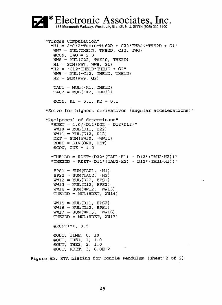
Electronic Associates, Inc.185 Monmouth Parkway, West Long Branch, N. J. 07764 (908) 229-1100
"Torque Computation""HI = 2*C12*THE1D*THE2D + C22*THE2D*THE2D + Gl"WW7 = MUL(THE1D, THE2D, C12, TWO)@CON, TWO =2.0WW8 = MUL(C22, THE2D, THE2D)HI = SUM(WW7, WW8, Gl)"H2 = -C12*THE1D*THE1D + G2"WW9 = MUL(-C12, THE1D, THE1D)H2 = SUM(WW9, G2)
TAU1 = MUL(-K1, THE1D)TAU2 = MUL(-K2, THE2D)
©CON, Kl = 0.1, K2 = 0.1
"Solve for highest derivatives (angular accelerations)"
"Reciprocal of determinant""RDET = 1.0/(D11*D22 - D12*D12)"WW10 = MUL(D11, D22)WWII = MUL(D12, D12)DET = SUM(WW10, -WWII)RDET = DIV(ONE, DET)@CON, ONE =1.0
"THE1DD = RDET*(D22*(TAU1-H1) - D12*(TAU2-H2))""THE2DD = RDET*(Dll*(TAU2-H2) - D12*(TAU1-H1))"
EPS1 = SUM(TAU1, -HI)EPS2 = SUM(TAU2, -H2)WW12 = MUL(D22, EPS1)WW13 = MUL(D12, EPS2)WW14 = SUM(WW12, -WW13)THE1DD = MUL(RDET, WW14)
WW15 = MUL(D11, EPS2)WW16 = MUL(D12, EPS1)WW17 = SUM(WW15, -WW16)THE2DD = MUL(RDET, WW17)
©RUNTIME, 9.5
©OUT, TIME, 0, 10©OUT, THE1, 1, 1.0©OUT, THE2, 2, 1.0©OUT, RDET, 3, 6.0E-2
Figure 5b. RTA Listing for Double Pendulum (Sheet 2 of 2)
49
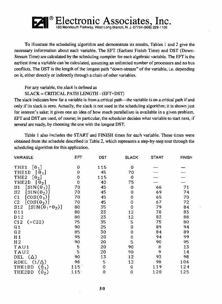
Electronic Associates, Inc.185 Monmouth Parkway, West Long Branch, N. J. 07764 (908) 229-1100
To illustrate the scheduling algorithm and demonstrate its results, Tables 1 and 2 give thenecessary information about each variable. The EFT (Earliest Finish Time) and DST (Down-Stream Time) are calculated by the scheduling compiler for each algebraic variable. The EFT is theearliest time a variable can be calculated, assuming an unlimited number of processors and no busconflicts. The DST is the length of the longest path "down-stream" of the variable, i.e. dependingon it, either directly or indirectly through a chain of other variables.
For any variable, the slack is defined asSLACK = CRITICAL PATH LENGTH - (EFT+DST)
The slack indicates how far a variable is from a critical path—the variable is on a critical path if andonly if its slack is zero. Actually, the slack is not used in the scheduling algorithm; it is shown justfor interest's sake; it gives one an idea of how much parallelism is available in a given problem.EFT and DST are used, of course; in particular, the scheduler decides what variable to start next, ifseveral are ready, by choosing the one with the longest DST.
Table 1 also includes the START and FINISH times for each variable. These times wereobtained from the schedule described in Table 2, which represents a step-by-step tour through thescheduling algorithm for this application.
VARIABLE EFT DST SLACK START RNISH
THE1 [0J 0 115 0 — —THE1D [0^ 0 45 70 — —THE2 [02] 0 115 0 — —THE2D [02] 0 40 75 — —51 [SIN(0,)] 70 45 0 66 7152 [SIN(02)j 70 45 0 69 74Cl [€03(00] 70 45 0 65 70C2 [COS(02)] 70 45 0 67 72S12 [SIN(01 + 02)J 80 35 0 79 84Dll 80 23 12 78 83D12 80 23 12 83 88C12 ( = C22) 75 35 5 75 80Gl 90 25 0 89 94G2 85 30 0 84 89HI 95 20 0 94 99H2 90 20 5 90 95TAU1 5 20 90 8 13TAU2 5 20 90 9 14DEL (A) 90 13 12 93 98RDEL (I/A) 98 5 12 98 106THE1DD ( © T ) 115 0 0 119 124THE2DD (02) 115 0 0 120 125
50

Electronic Associates, Inc.185 Monmouth Parkway, West Long Branch, N. J. 07764 (908) 229-1100
Table la. Variable List for the Double Pendulum (Sheet 1 of 3)VARIABLE*1*2*3#4*5*6*7#8*9*10*11*12*13*14*15*16*17*18*19*20*21*22*23*24*25*26*27*28*29*30*31*32*33*34*35*36*37*38*39*40*41*42*43#44*45*46
51
EFT51015202530354045505055556065656565333351015202530354045505055556065656565333375757575755
DST11010510095908580757060655560555050505055551101051009590858075706065556055505050505555404028283040
SLACK000000000505000000272700000000050500000027270012121070
START051015202530354047455250556057615830311611162126313641484653515662596364323372747376712
FINISH51015202530354045525057556065626663333461116212631364146535158566167646869353677797881767

D Electronic Associates. Inc.185 Monmouth Parkway, West Long Branch, N. J. 07764 (908) 229-1100
Table Ib. Variable List for the Double Pendulum (Sheet 2 of 3)VARIABLE EFT DST SLACK START RNISH
*47 5 30 80 4 9*48 80 25 10 82 87*49 10 35 70 7 12*50 80 30 5 80 85*51 5 35 75 3 8*52 80 30 5 81 86*53 85 25 5 86 91*54 85 18 12 85 90*55 85 18 12 88 93*56 100 15 0 104 109*57 95 15 5 95 100*58 105 10 0 109 114*59 100. 10 5 105 110*60 105 10 0 110 115*61 100 10 5 106 111*62 110 5 0 114 119*63 110 5 0 115 12
Table Ic. Variable List for the Double Pendulum (Sheet 3 of 3)
Notice that the state variables all have EFT of zero; they are available at the beginning of theframe. The highest derivatives have zero DST—they are terminal variables.
Table 1 indicates that 48 out of 81 algebraic variables have zero slack; in other words, mostof the variables are on a critical path. The maximum EFT and the maximum DST are the same—thelength of the critical path (in this case, 115 cycles).
There are 81 algebraic variables to be calculated for each derivative evaluation. Four of theseare indexed FETCH operations in the Data Memory. The other 77 are operations of the ArithmeticUnit. The Data Memory is not used very heavily in this application, which should not be toosurprising, since there are only four indexed memory fetch operations, and no I/O statements.
In a one-module RTA, with a single arithmetic unit, the resource limit is 77 cycles—theapplication cannot be completed in less time than that. But the critical path limit is 115 cycles.Clearly, adding more modules would not provide a significant speedup; this application is heavilybound by its sequential constraints.
The actual schedule generated by the scheduling compiler is 126 cycles long. This is less than10% above the critical-path limit, so that the scheduler is over 90% efficient on this application.Efficiency of 90% or better is typical, as shown by the results in Section 3 of this report for the tenbenchmark applications run to date.
Table 2 shows how the schedule is developed line-by-line. It works by stepping through
52

Electronic Associates, Inc.185 Monmouth Parkway, West Long Branch, N. J. 07764 (908) 229-1100
each cycle of the computation in the same order that the actual hardware will at run time. On eachcycle, we maintain a list of ready variables. A variable is defined as "ready" if its inputs areavailable, so that the computation of the variable is ready to start as soon as a processor becomesavailable.
At the start, the only values available are the state variables and the constants. A variabledepending only on these is ready at the start. These variables are listed at the beginning of the table.
Since most operations have a latency of five cycles, a variable that was "started" on cycle #Nwill normally be "finished," i.e. its value will become available, on cycle #N+5. Exception: theindexed memory fetch has a latency of 3 cycles, and the DIVIDE operation in the arithmetic unithas a latency of 8 cycles.
Since most operations have an Initiation Interval of 1, the arithmetic unit will be able to accepta new input on every cycle and produce a new output on every cycle. (Exception: division has asix-cycle latency; a division started on cycle #N will tie up the unit for 6 cycles, and the nextoperation (which may be another division or any other operation) may be started on cycle #N+6 (aspointed out above, the result does not emerge for two more cycles—on cycle #N+8).
The latency figures are "memory-to-memory," that is, they include time spent in bus transferswithin a module. Bus transfers between modules go through the intermodule bus; this transfertakes additional machine cycles. However, since the critical path is strongly dominant here, there isno incentive to use more than one module, even if several are available.
At each step, the algorithm first looks to see whether one or more variables are becomingavailable at component outputs (naturally, the answer will be "no" on the first few steps, since thisis a pipelined machine, but eventually, variables will start emerging).
Occasionally, a cycle will be encountered on which two or more variables appear at once.This is rare in the present program, since most operations use the arithmetic unit, and there is onlyone such unit in a one-module system. However, there are a few places (e.g. cycles 30 and 31)where two operations are started simultaneously—one in the arithmetic unit and one in the DataMemory. There are also a few places (e.g. cycles 35 and 36) where two variables become availableon the same cycle.
In any event, the emergence of a new variable indicates that some of the computations thisvariable needs can be moved onto the "ready" list. If a variable, say X, becomes available, theneach of the operations using X is examined:
• If the operation is a unary operation like FLOAT, SQRT, or ABS, then its variable is putonto the ready list.
53

Electronic Associates, Inc.185 Monmouth Parkway, West Long Branch, N. J. 07764 (908) 229-1100
• If the variable is a binary operation, like ADD, SUBTRACT, MULTIPLY, DIVIDE, AND,OR, etc., then its other input is checked. If it's already available, then the variable is put onto theready list.
On any given cycle, if any variables are ready, the one with the longest DST is chosen toschedule on the processor. In case of a tie, the present scheme simply picks the first (low-numbered) operation from the list of ready operations with minimal DST.
To facilitate following the schedule, Table 2 contains a column headed "NEWLY READY,"which lists each variable (with its DST in parentheses) on the cycle when it first becomes ready.
Variables initially ready, with their DSTs:#1(110), #21(110), TAU1(20), TAU2(20), #46(40), #47(30), #51(35)
CYCLE01234567891011121314151617181920212223242526272829303132
START#1#21#46#51#47#2#22#49TAU1TAU2#3#23
#4#24
#5#25
#6#26
#7, #19#27, #20#39
FINISH NEWLY READY
#1#21#46#51#47#2#22#49TAU1TAU2#3#23
#4#24
#25#25
#2(105)#22(105)#49(35)
#3(100)#23(100)
#4(95)#24(96)
#5(90)#25(90)
#6(85)#26(85)
#6(50), #19(55), #20(55)#26(85), #39(55), #40(55)
Table 2a. RTA Schedule for Double Pendulum (Sheet 1 of 3)
54

Electronic Associates, Inc.185 Monmouth Parkway, West Long Branch, N. J. 07764 (908) 229-1100
CYCLE START33 #403435 #836 #2837383940 #941 #2942434445 #1146 #3147 #1048 #304950 #1351 #3352 #1253 #325455 #1456 #3457 #1658 #1859 #3660 #1561 #1762 #3563 #3764 #3865 Cl66 SI67 C26869 S27071 #4572 #4173 #4374 #4275 C2276 #447778 Dll79 S1280 #50
FINISH#19#20#7, #39#27, #40
#8#28
#9#29
#11#31#10#30
#13#33#12#32
#14#34#16#18#36#15#17#35#37#38ClSIC2
S2
#45#41.#43#42C22
NEWLY READY
#8(75)#28(75)
#9(70)#29(70)
#10(60) ,#30(60) ,
#13(60)#33(60)#12(55)#32(55)
#14(55)#34(55)#36(50),#36(50),
#15(50),#35(50),
CK45)Sl(45)C2(45)
S2(45)
#45(30)#41(40),
#42 (40) ,
-
.Dll (23)S12 (35)#48(25),
#11(65)#31(65)
#18(50)#38(50)
#17(50)#37(50)
#43(28), #44(28)
C22 (35)
#50(30) , #52(30)
Table 2b. RTA Schedule for Double Pendulum (Sheet 2 of 3)
55

Electronic Associates. Inc.185 Monmouth Parkway, West Long Branch, N. J. 07764 (908) 229-1100
CYCLE
81828384858687888990919293949596979899100101102103104105106107108109110111112113114115116117118119120121122123124125
START
#52#48D12G2#54#53
#55GlH2
DELHI#57
RDEL
FINISH
#44
DllS12#50#52#48D12G2#54#53
#55Gl .H2
DELHI#57
#56#59#61
#58#60
#62#63
THE1DDTHE2DD
RDEL
#56#59#61
#58#60
#62#63
THE1DDTHE2DD
NEWLY READY
D12(23)
#54(18)G2(30)
#53(25)
#55(18)H2(20) , Gl(25)
DEL(13)HI(20)#57(15)
RDEL(5)#56(15)#59(10), #61(10)
#58(10), #60(10)
#62(5)#63(5)
THEIDD(O)THE2DD(0)
END OF PROGRAM
Table 2c. RTA Schedule for Double Pendulum (Sheet 3 of 3)
The manually-generated schedule, from the Phase 1 final report, takes 126 cycles. The compil-er-generated schedule requires 128. The cost of automatic scheduling is less than 2% in this case.
56

Electronic Associates, Inc.185 Monmouth Parkway, West Long Branch, N. J. 07764 (908) 229-1100
The Phase 1 final report estimated about 40 cycles more for the four integrations; the actualcompiler-generated program takes 34. Hence the overall frame time is 162 cycles, as comparedwith the original 165-cycle estimate. However, the clock period of the prototype is 50nanoseconds, while the original estimate was 40. Thus, the overall frame time of the prototype is
8.1 usec, as compared with the original estimate of 6.6. Except for the slightly slower clockfrequency, the speed of the system is within 2% of the value anticipated at the end of the first phasestudy.
6. CONCLUSIONS
The major goals of the Phase 2 project have been obtained. The feasibility of the originaldesign concept, including both hardware and software, has been established. Both the hardwareprototype and the scheduling compiler, supporting a high-level language, function essentially asanticipated.
Electronic Associates is currently proceeding, independent of U.S. Government funds, todevelop the RTA into a commercial product. The software is being enhanced to include a more"friendly" user interface, additional MACRO operators, and many other features, some of whichare described in Section 4 of this report. The hardware is being enhanced with I/O modules,allowing a single system to include up to 64 A/D channels, 64 D/A channels, 64 discrete logicsignals in either direction, and communication with sequential processors, for running mixedparallel/procedural code.
The compiler, loader, and run-time executive programs are being re-hosted to a UNIX work-station, allowing for enhanced graphics capability and a better programming environment
The product was announced on July 31, 1991, and first deliveries are scheduled for the thirdquarter of 1992.
57

NASANoiona *ecnautcs anaSuxe /
Report Documentation Page
1. Report No. 2. Government Accession No. 3. Recipient's Catalog No.
4. Title and Subtitle
Construction of a Parallel Processor for SimulatingManipulators and Other Mechanical Systems
5. Report Date
August, 1991
6. Performing Organization Code
7. Author(s)
George Hannauer8. Performing Organization Report No.
10. Work Unit No.
9. Performing Organization Name and Address
Electronic Associates, Inc.185 Monmouth ParkwayWest Long Branch, NJ 07764
11. Contract or Grant No.
NAS5-30905
12. Sponsoring Agency Name and Address
National Aeronautics & Space AdministrationWashington, DC 20546-0001Goddard Space Flight CenterGreenbelt, MD
13. Type of Report and Period Covered
final ReportApril 1990/August 1991.
14. Sponsoring Agency Code
15. Supplementary Notes
16. Abstract ABSTRACT
This report summarizes the results of Contract NAS5-30905, awarded under Phase 2 ofthe SBIR Program. The goal was to demonstrate the feasibility of a new simulationprocessor. The demonstration consisted of building a hardware prototype, writing arudimentary compiler, linker, and loader, and programming and running severalapplications benchmarks. The goal was to determine whether this system could meetits stated objectives: computation speed 10 to 100 times faster than conventionalmachines, and high-level language programmability.
The objectives were met, and EAI is now proceeding with Phase 3: development of acorrmercial product. This product is scheduled for introduction in the secondquarter of 1992.
17. Key Words (Suggested by Author(sl)
Parallel ProcessingSimulation
18, Distribution Statement
Unclassified - Unlimited
19. Security Classif. (of this report)
Unclassified
20. Security Classif. (of this page)
Unclassified
21. No. of pages
57
22. Price