Electromechanical Modeling of Piezoelectric Energy Harvesters

i

Electromechanical Modeling of Piezoelectric Energy Harvesters

Alper Erturk

Dissertation submitted to the faculty of the

Virginia Polytechnic Institute and State University

in partial fulfillment of the requirements for the degree of

Doctor of Philosophy

in

Engineering Mechanics

Daniel J. Inman, Chair

Scott L. Hendricks

Michael W. Hyer

Ishwar K. Puri

Liviu Librescu (deceased)

November 20, 2009

Blacksburg, VA

Keywords: Piezoelectricity, vibration energy harvesting, structural dynamics,

electromechanical modeling

Copyright © 2009 Alper Erturk

ii

Electromechanical Modeling of Piezoelectric Energy Harvesters

Alper Erturk

Abstract

Vibration-based energy harvesting has been investigated by several researchers over the last

decade. The ultimate goal in this research field is to power small electronic components

(such as wireless sensors) by using the vibration energy available in their environment.

Among the basic transduction mechanisms that can be used for vibration-to-electricity

conversion, piezoelectric transduction has received the most attention in the literature.

Piezoelectric materials are preferred in energy harvesting due to their large power densities

and ease of application. Typically, piezoelectric energy harvesters are cantilevered structures

with piezoceramic layers that generate alternating voltage output due to base excitation. This

work presents distributed-parameter electromechanical models that can accurately predict the

coupled dynamics of piezoelectric energy harvesters. First the issues in the existing models

are addressed and the lumped-parameter electromechanical formulation is corrected by

introducing a dimensionless correction factor derived from the electromechanically

uncoupled distributed-parameter solution. Then the electromechanically coupled closed-form

analytical solution is obtained based on the thin-beam theory since piezoelectric energy

harvesters are typically thin structures. The multi-mode electromechanical frequency

response expressions obtained from the analytical solution are reduced to single-mode

expressions for modal vibrations. The analytical solutions for the electromechanically

coupled voltage response and vibration response are validated experimentally for various

cases. The single-mode analytical equations are then used for deriving closed-form relations

for parameter identification and optimization. Asymptotic analyses of the electromechanical

frequency response functions are given along with expressions for the short-circuit and the

open-circuit resonance frequencies. A simple experimental technique is presented to identify

the optimum load resistance using only a single resistor and an open-circuit voltage

measurement. A case study is given to compare the power generation performances of

iii

commonly used monolithic piezoceramics and novel single crystals with a focus on the

effects of plane-stress material constants and mechanical damping. The effects of strain

nodes and electrode configuration on piezoelectric energy harvesting are discussed

theoretically and demonstrated experimentally. An approximate electromechanical solution

using the assumed-modes method is presented and it can be used for modeling of asymmetric

and moderately thick energy harvester configurations. Finally, a piezo-magneto-elastic

energy harvester is introduced as a non-conventional broadband energy harvester.

iv

Acknowledgements

First and foremost, I would like to extend my deepest gratitude to Prof. Daniel J. Inman for he

has been more than an academic advisor over the last three years. Prof. Inman has been a great

advisor who was always available to discuss and support the technical problems came to my

mind. He did make me feel like his colleague, more than a graduate student, throughout my

entire PhD study. He provides a very pleasant research environment in the lab and he really

knows how to communicate with his students. He has been a great mentor who was available to

discuss and advise on non-technical problems of life as well. Prof. Inman has given me the

opportunity to work on several research problems other than the subject of this dissertation and

he has offered the freedom to start developing my own academic style. He has given me the

opportunity to co-teach classes with him, to attend conferences several times and to take

responsibilities in the research community. I cannot think of a more fruitful and joyful post-

masters research than my last three years under the guidance of Prof. Inman at the Center for

Intelligent Material Systems and Structures (CIMSS).

Ms. Beth Howell, the program manager at CIMSS, has been very helpful since the first

day I started working at CIMSS. The friendly office environment and numerous beautiful aspects

of CIMSS have a lot to do with her presence and energy. She keeps so many things running

simultaneously with an amazing performance. I am indebted to Beth for several things she has

helped with.

The experience I have gained as a graduate student in the Department of Engineering

Science and Mechanics (ESM) is invaluable. I know that I am only at the beginning of my

academic career but my appreciation of Engineering Mechanics as a part of my life has been

enhanced dramatically after attending several classes by the pioneers of this field, such as Prof.

Liviu Librescu, Prof. Michael W. Hyer, Prof. Dean T. Mook, Prof. Raymond H. Plaut and Prof.

Ali H. Nayfeh, among others. I have been very proud of being an ESM student during my entire

graduate study.

I would like to thank Prof. Scott L. Hendricks, Prof. Michael W. Hyer, and Prof. Ishwar

K. Puri for serving on my PhD committee.

I would like to extend my appreciation to my Department, particularly the Graduate

Committee, once again, for honoring me with the “Liviu Librescu Memorial Scholarship.”

v

Words are not enough to express the value of being the first recipient of a scholarship named in

memory of the late member of my PhD committee and my teacher, Prof. Librescu. I will have to

work very hard to honor Prof. Librescu’s memory…

I truly enjoyed sharing the same office and the lab with several colleagues and friends at

CIMSS over the last three years and I have had research collaborations with some of them (on

topics not discussed in this dissertation). I owe thanks to Dr. Pablo Tarazaga (presently with the

University of Bristol, England) for introducing me the lab equipment when I was a junior PhD

student. It was in those days when he helped me with conducting the experiments of the strain

nodes demonstration together with Justin Farmer. Justin was also a great colleague during the

short period of time we were at CIMSS together. Dr. Jamil Renno (presently with the University

of Southampton, England) was an outstanding colleague and a wonderful desk neighbor when

we shared the same office before his graduation. I could not count how many nights we spent in

lab Steve Anton while developing the concept of self-charging structures (a novel energy

harvesting concept that is not discussed in this dissertation). Steve has been a fantastic colleague

to collaborate with. It was also a great pleasure to work with Na Kong (a PhD student in the

VLSI for Telecommunications Group) and observe how a skillful electrical engineer can

improve that electrical domain (that we mechanical engineers often simplify) with efficient

regulator circuits. If one is interested in how brittle single crystals can be, he/she should find me

or Onur Bilgen. We have had long nights of research collaboration with Onur as well on macro-

fiber composites and single crystals. The gentlemen presently sitting close to me in the office,

Austin Creasy and Kahlil Detrich, are the best office neighbors one can find. I really enjoyed the

break chats with Austin every time and I am very glad that the tower of books and papers on my

desk has not yet collapsed onto Kahlil’s desk. I would like to thank also Andy Sarles, Andy

Duncan, Woon Kim, Zach Hills, Mana Afshari, Amin Karami, Brad Butrym and all the members

of the CIMSS community I could not mention here, for making CIMSS what it has been.

I met another great colleague during his visit to our lab for about a year: Prof. Carlos De

Marqui Junior, an aeroelasticity professor of the University of São Paulo in São Carlos, Brazil. I

have enjoyed collaborating with him on piezo-aero-elasticity (not covered here) during my PhD

study as much as I enjoyed the caipirinha when I visited his university to give a lecture last

summer.

vi

I would like to thank Julien Hoffmann, a student (presently an engineer) I advised during

his visit as a senior engineering student from the Institut Catholique d’Arts et Métiers in Lille,

France, for his help in planning and rapidly completing the manufacturing of the piezo-magneto-

elastic device with the ESM Machine Shop (which reminds me that I owe thanks to Mr. David

Simmons as well). If Julien had not undertaken the manufacturing process of the piezo-magneto-

elastic device, the idea of using the magneto-elastic structure for energy harvesting (dates back to

the summer of 2008 when I had taken Prof. Francis Moon’s book from Prof. Inman’s library at a

party) was going wait for at least one more year!

I owe special thanks to my parents, Selma and Hikmet, for their patience and support

during my PhD study. It was wonderful to visit them in my hometown (Eskisehir, Turkey) every

July to regain the energy I needed. This work is dedicated to them.

This work has been supported by the U.S. Air Force Office of Scientific Research MURI

under grant number F 9550-06-1-0326 “Energy Harvesting and Storage Systems for Future Air

Force Vehicles” monitored by Dr B.L. Lee and recently by the U.S. Department of Commerce,

National Institute of Standards and Technology, Technology Innovation Program, under the

Cooperative Agreement Number 70NANB9H9007: “Self-Powered Wireless Sensor Network for

Structural Health Prognosis.”

vii

“These oscillations arise freely, and I have determined various

conditions, and have performed a great many beautiful

experiments on the position of the knot points and the pitch

of the tone, which agree beautifully with the theory.” [1]

– Daniel Bernoulli (from a letter to Leonhard Euler)

viii

Table of Contents

Abstract ................................................................................................................................ ii

Acknowledgements .............................................................................................................. iv

Table of Contents .............................................................................................................. viii

List of Figures ................................................................................................................... xvi

List of Tables .................................................................................................................. xxvii

1 Introduction ....................................................................................................................... 1

1.1 Vibration Energy Harvesting Using Piezoelectric Transduction ...................................... 1

1.2 Review of the Existing Piezoelectric Energy Harvester Models ...................................... 4

1.3 Objectives of the Dissertation .......................................................................................... 6

1.4 Layout of the Dissertation ................................................................................................ 8

2 Correction of the Existing Lumped-parameter Piezoelectric Energy Harvester

Model .................................................................................................................................. 11

2.1 Base Excitation Problem for the Transverse Vibrations of a Cantilevered Beam ................. 12

2.1.1 Response to General Base Excitation ..................................................................... 12

2.1.2 Steady-state Response to Harmonic Base Excitation ............................................. 17

2.1.3 Lumped-parameter Model of the Harmonic Base Excitation Problem .................. 18

2.1.4 Comparison of the Distributed-parameter and the Lumped-parameter Model

Predictions........................................................................................................................ 21

2.2 Correction of the Lumped-parameter Model for Transverse Vibrations ............................... 24

2.2.1 Correction Factor for the Lumped-parameter Model .............................................. 24

2.2.2 Effect of a Tip Mass on the Correction Factor ....................................................... 26

2.3 Experimental Case Studies for Validation of the Correction Factor ..................................... 29

2.3.1 Cantilevered Beam without a Tip Mass under Base Excitation ............................. 29

2.3.2 Cantilevered Beam with a Tip Mass under Base Excitation ................................... 33

2.4 Base Excitation Problem for Longitudinal Vibrations and Correction of Its Lumped-

parameter Model .......................................................................................................................... 35

2.4.1 Analytical Modal Analysis and Steady-state Response to Harmonic Base

Excitation ......................................................................................................................... 35

2.4.2 Correction Factor for Longitudinal Vibrations ....................................................... 37

ix

2.5 Correction Factor in the Electromechanically Coupled Lumped-parameter Equations and a

Theoretical Case Study ................................................................................................................ 39

2.5.1 An Electromechanically Coupled Lumped-parameter Model for Piezoelectric

Energy Harvesting ........................................................................................................... 39

2.5.2 Correction Factor in the Electromechanically Coupled Lumped-parameter Model

and a Theoretical Case Study ........................................................................................... 40

2.6 Summary and Conclusions .................................................................................................... 42

3 Distributed-parameter Electromechanical Modeling of Bimorph Piezoelectric Energy

Harvesters – Analytical Solutions ..................................................................................... 43

3.1 Fundamentals of the Electromechanically Coupled Distributed-parameter Model ............... 44

3.1.1 Modeling Assumptions and Bimorph Configurations ........................................... 44

3.1.2 Coupled Mechanical Equation and Modal Analysis of Bimorph Cantilevers ........ 46

3.1.3 Coupled Electrical Circuit Equation of a Thin Piezoceramic Layer under Dynamic

Bending ........................................................................................................................... 52

3.2 Series Connection of the Piezoceramic Layers ...................................................................... 55

3.2.1 Coupled Beam Equation in Modal Coordinates ..................................................... 56

3.2.2 Coupled Electrical Circuit Equation ....................................................................... 56

3.2.3 Closed-form Voltage Response and Vibration Response at Steady State .............. 57

3.3. Parallel Connection of the Piezoceramic Layers .................................................................. 59

3.3.1 Coupled Beam Equation in Modal Coordinates ..................................................... 59

3.3.2 Coupled Electrical Circuit Equation ....................................................................... 60

3.3.3 Closed-form Voltage Response and Vibration Response at Steady State .............. 60

3.4 Single-mode Electromechanical Expressions for Modal Excitations .................................... 62

3.4.1 Series Connection of the Piezoceramic Layers ....................................................... 62

3.4.2 Parallel Connection of the Piezoceramic Layers .................................................... 63

3.5 Multi-mode and Single-mode Electromechanical FRFs ........................................................ 63

3.5.1 Multi-mode Electromechanical FRFs ..................................................................... 64

3.5.1.1 Series Connection of the Piezoceramic Layers ........................................ 64

3.5.1.2 Parallel Connection of the Piezoceramic Layers ..................................... 65

3.5.2 Single-mode Electromechanical FRFs .................................................................... 66

x

3.5.2.1 Series Connection of the Piezoceramic Layers ....................................... 66

3.5.2.2 Parallel Connection of the Piezoceramic Layers ..................................... 67

3.6 Equivalent Representation of the Series and Parallel Connection Expressions .................... 67

3.6.1 Modal Electromechanical Coupling Terms ............................................................ 68

3.6.2 Equivalent Capacitance for Series and Parallel Connections ................................. 68

3.6.3 Equivalent Representation of the Electromechanical Expressions ......................... 69

3.6.4 Equivalent Representation of the Multi-mode Electromechanical FRFs ............... 70

3.6.5 Equivalent Representation of the Single-mode Electromechanical FRFs .............. 71

3.7 Theoretical Case Study .......................................................................................................... 72

3.7.1 Properties of the Bimorph Cantilever .................................................................... 72

3.7.2 Frequency Response of the Voltage Output .......................................................... 74

3.7.3 Frequency Response of the Current Output ............................................................ 78

3.7.4 Frequency Response of the Power Output .............................................................. 80

3.7.5 Frequency Response of the Relative Tip Displacement ......................................... 84

3.7.6 Parallel Connection of the Piezoceramic Layers .................................................... 88

3.7.7 Single-mode FRFs .................................................................................................. 91

3.8 Summary and Conclusions .................................................................................................... 95

4 Experimental Validations of the Analytical Solutions for Cantilevered Bimorph

Piezoelectric Energy Harvesters ...................................................................................... 97

4.1 PZT-5H Bimorph Cantilever without a Tip Mass ................................................................. 98

4.1.1 Experimental Setup ................................................................................................. 98

4.1.2 Validation of the Electromechanical FRFs for a Set of Resistors ........................ 105

4.1.3 Electrical Performance Diagrams at the Fundamental Short-Circuit and Open-

Circuit Resonance Frequencies ...................................................................................... 111

4.1.4 Vibration Response Diagrams at the Fundamental Short-Circuit and Open-Circuit

Resonance Frequencies .................................................................................................. 113

4.2 PZT-5H Bimorph Cantilever with a Tip Mass .................................................................... 114

4.2.1 Experimental Setup ............................................................................................... 114



Circuit Resonance Frequencies ...................................................................................... 122

xi



4.2.5 Model Predictions with the Point Mass Assumption ............................................ 125

4.2.6 Performance Comparison of the PZT-5H Bimorph without and with the Tip

Mass ............................................................................................................................... 127

4.3 PZT-5A Bimorph Cantilever ............................................................................................... 128



4.3.3 Comparison of the Single-mode and Multi-mode Electromechanical FRFs. ....... 133

4.4 Summary and Conclusions .................................................................................................. 135

5 Dimensionless Single-mode Electromechanical Equations, Asymptotic Analyses and

Closed-form Relations for Parameter Identification and Optimization ....................... 137

5.1 Equivalent Dimensionless Representation of the Single-Mode Electromechanical

FRFs ........................................................................................................................................... 138

5.1.1 Complex Forms ..................................................................................................... 138

5.1.2 Modulus-Phase Forms .......................................................................................... 139

5.1.3 Dimensionless Forms ............................................................................................ 139

5.2 Asymptotic Analyses, Resonance Frequencies and Closed-form Expressions for Parameter

Identification and Optimization ................................................................................................. 140

5.2.1 Short-circuit and Open-circuit Asymptotes of the Voltage FRF .......................... 140

5.2.2 Short-circuit and Open-circuit Asymptotes of the Tip Displacement FRF ......... 141

5.2.3 Short-circuit and Open-circuit Resonance Frequencies of the Voltage FRF ....... 142

5.2.4 Short-circuit and Open-circuit Resonance Frequencies of the Tip

Displacement FRF ......................................................................................................... 142

5.2.5 Identification of Modal Mechanical Damping Ratio in the Presence of a

Resistive Load ................................................................................................................ 143

5.2.6 Electrical Power FRF ............................................................................................ 145

5.2.7 Optimum Values of Load Resistance at the Short-circuit and Open-circuit


5.2.8 Vibration Attenuation from the Short-circuit to the Open-circuit

Conditions ..................................................................................................................... 146

xii

5.3 Intersection of the Voltage Asymptotes and a Simple Technique for Identification of the

Optimum Load Resistance from Experimental Measurements ................................................. 147

5.3.1 On the Intersection of the Voltage Asymptotes for Resonance Excitation ......... 147

5.3.2 A Simple Technique for the Experimental Identification of the Optimum

Load Resistance for Resonance Excitation .................................................................... 149

5.4 Experimental Validations for a PZT-5H Bimorph Cantilever ............................................. 150

5.4.1 Identification of Mechanical Damping ................................................................. 151

5.4.2 Fundamental Short-circuit and Open-circuit Resonance Frequencies .................. 151

5.4.3 Amplitude and Phase of the Voltage FRF ............................................................ 152

5.4.4 Voltage Asymptotes for Resonance Excitation .................................................... 152

5.4.5 Power vs. Load Resistance Diagrams and the Optimum Loads ........................... 154

5.4.6 Comment on the Optimum Load Resistance obtained from the Norton and

Thévenin Representations of a Piezoceramic Layer ..................................................... 154

5.5 Summary and Conclusions ..................................................................................... 156

6 Effects of Material Constants and Mechanical Damping on Piezoelectric Energy

Harvesting – A Comparative Study ................................................................................ 158

6.1 Properties of Typical Monolithic Piezoceramics and Single Crystals ..................... 159

6.2 Reduced Piezoelectric, Elastic and Permittivity Constants for a Thin Beam .......... 161

6.3 Theoretical Case Study for Performance Comparison of Various Monolithic

Piezoceramics and Single Crystals ................................................................................ 163

6.3.1 Properties of the Bimorph Cantilevers ...................................................... 163

6.3.2 Performance Comparison of the Original Configurations ........................ 165

6.3.3 On the Effect of Piezoelectric Strain Constant ......................................... 166

6.3.4 On the Effect of Elastic Compliance ........................................................ 167

6.3.5 On the Effect of Permittivity Constant ..................................................... 168

6.3.6 On the Effect of the Overhang Length ...................................................... 169

6.3.7 On the Effect of Mechanical Damping ..................................................... 170

6.4 Experimental Demonstration for PZT-5A and PZT-5H Cantilevers ....................... 171

6.4.1 Experimental Setup ................................................................................... 171

6.4.2 Identification of Mechanical Damping and Model Predictions ................ 172

6.4.3 Performance Comparison of the PZT-5A and PZT-5H Cantilevers ........ 174

xiii

6.5 Summary and Conclusions ...................................................................................... 177

7 Effects of Strain Nodes and Electrode Configuration on Piezoelectric Energy

Harvesting ........................................................................................................................ 179

7.1 Mathematical Background ....................................................................................... 180

7.2 Physical and Historical Backgrounds ...................................................................... 182

7.3 Strain Nodes of a Thin Cantilever without a Tip Mass ........................................... 184

7.4 Effect of Using a Tip Mass on the Strain Nodes of a Thin Cantilever .................... 186

7.5 Strain Nodes for Other Boundary Conditions .......................................................... 189

7.6 Experimental Demonstration ................................................................................... 192

7.7 Relationship with the Energy Harvesting Literature ............................................... 198

7.8 Avoiding Cancellation in the Electrical Circuit with Segmented Electrodes .......... 201

7.9 Summary and Conclusions ...................................................................................... 204

8 Approximate Distributed-parameter Modeling of Piezoelectric Energy Harvesters

Using the Electromechanical Assumed-modes Method ................................................. 205

8.1 Unimorph Piezoelectric Energy Harvester Configuration ................................................... 206

8.2 Electromechanical Euler-Bernoulli Model with Axial Deformations ........................... 207

8.2.1 Distributed-parameter Electromechanical Energy Formulation ..................... 207

8.2.2 Spatial Discretization of the Energy Equations .............................................. 211

8.2.3 Electromechanical Lagrange Equations ......................................................... 213

8.2.4 Solution of the Electromechanical Lagrange Equations ................................. 216

8.3 Electromechanical Rayleigh Model with Axial Deformations ..................................... 219





8.4 Electromechanical Timoshenko Model with Axial Deformations ................................ 221





8.5 Modeling of Symmetric Configurations ....................................................................... 233

xiv

8.5.1 Euler-Bernoulli and Rayleigh Models ............................................................ 233

8.5.2 Timoshenko Model ........................................................................................ 234

8.6 Presence of a Tip Mass in the Euler-Bernoulli, Rayleigh and Timoshenko Models ........... 235

8.7 Comments on the Kinematically Admissible Trial Functions ............................................ 236

8.7.1 Euler-Bernoulli and Rayleigh Models ............................................................ 236

8.7.2 Timoshenko Model ........................................................................................ 238

8.8 Experimental Validations of the Assumed-Modes Solution for a Bimorph Cantilever ..... 239

8.8.1 PZT-5H Bimorph Cantilever without a Tip Mass .......................................... 239

8.8.2 PZT-5H Bimorph Cantilever with a Tip Mass ............................................... 242

8.9 Summary and Conclusions ................................................................................................. 245

9 A Non-conventional Broadband Vibration Energy Harvester Using a Bi-stable

Piezo-magneto-elastic Structure ..................................................................................... 246

9.1 The Piezo-magneto-elastic Energy Harvester ...................................................................... 247

9.1.1 Lumped-parameter Electromechanical Equations Describing the Nonlinear System

Dynamics ....................................................................................................................... 247

9.1.2 Time-domain Numerical Simulations of the Electromechanical Response ......... 249

9.1.3 Performance Comparison of the Piezo-magneto-elastic and the Piezo-elastic

Structures in the Phase Space ........................................................................................ 250

9.2 Experimental Setup and Performance Results ..................................................................... 254


9.2.2 Performance Results ............................................................................................. 255

9.3 Broadband Voltage Generation Using the Piezo-magneto-elastic Energy Harvester ......... 256

9.3.1 Comments on the Chaotic and the Large-amplitude Regions in the Response .... 256

9.3.2 Comparison of the Piezo-magneto-elastic and Piezo-elastic Configurations for

Voltage Generation ....................................................................................................... 257

9.4 Broadband Power Generation Performance and Comparisons against the Piezo-elastic

Configuration ............................................................................................................................. 260


9.4.2 Comparison of the Electrical Power Outputs ........................................................ 261

9.5 Summary and Conclusions .................................................................................................. 264

10 Summary and Conclusions ......................................................................................... 265

xv

References ......................................................................................................................... 271

Appendices ........................................................................................................................ 280

A Constitutive Equations for a Monolithic Piezoceramic ......................................................... 280

B Numerical Data for Monolithic PZT-5A and PZT-5H Piezoceramics .................................. 285

C Constitutive Equations for an Isotropic Substructure ............................................................ 287

D Essential Boundary Conditions for Cantilevered Beams ....................................................... 289

E Electromechanical Lagrange Equations Based on the Extended Hamilton’s Principle ......... 290

xvi

List of Figures

Fig. 1.1 (a) A cantilevered piezoelectric energy harvester tested under base excitation on an

electromagnetic shaker (photo by A. Erturk, 2009) and (b) its schematic view ............................ 3

Fig. 2.1 Cantilevered beam transversely excited by the translation and small rotation of its

base .............................................................................................................................................. 12

Fig. 2.2 Lumped-parameter models of the base excitation problem; (a) the commonly used

representation and (b) the correct representation of external damping. ....................................... 19

Fig. 2.3 Contribution of excitation from air (or external) damping to the total excitation term as a

function of air damping ratio (for excitation at n ) .............................................................. 21

Fig. 2.4 Relative motion transmissibility functions for the transverse vibrations of a cantilevered

beam without a tip mass; (a) distributed-parameter model and (b) lumped-parameter model .... 23

Fig. 2.5 Error in the relative motion transmissibility due to using the lumped-parameter model

for a cantilevered beam without a tip mass in transverse vibrations ........................................... 23

Fig. 2.6 Relative motion transmissibility functions obtained from the distributed-parameter,

corrected lumped-parameter and the original lumped-parameter models for 0.05 .............. 25

Fig. 2.7 Variation of the correction factor for the fundamental transverse vibration mode with tip

mass – to – beam mass ratio ........................................................................................................ 28

Fig. 2.8 Experimental setup used for the frequency response measurements of a uniform bimorph

cantilever (photos by A. Erturk, 2009) ........................................................................................ 30

Fig. 2.9 Close views of the cantilever tested under base excitation (a) without and (b) with a tip

mass attachment (photos by A. Erturk, 2009) .............................................................................. 31

Fig. 2.10 Variation of the modified correction factor for the fundamental transverse vibration

mode with tip mass – to – beam mass ratio ................................................................................. 32

Fig. 2.11 (a) Tip velocity – to – base acceleration FRFs of a cantilever without a tip mass:

experimental measurement, corrected lumped-parameter and uncorrected lumped-parameter

model predictions; (b) coherence function of the experimental measurement ............................ 33

Fig. 2.12 (a) Tip velocity – to – base acceleration FRFs of a cantilever with a tip mass:


model predictions; (b) coherence function of the experimental measurement ............................ 34

xvii

Fig. 2.13 Cantilevered bar with a tip mass longitudinally excited by the translation of its

base .............................................................................................................................................. 35

Fig. 2.14 Variation of the correction factor for the fundamental longitudinal vibration mode with

tip mass – to – beam mass ratio ................................................................................................... 38

Fig. 2.15 A lumped-parameter piezoelectric energy harvester model with sample numerical

values by duToit et al. [16] .......................................................................................................... 39

Fig. 2.16 Corrected and uncorrected (a) relative tip displacement and (b) power output FRFs

obtained using the electromechanical lumped-parameter model for a load resistance of 10 k

and a base acceleration of 9.81 m/s2 ............................................................................................ 42

Fig. 3.1 Bimorph piezoelectric energy harvester configurations with (a) series connection of

piezoceramic layers, (b) parallel connection of piezoceramic layers and the (c) cross-sectional

view of a uniform bimorph cantilever ......................................................................................... 45

Fig. 3.2 (a) Bimorph cantilever with a single layer connected to a resistive load and (b) the

corresponding electrical circuit .................................................................................................... 52

Fig. 3.3 Electrical circuit representing the series connection of the piezoceramic layers ........... 57

Fig. 3.4 Electrical circuit representing the parallel connection of the piezoceramic layers ........ 60

Fig. 3.5 Voltage FRFs of the bimorph for a broad range of load resistance (series connection of

the piezoceramic layers) .............................................................................................................. 75

Fig. 3.6 Voltage FRFs of the bimorph with a focus on the first two vibration modes: (a) mode 1

and (b) mode 2 (series connection) .............................................................................................. 77

Fig. 3.7 Variation of the voltage output with load resistance for excitations at the short-circuit

and the open-circuit resonance frequencies of the first vibration mode (series connection) ....... 78

Fig. 3.8 Current FRFs of the bimorph for a broad range of load resistance (series connection of


Fig. 3.9 Current FRFs of the bimorph with a focus on the first two vibration modes: (a) mode 1


Fig. 3.10 Variation of the current output with load resistance for excitations at the short-circuit


Fig. 3.11 Power FRFs of the bimorph for a broad range of load resistance (series connection of


xviii

Fig. 3.12 Power FRFs of the bimorph with a focus on the first two vibration modes: (a) mode 1


Fig. 3.13 Variation of the power output with load resistance for excitations at the short-circuit




Fig. 3.15 Tip displacement FRFs (relative to the vibrating base) of the bimorph for a broad range

of load resistance (series connection of the piezoceramic layers) ............................................... 86

Fig. 3.16 Tip displacement FRFs of the bimorph with a focus on the first two vibration modes:

(a) mode 1 and (b) mode 2 (series connection) ............................................................................ 86

Fig. 3.17 Variation of the tip displacement (relative to the vibrating base) with load resistance for

excitations at the short-circuit and the open-circuit resonance frequencies of the first vibration

mode (series connection) ............................................................................................................. 88

Fig. 3.18 (a) Voltage FRFs for the parallel connection of the piezoceramic layers and (b) an

enlarged view around the first vibration mode ............................................................................ 89

Fig. 3.19 (a) Current FRFs for the parallel connection of the piezoceramic layers and (b) an


Fig. 3.20 (a) Power FRFs for the parallel connection of the piezoceramic layers and (b) an


Fig. 3.21 (a) Tip displacement FRFs for the parallel connection of the piezoceramic layers and

(b) an enlarged view around the first vibration mode .................................................................. 90

Fig. 3.22 Comparison of the series and parallel connection cases for excitations at the short-

circuit resonance frequency of the first vibration mode: (a) voltage vs. load resistance; (b) current

vs. load resistance; (c) power vs. load resistance; (d) tip displacement vs. load resistance ........ 91

Fig. 3.23 Comparison of the multi-mode and single-mode voltage FRFs (series connection) ... 92

Fig. 3.24 Comparison of the multi-mode and single-mode voltage FRFs with a focus on the first

two vibration modes: (a) mode 1 and (b) mode 2 (series connection) ......................................... 93

Fig. 3.25 Comparison of the multi-mode and single-mode tip displacement FRFs (series

connection) ................................................................................................................................... 94

Fig. 3.26 Comparison of the multi-mode and single-mode tip displacement FRFs with a focus on

the first two vibration modes: (a) mode 1 and (b) mode 2 (series connection) ........................... 94

xix

Fig. 3.27 Variations of the (a) power output and (b) tip displacement with load resistance for the

multi-mode and single mode-solutions (excitations at the fundamental short-circuit and open-

circuit resonance frequencies) ...................................................................................................... 95

Fig. 4.1 Experimental setup used for the electromechanical frequency response

measurements (photos by A. Erturk, 2009) ................................................................................. 99

Fig. 4.2 Equipments used in the experiments: (a) laser vibrometer, (b) charge amplifier,

(c) accelerometer, (d) fixed-gain amplifier, (e) data acquisition system, (f) computer with a

frequency response analyzer (photo by A. Erturk, 2009) .......................................................... 100

Fig. 4.3 A view of the shaker, low-mass accelerometer, PZT-5H bimorph cantilever without a tip

mass, its clamp and a set of resistors (photo by A. Erturk, 2009) ............................................. 101

Fig. 4.4 (a) Tip velocity and voltage output FRFs of the PZT-5H bimorph cantilever without a tip

mass and (b) their coherence functions (for a load resistance of 470 ) .................................. 102

Fig. 4.5 (a) A close view of the clamp showing the point of velocity measurement (photo by A.

Erturk, 2009) and (b) the clamp velocity – to – acceleration FRF capturing the clamp-related

mode ........................................................................................................................................... 103

Fig. 4.6 Measured and predicted (a) tip velocity and (b) voltage output FRFs of the PZT-5H

bimorph cantilever without a tip mass for a load resistance of 470 ...................................... 106

Fig. 4.7 Measured and predicted tip velocity and voltage output FRFs of the PZT-5H bimorph

cantilever without a tip mass for various resistors: (a) 1.2 k , (b) 44.9 k and

(c) 995 k ................................................................................................................................. 108

Fig. 4.8 Voltage output FRFs of the PZT-5H bimorph cantilever without a tip mass for 12

different resistive loads (ranging from 470 to 995 k )....................................................... 109

Fig. 4.9 Tip velocity FRFs of the PZT-5H bimorph cantilever without a tip mass for 12 different

resistive loads (ranging from 470 to 995 k ) ..................................................................... 109

Fig. 4.10 Enlarged views of the (a) voltage output, (b) current output, (c) power output and (d)

tip velocity FRFs of the PZT-5H bimorph cantilever without a tip mass for 12 different resistive

loads (ranging from 470 to 995 k ) .................................................................................... 110

Fig. 4.11 Variation of the voltage output with load resistance for excitations at the fundamental

short-circuit and open-circuit resonance frequencies of the PZT-5H bimorph cantilever without a

tip mass ...................................................................................................................................... 111

xx

Fig. 4.12 Variation of the current output with load resistance for excitations at the fundamental


tip mass ...................................................................................................................................... 112

Fig. 4.13 Variation of the power output with load resistance for excitations at the fundamental


tip mass ...................................................................................................................................... 113

Fig. 4.14 Variation of the tip velocity with load resistance for excitations at the fundamental


tip mass ...................................................................................................................................... 114

Fig. 4.15 A view of the experimental setup for the PZT-5H bimorph cantilever with a tip

mass (photo by A. Erturk, 2009) ................................................................................................ 115

Fig. 4.16 (a) A close view of the PZT-5H bimorph cantilever with a tip mass (photo by A.

Erturk, 2009) and (b) a schematic view showing the geometric detail of the cube-shaped tip

mass............................................................................................................................................ 116

Fig. 4.17 (a) Tip velocity and voltage output FRFs of the PZT-5H bimorph cantilever with a tip

mass and (b) their coherence functions (for a load resistance of 470 ) .................................. 117


bimorph cantilever with a tip mass for a load resistance of 470 ........................................... 118


cantilever with a tip mass for various resistors: (a) 1.2 k , (b) 44.9 k and (c) 995 k ..... 119

Fig. 4.20 Tip velocity FRFs of the PZT-5H bimorph cantilever with a tip mass for 12 different


Fig. 4.21 Voltage output FRFs of the PZT-5H bimorph cantilever with a tip mass for 12 different



tip velocity FRFs of the PZT-5H bimorph cantilever with a tip mass for 12 different resistive

loads (ranging from 470 to 995 k ) .................................................................................... 121


short-circuit and open-circuit resonance frequencies of the PZT-5H bimorph cantilever with a tip

mass............................................................................................................................................ 122

xxi



mass............................................................................................................................................ 123



mass............................................................................................................................................ 124



mass............................................................................................................................................ 125

Fig. 4.27 Comparison of the voltage FRFs predicted with and without considering the rotary

inertia of the tip mass ................................................................................................................. 126

Fig. 4.28 Comparison of the tip velocity FRFs predicted with and without considering the rotary

inertia of the tip mass ................................................................................................................. 126

Fig. 4.29 A view of the experimental setup for the PZT-5A bimorph cantilever (photo by A.

Erturk, 2009) .............................................................................................................................. 129

Fig. 4.30 (a) Tip velocity and voltage output FRFs of the PZT-5A bimorph cantilever and (b)

their coherence functions (for a load resistance of 470 ) ........................................................ 130

Fig. 4.31 Measured and predicted (a) tip velocity and (b) voltage output FRFs of the PZT-5A

bimorph cantilever for a load resistance of 470 .................................................................... 131

Fig. 4.32 Electromechanical FRFs of the PZT-5A bimorph cantilever: (a) voltage output, (b)

current output, (c) power output and (d) tip velocity FRFs for 12 different resistive loads

(ranging from 470 to 995 k ) ............................................................................................. 132

Fig. 4.33 Prediction of the modal voltage frequency response using the single-mode FRFs for (a)

mode 1 and (b) mode 2 of the PZT-5A bimorph cantilever ...................................................... 134

Fig. 4.34 Prediction of the modal tip velocity frequency response using the single-mode FRFs for

(a) mode 1 and (b) mode 2 of the PZT-5A bimorph cantilever ................................................. 135

Fig. 5.1 Similar triangles describing the relationship between the voltage measurement ( *v ) at a

low value of load resistance ( *lR ), the open-circuit voltage output ( ocv ) and the optimum load

resistance ( optlR ) for excitation at the short-circuit or open-circuit resonance frequency ......... 150

Fig. 5.2 PZT-5H bimorph cantilever without a tip mass under base excitation (revisited) ....... 151

xxii

Fig. 5.3 (a) Amplitude and (b) phase diagrams of the voltage FRF for three different resistive

loads: 1.2 k , 44.9 k and 995 k (experimental, analytical multi-mode solution, analytical

single-mode solution)................................................................................................................. 152

Fig. 5.4 Voltage versus load resistance diagrams for excitations (a) at the short-circuit resonance

frequency and (b) at the-open circuit resonance frequency (experimental measurements,

analytical multi-mode solution, analytical single-mode solution, single-mode asymptotes) .... 153



analytical multi-mode solution, analytical single-mode solution, single-mode asymptotes) .... 154

Figure 5.6 Comparison of the coupled and uncoupled distributed-parameter model predictions;

(a) electrical power FRFs for 4 different resistive loads and (b) variation of the electrical power

amplitude with load resistance for resonance excitation ........................................................... 156

Fig. 6.1 Variation of the piezoelectric constant for different piezoceramics ............................. 160

Fig. 6.2 Variation of the elastic compliance for different piezoceramics .................................. 161

Fig. 6.3 Variation of the reduced elastic modulus for different piezoceramics ......................... 162

Fig. 6.4 Variation of the reduced piezoelectric stress constant for different piezoceramics ..... 162

Fig. 6.5 Variation of the reduced permittivity constant for different piezoceramics ................ 163

Fig. 6.6 Variation of the mass density for different piezoceramics ........................................... 163

Fig. 6.7 (a) Power vs. load resistance curves for excitation at the short-circuit resonance

frequency of each bimorph and the (b) vibration FRFs of the bimorphs for 0lR ( 1 1% for

all bimorphs) .............................................................................................................................. 166

Fig. 6.8 Power versus load resistance curves for excitation at the short-circuit resonance

frequency of each bimorph ( 1 1% and 31 989.6d for all bimorphs) ............................... 167

Fig. 6.9 (a) Power versus load resistance curves for excitation at the short-circuit resonance

frequency of each bimorph and (b) vibration FRFs of the bimorphs for 0lR

( 1 1% , 11 56.2Es and 7850 kg/m3 for all bimorphs) ...................................................... 168


frequency of each bimorph ( 1 1% and 33 0/ 5220T

for all bimorphs) ............................. 169

xxiii

Fig. 6.11 (a) Power versus load resistance curves for excitation at the short-circuit resonance

frequency of each bimorph and (b) vibration FRFs of the bimorphs for 0lR ( 1 1% and the

lengths are chosen to satisfy 1 60 Hzscf for all bimorphs) ..................................................... 170


frequency of each bimorph showing the sensitivity of the power output to mechanical damping

ratio ............................................................................................................................................ 171

Fig. 6.13 (a) PZT-5A and (b) PZT-5H bimorph cantilevers under base excitation (photos by A.

Erturk, 2009) .............................................................................................................................. 172

Fig. 6.14 Voltage FRFs of the PZT-5A cantilever for a set of resistive loads (experimental

measurements and model predictions) ....................................................................................... 173

Fig. 6.15 Voltage FRFs of the PZT-5H cantilever for a set of resistive loads (experimental

measurements and model predictions) ....................................................................................... 174

Fig. 6.16 Voltage vs. load resistance curves of the PZT-5A and PZT-5H cantilevers for

excitation at the fundamental short-circuit resonance frequency (experimental measurements and

model predictions) ..................................................................................................................... 175

Fig. 6.17 Current vs. load resistance curves of the PZT-5A and PZT-5H cantilevers for excitation

at the fundamental short-circuit resonance frequency (experimental measurements and model

predictions) ................................................................................................................................ 175

Fig. 6.18 Power vs. load resistance curves of the PZT-5A and PZT-5H cantilevers for excitation


predictions) ................................................................................................................................ 176

Fig. 7.1 (a) Normalized displacement and (b) normalized strain mode shapes of a cantilevered

thin beam without a tip mass for the first three vibration modes .............................................. 185

Fig. 7.2 Variation of the (a) normalized displacement and (b) normalized strain mode shapes of

the second vibration mode with tip mass – to – beam mass ratio .............................................. 187

Fig. 7.3 (a) Variation of the strain node positions of the second and the third vibration modes and

(b) variation of the frequency numbers of the first five vibration modes with tip mass – to – beam

mass ratio ................................................................................................................................... 188

Fig. 7.4 Experimental setup for demonstration of the effect of strain nodes on the voltage

output (photo by A. Erturk, 2009) ............................................................................................. 193

xxiv

Fig. 7.5 Voltage responses across the electrodes of (a) PZT1 and (b) PZT2 for excitation at the

first natural frequency of the beam ............................................................................................ 195

Fig. 7.6 Voltage response across the continuous electrodes of PZT3 and the maximum voltage

response obtained by combining the electrodes of PZT1 and PZT2 for excitation at the first

natural frequency ....................................................................................................................... 196


second natural frequency of the beam ....................................................................................... 196


response obtained by combining the electrodes of PZT1 and PZT2 for excitation at the second

natural frequency ....................................................................................................................... 197

Fig. 7.9 Continuous electrodes are connected to a full-wave rectifier for harvesting energy from

the first vibration mode (causes cancellation in mode 2) .......................................................... 202

Fig. 7.10 Segmented electrode pairs are connected to a full-wave rectifier for harvesting energy

from the second vibration mode (causes cancellation in mode 1) ............................................. 203

Fig. 7.11 Segmented electrode pairs are connected to two separate full-wave rectifiers for

harvesting energy from the first or the second vibration modes (avoids cancellation both in

mode 1 and mode 2) ................................................................................................................... 203

Fig. 8.1 Unimorph piezoelectric energy harvester with changing cross-section ....................... 206

Fig. 8.2 Comparison of the (a) voltage FRFs and the (b) tip velocity FRFs of the PZT-5H

bimorph cantilever without a tip mass against the experimental data and the analytical solution

(1 mode is used in the assumed-modes solution) ....................................................................... 240



(3 modes are used in the assumed-modes solution) ................................................................... 240






(10 modes are used in the assumed-modes solution) ................................................................. 241

xxv


bimorph cantilever with a tip mass against the experimental data and the analytical solution

(1 mode is used in the assumed-modes solution) ....................................................................... 243









(10 modes are used in the assumed-modes solution) ................................................................. 244

Fig. 9.1 Schematics of the (a) magneto-elastic structure investigated by Moon and Holmes [87]

and the (b) piezo-magneto-elastic energy harvester proposed here ........................................... 248

Fig. 9.2 (a) Theoretical voltage history exhibiting the strange attractor motion for and (b) its

Poincaré map ( (0) 1x , (0) 0x , (0) 0v , 0.083f , 0.8 ) ........................................... 249

Fig. 9.3 Theoretical voltage histories: (a) Large-amplitude response due to the excitation

amplitude ( (0) 1x , (0) 0x , (0) 0v , 0.115f , 0.8 ); (b) Large-amplitude response due to

the initial conditions for a lower excitation amplitude ( (0) 1x , (0) 1.2x , (0) 0v , 0.083f ,

0.8 ) ..................................................................................................................................... 250

Fig. 9.4 Comparison of the (a) velocity vs. displacement and the (b) velocity vs. voltage phase

portraits of the piezo-magneto-elastic and piezo-elastic configurations

( (0) 1x , (0) 1.2x , (0) 0v , 0.083f , 0.8 ) .................................................................. 251

Fig 9.5 Comparison of the velocity vs. voltage phase portraits of the piezo-magneto-elastic and

piezo-elastic configurations for (a) 0.7 and (b) 0.9

( (0) 1x , (0) 1.2x , (0) 0v , 0.083f ) ................................................................................. 252

Fig. 9.6 Comparison of the voltage vs. velocity phase portraits of the piezo-magneto-elastic and

piezo-elastic configurations for (a) 0.5 , (b) 0.6 , (c) 0.7 , (d) 0.8 ,

(e) 0.9 , (f) 1 ( (0) 1x , (0) 1.2x , (0) 0v , 0.083f ) .............................................. 253

xxvi

Fig. 9.7 (a) A view of the experimental setup and (b) the piezo-magneto-elastic energy

harvester (photos by A. Erturk, 2009) ....................................................................................... 255

Fig. 9.8 (a) Experimental voltage history exhibiting the strange attractor motion for and (b) its

Poincaré map (excitation: 0.5g at 8 Hz) ..................................................................................... 255

Fig. 9.9 Experimental voltage histories: (a) Large-amplitude response due to the excitation

amplitude (excitation: 0.8g at 8 Hz); (b) Large-amplitude response due to a disturbance at 11t s

for a lower excitation amplitude (excitation: 0.5g at 8 Hz) ....................................................... 256

Fig. 9.10 Comparison of the input and output time histories of the piezo-magneto-elastic and

piezo-elastic configurations: (a) Input acceleration histories; (b) Voltage outputs in the chaotic

response region of the piezo-magneto-elastic configuration; (c) Voltage outputs in the response

region of the piezo-magneto-elastic configuration (excitation: 0.5g at 8 Hz) ........................... 258

Fig. 9.11 (a) Two-dimensional and (b) three-dimensional comparison of the electromechanical

(velocity vs. open-circuit voltage) phase portraits of the piezo-magneto-elastic and piezo-elastic

configurations (excitation: 0.5g at 8 Hz) ................................................................................... 259

Fig. 9.12 (a) RMS acceleration input at different frequencies (average value: 0.35g); (b) Open-

circuit RMS voltage output over a frequency range showing the broadband advantage of the

piezo-magneto-elastic energy harvester ..................................................................................... 260

Fig. 9.13 (a) Experimental setup used for investigating the power generation performance of the

piezo-magneto-elastic energy harvester; (b) Piezo-magneto-elastic configuration; (c) Piezo-

elastic configuration (photos by A. Erturk, 2009) .................................................................... 261

Fig. 9.14 Comparison of the acceleration input and power output of the piezo-magneto-elastic

and piezo-elastic configurations at steady state for a range of excitation frequencies:

(a) 5 Hz; (b) 6 Hz; (c) 7 Hz; (d) 8 Hz ........................................................................................ 262

Fig. 9.15 Comparison of the average power output of the piezo-magneto-elastic and piezo-elastic

energy harvester configurations (RMS acceleration input: 0.35g) ............................................ 263

xxvii

List of Tables

Table 2.1 Correction factor for the fundamental transverse vibration mode and the error in the

uncorrected lumped-parameter model for different tip mass – to – beam mass ratios ............... 29

Table 2.2 Correction factor for the longitudinal vibration mode and the error in the uncorrected

lumped-parameter model for different tip mass – to – bar mass ratios ....................................... 37

Table 3.1 Modal electromechanical coupling and equivalent capacitance of a uniform bimorph

piezoelectric energy harvester for series and parallel connections of the piezocermaic

layers ............................................................................................................................................ 70

Table 3.2 Geometric properties of the bimorph cantilever ......................................................... 74

Table 3.3 Material properties of the bimorph cantilever ............................................................. 74

Table 3.4 First three short-circuit and open-circuit resonance frequencies read from the voltage

FRF of the bimorph piezoelectric energy harvester ..................................................................... 76

Table 4.1 Geometric and material properties of the PZT-5H bimorph cantilever without a tip

mass............................................................................................................................................ 100

Table 4.2 The resistors used in the experiment and their effective values due to the impedance of

the data acquisition system ........................................................................................................ 104

Table 4.3 Fundamental short-circuit and open-circuit resonance frequencies of the PZT-5H

bimorph cantilever without a tip mass ....................................................................................... 107

Table 4.4 Geometric and material properties of the PZT-5H bimorph cantilever with a tip

mass............................................................................................................................................ 116


bimorph cantilever with a tip mass ............................................................................................ 120


bimorph cantilever with a tip mass in the presence and absence of the tip rotary inertia ......... 127

Table 4.7 Electrical performance comparisons of the PZT-5H bimorph cantilever without and

with a tip mass ........................................................................................................................... 128

Table 4.8 Geometric and material properties of the PZT-5A bimorph cantilever .................... 130

Table 4.9 First two short-circuit and open-circuit resonance frequencies of the PZT-5A bimorph

cantilever .................................................................................................................................... 133

xxviii

Table 6.1 Piezoelectric and elastic properties of different piezoceramics ................................ 160

Table 6.2 Mass densities and permittivity values of different piezoceramics .......................... 160

Table 6.3 Geometric properties of the bimorph cantilevers ...................................................... 164

Table 6.4 Short-circuit and open-circuit resonance frequencies of the bimorph cantilevers .... 164

Table 6.5 Geometric properties of the PZT-5A and PZT-5H bimorph cantilevers .................. 172

Table 6.6 Fundamental short-circuit resonance frequencies of the PZT-5A and PZT-5H bimorph

cantilevers .................................................................................................................................. 174

Table 6.7 Maximum Power Outputs and Identified Mechanical Damping Ratios ................... 177

Table 7.1 Frequency numbers and dimensionless positions of the strain nodes for a cantilevered

thin beam without a tip mass for the first five vibration modes ................................................ 184

Table 7.2 Strain nodes of a thin beam with pinned-pinned boundary conditions ..................... 191

Table 7.3 Strain nodes of a thin beam with clamped-clamped boundary conditions ................ 191

Table 7.4 Strain nodes of a thin beam with clamped-pinned boundary conditions .................. 191

Table 8.1 Assumed-mode predictions of the short-circuit and the open-circuit resonance

frequencies of the voltage FRF for the PZT-5H bimorph cantilever without a tip mass ........... 242


frequencies of the voltage FRF for the PZT-5H bimorph cantilever with a tip mass ................ 245

Table 9.1 Comparison of the average power outputs of the piezo-magneto-elastic and piezo-

elastic energy harvester configurations ...................................................................................... 263

Table B.1 Three-dimensional properties of PZT-5A and PZT-5H ........................................... 285

Table B.2 Reduced properties of PZT-5A and PZT-5H for the Euler-Bernoulli and Rayleigh

beam theories ............................................................................................................................. 286

Table B.3 Reduced properties of PZT-5A and PZT-5H for the Timoshenko beam theory ...... 286

Table B.4 Reduced properties of PZT-5A and PZT-5H for the Kirchhoff plate theory ........... 286

1

CHAPTER 1

INTRODUCTION

1.1 Vibration Energy Harvesting Using Piezoelectric Transduction

Vibration-based energy harvesting has received growing attention over the last decade. The

research motivation in this field is due to the reduced power requirement of small electronic

components, such as the wireless sensor networks used in structural health monitoring*

applications. The ultimate goal in this research field is to power such small electronic devices by

using the vibration energy available in their environment. If this can be achieved, the

requirement of an external power source as well as the maintenance requirement for periodic

battery replacement can be minimized.

It appears from the literature that the idea of vibration-to-electricity conversion first

appeared in a journal article by Williams and Yates [2] in 1996. They described the basic

transduction mechanisms that can be used for this purpose and provided a lumped-parameter

base excitation model to simulate the electrical power output for electromagnetic energy

harvesting. As stated by Williams and Yates [2], the three basic vibration-to-electric energy

conversion mechanisms are the electromagnetic [2-4], electrostatic [5,6] and piezoelectric [7,8]

transductions. Over the last decade, several articles have appeared on the use of these

transduction mechanisms for low power generation from ambient vibrations. Two of the review

articles covering mostly the experimental research on all transduction mechanisms are given by

Beeby et al. [9] and Cook-Chennault et al. [10]. Comparing the number of publications appeared

using each of these three transduction alternatives, it can be seen that the piezoelectric

transduction has received the greatest attention especially in the last five years. Four review

* As an example, one of the recently started energy harvesting projects in the Center for Intelligent Material Systems

and Structures at Virginia Tech aims to harvest ambient vibration energy to power the acoustic emission sensor

nodes in bridges for structural health prognosis (supported by the National Institute of Standards and Technology,

Technology Innovation Program, Cooperative Agreement Number 70NANB9H9007: Self-Powered Wireless Sensor

Network for Structural Health Prognosis).

2

articles [10-13] have appeared in four years (2004-2008) with an emphasis on piezoelectric

transduction to generate electricity from vibrations.

Piezoelectricity is a form of coupling between the mechanical and electrical behaviors of

certain materials. The materials exhibiting the piezoelectric effect are called the piezoelectric

materials. The piezoelectric effect is usually divided into two parts as the direct and the converse

piezoelectric effects. In the simplest terms, when a piezoelectric materials is squeezed (i.e.

mechanically strained) an electric charge collects at the electrodes located on its surface. This is

called the direct piezoelectric effect and it was first demonstrated by the Currie brothers in 1880.

If the same material is subjected to a voltage drop (i.e. an electrical potential difference applied

across its electrodes), it deforms mechanically. This is called the converse piezoelectric effect

and it was deduced mathematically (after the discovery of the direct piezoelectric effect) from

the fundamental principles of thermodynamics by Gabriel Lippmann in 1881 and then confirmed

experimentally by the Curie brothers. It is important to note that these two effects usually co-

exist in a piezoelectric material. Therefore in an application where the direct piezoelectric effect

is of the particular interest (which is the case in energy harvesting) ignoring the presence of the

converse piezoelectric effect would be thermodynamically inconsistent.

Several natural crystals have been observed to exhibit the piezoelectric effect in the first

half of the last century, e.g. Rochelle salt, quartz, etc. However, in order to use them in

engineering applications, the electromechanical coupling between the mechanical and the

electrical behaviors of the material has to be sufficiently strong. As a result, man-made

piezoelectric ceramics have been developed in the second half of the last century. The most

popular of engineering ceramics, PZT (lead zirconate titanate) was developed at the Tokyo

Institute of Technology in the 1950s and various versions of it (particularly PZT-5A and PZT-

5H) are today the most commonly used engineering piezoceramics. As far as energy harvesting

research is concerned, PZT-5A and PZT-5H are the most widely implemented piezoceramics

according to the literature [10].

The main advantages of piezoelectric materials in energy harvesting (compared to using

the other two transduction mechanisms) are their large power densities and ease of application.

When vibration input is applied, usable voltage output can be obtained directly from the

piezoelectric material itself based on the direct piezoelectric effect. In electrostatic energy

harvesting, for instance, an input voltage is required so that it can be alternated due to the relative

3

vibratory motion between the capacitor elements [5,6]. The voltage output in piezoelectric

energy harvesting emerges from the constitutive law of the material which eliminates the

requirement of an external voltage input. In addition, unlike electromagnetic devices,

piezoelectric devices can be fabricated both in macro-scale and micro-scale owing to the well-

established thin-film and thick-film fabrication techniques [8,14].

Typically, a piezoelectric energy harvester is a cantilevered beam with one or two

piezoceramic layers. The harvester beam is located on a vibrating host structure and the dynamic

strain induced in the piezoceramic layer(s) generates an alternating voltage output across the

electrodes covering the piezoceramic layer(s). An example of a cantilever tested under base

excitation is shown in Fig. 1.1 (referred from Chapter 4) along with its schematic view. An

alternating voltage output is obtained due to the oscillatory base motion applied to the structure.

In the mechanics research on piezoelectric energy harvesting as well as in the experimental

research conducted to estimate the device performance for power generation, it is a common

practice to consider a resistive load in the electrical domain [6-8,15-22] as depicted in Fig. 1.1b

(which is also the case in this dissertation). From the electrical engineering point of view, it is

often required to convert the alternating voltage output to a constant voltage using a rectifier

bridge (AC-to-DC converter) and a smoothing capacitor in order to reach a constant level of

voltage for charging a small battery or a capacitor using the harvested energy. Since the voltage

levels for charging batteries and capacitors are not arbitrary, it is usually required to use a DC-to-

DC converter (step-up or step-down) in order to regulate the rectified voltage output of the

piezoceramic according to the voltage requirement of the specific charging application. These

electrical engineering and power electronics aspects are beyond the scope of this dissertation and

the relevant electrical engineering work can be found in the literature [23-25].

Fig. 1.1 (a) A cantilevered piezoelectric energy harvester tested under base excitation (photo by

A. Erturk, 2009) and (b) its schematic view (referred from Chapter 4)

(a) (b)

4

1.2 Review of the Existing Piezoelectric Energy Harvesting Models

Research in the area of piezoelectric energy harvesting involves understanding the mechanics of

vibrating structures, the fundamental electrical circuit theory and the constitutive behavior of

piezoelectric materials. This promising way of powering small electronic components and

remote sensors has attracted researchers from different disciplines of engineering including

mechanical, electrical and civil as well as researchers from the field of material science [10-13]

and various modeling approaches have appeared as summarized in the following.

As shown with Fig. 1.1b, the modeling problem of vibration energy harvesting using

piezoelectric transduction is to estimate the voltage output across the resistive load in terms of

the base motion input. The voltage output can then be used to calculate the power delivered to

the given electrical load. The coupled problem of predicting the voltage across the resistive load

connected to the electrodes of a vibrating energy harvester (under base excitation) has been

investigated by several researchers. In the early mathematical modeling treatments, researchers

[15,16] employed lumped-parameter (single-degree-of-freedom) solutions. Lumped-parameter

modeling is a convenient modeling approach since the electrical domain already consists of

lumped parameters: a capacitor due to the internal (or inherent) capacitance of the piezoceramic

and a resistor due to an external load resistance. Hence, the only thing required is to obtain the

lumped parameters representing the mechanical domain so that the mechanical equilibrium and

electrical loop equations can be coupled through the piezoelectric constitutive relations [26]

(Appendix A) and a transformer relation can be established. This was the main procedure

followed by Roundy et al. [15] and duToit et al. [16] in their lumped-parameter model

derivations. Although lumped-parameter modeling gives initial insight into the problem by

allowing simple expressions, it is an approximation limited to a single vibration mode and it

lacks important aspects of the coupled physical system, such as the information of dynamic

mode shapes and accurate strain distribution as well as their effects on the electrical response.

Since cantilevered energy harvesters are basically excited due to the motion of their base,

the well-known lumped parameter harmonic base excitation relation taken from the elementary

vibration texts has been used in the energy harvesting literature both for modeling [16] and

studying the maximum power generation and parameter optimization [27,28]. In both lumped-

parameter models [15,16] (derived for the transverse vibrations and longitudinal vibrations,

5

respectively), the contribution of the distributed mass (spring mass in the lumped-parameter

sense) to the forcing amplitude in the base excitation problem is neglected. The contribution of

the distributed mass to the excitation amplitude can be important especially if the harvester does

not have a very large proof mass.

As an improved modeling approach, the Rayleigh-Ritz type discrete formulation

originally derived by Hagood et al. [29] for piezoelectric actuation (based on the generalized

Hamilton’s principle for electromechanical systems given by Crandall et al. [30]) was employed

by Sodano et al. [17] and duToit et al. [15,21] for modeling of cantilevered piezoelectric energy

harvesters (based on the Euler-Bernoulli beam theory). The Rayleigh-Ritz model gives a discrete

model of the distributed parameter system and it is a more accurate approximation compared to

lumped-parameter modeling with a single degree of freedom. It can be seen that the modeling the

force acting on the beam due to base excitation in the distributed-parameter formulation caused

some confusion [17]. The Rayleigh-Ritz model gives an approximate representation of the

distributed-parameter system (Fig. 1.1) as a discretized system by reducing its mechanical

degrees of freedom from infinity† to a finite dimension and usually it is computationally more

expensive than the analytical solution (if available).

In order to obtain an analytical expressions, Lu et al. [18] used the vibration mode shapes

obtained from the Euler-Bernoulli beam theory along with the piezoelectric constitutive relation

[26] that gives the electric displacement to relate the electrical outputs to the vibration mode

shape. Due to the derivation issues in Lu et al. [18], the most important concept in structural

dynamics, the resonance phenomenon, is completely lost and the resulting frequency response

curves do not have any peak. Another problem in the same work is due to the oversimplified

modeling of piezoelectric coupling as viscous damping (this work remains very frequently cited

regardless of these very important issues). Similar models were presented by Chen et al. [19] and

Lin et al. [20] where the electrical response is expressed in terms of the beam vibration response

in an effort to obtain an analytical representation. The deficiencies in these analytical modeling

attempts can be summarized as the lack of consideration of the resonance phenomenon,

ignorance of modal expansion (higher mode effects) and oversimplified modeling of

piezoelectric coupling in the beam equation as viscous damping. Representing the effect of

† Indeed the electromechanical system shown in Fig. 1.1b has infinite mechanical degrees of freedom from all

vibration modes and one electrical degree of freedom due to the RC circuit.

6

electromechanical coupling on the harvester structure as an electrically induced viscous damping

effect is a reasonable approximation for certain electromagnetic energy harvesters [2] where the

transduction force is proportional to the velocity. However, several other researchers [8,13,31]

represented the piezoelectric energy harvester problem referring to the early electromagnetic

energy harvesting model by Williams and Yates [2] although in the original work [2] the authors

explicitly state that they focus on electromagnetic energy harvesting. The experiments [32] show

that the form of the damping induced in the structure due to piezoelectric power generation is

considerably different from the effect of viscous damping. In a more recent work aiming to

obtain an analytical representation, Ajitsaria et al. [22] presented a cantilevered energy harvester

model, where they combined the static sensing/actuation equations (with constant radius of

curvature due to a static tip force) with the dynamic Euler-Bernoulli beam equation (where the

radius of curvature varies) under base excitation (where there is no tip force). Their model [22]

uses the static actuation formulation given by DeVoe and Pisano [33] (which is based on an

analogy that uses Timoshenko’s approach of modeling bi-metal thermostats [34]) clearly fails in

the dynamic problem of vibration energy harvesting.

The aforementioned papers are frequently cited modeling papers from the literature of

piezoelectric energy harvesting. Since this dissertation focuses on electromechanical modeling of

piezoelectric energy harvesters, several papers related to experimentation, materials research and

circuit design for piezoelectric energy harvesting are not reviewed here and such work can be

found in the existing review articles [10-13]. Based on the modeling review given in this section,

it can be seen that highly different modeling approaches have appeared in the literature of

vibration energy harvesting over the last five years. These modeling papers have originated from

different disciplines such as mechanical, electrical, civil and materials engineering. Considering

the propagation rate of some of the fundamentally incorrect results, there seems to be an urgent

need to develop reliable piezoelectric energy harvester models for the use of this particular

research community from different disciplines of engineering.

1.3 Objectives of the Dissertation

Considering the issues in the existing literature of mathematical modeling of piezoelectric energy

harvesters, the primary objective of this dissertation is to develop reliable mathematical models

7

for predicting the electromechanically coupled system dynamics of cantilevers used for

piezoelectric energy harvesting. For the particular research community of this rapidly growing

and multi-disciplinary area of engineering, developing computationally efficient but accurate

models that can be implemented by the researchers in academia and industry is essential.

Analytical solutions, as long as they are available, are usually much faster than the numerical

solution techniques such as the finite element modeling and other energy-based discretization

techniques. Moreover, the closed-form expressions associated with the analytical solutions often

provide an explicit understanding of the effects of systems parameters and the physics of the

problem clearly. Therefore the focus is placed on analytical modeling and a major part of this

work covers analytical formulations and their validations.

In addition to deriving and experimentally validating the analytical solutions, another

objective is to study the effects of system parameters such as the piezoelectric, elastic and

dielectric properties of the piezoceramic layers as well as mechanical damping. It is also aimed

to obtain closed-form expressions that can be used to identify the critical system parameters (e.g.

the optimum electrical load, the maximum voltage, mechanical damping ratio in the presence of

an electrical load, etc.) accurately from the experimental data. Such equations can be considered

as relations for experimental modal analysis in the presence of electromechanical coupling.

It is also aimed in this dissertation to compare the performances of the existing

piezoelectric materials for power generation in order to provide the materials scientists a physical

understanding of how different properties of various piezoceramics affect the resulting power

output so that the composition of the piezoelectric materials can be optimized using the models

developed here. Therefore, the models given here are for designing and optimizing not only the

mechanical structure of an energy harvester but also the materials aspects.

Since the analytical solutions are not available for all configurations, it is aimed to

develop the mathematical background for the relatively complicated problem of energy

harvesting using asymmetric and moderately thick beams based on an electromechanical version

of the assumed-modes method. Even though piezoelectric energy harvesters are usually designed

and manufactured as thin structures for larger flexibility and larger power, there might be need to

use configurations where the structure might have moderate thickness (e.g. due to the limitations

in the active material dimensions) where the shear deformation and the rotary inertia effects are

pronounced. It is also aimed to validate the predictions of the approximate formulation against

8

the experimental cases of the analytical solution part to observe the convergence of the assumed-

modes solution to the analytical solution (hence to the experimental results) with the increasing

number of modes.

1.4 Layout of the Dissertation

The main body of this work consists of eight chapters mostly focusing of modeling and analysis

of piezoelectric energy harvesters along with experimental validations. Starting with the second

chapter, the contents of the main body are as follows:

The second chapter of this dissertation improves the existing lumped-parameter

piezoelectric energy harvester model by considering the electromechanically uncoupled

distributed-parameter base excitation problem. The inaccuracy of the frequently referred lumped-

parameter base excitation equation is shown and correction factors are derived to improve it.

Experimental validations are given for the corrected lumped-parameter base excitation equation.

An amplitude correction factor is then introduced to the lumped-parameter piezoelectric energy

harvester equations.

The third chapter presents electromechanically coupled analytical solutions of

symmetric bimorph piezoelectric energy harvester configurations under base excitation for

the series and parallel connections of the piezoceramics layers. The formulation is given

based on the thin-beam theory since piezoelectric energy harvesters are typically thin

structures. The multi-mode solutions (for arbitrary excitation frequencies) and the single-

mode solutions (approximately valid for resonance excitation) are obtained and an extensive

theoretical case study is provided.

The fourth chapter provides detailed experimental validations for the analytical

expressions derived in Chapter 3. Three case studies are given with a focus on a brass-

reinforced PZT-5H cantilever without and with a tip mass and a PZT-5A cantilever.

Validations of the electromechanical frequency response equations are given along with the

electrical performance diagrams.

In Chapter 5, the analytical solutions are first expressed in dimensionless forms. The

asymptotic forms of the FRFs (frequency response functions) are obtained for the short-

circuit and the open-circuit conditions, which are then used to derive closed-form

9

expressions for identifying system parameters such as the short-circuit and the open-circuit

resonance frequencies, mechanical damping ratio and the optimum load resistance for the

maximum power output. Experimental validations of the closed-form modal

electromechanical expressions are also provided.

The electromechanical model is used in Chapter 6 for simulating and comparing the

performance results of conventional monolithic piezoceramics and commonly used single

crystals for energy harvesting. The effects of piezoelectric constant, elastic compliance,

permittivity and mechanical damping on the power output are addressed. The importance of

the reduced (plane-stress) piezoelectric stress constant (rather that the well-known d31 strain

constant) is highlighted since single crystals have not only very large d31 constant but also

very large elastic compliance (which tends to reduce the effective piezoelectric stress

constant). An experimental demonstration is given to demonstrate the effect of mechanical

damping with a focus on two bimorphs using PZT-5A and PZT-5H piezoceramics.

In Chapter 7, the effects of strain nodes are discussed in detail with an experimental

demonstration for the cancellation of the electrical output in the second vibration mode of a

cantilever. The cancellation problem due to the presence of the strain nodes is discussed and

dimensionless data for the strain node positions of thin beams are provided. The relationship

between this chapter and a recent paper on energy harvesting from the static deflection of a

clamped plate is explained. How to avoid the cancellation problem in the electrical circuit is

also discussed.

For relatively complicated structural configurations which do not allow analytical

solutions, an approximate analytical solution using an electromechanical version of the

assumed-modes method is given in Chapter 8. Euler-Bernoulli, Rayleigh and Timoshenko

solutions are presented. The formulation given here should be preferred for asymmetric

energy harvesters, moderately thick energy harvesters as well as energy harvesters with

varying cross section. Two of the experimental cases given in Chapter 4 are revisited for

validation of the approximate solutions using the electromechanical assumed-modes method.

Convergence of the assumed-modes solution to the analytical solution is also shown.

Chapter 9 introduces a piezo-magneto-elastic structure for broadband vibration energy

harvesting. The lumped-parameter equations describing the nonlinear system dynamics are

given along with the theoretical simulations. Experimental results are also presented to verify

10

the presence of high-energy orbits of the piezo-magneto-elastic energy harvester over a range

of frequencies. Energy harvesting from the large-amplitude oscillations on these orbits yields

an order of magnitude larger power compared to energy harvesting from the conventional

piezo-elastic configuration.

Finally, Chapter 10 summarizes the results of this work and draws conclusions from

the chapters.

11

CHAPTER 2

CORRECTION OF THE EXISTING LUMPED-PARAMETER

PIEZOELECTRIC ENERGY HARVESTER MODEL

The goal of this chapter is to improve the existing electromechanical lumped-parameter

piezoelectric energy harvester model by considering the (electromechanically) uncoupled

distributed-parameter formulation. First the general solution of the base excitation problem for

the transverse vibrations of a cantilevered Euler-Bernoulli beam is reviewed. The formal

treatment of mechanical damping as a combination of internal (strain-rate) and external (air)

damping mechanisms is addressed. The base motion is described by translation in the transverse

direction with superimposed small rotation and it is not restricted to be harmonic in time. The

general solution is then reduced to the particular case of harmonic base translation and the results

of the distributed-parameter model are compared with those of the lumped-parameter model in a

dimensionless basis. It is shown that the lumped-parameter model may yield highly inaccurate

results and an amplitude correction factor is derived for improving the lumped-parameter base

excitation model for transverse vibrations. The variation of correction factor with tip mass – to –

beam mass ratio is also given and it is observed that the uncorrected lumped-parameter model

can be accurate only when this ratio is sufficiently large. Case studies are presented for

experimental validation of the dimensionless correction factor. Then the base excitation problem

is summarized for the case of longitudinal vibrations and a correction factor is introduced for the

lumped-parameter harmonic base excitation model of longitudinal vibrations as well. Finally, the

amplitude correction factor is introduced to the electromechanically coupled lumped-parameter

piezoelectric energy harvester equations and a theoretical case study is given to demonstrate the

requirement of a correction factor in the lumped-parameter electromechanical equations.

12

2.1 Base Excitation Problem for the Transverse Vibrations of a Cantilevered Beam

2.1.1 Response to General Base Excitation. The clamped-free Euler-Bernoulli beam shown in

Fig. 2.1 is subjected to the translation ( )g t of its base in the transverse direction with

superimposed small rotation ( )h t . Deformations of the geometrically uniform thin beam are

assumed to be small and its composite structure (of isotropic or transversely isotropic layers)

exhibits linear-elastic material behavior. The shear deformation and the rotary inertia effects are

neglected based on the thin-beam assumption. For the purpose of demonstration, the cantilevered

beam is depicted as a symmetric bimorph with three layers. Typically the outer two layers are

piezoceramics (poled in the thickness direction) and the layer bracketed in between is a metallic

substructure. The distributed-parameter formulations given in this chapter do not consider the

piezoelectric coupling effect as the purpose here is to investigate the accuracy of the lumped-

parameter harmonic base excitation relation in the absence of electromechanical coupling.

Fig. 2.1 Cantilevered beam transversely excited by the translation and small rotation of its base

The transverse displacement of the beam at any point x along neutral axis is denoted by

( , )w x t . If the beam is assumed to be undamped, the equation of motion for free vibrations in the

absolute frame of reference can be written as [35]

4 2

4 2

( , ) ( , )0

w x t w x tYI m

x t

(2.1)

where YI is the bending stiffness and m is the mass per unit length of the beam.* Note that the

expression of the bending stiffness of a uniform bimorph cantilever is given in the

electromechanical derivations of Chapter 3.

* Y is preferred to denote the elastic modulus (Young’s modulus) in order to avoid confusion with the electric field

term (E) in the following chapters.

x

( )g t

( )h t YI, m

0x x L

z

13

Two types of damping mechanisms are included to the undamped beam: viscous air

damping and Kelvin-Voigt (or strain-rate) damping (then the material behavior is approximated

as linear-viscoelastic hereafter). The equation of motion of the damped beam becomes

4 5 2

4 4 2

( , ) ( , ) ( , ) ( , )0s a

w x t w x t w x t w x tYI c I c m

x x t t t

(2.2)

where ac is the viscous air damping coefficient and sc is the strain-rate damping coefficient

(appears as an effective term sc I for the composite structure). Viscous air damping is a simple

way of modeling the force acting on the beam due to the air particles displaced during the

vibratory motion and strain-rate damping accounts for the structural damping due to the friction

internal to the beam. Both of these damping mechanisms satisfy the proportional damping

criterion and hence they are mathematically convenient for the modal analysis solution

procedure. Other beam damping mechanisms and the identification procedures of their respective

damping parameters from experimental measurements are discussed by Banks and Inman [36].

In order to use analytical modal analysis techniques, one is basically restricted with the stiffness

and mass proportional damping mechanisms (often referred to as Rayleigh damping [37]

especially in dynamic analysis of discrete systems).

Following Timoshenko et al. [35], the absolute transverse displacement of the beam (i.e.

the transverse displacement relative to the absolute reference frame) at any point x and time t can

be written as

( , ) ( , ) ( , )b relw x t w x t w x t (2.3)

where ( , )relw x t is the transverse displacement relative to the clamped end of the beam and

( , )bw x t is the base displacement given by

1 2( , ) ( ) ( ) ( ) ( )bw x t x g t x h t (2.4)

Here, 1( )x and 2 ( )x are the displacement influence functions for the transverse base

displacement and small base rotation of the beam, respectively. For the cantilevered beam case,

1( ) 1x and 2 ( )x x [35]. Using Eq. (2.3) in Eq. (2.2) yields

4 5 2 2

4 4 2 2

( , ) ( , ) ( , ) ( , ) ( , ) ( , )rel rel rel rel b bs a a

w x t w x t w x t w x t w x t w x tYI c I c m m c

x x t t t t t

(2.5)

14

Note that, after expressing the absolute transverse displacement ( , )w x t in terms of the base

displacement ( , )bw x t and the relative transverse displacement ( , )relw x t , the free vibration

equation for the absolute vibratory motion of the beam given by Eq. (2.2) becomes a forced

vibration equation for the relative vibratory motion of the beam. There are two important points

to mention at this stage. First, the external damping acts on the absolute velocity whereas the

internal damping acts on the relative velocity of the beam. Secondly, for the same reason, the

excitation is not only due to the rigid body inertia of the beam but also it is due to the effect of

external damping on the rigid body motion. The latter may or may not be negligible depending

on the amount of external damping, which will be discussed later in this chapter.

The boundary conditions for the relative vibratory motion of the beam can be written as

(0, ) 0relw t , 0

( , )0rel

x

w x t

x

(2.6)

2 3

2 2

( , ) ( , )0rel rel

s

x L

w x t w x tYI c I

x x t

, 3 4

3 4

( , ) ( , )0rel rel

s

x L

w x t w x tYI c I

x x t

(2.7)

Note that the strain-rate damping results in a moment as well as a transverse force term that

appears in the natural boundary conditions written for the free end [36]. Based on the expansion

theorem, the solution of Eq. (2.5) can be represented by an absolutely and uniformly convergent

series of the eigenfunctions as

1

( , ) ( ) ( )rel r rr

w x t x t

(2.8)

where ( )r x and ( )r t are the mass normalized eigenfunction and the modal coordinate of the

clamped-free beam for the r-th mode, respectively. Since the system is proportionally damped,

the eigenfunctions denoted by ( )r x are indeed the mass normalized eigenfunctions of the

corresponding undamped free vibration problem [38] given by Eq. (2.1) along with the clamped-

free boundary conditions

(0, ) 0relw t , 0

( , )0rel

x

w x t

x

,

2

2

( , )0rel

x L

w x tYI

x

,

3

3

( , )0rel

x L

w x tYI

x

(2.9)

Therefore, the resulting mass normalized eigenfunction of the r-th vibration mode is

1( ) cosh cos sinh sinr r r r

r rx x x x xmL L L L L

(2.10)

15

where the r is the dimensionless frequency parameter of the r-th mode obtained from the

characteristic equation given by

1 cos cosh 0 (2.11)

and r is expressed as

sinh sin

cosh cosr r

rr r

(2.12)

It should be noted that Eqs. (2.10)-(2.12) are valid for a clamped-free beam without a tip mass.

The presence of a tip mass affects not only the eigenvalue problem but also the right hand side of

Eq. (2.5) since the inertia of a possible tip mass also contributes to the excitation of the beam in

that case (Section 2.2.2).

The mass normalized form of the eigenfunctions given by Eq. (2.10) satisfies the

following orthogonality conditions:

0

( ) ( )L

s r rsm x x dx ,

4

2

4

0

( )( )

L

r

s r rs

d xYI x dx

dx

(2.13)

where rs is the Kronecker delta, defined as being equal to unity for s r and equal to zero for

s r , and r is the undamped natural frequency of the r-th mode given by

24r r

YI

mL (2.14)

Using Eqs. (2.5)-(2.7) and (2.13), the partial differential equation of motion can be reduced to an

infinite set of ordinary differential equations

22

2

( ) ( )2 ( ) ( )r r

r r r r r

d t d tt f t

dt dt

(2.15)

where

2

2 s r ar r

c I c

YI m

(2.16)

Therefore, the damping ratio r includes the effects of both strain-rate damping and viscous air

damping and it can be expressed as s ar r r where the strain-rate and the air damping

components of the damping ratio are / 2sr s rc I YI and / 2a

r a rc m , respectively. It is

clear from Eq. (2.16) that the strain-rate damping coefficient is proportional to structural stiffness

16

and the viscous air damping coefficient is proportional to mass per unit length. It is worth

mentioning that identification of the proportional damping coefficients sc I and ac (from

experimental measurements) requires knowing the natural frequencies and modal damping ratios

of two separate modes [37]. If one knows the natural frequencies ( j , k ) and the modal

damping ratios† ( j , k ) of modes j and k, it is straightforward from Eq. (2.16) to obtain the sc I

and ac values using‡

2 2

2 j ks jk j

a kj kk j

YI YIc I

cm m

(2.17)

In Eq. (2.15), the modal forcing function ( )rf t can be expressed as

( ) ( ) ( )m cr r rf t f t f t (2.18)

Here, the inertial and the damping excitation terms are given by the following expressions,

respectively,

2 2

2 2

( ) ( )( )m w

r r r

d g t d h tf t m

dt dt

,

( ) ( )( )c w

r a r r

dg t dh tf t c

dt dt

(2.19)

where

0

( )L

wr r x dx ,

0

( )L

r rx x dx (2.20)

Then, the modal response can be obtained by using the Duhamel integral (for zero initial

conditions) as

( )

0

1( ) ( ) sin ( )r r

tt

r r rdrd

t f e t d

(2.21)

† Concepts such as the quality factor, half-power points or the Nyquist plot can be used for the identification of

modal damping ratio in frequency domain [39], or alternatively, logarithmic decrement can be used for its

identification in time domain [37]. ‡ This procedure assumes that the modal damping ratios of all the other modes can be determined if those of only

two modes are known (which is practically not the case for most physical systems). The reader is referred to Banks

and Inman [36] for a more realistic approach of identifying these damping coefficients. Often the damping ratios of

the individual vibration modes are identified separately from experiments.

17

where 21rd r r is the damped natural frequency of the r-th mode. Eventually, the modal

response obtained from Eq. (2.21) can be used in Eq. (2.8) along with the eigenfunction

expression given by Eq. (2.10) and the relative response ( , )relw x t at any point along the beam

axis can be obtained as

( )

1 0

( )( , ) ( ) sin ( )r r

ttr

rel r rdr rd

xw x t f e t d

(2.22)

Note that the displacement at the tip of the beam (relative to the moving base) can be obtained by

just setting x L in Eq. (2.22). If one is interested, the response of the beam relative to the

absolute reference frame can be obtained by just using the relative displacement and the base

displacement input in Eq. (2.3). However, the main concern in vibration energy harvesting is the

response of the beam relative to its base. The expression obtained for the relative vibratory

motion of the beam, Eq. (2.22), is not restricted to harmonic base excitation and it can handle

transient base histories (including small base rotations).

2.1.2 Steady-state Response to Harmonic Base Excitation. In most of the theoretical and

experimental work on piezoelectric energy harvesting, the base excitation is assumed to be

harmonic translation to simplify the problem and also to estimate the maximum power

generation from resonance excitation. If the base translation is of the form 0( ) j tg t W e (where

0W is the base displacement amplitude, is the excitation frequency and 1j is the unit

imaginary number) and if the base does not rotate (i.e. ( ) 0h t ), the steady-state modal response

can be obtained as

2

02 2( )

2w j ta

r rr r r

m j ct W e

j

(2.23)

where

0

2( )

Lw rr r

r

Lx dx

m

(2.24)

is obtained by integrating Eq. (2.10) over the beam length. Using Eqs. (2.8), (2.10) and (2.23),

one can obtain the expression for the relative response at point x and time t as

18

2

0 2 21

2( , ) 2 cosh cos sinh sin

2

ar r rj t r r r r

rel rr r r r r

jw x t W e x x x x

L L L L j

(2.25)

Then, by setting x L one obtains

2

0 2 21

2( , ) 2 cosh cos sinh sin

2

ar r rj t

rel r r r r rr r r r r

jw L t W e

j

(2.26)

which is the distributed-parameter (Euler-Bernoulli model) steady-state solution of the relative

tip displacement due to harmonic base excitation (when there is no tip mass).

2.1.3 Lumped-parameter Model of the Harmonic Base Excitation Problem. Lumped-

parameter modeling approach with a single degree of freedom requires describing the dynamics

of the point of interest (usually the free end of the beam) in terms of certain lumped parameters

which are the equivalent mass, stiffness and the damping of the beam denoted by eqm , eqk and

eqc , respectively (Fig. 2.2a). The equivalent stiffness is obtained from the static deflection

relation of a cantilevered beam due to a concentrated transverse load at the tip whereas the

equivalent mass is obtained by expressing the total kinetic energy of the beam in terms of the

velocity at the tip through Rayleigh’s quotient [40] for cantilevered end conditions where the

base is not moving. It should be highlighted at this point that, in the base excitation problem

(unlike the problem of a beam where the base is not moving), the cantilevered beam is excited by

its own inertia and there is an inertial contribution to the excitation from its distributed mass. The

contribution of this distributed inertia to the excitation amplitude can be very significant as will

be shown in the next section.

The commonly referred [2,3,8,10,13,16,22,27,28,31] lumped parameter model is shown

in Fig. 2.2a and the lumped parameter model with a more precise representation of damping is

depicted in Fig. 2.2b. The correction made in Fig. 2.2b is due to the modeling of the external

viscous damping (air damping). It is analogous to the Euler-Bernoulli model solution in the sense

that the structural damping acts on the relative velocity between the mass and the base however

the air damping acts on the absolute velocity of the mass.

19

Fig. 2.2 Lumped-parameter models of the base excitation problem; (a) the commonly used

representation and (b) a more precise representation of external damping

In Fig. 2.2, ( )y t is the harmonic base displacement ( 0( ) j ty t Y e ) whereas ( )x t is the

absolute displacement response of the mass (i.e. it is the absolute transverse displacement at the

free end of the beam). Let the response of the mass relative to the base be ( ) ( ) ( )z t x t y t .

Then, for the system shown in Fig. 2.2a, one can obtain the relative displacement of the mass as

2

02( ) eq j t

eq eq eq

mz t Y e

k m j c

(2.27)

which can be found in any elementary vibration text [41,42] and which has also been frequently

referred in order to describe dynamics of vibration energy harvesters [2,3,8,10,13,16,22,27,

28,31]. In Eq. (2.27), the equivalent flexural stiffness of the cantilever at the tip is

3

3eq

YIk

L (2.28)

and the equivalent mass is due to Lord Rayleigh [40]:

33

140eq tm mL M (2.29)

where tM is the tip mass (if exists). The undamped natural frequency (the fundamental natural

frequency of the structure) is§

§ It can be shown that the error due to using Eq. (2.30) in predicting the fundamental natural frequency is about 1.5

% in the absence of a tip mass (relative to the Euler-Bernoulli model fundamental natural frequency 1

obtained for

1r in Eq. (2.14)). The prediction of Eq. (2.30) is improved in the presence of a tip mass.

eqm

eqc

( )y t

( )x t

eqk

eqm

eqk seqc

( )x t

( )y t

aeqc

(a) (b)

20

33 /

(33 /140)eq

neq t

k YI L

m mL M

(2.30)

Then the equivalent damping coefficient is 2eq n eqc m where is the equivalent damping

ratio. According to Fig. 2.2a, this model assumes a single damping coefficient which acts on the

relative velocity of the tip mass.

Consider the lumped-parameter model presented in Fig. 2.2b where air damping and

structural damping are treated separately; the former acts on the absolute velocity of the mass

whereas the latter acts on the velocity of the mass relative to the base. The air damping

coefficient aeqc is assumed to be proportional to eqm ( 0

aeq eqc a m ) whereas the structural damping

coefficient seqc is assumed to be proportional to eqk ( 1

seq eqc a k ), where 0a and 1a are the

constants of proportionality. Once again, obtaining the proportionality constants 0a and 1a

(hence the damping coefficients aeqc and s

eqc ) from experimental measurements requires knowing

the damping ratios and natural frequencies of two separate modes of the physical (multi-mode)

system as in the case of the Euler-Bernoulli model (see Eq. (2.17)). For the lumped-parameter

model shown in Fig. 2.2b, the relative response of the mass can be expressed as

2

02( )

aeq eq j t

eq eq eq

m j cz t Y e

k m j c

(2.31)

Here, 2a aeq n eqc m and 2a s

eq eq eq n eqc c c m , where a is the damping ratio due to the

viscous damping effect of air. Clearly, in the commonly referred Eq. (2.27), the forcing term due

to air damping is missing. Therefore, representing all sources of mechanical damping by a single

damping ratio acting on the relative velocity of the tip mass [16] is not the most general case.

However, for the case where the damping ratio a due to the surrounding fluid (which is usually

air) is very low, it is reasonable to expect the forcing term aeqj c coming from the air damping

to be much less than the inertial forcing term 2eqm and consequently Eq. (2.31) reduces to Eq.

(2.27). For a dimensionless comparison, dividing both of these forcing terms by eqm gives the

inertia contribution as 2 and the air damping contribution as 2 anj . For the case of

excitation at the natural frequency ( n ), variation of the percentage forcing contribution of

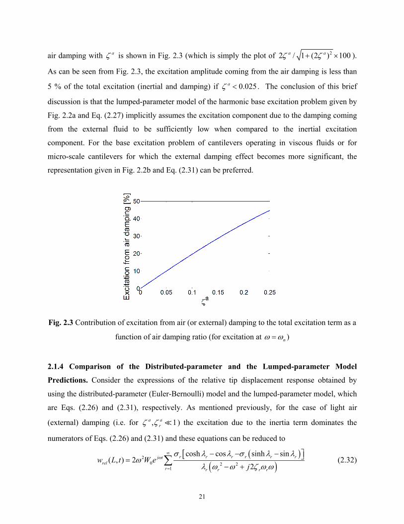
21

air damping with a is shown in Fig. 2.3 (which is simply the plot of 22 / 1 (2 ) 100a a ).

As can be seen from Fig. 2.3, the excitation amplitude coming from the air damping is less than

5 % of the total excitation (inertial and damping) if 0.025a . The conclusion of this brief

discussion is that the lumped-parameter model of the harmonic base excitation problem given by

Fig. 2.2a and Eq. (2.27) implicitly assumes the excitation component due to the damping coming

from the external fluid to be sufficiently low when compared to the inertial excitation

component. For the base excitation problem of cantilevers operating in viscous fluids or for

micro-scale cantilevers for which the external damping effect becomes more significant, the

representation given in Fig. 2.2b and Eq. (2.31) can be preferred.

Fig. 2.3 Contribution of excitation from air (or external) damping to the total excitation term as a

function of air damping ratio (for excitation at n )

2.1.4 Comparison of the Distributed-parameter and the Lumped-parameter Model

Predictions. Consider the expressions of the relative tip displacement response obtained by

using the distributed-parameter (Euler-Bernoulli) model and the lumped-parameter model, which

are Eqs. (2.26) and (2.31), respectively. As mentioned previously, for the case of light air

(external) damping (i.e. for , 1a ar ) the excitation due to the inertia term dominates the

numerators of Eqs. (2.26) and (2.31) and these equations can be reduced to

20 2 2

1

cosh cos sinh sin( , ) 2

2r r r r r rj t

relr r r r r

w L t W ej

(2.32)

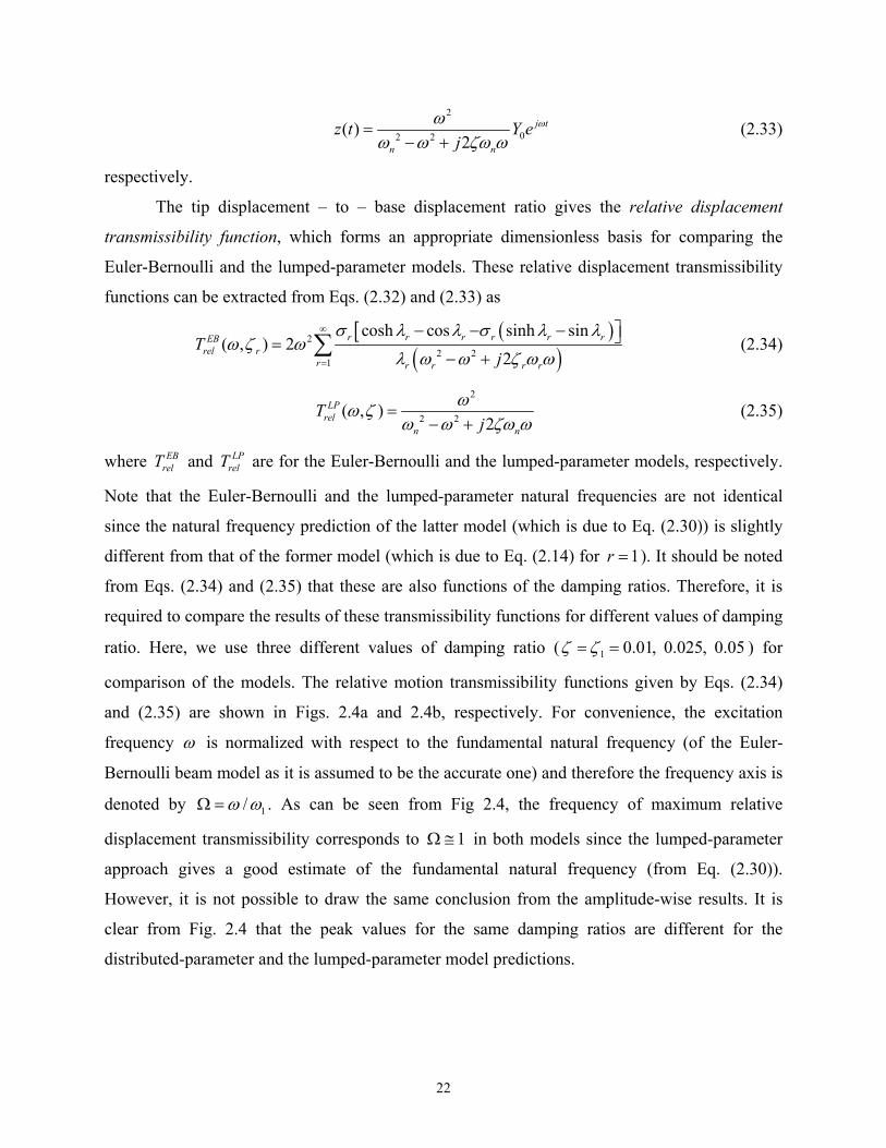
22

2

02 2( )

2j t

n n

z t Y ej

(2.33)

respectively.

The tip displacement – to – base displacement ratio gives the relative displacement

transmissibility function, which forms an appropriate dimensionless basis for comparing the

Euler-Bernoulli and the lumped-parameter models. These relative displacement transmissibility

functions can be extracted from Eqs. (2.32) and (2.33) as

2

2 21

cosh cos sinh sin( , ) 2

2r r r r r rEB

rel rr r r r r

Tj

(2.34)

2

2 2( , )

2LP

reln n

Tj

(2.35)

where EBrelT and LP

relT are for the Euler-Bernoulli and the lumped-parameter models, respectively.

Note that the Euler-Bernoulli and the lumped-parameter natural frequencies are not identical

since the natural frequency prediction of the latter model (which is due to Eq. (2.30)) is slightly

different from that of the former model (which is due to Eq. (2.14) for 1r ). It should be noted

from Eqs. (2.34) and (2.35) that these are also functions of the damping ratios. Therefore, it is

required to compare the results of these transmissibility functions for different values of damping

ratio. Here, we use three different values of damping ratio ( 1 0.01, 0.025, 0.05 ) for

comparison of the models. The relative motion transmissibility functions given by Eqs. (2.34)

and (2.35) are shown in Figs. 2.4a and 2.4b, respectively. For convenience, the excitation

frequency is normalized with respect to the fundamental natural frequency (of the Euler-

Bernoulli beam model as it is assumed to be the accurate one) and therefore the frequency axis is

denoted by 1/ . As can be seen from Fig 2.4, the frequency of maximum relative

displacement transmissibility corresponds to 1 in both models since the lumped-parameter

approach gives a good estimate of the fundamental natural frequency (from Eq. (2.30)).

However, it is not possible to draw the same conclusion from the amplitude-wise results. It is

clear from Fig. 2.4 that the peak values for the same damping ratios are different for the

distributed-parameter and the lumped-parameter model predictions.

23

Fig. 2.4 Relative motion transmissibility functions for the transverse vibrations of a cantilevered

beam without a tip mass; (a) distributed-parameter model and (b) lumped-parameter model

The percentage error in the lumped-parameter solution as a function of dimensionless

frequency ratio is given by Fig. 2.5 (relative to the Euler-Bernoulli model). As can be seen from

Fig 2.5, the relative error due to using the lumped-parameter approach in predicting the relative

motion at the tip of the beam is very large. In the vicinity of the first natural frequency (i.e. for

1 ), the error of the lumped-parameter model can be greater than 35 % regardless of the

damping ratio. The interesting behavior in the relative error plot around the resonance is due to

the 1.5 % error in the natural frequency predicted by the lumped-parameter approach. If the

lumped-parameter natural frequency were taken to be identical to the first natural frequency of

the Euler-Bernoulli model, one would obtain a smooth behavior in the error. Figure 2.5 shows

Fig. 2.5 Error in the relative motion transmissibility due to using the lumped-parameter model

for a cantilevered beam without a tip mass in transverse vibrations

(a) (b)

24

that the important error is in the prediction of the relative motion amplitude rather than the

natural frequency. The error in the lumped-parameter model increases drastically at higher

frequencies since higher vibration modes cannot be captured by the lumped-parameter approach.

2.2 Correction of the Lumped-parameter Model for Transverse Vibrations

2.2.1 Correction Factor for the Lumped-parameter Model. Since much of the vibration

energy harvesting literature uses lumped-parameter modeling for design and optimization

[2,3,8,10,13,16,22,27,28,31], a correction factor is presented for using the simplified lumped-

parameter model. Consider the relative motion transmissibility function of the Euler-Bernoulli

model given by Eq. (2.34). If the beam is excited around its first natural frequency, taking only

the first term in the summation sign (neglecting the terms for 2r ) gives a good approximation

for the resulting motion transmissibility. This reduced form of the Euler-Bernoulli model

solution is denoted by EBrelT :

2

* 12 2

1 1

( , )2

EBrelT

j

(2.36)

which can reduced to

2

12

( , )1 2

EBrelT

j

(2.37)

where 1/ is used and 1 corrects the excitation amplitude for the first transverse

vibration mode of a cantilevered Euler-Bernoulli beam without a tip mass (for predicting the

vibration response at x L ). Using 1 1.87510407 and 1 0.734095514 obtained from Eqs.

(2.11) and (2.12) gives the correction factor for the first mode as

1 1 1 1 1 11

1

2 cosh cos sinh sin1.566

(2.38)

It should be noted from Eqs. (2.35) and (2.36) that the reduced form of the Euler-Bernoulli

solution for the first mode is indeed the correction factor 1 multiplied by the lumped-parameter

solution (assuming that the lumped-parameter model natural frequency is accurate so that

1/ / n ). Therefore, 1 corrects the amplitude of the relative motion obtained from

the lumped-parameter solution. The comparison of the relative motion transmissibility functions

25

obtained by using the Euler-Bernoulli model, the lumped-parameter model and the corrected

lumped-parameter model are given in Fig. 2.6 for 0.05 . The agreement between the Euler-

Bernoulli model (Eq. (2.34)) and the corrected lumped-parameter model (Eq. (2.36)) is very

good over a wide frequency range around the fundamental resonance frequency and the

corrected lumped-parameter relative motion transmissibility function starts deviating close to the

region of the second natural frequency. The original lumped-parameter model prediction with

Eq. (2.35) underestimates the relative motion transmissibility amplitude considerably with an

error of about at least 35 % (see Fig. 2.5).

Fig. 2.6 Relative motion transmissibility functions obtained from the distributed-parameter,

corrected lumped-parameter and the original lumped-parameter models for 0.05

If the beam is to be excited not at the first natural frequency but at one of the higher mode

frequencies, one can obtain the correction factor of the mode of interest (r-th mode) from the

following relation

2 cosh cos sinh sinr r r r r rr

r

(2.39)

and then use it in the following expression of reduced relative motion transmissibility

2

2( , )

1 2EB r r

rel r rr r r

Tj

(2.40)

where the dimensionless frequency ratio is now /r r and r is the undamped natural

frequency of the r-th mode obtained from Eq. (2.14) and r is the modal damping ratio of the r-

26

th mode. Note that, since the modal parameters r and r do not depend on the aspect ratio of

the beam in the Euler-Bernoulli beam theory, the correction factor r of the r-th mode is unique

in the absence of a tip mass. That is, the correction factor for the fundamental mode is 1 1.566

for any uniform cantilevered Euler-Bernoulli beam without a tip mass in transverse vibrations

(so long as the beam aspect ratio justifies the Euler-Bernoulli beam assumptions).** However, the

presence of a tip mass affects the correction factor which is discussed in the following section.

2.2.2 Effect of a Tip Mass on the Correction Factor. In some cases, it is required to attach a

tip mass (proof mass) to the beam in order to tune its fundamental natural frequency to the

excitation frequency and to improve its dynamic flexibility. If the differential eigenvalue

problem is solved for a uniform cantilevered beam with a tip mass of tM rigidly attached at

x L , the eigenfunctions can be obtained as††

( ) cos cosh sin sinhr r r rr r rx C x x x x

L L L L

(2.41)

where r is obtained from

sin sinh cos cosh

cos cosh sin sinh

tr r r r r

rt

r r r r r

M

mLM

mL

(2.42)

and rC is a modal amplitude constant which should be evaluated by normalizing the

eigenfunctions according to the following orthogonality conditions:

** In the discussion given here, the correction factor is defined to predict the motion exactly at the tip. It should be

noted that distributed-parameter modeling allows predicting the motion transmitted from the base to any arbitrary

point of the beam. In such a case the numerical value of the correction factor obviously changes (e.g. 1

takes a

value lower that 1.566 for the fundamental mode) but it is still independent of the aspect ratio as long as the beam is

sufficiently thin, geometrically and materially uniform and linear vibrations are considered. †† Here, it is assumed that the uniform thin beam with a tip mass can be approximated as a normal-mode system so

that the eigenfunctions of the undamped problem can be used for modal analysis of the damped problem [38]. Banks

et al. [43] pointed out the mathematical limitations of the normal-mode assumption for combined dynamical

systems, i.e. distributed-parameter systems with discrete elements.

27

0

4 32

4 30

( ) ( ) ( ) ( )

( ) ( )( ) ( )

L

s r s t r rs

Lr r

s s r rs

x L

x m x dx L M L

d x d xx YI dx x YI

dx dx

(2.43)

The natural frequency expression given by Eq. (2.14) still holds but the dimensionless

eigenvalues ( r for the r-th mode) should be obtained from

1 cos cosh cos sinh sin cosh 0tMmL

(2.44)

where /tM mL is a dimensionless parameter as it is the tip mass – to – beam mass ratio. In the

above equations, the rotary inertia of the tip mass is neglected for convenience, i.e. the tip mass

is assumed to be a point mass.

In addition to the modification of the eigenvalue problem in the presence of a tip mass,

the forcing term due to base excitation also changes since the tip mass also contributes to the

inertia of the structure. Equation (2.5) becomes

4 5 2 2

4 4 2 2

( , ) ( , ) ( , ) ( , ) ( , )( )rel rel rel rel b

s a t

w x t w x t w x t w x t w x tYI c I c m m M x L

x x t t t t

(2.45)

where ( )x is the Dirac delta function and the forcing term due to external damping is neglected.

The modal forcing function corresponding to the right hand side of Eq. (2.45) is then

2 2 2 2

2 2 2 20 0

( ) ( ) ( ) ( )( ) ( ) ( ) ( )

L L

r r r t r

d g t d h t d g t d h tf t m x dx x x dx M L L

dt dt dt dt

(2.46)

Expectedly, the foregoing modification results in variation of the correction factor

defined in the previous section. Since the base is assumed to be not rotating (i.e. ( ) 0h t ) in

deriving the correction factor, one can extract the expression of the correction factor 1 in the

presence of a tip mass as

1 1 1 1

0

( ) ( ) ( )L

tL M L m x dx

(2.47)

The variation of the correction factor 1 of the fundamental transverse vibration mode given by

Eq. (2.47) with tip mass ( tM ) – to – beam mass ( mL ) ratio is shown in Fig. 2.7.

28

Fig. 2.7 Variation of the correction factor for the fundamental transverse vibration mode with tip

mass – to – beam mass ratio

It can be read from Fig. 2.7 that when there is no tip mass ( / 0tM mL ), 1 1.566 as

previously obtained, whereas as /tM mL becomes larger ( /tM mL ), 1 approaches to

unity. The important conclusion drawn from Fig. 2.7 is that the uncorrected lumped-parameter

model can be used safely only when the tip mass is sufficiently larger than the beam mass. From

the physical point of view, if the tip mass is sufficiently large, the inertia of the tip mass

dominates in the forcing function and the distributed inertia of the beam (as a component of

excitation) becomes negligible. Table 2.1 shows the values 1 takes for different /tM mL ratios.

It should be noted that, for the uncorrected lumped-parameter formulation 1 1 , and therefore,

the relative error in the motion at the tip of the beam predicted by the uncorrected lumped-

parameter model is estimated from 1 11 / 100 .

The following quadratic polynomial ratio obtained by using the Curve Fitting Toolbox of

MATLAB [44] gives an estimate of 1 with an error less than 39 10 % for all values of

/tM mL :

2

1 2

/ 0.603 / 0.08955

/ 0.4637 / 0.05718t t

t t

M mL M mL

M mL M mL

(2.48)

29

Table 2.1 Correction factor for the fundamental transverse vibration mode and the error in the

uncorrected lumped-parameter model for different tip mass – to – beam mass ratios

/tM mL 1 Error in the uncorrected

lumped-parameter model [%]

0 1.56598351 -36.14

0.1 1.40764886 -28.96

0.5 1.18922917 -15.91

1 1.11285529 -10.14

5 1.02662125 -2.59

10 1.01361300 -1.34

2.3 Experimental Case Studies for Validation of the Correction Factor

This section provides experimental demonstrations for the use of the correction factor in order to

improve the predictions of the lumped-parameter base excitation model in the absence and

presence of a tip mass. The bimorph cantilever discussed in the following is investigated

extensively in Chapter 4 for validation of the distributed-parameter electromechanical models

developed in Chapter 3. Detailed information regarding the cantilever and the experimental setup

can therefore be found in Chapter 4. Here, only the motion transmissibility FRFs are considered

in order to validate the amplitude correction factor derived in this chapter. Each one of the two

cases presented here uses the measurement taken for an external electrical load close to short-

circuit conditions of the electrodes (very low external impedance). Therefore, the following cases

can be considered as very close to being electromechanically uncoupled (i.e. having negligible

piezoelectric shunt damping effect), in agreement with the formulation given in this chapter

(where the purpose is to improve the mechanical aspect of the existing lumped-parameter

electromechanical model). The electromechanically coupled distributed-parameter dynamics of

these configurations are modeled and validated in Chapters 3 and 4, respectively.

2.3.1 Cantilevered Beam without a Tip Mass under Base Excitation. The cantilever

considered here is a T226-H4-203X type bimorph manufactured by Piezo Systems, Inc. [45].

30

Detailed electromechanical analysis of this sample can be found in Section 4.1. Here, the

experimental data for a 470 load resistance (close to short-circuit conditions) is considered to

validate the corrected lumped-parameter base excitation relation given by Eq. (2.36) and to

demonstrate the failure of the original relation given by Eq. (2.35) in predicting the vibration

response. It should be noted from Table 4.1 that the overhang length, width and the thickness of

the cantilever are 24.53 mm, 6.4 mm and 0.670 mm, respectively. Therefore the overhang length

– to – total thickness ratio of the bimorph cantilever is about 37.7 and the Euler-Bernoulli

formulation can safely be used as far as the fundamental vibration mode is concerned.

Fig. 2.8 Experimental setup used for the frequency response measurements of a uniform bimorph

cantilever (photos by A. Erturk, 2009)

The experimental setup used for the frequency response measurement is shown in Fig.

2.8 (referred from Chapter 4). The bimorph cantilever is clamped onto a small electromagnetic

shaker (TMC Model TJ-2 [46]). A small accelerometer (PCB Piezotronics Model U352C67 [47])

is attached via wax close to the root of the cantilever on the clamp. The tip velocity response of

the cantilever is measured using a laser vibrometer (Polytec PDV100 [48]) by attaching a small

reflector tape at the tip of the cantilever (see Fig. 2.9a for an enlarged view). Chirp excitation

(burst type with five averages) is used for the frequency response measurement through the data

acquisition system (SigLab Model 20-42) [49]. The ratio of the vibrometer measurement to the

(1)

(2)(3) (4)

(5)(6)

(1)

(1) Shaker with a small accelerometer and the cantilever (2) Laser vibrometer (3) Fixed gain amplifier (power supply) (4) Charge amplifier (5) Data acquisition system (6) Frequency response analyzer (software)

31

acceleration measurement in the frequency domain defines the tip velocity – to – base

acceleration FRF.

Fig. 2.9 Close views of the cantilever tested under base excitation (a) without and (b) with a tip

mass attachment (photos by A. Erturk, 2009)

It is important to note that the laser vibrometer measures the velocity response at the

center of the reflector tape that is attached near the tip of the cantilever (i.e. not exactly at x L ).

If the point of the velocity measurement is vx L , Eq. (2.47) should be modified to

*1 1 1 1

0

( ) ( ) ( )L

v tL M L m x dx

(2.49)

where *1 is the modified form of the correction factor that accounts for the small distance of the

point of velocity measurement from the tip. In the experiments, the position of the velocity

measurement on the cantilever is 23vL mm from the root (i.e. approximately 1.5 mm from the

tip). For this point of velocity measurement, the variation of the correction factor with tip mass –

to – beam mass ratio is given by Fig. 2.10. In the absence of a tip mass, the modified correction

factor is *1 1.431 and it can be used in Eq. (2.36) to predict the vibratory motion at vx L .

It should also be noted at this stage that the theoretical discussion given so far is for the

tip displacement – to – base displacement FRF. However, the measurements taken with this

experimental setup are the tip velocity and the base acceleration of the cantilever. Moreover, the

experimental velocity measurement is relative to the fixed frame, i.e. it is not the tip velocity of

the cantilever relative to its moving base. One option for comparing the experimental data and

the analytical predictions is to process the experimentally measured FRF to bring it to the form

(a) (b)

32

of Eqs. (2.35) and (2.36). The second option is to bring the analytical relative displacement

transmissibility functions given by these equations to the form of the experimental measurement.

The second option is preferred in order not to create a possible noise in the experimental data due

to post-processing. The relative displacement transmissibility FRF (Eqs. (2.35) and (2.36)) can

be used in the following relation to give the absolute tip velocity – to – base acceleration FRF as

20

( , )

1 ( , )vx L rel

j t

w x tt T

W e j

(2.50)

In addition, the experimental FRFs are given per gravitational acceleration ( 9.81g m/s2), i.e.

Eq. (2.50) should be multiplied by g in order to compare with the experimental data.

Fig. 2.10 Variation of the modified correction factor for the fundamental transverse vibration

mode with tip mass – to – beam mass ratio

Figure 2.11a shows the experimental frequency response measurement and its prediction

by Eqs. (2.35) and (2.36) (when used in Eq. (2.50)). The undamped natural frequency of the

cantilever (close to short-circuit conditions) is 502.5 Hz ( 3157.3n rad/s) and the mechanical

damping ratio identified in Section 4.1 is 0.874 % ( 0.00874 ). As can be seen in Fig. 2.11b,

the coherence [50,51] of the measurement is very good (unity). Therefore the measurement is

reliable for the frequency range of interest.

33

Since the cantilever does not have a tip mass ( / 0tM mL ), the modified amplitude

correction factor is obtained from Eq. (2.49) or from Fig 2.10 as *1 1.431 . It is observed from

Fig. 2.11a that the corrected lumped-parameter model (due to Eq. (2.36)) is in very good

agreement with the experimental FRF whereas the uncorrected lumped-parameter model (due to

Eq. (2.35)) underestimates the vibration amplitude considerably (note that the vertical axis in

Fig. 2.11a is given in log-scale).‡‡ Therefore, in agreement with the theoretical discussion given

with Fig. 2.6, the commonly referred form of the lumped-parameter base excitation model results

in significantly inaccurate prediction of the vibration response in the absence of a tip mass. The

inaccurate prediction is in the form of underestimation of the vibration response amplitude.

Fig. 2.11 (a) Tip velocity – to – base acceleration FRFs of a cantilever without a tip mass:


model predictions; (b) coherence function of the experimental measurement

2.3.2 Cantilevered Beam with a Tip Mass under Base Excitation. The second case study is

given for the same cantilever after a tip mass of 0.239 grams is attached at the tip using a slight

amount of wax (Fig. 2.9b). Detailed electromechanical analysis of the cantilever with a tip mass

is given in Section 4.2. The demonstration given here aims to estimate the correction factor and

‡‡ The form of the uncorrected lumped-parameter equation given by Eq. (2.35) is originally defined to predict the tip

motion but the experimental measurement belongs to the point v

x L . Nevertheless since this lumped-parameter

expression underestimates the motion amplitude at v

x L it would certainly underestimate the motion amplitude at

the exact point of x L where the vibration amplitude is larger for the fundamental mode.

(a) (b)

34

to verify the need for using it. For this tip mass ( 30.239 10tM kg) and for the numerical data

of the cantilever given with Table 4.4, the tip mass – to – beam mass ratio is / 0.291tM mL .

This ratio yields *1 1.149 either using Eq. (2.49) or Fig. 2.10. As discussed theoretically, in

the presence of a tip mass, predictions of the original lumped-parameter equation are not

expected to be as inaccurate as the case when there is no tip mass. Recall that, in the extreme

case of having a very large tip mass, the correction factor is not required. However, in this

experimental case study, the tip mass is not large enough to ignore the excitation coming from

the distributed mass of the cantilever.

Figure 2.12a shows the experimental tip velocity – to – base acceleration FRF (for a

470 load resistance) along with the predictions of Eqs. (2.35) and (2.36) when used in Eq.

(2.50). As can be seen from the enlarged view in Fig. 2.11a, the uncorrected lumped-parameter

model underestimates the experimental measurement but the error is not as large as in the case of

Fig. 2.11a. The prediction of the corrected lumped-parameter equation (obtained using

*1 1.149 in Eq. (2.36)) agrees very well with the experimental data.

Fig. 2.12 (a) Tip velocity – to – base acceleration FRFs of a cantilever with a tip mass:


model predictions; (b) coherence function of the experimental measurement

(a) (b)

35

2.4 Base Excitation Problem for Longitudinal Vibrations and Correction of Its Lumped-

parameter Model

So far the base excitation problem of a beam in transverse vibrations has been discussed in detail

and experimental validations have been provided for its corrected lumped-parameter model. This

section summarizes the same problem for longitudinal vibrations of a uniform cantilevered bar

under base excitation (Fig. 2.13). As in the case of transverse vibrations, the electromechanically

uncoupled problem is considered in order to correct the excitation amplitude of its lumped-

parameter model.

Fig. 2.13 Cantilevered bar with a tip mass longitudinally excited by the translation of its base

2.4.1 Analytical Modal Analysis and Steady-state Response to Harmonic Base Excitation.

The uniform clamped-free bar shown in Fig. 2.13 is subjected to the arbitrary translation of its

base, which is denoted by ( )bu t . The equation of motion for the longitudinal free vibrations of a

uniform bar can be written as

2 3 2

2 2 2

( , ) ( , ) ( , ) ( , )0s a

u x t u x t u x t u x tYA c A c m

x x t t t

(2.51)

where YA is the axial stiffness (Y is the elastic modulus and A is the cross-sectional area) and m

is the mass per unit length of the bar. The absolute longitudinal displacement at any point x can

be represented by ( , ) ( ) ( , )b relu x t u t u x t . The damping mechanism is again represented by two

terms: sc is due to internal (structural) friction and ac accounts for external viscous (air)

damping.§§ Proportional damping is assumed as it allows analytical modal analysis.

§§ Although the same notation is used for some of the terms (such as the damping coefficients) of the transverse

vibrations case, they are not necessarily identical.

z

x

( )bu t

YA, m

0x x L

tM

36

After following steps similar to the derivation given for the transverse vibrations case in

Section 2.1, the longitudinal vibration response of the bar relative to its moving base can be

obtained as

( )

1 0

( )( , ) ( ) sin ( )r r

ttr

rel r rdr rd

xu x t f e t d

(2.52)

Here, the modal forcing function is

2

20

( )( ) ( ) ( )

Lb

r r t r

d u tf t m x dx M L

dt

(2.53)

where the forcing term due to air damping is neglected. It should be noted from Eq. (2.53) that

the excitation coming from the tip mass is directly considered in the modal forcing.

The undamped natural frequency r of the r-th vibration mode is obtained from

2r r

EA

mL (2.54)

and rd in Eq. (2.52) is the damped natural frequency given by 21rd r r where r is the

modal damping ratio of the r-th vibration mode. The mass normalized eigenfunction ( )r x of

the r-th mode can be expressed as

2

1( ) sin

sin 21 sin

2 2

rr

rt r

r

x xLmL

M

(2.55)

Along with the geometric and natural boundary conditions at 0x and x L , respectively, the

eigenfunctions given by Eq. (2.55) satisfy the following orthogonality conditions:

0

22

20

( ) ( ) ( ) ( )

( ) ( )( ) ( )

L

s r s t r rs

Lr r

s s r rsx L

x m x dx L M L

d x d xx YA dx x YA

dx dx

(2.56)

The eigenvalues ( r for mode r) are the roots of the characteristic equation

sin cos 0tM

mL (2.57)

For a harmonic base displacement input, 0( ) j tbu t U e , the steady-state displacement response

relative to the moving base becomes

37

20

1 2 2 2

1 cossin sin

( , )2 sin 2

sin 24

j ttrr r

rrel

r tr rr r r r

r

MU e

mLu L t

Mj

mL

(2.58)

2.4.2 Correction Factor for Longitudinal Vibrations. The relative motion transmissibility

between the tip of the bar and the moving base can be extracted from Eq. (2.58) as

2

2 210

( , )( , )

2rel r

rel r j tr r r r

u L tT

U e j

(2.59)

where

2

1 cossin sin

2 sin 2sin

4

trr r

rr

tr rr

r

M

mLM

mL

(2.60)

is the correction factor for the lumped-parameter model of the r-th mode for longitudinal

vibrations (to predict the vibratory motion at x L ). Note that, r is a function of /tM mL and

r due to Eq. (2.60), and r is a function of /tM mL from Eq. (2.57). Therefore, for a given

vibration mode, the correction factor r is a function of /tM mL only. In the absence of a tip

mass ( / 0tM mL ), the correction factor for the fundamental mode can explicitly be obtained

from Eqs. (2.57) and (2.60) as 1 4 / 1.273 . However, in the presence of a tip mass, the

transcendental equation given by Eq. (2.57) should be solved numerically to obtain the

correction factor. The variation of the correction factor of the fundamental mode ( 1 ) with

/tM mL is given in Fig. 2.14.

As in the transverse vibrations case, the correction factor tends to unity as the tip mass to

beam mass ratio increases, meaning that the uncorrected lumped-parameter model can be used

only for bars whose tip mass is much larger than the bar mass. Table 2.2 shows the correction

factor 1 for lumped-parameter modeling of the fundamental longitudinal vibration mode for

different /tM mL ratios. Note that the error in the relative motion relu at the tip of the bar

predicted by using the uncorrected lumped-parameter model is simply obtained from

1 11 / 100 .

38

Fig. 2.14 Variation of the correction factor for the fundamental longitudinal vibration mode with

tip mass – to – beam mass ratio

The following quadratic polynomial ratio obtained by using the Curve Fitting Toolbox of

MATLAB [44] represents the behavior of the correction factor shown in Fig. 2.14 successfully

with a maximum error less than 24.5 10 % for all values of /tM mL :

2

1 2

/ 0.7664 / 0.2049

/ 0.6005 / 0.161t t

t t

M mL M mL

M mL M mL

(2.61)

Table 2.2 Correction factor for the longitudinal vibration mode and the error in the uncorrected

lumped-parameter model for different tip mass – to – bar mass ratios

/tM mL 1 Error in the uncorrected

lumped-parameter model [%]

0 1.27323954 -21.46

0.1 1.26196259 -20.76

0.5 1.17845579 -15.14

1 1.11913201 -10.65

5 1.03108765 -3.02

10 1.01609422 -1.58

39

2.5 Correction Factor in the Electromechanically Coupled Lumped-parameter Equations

and a Theoretical Case Study

This section introduces the amplitude correction factor to the electromechanically coupled

lumped-parameter piezoelectric energy harvester equations. The lumped-parameter

electromechanical equations of a piezoelectric energy harvester are obtained by applying

Newton’s second law (or d’Alembert’s principle) in the mechanical domain, Kirchhoff’s laws in

the electrical domain and also including the electromechanical coupling effects coming from the

piezoelectric constitutive relations [26].

2.5.1 An Electromechanically Coupled Lumped-parameter Model for Piezoelectric Energy

Harvesting. Recently, a lumped-parameter piezoelectric energy harvester model was introduced

by duToit et al. [16]. Figure 2.15 shows the schematic of their cantilevered energy harvester

which is excited by the motion of its base in the longitudinal direction. Therefore, this model

uses longitudinal vibrations of the piezoceramic for power generation. The design depicted in

Fig. 2.15 for longitudinal vibrations (almost like an accelerometer) typically results in a very

high fundamental natural frequency, which is not preferred for vibration energy harvesting as it

will not match with typical ambient vibration frequencies. Nevertheless this lumped-parameter

representation provides useful insight into the electromechanical problem for a simplified

analysis of the coupled system dynamics.

Fig. 2.15 A lumped-parameter piezoelectric energy harvester model with sample numerical

values by duToit et al. [16] (reproduced by adapting the displacement variables to this text)

40

As the longitudinal strain and the electric field directions are the same, the device shown

in Fig. 2.15 uses the 33-mode of piezoelectricity (and therefore the 33d constant of the

piezoceramic) where 3-direction (poling direction) is the longitudinal direction. The electrodes

are connected to an equivalent resistive load eqR (which is the parallel combination of the

piezoelectric leakage resistance pR and the load resistance lR where l pR R hence eq lR R ).

The coupled lumped-parameter equations are given by duToit et al. [16] as***

2 22 2

332 22rel rel b

m n n rel n

d u du d uu d v

dt dt dt (2.62)

233 0rel

eq p eq eq n

dudvR C v m R d

dt dt (2.63)

where eqm is the equivalent mass of the bar, m is the mechanical damping ratio, n is the

natural frequency, 33d is the piezoelectric constant, eqR is the equivalent resistance, pC is the

capacitance, bu is the harmonic base excitation, relu is the relative displacement of the proof

mass and v is the voltage output. One can then obtain the steady-state vibration response, voltage

output and the power output FRFs (per base acceleration) by assuming 0( ) j tbu t U e as

22

222 2 3

1/ 1

1 1 2 1 2

nrel

bm e m

ru

ur k r r

(2.64)

33

222 2 31 1 2 1 2

eff eq n

bm e m

m R dv

ur k r r

(2.65)

2 2

2 222 2 3

1/ /

1 1 2 1 2

eff n e eq l

b m e m

m rk R RP

u r k r r

(2.66)

where / n is the dimensionless frequency, ek is the lumped-parameter coupling

coefficient and n eq pr R C [16].

2.5.2 Correction Factor in the Electromechanically Coupled Lumped-parameter Model

and a Theoretical Case Study. From the theoretical discussion given in Section 2.4, it is known

*** Some of the variables have been adapted to the notation of this text.

41

that the right hand side of the mechanical equilibrium equation given by Eq. (2.62) should have a

correction factor (to be valid for all values of the proof mass). Therefore the corrected form of

Eq. (2.62) is

2 2

2 233 12 2

2rel rel bm n n rel n

d u du d uu d v

dt dt dt (2.67)

Then the steady-state vibration response, voltage and the power output FRFs given by Eqs.

(2.64)-(2.66) become

221

222 2 3

/ 1

1 1 2 1 2

nrel

bm e m

ru

ur k r r

(2.68)

1 33

222 2 31 1 2 1 2

eff eq n

bm e m

m R dv

ur k r r

(2.69)

2 2 21

2 222 2 3

1/ /

1 1 2 1 2

eff n e eq l

b m e m

m rk R RP

u r k r r

(2.70)

Note that the steady-state vibration response and the voltage response are linearly proportional to

1 . However, since it is proportional to the square of the voltage, the power output is

proportional to the square of 1 . Hence the inaccuracy of the predicted power output due to

using Eq. (2.66) is expected to be more significant than that of the vibration amplitude or the

voltage output.

Using the numerical values given Fig. 2.15 (referred from duToit et al. [16]), the tip mass

– to – bar mass ratio of this sample device is obtained as / 1.33tM mL . From Eq. (2.61), the

correction factor for the fundamental mode for this ratio is 1 1.0968 . If this factor is not used,

the relative error in the predicted proof mass motion and the voltage output is about 8.83 %

whereas the relative error in the estimated power output is about 16.9 %. Figure 2.16 shows the

vibration and the power FRFs obtained using the uncorrected and the corrected equations for an

arbitrary load resistance of 10 k and a base acceleration of 9.81 m/s2.

The inaccuracy due to ignoring the contribution of the distributed mass of the structure to

the excitation amplitude is also the case in the lumped-parameter model given by Roundy et al.

[6,7,15] for transverse vibrations (unless the tip mass is very large).

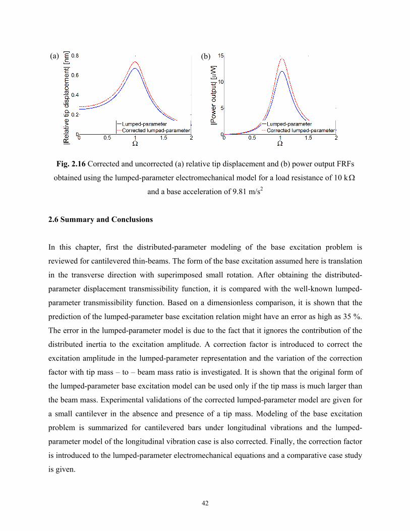
42

Fig. 2.16 Corrected and uncorrected (a) relative tip displacement and (b) power output FRFs

obtained using the lumped-parameter electromechanical model for a load resistance of 10 k

and a base acceleration of 9.81 m/s2

2.6 Summary and Conclusions

In this chapter, first the distributed-parameter modeling of the base excitation problem is

reviewed for cantilevered thin-beams. The form of the base excitation assumed here is translation

in the transverse direction with superimposed small rotation. After obtaining the distributed-

parameter displacement transmissibility function, it is compared with the well-known lumped-

parameter transmissibility function. Based on a dimensionless comparison, it is shown that the

prediction of the lumped-parameter base excitation relation might have an error as high as 35 %.

The error in the lumped-parameter model is due to the fact that it ignores the contribution of the

distributed inertia to the excitation amplitude. A correction factor is introduced to correct the

excitation amplitude in the lumped-parameter representation and the variation of the correction

factor with tip mass – to – beam mass ratio is investigated. It is shown that the original form of

the lumped-parameter base excitation model can be used only if the tip mass is much larger than

the beam mass. Experimental validations of the corrected lumped-parameter model are given for

a small cantilever in the absence and presence of a tip mass. Modeling of the base excitation

problem is summarized for cantilevered bars under longitudinal vibrations and the lumped-

parameter model of the longitudinal vibration case is also corrected. Finally, the correction factor

is introduced to the lumped-parameter electromechanical equations and a comparative case study

is given.

(a) (b)

43

CHAPTER 3

DISTRIBUTED-PARAMETER ELECTROMECHANICAL MODELING

OF BIMORPH PIEZOELECTRIC ENERGY HARVESTERS –

ANALYTICAL SOLUTIONS

In this chapter, electromechanically coupled analytical solutions are given for symmetric

bimorph piezoelectric energy harvester configurations with series and parallel connections of the

piezoceramic layers. The base excitation acting on the bimorph cantilever is assumed to be

translation in the transverse direction with superimposed small rotation. After describing the

modeling assumptions and the bimorph configurations, the distributed-parameter thin beam

equation (the Euler-Bernoulli beam equation) with piezoelectric coupling is derived and its

modal analysis in short-circuit conditions is given. The electromechanically coupled circuit

equation excited by infinitely many vibration modes is then derived based on the Gauss’s law

and the plane-stress piezoelectric constitutive relation for a thin beam. The governing

electromechanical equations are then reduced to ordinary differential equations in modal

coordinates and eventually an infinite set of algebraic equations are obtained for the complex

modal vibration response and the complex voltage response amplitudes of the energy harvester

beam. For the series and parallel connections of the piezoceramic layers, the closed-form

electromechanical expressions are first obtained for the steady-state response to harmonic

excitation at arbitrary frequencies. The resulting analytical multi-mode expressions are then

simplified to single-mode expressions by assuming modal excitation (i.e. excitation at or very

close to a particular natural frequency), which is the main concern in vibration-based energy

harvesting. The single-mode relations derived here are easier to use compared to the multi-mode

solutions but they provide approximations only around the respective resonance frequency. The

electromechanical FRFs which relate the voltage output and the vibration response of the

bimorph to the translational and the rotational base acceleration components are extracted both

for the multi-mode and single-mode solutions. A detailed theoretical case study is presented at

the end of this chapter. Experimental validations of the analytical solutions derived here are

presented in Chapter 4.

44

3.1 Fundamentals of the Electromechanically Coupled Distributed-parameter Model

3.1.1 Modeling Assumptions and Bimorph Configurations. The symmetric bimorph

cantilever configurations shown in Fig. 3.1 are modeled here as uniform composite beams based

on the Euler-Bernoulli beam theory. This is a reasonable assumption since typical cantilevered

piezoelectric energy harvesters are designed and manufactured as fairly thin beams and most of

the commercially available bimorphs are also thin structures (e.g. the samples used in Chapter 4

for model validation). Deformations are assumed to be small and the composite structure exhibits

linear-elastic material behavior. The mechanical losses are represented by internal and external

damping mechanisms as done in the electromechanically uncoupled discussion of Chapter 2. The

internal damping mechanism is assumed to be in the form of strain-rate (or Kelvin-Voigt)

damping and the effect of external (air) damping is considered with a separate damping

coefficient. The piezoceramic and the substructure layers are assumed to be perfectly bonded to

each other. The electrodes covering the opposite faces of piezoceramic layers are assumed to be

very thin when compared to the overall thicknesses of the harvester so that their contribution to

the thickness dimension is negligible. In the following formulation, therefore, only the

substructure and piezoceramic layers are assumed to be present. However, presence of additional

structural epoxy and Kapton layers can be handled easily.*

The continuous electrode pairs covering the top and the bottom faces of the piezoceramic

layers are assumed to be perfectly conductive so that a single electric potential difference can be

defined across them. Therefore, the instantaneous electric fields induced in the piezoceramic

layers are assumed to be uniform throughout the length of the beam. A resistive electrical load

(denoted by lR in Fig. 3.1) is considered in the circuit along with the internal capacitances of the

piezoceramic layers. Note that, considering a resistive load in the electrical domain is a common

practice in modeling of vibration-based energy harvesters [14-22]. As a consequence, it is

assumed that the base motion input is persistent so that continuous electrical outputs can be

extracted from the electromechanical system. The leakage resistance of the piezoceramic is

ignored here as it is typically very large. It can easily be added as an additional resistance parallel

* With the inclusion of additional inactive layers, the bending stiffness and the mass per length terms will be altered.

In addition, distance of the piezoceramic layers from the neutral axis will be modified, which changes the

piezoelectric coupling terms in the derivation.

45

to the load resistance (as in the lumped-parameter model of duToit et al. [16] discussed in

Section 2.5).

Fig. 3.1 Bimorph piezoelectric energy harvester configurations with (a) series connection of

piezoceramic layers, (b) parallel connection of piezoceramic layers and the (c) cross-sectional

view of a uniform bimorph cantilever

It is known from the literature of static sensing and actuation that, depending on the

voltage or current requirements, the piezoceramic layers of a symmetric bimorph can be

combined in series or in parallel (see, for instance, Wang and Cross [52]). This common practice

of static sensing and actuation problems is valid for the dynamic piezoelectric energy harvesting

problem as well. Each of the two bimorph configurations displayed in Figs. 3.1a and 3.1b

undergoes bending vibrations due to the motion of its base. The piezoceramic layers are assumed

to be identical and their conductive electrodes are assumed to be fully covering the respective

surfaces of these layers (top and bottom). The instantaneous bending strain in the top and the

bottom layers at an arbitrary position x over the beam length have the opposite sign (i.e. one is in

(a)

(b)

(c)

46

tension whereas the other is in compression). As a consequence, since the piezoceramic layers of

the bimorph shown in Fig. 3.1a are poled oppositely in the thickness direction (i.e. z-direction),

this configuration represents the series connection of the piezoceramic layers. Likewise, Fig.

3.1b represents the parallel connection of the piezoceramic layers because the layers are poled in

the same direction. The configuration in Fig. 3.1a produces a larger voltage output whereas the

one in Fig. 3.1b produces a larger current output under the optimal conditions.

3.1.2 Coupled Mechanical Equation and Modal Analysis of Bimorph Cantilevers. As far as

the purely mechanical aspect of the problem is concerned, the bimorph configurations shown in

Figs. 3.1a and 3.1b are identical. That is, they have the same geometric and material properties.

However, the backward piezoelectric coupling effect† in the beam equation due to piezoelectric

constitutive relations is different for series and parallel connections of the piezoceramic layers,

and expectedly, this affects the vibration response of the cantilever. In the following, the beam

equations are derived for these two configurations and the analytical modal analysis relations are

presented.

The motion of the base for each of the cantilevers shown in Figs. 3.1a and 3.1b is

represented by translation ( )g t in the transverse direction with superimposed small rotation

( ).h t Therefore, the effective base displacement ( , )bw x t in the transverse direction can be

written as

( , ) ( ) ( )bw x t g t xh t (3.1)

The partial differential equation governing the forced vibrations of a uniform cantilevered

bimorph (with a tip mass) under base excitation is

5 2 22

2 4 2 2

( , ) ( , ) ( , ) ( , )( , )( )rel rel rel b

s a t

w x t w x t w x t w x tM x tc I c m m M x L

x x t t t t

(3.2)

† Throughout this text, the term backward coupling represents the electrical effect induced in the harvester structure

due to the converse piezoelectric effect (feedback sent from the electrical domain to the mechanical domain due to

power generation). Hence the forward coupling term (to be defined later) is the term in the circuit equation due to

the direct piezoelectric effect.

47

where ( , )relw x t is the transverse displacement of the beam (neutral axis) relative to its base at

position x and time t, ac is the viscous air damping coefficient, sc is the strain-rate damping

coefficient (appears as an effective term sc I for the composite structure), m is the mass per unit

length of the beam, tM it is tip mass and ( )x is the Dirac delta function and ( , )M x t is the

internal bending moment‡ (excluding the strain-rate damping effect). Recall from Eq. (2.7) that

the effect of strain-rate damping is an internal bending moment, which, in Eq. (3.2), is directly

written outside the undamped bending moment term ( , )M x t .

The bimorph cantilevers shown in Fig. 3.1 are assumed to be proportionally damped so

that these configurations are normal-mode systems. Hence the eigenfunctions of the respective

undamped problem can be used for modal analysis. Indeed, instead of defining the damping

coefficients in the physical equation of motion, one could consider the corresponding undamped

equation (by setting 0s ac I c in Eq. (3.2)) and introduce modal damping to the equation of

motion in modal coordinates as a common practice in structural dynamics [55]. It is worth

recalling that the foregoing consideration of the mechanical damping components results in an

additional excitation term (peculiar to base excitation problems) due to external damping as

shown in Section 2.1.1. For cantilevers operating in air, the external damping excitation is

negligible when compared to the inertial excitation term (Fig. 2.3). Therefore the damping

excitation term is directly omitted in Eq. (3.2) for simplicity.

The internal bending moment term in Eq. (3.2) is the first moment of axial strain over the

cross-section:

/2/2 /2

1 1 1

/2 /2 /2

( , )p ss s

p s s s

h hh hp s p

h h h h

M x t b T zdz T zdz T zdz

(3.3)

where b is the width, ph is the thickness of each piezoceramic layer and sh is the thickness of

each substructure layer (Fig. 1c). Furthermore, 1pT and 1

sT are the axial stress components in the

piezoceramic and the substructure layers, respectively (1-direction is the longitudinal direction,

i.e. x-direction), and they are given by the following constitutive relations:

‡ The convention for the bending moment is such that the positive bending moment creates negative curvature as in

Sokolnikoff [53] and Dym and Shames [54], among others.

48

1 1s s

sT Y S , 1 11 1 31 3

p E pT c S e E (3.4)

where sY is the elastic modulus (i.e., Young’s modulus) of the substructure layer (which can be

isotropic or orthotropic), 11Ec is the elastic modulus of the piezoceramic layer at constant electric

field, 31e is the effective piezoelectric stress constant and 3E is the electric field component in

the 3-direction (i.e. z-direction or the poling direction). Here and hereafter, the subscripts and

superscripts p and s stand for the piezoceramic and the substructure layers, respectively. Based

on the plane-stress assumption for a transversely isotropic thin piezoceramic beam (about the z-

direction), the elastic modulus component of the piezoceramic can be expressed as 11 111/E Ec s ,

where 11Es is the elastic compliance at constant electric field. Furthermore, based on the same

assumption, 31e can be given in terms of the more commonly used piezoelectric strain constant

31d as 31 31 11/ Ee d s (Appendix A.2). The axial strain components in the piezoelectric and

substructure layers are defined as 1pS and 1

sS , respectively, and they are due to bending only.

Hence the axial strain at a certain level (z) from the neutral axis of the symmetric composite

beam is simply proportional to the curvature of the beam at that position (x):§

2

1 2

( , )( , , ) relw x t

S x z t zx

(3.5)

The electric field component 3E should be expressed in terms of the respective voltage

term for each bimorph configuration (Figs. 3.1a and 3.1b). This is the point where the resulting

mechanical equations for the series and parallel connections of the piezoceramic layers differ

from each other. Since the piezoceramic layers are assumed to be identical, voltage across the

electrodes of each piezoceramic layer is ( ) / 2sv t in the series connection case (Fig. 3.1a).

Expectedly, for the parallel connection case (Fig. 3.1b), voltage across the electrodes of each

piezoceramic layer is ( )pv t . It is worth adding that 31e has the opposite sign for the top and the

bottom piezoceramic layers for the series connection case (due to opposite poling) so that the

§ An independent axial displacement variable (in x-direction) is not included in the strain expression since it

decouples from the equation of motion for transverse vibrations due to the symmetric composite structure [56].

Since there is no excitation in the axial direction, there is no strain contribution from the decoupled axial

displacement.

49

instantaneous electric fields are in the same direction (i.e. 3( ) ( ) / 2s pE t v t h in both layers). For

the configuration with parallel connection, since 31e has the same sign in top and bottom

piezoceramic layers, the instantaneous electric fields are in the opposite directions (i.e.,

3( ) ( ) /p pE t v t h in the top layer and 3( ) ( ) /p pE t v t h in the bottom layer). Another important

point is that, for both configurations, the piezoelectric coupling term coming from Eq. (3.3) is a

function of time only. Hence, before substituting Eq. (3.3) into Eq. (3.2), the electrical term must

be multiplied by ( ) ( )H x H x L , where ( )H x is the Heaviside function. Since the voltage

outputs of the series and parallel connection cases are different, the piezoelectric coupling effect

in the mechanical equation (Eq. (3.2)) is expected to be different. Thus, in the rest of this chapter,

the mechanical response expressions of the series and parallel connection configurations are

denoted by ( , )srelw x t and ( , )p

relw x t , respectively. Note that, here and hereafter, the subscripts and

superscripts s and p, respectively, stand for the series and parallel connections of the

piezoceramic layers (which should not be confused with s and p formerly introduced for the

substructure and the piezoceramic layers, respectively). The internal bending moment terms are

then obtained from Eq. (3.3) as

2

2

( , )( , ) ( ) ( ) ( )

ss rel

s s

w x tM x t YI v t H x H x L

x

(3.6)

2

2

( , )( , ) ( ) ( ) ( )

pp rel

p p

w x tM x t YI v t H x H x L

x

(3.7)

where the coefficients of the backward coupling terms ( s and p ) for the series and parallel

connection cases can be expressed as

22

31

2 4 2s s

s pp

e b h hh

h

(3.8)

22

3124 2s s

p s pp

e b h hh

h

(3.9)

The bending stiffness term YI of the composite cross section for the constant electric field

condition of the piezoceramic is

50

33 3

11

2

3 8 2 8Es s s

s p

h h hbYI Y c h

(3.10)

From Eq. (3.2), the coupled beam equation can be obtained for the series connection case

(Fig. 3.1a) as follows:

4 5 2

4 4 2

2

2

( , ) ( , ) ( , ) ( , ) ( ) ( )( )

( , )( )

s s s srel rel rel rel

s a s s

bt

w x t w x t w x t w x t d x d x LYI c I c m v t

x x t t t dx dx

w x tm M x L

t

(3.11)

Similarly, one can obtain the equation of motion for the case (Fig. 3.1b) with the parallel

connection of the piezoceramic layers as

4 5 2

4 4 2

2

2

( , ) ( , ) ( , ) ( , ) ( ) ( )( )

( , )( )

p p p prel rel rel rel

s a p p

bt

w x t w x t w x t w x t d x d x LYI c I c m v t

x x t t t dx dx

w x tm M x L

t

(3.12)

It is useful to notice at this stage that the n-th distributional derivative of the Dirac delta function

satisfies [57,58]

( ) ( )

0 0( ) ( )

( ) ( )( ) ( 1)

n nn

n n

d x x d xx dx

dx dx

(3.13)

where ( )x is a smooth test function. The mass per unit length term m is simply

2s s p pm b h h (3.14)

where s and p are the mass densities of the substructure and the piezoceramic, respectively.

Based on the proportional damping (or modal damping) assumption, the vibration

response relative to the base of the bimorph (Figs. 3.1a and 3.1b) can be represented as an

absolutely and uniformly convergent series of the eigenfunctions as

1

( , ) ( ) ( )s srel r r

r

w x t x t

,

1

( , ) ( ) ( )p prel r r

r

w x t x t

(3.15)

where ( )r x is the mass normalized eigenfunction of the r-th vibration mode, and ( )sr t and

( )pr t are the modal mechanical response expressions of the series and parallel connection cases,

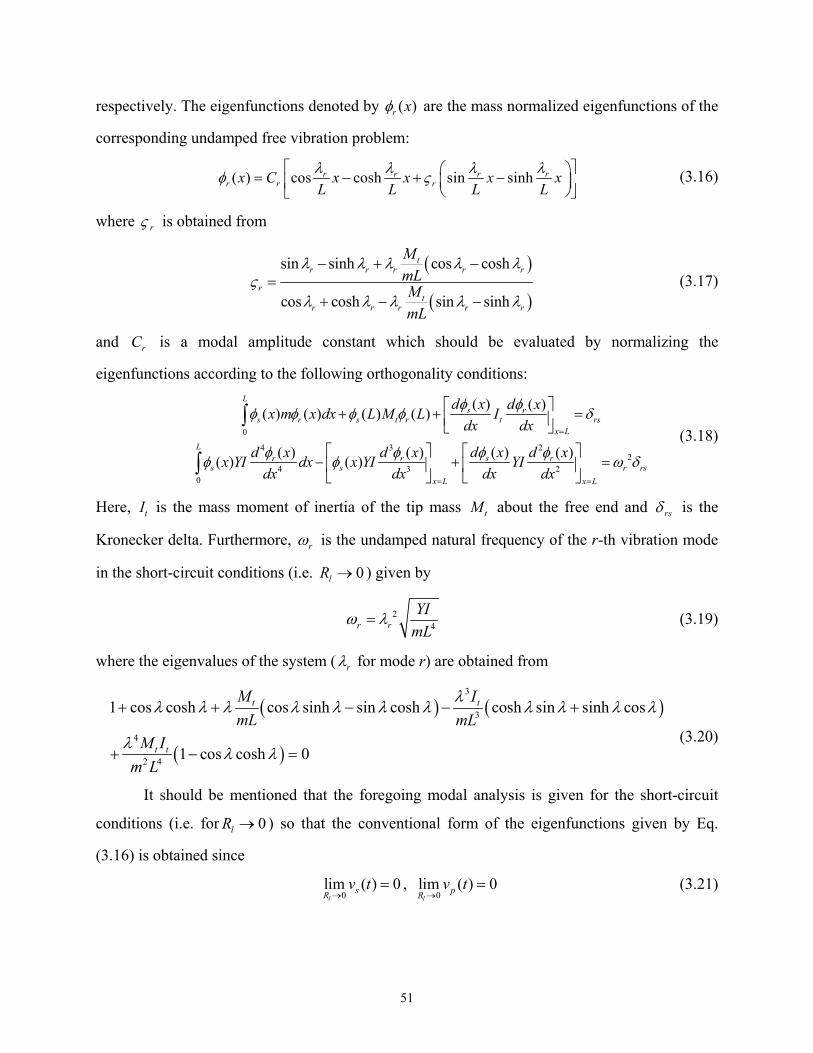
51

respectively. The eigenfunctions denoted by ( )r x are the mass normalized eigenfunctions of the

corresponding undamped free vibration problem:

( ) cos cosh sin sinhr r r rr r rx C x x x x

L L L L

(3.16)


sin sinh cos cosh

cos cosh sin sinh

tr r r r r

rt

r r r r r

M

mLM

mL

(3.17)

and rC is a modal amplitude constant which should be evaluated by normalizing the

eigenfunctions according to the following orthogonality conditions:

0

4 3 22

4 3 20

( ) ( )( ) ( ) ( ) ( )

( )( ) ( ) ( )( ) ( )

Ls r

s r s t r t rsx L

Lsr r r

s s r rs

x L x L

d x d xx m x dx L M L I

dx dx

d xd x d x d xx YI dx x YI YI

dx dx dx dx

(3.18)

Here, tI is the mass moment of inertia of the tip mass tM about the free end and rs is the

Kronecker delta. Furthermore, r is the undamped natural frequency of the r-th vibration mode

in the short-circuit conditions (i.e. 0lR ) given by

24r r

YI

mL (3.19)

where the eigenvalues of the system ( r for mode r) are obtained from

3

3

4

2 4

1 cos cosh cos sinh sin cosh cosh sin sinh cos

1 cos cosh 0

t t

t t

M I

mL mL

M I

m L

(3.20)

It should be mentioned that the foregoing modal analysis is given for the short-circuit

conditions (i.e. for 0lR ) so that the conventional form of the eigenfunctions given by Eq.

(3.16) is obtained since

0

lim ( ) 0l

sR

v t

, 0

lim ( ) 0l

pR

v t

(3.21)

52

in Eqs. (3.11) and (3.12), respectively (i.e. the voltage output vanishes for zero load resistance).

Note that the short-circuit condition is indeed a constant electric field condition ( 3 0E as

0lR ), in agreement with the piezoelectric constitutive relation used here.

For a given bimorph, the form of the eigenfunctions given by ( )r x and their mass

normalization conditions are the same regardless of the series or parallel connections of the

piezoceramic layers. For non-zero values of load resistance, the voltage terms in the mechanical

equations take finite values, generating point moment excitations at the boundaries of the

piezoceramic layer according to Eqs. (3.11) and (3.12), and yielding two different modal

mechanical response functions for these equations as ( )sr t and ( )p

r t , respectively. The

feedback received from the voltage response for a given load resistance alters the mechanical

response as well as the resonance frequency of the energy harvester, as discussed theoretically

here and validated experimentally in the next chapter.

3.1.3 Coupled Electrical Circuit Equation of a Thin Piezoceramic Layer under Dynamic

Bending. In order to derive the governing electrical circuit equations of the bimorph

configurations for the series and parallel connections of the piezoceramic layers, one should first

examine the electrical dynamics of a single layer under bending vibrations. Consider Fig. 3.2a,

where the electrodes of a single layer are connected to a resistive electrical load. The deflections

are exaggerated to highlight the space- and time-dependent radius of curvature at an arbitrary

point x on the neutral axis at time t.

Fig. 3.2 (a) Bimorph cantilever with a single layer connected to a resistive load and (b) the

corresponding electrical circuit

(a) (b)

53

Since the only source of mechanical strain is assumed to be the axial strain due to

bending, the tensorial representation of the relevant piezoelectric constitutive relation [26] that

gives the vector of electric displacements can be reduced to the following scalar equation

(Appendix A.2):

3 31 1 33 3p SD e S E (3.22)

where 3D is the electric displacement component and 33S is the permittivity component at

constant strain with the plane-stress assumption for a beam ( 233 33 31 11/S T Ed s where 33

T is the

permittivity component at constant stress as given in Appendix A.2) .

As the circuit admittance across the electrodes is 1/ lR , the electric current output can be

obtained from the Gauss’s law [26] as

( )

lA

d v tdA

dt R

D n (3.23)

where D is the vector of electric displacement components in the piezoceramic layer, n is the

unit outward normal and the integration is performed over the electrode area A. As can be

anticipated, the only contribution to the inner product of the integrand in Eq. (3.23) is from 3D ,

since the electrodes are perpendicular to 3-direction (i.e. z-direction). After expressing the

average bending strain in the piezoceramic layer in terms of the curvature (see Eq. (3.5)) and the

uniform electric field in terms of the electric potential difference ( 3( ) ( ) / pE t v t h ), Eq. (3.22)

can be used in equation Eq. (3.23) to obtain

333

31 20

( , )( ) ( ) LSrel

pcp l

bL w x tdv t v te h b dx

h dt R x t

(3.24)

where b , ph and L are the width, thickness and the length of the piezoceramic layer,

respectively, and pch is the distance between the neutral axis and the center of the piezoceramic

layer ( ( ) / 2pc p sh h h ). One can then substitute the modal expansion form of the transverse

vibration response (relative to the base) given by

1

( , ) ( ) ( )rel r rr

w x t x t

(3.25)

into Eq. (3.24) to obtain

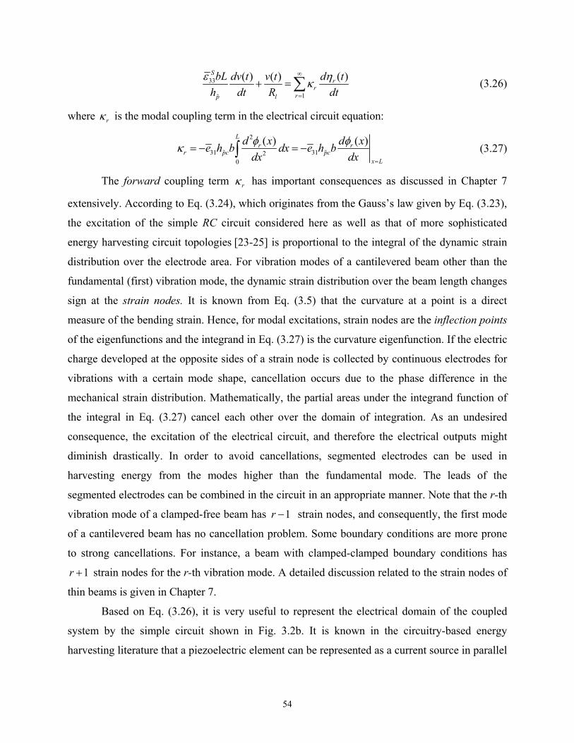
54

33

1

( )( ) ( )Sr

rrp l

bL d tdv t v t

h dt R dt

(3.26)

where r is the modal coupling term in the electrical circuit equation:

2

31 3120

( ) ( )Lr r

r pc pcx L

d x d xe h b dx e h b

dx dx

(3.27)

The forward coupling term r has important consequences as discussed in Chapter 7

extensively. According to Eq. (3.24), which originates from the Gauss’s law given by Eq. (3.23),

the excitation of the simple RC circuit considered here as well as that of more sophisticated

energy harvesting circuit topologies [23-25] is proportional to the integral of the dynamic strain

distribution over the electrode area. For vibration modes of a cantilevered beam other than the

fundamental (first) vibration mode, the dynamic strain distribution over the beam length changes

sign at the strain nodes. It is known from Eq. (3.5) that the curvature at a point is a direct

measure of the bending strain. Hence, for modal excitations, strain nodes are the inflection points

of the eigenfunctions and the integrand in Eq. (3.27) is the curvature eigenfunction. If the electric

charge developed at the opposite sides of a strain node is collected by continuous electrodes for

vibrations with a certain mode shape, cancellation occurs due to the phase difference in the

mechanical strain distribution. Mathematically, the partial areas under the integrand function of

the integral in Eq. (3.27) cancel each other over the domain of integration. As an undesired

consequence, the excitation of the electrical circuit, and therefore the electrical outputs might

diminish drastically. In order to avoid cancellations, segmented electrodes can be used in

harvesting energy from the modes higher than the fundamental mode. The leads of the

segmented electrodes can be combined in the circuit in an appropriate manner. Note that the r-th

vibration mode of a clamped-free beam has 1r strain nodes, and consequently, the first mode

of a cantilevered beam has no cancellation problem. Some boundary conditions are more prone

to strong cancellations. For instance, a beam with clamped-clamped boundary conditions has

1r strain nodes for the r-th vibration mode. A detailed discussion related to the strain nodes of

thin beams is given in Chapter 7.

Based on Eq. (3.26), it is very useful to represent the electrical domain of the coupled

system by the simple circuit shown in Fig. 3.2b. It is known in the circuitry-based energy

harvesting literature that a piezoelectric element can be represented as a current source in parallel

55

with its internal capacitance [23-25] (Norton equivalent**). Therefore, the simple circuit shown

in Fig. 3.2b is the complete circuit of the electrical domain for a single resistive load case. Note

that, this representation considers the electrical domain only and the electromechanical

representation of the coupled system is actually a transformer because of the voltage feedback

sent to the mechanical domain due to the piezoelectric coupling (which will be incorporated in

the formulation here). The components of the circuit are the internal capacitance pC of the

piezoceramic layer, the resistive load lR and the current source ( )pi t . In agreement with Fig.

3.2a, the voltage across the resistive load is denoted by ( )v t . Then, the Kirchhoff laws can be

applied to the electrical circuit shown in Fig. 3.2b to obtain

( ) ( )

( )p pl

dv t v tC i t

dt R (3.28)

where the internal capacitance and the current source terms can be extracted by matching Eqs.

(3.26) and (3.28) as

33S

pp

bLC

h

, 1

( )( ) r

p rr

d ti t

dt

(3.29)

Identification of the above terms (especially the current source term) has an important use

for modeling of multi-morph piezoelectric energy harvesters. This way, for a given number of

piezoceramic layers, there is no need to derive the electrical circuit equation by using the

constitutive relation and the Gauss’s law given by equations Eqs. (3.23) and (3.24), respectively.

Each piezoceramic layer will have a similar capacitance and current source term and the layers

can be combined to the resistive electrical load(s) in a desired way.

3.2 Series Connection of the Piezoceramic Layers

Based on the fundamentals given in Section 3.1, this section presents the derivation of the

closed-form expressions for the coupled voltage response ( )sv t and vibration response ( , )srelw x t

of the bimorph configuration shown in Fig. 3.1a. First the coupled mechanical equation is given

in modal coordinates and then the coupled circuit equation is derived. The resulting

** The alternative representation is the Thévenin equivalent (voltage source in series with its internal capacitance).

See a discussion in Section 5.4.6 regarding a misuse of these representations to obtain the optimum load resistance.

56

electromechanical equations are then solved for the steady-state voltage response and vibration

response for harmonic base motion inputs.

3.2.1 Coupled Beam Equation in Modal Coordinates. After substituting Eq. (3.15a) into Eq.

(3.11) and applying the orthogonality conditions of the eigenfunctions, the mechanical equation

of motion in modal coordinates can be obtained as

22

2

( ) ( )2 ( ) ( ) ( )

s ss sr r

r r r r r s r

d t d tt v t f t

dt dt

(3.30)

where the modal electromechanical coupling term is††

( )s rr s

x L

d x

dx

(3.31)

The modal mechanical forcing function can be expressed as

2 2 2 2

2 2 2 20 0

( ) ( ) ( ) ( )( ) ( ) ( ) ( )

L L

r r r t r

d g t d h t d g t d h tf t m x dx x x dx M L L

dt dt dt dt

(3.32)

In Eq. (3.30), r is the modal mechanical damping ratio that includes the combined

effects of strain-rate and air damping. In the absence of a tip mass, how to relate the modal

damping ratio to the strain-rate and air damping terms sc I and ac mathematically based on the

assumption of proportional damping was described in Chapter 2. However, as a common

experimental modal analysis practice, one can identify the modal damping ratio r of a desired

mode directly from the frequency response or time domain measurements (which avoids the

requirement of defining and obtaining the physical damping terms sc I and ac ). Chapter 5

provides closed-form relations to identify modal mechanical damping ratio from

electromechanical FRF measurements in the presence of a resistive electrical load.

3.2.2 Coupled Electrical Circuit Equation. As described in Section 3.1.1, the piezoceramic

layers of the bimorph configuration shown in Fig. 3.1a are connected in series. We know from

the practice given in Section 3.1.3 that each piezoceramic layer can be represented as a current

†† Note that, here, Eq. (3.13) is used to obtain the modal backward coupling term s

r where the test function is the

eigenfunction ( ( ) ( )r

x x ) multiplying the partial differential equation in the modal analysis solution procedure.

57

source in parallel with its internal capacitance. Therefore, Fig. 3.3 displays the series connection

of the identical piezoceramic layers of the bimorph configuration shown in Fig. 3.1a.

The Kirchhoff laws can be applied to the circuit depicted in Fig. 3.3 to obtain

( ) ( )( )

2p ss s

pl

C dv t v ti t

dt R

(3.33)

where the internal capacitance and the current source terms of the bimorph (for each layer) are

33S

pp

bLC

h

, 1

( )( )

ss rp r

r

d ti t

dt

(3.34)

The modal electromechanical coupling term is then

2

31

31 20

( ) ( )

2

Lp sr r

r pcx L

e h h bd x d xe h b dx

dx dx

(3.35)

where pch (the distance between the neutral axis and the center of the piezoceramic layer) is

expressed in terms of the piezoceramic and the substructure layer thicknesses ph and sh (Fig.

3.1c). Hence, Eq. (3.34) is the electrical circuit equation of the bimorph cantilever for the series

connection of the piezoceramic layers.

Fig. 3.3 Electrical circuit representing the series connection of the piezoceramic layers

3.2.3 Closed-form Voltage Response and Vibration Response at Steady State. Equations

(3.31) and (3.33) constitute the coupled equations for the modal mechanical response ( )sr t of

the bimorph and the voltage response ( )sv t across the resistive load. In this section, the steady-

state solution of these terms for harmonic motion inputs is derived. If the translational and

rotational components of the base displacement given by Eq. (3.1) are harmonic of the forms

0( ) j tg t W e and 0( ) j th t e , where 0W and 0 are the translational and the small rotational

58

displacement amplitudes of the base, is the excitation frequency and j is the unit imaginary

number, then the modal forcing function given by Eq. (3.32) can be expressed as ( ) j tr rf t F e

where the amplitude rF is

20 0 0 0

0 0

( ) ( ) ( )L L

r r r t rF m W x dx x x dx M L W L

(3.36)

For the harmonic base motions at frequency , the steady-state modal mechanical

response of the beam and the steady-state voltage response across the resistive load are assumed

to be harmonic at the same frequency as ( )s s j tr rt e and ( ) j t

s sv t V e (linear system

assumption), respectively, where the amplitudes sr and sV are complex valued. Therefore, Eqs.

(3.30) and (3.33) yield the following two equations for sr and sV :

2 2 2 s sr r r r r s rj V F (3.37)

1

10

2p s

s r rrl

Cj V j

R

(3.38)

The complex modal mechanical response amplitude sr can be extracted from Eq. (3.37)

and it can be substituted into Eq. (3.38) to obtain the complex voltage amplitude sV explicitly.

The resulting complex voltage amplitude can then be used in ( ) j ts sv t V e to express the steady-

state voltage response as

2 2

1

2 21

2( )

12 2

r r

r j tr r rs s

p r r

rl r r r

j Fj

v t eC j

jR j

(3.39)

The complex voltage amplitude sV can be substituted into Eq. (3.37) to obtain the steady-

state modal mechanical response of the bimorph as

2 2

12 2

2 21

2( )

1 22 2

r rj t

rs s r r rr r r s

p r r r r r

rl r r r

j Fj e

t FC j j

jR j

(3.40)

The transverse displacement response (relative to the base) at point x on the bimorph can

be obtained in physical coordinates by substituting Eq. (3.40) into Eq. (3.15a):

59

2 21

2 21

2 21

2 ( )( , )

1 22 2

r rj t

rs s r r r rrel r r s

pr r r r r r

rl r r r

j Fj x e

w x t FC j j

jR j

(3.41)

Note that the vibration response given by Eq. (3.41) is the displacement response of the

beam relative to its moving base. If one is interested in the coupled beam displacement in the

absolute physical coordinates (relative to the fixed frame), it is the superposition of the base

displacement and the vibratory displacement relative to base:

( , ) ( , ) ( , )s sb relw x t w x t w x t (3.42)

where ( , )bw x t is the effective base displacement given by Eq. (3.1).

3.3. Parallel Connection of the Piezoceramic Layers

This section aims to derive the steady-state voltage response ( )pv t and the vibration response

( , )prelw x t of the bimorph configuration shown in Fig. 3.1b to harmonic base motions. The

coupled beam equation in modal coordinates and the electrical circuit equations are derived and

the closed-form solutions are obtained in the following.

3.3.1 Coupled Beam Equation in Modal Coordinates. After substituting Eq. (3.15b) in Eq.

(3.11), the partial differential equation given by Eq. (3.11) can be reduced to an infinite set of

ordinary differential equations in modal coordinates as follows:

22

2

( ) ( )2 ( ) ( ) ( )

p pp pr r

r r r r r p r

d t d tt v t f t

dt dt

(3.43)

where the modal electromechanical coupling term is

( )p rr p

x L

d x

dx

(3.44)

and the modal mechanical forcing function is given by Eq. (3.32). The discussion regarding the

mechanical damping ratio r is the same as given in Section 3.2.1. Thus, Eq. (3.43) is the

coupled beam equation in modal coordinates for the bimorph configuration with the parallel

connection of the piezoceramic layers.

60

3.3.2 Coupled Electrical Circuit Equation. It was mentioned in Section 3.1.1 that the

piezoceramic layers of the bimorph configuration shown in Fig. 3.1b are connected in parallel.

Since each of the piezoceramic layers can be represented as a current source in parallel with its

internal capacitance (Section 3.1.3), Fig. 3.4 represents the parallel connection of the identical

top and bottom piezoceramic layers of the bimorph configuration shown in Fig. 3.1b.

One can then derive the governing electrical circuit equation based on the Kirchhoff laws

as follows:

( ) ( )( )

2p p p

p pl

dv t v tC i t

dt R (3.45)

where the internal capacitance and the current source terms for each layer are

33S

pp

bLC

h

, 1

( )( )

pp rp r

r

d ti t

dt

(3.46)

The modal coupling term r is given by Eq. (3.34). Equation (3.45) is the electrical circuit

equation of the bimorph cantilever for the parallel connection of the piezoceramic layers.

Fig. 3.4 Electrical circuit representing the parallel connection of the piezoceramic layers

3.3.3 Closed-form Voltage Response and Vibration Response at Steady State. In order to

solve for ( )pr t and ( )pv t in Eqs. (3.43) and (3.45), the same procedure of Section 3.2 is

followed by assuming the base excitation components in Fig. 3.1b to be harmonic as

0( ) j tg t W e and 0( ) j th t e . For these harmonic base motion inputs of the same frequency,

the modal forcing is harmonic as ( ) j tr rf t F e where the amplitude rF is given by Eq. (3.36).

Based on the linear system assumption, the modal mechanical response ( )pr t and the

voltage response ( )pv t are assumed to be harmonic at the frequency of excitation such that

61

( )p p j tr rt e and ( ) j t

p pv t V e , where the amplitudes pr and pV are complex valued. Hence,

Eqs. (3.43) and (3.45) yield the following equations for pr and pV :

2 2 2 p pr r r r r p rj V F (3.47)

1

10

2p

p p r rrl

j C V jR

(3.48)

where pr and pV can be obtained explicitly. Using the resulting complex voltage amplitude in

( ) j tp pv t V e gives the steady-state voltage response as

2 2

1

2 21

2( )

12 2

r r

r j tr r rp p

r rp

rl r r r

j Fj

v t ej

j CR j

(3.49)

Then the steady-state modal mechanical response of the bimorph can be obtained by

using pV in Eq. (3.47) as

2 2

12 2

2 21

2( )

1 22 2

r rj t

rp p r r rr r r p

r r r r rp

rl r r r

j F

j et F

j jj C

R j

(3.50)

The modal mechanical response expression can then be used in Eq. (3.15b) to obtain the

transverse displacement response (relative to the base) at point x on the bimorph:

2 21

2 21

2 21

2 ( )( , )

1 22 2

r rj t

rp p r r r rrel r r p

r r r r r rp

rl r r r

j Fj x e

w x t Fj j

j CR j

(3.51)

Having obtained the vibration response relative to the moving base, one can easily use

superimpose the base motion and the relative response to obtain the transverse displacement

response at point x relative to the fixed frame as follows:

( , ) ( , ) ( , )p pb relw x t w x t w x t (3.52)

where the base displacement ( , )bw x t is given by Eq. (3.1).

62

3.4 Single-mode Electromechanical Expressions for Modal Excitations

The steady-state voltage response and vibration response expressions obtained in Sections 3.2

and 3.3 are valid for harmonic excitations at any arbitrary frequency . That is, Eqs. (3.39) and

(3.41) for the series connection of the piezoceramic layers (Fig. 3.1a) and Eqs. (3.49) and (3.51)

for the parallel connection of the piezoceramic layers (Fig. 3.1b) are the multi-mode solutions as

they include all vibration modes of the bimorph harvester. Hence, these equations can predict the

coupled system dynamics at steady state not only for resonance excitation but also for excitations

at the off-resonance frequencies of the energy harvester.

In order to obtain the maximum electrical response, it is preferable to excite a given

energy harvester at its fundamental resonance frequency (or at one of the higher resonance

frequencies). Most of the studies in the literature have focused on the resonance excitation at the

fundamental resonance frequency in order to investigate the maximum power generation

performance. Consequently, excitation of a bimorph at or very close to one of its natural

frequencies is a very useful problem to investigate through the resulting equations derived here.

This is the modal excitation condition and mathematically it implies r . With this

assumption for the excitation frequency, the major contribution in the summation terms of Eqs.

(3.39), (3.41), (3.49) and (3.51) are from the r-th vibration mode. This approximation allows

simplifications in the coupled voltage response and vibration response expressions.

In the following, the reduced single-mode expressions are given for excitations at or very

close to the r-th natural frequency, however, it should be noted that the fundamental mode is the

main concern in the energy harvesting problem (which corresponds to 1r ).

3.4.1 Series Connection of the Piezoceramic Layers. If the bimorph configuration shown in

Fig. 3.1a is excited at r , the contribution of all vibration modes other than the r-th mode

can be ignored in the summation terms. Then, the steady-state voltage response given by Eq.

(3.39) can be reduced to

2 2

2ˆ ( )

2 2 2

j tl r r

s sl p r r r l r r

j R F ev t

j R C j j R

(3.53)

and the transverse displacement relative to the moving base is simply obtained from Eq. (3.41) as

63

2 2

2 ( )ˆ ( , )

2 2 2

j tl p r rs

rel sl p r r r l r r

j R C F x ew x t

j R C j j R

(3.54)

where the relevant terms can be found in Section 3.2. Here and hereafter, a hat (^) denotes that

the respective term is reduced from the full solution to a single mode for excitations very close to

a natural frequency.

3.4.2 Parallel Connection of the Piezoceramic Layers. Similarly, if the bimorph configuration

displayed in Fig. 3.1b is excited at r , the steady-state voltage response given by Eq. (3.49)

can be reduced to

2 2

2ˆ ( )

1 2 2 2

j tl r r

p pl p r r r l r r

j R F ev t

j R C j j R

(3.55)

and the transverse displacement relative to the base is obtained from Eq. (3.51) as

2 2

1 2 ( )ˆ ( , )

1 2 2 2

j tl p r rp

rel pl p r r r l r r

j R C F x ew x t

j R C j j R

(3.56)

where the relevant terms can be found in Section 3.3.

3.5 Multi-mode and Single-mode Electromechanical FRFs

In the electromechanical model proposed here, the two excitation inputs to the system are the

translation of the base in the transverse direction and its small rotation (Figs. 3.1a and 3.1b). For

these two inputs, the resulting electromechanical outputs are the voltage response and the

vibration response. Therefore, for harmonic base excitations, one can define four

electromechanical FRFs between these two outputs and two inputs: voltage output – to –

translational base acceleration, voltage output – to – rotational base acceleration, vibration

response – to – translational base acceleration and vibration response – to – rotational base

acceleration. This section extracts these FRFs from the multi-mode (for arbitrary frequency

excitations) and single-mode (for modal excitations) steady-state solutions derived in the

previous sections.

64

3.5.1 Multi-mode Electromechanical FRFs. Since the translational and the small rotational

displacements of the base are given by 0( ) j tg t W e and 0( ) j th t e , the modal forcing

function has the form of ( ) j tr rf t F e where rF is given by Eq. (3.36). Before identifying the

aforementioned FRFs, one should first rearrange the complex modal forcing amplitude given by

Eq. (3.36) as follows:

2 20 0r r rF W (3.57)

where

0

( ) ( )L

r r t rm x dx M L (3.58)

0

( ) ( )L

r r t rm x x dx M L L (3.59)

3.5.1.1 Series Connection of the Piezoceramic Layers. The steady-state voltage response given

by Eq. (3.39) can be written in terms of the translational and rotational base accelerations as

2 20 0( ) j t j t

s s sv t W e e (3.60)

where the FRF that relates the voltage output to the translational base acceleration is

2 2

1

2 21

2

12 2

r r

r r r rs s

p r r

rl r r r

jj

C jj

R j

(3.61)

and the voltage output per rotational base acceleration input can be given by

2 2

1

2 21

2

12 2

r r

r r r rs s

p r r

rl r r r

jj

C jj

R j

(3.62)

Similarly, the steady-state vibration response relative to the base of the bimorph given by

Eq. (3.41) can be expressed as

2 20 0( , ) , ,s j t j t

rel s sw x t x W e x e (3.63)

where the relative transverse displacement response – to – translational base acceleration FRF is

65

2 21

2 21

2 21

2 ( )( , )

1 22 2

r r

rs r r r rs r r s

pr r r r r r

rl r r r

jj x

xC j j

jR j

(3.64)

The relative transverse displacement response and the rotational base acceleration are related by

2 21

2 21

2 21

2 ( )( , )

1 22 2

r r

rs r r r rs r r s

pr r r r r r

rl r r r

jj x

xC j j

jR j

(3.65)

3.5.1.2 Parallel Connection of the Piezoceramic Layers. It is possible to derive similar FRFs

for the parallel connection of the piezoceramic layers. The steady-state voltage response given by

Eq. (3.49) can be rearranged to yield

2 20 0( ) j t j t

p p pv t W e e (3.66)

where the voltage output – to – translational base acceleration FRF is

2 2

1

2 21

2

12 2

r r

r r r rp p

r rp

rl r r r

jj

jj C

R j

(3.67)

and the voltage output – to – rotational base acceleration FRF can be given by

2 2

1

2 21

2

12 2

r r

r r r rp p

r rp

rl r r r

jj

jj C

R j

(3.68)

From Eq. (3.51), the steady-state vibration response relative to the base of the bimorph

can be expressed as

2 20 0( , ) , ,p j t j t

rel p pw x t x W e x e (3.69)


2 21

2 21

2 21

2 ( )( , )

1 22 2

r r

rp r r r rp r r p

r r r r r rp

rl r r r

jj x

xj j

j CR j

(3.70)

66

and the relative transverse displacement response – to – rotational base acceleration FRF is

2 21

2 21

2 21

2 ( )( , )

1 22 2

r r

rp r r r rp r r p

r r r r r rp

rl r r r

jj x

xj j

j CR j

(3.71)

3.5.2 Single-mode Electromechanical FRFs. In order to extract the respective FRFs of the

single-mode expressions, one should use Eqs. (3.53)-(3.56) along with Eq. (3.57). In the

following, Eq. (3.57) is substituted into each of Eqs. (3.53)-(3.56) and the relevant FRFs are

extracted as done for the multi-mode solution case. Note that the single-mode electromechanical

FRFs given here provide approximation of the full solution for modal excitations ( r ) only.

3.5.2.1 Series Connection of the Piezoceramic Layers. Equation (3.53) can be rearranged to

give the single-mode steady-state voltage response as

2 20 0ˆˆ ˆ( ) j t j t

s s sv t W e e (3.72)

where the single-mode FRF that relates the voltage output to the translational base acceleration is

2 2

2ˆ

2 2 2l r r

s sl p r r r l r r

j R

j R C j j R

(3.73)

and the single-mode voltage output – to – rotational base acceleration FRF is

2 2

2ˆ

2 2 2l r r

s sl p r r r l r r

j R

j R C j j R

(3.74)

The single-mode steady-state vibration response relative to the base of the bimorph given

by Eq. (3.54) can be rearranged to give

2 20 0

ˆ ˆˆ ( , ) , ,s j t j trel s sw x t x W e x e (3.75)

where the single-mode relative transverse displacement response – to – translational base

acceleration FRF is

2 2

2 ( )ˆ ( , )2 2 2

l p r r

s sl p r r r l r r

j R C xx

j R C j j R

(3.76)

and the single-mode relative transverse displacement response – to – rotational base acceleration

FRF can be given by

67

2 2

2 ( )ˆ ( , )

2 2 2

l p r r

s sl p r r r l r r

j R C xx

j R C j j R

(3.77)

3.5.2.2 Parallel Connection of the Piezoceramic Layers. The single-mode steady-state voltage

response given by Eq. (3.55) can be expressed in terms of the translational and the rotational

base accelerations as

2 20 0

ˆˆ ˆ( ) j t j tp p pv t W e e (3.78)

Here, the single-mode FRF that relates the voltage output to the translational base acceleration is

2 2

2ˆ

1 2 2 2l r r

p pl p r r r l r r

j R

j R C j j R

(3.79)

and the single-mode FRF that relates the voltage output to the rotational base acceleration is

2 2

2ˆ

1 2 2 2l r r

p pl p r r r l r r

j R

j R C j j R

(3.80)

Similarly, the single-mode steady-state vibration response relative to the base of the

bimorph given by Eq. (3.56) can be rewritten as

2 20 0

ˆ ˆˆ ( , ) , ,p j t j trel p pw x t x W e x e (3.81)


acceleration FRF can be given by

2 2

1 2 ( )ˆ ( , )1 2 2 2

l p r r

p pl p r r r l r r

j R C xx

j R C j j R

(3.82)


FRF is

2 2

1 2 ( )ˆ ( , )

1 2 2 2

l p r r

p pl p r r r l r r

j R C xx

j R C j j R

(3.83)

3.6 Equivalent Representation of the Series and Parallel Connection Expressions

This section aims to obtain an equivalent (or a unified) representation of the distributed-

parameter analytical solutions derived for the series and the parallel connection cases. For this

68

purpose, the equivalent electromechanical coupling and the capacitance terms are obtained first

and then the resulting equivalent representation is given.

3.6.1 Modal Electromechanical Coupling Terms. A careful investigation of the coefficient of

backward coupling term for the series connection case (Eq. (3.8)) yields

22

31 3131 312 4 2 2 2

p ss ss p p s p pc

p p

h he b h h e bh h h h e b e bh

h h

(3.84)

Then, Eq. (3.9) for the parallel connection case becomes

312 2p s pce bh (3.85)

From Eqs. (3.31) and (3.44), the backward modal coupling terms lead to

31

( )s rr pc

x L

d xe bh

dx

(3.86)

31

( )2p r

r pcx L

d xe bh

dx

(3.87)

One can then notice the similarity of these expressions to the forward modal coupling term given

by Eq. (3.35):

31

( )rr pc

x L

d xe bh

dx

(3.88)

3.6.2 Equivalent Capacitance for Series and Parallel Connections. The circuit equation for

the series connection case given by Eq. (3.33) can be re-written as

,

1

( ) ( ) ( )seq s s s rp r

rl

dv t v t d tC

dt R dt

(3.89)

where

, 33

2 2

Speq s

pp

C bLC

h

(3.90)

is the equivalent capacitance of two capacitors ( pC ) connected in series.

Likewise, the circuit equation for the parallel connection case given by Eq. (3.45) can be

re-arranged to give

69

,

1

( ) ( ) ( )2

pp peq p r

p rrl

dv t v t d tC

dt R dt

(3.91)

where

, 3322

Seq pp p

p

bLC C

h

(3.92)

is the equivalent capacitance of two capacitors ( pC ) connected in parallel. Note that the

difference between the representations of Eqs. (3.89) and (3.91) is a factor of two in the coupling

terms, as in the backward coupling terms given by Eqs. (3.86) and (3.87). Indeed, from Eqs.

(3.86)-(3.88), sr r and 2 p

r r .

3.6.3 Equivalent Representation of the Electromechanical Expressions. The equivalent

electromechanical equations governing the modal mechanical response and the voltage response

of a bimorph can be given by

22

2

( ) ( )2 ( ) ( ) ( )r r

r r r r r r

d t d tt v t f t

dt dt

(3.93)

1

( )( ) ( )eq rp r

rl

d tdv t v tC

dt R dt

(3.94)

where the modal electromechanical coupling term r and the equivalent capacitance eqpC depend

on the way piezoceramic layers are connected (Table 3.1). In Eqs. (3.93) and (3.94), ( )r t is the

modal mechanical response that gives the transverse displacement response of the cantilever

relative to its moving base when used in Eq. (3.25) whereas ( )v t is the voltage across the load

resistance (i.e. ( ) ( )sv t v t in Fig. 3.1a and ( ) ( )pv t v t in Fig. 3.1b).

As mentioned previously, for harmonic base displacement inputs of 0( ) j tg t W e and

0( ) j th t e , the modal forcing function is harmonic of the form ( ) j tr rf t F e where the

amplitude rF is given by Eq. (3.36). Substituting the steady-state response expressions

( ) j tr rt e and ( ) j tv t Ve into Eqs. (3.93) and (3.94) gives 1 coupled linear algebraic

equations for the complex amplitudes r and V (infinite mechanical degrees of freedom due to

1...r and one electrical degree of freedom):

70

2 2 2r r r r r rj V F (3.95)

1

10eq

p r rrl

j C V jR

(3.96)

Eventually one obtains the steady-state voltage response and the vibration response expressions

as follows:

2 21

2

2 21

2( )

12

r r

r j tr r r

eq rp

rl r r r

j Fj

v t ej

j CR j

(3.97)

2 21

2 221

2 21

2 ( )( , )

212

r rj t

r r r r rrel r r

r eq r r rrp

rl r r r

j Fj x e

w x t Fjj

j CR j

(3.98)

For modal excitations (i.e. r ), Eqs. (3.97) and (3.98) reduce to

2 2 2ˆ( )

1 2

j tl r r

eql p r r r l r

j R F ev t

j R C j j R

(3.99)

2 2 2

1 ( )ˆ ( , )

1 2

eq j tl p r r

rel eql p r r r l r

j R C F x ew x t

j R C j j R

(3.100)

Table 3.1 Modal electromechanical coupling and equivalent capacitance of a bimorph energy

harvester for the series and the parallel connections of the piezocermaic layers

Series connection Parallel connection

r 31

( )rpc

x L

d xe bh

dx

31

( )2 r

pcx L

d xe bh

dx

eqpC 33

2

S

p

bL

h

332 S

p

bL

h

3.6.4 Equivalent Representation of the Multi-mode Electromechanical FRFs. Equation

(3.97) can be re-expressed as

71

2 2

0 0( ) j t j tv t W e e (3.101)

where the voltage output – to – translational base acceleration FRF is

2 2

12

2 21

2

12

r r

r r r r

eq rp

rl r r r

jj

jj C

R j

(3.102)

and the voltage output – to – rotational base acceleration FRF can be given by

2 2

12

2 21

2

12

r r

r r r r

eq rp

rl r r r

jj

jj C

R j

(3.103)

Similarly, Eq. (3.98) can be written as

2 2

0 0( , ) , ,j t j trelw x t x W e x e (3.104)


2 21

2 221

2 21

2 ( )( , )

212

r r

r r r r rr r

r eq r r rrp

rl r r r

jj x

xjj

j CR j

(3.105)

and the relative transverse displacement response – to – rotational base acceleration FRF is

2 21

2 221

2 21

2 ( )( , )

212

r r

r r r r rr r

r eq r r rrp

rl r r r

j

j xx

jjj C

R j

(3.106)

3.6.5 Equivalent Representation of the Single-mode Electromechanical FRFs. From Eq.

(3.99):

2 20 0ˆˆ ˆ( ) j t j tv t W e e (3.107)

where the single-mode voltage output – to – translational base acceleration FRF is

2 2 2ˆ

1 2l r r

eql p r r r l r

j R

j R C j j R

(3.108)

and the single-mode voltage output – to – rotational base acceleration FRF is

72

2 2 2ˆ

1 2l r r

eql p r r r l r

j R

j R C j j R

(3.109)

Likewise, from Eq. (3.100):

2 2

0 0ˆ ˆˆ ( , ) , ,j t j t

relw x t x W e x e (3.110)


acceleration FRF is

2 2 2

1 ( )ˆ( , )

1 2

eql p r r

eql p r r r l r

j R C xx

j R C j j R

(3.111)


FRF can be given by

2 2 2

1 ( )ˆ ( , )

1 2

eql p r r

eql p r r r l r

j R C xx

j R C j j R

(3.112)

3.7 Theoretical Case Study

This section presents theoretical demonstrations of the analytical model developed in this

chapter. An extensive electromechanical analysis of a bimorph cantilever configuration is

presented in the following subsections. First the series and the parallel connections of the

piezoceramic layers are studied with a focus on multiple vibration modes. Then the electrical and

mechanical response simulations of the multi-mode and single-mode FRFs are compared. The

damping effect of piezoelectric power generation on the harvester beam is also investigated.

3.7.1 Properties of the Bimorph Cantilever. The geometric properties of the bimorph

cantilever investigated in this case study are given in Table 3.2. The overhang length – to – total

thickness ratio of the harvester is about 85.7 which makes it reasonable to neglect the shear

deformation and the rotary inertia effects for the practical vibration modes (in agreement with the

Euler-Bernoulli beam theory). The substructure layer is assumed to be aluminum, the

piezoceramic layer is taken to be PZT-5A and the configuration does not have a tip mass (i.e.

0t tM I ). The material properties of the substructure and the piezoceramic layers are shown

in Table 3.3. The elastic, piezoelectric and permittivity constants of PZT-5A are obtained from

73

Table B.2 in the Appendix (reduced constants for the Euler-Bernoulli beam theory). The analysis

given here considers the frequency range of 0-5000 Hz. It can easily be shown that this

cantilever has three vibration modes in this frequency range. The first three mechanically and

electrically undamped natural frequencies of the bimorph cantilever (for 0lR ) are

1 185.1f Hz, 2 1159.8f Hz and 3 3247.6f Hz (where / 2r rf ). For the purpose of

simulation, if one takes 1 0.010 and 2 0.012 as the mechanical damping ratios of the first

two modes and assumes proportional damping based on the discussion of Chapter 2, the

proportionality constants /sc I YI and /ac m are obtained from Eq. (2.17) (by using 1 , 2 , 1

and 2 ) as 6/ 2.93 10sc I YI s/rad and / 19.295ac m rad/s. Closed-form identification of

mechanical damping in the presence of an arbitrary load resistance based on the single-mode

approximation is presented in Chapter 5. Here, it can be assumed that the damping ratios are

identified by setting the electrical boundary condition to short circuit ( 0lR ) and using

conventional techniques (e.g. half-power points of the mechanical FRF [39]).

Before the simulation results are presented and discussed, it is worth adding a few words

regarding the assumption of proportional damping. The restriction about the proportional

damping assumption is such that, once the proportionality constants are identified using the

modal properties of two vibration modes, the rest of the damping ratios are not arbitrary and they

are automatically set equal to the following numbers due to Eq. (2.17): 3 0.030 , 4 0.059 ,

5 0.097 and so on. It should be noted that the concept of proportional damping is a

convenient mathematical modeling assumption (to force the system to be a normal-mode system)

and the physical system may not agree with this assumption [36]. In other words, the damping

ratios of higher modes identified experimentally from the physical system may not converge to

the aforementioned values. Therefore, as a relaxation in the proportional damping assumption,

one might prefer to use the identified damping ratios of the vibration modes of interest (to be

used in the modal expressions) directly without obtaining /sc I YI and /ac m since the resulting

electromechanical expressions developed here need only the r values. This is the modal

damping assumption and it is identical to starting with the respective undamped equation (the

normal-mode problem by definition) and introducing damping in the modal domain. The

proportional damping (in the form of Rayleigh damping) and modal damping assumptions are

74

often used in vibration engineering regardless of their practical limitations. As far as the problem

of vibration energy harvesting is concerned, it is the fundamental vibration mode that has the

highest importance and proportional damping (or modal damping) is a reasonable assumption to

establish the bridge between the partial differential equation and its closed-form analytical

solution given in this chapter.

Table 3.2 Geometric properties of the bimorph cantilever

Piezoceramic Substructure

Length ( L ) [mm] 30 30

Width (b ) [mm] 5 5

Thickness ( ph , sh ) [mm] 0.15 (each) 0.05

Table 3.3 Material properties of the bimorph cantilever


Material PZT-5A Aluminum

Elastic modulus ( 11Ec , sY ) [GPa] 61 70

Mass density ( p , s ) [kg/m3] 7750 2700

Piezoelectric constant ( 31e ) [C/m2] -10.4 -

Permittivity constant ( 33S ) [nF/m] 13.3 -

3.7.2 Frequency Response of the Voltage Output. In the simulations given here, the base of

the cantilever is assumed to be not rotating (i.e. ( ) 0h t in Fig. 3.1) and the series connection

case is considered first. The multi-mode voltage FRFs (per base acceleration) shown in Fig. 3.5

are obtained from

2 21

2 20

2 21

2( )

12

r r

r r r rj t

eq rp

rl r r r

jjv t

W e jj C

R j

(3.113)

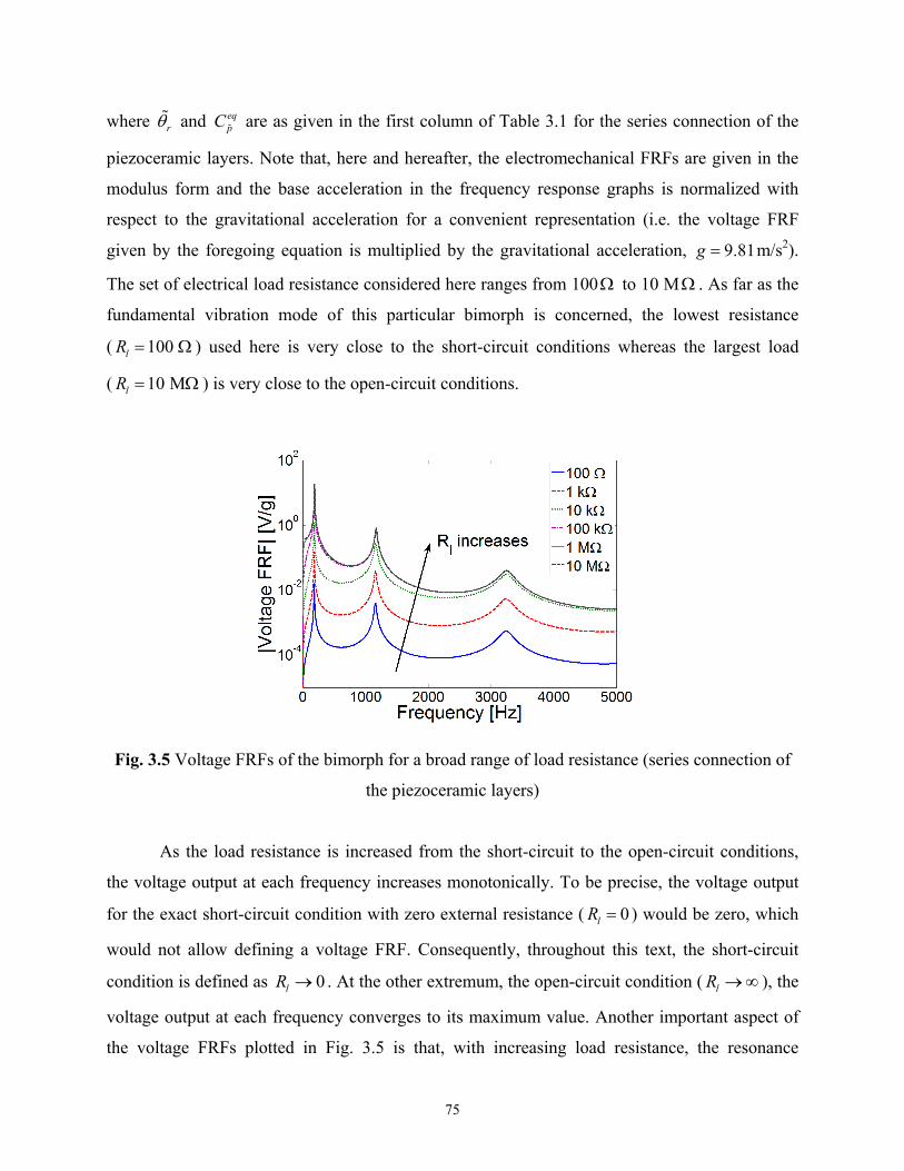
75

where r and eqpC are as given in the first column of Table 3.1 for the series connection of the

piezoceramic layers. Note that, here and hereafter, the electromechanical FRFs are given in the

modulus form and the base acceleration in the frequency response graphs is normalized with

respect to the gravitational acceleration for a convenient representation (i.e. the voltage FRF

given by the foregoing equation is multiplied by the gravitational acceleration, 9.81g m/s2).

The set of electrical load resistance considered here ranges from 100 to 10 M . As far as the

fundamental vibration mode of this particular bimorph is concerned, the lowest resistance

( 100lR ) used here is very close to the short-circuit conditions whereas the largest load

( 10 MlR ) is very close to the open-circuit conditions.

Fig. 3.5 Voltage FRFs of the bimorph for a broad range of load resistance (series connection of

the piezoceramic layers)

As the load resistance is increased from the short-circuit to the open-circuit conditions,

the voltage output at each frequency increases monotonically. To be precise, the voltage output

for the exact short-circuit condition with zero external resistance ( 0lR ) would be zero, which

would not allow defining a voltage FRF. Consequently, throughout this text, the short-circuit

condition is defined as 0lR . At the other extremum, the open-circuit condition ( lR ), the

voltage output at each frequency converges to its maximum value. Another important aspect of

the voltage FRFs plotted in Fig. 3.5 is that, with increasing load resistance, the resonance

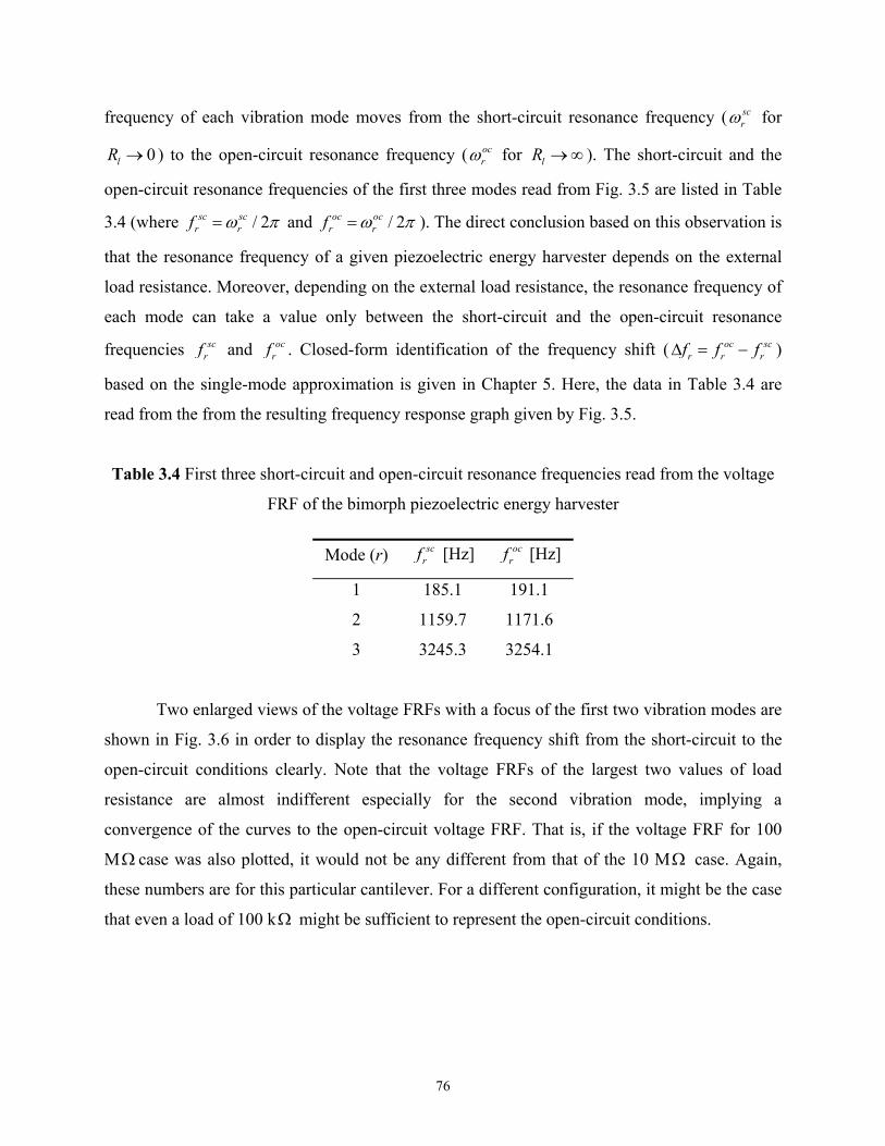
76

frequency of each vibration mode moves from the short-circuit resonance frequency ( scr for

0lR ) to the open-circuit resonance frequency ( ocr for lR ). The short-circuit and the

open-circuit resonance frequencies of the first three modes read from Fig. 3.5 are listed in Table

3.4 (where / 2sc scr rf and / 2oc oc

r rf ). The direct conclusion based on this observation is

that the resonance frequency of a given piezoelectric energy harvester depends on the external

load resistance. Moreover, depending on the external load resistance, the resonance frequency of

each mode can take a value only between the short-circuit and the open-circuit resonance

frequencies scrf and oc

rf . Closed-form identification of the frequency shift ( oc scr r rf f f )

based on the single-mode approximation is given in Chapter 5. Here, the data in Table 3.4 are

read from the from the resulting frequency response graph given by Fig. 3.5.

Table 3.4 First three short-circuit and open-circuit resonance frequencies read from the voltage

FRF of the bimorph piezoelectric energy harvester

Mode (r) scrf [Hz] oc

rf [Hz]

1 185.1 191.1

2 1159.7 1171.6

3 3245.3 3254.1

Two enlarged views of the voltage FRFs with a focus of the first two vibration modes are

shown in Fig. 3.6 in order to display the resonance frequency shift from the short-circuit to the

open-circuit conditions clearly. Note that the voltage FRFs of the largest two values of load

resistance are almost indifferent especially for the second vibration mode, implying a

convergence of the curves to the open-circuit voltage FRF. That is, if the voltage FRF for 100

M case was also plotted, it would not be any different from that of the 10 M case. Again,

these numbers are for this particular cantilever. For a different configuration, it might be the case

that even a load of 100 k might be sufficient to represent the open-circuit conditions.

77

Fig. 3.6 Voltage FRFs of the bimorph with a focus on the first two vibration modes: (a) mode 1

and (b) mode 2 (series connection)

As far as the fundamental vibration mode is concerned, the short-circuit and the open-

circuit resonance frequencies are 185.1 Hz and 191.1 Hz, respectively. Excitation at these two

frequencies will be of particular interest in this section as well as in the experimental validations

to be discussed in the next chapter. Variation of the voltage output for excitations at the

fundamental short-circuit resonance frequency and at the fundamental open-circuit resonance

frequency are plotted in Fig. 3.7. As can be seen from the figure, for low values of load

resistance, the voltage output at the short-circuit resonance frequency is larger since the system

(i.e. the electrical boundary condition) is close to short-circuit conditions. With increasing load

resistance, the curves intersect at a certain point (around 120 k ) and for the values of load

resistance larger than the value at the intersection point, the voltage output at the open-circuit

resonance frequency is larger. It is important at this stage to notice the linear asymptotic trends at

the extrema of 0lR and lR (which will be proved mathematically in Chapter 5). The

graph given here in log-log scale shows a linear increase in the voltage output with increasing

load resistance for low values of load resistance (both for the short-circuit and the open-circuit

resonance frequencies). The voltage output becomes less sensitive to the variations in the load

resistance for its large values due to the horizontal asymptotes of the lR extremum.

(a) (b)

78

Fig. 3.7 Variation of the voltage output with load resistance for excitations at the short-circuit

and the open-circuit resonance frequencies of the first vibration mode (series connection)

3.7.3 Frequency Response of the Current Output. If the voltage FRF given by Eq. (3.113) is

divided by the load resistance, the multi-mode current FRF is obtained as

2 21

2 20

2 21

2( ) 1

12

r r

r r r rj t

eql rp

rl r r r

jji t

W e R jj C

R j

(3.114)

The modulus of the current FRF is plotted against the frequency in Fig. 3.8. Unlike the

voltage FRF shown in Fig. 3.5, the amplitude of the current at every frequency decreases with

increasing load resistance. Indeed this is the opposite of the voltage behavior shown in Fig. 3.8

but the behavior is still monotonic. For every excitation frequency, the maximum value of the

current is obtained when the system is close to short-circuit conditions. The enlarged views of

the current FRFs around the first two resonance frequencies are plotted in Fig. 3.9, showing the

change in the resonance frequency with increasing load resistance. Moreover, being analogous to

the behavior of voltage output close to open-circuit conditions, the current FRFs become

indifferent close to short-circuit conditions. That is, if one plotted the current FRF of the 10

case, the resulting graph would not look any different than that of the 100 case.

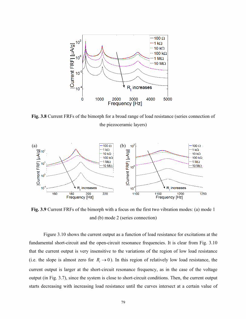
79

Fig. 3.8 Current FRFs of the bimorph for a broad range of load resistance (series connection of


Fig. 3.9 Current FRFs of the bimorph with a focus on the first two vibration modes: (a) mode 1


Figure 3.10 shows the current output as a function of load resistance for excitations at the

fundamental short-circuit and the open-circuit resonance frequencies. It is clear from Fig. 3.10

that the current output is very insensitive to the variations of the region of low load resistance

(i.e. the slope is almost zero for 0lR ). In this region of relatively low load resistance, the

current output is larger at the short-circuit resonance frequency, as in the case of the voltage

output (in Fig. 3.7), since the system is close to short-circuit conditions. Then, the current output

starts decreasing with increasing load resistance until the curves intersect at a certain value of

(b) (a)

80

load resistance (around 120 k ). For the values of load resistance larger than the value at this

intersection point, the current output at the open-circuit resonance frequency becomes larger

since the system approaches the open-circuit conditions. As in the voltage vs. load resistance

graph, the asymptotic trends for 0lR and lR appear to be linear.

Fig. 3.10 Variation of the current output with load resistance for excitations at the short-circuit


3.7.4 Frequency Response of the Power Output. The expression for the multi-mode power

FRF is obtained from Eq. (3.113) as

2

2 21

2 220

2 21

2( ) 1

12

r r

r r r r

j teql rp

rl r r r

jjp t

R jW e j CR j

(3.115)

Therefore the power output is proportional to the square of the voltage output. As a result, the

moduli of power FRFs plotted in Fig. 3.11 are normalized with respect to the square of base

acceleration (i.e. g2). According to Eq. (3.115), the power output is a product of two FRFs

(current and voltage) with the opposite trends against the load resistance. It is clear from Fig.

3.11 that the power output FRF does not necessarily exhibit a monotonic behavior with

increasing (or decreasing) load resistance for a given frequency. Among the sample values of the

load resistance considered in this work, the maximum power output for the first vibration mode

81

corresponds to the load of 100 k (see the enlarged view in Fig. 3.12a) at 187.5 Hz which is

expectedly a frequency in between the fundamental short-circuit and open-circuit resonance

frequencies. Considering the second vibration mode (see the second enlarged view in Fig.

3.12b), one observes that the maximum power output is obtained for 10 k at frequency 1161.9

Hz. It should be noted that the values of the load resistance used in this analysis are taken

arbitrarily to observe the general trends. Therefore, the maximum power outputs obtained from

each vibration mode are for these sample values and they are not necessarily for the maximum

possible (or the optimized) power outputs.‡‡ Another interesting aspect of the power FRFs given

in Fig. 3.11 is that they intersect one another. These intersections are observed not only around

the resonance frequencies (e.g. the curves of 10 k and 1 M intersect at 190.2 Hz and 193.9

Hz in Fig. 3.12a) but also they are observed at the off-resonance frequencies (e.g. the curves of

10 k and 100 k intersect at 723.7 Hz in Fig. 3.11). At these intersection frequencies, the two

respective load resistance values yield the same power output.

Fig. 3.11 Power FRFs of the bimorph for a broad range of load resistance (series connection of


The behavior of power output with changing load resistance for excitations at the

fundamental short-circuit and open-circuit resonance frequencies are given in Fig. 3.13. It can be

‡‡ Expressions of the optimum load resistance for modal excitations are given in Chapter 5.

82

recalled from Figs. 3.7 and 3.10 that the voltage and the current outputs obtained at the short-

circuit resonance frequency are larger than the ones obtained at the open-circuit resonance

frequency up to a certain load resistance (approximately 120 k in this case) after which the

opposite is valid. Since the power output is simply the product of the voltage and current, this

observation is valid for the power versus load resistance curves as well. As can be seen form Fig.

3.13, the power output at the short-circuit resonance frequency is larger before the intersection

point (at 120 k ) whereas the power output at the open-circuit resonance frequency is larger

after this point. The asymptotic trends for 0lR and lR are again linear and they appear

to have the same slope in log-log scale.

Fig. 3.12 Power FRFs of the bimorph with a focus on the first two vibration modes: (a) mode 1


Since the behavior of power with changing load resistance is not monotonic, both of the

power graphs shown in Fig. 3.13 exhibit peak values, which correspond to the optimum values of

load resistance at the fundamental short-circuit and open-circuit resonance frequencies. When the

optimum values of load resistance are used for each of the cases (short-circuit and open-circuit

excitations), both of them yield the same power output. Considering Figs. 3.7 and 3.10, it can be

observed that neither the voltages nor the currents are identical at these optimum values of load

resistance for excitations at the two special frequencies. Therefore, in practice, if one is flexible

in terms of the excitation frequency within this narrow frequency band, the short-circuit

resonance frequency is preferable for larger current whereas the open-circuit resonance

frequency is preferable for larger voltage (both yielding the same power output). Another aspect

(a) (b)

83

of Fig. 3.13 is that the optimum values of load resistance at these two frequencies are

considerably different (around 36 k for excitation at 185.1 Hz and around 405 k for

excitation at 191.1 Hz). From another perspective, therefore, if the load resistance is a constraint,

one can select the frequency of operation accordingly for the maximum power output.



It is worth adding a few words on the advantage of using the fundamental vibration mode

for energy harvesting compared to higher vibration modes. Figure 3.14 shows the power vs. load

resistance curves obtained for excitation at the six frequencies listed in Table 3.4 (i.e. the short-

circuit and the open-circuit resonance frequencies of the first three modes). The maximum power

for mode 1 excitation is around 0.23 mW/g2 at 185.1 Hz or at 191.1 Hz (for different optimum

loads). For mode 2 excitation, the maximum power output is around 7.5 W/g2 (at 1159.7 Hz or

at 1171.6 Hz). The maximum power output for mode 3 excitation is as low as 98 nW/g2 (at

3245.3 Hz or at 3254.1 Hz). As the moduli of the voltage and current FRFs decay by one order

of magnitude with increasing mode number according to Figs. 3.5 and 3.8, the modulus of the

power FRF decays by around two orders of magnitude with the increasing mode number.

Expectedly, the maximum power output is obtained for the fundamental vibration mode. For this

reason, the focus is usually placed on this vibration mode in practical considerations (as well as

in the experimental validations presented in the next chapter).

84

While considering the substantial difference between the moduli of the power FRFs for

different vibration modes, one should also note that these FRFs are normalized with respect to

base acceleration. A base acceleration input of 1g at 185.1 Hz implies a base displacement

amplitude of 7.25 m . This base displacement amplitude, for instance, creates a base

acceleration input of 39.3g at 1159.7 Hz (which may or may not be sustained by the brittle

piezoceramic layers§§). As a result, one should define the electromechanical FRF according to

the application and normalize with respect to the constant kinematic variable (displacement,

velocity or acceleration). In short, part of the reason of diminishing moduli at higher vibration

modes is that these FRFs are given here per base acceleration input (rather than displacement or

velocity).



3.7.5 Frequency Response of the Relative Tip Displacement. The multi-mode expression for

the tip displacement FRF (relative to the base) is

§§ Given the bending strength of the piezoceramic and a safety factor, one can obtain a critical stress FRF as a

function of load resistance by using the displacement and electric fields in the reduced piezoelectric constitutive

equation. This way, an estimate of the maximum acceleration level can be obtained for a given excitation frequency

and load resistance.

85

2 21

2 2 2210

2 21

( , ) 2 ( )

212

r r

rrel r r r rr rj t

r eq r r rrp

rl r r r

jw L t j L

W e jjj C

R j

(3.116)

This FRF differs from the solution of the electromechanically uncoupled vibration FRF due to

the voltage output induced as a result of piezoelectric coupling. The solution of the uncoupled

base excitation problem (addressed in Chapter 2) is obtained by neglecting the electrical term as

2 2 210

( , ) ( )

2rel r r

j tr r r r

w L t L

W e j

(3.117)

which is therefore identical to Eq. (3.116) for 0lR . The feedback of piezoelectric power

generation in the mechanical equation is associated with the r term in Eq. (3.116) and it is

basically a form of power dissipation due to Joule heating in the resistor. Therefore what happens

to the beam response due to power generation with a non-zero and finite load resistance is

damping of the structure, which has a relatively sophisticated form compared to conventional

viscous damping and structural damping mechanisms as demonstrated in the following.

Figure 3.15 shows the tip displacement FRFs*** (per base acceleration) for the set of

resistors and the frequency range of interest. One can see the three vibration modes in this figure

but it is not possible to distinguish between the curves of different load resistance. The enlarged

views of the first two vibration modes are shown in Fig. 3.16. The resistive shunt damping effect

results in both frequency shift and vibration attenuation. With increasing load resistance, the

electromechanical system moves from the short-circuit to the open-circuit conditions. In Fig.

3.16a, the peak vibration amplitude of 566.4 m for 100 (at 185.1 Hz) is attenuated to a peak

amplitude of 214.7 m for 100 k (at 187.4 Hz), which means a damping effect by a factor of

about 2.6. In the second vibration mode, the peak amplitude of 6.67 m for 100 (at 1159 Hz)

is attenuated to 4.97 m for 10 k (at 1160.8 Hz). One thing that is useful to mention is that,

*** The vibration FRFs investigated here are for the response at the tip of the cantilever ( x L ). However, the

distributed-parameter solution given here allows obtaining the coupled vibration response at any point px on the

beam by setting px x in the eigenfunction on the right hand side of Eq. (3.116). However, the motion at the tip of

the beam is of practical interest since it is the position of maximum deflection in the most flexible mode.

86

since the forms of the voltage and tip displacement FRFs are different, the resonance frequencies

in these FRFs are slightly different (Chapter 5). This is distinguishable only in the presence of

large mechanical damping. For instance, the short-circuit and the open-circuit resonance

frequencies of the third vibration mode in Fig. 3.15 are 3252.6 Hz and 3264.3 Hz, respectively.

Compared to those of the voltage FRF given in Table 3.4 (3245.3 Hz and 3254.1 Hz) these

numbers, respectively, are 0.2 % and 0.3 % larger. The difference is not considerable for the

fundamental vibration mode. Since the main concern in energy harvesting is the electrical

response, the short-circuit and the open-circuit resonance frequencies are defined here based on

the voltage FRF (as listed in Table 3.4).

Fig. 3.15 Tip displacement FRFs (relative to the vibrating base) of the bimorph for a broad range

of load resistance (series connection of the piezoceramic layers)

Fig. 3.16 Tip displacement FRFs of the bimorph with a focus on the first two vibration modes:

(a) mode 1 and (b) mode 2 (series connection)

(b) (a)

87

It is important to notice from the behavior around the modal frequencies of the vibration

FRFs that the form of damping caused by piezoelectric power generation (or power dissipation in

the resistor due to Joule heating) is more sophisticated that of viscous damping (although

oversimplification of the problem with the electrically induced viscous damping assumption has

been made by several researchers [18-20,22] over the last decade). First, with increasing load

resistance, the frequency of peak vibration amplitude changes considerably (and shifts to the

right in the FRF, unlike the case of viscous damping). Secondly, with further increase in the load

resistance, although the vibration amplitude at the original (short-circuit) resonance frequency is

attenuated to a certain amplitude, the vibration amplitude at the open-circuit resonance frequency

is amplified considerably. The reason is the frequency shift due to changing electrical boundary

condition. Indeed if one changes the load from one extremum ( 0lR ) to the other extremum

( lR ), the only modification in the energy harvester is a stiffness change. Physically, the

elastic modulus of the piezoceramic increases from the constant electric field value to the

constant electric displacement value and there is no overall energy dissipation. Only for non-zero

and finite values of load resistance, there is power dissipation in the mechanical domain (and

hence power generation in the electrical domain). All together with these, the resonance

frequency shift (from the mechanically damped natural frequency) associated with the presence

of a finite electrical resistance cannot be represented by a real-valued viscous damping ratio or

loss factor. Having discussed the mechanism of power dissipation in the mechanical domain, it is

worthwhile to point out the presence of a mechanical anti-resonance frequency between modes 2

and 3. Just like the resonance frequencies, this anti-resonance frequency also exhibits a shift

(from 2078.8 Hz to 2090.2 Hz) as the electrical load is changed from the short-circuit to the

open-circuit condition.

The behavior of vibration response at the tip of the beam is further studied for excitations

at the short-circuit and the open-circuit resonance frequencies of the fundamental vibration mode

in Fig. 3.17. It is interesting to note that the trends are not completely monotonic. For instance,

the minimum vibration amplitude at 185.1 Hz is obtained as 156.8 m for an electrical load of

about 500 k and a further increase of load resistance up to 10 M slightly amplifies the

vibration amplitude at this frequency (to 162 m ). Likewise, before it is amplified due to the

shift in the resonance frequency, the vibration amplitude at 191.1 Hz is slightly attenuated until

88

40 k (from 162 m to 157.7 m ). Then it is strongly amplified as the load resistance is

further increased. It is also useful to note that these electrical loads of maximum vibration

attenuation are not those of the maximum power generation. That is, the nature of

electromechanical coupling is such that, for the electrical load of maximum power generation,

the vibration amplitude at the tip of the beam does not necessarily take its minimum value.

Fig. 3.17 Variation of the tip displacement (relative to the vibrating base) with load resistance for

excitations at the short-circuit and the open-circuit resonance frequencies of the first vibration

mode (series connection)

3.7.6 Parallel Connection of the Piezoceramic Layers. In this section, the electromechanical

coupling and the equivalent capacitance terms used in Eqs. (3.113)-(3.116) are replaced by those

of the parallel connection case (from the second column in Table 3.1) and sample results are

presented. Figures 3.18-3.21 display the voltage, current, power and tip displacement FRFs along

with the enlarged views of the behavior around the fundamental vibration mode.

The short-circuit and the open-circuit resonance frequencies read from Fig. 3.18 for the

parallel connection case are identical to those listed in Table 3.4. The mathematical justification

is given in Chapter 5, where the single-mode approximation of the frequency shift

( oc scr r rf f f ) is shown to be proportional to 2 / eq

r pC . As a result, from Table 3.1, the single-

mode approximation of the resonance frequency shift for the series and parallel connection cases

are identical (in agreement with Figs. 3.18-3.21).

89

Fig. 3.18 (a) Voltage FRFs for the parallel connection of the piezoceramic layers and (b) an

enlarged view around the first vibration mode

Fig. 3.19 (a) Current FRFs for the parallel connection of the piezoceramic layers and (b) an


Fig. 3.20 (a) Power FRFs for the parallel connection of the piezoceramic layers and (b) an


(a) (b)

(a) (b)

(a) (b)

90

Fig. 3.21 (a) Tip displacement FRFs for the parallel connection of the piezoceramic layers and

(b) an enlarged view around the first vibration mode

Comparisons of the series and the parallel connection cases for excitation at the

fundamental short-circuit resonance frequency are given in Fig. 3.22. As can be anticipated, the

maximum power outputs of the series connection and parallel connection cases are identical but

they correspond to different values of optimum load. A maximum of 0.23 mW/g2 is delivered to

a resistive load of 36 k in the series connection case whereas the same maximum power output

is delivered to a resistive load of 9 k in the parallel connection case. The series connection

case generates this power with a current amplitude of 0.08 mA/g and a voltage amplitude of 2.8

V/g. In the parallel connection case, the same power output is obtained with a current amplitude

of 0.16 mA/g and a voltage amplitude of 1.4 V/g. Reasonably, series connection should be

preferred for large voltage output whereas parallel connection should be used for large current

output. The last graph in Fig. 3.22 shows that the resistive damping effect starts for lower values

of load resistance in the parallel connection case, which agrees with the behavior of maximum

power generation.

Piezoelectric energy harvesters, as observed in this case study, are poor current

generators.††† For instance, in the series connection case, for a base acceleration of 1g (achieved

for the base displacement amplitude of 7.25 m at 185.1 Hz) the voltage output is around 2.8 V

while the current associated with it is just 0.08 mA. While this voltage level is fairly good for

††† This fundamental fact about piezoelectric materials is indeed well known by the experimentalist vibration

engineer. It is the particular reason that piezoelectric-based transducers (such as accelerometers and impulse

hammers) are usually connected to a charge amplifier before the data acquisition system.

(a) (b)

91

charging a small battery, it is the current output that will make the duration of charging

substantially long (compared to a commercial battery charger). Several orders of magnitude

difference between the voltage and the current outputs of the generator is a very typical case in

piezoelectric energy harvesting. Therefore, if the purpose is to charge a battery using the

piezoelectric power output, parallel connection of the piezoceramic layers can be preferred so

long as the voltage limit for charging the battery is reached for a given excitation input.

Fig. 3.22 Comparison of the series and the parallel connection cases for excitations at the short-

circuit resonance frequency of the first vibration mode: (a) voltage vs. load resistance; (b) current

vs. load resistance; (c) power vs. load resistance; (d) tip displacement vs. load resistance

3.7.7 Single-mode FRFs. In the absence of base rotation, the single-mode voltage FRF can be

expressed as

2 2 2 20

ˆ( )

1 2l r r

j t eql p r r r l r

j Rv t

W e j R C j j R

(3.118)

(a)

(c)

(b)

(d)

92

and the single-mode tip displacement FRF (relative to the base) is

2 2 2 2

0

1 ( )ˆ ( , )

1 2

eql p r rrel

j t eql p r r r l r

j R C Lw L t

W e j R C j j R

(3.119)

In the following, the simulations of these single-mode expressions are compared with those of

the multi-mode expressions for the first three vibration modes in the series connection case (i.e.

r and eqpC are read from the first column of Table 3.1). Figure 3.23 shows the single-mode

FRFs obtained from Eq. (3.118) for 1r , 2r and 3r along with the multi-mode solution

for all values of load resistance considered here. As can be seen in this figure, the single-mode

solutions agree with the multi-mode solution only around the resonance frequency of the

respective mode of interest.

Fig. 3.23 Comparison of the multi-mode and the single-mode voltage FRFs (series connection)

Figures 3.24a and 3.24b, respectively, show the enlarged views of the single-mode and

the multi-mode voltage FRF comparisons for the first two modes. The single-mode

approximations work very well for all values of load resistance, yielding only slight

overestimations of the resonance frequency and the voltage amplitude. The single-mode

approximation for mode 1 shown in Fig. 3.24a predicts the short-circuit resonance frequency

accurately as 185.1 Hz and it overestimates the open-circuit resonance frequency as 191.3 Hz

(with an error of 0.1 %). In mode 2 prediction given by Fig. 3.24b, the short-circuit resonance

93

frequency is predicted as 1159.8 Hz (with an error of 0.009 %) whereas the open-circuit

resonance frequency is predicted as 1171.9 Hz (with an error of 0.03 %). The single-mode

voltage expression given by Eq. (3.118) can therefore successfully represent the resonance

behavior of the multi-mode voltage expression given by Eq. (3.113) for a given mode of interest

as a first approximation. The slight inaccuracy in the single-mode predictions is due to the

residual effects of the neighboring modes, which are ignored in the single-mode representation

given here.

Fig. 3.24 Comparison of the multi-mode and single-mode voltage FRFs with a focus on the first

two vibration modes: (a) mode 1 and (b) mode 2 (series connection)

The frequency response predictions of the single-mode tip displacement FRFs obtained

from Eq. (3.119) (for 1r , 2r and 3r ) are shown in Fig. 3.25 along with the multi-mode

tip displacement FRFs. Again, the single-mode FRFs exhibit agreement with the multi-mode

FRF around the modes of interest. The enlarged views for modes 1 and 2 are provided in Fig. 3.

26 for a clear view of the quality of agreement. The slight overestimation of the resonance

frequencies due to ignoring the neighboring vibration modes is the case here too and the error in

the single-mode resonance frequencies is less than 0.1 % for these practical vibration modes.

(a) (b)

94

Fig. 3.25 Comparison of the multi-mode and the single-mode tip displacement FRFs (series

connection)

Fig. 3.26 Comparison of the multi-mode and the single-mode tip displacement FRFs with a focus

on the first two vibration modes: (a) mode 1 and (b) mode 2 (series connection)

As a final comparison of the single-mode and the multi-mode simulations, the focus is

placed back on the fundamental vibration mode and variations of the electrical power and the

vibration response with load resistance are plotted in Figs. 3.27a and 3.27b, respectively, for

excitations at the fundamental short-circuit and open-circuit resonance frequencies. Note that the

slightly overestimated open-circuit resonance frequency is used in the single-mode simulations.

The predictions of the single-mode FRFs for this most important vibration mode are very

(a) (b)

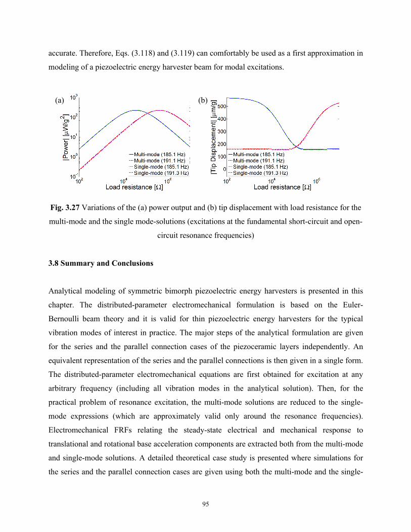
95

accurate. Therefore, Eqs. (3.118) and (3.119) can comfortably be used as a first approximation in

modeling of a piezoelectric energy harvester beam for modal excitations.

Fig. 3.27 Variations of the (a) power output and (b) tip displacement with load resistance for the

multi-mode and the single mode-solutions (excitations at the fundamental short-circuit and open-

circuit resonance frequencies)


Analytical modeling of symmetric bimorph piezoelectric energy harvesters is presented in this

chapter. The distributed-parameter electromechanical formulation is based on the Euler-

Bernoulli beam theory and it is valid for thin piezoelectric energy harvesters for the typical

vibration modes of interest in practice. The major steps of the analytical formulation are given

for the series and the parallel connection cases of the piezoceramic layers independently. An

equivalent representation of the series and the parallel connections is then given in a single form.

The distributed-parameter electromechanical equations are first obtained for excitation at any

arbitrary frequency (including all vibration modes in the analytical solution). Then, for the

practical problem of resonance excitation, the multi-mode solutions are reduced to the single-

mode expressions (which are approximately valid only around the resonance frequencies).

Electromechanical FRFs relating the steady-state electrical and mechanical response to

translational and rotational base acceleration components are extracted both from the multi-mode

and single-mode solutions. A detailed theoretical case study is presented where simulations for

the series and the parallel connection cases are given using both the multi-mode and the single-

(a) (b)

96

mode electromechanical FRFs. Accuracy of the single-mode FRFs in predicting the multi-mode

FRFs for modal excitations is also shown.

97

CHAPTER 4

EXPERIMENTAL VALIDATIONS OF THE ANALYTICAL SOLUTIONS

FOR CANTILEVERED BIMORPH PIEZOELECTRIC ENERGY

HARVESTERS

This chapter presents experimental validations of the analytical electromechanical relations

derived in Chapter 3. The first two experimental cases consider a brass-reinforced PZT-5H

bimorph cantilever without and with a tip mass attachment in two separate sections. The

voltage, current, power and the tip velocity FRFs of the bimorph (per base acceleration input) are

analyzed extensively for both configurations and the focus is placed on the fundamental

vibration mode in the frequency range of 0-1000 Hz. The general trends in the FRFs are

addressed and model predictions in the absence and presence of a tip mass are shown.

Excitations at the fundamental short-circuit and open-circuit resonance frequencies are

investigated in detail and the electrical performance diagrams at these two frequencies are

extracted. The shunt damping effect of piezoelectric power generation on the cantilever is also

studied based on the experimental measurements and model predictions. The effect of rotary

inertia of the tip mass is demonstrated by comparing the model predictions with the experimental

results (for the PZT-5H bimorph cantilever with a tip mass) including and excluding the rotary

inertia of the tip mass attachment. The electrical performance results of the same bimorph

without and with the tip mass are compared. The last case study investigates a brass-reinforced

PZT-5A bimorph cantilever with a focus on a wider frequency range (0-4000 Hz) covering the

first two vibration modes. The model predictions are compared with the experimental results

both using the multi-mode and the single-mode analytical FRFs.

98

4.1 PZT-5H Bimorph Cantilever without a Tip Mass

4.1.1 Experimental Setup. The first cantilever used for validation of the analytical model

developed in Chapter 3 is a brass-reinforced bimorph (T226-H4-203X) manufactured by Piezo

systems Inc. [45]. The experimental setup used for the electromechanical FRF measurements

given in this chapter is shown in Fig. 4.1 and the enlarged views of the equipments used in the

experiments are displayed in Fig. 4.2. A small electromagnetic shaker (TMC solution [46] TJ-2)

is used for excitation of the bimorph cantilever and the acceleration at the base of the cantilever

is measured by employing a small accelerometer (PCB Piezotronics [47] Model U352C67)

attached onto the aluminum clamp of the cantilever using wax. The tip velocity of the cantilever

in the transverse direction is measured using a laser vibrometer (Polytec [48] PDV100) by

attaching a small reflector tape at the tip of the cantilever. The data acquisition box (SigLab [49]

Model 20-42) has four input and two output channels. The base acceleration signal measured by

the accelerometer is sent to the reference channel after being processed by a charge amplifier

(PCB Piezotronics [47] Model 482A16). The reference channel automatically becomes the

denominator of the resulting FRFs in the frequency response analyzer. Two of the remaining

input channels are used for the laser vibrometer and the piezoelectric voltage output signals.

Therefore the two FRFs obtained using these three signal outputs are the tip velocity – to – base

acceleration FRF (or simply the tip velocity FRF) and the voltage output – to – base acceleration

FRF (or simply the voltage FRF). Therefore, in all frequency response measurements provided

here, the reference input is the base acceleration in agreement with the derivations of Chapter 3.

Chirp excitation (burst type with five averages) is provided to the shaker from the output channel

of the data acquisition box (which is connected to a Hewlett-Packard 6826A [59] fixed gain

amplifier before the electromagnetic shaker).

The bimorph used in the first two sections of the experimental validations given here

consists of two oppositely poled PZT-5H piezoelectric elements bracketing a brass substructure

layer. The brass layer provides electrical conductivity between the bottom electrode of the top

layer and the top electrode of the bottom layer. Therefore, collecting the charge output from the

outermost electrodes becomes the series connection case described in Fig. 3.1a (and that is what

is used here). The geometric and the material properties of the piezoceramic and the substructure

layers in the cantilevered condition are given in Table 4.1. The data sheet of the manufacturer

99

provides limited information regarding the elastic properties of the piezoceramic. Therefore,

typical properties of PZT-5H referred from the literature (Appendix B) are used here. The

reduced (plane-stress) properties of the piezoceramic for the Euler-Bernoulli beam theory are

referred from Table B.2 in Appendix B. Note that, in agreement with the formulation given in

the previous chapter, the length described by L is the overhang length of the harvester, i.e. it is

not the total free length (31.8 mm) of the bimorph as received from the manufacturer. The

overhang length of the cantilever is measured as 24.53 mm. A reflector tape of negligible mass is

attached close to the tip surface of the beam and the position of velocity measurement on the

reflector is approximately 1.5 mm from the free end ( 23vL mm). A close view of the bimorph

cantilever with the reflector tape is given in Fig. 4.3 along with the resistive loads.

Fig. 4.1 Experimental setup used for the electromechanical frequency response measurements

(photos by A. Erturk, 2009)

According to the geometric parameters in Table 4.1, the structure is assumed to be

perfectly symmetric. The nickel electrodes are covering the surfaces of the piezoceramic layers

are very thin and the thicknesses of the bonding layers are assumed to be neglibible. The total

thickness of the beam is 0.67 mm and therefore the overhang length – to – thickness ratio is

about 37.7. Since the focus in this case study (as well as in most energy harvesting applications)

is placed on the fundamental vibration mode, shear deformation and rotary inertia effects are

(1) Shaker with a small accelerometer and the cantilever (2) Laser vibrometer (3) Fixed gain amplifier (power supply) (4) Charge amplifier (5) Data acquisition system (6) Frequency response analyzer (software)

(1)

(2)(3) (4)

(5)(6)

(1)

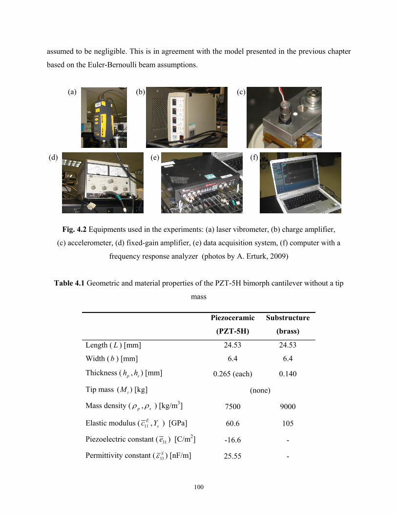
100

assumed to be negligible. This is in agreement with the model presented in the previous chapter

based on the Euler-Bernoulli beam assumptions.

Fig. 4.2 Equipments used in the experiments: (a) laser vibrometer, (b) charge amplifier,

(c) accelerometer, (d) fixed-gain amplifier, (e) data acquisition system, (f) computer with a

frequency response analyzer (photos by A. Erturk, 2009)

Table 4.1 Geometric and material properties of the PZT-5H bimorph cantilever without a tip

mass

Piezoceramic

(PZT-5H)

Substructure

(brass)

Length ( L ) [mm] 24.53 24.53

Width (b ) [mm] 6.4 6.4


Tip mass ( ) [kg]tM (none)


Elastic modulus ( 11Ec , sY ) [GPa] 60.6 105



(b) (a) (c)

(f) (e) (d)

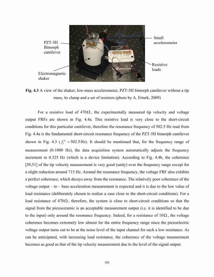
101

Fig. 4.3 A view of the shaker, low-mass accelerometer, PZT-5H bimorph cantilever without a tip

mass, its clamp and a set of resistors (photo by A. Erturk, 2009)

For a resistive load of 470 , the experimentally measured tip velocity and voltage

output FRFs are shown in Fig. 4.4a. This resistive load is very close to the short-circuit

conditions for this particular cantilever, therefore the resonance frequency of 502.5 Hz read from

Fig. 4.4a is the fundamental short-circuit resonance frequency of the PZT-5H bimorph cantilever

shown in Fig. 4.3 ( 1 502.5scf Hz). It should be mentioned that, for the frequency range of

measurement (0-1000 Hz), the data acquisition system automatically adjusts the frequency

increment to 0.325 Hz (which is a device limitation). According to Fig. 4.4b, the coherence

[50,51] of the tip velocity measurement is very good (unity) over the frequency range except for

a slight reduction around 715 Hz. Around the resonance frequency, the voltage FRF also exhibits

a perfect coherence, which decays away from the resonance. The relatively poor coherence of the

voltage output – to – base acceleration measurement is expected and it is due to the low value of

load resistance (deliberately chosen to realize a case close to the short-circuit conditions). For a

load resistance of 470 , therefore, the system is close to short-circuit conditions so that the

signal from the piezoceramic is an acceptable measurement output (i.e. it is identified to be due

to the input) only around the resonance frequency. Indeed, for a resistance of 10 , the voltage

coherence becomes extremely low almost for the entire frequency range since the piezoelectric

voltage output turns out to be at the noise level of the input channel for such a low resistance. As

can be anticipated, with increasing load resistance, the coherence of the voltage measurement

becomes as good as that of the tip velocity measurement due to the level of the signal output.

Resistive loads

Electromagnetic shaker

PZT-5H Bimorph cantilever

Small accelerometer

102

Fig. 4.4 (a) Tip velocity and voltage output FRFs of the PZT-5H bimorph cantilever without a tip

mass and (b) their coherence functions (for a load resistance of 470 )

The sudden reduction in the coherence around 715 Hz in Fig. 4.4b is the case for both

FRF measurements and it corresponds to a very small peak in the FRFs of Fig. 4.4a. As will be

seen from the model predictions shortly, the bimorph is not expected to have a mode around that

frequency. The fundamental resonance of the shaker itself (without the attachment on it) is not

expected for frequencies less than 15 kHz according to the manufacturer [46]. Therefore, the

only possible source of the low-amplitude peak around 715 Hz is the clamp of the bimorph that

is attached onto the shaker with a screw. This is checked very easily by pointing the laser

vibrometer to the clamp after attaching a reflector tape on it. Figure 4.5a shows the location of

the velocity measurement on the clamp and Fig. 4.5b shows the FRF obtained using the laser

vibrometer and the accelerometer measurements taken on the clamp. It can be seen from Fig.

4.5b that the unexpected peak around 715 Hz in Fig. 4.4a is indeed due to the clamp itself. If the

clamp behaved ideally for the purpose intended here (i.e. if all the points on it moved identically

in the vertical direction with a rigid body translation), the velocity – to – acceleration

measurement would be a monotonically decaying function of frequency without any peaks. More

precisely, this decaying function would be 1/ j (ratio of the velocity to acceleration in the

frequency domain). This ideal behavior agrees with the measurement shown in Fig. 4.5b very

well for all frequencies away from the unexpected peak around 715 Hz. The source of the peak

in the clamp FRF might be a possible rotation of the clamp as a result of the joint flexibility at

the clamp-shaker interface or it might be due to the dynamic interaction of the clamp

components. In either case the small peak appearing in the FRFs around this frequency is not a

(a) (b)

103

vibration mode of the bimorph cantilever. This imperfection will be ignored throughout this

chapter since it is sufficiently away from the fundamental vibration mode of the bimorph (which

is the main concern here).

Fig. 4.5 (a) A close view of the clamp showing the point of velocity measurement (photo by A.

Erturk, 2009) and (b) the clamp velocity – to – acceleration FRF capturing the clamp-related

imperfection

Before the model predictions are compared with the experimental measurements, it is

important to note that the tip velocity measurement taken by the laser vibrometer is the velocity

response of the cantilever relative to the absolute reference frame. In other words, it is not the

velocity response relative to the base of the beam. Therefore, the relative tip displacement FRF

given by Eq. (3.105), ( , )x , should be modified to express the velocity response at the tip of

the beam relative to the absolute frame of reference:

0modified

2 20 0

( , )( , ) 1

( , ) ( , )

j t

j t j t

w x tW e w x t

t tx j xW e W e j

(4.1)

where vx L (the point of velocity measurement) should be used to predict the measurement

taken by the laser vibrometer. Note that, instead of modifying the analytical FRF expression

given by by Eq. (3.105), one could as well process the experimental tip velocity FRF to obtain a

relative tip displacement FRF. However, post-processing of the analytical data is preferable in

order not to amplify any noise by further processing the experimental data.

The last item to mention on the experimental setup is regarding the resistance seen across

the electrodes of the piezoceramic. A measurement taken on the input channel of the data

Position of velocity measurement on the clamp

(a) (b)

104

acquisition system (when nothing is connected) shows a device resistance of 995 k . Therefore,

if the wires coming from the electrodes of the piezoceramic are directly connected to the data

acquisition system in the experiments (without a probe), the effective load resistance seen across

the electrodes of the piezoceramic is the equivalent resistance of the resistive load used and 995

k (which see each other in parallel): used 31/ (1/ 1/ 995 10 )l lR R . This observation implies

that the maximum resistance used in the experiments cannot exceed 995 k . As a consequence,

the equivalent of the resistor used and the device resistance constitutes the lR value to be used in

the model and these effective values are listed in the second column of Table 4.2. Therefore the

load resistance ( lR ) ranges from 470 (close to short-circuit conditions) to 995 k (close to

open-circuit conditions) in the experiments.

Table 4.2 The resistors used in the experiment and their effective values due to the impedance of

the data acquisition system

Resistance of the

resistor used

[k ]

Effective load

resistance ( lR ) seen by

the piezoceramic [k ]

0.470 0.470

1.2 1.2

6.7 6.7

10 9.9

22 21.5

47 44.9

100 90.9

330 247.8

470 319.2

680 403.9

1000 498.7

Open 995.0

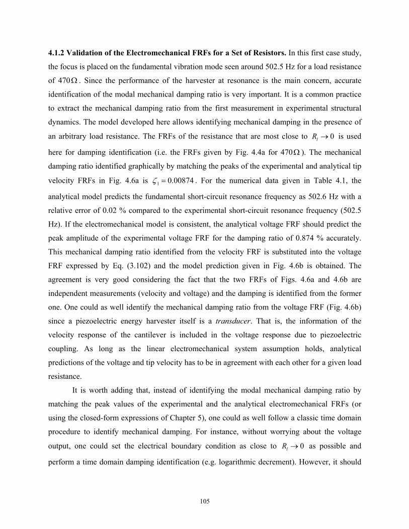
105

4.1.2 Validation of the Electromechanical FRFs for a Set of Resistors. In this first case study,

the focus is placed on the fundamental vibration mode seen around 502.5 Hz for a load resistance

of 470 . Since the performance of the harvester at resonance is the main concern, accurate

identification of the modal mechanical damping ratio is very important. It is a common practice

to extract the mechanical damping ratio from the first measurement in experimental structural

dynamics. The model developed here allows identifying mechanical damping in the presence of

an arbitrary load resistance. The FRFs of the resistance that are most close to 0lR is used

here for damping identification (i.e. the FRFs given by Fig. 4.4a for 470 ). The mechanical

damping ratio identified graphically by matching the peaks of the experimental and analytical tip

velocity FRFs in Fig. 4.6a is 1 0.00874 . For the numerical data given in Table 4.1, the

analytical model predicts the fundamental short-circuit resonance frequency as 502.6 Hz with a

relative error of 0.02 % compared to the experimental short-circuit resonance frequency (502.5

Hz). If the electromechanical model is consistent, the analytical voltage FRF should predict the

peak amplitude of the experimental voltage FRF for the damping ratio of 0.874 % accurately.

This mechanical damping ratio identified from the velocity FRF is substituted into the voltage

FRF expressed by Eq. (3.102) and the model prediction given in Fig. 4.6b is obtained. The

agreement is very good considering the fact that the two FRFs of Figs. 4.6a and 4.6b are

independent measurements (velocity and voltage) and the damping is identified from the former

one. One could as well identify the mechanical damping ratio from the voltage FRF (Fig. 4.6b)

since a piezoelectric energy harvester itself is a transducer. That is, the information of the

velocity response of the cantilever is included in the voltage response due to piezoelectric

coupling. As long as the linear electromechanical system assumption holds, analytical

predictions of the voltage and tip velocity has to be in agreement with each other for a given load

resistance.

It is worth adding that, instead of identifying the modal mechanical damping ratio by

matching the peak values of the experimental and the analytical electromechanical FRFs (or

using the closed-form expressions of Chapter 5), one could as well follow a classic time domain

procedure to identify mechanical damping. For instance, without worrying about the voltage

output, one could set the electrical boundary condition as close to 0lR as possible and

perform a time domain damping identification (e.g. logarithmic decrement). However, it should

106

be mentioned that even a wire (that can be used to short the electrodes to realize 0lR ) has a

certain resistance. Therefore the demonstration here is given for the presence of a finite load

resistance (that is still very close to 0lR ), which is the general case. Indeed, using a resistive

load that generates an acceptable voltage output (larger than the noise level) allows checking

whether or not the analytical model can predict the voltage output when the same damping ratio

is substituted into the voltage FRF (as done here in Fig. 4.6b). The upshot of this discussion is

that the mechanical damping can be identified in the presence of an arbitrary load resistance

using the electromechanical model. However, if one prefers to identify mechanical damping

using conventional techniques (e.g. half-power points of the vibration FRF, logarithmic

decrement in time domain, etc), the electrical boundary condition should be set to 0lR as

close as possible (which gives a noisy piezoelectric voltage output and does not allow checking

the voltage prediction). The important point is that the conventional techniques of damping

identification should not be used in the presence of arbitrary values of load resistance. In such a

case, damping due to piezoelectric coupling contributes to the mechanical damping in the

vibration response and the identified value would not be a pure mechanical damping ratio and it

cannot be used as r in the equations derived in this dissertation.


bimorph cantilever without a tip mass for a load resistance of 470

Having identified the mechanical damping ratio for a certain electrical load resistance,

the next step is to keep the damping ratio fixed and predict the tip velocity and voltage FRFs for

(a) (b)

107

different values of load resistance. Figure 4.7 displays experimental measurements and model

predictions for resistors of three different orders of magnitude: 1.2 k , 44.9 k and 995 k .

In all cases, the mechanical damping ratio is kept at 1 0.00874 and the model predictions are

very good. Note that, among these three different values of load resistance, 44.9 k results in

the strongest attenuation of the peak vibration amplitude. The peak voltage amplitude, as

expected from the theoretical case study of Chapter 3, increases monotonically with increasing

load resistance. The peak voltage amplitude increases by two orders of magnitude as the load

resistance is increased from 470 (Fig. 4.6b) to 995 k (Fig. 4.7c).

As the load resistance is increased from 470 to 995 k , the experimentally measured

fundamental resonance frequency moves from the short-circuit value of 502.5 Hz to the open-

circuit value of 524.7 Hz. The analytical model predicts these two resonance frequencies as

502.6 Hz and 524.5 Hz. Table 4.3 summarizes these results along with the errors in the model

prediction compared to the experimental frequencies. It will be seen from the modal

approximations given in Chapter 5 that the amount of the resonance frequency shift from the

short-circuit to the open-circuit value is directly proportional to the square of the

electromechanical coupling and is inversely proportional to the capacitance and the respective

undamped natural frequency. Although the errors in Table 4.3 are negligible for most practical

purposes, possible inaccuracies in the piezoelectric and permittivity constants contribute to the

error. In addition, the fact that the undamped natural frequency is slightly overestimated results

in underestimation of the open-circuit resonance frequency (as the frequency sift is inversely

proportional to the undamped natural frequency). The experimental source of error might be

more significant than all these, since the frequency increment is automatically set equal to 0.325

Hz when the frequency range of interest is adjusted to 0-1000 Hz.


bimorph cantilever without a tip mass

Fundamental resonance frequency Experiment Model % Error

1scf (short circuit) [Hz] 502.5 502.6 +0.02

1ocf (open circuit) [Hz] 524.7 524.5 -0.04

108


cantilever without a tip mass for various resistors: (a) 1.2 k , (b) 44.9 k and (c) 995 k

The piezoelectric voltage output and tip velocity FRFs measured experimentally and

predicted analytically for all resistors used here are given by Figs. 4.8 and 4.9, respectively. The

gradual increase of the voltage output with increasing load resistance (Fig. 4.8) is associated with

a gradual attenuation of the vibration amplitude at the short-circuit resonance frequency (Fig.

(a)

(b)

(c)

109

4.9). However, after a certain value of load resistance, the vibration amplitude at the short-circuit

resonance frequency get saturated and that at the open-circuit resonance frequency is amplified.

Hence, if one focuses on the fundamental open-circuit resonance frequency, both the vibration

amplitude and the voltage amplitude increase with increasing load resistance. Consequently,

modeling the effect of piezoelectric coupling in the form of an electrically induced viscous

damping term [18-20,22] fails in predicting what happens to the piezoelectric energy harvester

when it generates electricity (which also affects the electrical predictions in the coupled system).

Fig. 4.8 Voltage output FRFs of the PZT-5H bimorph cantilever without a tip mass for 12

different resistive loads (ranging from 470 to 995 k )

Fig. 4.9 Tip velocity FRFs of the PZT-5H bimorph cantilever without a tip mass for 12 different

resistive loads (ranging from 470 to 995 k )

110

The enlarged views of the voltage, current, power and the tip velocity FRFs are given in

Fig. 4.10 for all values of load resistance (in the 400-600 Hz region) with semi-log scale. It is

clear from Fig. 4.10a that the voltage FRFs monotonically converge to a single open-circuit

voltage FRF as the load resistance increases toward the lR extremum. The current FRFs in

Fig. 4.10b also behave monotonically and they become similar to a single short-circuit current

FRF for the 0lR extremum. The product of the voltage and the current FRFs gives the power

FRF, which results in a relatively complicated picture when all 12 curves are plotted together in

Fig. 4.10c. For a given frequency and range of load resistance, the behavior is not necessarily

monotonic, resulting in the intersections of the curves. One can define different values of


tip velocity FRFs of the PZT-5H bimorph cantilever without a tip mass for 12 different resistive

loads (ranging from 470 to 995 k )

(a) (b)

(d) (c)

111

optimum load resistance at different frequencies. The short-circuit and the open-circuit resonance

frequencies are of interest for the maximum power. Variation of the vibration response is also

non-monotonic and the trend of the peak vibration amplitude with load resistance is shown in

Fig. 4.10d. For a given excitation frequency, one can define an optimum load for the maximum

vibration attenuation.


Circuit Resonance Frequencies. Focusing on the fundamental short-circuit and open-circuit

resonance frequencies, the electrical performance diagrams are extracted next. These diagrams

can be useful for the electrical engineer to obtain an idea about the maximum voltage, current

and power output levels of the energy harvester as well as the optimum electrical load resistance

to design a sophisticated energy harvesting circuit. Figure 4.11 shows the variation of the

voltage amplitude at the fundamental short-circuit and open-circuit resonance frequencies. The

model predictions are in very good agreement with the experimental data points (for 12

resistors). The linear asymptotic trends can be noted from the experimental data as well. The

model predicts the maximum voltage outputs ( lR ) as 2.6 V/g and 12.8 V/g for excitations

at the fundamental short-circuit and open-circuit resonance frequencies, respectively.



tip mass

112

Variations of the electric current passing through the resistor for excitations at the

fundamental short-circuit and open-circuit resonance frequencies are plotted in Fig. 4.12. For

excitations at the fundamental short-circuit and open-circuit resonance frequencies, the

maximum current outputs ( 0lR ) are predicted as 336 A/g and 68 A/g . Just like the

asymptotic voltage behavior for lR , the asymptotic current trends are horizontal lines as

0lR .



tip mass

The final electrical performance diagram is the power versus load resistance diagram

shown in Fig. 4.13. According to the model, for excitations at the fundamental short-circuit and

open-circuit resonance frequencies, the maximum power output of about 0.22 mW/g2 is

delivered to the optimum electrical loads of 7.6 k and 189 k , respectively. Although these

exact values of load resistance are not used in the experiments, the loads of 6.7 k and 247.8

k are relatively close to these optimum ones. The resistive load of 6.7 k yields an

experimental power output of 0.218 mW/g2 at the fundamental short-circuit resonance frequency

whereas the resistive load of 247.8 k yields 0.212 mW/g2 at the fundamental open-circuit

resonance frequency. The model predicts the power outputs for 6.7 k and 247.8 k as 0.217

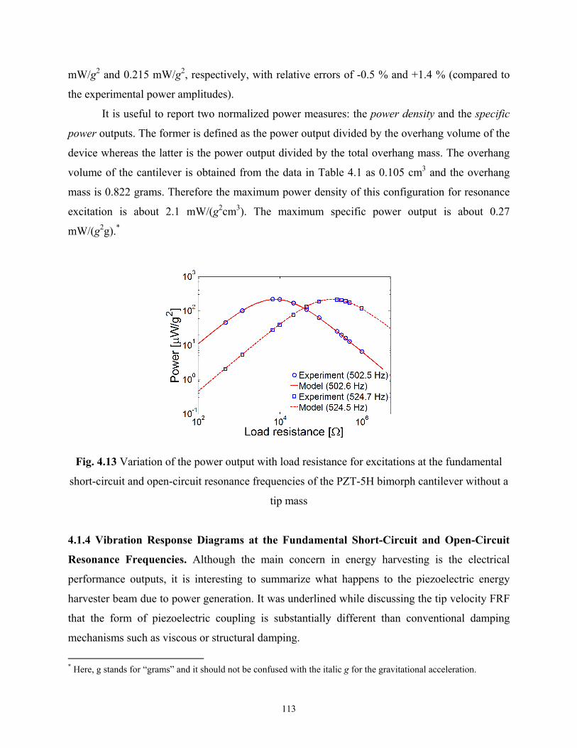
113

mW/g2 and 0.215 mW/g2, respectively, with relative errors of -0.5 % and +1.4 % (compared to

the experimental power amplitudes).

It is useful to report two normalized power measures: the power density and the specific

power outputs. The former is defined as the power output divided by the overhang volume of the

device whereas the latter is the power output divided by the total overhang mass. The overhang

volume of the cantilever is obtained from the data in Table 4.1 as 0.105 cm3 and the overhang

mass is 0.822 grams. Therefore the maximum power density of this configuration for resonance

excitation is about 2.1 mW/(g2cm3). The maximum specific power output is about 0.27

mW/(g2g).*



tip mass


Resonance Frequencies. Although the main concern in energy harvesting is the electrical

performance outputs, it is interesting to summarize what happens to the piezoelectric energy

harvester beam due to power generation. It was underlined while discussing the tip velocity FRF

that the form of piezoelectric coupling is substantially different than conventional damping

mechanisms such as viscous or structural damping.

* Here, g stands for “grams” and it should not be confused with the italic g for the gravitational acceleration.

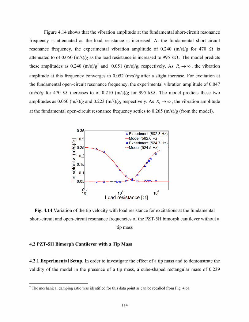
114

Figure 4.14 shows that the vibration amplitude at the fundamental short-circuit resonance

frequency is attenuated as the load resistance is increased. At the fundamental short-circuit

resonance frequency, the experimental vibration amplitude of 0.240 (m/s)/g for 470 is

attenuated to of 0.050 (m/s)/g as the load resistance is increased to 995 k . The model predicts

these amplitudes as 0.240 (m/s)/g† and 0.051 (m/s)/g, respectively. As lR , the vibration

amplitude at this frequency converges to 0.052 (m/s)/g after a slight increase. For excitation at

the fundamental open-circuit resonance frequency, the experimental vibration amplitude of 0.047

(m/s)/g for 470 increases to of 0.210 (m/s)/g for 995 k . The model predicts these two

amplitudes as 0.050 (m/s)/g and 0.223 (m/s)/g, respectively. As lR , the vibration amplitude

at the fundamental open-circuit resonance frequency settles to 0.265 (m/s)/g (from the model).



tip mass

4.2 PZT-5H Bimorph Cantilever with a Tip Mass

4.2.1 Experimental Setup. In order to investigate the effect of a tip mass and to demonstrate the

validity of the model in the presence of a tip mass, a cube-shaped rectangular mass of 0.239

† The mechanical damping ratio was identified for this data point as can be recalled from Fig. 4.6a.

115

grams is attached at the tip of the PZT-5H bimorph cantilever investigated in the previous

section (Fig. 4.15). The experimental setup and the devices used for the measurements are as

described in Section 4.1.1. The purpose here is to introduce the tip mass information to the

model directly and check the accuracy of the model predictions without changing the overhang

length of the beam (as well as the clamping condition).

Fig. 4.15 A view of the experimental setup for the PZT-5H bimorph cantilever with a tip mass

(photo by A. Erturk, 2009)

A close view of the PZT-5H bimorph cantilever with the tip mass is shown in Fig. 4.16a

and a schematic showing the configuration with the tip mass is given by Fig. 4.16b. Tip mass is

attached to the tip of the cantilever with a slight amount of wax (with negligible mass) such that

the center line of the cube is at the tip of the beam. Each edge of the tip mass (simply a rare-earth

magnet [60]) is 0.125 inch long ( 3.2a mm). As the center line of the tip mass lies on the tip of

the cantilever, the mass moment of inertia about the center axis of the bimorph is obtained from

22

6 2s

t t p

a haI M h

(4.2)

where 30.239 10tM kg (measured), the first term inside the parenthesis is for the mass

moment of inertia about the center axis of the cube and the second term is due to the parallel axis

theorem [61] to account for the offset of the tip mass to one side.‡ Substituting the numerical data

‡ Although the offset of the tip mass is taken into account in calculating the mass moment of inertia to improve the

model predictions, it can still be argued that the structural symmetry of the bimorph is distorted as the model in the

previous chapter is given for a symmetrically located tip mass. It should be noted that the tip mass is a mathematical

PZT-5H bimorph cantilever

Tip mass

116

into Eq. (4.2), the mass moment of inertia at the tip is calculated as 91.285 10 kg.m2. Therefore,

the numerical values of the mass and the mass moment of inertia at the tip are the only additions

to the data of the previous section as listed in Table 4.4. Following the same procedure, the first

step is to obtain the experimental tip velocity and voltage output FRFs for the load resistance of

470 .

Fig. 4.16 (a) A close view of the PZT-5H bimorph cantilever with a tip mass (photo by A.

Erturk, 2009) and (b) a schematic view showing the geometric detail of the cube-shaped tip mass

Table 4.4 Geometric and material properties of the PZT-5H bimorph cantilever with a tip mass

Piezoceramic

(PZT-5H)

Substructure

(brass)

Length ( L ) [mm] 24.53 24.53

Width (b ) [mm] 6.4 6.4


Tip mass ( ) [kg]tM 30.239 10

Mass moment of inertia at the tip 2( ) [kg m ]tI 91.285 10


Elastic modulus ( 11Ec , sY ) [GPa] 60.6 105



singularity at x L (normally associated with the Dirac delta function) and the analytical model takes it into

account through the eigenvalues and normalization of the eigenfunctions. Although the symmetry distortion is a

singularity only at the tip, it might be significant for a very large tip mass. This configuration is studied here to

check whether the formulation still works by comparing the model predictions with the experimental results.

0j tW e

(a) (b)

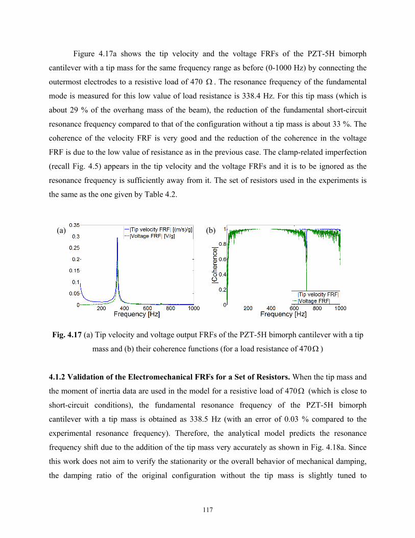
117

Figure 4.17a shows the tip velocity and the voltage FRFs of the PZT-5H bimorph

cantilever with a tip mass for the same frequency range as before (0-1000 Hz) by connecting the

outermost electrodes to a resistive load of 470 . The resonance frequency of the fundamental

mode is measured for this low value of load resistance is 338.4 Hz. For this tip mass (which is

about 29 % of the overhang mass of the beam), the reduction of the fundamental short-circuit

resonance frequency compared to that of the configuration without a tip mass is about 33 %. The

coherence of the velocity FRF is very good and the reduction of the coherence in the voltage

FRF is due to the low value of resistance as in the previous case. The clamp-related imperfection

(recall Fig. 4.5) appears in the tip velocity and the voltage FRFs and it is to be ignored as the

resonance frequency is sufficiently away from it. The set of resistors used in the experiments is

the same as the one given by Table 4.2.

Fig. 4.17 (a) Tip velocity and voltage output FRFs of the PZT-5H bimorph cantilever with a tip

mass and (b) their coherence functions (for a load resistance of 470 )

4.1.2 Validation of the Electromechanical FRFs for a Set of Resistors. When the tip mass and

the moment of inertia data are used in the model for a resistive load of 470 (which is close to

short-circuit conditions), the fundamental resonance frequency of the PZT-5H bimorph

cantilever with a tip mass is obtained as 338.5 Hz (with an error of 0.03 % compared to the

experimental resonance frequency). Therefore, the analytical model predicts the resonance

frequency shift due to the addition of the tip mass very accurately as shown in Fig. 4.18a. Since

this work does not aim to verify the stationarity or the overall behavior of mechanical damping,

the damping ratio of the original configuration without the tip mass is slightly tuned to

(a) (b)

118

1 0.00845 in order to better match the peak amplitude in Fig. 4.18a. This damping ratio is

then used in the analytical voltage FRF expression and the experimental voltage FRF shown in

Fig. 4.18b is predicted with very good accuracy. Therefore, the model exhibits consistency

between the vibration response and the electrical response in the presence of a tip mass as well.


bimorph cantilever with a tip mass for a load resistance of 470

To further study the performance of the electromechanical model, three particular resistive loads

are investigated next: 1.2 k , 44.9 k and 995 k . Figure 4.19 shows the tip velocity and the

voltage FRFs for these resistive loads (with fixed mechanical damping). The trend is very similar

to the previous case (bimorph without a tip mass). Compared to Fig. 4.7, both the vibration and

the voltage amplitudes are larger in Fig. 4.19. The main reason is the increased forcing amplitude

for the same acceleration input since the force amplitude in the base excitation problem of a

cantilever is proportional to the mass of the structure according to Eq. (3.36). Once again, among

the loads used here, 44.9 k results in a very strong attenuation of the peak vibration amplitude.

The electromechanical FRFs for these three resistive loads are successfully predicted in Fig.

4.19. The experimentally measured fundamental short-circuit and open-circuit resonance

frequencies are 338.4 Hz and 356.3 Hz and the model predicts these frequencies as 338.5 Hz and

355.4 as listed in Table 4.5. Once again, although the error levels are very low for practical

purposes, the primary theoretical sources of the slight inaccuracy in predicting the frequency

shift are the possible inaccuracies of the piezoelectric and permittivity constants. Overestimation

of the short-circuit resonance also results in underestimation of the frequency shift as mentioned

(a) (b)

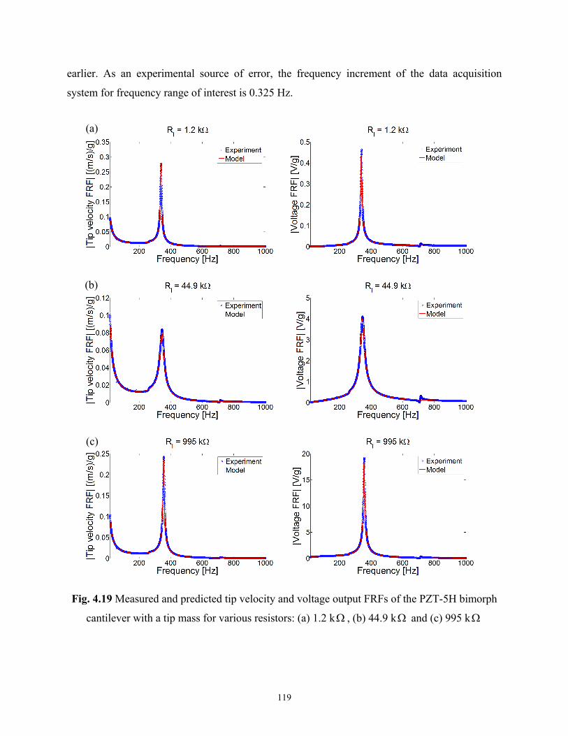
119

earlier. As an experimental source of error, the frequency increment of the data acquisition

system for frequency range of interest is 0.325 Hz.


cantilever with a tip mass for various resistors: (a) 1.2 k , (b) 44.9 k and (c) 995 k

(a)

(b)

(c)

120


bimorph cantilever with a tip mass

Fundamental resonance frequency Experiment Model % Error



Figures 4.20 and 4.21, respectively, display the tip velocity and the voltage output FRFs

of the PZT-5H bimorph cantilever with a tip mass for all values of load resistance used here.

Variation of the peak amplitudes and the resonance frequencies are successfully predicted in

both figures. The enlarged views of the voltage, current, power and the tip velocity FRFs for the

frequency range of 200-500 Hz are given in Fig. 4.22, where the variation of the resonance

frequency with load resistance is better visualized. All together with these graphs, one can

conclude that the model can successfully predict the amplitude-wise and the frequency-wise

coupled system dynamics of the bimorph cantilever in the presence of a tip mass as well.

Fig. 4.20 Tip velocity FRFs of the PZT-5H bimorph cantilever with a tip mass for 12 different


121

Fig. 4.21 Voltage output FRFs of the PZT-5H bimorph cantilever with a tip mass for 12 different



tip velocity FRFs of the PZT-5H bimorph cantilever with a tip mass for 12 different resistive

loads (ranging from 470 to 995 k )

(a) (b)

(c) (d)

122


Circuit Resonance Frequencies. In the electromechanical curves plotted in Fig. 4.22, the focus

is placed on the amplitude-wise results for excitations at the fundamental short-circuit and open-

circuit resonance frequencies.

Variations of the voltage amplitude at these two frequencies are plotted in Fig. 4.23 along

with the experimental data points for the 12 resistive loads. The analytical curve agrees very well

with the experimental data points and the analytical asymptotes of lR for excitations at the

short-circuit and the open-circuit resonance frequencies are 4.2 V/g and 24.7 V/g, respectively.



mass

The current versus load resistance diagrams for excitations at the fundamental short-

circuit and open-circuit resonance frequencies are plotted in Fig. 2.24, where the asymptotes of

0lR for these frequencies are 435 A/g and 75 A/g , respectively.

123



mass

The analytical power versus load resistance diagrams are shown in Fig. 4.25 for

excitations at the fundamental short-circuit and open-circuit resonance frequencies of the PZT-

5H bimorph with a tip mass. The analytical curves exhibit good agreement with the experimental

data points and predict a peak power amplitude of 0.46 mW/g2 for the optimum resistive loads of

9.7 k and 331 k , respectively, at the fundamental short-circuit and open-circuit resonance

frequencies. These exact values of the predicted optimum loads are not available in the set of

resistors used here. The experimental results for the nearest resistive loads are 0.460 mW/g2 for

9.9 k at the short-circuit resonance frequency and 0.463 mW/g2 for 319.2 k at the open-

circuit resonance frequency. These resistors are very close to the optimum ones and their power

outputs are in good agreement with the predicted maximum power output.

With the volume of the tip mass, the overhang volume of the cantilever becomes 0.137

cm3 and the overhang mass becomes 1.061 grams. Therefore the maximum power density of this

configuration for resonance excitation is about 3.4 mW/(g2cm3) and the maximum specific

power output is about 0.43 mW/(g2g).

124



mass


Resonance Frequencies. Variation of the tip velocity amplitude with load resistance for

excitations at the short-circuit and the open-circuit resonance frequencies are plotted in Fig. 4.26.

At the fundamental short-circuit resonance frequency, the experimental vibration amplitude of

0.296 (m/s)/g for 470 is attenuated to 0.054 (m/s)/g as the load resistance is increased to 995

k . The model predicts these amplitudes as 0.296 (m/s)/g§ and 0.055 (m/s)/g, respectively. For

lR , the vibration amplitude at the fundamental short-circuit resonance frequency converges

approximately to the same amplitude: 0.055 (m/s)/g. For excitation at the open-circuit resonance

frequency, the experimental vibration amplitude of 0.048 (m/s)/g for 470 increases to 0.242

(m/s)/g for 995 k . The model predicts these two amplitudes as 0.051 (m/s)/g and 0.246

(m/s)/g, respectively. As lR in the model, the vibration amplitude at the fundamental open-

circuit resonance frequency reaches 0.327 (m/s)/g.

§ This is the data point that was used for the identification of modal mechanical damping.

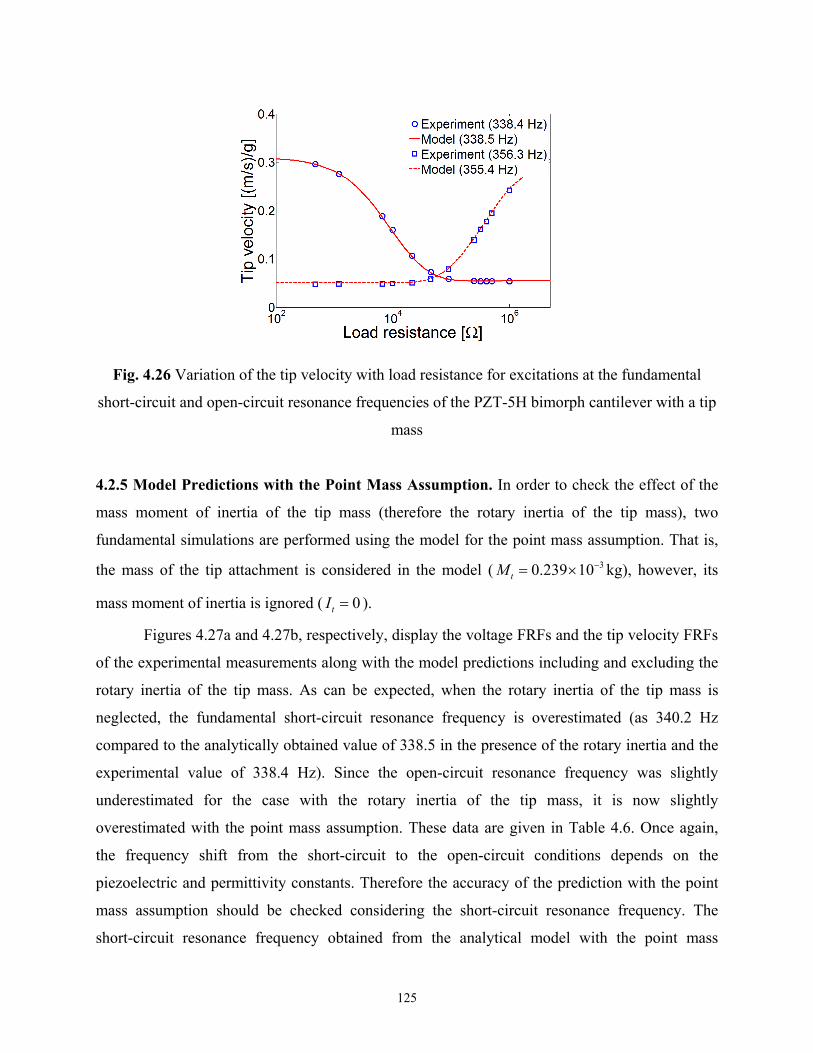
125



mass

4.2.5 Model Predictions with the Point Mass Assumption. In order to check the effect of the

mass moment of inertia of the tip mass (therefore the rotary inertia of the tip mass), two

fundamental simulations are performed using the model for the point mass assumption. That is,

the mass of the tip attachment is considered in the model ( 30.239 10tM kg), however, its

mass moment of inertia is ignored ( 0tI ).

Figures 4.27a and 4.27b, respectively, display the voltage FRFs and the tip velocity FRFs

of the experimental measurements along with the model predictions including and excluding the

rotary inertia of the tip mass. As can be expected, when the rotary inertia of the tip mass is

neglected, the fundamental short-circuit resonance frequency is overestimated (as 340.2 Hz

compared to the analytically obtained value of 338.5 in the presence of the rotary inertia and the

experimental value of 338.4 Hz). Since the open-circuit resonance frequency was slightly

underestimated for the case with the rotary inertia of the tip mass, it is now slightly

overestimated with the point mass assumption. These data are given in Table 4.6. Once again,

the frequency shift from the short-circuit to the open-circuit conditions depends on the

piezoelectric and permittivity constants. Therefore the accuracy of the prediction with the point

mass assumption should be checked considering the short-circuit resonance frequency. The

short-circuit resonance frequency obtained from the analytical model with the point mass

126

assumption overestimates the experimentally measured short-circuit resonance frequency by 0.5

%. This error is reduced to 0.03 % when the mass moment of inertia of the tip mass is included

in the model.

Fig. 4.27 Comparison of the voltage FRFs predicted with and without considering the rotary

inertia of the tip mass

Fig. 4.28 Comparison of the tip velocity FRFs predicted with and without considering the rotary

inertia of the tip mass

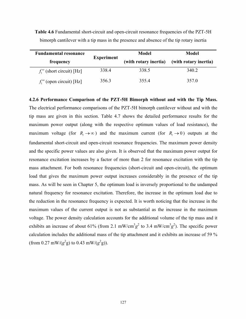
127


bimorph cantilever with a tip mass in the presence and absence of the tip rotary inertia

Fundamental resonance

frequency Experiment

Model

(with rotary inertia)

Model

(with rotary inertia)

1scf (short circuit) [Hz] 338.4 338.5 340.2

1ocf (open circuit) [Hz] 356.3 355.4 357.0

4.2.6 Performance Comparison of the PZT-5H Bimorph without and with the Tip Mass.

The electrical performance comparisons of the PZT-5H bimorph cantilever without and with the

tip mass are given in this section. Table 4.7 shows the detailed performance results for the

maximum power output (along with the respective optimum values of load resistance), the

maximum voltage (for lR ) and the maximum current (for 0lR ) outputs at the

fundamental short-circuit and open-circuit resonance frequencies. The maximum power density

and the specific power values are also given. It is observed that the maximum power output for

resonance excitation increases by a factor of more than 2 for resonance excitation with the tip

mass attachment. For both resonance frequencies (short-circuit and open-circuit), the optimum

load that gives the maximum power output increases considerably in the presence of the tip

mass. As will be seen in Chapter 5, the optimum load is inversely proportional to the undamped

natural frequency for resonance excitation. Therefore, the increase in the optimum load due to

the reduction in the resonance frequency is expected. It is worth noticing that the increase in the

maximum values of the current output is not as substantial as the increase in the maximum

voltage. The power density calculation accounts for the additional volume of the tip mass and it

exhibits an increase of about 61% (from 2.1 mW/cm3g2 to 3.4 mW/cm3g2). The specific power

calculation includes the additional mass of the tip attachment and it exhibits an increase of 59 %

(from 0.27 mW/(g2g) to 0.43 mW/(g2g)).

128

Table 4.7 Electrical performance comparisons of the PZT-5H bimorph cantilever without and

with a tip mass

Without the tip mass With the tip mass

1scf (experimental) [Hz] 502.5 338.4

1ocf (experimental) [Hz] 524.7 356.3

Maximum power at 1scf [mW/g2] 0.22 0.46

Optimum load at 1scf [k ] 7.6 9.7

Maximum power at 1ocf [mW/g2] 0.22 0.46

Optimum load at 1ocf [k ] 189 331

Maximum voltage at 1scf [mV/g] 2.6 4.2

Maximum voltage at 1ocf [mV/g] 12.8 24.7

Maximum current at 1scf [ A/g ] 336 435

Maximum current at 1ocf [ A/g ] 68 75

Maximum power density [mW/(g2cm3)] 2.1 3.4

Maximum specific power [mW/(g2g)] 0.27 0.43

4.3 PZT-5A Bimorph Cantilever

4.3.1 Experimental Setup. The last experimental case summarizes the analysis of a bimorph

cantilever made of a different type of piezoceramic: PZT-5A. The brass-reinforced PZT-5A

bimorph (T226-A4-203X) shown in Fig. 4.29 is manufactured by the same company [45]. It has

the same overall geometric properties (Table 4.8) and it is also manufactured for the series

connection of the oppositely poled layers (Fig. 3.1a). The main difference is due to the

piezoceramic material. The reduced form of the typical PZT-5A properties are referred from

Table B.2 in Appendix B (since the manufacturer provides limited data). The overhang length of

the configuration shown in Fig. 4.29 is 25.35 mm and the laser vibrometer measures the response

at a point that is approximately 23.2 mm away from the root ( 23.2vx L mm in Eq. (4.1)). The

129

experimental setup used and the procedure followed for the frequency response measurements

are identical to those of Section 4.1.1. The same set of resistors is used (Table 4.2).

Fig. 4.29 A view of the experimental setup for the PZT-5A bimorph cantilever (photo by A.

Erturk, 2009)

The two purposes of this section are to study a configuration with a different piezoelectric

material (PZT-5A) and to investigate a wider frequency range to include a higher vibration mode

(so that a demonstration using the single-mode FRFs can be presented). Therefore, the frequency

bandwidth in the experiments is increased, which affects the frequency resolution (in an

undesirable way) due to the limitations of the data acquisition system. For a frequency

bandwidth of 0-5000 Hz, the frequency increment automatically becomes 1.5625 Hz (which

should be taken into account as a source of error when comparing the model predictions).

For a resistive load of 470 , the tip velocity and voltage FRFs of the bimorph cantilever

are measured as shown in Fig. 4.30a. The FRFs are given in semi-log scale to view the second

vibration mode (which has about an order of magnitude less amplitude compared to the first

mode). The short-circuit resonance frequencies of the first and the second vibration modes are

read from the voltage FRF as 456.6 Hz and 2921.9 Hz. The coherence functions of these

measurements are given in Fig. 4.30b. The coherence of the tip velocity measurements drops

around the minimum between these vibration modes and after the second mode due to low

amplitude vibration response (low signal from the laser vibrometer). The poor behavior of the

coherence of the voltage measurement away from the resonance frequencies is due to the low

PZT-5A bimorph cantilever

130

load resistance used deliberately to be close to short-circuit conditions. However, the frequencies

around the peak values have acceptable coherence (close to unity).

Fig. 4.30 (a) Tip velocity and voltage output FRFs of the PZT-5A bimorph cantilever and (b)

their coherence functions (for a load resistance of 470 )

Table 4.8 Geometric and material properties of the PZT-5A bimorph cantilever

Piezoceramic

(PZT-5A)

Substructure

(brass)

Length ( L ) [mm] 25.35 25.35

Width (b ) [mm] 6.4 6.4


Tip mass ( ) [kg]tM (none)


Elastic modulus ( 11Ec , sY ) [GPa] 61 105



4.3.2 Validation of the Electromechanical FRFs for a Set of Resistors. When the numerical

data given in Table 4.7 is used in the model, the tip velocity FRF of the 470 case is predicted

as shown in Fig. 4.31a. The mechanical damping ratios of these two modes are identified using

(a) (b)

131

the model as 1 0.00715 and 2 0.00740 . When these damping ratios are used in the

voltage FRF expression, Fig. 4.31b is obtained. The voltage amplitude of the fundamental mode

is predicted with good accuracy (as 0.12 V/g compared to the experimental value of 0.13 V/g)

and that of the second mode is overestimated (as 0.036 V/g compared to the experimental value

of 0.028 V/g) for the mechanical damping ratios identified from the tip velocity FRF. The short-

circuit resonance frequencies of the first and the second vibration modes are obtained using from

the model as 466.2 Hz and 2921.3 Hz, respectively. Note that the noisy behavior in Figs. 4.31a

and 4.31b away from the resonance frequencies correspond to the low coherence regions in Fig.

4.30. The clamp-related imperfection is still in the FRFs (around 715 Hz) but it is sufficiently

away from both vibration modes.

Fig. 4.31 Measured and predicted (a) tip velocity and (b) voltage output FRFs of the PZT-5A

bimorph cantilever for a load resistance of 470

For the set of resistors used in the experiments (Table 4.2), the voltage, current, power

and the tip velocity FRFs are obtained as shown in Fig. 4.32. The overall analytical trends are in

good agreement with the experimental measurements (similar to the theoretical case study given

in Chapter 3). The amplitude-wise mismatch between the experimental and the analytical results

is particularly around the second vibration mode of the electrical FRFs. It should be noted that

the tip velocity FRF matches the experimental FRF better than the voltage FRF around the

second mode. One reason of the mismatch around the second mode in the voltage FRF (and in

the electrical FRFs derived from the voltage FRF) might be the low level of the voltage output

from the second vibration mode in the experiments. Another experimental source of error might

(a) (b)

132

be non-modeled imperfections in the bimorph that is more pronounced at high frequencies (since

the low frequency voltage predictions match perfectly around the first mode), such as possible

symmetry distortion in the structure or a relatively elastic behavior of the bonding layers that

becomes more important with a mode shape of larger cross-section rotation (the second mode

shape compared to the first mode shape).

Fig. 4.32 Electromechanical FRFs of the PZT-5A bimorph cantilever: (a) voltage output, (b)

current output, (c) power output and (d) tip velocity FRFs for 12 different resistive loads

(ranging from 470 to 995 k )

The frequency-wise predictions for the PZT-5A bimorph cantilever are listed in Table

4.9. The absolute value of the relative error in the model predictions is less than 0.6 %, meaning

that the Euler-Bernoulli theory works well even around the second natural frequency of this thin

structure. It should also be noted that for the large frequency band considered here, the

(a) (b)

(c) (d)

133

experimental frequency increment in the measured FRFs is relatively coarse (1.5625 Hz) for this

data acquisition system as mentioned previously.

Table 4.9 First two short-circuit and open-circuit resonance frequencies of the PZT-5A

bimorph cantilever

Resonance frequency Experiment Model % Error



2scf (short circuit) [Hz] 2921.9 2921.3 -0.02


4.3.3 Comparison of the Single-mode and Multi-mode Electromechanical FRFs. It is a

useful practice to check the performances of the single-mode electromechanical FRFs given by

Eqs. (3.108) and (3.111) for modes 1 and 2 briefly. When 1r is used in the single-mode

voltage FRF given by Eq. (3.108), the experimental voltage behavior is predicted as shown in

Fig. 4.33a. Substituting 2r into the same expression gives the single-mode curves shown in

Fig. 4.33b. Note that these two separate single-mode representations (for mode 1 and mode 2

independently) are approximately valid around the respective resonance frequencies only. Figure

4.33a lacks the information of all vibration modes other than the fundamental vibration mode

whereas Fig. 4.33b has the information of the second vibration mode only.

As discussed in the theoretical case study of Chapter 3, the effects of the neighboring

modes are lost in the single-mode representations. The fundamental single-mode open-circuit

resonance frequency is slightly overestimated as 484.3 Hz compared to the multi-mode case in

Fig. 4.33a. The single-mode open-circuit resonance frequency of the second mode in Fig. 4.33b

is also slightly overestimated compared to the multi-mode solution as 2953 Hz. In this case

study, these open-circuit resonance frequencies of the single-mode prediction agree better with

the experimental measurement compared to the multi-mode counterparts. However, one should

note that the experimental results are not necessarily perfectly accurate. Secondly, it is very

likely that the inaccuracy of the single-mode representation (due to excluding the residuals of the

134

neighboring modes) might be compensating the possible inaccuracy of the frequency shift

prediction (which depends on the piezoelectric and the permittivity constants).

Fig. 4.33 Prediction of the modal voltage frequency response using the single-mode FRFs for (a)

mode 1 and (b) mode 2 of the PZT-5A bimorph cantilever

Single-mode predictions of the tip velocity FRFs are shown in Fig. 4.34. As in the case of

Fig. 4.33, the single-mode representations in Fig. 4.34a are valid strictly around the fundamental

resonance frequency only whereas the single-mode representations in Fig. 4.34b are given for a

narrow band around the resonance frequency of the second vibration mode only.

(a)

(b)

135

Fig. 4.34 Prediction of the single-mode tip velocity frequency response using the single-mode

FRFs for (a) mode 1 and (b) mode 2 of the PZT-5A bimorph cantilever


The analytical solutions derived in the previous chapter are validated for various experimental

cases. The first experimental case is given for a brass-reinforced PZT-5H bimorph cantilever

without a tip mass. After validating the analytical model predictions using the voltage, current,

power and the tip velocity FRFs for this configuration and providing an extensive

electromechanical analysis, a tip mass is attached to create a configuration for the second case

study. The variations of the fundamental short-circuit and open-circuit resonance frequencies

after the attachment of the tip mass are successfully predicted by the model. Performance

(b)

(a)

136

diagrams for excitations at the fundamental short-circuit and open-circuit resonance frequencies

are extracted for both configurations (without and with the tip mass) and comparisons are made.

Improvement of the overall power output (as well as the power density and the specific power)

due to the addition of a tip mass is shown. The analytical model predicts the electrical and the

mechanical response with very good accuracy for all values of load resistance. Effect of the

rotary inertia of the tip mass is also studied by providing further analytical simulations with the

point mass assumption. It is shown that the resonance frequencies can be overestimated if the

rotary inertia of the tip mass is neglected. The damping effect of piezoelectric power generation

is discussed in detail based on the experimental measurements and the model predictions. The

final case study is given for a PZT-5A bimorph cantilever and the frequency range of interest is

increased to cover the second vibration mode as well. Predictions of the multi-mode and the

single-mode FRFs are provided (for the first two modes independently) and good agreement is

observed with the experimental results.

137

CHAPTER 5

DIMENSIONLESS SINGLE-MODE ELECTROMECHANICAL

EQUATIONS, ASYMPTOTIC ANALYSES AND CLOSED-FORM

RELATIONS FOR PARAMETER IDENTIFICATION AND

OPTIMIZATION

In this chapter, mathematical analyses of the single-mode electromechanical equations are

presented. Among the four FRF defined in Chapter 3, focus is placed on the voltage output and

the vibration response FRFs per translational base acceleration. The single-mode relations are

first expressed in the modulus-phase form and then they are represented with dimensionless

terms for convenience. The asymptotic trends of the voltage output and the tip displacement

FRFs are investigated and relations are obtained for the extreme conditions of load resistance.

Using the asymptotic FRFs, the resonance frequencies of the voltage and the tip displacement

FRFs are obtained and it is shown that they can be different. The linear asymptotes of the voltage

and vibration response (at a fixed frequency) observed in the previously given theoretical and

experimental case studies are mathematically verified here and the equations of these linear

asymptotes are obtained. Closed-form expressions for the optimum electrical loads of the

maximum power generation at the short-circuit and the open-circuit resonance frequencies at

extracted. It is mathematically proven that, for excitations at these two frequencies, the

intersections of the linear voltage asymptotes occur at the respective optimum load resistance.

Using this result, a simple technique is introduced to identify the optimum load resistance of a

piezoelectric energy harvester using a single resistive load with the open-circuit voltage

measurement. The asymptotes of the vibration resonance are also studied and expressions are

derived to estimate the percentage vibration attenuation/amplification at the short/open-circuit

resonance frequency as the load resistance is increased from the short-circuit to the open-circuit

conditions. An experimental case is visited to validate the major equations derived here. It should

be noted that, all the derivations given here are based on the single-mode approximation and they

are valid around the respective modal frequency (which is the fundamental natural frequency in

most practical applications).

138

5.1 Equivalent Dimensionless Representation of the Single-mode Electromechanical FRFs

5.1.1 Complex Forms. Recall from the equivalent representations of the single-mode

electromechanical equations presented for bimorph energy harvesters given by Eqs. (3.107) and

(3.110) that

2 20 0ˆˆ ˆ( ) j t j tv t W e e (5.1)

2 2

0 0ˆ ˆˆ ( , ) , ,j t j t

relw x t x W e x e (5.2)

where the respective electromechanical FRFs are

2 2 2ˆ

1 2l r r

eql p r r r l r

j R

j R C j j R

(5.3)

2 2 2ˆ

1 2l r r

eql p r r r l r

j R

j R C j j R

(5.4)

2 2 2

1 ( )ˆ( , )

1 2

eql p r r

eql p r r r l r

j R C xx

j R C j j R

(5.5)

2 2 2

1 ( )ˆ ( , )

1 2

eql p r r

eql p r r r l r

j R C xx

j R C j j R

(5.6)

Here, the electromechanical coupling term r and the equivalent capacitance term eqpC are read

from Table 3.1 for the series or parallel connection cases of the piezoceramic layers. According

to Eqs. (5.1) and (5.2), , , ˆ( , )x and ˆ ( , )x , respectively, are the single-mode

voltage output – to – translational base acceleration, voltage output – to – rotational base

acceleration, displacement response – to – translational base acceleration and the displacement

response – to – rotational base acceleration FRF. These expressions are the complex forms of the

single-mode electromechanical FRFs.

For convenience, in the following, the focus is placed on the FRFs for the translational

acceleration input (i.e. and ˆ( , )x ), and once can easily obtain the counterparts for

and ˆ ( , )x simply by replacing r with r . It is very important to note that, the single

mode relations derived in the following are approximately valid only around the natural

frequency ( r ) of the respective vibration mode.

139

5.1.2 Modulus-Phase Forms. The single-mode voltage FRF can be expressed in the modulus-

phase form as

ˆ ˆ je (5.7)

where the modulus (magnitude) of the FRF is

1/222

2 2 2 2 2

ˆ

1 2 2

l r r

eq eq eqr l p r r r r l p r p r

R

R C R C C

(5.8)

and the phase (the argument) is the phase between the base acceleration and the voltage output

2 2 2

1

2 2

2sgn tan

2 1 2

eq eqr r l p r p r

r r eqr l p r r

R C C

R C

(5.9)

where sgn stands for the signum function. The single-mode tip displacement FRF is then

( , )ˆ ˆ( , ) ( , ) j xx x e (5.10)

where its modulus and the phase are

1/22

1/2222 2 2 2 2

( ) 1ˆ( , )

1 2 2

eqr r l p

eq eq eqr l p r r r r l p r p r

x R Cx

R C R C C

(5.11)

2 2 2

1 1

2 2

2( )( , ) tan tan

( ) 1 2

eq eqeqr r l p r p rl p r r

eqr r r l p r r

R C CR C xx

x R C

(5.12)

5.1.3 Dimensionless Forms. Some of the terms in the modulus and phase of the voltage FRF can

be put into a dimensionless form to give

1/2222 3

/ˆ

1 1 2 2 1

r r r r

r r r r r r

(5.13)

31

2

2 1sgn tan

2 1 1 2r r r rr

r rr

(5.14)

Similarly, the modulus and the phase of the tip displacement FRF become

140

1/22

1/2222 2 3

( ) 1ˆ( , )

1 1 2 2 1

r r

r r r r r r r

f xx

(5.15)

31 1

2

2 1( )( , ) tan tan

1 1 2( )r r r rr r

r rr

f xx

f x

(5.16)

In Eqs. (5.13)-(5.16), the dimensionless terms are

eqr l p rR C (5.17)

2

2r

r eqp rC

(5.18)

r

(5.19)

( ) ( )r r rf x x (5.20)

Note that the voltage modulus given by Eq. (5.113) is dimensional due to /r (with the unit of

[Vs2/m]) whereas the tip displacement modulus given by Eq. (5.15) is dimensional due to 21/ r

(and it has the unit of [s2]).

5.2 Asymptotic Analyses, Resonance Frequencies and Closed-form Expressions for

Parameter Identification and Optimization

5.2.1 Short-circuit and Open-circuit Asymptotes of the Voltage FRF. Equation (5.13) can be

rewritten as

1/22 22 2 3

/ˆ

1 2 2 1

r r r

r r r r r

(5.21)

Taking the limit as 0r yields the following expression for very small values of load

resistance:*

* Note that, 0

r implies 0

lR (close to short-circuit conditions) and

r implies

lR (close to

open-circuit conditions) according to Eq. (5.17).

141

1/20 2 22

/ˆ ˆlim

1 2r

r r r r

sc

r

(5.22)

The limit as r leads to the following relation for very large values of load resistance:

1/22 22

/ˆ ˆlim

1 2r

r r r

oc

r r

(5.23)

Here, subscripts sc and oc stand for the short-circuit and the open-circuit conditions. Equations

(5.22) and (5.23) represent the moduli of the voltage FRF for the extreme cases of the load

resistance ( 0lR and lR , respectively). It is useful to note that the short-circuit voltage

asymptote depends on the load resistance linearly whereas the open-circuit voltage asymptote

does not depend on the load resistance.†

5.2.2 Short-circuit and Open-circuit Asymptotes of the Tip Displacement FRF. The modulus

of the tip displacement FRF can be re-expressed to give

1/22 2

1/22 22 2 2 3

( ) 1ˆ ,

1 2 2 1

r r

r r r r r r

f xx

(5.24)

The asymptotic FRF behaviors at the short-circuit and the open-circuit conditions are

1/20 2 22 2

( )ˆ ˆ, lim ,

1 2r

r

sc

r r

f xx x

(5.25)

1/22 22 2

( )ˆ ˆ, lim ,

1 2r

r

oc

r r r

f xx x

(5.26)

Note that the short-circuit and the open-circuit asymptotes obtained for the vibration response of

the beam do not depend on the load resistance.

† The asymptotes of the current FRFs are not discussed here and they can easily be derived from the voltage

asymptotes.

142

5.2.3 Short-circuit and Open-circuit Resonance Frequencies of the Voltage FRF. Having

obtained the modulus of the voltage FRF for electrical loads close to short-circuit conditions, one

can find its dimensionless resonance frequency ( resvsc ) as

1/22 22

/ˆ0 1

1 2resvsc

resvsc

r r r rsc resvsc

r

(5.27)

Therefore the dimensionless resonance frequency ( resvsc ) of the voltage FRF for very low values

of load resistance is simply unity.

Similarly, the dimensionless resonance frequency ( resvoc ) of the voltage FRF for very large

values of load resistance is obtained as

1/22

1/22 22

/ˆ0 1 2

1 2resvoc

resvoc

r r roc resvoc r r

r r

(5.28)

5.2.4 Short-circuit and Open-circuit Resonance Frequencies of the Tip Displacement FRF.

Using the short-circuit asymptote of the tip displacement FRF, the dimensionless resonance

frequency ( reswsc ) of the tip displacement response for very low values of load resistance is

obtained as

1/22

1/22 22 2

ˆ , ( )0 1 2

1 2reswsc res

wsc

sc r reswsc r

r r

x f x

(5.29)

The dimensionless resonance frequency ( reswoc ) of the tip displacement FRF for very large

values of load resistance is

1/22

1/22 22 2

ˆ , ( )0 1 2

1 2reswoc res

woc

oc r reswoc r r

r r r

x f x

(5.30)

143

Note that, the dimensionless short-circuit resonance frequencies of the voltage and the tip

displacement FRFs are not the same. The short-circuit resonance frequency of the voltage FRF

does not depend on mechanical damping whereas the open-circuit resonance frequencies of both

FRFs depend on mechanical damping.‡ Since the short-circuit and the open-circuit resonance

frequencies are defined based on the voltage FRF in this work (where the focus is placed on the

electrical response), one can express the single-mode approximations of these dimensionless

frequencies as

1scr (5.31)

1/221 2oc

r r r (5.32)

The dimensional forms are then

scr r (5.33)

1/221 2oc

r r r r (5.34)

Therefore the resonance frequency shift in the voltage – to – base acceleration FRF as the load

resistance is increased from 0lR to lR is

1/221 2 1oc sc

r r r r r (5.35)

According to Eq. (5.35), the resonance frequency shift from the short-circuit to the open-circuit

conditions is proportional to r , which means from Eq. (5.18) that it is directly proportional to

the square of the electromechanical coupling term ( 2

r ) and inversely proportional to the

equivalent capacitance ( eq

pC ) and square of the undamped natural frequency ( 2r ). The resonance

frequency shift is affected by the modal mechanical damping ratio ( r ) as well.

5.2.5 Identification of Modal Mechanical Damping Ratio in the Presence of a Resistive

Load. In the electromechanical system, one can identify the mechanical damping ratio either

using the voltage FRF or using the vibration FRF. The following derivations provide closed-form

expressions for the identification of mechanical damping at sc in the presence of an

‡ The mechanically undamped short-circuit and open-circuit natural frequencies of the voltage and tip displacement

FRFs, however, are identical, i.e. 1sc

r and 1/ 2

1oc

r r for 0

r .

144

arbitrary load resistance using both approaches (which can also be given for ocr in a similar

way).

In order to identify the modal mechanical damping ratio for an arbitrary but non-zero

value of r , one can set 1 in the modulus of the voltage FRF given by Eq. (5.13) and obtain

1/22 2

/ˆ 1

2 2

r r r r

r r r r r

(5.36)

where ˆ 1 is known from the experimental measurement (i.e. it is the experimental data point

used for damping identification). Equation (5.36) yields the following quadratic relation:

2 0r rA B C (5.37)

where

2

2 2 24 1 , 4 , ˆ 1

r r rr r r r r

r

A B C

(5.38)

The positive root of Eq. (5.37) gives the modal mechanical damping ratio as

1/22 4

2r

B AC B

A

(5.39)

Although r (the dimensionless measure of load resistance) is arbitrary in identifying the

mechanical damping ratio from the mathematical point of view, physically, it should be large

enough so that ˆ 1 is a meaningful voltage measurement (i.e. not noise) with acceptable

coherence (recall the discussions in Chapter 4).

Identification of the modal mechanical damping from the vibration measurement requires

using Eq. (5.15). Let the frequency of interest be 1 again. Equation (5.15) becomes

1/22

1/22 22

( ) 1ˆ(1, )

2 2

r r

r r r r r r

f xx

(5.40)

which yields the following alternative quadratic equation for r

2 0r rA B C (5.41)

where the coefficients are

145

2

2

2 2 22

4

( ) 14 1 , 4 ,

ˆ(1, )

r r

r r r r r

r

f xA B C

x

(5.42)

The modal mechanical damping ratio is the positive root of Eq. (5.41) given by Eq. (5.39). Note

that the value of ˆ(1, )x at point x on the beam is the experimental data point used in the

identification process (for 1 ). Unlike the case of mechanical damping identification using

the voltage FRF, the external load resistance can be chosen very close to zero here (since such a

load does not cause noise in the vibration FRF). Thus, for 0r , Eq. (5.41) simplifies to the

purely mechanical form of

2

( )

ˆ2 (1, )

r

r

r

f x

x

(5.43)

5.2.6 Electrical Power FRF. Using the dimensionless voltage FRF given by Eq. (5.13), the

electrical power FRF is obtained as

2

222 3

/ /ˆ

1 1 2 2 1

r r r r l

r r r r r r

R

(5.44)

For excitation at the short-circuit resonance frequency ( 1 ) the electrical power FRF is

2

2 2

/ /1

2 2 /

r r r l

r r r r

R

(5.45)

and for excitation at the open-circuit resonance frequency ( 1/221 2r r ), the electrical

power FRF becomes

2

1/222 22 2

/ /ˆ 1 2

1 1 2 1 2 / 1 2 2 1

r r r r l

r r

r r r r r r r r r

R

(5.46)

5.2.7 Optimum Values of Load Resistance at the Short-circuit and Open-circuit Resonance

Frequencies. Equation (5.44) can be used in order to obtain the optimum load resistance for the

maximum electrical power output at a given excitation frequency (around the respective

146

resonance frequency). The problem of interest is the resonance excitation and one can use Eq.

(5.31) for excitation at 1 to obtain

, 1

, 11/22

ˆ 1 10

1 2optl

optl

eqlr p r rR

RR C

(5.47)

which is the optimum load resistance for excitation at the short-circuit resonance frequency. A

similar practice can be followed for estimating the optimum load resistance for excitation at the

open-circuit resonance frequency as

1/22

1/22, 1 2

1/2 1/2222

1 2

2 2

ˆ 1 2 1 / 210

1 1 2r r

opt r rl

r rr r r

l eql r p r r r r

R

RR C

(5.48)

For excitations at the short-circuit and the open-circuit resonance frequencies, the optimum

values of load resistance are inversely proportional to the capacitance and the undamped natural

frequency. The electromechanical coupling and the mechanical damping ratio also affect the

optimum load resistance. The optimum resistive loads obtained in Eqs. (5.47) and (5.48) can be

back substituted into Eqs. (5.45) and (5.46) to obtain the maximum power expressions for

excitations at these two frequencies.

5.2.8 Vibration Attenuation from the Short-circuit to the Open-circuit Conditions. Consider

the asymptotic vibration response FRFs defined for point x on the beam given by Eqs. (5.25) and

(5.26). The ratio of the response amplitude at the open-circuit conditions to the response

amplitude at the short-circuit conditions at frequency is

1/22 22

1/22 22

ˆ 1 2,

ˆ , 1 2

r

r

oc

scr

x

x

(5.49)

Therefore the percentage variation of the vibration amplitude as the load resistance is increased

from 0lR to lR is

147

1/22 22

1/22 22

1 21 100

1 2

r

w

r r

(5.50)

For excitation at the short-circuit resonance frequency ( 1 ):

1/22

ˆ 1, 1ˆ 1, 1 / 2

oc

sc r r

x

x

(5.51)

yielding a percentage vibration attenuation of

1/22 2

11 1 100

1 4w

r r

(5.52)

The percentage of vibration amplification for excitation at the open-circuit resonance frequency

(due to an increase of the load resistance from 0lR to lR ) can be obtained by

substituting 1/221 2r r into Eq. (5.49) as

1/21/2 2 22 1/22 2 2 2

1/2 21/2 2 22 2 2

ˆ 1 2 , 2 2 1 2 / 2 1

1ˆ 1 2 , 2 2 1 2

oc r r r r r r rr r r

r rsc r r r r r r

x

x

(5.53)

Hence the percentage vibration amplification at the open-circuit resonance frequency is

1/22 21/22

2

/ 2 11 2 1 100

1r r r

w r rr r

(5.54)

5.3 Intersection of the Voltage Asymptotes and a Simple Technique for Identification of the

Optimum Load Resistance from Experimental Measurements

5.3.1 On the Intersection of the Voltage Asymptotes for Resonance Excitation. It was

noticed both in the theoretical case study of Chapter 3 and in the experimental case studies of

Chapter 4 that the asymptotic trends in the voltage FRF are linear, in agreement with Eqs. (5.22)

and (5.23). This observation leads to an interesting result if one further examines these linear

asymptotes at the short-circuit and the open-circuit resonance frequencies.

148

Substituting 1 into the short-circuit voltage asymptote gives

/

ˆ 12

r r r r

scr

(5.55)

Similarly, substituting 1 into the open-circuit voltage asymptote yields

1/22 2

/ˆ 1

1 2

r r r

oc

r r

(5.56)

Clearly, these asymptotes intersect at a finite but non-zero value of the dimensionless load

resistance

1/222

2ˆ ˆ1 1

2

rsc oc r

r r

(5.57)

and the dimensional form of this load resistance is

1/2

1

1 2l eq

r p r r

RC

(5.58)

which is nothing but the optimum load resistance for excitation at the short-circuit resonance

frequency as derived from the power FRF in Eq. (5.47).

Substituting 1/221 2r r into the short-circuit voltage asymptote gives

1/2 1/22 21/22

1/2 1/22 2 2 422 2

1 2 / 1 2 /ˆ 1 2

4 42 2 1 2

r r r r r r r r r r r r

sc r r

r r rr r r r r

(5.59)

Likewise, using 1/221 2r r in the open-circuit voltage results in

1/221/2 1/22 2 2 422 2

/ /ˆ 1 2

4 4 42 2 1 2

r r r r r r

oc r r

r r r rr r r r

(5.60)

The intersection of the voltage asymptotes for excitation and the open-circuit resonance

frequency gives

1/222

1/2 1/22 2

2 2

1 / 2ˆ ˆ1 2 1 2

1 1 2r r r

sc r r oc r r r

r r r r

(5.61)

149

which has the dimensional form of

1/222

2 2

1 / 21

1 1 2r r r

l eqr p r r r r

RC

(5.62)

The load resistance of the intersection point given by Equation (5.62) is the optimum load

resistance for excitation at the open-circuit resonance frequency as derived in Eq. (5.48).

5.3.2 A Simple Technique for the Experimental Identification of the Optimum Load

Resistance for Resonance Excitation. The observation given in the previous section leads to a

very simple technique for identifying the optimum load from the experimental voltage

measurements at 1 or at 1/221 2r r . It is often required to do a resistor sweep to

identify the optimum load resistance in the experiments. Either a variable resistor or a set of

several resistors is used for this purpose (as done in Chapter 4). Based on the observation given

in the previous section, a technique for identifying the optimum load resistance using only one

resistor along with an open-circuit voltage measurement is proposed here.

It is noted in the previous section is that the intersections of the voltage asymptotes for

excitations at the short-circuit and the open-circuit resonance frequencies correspond to the

respective optimum loads. Suppose that the experimentalist has fixed the excitation frequency to

one of these two frequencies for identifying the optimum load resistance under a certain

excitation amplitude. The horizontal asymptote of the open-circuit conditions is simply obtained

from the open-circuit voltage measurement (a horizontal line with the amplitude of ocv ). Then, a

low value of resistance is chosen ( *lR ), and the respective voltage output ( *v ) is measured.§ Since

the voltage output for zero load resistance (starting point of the short-circuit asymptote) is zero,

one has the short-circuit asymptote, which has a slope of * */ lv R . The value of load resistance for

which this line intersects the open-circuit voltage amplitude is the optimum load resistance. The

§ This test resistor of relatively low resistance should be on the linear asymptote. That is, it should be considerably

lower than the optimum load (which is unknown). Usually, for configurations similar to the ones covered in the

experimental cases of Chapter 4, a resistive load in the range of 10-100 is sufficiently low. One can check with

two different (low-valued) resistive loads to guarantee that the slope ( * */l

v R ) is the same (so that the measurements

are noise-free and on the linear asymptote).

150

problem is reduced to a problem of two similar triangles as depicted in Fig. 5.1. The optimum

load resistance is obtained from this schematic as

**

opt ocl l

vR R

v (5.63)

For an accurate open-circuit voltage measurement and a resistor chosen in the region of the

linear asymptote, the foregoing approach provides predictions with very good accuracy (both at

the short-circuit and the open-circuit resonance frequencies). In order to check the accuracy, one

can repeat the experiment for a second resistor and compare the results or do a fine tuning

around the identified value.

Fig. 5.1 Similar triangles describing the relationship between the voltage measurement ( *v ) at a

low value of load resistance ( *lR ), the open-circuit voltage output ( ocv ) and the optimum load

resistance ( optlR ) for excitation at the short-circuit or open-circuit resonance frequency

5.4 Experimental Validations for a PZT-5H Bimorph Cantilever

This section revisits the case study for the PZT-5H bimorph cantilever of Section 4.1 (Fig. 5.2)

for validation of the major single-mode relations derived in this chapter. Therefore the details

related to this setup and the bimorph can be found in Chapter 4. Note that the following study

focuses on the fundamental vibration mode ( 1r in the single-mode equations).

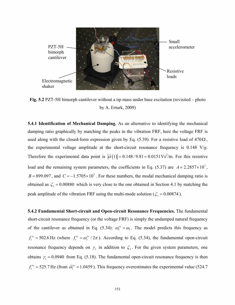
151

Fig. 5.2 PZT-5H bimorph cantilever without a tip mass under base excitation (revisited – photo

by A. Erturk, 2009)

5.4.1 Identification of Mechanical Damping. As an alternative to identifying the mechanical

damping ratio graphically by matching the peaks in the vibration FRF, here the voltage FRF is

used along with the closed-form expression given by Eq. (5.39). For a resistive load of 470 ,

the experimental voltage amplitude at the short-circuit resonance frequency is 0.148 V/g.

Therefore the experimental data point is ˆ 1 0.148 / 9.81 0.0151 Vs2/m. For this resistive

load and the remaining system parameters, the coefficients in Eq. (5.37) are 72.2857 10A ,

899.097B , and 71.5705 10C . For these numbers, the modal mechanical damping ratio is

obtained as 1 0.00880 which is very close to the one obtained in Section 4.1 by matching the

peak amplitude of the vibration FRF using the multi-mode solution ( 1 0.00874 ).

5.4.2 Fundamental Short-circuit and Open-circuit Resonance Frequencies. The fundamental

short-circuit resonance frequency (or the voltage FRF) is simply the undamped natural frequency

of the cantilever as obtained in Eq. (5.34):

1 1sc . The model predicts this frequency as

1 502.6scf Hz (where / 2sc scr rf ). According to Eq. (5.34), the fundamental open-circuit

resonance frequency depends on 1 in addition to 1 . For the given system parameters, one

obtains 1 0.0940 from Eq. (5.18). The fundamental open-circuit resonance frequency is then

1 525.7ocf Hz (from 1 1.0459oc ). This frequency overestimates the experimental value (524.7

Resistive loads

Electromagnetic shaker

PZT-5H bimorph cantilever

Small accelerometer

152

Hz) and the multi-mode analytical value (524.5 Hz). The reason single-mode solution deviates

from the multi-mode solution is the effect of the residuals of the neighboring modes which are

excluded in this approximation (and this is what makes the single-mode solution an

approximation). The relative errors in the single-mode short-circuit and the open-circuit

resonance frequencies are +0.02 % and +0.2 %, respectively.

5.4.3 Amplitude and Phase of the Voltage FRF. The modulus and phase diagrams of the

voltage FRFs for three different resistive loads (1.2 k , 44.9 k and 995 k ) are obtained and

compared against the experimental and the multi-mode model results. Figures 5.3a and 5.3b,

respectively, are plotted using Eqs. (5.8) and (5.9) with the damping ratio identified using a

single data point of the voltage FRF for 470 (Section 5.4.1). The modulus expression given by

Eq. (5.8) predicts the experimental voltage amplitude successfully in Fig. 5.3a, and the slight

inaccuracy is for the largest resistive load (due to the 0.2 % overestimation of the open-circuit

resonance frequency). The phase diagrams of these curves are also predicted very well for all of

these three resistive loads in Fig. 5.3b. It should be noted that these phase curves intersect each

other at the fundamental short-circuit and open-circuit resonance frequencies.

Fig. 5.3 (a) Amplitude and (b) phase diagrams of the voltage FRF for three different resistive

loads: 1.2 k , 44.9 k and 995 k (experimental measurement, analytical multi-mode

solution and analytical single-mode solution)

5.4.4 Voltage Asymptotes for Resonance Excitation. For excitations the fundamental short-

circuit resonance frequency, the short-circuit and the open-circuit voltage asymptotes are

(a) (b)

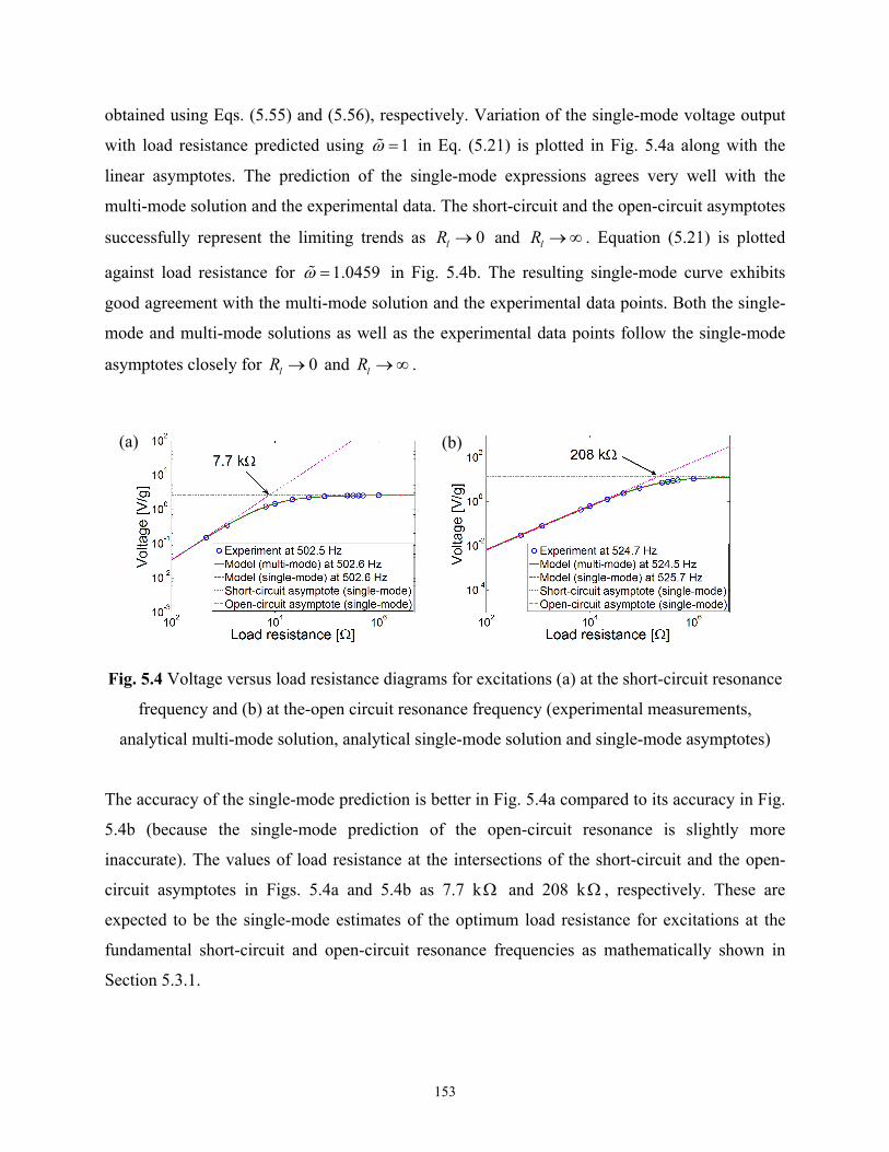
153

obtained using Eqs. (5.55) and (5.56), respectively. Variation of the single-mode voltage output

with load resistance predicted using 1 in Eq. (5.21) is plotted in Fig. 5.4a along with the

linear asymptotes. The prediction of the single-mode expressions agrees very well with the

multi-mode solution and the experimental data. The short-circuit and the open-circuit asymptotes

successfully represent the limiting trends as 0lR and lR . Equation (5.21) is plotted

against load resistance for 1.0459 in Fig. 5.4b. The resulting single-mode curve exhibits

good agreement with the multi-mode solution and the experimental data points. Both the single-

mode and multi-mode solutions as well as the experimental data points follow the single-mode

asymptotes closely for 0lR and lR .



analytical multi-mode solution, analytical single-mode solution and single-mode asymptotes)

The accuracy of the single-mode prediction is better in Fig. 5.4a compared to its accuracy in Fig.

5.4b (because the single-mode prediction of the open-circuit resonance is slightly more

inaccurate). The values of load resistance at the intersections of the short-circuit and the open-

circuit asymptotes in Figs. 5.4a and 5.4b as 7.7 k and 208 k , respectively. These are

expected to be the single-mode estimates of the optimum load resistance for excitations at the

fundamental short-circuit and open-circuit resonance frequencies as mathematically shown in

Section 5.3.1.

(a) (b)

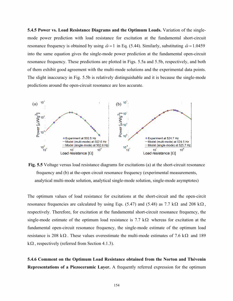
154

5.4.5 Power vs. Load Resistance Diagrams and the Optimum Loads. Variation of the single-

mode power prediction with load resistance for excitation at the fundamental short-circuit

resonance frequency is obtained by using 1 in Eq. (5.44). Similarly, substituting 1.0459

into the same equation gives the single-mode power prediction at the fundamental open-circuit

resonance frequency. These predictions are plotted in Figs. 5.5a and 5.5b, respectively, and both

of them exhibit good agreement with the multi-mode solutions and the experimental data points.

The slight inaccuracy in Fig. 5.5b is relatively distinguishable and it is because the single-mode

predictions around the open-circuit resonance are less accurate.



analytical multi-mode solution, analytical single-mode solution, single-mode asymptotes)

The optimum values of load resistance for excitations at the short-circuit and the open-circit

resonance frequencies are calculated by using Eqs. (5.47) and (5.48) as 7.7 k and 208 k ,

respectively. Therefore, for excitation at the fundamental short-circuit resonance frequency, the

single-mode estimate of the optimum load resistance is 7.7 k whereas for excitation at the

fundamental open-circuit resonance frequency, the single-mode estimate of the optimum load

resistance is 208 k . These values overestimate the multi-mode estimates of 7.6 k and 189

k , respectively (referred from Section 4.1.3).

5.4.6 Comment on the Optimum Load Resistance obtained from the Norton and Thévenin

Representations of a Piezoceramic Layer. A frequently referred expression for the optimum

(a) (b)

155

load resistance ( 1/opt eql r pR C , e.g. in references [9,18]) gives the optimum values of load

resistance for this cantilever at the fundamental short-circuit and open-circuit resonance

frequencies as 41.8 k and 40.1 k (which are highly inaccurate compared to multi-mode

predictions of 7.6 k and 189 k or the single-mode predictions of 7.7 k and 208 k ,

respectively). The reason of this inaccuracy is the thermodynamic inconsistency behind the

equation 1/opt eql r pR C . This expression is obtained for the simple electrical engineering

representation of a piezoceramic layer as an electrical source: either a current source in parallel

with its internal capacitance (Norton representation) or a voltage source in series with its

internal capacitance (Thévenin representation). One should note that the Norton representation

was reached in the derivations steps of the analytical model (Fig. 3.2b). In Fig. 3.2b, if one

assumes a constant current amplitude oscillating at frequency r (i.e. ( ) rj tp pi t I e ) and

proceeds to obtain the optimum load for maximum power generation using the circuit equation,

that load turns out to be 1/opt eql r pR C . However, note that the electric current in Eq. (3.28) is a

function of the velocity response of the structure due to Eq. (3.29). Therefore, the current source

in this Norton representation is not constant and it strongly depends on the load resistance

because the vibration response strongly depends on the load resistance as shown both

theoretically and experimentally in Chapters 3 and 4. Therefore, using 1/opt eql r pR C implies

that there is no shunt damping effect in the structure, i.e. there is no converse piezoelectric effect

although one generates electricity with the direct piezoelectric effect. A figure demonstrating the

meaning of ignoring piezoelectric coupling in the mechanical equation is shown in Fig. 5.6 for

excitation at the fundamental short-circuit resonance frequency of the cantilever discussed here.

As the load resistance is changed from the smallest load to the largest load, the correct peak of

the power in the FRF increases, moves to the right (on the frequency axis) and then decreases.

This trend is completely due to the feedback received in the mechanical domain. If the electrical

term in the mechanical domain was artificially set equal to zero to simulate the aforementioned

inconsistent scenario, the dashed curves in Figs. 5.6a and 5.6b are obtained. Therefore, if the

piezoelectric coupling in the mechanical equation is ignored, the power amplitude in Fig. 5.6a

increases much more than the real case (and there is no frequency shift). Indeed, when the

variation of the peak power with load resistance is plotted as shown in Fig. 5.6, the optimum load

156

resistance turns out to be this incorrect estimate ( 1/opt eql r pR C ) and the peak power is orders of

magnitude larger than the experimental measurement as well as the model prediction with

backward coupling in the mechanical equation.

Figure 5.6 Comparison of the coupled and uncoupled distributed-parameter model predictions;

(a) electrical power FRFs for 4 different resistive loads and (b) variation of the electrical power

amplitude with load resistance for resonance excitation


Detailed mathematical analyses of the single-mode electromechanical relations are presented.

Focus is placed on the voltage output and vibration response FRFs per translational base

acceleration input. The complex forms single-mode relations derived in Chapter 3 (based on the

multi-mode solutions) are first expressed in the modulus-phase form and then they are

represented with dimensionless terms. After expressing the asymptotic trends of the single

voltage and tip displacement FRFs, closed-form expressions are obtained for their short-circuit

and open-circuit resonance frequencies. It is shown that the short-circuit resonance frequencies

of the voltage FRF and the tip displacement FRF are slightly different. The linear asymptotes of

the voltage and tip displacement for the extreme conditions of the load resistance (observed in

the previous chapters) are mathematically verified here. Closed-form expressions for the

optimum electrical loads for the maximum power generation at the short-circuit and the open-

circuit resonance frequencies at extracted. It is shown that, for excitations at these two

(b) (a)

157

frequencies, the intersections of the linear voltage asymptotes correspond to the respective

optimum load resistance. Based on this observation, a simple technique is introduced to identify

the optimum load resistance of a piezoelectric energy harvester using a single resistive load

along with an open circuit voltage measurement. Relations are given to estimate the variation of

the tip vibration response as the load resistance is changed between the two extreme conditions.

The experimental case study for a PZT-5H bimorph is revisited and the major closed-form

relations derived here are validated. An important issue related to estimation of the optimum load

resistance from the Norton and Thévenin representations of the piezoceramic is clarified.

158

CHAPTER 6

EFFECTS OF MATERIAL CONSTANTS AND MECHANICAL

DAMPING ON PIEZOELECTRIC ENERGY HARVESTING

– A COMPARATIVE STUDY

This chapter investigates the effects of material constants and mechanical damping on

piezoelectric energy harvesting. The discussion is given here with a focus on the most popular

monolithic piezoceramics (PZT-5A and PZT-5H) and the novel single crystals (PMN-PT and

PMN-PZT).* The motivation of the following analysis is to understand the effects of

piezoelectric, elastic and dielectric constants as well as mechanical damping on piezoelectric

power generation and to clarify whether or not the substantially large piezoelectric strain

constants (particularly the d31 constant) of single crystals result in a substantially large power

generation performance compared to commonly employed monolithic piezoceramics. It is

therefore aimed to check whether the well-known d31 constant alone is a sufficient parameter to

choose an active material for piezoelectric energy harvesting. The performance comparisons

made for this purpose are presented for PZT-5A, PZT-5H, PMN-PT (with 30% PT), PMN-PT

(with 33% PT) and PMN-PZT type piezoelectric materials. Piezoelectric, elastic and dielectric

properties of these active materials differ from each other considerably. Individual effects of

these properties are investigated using the analytical model developed in this dissertation. The

reduced properties of these piezoelectric materials are obtained based on the plane-stress

assumption for a thin beam. The plane-stress constants are compared and the importance of the

elastic compliance as well as its effect on the reduced piezoelectric constant are highlighted. The

effect of mechanical damping on piezoelectric power generation is also discussed. An

experimental comparison between a PZT-5A bimorph and a PZT-5H bimorph is given in order

to verify some of the conclusions drawn here based on the analytical model simulations.

* PMN stands for lead magnesium niobate.

159

6.1 Properties of Typical Monolithic Piezoceramics and Single Crystals

Typical properties of monolithic PZT-5A and PZT-5H can be found in several sources on the

web [62] or the literature [63] and their data are listed in Appendix B. At room temperature,

PZT-5A has 31 171d pm/V (piezoelectric constant), 11 16.4Es pm2/N (elastic compliance) and

33 0/ 1700T (dielectric constant) whereas PZT-5A has 31 274d pm/V, 11 16.5Es pm2/N and

33 0/ 3400T (where 0 8.854 pF/m is the absolute permittivity of free space [26]).

The single-crystal technology is relatively new compared to the conventional PZT-5A

and PZT-5H monolithic piezoceramics which are widely used in engineering applications.

Limited literature is available for the material data of single-crystal piezoceramics. Cao et al.

[64] reported the relevant constants for a PMN-PT with 30% PT as 31 921d pm/V,

11 52Es pm2/N and 33 0/ 7800T whereas they reported 31 1330d pm/V, 11 69Es pm2/N and

33 0/ 8200T for a PMN-PT with 33% PT. Properties of a relatively new single crystal PMN-

PZT are reported by the manufacturer [65] as (product: CPSC200-115) as 31 2252d pm/V,

11 127Es pm2/N and 33 0/ 5000T .†

The relevant piezoelectric, elastic and dielectric data of these five different piezoelectric

materials (PZT-5A, PZT-5H, PMN-PT with 30% PT, PMN-PT with 33% PT and PMN-PZT) are

listed in Tables 6.1 and 6.2 along with the average value of each property. The mass densities of

these piezoceramics are also given in Table 6.2. The effective piezoelectric, elastic and dielectric

terms for the plane-stress conditions of a thin beam are also obtained (Appendix A.2) since the

reduced forms of the three-dimensional constants determine the performance of a thin generator.

As can be seen in Fig. 6.1, the piezoelectric constant 31d increases by more than an order

of magnitude from PZT-5A to PMN-PZT. It is observed that the large 31d constant comes with

large elastic compliance as plotted in Fig. 6.2. Approximately an order of magnitude difference

is seen between the elastic compliance values of PZT-5A to PMN-PZT.

† Composition of this PMN-PZT [65] is the company’s proprietary information.

160

Table 6.1 Piezoelectric and elastic properties of different piezoceramics

31d [pm/V] 11Es [pm2/N] 31e [C/m2]

PZT-5A -171 16.4 -10.4

PZT-5H -274 16.5 -16.6

PMN-PT (30% PT) -921 52 -17.7

PMN-PT (33% PT) -1330 69 -19.3

PMN-PZT -2252 127 -17.7

Average -989.6 56.2 -16.3

Table 6.2 Mass densities and dielectric constants of different piezoceramics

[kg/m3] 33 0/T 33S [nF/m]

PZT-5A 7750 1700 13.3

PZT-5H 7500 3400 25.6

PMN-PT (30% PT) 8040 7800 52.7

PMN-PT (33% PT) 8060 8200 47.0

PMN-PZT 7900 5000 4.34

Average 7850 5220 28.6

Fig. 6.1 Variation of the piezoelectric strain constant for different piezoceramics

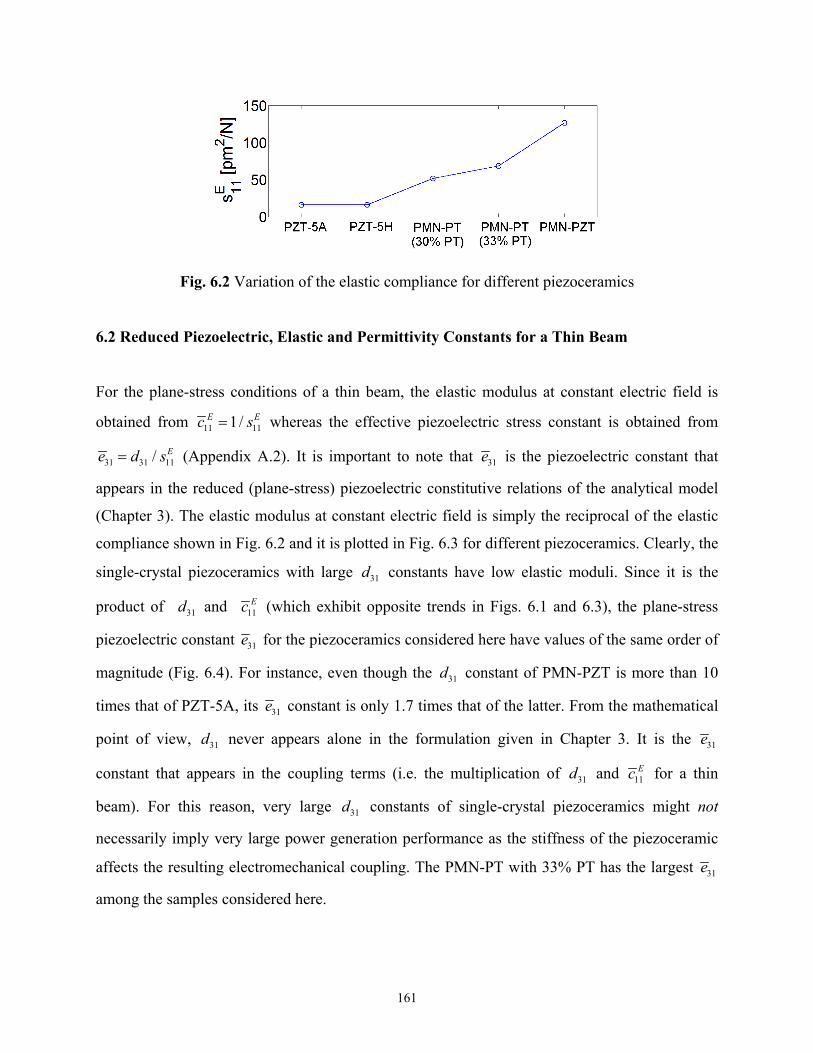
161

Fig. 6.2 Variation of the elastic compliance for different piezoceramics

6.2 Reduced Piezoelectric, Elastic and Permittivity Constants for a Thin Beam

For the plane-stress conditions of a thin beam, the elastic modulus at constant electric field is

obtained from 11 111/E Ec s whereas the effective piezoelectric stress constant is obtained from

31 31 11/ Ee d s (Appendix A.2). It is important to note that 31e is the piezoelectric constant that

appears in the reduced (plane-stress) piezoelectric constitutive relations of the analytical model

(Chapter 3). The elastic modulus at constant electric field is simply the reciprocal of the elastic

compliance shown in Fig. 6.2 and it is plotted in Fig. 6.3 for different piezoceramics. Clearly, the

single-crystal piezoceramics with large 31d constants have low elastic moduli. Since it is the

product of 31d and 11Ec (which exhibit opposite trends in Figs. 6.1 and 6.3), the plane-stress

piezoelectric constant 31e for the piezoceramics considered here have values of the same order of

magnitude (Fig. 6.4). For instance, even though the 31d constant of PMN-PZT is more than 10

times that of PZT-5A, its 31e constant is only 1.7 times that of the latter. From the mathematical

point of view, 31d never appears alone in the formulation given in Chapter 3. It is the 31e

constant that appears in the coupling terms (i.e. the multiplication of 31d and 11Ec for a thin

beam). For this reason, very large 31d constants of single-crystal piezoceramics might not

necessarily imply very large power generation performance as the stiffness of the piezoceramic

affects the resulting electromechanical coupling. The PMN-PT with 33% PT has the largest 31e

among the samples considered here.

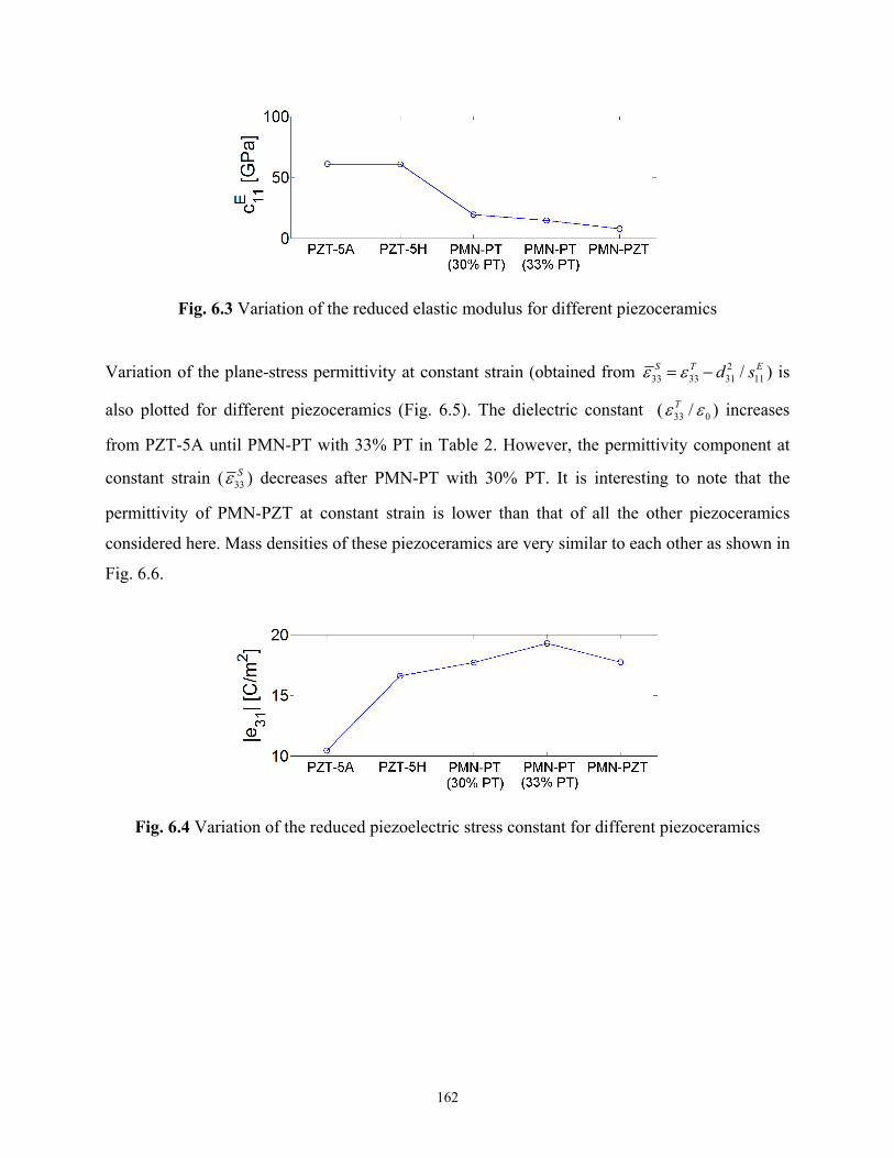
162

Fig. 6.3 Variation of the reduced elastic modulus for different piezoceramics

Variation of the plane-stress permittivity at constant strain (obtained from 233 33 31 11/S T Ed s ) is

also plotted for different piezoceramics (Fig. 6.5). The dielectric constant ( 33 0/T ) increases

from PZT-5A until PMN-PT with 33% PT in Table 2. However, the permittivity component at

constant strain ( 33S ) decreases after PMN-PT with 30% PT. It is interesting to note that the

permittivity of PMN-PZT at constant strain is lower than that of all the other piezoceramics

considered here. Mass densities of these piezoceramics are very similar to each other as shown in

Fig. 6.6.

Fig. 6.4 Variation of the reduced piezoelectric stress constant for different piezoceramics

163

Fig. 6.5 Variation of the reduced permittivity constant for different piezoceramics

Fig. 6.6 Variation of the mass density for different piezoceramics

6.3 Theoretical Case Study for Performance Comparison of Various Monolithic

Piezoceramics and Single Crystals

6.3.1 Properties of the Bimorph Cantilevers. In this section, power generation performances

of bimorph cantilevers with identical dimensions and substrate materials using PZT-5A, PZT-

5H, PMN-PT (with 30% PT and with 33% PT) and PMN-PZT are compared. The piezoceramic

layers of each bimorph cantilever are assumed to be connected in parallel (Fig. 3.1b). The

substrate material in all cases is aluminum with identical dimensions and properties ( 70Y GPa,

2700 kg/m3). For all cases considered here, the dimensions of the bimorph cantilever are as

given in Table 6.3.

164

Table 6.3 Geometric properties of the bimorph cantilevers


Length ( L ) [mm] 40 40

Width (b ) [mm] 6 6


The bimorph energy harvester model developed in Chapter 3 (experimentally validated in

Chapter 4) is used here. As the electrical load resistance is increased from zero to infinity, the

resonance frequencies of a bimorph shift from the short-circuit resonance frequencies to the

open-circuit resonance frequencies. The short-circuit resonance frequency scr (for 0lR ) of

the r-th mode in the voltage FRF is the undamped natural frequency r as shown in Chapter 5.

As lR , the resonance frequency moves to the open-circuit resonance frequency ( ocr ). The

short-circuit and the open-circuit resonance frequencies of the fundamental vibration mode

( 1r ) of the five bimorphs with identical dimensions are listed in Table 6.4 (where / 2f ).

Recall from Chapter 5 that the resonance frequency shift from the short-circuit to the open-

circuit conditions is as a measure of electromechanical coupling. Among the piezoceramics

considered here, with the second largest 31e constant and the smallest 33S (as well as the smallest

r

due to low stiffness), expectedly, PMN-PZT bimorph exhibits the largest relative resonance

frequency shift (recall Eq. (5.18)).

Table 6.4 Short-circuit and open-circuit resonance frequencies of the bimorph cantilevers

1scf

[Hz]

(short circuit)

1ocf

[Hz]

(open circuit)

PZT-5A cantilever 151.9 157.0

PZT-5H cantilever 153.8 160.5

PMN-PT (30% PT) cantilever 84.7 90.7

PMN-PT (33% PT) cantilever 73.8 82.2

PMN-PZT cantilever 55.8 83.6

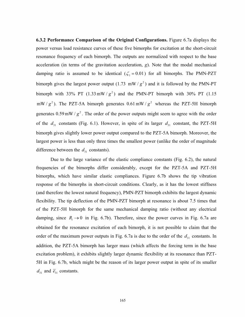
165

6.3.2 Performance Comparison of the Original Configurations. Figure 6.7a displays the

power versus load resistance curves of these five bimorphs for excitation at the short-circuit

resonance frequency of each bimorph. The outputs are normalized with respect to the base

acceleration (in terms of the gravitation acceleration, g). Note that the modal mechanical

damping ratio is assumed to be identical ( 1 0.01 ) for all bimorphs. The PMN-PZT

bimorph gives the largest power output (1.73 2mW / g ) and it is followed by the PMN-PT

bimorph with 33% PT (1.33 2mW / g ) and the PMN-PT bimorph with 30% PT (1.15

2mW / g ). The PZT-5A bimorph generates 0.61 2mW / g whereas the PZT-5H bimorph

generates 0.59 2mW / g . The order of the power outputs might seem to agree with the order

of the 31d constants (Fig. 6.1). However, in spite of its larger 31d constant, the PZT-5H

bimorph gives slightly lower power output compared to the PZT-5A bimorph. Moreover, the

largest power is less than only three times the smallest power (unlike the order of magnitude

difference between the 31d constants).

Due to the large variance of the elastic compliance constants (Fig. 6.2), the natural

frequencies of the bimorphs differ considerably, except for the PZT-5A and PZT-5H

bimorphs, which have similar elastic compliances. Figure 6.7b shows the tip vibration

response of the bimorphs in short-circuit conditions. Clearly, as it has the lowest stiffness

(and therefore the lowest natural frequency), PMN-PZT bimorph exhibits the largest dynamic

flexibility. The tip deflection of the PMN-PZT bimorph at resonance is about 7.5 times that

of the PZT-5H bimorph for the same mechanical damping ratio (without any electrical

damping, since 0lR in Fig. 6.7b). Therefore, since the power curves in Fig. 6.7a are

obtained for the resonance excitation of each bimorph, it is not possible to claim that the

order of the maximum power outputs in Fig. 6.7a is due to the order of the 31d constants. In

addition, the PZT-5A bimorph has larger mass (which affects the forcing term in the base

excitation problem), it exhibits slightly larger dynamic flexibility at its resonance than PZT-

5H in Fig. 6.7b, which might be the reason of its larger power output in spite of its smaller

31d and 31e constants.

166

Fig. 6.7 (a) Power vs. load resistance curves for excitation at the fundamental short-circuit

resonance frequency of each bimorph and the (b) vibration FRFs of the bimorphs for 0lR

( 1 1% for all bimorphs)

6.3.3 On the Effect of Piezoelectric Strain Constant. In order to understand the role of the 31d

constant in piezoelectric power generation, 31 989.6d pm/V is assumed for all bimorphs

(which is the average of the 31d constants of these five piezoceramics as shown in Table 6.1).

The geometry of the bimorph and the modal mechanical damping ratio are unchanged. Figure 6.8

shows the simulation results for this artificial case. The optimum loads are highly affected (as

the optimum electrical load depends on electromechanical coupling) but the maximum power

outputs are affected very slightly and the order of the power outputs is the same for the

bimorphs. This observation supports the idea that the large power outputs in Fig. 6.7a are due to

large dynamic flexibilities (originating from the large elastic compliance values) of the

respective bimorphs at their individual resonances rather than the substantial difference in the

31d constants.

(a)

(b)

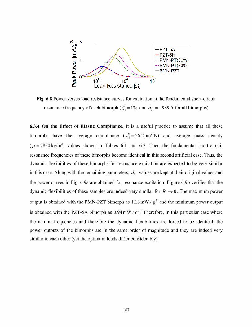
167

Fig. 6.8 Power versus load resistance curves for excitation at the fundamental short-circuit

resonance frequency of each bimorph ( 1 1% and 31 989.6d for all bimorphs)

6.3.4 On the Effect of Elastic Compliance. It is a useful practice to assume that all these

bimorphs have the average compliance ( 11 56.2Es pm2/N) and average mass density

( 7850 kg/m3) values shown in Tables 6.1 and 6.2. Then the fundamental short-circuit

resonance frequencies of these bimorphs become identical in this second artificial case. Thus, the

dynamic flexibilities of these bimorphs for resonance excitation are expected to be very similar

in this case. Along with the remaining parameters, 31d values are kept at their original values and

the power curves in Fig. 6.9a are obtained for resonance excitation. Figure 6.9b verifies that the

dynamic flexibilities of these samples are indeed very similar for 0lR . The maximum power

output is obtained with the PMN-PZT bimorph as 1.16 2mW / g and the minimum power output

is obtained with the PZT-5A bimorph as 0.94 2mW / g . Therefore, in this particular case where

the natural frequencies and therefore the dynamic flexibilities are forced to be identical, the

power outputs of the bimorphs are in the same order of magnitude and they are indeed very

similar to each other (yet the optimum loads differ considerably).

168

Fig. 6.9 (a) Power versus load resistance curves for excitation at the fundamental short-circuit

resonance frequency of each bimorph and (b) vibration FRFs of the bimorphs for 0lR

( 1 1% , 11 56.2Es and 7850 kg/m3 for all bimorphs)

The discussion so far shows that the order of magnitude difference in the electrical power

outputs is not like the order of magnitude difference between the 31d constants. The electrical

power outputs differ in the same order of magnitude (just like the 31e constants) and the dynamic

flexibility of the cantilever plays an important role.

6.3.5 On the Effect of Permittivity Constant. The last artificial case is to assume that the

constant stress dielectric constants are identical and equal to the average value given in Table 6.2

( 33 0/ 5220T ) to study how the difference in the relative permittivity affects the results. As can

be seen in Fig. 6.10, the qualitative order (in terms of the amplitude-wise results) is not changed

considerably compared to the original graph given by Fig. 6.7a except for the PZT-5A and PZT-

5H bimorphs. Now the PZT-5H bimorph gives slightly larger power output. Thus, the slightly

larger power output of the PZT-5A bimorph (compared to the PZT-5H bimorph) in the original

(a)

(b)

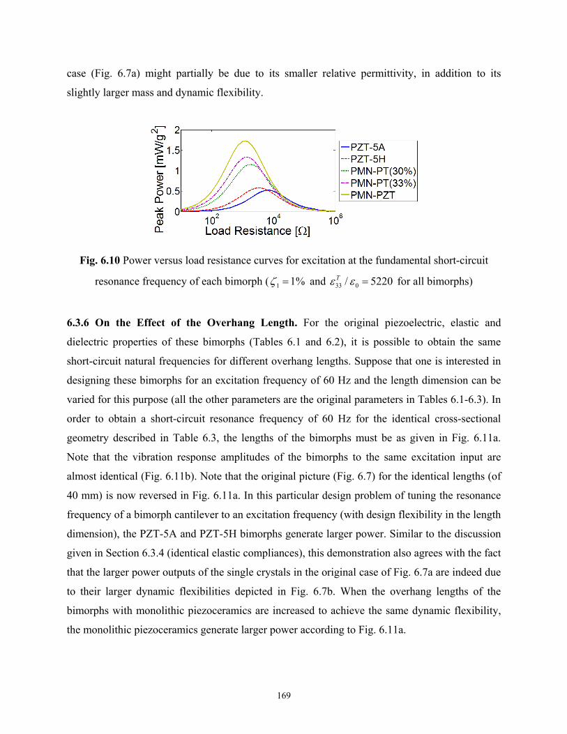
169

case (Fig. 6.7a) might partially be due to its smaller relative permittivity, in addition to its

slightly larger mass and dynamic flexibility.


resonance frequency of each bimorph ( 1 1% and 33 0/ 5220T

for all bimorphs)

6.3.6 On the Effect of the Overhang Length. For the original piezoelectric, elastic and

dielectric properties of these bimorphs (Tables 6.1 and 6.2), it is possible to obtain the same

short-circuit natural frequencies for different overhang lengths. Suppose that one is interested in

designing these bimorphs for an excitation frequency of 60 Hz and the length dimension can be

varied for this purpose (all the other parameters are the original parameters in Tables 6.1-6.3). In

order to obtain a short-circuit resonance frequency of 60 Hz for the identical cross-sectional

geometry described in Table 6.3, the lengths of the bimorphs must be as given in Fig. 6.11a.

Note that the vibration response amplitudes of the bimorphs to the same excitation input are

almost identical (Fig. 6.11b). Note that the original picture (Fig. 6.7) for the identical lengths (of

40 mm) is now reversed in Fig. 6.11a. In this particular design problem of tuning the resonance

frequency of a bimorph cantilever to an excitation frequency (with design flexibility in the length

dimension), the PZT-5A and PZT-5H bimorphs generate larger power. Similar to the discussion

given in Section 6.3.4 (identical elastic compliances), this demonstration also agrees with the fact

that the larger power outputs of the single crystals in the original case of Fig. 6.7a are indeed due

to their larger dynamic flexibilities depicted in Fig. 6.7b. When the overhang lengths of the

bimorphs with monolithic piezoceramics are increased to achieve the same dynamic flexibility,

the monolithic piezoceramics generate larger power according to Fig. 6.11a.

170

Fig. 6.11 (a) Power versus load resistance curves for excitation at the fundamental short-circuit

resonance frequency of each bimorph and (b) vibration FRFs of the bimorphs for 0lR

( 1 1% and the lengths are chosen to satisfy 1 60 Hzscf for all bimorphs)

6.3.7 On the Effect of Mechanical Damping. The final discussion in this section demonstrates

the sensitivity of the performance results to mechanical damping (which is not very easy to

predict and control in practice). For the original parameters of this case study (which yield Fig.

6.7a), if one assumes the damping ratios shown in Fig. 6.12 (instead of 1 1% for all

bimorphs), identical maximum power outputs are obtained. Note that these damping ratios are

typical values one can identify in practice. Although the individual loss factors of the

piezoceramic and the substructure layers can provide some insight, adhesive layers and clamped

interfaces are important sources of mechanical damping which can dominate the damping due to

the loss factors of the individual layers of a generator. The particular reason for the sensitivity of

the results to mechanical damping is because the electrical power outputs already have the same

order of magnitude. For instance, the favorable power output of the flexible PMN-PZT bimorph

in Fig. 6.7a can become worse than that of the PZT-5H bimorph if the bonding layer and/or the

clamped boundary of the PMN-PZT bimorph causes larger mechanical damping.

(a)

(b)

171


resonance frequency of each bimorph showing the sensitivity of the power output to mechanical

damping ratio

6.4 Experimental Demonstration for PZT-5A and PZT-5H Cantilevers

6.4.1 Experimental Setup. A PZT-5A bimorph and a PZT-5H bimorph are tested under base

excitation as shown in Fig. 6.13. The setup used for base excitation is very similar to the one

described in Section 4.1.1 and the focus is placed here directly on the voltage frequency response

measurements per base acceleration input. The excitation is provided using an electromagnetic

LDS [66] shaker and the base acceleration is measured with a small PCB [47] accelerometer.

The PZT-5A and PZT-5H bimorphs (T226-A4-203X and T226-H4-203X models) are

manufactured by Piezo Systems, Inc. [45] and the properties of PZT-5A and the PZT-5H

piezoceramics are listed in Tables 6.1 and 6.2. The layers of each bimorph are oppositely poled

and the brass substructure layer provides electrical conductivity (for the series connection of the

piezoceramic layers). When clamping these cantilevers, the overhang lengths are adjusted to

have similar short-circuit resonance frequencies. The PZT-5A cantilever is clamped with an

overhang length of 24.20 mm whereas the PZT-5H is clamped with an overhang length of 24.39

mm.

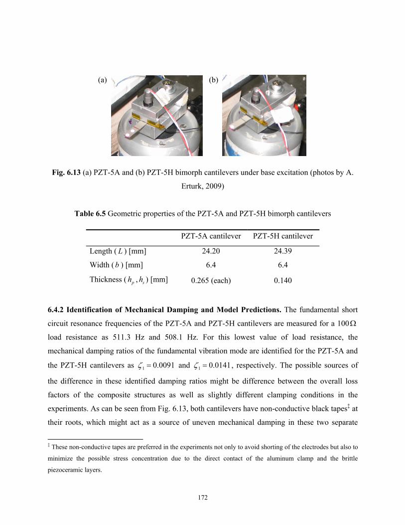
172

Fig. 6.13 (a) PZT-5A and (b) PZT-5H bimorph cantilevers under base excitation (photos by A.

Erturk, 2009)

Table 6.5 Geometric properties of the PZT-5A and PZT-5H bimorph cantilevers

PZT-5A cantilever PZT-5H cantilever

Length ( L ) [mm] 24.20 24.39

Width (b ) [mm] 6.4 6.4


6.4.2 Identification of Mechanical Damping and Model Predictions. The fundamental short

circuit resonance frequencies of the PZT-5A and PZT-5H cantilevers are measured for a 100

load resistance as 511.3 Hz and 508.1 Hz. For this lowest value of load resistance, the

mechanical damping ratios of the fundamental vibration mode are identified for the PZT-5A and

the PZT-5H cantilevers as 1 0.0091 and 1 0.0141 , respectively. The possible sources of

the difference in these identified damping ratios might be difference between the overall loss

factors of the composite structures as well as slightly different clamping conditions in the

experiments. As can be seen from Fig. 6.13, both cantilevers have non-conductive black tapes‡ at

their roots, which might act as a source of uneven mechanical damping in these two separate

‡ These non-conductive tapes are preferred in the experiments not only to avoid shorting of the electrodes but also to

minimize the possible stress concentration due to the direct contact of the aluminum clamp and the brittle

piezoceramic layers.

(a) (b)

173

configurations. Therefore these identified damping ratios are not purposely tuned and they are

not easy to control. No effort has been made to obtain a similar mechanical damping effect in the

experiments.

The voltage FRFs of the PZT-5A cantilever obtained for a set of resistive loads (ranging

from 100 to 248 k ) are shown in Fig. 6.14. The fundamental short-circuit resonance

frequency of the PZT-5A cantilever is predicted by the model as 511.5 Hz. As the load resistance

is increased from 100 to 248 k , the experimental value of the resonance frequency in Fig.

6.14 moves to 528.1 Hz and the analytical model predicts this frequency as 527.9 Hz. Note that,

for the bandwidth of 0-2000 Hz, the frequency resolution of the SigLab [49] data acquisition

system automatically adjust itself to give a frequency increment is 0.625 Hz. Therefore, both the

short-circuit and the open-circuit resonance frequency readings from the FRFs include

experimental error as in the cases discussed in Chapter 4.

Fig. 6.14 Voltage FRFs of the PZT-5A cantilever for a set of resistive loads (experimental

measurements and model predictions)

For the same set of load resistance, the model predictions for the PZT-5H cantilever are

plotted in Fig. 6.15 along with the experimental voltage FRFs. The model prediction of the

fundamental short-circuit resonance frequency is 508.4 Hz. In Fig. 6.15, as the load resistance is

increased from 100 to 248 k , the experimental value of the resonance frequency moves to

530.6 Hz and the model predicts this frequency as 530.3 Hz. The short-circuit and the open-

174

circuit resonance frequencies of the PZT-5A and PZT-5H cantilevers are listed in Table 6.6.

Predictions of the analytical model are very good in both cases.

Fig. 6.15 Voltage FRFs of the PZT-5H cantilever for a set of resistive loads (experimental

measurements and model predictions)

Table 6.6 Fundamental short-circuit resonance frequencies of the PZT-5A and PZT-5H bimorph

cantilevers


Experiment [Hz] 511.3 508.1

Model [Hz] 511.5 508.4

6.4.3 Performance Comparison of the PZT-5A and PZT-5H Cantilevers. Hereafter, the focus

is placed on the fundamental short-circuit resonance frequencies of these cantilevers in order to

compare their electrical performance results. For excitations at these frequencies, the variations

of the voltage and current outputs with load resistance are shown in Figs. 6.16 and 6.17,

respectively. Only for very low values of load resistance, the PZT-5H cantilever generates

slightly larger voltage and current. For a wide range of load resistance, the PZT-5A cantilever

generates considerably larger voltage and current.

175

Fig. 6.16 Voltage vs. load resistance curves of the PZT-5A and PZT-5H cantilevers for

excitation at the fundamental short-circuit resonance frequency (experimental measurements and

model predictions)

Fig. 6.17 Current vs. load resistance curves of the PZT-5A and PZT-5H cantilevers for excitation


predictions)

Using the voltage data for excitations at the fundamental short-circuit resonance

frequencies of the cantilevers, variations of the power output with load resistance are plotted in

Fig. 6.18. The maximum experimental power output of the PZT-5A cantilever is obtained as

176

0.202 mW/g2 (for a load resistance of 17.8 k - the optimum value among the resistors used).

The maximum experimental power output of the PZT-5H cantilever is 0.140 mW/g2 (for a load

resistance of 11.7 k - the optimum value among the resistors used). Since the overhang

volumes and masses of these cantilevers are slightly different, the power density and the specific

power values are also reported in Table 6.7.

Fig. 6.18 Power vs. load resistance curves of the PZT-5A and PZT-5H cantilevers for excitation


predictions)

As can be seen from Table 6.7, the maximum power density of the PZT-5A cantilever is

about 45 % larger than that of the PZT-5H cantilever. If the maximum specific power outputs are

compared, it is obtained that the PZT-5A cantilever generates 42 % larger specific power.

Therefore, choosing the PZT-5H cantilever due to its larger 31d constant (larger by 60 %

compared to that of PZT-5A) could result in surprising results in terms of the power output as the

mechanical damping can change the entire picture. Since the modal damping ratio of the PZT-5H

cantilever turns out to be 55 % larger than that of the PZT-5A cantilever (in this particular

experiment), the power output is controlled by mechanical damping. Recall from the theoretical

discussion given with Fig. 6.7a that, for the same amount of mechanical damping, the power

outputs of the PZT-5A and PZT-5H cantilevers are very similar. However, 55 % larger

mechanical damping relative to the PZT-5A cantilever results in 45 % less power density for

177

resonance excitation of the PZT-5H cantilever. This simple practice shows the importance of

mechanical damping in piezoelectric energy harvesting. Mechanical damping is probably the

most difficult parameter to control in the system (as in several other vibration engineering

problems) and it can change the entire picture regardless of the piezoelectric material of being

used.

Table 6.7 Maximum power outputs and identified mechanical damping ratios


Max. Power [mW/g2] 0.202 0.140

Max. Power Density [mW/(g2cm3)] 1.95 1.34

Max. Specific Power [mW/(g2g)]] 0.243 0.171

Mechanical Damping [%] 0.91 1.41


In this chapter, the effects of materials constants and mechanical damping on the power

generation performances of conventional piezoceramics (PZT-5A and PZT-5H) and novel single

crystals (PMN-PT and PMN-PZT) are investigated. The material constants of interest are the

piezoelectric, elastic and the dielectric constants. It is shown that the large piezoelectric strain

constants of the commercially available single crystals are associated with very large elastic

compliance and the combination of these two properties does not result in a substantial increase

in the effective piezoelectric stress constant ( 31e ) for a thin energy harvester beam. Although the

d31 constants can change by an order of magnitude from PZT-5A to PMN-PZT, the effective

piezoelectric constants of these active materials are in the same order of magnitude.

Consequently, the substantially large d31 constants of the commercially available single crystals

do not necessarily imply substantially large power output in energy harvesting. The concepts of

dynamic flexibility and mechanical damping are shown to be very important as far as the

maximum power output is concerned. When geometrically identical bimorphs employing these

piezoelectric materials are forced to have the same dynamic flexibility, the power outputs are

observed to be very similar. It is also observed that the power output under resonance excitation

178

is extremely sensitive to mechanical damping (which is a very difficult parameter to control in

practice). It is shown with an experimental case study using a PZT-5A bimorph and a PZT-5H

bimorph that the former cantilever gives 45 % larger power density when the latter has 55 %

larger mechanical damping ratio (although the d31 constant of PZT-5H is 60 % larger than that of

PZT-5A). Therefore, designing and manufacturing the energy harvester beam to have less

damping can be more important than the piezoelectric material being used.

179

CHAPTER 7

EFFECTS OF STRAIN NODES AND ELECTRODE CONFIGURATION

ON PIEZOELECTRIC ENERGY HARVESTING

As briefly mentioned in the analytical derivations, vibration modes of a cantilevered beam other

than the first mode have certain strain nodes where the dynamic strain distribution changes in the

direction of the beam length. In this chapter, it is theoretically discussed and experimentally

demonstrated that covering the strain nodes of vibration modes with continuous electrodes

results in strong cancellation of the electrical outputs. After a brief review of the mathematical

background, a detailed dimensionless analysis is given for predicting the locations of the strain

nodes of a uniform thin cantilever in the absence of a tip mass. The dimensionless derivations

and results are then presented for predicting the strain node positions and their variations in the

presence of a tip mass. Since the cancellation problem is not peculiar to clamped-free boundary

conditions, dimensionless data of modal strain nodes are tabulated for some other practical

boundary condition pairs as well. The locations of strain nodes tabulated in this chapter are

important also for applications of modal actuation since covering these positions with

piezoelectric actuators might require dramatically high voltage inputs, yielding inefficient

actuation processes. It is experimentally shown that the voltage output due to the second mode

excitation can be increased substantially if segmented electrodes are used instead of continuous

electrodes. The relationship between the discussion given here and a recent study on

piezoelectric energy harvesting from the static deflection of a clamped circular plate is also

explained. The use of segmented electrode pairs to avoid cancellations is described for single-

mode and multi-mode vibrations of a cantilevered piezoelectric energy harvester. Alternative

circuitry-based approaches can be investigated to handle the cancellation problem for multi-

mode excitations.

180

7.1 Mathematical Background

Recall from Chapter 3 that the circuit equation of a piezoceramic layer under dynamic bending

(such as the one shown in Fig. 3.2a) is obtained from the Gauss’s law as

( )

lA

d v tdA

dt R

D n (7.1)

where the electrodes are connected to a resistive load* of lR , ( )v t is the voltage output, D is the

vector of electric displacements components in the piezoceramic layer, n is the unit outward

normal and the integration is performed over the electrode area A. Since the only non-zero

component of the inner product in Eq. (7.1) is 3 3D n due to the electrode placement on the thin

layer (Appendix A.2), Eq. (7.1) reduces to†

333

31 20

( , )( ) ( ) LSrel

pcp l

bL w x tdv t v te h b dx

h dt R x t

(7.2)

As the vibration response is expanded in terms of the eigenfunctions of the undamped problem,

Eq. (7.2) is expressed as a first order circuit equation excited by all vibration modes:

1

( )( ) ( )eq rp r

rl

d tdv t v tC

dt R dt

(7.3)

where the electromechanical coupling term is

2

20

( ) ( )Lr r

rx L

d x d xdx

dx dx

(7.4)

Here, 31 pce bh for the series connection and 312 pce bh for the parallel connection of the

piezoceramic layers for a bimorph (Table 3.1). The equivalent capacitance term also depends on

the way the piezoceramic layers are connected as given in Table 3.1.

* If the circuit includes more linear elements than a resistive load, the 1 /

lR term on the right hand side is simply

replaced by the electrical admittance seen across the electrodes. Note that this electrical admittance should exclude

the admittance due to the inherent capacitance of the piezoceramic, which emerges from the electric displacement

term. † In agreement with the analytical formulation given in Chapter 3, it is assumed that the widths of the substructure,

piezoceramic and the electrodes are identical.

181

In Eq. (7.3), the forcing function on the right hand side is a modal summation where the

contribution from the r-th vibration mode is the product of r and ( )rd t dt . The modal

velocity response, ( )rd t dt , is also an output of the system to the base vibration input and it is

indeed affected by the voltage response due to the backward electromechanical coupling

(Chapter 3). A more critical term is the modal coupling term r , which is not only a function of

geometric, material and piezoelectric parameters of the energy harvester beam but also the

bending slope (cross-section rotation) eigenfunction evaluated at the boundaries of the

electrodes. In the foregoing derivation, since each of the electrodes is assumed to be covering the

entire respective surface of the piezoceramic layer (the top or the bottom) and since the slope at

the clamped end of the beam is already zero, the contribution to the forcing function from the r-

th vibration mode simply depends on the slope at the free end as in Eq. (7.4). If the electrodes

cover only a certain region 1 2x x x over the piezoceramic (which is still structurally

continuous), the boundaries of the integral in Eq. (7.5) change and the resulting expression for

r becomes‡

2

1

( )x x

rr

x x

d x

dx

(7.5)

According to Eq. (7.5), the modal electromechanical coupling term (which is a measure

of the modal forcing function in the circuit equation) depends on the region covered by the

electrodes on the surface of the piezoceramic. Therefore, the contribution to the forcing function

in Eq. (7.3) from the r-th vibration mode will be large if the difference of the slopes at the

boundaries of the electrodes for that particular mode is large and vice versa. As a consequence,

depending on the locations of the electrodes, modal electromechanical coupling and therefore the

contribution from certain vibration modes can be large or small. If it is aimed to harvest energy

from a specific vibration mode (say, from the r-th mode) by exciting the system harmonically at

the r-th natural frequency ( r ), the main contribution to the forcing function in the circuit will

be from the r-th term at the right hand side of Eq. (7.3), yielding

‡ In Eq. (7.5), the eigenfunction term can be updated according to the piecewise-defined electrical boundary

conditions (which will affect the elastic modulus of the piezoceramic) to be more precise.

182

( ) ( )rj teq

p r rl

dv t v tC A e

dt R

(7.6)

where rj trA e is the modal velocity response ( r rA j in terms of the complex modal

mechanical response r defined in Chapter 3) and it is indeed a function of the voltage response

given by ( )v t as shown in the analytical derivations of Chapter 3. Therefore, if the beam vibrates

under resonance excitation, the electrical circuit may or may not be excited very strongly

depending on the respective mode shape. Clearly, one prefers a large r for a stronger excitation

of the circuit.

7.2 Physical and Historical Backgrounds

It turns out from the foregoing derivation that the bending slopes (cross-section rotations) at the

boundaries of the electrodes constitute a strong parameter in piezoelectric energy harvesting

problem. If the slopes at the boundaries of continuous electrodes are very close to each other for

a particular mode shape, the contribution to the electrical output from that mode is very low.

Furthermore, the above derivation also directly shows that certain boundary conditions are not

useful for harvesting energy using continuous electrodes (e.g. clamped-clamped).

The physics behind this discussion is related to the strain distribution throughout the

length of the beam. If the strain distribution over the length of the beam changes sign (i.e. if its

phase changes by 180 degrees) for a certain vibration mode, collecting the charge developed by

using continuous electrodes results in cancellation of the electrical outputs in harvesting energy

from that vibration mode. The mechanism of cancellation is more obvious in the first term of Eq.

(7.4), where the integrand is the curvature eigenfunction (which is a measure of bending strain

for a symmetric thin beam). Hence, if the curvature changes sign for a vibration mode, the net

electric charge output is reduced due to cancellation of the positive and the negative areas under

the curvature eigenfunction in integrating the electric displacement over the electrode area.

Therefore a physical solution that allows handling the integration in a piecewise sense should be

preferred to using continuous electrodes.

The concept of strain nodes was formerly discussed in the literature of structural

actuation. Crawley and de Luis [67] addressed the importance of strain nodes in their work

183

(which focuses on the converse piezoelectric effect for actuation) with the following words:

“…the first mode has no strain nodes. Therefore, if this were the only mode to be excited, the

actuators could be placed anywhere along the beam. For maximum effectiveness, they would be

placed as near to the root as possible. The second mode has a strain node at x = 0.216L. The

PZA's (piezoelectric actuators) must be placed away from this point, so that the strain applied

over the entire length of the actuator has a constant phase with respect to the homogeneous

strain in the beam in this mode. If not, the modal force produced by the actuator will be

decreased, since one section of the actuator will be opposing the other… This reasoning also

indicates why it is necessary to use segmented actuators for the control of flexible structures. For

the second mode of a cantilevered beam, a PZA located at x<0.216 must be driven 180 deg out

of phase with a PZA located at x>0.2l6L”. It should be noted that the results of the above

formulation in the “direct sense” are in agreement with the observation of Crawley and de Luis

[67] in the “converse sense” of using piezoceramics in actuation for structural excitation and

control.

Indeed, more than 60 years ago, Cady [68] discussed this phenomenon for (longitudinal)

vibrations of crystals: “There is no external piezoelectric reaction due to longitudinal

deformations when rods with full-length electrodes are excited at an even multiple of the

fundamental frequency, since the effects of compressions and extensions in the various segments

cancel exactly”. He adds in another section of the same book on piezoelectric resonators that “by

the use of short (segmented) electrodes, however, intense vibrations, with correspondingly strong

electric reactions, can be secured at any value of h (mode number), even or odd… Resonators

with any number of pairs of electrodes can be prepared by silvering or evaporating a uniform

metallic deposit on the opposite sides of the bar and then dissolving away metal in the proper

regions to produce the desired number of pairs of separate electrodes”. Note that his reasoning

on even and odd modes is for longitudinal vibrations and the boundary conditions he uses.

However, the idea is the same and the “proper regions” he mentions are just the strain nodes.

In harvesting energy from the bending vibrations of a cantilevered thin beam like the one

shown in Fig. 3.1, the location of the electrodes and/or the piezoceramic layers can be very

important. The positions on the beam where the bending strain distribution (at a constant level

from the neutral axis) changes sign for a vibration mode are called the strain nodes. Since the

bending strain at a point is proportional to the curvature in the thin-beam theory, strain nodes of a

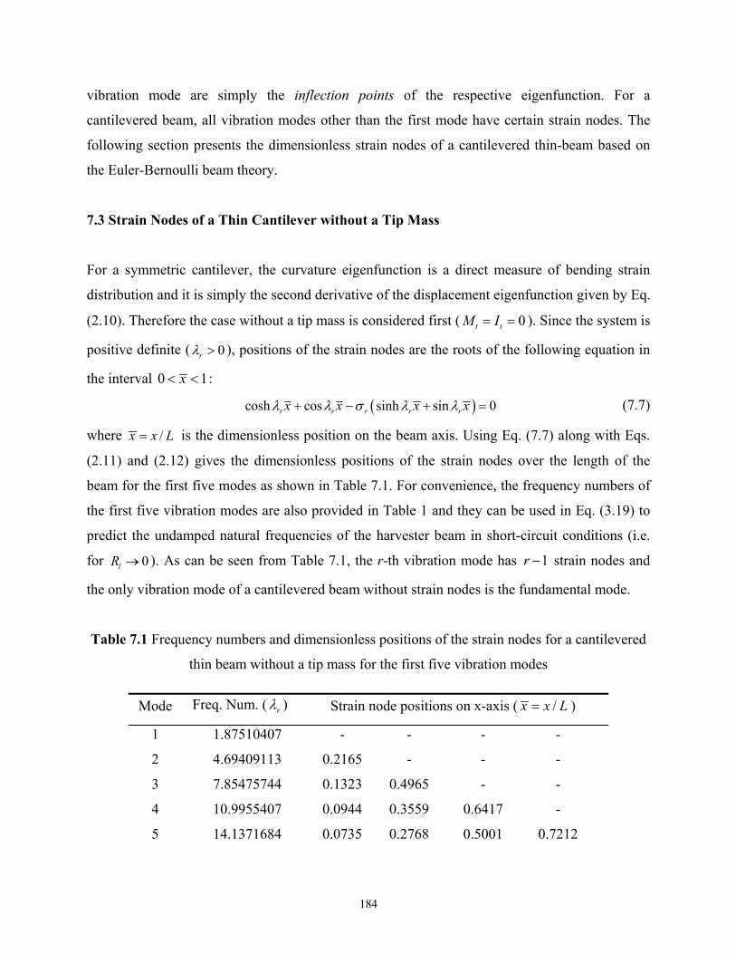
184

vibration mode are simply the inflection points of the respective eigenfunction. For a

cantilevered beam, all vibration modes other than the first mode have certain strain nodes. The

following section presents the dimensionless strain nodes of a cantilevered thin-beam based on

the Euler-Bernoulli beam theory.

7.3 Strain Nodes of a Thin Cantilever without a Tip Mass

For a symmetric cantilever, the curvature eigenfunction is a direct measure of bending strain

distribution and it is simply the second derivative of the displacement eigenfunction given by Eq.

(2.10). Therefore the case without a tip mass is considered first ( 0t tM I ). Since the system is

positive definite ( 0r ), positions of the strain nodes are the roots of the following equation in

the interval 0 1x :

cosh cos sinh sin 0r r r r rx x x x (7.7)

where /x x L is the dimensionless position on the beam axis. Using Eq. (7.7) along with Eqs.

(2.11) and (2.12) gives the dimensionless positions of the strain nodes over the length of the

beam for the first five modes as shown in Table 7.1. For convenience, the frequency numbers of

the first five vibration modes are also provided in Table 1 and they can be used in Eq. (3.19) to

predict the undamped natural frequencies of the harvester beam in short-circuit conditions (i.e.

for 0lR ). As can be seen from Table 7.1, the r-th vibration mode has 1r strain nodes and

the only vibration mode of a cantilevered beam without strain nodes is the fundamental mode.

Table 7.1 Frequency numbers and dimensionless positions of the strain nodes for a cantilevered

thin beam without a tip mass for the first five vibration modes

Mode Freq. Num. ( r ) Strain node positions on x-axis ( /x x L )

1 1.87510407 - - - -

2 4.69409113 0.2165 - - -

3 7.85475744 0.1323 0.4965 - -

4 10.9955407 0.0944 0.3559 0.6417 -

5 14.1371684 0.0735 0.2768 0.5001 0.7212

185

The normalized displacement mode shapes and the strain mode shapes of the first three

vibration modes of a cantilevered beam without a tip mass are displayed in Fig. 7.1. In

agreement with Table 7.1, the strain node of the second vibration mode is located at 0.2165x ,

and the third vibration mode has two strain nodes at 0.1323x and 0.4965x . These positions

give an idea about how to locate the segmented electrodes for harvesting energy from these

modes without cancellation. For instance, to avoid cancellation in harvesting energy from the

second vibration mode, two electrode pairs should be used to cover the regions 0 0.2165x

and 0.2165 1x separately. The voltage outputs of these electrode pairs will be out of phase

with each other by 180 degrees and they should be combined accordingly in the electrical circuit.

Otherwise, as can be seen in Fig. 7.1b, if continuous electrodes cover the entire length of the

beam ( 0 1x ), the negative area ( 0 0.2165x ) under the strain curve cancels a

considerable portion of the positive area ( 0.2165 1x ), yielding a reduced voltage output from

the harvester.

Fig. 7.1 (a) Normalized displacement and (b) normalized strain mode shapes of a cantilevered

thin beam without a tip mass for the first three vibration modes

(a)

(b)

186

The discussion so far has focused on a cantilevered beam without a tip mass. In some

energy harvesting applications, it is required to use a tip mass to tune the fundamental natural

frequency of the harvester beam to a dominant excitation frequency or just to reduce its natural

frequencies and increase its dynamic flexibility especially in micro-scale applications. The effect

of a tip mass on the strain nodes of a cantilever is investigated in the following section.

7.4 Effect of Using a Tip Mass on the Strain Nodes of a Thin Cantilever

If a tip mass tM of negligible rotary inertia ( 0tI ) is attached rigidly at x L to the

cantilevered beam shown in Fig. 3.1, the eigenfunctions and the eigenvalues are referred from

Eqs. (2.41) and (2.44), respectively. The curvature eigenfunction is the second derivative of Eq.

(2.41) with respect to x. It is then possible to study the effect of a tip mass on the strain nodes in

a dimensionless basis. As an example, Fig. 7.2a shows the variation of the displacement mode

shape whereas Fig. 7.2b displays the variation of the strain distribution of the second vibration

mode with increasing /tM mL . The shift of the strain node position due to increasing /tM mL is

shown in Fig. 7.2b. As the /tM mL ratio goes from 0 to 10, the strain node of the second mode

moves from 0.2165x to 0.2632x .

Figure 7.3a shows the strain node positions of the second and the third vibration modes

versus /tM mL ratio. As the /tM mL ratio increases from 0 to 10, the only strain node of the

second mode moves from 0.2165x to 0.2632x whereas the two strain nodes of the third

vibration mode move from 0.1323x and 0.4965x to 0.1468x and 0.5530x ,

respectively. It is also useful to investigate the variation of the frequency numbers with the

/tM mL ratio which is given in Fig. 7.3b for the first five vibration modes. Note that these

frequency numbers give the natural frequencies when they are used in Eq. (3.19). As can be seen

from Figs. 7.3a and 7.3b, the strain nodes move toward the free end of the beam and the

frequency numbers decrease with increasing /tM mL ratio. The positions of the strain nodes are

more sensitive to the variations in /tM mL ratio in the relatively low /tM mL region (i.e. for

0 / 1tM mL ).

187

Fig. 7.2 Variation of the (a) normalized displacement and (b) normalized strain mode shapes of

the second vibration mode with tip mass – to – beam mass ratio

As far as the frequency numbers given in Fig. 7.3b are concerned, other than the

frequency number of the first vibration mode, all the frequency numbers converge to a nonzero

value as /tM mL . A careful investigation shows that, as /tM mL , the frequency

number of the r-th mode of a clamped-free beam with a tip mass converges to that of the ( 1)r -

th mode of a clamped-pinned beam without a tip mass§ (except for the first frequency number

1 , which goes to zero with a very slow rate). That the boundary conditions of a cantilevered

harvester beam with a tip mass shift from clamped-free to clamped-pinned as /tM mL

makes sense, as the rotary inertia of the tip mass is neglected. Therefore, the direct consideration

§ The dominating term in Eq. (2.44) for /tM mL is the characteristic equation of a clamped-pinned beam:

tanh tan 0 (because the system is positive definite, 0 in the dominating term).

(a)

(b)

188

of the strain nodes of a clamped-pinned beam should give a good estimate of the strain nodes (of

modes 2r ) for very large values of /tM mL in modes other than the first mode. However, if

the rotary inertia of the tip mass is not negligible and if it increases uniformly as /tM mL ,

the boundary conditions shift from clamped-free to clamped-clamped and it becomes more

reasonable to estimate the strain node positions (of modes 2r ) from the eigenfunctions of a

clamped-clamped beam for large values of /tM mL . Hence, it is also insightful to examine the

characteristic equation of a thin cantilevered beam where the rotary inertia ( tI ) of the tip mass is

also considered (Eq. (3.20)).

Fig. 7.3 (a) Variation of the strain node positions of the second and the third vibration modes and

(b) variation of the frequency numbers of the first five vibration modes with tip mass – to – beam

mass ratio

(a)

(b)

189

In Eq. (3.20), the rotary inertia of the tip mass can be normalized with respect to the

rotary inertia of the free rigid beam about its centroid (or that of a rigid pendulum about its pivot)

and a similar dimensionless analysis can be performed. As can be seen from Eq. (3.20), the

rotary inertia of the tip mass introduces two additional terms to Eq. (2.44). The form of the

eigenfunction expression given by Eq. (2.41) is still the same; however, the eigenvalues to be

used in this equation should be extracted from Eq. (2.44). As mentioned before, for a large tip

mass and tip rotary inertia, the free end of the beam also acts as a clamped end. This fact is also

evident from the dominating term in Eq. (3.20) for 3/ /t tM mL I mL , which is the

characteristic equation of a uniform thin-beam beam with clamped-clamped boundary conditions

(1 cos cosh 0 ). Clamped-clamped boundary conditions may cause strong cancellations in

the electrical outputs if full electrodes are used for covering the piezoceramic layer(s). Therefore,

employing a large tip mass for reducing the natural frequencies of a cantilevered harvester has

the side effect of drastically reducing the electrical response of the vibration modes other than

the fundamental mode. If higher vibrations of a cantilevered energy harvester are to be excited in

a practical application (which is the case for the ambient vibration energy with random, varying

frequency or impulse-type excitation characteristics), addition of a tip mass results in a trade-off,

as it has an undesired effect on the vibration modes other than the first mode.

7.5 Strain Nodes for Other Boundary Conditions

Since the literature of energy harvesting [25,69] and the literature dealing with piezoelectric

beams [70] have considered boundary conditions other than clamped-free as well, the numerical

data of the strain node positions for some other practical boundary conditions are tabulated in

this section. The boundary condition pairs investigated in this section are pinned-pinned,

clamped-clamped and clamped-pinned pairs. Tables 7.2-7.4 display the positions of the strain

nodes for the first five vibration modes of uniform thin beams with these three boundary

condition pairs. The frequency numbers are also provided and they can be used in Eq. (3.19) to

predict the undamped natural frequencies (which are the resonance frequencies of the voltage

FRF in short-circuit conditions as shown in Chapter 5).

190

Since the pinned-pinned (Table 7.2) and clamped-clamped (Table 7.3) boundary

conditions are symmetric boundary conditions (yielding symmetric and antisymmetric mode

shapes for odd and even modes, respectively), the positions of the strain nodes (inflection points

of the mode shapes) are symmetric with respect to the center 0.5x of the beam. However, for

the clamped-pinned boundary conditions (Table 7.4), no such symmetry exists. It should be

noted that it is safe to cover the entire surface with continuous electrodes for harvesting energy

from the first vibration mode of a pinned-pinned beam. The rule for the pinned-pinned case is the

same as the clamped-free case, i.e. the r-th vibration mode has 1r strain nodes (Table 7.2).

However, a beam with clamped-clamped boundary conditions has two strain nodes in the first

vibration mode. According to Table 7.3, the r-th vibration mode of a clamped-clamped beam has

1r strain nodes. Hence, three electrode pairs (with discontinuities at 0.2242x and at

0.7758x ) can be used to extract the electrical outputs of a clamped-clamped energy harvester

without cancellation for vibrations with the first mode shape. Table 7.4 shows that the r-th

vibration mode has r strain nodes for a clamped-pinned beam. Thus, two electrode pairs (with a

discontinuity at 0.2642x ) can handle the cancellation issue for the fundamental mode

excitation of a harvester beam with clamped-pinned boundary conditions. Note that, in the

clamped-pinned case, the clamped boundary is the 0x point.

Among the boundary conditions investigated here, the clamped-clamped boundary

condition pair constitutes a unique case. Theoretically, for excitations at all vibration modes of a

clamped-clamped beam, the modal forcing term r in the electrical equation and therefore the

voltage response is zero, if full (continuous) electrodes cover the entire beam surface (see Eq.

(7.5)). A similar issue (of total cancellation) is expected for the even vibration modes

( 2,4,6,..., 2r n where n is an integer) of the pinned-pinned case, if full electrodes cover the

entire beam length. For the even modes of a beam with pinned-pinned boundary conditions, the

slopes at the pinned boundaries are not zero, but they are equal to each other, yielding a total

cancellation at these modes due to Eq. (7.5).

191

Table 7.2 Strain nodes of a thin beam with pinned-pinned boundary conditions


1 - - - -

2 2 1/ 2 - - -

3 3 1/ 3 2 / 3 - -

4 4 1/ 4 1/ 2 3 / 4 -

5 5 1/ 5 2 / 5 3 / 5 4 / 5

Table 7.3 Strain nodes of a thin beam with clamped-clamped boundary conditions


1 4.73004074 0.2242 0.7758 - - - -

2 7.85320462 0.1321 0.5000 0.8679 - - -

3 10.9956079 0.0944 0.3558 0.6442 0.9056 - -

4 14.1371655 0.0735 0.2768 0.5000 0.7232 0.9265 -

5 17.2787597 0.0601 0.2265 0.4091 0.5909 0.7735 0.9399

Table 7.4 Strain nodes of a thin beam with clamped-pinned boundary conditions


1 3.92660231 0.2642 - - -

2 7.06858275 0.1469 0.5536 - -

3 10.2101761 0.1017 0.3832 0.6924 -

4 13.3517688 0.0778 0.2931 0.5295 0.7647

5 16.4933614 0.0630 0.2372 0.4286 0.6190

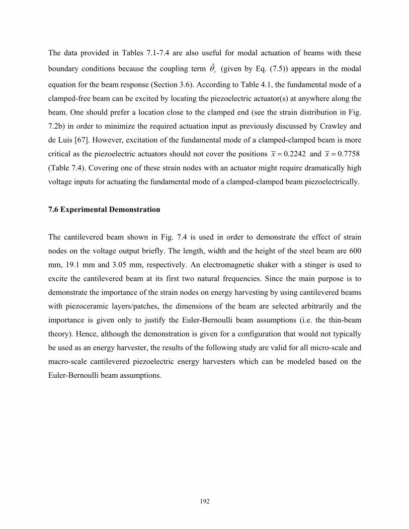
192

The data provided in Tables 7.1-7.4 are also useful for modal actuation of beams with these

boundary conditions because the coupling term r (given by Eq. (7.5)) appears in the modal

equation for the beam response (Section 3.6). According to Table 4.1, the fundamental mode of a

clamped-free beam can be excited by locating the piezoelectric actuator(s) at anywhere along the

beam. One should prefer a location close to the clamped end (see the strain distribution in Fig.

7.2b) in order to minimize the required actuation input as previously discussed by Crawley and

de Luis [67]. However, excitation of the fundamental mode of a clamped-clamped beam is more

critical as the piezoelectric actuators should not cover the positions 0.2242x and 0.7758x

(Table 7.4). Covering one of these strain nodes with an actuator might require dramatically high

voltage inputs for actuating the fundamental mode of a clamped-clamped beam piezoelectrically.

7.6 Experimental Demonstration

The cantilevered beam shown in Fig. 7.4 is used in order to demonstrate the effect of strain

nodes on the voltage output briefly. The length, width and the height of the steel beam are 600

mm, 19.1 mm and 3.05 mm, respectively. An electromagnetic shaker with a stinger is used to

excite the cantilevered beam at its first two natural frequencies. Since the main purpose is to

demonstrate the importance of the strain nodes on energy harvesting by using cantilevered beams

with piezoceramic layers/patches, the dimensions of the beam are selected arbitrarily and the

importance is given only to justify the Euler-Bernoulli beam assumptions (i.e. the thin-beam

theory). Hence, although the demonstration is given for a configuration that would not typically

be used as an energy harvester, the results of the following study are valid for all micro-scale and

macro-scale cantilevered piezoelectric energy harvesters which can be modeled based on the

Euler-Bernoulli beam assumptions.

193

Fig. 7.4 Experimental setup for demonstration of the effect of strain nodes on the voltage output


The first two vibration modes are considered for a simple demonstration of the voltage

cancellation at higher vibration modes. Note that the experimental validations of the analytical

model have already been given for several cases in Chapter 4. Hence the experimental

demonstration of cancellation given here does not aim to verify the electrical circuit equations

given in Section 7.1 quantitatively. The goal of this section is to provide a qualitative verification

of voltage cancellation at higher modes excitations, which is expected from the theory. For

convenience, small PZT-5A patches are used instead of covering the entire surface of the beam.

Since the first vibration mode has no strain nodes, we focus on the strain node of the second

mode, which is at 0.2165x L as given in Table 7.1. Therefore, theoretically, the distance of

this strain node is approximately 130 mm from the clamped end of the beam. Two PZT-5A

patches of dimensions 72 mm 19.1 mm 0.265 mm are obtained from a PZT-5A sheet by Piezo

Systems Inc. [45] (as the width of the beam is 19.1 mm and the lengths of the PZT-5A sheets are

restricted with 72 mm by the manufacturer). The piezoceramic sheets come from the

manufacturer with continuous nickel electrodes. Therefore, in order to realize the segmented-

electrodes configuration, one should either etch the electrodes from the surface of the

piezoceramic at the desired location or cut the piezoceramic directly to remove the electrical

conductivity of the electrodes at the strain node of the beam. The second option is preferred for

convenience and one of the two patches is cut into two identical parts to obtain two patches of

dimensions 36 mm 19.1 mm. First the small patches (PZT1 and PZT2) are attached onto the

x = 0.2165L

Shaker with a stinger

PZT3 (lower face)

PZT1 PZT2

PZT1 PZT2

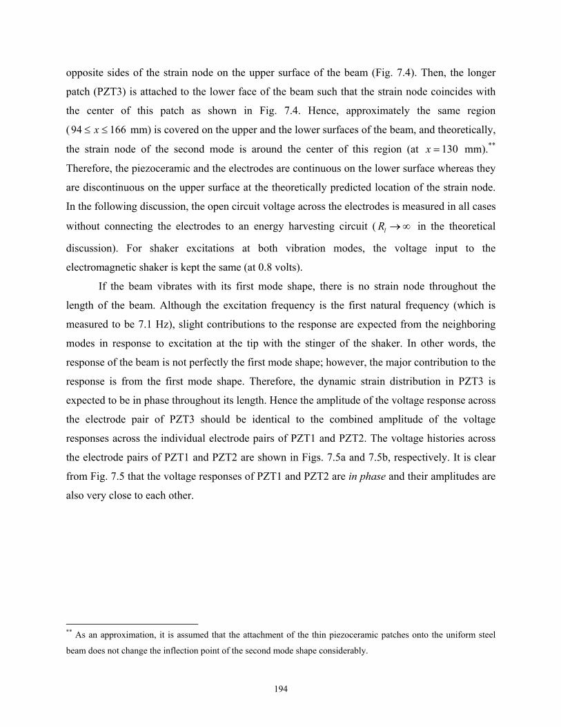
194

opposite sides of the strain node on the upper surface of the beam (Fig. 7.4). Then, the longer

patch (PZT3) is attached to the lower face of the beam such that the strain node coincides with

the center of this patch as shown in Fig. 7.4. Hence, approximately the same region

(94 166x mm) is covered on the upper and the lower surfaces of the beam, and theoretically,

the strain node of the second mode is around the center of this region (at 130x mm).**

Therefore, the piezoceramic and the electrodes are continuous on the lower surface whereas they

are discontinuous on the upper surface at the theoretically predicted location of the strain node.

In the following discussion, the open circuit voltage across the electrodes is measured in all cases

without connecting the electrodes to an energy harvesting circuit ( lR in the theoretical

discussion). For shaker excitations at both vibration modes, the voltage input to the

electromagnetic shaker is kept the same (at 0.8 volts).

If the beam vibrates with its first mode shape, there is no strain node throughout the

length of the beam. Although the excitation frequency is the first natural frequency (which is

measured to be 7.1 Hz), slight contributions to the response are expected from the neighboring

modes in response to excitation at the tip with the stinger of the shaker. In other words, the

response of the beam is not perfectly the first mode shape; however, the major contribution to the

response is from the first mode shape. Therefore, the dynamic strain distribution in PZT3 is

expected to be in phase throughout its length. Hence the amplitude of the voltage response across

the electrode pair of PZT3 should be identical to the combined amplitude of the voltage

responses across the individual electrode pairs of PZT1 and PZT2. The voltage histories across

the electrode pairs of PZT1 and PZT2 are shown in Figs. 7.5a and 7.5b, respectively. It is clear

from Fig. 7.5 that the voltage responses of PZT1 and PZT2 are in phase and their amplitudes are

also very close to each other.

** As an approximation, it is assumed that the attachment of the thin piezoceramic patches onto the uniform steel

beam does not change the inflection point of the second mode shape considerably.

195


first natural frequency of the beam

Figure 7.6 shows the voltage response of PZT3 along with the summation of the voltage

responses of PZT1 and PZT2 for excitation at the first natural frequency. As expected, the

voltage amplitude of PZT3 (which has the continuous electrode pair) is approximately identical

to the summation of the voltage amplitudes across the electrode pairs of PZT1 and PZT2 as they

are in phase. Also, the voltage response of PZT3 is 180 degrees out of phase with the summation

of PZT1 and PZT2 since the lower face of the beam is in tension when the upper face is in

compression, and vice versa. The slight difference in the amplitudes (Fig. 7.6) is expected to be

due to experimental imperfections. The PZTs were cut by hand and there is a finite spacing

between PZT1 and PZT2 as shown in Fig. 7.4 (so that the region covered by PZT1+PZT2

exceeds 94 166x mm slightly). Figure 7.6 is therefore a verification of the fact that the

piezoceramic patches with continuous electrodes can be used safely for harvesting energy from

the first vibration mode since the strain distribution is always in phase over the length of a

cantilevered beam.

(a) (b)

196


response obtained by combining the electrodes of PZT1 and PZT2 for excitation at the first

natural frequency

If the beam is excited at its second natural frequency (which is measured as 40.8 Hz), the

dominant vibration mode in the response is the second mode. The voltage outputs of PZT1 and

PZT2 are displayed in Fig.7.7 for excitation at the second natural frequency. Unlike the voltage

outputs for excitation at the first natural frequency, as expected, the voltage outputs of these

patches are now 180 degrees out of phase with each other. During the vibratory motion, when

PZT1 is in compression, PZT 2 is in tension, and vice versa. The phase difference in the

mechanical domain determines the phase difference in the voltage outputs. Note that the voltage

amplitudes of PZT1 and PZT2 are not identical, which means that the strain distributions at

different sides of 130x mm are not identical for excitation at the second natural frequency.


second natural frequency of the beam

(a) (b)

197

The continuous electrodes of PZT3 cover the entire region on the strain node of the

second mode. For excitation at the second natural frequency, the voltage response across the

electrodes of PZT3 is shown in Fig. 7.8 along with appropriate combination of PZT1 and PZT2

outputs for maximum voltage output. Since the charge developed in PZT3 is collected by

continuous electrodes, the phase difference in the strain distribution at opposite sides of the

second mode results in cancellation. Therefore the voltage output of PZT3 is less than even the

individual outputs of PZT1 and PZT2 for the same mechanical input (compare the solid line in

Fig. 7.8 with Figs. 7.7a and 7.7b). Clearly, it is not preferable to cover the strain node of a

harvester beam with continuous electrodes. In order to obtain the maximum voltage output from

this sample region (94 166x mm) for excitation at the second natural frequency, one should

collect the electric charge developed in regions 94 130x mm and 130 166x mm with

separate electrode pairs to obtain the individual voltage outputs given in Fig. 7.7. These voltage

outputs can then be combined by considering the phase difference (mathematically, by

subtracting the voltage outputs: PZT1-PZT2) to obtain the maximum voltage amplitude (dashed

line Fig. 7.8). The physical combination of these voltage outputs (i.e. realization of the

subtraction PZT1-PZT2) is done by combining the correct leads coming from the respective

segmented electrode pairs. According to Fig. 7.8, the voltage amplitude of the preferable

combination of PZT1 and PZT2 is more than 4 times the amplitude of the voltage response of

PZT3.


response obtained by combining the electrodes of PZT1 and PZT2 for excitation at the second

natural frequency

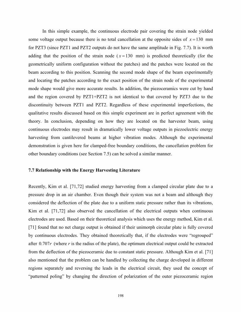
198

In this simple example, the continuous electrode pair covering the strain node yielded

some voltage output because there is no total cancellation at the opposite sides of 130x mm

for PZT3 (since PZT1 and PZT2 outputs do not have the same amplitude in Fig. 7.7). It is worth

adding that the position of the strain node ( 130x mm) is predicted theoretically (for the

geometrically uniform configuration without the patches) and the patches were located on the

beam according to this position. Scanning the second mode shape of the beam experimentally

and locating the patches according to the exact position of the strain node of the experimental

mode shape would give more accurate results. In addition, the piezoceramics were cut by hand

and the region covered by PZT1+PZT2 is not identical to that covered by PZT3 due to the

discontinuity between PZT1 and PZT2. Regardless of these experimental imperfections, the

qualitative results discussed based on this simple experiment are in perfect agreement with the

theory. In conclusion, depending on how they are located on the harvester beam, using

continuous electrodes may result in dramatically lower voltage outputs in piezoelectric energy

harvesting from cantilevered beams at higher vibration modes. Although the experimental

demonstration is given here for clamped-free boundary conditions, the cancellation problem for

other boundary conditions (see Section 7.5) can be solved a similar manner.

7.7 Relationship with the Energy Harvesting Literature

Recently, Kim et al. [71,72] studied energy harvesting from a clamped circular plate due to a

pressure drop in an air chamber. Even though their system was not a beam and although they

considered the deflection of the plate due to a uniform static pressure rather than its vibrations,

Kim et al. [71,72] also observed the cancellation of the electrical outputs when continuous

electrodes are used. Based on their theoretical analysis which uses the energy method, Kim et al.

[71] found that no net charge output is obtained if their unimorph circular plate is fully covered

by continuous electrodes. They obtained theoretically that, if the electrodes were “regrouped”

after 0.707r (where r is the radius of the plate), the optimum electrical output could be extracted

from the deflection of the piezoceramic due to constant static pressure. Although Kim et al. [71]

also mentioned that the problem can be handled by collecting the charge developed in different

regions separately and reversing the leads in the electrical circuit, they used the concept of

“patterned poling” by changing the direction of polarization of the outer piezoceramic region

199

(that is the region outside a specific radius) in their experimental work [72]. Changing the poling

direction implies etching the electrodes at a specific region (at 0.5r and 0.75r in two separate

cases of their work) and then applying a very high electric field in the desired portion of the

piezoceramic (in general, at a temperature above the Curie temperature of the piezoelectric

material). After the patterned poling process is completed, Kim et al. [72] used a conductive pen

to reconstruct the electrodes at the etched regions. Finally, the electric charge is collected using

the reconstructed full electrodes and improved results are obtained. They observed

experimentally that patterned poling after 0.75r gave the best results when compared to the

cases of patterned poling after 0.5r and the original case with full electrodes and unmodified

polarization (in agreement with their theoretical work [71] which predicted the optimum radius

as 0.707r which is close to 0.75r ). It should also be added that the unmodified case with full

electrodes still gave some nonzero electric charge output in the order of magnitude of the other

cases, most likely because of some physical imperfections, such as the difficulty in realization of

the clamped boundary [72].

Although the approach preferred by Kim et al. [72] appears to be a relatively complicated

way of solving the cancellation problem, it is worthwhile to relate it to our discussion on

cantilevered beams. The optimum location for etching the electrodes is where the electric

displacement changes sign and it corresponds to a strain node line in our study on cantilevered

harvesters. Once patterned polarization process is completed, continuous electrodes can be used

for collecting the charge output. Mathematically, as far as our relevant equations for beams are

concerned, the piezoelectric constant ( 31e ) changes sign in the modified region after the

patterned polarization process. The issue of cancellation in the integral given by Eq. (7.2) was

due to the opposite sign of the curvature at the opposite sides of the strain nodes when 31e had

the same sign throughout the length of the beam. The new polarization at one side of the strain

node makes the sign of the product of the piezoelectric constant and the curvature the same at the

opposite sides of the strain node. Hence no cancellation takes place during the integration of the

electric displacement over the continuous electrode area. Briefly, in order to avoid the

cancellation, either the polarization at one side of the strain node must be reversed (by patterned

poling) so that continuous electrodes can be used or the electrodes must be discontinuous at the

strain node if the polarization is to be kept the same over the length of the beam (as demonstrated

in the previous section).

200

Although the patterned polarization approach solved the static deflection problem of Kim

et al. [72] permanently, it may not be a flexible approach as far as the dynamic (vibration)

problem is concerned, since the deflection pattern changes with vibration modes. For a simple

explanation, consider the second vibration mode of a cantilevered energy harvester. If the

polarization of the harvester is reversed at one side of the strain node (which is located at

0.2165x ), one can use continuous electrodes (covering 0 1x ) to collect the charge

developed in the piezoceramic and this avoids the cancellation in the integral of Eq. (7.4) for

vibrations with the second mode shape. After patterned poling, if the beam with continuous

electrodes is used for harvesting energy at the first vibration mode, one ends up with a strong

cancellation although there is no strain node in the first vibration mode. Even though the

curvature has the same sign throughout the beam length for the first mode shape (Fig. 7.1b), the

change in the sign of 31e at 0.2165x makes it necessary to consider the integral in Eq. (7.4) in

two parts where a drastic cancellation occurs between the two areas ( 0 0.2165x and

0.2165 1x ) as far as the resultant of the inner product in Eq. (7.1) is concerned. Therefore, in

the dynamic problem, the patterned poling process can be favorable for a single vibration mode

only. Otherwise, one has to repeat the patterned poling process again in order to use the same

harvester beam (which was patterned poled for a certain mode shape) for excitations with

another mode shape.

Based on the above discussion, it is reasonable to claim that switching the leads of the

segmented electrodes (as demonstrated in Section 7.6) is more flexible and reversible compared

to the patterned poling process in the vibration-based energy harvesting problem. The patterned

poling process can be useful for static problems as a permanent solution since (for a given

loading) a single deflection pattern exists in linear static problems, unlike the vibration problems

(where the deflection pattern depends on the vibration mode). Using segmented electrodes is

easier to implement as the cancellation problem is mainly solved in the electrical circuit by

combining the leads of the electrodes accordingly. Moreover, considering the fact that most

piezoceramic patches come with integrated electrodes from the manufacturer, one may not have

to apply an etching process to obtain a discontinuity at the strain node of the harvester. In most

cases, it might be possible to cut the piezoceramic patch (and therefore its electrodes) as done in

the simple experimental demonstration of the previous section. The following section discusses a

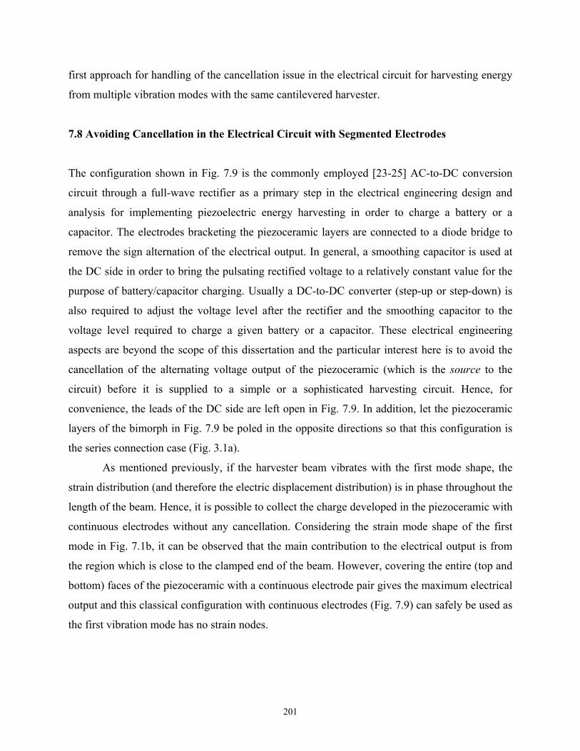
201

first approach for handling of the cancellation issue in the electrical circuit for harvesting energy

from multiple vibration modes with the same cantilevered harvester.

7.8 Avoiding Cancellation in the Electrical Circuit with Segmented Electrodes

The configuration shown in Fig. 7.9 is the commonly employed [23-25] AC-to-DC conversion

circuit through a full-wave rectifier as a primary step in the electrical engineering design and

analysis for implementing piezoelectric energy harvesting in order to charge a battery or a

capacitor. The electrodes bracketing the piezoceramic layers are connected to a diode bridge to

remove the sign alternation of the electrical output. In general, a smoothing capacitor is used at

the DC side in order to bring the pulsating rectified voltage to a relatively constant value for the

purpose of battery/capacitor charging. Usually a DC-to-DC converter (step-up or step-down) is

also required to adjust the voltage level after the rectifier and the smoothing capacitor to the

voltage level required to charge a given battery or a capacitor. These electrical engineering

aspects are beyond the scope of this dissertation and the particular interest here is to avoid the

cancellation of the alternating voltage output of the piezoceramic (which is the source to the

circuit) before it is supplied to a simple or a sophisticated harvesting circuit. Hence, for

convenience, the leads of the DC side are left open in Fig. 7.9. In addition, let the piezoceramic

layers of the bimorph in Fig. 7.9 be poled in the opposite directions so that this configuration is

the series connection case (Fig. 3.1a).

As mentioned previously, if the harvester beam vibrates with the first mode shape, the

strain distribution (and therefore the electric displacement distribution) is in phase throughout the

length of the beam. Hence, it is possible to collect the charge developed in the piezoceramic with

continuous electrodes without any cancellation. Considering the strain mode shape of the first

mode in Fig. 7.1b, it can be observed that the main contribution to the electrical output is from

the region which is close to the clamped end of the beam. However, covering the entire (top and

bottom) faces of the piezoceramic with a continuous electrode pair gives the maximum electrical

output and this classical configuration with continuous electrodes (Fig. 7.9) can safely be used as

the first vibration mode has no strain nodes.

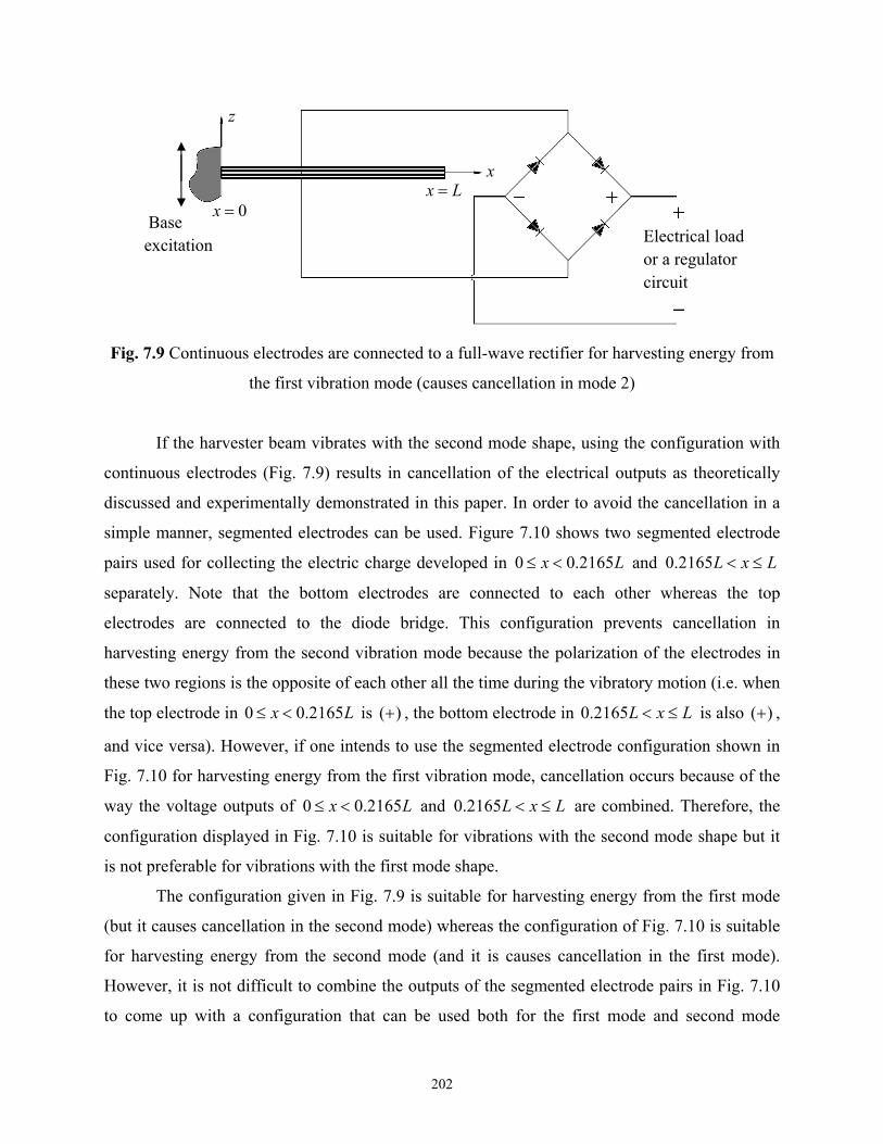
202

Fig. 7.9 Continuous electrodes are connected to a full-wave rectifier for harvesting energy from

the first vibration mode (causes cancellation in mode 2)

If the harvester beam vibrates with the second mode shape, using the configuration with

continuous electrodes (Fig. 7.9) results in cancellation of the electrical outputs as theoretically

discussed and experimentally demonstrated in this paper. In order to avoid the cancellation in a

simple manner, segmented electrodes can be used. Figure 7.10 shows two segmented electrode

pairs used for collecting the electric charge developed in 0 0.2165x L and 0.2165L x L

separately. Note that the bottom electrodes are connected to each other whereas the top

electrodes are connected to the diode bridge. This configuration prevents cancellation in

harvesting energy from the second vibration mode because the polarization of the electrodes in

these two regions is the opposite of each other all the time during the vibratory motion (i.e. when

the top electrode in 0 0.2165x L is ( ) , the bottom electrode in 0.2165L x L is also ( ) ,

and vice versa). However, if one intends to use the segmented electrode configuration shown in

Fig. 7.10 for harvesting energy from the first vibration mode, cancellation occurs because of the

way the voltage outputs of 0 0.2165x L and 0.2165L x L are combined. Therefore, the

configuration displayed in Fig. 7.10 is suitable for vibrations with the second mode shape but it

is not preferable for vibrations with the first mode shape.

The configuration given in Fig. 7.9 is suitable for harvesting energy from the first mode

(but it causes cancellation in the second mode) whereas the configuration of Fig. 7.10 is suitable

for harvesting energy from the second mode (and it is causes cancellation in the first mode).

However, it is not difficult to combine the outputs of the segmented electrode pairs in Fig. 7.10

to come up with a configuration that can be used both for the first mode and second mode

0x x L

x

z

Base excitation Electrical load

or a regulator circuit

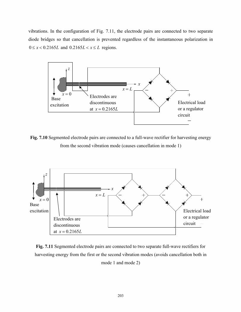
203

vibrations. In the configuration of Fig. 7.11, the electrode pairs are connected to two separate

diode bridges so that cancellation is prevented regardless of the instantaneous polarization in

0 0.2165x L and 0.2165L x L regions.

Fig. 7.10 Segmented electrode pairs are connected to a full-wave rectifier for harvesting energy

from the second vibration mode (causes cancellation in mode 1)

Fig. 7.11 Segmented electrode pairs are connected to two separate full-wave rectifiers for

harvesting energy from the first or the second vibration modes (avoids cancellation both in

mode 1 and mode 2)

z

x

0x x L

0x x L

x

Base excitation

z

Electrical load or a regulator circuit

Electrical load or a regulator circuit

Base excitation

Electrodes are discontinuous at 0.2165x L

Electrodes are discontinuous at 0.2165x L

204

The foregoing approach of avoiding the cancellation issue appears to be easier and more

flexible than the patterned poling technique [72]. Here, the only requirements are the removal of

electrodes at the strain nodes and simple considerations in the electrical circuit. The idea

described here is not limited to the first two vibration modes and it can easily be extended to

higher vibration modes and other boundary conditions. Alternative circuitry-based approaches

can be investigated to handle the cancellation problem for multi-mode excitations with less

number of diodes as the presence of diodes creates losses in the electrical circuit.


The positions of the beam where the dynamic strain distribution changes sign are called the

strain nodes. It is theoretically discussed and experimentally demonstrated that covering the

strain nodes of vibration modes with continuous electrodes results in cancellation of the

electrical outputs in piezoelectric energy harvesting. A detailed dimensionless analysis is given

for predicting the locations of the strain nodes of a thin cantilever in the absence of a tip mass.

Dimensionless derivations and results are then presented for predicting the strain node positions

and their variations in the presence of a tip mass. As the cancellation issue is not peculiar to

clamped-free boundary conditions, dimensionless data of modal strain nodes are tabulated for

some other practical boundary condition pairs as well. The locations of strain nodes tabulated in

this work are important also for applications of modal actuation since covering these positions

with piezoelectric actuators might require very high voltage inputs. It is experimentally

demonstrated that the voltage output due to the second mode excitation can be increased

dramatically if segmented electrodes are used instead of continuous electrodes. The relationship

between the discussion given here and a recent study on piezoelectric energy harvesting from the

static deflection of a clamped circular plate is also explained. The use of segmented electrode

pairs to avoid cancellations is described for single-mode and multi-mode vibrations of a

cantilevered harvester and alternative circuitry-based approaches can be investigated to handle

the cancellation problem for multi-mode excitations.

205

CHAPTER 8

APPROXIMATE DISTRIBUTED-PARAMETER MODELING OF

PIEZOELECTRIC ENERGY HARVESTERS USING THE

ELECTROMECHANICAL ASSUMED-MODES METHOD

This chapter covers the approximate distributed-parameter formulation of cantilevered

piezoelectric energy harvester beams under base excitation. Since the closed-form analytical

solutions for bimorph configurations were obtained in Chapter 3, this chapter provides

derivations with a focus on the unimorph configuration (Fig. 8.1). The technique used here is an

electromechanical version of the assumed-modes method*, which is based on the extended

Hamilton’s principle for electromechanical media. After obtaining the distributed-parameter

energy expressions, extended Hamilton’s principle is used to derive the discretized

electromechanical Lagrange equations. In order to model the asymmetric unimorph structure

precisely, an axial displacement variable is introduced to account for coupling of axial and

transverse displacement variables due to asymmetric laminates. The derivations are given in this

chapter in three parts: (1) the Euler-Bernoulli formulation, (2) the Rayleigh formulation and (3)

the Timoshenko formulation. The first type of formulation neglects the rotary inertia and the

transverse shear deformation effects whereas the second type includes the rotary inertia effect

but neglects the transverse shear deformation. The third solution type accounts for the influences

of both the transverse shear deformation and rotary inertia on the resulting electromechanical

behavior. Therefore the Euler-Bernoulli solution is valid for thin beams whereas the Timoshenko

solution is valid for moderately thick beams (and the Rayleigh solution lies in between).

Experimental validations are given for the thin-beam case by comparing the assumed-modes

predictions with the experimental and analytical results for different number of modes.

* As discussed by Meirovitch [41], the assumed-modes method for distributed-parameter systems is closely related

to the Rayleigh-Ritz method. Indeed the resulting discretized equations obtained in both methods are identical for

the same admissible functions. The difference is that the Rayleigh-Ritz method is concerned with spatial

discretization of the differential eigenvalue problem whereas the assumed-modes method directly begins with spatial

discretization of the boundary-value problem in an implicit manner.

206

8.1 Unimorph Piezoelectric Energy Harvester Configuration

Consider the piezoelectric energy harvester configuration shown in Fig. 8.1. The configuration

has a single piezoceramic layer bonded onto a substructure layer, therefore it is a unimorph

cantilever. The perfectly conductive electrode pair (of negligible thickness) fully covers the

upper and the lower faces of the piezoceramic and is connected to a resistive electrical load. The

layers are perfectly bonded to each other so there is no relative sliding at the interface. The

purpose is to find the voltage output of the piezoceramic ( ( )pv t ) across the load resistance in

response to imposed base excitation. As done in Chapter 3 (where the analytical solutions for

symmetric bimorph configurations were given), the base motion is represented as translation in

the transverse direction with superimposed small rotation. Deformations are assumed to be small

and the material behavior is assumed to be linear elastic. Note that the x, y and z directions,

respectively, are coincident with the 1, 2 and 3 directions of piezoelectricity (y-direction is into

the page). These directional subscripts are used interchangeably as the former is preferred for

mechanical derivations whereas the latter is used in the piezoelectric constitutive relations

(Appendix A). Note that the following Euler-Bernoulli, Rayleigh and Timoshenko type

derivations can handle modeling of beams with varying cross-section and changing material

properties in x-direction. The coupling between the axial and transverse displacement

components due to structural asymmetry is taken into consideration in all cases. The harvester

beam shown in Fig. 8.1 has no tip mass. The effect of a tip mass (with mass moment of inertia)

on the following formulation is discussed after the basic derivations (in Section 8.6).

Fig. 8.1 Unimorph piezoelectric energy harvester with varying cross-section

207

8.2 Electromechanical Euler-Bernoulli Model with Axial Deformations

8.2.1 Distributed-parameter Electromechanical Energy Formulation. The effective base

displacement acting on the beam is given by Eq. (3.1) as

( , ) ( ) ( )bw x t g t xh t (8.1)

where ( )g t is the translation in the transverse direction and ( )h t is the superimposed small

rotation.

The displacement field in the beam relative to the moving base can be given by

00 ( , )

( , , ) ( , )w x t

u x z t u x t zx

(8.2)

( , , ) 0v x z t (8.3)

0( , , ) ( , )w x z t w x t (8.4)

where 0 ( , )u x t and 0 ( , )w x t are the axial displacement and transverse displacement of the neutral

axis at point x and time t relative to the moving base.†

The vector form of the displacement field is

00 0( , )( , ) 0 ( , )

tw x t

u x t z w x tx

u (8.5)

where superscript t stands for transpose (otherwise it is time). From this displacement field, the

only non-zero strain component can be extracted as

0 2 0

2

( , , ) ( , ) ( , )( , , )xx

u x z t u x t w x tS x z t z

x x x

(8.6)

The total potential energy in the structure is

1

2s p

t ts p

V V

U dV dV S T S T (8.7)

where S is the vector of engineering strain components, T is the vector of engineering stress

components, the subscripts s and p stand for substructure and piezoceramic, respectively, and the

integrations are performed in the volume (V ) of the respective material.

† The subscript rel (used to denote the relative motion) used in Chapters 2 and 3 has been removed here to avoid

notation complexity. These terms are defined relative to the moving base throughout this chapter.

208

The isotropic substructure obeys Hooke’s law:

( , , ) ( , , )xx s xxT x z t Y S x z t (8.8)

where sY is the elastic modulus of the substructure layer.

The constitutive relation for the stress component in the piezoceramic is (Appendix A.2)

1 11 1 31 3 11 31

( )( , , ) ( , , ) pE E

xx xxp

v tT x z t T c S e E c S x z t e

h (8.9)

Here, the electric field is given in terms of the voltage across the load (i.e. 3( ) ( ) /p pE t v t h

where ( )pv t is the voltage across the electrodes and ph is the thickness of the piezoceramic), the

reduced elastic modulus, piezoelectric stress constant and the permittivity constant expressions

are 11 111/E Ec s , 31 31 11/ Ee d s and 233 33 31 11/S T Ed s , respectively (Appendix A.2).

Equation (8.7) becomes

20 2 0

2

20 2 0 0 2 0

11 312 2

1 ( , ) ( , )

2

( )1 ( , ) ( , ) ( , ) ( , )

2

s

p

s s

V

pEp

pV

u x t w x tU Y z dV

x x

v tu x t w x t u x t w x tc z e z dV

x x h x x

(8.10)

The total kinetic energy of the system can be given by

1

2s p

t tm m m m

s s p p

V V

T dV dVt t t t

u u u u (8.11)

where s and p are the mass densities of the substructure and piezoceramic layers, and mu is

the modified displacement vector that is the superposition of the base displacement input given

by Eq. (8.1) and the displacement vector u :‡

00 0( , )( , ) 0 ( , ) ( , )

t

m b

w x tu x t z w x t w x t

x

u (8.12)

‡ Note that the external forcing on the structure is due to the base motion. Since the total kinetic energy is written for

the velocity field of the beam relative to the absolute reference frame, the forcing function on the beam (in terms of

( , )b

w x t ) will emerge from this kinetic energy expression. Alternatively, one could express the total kinetic energy

relative to the moving base and include the (virtual) work done by the inertial excitation term (due to base

displacement ( , )b

w x t ) as a non-conservative effect.

209

Then the total kinetic energy becomes

2 20 2 0 0

2 20 2 0 0

( , )1 ( , ) ( , ) ( , )

2

( , )( , ) ( , ) ( , )

s

p

bs s

V

bp p

V

w x tu x t w x t w x tT z dV

t t x t t

w x tu x t w x t w x tz dV

t t x t t

(8.13)

The total potential energy can be re-expressed as follows:

2 20 2 0 0 2 0

2 20

2 20 2 0 0 2 0

11 2 2

0

1 ( , ) ( , ) ( , ) ( , )2 ...

2

( , ) ( , ) ( , ) ( , )2 ...

( , )( ) (

L

s s s s

Ep p p

p p p p

u x t w x t u x t w x tU Y A I H

x x x x

u x t w x t u x t w x tc A I H

x x x x

u x tB v t J v t

x

2 0

2

( , ))

w x tdx

x

(8.14)

The total kinetic energy in the expanded form is

2 2 20 0 0

0

20 2 0 2 0

( , ) ( , )1 ( , ) ( , ) ( , )2 ...

2

( , ) ( , ) ( , )2

Lb b

s s s s s

s s

w x t w x tu x t w x t w x tT A A A A

t t t t t

u x t w x t w x tH I

t t x t x

2 2 20 0 0

20 2 0 2 0

...

( , ) ( , )( , ) ( , ) ( , )2 ...

( , ) ( , ) ( , )2

b bp p p p p

p p

w x t w x tu x t w x t w x tA A A A

t t t t t


t t x t x

dx

(8.15)

where the kinetic energy contributions from the rotary inertia are neglected but the terms which

might cause inertial coupling between the axial and transverse displacement components due to

asymmetric laminates are kept. Here, the zero-th, first and the second moments of area for the

substructure and piezoceramic cross-sections at an arbitrary point x are

2, , 1, ,s s s

s

A H I z z dydz (8.16)

2, , 1, ,p p p

p

A H I z z dydz (8.17)

210

where sH and pH vanish for a structure that is symmetric with respect to the neutral axis of the

beam (just like a bimorph or any symmetric multi-morph). Therefore, for a symmetric structure,

there is no coupling between 0 ( , )u x t and 0 ( , )w x t . As a result, in a symmetric structure, the axial

displacement 0 ( , )u x t cannot be excited by the imposed base displacement ( , )bw x t , which

simplifies the problem (and allows analytical solutions as in Chapter 3). It is worth adding that,

in the foregoing expressions as well as in the following, ( )s sA A x , ( )p pA A x , ( )s sH H x ,

( )p pH H x , ( )s sI I x and ( )p pI I x are allowed.

The terms related to piezoelectric coupling are

31p

pp

eB dydz

h (8.18)

31p

pp

eJ zdydz

h (8.19)

where pB couples the voltage and the extension component and pJ couples the voltage and the

curvature component according to Eq. (8.14).

The internal electrical energy in the piezoceramic layer is

1

2p

tie p

V

W dV E D (8.20)

where E is the vector of electric field components and D is the vector of electric displacement

components. Substituting the respective terms (the non-zero electric field and the electric

displacement components from Appendix A.2) gives

0 2 0

31 332

0 2 02

20

( ) ( )1 ( , ) ( , )

2

1 ( , ) ( , ) 1( ) ( ) ( )

2 2

p

p pSie p

p pV

L

p p p p p p

v t v tu x t w x tW e z dV

h x x h

u x t w x tB v t J v t dx C v t

x x

(8.21)

Here, pC is the internal capacitance of the piezoceramic given by

33pS

pp

AC

h (8.22)

where pA is the electrode area.

211

In order to account for mechanical damping, Rayleigh’s dissipation function [41] can be

used. Alternatively, a damping matrix proportional to the resulting mass and stiffness matrices

can be introduced later (i.e. after the system is discretized in the assumed-modes solution

procedure). The second approach is preferred here for simplicity.

The extended Hamilton’s principle [30] with the internal electrical energy is

2

1

0t

ie nc

t

L W W dt (8.23)

where L is the Lagrangian,

L T U (8.24)

Here, L and ieW are the first variations [54] of the Lagrangian and the inertial electrical

energy, and ncW is the virtual work of the non-conservative mechanical force and electric

charge components. Since the effect of base excitation is considered in the total kinetic energy

term and the mechanical damping effect is to be introduced later, the only non-conservative

virtual work is due to the electric charge output ( ( )Q t ):

( ) ( )nc nce pW W Q t v t (8.25)

Following the regular procedure of the assumed-modes method [41], the next step is to discretize

the components of the extended Hamilton’s principle, which are the Lagrangian, internal

electrical energy and the virtual work of the non-conservative electric charge.

8.2.2 Spatial Discretization of the Energy Equations. The distributed-parameter variables in

the mechanical domain are 0 ( , )w x t and 0 ( , )u x t while the electrical variable is ( )pv t . Let the

following two finite series represent the two components of vibration response:

0

1

( , ) ( ) ( )N

r rr

w x t a t x

(8.26)

0

1

( , ) ( ) ( )N

r rr

u x t b t x

(8.27)

where ( )r x and ( )r x are the kinematically admissible trial functions which satisfy the

respective essential boundary conditions (Appendix D.1), ( )ra t and ( )rb t are the unknown

generalized coordinates. Using Eqs. (8.26) and (8.27) in Eq. (8.14), the total potential energy

equation becomes

212

11 111 1 0 0

11

0 0 0

1( ) ( ) ( ) ( ) ...

2

2 ( ) ( ) ( ) ( ) ( ) ( )

L LN NE E

r l s s p r l r l s s p r lr l

L L LE

r l s s p r l r p p r r p p r

U a a Y I c I x x dx b b Y A c A x x dx

a b Y H c H x x dx b v t B x dx a v t J x dx

(8.28)

where a prime represents ordinary differentiation with respect to space (variable x). Similarly,

the total kinetic energy expression given by Eq. (8.15) can be discretized to give

1 1 0 0

2

0 0

0

( , )1( ) ( ) 2 ( ) ...

2

( , )( ) ( ) ...

2 ( ) ( )

L LN Nb

r l s s p p r l r s s p p rr l

L Lb

s s p p r l s s p p r l

L

r l s s p p r l

w x tT a a A A x x dx a A A x dx

t

w x tA A dx b b A A x x dx

t

a b H H x x dx

(8.29)

where an over-dot represents ordinary differentiation with respect to time (variable t).

Substituting Eqs. (8.26) and (8.27) into Eq. (8.21), the internal electrical energy

expression becomes

2

1 0 0

1( ) ( ) ( ) ( ) ( )

2

L LN

ie r p p r r p p r p pr

W b v t B x dx a v t J x dx C v t

(8.30)

Equations (8.28)-(8.30) can be written as

1 1

12

2

N Naa bb ab a b

r l rl r l rl r l rl r p r r p rr l

U a a k b b k a b k a v b v

(8.32)

2

1 1 0

( , )12 2

2

LN Naa bb ab b

r l rl r l rl r l rl r r s s p pr l

w x tT a a m b b m a b m a p A A dx

t

(8.31)

2

1

1

2

Na b

ie r p r r p r p pr

W a v b v C v

(8.33)

Here,

0

( ) ( )L

aarl s s p p r lm A A x x dx (8.34)

0

( ) ( )L

bbrl s s p p r lm A A x x dx (8.35)

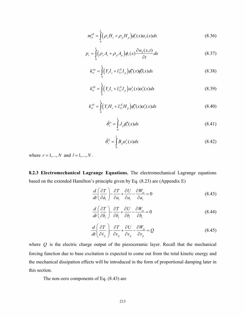
213

0

( ) ( )L

abrl s s p p r lm H H x x dx (8.36)

0

( , )( )

Lb

r s s p p r

w x tp A A x dx

t

(8.37)

11

0

( ) ( )L

aa Erl s s p r lk Y I c I x x dx (8.38)

11

0

( ) ( )L

bb Erl s s p r lk Y I c I x x dx (8.39)

11

0

( ) ( )L

ab Erl s s p r lk Y H c H x x dx (8.40)

0

( )L

ar p rJ x dx (8.41)

0

( )L

br p rB x dx (8.42)

where 1,...,r N and 1,...,l N .

8.2.3 Electromechanical Lagrange Equations. The electromechanical Lagrange equations

based on the extended Hamilton’s principle given by Eq. (8.23) are (Appendix E)

0ie

i i i i

Wd T T U

dt a a a a

(8.43)

0ie

i i ii

Wd T T U

dt b b bb

(8.44)

ie

p p p p

Wd T T UQ

dt v v v v

(8.45)

where Q is the electric charge output of the piezoceramic layer. Recall that the mechanical

forcing function due to base excitation is expected to come out from the total kinetic energy and

the mechanical dissipation effects will be introduced in the form of proportional damping later in

this section.

The non-zero components of Eq. (8.43) are

214

1 1

1 1 1

12 2

2

12 2

2

N Naa ablr r r

l r rl l rl rr li i i i i

N N Naa ab aa ab

ri l li r rl ri l rl ri r il l il l ir l l

aa a aTa a m b m p

a a a a a

a a m b m p m a m b p

(8.46)

1 1

1 1 1

12

2

1 12

2 2

N Naa ab alr r r

l r rl l rl p rr li i i i i

N N Naa ab a aa ab a

ri l li r rl ri l rl ri p r il l il l i pr l l

aa a aUa a k b k v

a a a a a

a a k b k v k a k b v

(8.47)

1 1

1 1 1

2 2 2

N Na a aie r

p r ri p r i pr ri i

W av v v

a a

(8.48)

Then the first set of Lagrange equations (for the generalized coordinate la ) become

1

0N

aa ab aa ab ail l il l il l il l i p i

l

m a m b k a k b v f

(8.49)

where if is the forcing component due to base excitation

2

20

2 2

2 20 0

( , )( )

( ) ( )( ) ( )

Li b

i s s p p i

L L

s s p p i s s p p i

p w x tf A A x dx

t t

d g t d h tA A x dx A A x x dx

dt dt

(8.50)

Similarly, the non-zero components in Eq. (8.44) are

1 1

1 1 1

12

2

12

2

N Nbb ablr r

l r rl l rlr li i i i

N N Nbb ab bb ab

ri l li r rl ri l rl il l il lr l l

bb bTb b m a m

b b b b

b b m a m m b m a

(8.51)

1 1

1 1 1

12

2

1 12

2 2

N Nbb ab blr r r


N N Nbb ab b bb ab b


bb b bUb b k a k v

b b b b b

b b k a k v k b k a v

(8.52)

1 1

1 1 1

2 2 2

N Nb b bie r


W bv v v

b b

(8.53)

The Lagrange equation for the generalized coordinate lb is

215

1

0N

bb ab bb ab bil l il l il l il l i p

l

m b m a k b k a v

(8.54)

The non-zero components on the left hand side of Eq. (8.45) are

1

1

2

Na b

r r r rrp

Ua b

v

(8.55)

1

1

2

Na bie

p p r r r rrp

WC v a b

v

(8.56)

yielding

1

0N

a bp p r r r r

r

C v Q a b

(8.57)

Taking the time derivative of Eq. (8.57) gives

1

0N

a bp p r r r r

r

C v Q a b

(8.58)

where the time rate of change of charge is the electric current passing through the resistor:

p

l

vQ

R (8.59)

The Lagrange equation for pv becomes

1

0N

p a bp p r r r r

rl

vC v a b

R

(8.60)

The first two Lagrange equations (Eqs. (8.49) and (8.54)) can be given in the matrix form as

pv

aa ab aa ab a

ab bb ab bb b

a a fm -m k -k θ+ + =

b b 0-m m -k k θ

(8.61)

Introducing Rayleigh damping to represent the dissipative electromechanical system as a normal-

mode system:

pv

aa ab aa ab aa ab a

ab bb ab bb ab bb b

a a a fm -m d -d k -k θ+ + + =

b b b 0-m m -d d -k k θ

(8.62)

where the damping matrix is

aa ab aa ab aa ab

ab bb ab bb ab bb

d -d m -m k -k

-d d -m m -k k (8.63)

Here, and are the constants of mass and stiffness proportionality, respectively.

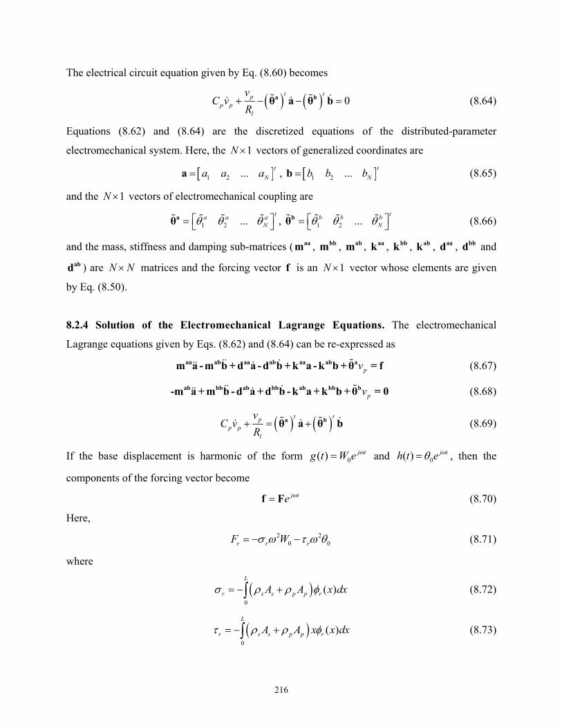
216

The electrical circuit equation given by Eq. (8.60) becomes

0t tp

p pl

vC v

R a bθ a θ b (8.64)

Equations (8.62) and (8.64) are the discretized equations of the distributed-parameter

electromechanical system. Here, the 1N vectors of generalized coordinates are

1 2 ...t

Na a aa , 1 2 ...t

Nb b bb (8.65)

and the 1N vectors of electromechanical coupling are

1 2 ...ta a a

N aθ , 1 2 ...

tb b bN

bθ (8.66)

and the mass, stiffness and damping sub-matrices ( aam , bbm , abm , aak , bbk , abk , aad , bbd and

abd ) are N N matrices and the forcing vector f is an 1N vector whose elements are given

by Eq. (8.50).

8.2.4 Solution of the Electromechanical Lagrange Equations. The electromechanical

Lagrange equations given by Eqs. (8.62) and (8.64) can be re-expressed as

pvaa ab aa ab aa ab am a - m b + d a - d b + k a - k b +θ = f (8.67)

pvab bb ab bb ab bb b-m a + m b - d a + d b - k a + k b +θ = 0 (8.68)

t tpp p

l

vC v

R a bθ a θ b (8.69)

If the base displacement is harmonic of the form 0( ) j tg t W e and 0( ) j th t e , then the

components of the forcing vector become

j te f F (8.70)

Here,

2 2

0 0r r rF W (8.71)

where

0

( )L

r s s p p rA A x dx (8.72)

0

( )L

r s s p p rA A x x dx (8.73)

217

Based on the linear electromechanical system assumption, the generalized coordinates and the

voltage output at steady state are j te a A , j te b B and j tp pv V e (where

1 2 ...t

NA A AA , 1 2 ...t

NB B BB and pV are complex valued). Equations (8.67)-

(8.69) become

2 2pj j V aa aa aa ab ab ab am d k A m d k B θ F (8.74)

2 2pj j V ab ab ab bb bb bb bm d k A m d k B θ 0 (8.75)

1 t t

p pl

j C V jR

a bθ A + θ B (8.76)

From Eq. (8.76):

1

1 t t

p pl

V j j CR

a bθ A + θ B (8.77)

Substituting Eq. (8.77) into Eqs. (8.74) and (8.75) gives

aa abΓ A Γ B F (8.78)

ba bbΓ A Γ B 0 (8.79)

where

1

2 1 t

pl

j j j CR

aa aa aa aa a aΓ m d k θ θ (8.80)

1

2 1 t

pl

j j j CR

bb bb bb bb b bΓ m d k θ θ (8.81)

1

2 1 t

pl

j j j CR

ab ab ab ab a bΓ m d k θ θ (8.82)

1

2 1 t

pl

j j j CR

ba ab ab ab b aΓ m d k θ θ (8.83)

From Eq. (8.79):

1 bb baB Γ Γ A (8.84)

Substituting Eq. (8.84) into Eq. (8.78) gives the complex generalize coordinate amplitudes rA :

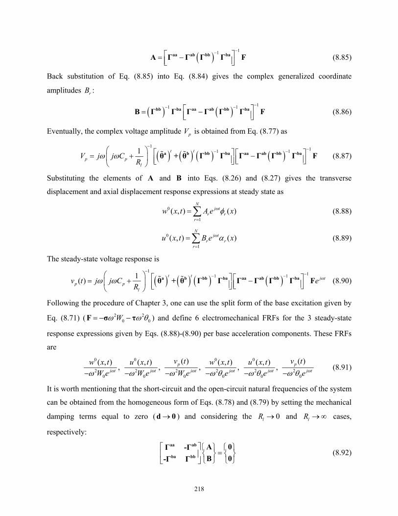
218

11

aa ab bb baA Γ Γ Γ Γ F (8.85)

Back substitution of Eq. (8.85) into Eq. (8.84) gives the complex generalized coordinate

amplitudes rB :

11 1

bb ba aa ab bb baB Γ Γ Γ Γ Γ Γ F (8.86)

Eventually, the complex voltage amplitude pV is obtained from Eq. (8.77) as

1

11 11 t t

p pl

V j j CR

a b bb ba aa ab bb baθ + θ Γ Γ Γ Γ Γ Γ F (8.87)

Substituting the elements of A and B into Eqs. (8.26) and (8.27) gives the transverse

displacement and axial displacement response expressions at steady state as

0

1

( , ) ( )N

j tr r

r

w x t A e x

(8.88)

0

1

( , ) ( )N

j tr r

r

u x t B e x

(8.89)

The steady-state voltage response is

1

11 11( )

t tj t

p pl

v t j j C eR


Following the procedure of Chapter 3, one can use the split form of the base excitation given by

Eq. (8.71) ( 2 20 0W F σ τ ) and define 6 electromechanical FRFs for the 3 steady-state

response expressions given by Eqs. (8.88)-(8.90) per base acceleration components. These FRFs

are

0 0 0 0

2 2 2 2 2 20 0 0 0 0 0

( ) ( )( , ) ( , ) ( , ) ( , ), , , , , p p

j t j t j t j t j t j t

v t v tw x t u x t w x t u x t

W e W e W e e e e (8.91)

It is worth mentioning that the short-circuit and the open-circuit natural frequencies of the system

can be obtained from the homogeneous form of Eqs. (8.78) and (8.79) by setting the mechanical

damping terms equal to zero ( d 0 ) and considering the 0lR and lR cases,

respectively:

aa ab

ba bb

A 0Γ -Γ

B 0-Γ Γ (8.92)

219

The characteristic equation is obtained from the determinant

0aa ab

ba bb

Γ -Γ

-Γ Γ (8.93)

After removing the mechanical damping terms in the sub-matrices aaΓ , abΓ , baΓ , bbΓ , if one

sets 0lR , the electrical coupling terms simply vanish and the resulting natural frequencies

obtained from Eq. (8.93) are the short-circuit natural frequencies (natural frequencies at the

constant electric field condition). If one sets lR , the resulting natural frequencies are the

open-circuit natural frequencies (natural frequencies at the constant electric displacement

condition) as the effective stiffness increases due to electromechanical coupling.

8.3 Electromechanical Rayleigh Model with Axial Deformations

8.3.1 Distributed-parameter Electromechanical Energy Formulation. The form of the total

potential energy is the same as that of the Euler-Bernoulli formulation:

2 20 2 0 0 2 0

2 20

2 20 2 0 0 2 0

11 2 2

0

1 ( , ) ( , ) ( , ) ( , )2 ...

2

( , ) ( , ) ( , ) ( , )2 ...

( , )( ) (

L

s s s s

Ep p p

p p p p

u x t w x t u x t w x tU Y A I H

x x x x

u x t w x t u x t w x tc A I H

x x x x

u x tB v t J v t

x

2 0

2

( , ))

w x tdx

x

(8.94)

The main difference in the Rayleigh formulation is that the rotary inertia terms are kept in the

total kinetic energy expression:

2 2 20 0 0

0

20 2 0 2 0

2 20 0

( , ) ( , )1 ( , ) ( , ) ( , )2 ...

2

( , ) ( , ) ( , )2 ...

( , ) ( , )

Lb b

s s s s s

s s

p p p


t t t t t


t t x t x

u x t w x tA A

t t

20 ( , ) ( , )( , )2 ...b b

p p

w x t w x tw x tA A

t t t

220

20 2 0 2 0( , ) ( , ) ( , )

2 p p

u x t w x t w x tH I dx

t t x t x

(8.95)

The internal electrical energy and the non-conservative work of the charge output are also the

same as in the previous discussion:

0 2 0

31 332

0 2 02

20

( ) ( )1 ( , ) ( , )

2

1 ( , ) ( , ) 1( ) ( ) ( )

2 2

p

p pSie p

p pV

L

p p p p p p

v t v tu x t w x tW e z dV

h x x h

u x t w x tB v t J v t dx C v t

x x

(8.96)

( ) ( )nc nce pW W Q t v t (8.97)

8.3.2 Spatial Discretization of the Energy Equations. The assumed vibration response

expressions are given by Eqs. (8.26) and (8.27), which discretize Eqs. (8.94)-(8.96) into

1 1

12

2

N Naa bb ab a b

r l rl r l rl r l rl r p r r p rr l

U a a k b b k a b k a v b v

(8.98)

2

1 1 0

( , )12 2

2

LN Naa bb ab b

r l rl r l rl r l rl r r s s p pr l

w x tT a a m b b m a b m a p A A dx

t

(8.99)

2

1

1

2

Na b

ie r p r r p r p pr

W a v b v C v

(8.100)

where

0

( ) ( ) ( ) ( )L

aarl s s p p r l s s p p r lm A A x x I I x x dx (8.101)

and the rest of the mass, stiffness and damping terms are as given by Eqs. (8.35)-(8.42).

Therefore, the rotary inertia effect modifies aarlm only.

8.3.3 Electromechanical Lagrange Equations. Since the discretized form of the

electromechanical equations does not change (other than the modification in the aarlm term), the

resulting Lagrange equations are

pvaa ab aa ab aa ab am a - m b + d a - d b + k a - k b +θ = f (8.102)

pvab bb ab bb ab bb b-m a + m b - d a + d b - k a + k b +θ = 0 (8.103)

221

t tpp p

l

vC v

R a bθ a θ b (8.104)

8.3.4 Solution of the Electromechanical Lagrange Equations. For harmonic base excitation

( 0( ) j tg t W e and 0( ) j th t e so that j te f F ), the vectors of complex generalized coordinate

amplitudes are

11

aa ab bb baA Γ Γ Γ Γ F (8.105)

11 1

bb ba aa ab bb baB Γ Γ Γ Γ Γ Γ F (8.106)

The complex voltage amplitude is

1

11 11 t t

p pl

V j j CR


Equations (8.105)-(8.107) can be used in Eqs. (8.88)-(8.90) to express the steady-state response

of the system. The discussion related to obtaining the short-circuit and the open-circuit natural

frequencies is the same as in the Euler-Bernoulli formulation. Hence, the only difference in the

foregoing equations is due to aarlm which includes the rotary inertia effect based on the Rayleigh

formulation.

8.4 Electromechanical Timoshenko Model with Axial Deformations

8.4.1 Distributed-parameter Electromechanical Energy Formulation. The displacement

field in the Timoshenko formulation is

0 0( , , ) ( , ) ( , )u x z t u x t z x t (8.108)

( , , ) 0v x z t (8.109)

0( , , ) ( , )w x z t w x t (8.110)

where 0 ( , )u x t and 0 ( , )w x t are the axial displacement and transverse displacement at point x on

the neutral axis relative to the moving base and 0 ( , )x t is the cross-section rotation.

The vector form of the displacement field is then

222

0 0 0( , ) ( , ) 0 ( , )t

u x t z x t w x t u (8.111)

The two non-zero strain components based on the given displacement field are

0 0( , , ) ( , ) ( , )( , , )xx

u x z t u x t x tS x z t z

x x x

(8.112)

0

0( , , ) ( , , ) ( , )( , ) ( , )xz

u x z t w x z t w x tS x t x t

z x x

(8.113)

where ( , , )xxS x z t is the axial strain component and ( , )xzS x t is the transverse engineering shear

strain component.

The isotropic substructure has the following constitutive relations:

( , , ) ( , , )xx s xxT x z t Y S x z t (8.114)

( , ) ( , )xz s xzT x t G S x t (8.115)

where is the cross-section dependent shear correction factor introduced by Timoshenko

[73,74] and it accounts for the non-uniform distribution of the shear stress over the cross-section

[73-83].§ Moreover, sG is the shear modulus of the substructure layer and it is related to the

elastic modulus of the substructure layer through

2 1s

ss

YG

(8.116)

where s is the Poisson’s ratio for the substructure layer.

The constitutive relation for the piezoceramic layer is (Appendix A.3)

1 11 1 31 3 11 31

( )( , , ) ( , , ) pE E

xx xxp

v tT x z t T c S e E c S x z t e

h (8.117)

§ Various expressions [73-83] for the shear correction factor have been derived in the literature since

Timoshenko’s beam theory [73] was established in 1921. A review of the shear correction factors proposed in 1921-

1975 was presented by Kaneko [78], concluding that the expressions derived by Timoshenko [74] should be

preferred. For rectangular cross-sections, Timoshenko [74] derived (5 5 ) / (6 5 )s s

theoretically whereas

Mindlin [75,76] obtained 2 / 12 experimentally (for crystal plates). Cowper’s [77] solution is also widely used

and it differs slightly from Timoshenko’s solution: (10 10 ) / (12 11 )s s

. The effect of width-to-depth ratio

of the cross-section has been taken into account by Stephen [80,81] and more recently by Hutchinson [82]. Recently,

an experimental study on the effect of width-to-depth ratio of the cross-section has been presented by Puchegger et

al. [83].

223

5 55 5 55( , , ) ( , )E Exz xzT x z t T c S c S x t (8.118)

where 55Ec is the shear modulus of the piezoceramic ( 55 551/E Ec s ).

The total potential energy in the structure is

1

2s p

t ts p

V V

U dV dV S T S T (8.119)

yielding

2 20 0 00

2 20 0 00

11 55

0 0

31

1 ( , ) ( , ) ( , )( , )

2

1 ( , ) ( , ) ( , )( , ) ...

2

( ) ( , ) ( , )

s

p

s s s

V

E E

V

p

p

u x t x t w x tU Y z G x t dV

x x x

u x t x t w x tc z c x t

x x x

v t u x t x te z dV

h x x

p

(8.120)

The total kinetic energy of the system can be given by

1

2s p

t tm m m m

s s p p

V V

T dV dVt t t t

u u u u (8.121)

where the modified displacement vector (including the base displacement) is

0 0 0( , ) ( , ) 0 ( , ) ( , )t

m bu x t z x t w x t w x t u (8.122)

Then the total kinetic energy becomes

2 20 0 0

2 20 0 0

( , )1 ( , ) ( , ) ( , )

2

( , )( , ) ( , ) ( , )

s

p

bs s

V

bp p

V

w x tu x t x t w x tT z dV

t t t t

w x tu x t x t w x tz dV

t t t t

(8.123)

Equations (8.120) can be written as

2 20 0 0 0

0

20 020 0

1 ( , ) ( , ) ( , ) ( , )2 ...

2

( , ) ( , )( , ) 2 ( , ) ...

L

s s s s

s s

u x t x t u x t x tU Y A I H

x x x x

w x t w x tG A x t x t

x x

224

2 20 0 0 0

11

20 020 0

55

0 0

( , ) ( , ) ( , ) ( , )2 ...

( , ) ( , )( , ) 2 ( , ) ...

( , ) ( , )( ) ( )

Ep p p

Ep

p p p p

u x t x t u x t x tc A I H

x x x x

w x t w x tc A x t x t

x x

u x t x tB v t J v t dx

x x

(8.124)

where pB and pJ are as given by Eqs. (8.18) and (8.19), respectively.

Equations (8.123) becomes

2 2 20 0 0

0

20 0 0

2 20 0

( , ) ( , )1 ( , ) ( , ) ( , )2 ...

2

( , ) ( , ) ( , )2 ...

( , ) ( , )2

Lb b

s s s s s

s s

p p p p


t t t t t

u x t x t x tH I

t t t

u x t w x tA A A

t t

20

20 0 0

( , ) ( , )( , )...

( , ) ( , ) ( , )2

b bp

p p

w x t w x tw x tA

t t t

u x t x t x tH I dx

t t t

(8.125)

where the kinetic energy contributions from the rotary inertia are kept. The area moments in the

foregoing equations are as given by Eqs. (8.16) and (8.17) and the argument related to

decoupling of 0 ( , )u x t from the equations mentioned in the Euler-Bernoulli formulation is still

valid. That is, for a symmetric structure, 0s pH H and 0 ( , )u x t is not excited due to the

transverse vibrations of the beam.

The internal electrical energy in the piezoceramic layer is

0 0

31 33

0 02

0

( ) ( )1 1 ( , ) ( , )

2 2

1 ( , ) ( , ) 1( ) ( ) ( )

2 2

p p

p pt Sie p p

p pV V

L

p p p p p p

v t v tu x t x tW dV e z dV

h x x h

u x t x tB v t G v t dx C v t

x x

E D

(8.126)

where the internal capacitance of the piezoceramic is given by Eq. (8.22).

As done in Section 8.2, the mechanical dissipation effects will be included in the form of

proportional damping after the equations are discretized. Therefore the only virtual work of non-

225

conservative forces in the extended Hamilton’s principle given by Eq. (8.23) is that of the

electric charge given by Eq. (8.25).

8.4.2 Spatial Discretization of the Energy Equations. The distributed-parameter variables in

the mechanical domain are 0 ( , )w x t , 0 ( , )u x t and 0 ( , )x t and the electrical variable is ( )pv t . Let

the following finite series represent the components of vibration response:

0

1

( , ) ( ) ( )N

r rr

w x t a t x

(8.127)

0

1

( , ) ( ) ( )N

r rr

u x t b t x

(8.128)

0

1

( , ) ( ) ( )N

r rr

x t c t x

(8.129)

where ( )r x , ( )r x and ( )r x are the kinematically admissible trial functions which satisfy the

essential boundary conditions (Appendix D.2), ( )ra t , ( )rb t and ( )rc t are the unknown

generalized coordinates. Using Eqs. (8.127)-(8.129) in Eq. (8.124), the total potential energy

equation becomes

55 111 1 0 0

11 55

0

55 11

0

1( ) ( ) ( ) ( ) ...

2

( ) ( ) ( ) ( ) ...

2 ( ) ( ) 2

L LN NE E

r l s s p r l r l s s p r lr l

LE E

r l s s p r l s s p r l

LE E

r l s s p r l r l s s p

U a a G A c A x x dx b b Y A c A x x dx

c c Y I c I x x G A c A x x dx

a c G A c A x x dx b c Y H c H

0

0 0

( ) ( ) ...

( ) ( ) ( ) ( )

L

r l

L L

r p p r r p p r

x x dx

b v t B x dx c v t J x dx

(8.130)

Similarly, the total kinetic energy expression is discretized into

1 1 0 0

2

0 0

( , )1( ) ( ) 2 ( ) ...

2

( , )( ) ( ) ...

L LN Nb

r l s s p p r l r s s p p rr l

L Lb

s s p p r l s s p p r l

w x tT a a A A x x dx a A A x dx

t

w x tA A dx b b A A x x dx

t

226

0 0

( ) ( ) 2 ( ) ( )L L

r l s s p p r l r l s s p p r lc c I I x x dx b c H H x x dx

(8.131)

The discretized internal electrical energy is then

2

1 0 0

1( ) ( ) ( ) ( ) ( )

2

L LN

ie r p p r r p p r p pr

W b v t B x dx c v t J x dx C v t

(8.132)

Equations (8.130)-(8.132) can be written as

1 1

12 2

2

N Naa bb cc ac bc b c

r l rl r l rl r l rl r l rl r l rl r p r r p rr l

U a a k b b k c c k a c k b c k b v c v

(8.133)

2

1 1 0

( , )12 2

2

LN Naa bb cc bc b

r l rl r l rl r l rl r l rl r r s s p pr l

w x tT a a m b b m c c m b c m a p A A dx

t

(8.134)

2

1

1

2

Nb c

ie r p r r p r p pr

W b v c v C v

(8.135)

Here,

0

( ) ( )L

aarl s s p p r lm A A x x dx (8.136)

0

( ) ( )L

bbrl s s p p r lm A A x x dx (8.137)

0

( ) ( )L

ccrl s s p p r lm I I x x dx (8.138)

0

( ) ( )L

bcrl s s p p r lm H H x x dx (8.139)

0

( , )( )

Lb

r s s p p r

w x tp A A x dx

t

(8.140)

55

0

( ) ( )L

aa Erl s s p r lk G A c A x x dx (8.141)

11

0

( ) ( )L

bb Erl s s p r lk Y A c A x x dx (8.142)

11 55

0

( ) ( ) ( ) ( )L

cc E Erl s s p r l s s p r lk Y I c I x x G A c A x x dx (8.143)

227

55

0

( ) ( )L

ac Erl s s p r lk G A c A x x dx (8.144)

11

0

( ) ( )L

bc Erl s s p r lk Y H c H x x dx (8.145)

0

( )L

br p rB x dx (8.146)

0

( )L

cr p rJ x dx (8.147)

where 1,...,r N and 1,...,l N .

8.4.3 Electromechanical Lagrange Equations. The electromechanical Lagrange equations are

expressed based on the extended Hamilton’s principle as

0ie

i i i i

Wd T T U

dt a a a a

(8.148)

0ie

i i ii

Wd T T U

dt b b bb

(8.149)

0ie

i i i i

Wd T T U

dt c c c c

(8.150)

ie

p p p p

Wd T T UQ

dt v v v v

(8.151)

where Q is the electric charge output and the forcing component due to base excitation will be

obtained from the total kinetic energy (more precisely from / iT a ).

The non-zero components of Eq. (8.148) are

1 1

1 1 1

12

2

12

2

N Naalr r

l r rl rr li i i i

N N Naa aa

ri l li r rl ri r il l ir l l

aa aTa a m p

a a a a

a a m p m a p

(8.152)

228

1 1

1 1 1

12

2

12

2

N Naa aclr r


N N Naa ac aa ac


aa aUa a k c k

a a a a

a a k c k k a k c

(8.153)

Then the first set of Lagrange equations (for the generalized coordinate la ) become

1

0N

aa aa acil l il l il l i

l

m a k a k c f

(8.154)

where the forcing component due to base excitation is

2

20

2 2

2 20 0

( , )( )

( ) ( )( ) ( )

Li b

i s s p p i

L L

s s p p i s s p p i

p w x tf A A x dx

t t

d g t d h tA A x dx A A x x dx

dt dt

(8.155)

The non-zero components in Eq. (8.149) are

1 1

1 1 1

12

2

12

2

N Nbb bclr r


N N Nbb bc bb bc


bb bTb b m c m

b b b b

b b m c m m b m c

(8.156)

1 1

1 1 1

12

2

1 12

2 2

N Nbb bc blr r r


N N Nbb bc b bb bc b


bb b bUb b k c k v

b b b b b

b b k c k v k b k c v

(8.157)

1 1

1 1 1

2 2 2

N Nb b bie r


W bv v v

b b

(8.158)

The Lagrange equation for the generalized coordinate lb is

1

0N

bb bc bb bc bil l il l il l il l i p

l

m b m c k b k c v

(8.159)

The non-zero components in Eq. (8.150) are

1 1

1 1 1

12

2

12

2

N Ncc bclr r

l r rl l rlr l i i ii

N N Ncc bc cc bc


cc cTc c m b m

c c cb

c c m b m m c m b

(8.160)

229

1 1

1 1

1

12 2

2

12 2

2

1

2

N Ncc ac bc clr r r r

l r rl l rl l rl p rr li i i i i i

N Ncc ac bc c

ri l li r rl ri l rl ri l rl ri p rr l

Ncc ac bc cil l il l il l i p

l

cc c c cUc c k a k b k v

b c c c c c

c c k a k b k v

k c k a k b v

(8.161)

1 1

1 1 1

2 2 2

N Nc c cie r


W cv v v

c c

(8.162)

Hence the Lagrange equation for the generalized coordinate lc is

1

0N

cc bc cc ac bc cil l il l il l il l il l i p

l

m c m b k c k a k b v

(8.163)

The non-zero components on the left hand side of Eq. (8.151) are

1

1

2

Nb c

r r r rrp

Ub c

v

(8.164)

1

1

2

Nb cie

p p r r r rrp

WC v b c

v

(8.165)

yielding

1

0N

b cp p r r r r

r

C v Q b c

(8.166)

Taking the time derivative of Eq. (8.166) and using /p lQ v R gives the Lagrange equation for

pv as

1

0N

p b cp p r r r r

rl

vC v b c

R

(8.167)

The first three Lagrange equations can be given in the matrix form as

pv

aa aa ac

bb bc bb bc b

bc cc ac bc cc c

m 0 0 a k 0 -k a 0 f

0 m -m b + 0 k -k b + θ = 0

0 -m m c -k -k k c θ 0

(8.168)

Rayleigh damping is introduced to account for the mechanical dissipative effects by preserving

the normal-mode system:

230

pv

aa aa ac aa ac

bb bc bb bc bb bc b

bc cc ac bc cc ac bc cc c

m 0 0 a d 0 -d a k 0 -k a 0 f

0 m -m b + 0 d -d b + 0 k -k b + θ = 0

0 -m m c -d -d d c -k -k k c θ 0

(8.169)

Here the damping matrix is

aa ac aa aa ac

bb bc bb bc bb bc

ac bc cc bc cc ac bc cc

d 0 -d m 0 0 k 0 -k

0 d -d 0 m -m 0 k -k

-d -d d 0 -m m -k -k k

(8.170)

where and are the constants of mass and stiffness proportionality.

Equation (8.167) can be expressed as

0t tp

p pl

vC v

R b cθ b θ c (8.171)

Equations (8.169) and (8.171) are the discretized equations of the distributed-parameter

electromechanical system where the 1N vectors of generalized coordinates are

1 2 ...t

Na a aa , 1 2 ...t

Nb b bb , 1 2 ...t

Nc c cc (8.172)

and the 1N vectors of electromechanical coupling are

1 2 ...tb b b

N bθ , 1 2 ...

tc c cN

cθ (8.173)

8.4.4 Solution of the Electromechanical Lagrange Equations. Rewriting the discretized

equations of the electromechanical system as

aa aa ac aa acm a + d a - d c + k a - k c = f (8.174)

pvbb bc bb bc bb bc bm b - m c + d b - d c + k b - k c +θ = 0 (8.175)

pvbc cc ac bc cc ac bc cc c-m b + m c - d a - d b + d c - k a - k b + k c +θ = 0 (8.176)

t tpp p

l

vC v

R b cθ b θ c (8.177)

For harmonic base displacement of the form 0( ) j tg t W e and 0( ) j th t e , the components of

the forcing vector become

j te f F (8.178)

231

Here,

2 2

0 0r r rF W (8.179)

where

0

( )L

r s s p p rA A x dx (8.180)

0

( )L

r s s p p rA A x x dx (8.181)

The steady-state generalized coordinates and the voltage output are j te a A , j te b B ,

j te c C and j tp pv V e (where the elements of A , B and C as well as pV are complex

valued).

The steady-state form of Eqs. (8.174)-(8.177) are then

2 j j aa aa aa ac acm d k A d k C F (8.182)

2 2 0pj j V bb bb bb bc bc bc bm d k B m d k C θ (8.183)

2 2pj j j V ac ac bc bc bc cc cc cc cd k A m d k B m d k C θ 0 (8.184)

1 t t

p pl

j C V jR

b cθ B + θ C (8.185)

From Eq. (8.185):

1

1 t t

p pl

V j j CR

b cθ B + θ C (8.186)

Substituting Eq. (8.186) into Eqs. (8.182)-(8.184) gives

aa acΓ A -Γ C = F (8.187)

bc bb-Γ C +Γ B = 0 (8.188)

ca cb cc-Γ A -Γ B +Γ C = 0 (8.189)

where

2 j aa aa aa aaΓ = m d k (8.190)

1

2 1 t

pl

j j j CR

bb bb bb bb b bΓ m d k θ θ (8.191)

232

1

2 1 t

pl

j j j CR

cc cc cc cc c cΓ m d k θ θ (8.192)

j ac ca ac acΓ Γ d k (8.193)

1

2 1 t

pl

j j j CR

bc bc bc bc b cΓ m d k θ θ (8.194)

1

2 1 t

pl

j j j CR

cb bc bc bc c bΓ m d k θ θ (8.195)

From Eq. (8.188):

1bb bcB = Γ Γ C (8.196)

Substituting Eq. (8.196) into Eq. (8.189) gives

1 1 ca cc cb bb bcA Γ Γ -Γ Γ Γ C (8.197)

Using Eq. (8.197) in Eq. (8.187) gives the vector of complex generalized coordinate amplitudes

C as

11 1

aa ca cc cb bb bc acC = Γ Γ Γ -Γ Γ Γ -Γ F (8.198)

which can be substituted into Eq. (8.196) to give vector B :

11 1 1

bb bc aa ca cc cb bb bc acB = Γ Γ Γ Γ Γ -Γ Γ Γ -Γ F (8.199)

Similarly, the vector of complex generalized coordinate amplitudes A is obtained as

11 1 1 1

ca cc cb bb bc aa ca cc cb bb bc acA Γ Γ -Γ Γ Γ Γ Γ Γ -Γ Γ Γ -Γ F (8.200)

and the complex voltage amplitude is

1 1

1 1 11 t t

p pl

V j j CR

b bb bc c aa ca cc cb bb bc acθ Γ Γ + θ Γ Γ Γ -Γ Γ Γ -Γ F

(8.201)

Substituting the elements of A , B and C into Eqs. (8.127)-(8.129) gives the transverse

displacement, axial displacement and the cross-section rotation response at steady state as

0

1

( , ) ( )N

j tr r

r

w x t A e x

(8.202)

233

0

1

( , ) ( )N

j tr r

r

u x t B e x

(8.203)

0

1

( , ) ( )N

j tr r

r

x t C e x

(8.204)

The steady-state voltage response is

1 1

1 1 11 t tj t

p pl

V j j C eR

b bb bc c aa ca cc cb bb bc acθ Γ Γ + θ Γ Γ Γ -Γ Γ Γ -Γ F

(8.205)

One can use the form of the base excitation given by Eq. (8.179) ( 2 20 0W F σ τ ) and

define the following 8 electromechanical FRFs for the 4 steady-state response expressions given

by Eqs. (8.202)-(8.205)

0 0 0 0 0 0

2 2 2 2 2 2 2 20 0 0 0 0 0 0 0

( ) ( )( , ) ( , ) ( , ) ( , ) ( , ) ( , ), , , , , , , p p

j t j t j t j t j t j t j t j t

v t v tw x t u x t x t w x t u x t x t

W e W e W e W e e e e e

(8.206)

The short-circuit and the open-circuit natural frequencies of the system can be obtained by

setting the mechanical damping terms equal to zero ( d 0 ) and considering the 0lR and

lR cases, respectively, in the following characteristic equation obtained from the free

vibration ( F 0 ) problem:

aa ac

bb bc

ca cb cc

Γ 0 Γ

0 Γ Γ = 0

Γ Γ Γ

(8.207)

8.5 Modeling of Symmetric Configurations

8.5.1 Euler-Bernoulli and Rayleigh Models. For a geometrically symmetric configuration (i.e.

symmetric laminates) such as the bimorph configurations shown in Fig. 3.1, the sH and pH

terms causing the coupling between the transverse displacement and axial displacement vanish,

reducing the governing discretized equations of the system (given by Eqs. (8.67)-(8.69)) to

pvaa aa aa am a + d a + k a +θ = f (8.208)

234

tpp p

l

vC v

R aθ a (8.209)

This simplest form is similar to the symmetric thin bimorph equations derived using the

Rayleigh-Ritz technique [16,21]. Following the well-known procedure with the assumption of

harmonic excitation ( j te f F ), the steady-state response expressions are harmonic of the forms

j te a A and j tp pv V e , yielding

2pj V aa aa aa am d k A +θ = F (8.210)

1

1 t

p pl

V j j CR

aθ A (8.211)

which give the complex generalized coordinate vector A and the complex voltage amplitude as

1aaA = Γ F (8.212)

1

11 t

p pl

V j j CR

a aaθ Γ F (8.213)

8.5.2 Timoshenko Model. For a symmetric bimorph cantilever, Eq. (8.175) decouples from the

electromechanical equations of the system:

aa aa ac aa acm a + d a - d c + k a - k c = f (8.214)

pvcc ac cc ac cc cm c - d a + d c - k a + k c +θ = 0 (8.215)

tpp p

l

vC v

R cθ c (8.216)

With the assumption of harmonic excitation ( j te f F ) the steady-state response expressions are

j te a A , j te c C and j tp pv V e . One obtains from Eqs. (8.214)-(8.216) that

11 1

ca cc aa ca cc acA Γ Γ Γ Γ Γ -Γ F (8.217)

11

aa ca cc acC = Γ Γ Γ -Γ F (8.218)

1

111 t

p pl

V j j CR

c aa ca cc acθ Γ Γ Γ -Γ F (8.219)

235

8.6 Presence of a Tip Mass in the Euler-Bernoulli, Rayleigh and Timoshenko Models

If the energy harvester configuration shown in Fig. 8.1 has a tip mass of tM with a mass

moment of inertia of tI , the total kinetic energy expressions should be modified in the

electromechanical models derived in this chapter.

In the Euler-Bernoulli and Rayleigh models, the total kinetic energy expression with the

kinetic energy contribution of a tip mass located at x L becomes

2 20 2 0 0

2 20 2 0 0

0

( , )1 ( , ) ( , ) ( , )

2

( , )( , ) ( , ) ( , )

( , )1 ( , )

2

s

p

bs s

V

bp p

V

bt

x L

w x tu x t w x t w x tT z dV

t t x t t

w x tu x t w x t w x tz dV

t t x t t

w x tw x tM

t t

2 2

2 01 ( , )

2 t

x L

w x tI

t x

(8.220)

which modifies the sub-matrix aarlm in the Euler-Bernoulli model to

0

( ) ( ) ( ) ( ) ( ) ( )L

aarl s s p p r l t r l t r lm A A x x dx M L L I L L (8.221)

and the sub-matrix aarlm in the Rayleigh model becomes

0

( ) ( ) ( ) ( ) ( ) ( ) ( ) ( )L

aarl s s p p r l s s p p r l t r l t r lm A A x x I I x x dx M L L I L L

(8.222)

In both Euler-Bernoulli and Rayleigh models, the term rp derived from the total kinetic energy

expression becomes

0

( , ) ( , )( ) ( )

Lb b

r s s p p r t rx L

w x t w x tp A A x dx M L

t t

(8.223)

which alters the effective force due to base excitation as follows

236

2 2

2 20

2 2

2 20 0

( , ) ( , )( ) ( )

( ) ( )( ) ( ) ( ) ( )

Lb br

r s s p p r t r

x L

L L

s s p p r t r s s p p r t r

w x t w x tpf A A x dx M L

t t t

d g t d h tA A x dx M L A A x x dx M L L

dt dt

(8.224)

and it modifies the r and r terms accordingly in the split representation of the forcing term

( 2 20 0r r rF W ).

With the inclusions of the tip mass, the total kinetic energy expression in the Timoshenko

model becomes

2 20 0 0

2 20 0 0

20

( , )1 ( , ) ( , ) ( , )

2

( , )( , ) ( , ) ( , )

( , )1 ( , ) 1

2 2

s

p

bs s

V

bp p

V

bt

x L

w x tu x t x t w x tT z dV

t t t t

w x tu x t x t w x tz dV

t t t t

w x tw x tM

t t

2

0 ( , )t

x L

x tI

t

(8.225)

The sub-matrices altered in the Timoshenko model due to this modification are aarlm and cc

rlm :

0

( ) ( ) ( ) ( )L

aarl s s p p r l t r lm A A x x dx M L L (8.226)

0

( ) ( ) ( ) ( )L

ccrl s s p p r l t r lm I I x x dx I L L (8.227)

The base excitation related terms derived from the total kinetic energy take the forms given by

Eqs. (8.223) and (8.224) (identical in Euler-Bernoulli, Rayleigh and Timoshenko models).

8.7 Comments on the Kinematically Admissible Trial Functions

8.7.1 Euler-Bernoulli and Rayleigh Models. The essential boundary conditions of a clamped-

free beam in the Euler-Bernoulli and Rayleigh models are given in Appendix D.1. According to

the kinematic boundary conditions at the clamped end, the admissible functions in Eqs. (8.26)

and (8.27) should satisfy

237

(0) 0r

(8.228)

(0) 0r

(8.229)

(0) 0r

(8.230)

For the admissible functions ( )r x of the transverse displacement, one can use the

eigenfunctions of the respective symmetric structure given in Chapter 3. Therefore,

( ) cos cosh sin sinhr r r r

r rx x x x xL L L L

(8.231)


sin sinh cos cosh

cos cosh sin sinh

tr r r r r

rt

r r r r r

M

mLM

mL

(8.232)

Here, r is the r-th root of the transcendental equation

3

3

4

2 4

1 cos cosh cos sinh sin cosh cosh sin sinh cos

1 cos cosh 0

t t

t t

M I

mL mL

M I

m L

(8.233)

where m is the mass per length of the beam:

0

L

s s p pm A A dx (8.234)

The foregoing expressions simplify considerably in the absence of a tip mass ( 0t tM I ).

Indeed, even in the presence of a tip mass, one can use the form of the ( )r x for 0t tM I ,

sin sinh( ) cos cosh sin sinh

cos coshr r r r r r

rr r

x x x x xL L L L

(8.235)

which is still kinematically admissible with r obtained from

1 cos cosh 0 (8.236)

However, in the presence of a tip mass, using the eigenvalues obtained from Eq. (8.233) might

lead to faster convergence (with less number of modes) in the discretized system. Note that the

foregoing admissible functions become the eigenfunctions for a symmetric structure.

238

If one prefers to avoid the hyperbolic functions appearing in the eigenfunctions of the

symmetric structure, the following is a typical admissible function used for clamped-free

boundary conditions [84]:

2 1( ) 1 cos

2r

r xx

L

(8.237)

which satisfies Eqs. (8.228) and (8.229). Polynomial forms and static solutions can also be used

to satisfy Eqs. (8.228) and (8.229).

Similarly, the eigenfunctions of the symmetric structure under longitudinal vibrations can

be used as the admissible functions of the asymmetric structure here. From Chapter 2,

( ) sin rr x x

L

(8.238)

where r is the r-th root of the transcendental equation

sin cos 0tr r r

M

mL (8.239)

Alternatively, the roots of cos 0r (i.e. (2 1) / 2r r , 1, 2,...,r N ) can be used in Eq.

(8.238) for simplicity.

8.7.2 Timoshenko Model. The essential boundary conditions of a clamped-free Timoshenko

beam are given in Appendix D.2. Based on the kinematic boundary conditions, the admissible

functions in Eqs. (8.127)-(8.129) should satisfy

(0) 0r

(8.240)

(0) 0r

(8.241)

(0) 0r

(8.242)

According to Eq. (8.240), one can use the form of ( )r x given by Eq. (8.231) since it satisfies

Eq. (8.240). However, it is useful to note that (0) 0r implies zero shear strain at the root (due

to (0) 0r ), which is not realistic for a clamped boundary. A simple trigonometric function

similar to Eq. (8.238) could be a better alternative compared to Eq. (8.231). Equations (8.241)

and (8.242) also accept trigonometric forms. However, using similar trigonometric functions

might result in cancellations of the cross-integrals in Eqs. (8.136)-(8.147) due to the

orthogonality of trigonometric functions. Polynomial forms can be employed as an alternative.

239

Several other alternatives exist in the literature, such as implementations of the Chebyshev

polynomials [85] and static solutions [86].

8.8 Experimental Validations of the Assumed-Modes Solution for a Bimorph Cantilever

8.8.1 PZT-5H Bimorph Cantilever without a Tip Mass. The experimental case study given for

the PZT-5H bimorph cantilever with a tip mass in Section 4.1 is revisited here for validation of

the electromechanical assumed-modes solution. The assumed-modes counterpart of the

analytical thin-beam solution given in Chapter 4 is the Euler-Bernoulli formulation given in

Section 8.2. Note that the structure is thin enough to neglect the effects of shear deformation and

rotary inertia in modeling. For a device with moderate thickness, the Timoshenko formulation

should be used. According to the geometric and materials properties of the cantilever given in

Table 4.1, the coupling between the transverse and the longitudinal displacement components

vanishes (i.e. due to the structural symmetry, 0s pH H ). The admissible function used in all

simulations is the trigonometric admissible function given by Eq. (8.237) (therefore the exact

eigenfunction, although is available, is not used). All the comparisons here are given against the

experimental measurements and the analytical solutions for the entire set of resistors used in

Section 4.1.

Figure 8.2 shows the assumed-modes prediction with only one mode ( 1N ). Both the

voltage and the tip velocity predictions are highly inaccurate (especially in terms of the

resonance frequency). If the number of modes in the assume-modes procedure is increased to

3N , the predictions are improved substantially as observed in Fig. 8.3 (see Table 8.1). Further

increase in the number of modes up to 5N (Fig. 8.4) and then to 10N (Fig. 8.5) provides

uniform convergence to the analytical frequencies (but not as dramatic as the improvement from

3 modes to 10 modes). Although increasing the number of modes does not seem to be improving

the model prediction considerably, including more number of modes improve the predictions of

higher vibration modes which are not discussed here.

Note that, the fundamental natural frequency estimated using this technique gives an

upper bound of the lowest natural frequency [41] (as in the Rayleigh-Ritz method) and

approximate fundamental natural frequency cannot underestimate the analytical value regardless

of the number of modes used.

240



(1 mode is used in the assumed-modes solution)



(3 modes are used in the assumed-modes solution)

(a) (b)

(a) (b)

241







(a) (b)

(b) (a)

242


frequencies of the voltage FRF for the PZT-5H bimorph cantilever without a tip mass

1scf [Hz] 1

ocf [Hz]

Experimental 502.5 524.7

Analytical 502.6 524.5

Assumed-modes ( 1N ) 523.8 555.3



Assumed-modes ( 10N ) 502.6 524.5

8.8.2 PZT-5H Bimorph Cantilever with a Tip Mass. The configuration in Section 4.2 (the

same cantilever of Section 8.8.1 with a tip mass attachment) is revisited next. The only

difference in the formulation (compared to that of Section 8.8.1) is due to the contribution of the

tip mass information and its mass moment of inertia to the mass matrix and the forcing vector as

discussed in Section 8.6. Therefore, Eqs. (8.221) and (8.223) should be used in order to calculate

the sub-matrix aarlm and the forcing vector rp in the assume-modes solution procedure of Section

8.2. Again, all resistors are considered in the comparisons against the analytical solutions and the

experimental results. The same admissible function given by Eq. (8.237) is used in the assumed-

modes simulations.

The assumed-modes prediction for only one mode ( 1N ) gives highly inaccurate

predictions as shown in Fig. 8.6 (as in the previous case). Just like in the previous case (without

the tip mass), if two mode modes added to the solution (so that 3N ), the predictions are

improved substantially as given in Fig. 8.7 which can also been seen from the predictions of the

short-circuit resonance and the open-circuit resonance frequency predictions in Table 8.2.

Further increase in the number of modes results in uniform convergence to the analytical

frequencies as shown in Figs. 8.8 and 8.9.

243



(1 mode is used in the assumed-modes solution)




(a) (b)

(a) (b)

244







(b) (a)

(a) (b)

245


frequencies of the voltage FRF for the PZT-5H bimorph cantilever with a tip mass

1scf [Hz] 1

ocf [Hz]

Experimental 338.4 356.3

Analytical 338.5 355.4




Assumed-modes ( 10N ) 338.5 355.4


Approximate distributed-parameter modeling of cantilevered piezoelectric energy harvesters is

given in this chapter. An electromechanical version of the assumed-modes method of structural

dynamics is used to discretize the energy equations into electromechanical Lagrange equations

derived from the extended Hamilton’s principle. The derivations are given based on the Euler-

Bernoulli, Rayleigh and Timoshenko beam theories. In all cases, an axial displacement variable

is defined to capture its coupling with the transverse displacement variable due to structural

asymmetry. To demonstrate modeling of an asymmetric configuration, focus is placed on the

unimorph configuration. Simplification of the governing equations for symmetric bimorph

configurations is also shown and the effect of a tip mass on the resulting formulation is

discussed. A short discussion regarding the kinematically admissible functions to be used in the

models derived here is also provided. Finally the experimental case studies for a thin cantilever

(without and with a tip mass) are revisited for validation of the assumed-modes solution using

different number of admissible trigonometric functions. The predictions of the assumed-modes

solution are also compared with the analytical solution and a very good agreement is observed.

The approximate formulations given in this chapter can be used to predict the electromechanical

response of cantilevers with asymmetric laminates, moderately thick cantilevers as well as

cantilevers with varying cross-section.

246

CHAPTER 9

A NON-CONVENTIONAL BROADBAND VIBRATION ENERGY

HARVESTER USING A BI-STABLE PIEZO-MAGNETO-ELASTIC

STRUCTURE

A primary issue in resonant vibration energy harvesters discussed in the previous chapters is that

the best performance of the device is limited to resonance excitation. That is, if the excitation

frequency slightly deviates from the fundamental resonance frequency of the energy harvester,

the power out is drastically reduced. In order to overcome this issue of the conventional resonant

cantilever configuration, a non-resonant piezo-magneto-elastic energy harvester is introduced in

this chapter. The magneto-elastic configuration is well known from the literature of nonlinear

dynamics as a mechanical structure that exhibits chaotic strange attractor motions. Here,

piezoelectric coupling is introduced to the structure in order to obtain a piezo-magneto-elastic

configuration for vibration energy harvesting. First the lumped-parameter electromechanical

equations describing the nonlinear system are given along with theoretical simulations to

demonstrate the existence of high-energy orbits at different frequencies. It is shown that, over a

range of frequencies, one can generate much larger voltage from the substantially large

amplitude oscillations on these orbits. An experimental prototype is built and the presence of

such high-energy orbits at several frequencies below the post-buckled natural frequency of the

structure is verified. In qualitative agreement with the theory, the experiments show that the

transient chaotic vibrations of the generator can turn into large-amplitude oscillations on a high-

energy orbit, which can also be realized by applying a disturbance to the structure oscillating on

a low-energy orbit around one of its foci. It is shown experimentally that, for the same excitation

input, the open-circuit voltage output of the piezo-magneto-elastic energy harvester can be three

times that of the conventional piezo-elastic cantilever configuration, yielding an order of

magnitude larger power output over a range of frequencies.

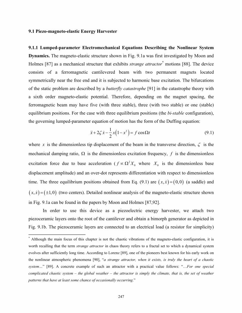
247

9.1 Piezo-magneto-elastic Energy Harvester

9.1.1 Lumped-parameter Electromechanical Equations Describing the Nonlinear System

Dynamics. The magneto-elastic structure shown in Fig. 9.1a was first investigated by Moon and

Holmes [87] as a mechanical structure that exhibits strange attractor* motions [88]. The device

consists of a ferromagnetic cantilevered beam with two permanent magnets located

symmetrically near the free end and it is subjected to harmonic base excitation. The bifurcations

of the static problem are described by a butterfly catastrophe [91] in the catastrophe theory with

a sixth order magneto-elastic potential. Therefore, depending on the magnet spacing, the

ferromagnetic beam may have five (with three stable), three (with two stable) or one (stable)

equilibrium positions. For the case with three equilibrium positions (the bi-stable configuration),

the governing lumped-parameter equation of motion has the form of the Duffing equation:

212 1 cos

2x x x x f t (9.1)

where x is the dimensionless tip displacement of the beam in the transverse direction, is the

mechanical damping ratio, is the dimensionless excitation frequency, f is the dimensionless

excitation force due to base acceleration ( 20f X where 0X is the dimensionless base

displacement amplitude) and an over-dot represents differentiation with respect to dimensionless

time. The three equilibrium positions obtained from Eq. (9.1) are , 0,0x x (a saddle) and

, 1,0x x (two centers). Detailed nonlinear analysis of the magneto-elastic structure shown

in Fig. 9.1a can be found in the papers by Moon and Holmes [87,92].

In order to use this device as a piezoelectric energy harvester, we attach two

piezoceramic layers onto the root of the cantilever and obtain a bimorph generator as depicted in

Fig. 9.1b. The piezoceramic layers are connected to an electrical load (a resistor for simplicity)

* Although the main focus of this chapter is not the chaotic vibrations of the magneto-elastic configuration, it is

worth recalling that the term strange attractor in chaos theory refers to a fractal set to which a dynamical system

evolves after sufficiently long time. According to Lorenz [89], one of the pioneers best known for his early work on

the nonlinear atmospheric phenomena [90], “a strange attractor, when it exists, is truly the heart of a chaotic

system…” [89]. A concrete example of such an attractor with a practical value follows: “…For one special

complicated chaotic system – the global weather – the attractor is simply the climate, that is, the set of weather

patterns that have at least some chance of occasionally occurring.”

248

and the voltage output of the generator across the load due to seismic excitation is the primary

interest in energy harvesting. Introducing piezoelectric coupling into Eq. (9.1) and applying the

Kirchhoff laws to the circuit with a resistive load (Fig. 9.1b) leads to the following

electromechanical equations describing the system dynamics:

212 1 cos

2x x x x v f t (9.2)

0v v x (9.3)

where v is the dimensionless voltage across the load resistance, is the dimensionless

piezoelectric coupling term in the mechanical equation, is the dimensionless piezoelectric

coupling term in the electrical circuit equation and is the reciprocal of the dimensionless time

constant ( 1/ l pR C where lR is the load resistance and pC is the equivalent capacitance of the

piezoceramic layers). Note that the possible nonlinearity coming from piezoelectric coupling is

ignored in Eqs. (9.2) and (9.3), assuming the standard form of the linear piezoelectric

constitutive relations [26] (Appendix A).

Fig. 9.1 Schematics of the (a) magneto-elastic structure investigated by Moon and Holmes [87]

and the (b) piezo-magneto-elastic energy harvester proposed here

The state-space form of Eqs. (9.2) and (9.3) can be expressed as

2

12

2 2 1 1 3

33 2

12 1 cos

2

uu

u u u u u f t

u u u

(9.4)

(a) (b)

249

where the state variables are 1u x , 2u x and 3u v . The electromechanically coupled

equations given by Eq. (9.4) can be used in an ordinary differential equation solver for numerical

simulations (the ode45 command of MATLAB [44] is used here).

9.1.2 Time-domain Numerical Simulations of the Electromechanical Response. The time-

domain voltage simulations shown in Figs. 9.2 and 9.3 are obtained using Eq. (9.4) with

0.8 , 0.01 , 0.05 , 0.5 and 0.05 (close to open-circuit conditions). In the

first case (Fig. 9.2a), the forcing term is 0.083f and the motion starts with an initial

deflection at one of the stable equilibrium positions ( (0) 1x with zero initial velocity and

voltage: (0) (0) 0x v ). The resulting vibratory motion is on a chaotic strange attractor

(yielding the chaotic voltage history shown in Fig. 9.2a) and the Poincaré map of this strange

attractor motion is shown in Fig. 9.2b on its phase portrait.

Fig. 9.2 (a) Theoretical voltage history exhibiting the strange attractor motion for and (b) its

Poincaré map ( (0) 1x , (0) 0x , (0) 0v , 0.083f , 0.8 )

If the excitation amplitude is increased by keeping the same initial conditions, the transient

chaotic behavior is followed by large-amplitude oscillations on a high-energy orbit with

improved voltage response (Fig. 9.3a). More importantly, Fig. 9.3b shows that this type of large-

amplitude voltage response can be obtained with the original excitation amplitude (of Fig. 9.2a)

and different initial conditions (simply by imposing an initial velocity condition so that (0) 1x ,

(0) 1.2x , (0) 0v ).

(a) (b)

250

Fig. 9.3 Theoretical voltage histories: (a) Large-amplitude response due to the excitation

amplitude ( (0) 1x , (0) 0x , (0) 0v , 0.115f , 0.8 ); (b) Large-amplitude response due to

the initial conditions for a lower excitation amplitude ( (0) 1x , (0) 1.2x , (0) 0v , 0.083f ,

0.8 )

9.1.3 Performance Comparison of the Piezo-magneto-elastic and the Piezo-elastic

Structures in the Phase Space. Having observed the large-amplitude electromechanical

response obtained on high-energy orbits of the piezo-magneto-elastic energy harvester

configuration described by Eqs. (9.2) and (9.3), a simple comparison can be made against the

conventional piezo-elastic configuration (which is the linear cantilever configuration without the

magnets causing the bi-stability).

The lumped-parameter equations of the linear piezo-elastic configuration are

2 cosx x x v f t (9.5)

0v v x (9.6)

which can be given in the state-space form as

1 2

2 2 1 3

3 3 2

2 cos

u u

u u u u f t

u u u

(9.7)

For the same numerical input ( 0.8 , 0.01 , 0.05 , 0.5 and 0.05 ), initial

conditions and the forcing amplitude of Fig. 9.3b ( (0) 1x , (0) 1.2x , (0) 0v , 0.083f ),

one can simulate the voltage response of the piezo-elastic configuration using Eq. (9.7).

(b) (a)

251

Figure 9.4a shows the velocity vs. displacement phase portrait of the piezo-magneto-

elastic and the piezo-elastic configurations. As can be seen from the steady-state orbits appearing

in this figure, for the same excitation amplitude, system parameters and the forcing amplitude,

the steady-state vibration amplitude of the piezo-magneto-elastic configuration can be much

larger than that of the piezo-elastic configuration. Expectedly, the large-amplitude response on

the high-energy orbit is also observed in the velocity vs. voltage phase portrait† shown in Fig.

9.4b.

Fig. 9.4 Comparison of the (a) velocity vs. displacement and the (b) velocity vs. voltage phase

portraits of the piezo-magneto-elastic and piezo-elastic configurations

( (0) 1x , (0) 1.2x , (0) 0v , 0.083f , 0.8 )

The superiority of the piezo-magneto-elastic configuration over the piezo-elastic configuration

can be shown by plotting these trajectories at several other frequencies except for the resonance

( 1 ) case of the linear problem for which the piezo-elastic configuration generates more

voltage. However, at several other frequencies (e.g. 0.6 , 0.7 , 0.9 ), a substantially

† For the system parameters used in these simulations, the phase between the voltage and the velocity is

approximately 90 degrees because the system is close to open-circuit conditions. Therefore, in open-circuit

conditions, it is reasonable to plot the velocity vs. voltage output as the electromechanical phase portrait (as an

alternative to the conventional velocity vs. displacement phase portrait). From the experimental point of view, it is

advantageous to plot these two independent measurements (voltage output of the piezoceramic vs. the velocity

signal from the laser vibrometer) rather than integrating the experimental velocity history (as it typically results in a

non-uniform drift).

(a) (b)

252

amplified response similar to the case of 0.8 can be obtained. The velocity vs. open-circuit

voltage phase portraits of the piezo-magneto-elastic and the piezo-elastic configurations are

plotted for 0.7 and 0.9 in Figs. 9.5a and 9.5b, respectively.

Fig 9.5 Comparison of the velocity vs. voltage phase portraits of the piezo-magneto-elastic and

piezo-elastic configurations for (a) 0.7 and (b) 0.9

( (0) 1x , (0) 1.2x , (0) 0v , 0.083f )

The three-dimensional voltage vs. velocity phase-space trajectories are given for the

frequency range of 0.5 1 in Fig. 9.6. In all cases, the system parameters, initial conditions

and the forcing amplitude‡ are the identical. In Fig. 9.6a, the electrical output of the piezo-

magneto-elastic configuration is not considerably larger because the trajectory oscillates around

one of its foci. That is, the forcing amplitude cannot overcome the attraction of the magnetic

force at the respective focus. As a result, the piezo-magneto-elastic configuration oscillates on a

low-energy orbit and its electrical response amplitude is indeed comparable to that of the piezo-

elastic configuration. In Figs. 9.6b-9.6e, over the frequency range of 0.6 0.9 , the piezo-

magneto-elastic configuration shows a very large amplitude electromechanical response on a

high-energy orbit compared to the orbit of the piezo-elastic configuration. Note that the response

amplitude of the piezo-elastic configuration grows as one moves close to the resonance ( 1 )

‡ Notice from the discussions in Chapter 3 that the forcing amplitude in the base excitation problem is proportional

to the square of the frequency ( 2

0f X ). Keeping the forcing amplitude f constant at different frequencies

implies keeping the base acceleration amplitude the same. Hence the base displacement amplitudes are different.

(a) (b)

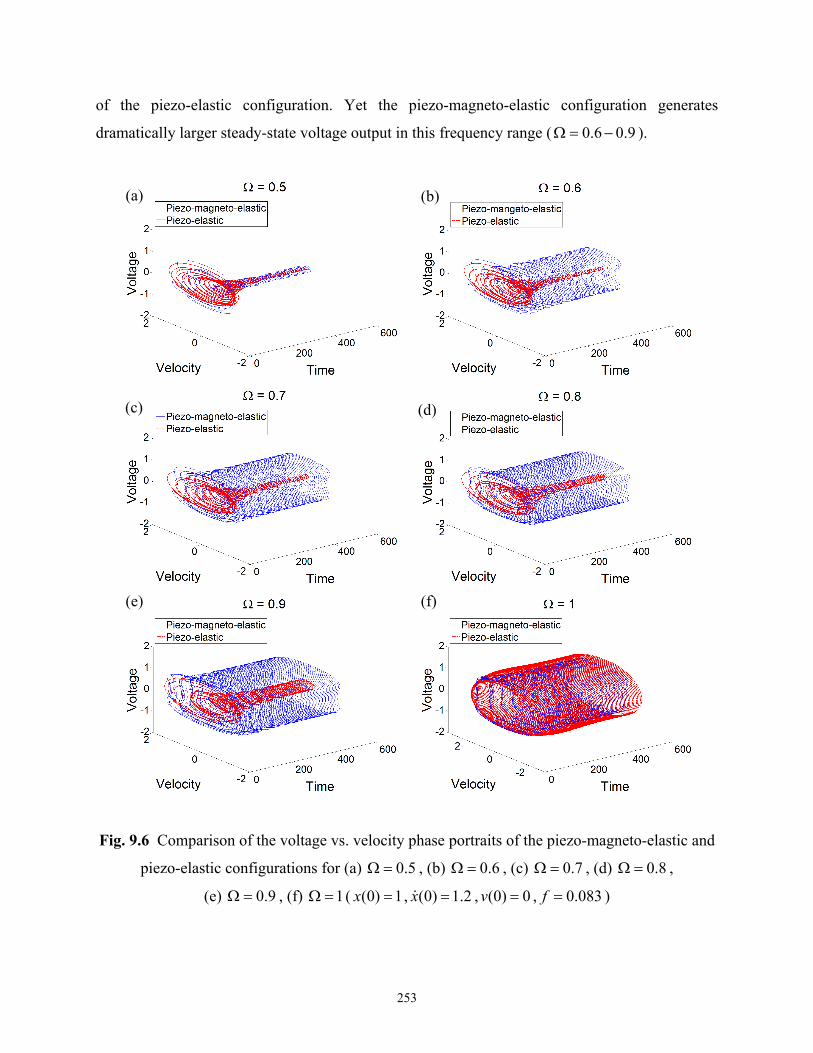
253

of the piezo-elastic configuration. Yet the piezo-magneto-elastic configuration generates

dramatically larger steady-state voltage output in this frequency range ( 0.6 0.9 ).

Fig. 9.6 Comparison of the voltage vs. velocity phase portraits of the piezo-magneto-elastic and

piezo-elastic configurations for (a) 0.5 , (b) 0.6 , (c) 0.7 , (d) 0.8 ,

(e) 0.9 , (f) 1 ( (0) 1x , (0) 1.2x , (0) 0v , 0.083f )

(c) (d)

(e) (f)

(a) (b)

254

Expectedly, at 1 , the response amplitude of the piezo-elastic configuration is larger (Fig.

9.6f). It is worth adding that, at this particular frequency where the resonant configuration

generates more voltage, the difference in the response amplitudes is not as dramatic as at other

frequencies where the non-resonant configuration is much superior.

Experimental verifications of the concept (i.e. the presence of these high-energy orbits to

utilize for piezoelectric energy harvesting) are given in the following sections.

9. 2 Experimental Setup and Performance Results

9.2.1 Experimental Setup. The piezo-magneto-elastic energy harvester and the setup used in the

first set of experiments are shown in Fig. 9.7. Harmonic base excitation is provided by a seismic

shaker (Acoustic Power Systems [93] APS-113), the acceleration at the base of the cantilever is

measured by a small accelerometer (PCB Piezotronics [47] Model U352C67) and the velocity

response of the cantilever is recorded by a laser vibrometer (Polytec [10] OFV303 laser head

with OFV3001 vibrometer). The time history of the base acceleration, voltage and vibration

responses are recorded by a National Instruments [94] NI cDAQ-9172 data acquisition system

(with a sampling frequency of 2000 Hz). The ferromagnetic beam (made of tempered blue steel)

is 145 mm long (overhang length), 26 mm wide and 0.26 mm thick. A lumped mass of 14 grams

is attached close to the tip for improved dynamic flexibility. Two PZT-5A piezoceramic layers

(QP16N, Midé Corporation [95]) are attached onto both faces of the beam at the root using a

high – shear strength epoxy and they are connected in parallel. The spacing between the

symmetrically located circular rare earth magnets is 50 mm (center to center) and this distance is

selected to realize the three equilibrium case described by Eqs. (9.2) and (9.3). The tip deflection

of the magnetically buckled beam in the static case to either side is approximately 15 mm

relative to the unstable equilibrium position. The post-buckled fundamental resonance frequency

of the beam is around 10.6 Hz (at both focus points) whereas the fundamental resonance

frequency of the unbuckled beam (when the magnets are removed) is 7.4 Hz (both under the

open-circuit conditions of piezoceramics – i.e. at constant electric displacement).

255

Fig. 9.7 (a) A view of the experimental setup and (b) the piezo-magneto-elastic energy harvester


9.2.2 Performance Results. For a harmonic base excitation amplitude of 0.5g (where g is the

gravitational acceleration: g = 9.81 m/s2) at 8 Hz with an initial deflection at one of the stable

equilibrium positions (15 mm to the shaker side), zero initial velocity and voltage, the chaotic

open-circuit voltage response shown in Fig. 9.8a is obtained. The Poincaré map of the strange

attractor motion is displayed in Fig. 9.8b. These figures are obtained from a measurement taken

for about 15 minutes (1,784,400 data points due to a sampling frequency of 2000 Hz) and they

exhibit very good qualitative agreement with the theoretical strange attractor given by Fig. 9.2.

Fig. 9.8 (a) Experimental voltage history exhibiting the strange attractor motion for and (b) its

Poincaré map (excitation: 0.5g at 8 Hz)

If the excitation amplitude is increased to 0.8g (at the same frequency), the structure goes

from transient chaos into a large-amplitude periodic motion with a strong improvement in the

voltage response as shown in Fig. 9.9a (i.e. the attractor is no longer a strange attractor). A

(a) (b)

(a) (b)

256

similar improvement is obtained in Fig. 9.9b where the excitation amplitude is kept as the

original one (0.5g) and a disturbance (hand impulse) is applied at 11t s (as a simple alternative

to creating a velocity initial condition). Such a disturbance can be realized in practice by

applying an impulse type voltage input through one of the piezoceramic layers for once. The

experimental evidence given with Fig. 9.9 is in agreement with the theoretical discussion given

with Fig. 9.3. Noticing the large-amplitude steady-state voltage response obtained at an off-

resonance frequency in Fig. 9.9, the broadband performance of the device is investigated and

comparisons against the piezo-elastic configuration are given in the next section.

Fig. 9.9 Experimental voltage histories: (a) Large-amplitude response due to the excitation

amplitude (excitation: 0.8g at 8 Hz); (b) Large-amplitude response due to a disturbance at 11t s

for a lower excitation amplitude (excitation: 0.5g at 8 Hz)

9.3 Broadband Voltage Generation Using the Piezo-magneto-elastic Energy Harvester

9.3.1 Comments on the Chaotic and the Large-amplitude Regions in the Response. Before

the comparisons of the piezo-magneto-elastic and piezo-elastic§ configurations are given over a

frequency range, reconsider the voltage history of Fig. 9.9b in two parts. The time history until

the instant of the disturbance is chaotic, which would yield a strange attractor motion similar to

what was shown in Fig. 9.8 if no disturbance was applied. After the disturbance is applied at

11t s, the large-amplitude response on a high-energy orbit is obtained as the steady-state

§ In the experiments, the piezo-elastic configuration is obtained simply by removing the magnets of the piezo-

magneto-elastic configuration after the experiments the latter are completed.

(a) (b)

257

response. In order to understand the advantage of the second region in the response history of

Fig. 9.9b, the open-circuit voltage histories of the piezo-magneto-elastic and piezo-elastic

configurations are compared for the same harmonic input (0.5g at 8 Hz). Figure 9.10a shows the

acceleration input to the piezo-magneto-elastic and the piezo-elastic configurations at an

arbitrary instant of time. The voltage input to the seismic shaker is identical for both

configurations, yielding very similar base acceleration amplitudes (according to the signal output

of the accelerometer) for a fair comparison. Figure 9.10b displays the comparison of the piezo-

magneto-elastic and the piezo-elastic configurations where the former exhibits chaotic response

and the latter has already reached its harmonic steady-state response amplitude at the input

frequency. As a rough comparison, from Fig. 9.10b, it is not possible to claim that the chaotic

response of the piezo-magneto-elastic configuration has any advantage over the harmonic

response of the piezo-elastic configuration as their amplitudes look very similar (a more accurate

comparison can be made through the RMS –root mean square [50,51] – amplitudes). Besides,

one would definitely prefer a periodic signal to a chaotic signal when it comes to processing the

harvested energy using an efficient energy harvesting circuit [23-25]. Figure 9.10c shows the

voltage histories of these configurations some time after the disturbance is applied to the piezo-

magneto-elastic configuration and the large-amplitude response is obtained. Obviously if the

same disturbance is applied to the piezo-elastic configuration, the trajectory (in the phase space)

returns to the same low-amplitude orbit after some transients. Therefore the response amplitude

of the piezo-elastic configuration is identical in Figs. 9.10b and 9.10c. Although the chaotic

response of the piezo-magneto-elastic structure has no considerable advantage according to Fig.

9.10b, the large-amplitude response of this structure can give more than 3 times larger RMS

voltage output according to Fig. 9.10.c.

9.3.2 Comparison of the Piezo-magneto-elastic and Piezo-elastic Configurations for Voltage

Generation. Figure 9.11a compares the velocity vs. voltage phase portraits of the piezo-

magneto-elastic and piezo-elastic configurations for excitation at 8 Hz with 0.5g, showing the

advantage of the large-amplitude orbit clearly. This figure is therefore analogous to the

theoretical demonstration given by Fig. 9.4b (additional harmonics are present in the

experimental data of the distributed-parameter piezo-magneto-elastic structure). The three-

dimensional view of the electromechanical trajectory in the phase space is shown in Fig. 9.11b in

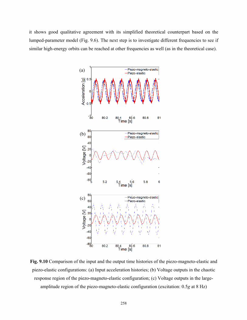
258

it shows good qualitative agreement with its simplified theoretical counterpart based on the

lumped-parameter model (Fig. 9.6). The next step is to investigate different frequencies to see if

similar high-energy orbits can be reached at other frequencies as well (as in the theoretical case).

Fig. 9.10 Comparison of the input and the output time histories of the piezo-magneto-elastic and

piezo-elastic configurations: (a) Input acceleration histories; (b) Voltage outputs in the chaotic

response region of the piezo-magneto-elastic configuration; (c) Voltage outputs in the large-

amplitude region of the piezo-magneto-elastic configuration (excitation: 0.5g at 8 Hz)

(a)

(b)

(c)

259

Fig. 9.11 (a) Two-dimensional and (b) three-dimensional comparison of the electromechanical

(velocity vs. open-circuit voltage) phase portraits of the piezo-magneto-elastic and piezo-elastic

configurations (excitation: 0.5g at 8 Hz)

For a harmonic base excitation amplitude of 0.5g (yielding an RMS acceleration of

0.35g), experiments are conducted at 4.5 Hz, 5 Hz, 5.5 Hz, 6 Hz, 6.5 Hz, 7 Hz, 7.5 Hz and 8 Hz.

At each frequency, a large-amplitude response is obtained the same way as in Fig. 9.9b by

applying a disturbance around 11t s. Then the magnets are removed for comparison of the

device performance with that of the conventional piezo-elastic configuration and the base

excitation tests are repeated for the same frequencies with approximately the same input

acceleration. The open-circuit RMS voltage outputs of the piezo-magneto-elastic and piezo-

elastic configurations at each frequency are obtained considering the steady-state response in the

80s-100s time interval. The RMS values of the input base acceleration are also extracted for the

same time interval.

Figure 9.12a shows that the excitation amplitudes of both configurations are indeed very

similar (with an average RMS value of approximately 0.35g). The broadband voltage generation

performance of the piezo-magneto-elastic energy harvester is shown in Fig. 9.12b. The resonant

piezo-elastic device gives larger voltage output only when the excitation frequency is at or very

close to its resonance frequency (7.4 Hz) whereas the voltage output of the piezo-magneto-elastic

device can be 3 times that of the piezo-elastic device at several other frequencies below its post-

buckled resonance frequency (10.6 Hz). It should be noted that power output is proportional to

the square of the voltage. Hence an order of magnitude larger power output over a frequency

range can be expected with this device.

(a) (b)

260

Fig. 9.12 (a) RMS acceleration input at different frequencies (average value: 0.35g); (b) Open-

circuit RMS voltage output over a frequency range showing the broadband advantage of the

piezo-magneto-elastic energy harvester

9. 4 Broadband Power Generation Performance and Comparisons against the Piezo-elastic

Configuration

9.4.1 Experimental Setup. After the first set of experiments, another setup was prepared to

compare the power generation performance of the piezo-magneto-elastic configuration with that

of the piezo-elastic configuration to verify the order of magnitude increase in the power output.

This section also aims to investigate whether or not the presence of a resistive load (which is

known to create shunt damping effect as discussed in Chapters 3 and 4) considerably reduces the

performance of the piezo-magneto-elastic configuration by modifying the attraction of the high-

energy orbit discussed here. The experimental setup used for this purpose is shown in Fig. 9.13a

and it is similar to the former setup shown in Fig. 9.7. These experiments have been conducted

two months after the previous ones and the cantilever was unclamped and the magnets were

removed in between (which is usually undesired). Therefore, effort has been made to clamp the

beam with the same overhang length and to relocate the magnets in a similar way to stay in the

same frequency range.

Figures 9.13b and 9.13c, respectively, display the piezo-magneto-elastic and piezo-elastic

configurations tested for power generation under base excitation. A harmonic base excitation

amplitude of 0.5g (yielding an RMS value of approximately 0.35g) is applied at frequencies of 5

(a) (b)

261

Hz, 6 Hz, 7 Hz and 8 Hz. From the previous discussion related to the open-circuit voltage output

given with Fig. 9.12b, it is expected to obtain an order of magnitude larger power with the piezo-

magneto-elastic device at three of these frequencies (5 Hz, 6 Hz and 8 Hz). However, it is

anticipated to obtain larger power from the piezo-elastic configuration around its resonance and

7 Hz is close to the resonance frequency of this linear system (as can be noted from Fig. 9.12b).

Fig. 9.13 (a) Experimental setup used for investigating the power generation performance of the

piezo-magneto-elastic energy harvester; (b) Piezo-magneto-elastic configuration; (c) Piezo-

elastic configuration (photos by A. Erturk, 2009)

9.4.2 Comparison of the Electrical Power Outputs. Figure 9.14 shows the comparison of the

average steady-state power vs. load resistance graphs of the piezo-magneto-elastic and piezo-

elastic configurations at the frequencies of interest. Note that the excitation amplitudes (i.e. the

base acceleration) of both configurations are very similar in all cases. As anticipated, the piezo-

magneto-elastic energy harvester gives an order of magnitude larger power at 5 Hz, 6 Hz and 8

Hz whereas the piezo-elastic configuration gives larger power only at 7 Hz (by a factor of 2.3).

The average power outputs read from these graphs for the optimum values of load resistance are

listed in Table 9.1.

(a) (b) (c)

262

Fig. 9.14 Comparison of the acceleration input and power output of the piezo-magneto-

elastic and piezo-elastic configurations at steady state for a range of excitation frequencies:

(a) 5 Hz; (b) 6 Hz; (c) 7 Hz; (d) 8 Hz

(a)

(b)

(c)

(d)

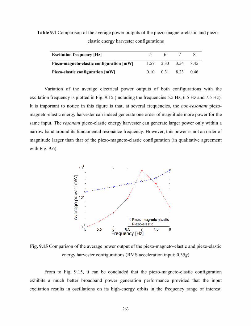
263

Table 9.1 Comparison of the average power outputs of the piezo-magneto-elastic and piezo-

elastic energy harvester configurations

Excitation frequency [Hz] 5 6 7 8

Piezo-magneto-elastic configuration [mW] 1.57 2.33 3.54 8.45

Piezo-elastic configuration [mW] 0.10 0.31 8.23 0.46

Variation of the average electrical power outputs of both configurations with the

excitation frequency is plotted in Fig. 9.15 (including the frequencies 5.5 Hz, 6.5 Hz and 7.5 Hz).

It is important to notice in this figure is that, at several frequencies, the non-resonant piezo-

magneto-elastic energy harvester can indeed generate one order of magnitude more power for the

same input. The resonant piezo-elastic energy harvester can generate larger power only within a

narrow band around its fundamental resonance frequency. However, this power is not an order of

magnitude larger than that of the piezo-magneto-elastic configuration (in qualitative agreement

with Fig. 9.6).

Fig. 9.15 Comparison of the average power output of the piezo-magneto-elastic and piezo-elastic

energy harvester configurations (RMS acceleration input: 0.35g)

From to Fig. 9.15, it can be concluded that the piezo-magneto-elastic configuration

exhibits a much better broadband power generation performance provided that the input

excitation results in oscillations on its high-energy orbits in the frequency range of interest.

264

Given the frequency range and the amplitude of harmonic base excitation at these frequencies,

the piezo-magneto-elastic energy harvester should be designed to catch these high-energy orbits

at steady state.


In this chapter, a non-resonant piezo-magneto-elastic energy harvester is introduced for

broadband vibration energy harvesting. The magneto-elastic configuration is known from the

literature of chaos theory in structural mechanics. Here, piezoelectric coupling is introduced to

the structure and a piezo-magneto-elastic vibration energy harvester is obtained. The lumped-

parameter electromechanical equations describing the nonlinear system are given along with

theoretical simulations. The existence of high-energy orbits at different frequencies is

demonstrated. It is shown that, over a range of frequencies, one can obtain much larger voltage

from the large amplitude oscillations on these orbits (compared to the conventional piezo-elastic

configuration). An experimental prototype is built and the presence of such high-energy orbits at

several frequencies below the post-buckled natural frequency of the structure is verified. It is

shown experimentally that, the open-circuit voltage output of the piezo-magneto-elastic energy

harvester can be three times that of the conventional piezo-elastic cantilever configuration,

yielding an order of magnitude larger power output over a range of frequencies (for the same

base acceleration input). The substantial broadband power generation performance of the

magneto-elastic configuration is discussed here for piezoelectric energy harvesting and it can

easily be extended to electromagnetic, electrostatic and magnetostrictive energy harvesting

techniques as well as to their hybrid combinations.

265

CHAPTER 10

SUMMARY AND CONCLUSIONS

In the first chapter, distributed-parameter modeling of the base excitation problem is reviewed

for cantilevered thin beams. The distributed-parameter displacement transmissibility function is

compared with the well-known lumped-parameter transmissibility function and it is shown that

the prediction of the lumped-parameter base excitation relation might have an error as high as

35 % in predicting the tip motion for a given base excitation input. The error in the lumped-

parameter model is due to ignoring the contribution of the distributed inertia to the excitation

amplitude. A correction factor is introduced to improve the predictions of the lumped-parameter

representation and the variation of the correction factor with tip mass – to – beam mass ratio is

investigated. It is shown that the original form of the lumped-parameter base excitation model

can be used only if the tip mass is much larger than the beam mass (so that the contribution of

the distributed mass to the excitation amplitude becomes negligible). Experimental validations of

the corrected lumped-parameter model are given for a small cantilever in the absence and

presence of a tip mass. Modeling of the base excitation problem is summarized for cantilevered

bars under longitudinal vibrations and the lumped-parameter model of the longitudinal vibration

case is also corrected. The correction factor is then introduced to the lumped-parameter

electromechanical equations for energy harvesting and a theoretical case study is given.

Analytical modeling of bimorph piezoelectric energy harvesters with symmetric

laminates is presented in the second chapter. The distributed-parameter electromechanical

formulation is based on the Euler-Bernoulli beam theory and it is valid for thin piezoelectric

energy harvesters for the typical vibration modes of interest in practice. The major steps of the

analytical formulation are given for the series and parallel connection cases of the piezoceramic

layers independently. An equivalent representation of the series and parallel connections is then

given in a single form. The distributed-parameter electromechanical equations are first obtained

for excitation at any arbitrary frequency by including all vibration modes in the analytical

solution. Then, for the practical problem of resonance excitation, the multi-mode solutions are

reduced to single-mode expressions (which are approximately valid only around the respective

266

resonance frequency). The electromechanical FRFs relating the steady-state electrical and

mechanical response to the translational and rotational base acceleration components are

extracted both from the multi-mode and single-mode solutions. A detailed theoretical case study

is presented where simulations for the series and parallel connection cases are given using both

multi-mode and single-mode electromechanical FRFs.

The analytical solutions derived in the Chapter 3 are validated for various experimental

cases in Chapter 4. The first experimental case is given for a brass-reinforced PZT-5H bimorph

cantilever without a tip mass. After validating the analytical model predictions using the voltage,

current, power and the tip velocity FRFs for this configuration and providing an extensive

electromechanical analysis, a tip mass is attached to create a configuration for the second case

study. The variations of the fundamental short-circuit and open-circuit resonance frequencies

after the attachment of the tip mass are successfully predicted by the model. Performance

diagrams for excitations at the fundamental short-circuit and open-circuit resonance frequencies

are extracted for both configurations (without and with the tip mass) and comparisons are made.

Improvement of the overall power output (as well as the power density and the specific power)

due to the addition of a tip mass is verified. Effect of the rotary inertia of the tip mass is also

studied by providing further analytical simulations with the point mass assumption. It is shown

that the resonance frequencies can be overestimated if the rotary inertia of the tip mass is

neglected. The damping effect of piezoelectric power generation is discussed in detail based on

the experimental measurements and the model predictions. The final case study is given for a

brass-reinforced PZT-5A bimorph cantilever and the frequency range of interest is increased to

cover the second vibration mode as well. Predictions of the multi-mode and the single-mode

FRFs are provided (for the first two modes independently) and a very good agreement is

observed with the experimental results.

In Chapter 5, detailed mathematical analyses of the single-mode electromechanical

relations are presented. Focus is placed on the voltage output and vibration response FRFs per

translational base acceleration. The single-mode relations derived in Chapter 3 (based on the

multi-mode solutions) are first expressed in the modulus-phase form and then they are

represented with dimensionless terms. After expressing the asymptotic trends of the single

voltage and tip displacement FRFs, closed-form expressions are obtained for their short-circuit

and open-circuit resonance frequencies. It is shown that the short-circuit resonance frequencies

267

of the voltage FRF and the tip displacement FRF are slightly different. The linear asymptotes of

the voltage output and the tip displacement for the extreme conditions of load resistance

(observed in the previous chapters) are mathematically verified here. Closed-form expressions

for the optimum electrical loads for the maximum power generation at the short-circuit and the

open-circuit resonance frequencies are extracted. It is shown that, for excitations at these two

frequencies, the intersections of the linear voltage asymptotes correspond to the respective

optimum load resistance. Based on this observation, a simple technique is introduced to identify

the optimum load resistance of a piezoelectric energy harvester using a single resistive load

along with an open-circuit voltage measurement. Relations are given to estimate the variation of

the tip vibration response as the load resistance is changed between the two extreme conditions.

The experimental case study for a PZT-5H bimorph is revisited and the major closed-form

relations derived here are validated. An important issue related to estimation of the optimum load

resistance from the Norton and Thévenin representations of the piezoceramic is clarified.

In Chapter 6, the effects of materials constants and mechanical damping on the power

generation performances of conventional piezoceramics (PZT-5A and PZT-5H) and novel single

crystals (PMN-PT and PMN-PZT) are investigated. It is shown that the large d31 strain constants

of the commercially available single crystals are associated with very large elastic compliance

and the combination of these two properties does not result in a substantial increase in the

effective piezoelectric stress constant ( 31e ) for a thin energy harvester beam. Although the d31

constants can change by an order of magnitude from PZT-5A to PMN-PZT, the effective

piezoelectric constants of these active materials are in the same order of magnitude.

Consequently, the substantially large d31 constants of the commercially available single crystals

do not necessarily imply substantially large power output in energy harvesting. The concepts of

dynamic flexibility and mechanical damping are shown to be very important as far as the

maximum power output is concerned. When geometrically identical bimorphs using these

piezoelectric materials are forced to have the same dynamic flexibility, the power outputs are

observed to be very similar. It is also observed that the power output under resonance excitation

is extremely sensitive to mechanical damping (which is very difficult parameter control in

practice). It is shown with an experimental case study using a PZT-5A bimorph and a PZT-5H

bimorph that the former cantilever gives 45 % larger power density when the latter has 55 %

larger mechanical damping ratio (although the d31 constant of PZT-5H is 60 % larger than that of

268

PZT-5A). Therefore, designing and manufacturing the energy harvester beam to have less

damping can be more important than the piezoelectric material being used.

The concept of strain nodes and its effect on energy harvesting is discussed in Chapter 7.

It is theoretically discussed and experimentally demonstrated that covering the strain nodes of

vibration modes with continuous electrodes results in cancellation of the electrical outputs in

energy harvesting. A detailed dimensionless analysis is given for predicting the locations of the

strain nodes of a thin cantilever in the absence of a tip mass. Dimensionless derivations and

results are then presented for predicting the strain node positions and their variations in the

presence of a tip mass. Dimensionless data of modal strain nodes are tabulated for some other

practical boundary condition pairs as well. It is experimentally demonstrated using a cantilever

that the voltage output due to the second mode excitation can be increased dramatically if

segmented electrodes are used instead of continuous electrodes. The relationship between the

discussion given here and a recent study on piezoelectric energy harvesting from the static

deflection of a clamped circular plate is also explained. The use of segmented electrode pairs to

avoid cancellations is described for single-mode and multi-mode vibrations of a cantilevered

harvester and alternative circuitry-based approaches can be investigated to handle the

cancellation problem for multi-mode excitations.

In Chapter 8, approximate distributed-parameter modeling of cantilevered piezoelectric

energy harvesters is given. An electromechanical version of the assumed-modes method of

structural dynamics is used to discretize the energy equations into electromechanical Lagrange

equations derived from the extended Hamilton’s principle. The derivations are given based on

the Euler-Bernoulli, Rayleigh and Timoshenko beam theories. In all cases, an axial displacement

variable is defined to capture its coupling with the transverse displacement variable in the

presence of structural asymmetry. To demonstrate modeling of an asymmetric configuration,

focus is placed on the unimorph configuration. Simplification of the resulting equations for

symmetric bimorph configurations is also shown and the effect of a tip mass on the resulting

formulation is discussed. A short discussion regarding the kinematically admissible functions to

be used in the models derived here is also provided. Finally the experimental case studies for a

thin cantilever (without and with a tip mass) are revisited for validation of the assumed-modes

solution using different number of admissible trigonometric functions. The predictions of the

assumed-modes solution are also compared with the analytical solution and a very good

269

agreement is observed. The approximate formulations given in Chapter 8 can be used to predict

the electromechanical response of asymmetric cantilevers, moderately thick cantilevers as well

as cantilevers with varying cross-section.

In Chapter 9, a piezo-magneto-elastic energy harvester is introduced for broadband

vibration energy harvesting. The magneto-elastic configuration is known from the literature of

chaos theory in nonlinear structural mechanics. Here, piezoelectric coupling is introduced to the

structure and a piezo-magneto-elastic vibration energy harvester is obtained. The lumped-

parameter electromechanical equations describing the nonlinear system are given along with

theoretical simulations. The existence of high-energy orbits at different frequencies is

demonstrated. It is shown that, over a range of frequencies, one can generate much larger voltage

from the large amplitude oscillations on these orbits (compared to the conventional piezo-elastic

configuration). An experimental prototype is built and the presence of such high-energy orbits at

several frequencies below the post-buckled natural frequency of the structure is verified. It is

shown experimentally that, the open-circuit voltage output of the piezo-magneto-elastic energy

harvester can be three times that of the conventional piezo-elastic cantilever configuration,

yielding an order of magnitude larger power output over a range of frequencies. The substantial

broadband power generation performance of the magneto-elastic configuration is discussed here

for piezoelectric energy harvesting and it can easily be extended to other vibration energy

harvesting techniques (e.g. electromagnetic, electrostatic, magnetostrictive) as well as to their

hybrid combinations.

Each dissertation produced in the Department of Engineering Science and Mechanics at

Virginia Tech must address the social impact. While harvesting energy at the level discussed

here does not have a major impact on reducing the world's energy demands (compared to well-

known forms of green energy, e.g. wind energy and solar energy) it does have the potential for

substantially reducing the world's reliance on chemical batteries, thereby reducing the amount of

chemical waste produced by conventional batteries.

Future applications of vibration energy harvesting that eliminate the requirement of

battery replacement and the relevant maintenance efforts can lead to durable wireless sensor

networks and similar low-power electronic components. It should be noted that the energy

required to keep such wireless low-power systems running include the maintenance costs as well,

which can be dramatically large in applications such as wireless damage detection systems in

270

critical civil engineering structures at remote locations. In addition, even though the power

outputs are not in the same order of magnitude, vibration energy is often available when/where

solar energy and wind energy are not available.

One of the limitations regarding the use of piezoelectric materials is their present cost,

which can be reduced in mass production as the technology becomes mature. An environmental

issue related to using PZT-based piezoceramics is the lead content in piezoelectric materials.

There is ongoing research in the materials science domain of the problem for developing lead-

free piezoceramics [96,97].

271

REFERENCES

[1] Timoshenko, S.P., 1953, History of Strength of Materials (with a brief account of the

history of theory of elasticity and theory of structures), McGraw-Hill Book Company, New

York.

[2] Williams, C.B. and Yates, R.B., 1996, “Analysis of a Micro-electric Generator for

Microsystems,” Sensors and Actuators A, 52, pp. 8–11.

[3] Glynne-Jones P., Tudor, M.J., Beeby, S.P. and White, N.M., 2004, “An Electromagnetic,

Vibration-powered Generator for Intelligent Sensor Systems,” Sensors and Actuators A,

110, pp. 344-349.

[4] Arnold, D., 2007, “Review Of Microscale Magnetic Power Generation,” IEEE

Transactions on Magnetics, 43, pp. 3940–3951.

[5] Mitcheson, P., Miao, P., Start, B., Yeatman, E., Holmes, A. and Green, T., 2004, “MEMS

Electrostatic Micro-Power Generator for Low Frequency Operation,” Sensors and

Actuators A, 115, pp. 523-529.

[6] Roundy, S., Wright, P. and Rabaey, J., 2003, Energy Scavenging for Wireless Sensor

Networks, Kluwer Academic Publishers, Boston.

[7] Roundy, S., Wright, P.K. and Rabaey, J.M., 2003, “A Study of Low Level Vibrations as a

Power Source for Wireless Sonsor Nodes,” Computer Communications, 26, pp.1131-1144.

[8] Jeon, Y. B., Sood, R., Jeong, J. H. and Kim, S., 2005, “MEMS Power Generator with

Transverse Mode Thin Film PZT,” Sensors & Actuators A, 122, pp. 16-22.

[9] Beeby, S.P., Tudor, M.J. and White, N.M., 2006, “Energy Harvesting Vibration Sources

for Microsystems Applications”, Measurement Science and Technology, 17, pp. R175-

R195.

272

[10] Cook-Chennault, K.A., Thambi, N., Sastry, A.M., 2008, “Powering MEMS Portable

Devices – a Review of Non-Regenerative and Regenerative Power Supply Systems with

Emphasis on Piezoelectric Energy Harvesting Systems,” Smart Materials and Structures,

17, 043001 (33pp).

[11] Sodano, H., Park G. and Inman, D.J., 2004, “A Review of Power Harvesting from

Vibration Using Piezoelectric Materials”, Shock and Vibration Digest, 36, pp. 197-205.

[12] Anton, S.R. and Sodano, H.A., 2007, “A Review of Power Harvesting Using Piezoelectric

Materials (2003-2006),” Smart Materials and Structures, 16, pp. R1-R21.

[13] Priya, S., 2007, “Advances in Energy Harvesting Using Low Profile Piezoelectric

Transducers,” Journal of Electroceramics, 19, pp. 167–184.

[14] Choi, W.J., Jeon, Y., Jeong, J.H., Sood, R. and Kim, S.G., 2006, “Energy Harvesting

MEMS Device Based on Thin Film Piezoelectric Cantilevers,” Journal of Electroceramics,

17, pp. 543–8.

[15] Roundy, S. and Wright, P.K., 2004, “A Piezoelectric Vibration Based Generator for

Wireless Electronics,” Smart Materials and Structures, 13, pp.1131-1144.

[16] duToit, N.E., Wardle, B.L. and Kim, S., 2005, “Design Considerations for MEMS-Scale

Piezoelectric Mechanical Vibration Energy Harvesters,” Journal of Integrated

Ferroelectrics, 71, pp. 121-160.

[17] Sodano, H.A., Park, G. and Inman, D.J., 2004, “Estimation of Electric Charge Output for

Piezoelectric Energy Harvesting,” Strain, 40, pp. 49-58.

[18] Lu, F., Lee, H.P. and Lim, S.P., 2004, “Modeling and Analysis of Micro Piezoelectric

Power Generators for Micro-Electromechanical-Systems Applications,” Smart Materials

and Structures, 13, pp. 57-63.

[19] Chen, S.-N., Wang, G.-J. and Chien, M.-C., 2006, “Analytical Modeling of Piezoelectric

Vibration-Induced Micro Power Generator,” Mechatronics, 16, pp. 397-387.

273

[20] Lin, J.H., Wu, X.M., Ren, T.L. and Liu, L.T., 2007, “Modeling and Simulation of

Piezoelectric MEMS Energy Harvesting Device,” Integrated Ferroelectrics, 95, pp. 128-

141.

[21] duToit, N.E. and Wardle, B.L., 2007, “Experimental Verification of Models for

Microfabricated Piezoelectric Vibration Energy Harvesters,” AIAA Journal, 45, pp. 1126-

1137.

[22] Ajitsaria, J., Choe, S.Y., Shen, D. and Kim, D.J., 2007, “Modeling and Analysis of a

Bimorph Piezoelectric Cantilever Beam for Voltage Generation,” Smart Materials and

Structures, 16, pp. 447-454.

[23] Ottman, G.K., Hofmann, H.F., Bhatt, A.C. and Lesieutre, G.A., 2002, “Adaptive

Piezoelectric Energy Harvesting Circuit for Wireless Remote Power Supply,” IEEE

Transactions on Power Electronics, 17, pp. 669-676.

[24] Ottman, G.K., Hofmann, H.F., and Lesieutre, G.A., 2003, “Optimized Piezoelectric

Energy Harvesting Circuit Using Step-down Converter in Discontinuous Conduction

Mode,” 18, pp. 696-703.

[25] Guan, M.J. and Liao, W.H., 2007, “On the Efficiencies of Piezoelectric Energy Harvesting

Circuits Towards Storage Device Voltages,” Smart Materials and Structures, 16, pp. 498-

505.

[26] IEEE Standard on Piezoelectricity, 1987, IEEE, NY.

[27] Stephen, N.G., 2006, “On Energy Harvesting from Ambient Vibration,” Journal of Sound

and Vibration, 293, pp. 409-425.

[28] Daqaq, F.M., Renno J.M., Farmer, J.R. and Inman, D.J., 2007, “Effects of System

Parameters and Damping on an Optimal Vibration-Based Energy Harvester,” Proceedings

of the 48th AIAA/ASME/ASCE/AHS/ASC Structures, Structural Dynamics, and Materials

Conference, 23 - 26 April 2007, Honolulu, Hawaii.

274

[29] Hagood, N.W., Chung, W.H. and Von Flotow, A., 1990, “Modelling of piezoelectric

actuator dynamics for active structural control,” Journal of Intelligent Material Systems and

Structures, 1, pp.327-354.

[30] Crandall, S.H., Karnopp, D.C., Kurtz, Jr. E.F. and Pridmore-Brown, D.C., 1968, Dynamics

of Mechanical and Electromechanical Systems, McGraw-Hill, New York.

[31] Fang, H.-B., Liu, J.-Q., Xu, Z.-Y., Dong, L., Chen, D., Cai, B.-C. and Liu, Y., 2006, “A

MEMS-Based Piezoelectric Power Generator for Low Frequency Vibration Energy

Harvesting,” Chinese Physics Letters, 23, pp. 732-734.

[32] Lesieutre, G.A., Ottman, G.K. and Hofmann, H.F., 2004, “Damping as a Result of

Piezoelectric Energy Harvesting,” Journal of Sound and Vibration, 269, pp. 991-1001.

[33] DeVoe, D.L. and Pisano, A.P., 1997, Modeling and Optimal Design of Piezoelectric

Cantilever Microactuators,” Journal of Microelectromechanical Systems, 6, pp. 266–270.

[34] Timoshenko, S.P., 1925, “Analysis of Bi-metal Thermostats,” Journal of Optical Society of

America, 11, pp. 233-56.

[35] Timoshenko, S., Young, D.H. and Weaver, W., 1974, Vibration Problems in Engineering,

John Wiley and Sons, New York.

[36] Banks, H.T. and Inman D.J., 1991, “On Damping Mechanisms in Beams,” ASME Journal

of Applied Mechanics, 58, pp. 716–723.

[37] Clough, R.W. and Penzien, J., 1975, Dynamics of Structures, John Wiley and Sons, New

York.

[38] Caughey, T.K. and O’Kelly, M.E.J., 1965, “Classical Normal Modes in Damped Linear

Dynamic Systems,” ASME Journal of Applied Mechanics, 32, pp. 583-588.

[39] Ewins, D.J., 2000, Modal Testing: Theory, Practice and Application, Research Studies

Press, Baldock, Hertfordshire, UK.

275

[40] Strutt, J. W. (Lord Rayleigh), 1894, The Theory of Sound, MacMillan Company, London,

UK.

[41] Meirovitch, L., 2001, Fundamentals of Vibrations, McGraw Hill, New York.

[42] Inman, D.J., 2007, Engineering Vibration, Prentice Hall, Englewood Cliffs, New Jersey.

[43] Banks, H.T., Luo, Z.H., Bergman, L.A. and Inman D.J., 1998, “On the Existence of

Normal Modes of Damped Discrete-Continuous Systems,” ASME Journal of Applied

Mechanics, 65, pp. 980–989.

[44] The MathWorks, Inc. http://www.mathworks.com.

[45] Piezo Systems, Inc. (www.piezo.com).

[46] TMC Solution http://www.tmcsolution.com.cn.

[47] PCB Piezotronics http://www.pcb.com.

[48] Polytec http://www.polytec.com.

[49] Spectral Dynamics, Inc. http://www.spectraldynamics.com.

[50] Bendat, J.S. and Piersol, A.G., 1986, Random Data Analysis and Measurement Procedures,

John Wiley and Sons, New York.

[51] Newland, D.E., 1993, Random Vibrations, Spectral and Wavelet Analysis, John Wiley and

Sons, New York.

[52] Wang, Q.M. and Cross, L.E., 1999, “Constitutive Equations of Symmetrical Triple Layer

Piezoelectric Benders,” IEEE Transactions on Ultrasonics, Ferroelectrics, and Frequency

Control, 46, pp. 1343–1351.

[53] Sokolnikoff, 1946, Mathematical Theory of Elasticity, McGraw-Hill, New York.

[54] Dym, C.L. and Shames, I.H., 1973, Solid Mechanics: A Variational Approach, McGraw–

Hill, New York.

276

[55] Chopra, A.K., 2006, Dynamics of Structures: Theory and Applications to Earthquake

Engineering, Prentice-Hall, Englewood Cliffs, New Jersey.

[56] Hyer, M.W., 1998, Stress Analysis of Fiber-Reinforced Composite Materials, McGraw–

Hill, New York.

[57] Schwartz, L., 1978, Théorie des Distributions, Hermann, Paris, France.

[58] Friedlander, F.G., 1998, Introduction to the Theory of Distributions, Cambridge University

Press, Cambridge (with additional material by M. Joshi).

[59] Hewlett-Packard Development Company http://www.hp.com.

[60] Magcraft Advanced Magnetic Materials http://www.magcraft.com.

[61] Meriam, J.L and Kraige, L.G., 2001, Engineering Mechanics: Dynamics, John Wiley and

Sons, New York.

[62] Engineering Fundamentals, Inc. (www.efunda.com).

[63] Heinonen, E., Juuti, J. and Leppavuori, S., 2005, “Characterization and Modelling of 3D

Piezoelectric Ceramic Structures with ATILA Software,” Journal of European Ceramic

Society, 25, pp. 2467-2470.

[64] Cao, H., Schmidt, V. H., Zhang, R., Cao, W. and Luo, H., 2004, “Elastic, Piezoelectric, and

Dielectric Properties of 0.58Pb(Mg1/3Nb2/3)O3-0.42PbTiO3 Single Crystal,” Journal of

Applied Physics, 96, 549.

[65] Ceracomp Co., Ltd. www.ceracomp.com.

[66] LDS Group http://www.lds-group.com.

[67] Crawley, E.F. and de Luis, J., 1987, “Use of Piezoelectric Actuators as Elements of

Intelligent Structures”, AIAA Journal, 25, pp.1373-1385.

[68] Cady, W.G., 1946, Piezoelectricity: An Introduction to the Theory and Applications of

Electromechanical Phenomena in Crystals, McGraw-Hill, New York.

277

[69] Elvin, N. G., Elvin, A. A., and Spector, M., 2001, “A Self-Powered Mechanical Strain

Energy Sensor,” Smart Materials and Structures, 10, pp. 293–299.

[70] Lesieutre, G.A. and Davis, C.L., 1997, “Can a Coupling Coefficient of a Piezoelectric

Device Be Higher Than Its Active Material?,” Journal of Intelligent Material Systems and


[71] Kim, S., Clark, W.W. and Wang, Q.M., 2005, “Piezoelectric Energy Harvesting with a

Clamped Circular Plate: Analysis,” Journal of Intelligent Material Systems and Structures,

16, pp. 847-854.

[72] Kim, S., Clark, W.W. and Wang, Q.M., 2005, “Piezoelectric Energy Harvesting with a

Clamped Circular Plate: Experimental Study,” Journal of Intelligent Material Systems and


[73] Timoshenko, S.P., 1921, “On the Correction for Shear of the Differential Equation for

Transverse Vibrations of Prismatic Bars,” Philosophical Magazine, 41, pp. 744–746.

[74] Timoshenko, S.P., 1922, “On the Transverse Vibrations of Bars of Uniform Cross-section,”

Philosophical Magazine, 43, pp.125–131.

[75] Mindlin, R.D., 1951, “Thickness-shear and Flexural Vibrations of Crystal Plates,” Journal

of Applied Physics, 22, pp. 316-323.

[76] Mindlin, R.D., 1952, “Forced Thickness-shear and Flexural Vibrations of Piezoelectric

Crystal Plates,” Journal of Applied Physics, 23, pp. 83-88.

[77] Cowper, G.R., 1966, “The Shear Coefficient in Timoshenko Beam Theory,” ASME Journal

of Applied Mechanics, 33, pp. 335-340.

[78] Kaneko, T., 1975, “On Timoshenko’s Correction for Shear in Vibrating Beams,” Journal of

Physics D, 8, pp. 1927-1936.

[79] Stephen, N.G., 1978, “On the Variation of Timoshenko’s Shear Coefficient with

Frequency,” ASME Journal of Applied Mechanics, 45, pp. 695-697.

278

[80] Stephen, N.G., 1980, “Timoshenko’s Shear Coefficient from a Beam Subjected to Gravity

Loading,” ASME Journal of Applied Mechanics, 47, pp. 121-127.

[81] Stephen, N.G. and Hutchinson, J.R., 2001, “Discussion: Shear Coefficients for Timoshenko

Beam Theory,” ASME Journal of Applied Mechanics, 68, pp. 959–961.

[82] Hutchinson, J.R., 2001, “Shear Coefficients for Timoshenko Beam Theory,” ASME

Journal of Applied Mechanics, 68, pp. 87-92.

[83] Puchegger, S., Bauer, S., Loidl, D., Kromp, K. and Peterlik, H., 2003, “Experimental

Validation of the Shear Correction Factor,” Journal of Sound and Vibration, 261, pp. 177-

184.

[84] Den Hartog, J.P., 1956, Mechanical Vibrations, McGraw-Hill, New York.

[85] Lee, J. and Schultz, W.W., 2004, “Eigenvalue Analysis of Timoshenko Beams and

Axisymmetric Mindlin Plates by the Pseudospectral Method,” Journal of Sound and

Vibration, 269, pp. 609-621.

[86] Zhou, D. and Cheung, Y. K., 2001, “Vibrations of Tapered Timoshenko Beams in Terms

of Static Timoshenko Beam Functions,” ASME Journal of Applied Mechanics, 68, pp.

596-602.

[87] Moon, F.C. and Holmes P.J., 1979, “A Magnetoelastic Strange Attractor,” Journal of

Sound and Vibration, 65, pp. 275-296.

[88] Moon, F.C., 1987, Chaotic Vibrations, John Wiley and Sons, New York.

[89] Lorenz, E.N., 1993, The Essence of Chaos, University of Washington Press, Seattle.

[90] Lorenz, E.N., 1963, “Deterministic Nonperiodic Flow,” Journal of Atmospheric Sciences,

26, pp. 636-646.

[91] Poston, T. and Stewart, O., 1978, Catastrophe Theory and Its Applications, Pitman,

London.

279

[92] Holmes, P., 1979, “A Nonlinear Oscillator with a Strange Attractor,” Philosophical

Transactions of the Royal Society of London, Series A, 292, pp. 419449.

[93] APS Dynamics http://www.apsdynamics.com.

[94] National Instruments http://www.ni.com.

[95] Midé Corporation http://www.mide.com.

[96] Saito, Y., Takao, H. Tani, I., Nonoyama, T., Takatori, K., Homma, T., Nagaya, T. and

Nakamura, M., 2004, ‘‘Lead-Free Piezoceramics,’’ Nature, 432, pp. 84-87.

[97] Shrout, T.R. and Zhang, S.J., 2007, “Lead-free Piezoelectric Ceramics – Alternatives for

PZT?,” Journal of Electroceramics, 19, pp. 111–124.

280

APPENDIX A

CONSTITUTIVE EQUATIONS FOR A MONOLITHIC PIEZOCERAMIC

A.1 Three-dimensional Form of the Piezoelectric Constitutive Equations

In general, poled monolithic piezoceramics are transversely isotropic materials. To be in

agreement with the IEEE Standard on Piezoelectricity [26], the plane of isotropy is defined here

as the 12-plane (or the xy-plane). The piezoelectric material therefore exhibits symmetry about

the 3-direction (or the z-direction), which is the poling direction of the material. The field

variables are the stress components ( ijT ), strain components ( ijS ), electric field components ( kE )

and the electric displacement components ( kD ).

The standard form of the piezoelectric constitutive equations can be given in four

different forms by taking either two of the four field variables as the independent variables.

Consider the tensorial representation of the strain – electric displacement form [26] where the

independent variables are the stress components and the electric field components:

Eij ijkl kl kij kS s T d E (A.1)

Ti ikl kl ik kD d T E (A.2)

which is the preferred form of the piezoelectric constitutive relations for bounded media (to

eliminate some of the stress components depending on the geometry and some of the electric

field components depending on the placement of the electrodes). Equations (A.1) and (A.2) can

be given in the matrix form as

E t

T

S Ts d

D Ed ε (A.3)

where superscripts E and T represent that the respective constants are evaluated at constant

electric field and constant stress, respectively, and superscript t stands for the transpose. The

expanded form of Eq. (A.3) is

281

1 11 12 13 31

2 12 11 13 31

3 13 13 33 33

4 55 15

5 55 15

6 66

1 15 11

2 15 11

3 31 31 33 33

0 0 0 0 0

0 0 0 0 0

0 0 0 0 0

0 0 0 0 0 0 0

0 0 0 0 0 0 0

0 0 0 0 0 0 0 0

0 0 0 0 0 0 0

0 0 0 0 0 0 0

0 0 0 0 0

E E E

E E E

E E E

E

E

E

T

T

T

S s s s d

S s s s d

S s s s d

S s d

S s d

S s

D d

D d

D d d d

1

2

3

4

5

6

1

2

3

T

T

T

T

T

T

E

E

E

(A.4)

where the contracted notation (i.e. Voigt’s notation: 11 1 , 22 2 , 33 3 , 23 4 , 13 5 ,

12 6 ) is used so that the vectors of strain and stress components are

1 11

2 22

3 33

4 23

5 13

6 12

2

2

2

S S

S S

S S

S S

S S

S S

,

1 11

2 22

3 33

4 23

5 13

6 12

T T

T T

T T

T T

T T

T T

(A.5)

Therefore the shear strain components in the contracted notation are the engineering shear

strains. It should be noted from the elastic, piezoelectric and dielectric constants in Eq. (A.4) that

the poled piezoceramic considered here is a monolithic piezoceramic so that the symmetries of

transversely isotropic material behavior ( 11 22E Es s , 31 32d d , etc) are directly applied.

A.2 Reduced Equations for a Thin Beam

If the piezoelastic behavior of the thin monolithic structure is to be modeled as a thin beam based

on the Euler-Bernoulli beam theory or Rayleigh beam theory, the only non-zero stress

component is 1T (stress component in the axial direction) so that

2 3 4 5 6 0T T T T T (A.6)

Along with this simplification, if an electrode pair covers the faces perpendicular to 3-direction,

Eq. (A.4) becomes

282

1 111 31

3 331 33

E

T

S Ts d

D Ed

(A.7)

which can be written as

1 31 111

3 33 331

10

01

E

T

T d Ss

D Ed

(A.8)

Therefore the stress – electric displacement form of the reduced constitutive equations for a thin

beam is

1 111 31

3 331 33

E

S

T Sc e

D Ee

(A.9)

where the reduced matrix of elastic, piezoelectric and dielectric constants is

1

3111 31 11

3331 33 31

10

01

E E

TS

dc e s

e d

C (A.10)

Here and hereafter, an over-bar denotes that the respective constant is reduced from the three-

dimensional form to the plane-stress condition. In Eq. (A.10),

1111

1EE

cs

, 3131

11E

de

s ,

231

33 3311

S TE

d

s (A.11)

where superscript S denotes that the respective constant is evaluated at constant strain.

A.3 Reduced Equations for a Moderately Thick Beam

If the piezoelasticity of the monolithic structure is to be modeled as a moderately thick beam

based on the Timoshenko beam theory, the only non-zero stress components are 1T (stress

component in the axial direction) and 5T (transverse shear stress) so that

2 3 4 6 0T T T T (A.12)

is applied in Eq. (A.4). Then,

1 11 31 1

5 55 5

3 31 33 3

0

0 0

0

E

E

T

S s d T

S s T

D d E

(A.13)

which can be written as

283

11 1 31 1

55 5 5

31 3 33 3

0 0 1 0

0 0 0 1 0

0 1 0 0

E

E

T

s T d S

s T S

d D E

(A.14)

Therefore the stress – electric displacement form of the reduced constitutive equations is

1 11 31 1

5 55 5

3 31 33 3

0

0 0

0

E

E

S

T c e S

T c S

D e E

(A.15)

Here, the reduced matrix of elastic, piezoelectric and permittivity constants are

1

11 31 11 31

55 55

31 33 31 33

0 0 0 1 0

0 0 0 0 0 1 0

0 0 1 0 0

E E

E E

S T

c e s d

c s

e d

C (A.16)

where

1111

1EE

cs

, 5555

1EE

cs

, 3131

11E

de

s ,

231

33 3311

S TE

d

s (A.17)

Note that the transverse shear stress in Eq. (A.15) is corrected due to Timoshenko [73,74]

5 55 5ET c S (A.18)

where is the shear correction factor [73-83].

A.4 Reduced Equations for a Thin Plate

If the thin monolithic structure is to be modeled as a thin plate (i.e. Kirchhoff plate), the normal

stress through the thickness of the piezoceramic and the respective transverse shear stress

components vanish:

3 4 5 0T T T (A.19)

Equation (A.4) becomes

1 111 12 31

2 212 11 31

6 666

3 331 31 33

0

0

0 0 0

0

E E

E E

E

T

S Ts s d

S Ts s d

S Ts

D Ed d

(A.20)

which can be rearranged to give

284

1 31 111 12

2 31 212 11

6 666

3 33 331 31

1 0 00 0

0 1 00 0

0 0 1 00 0 0

0 0 00 1

E E

E E

E

T

T d Ss s

T d Ss s

T Ss

D Ed d

(A.21)

The stress – electric displacement form of the reduced constitutive equations becomes

1 111 12 31

2 212 11 31

6 666

3 331 31 33

0

0

0 0 0

0

E E

E E

E

S

T Sc c e

T Sc c e

T Sc

D Ee e

(A.22)

where

1

3111 12 31 11 12

3112 11 31 12 11

66 66

3331 31 33 31 31

1 0 00 0 0

0 1 00 0 0

0 0 1 00 0 0 0 0 0

0 0 00 0 1

E E E E

E E E E

E E

TS

dc c e s s

dc c e s s

c s

e e d d

C (A.23)

Here, the reduced elastic, piezoelectric and permittivity constants are

1111

11 12 11 12

EE

E E E E

sc

s s s s

(A.24)

1212

11 12 11 12

EE

E E E E

sc

s s s s

(A.25)

6666

1EE

cs

(A.26)

3131

11 12E E

de

s s

(A.27)

231

33 3311 12

2S TE E

d

s s

(A.28)

For one-dimensional bending vibration of a thin plate without any torsional mode (due to the

base excitation of a cantilever that is symmetric with respect to the central axis in x-direction),

the relevant terms are Eqs. (A.24), (A.27) and (A.28).* * Theoretically, the thin-plate parameters should be preferred for large width-to-thickness ratios to account for the

Poisson effect. In the experimental case studies of this dissertation (Chapter 4), the thin-beam parameters given in

Section A.2 are used as they exhibit substantially better agreement with the experimental results.

285

APPENDIX B

NUMERICAL DATA FOR MONOLITHIC PZT-5A AND PZT-5H

PIEZOCERAMICS

PZT-5A and PZT-5H piezoceramics are the most commonly used engineering piezoceramics.

Their typical three-dimensional piezoelastic properties can be found on the web [62] or in the

literature [63] as given in Table B.1.

Table B.1 Three-dimensional properties of PZT-5A and PZT-5H

PZT-5A PZT-5H

11Es [pm2/N] 16.4 16.5

12Es [pm2/N] -5.74 -4.78

13Es [pm2/N] -7.22 -8.45

33Es [pm2/N] 18.8 20.7

55Es [pm2/N] 47.5 43.5

66Es [pm2/N] 44.3 42.6

31d [pm/V] -171 -274

33d [pm/V] 374 593

15d [pm/V] 584 741

11 0/T 1730 3130

33 0/T 1700 3400

In addition to these data, the mass densities of PZT-5A and PZT-5H are reported [62,63] as 7750

kg/m3 and 7500 kg/m3, respectively. The permittivity components at constant stress are given in

Table B.1 in the form of the dielectric constants ( 11 0/T , 33 0/T ) where the permittivity of free

286

space is 0 8.854 pF/m [26]. The reduced constants for the Euler-Bernoulli and Rayleigh beam

theories are obtained using Eq. (A.11) as listed in Table B.2 whereas those for the Timoshenko

beam theory are obtained from Eqs. (A.17) as in Table B.3.

Table B.2 Reduced properties of PZT-5A and PZT-5H for the Euler-Bernoulli and Rayleigh

beam theories

PZT-5A PZT-5H

11Ec [MPa] 61.0 60.6

31e [C/m2] -10.4 -16.6

33S [nF/m] 13.3 25.55

Table B.3 Reduced properties of PZT-5A and PZT-5H for the Timoshenko beam theory

PZT-5A PZT-5H

11Ec [MPa] 61.0 60.6

55Ec [MPa] 21.1 23.0

31e [C/m2] -10.4 -16.6

33S [nF/m] 13.3 25.6

Table B.4 Reduced properties of PZT-5A and PZT-5H for the Kirchhoff plate theory

PZT-5A PZT-5H

11Ec [MPa] 69.5 66.2

12Ec [MPa] 24.3 19.2

66Ec [MPa] 22.6 23.5

31e [C/m2] -16.0 -23.4

33S [nF/m] 9.57 17.3

287

APPENDIX C

CONSTITUTIVE EQUATIONS FOR AN ISOTROPIC SUBSTRUCTURE

C.1 Three-dimensional Form of the Constitutive Equations for an Isotropic Material

The tensorial representation of the three-dimensional constitutive law for an isotropic

substructure material is [53]

11ij s ij s kk ij

s

S T TY

(C.1)

where sY is the elastic modulus and s is the Poisson’s ratio (subscript s denotes the

substructure). The expanded form of Eq. (C.1) can be given as

1 1

2 2

3 3

4 4

5 5

6 6

1 0 0 0

1 0 0 0

1 0 0 010 0 0 2 1 0 0

0 0 0 0 2 1 0

0 0 0 0 0 2 1

s s

s s

s s

ss

s

s

S T

S T

S T

S TY

S T

S T

(C.2)

where the contracted notation is used and the shear strains are the engineering shear strains

defined in Eq. (A.5).

C.2 Reduced Equations for a Thin Beam

If the elastic behavior of the thin substructure is to be modeled as a thin beam based on the

Euler-Bernoulli or Rayleigh beam theory, the only non-zero stress component is 1T so that

2 3 4 5 6 0T T T T T (C.3)

Therefore, Eq. (C.2) simply reduces to

1 1sT Y S (C.4)

288

C.3 Reduced Equations for a Moderately Thick Beam

If the elasticity of the thin substructure is to be modeled as a moderately thick beam (based on

the Timoshenko beam theory), the conditions on the stress are

2 3 4 6 0T T T T (C.5)

Equation (C.2) can be rearranged to give

1 1

5 5

0

0s

s

T Y S

T G S

(C.6)

Here, the shear modulus is defined in terms of the elastic modulus and the Poisson’s ratio as

2 1s

s

YG

(C.7)

and the transverse shear stress in its corrected form [73-83] is

5 5sT G S (C.8)

C.4 Reduced Equations for a Thin Plate

If the elastic behavior of the substructure is modeled as a thin plate, the following stress

components vanish:

3 4 5 0T T T (C.9)

Equation (C.2) simplifies to

1 1

2 2

6 6

1 0

1 0

0 0 2 1

s

s s

s

S T

S Y T

S T

(C.10)

which can be rearranged to give stress components in terms of strain components as

1 1

2 22

6 6

1 0

1 01

0 0 1 / 2

s

ss

ss

T SY

T S

T S

(C.11)

As far as one-dimensional bending vibration of a thin plate without any torsional mode is

concerned (due to base excitation of a cantilever that is symmetric with respect to the central axis

in x-direction), the relevant elastic term is the first element in Eq. (C.11).

289

APPENDIX D

ESSENTIAL BOUNDARY CONDITIONS FOR CANTILEVERED BEAMS

D.1 Euler-Bernoulli and Rayleigh Beam Theories

If the beam is clamped at 0x and free at x L , the essential boundary conditions are defined

at the clamped boundary as

0 (0, ) 0w t (D.1)

0

0

( , )0

x

w x t

x

(D.2)

0 (0, ) 0u t (D.3)

where 0 ( , )w x t is the transverse displacement and 0 ( , )u x t is the axial displacement of the neutral

axis.

D.2 Timoshenko Beam Theory

The essential boundary conditions are given at the clamped end ( 0x ) of a cantilevered

Timoshenko beam as

0 (0, ) 0w t (D.4)

0 (0, ) 0t (D.5)

0 (0, ) 0u t (D.6)

where 0 ( , )x t is the cross-section rotation.

290

APPENDIX E

ELECTROMECHANICAL LAGRANGE EQUATIONS BASED ON THE

EXTENDED HAMILTON’S PRINCIPLE

This section summarizes derivation of the electromechanical Lagrange’s equations from the

extended Hamilton’s principle. For the most general case [41], the total kinetic energy is given as

a function of the generalized coordinates and their time derivatives:

1 2 1 2, ,..., , , ,...,n nT T q q q q q q (E.1)

The total potential energy and the internal electrical energy are functions of generalized

coordinates only†

1 2, ,..., nU U q q q (E.2)

1 2, ,...,ie ie nW W q q q (E.3)

The first variations of Eqs. (E.1)-(E.3) are

1

n

k kk k k

T TT q q

q q

(E.4)

1

n

kk k

UU q

q

(E.5)

1

nie

ie kk k

WW q

q

(E.6)

The virtual work done by the generalized non-conservative forces ( kQ ) is

1

n

nc k kk

W Q q

(E.7)

The extended Hamilton’s principle becomes

2 2

1 11

0t t n

ieie nc k k k

k k k k kt t

WT U TT U W W dt Q q q dt

q q q q

(E.8)

† In the electromechanical Lagrange formulation given here, one of the generalized coordinates is the electrical

across variable, i.e. the voltage output across the load.

291

with the auxiliary conditions 0kq ( 1, 2,...,k n ) at 1t t and 2t t . Integration by parts is

applied to the last term to give

22 2 2 2

1 1 1 11

tt t t tk

k k k kk k k k kt t t tt

d qT T T d T d Tq dt dt q q dt q dt

q q dt q dt q dt q

(E.9)

Using Eq. (E.9) in Eq. (E.8) gives

2

11

0t n

iek k

k k k k kt

WT U d TQ q dt

q q q dt q

(E.10)

For the extended Hamilton’s principle to hold for arbitrary virtual displacements, Eq. (E.10)

reduces to the electromechanical Lagrange equations:

iek

k k k k

Wd T T UQ

dt q q q q

(E.11)

where the dissipative effects can be represented as generalized non-conservative terms.

Electromechanical Modeling of Piezoelectric Energy Harvesters

Documents

Transcript of Electromechanical Modeling of Piezoelectric Energy Harvesters