
Electromagnetic testing emt chapter 13 - Material Identifications
Upload
charlie-chongCategory
view
228download
2description

Charlie Chong/ Fion Zhang
Electromagnetic TestingMFLT/ ECT/ Microwave/RFTChapter 9 – Magnetic Flux Leakage Testing 漏磁检测1st Feb 2015My ASNT Level III Pre-Exam Preparatory Self Study Notes

Charlie Chong/ Fion Zhang
Deuterium Uranium reactor
http://en.wikipedia.org/wiki/CANDU_reactor

Charlie Chong/ Fion Zhang
Deuterium Uranium reactor
http://en.wikipedia.org/wiki/CANDU_reactor

Charlie Chong/ Fion Zhang
Deuterium Uranium reactor
http://en.wikipedia.org/wiki/CANDU_reactor

Charlie Chong/ Fion Zhang
Deuterium Uranium reactor
http://en.wikipedia.org/wiki/CANDU_reactor

Charlie Chong/ Fion Zhang
Deuterium Uranium reactor
http://en.wikipedia.org/wiki/CANDU_reactor

Charlie Chong/ Fion Zhang
Deuterium Uranium reactor- Qinshan Phase III Units 1 & 2, located in Zhejiang China (30.436 N 120.958 E): Two CANDU 6 reactors, designed by Atomic Energy of Canada Limited (AECL), owned and operated by the Third Qinshan Nuclear Power Company Limited
http://en.wikipedia.org/wiki/CANDU_reactor

Charlie Chong/ Fion Zhang
Pipeline & Piping

Charlie Chong/ Fion Zhang
Pipeline & Piping

Charlie Chong/ Fion Zhang
Pipeline & Piping

Charlie Chong/ Fion Zhang
Pipeline & Piping

Charlie Chong/ Fion Zhang
Pipeline & Piping

Charlie Chong/ Fion Zhang
Pipeline & Piping

Charlie Chong/ Fion Zhang
Pipeline & Piping

Charlie Chong/ Fion Zhang
Pipeline & Piping

Charlie Chong/ Fion Zhang
Pipeline & Piping

Charlie Chong/ Fion Zhang
Pipeline & Piping

Charlie Chong/ Fion Zhang
Pipeline & Piping

Charlie Chong/ Fion Zhang
Pipeline & Piping

Charlie Chong/ Fion Zhang
Pipeline & Piping

Charlie Chong/ Fion Zhang

Fion Zhang at Shanghai2015 February
Charlie Chong/ Fion Zhang Shanghai 上海

Charlie Chong/ Fion Zhang

Charlie Chong/ Fion Zhang
NDT Level III ExaminationsBasic and Method ExamsASNT NDT Level III certification candidates are required to pass both the NDT Basic and a method examination in order to receive the ASNT NDT Level III certificate.Exam SpecificationsThe table below lists the number of questions and time allowed for each exam. Clicking on an exam will take you to an abbreviated topical outline and reference page for that exam. For the full topical outlines and complete list of references, see the topical outlines listed in the American National Standard ANSI/ASNT CP-105, Standard Topical Outlines for Qualification of Nondestructive Testing Personnel.
MFLMagnetic Flux Leakage Testing90 Questions Time: 2 hrs Certification: NDT only

Charlie Chong/ Fion Zhang
Chapter Nine:Magnetic Flux Leakage Testing

Charlie Chong/ Fion Zhang
9.1 PART 1. Introduction to Magnetic Flux Leakage Testing MFLT
9.1.0 IntroductionMagnetic flux leakage testing is part of the widely used family of electromagnetic nondestructive techniques. Magnetic particle testing is a variation of flux leakage testing that uses particles to show indications. When used with other methods, magnetic tests can provide a quick and relatively inexpensive assessment of the integrity of ferromagnetic materials. The theory and practice of electromagnetic techniques are discussed elsewhere in this volume. The origins of magnetic particle testing are described in the literature1 and information that the practicing magnetic test engineer might require is available from a variety of manuals and journal articles. The magnetic circuit and the means for producing the magnetizing force that causes magnetic flux leakage are described below. Theories developed for surface and subsurface discontinuities are outlined along with some results that can be expected.

Charlie Chong/ Fion Zhang
9.1.1 Industrial Uses
Magnetic flux leakage testing is used in many industries to find a wide variety of discontinuities. Much of the world’s production of ferromagnetic steel is tested by magnetic or electromagnetic techniques. Steel is tested many times before it is used and some steel products are tested during use for safety and reliability and to maximize their length of service.
9.1.1.1 Production Testing
Typical applications of magnetic flux leakage testing are by the steel producer, where blooms, billets, rods, bars, tubes and ropes are tested to establish the integrity of the final product. In many instances, the end user will not accept delivery of steel product without testing by the mill and independent agencies.

Charlie Chong/ Fion Zhang
9.1.1.2 Receiving TestingThe end user often uses magnetic flux leakage tests before fabrication. This test ensures the manufacturer’s claim that the product is within agreed specifications. Such tests are frequently performed by independent testing companies or the end user’s quality assurance department. Oil field tubular goods are often tested at this stage.
9.1.1.3 In-service TestingGood examples of in-service applications are the testing of used wire rope, installed tubing, or retrieved oil field tubular goods by independent facilities. Many laboratories also use magnetic techniques (along with metallurgical sectioning and other techniques) for the assessment of steel products and prediction of failure modes.

Charlie Chong/ Fion Zhang
9.1.2 DiscontinuitiesDiscontinuities can be divided into two general categories: those caused during manufacture in new materials and those caused after manufacture in used materials. Discontinuities caused during manufacture include cracks, seams, forging laps, laminations and inclusions.
1. Cracking occurs when quenched steel cools too rapidly. 2. Seams occur in several ways, depending on when they originate during
fabrication. 3. Discontinuities such as piping or inclusions within a bloom or billet can be
elongated until they emerge as long tight seams or gouges during initial forming processes. They may later be closed with additional forming.
4. Their metallurgical structures are often different but the origin of manufactured discontinuities is not usually taken into account when rejecting a part.

Charlie Chong/ Fion Zhang
5. Forging laps occur when gouges or fins created in one metal working process are rolled over at an angle to the surface in subsequentprocesses.
6. Inclusions are pieces of nonmagnetic or nonmetallic materials embedded inside the metal during cooling. Inclusions are not necessarily detrimental to the use of the material.
7. The pouring and cooling processes can also result in lack of fusion within the steel. Such regions may be worked into internal laminations.
Discontinuities in used materials include fatigue cracks, pitting corrosion, erosion and abrasive wear.

Charlie Chong/ Fion Zhang
Much steel is acceptable to the producer’s quality assurance department if no discontinuities are found or if discontinuities are considered to be of a depth or size less than some prescribed maximum. Specifications exist for the acceptance or rejection of such materials and such specifications sometimes lead to debate between the producer and the end user. Discontinuities can either remain benign or can grow and cause premature failure of the part. Abrasive wear can turn benign subsurface discontinuities into detrimental surface breaking discontinuities.

Charlie Chong/ Fion Zhang
For used materials, fatigue cracking commonly occurs as the material is cyclically stressed. Fatigue cracks grow rapidly under stress or in the presence of corrosive materials such as hydrogen sulfide, chlorides, carbon dioxide and water. For example, drill pipe failure from fatigue often initiates at the bases of pits, at tong marks or in regions where the tube has been worn by abrasion. Pitting is caused by corrosion and erosion between the steel and a surrounding or containing fluid. Abrasive wear occurs in many steel structures.
Good examples are:
(1) the wear on drill pipe caused by hard formations when drilling crooked holes or
(2) the wear on both the sucker rod and the producing tubing in rod pumping oil wells.
Specifications exist for the maximum permitted wear under these and other circumstances. In many instances, such induced damage is first found by automated magnetic techniques.

Charlie Chong/ Fion Zhang
9.1.3 Steps in Magnetic Flux Leakage TestingThere are four steps in magnetic flux leakage testing:
(1) magnetize the test object so that discontinuities perturb the flux, (2) scan the surface of the test object with a magnetic flux sensitive detector, (3) process the raw data from these detectors in a manner that best
accentuates discontinuity signals and (4) present the test results clearly for interpretation.
The next section discussion deals with the first step, producing the magnetizing force.

Charlie Chong/ Fion Zhang
Steel Mill – Expert at Works

Charlie Chong/ Fion Zhang
Steel Mill – Expert at Works

Charlie Chong/ Fion Zhang
Steel Mill

Charlie Chong/ Fion Zhang
Steel Mill
http://jyhengrun.en.made-in-china.com/productimage/LXxJqIKWhmhC-2f1j00bScaFVoCEUql/China-Rolling-Ring-Forging-Stainless-Steel-Flange.html

Charlie Chong/ Fion Zhang
Seams & Laps
http://azterlan.blogspot.com/2013/09/sensitivity-in-magnetic-particle.html

Charlie Chong/ Fion Zhang
9.2 PART 2. Magnetization Techniques9.2.0 IntroductionSuccessful testing requires the test object to be magnetized properly. The magnetization can be accomplished using one of several approaches:
(1) permanent magnets, (2) electromagnets and (3) electric currents used to induce the required magnetic field.
Excitation systems that use permanent magnets offer the least flexibility. Such systems use high energy product permanent magnet materials such as neodymium iron boron, samarium cobalt and aluminum nickel. The major disadvantage with such systems lies in the fact that the excitation cannot be switched off. Because the magnetization is always turned on, it is difficult to insert and remove the test object from the test rig. Although the magnetization level can be adjusted using appropriate magnetic shunts, it is awkward to do so. Consequently, permanent magnets are very rarely used for magnetization.

Charlie Chong/ Fion Zhang
Keywords:
Excitation systems. Neodymium iron boron, samarium cobalt and aluminum nickel. Appropriate magnetic shunts.
http://en.wikipedia.org/wiki/Neodymium_magnet
Charlie Chong/ Fion Zhang
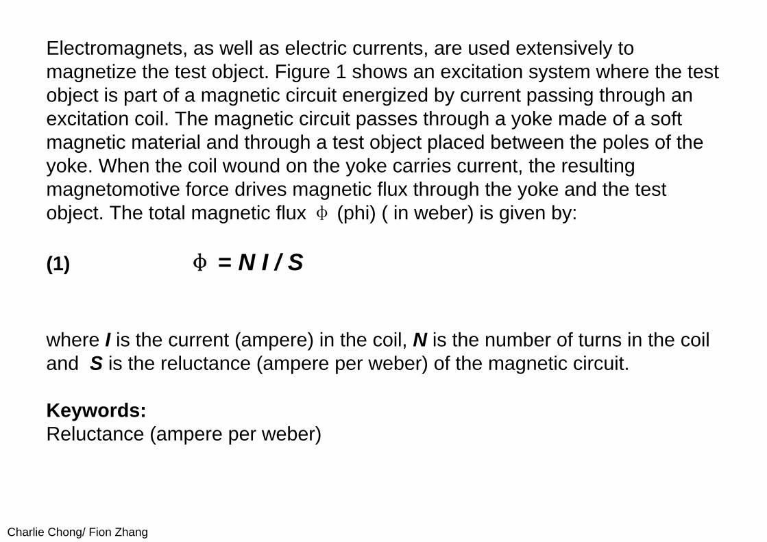
Electromagnets, as well as electric currents, are used extensively to magnetize the test object. Figure 1 shows an excitation system where the test object is part of a magnetic circuit energized by current passing through an excitation coil. The magnetic circuit passes through a yoke made of a soft magnetic material and through a test object placed between the poles of the yoke. When the coil wound on the yoke carries current, the resulting magnetomotive force drives magnetic flux through the yoke and the test object. The total magnetic flux φ (phi) ( in weber) is given by:
(1) φ = N I / S
where I is the current (ampere) in the coil, N is the number of turns in the coil and S is the reluctance (ampere per weber) of the magnetic circuit.
Keywords:Reluctance (ampere per weber)

Charlie Chong/ Fion Zhang
FIGURE 1. Electromagnetic yoke for magnetizing of test object.

Charlie Chong/ Fion Zhang
Reluctance.Magnetic reluctance, or magnetic resistance, is a concept used in the analysis of magnetic circuits. It is analogous to resistance in an electrical circuit, but rather than dissipating electric energy it stores magnetic energy. In likeness to the way an electric field causes an electric current to follow the path of least resistance, a magnetic field causes magnetic flux to follow the path of least magnetic reluctance. It is a scalar, extensive quantity, akin to electrical resistance. The unit for magnetic reluctance is inverse henry, H-1.
In a DC field, the reluctance is the ratio of the "magnetomotive force” (MMF) in a magnetic circuit to the magnetic flux in this circuit. In a pulsating DC or AC field, the reluctance is the ratio of the amplitude of the "magnetomotive force” (MMF) in a magnetic circuit to the amplitude of the magnetic flux in this circuit. (see phasors)
S = N I / Ф, F =NI
whereS is the reluctance in ampere-turns per weber (a unit that is equivalent to turns per henry). F is the magnetomotive force (MMF) in ampere-turnsФ is the magnetic flux in webers.
"Turns" refers to the winding number of an electrical conductor comprising an inductor
1/Henry = ampere/ weber, Henry= Weber/ampere?
http://en.wikipedia.org/wiki/Magnetic_reluctance

Charlie Chong/ Fion Zhang
Henry, unit of either self-inductance or mutual inductance, abbreviated h, and named for the American physicist Joseph Henry. One henry is the value of self-inductance in a closed circuit or coil in which one volt is produced by a variation of the inducing current of one ampere per second. One henry is also the value of the mutual inductance of two coils arranged such that an electromotive force of one volt is induced in one if the current in the other is changing at a rate of one ampere per second.
Weber, unit of magnetic flux in the International System of Units (SI), defined as the amount of flux that, linking an electrical circuit of one turn (one loop of wire), produces in it an electromotive force of one volt as the flux is reduced to zero at a uniform rate in one second.
Tesla, a flux density of one Wb/m2 (one weber per square metre) is one tesla.
http://global.britannica.com/EBchecked/topic/261372/henry

Charlie Chong/ Fion Zhang
Keywords:
Henry – magnetic field intensity Weber – magnetic flux Tesla – magnetic flux density (1 weber / m2)Reluctance – Ampere Turn/ weberMagnetomotive force – Ampere Turn
http://global.britannica.com/EBchecked/topic/261372/henry

Charlie Chong/ Fion Zhang
Yangtze River China - 水落石出
http://en.wikipedia.org/wiki/Magnetic_field

Charlie Chong/ Fion Zhang
More Reading on: Magnetic fieldA magnetic field is the magnetic influence of electric currents and magnetic materials. The
magnetic field at any given point is specified by both a direction and a magnitude (or strength); as such it is a vector field. The term is used for two distinct but closely related fields denoted by the symbols B and H,
Where:H (magnetic field intensity) is measured in units of amperes per meter (symbol: A·m−1 or A/m)
in the SI.
B (magnetic flux density) is measured in teslas (symbol: T) and newtons per meter per ampere (symbol: N·m−1 ·A−1 or Newtons per Ampere meter N/(m·A)) or weber/m2 in the SI.
B is most commonly defined in terms of the Lorentz force it exerts on moving electric charges.
http://en.wikipedia.org/wiki/Magnetic_field

Charlie Chong/ Fion Zhang
Magnetic fields are produced by moving electric charges and the intrinsic magnetic moments of elementary particles associated with a fundamental quantum property, their spin. In special relativity, electric and magnetic fields are two interrelated aspects of a single object, called the electromagnetic tensor; the split of this tensor into electric and magnetic fields depends on the relative velocity of the observer and charge. In quantum physics, the electromagnetic field is quantized and electromagnetic interactions result from the exchange of photons.(?)
In everyday life, magnetic fields are most often encountered as a force created by permanent magnets, which pull on ferromagnetic materials such as iron, cobalt, or nickel and attract or repel other magnets. Magnetic fields are widely used throughout modern technology, particularly in electrical engineering and electromechanics. The Earth produces its own magnetic field, which is important in navigation, and it guards Earth's atmosphere from solar wind. Rotating magnetic fields are used in both electric motors and generators. Magnetic forces give information about the charge carriers in a material through the Hall effect. The interaction of magnetic fields in electric devices such as transformers is studied in the discipline of magnetic circuits.
http://en.wikipedia.org/wiki/Magnetic_field

Charlie Chong/ Fion Zhang
History:Although magnets and magnetism were known much earlier, the study of magnetic fields began
in 1269 when French scholar Petrus Peregrinus de Maricourt mapped out the magnetic field on the surface of a spherical magnet using iron needles Noting that the resulting field lines crossed at two points he named those points 'poles' in analogy to Earth's poles. He also clearly articulated the principle that magnets always have both a north and south pole, no matter how finely one slices them.
Almost three centuries later, William Gilbert of Colchester replicated Petrus Peregrinus' work and was the first to state explicitly that Earth is a magnet Published in 1600, Gilbert's work, De Magnete, helped to establish magnetism as a science.
In 1750, John Michell stated that magnetic poles attract and repel in accordance with an inverse square law. Charles-Augustin de Coulomb experimentally verified this in 1785 and stated explicitly that the north and south poles cannot be separated. Building on this force between poles, Siméon Denis Poisson (1781–1840) created the first successful model of the magnetic field, which he presented in 1824. In this model, a magnetic H-field is produced by 'magnetic poles' and magnetism is due to small pairs of north/south magnetic poles.
http://en.wikipedia.org/wiki/Magnetic_field
Charlie Chong/ Fion Zhang
Three discoveries challenged this foundation of magnetism, though.
First, in 1819, Hans Christian Oersted discovered that an electric current generates a magnetic field encircling it. Then in 1820, André-Marie Ampère showed that parallel wires having currents in the same direction attract one another. Finally, Jean-Baptiste Biot and FélixSavart discovered the Biot–Savart law in 1820, which correctly predicts the magnetic field around any current-carrying wire.
Extending these experiments, Ampère published his own successful model of magnetism in 1825. In it, he showed the equivalence of electrical currents to magnets and proposed that magnetism is due to perpetually flowing loops of current instead of the dipoles of magnetic charge in Poisson's model. This has the additional benefit of explaining why magnetic charge can not be isolated. Further, Ampère derived both Ampère's force law describing the force between two currents and Ampère's law, which, like the Biot–Savart law, correctly described the magnetic field generated by a steady current. Also in this work, Ampère introduced the term electrodynamics to describe the relationship between electricity and magnetism.
http://en.wikipedia.org/wiki/Magnetic_field

Charlie Chong/ Fion Zhang
In 1831, Michael Faraday discovered electromagnetic induction when he found that a changing magnetic field generates an encircling electric field. He described this phenomenon in what is known as Faraday's law of induction. Later, Franz Ernst Neumann proved that, for a moving conductor in a magnetic field, induction is a consequence of Ampère's force law. In the process he introduced the magnetic vector potential, which was later shown to be equivalent to the underlying mechanism proposed by Faraday.
In 1850, Lord Kelvin, then known as William Thomson, distinguished between two magnetic fields now denoted H and B. The former applied to Poisson's model and the latter to Ampère's model and induction. Further, he derived how H and B relate to each other.
Between 1861 and 1865, James Clerk Maxwell developed and published Maxwell's equations, which explained and united all of classical electricity and magnetism. The first set of these equations was published in a paper entitled On Physical Lines of Force in 1861. These equations were valid although incomplete. Maxwell completed his set of equations in his later 1865 paper A Dynamical Theory of the Electromagnetic Field and demonstrated the fact that light is an electromagnetic wave. Heinrich Hertz experimentally confirmed this fact in 1887.
http://en.wikipedia.org/wiki/Magnetic_field

Charlie Chong/ Fion Zhang http://en.wikipedia.org/wiki/Magnetic_field
The twentieth century extended electrodynamics to include relativity and quantum mechanics. Albert Einstein, in his paper of 1905 that established relativity, showed that both the electric and magnetic fields are part of the same phenomena viewed from different reference frames. (See moving magnet and conductor problem for details about the thought experiment that eventually helped Albert Einstein to develop special relativity.) Finally, the emergent field of quantum mechanics was merged with electrodynamics to form quantum electrodynamics (QED).

Charlie Chong/ Fion Zhang http://en.wikipedia.org/wiki/Magnetic_field
The B-field:The magnetic field can be defined in several equivalent ways based on the effects it has on its
environment.
Often the magnetic field is defined by the force it exerts on a moving charged particle. It is known from experiments in electrostatics that a particle of charge q in an electric field E experiences a force F = q·E. However, in other situations, such as when a charged particle moves in the vicinity of a current-carrying wire, the force also depends on the velocity of that particle. Fortunately, the velocity dependent portion can be separated out such that the force on the particle satisfies the Lorentz force law,
F = q·(E + v × B)
Here v is the particle's velocity and × denotes the cross product. The vector B is termed the magnetic field, and it is defined as the vector field necessary to make the Lorentz force law correctly describe the motion of a charged particle. This definition allows the determination of B in the following way.

Charlie Chong/ Fion Zhang http://en.wikipedia.org/wiki/Magnetic_field
"Measure the direction and magnitude of the vector B at such and such a place," calls for the following operations: Take a particle of known charge q. Measure the force on q at rest, to determine E. Then measure the force on the particle when its velocity is v; repeat with v in some other direction. Now find a B that makes [the Lorentz force law] fit all these results—that is the magnetic field at the place in question. Alternatively, the magnetic field can be defined in terms of the torque it produces on a magnetic dipole (see magnetic torque on permanent magnets below).

Charlie Chong/ Fion Zhang
Lorentz Force LawBoth the electric field and magnetic field can be defined from the Lorentz force law: The electric
force is straightforward, being in the direction of the electric field if the charge q is positive, but the direction of the magnetic part of the force is given by the right hand rule.
http://hyperphysics.phy-astr.gsu.edu/hbase/magnetic/magfor.html

Charlie Chong/ Fion Zhang http://en.wikipedia.org/wiki/Magnetic_field
Electric Force
F = q·E
Magnetic ForceThe magnetic field B is defined from the Lorentz Force Law, and specifically from the magnetic
force on a moving charge:
The implications of this expression include:
1. The force is perpendicular to both the velocity v of the charge q and the magnetic field B.2. The magnitude of the force is F = qvB sinϴ where ϴ is the angle < 180 degrees between the
velocity and the magnetic field. This implies that the magnetic force on a stationary charge or a charge moving parallel to the magnetic field is zero.
3. The direction of the force is given by the right hand rule. The force relationship above is in the form of a vector product.

Charlie Chong/ Fion Zhang http://en.wikipedia.org/wiki/Magnetic_field
From the force relationship above it can be deduced that the units of magnetic field are Newton seconds /(Coulomb meter) or Newtons per Ampere meter. This unit is named the Tesla. It is a large unit, and the smaller unit Gauss is used for small fields like the Earth's magnetic field. A Tesla is 10,000 Gauss. The Earth's magnetic field at the surface is on the order of half a Gauss.
Keywords:
Fmagnetic = qv · B sinϴ
The magnitude of the force is F = qv · B sinϴ where ϴ is the angle < 180 degrees between the velocity and the magnetic field. This implies that the magnetic force on a stationary charge or a charge moving parallel to the magnetic field is zero.

Charlie Chong/ Fion Zhang http://en.wikipedia.org/wiki/Magnetic_field
The H-fieldIn addition to B, there is a quantity H, which is also sometimes called the magnetic field. In a
vacuum, B and H are proportional to each other, with the multiplicative constant depending on the physical units. Inside a material they are different (see H and B inside and outside of magnetic materials). The term "magnetic field" is historically reserved for H while using other terms for B. Informally, though, and formally for some recent textbooks mostly in physics, the term 'magnetic field' is used to describe B as well as or in place of H.There are many alternative names for both

Charlie Chong/ Fion Zhang http://www.encyclopedia-magnetica.com/doku.php/magnetism

Charlie Chong/ Fion Zhang http://www.electronenergy.com/magnetic-design/magnetic-design.htm

Charlie Chong/ Fion Zhang http://en.wikipedia.org/wiki/Magnetic_field
Alternative names for B
Magnetic flux density Magnetic induction Magnetic field
Alternative names for H
Magnetic field intensity Magnetic field strength Magnetic field Magnetizing field

Charlie Chong/ Fion Zhang
Reluctance S is the sum of the reluctance Sg of air gaps (between the testobject and the yoke), test object reluctance Ss and yoke reluctance Sy. The reluctance values of the air gaps, test object and yoke are given by Eq. 2 to 4:
(2) (3)
(4)
Where:ax is the cross sectional area (square meter) of the air gaps, test object or yoke; Lx is the length (meter) of the air gaps, test object or yoke; μ0 is the permeability of free space (μ0 = 4π.10–7 H·m–1); μr is relative permeability; and subscripts g, s and y denote the air gaps, test object and yoke, respectively. Note that the magnetic circuit consists of two air gaps, one at each end of the test object. Both air gaps need to be taken into account in calculating the total reluctance of the magnetic circuit.

Charlie Chong/ Fion Zhang
Reluctance S
Reluctance S = Length L / cross sectional area a ∙ permeability μ

Charlie Chong/ Fion Zhang
To obtain maximum sensitivity, it is necessary to ensure that the magnetic flux is perpendicular to the discontinuity. This direction is in contrast to the orientation in techniques that use an electric current for inspection of a test object, where it may be more advantageous to orient the direction of current so that a discontinuity would impede the current as much as possible. Because the orientation of the discontinuity is unknown, it is necessary to test twice with the yoke, in two directions perpendicular to each other. A grid is usually drawn on the test object to facilitate the tests.

Charlie Chong/ Fion Zhang
9.2.1 Magnetizing CoilA commonly used encircling coil is shown in Fig. 2. The field direction follows the right hand rule. (The right hand rule states that, if someone grips a rod, holds it out and imagines an electric current flowing down the thumb, the induced circular field in the rod would flow in the direction that the fingers point.) With no test object present, the field lines form closed loops that encircle the current carrying conductors. The value of the field at any point has been established for a great many coil configurations. The value depends on the current in the coils, the number of turns N and a geometrical factor. Calculation of the field from first principles is generally unnecessary for nondestructive testing; a hall element tesla meter will measure this field.

Charlie Chong/ Fion Zhang
FIGURE 2. Encircling coil using direct current to produce magnetizing force.
LegendI = electric currentP, Q = points of discontinuities in exampleR = point at which magnetic field intensity H is measuredS = point at which magnetic flux density B is measured

Charlie Chong/ Fion Zhang
Introduction of the test object into the field of the coil changes the field. The metal becomes part of the magnetic circuit, with the result that, close to the surface of the test object, magnetic field intensity H is lower than it would be if the test object were removed. Again, a hall element tesla meter will show the field intensity at the test object. This reduces the need for semi-empirical formulas. With the test object inserted, the flux density changes and the flux lines get concentrated within the test object. Thus, the fields inside and outside the test object are not the same. However, two boundary conditions allow assessment of the magnetic state of the test object. The fact that the tangential field is continuous across the air-to-metal interface allows measurement of H at the point R to yield the value of the tangential field at the test surface. In addition, because the normal component of magnetic flux density B is continuous, a tesla meter at point S will yield B inside the test object at that point. Two totally different situations, common in magnetic flux leakage testing, are described below.

Charlie Chong/ Fion Zhang
9.2.1.1 Testing in Active Field
In this technique, the test object is scanned by probes near position R in Fig. 2, in the presence of an active field. Air fields of 16 to 24 kA·m–1 (200 to 300 Oe) are commonly used. In this situation, application of small fields is sufficient to cause magnetic flux leakage from transversely oriented surface breaking discontinuities. For subsurface discontinuities or those on the inside surface of tubes, larger fields are required. The inspector must experiment to optimize the applied field for the particular discontinuity.

Charlie Chong/ Fion Zhang
9.2.1.2 Testing in Residual Field
Test objects are first passed through the coil field and then tested in the resulting residual field. Elongating the coil and placing the test object next to the inside surface of the coil will expose the test object to the largest field that the coil can produce. This technique is often used in magnetic particle testing. The main problem to avoid is the induction of so much magnetic flux in the test object that the magnetic particles stand out like fur along the field lines that enter and leave the test object, especially close to its ends. Optimum conditions require that the test object be somewhat less than saturated. The inspector should experiment to optimize the coil field requirements for the test object because this field depends on test object geometry.

Charlie Chong/ Fion Zhang
9.2.2 Applied Direct CurrentIf an electric current is used to magnetize the test object, it may be more advantageous to orient the direction of current in a manner where the presence of a discontinuity impedes the current flow as much as possible. Bars, billets and tubes are often magnetized by application of a direct current I to their ends (Fig. 3). Figure 4 shows a system where the current I is passed directly through a tubular test object to magnetize the test object circularly. Figure 5 shows a central conductor energized by a current source I, again, to establish a circular magnetic field intensity H (ampere per square meter) in a tubular test object:
(5)
where a is area (square meter).
Question: a or r?

Charlie Chong/ Fion Zhang
FIGURE 3. Circumferential magnetization by application of direct current: (a) rectilinear bar; (b) round bar; (c) tube.
LegendH = magnetic field intensityI = electric current

Charlie Chong/ Fion Zhang
FIGURE 4. Current carrying clamp electrodes used for testing ferromagnetictubular objects with small diameters.

Charlie Chong/ Fion Zhang
FIGURE 5. Simple technique for circumferential magnetization of ferromagnetic tube.
LegendH = magnetic field intensityI = electric currentr = tube radius

Charlie Chong/ Fion Zhang
9.2.2.1 Capacitor Discharge Devices
For the circular magnetization of tubes or the longitudinal magnetization of the ends of elongated test objects, a capacitor discharge device is sometimes used. The capacitor discharge unit represents a practical advance over battery packs and consists of a capacitor bank charged to a voltage V and then discharged through a rod, a cable and a silicon controlled rectifier of total resistance R. The full system, considered mathematically, also contains a variable amount of inductance, so that if the current Ic were allowed to oscillate, it would do so according to the theory of LCR circuits (that is, circuits described by inductance L, capacitance C and resistance R). The theory is complicated by the time required to magnetize the material and to induce an eddy current in the test object.

Charlie Chong/ Fion Zhang
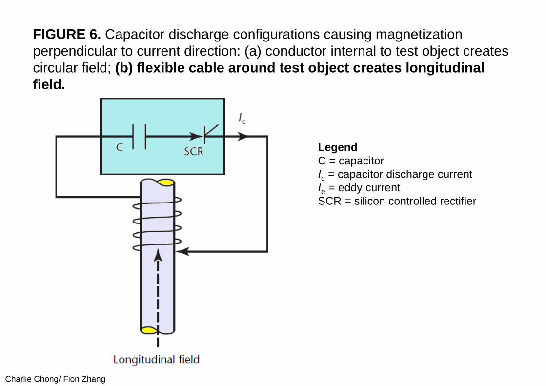
Typical configurations shown in Fig. 6 illustrate the complexity of the situation. In the case of the magnetization of a tube, the current Ic first rises rapidly, inducing magnetic flux in the tube. This time varying flux changes rapidly and induces an electromotive force in the tube, as dictated by Faraday’s law, the result being that an eddy current Ie flows around the tube as shown in Fig. 6a, where the dashed line is the inner surface eddy current and the solid line is the outer surface current.

Charlie Chong/ Fion Zhang
FIGURE 6. Capacitor discharge configurations causing magnetization perpendicular to current direction: (a) conductor internal to test object creates circular field; (b) flexible cable around test object creates longitudinal field.
LegendC = capacitorIc = capacitor discharge currentIe = eddy currentSCR = silicon controlled rectifier

Charlie Chong/ Fion Zhang
The net result is a lack of penetration of the field caused by the capacitor discharge current Ic. For a centered rod, in effect, the magnetic field intensity in the test object at radius r is given not by H = Ic·(2πr)–1 but rather by Eq. 6:
(6)
Here Ie is the amount of eddy current (ampere) contained within the cylinder of radius r (meter). Investigation of the effect of the eddy current is theoretically quite complicated because of its effect on the inductance, which in turn affects Ic. In practice, however, measurement of the magnetic flux density B in the material will yield the final degree of magnetization of that material.

Charlie Chong/ Fion Zhang
A good rule is that, if H(r) in Eq. 6 can be maintained at about 3.2 kA·m–1
(40 Oe), the material will be magnetized almost to saturation and can be tested for both surface and subsurface discontinuities.
Several other practical conclusions can be drawn from the above discussion.
• Pulse duration plays a greater role than pulse amplitude Ic(max) in determining the amount of flux induced in a test object. This is intuitively seen in direct current tests.
• It is not possible to give simple rules that relate Ic(max) to magnetization requirements. This relationship can be shown with a magnetic flux meter.
• The eddy currents induced during pulse magnetization play an important role in the result. They can shield midwall regions from magnetization.
• Larger capacitances at lower voltages provide better magnetization than smaller capacitances at higher voltages because larger capacitances at lower voltages lead to longer duration pulses and therefore to lower eddy currents. The lower voltage is an essential safety feature for outdoor use. A maximum of 50 V is recommended.

Charlie Chong/ Fion Zhang
9.2.3 Magnitudes of Magnetic Flux Leakage FieldsThe magnitude of the magnetic flux leakage field under active direct current excitation naturally depends on the applied field. An applied field of 3.2 to 4.0 kA·m–1 (40 to 50 Oe) inside the material can cause leakage fields with peak values of tens of millitesla (hundreds of gauss). However, in the case of residual induction, the magnetic flux leakage fields may be only a few hundred microtesla (a few gauss). Furthermore, with residual field excitation, an interesting field reversal may occur, depending on the value of the initial active field excitation and the dimensions of the discontinuity.

Charlie Chong/ Fion Zhang
9.2.4 Optimal Operating Point
Consider raising the magnetization level in a block of steel containing a discontinuity (Fig. 7). At low flux density levels, the field lines tend to crowd together in the steel around the discontinuity rather than go through the nonmagnetic region of the discontinuity. The field lines are therefore more crowded above and below the discontinuity than they are on the left or right. The material can hold more flux as the permeability rises, so there is no significant leakage flux at the surfaces (Fig. 7a). However, an increase in the number of lines causes ΔB·(ΔH)–1 to fall — the material is becoming less permeable. At about this point, magnetic flux leakage is first noticed at the surfaces. Although the lines are now closer together, representing a higher magnetic flux density, they do not have the ability to crowd closer together around the discontinuity where the permeability is low.

Charlie Chong/ Fion Zhang
FIGURE 7. Effects of induction on magnetic flux lines at discontinuity: (a) no surface flux leakage occurs where magnetic flux lines are compressed at low levels of induction around discontinuity; (b) lack of compression at high magnetization results in surface magnetic flux leakage.

Charlie Chong/ Fion Zhang
At higher and higher values of applied field, the permeability falls. It is, however, still large compared to the permeability of air, so the reluctance of the path through the discontinuity is still larger than through the metal. As a result, magnetic flux leakage at the outside surface helps provide a sufficiently high flux density in the material for the leakage of magnetic flux from discontinuities (Fig. 7b) while partially suppressing long range surface noise. For residual field testing, it is best to ensure that the material is saturated. The magnetic field starts to decay as soon as the energizing current is removed.

Charlie Chong/ Fion Zhang
The Great Rationalizer
http://www.heitu5.com/kehuan/mojingxianzong/player-0-0.html

Charlie Chong/ Fion Zhang
9.3 PART 3. Magnetic Flux Leakage Test Results9.3.0 IntroductionMagnetic flux leakage testing continues to be one of the most popular nondestructive test techniques in industry. A number of factors, including low cost and simplicity of the data interpretation process, contribute to this popularity. The underlying principles and modeling techniques are described elsewhere in this volume. The discussion below focuses on probes and excitation schemes to detect and measure magnetic leakage fields.

Charlie Chong/ Fion Zhang
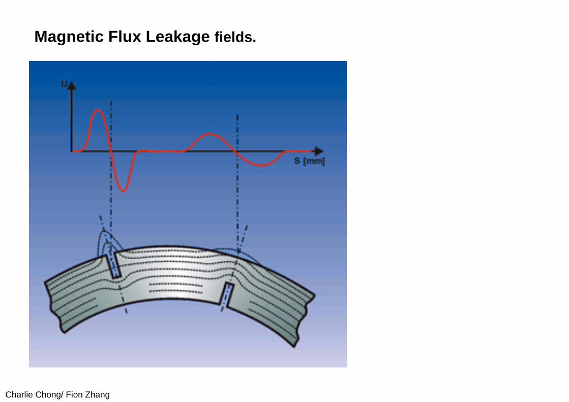
9.3.1 Magnetic Flux Leakage ProbesThe purpose of probes for magnetic testing is to detect and possibly quantify the magnetic flux leakage field generated by heterogeneities in the test object. The leakage fields tend to be local and concentrated near the discontinuities. The leakage field can be divided into three orthogonal components: normal (vertical), tangential (horizontal) and axial directions. Probes are usually either designed or oriented to measure one of these components. Typical plots of these components near discontinuities are shown in this volume’s chapter on probes. A variety of probes (or transducers) are used in industry for detecting and measuring leakage fields.
Charlie Chong/ Fion Zhang
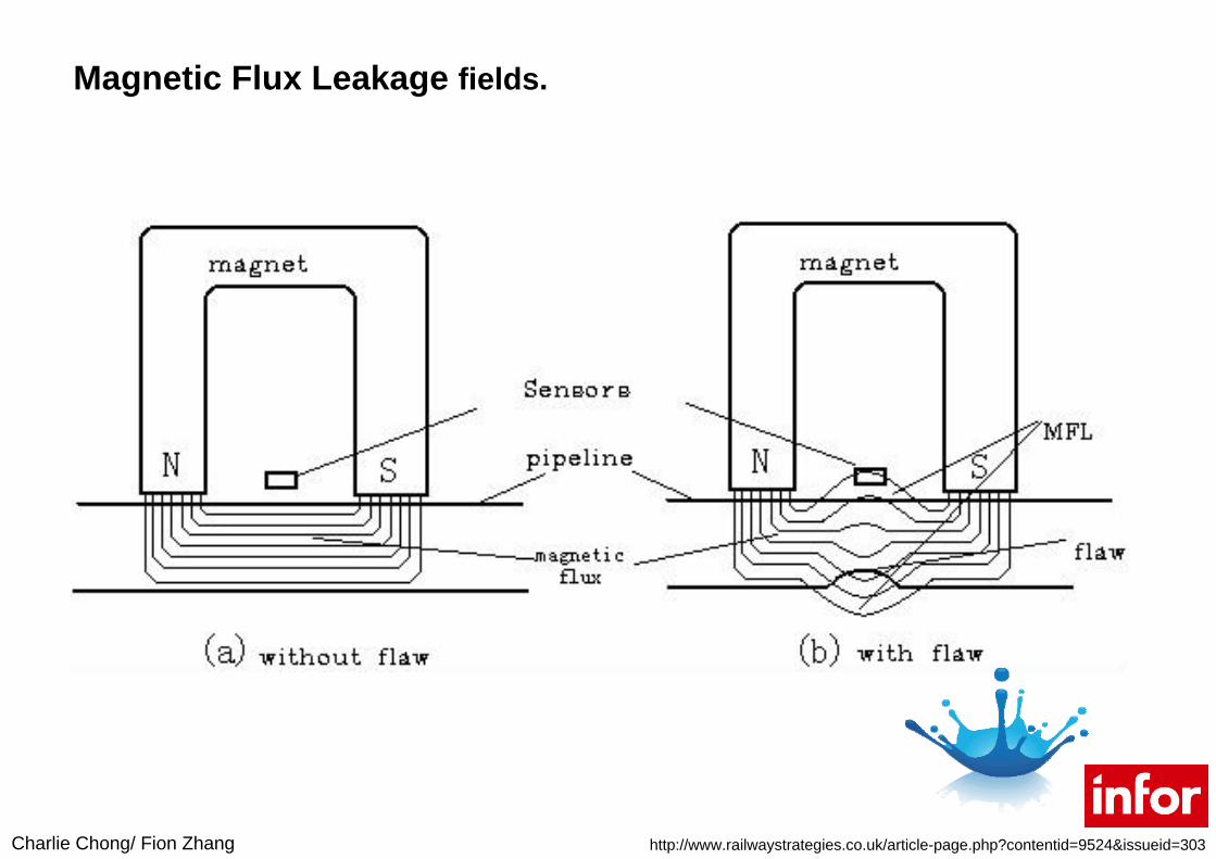
Magnetic Flux Leakage fields.

Charlie Chong/ Fion Zhang
Magnetic Flux Leakage fields.

Charlie Chong/ Fion Zhang
BS EN 10246-5:2000 MFLT Set-up
1: Transducer 2: Tube 3: Rotating Magnet & Transducer
BS EN 10246-5:2000
Charlie Chong/ Fion Zhang
Magnetic Flux Leakage fields.
http://www.railwaystrategies.co.uk/article-page.php?contentid=9524&issueid=303

Charlie Chong/ Fion Zhang
MFLT- Expert at Work

Charlie C
hong/ Fion Zhang
MFLT- Expert at Works

Charlie Chong/ Fion Zhang
MFLT- Expert at Works
http://www.puretechltd.com/articles/newsletter/2012/03/California_MFL.shtml

Charlie Chong/ Fion Zhang
MFLT- Expert at Works
http://www.puretechltd.com/articles/newsletter/2012/03/California_MFL.shtml

Charlie Chong/ Fion Zhang
The most commonly used in-service inspection tools utilize the Magnetic Flux Leakage (MFL)technique in order to detect internal or external corrosion. The MFL inspection pig uses a circumferential array of MFL detectors embodying strong permanent magnets to magnetize the pipe wall to near saturation flux density. Abnormalities in the pipe wall, such as corrosion pits, result in magnetic flux leakage near the pipe's surface. These leakage fluxes are detected by Hall probes or induction coils moving with the MFL detector. The demands now being placed on magnetic inspection tools are shifting from the mere detection, location and classification of pipeline defects, to the accurate measurements of defect size and geometry. Modern, high-resolution MFL inspection tools are capable of giving very detailed signals. However, converting these signals to accurate estimates of size requires considerable expertise, as well as a detailed understanding of the effects of inspection conditions and the magnetic behaviour of the type of pipeline steel used.
http://www.physics.queensu.ca/~amg/expertise/inline.html

Charlie Chong/ Fion Zhang
Magnetic Flux Leakage fields.
http://www.physics.queensu.ca/~amg/expertise/inline.html

Charlie Chong/ Fion Zhang
Magnetic Flux Leakage fields.
http://www.physics.queensu.ca/~amg/expertise/inline.html

Charlie Chong/ Fion Zhang
Intelligence Pigging with MFLT
http://www.physics.queensu.ca/~amg/expertise/inline.html

Charlie Chong/ Fion Zhang
Intelligence Piggy
http://www.physics.queensu.ca/~amg/expertise/inline.html
Charlie Chong/ Fion Zhang
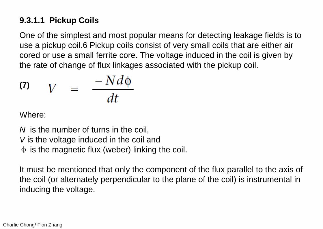
9.3.1.1 Pickup Coils
One of the simplest and most popular means for detecting leakage fields is to use a pickup coil.6 Pickup coils consist of very small coils that are either air cored or use a small ferrite core. The voltage induced in the coil is given by the rate of change of flux linkages associated with the pickup coil.
(7)
Where:
N is the number of turns in the coil, V is the voltage induced in the coil and φ is the magnetic flux (weber) linking the coil.
It must be mentioned that only the component of the flux parallel to the axis of the coil (or alternately perpendicular to the plane of the coil) is instrumental in inducing the voltage.

Charlie Chong/ Fion Zhang
This induction direction makes it possible to orient the pickup coil so as to measure any of the three leakage field components selectively. Thus, a coil A whose axis is perpendicular to the surface of the test object (Fig. 8a), is sensitive only to the normal component. In contrast, the coil in Fig. 8b is sensitive only to the tangential component. Consider the case where the pickup coil is moving over the test object in the X direction. Making use of the fact that φ = B·A, where B is the magnetic flux density (tesla) and A is the cross sectional area (square meter) of the pickup coil, Eq. 7 can be rewritten:
(8)

Charlie Chong/ Fion Zhang
FIGURE 8. Effect of pickup coil orientation on sensitivity to components of magnetic flux density: (a) coil sensitive to normal component; (b) coil sensitive to tangential component.
(b)(a)

Charlie Chong/ Fion Zhang
This equation indicates that the output of the pickup coil is proportional to the spatial gradient of the flux along the direction of the coil movement as well as the velocity of the coil. Two issues arise as a result.
1. It is essential that the probe scan velocity (relative to the test object) should be constant to avoid introducing artifacts into the signal through probe velocity variations.
2. The output is proportional to the spatial gradient of the flux in the direction of the coil. The output of the pickup coil can be integrated formeasurement of the leakage flux density rather than of its gradient.

Charlie Chong/ Fion Zhang
Figure 9 shows the output of a pickup coil and the signal obtained after integrating the output.7 The coil is used to measure, in units of tesla (or gauss), the magnetic flux density B leaking from a rectangular slot. The sensitivity of the pickup coil can be improved by using a ferrite core. Tools for designing pickup coils, as well as predicting their performance, are described elsewhere in this volume.

Charlie Chong/ Fion Zhang
FIGURE 9. Pickup coil and signal integrator (magnetic flux leakage) output for rectangular discontinuity.

Charlie Chong/ Fion Zhang
Signal and Magnetic Disturbances

Charlie Chong/ Fion Zhang
Magnetic Flux Leakage & Signals

Charlie Chong/ Fion Zhang
Magnetic Flux Leakage & Signals

Charlie Chong/ Fion Zhang
Magnetic Flux Leakage & Signals

Charlie Chong/ Fion Zhang
9.3.1.2 Magnetodiodes
The magnetodiode is suitable for sensing leakage fields from discontinuities because of its small size and its high sensitivity. Because the coil probe is usually larger than the magnetodiode, it is less sensitive to longitudinally angled discontinuities than the magnetodiode is. However, the coil probe is better than the magnetodiode for large discontinuities, such as cavities.

Charlie Chong/ Fion Zhang
Magnetodiodes
http://www.craft-3.com/Semiconductor/SONY_Transistor/sony_diode.html

Charlie Chong/ Fion Zhang
9.3.1.3 Hall Effect Detectors
Hall effect detector probes are used extensively in industry for measuring magnetic flux leakage fields in units of tesla (or gauss). Hall effect detector probes are described in this volume’s chapter on probes for electromagnetic testing.

Charlie Chong/ Fion Zhang
Hall Effect Detectors

Charlie Chong/ Fion Zhang
Hall Effect Detectors
http://movableparts.org/rear-wheel-tachometer/

Charlie Chong/ Fion Zhang
9.3.1.4 Giant Magnetoresistive Probes
Magnetic field sensitive devices called giant magnetoresistive probes, at the most basic level, consist of a nonmagnetic layer sandwiched between two magnetic layers. The apparent resistivity of the structure varies depending on whether the direction of the electron spin is parallel or antiparallel to the moments of the magnetic layers. When the moments associated with the magnetic layers are aligned antiparallel, the electrons with spin in one direction (up) that are not scattered in one layer will be scattered in the other layer. This increases the resistance of the device. This is in contrast to the situation when the magnetic moments associated with the layers are parallel where the electrons that are not scattered in one layer are not scattered in the other layer, either. Giant magnetoresistive probes use a biasing current to push the magnetic layers into an antiparallel moment state and the external field is used to overcome the effect of the bias. The resistance of the device, therefore, decreases with increasing field intensity values. Figure 10 shows a typical response of a giant magnetoresistive probe.
Charlie Chong/ Fion Zhang
Keywords:
The resistance of the device, therefore, decreases with increasing field intensity values.

Charlie Chong/ Fion Zhang
FIGURE 10. Resistance versus applied field for 2 μm (8 . 10–5 in.) wide strip of anti-ferromagnetically coupled, multilayer test object composed of 14 percent giant magnetoresistive material.

Charlie Chong/ Fion Zhang
More Reading on: Giant Magnetoresistive ProbesThere are better alternatives to detect pneumatic cylinder end of stroke position than reed switches or proximity switches. By better, I mean they are faster and easier to implement into your control system. In addition, you can realize other benefits such as commonality of spare sensors and lower long-term costs. So what are the better solutions? Three types of sensor technologies lead the way to better alternatives. First, there is the Hall Effect magnetic field sensor, see figure 1. The benefit of Hall Effect sensors is speed; they are electronic so there are no moving parts and nothing to wear out. They are not affected by shock and vibration unlike the reed switch.
figure 1
https://sensortech.wordpress.com/2010/06/25/better-alternatives-to-pneumatic-cylinder-end-of-stroke-detection/

Charlie Chong/ Fion Zhang
However, there are some disadvantages of Hall Effects such as they typically require fairly high magnetic gauss strength and they require a radially magnetized magnet. Typically, a Hall Effect will not work as a replacement of a reed switch or if it does operate, it may produce double switch points. A Hall Effect sensor is looking for a single magnetic pole, so if it is used with an axially magnetized magnet, it will switch when it sees the north pole and then again with the south pole, thus causing the double switch points.
The second and newer technology is the magnetoresistive sensor shown in figure 2 or sometimes referred to as AMR (Anisotropic magnetoresistance). Unlike the Hall Effect sensor that uses a change in voltage the AMR is based off a change in resistance. This change in resistance is more sensitive thus; a lower strength magnet can be utilized. The best advantage of the AMR sensor is that it will work with the axially magnetized magnet and in most cases the radially magnetized magnet. Like the Hall Effect, the AMR has no moving parts and nothing to wear out and is fast therefore it is a good solution for high-speed applications. The magnetoresistive sensor does not suffer from double switch points and has a much better noise immunity than Hall Effects.

Charlie Chong/ Fion Zhang
Figure 2:
https://sensortech.wordpress.com/2010/06/25/better-alternatives-to-pneumatic-cylinder-end-of-stroke-detection/

Charlie Chong/ Fion Zhang
Giant Magnetoresistive or GMR sensors shown in figure 3 are technologically the newer of the magnetic field sensors. They operate on a change in resistance, as does the AMR, however; the magnetic field causes a larger or giant change in resistance. Although you would think the GMR sensors are physically larger than the AMR, they are actually smaller. Major advantages of the GMR sensor are they are more sensitive, are more precise and have a better hysteresis than the AMR.
https://sensortech.wordpress.com/2010/06/25/better-alternatives-to-pneumatic-cylinder-end-of-stroke-detection/

Charlie Chong/ Fion Zhang
Giant Magnetoresistive Probes
https://sensortech.wordpress.com/2010/06/25/better-alternatives-to-pneumatic-cylinder-end-of-stroke-detection/

Charlie Chong/ Fion Zhang
Okay so the AMR and GMR sensors seem to be the better or even the best solution. Are there other advantages to them? Higher quality sensor manufacturers offer better output circuitry that includes reverse polarity protection, overload protection and short circuit protection. Couple that with lifetime warranty offered on some manufacturer’s sensors and you end up with a better alternative to the pneumatic cylinder end of stroke sensor.
I know what you are thinking there must be some negatives. The initial cost of the AMR or GMR sensor may be slightly more than the reed sensor however this cost is becoming less and less and it is even less once you figure the cost of down time after your reed switch fails or the proximity flag is moved. In addition, the AMR and GMR sensors are 3-wire devices unlike the 2-wire reed switch. However, in the end the AMR and GMR sensors are still the better solution.
https://sensortech.wordpress.com/2010/06/25/better-alternatives-to-pneumatic-cylinder-end-of-stroke-detection/

Charlie Chong/ Fion Zhang
9.3.1.5 Magnetic Tape
For the testing of flat surfaces, magnetic tape can be used. The tape is pressed to the surface of the magnetized billet and then scanned by small probes before being erased. This technique is sometimes called magnetography. In automated systems, magnetic tape can be fed from a spool. The signals can be read and the tape can be erased and reused. Unfortunately, the tangential leakage field intensity at the surface of the material is not constant. To optimize the response, the amplification of the signals can be varied. Scabs or slivers projecting from the test surface can easily tear the tape

Charlie Chong/ Fion Zhang
9.3.2 Magnetic ParticlesMagnetic particles are one of the most popular means used in industry for detecting magnetic fields. Indeed, magnetic particle testing is so popular that an entire volume of the Nondestructive Testing Handbook is devoted to the subject. The descriptions below are therefore cursory. Magnetic particle testing involves the application of magnetic particles to the test object after it is magnetized by using an appropriate technique. The ferromagnetic particles preferentially adhere to the surface of the test object in areas where the flux is diverted, or leaks out. The magnetic flux leakage near discontinuities causes the magnetic particles to accumulate in the region and in some cases form an outline of the discontinuity. Heterogeneities can therefore be detected by looking for indications of magnetic particle accumulations on the surface of the test object either with the naked eye or through a camera. The indications are easier to see if the particles are bright and reflective. Alternately, particles that fluoresce under ultraviolet or visible radiation may be used. The test object has to be viewed under appropriate levels of illumination with radiation of appropriate wavelength (visible, ultraviolet or other).

Charlie Chong/ Fion Zhang
9.3.2.1 Application TechniquesMagnetic particles are applied to the surface by two different techniques inindustry.
(A) Dry Testing.
Dry techniques use particles applied in the form of a fine stream or an aerosol. They consist of high permeability ferromagnetic particles coated with either reflective or fluorescent pigments. The particle size is chosen according to the dimensions of the discontinuity sought. Particle diameters range from ≤50μmto 180 μm (≤0.002 to 0.007 in.). Finer particles are used for detecting smaller discontinuities where the leakage intensity is low. Dry techniques are used extensively for testing welds and castings where heterogeneities of interest are relatively large.
Charlie Chong/ Fion Zhang
(B) Wet Testing.
Wet techniques are used for detecting relatively fine cracks. The magnetic particles are suspended in a liquid (usually oil or water) usually sprayed on the test object. Particle sizes are significantly smaller than those used with dry techniques and vary in size within a normal distribution, with most particles measuring from 5 to 20μm (2·10–4 to 8·10–4 in.). As in the case of dry powders, the ferromagnetic particles are coated with either reflective or fluorescent pigments. More information on this subject is available elsewhere.

Charlie Chong/ Fion Zhang
MPI

Charlie Chong/ Fion Zhang
9.3.2.2 Imaging of Magnetic Particle IndicationsThe magnetic particle distribution can be examined visually after illuminating the surface or the surface can be scanned with a flying spot system or imaged with a charge coupled device camera.
(A) Flying Spot Scanners.
To illuminate the test object (Fig. 11), flying spot scanners10,11 use a narrow beam of radiation — visible light for non-fluorescent particles and ultraviolet radiation for fluorescent ones. The source of the beam is usually a laser. The wavelength of the beam is chosen carefully to excite the pigment of the magnetic particles. The incidence of the radiation beam on the test object can be varied by moving the scanning mirror. The photocell does not sense any light when the test object is scanned by the narrow radiation beam until the beam is directly incident on the magnetic particles adhering to the test object near a discontinuity. When this occurs, a large amount of light is emitted, called fluorescence if excited by ultraviolet radiation. The fluorescence is detected by a single phototube equipped with a filter that renders the system blind to the radiation from the irradiating source. The output of the photocell is suitably amplified, digitized and processed by a computer.

Charlie Chong/ Fion Zhang
FIGURE 11. Flying spot scanner for automated magnetic particle testing.

Charlie Chong/ Fion Zhang
(B) Charge Coupled Devices.
An alternative approach is to flood the test object with radiation whose wavelength is carefully chosen to excite the pigment of the magnetic particles. Charge coupled device cameras, equipped with optical filters that render the camera blind to radiation from the source but are transparent to light emitted by the magnetic particles, can be used to image the surface very rapidly. In very simple terms, charge coupled devices each consist of a two dimensional array of tiny pixels that each accumulates a charge corresponding to the number of photons incident on it. When a readout pulse is applied to the device, the accumulated charge is transferred from the pixel to a holding or charge transfer cell. The charge transfer cells are connected in a manner that allows them to function as a bucket brigade or shift register. The charges can, therefore, be serially clocked out through a charge-to-voltage amplifier that produces a video signal.

Charlie Chong/ Fion Zhang
In practice, charge coupled device cameras can be interfaced to a personal computer through frame grabbers, which are commercially available. Vendors of frame grabbers usually provide software that can be executed on the personal computer to process the image. Image processing software can be used for example to improve contrast, highlight the edges of discontinuity or to minimize noise in the image.
Charlie Chong/ Fion Zhang
9.3.3 Test CalculationsIn determining the magnetic flux leakage from a discontinuity, certain conditions must be known:
1. the discontinuity’s location with respect to the surfaces from which measurements are made,
2. the relative permeability of the material containing the discontinuity and 3. the levels of magnetic field intensity H and magnetic flux density B in the
vicinity of the discontinuity.
Even with this knowledge, the solution of the applicable field equations (derived from Maxwell’s equations of electromagnetism) is difficult and is generally impossible in closed algebraic form. Under certain circumstances, such as those of discontinuity shapes that are easy to handle mathematically, relatively simple equations can be derived for the magnetic flux leakage if simplifying assumptions are made. This simplification does not apply to subsurface inclusions.

Charlie Chong/ Fion Zhang
9.3.3.1 Finite Element Techniques
An advance in magnetic theory since 1980 has been the introduction of finite element computer codes to the solution of magnetostatic problems. Such codes came originally from a desire to minimize electrical losses from electromagnetic machinery but soon found application in magnetic flux leakage theory. The advantage of such codes is that, once set up, discontinuity leakage fields can be calculated by computer for any size and shape of discontinuity, under any magnetization condition, so long as the B,H curve for the material is known. In the models of magnetic flux leakage discussed so far, the implicit assumptions are (1) that the field within a discontinuity is uniform and (2) that the nonlinear magnetization characteristic (B,H curve) of the tested material can be ignored. Much of the early pioneering work in magnetic flux leakage modeling used these assumptions to obtain closed form solutions for leakage fields.

Charlie Chong/ Fion Zhang
Nonlinear magnetization characteristic (B,H curve) of the tested material
http://www.electronics-tutorials.ws/electromagnetism/magnetic-hysteresis.html

Charlie Chong/ Fion Zhang
The solutions of classical problems in electrostatics have been well known to physicists for almost a century and their magnetostatic analogs were used to approximate discontinuity leakage fields. Such techniques work reasonably well when the permeability around a discontinuity is constant or when nonlinear permeability effects can be ignored. The major problem that remains is how to deal with real discontinuity shapes often impossible to handle by classical techniques. Such deficiencies are overcome by the use of computer programs written to allow for nonlinear permeability effects around oddly shaped discontinuities. Specifically, computerized finite element techniques, originally developed for studying magnetic flux distributions in electromagnetic machinery, have also been developed for nondestructive testing. Both active and residual excitation are discussed above. The extension of the technique to include eddy currents is detailed elsewhere in this volume.

Charlie Chong/ Fion Zhang
Further Reading:Understanding Magnetic Flux Leakage Signals from Mechanical Damage in Pipelines
In-line inspection using the Magnetic Flux Leakage (MFL) technique is sensitive both to pipe wall geometry and pipe wall stresses. Therefore, MFL inspection tools have the potential to locate and characterize mechanical damage in pipelines. However, the combined influence of stress and geometry make MFL signals from dents and gouges difficult to interpret. Accurate magnetic models that can incorporate both stress and geometry effects are essential to improve the current understanding of MFL signals from mechanical damage. MFL signals from dents include a geometry component in addition to a component due to residual stresses. If gouging is present, then there may also be an additional magnetic contribution from the heavily worked material at the gouge surface. The relative contribution of each of these components to the MFL signal depends on the size and shape of the dent in addition to other effects such as metal loss, wall thinning, corrosion, etc.
http://prci.org/index.php/site/projects_single/understanding_magnetic_flux_leakage_signals_from_mechanical_damage_in_pipel/

Charlie Chong/ Fion Zhang
FEA Model
http://prci.org/index.php/site/projects_single/understanding_magnetic_flux_leakage_signals_from_mechanical_damage_in_pipel/

Charlie Chong/ Fion Zhang
Key ResultsMagnetic Finite Element Analysis (FEA) can be applied to model MFL signals from mechanical damage defects having various sizes, shapes, andconfigurations. These models included geometry effects, contributions due to elastic strain (either residual strain or strain due to in-service loading), and also magnetic behavior changes due to severe deformation. The modeled results were then compared with experimental MFL signal measurements on dents and gouges produced in the laboratory as well under “field”conditions. Magnetic FEA models were produced of circular dents as well as dents elongated in the pipe axial and pipe hoop directions. Residual stress patterns were predicted in and around the dent using stress FEA modeling. The magnetic effects of these predicted residual stresses were incorporated into the magnetic FEA model by modifying the magnetic permeability in stressed regions in and around the dent. The modeled stress and geometry contributions to the MFL signal were examined separately, and also combined for comparison with experimental MFL results. Agreement between modeled and measured MFL signals was generally good, and the measured MFL signals were used to validate and refine the models.
http://prci.org/index.php/site/projects_single/understanding_magnetic_flux_leakage_signals_from_mechanical_damage_in_pipel/

Charlie Chong/ Fion Zhang
Other Reading:Leakage signals due the two defects. Field shown in (a) corresponds to the deeper defect and field shown in (b) to the shallow one.
http://www.ndt.net/article/wcndt00/papers/idn269/idn269.htm

Charlie Chong/ Fion Zhang
9.4 PART 4. Applications of Magnetic Flux LeakageTesting
9.4.0 IntroductionMagnetic flux leakage testing is a commonly used technique. Signals from probes are processed electronically and presented in a manner that indicates the presence of discontinuities. Although some techniques of magnetic flux leakage testing may not be as sophisticated as others, it is probable that more ferromagnetic material is tested with magnetic flux leakage than with any other technique. Magnetizing techniques have evolved to suit the geometry of the test objects. The techniques include yokes, coils, the application of current to the test object and conductors that carry current through hollow test objects. Many situations exist in which current cannot be applied directly to the test object because of the possibility of arc burns.

Charlie Chong/ Fion Zhang
Design considerations for magnetization of test objects often require minimizing the reluctance of the magnetic circuit, consisting of
(1) the test object, (2) the magnetizing system and (3) any air gaps that might be present.
Charlie Chong/ Fion Zhang
9.4.1 Test Object Configurations9.4.1.1 Short Asymmetrical Objects
A short test object with little or no symmetry may be magnetized to saturation by passing current through it or by placing it in an encircling coil. If hollow, a conductor can be passed through the test object and magnetization achieved by any of the standard techniques (these include half-wave and full-wave rectified alternating current, pure direct current from battery packs or pulses from capacitor discharge systems). For irregularly shaped test objects, testing by wet or dry magnetic particles is often performed, especially if specifications require that only surface breaking discontinuities be found.
Charlie Chong/ Fion Zhang
9.4.1.2 Elongated Objects
The cylindrical symmetry of elongated test objects such as wire rope permits the use of a relatively simple flux loop to magnetize a relatively short section of the rope. Encircling probes are placed at some distance from the rope to permit the passage of splices. Such systems are also suited for pumping well sucker rods and other elongated oil field test objects. After a well is drilled, the sides of the well are lined with a relatively thin steel casing material, which is then cemented in. This casing can be tested only from the inside surface. The cylindrical geometry of the casing permits the flux loop to be easily calculated so that magnetic saturation of the well casing is achieved. As with in-service well casing, buried pipelines are accessible only from the inside surface. The magnetic flux loop is the same as for the well casing test system. In this case, a drive mechanism must be provided to propel the test system through the pipeline.

Charlie Chong/ Fion Zhang
Elongated Objects- Pump Jack
Charlie Chong/ Fion Zhang
9.4.1.3 Threaded Regions of Pipe
An area that requires special attention during the inservice testing of drill pipe is the threaded region of the pin and box connections. Common problems that occur in these regions include fatigue cracking at the roots of the threads and stretching of the thread metal. Automated systems that use both active and residual magnetic flux techniques can be used for detecting suchdiscontinuities.

Charlie Chong/ Fion Zhang
Threaded Regions of Sucker Rod

Charlie Chong/ Fion Zhang
9.4.1.4 Ball Bearings and RacesSystems have been built for the magnetization of both steel ball bearingsand their races. One such system uses specially fabricated hall elements as detectors.
9.4.1.5 Relatively Flat SurfacesThe testing of welded regions between flat or curved plates is often performed using a magnetizing yoke. Probe systems include coils, hall effect detectors, magnetic particles and magnetic tape.

Charlie Chong/ Fion Zhang
Relatively Flat Surfaces

Charlie Chong/ Fion Zhang
Relatively Flat Surfaces

Charlie Chong/ Fion Zhang
9.4.2 Discontinuity MechanismsIn the metal forming industry, discontinuities commonly found by magnetic flux leakage techniques include overlaps, seams, quench cracks, gouges, rolled-in slugs and subsurface inclusions. In the case of tubular goods, internal mandrel marks (plug scores) can also be identified when they result in remaining wall thicknesses below some specified minimum. Small marks of the same type can also act as stress raisers and cracking can originate from them during quench and temper procedures. Depending on the use to which the material is put, subsurface discontinuities such as porosity and laminations may also be considered detrimental. These types of discontinuities may be acceptable in welds where there are no cyclic stresses but may cause injurious cracking when such stresses are present.

Charlie Chong/ Fion Zhang
In the metal processing industries, grinding especially can lead to surface cracking and to some changes in surface metallurgy. Such discontinuities as cracking have traditionally been found by magnetic flux leakage techniques, especially wet magnetic particle testing. Service induced discontinuities include cracks, corrosion pitting, stress induced metallurgy changes and erosion from turbulent fluid flow or metal-to-metal contact. In those materials placed in tension and under torque, fatigue cracking is likely to occur. A discontinuity that arises from metal-to-metal wear is sucker rod wear in tubing from producing oil wells. Here, the pumping rod can rub against the inner surface of the tube and both the rod and tube wear thin. In wire rope, the outer strands will break after wearing thin and inner strands sometimes break at discontinuities present when the rope was made. Railroad rails are subject to cyclic stresses that can cause cracking to originate from otherwise benign internal discontinuities.

Charlie Chong/ Fion Zhang
Loss of metal caused by a conducting fluid near two slightly dissimilar metals is a very common form of corrosion. The dissimilarity can be quite small, as for example, at the heat treated end of a rod or tube. The result is preferential corrosion by electrolytic processes, compounded by erosion from a contained flowing fluid. Such loss mechanisms are common in subterranean pipelines, installed petroleum well casing and in refinery and chemical plant tubing. The stretching and cracking of threads is a common problem. For example, when tubing, casing and drill pipe are overtorqued at the coupling, the threads exist in their plastic region. This causes metallurgical changes in the metal and can create regions where stress corrosion cracking takes place in highly stressed areas at a faster rate than in areas of less stress. Couplings between tubes are a good example of places where material may be highly stressed. Drill pipe threads are a good example of places where such stress causes plastic deformation and thread root cracking.

Charlie Chong/ Fion Zhang
9.4.3 Typical Magnetic Flux Leakage Techniques 9.4.3.1 Short PartsFor many short test objects, the most convenient probe to use is the magnetic particle. The test object can be inspected for surface breaking discontinuities during or after it has been magnetized to saturation. For active field testing, the test object can be placed in a coil carrying alternating current and sprayed with magnetic particles. Or it can be magnetized to saturation by a direct current coil and the resulting residual induction can be shown with magnetic particles. In the latter case, the induction in the test object can be measured with a flux meter. Wet particles perform better than dry ones because there is less tendency for the wet particles to fur (that is, to stand up like short hairs) along the field lines that leave the test object. These techniques will detect transversely oriented, tight discontinuities.

Charlie Chong/ Fion Zhang
The magnetic flux leakage field intensity from a tight crack is roughly proportional to the magnetic field intensity Hg across the crack, multiplied by crack width Lg. If the test is performed in residual induction, the value of Hg (which depends on the local value of the demagnetization field in the test object) will vary along the test object. Thus, the sensitivity of the technique to discontinuities of the same geometry varies along the length of the test object. For longitudinally oriented discontinuities, the test object must be magnetized circumferentially. If the test object is solid, then current can be passed through the test object, the surface field intensity being given by Ampere’s law:
(9)
Where:dl is an element of length (meter), H is the magnetic field intensity (ampere per meter) and I is the current (ampere) in the test object.
Charlie Chong/ Fion Zhang
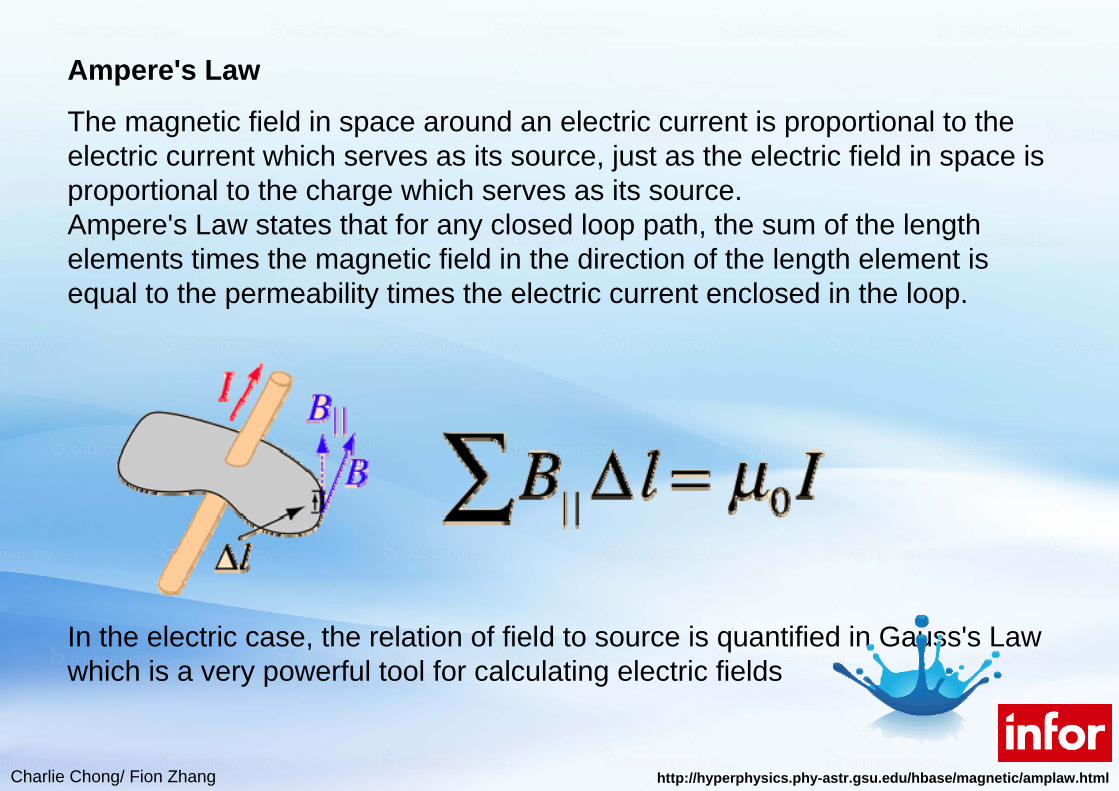
Ampere's Law
The magnetic field in space around an electric current is proportional to the electric current which serves as its source, just as the electric field in space is proportional to the charge which serves as its source. Ampere's Law states that for any closed loop path, the sum of the length elements times the magnetic field in the direction of the length element is equal to the permeability times the electric current enclosed in the loop.
In the electric case, the relation of field to source is quantified in Gauss's Law which is a very powerful tool for calculating electric fields
http://hyperphysics.phy-astr.gsu.edu/hbase/magnetic/amplaw.html

Charlie Chong/ Fion Zhang
If the test object is a cylindrical bar, the symmetry of the situation allows H to be constant around the circumference, so the closed integral reduces:
(10)
(11)
Where:R is the radius (meter) of the cylindrical test object. A surface field intensity that creates an acceptable magnetic flux leakage field from the minimum sized discontinuity must be used. Such fields are often created by specifying the amperage per meter of the test object’s outside diameter.

Charlie Chong/ Fion Zhang
9.4.3.2 Transverse Discontinuities
Because of the demagnetizing effect at the end of a tube, automated magnetic flux leakage test systems do not generally perform well when scanning for transverse discontinuities at the ends of tubes. The normal component Hy of the field outside the tube is large and can obscure discontinuity signals. Test specifications for such regions often include the requirement of additional longitudinal magnetization at the tube ends and subsequent magnetic particle tests during residual induction. This situation is equivalent to the magnetization and testing of short test objects as outlined above.

Charlie Chong/ Fion Zhang
The flux lines must be continuous and must therefore have a relatively short path in the metal. Large values of the magnetizing force at the center of the coil are usually specified. Such values depend on the weight per unit length of the test object because this quantity affects the ratio of length L to diameter D.
Where the test object is a tube, the L·D–1 ratio is given by the length between the poles divided by twice the wall thickness of the tube. (The distance L from pole to pole can be longer or shorter than the actual length of the test object and must be estimated by the operator.)
As a rough example, with L = 460 mm (18 in.) and D = 19 (0.75 in.), the L·D–1
ratio is 24.

Charlie Chong/ Fion Zhang
The effective permeability of the metal under test is small because of the large demagnetization field created in the test object by the physical end of the test object. An empirical formula is often used to calculate approximately the effective permeability μ:
(12)
so effective permeability μ = 139 in the above example. For wet magnetic particle testing, the surface tension of the fluids that carry the particles is large enough to confine the particles to the surface of the test object. This is not the case with dry particles, which have the tendency to stand up like fur along lines of magnetizing force. In many instances, it may be better to use some other test technique for transverse discontinuities, such as ultrasonic or eddy current techniques.

Charlie Chong/ Fion Zhang
9.4.3.3 Alternating Current versus Direct Current Magnetization
Alternating current magnetization is more suitable for detection of outer surface discontinuities because it concentrates the magnetic flux at the surface. For equal magnetizing forces, an alternating current field is better for detecting outside surface imperfections but a direct current field is better for detecting imperfections below the surface. In practice, the ends of tubes are tested for transverse discontinuities by the following magnetic flux leakage techniques.

Charlie Chong/ Fion Zhang
1. Where there is a direct current active field from an encircling coil, magnetic particles are thrown at the tested material while it is maintained at a high level of magnetic induction by a direct current field in the coil. This technique is particularly effective for internal cracks. Fatigue cracks in drill pipe are often found by this technique.
2. Where there is an alternating current active field from an encircling coil, magnetic particles are thrown at the tested material while it lies inside a coil carrying alternating current. Using 50 or 60 Hz alternating current, the penetration of the magnetic field into the material is small and the technique is good only for the detection of outside surface discontinuities. When tests for both outer surface and inner surface discontinuities are necessary, it may be best to test first for outer surface discontinuities with an alternating current field, then for inner surface discontinuities with a direct current field.
Charlie Chong/ Fion Zhang
9.4.3.4 Liftoff Control of Scanning Head
To obtain a stable detection of discontinuities, liftoff between the probe and the surface of the material must be kept constant. Usually liftoff is kept constant by contact of the probe with the surface but the probe tends to wear with this technique. A magnetic floating technique has been used for noncontact scanning. In this technique, liftoff is measured by a gap probe and the probe holder is moved by a voice coil motor, controlled by the gap signal. This system and related technology are described in this volume’s chapter on primary metals applications.
Charlie Chong/ Fion Zhang
9.4.4 Particular Applications9.4.4.1 Wire Ropes
An interesting example of an elongated steel product inspected by magnetic flux leakage testing is wire rope. Such ropes are used in the construction, marine and oil production industries, in mining applications and elevators for personnel and raw material transportation. Testing is performed to determine cross sectional loss caused by corrosion and wear and to detect internal and external broken wires. The type of flux loop used (electromagnet or permanent magnet) can depend on the accessibility of the rope. Permanent magnets might be used where taking power to an electromagnet might cause logistic or safety problems. By making suitable estimates of the parameters involved, a reasonably good estimate of the flux in the rope can be made. Because discontinuities can occur deep inside the rope material, it is essential to maintain the rope at a high value of magnetic flux density, 1.6 to 1.8 T (16 to 18 kG). Under these conditions, breaks in the inner regions of the rope will produce magnetic flux leakage at the surface of the rope.

Charlie Chong/ Fion Zhang
The problem of detecting magnetic flux leakage from inner discontinuities is compounded by the need to maintain the magnetic probes far enough from the rope for splices in the rope to pass through the test head. Common probes include hall effect detectors and encircling coils. The cross sectional area of the rope can be measured by sensing changes in the magnetic flux loop that occur when the rope gets thinner. The air gap becomes larger and so the value of the field intensity falls. This change can easily be sensed by placing hall effect probes anywhere within the magnetic circuit.
Charlie Chong/ Fion Zhang
9.4.4.2 Internal Casing or Pipelines
The testing of in-service well casing or buried pipelines is often performed by magnetic flux leakage techniques. Various types of wall loss mechanisms occur, including internal and external pitting, erosion and corrosion caused by the proximity of dissimilar metals. From the point of view of magnetizing the pipe metal in the longitudinal direction, the two applications are identical. The internal diameters and metal masses involved in the magnetic flux loop indicate that some form of active field excitation must be used. Internal diameters of typical production or transportation tubes range from about 100 mm (4 in.) to about 1.2 m (4 ft). If the material is generally horizontal, some form of drive mechanism is required. Because the test device (a robotic crawler) may move at differing speeds, the magnetic flux leakage probe should have a signal response independent of velocity.

Charlie Chong/ Fion Zhang
For devices that operate vertically, such as petroleum well casing test systems, coil probes can be used if the tool is pulled from the bottom of the well at a constant speed. In both types of instrument, the probes are mounted in pads pressed against the inner wall of the pipe. Because both line pipe and casing are manufactured to outside diameter size, there is a range of inside diameters for each pipe size. Such ranges may be found in specifications. To make the air gap as small as possible, soft iron attachments can be screwed to the pole pieces. For the pipeline crawler, a recorder package is added and the signals from discontinuities are tape recorded. When the tapes are retrieved and played back, the areas of damage are located. Pipe welds provide convenient magnetic markers. With the downhole tool, the magnetic flux leakage signals are sent up the wire line and processed in the logging truck at the wellhead. A common problem with this and other magnetic flux leakage equipment is the need to determine whether the signals originate from discontinuities on the inside or the outside surface of the pipe.

Charlie Chong/ Fion Zhang
Production and transmission companies require this information because it lets them determine which form of corrosion control to use. The test shoes sometimes contain a high frequency eddy current probe system that responds only to inside surface discontinuities. Thus, the occurrence of both magnetic flux leakage and eddy current signals indicates an inside surface discontinuity whereas the occurrence of a magnetic flux leakage signal indicates only an outside surface discontinuity. Problems with this form of testing include the following:
1. The magnetic flux leakage system cannot measure elongated changes in wall thickness, such as might occur with general erosion.
2. If there is a second string around the tested string, the additional metal contributes to the flux loop, especially in areas where the two strings touch.
3. A relatively large current must be sent down the wire line to raise the pipe wall to saturation. Temperatures in deep wells can exceed 200 °C (325 °F).
4. The tool may stick downhole or underground if external pressures cause the pipe to buckle.

Charlie Chong/ Fion Zhang
9.4.4.3 Cannon Tubes
In elongated tubing, the presence of rifling affects the ability to perform a good test, especially for discontinuities that occur in the roots of the rifling. Despite the presence of extraneous signals from internal rifling, however, rifling causes a regular magnetic flux leakage signal that can be distinguished from discontinuity signals. As a simulated discontinuity is made narrower and shallower, the signal will eventually be indistinguishable from the rifle bore noise. In magnetic flux leakage testing, cannon tubes can be magnetized to saturation and scanned with hall elements to measure residual induction.

Charlie Chong/ Fion Zhang
Cannon Tubes

Charlie Chong/ Fion Zhang
9.4.4.5 Round Bars and Tubes
In some test systems, round bars and tubes have been magnetized by an alternating current magnet and rotated under the magnet poles. Because the leakage flux from surface discontinuities is very weak and confined to a small area, the probes must be very sensitive and extremely small. The system uses a differential pair of magnetodiodes to sense leakage flux from the discontinuity. The differential output of these twin probes is amplified to separate the leakage flux from the background flux. In this system, pipes are fed spirally under the scanning station, which has an alternating current magnet and an array of probe pairs. The system usually has three scanning stations to increase the test rate. In one similar system, round billets are rotated by a set of rollers while the billet surface is scanned by a transducer array moving straight along the billet axis. Seamless pipes and tubes are made from the round billets. In another tube test system, the transducers rotate around the pipe as the pipe is conveyed longitudinally. Overlapping elliptical printed circuit coils are used instead of magnetodiodes and are coupled to electronic circuits by slip rings. The system can separate seams into categories according to crack depth.

Charlie Chong/ Fion Zhang
9.4.4.6 Billets
A relatively common problem with square billets is elongated surface breaking cracks. By magnetizing the billet circumferentially, magnetic flux leakage can be induced in the resulting residual magnetic field. Magnetic flux leakage systems for testing tubes exhibit the same general ability to classify seam depth. It is generally accepted that even with the lack of correlation between some of the instrument readings and the actual discontinuity depths, the automatic readout of these two systems still represents an improvement over visual or magnetic particle testing. One technique, often called magnetography, for the detection of discontinuities uses a belt of flux sensitive material, magnetic tape, to record indications. Discontinuity fields magnetize the tape, which is then scanned with an array of microprobes or hall effect detectors. Finally, the tape passes through an erase head before contacting the billet again. Because the field intensity at the corners is less than at the center of the flat billet face, a compensation circuit is required for equal sensitivity across the entire surface.

Charlie Chong/ Fion Zhang
9.4.5 Damage AssessmentIn most forms of magnetic flux leakage testing, discontinuity dimensions cannot be accurately measured by using the signals they produce. The final signal results from more than one dimension and perhaps from changes in the magnetic properties of the metal surrounding the discontinuity. Signal shapes differ widely, depending on location, dimensions and magnetization level. It is therefore impossible to accurately assess the damage in the test object with existing equipment. Under special circumstances (for example, when surface breaking cracks can be assumed to share the same width and run normal to the material surface), it may be possible to correlate magnetic flux leakage signals and discontinuity depths. This correlation is normally impossible. Commercially available equipment does not reconstruct all the desired discontinuity parameters from magnetic flux leakage signals. For example, the signal shape caused by a surface breaking forging lap is different from that caused by a perpendicular crack but no automated equipment uses this difference to distinguish between these discontinuities.

Charlie Chong/ Fion Zhang
As with many forms of nondestructive testing, the detection of a discontinuity and subsequent follow up by either nondestructive or destructive methods pose no serious problems for the inspector.
Ultrasonic techniques, especially a combination of shear wave and compression wave techniques, work well for discontinuity assessment after magnetic flux leakage has detected them. In some cases, however, the discontinuity is forever hidden. Such is very often the case for corrosion in downhole and subterranean pipes.

Charlie Chong/ Fion Zhang
9.5 PART 5. Residual Magnetic Flux Leakage: A Possible Tool for Studying Pipeline DefectsVijay Babbar and Lynann Clapham
9.5.0 PrefaceSimulated defects of different shapes and sizes were created in a section of API X70 steel line pipe and were investigated using a residual magnetic flux leakage (MFL) technique. The MFL patterns reflected the actual shape and size of the defects, although there was a slight shift in their position. The defect features were apparent even at high stresses of 220 MPa when the samples were magnetized at those particular stresses. However, unlike the active flux technique, the residual MFL needs a sensitive flux detector to detect the comparatively weaker flux signals.
Journal of Nondestructive Evaluation, Vol. 22, No. 4, December 2003 (© 2004)

Charlie Chong/ Fion Zhang
9.5.1 IntroductionThe magnetic flux leakage (MFL) technique is frequently used for in-service monitoring of oil and gas steel pipelines, which may develop defects such as corrosion pits as they age in service. Under the effect of typical operating pressures, these defects act as “stress raisers” where the stress concentrations may exceed the yield strength of the pipe wall. The main objective of MFL inspection is thus to determine the exact location, size, and shape of the defects and to use this information to determine the optimum operating pressure and estimate the life of a pipeline. Most MFL tools rely on active magnetization in which the pipe wall is magnetized to near saturation by using a strong permanent magnet, and the flux leaking out around a defect is measured at the surface of the pipeline.
Keywords:■ Near saturation■ Active magnetization■ Flux leaking out

Charlie Chong/ Fion Zhang
The magnitude of the leakage flux density depends on the strength of the magnet, the width and depth of the defect, the magnetic properties of the pipeline material. and running conditions such as velocity and stress. A typical peak-to-peak value of leakage flux density from a surface defect may be around 30 G. Another way of employing the MFL technique for studying the pipeline defects is through residual magnetization. After a magnet is passed over a portion of the steel pipe, some residual magnetization remains. A study of the residual magnetization MFL signal can provide useful information about the size and shape of the defect. However, little published work exists about residual MFL, probably because of the comparatively weak leakage flux signals, which require sensitive detectors.
Keywords:■ 30 G (Gauss)

Charlie Chong/ Fion Zhang
An earlier study of samples magnetized by strong electric currents revealed that the residual flux patterns are basically similar to the active flux patterns, with exceptions that they are very weak and may have opposite magnetic polarity in comparison to the latter. The opposite polarity occurs only when the excitation current is low, whereas for high excitation current level, there is no reversal of polarity. A finite element modeling technique has been proposed by Satish to predict the reversal of the residual leakage field.
Keywords:■ Residual flux patterns are basically similar to the active flux patterns.■ Very weak and may have opposite magnetic polarity■ For high excitation current level, there is no reversal of polarity

Charlie Chong/ Fion Zhang
The present work investigates the residual flux patterns of defects after the passing of a permanent magnet (similar to the situation in pipeline inspection). The residual flux patterns of three different blind defects, that is, circular, elongated pit (henceforth named racetrack), and irregular gouge, are investigated. The effect of pipe wall stresses on the active and residual leakage flux signals from some of the defects is also reported.
Note: “Blind” indicates a hole that is not completely through-wall.

Charlie Chong/ Fion Zhang
9.5.2 EXPERIMENTALThree simulated defects were used in the present study: a circular blind hole, a blind racetrack-shaped defect, and a gouge. The first two defects were produced on the surface of a hydraulic pressure vessel (HPV) constructed for a previous study and were nearly 50% of the wall thickness. These are illustrated in Figure 1. The circular defect has a 15-mm diameter and 5-mm depth; the racetrack has about a 53-mm length, 15-mm width and 4.4-mm depth. An electrochemical-milling process, which prevents the introduction of additional stresses around the defects, was used for creating the first two defects in the HPV. The gouge of about 125-mm length, 26-mm width, and a graded maximum depression of about 14 mm was created on another section of similar steel pipe by using a single backhoe tooth. It is shown in Figure 2.

Charlie Chong/ Fion Zhang
Fig. 1. Geometric details of blind hole (a) and blind racetrack (b) defects.

Charlie Chong/ Fion Zhang
Fig. 2. Camera picture of a gouge on a steel line pipe section. The main groove is nearly rectangular, having dimensions of 53 mm 15 mm and depth varying from zero to 4.4 mm maximum. An extended depression as indicated by a closed contour is present around the gouge.

Charlie Chong/ Fion Zhang
The HPV used in the present study is shown in Figure 3 and is briefly described here; the details can be found elsewhere. It consists of an outer section of API X70 steel pipeline of 635-mm length, 610-mm diameter, and 9-m wall thickness separated from an inner steel spool by a hydraulic chamber that contains hydraulic oil. On pressurizing the chamber, circumferential (hoop) stresses can be created in the outer wall of the pipeline and hence the in-service pressure stresses can be simulated. Axial stresses are minimized because they are carried by free end caps sealed with O-rings to prevent leakage.

Charlie Chong/ Fion Zhang
Fig. 3. Outline of pipeline sample (high-pressure vessel), magnet, the Hall probe, and scanning system assembly.

Charlie Chong/ Fion Zhang
The pipe wall was magnetized by using an assembly of strong permanent magnets. High-strength NdFeB permanent magnet blocks, approximately 55 x 55 x 6 mm3, were connected in parallel and held in place by aluminum cover plates at each pole piece. Steel brushes, having the same curvature as the pipe, were used to couple the flux into the pipe wall. A back-iron mounting plate was connected to the pole pieces, thus completing the magnetic circuit from the NdFeB magnets through to the pipe wall and back again. To magnetize the defect, the magnet was pulled along the axis and across the surface of the HPV over the defect from left to right with south pole ahead. This is consistent with typical inspection procedures, although in this case the detector is on the outer wall of the pipe while inspection is internal. The magnet was pushed from the pipe end to a cylindrical aluminum platform, where it was lifted off, turned in a direction perpendicular to the axis, and returned to the left of the pressure vessel. This procedure was repeated three times for each magnetization process.

Charlie Chong/ Fion Zhang
After the three magnetization cycles the magnet remained on the HPV producing a flux density of 1.4 T (tesla). The gouge was similarly magnetized. All the measurements were repeated three times with time intervals of several days to verify the reproducibility of results, keeping the direction of magnetization always the same. The scanning system used in the present investigation can be seen in Figure 3. More details are available in a previous paper. It consisted of an SS94A1 Micro-Switch Hall probe that was controlled by a computer software and moved smoothly over the surface of defects in a two- imensional grid with increments of 1 x 1 mm2. It was connected to a Roland DXY-1100 XY digital plotter, which was controlled by a Tecmar A/D board operated by a compiled Microsoft Visual BASIC 4.0 program called Aquis. Finally, a three-dimensional plotting package called Surfer 7.0 from Golden Software was used for obtaining surface and contour maps.

Charlie Chong/ Fion Zhang
9.5.3 RESULTS AND DISCUSSION9.5.3.1 Active and Residual MFL Results in an Unstressed Pipe Wall
(A) Active MFL
The contour map of the active radial MFL scan from the circular blind-hole defect is shown in Figure 4. The magnetic field lies along the axial direction, whereas the stress is circumferential. A corresponding axial line scan through the center of the blind hole is shown in Figure 5, where the solid line is only a guide to the eye. The scan is approximately symmetric along the axis of the pipe; a region of high positive flux is present on one side of the defect and a high negative flux on the other. The peak-to-peak value of the radial leakage flux (MFLpp) is about 27.0 Gauss. The shape of the flux pattern is well understood and has been reported by many workers. Although the size and shape of the circular defect are not obvious from this contour map, some useful information can be obtained. For example, this type of circular defect is typically located between high positive and high negative flux regions, with its center almost on the zero flux line. Also, the MFLpp is used to determine the defect depth. However, for irregular defect shapes, such contour maps may not reveal very useful information about the defect geometry.

Charlie Chong/ Fion Zhang
Fig. 4. Contour map of radial active magnetic leakage flux density (B) from circular blind-hole defect. Solid circle represents the actual location of the defect. The applied magnetic field and stress are along the axial and circumferential directions, respectively.

Charlie Chong/ Fion Zhang
Fig. 5. Radial active MFL axial line scan through the center of the circular defect showing the variation of the radial active magnetic leakage flux density (B) along the axial direction.
MFLpp

Charlie Chong/ Fion Zhang
Keywords:■ Contour map scan■ MFL axial line scan

Charlie Chong/ Fion Zhang
(B1) Vertical Lift-Off- Residual MFL
The residual radial MFL scan and the corresponding axial line scan through the center of the defect are shown in Figures 6 and 7, respectively. These were obtained after lifting the magnet perpendicularly upward from the defect. The residual flux pattern shows magnetic polarity exactly opposite to that of active flux pattern of Figure 4. This is consistent with reports by Heath for comparatively low excitation levels. The residual peak-to-peak flux density in the present case is about 4.3 Gauss. It may also be noted from Figures 6 and 7 that, as for active flux patterns, the regions of positive and negative flux in the residual pattern appear to exhibit axial symmetry around the center of the defect. A small change in orientation of the flux pattern with respect to the axial direction is believed to be due to the rotation of the magnet after lifting it off the pipe. To summarize, as for active MFL patterns, the residual patterns with perpendicular liftoff can reveal information about the size and shape of the defect only on the basis of positions of high positive and negative flux regions. However, as with active MFL patterns, the shape of the defect is not directly obvious from the signal.

Charlie Chong/ Fion Zhang
Fig. 6. Contour map of radial residual magnetic leakage flux density (B) after perpendicular lift-off of the magnet from the circular defect. Solid circle represents the actual location of the defect.
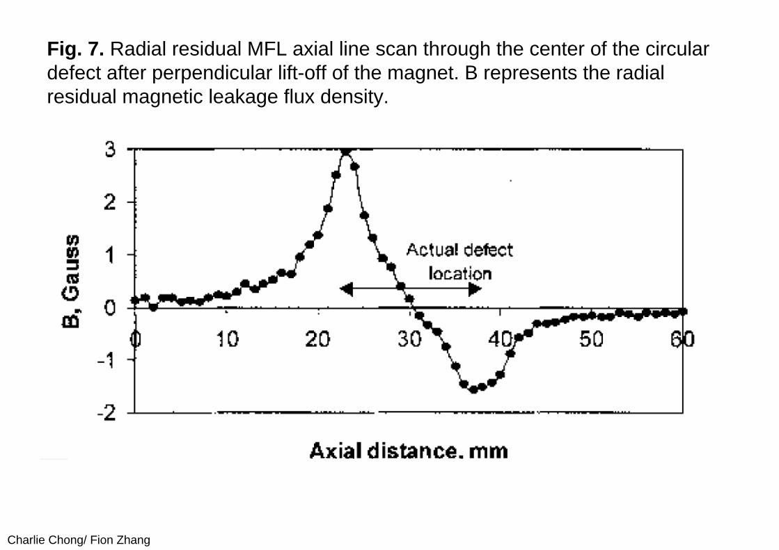
Charlie Chong/ Fion Zhang
Fig. 7. Radial residual MFL axial line scan through the center of the circular defect after perpendicular lift-off of the magnet. B represents the radial residual magnetic leakage flux density.

Charlie Chong/ Fion Zhang
Compare the magnetic flux density of active & residual MFLT
Charlie Chong/ Fion Zhang
(B2) Sliding the magnet along the axial direction- Residual MFL
During actual service conditions the magnets always slide along the pipe axis; therefore subsequent residual scans were made after sliding the magnet along the axial direction on the outer surface of the pipe wall with south pole leading. The contour map and the line scan obtained with this end lift-off method are shown in Figures 8 and 9 and are markedly different from those shown for perpendicular lift-off. There is now a marked asymmetry between the regions of positive and negative flux; the center of positive and negative regions no longer coincide with the edges of the defect, and the region of positive flux is more spread out over the defect.

Charlie Chong/ Fion Zhang
Fig. 8. Contour map of radial residual magnetic leakage flux density (B) after end lift-off of the magnet. Solid and dotted circles represent the actual and apparent locations of the defect, respectively.

Charlie Chong/ Fion Zhang
Fig. 9. Radial residual MFL axial line scan through the center of the circular defect after end lift-off of the magnet. B represents the radial residual magnetic leakage flux density.

Charlie Chong/ Fion Zhang
Active and residual flux distributions
The possible active and residual flux distributions for the above cases are depicted in Figure 10. In the active case when magnet is on the defect, the flux and hence the domains are parallel to the top horizontal surface of the pipe, while those near the sides are oriented almost vertically. The path of flux lines near the edges of the defect is shown in Figure 10(a). When the magnet is lifted perpendicularly, the domains on either side of the defect tend to remain in the vertical orientation. A localized symmetric flux distribution is thus established around the defect, with flux being directed downward on the left, upward on the right, and from right to left over the defect. The flux path is shown in Figure 10(b) and is similar to that reported by Heath. There appear to be induced south and north polarities near the edges of the defect along the axial direction.

Charlie Chong/ Fion Zhang
In the third case of end lift-off with north pole leaving the pipe at the end, the asymmetric flux distribution shown in Figure 10(c) appears to account for the asymmetric MFL pattern of Figure 9. This is due apparently to the slight displacement of the S-N dipole developed on the axial diameter of the defect toward the left, owing to the repulsion from the north pole of the magnet before end lift-off. However, there is a need to verify these results by other methods. Unfortunately, finite element model simulations cannot be used for this purpose unless the domain level phenomena are incorporated into the model.

Charlie Chong/ Fion Zhang
Fig. 10. Probable flux distributions around the circular defect: (a) active, (b) residual with perpendicular lift-off, and (c) residual with end lift-off.
Active magnetization

Charlie Chong/ Fion Zhang
Fig. 10. Probable flux distributions around the circular defect: (a) active, (b) residual with perpendicular lift-off, and (c) residual with end lift-off.
NS End lift-off
Vertical lift-off

Charlie Chong/ Fion Zhang
One of the interesting features of the asymmetric contour map of residual MFL scan with end lift-off of the magnet is that the defect shape is reflected in the radial MFL signal. It is also easy to estimate the size and position of the defect. A close look at Figure 8 indicates an almost circular defect centered on a point of high positive flux marked by the dotted circle. The true location is marked by the solid circle and is slightly toward the negative flux region. The magnitude of the shift in the position of the defect apparently depends on the strength of the magnet and the magnetic properties of the pipeline and can be determined experimentally. It is about 3 mm for the present system. It is also possible to estimate the size of the defect from the axial line scan shown in Figure 9. The diameter of the apparent defect is approximately the length of the horizontal projection of the positive peak.

Charlie Chong/ Fion Zhang
Racetrack defect
The active and residual radial MFL contour maps of the racetrack defect are shown in Figure 11. The solid racetrack boundary in Figure 11(a) indicates the true location of the defect, and the broken boundary in Figure 11(b) indicates its apparent location according to the residual signal. In the active scan, the ends of the defect are located slightly outside the positive and negative peak positions of the flux density but the shape and size of the defect cannot be seen clearly. Conversely, the residual scan gives a clear view of the size and shape of the defect, except with an axial shift of about 3 mm as observed in case of circular defect. The nature of flux pattern of this residual scan, however, differs from that of circular defect. In the residual racetrack pattern, the region of high negative flux is not concentrated at the end of the defect, but on the axial side of it, while the region of high positive flux is present almost everywhere over the defect as observed for circular defect.

Charlie Chong/ Fion Zhang
Fig. 11. Active (a) and residual (b) MFL radial contour maps of racetrackdefect in the absence of stress. The actual and apparent locations of defect are indicated by the solid and broken racetrack boundaries, respectively.

Charlie Chong/ Fion Zhang
This 90-degree rotation of the magnetic flux pattern from the expected axial direction is probably due to the large length of the defect, which does not permit the flux to make long axial loops. Instead, short circumferential flux loops around the defect are energetically more favorable wherein most of the flux lines emerge out of the defect, make loops around one of the long axial sides, and reenter the pipe slightly outside the region of defect. The domains are apparently aligned horizontally along the circumferential direction beneath the defect, but vertically along the axial wall of the defect. This is in spite of the fact that, even in the absence of applied stress, there exists a macroscopic easy axis that is parallel to the axis of the steel pipe section.

Charlie Chong/ Fion Zhang
Irregular gouge
The active and residual MFL scans of the third defect, an irregular gouge, are shown in Figure 12. Although the actual length, width, and maximum depression of the gouge are about 125 mm, 26 mm, and 14 mm, respectively, the overall depression is not limited to an area of just 125 mm 26 mm because of depression of the surrounding region during the gouge formation. The defect is spread over a non-uniform area of about 155 mm 65 mm as indicated in Figure 12 by the elongated closed contour. The active flux pattern of the gouge, as shown in Figure 12(a), does not exhibit longitudinal symmetry, which is expected owing to the non-uniformity in depression as well as width. The only resemblance this pattern has to the racetrack flux pattern of Figure 11(a) is that the upper half pattern shows a region of positive active flux and the lower half shows a region of relatively weak negative flux. The shape of the gouge is not apparent from this pattern.

Charlie Chong/ Fion Zhang
The extreme axial regions of high positive and negative flux are not due to the defect itself, but to the closer approach of the Hall probe detector to the magnetic brushes, where the induced magnetic poles produce spurious flux leakage signals. The residual flux pattern of Figure 12(b), on the other hand, shows a region of positive flux spread over the defect, which helps to estimate the size of the defect more conveniently. Thus, instead of active scans, the residual scans look more promising to reveal the size and shape of this type of irregular defect.

Charlie Chong/ Fion Zhang
Fig. 12. Active (a) and residual (b) radial contour maps of the gouge in the absence of stress. The approximate location of the defect is shown in both.

Charlie Chong/ Fion Zhang
9.5.3.2 Active and Residual MFL Results as a Function of Pipe Wall Stress
In-service oil and gas pipelines are subjected to high stresses (up to 70% of the yield strength); thus the variations in the active MFL patterns brought about by the increased level of stress have been the subject of study. When the pipe is axially magnetized, the higher circumferential stresses are known to affect the active MFL signals and patterns from circular blind-hole defects in two ways:
(1) they rotate the macroscopic magnetic easy axis of the pipe from the axial direction toward the circumferential direction, which causes the change in MFLpp, and
(2) they modify the MFL pattern by producing localized flux variations as a result of stress concentrations around defects.
To study such changes in the residual MFL patterns, measurements were made on circular and racetrack defects at different stress levels.

Charlie Chong/ Fion Zhang
The main interest was to determine if, as at zero stress, the residual patterns could reveal the shape and size of the defects at high stress levels. Figure 13 depicts the residual MFL patterns of both circular and racetrack defects, which were magnetized at a stress level of 0 MPa but then studied at 220 MPa. The corresponding 0 MPa patterns are shown in Figure 8 and 11(b). A comparison of these patterns indicates that a flux rotation of 180 degrees occurs at stress values of 220 MPa, with positive and negative flux regions interchanging their locations. In the case of a circular defect, the negative flux region has two localized regions of comparatively higher flux along the circumferential or stress direction where the stress concentration is higher. Two similar localized positive flux regions, though not clearly seen in Figure 13(a), are developed on the positive side of the flux at higher stresses. The positions of such localized flux regions may be linked to the localized stress concentrations around the defect. The residual pattern of the racetrack defect in Figure 13(b) also shows two pockets of positive and negative flux regions near the four corners of the racetrack.

Charlie Chong/ Fion Zhang
The residual patterns of Figure 13 do not depict the shape of the defects as clearly as seen from patterns of Figures 8 and 11(b), which indicates that the application of stress reorients the magnetic domains along the stress direction, thus disturbing the original pattern. However, if the stress is applied before magnetization, as is done during in-service operation, the residual patterns can still be employed to get useful information about the shape and size of the defect. This is obvious from the residual patterns shown in Figure 14, where the defects were magnetized and also scanned at 220 MPa.

Charlie Chong/ Fion Zhang
Fig. 13. Residual MFL scans of circular (a) and racetrack (b) defects taken at a stress of 220 MPa after magnetizing at 0 MPa. The actual defect locations are shown.

Charlie Chong/ Fion Zhang
Fig. 14. Residual MFL scans of circular (a) and racetrack (b) defects taken at a stress of 220 MPa after magnetizing at the same stress. The actual defect locations are shown.

Charlie Chong/ Fion Zhang
9.5.4 CONCLUSIONSThe residual MFL technique with end lift-off of the magnet appears to be very promising to provide useful information about defect geometry. Although the flux leakage signals weaken at high pressures, the technique still can be used to obtain reasonably good information provided the samples are magnetized at the same high pressure. However, the technique involves the use of sensitive probes to detect the flux leakage signals, which have about one tenth of the strength of the active flux leakage commonly used.

Charlie Chong/ Fion Zhang
Intelligence Pigging – Experts at Work

Charlie Chong/ Fion Zhang
Intelligence Pigging – Experts at Work

Charlie Chong/ Fion Zhang
Deuterium Uranium reactor

Charlie Chong/ Fion Zhang
Deuterium Uranium reactor

Charlie Chong/ Fion Zhang
Offshore E&P

Charlie Chong/ Fion Zhang
Offshore E&P

Charlie Chong/ Fion Zhang http://www.nbcnews.com/id/43455859/ns/us_news-environment/t/safety-rules-loosened-aging-nuclear-reactors/#.VM4fSpCS3IU
Rusted piping at the Byron nuclear plant in Illinois caused this 10-gallon-per-minute leak in Oct. 19, 2007. The water from the pipe cools the reactor in an emergency. The plant was immediately taken offline for repairs.

Charlie Chong/ Fion Zhang
Offshore E&P

Charlie Chong/ Fion Zhang
123
http://www.tudou.com/albumplay/Cdfr-HWahGw/LHxGJ2stVIc.html

Charlie Chong/ Fion Zhang http://www.youku.com/show_page/id_zcbffdabe962411de83b1.html

Charlie Chong/ Fion Zhang

Charlie Chong/ Fion Zhang
ass


