NASA Contractor Report 4697

Electromagnetic Scattering From a Rectangular Cavity Recessed in a 3-D Conducting Surface M. D. Deshpande and C. J. Reddy

Contract NASl-19341 Prepared for Langley Research Center

October 1995

https://ntrs.nasa.gov/search.jsp?R=19960021054 2018-06-16T04:01:22+00:00Z

NASA Contractor Report 4697

Electromagnetic Scattering From a Rectangular Cavity Recessed in a 3-D Conducting Surface M. D. Deshpande ViGYAN, Inc. Hampton, Virginia

C. J. Reddy Hampton University Hampton, Virginia

National Aeronautics and Space Administration Langley Research Center Hampton, Virginia 23681 -0001

Prepared for Langley Research Center under Contract NASI -1 9341

October 1995

Printed copies available from the following:

NASA Center for Aerospace Information 800 Elkridge Landing Road Linthicum Heights, MD 21090-2934 (301) 621-0390

National Technical Information Service (NTIS) 5285 Port Royal Road Springfield, VA 22161-2171 (703) 487-4650

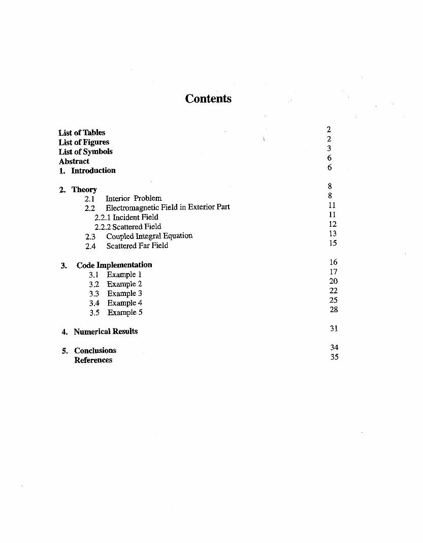
Contents

List of Tables List of Figures List of Symbols Abstract 1. Introduction

2. Theory 2.1 Interior Problem 2.2 Electromagnetic Field in Exterior Part

2.2.1 Incident Field 2.2.2 Scattered Field

2.3 Coupled Integral Equation 2.4 Scattered Far Field

3. Code Implementation 3.1 Example 1 3.2 Example 2 3.3 Example 3 3.4 Example4 3.5 Example5

4. Numerical Results

5. Conclusions References

2 2 3 6 6

8 8 11 11 12 13 15

16 17 20 22 25 28

31

34 35

List of Tables

Table 1 Table 1.1 Table 1.2 Table 1.3 Table 2.1 Table 2.2 Table 2.3 Table 3.1 Table 3.2 Table 3.3 Table 4.1 Table 4.2 Table 4.3 Table 5.1 Table 5.2 Table 5.3

description of *. in ........................................ listing of fileJigure3.SES. ................................. listing of fileJigure3.in ..................................... listing of file Jigure3,out .................................. listing of filefigure4.SES ............................... listing of fileJigure4.in ...................................

listing of fileJigure5SES ............................. listing of fileJigure5.in ..................................

listing of fileJigure6.SES .............................. listing of fileJigure6.in ...................................

listing of fileJigure7.SES ................................ listing of filefigure7.i~~ .....................................

listing of filejgure4.out ................................

listing of fileJigure5.out ................................

listing of fileJigure6.out ................................

listing of fileJigure7.out ...................................

18 19 20 20 21 22 23 24 25 25 26 28 29 29 31 32

List of Figures

Figure 1 A open ended rectangular cavity receeed in a 3D conducting surface and illumi- nated by a plane wave. ..................... 39

Figure 2 Equivalent electric and magnetic surface currents. ...... 40 Figure 3 Backscatter RCS patterns for a rectangular cavity as shown with dimensions

a=0.3 h , b= 0.3 h , c= 0.2 without a ground plane for E- and H- polarized inci- dent plane wave. Solid and hollow triangles indicate numerical

41 Backscatter RCS patterns for a rectangular cavity (a=0.3 h , b a . 3 h, c=0.2h ) embedded in a solid cube with side S =0.5 h, as shown for E- and H-polarized plane wave incidenc ( $i = 0'). Solid and hollow triangles indicate results

42 Backscatter RCS pattern of rectangular cavity with a= 0.3 h, b = 0.3 h, and c = 0.2 h embedded in a conducting circular cylinder as shown with L =0.5 h and r

43. - 0.5 2. ............................. Backscatter RCS pattern of rectangular cavity with x width = 0.7 h, y width 0.31 h, and depth = 0.2 h,, embedded in a conducting circular cylinder as

Backscatter RCS pattern of rectangular cavity with x width = 0.31 h, y width 0.7 h, and depth = 0.2 h,, embedded in a conducting circular cylinder as shown

data obtained using FEM-MOM. ................................. Figure 4

obtained by the method of moments. .... Figure 5

- Figure 6

shown with L = 1 h, r = 0.5 h ....................................

withL =1h,r=0.5h .......................................... 45

44 Figure 7

2

P a

bP

8, (>)

Dn+, D,

List of Symbols x-, y-, and z-dimensions of rectangular cavity

8, (p components of magnetic vector potential due to Bn

areasof D; and D, triangles

magnetic vector potential

complex modal amplitude of p

complex modal amplitude of p

vector basis function for triangular subdomain

matrices resulting from MOM method

(n’, n) th element of matrix [d two triangles associated with n common edge

(n‘, m)

+

th

th

forward travelling mode

backward travelling mode

th

element of matrix [d th

rectangular waveguide vector modal functions for pth mode

transverse electric field vector inside cavity

incident electric field vector

8, (p components of incident electric field

x-, y-, and z-components of incident electric field

magnitude of incident electric field

scattered electric field vector due to ma

scattered electric field vector due to j 8, (p components of scattered electric far field

-+

>

electric vector potential

8, <p components of electric vector potential due to Bm 4

transverse magnetic field vector inside cavity

scattered magnetic field vector due to j

scattered magnetic field vector due to ma

>

+

3

+ Hin incident magnetic field

3 electric surface current density > jl, j

k0

k

electric surface current density over aperture

=A free-space wave number

kx (mn) / a propagation constants along x-direction inside cavity

(nn) / b propagation constants along y-direction inside cavity kY

+ ki L

propagation vector along incidence direction

length of cavity

1, length of nrh edge

magnetic surface current density

integer associated with triangular subdomains total number of triangular elements on aperture total number of triangular elements on 3D surface integer, waveguide modal index

(m', a ) element of matrix [pl (m', rn) element of matrix [Q]

th

th

+ + th rl' r2 position vectors of vertices opposite the n edge

f P Sa

position vector of field point

position vector of source point cavity aperture surface

> surface area over which j exist s c

Tn, r m complex constants

(nl) th element of column matrix [U] (m') rh element of column matrix [V] unit vector along the x-, y-, and z-axis, respectively

%'

'm*

2 , j , 2

4

a0

YO & 0 7 Po

%e

%(P

%q' o(Pe J?EM-MoM ME-MOM EM EFIE 3D RCS

rh propagation constant of p

plane wave incident angle in degrees

mode of cavity

unit vectors

angle in degrees

free-space impedance

permittivity and permeability of fi-ee-space

H co-polarized radar cross section pattern

E co-polarized radar cross section pattern

cross polarized radar cross section pattern finite element method- method of moments modal expansion-method of moments electromagnetic electric field integral equation three dimensional radar cross section

5

Abstract

The problem of electromagnetic (EM) scattering from an aperture backed by

a rectangular cavity recessed in a 3D conducting body is analyzed using the coupled field

integral equation approach. Using the free-space Green’s function, EM fields scattered out-

side the cavity are determined in terms of 1) an equivalent electric surface current density

flowing on the 3D conducting surface of the object including the cavity aperture and 2) an

equivalent magnetic surface current density flowing over the aperture only. The EM fields

inside the cavity are determined using the waveguide modal expansion functions. Making

the total tangential electric and magnetic fields across the aperture continuous and subjecting

the total tangential electric field on the outer conducting 3D surface of the object to zero, a set

of coupled integral equations is obtained. The equivalent electric and magnetic surface cur-

rents are then obtained by solving the coupled integral equation using the Method of

Moments (MOM). The numerical results on scattering from rectangular cavities embedded

in various 3-D objects are compared with the results obtained by other numerical techniques.

1. INTRODUCTION

Electromagnetic scattering characteristic of metallic cavities is useful in studying

radar cross section and electromagnetic penetration properties of objects consisting of these

cavities as substructures. A large amount of analytical work has been done to characterize these

cavity structures. A few references, but not a complete list, are given in [l- 81. However, in

these and similar work, it is assumed that the aperture backed by a cavity is in an infinite flat

ground plane. For a characterization of an aperture formed by a cavity recessed in a finite gound

plane or no ground plane, the asymptotic techniques described in [9- 111 may be used. However,

6

these asymptotic techniques are applicable when the frequency is high or when the cavities are

large in size compared to the operating wavelength. For cavities with size comparable with a

wavelength, a rigorous integral equation formulation has been used to analyze cylindrical circular

cavities [12-131. However, the approach described in [12-131 uses entire domain expansion

functions to represent surface current density and hence is limited to only cylindrical circular

cylinders. A need, therefore, exists to develop general analytical tools to detennine low

frequency electromagnetic characteristics of open-ended waveguide cavities without a flang or

recessed in 3D counducting surface.

In this paper the problem of EM scattering of plane waves by a cylindrical cavity

recessed in a 3D metallic object is studied. Using the equivalence principle, the electromagnetic

field scattered outside the object is determined using free space Green’s function and the

equivalent electric and magnetic surface currents assumed to be present on the outer surface of the

object. The equivalent electric surface current is assumed to be flowing over the complete 3D

surface including the aperture and the equivalent magnetic surface current is assumed to be

flowing over only aperture. The field inside the cavity are obtained using waveguide modal

expansion functions. Making the total tangential electric and magnetic fields across the aperture

continuous and the total tangential electric field zero over the conducting surface only, a set of

coupled integral equations is obtained. Expanding the surface currents in triangular subdomain

. functions [ 141 and using the Method of Moments, the coupled integral equations are reduced to

algebric equations which are solved for the surface current densities. From the surface currents

the radar cross sections of these cavities recessed in an arbitrarily shaped conducting objects are

determined. For future reference, this method is refered to as Modal Expansion and Method of

Moments ( ME-MOM).

7

The remainder of report is organized as follows. The formulation of the problem in

terms of coupled integral equations using surface equivalence principle is developed in section 2.

Numerical results on radar cross section of open-ended rectangular cavities recessed in a

rectangular and finite circular cylinder are presented in section 3. Comparison of the numerical

results obtained by the present method with other numerical techniques is also presented in

section 3. The advantages and limitations of the present formulation are discussed in section 4.

2. THEORY

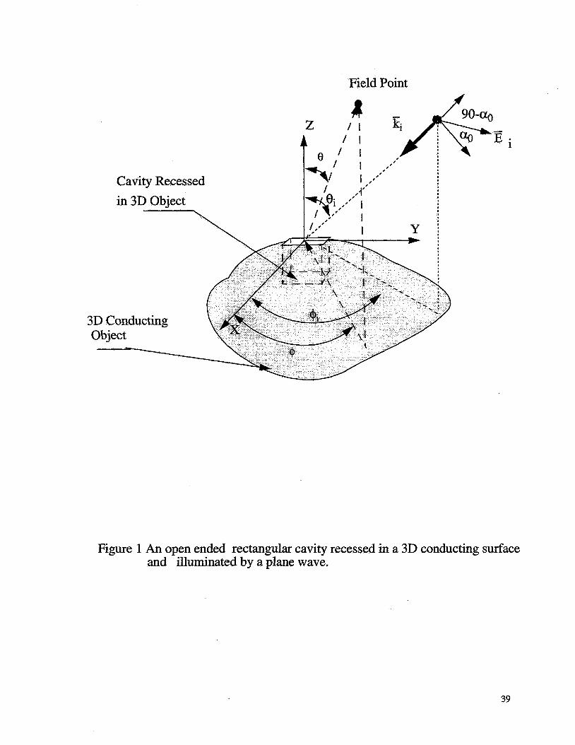
Consider a time harmonic electromagnetic plane wave incident on a 3D conducting

object with an aperture backed by a rectangular cavity as shown in figure 1. The cavity is formed

by a shorting plate at z = -L. To facilitate the solution of the problem, the equivalence principle is

applied by using the equivalent surface currents as shown in figure 2. For determining the fields

> outside the cavity (exterior problem), we consider the equivalent currents j and &a radiating in

free space. The electromagnetic field inside the cavity ( interior problem ) is obtained using

modal expansion.

2.1 Interior Problem:

The transverse components of fields inside the cavity may be obtained using the

procedure given in [l5]. Expressing the transverse electric and magnetic fields in terms

of vector modal functions and satisfymg the boundary conditions, the fields inside the

cavity may be written as

8

2 2 where yp is the propagation constant, equal to ,,/- , k = kOE,p,, ( E, and pr

are relative permittivity and permeability of medium inside the cavity ),

admittance, > 3 + j l A = 2 x H t , Ht being the tangential magnetic

ep (x , y ) = hp (x , y ) x 2 , 2 being the unit vector along the z-axis.

Yp is the modal

e p ( x , y ) and h p ( x , y ) are the vector modal functions as defined in [15],

and

+ +

field over the aperture, + +

If the 3D surface is divided into triangular subdomains, the electric current over

the surface of the 3D object including the aperture may be expressed in terms of

triangular basis functions as E141 N

n = l

th + where Tn is the amplitude of electric current normal to the n edge, B n (P) is the

edge, and N is the number of non-boundary edges on the th vector basis fuction associated with n

surface of the object. The expression for basis function is given by [ 141

2 A -

when

when

+ r' in

+ r' in

(4)

+ where Dn+ and D i are the two triangles with the nth common edge, A and A - are + + +

the areas of D, and D, triangles, respectively, and rl and r2 are position vectors of vertices

th opposite the the n common edge of Dn+ and D i triangles, respectively. Likewise the

magnetic current over the aperture may be written as

9

m = I

where rm is amplitude of magnetic current normal to the mth edge, and M is the number

of non-boudary edges over the aperture. Substituting (3) in equations (1) and (2), the total fields

inside the cavity are obtained as

2.2 Electromagnetic Field in Exterior Part:

In the exterior part, the total electromagnetic field is obtained by superposing the

> scattered field due to j and & , and the incident field.

2.2.1 Incident Field:

The incident field with time variation ejor may be written as + > + -jk; r

Ein = ( biEei + + i ~ + ) e (8)

3 9 where ki = -ko [?Cos (@i) Sin ( ei) + f S i n (Qi) Sin (e,) + &Cos ( O i ) ] , Y = ?x + fy + 22,

E,; = lE4 Cos (a,) , and E+i = lE4 Sin (a,) , and k, being the free-space wave number. With

reference to figure 1, a, = 0 corresponds to H-polarization anda, = 90 corresponds to E-

polarization.

written, respectively, as

3 3

0

From equation (8), the x-, y-, and z-components of the incident field may be

Exi = Ee;COS (Eli) Cos ( @i) - Egisin ( qi) (9)

10

EYi = EeiCOS ( ei) Sin (q i ) + E 4 i C ~ ~ (qi)

Ezi = -EeiSin (ei)

The corresponding magnetic field components are obtained through

where qo is the free-space impedance. The incident field with Eei f 0 and E+i = 0 is called

H-polarized wave and Eei = 0 and E$j f 0 is called the E-polarized wave.

2.2.2 Scattered Field:

> The scattered field outside the cavity due to j and za may be obtained through

vector electric and magnetic potentials as

1 + SS[>) = -vxA PO

where the electric and magnetic vector potentials are given by

11

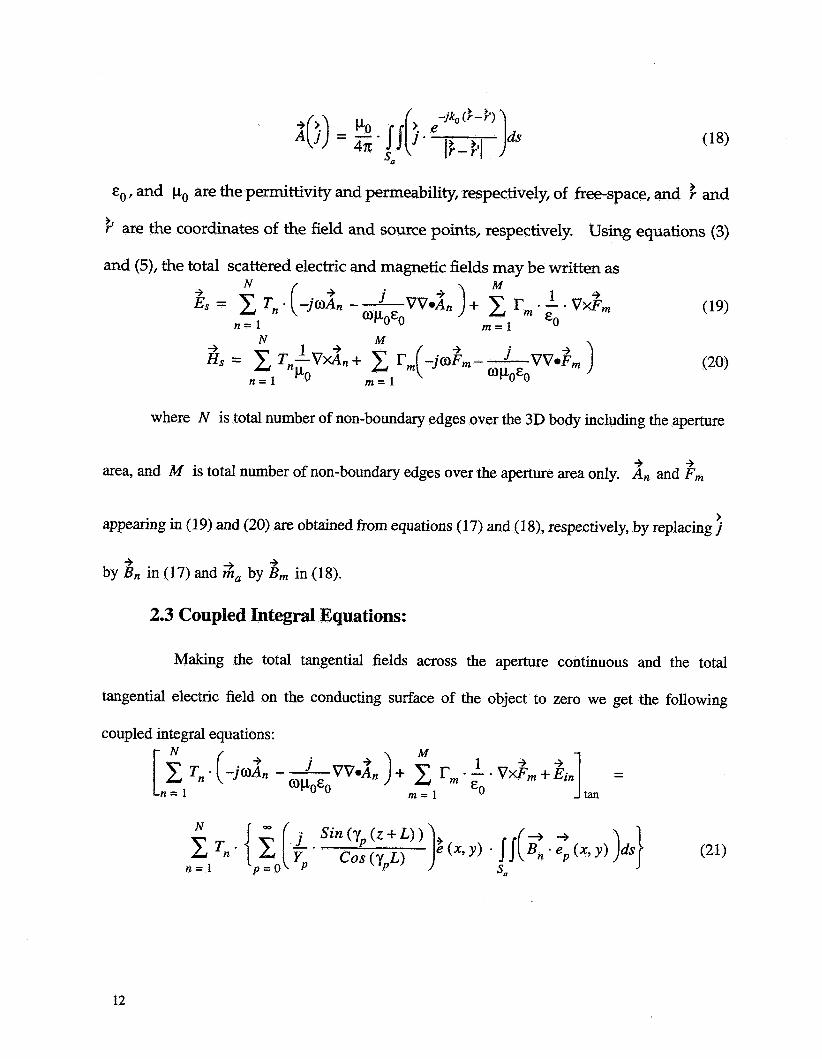
, and p,, are the permittivity and permeability, respectively, of free-space, and f and

> are the coordinates of the field and source points, respectively. Using equations (3)

and (5), the total scattered electric and magnetic fields may be written as

where N is total number of non-boundary edges over the 3D body including the aperture

+ + area, and M is total number of non-boundary edges over the aperture area only. An and Fm

> appearing in (1 9) and (20) are obtained from equations (17) and (1 S), respectively, by replacing j

+ + by B n in (17) and &a by B m in (18).

2.3 Coupled Integral Equations:

Making the total tangential fields across the aperture continuous and the total

tangential electric field on the conducting surface of the object to zero we get the following

coupled integral N

N

equations:

12

1

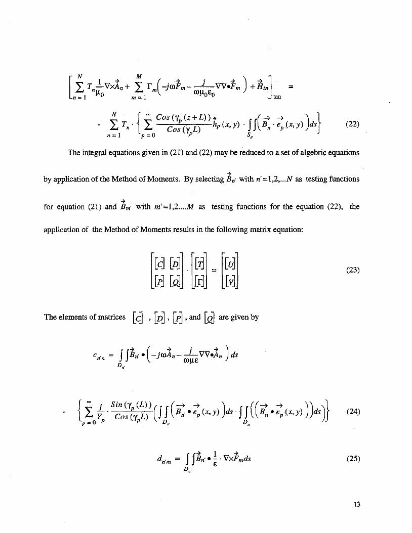
The integral equations given in (21) and (22) may be reduced to a set of algebric equations

+ by application of the Method of Moments. By selecting Bnl with n' =1,2, ... N as testing functions

+ for equation (21) and Bm* with m'=1,2 .... M as testing functions for the equation (22), the

application of the Method of Moments results in the following matrix equation:

The elements of matrices [d , [d , [d , and [d are given by

13

The elements of column matrices [d and [~ are given by

In evaluating numerical values of expressions (24)-(28), numerical integration over

the triangles are perfonned using thirteen point gauss quadrature formula 1161. For evaluation of

self terms; i.e., when n = n' or m = m' , closed form expressions for these expressions given in

1.171 are used. The unknown electric and magnetic current amplitudes obtained after solving the

matrix equation (23) can be used to detennine scattered far field using expression (19) and (20).

2.4 Scattered Far Field:

Using the far field approximation, the scattered electric far field may be obtained from

equation (19) as N M

Ese = - Tn - @Ane - T,Jko. Fmo n = 1 m = l

N M

n = l m = l

14

The copolarized radar cross section patterns of an aperture backed by a cavity in a 3D conducting

surface can be obtained from .. 21Ese12 c,, = lim 4xr -

r+oJ

for H-polarized incidence and

cqq = lim4n;r - r + =

for E-polarized incidence. The cross-polarized radar cross section pattern is obtained from

(33)

(34)

15

3. CODE ~ P L E ~ N T A T I O N

Variable

*.MOD

output file name

The coupled field integral equation approach to solve the problem of scattering from a

rectangular waveguide embedded in a 3D conducting surface has been implemented through a

code named scatt-reap-recav-3d (scattering from s tangular a+pxture backed by a stangular

Description

Name of input file containing nodes and element infor- mation

Name of output file where output is stored

- a i t y embedded in a &conducting object).

For running the scatt-reap-recav-3d code, the given geometry is modelled using

COSMOSN. In using COSMOS/M, it is assumed that user is familiar with operation of

COSMOSN. All dimensions of 3D surface and rectangular cavity are normalized with respect to

the operating wavelength.

The input variables must be defined in a file called *.in before running scatt-reap-recuv-3d

ihigher

ite, itm

alpha

A sample of *.in is given in Table 1.

an integer, if zero only dominant mode in the cavity is considered. It also skips next line if " ihigher " is zero

integers, read only if " ihigher" is not zero. ite is number of T.E modes and itm is number of TM modes to be con- sidered in the cavity

0 for H-polarization 90 for E-polarization

aa,bb x- and y-dimensions of rectangular cavity in wavelength

al0 length of cavity in wavelength

16

Table 1: Description ofl' .in file

die, emie complex relative permittivity and permeability of medium inside the cavity

To demonstrate use of the code, the following examples are considered in this report

1) rectangular cavity without a ground plane

2) rectangular cavity embedded in a conducting cube

3) rectangular cavity embedded at the end of finite circular cylinder

4) rectangular cavity embedded in the curve surface of finite circular cylinder

3.1 EXAMPLE 1

To illustrate use of variables defined in Table I, a rectangular cavity shown in figure 3 is

taken as an example. To generate *.MOD file for the geometry of figure 3 ,&ur&.SSfile given

in Table 1.1 is first run with COSMOSN. The *.MOD file thus generated is named as

&urd.MOz>. The&urd.infile used for running the scatt_reu.~reuzv_36code is shown in Table 1.2

and a sample output of scatt_reap_recau_36 shown in Table 1.3.

Table 1.1 Listing of&urd.=

C* COSMOSN Geostar V1.70 C* Problem : cube C" PT 1 0 0 0 pT 2 -0.15 -0.15 0 PT 3 0.15 -0.15 0

Date : 11-29-94 Time : 8:47: 4

pT4 0.15 0.15 0

17

PT 5 -0.15 0.15 0 PT 6 -0.15 -0.15 -0.2 PT 7 0.15 -0.15 -0.2 Pl” 8 0.15 0.15 -0.2 FT 9 -0.15 0.15 -0.2 SCALE 0 CRLINE123 C R L N 2 3 4 cRLINE345 CRLINE452 CRLINE567 CRLINE678 CRLINE 7 8 9 CRLINE896 CRLLNE926 CRLINE 10 3 7 CRLINE 11 4 8 CRLINE 12 5 9 CT 100.064 1 2 3 4 0 CT200.0642 106 110 1 C T 3 0 0 . 0 6 4 6 7 8 5 0 1 CT400.064498 120 1 CT500.064 1 1 0 5 9 0 1 CT600.0643 11 7 120 1 R G 1 1 1 0 R G 2 1 2 0 R G 3 1 3 0 R G 4 1 4 0 RG5 1 5 0 R G 6 1 6 0 PH 1 RG 1 0.06 0.0001 1 MA-PH 1 1 1 P R G 1 1 1 1 1 4 NMERGE NCOMPRESS NTCR1111 NPCR2221 NJCR333 1 QCR444 1

Table 1.2 Listing of &ure3.in

figure3,MOD figure3 .out 0.3,0.3 0.2

“ Input file with node and element information” “ Output file with RCS as a function of look angle” “ x- and y- dimensions normalized with wavelength of rectangular cavity length of cavity normalized with respect to wavelength

18

1 10 10 0 o.,o. 1 .,o 30. frequency in GHz (l.,O.),(l.,O.) complex relative permittivity and permeability of medium inside cavity

integer flag to consider higher order modes in the cavity number of TE modes to be considered number of TM modes to be considered alpha = 0 for H-polarization theta and phi incident angles in degrees increment in theta and phi in degrees

Table 1.3 Listing of &we3.out

X-dimension of WG = 0.3000000 wavelength Y-dimension of WG = 0.3000000 wavelength Length of WG cavity = 0.2000000 wavelength

20 Number of Nodes Used = 128 Number of Elements Used = Number of nonboundary edges = Number of nonboundary edges (aperture) = 65 Frequency in Ghz = 30.00000 alphatheta Phi cross-pol(RCS)co-pol(RCS )

Number of waveguide modes =

252 378

0.0. 0. -42.90524 0.1645633 0.1 .oooooo 0. -42.87325 0.1629779 0.2.000000 0. -42.85700 0.1584223 0.3.000000 0. -42.85587 0.1508932 0.4.000000 0. -42.86822 0.140369 1 0.5.000000 0. -42.89356 0.1268443 0.6.oooO00 0. -42.93044 0.1 1029 18 0.7.000000 0. -42.97783 9.067788OE-02 0.8.000000 0. -43.03438 6.7987286E-02 0.9.Oooo00 0. -43.09773 4.2 179674E-02 0.10.00000 0. -43.1657 1 1.3209 175E-02 ********** *** ******** ************ ********** *** ******** ************ 0.17 1 .OOOO 0. -49.14130 -0.9871500 0.172.0000 0. -49.60229 -0.9702910 0.173.0000 0. -50.03440 -0.9554753 0.174.0000 0. -50.42996 -0.9426595 0.175.0000 0. -50.78228 -0.93 18268 0.176.0000 0. -5 1.08 1 17 -0.9229562 0.177.0000 0. -5 1.32377 -0.9 160256 0.178.0000 0. -51.50285 -0.9110218 0.179.0000 0. -5 1.6 1285 -0.9079247 0.180.0000 0. -5 1.65466 -0.906749 1

19

3.2 EXAMPLE 2

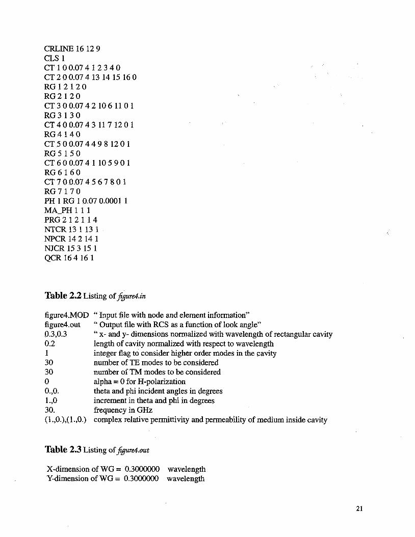
A rectangular cavity embedded in a metal cube as shown in figure 4 is considered as a second example. The *.SES, *. in, and *. out files used to for the problem are shown in Tables 2.1,2.2, and 2.3.

Table 2.1 Listing of & u r e 4 . ~ ~

C" C* COSMOSM Geostar V1.70 C* Problem : figur4 C" PLANEZ01 VIEW0010 PT 1 -0.25 -0.25 0 PT. 2 0.25 -0.25 0

Date : 1-11-95 Time : 10:25:41

PT 3 0.25 0.25 0

SCALE 0 PT 4 -0.25 0.25 0

PT 5 -0.25 -0.25 -0.5 PT 6 0.25 -0.25 -0.5 PT 7 0.25 0.25 -0.5 PT 8 -0.25 0.25 -0.5 PT 9 -0.15 -0.15 0 PT 10 0.15 -0.15 0 PT 11 0.15 0.15 0 PT 12 -0.15 0.15 0 VIEW1110 SCALE 0 cRLINE112 CFiLlNE223 cRLINE334 CRLINE441 CRLINE556 CRLINE667 C K I N E 7 7 8 CRLINE885 CRLINE9 1 5 CRLINE 10 2 6 CRLINE 11 3 7 CRLINE1248 CRLINE 13 9 10 CRLINE 14 10 11 C R L m 15 11 12

20

CRLINE 16 12 9 CLS 1 CT 100.07 4 1 2 3 4 0 CT200.074 13 14 15 160 R G 1 2 1 2 0 R G 2 1 2 0 CT300.0742 106 11 0 1 RG3 1 3 0 CT400.0743 11 7 120 1 R G 4 1 4 0 CT500.074498 1201 R G 5 1 5 0 CT600.074 1 1 0 5 9 0 1 RG6 1 6 0 CT700 .074567801 R G 7 1 7 0 PH 1 RG 1 0.07 0.0001 1 MA-PH 1 1 1 PRG212114 NTCR 13 1 13 1 NPCR 14 2 14 1 NJCR 15 3 15 1 QCR 164 16 1

Table 2.2 Listing of &ured.in

figure4.MOD I‘ Input file with node and element information” figure4.out “ Output file with RCS as a function of look angle” 0.3,0.3 “ x- and y- dimensions normalized with wavelength of rectangular cavity 0.2 length of cavity normalized with respect to wavelength 1 integer flag to consider higher order modes in the cavity 30 number of TE modes to be considered 30 number of TM modes to be considered 0 alpha = 0 for H-polarization o.,o. theta and phi incident angles in degrees 1 .,o increment in theta and phi in degrees 30. frequency in GHz (1 .,O.),( 1 .,O.) complex relative permittivity and permeability of medium inside cavity

Table 2.3 Listing of &ure4.out

X-dimension of WG = 0.300oooO wavelength Y-dimension of WG = 0.3000000 wavelength

21

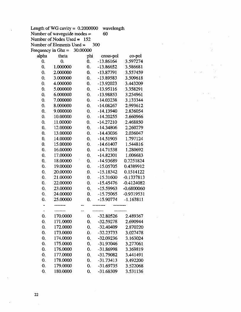
Length of WG cavity = 0.2oooO00 wavelength Number of waveguide modes = 60 Number of Nodes Used = 152 Number of Elements Used = Frequency in Ghz = 30.00000

300

alpha 0. 0. 0. 0. 0. 0. 0. 0. 0. 0. 0. 0. 0. 0. 0. 0. 0. 0. 0. 0. 0. 0. 0. 0. 0. 0. - - 0. 0. 0. 0. 0. 0. 0. 0. 0. 0. 0.

22

theta 0.

1 . 0 0 m 2.000000 3.000000 4.000000 5.000000 6.000000 7.000000 8.000000 9 . o o m 1 0,00000 1 1 .00000 12.00000 13.00000 14.00000 15.00000 16.000OO 17.00000 18.00000 19.00000 20.00000 2 1 .00000 22.00000 23.00000 24.00000 25.00000 - - - - - - - ------- 170.0000 17 1 .0000 172.0000 173.0000 174.0OOO 175.oooO 176.0000 177.0000 178.0000 179.0000 180.0000

Phi 0. 0. 0. 0. 0. 0. 0. 0. 0. 0. 0. 0. 0. 0. 0. 0. 0. 0. 0. 0. 0. 0. 0. 0. 0. 0.

cross-pol - 13.86164 - 13.86652 - 13.8779 1 -13.89583 -13.92023 - 13.95 116 -13.98853 - 14.03238 - 14.08267 - 14.13940 -14.20255 -14.27210 -14.34806 - 14.43036 - 14.5 1905 - 14.6 1407 -14.71538 -14.82301 -14.93689 -15.05705 -15.18342 - 15.3 1600 - 1 5.45476 -15.59963 - 15.75065 -15.90774

eo-pol 3.597274 3.586681 3.557459 3.5096 18 3 .443209 3.358291 3.25496 1 3.133344 2.993612 2.836054 2.660966 2.468850 2.260279 2.036047 1.797 124 1.544816 1.280692 1.006683

0.725 1824 0.4389912 0.15 14 122 -0.1337813 -0.4 124082 -0.6800060 -0.93 1953 1 -1.16381 1

-- ------- -------- 0. -32.80526 2.489367 0. -32.59278 2.690944 0. -32.40409 2.870220 0. -32.23733 3.027478 0. -32.09236 3.163024 0. -3 1.97046 3.277061 0. -31.86998 3.369819 0. -31.79082 3.441491 0. -3 1.734 13 3.492200 0. -31.69735 3.522068 0. -31.68309 3.531136

3.3 Example 3 In this example a rectangular aperture backed by a rectangular cavity placed at the one end of a finite circular cylinder as shown in figure 5 is considered. *. SES, *. in, and *. out files used for this problem are shown in Tables 3.1,3.2, and 3.3, respectively.

Table 3.1 Listing of&rd .m

C* C* COSMOSM Geostar V1.70 C* Problem : figure5 C* C* FILE temp1.SES 1 1 1 1 PLANEZO 1 VIEW00 1 0 PT 1 0 0 0 PT 2 0.35 0.35 0 SCALE 0 CRPCIRC 1 1 2 0.494975 360 4 SCALE 0 SCALE 0

Date : 1-25-95 Time : 15:52:43

PT 6 0 0 -0.5 PT 7 0.35 0.35 -0.5 SCALE 0 VIEW1110 CRPCIRC 5 6 7 0.494975 360 4 PT 11 -0.15 -0.15 0 PT 12 0.15 -0.15 0 PT 13 0.15 0.15 0

CRLINE927 CRLINE 10 3 8 CRLINE 11 4 9 CRLINE 12 5 10 CRLINE 13 11 12 CRLINE 14 12 13 CRLINE 15 13 14 CRLINE 16 14 11 CRLINE 17 12 5 CRLINE 18 13 2 CRLINE 19 14 3 CRLINE 20 11 4

PT 14 -0.15 0.15 0

23

SF4CR 1 3 17 13 20 0 SF4CR 2 17 4 18 14 0 SF4CR 3 18 1 19 15 0 SF4CR 4 19 2 20 16 0 SF4CR 5 13 14 15 16 0 SF4CR6 1 9 5 100 SF4CR71061120 SF4CR 8 11 3 12 7 0 SF4CR9 1 2 8 9 4 0 SF4CR 10 5 6 7 8 0 PH 1 SF 1 0.1 0.0001 1 MA-PH 1 1 1 NTCR 13 1 13 1 NPCR 14 2 14 1 NJCR 15 3 15 1 QCR 164 16 1 PSF 5 1 5 1 1 1 4 NMERGE 1 831 1 O.OOO10 1 0 NCOMPRESS 1 831

Table 3.2 Listing of &preGn

figure5.MOD “ Input file with node and element information” figure5.out “ Output file with RCS as a function of look angle” 0.3,0.3 “ x- and y- dimensions normalized with wavelength of rectangular cavity 0.2 length of cavity normalized with respect to wavelength 1 integer flag to consider higher order modes in the cavity 10 number of TE modes to be considered 10 number of TM modes to be considered 0 alpha = 0 for H-polarization ( for E-polarization alpha =90) o.,o. theta and phi incident angles in degrees 1.,0 increment in theta and phi in degrees 30. frequency in GHz (1 .,O.),( 1 .,O.) complex relative permittivity and permeability of medium inside cavity

Table 3.3 Listing of@ref;.out

X-dimension of WG = 0.3000000 wavelength Y-dimension of WG = 0.3000000 wavelength Length of WG cavity = 0.2000000 wavelength

20 Number of Nodes Used = 83 1 Number of Elements Used = Frequency in Ghz = 30.00000

Number of waveguide modes =

1658

24

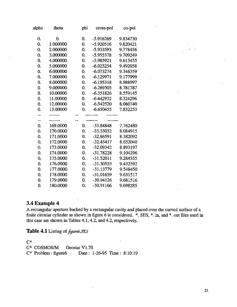
alpha theta phi cross-pol co-pol

0. 0. 0. 0. 0. 0. 0. 0. 0. 0. 0. 0. 0. 0. -- -- 0. 0. 0. 0. 0. 0. 0. 0. 0. 0. 0. 0.

0. 1 .000000 2.000000 3.000000 4 . m 0 0 5.000000 6.oooO00 7.000000 8 . m o o 9.000000 10.00000 1 1 .00000 12.00000 13.00000 - - - - - - - - - - - - - 169.0000 170.oooO 17 1 .OOOO 172.0000 173.0000 174.00OO 175.oooO 176.0000 177.0000 178.0000 179.0000 18O.oooo

0. 0. 0. 0. 0. 0. 0. 0. 0. 0. 0. 0. 0. 0.

-- ---.

-5.9 16269 -5.9205 16 -5.933593 -5.955378 -5.98592 1 -6.025254 -6.073274 -6.12997 1 -6.1953 18 -6.269305 -6.351826 -6.442932 -6.542520 -6.650455

----- - - - - - - - -- ------- --_----

0. -33.84848 0. -33.33032 0. -32.86591 0. -32.45417 0. -32.09342 0. -31.78228 0. -31.52011 0. -31.30555 0. -31.13779 0. -31.01659 0. -30.94126 0. -30.91166

9.834730 9.820421 9.778456 9.709249 9.613455 9.492058 9.346359 9.177999 8.988997 8.781787 8.559145 8.3 24296 8.080740 7.832253

7.762480 8.084915 8.3 82092 8.652040 8.893 197 9.104296 9.284355 9.432592 9.548450 9.63 1517 9.68 15 16 9.698285

3.4 Example 4 A rectangular aperture backed by a rectangular cavity and placed over the curved surface of a finite circular cylinder as shown in figure 6 is considered. *. SES, *. in, and *. out files used in this case are shown in Tables 4.1,4.2, and 4.2, respectively.

Table 4.1 Listing of&m6.S=

C" C* COSMOSM Geostar V1.70 C* Problem : figure6 Date : 1-26-95 Time : 8: 10: 19

25

C* C* FILE temp1.SES 1 1 1 1 PLANEZO 1 VIEW0010 PTlOOO PT 2 -0.35 -0.1505 0 PT 3 0.35 -0.1505 0 PT 4 0.35 0.1505 0 PT 5 -0.35 0.1505 0 PT 6 -0.35 -0.1505 0.1 PT 7 0.35 -0.1505 0.1 PT 8 0.35 0.1505 0.1 PT 9 -0.35 0.1505 0.1 SCALE 0 VIEW1110 PT 10 -0.35 0 -0.38 SCALE 0 PLANEXO 1 CRPCIRC 1 10 9 0.503041 34.82 1 CRPCIRC 2 10 6 0.503041 55.18 1 CRPCIRC 3 10 11 0.503041 270 3 SCALE 0 PT 14 -0.5 0 -0.38 PT 15 -0.5 0.1505 0.1 PT 16 -0.5 -0.1505 0.1 CRPCIRC 6 14 15 0.503041 34.82 1 CRPCIRC 7 14 16 0.503041 55.18 1 CRPCIRC 8 14 17 0.503041 270 3 CT100 .1556789100 R G 1 1 1 0 CRLINE 11 15 9 CRLINE 12 16 6 CRLINE 13 17 11 CRLINE 14 18 12 CRLINE 15 19 13 SF4CR 1 6 12 1 11 0 SF4CR 2 12 7 13 2 0 SF4CR 3 13 3 14 8 0 SF4CR41441590 SF4CR5 15 10 11 5 0 CRLINE 16 9 5 CRLINE 17 5 2 CRLINE 18 6 2 SF4CR 6 1 18 17 16 0 CRLINE 19 9 8 CRLINE 20 5 4

26

C R L M 2 1 8 4 SF4CR 7 16 19 21 20 0 CRLINE 22 8 7 CRLINE 23 4 3 C R L N 24 7 3 PT 20 0.35 0 -0.38 PLANEX01 CRPCIRC 27 20 8 0.503041 34.82 1 SF4CR 8 27 24 23 21 0 C R L M 25 6 7 CRLINE 26 2 3 SF4CR 9 18 26 24 25 0 SF4CR 10 17 20 23 26 0 CRPCIRC 28 20 7 0.503041 55.18 1 CRPCIRC 29 20 21 0.503041 270 3 CRLINE 32 9 6

PT 25 0.5 0.1505 0.1 PT 26 0.5 -0.1505 0.1 PLANEXO 1 CRPCIRC 37 24 25 0.503041 34.82 1 CRPCIRC 38 24 26 0.503041 55.18 1 CRPCIRC 39 24 27 0.503041 270 3 CT 2 0 0.15 5 37 38 39 40 41 0 R G 2 1 2 0 CRLINE 42 8 25 CRLINE 43 7 26 SF4CR 13 42 37 43 27 0 CRLINE44 21 27 SF4CR 14 43 38 44 28 0 CRLINE 45 22 28 SF4CR 15 29 44 39 45 0 CRLINE 46 23 29 SF4CR 16 45 40 46 30 0 SF4CR 17 46 41 42 31 0 cRLINE47 11 21 CLS 1 SF4CR 18 2 47 28 25 0 CRLINE48 12 22 SF4CR 19 3 47 29 48 0

SF4CR 20 4 48 30 49 0 SF4CR 21 5 49 31 19 0 PH 1 SF 1 0.1 0.0001 1 CLS 1 MA-PH 1 1 1

PT 24 0.5 0 -0.38

cmm 49 13 23

27

v E w 0 0 1 0 VIEW1110 PSF 10 1 10 1 1 1 4 CLS 1 CLS 1 NTCR26 126 1 NPCR 23 2 23 1 NJCR 20 3 20 1 QCR 174 17 1 CLS 1

Table 4.2 Listing of f iure6. i~~

figure6.MOD figure6.out 0.7,0.3 1 0.1 1 30 30 0 o.,o. 1 .,o 30. (1 .,O.),(l.,OJ

“ Input file with node and element information” “ Output file with RCS as a function of look angle” “ x- and y- dimensions normalized with wavelength of rectangular cavity length of cavity normalized with respect to wavelength integer flag to consider higher order modes in the cavity number of TE modes to be considered number of TM modes to be considered alpha = 0 for H-polarization ( for E-polarization alpha =90) theta and phi incident angles in degrees increment in theta and phi in degrees frequency in GHz complex relative permittivity and permeability of medium inside cavity

Table 4.3 Listing of &ure6.out

X-dimension of WG = 0.7oooO00 wavelength Y-dimension of WG = 0.3 100OOO wavelength Length of WG cavity = 0.1000000 wavelength Number of waveguide modes = 60 Number of Nodes Used = 552 Number of Elements Used = Frequency in Ghz = 30.00000

1100

alpha theta phi cross-pol co-pol

0. 0. 0. -5.933923 6.34727 1 0. 1.000000 0. -5.935130 6.339834 0. 2.000000 0. -5.946536 6.312681

28

0. 0. 0. 0. 0. 0. 0. 0. -- -- 0. 0. 0. 0. 0. 0. 0.

3 .m 4.000000 5.000000 6.000000 7.000000 8.000000 9.000000 10.00000 ------- - - - - - - - 174.oooO 175.0000 176.oooO 177.0000 178 .WOO 179.0000 180.0000

0. -5.968001 6.266007 0. -5.999329 6.200232 0. -6.0405 10 6.115752 0. -6.09 1329 6.0 13002 0. -6.151697 5.892314 0. -6.221767 5.753819 0. -6.301365 5.597322 0. -6.390241 5.422188

-- ------- -------- -- ------ --------

0. -58.31413 4.871758 0. -57.79329 5.028406 0. -57.26915 5.159277 0. -56.59153 5.262630 0. -55.61058 5.337103 0. -54.31091 5.381660 0. -52.79220 5.395699

3.5 Example 5 In this example a rectangular aperture by backed by a rectangular cavity and placed dong the circumference of a finite conducting circular cylinder, as shown in figure 7 is considered. *.SES, *. in, and *. out files used to run this case are shown in Tables 5.1,5.2, and 5.3, respectively.

Table 5.1 Listing of&ure7..SZS

C* C* COSMOSN Geostar V1.70 C* Problem : figure7 C* C* F?LE figure7.SES 1 1 1 1 PLANEZO 1 VIEW 0 0 1 0 PTlOOO PT 2 -0.1505 -0.35 0 PT 3 0.1505 -0.35 0

Date : 1-30-95 Time : 11:33:48

PT 4 0.1505 0.35 0 PT 5 -0.1505 0.35 0

29

PT 6 -0.1505 -0.35 0.1 PT 7 0.1505 -0.35 0.1 PT 8 0.1505 0.35 0.1 PT 9 -0.1505 0.35 0.1 PT 10 -0.1505 0 -0.25 SCALE 0 VIEW1110 PLANEX01 CRPCIRC 1 10 9 0.494975 90 1 CRPCIRC 2 10 6 0.494975 270 3 SCALE 0 PT 13 -0.1505 0 -0.25 PT 13 -0.5 0 -0.25 PT 14 -0.5 0.35 0.1 PT 15 -0.5 -0.35 0.1 CRPCIRC 5 13 14 0.494975 90 1 CRPCIRC 6 13 15 0.494975 270 3 SCALE 0 CT 100.1 4 5 6 7 8 0 R G l l l O CRLINE 10 15 6 CRLINE 11 14 9 SF4CR11115100 CRLINE 12 16 11 SF4CR 2 10 2 12 6 0 CRLINE 13 17 12 SF4CR 3 12 3 13 7 0 SF4CR4 134 11 8 0 CRLINE 14 9 5 CRLINE 15 6 2 CRLINE 16 2 5 CRLINE 17 5 4 CRLINE 18 4 3 CFUNE 19 3 2 CRLINE 20 8 4 CRLINE 21 7 3

CRPCIRC 22 18 8 0.494975 90 1 CRPCIRC 23 18 7 0.494975 270 3 CRLINE 26 9 8 CRLINE27 1220 SF4CR 5 26 25 27 4 0 CRLINE 28 11 19 SF4CR 6 27 24 28 3 0 CRLINE 29 6 7 SF4CR 7 28 23 29 2 0

PT 18 0.1505 0 -0.25

30

SF4CR9 1 14 16 15 0 SF4CR 10 26 20 17 14 0 SF4CR 11 22 21 18 20 0 SF4CR 12 29 21 19 15 0 SF4CR 13 16 19 18 17 0

PT 22 0.5 0.35 0.1

SCALE 0 CRPCIRC 30 21 22 0.494975 90 1 CRPCIRC 3 1 2 1 23 0.494975 270 3 CT 2 0 0.1 4 30 31 32 33 0 R G 2 1 2 0 CRLINE 34 8 22 CRLINE 35 7 23 SF4CR 14 34 30 35 22 0 CRLINE 36 19 24 SF4CR 15 35 31 36 23 0 CRLINE 37 20 25 SF4CR 16 36 32 37 24 0 SF4CR 17 37 33 34 25 0 PH 1 SF 10.1 0.0001 1 CLS 1 MA-PH 1 1 1 CLS 1 PSF 13 1 13 1 1 1 4 NTCR 19 1 19 1 NPCR 18 2 18 1 NJCR 17 3 17 1 QCR 164 16 1

Table 5.2 Listing of figuTe7.in

PT 21 0.5 0 -0.25

PT 23 0.5 -0.35 0.1

figure7.MOD figure7.0~ 0.3 1,0.7 0.1 1 30 30 0 o.,o. 1 .,o 30. (1 .,0.),(1$.)

" Input file with node and element information7' " Output file with RCS as a function of look angle" " x- and y- dimensions normalized with wavelength of rectangular cavity length of cavity normalized with respect to wavelength integer flag to consider higher order modes in the cavity number of TE modes to be considered number of TM modes to be considered alpha = 0 for H-polarization ( for E-polarization alpha =90) theta and phi incident angles in degrees increment in theta and phi in degrees frequency in GHz complex relative permittivity and permeability of medium inside cavity

31

Table 5.3 Listing of&urei'.out

X-dimension of WG = 0.3 1000000 wavelength Y-dimension of WG = 0.700000 wavelength Length of WG cavity = O.1oooOOO wavelength Number of waveguide modes = 60 Number of Nodes Used = 550 Number of Elements Used = Frequency in Ghz = 30.00000

1096

alpha

0. 0. 0. 0. 0. 0. 0. 0. 0. 0. 0. 0. 0. 0. -- -- 0. 0. 0. 0. 0. 0. 0. 0. 0.

theta

0. 1 .oooooo 2.000000 3.000000 4.000000 5 .OOOOOO 6.000000 7.000000 8.000000 9.000000 10.00000 11 .00000 12.00000 13.00000 -------- -------- 172.0000 173 .OOOO 174.0000 175.0000 176.0000 177.0000 178.0000 179.0000 180.0000

phi cross-pol

0. 0. 0. 0. 0. 0. 0. 0. 0. 0. 0. 0. 0. 0.

-14.81105 -14.86441 -14.92570 - 14.99266 - 15.06429 -15.13739 -15.21013 - 15.28020 -1 5.34564 -15.40529 - 15.45568 - 15.49823 - 15.53 147 - 15.55477

-- 0. 0. 0. 0. 0. 0. 0. 0. 0.

.-------- -35.59557 -35.00657 -34.46977 -33.97979 -33.539 17 -33.14160 -32.78939 -32.47799 -32.20755

co-pol

6.143041 6.12502 1 6.073569 5.989009 5.871937 5.723056 5.543458 5.334379 5.097300 4.833958 4.546342 4.236658 3.9073 34 3.560932

-------- --------

4.24 1209 4.387676 4.5 16529 4.6273 16 4.719339 4.79 1856 4.844146 4.875624 4.885905

32

4. NUMERICAL RESULTS

To validate the present analysis and computer code, various numerical examples are

considered. For validation, the numerical results obtained by ME-MOM are compared with

results obtained by the hybrid Finite Element Method and Method of Moments ( FEM-MOM )

method. In the EM-MOM method, EM fields inside the cavity are obtained using the Finite

Element Method and the fields outside the cavity are obtained using the Method of Moments.

The unknown fields are obtained by subjecting the total electric fields to appropriate boundary

conditions. The results obtained by ME-MOM are also compared with the pure MOM approach.

In the pure MOM approach, the inner wall of cavity along with the outer surface of the conducting

body is considered as one closed 3D conducting surface. The Electric Field Integral Equation

(Em) with electric surface current density as unknown is then obtained by subjecting the total

tangential electric field on the entire closed surface to zero. The electric surface current density

obtained after solving the EFlE is then used to determine scattering pattern of cavity backed

aperture recessed in a 3D conducting body.

As a first example, the radar cross section of a rectangular cavity, as shown in figure

3, with dimensions a= 0.3 h 0, b=0.3h oand c = 0.2h 0 is calculated. The cavity is assumed to be

open at the z = 0 plane. For the numerical solution of equation (23), the infinite summations with

respect to index p must be truncated to some finite number P , where P is the number of modes

considered in ascending order of their cutoff frequencies. Numerical convergence of matrix

equation (23) depends upon the choices of values of M , N , and P . For numerical convergence,

sufficiently large values of M , N , and P must be selected. For M = 42 , N = 252, and

P = 20, the Radar Cross Section (RCS) of the rectangular cavity is calculated and presented in

figure 3 along with the results obtained from the hybrid FEM-MOM. Further increases in values

33

A4 , N , and P were found to result in very insignificant changes in the RCS. The numerical

results obtained using both methods agree very well verifying the validity of the combined field

integral equation approach presented in this paper.

A second example considered for validation of the present approach is a rectangular

cavity embedded in a solid conducting cubical box as shown in figure 4. The cavity dimensions

are the same as described in figure 3. The cubical box with sides equal to 0.5 h is considered.

For N = 300 , M = 42 , and P = 60, the RCS pattern of the cavity embedded in a cubical solid

box is calculated and presented in figure 4 along with the numerical results obtained using the

pure MOM approach. In the pure MOM approach, the cubical box with the inner surface of

cavity was considered as a closed conducting surface. From the plots in figure 4, it may be

concluded that the results obtained by both methods agree well.

The present approach is also used to predict monostatic RCS’s of cavities embedded

in a finite metallic circular cylinder. In figure 5, a monostatic pattern of a rectangular cavity with

dimensions a = 0.3h, b = 0.3h , and c = 0.2h, which is embedded in one of the ends of the

finite circular cylinder, is presented. The finite metallic cylinder is of length L = lh and

diameter r = 0.5h. The monostatic pattern of the cavity is also calculated using the pure MOM

approach and is presented in figure 5. The results obtained by both methods agree well.

To demonstrate the application of the present approach to a cavity backed aperture

mounted on curve surfaces, a rectangular cavity with x width equal to 0.7h, y width equal to

0.3 1 h , and z depth equal to 0.21 embedded in the finite metallic cylinder as shown in figure 6 is

considered. To be able to match the cavity modal fields with electromagnetic fields outside the

cavity across the cavity aperture, the aperture surface must be planar and normal to z-axis.

However, for the example shown in figure 6 the aperture plane is not planar. To avoid this

34

difficulty for apertures on curve surfaces, the equivalent cavity aperture which is a little inside

the curved surface is considered for matching fields across the cavity aperture. For the example

under consideration, the cavity aperture at z = -0.1 h is considered. The monostatic pattern of

the cavity mounted on cylindrical surface calculated using the present method and the pure MOM

method is shown in figure 6. There is good agreement between the two results.

Monostatic patterns of a rectangular cavity with longer dimension along the

circumferential direction of a finite metallic cylinder are calculated using the present method

and the pure MOM technique. The results are presented in figure 7. For these results, a

rectangular cavity with x width equal to 0.31h , y width equal to 0.73L, and z depth equal to

0.2h embedded in a finite metallic cylinder of length L equal to 1 .Oh and the diameter r equal to

0.5% was considered. The results obtained by both methods agree well with little disagreement

near broad side angles.

5. CONCLUSION

The problem of electromagnetic scattering from a cavity backed aperture recessed in a

3D conducting body has been analyzed using the combined field integral equation approach. The

EM fields outside the cavity are obtained in terms of the free space Green’s function and electric

and magnetic surface current densities present on the surface of conducting bodies including the

aperture. The EM fields inside the cavity are obatined in terms of cavity modal functions. The

combined field integral equations are then derived by subjecting the electric and magnetic fields

to appropriate boundary conditions. Using the Method of Moments, the integral equations are

solved for unknown surface current densities. The scattering characteristic of the cavity backed

aperture is then determined from the surface current densities. The numerical results obtained by

35

the present method are compared with the numerical results obtained by FEM-MOM and the pure

MOM methods. The computed results for the rectangualr cavities considered in this paper agree

well with the results obtained by the hybrid FEM-MOM and the pure MOM methods. The

limitation of the present method is that it can be used to analyze regularly shaped cavities filled

with homogeneous material.

REFERENCES

[l] D. T. Auckland and R. E Harrington, “ Electromagnetic transmission through a filled slit in

a conducting plane of finite thickness, TE case,” IEEE Trans. on Microwave Theory &

Tech., Vol. MTT-26, pp. 499-505, July 1978.

[2] D. T. Auckland and R. E Harrington, “ A nonmodal formulation for electromagnetic

transmission through a filled slot of arbitrary cross-section in a thick conducting screen,”

IEEE Trans. on Microwave Theory & Tech., Vol. M’IT-28, pp. 548-555, June 1980

[3] R. E Harrington and J. R. Mautz, “A generalized network formulation for aperture

problems,” IEEE Trans. on Antennas and Propagation, Vol. AP-24, pp. 870-873, Nov.

1976.

[4] J. R. Butler, Y. Rahmat-Samii, and R. Mitra, “Electromagnetic penetration through

apertures in conducting surfaces,” IEEE Trans. on Antennas and Propagation, Vol. AP-26,

pp. 82-93, Jan. 1978.

[5] J. M. Jin, and J. L. Volakis, “ TE scattering by an inhomogeneously filled aperture in a thick

conducting plane,” IEEE Trans. on Antennas and Propagation, Vol. AP-38, 1990.

[6] J. M. Jin, and J. L. Volakis, ‘‘ A finite element boundary integral formulation for scatteiing

by three dimensional cavity backed apertures,” IEEE Trans. on Antennas and Propagation,

Vol. AP-39, Jan. 1991.

36

[7] Barkeshli K., and Volakis J. L., “ TE scattering by a two dimensional groove in a ground

plane using higher order boundary conditions,” IEEE Trans. Antennas and Propagation,

Vol. AP-38, Oct. 1990.

[SI K. Barkeshli., and J. L. Volakis, “ Electromagnetic scattering from an aperture formed by a

rectangular cavity recessed in a ground plane,” Journal of Electromagnetic Waves and

Applications, Vol. No. 7, pp. 715-734, 1991.

E. Heyman, et al, “ Ray-mode analysis of complex resonances of an open cavity,” Proc.

IEEE, Vol. 77, no. 5, pp. 780-787, May 1989.

[9]

[ 103 P. K. Pathak and R. J. Buckholder, “ Modal, ray, and beam techniques for analyzing the EM

scattering by open ended waveguide cavities,” IEEE Trans. on Antennas and propagation,

Vol. Ap-37, no. 5, pp. 635-647, May 1989.

[ll] H. Ling, S. W. Lee, and R. C. Chou, “ High-frequency RCS of open cavities with

recangular and circular cross sections,” IEEE Trans. on Antennas and Propagation,

Vol. AP-37, No. 5, pp. 648-654, May 1989.

[12] L. N. Medyesi-Mitschang, and C. Eftimiu, “Scattering from wires and open circular

cylinders of finite length using entire domain Galerkin expansions,” IEEE Trans. on

Antennas and Propagation, Vol. AP-30, No. 4, pp. 628-636, July 1982.

[13] P. L. Huddleston, “ Scattering from conducting finite cylinders with thin coatings,”

IEEE Trans. on Antennas and Propagation, Vol. AP-35, No. 10, pp. 1128-1134, Oct.,

1987.

[ 141 S. M. Rao, D. R. Wilton, and A. W. Glisson, “ Electromagnetic scattering by surfaces .of

arbitrary shape,” IEEE Trans. on Antennas and Propagation, Vol. AP-30, pp. 409-418, May

1982.

37

[15] R. E Harrington, Time Harmonic Electromagrztic Fields, McGraw-Hill Book

Company, 1961.

[16] 0. C. Zienkiewicz, The Finite Elements Method in Engineering Science, McGraw-Hill

Book Company, London, England, 1971.

{ 171 D. R. Wilton, et al., “ Potential integrals for uniform and linear source distributions on

polygonal and polyhedral domains,” EEE Trans. on Antennas and Propagation, Vol. AP-

32, pp. 276-281, March 1984.

38

Field Point

Cavity Recessed in 3D Object

Figure 1 An open ended rectangular cavity recessed in a 3D conducting surface and illuminated by a plane wave.

39

Figure 2 Equivalent electric and magnetic surface currents

H-pO1. Present Method _ _ _ _ _ E-Pol.

FEM-MOM H-Pol.

A E-POI.

0 30 60 90 120 150 1 $0 9 i (in degrees)

Figure 3 Backscatter RCS patterns for a rectangular cavity as shown with dimensions a=0.3 h , b= 0.3 h , e= 0.2 h without a ground plane for E- and H- polarized incident plane wave. Solid and hollow triangles indicate numerical data obtained using EM-MOM

41

H-pO1' Present Method - - - - - E-Pol.

A H-Pol.

E-Pol. MOM

I I I I I I I I I I I I I l l 1 I I I I I l l 1

42

10

0

H-Pol. ( 4i = 0 O) E-Pol. ( $i = 90 O)

Present Method

0 30 60 90 120 150 180 8 i (in degrees)

Figure 5 Backscatter RCS pattern of rectangular cavity with a= 0.3 h, b = 0.3 h, and c = 0.2 h embedded in a conducting circular cylinder as shown with L =0.5 3 and r = 0.5 h.

43

10

0 iz

3

a x I

e4

-1 0

-20

A

.I d 2r

I I I I I I I I I I I I I I I I I I I I

0 30 60 90 120 150 180. 8 (in degrees)

Figure 6 Backscatter RCS pattern of rectangular cavity with x width = 0.7 h, y width 0.31 A, and depth = 0.2 A, embedded in a conducting circular cylinder with L = 1 A, r = 0.5 A.

44

MOM H-Pol.( XZ Plane)

E-Pol. (YZ Plane) H-Pol. (XZ Plane)

- - - - - E-Pol. (YZ Plane)

A n

Present Method

10

s o a W

cu x 5

-10 -

-20 -

X

~ i--- --

Z

2r

f

- 3 0 t ' " ' ' " " " " " " ' " " " " ' ' ~ ~ 0 30 60 90 1 20 1 50 180

Figure 7 Backscatter RCS pattern of rectangular cavity with x width = 0.31 h, width =0.7h, and depth = 0.2 h embedded in a conducting circular cyLder with L = 1.0h and r = 0.5h.

45

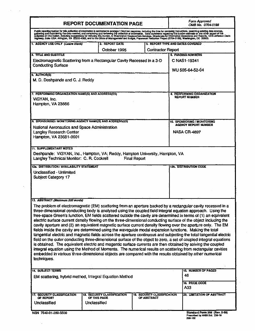
Form Approved REPORT DOCUMENTATION PAGE I OMB No. 07040188

. AGENCY USE ONLY (Leave blank) 2. REPORTDATE 3. REPORT TYPE AND DATES COVERED

October 1995 Contractor Report I I

I. TITLE AND SUBTITLE

Electromagnetic Scattering from a Rectangular Cavity Recessed in a 3-0 Conducting Surface

M. D. Deshpande and C. J. Reddy I. AUTHOR(S)

’. PERFORMING ORGANIZATION NAME(S) AND ADDRESYES)

WGYAN, lnc. Hampton, VA 23666

1. SPONSORING I MONITORING AGENCY NAMQS) AND ADDRESS(ES)

National Aeronautics and Space Administration Langley Research Center Hampton, VA 23681 -0001

5. FUNDING NUMBERS

C NAS1-19341

WU 505-64-52-04

8. PERFORMING ORGANIZATION REPORT NUMBER

IO. SPONSORING I MONITORING AGENCY REPORT NUMBER

NASA CR-4697

1. SUPPLEMENTARY NOTES

Deshpande: ViGYAN, Inc., Hampton, VA; Reddy, Hampton University, Hampton, VA Langley Technical Monitor: C. R. Cockrell Final Report

2a. DISTRIBUTION I AVAILABILITY STATEMENT 112b. DISTRIBUTION CODE

Unclassified - Unlimited Subject Category 17

13. ABSTRACT (Naximum 200 words)

The problem of electromagnetic (EM) scattering from an aperture backed by a rectangular cavity recessed in a three-dimensional conducting body is analyzed using the coupled field integral equation approach. Using the free-space Green’s function, EM fields scattered outside the cavity are determined in terms of (1) an equivalent electric surface current density flowing on the three-dimensional conducting surface of the object including the cavity aperture and (2) an equivalent magnetic surface current density flowing over the aperture only. The EM fields inside the cavity are determined using the waveguide modal expansion functions. Making the total tangential electric and magnetic fields across the aperture continuous and subjecting the total tangential electric field on the outer conducting three-dimensional surface of the object to zero, a set of coupled integral equations is obtained. The equivalent electric and magentic surface currents are then obtained by solving the coupled integral equation using the Method of Moments. The numerical results on scattering from rectangular cavities embedded in various‘three-dimensional objects are compared with the results obtained by other numerical techniques.

14. SUBJECTTERMS 15. NUMBER OF PAGES

EM scattering, hybrid method, Integral Equation Method 46

A03 16. PRICECODE

I 17. SECURITY CLASSIFICATION 18. SECURITY CLASSIFICATDN 19. SECURITY CLASSIFICATION 20. LIMITATION OF ABSTRACT

OF REPORT OF THIS PAGE OF ABSTRACT

I I Unclassified I Unclassified 1 1 1

Standard Form 298 (Rev. 2-89) Pf6SUlbd byANsIstd. -18 -102

NSN 754001-280-5500