Electromagnetic Fields and Energy - RLE at MIT Fields and Energy. Englewood Cliffs, NJ:...

MIT OpenCourseWare httpocwmitedu

Haus Hermann A and James R Melcher Electromagnetic Fields and Energy Englewood Cliffs NJ Prentice-Hall 1989 ISBN 9780132490207

Please use the following citation format

Haus Hermann A and James R Melcher Electromagnetic Fields and Energy (Massachusetts Institute of Technology MIT OpenCourseWare) httpocwmitedu (accessed [Date]) License Creative Commons Attribution-NonCommercial-Share Alike

Also available from Prentice-Hall Englewood Cliffs NJ 1989 ISBN 9780132490207

Note Please use the actual date you accessed this material in your citation

For more information about citing these materials or our Terms of Use visit httpocwmiteduterms

10

MAGNETOQUASISTATIC RELAXATION AND DIFFUSION

100 INTRODUCTION

In the MQS approximation Amperersquos law relates the magnetic field intensity H to the current density J

times H = J (1)

Augmented by the requirement that H have no divergence this law was the theme of Chap 8 Two types of physical situations were considered Either the current density was imposed or it existed in perfect conductors In both cases we were able to determine H without being concerned about the details of the electric field distribution

In Chap 9 the effects of magnetizable materials were represented by the magnetization density M and the magnetic flux density defined as B equiv microo(H+M) was found to have no divergence

middot B = 0 (2)

Provided that M is either given or instantaneously determined by H (as was the case throughout most of Chap 9) and that J is either given or subsumed by the boundary conditions on perfect conductors these two magnetoquasistatic laws determine H throughout the volume

In this chapter our first objective will be to determine the distribution of E around perfect conductors Then we shall broaden our physical domain to include finite conductors especially in situations where currents are caused by an E that

1

2 Magnetoquasistatic Relaxation and Diffusion Chapter 10

is induced by the time rate of change of B In both cases we make explicit use of Faradayrsquos law

partB =

(3)times E minus

partt

In the EQS systems considered in Chaps 4ndash7 the curl of H generated by the time rate of change of the displacement flux density was not of interest Amperersquos law was adequately incorporated by the continuity law However in MQS systems the curl of E generated by the magnetic induction on the right in (1) is often of primary importance We had fields that depended on time rates of change in Chap 7

We have already seen the consequences of Faradayrsquos law in Sec 84 where MQS systems of perfect conductors were considered The electric field intensity E inside a perfect conductor must be zero and hence B has to vanish inside the perfect conductor if B varies with time This leads to n B = 0 on the surface of a middot perfect conductor Currents induced in the surface of perfect conductors assure the proper discontinuity of ntimes H from a finite value outside to zero inside

Faradayrsquos law was in evidence in Sec 84 and accounted for the voltage at terminals connected to each other by perfect conductors Faradayrsquos law makes it possible to have a voltage at terminals connected to each other by a perfect ldquoshortrdquo A simple experiment brings out some of the subtlety of the voltage definition in MQS systems Its description is followed by an overview of the chapter

Demonstration 1001 Nonuniqueness of Voltage in an MQS System

A magnetic flux is created in the toroidal magnetizable core shown in Fig 1001 by driving the winding with a sinsuoidal current Because it is highly permeable (a ferrite) the core guides a magnetic flux density B that is much greater than that in the surrounding air

Looped in series around the core are two resistors of unequal value R1 = R2 Thus the terminals of these resistors are connected together to form a pair of ldquonodesrdquo One of these nodes is grounded The other is connected to highshyimpedance voltmeters through two leads that follow the different paths shown in Fig 1001 A dualshytrace oscilloscope is convenient for displaying the voltages

The voltages observed with the leads connected to the same node not only differ in magnitude but are 180 degrees out of phase

Faradayrsquos integral law explains what is observed A crossshysection of the core showing the pair of resistors and voltmeter leads is shown in Fig 1002 The scope resistances are very large compared to R1 and R2 so the current carried by the voltmeter leads is negligible This means that if there is a current i through one of the series resistors it must be the same as that through the other

The contour Cc follows the closed circuit formed by the series resistors Farashydayrsquos integral law is now applied to this contour The flux passing through the surface Sc spanning Cc is defined as Φλ Thus

dΦλE ds = middot minus

dtC1

= i(R1 + R2) (4)

where Φλ equiv B damiddot (5)

Sc

Cite as Haus Hermann A and James R Melcher Electromagnetic Fields and Energy Englewood Cliffs NJ Prentice-Hall 1989 ISBN 9780132490207 Also available online at MIT OpenCourseWare (httpocwmitedu) Massachusetts Institute of Technology Downloaded on [DD Month YYYY]

3 Sec 100 Introduction

Fig 1001 A pair of unequal resistors are connected in series around a magnetic circuit Voltages measured between the terminals of the reshysistors by connecting the nodes to the dualshytrace oscilloscope as shown differ in magnitude and are 180 degrees out of phase

Fig 1002 Schematic of circuit for experiment of Fig 1001 showing contours used with Faradayrsquos law to predict the differing voltages v1 and v2

Given the magnetic flux (4) can be solved for the current i that must circulate around the loop formed by the resistors

To determine the measured voltages the same integral law is applied to conshytours C1 and C2 of Fig 1002 The surfaces spanning the contours link a negligible flux density so the circulation of E around these contours must vanish

E ds = v1 + iR1 = 0 (6)middot C1

E ds = minusv2 + iR2 = 0 (7)middot C2


The observed voltages are found by solving (4) for i which is then substituted into (6) and (7)

R1 dΦλ v1 = (8)

R1 + R2 dt

R2 dΦλ v2 = minus

R1 + R2 dt (9)

From this result it follows that

v1 R1

v2 = minus

R2 (10)

Indeed the voltages not only differ in magnitude but are of opposite signs Suppose that one of the voltmeter leads is disconnected from the right node

looped through the core and connected directly to the grounded terminal of the same voltmeter The situation is even more remarkable because we now have a voltage at the terminals of a ldquoshortrdquo However it is also more familiar We recognize from Sec 84 that the measured voltage is simply dλdt where the flux linkage is in this case Φλ

In Sec 101 we begin by investigating the electric field in the free space regions of systems of perfect conductors Here the viewpoint taken in Sec 84 has made it possible to determine the distribution of B without having to determine E in the process The magnetic induction appearing on the right in Faradayrsquos law (1) is therefore known and hence the law prescribes the curl of E From the introduction to Chap 8 we know that this is not enough to uniquely prescribe the electric field Information about the divergence of E must also be given and this brings into play the electrical properties of the materials filling the regions between the perfect conductors

The analyses of Chaps 8 and 9 determined H in two special situations In one case the current distribution was prescribed in the other case the currents were flowing in the surfaces of perfect conductors To see the more general situation in perspective we may think of MQS systems as analogous to networks composed of inductors and resistors such as shown in Fig 1003 In the extreme case where the source is a rapidly varying function of time the inductors alone determine the currents Finding the current distribution in this ldquohigh frequencyrdquo limit is analogous to finding the Hshyfield and hence the distribution of surface currents in the systems of perfect conductors considered in Sec 84 Finding the electric field in perfectly conducting systems the objective in Sec 101 of this chapter is analogous to determining the distribution of voltage in the circuit in the limit where the inductors dominate

In the opposite extreme if the driving voltage is slowly varying the inducshytors behave as shorts and the current distribution is determined by the resistive network alone In terms of fields the response to slowly varying sources of current is essentially the steady current distribution described in the first half of Chap 7 Once this distribution of J has been determined the associated magnetic field can be found using the superposition integrals of Chap 8

In Secs 102ndash104 we combine the MQS laws of Chap 8 with those of Faraday and Ohm to describe the evolution of J and H when neither of these limiting cases prevails We shall see that the field response to a step of excitation goes from a

5 Sec 101 MQS Electric Fields

Fig 1003 Magnetoquasistatic systems with Ohmic conductors are genshyeralizations of inductorshyresistor networks The steady current distribution is determined by the resistors while the highshyfrequency response is governed by the inductors

distribution governed by the perfect conductivity model just after the step is applied (the circuit dominated by the inductors) to one governed by the steady conduction laws for J and BiotshySavart for H after a long time (the circuit dominated by the resistors with the flux linkages then found from λ = Li) Under what circumstances is the perfectly conducting model appropriate The characteristic times for this magnetic field diffusion process will provide the answer

101 MAGNETOQUASISTATIC ELECTRIC FIELDS IN SYSTEMS OF PERFECT CONDUCTORS

The distribution of E around the conductors in MQS systems is of engineering interest For example the amount of insulation required between conductors in a transformer is dependent on the electric field

In systems composed of perfect conductors and free space the distribution of magnetic field intensity is determined by requiring that n B = 0 on the perfectly middot conducting boundaries Although this condition is required to make the electric field tangential to the perfect conductor vanish as we saw in Sec 84 it is not necessary to explicitly refer to E in finding H Thus in Faradayrsquos law of induction (1003) the rightshyhand side is known The source of curl E is thus known To determine the source of div E further information is required

The regions outside the perfect conductors where E is to be found are preshysumably filled with relatively insulating materials To identify the additional inforshymation necessary for the specification of E we must be clear about the nature of these materials There are three possibilities

Although the material is much less conducting than the adjacent ldquoperfectrdquo bull conductors the charge relaxation time is far shorter than the times of interest Thus partρpartt is negligible in the charge conservation equation and as a result the current density is solenoidal Note that this is the situation in the MQS approximation In the following discussion we will then presume that if this situation prevails the region is filled with a material of uniform conductivity in which case E is solenoidal within the material volume (Of course there


may be surface charges on the boundaries)

middot E = 0 (1)

The second situation is typical when the ldquoperfectrdquo conductors are surrounded bull by materials commonly used to insulate wires The charge relaxation time is generally much longer than the times of interest Thus no unpaired charges can flow into these ldquoinsulatorsrdquo and they remain charge free Provided they are of uniform permittivity the E field is again solenoidal within these materials

If the charge relaxation time is on the same order as times characterizing the bull currents carried by the conductors then the distribution of unpaired charge is governed by the combination of Ohmrsquos law charge conservation and Gaussrsquo law as discussed in Sec 77 If the material is not only of uniform conductivity but of uniform permittivity as well this charge density is zero in the volume of the material It follows from Gaussrsquo law that E is once again solenoidal in the material volume Of course surface charges may exist at material interfaces

The electric field intensity is broken into particular and homogeneous parts

E = Ep + Eh (2)

where in accordance with Faradayrsquos law (1003) and (1)

partB times Ep =minus partt

(3)

middot Ep = 0 (4)

and times Eh = 0 (5)

middot Eh = 0 (6)

Our approach is reminiscent of that taken in Chap 8 where the roles of E and partBpartt are respectively taken by H and minusJ Indeed if all else fails the particular solution can be generated by using an adaptation of the BiotshySavart law (827)

Ep =1

partpartt B (r)times ir r

dv (7)minus 4π V |rminus r|2

Given a particular solution to (3) and (4) the boundary condition that there be no tangential E on the surfaces of the perfect conductors is satisfied by finding a solution to (5) and (6) such that

ntimes E = 0 rArr n times Eh =minusntimes Ep (8)

on those surfaces Given the particular solution the boundary value problem has been reduced

to one familiar from Chap 5 To satisfy (5) we let Eh = minusΦ It then follows from (6) that Φ satisfies Laplacersquos equation


Fig 1011 Side view of long inductor having radius a and length d

Example 1011 Electric Field around a Long Coil

What is the electric field distribution in and around a typical inductor An apshyproximate analysis for a coil of many turns brings out the reason why transformer and generator designers often speak of the ldquovolts per turnrdquo that must be withstood by insulation The analysis illustrates the concept of breaking the solution into a particular rotational field and a homogeneous conservative field

Consider the idealized coil of Fig 1011 It is composed of a thin perfectly conducting wire wound in a helix of length d and radius a The magnetic field can be found by approximating the current by a surface current K that is φ directed about the z axis of a cylindrical coodinate system having the z axis coincident with the axis of the coil For an N shyturn coil this surface current density is Kφ = Nid If the coil is very long d a the magnetic field produced within is approximately uniform

Ni Hz = (9)

d

while that outside is essentially zero (Example 821) Note that the surface current density is just that required to terminate H in accordance with Amperersquos continuity condition

With such a simple magnetic field a particular solution is easily obtained We recognize that the perfectly conducting coil is on a natural coordinate surface in the cylindrical coordinate system Thus we write the z component of (3) in cylindrical coordinates and look for a solution to E that is independent of φ The solution resulting from an integration over r is

microor dHz r lt a minus

2 dtEp = iφ microoa 2 dHz (10) minus r gt a

2r dt

Because there is no magnetic field outside the coil the outside solution for Ep is irrotational

If we adhere to the idealization of the wire as an inclined current sheet the electric field along the wire in the sheet must be zero The particular solution does not satisfy this condition and so we now must find an irrotational and solenoidal Eh that cancels the component of Ep tangential to the wire

A section of the wire is shown in Fig 1012 What axial field Ez must be added to that given by (10) to make the net E perpendicular to the wire If Ez and Eφ are to be components of a vector normal to the wire then their ratio must be


Fig 1012 With the wire from the inductor of Fig 1011 stretched into a straight line it is evident that the slope of the wire in the inductor is essentially the total length of the coil d divided by the total length of the wire 2πaN

the same as the ratio of the total length of the wire to the length of the coil

Ez 2πaN = r = a (11)

Eφ d

Using (9) and (10) at r = a we have

Ez = microoπa2N2 di

(12)minus d2 dt

The homogeneous solution possesses this field Ez on the surface of the cylinder of radius a and length d This field determines the potential Φh over the surface (within an arbitrary constant) Since 2Φh = 0 everywhere in space and the tangential Eh

field prescribes Φh on the cylinder Φh is uniquely determined everywhere within an additive constant Hence the conservative part of the field is determined everywhere

The voltage between the terminals is determined from the line integral of E ds between the terminals The field of the particular solution is φshydirected andmiddot gives no contribution The entire contribution to the line integral comes from the homogeneous solution (12) and is

microoN2πa2 di

v = minusEzd = (13)d dt

Note that this expression takes the form Ldidt where the inductance L is in agreeshyment with that found using a contour coincident with the wire (8418)

We could think of the terminal voltage as the sum of N ldquovoltages per turnrdquo EzdN If we admit to the finite size of the wires the electric stress between the wires is essentially this ldquovoltage per turnrdquo divided by the distance between wires

The next example identifies the particular and homogeneous solutions in a somewhat more formal fashion

Example 1012 Electric Field of a OneshyTurn Solenoid

The crossshysection of a oneshyturn solenoid is shown in Fig 1013 It consists of a circular cylindrical conductor having an inside radius a much less than its length in


Fig 1013 A oneshyturn solenoid of infinite length is driven by the distributed source of current density K(t)

Fig 1014 Tangential component of homogeneous electric field at r = a in the configuration of Fig 1013

the z direction It is driven by a distributed current source K(t) through the plane parallel plates to the left This current enters through the upper sheet conductor circulates in the φ direction around the one turn and leaves through the lower plate The spacing between these plates is small compared to a

As in the previous example the field inside the solenoid is uniform axial and equal to the surface current

H = izK(t) (14)

and a particular solution can be found by applying Faradayrsquos integral law to a contour having the arbitrary radius r lt a (10)

microor dK Ep = Eφpiφ Eφp equiv minus

2 dt (15)

This field clearly does not satisfy the boundary condition at r = a where it has a tangential value over almost all of the surface The homogeneous solution must have a tangential component that cancels this one However this field must also be conservative so its integral around the circumference at r = a must be zero Thus the plot of the φ component of the homogeneous solution at r = a shown in Fig 1014 has no average value The amplitude of the tall rectangle is adjusted so that the net area under the two functions is zero

Eφp(2π minus α) = hα h = Eφp

2π minus 1

(16)rArr α

The field between the edges of the input electrodes is approximated as being uniform right out to the contacts with the solenoid

We now find a solution to Laplacersquos equation that matches this boundary condition on the tangential component of E Because Eφ is an even function of φ Φ is taken as an odd function The origin is included in the region of interest so the polar coordinate solutions (Table 571) take the form

infin nΦ =

Anr sin nφ (17)

n=1


Fig 1015 Graphical representation of solution for the electric field in the configuration of Fig 1013

It follows that

1 partΦ infin

Eφh = minus r partφ

= minus

nAnr nminus1 cos nφ (18)

n=1

The coefficients An are evaluated as in Sec 55 by multiplying both sides of this expression by cos(mφ) and integrating from φ = minusπ to φ = π

minusα2 α2

minus Eφp cos mφdφ + Eφp

2π minus 1 cos mφdφ

α minusπ minusα2 (19)

π mminus1+ minusEφp cos mφdφ = minusmAma π

α2

Thus the coefficients needed to evaluate the potential of (17) are

4Eφp(r = a) mα Am = sin (20)minus

m2amminus1α 2

Finally the desired field intensity is the sum of the particular solution (15) and the homogeneous solution the gradient of (17)

microoa dK

r infin

2E =minus iφ + 4 sin nα r nminus1

cos nφiφ2 dt a αn a

n=1

infin sin nα

(21)

+ 4

2 r nminus1

sin nφirnα a

n=1

The superposition of fields represented in this solution is shown graphically in Fig 1015 A conservative field is added to the rotational field The former has

Sec 102 Nature of MQS Electric Fields 11

Fig 1021 Current induced in accordance with Faradayrsquos law circulates on contour Ca Through Amperersquos law it results in magnetic field that follows contour Cb

a potential at r = a that is a linearly increasing function of φ between the input electrodes increasing from a negative value at the lower electrode at φ = minusα2 passing through zero at the midplane and reaching an equal positive value at the upper electrode at φ = α2 The potential decreases in a linear fashion from this high as φ is increased again passing through zero at φ = 180 degrees and reaching the negative value upon returning to the lower input electrode Equipotential lines therefore join points on the solenoid periphery with points at the same potential between the input electrodes Note that the electric field associated with this potenshytial indeed has the tangential component required to cancel that from the rotational part of the field the proof of this being in the last of the plots

Often the vector potential provides conveniently a particular solution With B replaced by times A

partA

times E + partt

= 0 (22)

Suppose A has been determined Then the quantity in parantheses must be equal to the gradient of a potential Φ so that

partAE = (23)minus

partt minusΦ

In the examples treated the first term in this expression is the particular solution while the second is the homogeneous solution

102 NATURE OF FIELDS INDUCED IN FINITE CONDUCTORS

If a conductor is situated in a timeshyvarying magnetic field the induced electric field gives rise to currents From Sec 84 we have shown that these currents prevent the penetration of the magnetic field into a perfect conductor How high must σ be to treat a conductor as perfect In the next two sections we use specific analytical models to answer this question Here we preface these developments with a discussion of the interplay between the laws of Faraday Ampere and Ohm that determines the distribution duration and magnitude of currents in conductors of finite conductivity

The integral form of Faradayrsquos law applied to the surface Sa and contour Ca

of Fig 1021 is d

Ca

E middot ds = minus dt Sa

B middot da (1)


Ohmrsquos law J = σE introduced into (1) relates the current density circulating around a tube following Ca to the enclosed magnetic flux

J d

Ca σ middot ds = minus

dt Sa

B middot da (2)

This statement applies to every circulating current ldquohoserdquo in a conductor Let us concentrate on one such hose The current flows parallel to the hose and therefore J ds = Jds Suppose that the crossshysectional area of the hose is A(s) Then middot JA(s) = i the current in the hose and

A(s)

ds = R (3)σ

is the resistance of the hose Therefore

dλ iR = minus

dt (4)

Equation (2) describes how the timeshyvarying magnetic flux gives rise to a circulating current Amperersquos law states how that current in turn produces a magshynetic field

H ds = J da (5)middot middotCb Sb

Typically that field circulates around a contour such as Cb in Fig 1021 which is pierced by J With Gaussrsquo law for B Amperersquos law provides the relation for H produced by J This information is summarized by the ldquolumped circuitrdquo relation

λ = Li (6)

The combination of (4) and (6) provides a differential equation for the circuit current i(t) The equivalent circuit for the differential equation is the series intershyconnection of a resistor R with an inductor L as shown in Fig 1021 The solution is an exponentially decaying function of time with the time constant LR

The combination of (2) and (5)ndash of the laws of Faraday Ampere and Ohmndash determine J and H The field problem corresponds to a continuum of ldquocircuitsrdquo We shall find that the time dependence of the fields is governed by time constants having the nature of LR This time constant will be of the form

τm = microσl1l2 (7)

In contrast with the charge relaxation time σ of EQS this magnetic diffusion time depends on the product of two characteristic lengths denoted here by l1 and l2 For given time rates of change and electrical conductivity the larger the system the more likely it is to behave as a perfect conductor

Although we will not use the integral laws to determine the fields in the finite conductivity systems of the next sections they are often used to make engineering


Fig 1022 When the spark gap switch is closed the capacitor disshycharges into the coil The contour Cb is used to estimate the average magnetic field intensity that results

approximations The following demonstration is quantified using rough approximashytions in a style that typifies how field theory is often applied to practical problems

Demonstration 1021 Edgertonrsquos Boomer

The capacitor in Fig 1022 C = 25microF is initially charged to v = 4kV The spark gap switch is then closed so that the capacitor can discharge into the 50shyturn coil This demonstration has been seen by many visitors to Prof Harold Edgertonrsquos Strobe Laboratory at MIT

Given that the average radius of a coil winding a = 7 cm and that the height of the coil is also on the order of a roughly what magnetic field is generated Amperersquos integral law (5) can be applied to the contour Cb of the figure to obtain an approximate relation between the average H which we will call H1 and the coil current i1

N1i1H1 asymp (8)

2πa

To determine i1 we need the inductance L11 of the coil To this end the flux linkage of the coil is approximated by N1 times the product of the average coil area and the average flux density

λ asymp N1(πa2)microoH1 (9)

From these last two equations one obtains λ = L11i1 where the inductance is

microoaN12

L11 asymp (10)2

Evaluation gives L11 = 01 mH With the assumption that the combined resistance of the coil switch and

connecting leads is small enough so that the voltage across the capacitor and the current in the inductor oscillate at the frequency

1 ω = (11)radic

CL11

we can determine the peak current by recognizing that the energy 12Cv2 initially

stored in the capacitor is one quarter of a cycle later stored in the inductor

1 2 1 2

2 L11ip asymp

2 Cvp rArr ip = vp

CL11 (12)


Fig 1023 Metal disk placed on top of coil shown in Fig 1022

Thus the peak current in the coil is i1 = 2 000A We know both the capacitance and the inductance so we can also determine the frequency with which the current oscillates Evaluation gives ω = 20 times 103 sminus1 (f = 3kHz)

The H field oscillates with this frequency and has an amplitude given by evaluating (8) We find that the peak field intensity is H1 = 23times 105 Am so that the peak flux density is 03 T (3000 gauss)

Now suppose that a conducting disk is placed just above the driver coil as shown in Fig 1023 What is the current induced in the disk Choose a contour that encloses a surface Sa which links the upwardshydirected magnetic flux generated at the center of the driver coil With E defined as an average azimuthally directed electric field in the disk Faradayrsquos law applied to the contour bounding the surface Sa gives

d

d 2πaEφ = B (microoH1πa2) (13)minus

dt Sa

middot da asymp minus dt

The average current density circulating in the disk is given by Ohmrsquos law

σmicrooa dH1Jφ = σEφ = (14)minus

2 dt

If one were to replace the disk with his hand what current density would he feel To determine the peak current the derivative is replaced by ωH1 For the hand σ asymp 1 Sm and (14) gives 20 mAcm2 This is more than enough to provide a ldquoshockrdquo

The conductivity of an aluminum disk is much larger namely 35times 107 Sm According to (14) the current density should be 35 million times larger than that in a human hand However we need to remind ourselves that in using Amperersquos law to determine the driving field we have ignored contributions due to the induced current in the disk

Amperersquos integral law can also be used to approximate the field induced by the current in the disk Applied to a contour that loops around the current circulating in the disk rather than in the driving coil (2) requires that

i2 ΔaJφHind (15)asymp

2πa asymp

2πa

Here the crossshysectional area of the disk through which the current circulates is approximated by the product of the disk thickness Δ and the average radius a

It follows from (14) and (15) that the induced field gets to be on the order of the imposed field when

Hind Δσmicrooa 1 dH1 τm ω (16)

H1 asymp

4π |H1| dt

asymp 4π


where τm equiv microoσΔa (17)

Note that τm takes the form of (7) where l1 = Δ and l2 = a For an aluminum disk of thickness Δ = 2 mm a = 7 cm τm = 6 ms so

ωτm4π asymp 10 and the field associated with the induced current is comparable to that imposed by the driving coil1 The surface of the disk is therefore one where n B asymp 0 The lines of magnetic flux density passing upward through the center middot of the driving coil are trapped between the driver coil and the disk as they turn radially outward These lines are sketched in Fig 1024

In the terminology introduced with Example 974 the disk is the secondary of a transformer In fact τm is the time constant L22R of the secondary where L22

and R are the inductance and resistance of a circuit representing the disk Indeed the condition for ideal transformer operation (9726) is equivalent to having ωτm4π 1 The windings in power transformers are subject to the forces we now demonstrate

If an aluminum disk is placed on the coil and the switch closed a number of applications emerge First there is a bang correctly suggesting that the disk can be used as an acoustic transducer Typical applications are to deepshysea acoustic sounding The force density F(Nm3) responsible for this sound follows from the Lorentz law (Sec 119)

F = Jtimes microoH (18)

Note that regardless of the polarity of the driving current and hence of the average H this force density acts upward It is a force of repulsion With the current distrishybution in the disk represented by a surface current density K and B taken as one half its average value (the factor of 12 will be explained in Example 1193) the total upward force on the disk is

1 2f = Jtimes BdV asymp KB(πa )iz (19)2

V

By Amperersquos law the surface current K in the disk is equal to the field in the region between the disk and the driver and hence essentially equal to the average H Thus with an additional factor of 1

2 to account for time averaging the sinusoidally varying

drive (19) becomes 1 2 2f asymp fo equiv 4microoH (πa ) (20)

In evaluating this expression the value of H adjacent to the disk with the disk resting on the coil is required As suggested by Fig 1024 this field intensity is larger than that given by (8) Suppose that the field is intensified in the gap between coil and plate by a factor of about 2 so that H 5times 105A Then evaluation of (20) gives 103N or more than 1000 times the force of gravity on an 80g aluminum disk How high would the disk fly To get a rough idea it is helpful to know that the driver current decays in several cycles Thus the average driving force is essentially an impulse perhaps as pictured in Fig 1025 having the amplitude of (20) and a duration T = 1 ms With the aerodynamic drag ignored Newtonrsquos law requires that

dV M = foTuo(t) (21)

dt

1 As we shall see in the next sections because the calculation is not selfshyconsistent the inequality ωτm 1 indicates that the induced field is comparable to and not in excess of the one imposed


Fig 1024 Currents induced in the metal disk tend to induce a field that bucks out that imposed by the driving coil These currents result in a force on the disk that tends to propel it upward

Fig 1025 Because the magnetic force on the disk is always positive and lasts for a time T shorter than the time it takes the disk to leave the vicinity of the coil it is represented by an impulse of magnitude foT

where M = 008kg is the disk mass V is its velocity and uo(t) is the unit impulse Integration of this expression from t = 0minus (when the velocity V = 0) to t = 0+ gives

MV (O+) = foT (22)

For the numbers we have developed this initial velocity is about 10 ms or about 20 mileshr Perhaps of more interest is the height h to which the disk would be expected to travel If we require that the initial kinetic energy 1

2MV 2 be equal

to the final potential energy Mgh (g = 98 ms2) this height is 1V 2g 5 m2

The voltage and capacitance used here for illustration are modest Even so if the disk is thin and malleable it is easily deformed by the field Metal forming and transport are natural applications of this phenomenon

103 DIFFUSION OF AXIAL MAGNETIC FIELDS THROUGH THIN CONDUCTORS

This and the next section are concerned with the influence of thinshysheet conductors of finite conductivity on distributions of magnetic field The demonstration of the previous section is typical of physical situations of interest By virtue of Faradayrsquos law an applied field induces currents in the conducting sheet Through Amperersquos law these in turn result in an induced field tending to buck out the imposed field The resulting field has a time dependence reflecting not only that of the applied field but the conductivity and dimensions of the conductor as well This is the subject of the next two sections

A class of configurations with remarkably simple fields involves one or more sheet conductors in the shape of cylinders of infinite length As illustrated in Fig

Sec 103 Axial Magnetic Fields 17

Fig 1031 A thin shell having conductivity σ and thickness Δ has the shape of a cylinder of arbitrary crossshysection The surface current density K(t) circulates in the shell in a direction perpendicular to the magnetic field which is parallel to the cylinder axis

1031 these are uniform in the z direction but have an arbitrary crossshysectional geometry In this section the fields are z directed and the currents circulate around the z axis through the thin sheet Fields and currents are pictured as independent of z

The current density J is divergence free If we picture the current density as flowing in planes perpendicular to the z axis and as essentially uniform over the thickness Δ of the sheet then the surface current density must be independent of the azimuthal position in the sheet

K = K(t) (1)

Amperersquos continuity condition (953) requires that the adjacent axial fields are related to this surface current density by

minusHa + Hb = Kz z (2)

In a system with a single cylinder with a given circulating surface current density K and insulating materials of uniform properties both outside (a) and inside (b) a uniform axial field inside and no field outside is the exact solution to Amperersquos law and the flux continuity condition (We saw this in Demonstration 821 and in Example 842 for a solenoid of circular crossshysection) In a system consisting of nested cylinders each having an arbitrary crossshysectional geometry and each carrying its own surface current density the magnetic fields between cylinders would be uniform Then (2) would relate the uniform fields to either side of any given sheet

In general K is not known To relate it to the axial field we must introduce the laws of Ohm and Faraday The fact that K is uniform makes it possible to exploit the integral form of the latter law applied to a contour C that circulates through the cylinder

d

C

E middot ds = minus dt S

B middot da (3)


To replace E in this expression we multiply J = σE by the thickness Δ to relate the surface current density to E the magnitude of E inside the sheet

K K equiv ΔJ = ΔσE E = (4)rArr

Δσ

If Δ and σ are uniform then E (like K) is the same everywhere along the sheet However either the thickness or the conductivity could be functions of azimuthal position If σ and Δ are given the integral on the left in (3) can be taken since K is constant With s denoting the distance along the contour C (3) and (4) become

ds d

K = B da

C Δ(s)σ(s) minus

dt S

middot (5)

Of most interest is the case where the thickness and conductivity are uniform and (5) becomes

KP d

Δσ = minus

dt S

B middot da (6)

with P denoting the peripheral length of the cylinder The following are examples based on this model

Example 1031 Diffusion of Axial Field into a Circular Tube

The conducting sheet shown in Fig 1032 has the shape of a long pipe with a wall of uniform thickness and conductivity There is a uniform magnetic field H = izHo(t) in the space outside the tube perhaps imposed by means of a coaxial solenoid What current density circulates in the conductor and what is the axial field intensity Hi

inside Representing Ohmrsquos law and Faradayrsquos law of induction (6) becomes

K d 2

Δσ 2πa = minus

dt (microoπa Hi) (7)

Amperersquos law represented by the continuity condition (2) requires that

K = minusHo + Hi (8)

In these two expressions Ho is a given driving field so they can be combined into a single differential equation for either K or Hi Choosing the latter we obtain

dHi Hi +

Ho = (9)

dt τm τm

where 1

τm = microoσΔa (10)2

This expression pertains regardless of the driving field In particular suppose that before t = 0 the fields and surface current are zero and that when t = 0 the outside Ho is suddenly turned on The appropriate solution to (9) is the combination


Fig 1032 Circular cylindrical conducting shell with external axial field intensity Ho(t) imposed The response to a step in applied field is a current density that initially shields the field from the inner region As this current decays the field penetrates into the interior and is finally uniform throughout

of the particular solution Hi = Ho and the homogeneous solution exp(minustτm) that satisfies the initial condition

Hi = Ho(1 minus eminustτm ) (11)

It follows from (8) that the associated surface current density is

K = minusHoeminustτm (12)

At a given instant the axial field has the radial distribution shown in Fig 1032b Outside the field is imposed to be equal to Ho while inside it is at first zero but then fills in with an exponential dependence on time After a time that is long compared to τm the field is uniform throughout Implied by the discontinuity in field intensity at r = a is a surface current density that initially terminates the outside field When t = 0 K = minusHo and this results in a field that bucks out the field imposed on the inside region The decay of this current expressed by (12) accounts for the penetration of the field into the interior region

This example illustrates what one means by ldquoperfect conductor approximashytionrdquo A perfect conductor would shield out the magnetic field forever A physical conductor shields it out for times t τm Thus in the MQS approximation a conductor can be treated as perfect for times that are short compared with the characteristic time τm The electric field Eφ equiv E is given by applying (3) to a contour having an arbitrary radius r

d 2 microor dHi2πrE = minus

dt (microoHiπr ) rArr E = minus

2 dt r lt a (13)

2πrE = d

(microoHiπa2 d 2 2)]minus dt

)minus dt

[microoHoπ(r minus a rArr

microoa

a dHi +

r a dHo

(14) E = r gt aminus

2 r dt a minus

r dt


At r = a this particular solution matches that already found using the same integral law in the conductor In this simple case it is not necessary to match boundary conshyditions by superimposing a homogeneous solution taking the form of a conservative field

We consider next an example where the electric field is not simply the particshyular solution

Example 1032 Diffusion into Tube of Nonuniform Conductivity

Once again consider the circular cylindrical shell of Fig 1032 subject to an imshyposed axial field Ho(t) However now the conductivity is a function of azimuthal position

σoσ = (15)

1 + α cos φ

The integral in (5) resulting from Faradayrsquos law becomes

2π ds K

2πa

K = (1 + α cos φ)adφ = K (16)Δ(s)σ(s) Δσo ΔσoC 0

and hence2πa d 2

Δσo K = minus

dt (πa microoHi) (17)

Amperersquos continuity condition (2) once again becomes


Thus Hi is determined by the same expressions as in the previous example except that σ is replaced by σo The surface current response to a step in imposed field is again the exponential of (12)

It is the electric field distribution that is changed Using (15) (4) gives

K E = (1 + α cos φ) (19)

Δσo

for the electric field inside the conductor The E field in the adjacent free space regions is found using the familiar approach of Sec 101 The particular solution is the same as for the uniformly conducting shell (13) and (14) To this we add a homogeneous solution Eh = minusΦ such that the sum matches the tangential field given by (19) at r = a The φshyindependent part of (19) is already matched by the particular solution and so the boundary condition on the homogeneous part requires that

1 partΦ Kα Kαa minus a partφ

(r = a) =Δσo

cos φ rArr Φ(r = a) = minus Δσo

sin φ (20)

Solutions to Laplacersquos equation that vary as sin(φ) match this condition Outside the appropriate r dependence is 1r while inside it is r With the coefficients of these potentials adjusted to match the boundary condition given by (20) it follows that the electric field outside and inside the shell is

⎧2 dt

r lt a⎨ minus microor dHi iφ minusΦi

E = microoa

a dHi +

r a

dHo

a lt r

(21) 2 r dt r dt⎩ minus

a minus iφ minusΦo

Sec 104 Transverse Magnetic Fields 21

Fig 1033 Electric field induced in regions inside and outside shell (having conductivity that varies with azimuthal position) portrayed as the sum of a particular rotational and homogeneous conservative solushytion Conductivity is low on the right and high on the left α = 05

where

Kα Φi = r sin φ (22)minus

Δσo

Kαa2 sin φ Φo = (23)minus

Δσo r

These expressions can be evaluated using (11) and (12) for Hi and K for the electric field associated with a step in applied field It follows that E like the surface current and the induced H decays exponentially with the time constant of (10) At a given instant the distribution of E is as illustrated in Fig 1033 The total solution is the sum of the particular rotational and homogeneous conservative parts The degree to which the latter influences the total field depends on α which reflects the inhomogeneity in conductivity

For positive α the conductivity is low on the right (when φ = 0) and high on the left in Fig 1033 In accordance with (728) positive unpaired charge is induced in the transition region where the current flows from high to low conductivity and negative charge is induced in the transition region from low to high conductivity The field of the homogeneous solution shown in the figure originates and terminates on the induced charges

We shall return to models based on conducting cylindrical shells in axial fields Systems of conducting shells can be used to represent the nonuniform flow of current in thick conductors The model will also be found useful in determining the rate of induction heating for cylindrical objects


Fig 1041 Crossshysection of circular cylindrical conducting shell having its axis perpendicular to the magnetic field

104 DIFFUSION OF TRANSVERSE MAGNETIC FIELDS THROUGH THIN CONDUCTORS

In this section we study magnetic induction of currents in thin conducting shells by fields transverse to the shells In Sec 103 the magnetic fields were automatically tangential to the conductor surfaces so we did not have the opportunity to explore the limitations of the boundary condition n B = 0 used to describe a ldquoperfect middot conductorrdquo In this section the imposed fields generally have components normal to the conducting surface

The steps we now follow can be applied to many different geometries We specifically consider the circular cylindrical shell shown in crossshysection in Fig 1041 It has a length in the z direction that is very large compared to its rashydius a Its conductivity is σ and it has a thickness Δ that is much less than its radius a The regions outside and inside are specified by (a) and (b) respectively

The fields to be described are directed in planes perpendicular to the z axis and do not depend on z The shell currents are z directed A current that is directed in the +z direction at one location on the shell is returned in the minusz direction at another The closure for this current circulation can be imagined to be provided by perfectly conducting endplates or by a distortion of the current paths from the z direction near the cylinder ends (end effect)

The shell is assumed to have essentially the same permeability as free space It therefore has no tendency to guide the magnetic flux density Integration of the magnetic flux continuity condition over an incremental volume enclosing a section of the shell shows that the normal component of B is continuous through the shell

n (Ba minus Bb) = 0 Bra = Bb (1)middot rArr r

Ohmrsquos law relates the axial current density to the axial electric field Jz = σEz This density is presumed to be essentially uniformly distributed over the radial crossshysection of the shell Multiplication of both sides of this expression by the thickness Δ of the shell gives an expression for the surface current density in the shell

Kz equiv ΔJz = ΔσEz (2) Faradayrsquos law is a vector equation Of the three components the radial one is dominant in describing how the timeshyvarying magnetic field induces electric fields and hence currents tangential to the shell In writing this component we assume that the fields are independent of z

1 a

partEz

partφ = minus

partBr

partt (3)


Fig 1042 Circular cylindrical conducting shell filled by insulating material of permeability micro and surrounded by free space A magnetic field Ho(t) that is uniform at infinity is imposed transverse to the cylinshyder axis

Amperersquos continuity condition makes it possible to express the surface current density in terms of the tangential fields to either side of the shell

HaKz = φ minus Hφb (4)

These last three expressions are now combined to obtain the desired continuity condition

1 part partBr

Δσa partφ(Hφ

a minus Hφb) = minus

partt (5)

Thus the description of the shell is encapsulated in the two continuity conditions (1) and (5)

The thinshyshell model will now be used to place in perspective the idealized boundary condition of perfect conductivity In the following example the conductor is subjected to a field that is suddenly turned on The field evolution with time places in review the perfect conductivity mode of MQS systems in Chap 8 and the magnetization phenomena of Chap 9 Just after the field is turned on the shell acts like the perfect conductors of Chap 8 As time goes on the shell currents decay to zero and only the magnetization of Chap 9 persists

Example 1041 Diffusion of Transverse Field into Circular Cylindrical Conducting Shell with a Permeable Core

A permeable circular cylindrical core having radius a is shown in Fig 1042 It is surrounded by a thin conducting shell having thickness Δ and conductivity σ A uniform timeshyvarying magnetic field intensity Ho(t) is imposed transverse to the axis of the shell and core The configuration is long enough in the axial direction to justify representing the fields as independent of the axial coordinate z

Reflecting the fact that the region outside (o) is free space while that inside (i) is the material of linear permeability are the constitutive laws

Bo = microoHo Bi = microHi (6)

For the twoshydimensional fields in the r minus φ plane where the sheet current is in the z direction the scalar potential provides a convenient description of the field

H = (7)minusΨ


We begin by recognizing the form taken by Ψ far from the cylinder

Ψ = minusHor cos φ (8)

Note that substitution of this relation into (7) indeed gives the uniform imposed field

Given the φ dependence of (8) we assume solutions of the form

cos φ Ψo = minusHor cos φ + A (9)

r

Ψi = Cr cos φ

where A and C are coefficients to be determined by the continuity conditions In preparation for the evaluation of these conditions the assumed solutions are substishytuted into (7) to give the flux densities

Bo = microo

Ho +

A cos φir minus microo

Ho minus

A sin φiφ (10)

2 2r r

Bi = minusmicroC(cos ir minus sin φiφ)

Should we expect that these functions can be used to satisfy the continuity conditions at r = a given by (1) and (5) at every azimuthal position φ The inside and outside radial fields have the same φ dependence so we are assured of being able to adjust the two coefficients to satisfy the flux continuity condition Moreover in evaluating (5) the φ derivative of Hφ has the same φ dependence as Br Thus satisfying the continuity conditions is assured

The first of two relations between the coefficients and Ho follows from substishytuting (10) into (1)

microo

Ho +

A = minusmicroC (11)

2a

The second results from a similar substitution into (5)

1 A C

dHo 1 dA

= + (12)minus Δσa

Ho minus

a2

minus

Δσa minusmicroo

dt a2 dt

With C eliminated from this latter equation by means of (11) we obtain an ordinary differential equation for A(t)

dA A 2 dHo Hoa microo + = minusa +

1minus

(13)

dt τm dt microoΔσ micro

The time constant τm takes the form of (1027)

microτm = microoσΔa

(14)

micro + microo

In (13) the time dependence of the imposed field is arbitrary The form of this expression is the same as that of (7928) so techniques for dealing with initial conditions and for determining the sinusoidal steady state response introduced there are directly applicable here


Response to a Step in Applied Field Suppose there is no field inside or outside the conducting shell before t = 0 and that Ho is a step function of magnitude Hm turned on when t = 0 With D a coefficient determined by the initial condition the solution to (13) is the sum of a particular and a homogeneous solution

A = Hma 2 (microminus microo)

+ Deminustτm (15)(micro + microo)

Integration of (13) from t = 0minus to t = 0+ shows that A(0) = minusHma 2 so that D is evaluated and (15) becomes

2

(microminus microo)

(1 minus eminustτm )minus eminustτm

A = Hma (16)

(micro + microo)

This expression makes it possible to evaluate C using (11) Finally these coefficients are substituted into (9) to give the potential outside and inside the shell

r a

(microminus microo)


Ψo = minusHma

a minus

r (micro + microo) cos φ (17)

Ψi = minusHmaa

r

(micro

2

+

microo

microo)(1 minus eminustτm ) cos φ (18)

The field evolution represented by these expressions is shown in Fig 1043 where lines of B are portrayed When the transverse field is suddenly turned on currents circulate in the shell in such a direction as to induce a field that bucks out the one imposed For an applied field that is positive this requires that the surface current be in the minusz direction on the right and returned in the +z direction on the left This surface current density can be analytically expressed first by using (10) to evaluate Amperersquos continuity condition

microo

A

microo

Kz = Hφ

o minus Hφi = minus Ho 1minus

micro +

a2 1 +

micro sin φ (19)

and then by using (15)

Kz = minus2Hmeminustτm sin φ (20)

With the decay of Kz the external field goes from that for a perfect conductor (where n B = 0) to the field that would have been found if there were no conducting middot shell The magnetizable core tends to draw this field into the cylinder

The coefficient A represents the amplitude of a twoshydimensional dipole that has a field equivalent to that of the shell current Just after the field is applied A is negative and hence the equivalent dipole moment is directed opposite to the imposed field This results in a field that is diverted around the shell With the passage of time this dipole moment can switch sign This sign reversal occurs only if micro gt microo making it clear that it is due to the magnetization of the core In the absence of the core the final field is uniform

Under what conditions can the shell be regarded as perfectly conducting The answer involves not only σ but also the time scale and the size and to some extent


Fig 1043 When t = 0 a magnetic field that is uniform at infinity is suddenly imposed on the circular cylindrical conducting shell The cylinder is filled by an insulating material of permeability micro = 200microo When tτ = 0 an instant after the field is applied the surface currents completely shield the field from the central region As time goes on these currents decay until finally the field is no longer influenced by the conducting shell The final field is essentially perpendicular to the highly permeable core In the absence of this core the final field would be uniform

the permeability For our step response the shell shields out the field for times that are short compared to τm as given by (14)

Demonstration 1041 Currents Induced in a Conducting Shell

The apparatus of Demonstration 1021 can be used to make evident the shell currents predicted in the previous example A cylinder of aluminum foil is placed on the driver coil as shown in Fig 1044 With the discharge of the capacitor through the coil the shell is subjected to an abruptly applied field By contrast with the step function assumed in the example this field oscillates and decays in a few cycles However the reversal of the field results in a reversal in the induced shell current so regardless of the time dependence of the driving field the force density Jtimes B is in the same direction

Sec 105 Magnetic Diffusion Laws 27

Fig 1044 In an experiment giving evidence of the currents induced when a field is suddenly applied transverse to a conducting cylinder an aluminum foil cylinder subjected to the field produced by the experishyment of Fig 1022 is crushed

The force associated with the induced current is inward If the applied field were truly uniform the shell would then be ldquosquashedrdquo inward from the right and left by the field Because the field is not really uniform the cylinder of foil is observed to be compressed inward more at the bottom than at the top as suggested by the force vectors drawn in Fig 1044 Remember that the postulated currents require paths at the ends of the cylinder through which they can circulate In a roll of aluminum foil these return paths are through the shell walls in those end regions that extend beyond the region of the applied field

The derivation of the continuity conditions for a circular cylindrical shell folshylows a format that is applicable to other geometries Examples are a planar sheet and a spherical shell

105 MAGNETIC DIFFUSION LAWS

The selfshyconsistent evolution of the magnetic field intensity H with its source J induced in Ohmic materials of finite conductivity is familiar from the previous two sections In the models so far considered the induced currents were in thin conducting shells Thus in the processes of magnetic relaxation described in these sections the currents were confined to thin regions that could be represented by dynamic continuity conditions

In this and the next two sections the conductor extends throughout at least part of a volume of interest Like H the current density in Amperersquos law

times H = J (1)

is an unknown function For an Ohmic material it is proportional to the local electric field intensity

J = σE (2)

In turn E is induced in accordance with Faradayrsquos law

= (3)times E minus partmicro

partt

H

The conductor is presumed to have uniform conductivity σ and permeability micro For linear magnetization the magnetic flux continuity law is

middot microH = 0 (4)


In the MQS approximation the current density J is also solenoidal as can be seen by taking the divergence of Amperersquos law

middot J = 0 (5)

In the previous two sections we combined the continuity conditions implied by (1) and (4) with the other laws to obtain dynamic continuity conditions representing thin conducting sheets The regions between sheets were insulating and so the field distributions in these regions were determined by solving Laplacersquos equation Here we combine the differential laws to obtain a new differential equation that takes on the role of Laplacersquos equation in determining the distribution of magnetic field intensity

If we solve Ohmrsquos law (2) for E and substitute for E in Faradayrsquos law we have in one statement the link between magnetic induction and induced current density

J

partmicroH times = minus (6)σ partt

The current density is eliminated from this expression by using Amperersquos law (1) The result is an expression of H alone

times H

= partmicroH

(7)times σ

minus partt

This expression assumes a somewhat more familiar appearance when σ and micro are constants so that they can be taken outside the operations Further it follows from (4) that H is solenoidal so the use of a vector identity2 turns (7) into

1 partH =

microσ 2H

partt (8)

At each point in a material having uniform conductivity and permeability the magnetic field intensity satisfies this vector form of the diffusion equation The distribution of current density implied by the H found by solving this equation with appropriate boundary conditions follows from Amperersquos law (1)

Physical Interpretation With the understanding that H and J are solenoidal the derivation of (8) identifies the feedback between source and field that underlies the magnetic diffusion process The effect of the (timeshyvarying) field on the source embodied in the combined laws of Faraday and Ohm (6) is perhaps best appreshyciated by integrating (6) over any fixed open surface S enclosed by a contour C By Stokesrsquo theorem the integration of the curl over the surface transforms into an integration around the enclosing contour Thus (6) implies that

J d

minus

C σ middot ds =

dt S

microH middot da (9)

2 timestimes H = ( middot H)minus2H


Fig 1051 Configurations in which cylindrically shaped conductors having axes parallel to the magnetic field have currents transverse to the field in xminus y planes

and requires that the electromotive force around any closed path must be equal to the time rate of change of the enclosed magnetic flux Numerical approaches to solving magnetic diffusion problems may in fact approximate a system by a finite number of circuits each representing a current tube with its own resistance and flux linkage To represent the return effect of the current on H the diffusion equation also incorporates Amperersquos law (1)

The relaxation of axial fields through thin shells developed in Sec 103 is an example where the geometry of the conductor and the symmetry make the current tubes described by (9) readily discernible The diffusion of an axial magnetic field Hz into the volume of cylindrically shaped conductors as shown in Fig 1051 is a generalization of the class of axial problems described in Sec 103 As the only component of H Hz(x y) must satisfy (8)

1 partHz

microσ 2Hz =

partt (10)

The current density is then directed transverse to this field and given in terms of Hz by Amperersquos law

J = ix partHz partHz (11)party

minus iy partx

Thus the current density circulates in x minus y planes Methods for solving the diffusion equation are natural extensions of those

used in previous chapters for dealing with Laplacersquos equation Although we confine ourselves in the next two sections to diffusion in one spatial dimension the thinshyshell models give an intuitive impression as to what can be expected as magnetic fields diffuse into solid conductors having a wide range of geometries

Consider the coaxial thin shells shown in Fig 1052 as a model for a solid cylindrical conductor Following the approach outlined in Sec 103 suppose that the exterior field Ho is an imposed function of time Then the fields between sheets (H1


Fig 1052 Example of an axial field configuration composed of coaxial conshyducting shells of infinite axial length When an exterior field Ho is applied currents circulating in the shells tend to shield out the imposed field

and H2) and in the central region (H3) are determined by a system of three ordinary differential equations having Ho(t) as a drive Associated with the evolution of these fields are surface currents in the shells that tend to shield the field from the region within In the limit where the number of shells is infinite the field distribution in a solid conductor could be represented by such coupled thin shells However the more practical approach used in the next sections is to solve the diffusion equation exactly The situations considered are in cartesian rather than polar coordinates

106 MAGNETIC DIFFUSION TRANSIENT RESPONSE

The selfshyconsistent distribution of current density and magnetic field intensity in the volume of a uniformly conducting material is determined from the laws given in Sec 105 and summarized by the magnetic diffusion equation (1058) In this section we illustrate magnetic diffusion phenomena by considering the transient that results when a current is abruptly turned on or off

In contrast to Laplacersquos equation the diffusion equation involves a time rate of change and so it is necessary to deal with the time dependence in much the same way as the space dependence The diffusion process considered in this section is in one spatial dimension with time as the second ldquodimensionrdquo Our approach builds on product solutions and the solution of boundary value problems by superposition as introduced in Chap 5

The class of configurations of interest is illustrated in Fig 1061 Perfectly conducting electrodes are driven along their edges at x = minusb by a distributed current source The uniformly conducting material is sandwiched between these electrodes The current originating in the source then circulates in the x direction through the electrode in the y = 0 plane to a point where it passes in the y direction through the conducting material It is then returned to the source through the other perfectly conducting plate Note that this configuration is a special case of

Sec 106 Magnetic Diffusion Transient 31

Fig 1061 A block of uniformly conducting material having length b and thickness a is sandwiched between perfectly conducting electrodes that are driven along their edges at x = minusb by a distributed current source Current density and field intensity in the block are respectively y and z directed each depending on (x t)

that shown in Fig 1051 where the current density is transverse to a magnetic field intensity that has only one component Hz

If this field and the associated current density are indeed independent of y then it follows from (10510) and (10511) that Hz satisfies the oneshydimensional diffusion equation

1 part2Hz partHz = (1)microσ partx2 partt

and the only component of the current density is related to Hz by Amperersquos law

J = minusiy partHz (2)partx

Note that this oneshydimensional model correctly requires that the current density and hence the electric field intensity be normal to the perfectly conducting elecshytrodes at y = 0 and y = a

The distributed current source perfectly conducting sheets and conducting block form a closed path for currents that circulate in xminus y planes These extend to infinity in the + and minusz directions in the manner of an infinite oneshyturn solenoid The field outside the outermost of these current paths is therefore taken as being zero Amperersquos continuity condition then requires that at the surface x = minusb where the distributed current source is located the enclosed magnetic field intensity be equal to the imposed surface current density Ks In the plane x = 0 the situation is similar except that there is no surface current density and so the magnetic field intensity must be zero Thus consistent with solving a differential equation that is second order in x are the two boundary conditions

Hz(minusb t) = Ks(t) Hz(0 t) = 0 (3)

The equation is first order in its time dependence suggesting that to complete the specification of the transient solution the initial value of Hz must also be given

Hz(x 0) = Hi(x) (4)


Fig 1062 Boundary and initial conditions for oneshydimensional magnetic diffusion pictured in the x minus t plane (a) The total fields at the ends of the block are constrained to be equal to the driving surface current density and to zero respectively while there is one initial condition when t = 0 (b) The transient part of the solution is zero at the boundaries and satisfies the initial condition that makes the total solution assume the current value when t = 0

It is helpful to picture the boundary and initial conditions needed to uniquely specify solutions to (2) in the x minus t plane as shown in Fig 1062a Here the conducting block can be pictured as extending from x = 0 to x = minusb with the field between a function of x that evolves in the t ldquodirectionrdquo Presumably the distribution of Hz in the xminust space is predicted by (1) with the boundary conditions of (3) at x = 0 and x = minusb and the initial condition of (4) when t = 0

Is the solution for Hz(t) uniquely specified by (1) the boundary conditions of (3) and the initial condition of (4) A proof that it is can be made following a line of reasoning suggested by the EQS uniqueness arguments of Sec 78

Suppose that the drive is a step function of time so that the final state is one of uniform steady conduction Then the linearity of (1) makes it possible to think of the total field as being the superposition of this steady field and a transient part

Hz = H (x) + Ht(x t) (5)infin

The steady solution which presumably prevails as t rarr infin satisfies (1) with the time derivative set equal to zero

part2Hinfin = 0 partx2

(6)

while the transient part satisfies the complete equation

1 part2Ht

microσ partx2

partHt = partt

(7)

Because the steady solution satisfies the boundary conditions for all time t gt 0 the boundary conditions satisfied by the transient part are homogeneous

Ht(minusb t) = 0 Ht(0 t) = 0 (8)

However the steady solution does not satisfy the initial condition The transient solution is therefore adjusted so that the total solution does

Ht(x 0) = Hi(x)minus Hinfin(x) (9)


The conditions satisfied by the transient part of the solution on the boundaries in the x minus t space are pictured in Fig 1062b

Product Solutions to the OneshyDimensional Diffusion Equation The apshyproach now used to find the Ht that satisfies (7) and the conditions of (8) and (9) is familiar from finding Cartesian coordinate product solutions to Laplacersquos equation in two dimensions in Sec 54 Here the second ldquodimensionrdquo is t and we consider solutions that take the form Ht = X(x)T (t) Substitution into (7) and division by XT gives

1 d2X microσ dT

X dx2 minus

T dt = 0 (10)

With the first term taken as minusk2 and the second as k2 it follows that

1 d2X d2X

X dx2 = minusk2 rArr

dx2 + k2X = 0 (11)

and microσ dT

= k2 dT +

k2

T = 0 (12)minus T dt

rArr dt microσ

Given the boundary conditions of (8) the appropriate solution to (11) is

nπ X = sin kx k = (13)

b

where n can be any integer Associated with each of these modes is a time depenshydence given by (12) as a decaying exponential with the time constant

microσb2

τn = (14)(nπ)2

Thus we are led to a transient part of the solution that is itself a superposition of modes each satisfying the boundary conditions

infin

xeminustτnHt =

Cn sin

nπ (15)

b n=1

When t = 0 the modes take the form of a Fourier series Thus the coefficients Cn

can be used to satisfy the initial condition (9) In the following example the coefficients are evaluated for specific initial conshy

ditions However because the ldquoshort timerdquo and ldquolong timerdquo field and current disshytributions are known at the outset much of the dynamics can be anticipated at the outset For times that are very short compared to the magnetic diffusion time microσb2 the conducting block must act as a perfect conductor In this short time limit we know from Chap 8 that the current from the distributed source is confined to the surface at x = minusb Thus for early times the distribution represented by the series of (15) tends to be an impulse function of x After many magnetic diffusion


times the current reaches a steady state and achieves a distribution that would be predicted in the first half of Chap 7 The following example fills in the evolution from the field of a perfectly conducting system to that for steady conduction

Example 1061 Response to a Step in Current

When t = 0 suppose that there are no currents or associated fields Then the current source suddenly becomes the constant Kp The solution to (6) that is zero at x = 0 and is Kp at x = minusb is

x Hinfin = minusKp

b (16)

This is the field associated with a constant current density Kpb that is uniformly distributed over the crossshysection of the block

Because there is no initial magnetic field it follows from (9) that the initial transient part of the field must cancel the steady part

x Ht(x 0) = Kp (17)

b

This must be the distribution of Ht given by (15) when t = 0

x infin

Kp =

Cn sin nπ

x

(18)b b

n=1

Following the procedure familiar from Sec 55 the coefficients Cn are now evaluated by multiplying both sides of this expression by sin(mπb) multiplying by dx and integrating from x = minusb to x = 0

0 infin 0 Kp

x sin

mπxdx =

Cn

sin

nπx sin

mπxdx (19)

b b b b minusb n=1 minusb

From the series on the right only the term m = n is not zero Carrying out the integration on the left3 then gives an expression that can be solved for Cm Replacing m n then gives rarr

Cn = minus2Kp (minus1)n

(20)nπ

Finally (16) and (15) [the latter evaluated using (20)] are superimposed as required by (5) to give the desired description of how the field evolves as a function of space and time

x infin

(minus1)n

Hz = minusKp

2Kp sin

nπx eminustτn (21)

b minus

nπ b n=1

The distribution of current density follows from this expression substituted into Amperersquos law (2)

infin

Jy = Kp

+

2Kp (minus1)n

cos nπx

eminustτn (22)b b b

n=1

3

sin(u)udu = sin(u)minus u cos(u)

Sec 107 Skin Effect 35

Fig 1063 (a) Distribution of Hz in the conducting block of Fig 1061 in response to applying a step in current with no initial field In terms of time normalized to the magnetic diffusion time based on the length b the field diffuses into the block finally assuming the linear distribution expected for steady conduction (b) Distribution of Jy with normalized time as a parameter The initial distribution is an impulse (a surface current density) at x = minusb while the final distribution is uniform

These expressions are pictured in Fig 1063 Note that the higher the order of a term the more rapid its exponential decay with time As a result the most terms in the series are needed when t = 0+ These are needed to make the initial magnetic field intensity zero and the initial current density an impulse at x = minusb Because the lowest mode in the transient part of either Hz or Jy has the longest time constant the longshytime response is dominated by the steady response and the first term in the series Of course with the decay of the transient part the field approaches a linear x dependence while the current density assumes the uniform distribution expected for a steady current

107 SKIN EFFECT

If the surface current source driving the conducting block of Fig 1061 is a sinushysoidal function of time

jωt Ks(t) = Re K se (1)

the current density tends to circulate through the block in the neighborhood of the surface adjacent to the source This tendency for the sinusoidal steady state current to return to the source through the thin zone or skin region nearest to the source gives another view of magnetic diffusion

To illustrate skin effect in specific terms we return to the oneshydimensional diffusion configuration of Sec 106 Fig 1061 Once again the distributions of Hz


and Jy are governed by the oneshydimensional diffusion equation and Amperersquos law (1061) and (1062)

The diffusion equation is linear and has coefficients that are independent of time We can expect a sinusoidal steady state response having the same frequency as the drive (1) The solution to the diffusion equation is therefore taken as having a product form but with the time dependence stipulated at the outset

jωt Hz = Re H z(x)e (2)

At a given location x the coefficient of the exponential is a complex number specshyifying the magnitude and phase of the field

Substitution of (2) into the diffusion equation (1061) shows that the comshyplex amplitude has an x dependence governed by

d2Hz minus γ2H z = 0 (3)

dx2

where γ2 equiv jωmicroσ

radicj

Solutions to (3) are simply exp(γx) However γ is complex If we note that= (1 + j)

radic2 then it follows that

γ =

jωmicroσ = (1 + j)

ωmicroσ (4)

2

In terms of the skin depth δ defined by

2

δ equiv ωmicroσ

(5)

One can also write (4) as (1 + j)

γ = (6)δ

With C+ and C arbitrary coefficients solutions to (3) are therefore minus

δ δH z = C+eminus(1+j) x

+ Cminuse(1+j) x

(7)

Before considering a detailed example where these coefficients are evaluated using the boundary conditions consider the x minus t dependence of the field represented by the first solution in (7) Substitution into (2) gives

x xj(ωtminusHz = Re C1e

minus δ e δ )

(8)

making it clear that the field magnitude is an exponentially decaying function of x Within the envelope with the decay length δ shown in Fig 1071 the field propashygates in the x direction That is points of constant phase on the field distribution have ωtminus xδ = constant and hence move in the x direction with the velocity ωδ


Fig 1071 Magnetic diffusion wave in the sinusoidal steady state showing envelope with decay length δ and instantaneous field at two different times The point of zero phase propagates with the velocity ωδ

Fig 1072 (a) Oneshydimensional magnetic diffusion in the sinusoidal steady state in the same configuration as considered in Sec 106 (b) Distribution of the magnitude of Hz in the conducting block of (a) as a function of the skin depth Decreasing the skin depth is equivalent to raising the frequency

Although the phase propagation signifies that at a given instant the field (and curshyrent density) are positive in one region while negative in another the propagation is difficult to discern because the decay is very rapid

The second solution in (7) represents a similar diffusion wave but decaying and propagating in the minusx rather than the +x direction The following illustrates how the two diffusion waves combine to satisfy boundary conditions

Example 1071 Diffusion into a Conductor of Finite Thickness

We consider once again the field distribution in a conducting material sandwiched between perfectly conducting plates as shown in either Fig 1072 or Fig 1061 The surface current density of the drive is given by (1) and it is assumed that any transient reflecting the initial conditions has died out How does the frequency dependence of the field distribution in the conducting block reflect the magnetic diffusion process


Boundary conditions on Hz are the same as in Sec 106 Hz(minusb t) = Ks(t) and Hz(0 t) = 0 These are satisfied by adjusting the complex amplitude so that

H z(minusb) = K

s H z(0) = 0 (9)

It follows from (7) that the second of these is satisfied if C+ = minusCminus The first condition then serves to evaluate C+ and hence Cminus so that

x xeminus(1+j)

δ (1+j)

δ

H z = K

s

minus e(10)

e(1+j) b minus eminus(1+j)δb

δ

This expression represents the superposition of fields propagating and decaying in the plusmnx directions respectively Evaluated at a given location x it is a complex number In accordance with (2) Hz is the real part of this number multiplied by exp(jωt) The magnitude of Hz is the magnitude of (10) and is shown with the skin depth as a parameter by Fig 1072

Consider the field distribution in two limits First suppose that the skin depth is very large compared to the thickness b of the conducting block This might be the limit in which the frequency is made very low compared to the reciprocal magnetic diffusion time based on the conductor thickness

2 2 2 δ b rArr

ωmicroσ b rArr

microσb2 ω (11)

In this limit the arguments of the exponentials in (10) are small Using the approxshyimation exp(u) asymp 1 + u (10) becomes

ˆ ˆ

1minus (1 + j)x

minus

1 + (1 + j)x

= minus ˆ x (12)δ δHz Ks Ksrarr

1 + (1 + j) b minus

1minus (1 + j) b

b

δ δ

Substitution of this complex amplitude into (2) gives the spaceshytime dependence

jωt Hz minusx

ReK se (13)rarr

b

The field has the linear distribution expected if the current density is uniformly distributed over the length of the conductor In this large skin depth limit the field and current density spatial distributions are essentially the same as if the current source were time independent

In the opposite extreme the skin depth is short compared to the conductor length Perhaps this is accomplished by making the frequency very high compared to the reciprocal magnetic diffusion time based on the conductor length

2 δ b rArr

microσb2 ω (14)

Then the first term in the denominator of (10) is large compared with the second Division of the numerator by this first term gives

ˆ ˆ δ δ δHz rarr Ks

eminus(1+j) x+b minus e(1+j) xminusb

asymp K

seminus(1+j)

x+b

(15)


Fig 1073 Skin depth as a function of frequency

In justifying the second of these expressions remember that x is negative throughout the region of interest Substitution of (15) into (2) shows that in this short skin depth limit

(x+b) (x+b)

ˆ

j

ωtminus

δ δHz = Re Kse

minus e (16)

With the origin shifted from x = 0 to x = minusb this field has the x minus t dependence of the diffusion wave represented by (8) So it is that in the short skin depth limit the distribution of the field magnitude shown in Fig 1072 has the exponential decay typical of skin effect

The skin depth (5) is inversely proportional to the square root of ωmicroσ Thus an order of magnitude variation in frequency or in conductivity only changes δ by about a factor of about 3 Even so skin depths found under practical conditions are widely varying because these parameters have enormous ranges In good conductors such as copper or aluminum Fig 1073 illustrates how δ varies from about 1 cm at 60 Hz to less than 01 mm at l MHz Of interest in determining magnetically induced currents in flesh is the curve for skin depth in materials having the ldquophysiologicalrdquo conductivity of about 02 Sm (Demonstration 791)

If the frequency is high enough so that the skin depth is small compared with the dimensions of interest then the fields external to the conductor are essentially determined using the perfect conductivity model introduced in Sec 84 In Demonshystration 861 the fields around a conductor above a ground plane line were derived and the associated surface current densities deduced If these currents are in the sinusoidal steady state we can now picture them as actually extending into the conductors a distance that is on the order of δ

Although skin effect determines the paths of current flow at radio frequencies as the following demonstrates it can be important even at 60 Hz

Demonstration 1071 Skin Effect

The core of magnetizable material shown in Fig 1074 passes through a slit cut from an aluminum block and through a winding that is driven at a frequency in the range of 60ndash240 Hz The winding and the block of aluminum respectively comprise


Fig 1074 Demonstration of skin effect Currents induced in the conshyducting block tend to follow paths of minimum reactance nearest to the slot Thus because the aluminum block is thick compared to the skin depth the field intensity observed decreases exponentially with distance X In the experiment the block is 10 times 10 times 26 cm with thickness of 6 cm between the right face of the slot and the right side of the block In aluminum at 60 Hz δ = 11 cm while at 240 Hz δ is half of that To avoid distortion of the field the yoke is placed at one end of the slot

the primary and secondary of a transformer In effect the secondary is composed of one turn that is shorted on itself

The thickness b of the aluminum block is somewhat larger than a skin depth at 60 Hz Therefore currents circulating through the block around the leg of the magnetic circuit tend to follow the paths of least reactance closest to the slit By making the length of the block and slit in the y direction large compared to b we expect to see distributions of current density and associated magnetic field intensity at locations in the block well removed from the ends that have the x dependence found in Example 1071

In the limit where δ is small compared to b the magnitude of the expected magnetic flux density Bz (normalized to its value where X = 0) has the exponential decay with distance x of the inset to Fig 1074 The curves shown are for aluminum at frequencies of 60 Hz and 240 Hz According to (5) increasing the frequency by a factor of 4 should decrease the skin depth by a factor of 2 Provision is made for measuring this field by having a small slit milled in the block with a large enough width to permit the insertion of a magnetometer probe oriented to measure the magnetic flux density in the z direction

As we have seen in this and previous sections currents induced in a conductor tend to exclude the magnetic field from some region Conductors are commonly used as shields that isolate a region from its surroundings Typically the conductor is made thick compared to the skin depth based on the fields to be shielded out


Fig 1075 Perfectly conducting supshyshaped conductors are driven by a disshytributed current source at the left The magnetic field is shielded out of the region to the right enclosed by the perfect conductors by (a) a block of conshyductor that fills the region and has a thickness b that is large compared to a skin depth and (b) a sheet conductor having a thickness Δ that is less than the skin depth

However our studies of currents induced in thin conducting shells in Secs 103 and 104 make it clear that this can be too strict a requirement for good shielding The thinshysheet model can now be seen to be valid if the skin depth δ is large compared to the thickness Δ of the sheet Yet we found that for a cylindrical shell of radius R provided that ωmicroσΔR 1 a sinusoidally varying applied field would be shielded from the interior of the shell Apparently under certain circumstances even a conductor that is thin compared to a skin depth can be a good shield

To understand this seeming contradiction consider the oneshydimensional conshyfigurations shown in Fig 1075 In the first of the two plane parallel perfectly conducting electrodes again sandwich a block of conductor in a system that is very long in a direction perpendicular to the paper However now the plates are shorted by a perfect conductor at the right Thus at very low frequencies all of the current from the source circulates through the perfectly conducting plates bypassing the block As a result the field throughout the conductor is uniform As the frequency is raised the electric field generated by the timeshyvarying magnetic flux drives a current through the block much as in Example 1071 with the current in the block tending to circulate through paths of least reactance near the left edge of the block For simplicity suppose that the skin depth δ is shorter than the length of the block b so that the decay of current density and field into the block is essentially the exponential sketched in Fig 1075a With the frequency high enough to make the skin depth short compared to b the field tends to be shielded from points within the block

In the configuration of Fig 1075b the block is replaced by a sheet having the same σ and micro but a thickness Δ that is less than a skin depth δ Is it possible that this thin sheet could suppress the field in the region to the right as well as the thick conductor

The answer to this question depends on the location of the observer and the extent b of the region with which he or she is associated In the conducting block shielding is poor in the neighborhood of the left edge but rapidly improves at


distances into the interior that are of the order of δ or more By contrast the sheet conductor can be represented as a current divider The surface current Ks of the source is tapped off by the sheet of conductivity per unit width G = σΔh (where h is the height of the structure) connected to the inductance (assigned to unit width) L = microbh of the singleshyturn inductor The current through the singleshyturn inductor is

1jωL KsKs

G + 1 =

1 + jωLG (17)

jωL

This current and the associated field is shielded out effectively when ωLG =| |ωmicroσbΔ 1 With the sheet the shielding strategy is to make equal use of all of the volume to the right for generating an electric field in the sheet conductor The efficiency of the shielding is improved by making ωmicroσΔb large The interior field is made small by making the shielded volume large

108 SUMMARY

Before tackling the concepts in this chapter we had studied MQS fields in two limiting situations

In the first currents in Ohmic conductors were essentially stationary with bull distributions governed by the steady conduction laws investigated in Secs 72ndash76 The associated magnetic fields were then found by using these curshyrent distributions as sources In the absence of magnetizable material the BiotshySavart law of Sec 82 could be used for this purpose With or without magnetizable material the boundary value approaches of Secs 85 and 96 were applicable

In the second extreme where fields were so rapidly varying that conductors bull were ldquoperfectrdquo the effect on the magnetic field of currents induced in accorshydance with the laws of Faraday Ampere and Ohm was to nullify the magnetic flux density normal to conducting surfaces The boundary value approach used to find selfshyconsistent fields and surface currents in this limit was the subject of Secs 84 and 86

In this chapter the interplay of the laws of Faraday Ohm and Ampere has again been used to find selfshyconsistent MQS fields and currents However in this chapter the conductivity has been finite This has made it possible to explore the dynamics of fields with source currents that were neither distributed throughout the volumes of conductors in accordance with the laws of steady conduction nor confined to the surfaces of perfect conductors

In dealing with perfect conductors in Chaps 8 and 9 the allshyimportant role of E could be placed in the background Left for a study of this chapter was the electric field induced by a timeshyvarying magnetic induction So we began in Sec 101 by picturing the electric field in systems of perfect conductors The approach was familiar from solving EQS (Chap 5) and MQS (Chap 8) boundary value problems involving Poissonrsquos equation The electric field intensity was represented by the superposition of a particular part having a curl that balanced minuspartBpartt at

Sec 108 Summary 43

each point in the volume and an irrotational part that served to make the total field tangential to the surfaces of the perfect conductors

Having developed some insight into the rotational electric fields induced by magnetic induction we then undertook case studies aimed at forming an appreciashytion for spatial and temporal distributions of currents and fields in finite conductors By considering the effects of finite conductivity we could answer questions left over from the previous two chapters

Under what conditions are distributions of current and field quasistationary bull in the sense of being essentially snapshots of a sequence of static fields Under what conditions do they consist of surface currents and fields having bull negligible normal components at the surfaces of conductors

We now know that the answer comes in terms of characteristic magnetic diffusion (or relaxation) times τ that depend on the electrical conductivity the permeability and the product of lengths

τ = microσΔb (1)

The lengths in this expression make it clear that the size and topology of the conductors plays an important role This has been illustrated by the thinshysheet models of Secs 103 and 104 and oneshydimensional magnetic diffusion into the bulk of conductors in Secs 106 and 107 In each of these classes of configurations the role played by τ has been illustrated by the step response and by the sinusoidal steady state response For the former the answer to the question ldquoWhen is a conductor perfectrdquo was literal The conductor tended to be perfect for times that were short compared to a properly defined τ For the latter the answer came in the form of a condition on the frequency If ωτ 1 the conductor tended to be perfect

In the sinusoidal state a magnetic field impressed at the surface of a conductor penetrates a distance δ into the conductor that is the skin depth and is given by setting ωτ = ωmicroσδ2 = 2 and solving for δ

2

δ = (2)ωmicroσ

It is true that conductors will act as perfect conductors if this skin depth is much shorter than all other dimensions of interest However the thin sheet model of Sec 104 teaches the important lesson that the skin depth may be larger than the conductor thickness and yet the conductor can still act to shield out the normal flux density Indeed in Sec 104 it was assumed that the current was uniform over the conductor crossshysection and hence that the skin depth was large not small compared to the conductor thickness Demonstration 861 where current passes through a cylindrical conductor at a distance l above a conducting ground plane is an example It would be found in that demonstration that if l is large compared to the conductor thickness the surface current in the ground plane would distribute itself in accordance with the perfectly conducting model even if the frequency is so low that the skin depth is somewhat larger than the thickness of the ground plane If Δ is the ground plane thickness we would expect the normal flux density to be small so long as ωτm = ωmicroσΔl 1 Typical of such situations is that the electrical dissipation due to conduction is confined to thin conductors and the magnetic


energy storage occupies relatively larger regions that are free of dissipation Energy storage and power dissipation are subjects taken up in the next chapter

Sec 102 Problems 45

Fig P1002

P R O B L E M S

101 Introduction

1011lowast In Demonstration 1001 the circuit formed by the pair of resistors is reshyplaced by the one shown in Fig 1001 composed of four resistors of equal resistance R The voltmeter might be the oscilloscope shown in Fig 1001 The ldquogroundedrdquo node at (4) is connected to the negative terminal of the voltmeter

Fig P1001

(a) Show that the voltage measured with the positive lead connected at (1) so that the voltmeter is across one of the resistors is v = (dΦλdt)4

(b) Show that if the positive voltmeter lead is connected to (2) then to (3) and finally to (4) (so that the lead is wrapped around the core once and connected to the same grounded node as the negative voltmeter lead) the voltages are respectively twice three times and four times this value Show that this last result is as would be expected for a transformer with a oneshyturn secondary

1012 Plane parallel perfectly conducting plates are shorted to form the oneshyturn inductor shown in Fig 1002 The current source is distributed so that it supplies i amps over the width d (a) Given that d and l are much greater than the spacing s determine

the voltage measured across the terminals of the current source by the voltmeter v2


Fig P1012

(b) What is the voltage measured by the voltmeter v1 connected as shown in the figure across these same terminals

102 Magnetoquasistatic Electric Fields in Systems of Perfect Conductors

1021lowast In Prob 841 the magnetic field of a dipole surrounded by a perfectly conducting spherical shell is found Show that

E = iφ microoa

2 dI

R

r minus (Rr)2 sin θ (a)

4R2 dt

in the region between the dipole and the shell

1022 The oneshyturn inductor of Fig P1012 is driven at the left by a current source that evenly distributes the surface current density K(t) over the width w The dimensions are such that g a w

(a) In terms of K(t) what is H between the plates (b) Determine a particular solution having the form Ep = ixExp(y t)

and find E

1023 The oneshyturn solenoid shown in crossshysection in Fig P1013 consists of pershyfectly conducting sheets in the planes φ = 0 φ = α and r = a The latter is broken at the middle and driven by a current source of K(t) ampsunit length in the z direction The current circulates around the perfectly conshyducting path provided by the sheets as shown in the figure Assume that the angle α δ and that the system is long enough in the z direction to justify taking the fields as two dimensional

(a) In terms of K(t) what is H in the pieshyshaped region (b) What is E in this region

1024lowast By constrast with previous examples and problems in this section conshysider here the induction of currents in materials that have relatively low conductivity An example would be the induction heating of silicon in the manufacture of semiconductor devices The material in which the currents are to be induced takes the form of a long circular cylinder of radius b

47 Sec 102 Problems

Fig P1013

Fig P1014

A long solenoid surrounding this material has N turns a length d that is much greater than its radius and a driving current i(t) as shown in Fig P1014

Because the material to be heated has a small conductivity the inshyduced currents are small and contribute a magnetic field that is small comshypared to that imposed Thus the approach to determining the distribution of current induced in the semiconductor is 1) to first find H ignoring the effect of the induced current This amounts to solving Amperersquos law and the flux continuity law with the current density that of the excitation coil Then 2) with B known the electric field in the semiconductor is determined using Faradayrsquos law and the MQS form of the conservation of charge law middot (σE) = 0 The approach to finding the fields can then be similar to that illustrated in this section

(a) Show that in the semiconductor and in the annulus B asymp (microoNid)iz (b) Use the symmetry about the z axis to show that in the semiconductor

where there is no radial component of J and hence of E at r = b E = minus(microoNr2d)(didt)iφ

(c) To investigate the conditions under which this approximation is useshyful suppose that the excitation is sinusoidal with angular frequency ω Approximate the magnetic field intensity Hinduced associated with the induced current Show that for the approximation to be good Hinduced Himposed = ωmicrooσb24 1

1025 The configuration for this problem is the same as for Prob 1014 except that the slightly conducting material is now a cylinder having a rectangular crossshysection as shown in Fig P1015 The imposed field is therefore the same as before


Fig P1015

(a) In terms of the coordinates shown find a particular solution for E that takes the form E = iyEyp(x t) and satisfies the boundary conditions at x = 0 and x = b

(b) Determine E inside the material of rectangular crossshysection (c) Sketch the particular homogeneous and total electric fields making

clear how the first two add up to satisfy the boundary conditions (Do not take the time to evaluate your analytical formula but rather use your knowledge of the nature of the solutions and the boundary conditions that they must satisfy)

103 Nature of Fields Induced in Finite Conductors

1031lowast The ldquoBoomerrdquo might be modeled as a transformer with the disk as the oneshyturn secondary terminated in its own resistance We have found here that if ωτm 1 then the flux linked by the secondary is small In Example 974 it was shown that operation of a transformer in its ldquoidealrdquo mode also implies that the flux linked by the secondary be small There it was found that to achieve this condition the time constant L22R of the secondary must be long compared to times of interest Approximate the inductance and resistance of the disk in Fig 1023 and show that L22R is indeed roughly the same as the time given by (10217)

1032 It is proposed that the healing of bone fractures can be promoted by the passage of current through the bone normal to the fracture Using magnetic induction a transient current can be induced without physical contact with the patient Suppose a nonunion of the radius (a nonhealing fracture in the long bone of the forearm as shown in Fig P1022) is to be treated How would you arrange a driving coil so as to induce a longitudinal current along the bone axis through the fracture

1033lowast Suppose that a driving coil like that shown in Fig 1022 is used to produce a magnetic flux through a conductor having the shape of the circular cylinshydrical shell shown in Fig 1032 The shell has a thickness Δ and radius a Following steps parallel to those represented by (10213)ndash(10216) show that Hind H1 is roughly ωτm where τm is given by (10310) (Assume that the applied field is essentially uniform over the dimensions of the shell)

49 Sec 104 Problems

Fig P1022

Fig P1031

104 Diffusion of Axial Magnetic Fields through Thin Conductors

1041lowast A metal conductor having thickness Δ and conductivity σ is formed into a cylinder having a square crossshysection as shown in Fig P1031 It is very long compared to its crossshysectional dimensions a When t = 0 there is a surface current density Ko circulating uniformly around the shell Show that the subsequent surface current density is K(t) = Ko exp(minustτm) where τm = microoσΔa4

1042 The conducting sheet of thickness Δ shown in crossshysection by Fig P1032 forms a oneshyturn solenoid having length l that is large compared to the length d of two of the sides of its rightshytriangular crossshysection When t = 0 there is a circulating current density Jo uniformly distributed in the conductor

(a) Determine the surface current density K(t) = ΔJ(t) for t gt 0 (b) A highshyimpedance voltmeter is connected as shown between the lower

right and upper left corners What v(t) is measured (c) Now lead (1) is connected following path (2) What voltage is meashy

sured

1043lowast A system of two concentric shells as shown in Fig 1052 without the center shell is driven by the external field Ho(t) The outer and inner shells have thicknesses Δ and radii a and b respectively

(a) Show that the fields H1 and H2 between the shells and inside the inshy


Fig P1032

ner shell respectively are governed by the equations ( τm = microoσΔb2)

dH2τm + H2 minus H1 = 0 (a)

dt

(ba)dH2 a b dH1 (t) (b)τmdt

+ τmb minus

a dt + H1 = Ho

(b) Given that Ho = Hm cos ωt show that the sinusoidal steady state fields are H1 = Re [Hm(1+jωτ m)D] exp jωt and H2 = Re [HmD] exp jωt where D = [1 + jωτ m(ab minus ba)](1 + jωτ m) + jωτ m(ba)

Fig P1034

1044 The supshyshaped perfect conductor shown in Fig P1034 is driven along its left edge by a current source having the uniformly distributed density Ko(t) At x = minusa there is a thin sheet having the nonuniform conductivity σ = σo[1 + α cos(πyb)] The length in the z direction is much greater than the other dimensions

(a) Given Ko(t) find a differential equation for K(t) (b) In terms of the solution K(t) to this equation determine E in the

region minusa lt x lt 0 0 lt y lt b

51 Sec 105 Problems

Fig P1041

Fig P1042

105 Diffusion of Transverse Magnetic Fields through Thin Conductors

1051lowast A thin planar sheet having conductivity σ and thickness Δ extends to infinity in the x and z directions as shown in Fig P1041 Currents in the sheet are z directed and independent of z

(a) Show that the sheet can be represented by the boundary conditions

Bya minus By

b = 0 (a)

part (Hx

a minus Hxb) = minusΔσ

partBy (b)partx partt

(b) Now consider the special case where the regions above and below are free space and extend to infinity in the +y and minusy directions respectively When t = 0 there is a surface current density in the sheet K = izKo sin βx where Ko and β are given constants Show that for t gt 0 Kz = Ko exp(minustτ) where τ = microoσΔ2β

1052 In the twoshydimensional system shown in crossshysection by Fig P1042 a planar air gap of width d is bounded from above in the surface y = d by a thin conducting sheet having conductivity σ and thickness Δ This sheet is in turn backed by a material of infinite permeability The region below is also infinitely permeable and at the interface y = 0 there is a winding used to impose the surface current density K = K(t) cosβxiz The system extends to infinity in the plusmnx and plusmnz directions

(a) The surface current density K(t) varies so rapidly that the conducting sheet acts as a perfect conductor What is Ψ in the air gap

(b) The current is slowly varying so that the sheet supports little induced current What is Ψ in the air gap

(c) Determine Ψ(x y t) if there is initially no magnetic field and a step K = Kouminus1(t) is applied Show that the early and longshytime response matches that expected from parts (a) and (b)


1053lowast The crossshysection of a spherical shell having conductivity σ radius R and thickness Δ is as shown in Fig 845 A magnetic field that is uniform and z directed at infinity is imposed

(a) Show that boundary conditions representing the shell are

Bra minus Br

b = 0 (a)

1 part b)

= partHr

R sin θ partθ

sin θ(Ha minus Hθ minusmicrooΔσ

partt (b)θ

(b) Given that the driving field is Ho(t) = ReH o exp(jωt) show that

the magnetic moment of a dipole at the origin that would have an effect on the external field equivalent to that of the shell is

Hom = Reminusjωτ(2πR3 ˆ )exp(jωt)

1 + jωτ

where τ equiv microoσΔR3 (c) Show that in the limit where ωτ rarrinfin the result is the same as found

in Example 843

1054 A magnetic dipole having moment i(t)a (as defined in Example 832) oriented in the z direction is at the center of a spherical shell having radius R thickness Δ and conductivity σ as shown in Fig P1044 With i = Rei exp(jωt) the system is in the sinusoidal steady state

(a) In terms of i(t)a what is Ψ in the neighborhood of the origin (b) Given that the shell is perfectly conducting find Ψ Make a sketch of

H for this limit (c) Now with σ finite determine Ψ (d) Take the appropriate limit of the fields found in (c) to recover the

result of (b) In terms of the parameters that have been specified under what conditions does the shell behave as though it had infinite conductivity

1055lowast In the system shown in crossshysection in Fig P1045 a thin sheet of conducshytor having thickness Δ and conductivity σ is wrapped around a circular cylinder having infinite permeability and radius b On the other side of an air gap at the radius r = a is a winding used to impose the surface current density K = K(t) sin 2φiz backed by an infinitely permeable material in the region a lt r

(a) The current density varies so rapidly that the sheet behaves as an infinite conductor In this limit show that Ψ in the air gap is

aK

rb

2 +

rb2

Ψ = minus 2

ab

2 +

ab2 cos 2φ (a)

53 Sec 106 Problems

Fig P1044

Fig P1045

(b) Now suppose that the driving current is so slowly varying that the current induced in the conducting sheet is negligible Show that

aK

r 2 minus

b2

Ψ = b

minus r

b2 cos 2φ (b)minus

2 ab

2

a

(c) Show that if the fields are zero when t lt 0 and there is a step in current K(t) = Kouminus1(t)

aKo cos 2φ

r 2 minus

ar

2

eminustτ

rb

2 minus

rb2

Ψ = a (c) a2 minus

b2

a2 +

b2 minus

2 b a b a

where microoσΔb

b2 +

a2

τ = a b (d)2

a2 minus

b2

b a

Show that the early and longshytime responses do indeed match the results found in parts (a) and (b)

1056 The configuration is as described in Prob 1045 except that the conducting shell is on the outside of the air gap at r = a while the windings are on the inside surface of the air gap at r = b Also the windings are now arranged


so that the imposed surface current density is K = Ko(t) sin φ For this configuration carry out parts (a) (b) and (c) of Prob 1045

106 Magnetic Diffusion Laws

1061lowast Consider a class of problems that are analogous to those described by (10510) and (10511) but with J rather than H written as a solution to the diffusion equation

(a) Use (1051)ndash(1055) to show that

partJ 2(Jσ) = micro partt

(a)

(b) Now consider J (rather than H) to be z directed but independent of z J = Jz(x y t)iz and H (rather than J) to be transverse H = Hx(x y t)ix + Hy(x y t)iy Show that

2 Jz

= micro partJz (b)

σ partt

where H can be found from J using

partH =

part Jz ix + part Jz iy (c)

partt minus

party σmicro partx σmicro

Note that these expressions are of the same form as (1058) (10510) and (10511) respectively but with the roles of J and H reversed

107 Magnetic Diffusion Step Response

1071lowast In the configuration of Fig 1061 a steady state has been established with Ks = Kp = constant When t = 0 this driving current is suddenly turned off Show that H and J are given by (10621) and (10622) with the first term in each omitted and the sign of the summation in each reversed

1072 Consider the configuration of Fig 1061 but with a perfectly conducting electrode in the plane x = 0 ldquoshortingrdquo the electrode at y = 0 to the one at y = a

(a) A steady driving current has been established with Ks = Kp = constant What are the steady H and J in the conducting block

(b) When t = 0 the driving current is suddenly turned off Determine H and J for t gt 0

Sec 108 Problems 55

108 Skin Effect

1081lowast For Example 1071 the conducting block has length d in the z direction

(a) Show that the impedance seen by the current source is

a(1 + j)e(1+j)bδ + eminus(1+j)bδ

Z = (a)e(1+j)bδ minus eminus(1+j)bδ

dσδ

(b) Show that in the limit where b δ Z becomes the dc resistance adbσ

(c) Show that in the opposite extreme where b δ so that the current is concentrated near the surface the block impedance has resistive and inductiveshyreactive parts of equal magnitude and that the resistance is equivalent to that for a slab having thickness δ in the x direction carrying a current that is uniformly distributed with respect to x

1082 In the configuration of Example 1071 the perfectly conducting electrodes are terminated by a perfectly conducting electrode in the plane x = 0

(a) Determine the sinusoidal steady state response H (b) Show that even though the current source is now ldquoshortedrdquo by pershy

fectly conducting electrodes the highshyfrequency field distribution is still given by (10716) so that in this limit the current still concenshytrates at the surface

(c) Determine the impedance of a length d (in the z direction) of the block

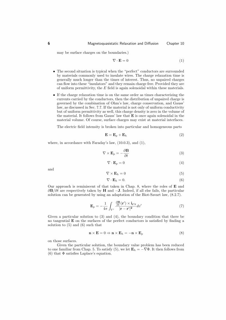
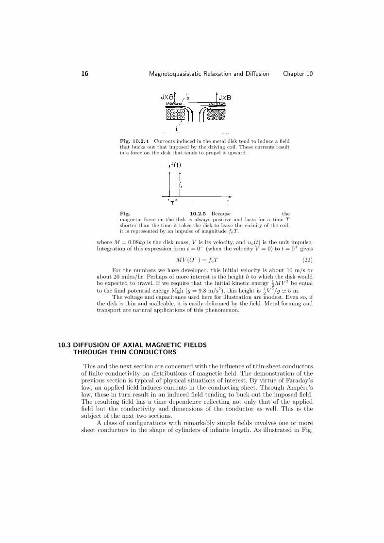
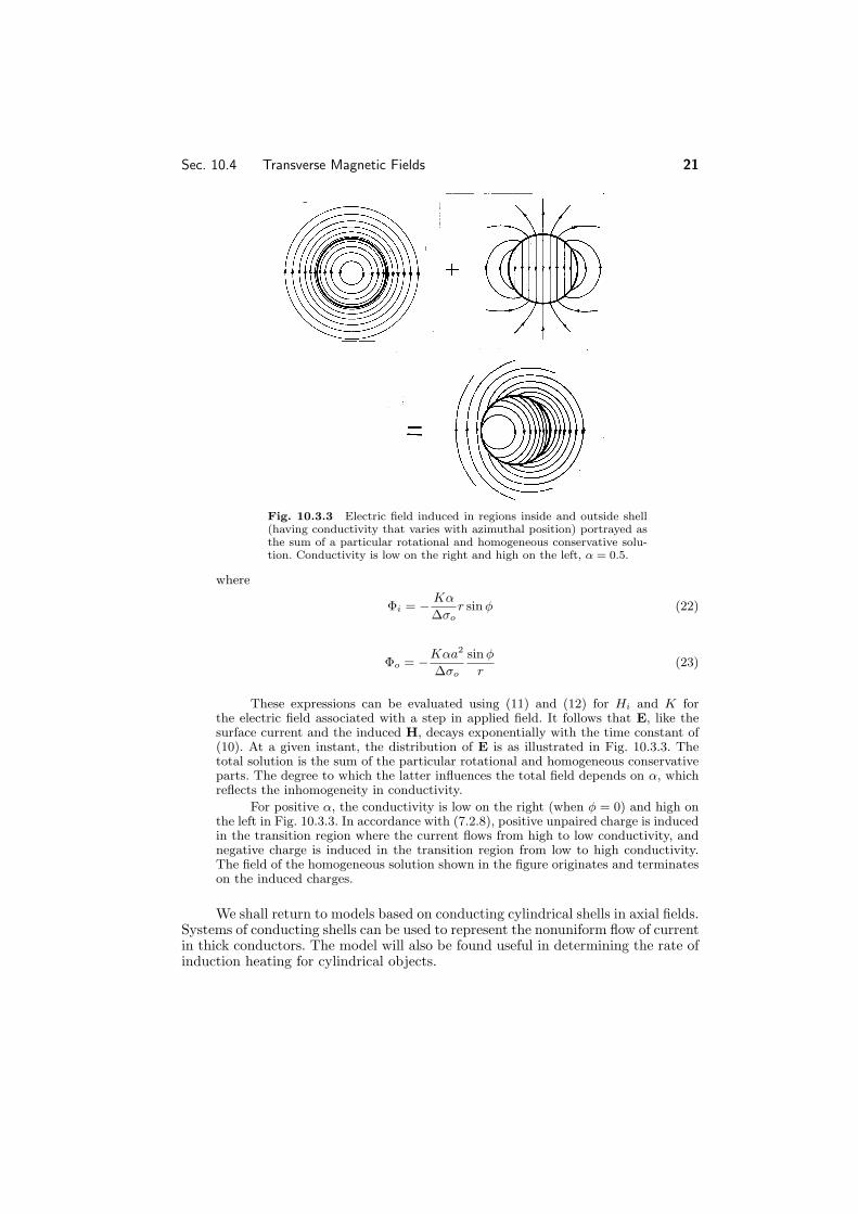
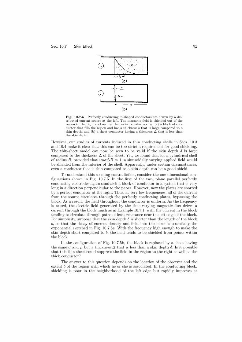
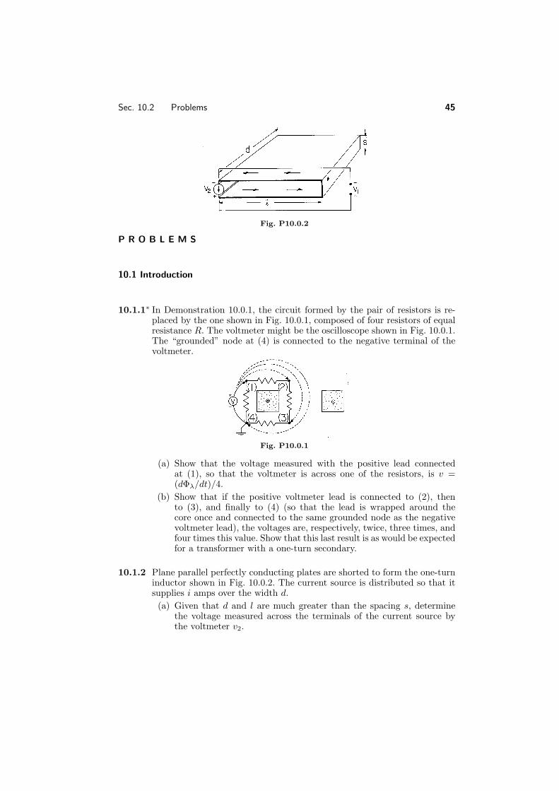10

MAGNETOQUASISTATIC RELAXATION AND DIFFUSION

100 INTRODUCTION

In the MQS approximation Amperersquos law relates the magnetic field intensity H to the current density J

times H = J (1)

Augmented by the requirement that H have no divergence this law was the theme of Chap 8 Two types of physical situations were considered Either the current density was imposed or it existed in perfect conductors In both cases we were able to determine H without being concerned about the details of the electric field distribution

In Chap 9 the effects of magnetizable materials were represented by the magnetization density M and the magnetic flux density defined as B equiv microo(H+M) was found to have no divergence

middot B = 0 (2)

Provided that M is either given or instantaneously determined by H (as was the case throughout most of Chap 9) and that J is either given or subsumed by the boundary conditions on perfect conductors these two magnetoquasistatic laws determine H throughout the volume

In this chapter our first objective will be to determine the distribution of E around perfect conductors Then we shall broaden our physical domain to include finite conductors especially in situations where currents are caused by an E that

1



partB =

(3)times E minus

partt











dtC1

= i(R1 + R2) (4)


Sc











R1 dΦλ v1 = (8)

R1 + R2 dt

R2 dΦλ v2 = minus

R1 + R2 dt (9)


v1 R1

v2 = minus

R2 (10)

















middot E = 0 (1)




E = Ep + Eh (2)



(3)

middot Ep = 0 (4)


middot Eh = 0 (6)


Ep =1












Ni Hz = (9)

d





2r dt







Ez 2πaN = r = a (11)

Eφ d



(12)minus d2 dt




microoN2πa2 di












H = izK(t) (14)



2 dt (15)



2π minus 1

(16)rArr α



infin nΦ =

Anr sin nφ (17)

n=1



It follows that

1 partΦ infin


= minus


n=1


minusα2 α2





α2



m2amminus1α 2


microoa dK

r infin



n=1

infin sin nα

(21)

+ 4

2 r nminus1

sin nφirnα a

n=1






partA

times E + partt

= 0 (22)


partAE = (23)minus

partt minusΦ





of Fig 1021 is d

Ca


B middot da (1)



J d


dt Sa

B middot da (2)


A(s)

ds = R (3)σ


dλ iR = minus

dt (4)




λ = Li (6)












N1i1H1 asymp (8)

2πa




microoaN12

L11 asymp (10)2



1 ω = (11)radic

CL11



1 2 1 2

2 L11ip asymp

2 Cvp rArr ip = vp

CL11 (12)






d


dt Sa




2 dt





2πa asymp

2πa




H1 asymp

4π |H1| dt

asymp 4π











V






dt






MV (O+) = foT (22)


2MV 2 be equal










K = K(t) (1)





d

C


B middot da (3)




Δσ


ds d

K = B da

C Δ(s)σ(s) minus

dt S

middot (5)


KP d

Δσ = minus

dt S

B middot da (6)





K d 2

Δσ 2πa = minus





dHi Hi +

Ho = (9)

dt τm τm

where 1













2 dt r lt a (13)

2πrE = d


)minus dt


microoa

a dHi +

r a dHo


2 r dt a minus

r dt






σoσ = (15)

1 + α cos φ


2π ds K

2πa


and hence2πa d 2

Δσo K = minus






K E = (1 + α cos φ) (19)

Δσo



(r = a) =Δσo


sin φ (20)


⎧2 dt


E = microoa

a dHi +

r a

dHo

a lt r





where


Δσo


Δσo r














1 a

partEz

partφ = minus

partBr

partt (3)






1 part partBr

Δσa partφ(Hφ


partt (5)








H = (7)minusΨ







r

Ψi = Cr cos φ


Bo = microo

Ho +


Ho minus

A sin φiφ (10)

2 2r r




microo

Ho +


2a


1 A C

dHo 1 dA

= + (12)minus Δσa

Ho minus

a2

minus

Δσa minusmicroo

dt a2 dt



1minus

(13)




(14)

micro + microo







2

(microminus microo)


A = Hma (16)

(micro + microo)


r a

(microminus microo)


Ψo = minusHma

a minus


Ψi = minusHmaa

r

(micro

2

+

microo



microo

A

microo

Kz = Hφ


micro +

a2 1 +

micro sin φ (19)


















times H = J (1)


J = σE (2)



partt

H





middot J = 0 (5)



J



times H

= partmicroH

(7)times σ

minus partt


1 partH =

microσ 2H

partt (8)



J d

minus

C σ middot ds =

dt S







1 partHz

microσ 2Hz =

partt (10)



minus iy partx






















Hz(x 0) = Hi(x) (4)









(6)


1 part2Ht

microσ partx2

partHt = partt

(7)


Ht(minusb t) = 0 Ht(0 t) = 0 (8)






1 d2X microσ dT

X dx2 minus

T dt = 0 (10)


1 d2X d2X


dx2 + k2X = 0 (11)

and microσ dT

= k2 dT +

k2


rArr dt microσ



b


microσb2

τn = (14)(nπ)2


infin

xeminustτnHt =

Cn sin

nπ (15)

b n=1








x Hinfin = minusKp

b (16)



x Ht(x 0) = Kp (17)

b


x infin

Kp =

Cn sin nπ

x

(18)b b

n=1


0 infin 0 Kp

x sin

mπxdx =

Cn

sin

nπx sin

mπxdx (19)




(20)nπ


x infin

(minus1)n

Hz = minusKp

2Kp sin


b minus

nπ b n=1


infin

Jy = Kp

+

2Kp (minus1)n

cos nπx


n=1

3





107 SKIN EFFECT












dx2


radicj



γ =


ωmicroσ (4)

2


2

δ equiv ωmicroσ

(5)


γ = (6)δ



+ Cminuse(1+j) x

(7)



minus δ e δ )

(8)











H z(minusb) = K

s H z(0) = 0 (9)


x xeminus(1+j)

δ (1+j)

δ

H z = K

s

minus e(10)


δ



2 2 2 δ b rArr

ωmicroσ b rArr

microσb2 ω (11)


ˆ ˆ

1minus (1 + j)x

minus

1 + (1 + j)x


1 + (1 + j) b minus

1minus (1 + j) b

b

δ δ


jωt Hz minusx

ReK se (13)rarr

b



2 δ b rArr

microσb2 ω (14)




asymp K

seminus(1+j)

x+b

(15)




(x+b) (x+b)

ˆ

j

ωtminus

δ δHz = Re Kse

minus e (16)





















1jωL KsKs

G + 1 =

1 + jωLG (17)

jωL


108 SUMMARY






Sec 108 Summary 43





τ = microσΔb (1)



2

δ = (2)ωmicroσ




Sec 102 Problems 45

Fig P1002

P R O B L E M S

101 Introduction


Fig P1001






Fig P1012




E = iφ microoa

2 dI

R


4R2 dt




and find E




47 Sec 102 Problems

Fig P1013

Fig P1014








Fig P1015








49 Sec 104 Problems

Fig P1022

Fig P1031






sured




Fig P1032



dt


+ τmb minus

a dt + H1 = Ho


Fig P1034




51 Sec 105 Problems

Fig P1041

Fig P1042




Bya minus By

b = 0 (a)

part (Hx











Bra minus Br

b = 0 (a)

1 part b)

= partHr

R sin θ partθ


partt (b)θ




1 + jωτ


in Example 843







aK

rb

2 +

rb2

Ψ = minus 2

ab

2 +

ab2 cos 2φ (a)

53 Sec 106 Problems

Fig P1044

Fig P1045


aK

r 2 minus

b2

Ψ = b

minus r

b2 cos 2φ (b)minus

2 ab

2

a


aKo cos 2φ

r 2 minus

ar

2

eminustτ

rb

2 minus

rb2

Ψ = a (c) a2 minus

b2

a2 +

b2 minus

2 b a b a

where microoσΔb

b2 +

a2

τ = a b (d)2

a2 minus

b2

b a









(a)


2 Jz

= micro partJz (b)

σ partt


partH =


partt minus








Sec 108 Problems 55

108 Skin Effect





dσδ









partB =

(3)times E minus

partt











dtC1

= i(R1 + R2) (4)


Sc











R1 dΦλ v1 = (8)

R1 + R2 dt

R2 dΦλ v2 = minus

R1 + R2 dt (9)


v1 R1

v2 = minus

R2 (10)

















middot E = 0 (1)




E = Ep + Eh (2)



(3)

middot Ep = 0 (4)


middot Eh = 0 (6)


Ep =1












Ni Hz = (9)

d





2r dt







Ez 2πaN = r = a (11)

Eφ d



(12)minus d2 dt




microoN2πa2 di












H = izK(t) (14)



2 dt (15)



2π minus 1

(16)rArr α



infin nΦ =

Anr sin nφ (17)

n=1



It follows that

1 partΦ infin


= minus


n=1


minusα2 α2





α2



m2amminus1α 2


microoa dK

r infin



n=1

infin sin nα

(21)

+ 4

2 r nminus1

sin nφirnα a

n=1






partA

times E + partt

= 0 (22)


partAE = (23)minus

partt minusΦ





of Fig 1021 is d

Ca


B middot da (1)



J d


dt Sa

B middot da (2)


A(s)

ds = R (3)σ


dλ iR = minus

dt (4)




λ = Li (6)












N1i1H1 asymp (8)

2πa




microoaN12

L11 asymp (10)2



1 ω = (11)radic

CL11



1 2 1 2

2 L11ip asymp

2 Cvp rArr ip = vp

CL11 (12)






d


dt Sa




2 dt





2πa asymp

2πa




H1 asymp

4π |H1| dt

asymp 4π











V






dt






MV (O+) = foT (22)


2MV 2 be equal










K = K(t) (1)





d

C


B middot da (3)




Δσ


ds d

K = B da

C Δ(s)σ(s) minus

dt S

middot (5)


KP d

Δσ = minus

dt S

B middot da (6)





K d 2

Δσ 2πa = minus





dHi Hi +

Ho = (9)

dt τm τm

where 1













2 dt r lt a (13)

2πrE = d


)minus dt


microoa

a dHi +

r a dHo


2 r dt a minus

r dt






σoσ = (15)

1 + α cos φ


2π ds K

2πa


and hence2πa d 2

Δσo K = minus






K E = (1 + α cos φ) (19)

Δσo



(r = a) =Δσo


sin φ (20)


⎧2 dt


E = microoa

a dHi +

r a

dHo

a lt r





where


Δσo


Δσo r














1 a

partEz

partφ = minus

partBr

partt (3)






1 part partBr

Δσa partφ(Hφ


partt (5)








H = (7)minusΨ







r

Ψi = Cr cos φ


Bo = microo

Ho +


Ho minus

A sin φiφ (10)

2 2r r




microo

Ho +


2a


1 A C

dHo 1 dA

= + (12)minus Δσa

Ho minus

a2

minus

Δσa minusmicroo

dt a2 dt



1minus

(13)




(14)

micro + microo







2

(microminus microo)


A = Hma (16)

(micro + microo)


r a

(microminus microo)


Ψo = minusHma

a minus


Ψi = minusHmaa

r

(micro

2

+

microo



microo

A

microo

Kz = Hφ


micro +

a2 1 +

micro sin φ (19)


















times H = J (1)


J = σE (2)



partt

H





middot J = 0 (5)



J



times H

= partmicroH

(7)times σ

minus partt


1 partH =

microσ 2H

partt (8)



J d

minus

C σ middot ds =

dt S







1 partHz

microσ 2Hz =

partt (10)



minus iy partx






















Hz(x 0) = Hi(x) (4)









(6)


1 part2Ht

microσ partx2

partHt = partt

(7)


Ht(minusb t) = 0 Ht(0 t) = 0 (8)






1 d2X microσ dT

X dx2 minus

T dt = 0 (10)


1 d2X d2X


dx2 + k2X = 0 (11)

and microσ dT

= k2 dT +

k2


rArr dt microσ



b


microσb2

τn = (14)(nπ)2


infin

xeminustτnHt =

Cn sin

nπ (15)

b n=1








x Hinfin = minusKp

b (16)



x Ht(x 0) = Kp (17)

b


x infin

Kp =

Cn sin nπ

x

(18)b b

n=1


0 infin 0 Kp

x sin

mπxdx =

Cn

sin

nπx sin

mπxdx (19)




(20)nπ


x infin

(minus1)n

Hz = minusKp

2Kp sin


b minus

nπ b n=1


infin

Jy = Kp

+

2Kp (minus1)n

cos nπx


n=1

3





107 SKIN EFFECT












dx2


radicj



γ =


ωmicroσ (4)

2


2

δ equiv ωmicroσ

(5)


γ = (6)δ



+ Cminuse(1+j) x

(7)



minus δ e δ )

(8)











H z(minusb) = K

s H z(0) = 0 (9)


x xeminus(1+j)

δ (1+j)

δ

H z = K

s

minus e(10)


δ



2 2 2 δ b rArr

ωmicroσ b rArr

microσb2 ω (11)


ˆ ˆ

1minus (1 + j)x

minus

1 + (1 + j)x


1 + (1 + j) b minus

1minus (1 + j) b

b

δ δ


jωt Hz minusx

ReK se (13)rarr

b



2 δ b rArr

microσb2 ω (14)




asymp K

seminus(1+j)

x+b

(15)




(x+b) (x+b)

ˆ

j

ωtminus

δ δHz = Re Kse

minus e (16)





















1jωL KsKs

G + 1 =

1 + jωLG (17)

jωL


108 SUMMARY






Sec 108 Summary 43





τ = microσΔb (1)



2

δ = (2)ωmicroσ




Sec 102 Problems 45

Fig P1002

P R O B L E M S

101 Introduction


Fig P1001






Fig P1012




E = iφ microoa

2 dI

R


4R2 dt




and find E




47 Sec 102 Problems

Fig P1013

Fig P1014








Fig P1015








49 Sec 104 Problems

Fig P1022

Fig P1031






sured




Fig P1032



dt


+ τmb minus

a dt + H1 = Ho


Fig P1034




51 Sec 105 Problems

Fig P1041

Fig P1042




Bya minus By

b = 0 (a)

part (Hx











Bra minus Br

b = 0 (a)

1 part b)

= partHr

R sin θ partθ


partt (b)θ




1 + jωτ


in Example 843







aK

rb

2 +

rb2

Ψ = minus 2

ab

2 +

ab2 cos 2φ (a)

53 Sec 106 Problems

Fig P1044

Fig P1045


aK

r 2 minus

b2

Ψ = b

minus r

b2 cos 2φ (b)minus

2 ab

2

a


aKo cos 2φ

r 2 minus

ar

2

eminustτ

rb

2 minus

rb2

Ψ = a (c) a2 minus

b2

a2 +

b2 minus

2 b a b a

where microoσΔb

b2 +

a2

τ = a b (d)2

a2 minus

b2

b a









(a)


2 Jz

= micro partJz (b)

σ partt


partH =


partt minus








Sec 108 Problems 55

108 Skin Effect





dσδ
















R1 dΦλ v1 = (8)

R1 + R2 dt

R2 dΦλ v2 = minus

R1 + R2 dt (9)


v1 R1

v2 = minus

R2 (10)

















middot E = 0 (1)




E = Ep + Eh (2)



(3)

middot Ep = 0 (4)


middot Eh = 0 (6)


Ep =1












Ni Hz = (9)

d





2r dt







Ez 2πaN = r = a (11)

Eφ d



(12)minus d2 dt




microoN2πa2 di












H = izK(t) (14)



2 dt (15)



2π minus 1

(16)rArr α



infin nΦ =

Anr sin nφ (17)

n=1



It follows that

1 partΦ infin


= minus


n=1


minusα2 α2





α2



m2amminus1α 2


microoa dK

r infin



n=1

infin sin nα

(21)

+ 4

2 r nminus1

sin nφirnα a

n=1






partA

times E + partt

= 0 (22)


partAE = (23)minus

partt minusΦ





of Fig 1021 is d

Ca


B middot da (1)



J d


dt Sa

B middot da (2)


A(s)

ds = R (3)σ


dλ iR = minus

dt (4)




λ = Li (6)












N1i1H1 asymp (8)

2πa




microoaN12

L11 asymp (10)2



1 ω = (11)radic

CL11



1 2 1 2

2 L11ip asymp

2 Cvp rArr ip = vp

CL11 (12)






d


dt Sa




2 dt





2πa asymp

2πa




H1 asymp

4π |H1| dt

asymp 4π











V






dt






MV (O+) = foT (22)


2MV 2 be equal










K = K(t) (1)





d

C


B middot da (3)




Δσ


ds d

K = B da

C Δ(s)σ(s) minus

dt S

middot (5)


KP d

Δσ = minus

dt S

B middot da (6)





K d 2

Δσ 2πa = minus





dHi Hi +

Ho = (9)

dt τm τm

where 1













2 dt r lt a (13)

2πrE = d


)minus dt


microoa

a dHi +

r a dHo


2 r dt a minus

r dt






σoσ = (15)

1 + α cos φ


2π ds K

2πa


and hence2πa d 2

Δσo K = minus






K E = (1 + α cos φ) (19)

Δσo



(r = a) =Δσo


sin φ (20)


⎧2 dt


E = microoa

a dHi +

r a

dHo

a lt r





where


Δσo


Δσo r














1 a

partEz

partφ = minus

partBr

partt (3)






1 part partBr

Δσa partφ(Hφ


partt (5)








H = (7)minusΨ







r

Ψi = Cr cos φ


Bo = microo

Ho +


Ho minus

A sin φiφ (10)

2 2r r




microo

Ho +


2a


1 A C

dHo 1 dA

= + (12)minus Δσa

Ho minus

a2

minus

Δσa minusmicroo

dt a2 dt



1minus

(13)




(14)

micro + microo







2

(microminus microo)


A = Hma (16)

(micro + microo)


r a

(microminus microo)


Ψo = minusHma

a minus


Ψi = minusHmaa

r

(micro

2

+

microo



microo

A

microo

Kz = Hφ


micro +

a2 1 +

micro sin φ (19)


















times H = J (1)


J = σE (2)



partt

H





middot J = 0 (5)



J



times H

= partmicroH

(7)times σ

minus partt


1 partH =

microσ 2H

partt (8)



J d

minus

C σ middot ds =

dt S







1 partHz

microσ 2Hz =

partt (10)



minus iy partx






















Hz(x 0) = Hi(x) (4)









(6)


1 part2Ht

microσ partx2

partHt = partt

(7)


Ht(minusb t) = 0 Ht(0 t) = 0 (8)






1 d2X microσ dT

X dx2 minus

T dt = 0 (10)


1 d2X d2X


dx2 + k2X = 0 (11)

and microσ dT

= k2 dT +

k2


rArr dt microσ



b


microσb2

τn = (14)(nπ)2


infin

xeminustτnHt =

Cn sin

nπ (15)

b n=1








x Hinfin = minusKp

b (16)



x Ht(x 0) = Kp (17)

b


x infin

Kp =

Cn sin nπ

x

(18)b b

n=1


0 infin 0 Kp

x sin

mπxdx =

Cn

sin

nπx sin

mπxdx (19)




(20)nπ


x infin

(minus1)n

Hz = minusKp

2Kp sin


b minus

nπ b n=1


infin

Jy = Kp

+

2Kp (minus1)n

cos nπx


n=1

3





107 SKIN EFFECT












dx2


radicj



γ =


ωmicroσ (4)

2


2

δ equiv ωmicroσ

(5)


γ = (6)δ



+ Cminuse(1+j) x

(7)



minus δ e δ )

(8)











H z(minusb) = K

s H z(0) = 0 (9)


x xeminus(1+j)

δ (1+j)

δ

H z = K

s

minus e(10)


δ



2 2 2 δ b rArr

ωmicroσ b rArr

microσb2 ω (11)


ˆ ˆ

1minus (1 + j)x

minus

1 + (1 + j)x


1 + (1 + j) b minus

1minus (1 + j) b

b

δ δ


jωt Hz minusx

ReK se (13)rarr

b



2 δ b rArr

microσb2 ω (14)




asymp K

seminus(1+j)

x+b

(15)




(x+b) (x+b)

ˆ

j

ωtminus

δ δHz = Re Kse

minus e (16)





















1jωL KsKs

G + 1 =

1 + jωLG (17)

jωL


108 SUMMARY






Sec 108 Summary 43





τ = microσΔb (1)



2

δ = (2)ωmicroσ




Sec 102 Problems 45

Fig P1002

P R O B L E M S

101 Introduction


Fig P1001






Fig P1012




E = iφ microoa

2 dI

R


4R2 dt




and find E




47 Sec 102 Problems

Fig P1013

Fig P1014








Fig P1015








49 Sec 104 Problems

Fig P1022

Fig P1031






sured




Fig P1032



dt


+ τmb minus

a dt + H1 = Ho


Fig P1034




51 Sec 105 Problems

Fig P1041

Fig P1042




Bya minus By

b = 0 (a)

part (Hx











Bra minus Br

b = 0 (a)

1 part b)

= partHr

R sin θ partθ


partt (b)θ




1 + jωτ


in Example 843







aK

rb

2 +

rb2

Ψ = minus 2

ab

2 +

ab2 cos 2φ (a)

53 Sec 106 Problems

Fig P1044

Fig P1045


aK

r 2 minus

b2

Ψ = b

minus r

b2 cos 2φ (b)minus

2 ab

2

a


aKo cos 2φ

r 2 minus

ar

2

eminustτ

rb

2 minus

rb2

Ψ = a (c) a2 minus

b2

a2 +

b2 minus

2 b a b a

where microoσΔb

b2 +

a2

τ = a b (d)2

a2 minus

b2

b a









(a)


2 Jz

= micro partJz (b)

σ partt


partH =


partt minus








Sec 108 Problems 55

108 Skin Effect





dσδ

















middot E = 0 (1)




E = Ep + Eh (2)



(3)

middot Ep = 0 (4)


middot Eh = 0 (6)


Ep =1












Ni Hz = (9)

d





2r dt







Ez 2πaN = r = a (11)

Eφ d



(12)minus d2 dt




microoN2πa2 di












H = izK(t) (14)



2 dt (15)



2π minus 1

(16)rArr α



infin nΦ =

Anr sin nφ (17)

n=1



It follows that

1 partΦ infin


= minus


n=1


minusα2 α2





α2



m2amminus1α 2


microoa dK

r infin



n=1

infin sin nα

(21)

+ 4

2 r nminus1

sin nφirnα a

n=1






partA

times E + partt

= 0 (22)


partAE = (23)minus

partt minusΦ





of Fig 1021 is d

Ca


B middot da (1)



J d


dt Sa

B middot da (2)


A(s)

ds = R (3)σ


dλ iR = minus

dt (4)




λ = Li (6)












N1i1H1 asymp (8)

2πa




microoaN12

L11 asymp (10)2



1 ω = (11)radic

CL11



1 2 1 2

2 L11ip asymp

2 Cvp rArr ip = vp

CL11 (12)






d


dt Sa




2 dt





2πa asymp

2πa




H1 asymp

4π |H1| dt

asymp 4π











V






dt






MV (O+) = foT (22)


2MV 2 be equal










K = K(t) (1)





d

C


B middot da (3)




Δσ


ds d

K = B da

C Δ(s)σ(s) minus

dt S

middot (5)


KP d

Δσ = minus

dt S

B middot da (6)





K d 2

Δσ 2πa = minus





dHi Hi +

Ho = (9)

dt τm τm

where 1













2 dt r lt a (13)

2πrE = d


)minus dt


microoa

a dHi +

r a dHo


2 r dt a minus

r dt






σoσ = (15)

1 + α cos φ


2π ds K

2πa


and hence2πa d 2

Δσo K = minus






K E = (1 + α cos φ) (19)

Δσo



(r = a) =Δσo


sin φ (20)


⎧2 dt


E = microoa

a dHi +

r a

dHo

a lt r





where


Δσo


Δσo r














1 a

partEz

partφ = minus

partBr

partt (3)






1 part partBr

Δσa partφ(Hφ


partt (5)








H = (7)minusΨ







r

Ψi = Cr cos φ


Bo = microo

Ho +


Ho minus

A sin φiφ (10)

2 2r r




microo

Ho +


2a


1 A C

dHo 1 dA

= + (12)minus Δσa

Ho minus

a2

minus

Δσa minusmicroo

dt a2 dt



1minus

(13)




(14)

micro + microo







2

(microminus microo)


A = Hma (16)

(micro + microo)


r a

(microminus microo)


Ψo = minusHma

a minus


Ψi = minusHmaa

r

(micro

2

+

microo



microo

A

microo

Kz = Hφ


micro +

a2 1 +

micro sin φ (19)


















times H = J (1)


J = σE (2)



partt

H





middot J = 0 (5)



J



times H

= partmicroH

(7)times σ

minus partt


1 partH =

microσ 2H

partt (8)



J d

minus

C σ middot ds =

dt S







1 partHz

microσ 2Hz =

partt (10)



minus iy partx






















Hz(x 0) = Hi(x) (4)









(6)


1 part2Ht

microσ partx2

partHt = partt

(7)


Ht(minusb t) = 0 Ht(0 t) = 0 (8)






1 d2X microσ dT

X dx2 minus

T dt = 0 (10)


1 d2X d2X


dx2 + k2X = 0 (11)

and microσ dT

= k2 dT +

k2


rArr dt microσ



b


microσb2

τn = (14)(nπ)2


infin

xeminustτnHt =

Cn sin

nπ (15)

b n=1








x Hinfin = minusKp

b (16)



x Ht(x 0) = Kp (17)

b


x infin

Kp =

Cn sin nπ

x

(18)b b

n=1


0 infin 0 Kp

x sin

mπxdx =

Cn

sin

nπx sin

mπxdx (19)




(20)nπ


x infin

(minus1)n

Hz = minusKp

2Kp sin


b minus

nπ b n=1


infin

Jy = Kp

+

2Kp (minus1)n

cos nπx


n=1

3





107 SKIN EFFECT












dx2


radicj



γ =


ωmicroσ (4)

2


2

δ equiv ωmicroσ

(5)


γ = (6)δ



+ Cminuse(1+j) x

(7)



minus δ e δ )

(8)











H z(minusb) = K

s H z(0) = 0 (9)


x xeminus(1+j)

δ (1+j)

δ

H z = K

s

minus e(10)


δ



2 2 2 δ b rArr

ωmicroσ b rArr

microσb2 ω (11)


ˆ ˆ

1minus (1 + j)x

minus

1 + (1 + j)x


1 + (1 + j) b minus

1minus (1 + j) b

b

δ δ


jωt Hz minusx

ReK se (13)rarr

b



2 δ b rArr

microσb2 ω (14)




asymp K

seminus(1+j)

x+b

(15)




(x+b) (x+b)

ˆ

j

ωtminus

δ δHz = Re Kse

minus e (16)





















1jωL KsKs

G + 1 =

1 + jωLG (17)

jωL


108 SUMMARY






Sec 108 Summary 43





τ = microσΔb (1)



2

δ = (2)ωmicroσ




Sec 102 Problems 45

Fig P1002

P R O B L E M S

101 Introduction


Fig P1001






Fig P1012




E = iφ microoa

2 dI

R


4R2 dt




and find E




47 Sec 102 Problems

Fig P1013

Fig P1014








Fig P1015








49 Sec 104 Problems

Fig P1022

Fig P1031






sured




Fig P1032



dt


+ τmb minus

a dt + H1 = Ho


Fig P1034




51 Sec 105 Problems

Fig P1041

Fig P1042




Bya minus By

b = 0 (a)

part (Hx











Bra minus Br

b = 0 (a)

1 part b)

= partHr

R sin θ partθ


partt (b)θ




1 + jωτ


in Example 843







aK

rb

2 +

rb2

Ψ = minus 2

ab

2 +

ab2 cos 2φ (a)

53 Sec 106 Problems

Fig P1044

Fig P1045


aK

r 2 minus

b2

Ψ = b

minus r

b2 cos 2φ (b)minus

2 ab

2

a


aKo cos 2φ

r 2 minus

ar

2

eminustτ

rb

2 minus

rb2

Ψ = a (c) a2 minus

b2

a2 +

b2 minus

2 b a b a

where microoσΔb

b2 +

a2

τ = a b (d)2

a2 minus

b2

b a









(a)


2 Jz

= micro partJz (b)

σ partt


partH =


partt minus








Sec 108 Problems 55

108 Skin Effect





dσδ












Ni Hz = (9)

d





2r dt







Ez 2πaN = r = a (11)

Eφ d



(12)minus d2 dt




microoN2πa2 di












H = izK(t) (14)



2 dt (15)



2π minus 1

(16)rArr α



infin nΦ =

Anr sin nφ (17)

n=1



It follows that

1 partΦ infin


= minus


n=1


minusα2 α2





α2



m2amminus1α 2


microoa dK

r infin



n=1

infin sin nα

(21)

+ 4

2 r nminus1

sin nφirnα a

n=1






partA

times E + partt

= 0 (22)


partAE = (23)minus

partt minusΦ





of Fig 1021 is d

Ca


B middot da (1)



J d


dt Sa

B middot da (2)


A(s)

ds = R (3)σ


dλ iR = minus

dt (4)




λ = Li (6)












N1i1H1 asymp (8)

2πa




microoaN12

L11 asymp (10)2



1 ω = (11)radic

CL11



1 2 1 2

2 L11ip asymp

2 Cvp rArr ip = vp

CL11 (12)






d


dt Sa




2 dt





2πa asymp

2πa




H1 asymp

4π |H1| dt

asymp 4π











V






dt






MV (O+) = foT (22)


2MV 2 be equal










K = K(t) (1)





d

C


B middot da (3)




Δσ


ds d

K = B da

C Δ(s)σ(s) minus

dt S

middot (5)


KP d

Δσ = minus

dt S

B middot da (6)





K d 2

Δσ 2πa = minus





dHi Hi +

Ho = (9)

dt τm τm

where 1













2 dt r lt a (13)

2πrE = d


)minus dt


microoa

a dHi +

r a dHo


2 r dt a minus

r dt






σoσ = (15)

1 + α cos φ


2π ds K

2πa


and hence2πa d 2

Δσo K = minus






K E = (1 + α cos φ) (19)

Δσo



(r = a) =Δσo


sin φ (20)


⎧2 dt


E = microoa

a dHi +

r a

dHo

a lt r





where


Δσo


Δσo r














1 a

partEz

partφ = minus

partBr

partt (3)






1 part partBr

Δσa partφ(Hφ


partt (5)








H = (7)minusΨ







r

Ψi = Cr cos φ


Bo = microo

Ho +


Ho minus

A sin φiφ (10)

2 2r r




microo

Ho +


2a


1 A C

dHo 1 dA

= + (12)minus Δσa

Ho minus

a2

minus

Δσa minusmicroo

dt a2 dt



1minus

(13)




(14)

micro + microo







2

(microminus microo)


A = Hma (16)

(micro + microo)


r a

(microminus microo)


Ψo = minusHma

a minus


Ψi = minusHmaa

r

(micro

2

+

microo



microo

A

microo

Kz = Hφ


micro +

a2 1 +

micro sin φ (19)


















times H = J (1)


J = σE (2)



partt

H





middot J = 0 (5)



J



times H

= partmicroH

(7)times σ

minus partt


1 partH =

microσ 2H

partt (8)



J d

minus

C σ middot ds =

dt S







1 partHz

microσ 2Hz =

partt (10)



minus iy partx






















Hz(x 0) = Hi(x) (4)









(6)


1 part2Ht

microσ partx2

partHt = partt

(7)


Ht(minusb t) = 0 Ht(0 t) = 0 (8)






1 d2X microσ dT

X dx2 minus

T dt = 0 (10)


1 d2X d2X


dx2 + k2X = 0 (11)

and microσ dT

= k2 dT +

k2


rArr dt microσ



b


microσb2

τn = (14)(nπ)2


infin

xeminustτnHt =

Cn sin

nπ (15)

b n=1








x Hinfin = minusKp

b (16)



x Ht(x 0) = Kp (17)

b


x infin

Kp =

Cn sin nπ

x

(18)b b

n=1


0 infin 0 Kp

x sin

mπxdx =

Cn

sin

nπx sin

mπxdx (19)




(20)nπ


x infin

(minus1)n

Hz = minusKp

2Kp sin


b minus

nπ b n=1


infin

Jy = Kp

+

2Kp (minus1)n

cos nπx


n=1

3





107 SKIN EFFECT












dx2


radicj



γ =


ωmicroσ (4)

2


2

δ equiv ωmicroσ

(5)


γ = (6)δ



+ Cminuse(1+j) x

(7)



minus δ e δ )

(8)











H z(minusb) = K

s H z(0) = 0 (9)


x xeminus(1+j)

δ (1+j)

δ

H z = K

s

minus e(10)


δ



2 2 2 δ b rArr

ωmicroσ b rArr

microσb2 ω (11)


ˆ ˆ

1minus (1 + j)x

minus

1 + (1 + j)x


1 + (1 + j) b minus

1minus (1 + j) b

b

δ δ


jωt Hz minusx

ReK se (13)rarr

b



2 δ b rArr

microσb2 ω (14)




asymp K

seminus(1+j)

x+b

(15)




(x+b) (x+b)

ˆ

j

ωtminus

δ δHz = Re Kse

minus e (16)





















1jωL KsKs

G + 1 =

1 + jωLG (17)

jωL


108 SUMMARY






Sec 108 Summary 43





τ = microσΔb (1)



2

δ = (2)ωmicroσ




Sec 102 Problems 45

Fig P1002

P R O B L E M S

101 Introduction


Fig P1001






Fig P1012




E = iφ microoa

2 dI

R


4R2 dt




and find E




47 Sec 102 Problems

Fig P1013

Fig P1014








Fig P1015








49 Sec 104 Problems

Fig P1022

Fig P1031






sured




Fig P1032



dt


+ τmb minus

a dt + H1 = Ho


Fig P1034




51 Sec 105 Problems

Fig P1041

Fig P1042




Bya minus By

b = 0 (a)

part (Hx











Bra minus Br

b = 0 (a)

1 part b)

= partHr

R sin θ partθ


partt (b)θ




1 + jωτ


in Example 843







aK

rb

2 +

rb2

Ψ = minus 2

ab

2 +

ab2 cos 2φ (a)

53 Sec 106 Problems

Fig P1044

Fig P1045


aK

r 2 minus

b2

Ψ = b

minus r

b2 cos 2φ (b)minus

2 ab

2

a


aKo cos 2φ

r 2 minus

ar

2

eminustτ

rb

2 minus

rb2

Ψ = a (c) a2 minus

b2

a2 +

b2 minus

2 b a b a

where microoσΔb

b2 +

a2

τ = a b (d)2

a2 minus

b2

b a









(a)


2 Jz

= micro partJz (b)

σ partt


partH =


partt minus








Sec 108 Problems 55

108 Skin Effect





dσδ










Ez 2πaN = r = a (11)

Eφ d



(12)minus d2 dt




microoN2πa2 di












H = izK(t) (14)



2 dt (15)



2π minus 1

(16)rArr α



infin nΦ =

Anr sin nφ (17)

n=1



It follows that

1 partΦ infin


= minus


n=1


minusα2 α2





α2



m2amminus1α 2


microoa dK

r infin



n=1

infin sin nα

(21)

+ 4

2 r nminus1

sin nφirnα a

n=1






partA

times E + partt

= 0 (22)


partAE = (23)minus

partt minusΦ





of Fig 1021 is d

Ca


B middot da (1)



J d


dt Sa

B middot da (2)


A(s)

ds = R (3)σ


dλ iR = minus

dt (4)




λ = Li (6)












N1i1H1 asymp (8)

2πa




microoaN12

L11 asymp (10)2



1 ω = (11)radic

CL11



1 2 1 2

2 L11ip asymp

2 Cvp rArr ip = vp

CL11 (12)






d


dt Sa




2 dt





2πa asymp

2πa




H1 asymp

4π |H1| dt

asymp 4π











V






dt






MV (O+) = foT (22)


2MV 2 be equal










K = K(t) (1)





d

C


B middot da (3)




Δσ


ds d

K = B da

C Δ(s)σ(s) minus

dt S

middot (5)


KP d

Δσ = minus

dt S

B middot da (6)





K d 2

Δσ 2πa = minus





dHi Hi +

Ho = (9)

dt τm τm

where 1













2 dt r lt a (13)

2πrE = d


)minus dt


microoa

a dHi +

r a dHo


2 r dt a minus

r dt






σoσ = (15)

1 + α cos φ


2π ds K

2πa


and hence2πa d 2

Δσo K = minus






K E = (1 + α cos φ) (19)

Δσo



(r = a) =Δσo


sin φ (20)


⎧2 dt


E = microoa

a dHi +

r a

dHo

a lt r





where


Δσo


Δσo r














1 a

partEz

partφ = minus

partBr

partt (3)






1 part partBr

Δσa partφ(Hφ


partt (5)








H = (7)minusΨ







r

Ψi = Cr cos φ


Bo = microo

Ho +


Ho minus

A sin φiφ (10)

2 2r r




microo

Ho +


2a


1 A C

dHo 1 dA

= + (12)minus Δσa

Ho minus

a2

minus

Δσa minusmicroo

dt a2 dt



1minus

(13)




(14)

micro + microo







2

(microminus microo)


A = Hma (16)

(micro + microo)


r a

(microminus microo)


Ψo = minusHma

a minus


Ψi = minusHmaa

r

(micro

2

+

microo



microo

A

microo

Kz = Hφ


micro +

a2 1 +

micro sin φ (19)


















times H = J (1)


J = σE (2)



partt

H





middot J = 0 (5)



J



times H

= partmicroH

(7)times σ

minus partt


1 partH =

microσ 2H

partt (8)



J d

minus

C σ middot ds =

dt S







1 partHz

microσ 2Hz =

partt (10)



minus iy partx






















Hz(x 0) = Hi(x) (4)









(6)


1 part2Ht

microσ partx2

partHt = partt

(7)


Ht(minusb t) = 0 Ht(0 t) = 0 (8)






1 d2X microσ dT

X dx2 minus

T dt = 0 (10)


1 d2X d2X


dx2 + k2X = 0 (11)

and microσ dT

= k2 dT +

k2


rArr dt microσ



b


microσb2

τn = (14)(nπ)2


infin

xeminustτnHt =

Cn sin

nπ (15)

b n=1








x Hinfin = minusKp

b (16)



x Ht(x 0) = Kp (17)

b


x infin

Kp =

Cn sin nπ

x

(18)b b

n=1


0 infin 0 Kp

x sin

mπxdx =

Cn

sin

nπx sin

mπxdx (19)




(20)nπ


x infin

(minus1)n

Hz = minusKp

2Kp sin


b minus

nπ b n=1


infin

Jy = Kp

+

2Kp (minus1)n

cos nπx


n=1

3





107 SKIN EFFECT












dx2


radicj



γ =


ωmicroσ (4)

2


2

δ equiv ωmicroσ

(5)


γ = (6)δ



+ Cminuse(1+j) x

(7)



minus δ e δ )

(8)











H z(minusb) = K

s H z(0) = 0 (9)


x xeminus(1+j)

δ (1+j)

δ

H z = K

s

minus e(10)


δ



2 2 2 δ b rArr

ωmicroσ b rArr

microσb2 ω (11)


ˆ ˆ

1minus (1 + j)x

minus

1 + (1 + j)x


1 + (1 + j) b minus

1minus (1 + j) b

b

δ δ


jωt Hz minusx

ReK se (13)rarr

b



2 δ b rArr

microσb2 ω (14)




asymp K

seminus(1+j)

x+b

(15)




(x+b) (x+b)

ˆ

j

ωtminus

δ δHz = Re Kse

minus e (16)





















1jωL KsKs

G + 1 =

1 + jωLG (17)

jωL


108 SUMMARY






Sec 108 Summary 43





τ = microσΔb (1)



2

δ = (2)ωmicroσ




Sec 102 Problems 45

Fig P1002

P R O B L E M S

101 Introduction


Fig P1001






Fig P1012




E = iφ microoa

2 dI

R


4R2 dt




and find E




47 Sec 102 Problems

Fig P1013

Fig P1014








Fig P1015








49 Sec 104 Problems

Fig P1022

Fig P1031






sured




Fig P1032



dt


+ τmb minus

a dt + H1 = Ho


Fig P1034




51 Sec 105 Problems

Fig P1041

Fig P1042




Bya minus By

b = 0 (a)

part (Hx











Bra minus Br

b = 0 (a)

1 part b)

= partHr

R sin θ partθ


partt (b)θ




1 + jωτ


in Example 843







aK

rb

2 +

rb2

Ψ = minus 2

ab

2 +

ab2 cos 2φ (a)

53 Sec 106 Problems

Fig P1044

Fig P1045


aK

r 2 minus

b2

Ψ = b

minus r

b2 cos 2φ (b)minus

2 ab

2

a


aKo cos 2φ

r 2 minus

ar

2

eminustτ

rb

2 minus

rb2

Ψ = a (c) a2 minus

b2

a2 +

b2 minus

2 b a b a

where microoσΔb

b2 +

a2

τ = a b (d)2

a2 minus

b2

b a









(a)


2 Jz

= micro partJz (b)

σ partt


partH =


partt minus








Sec 108 Problems 55

108 Skin Effect





dσδ












H = izK(t) (14)



2 dt (15)



2π minus 1

(16)rArr α



infin nΦ =

Anr sin nφ (17)

n=1



It follows that

1 partΦ infin


= minus


n=1


minusα2 α2





α2



m2amminus1α 2


microoa dK

r infin



n=1

infin sin nα

(21)

+ 4

2 r nminus1

sin nφirnα a

n=1






partA

times E + partt

= 0 (22)


partAE = (23)minus

partt minusΦ





of Fig 1021 is d

Ca


B middot da (1)



J d


dt Sa

B middot da (2)


A(s)

ds = R (3)σ


dλ iR = minus

dt (4)




λ = Li (6)












N1i1H1 asymp (8)

2πa




microoaN12

L11 asymp (10)2



1 ω = (11)radic

CL11



1 2 1 2

2 L11ip asymp

2 Cvp rArr ip = vp

CL11 (12)






d


dt Sa




2 dt





2πa asymp

2πa




H1 asymp

4π |H1| dt

asymp 4π











V






dt






MV (O+) = foT (22)


2MV 2 be equal










K = K(t) (1)





d

C


B middot da (3)




Δσ


ds d

K = B da

C Δ(s)σ(s) minus

dt S

middot (5)


KP d

Δσ = minus

dt S

B middot da (6)





K d 2

Δσ 2πa = minus





dHi Hi +

Ho = (9)

dt τm τm

where 1













2 dt r lt a (13)

2πrE = d


)minus dt


microoa

a dHi +

r a dHo


2 r dt a minus

r dt






σoσ = (15)

1 + α cos φ


2π ds K

2πa


and hence2πa d 2

Δσo K = minus






K E = (1 + α cos φ) (19)

Δσo



(r = a) =Δσo


sin φ (20)


⎧2 dt


E = microoa

a dHi +

r a

dHo

a lt r





where


Δσo


Δσo r














1 a

partEz

partφ = minus

partBr

partt (3)






1 part partBr

Δσa partφ(Hφ


partt (5)








H = (7)minusΨ







r

Ψi = Cr cos φ


Bo = microo

Ho +


Ho minus

A sin φiφ (10)

2 2r r




microo

Ho +


2a


1 A C

dHo 1 dA

= + (12)minus Δσa

Ho minus

a2

minus

Δσa minusmicroo

dt a2 dt



1minus

(13)




(14)

micro + microo







2

(microminus microo)


A = Hma (16)

(micro + microo)


r a

(microminus microo)


Ψo = minusHma

a minus


Ψi = minusHmaa

r

(micro

2

+

microo



microo

A

microo

Kz = Hφ


micro +

a2 1 +

micro sin φ (19)


















times H = J (1)


J = σE (2)



partt

H





middot J = 0 (5)



J



times H

= partmicroH

(7)times σ

minus partt


1 partH =

microσ 2H

partt (8)



J d

minus

C σ middot ds =

dt S







1 partHz

microσ 2Hz =

partt (10)



minus iy partx






















Hz(x 0) = Hi(x) (4)









(6)


1 part2Ht

microσ partx2

partHt = partt

(7)


Ht(minusb t) = 0 Ht(0 t) = 0 (8)






1 d2X microσ dT

X dx2 minus

T dt = 0 (10)


1 d2X d2X


dx2 + k2X = 0 (11)

and microσ dT

= k2 dT +

k2


rArr dt microσ



b


microσb2

τn = (14)(nπ)2


infin

xeminustτnHt =

Cn sin

nπ (15)

b n=1








x Hinfin = minusKp

b (16)



x Ht(x 0) = Kp (17)

b


x infin

Kp =

Cn sin nπ

x

(18)b b

n=1


0 infin 0 Kp

x sin

mπxdx =

Cn

sin

nπx sin

mπxdx (19)




(20)nπ


x infin

(minus1)n

Hz = minusKp

2Kp sin


b minus

nπ b n=1


infin

Jy = Kp

+

2Kp (minus1)n

cos nπx


n=1

3





107 SKIN EFFECT












dx2


radicj



γ =


ωmicroσ (4)

2


2

δ equiv ωmicroσ

(5)


γ = (6)δ



+ Cminuse(1+j) x

(7)



minus δ e δ )

(8)











H z(minusb) = K

s H z(0) = 0 (9)


x xeminus(1+j)

δ (1+j)

δ

H z = K

s

minus e(10)


δ



2 2 2 δ b rArr

ωmicroσ b rArr

microσb2 ω (11)


ˆ ˆ

1minus (1 + j)x

minus

1 + (1 + j)x


1 + (1 + j) b minus

1minus (1 + j) b

b

δ δ


jωt Hz minusx

ReK se (13)rarr

b



2 δ b rArr

microσb2 ω (14)




asymp K

seminus(1+j)

x+b

(15)




(x+b) (x+b)

ˆ

j

ωtminus

δ δHz = Re Kse

minus e (16)





















1jωL KsKs

G + 1 =

1 + jωLG (17)

jωL


108 SUMMARY






Sec 108 Summary 43





τ = microσΔb (1)



2

δ = (2)ωmicroσ




Sec 102 Problems 45

Fig P1002

P R O B L E M S

101 Introduction


Fig P1001






Fig P1012




E = iφ microoa

2 dI

R


4R2 dt




and find E




47 Sec 102 Problems

Fig P1013

Fig P1014








Fig P1015








49 Sec 104 Problems

Fig P1022

Fig P1031






sured




Fig P1032



dt


+ τmb minus

a dt + H1 = Ho


Fig P1034




51 Sec 105 Problems

Fig P1041

Fig P1042




Bya minus By

b = 0 (a)

part (Hx











Bra minus Br

b = 0 (a)

1 part b)

= partHr

R sin θ partθ


partt (b)θ




1 + jωτ


in Example 843







aK

rb

2 +

rb2

Ψ = minus 2

ab

2 +

ab2 cos 2φ (a)

53 Sec 106 Problems

Fig P1044

Fig P1045


aK

r 2 minus

b2

Ψ = b

minus r

b2 cos 2φ (b)minus

2 ab

2

a


aKo cos 2φ

r 2 minus

ar

2

eminustτ

rb

2 minus

rb2

Ψ = a (c) a2 minus

b2

a2 +

b2 minus

2 b a b a

where microoσΔb

b2 +

a2

τ = a b (d)2

a2 minus

b2

b a









(a)


2 Jz

= micro partJz (b)

σ partt


partH =


partt minus








Sec 108 Problems 55

108 Skin Effect





dσδ









It follows that

1 partΦ infin


= minus


n=1


minusα2 α2





α2



m2amminus1α 2


microoa dK

r infin



n=1

infin sin nα

(21)

+ 4

2 r nminus1

sin nφirnα a

n=1






partA

times E + partt

= 0 (22)


partAE = (23)minus

partt minusΦ





of Fig 1021 is d

Ca


B middot da (1)



J d


dt Sa

B middot da (2)


A(s)

ds = R (3)σ


dλ iR = minus

dt (4)




λ = Li (6)












N1i1H1 asymp (8)

2πa




microoaN12

L11 asymp (10)2



1 ω = (11)radic

CL11



1 2 1 2

2 L11ip asymp

2 Cvp rArr ip = vp

CL11 (12)






d


dt Sa




2 dt





2πa asymp

2πa




H1 asymp

4π |H1| dt

asymp 4π











V






dt






MV (O+) = foT (22)


2MV 2 be equal










K = K(t) (1)





d

C


B middot da (3)




Δσ


ds d

K = B da

C Δ(s)σ(s) minus

dt S

middot (5)


KP d

Δσ = minus

dt S

B middot da (6)





K d 2

Δσ 2πa = minus





dHi Hi +

Ho = (9)

dt τm τm

where 1













2 dt r lt a (13)

2πrE = d


)minus dt


microoa

a dHi +

r a dHo


2 r dt a minus

r dt






σoσ = (15)

1 + α cos φ


2π ds K

2πa


and hence2πa d 2

Δσo K = minus






K E = (1 + α cos φ) (19)

Δσo



(r = a) =Δσo


sin φ (20)


⎧2 dt


E = microoa

a dHi +

r a

dHo

a lt r





where


Δσo


Δσo r














1 a

partEz

partφ = minus

partBr

partt (3)






1 part partBr

Δσa partφ(Hφ


partt (5)








H = (7)minusΨ







r

Ψi = Cr cos φ


Bo = microo

Ho +


Ho minus

A sin φiφ (10)

2 2r r




microo

Ho +


2a


1 A C

dHo 1 dA

= + (12)minus Δσa

Ho minus

a2

minus

Δσa minusmicroo

dt a2 dt



1minus

(13)




(14)

micro + microo







2

(microminus microo)


A = Hma (16)

(micro + microo)


r a

(microminus microo)


Ψo = minusHma

a minus


Ψi = minusHmaa

r

(micro

2

+

microo



microo

A

microo

Kz = Hφ


micro +

a2 1 +

micro sin φ (19)


















times H = J (1)


J = σE (2)



partt

H





middot J = 0 (5)



J



times H

= partmicroH

(7)times σ

minus partt


1 partH =

microσ 2H

partt (8)



J d

minus

C σ middot ds =

dt S







1 partHz

microσ 2Hz =

partt (10)



minus iy partx






















Hz(x 0) = Hi(x) (4)









(6)


1 part2Ht

microσ partx2

partHt = partt

(7)


Ht(minusb t) = 0 Ht(0 t) = 0 (8)






1 d2X microσ dT

X dx2 minus

T dt = 0 (10)


1 d2X d2X


dx2 + k2X = 0 (11)

and microσ dT

= k2 dT +

k2


rArr dt microσ



b


microσb2

τn = (14)(nπ)2


infin

xeminustτnHt =

Cn sin

nπ (15)

b n=1








x Hinfin = minusKp

b (16)



x Ht(x 0) = Kp (17)

b


x infin

Kp =

Cn sin nπ

x

(18)b b

n=1


0 infin 0 Kp

x sin

mπxdx =

Cn

sin

nπx sin

mπxdx (19)




(20)nπ


x infin

(minus1)n

Hz = minusKp

2Kp sin


b minus

nπ b n=1


infin

Jy = Kp

+

2Kp (minus1)n

cos nπx


n=1

3





107 SKIN EFFECT












dx2


radicj



γ =


ωmicroσ (4)

2


2

δ equiv ωmicroσ

(5)


γ = (6)δ



+ Cminuse(1+j) x

(7)



minus δ e δ )

(8)











H z(minusb) = K

s H z(0) = 0 (9)


x xeminus(1+j)

δ (1+j)

δ

H z = K

s

minus e(10)


δ



2 2 2 δ b rArr

ωmicroσ b rArr

microσb2 ω (11)


ˆ ˆ

1minus (1 + j)x

minus

1 + (1 + j)x


1 + (1 + j) b minus

1minus (1 + j) b

b

δ δ


jωt Hz minusx

ReK se (13)rarr

b



2 δ b rArr

microσb2 ω (14)




asymp K

seminus(1+j)

x+b

(15)




(x+b) (x+b)

ˆ

j

ωtminus

δ δHz = Re Kse

minus e (16)





















1jωL KsKs

G + 1 =

1 + jωLG (17)

jωL


108 SUMMARY






Sec 108 Summary 43





τ = microσΔb (1)



2

δ = (2)ωmicroσ




Sec 102 Problems 45

Fig P1002

P R O B L E M S

101 Introduction


Fig P1001






Fig P1012




E = iφ microoa

2 dI

R


4R2 dt




and find E




47 Sec 102 Problems

Fig P1013

Fig P1014








Fig P1015








49 Sec 104 Problems

Fig P1022

Fig P1031






sured




Fig P1032



dt


+ τmb minus

a dt + H1 = Ho


Fig P1034




51 Sec 105 Problems

Fig P1041

Fig P1042




Bya minus By

b = 0 (a)

part (Hx











Bra minus Br

b = 0 (a)

1 part b)

= partHr

R sin θ partθ


partt (b)θ




1 + jωτ


in Example 843







aK

rb

2 +

rb2

Ψ = minus 2

ab

2 +

ab2 cos 2φ (a)

53 Sec 106 Problems

Fig P1044

Fig P1045


aK

r 2 minus

b2

Ψ = b

minus r

b2 cos 2φ (b)minus

2 ab

2

a


aKo cos 2φ

r 2 minus

ar

2

eminustτ

rb

2 minus

rb2

Ψ = a (c) a2 minus

b2

a2 +

b2 minus

2 b a b a

where microoσΔb

b2 +

a2

τ = a b (d)2

a2 minus

b2

b a









(a)


2 Jz

= micro partJz (b)

σ partt


partH =


partt minus








Sec 108 Problems 55

108 Skin Effect





dσδ











partA

times E + partt

= 0 (22)


partAE = (23)minus

partt minusΦ





of Fig 1021 is d

Ca


B middot da (1)



J d


dt Sa

B middot da (2)


A(s)

ds = R (3)σ


dλ iR = minus

dt (4)




λ = Li (6)












N1i1H1 asymp (8)

2πa




microoaN12

L11 asymp (10)2



1 ω = (11)radic

CL11



1 2 1 2

2 L11ip asymp

2 Cvp rArr ip = vp

CL11 (12)






d


dt Sa




2 dt





2πa asymp

2πa




H1 asymp

4π |H1| dt

asymp 4π











V






dt






MV (O+) = foT (22)


2MV 2 be equal










K = K(t) (1)





d

C


B middot da (3)




Δσ


ds d

K = B da

C Δ(s)σ(s) minus

dt S

middot (5)


KP d

Δσ = minus

dt S

B middot da (6)





K d 2

Δσ 2πa = minus





dHi Hi +

Ho = (9)

dt τm τm

where 1













2 dt r lt a (13)

2πrE = d


)minus dt


microoa

a dHi +

r a dHo


2 r dt a minus

r dt






σoσ = (15)

1 + α cos φ


2π ds K

2πa


and hence2πa d 2

Δσo K = minus






K E = (1 + α cos φ) (19)

Δσo



(r = a) =Δσo


sin φ (20)


⎧2 dt


E = microoa

a dHi +

r a

dHo

a lt r





where


Δσo


Δσo r














1 a

partEz

partφ = minus

partBr

partt (3)






1 part partBr

Δσa partφ(Hφ


partt (5)








H = (7)minusΨ







r

Ψi = Cr cos φ


Bo = microo

Ho +


Ho minus

A sin φiφ (10)

2 2r r




microo

Ho +


2a


1 A C

dHo 1 dA

= + (12)minus Δσa

Ho minus

a2

minus

Δσa minusmicroo

dt a2 dt



1minus

(13)




(14)

micro + microo







2

(microminus microo)


A = Hma (16)

(micro + microo)


r a

(microminus microo)


Ψo = minusHma

a minus


Ψi = minusHmaa

r

(micro

2

+

microo



microo

A

microo

Kz = Hφ


micro +

a2 1 +

micro sin φ (19)


















times H = J (1)


J = σE (2)



partt

H





middot J = 0 (5)



J



times H

= partmicroH

(7)times σ

minus partt


1 partH =

microσ 2H

partt (8)



J d

minus

C σ middot ds =

dt S







1 partHz

microσ 2Hz =

partt (10)



minus iy partx






















Hz(x 0) = Hi(x) (4)









(6)


1 part2Ht

microσ partx2

partHt = partt

(7)


Ht(minusb t) = 0 Ht(0 t) = 0 (8)






1 d2X microσ dT

X dx2 minus

T dt = 0 (10)


1 d2X d2X


dx2 + k2X = 0 (11)

and microσ dT

= k2 dT +

k2


rArr dt microσ



b


microσb2

τn = (14)(nπ)2


infin

xeminustτnHt =

Cn sin

nπ (15)

b n=1








x Hinfin = minusKp

b (16)



x Ht(x 0) = Kp (17)

b


x infin

Kp =

Cn sin nπ

x

(18)b b

n=1


0 infin 0 Kp

x sin

mπxdx =

Cn

sin

nπx sin

mπxdx (19)




(20)nπ


x infin

(minus1)n

Hz = minusKp

2Kp sin


b minus

nπ b n=1


infin

Jy = Kp

+

2Kp (minus1)n

cos nπx


n=1

3





107 SKIN EFFECT












dx2


radicj



γ =


ωmicroσ (4)

2


2

δ equiv ωmicroσ

(5)


γ = (6)δ



+ Cminuse(1+j) x

(7)



minus δ e δ )

(8)











H z(minusb) = K

s H z(0) = 0 (9)


x xeminus(1+j)

δ (1+j)

δ

H z = K

s

minus e(10)


δ



2 2 2 δ b rArr

ωmicroσ b rArr

microσb2 ω (11)


ˆ ˆ

1minus (1 + j)x

minus

1 + (1 + j)x


1 + (1 + j) b minus

1minus (1 + j) b

b

δ δ


jωt Hz minusx

ReK se (13)rarr

b



2 δ b rArr

microσb2 ω (14)




asymp K

seminus(1+j)

x+b

(15)




(x+b) (x+b)

ˆ

j

ωtminus

δ δHz = Re Kse

minus e (16)





















1jωL KsKs

G + 1 =

1 + jωLG (17)

jωL


108 SUMMARY






Sec 108 Summary 43





τ = microσΔb (1)



2

δ = (2)ωmicroσ




Sec 102 Problems 45

Fig P1002

P R O B L E M S

101 Introduction


Fig P1001






Fig P1012




E = iφ microoa

2 dI

R


4R2 dt




and find E




47 Sec 102 Problems

Fig P1013

Fig P1014








Fig P1015








49 Sec 104 Problems

Fig P1022

Fig P1031






sured




Fig P1032



dt


+ τmb minus

a dt + H1 = Ho


Fig P1034




51 Sec 105 Problems

Fig P1041

Fig P1042




Bya minus By

b = 0 (a)

part (Hx











Bra minus Br

b = 0 (a)

1 part b)

= partHr

R sin θ partθ


partt (b)θ




1 + jωτ


in Example 843







aK

rb

2 +

rb2

Ψ = minus 2

ab

2 +

ab2 cos 2φ (a)

53 Sec 106 Problems

Fig P1044

Fig P1045


aK

r 2 minus

b2

Ψ = b

minus r

b2 cos 2φ (b)minus

2 ab

2

a


aKo cos 2φ

r 2 minus

ar

2

eminustτ

rb

2 minus

rb2

Ψ = a (c) a2 minus

b2

a2 +

b2 minus

2 b a b a

where microoσΔb

b2 +

a2

τ = a b (d)2

a2 minus

b2

b a









(a)


2 Jz

= micro partJz (b)

σ partt


partH =


partt minus








Sec 108 Problems 55

108 Skin Effect





dσδ









J d


dt Sa

B middot da (2)


A(s)

ds = R (3)σ


dλ iR = minus

dt (4)




λ = Li (6)












N1i1H1 asymp (8)

2πa




microoaN12

L11 asymp (10)2



1 ω = (11)radic

CL11



1 2 1 2

2 L11ip asymp

2 Cvp rArr ip = vp

CL11 (12)






d


dt Sa




2 dt





2πa asymp

2πa




H1 asymp

4π |H1| dt

asymp 4π











V






dt






MV (O+) = foT (22)


2MV 2 be equal










K = K(t) (1)





d

C


B middot da (3)




Δσ


ds d

K = B da

C Δ(s)σ(s) minus

dt S

middot (5)


KP d

Δσ = minus

dt S

B middot da (6)





K d 2

Δσ 2πa = minus





dHi Hi +

Ho = (9)

dt τm τm

where 1













2 dt r lt a (13)

2πrE = d


)minus dt


microoa

a dHi +

r a dHo


2 r dt a minus

r dt






σoσ = (15)

1 + α cos φ


2π ds K

2πa


and hence2πa d 2

Δσo K = minus






K E = (1 + α cos φ) (19)

Δσo



(r = a) =Δσo


sin φ (20)


⎧2 dt


E = microoa

a dHi +

r a

dHo

a lt r





where


Δσo


Δσo r














1 a

partEz

partφ = minus

partBr

partt (3)






1 part partBr

Δσa partφ(Hφ


partt (5)








H = (7)minusΨ







r

Ψi = Cr cos φ


Bo = microo

Ho +


Ho minus

A sin φiφ (10)

2 2r r




microo

Ho +


2a


1 A C

dHo 1 dA

= + (12)minus Δσa

Ho minus

a2

minus

Δσa minusmicroo

dt a2 dt



1minus

(13)




(14)

micro + microo







2

(microminus microo)


A = Hma (16)

(micro + microo)


r a

(microminus microo)


Ψo = minusHma

a minus


Ψi = minusHmaa

r

(micro

2

+

microo



microo

A

microo

Kz = Hφ


micro +

a2 1 +

micro sin φ (19)


















times H = J (1)


J = σE (2)



partt

H





middot J = 0 (5)



J



times H

= partmicroH

(7)times σ

minus partt


1 partH =

microσ 2H

partt (8)



J d

minus

C σ middot ds =

dt S







1 partHz

microσ 2Hz =

partt (10)



minus iy partx






















Hz(x 0) = Hi(x) (4)









(6)


1 part2Ht

microσ partx2

partHt = partt

(7)


Ht(minusb t) = 0 Ht(0 t) = 0 (8)






1 d2X microσ dT

X dx2 minus

T dt = 0 (10)


1 d2X d2X


dx2 + k2X = 0 (11)

and microσ dT

= k2 dT +

k2


rArr dt microσ



b


microσb2

τn = (14)(nπ)2


infin

xeminustτnHt =

Cn sin

nπ (15)

b n=1








x Hinfin = minusKp

b (16)



x Ht(x 0) = Kp (17)

b


x infin

Kp =

Cn sin nπ

x

(18)b b

n=1


0 infin 0 Kp

x sin

mπxdx =

Cn

sin

nπx sin

mπxdx (19)




(20)nπ


x infin

(minus1)n

Hz = minusKp

2Kp sin


b minus

nπ b n=1


infin

Jy = Kp

+

2Kp (minus1)n

cos nπx


n=1

3





107 SKIN EFFECT












dx2


radicj



γ =


ωmicroσ (4)

2


2

δ equiv ωmicroσ

(5)


γ = (6)δ



+ Cminuse(1+j) x

(7)



minus δ e δ )

(8)











H z(minusb) = K

s H z(0) = 0 (9)


x xeminus(1+j)

δ (1+j)

δ

H z = K

s

minus e(10)


δ



2 2 2 δ b rArr

ωmicroσ b rArr

microσb2 ω (11)


ˆ ˆ

1minus (1 + j)x

minus

1 + (1 + j)x


1 + (1 + j) b minus

1minus (1 + j) b

b

δ δ


jωt Hz minusx

ReK se (13)rarr

b



2 δ b rArr

microσb2 ω (14)




asymp K

seminus(1+j)

x+b

(15)




(x+b) (x+b)

ˆ

j

ωtminus

δ δHz = Re Kse

minus e (16)





















1jωL KsKs

G + 1 =

1 + jωLG (17)

jωL


108 SUMMARY






Sec 108 Summary 43





τ = microσΔb (1)



2

δ = (2)ωmicroσ




Sec 102 Problems 45

Fig P1002

P R O B L E M S

101 Introduction


Fig P1001






Fig P1012




E = iφ microoa

2 dI

R


4R2 dt




and find E




47 Sec 102 Problems

Fig P1013

Fig P1014








Fig P1015








49 Sec 104 Problems

Fig P1022

Fig P1031






sured




Fig P1032



dt


+ τmb minus

a dt + H1 = Ho


Fig P1034




51 Sec 105 Problems

Fig P1041

Fig P1042




Bya minus By

b = 0 (a)

part (Hx











Bra minus Br

b = 0 (a)

1 part b)

= partHr

R sin θ partθ


partt (b)θ




1 + jωτ


in Example 843







aK

rb

2 +

rb2

Ψ = minus 2

ab

2 +

ab2 cos 2φ (a)

53 Sec 106 Problems

Fig P1044

Fig P1045


aK

r 2 minus

b2

Ψ = b

minus r

b2 cos 2φ (b)minus

2 ab

2

a


aKo cos 2φ

r 2 minus

ar

2

eminustτ

rb

2 minus

rb2

Ψ = a (c) a2 minus

b2

a2 +

b2 minus

2 b a b a

where microoσΔb

b2 +

a2

τ = a b (d)2

a2 minus

b2

b a









(a)


2 Jz

= micro partJz (b)

σ partt


partH =


partt minus








Sec 108 Problems 55

108 Skin Effect





dσδ













N1i1H1 asymp (8)

2πa




microoaN12

L11 asymp (10)2



1 ω = (11)radic

CL11



1 2 1 2

2 L11ip asymp

2 Cvp rArr ip = vp

CL11 (12)






d


dt Sa




2 dt





2πa asymp

2πa




H1 asymp

4π |H1| dt

asymp 4π











V






dt






MV (O+) = foT (22)


2MV 2 be equal










K = K(t) (1)





d

C


B middot da (3)




Δσ


ds d

K = B da

C Δ(s)σ(s) minus

dt S

middot (5)


KP d

Δσ = minus

dt S

B middot da (6)





K d 2

Δσ 2πa = minus





dHi Hi +

Ho = (9)

dt τm τm

where 1













2 dt r lt a (13)

2πrE = d


)minus dt


microoa

a dHi +

r a dHo


2 r dt a minus

r dt






σoσ = (15)

1 + α cos φ


2π ds K

2πa


and hence2πa d 2

Δσo K = minus






K E = (1 + α cos φ) (19)

Δσo



(r = a) =Δσo


sin φ (20)


⎧2 dt


E = microoa

a dHi +

r a

dHo

a lt r





where


Δσo


Δσo r














1 a

partEz

partφ = minus

partBr

partt (3)






1 part partBr

Δσa partφ(Hφ


partt (5)








H = (7)minusΨ







r

Ψi = Cr cos φ


Bo = microo

Ho +


Ho minus

A sin φiφ (10)

2 2r r




microo

Ho +


2a


1 A C

dHo 1 dA

= + (12)minus Δσa

Ho minus

a2

minus

Δσa minusmicroo

dt a2 dt



1minus

(13)




(14)

micro + microo







2

(microminus microo)


A = Hma (16)

(micro + microo)


r a

(microminus microo)


Ψo = minusHma

a minus


Ψi = minusHmaa

r

(micro

2

+

microo



microo

A

microo

Kz = Hφ


micro +

a2 1 +

micro sin φ (19)


















times H = J (1)


J = σE (2)



partt

H





middot J = 0 (5)



J



times H

= partmicroH

(7)times σ

minus partt


1 partH =

microσ 2H

partt (8)



J d

minus

C σ middot ds =

dt S







1 partHz

microσ 2Hz =

partt (10)



minus iy partx






















Hz(x 0) = Hi(x) (4)









(6)


1 part2Ht

microσ partx2

partHt = partt

(7)


Ht(minusb t) = 0 Ht(0 t) = 0 (8)






1 d2X microσ dT

X dx2 minus

T dt = 0 (10)


1 d2X d2X


dx2 + k2X = 0 (11)

and microσ dT

= k2 dT +

k2


rArr dt microσ



b


microσb2

τn = (14)(nπ)2


infin

xeminustτnHt =

Cn sin

nπ (15)

b n=1








x Hinfin = minusKp

b (16)



x Ht(x 0) = Kp (17)

b


x infin

Kp =

Cn sin nπ

x

(18)b b

n=1


0 infin 0 Kp

x sin

mπxdx =

Cn

sin

nπx sin

mπxdx (19)




(20)nπ


x infin

(minus1)n

Hz = minusKp

2Kp sin


b minus

nπ b n=1


infin

Jy = Kp

+

2Kp (minus1)n

cos nπx


n=1

3





107 SKIN EFFECT












dx2


radicj



γ =


ωmicroσ (4)

2


2

δ equiv ωmicroσ

(5)


γ = (6)δ



+ Cminuse(1+j) x

(7)



minus δ e δ )

(8)











H z(minusb) = K

s H z(0) = 0 (9)


x xeminus(1+j)

δ (1+j)

δ

H z = K

s

minus e(10)


δ



2 2 2 δ b rArr

ωmicroσ b rArr

microσb2 ω (11)


ˆ ˆ

1minus (1 + j)x

minus

1 + (1 + j)x


1 + (1 + j) b minus

1minus (1 + j) b

b

δ δ


jωt Hz minusx

ReK se (13)rarr

b



2 δ b rArr

microσb2 ω (14)




asymp K

seminus(1+j)

x+b

(15)




(x+b) (x+b)

ˆ

j

ωtminus

δ δHz = Re Kse

minus e (16)





















1jωL KsKs

G + 1 =

1 + jωLG (17)

jωL


108 SUMMARY






Sec 108 Summary 43





τ = microσΔb (1)



2

δ = (2)ωmicroσ




Sec 102 Problems 45

Fig P1002

P R O B L E M S

101 Introduction


Fig P1001






Fig P1012




E = iφ microoa

2 dI

R


4R2 dt




and find E




47 Sec 102 Problems

Fig P1013

Fig P1014








Fig P1015








49 Sec 104 Problems

Fig P1022

Fig P1031






sured




Fig P1032



dt


+ τmb minus

a dt + H1 = Ho


Fig P1034




51 Sec 105 Problems

Fig P1041

Fig P1042




Bya minus By

b = 0 (a)

part (Hx











Bra minus Br

b = 0 (a)

1 part b)

= partHr

R sin θ partθ


partt (b)θ




1 + jωτ


in Example 843







aK

rb

2 +

rb2

Ψ = minus 2

ab

2 +

ab2 cos 2φ (a)

53 Sec 106 Problems

Fig P1044

Fig P1045


aK

r 2 minus

b2

Ψ = b

minus r

b2 cos 2φ (b)minus

2 ab

2

a


aKo cos 2φ

r 2 minus

ar

2

eminustτ

rb

2 minus

rb2

Ψ = a (c) a2 minus

b2

a2 +

b2 minus

2 b a b a

where microoσΔb

b2 +

a2

τ = a b (d)2

a2 minus

b2

b a









(a)


2 Jz

= micro partJz (b)

σ partt


partH =


partt minus








Sec 108 Problems 55

108 Skin Effect





dσδ












d


dt Sa




2 dt





2πa asymp

2πa




H1 asymp

4π |H1| dt

asymp 4π











V






dt






MV (O+) = foT (22)


2MV 2 be equal










K = K(t) (1)





d

C


B middot da (3)




Δσ


ds d

K = B da

C Δ(s)σ(s) minus

dt S

middot (5)


KP d

Δσ = minus

dt S

B middot da (6)





K d 2

Δσ 2πa = minus





dHi Hi +

Ho = (9)

dt τm τm

where 1













2 dt r lt a (13)

2πrE = d


)minus dt


microoa

a dHi +

r a dHo


2 r dt a minus

r dt






σoσ = (15)

1 + α cos φ


2π ds K

2πa


and hence2πa d 2

Δσo K = minus






K E = (1 + α cos φ) (19)

Δσo



(r = a) =Δσo


sin φ (20)


⎧2 dt


E = microoa

a dHi +

r a

dHo

a lt r





where


Δσo


Δσo r














1 a

partEz

partφ = minus

partBr

partt (3)






1 part partBr

Δσa partφ(Hφ


partt (5)








H = (7)minusΨ







r

Ψi = Cr cos φ


Bo = microo

Ho +


Ho minus

A sin φiφ (10)

2 2r r




microo

Ho +


2a


1 A C

dHo 1 dA

= + (12)minus Δσa

Ho minus

a2

minus

Δσa minusmicroo

dt a2 dt



1minus

(13)




(14)

micro + microo







2

(microminus microo)


A = Hma (16)

(micro + microo)


r a

(microminus microo)


Ψo = minusHma

a minus


Ψi = minusHmaa

r

(micro

2

+

microo



microo

A

microo

Kz = Hφ


micro +

a2 1 +

micro sin φ (19)


















times H = J (1)


J = σE (2)



partt

H





middot J = 0 (5)



J



times H

= partmicroH

(7)times σ

minus partt


1 partH =

microσ 2H

partt (8)



J d

minus

C σ middot ds =

dt S







1 partHz

microσ 2Hz =

partt (10)



minus iy partx






















Hz(x 0) = Hi(x) (4)









(6)


1 part2Ht

microσ partx2

partHt = partt

(7)


Ht(minusb t) = 0 Ht(0 t) = 0 (8)






1 d2X microσ dT

X dx2 minus

T dt = 0 (10)


1 d2X d2X


dx2 + k2X = 0 (11)

and microσ dT

= k2 dT +

k2


rArr dt microσ



b


microσb2

τn = (14)(nπ)2


infin

xeminustτnHt =

Cn sin

nπ (15)

b n=1








x Hinfin = minusKp

b (16)



x Ht(x 0) = Kp (17)

b


x infin

Kp =

Cn sin nπ

x

(18)b b

n=1


0 infin 0 Kp

x sin

mπxdx =

Cn

sin

nπx sin

mπxdx (19)




(20)nπ


x infin

(minus1)n

Hz = minusKp

2Kp sin


b minus

nπ b n=1


infin

Jy = Kp

+

2Kp (minus1)n

cos nπx


n=1

3





107 SKIN EFFECT












dx2


radicj



γ =


ωmicroσ (4)

2


2

δ equiv ωmicroσ

(5)


γ = (6)δ



+ Cminuse(1+j) x

(7)



minus δ e δ )

(8)











H z(minusb) = K

s H z(0) = 0 (9)


x xeminus(1+j)

δ (1+j)

δ

H z = K

s

minus e(10)


δ



2 2 2 δ b rArr

ωmicroσ b rArr

microσb2 ω (11)


ˆ ˆ

1minus (1 + j)x

minus

1 + (1 + j)x


1 + (1 + j) b minus

1minus (1 + j) b

b

δ δ


jωt Hz minusx

ReK se (13)rarr

b



2 δ b rArr

microσb2 ω (14)




asymp K

seminus(1+j)

x+b

(15)




(x+b) (x+b)

ˆ

j

ωtminus

δ δHz = Re Kse

minus e (16)





















1jωL KsKs

G + 1 =

1 + jωLG (17)

jωL


108 SUMMARY






Sec 108 Summary 43





τ = microσΔb (1)



2

δ = (2)ωmicroσ




Sec 102 Problems 45

Fig P1002

P R O B L E M S

101 Introduction


Fig P1001






Fig P1012




E = iφ microoa

2 dI

R


4R2 dt




and find E




47 Sec 102 Problems

Fig P1013

Fig P1014








Fig P1015








49 Sec 104 Problems

Fig P1022

Fig P1031






sured




Fig P1032



dt


+ τmb minus

a dt + H1 = Ho


Fig P1034




51 Sec 105 Problems

Fig P1041

Fig P1042




Bya minus By

b = 0 (a)

part (Hx











Bra minus Br

b = 0 (a)

1 part b)

= partHr

R sin θ partθ


partt (b)θ




1 + jωτ


in Example 843







aK

rb

2 +

rb2

Ψ = minus 2

ab

2 +

ab2 cos 2φ (a)

53 Sec 106 Problems

Fig P1044

Fig P1045


aK

r 2 minus

b2

Ψ = b

minus r

b2 cos 2φ (b)minus

2 ab

2

a


aKo cos 2φ

r 2 minus

ar

2

eminustτ

rb

2 minus

rb2

Ψ = a (c) a2 minus

b2

a2 +

b2 minus

2 b a b a

where microoσΔb

b2 +

a2

τ = a b (d)2

a2 minus

b2

b a









(a)


2 Jz

= micro partJz (b)

σ partt


partH =


partt minus








Sec 108 Problems 55

108 Skin Effect





dσδ

















V






dt






MV (O+) = foT (22)


2MV 2 be equal










K = K(t) (1)





d

C


B middot da (3)




Δσ


ds d

K = B da

C Δ(s)σ(s) minus

dt S

middot (5)


KP d

Δσ = minus

dt S

B middot da (6)





K d 2

Δσ 2πa = minus





dHi Hi +

Ho = (9)

dt τm τm

where 1













2 dt r lt a (13)

2πrE = d


)minus dt


microoa

a dHi +

r a dHo


2 r dt a minus

r dt






σoσ = (15)

1 + α cos φ


2π ds K

2πa


and hence2πa d 2

Δσo K = minus






K E = (1 + α cos φ) (19)

Δσo



(r = a) =Δσo


sin φ (20)


⎧2 dt


E = microoa

a dHi +

r a

dHo

a lt r





where


Δσo


Δσo r














1 a

partEz

partφ = minus

partBr

partt (3)






1 part partBr

Δσa partφ(Hφ


partt (5)








H = (7)minusΨ







r

Ψi = Cr cos φ


Bo = microo

Ho +


Ho minus

A sin φiφ (10)

2 2r r




microo

Ho +


2a


1 A C

dHo 1 dA

= + (12)minus Δσa

Ho minus

a2

minus

Δσa minusmicroo

dt a2 dt



1minus

(13)




(14)

micro + microo







2

(microminus microo)


A = Hma (16)

(micro + microo)


r a

(microminus microo)


Ψo = minusHma

a minus


Ψi = minusHmaa

r

(micro

2

+

microo



microo

A

microo

Kz = Hφ


micro +

a2 1 +

micro sin φ (19)


















times H = J (1)


J = σE (2)



partt

H





middot J = 0 (5)



J



times H

= partmicroH

(7)times σ

minus partt


1 partH =

microσ 2H

partt (8)



J d

minus

C σ middot ds =

dt S







1 partHz

microσ 2Hz =

partt (10)



minus iy partx






















Hz(x 0) = Hi(x) (4)









(6)


1 part2Ht

microσ partx2

partHt = partt

(7)


Ht(minusb t) = 0 Ht(0 t) = 0 (8)






1 d2X microσ dT

X dx2 minus

T dt = 0 (10)


1 d2X d2X


dx2 + k2X = 0 (11)

and microσ dT

= k2 dT +

k2


rArr dt microσ



b


microσb2

τn = (14)(nπ)2


infin

xeminustτnHt =

Cn sin

nπ (15)

b n=1








x Hinfin = minusKp

b (16)



x Ht(x 0) = Kp (17)

b


x infin

Kp =

Cn sin nπ

x

(18)b b

n=1


0 infin 0 Kp

x sin

mπxdx =

Cn

sin

nπx sin

mπxdx (19)




(20)nπ


x infin

(minus1)n

Hz = minusKp

2Kp sin


b minus

nπ b n=1


infin

Jy = Kp

+

2Kp (minus1)n

cos nπx


n=1

3





107 SKIN EFFECT












dx2


radicj



γ =


ωmicroσ (4)

2


2

δ equiv ωmicroσ

(5)


γ = (6)δ



+ Cminuse(1+j) x

(7)



minus δ e δ )

(8)











H z(minusb) = K

s H z(0) = 0 (9)


x xeminus(1+j)

δ (1+j)

δ

H z = K

s

minus e(10)


δ



2 2 2 δ b rArr

ωmicroσ b rArr

microσb2 ω (11)


ˆ ˆ

1minus (1 + j)x

minus

1 + (1 + j)x


1 + (1 + j) b minus

1minus (1 + j) b

b

δ δ


jωt Hz minusx

ReK se (13)rarr

b



2 δ b rArr

microσb2 ω (14)




asymp K

seminus(1+j)

x+b

(15)




(x+b) (x+b)

ˆ

j

ωtminus

δ δHz = Re Kse

minus e (16)





















1jωL KsKs

G + 1 =

1 + jωLG (17)

jωL


108 SUMMARY






Sec 108 Summary 43





τ = microσΔb (1)



2

δ = (2)ωmicroσ




Sec 102 Problems 45

Fig P1002

P R O B L E M S

101 Introduction


Fig P1001






Fig P1012




E = iφ microoa

2 dI

R


4R2 dt




and find E




47 Sec 102 Problems

Fig P1013

Fig P1014








Fig P1015








49 Sec 104 Problems

Fig P1022

Fig P1031






sured




Fig P1032



dt


+ τmb minus

a dt + H1 = Ho


Fig P1034




51 Sec 105 Problems

Fig P1041

Fig P1042




Bya minus By

b = 0 (a)

part (Hx











Bra minus Br

b = 0 (a)

1 part b)

= partHr

R sin θ partθ


partt (b)θ




1 + jωτ


in Example 843







aK

rb

2 +

rb2

Ψ = minus 2

ab

2 +

ab2 cos 2φ (a)

53 Sec 106 Problems

Fig P1044

Fig P1045


aK

r 2 minus

b2

Ψ = b

minus r

b2 cos 2φ (b)minus

2 ab

2

a


aKo cos 2φ

r 2 minus

ar

2

eminustτ

rb

2 minus

rb2

Ψ = a (c) a2 minus

b2

a2 +

b2 minus

2 b a b a

where microoσΔb

b2 +

a2

τ = a b (d)2

a2 minus

b2

b a









(a)


2 Jz

= micro partJz (b)

σ partt


partH =


partt minus








Sec 108 Problems 55

108 Skin Effect





dσδ











MV (O+) = foT (22)


2MV 2 be equal










K = K(t) (1)





d

C


B middot da (3)




Δσ


ds d

K = B da

C Δ(s)σ(s) minus

dt S

middot (5)


KP d

Δσ = minus

dt S

B middot da (6)





K d 2

Δσ 2πa = minus





dHi Hi +

Ho = (9)

dt τm τm

where 1













2 dt r lt a (13)

2πrE = d


)minus dt


microoa

a dHi +

r a dHo


2 r dt a minus

r dt






σoσ = (15)

1 + α cos φ


2π ds K

2πa


and hence2πa d 2

Δσo K = minus






K E = (1 + α cos φ) (19)

Δσo



(r = a) =Δσo


sin φ (20)


⎧2 dt


E = microoa

a dHi +

r a

dHo

a lt r





where


Δσo


Δσo r














1 a

partEz

partφ = minus

partBr

partt (3)






1 part partBr

Δσa partφ(Hφ


partt (5)








H = (7)minusΨ







r

Ψi = Cr cos φ


Bo = microo

Ho +


Ho minus

A sin φiφ (10)

2 2r r




microo

Ho +


2a


1 A C

dHo 1 dA

= + (12)minus Δσa

Ho minus

a2

minus

Δσa minusmicroo

dt a2 dt



1minus

(13)




(14)

micro + microo







2

(microminus microo)


A = Hma (16)

(micro + microo)


r a

(microminus microo)


Ψo = minusHma

a minus


Ψi = minusHmaa

r

(micro

2

+

microo



microo

A

microo

Kz = Hφ


micro +

a2 1 +

micro sin φ (19)


















times H = J (1)


J = σE (2)



partt

H





middot J = 0 (5)



J



times H

= partmicroH

(7)times σ

minus partt


1 partH =

microσ 2H

partt (8)



J d

minus

C σ middot ds =

dt S







1 partHz

microσ 2Hz =

partt (10)



minus iy partx






















Hz(x 0) = Hi(x) (4)









(6)


1 part2Ht

microσ partx2

partHt = partt

(7)


Ht(minusb t) = 0 Ht(0 t) = 0 (8)






1 d2X microσ dT

X dx2 minus

T dt = 0 (10)


1 d2X d2X


dx2 + k2X = 0 (11)

and microσ dT

= k2 dT +

k2


rArr dt microσ



b


microσb2

τn = (14)(nπ)2


infin

xeminustτnHt =

Cn sin

nπ (15)

b n=1








x Hinfin = minusKp

b (16)



x Ht(x 0) = Kp (17)

b


x infin

Kp =

Cn sin nπ

x

(18)b b

n=1


0 infin 0 Kp

x sin

mπxdx =

Cn

sin

nπx sin

mπxdx (19)




(20)nπ


x infin

(minus1)n

Hz = minusKp

2Kp sin


b minus

nπ b n=1


infin

Jy = Kp

+

2Kp (minus1)n

cos nπx


n=1

3





107 SKIN EFFECT












dx2


radicj



γ =


ωmicroσ (4)

2


2

δ equiv ωmicroσ

(5)


γ = (6)δ



+ Cminuse(1+j) x

(7)



minus δ e δ )

(8)











H z(minusb) = K

s H z(0) = 0 (9)


x xeminus(1+j)

δ (1+j)

δ

H z = K

s

minus e(10)


δ



2 2 2 δ b rArr

ωmicroσ b rArr

microσb2 ω (11)


ˆ ˆ

1minus (1 + j)x

minus

1 + (1 + j)x


1 + (1 + j) b minus

1minus (1 + j) b

b

δ δ


jωt Hz minusx

ReK se (13)rarr

b



2 δ b rArr

microσb2 ω (14)




asymp K

seminus(1+j)

x+b

(15)




(x+b) (x+b)

ˆ

j

ωtminus

δ δHz = Re Kse

minus e (16)





















1jωL KsKs

G + 1 =

1 + jωLG (17)

jωL


108 SUMMARY






Sec 108 Summary 43





τ = microσΔb (1)



2

δ = (2)ωmicroσ




Sec 102 Problems 45

Fig P1002

P R O B L E M S

101 Introduction


Fig P1001






Fig P1012




E = iφ microoa

2 dI

R


4R2 dt




and find E




47 Sec 102 Problems

Fig P1013

Fig P1014








Fig P1015








49 Sec 104 Problems

Fig P1022

Fig P1031






sured




Fig P1032



dt


+ τmb minus

a dt + H1 = Ho


Fig P1034




51 Sec 105 Problems

Fig P1041

Fig P1042




Bya minus By

b = 0 (a)

part (Hx











Bra minus Br

b = 0 (a)

1 part b)

= partHr

R sin θ partθ


partt (b)θ




1 + jωτ


in Example 843







aK

rb

2 +

rb2

Ψ = minus 2

ab

2 +

ab2 cos 2φ (a)

53 Sec 106 Problems

Fig P1044

Fig P1045


aK

r 2 minus

b2

Ψ = b

minus r

b2 cos 2φ (b)minus

2 ab

2

a


aKo cos 2φ

r 2 minus

ar

2

eminustτ

rb

2 minus

rb2

Ψ = a (c) a2 minus

b2

a2 +

b2 minus

2 b a b a

where microoσΔb

b2 +

a2

τ = a b (d)2

a2 minus

b2

b a









(a)


2 Jz

= micro partJz (b)

σ partt


partH =


partt minus








Sec 108 Problems 55

108 Skin Effect





dσδ











K = K(t) (1)





d

C


B middot da (3)




Δσ


ds d

K = B da

C Δ(s)σ(s) minus

dt S

middot (5)


KP d

Δσ = minus

dt S

B middot da (6)





K d 2

Δσ 2πa = minus





dHi Hi +

Ho = (9)

dt τm τm

where 1













2 dt r lt a (13)

2πrE = d


)minus dt


microoa

a dHi +

r a dHo


2 r dt a minus

r dt






σoσ = (15)

1 + α cos φ


2π ds K

2πa


and hence2πa d 2

Δσo K = minus






K E = (1 + α cos φ) (19)

Δσo



(r = a) =Δσo


sin φ (20)


⎧2 dt


E = microoa

a dHi +

r a

dHo

a lt r





where


Δσo


Δσo r














1 a

partEz

partφ = minus

partBr

partt (3)






1 part partBr

Δσa partφ(Hφ


partt (5)








H = (7)minusΨ







r

Ψi = Cr cos φ


Bo = microo

Ho +


Ho minus

A sin φiφ (10)

2 2r r




microo

Ho +


2a


1 A C

dHo 1 dA

= + (12)minus Δσa

Ho minus

a2

minus

Δσa minusmicroo

dt a2 dt



1minus

(13)




(14)

micro + microo







2

(microminus microo)


A = Hma (16)

(micro + microo)


r a

(microminus microo)


Ψo = minusHma

a minus


Ψi = minusHmaa

r

(micro

2

+

microo



microo

A

microo

Kz = Hφ


micro +

a2 1 +

micro sin φ (19)


















times H = J (1)


J = σE (2)



partt

H





middot J = 0 (5)



J



times H

= partmicroH

(7)times σ

minus partt


1 partH =

microσ 2H

partt (8)



J d

minus

C σ middot ds =

dt S







1 partHz

microσ 2Hz =

partt (10)



minus iy partx






















Hz(x 0) = Hi(x) (4)









(6)


1 part2Ht

microσ partx2

partHt = partt

(7)


Ht(minusb t) = 0 Ht(0 t) = 0 (8)






1 d2X microσ dT

X dx2 minus

T dt = 0 (10)


1 d2X d2X


dx2 + k2X = 0 (11)

and microσ dT

= k2 dT +

k2


rArr dt microσ



b


microσb2

τn = (14)(nπ)2


infin

xeminustτnHt =

Cn sin

nπ (15)

b n=1








x Hinfin = minusKp

b (16)



x Ht(x 0) = Kp (17)

b


x infin

Kp =

Cn sin nπ

x

(18)b b

n=1


0 infin 0 Kp

x sin

mπxdx =

Cn

sin

nπx sin

mπxdx (19)




(20)nπ


x infin

(minus1)n

Hz = minusKp

2Kp sin


b minus

nπ b n=1


infin

Jy = Kp

+

2Kp (minus1)n

cos nπx


n=1

3





107 SKIN EFFECT












dx2


radicj



γ =


ωmicroσ (4)

2


2

δ equiv ωmicroσ

(5)


γ = (6)δ



+ Cminuse(1+j) x

(7)



minus δ e δ )

(8)











H z(minusb) = K

s H z(0) = 0 (9)


x xeminus(1+j)

δ (1+j)

δ

H z = K

s

minus e(10)


δ



2 2 2 δ b rArr

ωmicroσ b rArr

microσb2 ω (11)


ˆ ˆ

1minus (1 + j)x

minus

1 + (1 + j)x


1 + (1 + j) b minus

1minus (1 + j) b

b

δ δ


jωt Hz minusx

ReK se (13)rarr

b



2 δ b rArr

microσb2 ω (14)




asymp K

seminus(1+j)

x+b

(15)




(x+b) (x+b)

ˆ

j

ωtminus

δ δHz = Re Kse

minus e (16)





















1jωL KsKs

G + 1 =

1 + jωLG (17)

jωL


108 SUMMARY






Sec 108 Summary 43





τ = microσΔb (1)



2

δ = (2)ωmicroσ




Sec 102 Problems 45

Fig P1002

P R O B L E M S

101 Introduction


Fig P1001






Fig P1012




E = iφ microoa

2 dI

R


4R2 dt




and find E




47 Sec 102 Problems

Fig P1013

Fig P1014








Fig P1015








49 Sec 104 Problems

Fig P1022

Fig P1031






sured




Fig P1032



dt


+ τmb minus

a dt + H1 = Ho


Fig P1034




51 Sec 105 Problems

Fig P1041

Fig P1042




Bya minus By

b = 0 (a)

part (Hx











Bra minus Br

b = 0 (a)

1 part b)

= partHr

R sin θ partθ


partt (b)θ




1 + jωτ


in Example 843







aK

rb

2 +

rb2

Ψ = minus 2

ab

2 +

ab2 cos 2φ (a)

53 Sec 106 Problems

Fig P1044

Fig P1045


aK

r 2 minus

b2

Ψ = b

minus r

b2 cos 2φ (b)minus

2 ab

2

a


aKo cos 2φ

r 2 minus

ar

2

eminustτ

rb

2 minus

rb2

Ψ = a (c) a2 minus

b2

a2 +

b2 minus

2 b a b a

where microoσΔb

b2 +

a2

τ = a b (d)2

a2 minus

b2

b a









(a)


2 Jz

= micro partJz (b)

σ partt


partH =


partt minus








Sec 108 Problems 55

108 Skin Effect





dσδ










Δσ


ds d

K = B da

C Δ(s)σ(s) minus

dt S

middot (5)


KP d

Δσ = minus

dt S

B middot da (6)





K d 2

Δσ 2πa = minus





dHi Hi +

Ho = (9)

dt τm τm

where 1













2 dt r lt a (13)

2πrE = d


)minus dt


microoa

a dHi +

r a dHo


2 r dt a minus

r dt






σoσ = (15)

1 + α cos φ


2π ds K

2πa


and hence2πa d 2

Δσo K = minus






K E = (1 + α cos φ) (19)

Δσo



(r = a) =Δσo


sin φ (20)


⎧2 dt


E = microoa

a dHi +

r a

dHo

a lt r





where


Δσo


Δσo r














1 a

partEz

partφ = minus

partBr

partt (3)






1 part partBr

Δσa partφ(Hφ


partt (5)








H = (7)minusΨ







r

Ψi = Cr cos φ


Bo = microo

Ho +


Ho minus

A sin φiφ (10)

2 2r r




microo

Ho +


2a


1 A C

dHo 1 dA

= + (12)minus Δσa

Ho minus

a2

minus

Δσa minusmicroo

dt a2 dt



1minus

(13)




(14)

micro + microo







2

(microminus microo)


A = Hma (16)

(micro + microo)


r a

(microminus microo)


Ψo = minusHma

a minus


Ψi = minusHmaa

r

(micro

2

+

microo



microo

A

microo

Kz = Hφ


micro +

a2 1 +

micro sin φ (19)


















times H = J (1)


J = σE (2)



partt

H





middot J = 0 (5)



J



times H

= partmicroH

(7)times σ

minus partt


1 partH =

microσ 2H

partt (8)



J d

minus

C σ middot ds =

dt S







1 partHz

microσ 2Hz =

partt (10)



minus iy partx






















Hz(x 0) = Hi(x) (4)









(6)


1 part2Ht

microσ partx2

partHt = partt

(7)


Ht(minusb t) = 0 Ht(0 t) = 0 (8)






1 d2X microσ dT

X dx2 minus

T dt = 0 (10)


1 d2X d2X


dx2 + k2X = 0 (11)

and microσ dT

= k2 dT +

k2


rArr dt microσ



b


microσb2

τn = (14)(nπ)2


infin

xeminustτnHt =

Cn sin

nπ (15)

b n=1








x Hinfin = minusKp

b (16)



x Ht(x 0) = Kp (17)

b


x infin

Kp =

Cn sin nπ

x

(18)b b

n=1


0 infin 0 Kp

x sin

mπxdx =

Cn

sin

nπx sin

mπxdx (19)




(20)nπ


x infin

(minus1)n

Hz = minusKp

2Kp sin


b minus

nπ b n=1


infin

Jy = Kp

+

2Kp (minus1)n

cos nπx


n=1

3





107 SKIN EFFECT












dx2


radicj



γ =


ωmicroσ (4)

2


2

δ equiv ωmicroσ

(5)


γ = (6)δ



+ Cminuse(1+j) x

(7)



minus δ e δ )

(8)











H z(minusb) = K

s H z(0) = 0 (9)


x xeminus(1+j)

δ (1+j)

δ

H z = K

s

minus e(10)


δ



2 2 2 δ b rArr

ωmicroσ b rArr

microσb2 ω (11)


ˆ ˆ

1minus (1 + j)x

minus

1 + (1 + j)x


1 + (1 + j) b minus

1minus (1 + j) b

b

δ δ


jωt Hz minusx

ReK se (13)rarr

b



2 δ b rArr

microσb2 ω (14)




asymp K

seminus(1+j)

x+b

(15)




(x+b) (x+b)

ˆ

j

ωtminus

δ δHz = Re Kse

minus e (16)





















1jωL KsKs

G + 1 =

1 + jωLG (17)

jωL


108 SUMMARY






Sec 108 Summary 43





τ = microσΔb (1)



2

δ = (2)ωmicroσ




Sec 102 Problems 45

Fig P1002

P R O B L E M S

101 Introduction


Fig P1001






Fig P1012




E = iφ microoa

2 dI

R


4R2 dt




and find E




47 Sec 102 Problems

Fig P1013

Fig P1014








Fig P1015








49 Sec 104 Problems

Fig P1022

Fig P1031






sured




Fig P1032



dt


+ τmb minus

a dt + H1 = Ho


Fig P1034




51 Sec 105 Problems

Fig P1041

Fig P1042




Bya minus By

b = 0 (a)

part (Hx











Bra minus Br

b = 0 (a)

1 part b)

= partHr

R sin θ partθ


partt (b)θ




1 + jωτ


in Example 843







aK

rb

2 +

rb2

Ψ = minus 2

ab

2 +

ab2 cos 2φ (a)

53 Sec 106 Problems

Fig P1044

Fig P1045


aK

r 2 minus

b2

Ψ = b

minus r

b2 cos 2φ (b)minus

2 ab

2

a


aKo cos 2φ

r 2 minus

ar

2

eminustτ

rb

2 minus

rb2

Ψ = a (c) a2 minus

b2

a2 +

b2 minus

2 b a b a

where microoσΔb

b2 +

a2

τ = a b (d)2

a2 minus

b2

b a









(a)


2 Jz

= micro partJz (b)

σ partt


partH =


partt minus








Sec 108 Problems 55

108 Skin Effect





dσδ

















2 dt r lt a (13)

2πrE = d


)minus dt


microoa

a dHi +

r a dHo


2 r dt a minus

r dt






σoσ = (15)

1 + α cos φ


2π ds K

2πa


and hence2πa d 2

Δσo K = minus






K E = (1 + α cos φ) (19)

Δσo



(r = a) =Δσo


sin φ (20)


⎧2 dt


E = microoa

a dHi +

r a

dHo

a lt r





where


Δσo


Δσo r














1 a

partEz

partφ = minus

partBr

partt (3)






1 part partBr

Δσa partφ(Hφ


partt (5)








H = (7)minusΨ







r

Ψi = Cr cos φ


Bo = microo

Ho +


Ho minus

A sin φiφ (10)

2 2r r




microo

Ho +


2a


1 A C

dHo 1 dA

= + (12)minus Δσa

Ho minus

a2

minus

Δσa minusmicroo

dt a2 dt



1minus

(13)




(14)

micro + microo







2

(microminus microo)


A = Hma (16)

(micro + microo)


r a

(microminus microo)


Ψo = minusHma

a minus


Ψi = minusHmaa

r

(micro

2

+

microo



microo

A

microo

Kz = Hφ


micro +

a2 1 +

micro sin φ (19)


















times H = J (1)


J = σE (2)



partt

H





middot J = 0 (5)



J



times H

= partmicroH

(7)times σ

minus partt


1 partH =

microσ 2H

partt (8)



J d

minus

C σ middot ds =

dt S







1 partHz

microσ 2Hz =

partt (10)



minus iy partx






















Hz(x 0) = Hi(x) (4)









(6)


1 part2Ht

microσ partx2

partHt = partt

(7)


Ht(minusb t) = 0 Ht(0 t) = 0 (8)






1 d2X microσ dT

X dx2 minus

T dt = 0 (10)


1 d2X d2X


dx2 + k2X = 0 (11)

and microσ dT

= k2 dT +

k2


rArr dt microσ



b


microσb2

τn = (14)(nπ)2


infin

xeminustτnHt =

Cn sin

nπ (15)

b n=1








x Hinfin = minusKp

b (16)



x Ht(x 0) = Kp (17)

b


x infin

Kp =

Cn sin nπ

x

(18)b b

n=1


0 infin 0 Kp

x sin

mπxdx =

Cn

sin

nπx sin

mπxdx (19)




(20)nπ


x infin

(minus1)n

Hz = minusKp

2Kp sin


b minus

nπ b n=1


infin

Jy = Kp

+

2Kp (minus1)n

cos nπx


n=1

3





107 SKIN EFFECT












dx2


radicj



γ =


ωmicroσ (4)

2


2

δ equiv ωmicroσ

(5)


γ = (6)δ



+ Cminuse(1+j) x

(7)



minus δ e δ )

(8)











H z(minusb) = K

s H z(0) = 0 (9)


x xeminus(1+j)

δ (1+j)

δ

H z = K

s

minus e(10)


δ



2 2 2 δ b rArr

ωmicroσ b rArr

microσb2 ω (11)


ˆ ˆ

1minus (1 + j)x

minus

1 + (1 + j)x


1 + (1 + j) b minus

1minus (1 + j) b

b

δ δ


jωt Hz minusx

ReK se (13)rarr

b



2 δ b rArr

microσb2 ω (14)




asymp K

seminus(1+j)

x+b

(15)




(x+b) (x+b)

ˆ

j

ωtminus

δ δHz = Re Kse

minus e (16)





















1jωL KsKs

G + 1 =

1 + jωLG (17)

jωL


108 SUMMARY






Sec 108 Summary 43





τ = microσΔb (1)



2

δ = (2)ωmicroσ




Sec 102 Problems 45

Fig P1002

P R O B L E M S

101 Introduction


Fig P1001






Fig P1012




E = iφ microoa

2 dI

R


4R2 dt




and find E




47 Sec 102 Problems

Fig P1013

Fig P1014








Fig P1015








49 Sec 104 Problems

Fig P1022

Fig P1031






sured




Fig P1032



dt


+ τmb minus

a dt + H1 = Ho


Fig P1034




51 Sec 105 Problems

Fig P1041

Fig P1042




Bya minus By

b = 0 (a)

part (Hx











Bra minus Br

b = 0 (a)

1 part b)

= partHr

R sin θ partθ


partt (b)θ




1 + jωτ


in Example 843







aK

rb

2 +

rb2

Ψ = minus 2

ab

2 +

ab2 cos 2φ (a)

53 Sec 106 Problems

Fig P1044

Fig P1045


aK

r 2 minus

b2

Ψ = b

minus r

b2 cos 2φ (b)minus

2 ab

2

a


aKo cos 2φ

r 2 minus

ar

2

eminustτ

rb

2 minus

rb2

Ψ = a (c) a2 minus

b2

a2 +

b2 minus

2 b a b a

where microoσΔb

b2 +

a2

τ = a b (d)2

a2 minus

b2

b a









(a)


2 Jz

= micro partJz (b)

σ partt


partH =


partt minus








Sec 108 Problems 55

108 Skin Effect





dσδ












σoσ = (15)

1 + α cos φ


2π ds K

2πa


and hence2πa d 2

Δσo K = minus






K E = (1 + α cos φ) (19)

Δσo



(r = a) =Δσo


sin φ (20)


⎧2 dt


E = microoa

a dHi +

r a

dHo

a lt r





where


Δσo


Δσo r














1 a

partEz

partφ = minus

partBr

partt (3)






1 part partBr

Δσa partφ(Hφ


partt (5)








H = (7)minusΨ







r

Ψi = Cr cos φ


Bo = microo

Ho +


Ho minus

A sin φiφ (10)

2 2r r




microo

Ho +


2a


1 A C

dHo 1 dA

= + (12)minus Δσa

Ho minus

a2

minus

Δσa minusmicroo

dt a2 dt



1minus

(13)




(14)

micro + microo







2

(microminus microo)


A = Hma (16)

(micro + microo)


r a

(microminus microo)


Ψo = minusHma

a minus


Ψi = minusHmaa

r

(micro

2

+

microo



microo

A

microo

Kz = Hφ


micro +

a2 1 +

micro sin φ (19)


















times H = J (1)


J = σE (2)



partt

H





middot J = 0 (5)



J



times H

= partmicroH

(7)times σ

minus partt


1 partH =

microσ 2H

partt (8)



J d

minus

C σ middot ds =

dt S







1 partHz

microσ 2Hz =

partt (10)



minus iy partx






















Hz(x 0) = Hi(x) (4)









(6)


1 part2Ht

microσ partx2

partHt = partt

(7)


Ht(minusb t) = 0 Ht(0 t) = 0 (8)






1 d2X microσ dT

X dx2 minus

T dt = 0 (10)


1 d2X d2X


dx2 + k2X = 0 (11)

and microσ dT

= k2 dT +

k2


rArr dt microσ



b


microσb2

τn = (14)(nπ)2


infin

xeminustτnHt =

Cn sin

nπ (15)

b n=1








x Hinfin = minusKp

b (16)



x Ht(x 0) = Kp (17)

b


x infin

Kp =

Cn sin nπ

x

(18)b b

n=1


0 infin 0 Kp

x sin

mπxdx =

Cn

sin

nπx sin

mπxdx (19)




(20)nπ


x infin

(minus1)n

Hz = minusKp

2Kp sin


b minus

nπ b n=1


infin

Jy = Kp

+

2Kp (minus1)n

cos nπx


n=1

3





107 SKIN EFFECT












dx2


radicj



γ =


ωmicroσ (4)

2


2

δ equiv ωmicroσ

(5)


γ = (6)δ



+ Cminuse(1+j) x

(7)



minus δ e δ )

(8)











H z(minusb) = K

s H z(0) = 0 (9)


x xeminus(1+j)

δ (1+j)

δ

H z = K

s

minus e(10)


δ



2 2 2 δ b rArr

ωmicroσ b rArr

microσb2 ω (11)


ˆ ˆ

1minus (1 + j)x

minus

1 + (1 + j)x


1 + (1 + j) b minus

1minus (1 + j) b

b

δ δ


jωt Hz minusx

ReK se (13)rarr

b



2 δ b rArr

microσb2 ω (14)




asymp K

seminus(1+j)

x+b

(15)




(x+b) (x+b)

ˆ

j

ωtminus

δ δHz = Re Kse

minus e (16)





















1jωL KsKs

G + 1 =

1 + jωLG (17)

jωL


108 SUMMARY






Sec 108 Summary 43





τ = microσΔb (1)



2

δ = (2)ωmicroσ




Sec 102 Problems 45

Fig P1002

P R O B L E M S

101 Introduction


Fig P1001






Fig P1012




E = iφ microoa

2 dI

R


4R2 dt




and find E




47 Sec 102 Problems

Fig P1013

Fig P1014








Fig P1015








49 Sec 104 Problems

Fig P1022

Fig P1031






sured




Fig P1032



dt


+ τmb minus

a dt + H1 = Ho


Fig P1034




51 Sec 105 Problems

Fig P1041

Fig P1042




Bya minus By

b = 0 (a)

part (Hx











Bra minus Br

b = 0 (a)

1 part b)

= partHr

R sin θ partθ


partt (b)θ




1 + jωτ


in Example 843







aK

rb

2 +

rb2

Ψ = minus 2

ab

2 +

ab2 cos 2φ (a)

53 Sec 106 Problems

Fig P1044

Fig P1045


aK

r 2 minus

b2

Ψ = b

minus r

b2 cos 2φ (b)minus

2 ab

2

a


aKo cos 2φ

r 2 minus

ar

2

eminustτ

rb

2 minus

rb2

Ψ = a (c) a2 minus

b2

a2 +

b2 minus

2 b a b a

where microoσΔb

b2 +

a2

τ = a b (d)2

a2 minus

b2

b a









(a)


2 Jz

= micro partJz (b)

σ partt


partH =


partt minus








Sec 108 Problems 55

108 Skin Effect





dσδ









where


Δσo


Δσo r














1 a

partEz

partφ = minus

partBr

partt (3)






1 part partBr

Δσa partφ(Hφ


partt (5)








H = (7)minusΨ







r

Ψi = Cr cos φ


Bo = microo

Ho +


Ho minus

A sin φiφ (10)

2 2r r




microo

Ho +


2a


1 A C

dHo 1 dA

= + (12)minus Δσa

Ho minus

a2

minus

Δσa minusmicroo

dt a2 dt



1minus

(13)




(14)

micro + microo







2

(microminus microo)


A = Hma (16)

(micro + microo)


r a

(microminus microo)


Ψo = minusHma

a minus


Ψi = minusHmaa

r

(micro

2

+

microo



microo

A

microo

Kz = Hφ


micro +

a2 1 +

micro sin φ (19)


















times H = J (1)


J = σE (2)



partt

H





middot J = 0 (5)



J



times H

= partmicroH

(7)times σ

minus partt


1 partH =

microσ 2H

partt (8)



J d

minus

C σ middot ds =

dt S







1 partHz

microσ 2Hz =

partt (10)



minus iy partx






















Hz(x 0) = Hi(x) (4)









(6)


1 part2Ht

microσ partx2

partHt = partt

(7)


Ht(minusb t) = 0 Ht(0 t) = 0 (8)






1 d2X microσ dT

X dx2 minus

T dt = 0 (10)


1 d2X d2X


dx2 + k2X = 0 (11)

and microσ dT

= k2 dT +

k2


rArr dt microσ



b


microσb2

τn = (14)(nπ)2


infin

xeminustτnHt =

Cn sin

nπ (15)

b n=1








x Hinfin = minusKp

b (16)



x Ht(x 0) = Kp (17)

b


x infin

Kp =

Cn sin nπ

x

(18)b b

n=1


0 infin 0 Kp

x sin

mπxdx =

Cn

sin

nπx sin

mπxdx (19)




(20)nπ


x infin

(minus1)n

Hz = minusKp

2Kp sin


b minus

nπ b n=1


infin

Jy = Kp

+

2Kp (minus1)n

cos nπx


n=1

3





107 SKIN EFFECT












dx2


radicj



γ =


ωmicroσ (4)

2


2

δ equiv ωmicroσ

(5)


γ = (6)δ



+ Cminuse(1+j) x

(7)



minus δ e δ )

(8)











H z(minusb) = K

s H z(0) = 0 (9)


x xeminus(1+j)

δ (1+j)

δ

H z = K

s

minus e(10)


δ



2 2 2 δ b rArr

ωmicroσ b rArr

microσb2 ω (11)


ˆ ˆ

1minus (1 + j)x

minus

1 + (1 + j)x


1 + (1 + j) b minus

1minus (1 + j) b

b

δ δ


jωt Hz minusx

ReK se (13)rarr

b



2 δ b rArr

microσb2 ω (14)




asymp K

seminus(1+j)

x+b

(15)




(x+b) (x+b)

ˆ

j

ωtminus

δ δHz = Re Kse

minus e (16)





















1jωL KsKs

G + 1 =

1 + jωLG (17)

jωL


108 SUMMARY






Sec 108 Summary 43





τ = microσΔb (1)



2

δ = (2)ωmicroσ




Sec 102 Problems 45

Fig P1002

P R O B L E M S

101 Introduction


Fig P1001






Fig P1012




E = iφ microoa

2 dI

R


4R2 dt




and find E




47 Sec 102 Problems

Fig P1013

Fig P1014








Fig P1015








49 Sec 104 Problems

Fig P1022

Fig P1031






sured




Fig P1032



dt


+ τmb minus

a dt + H1 = Ho


Fig P1034




51 Sec 105 Problems

Fig P1041

Fig P1042




Bya minus By

b = 0 (a)

part (Hx











Bra minus Br

b = 0 (a)

1 part b)

= partHr

R sin θ partθ


partt (b)θ




1 + jωτ


in Example 843







aK

rb

2 +

rb2

Ψ = minus 2

ab

2 +

ab2 cos 2φ (a)

53 Sec 106 Problems

Fig P1044

Fig P1045


aK

r 2 minus

b2

Ψ = b

minus r

b2 cos 2φ (b)minus

2 ab

2

a


aKo cos 2φ

r 2 minus

ar

2

eminustτ

rb

2 minus

rb2

Ψ = a (c) a2 minus

b2

a2 +

b2 minus

2 b a b a

where microoσΔb

b2 +

a2

τ = a b (d)2

a2 minus

b2

b a









(a)


2 Jz

= micro partJz (b)

σ partt


partH =


partt minus








Sec 108 Problems 55

108 Skin Effect





dσδ

















1 a

partEz

partφ = minus

partBr

partt (3)






1 part partBr

Δσa partφ(Hφ


partt (5)








H = (7)minusΨ







r

Ψi = Cr cos φ


Bo = microo

Ho +


Ho minus

A sin φiφ (10)

2 2r r




microo

Ho +


2a


1 A C

dHo 1 dA

= + (12)minus Δσa

Ho minus

a2

minus

Δσa minusmicroo

dt a2 dt



1minus

(13)




(14)

micro + microo







2

(microminus microo)


A = Hma (16)

(micro + microo)


r a

(microminus microo)


Ψo = minusHma

a minus


Ψi = minusHmaa

r

(micro

2

+

microo



microo

A

microo

Kz = Hφ


micro +

a2 1 +

micro sin φ (19)


















times H = J (1)


J = σE (2)



partt

H





middot J = 0 (5)



J



times H

= partmicroH

(7)times σ

minus partt


1 partH =

microσ 2H

partt (8)



J d

minus

C σ middot ds =

dt S







1 partHz

microσ 2Hz =

partt (10)



minus iy partx






















Hz(x 0) = Hi(x) (4)









(6)


1 part2Ht

microσ partx2

partHt = partt

(7)


Ht(minusb t) = 0 Ht(0 t) = 0 (8)






1 d2X microσ dT

X dx2 minus

T dt = 0 (10)


1 d2X d2X


dx2 + k2X = 0 (11)

and microσ dT

= k2 dT +

k2


rArr dt microσ



b


microσb2

τn = (14)(nπ)2


infin

xeminustτnHt =

Cn sin

nπ (15)

b n=1








x Hinfin = minusKp

b (16)



x Ht(x 0) = Kp (17)

b


x infin

Kp =

Cn sin nπ

x

(18)b b

n=1


0 infin 0 Kp

x sin

mπxdx =

Cn

sin

nπx sin

mπxdx (19)




(20)nπ


x infin

(minus1)n

Hz = minusKp

2Kp sin


b minus

nπ b n=1


infin

Jy = Kp

+

2Kp (minus1)n

cos nπx


n=1

3





107 SKIN EFFECT












dx2


radicj



γ =


ωmicroσ (4)

2


2

δ equiv ωmicroσ

(5)


γ = (6)δ



+ Cminuse(1+j) x

(7)



minus δ e δ )

(8)











H z(minusb) = K

s H z(0) = 0 (9)


x xeminus(1+j)

δ (1+j)

δ

H z = K

s

minus e(10)


δ



2 2 2 δ b rArr

ωmicroσ b rArr

microσb2 ω (11)


ˆ ˆ

1minus (1 + j)x

minus

1 + (1 + j)x


1 + (1 + j) b minus

1minus (1 + j) b

b

δ δ


jωt Hz minusx

ReK se (13)rarr

b



2 δ b rArr

microσb2 ω (14)




asymp K

seminus(1+j)

x+b

(15)




(x+b) (x+b)

ˆ

j

ωtminus

δ δHz = Re Kse

minus e (16)





















1jωL KsKs

G + 1 =

1 + jωLG (17)

jωL


108 SUMMARY






Sec 108 Summary 43





τ = microσΔb (1)



2

δ = (2)ωmicroσ




Sec 102 Problems 45

Fig P1002

P R O B L E M S

101 Introduction


Fig P1001






Fig P1012




E = iφ microoa

2 dI

R


4R2 dt




and find E




47 Sec 102 Problems

Fig P1013

Fig P1014








Fig P1015








49 Sec 104 Problems

Fig P1022

Fig P1031






sured




Fig P1032



dt


+ τmb minus

a dt + H1 = Ho


Fig P1034




51 Sec 105 Problems

Fig P1041

Fig P1042




Bya minus By

b = 0 (a)

part (Hx











Bra minus Br

b = 0 (a)

1 part b)

= partHr

R sin θ partθ


partt (b)θ




1 + jωτ


in Example 843







aK

rb

2 +

rb2

Ψ = minus 2

ab

2 +

ab2 cos 2φ (a)

53 Sec 106 Problems

Fig P1044

Fig P1045


aK

r 2 minus

b2

Ψ = b

minus r

b2 cos 2φ (b)minus

2 ab

2

a


aKo cos 2φ

r 2 minus

ar

2

eminustτ

rb

2 minus

rb2

Ψ = a (c) a2 minus

b2

a2 +

b2 minus

2 b a b a

where microoσΔb

b2 +

a2

τ = a b (d)2

a2 minus

b2

b a









(a)


2 Jz

= micro partJz (b)

σ partt


partH =


partt minus








Sec 108 Problems 55

108 Skin Effect





dσδ












1 part partBr

Δσa partφ(Hφ


partt (5)








H = (7)minusΨ







r

Ψi = Cr cos φ


Bo = microo

Ho +


Ho minus

A sin φiφ (10)

2 2r r




microo

Ho +


2a


1 A C

dHo 1 dA

= + (12)minus Δσa

Ho minus

a2

minus

Δσa minusmicroo

dt a2 dt



1minus

(13)




(14)

micro + microo







2

(microminus microo)


A = Hma (16)

(micro + microo)


r a

(microminus microo)


Ψo = minusHma

a minus


Ψi = minusHmaa

r

(micro

2

+

microo



microo

A

microo

Kz = Hφ


micro +

a2 1 +

micro sin φ (19)


















times H = J (1)


J = σE (2)



partt

H





middot J = 0 (5)



J



times H

= partmicroH

(7)times σ

minus partt


1 partH =

microσ 2H

partt (8)



J d

minus

C σ middot ds =

dt S







1 partHz

microσ 2Hz =

partt (10)



minus iy partx






















Hz(x 0) = Hi(x) (4)









(6)


1 part2Ht

microσ partx2

partHt = partt

(7)


Ht(minusb t) = 0 Ht(0 t) = 0 (8)






1 d2X microσ dT

X dx2 minus

T dt = 0 (10)


1 d2X d2X


dx2 + k2X = 0 (11)

and microσ dT

= k2 dT +

k2


rArr dt microσ



b


microσb2

τn = (14)(nπ)2


infin

xeminustτnHt =

Cn sin

nπ (15)

b n=1








x Hinfin = minusKp

b (16)



x Ht(x 0) = Kp (17)

b


x infin

Kp =

Cn sin nπ

x

(18)b b

n=1


0 infin 0 Kp

x sin

mπxdx =

Cn

sin

nπx sin

mπxdx (19)




(20)nπ


x infin

(minus1)n

Hz = minusKp

2Kp sin


b minus

nπ b n=1


infin

Jy = Kp

+

2Kp (minus1)n

cos nπx


n=1

3





107 SKIN EFFECT












dx2


radicj



γ =


ωmicroσ (4)

2


2

δ equiv ωmicroσ

(5)


γ = (6)δ



+ Cminuse(1+j) x

(7)



minus δ e δ )

(8)











H z(minusb) = K

s H z(0) = 0 (9)


x xeminus(1+j)

δ (1+j)

δ

H z = K

s

minus e(10)


δ



2 2 2 δ b rArr

ωmicroσ b rArr

microσb2 ω (11)


ˆ ˆ

1minus (1 + j)x

minus

1 + (1 + j)x


1 + (1 + j) b minus

1minus (1 + j) b

b

δ δ


jωt Hz minusx

ReK se (13)rarr

b



2 δ b rArr

microσb2 ω (14)




asymp K

seminus(1+j)

x+b

(15)




(x+b) (x+b)

ˆ

j

ωtminus

δ δHz = Re Kse

minus e (16)





















1jωL KsKs

G + 1 =

1 + jωLG (17)

jωL


108 SUMMARY






Sec 108 Summary 43





τ = microσΔb (1)



2

δ = (2)ωmicroσ




Sec 102 Problems 45

Fig P1002

P R O B L E M S

101 Introduction


Fig P1001






Fig P1012




E = iφ microoa

2 dI

R


4R2 dt




and find E




47 Sec 102 Problems

Fig P1013

Fig P1014








Fig P1015








49 Sec 104 Problems

Fig P1022

Fig P1031






sured




Fig P1032



dt


+ τmb minus

a dt + H1 = Ho


Fig P1034




51 Sec 105 Problems

Fig P1041

Fig P1042




Bya minus By

b = 0 (a)

part (Hx











Bra minus Br

b = 0 (a)

1 part b)

= partHr

R sin θ partθ


partt (b)θ




1 + jωτ


in Example 843







aK

rb

2 +

rb2

Ψ = minus 2

ab

2 +

ab2 cos 2φ (a)

53 Sec 106 Problems

Fig P1044

Fig P1045


aK

r 2 minus

b2

Ψ = b

minus r

b2 cos 2φ (b)minus

2 ab

2

a


aKo cos 2φ

r 2 minus

ar

2

eminustτ

rb

2 minus

rb2

Ψ = a (c) a2 minus

b2

a2 +

b2 minus

2 b a b a

where microoσΔb

b2 +

a2

τ = a b (d)2

a2 minus

b2

b a









(a)


2 Jz

= micro partJz (b)

σ partt


partH =


partt minus








Sec 108 Problems 55

108 Skin Effect





dσδ













r

Ψi = Cr cos φ


Bo = microo

Ho +


Ho minus

A sin φiφ (10)

2 2r r




microo

Ho +


2a


1 A C

dHo 1 dA

= + (12)minus Δσa

Ho minus

a2

minus

Δσa minusmicroo

dt a2 dt



1minus

(13)




(14)

micro + microo







2

(microminus microo)


A = Hma (16)

(micro + microo)


r a

(microminus microo)


Ψo = minusHma

a minus


Ψi = minusHmaa

r

(micro

2

+

microo



microo

A

microo

Kz = Hφ


micro +

a2 1 +

micro sin φ (19)


















times H = J (1)


J = σE (2)



partt

H





middot J = 0 (5)



J



times H

= partmicroH

(7)times σ

minus partt


1 partH =

microσ 2H

partt (8)



J d

minus

C σ middot ds =

dt S







1 partHz

microσ 2Hz =

partt (10)



minus iy partx






















Hz(x 0) = Hi(x) (4)









(6)


1 part2Ht

microσ partx2

partHt = partt

(7)


Ht(minusb t) = 0 Ht(0 t) = 0 (8)






1 d2X microσ dT

X dx2 minus

T dt = 0 (10)


1 d2X d2X


dx2 + k2X = 0 (11)

and microσ dT

= k2 dT +

k2


rArr dt microσ



b


microσb2

τn = (14)(nπ)2


infin

xeminustτnHt =

Cn sin

nπ (15)

b n=1








x Hinfin = minusKp

b (16)



x Ht(x 0) = Kp (17)

b


x infin

Kp =

Cn sin nπ

x

(18)b b

n=1


0 infin 0 Kp

x sin

mπxdx =

Cn

sin

nπx sin

mπxdx (19)




(20)nπ


x infin

(minus1)n

Hz = minusKp

2Kp sin


b minus

nπ b n=1


infin

Jy = Kp

+

2Kp (minus1)n

cos nπx


n=1

3





107 SKIN EFFECT












dx2


radicj



γ =


ωmicroσ (4)

2


2

δ equiv ωmicroσ

(5)


γ = (6)δ



+ Cminuse(1+j) x

(7)



minus δ e δ )

(8)











H z(minusb) = K

s H z(0) = 0 (9)


x xeminus(1+j)

δ (1+j)

δ

H z = K

s

minus e(10)


δ



2 2 2 δ b rArr

ωmicroσ b rArr

microσb2 ω (11)


ˆ ˆ

1minus (1 + j)x

minus

1 + (1 + j)x


1 + (1 + j) b minus

1minus (1 + j) b

b

δ δ


jωt Hz minusx

ReK se (13)rarr

b



2 δ b rArr

microσb2 ω (14)




asymp K

seminus(1+j)

x+b

(15)




(x+b) (x+b)

ˆ

j

ωtminus

δ δHz = Re Kse

minus e (16)





















1jωL KsKs

G + 1 =

1 + jωLG (17)

jωL


108 SUMMARY






Sec 108 Summary 43





τ = microσΔb (1)



2

δ = (2)ωmicroσ




Sec 102 Problems 45

Fig P1002

P R O B L E M S

101 Introduction


Fig P1001






Fig P1012




E = iφ microoa

2 dI

R


4R2 dt




and find E




47 Sec 102 Problems

Fig P1013

Fig P1014








Fig P1015








49 Sec 104 Problems

Fig P1022

Fig P1031






sured




Fig P1032



dt


+ τmb minus

a dt + H1 = Ho


Fig P1034




51 Sec 105 Problems

Fig P1041

Fig P1042




Bya minus By

b = 0 (a)

part (Hx











Bra minus Br

b = 0 (a)

1 part b)

= partHr

R sin θ partθ


partt (b)θ




1 + jωτ


in Example 843







aK

rb

2 +

rb2

Ψ = minus 2

ab

2 +

ab2 cos 2φ (a)

53 Sec 106 Problems

Fig P1044

Fig P1045


aK

r 2 minus

b2

Ψ = b

minus r

b2 cos 2φ (b)minus

2 ab

2

a


aKo cos 2φ

r 2 minus

ar

2

eminustτ

rb

2 minus

rb2

Ψ = a (c) a2 minus

b2

a2 +

b2 minus

2 b a b a

where microoσΔb

b2 +

a2

τ = a b (d)2

a2 minus

b2

b a









(a)


2 Jz

= micro partJz (b)

σ partt


partH =


partt minus








Sec 108 Problems 55

108 Skin Effect





dσδ












2

(microminus microo)


A = Hma (16)

(micro + microo)


r a

(microminus microo)


Ψo = minusHma

a minus


Ψi = minusHmaa

r

(micro

2

+

microo



microo

A

microo

Kz = Hφ


micro +

a2 1 +

micro sin φ (19)


















times H = J (1)


J = σE (2)



partt

H





middot J = 0 (5)



J



times H

= partmicroH

(7)times σ

minus partt


1 partH =

microσ 2H

partt (8)



J d

minus

C σ middot ds =

dt S







1 partHz

microσ 2Hz =

partt (10)



minus iy partx






















Hz(x 0) = Hi(x) (4)









(6)


1 part2Ht

microσ partx2

partHt = partt

(7)


Ht(minusb t) = 0 Ht(0 t) = 0 (8)






1 d2X microσ dT

X dx2 minus

T dt = 0 (10)


1 d2X d2X


dx2 + k2X = 0 (11)

and microσ dT

= k2 dT +

k2


rArr dt microσ



b


microσb2

τn = (14)(nπ)2


infin

xeminustτnHt =

Cn sin

nπ (15)

b n=1








x Hinfin = minusKp

b (16)



x Ht(x 0) = Kp (17)

b


x infin

Kp =

Cn sin nπ

x

(18)b b

n=1


0 infin 0 Kp

x sin

mπxdx =

Cn

sin

nπx sin

mπxdx (19)




(20)nπ


x infin

(minus1)n

Hz = minusKp

2Kp sin


b minus

nπ b n=1


infin

Jy = Kp

+

2Kp (minus1)n

cos nπx


n=1

3





107 SKIN EFFECT












dx2


radicj



γ =


ωmicroσ (4)

2


2

δ equiv ωmicroσ

(5)


γ = (6)δ



+ Cminuse(1+j) x

(7)



minus δ e δ )

(8)











H z(minusb) = K

s H z(0) = 0 (9)


x xeminus(1+j)

δ (1+j)

δ

H z = K

s

minus e(10)


δ



2 2 2 δ b rArr

ωmicroσ b rArr

microσb2 ω (11)


ˆ ˆ

1minus (1 + j)x

minus

1 + (1 + j)x


1 + (1 + j) b minus

1minus (1 + j) b

b

δ δ


jωt Hz minusx

ReK se (13)rarr

b



2 δ b rArr

microσb2 ω (14)




asymp K

seminus(1+j)

x+b

(15)




(x+b) (x+b)

ˆ

j

ωtminus

δ δHz = Re Kse

minus e (16)





















1jωL KsKs

G + 1 =

1 + jωLG (17)

jωL


108 SUMMARY






Sec 108 Summary 43





τ = microσΔb (1)



2

δ = (2)ωmicroσ




Sec 102 Problems 45

Fig P1002

P R O B L E M S

101 Introduction


Fig P1001






Fig P1012




E = iφ microoa

2 dI

R


4R2 dt




and find E




47 Sec 102 Problems

Fig P1013

Fig P1014








Fig P1015








49 Sec 104 Problems

Fig P1022

Fig P1031






sured




Fig P1032



dt


+ τmb minus

a dt + H1 = Ho


Fig P1034




51 Sec 105 Problems

Fig P1041

Fig P1042




Bya minus By

b = 0 (a)

part (Hx











Bra minus Br

b = 0 (a)

1 part b)

= partHr

R sin θ partθ


partt (b)θ




1 + jωτ


in Example 843







aK

rb

2 +

rb2

Ψ = minus 2

ab

2 +

ab2 cos 2φ (a)

53 Sec 106 Problems

Fig P1044

Fig P1045


aK

r 2 minus

b2

Ψ = b

minus r

b2 cos 2φ (b)minus

2 ab

2

a


aKo cos 2φ

r 2 minus

ar

2

eminustτ

rb

2 minus

rb2

Ψ = a (c) a2 minus

b2

a2 +

b2 minus

2 b a b a

where microoσΔb

b2 +

a2

τ = a b (d)2

a2 minus

b2

b a









(a)


2 Jz

= micro partJz (b)

σ partt


partH =


partt minus








Sec 108 Problems 55

108 Skin Effect





dσδ



















times H = J (1)


J = σE (2)



partt

H





middot J = 0 (5)



J



times H

= partmicroH

(7)times σ

minus partt


1 partH =

microσ 2H

partt (8)



J d

minus

C σ middot ds =

dt S







1 partHz

microσ 2Hz =

partt (10)



minus iy partx






















Hz(x 0) = Hi(x) (4)









(6)


1 part2Ht

microσ partx2

partHt = partt

(7)


Ht(minusb t) = 0 Ht(0 t) = 0 (8)






1 d2X microσ dT

X dx2 minus

T dt = 0 (10)


1 d2X d2X


dx2 + k2X = 0 (11)

and microσ dT

= k2 dT +

k2


rArr dt microσ



b


microσb2

τn = (14)(nπ)2


infin

xeminustτnHt =

Cn sin

nπ (15)

b n=1








x Hinfin = minusKp

b (16)



x Ht(x 0) = Kp (17)

b


x infin

Kp =

Cn sin nπ

x

(18)b b

n=1


0 infin 0 Kp

x sin

mπxdx =

Cn

sin

nπx sin

mπxdx (19)




(20)nπ


x infin

(minus1)n

Hz = minusKp

2Kp sin


b minus

nπ b n=1


infin

Jy = Kp

+

2Kp (minus1)n

cos nπx


n=1

3





107 SKIN EFFECT












dx2


radicj



γ =


ωmicroσ (4)

2


2

δ equiv ωmicroσ

(5)


γ = (6)δ



+ Cminuse(1+j) x

(7)



minus δ e δ )

(8)











H z(minusb) = K

s H z(0) = 0 (9)


x xeminus(1+j)

δ (1+j)

δ

H z = K

s

minus e(10)


δ



2 2 2 δ b rArr

ωmicroσ b rArr

microσb2 ω (11)


ˆ ˆ

1minus (1 + j)x

minus

1 + (1 + j)x


1 + (1 + j) b minus

1minus (1 + j) b

b

δ δ


jωt Hz minusx

ReK se (13)rarr

b



2 δ b rArr

microσb2 ω (14)




asymp K

seminus(1+j)

x+b

(15)




(x+b) (x+b)

ˆ

j

ωtminus

δ δHz = Re Kse

minus e (16)





















1jωL KsKs

G + 1 =

1 + jωLG (17)

jωL


108 SUMMARY






Sec 108 Summary 43





τ = microσΔb (1)



2

δ = (2)ωmicroσ




Sec 102 Problems 45

Fig P1002

P R O B L E M S

101 Introduction


Fig P1001






Fig P1012




E = iφ microoa

2 dI

R


4R2 dt




and find E




47 Sec 102 Problems

Fig P1013

Fig P1014








Fig P1015








49 Sec 104 Problems

Fig P1022

Fig P1031






sured




Fig P1032



dt


+ τmb minus

a dt + H1 = Ho


Fig P1034




51 Sec 105 Problems

Fig P1041

Fig P1042




Bya minus By

b = 0 (a)

part (Hx











Bra minus Br

b = 0 (a)

1 part b)

= partHr

R sin θ partθ


partt (b)θ




1 + jωτ


in Example 843







aK

rb

2 +

rb2

Ψ = minus 2

ab

2 +

ab2 cos 2φ (a)

53 Sec 106 Problems

Fig P1044

Fig P1045


aK

r 2 minus

b2

Ψ = b

minus r

b2 cos 2φ (b)minus

2 ab

2

a


aKo cos 2φ

r 2 minus

ar

2

eminustτ

rb

2 minus

rb2

Ψ = a (c) a2 minus

b2

a2 +

b2 minus

2 b a b a

where microoσΔb

b2 +

a2

τ = a b (d)2

a2 minus

b2

b a









(a)


2 Jz

= micro partJz (b)

σ partt


partH =


partt minus








Sec 108 Problems 55

108 Skin Effect





dσδ









middot J = 0 (5)



J



times H

= partmicroH

(7)times σ

minus partt


1 partH =

microσ 2H

partt (8)



J d

minus

C σ middot ds =

dt S







1 partHz

microσ 2Hz =

partt (10)



minus iy partx






















Hz(x 0) = Hi(x) (4)









(6)


1 part2Ht

microσ partx2

partHt = partt

(7)


Ht(minusb t) = 0 Ht(0 t) = 0 (8)






1 d2X microσ dT

X dx2 minus

T dt = 0 (10)


1 d2X d2X


dx2 + k2X = 0 (11)

and microσ dT

= k2 dT +

k2


rArr dt microσ



b


microσb2

τn = (14)(nπ)2


infin

xeminustτnHt =

Cn sin

nπ (15)

b n=1








x Hinfin = minusKp

b (16)



x Ht(x 0) = Kp (17)

b


x infin

Kp =

Cn sin nπ

x

(18)b b

n=1


0 infin 0 Kp

x sin

mπxdx =

Cn

sin

nπx sin

mπxdx (19)




(20)nπ


x infin

(minus1)n

Hz = minusKp

2Kp sin


b minus

nπ b n=1


infin

Jy = Kp

+

2Kp (minus1)n

cos nπx


n=1

3





107 SKIN EFFECT












dx2


radicj



γ =


ωmicroσ (4)

2


2

δ equiv ωmicroσ

(5)


γ = (6)δ



+ Cminuse(1+j) x

(7)



minus δ e δ )

(8)











H z(minusb) = K

s H z(0) = 0 (9)


x xeminus(1+j)

δ (1+j)

δ

H z = K

s

minus e(10)


δ



2 2 2 δ b rArr

ωmicroσ b rArr

microσb2 ω (11)


ˆ ˆ

1minus (1 + j)x

minus

1 + (1 + j)x


1 + (1 + j) b minus

1minus (1 + j) b

b

δ δ


jωt Hz minusx

ReK se (13)rarr

b



2 δ b rArr

microσb2 ω (14)




asymp K

seminus(1+j)

x+b

(15)




(x+b) (x+b)

ˆ

j

ωtminus

δ δHz = Re Kse

minus e (16)





















1jωL KsKs

G + 1 =

1 + jωLG (17)

jωL


108 SUMMARY






Sec 108 Summary 43





τ = microσΔb (1)



2

δ = (2)ωmicroσ




Sec 102 Problems 45

Fig P1002

P R O B L E M S

101 Introduction


Fig P1001






Fig P1012




E = iφ microoa

2 dI

R


4R2 dt




and find E




47 Sec 102 Problems

Fig P1013

Fig P1014








Fig P1015








49 Sec 104 Problems

Fig P1022

Fig P1031






sured




Fig P1032



dt


+ τmb minus

a dt + H1 = Ho


Fig P1034




51 Sec 105 Problems

Fig P1041

Fig P1042




Bya minus By

b = 0 (a)

part (Hx











Bra minus Br

b = 0 (a)

1 part b)

= partHr

R sin θ partθ


partt (b)θ




1 + jωτ


in Example 843







aK

rb

2 +

rb2

Ψ = minus 2

ab

2 +

ab2 cos 2φ (a)

53 Sec 106 Problems

Fig P1044

Fig P1045


aK

r 2 minus

b2

Ψ = b

minus r

b2 cos 2φ (b)minus

2 ab

2

a


aKo cos 2φ

r 2 minus

ar

2

eminustτ

rb

2 minus

rb2

Ψ = a (c) a2 minus

b2

a2 +

b2 minus

2 b a b a

where microoσΔb

b2 +

a2

τ = a b (d)2

a2 minus

b2

b a









(a)


2 Jz

= micro partJz (b)

σ partt


partH =


partt minus








Sec 108 Problems 55

108 Skin Effect





dσδ











1 partHz

microσ 2Hz =

partt (10)



minus iy partx






















Hz(x 0) = Hi(x) (4)









(6)


1 part2Ht

microσ partx2

partHt = partt

(7)


Ht(minusb t) = 0 Ht(0 t) = 0 (8)






1 d2X microσ dT

X dx2 minus

T dt = 0 (10)


1 d2X d2X


dx2 + k2X = 0 (11)

and microσ dT

= k2 dT +

k2


rArr dt microσ



b


microσb2

τn = (14)(nπ)2


infin

xeminustτnHt =

Cn sin

nπ (15)

b n=1








x Hinfin = minusKp

b (16)



x Ht(x 0) = Kp (17)

b


x infin

Kp =

Cn sin nπ

x

(18)b b

n=1


0 infin 0 Kp

x sin

mπxdx =

Cn

sin

nπx sin

mπxdx (19)




(20)nπ


x infin

(minus1)n

Hz = minusKp

2Kp sin


b minus

nπ b n=1


infin

Jy = Kp

+

2Kp (minus1)n

cos nπx


n=1

3





107 SKIN EFFECT












dx2


radicj



γ =


ωmicroσ (4)

2


2

δ equiv ωmicroσ

(5)


γ = (6)δ



+ Cminuse(1+j) x

(7)



minus δ e δ )

(8)











H z(minusb) = K

s H z(0) = 0 (9)


x xeminus(1+j)

δ (1+j)

δ

H z = K

s

minus e(10)


δ



2 2 2 δ b rArr

ωmicroσ b rArr

microσb2 ω (11)


ˆ ˆ

1minus (1 + j)x

minus

1 + (1 + j)x


1 + (1 + j) b minus

1minus (1 + j) b

b

δ δ


jωt Hz minusx

ReK se (13)rarr

b



2 δ b rArr

microσb2 ω (14)




asymp K

seminus(1+j)

x+b

(15)




(x+b) (x+b)

ˆ

j

ωtminus

δ δHz = Re Kse

minus e (16)





















1jωL KsKs

G + 1 =

1 + jωLG (17)

jωL


108 SUMMARY






Sec 108 Summary 43





τ = microσΔb (1)



2

δ = (2)ωmicroσ




Sec 102 Problems 45

Fig P1002

P R O B L E M S

101 Introduction


Fig P1001






Fig P1012




E = iφ microoa

2 dI

R


4R2 dt




and find E




47 Sec 102 Problems

Fig P1013

Fig P1014








Fig P1015








49 Sec 104 Problems

Fig P1022

Fig P1031






sured




Fig P1032



dt


+ τmb minus

a dt + H1 = Ho


Fig P1034




51 Sec 105 Problems

Fig P1041

Fig P1042




Bya minus By

b = 0 (a)

part (Hx











Bra minus Br

b = 0 (a)

1 part b)

= partHr

R sin θ partθ


partt (b)θ




1 + jωτ


in Example 843







aK

rb

2 +

rb2

Ψ = minus 2

ab

2 +

ab2 cos 2φ (a)

53 Sec 106 Problems

Fig P1044

Fig P1045


aK

r 2 minus

b2

Ψ = b

minus r

b2 cos 2φ (b)minus

2 ab

2

a


aKo cos 2φ

r 2 minus

ar

2

eminustτ

rb

2 minus

rb2

Ψ = a (c) a2 minus

b2

a2 +

b2 minus

2 b a b a

where microoσΔb

b2 +

a2

τ = a b (d)2

a2 minus

b2

b a









(a)


2 Jz

= micro partJz (b)

σ partt


partH =


partt minus








Sec 108 Problems 55

108 Skin Effect





dσδ

























Hz(x 0) = Hi(x) (4)









(6)


1 part2Ht

microσ partx2

partHt = partt

(7)


Ht(minusb t) = 0 Ht(0 t) = 0 (8)






1 d2X microσ dT

X dx2 minus

T dt = 0 (10)


1 d2X d2X


dx2 + k2X = 0 (11)

and microσ dT

= k2 dT +

k2


rArr dt microσ



b


microσb2

τn = (14)(nπ)2


infin

xeminustτnHt =

Cn sin

nπ (15)

b n=1








x Hinfin = minusKp

b (16)



x Ht(x 0) = Kp (17)

b


x infin

Kp =

Cn sin nπ

x

(18)b b

n=1


0 infin 0 Kp

x sin

mπxdx =

Cn

sin

nπx sin

mπxdx (19)




(20)nπ


x infin

(minus1)n

Hz = minusKp

2Kp sin


b minus

nπ b n=1


infin

Jy = Kp

+

2Kp (minus1)n

cos nπx


n=1

3





107 SKIN EFFECT












dx2


radicj



γ =


ωmicroσ (4)

2


2

δ equiv ωmicroσ

(5)


γ = (6)δ



+ Cminuse(1+j) x

(7)



minus δ e δ )

(8)











H z(minusb) = K

s H z(0) = 0 (9)


x xeminus(1+j)

δ (1+j)

δ

H z = K

s

minus e(10)


δ



2 2 2 δ b rArr

ωmicroσ b rArr

microσb2 ω (11)


ˆ ˆ

1minus (1 + j)x

minus

1 + (1 + j)x


1 + (1 + j) b minus

1minus (1 + j) b

b

δ δ


jωt Hz minusx

ReK se (13)rarr

b



2 δ b rArr

microσb2 ω (14)




asymp K

seminus(1+j)

x+b

(15)




(x+b) (x+b)

ˆ

j

ωtminus

δ δHz = Re Kse

minus e (16)





















1jωL KsKs

G + 1 =

1 + jωLG (17)

jωL


108 SUMMARY






Sec 108 Summary 43





τ = microσΔb (1)



2

δ = (2)ωmicroσ




Sec 102 Problems 45

Fig P1002

P R O B L E M S

101 Introduction


Fig P1001






Fig P1012




E = iφ microoa

2 dI

R


4R2 dt




and find E




47 Sec 102 Problems

Fig P1013

Fig P1014








Fig P1015








49 Sec 104 Problems

Fig P1022

Fig P1031






sured




Fig P1032



dt


+ τmb minus

a dt + H1 = Ho


Fig P1034




51 Sec 105 Problems

Fig P1041

Fig P1042




Bya minus By

b = 0 (a)

part (Hx











Bra minus Br

b = 0 (a)

1 part b)

= partHr

R sin θ partθ


partt (b)θ




1 + jωτ


in Example 843







aK

rb

2 +

rb2

Ψ = minus 2

ab

2 +

ab2 cos 2φ (a)

53 Sec 106 Problems

Fig P1044

Fig P1045


aK

r 2 minus

b2

Ψ = b

minus r

b2 cos 2φ (b)minus

2 ab

2

a


aKo cos 2φ

r 2 minus

ar

2

eminustτ

rb

2 minus

rb2

Ψ = a (c) a2 minus

b2

a2 +

b2 minus

2 b a b a

where microoσΔb

b2 +

a2

τ = a b (d)2

a2 minus

b2

b a









(a)


2 Jz

= micro partJz (b)

σ partt


partH =


partt minus








Sec 108 Problems 55

108 Skin Effect





dσδ















(6)


1 part2Ht

microσ partx2

partHt = partt

(7)


Ht(minusb t) = 0 Ht(0 t) = 0 (8)






1 d2X microσ dT

X dx2 minus

T dt = 0 (10)


1 d2X d2X


dx2 + k2X = 0 (11)

and microσ dT

= k2 dT +

k2


rArr dt microσ



b


microσb2

τn = (14)(nπ)2


infin

xeminustτnHt =

Cn sin

nπ (15)

b n=1








x Hinfin = minusKp

b (16)



x Ht(x 0) = Kp (17)

b


x infin

Kp =

Cn sin nπ

x

(18)b b

n=1


0 infin 0 Kp

x sin

mπxdx =

Cn

sin

nπx sin

mπxdx (19)




(20)nπ


x infin

(minus1)n

Hz = minusKp

2Kp sin


b minus

nπ b n=1


infin

Jy = Kp

+

2Kp (minus1)n

cos nπx


n=1

3





107 SKIN EFFECT












dx2


radicj



γ =


ωmicroσ (4)

2


2

δ equiv ωmicroσ

(5)


γ = (6)δ



+ Cminuse(1+j) x

(7)



minus δ e δ )

(8)











H z(minusb) = K

s H z(0) = 0 (9)


x xeminus(1+j)

δ (1+j)

δ

H z = K

s

minus e(10)


δ



2 2 2 δ b rArr

ωmicroσ b rArr

microσb2 ω (11)


ˆ ˆ

1minus (1 + j)x

minus

1 + (1 + j)x


1 + (1 + j) b minus

1minus (1 + j) b

b

δ δ


jωt Hz minusx

ReK se (13)rarr

b



2 δ b rArr

microσb2 ω (14)




asymp K

seminus(1+j)

x+b

(15)




(x+b) (x+b)

ˆ

j

ωtminus

δ δHz = Re Kse

minus e (16)





















1jωL KsKs

G + 1 =

1 + jωLG (17)

jωL


108 SUMMARY






Sec 108 Summary 43





τ = microσΔb (1)



2

δ = (2)ωmicroσ




Sec 102 Problems 45

Fig P1002

P R O B L E M S

101 Introduction


Fig P1001






Fig P1012




E = iφ microoa

2 dI

R


4R2 dt




and find E




47 Sec 102 Problems

Fig P1013

Fig P1014








Fig P1015








49 Sec 104 Problems

Fig P1022

Fig P1031






sured




Fig P1032



dt


+ τmb minus

a dt + H1 = Ho


Fig P1034




51 Sec 105 Problems

Fig P1041

Fig P1042




Bya minus By

b = 0 (a)

part (Hx











Bra minus Br

b = 0 (a)

1 part b)

= partHr

R sin θ partθ


partt (b)θ




1 + jωτ


in Example 843







aK

rb

2 +

rb2

Ψ = minus 2

ab

2 +

ab2 cos 2φ (a)

53 Sec 106 Problems

Fig P1044

Fig P1045


aK

r 2 minus

b2

Ψ = b

minus r

b2 cos 2φ (b)minus

2 ab

2

a


aKo cos 2φ

r 2 minus

ar

2

eminustτ

rb

2 minus

rb2

Ψ = a (c) a2 minus

b2

a2 +

b2 minus

2 b a b a

where microoσΔb

b2 +

a2

τ = a b (d)2

a2 minus

b2

b a









(a)


2 Jz

= micro partJz (b)

σ partt


partH =


partt minus








Sec 108 Problems 55

108 Skin Effect





dσδ










1 d2X microσ dT

X dx2 minus

T dt = 0 (10)


1 d2X d2X


dx2 + k2X = 0 (11)

and microσ dT

= k2 dT +

k2


rArr dt microσ



b


microσb2

τn = (14)(nπ)2


infin

xeminustτnHt =

Cn sin

nπ (15)

b n=1








x Hinfin = minusKp

b (16)



x Ht(x 0) = Kp (17)

b


x infin

Kp =

Cn sin nπ

x

(18)b b

n=1


0 infin 0 Kp

x sin

mπxdx =

Cn

sin

nπx sin

mπxdx (19)




(20)nπ


x infin

(minus1)n

Hz = minusKp

2Kp sin


b minus

nπ b n=1


infin

Jy = Kp

+

2Kp (minus1)n

cos nπx


n=1

3





107 SKIN EFFECT












dx2


radicj



γ =


ωmicroσ (4)

2


2

δ equiv ωmicroσ

(5)


γ = (6)δ



+ Cminuse(1+j) x

(7)



minus δ e δ )

(8)











H z(minusb) = K

s H z(0) = 0 (9)


x xeminus(1+j)

δ (1+j)

δ

H z = K

s

minus e(10)


δ



2 2 2 δ b rArr

ωmicroσ b rArr

microσb2 ω (11)


ˆ ˆ

1minus (1 + j)x

minus

1 + (1 + j)x


1 + (1 + j) b minus

1minus (1 + j) b

b

δ δ


jωt Hz minusx

ReK se (13)rarr

b



2 δ b rArr

microσb2 ω (14)




asymp K

seminus(1+j)

x+b

(15)




(x+b) (x+b)

ˆ

j

ωtminus

δ δHz = Re Kse

minus e (16)





















1jωL KsKs

G + 1 =

1 + jωLG (17)

jωL


108 SUMMARY






Sec 108 Summary 43





τ = microσΔb (1)



2

δ = (2)ωmicroσ




Sec 102 Problems 45

Fig P1002

P R O B L E M S

101 Introduction


Fig P1001






Fig P1012




E = iφ microoa

2 dI

R


4R2 dt




and find E




47 Sec 102 Problems

Fig P1013

Fig P1014








Fig P1015








49 Sec 104 Problems

Fig P1022

Fig P1031






sured




Fig P1032



dt


+ τmb minus

a dt + H1 = Ho


Fig P1034




51 Sec 105 Problems

Fig P1041

Fig P1042




Bya minus By

b = 0 (a)

part (Hx











Bra minus Br

b = 0 (a)

1 part b)

= partHr

R sin θ partθ


partt (b)θ




1 + jωτ


in Example 843







aK

rb

2 +

rb2

Ψ = minus 2

ab

2 +

ab2 cos 2φ (a)

53 Sec 106 Problems

Fig P1044

Fig P1045


aK

r 2 minus

b2

Ψ = b

minus r

b2 cos 2φ (b)minus

2 ab

2

a


aKo cos 2φ

r 2 minus

ar

2

eminustτ

rb

2 minus

rb2

Ψ = a (c) a2 minus

b2

a2 +

b2 minus

2 b a b a

where microoσΔb

b2 +

a2

τ = a b (d)2

a2 minus

b2

b a









(a)


2 Jz

= micro partJz (b)

σ partt


partH =


partt minus








Sec 108 Problems 55

108 Skin Effect





dσδ











x Hinfin = minusKp

b (16)



x Ht(x 0) = Kp (17)

b


x infin

Kp =

Cn sin nπ

x

(18)b b

n=1


0 infin 0 Kp

x sin

mπxdx =

Cn

sin

nπx sin

mπxdx (19)




(20)nπ


x infin

(minus1)n

Hz = minusKp

2Kp sin


b minus

nπ b n=1


infin

Jy = Kp

+

2Kp (minus1)n

cos nπx


n=1

3





107 SKIN EFFECT












dx2


radicj



γ =


ωmicroσ (4)

2


2

δ equiv ωmicroσ

(5)


γ = (6)δ



+ Cminuse(1+j) x

(7)



minus δ e δ )

(8)











H z(minusb) = K

s H z(0) = 0 (9)


x xeminus(1+j)

δ (1+j)

δ

H z = K

s

minus e(10)


δ



2 2 2 δ b rArr

ωmicroσ b rArr

microσb2 ω (11)


ˆ ˆ

1minus (1 + j)x

minus

1 + (1 + j)x


1 + (1 + j) b minus

1minus (1 + j) b

b

δ δ


jωt Hz minusx

ReK se (13)rarr

b



2 δ b rArr

microσb2 ω (14)




asymp K

seminus(1+j)

x+b

(15)




(x+b) (x+b)

ˆ

j

ωtminus

δ δHz = Re Kse

minus e (16)





















1jωL KsKs

G + 1 =

1 + jωLG (17)

jωL


108 SUMMARY






Sec 108 Summary 43





τ = microσΔb (1)



2

δ = (2)ωmicroσ




Sec 102 Problems 45

Fig P1002

P R O B L E M S

101 Introduction


Fig P1001






Fig P1012




E = iφ microoa

2 dI

R


4R2 dt




and find E




47 Sec 102 Problems

Fig P1013

Fig P1014








Fig P1015








49 Sec 104 Problems

Fig P1022

Fig P1031






sured




Fig P1032



dt


+ τmb minus

a dt + H1 = Ho


Fig P1034




51 Sec 105 Problems

Fig P1041

Fig P1042




Bya minus By

b = 0 (a)

part (Hx











Bra minus Br

b = 0 (a)

1 part b)

= partHr

R sin θ partθ


partt (b)θ




1 + jωτ


in Example 843







aK

rb

2 +

rb2

Ψ = minus 2

ab

2 +

ab2 cos 2φ (a)

53 Sec 106 Problems

Fig P1044

Fig P1045


aK

r 2 minus

b2

Ψ = b

minus r

b2 cos 2φ (b)minus

2 ab

2

a


aKo cos 2φ

r 2 minus

ar

2

eminustτ

rb

2 minus

rb2

Ψ = a (c) a2 minus

b2

a2 +

b2 minus

2 b a b a

where microoσΔb

b2 +

a2

τ = a b (d)2

a2 minus

b2

b a









(a)


2 Jz

= micro partJz (b)

σ partt


partH =


partt minus








Sec 108 Problems 55

108 Skin Effect





dσδ










107 SKIN EFFECT












dx2


radicj



γ =


ωmicroσ (4)

2


2

δ equiv ωmicroσ

(5)


γ = (6)δ



+ Cminuse(1+j) x

(7)



minus δ e δ )

(8)











H z(minusb) = K

s H z(0) = 0 (9)


x xeminus(1+j)

δ (1+j)

δ

H z = K

s

minus e(10)


δ



2 2 2 δ b rArr

ωmicroσ b rArr

microσb2 ω (11)


ˆ ˆ

1minus (1 + j)x

minus

1 + (1 + j)x


1 + (1 + j) b minus

1minus (1 + j) b

b

δ δ


jωt Hz minusx

ReK se (13)rarr

b



2 δ b rArr

microσb2 ω (14)




asymp K

seminus(1+j)

x+b

(15)




(x+b) (x+b)

ˆ

j

ωtminus

δ δHz = Re Kse

minus e (16)





















1jωL KsKs

G + 1 =

1 + jωLG (17)

jωL


108 SUMMARY






Sec 108 Summary 43





τ = microσΔb (1)



2

δ = (2)ωmicroσ




Sec 102 Problems 45

Fig P1002

P R O B L E M S

101 Introduction


Fig P1001






Fig P1012




E = iφ microoa

2 dI

R


4R2 dt




and find E




47 Sec 102 Problems

Fig P1013

Fig P1014








Fig P1015








49 Sec 104 Problems

Fig P1022

Fig P1031






sured




Fig P1032



dt


+ τmb minus

a dt + H1 = Ho


Fig P1034




51 Sec 105 Problems

Fig P1041

Fig P1042




Bya minus By

b = 0 (a)

part (Hx











Bra minus Br

b = 0 (a)

1 part b)

= partHr

R sin θ partθ


partt (b)θ




1 + jωτ


in Example 843







aK

rb

2 +

rb2

Ψ = minus 2

ab

2 +

ab2 cos 2φ (a)

53 Sec 106 Problems

Fig P1044

Fig P1045


aK

r 2 minus

b2

Ψ = b

minus r

b2 cos 2φ (b)minus

2 ab

2

a


aKo cos 2φ

r 2 minus

ar

2

eminustτ

rb

2 minus

rb2

Ψ = a (c) a2 minus

b2

a2 +

b2 minus

2 b a b a

where microoσΔb

b2 +

a2

τ = a b (d)2

a2 minus

b2

b a









(a)


2 Jz

= micro partJz (b)

σ partt


partH =


partt minus








Sec 108 Problems 55

108 Skin Effect





dσδ














dx2


radicj



γ =


ωmicroσ (4)

2


2

δ equiv ωmicroσ

(5)


γ = (6)δ



+ Cminuse(1+j) x

(7)



minus δ e δ )

(8)











H z(minusb) = K

s H z(0) = 0 (9)


x xeminus(1+j)

δ (1+j)

δ

H z = K

s

minus e(10)


δ



2 2 2 δ b rArr

ωmicroσ b rArr

microσb2 ω (11)


ˆ ˆ

1minus (1 + j)x

minus

1 + (1 + j)x


1 + (1 + j) b minus

1minus (1 + j) b

b

δ δ


jωt Hz minusx

ReK se (13)rarr

b



2 δ b rArr

microσb2 ω (14)




asymp K

seminus(1+j)

x+b

(15)




(x+b) (x+b)

ˆ

j

ωtminus

δ δHz = Re Kse

minus e (16)





















1jωL KsKs

G + 1 =

1 + jωLG (17)

jωL


108 SUMMARY






Sec 108 Summary 43





τ = microσΔb (1)



2

δ = (2)ωmicroσ




Sec 102 Problems 45

Fig P1002

P R O B L E M S

101 Introduction


Fig P1001






Fig P1012




E = iφ microoa

2 dI

R


4R2 dt




and find E




47 Sec 102 Problems

Fig P1013

Fig P1014








Fig P1015








49 Sec 104 Problems

Fig P1022

Fig P1031






sured




Fig P1032



dt


+ τmb minus

a dt + H1 = Ho


Fig P1034




51 Sec 105 Problems

Fig P1041

Fig P1042




Bya minus By

b = 0 (a)

part (Hx











Bra minus Br

b = 0 (a)

1 part b)

= partHr

R sin θ partθ


partt (b)θ




1 + jωτ


in Example 843







aK

rb

2 +

rb2

Ψ = minus 2

ab

2 +

ab2 cos 2φ (a)

53 Sec 106 Problems

Fig P1044

Fig P1045


aK

r 2 minus

b2

Ψ = b

minus r

b2 cos 2φ (b)minus

2 ab

2

a


aKo cos 2φ

r 2 minus

ar

2

eminustτ

rb

2 minus

rb2

Ψ = a (c) a2 minus

b2

a2 +

b2 minus

2 b a b a

where microoσΔb

b2 +

a2

τ = a b (d)2

a2 minus

b2

b a









(a)


2 Jz

= micro partJz (b)

σ partt


partH =


partt minus








Sec 108 Problems 55

108 Skin Effect





dσδ
















H z(minusb) = K

s H z(0) = 0 (9)


x xeminus(1+j)

δ (1+j)

δ

H z = K

s

minus e(10)


δ



2 2 2 δ b rArr

ωmicroσ b rArr

microσb2 ω (11)


ˆ ˆ

1minus (1 + j)x

minus

1 + (1 + j)x


1 + (1 + j) b minus

1minus (1 + j) b

b

δ δ


jωt Hz minusx

ReK se (13)rarr

b



2 δ b rArr

microσb2 ω (14)




asymp K

seminus(1+j)

x+b

(15)




(x+b) (x+b)

ˆ

j

ωtminus

δ δHz = Re Kse

minus e (16)





















1jωL KsKs

G + 1 =

1 + jωLG (17)

jωL


108 SUMMARY






Sec 108 Summary 43





τ = microσΔb (1)



2

δ = (2)ωmicroσ




Sec 102 Problems 45

Fig P1002

P R O B L E M S

101 Introduction


Fig P1001






Fig P1012




E = iφ microoa

2 dI

R


4R2 dt




and find E




47 Sec 102 Problems

Fig P1013

Fig P1014








Fig P1015








49 Sec 104 Problems

Fig P1022

Fig P1031






sured




Fig P1032



dt


+ τmb minus

a dt + H1 = Ho


Fig P1034




51 Sec 105 Problems

Fig P1041

Fig P1042




Bya minus By

b = 0 (a)

part (Hx











Bra minus Br

b = 0 (a)

1 part b)

= partHr

R sin θ partθ


partt (b)θ




1 + jωτ


in Example 843







aK

rb

2 +

rb2

Ψ = minus 2

ab

2 +

ab2 cos 2φ (a)

53 Sec 106 Problems

Fig P1044

Fig P1045


aK

r 2 minus

b2

Ψ = b

minus r

b2 cos 2φ (b)minus

2 ab

2

a


aKo cos 2φ

r 2 minus

ar

2

eminustτ

rb

2 minus

rb2

Ψ = a (c) a2 minus

b2

a2 +

b2 minus

2 b a b a

where microoσΔb

b2 +

a2

τ = a b (d)2

a2 minus

b2

b a









(a)


2 Jz

= micro partJz (b)

σ partt


partH =


partt minus








Sec 108 Problems 55

108 Skin Effect





dσδ










(x+b) (x+b)

ˆ

j

ωtminus

δ δHz = Re Kse

minus e (16)





















1jωL KsKs

G + 1 =

1 + jωLG (17)

jωL


108 SUMMARY






Sec 108 Summary 43





τ = microσΔb (1)



2

δ = (2)ωmicroσ




Sec 102 Problems 45

Fig P1002

P R O B L E M S

101 Introduction


Fig P1001






Fig P1012




E = iφ microoa

2 dI

R


4R2 dt




and find E




47 Sec 102 Problems

Fig P1013

Fig P1014








Fig P1015








49 Sec 104 Problems

Fig P1022

Fig P1031






sured




Fig P1032



dt


+ τmb minus

a dt + H1 = Ho


Fig P1034




51 Sec 105 Problems

Fig P1041

Fig P1042




Bya minus By

b = 0 (a)

part (Hx











Bra minus Br

b = 0 (a)

1 part b)

= partHr

R sin θ partθ


partt (b)θ




1 + jωτ


in Example 843







aK

rb

2 +

rb2

Ψ = minus 2

ab

2 +

ab2 cos 2φ (a)

53 Sec 106 Problems

Fig P1044

Fig P1045


aK

r 2 minus

b2

Ψ = b

minus r

b2 cos 2φ (b)minus

2 ab

2

a


aKo cos 2φ

r 2 minus

ar

2

eminustτ

rb

2 minus

rb2

Ψ = a (c) a2 minus

b2

a2 +

b2 minus

2 b a b a

where microoσΔb

b2 +

a2

τ = a b (d)2

a2 minus

b2

b a









(a)


2 Jz

= micro partJz (b)

σ partt


partH =


partt minus








Sec 108 Problems 55

108 Skin Effect





dσδ





















1jωL KsKs

G + 1 =

1 + jωLG (17)

jωL


108 SUMMARY






Sec 108 Summary 43





τ = microσΔb (1)



2

δ = (2)ωmicroσ




Sec 102 Problems 45

Fig P1002

P R O B L E M S

101 Introduction


Fig P1001






Fig P1012




E = iφ microoa

2 dI

R


4R2 dt




and find E




47 Sec 102 Problems

Fig P1013

Fig P1014








Fig P1015








49 Sec 104 Problems

Fig P1022

Fig P1031






sured




Fig P1032



dt


+ τmb minus

a dt + H1 = Ho


Fig P1034




51 Sec 105 Problems

Fig P1041

Fig P1042




Bya minus By

b = 0 (a)

part (Hx











Bra minus Br

b = 0 (a)

1 part b)

= partHr

R sin θ partθ


partt (b)θ




1 + jωτ


in Example 843







aK

rb

2 +

rb2

Ψ = minus 2

ab

2 +

ab2 cos 2φ (a)

53 Sec 106 Problems

Fig P1044

Fig P1045


aK

r 2 minus

b2

Ψ = b

minus r

b2 cos 2φ (b)minus

2 ab

2

a


aKo cos 2φ

r 2 minus

ar

2

eminustτ

rb

2 minus

rb2

Ψ = a (c) a2 minus

b2

a2 +

b2 minus

2 b a b a

where microoσΔb

b2 +

a2

τ = a b (d)2

a2 minus

b2

b a









(a)


2 Jz

= micro partJz (b)

σ partt


partH =


partt minus








Sec 108 Problems 55

108 Skin Effect





dσδ







Sec 108 Summary 43





τ = microσΔb (1)



2

δ = (2)ωmicroσ




Sec 102 Problems 45

Fig P1002

P R O B L E M S

101 Introduction


Fig P1001






Fig P1012




E = iφ microoa

2 dI

R


4R2 dt




and find E




47 Sec 102 Problems

Fig P1013

Fig P1014








Fig P1015








49 Sec 104 Problems

Fig P1022

Fig P1031






sured




Fig P1032



dt


+ τmb minus

a dt + H1 = Ho


Fig P1034




51 Sec 105 Problems

Fig P1041

Fig P1042




Bya minus By

b = 0 (a)

part (Hx











Bra minus Br

b = 0 (a)

1 part b)

= partHr

R sin θ partθ


partt (b)θ




1 + jωτ


in Example 843







aK

rb

2 +

rb2

Ψ = minus 2

ab

2 +

ab2 cos 2φ (a)

53 Sec 106 Problems

Fig P1044

Fig P1045


aK

r 2 minus

b2

Ψ = b

minus r

b2 cos 2φ (b)minus

2 ab

2

a


aKo cos 2φ

r 2 minus

ar

2

eminustτ

rb

2 minus

rb2

Ψ = a (c) a2 minus

b2

a2 +

b2 minus

2 b a b a

where microoσΔb

b2 +

a2

τ = a b (d)2

a2 minus

b2

b a









(a)


2 Jz

= micro partJz (b)

σ partt


partH =


partt minus








Sec 108 Problems 55

108 Skin Effect





dσδ









Sec 102 Problems 45

Fig P1002

P R O B L E M S

101 Introduction


Fig P1001






Fig P1012




E = iφ microoa

2 dI

R


4R2 dt




and find E




47 Sec 102 Problems

Fig P1013

Fig P1014








Fig P1015








49 Sec 104 Problems

Fig P1022

Fig P1031






sured




Fig P1032



dt


+ τmb minus

a dt + H1 = Ho


Fig P1034




51 Sec 105 Problems

Fig P1041

Fig P1042




Bya minus By

b = 0 (a)

part (Hx











Bra minus Br

b = 0 (a)

1 part b)

= partHr

R sin θ partθ


partt (b)θ




1 + jωτ


in Example 843







aK

rb

2 +

rb2

Ψ = minus 2

ab

2 +

ab2 cos 2φ (a)

53 Sec 106 Problems

Fig P1044

Fig P1045


aK

r 2 minus

b2

Ψ = b

minus r

b2 cos 2φ (b)minus

2 ab

2

a


aKo cos 2φ

r 2 minus

ar

2

eminustτ

rb

2 minus

rb2

Ψ = a (c) a2 minus

b2

a2 +

b2 minus

2 b a b a

where microoσΔb

b2 +

a2

τ = a b (d)2

a2 minus

b2

b a









(a)


2 Jz

= micro partJz (b)

σ partt


partH =


partt minus








Sec 108 Problems 55

108 Skin Effect





dσδ








Fig P1012




E = iφ microoa

2 dI

R


4R2 dt




and find E




47 Sec 102 Problems

Fig P1013

Fig P1014








Fig P1015








49 Sec 104 Problems

Fig P1022

Fig P1031






sured




Fig P1032



dt


+ τmb minus

a dt + H1 = Ho


Fig P1034




51 Sec 105 Problems

Fig P1041

Fig P1042




Bya minus By

b = 0 (a)

part (Hx











Bra minus Br

b = 0 (a)

1 part b)

= partHr

R sin θ partθ


partt (b)θ




1 + jωτ


in Example 843







aK

rb

2 +

rb2

Ψ = minus 2

ab

2 +

ab2 cos 2φ (a)

53 Sec 106 Problems

Fig P1044

Fig P1045


aK

r 2 minus

b2

Ψ = b

minus r

b2 cos 2φ (b)minus

2 ab

2

a


aKo cos 2φ

r 2 minus

ar

2

eminustτ

rb

2 minus

rb2

Ψ = a (c) a2 minus

b2

a2 +

b2 minus

2 b a b a

where microoσΔb

b2 +

a2

τ = a b (d)2

a2 minus

b2

b a









(a)


2 Jz

= micro partJz (b)

σ partt


partH =


partt minus








Sec 108 Problems 55

108 Skin Effect





dσδ







47 Sec 102 Problems

Fig P1013

Fig P1014








Fig P1015








49 Sec 104 Problems

Fig P1022

Fig P1031






sured




Fig P1032



dt


+ τmb minus

a dt + H1 = Ho


Fig P1034




51 Sec 105 Problems

Fig P1041

Fig P1042




Bya minus By

b = 0 (a)

part (Hx











Bra minus Br

b = 0 (a)

1 part b)

= partHr

R sin θ partθ


partt (b)θ




1 + jωτ


in Example 843







aK

rb

2 +

rb2

Ψ = minus 2

ab

2 +

ab2 cos 2φ (a)

53 Sec 106 Problems

Fig P1044

Fig P1045


aK

r 2 minus

b2

Ψ = b

minus r

b2 cos 2φ (b)minus

2 ab

2

a


aKo cos 2φ

r 2 minus

ar

2

eminustτ

rb

2 minus

rb2

Ψ = a (c) a2 minus

b2

a2 +

b2 minus

2 b a b a

where microoσΔb

b2 +

a2

τ = a b (d)2

a2 minus

b2

b a









(a)


2 Jz

= micro partJz (b)

σ partt


partH =


partt minus








Sec 108 Problems 55

108 Skin Effect





dσδ








Fig P1015








49 Sec 104 Problems

Fig P1022

Fig P1031






sured




Fig P1032



dt


+ τmb minus

a dt + H1 = Ho


Fig P1034




51 Sec 105 Problems

Fig P1041

Fig P1042




Bya minus By

b = 0 (a)

part (Hx











Bra minus Br

b = 0 (a)

1 part b)

= partHr

R sin θ partθ


partt (b)θ




1 + jωτ


in Example 843







aK

rb

2 +

rb2

Ψ = minus 2

ab

2 +

ab2 cos 2φ (a)

53 Sec 106 Problems

Fig P1044

Fig P1045


aK

r 2 minus

b2

Ψ = b

minus r

b2 cos 2φ (b)minus

2 ab

2

a


aKo cos 2φ

r 2 minus

ar

2

eminustτ

rb

2 minus

rb2

Ψ = a (c) a2 minus

b2

a2 +

b2 minus

2 b a b a

where microoσΔb

b2 +

a2

τ = a b (d)2

a2 minus

b2

b a









(a)


2 Jz

= micro partJz (b)

σ partt


partH =


partt minus








Sec 108 Problems 55

108 Skin Effect





dσδ







49 Sec 104 Problems

Fig P1022

Fig P1031






sured




Fig P1032



dt


+ τmb minus

a dt + H1 = Ho


Fig P1034




51 Sec 105 Problems

Fig P1041

Fig P1042




Bya minus By

b = 0 (a)

part (Hx











Bra minus Br

b = 0 (a)

1 part b)

= partHr

R sin θ partθ


partt (b)θ




1 + jωτ


in Example 843







aK

rb

2 +

rb2

Ψ = minus 2

ab

2 +

ab2 cos 2φ (a)

53 Sec 106 Problems

Fig P1044

Fig P1045


aK

r 2 minus

b2

Ψ = b

minus r

b2 cos 2φ (b)minus

2 ab

2

a


aKo cos 2φ

r 2 minus

ar

2

eminustτ

rb

2 minus

rb2

Ψ = a (c) a2 minus

b2

a2 +

b2 minus

2 b a b a

where microoσΔb

b2 +

a2

τ = a b (d)2

a2 minus

b2

b a









(a)


2 Jz

= micro partJz (b)

σ partt


partH =


partt minus








Sec 108 Problems 55

108 Skin Effect





dσδ








Fig P1032



dt


+ τmb minus

a dt + H1 = Ho


Fig P1034




51 Sec 105 Problems

Fig P1041

Fig P1042




Bya minus By

b = 0 (a)

part (Hx











Bra minus Br

b = 0 (a)

1 part b)

= partHr

R sin θ partθ


partt (b)θ




1 + jωτ


in Example 843







aK

rb

2 +

rb2

Ψ = minus 2

ab

2 +

ab2 cos 2φ (a)

53 Sec 106 Problems

Fig P1044

Fig P1045


aK

r 2 minus

b2

Ψ = b

minus r

b2 cos 2φ (b)minus

2 ab

2

a


aKo cos 2φ

r 2 minus

ar

2

eminustτ

rb

2 minus

rb2

Ψ = a (c) a2 minus

b2

a2 +

b2 minus

2 b a b a

where microoσΔb

b2 +

a2

τ = a b (d)2

a2 minus

b2

b a









(a)


2 Jz

= micro partJz (b)

σ partt


partH =


partt minus








Sec 108 Problems 55

108 Skin Effect





dσδ







51 Sec 105 Problems

Fig P1041

Fig P1042




Bya minus By

b = 0 (a)

part (Hx











Bra minus Br

b = 0 (a)

1 part b)

= partHr

R sin θ partθ


partt (b)θ




1 + jωτ


in Example 843







aK

rb

2 +

rb2

Ψ = minus 2

ab

2 +

ab2 cos 2φ (a)

53 Sec 106 Problems

Fig P1044

Fig P1045


aK

r 2 minus

b2

Ψ = b

minus r

b2 cos 2φ (b)minus

2 ab

2

a


aKo cos 2φ

r 2 minus

ar

2

eminustτ

rb

2 minus

rb2

Ψ = a (c) a2 minus

b2

a2 +

b2 minus

2 b a b a

where microoσΔb

b2 +

a2

τ = a b (d)2

a2 minus

b2

b a









(a)


2 Jz

= micro partJz (b)

σ partt


partH =


partt minus








Sec 108 Problems 55

108 Skin Effect





dσδ










Bra minus Br

b = 0 (a)

1 part b)

= partHr

R sin θ partθ


partt (b)θ




1 + jωτ


in Example 843







aK

rb

2 +

rb2

Ψ = minus 2

ab

2 +

ab2 cos 2φ (a)

53 Sec 106 Problems

Fig P1044

Fig P1045


aK

r 2 minus

b2

Ψ = b

minus r

b2 cos 2φ (b)minus

2 ab

2

a


aKo cos 2φ

r 2 minus

ar

2

eminustτ

rb

2 minus

rb2

Ψ = a (c) a2 minus

b2

a2 +

b2 minus

2 b a b a

where microoσΔb

b2 +

a2

τ = a b (d)2

a2 minus

b2

b a









(a)


2 Jz

= micro partJz (b)

σ partt


partH =


partt minus








Sec 108 Problems 55

108 Skin Effect





dσδ







53 Sec 106 Problems

Fig P1044

Fig P1045


aK

r 2 minus

b2

Ψ = b

minus r

b2 cos 2φ (b)minus

2 ab

2

a


aKo cos 2φ

r 2 minus

ar

2

eminustτ

rb

2 minus

rb2

Ψ = a (c) a2 minus

b2

a2 +

b2 minus

2 b a b a

where microoσΔb

b2 +

a2

τ = a b (d)2

a2 minus

b2

b a









(a)


2 Jz

= micro partJz (b)

σ partt


partH =


partt minus








Sec 108 Problems 55

108 Skin Effect





dσδ













(a)


2 Jz

= micro partJz (b)

σ partt


partH =


partt minus








Sec 108 Problems 55

108 Skin Effect





dσδ







Sec 108 Problems 55

108 Skin Effect





dσδ







Electromagnetic Fields and Energy - RLE at MIT Fields and Energy. Englewood Cliffs, NJ:...

Documents

Transcript of Electromagnetic Fields and Energy - RLE at MIT Fields and Energy. Englewood Cliffs, NJ:...