Electroluminescence in Molecular Junctions: A Diagrammatic ... · Electroluminescence in Molecular...

Electroluminescence in Molecular Junctions: A DiagrammaticApproachHimangshu Prabal Goswami,*,† Weijie Hua,‡ Yu Zhang,‡ Shaul Mukamel,‡ and Upendra Harbola*,†

†Department of Inorganic and Physical Chemistry, Indian Institute of Science, Bangalore 560012, India‡Department of Chemistry, University of California, Irvine, California 92697-2025, United States

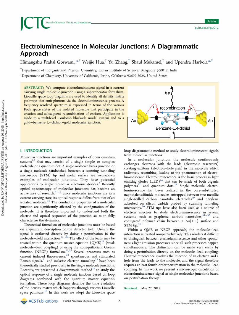
ABSTRACT: We compute electroluminescent signal in a currentcarrying single molecule junction using a superoperator formalism.Liouville space loop diagrams are used to identify all density matrixpathways that emit photons via the electroluminescence process. Afrequency resolved spectrum is expressed in terms of the variousFock space states of the isolated molecule that participate in thecreation and subsequent recombination of exciton. Application ismade to a multilevel Coulomb blockade model system and to agold−benzene-1,4-dithiol−gold molecular junction.

I. INTRODUCTION

Molecular junctions are important examples of open quantumsystems1,2 that may consist of a single simple or complexmolecule or a quantum dot. A single molecule break junction ora single molecule sandwiched between a scanning tunnelingmicroscopy (STM) tip and metal surface are well-knownexamples of molecular junctions. They have potentialapplications to single molecular electronic devices.3 Recentlyoptical spectroscopy of molecular junctions has become anactive area of research.4−15 Since molecular junctions are in acurrent carrying state, its optical response differs from that of anisolated molecule.16 The conduction properties of a molecularjunction are significantly affected by the configuration of themolecule. It is therefore important to understand both theelectric and optical responses of the junction so as to fullycharacterize the dynamics.Theoretical formalism of molecular junctions must be based

on a quantum description of the detected field. Usually thesignal is evaluated directly by doing a perturbation in themolecule−field interaction.17−20 The effect of the leads may betreated within the quantum master equation (QME)21 (weakmolecule−lead coupling) or using the nonequilibrium Greensfunction (NEGF) formalism.22,23 Several processes such ascurrent induced fluorescence,24 spontaneous and stimulatedRaman signals,21 and inelastic electron tunneling25 have beentheoretically studied previously in the single molecule junctions.Recently, we presented a diagrammatic method21 to study theoptical response of a single molecule junction based on loopdiagrams combined with the quantum master equationformalism. These loop diagrams describe the time evolutionof the density matrix which happens through various Liouvillespace pathways.17 In this work we adopt the Liouville space

loop diagrammatic method to study electroluminescent signalsfrom molecular junctions.In a molecular junction, the molecule continuously

exchanges electrons with the leads (electronic reservoirs)creating excitons (electron−hole pair) in the molecule whichradiatively recombine, leading to the phenomenon of electro-luminescence. Electroluminescence is the basic process in lightemitting diodes (LED)26 that can be made of both organicpolymers27 and quantum dots.28 Single molecule electro-luminescence has been realized in the core-substitutednaphthalenediimide molecules entrapped between two metallicsingle-walled carbon nanotube electrodes29 and peryleneadsorbed on silicon carbide probed by scanning tunnelingmicroscopy.30 STM tips have also been used as a source ofelectron injectors to study electroluminescence in severalsystems such as graphene, carbon nanotubes,31−33 andconjugated polymer chain between a Au(111) surface andSTM tip.34

Within a QME or NEGF approach, the molecule−leadinteraction is treated nonperturbatively. This renders it difficultto distinguish between electroluminescence and other sponta-neous light emission processes since all such processes happensimultaneously. The distinction can be made very easily bydoing a perturbation directly on the molecule−lead coupling.Electroluminescence involves the injection of an electron and ahole from the leads to the molecule, and the signal thereforerequires at least fourth-order perturbation in the molecule−leadcoupling. In this work we present a microscopic calculation ofelectroluminescence signal at single molecular junctions basedon perturbation theory.

Received: May 27, 2015

Article

pubs.acs.org/JCTC

© XXXX American Chemical Society A DOI: 10.1021/acs.jctc.5b00500J. Chem. Theory Comput. XXXX, XXX, XXX−XXX

Dow

nloa

ded

by U

NIV

OF

CA

LIF

OR

NIA

IR

VIN

E o

n A

ugus

t 26,

201

5 | h

ttp://

pubs

.acs

.org

P

ublic

atio

n D

ate

(Web

): A

ugus

t 21,

201

5 | d

oi: 1

0.10

21/a

cs.jc

tc.5

b005

00

pubs.acs.org/JCTC

http://dx.doi.org/10.1021/acs.jctc.5b00500

The loop diagrams that contribute to the formation of anexciton and the subsequent optical detection can be intuitivelydrawn. The diagrams represent the several pathways by which asignal can be obtained. We account for the electroluminescentsignal by considering the rate of change of photon occupationin the detected mode as a perturbation in the molecule−fieldand molecule−lead coupling and then combine it with themany-body states (Fock states) of the isolated molecule. Theloop diagrams clearly show how various molecular states(neutral or charged) are involved during the process. Hence thecomputation is based on the isolated molecule’s Fock stateswhich can be obtained with standard quantum chemistrycalculations. Interpretation of these diagrams is based onLiouville space superoperator algebra.35 We present a set ofrules that can be used to read the electroluminescent signaldirectly from the diagrams. We apply these rules to a genericmultilevel Coulomb blockade model and a gold−benzene-1,4-dithiol−gold molecular junction to compute the signal.This work is organized as follows. In the next section, section

II, we introduce the Hamiltonian and formulate electro-luminescence in terms of Liouville space loop diagrams. Insection III, we use Liouville space superoperator formalism toevaluate the electroluminescence signal perturbatively. Wediscuss rules to read the diagrams and write down the algebraicexpression for the signal directly from the loop diagrams. Insection IV, we apply these rules to evaluate the electro-luminescent spectrum in a multilevel Coulomb blockade modelsystem. In section V, we evaluate the electroluminescence signalfrom a benzene-1,5-dithiol molecular junction coupled to twogold leads. We conclude in section VI.

II. DIAGRAMMATIC FORMULATION OFELECTROLUMINESCENCE IN MOLECULARJUNCTIONS

Consider a molecule sandwiched between two metal contacts(leads) or an STM tip and a metal surface. A manifold of many-body states (neutral or charged) with different oxidation statescan participate in the electron transfer process between themolecule and leads. Electron exchange may occur either fromthe ground states of the neutral molecule or the chargedmolecule. This leads to excitations in the molecule. This mayinduce transfer of an electron or a hole or both (Figure 1).Transfer of electrons and holes leads to the creation of excitonsin the molecular junction. Radiative recombination of excitonscreated by the charge current gives rise to electroluminescence.The molecule−lead Hamiltonian can be written as H = Ho +

Hint

∑

= + +

= + ϵ + ϵ

= +

†

∈

†

H H H H

H a a c c

H H H

(1)

(2)

(3)

o m f x

m f f fx l r

x x x

int ml mf

,

Here Hm, Hf, and Hx are the molecular, the radiation field, andthe lead Hamiltonians, respectively. Hml and Hmf are themolecule−lead coupling and molecule−field interaction Ham-iltonians, respectively, defined as

∑ = + *

= +

† †

† †

H T c c T c c

H t V t t V t

( ) (4)

( ) ( ) ( ) ( ) (5)

mlx s

sx s x sx x s

mf f f

,

The molecular Hamiltonian need not be specified at thispoint and may contain many-body effects, e.g., electron−electron and electron−phonon interactions.

f (r,t) = Ef(r,t)a f(t) represents the complex amplitude of the field, and Ef(r,t)is the envelope of the field. a f (a f†) is the annihilation (creation)operator in the field mode of energy ϵf. c

† (c) is the Fermioncreation (annihilation) operator belonging to the system (s),left (l), and right (r) leads and ϵx is the energy of the x-th modein the lead. V (V†) is the system dipole operator which destroys(creates) an excitation in the molecule. Tsx is the system−leadtunneling coefficient from the x-th mode of the lead to the s-thorbital of the molecule.In molecular junctions, the leads create excitations between

the many-body states which can radiatively relax and can bedetected optically. We are interested in electroluminescence,the optically detected radiative recombination of an electron−hole pair (exciton) created in the same oxidation state. Tolowest order, excited states of the ionic charged states, N ± 1,can be created by two molecule−lead interactions that inject anelectron or a hole into the molecule. Fluorescence can thenarise by a transition between two states belonging to the ionicspecies (two different oxidation states). We had denoted thisprocess as current induced fluorescence (CIF).24 Here we focusemission from the same charged state (oxidation state). Thisrequires an injection of an electron and a hole into the moleculeand involves four molecule−lead interactions. We call itelectroluminescence.In electroluminescence, formation of an exciton population

requires four interactions with the leads which provide severalpathways for the evolution of system states that contribute tothe signal. We identify all of the possible pathways thatpopulate excitons (electron−hole pair) in the form of twoLiouville space loop diagrams17,19 as shown in Figure 2. These

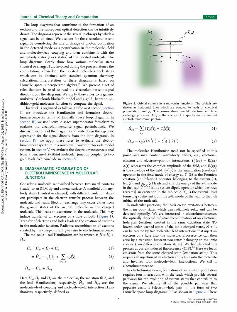
Figure 1. Orbital scheme in a molecular junctions. The orbitals areshown as horizontal lines which are coupled to leads at chemicalpotentials μl and μr. The arrows show possible electron and holeexchange processes. ℏωf is the energy of a spontaneously emittedelectroluminescence photon.

Journal of Chemical Theory and Computation Article

DOI: 10.1021/acs.jctc.5b00500J. Chem. Theory Comput. XXXX, XXX, XXX−XXX

B

Dow

nloa

ded

by U

NIV

OF

CA

LIF

OR

NIA

IR

VIN

E o

n A

ugus

t 26,

201

5 | h

ttp://

pubs

.acs

.org

P

ublic

atio

n D

ate

(Web

): A

ugus

t 21,

201

5 | d

oi: 1

0.10

21/a

cs.jc

tc.5

b005

00


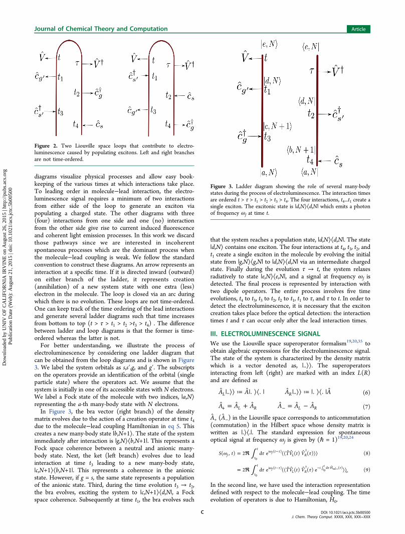
diagrams visualize physical processes and allow easy book-keeping of the various times at which interactions take place.To leading order in molecule−lead interaction, the electro-luminescence signal requires a minimum of two interactionsfrom either side of the loop to generate an exciton viapopulating a charged state. The other diagrams with three(four) interactions from one side and one (no) interactionfrom the other side give rise to current induced fluorescenceand coherent light emission processes. In this work we discardthose pathways since we are interested in incoherentspontaneous processes which are the dominant process whenthe molecule−lead coupling is weak. We follow the standardconvention to construct these diagrams. An arrow represents aninteraction at a specific time. If it is directed inward (outward)on either branch of the ladder, it represents creation(annihilation) of a new system state with one extra (less)electron in the molecule. The loop is closed via an arc duringwhich there is no evolution. These loops are not time-ordered.One can keep track of the time ordering of the lead interactionsand generate several ladder diagrams such that time increasesfrom bottom to top (t > τ > t1 > t2 >t3 > t4) . The differencebetween ladder and loop diagrams is that the former is time-ordered whereas the latter is not.For better understanding, we illustrate the process of

electroluminescence by considering one ladder diagram thatcan be obtained from the loop diagrams and is shown in Figure3. We label the system orbitals as s,s′,g, and g′. The subscriptson the operators provide an identification of the orbital (singleparticle state) where the operators act. We assume that thesystem is initially in one of its accessible states with N electrons.We label a Fock state of the molecule with two indices, |a,N⟩representing the a-th many-body state with N electrons.In Figure 3, the bra vector (right branch) of the density

matrix evolves due to the action of a creation operator at time t4due to the molecule−lead coupling Hamiltonian in eq 5. Thiscreates a new many-body state |b,N+1⟩. The state of the systemimmediately after interaction is |g,N⟩⟨b,N+1|. This represents aFock space coherence between a neutral and anionic many-body state. Next, the ket (left branch) evolves due to leadinteraction at time t3 leading to a new many-body state,|c,N+1⟩⟨b,N+1|. This represents a coherence in the anionicstate. However, if g = s, the same state represents a populationof the anionic state. Third, during the time evolution t3 → t2,the bra evolves, exciting the system to |c,N+1⟩⟨d,N|, a Fockspace coherence. Subsequently at time t1, the bra evolves such

that the system reaches a population state, |d,N⟩⟨d,N|. The state|d,N⟩ contains one exciton. The four interactions at t4, t3, t2, andt1 create a single exciton in the molecule by evolving the initialstate from |g,N⟩⟨g,N| to |d,N⟩⟨d,N| via an intermediate chargedstate. Finally during the evolution τ → t, the system relaxesradiatively to state |e,N⟩⟨e,N|, and a signal at frequency ωf isdetected. The final process is represented by interaction withtwo dipole operators. The entire process involves five timeevolutions, t4 to t3, t3 to t2, t2 to t1, t1 to τ, and τ to t. In order todetect the electroluminescence, it is necessary that the excitoncreation takes place before the optical detection: the interactiontimes t and τ can occur only after the lead interaction times.

III. ELECTROLUMINESCENCE SIGNALWe use the Liouville space superoperator formalism19,20,35 toobtain algebraic expressions for the electroluminescence signal.The state of the system is characterized by the density matrixwhich is a vector denoted as, |..⟩⟩. The superoperatorsinteracting from left (right) are marked with an index L(R)and are defined as

| ⟩⟩ ≔ | ⟩⟨ | | ⟩⟩ ≔ | ⟩⟨ | A A A A.. . . .. . .L R (6)

= + = − + −A A A A A AL R L R (7)

A+ (A−) in the Liouville space corresponds to anticommutation(commutation) in the Hilbert space whose density matrix iswritten as |.⟩⟨.|. The standard expression for spontaneousoptical signal at frequency ωf is given by (ℏ = 1)19,20,24

∫

∫

ω τ τ

τ τ

= ℜ ⟨⟨ ⟩⟩

= ℜ ⟨⟨ ⟩⟩

ω τ

ω τ τ τ

− †

− † − ∫ −

S t TV t V

TV t V

( , ) 2 d e ( ) ( ) (8)

2 d e ( ) ( ) e (9)

ft

ti t

L R

t

ti t

L Ri H

o

( )

( ) d ( )

f

f tt

ml

0

00

In the second line, we have used the interaction representationdefined with respect to the molecule−lead coupling. The timeevolution of operators is due to Hamiltonian, H0.

Figure 2. Two Liouville space loops that contribute to electro-luminescence caused by populating excitons. Left and right branchesare not time-ordered.

Figure 3. Ladder diagram showing the role of several many-bodystates during the process of electroluminescence. The interaction timesare ordered t > τ > t1 > t2 > t3 > t4. The four interactions, t4...t1 create asingle exciton. The excitonic state is |d,N⟩⟨d,N| which emits a photonof frequency ωf at time t.



C

Dow

nloa

ded

by U

NIV

OF

CA

LIF

OR

NIA

IR

VIN

E o

n A

ugus

t 26,

201

5 | h

ttp://

pubs

.acs

.org

P

ublic

atio

n D

ate

(Web

): A

ugus

t 21,

201

5 | d

oi: 1

0.10

21/a

cs.jc

tc.5

b005

00


We can now expand eq 9 to fourth order in molecule−leadinteraction, Hml− (Appendix A). We assume that contributionsfrom coherent processes, where the charged state is neverpopulated (Appendix A), is small as compared to incoherentprocesses and ignore these pathways. We further neglect thepathways which involve Fock space coherences between many-body states separated by more than one charge units (AppendixA). Such processes contribute with extremely low probability(fast Fock space decoherence). The electroluminescence signalthen involves a time-integrated product of a six-point time-dependent system correlation function and a four-point time-dependent lead correlation function given by

∫ ∫ ∫ ∫ ∫∑ ∑ ∑

ω τ

τ

τ

= ℜ

× * *

× ⟨⟨ ⟩⟩

× ⟨⟨ ⟩⟩

+ ⟨⟨ ⟩⟩

× ⟨⟨ ⟩⟩

ω τ−

′ ′ ′∈ ′∈′ ′ ′ ′

′†

′†

′†

′†

′†

′†

†′†

′†

S t t t t

T T T T

Tc t c t c t c t

TV t V c t c t c t c t

Tc t c t c t c t

TV t V c t c t c t c t

( ) 2 d e d d d d

[ ( ) ( ) ( ) ( )

( ) ( ) ( ) ( ) ( ) ( )

( ) ( ) ( ) ( )

( ) ( ) ( ) ( ) ( ) ( ) ]

elf

t

ti t

t

t

t

t

t

t

t

t

s g s g x x l r y y l rs x sx g y gy

y L yR x L xR o

L R g L gR s L sR o

x L xR y L yR o

L R s L sR g L gR o

( )1 2 3 4

, , , , , , ,

1 2 3 4

1 2 3 4

1 2 3 4

1 2 3 4

f

o0 0 0 0

(10)

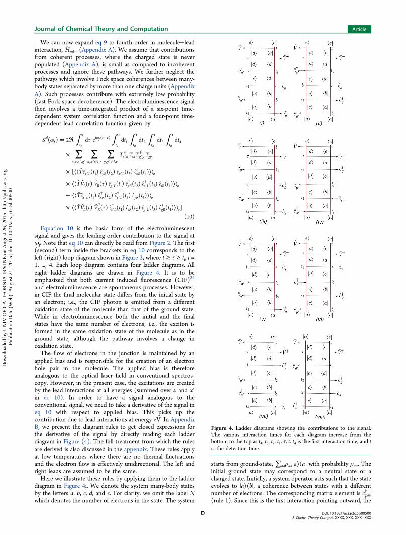
Equation 10 is the basic form of the electroluminescentsignal and gives the leading order contribution to the signal atωf. Note that eq 10 can directly be read from Figure 2. The first(second) term inside the brackets in eq 10 corresponds to theleft (right) loop diagram shown in Figure 2, where t ≥ τ ≥ ti, i =1, ..., 4. Each loop diagram contains four ladder diagrams. Alleight ladder diagrams are drawn in Figure 4. It is to beemphasized that both current induced fluorescence (CIF)24

and electroluminescence are spontaneous processes. However,in CIF the final molecular state differs from the initial state byan electron; i.e., the CIF photon is emitted from a differentoxidation state of the molecule than that of the ground state.While in electroluminescence both the initial and the finalstates have the same number of electrons; i.e., the exciton isformed in the same oxidation state of the molecule as in theground state, although the pathway involves a change inoxidation state.The flow of electrons in the junction is maintained by an

applied bias and is responsible for the creation of an electronhole pair in the molecule. The applied bias is thereforeanalogous to the optical laser field in conventional spectros-copy. However, in the present case, the excitations are createdby the lead interactions at all energies (summed over x and x′in eq 10). In order to have a signal analogous to theconventional signal, we need to take a derivative of the signal ineq 10 with respect to applied bias. This picks up thecontribution due to lead interactions at energy eV. In AppendixB, we present the diagram rules to get closed expressions forthe derivative of the signal by directly reading each ladderdiagram in Figure (4). The full treatment from which the rulesare derived is also discussed in the appendix. These rules applyat low temperatures where there are no thermal fluctuationsand the electron flow is effectively unidirectional. The left andright leads are assumed to be the same.Here we illustrate these rules by applying them to the ladder

diagram in Figure 4i. We denote the system many-body statesby the letters a, b, c, d, and e. For clarity, we omit the label Nwhich denotes the number of electrons in the state. The system

starts from ground-state, ∑aaρaa|a⟩⟨a| with probability ρaa. Theinitial ground state may correspond to a neutral state or acharged state. Initially, a system operator acts such that the stateevolves to |a⟩⟨b|, a coherence between states with a differentnumber of electrons. The corresponding matrix element is cg,ab

†

(rule 1). Since this is the first interaction pointing outward, the

Figure 4. Ladder diagrams showing the contributions to the signal.The various interaction times for each diagram increase from thebottom to the top as t4, t3, t2, t1, τ, t. t4 is the first interaction time, and tis the detection time.



D

Dow

nloa

ded

by U

NIV

OF

CA

LIF

OR

NIA

IR

VIN

E o

n A

ugus

t 26,

201

5 | h

ttp://

pubs

.acs

.org

P

ublic

atio

n D

ate

(Web

): A

ugus

t 21,

201

5 | d

oi: 1

0.10

21/a

cs.jc

tc.5

b005

00


Green function during the evolution t4 → t3 does notcontribute to the signal (rule 3). At time t3, another interactionfrom the left destroys the ket state and the system evolvesduring t3 → t2 to create Fock space coherence between stateswith the same number of electrons, |c⟩⟨b|. The correspondingoverlap matrix element is read top to bottom as cg′,ca The Fockstates involved are |c⟩ and |b⟩. t3 → t2 evolution is (ωcb) (rule2). Similarly, the next interaction takes place from the rightsuch that there is a creation in the bra taking the system to thecoherent state |c⟩⟨d| with a different number of electrons. Thematrix element is cs,bd. Since this interaction is the first inwardinteraction, the Greens function is (ωcd+eV) (rule 4). Thenext interaction from the left takes the system to a populationstate |d⟩⟨d|. The corresponding matrix element and the Greensfunction are cs′,dc

† and (ωdd) = (0), respectively. Finally, dueto interaction with the field, the ket evolves to state |e⟩ from |d⟩which is the final state. The matrix element is Ved

† , and thecorresponding Greens function is (ωde−ωf) (rule 5). Thedetection interaction contributes via the matrix element Vde.Following rule 6, the signal is written as (ℏ = 1)

∑ ∑ ∑ω ρ

ω ω ω ω

= ℜ Ω

× * * | |

× − +

ν

ν ν ν ν

′ ′ =

′′

′′ †

′ ′†

S

T T T T V c c c c

ddeV

( ) 2

(0) ( ) ( eV) ( )

eli

fabcde ss gg l r

aa

s s g g de g ab g ca s bd s dc

de f cd cb

(( ))

,

2

2, , , ,

(11)

where Ω is the wide-band approximated lead density of states.All of the diagrams can be interpreted in a similar manner. Afterwriting down all of the expressions, we can combine diagram iwith ii since their contributions become equal. Similarly we cancombine diagram iii with vii, diagram iv with viii, and diagram vwith vi. The total electroluminescence signal can now be recastas

∑ ∑ ∑ω ρ

ω ω ω

ω

ω

ω

ω

= ℜ Ω

× * * | | −

× +

+ +

+ −

+ −

ν

ν ν ν ν

′ ′ =

′′

′′

′†

′†

′† †

′

†′ ′

†

†′ ′

†

S

T T T T V

c c c c

c c c c G

c c c c G

c c c c G

ddeV

( ) 4

(0) ( ) ( )

[ ( eV)

( eV)

( eV)

( eV)]

el fabcde ss gg l r

aa

s s g g de de f cb

g ca g ab s bd s dc cd

g bd g dc s ca s ab ab

g bd g dc s ab s ca ca

g ab g ca s bd s dc db

,

2

2

, , , ,

, , , ,

, , , ,

, , , , (12)

Equation 12 is equivalent but a simplified version of eq 10. Thetime-dependent system and lead correlation functions in eq 10have been explicitly evaluated and put in closed forms in termsof the system-only Greens functions and the matrix elements ofeach system operator interacting with a system-only many-bodystate. We can substitute for the Greens functions as defined ineq B26 and obtain an algebraic expression for the frequencyresolved electroluminescence signal given as

∑ ∑ ∑ω ρ

ω ω ω

ω ω

ω ω

= − ℑ Ω

×* * | |

Γ − − Γ − Γ

×+ − Γ

++ − Γ

+− − Γ

+− − Γ

ν

ν ν ν ν

′ ′ =

′′

′′

′†

′†

′† †

′

†′ ′

† †′ ′

†

⎡⎣⎢⎢

⎤⎦⎥⎥

S

T T T T V

i i

c c c c

i

c c c c

i

c c c c

i

c c c c

i

ddeV

( ) 4

( )( )

( eV ) ( eV )

( eV ) ( eV )

el fabcde ss gg l r

aa

s s g g de

de f de cb cb

g ca g ab s bd s dc

cd cd

g bd g dc s ca s ab

ab ab

g bd g dc s ab s ca

ca ab

g ab g ca s bd s

db db

, ,

2

2

, , , , , , , ,

, , , , , , , ,dc

(13)

Since the signal is expressed in terms of the isolated molecule’sFock states, any quantum chemistry calculation done on themolecule will allow us to identify the system states and thecorresponding overlap matrix elements. These can be used tocompute the signal. We shall discuss it in more detail in sectionV.

IV. APPLICATION TO A MULTILEVEL MODEL SYSTEM

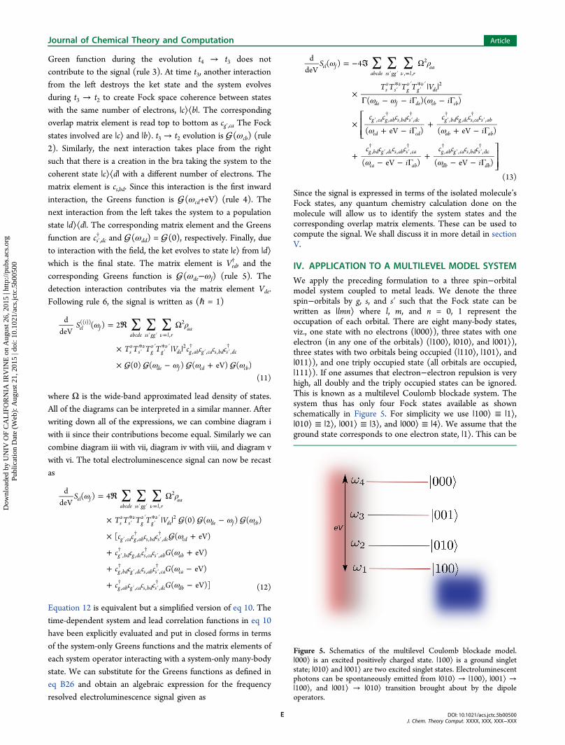
We apply the preceding formulation to a three spin−orbitalmodel system coupled to metal leads. We denote the threespin−orbitals by g, s, and s′ such that the Fock state can bewritten as |lmn⟩ where l, m, and n = 0, 1 represent theoccupation of each orbital. There are eight many-body states,viz., one state with no electrons (|000⟩), three states with oneelectron (in any one of the orbitals) (|100⟩, |010⟩, and |001⟩),three states with two orbitals being occupied (|110⟩, |101⟩, and|011⟩), and one triply occupied state (all orbitals are occupied,|111⟩). If one assumes that electron−electron repulsion is veryhigh, all doubly and the triply occupied states can be ignored.This is known as a multilevel Coulomb blockade system. Thesystem thus has only four Fock states available as shownschematically in Figure 5. For simplicity we use |100⟩ ≡ |1⟩,|010⟩ ≡ |2⟩, |001⟩ ≡ |3⟩, and |000⟩ ≡ |4⟩. We assume that theground state corresponds to one electron state, |1⟩. This can be

Figure 5. Schematics of the multilevel Coulomb blockade model.|000⟩ is an excited positively charged state. |100⟩ is a ground singletstate; |010⟩ and |001⟩ are two excited singlet states. Electroluminescentphotons can be spontaneously emitted from |010⟩ → |100⟩, |001⟩ →|100⟩, and |001⟩ → |010⟩ transition brought about by the dipoleoperators.



E

Dow

nloa

ded

by U

NIV

OF

CA

LIF

OR

NIA

IR

VIN

E o

n A

ugus

t 26,

201

5 | h

ttp://

pubs

.acs

.org

P

ublic

atio

n D

ate

(Web

): A

ugus

t 21,

201

5 | d

oi: 1

0.10

21/a

cs.jc

tc.5

b005

00


a situation when the Fermi energy of the leads is between theground doublet state and the next excited doublet state of themolecule. The next excited state is |2⟩ followed by anotherexcited singlet state |3⟩. |4⟩ represents a cationic state which isthe highest in energy.In this model, the loop diagrams in Figure 2 contribute to the

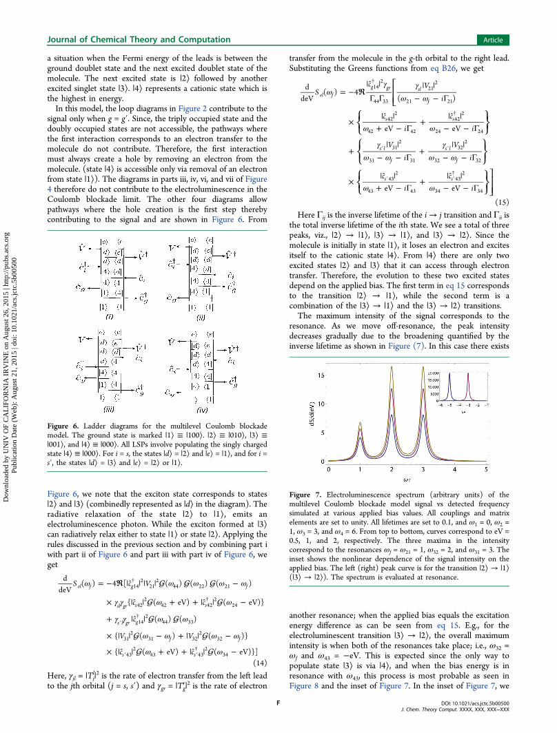
signal only when g = g′. Since, the triply occupied state and thedoubly occupied states are not accessible, the pathways wherethe first interaction corresponds to an electron transfer to themolecule do not contribute. Therefore, the first interactionmust always create a hole by removing an electron from themolecule. (state |4⟩ is accessible only via removal of an electronfrom state |1⟩). The diagrams in parts iii, iv, vi, and vii of Figure4 therefore do not contribute to the electroluminescence in theCoulomb blockade limit. The other four diagrams allowpathways where the hole creation is the first step therebycontributing to the signal and are shown in Figure 6. From

Figure 6, we note that the exciton state corresponds to states|2⟩ and |3⟩ (combinedly represented as |d⟩ in the diagram). Theradiative relaxation of the state |2⟩ to |1⟩, emits anelectroluminescence photon. While the exciton formed at |3⟩can radiatively relax either to state |1⟩ or state |2⟩. Applying therules discussed in the previous section and by combining part iwith part ii of Figure 6 and part iii with part iv of Figure 6, weget

ω ω ω ω ω

γ γ ω ω

γ γ ω ω

ω ω ω ω

ω ω

= − ℜ | | | | −

× | | + + | | −

+ | |

× | | − + | | −

× | | + + | | −

†

†

′†

′ ′†

S c V

c c

c

V V

c c

ddeV

( ) 4 [ ( ) ( ) ( )

{ ( eV) ( eV)}

( ) ( )

{ ( ) ( )}

{ ( eV) ( eV)}]

el f g f

sl gr s s

s l gr g

f f

s s

142

212

44 22 21

422

42 422

24

142

44 33

312

31 322

32

432

43 432

34

(14)

Here, γjl = |Tjl|2 is the rate of electron transfer from the left lead

to the jth orbital (j = s, s′) and γgr = |Tgr|2 is the rate of electron

transfer from the molecule in the g-th orbital to the right lead.Substituting the Greens functions from eq B26, we get

ωγ γ

ω ω

ω ω

γω ω

γω ω

ω ω

= − ℜ| |

Γ Γ| |

− − Γ

×| |

+ − Γ+

| |− − Γ

+| |

− − Γ+

| |− − Γ

×| |

+ − Γ+

| |− − Γ

†

†

′ ′

′ ′†

⎪ ⎪

⎪ ⎪

⎪ ⎪

⎪ ⎪

⎪ ⎪

⎪ ⎪

⎡⎣⎢⎢

⎧⎨⎩

⎫⎬⎭

⎧⎨⎩

⎫⎬⎭

⎧⎨⎩

⎫⎬⎭

⎤⎦⎥⎥

Sc V

i

ci

ci

V

i

V

i

ci

ci

ddeV

( ) 4( )

eV eV

eV eV

el fg gr sl

f

s s

s l

f

s l

f

s s

142

44 33

212

21 21

422

42 42

422

24 24

312

31 31

322

32 32

432

43 43

432

34 34

(15)

Here Γij is the inverse lifetime of the i→ j transition and Γii isthe total inverse lifetime of the ith state. We see a total of threepeaks, viz., |2⟩ → |1⟩, |3⟩ → |1⟩, and |3⟩ → |2⟩. Since themolecule is initially in state |1⟩, it loses an electron and excitesitself to the cationic state |4⟩. From |4⟩ there are only twoexcited states |2⟩ and |3⟩ that it can access through electrontransfer. Therefore, the evolution to these two excited statesdepend on the applied bias. The first term in eq 15 correspondsto the transition |2⟩ → |1⟩, while the second term is acombination of the |3⟩ → |1⟩ and the |3⟩ → |2⟩ transitions.The maximum intensity of the signal corresponds to the

resonance. As we move off-resonance, the peak intensitydecreases gradually due to the broadening quantified by theinverse lifetime as shown in Figure (7). In this case there exists

another resonance; when the applied bias equals the excitationenergy difference as can be seen from eq 15. E.g., for theelectroluminescent transition |3⟩ → |2⟩, the overall maximumintensity is when both of the resonances take place; i.e., ω32 =ωf and ω43 = −eV. This is expected since the only way topopulate state |3⟩ is via |4⟩, and when the bias energy is inresonance with ω43, this process is most probable as seen inFigure 8 and the inset of Figure 7. In the inset of Figure 7, we

Figure 6. Ladder diagrams for the multilevel Coulomb blockademodel. The ground state is marked |1⟩ ≡ |100⟩. |2⟩ ≡ |010⟩, |3⟩ ≡|001⟩, and |4⟩ ≡ |000⟩. All LSPs involve populating the singly chargedstate |4⟩ ≡ |000⟩. For i = s, the states |d⟩ = |2⟩ and |e⟩ = |1⟩, and for i =s′, the states |d⟩ = |3⟩ and |e⟩ = |2⟩ or |1⟩.

Figure 7. Electroluminescence spectrum (arbitrary units) of themultilevel Coulomb blockade model signal vs detected frequencysimulated at various applied bias values. All couplings and matrixelements are set to unity. All lifetimes are set to 0.1, and ω1 = 0, ω2 =1, ω3 = 3, and ω4 = 6. From top to bottom, curves correspond to eV =0.5, 1, and 2, respectively. The three maxima in the intensitycorrespond to the resonances ωf = ω21 = 1, ω32 = 2, and ω31 = 3. Theinset shows the nonlinear dependence of the signal intensity on theapplied bias. The left (right) peak curve is for the transition |2⟩ → |1⟩(|3⟩ → |2⟩). The spectrum is evaluated at resonance.



F

Dow

nloa

ded

by U

NIV

OF

CA

LIF

OR

NIA

IR

VIN

E o

n A

ugus

t 26,

201

5 | h

ttp://

pubs

.acs

.org

P

ublic

atio

n D

ate

(Web

): A

ugus

t 21,

201

5 | d

oi: 1

0.10

21/a

cs.jc

tc.5

b005

00


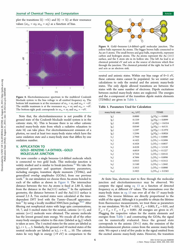
plot the transitions |2⟩ →|1⟩ and |3⟩ → |2⟩ at their resonancevalues (ω21 = ωf; ω32 = ωf) as a function of bias.

Note that, the electroluminescence is not possible if theground state of the Coulomb blockade model system is in thecationic state, |4⟩. This is because there is no other cationicexcited many-body state from which a radiative relaxation tostate |4⟩ can take place. For electroluminescent emission of aphoton, we need at least two many-body states which have thesame oxidation state and a many-body state that differs by oneoxidation number.

V. APPLICATION TOGOLD−BENZENE-1,4-DITHIOL−GOLDMOLECULAR JUNCTION

We now consider a single benzene-1,4-dithiol molecule whichis connected to two gold leads. This molecular junction iswidely studied and is similar to break-junctions.36 We take theoptimized geometry and quantum chemistry parameters,including energies, transition dipole moments (TDMs), andgeneralized overlap amplitudes (GOAs), from our previouswork.37 In our simulation we choose three Au-atoms bonded toeach of the sulfurs as shown in Figure 9. The internucleardistance between the two Au atoms is fixed at 2.88 Å, takenfrom the distance in the Au(111) surface.38 In the optimizedgeometry, the distance between S and the Au(111) surface isaround 2.3 Å. Ten excited states were calculated at the time-dependent DFT level with the Tamm−Dancoff approxima-tion39 by using a locally modified NWChem package.40,41 Afterfiltering out nonphysical states with large spin contaminations,10, 7, and 5 excited states for the neutral, cationic (n−1), andanionic (n+1) molecule were obtained. The anionic moleculehas the lowest ground state energy. We rescale all of the othermany-body energies relative to this state (labeled as |g0⟩) whichis taken as zero. The 5 excited states for the anion are labeled as|gi⟩, i = 1, ..., 5. Similarly, the ground and 10 excited states of theneutral molecule are labeled as |ei⟩, i = 0, ..., 10. The cationicstates lie very high in energy (>9 eV) in comparison to the

neutral and anionic states. Within our bias range of 0−5 eV,these cationic states cannot be populated. So we restrict ourcalculations to only the neutral and the anionic many-bodystates. The only dipole allowed transitions are between thestates with the same number of electrons. Dipole excitationsbetween excited many-body states are neglected. The energiesand the x-component of the transition dipole matrix elements(TDMEs) are given in Table 1.

At finite bias, electrons start to flow through the molecularjunction and electroluminescence may be observed. Wecompute the signal using eq 13 as a function of detectedfrequency ωf at different eV values. The summations over themany-body states in eq 13 run over all of the 17 many-bodystates. The inverse lifetimes are directly proportional to thewidth of the signal. Although it is possible to obtain the lifetimefrom fluorescence measurements, we treat these as parametersin our simulation. We fix Γ = 0.01, Γde = 0.005, Γcb = 0.01, andΓcd = Γab = Γca = Γdb = 0.001. All energies are given in eV.Plugging the respective values for the matrix elements andenergies from Table 1 and constructing the GOAs, the signalcan be numerically evaluated. Since the ground statecorresponds to the anionic (N+1) state, the emission of theelectroluminescent photon comes from the anionic many-bodystate. We expect a total of five peaks in the signal emitted fromthe excited anionic many-body states. However, the transition

Figure 8. Electroluminescence spectrum in the multilevel Coulombblockade system vs the bias voltage vs all emitted frequency ωf. Thebottom left maximum is at the resonance of ω21 = ωf and ω42 = −eV.The middle maximum is at the resonance ω32 = ωf and ω43 = −eV.The bottom-right peak corresponds to ω31 = ωf and ω43 = −eV.

Figure 9. Gold−benzene-1,4-dithiol−gold molecular junction. Theyellow balls represent Au atoms. The bigger brown balls connected toAu are S atoms. The small brown and gray balls, respectively, representcarbon and hydrogen atoms. The Au atoms represent the Au (111)surface, and the S atom sits in its hollow site. The left Au lead is atchemical potential eV and acts as the source of electrons which flowthrough the junction. The chemical potential of the right Au lead is 0and acts as an electron sink.

Table 1. Parameters Used for Calculation

many-body state ωm (eV) TDME

|go⟩ 0.0000 ⟨go|V|go⟩ = 0.0000|g1⟩ 0.1339 ⟨go|V|g1⟩ = 0.0099|g2⟩ 0.1602 ⟨ go|V|g2⟩ = 0.6354|g3⟩ 0.8549 ⟨go|V|g3⟩ = 4.6131|g4⟩ 1.2397 ⟨go|V|g4⟩ = 0.1970|g5⟩ 1.2596 ⟨go|V|g5⟩ = 0.0026|eo⟩ 2.7950 ⟨eo|V|eo⟩ = 0.0000|e1⟩ 4.1422 ⟨eo|V|e1⟩ = 0.2098|e2⟩ 4.1628 ⟨eo|V|e2⟩ = 0.0037|e3⟩ 4.4538 ⟨eo|V|e3⟩ = 3.3120|e4⟩ 4.6019 ⟨eo|V|e4⟩ = 0.1227|e5⟩ 4.7224 ⟨eo|V|e5⟩ = 0.0122|e6⟩ 4.7684 ⟨eo|V|e6⟩ = 0.0096|e7⟩ 5.0353 ⟨eo|V|e7⟩ = 0.3512|e8⟩ 5.1160 ⟨eo|V|e8⟩ = 1.2642|e9⟩ 5.1613 ⟨eo|V|e9⟩ = 0.0080|e10⟩ 5.1823 ⟨eo|V|e10⟩ = 0.2363



G

Dow

nloa

ded

by U

NIV

OF

CA

LIF

OR

NIA

IR

VIN

E o

n A

ugus

t 26,

201

5 | h

ttp://

pubs

.acs

.org

P

ublic

atio

n D

ate

(Web

): A

ugus

t 21,

201

5 | d

oi: 1

0.10

21/a

cs.jc

tc.5

b005

00


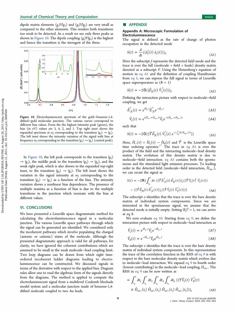
dipole matrix elements ⟨go|V|g1⟩ and ⟨go|V|g5⟩ are very small ascompared to the other elements. This renders both transitionstoo weak to be detected. As a result we see only three peaks asshown in Figure 10. The dipole coupling ⟨go|V|g3⟩ is the highestand hence the transition is the strongest of the three.

In Figure 10, the left peak corresponds to the transition |g2⟩→ |go⟩, the middle peak to the transition |g3⟩ → |go⟩, and theweak right peak, which is also shown in the expanded top-rightinset, to the transition |g4⟩ → |go⟩. The left inset shows thevariation in the signal intensity at ωf corresponding to thetransition |g3⟩ → |go⟩ as a function of the bias. The intensityvariation shows a nonlinear bias dependence. The presence ofmultiple maxima as a function of bias is due to the multipletransitions in the junction which resonate with the bias atdifferent values.

VI. CONCLUSIONS

We have presented a Liouville space diagrammatic method forcalculating the electroluminescence signal in a molecularjunction. The various Liouville space pathways through whichthe signal can be generated are identified. We considered onlythe incoherent pathways which involve populating the charged(anionic or cationic) states of the molecule. Although thepresented diagrammatic approach is valid for all pathways, forclarity, we have ignored the coherent contributions which areassumed to be small in the weak molecule−lead coupling limit.Two loop diagrams can be drawn from which eight time-ordered incoherent ladder diagrams leading to electro-luminescence can be constructed. We discussed signals interms of the derivative with respect to the applied bias. Diagramrules allow one to read the algebraic form of the signals directlyfrom the diagrams. The method is applied to compute theelectroluminescent signal from a multilevel Coulomb blockademodel system and a molecular junction made of benzene-1,4-dithiol molecule coupled to two Au leads.

■ APPENDIX

Appendix A: Microscopic Formulation ofElectroluminescenceThe signal is defined as the rate of change of photonoccupation in the detected mode

= ⟨⟨ ⟩⟩†S tt

a t a t( )dd

( ) ( )f f F (A1)

Here the subscript f represents the detected field mode and thetrace is over the full (molecule + field + leads) density matrixdenoted as a subscript F. Using the Heisenberg’s equation ofmotion in eq A1 and the definition of coupling Hamiltonianfrom eq 5, we can express the full signal in terms of Liouvillespace superoperators as (ℏ = 1)

= − ℑ⟨⟨ ⟩⟩†S t t V t( ) 2 ( ) ( )fL L F (A2)

Defining the interaction picture with respect to molecule−fieldcoupling, we get

=

=

† † −

+ − +

− −

− − − −

t

V t V

( ) e e (A3)

( ) e e (A4)

fLiH t

fLiH t

Li H H t

Li H H t( ) ( )

f f

m ml m ml

such that

= − ℑ⟨⟨ ⟩⟩τ τ† − ∫ −S t t V t( ) 2 ( ) ( ) efL Li Hd ( )t

tmf0 (A5)

Here, H−(τ) = HL(τ) − HR(τ) and is the Liouville spacetime ordering operator.17 The trace in eq A5 is over theproduct of the field and the interacting molecule−lead densitymatrix. The evolution of this density matrix is due tomolecule−field interaction. eq A5 contains both the sponta-neous and the stimulated light emission processes. To leadingorder in the detected field (molecule−field interaction, Hmf−),we can recast the signal as

∫ τ τ τ

τ τ

= − ℜ ⟨⟨ ⟩⟩ ⟨⟨ ⟩⟩

− ⟨⟨ ⟩⟩ ⟨⟨ ⟩⟩

† †

† †

S t t V t V

t V t V

( ) 2 { d ( ) ( ) ( ) ( )

( ) ( ) ( ) ( ) }

t

t

fL fL o L L

fR fL o L R

0

(A6)

The subscript o identifies that the trace is over the bare densitymatrix of individual system components. Since we areinterested in the spontaneous signal, we assume that thedetected mode is initially empty. Setting |Ef |

2 = 1, we can arriveat eq 8.We now evaluate eq 10. Starting from eq 9, we define the

interaction picture with respect to molecule−lead interaction as

=

=

−

−

− −

− −

V t V

V t V

( ) e e (A7)

( ) e e (A8)

LiH t

LiH t

RiH t

RiH t

m m

m m

The subscript o identifies that the trace is over the bare densitymatrix of individual system components. In this representationthe trace of the correlation function in the RHS of eq 9 is withrespect to the bare molecular density matrix which evolves dueto molecule−lead interaction. We expand eq 9 to fourth order(lowest contributing) in the molecule−lead coupling, Hml−. TheRHS in eq 9 can be now written as

∫ ∫ ∫ ∫ τ= ⟨⟨

× ⟩⟩

†

− − − −

t t t t V t V

H t H t H t H t

d d d d ( ) ( )

( ) ( ) ( ) ( )

t

t

t

t

t

t

t

t

L R

ml ml ml ml o

1 2 3 4

1 2 3 4

0 0 0 0

(A9)

Figure 10. Electroluminescent spectrum of the gold−benzene-1,4-dithiol−gold molecular junction. The various curves correspond todifferent bias values. From the the highest intensity peak (green), thebias (in eV) values are 3, 4, 2, and 1. Top right inset shows theexpanded spectrum at ωf corresponding to the transition |g4⟩ → |go⟩.The left inset shows the intensity variation of the signal with bias atfrequency ωf corresponding to the transition |g3⟩→ |go⟩ (central peak).



H

Dow

nloa

ded

by U

NIV

OF

CA

LIF

OR

NIA

IR

VIN

E o

n A

ugus

t 26,

201

5 | h

ttp://

pubs

.acs

.org

P

ublic

atio

n D

ate

(Web

): A

ugus

t 21,

201

5 | d

oi: 1

0.10

21/a

cs.jc

tc.5

b005

00


The time arguments get integrated since they are not controlledexternally. Upon substituting Hml− = HmlL − HmlR, we get 16terms in the equation. Out of the 16 terms only the terms withtwo Ls and two Rs in the lead operators contribute toelectroluminescence. The other terms contribute to currentinduced fluorescent signals which may come from either theneutral or the charged states. The electroluminescent signal canbe expressed as

∫ ∫ ∫ ∫ ∫ω τ

τ

τ

τ

τ

τ

τ

= ℜ

× ⟨⟨ ⟩⟩

+ ⟨⟨ ⟩⟩

+ ⟨⟨ ⟩⟩

+ ⟨⟨ ⟩⟩

+ ⟨⟨ ⟩⟩

+ ⟨⟨ ⟩⟩

ω τ−

†

†

†

†

†

†

S t t t t t

V t V H t H t H t H t






( , ) 2 d e d d d d

( ( ) ( ) ( ) ( ) ( ) ( )

( ) ( ) ( ) ( ) ( ) ( )

( ) ( ) ( ) ( ) ( ) ( )

( ) ( ) ( ) ( ) ( ) ( )

( ) ( ) ( ) ( ) ( ) ( )

( ) ( ) ( ) ( ) ( ) ( ) )

elf

t

ti t

t

t

t

t

t

t

t

t

L R mlL mlL mlR mlR o

L R mlL mlR mlL mlR o

L R mlL mlR mlR mlL o

L R mlR mlL mlL mlR o

L R mlR mlL mlR mlL o

L R mlR mlR mlL mlL o

( )1 2 3 4

1 2 3 4

1 2 3 4

1 2 3 4

1 2 3 4

1 2 3 4

1 2 3 4

f

o0 0 0 0

(A10)

For weak system bath coupling, the perturbation formulationallows us to factorize the system and lead correlation functionsafter substituting the molecule−lead coupling Hamiltonianfrom eq 5 in eq A10. The system correlation function includesthe product of all of the system operators along with their timearguments in the loop diagrams. The product is averaged overthe system density matrix, |ρ⟩⟩. For each system operator thereis a corresponding lead operator. Since creation of electron inthe system is annihilation of an electron in the lead, the leadoperators are conjugate to each of the system operators. Thedipole operators have no lead counterpart.In the first term of eq A10, one of the system correlation

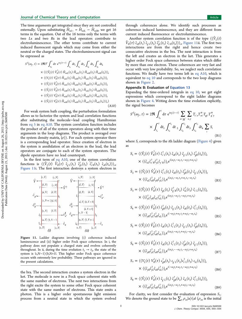
functions is ⟨⟨VL(t) VR(τ) cg′L(t1) cgL† (t2) cs′R

† (t3) csR(t4)⟩⟩o,Figure 11i. The first interaction destroys a system electron in

the bra. The second interaction creates a system electron in theket. The molecule is now in a Fock space coherent state withthe same number of electrons. The next two interactions fromthe right excite the system to some other Fock space coherentstate with the same number of electrons. This state emits aphoton. This is a higher order spontaneous light emissionprocess from a neutral state in which the system evolved

through coherences alone. We identify such processes ascoherence induced luminescence, and they are different fromcurrent induced fluorescence or electroluminescence.Another system correlation function is of the type ⟨⟨VL(t)

VR(τ) csR(t1) cg′L(t2) cgL† (t3) cs′R(t4)⟩⟩o, Figure 11ii. The first two

interactions are from the right and hence create twoconsecutive electrons in the bra. The next interaction is fromthe left and creates an electron in the ket. This generates ahigher order Fock space coherence between states which differby more than one electron. These coherences are very fast andoccur with very low probability. So, we neglect such correlationfunctions. We finally have two terms left in eq A10, which isequivalent to eq 10 and corresponds to the two loop diagramsshown in Figure 2.Appendix B: Evaluation of Equation 13Expanding the time-ordered integrals in eq 10, we get eightexpressions which correspond to the eight ladder diagramsshown in Figure 4. Writing down the time evolution explicitly,the signal becomes

∫

∫ ∫ ∫ ∫

∑ ∑

∑

ω τ= ℜ * *

×

ω τ

τ

−

′ ′′ ′ ′ ′S t T T T T

t t t t S

( , ) 2 d e

d d d d

elf

t

ti t

ss gg x ys x sx gy g y

t t

t

t

t

t

t

ii

( )

,

1 2 3 4

f

o

0

0

1

0

2

0

3

(B1)

where Si corresponds to the ith ladder diagram (Figure 4) givenas

τ= ⟨⟨ ⟩⟩

× ⟨⟨ ⟩⟩ ω ω ω ω

†′†

′†

′† †

′− − +′ ′

S V t V c t c t c t c t

c c c c

( ) ( ) ( ) ( ) ( ) ( )

e

L R s L sR g L gR o

xL x R yL y R oi t t t t

1 1 2 3 4

( )x x y y1 2 3 4(B2)

τ= ⟨⟨ ⟩⟩

× ⟨⟨ ⟩⟩ ω ω ω ω

†′† †

′

† † − + −′ ′ ′


c c c c

( ) ( ) ( ) ( ) ( ) ( )

e

L R s L sR gR g L o

xL xR yR yL oi t t t t

2 1 2 3 4

( )x x y y1 2 3 4(B3)

τ= ⟨⟨ ⟩⟩

× ⟨⟨ ⟩⟩ ω ω ω ω

†′

† †′

† † − − +′ ′


c c c c

( ) ( ) ( ) ( ) ( ) ( )

e

L R gL g R sL s L o

yL yR xL xL oi t t t t

3 1 2 3 4

( )y y x x1 2 3 4(B4)

τ= ⟨⟨ ⟩⟩

× ⟨⟨ ⟩⟩ ω ω ω ω

† †′ ′

†

† † − + + −′ ′


c c c c

( ) ( ) ( ) ( ) ( ) ( )

e

L R gR g L sR s L o

yR yL xR xL oi t t t t

4 1 2 3 4

( )y y x x1 2 3 4(B5)

τ= ⟨⟨ ⟩⟩

× ⟨⟨ ⟩⟩ ω ω ω ω

†′†

′†

† † − + −′ ′


c c c c

( ) ( ) ( ) ( ) ( ) ( )

e

L R sR s L g L gR o


5 1 2 3 4

( )x x y y1 2 3 4(B6)

τ= ⟨⟨ ⟩⟩

× ⟨⟨ ⟩⟩ ω ω ω ω

†′† †

′

† † −− − +′ ′


c c c c

( ) ( ) ( ) ( ) ( ) ( )

e

L R sR s L gR g L o


6 1 2 3 4

( )x x y y1 2 3 4(B7)

τ= ⟨⟨ ⟩⟩

× ⟨⟨ ⟩⟩ ω ω ω ω

† †′ ′

†

† † − + − +′ ′


c c c c

( ) ( ) ( ) ( ) ( ) ( )

e

L R gR g L s L sL o


7 1 2 3 4

( )y y x x1 2 3 4(B8)

τ= ⟨⟨ ⟩⟩

× ⟨⟨ ⟩⟩ ω ω ω ω

†′

†′†

† † − + −′ ′


c c c c

( ) ( ) ( ) ( ) ( ) ( )

e

L R g L gR sL s L o


8 1 2 3 4

( )y y x x1 2 3 4(B9)

For clarity, we first consider the evaluation of expression S1.We denote the ground state to be ∑a ρaa|a⟩⟨a| (ρaa is the initial

Figure 11. Ladder diagrams involving (i) coherence inducedluminescence and (ii) higher order Fock space coherence. In i, thepathway does not populate a charged state and evolves coherentlythroughout. In ii, during the time evolution t3 → t2, the state of thesystem is |c,N−1⟩⟨b,N+1|. This higher order Fock space coherenceoccurs with extremely low probability. These pathways are ignored inthe present calculations.



I

Dow

nloa

ded

by U

NIV

OF

CA

LIF

OR

NIA

IR

VIN

E o

n A

ugus

t 26,

201

5 | h

ttp://

pubs

.acs

.org

P

ublic

atio

n D

ate

(Web

): A

ugus

t 21,

201

5 | d

oi: 1

0.10

21/a

cs.jc

tc.5

b005

00


probability) and insert the identity I = ∑n|n⟩ ⟨n|, in terms ofmolecular many-body states |n⟩. Using the mapping betweenLiouville space and Hilbert space,35 we have

ρ ρ

ρ ρ

ρ ρ

ρ ρ

| ⟩⟩ ≡

| ⟩⟩ ≡

| ⟩⟩ ≡ −

| ⟩⟩ ≡ −

† †

−

† − + †

c c

c c

c c

c c

(B10)

(B11)

( 1) (B12)

( 1) (B13)

iL i

iL i

iRM N

i

iRM N

i1

where ρ = ∑|M⟩⟨N| is the Hilbert space density matrix. Thesystem-only correlation function in S1 can be recast into theHilbert space operators.

∑τ

ρ

⟨⟨ ⟩⟩

= | |

× ω ω ω ω ω ω τ

†′†

′†

†′ ′

†

+ + + − + −

V t V c t c t c t c t

V c c c c

( ) ( ) ( ) ( ) ( ) ( )

e

L R s L sR g L gR o

abcdeaa de g g s s

i t t t t t

1 2 3 4

2,ab ,ca ,bd ,dc

( ( )( ))ab bc dc de f ed4 3 2 1 (B14)

where we denoted the matrix element, Ak,nn′ = ⟨n|Ak|n′⟩.The lead correlation function in S1 can be recast into the

Hilbert space as ⟨⟨cxLcx′RcyL† cy′R⟩⟩o = ⟨cy′cx′

† cxcy†⟩. Since the two

leads do not interact among themselves one can separate thefour point correlation function as a product of two separate twopoint correlation functions, ⟨cy′cx′

† cxcy†⟩ = ⟨cycy

†⟩⟨cx†cx⟩ +

⟨cxcx†⟩⟨cy

†cy⟩ + ⟨cycy†⟩⟨cy

†cy⟩ + ⟨cxcx†⟩⟨cx

†cx⟩. So, ⟨cx†cx⟩ = f x and

⟨cxcx†⟩ = 1 − f x = fx, where f x’s are the Fermi functions of the

lead at the energy ωx such that x ∈ l, r defined as f x = 1/(e(ℏωx−μx)/kTx + 1) and μx is the chemical potential of the xthlead which are at temperatures Tx. The contribution from S1 tothe signal after simplification can be written down as

∫ ∫ ∫ ∫ ∫

∑ ∑ ∑ω ρ

τ

= ℜ | |

× + + +

×

×

ω ττ

ω ω ω ω ω ω ω ω ω ω τ

′ ′′

*′*

†′ ′

†

−

+ + − + − + + − + −

S t T T T T V

c c c c f f f f f f f f

t t t t

( , ) 2

( )

d e d d d d

e

elf

ss gg xy abcdesx

sx

gy

gy

aa de

g ab g ca s bd s dc x y y x x x y y

t

ti t

t t

t

t

t

t

t

i t t t t t

12

, , , ,

( )1 2 3 4

[( ) ( ) ( ) ( ) ( )( ))]

f

x dc bd x ca y y ab f ed

0 0 0

1

0

2

0

3

1 2 3 4

(B15)

The time integrals can be done by following the standardintegral

∫ ω′ =

− Γω

ω

−∞

′

Γ →t

iei

d e lim( )

ki t

i k

mn mn0mn

mn

mn

(B16)

These integrals correspond to the Greens functions discussedin rule 2. Here Γmn is interpreted as the inverse lifetime of thetransition m → n. By taking t0 → ∞ and simplifying S1

el, we get

∑ ∑ ∑ωρ

ω ω ω ω= − ℜ

| |

×Γ

+ + +

′ ′′

*′*

†′ ′

†

S T T T TV

ic c c c g f f f f f f f f

( ) 2

1( )

elf

ss gg xy abcdesx

sx

gy

gy aa de

ab cb cd de

g ab g ca s bd s dc x y y x x x y y

1

2

, , , ,

(B17)

where

ωω ω

ωω

=+ − Γ

=− Γi i

1( )

1( )ab

y ab abcb

cb cb

(B18)

ωω ω

ωω ω

=+ − Γ

=− − Γi i

1( )

1( )cd

cd x cdde

de f de

(B19)

We now assume the lead states form a continuum andreplace the summation over lead states by integrations over leadenergies. This allows us to include the density of states (Ων)corresponding to the leads. We further assume that thetunneling coefficients are independent of energy. So we get

∫ ∫∑ ∑ ∑ω ω ω ω ω

ρ

ω ω ω ω

= − ℑ Ω Ω

×| |

Γ

× + + +

ν ν

ν ν ν ν

′ ′ ′∈

′* ′

′′*

†′ ′

†

S

T T T TV c c c c

f f f f f f f f

( ) 2 d ( ) d ( )

( )

elf

ss gg abcde l rx x x y x y

s s g gaa de g ab g ca s bd s dc

ab cb cd de

x y y x x x y y

1, ,

2, , , ,

(B20)

The evaluation of eq B20 is far from a triviality. However, onecan analytically evaluate the signal at zero temperature wherethere exists only unidirectional flow and no thermal effects ( f l =1 and f r = 0). Thermal effects are known to play an importantrole in affecting electron transfer processes42 which in turn mayaffect the optical properties. However, due to analyticalrestrictions to evaluate a thermally affected optical signal eqB20, we invoke the zero temperature limit. A particularadvantage of the zero temperature limit is that it allowsidentification of the ground state (ρaa = 1 can be achieved.) Wepoint out that eq B20 can be numerically evaluated using somemathematical form of the lead density of states to obtain athermally affected electroluminescent signal. We are howeverinterested in analytical evaluation and reduction of computa-tional costs. So, in the zero temperature limit, we have

∫ ∫

∑ ∑ ∑ω

ρ

ω ω

ωω ω

ωω ω

= − ℑ

×| |

Γ

×Ω

− − ΓΩ

+ − Γ

ν ν

ν ν ν ν

′ ′ ′∈′

′*′′*

†′ ′

†

S T T T T

V c c c c

i i

( ) 2

d d

elf

ss gg l r abcdes s g g

aa de g ab g ca s bd s dc

de cb

xx

cd x cdy

y

ab y ab

1, ,

2, , , ,

(B21)

A realistic quantity is the derivative of the signal with respectto external bias. The bias eV in molecular junctions is analogousto an incoming excitation field in conventional spectroscopy.We use μl = μ0 + eV and μr = μ0 and assume μ0 = 0. Wedifferentiate the preceding signal with respect to external bias toget

∫

∑ ∑ ∑ω

ρ

ω ω

ωω

ωω ω

= − ℑ

×| |

×Ω+ − Γ

Ω− − Γ

ν ν

ν ν ν ν

ν ν

′ ′ ′∈′

* ′ ′*

†′ ′

†

−∞

′

S T T T T

V c c c c

i i

ddeV

( ) 2

(eV)eV

d( )

elf



de cb

cd cdx

x

ab x ab

1, ,

2, , , ,

0

(B22)

The differentiation with respect to bias gives the eVdependence in the first inward interaction (rule 4). Assuminga slowly varying density of states, we can make use of theintegral



J

Dow

nloa

ded

by U

NIV

OF

CA

LIF

OR

NIA

IR

VIN

E o

n A

ugus

t 26,

201

5 | h

ttp://

pubs

.acs

.org

P

ublic

atio

n D

ate

(Web

): A

ugus

t 21,

201

5 | d

oi: 1

0.10

21/a

cs.jc

tc.5

b005

00


∫ ∫χδ χ χϑ

Ω ϑ+ ϑ − Γ

= ϑ Ω ϑ +ϑ = ΩΓ→

∞ ∞

ilim d

( )( )

d ( ) ( ) ( )ii i

0 0 0

(B23)

We get

∑ ∑ ∑ω

ρ

ω ωω

ω

= − ℑ

×| |

Γ Ω Ω

+ − Γ

ν ν

ν ν ν ν

ν ν

′ ′ ′∈′

′*′′*

†′ ′

†′

S T T T T

V c c c c

i

ddeV

( ) 2

(eV) ( )eV

elf



de cb

ab

cd cd

1, ,

2, , , ,

(B24)

This integral gets rid of the first outward interaction asdiscussed in rule 3. We assume that the density of states isindependent of energy (wide band approximation) and is equalin left and right leads. Now we get

∑ ∑ ∑ωω ω

ρ

ω ω

= − ℑΓ − − Γ

×Ω | |− Γ + − Γ

ν ν

ν ν ν ν

′ ′ ′∈

′′*

′′*

†′ ′

†

ST T T T

i

V c c c c

i i

ddeV

( ) 2( )

2

( )( eV )

elf

ss gg l r abcde

s s g g

de f de


cb cb cd cd

1, ,

2 2, , , ,

(B25)

This expression is identical to eq 11 if one writes the frequencydependences in terms of the Greens function. Similar steps canbe followed for all of the diagrams to evaluate the full signal.The same result for the signal is obtained by reading the ladderdiagrams directly following the subsequently mentioned rules.(1) Each interaction with an operator A contributes a matrix

element of the type ⟨m|Ak|n⟩ = Ak,mn. The many-body state m(n) corresponds to the state after (before) the interaction. Onthe ket (bra) side, these are written down from top to bottom(bottom to top). For example, in Figure 4, the interaction attime t4 contributes as †cg ab, while the one at t3 contributes as ′cg ca, .(2) Each time evolution from bottom to top in the ladder

diagram is represented by a system Greens function whichdepends only on the energies of the states involved during thatspecific evolution and is defined as

ωω

=− Γi

i( )mn

mn mn (B26)

Γ mn is the inverse lifetime of the excitation m → n, and ωmn =ωm − ωn is the energy difference between the involved states.(3) The evolution starting from the first outward interaction

does not contribute to the signal.(4) The Greens function corresponding to the first inward

interaction has an additional energy dependence due to theapplied bias, (ωmn±eV). For the left (right) branch, the signon eV is − (+).(5) The Greens function in the final evolution gets an extra

frequency dependence of the detected signal, (ωde−ωf) suchthat |d⟩ → |e⟩ is the detected transition. Each lead interactionbrings in a factor of molecule−lead coupling coefficient.(6) The full signal is equal to twice the real part of the

product of all of the preceding factors and square of the leaddensity of states.In section III, we used these rules to write down the

contribution from the ladder diagram shown in Figure 4i.

■ AUTHOR INFORMATIONCorresponding Authors*(H.P.G.) E-mail: [email protected].

*(U.H.) E-mail: [email protected].

FundingH.P.G. acknowledges the financial support from the UniversityGrants Commission, New Delhi, India, under the SeniorResearch Fellowship scheme. S.M. gratefully acknowledges thesupport of the National Science Foundation (NSF) throughGrant No. CHE-1361516 and from Chemical Sciences,Geosciences, and Biosciences Divison, Office of Basic EnergySciences, Office of Science, (U.S.), Department of Energy(DOE). U.H. acknowledges support from the Indian Instituteof Science, Bangalore, India.

NotesThe authors declare no competing financial interest.

■ ACKNOWLEDGMENTSH.P.G. thanks Dr. Bijay K. Agarwalla for helpful discussions.

■ REFERENCES(1) Breuer, H. P.; Petruccione, F. The theory of open quantum systems,1st ed.; Oxford University Press: Oxford, U.K., 2002; pp 109−171.(2) Weiss, U. Quantum dissipative systems, Vol. 13, 3rd ed.; WorldScientific: Singapore, 2008; pp 5−56.(3) Sun, L.; Diaz-Fernandez, Y. A.; Gschneidtner, T. A.; Westerlund,F.; Lara-Avila, S.; Moth-Poulsen, K. Single-molecule electronics: fromchemical design to functional devices. Chem. Soc. Rev. 2014, 43, 7378−7411.(4) Stipe, B. C.; Rezaei, M. A.; Ho, W. Single-molecule vibrationalspectroscopy and microscopy. Science 1998, 280, 1732−1735.(5) Nazin, G. V.; Qiu, X. H.; Ho, W. Visualization and spectroscopyof a metal-molecule-metal bridge. Science 2003, 302, 77−81.(6) Shamai, T.; Selzer, Y. Spectroscopy of molecular junctions. Chem.Soc. Rev. 2011, 40, 2293−2305.(7) Tao, N. J. Electron transport in molecular junctions. Nat.Nanotechnol. 2006, 1, 173−181.(8) Tian, J.-H.; Liu, B.; Xiulan; Yang, Z.-L.; Ren, B.; Wu, S.-T.;Nongjian; Tian, Z.-Q. Study of Molecular Junctions with a CombinedSurface-Enhanced Raman and Mechanically Controllable BreakJunction Method. J. Am. Chem. Soc. 2006, 128, 14748−14749.(9) Abramavicius, D.; Palmieri, B.; Voronine, D. V.; Sanda, F.;Mukamel, S. Coherent multidimensional optical spectroscopy ofexcitons in molecular aggregates; quasiparticle versus supermoleculeperspectives. Chem. Rev. 2009, 109, 2350−2408.(10) Biggs, J. D.; Zhang, Y.; Healion, D.; Mukamel, S. Watchingenergy transfer in metalloporphyrin heterodimers using stimulated X-ray Raman spectroscopy. Proc. Natl. Acad. Sci. U. S. A. 2013, 110,15597−15601.(11) Sonntag, M. D.; Klingsporn, J. M.; Zrimsek, A. B.; Sharma, B.;Ruvuna, L. K.; Van Duyne, R. P. Nano plasmonics for nanoscalespectroscopy. Chem. Soc. Rev. 2014, 43, 1230−1247.(12) Sukharev, M.; Seideman, T.; Gordon, R. J.; Salomon, A.; Prior,Y. Ultrafast Energy Transfer Between Molecular Assemblies andSurface Plasmons in the Strong Coupling Regime. ACS Nano 2014, 8,807−817.(13) Parker, S. M.; Smeu, M.; Franco, I.; Ratner, M. A.; Seideman, T.Molecular junctions: can pulling influence optical controllability? NanoLett. 2014, 14, 4587−4591.(14) Zhitenev, N. B.; Meng, H.; Bao, Z. Conductance of smallmolecular junctions. Phys. Rev. Lett. 2002, 88, 226801.(15) Chung, H. S.; Gopich, I. V. Fast single-molecule FRETspectroscopy: theory and experiment. Phys. Chem. Chem. Phys. 2014,16, 18644−18657.(16) Barkai, E.; Jung, Y.; Silbey, R. Theory of single-moleculespectroscopy: beyond the ensemble average. Annu. Rev. Phys. Chem.2004, 55, 457−507.(17) Mukamel, S. Principles of Nonlinear Optical Spectroscopy, 1st ed.;Oxford University Press: New York, 1999; pp 265.



K

Dow

nloa

ded

by U

NIV

OF

CA

LIF

OR

NIA

IR

VIN

E o

n A

ugus

t 26,

201

5 | h

ttp://

pubs

.acs

.org

P

ublic

atio

n D

ate

(Web

): A

ugus

t 21,

201

5 | d

oi: 1

0.10

21/a

cs.jc

tc.5

b005

00

mailto:[email protected]

mailto:[email protected]


(18) Mukamel, S.; Tanimura, Y.; Hamm, P. Coherent multidimen-sional optical spectroscopy. Acc. Chem. Res. 2009, 42, 1207−1209.(19) Marx, C. A.; Harbola, U.; Mukamel, S. Nonlinear opticalspectroscopy of single, few, and many molecules: NonequilibriumGreen’s function QED approach. Phys. Rev. A: At., Mol., Opt. Phys.2008, 77, 022110.(20) Rahav, S.; Mukamel, S. Multidimensional optical spectroscopyof a single molecule in a current-carrying state. J. Chem. Phys. 2010,133, 244106.(21) Harbola, U.; Agarwalla, B. K.; Mukamel, S. Frequency-domainstimulated and spontaneous light emission signals at molecularjunctions. J. Chem. Phys. 2014, 141, 074107.(22) Galperin, M.; Ratner, M. A.; Nitzan, A. Raman scattering fromnonequilibrium molecular conduction junctions. Nano Lett. 2009, 9,758−762.(23) Galperin, M.; Nitzan, A. Current-induced light emission andlight-induced current in molecular-tunneling junctions. Phys. Rev. Lett.2005, 95, 206802.(24) Harbola, U.; Maddox, J. B.; Mukamel, S. Many-body theory ofcurrent-induced fluorescence in molecular junctions. Phys. Rev. B:Condens. Matter Mater. Phys. 2006, 73, 075211.(25) Galperin, M.; Ratner, M. A.; Nitzan, A. Inelastic electrontunneling spectroscopy in molecular junctions: Peaks and dips. J.Chem. Phys. 2004, 121, 11965−11979.(26) Schubert, E. F. Light emitting diodes, 2nd ed.; CambridgeUniversity Press: Cambridge, U.K., 2006; pp 1−56.(27) Burroughes, J. H.; Bradley, D. D. C.; Brown, A. R.; Marks, R. N.;Mackay, K.; Friend, R. H.; Burns, P. L.; Holmes, A. B. Light-emittingdiodes based on conjugated polymers. Nature 1990, 347, 539−541.(28) Caruge, J. M.; Halpert, J. E.; Wood, V.; Bulovic, V.; Bawendi, M.G. Colloidal quantum-dot light-emitting diodes with metal-oxidecharge transport layers. Nat. Photonics 2008, 2, 247−250.(29) Marquardt, C. W.; Grunder, S.; Błaszczyk, A.; Dehm, S.;Hennrich, F.; Lohneysen, H. V.; Mayor, M.; Krupke, R. Electro-luminescence from a single nanotube-molecule-nanotube junction.Nat. Nanotechnol. 2010, 5, 863−867.(30) Yang, H.; Mayne, A. J.; Comtet, G.; Dujardin, G.; Kuk, Y.;Nagarajan, S.; Gourdon, A. Single-molecule light emission at roomtemperature on a wide-band-gap semiconductor. Phys. Rev. B: Condens.Matter Mater. Phys. 2014, 90, 125427.(31) Beams, R.; Bharadwaj, P.; Novotny, L. Electroluminescencefrom graphene excited by electron tunneling. Nanotechnology 2014, 25,055206.(32) Uemura, T.; Yamaguchi, S.; Akai-Kasaya, M.; Saito, A.; Aono,M.; Kuwahara, Y. Tunneling-current-induced light emission fromindividual carbon nanotubes. Surf. Sci. 2006, 600, L15−9.(33) Misewich, J. A.; Martel, R.; Avouris, Ph.; Tsang, J. C.; Heinze, S.;Tersoff, J. Electrically induced optical emission from a carbonnanotube FET. Science 2003, 300, 783−786.(34) Reecht, G.; Scheurer, F.; Speisser, V.; Dappe, Y. J.; Mathevet, F.;Schull, G. Electroluminescence of a polythiophene molecular wiresuspended between a metallic surface and the tip of a scanningtunneling microscope. Phys. Rev. Lett. 2014, 112, 047403.(35) Harbola, U.; Mukamel, S. Superoperator nonequilibrium Greensfunction theory of many-body systems; applications to charge transferand transport in open junctions. Phys. Rep. 2008, 465, 191.(36) Reed, M. A.; Zhou, C.; Muller, C. J.; Burgin, T. P.; Tour, J. M.Conductance of a Molecular Junction. Science 1997, 278, 252−254.(37) Agarwalla, B. K.; Harbola, U.; Hua, W.; Zhang, Y.; Mukamel, S.Coherent (photon) vs incoherent (current) detection of multidimen-sional optical signals from single molecules in open junctions. J. Chem.Phys. 2015, 142, 212445.(38) Yaliraki, S. N.; Roitberg, A. E.; Gonzalez, C.; Mujica, V.; Ratner,M. A. he injecting energy at molecule/metal interfaces: Implicationsfor conductance of molecular junctions from an ab initio moleculardescription. J. Chem. Phys. 1999, 111, 6997.(39) Hirata, S.; Head-Gordon, M. Time-dependent density functionaltheory within the Tamm-Dancoff approximation. Chem. Phys. Lett.1999, 314, 291−299.

(40) Valiev, M.; Bylaska, E.; Govind, N.; Kowalski, K.; Straatsma, T.;Van Dam, H.; Wang, D.; Nieplocha, J.; Apra, E.; Windus, T.; de Jong,W. NWChem: A comprehensive and scalable open-source solution forlarge scale molecular simulations. Comput. Phys. Commun. 2010, 181,1477−1489.(41) Zhang, Y.; Biggs, J. D.; Healion, D.; Govind, N.; Mukamel, S.Core and Valence Excitations in Resonant X-ray Spectroscopy UsingRestricted Excitation Window Time-Dependent Density FunctionalTheory (REW-TDDFT). J. Chem. Phys. 2012, 137, 194306.(42) Goswami, H. P.; Harbola, U. Electron transfer statistics andthermal fluctuations in molecular junctions. J. Chem. Phys. 2015, 142,084106.



L

Dow

nloa

ded

by U

NIV

OF

CA

LIF

OR

NIA

IR

VIN

E o

n A

ugus

t 26,

201

5 | h

ttp://

pubs

.acs

.org

P

ublic

atio

n D

ate

(Web

): A

ugus

t 21,

201

5 | d

oi: 1

0.10

21/a

cs.jc

tc.5

b005

00


Electroluminescence in Molecular Junctions: A Diagrammatic ... · Electroluminescence in Molecular...

Documents

Transcript of Electroluminescence in Molecular Junctions: A Diagrammatic ... · Electroluminescence in Molecular...