Università degli Studi di Padova

Dipartimento di Ingegneria Industriale

Corso di Magistrale in Ingegneria Elettrica

Tesi di Laurea Magistrale

Electrodynamic transients in the ITER electrical network due to MV motor starting and faults on

the supply grid

Relatore: Prof. Roberto TURRI

Correlatori: Ivone BENFATTO, David BALAGUER (ITER Organization)

Laureando: Davide CORDIOLI

Anno Accademico 2014/2015

i

Summary

Introduction

1. ITER Plant………………………………………………………………………………………. 3

1.1 Overview……………………………………………………………………………………….. 3

1.2 ITER Electrical Power Network………………………………………………………………... 8

1.2.1 Pulsed Power Electrical Network……………………………………………………... 10

1.2.2 Steady State Electrical Network………………………………………………………. 11

1.2.3 Reactive Power Compensation and Harmonic Filtering……………………………… 12

1.2.4 Coil Power Supply…………………………………………………………………….. 13

1.3 Cryogenic System……………………………………………………………………………… 14

2. User Guide for ETAP and SimPowerSys………………………………………………... 17

2.1 General Information…………………………………………………………………………….. 17

2.2 ETAP……………………………………………………………………………………………. 17

2.3 Matlab Simulink – SimPowerSys………………………………………………………………. 18

2.4 Input Data for Electrical Motors………………………………………………………………... 18

2.4.1 ETAP Specifications…………………………………………………………………... 18

2.4.2 SimPowerSys Specifications………………………………………………………….. 20

2.5 Input Data for Transformers……………………………………………………………………. 22

2.5.1 ETAP Specifications………………………………………………………………….. 22

2.5.2 SimPowerSys Specifications………………………………………………………….. 23

3. Input Data………………………………………………………………………………………….. 27

3.1 MV Busbars JB-3000 and JB-4000…………………………………………………………….. 27

3.2 LN2 GAN Motors Data………………………………………………………………………… 28

3.2.1 Main Data…………………………………………………………………………….. 29

3.2.2 Electrical Model………………………………………………………………………. 29

ii

3.2.3 Load Model…………………………………………………………………………... 29

3.3 LN2 and LHe Motors Data……………………………………………………………………... 30

3.3.1 Main Data…………………………………………………………………………….. 31

3.3.2 Electrical Model…………………………………………………………….………… 31

3.3.3 Load Connected……………………………………………………………………… 31

4. Motor Starting Analysis………………………………………………………………………... 33

4.1 Starting Methods for Induction Motors………………………………………………………… 33

4.1.1 Soft Starter……………………………………………………………………………. 34

4.2 Motor Starting Study…………………………………………………………………………… 36

4.2.1 Criteria to Respect……………………………………………………………………. 37

4.2.2 Starting Scenarios…………………………………………………………………….. 38

4.3 Analysis and Results with ETAP……………………………………………………………….. 40

4.3.1 Normal Study Case…………………………………………………………………… 42

4.3.2 Intermediate Study Case……………………………………………………………… 43

4.3.3 Unfavourable Study Case…………………………………………………………….. 44

4.3.4 Most Unfavourable Study Case………………………………………………………. 45

4.4 Analysis with SimPowerSys……………………………………………………………………. 46

4.4.1 LN2 GAN Motor in SimPowerSys…………………………………………………… 47

4.4.2 Soft Starter in SimPowerSys…………………………………………………………. 49

4.5 Comparison and Results………………………………………………………………………… 51

4.5.1 Differences with DOL Technique…………………………………………………….. 52

4.5.2 Differences using the Soft Starter…………………………………………………….. 54

5. Voltage Reduction due to External Faults and Effects on the MV-01 Motors..……….. 57

5.1 Faults and Consequences on the MV Motors……………………………………………………. 57

5.2 External Electrical Grid………………………………………………………………………….. 58

5.2.1 Known Data and Assumptions ……………………………………………………….. 60

5.3 External Grid Equivalent Model with SimPowerSys……………………………………………. 62

iii

5.4 Simulations and Results…………………………………………………………………………. 65

5.5 Effects on the MV Motors………………………………………………………………………. 67

5.5.1 Voltage Source………………………………………………………………………... 70

5.5.2 Results………………………………………………………………………………… 71

6. Conclusions and Future Developments…………………………………………………... 75

7. References………………………………………………………………………………………… 77

1

Introduction

The increasing and continuous technologic development of the last century had, and still has, a direct

consequence on the growth of the worldwide energy need. In recent years several renewable energy plants

have been included in the electrical grid in order to add power to that produced by the traditional plants such

as the oil, coal, natural gas and fission nuclear power stations.

Even with the actual big use of renewable energy, there is a common opinion that a different and valid

alternative must be provide and for several reasons: first of all the fossil fuels are not a renewable source of

energy and moreover they are one of the biggest causes for pollution in the world; on the other hand, even if

the energy produced with fission reaction is millions time higher than the one obtained with the process of

combustion, products of discard are strongly radioactive and they require thousands of years for the disposal

of the waste to reach an acceptable security level; the renewable energy are useful to reduce the problems

expressed but unfortunately, due to their lack of programmability and the demand of the electric grids (for

matter such as the stability), they cannot replace completely the traditional power plants.

An alternative energy source is nuclear fusion: this gives the possibility to generate an enormous quantity of

power, in fact the energy gain factor (Q) is equal to 10 and so much higher than the factor of a coal fired

power station (1/3), but also this power is “clean” and “pure” since the radioactive products have a half-life

of 12.3 years. Indeed, the future fusion power plants have good prospects to be an economic benign base for

electricity generation stations. The progress of fusion development has been remarkable, all available

techno-scientific information shows that a significant process was made towards a successful reactor, but a

lot of study and research remains to be done in order to reach the final product.

At the moment the largest project for a thermonuclear experimental reactor is ITER, the international project

funded and run by seven member entities, European Union, India, Japan, China, Russia, South Korea and

United States: its main goal is to make the transition from experimental studies of plasma physics to a full

scale electricity fusion power plant. Within ITER project there are numerous of divisions and sections, each

one specialized in a specific area of research since this is a large project.

This thesis describes the work I have done at the ITER Electrical Engineering Department: the aim of this

work is to analyze the possible electrical disturbances between the Cryogenic system and the ITER electrical

network, more precisely the problems that occur due to the effects of voltage drops and faults both inside

and outside the ITER grid.

A part of the thesis is dedicated to the problem of the voltage drops linked to the starting process of the

largest motor of the network, a 4.7 MW asynchronous motor connected to a 6.6 kV busbar: the analysis has

been made considering the use of a the soft starter in order to verify some criteria and reduce the impact on

the voltage.

Subsequently there are described studies regarding the effects generated by internal and external faults on

the ITER Network and some of its loads, because the voltage reductions that they could bring are dangerous

for the plant operation and it is important to consider the impact they could have on the load side in order to

prevent problems to the entire system.

2

3

1. ITER Plant

In this chapter will be briefly summarized some basic concept regarding nuclear fusion, giving also a look at

ITER Organization, specifically to the Power Supply and Cryogenic Systems.

1.1 Overview

ITER is a large scale scientific experiment to demonstrate that it is possible to realize an environmentally

friendly energy source for humanity from nuclear fusion [1]. It is presently under construction in Saint Paul Les

Durance in southern France and it is a unique international scientific collaboration, probably the largest

undertaken by humankind.

Fig. 1.1 ITER Tokamak Machine

The ITER Agreement, signed in 2006, includes the following members: People's Republic of China, the

European Union, the Republic of India, Japan, the Republic of Korea, the Russian Federation and the United

States of America, together representing over half of the world's population.

Fusion is the most natural phenomenon in the universe: nuclear fusion powers the Sun and the stars. In a fusion

reaction, two light atomic nuclei combine form a heavier nucleus and release energy. Magnetic fusion aims at

reproducing a similar reaction on Earth.

Nuclear fusion is a reaction in which light nuclei are fused to form more massive nuclei with a simultaneous

release of energy as shown in Fig. 1.2.

4

Fig. 1.2 The Fusion Reaction

From a physical point of view fusion of Deuterium and Tritium nuclei generates one neutron and 14.1 MeV

Energy plus Helium 4 and 3.5 MeV Energy. To get the above nuclear reaction, fusion on the earth is simulated

through the following steps [2]:

• Heat Deuterium plus Tritium (DT) plasma to more than 100 million °C;

• Keep hot plasma away from walls by strong magnetic fields (both poloidal and toroidal);

• Neutrons transfer their energy to the Blanket which works also fuel breeding;

• In a fusion power plant, conventional steam generator, turbine and alternator will transform the heat into

electricity (as per Fig. 1.3). It is important to outline that 1 gram of fusion fuel is equivalent to 8 tonnes of

oil.

Fig. 1.3 Fusion Plant for generating energy

The overall programmatic objective of the ITER project is to demonstrate the scientific and technological

feasibility of fusion energy for peaceful purposes. Its principal goal is to design, construct and operate a

Tokamak experiment at a scale which satisfies this objective. ITER is designed to confine a Deuterium-Tritium

plasma in which -particle heating dominates all other forms of plasma heating: it means that ITER is a burning

plasma experiment. As ultimate goal ITER will develop steady state fusion power production and will integrate

and test all essential fusion power reactor technologies and components. ITER has to demonstrate safety and

environmental acceptability of fusion (Fig. 1.4). The self-sustained D-T burning plasma in ITER generates 10

times more power than it receives: the input power is equal to 50 MW, the output power will be in terms of

5

design performance approximately equal to 500 MW: it means ITER is a power amplifier [3] [4]. For all these

reasons ITER is a necessary step on the way to commercial fusion reactor.

Fig. 1.4 ITER Machine Assembly – Components Identification

ITER will exploit the process by magnetic confinement of plasma whereby it is contained within toroidal vessel

walls by strong magnetic fields, produced by superconducting coils surrounding the vessel and an electrical

current driven in the plasma, a magnetic configuration called Tokamak.

Fig. 1.5 Toroidal and Poloidal Fields in ITER Machine

The ITER Tokamak uses magnetic fields to confine plasma in the shape of a torus (donut). Stable plasma

equilibrium requires magnetic field lines that move around the torus in a helical shape. The helical field is the

result of adding a toroidal field (travelling around the torus in circles) and a poloidal field (travelling in circles

orthogonal to the toroidal field) as per Figure 1.5.

6

In ITER 18 superconducting electromagnet coils surrounding the torus will produce the Toroidal Field (TF); the

Poloidal Field (PF) is the result of a Toroidal electric current flowing in the plasma induced by six

superconducting electromagnet coils in the Central Solenoid (CS) as per Fig. 1.6 and Fig. 1.7.

In addition, six superconducting electromagnet coils are positioned externally to permit variations of radial and

vertical fields to control the plasma position and shape and there are three sets of three correction coils for stray

error field compensation.

Fig. 1.6 Arrangement of Magnet Coils

Further in-vessel coils are proposed for vertical plasma stabilisation and edge phenomena or Edge Localised

Modes (ELM) control.

Fig. 1.7 Central Solenoid – Pair of Toroidal Field Coils – Poloidal Field Coils

Plasma has to be intended as the fourth status of the matter characterized by high energy density being a warm

dense matter. Non Linear phenomena and far equilibrium state characterize Plasma behaviour.

The plasma comprises charged particles - positive nuclei and negative electrons that can be confined and shaped

by magnetic fields, particles in the plasma will follow magnetic field lines.

7

The walls of the vacuum vessel (Fig. 1.8), the first safety confinement barrier, will not be in contact with the

plasma due to the magnetic confinement with it.

Separation of the plasma and the ‘first wall’ vessel wall is vital to limit heat loading, damage and plasma

contamination [5] [6].

Fig. 1.8 Vacuum Vessel

All the Machine Assembly is confined into the Vacuum Barrier (named Cryostat) which has the containment

function for the ITER Machine Assembly (Fig.1.9) [7].

Fig. 1.9 Cryostat and vacuum system

Few questions have to be satisfied before closing the short overview in ITER project:

• How safe is ITER Machine [2] [4];

• Radioactivity Release and Radiological wastes for next generations [7] [8] [9].

Nuclear Accidents like Fukushima or Chernobyl or Three Miles Island, which represent the milestones in the

Fission Reactors Story, are physically and technologically impossible because there is no reactivity factor that

can diverge as for nuclear fission plants. The fusion reaction is intrinsically safe. Additionally fuel inventory is

very small: less than one gram of fuel is reacting at any given moment in the reactor core. Any disturbance will

8

stop the plasma and the nuclear fusion reaction switches off. As a consequence runaway reactions and core-

meltdown are impossible. Cooling is not a safety function: if power is lost, heat evacuation happens naturally.

In the frame of the control of radiological wastes it has to be understood that ITER will not generate long-

life/high activity waste.

During normal operation, ITER’s radiological impact on the most exposed populations will be one thousand

times less than natural background radiation [10]. “Worst-case scenarios”, such as fire in the Tritium Plant,

would have a lesser impact on neighbouring populations than natural background radiation. The ITER facility is

being licensed in France as a Basic Nuclear Installation (INB) and will observe French safety and security

regulations. Nevertheless, as per all the other fission Nuclear reactors following Fukushima event, a stress test in

the frame of WENRA and IAEA framework requirements, will be conducted by Nuclear Safety Authority to

demonstrate safety margins of the ITER Machine considering beyond design basis events (Fig. 1.10).

Fig. 1.10 ITER Machine Assembly and Plant

1.2 ITER Electrical Power Network

The Department for ITER Project (DIP) regroups the six technical directorates, responsible for the construction

of the ITER device. The Department's goal is the timely construction of ITER. The DIP is composed of six

technical directorates:

• Tokamak (TKM) takes care of the studies and research of the magnets (toroidal and poloidal fields,

central solenoid) and the vacuum vessel;

• Plasma Operation (POP) deals with confinement, stability and control of plasma;

• CODAC Heating and Diagnostic (CHD) deals with the control system responsible for operating the

ITER device, heating process and all the measurements necessary to control, evaluate and optimize

plasma performance;

9

• Building and Site Infrastructure (BSI) has to ensure that the site infrastructure and buildings required

are designed and constructed in a timely and cost efficient manner and in accordance with specified

requirements;

• Plant System Engineering (PSE) is responsible for the procurement arrangements, fabrication and

testing of the following systems: cooling water system, cryogenics, hot cell, fuelling and wall

conditioning, tritium, maintenance and remote handling and the steady state and pulsed electrical power

supply;

• Project Control and Assembly (PCA) is responsible for monitoring the ITER project schedule and

schedule recovery actions.

The ITER Electrical Power Supplies has the aim to provide the electrical power for the ITER plant and the

facilities, both in steady state and peak periods during plasma operation. Typically the power is between 130

MW and 630 MW.

ITER Network is comprehensive of the following two major systems [11] [12] [13]:

• Pulsed Power Electrical Network (PPEN), designed to supply AC power to the coil and also to the

Heating and Current Drive (H&CD) PS. It will absorb 500 MW and 200 MVar;

• Steady State Electrical Network (SSEN), dedicated to provide AC power to various loads, primarily

motors, within the plant systems such as cooling water system, cryoplant, buildings and HVAC as well

as Tritium Plant. It will receive up to 130 MW.

There are also other two “minor” systems:

• Reactive Power Compensation and Harmonic Filtering (RPC&HF), used to reduce the reactive power

and the voltage distortion of the grid but also the disturbances generated by the ITER plant (~ 750

MVar, the largest in Europe, most likely the 3rd largest in the world);

• Coil Power Supplies (CPS), useful to provide controlled DC current to the Toroidal Field and Poloidal

Field coils.

Electrical power requirements for the ITER plant and facilities will range from 130 MW for steady state

auxiliary supplies, plus 500 MW for peak periods (pulsed) during plasma operation. Both the PPEN and SSEN

systems will be connected to the French 400 kV transmission network operated by RTE (Gestionnaire du Réseau

de Transport d'Electricité): it is capable of providing the steady-state power required by the SSEN in addition to

500 MW, 200 MVar pulsed power for the pre-programed PF scenarios, the plasma current, position and shape

control, including vertical stabilization, the H&CD PS, the superconducting magnet coils and in the vessel coils

[14]. This substation will be connected to the 400 kV grid by a double circuit line as showed in Fig. 1.11. For

this aim, the current nearby 400 kV overhead line will be diverted and a new 5 km overhead line will be pulled.

10

Fig. 1.11 400kV and 225kV grids in the ITER area

During ITER operation, the 400 kV grid might be disturbed because of the pulsed loads. In order to evaluate and

mitigate disturbances in the grid, RTE carried out a dynamic study necessary to check that these disturbances

generated by ITER pulsed loads remain within an acceptable range in terms of voltage drops (maximum 3%),

and concerning electromechanical constraints on power generation units.

1.2.1 Pulsed Power Electrical Network

The PPEN will supply alternating current power to the superconducting magnet coils, in-vessel coils and the

Heating and Current Drives [11] [15] [16]. It will absorb 500 MW and 200 MVar pulsed power for the pre-

programed physics scenarios and plasma current, position and shape control. For the PPEN the 400 kV supply is

transformed via three step-down transformers, each rated at 300 MVA continuous power to intermediate voltage

(IV) at 66 kV (secondary winding - star connected) and to medium voltage (MV) at 22 kV (tertiary winding -

delta connected).

The grid voltage is transformed at 66 kV and 22 kV voltage levels as required by the systems to be supplied.

Most of the loads - AC/DC converters for the magnet coils of the Toroidal Field (TF), Central Solenoid (CS),

Poloidal Field (PF) and Correction Coils (CC), and the H&CD PS - will be shared among the three 66 kV

busbars. The loads with relatively lower power per unit, i.e. less than 20 MVA, will be connected to the 22 kV

MV busbars. A simplified one-line diagram of the PPEN with the loads connected is shown in Fig. 1.12.

The power is distributed from three main 66 kV busbars and three main 22 kV busbars that will normally operate

uncoupled from each other. The loads connected to PPEN are mainly large thyristors based AC/DC converters

rated typically in the range from 5 to 90 MVA [18]. Most of the large and dynamic loads are directly fed from

the 66 kV busbars, i.e. the AC/DC converters feeding the superconducting magnet coils and the Neutral Beam

system to provide plasma current. The Loads with relatively lower power (normally less than 20 MVA/unit) are

fed from the 22 kV busbars.

11

Fig. 1.12 PPEN simplified one-line diagram

Accordingly PPEN has been designed to be expanded in future in order to operate upgraded plasma scenarios

demanding mainly more heating and current drive systems (extended phase). The expected total PPEN power

profile at 400kV in normal operation is shown in Figure 1.13.

Fig. 1.13 PPEN expected power profile

In order to ensure the voltage stability in the 400 kV grid and reduced the harmonic distortion in PPEN, three

250 MVar Reactive Power Compensators (RPC) and Harmonic Filters (HF) units are connected, one to each of

three 66 kV busbars. These are based on Static Var Compensator (SVC) technology comprising a Thyristor

Controlled Reactor (TCR) and Harmonic Filters (HF). The present PPEN loads have been distributed between

the three main step-down transformers in order to balance power and avoid getting transformers overloaded

during plasma operation. The whole PPEN is capable to ensure that the system meets 400kV grid requirements

and converges with the voltage regulation and harmonics distortion at 66kV and 22kV levels accepted by loads.

1.2.2 Steady State Electrical Network

The SSEN will receive up to 130 MW continuous power from the French 400 kV transmission network operated

by RTE through two independent connectors, each capable of supplying the maximum load of the entire plant.

12

The normal operation voltage of the grid power source is 400 kV ± 5% at 50 Hz ± 1%. The grid power is then

transformed to the 22 kV level by four, 2-winding, step-down transformers, each rated at 75 MVA, as per

Fig.1.14. Rated load can be delivered with any one of the four step-down transformers out of service.

The emergency backup power will be generated by four diesel generators, two for safety and two for investment

protection, each rated at 3.5 MW: these generators are connected to separate 6.6 kV busbars for supplying Class

III (temporarily interruptible AC) power to the loads, which are safety or IP classified [17]. The loads with

power requirements greater than 200 kW are supplied at the 6.6 kV level, through additional 22 kV/6.6 kV step-

down transformers and 6.6 kV busbars of class IV and class III.

A capacitor bank for reactive power compensation is connected to each of the eight 6.6kV busbars to improve

the power factor in nominal operating conditions to 0.93.

The remaining smaller loads will be connected to the 400/230 V network consisting of 14 transformer load-

centre substations or load centres (LC).

The SSEN will provide AC power to several electrical loads: the major consumers are the cooling water and

cryogenic systems requiring together about 80% of the total demand of 130 MW. About 13 MW - 8.7% of the

total demand - must be provided even in case of a loss of off-site power: because of this autonomous diesel

power generators will be used as backup during such events. Loads that cannot tolerate the 30 seconds of

interruption time needed to start up the generators will be powered from AC or DC uninterruptable power

supplies (UPS or CD chargers). This service, provided to safety or investment protection will be centralized;

other interruptible supplies will be decentralized in order to optimize the design.

Fig. 1.14.SSEN Configuration

1.2.3 Reactive Power Compensation and Harmonic Filtering

The PPEN includes several AC/DC converters producing reactive power and harmonic currents at a higher level

than acceptable to the French 400 kV transmission network. Therefore, a Reactive Power Compensator and

13

Harmonic Filtering (RPC&HF) system will be installed to reduce reactive power and the voltage distortion

below the levels indicated in agreement between RTE and the Host (Agency ITER France). This RPC&HF

system will be amongst the largest of its type installed in the world.

The RPC&HF units are connected to the 66 kV busbars (one unit for each busbar) and are based on Static Var

Compensation (SVC) technology. In comparison with conventional SVCs, the ITER RPC&HF does not need the

Thyristor Switched Capacitor (TSC) to generate inductive reactive power, thus providing cost reduction; these

capacitor banks as harmonic filters are required to be permanently connected to the PPEN.

Taking account of the expected development of Thyristor Controlled Reactor (TCR) technology, the TCRs

would be directly connected to the 66 kV busbars. Direct connection removes the need for TCR step down

transformers. The disadvantage of this concept is that the 6-pulse operation of the TCRs will produce 5th and 7th

harmonic currents and require corresponding harmonic filters. Nevertheless, the solution without TCR step-

down transformer is the best choice for convenience and cost effectiveness.

A 200 - 250 MVar RPC&HF comprising a TCR and 6 LC filters is connected to each 66 kV busbar as shown in

the one-line diagram in Figure 4.6

A 3D model of a typical 66 kV Thyristor Valve is shown in Fig. 1.15.

Figure 1.15 Single Line Diagram of a RPC & HF Unit

1.2.4 Coil Power Supplies

The Coil PS (Fig. 1.16) will include the following nine systems to supply controlled DC current to the TF and PF

coils and the CS modules:

• One common PS for the 18 TF coils;

• One common PS system for the CS1 upper and lower modules connected in series;

• Four PS systems for the CS2 upper, CS2 lower, CS3 upper and CS3 lower modules;

• Two PS systems for individual supply of the PF1 and PF6 coils;

14

• One common system for the four outer PF coils, i.e. PF2, PF3, PF4 and PF5, used for plasma vertical

stabilization.

In addition, nine relatively small PS systems with very similar configurations will supply the flux

error Correction Coils (CCs).

Fig. 1.16 Configuration of Coil Power Supplies

1.3 Cryogenic System

Cryogenics is the branch of physics and engineering that deals with very low temperatures that do not naturally

occur on Earth (the word cryos - κρύο - is Greek and means "icy cold"): at ITER the cryogenic technology will

be extensively used to create and maintain low temperature conditions (3.7 K, -270° C) for the magnet, vacuum

pumping and some diagnostics systems, and it will produce the required cooling power and distribute it through

a complex system of cryolines and cold boxes that make up the cryo-distribution system.

It is the second most important system inside the plant with 41 MW required for the operation, second only to

the Cooling Water system (almost 80 MW).

Consider that the large pulsed heat loads are deposited in the magnet system due to electromagnetic field

variation and nuclear heating: for example, an instant value of the nuclear heating during the plasma burn phase

is close to 14 kW for a fusion power of 500 MW, so the total heat deposition due to AC and eddy current losses

is about 13 MJ for one plasma pulse.

It is easy to understand that a refrigerator system is necessary to operate the fusion process.

The cryogenic system must operate over a wide range of ITER plasma scenarios, such as the 400 seconds

plasma pulses with the fusion power of 500 MW, the extended plasma pulses with an enlarged plasma burn

phase of 1000 seconds and 3000 seconds for the fusion power of 400 MW, short plasma pulses with an enlarged

fusion power of 700 MW.

15

The ITER cryoplant is composed of helium and nitrogen refrigerators combined with an 80 K helium loop.

Storage and recovery of the helium inventory (25 tons) is provided in warm and cold (4 K and 80 K) gaseous

helium tanks:

• Three helium refrigerators supply the required cooling power via an interconnection box providing the

interface to the cryo-distribution system;

• Two nitrogen refrigerators provide cooling power for the thermal shields and the 80 K pre-cooling of

the helium refrigerators. The ITER cryogenic system will be capable of providing cooling power at

three different temperature levels, i.e. 4 K, 50 K and 80 K.

The distribution of cooling power is accomplished through cryo-distribution boxes with helium circulating

pumps for the cooling of the magnets and cryo-pumps, and a complex system of cryogenic transfer lines located

both within the Tokamak Building, within the Cryoplant buildings, and between the two.

Fig. 1.17 Principal arrangement of ITER cryogenic plant

The ITER cryogenic system will be the largest concentrated system in the world with an installed cooling power

of 65 kW at 4.5 K (helium) and 1300 kW at 80 K (nitrogen). After the Large Hadron Collider at CERN, it is the

largest cryogenic system ever built. The design of the ITER cryogenic system was validated during tests at

existing facilities around the world [19] [20].

This information is useful to understand the explanations in the following chapters: the analyses of the effects

caused by the variation of voltage were all made on MV motors whose loads are compressors or pumps

operating for the cryogenic system. It is very important to understand that possible electrical disturbances cannot

be considered as just electric problems, but they are linked to the load side: in fact a variation of voltage can

change the speed of the MV motors and if this speed is not in the tolerance of the motor it could be required to

stop the operation of the fusion plant for several hours, so with consequences for the production and financial

losses, since during this time no power would be generated and no energy would be sold.

Electrical circuit and its load sides must be considered together, since one affects the other and vice versa.

16

17

2. User Guide for ETAP and SimPowerSys

This chapter will give some useful information regarding the two programs used for the studies described in

the following.

2.1 General Information

The most part of the analyses done at ITER are based on two different software, i.e. ETAP and Matlab

Simulink: these programs are very different but both can offer the possibility to create complex systems,

ETAP just for electrical studies and Matlab Simulink for many other fields, such as electronics, mechanics,

hydraulics.

Following an extensive use of these software packages, I have developed some knowledge and experience

useful to be shared, especially about the passage from one to the other and vice versa: consequently, the aim

of the following paragraphs is to describe this type of information and, at the same time, to introduce some

aspect of the works done.

2.2 ETAP

ETAP is a graphical electrical power system analysis program designated and developed for engineers to

manage the diverse discipline of power systems in one integrated package with multiple interface views

such as AC and DC networks, lines, panels.

It has a quite large and comprehensive library of AC and DC electrical components for power distribution

and consumers; inside the various elements available, ETAP combines the electrical, logical, mechanical

aspects of systems in a unique database: for example, for a cable there is the possibility to underline the

electrical properties, the physical dimensions, but also some information regarding the raceways [21].

ETAP has a user face relatively simple and this allows to quickly build up a model to be analysed.

There are also several modules useful to study different scenarios, always with elasticity but according to

the standards. The modules mainly used in the following analyses are the Short Circuit, Motor Starting and

Transient Stability.

The solver is basically in the frequency domain and therefore it cannot be used for transients shorter than the

period of the fundamental AC frequency.

ETAP 12.5 and 12.6 are the versions used for the studies made.

18

2.3 Matlab Simulink – SimPowerSys

Matlab is well known to be a numerical computing environment which allows matrix manipulation, plotting

functions and data, implementation of algorithms and other options. It is intended primarily for numerical

computing and so Simulink is introduced as an additional package to implement graphical multi-domain

simulations [22].

Simulink has as primary interface a graphic block-diagramming tool and a very large library with a

customizable set of blocks. Inside its libraries there are many toolboxes, each one useful for diverse fields of

studies, such as electronics, mechanical and electrical systems: one of these toolboxes is SimPowerSys,

which is suitable for electric studies and, in fact, most of the following analyses are made with it.

SimPowerSys has a vast library, larger than the one in ETAP, and this aspect allows to build very detailed

and custom-made models and to reproduce a bigger number of scenarios: sometimes there is the possibility

to analyse situations not reproducible with ETAP. This is one the reason why some study has been made

using SimPowerSys instead of ETAP.

It also has different solvers, including one in the time domain useful to study fast transients.

The version used is R2014a.

2.4 Input data for Electrical Motors

The differences between ETAP and SimPowerSys are not only in the available blocks inside the libraries or

in the solver: in fact, sometimes the same element could have a diverse way to fill the input data and this

aspect could develop irregularities when there is the transfer from one program to the other. The difficulties

could be due to the fact that some input data is not directly provided in the datasheet or this latter could give

precise details but not the ones needed.

For this reason, in the following paragraphs are described some of the problems that could be faced during

the use of both ETAP and SimPowerSys and with the solutions to use; the attention is paid on the electrical

motors and the transformers, since they are the most used elements in the equivalent scheme built for the

analyses performed.

2.4.1 ETAP Specifications

In ETAP the motor block allows to describe the machine in a very complete way, but to do it several details

are required from the manufacturer. Inside the block there are different entry fields:

Nameplate, Impedance and Inertia, where data like power (kW), efficiency (%), power factor (%),

mechanical details such as torque (Nm) and inertia (kg⋅m2) have to be inserted;

19

Load, where it is possible to select the load curve between one of those proposed or others custom-

made;

Fig. 2.1 ETAP Motor Block – Load

Model, where it is described the electrical circuit of the motor and the consequent torque-slip

characteristic;

Fig. 2.2 ETAP Motor Block – Model

The parameters indicated in Fig. 2.2 are the following:

Rs Stator resistance Xs Stator reactance Rrfl Rotor resistance at full load Rrlr Rotor resistance at locked rotor Xrfl Rotor reactance at full load Xrlr Rotor reactance at locked rotor

20

Tab. 2.1

All these values should be provided by the manufacturer and in ETAP are in per unit (p.u.),

expressed in percentage. Rotor resistance and reactance are referred to the stator.

The p.u. impedance is defined as follows:

𝑍𝑝𝑢% = 𝑍𝑎𝑏𝑠

𝑍𝑏𝑎𝑠𝑒

⋅ 100 [2.1]

𝑍𝑏𝑎𝑠𝑒 = 𝑉𝑟

√3 ⋅ 𝐼𝑟

[2.2]

Where

- Zabs is the magnitude of the impedance [Ohm];

- Vr is the rated voltage [V];

- Ir is the rated current [A].

2.4.2 SimPowerSys Specifications

In Simulink there is the possibility to choose between motors with SI Units or p.u.: since the motors used in

the analyses need to have as input the load-speed characteristic, it was decided to use the SI Units in order to

avoid mistakes creating the curves. The biggest differences between the two programs are that

SimPowerSys makes the distinction between stator and rotor impedance and moreover there is no reference

to the locked rotor and full load conditions, as shown in Fig. 2.3.

Fig. 2.3 SimPowerSys Asynchronous Motor Block

Xm Magnetizing reactance

21

Since in ETAP the values are all in percentage of p.u, in SimPowerSys it is necessary to convert them in Ohm in

order to fill correctly the spots.

The following formulas describe the way to pass from the p.u values of ETAP to the SI Units of SimPowerSys

for an asynchronous motor with a squirrel cage.

a) Calculate the base impedance as shown in [2.2];

b) Take the p.u. values [Tab. 2.1] and multiply the for Zbase in order to get Ohm as unit:

𝑅𝑠 = 𝑍𝑏𝑎𝑠𝑒

𝑅𝑆 𝑝𝑢

100

[2.3]

𝑋𝑠 = 𝑍𝑏𝑎𝑠𝑒

𝑋𝑆 𝑝𝑢

100

𝑅𝑅𝑆 = 𝑍𝑏𝑎𝑠𝑒

𝑅𝑅𝑙𝑟 𝑝𝑢

100

𝑋𝑅𝑆 = 𝑍𝑏𝑎𝑠𝑒

𝑅𝑅𝑙𝑟 𝑝𝑢

100

𝑋𝑚 = 𝑍𝑏𝑎𝑠𝑒

𝑅𝑆𝑝𝑢

100

Where

- Rs is the stator resistance [Ohm]

- Xs is the stator reactance [Ohm]

- RRS is the rotor resistance seen from the stator [Ohm]

- XRS is the rotor reactance seen from the stator [Ohm]

- Xm is the magnetizing reactance [Ohm]

These are the values to use in SimPowerSys. Fundamental for the calculations are the rated voltage and

current, since they determine the Zbase which allows the conversion.

For example, taking the data of Tab. 2.2 and using formulas [2.2] [2.3], the impedance will be as follows:

Vn [V] 6600 In [A] 122

Rs [% p.u] 0.724 Xs [% p.u] 13.919

Rrlr [% p.u] 1.575 Xrlr [% p.u] 2.72 Xm [% p.u] 474.2

Tab. 2.2

22

𝑍𝑏𝑎𝑠𝑒 = 6600

√3 ⋅ 122= 31.2337 [Ω]

𝑅𝑠 = 31.2337 ⋅0.724

100= 0.22613 [Ω]

𝑋𝑠 = 4.34742 [Ω]

𝑅𝑅𝑆 = 0.492 [Ω]

𝑋𝑅𝑠 = 0.8495 [Ω]

𝑋𝑚 = 148.110 [Ω]

2.5 Input data for Transformers

As done for the motors, also the differences regarding the transformers in the two programs will be

described, focusing again the attention on the way to convert the impedances.

2.5.1 ETAP Specifications

The transformers can be well described in ETAP since there are several voices to fill: in fact, there is the

possibility to precise all the standard parameters such as the short circuit impedance (Z%), the rated voltages,

the rated power (Sn), the windings connection, the isolation and also something about the working

conditions (altitude, ambient temperature).

The voices regarding the impedance are easy to complete, because once the Z% and the ratio X/R (the

parameters typically provided) are set then all the other data are directly calculated by ETAP.

Fig. 2.4 ETAP Transformer Block - Impedance

23

Again, the values for the resistance (%R) and reactance (%X) are expressed in percentage of p.u.

2.5.2 SimPowerSys Specifications

The differences between the two programs are almost the same seen with the asynchronous motors, because in

SimPowerSys there is

The possibility to use SI Units;

The distinction between primary and secondary winding and not a unique compact value.

Fig. 2.5 SimPowerSys Transformer Block

The following formulas show how to fill the correct parameters in a transformer block, both in p.u. and SI

Units.

1) Per Unit

In p.u. it is sufficient to take “compact” value of the resistance and reactance in ETAP and divide

them by 2:

𝑅𝑆𝑃𝑆 = 𝑅𝐸𝑇𝐴𝑃

2 ⋅ 100

[2.4]

24

𝑋𝑆𝑃𝑆 = 𝑋𝐸𝑇𝐴𝑃

2 ⋅ 100

Where

- RSPS and XSPS, are the resistance and reactance [p.u] in SimPowerSys;

- RETAP and XETAP, are the resistance and reactance taken from ETAP [p.u.].

These are the values to be used in both the windings and the reason will be clear with the

description of the formulas for the SI Units transformer.

2) SI Units

a) Calculate the base impedances for the two windings (subscript 1 is referred to the primary, 2 to the

secondary):

𝑍𝑏𝑎𝑠𝑒1 = 𝑉𝑟1

2

𝑆𝑅

[2.5]

𝑍𝑏𝑎𝑠𝑒2 = 𝑉𝑟2

2

𝑆𝑅

SR is the rated power (VA).

b) Evaluate the resistance and reactance in the windings using RSPS, XSPS and Zbase from [2.4] [2.5]:

𝑅1 = 𝑍𝑏𝑎𝑠𝑒1 ⋅ 𝑅𝑆𝑃𝑆 [2.6]

𝑋1 = 𝑍𝑏𝑎𝑠𝑒1 ⋅ 𝑋𝑆𝑃𝑆

𝑅2 = 𝑍𝑏𝑎𝑠𝑒2 ⋅ 𝑅𝑆𝑃𝑆

𝑋2 = 𝑍𝑏𝑎𝑠𝑒2 ⋅ 𝑋𝑆𝑃𝑆

The results from [2.6] are the values to use in the transformer block, remembering to convert the

reactance in inductance.

To bring R2 and X2 from the secondary to the primary do as follows:

𝑅12 = 𝑅2 ⋅𝑉𝑟1

2

𝑉𝑟22

[2.7]

𝑋12 = 𝑋2 ⋅𝑉𝑟1

2

𝑉𝑟22

The magnitude of the total impedance of the transformer seen from the primary is the following:

25

𝑍𝑡𝑜𝑡 = √(𝑅1 + 𝑅12)2 + (𝑋1 + 𝑋12)2 [2.8]

It can be easily verified that

𝑍% = 𝑍𝑡𝑜𝑡

𝑍𝑏𝑎𝑠𝑒1

⋅ 100 [2.9]

For example, consider the data in Tab. 2.3:

Vr1 [V] 22000 Vr2 [V] 6600

Z% 11 X/R 30

Sr [MVA] 35 RETAP [%] 0.366 XETAP [%] 10.994

Tab. 2.3

For the transformer in p.u. it will be as follows:

𝑅𝑆𝑃𝑆 = 0.366

2 ⋅ 100= 0.00183 [p. u]

𝑋𝑆𝑃𝑆 = 10.994

2 ⋅ 100= 0.05497 [p. u]

According to formulas [2.4]-[2.9], the equivalent values in SI units are these:

𝑍𝑏𝑎𝑠𝑒1 =220002

35 ⋅ 106= 13.8285 [Ω]

𝑍𝑏𝑎𝑠𝑒2 = 66002

35 ⋅ 106= 1.24457 [Ω]

𝑅1 = 13.8285 ⋅ 0.00183 = 0.025306 [Ω]

𝑋1 = 0.76015 [Ω]

𝑅12 = 0.025306 [Ω]

𝑋12 = 0.76015 [Ω]

𝑍𝑡𝑜𝑡 = 1.5211 [Ω]

𝑍% = 11 %

The short circuit impedance corresponds to the one given in Tab. 2.3, showing the correctness of the formulas.

26

27

3. Input Data

In this chapter there is some useful information regarding the MV motors and other elements taken into

account in the following analyses.

3.1 MV Busbars JB-3000 and JB-4000

Before going into the details of the studies made, it is important to give some information on what I have

undertaken in order to put in the right context and understand the analyses performed.

As shown in Fig. 1.14, the Steady State Electrical Network is made by many busbars at different voltages (22

kV, 6.6 kV and 400 V), each one with its loads (especially motors) and connected with a precise system of the

fusion plant (cooling water, cryogenic system or others): in the following studies the attention is on the motors of

two 6.6 kV busbars, individually identified in the ITER Network as 43ALM1-JB-3000 and 43ALM1-JB-4000

and together as MV-01. This portion of the Network is dedicated to the cryoplant and it is shown is Fig. 3.1.

Fig. 3.1 JB-3000 and JB-4000 busbars

These busbars can work in two different configurations, i.e. coupled or uncoupled: in normal conditions they

will not be connected through the circuit breaker (43ALM1-JA-3100).

The power will be provided by two three-phase transformers, whose main data are in Tab. 3.1.

28

Transformers 43AEM1-TR-3000 43AEM1-TR-4000 V1r [kV] 22.0 22.0 V2r [kV] 6.6 6.6

Sr [MVA] 35 35 Zcc [%] 11 11

Connection Dyn11 Dyn11 Tab.3.1

The minimum short circuit power on the two busbars, calculated when they are not coupled and following

the IEC 60909 standards, is around 305 MVA (Ik = 26.9 kA).

The motors have different characteristics, not only for the electrical data but also for the type of load

connected: more details about these motors are in the following paragraphs.

Note that some of the values reported could see some change because currently they are still not the final

ones: this means that the results obtained from the analyses performed will be different in case of future

upgrades of the data.

What is currently certain is the type of mechanical load that will be connected to each motor, i.e. centrifugal

or screw compressor.

Centrifugal compressors are continuous flow machines in which one or more rotating impellers accelerate

the gas when it passes through them; the high kinetic energy obtained is then converted in static pressure by

slowing the flow with a diffuser. They are typically used when a large flowrates is needed and in the ITER

cryogenic plant they will compress nitrogen.

A screw compressor uses a rotatory type positive displacement mechanism with two meshing helical screws,

better known as rotors, to compress the gas: in fact, rotating twin rotors work as the pistons in the

centrifugal compressor. In this way the compression is done continuously by the rotation of the rotors.

Screw compressors are suitable to produce large volumes of high-pressure gas and in the cryogenic system

they are used to work on helium. There are two types of screw compressor technologies, i.e. with and

without oil flooded: the IO Cryogenic team selected the first one because the use of oil allows to increase

the efficiency of the helium compressed.

The identification code used is useful to understand which type of compressor is connected to the MV

motors of Fig. 3.1: the letter “N” indicates nitrogen, while letter “H” helium. Note also that the tag “LC” is

referred to compressors working on helium, in this case on the 80 K loop.

3.2 LN2 GAN Motors Data

The 4.7 MW three-phase squirrel cage asynchronous motors connected to busbars JB-3000 and JB-4000 are

the biggest ones inside the ITER Network and they play an important role due to their load: they are both

coupled with a centrifugal compressor useful to produce liquid nitrogen (LN2) and gaseous nitrogen (GAN)

which will be used in two refrigerators to provide cooling power for the thermal shields and in the 80 K pre-

cooling of the helium refrigerators of the cryogenic plant. If the motors stop to operate, all the refrigeration

process will be lost and therefore there will be no possibility to maintain the low temperature conditions for

29

the magnet, vacuum pumping and some diagnostics systems: in this situation the entire fusion plant has to

be stopped and before being able to work again it will take several hours.

3.2.1 Main Data

According to the manufacturer documents, the general data are the following:

LN2 GAN Motors 341NC1-GM-3310 341NC2-GM-3310 Busbar 43ALM1-JB-3000 43ALM1-JB-4000

Power [kW] 4700 4700 Rated Voltage [V] 6600 6600

Rated Frequency [Hz] 50 50 Rated Speed [rpm] 2972 2972

Nr of poles 2 2 Efficiency [%] 96.5 96.5 Power Factor 0.89 0.89

Rated Torque [Nm] 15103 15103 Rated Current [A] 478.7 478.7

Motor Inertia [kg⋅m2] 80 80 Driven Inertia [kg⋅m2] 169 169

Tab. 3.1

3.2.2 Electrical Model

Following the definitions given in Tab. 2.2, the electrical model used for these motors is the following:

Rs [p.u] 0.0137 Xs [p.u] 0.0955

Rrlr [p.u] 0.0212 Rrfl [p.u] 0.0112 Xrlr [p.u] 0.0955 Xrfl [p.u] 0.1435 Xm [p.u] 6.38

Tab. 3.2

3.2.3 Load Model

Torque and current diagrams are also available for the LN2 GAN motor load.

Speed [%] Slip [%] Torque [%] 0 100 6 10 90 3.5 20 80 6 30 70 9 40 60 15

30

50 50 20 60 40 26 70 30 30 80 20 34 90 10 36

100 0 39 Tab. 3.3

Fig. 3.2 LN2 GAN torque and current

3.3 LN2 and LHe Motors Data

In the following tables are shown the main data of the other three-phase asynchronous motors connected to

busbars JB-3000 and JB-4000. Note that:

Motor 341LC1-GM-3110 (800 kW) is not included since no precise value is available;

The 1175 kW motors have a different power (1100 kW): this difference is due to some

inaccuracy in the actual information, especially regarding the impedance. Anyway, the main data

of these motors are very close;

341NC1-GM-3110 and 341NC2-GM-3110 motors in Fig. 3.1 are indicated with a power equal

to 986 kW, but in the reality they will have 978 kW: this change is due to the lack of information

about the correct machine and so it was decided to use the same values of the one with 986 kW.

Consider that the correct motors will be connected to centrifugal compressor and not to a screw

compressor like the 986 kW motor.

31

3.3.1 Main Data

Note that total inertia is the sum of motor and driven inertia.

Power [kW]

Rated Voltage

[V]

Frequency [Hz]

Rated Current

[A]

Rated Speed [rpm]

Rated Toque [Nm]

Nr. of Poles

Tot. Inertia [kg⋅m2]

2500 6600 50 248 2987 7992 2 44.6 1175 6600 50 122 2985 3759 2 23.3 986 6600 50 98.9 2969 3172 2 23.2

Tab. 3.4

3.3.2 Electrical Model

The values are expressed in p.u (%):

Motor Rs Xs Rrlr Rrfl Xrlr Xrfl 2500 0.755 12.325 1.72 0.416 7.396 11.44 1175 0.724 13.919 1.575 0.49 2.72 2.959 986 0.817 11.29 9.29 1.023 7.137 2.57 Tab. 3.5

3.3.3 Load Connected

The following table summarize which loads are connected to the motors.

Motor Compressor Gas Compressed

2500 Screw He 1175 Screw He 986 Screw He 978 Centrifugal N2

Tab. 3.6

32

33

4. Motor Starting Analysis

In this chapter are described the analyses and the results regarding the LN2 GAN motor starting process in

order to foresee the consequent impact on the voltage.

4.1 Starting Methods for Induction Motors

The starting of a three-phase asynchronous motor for applications which does not require to change the

speed can be obtained in several different ways, according to the modality of the application of the voltage

across the stator windings and also to the electrical and mechanical parameters which characterize the

machine. The major concern regarding the starting process of an induction motor is the high inrush current,

caused by the fact that the motor at the beginning has no load connected and, seen from the electrical point

of view, this situation looks like a short circuit.

The choice of the best suitable starting process is dependent on the application (load connected, torque

required) and eventually the economic aspects as well.

The simplest and perhaps most traditional method is the Direct on Line starting (abbreviated as DOL) and

consists in connecting the motor directly to the electrical network, so to the full supply voltage. The main

problem linked to this process is the inrush current, which can reach values around 10-12 times the rated one

in the first instants and then it can decrease to 6-8 times: the effects of this current are the high

electrodynamic stresses on the motor, both on the windings and the body of the machine. Moreover, if the

motor has a high power, there is also the problem of voltage drops on the supply grid that could create

negative impacts on other possible loads connected besides the motor itself. This brings typically to use the

DOL method with small power motors.

Considering the problems with the DOL technique, other methods could be used in order to reduce the

starting current: the better solution is to apply a reduced voltage to the motor, because this can limit the

inrush current but unfortunately also the torque. The most common types of starting process which allow to

apply the mentioned voltage reduction are those that use star-delta transitions on the windings, or

autotransformer, or a connection of stator resistors and/or reactors or specific electronic devices such as

inverter and soft starter.

The star-delta (Y/Δ) starting is the most known and commonest starting system to reduce the

voltage: it consists in connecting by first the stator windings in star configuration (Y) and then,

after that the motor reaches a precise speed, the connection is changed into the delta configuration

(Δ). It is suitable when the motor starts with no load connected or when the load torque is low and

constant;

With the autotransformer starting the reduction is obtained changing the position of the tap in order

to modify the transformation factor (k) between the primary and secondary voltage. At the

34

beginning, the motor receives a precise voltage which is then reduced through the tap-changer.

Starting with the autotransformer is more expensive than the Y/Δ process and typically it is used

with medium and high power motors with a big inertia;

Connecting before the motor resistors or rectors in series to the stator is another way to reduce the

voltage: the total impedance is higher at the beginning and this enables to contain the inrush

currents. When the acceleration phase is finished, the reactors and resistors are disconnected and

the motor is directly connected to the supply point;

A modern and alternative method is based on the use of electronic static devices: they control the

starting process, to limit the inrush current and to set the total time, so making the starting process

softer than previous ones. On the other hand, this method requires a high initial investment. A soft

starter and the frequency inverter are two of the most used possibilities: the following paragraph

gives some information regarding the soft starter, since it is the device connected to the 4.7 MW

motors.

Fig. 4.1 Soft Starter Connection

4.1.1 Soft Starter

This electronic device provides a remedy to the problems described: in fact, producing a continuous increase

of the voltage (and so of the torque) it gives the possibility for a selective reduction of the inrush currents.

The motor voltage is slowly ramping-up within a precise period (see Fig.4.4), which has to be the most

suitable for the connected motor.

35

The voltage at the motor terminal bus is changed with a phase angle control of the sinusoidal half wave, as

shown in Fig. 4.2: two thyristors are connected in each phase in anti-parallel, so one is for the positive half

wave and the other one for the negative half wave.

Fig. 4.2 Phase Angle Control and By-pass Contact

The effect of the thyristors control on the voltage and the power is shown in Fig. 4.3: the voltage is available

only during a period equal to theta (θ) during the semi-waves and therefore the magnitude can be different

according to the value of this conduction angle.

Fig. 4.3 Voltage RMS and Power

After that the time of ramp (TOR), i.e. the starting time set, is completed the thyristors are fully controlled in

the semi-period (θ = 180°) and then the soft starter could be bypassed, so leaving the motor directly

36

connected to the supply grid. The losses in the soft starter can be reduced by using a lower contact resistance

in the mechanical switching contacts [23].

The acceleration time results from the setting of the starting voltage (Ustart) and the time of the ramp (tstart):

these two parameters determine the progression of the voltage applied to the motor terminal bus and

therefore of the inrush current. In the process the current rises to its maximum values and then falls down to

the rated one after that the motor rated speed is reached. Note that a maximum limit for the current can be

set and it can be different from the value in DOL.

Fig. 4.4 Voltage RMS Curve in a Soft Starter

Unlike the other starting techniques described, a soft starter gives also the possibility to control the

slowdown of the motors: the set stopping time (tstop) must be longer than the natural one that occurs without

the soft starter (and the load connected).

Both the starting and stopping process depends on the mechanical load coupled.

This description of the soft starter is useful to understand better some of the choices made in the following

analyses, since this device has been used in connection with the LN2 GAN motor.

4.2 Motor Starting Study

The aim of this study is to perform an investigation of the starting process of the LN2 GAN motor in

different scenarios considering the use of a soft starter. The analyses are based on the last CAPSIM’s study

regarding the same starting process but without the soft starter connected to the motor: in fact, this is a sort

of continuation of what was done before and therefore, to highlight the differences between the different

configurations, it followed the same principles in the settings of the analyses.

Note that between the last CAPSIM’s study and this one there are many differences in

The data of the MV motors of busbars JB-3000 and JB-4000;

37

The motor disposition in the busbars;

The mechanical loads, connected since now some information is available.

The reason why the soft starter is needed in the system is very clear looking at Fig. 4.5: with the 4.7 MW motor

started in DOL the voltage drop is almost 15% of the rated one and so very close to the limit authorized at the

motor terminals (the minimum start-up voltage is 85%), therefore it is easy to understand that this impact must

be reduced. Considering that this motor will see several starting processes during the tests that ITER will

perform, it becomes important containing the drops in order to minimize the problems on the supply grid.

Fig. 4.5 Voltage Drop at the motor terminal with DOL starting

Location

Voltage BEFORE

Starting [%]

Voltage DURING

Starting [%]

Voltage AFTER

Starting [%]

Duration

[s] 43ALM1-JB-3000 99.75 85.24 98.45 11

Tab. 4.1

The studies are made with ETAP and in part with SimPowerSys in order to compare the results.

4.2.1 Criteria to Respect

In order to estimate the voltage drop of the LN2 GAN motor with the soft starter in the worst conditions, the

following criteria are considered:

The minimum 400 kV off-site short circuit power (3.6 GVA) is assumed;

400 kV off-site voltage of 94% (pulse influence on 400 kV grid is not taken into consideration, as per

SRD-43 (v3.1);

The minimum startup voltage authorized at the motor terminals is 85% of their rated voltage;

38

Limit of voltage variations for the 6.6 kV power, including the transients that are produced by motor

starting is ± 8%.

Note that the capacitor banks are connected when all motors are connected, so there is no capacitor bank when

the 4.7 MW motor studied is the first one to be started [25].

4.2.2 Starting Scenarios

In order to have a complete overview of the impact on the voltage drop, four different scenarios are taken into

account, following the same setting used in the CAPSIM’s report.

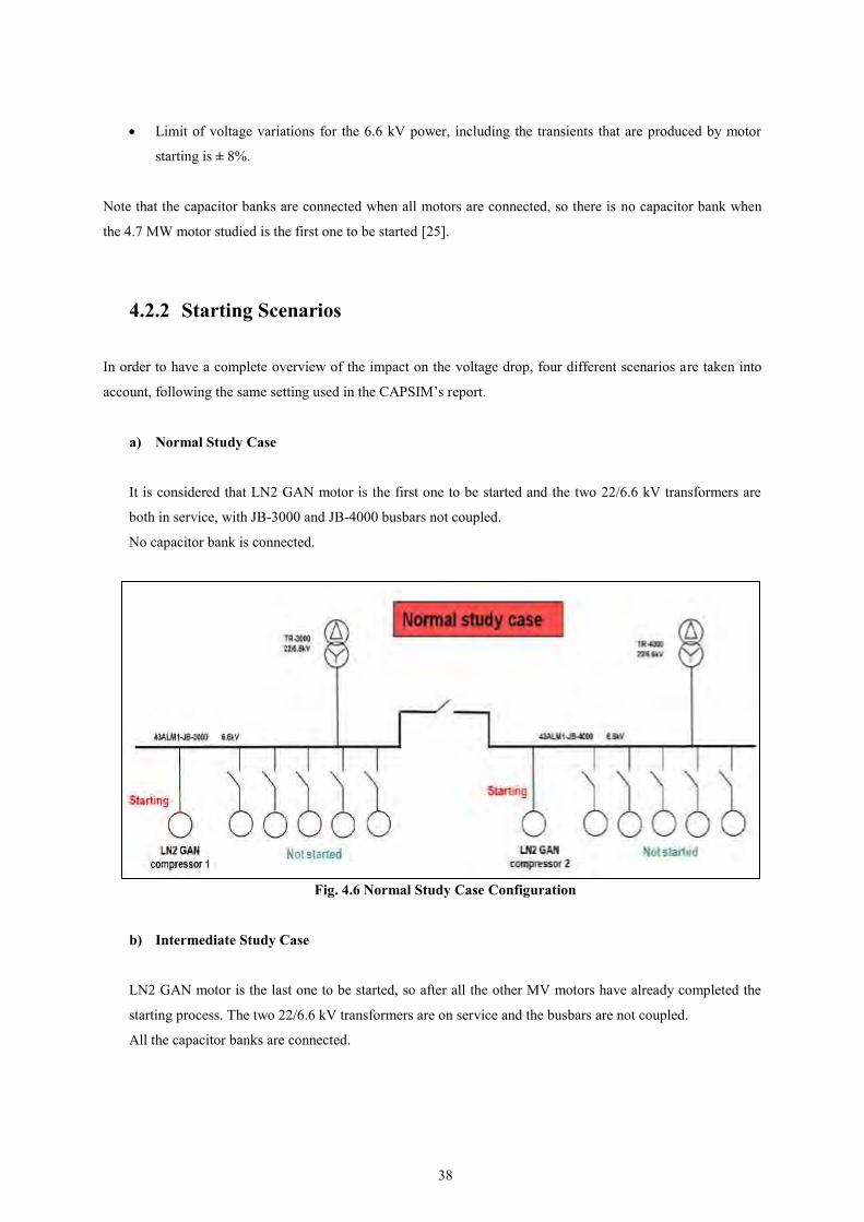
a) Normal Study Case

It is considered that LN2 GAN motor is the first one to be started and the two 22/6.6 kV transformers are

both in service, with JB-3000 and JB-4000 busbars not coupled.

No capacitor bank is connected.

Fig. 4.6 Normal Study Case Configuration

b) Intermediate Study Case

LN2 GAN motor is the last one to be started, so after all the other MV motors have already completed the

starting process. The two 22/6.6 kV transformers are on service and the busbars are not coupled.

All the capacitor banks are connected.

39

Fig. 4.7 Intermediate Study Case Configuration

c) Unfavourable Study Case

It is considered that LN GAN motor is the second one to be started (the other LN2 GAN compressor is

already started) and one 22/6.6kV transformer is out of service. The busbars are coupled and the capacitor

banks are not connected.

Fig. 4.8 Unfavourable Study Case Configuration

d) Most Unfavourable Study Case

The LN2 GAN motor is the last one to be started after that all the other MV motors are already at steady

state and only one of the two 22/6.6 kV transformers is on service. The busbars are coupled and the

capacitors banks are all connected.

40

Consider that the probability to have this last scenario during the starting process is very low, but it is

analyzed in order to see the worst effects on the voltage.

Fig. 4.9 Most Unfavourable Study Case Configuration

4.3 Analysis and Results with ETAP

For each scenario described are shown the following results, obtained using ETAP:

The speed of the LN2 GAN motor which is set to start with the soft starter, in order to evaluate the

time needed by the machine to complete the process;

The voltage on the motor terminal bus and on busbar 43ALM1-JB-3000, so it is possible to see the

impact of the starting process on the voltage and therefore to understand if the mentioned criteria

are respected or not. Consider that between the motor and busbar JB-3000 there is a 100 meters

cable.

To show these results within ETAP it is necessary to perform the simulations with two different modules

available in the software:

The Motor Starting Analysis (MSA), that allows to determine if a motor can be started and how

much time is needed to reach the rated speed, as well as to evaluate the effects on the voltage in an

electrical system. This analysis is used to see the motor speed curve and not the voltage, since this

module shows some inaccuracy regarding this aspect that has still to be solved;

The Transient Stability Analysis (TSA), which is designed to investigate the system dynamic

responses and limits after some change or disturbance in the electrical equivalent model created

[24]. It allows the reproduction of many events, such as short-circuits, opening and closing of

circuit breakers and also the starting (or stopping) process of motors. In the following study this

41

module is used to report the voltage curves: it seems that the electrical and load models are

considered more accurately and this gives better results that the ones obtainable with the MSA.

The LN2 GAN motor is coupled with a soft starter, whose settings are the following:

Starting Voltage [%] 60 TOR [seconds] 30

Current Limit [%] 295 Tab. 4.2

Before choosing these values several other combinations have been tried. The reasons of these settings are

also due to the details in the datasheet and to requirements from the system:

The voltage is set at 60% because with a lower value the motor has some trouble to start and the

whole process takes more time: this aspect is linked to the big inertia of the motor-load complex

(249 kg⋅m2). Moreover, even if a greater value set, ETAP does not use it as the start voltage: in Fig.

4.10 it is set at 80% and it is taken into account for just an instant. This is due to the selection of the

current limit, because keeping the current at a low constant value affects the natural progression of

the voltage: in fact, it remains at a constant level related to the current limit selected;

The time of the ramp is 30 seconds because in this way all the starting period is covered, bringing

benefits to the voltage during the process;

The 295% of current limit is provided by the datasheet of the soft starter and represents a big

reduction considering that the starting current is 515% of the rated one without the soft starter.

Fig. 4.10 Voltage ramp progression limited by the current limit option set

42

4.3.1 Normal Study Case

The speed progression is represented in Fig. 4.11: it is clear that the soft starter has an impact on the process

since the motor needs almost 30 seconds to start instead of 11, as shown in Fig. 4.5 and Tab.4.1.

Fig. 4.11 Motor Speed with Normal Scenario

The impact on the voltage at the motor terminal and at busbar JB-3000 is the following:

Fig. 4.12 Voltage Drop with Normal Scenario

Location

Voltage BEFORE

Starting [%]

Voltage DURING

Starting [%]

Voltage AFTER

Starting [%]

Duration

[s] 43ALM1-JB-3000 99.07 93.06 98.4 30.6

43

Motor Terminal 99.07 92.78 98.34 30.6

Tab. 4.3

From Tab. 4.3 we can conclude that

a) The voltage at the beginning is the same in the two points considered; b) After that the motor starts and at the end the voltage has a little difference in the two busses; c) Before completing the process, there is a quick reduction on the voltage (t = 31 seconds) caused by the

big inertia of the motor; d) The voltage drop at JB-3000 is almost 6%, so the limit is respected.

4.3.2 Intermediate Study Case

The results for this scenario are the following:

Fig. 4.13 Motor Speed with Intermediate Scenario

Fig. 4.14 Voltage Drop with Intermediate Scenario

44

Location

Voltage BEFORE

Starting [%]

Voltage DURING

Starting [%]

Voltage AFTER

Starting [%]

Duration

[s] 43ALM1-JB-3000 102.43 96.3 101.72 30.7

Motor Terminal 102.43 95.5 101.63 30.7

Tab. 4.4

Like for the Normal Study Case, points a), b) and c) are present. The voltage drop at busbar JB-3000 is respected

again even if the starting configuration is less favorable for the system.

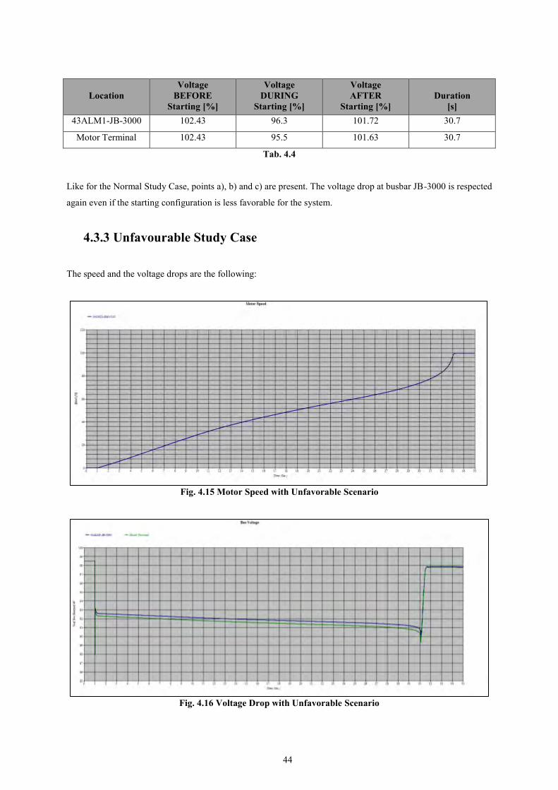
4.3.3 Unfavourable Study Case

The speed and the voltage drops are the following:

Fig. 4.15 Motor Speed with Unfavorable Scenario

Fig. 4.16 Voltage Drop with Unfavorable Scenario

45

Location

Voltage BEFORE

Starting [%]

Voltage DURING

Starting [%]

Voltage AFTER

Starting [%]

Duration

[s] 43ALM1-JB-3000 98.46 92.5 97.83 30.4

Motor Terminal 98.46 92.3 97.75 30.4

Tab. 4.5

Even in this configuration points a), b) and c) are present and the voltage drop at busbar JB-3000 is respected.

4.3.4 Most Unfavourable Study Case

The results for this scenario are shown in the following images.

Fig. 4.17 Motor Speed with Most Unfavorable Scenario

Fig. 4.18 Voltage Drop with Most Unfavorable Scenario

46

Location

Voltage BEFORE

Starting [%]

Voltage DURING

Starting [%]

Voltage AFTER

Starting [%]

Duration

[s] 43ALM1-JB-3000 104.6 98.5 103.87 30.5

Motor Terminal 104.6 98.2 103.79 30.5

Tab. 4.6

In the worst scenario points a), b) and c) are present again and moreover the voltage limit of 8% is not exceeded.

In conclusion, all the results obtained with ETAP show that the limits regarding the voltage drop (<8%) on MV-

01 busbars and the minimum startup voltage authorized (<15%) are respected: this means that the soft starter is

useful for the system as it is set, since it allows to reduce the electrical and mechanical stresses due to the starting

process of such a large motor like LN2 GAN.

4.4 Analysis with SimPowerSys

A starting motor study has been done using SimPowerSys, but not with the aim of repeating the same identical

simulations made with ETAP: since it is the first time at ITER that this type of analysis has been conducted in

Simulink, the main goal is to start comparing some result obtained with the two programs, in order to have the

possibility to do a crosscheck and to be able to evaluate in a more detailed way the systems taken into exam in

the future. So the analyses studied are different from the ones shown before with ETAP.

Consequently, the Simulink model created has some simplification:

Not the entire ITER Electrical Network is reported in the scheme, just the single branch to the 4.7 MW

motor;

Only busbar JB-3000 is included, but not JB-4000;

Only LN2 GAN motor is in the scheme, the other MV motors are not included.

Before going into the details of the simulations done, it is appropriate to describe the SimPowerSys model built.

In the equivalent model of Fig. 4.19 there are several elements, a part of them has already been described in

Chapter 3 (such as the 22/6.6 kV transformer and the LN2 GAN motor), but other blocks are included because

they are important to reproduce the system in the best way. Note that in Fig. 3.1, taken from the ETAP model,

only MV-01 busbars are shown, but obviously in the entire electrical scheme there are other elements such as the

supply electrical grid, the 400/22 kV transformers and all the busbars included in the SSEN.

The main elements of the single branch model in SimPowerSys are the following:

47

Fig. 4.19 Single Branch Equivalent Model

The supply grid is represented with the Three-Phase Source block; the phases have a Y connection with

an internal grounded neutral, the rated voltage used is 400 kV and the short-circuit power is set at 30

GVA (this value is justify in Chapter 5);

Following the ETAP model construction, after the Three-Phase Source there is a combination of

impedances useful to represent the maximum and minimum configuration for the short-circuit currents

at the ITER 400 kV Substation and the values are provided by RTE;

Transformers 400/22 kV and 22/6.6 kV are included in the scheme and the data used as input are those

reported in Tab. 4.7:

Transformer Voltage [kV] Power [MVA] R1, R2 [p.u] L1, L2 [p.u]

43AC00-TS-2000 400/22 75 0.002655 0.0849 43AEM1-TR-4000 22/6.6 35 0.00183 0.05497

Tab. 4.7

The model includes also some cable, such as 43AE00-JL-2000 and JL-0044, represented with the

Three-Phase series RLC Branch block, selecting only the combination RL;

Both the LN2 GAN motor and the soft starter are built inside a subsystem and they require a deeper

description since they are the core of the model.

4.4.1 LN2 GAN Motor in SimPowerSys

The motor subsystem is shown in Fig. 4.20.

48

Fig. 4.20 Asynchronous Motor in Simulink

The motor used is asynchronous with a single squirrel cage, with the input data taken from Tab. 3.1-3.2 and

expressed in the SI units following formulas [2.2] [2.3]. Since this analysis is dedicated to the starting process,

under the entry field Initial Conditions, inside the motor block, are used the following parameters:

Slip Electrical Angle [°]

Stator Current Magnitude [A]

Stator Current Phase [°]

1.0 0 0 0 Tab. 4.8

The output signals measured are the electromagnetic torque (Nm) and the speed (rpm): both are shown in order

to verify if the machine is acting like a motor during the simulation and to have an idea of the starting process as

well. The speed is also used as input in a Lookup Table used to create the correct torque-speed characteristic of

the load connected to the motor: the values of the torque are taken from Tab. 3.3, but expressed in Nm and not in

percentage.

Fig. 4.21 Lookup Table Output

49

4.4.2 Soft Starter in SimPowerSys

The model created is a draft, i.e. it is a starting point to be used for preliminary analyses, such as this one, and

therefore it needs to be improved and upgraded. Not many details about the soft starter are available: this aspect

is positive and negative at the same time, because it allows a custom made control to be created, but on the other

hand there is no precise indication if it is correct or not.

The final goal is to reproduce a voltage in output from the soft starter similar to the ramp shown in Fig. 4.4: in

achieving this, for each phase two thyristors are connected in an antiparallel configuration, so one will conduct

during the positive semi-wave and the other during the negative semi-wave.

Fig. 4.22 Disposition of the thyristors

The phase-to-ground voltage of each phase is measured and sent to the loop of Fig. 4.23 and the signal useful to

control these thyristors is generated in the following way:

Fig. 4.23 Phase a Control

50

a) At first, the voltage goes through a low-pass and high-pass filter in order to obtain and use only a wave

closer to the fundamental as reference;

b) Two Compare to Zero blocks allow to divide the filtered signal: whenever it is positive it will pass only

through the upper block, vice versa when it is negative through the lower one. In this way it is possible

to distinguish the signals to control the two thyristors in antiparallel;

c) When the output signal from the Compare to Zero block is not zero, an Integrator block will integrate a

constant equal to 1 in order to generate a ramp of time ( ʃ1dt = t), which goes from zero to 0.01 (i.e. half

of the period with 50 Hz as frequency);

d) This ramp is then compared through a Relational Operator block with “deltaT”, i.e. the required delay

expressed as a time and not as an angle: when the first input (the ramp) is greater than or equal to the

second one (deltaT) then the block will generate a signal. In this way it is possible to determine the

conduction time of each thyristor during the appropriate semi-period (0-0.01 seconds): until “deltaT” is

greater than the ramp the thyristor will not be able to conduct, after that the delay is inferior it will start

to operate. This reasoning is described in Fig. 4.24 where it is used a “deltaT” equal to 0.004 seconds:

the conduction will start at 0.004 and will continue until 0.01 seconds.

Fig. 4.24 Conduction Period

e) The result is then sent to a Logical Operator (applying the “AND” function) together with the signal in

output from the Compare to Zero block: this is just a precaution to be sure that the control is generated

during the correct portion of semi-period.

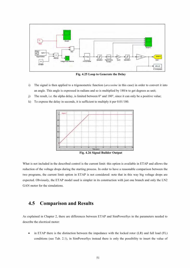
The delay “deltaT” introduced in point “d” is created in this way (see Fig. 4.25):

f) The phase-to-ground voltage measured at the motor terminal is compared with a reference signal

generated by a Signal Builder block (Fig. 4.26): the reference taken is a ramp and is fundamental for

managing the delay;

g) The difference between the two signals is sent to a PI regulator (P = 0.00005, I = 0.001);

h) The output from the regulator is then limited between +1 and -1 by a Saturation block;

51

Fig. 4.25 Loop to Generate the Delay

i) The signal is then applied to a trigonometric function (arccosine in this case) in order to convert it into

an angle. This angle is expressed in radians and so is multiplied by 180/π to get degrees as unit;

j) The result, i.e. the alpha delay, is limited between 0° and 180°, since it can only be a positive value;

k) To express the delay in seconds, it is sufficient to multiply it per 0.01/180.

Fig. 4.26 Signal Builder Output

What is not included in the described control is the current limit: this option is available in ETAP and allows the

reduction of the voltage drops during the starting process. In order to have a reasonable comparison between the

two programs, the current limit option in ETAP is not considered: note that in this way big voltage drops are

expected. Obviously, the ETAP model used is simpler in its construction with just one branch and only the LN2

GAN motor for the simulations.

4.5 Comparison and Results

As explained in Chapter 2, there are differences between ETAP and SimPowerSys in the parameters needed to

describe the electrical motor:

in ETAP there is the distinction between the impedance with the locked rotor (LR) and full load (FL)

conditions (see Tab. 2.1), in SimPowerSys instead there is only the possibility to insert the value of

52

resistance and reactance characteristic of the stator and rotor windings inside the motor, so there is no

way to distinguish the impedance in LR and FL scenarios;

In ETAP there are numerous data to fill, such as breakdown torque, locked rotor current, power factor

and efficiency in many different load condition (100%, 75%, 50% of the load), while in SimPowerSys

the required data are less, only some information regarding the power, the voltage, the impedance and

the inertia.

These aspects bring differences in the results, so the two programs are unlikely to give the same identical output.

To start comparing the two softwares, it is better to evaluate the differences in the motor starting with the DOL

technique and then introduce the soft starter in the process.

4.5.1 Differences with DOL Technique

In the first DOL starting comparison made, the distinction between the LR and FL impedance in ETAP is

retained, so the values used are the following:

ETAP Rs [p.u] 0.0137 Xs [p.u] 0.0955

Rrlr [p.u] 0.0212 Rrfl [p.u] 0.0112 Xrlr [p.u] 0.0955 Xrfl [p.u] 0.1435 Xm [p.u] 6.38

Tab. 4.8

SimPowerSys Rs [Ohm] 0.109 Ls [mH] 2.42

Rr [Ohm] 0.1687 Lr [mH] 2.42 Lm [H] 0.16174

Tab. 4.9

The results with the values of Tab. 4.8 and 4.9 are the following:

Program Δt [s] Vmin [%] Imax [%] ETAP 13.1 84.9 440

SimPowerSys 7.6 85.6 443 Tab. 4.10

The starting time is not the same, 13.1 seconds versus 7.6, and this is caused by the distinction in ETAP between

LR and FL: in fact, with different values the torque produced by the motor is lower during the entire starting

53

process and therefore it takes more time to complete it; instead using the same impedance in LR and FL

conditions the electromagnetic torque is higher and the process is faster, as actually happens in Simulink.

Essentially the motor is not the same and so the characteristic is different in the two cases.

Fig. 4.27 Different Torque-Speed Characteristic

If the same simulation with DOL is repeated using the same values in LR and FL, then the results will be similar:

ETAP Rs [p.u] 0.0137 Xs [p.u] 0.0955

Rrlr [p.u] 0.0212 Rrfl [p.u] 0.0212 Xrlr [p.u] 0.0955 Xrfl [p.u] 0.0955 Xm [p.u] 6.38

Tab. 4.11

Program Δt [s] Vmin [%] Imax [%] ETAP 8.5 85.9 440

SimPowerSys 7.6 85.6 443 Tab. 4.12

Now the starting times are closer and moreover the voltage drop along with the maximum current reached during

the process are almost the same for both the software.

In conclusion, the DOL technique for the LN2 GAN motor gives an identical result when the same values of

resistance and reactance for LR and FL are used in ETAP.

54

4.5.2 Differences Using the Soft Starter

The right way to compare the two softwares is using the same identical settings in both and to do this it is

necessary to recreate the same voltage ramp through the soft starter and without including the current limit

option in ETAP.

In order to have a better overview of the possible differences, three ramps are simulated and the settings used are

the following:

Time of the ramp equal to 20, 30 and 40 seconds respectively;

Initial voltage set at 60% of the rated one;

Finale voltage at 100%.

With these settings ETAP gives the results shown in Tab. 4.14:

TOR [s] Starting Time [s] Vmin [%] Imax [%] 20 12 88.23 391 30 14 89.7 367 40 16 90.4 353

Tab. 4.14

On the other side, in SimPowerSys the results obtained are the following:

TOR [s] Starting Time [s] Vmin [%] Imax [%] 20 12 88 386 30 13.5 88 365 40 15 89 355

Tab. 4.15

In Fig. 4.28 and 4.29 are reported an example of the speed and the voltage drop curves in output from

SimPowerSys in order to give a better idea of the quality of the results.

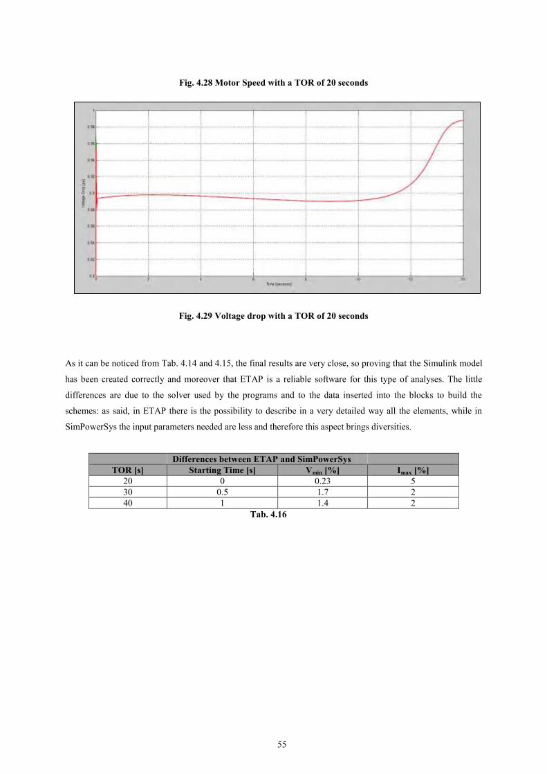
55

Fig. 4.28 Motor Speed with a TOR of 20 seconds

Fig. 4.29 Voltage drop with a TOR of 20 seconds

As it can be noticed from Tab. 4.14 and 4.15, the final results are very close, so proving that the Simulink model

has been created correctly and moreover that ETAP is a reliable software for this type of analyses. The little

differences are due to the solver used by the programs and to the data inserted into the blocks to build the

schemes: as said, in ETAP there is the possibility to describe in a very detailed way all the elements, while in

SimPowerSys the input parameters needed are less and therefore this aspect brings diversities.

Differences between ETAP and SimPowerSys TOR [s] Starting Time [s] Vmin [%] Imax [%]

20 0 0.23 5 30 0.5 1.7 2 40 1 1.4 2

Tab. 4.16

56

57

5. VOLTAGE REDUCTION DUE TO EXTERNAL

FAULTS AND EFFECTS ON THE MV-01

MOTORS

This chapter will deal the problem of faults, both three phase and line-ground, on the external line in order

to quantify the reduction of voltage at ITER Prionnet.

5.1 Faults and the Consequences on the MV Motors

One of the problems that ITER plant will have to face, when it will be in operation, is the possible presence of

faults, both internal and external to the network. These faults, primarily short circuits, could cause a reduction on

the voltage and the drop can be different considering the type of the fault (three phase or line-ground) and its

position.

As said, in the SSEN the majority of the loads are asynchronous motors, whose operation could be affected by

the voltage changes: in fact, the speed of the motors starts to decrease when the voltage is reduced, with a

duration related to that of the fault, and this means that

When the fault is solved the motors begin a new and unexpected starting process, much shorter than the

programmed one, with all the problems related to the high current and high demand of power;

The speed could go even below the accepted limit for a safe operation of the load connected and this

requires a disconnection of the motor, so compromising the fusion process.

If the fault is extinguished after that the circuit breaker recloses the circuit the problem is just for hundreds of

milliseconds and so not very dangerous since the inertia of the motors-load complex is not low, but if it would

last longer there is the possibility that the speed will decrease over the accepted limit, bringing the motor out of

service. Of course the faults cannot be foresee and prevented, but what can be studied is the magnitude of the

voltage drop with all the types of short circuit faults and in different positions: in fact in this way it is possible to

know which are the worst situations for the operation of the motors and, as a result, it could be found a solution

to avoid to disconnect them and to keep the plant on service.

The studies made are focused only on the external faults because, since they can happen in different positions of

the line, they bring diverse impacts on the voltage measured at ITER Prionnet and therefore on the speed of the

motors and the fusion process: for example, a short circuit far from ITER substation could bring a lower impact

on the voltage than one close to the plant.

The types of faults considered are line-ground and line-line caused by lightning strikes: after that a lighting hits a

phase, or all the phases, there are waves of high voltage and current propagating over the line and consequently

58

the circuit breakers will open; with the breakers open for a short period of time (typically 100 milliseconds) the

voltage will be equal to zero in the strike point.

The aims of the analysis are, as first, to evaluate the magnitude of the voltage reduction at ITER Prionnet caused

by faults applied in various points of the grid and secondly to verify the effects on the motors connected to the

43ALM1-JB-3000 and 4000 busbars: in undertaking the study, an equivalent SimpowerSys model of the

external grid and a scheme of the internal network of the plant were created.

For this study several assumptions have been made due to the lack of precise information about the lines, the

electrical grid, the loads connected to the busbars and moreover because some data are not the definitive ones:

this is a preliminary work useful to start to understand the impact of some of the problems originating from the

external grid and later when ITER will be in possession of more information regarding the various elements the

model has to be updated.

5.2 External Electrical Grid

As said before, ITER will be connected to the French 400 kV transmission network operated by RTE and this

grid has many branches.

What will be described are the lines, the elements directly connected to ITER, and not all the electrical systems,

since the following analysis will be focused on faults applied on one of these lines.

In Fig. 5.1 it is shown an equivalent model of the external grid.

Fig. 5.1 Equivalent scheme of the external grid

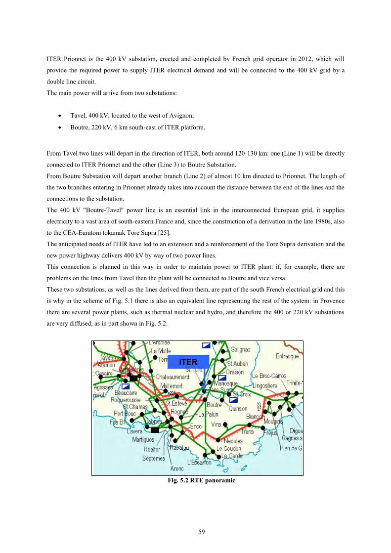
59

ITER Prionnet is the 400 kV substation, erected and completed by French grid operator in 2012, which will

provide the required power to supply ITER electrical demand and will be connected to the 400 kV grid by a

double line circuit.

The main power will arrive from two substations:

Tavel, 400 kV, located to the west of Avignon;

Boutre, 220 kV, 6 km south-east of ITER platform.

From Tavel two lines will depart in the direction of ITER, both around 120-130 km: one (Line 1) will be directly

connected to ITER Prionnet and the other (Line 3) to Boutre Substation.

From Boutre Substation will depart another branch (Line 2) of almost 10 km directed to Prionnet. The length of

the two branches entering in Prionnet already takes into account the distance between the end of the lines and the

connections to the substation.

The 400 kV "Boutre-Tavel" power line is an essential link in the interconnected European grid, it supplies

electricity to a vast area of south-eastern France and, since the construction of a derivation in the late 1980s, also

to the CEA-Euratom tokamak Tore Supra [25].

The anticipated needs of ITER have led to an extension and a reinforcement of the Tore Supra derivation and the

new power highway delivers 400 kV by way of two power lines.

This connection is planned in this way in order to maintain power to ITER plant: if, for example, there are

problems on the lines from Tavel then the plant will be connected to Boutre and vice versa.

These two substations, as well as the lines derived from them, are part of the south French electrical grid and this

is why in the scheme of Fig. 5.1 there is also an equivalent line representing the rest of the system: in Provence

there are several power plants, such as thermal nuclear and hydro, and therefore the 400 or 220 kV substations

are very diffused, as in part shown in Fig. 5.2.

Fig. 5.2 RTE panoramic

60

5.2.1 Known Data and Assumptions This analysis includes available information about the external lines, the HV substations, ITER intended as an

unique load, but currently not all details are available or definitive: in fact RTE does not share a lot of data about

the grid and it is not easy to reproduce an equivalent model of it. Moreover, ITER will be a dynamic load since

steady state and pulse state operations are foreseen: it is not simple to determine the precise power that will be

required by the plant and to report it in the simulations.

Consequently several hypotheses have been made in order to recreate a model and to do the simulations.

In the first instance, it is better to start from the known data.

a) Electrical Lines

RTE has furnished a document with information about Line 1 and Line 2 (referring to Fig. 5.1), the short

circuit currents at ITER Prionnet and also some criteria to respect, such as the elimination of a fault inside

the network or the grounding system [26].

The actual details regarding Line 1 and 2 are the following:

Line Rd [Ohm/km]

Ro [Ohm/km]

Ld [mH/km]

Lo [mH/km]

D [km]

1 0.0198 0.16682 0.84225 2.4366 125.7 2 0.0176 0.15375 0.892 2.46 9.6

Tab. 5.1

What can be noticed from Tab. 5.1 are the similar values of the two lines: this is an aspect that was taken

into account to determine the input data of the rest of the electrical grid.

On the other side, note that RTE does not give the capacity to the ground (F/km) and therefore this is one of

the values hypothesized for all the lines.

In the simulations the faults are applied only in different positions of Line 1, because it is longer than Line 2

and the data reported are reliable since they are given by RTE.

b) ITER Prionnet

When considering the short circuit currents at Prionnet, RTE makes the distinction between two different

configurations for both line-line and line-ground fault:

“Maximum” configuration, when both the circuit breakers CB1 and CB2 are closed, so the current is

distributed between all the incoming lines;

“Minimum” configuration, with just CB1 closed and CB2 open. In this scenario only Line 1 is

connected to Prionnet.

61

The short circuit currents are calculated according to the IEC 60909 standard [27] and the consequent power

represents the RTE grid seen from Prionnet, with the substation considered as a passive element. According

to IEC 60909, the c factor applied to calculate the maximum current is 1.1.

The short circuit currents and powers are shown in the following table:

ITER Prionnet Maximum Configuration Minimum Configuration

Isc L-L [kA] 15.9 5.6

Isc L-G [kA] 13.6 4.5

SC L-L Power [GVA] 12.117 3.88

SC L-G Power [GVA] 10.364 3.117

Tab. 5.2

The power chosen to represent the ITER loads is shown in Tab. 5.3:

Active Power [MW] Reactive Power [MVar]

450 250

Tab. 5.3

This choice consists of the both the steady state operation power (130 MW required) and an average of the

pulsed power (fixed as maximum at 500 MW): the plant will have to maintain constantly a certain pulsed

power and also additional heating system but not at the maximum performances, because the type of pulse

foreseen will be around some hundreds of seconds and for this it is estimated that 300-350 MW should be

sufficient. Therefore, an active total power of 450 MW could be a correct value for the simulations.

c) Tavel 400 kV Substation

Regarding Tavel Substation, the only known information is that the maximum short circuit current is around

40 kA and so, considering this value as the starting point, the related power and the representative

impedance are the following:

Short circuit power

𝑆𝑠𝑐 = √3 𝑐 𝑉𝑛𝐼𝑠𝑐

𝑆𝑠𝑐 = √3 ⋅ 1.1 ⋅ 400000 ⋅ 40000

𝑆𝑠𝑐 = 30 [𝐺𝑉𝐴]

[5.1]

Impedance

𝑧𝑇𝑎𝑣𝑒𝑙 =𝑐 ⋅ 𝑉𝑛/√3

𝐼𝑠𝑐

[5.2]

62

𝑧𝑇𝑎𝑣𝑒𝑙 =1.1 ⋅ 400000/√3

40000

𝑧𝑇𝑎𝑣𝑒𝑙 = 6.4533 [Ω]

With the hypothesis of X/R = 10, the resistance and the reactance can be calculated in this way:

𝑧𝑇𝑎𝑣𝑒𝑙 = √𝑅 2 + 𝑋2 = 6.4533 [Ω]

𝑧𝑇𝑎𝑣𝑒𝑙 = √𝑅 2 + 100 ⋅ 𝑋2

𝑧𝑇𝑎𝑣𝑒𝑙 = √101 ⋅ 𝑅 2

𝑅 =𝑧𝑇𝑎𝑣𝑒𝑙

√101= 6.4533

𝑅 = 0.64213 [Ω]

𝑋 = 6.4213 [Ω]

[5.3]

Tavel Substation will have these data in the equivalent model:

R [Ohm] X [Ohm] Isc [kA] Ssc [GVA] 0.64213 6.4213 40 30

Tab. 5.4

With regard to the rest of the grid, the method used to determine the impedance of the lines is explained in

the following chapter, with the help of the Simulink model created.

5.3 External Grid Equivalent Model with SimPowerSys

In Fig. 5.3 the diagram that has been implemented in Simulink.

In this scheme are clearly distinguished the elements described previously and they are modelled and adapted to

Simulink in the following way:

Tavel Substation is represented by the Three Phase Voltage Source block, with the short circuit

power and the impedance set with the values shown in Tab. 5.4. The three sources are connected in

Y to an internal grounded neutral and the nominal phase-to-phase voltage is 400 kV; note that the

voltage is set to 440 kV (i.e. c⋅Vn) when we want to calculate the maximum short circuit current;

ITER is modelled with the Three-Phase Series Load, choosing the combination R-L (so without any

C) with the neutral grounded; the block is filled with the values of Tab. 5.3;

For Line 1 and Line 2 are used the data of Tab. 5.1, but with some change and addiction:

63

- The value of the zero sequence inductance in Line 1 has been changed in 1.85 mH/km in order

to obtain the correct line-ground short circuit current with the minimum configuration (see Tab.

5.2);

Fig. 5.3 Simulink model of the external grid

- The direct and zero sequence capacities are intended to respect the short circuit currents and

based on realistic values:

Cd [nF/km] Co [nF/km]

Line 1 0.134 8.57 Line 2 0.134 8.57

Tab. 5.5

With these values, together with the other ones reported in Tab. 5.1, the short circuit current in both

the configurations is similar to that given by RTE;

- In Fig. 5.3 Line 1 is divided into two parts, with the total length equal to 125.7 km, in this way it is

possible to apply the faults in different positions.

In addition, in the scheme there are several measurements blocks that are useful to control the values measured

in various points and to understand if they are realistic or not.

The creation of this Simulink model has been difficult due to the need to represent of the remainder of the grid.

First of all, there is no information regarding Boutre Substations and its 220/400 kV transformers and so it

cannot be directly reproduced in Simulink, but above all the entire electrical system is full of branches and other

substations which provide ITER the required power and without knowing their characteristics and how they are

distributed it is impossible to propose an accurate scheme.

64

Therefore the following has been created:

The initial idea was that to insert in parallel to Line 1 and 2 one or more electrical lines and to adapt

their impedances and lengths in order to obtain at ITER Prionnet the short circuit currents provided by

RTE;

The first values used for the resistance, inductance and capacity were similar to those of Line 1 and 2;

Additional combinations have been tried, changing several times the number of the lines and then their

characteristics, until reasonable results in term of the current were obtained. Finally, three other lines

were added (Line 3, 4 and 5 in Fig. 5.3), because with just one the short circuit currents were correct

only with a length of around 15-20 km, which is not realistic, but also because this is a better way to

represent an extended electrical grid. Consequently, Line 3, 4 and 5 include Boutre Substation and also

the rest of the system.

The values used in Tab. 5.6 are the results of the various attempts:

Equivalent Grid

Rd [Ohm/km]

Ro [Ohm/km]

Ld [mH/km]

Lo [mH/km]

Cd [nF/km]

Co [nF/km]

d [km]

Line 3 0.0187 0.1603 0.56792 1.4515 0.2041 8.57 125

Line 4 0.0187 0.1603 0.86792 1.4515 0.1541 8.57 125

Line 5 0.0187 0.1603 0.86792 1.4515 0.1541 8.57 125 Tab. 5.6

With these data the short circuit currents and powers at Prionnet become the following:

ITER Prionnet Maximum Configuration Minimum Configuration

Isc L-L [kA] 15.67 5.82

Isc L-G [kA] 13.2 4.5

SC L-L Power [GVA] 11.942 4.032

SC L-G Power [GVA] 10.06 3.117

Tab. 5.7

The differences, as absolute values, between Tab. 5.2 and Tab. 5.7 are the following:

Differences Maximum Configuration Minimum Configuration

Isc L-L [kA] 0.23 0.22

Isc L-G [kA] 0.4 0

SC L-L Power [GVA] 0.175 0.152

SC L-G Power [GVA] 0.304 0

Tab. 5.8

65

It is evident that this Simulink model respects well enough the reality seen from ITER Prionnet, but nevertheless

the biggest omission, and therefore the biggest error, of the scheme is the absence of other voltage sources: in

fact in the simulations ITER receives power only from Tavel Substation, when in the reality it comes from

several points and consequently this aspect compromises part of the results.

5.4 Simulations and Results

The simulations of the faults are applied only on Line 1 because compared with Line 2 it is longer (125.7 km)

and so there is the possibility to see the impact even when this is applied beyond a distance of 9.6 km from ITER

Prionnet, but also it is directly connected to the voltage source (Tavel Substation in the Simulink model);

instead, in comparison with Line 3, 4 and 5, the data are reliable since they are provided by RTE.

At first the line-line and line-ground faults are performed directly at ITER Prionnet (distance equal to zero km)

and then they are moved on Line 1 in direction of Tavel Substation with a step of 10 km at the time, until the end

of the line.

The progression of the events is set in the following way:

At the beginning, t = 0 seconds, the system is in steady state, with the voltage set at 400 kV in the

three-phase source;

At t = 0.1 seconds the fault is applied;

At t = 0.2 seconds, so 100 milliseconds after the fault, the circuit breakers 1 and 2 (see Fig. 5.3)

are open and remain in this state for 300 milliseconds;

At t = 0.3 seconds the fault is solved and deleted;

At t = 0.5 seconds the breakers are close, so 300 milliseconds after their opening.

During this succession the voltage is always kept at 400 kV at Tavel and it is not increase to 440 kV, because the

aim of the analysis is to evaluate the voltage reduction and not the short circuit currents.

The results of the simulations are shown in the next tables and images.

a) Line-Line Fault:

Distance From

Prionnet [km]

Voltage RMS

[kV]

ΔV

[%]

0 0.042 99.989 10 39.98 90.005 20 70.32 82.42 30 93.6 76.6 40 111.37 72.15

66

50 124.59 68.85 60 133.76 66.56 70 138.92 65.27 80 139.82 65.045 90 135.4 66.15

100 132.61 66.85 110 99.5 75.125

125.7 0.104 99.97 Tab. 5.9

Fig. 5.4 Voltage Reduction with a line-line fault in different positions of Line 1

Fig. 5.5 Voltage profile with a three phase fault, d = 20 km

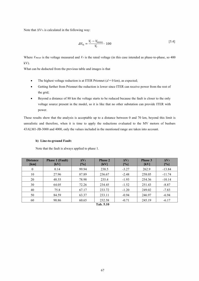
67

Note that ΔV% is calculated in the following way:

𝛥𝑉% =𝑉𝑟 − 𝑉𝑚𝑒𝑎𝑠.

𝑉𝑟

⋅ 100 [5.4]

Where Vmeas is the voltage measured and Vr is the rated voltage (in this case intended as phase-to-phase, so 400

kV).

What can be deducted from the previous table and images is that

The highest voltage reduction is at ITER Prionnet (d = 0 km), as expected;

Getting further from Prionnet the reduction is lower since ITER can receive power from the rest of

the grid;

Beyond a distance of 80 km the voltage starts to be reduced because the fault is closer to the only

voltage source present in the model, so it is like that no other substation can provide ITER with

power.

These results show that the analysis is acceptable up to a distance between 0 and 70 km, beyond this limit is

unrealistic and therefore, when it is time to apply the reductions evaluated to the MV motors of busbars

43ALM1-JB-3000 and 4000, only the values included in the mentioned range are taken into account.

b) Line-to-ground Fault:

Note that the fault is always applied to phase 1.

Distance [km]

Phase 1 (Fault) [kV]

ΔV1 [%]

Phase 2 [kV]

ΔV2 [%]

Phase 3 [kV]

ΔV3 [%]

0 0.14 99.94 238.5 -3.27 262.9 -13.84 10 27.96 87.89 236.67 -2.48 258.05 -11.74 20 48.55 78.98 235.4 -1.93 254.36 -10.14 30 64.05 72.26 234.45 -1.52 251.43 -8.87 40 75.8 67.17 233.72 -1.20 249.02 -7.83 50 84.59 63.37 233.11 -0.94 246.97 -6.94 60 90.86 60.65 232.58 -0.71 245.19 -6.17

Tab. 5.10

68

Fig. 5.6 Voltage Reduction with a line-ground fault in different positions of Line 1

Fig. 5.7 Voltage profile with a line-ground fault, d = 20 km

In Tab 5.10 are shown the changes on all the phases and in fact

Since the fault is applied on phase 1, this sees a reduction of the voltage magnitude, as foreseen;

On the other side phase 2 and 3 are increased and this is why their ΔV is negative.

The line-line faults are not proposed for the results with distances greater than 60 km, because of the reason

described previously regarding the inaccuracy of the Simulink model.

-20-15-10

-505

101520253035404550556065707580859095

100105

0 10 20 30 40 50 60

ΔV1 [%]

ΔV2 [%]

ΔV3 [%]

69

5.5 Effects on the MV Motors

The final goal of this analysis is to evaluate which impact could create such variations of voltage on the MV

motors and their load and consequently understand if they could be dangerous for the fusion process.

To verify if the reductions of Tab. 5.9 and 5.10 could give problems to the system it is necessary to apply

the calculated voltages on a Simulink model representing the ITER Network.

The model proposed in Fig. 5.8 is an extension of the one analysed in Paragraph 4.4 but with some

difference:

Fig. 5.8 ITER Network

There are both busbars 43ALM1-JB-3000 and JB-4000, with all the MV motors shown in Fig.

3.1, and the four 400/22 kV transformers, because when a fault occurs on the external grid it is

supposed that the entire plant will be in operation. Obviously, there is the possibility for the fault

to happen in different scenarios. On the other side, with the starting analysis there was only a

single branch with the LN2 GAN motor alone and not the entire ITER Network, because in the

reality the various loads will be activated progressively and not simultaneously in order not to

require much power at the same time from the electrical grid.

The motors do not have to be started, they are already in a steady state condition at the beginning

of the simulation: to do so in the motor block, in the Initial Condition entry field, there are the

values of current (magnitude and phase) and the slip distinctive for the steady state. In this way it

is not necessary to wait for the motors to complete the starting process and therefore the duration

of the simulation is much shorter;

70

The transformers 43AC00-TS-1000 and TS-3000 are not connected to any load, so their voltage

is set at 23.1 kV, according to the datasheet. Their impedance is the same of the other two

transformers (see Tab. 4.7);

The biggest change is in the voltage source: in this instance the Three Phase Voltage Source

block is not used because there is the necessity to manipulate the voltage in each single phase in

order to apply the voltage calculated in Tab. 5.9 and 5.10. To do so the system shown in Fig. 5.9

has been created for all the three phases: note that in the image there is only the regulator of

phase A, but in the model there is the same scheme for all the other two phases.

Fig. 5.9 Voltage Regulator – phase A

5.5.1 Voltage Source

This subsystem works in the following way:

There are two constant blocks with the peak of the rated voltage in the Y configuration (√2/3 ∙

400 kV);

The product between one of these blocks and a Signal Builder generates the reduction to be

applied to the rated voltage: by managing the signal produced by this last block it is possible to

modify the peak for a precise period. An example of this signal is shown in Fig. 5.10.

Fig. 5.10 Signal used to reduce the voltage

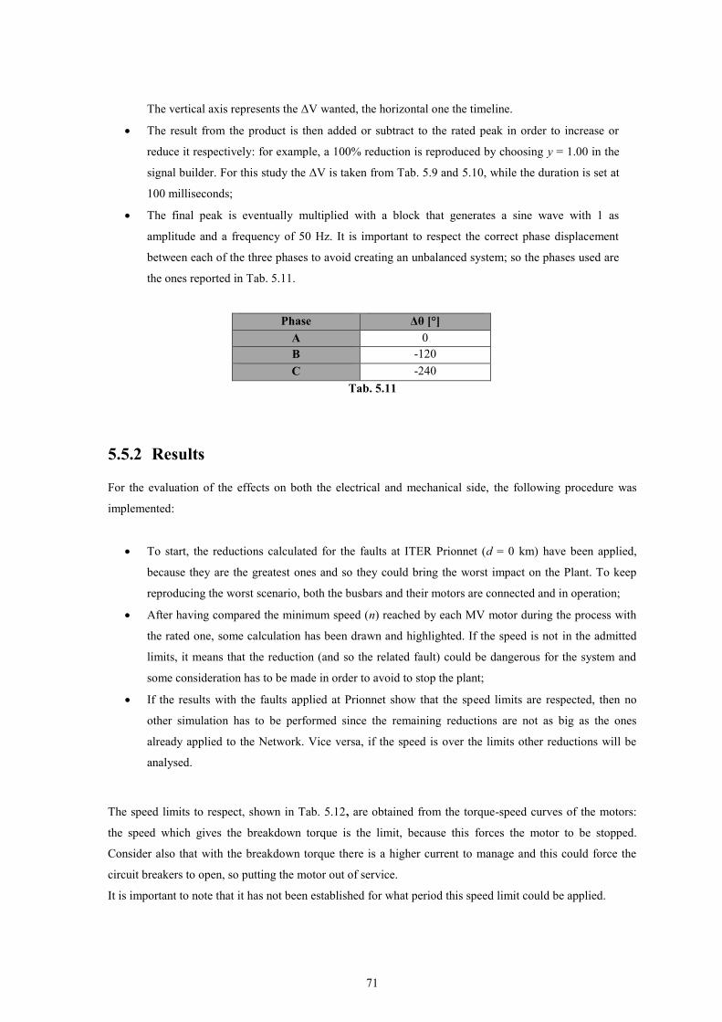
71

The vertical axis represents the ΔV wanted, the horizontal one the timeline.

The result from the product is then added or subtract to the rated peak in order to increase or

reduce it respectively: for example, a 100% reduction is reproduced by choosing y = 1.00 in the

signal builder. For this study the ΔV is taken from Tab. 5.9 and 5.10, while the duration is set at

100 milliseconds;

The final peak is eventually multiplied with a block that generates a sine wave with 1 as

amplitude and a frequency of 50 Hz. It is important to respect the correct phase displacement

between each of the three phases to avoid creating an unbalanced system; so the phases used are

the ones reported in Tab. 5.11.

Phase Δθ [°] A 0 B -120 C -240

Tab. 5.11

5.5.2 Results

For the evaluation of the effects on both the electrical and mechanical side, the following procedure was

implemented:

To start, the reductions calculated for the faults at ITER Prionnet (d = 0 km) have been applied,

because they are the greatest ones and so they could bring the worst impact on the Plant. To keep

reproducing the worst scenario, both the busbars and their motors are connected and in operation;

After having compared the minimum speed (n) reached by each MV motor during the process with

the rated one, some calculation has been drawn and highlighted. If the speed is not in the admitted

limits, it means that the reduction (and so the related fault) could be dangerous for the system and

some consideration has to be made in order to avoid to stop the plant;

If the results with the faults applied at Prionnet show that the speed limits are respected, then no

other simulation has to be performed since the remaining reductions are not as big as the ones

already applied to the Network. Vice versa, if the speed is over the limits other reductions will be

analysed.

The speed limits to respect, shown in Tab. 5.12, are obtained from the torque-speed curves of the motors:

the speed which gives the breakdown torque is the limit, because this forces the motor to be stopped.

Consider also that with the breakdown torque there is a higher current to manage and this could force the

circuit breakers to open, so putting the motor out of service.

It is important to note that it has not been established for what period this speed limit could be applied.

72

Speed Limit 4700 kW 2500 kW 1175 kW 986 kW

Speed [rpm] 2930 2936 2934 2820

Tab. 5.12

a) Line-line Fault at ITER Prionnet:

Distance [km] ΔV [%] Time [ms]

0 99.989 100 Tab. 5.13

This combination of voltage and time affects the speed as follows:

4700 kW 2500 kW 1175 kW 986 kW

Minimum n [rpm] 2876 2720 2600 2650

Δn [%] 3.4 8.75 12.51 10.98

Total Duration [s] 0.6 0.6 0.6 0.6 Tab. 5.14

Fig. 5.11 Example of how the speed changes after the voltage reduction

As it can be seen from Tab. 5.14, the biggest change of speed happens in the 986 kW and 1175 kW motors

because their inertia is much lower than the 4700 kW and 2500 kW motors: in fact, a big inertia is harder to

decelerate and stop in a short period and this means that the LN2 GAN motor is less affected by this type of

events. Comparing the results of Tab. 5.14 with the limits mentioned, what emerges is the following:

Each motor goes beyond the limit;

The minimum speed is reached for an instant and it does not last longer;

The total variation (Δn) is about 600 milliseconds.

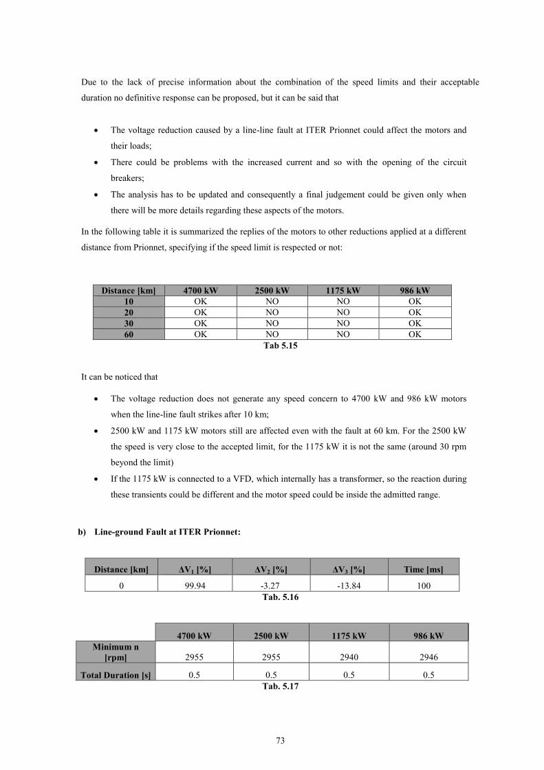
73

Due to the lack of precise information about the combination of the speed limits and their acceptable

duration no definitive response can be proposed, but it can be said that

The voltage reduction caused by a line-line fault at ITER Prionnet could affect the motors and

their loads;

There could be problems with the increased current and so with the opening of the circuit

breakers;

The analysis has to be updated and consequently a final judgement could be given only when

there will be more details regarding these aspects of the motors.

In the following table it is summarized the replies of the motors to other reductions applied at a different

distance from Prionnet, specifying if the speed limit is respected or not:

Distance [km] 4700 kW 2500 kW 1175 kW 986 kW 10 OK NO NO OK 20 OK NO NO OK 30 OK NO NO OK 60 OK NO NO OK

Tab 5.15

It can be noticed that

The voltage reduction does not generate any speed concern to 4700 kW and 986 kW motors

when the line-line fault strikes after 10 km;

2500 kW and 1175 kW motors still are affected even with the fault at 60 km. For the 2500 kW

the speed is very close to the accepted limit, for the 1175 kW it is not the same (around 30 rpm

beyond the limit)

If the 1175 kW is connected to a VFD, which internally has a transformer, so the reaction during

these transients could be different and the motor speed could be inside the admitted range.

b) Line-ground Fault at ITER Prionnet:

Distance [km] ΔV1 [%] ΔV2 [%] ΔV3 [%] Time [ms]

0 99.94 -3.27 -13.84 100 Tab. 5.16

4700 kW 2500 kW 1175 kW 986 kW

Minimum n [rpm] 2955 2955 2940 2946

Total Duration [s] 0.5 0.5 0.5 0.5 Tab. 5.17

74

A line-ground fault directly applied at ITER Prionnet does not seem to affect seriously the speed of the MV

motors as was conversely seen with the line-line fault, because even if one phase has a magnitude equal to

zero the other two can still create the phase-phase voltage and give power to the motors. Moreover the fault

is very short and again the inertia plays a big part in limiting the reduction of speed.

In this case the speed limits are always respected: this means that a line-ground fault should not bring

particular problems to these motors.

In conclusion, as shown and often underlined, this analysis has omissions that obviously bring errors and

imperfections to the results: what is important to remember is the necessity to improve and update the

models when more precise details are available.

75

6. Conclusions and Future Developments

This thesis is prevalently based on work to identify various dynamic related to the asynchronous motors

connected to busbars MV-01, related to the Cryogenic system.

In the first part, chapters 2 and 3, are given some important detail on the motors and on how to use them inside

ETAP and SimPowerSys: these evaluations represent a big and fundamental part of the work done at ITER,

because the motor data can be changed often and it was the first time that this type of studies have been made.

Using the developed knowledge on ETAP and SimPowerSys and the theories of the power distribution, in the

second part (chapter 4) it was analyzed the starting process of the LN2 GAN motor: in both softwares were

found and used the most suitable settings, considering the study cases to perform and the options available. From

the simulations came out that the 4.7 MW motor can have a huge impact on the ITER Electrical Network and on

the external grid if it is started connected directly on line; so, coupling it with a soft starter set as shown, the

effects on the voltage are considerably reduced and the limits imposed are always respected. The results from

ETAP can be considered reliable since the comparison made with Simulink has proved that it represents well

enough the electrical system examined. What can be done subsequently is to extend the SimPowerSys equivalent

model in order to do other similar analyses for different portions of the SSEN.

In the last part, chapter 5, the impact on the MV motors caused by a fault on the external electrical grid was

studied. This analysis is a sort of draft, because many details necessary to recreate the grid are not available and

so many assumptions have been taken. The results obtained give an idea of how the MV-01 motors react to the

faults and this can be considered as a starting point for this type of studies, because when more information

regarding the grid and the SSEN will be provided it will be sufficient to update the current model built up in

Simulink. Initially there was the idea to do the same simulations both in SimPowerSys and ETAP, but the latter

is actually not complete for these study cases and therefore the comparison between the two softwares can be

done when there will be upgrades in ETAP.

The most important aspect to keep in mind is that ITER is a project in continuous development which sees many

changes, not only in the data to be used but in the analyses too, so everything reported in this thesis could be

partially updated and modified or even totally changed in the future according to need of the project: for

example, the number of MV motors, or their power, or the soft started connected could be different, so bringing

the need of new analyses on the same topics done previously. What is also important is that the knowledge

developed and shown in this thesis can be apply to other important electrical users inside the ITER network, such

as the loads operating for the Cooling Water System and the Tritium Breeding System.

76

77

7. References

Note: The following documents with alphanumeric code are uniquely identified in ITER.

[1] O. Motojima - ITER DG - ITER: New technology for a New Industry - Enter Fusion technology Today

between Research and production - Lesson Lecture - PISA University MScNE - May 10th 2013

[2] R. Haange - The ITER Project - Visit of Turkish Delegation in ITER Office - Saint Paul Les Durance

September 2nd, 2013

[3] Sergio Orlandi - ITER Project: Lesson for a nuclear engineer - Enter Fusion Technology in ITER after thirty

three years of experience in an industrial system on fission technology in Chernobyl and Fukushima - Lesson

Lecture - PISA University MScNE - May 10th 2013

[4] R. Haange - ITER Project - Specific Goals, Progress and present status of Construction – Visit of EdF to

ITER Office - Saint Paul Les Durance - September 2013

[5] Sergio Orlandi - Industrial policy and ITER Organization - An important challenge to assure industrial

business opportunities - ITER Business Forum - Toulon France - March 21-22 , 2013

[6] G. Sanguinetti - Preproduction Qualification for the ITER Divertor Inner Vertical Target – ITER Business

Forum - Toulon France - March 21-22, 2013

[7] M. Glugla - Fuel Cycle: Design, Technologies and Schedule - ITER Business Forum Toulon France –

March 21-22 2013

[8] L. Serio - Cooling Systems for ITER: Required Technologies, Design and Procurement status -ITER

Business Forum - Toulon France - March 21-22 2013

[9] I. Benfatto - The ITER power supply systems and cable engineering - ITER Business Forum Toulon France

– March 21-22 2013

[10] Sergio Orlandi - ITER Plant maintenance strategy and remote maintenance: Requirements for solutions -

Together let us find cost effective solutions- TOBO Business Europe – Genova – April 11- 12 2013

[11] Preliminary Safety Report for ITER - RPrS - 3ZR2NC - 12 Dec 2011 / 3.0 / Approved - Chapter 6.4.4:

Power supply description - Pages 1/34

78

[12] J.C. Gascon, J. Hourtoule, I. Benfatto, S. Nair, J. Tao, J. Goff - Design, Challenges and key Features

for the ITER Electrical Power Distribution - ITER Organization, CS 90 046, 13067 St Paul Lez Durance,

France

[13] Jeremy Goff1, José Gascon, Ashok Mankani, Inho Song - The ITER Magnet Power Supplies and

Control System - ITER Organization, CS 90 046, 13067 St Paul Lez Durance, France

[14] European Iter Site Studies - EISS Cadarache - Report on the Functional Description of the ITER Plant

for “Dossier d’Óptions de Surete” -GAC2-DEL-2001-00081 - June 2001

[15] J.C. Gascon - Design, challenges and key features for the ITER electrical power distribution - 15th

International Conference on Emerging Nuclear Energy System - May 15-19, 2011 - Hyatt Hotel at Fisherman's

Wharf San Francisco, California

[16] C. Neumeyer1, I. Benfatto2, J. Hourtoule2, J. Tao2, A. Mankani2, F. Milani2, S. Nair2, I. Suh2, H. Tan2,

M. Wang3, J.S. Oh4, A. Roshal5 - ITER Power Supply Innovations and Advances - 1Princeton Plasma Physics

Laboratory (PPPL), Princeton, NJ 08543-0451, USA, 2ITER Organization, Route de Vinon sur Verdon, 13115

Saint Paul-lez-Durance, France, 3China Int’l Nuclear Fusion Energy Program Execution Center (CN DA), 15B,

FuXing Road, Beijing 100862, China, 4National Fusion Research Institute (NFRI), 169-148 Gwahak-ro,

Yuseong-gu, Daejeon 305-806, Korea, 5 Federal State Unitary Interprise Efremov Scientific Research Institute of

Electrophysical Apparatus (NIIEFA Efremov), 3, Road to Metallostroy, Metallostroy, St Petersburg, 196641,

Russia

[17] ITER Design Report - System Functional Description - EPS (Emergency Power Supply) System 3F8KAD

– 20th Sep 2012 - 1.3

[18] ITER - PPEN Power Loads Excel File - 2DXJJF - Power rating of PPEN Loads - Rev 2.4 - February 21st

2013

[19] L. Serio - Cryogenic System Introduction - ITER Business Forum – 1st October 2010

[20] V. Kalinin, E Tada, F. Millet, N. Shatil - ITER Cryogenic System – 27th Feb 2006

[21] ETAP 7.0.0 DEMO – Getting Started

[22] http://en.wikipedia.org/wiki/MATLAB

[23] Jörg Randermann – Starting and control of three-phase asynchronous motors – EATON

[24] ETAP Enterprise Solution for Electrical Power Systems – Online Help

79

[25] David Balaguer, Davide Cordioli - Motor starting analysis of 6.6kV LN2 GAN compressors using Soft-

Starter – ITER Organization

[25] http://www.iter.org/newsline/219/1145

[26] RTE - Cahier des charges du systeme de protections d’ITER Organization, au poste de Prionnet 400 kV

[27] RTE - Référentiel Technique de RTE