Electricity in a 2D mechanics simulator for education · · 2011-03-14Electricity in a 2D...

Electricity in a 2D mechanicssimulator for education

Emanuel Dahlberg

January 31, 2011Master’s Thesis in Computing Science, 30 credits

Supervisor at CS-UmU: Niclas BorlinExaminer: Fredrik Georgsson

Umea UniversityDepartment of Computing Science

SE-901 87 UMEASWEDEN

Abstract

Electricity can be a difficult topic to grasp since it is abstract, it is e.g. not possible to seethe current and the voltage in a circuit. If electricity can be simulated and visualized, it canbecome less abstract and easier to understand. This thesis covers the process of simulatingelectricity in real-time together with a mechanics simulator, called Algodoo.

The process of analyzing electric circuits from a computers point of view is covered aswell as different ways of simulating electric motors, generators and lasers. A large part of thethesis covers how to integrate the electricity and the mechanics simulators in a stable andaccurate way. Furthermore, making the objects of the mechanics simulator able to conductelectricity is also covered.

The thesis shows that it is possible to simulate electricity in real-time, and that phys-ically correct conducting objects requires a lot of processing power, but can be simplifiedwithout losing too much correctness. The thesis also shows that the electrical and mechanicssimulators preferably should be solved together to get a stable simulation.

Simulating electricity opens up an endless number of interactive scenarios, e.g. mechan-ical switches, potentiometers, relays and even logic gates. It can be a helpful aid as anintroduction to electronics and since the simulators are integrated, it can also provide anintroduction to mechanical work. The amount of energy required to perform different taskscan be compared and analyzed.

Contents

1 Introduction 11.1 Background . . . . . . . . . . . . . . . . . . . . . . . . . . . . . . . . . . . . . 11.2 Goals . . . . . . . . . . . . . . . . . . . . . . . . . . . . . . . . . . . . . . . . 11.3 Related work . . . . . . . . . . . . . . . . . . . . . . . . . . . . . . . . . . . . 21.4 Organization of this thesis . . . . . . . . . . . . . . . . . . . . . . . . . . . . . 2

2 Algodoo 32.1 Rigid bodies . . . . . . . . . . . . . . . . . . . . . . . . . . . . . . . . . . . . . 32.2 Hinges . . . . . . . . . . . . . . . . . . . . . . . . . . . . . . . . . . . . . . . . 32.3 Motors . . . . . . . . . . . . . . . . . . . . . . . . . . . . . . . . . . . . . . . . 32.4 Lasers . . . . . . . . . . . . . . . . . . . . . . . . . . . . . . . . . . . . . . . . 32.5 Springs . . . . . . . . . . . . . . . . . . . . . . . . . . . . . . . . . . . . . . . 52.6 Fluids . . . . . . . . . . . . . . . . . . . . . . . . . . . . . . . . . . . . . . . . 5

3 User’s stories 93.1 Train . . . . . . . . . . . . . . . . . . . . . . . . . . . . . . . . . . . . . . . . . 93.2 Car . . . . . . . . . . . . . . . . . . . . . . . . . . . . . . . . . . . . . . . . . . 93.3 Ohm’s law . . . . . . . . . . . . . . . . . . . . . . . . . . . . . . . . . . . . . . 103.4 Gear ratio . . . . . . . . . . . . . . . . . . . . . . . . . . . . . . . . . . . . . . 103.5 Hydroelectric power station . . . . . . . . . . . . . . . . . . . . . . . . . . . . 103.6 Electric ball pit . . . . . . . . . . . . . . . . . . . . . . . . . . . . . . . . . . . 103.7 Logic gates . . . . . . . . . . . . . . . . . . . . . . . . . . . . . . . . . . . . . 11

4 Simulating electricity 134.1 Electricity . . . . . . . . . . . . . . . . . . . . . . . . . . . . . . . . . . . . . . 13

4.1.1 The hydraulic analogy . . . . . . . . . . . . . . . . . . . . . . . . . . . 134.1.2 Symbols . . . . . . . . . . . . . . . . . . . . . . . . . . . . . . . . . . . 144.1.3 Circuits . . . . . . . . . . . . . . . . . . . . . . . . . . . . . . . . . . . 164.1.4 Fundamental electric laws & theorems . . . . . . . . . . . . . . . . . . 174.1.5 Circuit analysis . . . . . . . . . . . . . . . . . . . . . . . . . . . . . . . 194.1.6 Time-dependent vs. time-independent circuits . . . . . . . . . . . . . . 20

iii

iv CONTENTS

4.1.7 Active vs. passive circuits . . . . . . . . . . . . . . . . . . . . . . . . . 20

4.2 Battery . . . . . . . . . . . . . . . . . . . . . . . . . . . . . . . . . . . . . . . 20

4.2.1 Ideal battery . . . . . . . . . . . . . . . . . . . . . . . . . . . . . . . . 21

4.2.2 Non-ideal battery . . . . . . . . . . . . . . . . . . . . . . . . . . . . . . 21

4.3 Node . . . . . . . . . . . . . . . . . . . . . . . . . . . . . . . . . . . . . . . . . 21

4.4 Wire . . . . . . . . . . . . . . . . . . . . . . . . . . . . . . . . . . . . . . . . . 21

4.5 Resistor . . . . . . . . . . . . . . . . . . . . . . . . . . . . . . . . . . . . . . . 22

4.6 Potentiometer . . . . . . . . . . . . . . . . . . . . . . . . . . . . . . . . . . . . 23

4.7 Electric laser . . . . . . . . . . . . . . . . . . . . . . . . . . . . . . . . . . . . 23

4.8 Inductor . . . . . . . . . . . . . . . . . . . . . . . . . . . . . . . . . . . . . . . 23

4.9 Capacitor . . . . . . . . . . . . . . . . . . . . . . . . . . . . . . . . . . . . . . 23

4.10 Motor & generator . . . . . . . . . . . . . . . . . . . . . . . . . . . . . . . . . 24

4.10.1 Energy representation . . . . . . . . . . . . . . . . . . . . . . . . . . . 24

4.10.2 Electrical representation . . . . . . . . . . . . . . . . . . . . . . . . . . 24

4.10.3 Incorporate the motor with the mechanics . . . . . . . . . . . . . . . . 25

4.11 Circuit simulation . . . . . . . . . . . . . . . . . . . . . . . . . . . . . . . . . 25

4.11.1 Differential equation method . . . . . . . . . . . . . . . . . . . . . . . 26

4.11.2 Steady state method . . . . . . . . . . . . . . . . . . . . . . . . . . . . 26

4.12 Conducting rigid bodies . . . . . . . . . . . . . . . . . . . . . . . . . . . . . . 26

4.12.1 Finite element method . . . . . . . . . . . . . . . . . . . . . . . . . . . 27

4.12.2 Distance method . . . . . . . . . . . . . . . . . . . . . . . . . . . . . . 27

4.13 Switch . . . . . . . . . . . . . . . . . . . . . . . . . . . . . . . . . . . . . . . . 29

4.14 Visualization . . . . . . . . . . . . . . . . . . . . . . . . . . . . . . . . . . . . 29

5 Design choices & experiments 31

5.1 Choice of simulation paradigm . . . . . . . . . . . . . . . . . . . . . . . . . . 31


5.3 Battery . . . . . . . . . . . . . . . . . . . . . . . . . . . . . . . . . . . . . . . 36

5.4 Motor & generator . . . . . . . . . . . . . . . . . . . . . . . . . . . . . . . . . 36

5.5 Switch & relay . . . . . . . . . . . . . . . . . . . . . . . . . . . . . . . . . . . 38

5.6 Visualization . . . . . . . . . . . . . . . . . . . . . . . . . . . . . . . . . . . . 38

6 Results 41


6.2 Battery . . . . . . . . . . . . . . . . . . . . . . . . . . . . . . . . . . . . . . . 41

6.3 Motor & generator . . . . . . . . . . . . . . . . . . . . . . . . . . . . . . . . . 43

6.4 Switch & relay . . . . . . . . . . . . . . . . . . . . . . . . . . . . . . . . . . . 47

6.5 Visualization . . . . . . . . . . . . . . . . . . . . . . . . . . . . . . . . . . . . 47

CONTENTS v

7 Discussion & conclusions 497.1 Circuit simulation . . . . . . . . . . . . . . . . . . . . . . . . . . . . . . . . . 497.2 Battery . . . . . . . . . . . . . . . . . . . . . . . . . . . . . . . . . . . . . . . 497.3 Motor & generator . . . . . . . . . . . . . . . . . . . . . . . . . . . . . . . . . 497.4 Switch & relay . . . . . . . . . . . . . . . . . . . . . . . . . . . . . . . . . . . 507.5 Visualization . . . . . . . . . . . . . . . . . . . . . . . . . . . . . . . . . . . . 50

8 Summary 518.1 Goals . . . . . . . . . . . . . . . . . . . . . . . . . . . . . . . . . . . . . . . . 518.2 Limitations . . . . . . . . . . . . . . . . . . . . . . . . . . . . . . . . . . . . . 518.3 Future work . . . . . . . . . . . . . . . . . . . . . . . . . . . . . . . . . . . . . 518.4 Personal reflections . . . . . . . . . . . . . . . . . . . . . . . . . . . . . . . . . 52

9 Acknowledgments 55

References 57

vi CONTENTS

Chapter 1

Introduction

Physics simulation is a young area of usage for personal computers. With the decliningnumber of students that choose natural science in schools [Lavonen et al., 2005], morecreative and practical physics software on computers in schools might increase the interestand help with the learning process.

1.1 Background

Algoryx Simulation AB is a company developing interactive multiphysics simulators locatedin Umea, Sweden1. Their two main products are AgX Multiphysics, a 3D toolkit usedin software that requires accurate and high performance real-time simulations, and a soft-ware called Algodoo2. Algoryx is a spin-off company from Umea University and they haveprovided a lot of students with the resources to write a Master’s Thesis.

Algodoo is a 2D physics simulator with focus on learning and creativity. It is designedto be a software that the students can grow with, but at the same time the developers doesnot want to put any limitations on the possible usages [Algoryx Simulation AB, 2009]. Ithas the ability to simulate rigid bodies, fluids, hinges, springs, chains, gears and optics inthe form of lasers, all with accurate values that the user can study. Algodoo is a furtherdevelopment of a software called Phun which is a result of Ernerfeldt [2011].

One field of physics that is missing from Algodoo is electricity. Electricity is quiteabstract since it is impossible to watch the current that travels through a wire and thevoltage over an electric component. With electricity simulators, current and voltage can bedisplayed and are therefore often an appreciated aid for students.

1.2 Goals

The goal of this thesis is to extend Algodoo with the ability to simulate electricity. SinceAlgodoo is an educational software the main focus will be to integrate the electricity intothe mechanics and optics in a seamless way. This will provide an informative learning basiswith room to explore without the risk of destroying any equipments or hurting any students.Simulating electricity can provide students with tools to explore different electrical theories.

1www.algoryx.se2www.algodoo.com

1

www.algoryx.se

www.algodoo.com

2 Chapter 1. Introduction

Scenarios that are hard to achieve in the real world can easily be studied and tested withsimulators.

The mechanical simulation in Algodoo contain motors, which can be specified with avalue of torque and a value of speed. By integrating electricity, the torque and speed ofthe motors could be controlled by the current and voltage across the motor. The rigidbodies should be able to conduct electricity, and therefore be used as wires and switches.Rechargeable batteries as well as ideal batteries and electrical components such as resistors,should also be available. The electricity should be solved separated from the mechanics, i.e.the mechanics is first solved and then the electricity is solved after.

Since the simulator will be used by students, it is important that accurate values arepresented to the user. Furthermore, the simulator must be able to run in real-time withas low requirements on the computer as possible. Some considerations between speed andphysically correct behavior must therefore be taken. There should however be some truthto the modeling of all components. Different methods to simulate and visualize electricalcircuits should therefore be evaluated.

1.3 Related work

There exists many electric circuit simulators for analyzing circuits, e.g. SPICE (SimulationProgram with Integrated Circuit Emphasis, Quarles et al. [1993]) and the Electric VLSIDesign System [Rubin, 2010]. They are often designed to help engineers try out advancedcircuits and assumes the user has knowledge in the area of electronics. This leads to com-plicated programs which might have a to step learning curve for students to manage.

Another related type of software that will be used for inspiration is Paul Falstad’s CircuitSimulator [Falstad, 2010]. It is more beginner friendly than most other circuit simulatorsand it has many advanced electronic components available. However, the mechanical aspectis missing from the simulator.

Logisim is a simulator that only handles logical circuits, but the focus is on learning[Burch, 2010]. It also requires some prior knowledge of electronics. If the goals of this thesisare reached, Algodoo will be able to simulate logical circuits as well.

1.4 Organization of this thesis

The rest of the thesis is organized as follows. Chapter 2 explains some of the features ofAlgodoo in more detail. Chapter 3 describes the user’s stories that the thesis is built on.Chapter 4 covers the theory behind the simulation and the different ways to implement thesimulator. Chapter 5 lists the design choices and experiments that were performed to findout what is stable and accurate, followed by the results of the experiments in Chapter 6.Chapter 7 presents the conclusions that could be drawn from the results. Finally, Chapter8 covers the achievements and limitations of the work. It also covers what was left out, butcan be accomplished with more time.

Chapter 2

Algodoo

This chapter gives a brief introduction to some of the features of Algodoo.

2.1 Rigid bodies

Algodoo has the ability to simulate rigid bodies affected by gravity in 2D. Rigid bodies arephysical objects that does not deform under any amount of pressure and the material of thebodies can be set to change the properties of the body. The forces and velocities that actson a body can be displayed for the user to study.

The user can create rigid bodies with the help of the box tool, the circle tool or drawingby free hand. Bodies can also be merged together to create more complicated constructions.

A fixate can be set on a body to make it unable to move. Gravity will not affect thebody and other bodies colliding with the fixated body will bounce off. See Figure 2.1 forsome of the ways that rigid bodies can be used.

2.2 Hinges

A hinge joins two bodies together. The bodies can rotate freely around the hinge, makinghinges perfect for creating the wheels of a car and the like. A body can also be attachedto the world with a hinge, which means that a body, e.g. a gear, can be attach to thebackground and rotate freely without falling down, see Figure 2.2.

2.3 Motors

A hinge can be used as a motor where the user sets a target speed and a maximum appliedtorque, see Figure 2.3. The torque will be applied until the target speed is achieved, but ifthe body can not be turned with the applied torque, the target speed will not be achieved.

2.4 Lasers

Lasers follows the optical laws, i.e. the refractive index of a material will determine if a laserbounces of a body or goes through it. A white laser can be split into colors with a prism.Even the speed of light can be set, see Figure 2.4.

3

4 Chapter 2. Algodoo

Figure 2.1: Rigid bodies with the forces displayed. The circular body to the right is madeof the material steel, i.e. it is heavy. A fixated body has a circle on it with the letter X inthe middle and can be seen to the left.

Figure 2.2: Hinges between two bodies and hinges between the world and a body. Thebodies can rotate freely around the hinge.

2.5. Springs 5

2.5 Springs

A spring will create a force to keep its target length, see Figure 2.5. The strength as wellas the damping can also be set on the spring.

2.6 Fluids

Water can be simulated with the correct density. Bodies made of different materials can bedropped into the water and the behavior can be studied. A body made of steel will sink, abody made of wood will float up in the water and a body made of helium will float up inthe air, see Figure 2.6.


Figure 2.3: A hinge can be made into a motor and a torque will then be applied to rotatethe bodies attached to the hinge. A target speed and and max torque is set on the motor.

Figure 2.4: White and red lasers. The white laser can be split into colors. The speed oflight can also be set on a laser, as with the laser to the right.

2.6. Fluids 7

Figure 2.5: Springs between bodies and the world. A spring provides a force to keep itstarget length.

Figure 2.6: Water can be used to illustrate density. The body to the left is made of wood,the body in the middle is made of steel and the body to the right is made of helium.

Chapter 3

User’s stories

This chapter describes some user’s stories that the developers of Algodoo and the authorput together to find out what components are needed and should be developed. The storiesare just the first ideas that came to mind. There will be more possible scenarios to do if thegoals are reached. The stories will be used when the design choices are to be made.

3.1 Train

A locomotive is connected together with a number of railroad cars and wires between thecars lights up the cars.

Components needed:

– Battery

– Electric motors

– Wires

– Lamps or something similar (a fan could also be used)

3.2 Car

Three different cars are built with two separate motors in the front and in the back. Onecar has the motors connected in series, another car has the motors connected in parallel andthe last car has a connected car body with a more unpredictable circuit.

The car can later be used to finish a track. By changing the weight of the car or by notdriving as fast, the car can finish the track with more energy left. The user can experimentwith different sizes of the wheels, with different grip on the wheels and other small detailsthat could change the amount of energy consumed.

Components needed:

– Battery

– Electric motors

– Wires

– Conducting bodies

9

10 Chapter 3. User’s stories

3.3 Ohm’s law

A more modern demonstration of Ohm’s electricity law. Two different cars with batteriesand motors are connected with resistors of different resistance.

Components needed:

– Battery

– Electric motors

– Wires

– Resistors

3.4 Gear ratio

The gear ratio can be used to show how the same amount of work can be performed overa different time period. Gears can also be used to show how much more energy it takes torotate a gear twice as large as another gear.

Components needed:

– Battery

– Electric motors

– Wires

3.5 Hydroelectric power station

Since Algodoo has the ability to simulate fluids, e.g. water, a power plant that charges abattery with the help of water could be made.

Components needed:

– Rechargeable battery

– Electric generator

– Wires

3.6 Electric ball pit

A ball pit with balls that can conduct electricity. Some balls can have unlimited resistivityto be non-conducting and others can have zero resistivity to be preferable by the electricity.The battery connects to a laser with the balls in between, making it easy to see when acurrent is flowing.

Components needed:

– Battery

– Laser

– Conducting bodies

– Wires

3.7. Logic gates 11

3.7 Logic gates

All the logic gates can be created with relays. Lasers can be used to show when a input oroutput is true or false (on or off, one or zero).

Components needed:

– Battery

– Lasers

– Relays in the form of electric motors and conducting bodies

– Wires

12 Chapter 3. User’s stories

Chapter 4

Simulating electricity

This chapter explains some different ways of simulating electricity and the challenges thatmust be overcome. Section 4.1 can be skipped if the reader knows the basics about electricity.Unless otherwise stated, this chapter follows Gates [2006].

4.1 Electricity

The three basic components of electricity is current, voltage and resistance. Current canbe seen as the rate of flow of electric charge. The SI unit is ampere (A). Voltage is theelectrical force that drives current. The SI unit is volt (V). Resistance of a component isthe opposition of the flow of current. The SI unit is ohm (Ω). A closed loop is required forthe electrical force to be applied, in other words, the resistance over air is very large. Theamount of power (energy per second) used by a component is measured in watts (W) andis calculated as

P = I · V,

where P is the power used, I is the ampere through the component and V is the voltageover the component.

There are two basic sources of energy within electricity; voltage sources and currentsources. Both have infinite energy in theory, but do not exists in the real world. Thevoltage source has a static voltage and the current changes depending on the resistance. Aclosed loop with no resistance would need infinite current and therefore infinite energy. Thecurrent sources has a static current and the voltage changes depending on the resistance.An open loop would need infinite voltage and therefore infinite energy.

The directional flow of current through a circuit is by convention from the positive to thenegative pole, even though it is most often negatively charged electrons that flow througha circuit. Used in this thesis is the conventional direction of flow.

4.1.1 The hydraulic analogy

Another way of looking at electricity is with the hydraulic analogy, which models electricityas a fluid flowing through pipes. The analogy can help with understanding the basics ofelectricity and the equivalents to electricity can be found in Table 4.1.

Electric wires can be seen as pipes that holds water. Voltage can be seen as a pressuredifference that sets the water in motion. Current can be seen as the volume flow rate of

13

14 Chapter 4. Simulating electricity

Table 4.1: The hydraulic analogy to electricity.Electricity HydraulicWires PipeVoltage Pressure differenceCurrent Volume flow rateIdeal voltage source Pump with constant pressureIdeal current source Pump with constant speedResistor A tighter pipeInductors A pipe with a wheel of paddles in the middle

the water in the pipes. A resistor can be seen as a tighter pipe, making the water flow at aslower rate.

An ideal voltage source can be seen as a pump that keeps a constant pressure, but witha changing volume flow rate. An ideal current source can be seen as a pump that keeps aconstant volume flow rate, but with a changing pressure.

An inductor can be seen as a wheel of paddles placed in the middle of a pipe. The paddleswill make a change in volume flow rate more difficult, which means that both picking upspeed and slowing the water down will take some time.

The hydraulic analogy does however not cover every aspect of electricity and can betaken too far. If a hole is made to the pipes, water will leak, but electricity can not be poredout. For the same reason, water can flow without a closed pipe system, but electricity cannot. The volume flow rate of water is much greater than that of electricity.

4.1.2 Symbols

A couple of symbols will be used to describe the different electrical components. Thesymbols used for voltage sources and current sources can be seen in Figure 4.1(a) and 4.1(b)respectively. Batteries are made up of one or more cells and are displayed with the symbolin Figure 4.1(c). Two lines of different length is used per cell and the longer line indicatesthe positive pole.

Resistors use different symbols in Europe and America, but both can be seen in Figure4.2. The European symbol will be used in this thesis. A variable European resistor, calleda potentiometer, can also be seen in Figure 4.2.

V(a)

I(b)

+

-(c)

Figure 4.1: The symbols used for a voltage source (a), a current source (b) and a batterywith two cells (c).

4.1. Electricity 15

Figure 4.2: The symbol for a resistor in a circuit. The European symbol is to the left, theAmerican is in the middle and a variable European resistor (potentiometer) is to the right.

The symbol used for inductors and capacitors can be seen in Figure 4.3(a) and 4.3(b)respectively. A capacitor can be seen as a small rechargeable battery. A motor is displayedwith the symbol in Figure 4.3(c) hiding the internal components. A lamp use the symbolshown in Figure 4.3(d). Finally, there are a number of different types of switches and someof them can be seen in Figure 4.4.

(a) (b)

M

(c) (d)

Figure 4.3: The symbols used for an inductor (a), a capacitor (b), a motors (c) and a lamp(d).


(a) Single Pole,Single Throw(SPST).

(b) Single Pole,Double Throw(SPDT).

(c) Double Pole,Single Throw(DPST).

(d) Double Pole,Double Throw(DPDT).

Figure 4.4: Some of the symbols used for switches.

4.1.3 Circuits

A circuit is a connection of components with wires. For current to flow through a circuit,there must be a source of energy, e.g. a battery, and the circuit must be in a closed loop. Inother words, there must be a potential difference (created by the battery) over a component,otherwise no current will flow. A battery connected with only one pole does not create adifference, both poles are required.

Circuits are often drawn as circuit diagrams with wires as line. Wires joined is displayeddifferent from wires not joined (see Figure 4.5) so that they can be distinguished.

One simple example circuit diagram can be seen in Figure 4.6 and is made up of a batteryand a motor. Figure 4.7 shows a more complicated circuit diagram.

(a) Some different wires. (b) Wires that arejoined.

(c) Wires thatare not joined.

Figure 4.5: Wires as seen in circuit diagrams.

4.1. Electricity 17

+

-M

Figure 4.6: A simple circuit with a battery and a motor.

+-

+

-

Figure 4.7: A more complicated circuit with batteries and resistors.

4.1.4 Fundamental electric laws & theorems

A couple of laws and theorems are useful for analyzing electric circuits and they are describedbelow.

Ohm’s law

Ohm’s law states that

V = R · I,

where V is the voltage, R is the resistance and I is the current. In other words the currentthrough a component is the voltage over the component divided by its resistance. Whatthis means is that the resistance blocks the rate at which the current is flowing, and can becompared to a smaller pipe that blocks the rate at which water is flowing, if the pressure(voltage) is constant. See figure 4.8.

V R

I

Figure 4.8: Ohm’s law can be used to determine the current that flows through a resistor.


Kirchhoff’s circuit laws

Kirchhoff’s current law (KCL) states that for every node in a circuit, the current enteringthe node must equal to the current leaving the node. Kirchhoff’s voltage law (KVL) on theother hand states that the sum of the voltage around any closed circuit must equal to zero.Both Kirchhoff’s circuit laws are needed to analyze complicated circuits. See figure 4.9.

I1

I2

I3I4I5

(a) I1 +I2 +I3 = I4 +I5

V1 V3

V2

V4

M

(b) V1 − V2 − V3 − V4 = 0

Figure 4.9: Kirchhoff’s circuit laws. The current law is to the left and the voltage law is tothe right.

Thevenin’s theorem & Mayer-Norton theorem

Thevenin’s theorem states that any circuit with voltage sources, current sources and resistorscan be replaced with a circuit with only a voltage source in series with a resistor. Mayer-Norton theorem states that any circuit with voltage sources, current sources and resistorscan be replaced with a circuit with only a current source in parallel with a resistor. Boththeorems are in some way each others opposite and are useful for confirming that largecircuits are solved correctly. See figure 4.10.

Figure 4.10: The circuit is reduced using Thevenin’s theorem on the top right and Mayer-Norton theorem on the bottom right.

4.1. Electricity 19

4.1.5 Circuit analysis

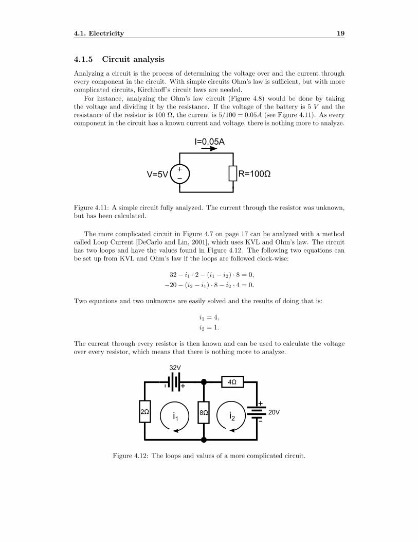
Analyzing a circuit is the process of determining the voltage over and the current throughevery component in the circuit. With simple circuits Ohm’s law is sufficient, but with morecomplicated circuits, Kirchhoff’s circuit laws are needed.

For instance, analyzing the Ohm’s law circuit (Figure 4.8) would be done by takingthe voltage and dividing it by the resistance. If the voltage of the battery is 5 V and theresistance of the resistor is 100 Ω, the current is 5/100 = 0.05A (see Figure 4.11). As everycomponent in the circuit has a known current and voltage, there is nothing more to analyze.

V=5V R=100Ω

I=0.05A

Figure 4.11: A simple circuit fully analyzed. The current through the resistor was unknown,but has been calculated.

The more complicated circuit in Figure 4.7 on page 17 can be analyzed with a methodcalled Loop Current [DeCarlo and Lin, 2001], which uses KVL and Ohm’s law. The circuithas two loops and have the values found in Figure 4.12. The following two equations canbe set up from KVL and Ohm’s law if the loops are followed clock-wise:

32 − i1 · 2 − (i1 − i2) · 8 = 0,−20 − (i2 − i1) · 8 − i2 · 4 = 0.

Two equations and two unknowns are easily solved and the results of doing that is:

i1 = 4,i2 = 1.

The current through every resistor is then known and can be used to calculate the voltageover every resistor, which means that there is nothing more to analyze.

+

-

4Ω

8Ω2Ω

32V

20Vi1 i2

+-

Figure 4.12: The loops and values of a more complicated circuit.


4.1.6 Time-dependent vs. time-independent circuits

Time-dependent circuits are circuits that contains components that depend on time. Somecomponents changes behavior over time and the scale of change can vary by orders ofmagnitude, from small capacitors that take microseconds to charge to large batteries thattake hours to charge. A mechanics simulator, such as Algodoo, often runs in 100Hz, i.e.with a cycle time of 0.01 seconds, but circuits often require a lot higher frequencies toavoid instability, depending on which time-dependent components that are used. Time-independent circuits does not change with time and are therefore easier to analyze.

4.1.7 Active vs. passive circuits

Active circuits are circuits that contains components that produce power or gain, calledactive components. They can be used to amplify a weak signal, i.e. a radio signal, and makeit more usable, i.e. making speakers able to play music at a high volume. The operationof active components depend on the voltage over the component and must therefore beanalyzed in multiple steps that makes them harder and more time consuming to analyze.Passive circuits can be analyzed in one step and are therefore easier to analyze.

V

Internalresistance

Figure 4.13: The replacement circuit for a battery.

4.2 Battery

Batteries can be seen as a voltage source connected in series with a resistor, called theinternal resistance, see Figure 4.13. The resistance is due to the chemical properties of thebattery, but can nonetheless be seen as a resistor, which can help the user to understandhow they work.

With an ideal battery the internal resistance is zero. Ideal batteries do not exist in thereal world, but are valuable for understanding electrical theories, because they simplify theprocess of analysis circuits. With rechargeable batteries the electrochemical reactions areelectrically reversible, which means that rechargeable batteries can be restored with energyif the current flows in the opposite direction.

Ideal, rechargeable and disposable batteries should be possible to simulate. Disposablebatteries can be seen as a special case of rechargeable batteries that are not possible torecharge and are therefore easy to simulate if rechargeable batteries are implemented suc-cessfully.

4.3. Node 21

4.2.1 Ideal battery

An ideal battery can be simulated by replacing the battery with an voltage source. Asdescribed earlier, this implies that the battery has an unlimited amount of energy, and thatthe energy can be provided instantaneously.

4.2.2 Non-ideal battery

Simulation of a non-ideal battery is time-dependent, but on a relatively long time-scale.The amount of energy stored is limited and will change over time. Stepping forward in timein a stable way can be done by a method called semi-implicit Euler [Erleben et al., 2005].

The capacity of a battery is often written in Ah (ampere hour) or Wh (watt hour), butcould also be written in J (joule). Most users are used to Ah and Wh for batteries, butneither of them are SI-units.

The internal resistance and the output voltage can be changed to simulate a batterythat is discharged and possibly charged. The internal resistance provides a battery withtwo important properties. It puts a cap on how much current that can be drawn from abattery in a period of time and it describes how discharged a battery is. A real battery isnot completely out of energy when it stops being usable, but the voltage that the batterycan provide is not enough for most devices [Klein et al., 2002].

The internal resistance alone could be used to lower the output voltage of a simulatedbattery. However, when the battery is completely empty, the resistance will be so largethat it will be very difficult to recharge. To simulate the effect of a completely dischargedbattery, but keep the resistance at a low lever, the voltage can also be lowered when thebattery is discharged.

There are therefore at least two different ways to simulate a battery. If only the resistanceis changed the result will be a unusable battery that does not show 0% charged, but isrealistic. If both the resistance and the voltage is changed the result will be a battery thatshows exactly 0% charged when it is unusable, and will be easy to recharged at that level.

4.3 Node

A node is where two or more components connect. One method of analyzing a circuit is todetermine the voltage at every single node.

4.4 Wire

There are two different types of wires that needs to be considered. Ideal wires with zeroresistance and realistic wires where the resistance depends on the length, width and materialof the wire [Giancoli, 1998]. Ideal wires only contribute to the connection graph of thecircuit. The wires in them self are ignored and the nodes connected to an ideal wire couldbe combined into one.

Since the simulator will be used for educational purposes, the current should preferablybe known everywhere in the circuit. This can be done by replacing the wire with a voltagesource of zero voltage. It will create a larger circuit to analyze and with some circuits, likethe one in Figure 4.14, there will not be a solution. The reason it is that a voltage sourceloop with no resistance would result in infinite energy usage (division by zero with Ohm’slaw).


+

-

+

-

Figure 4.14: A circuit without a solution, if the wires are replaced with voltage sources.

Another method of providing the users with a way of knowing the current and voltageeverywhere in the circuit is to create a ammeter and a voltmeter. A voltmeter is used tomeasure voltage and can in a simulation be created with a very large resistor. A ammeteris used to measure ampere and can in a simulation be created with a voltage source withzero voltage (like the replacement wire).

4.5 Resistor

Ignoring temperature differences, resistors can be simulated with Ohm’s law and Kirchhoff’scircuit laws. They are the easiest component to simulate, and they are useful for controllingthat the simulator is working as it should. This is because their behavior when connectedin parallel and in series are simple to analyze.

The combined resistance of two resistors in series is R1 +R2 = RTotal, if R1 is the firstresistance, R2 is the second resistance and RTotal is the combined resistance.

The combined resistance of two resistors in parallel is 1/R1 + 1/R2 = 1/RTotal. SeeFigure 4.15.

+

-

+

-

100Ω 100Ω 200Ω

+ -

100Ω

+ -

50Ω

100Ω

Figure 4.15: Reducing resistors in series can be seen above and reducing resistors in parallelcan be seen below.

4.6. Potentiometer 23

4.6 Potentiometer

Potentiometers are resistors with a variable resistance that can be changed by the user.They are often used for volume knobs and for similar applications.

4.7 Electric laser

Algodoo does not have a lamp, but it does have a laser pen where the laser fades away aftera specified distance, called the fade distance. If the laser pen is seen as a lamp, the currentthat flows through it can represent the fade distance of the laser pen. A lamp is really justa resistor that emits light when heated up. However, the resistance of a lamp is dependingon the temperature, which changes rather quickly when turned on. The temperature cantherefore be ignored and the circuit only sees the laser as a static resistor.

4.8 Inductor

An inductor is time-varying and can be created with a wire that is looped a number oftimes. It stores energy in a magnetic field, which induces a voltage. The induces voltagecan be calculated with the following equation:

v(t) = Ldi(t)dt

,

where v(t) is the time-varying voltage, L is the inductance of the inductor and i(t) is thetime-varying current thats flowing through the inductor. Simulating an inductor completelytherefore requires solving a differential equation.

The combined inductance of two inductors in series is L1 +L2 = LTotal, if L1 is the firstinductance, L2 is the second inductance and LTotal is the total inductance.

The combined inductance of the two inductors in parallel is 1/L1 + 1/L2 = 1/LTotal. Inother words, the inductance of inductors in series and parallel works the same way as theresistance of resistors in series and parallel do (see Figure 4.15).

4.9 Capacitor

A capacitor is time-varying and can be created with two conductors separated by a non-conductive region. It is able to store energy in a static electric field. Charging a capacitorcan be calculated with the following equation:

dW =q

Cdq,

where dW is the work needed, C is the capacitance and q is the charge. Simulating acapacitor therefore also requires solving a differential equation.

The combined capacitance of two capacitors in series is 1/C1 + 1/C2 = 1/CTotal, if C1

is the first capacitance, C2 is the second capacitance and CTotal is the total capacitance.The combined capacitance of the two capacitors in parallel is C1 +C2 = CTotal. In other

words, the capacitance of capacitors in series and parallel works the opposite way of theresistance of resistors in series and parallel (see Figure 4.15).


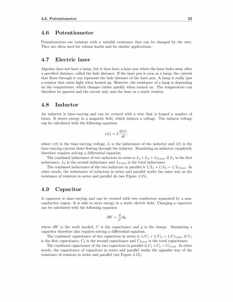
4.10 Motor & generator

An electric motor can be simulated in a number of different ways because there are manydifferent ways of constructing an electric motor.

4.10.1 Energy representation

One way of simulating an electric motor is by looking at it from a energy point of view. Theenergy used by a component can be calculated as

P = I · V,

where P is the (electrical) power used, I is the current and V is the voltage. The powerproduced by a motor can be calculated as

P = τ · ω,

where P is the (mechanical) power produced, τ is the torque and ω is the angular velocity.Some way of controlling the energy used in the circuit is needed because the motor

would otherwise never stop accelerating. This can be provided by replacing the motor witha resistor or by skipping the acceleration period and directly calculate the steady speed ofthe motor. The electrical motor can be seen as displayed in Figure 4.16.

+

-M

+

-

Figure 4.16: The replacement circuit for an electric motor simulated with the energy repre-sentation.

There is however a problem with this model. The motor should be able to work as agenerator, but it is difficult to know when the mechanical system is providing energy andwhen it is requiring energy. One solution is to let the user decide if the motor is a generator,which would make it less realistic.

The good thing about the model is that the system is energy balanced. No energy isadded and that should result in a stable simulation.

4.10.2 Electrical representation

Another way of simulating an electric motor is by looking at its electrical characteristics.From the circuits point of view the motor can be replaced with a resistance in series withan inductor and a voltage source [White, 1997], see Figure 4.17.

4.11. Circuit simulation 25

+

-M

+

-

Figure 4.17: The replacement circuit for an electric motor simulated with the electricalrepresentation.

The voltage, called the back EMF (electromotive force), is induced because the motoris spinning and it opposes the voltage over the whole motor. At low speed, the back EMFis small, and the current through the motor is high. With increasing speed, the back EMFwill increase, and the current through the motor will decrease. The voltage over the wholemotor will also decrease, making the acceleration decrease.

The model has the generator capabilities built in, and it is easy to change the charac-teristics of the motor. The motor will have a realistic acceleration curve, that correspondswell to basic real world motors. However, no obvious link between the electrical energy usedand the mechanical energy produced exists.

4.10.3 Incorporate the motor with the mechanics

Whichever model is used, it must be incorporated with the mechanics. The mechanicalmotor in Algodoo is controlled with a speed and a torque. The motor tries to rotate theattached body at the specified speed, but only with the maximum torque specified. In otherwords, if the motor does not have enough torque to turn the body, the specified speed willnot be achieved. There are therefore two different speeds that must be taken into account.The target speed that the motor is trying to achieve and the real speed of the motor.

With the electrical motor model, the real speed of the motor controls the back EMF andthe voltage over the whole motor is controlling the target speed that the motor is trying toachieve. With the energy motor model, the real speed of the motor times the torque shouldmatch the voltage over the whole motor times the current that goes through the motor.

4.11 Circuit simulation

The most common approach to simulate circuits is to first solve the circuit without anytime-varying components, that is with voltage sources, current sources and resistors. Thiscan be done with a method called Modified Nodal Analysis (MNA)[Litovski and Zwolinski,1997], in which every node is calculated a voltage and every battery a opposite current. Themethod use KCL and Ohm’s law to set up a linear equation system that can easily be solvedby a computer. A ground node must be chosen that is the reference point with voltage 0V .When the linear equations are solved the voltage at every node is known and can be usedto calculate the voltage over and the current through every component. Figure 4.18 showwhat the method needs to analyze the circuit shown i Figure 4.7 on page 17. It also showthe output of the method, i.e. the node voltages and the current through every battery.


+-

R

RR

V

V

Node

0

(gro

und)

Node

1

Node

2

Node

3I

+

-

I

Figure 4.18: The input and output when analyzing a circuit with MNA.

4.11.1 Differential equation method

To deal with time-varying components, one or more differential equations must be solved.This is often done by stepping forward in time and approximating the derivative. Theamount of time stepped forward is called the time-step and can be difficult to choose whensimulating time-varying objects. A too large time-step might introduce instability andinteresting parts of the simulation might be skipped. A too small time-step will make thesimulator slow or require a lot of processing power. If the time-step has to be shared withthe mechanical simulator, the size is even harder to choose. This is because mechanicalsimulators most often are stable with a different sized time-step than the circuit simulator.

4.11.2 Steady state method

Another approach to deal with time-varying components is to use a steady state approach.What this mean is that the simulator calculates how the circuit would look after it is stable,instead of going forward with small time steps. In other words, the simulator jumps forwardone very large time-step, but does so by exactly calculating how the simulated environmentwould look like after the time-step. Inductors can therefore be replaced with wires andcapacitors can be replaced with open connections when using steady state.

The method makes it a lot easier to get a stable system, but the drawback is of coursethat inductors and capacitors works as if they are non existing. The state of rechargeablebatteries could in theory be skipped until they are out of energy, but the time-scale are mostoften large enough to handle in 100Hz.

4.12 Conducting rigid bodies

To make rigid bodies able to conduct electricity, a couple of different methods can be used.The main difference between the methods are how accurate they are. The more accurate,the more time it takes to calculate.

The resistance between two connection points on a body depends on a couple of things.A larger distance will increase the resistance, but a larger cross-sectional area will decrease

4.12. Conducting rigid bodies 27

it. The ability of the material to oppose the flow of electric current, called the resistivity,as well as the temperature of the body also matters.

Some difficulties arise because Algodoo is in two dimensions, which makes the cross-sectional area undefined. Calculating the physically correct resistance over a body is non-trivial since the contact area must be known.

4.12.1 Finite element method

The most accurate method is to divide the body into small sections and for every sectioncalculate the resistance [Humphries, 1998]. Important areas can be divided into smallersections, which would give a better value. Overall it is a very expensive method which takesa lot of time to implement.

4.12.2 Distance method

A simpler method is to use the distance between contact points together with the resistivityof the material and add resistor between every two contact points. An example of this canbe seen in Figure 4.19.

The size of every contact is assumed to be 0.5 mm and if the contact is wider it will beseparated into two or more contacts, see Figure 4.20. This is not 100% physically correct,however, it may be accurate enough for the environment the bodies will be used in.

An artifact of the model will in some scenarios make the total resistance between twocontacting bodies incorrectly change. If two bodies are in contact, a third body may addanother contact which creates two more resistors and an alternative path for the current totravel, see Figure 4.21. This will create the incorrect scenario that the more contacts a bodyhas from different bodies, the less resistance it has, since the total resistance is reduced withresistors in parallel.

A way to handle this artifact is by calculating a minimum spanning tree of the body’sresistors. Every node will therefore be connected, but no parallel resistors will be created,see Figure 4.22. This is still not physically correct, but behaves more logical and may beenough.

Figure 4.19: Two examples of resistor graphs of conducting rigid bodies in contact. Therectangular objects at the top and bottom of the figure have a very small resistivity andthe circular objects between have a large enough resistivity to create resistors in the circuitdiagram. The resistors inside the bodies indicate the resistance over the body between thecontact points.


Figure 4.20: The resistor graph of conducting rigid bodies in contact. The triangular objectat the top has a wide contact area, but it is separated into two contacts instead.

AA

Figure 4.21: The resistor graph of three and four conducting rigid bodies in contact. Thebody A will change the resistance between the first three bodies.

A A

Figure 4.22: The resistor graph of conducting rigid bodies in contact. The body A does notchange the resistance between the first three bodies if a minimum spanning tree is used.

4.13. Switch 29

4.13 Switch

Switches are used to open a closed circuit, i.e. stopping the flow of current, or changingthe loops of a circuit. They open up an endless number of possible interactive scenarios.Switches can be made as a separate electric component or with the already existing rigidbodies, that will be able to conduct electricity. Switches made with rigid bodies mightprovide a more realistic approach, but are more difficult to quickly put together. Algodoodoes however provide small Phunlets, that works kind of like small scenes that can beimported into any other scene. If this works with rigid body switches, there might be noreal down-side to them.

4.14 Visualization

One advantage of simulating electricity is that the current can be visualized, which can helpusers to understand what is really happening. Voltage can e.g. be shown with color andthe current that travels through a wire can be displayed with the speed of yellow blobs oralternatively a shade of yellow. To get the actual values of the voltage and current througha wire, the user could be provided with ammeters and voltmeters. The values could bedisplayed directly, but might make the scene harder to work with and might not be aseducational.

Chapter 5

Design choices & experiments

This chapter describes the choices taken before the experiments and how the experimentswas put together. The user’s stories was used as the basis for the decisions, but someconsiderations about features that might be useful in a future version of the simulator wasalso taken.

Whenever possible, the scripting language Python with the modules NymPy1 and SciPy2

was used for the experiments. The modules add functions to Python, making it more likethe numerical computing environment MATLAB3. Using a scripting language saves a lot oftime when many experiments are to be done, but some experiments were also done in thefinal environment, i.e. Algodoo.

5.1 Choice of simulation paradigm

None of the user’s stories presented in Chapter 3 include any active nor time-varying com-ponents, apart from the battery. Making the simulator faster and more reliable by using thesteady state approach and only passive circuits was therefore an easy choice. This meansthat no inductors, capacitors nor active components will be simulated. However, conductingbodies together with electric motors should be able to provide some of the functions activecomponents provide.

As discussed in Section 4.12, creating a physically correct model of conducting bodies,has the potential to consume a lot of time and processing power without adding anythingsignificant to the user experience. The simplified distance method for conducting bodieswas therefore used as the basis for the experiment.


The following circuits were simulated. Circuit A (Figure 5.1) is a small circuit that caneasily be analyzed by hand. Circuit B (Figure 5.2) is a simple, but larger circuit. CircuitC (Figure 5.3) is a circuit with a trivial solution, i.e. no source of power. Circuit D (Figure5.4) has unconnected components. Circuit E (Figure 5.5) is a large open circuit. Finally,

1numpy.scipy.org2scipy.org3www.mathworks.com/products/matlab/

31

32 Chapter 5. Design choices & experiments

Table 5.1: A couple of circuits experimented with.Circuit # comp # nodesA 13 12B 304 209C 6 6D 18 18E 324 219F 180 130

circuit F (Figure 5.6) has components with zero and unlimited resistance. The componentand node counts are located in Table 5.1.

Two algorithms to set up the MNA linear equations were implemented. In Alg. 1,information about the connected nodes was stored on every component. In Alg. 2, twomore items were stored in each node; the index into the MNA linear system of equations(4 bytes) and the set of components attached to the specific node (4n bytes). The memoryoverhead for a node is therefore 4+4n bytes, where n is the number of components connectedto the node.

Two solvers were implemented to solve the MNA linear equations. One with singleprecision (float) and the other with double precision.

To verify that MNA analyzes circuits correctly, circuit A was simulated by Alg. 1 and2 and solved by both solvers. The result was compared to the analysis presented in section4.1.5 on page 19.

To compare memory usage and speed, circuits A and B were simulated by Alg. 1 and2 and solved with double precision. The time was recorded by the Algodoo profiler as theaverage over 60 seconds. The simulation rate of Algodoo was reduced to 30 frames persecond to reduces the possible interference from other programs running, by letting theprocessor usage stay below 100%.

Finally, to verify that some special cases are analyzed correctly, circuits C, D, E and Fwere simulated by Alg. 1 and 2 and solved by both solvers. For comparison, circuit E wassolved by hand.


Figure 5.1: Circuit A. The blue and green boxes are batteries. The amount of energy leftin a battery is showed with a green rectangle in the middle of the battery. The blackrectangular boxes are resistors. The circles are connection nodes. The yellow blobs showshow the current travels through the wires. A green wire indicates positive voltage, a redwire indicates negative voltage, and a black wire indicates zero voltage. A voltage drop canbe seen over the two horizontal resistors. This circuit contains twelve nodes, six of which arerepresented as black circles. Furthermore, each battery additionally contains two connectionnodes and one invisible node for the internal resistor. The circuit contains 13 components,three of which are resistors and six of with are wires. Each battery additionally contains aresistor and a voltage source.


Figure 5.2: Circuit B. The pac-man-like circles are simulated as conducting bodies, creatinga simple yet large circuit. The red rectangular box is simulating a laser. The laser is glowingsince a current is running through it, i.e. the circuit is closed.

Figure 5.3: Circuit C. A trivial circuit without any power source.


Figure 5.4: Circuit D with unconnected components, i.e. two independent circuits.

Figure 5.5: Circuit E. The same circuit as Circuit B, except that the ball connected to theminus pole is not touching the other, i.e. the circuit is open.


Figure 5.6: Circuit F. The green circular bodies conduct electricity while the red circularbodies are insulators, i.e. they have high resistivity.

5.3 Battery

The simple circuit (Figure 5.7) was used to simulate the discharge cycle of the battery modelsfound in Section 4.2.2. The model parameters were varied manually to find a voltage curvethat matched the real world curve found in Energizer [2010], see Figure 6.3 on page 45.However, the voltage drop over the first 15 minutes of the real world curve was ignored tomake the use of the battery more predictable.

Another circuit was used together with the second model to verify that special cases couldbe handled, see Figure 5.8. Different extreme values with high voltage and low capacity wasused to verify that the battery can handle being uncharged in a single time-step, e.g. avoltage of 200 V and a capacity of 1 J .

Both experiments used Alg. 2 together with the double precision solver.


A hybrid motor and generator model was constructed as a combination of the energy andelectrical motor model (Section 4.10.1 and 4.10.2 respectively). The voltage over the motorsets the target speed of the motor, and the torque τ is solved for in the equation τ ·ω = V ·I,where ω is the real speed of the motor. If the body is stationary, the torque will be infiniteand is therefore clamped to the supplied power to the motor. The inductor in the electricmodel was replaced with a wire since the steady state approach was used.

Two scenes were set up to test the behavior of the motor and generator. In SceneI (Figure 5.9), a motor is connected to a battery and lifting a weight. The energy in the

5.4. Motor & generator 37

Figure 5.7: A basic circuit with a battery and a known current to verify that the battery isworking as it should.

Figure 5.8: A special case circuit where two batteries are connected together.


Figure 5.9: The circular object with arrows in the middle of the lower left gear is an electricmotor. The gear attached to the motor will start to turn if a current is running through themotor. If the current is strong enough, the weight in the middle will be lifted. The threeother gears can rotate freely and stabilizes the weight.

battery is known and the height that the weight should be lifted with the provided energy canbe calculated. In Scene II (Figure 5.10), a motor and generator are mechanically connected.Each has their own battery. At the start of the simulation, the battery connected to themotor was fully charged and the battery connected to the generator was empty. Both sceneswhere tested with different internal resistances on the motors, generator, and batteries. Thetested resistances and voltages were 0.1 Ω and 100 Ω and 5 V and 200 V , respectively.

5.5 Switch & relay

Mechanical switches was experimented on to get a picture of how well they work, see Figure5.11. Mechanical relays were also tested by creating an AND gate, see Figure 5.12.

5.6 Visualization

Two methods to visualize the current through a wire were evaluated by a software engineer(the author), a graphical designer and an educator. The first method used yellow blobstraveled of different speeds through the wire to indicate the current strength. The secondmethod colored the wire with different shades of yellow to indicate the current strength.

5.6. Visualization 39

Figure 5.10: An electric motor is recharging the battery to the right with the help of anelectric generator.

Figure 5.11: The switch to the left is closed sending a current through the laser while theswitch to the right is open.


(a) AND-gate in the false state. The purple rectangles are working as mechanical relays. If theattached motor is turned on, the rectangle will come in contact with the blue rectangle and conductelectricity. The electrical switches in the top of the scene turns the relays on and off. The gate is inthe false state since only one of the two inputs are true.

(b) AND-gate in the true state. Both inputs are true and a current can run through the laser.

Figure 5.12: Relays used as an AND-gate in false and true state.

Chapter 6

Results

This chapter covers the results that were collected from the experiments.


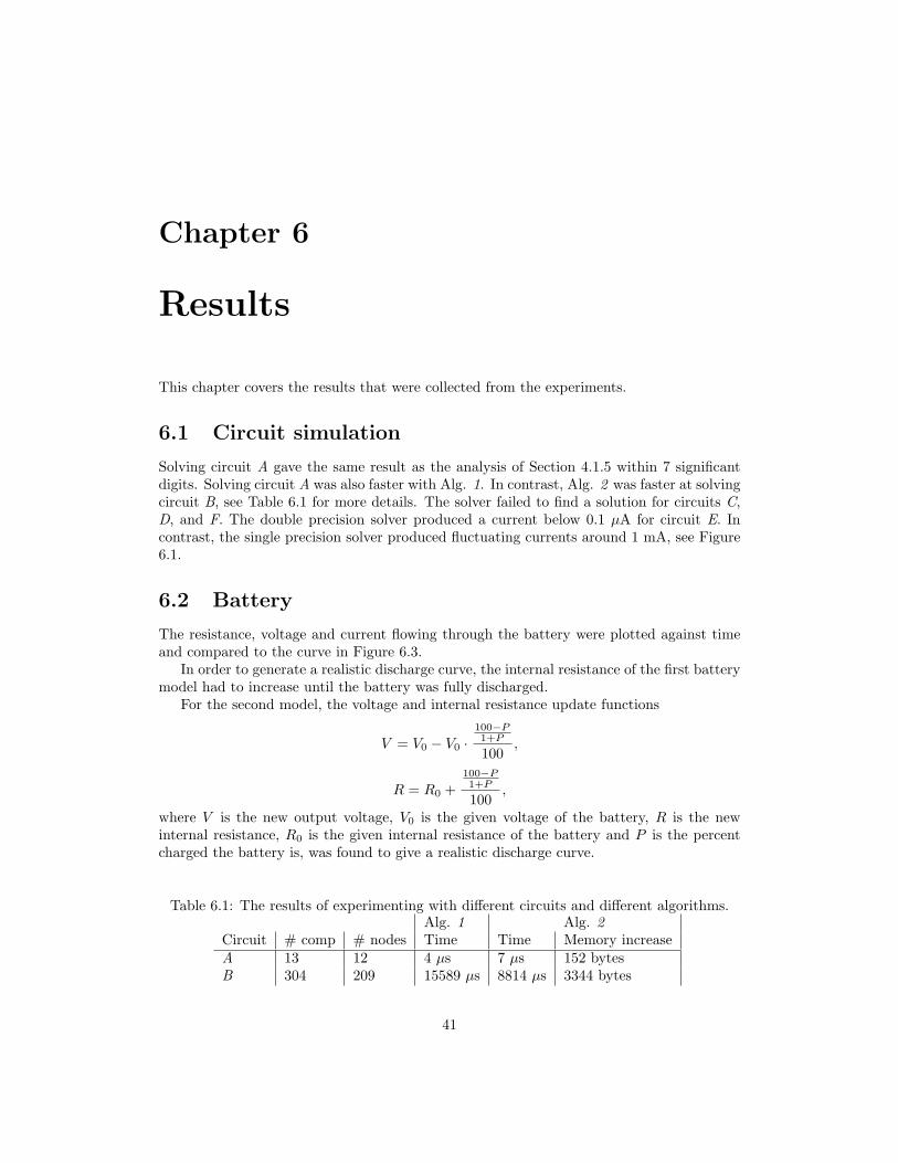
Solving circuit A gave the same result as the analysis of Section 4.1.5 within 7 significantdigits. Solving circuit A was also faster with Alg. 1. In contrast, Alg. 2 was faster at solvingcircuit B, see Table 6.1 for more details. The solver failed to find a solution for circuits C,D, and F. The double precision solver produced a current below 0.1 µA for circuit E. Incontrast, the single precision solver produced fluctuating currents around 1 mA, see Figure6.1.

6.2 Battery

The resistance, voltage and current flowing through the battery were plotted against timeand compared to the curve in Figure 6.3.

In order to generate a realistic discharge curve, the internal resistance of the first batterymodel had to increase until the battery was fully discharged.

For the second model, the voltage and internal resistance update functions

V = V0 − V0 ·100−P1+P

100,

R = R0 +100−P1+P

100,

where V is the new output voltage, V0 is the given voltage of the battery, R is the newinternal resistance, R0 is the given internal resistance of the battery and P is the percentcharged the battery is, was found to give a realistic discharge curve.

Table 6.1: The results of experimenting with different circuits and different algorithms.Alg. 1 Alg. 2

Circuit # comp # nodes Time Time Memory increaseA 13 12 4 µs 7 µs 152 bytesB 304 209 15589 µs 8814 µs 3344 bytes

41

42 Chapter 6. Results

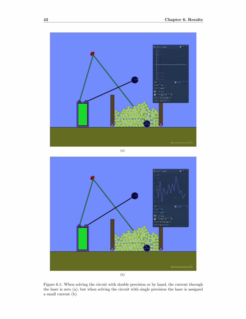
(a)

(b)

Figure 6.1: When solving the circuit with double precision or by hand, the current throughthe laser is zero (a), but when solving the circuit with single precision the laser is assigneda small current (b).


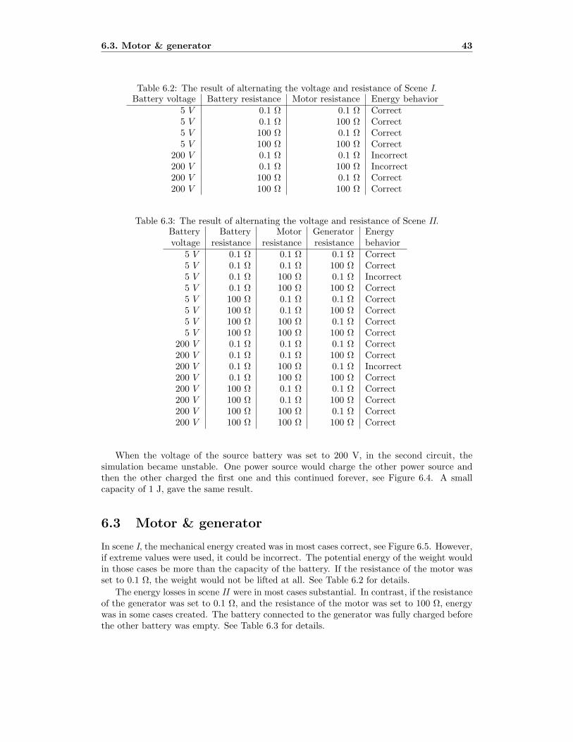
Table 6.2: The result of alternating the voltage and resistance of Scene I.Battery voltage Battery resistance Motor resistance Energy behavior

5 V 0.1 Ω 0.1 Ω Correct5 V 0.1 Ω 100 Ω Correct5 V 100 Ω 0.1 Ω Correct5 V 100 Ω 100 Ω Correct

200 V 0.1 Ω 0.1 Ω Incorrect200 V 0.1 Ω 100 Ω Incorrect200 V 100 Ω 0.1 Ω Correct200 V 100 Ω 100 Ω Correct

Table 6.3: The result of alternating the voltage and resistance of Scene II.Battery Battery Motor Generator Energyvoltage resistance resistance resistance behavior

5 V 0.1 Ω 0.1 Ω 0.1 Ω Correct5 V 0.1 Ω 0.1 Ω 100 Ω Correct5 V 0.1 Ω 100 Ω 0.1 Ω Incorrect5 V 0.1 Ω 100 Ω 100 Ω Correct5 V 100 Ω 0.1 Ω 0.1 Ω Correct5 V 100 Ω 0.1 Ω 100 Ω Correct5 V 100 Ω 100 Ω 0.1 Ω Correct5 V 100 Ω 100 Ω 100 Ω Correct

200 V 0.1 Ω 0.1 Ω 0.1 Ω Correct200 V 0.1 Ω 0.1 Ω 100 Ω Correct200 V 0.1 Ω 100 Ω 0.1 Ω Incorrect200 V 0.1 Ω 100 Ω 100 Ω Correct200 V 100 Ω 0.1 Ω 0.1 Ω Correct200 V 100 Ω 0.1 Ω 100 Ω Correct200 V 100 Ω 100 Ω 0.1 Ω Correct200 V 100 Ω 100 Ω 100 Ω Correct

When the voltage of the source battery was set to 200 V, in the second circuit, thesimulation became unstable. One power source would charge the other power source andthen the other charged the first one and this continued forever, see Figure 6.4. A smallcapacity of 1 J, gave the same result.


In scene I, the mechanical energy created was in most cases correct, see Figure 6.5. However,if extreme values were used, it could be incorrect. The potential energy of the weight wouldin those cases be more than the capacity of the battery. If the resistance of the motor wasset to 0.1 Ω, the weight would not be lifted at all. See Table 6.2 for details.

The energy losses in scene II were in most cases substantial. In contrast, if the resistanceof the generator was set to 0.1 Ω, and the resistance of the motor was set to 100 Ω, energywas in some cases created. The battery connected to the generator was fully charged beforethe other battery was empty. See Table 6.3 for details.


(a)

(b)

Figure 6.2: Figure (a) shows the resulting curve when the load of the battery is around 2A. Figure (b) shows the resulting curve when the load of the battery is around 4 A.


AA

Classification: Rechargeable Chemical System: Nickel-Metal Hydride (NiMH)Designation: ANSI-1.2H2Nominal Voltage: 1.2 VoltsRated Capacity: 2000 mAh* at 21°C (70°F)Typical Weight: 30.0 grams (1.1 oz.)Typical Volume: 8.3 cubic centimeters (0.5 cubic inch)Terminals: Flat ContactJacket: Plastic

* Based on 400 mA (0.2C rate) continuous discharge to 1.0 volts.

0ºC to 40ºC (32ºF to 104ºF) 0ºC to 50ºC (32ºF to 122ºF)

Storage: -20ºC to 30ºC (-4ºF to 86ºF)Humidity: 65±20%

Impedance (milliohms)

(tolerance of ±20% applies to above values)

AC Impedance (no load):

The impedance of the charged cell varies with frequency, as follows:

Frequency (Hz)

This data sheet contains typical information specific to products manufactured at the time of its publication. Important Notice

Charge:Discharge:

NOTE: Operating at extreme temperatures, will significantly impact battery cycle life.

To maintain maximum performance, observe the following general

©Energizer Holdings, Inc. - Contents herein do not constitute a warranty.

Industry Standard Dimensions

Discharge Characteristics

ENERGIZER NH15-2000Specifications

mm (inches)

Cell Charged Cell 1/2 Discharged

Value tolerances are ±20%.

guidelines regarding environmental conditions:

(charged cell)1000 12

Above values based on AC current set at 1.0 ampere.

Internal Resistance:

The internal resistance of the cell varies with state of charge, as follows:

30 milliohms 40 milliohms

Operating and Storage Temperatures:

0.9

1.0

1.1

1.2

1.3

1.4

0.0 0.5 1.0 1.5 2.0 2.5

Cell

Volta

ge

Hours of Discharge

1000 mA(0.5C)

4000 mA(2.0C)

2000 mA(1.0C)

PRODUCT DATASHEET

0.9

1.0

1.1

1.2

1.3

1.4

0 3 6 9 12

Cell

Volta

ge

Hours of Discharge

Typical Performance at 21ºC (70ºF)

200 mA(0.1C)

400 mA(0.2C)

1-800-383-7323 USA/CANwww.energizer.com

14.50 (0.571)13.50 (0.531)

5.50 (0.217)Maximum

1.00 (0.039)Minimum

50.50 (1.988)49.20 (1.937)

7.00 (0.276)Minimum

Form No. EBC - 7102PB Page 1 of 1

Figure 6.3: The real world curve of a discharging battery.

Figure 6.4: The voltage and current of two batteries connected together with high voltageand low capacity. The simulation becomes unstable.


Figure 6.5: The left graph shows the increase of gravitational energy and the right graphshows the loss of electric energy. After the battery is out of energy, the weight begins tofall, i.e. it loses potential energy. This is the expected behavior.

6.4. Switch & relay 47

6.4 Switch & relay

Both the mechanical switches and the relay worked well.

6.5 Visualization

All three observers agreed that showing the current as yellow blobs was easier to understandthan coloring the wires yellow.

Chapter 7

Discussion & conclusions

This chapter covers the conclusions that could be drawn from the results and it also suggesthow some of the problems discovered from the experiments could be handled.


The circuit A simulation confirmed that the MNA approach works for solving circuits. Forlarge circuits, the speed vs. memory simulation (Table 6.1 on page 41) shows a substantialtime reduction for a modest memory increase. Real-time simulation is very important ina simulator such as Algodoo. Spending memory to decrease execution time is thereforeacceptable. Circuits without a power source, unconnected circuits and circuits with zero orunlimited resistance must be handled explicitly, i.e. they can not be directly run throughthe solver. Circuits without a power source can be skipped all together. Unconnectedcircuits must be separated and analyzed one by one. Handling zero resistivity can be doneby merging the resistors nodes together. If a resistor has unlimited resistivity, it can beskipped altogether. Additionally, a double precision solver is needed to prevent round-offerrors.

7.2 Battery

Only changing the resistance when the battery was discharged was confirmed to give a hardto recharge but stable battery. In contrast, a battery with a variable voltage and internalresistance was confirmed to give a more usable battery. However, high voltage and lowcapacity, were found to be potentially unstable. The problem was found out to be becausethe energy left in the battery was reduced after every time step without first checking ifenough energy was available.


The motor model is one of the most important decisions of the whole thesis since it is theonly direct link between the electricity and the mechanics. A battery with a finite amountof energy should only be able to convert the energy into mechanical energy and heat. Noenergy should be created and it should be known where the energy losses are. Failing to

49

50 Chapter 7. Discussion & conclusions

follow these physical laws can make the whole simulation unstable and does not provide theuser with reliable scenarios.

The case with low resistance of the motor in Scene I is the expected behavior sincemost of the energy is lost in the internal resistance of the battery (to heat). In Scene II,some energy is lost in the resistors in both the batteries and in the motors and generators,other energy is lost due to friction. However, the expected efficiency of the motor andgenerator is still higher than the results showed. All in all, the motor and generator can nothandle large differences in resistance, and the motor have problems with high voltage. Inother words, solving the electricity separated from the mechanics does not provide a reliablesimulation. The reason is because the feedback from the mechanics are always one time-stepbehind. This sometimes introduces energy because the generator can be turned in smallbursts, which makes the generator start braking to late, after the body has stopped turning.The creation of energy is most noticeable with extreme differences between the values of agenerator and a motor. The problem can be minimized by making the motor and generatorless configurable.

To confirm that the separation of the simulators really were the problem, a small testwith connected simulators were performed. The test iterated a solution between the circuitsimulator and the mechanical simulator before setting any final values. It was not fullyimplemented because of lack of time, but resulted in a much more stable simulation. Sincethe circuit must be solved between every iteration and there are a few iterations for everytime-step, the test resulted in a more expensive solution, but could probably be withinreasonable limits if more time was spent on optimizing it.

7.4 Switch & relay

No separate electric switches are needed since the mechanical switches work so well.

7.5 Visualization

The current that is traveling through a wire should be displayed with yellow blobs.

Chapter 8

Summary

This chapter covers how well the goals were met, what limitations the solution suffers fromand what more could be accomplished if more time was given.

8.1 Goals

With the extension, Algodoo now has the ability to simulate electricity. Rigid bodies has theability to conduct electricity, although with a simplified model. The electricity is integratedwith the mechanics, but not in a perfect way. More advanced electric components has notbeen implemented. However, the extension can be used to test many different circuits andit works well with logical circuits, built with motor relays. Many other electric componentscan also be created with motor relays.

8.2 Limitations

The biggest limitation is how the motor is integrated with Algodoo. The importance ofthe motor was unfortunately realized too late, but a lot was learned in the progress. Thedecision to solve the circuits separated from the mechanics was taken because Algodoo wasplanned to have a new solver. It would probably have been better to try to solve themtogether from the beginning. This would make the motor smoother and it would use energymore accurately.

Another problem is the precision of the solver, however, it could possibly be solved withsingle precision if more time was spent on it. Double precision works well enough, but doesmost often require more memory.

More advanced electric components would open up some more possible scenes. Theycould, however, change the direction of Algodoo from a mechanics simulator into a circuitsimulator.

8.3 Future work

The following improvements are sorted in approximate time and work required, from fastand small to slow and large. The order also somewhat shows how useful the improvementsare.

51

52 Chapter 8. Summary

– A lot of visual improvements can easily be made (by a graphical designer) and wouldprovide a more finished look to the solution. For instance, making the cables look andbehave more realistic, visualize the capacity of a battery in a more elegant way andimprove how a resistor is displayed, are some ways to improve the visual appearance.

– Some functional and educational components like an ammeter, an voltmeter and anohmmeter would probably not take much time to implement, but it would link to howa real circuit could be analyzed. Some other more advanced electric components couldalso add to the user experience, but as stated earlier, care must be taken to not makeAlgodoo into two separate simulators.

– More time spent on implementing a more accurate motor model is probably requiredfor the solution to be used for education, to prevent that impossible scenarios can becreated. This would require the circuit solver to be integrated with the mechanicssolver.

– Analyzing the circuits can be made faster by utilizing the properties of the linearequations. It could also be improved by storing all the data in a more easily accessibleform.

– A dynamic scale model could speed up the solver by allowing single precision. It wouldalso make the solution more dynamic, but might require some research.

– Even though pure water conduct electricity poorly, making the water in Algodoo ableto conduct electricity would make some interesting scenes possible. It could be usedto show how dangerous it is to mix (impure) water and electricity.

– A correct conducting bodies model could be implemented and would be more phys-ically correct, but is hard to make fast enough. The contact area could be moreaccurately calculated, which would result in a better cross-sectional area approxima-tion. If air were to conduct electricity, an even better approximation could be found.However, the distance between every body and between different parts of the individ-ual bodies would have to be known. With a high enough voltage, an arc could becreated if two charged bodies are close enough.

– Another complicated improvement would be to make electricity create magnetic fieldsin Algodoo, and the existing attraction attribute of bodies could be changed to rep-resent magnets which could create electricity.

– An alternative to the whole solution could be to simulating electricity at a much lowerlevel, as particles. This would probably be hard to make fast enough, but wouldprovide Algodoo with other interesting properties as well.

8.4 Personal reflections

One useful feature that has helped me a lot throughout the thesis is the built-in profiler ofAlgodoo, see Figure 8.1. The profiler shows how the processing power is used by the differentmethods and methods can even be examined further by splitting them into sub-methods.Some small performance improvements could be done by rearrange how code was executedand improving code that had something to do with contact circuits and solving the linearequations, i.e. code that are executed every time-step, of course gave the best results.

8.4. Personal reflections 53

Figure 8.1: The build-in profiler of Algodoo. Methods with a star can be examined further.

54 Chapter 8. Summary

The usability was always in the back of my mind and it is important in a software thatis to be used for education, but it can be hard to know what works best. Fortunately it isquite easy to change the graphical components of the solutions because it is separated fromthe calculated data. I tried to keep the number of buttons to a minimum. The solutiononly adds one tool, but does add a few menus that are required to be able to change theproperties of the component and converting boxes into batteries.

Overall the extension has taught me a lot and I am more than pleased with the result.

Chapter 9

Acknowledgments

First of all, I am grateful to Kenneth Bodin for getting the thesis starting and for providingideas of how Algodoo could be extended. I would also like to thank Emil Ernerfeldt and JoelCarlquist. Emil has helped a lot throughout the thesis with anything Algodoo related andhe has also contributed with knowledge about other more specific implementation problems.Joel has also answered any random questions about anything Algodoo.

I would like to thank both Claude Lacoursiere and Fredrik Nordfelth for helping withphysical theories. Claude took an interest in figuring out a working motor model. Fredrikhas helped with how to analyze circuits and he has also helped with the final touches of thewritten thesis.

My supervisor Niclas Borlin has helped me a lot with writing this thesis, the qualityof the thesis would not have been nearly as good without him. He also helped me withseeing some of the problems from a different angle. Jonatan Persson and Madelen Bodinhas helped with inspiration of a couple of user’s stories and also how the interface can bemore intuitive and user friendly. I would also like to thank all the employees of Algoryx fortheir warm welcome.

Lastly I would like to thank my family for being who they are.

55

56 Chapter 9. Acknowledgments

References

Algoryx Simulation AB. FAQ - Algodoo. http://www.algodoo.com/wiki/FAQ (visited2010-10-11), 2009.

Dr. Carl Burch. Logisim. http://ozark.hendrix.edu/~burch/logisim/ (visited 2010-11-19), 2010.

Raymond A. DeCarlo and Pen-Min Lin. Linear Circuit Analysis: Time Domain, Phasor,and Laplace Transform Approaches. Oxford University Press, New York, 2001. ISBN0-1951-3666-7.

Energizer. NH15-2000 Product Datasheet. http://data.energizer.com/PDFs/nh15-2000.pdf (visited 2011-01-12), 2010.

Kenny Erleben, Jon Sporring, Knud Henriksen, and Henrik Dohlmann. Physics-Based An-imation. Charles River Media, Inc, Hingham, Massachusetts, 2005. ISBN 1-58450-380-7.

Emil Ernerfeldt. Title not yet known. Master’s thesis, Dept. of Comp. Sc., Umea University,Sweden, 2011. Not yet published.

Paul Falstad. Circuit Simulator Applet. http://www.falstad.com/circuit/ (visited 2010-10-11), 2010.

Earl Gates. Introduction to Electronics. Delmar Cengage Learning, Clifton Park, NY, 2006.ISBN 1-4018-8900-X.

Douglas C. Giancoli. Physics: Principles with Applications. Prentice Hall, Upper SaddleRiver, N.J., 1998. ISBN 0-1361-1971-9.

Stanley Humphries. Field Solutions on Computers. CRC Press, Boca Raton, 1998. ISBN0-8493-1668-5.

Martin G. Klein, Michael Eskra, Robert Plivelich, and Paula Ralston. Bipolar Nickel MetalHydride Battery. Technical paper. http://www.haszstudios.com/electro/products/technicalpapers/BipolarNickel.pdf (visited 2010-10-11), 2002.

Jari Lavonen, Veijo Meisalo, Reijo Byman, Anna Uitto, and Kalle Juuti. Pupil Interest inPhysics: A survey in Finland. PhD thesis, Dept. of Applied Sc. of Education, Universityof Helsinki, Finland, 2005. Electronic version at http://www.naturfagsenteret.no/tidsskrift/Nordina_205_Lavonen.pdf (visited 2010-10-11).

V. Litovski and M. Zwolinski. VLSI Circuit Simulation and Optimization. Chapman &Hall, London, 1997. ISBN 0-4126-3860-6.

57

http://www.algodoo.com/wiki/FAQ

http://ozark.hendrix.edu/~burch/logisim/

http://data.energizer.com/PDFs/nh15-2000.pdf

http://data.energizer.com/PDFs/nh15-2000.pdf

http://www.falstad.com/circuit/

http://www.haszstudios.com/electro/products/technicalpapers/BipolarNickel.pdf

http://www.haszstudios.com/electro/products/technicalpapers/BipolarNickel.pdf

http://www.naturfagsenteret.no/tidsskrift/Nordina_205_Lavonen.pdf

http://www.naturfagsenteret.no/tidsskrift/Nordina_205_Lavonen.pdf

58 REFERENCES

T. Quarles, D. Pederson, R. Newton, A. Sangiovanni-Vincentelli, and Christopher Wayne.The Spice Home Page. http://bwrc.eecs.berkeley.edu/classes/icbook/spice/(visited 2010-11-19), 1993.

Steven M. Rubin. Static Free Software Home Page. http://www.staticfreesoft.com/(visited 2010-11-19), 2010.

J. R. White. Dynamic Model of a Permanent Magnet DC Motor. http://gershwin.ens.fr/vdaniel/Doc-Locale/Cours-Mirrored/Methodes-Maths/white/sdyn/s6/s6fmathm/s6fmathm.html (visited 2010-10-11), 1997.

http://bwrc.eecs.berkeley.edu/classes/icbook/spice/

http://www.staticfreesoft.com/

http://gershwin.ens.fr/vdaniel/Doc-Locale/Cours-Mirrored/Methodes-Maths/white/sdyn/s6/s6fmathm/s6fmathm.html



Electricity in a 2D mechanics simulator for education · · 2011-03-14Electricity in a 2D...

Documents

Transcript of Electricity in a 2D mechanics simulator for education · · 2011-03-14Electricity in a 2D...