LECTURE NOTES

ON

Electrical Power Transmission

Systems

III B. Tech I semester (JNTUA -R13)

K SIVA KUMAR

Associate Professor & HOD

DEPARTMENT OF

ELECTRICAL AND ELECTRONICS ENGINEERING

CHADALAWADA RAMANAMMA ENGINEERING COLLEGE: TIRUPATHI

Course Objective:

This course is an extension of Generation of Electric Power course. It deals with basic theory of

transmission lines modeling and their performance analysis. Also this course gives emphasis on

mechanical design of transmission lines, cables and insulators.

UNIT I : TRANSMISSION LINE PARAMETERS

Types of Conductors – ACSR, Bundled and Standard Conductors- Resistance For Solid Conductors –

Skin Effect- Calculation of Inductance for Single Phase and Three Phase, Single and Double Circuit

Lines, Concept of GMR & GMD, Symmetrical and Asymmetrical Conductor Configuration with and

without Transposition, Numerical Problems, Capacitance Calculations for Symmetrical and

Asymmetrical Single and Three Phase, Single and Double Circuit Lines, Effect of Ground on

Capacitance, Numerical Problems.

UNIT II: PERFORMANCE OF TRANSMISSION LINES:

Classification of Transmission Lines - Short, Medium and Long Line and Their Exact Equivalent

Ciruits- Nominal-T, Nominal-Pie. Mathematical Solutions to Estimate Regulation and Efficiency of

All Types of Lines. Long Transmission Line-Rigorous Solution, Evaluation of A,B,C,D Constants,

Interpretation of the Long Line Equations – Surge Impedance and Surge Impedance Loading -

Wavelengths and Velocity of Propagation – Ferranti Effect , Charging Current-Numerical Problems.

UNIT III: MECHANICAL DESIGN OF TRANSMISSION LINES

Overhead Line Insulators: Types of Insulators, String Efficiency and Methods for Improvement,

Capacitance Grading and Static Shielding.

Corona: Corona Phenomenon, Factors Affecting Corona, Critical Voltages and Power Loss, Radio

Interference.

Sag and Tension Calculations: Sag and Tension Calculations with Equal and Unequal Heights of

Towers, Effect of Wind and Ice on Weight of Conductor, Stringing Chart and Sag Template and Its

Applications, Numerical Problems.

UNIT IV :POWER SYSTEM TRANSIENTS & TRAVELLING WAVES

Types of System Transients - Travelling or Propagation of Surges - Attenuation, Distortion,

Reflection and Refraction Coefficients - Termination of Lines with Different Types of Conditions -

Open Circuited Line, Short Circuited Line, T-Junction, Lumped Reactive Junctions (Numerical

Problems). Bewley’s Lattice Diagrams (for all the cases mentioned with numerical examples).

UNIT V :CABLES

Types of Cables, Construction, Types of Insulating Materials, Calculations of Insulation Resistance

and Stress in Insulation, Numerical Problems. Capacitance of Single and 3-Core Belted Cables,

Numerical Problems. Grading of Cables - Capacitance Grading, Numerical Problems, Description of

Inter-Sheath Grading

Text Books:

1. Electrical power systems - by C.L.Wadhwa, New Age International (P) Limited, Publishers,4th

Edition, 2005.

2. Power system Analysis-by John J Grainger, William D Stevenson, TMC Companies, 4th edition,

1994.

Reference Books:

1. Power System Analysis and Design by B.R.Gupta, S. Chand & Co, 6th Revised Edition, 2010.

2. Modern Power System Analysis by I.J.Nagrath and D.P.Kothari, Tata McGraw Hill, 3rd Edition,

2008.

3. Electric Power Transmission System Engineering: Analysis and Design, by Turan Gonen, 2nd

Edition, CRC Press, 2009.

4. Electric Power Systems by S. A. Nasar, Schaum‟s Outline Series, TMH, 3rd Edition, 2008.

5. A Text Book on Power System Engineering by M.L.Soni, P.V.Gupta, U.S.Bhatnagar,

A.Chakrabarti, Dhanpat Rai & Co Pvt. Ltd., 2003.

UNIT-I

Transmission Line Parameters

Conductor is a physical medium to carry electrical energy form one place to other. It is an

important component of overhead and underground electrical transmission and distribution

systems. The choice of conductor depends on the cost and efficiency. An ideal conductor has

following features.

1. It has maximum conductivity

2. It has high tensile strength

3. It has least specific gravity i.e. weight / unit volume

4. It has least cost without sacrificing other factors.

1.Types of Conductors:

In the early days conductor used on transmission lines were usually Copper, but Aluminum

Conductors have Completely replaced Copper because of the much lower cost and lighter

weight of Aluminum conductor compared with a Copper conductor of the same resistance.

The fact that Aluminum conductor has a larger diameter than a Copper conductor of the same

resistance is also an advantage. With a larger diameter the lines of electric flux originating on

the conductor will be farther apart at the conductor surface for the same voltage. This means a

lower voltage gradient at the conductor surface and less tendency to ionise the air around the

conductor. Ionization produces the undesirable effect called corona.

The symbols identifying different types of Aluminium conductors are as follows:-

AAC: AllAluminiumconductors.

AAAC: AllAluminiumAlloyconductors

ACSR: Aluminiumconductors,Steel-Reinforced

ACAR : Aluminum conductor, Alloy-Reinforced

Aluminium alloy conductors have higher tensile strength than the conductor of EC grade

Aluminium or AAC, ACSR consists of a central core of steel strands surrounded by layers of

Aluminium strands. ACAR has a central core of higher strength Aluminium Alloy

surrounded by layer of Electrical-Conductor-Grade Aluminium.

1.1 ACSR (Aluminum Conductor Steel Reinforced)

Aluminum Conductor Steel Reinforced (ACSR) is concentrically stranded conductor

with one or more layers of hard drawn 1350-H19 aluminum wire on galvanized steel

wire core.

The core can be single wire or stranded depending on the size.

Steel wire core is available in Class A ,B or Class C galvanization for corrosion

protection.

Additional corrosion protection is available through the application of grease to the

core or infusion of the complete cable with grease.

The proportion of steel and aluminum in an ACSR conductor can be selected based on

the mechanical strength and current carrying capacity demanded by each application.

ACSR conductors are recognized for their record of economy, dependability and

favorable strength / weight ratio. ACSR conductors combine the light weight and

good conductivity of aluminum with the high tensile strength and ruggedness of steel.

In line design, this can provide higher tensions, less sag, and longer span lengths than

obtainable with most other types of overhead conductors.

The steel strands are added as mechanical reinforcements.

ACSR conductors are recognized for their record of economy, dependability and

favorable strength / weight ratio.

ACSR conductors combine the light weight and good conductivity of aluminum with

the high tensile strength and ruggedness of steel.

In line design, this can provide higher tensions, less sag, and longer span lengths than

obtainable with most other types of overhead conductors.

The steel strands are added as mechanical reinforcements.

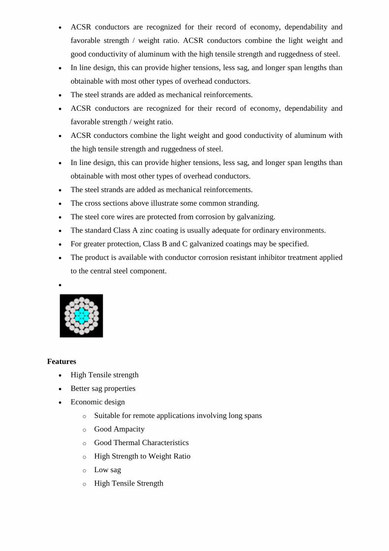
The cross sections above illustrate some common stranding.

The steel core wires are protected from corrosion by galvanizing.

The standard Class A zinc coating is usually adequate for ordinary environments.

For greater protection, Class B and C galvanized coatings may be specified.

The product is available with conductor corrosion resistant inhibitor treatment applied

to the central steel component.

Features

High Tensile strength

Better sag properties

Economic design

o Suitable for remote applications involving long spans

o Good Ampacity

o Good Thermal Characteristics

o High Strength to Weight Ratio

o Low sag

o High Tensile Strength

Typical Application

Commonly used for both transmission and distribution circuits.

Compact Aluminum Conductors, Steel Reinforced (ACSR) are used for overhead

distribution and transmission lines.

BUNDLED CONDUCTORS:

Bundle conductors are widely use for transmission line and has its own advantages and

disadvantages.

Bundle conductor is a conductor which consist several conductor cable which connected.

Bundle conductors also will help to increase the current carried in the transmission line. The

main disadvantage of Transmission line is its having high wind load compare to other

conductors.

(Or)

The combination of more than one conductor per phase in parallel suitably spaced from each

other used in overhead Transmission Line is defined as conductor bundle. The individual

conductor in a bundle is defined as Sub-conductor.

At Extra High Voltage (EHV), i.e. voltage above 220 KV corona with its resultant power loss

and particularly its interference with communication is excessive if the circuit has only one

conductor per phase. The High-Voltage Gradient at the conductor in the EHV range is

reduced considerably by having two or more conductors per phase in close proximity

compared with the spacing between conductor-bundle spaced 450 mm is used in India

The three conductor bundle usually has the conductors at the vertices of an equilateral

triangle and four conductors bundle usually has its conductors at the corners of a square.

The current will not divide exactly between the conductor of the bundle unless there is a

transposition of the conductors within the bundle, but the difference is of no practical

importance.

Reduced reactance is the other equally important advantage of bundling. Increasing the

number of conductor in a bundle reduces the effects of corona and reduces the reactance. The

reduction of reactance results from the increased Geometric Mean Radius (GMR) of the

bundle.

2. TRANSMISSION LINES:

The electric parameters of transmission lines (i.e. resistance, inductance, and capacitance)

can be determined from the specifications for the conductors, and from the geometric

arrangements of the conductors.

UNIT-II

Performance of Short and Medium

Length Transmission Lines

SHORT TRANSMISSION LINES

The transmission lines are categorized as three types

1) Short transmission line – the line length is up to 80 km

2) Medium transmission line – the line length is between 80km to 160 km

3) Long transmission line – the line length is more than 160 km

Whatever may be the category of transmission line, the main aim is to transmit power from

one end to another. Like other electrical system, the transmission network also will have

some power loss and voltage drop during transmitting power from sending end to receiving

end. Hence, performance of transmission line can be determined by its efficiency and voltage

regulation.

power sent from sending end – line losses = power delivered at receiving end

Voltage regulation of transmission line is measure of change of receiving end voltage from

no-load to full load condition.

Every transmission line will have three basic electrical parameters. The conductors of the

line will have resistance, inductance, and capacitance. As the transmission line is a set of

conductors being run from one place to another supported by transmission towers, the

parameters are distributed uniformly along the line.

The electrical power is transmitted over a transmission line with a speed of light that is 3X108

m ⁄ sec. Frequency of the power is 50Hz. The wave length of the voltage and current of the

power can be determined by the equation given below,

f.λ = v where f is power frequency, &labda is wave length and v is the speed of light.

Hence the wave length of the transmitting power is quite long compared to the generally

used line length of transmission line.

For this reason, the transmission line, with length less than 160 km, the parameters are

assumed to be lumped and not distributed. Such lines are known as electrically short

transmission line. This electrically short transmission lines are again categorized as short

transmission line (length up to 80 km) and medium transmission line(length between 80 and

160 km). The capacitive parameter of short transmission line is ignored whereas in case of

medium length line the capacitance is assumed to be lumped at the middle of the line or half

of the capacitance may be considered to be lumped at each ends of the transmission line.

Lines with length more than 160 km, the parameters are considered to be distributed over the

line. This is called long transmission line.

ABCD PARAMETERS

A major section of power system engineering deals in the transmission of electrical power

from one particular place (eg. Generating station) to another like substations or distribution

units with maximum efficiency. So its of substantial importance for power system engineers

to be thorough with its mathematical modeling. Thus the entire transmission system can be

simplified to a two port network for the sake of easier calculations.

The circuit of a 2 port network is shown in the diagram below. As the name suggests, a 2 port

network consists of an input port PQ and an output port RS. Each port has 2 terminals to

connect itself to the external circuit. Thus it is essentially a 2 port or a 4 terminal circuit,

having

Supply end voltage = VS

and Supply end current = IS

Given to the input port P Q.

And there is the Receiving end Voltage = VR

and Receiving end current = IR

Given to the output port R S.

As shown in the diagram below.

Now the ABCD parameters or the transmission line parameters provide the link between

the supply and receiving end voltages and currents, considering the circuit elements to be

linear in nature.

Thus the relation between the sending and receiving end specifications are given using

ABCD parameters by the equations below.

VS = A VR + B IR ———————-(1)

IS = C VR + D IR ———————-(2)

Now in order to determine the ABCD parameters of transmission line let us impose the

required circuit conditions in different cases.

ABCD parameters, when receiving end is open circuited

The receiving end is open circuited meaning receiving end current IR = 0.

Applying this condition to equation (1) we get.

Thus its implies that on applying open circuit condition to ABCD parameters, we get

parameter A as the ratio of sending end voltage to the open circuit receiving end voltage.

Since dimension wise A is a ratio of voltage to voltage, A is a dimension less parameter.

Applying the same open circuit condition i.e IR = 0 to equation (2)

Thus its implies that on applying open circuit condition to ABCD parameters of

transmission line, we get parameter C as the ratio of sending end current to the open

circuit receiving end voltage. Since dimension wise C is a ratio of current to voltage, its

unit is mho.

Thus C is the open circuit conductance and is given

by C = IS ⁄ VR mho.

ABCD parameters when receiving end is short circuited

Receiving end is short circuited meaning receiving end voltage VR = 0

Applying this condition to equation (1) we get

Thus its implies that on applying short circuit condition to ABCD parameters, we get

parameter B as the ratio of sending end voltage to the short circuit receiving end current.

Since dimension wise B is a ratio of voltage to current, its unit is Ω. Thus B is the short

circuit resistance and is

given by

B = VS ⁄ IR Ω.

Applying the same short circuit condition i.e VR = 0 to equation (2) we get

Thus its implies that on applying short circuit condition to ABCD parameters, we get

parameter D as the ratio of sending end current to the short circuit receiving end current.

Since dimension wise D is a ratio of current to current, it’s a dimension less parameter. ∴ the

ABCD parameters of transmission line can be tabulated as:-

Parameter Specification Unit

A = VS / VR Voltage ratio Unit less

B = VS / IR Short circuit

resistance Ω

C = IS / VR Open circuit conductance mho

D = IS / IR Current ratio Unit less

SHORT TRANSMISSION LINE

The transmission lines which have length less than 80 km are generally referred as

short transmission lines.

For short length, the shunt capacitance of this type of line is neglected and other parameters

like resistance and inductance of these short lines are lumped, hence the equivalent circuit is

represented as given below,

Let’s draw the vector diagram for this equivalent circuit, taking receiving end current Ir as

reference. The sending end and receiving end voltages make angle with that reference

receiving end current, of φs and φr, respectively.

As the shunt capacitance of the line is neglected, hence sending end current and receiving

end current is same, i.e.

Is = Ir.

Now if we observe the vector diagram carefully, we will

get, Vs is approximately equal to

Vr + Ir.R.cosφr + Ir.X.sinφr

That means,

Vs ≅ Vr + Ir.R.cosφr + Ir.X.sinφr as the it is assumed that φs ≅ φr

As there is no capacitance, during no load condition the current through the line is considered

as zero, hence at no load condition, receiving end voltage is the same as sending end voltage

As per dentition of voltage regulation,

Here, vr and vx are the per unit resistance and reactance of the short transmission line.

Any electrical network generally has two input terminals and two output terminals. If we

consider any complex electrical network in a black box, it will have two input terminals and

output terminals. This network is called two – port network. Two port model of a network

simplifies the network solving technique. Mathematically a two port network can be solved

by 2 by 2 matrixes.

A transmission as it is also an electrical network; line can be represented as two port network.

Hence two port network of transmission line can be represented as 2 by 2 matrixes. Here

the concept of ABCD parameters comes. Voltage and currents of the network can

represented as ,

Vs= AVr + BIr…………(1)

Is= CVr + DIr…………(2)

Where A, B, C and D are different constant of the network.

If we put Ir = 0 at equation (1), we get

Hence, A is the voltage impressed at the sending end per volt at the receiving end when

receiving end is open. It is dimension less.

If we put Vr = 0 at equation (1), we get

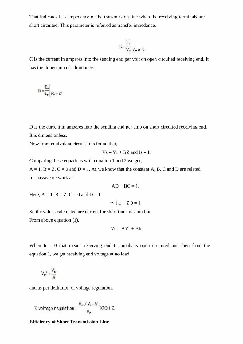
That indicates it is impedance of the transmission line when the receiving terminals are

short circuited. This parameter is referred as transfer impedance.

C is the current in amperes into the sending end per volt on open circuited receiving end. It

has the dimension of admittance.

D is the current in amperes into the sending end per amp on short circuited receiving end.

It is dimensionless.

Now from equivalent circuit, it is found that,

Vs = Vr + IrZ and Is = Ir

Comparing these equations with equation 1 and 2 we get,

A = 1, B = Z, C = 0 and D = 1. As we know that the constant A, B, C and D are related

for passive network as

AD − BC = 1.

Here, A = 1, B = Z, C = 0 and D = 1

⇒ 1.1 − Z.0 = 1

So the values calculated are correct for short transmission line.

From above equation (1),

Vs = AVr + BIr

When Ir = 0 that means receiving end terminals is open circuited and then from the

equation 1, we get receiving end voltage at no load

and as per definition of voltage regulation,

Efficiency of Short Transmission Line

The efficiency of short line as simple as efficiency equation of any other electrical

equipment, that means

MEDIUM TRANSMISSION LINE

The transmission line having its effective length more than 80 km but less than 250 km, is

generally referred to as a medium transmission line. Due to the line length being

considerably high, admittance Y of the network does play a role in calculating the effective

circuit parameters, unlike in the case of short transmission lines. For this reason the modelling

of a medium length transmission line is done using lumped shunt admittance along with the

lumped impedance in series to the circuit.

These lumped parameters of a medium length transmission line can be represented using

two different models, namely.

1) Nominal Π representation.

2) Nominal T representation.

Let’s now go into the detailed discussion of these above mentioned models.

Nominal Π representation of a medium transmission line

In case of a nominal Π representation, the lumped series impedance is placed at the middle of

the circuit where as the shunt admittances are at the ends. As we can see from the diagram of

the Π network below, the total lumped shunt admittance is divided into 2 equal halves, and

each half with value Y ⁄ 2 is placed at both the sending and the receiving end while the entire

circuit impedance is between the two. The shape of the circuit so formed resembles that of a

symbol Π, and for this reason it is known as the nominal Π representation of a medium

transmission line. It is mainly used for determining the general circuit parameters and

performing load flow analysis.

As we can see here, VS and VR is the supply and receiving end voltages respectively,

and Is is the current flowing through the supply end.

IR is the current flowing through the receiving end of the circuit.

I1 and I3 are the values of currents flowing through the admittances.

And I2 is the current through the impedance Z.

Now applying KCL, at node P, we

get. IS = I1 + I2 —————(1)

Similarly applying KCL, to node

Q. I2 = I3 + IR —————(2)

Now substituting equation (2) to equation

(1) IS = I1 + I3 + IR

Now by applying KVL to the circuit,

VS = VR + Z I2

Comparing equation (4) and (5) with the standard ABCD parameter equations

VS = A VR + B IR

IS = C VR + D IR

We derive the parameters of a medium transmission line as:

Nominal T representation of a medium transmission line

In the nominal T model of a medium transmission line the lumped shunt admittance is placed

in the middle, while the net series impedance is divided into two equal halves and and placed

on either side of the shunt admittance. The circuit so formed resembles the symbol of a

capital T, and hence is known as the nominal T network of a medium length transmission line

and is shown in the diagram below.

Here also Vs and Vr is the supply and receiving end voltages respectively, and

Is is the current flowing through the supply end. Ir is the current flowing through the

receiving end of the circuit. Let M be a node at the midpoint of the circuit, and the drop at

M, be given by

Vm. Applying KVL to the above network we get

Now the sending end current is

Is = Y VM + IR ——————(9)

Substituting the value of VM to equation (9) we get,

Again comparing Comparing equation (8) and (10) with the standard ABCD parameter

equations

VS = A VR + B IR

IS = C VR + D IR

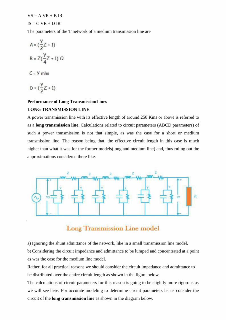
The parameters of the T network of a medium transmission line are

Performance of Long TransmissionLines

LONG TRANSMISSION LINE

A power transmission line with its effective length of around 250 Kms or above is referred to

as a long transmission line. Calculations related to circuit parameters (ABCD parameters) of

such a power transmission is not that simple, as was the case for a short or medium

transmission line. The reason being that, the effective circuit length in this case is much

higher than what it was for the former models(long and medium line) and, thus ruling out the

approximations considered there like.

a) Ignoring the shunt admittance of the network, like in a small transmission line model.

b) Considering the circuit impedance and admittance to be lumped and concentrated at a point

as was the case for the medium line model.

Rather, for all practical reasons we should consider the circuit impedance and admittance to

be distributed over the entire circuit length as shown in the figure below.

The calculations of circuit parameters for this reason is going to be slightly more rigorous as

we will see here. For accurate modeling to determine circuit parameters let us consider the

circuit of the long transmission line as shown in the diagram below.

Here a line of length l > 250km is supplied with a sending end voltage and current of VS and

IS respectively, where as the VR and IR are the values of voltage and current obtained from

the receiving end. Lets us now consider an element of infinitely small length Δx at a distance

x from the receiving end as shown in the figure where.

V = value of voltage just before entering the element Δx.

I = value of current just before entering the element Δx.

V+ΔV = voltage leaving the element Δx.

I+ΔI = current leaving the element Δx.

ΔV = voltage drop across element Δx.

zΔx = series impedence of element Δx

yΔx = shunt admittance of element Δx

Where Z = z l and Y = y l are the values of total impedance and admittance of the

long transmission line.

∴ the voltage drop across the infinitely small element Δx is given by

ΔV = I z Δx

Or I z = ΔV ⁄ Δx

Or I z = dV ⁄ dx —————————(1)

Now to determine the current ΔI, we apply KCL to node A.

ΔI = (V+ΔV)yΔx = V yΔx + ΔV yΔx

Since the term ΔV yΔx is the product of 2 infinitely small values, we can ignore it for the

sake of easier calculation.

∴ we can write dI ⁄ dx = V y —————–(2)

Now derevating both sides of eq (1) w.r.t x,

d2 V ⁄ d x

2 = z dI ⁄ dx

Now substituting dI ⁄ dx = V y from equation (2)

d2 V ⁄ d x

2 = zyV

or d2 V ⁄ d x

2 − zyV = 0 ————(3)

The solution of the above second order differential equation is given by.

V = A1 ex√yz

+ A2 e−x√yz

————–(4)

Derivating equation (4) w.r.to x.

dV/dx = √(yz) A1 ex√yz

− √(yz)A2 e−x√yz

————

(5) Now comparing equation (1) with equation (5)

Now to go further let us define the characteristic impedance Zc and propagation constant δ

of a long transmission line as

Zc = √(z/y)

Ω δ = √(yz)

Then the voltage and current equation can be expressed in terms of characteristic impedance

and propagation constant as

V = A1 eδx

+ A2 e−δx

———–(7)

I = A1/ Zc eδx

+ A2 / Zc e−δx

—————(8)

Now at x=0, V= VR and I= Ir. Substituting these conditions to equation (7) and (8)

respectively. VR = A1 + A2 —————(9)

IR = A1/ Zc + A2 / Zc —————(10)

Solving equation (9) and

(10), We get values of A1

and A2 as,

A1 = (VR + ZCIR) ⁄ 2

And A1 = (VR − ZCIR)

Now applying another extreme condition at x=l, we have V = VS and I = IS.

Now to determine VS and IS we substitute x by l and put the values of A1 and A2 in

equation (7) and (8) we get

VS = (VR + ZC IR)eδl ⁄ 2 + (VR − ZC IR)e

−δl/2 ————–(11)

IS = (VR ⁄ ZC + IR)eδl/2 − (VR / ZC − IR)e

−δl/2————— (12

By trigonometric and exponential operators we know

sinh δl = (eδl − e

−δl) ⁄ 2

And cosh δl = (eδl + e

−δl) ⁄2

∴ equation(11) and (12) can be re-written

as

VS = VRcosh δl + ZC IR sinh δl

IS = (VR sinh δl)/ZC + IRcosh δl

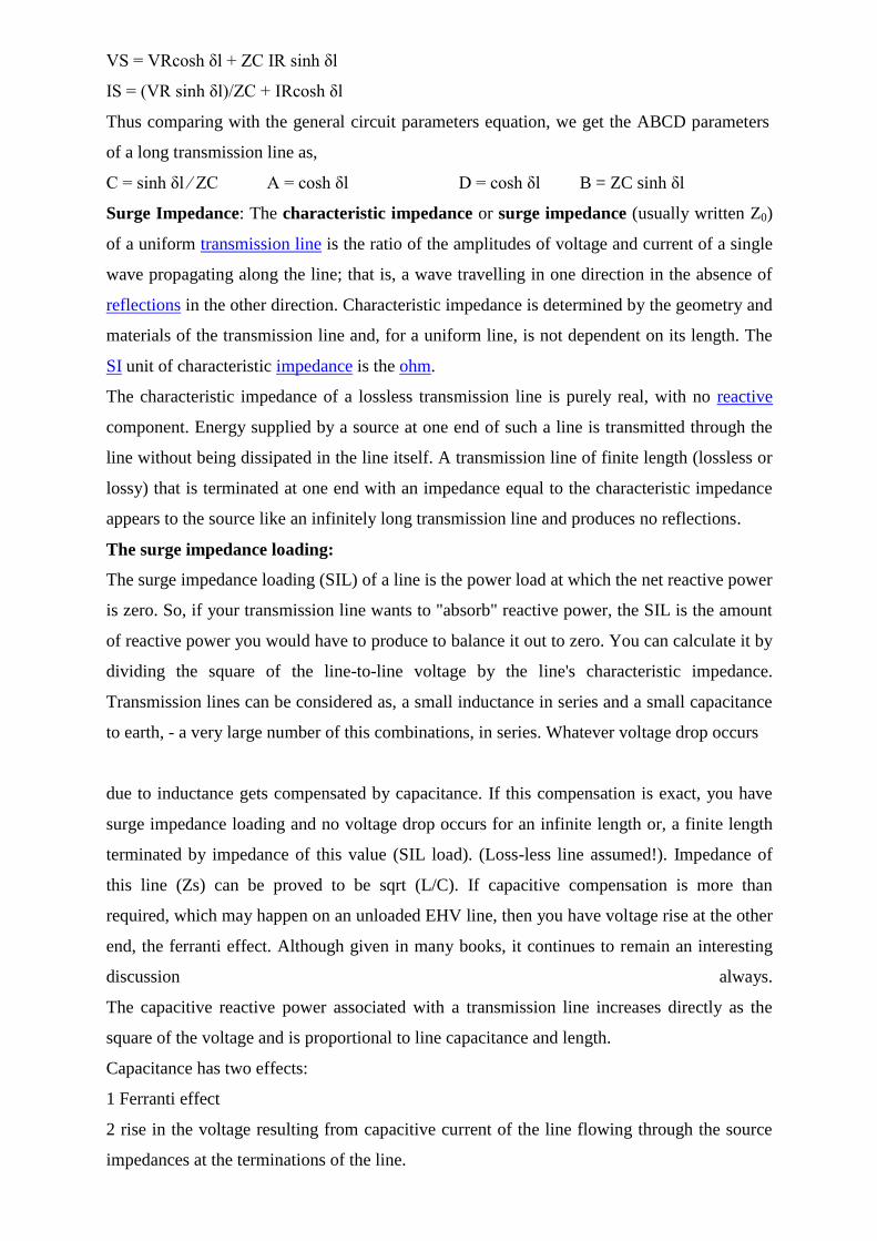
Thus comparing with the general circuit parameters equation, we get the ABCD parameters

of a long transmission line as,

C = sinh δl ⁄ ZC A = cosh δl D = cosh δl B = ZC sinh δl

Surge Impedance: The characteristic impedance or surge impedance (usually written Z0)

of a uniform transmission line is the ratio of the amplitudes of voltage and current of a single

wave propagating along the line; that is, a wave travelling in one direction in the absence of

reflections in the other direction. Characteristic impedance is determined by the geometry and

materials of the transmission line and, for a uniform line, is not dependent on its length. The

SI unit of characteristic impedance is the ohm.

The characteristic impedance of a lossless transmission line is purely real, with no reactive

component. Energy supplied by a source at one end of such a line is transmitted through the

line without being dissipated in the line itself. A transmission line of finite length (lossless or

lossy) that is terminated at one end with an impedance equal to the characteristic impedance

appears to the source like an infinitely long transmission line and produces no reflections.

The surge impedance loading:

The surge impedance loading (SIL) of a line is the power load at which the net reactive power

is zero. So, if your transmission line wants to "absorb" reactive power, the SIL is the amount

of reactive power you would have to produce to balance it out to zero. You can calculate it by

dividing the square of the line-to-line voltage by the line's characteristic impedance.

Transmission lines can be considered as, a small inductance in series and a small capacitance

to earth, - a very large number of this combinations, in series. Whatever voltage drop occurs

due to inductance gets compensated by capacitance. If this compensation is exact, you have

surge impedance loading and no voltage drop occurs for an infinite length or, a finite length

terminated by impedance of this value (SIL load). (Loss-less line assumed!). Impedance of

this line (Zs) can be proved to be sqrt (L/C). If capacitive compensation is more than

required, which may happen on an unloaded EHV line, then you have voltage rise at the other

end, the ferranti effect. Although given in many books, it continues to remain an interesting

discussion always.

The capacitive reactive power associated with a transmission line increases directly as the

square of the voltage and is proportional to line capacitance and length.

Capacitance has two effects:

1 Ferranti effect

2 rise in the voltage resulting from capacitive current of the line flowing through the source

impedances at the terminations of the line.

SIL is Surge Impedance Loading and is calculated as (KV x KV) / Zs their units are

megawatts.

Where Zs is the surge impedance....be aware...one thing is the surge impedance and other

very different is the surge impedance loading.

Wavelength:

Wavelength is the distance between identical points in the adjacent cycles of a waveform

signal propagated in space or along a wire, as shown in the illustration. In wireless systems,

this length is usually specified in meters, centimeters, or millimeters. Inthe case of infrared,

visible light, ultraviolet, and gamma radiation, the wavelength ismore often specified in

nanometers (units of 10-9

meter) or Angstrom units(units of 10-10

meter).

Wavelength is inversely related to frequency. The higher the frequency of the signal, the

shorter the wavelength. Iff is the frequency of the signal as measured in megahertz, and w

isthe wavelength as measuredin meters, then

w = 300/f and conversely

f = 300/w

Wavelength is sometimes represented by the Greek letter lambda.

Velocity of Propagation:

Velocity of propagation is a measure of how fast a signal travels over time, or the speed of

the transmitted signal as compared to the speed of light.

In computer technology, the velocity of propagation of an electrical or electromagnetic signal

is the speed of transmission through a physical medium such as a coaxial cable or optical

fiber.

There is also a direct relation between velocity of propagation and wavelength. Velocity of

propagation is often stated either as a percentage of the speed of light or as time-to distance.

FERRANTI EFFECT

In general practice we know, that for all electrical systems current flows from the region of

higher potential to the region of lower potential, to compensate for the potential difference

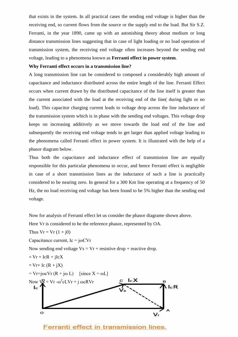
that exists in the system. In all practical cases the sending end voltage is higher than the

receiving end, so current flows from the source or the supply end to the load. But Sir S.Z.

Ferranti, in the year 1890, came up with an astonishing theory about medium or long

distance transmission lines suggesting that in case of light loading or no load operation of

transmission system, the receiving end voltage often increases beyond the sending end

voltage, leading to a phenomena known as Ferranti effect in power system.

Why Ferranti effect occurs in a transmission line?

A long transmission line can be considered to composed a considerably high amount of

capacitance and inductance distributed across the entire length of the line. Ferranti Effect

occurs when current drawn by the distributed capacitance of the line itself is greater than

the current associated with the load at the receiving end of the line( during light or no

load). This capacitor charging current leads to voltage drop across the line inductance of

the transmission system which is in phase with the sending end voltages. This voltage drop

keeps on increasing additively as we move towards the load end of the line and

subsequently the receiving end voltage tends to get larger than applied voltage leading to

the phenomena called Ferranti effect in power system. It is illustrated with the help of a

phasor diagram below.

Thus both the capacitance and inductance effect of transmission line are equally

responsible for this particular phenomena to occur, and hence Ferranti effect is negligible

in case of a short transmission lines as the inductance of such a line is practically

considered to be nearing zero. In general for a 300 Km line operating at a frequency of 50

Hz, the no load receiving end voltage has been found to be 5% higher than the sending end

voltage.

Now for analysis of Ferranti effect let us consider the phasor diagrame shown above.

Here Vr is considered to be the reference phasor, represented by OA.

Thus Vr = Vr (1 + j0)

Capacitance current, Ic = jωCVr

Now sending end voltage Vs = Vr + resistive drop + reactive drop.

= Vr + IcR + jIcX

= Vr+ Ic (R + jX)

= Vr+jωcVr (R + jω L) [since X = ωL]

Now Vs = Vr -ω2cLVr + j ωcRVr

This is represented by the phasor OC.

Now in case of a long transmission line, it has been practically observed that the line

resistance is negligibly small compared to the line reactance, hence we can assume the

length of the phasor Ic R = 0, we can consider the rise in the voltage is only due to OA –

OC = reactive drop in the line.

Now if we consider c0 and L0 are the values of capacitance and inductance per km of

the transmission line, where l is the length of the line.

Thus capacitive reactance Xc = 1/(ω l c0)

Since, in case of a long transmission line the capacitance is distributed throughout its

length, the average current flowing is,

Ic = 1/2 Vr/Xc =

1/2 Vrω l c0

Now the inductive reactance of the line = ω L0 l

Thus the rise in voltage due to line inductance is given by,

IcX = 1/2Vrω l c0 X ω L0 l

Voltage rise = 1/2 Vrω

2 l

2 c0L0

From the above equation it is absolutely evident, that the rise in voltage at the receiving

end is directly proportional to the square of the line length, and hence in case of a long

transmission line it keeps increasing with length and even goes beyond the applied

sending end voltage at times, leading to the phenomena called Ferranti effect in power

system.

UNIT – III

MECHANICAL DESIGN OF TRANSMISSION LINES

Insulators

The overhead line conductors should be supported on the poles or towers in such a way that

currents from conductors do not flow to earth through supports i.e., line conductors must be

properly insulated from supports. This is achieved by securing line conductors to supports

with the help of insulators. The insulators provide necessary insulation between line

conductors and supports and thus prevent any leakage current from conductors to earth. In

general, the insulators should have the following desirable properties :

(i) High mechanical strength in order to withstand conductor load, wind load etc.

(ii) High electrical resistance of insulator material in order to avoid leakage currents to earth.

(iii) High relative permittivity of insulator material in order that dielectric strength is high.

(iv) The insulator material should be non-porous, free from impurities and cracks otherwise

the permittivity will be lowered.

(v) High ratio of puncture strength to flashover.

The most commonly used material for insulators of overhead line is porcelain but glass,

steatite and special composition materials are also used to a limited extent. Porcelain is

produced by firing at a high temperature a mixture of kaolin, feldspar and quartz. It is

stronger mechanically than glass, gives less trouble from leakage and is less effected by

changes of temperature.

Types of Insulators

The successful operation of an overhead line depends to a considerable extent upon the

proper selection of insulators. There are several types of insulators but the most commonly

used are pin type, suspension type, strain insulator and shackle insulator.

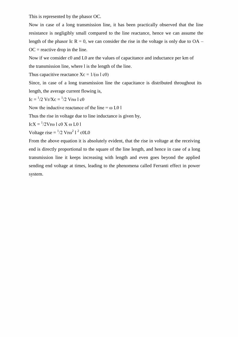
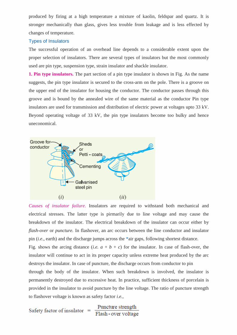
1. Pin type insulators. The part section of a pin type insulator is shown in Fig. As the name

suggests, the pin type insulator is secured to the cross-arm on the pole. There is a groove on

the upper end of the insulator for housing the conductor. The conductor passes through this

groove and is bound by the annealed wire of the same material as the conductor Pin type

insulators are used for transmission and distribution of electric power at voltages upto 33 kV.

Beyond operating voltage of 33 kV, the pin type insulators become too bulky and hence

uneconomical.

Causes of insulator failure. Insulators are required to withstand both mechanical and

electrical stresses. The latter type is pirmarily due to line voltage and may cause the

breakdown of the insulator. The electrical breakdown of the insulator can occur either by

flash-over or puncture. In flashover, an arc occurs between the line conductor and insulator

pin (i.e., earth) and the discharge jumps across the *air gaps, following shortest distance.

Fig. shows the arcing distance (i.e. a + b + c) for the insulator. In case of flash-over, the

insulator will continue to act in its proper capacity unless extreme heat produced by the arc

destroys the insulator. In case of puncture, the discharge occurs from conductor to pin

through the body of the insulator. When such breakdown is involved, the insulator is

permanently destroyed due to excessive heat. In practice, sufficient thickness of porcelain is

provided in the insulator to avoid puncture by the line voltage. The ratio of puncture strength

to flashover voltage is known as safety factor i.e.,

It is desirable that the value of safety factor is high so that flash-over takes place before the

insulator gets punctured. For pin type insulators, the value of safety factor is about 10.

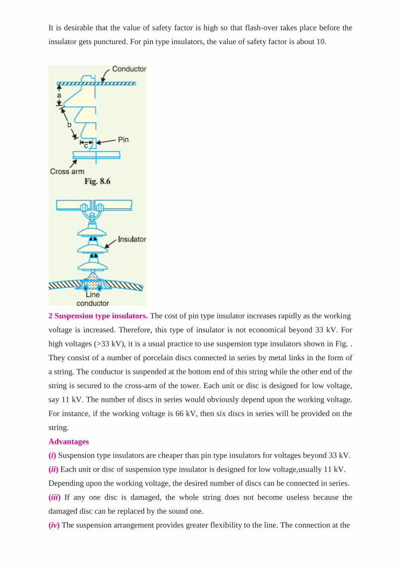
2 Suspension type insulators. The cost of pin type insulator increases rapidly as the working

voltage is increased. Therefore, this type of insulator is not economical beyond 33 kV. For

high voltages (>33 kV), it is a usual practice to use suspension type insulators shown in Fig. .

They consist of a number of porcelain discs connected in series by metal links in the form of

a string. The conductor is suspended at the bottom end of this string while the other end of the

string is secured to the cross-arm of the tower. Each unit or disc is designed for low voltage,

say 11 kV. The number of discs in series would obviously depend upon the working voltage.

For instance, if the working voltage is 66 kV, then six discs in series will be provided on the

string.

Advantages

(i) Suspension type insulators are cheaper than pin type insulators for voltages beyond 33 kV.

(ii) Each unit or disc of suspension type insulator is designed for low voltage,usually 11 kV.

Depending upon the working voltage, the desired number of discs can be connected in series.

(iii) If any one disc is damaged, the whole string does not become useless because the

damaged disc can be replaced by the sound one.

(iv) The suspension arrangement provides greater flexibility to the line. The connection at the

cross arm is such that insulator string is free to swing in any direction and can take up the

position where mechanical stresses are minimum.

(v) In case of increased demand on the transmission line, it is found more satisfactory to

supply the greater demand by raising the line voltage than to provide another set of

conductors. The additional insulation required for the raised voltage can be easily obtained in

the suspension

arrangement by adding the desired number of discs.

(vi) The suspension type insulators are generally used with steel towers. As the conductors

run below the earthed cross-arm of the tower, therefore, this arrangement provides partial

protection from lightning.

3. Strain insulators. When there is a dead end of the line or there is corner or sharp curve,

the line is subjected to greater tension. In order to relieve the line of excessive tension, strain

insulators are used. For low voltage lines (< 11 kV), shackle insulators are used as strain

insulators. However,

for high voltage transmission lines, strain insulator consists of an assembly of suspension

insulators as shown in Fig. The discs of strain insulators are used in the vertical plane. When

the tension in lines is exceedingly high, as at long river spans, two or more strings are used in

parallel.

4. Shackle insulators. In early days, the shackle insulators were used as strain insulators. But

now a days, they are frequently used for low voltage distribution lines. Such insulators can be

used either in a horizontal position or in a vertical position. They can be directly fixed to the

pole with a bolt or to the cross arm. Fig. shows a shackle insulator fixed to the pole. The

conductor in the groove is fixed with a soft binding wire.

Potential Distribution over Suspension Insulator String

A string of suspension insulators consists of a number of porcelain discs connected in series

through metallic links. Fig. (i) shows 3-disc string of suspension insulators. The porcelain

portion of each disc is inbetween two metal links. Therefore, each disc forms a

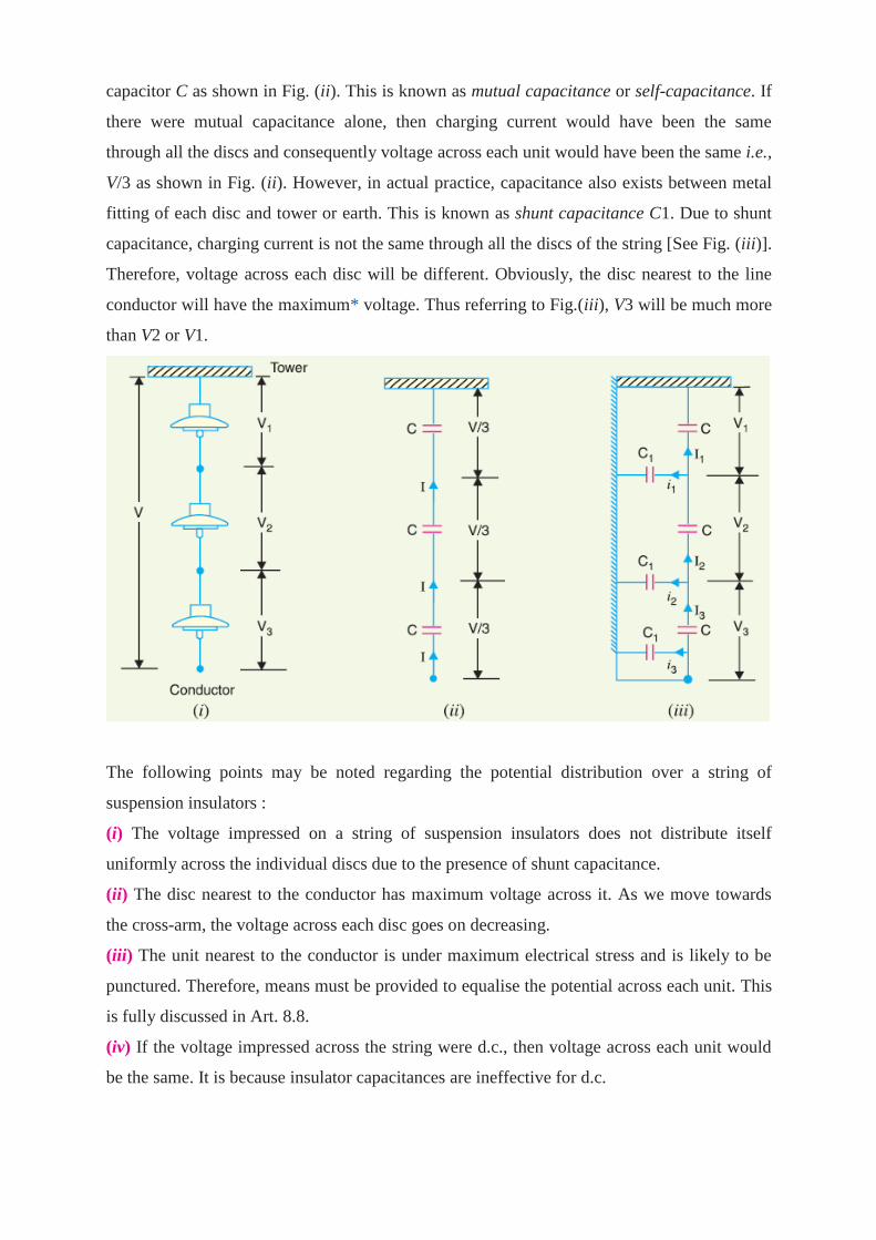
capacitor C as shown in Fig. (ii). This is known as mutual capacitance or self-capacitance. If

there were mutual capacitance alone, then charging current would have been the same

through all the discs and consequently voltage across each unit would have been the same i.e.,

V/3 as shown in Fig. (ii). However, in actual practice, capacitance also exists between metal

fitting of each disc and tower or earth. This is known as shunt capacitance C1. Due to shunt

capacitance, charging current is not the same through all the discs of the string [See Fig. (iii)].

Therefore, voltage across each disc will be different. Obviously, the disc nearest to the line

conductor will have the maximum* voltage. Thus referring to Fig.(iii), V3 will be much more

than V2 or V1.

The following points may be noted regarding the potential distribution over a string of

suspension insulators :

(i) The voltage impressed on a string of suspension insulators does not distribute itself

uniformly across the individual discs due to the presence of shunt capacitance.

(ii) The disc nearest to the conductor has maximum voltage across it. As we move towards

the cross-arm, the voltage across each disc goes on decreasing.

(iii) The unit nearest to the conductor is under maximum electrical stress and is likely to be

punctured. Therefore, means must be provided to equalise the potential across each unit. This

is fully discussed in Art. 8.8.

(iv) If the voltage impressed across the string were d.c., then voltage across each unit would

be the same. It is because insulator capacitances are ineffective for d.c.

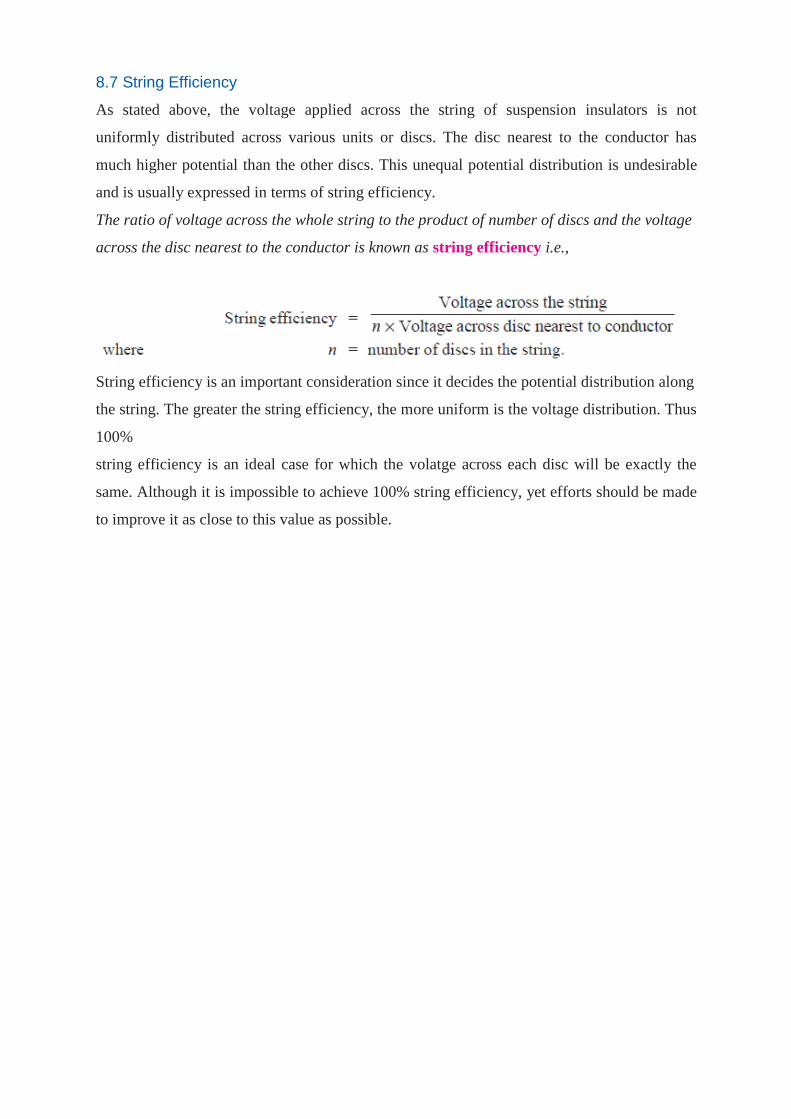
8.7 String Efficiency

As stated above, the voltage applied across the string of suspension insulators is not

uniformly distributed across various units or discs. The disc nearest to the conductor has

much higher potential than the other discs. This unequal potential distribution is undesirable

and is usually expressed in terms of string efficiency.

The ratio of voltage across the whole string to the product of number of discs and the voltage

across the disc nearest to the conductor is known as string efficiency i.e.,

String efficiency is an important consideration since it decides the potential distribution along

the string. The greater the string efficiency, the more uniform is the voltage distribution. Thus

100%

string efficiency is an ideal case for which the volatge across each disc will be exactly the

same. Although it is impossible to achieve 100% string efficiency, yet efforts should be made

to improve it as close to this value as possible.

The following points may be noted from the above mathematical analysis :

(i) If K = 0·2 (Say), then from exp. (iv), we get, V2 = 1·2 V1 and V3 = 1·64 V1. This clearly

shows that disc nearest to the conductor has maximum voltage across it; the voltage across

other discs decreasing progressively as the cross-arm in approached.

(ii) The greater the value of K (= C1/C), the more non-uniform is the potential across the

discs and lesser is the string efficiency.

(iii) The inequality in voltage distribution increases with the increase of number of discs in

the string. Therefore, shorter string has more efficiency than the larger one.

Methods of Improving String Efficiency

It has been seen above that potential distribution in a string of suspension insulators is not

uniform. The maximum voltage appears across the insulator nearest to the line conductor and

decreases progressively as the crossarm is approached. If the insulation of the highest stressed

insulator (i.e. nearest to conductor) breaks down or flash over takes place, the breakdown of

other units will take place in succession. This necessitates to equalise the potential across the

various units of the string i.e. to improve the string efficiency. The various methods for this

purpose are :

(i) By using longer cross-arms. The value of string efficiency

depends upon the value of K i.e., ratio of shunt capacitance to mutual capacitance. The lesser

the value of K, the greater is the string efficiency and more uniform is the voltage

distribution. The value of K can be decreased by reducing the shunt capacitance. In order to

reduce shunt capacitance, the distance of conductor from tower must be increased i.e., longer

cross-arms should be used. However, limitations of cost and strength of tower do not allow

the use of very long cross-arms. In practice, K = 0·1 is the limit that can be achieved by this

method.

(ii) By grading the insulators. In this method, insulators of different dimensions are so chosen

that each has a different capacitance. The insulators are capacitance graded i.e. they are

assembled in the string in such a way that the top unit has the minimum capacitance,

increasing progressively as the bottom unit (i.e., nearest to conductor) is reached. Since

voltage is inversely proportional to capacitance, this method tends to equalise the potential

distribution across the units in the string. This method has the disadvantage that a large

number of different-sized insulators are required. However, good results can be obtained by

using standard insulators for most of the string and larger units for that near to the line

conductor.

(iii) By using a guard ring. The potential across each unit in a string can be equalised by

using a guard ring which is a metal ring electrically connected to the conductor and

surrounding the bottom insulator as shown in the Fig. The guard ring introduces capacitance

between metal fittings and the line conductor. The guard ring is contoured in such a way that

shunt capacitance currents i1, i2 etc. are equal to metal fitting line capacitance currents i1,

i2 etc. The result is that same charging current I flows through each unit of string.

Consequently, there will be uniform potential distribution across the units.

Important Points

While solving problems relating to string efficiency, the following points must be kept in

mind:

(i) The maximum voltage appears across the disc nearest to the conductror (i.e., line

conductor).

(ii) The voltage across the string is equal to phase voltage i.e., Voltage across string =

Voltage between line and earth = Phase Voltage

(iii) Line Voltage = 3 √Voltage across string

CORONA

Electric-power transmission practically deals in the bulk transfer of electrical energy,

from generating stations situated many kilometers away from the main consumption

centers or the cities. For this reason the long distance transmission cables are of utmost

necessity for effective power transfer, which in-evidently results in huge losses across the

system. Minimizing those has been a major challenge for power engineers of late and to

do that one should have a clear understanding of the type and nature of losses. One of

them being the corona effect in power system, which has a predominant role in reducing

the efficiency of EHV(extra high voltage lines) which we are going to concentrate on, in

this article.

What is corona effect in power system and why it occurs?

For corona effect to occur effectively, two factors here are of prime importance as

mentioned below:-

1) Alternating potential difference must be supplied across the line.

2) The spacing of the conductors, must be large enough compared to the line diameter.

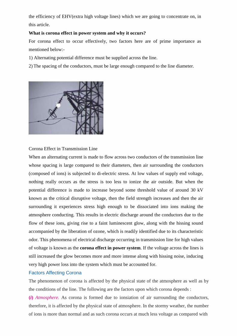
Corona Effect in Transmission Line

When an alternating current is made to flow across two conductors of the transmission line

whose spacing is large compared to their diameters, then air surrounding the conductors

(composed of ions) is subjected to di-electric stress. At low values of supply end voltage,

nothing really occurs as the stress is too less to ionize the air outside. But when the

potential difference is made to increase beyond some threshold value of around 30 kV

known as the critical disruptive voltage, then the field strength increases and then the air

surrounding it experiences stress high enough to be dissociated into ions making the

atmosphere conducting. This results in electric discharge around the conductors due to the

flow of these ions, giving rise to a faint luminescent glow, along with the hissing sound

accompanied by the liberation of ozone, which is readily identified due to its characteristic

odor. This phenomena of electrical discharge occurring in transmission line for high values

of voltage is known as the corona effect in power system. If the voltage across the lines is

still increased the glow becomes more and more intense along with hissing noise, inducing

very high power loss into the system which must be accounted for.

Factors Affecting Corona

The phenomenon of corona is affected by the physical state of the atmosphere as well as by

the conditions of the line. The following are the factors upon which corona depends :

(i) Atmosphere. As corona is formed due to ionsiation of air surrounding the conductors,

therefore, it is affected by the physical state of atmosphere. In the stormy weather, the number

of ions is more than normal and as such corona occurs at much less voltage as compared with

fair weather.

(ii) Conductor size. The corona effect depends upon the shape and conditions of the

conductors. The rough and irregular surface will give rise to more corona because unevenness

ofthe surface decreases the value of breakdown voltage. Thus a stranded conductor has

irregular surface and hence gives rise to more corona that a solid conductor.

(iii) Spacing between conductors. If the spacing between the conductors is made very large as

compared to their diameters, there may not be any corona effect. It is because larger distance

between conductors reduces the electro-static stresses at the conductor surface, thus avoiding

corona formation.

(iv) Line voltage. The line voltage greatly affects corona. If it is low, there is no change in the

condition of air surrounding the conductors and hence no corona is formed. However, if the

line voltage has such a value that electrostatic stresses developed at the conductor surface

make the air around the conductor conducting, then corona is formed.

8.12 Important Terms

The phenomenon of corona plays an important role in the design of an overhead transmission

line. Therefore, it is profitable to consider the following terms much used in the analysis of

corona effects:

(i) Critical disruptive voltage. It is the minimum phase-neutral voltage at which corona

occurs. Consider two conductors of radii r cm and spaced d cm apart. If V is the phase-neutral

potential, then potential gradient at the conductor surface is given by:

In order that corona is formed, the value of g must be made equal to the breakdown strength

of air. The breakdown strength of air at 76 cm pressure and temperature of 25ºC is 30 kV/cm

(max) or 21·2 kV/cm (r.m.s.) and is denoted by go. If Vc is the phase-neutral potential

required under these conditions, then,

The above expression for disruptive voltage is under standard conditions i.e., at 76 cm of Hg

and 25ºC. However, if these conditions vary, the air density also changes, thus altering the

value of go. The value of go is directly proportional to air density. Thus the breakdown

strength of air at a barometric pressure of b cm of mercury and temperature of tºC becomes

go where

Advantages and Disadvantages of Corona

Corona has many advantages and disadvantages. In the correct design of a high voltage

overhead line, a balance should be struck between the advantages and disadvantages.

Advantages

(i) Due to corona formation, the air surrounding the conductor becomes conducting and hence

virtual diameter of the conductor is increased. The increased diameter reduces the

electrostatic stresses between the conductors.

(ii) Corona reduces the effects of transients produced by surges.

Disadvantages

(i) Corona is accompanied by a loss of energy. This affects the transmission efficiency of the

line.

(ii) Ozone is produced by corona and may cause corrosion of the conductor due to chemical

action.

(iii) The current drawn by the line due to corona is non-sinusoidal and hence non-sinusoidal

voltage drop occurs in the line. This may cause inductive interference with neighbouring

communication lines.

8.14 Methods of Reducing Corona Effect

It has been seen that intense corona effects are observed at a working voltage of 33 kV or

above. Therefore, careful design should be made to avoid corona on the sub-stations or bus-

bars rated for 33 kV and higher voltages otherwise highly ionised air may cause flash-over in

the insulators or between the phases, causing considerable damage to the equipment. The

corona effects can be reduced by the following methods :

(i) By increasing conductor size. By increasing conductor size, the voltage at which corona

occurs is raised and hence corona effects are considerably reduced. This is one of the reasons

that ACSR conductors which have a larger cross-sectional area are used in transmission lines.

(ii) By increasing conductor spacing. By increasing the spacing between conductors, the

voltage at which corona occurs is raised and hence corona effects can be eliminated.

However, spacing cannot be increased too much otherwise the cost of supporting structure

(e.g., bigger cross arms and supports) may increase to a considerable extent.

Sag in Overhead Lines:

While erecting an overhead line, it is very important that conductors are under safe tension. If

the conductors are too much stretched between supports in a bid to save conductor material,

the stress in the conductor may reach unsafe value and in certain cases the conductor may

break due to excessive tension. In order to permit safe tension in the conductors, they are not

fully stretched but are allowed to have a dip or sag.

The difference in level between points of supports and the lowest point on the conductor is

called sag.

Fig. shows a conductor suspended between two equilevel supports A and B. The conductoris

not fully stretched but is allowed to have a dip. The lowest point on the conductor is O and

the sag is S. The following points may be noted :

(i) When the conductor is suspended between two supports at the same level, it takes the

shape of catenary. However, if the sag is very small compared with the span, then sag-span

curve is like a parabola.

(ii) The tension at any point on the conductor acts tangentially. Thus tension TO at the lowest

point O acts horizontally as shown in Fig.(ii).

(iii) The horizontal component of tension is constant throughout the length of the wire.

(iv) The tension at supports is approximately equal to the horizontal tension acting at any

point on the wire. Thus if T is the tension at the support B, then T = TO.

Conductor sag and tension. This is an important consideration in the mechanical design of

overhead lines. The conductor sag should be kept to a minimum in order to reduce the

conductor material required and to avoid extra pole height for sufficient clearance above

ground level. It is also desirable that tension in the conductor should be low to avoid the

mechanical failure of conductor and to permit the use of less strong supports. However, low

conductor tension and minimum sag are not possible. It is because low sag means a tight wire

and high tension, whereas a low tension means a loose wire and increased sag. Therefore, in

actual practice, a compromise in made between the two.

8.16 Calculation of Sag

In an overhead line, the sag should be so adjusted that tension in the conductors is within safe

limits. The tension is governed by conductor weight, effects of wind, ice loading and

temperature variations. It is a standard practice to keep conductor tension less than 50% of its

ultimate tensile strength i.e., minimum factor of safety in respect of conductor tension should

be 2. We shall now calculate sag and tension of a conductor when (i) supports are at equal

levels and (ii) supports are at unequal levels.

(i) When supports are at equal levels. Consider a conductor between two equilevel supports

A and B with O as the lowest point as shown in Fig. It can be proved that lowest point will be

at the mid-span.

Let

l = Length of span

w = Weight per unit length of conductor

T = Tension in the conductor.

Consider a point P on the conductor. Taking the lowest point O as the origin, let the co-

ordinates of point P be x and y. Assuming that the curvature is so small that curved length is

equal to its horizontal projection (i.e., OP = x), the two forces acting on the portion OP of the

conductor are :

(a) The weight wx of conductor acting at a distance x/2 from o

(b) The tension T acting at O.

Equating the moments of above two forces about point O, we get,

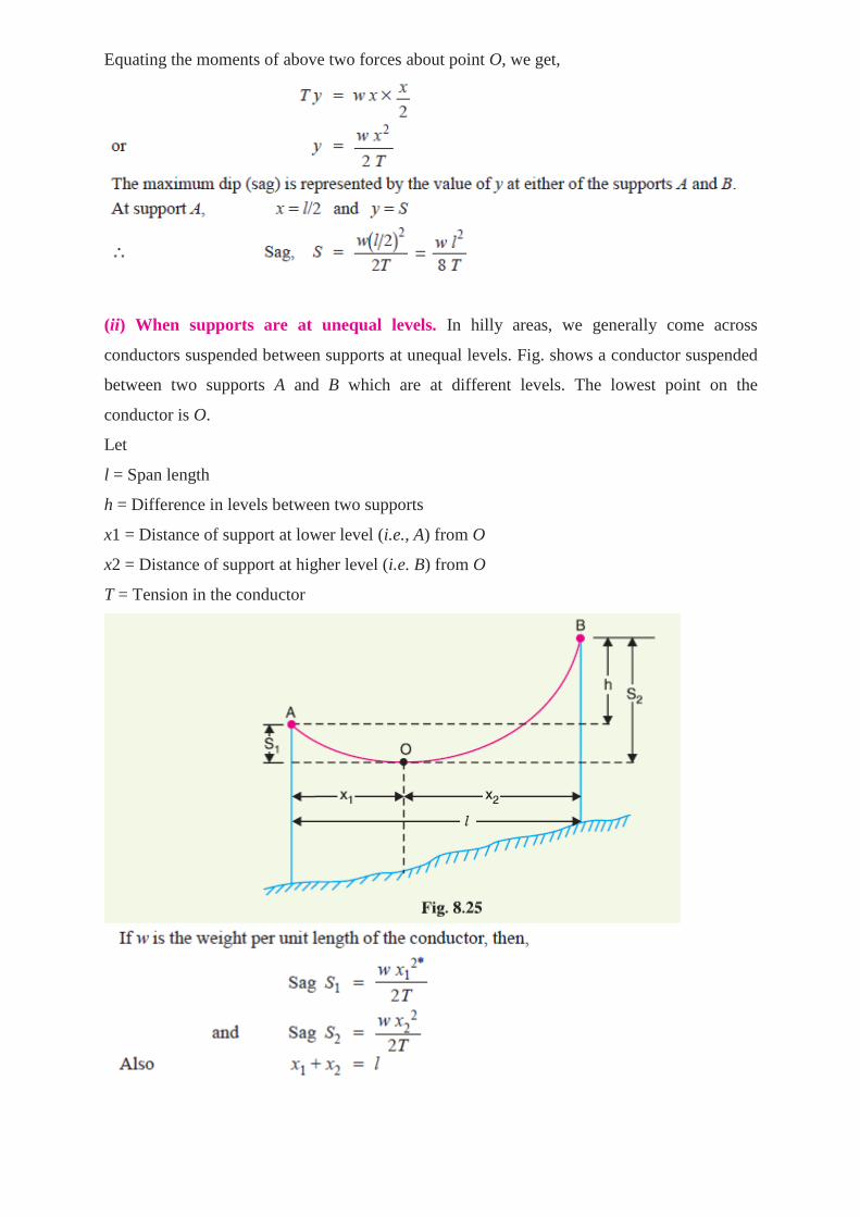
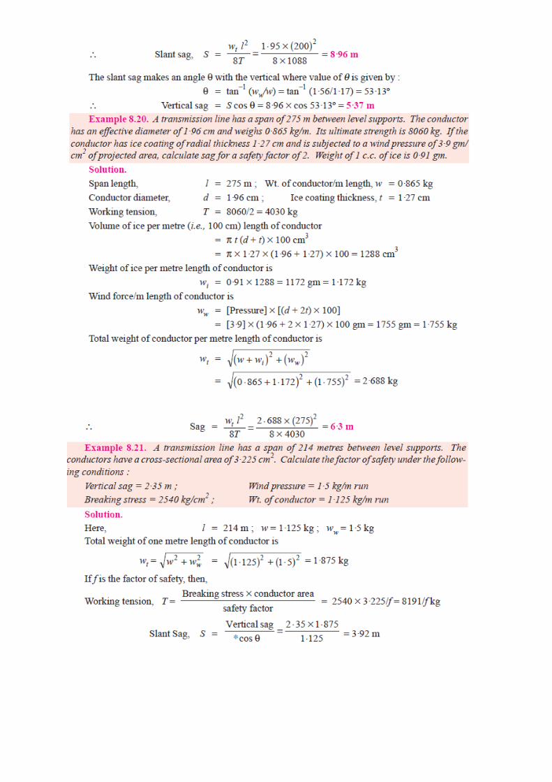
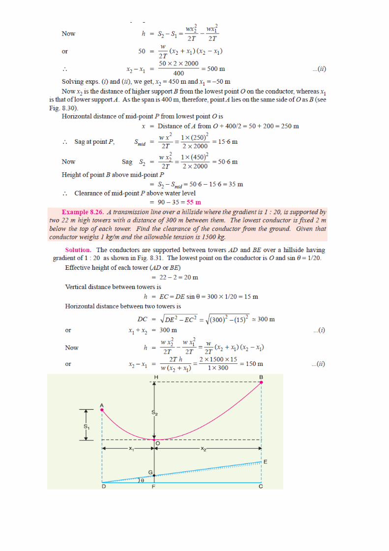
(ii) When supports are at unequal levels. In hilly areas, we generally come across

conductors suspended between supports at unequal levels. Fig. shows a conductor suspended

between two supports A and B which are at different levels. The lowest point on the

conductor is O.

Let

l = Span length

h = Difference in levels between two supports

x1 = Distance of support at lower level (i.e., A) from O

x2 = Distance of support at higher level (i.e. B) from O

T = Tension in the conductor

Having found x1 and x2, values of S1 and S2 can be easily calculated.

Effect of wind and ice loading. The above formulae for sag are true only in still air and at

normal temperature when the conductor is acted by its weight only. However, in actual

practice, a conductor may have ice coating and simultaneously subjected to wind pressure.

The weight of ice acts vertically downwards i.e., in the same direction as the weight of

conductor. The force due to the wind is assumed to act horizontally i.e., at right angle to the

projected surface of the conductor. Hence, the total force on the conductor is the vector sum

of horizontal and vertical forces as shown in Fig. (iii).

UNIT – V

CABLES

Underground Cables

An underground cable essentially consists of one or more conductors covered with suitable

insulation and surrounded by a protecting cover. Although several types of cables are available, the

type of cable to be used will depend upon the Working voltage and service requirements. In general,

a cable must fulfil the following necessary requirements :

(i) The conductor used in cables should be tinned stranded copper or aluminium of high

conductivity. Stranding is done so that conductor may become flexible and carry more current.

(ii) The conductor size should be such that the cable carries the desired load current without

overheating and causes voltage drop within permissible limits.

(iii) The cable must have proper thickness of insulation in order to give high degree of safety and

reliability at the voltage for which it is designed.

(iv) The cable must be provided with suitable mechanical protection so that it may withstand the

rough use in laying it.

(v) The materials used in the manufacture of cables should be such that there is complete chemical

and physical stability throughout.

11.2 Construction of Cables

Fig. shows the general construction of a 3-conductor cable. The various parts are : (i) Cores or

Conductors. A cable may have one or more than one core (conductor) depending upon the type of

service for which it is intended. For instance, the 3-conductor cable shown in Fig. is used for 3-

phase service. The conductors are made of tinned copper or aluminium and are usually stranded in

order to provide flexibility to the cable.

(ii) Insulatian. Each core or conductor is provided with a suitable thickness of insulation, the

thickness of layer depending upon the voltage to be withstood by the cable. The commonly used

materials for insulation are impregnated paper, varnished cambric or rubber mineral compound.

(iii) Metallic sheath. In order to protect the cable from moisture, gases or other damaging liquids

(acids or alkalies) in the soil and atmosphere, a metallic sheath of lead or aluminium is provided

over the insulation as shown in Fig.

(iv) Bedding. Over the metallic sheath is applied a layer of bedding which consists of a fibrous

material like jute or hessian tape. The purpose of bedding is to protect the metallic sheath against

corrosion and from

mechanical injury due to armouring.

(v) Armouring. Over the bedding, armouring is provided which consists of one or two layers of

galvanised steel wire or steel tape. Its purpose is to protect the cable from mechanical injury while

laying it and during the course of handling. Armouring may not be done in the case of

some cables.

(vi) Serving. In order to protect armouring from atmospheric conditions, a layer of fibrous material

(like jute) similar to bedding is provided over the armouring. This is known as serving. It may not be

out of place to mention here that bedding, armouring and serving are only applied to the cables for

the protection of conductor insulation and to protect the metallic sheath from mechanical injury.

11.3 Insulating Materials for Cables

The satisfactory operation of a cable depends to a great extent upon the characteristics of insulation

used. Therefore, the proper choice of insulating material for cables is of considerable importance. In

general, the insulating materials used in cables should have the following properties :

(i) High insulation resistance to avoid leakage current.

(ii) High dielectric strength to avoid electrical breakdown of the cable.

(iii) High mechanical strength to withstand the mechanical handling of cables.

(iv) Non-hygroscopic i.e., it should not absorb moisture from air or soil. The moisture tends to

decrease the insulation resistance and hastens the breakdown of the cable. In case the insulating

material is hygroscopic, it must be enclosed in a waterproof covering like lead sheath.

(v) Non-inflammable.

(vi) Low cost so as to make the underground system a viable proposition.

(vii) Unaffected by acids and alkalies to avoid any chemical action. No one insulating material

possesses all the above mentioned properties. Therefore, the type of insulating material to be used

depends upon the purpose for which the cable is required and the quality of insulation to be aimed

at. The principal insulating materials used in cables are rubber, vulcanised India rubber, impregnated

paper, varnished cambric and polyvinyl chloride.

1. Rubber. Rubber may be obtained from milky sap of tropical trees or it may be produced from oil

products. It has relative permittivity varying between 2 and 3, dielectric strength is about 30 kV/mm

and resistivity of insulation is 1017cm. Although pure rubber has reasonably high insulating

properties, it suffers form some major drawbacks viz., readily absorbs moisture, maximum safe

temperature is low (about 38ºC), soft and liable to damage due to rough handling and ages when

exposed to light. Therefore, pure rubber cannot be used as an insulating material.

2. Vulcanised India Rubber (V.I.R.). It is prepared by mixing pure rubber with mineral matter such

as zine oxide, red lead etc., and 3 to 5% of sulphur. The compound so formed is rolled into thin

sheets and cut into strips. The rubber compound is then applied to the conductor and is heated to a

temperature of about 150ºC. The whole process is called vulcanisation and the product obtained is

known as vulcanised India rubber. Vulcanised India rubber has greater mechanical strength,

durability and wear resistant property than pure rubber. Its main drawback is that sulphur reacts very

quickly with copper and for this reason, cables using VIR insulation have tinned copper conductor.

The VIR insulation is generally used for low and moderate voltage cables.

3. Impregnated paper. It consists of chemically pulped paper made from wood chippings and

impregnated with some compound such as paraffinic or napthenic material. This type of insulation

has almost superseded the rubber insulation. It is because it has the advantages of low cost, low

capacitance, high dielectric strength and high insulation resistance. The only disadvantage is that

paper is hygroscopic and even if it is impregnated with suitable compound, it absorbs moisture and

thus lowers the insulation resistance of the cable. For this reason, paper insulated cables are always

provided with some protective covering and are never left unsealed. If it is required to be left unused

on the site during laying, its ends are temporarily covered with wax or tar. Since the paper insulated

cables have the tendency to absorb moisture, they are used where the cable route has a *few joints.

For instance, they can be profitably used for distribution at low voltages in congested areas where

the joints are generally provided only at the terminal apparatus. However, for smaller installations,

where the lenghts are small and joints are required at a number of places, VIR cables will be cheaper

and durable than paper insulated cables.

4. Varnished cambric. It is a cotton cloth impregnated and coated with varnish. This type of

insulation is also known as empire tape. The cambric is lapped on to the conductor in the form of a

tape and its surfaces are coated with petroleum jelly compound to allow for the sliding of one turn

over another as the cable is bent. As the varnished cambric is hygroscopic, therefore, such cables are

always provided with metallic sheath. Its dielectric strength is about 4 kV/mm and permittivity is 2.5

to 3.8.

5. Polyvinyl chloride (PVC). This insulating material is a synthetic compound. It is obtained from

the polymerisation of acetylene and is in the form of white powder. For obtaining this material as a

cable insulation, it is compounded with certain materials known as plasticizers which are liquids

with high boiling point. The plasticizer forms a gell and renders the material plastic over the desired

range of temperature. Polyvinyl chloride has high insulation resistance, good dielectric strength and

mechanical toughness over a wide range of temperatures. It is inert to oxygen and almost inert to

many alkalies and acids. Therefore, this type of insulation is preferred over VIR in extreme

enviormental conditions such as in cement factory or chemical factory. As the mechanical properties

(i.e., elasticity etc.) of PVC are not so good as those of rubber, therefore, PVC insulated cables are

generally used for low and medium domestic lights and power installations.

11.4 Classification of Cables

Cables for underground service may be classified in two ways according to (i) the type of insulating

material used in their manufacture (ii) the voltage for which they are manufactured. However, the

latter method of classification is generally preferred, according to which cables can be divided into

the following groups :

(i) Low-tension (L.T.) cables — upto 1000 V

(ii) High-tension (H.T.) cables — upto 11,000 V

(iii) Super-tension (S.T.) cables — from 22 kV to 33 kV

(iv) Extra high-tension (E.H.T.) cables — from 33 kV to 66 kV

(v) Extra super voltage cables — beyond 132 Kv

A cable may have one or more than one core depending upon the type of service for which it is

intended. It may be (i) single-core (ii) two-core (iii) three-core (iv) four-core etc. For a 3-phase

service, either 3-single-core cables or three-core cable can be used depending upon the operating

voltage and load demand. Fig. shows the constructional details of a single-core low tension cable.

The cable has ordinary construction because the stresses developed in the cable for low voltages

(upto 6600 V) are generally small. It consists of one circular core of tinned stranded copper (or

aluminium) insulated by layers of impregnated paper. The insulation is surrounded by a lead sheath

which prevents the entry of moisture into the inner parts. In order to protect the lead sheath from

corrosion, an overall serving of compounded fibrous material (jute etc.) is provided. Single-core

cables are not usually armoured in order to avoid excessive sheath losses. The principal advantages

of single-core cables are simple construction and availability of larger copper section.

Cables for 3-Phase Service

In practice, underground cables are generally required to deliver 3-phase power. For the purpose,

either three core cable or *three single core cables may be used. For voltages upto 66 kV, 3-core

cable (i.e., multi-core construction) is preferred due to economic reasons. However, for voltages

beyond 66 kV, 3-core-cables become too large and unwieldy and, therefore, single-core cables are

used. The following types of cables are generally used for 3-phase service :

1. Belted cables — upto 11 kV

2. Screened cables — from 22 kV to 66 kV

3. Pressure cables — beyond 66 kV.

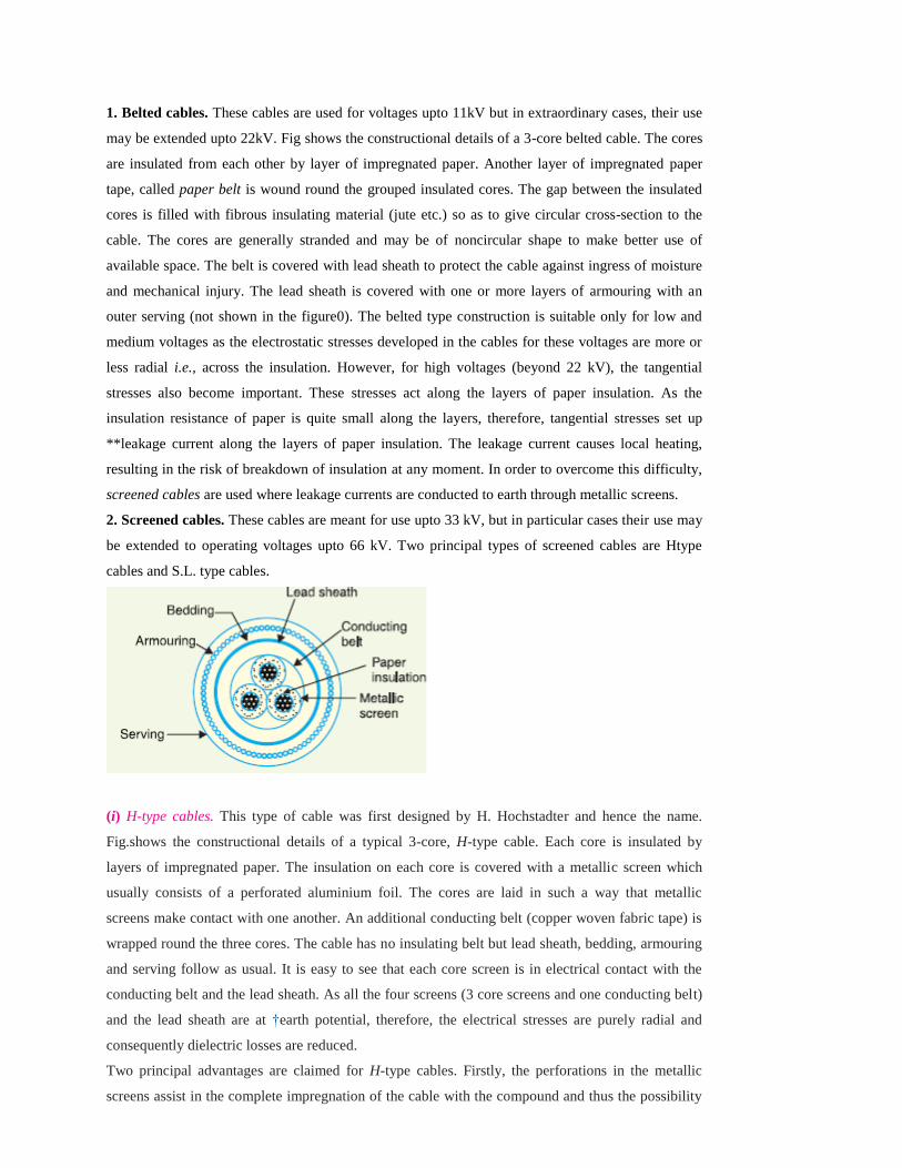
1. Belted cables. These cables are used for voltages upto 11kV but in extraordinary cases, their use

may be extended upto 22kV. Fig shows the constructional details of a 3-core belted cable. The cores

are insulated from each other by layer of impregnated paper. Another layer of impregnated paper

tape, called paper belt is wound round the grouped insulated cores. The gap between the insulated

cores is filled with fibrous insulating material (jute etc.) so as to give circular cross-section to the

cable. The cores are generally stranded and may be of noncircular shape to make better use of

available space. The belt is covered with lead sheath to protect the cable against ingress of moisture

and mechanical injury. The lead sheath is covered with one or more layers of armouring with an

outer serving (not shown in the figure0). The belted type construction is suitable only for low and

medium voltages as the electrostatic stresses developed in the cables for these voltages are more or

less radial i.e., across the insulation. However, for high voltages (beyond 22 kV), the tangential

stresses also become important. These stresses act along the layers of paper insulation. As the

insulation resistance of paper is quite small along the layers, therefore, tangential stresses set up

**leakage current along the layers of paper insulation. The leakage current causes local heating,

resulting in the risk of breakdown of insulation at any moment. In order to overcome this difficulty,

screened cables are used where leakage currents are conducted to earth through metallic screens.

2. Screened cables. These cables are meant for use upto 33 kV, but in particular cases their use may

be extended to operating voltages upto 66 kV. Two principal types of screened cables are Htype

cables and S.L. type cables.

(i) H-type cables. This type of cable was first designed by H. Hochstadter and hence the name.

Fig.shows the constructional details of a typical 3-core, H-type cable. Each core is insulated by

layers of impregnated paper. The insulation on each core is covered with a metallic screen which

usually consists of a perforated aluminium foil. The cores are laid in such a way that metallic

screens make contact with one another. An additional conducting belt (copper woven fabric tape) is

wrapped round the three cores. The cable has no insulating belt but lead sheath, bedding, armouring

and serving follow as usual. It is easy to see that each core screen is in electrical contact with the

conducting belt and the lead sheath. As all the four screens (3 core screens and one conducting belt)

and the lead sheath are at †earth potential, therefore, the electrical stresses are purely radial and

consequently dielectric losses are reduced.

Two principal advantages are claimed for H-type cables. Firstly, the perforations in the metallic

screens assist in the complete impregnation of the cable with the compound and thus the possibility

of air pockets or voids (vacuous spaces) in the dielectric is eliminated. The voids if present tend to

reduce the breakdown strength of the cable and may cause considerable damage to the paper

insulation. Secondly, the metallic screens increase the heat dissipating power of the cable.

(ii) S.L. type cables. Fig. shows the constructional details of a 3-core *S.L. (separate lead) type

cable. It is basically H-type cable but the screen round each core insulation is covered by its own

lead sheath. There is no overall lead sheath but only armouring and serving are provided. The S.L.

type cables have two main advantages

over H-type cables. Firstly, the separate sheaths minimise the possibility of core-to-core breakdown.

Secondly, bending of cables becomes easy due to the elimination of overall lead sheath. However,

the disadvantage is that the three lead sheaths of S.L. cable are much thinner than the single sheath

of H-cable and, therefore, call for greater care in manufacture

3. Pressure cables For voltages beyond 66 kV, solid type cables are unreliable because there is a

danger of breakdown of insulation due to the presence of voids. When the operating voltages are

greater than 66 kV, pressure cables are used. In such cables, voids are eliminated by increasing the

pressure of compound and for this reason they are called pressure cables. Two types of pressure

cables viz oil-filled cables and gas pressure cables are commonly used.

Insulation Resistance of a Single-Core Cable

The cable conductor is provided with a suitable thickness of insulating material in order to prevent

leakage current. The path for leakage current is radial through the insulation. The opposition offered

by insulation to leakage current is known as insulation resistance of the cable. For satisfactory

operation, the insulation resistance of the cable should be very high. Consider a single-core cable of

conductor radius r1 and internal sheath radius r2 as shown in Fig. Let l be the length of the cable and

be the resistivity of the insulation.

Consider a very small layer of insulation of thickness dx at a radius x. The length through which

leakage current tends to flow is dx and the area of X-section offered to this flow is 2πx l.

Capacitance of a Single-Core Cable

A single-core cable can be considered to be equivalent to two long co-axial cylinders. The conductor

(or core) of the cable is the inner cylinder while the outer cylinder is represented by lead sheath

which is at earth potential. Consider a single core cable with conductor diameter d and inner sheath

diameter D. Let the charge per metre axial length of the cable be Q coulombs and be the

permittivity of the insulation material between core and lead sheath. Obviously *= 0 r where r

is the relative permittivity of the insulation.

Consider a cylinder of radius x metres and axial length 1 metre. The surface area of this cylinder is

= 2πx × 1 = 2 πx m2

The work done in moving a unit positive charge from point P through a distance dx in the direction

of electric field is Ex dx. Hence, the work done in moving a unit positive charge from conductor to

sheath, which is the potential difference V between conductor and sheath, is given by :

Dielectric stress in a single core cable:

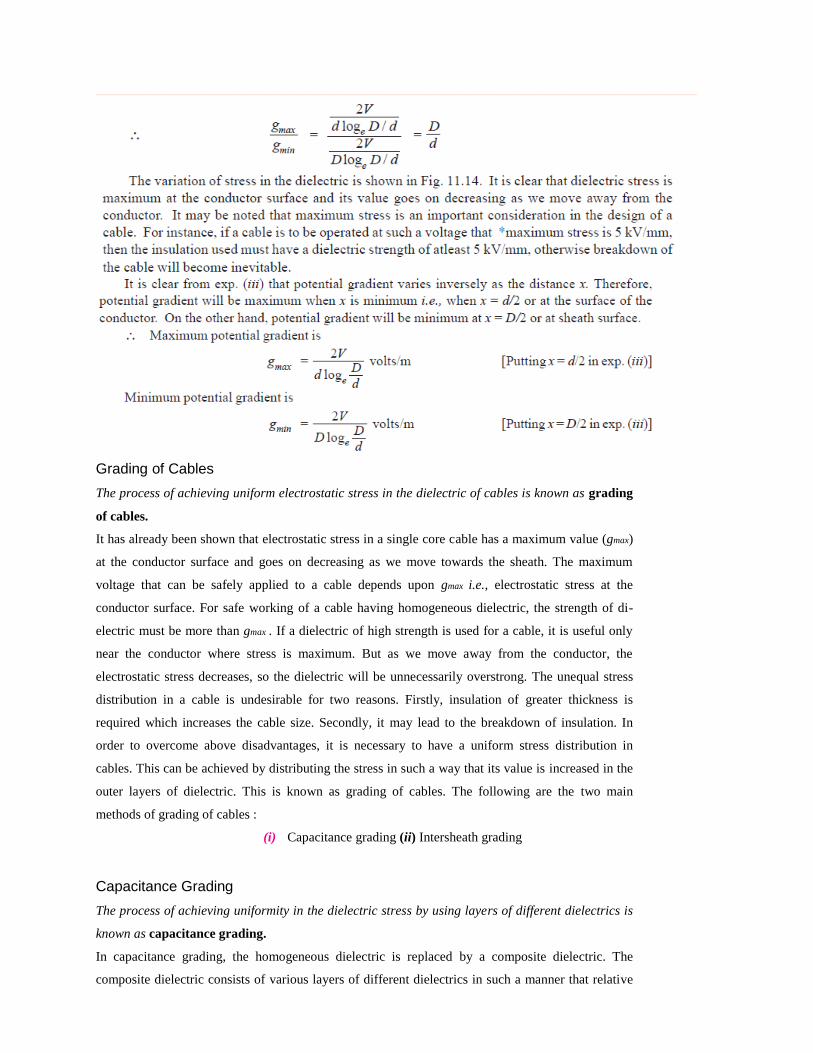
Grading of Cables

The process of achieving uniform electrostatic stress in the dielectric of cables is known as grading

of cables.

It has already been shown that electrostatic stress in a single core cable has a maximum value (gmax)

at the conductor surface and goes on decreasing as we move towards the sheath. The maximum

voltage that can be safely applied to a cable depends upon gmax i.e., electrostatic stress at the

conductor surface. For safe working of a cable having homogeneous dielectric, the strength of di-

electric must be more than gmax . If a dielectric of high strength is used for a cable, it is useful only

near the conductor where stress is maximum. But as we move away from the conductor, the

electrostatic stress decreases, so the dielectric will be unnecessarily overstrong. The unequal stress

distribution in a cable is undesirable for two reasons. Firstly, insulation of greater thickness is

required which increases the cable size. Secondly, it may lead to the breakdown of insulation. In

order to overcome above disadvantages, it is necessary to have a uniform stress distribution in

cables. This can be achieved by distributing the stress in such a way that its value is increased in the

outer layers of dielectric. This is known as grading of cables. The following are the two main

methods of grading of cables :

(i) Capacitance grading (ii) Intersheath grading

Capacitance Grading

The process of achieving uniformity in the dielectric stress by using layers of different dielectrics is

known as capacitance grading.

In capacitance grading, the homogeneous dielectric is replaced by a composite dielectric. The

composite dielectric consists of various layers of different dielectrics in such a manner that relative

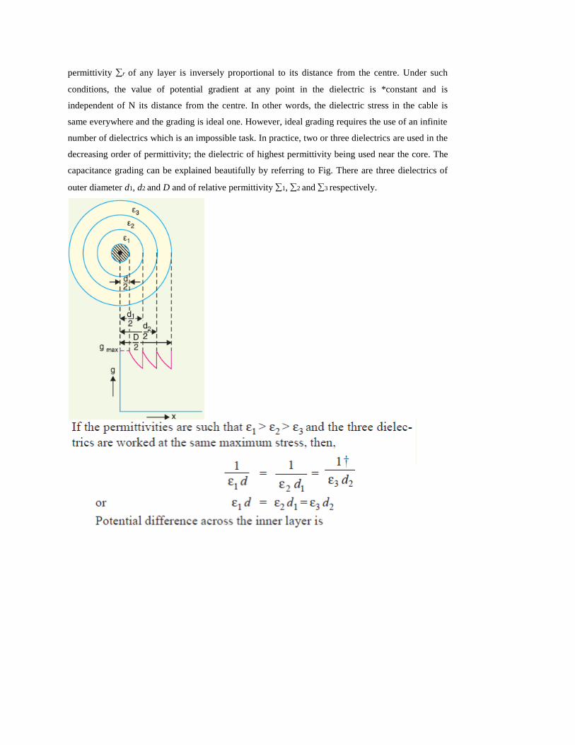
permittivity r of any layer is inversely proportional to its distance from the centre. Under such

conditions, the value of potential gradient at any point in the dielectric is *constant and is

independent of N its distance from the centre. In other words, the dielectric stress in the cable is

same everywhere and the grading is ideal one. However, ideal grading requires the use of an infinite

number of dielectrics which is an impossible task. In practice, two or three dielectrics are used in the

decreasing order of permittivity; the dielectric of highest permittivity being used near the core. The

capacitance grading can be explained beautifully by referring to Fig. There are three dielectrics of

outer diameter d1, d2 and D and of relative permittivity 1, 2 and 3 respectively.

Intersheath Grading

In this method of cable grading, a homogeneous dielectric is used, but it is divided into various

layers by placing metallic inter sheaths between the core and lead sheath. The inter sheaths are held

at suitable potentials which are in between the core potential and earth potential. This arrangement

im-proves voltage distribution in the dielectric of the cable and consequently more uniform potential

gradient is obtained.

Consider a cable of core diameter d and outer lead sheath of diameter D. Suppose that two inter

sheaths of diameters d1 and d2 are inserted into the homogeneous dielectric and maintained at some

fixed potentials. Let V1,

V2 and V3 respectively be the voltage between core and inter sheath 1, between inter sheath 1 and 2

and between

Inter sheath 2 and outer lead sheath. As there is a definite potential difference between the inner and

outer layers of each inter sheath, therefore, each sheath can be treated like a homogeneous single

core cable. As proved in Maximum stress between core and inter sheath 1 is

Capacitance of 3-Core Cables

The capacitance of a cable system is much more important than that of overhead line because in

cables (i) conductors are nearer to each other and to the earthed sheath (ii) they are separated by a

dielectric of permittivity much greater than that of air. Fig. shows a system of capacitances in a 3-

core belted cable used for 3 phase system. Since potential difference exists between pairs of

conductors and between each conductor and the sheath, electrostatic fields are set up in the cable as

shown in Fig.(i). These electrostatic fields give rise to core-core capacitances Cc and conductor-

earth capacitances Ce as shown in Fig. (ii). The three Cc are delta connected whereas the three Ce are

star connected, the sheath forming the star point

They lay of a belted cable makes it reasonable to assume equality of each Cc and each Ce. The three

delta connected capacitances Cc [See Fig.( i)] can be converted into equivalent star connected

capacitances as shown in Fig.(ii). It can be easily *shown that equivalent star capacitance Ceq is

equal to three times the delta capacitance Cc i.e. Ceq = 3Cc.

The system of capacitances shown in Fig.(iii) reduces to the equivalent circuit shown in Fig. (i).

Therefore, the whole cable is equivalent to three star-connected capacitors each of capacitance

Measurements of Ce and Cc

Although core-core capacitance Cc and core-earth capacitance Ce can be obtained from the empirical

formulas for belted cables, their values can also be determined by measurements. For this purpose,

the following two measurements are required :

(i) In the first measurement, the three cores are bunched together (i.e. commoned) and the

capacitance is measured between the bunched cores and the sheath. The bunching eliminates all the

three capacitors Cc, leaving the three capacitors Ce in parallel. Therefore, if C1 is the measured

capacitance, this test yields :

Knowing the value of C1, the value of Ce can be determined.

(ii) In the second measurement, two cores are bunched with the sheath and capacitance is measured

between them and the third core. This test yields 2Cc + Ce. If C2 is the measured capacitance, then,

C2 = 2Cc + Ce

As the value of Ce is known from first test and C2 is found experminentally, therefore, value of Cc

can be determined. It may be noted here that if value of CN (= Ce + 3Cc) is desired, it can be found

directly by another test. In this test, the capacitance between two cores or lines is measured with the

third core free or connected to the sheath. This eliminates one of the capacitors Ce so that if C3 is the

measured capacitance, then,

1

Transmission Line Transient Overvoltages (Travelling Waves on Power Systems)

The establishment of a potential difference between the conductors of an overhead transmission line is accompanied by the production of an electrostatic flux, whilst the flow of current along the conductor results in the creation of a magnetic field. The electrostatic fields are due, in effect, to a series of shunt capacitors whilst the inductances are in series with the line.

Consider the section of the line adjacent to the generator in Figure 1.

Figure 1.

Figure 2.

Let the voltage E suddenly applied to the circuit by closing the switch. Under these conditions, the capacitance C1 takes a large initial charging current the whole of the voltage will at first be used in driving a charging current through the circuit consisting of L1 and C1 in series. As the charge on C1 builds up its voltage will increase and this voltage will begin to charge C2 by driving a current through the inductance L2 (Figure 2), and so on, showing that the greater the distance from the generator, the greater will be the time elapsed from the closing the switch to the establishment of the full line voltage E. It is also clear that voltage and current are intimately associated and that any voltage phenomenon is associated with an attendant current phenomenon.

The gradual establishment of the line voltage can be regarded as due to a voltage wave travelling from the generator towards the far end and the progressing charging of the line capacitances will account for the associated current wave.

G

L2

L3

L1

C3 C

2C1E

G

L2

L3

L1

C3 C

2

C1

E

2

Effect of the 60 Hz Alternating Voltage

In the above treatment, the voltage E has been assumed constant and in practice such an assumption is usually adequate owing to the very high velocity of propagation. So far as most lines are concerned, the impulse would have completely traversed the whole length before sufficient time had elapsed for an appreciable change in the 60 Hz voltage to occur. Assuming that v is equal 3 × 108 m/sec in an actual case, the first impulse will have travelled a distance of (3 × 108)/60 i.e. 5 × 106 meters by the end of the first cycle which means that the line would have to be 5000 km long to carry the whole of the voltage distribution corresponding to one cycle. A line of such a length is impossible.

The Open-Circuited Line

Let a source of constant voltage E be switched suddenly on a line open-circuited at the far end. Then neglecting the effect of line resistance and possible conductance to earth, a rectangular voltage wave of amplitude E and its associated current wave of amplitude I = E/Zc will travel with velocity v towards the open end. Figure 3.a shows the conditions at the instant when the waves have reached the open end, the whole line being at the voltage E and carrying a current I.

Figure 3.a

At the open end, the current must of necessity fall to zero, and consequently the energy stored in the magnetic field must be dissipated in some way. In the case under consideration, since resistance and conductance have been neglected, this energy can only be used in the production of an equal amount of electrostatic field. If this is done, the voltage at the point will be increased by an amount e such that the energy lost by the electromagnetic field (0.5 LI2) is equal to the energy gained by the electrostatic field (0.5Cv2), or: 12 = 12

Whence, = = =

Hence, the total voltage at the open end becomes 2E. The open end of the line can thus be regarded as the origin of a second voltage wave of amplitude E, this second wave travelling back to the source with the same velocity v. At some time subsequent to arrival of the initial wave at the open end, i.e. the condition shown in Figure 3.a, the state affairs on the line will be as in Figure 3.b in which the incoming and reflected voltage waves are superposed, resulting in a step in the voltage wave which will travel back towards the source with a velocity v. The doubling of the voltage at the open end must be associated with the disappearance of the current since none can flow beyond the open circuit. This is equivalent to the establishment of a reflected current

E I = E/Zc

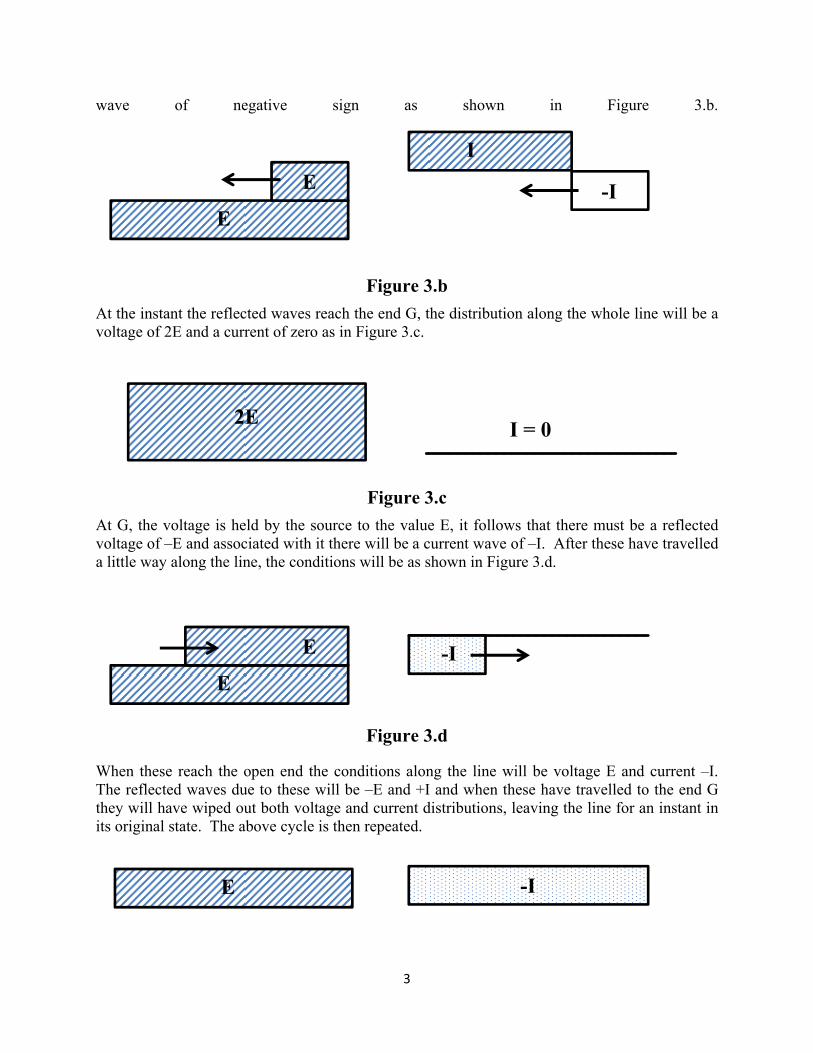
3

wave of negative sign as shown in Figure 3.b.

Figure 3.b

At the instant the reflected waves reach the end G, the distribution along the whole line will be a voltage of 2E and a current of zero as in Figure 3.c.

Figure 3.c

At G, the voltage is held by the source to the value E, it follows that there must be a reflected voltage of –E and associated with it there will be a current wave of –I. After these have travelled a little way along the line, the conditions will be as shown in Figure 3.d.

Figure 3.d

When these reach the open end the conditions along the line will be voltage E and current –I. The reflected waves due to these will be –E and +I and when these have travelled to the end G they will have wiped out both voltage and current distributions, leaving the line for an instant in its original state. The above cycle is then repeated.

E

I E -I

2E I = 0

E

E -I

E -I

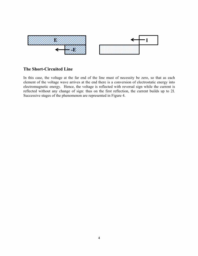
4

The Short-Circuited Line

In this case, the voltage at the far end of the line must of necessity be zero, so that as each element of the voltage wave arrives at the end there is a conversion of electrostatic energy into electromagnetic energy. Hence, the voltage is reflected with reversal sign while the current is reflected without any change of sign: thus on the first reflection, the current builds up to 2I. Successive stages of the phenomenon are represented in Figure 4.

E

-E

I

5

Figure 4

A. Original current and voltage waves just prior to the first reflection. B. Distributions just after the first reflection.

E

-E

E

I

I

I

E = 0 2I

E

3I

E

2I

A

B

C

D

E

I

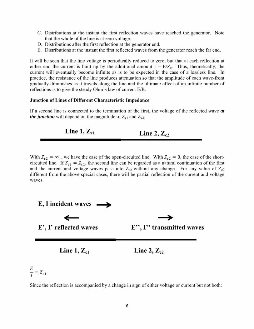
6

C. Distributions at the instant the first reflection waves have reached the generator. Note that the whole of the line is at zero voltage.

D. Distributions after the first reflection at the generator end. E. Distributions at the instant the first reflected waves from the generator reach the far end.

It will be seen that the line voltage is periodically reduced to zero, but that at each reflection at either end the current is built up by the additional amount I = E/Zc. Thus, theoretically, the current will eventually become infinite as is to be expected in the case of a lossless line. In practice, the resistance of the line produces attenuation so that the amplitude of each wave-front gradually diminishes as it travels along the line and the ultimate effect of an infinite number of reflections is to give the steady Ohm’s law of current E/R.

Junction of Lines of Different Characteristic Impedance

If a second line is connected to the termination of the first, the voltage of the reflected wave at the junction will depend on the magnitude of Zc1 and Zc2.

With = ∞ , we have the case of the open-circuited line. With = 0, the case of the short-circuited line. If = , the second line can be regarded as a natural continuation of the first and the current and voltage waves pass into Zc2 without any change. For any value of Zc2

different from the above special cases, there will be partial reflection of the current and voltage waves.

=

Since the reflection is accompanied by a change in sign of either voltage or current but not both:

Line 1, Zc1 Line 2, Zc2

Line 1, Zc1 Line 2, Zc2

E, I incident waves

E’, I’ reflected waves E’’, I’’ transmitted waves

7

= −

The voltage entering the second line at any instant will be the algebraic sum of the incident and reflected voltages in the first line. ∴ = +

The difference between the incident current I and the current I’’ transmitted into the second circuit is the reflected current I’ or = " − where I’ carries the appropriate sign

Also = = = + = − = − −

Giving = =

And = − = − =

Also = =

And = − = −

= = = (1) = (2)

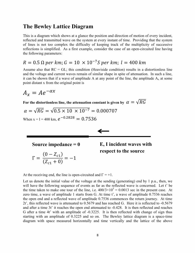
8

The Bewley Lattice Diagram

This is a diagram which shows at a glance the position and direction of motion of every incident, reflected and transmitted wave on the system at every instant of time. Providing that the system of lines is not too complex the difficulty of keeping track of the multiplicity of successive reflections is simplified. As a first example, consider the case of an open-circuited line having the following parameters: = 0.5 Ω ; = 10 × 10 ; = 400

Assume also that RC = GL; this condition (Heaviside condition) results in a distortionless line and the voltage and current waves remain of similar shape in spite of attenuation. In such a line, it can be shown that if a wave of amplitude A at any point of the line, the amplitude Ax at some point distant x from the original point is =

For the distortionless line, the attenuation constant is given by = √

= √ = √0.5 × 10 × 10 = 0.000707

When x = l = 400 km, . = 0.7536

At the receiving end, the line is open-circuited and = +1.

Let us denote the initial value of the voltage at the sending (generating) end by 1 p.u., then, we will have the following sequence of events as far as the reflected wave is concerned. Let t’ be the time taken to make one tour of the line, i.e. 400/3×105 = 0.0013 sec in the present case. At zero time, a wave of amplitude 1 starts from G. At time t’, a wave of amplitude 0.7536 reaches the open end and a reflected wave of amplitude 0.7536 commences the return journey. At time 2t’, this reflected wave is attenuated to 0.5679 and has reached G. Here it is reflected to -0.5679 and after a time 3t’ it reaches the open end attenuated to -0.428. It is then reflected and reaches G after a time 4t’ with an amplitude of -0.3225. It is then reflected with change of sign thus starting with an amplitude of 0.3225 and so on. The Bewley lattice diagram is a space-time diagram with space measured horizontally and time vertically and the lattice of the above

Γ = 0 −+ 0 = −1

Source impedance = 0 E, I incident waves with respect to the source

9

example is shown in Figure 5. The final voltage at the receiving end is the sum to infinity of all such increments. Thus, in the above example, it is: 2 0.7536 − 0.428 + ⋯ … It is simpler to express the series generally in terms of α, thus = 2 − + − + ⋯ … = 2 + + + ⋯ … − + + + ⋯ … = 21 +

When the given values are substituted in the above expression its value is 0.9613.

Thus, even when open-circuited, such a line gives a far end voltage less than the sending end voltage, the reason being that the shunt conductance current produces a drop in the series resistance.

10

Figure 5: Lattice diagram for line with attenuation.

0 0

t’ t’

2t’ 2t’

3t’ 3t’

4t’ 4t’

5t’ 5t’

0.7536

0.7536

0.5679

-0.5679

-0.428

-0.3225

0.322

Receiving end Reflection operator = +1

Sending end

Reflection operator = -1

0.2431

1

645 km

-0.428

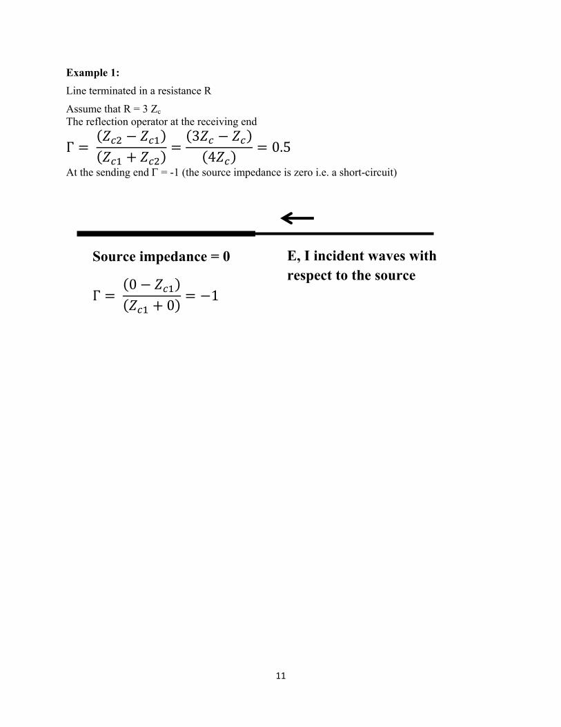
11

Example 1:

Line terminated in a resistance R

Assume that R = 3 Zc

The reflection operator at the receiving end Γ = −+ = 3 −4 = 0.5

At the sending end = -1 (the source impedance is zero i.e. a short-circuit)

Γ = 0 −+ 0 = −1

Source impedance = 0

E, I incident waves with respect to the source

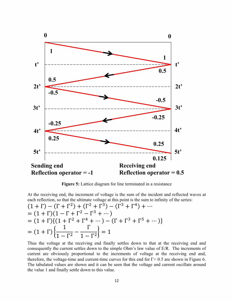
12

Figure 5: Lattice diagram for line terminated in a resistance

At the receiving end, the increment of voltage is the sum of the incident and reflected waves at each reflection, so that the ultimate voltage at this point is the sum to infinity of the series: 1 + Γ − Γ + Γ + Γ + Γ − Γ + Γ + ⋯ = 1 + Γ 1 − Γ + Γ − Γ + ⋯ = 1 + Γ 1 + Γ + Γ + ⋯ − Γ + Γ + Γ + ⋯ = 1 + Γ 11 − Γ − Γ1 − Γ = 1

Thus the voltage at the receiving end finally settles down to that at the receiving end and consequently the current settles down to the simple Ohm’s law value of E/R. The increments of current are obviously proportional to the increments of voltage at the receiving end and, therefore, the voltage-time and current-time curves for this end for = 0.5 are shown in Figure 6. The tabulated values are shown and it can be seen that the voltage and current oscillate around the value 1 and finally settle down to this value.

0 0

t’ t’

2t’ 2t’

3t’ 3t’

4t’ 4t’

5t’ 5t’

1

0.5

0.5

-0.5

-0.5

-0.25

0.25

Receiving end Reflection operator = 0.5

Sending end

Reflection operator = -1

0.25

0.125

1

-0.25

13

Time Increment of voltage or current Sum of increments

0 0 0

t’ 1.5 1.5

3t’ -0.75 0.75

5t’ 0.375 1.125

7t’ -0.188 0.937

9t’ 0.094 1.031

Figure 6: Building up of current and voltage in a line terminated in a resistance.

0.5

1.5

0

t’ 7t’ 3t’ 9t’ 5t’

1

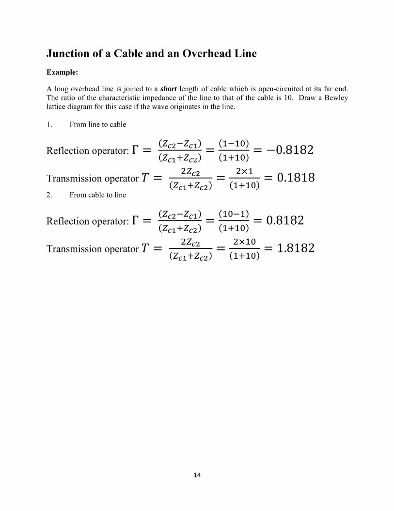
14

Junction of a Cable and an Overhead Line

Example:

A long overhead line is joined to a short length of cable which is open-circuited at its far end. The ratio of the characteristic impedance of the line to that of the cable is 10. Draw a Bewley lattice diagram for this case if the wave originates in the line. 1. From line to cable

Reflection operator: Γ = = = −0.8182

Transmission operator = = × = 0.1818 2. From cable to line

Reflection operator: Γ = = = 0.8182

Transmission operator = = × = 1.8182

15

Lattice diagram for a line consisting of two sections with different constants.

Open end

1

Overhead line, Zc1 Cable, Zc2

Junction Reflection 1

Reflection – 0.8182 0.8182

Refraction 1.8182 0.1818

16

Since the characteristic impedance of an (Extra High Voltage) EHV cable is about 30 to 50 Ω whereas that for a line is frequently about 250 to 350 Ω, the voltage transmitted from a line into a cable is of the order 40/(40+300), i.e. about 0.125 of the surge voltage travelling along the line. For this reason, a transmission line is sometimes connected to a substation by a cable of perhaps less than 2 km length so that lightning or switching surges travelling along the line are much attenuated by the cable and are less likely to flashover or damage apparatus in the substation.

Example:

An overhead line for which L = 1.5 mH/km and C = 0.015 F/km is connected to a cable for which L = 0.25 mH/km and C = 0.45 F/km. If a surge of 10 kV originates in the line and enters the cable, calculate the voltage and current in the cable. = 1.5 × 100.015 × 10 = 316.2278 Ω

= 0.25 × 100.45 × 10 = 23.5702 Ω

Original current in the overhead line = 1 = 31.6228

Voltage in cable = = × . ×. . = 1387.3066 Current in cable = 1387.306623.5702 = 58.8585

Example:

The ends of two long transmission lines A and B are connected by a cable C 1.5 km long. The lines have capacitance of 10 pF/m and inductance 1.6 × 10-6 H/m and the cable has capacitance 89 pF/m and inductance 5× 10-7 H/m. A rectangular voltage wave of magnitude 10 kV and of long duration travels along line A towards the cable. Find the magnitude of the second voltage step occurring at the junction of the cable and line B. What will be the voltage at the junction of line A and the cable 20 sec after the initial surge reaches this point?

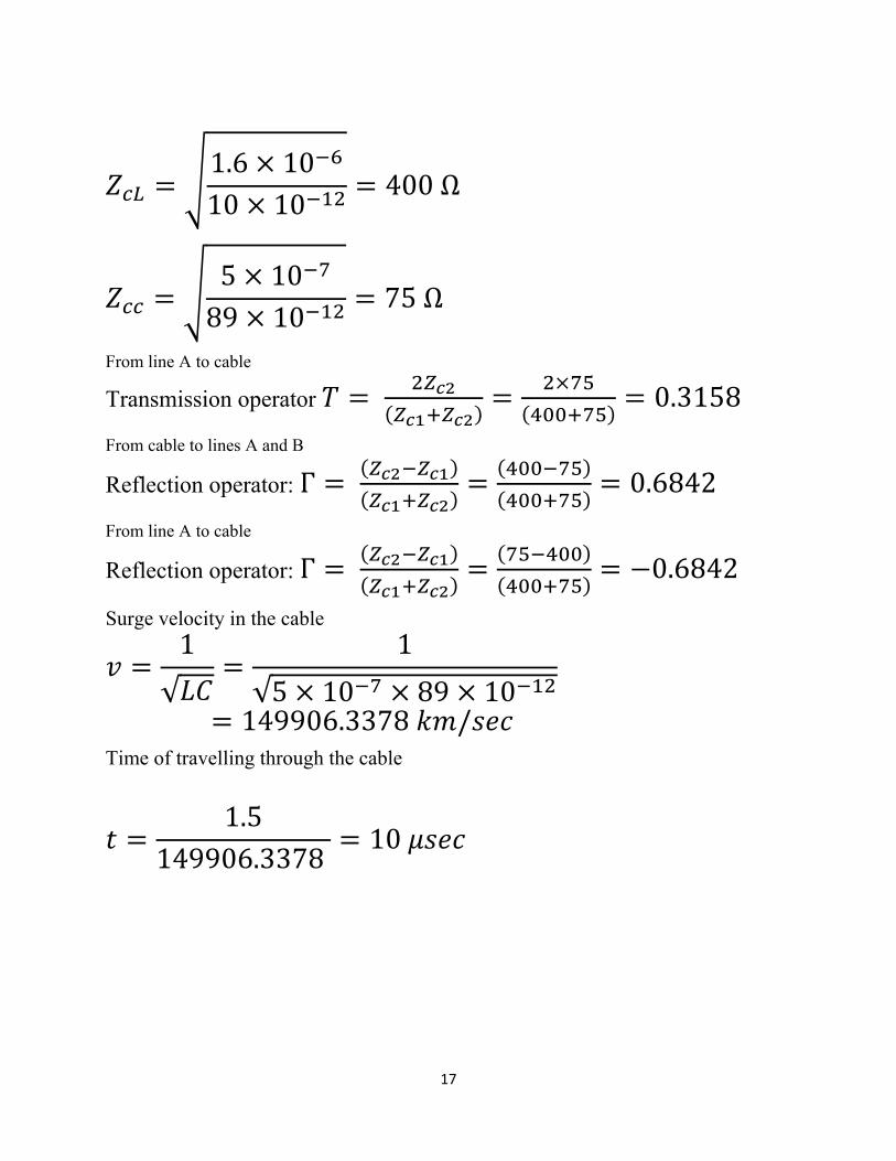
17

= 1.6 × 1010 × 10 = 400 Ω

= 5 × 1089 × 10 = 75 Ω

From line A to cable

Transmission operator = = × = 0.3158 From cable to lines A and B

Reflection operator: Γ = = = 0.6842

From line A to cable

Reflection operator: Γ = = = −0.6842

Surge velocity in the cable = 1√ = 1√5 × 10 × 89 × 10= 149906.3378 / Time of travelling through the cable

= 1.5149906.3378 = 10

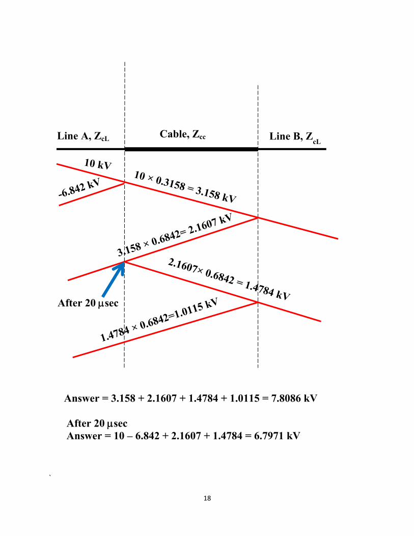
18

`

Line A, ZcL Cable, Zcc Line B, ZcL

Answer = 3.158 + 2.1607 + 1.4784 + 1.0115 = 7.8086 kV

After 20 sec Answer = 10 – 6.842 + 2.1607 + 1.4784 = 6.7971 kV

After 20 sec

19

Example: A 500 kV surge on a long overhead line of characteristic impedance 400 Ω, arrives at a point where the line continues into a cable AB of length 1 km having a total inductance of 264 H and a total capacitance of 0.165 F. At the far end of the cable, connection is made to a transformer of characteristic impedance 1000 Ω. The surge has negligible rise-time and its amplitude may be considered to remain constant at 500 kV for a time-longer than the transient times involved here.

Draw the Bewley lattice diagram at the junction A of the cable for 26.4 sec after the arrival at this junction of the original surge.

= 264 × 100.165 × 10 = 40 Ω

Velocity of the surge through the cable: = 1√264 × 10 × 0.165 × 10 = 151515.2 /

Time for the surge to travel through the cable: t = 1151.5152 = 6.6

From Line to cable:

Transmission operator = = × = 0.1818 Reflection operator: Γ = = = −0.8182

From Cable to Line:

Reflection operator: Γ = = = 0.8182

Line Cable Transforme

20

Transmission operator = = × = 1.8182 From cable to transformer

Reflection operator: Γ = = = 0.9231

90.9 kV up to 13.2 sec, 243.46 kV from 13.2 to 26.4 sec, rising to 358.69 kV at 26.4 sec.

Transformer

Overhead line, Zc1 Cable, Zc2

Junction Reflection 0.9231

21

Reactive Termination

When a loss-free line is terminated by an impedance which contains inductive or capacitive elements, the resulting voltages can be obtained by Laplace transformation. In simple cases, of say a single capacitance or inductor, the impedance of these elements may be written as 1/Cs and Ls respectively (s is the Laplace operator) and the voltage and current will vary exponentially.

If a unit function surge of voltage V is switched on to a line which is terminated by an initially uncharged shunt capacitor of C farads, then the Laplace transform of the voltage reflected is:

= 1 −1 + = Γ = 1 −1 +

= 1 −+ 1 1 = + + 1

= and B = −2 = + −2+ 1

= 1 − 2 (3)

It should be noted that t is here measured from the time the surge reaches the capacitor.

Γ = 1 −1 + C

22

The voltages and currents are illustrated in the figure below. The currents follow from I = V/Zc , = − and the above vreflected equation. The distributions of voltages and current shown in

this figure and the time variations of voltage given by Equation (3) might have been deduced from the fact that the applied surge is assumed to be of infinitely steep wavefront so that it contains a range of frequencies extending to infinity. The capacitor, therefore, acts initially as a short-circuit so that the reflected wave is negative and brings the voltage at that point to zero. The capacitor then charges up with a time constant of CZc until, when completely charges, it constitutes an open circuit and the voltage is then 2V.

Voltages and currents at a capacitor line termination.

The corresponding case of a shunt inductor of L Henrys gives the transform reflected voltage as

ℒ = −+ = 1 − 2 +

= −1 + 2 (4)

The voltage and current distributions are shown in the figure below. The voltages and current for this case are the duals of those for the capacitor termination. At the instant the surge arrives the inductor appears as an open circuit so that the voltage doubles. The current increases exponentially from zero in L until finally it corresponds to a short-circuit if the resistance of the inductor is negligible.

23

Voltages and currents at an inductive line termination.

Example:

A rectangular surge of 100 kV and 20 sec duration travels along a line of surge impedance 500 Ω and 100 km long with a velocity of 3×108 m/sec, towards the end of the line which is terminated with a 0.02 F capacitor. Calculate the maximum voltage appearing across the capacitor. = 0.02 × 10 × 500 = 1 × 10 = 100 1 − 2 ×× = 72.9329

Maximum voltage = 100 + 72.9329 = 172.9329 kV

Γ = −+ L

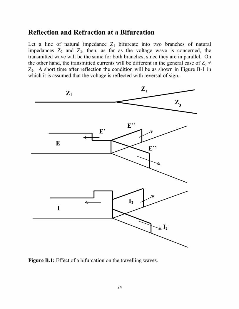
24

Reflection and Refraction at a Bifurcation

Let a line of natural impedance Z1 bifurcate into two branches of natural impedances Z2 and Z3, then, as far as the voltage wave is concerned, the transmitted wave will be the same for both branches, since they are in parallel. On the other hand, the transmitted currents will be different in the general case of Z3 ≠ Z2. A short time after reflection the condition will be as shown in Figure B-1 in which it is assumed that the voltage is reflected with reversal of sign.

Figure B.1: Effect of a bifurcation on the travelling waves.

Z1

Z3

E E’’

E’’

Z2

E’

I

I2

I2

25

Let E1, I1 be the incident voltage and current

E’, I’ be the reflected voltage and current

E’’, I2 be the transmitted voltage and current along Z2

E’’, I3 be the transmitted voltage and current along Z3

Then = and =

Also − = +

The solution of which is

= 21 + 1 + 1

Knowing E1, all the other quantities can be calculated. If we put Z3 = ∞ in the above expression, we have = 2 +

The case becoming that of a simple junction of two lines having different characteristics.

Example

An overhead transmission line having a surge impedance of 450 ohms runs between two substations A and B; at B it branches into two lines C and D, of surge impedances 400 and 50 ohms respectively. If a travelling wave of vertical front and magnitude 25 kV travels along the line AB, calculate the magnitude of the voltage and current waves which enter the branches at C and D.

26

Incident voltage = E1 =25000 V

Incident current = I1 = E1/Z1 = 25000/450 = 55.6 A

Transmitted voltage along BC and BD

= 21 + 1 + 1

×

Transmitted current along BC:

I2 = E’’/Z2 = 4500/400 = 11.25 A

Transmitted current along BD:

I3 = E’’/Z3 = 4500/50 = 90 A

Thus, the current reflected back into line AB = 90 + 11.25 – 55.6 = 45.65 A

Z1 = 450 Ω

E1 C

B

A

Z2 = 400 Ω

Z3 = 50 Ω